Embed Size (px)
Citation preview

Improvements in Finite State Machine
Based Testing
by Uraz Cengiz Turker
Submitted to the Graduate School of Sabancı University
in Partial Fulfilment of the Requirements for the Degree of
Doctor of Philosophy
in Computer Science and Engineering
Sabancı University
January, 2014
II

Dedicated to Sema Turker, Tayla Turker, Yagmur Ozlem Safak
And
Beloved Kıtmir
III

Improvements in Finite State Machine Based TestingUraz Cengiz Turker
Computer Science and Engineering
Ph.D. Thesis, 2014
Thesis Supervisor: Assistant Prof. Husnu Yenigun
Thesis Co-supervisor: Prof. Dr. Robert Hierons
Keywords: Finite State Machines, Fault Detection Experiments, Checking Sequences,
Checking Experiments, Distributed Testing, Distinguishing Sequences.
ABSTRACT
Finite State Machine (FSM) based testing methods have a history of over half a cen-
tury, starting in 1956 with the works on machine identification. This was then followed
by works checking the conformance of a given implementation to a given specification.
When it is possible to identify the states of an FSM using an appropriate input sequence,
it’s been long known that it is possible to generate a Fault Detection Experiment with
fault coverage with respect to a certain fault model in polynomial time. In this thesis, we
investigate two notions of fault detection sequences; Checking Sequence (CS), Checking
Experiment (CE). Since a fault detection sequence (either a CS or a CE) is constructed
once but used many times, the importance of having short fault detection sequences
is obvious and hence recent works in this field aim to generate shorter fault detection
sequences.

In this thesis, we first investigate a strategy and related problems to reduce the length
of a CS. A CS consists several components such as Reset Sequences and State Identifi-
cation Sequences. All works assume that for a given FSM, a reset sequence and a state
identification sequence are also given together with the specification FSM M. Using the
given reset and state identification sequences, a CS is formed that gives full fault cov-
erage under certain assumptions. In other words, any faulty implementation N can be
identified by using this test sequence. In the literature, different methods for CS con-
struction take different approaches to put these components together, with the aim of
coming up with a shorter CS incorporating all of these components. One obvious way
of keeping the CS short is to keep components short. As the reset sequence and the
state identification sequence are the biggest components, having short reset and state
identification sequences is very important as well.
It was shown in 1991 that for a given FSM M, shortest reset sequence cannot be
computed in polynomial time if P 6= NP. Recently it was shown that when the FSM has
particular type (“monotonic”) of transition structure, constructing one of the shortest
reset word is polynomial time solvable. However there has been no work on constructing
one of the shortest reset word for a monotonic partially specified machines. In this
thesis, we showed that this problem is NP-hard.
On the other hand, in 1994 it was shown that one can check if M has special type
of state identification sequence (known as an adaptive distinguishing sequence) in poly-
nomial time. The same work also suggests a polynomial time algorithm to construct
a state identification sequence when one exists. However, this algorithm generates a
state identification sequence without any particular emphasis on generating a short one.
There has been no work on the generation of state identification sequences for com-
plete or partial machines after this work. In this thesis, we showed that construction
of short state identification sequences is NP-complete and NP-hard to approximate. We
propose methods of generating short state identification sequences and experimentally
validate that such state identification sequences can reduce the length of fault detection
sequences by 29.2% on the average.
V
Another line of research, in this thesis, devoted for reducing the cost of checking
experiments. A checking experiment consist of a set of input sequences each of which aim
to test different properties of the implementation. As in the case of CSs, a large portion
of these input sequences contain state identification sequences. There are several kinds of
state identification sequences that are applicable in CEs. In this work, we propose a new
kind of state identification sequence and show that construction of such sequences are
PSPACE-complete. We propose a heuristic and we perform experiments on benchmark
FSMs and experimentally show that the proposed notion of state identification sequence
can reduce the cost of CEs by 65% in the extreme case.
Testing distributed architectures is another interesting field for FSM based fault detec-
tion sequence generation. The additional challenge when such distributed architectures
are considered is to generate a fault detection sequence which does not pose control-
lability or observability problem. Although the existing methods again assume that
a state identification sequence is given using which a fault detection sequence is con-
structed, there is no work on how to generate a state identification sequence which do
not have controllability/observability problem itself. In this thesis we investigate the
computational complexities to generate such state identification sequences and show
that no polynomial time algorithm can construct a state identification sequence for a
given distributed FSM.
VI
Sonlu Durum Makinelerine Dayalı Sınama DizilerindeIyilestirmelerUraz Cengiz Turker
Bilgisayar Bilmi ve Muhendisligi
Doktora Tezi, 2014
Tez danısmanı: Yrd. Doc. Dr. Husnu Yenigun
Tez Yrd. danısmanı: Prof. Dr. Robert Hierons
Keywords: Sonlu durum Makineleri, Hata bulma deneyleri, Sınama dizileri, Sınama
Denyleri, Dagıtık Sınama, Ayrıstırma Dizileri.
Ozet
Sonlu durum makinelerine (SDM’e) dayalı sınama yontemleri 1956 yılında makine
tanıma uzerine yapılan calısmalar ile baslamıs ve elli yılı askın bir suredir uzerinde
calısılan bir konu olmustur. Makine tanıma calısmalarını takiben bir gerceklestirmenin
bir spesifikasyona uygun olup olmadıgının sınanması uzerine calısmalar baslamıs ve ver-
ilen SDM’nin durumları tanımlandıgı ve belli bir hata kumesi goz onune anlındıgı zaman
verilen bir SDM icin sınama dizilerinin uretilmesi icin polinom zamana ihtiyac duyuldugu
bilinmektedir. Bu tezde iki farklı sınama dizisi ele alınmıstır: Sınama Dizisi (SDi) ve
Sınama Deneyleri (SDe). Sınama dizileri ister SDi ister SDe olsun genelde belli bir pren-
sipte calısır: bir kez uret ve cok kez kullan. Bu yuzden sınama dizilerinin boylarının kısa
olması sınama sırasında gecen yekun sureyi azaltacagı gerekcesi ile oldukca onemlidir.
Bu yuzden literaturde bu alanda calısmalar yapılmaya baslanmıstır.

Bu tezde ilk once SDi’lerin boylarını kısaltmayı amaclayan stratejiler gosterilmistir.
Bir SDi birden fazla, kendisinden ufak Sıralama Dizisi, Durum Tanıma Dizisi gibi
dizilerinden olusur. Bu konu uzerine yapılan hemen hemen tum calısmalar bu dizilerin
SDM ile birlikte verildigini tahmin etmislerdir ve bu diziler ile olusturulacak SDi’ler
belli bir hata kumesi goz onunde bulundurularak uretildiginde bir spesifikasyonun hatalı
tum gerceklestirmelerini saptayacagı bilinmektedir. Bir baska degis ile verilen hatalı bir
gerceklestirme uretilen bir SDi tarafından belirlenebilir. Farklı SDi olusturma yontemleri
bu dizileri farklı sekilde bir araya getirerek SDi’leri daha kısa boyda olusturmayı amaclamıslardır.
Ancak sıralama ve durum tanıma dizileri bir SDi’nin en buyuk parcaları oldugu bilgisi ile
hareket edersek bu dizilerin boylarının kısaltılması, olusturulacak SDi’lerin boylarını’da
kısaltacagı dusunulmelidir.
1991’de verilen bir SDM’nin en kısa sıralama dizinin uretilmesinin NP != P esitsizligi
var oldugu surece polinom zamanda uretilemeyecegi ispat edilmistir. Ancak yakın gecmiste
bir SDM’nin durumlar arası gecislerinin ozel bir turde olması ”monotonik” durumunda
en kısa sıralama dizisinin polinom zamanda uretilecegi gosterilmistir. Ancak kısmi
tanımlı bir monotonik SDM’nin en kısa sıralama dizisinin hesaplanma zorlugu acık bir
problemdi. Bu tezde bu problemin NP-Zor oldugunu gosterdik.
Oteyandan, 1994 yılında ozellikli bir durum tanıma dizisinin (uyarlamalı ayrıstırma
dizisi (UAD)) polinom zamanda uretilebilecegi gosterilmistir. Aynı calısmada yazarlar
bir SDM icin bu diziyi polinom zamanda uretebilen bir algoritma da gostermislerdir. An-
cak bu algoritma herhangi bir ayrıstırma dizisini buyuklugune bakmadan uretmektedir.
Bu calısmadan baska tam tanımlı yada kısmi tanımlı SDM’ler icin uyarlamalı ayrıstırma
dizisi uretebilen baska bir calısma yoktur. Bu tezde kısa uyarlamalı ayrıstırma dizisi
uretmenin NP-TAM ve en kısa UAD’ye yaklasmanın da NP-Zor oldugunu gosterdik.
Bunun yanında SDi’lerin boyunu ortalama %29.2 kadar kısaltabilmeye yarayan UAD’leri
retebilen sezgisel yontemler sunduk.
Bu tezde SDe’lerin boyunu kısaltmayı hedefleyen calısmalar yaptık. SDe’ler SDi’lerin
aksine birbiri ile birlesmeyen cok sayıda ufak sınama konuları icerir ve her bir sınama
konusu gerceklestirmenin farklı bir yonunu sınar. Ancak SDi’ler de oldugu gibi bu sınama
VIII

konularının buyuk bir bolumu yine durum tanıma dizilerinden olusur. SDe’ler icin sınırlı
sayıda durum tanıma dizisi mevcuttur, bu tezde yeni bir durum tanıma dizisi sunduk ve
gosterdik ki bu yeni durum tanıma dizisinin olusturulmasının zorlugu PSPACE-Tam. Bu
sonucu takiben bu dizileri uretmek icin sezgisel yontem urettik ve endustriden alınmıs
SDM’ler uzerinde deneylar yaptık ve teklif edilen yontem ile SDe’lerin boylarını %65’e
varan oranlarda kısaltılabilecegini gosterdik.
Dagıtık SDM’lerin (DSDM’lerin) sınanması SDM tabanlı sınama calısmalarının il-
ginc bir ayagı olmaktadır. Sınama dizilerinin uretiminde yasanan zorluklara ek olarak
dagıtık mimarilerin getirmis oldugu kontrolledilebilirlik ve gozlemlenebilirlik problemleri
karsımıza cıkmaktadır. Her ne kadar mevcut SDi uretme yontemlerinde durum tanıma
dizilerinin DSDM ile birlikte verildigi dusunulmussede kontroledilebir durum tanıma
disizin uretlimesine deginen bir calısma yoktur. Bu tezde bu dizilerin uretilmesinin
zorlugunu arastırmıs ve bu dizilerin polinom zamanda uretilemeyecegini ispatlams bu-
lunmaktayz.
IX

Contents
1. Introduction 1
1.1. Contributions . . . . . . . . . . . . . . . . . . . . . . . . . . . . . . . . . 7
1.2. Outline of the Thesis . . . . . . . . . . . . . . . . . . . . . . . . . . . . . 8
2. Preliminaries 9
2.1. Finite State Machines . . . . . . . . . . . . . . . . . . . . . . . . . . . . . 9
2.1.1. Multi–port Finite State Machines . . . . . . . . . . . . . . . . . . 15
2.1.2. Finite Automata . . . . . . . . . . . . . . . . . . . . . . . . . . . 19
3. Complexities of Some Problems Related to Synchronizing, Non-synchronizing
and Monotonic Automata 21
3.1. Introduction . . . . . . . . . . . . . . . . . . . . . . . . . . . . . . . . . . 21
3.1.1. Problems . . . . . . . . . . . . . . . . . . . . . . . . . . . . . . . 22
3.2. Minimum Synchronizable Sub-Automaton Problem . . . . . . . . . . . . 26
3.3. Exclusive Synchronizing Word Problems . . . . . . . . . . . . . . . . . . 28
3.4. Synchronizing Monotonic Automata . . . . . . . . . . . . . . . . . . . . . 32
3.5. Chapter Summary and Future Directions . . . . . . . . . . . . . . . . . . 37
4. Hardness and Inaproximability of Minimizing Adaptive Distinguishing Se-
quences 39
4.1. Introduction . . . . . . . . . . . . . . . . . . . . . . . . . . . . . . . . . . 39
4.1.1. A Motivating Example . . . . . . . . . . . . . . . . . . . . . . . . 41
4.2. Binary Decision Trees . . . . . . . . . . . . . . . . . . . . . . . . . . . . . 44
X

4.3. Minimizing Adaptive Distinguishing Sequences . . . . . . . . . . . . . . . 48
4.4. Modeling a Decision Table as a Finite State Machine . . . . . . . . . . . 49
4.4.1. Mapping . . . . . . . . . . . . . . . . . . . . . . . . . . . . . . . . 50
4.4.2. Hardness and Inapproximability Results . . . . . . . . . . . . . . 50
4.5. Experiment Results . . . . . . . . . . . . . . . . . . . . . . . . . . . . . . 53
4.5.1. LY Algorithm . . . . . . . . . . . . . . . . . . . . . . . . . . . . . 53
4.5.2. Modifications on LY algorithm . . . . . . . . . . . . . . . . . . . . 56
4.5.3. A Lookahead Based ADS Construction Algorithm . . . . . . . . . 57
4.5.4. FSMs used in the Experiments . . . . . . . . . . . . . . . . . . . 64
4.5.5. Results . . . . . . . . . . . . . . . . . . . . . . . . . . . . . . . . . 65
4.5.6. Threats to Validity . . . . . . . . . . . . . . . . . . . . . . . . . . 78
4.6. Chapter Summary . . . . . . . . . . . . . . . . . . . . . . . . . . . . . . 79
5. Using Incomplete Distinguishing Sequences when Testing from a Finite
State Machine 81
5.1. Introduction . . . . . . . . . . . . . . . . . . . . . . . . . . . . . . . . . . 81
5.2. Preliminaries . . . . . . . . . . . . . . . . . . . . . . . . . . . . . . . . . 84
5.3. Incomplete Preset Distinguishing Sequences . . . . . . . . . . . . . . . . 86
5.4. Incomplete Adaptive Distinguishing Sequences . . . . . . . . . . . . . . . 89
5.5. Test Generation Using Incomplete DSs . . . . . . . . . . . . . . . . . . . 93
5.6. Practical Evaluation . . . . . . . . . . . . . . . . . . . . . . . . . . . . . 99
5.6.1. Greedy Algorithm . . . . . . . . . . . . . . . . . . . . . . . . . . . 99
5.6.2. Experimental results . . . . . . . . . . . . . . . . . . . . . . . . . 107
5.7. Chapter Summary and Future Directions . . . . . . . . . . . . . . . . . . 129
6. Distinguishing Sequences for Distributed Testing 132
6.1. Introduction . . . . . . . . . . . . . . . . . . . . . . . . . . . . . . . . . . 132
6.2. Test Strategies for distributed testing . . . . . . . . . . . . . . . . . . . . 133
6.2.1. Global Test Strategies . . . . . . . . . . . . . . . . . . . . . . . . 134
6.2.2. Local and Distributed Test Strategies . . . . . . . . . . . . . . . . 140
XI

6.3. Generating controllable PDSs . . . . . . . . . . . . . . . . . . . . . . . . 146
6.4. PDS generation: a special case . . . . . . . . . . . . . . . . . . . . . . . 150
6.5. Generating controllable ADSs . . . . . . . . . . . . . . . . . . . . . . . . 155
6.6. Chapter Summary and Future Directions . . . . . . . . . . . . . . . . . . 161
7. Conclusions 163
XII

List of Figures
1.1. Localized and Distributed Architectures . . . . . . . . . . . . . . . . . . 6
2.1. An example FSM M1 . . . . . . . . . . . . . . . . . . . . . . . . . . . . 10
2.2. An ADS for M1 of Figure 2.1 . . . . . . . . . . . . . . . . . . . . . . . . 13
2.3. Another ADS for M1 of Figure 2.1 . . . . . . . . . . . . . . . . . . . . . . 13
2.4. PSFSM M1 . . . . . . . . . . . . . . . . . . . . . . . . . . . . . . . . . . 14
2.5. Example MPFSMM1 and its faulty implementation M′1 . . . . . . . . . 17
2.6. Example MPFSM M2 . . . . . . . . . . . . . . . . . . . . . . . . . . . . 18
3.1. Synchronizable AutomatonA constructed from an FA-INT problem. States
q01, q
02, q
03, . . . , q
0n form Q . . . . . . . . . . . . . . . . . . . . . . . . . . . . 30
3.2. Monotonic Partially Specified Automaton F(U1, C1) constructed from the
Exact Cover instance U1 = {1, 2, 3, 4, 5, 6} and C1 = {(1, 2, 5), (3, 4, 6), (1, 4, 2)}
. . . . . . . . . . . . . . . . . . . . . . . . . . . . . . . . . . . . . . . . . 33
3.3. Monotonicity of the automaton F(U1, C1) constructed from the Exact
Cover problem instance (U1, C1). . . . . . . . . . . . . . . . . . . . . . . 34
3.4. A 5x5 Chessboard in which a queen is placed at board position (e, 2) (left
image). Chessboard places with red crosses are dead cells and chessboard
places with green squares are live cells (right image). . . . . . . . . . . . 35
3.5. Monotonicity of the automaton F(B) constructed from the N–Queens
instance B. . . . . . . . . . . . . . . . . . . . . . . . . . . . . . . . . . . 37
4.1. An example FSM M2 . . . . . . . . . . . . . . . . . . . . . . . . . . . . 41
XIII
4.2. An ADS A1 for M2 of Figure 4.1 generated by LY algorithm . . . . . . . 42
4.3. A manually designed minimum size ADS A2 for M1 of Figure 4.1 . . . . 42
4.4. A decision tree for the decision table of Table 4.2 . . . . . . . . . . . . . 46
4.5. Another decision tree for the decision table of Table 4.2 . . . . . . . . . . 46
4.6. An example FSM M3. . . . . . . . . . . . . . . . . . . . . . . . . . . . . 49
4.7. An ADS A1 for M3 of Figure 4.6. . . . . . . . . . . . . . . . . . . . . . . 49
4.8. Another ADS A2 for M3 of Figure 4.6. . . . . . . . . . . . . . . . . . . . 49
4.9. The FSM MD corresponding to the decision table given in Table 4.2 . . . 51
4.10. An ADS for MD given in Figure 4.9, which is not always branching . . . 52
4.11. An always branching ADS constructed from the ADS given in Figure 4.10 52
5.1. An example FSM M5 . . . . . . . . . . . . . . . . . . . . . . . . . . . . . 86
5.2. An incomplete ADS for machine M2 presented in Figure 5.1 where S =
{s1, s2, s4} . . . . . . . . . . . . . . . . . . . . . . . . . . . . . . . . . . 86
5.3. An FSMM1(A) constructed from an FA-INT problem instance with S =
{011, 0
21, . . . , 0
1z, 0
2z} . . . . . . . . . . . . . . . . . . . . . . . . . . . . . . . 88
5.4. Incomplete ADS A1 for S = {s1, s2, s4} . . . . . . . . . . . . . . . . . . 97
5.5. Incomplete ADS A2 for S = {s1, s3} . . . . . . . . . . . . . . . . . . . . 97
5.6. Incomplete ADS A3 for S = {s2, s3} . . . . . . . . . . . . . . . . . . . . 97
5.7. Incomplete ADS A4 for S = {s3, s4} . . . . . . . . . . . . . . . . . . . . 97
5.8. An incomplete ADSs for machine M1 presented in Figure 5.1 . . . . . . 97
5.9. An FSM M6 . . . . . . . . . . . . . . . . . . . . . . . . . . . . . . . . . . 104
5.10. Comparison of test suite lengths. Each boxplot summarises the distribu-
tions of 100 FSMs where p = 4, q = 4 . . . . . . . . . . . . . . . . . . . . 109
5.11. Comparison of test suite lengths. Each boxplot summarises the distribu-
tions of 100 FSMs where p = 6, q = 6 . . . . . . . . . . . . . . . . . . . . 110
5.12. Comparison of test suite lengths. Each boxplot summarises the distribu-
tions of 100 FSMs where p = 8, q = 8 . . . . . . . . . . . . . . . . . . . . 111
5.13. Comparison of average test case lengths. Each boxplot summarises the
distributions of 100 FSMs where p = 4, q = 4 . . . . . . . . . . . . . . . . 115
XIV

5.14. Comparison of average test case lengths. Each boxplot summarises the
distributions of 100 FSMs where p = 6, q = 6 . . . . . . . . . . . . . . . . 116
5.15. Comparison of average test case lengths. Each boxplot summarises the
distributions of 100 FSMs where p = 8, q = 8 . . . . . . . . . . . . . . . . 116
5.16. Comparison of number of resets required for methods. Each boxplot sum-
marises the distributions of 100 FSMs where p = 4, q = 4 . . . . . . . . . 119
5.17. Comparison of number of resets required for methods. Each boxplot sum-
marises the distributions of 100 FSMs where p = 6, q = 6 . . . . . . . . . 119
5.18. Comparison of number of resets required for methods. Each boxplot sum-
marises the distributions of 100 FSMs where p = 8, q = 8 . . . . . . . . . 120
5.19. Comparison of number of DS and SI per state. Each boxplot summarises
the distributions of 100 FSMs where p = 4, q = 4. . . . . . . . . . . . . . 122
5.20. Comparison of number of DS and SI per state. Each boxplot summarises
the distributions of 100 FSMs where p = 6, q = 6. . . . . . . . . . . . . . 123
5.21. Comparison of number of DS and SI per state. Each boxplot summarises
the distributions of 100 FSMs where p = 8, q = 8. . . . . . . . . . . . . . 125
6.1. MPFSM M3 for Example 1 . . . . . . . . . . . . . . . . . . . . . . . . . 134
6.2. Figure for Example 2 . . . . . . . . . . . . . . . . . . . . . . . . . . . . . 137
6.3. An example reduction. . . . . . . . . . . . . . . . . . . . . . . . . . . . . 160
XV

List of Tables
4.1. Comparison of checking sequence lengths for FSM M1 . . . . . . . . . . . 44
4.2. An example decision table . . . . . . . . . . . . . . . . . . . . . . . . . . 45
4.3. The list of heuristics/algorithms used to construct ADSs . . . . . . . . 64
4.4. Size of Case Studies . . . . . . . . . . . . . . . . . . . . . . . . . . . . . 66
4.5. Comparison of algorithms in terms ofM1 andM2 with respect to number
of states. |M | is the number of states. . . . . . . . . . . . . . . . . . . . 68
4.6. Comparison of algorithms in terms ofM1 andM2 with respect to size of
input output alphabets. |M | is the number of states. . . . . . . . . . . . 70
4.7. Comparison of algorithms in terms of M1 and M2 with respect to pa-
rameter k. |M | is the number of states. . . . . . . . . . . . . . . . . . . 71
4.8. Comparison of algorithms in terms ofM1 andM2. |M | is the number of
states. . . . . . . . . . . . . . . . . . . . . . . . . . . . . . . . . . . . . . 72
4.9. Height and External Path Length Comparison for Case Studies. . . . . . 73
4.10. Checking Sequence Length Comparison for FLY and GLY1 . . . . . . . 75
4.11. Checking Sequence Length Comparison for FLY and GLY2 . . . . . . . 75
4.12. Checking Sequence Length Comparison for FLY and HU . . . . . . . . 75
4.13. Checking Sequence Length Comparison for FLY and HLY . . . . . . . . 75
4.14. Checking Sequence Length Comparison for FLY and LU . . . . . . . . . 75
4.15. Checking Sequence Length Comparison for FLY and LLY . . . . . . . . 75
4.16. Checking Sequence Length Comparison for Case Studies. . . . . . . . . 76
4.17. Improvement in checking sequence length by using the shallowest ADS. 77
XVI
4.18. Improvement in checking sequence length by using the ADS with mini-
mum external path length. . . . . . . . . . . . . . . . . . . . . . . . . . 78
5.1. Nomenclature for the greedy algorithm . . . . . . . . . . . . . . . . . . . 100
5.2. The results of a Kruskal-Wallis Significance Tests performed on the Check-
ing Experiments Length . . . . . . . . . . . . . . . . . . . . . . . . . . . 112
5.3. Pairwise differences of CE Lengths. Each value corresponds to the occur-
rence of the comparison criteria in 100 FSMs. . . . . . . . . . . . . . . . 114
5.4. Results for Non-parametric Kruskal-Wallis Significance Tests . . . . . . . 118
5.5. The results of a Kruskal-Wallis Significance Tests performed on the Num-
ber of Resets . . . . . . . . . . . . . . . . . . . . . . . . . . . . . . . . . 121
5.6. The results of a Kruskal-Wallis Significance Tests performed on the SI
and DI values . . . . . . . . . . . . . . . . . . . . . . . . . . . . . . . . . 124
5.7. Pairwise differences of number of resets . . . . . . . . . . . . . . . . . . . 126
5.8. Results of Case Studies . . . . . . . . . . . . . . . . . . . . . . . . . . . . 128
XVII

Acknowledgements
My first debt of gratitude must go to my advisor, Dr. Husnu Yenigun. His brilliant
ideas, personal trust and positive comments and personal supports helped me not only
to make a research about Formal Methods but to prepare this thesis. He patiently
provided the vision, encouragement and advise necessary for me to proceed through
the doctoral program and complete my dissertation. I want to thank Dr. Yenigun for
his unflagging encouragement and serving as a role model to me as a junior member
of academia. He has been a strong and supportive adviser to me throughout my PhD
years, but he has always given me great freedom to pursue independent work. I would
like to emphasize that i am proud of being the first PhD student of Dr. Husnu Yenigun,
i will forever be thankful to him.
I would like to express my special appreciation and thanks to my co-advisor Professor
Robert Hierons, he has also been a tremendous mentor for me. Robert has been helpful
in providing advice infinitely many times while preparing this work. He was and remains
one of the best role model for a scientist, mentor, and teacher. I still think fondly of
my time as an researcher in his lab. Robert was the reason of why I decided to make
a research on distributed testing. His enthusiasm, quickness and love for teaching is
contagious.
I would also like to thank my committee members, Assitant Prof. Dr. Tonguc Un-
luyurt, Associated Prof. Dr. Berrin Yankolu and Assitant Prof. Dr. Cemal Yilmaz and
Prof. Kemal Inan for serving as my committee members even at hardship. I also want
to thank you for letting my defence be an enjoyable moment, and for your brilliant com-
ments and suggestions, thanks to you. I would especially like to thank to my colleagues
and officers at Sabanci University. All of you have been there to support me when and
where necessary.
A special thanks to my family especially my mother. Words cannot express how
grateful I am to my mother, and sisters for all of the sacrifices that you’ve made on my
behalf. I would also like to thank all of my friends who supported me in writing papers
and my thesis.
XVIII

1. Introduction
Although the concept of Finite State Machines (FSMs) had been existed for so long,
its popularity today in the computer science and engineering fields can be attributed to
the pioneering efforts of George H. Mealy [1] and Edward Forrest Moore [2] performed
at Bell Labs and IBM around 1960s. After their efforts, finite state machines became
popular in computer science and engineering disciplines, remarkably due to the ability of
modelling systems such as sequential circuits [3], communication protocols [4, 5, 6, 7, 8,
9, 10, 11, 12, 13, 14], object-oriented systems [15], and web services [4, 16, 17, 18, 19, 20].
The operation of an FSM can be described as follows: the system is always in one
of the defined states. It reacts to an input by producing an output, and by changing
its state. For a Mealy machine, the output is generated by a transition. For a Moore
machine, an output is generated by a state. Due to this reactive behaviour, FMSs are
also called reactive systems. An input to an FSM may be a message, or a simple event
flag. Likewise, an output from an FSM may be a message interpreted by an observer,
or setting an event flag. Multiple transitions are allowed from one state to other states.
We refer [21, 22] for detailed information on FSMs. In this work we focus on Mealy
machines. However, Mealy and Moore machines are equivalent and can be converted to
each other [2].
When a system is modelled by an FSM, it is possible to generate a test from this
model. Here, by testing we refer to the Black Box Testing where the tester is only
allowed to observe outputs. The first paper in this field was given by Moore [2], where
Moore suggested to generate a machine identification sequence: a special input sequence
which is capable of distinguishing a copy of M from any other FSMs which have same
1

number of input/output symbols and states as M .
In principle, testing FSM refers to a Fault Detection Experiment [22] which consists of
applying an experiment (derived from a specification FSM M ) to an implementation N
of M, observing the output sequence produced by N in response to the application of the
experiment, and comparing the output sequence to the expected output sequence. In
this thesis, we consider two notions of fault detection experiments: Checking Sequences
(CSs) [23] and Checking Experiments (CEs)[4]. If the applied experiment contains a
single input sequence then it is called a CS and if the applied experiment contains a set
of input sequences then it is called a CE. These fault detection experiments determine
whether System Under Test (SUT) N is a correct or faulty implementation of M [4, 21,
23]. After Moore, Arthur Gill [21] and Frederick C. Hennie [23, 24] present a line of
research on testing FSMs. As fault detection experiments (CSs/CEs) are used to test an
implementation, and the fact that a specification may have multiple implementations,
reducing the size of fault detection experiments is important. In [23], Hennie considers
the specification machine as the master plan, and he encodes the behaviour of this
master plan as a CS. Then based on this sequence he tests if the implementation has
the same behaviour. Due to this strategy; a CS refers to an input sequence that is
constructed from M and is guaranteed to distinguish a correct implementation from
any faulty implementation, which have the same input and output alphabets as M and
no more states than M . Following him, Charles R. Kime enhanced the methods given
by Hennie and lessen the lengths of the CS to some extend [25]. Following Kime and
Hennie another influential scientist Guney Gonenc proposed an algorithm that shortens
the length of such sequences considerably [26]. After this point researchers have been
working on to shorten the lengths of the CSs by putting the pieces that need to exist in
such a CS together in a better way [4, 17, 27, 28, 29, 30, 31, 32, 33].
In general, a CS consists of four different type of components. Reset Sequence is
a component in which the machine N is brought to the initial state regardless of the
current state of N and the output produced by N . State Verification component is
carried out by bringing N to a certain state s of M , checking if N is at state s by
2
applying a state identification sequence for s and repeating this procedure until all the
states of M are recognised in N . The transition verification component is performed
for each transition of M in N . To verify a transition, one brings N to the state from
which the transition starts, applies the input that labels the transition (to check correct
implementation of the output of the transition) and then verifies the ending state by
using a state identification sequence. The final component is transfer sequences. Transfer
sequences are used to combine all the components to form the final CS.
When examining the structure of a CS, the motivation to study reset sequences be-
comes natural i.e. shorter reset sequences lead to shorter CSs. However for a given FSM
computing the shortest reset sequence is known to be NP-complete in general [34]. There-
fore, we investigated open problems and raise several problems related to constructing
reset sequences and try to draw the computational complexities for these problems.
State identification sequences are used many times in a CS and there are differ-
ent type of state identification sequences: Unique Input Output (UIO) sequences, or
Separating Family (also known as the Characterizing Set), or Distinguishing sequences
(DSs). A UIOs is a set of input sequences that verifies the states of an FSM. Since it
is PSPACE-complete to construct UIOs for an FSM [35], it may be impractical to use
UIOs for large FSMs [7, 13, 36, 37, 38, 39, 40, 41]. Separating family can also be used
to verify states and transitions of an FSM [4]. Although this method is strong in the
sense that every minimal FSM posseses a characterizing set and it is polynomial time
computable, it requires a reliable reset feature in the implementation or otherwise re-
sults in exponentially long CSs [4, 22, 21]. DSs are used to identify the current state
of N . Thanks to the efficient state identification capabilities, distinguishing sequences
simplify the problem of generating CSs. They do not require reliable reset, and by using
a distinguishing sequence, one can construct a CS of a length polynomial in the size
of the FSM and the distinguishing sequence1 [23, 29, 35, 42, 43, 44]. Therefore many
techniques for constructing CSs use DSs to resolve the state identification problem.
1That is, the FSM and its distinguishing sequence are considered as the inputs for such CS generation
algorithms.
3
There are two types of distinguishing sequences, Preset Distinguishing Sequences, and
Adaptive Distinguishing Sequences (also known as Distinguishing Sets). As it was noted
before [35, 42], the use of ADS instead of PDS is also possible for these methods and
shown to yield polynomial length CSs [43]. There are numerous advantages of using
ADSs over PDSs. Lee and Yannakakis have reported that checking the existence and
computing a PDS is a PSPACE-complete problem whereas it is polynomial time solvable
in case of ADS [35]. They have also shown that an FSM which posses an ADS may
not have a PDS and not the other way around [35, 42]. Moreover, it is also known that
the shortest ADS for an FSM can not be longer than the shortest PDS of the same
FSM [35, 42, 24]. Furthermore, because during the distinguishing experiment the next
input is chosen according to the previous response of FSM, ADS based testing methods
is accepted as more powerful means of testing than the PDS based methods [45, chp.2].
Hierons et al.[43] reported that CSs are relatively shorter when designed by ADS.
All ADS based CS generation methods start with the assumption that an ADS is given.
The given ADS is repeatedly applied in state verification and transition verification
components of the CS. Thus, these ADS applications form a considerably large part of
the CS and hence, reducing the size of ADSs is a reasonable way to reduce the length
of the CSs.
Earlier ADS construction algorithms [21, 22, 23] are exhaustive and require expo-
nential space and time. The only polynomial time algorithm was proposed by Lee and
Yannakakis (LY Algorithm). Let us assume that p, n refers to the number of inputs
and number of states respectively then the LY algorithm can check if M has an ADS in
O(pn log n) time [35], and if one exists, we can construct an ADS in O(pn2) time [35].
Alur et al. show that checking the existence of an ADS for non-deterministic FSMs is
EXPTIME-complete [46]. Recently, Kushik et al. present an algorithm (KEY algorithm)
for constructing ADSs for non-deterministic observable FSMs [47]. We believe that
the KEY algorithm can also construct ADSs for deterministic FSMs, since the class of
deterministic FSMs is a sub-class of non-deterministic FSMs.
These ADS construction algorithms are not guaranteed to compute the minimum cost
4
ADS for a given FSM. Moreover, to our knowledge, there is no work that analyses the
computational complexity of constructing minimum cost ADSs. In this thesis, we also
analyse the computational complexity of constructing minimum cost ADSs and devise
methods for computing such ADSs.
Although the existence of ADSs and PDSs are very useful, not all FSMs possess an
ADS or PDS. For such cases instead of CSs, another fault detection sequence Checking
Experiments (CEs) are constructed. The key difference between CSs and CEs is that a
CE can contain multiple test sequences (or test cases). A test sequence is simply an input
sequence that, when applied, the machine N has to produce expected output. Most of
the approaches use separating family, or an enhanced version called Harmonized State
Identifiers to identify the states [4, 21, 48, 49, 50, 51, 52]. We refer [53] for comparison of
such methods. In this thesis we to try to broaden the use of ADSs and PDSs on FSMs
that do not have one, by introducing Incomplete ADSs/PDSs and use these sequences
for constructing CEs.
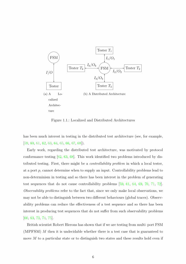
As a matter of fact, most CS generation approaches2 assume that the SUT interacts
with a single tester (Figure 1.1a). However, many systems interact with their environ-
ment at multiple physically distributed interfaces, called ports (Figure 1.1b). Examples
include communications protocols, cloud systems, web services, and wireless sensor net-
works. In testing such a system, we might place a separate independent (local) tester at
each port. The ISO standardised distributed test architecture dictates that while testing
there is no global clock and testers do not synchronize during testing [55]. However,
sometimes, rather than using the distributed test architecture, we allow the testers to
exchange coordination messages through a network in order to synchronise their actions
(see, for example, [56, 57, 58]). However, this can make testing more expensive, since
it requires us to establish a network to connect the local testers, and may not be feasi-
ble where there are timing constraints. In addition, the message exchange may use the
same network as the SUT and so change the behaviour of the SUT. As a result, there
2Such as HEN method given in [23], UWZ method given in [30], HIU method given in [29], SP
method given in [33], and DY method given in [54].
5
Tester
FSM
I/O
(a) A Lo-
calized
Architec-
ture
Tester T2
Tester T3
Tester T1
Tester Tk FSM
I1/O1
I2/O2
I3/O3
Ik/Ok
(b) A Distributed Architecture
Figure 1.1.: Localized and Distributed Architectures
has been much interest in testing in the distributed test architecture (see, for example,
[59, 60, 61, 62, 63, 64, 65, 66, 67, 68]).
Early work, regarding the distributed test architecture, was motivated by protocol
conformance testing [62, 63, 68]. This work identified two problems introduced by dis-
tributed testing. First, there might be a controllability problem in which a local tester,
at a port p, cannot determine when to supply an input. Controllability problems lead to
non-determinism in testing and so there has been interest in the problem of generating
test sequences that do not cause controllability problems [59, 61, 64, 69, 70, 71, 72].
Observability problems refer to the fact that, since we only make local observations, we
may not be able to distinguish between two different behaviours (global traces). Observ-
ability problems can reduce the effectiveness of a test sequence and so there has been
interest in producing test sequences that do not suffer from such observability problems
[60, 63, 73, 74, 75].
British scientist Robert Hierons has shown that if we are testing from multi–port FSM
(MPFSM) M then it is undecidable whether there is a test case that is guaranteed to
move M to a particular state or to distinguish two states and these results hold even if
6

M is deterministic [66]. In contrast, these problems can be solved in low order polyno-
mial time if we have a deterministic FSM M . If we restrict attention to controllable test
sequences3 then there are low-order polynomial time algorithms to decide whether there
is a separating sequence for two states [65] and to decide whether there is a controllable
sequence that forces M into a particular state [76]. However, as noted above, if we
use separating sequences then we require many test sequences to test a single transi-
tion. This motivates the final leg of this thesis: investigate computational complexity of
constructing PDSs and ADSs for distributed testing.
1.1. Contributions
The contributions of this thesis are manifold. However, we believe that all these contri-
butions aim to enhance FSM based testing by presenting new problems and investigating
their computational complexities, providing algorithms for the proposed problems and
introducing new problems.
The major contributions of our work can be summarized as follows:
1. We introduce several problems related to reset sequences: We investigate their
computational complexities.
2. We provide a rather unique way of reducing the length of checking sequences: We
propose several objective functions to minimize adaptive distinguishing sequences
and we show that constructing a minimum cost ADS is computationally hard
and hard to approximate. We provide two modifications on the existing ADS
construction algorithm that aim to construct minimum cost ADSs and provide
a new lookahead based algorithm to construct minimum cost ADSs. Finally,
we experimentally show that minimum cost ADSs can reduce the length of the
checking sequence by 29.20% on the average.
3. We show how the state identification capabilities of DSs can be utilized on FSMs
3Controllable test sequences are formally defined in Section 6.2.
7
that do not have a DS: We introduce the notion of Incomplete DSs. We investigate
the computational complexity of constructing such incomplete DSs and we provide
a heuristic to compute incomplete DSs. We experimentally show that the use of
incomplete DSs reduce the cost of checking experiments.
4. We investigate computational complexities of constructing preset and adaptive dis-
tinguishing sequences for distributed testing: We show that constructing adaptive
and preset distinguishing sequences are computationally hard. We left the bounds
of ADSs and PDSs as open problems. We consider DSs with limited size and
provide computational complexities of constructing such DSs. We also provide a
sub–class of multi–port FSMs where the PDS construction is decidable.
1.2. Outline of the Thesis
The organization of this thesis is as follows: Chapter 2, introduces some basic notation
that are going to be used throughout the thesis. In Chapter 3, we examine the problems
related to reset sequences, focusing mainly on computational complexities of open and
introduced problems. In Chapter 4, we describe the computational complexity of con-
structing minimum cost ADSs provide methods to construct minimum cost ADSs and
experimentally show what we can earn by using minimum cost ADSs while constructing
CSs. In Chapter 5, we introduce the notion of incomplete ADSs/PDSs, give compu-
tational cost of constructing them, and experimentally show the effect of using such
ADSs/ PDSs while constructing CEs. The Chapter 6 is devoted for the contributions
related to the distributed testing and in Chapter 7 we conclude the thesis.
All the proofs for Lemmas, Propositions, and Theorems of Chapter 3, Chapter 4,
Chapter 5 and Chapter 6 are given in Appendix A, Appendix B, Appendix C and
Appendix D, respectively.
8

2. Preliminaries
2.1. Finite State Machines
An FSM is formally defined as a 5-tuple M = (S, s0, X, Y, δ, λ) where:
• S is the finite set of states.
• X is the finite set of input symbols
• Y is the set of output symbols
• s0 is the initial state1
• δ is the transition function δ : S ×X → S
• λ is the output function λ : S ×X → Y
At any given time, M is at one of its states. If an input x ∈ X is applied when M is
at state s, M changes its state to δ(s, x) and during this transition, the output symbol
λ(s, x) is produced. It is assumed that only one input is applied at a time and similarly
only one output is produced at a time.
When δ and λ are described as functions as above, the FSM is called deterministic.
For an FSM which is not deterministic (in which case it is called non-deterministic), δ
and λ are defined as relations. In this thesis we will only be interested in deterministic
FSMs. To denote a transition from a state s to a state s′ with an input x and an output
y, we write (s, s′, x/y), where s′ = δ(s, x) and y = λ(s, x). We call x/y an input/output
1In this thesis we mostly omit the initial states from definitions of FSMs.
9
pair. For a transition τ = (s, s′, x/y), we use start(τ), end(τ), input(τ), output(τ), and
label(τ) to refer to state s (the starting state of τ), state s′ (the ending state of τ),
input x (the input of τ), output y (the output of τ), and input/output pair x/y (the
input/output label of τ), respectively.
An FSM M can be by a directed graph with a set of vertices and a set of edges. Each
vertex represents one state and each edge represents one transition between the states
of the machine M.
s1
s2
s3a/1
b/2
a/2
b/1
a/2b/1
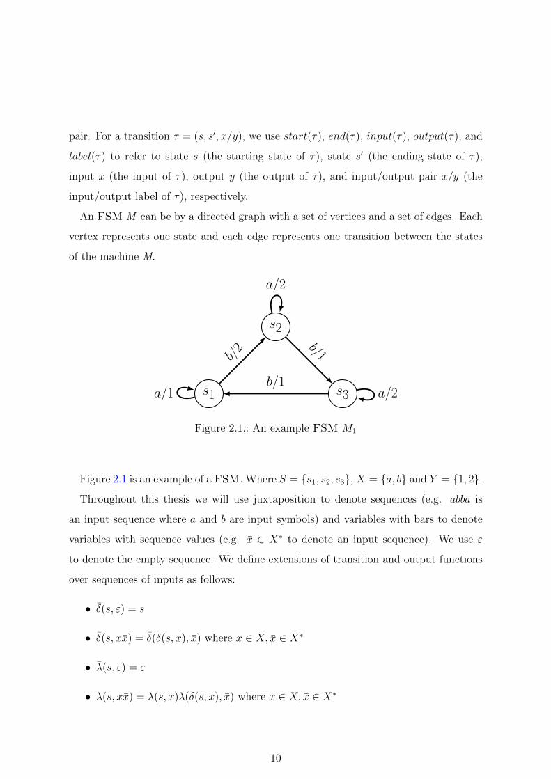
Figure 2.1.: An example FSM M1
Figure 2.1 is an example of a FSM. Where S = {s1, s2, s3}, X = {a, b} and Y = {1, 2}.
Throughout this thesis we will use juxtaposition to denote sequences (e.g. abba is
an input sequence where a and b are input symbols) and variables with bars to denote
variables with sequence values (e.g. x ∈ X∗ to denote an input sequence). We use ε
to denote the empty sequence. We define extensions of transition and output functions
over sequences of inputs as follows:
• δ(s, ε) = s
• δ(s, xx) = δ(δ(s, x), x) where x ∈ X, x ∈ X∗
• λ(s, ε) = ε
• λ(s, xx) = λ(s, x)λ(δ(s, x), x) where x ∈ X, x ∈ X∗
10

By abusing the notation, we will again use δ and λ instead of δ and λ.
A walk in M is a sequence (s1, s2, x1/y1), . . . , (sm, sm+1, xm/ym) of consecutive transi-
tions. This walk has starting state s1, ending state sm+1, and label x1/y1, x2/y2, . . . , xm/ym.
Here x1/y1, x2/y2, . . . , xm/ym is an input/output sequence, also called a global trace, and
x1, x2, . . . , xm is the input portion and y1, y2, . . . , ym is the output portion of this global
trace. An example walk in M2 of Figure 2.1 is τ = (s1, s2, b/2)(s2, s3, b/1), its starting
state is s1 and ending state is s3 its label is b/2 b/1, which has input portion bb and
output portion 2, 1.
An FSM M defines the language L(M) of labels of walks with starting state s0.
Likewise, LM(s) denotes the set of labels of walks of M with starting state s. For
example, L(M1) contains the global trace2 b/2, a/2 and LM1(s3) contains the global
trace b/1, b/2. Given S ′ ⊆ S we let LM(S ′) denote the set of labels of walks of M with
starting state in S ′ and so LM(S ′) = ∪s∈S′LM(s). Two states s, s′ are indistinguishable
or equivalent if LM(s) = LM(s′). Similarly, FSMs M and N are equivalent if L(M) =
L(N). An FSM M is said to be minimal if there is no equivalent FSM that has
fewer states. Assuming every state s of M is reachable we have that M is minimal if
and only if LM(s) 6= LM(s′) for all s, s′ ∈ S with s 6= s′. We write pre to denote a
function that takes a set of sequences and returns the set of prefixes of these, similarly
we write post to denote a function that returns the set of postfixes of these. Note that
if x1/y1, x2/y2, . . . , xm/ym is an input/output sequence then its prefixes are of the form
x1/y1, x2/y2, . . . , xn/yn for n ≤ m. Formal definitions for PDSs and ADSs (DSs) are
given respectively.
We use barred symbols to denote sequences and ε for the empty sequence. Suppose
that we are given a rooted tree K where the nodes and the edges are labeled. The term
internal node is used to refer to a node which is not a leaf. For two nodes p and q in
K, we say p is under q, if p is a node in the subtree rooted at node q. A node is by
definition under itself. Consider a node p in K. We use the notation pv (v for vertices)
to denote the sequence obtained by concatenating the node labels on the path from the
2Assume s1 is the initial state.
11

root of K to p excluding the label of p. The notation pv is used to denote the label of
p itself. Similarly, pe (e for edges) denotes the sequence obtained by concatenating the
edge labels on the path from the root of K to p. If p is the root, pv and pe are both
considered ε. For a child p′ of p, if the label of the edge from p to p′ is l, then we call
p′ the l–successor of p. In this thesis, we will always have distinct labels for the edges
emanating from an internal node, hence l–successor of a node will always be unique.
Definition 1 Given FSM M = (S,X, Y, δ, λ) and S, input sequence x is a Preset
Distinguishing Sequence (PDS) for S if for all s, s′ ∈ S with s 6= s′ we have that
λ(s, x) 6= λ(s′, x).
On the other hand, an ADS can be thought as a decision tree. The nodes of the tree
are labeled by input symbols, edges are labeled by output symbols providing that edges
emanating from a common node have different labels and leaves are labeled by state ids.
Definition 2 An Adaptive Distinguishing Sequence of an FSM M = (S,X, Y, δ, λ) with
n states is a rooted tree A with n leaves such that:
1. Each leaf of A is labeled by a distinct state s ∈ S.
2. Each internal node of A is labeled by an input symbol x ∈ X.
3. Each edge is labeled by an output symbol y ∈ Y .
4. If an internal node has two or more outgoing edges, these edges are labeled by
distinct output symbols.
5. For a leaf node p, λ(pv, pv) = pe (i.e. the state labeling a leaf node p produces the
output sequence labeling the path from the root to p to the input sequence labeling
the path from the root to p).
The use of ADS is straightforward: to identify the current state of the FSM apply
the input symbol that labels the current node of the tree, and select the outgoing edge
of the current node that is labeled by the output symbol produced by the FSM and read
12
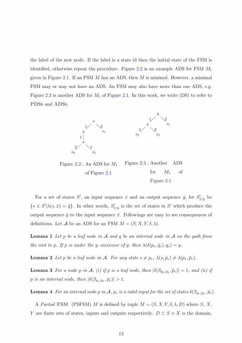
the label of the new node. If the label is a state id then the initial state of the FSM is
identified, otherwise repeat the procedure. Figure 2.2 is an example ADS for FSM M1
given in Figure 2.1. If an FSM M has an ADS, then M is minimal. However, a minimal
FSM may or may not have an ADS. An FSM may also have more than one ADS, e.g.
Figure 2.3 is another ADS for M1 of Figure 2.1. In this work, we write (DS) to refer to
PDSs and ADSs.
a
b
a
s3
2s2
1
1
1s1
2
Figure 2.2.: An ADS for M1
of Figure 2.1
b
b
s2
1s3
2
1s1
2
Figure 2.3.: Another ADS
for M1 of
Figure 2.1
For a set of states S ′, an input sequence x and an output sequence y, let S ′x/y be
{s ∈ S ′|λ(s, x) = y}. In other words, S ′x/y is the set of states in S ′ which produce the
output sequence y to the input sequence x. Followings are easy to see consequences of
definitions. Let A be an ADS for an FSM M = (S,X, Y, δ, λ).
Lemma 1 Let p be a leaf node in A and q be an internal node in A on the path from
the root to p. If p is under the y–successor of q, then λ(δ(pv, qv), qv) = y.
Lemma 2 Let p be a leaf node in A. For any state s 6= pv, λ(s, pv) 6= λ(pv, pv).
Lemma 3 For a node p in A, (i) if p is a leaf node, then |δ(Spv/pe , pv)| = 1, and (ii) if
p is an internal node, then |δ(Spv/pe , pv)| > 1.
Lemma 4 For an internal node p in A, pv is a valid input for the set of states δ(Spv/pe , pv).
A Partial FSM (PSFSM) M is defined by tuple M = (S,X, Y, δ, λ,D) where S, X,
Y are finite sets of states, inputs and outputs respectively. D ⊂ S ×X is the domain,
13

δ : D → S is the transition function, and λ : D → Y is the output function. If (s, x) ∈ D
then x is defined at s. Given input sequence x = x1x2 . . . xk and s ∈ S, x is defined at
s if there exist s1, s2, . . . sk ∈ S such that s = s1 and for all 1 ≤ i ≤ k, xi is defined at
si and δ(si, xi) = si+1. The transition and output functions can be extended to input
sequences as described above. An example PSFSM M1 is given in Figure 2.4 where
X = {a, b}, Y = {0, 1} S = {s1, s2, s3}. Note that input a is not defined at state s3.
s1
s2
s3
a/0
b/1
a/0
b/1
b/0
Figure 2.4.: PSFSM M1
Although DSs are important and useful on their own right, they are important for
another reason: they have been useful to solve fault detection problem.
Fault detection problem is referred to also as the machine verification or conformance
testing problem depending on the subject (i.e. it is refereed as conformance testing in
communication protocol spectra). Let us assume that we are given an FSM M with n
number of states, and a finite set φ(M) of all faulty FSMs such that each of which has
at most n number of states. Also let us assume that we are given an FSM N which
is known to be an implementation of M , the Fault Detection Problem is to decide if
N 6∈ φ(M). The Fault Detection Experiment is an experiment that solves the fault
14

detection problem. The underlying input sequence can be a CS or CE. A CS of M is an
input sequence starting at the initial state s0 of M that distinguishes M from any fault
implementation of M that is not isomorphic to M . (i.e., the output sequence produced
by any such N of φ(M) is different from the output sequence produced by M). Formally;
Definition 3 An input sequence x is a checking sequence if and only if λ(sM , x) 6=
λ(sN , x) where N ∈ φ(M), and sM , sN are initial states of FSMs M and N respectively.
On the other hand, a CE contains a set of input sequences called test sequences. A
test sequence is simply an input sequence. In testing we will apply the inputs from a test
sequence in the order specified and compare the outputs produced with those specified.
Definition 4 Given FSM M = (S,X, Y, δ, λ, s0) and integer m, a test suite T ⊆ X∗ is
a checking experiment if, for every FSM N = (S ′, X, Y, δ′, λ′, s′0) that has the same input
alphabet as M and no more than m states, N produces expected output for T if and only
if ∀x ∈ T we have that λ(s0, x) = λ(s′0, x).
2.1.1. Multi–port Finite State Machines
A multi-port finite state machine MPFSM is an FSM with a set P of ports at which
it interacts with its environment. The ports are physically distributed and each has its
own input/output alphabet. An input can only be applied at a specific port, and an
output can only be observed at a specific port. Therefore, for each port p ∈ P there is
a separate local tester that applies the inputs to p and observes the outputs produced
at p.
A deterministic MPFSM is defined by a tuple M = (P , S, s0, X, Y, δ, λ) where:
• P = {1, 2, . . . , k} is the set of ports.
• S is the finite set of states and s0 ∈ S is the initial state.
• X is the finite set of inputs and X = X1 ∪ X2 ∪ · · · ∪ Xk where Xp (1 ≤ p ≤ k)
is the input alphabet for port p. We assume that the input alphabets of the ports
15

are disjoint: for all p, p′ ∈ P , such that p 6= p′, we have Xp ∩ Xp′ = ∅. For an
input x ∈ X, we use inport(x) to denote the port to which x belongs and so
inport(x) = p if x ∈ Xp. We consider the projection of an input onto a port and
defined it as πp(x) = x if x ∈ Xp, and πp(x) = ε if x 6∈ Xp. The symbol “ε” will
be used to denote an empty/null input or output and also the empty sequence.
• Y =∏k
p=1(Yp ∪ {ε}) is the set of outputs where Yp is the output alphabet for port
p. We assume that the output alphabets of the ports are disjoint: for two ports
p, p′ ∈ P , such that p 6= p′, we have Yp ∩ Yp′ = ∅. An output y ∈ Y is a vector
〈o1, o2, . . . , ok〉 where op ∈ Yp ∪ {ε} for all 1 ≤ p ≤ k. We also assume that X is
disjoint from ∪1≤i≤kYk. The notation πp(y) is used to denote the projection of y
onto port p, which is simply the pth component of the output vector y. We define
outport(y) = {p ∈ P | πp(y) 6= ε}, which is the set of ports at which an output is
produced.
• δ is the state transfer function of type S ×X → S.
• During a state transition M also produces an output vector. The output function
λ : S ×X → Y gives the output vector produced in response to an input.
Let (s, s′, x/y) be a transition of M then we define inport(τ) = inport(x/y) =
inport(x) and we also define outport(τ) = outport(x/y) = outport(y) and finally we
define ports(τ) = ports(x/y) = {inport(x)}∪ outport(y) to denote the ports used in the
transition. Figure 2.5a gives an example of a 2-port MPFSM. The output and state
transfer functions can be extended to input sequences as usual.
Since we assume that the ports are physically distributed, no tester observes a global
trace: the tester connected to port p will observe only the inputs and outputs at p. We
use Σ to denote the set of global observations (inputs and outputs) that a hypothetical
global tester can observe and Σp to denote the set of observations that can be made at
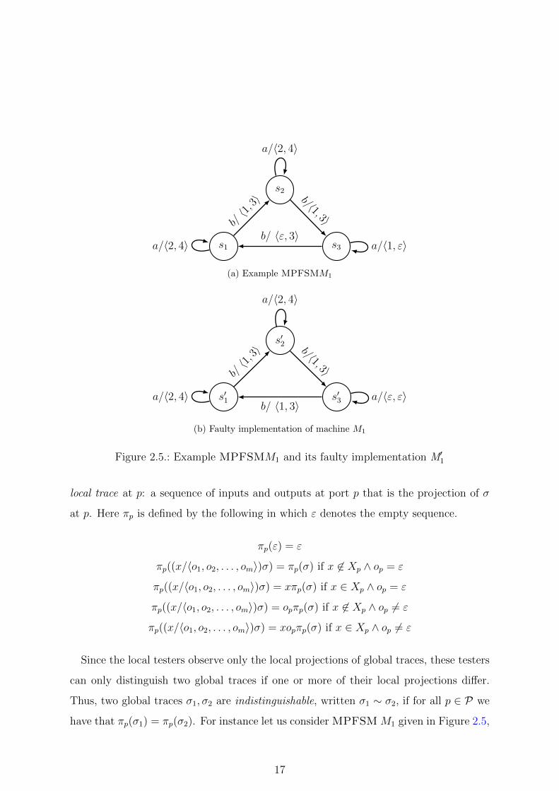
port p. Thus, Σ = X ∪ Y contains inputs and vectors of outputs while Σp = Xp ∪ Ypcontains only inputs and outputs at p. Let σ ∈ Σ∗ be a global trace, then πp(σ) is the
16
s1
s2
s3a/〈2, 4〉
b/〈1,
3〉
a/〈2, 4〉
b/〈1, 3〉
a/〈1, ε〉b/ 〈ε, 3〉
(a) Example MPFSMM1
s′1
s′2
s′3a/〈2, 4〉
b/〈1,
3〉
a/〈2, 4〉
b/〈1, 3〉
a/〈ε, ε〉b/ 〈1, 3〉
(b) Faulty implementation of machine M1
Figure 2.5.: Example MPFSMM1 and its faulty implementation M′1
local trace at p: a sequence of inputs and outputs at port p that is the projection of σ
at p. Here πp is defined by the following in which ε denotes the empty sequence.
πp(ε) = ε
πp((x/〈o1, o2, . . . , om〉)σ) = πp(σ) if x 6∈ Xp ∧ op = ε
πp((x/〈o1, o2, . . . , om〉)σ) = xπp(σ) if x ∈ Xp ∧ op = ε
πp((x/〈o1, o2, . . . , om〉)σ) = opπp(σ) if x 6∈ Xp ∧ op 6= ε
πp((x/〈o1, o2, . . . , om〉)σ) = xopπp(σ) if x ∈ Xp ∧ op 6= ε
Since the local testers observe only the local projections of global traces, these testers
can only distinguish two global traces if one or more of their local projections differ.
Thus, two global traces σ1, σ2 are indistinguishable, written σ1 ∼ σ2, if for all p ∈ P we
have that πp(σ1) = πp(σ2). For instance let us consider MPFSMM1 given in Figure 2.5,
17

s1
s2
s3
x 1/〈a,b〉,x 2
/〈ε,b〉 x
1 /〈a, b〉, x2 / 〈ε, b〉
x2/ 〈ε, b〉
x1/ 〈a, ε〉
Figure 2.6.: Example MPFSM M2
and global traces σ1 = b/〈1, 3〉, b/〈ε, 3〉, σ2 = b/〈ε, 3〉, b/〈1, 3〉, then π2(σ1) = 1, π1(σ1) =
b3b3, π2(σ2) = 1 and π1(σ2) = b3b3 and so σ1 ∼ σ2.
Recall that in distributed testing, the testers are physically distributed and they are
not capable of communicating between other testers. This reduced observational power
can lead to situations in which a traditional PDS or ADS fails to distinguish certain
states.
Example 1 Consider the FSM given in Figure 2.6. We have that x1x1 is a tradi-
tional PDS since it leads to different global traces from the states: from s1 we have
x1/〈a, b〉, x1/〈a, b〉; from s2 we have x1/〈a, b〉, x1/〈a, ε〉; and from s3 we have x1/〈a, ε〉, x1/〈a, b〉.
However, if we consider the local traces we find that x1x1 does not distinguish states s2
and s3 in distributed testing since in each case the project at port 1 is x1ax1a and the
projection at port 2 is b.
We can formalise this observation as follows.
Proposition 1 Given FSM M , a traditional PDS x of M might fail to distinguish
some states of M when local observations are made.
Since PDS defines an ADS the result immediately follows to ADSs.
Proposition 2 Given FSM M , a traditional ADS x of M might fail to distinguish
some states of M when local observations are made.
18

Therefore the definitions supplied for PDSs and ADSs are slightly different when we
consider distributed architectures. We will present formal definitions for such sequences
in Chapter 6.
2.1.2. Finite Automata
A Deterministic Finite Automaton (or simply an automaton) is defined by a triple
A = (Q,Σ, δ) where,
• Q is a finite set of states.
• Σ is a finite set of input alphabet.
• δ : Q× Σ→ Q is a transition function.
If δ is a partial function, A is called a partially specified automaton (PSA). Otherwise,
when δ is a total function, A is called a completely specified automaton (CSA). The
transition function can be extended for a sequence of input symbols in the usual way.
Moreover, for a Q ⊆ Q, we use δ(Q, x) to denote the set ∪q∈Qδ(q, x). For a PSA, a word
x ∈ Σ? is said to be defined at a state q ∈ Q, if ∀x′, x′′ ∈ Σ?,∀x ∈ Σ such that x = x′xx′′,
δ(δ(q, x′), x) is defined. Throughout this thesis, we use the term automaton to refer to
general automata (both PSA and CSA). We will specifically use PSA or CSA to refer
to the respective classes of automata.
A CSA A = (Q,Σ, δ) is synchronizable if there exists a word x ∈ Σ? such that
|δ(Q, x)| = 1. A synchronizable CSA has a reset functionality, i.e. it can be reset to
a single state by reading a special word. In this case x is called a reset word (or a
synchronizing sequence). Similarly, a PSA A = (Q,Σ, δ) is synchronizable if there exists
a word x ∈ Σ? such that x is defined at all states and |δ(Q, x)| = 1. Throughout this
thesis, we use terms reset word and synchronizing sequence interchangeably. It is known
that not all automata are synchronizing. We call such automata non–synchronizable
automata (NSA). A CSA is a monotonic CSA when states preserve a linear order <
under the transition function. In other words, a CSA A = (Q,Σ, δ) is monotonic if
19

for all q, q′ ∈ Q where q < q′ then we have that δ(q, a) < δ(q′, a) or δ(q, a) = δ(q′, a).
Similarly, a PSA is a monotonic PSA3 when states preserve a linear order < under the
transition function when they are defined. Formally, a PSA A = (Q,Σ, δ) is monotonic
if for all q, q′ ∈ Q where q < q′ such that both δ(q, a) and δ(q′, a) are defined, then we
have δ(q, a) < δ(q′, a) or δ(q, a) = δ(q′, a).
3It is called Partially Monotonic in [77]
20

3. Complexities of Some Problems
Related to Synchronizing,
Non-synchronizing and Monotonic
Automata
3.1. Introduction
A Reset Sequence / Reset Word, or a Synchronizing Sequence / Synchronizing Word of
an FSM M takes M to a specified state, regardless of the initial state of the M and
the output sequence produced by the M . As output sequence produced by M is not
important, the problem of constructing synchronizing sequence usually studied on finite
automata. Therefore in the rest of this chapter, we are going to consider finite automata.
As the need for reset operation is natural, synchronizing sequences are used in vari-
ous fields including automata theory, robotics, bio–computing, set theory, propositional
calculus and many more [4, 34, 38, 42, 48, 49, 78, 79, 80, 81, 82].
For instance, consider an automaton A = (Q,Σ, δ). The transition function introduces
functions on the set of states of the form fx : Q → Q for all x ∈ Σ, where fx(q) = q′
iff δ(q, x) = q′. Finding a synchronizing sequence can then be seen as the problem of
finding a composition g of the functions fx in the form g(q) = fx1(fx2(. . . fxk(q)))) such
that x1, x2, . . . , xk ∈ Σ and g is a constant function.
An other interesting example arises in bio–computing. In [80, 83] researchers use a set
21

of automata (in work [83] authors mentioned the number of automata is 3∗1012/µ`, and
can perform a total of 6.6∗1013 transitions per second) made of synthetic molecules and
the task is to construct reset sequences, which is a synthetic DNA made of synthetic nu-
cleotides, in order to be able to re-use the automata. Moreover, in [84] authors propose
an automaton called MAYA, a molecular automaton that plays TIC-TAC-TOE against
human opponent. Such an automaton, after a game ends, requires a reset word to bring
the automaton to the “new game state”. For a survey of automata based bio-computing,
we direct the reader to [85]. In model based testing, the checking experiment construc-
tion requires a synchronizing sequence to bring the implementation to the specific state
at which the designed test sequence is to be applied (e.g. see [26, 30, 31]).
On the other hand, for NSAs instead of resetting all the states in Q into a single state,
one may consider restricted type of reset operations, such as resetting into a given set of
states F ⊂ Q, or resetting a certain number K of states into F . A word x ∈ Σ? is called
K/F–reducing word for automata A = (Q,Σ, δ) if there exists a subset Q of states such
that δ(Q, x) ⊆ F and |Q| = K. A word x is called Max/F–reducing word for automata
A = (Q,Σ, δ) if x is a K/F–reducing work for A and there does not exist x′ and K′ > K
such that x′ is a K′/F–reducing word for A. These problems are introduced in [86] and
solved negatively.
3.1.1. Problems
Consider an FSM M such that W : X → Z+ be a function assigning a cost to each input
symbol of machine M and we have a budget K ∈ Z>0. Our aim is to extract subset of
these inputs such that the total implementation of costs of these inputs are not higher
than the budget and we can still construct a synchronizing sequence for the FSM M .
Suprisingly this problem is also find practical application in robotics. In the seminal
work [79], Natarajan studied a practical problem of automated part orienting on an
assembly line. He, having some assumptions, converted the parts orienting problem to
the problem of constructing synchronizing sequences for deterministic finite automata
as follows: He considered an assembly line on which parts to be process are dropped in
22

a random fashion. Therefore, the initial orientation of the parts are not known. The
next station that will process the parts, however, requires that parts have a particular
orientation. One can change the orientation of the parts on the assembly line by putting
some obstacles, or by using tilted surfaces. The task is to find a sequence of such orienting
steps such that no matter which orientation a part has at the beginning, it ends up in
a certain orientation after it passes through these orienting steps. Natarajan modelled
this problem as an automaton A as follows: he considers each orientation as a state and
orienting functions as input alphabet such that the reset word of A corresponds to a
sequence of orienting operations that brings these parts to unique orientation no matter
which orientation it started at. Following Natarajans analogy, we considered an assembly
line, a description of a part, and a set of tilt functions with implementation costs. Our
aim is to extract a subset of these tilt functions such that the total implementation
costs of these tilt functions are minimum and we can still rotate the part to a single
orientation.
A similar problem might appear in bio–computing. As discussed in [80, 83, 84] in
order to re-use automata one has to supply reset words (reset DNA’s) which made of
DNAs. As these DNA’s made of commercially obtained synthetic deoxyoligonucleotides,
it is sometimes possible, due to the lack of some nucleotides or due to the cost, for one
to construct reset DNA’s by the use of only a subset of nucleotides. That is, we want
to find the cheapest set of synthetic deoxyoligonucleotides to construct a synchroniz-
able subautomaton, knowing that we can construct reset DNA’s using the cheapest (or
available) synthetic deoxyoligonucleotides.
Now consider the automaton A = (Q,Σ, δ). Sub-automaton A|Σ with respect to Σ
is defined in the following way: A|Σ = (Q, Σ, δ′) where for two states s, s′ ∈ S and an
input x ∈ Σ, δ′(s, x) = s′ if δ(s, x) = s′. In other words, we simply keep the transitions
with the inputs in Σ and delete the other transitions from A. If A is a CSA, then so is
A|Σ. However, for if A is a PSA, we may have A|Σ as a PSA or a CSA.
We first formalize the problem for CSAs as follows:
Definition 5 Minimum Synchronizable Sub-Automaton Problem(MSS–Problem):
23

Let A = (Q,Σ, δ) be a synchronizable CSA, W : Σ→ Z+ be a function assigning a cost
to each input symbol, and K ∈ Z+. Find a sub-automaton A|Σ such that Σ ⊆ Σ and∑x∈Σ W (x) ≤ K and A|Σ is synchronizable.
We show that the MSS–Problem is an NP-complete problem, implying that the mini-
mization version of the MSS–Problem is NP-hard. We also show that the minimization
version is hard to approximate.
Having determined the complexity of the MSS–Problem for CSAs, we consider the
computational complexity of the MSS–Problem for PSAs. The primary motivation be-
hind to study PSAs is obvious; finite automata with partial transition function is a
generalization of completely specified finite automata; that is, partially specified au-
tomata can model a wider range of problems. The decision version of the MSS–Problem
for PSA is defined as follows:
Definition 6 Minimum Synchronizable Sub-Automaton Problem for PSA:
Let A = (Q,Σ, δ) be a synchronizable PSA, W : Σ→ Z+ be a function assigning a cost
to each input symbol, and K ∈ Z+. Find a sub-automaton A|Σ such that Σ ⊆ Σ and∑x∈Σ W (x) ≤ K and A|Σ is synchronizable.
We show that finding such partially specified sub automaton is PSPACE-complete.
Consider an FSM M such that taking M to a specified state is very expensive from a
subset of state and we want to construct a synchronizing sequence that takes FSM to a
specified state if and only if the current state of the FSM is not in this set. That is let
M = (S1 ∪ S2, X, Y, δ, λ) is given and our aim is to construct a synchronizing sequence
x such that δ(s, x) ∈ S if and only if s ∈ S1, where S ∈ S.
This problem might also appear in robotics, consider the Natarjans analogy again.
We are given an assembly line with a set of orienting functions and a set of parts. These
parts have identical shapes but they are made of different materials. The set of initial
positions of these parts are disjoint. Our aim is to find a sequence of tilt operations such
that we can orient a given part to predefined position where parts with different types
are guaranteed to be oriented at different positions. The problem is formally defined as
follows:
24

Definition 7 Exclusive Synchronizing-Word Problem for Synchronizable Automata
(ESW–SA): Given a synchronizable automaton A = (Q,Σ, δ) and subsets of states
Q ⊆ Q and F ⊂ Q. Is there a word x such that δ(q, w) ⊆ F if and only if q ∈ Q?
We show that although the underlying automaton is synchronizable this problem is
PSPACE-complete and there exist a constant ε > 0 such that approximating the maxi-
mization version of the problem within ratio nε is PSPACE-hard.
In the second part of this work, we investigate the computational complexities of
problems related to monotonic automata. In particular we consider Partially Specified
Monotonic Automata (PSMA) and Non-Synchronizing Monotonic Automata (NSMA).
In [87], Martyugin showed that constructing a reset word for a PSA is PSPACE-complete.
Recall that there exist a complexity reduction for computing shortest synchronizing
sequences when monotonic automata are considered [78, 34]. Hence it is natural to ask
if we have a similar complexity reduction for computing a synchronizing sequence when
we consider a monotonic PSA. However, until now no work revealed the complexity of
computing a synchronizing sequence for a given PSMA.
Definition 8 Synchronizability Problem for PSMA: Given a monotonic PSA
A = (Q,Σ, δ), is A synchronizable ?
Definition 9 Synchronizing Word Problem for PSMA: Given a monotonic
PSA A = (Q,Σ, δ), find a synchronizing sequence for A.
Definition 10 Minimum Synchronizing Word Problem for PSMA: Given a
monotonic PSA A = (Q,Σ, δ), find a shortest synchronizing word for A.
Unfortunately we show that these problems are at least as hard as NP-complete prob-
lems.
In [86] K/F–reducing problem is introduced as follows: “Given a non-synchronizable
automata A, is there a reset word that can reset K states into a set of states F?” and
they proved that it is PSPACE-complete for the general automata. Again we investigate
if monotonicity reduces the complexity of the original problem. The formal definition of
the problem is given as follows:
25

Definition 11 K/F−Reducing-Word Problem for Non-Synchronizable Monotonic
Automata (KFW–NSMA): Given a non-synchronizable monotonic automaton A =
(Q,Σ, δ), a constant K ∈ Z+, and a subset of states F ⊂ Q, find a K/F−reducing word
for automaton A.
We also study the maximization version of the problem.
Definition 12 Max/F Reducing-Word Problem for Non-Synchronizable Monotonic
Automata (MFW–NSMA): Given a non-synchronizable monotonic automaton A =
(Q,Σ, δ) and a subset of states F ⊆ Q, find a Max/F–reducing word for automaton A.
Although the underlying automata is monotonic, we report that they are all NP-hard prob-
lems.
The rest of the chapter is organized as follows: In the next three sections we discuss
and present our results related to MSS–Problem, ESW–SA problem and problems related
to monotonic automata, respectively. In the last section we summarize the key results
of this study and present some future directions.
3.2. Minimum Synchronizable Sub-Automaton Problem
We show that the MSS–Problem is computationally hard by reducing the Set Cover prob-
lem to the MSS–Problem.
In Set Cover problem, we are given a finite set of items U = {u1, u2, . . . , um} called
the Universal Set and a finite set of set of items C = {c1, c2, . . . , cn} where ∀c ∈ C, c ⊂ U .
A subset C ′ of C is called a cover if ∪c∈C′ = U . The problem is to find a cover C ′ where
|C ′| is minimized. The decision version of the Set Cover problem is NP-complete and
its optimization version is NP-hard [88, 89].
From a given instance (U,C) of Set Cover problem we construct an automaton
F(U,C) = (Q,Σ, δ) as follows: for each item u in the universal set U we introduce a
state qu and we introduce another state Sink. For each set of items ci ∈ C we introduce
an input symbol xi. We construct the transition function of the automaton F(U,C) as
follows:
26

• ∀qu ∈ Q \ {Sink}, ∀xi ∈ Σ
δ(qu, xi) =
Sink, u ∈ ciqu, otherwise
• ∀xi ∈ Σ, δ(Sink, xi) = Sink
Lemma 5 Let (U,C) be an instance of a Set Cover problem and C ′ = {c1, c2, . . . , cm}
be a cover. Then the sub-automaton F(U,C)|Σ is synchronizable, where Σ = {xi|ci ∈ C ′}.
Lemma 6 Let Σ = {x1, x2, . . . , xm} be a subset of alphabet of F(U,C) such that F(U,C)|Σis synchronizable. Then C ′ = {c1, c2, . . . , cm} is a cover.
Hence we reach to the following result.
Theorem 1 Given a synchronizable CSA A = (Q,Σ, δ) and a constant K ∈ Z+, it
is NP-complete to decide if there exists a set Σ ⊆ Σ such that |Σ| < K and A|Σ is
synchronizable.
Theorem 2 MSS–Problem is NP-complete.
In [90, 91] authors reported that the minimization version of the Set Cover problem
cannot be approximated within a factor in o(log n) unless NP has quasipolynomial time
algorithms. Moreover, it was also shown that Set Cover problem does not admit an
o(log n) approximation under the weaker assumption that P 6= NP [92, 93]. Therefore
relying on the construction of the automaton F(U,C), it is also possible for us to deduce
such inapproximability results apply to the MSS–Problem.
Lemma 7 Let OPTsc is the size of minimum cover for the Set Cover problem in-
stance (U,C), and let OPTΣ is the size of minimum cardinality input alphabet such that
F(U,C)|Σ is synchronizable. Then OPTsc = OPTΣ.
Theorem 3 MSS–Problem does not admit an o(log n) approximation algorithm unless
P = NP.
27

Although checking the existence and constructing one synchronizing sequence for a
CSA are polynomial time solvable problems, we seen that the MSS–Problem is NP-complete
for CSAs. That is, under the assumption that P 6= NP there is a complexity jump. Re-
call that in [87] Pavel Martyugin showed that it is PSPACE-complete to construct a reset
word for a PSA. Having these observations, it is natural to ask if there is a complexity
jump when we consider the MSS–Problem for PSAs.
Before going any further please note that for a synchronizable PSA A, the sub-
automaton A|Σ can be a CSA. To see that this is the case, consider a synchronizable
PSA with input alphabet {a, b, c} such that only input b is not defined at some states.
When we drop transitions that are labeled with input b, we obtain a completely speci-
fied automaton. Therefore since we showed, for CSAs, that the problem is NP-hard, we
assume that, from now on, for any non-empty subset Σ ⊂ Σ the sub-automaton A|Σ is
a PSA if and only if A is a PSA.
Lemma 8 MSS–Problem for PSA is in PSPACE.
Now we are going to show that MSS–Problem for PSA is PSPACE-hard.
Lemma 9 MSS–Problem for PSA is PSPACE-hard.
Finally using Lemma 8 and Lemma 9 we reach to the following conclusion.
Theorem 4 MSS–Problem for PSA is PSPACE-complete.
3.3. Exclusive Synchronizing Word Problems
In [86], Igor K. Rystsov considers the problem of constructing a word that synchronizes
a given set of states Q ⊂ Q at a given set of states F where the underlying automaton is
non–synchronizable. The problem is named as Inclusion Problem for the Weakly Syn-
chronizing Automaton. Rystsov showed that this problem is PSPACE-complete. However
the problem we consider here is different for two reasons: (1) We consider synchronizable
automata and (2) We prohibit resetting a state q ∈ Q at F .
28
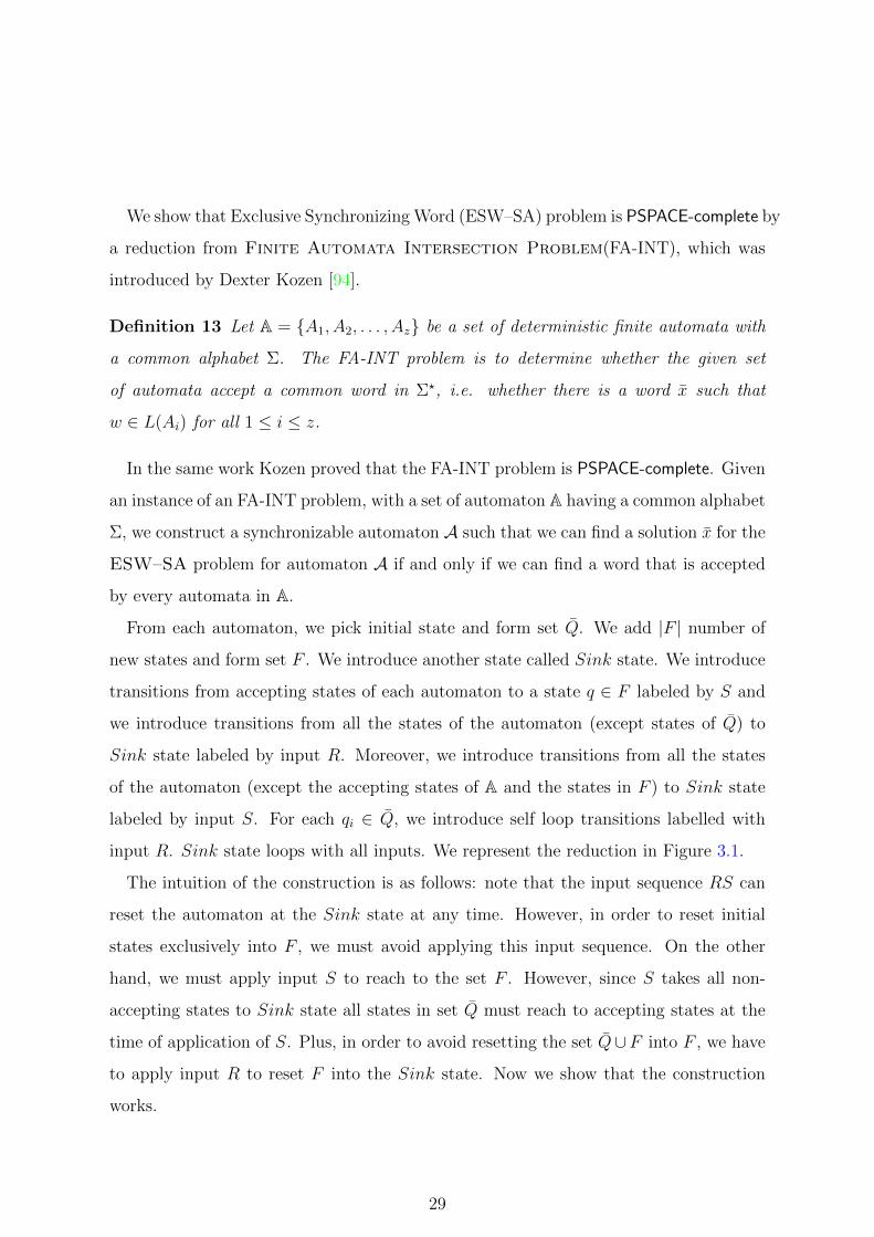
We show that Exclusive Synchronizing Word (ESW–SA) problem is PSPACE-complete by
a reduction from Finite Automata Intersection Problem(FA-INT), which was
introduced by Dexter Kozen [94].
Definition 13 Let A = {A1, A2, . . . , Az} be a set of deterministic finite automata with
a common alphabet Σ. The FA-INT problem is to determine whether the given set
of automata accept a common word in Σ?, i.e. whether there is a word x such that
w ∈ L(Ai) for all 1 ≤ i ≤ z.
In the same work Kozen proved that the FA-INT problem is PSPACE-complete. Given
an instance of an FA-INT problem, with a set of automaton A having a common alphabet
Σ, we construct a synchronizable automaton A such that we can find a solution x for the
ESW–SA problem for automaton A if and only if we can find a word that is accepted
by every automata in A.
From each automaton, we pick initial state and form set Q. We add |F | number of
new states and form set F . We introduce another state called Sink state. We introduce
transitions from accepting states of each automaton to a state q ∈ F labeled by S and
we introduce transitions from all the states of the automaton (except states of Q) to
Sink state labeled by input R. Moreover, we introduce transitions from all the states
of the automaton (except the accepting states of A and the states in F ) to Sink state
labeled by input S. For each qi ∈ Q, we introduce self loop transitions labelled with
input R. Sink state loops with all inputs. We represent the reduction in Figure 3.1.
The intuition of the construction is as follows: note that the input sequence RS can
reset the automaton at the Sink state at any time. However, in order to reset initial
states exclusively into F , we must avoid applying this input sequence. On the other
hand, we must apply input S to reach to the set F . However, since S takes all non-
accepting states to Sink state all states in set Q must reach to accepting states at the
time of application of S. Plus, in order to avoid resetting the set Q∪F into F , we have
to apply input R to reset F into the Sink state. Now we show that the construction
works.
29
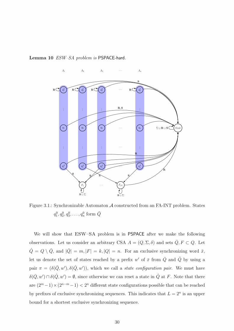
Lemma 10 ESW–SA problem is PSPACE-hard.
A1 A2 A3. . . An
q01 q0
2 q03
. . . q0n
......
.... . . ...
q1 q2 q3 . . . qn
......
.... . . ...
qA1 qA2 qA3 . . . qAn
F1. . . F|F |
Sink
R,S
R
S
R R R
R
R
SSS S
S ∪ Σ S ∪ Σ
Σ ∪R ∪ S
Figure 3.1.: Synchronizable Automaton A constructed from an FA-INT problem. States
q01, q
02, q
03, . . . , q
0n form Q
We will show that ESW–SA problem is in PSPACE after we make the following
observations. Let us consider an arbitrary CSA A = (Q,Σ, δ) and sets Q, F ⊂ Q. Let
Q = Q \ Q, and |Q| = m, |F | = k, |Q| = n. For an exclusive synchronizing word x,
let us denote the set of states reached by a prefix w′ of x from Q and Q by using a
pair π = (δ(Q, w′), δ(Q, w′)), which we call a state configuration pair. We must have
δ(Q, w′) ∩ δ(Q, w′) = ∅, since otherwise we can reset a state in Q at F . Note that there
are (2m−1)× (2n−m−1) < 2n different state configurations possible that can be reached
by prefixes of exclusive synchronizing sequences. This indicates that L = 2n is an upper
bound for a shortest exclusive synchronizing sequence.
30

Now we can propose a PSPACE algorithm for ESW–SA problem.
Lemma 11 ESW–SA problem is in PSPACE.
Consequently we have the following result.
Theorem 5 ESW–SA problem is PSPACE-complete.
We now consider the inapproximability of the ESW–SA problem. Condon et al
introduce the maximization version of the FA–INT problem [95].
Definition 14 Maximization of FA-INT Problem: Let A = {A1, A2, . . . , Am}
be a set of deterministic finite automata with input alphabet Σ. Maximum Finite
Automaton Intersection Problem(MAX FA-INT) problem is to find a subset A′
of A such that automata in A′ accept a common word w ∈ Σ?, and |A′| is maximized.
However they proved that it is PSPACE-hard to approximate MAX FA-INT problem
within a factor nε for ε > 0. As we reduce from the FA-INT problem, we can give a
similar result for the maximization version of the ESW–SA problem.
Definition 15 Max Exclusive Synchronizing Word for Synchronizable Au-
tomata (Max ESW–SA): Given a synchronizable automaton A = (Q,Σ, δ), subsets
Q and F of states Q, find a subset Q′ ⊆ Q where there exists an exclusive synchronizing
word for Q′ to F , such that |Q′| is maximized.
Lemma 12 Let A′ be a subset of A where automata in A′ has a common word and |A′|
is maximized. Also let Q′ be a subset of states Q of A, where there exists an exclusive
synchronizing word for Q′ to F and |Q′| is maximized. Then |Q′| = |A′|.
Therefore we reach to the following result.
Theorem 6 There exists a constant ε > 0 such that approximating Max ESW–SA
problem within ratio nε is PSPACE-hard.
31

3.4. Synchronizing Monotonic Automata
In this section we consider problems related to monotonic automata. We first show that
Synchronizability Problem for PSMA is an NP-hard problem by reducing the Exact
Cover problem which is defined as follows:
Definition 16 Exact Cover Problem: Let U = {1, 2, . . . ,m} be the universal set
and C = {c1, c2, . . . , cn} is a finite set of set of items such that ∀c ∈ C, c ⊂ U . Is there
a subset C ′ of C such that ∪c∈C′ = U and for all c, c′ ∈ C ′ we have c ∩ c′ = ∅.
Let us assume that we are given an instance of an Exact Cover problem (U,C).
We now introduce a reduction F that maps a given Exact Cover instance (U,C) into
a partially specified monotonic automaton F(U,C) = (Q,Σ, δ).
We form the set Q as follows: for each u ∈ U we introduce two states q0u and q1
u. We
refer to states with superscript 1 (i.e. q1u) as the satellite state of u and we refer to states
with superscript 0 (i.e. q0u) as the base state of u. The pair (q0
u, q1u) is called as the pair
set of u and denoted as Qu. Finally we introduce a state S such that the state set Q is
given as Q = {q0i |i ∈ U} ∪ {q1
i |i ∈ U} ∪ {S}.
The input alphabet and the transition function of the automaton F(U,C) are given
by:
• Σ = {x1, x2, . . . , x|C|} ∪ {X, Y }
• ∀q ∈ Q,∀x ∈ Σ
δ(q, x) =
q0u, if q = q0
u and x = xi where u /∈ ciq1u, if q = q0
u and x = xi where u ∈ ciq1u, if q = q1
u and x = xi where u /∈ ciq0u, if q ∈ {q1
u, q0u} where x = X
S, if q = q1u where x = Y
q01, if q = S and x = X
Clearly, any input sequence w ∈ Σ∗ must begin with input symbol X such that for any
q ∈ Q, δ(q,X) is a base state. Moreover, the transition structure of the automaton
32
F(U,C) allows us to reset Q into state S by input symbol Y only. However the input
Y is only defined at the satellite states. Therefore after the application of input symbol
X and before the application of input symbol Y , we must apply some input sequence
w ∈ Σ∗ such that for all states q ∈ Q of F(U,C) we have that δ(q, w) is a satellite state.
Moreover in order to take a base state q0u to a satellite state q1
u, we must apply an input
symbol xc if and only if u ∈ c. Besides since the input xc′ is defined at a satellite state
q1u if and only if u /∈ c′, input xc can appear in x at most once.
We demonstrate the reduction with an example. Let (U1, C1) be given as U1 =
{1, 2, 3, 4, 5, 6} and C1 = {(1, 2, 5), (3, 4, 6), (1, 4, 2)}. The automaton F(U1, C1) obtained
by the reduction is given in Figure 3.2:
q01 q1
1
q12q0
2
q13q0
3
q04 q1
4
q05 q1
5
q06 q1
6
S
X,x2 x1,x3
X,x2 x1,x3
X,x1,x3 x2
X,x1 x2,x3
X,x2,x3 x1
X,x1,x3 x2
x2X
Y
x2X
Y
x1,x3
X
Y
x1X
Y
x2,x3
X
Y
x1,x3
X
Y
X
Figure 3.2.: Monotonic Partially Specified Automaton F(U1, C1) constructed from
the Exact Cover instance U1 = {1, 2, 3, 4, 5, 6} and C1 =
{(1, 2, 5), (3, 4, 6), (1, 4, 2)}
The automaton is synchronizable (with word w = X12Y ), which suggests that the
corresponding Exact Cover problem instance has a solution (C ′ = {c1, c2}).
Now we show that the transition function of the automaton F(U,C) preserves some
linear ordering < of the states and so it is monotonic.
Lemma 13 Let (U,C) be an arbitrary Exact Cover problem instance, then the states
of the automaton F(U,C) admits a linear order for all input symbols in set Σ.
33
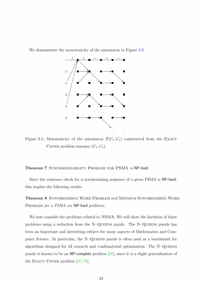
We demonstrate the monotonicity of the automaton in Figure 3.3.
S
q01
q11
q02
q12
q03
. . .
. . .
. . .
. . .
. . .
. . .
......
......
......
...
Y X x1 x2 x3
Figure 3.3.: Monotonicity of the automaton F(U1, C1) constructed from the Exact
Cover problem instance (U1, C1).
Theorem 7 Synchronizability Problem for PSMA is NP-hard.
Since the existence check for a synchronizing sequence of a given PSMA is NP-hard,
this implies the following results.
Theorem 8 Synchronizing Word Problem and Minimum Synchronizing Word
Problem for a PSMA are NP-hard problems.
We now consider the problems related to NSMA. We will show the hardness of these
problems using a reduction from the N–Queens puzzle. The N–Queens puzzle has
been an important and interesting subject for many aspects of Mathematics and Com-
puter Science. In particular, the N–Queens puzzle is often used as a benchmark for
algorithms designed for AI research and combinatorial optimization. The N–Queens
puzzle is known to be an NP-complete problem [96], since it is a slight generalization of
the Exact Cover problem [97, 98].
34

Definition 17 N Queens Puzzle: Given an integer N the N–Queens puzzle is to
produce a placements of N number of Queens on an N × N chessboard such that no
queen is under attack.
In the N–Queens puzzle, we have an N ×N chessboard, each cell being represented
by a pair (i, j) of integers with 1 ≤ i, j ≤ N . A cell is said to be occupied if there is
a queen at that cell. A queen can move an unlimited distance up and down, left and
right, and diagonally. Thus, a queen in cell (i, j) attacks another cell (n,m) (or a queen
in that cell) if i = n, or j = m, or |n− i| = |m− j|.
A cell that is attacked by a queen is said to be a dead cell ; otherwise it is called a live
cell. A simple case is demonstrated in Figure 3.4.
5 Z0Z0Z4 0Z0Z03 Z0Z0Z2 0Z0ZQ1 Z0Z0Z
a b c d e
a5 c5 e5
b4 d4
a3 c3 e3
b2 d2
a1 c1 e1
b5 d5
a4 c4 e4
b3 d3
a2 c2 e2
b1 d1
5 Z0Z0Z4 0Z0Z03 Z0Z0Z2 0Z0ZQ1 Z0Z0Z
a b c d e
a5 c5 e5
b4 d4
a3 c3 e3
b2 d2
a1 c1 e1
b5 d5
a4 c4 e4
b3 d3
a2 c2 e2
b1 d1
Figure 3.4.: A 5x5 Chessboard in which a queen is placed at board position (e, 2) (left
image). Chessboard places with red crosses are dead cells and chessboard
places with green squares are live cells (right image).
For a given an instance B of an N–Queens puzzle, we construct a monotonic au-
tomaton F(B) = (Q,Σ, δ) such that a solution to the N–Queens puzzle instance B
constitutes a solution to the KFW–NSMA problem for the automaton F(B).
For each board position (i, j), we introduce three states {q0i,j, q
+i,j, q
−i,j}. We group states
with (0), (−) and (+) superscripts as Q0, Q− and Q+ respectively i.e. Q = Q0∪Q−∪Q+
where Q0 = {q0i,j|1 ≤ i, j ≤ N}, Q− = {q−i,j|1 ≤ i, j ≤ N} and Q+ = {q+
i,j|1 ≤ i, j ≤ N}.
35

From now on states in Q+ ∪ Q− are called the satellite states and states in set Q0 are
called the board states.
The input alphabet and the transition function of F(B) are given as follows:
• Σ = {xi,j|1 ≤ i, j ≤ N}
• ∀q0i,j ∈ Q0,∀xk,l ∈ Σ
δ(q0i,j, xk,l) =
q+i,j, i = k, j = l
q−i,j, (i, j) attacks (k, l)
q0i,j, else
For a board state q0i,j, an input symbol xk,l is called an attacking input if (i, j)
attacks (k, l).
• ∀q ∈ Q+ ∪Q−,∀x ∈ Σ we have δ(q, x) = q
As a final, step we set K and the set F as follows: K = N +N2, F = Q+.
Before going any further, we first show that for any N–Queens puzzle instance B,
automaton F(B) is monotonic.
Lemma 14 Let B be an arbitrary N–Queens puzzle instance, the states Q of the au-
tomaton F(B) admits a linear order.
In Figure 3.5, we show that the states of the automaton F(B) admits a linear order. Due
to space limitations we present a small portion, however the reader can easily verify that
the linear order is preserved for all input symbols at all the states of the automaton.
Let w ∈ Σ? be a word that resets N + N2 states of the automaton F(B) at F . For
a decomposition w = w′xi,jx′′ of x, where w′, x′′ ∈ Σ?, xi,j is called an effective input if
δ(q0i,j, w
′) = q0i,j.
Lemma 15 Let w ∈ Σ? be a reset word that resets N + N2 states of the automaton
F(B) at F . Then x defines a solution for the N–Queens puzzle instance B.
36

q+1,1
q01,1
q−1,1
q+1,2
q1,2
q−1,2
. . .
. . .
. . .
. . .
. . .
. . .
......
......
......
......
x1,1 x1,2 x1,3 x1,4 x1,5 x1,6
Figure 3.5.: Monotonicity of the automaton F(B) constructed from the N–Queens in-
stance B.
Lemma 16 Let {(i1, j1), (i2, j2) , . . . , (iN , jN)} be a solution to the N–Queens puz-
zle. Then set of positions (i1, j1), (i2, j2) , . . . , (iN , jN) defines a solution for the KFW–
NSMA Problem for automaton F(B).
Theorem 9 KFW–NSMA Problem is NP-hard.
Note that given an N–Queens problem instance B, for automaton F(B) and let F =
Q+. In this case, there is a word x that resets at most N + N2 states at F , however
finding such a word is NP-hard. Therefore MFW–NSMA is NP-hard.
Theorem 10 MFW–NSMA Problem is NP-hard.
3.5. Chapter Summary and Future Directions
In this chapter we introduced several problems. In the first problem (MSS problem),
we assume that the input symbols of the underlying FSM (Automaton) have costs and
our aim is to extract a subset of input alphabet such that one can construct a reset
37

word using transitions that are labeled by symbols from the reduced input alphabet and
the cost of the reduced input alphabet is less than K. We show that if the transition
function of the underlying automata is a total function, then the problem is NP-complete.
Otherwise, if the transition function is partial then the problem is PSPACE-complete.
In the second problem we consider constructing an exclusive reset word (ESW-SA).
By exclusive we mean that the reset word resets a set of states and is guaranteed not
to reset states out of this set. We show that even if the underlying automaton is syn-
chronizable the problem is PSPACE-complete and there exists a constant ε > 0 such that
approximating the maximization version of the problem within ratio nε is PSPACE-hard.
Later we consider problems related to monotonic automata. We first consider mono-
tonic automata with partial transition functions. Monotonicity is a feature that simpli-
fies the complexity of the synchronizability problems. On the contrary, having a partial
transition function makes the related synchronizability problems harder. We investigated
the case when we have both of these features. We showed that checking the existence,
computing one and computing a shortest synchronizing sequence are NP-hard problems.
Later we consider non-snychronizing monotonic automata. We showed that resetting
K number of states (KFW–NSMA problem), or maximum number of states (MFW-
NSMA problem) of a monotonic non-synchronizing automaton are NP-hard problems.
In line with these results we can propose some future works. Hardness results indicate
that instead of exact algorithms we must design greedy algorithms for the problems
introduced in this work. Consequently, designing and implementing such greedy algo-
rithms for the MSS and the ESW–SA problems is one possible research direction. For
monotonic partially specified machines, the problems investigated in this Chapter are
shown to be NP-hard. It is also known that these problems are in PSPACE, since these
are partially specified. Hence, for these problems we currently have a gap and it remains
open to show whether these problems are in NP or PSPACE-hard. The upper bounds for
the KFW–NSMA and MFW–NSMA problems remain open. Thus it would also be an
interesting research direction to find upper bounds for these problems.
38

4. Hardness and Inaproximability of
Minimizing Adaptive Distinguishing
Sequences
4.1. Introduction
Usually, for a given specification M , a checking sequence is constructed and afterwards
the checking sequence is applied to all implementations of M . Due to this “construct
once and use many times” nature, one clearly desire a short checking sequence.
Until now, most of the efforts spent on to construct short checking sequences aim to
overlap the contents of the checking sequences to reduce their lengths. In this Chapter,
we consider a rather unique way of reducing the length of checking sequences. All ADS
based checking sequence generation methods start with the assumption that an ADS is
given. The given ADS is repeatedly applied within the checking sequence to identify the
states and to verify the transitions. These ADS applications form a considerably large
part of the checking sequence. Therefore we believe that reducing the size of ADSs is
a reasonable way to reduce the length of the checking sequences.
Earlier ADS construction algorithms [22, 21, 23] are exhaustive and require expo-
nential space and time. The only polynomial time algorithm was proposed by Lee and
Yannakakis (LY Algorithm). It can check if M has an ADS in O(pn log n) time [35],
and if one exists, we can construct an ADS in O(pn2) time [35]. Alur et al. show that
checking the existence of an ADS for non-deterministic FSMs is EXPTIME-complete [46].
39

Recently, Kushik et al. present an algorithm (KEY algorithm) for constructing ADSs
for non-deterministic observable FSMs [47]. We believe that the KEY algorithm can also
construct ADSs for deterministic FSMs, since the class of deterministic FSMs is a sub-
class of non-deterministic FSMs. However, since the KEY algorithm tends to construct
all subset of states for the state set, it may require exponential time and space.
In summary, these ADS construction algorithms are not guaranteed to compute the
minimum cost ADS for a given FSM. Moreover, to our knowledge, there is no work that
analyses the computational complexity of constructing minimum cost ADSs.
In this Chapter, we investigate the complexity of constructing minimum sized ADS.
We consider a number of different size definitions for an ADS, such as the height of
the ADS (MinHeightADS problem), the total root–to–leaf path length over all the
leaves of the ADS tree (MinADS problem), and the depth of a particular leaf node in
the ADS tree (MinSDS problem). We show that for each one of these definitions, the
minimization problem is hard to decide, and hard to approximate.
When the height of the ADS tree is considered as the size of an ADS, it was proven
by Sokolovskii that if an FSM M with n states has an ADS, the shortest ADS for M
cannot be longer than π2n2/12 [99]. A known lower bound is n(n− 1)/2 [35], i.e. there
exist FSMs with a shortest ADS of length n(n− 1)/2.
The LY algorithm can compute ADSs having the upper bound of n(n− 1)/2 for the
height of ADS and therefore matches this known lower bound. Thus, LY algorithm
can actually generate the minimum ADS for those FSMs with shortest ADS of height
n(n − 1)/2. However, LY algorithm is not guaranteed to produce a minimum ADS in
general. Although the use of a reduced ADS can be useful in several contexts (e.g.
for constructing test sequences), except the exhaustive algorithms [22, 21, 23], there is
no work in the literature on constructing reduced size ADS. As we emphasize, to our
knowledge, there is no work that analyses the computational complexity of constructing
minimum cost ADSs. As a matter of fact, in this work we show that this is a hard
problem and polynomial time algorithms for constructing an ADS, may not generate
minimum ADSs.
40
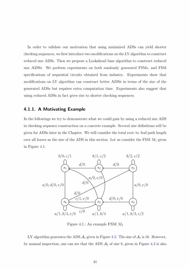
In order to validate our motivation that using minimized ADSs can yield shorter
checking sequences, we first introduce two modifications on the LY algorithm to construct
reduced size ADSs. Then we propose a Lookahead base algorithm to construct reduced
size ADSs. We perform experiments on both randomly generated FSMs, and FSM
specifications of sequential circuits obtained from industry. Experiments show that
modifications on LY algorithm can construct better ADSs in terms of the size of the
generated ADSs but requires extra computation time. Experiments also suggest that
using reduced ADSs in fact gives rise to shorter checking sequences.
4.1.1. A Motivating Example
In the followings we try to demonstrate what we could gain by using a reduced size ADS
in checking sequence construction on a concrete example. Several size definitions will be
given for ADSs later in the Chapter. We will consider the total root–to–leaf path length
over all leaves as the size of the ADS in this section. Let us consider the FSM M1 given
in Figure 4.1.
s1 s2 s3
s4s5s6
a/0, d/0, e/0
b/0, c/1
d/0
b/1, c/2
a/0, e/0
a/0, e/0
b/2, c/2
d/0
d/0, e/0
a/1, b/3, c/2
d/0
c/1, e/0
a/1, b/4
d/0
a/1, b/4, e/0c/0
Figure 4.1.: An example FSM M2
LY algorithm generates the ADSA1 given in Figure 4.2. The size ofA1 is 16. However,
by manual inspection, one can see that the ADS A2 of size 8, given in Figure 4.3 is also
41
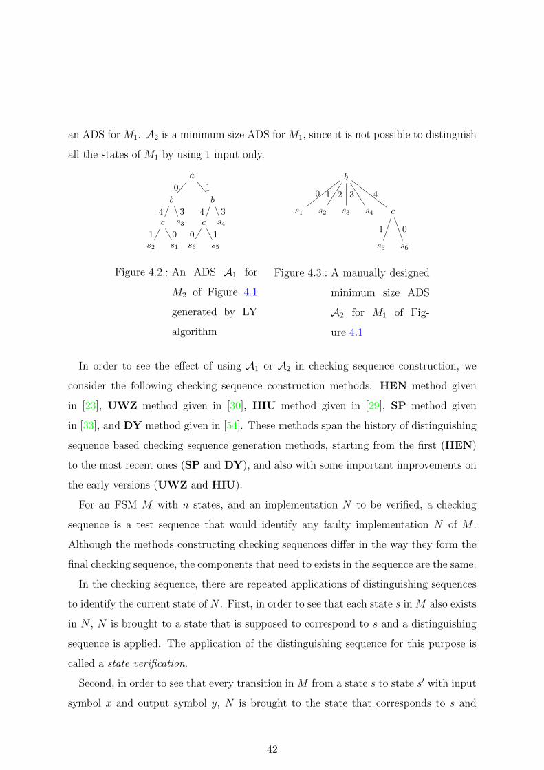
an ADS for M1. A2 is a minimum size ADS for M1, since it is not possible to distinguish
all the states of M1 by using 1 input only.
a
b
c
s2
1s1
0
4s33
0
b
c
s6
0s5
1
4s43
1
Figure 4.2.: An ADS A1 for
M2 of Figure 4.1
generated by LY
algorithm
b
s1
0
s2
1
s3
2
s4
3
c
s5
1
s6
0
4
Figure 4.3.: A manually designed
minimum size ADS
A2 for M1 of Fig-
ure 4.1
In order to see the effect of using A1 or A2 in checking sequence construction, we
consider the following checking sequence construction methods: HEN method given
in [23], UWZ method given in [30], HIU method given in [29], SP method given
in [33], and DY method given in [54]. These methods span the history of distinguishing
sequence based checking sequence generation methods, starting from the first (HEN)
to the most recent ones (SP and DY), and also with some important improvements on
the early versions (UWZ and HIU).
For an FSM M with n states, and an implementation N to be verified, a checking
sequence is a test sequence that would identify any faulty implementation N of M .
Although the methods constructing checking sequences differ in the way they form the
final checking sequence, the components that need to exists in the sequence are the same.
In the checking sequence, there are repeated applications of distinguishing sequences
to identify the current state of N . First, in order to see that each state s in M also exists
in N , N is brought to a state that is supposed to correspond to s and a distinguishing
sequence is applied. The application of the distinguishing sequence for this purpose is
called a state verification.
Second, in order to see that every transition in M from a state s to state s′ with input
symbol x and output symbol y, N is brought to the state that corresponds to s and
42

the input symbol x is applied (with the hope that y will be observed). In order to see
that N made a transition into the state that corresponds to s′, another application of
distinguishing sequence takes place. The application of the input symbol x followed by
the application of the distinguishing sequence is called transition verification.
Therefore, for a completely specified FSM M with n states and input alphabet X,
there will be n state verification and n|X| transition verification components, each one
having an application of the distinguishing sequence.
The state verification and transition verification components can be performed in any
order, and they are combined by using appropriate transfer sequences, which is an input
sequence that transfers M from one state to another state. The methods HEN, UWZ,
HIU, SP, and DY mainly differ in what order they consider state verification and
transition verification components, and how they select the transfer sequences to put
these components together. The earliest method we consider, HEN, imposes a prior
ordering of these components, and then finds the necessary transfer sequences to combine
the components. The later improvements on HEN (namely UWZ and HIU) let the
components be combined in any order (without fixing a prior ordering), hence they
are able to use shorter transfer sequences, using empty transfer sequences whenever
possible. Therefore, the total length of transfer sequences used in UWZ and HIU
is shorter compared to HEN. The most recent methods (SP and DY) even consider
overlapping these components, hence the transfer sequence lengths become even shorter.
For more details on these methods, we direct reader to the references [23, 30, 29, 33, 54].
Table 4.1 gives the length of checking sequences when A1 and A2 are used with these
methods.
The results on this single example are promising and show that reducing the height
of ADS does provide an opportunity to reduce the length of checking sequences. Of
course, an extensive set of experiments would establish a more convincing evidence in
this direction. We present the results of such experiments later in Section 4.5. We will
first focus on the question of whether it is possible to find minimum ADSs efficiently.
In order to show the hardness of constructing a minimum ADS, we will use reduc-
43

A1 A2 Reduction (%)
HEN 299 224 25%
UWZ 176 96 45%
HIU 158 92 41%
SP 149 111 25%
DY 105 83 20%
Table 4.1.: Comparison of checking sequence lengths for FSM M1
tions from known NP-complete problems. These problems are related to the binary
identification problem [100]. In next section we introduce this problem and review ex-
isting hardness results related to binary decision trees used in the context of the binary
identification problem.
4.2. Binary Decision Trees
Let Z = {z1, z2, . . . , zn} be a finite set of distinct objects and T = {t1, t2, . . . , tm} be a
finite set of tests where each test t ∈ T is a function t : Z → {0, 1}. Intuitively, when a
test t is applied to an object z, the object z produces the response t(z), i.e. either a 0
or a 1 is obtained as an answer.
The set of objects Z = {z1, z2, . . . , zn} and the set of tests T = {t1, t2, . . . , tm} can
also be presented as a table D[T, Z] (which we will call a decision table) with m rows
and n columns where the rows are indexed by the tests and the columns are indexed by
the objects. An element D[t, z] is set to the value t(z). Table 4.2 is an example of such
a decision table where there are 4 objects and 3 tests. A row corresponds to a test t and
it gives the vector of responses of the objects to t. Similarly, a column corresponds to an
object z and it gives the vector of responses of z to the tests. For a test t and an object
z, we will use the notation D[t, .] and D[., z] to refer to the row of D[T, Z] corresponding
to the test t and the column of D[T, Z] corresponding to the object z, respectively.
44

D z1 z2 z3 z4
t1 0 1 1 0
t2 1 0 1 0
t3 1 0 1 1
Table 4.2.: An example decision table
Suppose that we are given a decision table D[T, Z] and an unknown object from Z, and
we are asked to identify this object. One can apply all the tests in T and the results of
the tests will be corresponding to a unique column of the table identifying the unknown
object, provided that for all objects z ∈ Z, D[., z] is unique, which we will assume
throughout the work (as otherwise such an identification is not possible). Note that if
for a test t, D[t, .] is a row where every elements is 0 (or every element is 1), this means t
does not distinguish between any objects, hence the test t is useless for the identification
of the unknown object. Therefore, we assume that there is no such useless test t in
T . We can in fact find such useless tests and eliminate them in polynomial time, by
performing a single pass over the table D[T, Z]. Also note that if there are two different
tests t and t′ such that D[t, .] and D[t′, .] are the same, then the information provided
by t and t′ are the same, hence they are duplicate tests. We will also assume that no
such duplicate tests exist, as otherwise we can find and eliminate them in polynomial
time as well, by checking the equality of every pair of rows of D[T, Z].
Identifying an unknown object of Z by using tests in T can also be performed adap-
tively. In this case the procedure to be applied can be described in the form of a (binary)
decision tree T having the following properties.
Definition 18 A decision tree for a decision table D[T, Z] where Z = {z1, z2, . . . , zn}
and T = {t1, t2, . . . , tm} is a rooted tree T with n leaves such that:
1. Each leaf of T is labeled by a distinct object z ∈ Z.
2. Each internal node of T is labeled by a test t ∈ T .
45
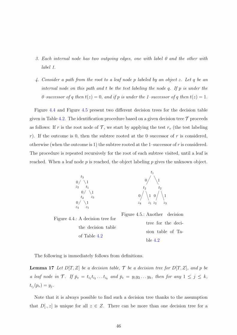
3. Each internal node has two outgoing edges, one with label 0 and the other with
label 1.
4. Consider a path from the root to a leaf node p labeled by an object z. Let q be an
internal node on this path and t be the test labeling the node q. If p is under the
0–successor of q then t(z) = 0, and if p is under the 1–successor of q then t(z) = 1.
Figure 4.4 and Figure 4.5 present two different decision trees for the decision table
given in Table 4.2. The identification procedure based on a given decision tree T proceeds
as follows: If r is the root node of T , we start by applying the test rv (the test labeling
r). If the outcome is 0, then the subtree rooted at the 0–successor of r is considered,
otherwise (when the outcome is 1) the subtree rooted at the 1–successor of r is considered.
The procedure is repeated recursively for the root of each subtree visited, until a leaf is
reached. When a leaf node p is reached, the object labeling p gives the unknown object.
t3
z20
t1
t2
z40
z11
0z31
1
Figure 4.4.: A decision tree for
the decision table
of Table 4.2
t1
t2
z4
0
z1
1
0
t2
z2
0
z3
1
1
Figure 4.5.: Another decision
tree for the deci-
sion table of Ta-
ble 4.2
The following is immediately follows from definitions.
Lemma 17 Let D[T, Z] be a decision table, T be a decision tree for D[T, Z], and p be
a leaf node in T . If pv = ti1ti2 . . . tik and pe = y1y2 . . . yk, then for any 1 ≤ j ≤ k,
tij(pv) = yj.
Note that it is always possible to find such a decision tree thanks to the assumption
that D[., z] is unique for all z ∈ Z. There can be more than one decision tree for a
46

given decision table, e.g. Figure 4.4 and Figure 4.5 are two different decision trees for
the decision table given in Table 4.2. Since the identification procedure for the unknown
object is directly based on the decision tree used, the cost of the procedure depends
on the decision tree. One may want to minimize this effort by using an appropriate
decision tree. However, there can be different measures that can be used to describe
the effort. Given a decision tree T and an object z ∈ Z, let dT (z) be the depth of the
leaf node labeled by z in T . For the decision tree in Figure 4.4, we have dT (z1) = 3,
dT (z2) = 1, dT (z3) = 2, and dT (z4) = 3. One measure can be the expected number
of tests to be applied, which corresponds to minimizing the sum∑
z∈Z dT (z) assuming
each object is equiprobable. Another measure can be the depth of the decision tree T
in order to minimize the worst case behaviour of the identification procedure based on
T . The following definitions state these problems formally.
Definition 19 MinDT problem: Given a decision table D[T, Z], find a decision tree T
such that∑
z∈Z dT (z) is minimized.
Definition 20 MinHeightDT problem: Given a decision table D[T, Z], find a decision
tree T such that max{dT (z)|z ∈ Z} is minimized.
Another measure can be motivated as follows. Suppose that the objects are diagnoses
in a medical emergency room where some binary tests are applied to reach a diagno-
sis. The tests all take the same amount of time, however one of the diagnosis is more
important than the others, since it requires a much more urgent action to be taken. In
such a case, the situation can be modeled as a binary identification problem, where one
would like to find a decision tree whose root–to–leaf path corresponding to this urgent
diagnosis is minimized. Definition 21 states the problem formally.
Definition 21 MinPathDT problem: Given a decision table D[T, Z] and an object
z ∈ Z, find a decision tree T such that dT (z) is minimized.
Decision version of the problems MinDT, MinHeightDT, and MinPathDT are
NP-complete [100, 101, 102]. Besides they are also known to be hard to approxi-
47

mate [103, 104, 105, 102]. In the following sections, we introduce analogous definitions
as minimization metrics for ADSs.
4.3. Minimizing Adaptive Distinguishing Sequences
Given an ADS A and a state s, let dA(s) be the depth of the leaf node labeled by the
state s in A. One measure that we can use to minimize ADSs can be the expected
number of inputs to be applied, which corresponds to minimizing the sum∑
s∈S dA(s)
assuming each state is equiprobable. Another measure can be the depth of the ADS A
in order to minimize the worst case behaviour of the state identification based on A.
The following definitions state these problems formally.
Definition 22 MinADS problem: Given an FSM M , find an ADS A for M such that∑s∈S dA(s) is minimized.
Definition 23 MinHeightADS problem: Given an FSM M , find an ADS A for M
such that max{dA(s)|s ∈ S} is minimized.
For an ADS A, let p be a leaf node labeled by a state s and let αs = pv. The input
sequence αs can be used to check whether an unknown state of M is s or not, since
for any state s′ 6= s, λ(s, αs) 6= λ(s′, αs) by Lemma 2. We call the sequence αs a state
distinguishing sequence (SDS) for s. In order to find an ADS in which an SDS for a
state s is minimized, one may want to solve the following problem.
Definition 24 MinSDS problem: Given an FSM M and a state s of M , find an ADS
A for M such that dA(s) is minimized.
It is also possible to consider a more general problem with the observation that,
each SDS given by an ADS may be used different number of times. As an illustration,
consider Figures 4.6, 4.7 and 4.8. There are thirteen incoming transitions of state s1,
and for each incoming transition, the SDS of s1 will be applied in a checking sequence
(see the discussion on transition verifications given in Section 4.1.1). Although the ADS
48

given in Figure 4.7 is better with respect to the MinADS problem, the length of the
SDS for the state s1 in this ADS is longer. Therefore, the ADS given in Figure 4.8 may
be preferred. The following problem definition is motivated by such uses of an ADS.
s1 s2
s3s4
a/0, b/0, c/0, d/1e/0
a/0, b/0, c/0
e/0
d/0
e/2, d/0
e/2
a/0, b/0, c/0
e/1, d/0
a/0, b/0, c/0
Figure 4.6.: An example
FSM M3.
e
s4
1
s3
2
e
s2
2
s1
0
0
Figure 4.7.: An ADS A1
for M3 of Fig-
ure 4.6.
d
s1
1
e
s2
0
s4
1
s3
2
0
Figure 4.8.: Another ADS
A2 for M3 of
Figure 4.6.
Definition 25 MinWeightedADS problem: Given an FSM M , let s be a state in M
and ws be a constant representing the weight for the state s. Find an ADS A for M
such that∑
s∈S(wsdA(s)) is minimized.
4.4. Modeling a Decision Table as a Finite State
Machine
The similarity between a decision table and an FSM is in fact clear. Objects and tests
in the given decision table correspond to the states and the inputs of the FSM that
will be generated. Hence applying a test will be corresponding to applying an input,
and the output to be produced in this case will be the response of the object to the
test. However, one major difference is the fact that objects do not change as the tests
are applied whereas states can perform a transition into another state when an input is
applied. In order to have the direct correspondence between the objects and the states,
we will have self looping transitions with the inputs corresponding to the tests. This
would yield an FSM where each state is isolated. We will add extra input symbols, one
49

for each state, to make the generated FSM strongly connected. The transitions with
these extra inputs will be defined in such a way that they cannot play any role in forming
an ADS. We now give the formal definition of the mapping of a decision table into an
FSM.
4.4.1. Mapping
We call the mapping function β which is formally defined below.
Mapping β: Given a decision table D[T, Z], we construct an FSM MD = (S,X, Y, δ, λ)
where
1. S = {sz|z ∈ Z}
2. X = XT ∪ XZ where XT = {xt|t ∈ T} and XZ = {xz|z ∈ Z} (we assume that
T ∩ Z = ∅)
3. Y = {0, 1, 2}
4. For a state sz ∈ S and an input xt ∈ XT , δ(sz, xt) = sz and λ(sz, xt) = t(z)
5. For a state sz ∈ S and an input xz′ ∈ XZ , δ(sz, xz′) = sz′ and λ(sz, xz′) = 2
As an example, for the decision table given in Table 4.2, the corresponding FSM is
given in Figure 4.9. The bold solid edges indicate the transitions for the inputs in XT ,
and the dashed edges indicate the transitions for the inputs in XZ .
Below, we assume that we are given a decision table D[T, Z] (which we will simply
refer as D) where T = {t1, t2, . . . , tm} and Z = {z1, z2, . . . , zn} and we assume that
MD is the FSM generated by using the mapping β given above. MD has n states and
n(n+m) transitions.
4.4.2. Hardness and Inapproximability Results
An FSM MD generated by the mapping β from a decision table D has two types of input
symbols, XT and XZ . We now prove that no ADS of MD would be able to use inputs
in XZ .
50
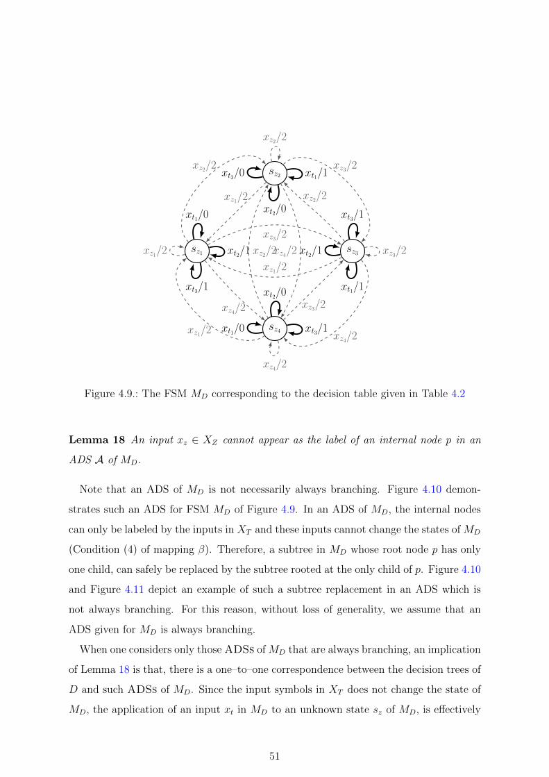
sz1
sz2
sz3
sz4
xt1/0
xt2/1
xt3/1
xz1/2
xz2/2
xz3/2
xz4/2
xt1/1
xt2/0
xt3/0
xz1/2
xz2/2
xz3/2
xz4/2
xt1/1
xt2/1
xt3/1
xz1/2
xz2/2
xz3/2
xz4/2
xt1/0
xt2/0
xt3/1xz1/2
xz2/2
xz3/2
xz4/2
Figure 4.9.: The FSM MD corresponding to the decision table given in Table 4.2
Lemma 18 An input xz ∈ XZ cannot appear as the label of an internal node p in an
ADS A of MD.
Note that an ADS of MD is not necessarily always branching. Figure 4.10 demon-
strates such an ADS for FSM MD of Figure 4.9. In an ADS of MD, the internal nodes
can only be labeled by the inputs in XT and these inputs cannot change the states of MD
(Condition (4) of mapping β). Therefore, a subtree in MD whose root node p has only
one child, can safely be replaced by the subtree rooted at the only child of p. Figure 4.10
and Figure 4.11 depict an example of such a subtree replacement in an ADS which is
not always branching. For this reason, without loss of generality, we assume that an
ADS given for MD is always branching.
When one considers only those ADSs of MD that are always branching, an implication
of Lemma 18 is that, there is a one–to–one correspondence between the decision trees of
D and such ADSs of MD. Since the input symbols in XT does not change the state of
MD, the application of an input xt in MD to an unknown state sz of MD, is effectively
51
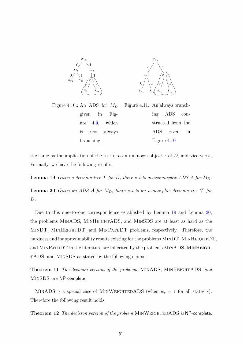
xt2
xt1
sz4
0sz2
1
0xt3
xt1
sz1
0sz3
1
1
1
Figure 4.10.: An ADS for MD
given in Fig-
ure 4.9, which
is not always
branching
xt2
xt1
sz4
0
sz2
1
0
xt1
sz1
0
sz3
1
1
Figure 4.11.: An always branch-
ing ADS con-
structed from the
ADS given in
Figure 4.10
the same as the application of the test t to an unknown object z of D, and vice versa.
Formally, we have the following results.
Lemma 19 Given a decision tree T for D, there exists an isomorphic ADS A for MD.
Lemma 20 Given an ADS A for MD, there exists an isomorphic decision tree T for
D.
Due to this one–to–one correspondence established by Lemma 19 and Lemma 20,
the problems MinADS, MinHeightADS, and MinSDS are at least as hard as the
MinDT, MinHeightDT, and MinPathDT problems, respectively. Therefore, the
hardness and inapproximability results existing for the problems MinDT, MinHeightDT,
and MinPathDT in the literature are inherited by the problems MinADS, MinHeigh-
tADS, and MinSDS as stated by the following claims.
Theorem 11 The decision version of the problems MinADS, MinHeightADS, and
MinSDS are NP-complete.
MinADS is a special case of MinWeightedADS (when ws = 1 for all states s).
Therefore the following result holds.
Theorem 12 The decision version of the problem MinWeightedADS is NP-complete.
52

Similarly, the inapproximability results existing in the literature for decision trees are
inherited by ADS minimization.
Theorem 13 For any constant c > 0, it is NP-hard to approximate MinADS and
MinWeightedADS problems within a ratio of (2− c).
Theorem 14 Unless P = NP, there cannot be an o(log n) approximation for Min-
HeightADS and MinSDS problems.
4.5. Experiment Results
As shown above, minimizing ADSs with respect to the metrics are hard. Therefore, the
best we can hope to do at this point is to design heuristic algorithms.
In this section, we first briefly describe LY algorithm and explain three modified
versions (GLY1, GLY2 and RLY) of LY algorithm. We compare these modifications
both with respect to the size of ADSs they produce, and with respect to the length of
checking sequences constructed by using these ADSs.
The experiments were carried out on a computer with an Intel Quad-Core CPU and
4GB RAM.
4.5.1. LY Algorithm
In this section, we briefly describe how LY algorithm given in [35] constructs an ADS
for a given FSM M = (S,X, Y, δ, λ).
An input sequence x ∈ X? is said to be a splitting sequence for a set S ′ ⊆ S of states,
if |λ(S ′, x)| > 1, and for any x′, x′′ ∈ X?, x ∈ X such that x = x′xx′′, x is a valid input
for δ(S ′, x′). An input symbol x ∈ X is called a valid input for a set of states S ⊆ S,
if the following holds: ∀si, sj ∈ S, si 6= sj, δ(si, x) = δ(sj, x) ⇒ λ(si, x) 6= λ(sj, x).
Intuitively, x is an input sequence such that at least two states in S ′ produce different
output sequences for x, and no two states in S ′ are merged without distinguishing them.
53

In other words, x splits S ′, hence the name. We call an input symbol x a splitting input
for S ′, if x is a splitting sequence of length one for S ′.
LY algorithm constructs an ADS tree in two steps as explained in the following
sections.
Forming a Splitting Tree
In the first step, LY algorithm constructs a tree called the splitting tree (ST). An ST is
a rooted tree where every node is associated with a set of states called a block (B ⊆ S)
and an input sequence (x ∈ X?). The leaves are labeled by singleton blocks and the
empty input sequence. The block of the root node is set to S. For an internal node p
labeled by a block B and an input sequence x, x is a splitting sequence for B. There is
a child node p′ of p for each y ∈ λ(B, x). The block of p′ is set to be the block Bx/y.
Therefore, the blocks of the children of an internal node p with block B is a partitioning
of B.
The construction of an ST starts by creating a partial ST with only the root node
with block B = S. This partial ST is processed iteratively, until all the leaves become
nodes with singleton blocks. In each iteration, a leaf node p in the partial ST is chosen,
where p has a block B such that |B| > 1. The algorithm finds a splitting sequence x
for B. The input sequence label of p is set to be x. The children of p are created as
explained in the previous paragraph.
The block of a node p is set when the node p is created. However, the input sequence
labeling a node is set when the algorithm processes the node p.
For our purposes, it is important to explain how a splitting sequence is found for a
block B. LY algorithm, first attempts to find a splitting input by considering every
input symbol x ∈ X. LY algorithm does not specify any specific order on the input
symbols to be considered for this check. Therefore, a typical implementation of LY
algorithm would use some fixed (possibly lexicographical) ordering of the input symbols
for this check. This is exactly where our modifications on LY algorithm take place. We
give the details of these suggested modifications in Section 4.5.2.
54

The partial ST can be expanded in this way as long as we can find leaf nodes for which
there exists a splitting input. When there is no such leaf node, the algorithm finds a
leaf node p in the partial ST with a block B, an input symbol x that is valid for B, an
internal node p′ with block B′ such that δ(B, x) ⊆ B′, and none of the children p′′ of
p′ has a block B′′ where δ(B, x) ⊆ B′′. The existence of such nodes p, p′ and the valid
input x are guaranteed when an ADS exists1. Since p′ is an internal node, it has been
processed by the algorithm before, and therefore there is a splitting sequence x labeling
the node p′. The splitting sequence to be used for p is then obtained as xx.
Forming an ADS
After the ST is constructed, LY algorithm uses the ST to construct a tree T that defines
an ADS. The tree T has a similar structure and construction with an ST. The difference
is that, in ST the initial states are considered, whereas in the construction of T , the final
states reached are considered.
Each node p of T is associated with an input sequence X (p) and with a set of states
B(p). The edges of T are labeled by output sequences. For a leaf node p of T , we have
|B(p)| = 1 and X (p) = ε. For an internal node p, |B(p)| > 1.
Let p be an internal node in T with X (p) = x and B(p) = B. Also let p′ be a child
of p, where the edge from p to p′ is labeled by an output sequence y. In this case,
B(p′) = δ(Bx/y, x). Note that unlike ST, the states labeling the children of a node p do
not necessarily form a partition of B(p).
The construction of T is performed iteratively. First a partial tree is created which
only includes the root node p of T , with B(p) = S. As long as there is a leaf node p
where B(p) = B with |B| > 1 in the partial tree, p is processed in the following way.
The ST is consulted to find the deepest node p′ in ST such that the block B′ of p′ in
ST includes B, i.e. B ⊆ B′. Let x be the splitting sequence labeling p′ in ST. Then,
X (p) is set to x and for each y ∈ λ(B, x), a child p′′ of p is created in T , by setting
1Since the proof of correctness of LY algorithm is out of scope of this Thesis, we refer the reader
to [35] to see why such nodes have to exist in the partial ST.
55
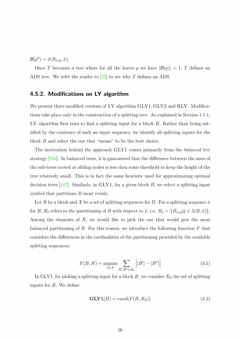
B(p′′) = δ(Bx/y, x).
Once T becomes a tree where for all the leaves p we have |B(p)| = 1, T defines an
ADS tree. We refer the reader to [35] to see why T defines an ADS.
4.5.2. Modifications on LY algorithm
We present three modified versions of LY algorithm GLY1,GLY2 and RLY. Modifica-
tions take place only in the construction of a splitting tree. As explained in Section 4.5.1,
LY algorithm first tries to find a splitting input for a block B. Rather than being sat-
isfied by the existence of such an input sequence, we identify all splitting inputs for the
block B and select the one that “seems” to be the best choice.
The motivation behind the approach GLY1 comes primarily from the balanced tree
strategy [106]. In balanced trees, it is guaranteed that the difference between the sizes of
the sub-trees rooted at sibling nodes is less then some threshold to keep the height of the
tree relatively small. This is in fact the same heuristic used for approximating optimal
decision trees [107]. Similarly, in GLY1, for a given block B, we select a splitting input
symbol that partitions B most evenly.
Let B be a block and X be a set of splitting sequences for B. For a splitting sequence x
for B, Bx refers to the partitioning of B with respect to x, i.e. Bx = {Bx/y|y ∈ λ(B, x)}.
Among the elements of X , we would like to pick the one that would give the most
balanced partitioning of B. For this reason, we introduce the following function F that
considers the differences in the cardinalities of the partitioning provided by the available
splitting sequences:
F (B,X ) = argminx∈X
∑B′,B′′∈Bx
∣∣∣|B′| − |B′′|∣∣∣ (4.1)
In GLY1, for picking a splitting input for a block B, we consider XB the set of splitting
inputs for B. We define:
GLY1(B) = rand(F (B,XB)) (4.2)
56

where the function rand(.) chooses an element of the set given as its input randomly2.
In GLY2, we aim to select input symbol x in XB that maximizes the size of the
partitioning Bx, without concerning the sizes of the elements in Bx. If there are two or
more input symbols that give the same maximum value, among these the one that gives
the most even partitioning is chosen by using the function F . Formally,
GLY2(B) =
x′, if argmaxx∈XB|Bx| = {x′}
F (B, argmaxx∈XB|Bx|), otherwise
(4.3)
Besides these versions, we also consider a version of the LY algorithm in which a
splitting input is selected randomly. We call this version as RLY and formally for a
block B, we have
RLY(B) = rand(XB) (4.4)
Except these modifications, GLY1, and GLY2 are exactly the same as LY algo-
rithm. Similarly, instead of LY, from now on we write FLY to refer to version of the
LY algorithm which chooses the splitting input according to some fixed ordering (i.e.
alphabetical ordering).
4.5.3. A Lookahead Based ADS Construction Algorithm
In this subsection, we explain the details of the proposed algorithm to construct a re-
duced ADS for an FSM M = (S,X, Y, δ, λ) which is minimal, deterministic, completely
specified and known to have an ADS. Before presenting the details of the actual al-
gorithm, we provide some definitions and routines that are going to be used in this
section.
In [24] Hennie introduces the use of a tree, called the successor tree, for construct-
ing adaptive homing/distinguishing sequences. The successor tree grows exponentially
and it possesses information that can be used to find the minimum cost adaptive hom-
ing/distinguishing sequences. However since it grows exponentially (with the number of
states), it becomes impractical to construct a successor tree to obtain a reduced adaptive
homing/distinguishing sequences as the size of the FSM gets larger.
2Note that operators argmin/argmax return the set of arguments achieving the optimum value.
57

Our method has two phases. In the first phase, a tree called the Enhanced Successor
Tree (EST) similar to a successor tree is generated. In the second phase, EST is used to
construct an ADS.
An EST contains two types of nodes; input nodes I and output nodes O. The root
and the leaves of an EST are output nodes. Except the leaves, the children of an output
node are input nodes, and the children of an input node are output nodes. In other
words, on a path from the root to a leaf, one observes a sequence of output and input
nodes alternatingly, starting and ending with an output node.
Each input node p is labeled by an input symbol in(p). Similarly, each output node
q is labeled by an output symbol out(q), except the root node for which out(q) = ε. An
output node q is also associated with a block bl(q). For the root node q, bl(q) = S. An
output node q is a leaf node iff |bl(q)| = 1. A non-leaf output node q that is associated
with a block bl(q), has a separate input node p as its child for each input symbol x that
is valid for bl(q), with in(p) = x. An input node p (where x = in(p)) with a parent
output node q (where B = bl(q)), has a separate output node r as its child for each
output symbol y ∈ λ(B, x), with out(r) = y and bl(r) = δ(Bx/y, x).
The EST of an FSM M is potentially an infinite tree. Instead of the whole tree, the
algorithm constructs a limited size partial EST, using which an ADS can be produced.
The algorithm uses heuristic approaches to explore the relevant and promising parts of
the EST to find a reduced size ADS with respect to different metrics, such as the height
and the external path length.
The partial EST constructed by the algorithm will be the EST where the tree is
pruned at several nodes. For a leaf q in an EST we have |bl(q)| = 1. However, for a leaf
node q in a partial EST, we have |bl(q)| ≥ 1.
Initially, the algorithm starts with the partial EST consisting of only the root node. In
each iteration, an output node q is handled and the partial EST rooted at q is expanded
exhaustively upto depth k, where k is a parameter given to the algorithm. Among the
children of q, an input node p that seems to be the best (according to the objective
and the heuristic being used) is selected, and the search continues recursively under the
58

subtrees rooted at the children of p.
During the construction of the partial EST T , some nodes are marked as the nodes to
be used for ADS construction later. Namely, a set of output nodes L and a set of input
nodes I are marked. Each output node q ∈ L has the property that |bl(q)| = 1 and it
corresponds to a leaf node in the ADS that will be constructed later. Also the nodes in
I will be corresponding to the non–leaf nodes of the ADS.
The algorithm constructing a partial EST is given in Algorithm 1.
Algorithm 1: Construct a partial EST for MInput: FSM M = (S,X, Y, δ, λ), k ∈ Z≥1
Output: A partial EST T , a set of leaves L, and a set of input nodes I
begin
1 L← ∅, I ← ∅
2 Construct an output node q0 with bl(q0) = S, out(q0) = ε
3 Initialize T to be a tree consisting of the root q0 only
4 Q← {q0} // Q is the set of output nodes yet to be processed
5 while Q 6= ∅ do
6 Pick an output node q ∈ Q to process
7 Q← Q \ {q}
8 ExpandEST(q,k) // expand subtree under q exhaustively upto a certain depth
9 Choose a child node p of q // based on the objective and the heuristic used
10 I ← I ∪ {p} // The input node p will be used for the ADS
11 foreach child r of p do
if |bl(r)| > 1 then
12 Q← Q ∪ {r} // not a singleton yet, needs to be processed
else
13 L← L ∪ {r} // reached a singleton block
The procedure “ExpandEST(q, k)”, constructs the partial EST rooted at the node q
exhaustively upto the given depth k. If in this partial subtree, for every leaf node r,
we have |bl(q)| = |bl(r)| (which means the block bl(q) could not be divided into smaller
blocks by using input sequences of length upto k that are valid for bl(q)), the procedure
increases the depth of the subtree rooted at q until it encounters a level at which there
exists a leaf node r with |bl(r)| < |bl(q)|. Clearly, this is always possible since the FSM
M has an ADS.
At line 9 of Algorithm 1, a child node p of q is chosen heuristically. This choice is based
on the scores of the nodes which are calculated by processing the nodes in the subtree
59

rooted at q in a bottom–up manner. First the scores of the leaves in this subtree are
assigned. This is followed by the score evaluation of the internal nodes in the subtree.
The score of a non–leaf node depends on the scores of its children. The score of a node
reflects the potential size of the ADS that will be eventually formed if that node is
decided to be used in the ADS to be formed.
When the score of an output node q is computed based on the scores of its children,
since we have the control over the input to be chosen, the child node of q having the
minimum score is chosen. However, when the score of an input node p is computed
based on the scores of its children, since we do not have the control of the output to
be produced, we prepare for the worst and use the maximum score of the children of
p. A similar approach is in fact also suggested by Hennie [24] (please see Chapter 3).
The process of calculating the scores of the nodes depends on the heuristic used and the
details are given in Section 20.
Before presenting the algorithm to construct an ADS, we will give some properties of
the nodes L and I marked by Algorithm 1. For an output node q, consider the path
from the root of T to q (including q). Let w and v be the concatenation of input symbols
and output symbols on this path, respectively. We use below the notation io(q) to refer
to the input/output sequence w/v.
Proposition 3 Let q be an output node in T , let io(q) = w/v. Then we have bl(q) =
δ(Sw/v, w).
Proposition 4 |L|+∑
q∈Q |bl(q)| = |S| is an invariant of Algorithm 1 before and after
every iteration the while loop.
Proposition 4 implies the following result, since when Algorithm 1 terminates we have
Q = ∅.
Corollary 1 When Algorithm 1 terminates, |L| = |S|.
Proposition 5 Let q be an output node in T with |bl(q)| = 1, and let w/v = io(q).
There exists a unique state s ∈ S such that λ(s, w) = v.
60

Algorithm 2 describes how an ADS can be constructed based on the partial EST T ,
the set of marked nodes L and I in T by Algorithm 1. Note that at line 6 of Algorithm 2,
Sw/v is claimed to be a singleton, which is guaranteed by Proposition 5. In order to show
that A which is generated by Algorithm 2 is an ADS, we also prove the following.
Proposition 6 The leaves of A constructed by Algorithm 2 is labeled by distinct states.
Theorem 15 A constructed by Algorithm 2 is an ADS.
Algorithm 2: Construct an ADSInput: The partial EST T , the set of marked nodes L and I by Algorithm 1
Output: An ADS A
begin
// Construct and label the internal nodes of A
1 foreach node p ∈ I do
2 Construct an internal node p′ in A
3 Label p′ by in(p)
// Construct and label the leaf nodes of A
4 foreach node q ∈ L do
5 Let w/v = io(q)
6 Let s be the state such that {s} = Sw/v
7 Construct a leaf node q′ in A
8 Label q′ by s
// Construct the edges to the leaves
9 foreach leaf node q′ ∈ A do
10 Let q be the corresponding node of q′ in T
11 Let p be the parent of q in T
12 Let p′ be the corresponding node of p in A
13 Insert an edge between p′ and q′ with the label out(q)
// Construct the remaining edges
14 foreach internal node p′ ∈ A do
15 Let p be the corresponding node of p′ in T
16 if p has a grandparent in T then
// except the root of A
17 Let q be the parent of p in T
18 Let r be the parent of q in T
19 Let r′ be the corresponding node of p in A
20 Insert an edge between p′ and r′ with the label out(q)
61

Heuristics
We use different heuristic approaches to minimize the size of ADSs with respect to two
different metrics, which are minimizing the height and minimizing the external path
length of the ADS.
As mentioned above, the score of a node q in the partial EST constructed so far is
an estimation of the size of the ADS that will be formed by using a child of q in ADS.
Let d(q) be the depth of q in the EST and v(q) be the score of q. We also keep track
of another information, z(q). It is the number of singleton output nodes in the winner
subtrees under q in the current partial EST, and used to break the ties as explained
below.
Let us consider a leaf node q, where |bl(q)| = 1. This is in fact a leaf node also in
the complete EST. For such leaf nodes, we set v(q) = d(q) and z(q) = 1. However, for
a leaf node q in the current partial EST with |bl(q)| > 1, we set z(q) = 0. Although
q is currently a leaf node in the partial EST, if we were to expand q, there will appear
a subtree under q. In order to take into account the size of the subtree rooted at q
(without actually constructing this subtree), we need to estimate the size of the subtree
under q. Note that bl(q) is the set of states yet to be distinguished from each other.
We consider two different metrics as the size of an ADS: height or external path length.
Depending on the objective, we estimate the size of the subtree that would appear under
a (yet to be processed) output node q in different ways. While minimizing for height,
we use two different heuristic functions HU : O → R+ and HLY : O → R+. Similarly,
while optimizing for external path length, we use heuristic functions LU : O → R+ and
LLY : O → R+.
For an FSM with n states the height of an ADS is bounded above by n(n− 1)/2 [35].
We use this bound for heuristic functions HU and LU in the following way. The score
of node q with respect to function HU is given as HU(q) = d(q) + |bl(q)|(|bl(q)| − 1)/2,
where d(q) is the depth of q. On the other hand, function LU multiplies the number
of states with the expected height of the subtree to approximate the expected external
path length. That is, LU(q) = (d(q) + |bl(q)|(|bl(q)| − 1)/2)|bl(q)|.
62

As another estimation method for the size of the subtree to appear under an output
node q, one can use LY algorithm to construct an ADS for the states in bl(q). The
heuristic functions HLY and LLY use this idea. Let A′ be the ADS computed by LY
algorithm for the states in bl(q), and let hA′ and lA′ be the height and the external
path length of A′. Then the heuristic functions HLY and LLY are defined as HLY (q) =
d(q) + hA′ and LLY (q) = d(q)|bl(q)|+ lA′ .
At line 9 of Algorithm 1, for the output node q being processed in that iteration, an
input node p which is a child of q is chosen. Let T ′ refer to the subtree rooted at q in the
partial EST at this point. While choosing the child input node p to be used, the scores
of the nodes in T ′ are calculated in a bottom up manner. First, for each (current) leaf
node q′ (which is an output node) in T ′, v(q′) is assigned by using one of the heuristic
functions (HU(q′) or HLY (q′) for height optimization, and LU(q′) or LLY (q′) for external
path length optimization) and z(q′) is assigned. The score of the remaining nodes in T ′
are based on the scores of its children and are calculated as follows.
When minimizing for height, for an input node p′, v(p′) is set to the maximum score of
its children and z(p′) is set to the sum of singleton scores of its children. For an output
node q′, v(q′) is set to the minimum score of its children, and z(q′) is set to the z(.)
value of the winner child. When minimizing for external path length, for an input node
p′, v(p′) and z(p′) is set to the sum of the scores of its children. For an output node
q′ on the other hand, v(q′) is set to the minimum score of its children and z(q′) is set
to the z(.) value of the winner child. Note that, there may be ties during this process
when we attempt to take minimum or maximum. Among the nodes achieving the same
minimum/maximum, the tie is first tried to be broken by maximizing the number of
singleton values (z(.)). If still there is a tie, this is broken randomly. From now on we
will write LEA to refer to the Lookahead driven ADS construction algorithm on EST.
We present a summary of the heuristics and algorithms used in this section in Table ??.
63

Table 4.3.: The list of heuristics/algorithms used to construct ADSs
Method Abbreviation
LEA Lookahead Algorithm that uses Heuristics HU ,HLY ,LU , and LLYGLY1 Modified version of LY algorithm #1
GLY2 Modified version of LY algorithm #2
RLY Randomized version of LY algorithm
HU Heuristic for MinHeightADS that uses local information
LU Heuristic for MinADS that uses local information
HLY Heuristic for MinHeightADS that uses LY algorithm
LLY Heuristic for MinADS that uses LY algorithm
FLY The LY algorithm with fixed ordering of inputs
BF The Brute–Force algorithm given in [21]
4.5.4. FSMs used in the Experiments
For our experiments, we used both randomly generated FSMs and a set of FSMs available
as a benchmark as explained below.
Random FSM Generation
We randomly generate FSMs using the tool utilised in [43, 108]. An FSM M is con-
structed randomly as follows: First, for each input x and state s we randomly assign the
values of δ(s, x) and λ(s, x). Then we check whether M is strongly connected, minimal
and has an ADS. We omit the FSMs that could not pass these tests. Consequently, all
FSMs used are strongly connected, minimal, and has an ADS.
By following this procedure we generated two test suites, TS1 and TS2. In each test
suite we have 6 classes of FSMs. Each class contains 100 FSMs. Thus the number of
FSMs used in these experiments is 600(TS1) + 600(TS2) = 1200. In TS1, the number
of states range in {50, 60, . . . , 100}, but the size of input and output alphabets are fixed
to four. In TS2, the state and input/output alphabet cardinalities of the classes are
64

(30, 4/4), (30, 8/8), (30, 16/16), (60, 4/4), (60, 8/8) and (60, 16/16).
We use Intel Xeon E5-1650 @3.2-GHZ CPU with 16 GB RAM to carry out these tests.
We implemented proposed algorithm, LY algorithm and the brute-force algorithm using
C++ and compiled them using Microsoft Visual Studio .Net 2012 under 64 bit Windows
7 operating system.
Benchmark FSMs
Random FSMs allow us to perform experiments and grasp some properties of different
versions of FLY algorithm, however it is possible that FSMs used in real-life situations
differ from these randomly generated FSMs. Therefore we carry out some case studies on
FSM specifications used in workshops between 1989-1993 [109]. The benchmark suite has
59 FSM specifications ranging from simple circuits to advanced circuits obtained from
industry. We extract specifications that are minimal, deterministic, strongly connected
and having an ADS. We discarded sequential circuits that have larger than 10 input
bits. Note that the FSM specification of the sequential circuit having n input bits has
2n number of inputs, that is there is an exponential growth in the number of inputs.
After post-processing, we obtain FSM specifications of circuits DVRAM, Ex4, Log,
Rie, and Shift Register 3. In Table 4.4 we present the size (number of states and the
number of transitions) of these FSMs.
4.5.5. Results
We present the results of the experiments in three sections. We first compare the external
path length, the height of the ADSs, and the running times for FLY, LEA (Lookahead
Approach using heuristics HU , HLY , LU , LLY ), GLY1 GLY2, and RLY. Next, we
compare the length of the checking sequences constructed by using ADSs generated by
these methods. Finally, we show how using minimum cost ADSs affects the length of
the checking sequences.
3FSM specification Ex4 is partially specified. We complete the missing transitions by adding self
looping transitions with a special output symbol, and do not use these inputs for ADS construction.
65
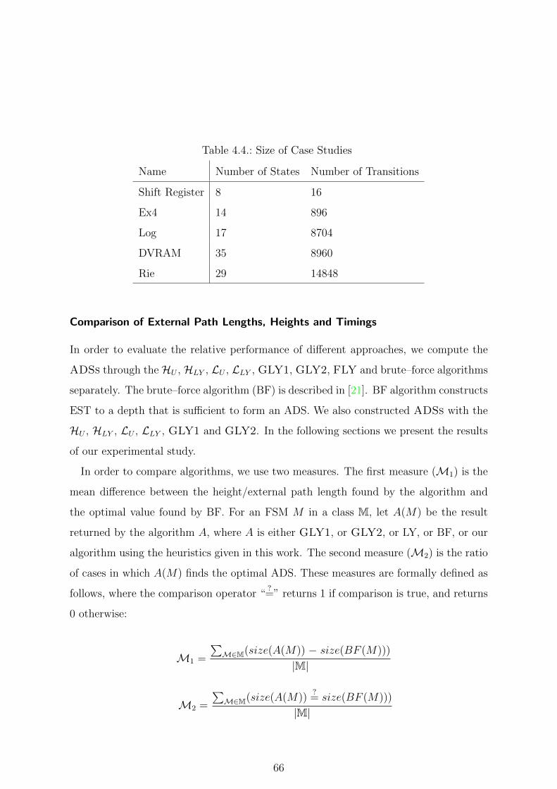
Table 4.4.: Size of Case Studies
Name Number of States Number of Transitions
Shift Register 8 16
Ex4 14 896
Log 17 8704
DVRAM 35 8960
Rie 29 14848
Comparison of External Path Lengths, Heights and Timings
In order to evaluate the relative performance of different approaches, we compute the
ADSs through the HU , HLY , LU , LLY , GLY1, GLY2, FLY and brute–force algorithms
separately. The brute–force algorithm (BF) is described in [21]. BF algorithm constructs
EST to a depth that is sufficient to form an ADS. We also constructed ADSs with the
HU , HLY , LU , LLY , GLY1 and GLY2. In the following sections we present the results
of our experimental study.
In order to compare algorithms, we use two measures. The first measure (M1) is the
mean difference between the height/external path length found by the algorithm and
the optimal value found by BF. For an FSM M in a class M, let A(M) be the result
returned by the algorithm A, where A is either GLY1, or GLY2, or LY, or BF, or our
algorithm using the heuristics given in this work. The second measure (M2) is the ratio
of cases in which A(M) finds the optimal ADS. These measures are formally defined as
follows, where the comparison operator “?=” returns 1 if comparison is true, and returns
0 otherwise:
M1 =
∑M∈M(size(A(M)) − size(BF (M)))
|M|
M2 =
∑M∈M(size(A(M))
?= size(BF (M)))
|M|
66

We evaluate the methods with respect to the number of states, size of input/output
alphabets, and the parameter k.
The effect of number of states: To see the effect of the number of states, we
performed experiments on FSMs in TS1 by using k = 1 for Algorithm 1. Note that,
using a larger k value would intuitively increase the quality of our results at the expense
of increased running time. We discuss the effect of different k values separately below.
We present the results in Table 4.5.
The results are quite promising. We see that when |M | = 50, HLY can find the
shallowest tree in 99% of the instances. Comparing FLY and GLY2, we see that GLY2
is better than FLY. Moreover, considering the results of measureM1, we see that LEA
constructs ADS trees closer to the optimum than the trees generated by approaches
FLY, GLY1 and GLY2. We observe that this rate gradually decreases as the number
of states increases. Moreover, in terms of running times, we see that HU is the fastest,
and HLY is the slowest approach and HLY is slower than FLY by nearly 3 fold.
We observe that heuristics LU and LLY cannot compute the optimum ADSs most of
the times, but compared to the FLY, GLY1 and GLY2, we see that LU and LLY are
able to reduce the average gap to the optimal external path length by at least 3, at most
6 fold.
The effect of the size of the input/output alphabet: We again use the measures
M1 and M2 to analyze the effect of the size of the input/output alphabet on the
performances. We use Algorithm 1 with k = 1. In this experiment we used FSMs in
TS2. Table 4.6 summarizes the results.
Clearly the results indicate that the FLY algorithm computes ADSs quicker than the
other methods when input size is increased. In terms of M1, HLY produces the best
results when the objective function is to minimize the height.
We observe that as the number of input/output symbols increases, LEA tends to
produce optimum ADSs. Moreover as the number of input/output symbols increases,
LEA, GLY1 and GLY2 tend to be slower. We observe that as we increment the size of
input/output symbols by a factor of 4 (4 to 16) the time required to compute ADSs is
67
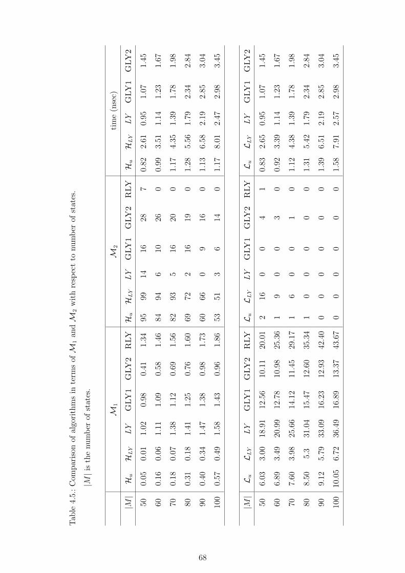
Tab
le4.
5.:
Com
par
ison
ofal
gori
thm
sin
term
sofM
1an
dM
2w
ith
resp
ect
tonum
ber
ofst
ates
.
|M|i
sth
enum
ber
ofst
ates
.
M1
M2
tim
e(n
sec)
|M|HuHLY
LY
GLY1
GLY2
RLYHuHLY
LY
GLY1
GLY2
RLY
HuHLY
LY
GLY1
GLY2
500.
050.
011.
020.
980.
411.
3495
9914
1628
70.
822.
610.
951.
071.
45
600.
160.
061.
111.
090.
581.
4684
946
1026
00.
993.
511.
141.
231.
67
700.
180.
071.
381.
120.
691.
5682
935
1620
01.
174.
351.
391.
781.
98
800.
310.
181.
411.
250.
761.
6069
722
1619
01.
285.
561.
792.
342.
84
900.
400.
341.
471.
380.
981.
7360
660
916
01.
136.
582.
192.
853.
04
100
0.57
0.49
1.58
1.43
0.96
1.86
5351
36
140
1.17
8.01
2.47
2.98
3.45
|M|Lu
LLY
LY
GLY1
GLY2
RLYLuLLY
LY
GLY1
GLY2
RLY
LuLLY
LY
GLY1
GLY2
506.
033.
0018
.91
12.5
610
.11
20.0
12
160
04
10.
832.
650.
951.
071.
45
606.
893.
4920
.99
12.7
810
.98
25.3
61
90
03
00.
923.
391.
141.
231.
67
707.
603.
9825
.66
14.1
211
.45
29.1
71
60
01
01.
124.
381.
391.
781.
98
808.
505.
331
.04
15.4
712
.60
35.3
41
00
00
01.
315.
421.
792.
342.
84
909.
125.
7933
.09
16.2
312
.93
42.4
00
00
00
01.
396.
512.
192.
853.
04
100
10.0
56.
7236
.49
16.8
913
.37
43.6
70
00
00
01.
587.
912.
572.
983.
45
68
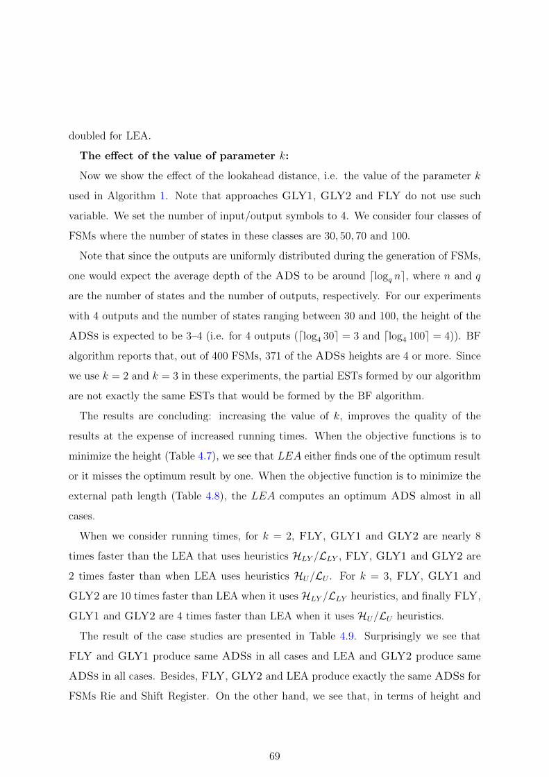
doubled for LEA.
The effect of the value of parameter k:
Now we show the effect of the lookahead distance, i.e. the value of the parameter k
used in Algorithm 1. Note that approaches GLY1, GLY2 and FLY do not use such
variable. We set the number of input/output symbols to 4. We consider four classes of
FSMs where the number of states in these classes are 30, 50, 70 and 100.
Note that since the outputs are uniformly distributed during the generation of FSMs,
one would expect the average depth of the ADS to be around dlogq ne, where n and q
are the number of states and the number of outputs, respectively. For our experiments
with 4 outputs and the number of states ranging between 30 and 100, the height of the
ADSs is expected to be 3–4 (i.e. for 4 outputs (dlog4 30e = 3 and dlog4 100e = 4)). BF
algorithm reports that, out of 400 FSMs, 371 of the ADSs heights are 4 or more. Since
we use k = 2 and k = 3 in these experiments, the partial ESTs formed by our algorithm
are not exactly the same ESTs that would be formed by the BF algorithm.
The results are concluding: increasing the value of k, improves the quality of the
results at the expense of increased running times. When the objective functions is to
minimize the height (Table 4.7), we see that LEA either finds one of the optimum result
or it misses the optimum result by one. When the objective function is to minimize the
external path length (Table 4.8), the LEA computes an optimum ADS almost in all
cases.
When we consider running times, for k = 2, FLY, GLY1 and GLY2 are nearly 8
times faster than the LEA that uses heuristics HLY /LLY , FLY, GLY1 and GLY2 are
2 times faster than when LEA uses heuristics HU/LU . For k = 3, FLY, GLY1 and
GLY2 are 10 times faster than LEA when it uses HLY /LLY heuristics, and finally FLY,
GLY1 and GLY2 are 4 times faster than LEA when it uses HU/LU heuristics.
The result of the case studies are presented in Table 4.9. Surprisingly we see that
FLY and GLY1 produce same ADSs in all cases and LEA and GLY2 produce same
ADSs in all cases. Besides, FLY, GLY2 and LEA produce exactly the same ADSs for
FSMs Rie and Shift Register. On the other hand, we see that, in terms of height and
69
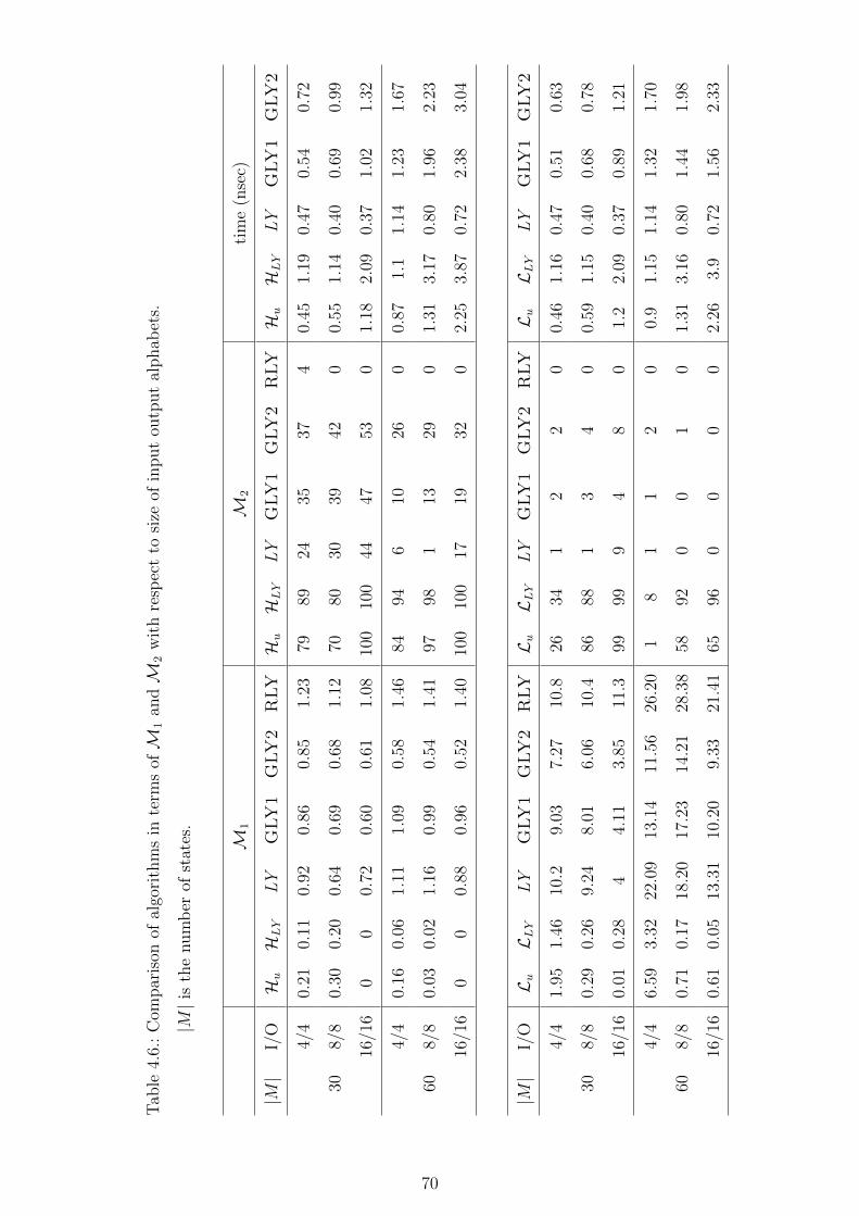
Tab
le4.
6.:
Com
par
ison
ofal
gori
thm
sin
term
sofM
1an
dM
2w
ith
resp
ect
tosi
zeof
input
outp
ut
alphab
ets.
|M|i
sth
enum
ber
ofst
ates
.
M1
M2
tim
e(n
sec)
|M|
I/O
HuHLY
LY
GLY1
GLY2
RLYHuHLY
LY
GLY1
GLY2
RLY
HuHLY
LY
GLY1
GLY2
4/4
0.21
0.11
0.92
0.86
0.85
1.23
7989
2435
374
0.45
1.19
0.47
0.54
0.72
308/
80.
300.
200.
640.
690.
681.
1270
8030
3942
00.
551.
140.
400.
690.
99
16/1
60
00.
720.
600.
611.
0810
010
044
4753
01.
182.
090.
371.
021.
32
4/4
0.16
0.06
1.11
1.09
0.58
1.46
8494
610
260
0.87
1.1
1.14
1.23
1.67
608/
80.
030.
021.
160.
990.
541.
4197
981
1329
01.
313.
170.
801.
962.
23
16/1
60
00.
880.
960.
521.
4010
010
017
1932
02.
253.
870.
722.
383.
04
|M|
I/O
LuLLY
LY
GLY1
GLY2
RLY
LuLLY
LY
GLY1
GLY2
RLY
LuLLY
LY
GLY1
GLY2
4/4
1.95
1.46
10.2
9.03
7.27
10.8
2634
12
20
0.46
1.16
0.47
0.51
0.63
308/
80.
290.
269.
248.
016.
0610
.486
881
34
00.
591.
150.
400.
680.
78
16/1
60.
010.
284
4.11
3.85
11.3
9999
94
80
1.2
2.09
0.37
0.89
1.21
4/4
6.59
3.32
22.0
913
.14
11.5
626
.20
18
11
20
0.9
1.15
1.14
1.32
1.70
608/
80.
710.
1718
.20
17.2
314
.21
28.3
858
920
01
01.
313.
160.
801.
441.
98
16/1
60.
610.
0513
.31
10.2
09.
3321
.41
6596
00
00
2.26
3.9
0.72
1.56
2.33
70
Tab
le4.
7.:
Com
par
ison
ofal
gori
thm
sin
term
sofM
1an
dM
2w
ith
resp
ect
topar
amet
erk.
|M|i
sth
enum
ber
ofst
ates
.
M1
M2
tim
e(n
sec)
|M|
kHuHLY
LY
GLY1
GLY2
RLYHuHLY
LY
GLY1
GLY2
RLY
HuHLY
LY
GLY1
GLY2
10.
210.
110.
920.
860.
851.
2379
8924
3537
40.
451.
190.
470.
540.
72
302
00
0.92
0.86
0.85
1.23
100
100
2435
374
0.83
2.44
0.47
0.54
0.72
30
00.
920.
860.
851.
2310
010
024
3537
41.
232.
670.
470.
540.
72
10.
050.
011.
020.
980.
411.
3495
9914
1628
70.
822.
610.
951.
071.
98
502
00
1.02
0.98
0.41
1.34
100
100
1416
287
1.56
3.95
0.95
1.07
1.98
30
01.
020.
980.
411.
3410
010
014
1628
72.
936.
120.
951.
071.
98
10.
180.
071.
381.
120.
691.
5682
935
1620
01.
174.
351.
391.
781.
98
702
0.04
01.
381.
120.
691.
5696
100
516
200
2.28
6.62
1.39
1.78
1.98
30
01.
381.
120.
691.
5610
010
05
1620
04.
314
.38
1.39
1.78
1.98
10.
570.
491.
581.
430.
961.
8653
513
614
01.
178.
012.
572.
983.
45
100
20.
190.
121.
581.
430.
961.
8681
883
614
03.
1821
.62
2.57
2.98
3.45
30
01.
581.
430.
961.
8610
010
03
614
06.
7721
.62
2.57
2.98
3.45
71
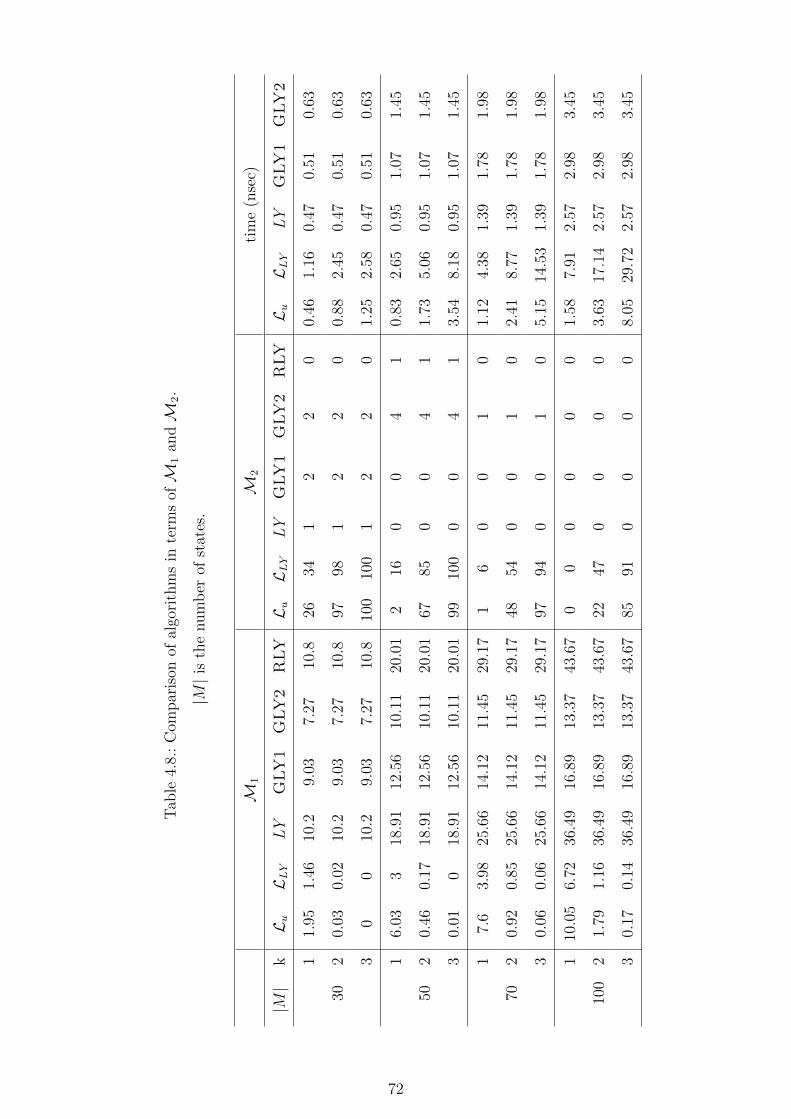
Tab
le4.
8.:
Com
par
ison
ofal
gori
thm
sin
term
sofM
1an
dM
2.
|M|i
sth
enum
ber
ofst
ates
.
M1
M2
tim
e(n
sec)
|M|
kLuLLY
LY
GLY1
GLY2
RLY
LuLLY
LY
GLY1
GLY2
RLY
LuLLY
LY
GLY1
GLY2
11.
951.
4610
.29.
037.
2710
.826
341
22
00.
461.
160.
470.
510.
63
302
0.03
0.02
10.2
9.03
7.27
10.8
9798
12
20
0.88
2.45
0.47
0.51
0.63
30
010
.29.
037.
2710
.810
010
01
22
01.
252.
580.
470.
510.
63
16.
033
18.9
112
.56
10.1
120
.01
216
00
41
0.83
2.65
0.95
1.07
1.45
502
0.46
0.17
18.9
112
.56
10.1
120
.01
6785
00
41
1.73
5.06
0.95
1.07
1.45
30.
010
18.9
112
.56
10.1
120
.01
9910
00
04
13.
548.
180.
951.
071.
45
17.
63.
9825
.66
14.1
211
.45
29.1
71
60
01
01.
124.
381.
391.
781.
98
702
0.92
0.85
25.6
614
.12
11.4
529
.17
4854
00
10
2.41
8.77
1.39
1.78
1.98
30.
060.
0625
.66
14.1
211
.45
29.1
797
940
01
05.
1514
.53
1.39
1.78
1.98
110
.05
6.72
36.4
916
.89
13.3
743
.67
00
00
00
1.58
7.91
2.57
2.98
3.45
100
21.
791.
1636
.49
16.8
913
.37
43.6
722
470
00
03.
6317
.14
2.57
2.98
3.45
30.
170.
1436
.49
16.8
913
.37
43.6
785
910
00
08.
0529
.72
2.57
2.98
3.45
72
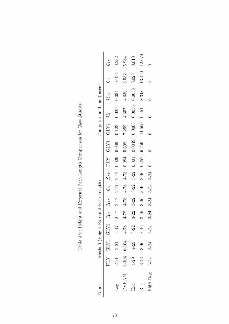
Tab
le4.
9.:
Hei
ght
and
Exte
rnal
Pat
hL
engt
hC
ompar
ison
for
Cas
eStu
die
s.
Nam
eM
ethod
(Hei
ght-
Exte
rnal
Pat
hL
engt
h)
Com
puta
tion
Tim
e(m
sec)
FLY
GLY
1G
LY
2HUHLYLULLY
FLY
GLY
1G
LY
2HU
HLY
LU
LLY
Log
2-21
2-21
2-17
2-17
2-17
2-17
2-17
0.02
90.
069
0.12
30.
025
0.03
40.
196
0.23
2
DV
RA
M6-
104
6-10
44-
784-
784-
784-
784-
780.
084
5.69
87.
259
4.35
74.
630
6.58
25.
984
Ex4
4-29
4-29
3-22
3-22
3-22
3-22
3-22
0.00
10.
0049
0.00
630.
0056
0.00
580.
023
0.01
8
Rie
3-46
3-46
3-46
3-46
3-46
3-46
3-46
0.25
76.
256
11.5
909.
454
8.34
813
.450
12.6
74
Shif
tR
eg.
3-24
3-24
3-24
3-24
3-24
3-24
3-24
00
00
00
0
73
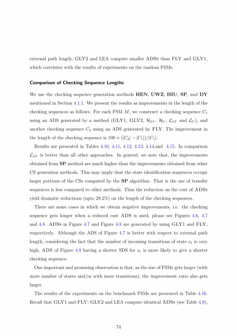
external path length, GLY2 and LEA compute smaller ADSs than FLY and GLY1,
which correlates with the results of experiments on the random FSMs.
Comparison of Checking Sequence Lengths
We use the checking sequence generation methods HEN, UWZ, HIU, SP, and DY
mentioned in Section 4.1.1. We present the results as improvements in the length of the
checking sequences as follows. For each FSM M , we construct a checking sequence C1
using an ADS generated by a method (GLY1, GLY2, HLY , HU , LLY and LU), and
another checking sequence C2 using an ADS generated by FLY. The improvement in
the length of the checking sequence is 100× (|C2| − |C1|)/|C1|.
Results are presented in Tables 4.10, 4.11, 4.12, 4.13, 4.14,and 4.15. In comparison
LLY is better than all other approaches. In general, we note that, the improvements
obtained from SP method are much higher than the improvements obtained from other
CS generation methods. This may imply that the state identification sequences occupy
larger portions of the CSs computed by the SP algorithm. That is the use of transfer
sequences is less compared to other methods. Thus the reduction on the cost of ADSs
yield dramatic reductions (upto 29.2%) on the length of the checking sequences.
There are some cases in which we obtain negative improvements, i.e. the checking
sequence gets longer when a reduced cost ADS is used, please see Figures 4.6, 4.7
and 4.8. ADSs in Figure 4.7 and Figure 4.8 are generated by using GLY1 and FLY,
respectively. Although the ADS of Figure 4.7 is better with respect to external path
length, considering the fact that the number of incoming transitions of state s1 is very
high, ADS of Figure 4.8 having a shorter SDS for s1 is more likely to give a shorter
checking sequence.
One important and promising observation is that, as the size of FSMs gets larger (with
more number of states and/or with more transitions), the improvement ratio also gets
larger.
The results of the experiments on the benchmark FSMs are presented in Table 4.16.
Recall that GLY1 and FLY; GLY2 and LEA compute identical ADSs (see Table 4.9),
74
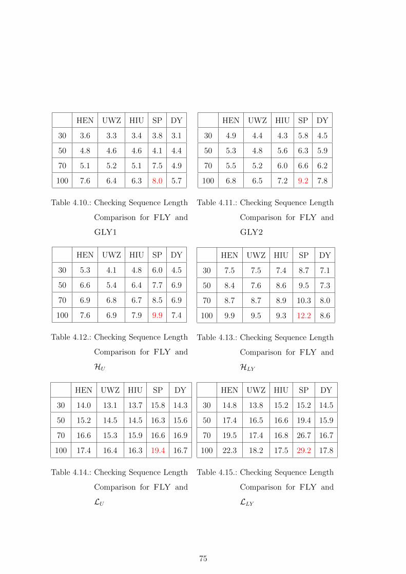
HEN UWZ HIU SP DY
30 3.6 3.3 3.4 3.8 3.1
50 4.8 4.6 4.6 4.1 4.4
70 5.1 5.2 5.1 7.5 4.9
100 7.6 6.4 6.3 8.0 5.7
Table 4.10.: Checking Sequence Length
Comparison for FLY and
GLY1
HEN UWZ HIU SP DY
30 4.9 4.4 4.3 5.8 4.5
50 5.3 4.8 5.6 6.3 5.9
70 5.5 5.2 6.0 6.6 6.2
100 6.8 6.5 7.2 9.2 7.8
Table 4.11.: Checking Sequence Length
Comparison for FLY and
GLY2
HEN UWZ HIU SP DY
30 5.3 4.1 4.8 6.0 4.5
50 6.6 5.4 6.4 7.7 6.9
70 6.9 6.8 6.7 8.5 6.9
100 7.6 6.9 7.9 9.9 7.4
Table 4.12.: Checking Sequence Length
Comparison for FLY and
HU
HEN UWZ HIU SP DY
30 7.5 7.5 7.4 8.7 7.1
50 8.4 7.6 8.6 9.5 7.3
70 8.7 8.7 8.9 10.3 8.0
100 9.9 9.5 9.3 12.2 8.6
Table 4.13.: Checking Sequence Length
Comparison for FLY and
HLY
HEN UWZ HIU SP DY
30 14.0 13.1 13.7 15.8 14.3
50 15.2 14.5 14.5 16.3 15.6
70 16.6 15.3 15.9 16.6 16.9
100 17.4 16.4 16.3 19.4 16.7
Table 4.14.: Checking Sequence Length
Comparison for FLY and
LU
HEN UWZ HIU SP DY
30 14.8 13.8 15.2 15.2 14.5
50 17.4 16.5 16.6 19.4 15.9
70 19.5 17.4 16.8 26.7 16.7
100 22.3 18.2 17.5 29.2 17.8
Table 4.15.: Checking Sequence Length
Comparison for FLY and
LLY
75
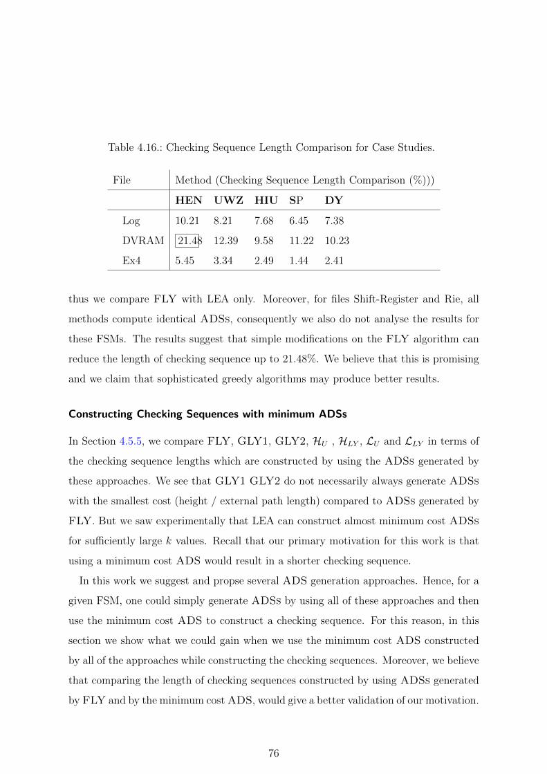
Table 4.16.: Checking Sequence Length Comparison for Case Studies.
File Method (Checking Sequence Length Comparison (%)))
HEN UWZ HIU SP DY
Log 10.21 8.21 7.68 6.45 7.38
DVRAM 21.48 12.39 9.58 11.22 10.23
Ex4 5.45 3.34 2.49 1.44 2.41
thus we compare FLY with LEA only. Moreover, for files Shift-Register and Rie, all
methods compute identical ADSs, consequently we also do not analyse the results for
these FSMs. The results suggest that simple modifications on the FLY algorithm can
reduce the length of checking sequence up to 21.48%. We believe that this is promising
and we claim that sophisticated greedy algorithms may produce better results.
Constructing Checking Sequences with minimum ADSs
In Section 4.5.5, we compare FLY, GLY1, GLY2, HU , HLY , LU and LLY in terms of
the checking sequence lengths which are constructed by using the ADSs generated by
these approaches. We see that GLY1 GLY2 do not necessarily always generate ADSs
with the smallest cost (height / external path length) compared to ADSs generated by
FLY. But we saw experimentally that LEA can construct almost minimum cost ADSs
for sufficiently large k values. Recall that our primary motivation for this work is that
using a minimum cost ADS would result in a shorter checking sequence.
In this work we suggest and propse several ADS generation approaches. Hence, for a
given FSM, one could simply generate ADSs by using all of these approaches and then
use the minimum cost ADS to construct a checking sequence. For this reason, in this
section we show what we could gain when we use the minimum cost ADS constructed
by all of the approaches while constructing the checking sequences. Moreover, we believe
that comparing the length of checking sequences constructed by using ADSs generated
by FLY and by the minimum cost ADS, would give a better validation of our motivation.
76
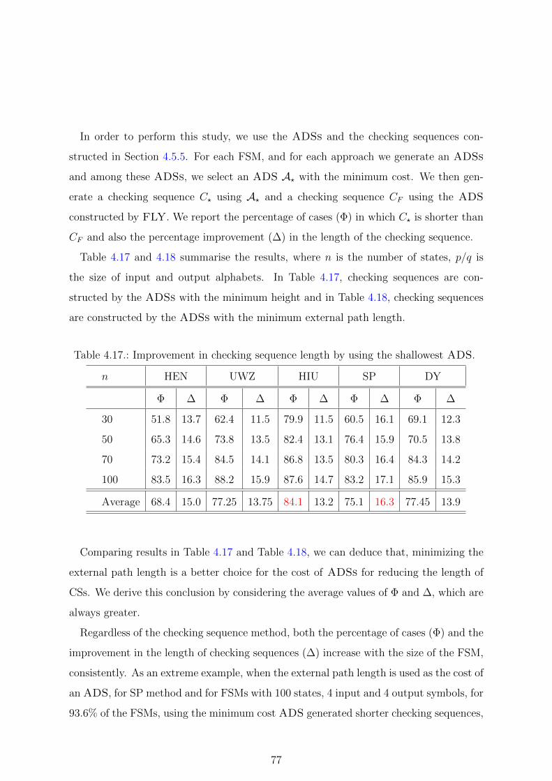
In order to perform this study, we use the ADSs and the checking sequences con-
structed in Section 4.5.5. For each FSM, and for each approach we generate an ADSs
and among these ADSs, we select an ADS A? with the minimum cost. We then gen-
erate a checking sequence C? using A? and a checking sequence CF using the ADS
constructed by FLY. We report the percentage of cases (Φ) in which C? is shorter than
CF and also the percentage improvement (∆) in the length of the checking sequence.
Table 4.17 and 4.18 summarise the results, where n is the number of states, p/q is
the size of input and output alphabets. In Table 4.17, checking sequences are con-
structed by the ADSs with the minimum height and in Table 4.18, checking sequences
are constructed by the ADSs with the minimum external path length.
Table 4.17.: Improvement in checking sequence length by using the shallowest ADS.
n HEN UWZ HIU SP DY
Φ ∆ Φ ∆ Φ ∆ Φ ∆ Φ ∆
30 51.8 13.7 62.4 11.5 79.9 11.5 60.5 16.1 69.1 12.3
50 65.3 14.6 73.8 13.5 82.4 13.1 76.4 15.9 70.5 13.8
70 73.2 15.4 84.5 14.1 86.8 13.5 80.3 16.4 84.3 14.2
100 83.5 16.3 88.2 15.9 87.6 14.7 83.2 17.1 85.9 15.3
Average 68.4 15.0 77.25 13.75 84.1 13.2 75.1 16.3 77.45 13.9
Comparing results in Table 4.17 and Table 4.18, we can deduce that, minimizing the
external path length is a better choice for the cost of ADSs for reducing the length of
CSs. We derive this conclusion by considering the average values of Φ and ∆, which are
always greater.
Regardless of the checking sequence method, both the percentage of cases (Φ) and the
improvement in the length of checking sequences (∆) increase with the size of the FSM,
consistently. As an extreme example, when the external path length is used as the cost of
an ADS, for SP method and for FSMs with 100 states, 4 input and 4 output symbols, for
93.6% of the FSMs, using the minimum cost ADS generated shorter checking sequences,
77
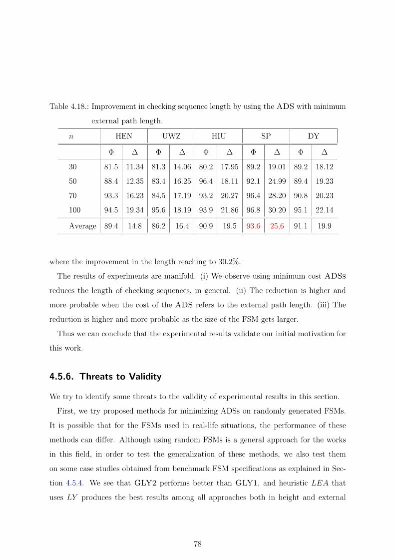
Table 4.18.: Improvement in checking sequence length by using the ADS with minimum
external path length.
n HEN UWZ HIU SP DY
Φ ∆ Φ ∆ Φ ∆ Φ ∆ Φ ∆
30 81.5 11.34 81.3 14.06 80.2 17.95 89.2 19.01 89.2 18.12
50 88.4 12.35 83.4 16.25 96.4 18.11 92.1 24.99 89.4 19.23
70 93.3 16.23 84.5 17.19 93.2 20.27 96.4 28.20 90.8 20.23
100 94.5 19.34 95.6 18.19 93.9 21.86 96.8 30.20 95.1 22.14
Average 89.4 14.8 86.2 16.4 90.9 19.5 93.6 25,6 91.1 19.9
where the improvement in the length reaching to 30.2%.
The results of experiments are manifold. (i) We observe using minimum cost ADSs
reduces the length of checking sequences, in general. (ii) The reduction is higher and
more probable when the cost of the ADS refers to the external path length. (iii) The
reduction is higher and more probable as the size of the FSM gets larger.
Thus we can conclude that the experimental results validate our initial motivation for
this work.
4.5.6. Threats to Validity
We try to identify some threats to the validity of experimental results in this section.
First, we try proposed methods for minimizing ADSs on randomly generated FSMs.
It is possible that for the FSMs used in real-life situations, the performance of these
methods can differ. Although using random FSMs is a general approach for the works
in this field, in order to test the generalization of these methods, we also test them
on some case studies obtained from benchmark FSM specifications as explained in Sec-
tion 4.5.4. We see that GLY2 performs better than GLY1, and heuristic LEA that
uses LY produces the best results among all approaches both in height and external
78

path length metrics, similar to the results we obtained from random FSMs. However,
GLY1 performs similarly to FLY, which we believe is due to the fact that ADSs for
these examples are quite shallow.
Another threat could be our incorrect implementation of these approaches. To elimi-
nate this threat, we also used an existing tool that checks if a given tree is an ADS for
an FSM. The ADSs generated by all approaches are all double checked with this tool
to see what is produced is really an ADS.
A threat to our motivation for using minimized ADSs could be that, the actual
method used for checking sequence generation may or may not support this motivation.
In order to see the effect of minimizing ADSs for checking sequence construction, we
considered several checking sequence construction methods. The results suggest that,
in general, regardless of the checking sequence method, using minimized ADS result
in shorter checking sequences. There are occasional cases where using a minimized
ADS actually generates a longer checking sequence. A possible reason for such cases
is explained in Section 4.5.5. As stated in that part, the number of such cases would
possibly decrease if MinWeightedADS problem is considered (instead of MinADS
and MinHeightADS) while minimizing ADSs.
4.6. Chapter Summary
In this work, we studied the problem of computing a minimum ADS for a given de-
terministic, minimal and complete FSM. We introduced several metrics with respect to
which such a minimization can be defined, where each metric resulted in a definition of
a separate minimization problem. For each metric defined, we showed the problem of
deciding a minimum ADS with respect to that metric is NP-complete. We also presented
inapproximability results for each one of these minimization problems. Since determin-
istic FSMs are special cases of nondeterministic FSMs, our results directly apply to
nondeterministic FSMs as well.
Our initial motivation for minimizing ADSs is the use of ADSs in the context of check-
79

ing sequence generation. Generating a minimum ADS is important in such a context,
since state recognitions and state verifications are performed by using an ADS, and a
considerable part of a checking sequence consists of such state recognitions/verifications.
Therefore the length of a checking sequence generated by using an ADS, correlates with
the size of that ADS. Due to the hardness and inapproximability of ADS minimization,
heuristic algorithms can be used to generate shorter ADSs than the ones that are gen-
erated by the only polynomial time algorithm known for ADS generation given in [35].
In order to validate our initial motivation, we considered two different modifications on
LY algorithm leading to two different heuristics. The experimental results validate our
initial motivation, and show that using shorter ADSs in checking sequence construction
improves the length of checking sequences.
80

5. Using Incomplete Distinguishing
Sequences when Testing from a
Finite State Machine
5.1. Introduction
In this chapter, we consider constructing Checking Experiments for FSMs that do not
have a PDS or an ADS. Many techniques for constructing CEs use DSs to resolve the
state identification problem for two reasons: There are polynomial time algorithms that
generate CEs when there is a known DS and the length of the CEs is relatively short
when designed with a DS [29, 42, 43, 44, 35].
In this Chapter, we use the term complete PDS/ADS to denote the Definition 1
and Definition 2 respectively. Although complete DSs have a number of advantages
over other approaches used to distinguish states, not all FSMs possess a complete DS,
and if there is no complete DS then the state recognition task is carried out by other
approaches such as UIOs or W-Sets. However, as explained in [110], using UIOs or
W-Sets typically leads to significantly longer CEs. Thus the motivation for the work
reported in this text comes primarily from the desire to obtain some of the benefits of
complete DSs when constructing CEs for specifications that do not have complete DSs.
We therefore consider the case where the FSM does not have a complete DS but instead
we would like to form a collection of DSs that, between them, distinguish all of the states
of FSM M .
81

A collection of DSs achieves this when for every pair of states s, s′ with s 6= s′ there is
some DS in the collection that distinguishes s and s′. Another way of describing this is
to require a set PS of subsets of the state set S such that: for all s, s′ ∈ S with s 6= s′ we
have some S ∈ PS such that s, s′ ∈ S; and for all S ∈ PS there is a DS that distinguishes
the states of S. We show how a CE can be generated using a set of incomplete DSs that
distinguish all of the states of the specification. We also explore problems associated
with generating ‘optimal’ sets of incomplete DSs.
While it might seem that complete ADSs are always preferable to complete PDSs,
the use of complete PDSs is beneficial in some circumstances. The key advantage of
complete PDSs is that they simplify the testing process since there is no need to adapt
test input to the observations made. This allows the use of a simpler/cheaper test infras-
tructure and is also important when the observation and processing of outputs incurs
a significant cost by, for example, making testing take longer. In addition, sometimes
adaptivity is not possible due to timing constraints; it might take too long for the test
infrastructure to make decisions.
In Section 5.3 we consider problems associated with incomplete PDSs, motivated by
the fact that sometimes we require test sequences that are not adaptive. We study the
following question.
Definition 26 (MaxSubSetPDS problem) Given FSM M with a finite set of states
S and S ⊆ S, find a subset S ′ of S that has a PDS such that |S ′| is maximised.
One way of expressing the problem of looking for a set of PDSs to distinguish all of
the states of an FSM M with state set S is to look for a set PS of subsets of S such that
the followings hold.
• For every pair of states s, s′ ∈ S with s 6= s′ there is some S ∈ PS such that
s, s′ ∈ S; and
• for every S ∈ PS there is some PDS that distinguishes all of the states of S.
This leads to the following definition of the MinSetPDS problem.
82

Definition 27 (MinSetPDS problem) Given FSM M and a finite set of states S,
find a smallest set PS of subsets of S such that each set in PS has a PDS and for all
s, s′ ∈ S with s 6= s′ we have that there exists S ∈ PS such that s, s′ ∈ S.
We show that the MaxSubSetPDS and MinSetPDS problems are PSPACE-complete.
Moreover, we use results given in [95] to show that the MaxSubSetPDS problem is
inapproximable. In Section 5.4 we adapt the problems introduced so far to incomplete
ADSs.
Definition 28 (MaxSubSetADS problem) Given FSM M with a finite set of states
S and S ⊆ S, find a subset S ′ of S that has an ADS such that |S ′| is maximised.
Definition 29 (MinSetADS problem) Given FSM M and a finite set of states S,
find a smallest set PS of subsets of S such that each set in PS has an ADS and for all
s, s′ ∈ S with s 6= s′ we have that there exists S ∈ PS such that s, s′ ∈ S.
We show that the MaxSubSetADS and MinSetADS problems are PSPACE-complete.
We also show that the MaxSubSetADS problem is inapproximable. This contrasts
with the case where we are looking for a complete ADS, a problem that can be solved
in polynomial time.
Having determined the complexity of these problems, we consider how incomplete
ADSs can be used in generating checking experiments. We show how the W-method
and the HSI-method can be adapted to produce checking experiments based on ADSs
(and so PDSs). We also demonstrate that the optimisation problems we consider relate
very naturally to test optimisation problems for these checking experiment generation
methods. A combination of these results shows that the optimisation problems are also
relevant to the W-method and the HSI-method. We then propose a greedy algorithm for
the MinSetADS problem and report on the results of experiments that evaluated the
combination of the proposed CE generation algorithm and the greedy algorithm. The
experiments used a set of FSMs and compared the checking experiment size for the W-
method, the HSI-method, and the HSI-method adapted to use ADSs. The experimental
83

subjects included randomly generated FSMs and FSMs drawn from a benchmark and
suggest that the proposed method produces shorter CEs that contain fewer resets.
This Chapter is organised as follows. In the next section, we define the terminology
and notation used throughout the Chapter. In Section 5.3 we present results related to
PDSs and subsequently, in Section 5.4, we present results related to ADSs. In Section
5.5 we show how the W-method and HSI-method can be adapted to use ADSs and in
Section 5.6 we report on the results of experiments. In Section 5.7, we summary the
chapter and discuss some possible lines of future work.
5.2. Preliminaries
In this Chapter, we consider incomplete ADSs and PDSs and now we provide definitions
of incomplete Preset and Adaptive Distinguishing Sequences.
Definition 30 Given FSM M = (S,X, Y, δ, λ) and S ⊆ S, input sequence w is an
incomplete Preset Distinguishing Sequence (PDS) for S if for all s, s′ ∈ S with s 6= s′
we have that λ(s, w) 6= λ(s′, w).
Definition 31 Given FSM M = (S,X, Y, δ, λ) and S ⊆ S, an Incomplete Adaptive
Distinguishing Sequence (ADS) for S is a rooted tree A such that the following hold.
1. Each node is labelled by a set of states and the root is labelled by S.
2. Each leaf of A is labeled by a singleton set (i.e. {s} for some s ∈ S).
3. Each edge is labeled by an input/output pair.
4. Let us suppose that node v has state set S ′ ⊆ S. If v has one or more outgoing edges
then these edges are labeled by the same input x and have the following property:
if there is some s ∈ S ′ such that λ(s, x) = y then there is a unique edge (v, x/y, v′)
such that v′ is labelled with the set S ′′ = {s′′ ∈ S|∃s′ ∈ S ′.λ(s′, x) = y ∧ δ(s′, x) =
s′′} of states that we can reach from S ′ with a transition that has label x/y.
84

5. If v has state set S ′ ⊆ S and has one or more outgoing edges then the input x on
these edges satisfies the following property: for all s, s′ ∈ S ′ with s 6= s′ we have
that either λ(s, x) 6= λ(s′, x) or δ(s, x) 6= δ(s′, x).
The idea is similar to the rationale given for complete ADSs: an incomplete ADS for
S defines an experiment where the next input to be applied depends on the previously
observed input/output sequence (and so the node reached). The last condition ensures
that two states of S cannot be mapped to the same state by an incomplete ADS for S
unless they have already been distinguished. If we apply A in a state s ∈ S then the
resultant input/output sequence is that which labels the path of A from the root of A
to a leaf and is also the label of a path of M that has starting state s. By the definition
of an incomplete ADS the input/output sequences for two distinct states from S must
differ and so A distinguishes the states from S. When we set S = S these correspond
to the classical notion of Preset and Adaptive Distinguishing sequences. From now on
we will write PDSs/ADSs to denote incomplete PDSs/ADSs and throughout this
Chapter we refer to the depth of ADS tree A when we write the length of A.
We present an example FSM, which will be used throughout the Chapter in Fig-
ure 5.1. We also present manually computed incomplete ADS for states s1, s2 and s4
in Figure 5.2. The input sequences retrieved from the incomplete ADS are as follows:
baab for s1, b for s2 and baab for s4. Note that input sequence b cannot differentiate
states s2 and s3 but it can differentiate s2 from s1 and s4, moreover input sequence baab
can distinguish states s1 and s4 from all of the states of the FSM M2.
85
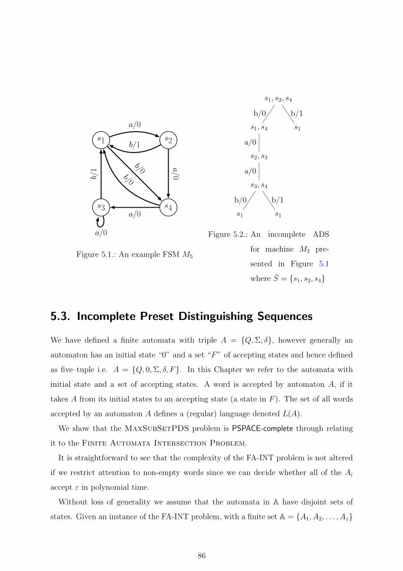
s1 s2
s3 s4
a/0
b/0
b/1
a/0
a/0
b/1
b/0
a/0
Figure 5.1.: An example FSM M5
s1, s2, s4
s1, s4
s2, s3
s3, s4
s1
b/0
s1
b/1
a/0
a/0
b/0
s1
b/1
Figure 5.2.: An incomplete ADS
for machine M2 pre-
sented in Figure 5.1
where S = {s1, s2, s4}
5.3. Incomplete Preset Distinguishing Sequences
We have defined a finite automata with triple A = {Q,Σ, δ}, however generally an
automaton has an initial state “0” and a set “F” of accepting states and hence defined
as five–tuple i.e. A = {Q, 0,Σ, δ, F}. In this Chapter we refer to the automata with
initial state and a set of accepting states. A word is accepted by automaton A, if it
takes A from its initial states to an accepting state (a state in F ). The set of all words
accepted by an automaton A defines a (regular) language denoted L(A).
We show that the MaxSubSetPDS problem is PSPACE-complete through relating
it to the Finite Automata Intersection Problem.
It is straightforward to see that the complexity of the FA-INT problem is not altered
if we restrict attention to non-empty words since we can decide whether all of the Ai
accept ε in polynomial time.
Without loss of generality we assume that the automata in A have disjoint sets of
states. Given an instance of the FA-INT problem, with a finite set A = {A1, A2, . . . , Az}
86

of automata on a common finite alphabet Σ (Ai = (Qi,Σ, δi, 0i, Fi)), we construct an
FSM M1(A) = (S,X, Y, δ, λ, s0) as follows.
We introduce two new states Sink1, Sink2. Then we take two copiesA1i = (Q1
i ,Σ, δ1i , 0
1i , F
1i ), A2
i =
(Q2i ,Σ, δ
2i , 0
2i , F
2i ) of each automaton Ai and call them pair automata. Given q ∈ Qi
we let q1 and q2 denote the corresponding states in Q1i and Q2
i respectively. We let
S = {011, 0
21, . . . , 0
1z, 0
2z}, which is the set of initial states of the copies of the automata.
The set of states of the FSM to be constructed is given by S = Q11 ∪ Q2
1 ∪ Q12 ∪ Q2
2 ∪
. . . ∪ Q2z ∪ {Sink1, Sink2}, where the initial state is selected as 01
1. The input alphabet
of the FSM is given by X = Σ ∪ {D} and the output alphabet of the FSM is given by
Y = Q1 ∪Q2 ∪ . . . ∪Qz ∪ {0, 1, 2}.
The state transitions of the automata in A are inherited: if a ∈ Σ and qji ∈ Qji
for 1 ≤ i ≤ z and 1 ≤ j ≤ 2 then δ(qji , a) = rji for the state ri of Ai such that
δi(qi, a) = ri. The state transitions with input D are as follows: δ(s,D) = Sink1 if and
only if (s = Sink1 or there exists i such that s ∈ Q1i ) and δ(s,D) = Sink2 if and only if
(s = Sink2 or there exists i such that s ∈ Q2i ). That is, the states of each pair automata
(A1i and A2
i ) end in different sink states if input D is supplied.
The output function λ of M1(A) is defined as follows, in which 1 ≤ i ≤ z.
λ(s, x) =
qi, If s = qji for some qji ∈ Q1i ∪Q2
i and x 6= D,
qi, If s = qji for some qji ∈ (Q1i ∪Q2
i ) \ (F 1i ∪ F 2
i ) and x = D.
0, If s = Sink1 or s = Sink2,
1, If s ∈ F 1i and x = D,
2, If s ∈ F 2i and x = D,
We demonstrate the construction in Figure 5.3.
The basic idea is that until D is received the transitions from a state in Q1i ∪ Q2
i
simulate the state transitions of Ai but also tell us which states of Ai are being traversed
and so the value of i (the Ai have disjoint state sets). If D is received in a state qji from
Qji then the output tells us the value of j if and only if the state qji is such that qi is an
accepting state of Ai. We now explore properties ofM1(A), proving results that will be
brought together in Theorem 16.
87
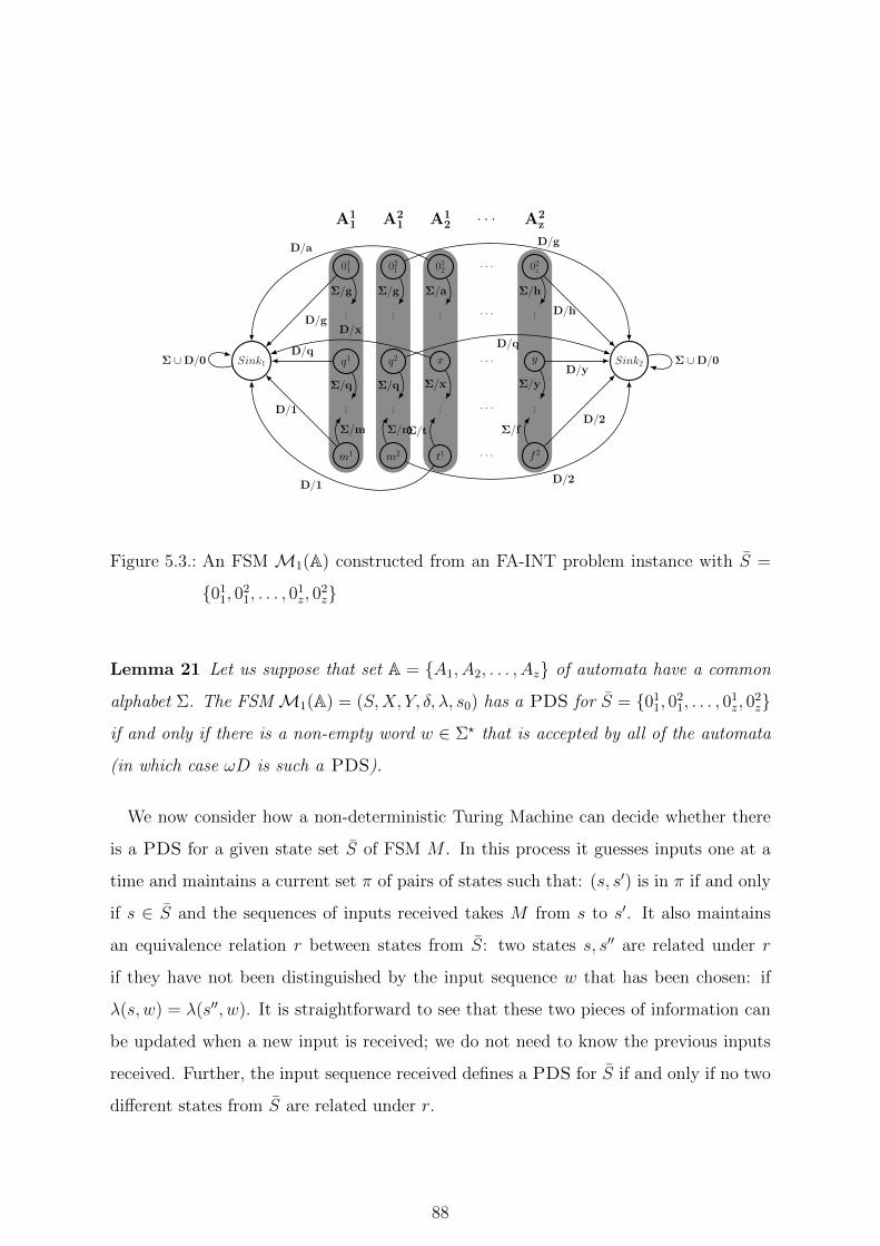
A11 A2
1 A12
. . . A2z
011 02
1 012
. . . 02z
... ... ... . . . ...
q1 q2 x . . . y
... ... ... . . . ...
m1 m2 t1 . . . f 2
Sink2Sink1
D/g
D/gD/a
D/h
Σ/g Σ/g Σ/a Σ/h
D/1
D/2D/1
D/2
Σ/q Σ/q Σ/x Σ/y
D/qD/q
D/x
D/y
Σ/m Σ/mΣ/t Σ/f
Σ ∪D/0Σ ∪D/0
Figure 5.3.: An FSM M1(A) constructed from an FA-INT problem instance with S =
{011, 0
21, . . . , 0
1z, 0
2z}
Lemma 21 Let us suppose that set A = {A1, A2, . . . , Az} of automata have a common
alphabet Σ. The FSM M1(A) = (S,X, Y, δ, λ, s0) has a PDS for S = {011, 0
21, . . . , 0
1z, 0
2z}
if and only if there is a non-empty word w ∈ Σ? that is accepted by all of the automata
(in which case ωD is such a PDS).
We now consider how a non-deterministic Turing Machine can decide whether there
is a PDS for a given state set S of FSM M . In this process it guesses inputs one at a
time and maintains a current set π of pairs of states such that: (s, s′) is in π if and only
if s ∈ S and the sequences of inputs received takes M from s to s′. It also maintains
an equivalence relation r between states from S: two states s, s′′ are related under r
if they have not been distinguished by the input sequence w that has been chosen: if
λ(s, w) = λ(s′′, w). It is straightforward to see that these two pieces of information can
be updated when a new input is received; we do not need to know the previous inputs
received. Further, the input sequence received defines a PDS for S if and only if no two
different states from S are related under r.
88

Lemma 22 The problem of deciding whether a set S of states of FSM M has a PDS
is in PSPACE.
We claim that based on the approach used to prove Lemma 21, we can provide an
inapproximability result for the MaxSubSetPDS problem but before this we explore
the relationship between the optimum solutions of MaxSubSetPDS and MAX FA-INT
problems.
Below, given a property P (such as distinguishing k states of an FSM) a word w is
said to be a minimal word satisfying P if w satisfies P and no proper prefix of w satisfies
P . The following is clear from the proof of Lemma 21.
Lemma 23 Given set A of automata, let OPTA be the set of minimal words that are
accepted by the maximum number of automata from A. Further, given M1(A) let
OPTM1(A) be the set of minimal words that maximise the size of the subset of S whose
states are pairwise distinguished. Then w ∈ OPTA if and only if wD ∈ OPTM1(A).
We can now show that the MaxSubSetPDS problem, of finding a PDS that distin-
guishes the most states from some set S, is PSPACE-complete and inapproximable.
Theorem 16 The MaxSubSetPDS problem is PSPACE-complete and for any con-
stant ε > 0 approximating the MaxSubSetPDS problem within ratio nε is PSPACE-hard.
Finally, we consider the problem of finding a smallest set PS of sets of states such that
each set has a PDS (MinSetPDS).
Theorem 17 The MinSetPDS problem is PSPACE-complete.
5.4. Incomplete Adaptive Distinguishing Sequences
In some situations we want to use preset input sequences in testing since this requires
a relatively simple test infrastructure: one that simply applies a sequence of inputs and
observes the resultant outputs. However, testing can be more efficient if we use adaptive
89

tests, where the next input to be applied is chosen on the basis of the observations made.
In addition, it is known that the problem of deciding whether an FSM has a (complete)
ADS can be solved in polynomial time and there is a polynomial upper bound on the
size of such an ADS [35]. These results, together with complexity results in Section 5.3,
provide the motivation for considering incomplete ADSs. In this section we therefore
explore incomplete ADSs and report that complexity results given for problems related
to PDSs hold when we consider ADSs.
We assume that we are given a set A = {A1, A2, . . . , Az} of automata with alphabet Σ
and now describe the FSMM2(A) that we construct. We mark the initial states of the
automata so that the initial state of Ai is called 0i and will let S = {01, 02 . . . , 0z, Sink}
for a state Sink described below. We introduce a set D = {d1, d2, . . . , dz} of new inputs
and so there exists one such input di for each Ai ∈ A. The transitions of automata from
A with input Σ are inherited (and given output 0) and the remaining transitions are as
follows
• δ(Sink, x) = Sink for any input x ∈ Σ ∪ D.
• If x ∈ D then:
– If s ∈ Fi then δ(s, x) = s; and
– δ(s, x) = Sink otherwise.
The output function λ of M2(A) is defined as follows in which 1 ≤ i ≤ z.
λ(s, x) =
i, If s ∈ F 1i and x = di,
0 For all other cases,
Unlike the previous reduction the output function does not enable us to recognise
the states of automaton Ai while we are visiting the states in Qi \ Fi. Instead, we can
only distinguish states through applying an input from D, possibly after a sequence of
previous inputs. Further, we can only distinguish a state 0i from Sink through applying
an input sequence w that takes Ai to an accepting state and then apply di. We now
90

prove that we can construct an ADS for S if and only if the automata in A accept a
common word.
In the following we represent an ADS by a set of input/output sequences: the in-
put/output sequences produced from the different states of the FSM M being consid-
ered.
Lemma 24 Let us suppose that set A = {A1, A2, . . . , Az} of automata have a common
alphabet Σ. The FSMM2(A) = (S,X, Y, δ, λ, s0) has an ADS for S = {01, 02 . . . , 0z, Sink}
if and only if there is a non-empty word w ∈ Σ? that is accepted by all of the automata
(in which case input sequences wd1, wd1d2, wd1d2d3, . . . , wd1d2d3 . . . dz define an ADS).
We now show that we can check in PSPACE whether a set of states has an ADS.
Lemma 25 Given FSM M and state set S, the problem of deciding whether S has an
ADS is in PSPACE.
The structure of M2(A) ensures that when trying to distinguish states in S we gain
nothing from adaptivity: once we have observed a non-zero output from one of the states
we have distinguished this state from all other states in S (we must only observe zeros
when starting in Sink ∈ S). Thus, when exploring ADSs for S it is sufficient to consider
input sequences.
We now show that the MaxSubSetADS problem, of finding an ADS that distin-
guishes the most states from some S, is PSPACE-complete.
Theorem 18 The MaxSubSetADS problem is PSPACE-complete.
Lemma 24 implies that the optimum solution to the MAX FA-INT problem constitutes
an optimum solution to the MaxSubSetADS problem and hence we can reach the
following conclusion.
Lemma 26 Given a set A of automata, let OPTA be the set of minimal words accepted
by the maximum number of automata from A. Further, let M2(A) be the FSM con-
structed from A and also let OPTM2(A) be the set of minimal ADSs that maximise the
91

size of the subset of S whose states are pairwise distinguished by ADSs. Then w ∈ OPTAif and only if ADS wd1, wd1d2, . . . , wd1 . . . dz is in OPTM.
Theorem 19 For any constant ε > 0 approximating the MaxSubSetADS problem
within ratio nε is PSPACE-hard.
As with PDSs, in testing we might want a smallest set of ADSs that, between them,
distinguish all states of M (MinSetADS).
Lemma 27 The MinSetADS problem is in PSPACE.
In the proof of the following, given an instance of FA-INT problem A = {A1, A2, . . . , Ak},
we will define an FSM M3(A) that is the same as M2(A) except for the following:
• For all 1 ≤ i ≤ z we add a state 0′i;
• We set S = {0′1, 0′2, . . . , 0′z, Sink};
• We introduce new input st; and
• We add the following transitions: from state 0′i there is a transition to 0i with label
st/0 and all other inputs take 0′i to Sink with output 0. From all states other than
the 0′i the input of st leads to state Sink and output 0.
The essential idea is that in order to distinguish two states from S an ADS must start
with input st but this ensures that this ADS does not distinguish any two states from
S \ S (and also does not distinguish any state in S \ S from Sink). Thus, any set of
ADSs that distinguishes all of the states ofM3(A) can be partitioned into a subset that
distinguishes the states of S and a subset that distinguish the states in (S \ S)∪{Sink}
and so there is an ADS for S if and only if a smallest set of ADSs for M3(A) defines
such an ADS.
Lemma 28 The MinSetADS problem is PSPACE-hard.
We therefore have the following result.
Theorem 20 The MinSetADS problem is PSPACE-complete.
92
5.5. Test Generation Using Incomplete DSs
The focus of test generation using complete DSs has largely been on producing checking
sequences, where a checking sequence is an input sequence that distinguishes the specifi-
cation from all faulty FSMs in the given fault model F . However, if we have incomplete
DSs then there is a need to follow each transition by more than one DS and to ensure
that this is always done from the same state of the SUT (not just the same state of
the specification FSM). Algorithms that achieve this when using unique input output
sequences or a characterisation set to distinguish states require the generation and use
of exponentially long subsequences [82] and so are unlikely to scale well. We therefore
concentrate instead on the generation of checking experiments.
In order to apply a checking experiment one typically requires the presence of a reliable
reset r: a process or input that takes the SUT to its initial state irrespective of the state
from which it was applied. Therefore a test case α ∈ T will have the form rβ where r
is the reset operation and β ∈ X∗. From now on, we will omit the reset operation from
all test cases. The reliable reset is used in order to ensure that each test sequence in
the checking experiment is applied from the same state of the SUT. Many systems have
a reliable reset, which can often be implemented through simply turning the system off
and then on again. In this section we assume that the SUT has a reliable reset but we
return later to discuss this assumption further. We explore the generation of checking
experiments using a set of ADSs since such methods can also be used with PDSs (a
PDS defines an ADS).
We initially describe the W-method [4, 48], which is also called the Chow-Vasilevskii
method. This techniques requires us to have a known upper bound m on the number
of states of the SUT and returns a checking experiment. The W-method uses several
components. A state cover is a set of input sequences that reach the states of M and
also includes the empty sequence.
Definition 32 A set V of input sequences is a state cover for FSM M if ε ∈ V and for
each state si of M there is some vi ∈ V such that δ(s0, vi) = si.
93
The W-method also uses a characterisation set W , which is a set of input sequences
that between them distinguish the states of M .
Definition 33 A set W of input sequences is a characterisation set for FSM M if for
all pairs si, sj of distinct states of M there is some w ∈ W such that λ(si, w) 6= λ(sj, w).
If the SUT is known to have no more states than the specification (m = n) then the
following is the checking experiment returned.
VW ∪ V XW
The more general case is given by the following
V ({ε} ∪X ∪ . . . ∪Xm−n+1)W
For the FSM presented in Figure 5.1 the set V X is given as {a, b, aa, ab, baa, bab, ba, bb}
and the characterising set (according to the algorithm presented in [21]) is given as
W = {b, ab, aab}. Using the algorithm from [4] the checking experiment produced is fol-
lows (after proper prefixes are removed) T = {aab, aaab, aaaab, abb, abaab, abab, baaaab,
baaab, babb, babaab, babab, baab, bbb, bbaab, bbab}. The length of the test suite is |T | = 66.
The number of test cases is 15 and the average test case length is 4.4.
Let us suppose that we have a set A = {A1,A2, . . . ,Ak} of incomplete ADSs such
that every pair of distinct states of M is distinguished by some ADS from A; such a set
will be said to be fully distinguishing. We can find the set of input sequences that can
be used by the ADSs in A when they are applied in states of M and we can use this
as a characterisation set in the W-method. However, in doing so we lose the benefits
of adaptivity. The Harmonized State Identifiers (HSI) method [49] gives us some clues
as to how we can incorporate adaptivity. The HSI method uses separate sets of state
identifiers: for a state si it uses a set Hi of input sequences such that if si, sj are distinct
states of M then there are input sequences wi ∈ Hi and wj ∈ Hj such that a common
prefix of wi and wj distinguishes si and sj. In test generation, if an input sequence
α ∈ V ({ε} ∪ X ∪ . . . ∪ Xm−n+1) reaches the state si of M then it is followed by all
94

input sequences from Hi. This leads to the following checking experiment in which
App(H) is a process that applies the set Hi after an input sequence α if δ(s0, α) = si
(H = {H1, . . . , Hn}).
V ({ε} ∪X ∪ . . . ∪Xm−n+1)App(H)
According to the algorithm given in [50] the harmonized state identifiers 1 for the
FSM presented in Figure 5.1 are given as H1 = {b, aab}, H2 = {b, ab}, H3 = {b, ab}
and H4 = {b, aab}. The test suite generated with the harmonized state identifiers is
as follows (after proper prefixes are removed) T = {aab, aaaab, abb, abaab, baaab, babb,
babaab, baab, bbb, bbaab} the test suite length is |T | = 43, where the number of test case
is 10 and the average test case length is 4.3. In comparison with the W method, the
HSI method reduces the length of the checking experiment by 34.8%.
The HSI method allows different input sequences to be applied in identifying different
states. Naturally, adaptivity can also be used to achieve this and below we prove that
a fully distinguishing set of ADSs defines a set of state identifiers and so we can adapt
the HSI method to use ADSs. Given ADS Aj and state si, let H(si,Aj) ∈ X∗ denote
the input portion of the input/output sequence produced when Aj is applied in state si.
This is also the input portion of the input/output sequence that labels both a path of
Aj from the root to a leaf and also a path of M starting at si. Given state si, we will let
the set Hi(A) be {H(si,Aj)|1 ≤ j ≤ k} with prefixes removed: this is the set of input
sequences applied when using ADSs from A in state si. Then we obtain the following
result.
Proposition 7 Given fully distinguishing set A = {A1,A1, . . . ,Ak} for FSM M , the
Hi(A) are state identifiers for M .
As a result of this we know that a fully distinguishing set of ADSs defines a set of
state identifiers that can be used in the HSI method. In addition, by the definition of
H(si,Aj), if we use the state identifiers then when we apply these in a state of the SUT
1 Where the W set is as given above
95

that should be si we only apply the input sequences that we expect to require; the only
condition under which we would apply different input sequences using the ADSs is if
a failure is observed. Thus, whether we use the ADSs or the resultant state identifiers
does not affect the ability of the test suite to find failures in an SUT that has no more
than m states. As a result, given a fully distinguishing set A of ADSs we obtain a test
suite in which an input sequence α followed by A involves separately applying α followed
by each ADS (required) from A. This leads to the following test suite in which App(A)
is a process that, after input sequence α with si = δ(s0, α), applies the set of ADSs
from A required to distinguish si from other states of M .
CE(M,A,m) = V ({ε} ∪X ∪ . . . ∪Xm−n+1)App(A)
Theorem 21 Given an FSM M and upper bound m on the number of states of the
SUT, if A is a fully distinguishing set of ADSs for M then CE(M,A,m) is a checking
experiment for M .
The overall size of CE(M,A,m) depends both on the number of ADSs in A and
the lengths of these. However, each input sequence used is followed by a reset and it
has been observed that reliable resets can be hard to realise and expensive to apply
since they may require a complex system to be reinitialised or may require manual
involvement [111, 112]. This has motivated work that aims to minimise the number of
input sequences (and so resets) used [38, 81]. In such situations we want to minimise the
number of input sequences in the checking experiment and this motivates our interest
in the MinSetADS problem.
The use of ADSs does have potential advantages when compared to state identifiers.
First, we will typically want to avoid using a redundant set of tests to distinguish states,
where redundancy corresponds to the ability to remove some tests without losing the
ability to distinguish the states. For example, consider the FSM given in Figure 5.1
again. For M1, we manually computed the fully distinguishing set A = {A1,A2,A3,A4}
and we present the incomplete ADSs in Figure 5.8.
96
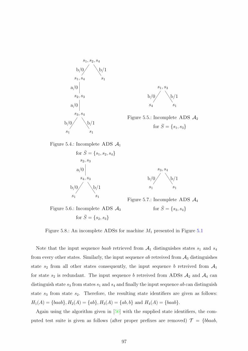
s1, s2, s4
s1, s4
s2, s3
s3, s4
s1
b/0
s1
b/1
a/0
a/0
b/0
s1
b/1
Figure 5.4.: Incomplete ADS A1
for S = {s1, s2, s4}
s1, s3
s4
b/0
s1
b/1
Figure 5.5.: Incomplete ADS A2
for S = {s1, s3}
s2, s3
s4, s3
s1
b/0
s1
b/1
a/0
Figure 5.6.: Incomplete ADS A3
for S = {s2, s3}
s3, s4
s1
b/0
s1
b/1
Figure 5.7.: Incomplete ADS A4
for S = {s3, s4}
Figure 5.8.: An incomplete ADSs for machine M1 presented in Figure 5.1
Note that the input sequence baab retrieved from A1 distinguishes states s1 and s4
from every other states. Similarly, the input sequence ab retreived from A3 distinguishes
state s2 from all other states consequently, the input sequence b retreived from A1
for state s2 is redundant. The input sequence b retreived from ADSs A2 and A4 can
distinguish state s3 from states s1 and s4 and finally the input sequence ab can distinguish
state s3 from state s2. Therefore, the resulting state identifiers are given as follows:
H1(A) = {baab}, H2(A) = {ab}, H3(A) = {ab, b} and H4(A) = {baab}.
Again using the algorithm given in [50] with the supplied state identifiers, the com-
puted test suite is given as follows (after proper prefixes are removed) T = {bbaab,
97
aabaab, abbaab, baab, babbaab, baab, bbaab} |T | = 39. There are 8 test cases and thus the
average test case length is 4.8. Recall that we obtained a test suit with length 43 with
HSIs. Using ADSs we able to reduce the length of the test suite by 9.3%. Notice that
the average test case length is slightly elevated (from 4.3 (HSI) to 4.8 (ADS)), but the
number of test cases is reduced (from 10 (HSI) to 8 (ADS)).
There are some advantages to using ADSs. If we have non-redundant ADSs then
we are guaranteed to define non-redundant state identifiers; conceptually it is easier to
reason about redundancy in a set of ADSs rather than a set of state identifiers that
have to relate in a particular way. Second, if we apply the ADSs rather than the
state identifier sets then we may obtain additional information that will be useful in
debugging: if we apply the ADSs when we expect the state to be si and we observe the
response for state sj then we have a possible explanation for the failure (the transition
took the SUT to sj rather than si). The HSI method might not provide this information
since it only applies the input sequences required to check that the state is si; adaptivity
in the ADSs can lead to other input sequences being applied based on the response and
can help identify the state reached even if it is not that expected.
We have shown that a fully distinguishing set of ADSs defines a set of identifying
sets that we can use in the HSI technique. We also have the converse, that a set of
identifying sets can be used to construct a fully distinguishing set of ADSs, since each
sequence in an identifying set defines an ADS (in which there is no adaptivity). Thus,
the complexity results in this work regarding ADSs correspond to equivalent results
regarding identifying sets and so are relevant to the HSI method.
Given a set S of states and identifying sets {H1, H2, . . . , Hn}, we can identify alterna-
tive subsets of the Hi that are sufficient to distinguish the states of S. Let us suppose
that H ′i ⊆ Hi for all si ∈ S. Then we will say that the H ′i form an identifying set for S
if for all distinct si, sj ∈ S we have sequences wi ∈ H ′i and wj ∈ H ′j such that a common
prefix of wi and wj distinguishes si and sj.
The following shows how the MaxSubSetADS problem relates to problems regarding
identifying sets.
98

Proposition 8 Let us suppose that S is a set of states of FSM M . Then the states
in S can be distinguished by a single ADS if and only if there is an identifying set
{H1, H2, . . . , Hn} for M such that we can choose subsets H ′i ⊆ Hi of each identifying
set, si ∈ S, under which each H ′i contains only one input sequence.
The following shows relationship between an HSI problem and MinSetADS.
Proposition 9 If the states in S can be distinguished by k ADS then there is an iden-
tifying set {H1, H2, . . . , Hn} such that for all si ∈ S we have that Hi has at most k input
sequences.
5.6. Practical Evaluation
In this section, we first present a greedy algorithm that aims to compute a fully dis-
tinguishing set with minimum cardinality for a given FSM M . Later we present the
results of experiments using randomly generated FSMs and some benchmark FSMs. We
emphasise that the main aim of the experiments was to explore the effect of using a set
of ADSs instead of harmonised state identifiers. Other techniques such as H [113] and
SPY [52] that use such sets of tests are likely to similarly benefit. The experiments com-
pared the ADS method with the W and HSI methods. In order to analyse the effect of
using incomplete ADSs, we study the cost of checking experiments that are constructed
by these methods. As reported in [114, 53], the cost of a checking experiment is given by
three properties: 1) The length of the checking experiment, 2) Average test case lengths
and 3) The number of resets. In the experiments we analyse these three properties of
the constructed checking experiments.
5.6.1. Greedy Algorithm
Before the actual algorithm is presented, we first have to define some important notions
concerning the greedy algorithm. We present the list of symbols with their definitions
in Table 5.1. In summary, the greedy algorithm receives an FSM M and integer value `
99

Symbol Description
T A set of tree structures.
T A tree structure.
N,E Set of nodes, set of edges.
I(n),C(n) Initial and Current sets for node n.
x(n), y(n) Input sequence, output sequence for node n.
M A set of current sets.
L Set of nodes returned by the Refine procedure.
V Set of set of nodes used by the Refine procedure.
N Set of set of nodes used by the Greedy algorithm.
` ∈ Z≥1 Upper bound on the tree height.
Q A set of pairs of states.
φ(Q,N [x]) ∈ R≥0 Heuristic function 1.
Θx(M,N [x]) ∈ Z≥0 Heuristic function 2.
F : S × S →∈ {0, 1} A function used by the Heuristic function 2.
Table 5.1.: Nomenclature for the greedy algorithm
100

and it returns a set of trees T = {T1, T2, . . . } such that all trees in this set have depth
at most ` and set T defines a fully distinguishing set. The aim is to produce a set
with minimum cardinality but, since a heuristic is used (a greedy algorithm), this is not
guaranteed.
Basic Notation
A tree T (E,N) ∈ T consists of a set of edges (E) and nodes (N). An edge e ∈ E has a
label that is an input output pair x/y where x ∈ X and y ∈ Y . A node n ∈ N captures
the following information: The initial set I(n), the current set C(n) and strings x(n)
and y(n) that give the input and output sequences that label the path from the root
of T (E,N) to the node n. For the root node n1 we have that x(n1) = y(n1) = ε and
I(n1) = C(n1) = S. Input sequence x(n) is defined as x(n) = x(n′)x where n′ is the
parent node of the current node n and x is the input retrieved from the edge between
n′ and n. Further, y(n) = y(n′)y where n′ is the parent node of the current node n and
y is the output retrieved from the edge between n′ and n. We define initial and current
sets as follows: I(n) = {s ∈ I(n′)|y(n) = λ(s, x(n))} and C(n) = {δ(s, x(n))|s ∈ I(n)}.
There are two types of nodes: a node is a leaf node if and only if it has no outgoing
edges; otherwise it is an internal node.
The greedy algorithm repeatedly executes a routine called refine. The refine routine
receives a node n and a single input x and produces a set of nodes L or returns failure.
The Refine routine is summarised in Algorithm 3.
In lines 4 and 5 the refine routine forms groups of states according to the observed
outputs, putting together states that lead to the same output. In lines 8-12, for each
group, the refine algorithm forms a node. The key point here is that we do not ignore
an input if it merges states i.e. δ(s, x) = δ(s′, x) and λ(s, x) = λ(s′, x). The reason
for such flexibility comes primarily from the fact that instead of a single tree, the aim
of the greedy algorithm is to construct a set of trees. Thus, one tree does not need to
distinguish all pairs of states: a leaf node of a tree can have two or more initial states
as long as other trees distinguish these.
101

Algorithm 3: Refine
Data: n, x
Result: L or failure.
begin
1 V [|Y |],L ←− ∅;
2 if |C(n)| = 1 then
3 Return failure;
4 for s ∈ C(n) do
5 Push δ(s, x) onto V [λ(s, x)];
6 i← 0;
7 for i < |Y | do
8 if V [i] 6= ∅ then
9 Declare new node n′;
10 C(n′) = V [i];
11 I(n′) = {s ∈ I(n)|i = λ(δ(s, x(n)), x)};
12 x(n′) = x(n′)x;
13 y(n′) = y(n′)i;
14 Push n′ to L ;
15 Return L;
102

The Algorithm
The greedy algorithm is recursive. It receives an FSM M , positive integer `, a set Q
of pairs of states not yet distinguished, and a set M of sets of states. The summary
of the Greedy Algorithm is given in Algorithm 4. Initially Q contains the set of all
pairs of distinct states. At each iteration, the greedy algorithm forms a tree structure
T . We initiate a tree T by introducing a root node n1 (Line 2). The root node has the
following information: I(n1) = S, C(n1) = S, x(n1) = ε, y(n1) = ε. Then for each input
x ∈ X, it executes the refine routine once and notes the obtained set of set N of nodes
as ni, nj . . . nk for some k ≥ 1 (Lines 6 – 7 ).
The setM holds the set of current sets that belong to nodes which cannot be refined.
Intuitively, if current sets of all possible sons of the current node are in set M, there is
no point for investigating this node any more, consequently, we also add the current set
of such node to M as well (Lines 8 – 9).
Otherwise the greedy algorithm evaluates the “goodness” of inputs by calling (Line
10) a heuristic function which is defined as follows:
Φx(Q,N [x]) =∑
n 6=n′∈N [x]
|Q ∩ I(n)× I(n′)| (5.1)
For any pair of nodes Heuristic 5.1 forms a set of pairs of states and counts the number
of occurrences of pairs in set Q. That is to say Heuristic 5.1 will return the number of
pairs of states in Q distinguished. Intuitively a “good” input is an input that maximises
this mass function: ∀x′ ∈ X, x 6= x′ we have that Φ′x ≤ Φx.
Now consider the machine M2 in Figure 5.9. According to Heuristic 5.1, the greedy
algorithm will initially select input A to distinguish state s3 from other states. After-
wards, the algorithm will try to distinguish states s1, s2 and s4. However, according
to Heuristic 5.1, there is no difference between inputs A and B and thus, the greedy
algorithm can try input A repeatedly and fall into an infinite loop. To prevent, this
in such cases, (i.e. if Heuristic function 5.1 cannot differentiate between inputs (Line
10)), the greedy algorithm decides the next input by the usage of the following greedy
103
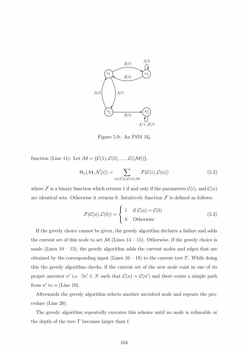
s1
s2
s4
s3
B/0
B/0
A/0
A/1, B/0
A/0
B/0
A/0
Figure 5.9.: An FSM M6
function (Line 11): Let M = {C(1), C(2), . . . , C(|M|)},
Θx(M,N [x]) =∑
n∈N [x],C(i)∈M
F(C(i), C(n)) (5.2)
where F is a binary function which returns 1 if and only if the parameters C(i), and C(n)
are identical sets. Otherwise it returns 0. Intuitively function F is defined as follows:
F(C(a), C(b)) =
1 if C(a) = C(b)
0 Otherwise(5.3)
If the greedy choice cannot be given, the greedy algorithm declares a failure and adds
the current set of this node to setM (Lines 14 – 15). Otherwise, if the greedy choice is
made (Lines 10 – 13), the greedy algorithm adds the current nodes and edges that are
obtained by the corresponding input (Lines 16 – 19) to the current tree T . While doing
this the greedy algorithm checks, if the current set of the new node exist in one of its
proper ancestor n′ i.e. ∃n′ ∈ N such that C(n) = C(n′) and there exists a simple path
from n′ to n (Line 19).
Afterwards the greedy algorithm selects another unvisited node and repeats the pro-
cedure (Line 20).
The greedy algorithm repeatedly executes this scheme until no node is refineable or
the depth of the tree T becomes larger than `.
104

After the tree is constructed the greedy algorithm removes pair of states (s, s′) from
Q if s, s′ are members of initial sets of different leaf nodes i.e. s ∈ I(n) ∧ s′ ∈ I(n′)
for n 6= n′ (Lines 22 – 24). Finally, if |Q| > 0 the algorithm calls itself (Lines 25 – 26).
The Greedy algorithm stops when |Q| = 0 (Lines 27 – 28). Since the greedy algorithm
is a heuristic the resultant tree T need not be optimal; later we report the results of
experiments used to explore the effectiveness of this approach.
We now need to show that at each iteration the greedy algorithm computes an in-
complete ADS. In order to achieve this we first need to emphasise some properties of
tree T . First recall that the greedy algorithm selects a single set of nodes N [x] while
constructing a tree T and since N [x] is constructed by a single input x, the outgoing
edges are labeled by identical inputs and are labeled with different outputs. Therefore
the following immediately follows from the construction of tree T .
Lemma 29 Let n be an internal node of tree T with children n1, n2, . . . , np and let x be
the input portion of the labels of the edges from node n. The following hold:
1. δ(C(n), x) = ∪pi=1C(ni).
2. For all 1 ≤ i ≤ p we have that |λ(I(ni), x(ni))| = 1.
3. For all 1 ≤ i < j ≤ p we have that λ(I(ni), x(n)) = λ(I(nj), x(n)) and λ(I(ni), x(n)x) 6=
λ(I(nj), x(n)x).
Moreover, consider distinct leaf nodes (n, n′) then using Corollary 29 we know that
the output observed from any pair of states s ∈ I(n) and s′ ∈ I(n′) are different.
Lemma 30 Let n, n′ be distinct leaf nodes of tree T . If s ∈ I(n) and s′ ∈ I(n′) then
λ(s, x(n)) 6= λ(s′, x(n)) and λ(s, x(n′)) 6= λ(s′, x(n′)).
Now we show that a tree T returned by the greedy algorithm defines an incomplete
ADS.
Lemma 31 Let T be a tree returned by the greedy algorithm such that N = {n1, . . . , np}
is the set of leaf nodes of T . Let S be a set of states such that for all 1 ≤ i ≤ p we have
that |I(ni) ∩ S| ≤ 1. Then T defines an incomplete ADS for set S.
105
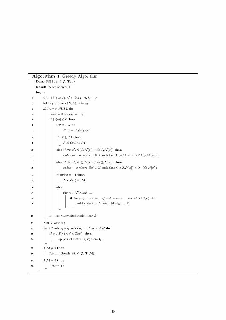
Algorithm 4: Greedy AlgorithmData: FSM M , `, Q, T, M
Result: A set of trees T
begin
1 n1 ← (S, S, ε, ε), N ← ∅,a := 0, h := 0;
2 Add n1 to tree T (N,E), v ← n1;
3 while v 6= NULL do
4 max := 0, index := −1;
5 if |x(v)| ≤ ` then
6 for x ∈ X do
7 N [x] = Refine(v,x);
8 if N ⊆M then
9 Add C(v) to M
10 else if ∀x, x′, Φ(Q,N [x]) = Φ(Q,N [x′]) then
11 index← x where 6 ∃x′ ∈ X such that Θx′ (M,N [x′]) < Θx(M,N [x])
12 else if ∃x, x′, Φ(Q,N [x]) 6= Φ(Q,N [x′]) then
13 index← x where 6 ∃x′ ∈ X such that Φx(Q,N [x]) < Φx′ (Q,N [x′])
14 if index = −1 then
15 Add C(v) to M
16 else
17 for n ∈ N [index] do
18 if No proper ancestor of node v have a current set C(n) then
19 Add node n to N and add edge to E.
20 v ← next unvisited node, clear B;
21 Push T onto T;
22 for All pair of leaf nodes n, n′ where n 6= n′ do
23 if s ∈ I(n) ∧ s′ ∈ I(n′), then
24 Pop pair of states (s, s′) from Q ;
25 if M 6= ∅ then
26 Return Greedy(M , `, Q, T,M);
27 if M = ∅ then
28 Return T;
106

Although the algorithm is easy to implement, it may not compute a fully distinguishing
set for a given FSM. This will happen if the upper bound on ADS length is too short.
Note that for an FSM M with n states, every pair of states is distinguished by a sequence
of length at most n− 1 and it is sufficient to use at most n− 1 such sequences in order
to distinguish all of the states of M . Thus, the algorithm is guaranteed to return a fully
distinguishing set if we use value of ` as n− 1 or larger.
5.6.2. Experimental results
Test Generation
This section describes experiments used to explore the performance of the greedy algo-
rithm and the effect of using fully distinguishing sets by evaluating the resultant checking
experiments. We randomly generated FSMs with 4, 6, and 8 inputs and outputs using
the tool utilised in [43, 108]. The FSMs were constructed as follows: First, for each input
x and state si we randomly assigned the values of δ(si, x) and λ(si, x). After an FSM M
was generated we checked its suitability as follows. We first checked that M is synchro-
nisable, that is whether M has a reset. In order to do this we implemented the existence
check algorithm described in [34]. Then we checked whether M is strongly connected2.
Afterwards we checked that M is minimal and then used the LY-algorithm [35] to check
that M does not have a complete ADS. If the FSM failed one or more of these tests
then we omitted this FSM and produced another. Consequently, all FSMs used had a
reset, were strongly connected and minimal, and had no complete ADS. By following
this procedure we constructed 100 FSMs with 5 states, 100 FSMs with 10 states, . . . ,
100 FSMs with 100 states. This was done for each size of the input and output alphabets
so in total we used 6 ∗ 103 FSMs. We used an Intel i7 3630 Q3 Ivy-Bridge CPU with 8
GB RAM to carry out these tests. We implemented W , HSI and the greedy algorithm
using C++ language and compiled on Visual Studio .Net 2012.
The checking experiment generation methods considered the care where the SUT
2M is strongly connected if for any pair (s, s′) of states of M there is some input sequence that takes
M from s to s′.
107

has no more states than the specification FSM. The W and the HSI methods were
implemented according to the descriptions presented in references [4, 50]. As explained
earlier, we also implemented the HSI method adapted for a fully distinguishing set of
ADSs and used the greedy algorithm to produce the ADSs. Since the outputs are
uniformly distributed during the generation of FSMs, one would expect the average
depth of the ADS to be around dlogq ne, where n and q are the number of states and
the number of outputs, respectively. For our experiments with 4,6 and 8 outputs and
the number of states ranging between 5 and 100, the length of ` is expected to be 2–4
for 4 outputs (dlog4 5e = 2 and dlog4 100e = 4), 1–3 for 6 outputs (dlog6 5e = 1 and
dlog6 100e = 3), and 1–3 for 8 outputs (dlog8 5e = 1 and dlog8 100e = 3). For each FSM
we set the upper bound on ADS depth to be twice this value dlogq ne i.e. ` = 2∗dlogq ne.
With these values, we were able to produce fully distinguishing sets.
Checking Experiment Length
We present the results using boxplot diagrams generated by ggplot2 library of the tool
R [115, 116, 117]. For each box the first quartile corresponds to the lowest 25% of data,
the second quartile gives the median, and the third quartile corresponds to the highest
25%. For each boxplot we added the smoothing line computed with the LOESS [118]
method, and the semi-transparent ribbon surrounding the solid line is the 95% confidence
interval. We also give the jitter plot3 where each dot corresponds to the result of an
execution of the corresponding method, where input is a single FSM.
Figure 5.10 presents information regarding the checking experiment length for FSMs
where p/q = 4/4. The figure suggest that except for the FSMs with n = 5, the checking
experiment length obtained by the modified HSI method (ADS method) is less than the
HSI and W methods. Moreover, when n ≥ 40 the third quantile of the boxplots drawn
for the ADS method are lower than the first quantile of the boxplots drawn for the HSI
method. These results suggest that usually the ADS method produces shorter test suites
3The Jitter plot adds a noise to the data to prevent occlusion in the statistical visualizations. Each
data point displace on horizontal axis.
108
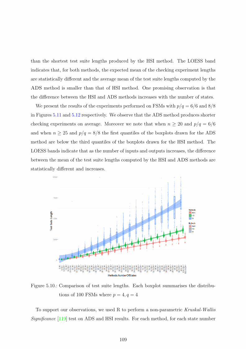
than the shortest test suite lengths produced by the HSI method. The LOESS band
indicates that, for both methods, the expected mean of the checking experiment lengths
are statistically different and the average mean of the test suite lengths computed by the
ADS method is smaller than that of HSI method. One promising observation is that
the difference between the HSI and ADS methods increases with the number of states.
We present the results of the experiments performed on FSMs with p/q = 6/6 and 8/8
in Figures 5.11 and 5.12 respectively. We observe that the ADS method produces shorter
checking experiments on average. Moreover we note that when n ≥ 20 and p/q = 6/6
and when n ≥ 25 and p/q = 8/8 the first quantiles of the boxplots drawn for the ADS
method are below the third quantiles of the boxplots drawn for the HSI method. The
LOESS bands indicate that as the number of inputs and outputs increases, the difference
between the mean of the test suite lengths computed by the HSI and ADS methods are
statistically different and increases.
Figure 5.10.: Comparison of test suite lengths. Each boxplot summarises the distribu-
tions of 100 FSMs where p = 4, q = 4
To support our observations, we used R to perform a non-parametric Kruskal-Wallis
Significance [119] test on ADS and HSI results. For each method, for each state number
109
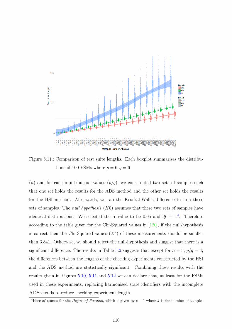
Figure 5.11.: Comparison of test suite lengths. Each boxplot summarises the distribu-
tions of 100 FSMs where p = 6, q = 6
(n) and for each input/output values (p/q), we constructed two sets of samples such
that one set holds the results for the ADS method and the other set holds the results
for the HSI method. Afterwards, we ran the Kruskal-Wallis difference test on these
sets of samples. The null hypothesis (H0) assumes that these two sets of samples have
identical distributions. We selected the α value to be 0.05 and df = 14. Therefore
according to the table given for the Chi-Squared values in [120], if the null-hypothesis
is correct then the Chi-Squared values (X 2) of these measurements should be smaller
than 3.841. Otherwise, we should reject the null-hypothesis and suggest that there is a
significant difference. The results in Table 5.2 suggests that except for n = 5, p/q = 4,
the differences between the lengths of the checking experiments constructed by the HSI
and the ADS method are statistically significant. Combining these results with the
results given in Figures 5.10, 5.11 and 5.12 we can declare that, at least for the FSMs
used in these experiments, replacing harmonised state identifiers with the incomplete
ADSs tends to reduce checking experiment length.
4Here df stands for the Degree of Freedom, which is given by k − 1 where k is the number of samples
110
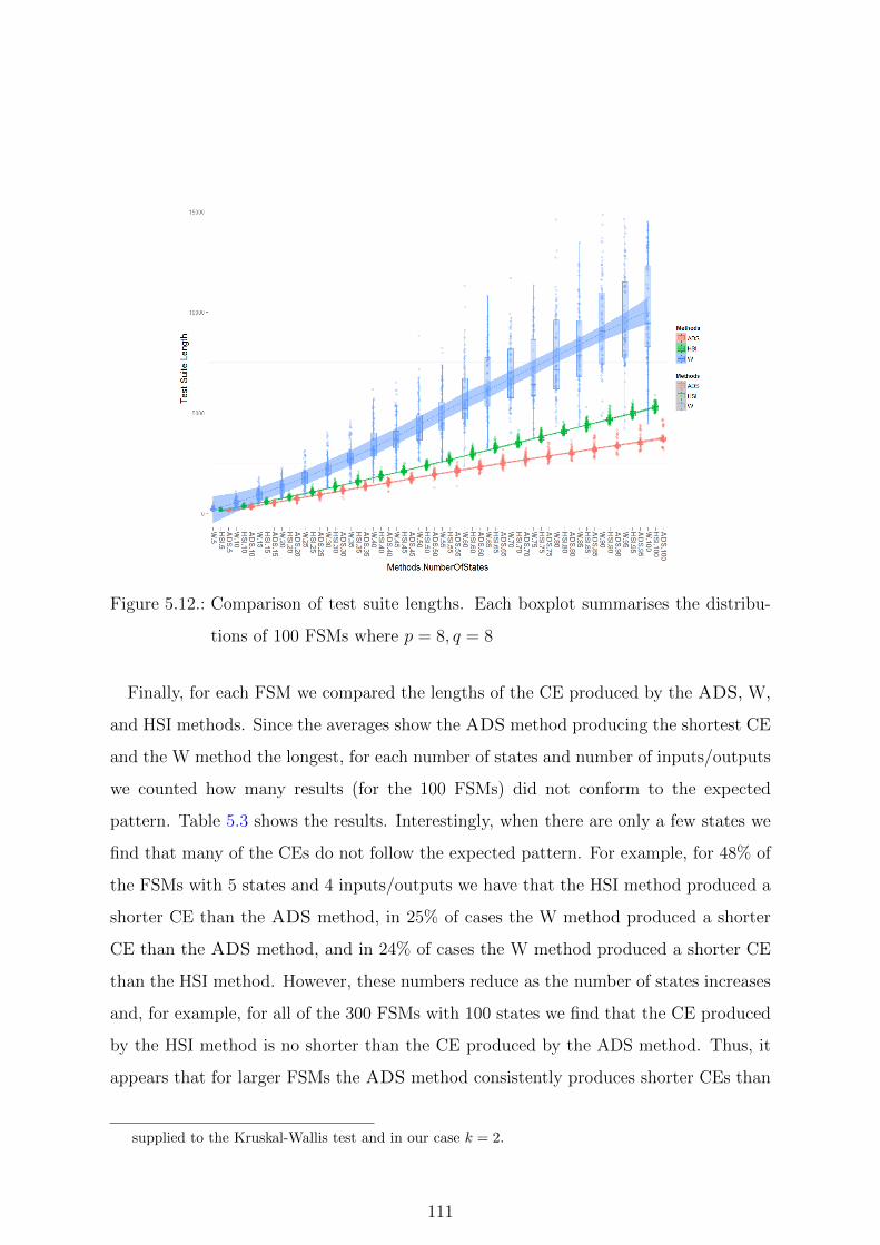
Figure 5.12.: Comparison of test suite lengths. Each boxplot summarises the distribu-
tions of 100 FSMs where p = 8, q = 8
Finally, for each FSM we compared the lengths of the CE produced by the ADS, W,
and HSI methods. Since the averages show the ADS method producing the shortest CE
and the W method the longest, for each number of states and number of inputs/outputs
we counted how many results (for the 100 FSMs) did not conform to the expected
pattern. Table 5.3 shows the results. Interestingly, when there are only a few states we
find that many of the CEs do not follow the expected pattern. For example, for 48% of
the FSMs with 5 states and 4 inputs/outputs we have that the HSI method produced a
shorter CE than the ADS method, in 25% of cases the W method produced a shorter
CE than the ADS method, and in 24% of cases the W method produced a shorter CE
than the HSI method. However, these numbers reduce as the number of states increases
and, for example, for all of the 300 FSMs with 100 states we find that the CE produced
by the HSI method is no shorter than the CE produced by the ADS method. Thus, it
appears that for larger FSMs the ADS method consistently produces shorter CEs than
supplied to the Kruskal-Wallis test and in our case k = 2.
111

Tab
le5.
2.:
The
resu
lts
ofa
Kru
skal
-Wal
lis
Sig
nifi
cance
Tes
tsp
erfo
rmed
onth
eC
hec
kin
gE
xp
erim
ents
Len
gth
Input/
outp
ut
(p/q
)va
l-
ues
Cor
resp
ondin
gX
2–v
alues
for
diff
eren
tnum
ber
ofst
ates
(n).
Rej
ectH
0w
henX
2>
3.84
1
510
1520
2530
3540
4550
5560
6570
7580
8590
9510
0
4/4
9e-0
416
.39
52.7
963
.173
.36
88.9
873
.53
105.
2110
0.94
91.9
297
.34
97.3
211
1.65
123.
8912
7.56
140.
5214
0.29
145.
1914
1.3
147.
17
6/6
47.0
521
.95
58.3
610
0.21
128.
413
7.75
142.
0313
9.1
144.
2814
0.29
148.
0314
9.25
147.
1114
8.6
148.
8914
9.01
149.
2514
9.25
149.
2514
9.25
8/8
55.9
714
.72
10.9
726
.15
87.8
781
.412
2.51
140.
4614
5.4
142.
4614
7.67
146.
414
7.08
147.
0814
9.22
149.
2514
9.25
149.
2514
9.25
149.
25
112

the HSI and W methods.
Average Test Case Length
In the previous subsection we showed that using a fully distinguishing set can reduce
the overall length of a checking experiment. In this and next subsections we investigate
possible reasons for this achievement.
Figure 5.13 shows how the average test case length varied with the number of states
when the number of inputs and outputs is four. Although the graphical representation
suggests that the distribution and the expected mean of the average test case lengths are
different, this difference is not more than 2.5 inputs on average. Moreover, as we increase
the number of inputs and outputs to six and eight we observe that this difference does
not change. That is both the W, HSI and the ADS methods produce comparable test
cases. However, we note that as the number of inputs and outputs increases, the average
lengths of test cases reduces. This is expected since having more inputs and outputs
increases the number of transitions and therefore the length of a path from the initial
state to another state decreases. What is more, more inputs and outputs allows the
use of shorter characterising sets, harmonized state identifiers and ADSs to distinguish
states.
113

Tab
le5.
3.:
Pai
rwis
ediff
eren
ces
ofC
EL
engt
hs.
Eac
hva
lue
corr
esp
onds
toth
eocc
urr
ence
ofth
eco
mpar
ison
crit
eria
in10
0
FSM
s.
Inp
ut/
outp
ut
(p/q
)va
l-
ues
Com
par
ison
Cri
teri
a
Nu
mb
erof
Sta
tes.
510
1520
2530
3540
4550
5560
6570
7580
8590
9510
0
W<HSI
249
1410
52
84
62
14
21
00
10
00
4/4
W<ADS
256
57
40
30
41
12
10
02
00
00
HSI<ADS
4832
1519
165
127
610
1211
45
32
00
20
W<HSI
216
69
32
15
54
33
22
43
20
01
6/6
W<ADS
76
27
01
00
21
01
11
20
10
01
HSI<ADS
1528
132
21
01
00
00
00
00
00
00
W<HSI
1510
77
46
33
20
21
10
01
10
23
8/8
W<ADS
47
42
10
00
00
11
00
00
00
00
HSI<ADS
131
3818
67
10
00
00
00
00
00
00
114
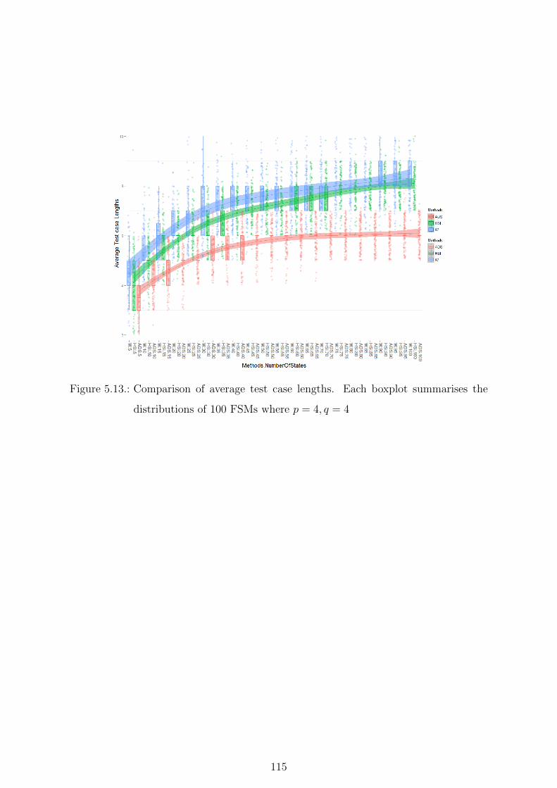
Figure 5.13.: Comparison of average test case lengths. Each boxplot summarises the
distributions of 100 FSMs where p = 4, q = 4
115
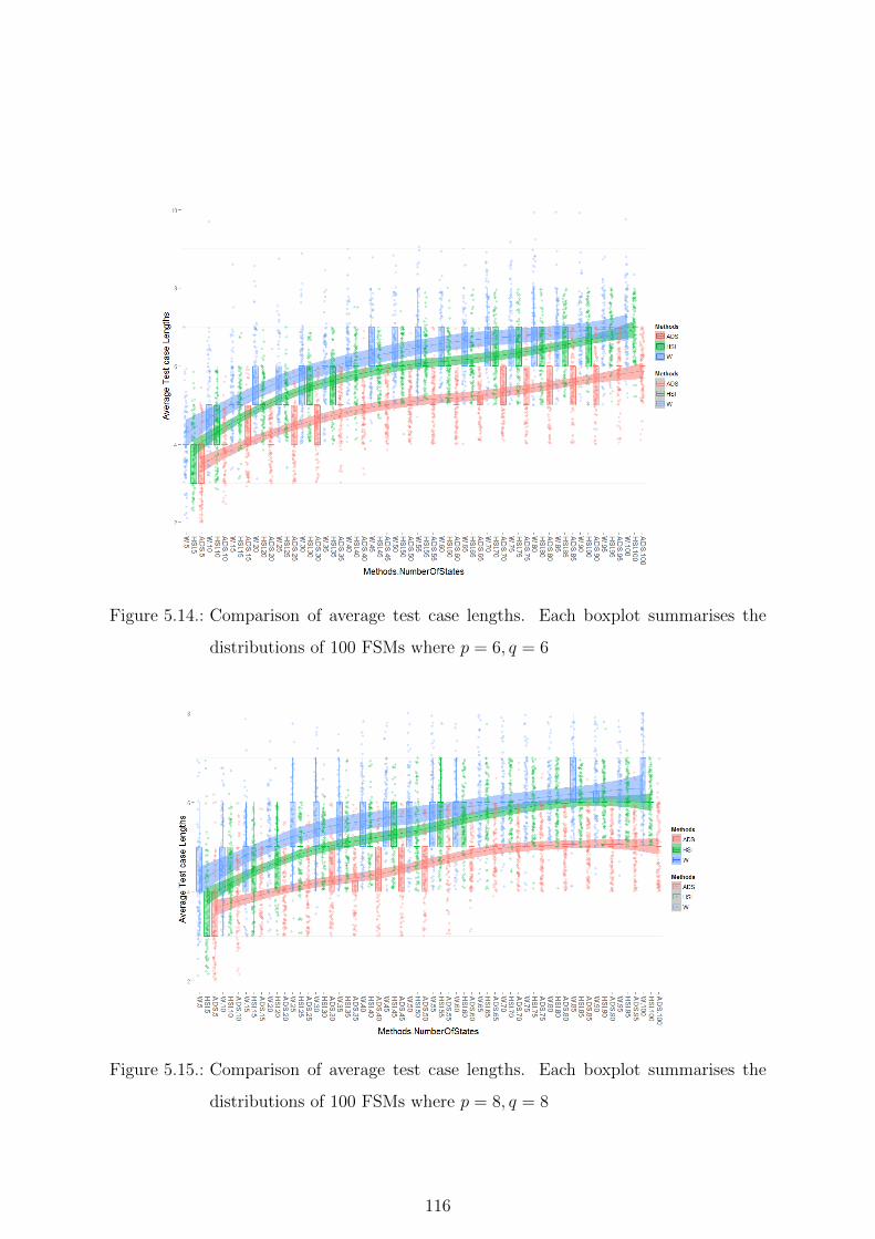
Figure 5.14.: Comparison of average test case lengths. Each boxplot summarises the
distributions of 100 FSMs where p = 6, q = 6
Figure 5.15.: Comparison of average test case lengths. Each boxplot summarises the
distributions of 100 FSMs where p = 8, q = 8
116

We performed a Kruskal-Wallis test on the test case lengths. Table 5.4 suggest thatthe distributions are statistically different. Therefore we can conclude that the ADSmethod produces shorter test cases compared to the HSI method.
Although we showed that the average test cases are shorter when ADS method is
used, we claim that the small difference (2.5 inputs maximum) probably cannot explain
the reduction of the checking experiment lengths. Therefore we now investigate the
average number of resets of the computed checking experiments.
Number of Resets
As a reset is applied before a test case, the number of resets is the same as the number of
test cases in a checking experiment. Figure 5.16 represents the results of the conducted
experiments when p/q = 4/4.
Based on results in [53], we expect that the number of resets when using ADSs to be
less than that for the W method and similar to the value for the HSI method. Although
the distributions are different, the maximum difference between the means is only 3.3%.
This is the case when p/q = 4/4. However, the difference between the HSI and ADS
methods increases with the number of inputs/outputs. We observe that when p/q = 6/6
and n ≥ 20 and when p/q = 8/8 and n ≥ 20, the average number of resets is lower when
using the ADS method. It appears that as the number of inputs/outputs increases the
difference between the HSI and the ADS methods increases. These observations are
similar to those for the checking experiment lengths.
117

Tab
le5.
4.:
Res
ult
sfo
rN
on-p
aram
etri
cK
rusk
al-W
allis
Sig
nifi
cance
Tes
ts
Input/
outp
ut
(p/q
)
valu
es
Cor
resp
ondin
gX
2–v
alues
for
diff
eren
tnum
ber
ofst
ates
(n)
510
1520
2530
3540
4550
5560
6570
7580
8590
9510
0
4/4
32.0
924
.418
.34
17.2
78.
8319
.71
20.5
311
.36
14.5
59.
473.
9913
.85
8.11
12.5
612
.89
11.1
916
.14
28.3
37.
864.
07
6/6
26.4
068
13.3
254
17.5
1820
.142
519
.73
16.3
312
.14
7.18
14.8
27.7
641
.72
13.9
432
19.4
512
.99
14.4
17.4
415
.13
12.9
212
.83
8/8
46.5
737
.39
17.7
910
.21
7.24
20.1
413
.26
12.5
523
.15
10.1
412
.87
11.8
916
.13
15.4
113
.06
12.0
35.
768.
3824
15.6
6
118
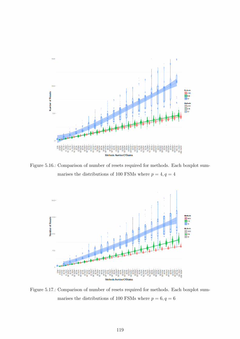
Figure 5.16.: Comparison of number of resets required for methods. Each boxplot sum-
marises the distributions of 100 FSMs where p = 4, q = 4
Figure 5.17.: Comparison of number of resets required for methods. Each boxplot sum-
marises the distributions of 100 FSMs where p = 6, q = 6
119
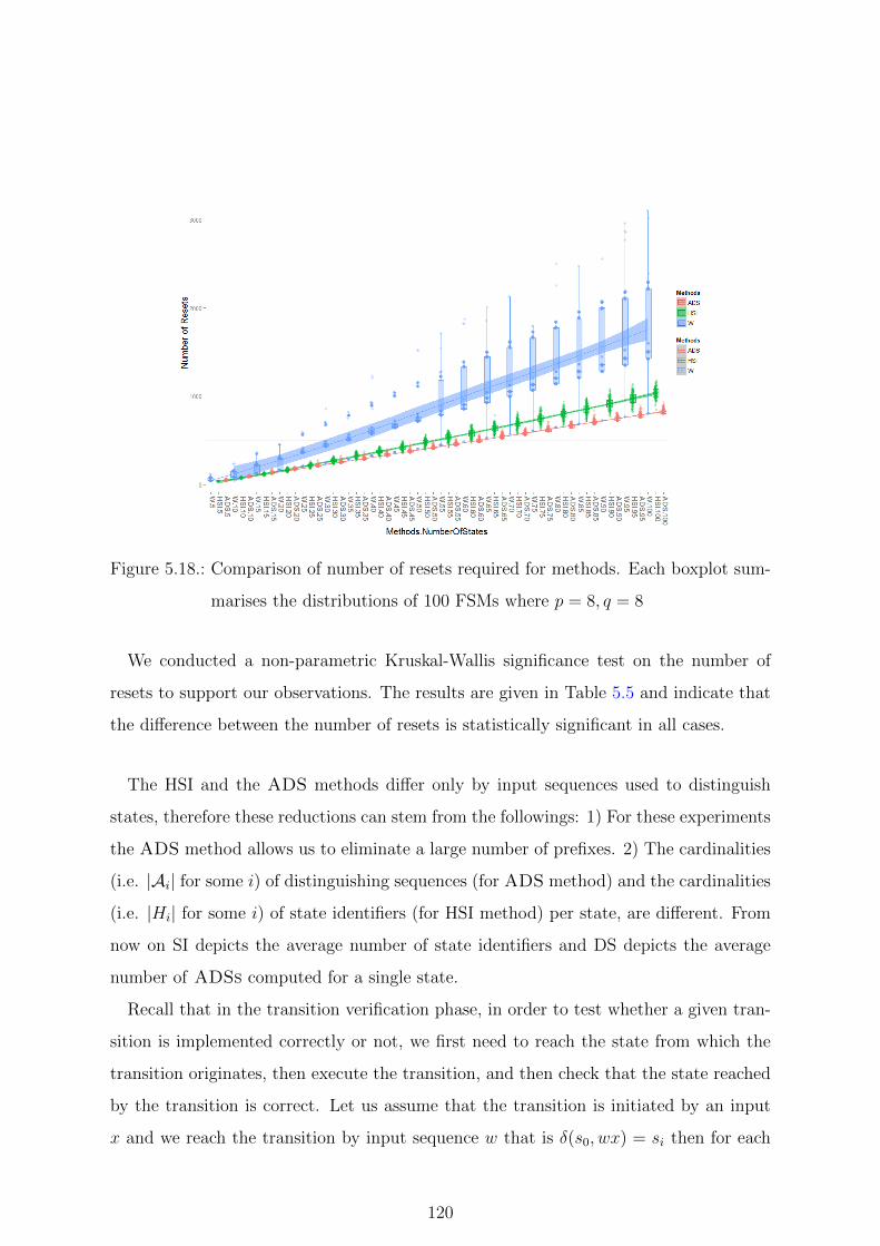
Figure 5.18.: Comparison of number of resets required for methods. Each boxplot sum-
marises the distributions of 100 FSMs where p = 8, q = 8
We conducted a non-parametric Kruskal-Wallis significance test on the number of
resets to support our observations. The results are given in Table 5.5 and indicate that
the difference between the number of resets is statistically significant in all cases.
The HSI and the ADS methods differ only by input sequences used to distinguish
states, therefore these reductions can stem from the followings: 1) For these experiments
the ADS method allows us to eliminate a large number of prefixes. 2) The cardinalities
(i.e. |Ai| for some i) of distinguishing sequences (for ADS method) and the cardinalities
(i.e. |Hi| for some i) of state identifiers (for HSI method) per state, are different. From
now on SI depicts the average number of state identifiers and DS depicts the average
number of ADSs computed for a single state.
Recall that in the transition verification phase, in order to test whether a given tran-
sition is implemented correctly or not, we first need to reach the state from which the
transition originates, then execute the transition, and then check that the state reached
by the transition is correct. Let us assume that the transition is initiated by an input
x and we reach the transition by input sequence w that is δ(s0, wx) = si then for each
120

Tab
le5.
5.:
The
resu
lts
ofa
Kru
skal
-Wal
lis
Sig
nifi
cance
Tes
tsp
erfo
rmed
onth
eN
um
ber
ofR
eset
s
Inp
ut/
outp
ut
(p/q
)
valu
es
Cor
resp
ond
ingX
2–v
alues
for
diff
eren
tnu
mb
erof
stat
es(n
).R
ejec
tH
0w
henX
2>
3.84
1
510
1520
2530
3540
4550
5560
6570
7580
8590
9510
0
4/4
19.8
315
.65
23.5
429
.91
30.6
434
.12
32.4
240
33.6
842
.06
49.4
551
.58
48.8
243
.51
4646
.366
.34
51.2
51.0
353
.24
6/6
34.4
722
.95
25.5
26.0
823
.728
.51
38.8
327
.83
.37.
0929
.49
38.6
538
.09
49.1
637
.53
46.2
456
.87
64.3
156
.67
46.3
345
.01
8/8
41.4
820
.81
36.5
130
.430
.48
33.8
26.4
435
.78
23.3
332
24.6
139
.74
35.9
134
.25
46.9
132
.24
38.9
133
.625
.89
40.9
1
121

input sequences in Hi and Ai we need to generate test cases. For the HSI method for all
α ∈ Hi we add wxα and for the ADS method for all β ∈ Ai we add wxβ to the checking
experiment. Therefore the values of SI and DS can potentially affect the number of
resets.
We investigated the average values of SI and DS. For each FSM M we computed the
sum (over the states) of the cardinalities of sets Hi and also the sum of the cardinalities
of the Ai and divided these sums by the number of states n. We summarise this study
in Figures 5.19, 5.20 and 5.21, where p/q = 4/4, 6/6 and 8/8 respectively.
In Figure 5.19, we observe that boxplot and jitterplot are similar to the results pre-
sented in Figure 5.16 and indicate that the values of DS and SI are comparable for
ADS and the HSI methods. Moreover, we observe that the values of DS and SI increase
with the number of states. In Figure 5.20 we see that when n ≥ 30 the DS values is
lower compared to the SI values and in Figure 5.21 we see that when n ≥ 25 the DS
values is lower compared to the SI values. Moreover we notice that as the number of
inputs/outputs increases the values of SI and DS appear to decrease.
Figure 5.19.: Comparison of number of DS and SI per state. Each boxplot summarises
the distributions of 100 FSMs where p = 4, q = 4.
122
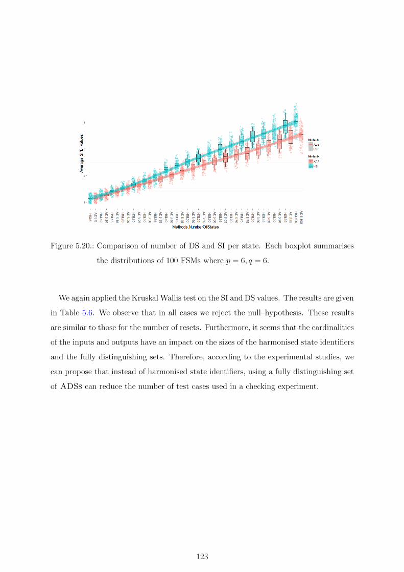
Figure 5.20.: Comparison of number of DS and SI per state. Each boxplot summarises
the distributions of 100 FSMs where p = 6, q = 6.
We again applied the Kruskal Wallis test on the SI and DS values. The results are given
in Table 5.6. We observe that in all cases we reject the null–hypothesis. These results
are similar to those for the number of resets. Furthermore, it seems that the cardinalities
of the inputs and outputs have an impact on the sizes of the harmonised state identifiers
and the fully distinguishing sets. Therefore, according to the experimental studies, we
can propose that instead of harmonised state identifiers, using a fully distinguishing set
of ADSs can reduce the number of test cases used in a checking experiment.
123

Tab
le5.
6.:
The
resu
lts
ofa
Kru
skal
-Wal
lis
Sig
nifi
cance
Tes
tsp
erfo
rmed
onth
eSI
and
DI
valu
es
Input/
outp
ut
(p/q
)
valu
es
Cor
resp
ondin
gX
2–v
alues
for
diff
eren
tnum
ber
ofst
ates
(n).
Rej
ectH
0w
henX
2>
3.84
1
510
1520
2530
3540
4550
5560
6570
7580
8590
9510
0
4/4
46,1
565
.71
76.8
961
.47
63.4
965
.79
77.6
969
.09
73.9
765
.95
75.0
653
.54
65.8
367
.42
64.4
174
.27
53.9
569
.37
80.8
860
.91
6/6
46.6
358
.29
69.1
069
.96
52.7
263
.36
68.8
881
.10
68.3
551
.02
59.3
065
.48
63.2
360
.43
68.1
670
.64
68.6
760
.98
71.7
361
.39
8/8
34.8
470
.11
68.6
275
.32
57.2
959
.79
64.1
464
.74
64.4
669
.43
69.1
463
.60
66.7
359
.38
76.9
664
.18
69.7
374
.44
62.9
479
.08
124
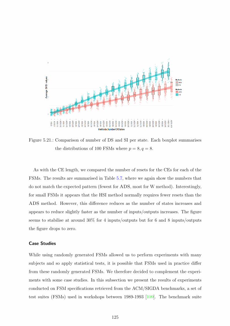
Figure 5.21.: Comparison of number of DS and SI per state. Each boxplot summarises
the distributions of 100 FSMs where p = 8, q = 8.
As with the CE length, we compared the number of resets for the CEs for each of the
FSMs. The results are summarised in Table 5.7, where we again show the numbers that
do not match the expected pattern (fewest for ADS, most for W method). Interestingly,
for small FSMs it appears that the HSI method normally requires fewer resets than the
ADS method. However, this difference reduces as the number of states increases and
appears to reduce slightly faster as the number of inputs/outputs increases. The figure
seems to stabilise at around 30% for 4 inputs/outputs but for 6 and 8 inputs/outputs
the figure drops to zero.
Case Studies
While using randomly generated FSMs allowed us to perform experiments with many
subjects and so apply statistical tests, it is possible that FSMs used in practice differ
from these randomly generated FSMs. We therefore decided to complement the experi-
ments with some case studies. In this subsection we present the results of experiments
conducted on FSM specifications retrieved from the ACM/SIGDA benchmarks, a set of
test suites (FSMs) used in workshops between 1989-1993 [109]. The benchmark suite
125
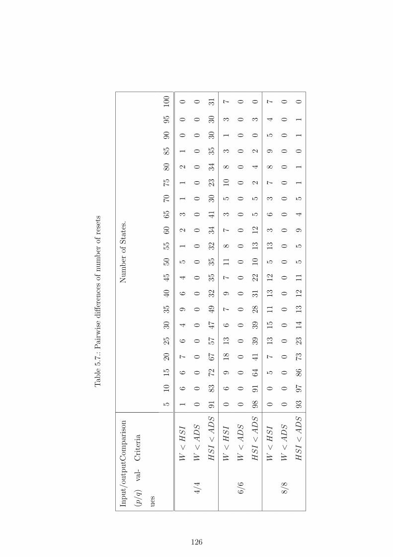
Tab
le5.
7.:
Pai
rwis
ediff
eren
ces
ofnum
ber
ofre
sets
Inp
ut/
outp
ut
(p/q
)va
l-
ues
Com
par
ison
Cri
teri
a
Nu
mb
erof
Sta
tes.
510
1520
2530
3540
4550
5560
6570
7580
8590
9510
0
W<HSI
16
67
64
96
45
12
31
12
10
00
4/4
W<ADS
00
00
00
00
00
00
00
00
00
00
HSI<ADS
9183
7267
5747
4932
3535
3234
4130
2334
3530
3031
W<HSI
06
918
136
79
711
87
35
108
31
37
6/6
W<ADS
00
00
00
00
00
00
00
00
00
00
HSI<ADS
9891
6441
3939
2831
2210
1312
55
24
20
30
W<HSI
00
57
1315
1113
125
133
63
78
95
47
8/8
W<ADS
00
00
00
00
00
00
00
00
00
00
HSI<ADS
9397
8673
2314
1312
115
59
45
11
01
10
126

has 59 FSM specifications ranging from simple circuits to advanced circuits obtained
from industry. The FSM specifications are presented in the kiss2 format. In order to
precess FSMs, we converted the kiss2 file format to our FSM specification format. We
only used FSMs from the benchmark that were minimal, deterministic, had no complete
ADS, were synchronisable, and had fewer than 10 input bits5. 19% of the FSMs had
more than 10 input bits, 15% FSMs had complete ADS, 38% were not minimal and
20% had no synchronising sequence. 11% of the FSM specifications passed all of the
tests. We computed checking experiments using the W, HSI and ADS methods and in
Table 5.8 we present the results.
The case studies indicate that the use of ADSs led to the smallest checking experi-
ments. We see that for FSM bbsse the test suite length is 64% shorter when the set of
ADSs are used in the HSI method. For planet the reduction is 58%, for s1 the reduc-
tion is 54%, for dk17 the reduction is 50%, for s386 the reduction is 48% and finally
for dk27 the reduction is 43%. The difference between the average number of resets are
summarised as follows: For bbsse the reduction is 63%, for s386 the reduction is 57%,
for s1 the reduction is 56%, for planet the reduction is 49%, for dk17 the reduction is
46%, for bbtas the reduction is 38% and finally for dk27 the reduction is 34%
Interestingly, Table 5.8 indicates that the average test case lengths for the HSI and
the ADS method were similar but in one FSM (s386) the average test case length is
shorter when the harmonized state identifiers are used (red coloured values). However,
we can say that these results are similar to those obtained from randomly generated
FSMs. We finally note that, as expected, it appears that as the ratio of the number of
outputs to the number of inputs reduces, the number of resets and the average test case
length increase.
Discussion
Based on the experimental results we can make the following main observations.
5Since the circuits receive inputs in bits, and since n bits correspond to 2n inputs, we do not consider
FSMs with n ≥ 10 bits
127
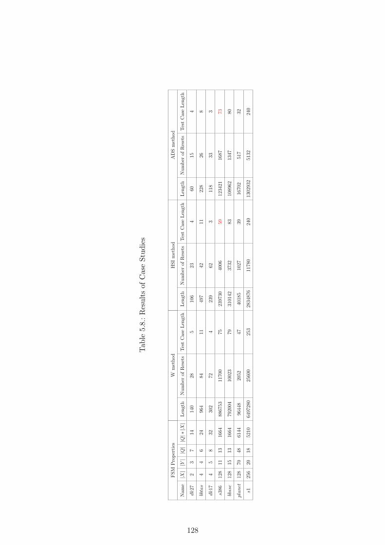
Tab
le5.
8.:
Res
ult
sof
Cas
eStu
die
s
FS
MP
rop
erti
esW
met
hod
HS
Im
eth
od
AD
Sm
eth
od
Nam
e|X||Y||Q||Q|∗|X|
Len
gth
Nu
mb
erof
Res
ets
Tes
tC
ase
Len
gth
Len
gth
Nu
mb
erof
Res
ets
Tes
tC
ase
Len
gth
Len
gth
Nu
mb
erof
Res
ets
Tes
tC
ase
Len
gth
dk27
23
714
140
285
106
234
6015
4
bbtas
44
624
964
8411
497
4211
228
268
dk17
45
832
302
724
239
623
118
333
s386
128
1113
1664
8867
5311
700
7523
9730
4006
5912
3421
1687
73
bbsse
128
1513
1664
7920
0410
023
7931
0142
3732
8310
8962
1347
80
planet
128
7048
6144
9644
820
5247
4018
510
2739
1670
251
732
s125
620
1852
1064
9728
025
600
253
2834
876
1178
024
013
0293
251
3224
0
128

1. Using ADSs instead of harmonised state identifiers is advantageous:
We used 6 ∗ 103 randomly generated FSMs of varying number of states and in-
puts/outputs and found that the ADS method produced shorter checking experi-
ments that have fewer resets. We also analysed the FSMs from the ACM/SIGDA
dataset that are minimal, deterministic, have no complete ADSs, and are syn-
chronisable. In all of these FSMs the ADS method produced shorter checking
experiments with fewer resets.
2. The ADS method computes test cases with slightly shorter lengths:
This results indicate that there are differences in the average test case lengths but
that these do not fully explain the differences in the checking experiment lengths.
3. The ADS method computes checking experiments with fewer resets:
The results suggest that ADS method produces fewer test cases. These results
are similar to those for the lengths of the checking experiments except that the
differences are smaller. Thus, the differences in CE length appear to come from
both differences in mean test sequence length and differences in number of resets.
4. The number of harmonised state identifiers (Hi’s) computed per state
is usually larger than the number of distinguishing sequences (Ai) com-
puted per state:
We see that the ADS method produces fewer distinguishing sequence per state
than the harmonised state identifiers and this explains the difference in the number
of resets.
5.7. Chapter Summary and Future Directions
Software testing is typically performed manually and is an expensive, error prone process.
This has led to interest in automated test generation, including significant interest in
model based testing (MBT). Most MBT techniques generate tests from either finite
129

state machines (FSMs) or labelled transition systems. Many automated FSM based test
techniques use complete distinguishing sequences (DSs) to check the state of the system
under test after a transition. While complete DSs have many desirable properties, an
FSM M need not have a complete DS that distinguishes all of its states. However, we
might still have (incomplete) DSs that distinguish some of the states of M and such DSs
might be used in automated test generation.
In this work we explored the problem of constructing DSs for subsets of states of
FSMs. We showed that it is PSPACE-complete to find a preset DS (PDS) that max-
imises the number of states distinguished and it is PSPACE-hard to approximate this
problem. It is also PSPACE-complete to find a smallest set of sets of states that cor-
respond to PDSs that distinguish all of the states of the FSM. We then explored the
corresponding problems for Adaptive DSs (ADSs). It is known that we can decide in
polynomial time whether an FSM has a complete ADS. However, the results for ADSs
were similar to those for such PDSs: the problems considered were PSPACE-complete
and it is PSPACE-hard to approximate the corresponding optimisation problem.
Having produced these results we showed that the well-known W and HSI checking
experiment generation methods can be adapted to use (incomplete) ADSs and so also
PDSs. In addition, we showed that the optimisation problems considered in this work
are relevant to these adapted versions of the W and HSI method and also the stan-
dard HSI method. We then used experiments to explore the effect of optimisation by
randomly generating FSMs and comparing the sizes of the checking experiments pro-
duced using the W-method, the HSI-method, and the HSI-method with an optimised
set of ADSs. In the experiments, the proposed method, that uses ADSs, produced the
smallest checking experiments and the W-method produced the largest checking experi-
ments. In addition, the proposed method required the fewest resets. We extended these
experiments to consider six FSMs from a benchmark and again found that the proposed
method produced smaller test suites that required fewer resets.
There are several lines of future work. First, it would be interesting to explore re-
alistic conditions under which the decision and optimisation problems can be solved in
130

polynomial time. Such conditions might lead to new notions of testability. There is also
the question as to how effective is the greedy approach to generating incomplete ADSs:
while the checking experiments returned were smaller than those produced using the
W and HSI methods there may be approaches that return smaller sets of ADSs and
smaller checking experiments. Although the results of the experiments suggest that the
use of incomplete ADSs produce shorter test suites that require fewer resets, it would
be interesting to extend the experiments and possibly also to consider the H and SPY
algorithms. Finally, it would be interesting to extend this work to non-deterministic
FSMs.
131

6. Distinguishing Sequences for
Distributed Testing
6.1. Introduction
Early work, regarding the distributed test architecture, was motivated by protocol con-
formance testing [68, 62, 63]. This work identified two problems introduced by dis-
tributed testing. First, there might be a controllability problem in which a local tester,
at a port p, cannot determine when to supply an input. Let us suppose, for example,
that the tester at port 1 should start by sending input x1, this is expected to lead to
output o1 at port 1, and the tester at port 2 should then send input x2. The problem
here is that the tester at port 2 does not observe the earlier input or output and so
cannot know when to send its input. Controllability problems lead to non-determinism
in testing and so there has been interest in the problem of generating test sequences that
do not cause controllability problems [59, 61, 64, 69, 70, 71, 72]. Observability problems
refer to the fact that, since we only make local observations, we may not be able to dis-
tinguish between two different behaviours (global traces). Let us suppose, for example,
that the specification says that the input of x1 at port 1 should lead to output o1 at port
1 and that if we apply x1 again then we should get o1 at port 1 and o2 at port 2. This
defines the allowed global trace x1/〈o1, ε〉, x1/〈o1, o2〉 in which ε denotes null output at a
particular port. Here the tester at port 1 expects to observe x1o1x1o1 and the tester at
port 2 expects to observe o2. If instead the SUT produced x1/〈o1, o2〉, x1/〈o1, ε〉 then the
SUT produced a global trace not allowed by the specification but the local testers made
132

the expected observations: the tester at port 1 observed x1o1x1o1 and the tester at port
2 observed o2. Observability problems can reduce the effectiveness of a test sequence
and so there has been interest in producing test sequences that do not suffer from such
observability problems [60, 63, 73, 74, 75].
This Chapter is structured as follows. In Section 6.2, we formally define the notion
of a global ADS and what it means for such an ADS to be controllable and prove that
a controllable ADS can be implemented using a set of distributed testers. Section 6.3
explores the complexity of problems associated with PDSs, proving that this problem is
generally undecidable. Section 6.4 gives a condition under which it is decidable whether
an MPFSM has a PDS while Section 6.5 then examines ADSs. Finally, Section 6.6
draws conclusions and discusses possible future work.
6.2. Test Strategies for distributed testing
Previous work has observed that when testing from an MPFSM we may require test
cases that are adaptive and in this section we formalise such test cases as test strategies.
We start by defining what we mean by a global test strategy, which can be seen as being
a central tester that controls all of the ports, and we define what it means for such a
strategy to be controllable. We also define what it means for a global strategy to be an
adaptive distinguishing sequence. We then consider distributed test strategies, where
we have a separate tester at each port, and show how a controllable global strategy can
be mapped to such a distributed test strategy.
Before extending the notion of a strategy to distributed testing, and formally defining
what we mean by an ADS in distributed testing, we briefly discuss what we mean for a
test to distinguish states of an MPFSM if we have a single tester that observes the global
order of events at the separate ports. Since MPFSMs only differ from the traditional
notion of an FSM throughout the output being a tuple of values, the usual definitions of
PDSs and ADSs apply and we will call these traditional PDSs and traditional ADSs.
However, from Proposition 1 we know that, in the distributed test architecture a local
133

s1
s2
s3
x 1/〈a,b〉,x 2
/〈ε,b〉 x
1 /〈a, b〉, x2 / 〈ε, b〉
x2/ 〈ε, b〉
x1/ 〈a, ε〉
Figure 6.1.: MPFSM M3 for Example 1
tester only observes the events at its port. This reduced observational power can lead
to situations in which a traditional PDS or ADS fails to distinguish certain states.
This section builds on previous work that has discussed the notion of a test strategy for
the case where the system has a single port [46] and also where we have multiple ports and
a local tester has its own strategy [66]. However, as we explain below, the formalisation
in this section is, by necessity, different. In addition, the notion of a strategy (for
testing from an MPFSM) being controllable has not previously been discussed (the
focus has been on controllable input sequences from a single state) and previous work
has not considered the problem of using a strategy to distinguish more than two states
in distributed testing.
6.2.1. Global Test Strategies
In this section we describe global strategies, where there is a single tester that observes
all of the events and supplies all inputs. When testing from an MPFSM an observation
is a trace: an input/output sequence. The tester will make a decision, regarding what to
do next, on the basis of such a trace. We therefore define a global test strategy µ to be a
partial function from (X/Y )∗ to X, where (X/Y )∗ denotes the set of traces (sequences
of input/output pairs). That is to say, if σ is a trace produced by the SUT then µ(σ)
determines what the tester does next: if µ(σ) = x (x ∈ X) then the tester applies x and
134

otherwise µ is not defined on σ and testing ends. We include a finiteness requirement in
order to ensure that testing terminates.
Definition 34 A global strategy µ is a partial function from (X/Y )∗ to X such that
only finitely many traces from (X/Y )∗ are mapped to elements of X.
When the tester applies a strategy µ one obtains what has been called an evolution1
of µ [66]. We can restrict the set of evolutions if we start testing an MPFSM M when
it is in state s since we must observe a trace from LM(s), and similarly we can define
the set of evolutions when we know that a global strategy will be applied in a state from
some set S ′. The following adapts the previous notion of an evolution to testing from
an MPFSM.
Definition 35 Trace σ ∈ (X/Y )∗ is an evolution of global strategy µ if the following
hold.
1. If σ′x/y is a prefix of σ for x ∈ X and y ∈ Y then µ(σ′) = x.
2. If σ′ is a prefix of σ and µ(σ′) = x then there exists y ∈ Y such that σ′x/y is prefix
of σ.
Given global strategy µ, we let Ev(µ) denote the set of evolutions of µ. Given MPFSM
M and state s of M , we let the set of evolutions of µ from s be Ev(µ,M, s) = Ev(µ) ∩
LM(s). Further, given MPFSM M with set of states S and S ′ ⊆ S we let the set of
evolutions of µ from S ′ be Ev(µ,M, S ′) =⋃s∈S′ Ev(µ,M, s).
This definition states that an input will only be applied after σ′ if this is specified by
the strategy and also that whenever the strategy can apply an input it does so. We will
assume that a global strategy µ is not defined on traces that cannot occur when µ is
applied and so σ 6∈ pre(Ev(µ)) implies that µ is not defined on σ. Clearly, this does
not reduce the effectiveness of the global strategies we consider; it simply avoids some
redundancy.
1Previous work concerned a single (local) tester and so strategies were mappings from Σ∗p.
135

While executing a global test case a controllability problem may arise. For example
let x1, x′1 ∈ X1 be two different inputs at port 1, x2 ∈ X2, and let us suppose that
there are traces x2/〈o1, o2〉, x1/y and x2/〈ε, o2〉, x2/〈o1, ε〉, x′1/y′ in pre(Ev(µ)). Since
π1(x2/〈o1, o2〉) = π1(x2/〈ε, o2〉, x2/〈o1, ε〉) = o1, tester 1 cannot differentiate between
x2/〈o1, o2〉 and x2/〈ε, o2〉, x2/〈o1, ε〉, and so it cannot know which input (x1 or x′1) to
send after observing o1. Following this observation, we define what it means for a global
strategy to be controllable.
Definition 36 Global strategy µ is controllable if for all σ, σ′ ∈ pre(Ev(µ)), if there
exists port p such that πp(σ) = πp(σ′) and µ(σ) ∈ Xp then µ(σ′) = µ(σ).
We can now adapt the notion of controllability to the case where we have a strategy
and a set of states from which we might apply this.
Definition 37 Given set S ′ of states of M , strategy µ is controllable for S ′ if for all
σ, σ′ ∈ pre(Ev(µ,M, S ′)), if there exists port p such that πp(σ) = πp(σ′) and µ(σ) ∈ Xp
then µ(σ′) = µ(σ).
The following shows that this is less restrictive than controllability: a strategy might
be controllable for a given M and S ′ but not controllable in general.
Proposition 10 If a strategy µ is controllable then for every MPFSM M and state
set S ′ we have that µ is controllable for S ′. However, it is possible that strategy µ is
controllable for S ′ for some MPFSM M and state set S ′ and yet µ is not controllable.
We can now define what it means for a global strategy µ to be an adaptive distinguish-
ing sequence for an MPFSMM or for a set of states of M . Ideally, we have a single test
strategy that distinguishes all of the states of M . However, even for single-port FSMs
such a strategy need not exist. Where such ADSs do not exist, we might use a set of
strategies that, between them, distinguish the states. In addition, in some situations we
will only need to distinguish a subset S ′ of states since, for example, we have additional
information that tells us that after a trace σ the state of the SUT must be in S ′. Thus,
136

sx
s s′
sa sb
xa/ 〈−,−, o3〉
x1/ 〈−, o2,−〉 x1/ 〈−,−, o3〉
(a) Scenario 1
sx
s s′
sa sb
xa/ 〈−, o2,−〉
x1/ 〈−, o2,−〉 x1/ 〈−,−, o3〉
(b) Scenario 2
Figure 6.2.: Figure for Example 2
we use the following definition of what it means for a global strategy to be an ADS for
an MPFSM M and for a set S ′ of states of M .
Definition 38 Global strategy µ is an adaptive distinguishing sequence (ADS) for state
set S ′ ⊆ S of M if for all s, s′ ∈ S ′ with s′ 6= s, σ ∈ Ev(µ,M, s), and σ′ ∈ Ev(µ,M, s′),
we have that σ 6∼ σ′. Further, µ is an adaptive distinguishing sequence (ADS) for M
if it is an adaptive distinguishing sequence for S.
The main difference, when compared to ADSs for testing from a single-port MPFSM
is that we compare global traces using ∼ rather than equality, this being an inevitable
consequence of the reduced observational power of distributed testing.
In testing, an adaptive distinguishing sequence will be used to check the state of the
SUT after some input sequence. For distributed testing, however, even if µ is a con-
trollable ADS for M , we have an additional issue: there may be observability problems
between the application of µ and the response of the SUT to earlier inputs. To see this,
consider the following example.
Example 2 Let us suppose that an ADS µ applies input x1 at port 1, from state s the
MPFSM M produces output o2 at port 2 and from s′ the MPFSM M instead produces
o3 at port 3. In each case, µ then terminates. Then clearly µ distinguishes s and s′.
(Scenario 1 presented in figure 6.2a.) However, now suppose that the input before µ is
applied should lead to o3 being output and the SUT moving to state s but instead the
137

SUT produces o2 and moves to state s′. In each case, the tester at port 2 observes o2
and the tester at port 3 observes o3. (Scenario 2 presented in figure 6.2b.)
In Example 2, the incorrect output in the previous transition and the differences in
the response to µ have masked one another but this could not have happened if there
was a difference at port 1 since the tester at port 1 can determine which outputs were
produced at 1 after x1 was input. In order to avoid situations such as that given in
Example 2, it is therefore sufficient to require that the ADS µ leads to differences at a
particular port p and also that µ starts with an input at p: the input at p then precedes
the different outputs at p (in response to µ).
Definition 39 Given p ∈ P, a global strategy µ is an adaptive distinguishing sequence
at p (a p-ADS) for state set S ′ ⊆ S if µ(ε) ∈ Xp and for all s, s′ ∈ S ′ with s′ 6= s,
σ ∈ Ev(µ,M, s), and σ′ ∈ Ev(µ,M, s′), we have that πp(σ) 6= πp(σ′). In addition, µ is
an adaptive distinguishing sequence at p (a p-ADS) for M if µ is a p-ADS for S.
We will use capital P in p-ADS when we refer to an adaptive distinguishing sequence
at p for some unspecified port p; we use lowercase p-ADS to refer to such an ADS that
explicitly starts with input at p.
When testing a single-port system a PDS is defined by a fixed input sequence: the
tester simply applies this input sequence and observes the resultant output sequence.
A major benefit of using such a PDS is that the test infrastructure does not have to
be adaptive. To obtain such benefits in distributed testing we require that the local
testers do not have to be adaptive. Consider the input sequence x1, x1, x2 and the
process of applying this from a state set S ′ = {s1, s2, s3} such that from s1 we should
obtain the trace σ1 = x1/〈o1,−〉, x1/〈o1, o2〉, x2/〈o1,−〉, from s2 we should obtain the
trace σ2 = x1/〈o1,−〉, x1/〈o1, o2〉, x2/〈o′1,−〉 and from s3 we should obtain the trace
σ3 = x1/〈o1, o′2〉, x1/〈o1, o
′2〉, x2/〈o1,−〉. Here we have that in σ1 and σ2 the tester at
port 2 applies input x2 after observing o2 and in σ3 the tester at port 2 applies input
x2 after observing o′2o′2. Thus, although x1, x1, x2 is a fixed input sequence that causes
no controllability problems for S ′ and distinguishes the states from S ′, its application
138

requires the tester at port 2 to be adaptive and thus it cannot be applied using local
testers that are not adaptive. We therefore need to restriction the notion of a PDS to
ensure that the local testers do not need to be adaptive.
Given a controllable test case µ and port p we will require that the observations made
at p before an input x is supplied are identical for all states in S ′: the tester at p thus
simply waits for this local trace to be observed before applying x.
Definition 40 A global strategy µ that is controllable for set S ′ of states of MPFSM
M is a controllable PDS for S ′ if and only if the followings hold:
1. Given states s, s′ ∈ S ′ with s 6= s′, if σ and σ′ are the global traces that result from
applying µ in states s and s′ respectively then σ 6∼ σ′.
2. Given states s, s′ ∈ S ′ with s 6= s′, if σ and σ′ are the global traces that result
from applying µ in states s and s′ respectively then for all ports p we have that the
longest prefixes of πp(σ) and πp(σ′) that end in an input are identical.
When this holds each local tester follows a fixed pattern until its last input has been
supplied and then it simply observes any further output. As a result, the local testers
do not have to be adaptive. We now turn our attention to p-PDSs.
It is known that this problem (generating controllable PDSs) can be solved in low-
order polynomial time when S ′ contains two states [76]. However, it will transpire that
the problem becomes undecidable if we allow S ′ to have more states even if we restrict
to there being two ports.
We can extend the definition of a PDS to p-PDSs. The only difference between the
definitions of p-PDSs and PDSs is that the first input must be applied at port p and the
tester at port p should observe different local traces from different states of MPFSM.
Definition 41 A global strategy µ that is controllable for set S ′ of states of MPFSM
M is a controllable p-PDS for S ′ if and only if the followings hold:
1. µ(ε) ∈ Xp.
139

2. Given states s, s′ ∈ S ′ with s 6= s′, if σ and σ′ are the global traces that result from
applying µ in states s and s′ respectively then πp(σ) 6= πp(σ′).
3. Given states s, s′ ∈ S ′ with s 6= s′, if σ and σ′ are the global traces that result
from applying µ in states s and s′ respectively then for all ports q we have that the
longest prefixes of πq(σ) and πq(σ′) that end in an input are identical.
6.2.2. Local and Distributed Test Strategies
While global strategies can be used to define what we want to happen in testing, if there
are distributed testers then we need to use separate local strategies for these testers.
This section defines what we mean by local and distributed strategies and proves that if
a global strategy is controllable then we can implement it using a distributed strategy.
This shows the value of generating controllable global strategies for use in testing, which
is the problem we investigate in this work.
In the distributed test architecture, there are |P| physically distributed local testers
that engage in executing a test strategy. A global strategy was a partial function from
(X/Y )∗ to X and so it might appear that a local strategy for port p will be a partial
function from (Xp/Yp)∗ to Xp. However, the observations made by the tester at port
p need not alternate between inputs and outputs. For example, there might be a trace
such as σ = x1/〈ε, o2〉, x1/〈o1, o2〉, x2/〈o1, ε〉 and here π2(σ) = o2o2x2. As a result, a
local strategy will be a partial function from sequences of observations at p (elements of
Σ∗p) and not from (Xp/Yp)∗. We include ε in the set of values that can be returned by
the local strategy, with this denoting the case where the tester waits to observe further
output. In contrast to global strategies, if the local tester at port p chooses to not send
an input then it might not have terminated since input can be supplied by other local
testers and this can result in additional observations at p. In distributed testing the
overall test system can be seen as a set of local testers and thus can be represented by
a tuple of local strategies.
Definition 42 A local strategy µp for port p is a function from Σ∗p to Xp∪{ε} such that
140

only finitely many traces from Σ∗p are mapped to Xp. Given port set P = {1, 2, . . . , k},
a distributed strategy µ is a tuple (µ1, µ2, . . . , µk) such that for all p ∈ P we have that
µp is a local strategy for p. Further, σ ∈ Σ∗p is an evolution of local strategy µp if the
following hold:
1. If σ′x is a prefix of σ for x ∈ Xp then µp(σ′) = x.
2. If σ′ is a prefix of σ and µp(σ′) = x then σ′x a prefix of σ.
We let Ev(µp) denote the set of evolutions of µp.
Given distributed strategy (µ1, µ2, . . . , µk), if σ is a global trace and µp(πp(σ)) = x ∈
Xp then the tester at port p will apply input x whenever it observes πp(σ).
When a distributed strategy µ = (µ1, µ2, . . . , µk) is applied, each local tester makes
decisions regarding when to supply input and does so on the basis of its observations.
In defining the evolutions of such a strategy we need to consider a situation that could
not occur with global strategies: we may get a point where more than one local strategy
can supply the next input and so we have a race. This is clearly undesirable and so we
define what it means for a distributed strategy to be deterministic (to not have such
races) or to be deterministic from a given set of states.
Definition 43 Given MPFSMM and state set S ′, a distributed strategy µ = (µ1, µ2, . . . , µk)
is deterministic for S ′ if there does not exist a trace σ ∈ LM(S ′) such that the following
hold:
1. for all p ∈ P we have that πp(σ) ∈ pre(Ev(µp)); and
2. there exist p, p′ ∈ P, p 6= p′, such that µp(πp(σ)) ∈ Xp and µp′(πp′(σ)) ∈ Xp′.
Further, µ is deterministic if there does not exist a trace σ ∈ (X/Y )∗, such that the
following hold:
1. for all p ∈ P we have that πp(σ) ∈ pre(Ev(µp)); and
2. there exists p, p′ ∈ P, p 6= p′, such that µp(πp(σ)) ∈ Xp and µp′(πp′(σ)) ∈ Xp′.
141

This requires that we cannot have a trace σ that can occur when applying µ (all the
projections of σ are prefixes of evolutions of the local strategies) after which two different
testers can supply the next input. Clearly, the µp being functions then ensures that any
next input after a global trace σ is uniquely defined.
It is straightforward to extend the notion of an evolution to deterministic distributed
strategies.
Definition 44 Trace σ ∈ (X/Y )∗ is an evolution of a (deterministic) distributed strat-
egy µ = (µ1, µ2, . . . , µk) if the following hold:
1. If σ′x/y is a prefix of σ for x ∈ Xp then µp(πp(σ′)) = x; and
2. If σ′ is a prefix of σ and µp(πp(σ′)) = x, x ∈ Xp, then there exists y ∈ Y such that
σ′x/y is a prefix of σ.
Given deterministic distributed strategy µ, we let Ev(µ) denote the set of evolutions of
µ.
This can be extended to the case where we have a set S ′ of states from which a
distributed strategy might be applied.
Definition 45 Given MPFSM M , state set S ′ of M , and distributed strategy µ =
(µ1, µ2, . . . , µk) that is deterministic for S ′, trace σ ∈ (X/Y )∗ is an evolution of µ from
S ′ if σ ∈ LM(S ′) and the following hold:
1. If σ′x/y is a prefix of σ for x ∈ Xp then µp(πp(σ′)) = x; and
2. If σ′ is a prefix of σ and µp(πp(σ′)) = x, x ∈ Xp, then there exists y ∈ Y such that
σ′x/y is a prefix of σ.
We let Ev(µ,M, S ′) denote the set of such evolutions of µ from S ′.
Given a global strategy µ and port p we can define the projection of µ at p and, in
an abuse of notation, call this πp(µ). We initially define πp(µ) to be a relation between
Σ∗p and Xp ∪ {ε}: for some σp ∈ Σ∗p we may have that πp(µ) maps σp to more than one
element of Xp ∪ {ε}.
142

Definition 46 Given a global strategy µ and port p ∈ P, πp(µ) is a relation µp between
Σ∗p and Xp ∪ {ε} defined by: x ∈ µp(σp) for x ∈ Xp ∪ {ε} and σp ∈ Σ∗p if and only if
there exists some σ ∈ Ev(µ) such that x = µ(σ) and πp(σ) = σp.
Importantly, if a global strategy is controllable then the projections form a determin-
istic distributed strategy.
Proposition 11 If global strategy µ is controllable then the distributed strategy (π1(µ), π2(µ),
. . . .πk(µ)) is deterministic.
This also tells us that if we have a controllable global strategy µ then the set of evo-
lutions is defined for the distributed strategy (π1(µ), π2(µ), . . . , πk(µ)) since evolutions
are defined for deterministic distributed strategies.
When considering a set S ′ of states we restrict attention to traces in LM(S ′). As
a result, one might think that given MPFSM M and set S ′ of states of M , if global
strategy µ is controllable for S ′ then the distributed strategy (π1(µ), π2(µ) . . . πk(µ)) is
deterministic for S ′. However, this is not necessarily the case since in forming the local
strategies we consider all evolutions of a global strategy, not only those allowed from S ′.
Proposition 12 It is possible that global strategy µ is controllable for S ′ but the dis-
tributed strategy (π1(µ), π2(µ), . . . πk(µ)) is not deterministic for S ′.
This leads us to define the projection of a global strategy in the presence of a set S ′
of states.
Definition 47 Given global strategy µ, port p ∈ P and set S ′ of states of an MPFSM
M , πS′
p (µ) is a relation µp between Σ∗p and Xp∪{ε} defined by: x ∈ µp(σp) for x ∈ Xp∪{ε}
and σp ∈ Σ∗p if and only if there exists some σ ∈ Ev(µ,M, S ′) such that x = µ(σ) and
πp(σ) = σp.
We can now generalise Proposition 11 for the case where we have a set S ′ of states.
The proof of the following is equivalent to that of Proposition 11 except that we restrict
attention to traces in Ev(µ,M, S ′).
143

Proposition 13 Given state set S ′ of an MPFSMM , if global strategy µ is controllable
for S ′ then the distributed strategy (πS′
1 (µ), πS′
2 (µ), . . . .πS′
k (µ)) is deterministic for S ′.
We have shown that the projections of a controllable global strategy define a determin-
istic distributed strategy. We now prove that if we take the projections of a controllable
global strategy then the distributed strategy we obtain has the same set of evolutions.
This shows that we can safely implement a controllable global strategy using distributed
testers.
Proposition 14 Let us suppose that µ is a controllable global strategy and for all p ∈ P
we have that µp = πp(µ). Then the distributed strategy µ′ = (µ1, µ2, . . . , µk) is such that
Ev(µ) = Ev(µ′).
We now extend the above to the case where we are considering a given set of states,
with the proof of the following being the same as that of Proposition 14 except that we
restrict attention to traces from Ev(µ,M, S ′)).
Proposition 15 Let us suppose that µ is a controllable global strategy for set S ′ of
states of MPFSM M and for all p ∈ P we have that µp = πS′
p (µ). Then the distributed
strategy µ′ = (µ1, µ2, . . . , µk) is such that Ev(µ,M, S ′) = Ev(µ′,M, S ′).
While we earlier represented an ADS as a single global strategy, in practice we use a
distributed strategy, and so we now define what it means for a distributed strategy to
be an adaptive distinguishing sequence. This is a (deterministic) distributed strategy
that distinguishes the states of an MPFSM M being considered, or some specified set
of states.
Definition 48 A distributed strategy µ is an adaptive distinguishing sequence for state
set S ′, S ′ ⊆ S, if µ is deterministic for S ′ and for all s, s′ ∈ S ′ with s′ 6= s, σ ∈
Ev(µ,M, s), and σ′ ∈ Ev(µ,M, s′) we have that σ′ 6∼ σ. Further, µ is an adaptive
distinguishing sequence for M if µ is an adaptive distinguishing sequence for S.
We can extend this to p-ADS s.
144

Definition 49 Let us suppose that p is a port of M . A distributed strategy µ is an
adaptive distinguishing sequence at p (a p-ADS) for state set S ′, S ′ ⊆ S, if µ is
deterministic for S ′, µ(ε) ∈ Xp, and for all s, s′ ∈ S ′ with s′ 6= s, σ ∈ Ev(µ,M, s), and
σ′ ∈ Ev(µ,M, s′) we have that πp(σ′) 6= πp(σ). Further, µ is an adaptive distinguishing
sequence at p (a p-ADS) for M if µ is an adaptive distinguishing sequence at p for S.
We can now prove that if a global strategy is controllable and is an ADS (or p-ADS)
for an MPFSM M then the distributed strategy obtained by taking the projections of
µ is also an ADS (or p-ADS).
Proposition 16 Let us suppose that MPFSMM has port set P = {1, 2, . . . , k}. If µ is
controllable and is an adaptive distinguishing sequence for M then µ′ = (π1(µ), π2(µ), . . . , πk(µ))
is an adaptive distinguishing sequence for M .
Proposition 17 Given S ′ ⊆ S, if µ is controllable for S ′ and is an adaptive distinguish-
ing sequence for S ′ then µ′ = (πS′
1 (µ), πS′
2 (µ), . . . , πS′
k (µ)) is an adaptive distinguishing
sequence for M from S ′.
The proofs of the following are almost identical to those of the two results above.
Proposition 18 If µ is controllable and is a p-ADS for M then µ′ = (π1(µ), π2(µ), . . . , πk(µ))
is a p-ADS for M .
Proposition 19 Given S ′ ⊆ S, if µ is controllable for S ′ and is a p-ADS for S ′ then
µ′ = (πS′
1 (µ), πS′
2 (µ), . . . , πS′
k (µ)) is a p-ADS for M from S ′.
These results are important since they tell us that as long as we restrict attention to
controllable strategies, it is safe to generate global strategies that are ADSs/PDSs (and
so also p-ADSs/p-PDSs) and then take their projections. If a global strategy µ is not
controllable then there must be a port p and traces σ and σ′ such that πp(σ) = πp(σ′),
µ(σ) ∈ Xp and µ(σ′) 6= µ(σ). But it is straightforward to see that the set of projections
of µ do not define a distributed strategy in which the local testers are deterministic: we
have that πp(µ) must relate πp(σ) to more than one element of Xp ∪ {ε}. Thus, a local
145

tester cannot determine what to do next based on its observations and, in addition, µ
and (π1(µ), π2(µ) . . . , πk(µ)) will have different sets of evolutions. As a result, we know
that it is safe to consider controllable global strategies and also that if a global strategy
is not controllable then we cannot implement it using distributed testers. In the rest of
the work we therefore focus on the problem of generating controllable global strategies
that are ADSs/PDSs (and so also p-ADSs/p-PDSs).
6.3. Generating controllable PDSs
We have seen that a global controllable ADS can be implemented by local testers.
However, a PDS is an ADS in which there is no adaptivity and so this result also holds
for PDSs. Motivated by this, this section explores the problem of deciding whether an
MPFSM has a controllable PDS.
We will prove that this problem is PSPACE-hard and in doing so we will use a special
class of the problem of generating a PDS for a single-port MPFSMWe then show that
any algorithm that generates controllable PDSs for an MPFSM can be used to produce
PDSs for this class of single-port MPFSM.
Lemma 32 The following problem is PSPACE-complete: given a single-port MPFSM
M in which no transition produces empty output, does M have a distinguishing sequence?
We can now show that the problem of deciding whether an MPFSM has a controllable
PDS that distinguishes all of its states is PSPACE-hard.
Proposition 20 The following problem is PSPACE-hard: given a multi-port MPFSM
M , is there a controllable PDS that distinguishes all of the states of M? In addition,
this result still holds if we restrict attention to MPFSMs that have two ports.
It is known that for a single port MPFSMs there are MPFSMs such that the shortest
PDSs are of exponential length [35]. Relying on the reduction presented above, we
deduce that this result is valid for multi–port MPFSMs.
146

Corollary 2 There is a class of MPFSMs where the shortest PDS is of exponential
length.
We now explain a construction that will be used in the proof of Proposition 21. Let
us assume that M = (S,X, Y, δ, λ) is a single-port MPFSM in which all the transitions
have non-empty outputs. We construct a multi-port MPFSMM ′′ = (P , S ′, X ′, Y ′, δ′, λ′)
as follows. For each state si ∈ S, we introduce states si and s?i to give the state set
S ′ = S ∪ {s?i |si ∈ S}. The MPFSM has two ports P = {1, 2}. The input and output
alphabets are: X1 = {R}, X2 = X, Y1 = Y ∪ {0, 1}, Y2 = {ε, L}. For each state
s?i , we introduce the transition from s?i to si with label R/〈0, L〉. Moreover, for each
input x ∈ X and state s?i ∈ S ′, we introduce a transition from s?i to δ(si, x) with label
x/〈λ(si, x), ε〉. In addition for each input x ∈ X and state si ∈ S ′, we introduce a
transition from si to δ(si, x) with label x/〈λ(si, x), ε〉. Finally, for each state si, we
introduce a self-loop transition with label R/〈1, L〉.
Clearly the machine M ′′ is completely specified. The intuition behind the reduction
is as follows, in order to distinguish between states si, s?i at port 1, the first input to
be applied is input R (at port 1). Otherwise, if an input x ∈ X is applied first (at
port s), states si, s?i are merged without being distinguished at port 1. Moreover the
construction also guarantees that states can only be distinguished at port 1.
Proposition 21 The problem of deciding whether a MPFSM has a p-PDS is PSPACE-hard.
It has been shown that for a given MPFSM and a port p ∈ P it is possible to
construct a separating word for two states in polynomial time and this word has length
at most k(n− 2) + 1 [65]. Therefore we may consider bounded PDSs.
Definition 50 The Bounded PDS problem is to decide if there is a controllable PDS
µ for a given MPFSM M such that the length of the longest evolution in Ev(M,µ, S)
is not more than ` ∈ Z>0.
We will show that the bounded PDS problem is in EXPSPACE.
147

Proposition 22 The problem of deciding whether an MPFSM M has a PDS of length
` is in EXPSPACE.
Therefore Proposition 20 and Proposition 22 together lead us to the following result.
Theorem 22 The problem of deciding whether there is a controllable PDS of length
` for MPFSM M is in EXPSPACE and PSPACE-hard. This holds even if we restrict
attention to MPFSMs with two ports.
We extend this result to p-PDSs.
Theorem 23 The problem of deciding whether there is a controllable p-PDS of length
` for MPFSM M is in EXPSPACE and PSPACE-hard. This holds even if we restrict
attention to MPFSMs with two ports.
We now focus on the problem of deciding whether an MPFSM M has a controllable
PDS for some state set S ′. We show that the problem is undecidable through reducing
the undecidable Post’s Correspondence Problem [121]. Post’s Correspondence Problem
is defined as follows:
Definition 51 Post’s Correspondence Problem (PCP) is to decide, for sequences α1, α2, . . . , αb
and β1, β2, . . . , βb, whether there is a sequence a1, a2, . . . , an of indices in [1..b] such that
αa1αa2 . . . αan = βa1βa2 . . . βan.
Theorem 24 The problem of deciding whether there is a controllable PDS for state
set S ′ of MPFSM M is undecidable and this holds even if we restrict attention to
MPFSMs with two ports.
We now show that the p-PDS problem is again undecidable.
Theorem 25 The problem of deciding whether there is a controllable p-PDS for state
set S ′ of MPFSM M is undecidable and this holds even if we restrict attention to
MPFSMs with two ports.
148

Hunt et al. [122] introduced a variation of PCP that is defined as follows:
Definition 52 The Bounded Posts Correspondence Problem (B-PCP) is to decide, for
sequences α1, α2, . . . , αb and β1, β2, . . . , βb, whether there is a sequence a1, a2, . . . , an of
indices in [1 . . . b] such that αa1αa2 . . . αan = βa1βa2 . . . βan and n ≤ K where K ∈ Z>0 is
a positive integer.
In other words in the B-PCP problem our objective is to find a solution that uses
at most K sequences. In the same work the authors state that finding a solution is
NP-complete.
Theorem 26 It is NP-complete to decide whether an instance of the B-PCP has a
solution.
We now consider the problem of finding a bounded PDS for a subset of states i.e. we
decide, given an MPFSMM , a state set S ′ and bound `, whether there is a controllable
PDS for S ′ that has length at most `.
Theorem 27 The Bounded PDS problem is in EXPSPACE and is NP-hard.
Theorem 28 The Bounded p-PDS problem is in EXPSPACE and is NP-hard.
Finally, we consider the case where ` is bounded above by a polynomial function of
the number of states of M .
Theorem 29 If ` is defined by a polynomial in term of the number of states of M then
the Bounded PDS problem is NP-complete.
Theorem 30 If ` is defined by a polynomial in term of the number of states of M then
the Bounded p-PDS problem is NP-complete.
As noted before, instead of using a PDS we could instead use a characterisation set
containing controllable separating sequences and we have a polynomial upper bound on
the sum of the lengths of the sequences in such a characterisation set. Thus, in practice
we are likely to have a polynomial upper bound in the length of PDSs in which we
are interested. This observation motivates the above result. In the following section we
consider the problem of PDS generation for a class of MPFSMs we call C-MPFSMs.
149

6.4. PDS generation: a special case
In this section we prove that the PDS existence problem is decidable for a special class
of MPFSMIn this class of MPFSM if the input of x leads to no output at port p for
some state of an MPFSM M then the input of x leads to no output at p for all states
of M . This can be seen as imposing a fixed pattern on the communication that occurs
between the agents at the ports through interacting with M .
Definition 53 An MPFSM M = (P , S, s0, X, Y, δ, λ) is said to be consistent if for all
s, s′ ∈ S, x ∈ X, and p ∈ P, πp(λ(s, x)) = ε implies that πp(λ(s′, x)) = ε.
We will call an MPFSM that is consistent a C-MPFSM. C-MPFSMs have the
following important properties, the first two relating to controllability. Note that our
definition of a strategy being controllable extends immediately to input sequences since
an input sequence defines a strategy. Therefore, throughout this section we will use
input sequence x and a strategy µ interchangeably.
Proposition 23 Given distinct states s and s′ of C-MPFSM M , if input sequence x
is controllable from state s then x is controllable from s′.
We can extend this result to a set of states.
Proposition 24 Given C-MPFSM M with state set S, state s ∈ S and set S ′ ⊆ S of
states of M , if input sequence x is controllable from s then x is controllable from S ′.
The following relates to observability problems.
Proposition 25 Given C-MPFSM M , states s and s′ of M , and input sequence x, if
λ(s, x) 6= λ(s′, x) then there is some port p such that πp(λ(s, x)) 6= πp(λ(s′, x)).
In other words, for a given C-MPFSM when an input sequence x ‘globally distin-
guishes’ states s, s′ of M then x also ‘locally distinguish’ the states s, s′ of M . In the
following we extend this property.
150

Proposition 26 Given C-MPFSM M with state set S, if x is a controllable input
sequence and for all s, s′ ∈ S ′, S ′ ⊆ S, we have that s 6= s′ ⇒ λ(s, x) 6= λ(s′, x) then x
is a controllable PDS for S ′.
We can therefore conclude that when testing from C-MPFSMs there are no ob-
servability problems and an input sequence is controllable for a state if and only if it
is controllable for all non-empty sets of states. It will transpire that these properties
simplify the PDS existence problem.
In the following we use a canonical MPFSM [76] χpmin(M) of a C-MPFSM M with
respect to port p with the motivation that by considering χpmin(M) we avoid controllabil-
ity problems (for PDSs that start with input at p). This will simplify PDS construction:
by Proposition 25 we do not have to worry about observability problems and by using
χpmin(M) we will also avoid controllability problems.
The canonical MPFSM χpmin(M) is constructed in two steps. First we construct a
partial MPFSM χmin(M), second from χmin(M) we construct χpmin(M). We can now
define the (incomplete) MPFSM χmin(M) = (P , Smin, s′0, X, Y, δmin, λmin), based on
[76] (which uses ideas from [37]).
For each si ∈ S and P ⊆ P there can be vertex sPi representing the situation in which
the state is si and the next input must be at a port in P (since otherwise there will be
a controllability problem). In this construction we will use the following in which T is
the set of transitions of M .
• Departp(si) = {(si, sj, x/y) ∈ T |x ∈ Xp} is the set of transitions from si whose
input is at p.
• ArriveP (si) = {(sj, si, x/y) ∈ T |ports(x/y) = P} is the set of transitions ending
at si that involve the set P of ports.
The set Smin of states of χmin(M) is defined by the following.
1. For all 1 ≤ i ≤ n and P ⊆ P , sPi ∈ Smin if ArriveP (si) 6= ∅.
2. State sP0 is in Smin and sP0 is the initial state of χmin(M).
151

The state sP0 represents the situation before testing starts: the SUT is in the initial
state and since no inputs have been applied the first input can be applied at any port
without causing a controllability problem. The set Tmin of transitions of χmin(M) (and
so the functions δmin and λmin) is defined by, for each transition t = (si, sj, x/y) ∈ T
and sPi ∈ Smin with port(x) ∈ P , including in Tmin the transition (sPi , sPtj , x/y) where
Pt = ports(x/y).
The following results are known [76].
Proposition 27 For each controllable path ρ in M that starts at s0, there is a unique
controllable path ρ′ in χmin(M) that starts at sP0 such that label(ρ) = label(ρ′).
Proposition 28 For each path ρ′ in χmin(M) that starts at sP0 , there is a unique con-
trollable path ρ in M that starts at s0 such that label(ρ) = label(ρ′).
Importantly, χmin(M) captures the controllable paths of M and since an input se-
quence is controllable from one state if and only if it is controllable from all non-empty
sets of states (Proposition 24), it captures the set of input sequences that are controllable
from sets of states of M and the corresponding behaviours.
The final step is to create a completely specified MPFSM χpmin(M) = (P , Spmin, X, Y, δpmin, λ
pmin)
from χmin(M) in which for each state s and port p there is a state s{p}; this will allow us
to explore controllable PDSs that start with input at p. This is achieved by applying
the following.
1. For every state s of M such that s{p} is not in Smin.
a) Add the state s{p}.
b) For every input x at p, if si = δ(s, x) and y = λ(s, x) then add the transition
(s{p}, sPi , x/y) such that and P = ports(x/y).
2. For every input x and state s ∈ Smin such that there is no transition from s with
input x, add a self-loop transition from s to s with input x and output ε at all
ports.
152

We can now show how controllable PDS construction for M relates to PDS construc-
tion for χpmin(M). Note that we require a particular type of PDS for χpmin(M): since
a PDS will be applied by distributed testers we require that the trace before apply an
input at p has fixed projection at p (see Definition 40). In the following, a PDS for
χpmin(M) is said to be non-redundant if it does not lead to the execution of any of the
self-loops added to make χpmin(M) completely-specified.
Proposition 29 An input sequence x is a controllable PDS that starts with input at p
for set S ′ = {s1, s2 . . . , sr} ⊆ S of states of M if and only if x is a non-redundant PDS
for set S ′′ = {s{p}1 , s{p}2 , . . . , s
{p}r } of states of χpmin(M) such that for all 1 < i ≤ |x|, if xi ∈
Xq then for all s{p}i , s
{p}j ∈ S ′′ we have that πq(λ
pmin(s
{p}i , xi−1)) = πq(λ
pmin(s
{p}j , xi−1)).
The definition of χpmin(M) uses sets of ports as labels on states and this might appear
to lead to a combinatorial explosion. However, the number of states of χpmin(M) is
bounded above by the number of transitions of M plus one (for the initial state) plus
an additional |S||P| states of the form s{p}. Let n be the number of states, k be the
number of ports and m be the number of inputs of C-MPFSM M . Also let nmin be the
number of states of machine χpmin(M), then nmin ≤ nk + nm + 1. Thus, χpmin(M) can
be constructed in polynomial time.
We now present some definitions and observations related to PDSs and then we give
an upper bound on the length of a minimal controllable PDSs for C-MPFSMs 2.
Given an input sequence x, we will let Bx denote the set of sets of ‘current states’ that
can occur if we know that x has been applied from a state in S ′′. Thus, if one or more
states in S ′′ leads to output y when x is applied then one of the sets in Bx is the set of
states that can be reached from states in S ′′ = {s{p}1 , . . . , s{p}n } by paths with label x/y
(the set {δpmin(s{p}, x)|λpmin(s{p}, x) = y}). More formally, we have that
Bx = {{δpmin(s{p}, x)|λpmin(s{p}, x) = y}|∃s{p} ∈ S ′′.y = λpmin(s{p}, x)}
2This upper bound is used in the proof that the decision problem is in PSPACE; it seems likely that
smaller upper bounds can be found but that is not a concern here.
153

While applying an input sequence xi, different states of S ′′ may produce different traces.
This will lead to the splitting of the set S ′′ into smaller sets of states. On the other hand
if a state s{p} produces a different output trace from all other states in set S ′′ \ {s{p}}
then s{p} is distinguished from states S ′′ \ {s{p}}.
We use δpmin(B, xi) to denote the set Bxi . Clearly the application of a PDS x from
set S ′′ will lead to a set Bx of cardinality n; each set is a singleton set. We now give an
upper bound on PDS length for C-MPFSMs.
Lemma 33 Given a C-MPFSM M with n states, k ports, and m inputs, M has a
controllable PDS if and only if it has one of length at most n(nmin)n where nmin =
nk + nm+ 1.
Thus we conclude that PDS existence check for C-MPFSM is decidable (it is sufficient
to check all input sequences of length at most n(nmin)n).
Theorem 31 It is decidable whether a C-MPFSM has a PDS.
We will show that the problem is PSPACE-complete. First we define a nondeterministic
Turing Machine T that can decide the existence of a PDS for a given C-MPFSM for a
state set S ′ of C-MPFSM M . T will apply inputs one at a time and maintain a current
set C of pairs of states such that (s, s′) is in C if and only if s ∈ S ′ and the sequences of
inputs received takes M from s to s′. T also maintains an equivalence relation r defined
by two states s, s′′ ∈ S ′ being related under r if and only if the currently guessed input
sequence x does not distinguish s and s′ (λ(s, x) = λ(s′′, x)). Finally, T maintains a
set of ports Pc from which an input can be supplied (the ports where no differences in
outputs have been observed).
Clearly, these pieces of information can be updated when a new input is received: after
an input is guessed, T updates the current set information, the equivalence relation r
and finally the set of ports (a port is removed from Pc if the latest input leads to different
outputs at this port). Since the problem is to decide existence, T does not need to store
the sequence of previous inputs received. Further, the input sequence received defines a
154

PDS for S ′ if and only if no two different states from S ′ are related under r. We now
prove that the PDS problem is in PSPACE for C-MPFSMs.
Proposition 30 The problem of deciding whether a C-MPFSM M has a PDS is in
PSPACE.
Thus we conclude that deciding whether a given C-MPFSM has a PDS is PSPACE-complete.
Theorem 32 The problem of deciding whether a C-MPFSM has a PDS is PSPACE-complete.
Likewise the MPFSM M ′′ constructed in Proposition 21 is a C-MPFSM and so we
have the following result.
Proposition 31 The problem of deciding whether a C-MPFSM has a p-PDS is PSPACE-hard.
The proof of the following is identical to that of Proposition 30 except that the non-
deterministic Turing Machine, in looking for a p-PDS, chooses the first input to be at
p and only considers whether each pair of states produce different outputs at p.
Proposition 32 The problem of deciding whether a C-MPFSM M has a p-PDS is in
PSPACE.
We therefore have the following result.
Theorem 33 The problem of deciding whether a C-MPFSM has a p-PDS is PSPACE-complete.
6.5. Generating controllable ADSs
In Section 6.2 we defined what we mean by a controllable global ADS and showed that it
is sufficient to consider such ADSs. In addition, potential observability problems between
an ADS and the transitions before this, which might adversely affect the effectiveness
of the ADS, are avoided if we produce a p-ADS.
We now show that the problem of deciding whether an MPFSM M has an ADS that
distinguishes all of its states is PSPACE-hard. We will rely on Lemma 32 that tells us that
the problem of deciding whether a single-port MPFSM has a PDS is PSPACE-hard
even if all transitions have non-empty output.
155

Theorem 34 The following problem is PSPACE-hard: given a multi-port MPFSM M ,
is there a controllable ADS that distinguishes all of the states of M? In addition, this
result still holds if we restrict attention to MPFSMs that have two ports.
We have the same result if we are interested in p-ADSs.
Theorem 35 The following problem is PSPACE-hard: given a multi-port MPFSM M
and port p of M , is there a controllable p-ADS that distinguishes all of the states of M?
In addition, this result still holds if we restrict attention to MPFSMs that only have
two ports.
We might have the situation in which there is no ADS for the MPFSM being con-
sidered but there are controllable strategies that allow us to distinguish sets of states.
Theorem 36 The following problems are PSPACE-hard:
1. Given a multi-port MPFSM M , find a controllable ADS µ and state set S ′ where
µ is a controllable ADS for S ′ and µ and S ′ are such that S ′ has maximal size.
2. Given a multi-port MPFSM M and port p of M , find a controllable p-ADS µ
and state set S ′ where µ is a controllable p-ADS for S ′ and µ and S ′ are such
that S ′ has maximal size.
Given MPFSM M with state set S, we say that the length of the longest evolution
in Ev(µ,M, S) is the height of µ. We now extend our observations using results given
in [35].
Theorem 37 There is a class of MPFSMs that contain ADS (or p-ADS) such that
the shortest evolution is of exponential length.
Finally, since existence is PSPACE-hard so are the corresponding optimisation prob-
lems.
Theorem 38 The following problems are PSPACE-hard.
156

1. Given a multi-port MPFSM M , what is the smallest value of ` such that M has
an ADS of height `?
2. Given a multi-port MPFSM M , what is the smallest value of ` such that M has
a p-ADS of height `?
The results in this section showed that ADS generation problems are computationally
hard, in contrast to the situation with single-port FSMs, but left open the question of
whether these problems are decidable. In the next section we show that we can reduce
these negative results to some extent when we limit the height of the ADS (or p-ADS).
We now consider the problem of constructing a complete ADS or p-ADS µ for an
MPFSMM where we bound the height of µ. We are therefore interested in the following
problem.
Definition 54 Given MPFSM M and natural number `, the EXACT-HEIGHT prob-
lem for M and ` is to determine whether M has a controllable ADS with height `.
Naturally, this corresponds also to the problem of deciding whether there is a con-
trollable ADS with height at most ` and it is straightforward to adapt the proofs in
this section to the case where we have a bound on the height of an ADS. We therefore
focus on the EXACT-HEIGHT problem. This problem is motivated by the fact that
it is possible to use a set of separating sequences instead of an ADS or PDS in order
to identify states. It is known that for any two states si and sj of an MPFSM M
with n states, k ports and m inputs, we can decide in O(mn2) time whether there is
a controllable separating sequence that distinguishes si and sj and if so there is such
a sequence of length at most k(n − 1). Thus, one can construct a set of controllable
separating sequences to form a characterisation set of polynomial size and this can be
achieved in polynomial time.
We will show that the Directed Hamiltonian Path (DHP) problem for strongly
connected directed graphs, which is NP-complete [88, 89], is polynomial time reducible
to the EXACT-HEIGHT problem. An instance of a DHP problem can be defined as
157

follows, where a walk is said to visit a vertex v if v is the starting vertex or the ending
vertex of at least one edge in the walk.
Definition 55 Consider a strongly connected directed graph G = (V,E) with vertex
set V = {v1, v2, . . . , vn} and edge set E = {e1, e2, . . . , em}. We say that walk ρ of
G is a Hamiltonian path if and only if the walk visits each vertex of G exactly once.
The Directed Hamiltonian Path problem is to decide whether a strongly connected
directed graph G has a Hamiltonian path.
Given an instance G of the DHP problem, we will construct an MPFSM M(G) =
(P , S, s0, X, Y, δ, λ). The aim will be to construct the transition structure of the MPFSM
in such a way that an ADS µ simulates the rules that govern the DHP problem. We
will then prove that if G has n vertices then there is an ADS µ for M whose longest
evolution in Ev(µ,M, S) is of length n− 1 if and only if the corresponding sequence of
symbols constitutes a solution to the DHP problem for G.
We now show how we construct M(G). We represent vertex vi of G by a state si of
M and add an additional state se and so S = {s1, . . . , sn} ∪ {se}. For each edge ei of G
there will be a corresponding port i of M and unique input xi at port i. We include an
extra port 0 and so the port set of M is P = {0}∪{1, 2, . . . ,m}. There are no inputs at
port 0. The output alphabets are: Y0 = {1, 2, . . . , n} and for all 1 ≤ i ≤ m, Yi = {oi}.
If ei is an edge from vertex vj to vertex vl then the state changes associated with
transitions of M(G) that have input xi are defined by the following rules:
1. We include in M(G) a transition from sj to sl with input xi.
2. From every state s ∈ S with s 6= sj there is a self-loop transition from s with input
xi. These are included to make M(G) completely specified and all transitions from
se are of this form.
Thus, for each state s of M(G), a walk in G has a corresponding walk in M(G) that
starts at s. We define the output in response to input xi in order to ensure that in
controllable testing xi can only be followed by an input xj if ei can be followed by ej
158

in G. As a result, controllable walks through M(G) will correspond to walks of G. Let
us suppose that ei is an edge from vertex vj to vertex vl and in G the edges that leave
vl (and so can follow ei) are are those in E ′ ⊆ E. Then for port p, 1 ≤ p ≤ m, the
transitions with input xi produce output op at p if ep ∈ E ′ and otherwise they produce
no output at p. As a result, input xi can be followed by input xj in controllable testing
if and only if ei can be followed by ej in G. At port 0 there are two case: the input of
xi leads to output j at 0 if xi is input when M is in state sj (recall that ei leaves vertex
vj) and otherwise, if xi is input when M(G) is in a state sj′ 6= sj, it leads to no output
at 0.
As a result of this construction, any input of xi leads to the same output at all ports
in {1, 2, . . . ,m} irrespective of the state in which it is applied. Thus, only the output
at port 0 can be used to distinguish states. In addition, no output can be produced
at 0 when an input sequence is applied from se. For example consider an instance G
of Directed Hamiltonian Path problem given in Figure 6.3a and corresponding
MPFSM M(G) given in Figure 6.3b.
In terms of distinguishing states there is no value in following input immediately by
itself (e.g. having a subsequence of the form xixi). We will say that a strategy for M(G)
is non-redundant if it cannot lead to an input being immediately followed by itself and
results will restrict attention to non-redundant strategies.
We now prove that a controllable global strategy of M(G) has a particular form.
Proposition 33 Given directed graph G and MPFSM M(G) with state set S, if µ is a
non-redundant controllable global strategy for M(G) then all traces in Ev(µ,M(G), S \
{se}) have the same input portion xi1 , . . . , xil and this has the property that ei1 , . . . , eil
is a walk of G.
We now show how the DHP problem for strongly connected G relates to the existence
of an ADS µ for M(G) whose longest evolution has length ` = n.
Proposition 34 Strongly connected directed graph G has a Hamiltonian path if and
only if M(G) has a controllable ADS that distinguishes all of the state of M(G) and
159
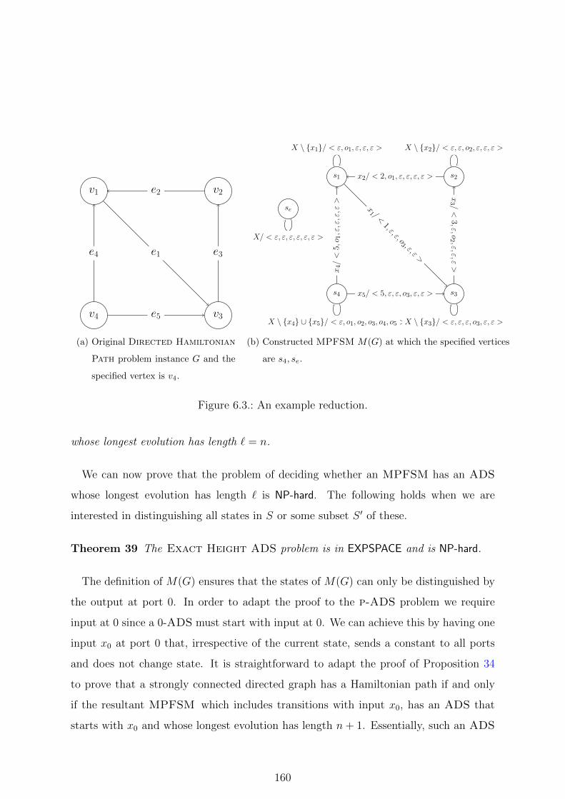
v1
v4 v3
v2
e4
e5
e3
e2
e1
(a) Original Directed Hamiltonian
Path problem instance G and the
specified vertex is v4.
s1
s4 s3
s2
se
x4/<
5,o 1,ε,ε,ε,ε>
x5/ < 5, ε, ε, o3, ε, ε >
x3 /<
3,ε,o2 ,ε,ε,ε
>
x2/ < 2, o1, ε, ε, ε, ε >
x1 /<
1, ε, ε, o3 , ε, ε
>X \ {x1}/ < ε, o1, ε, ε, ε >
X \ {x4} ∪ {x5}/ < ε, o1, o2, o3, o4, o5 >X \ {x3}/ < ε, ε, ε, o3, ε, ε >
X/ < ε, ε, ε, ε, ε, ε >
X \ {x2}/ < ε, ε, o2, ε, ε, ε >
(b) Constructed MPFSM M(G) at which the specified vertices
are s4, se.
Figure 6.3.: An example reduction.
whose longest evolution has length ` = n.
We can now prove that the problem of deciding whether an MPFSM has an ADS
whose longest evolution has length ` is NP-hard. The following holds when we are
interested in distinguishing all states in S or some subset S ′ of these.
Theorem 39 The Exact Height ADS problem is in EXPSPACE and is NP-hard.
The definition of M(G) ensures that the states of M(G) can only be distinguished by
the output at port 0. In order to adapt the proof to the p-ADS problem we require
input at 0 since a 0-ADS must start with input at 0. We can achieve this by having one
input x0 at port 0 that, irrespective of the current state, sends a constant to all ports
and does not change state. It is straightforward to adapt the proof of Proposition 34
to prove that a strongly connected directed graph has a Hamiltonian path if and only
if the resultant MPFSM which includes transitions with input x0, has an ADS that
starts with x0 and whose longest evolution has length n+ 1. Essentially, such an ADS
160

must start with x0 and then apply an ADS that does not contain x0. Since the Exact
Height ADS problem is in EXPSPACE we obtain the following result3.
Theorem 40 The Exact Height p-ADS problem is in EXPSPACE and is NP-hard.
Finally, if we suitably bound ` then the problems are NP-complete.
Theorem 41 The Exact Height ADS and Exact Height p-ADS problems for an
MPFSM with n states are NP-complete if ` = poly(n), where poly(n) is a polynomial
function of n.
As noted before, in testing it is possible to use a characterisation set containing con-
trollable separating sequences. Thus, in practice we are unlikely to be interested in
ADSs that are significantly longer than the sum of the lengths of the sequences in such
a characterisation set and we know that there is a polynomial upper bound on this value.
This provides clear motivation for the above result: in practice we are likely to have a
polynomial upper bound on the height of an ADS that we are ready to use.
6.6. Chapter Summary and Future Directions
Many automated test generation algorithms for testing from a single-port FSM M use
tests that distinguish states of M and there has been particular interest in preset dis-
tinguishing sequences (PDSs) and adaptive distinguishing sequences (ADSs). There
has been interest in both approaches since when applying PDSs it is possible to use
a less complex test infrastructure but ADSs can be shorter, are computationally less
expensive to produce, and there are FSMs that have ADSs but no PDS.
This work has shown how the concepts of PDSs and ADSs can be extended to
distributed testing. We showed that if a PDS or ADS is controllable then it can be
implemented by a set of distributed local testers but otherwise this is not possible. We
also showed how these local testers can be devised. We then explored the problems of
3The problem being NP-hard follows as before since the DHP problem allows a polynomial bound.
161

deciding whether an MPFSM has a PDS, proving that this problem is PSPACE-hard
and is generally undecidable if we consider subsets of the set of states. Having shown
this we gave a condition under which the latter problem is decidable but NP-hard and a
second stronger condition under which it is NP-complete.
Having explored PDSs we then considered ADSs. We proved that the problem of
deciding whether an MPFSM has an ADS is PSPACE-hard but left decidability open.
This situation is significantly different from the single-port MPFSM problem, which can
be solved in low-order polynomial time. We also showed that the problem of deciding
whether there is an ADS with height ` (or height at most `) is NP-hard. However, we
observed that in practice we can use a set of separating sequences of polynomial size and
so it makes sense to assume that the upper bound ` is bounded above by a polynomial
in the size of M . For such bounds the problem of deciding whether an MPFSM has an
ADS is NP-complete.
There are several lines of future work. First, it is still open whether the ADS existence
problem is decidable. There is also the problem of finding sensible conditions under which
the problems studied can be solved in polynomial time. Finally, there is the problem of
exploring heuristics for devising controllable PDSs and ADSs and here it is encouraging
that although the PDS existence problem is PSPACE-hard for single-port FSMs it has
been found that SAT solvers can be effective in solving this problem [108].
162
7. Conclusions
In Finite State Machine (FSM) based testing, a Fault Detection Sequence is applied to
an implementation and the response of the implementation is analysed. If the imple-
mentation produces the expected output then the implementation is said to be a correct
implementation.
We first aimed to reduce the costs of components of a CS by hoping that this will
reduce the cost of the CS. The first component that we investigated is a Reset Sequence.
The second component that we studied is State Identification Sequence.
In this thesis, we aim to reduce the cost of fault detection sequences. We first intro-
duced several problems related to reset sequences: an input sequence that resets the FSM
under consideration, and investigated their computational complexities. It is known that
constructing one of the shortest reset sequence is an NP-complete problem [34]. However
when the transition structure of a machine is monotonic (transitions of machine pre-
serve some linear order of the states) one can construct one of the shortest reset word in
polynomial time. However the complexity of constructing shortest reset sequences for
monotonic partial machines was an open problem. We, therefore, investigated to reveal
if this desirable complexity condition survives when the machine has partial transitions.
This is interesting, because if the underlying machine is not monotonic and is partial
then constructing a reset sequence is know to be PSPACE-complete. We showed that this
problem is NP-hard. Currently, the upper bound is not set and we left this as an open
problem. Therefore, it would be interesting to see if the problem is in NP or in PSPACE.
Moreover we believe that proposing heuristics for these problems are also important.
Secondly, as state identification components form a large portion of a CS, we studied
163

strategies to reduce the length of state identification sequences. There are different kinds
of state identification sequences: Unique Input Output (UIO) sequences, Separating
Family or Distinguishing Sequences. Among others, distinguishing sequences are known
to be the most efficient state identification sequences and it has been known that the
use of distinguishing sequences allow to construct shorter CSs.
There are two types of distinguishing sequences, Preset Distinguishing Sequences
(PDS) and Adaptive Distinguishing Sequences (ADS). For a given FSM checking the
existence of a PDS is known to be PSPACE-complete and it is know that there are FSMs
whose shortest PDS is given by exponential function with the number of states of the
underlying FSM. On the other hand, there are polynomial time algorithms to construct
ADSs and the length of the ADSs is bounded by a polynomial function of the size of
the underlying FSM.
The standard ADS generation algorithm runs in polynomial time but not guaranteed
to compute the minimum cost ADS. As an ADS defines a tree, the “cost” may not be
immediately clear. In this thesis, we introduced several problems related to minimizing
ADSs and we showed that all these problems are hard to solve and hard to approxi-
mate. We introduced several modification strategies for the exiting ADS construction
algorithm and also proposed a heuristic approach for constructing reduced cost ADSs.
We further performed a set of experiments and reveal what one can gain if one use
reduced cost ADSs while constructing CS. We revealed that it is possible to reduce the
length of CS by 29.2% on the average.
Although distinguishing sequences are important and reduce the cost of CS, not all
FSMs have a distinguishing sequence. For such cases instead of a CS a CE (set of
input sequences) are applied and used to detect fault. For a given FSM with no DS,
state identification problem can be solved by using either UIOs or Separating Family or
enhanced version of separating family called Harmonized State Identifiers. In this thesis,
we introduce the notion of Incomplete Distinguishing Sequences and show how to use
these sequences while constructing CEs. The motivation of this research comes primarily
from the desire to establish a tactic of utilizing desired properties of distinguishing
164

sequences. In order to achieve this, we first investigate the hardness of constructing such
incomplete distinguishing sequences and show that construction of such sequences are
PSPACE-complete. Moreover, we introduce a heuristic approach that aims to construct a
set of incomplete distinguishing sequences with reduced cardinality. We experimentally
showed that the use of incomplete distinguishing sequences give rise to construct shorter
checking experiments.
Finally, in this thesis we studied the computational complexity of constructing distin-
guishing sequences for distributed testing. In distributed testing the underlying FSM has
a finite set of ports (multi–port FSMs MPFSM) and each port is controlled by distinct
tester. Moreover, the testers are assumed to be disconnected, that is, testers do not have
a capability of using any form of communication method which means that no tester has
the capability of acquiring the global trace of the underlying MPFSM. This restricted
observation power of testers, necessarily change the nature of testing. Such restrictions
introduces Controllability and Observability problems. Controllability problem refers
to the condition in which a tester cannot decide whether it should apply an input by
evaluating its local trace. Observability problem refers to the condition in which the
testers cannot detect the faults of the implementation by analysing their local traces.
Controllability and observability problems reduce the effectiveness of fault detection se-
quences designed for single–port FSMs. Similarly, these problems invalidate the state
identification capabilities of distinguishing sequences. However, distinguishing sequences
are still desirable for constructing fault detection experiments for MPFSMs. The for-
mal definition of distinguishing sequences and the undecidability results for constructing
distinguishing sequences for distributed testing has been set. However the hardness of
computing and the definitions of controllable distinguishing sequences have not been
addressed. In this thesis, we define what it means for a distinguishing sequence to be
a controllable and investigate the hardness of constructing such sequences. The results
are disappointing, they are all hard problems and the bounds for these sequences have
not been set yet. We propose a subclass of MPFSMs for which constructing a PDS
is decidable. As a future work it would be interesting to set bounds for controllable
165

distinguishing sequences for MPFSMs.
166

Appendix ALemma 5 Let (U,C) be an instance of a Set Cover problem and C ′ = {c1, c2, . . . , cm}
be a cover. Then the sub-automaton F(U,C)|Σ is synchronizable, where Σ = {xi|ci ∈ C ′}.
Proof 1 Consider F(U,C) as defined above. If C ′ = {c1, c2, . . . , cm} is a cover, we
claim that for w = x1x2 . . . xm, we have δ(Q,w) = {S}, hence w is a reset word for
F(U,C). This is evident from the fact that, for any u ∈ U , there exists a c ∈ C ′ such
that u ∈ c (since C ′ is a cover). For a u ∈ U , let xi be the first input symbol in w
such that u ∈ ci. In this case, δ(qu, x1x2 . . . xi−1xixi+1 . . . xm) = δ(qu, xixi+1 . . . xm) =
δ(Sink, xi+1 . . . xm) = Sink. Now consider, F(U,C)|Σ where Σ = {x1, x2, . . . , xm}. Note
that F(U,C) is a CSA, and therefore so is F(U,C)|Σ. The sequence w = x1x2 . . . xm is
defined at all states of F(U,C)|Σ and therefore is a reset word for F(U,C)|Σ.
Lemma 6 Let Σ = {x1, x2, . . . , xm} be a subset of alphabet of F(U,C) such that F(U,C)|Σis synchronizable. Then C ′ = {c1, c2, . . . , cm} is a cover.
Proof 2 Let w = x1x2 . . . xk be a reset word for the synchronizable CSA F(U,C)|Σ.
Since δ(Sink, w) = Sink, we must have δ(q, w) = Sink for all qu ∈ Q \ {Sink}. Due
to the structure of the transition function δ, we can divide w as w = w′xiw′′ such that
δ(qu, w′) = qu and δ(qu, xi) = S. This implies that u ∈ ci.
Theorem 1 Given a synchronizable CSA A = (Q,Σ, δ) and a constant K ∈ Z+, it
is NP-complete to decide if there exists a set Σ ⊆ Σ such that |Σ| < K and A|Σ is
synchronizable.
Proof 3 The proof is trivial using Lemma 5 and Lemma 6, and using the fact that Set
Cover is NP-complete.
Theorem 2 MSS–Problem is NP-complete.
Proof 4 MSS is obviously in NP. Note that a special case of MSS is where we have
the cost function W assigning costs to the input symbols is a constant function. Using
Theorem 1, this special case is NP-complete, hence so is MSS.
167

Lemma 7 Let OPTsc is the size of minimum cover for the Set Cover problem in-
stance (U,C), and let OPTΣ is the size of minimum cardinality input alphabet such that
F(U,C)|Σ is synchronizable. Then OPTsc = OPTΣ.
Proof 5 The proof is trivial using using Lemma 5 and Lemma 6.
Theorem 3 MSS–Problem does not admit an o(log n) approximation algorithm unless
P = NP.
Proof 6 Consider again the special case of MSS–Problem where we have the function
W as a constant function. Suppose that P 6= NP and there exists a polynomial time
algorithm P which returns an o(log n) approximation for MSS–Problem. Therefore for
given Set Cover problem instance (U,C), one can construct automaton F(U,C)|Σ, and
using P, can obtain a solution Σ ⊆ Σ. In this case, Lemma 5, Lemma 6 and Lemma 7
together imply that Σ defines a solution C ′ for (U,C) which is also an o(log n) approx-
imation for the Set Cover problem instance (U,C), which we know to be impossible
when P 6= NP.
Lemma 8 MSS–Problem for PSA is in PSPACE.
Proof 7 For a given subset Σ of Σ, A|Σ is either a CSA or a PSA. In either case, we
know checking if A|Σ is synchronizable can be performed in PSPACE. Using a nondeter-
ministic Turing Machine, one can try all possible subsets Σ, and hence the problem can be
solved in NPSPACE. Using Savitch’s Theorem [123], we conclude that the MSS–Problem
for PSAs is in PSPACE.
Lemma 9 MSS–Problem for PSA is PSPACE-hard.
Proof 8 We will reduce from the problem of checking if a PSA is synchronizable or
not, which is known to be PSPACE-hard. Let A = (Q,Σ, δ) be a PSA. Suppose that we
construct a PSA A′ = (Q,Σ∪{a}, δ′), where ∀q ∈ Q, x ∈ Σ, δ′(q, x) = δ(q, x). However,
for the input symbol a, δ′ is defined in such a way that |δ′(Q, a)| = 1 (that is A′ is
synchronizable by the sequence w = a). Let us define W : Σ ∪ {a} → Z+ as ∀x ∈ Σ,
168

W (x) = 0, and W (a) =∞. We then consider an instance of MSS–Problem for PSA A′
with K = 0. Note that, this instance of the MSS–Problem has a solution iff the original
PSA A is synchronizable. Therefore, MSS–Problem for a PSA is at least as hard as
deciding if a PSA is syncrhonizable.
Theorem 4 MSS–Problem for PSA is PSPACE-complete.
Lemma 10 ESW–SA problem is PSPACE-hard.
Proof 9 Let us consider a non–deterministic Turing Machine which starts with the
state configuration π0 = (Q0, Q0) = (Q, Q). At each step where we have the state
configuration πi = (Qi, Qi), we pick an input symbol x ∈ Σ randomly, and compute the
next state configuration πi+1 as πi+1 = (δ(Qi, x), δ(Qi, x)). If δ(Qi, x) ∩ δ(Qi, x) 6= ∅ the
algorithm stops the search. Otherwise, if δ(Qi, x) ⊆ F , the algorithm reports success.
If this is not the case, the algorithm picks another random input symbol to proceed with
the search. Since the maximum length L of an exclusive synchronizing sequence is less
than 2n, the algorithm can stop after executing at most L steps. The space needed to
count the number of steps and handling the bookkeeping for the state configurations is
polynomial in n. Therefore, the entire search in this way can be performed in NPSPACE.
Based on Savitch’s Theorem [123], ESW–SA problem is in PSPACE as required.
Lemma 11 ESW–SA problem is in PSPACE.
Theorem 5 ESW–SA problem is PSPACE-complete.
Lemma 12 Let A′ be a subset of A where automata in A′ has a common word and |A′|
is maximized. Also let Q′ be a subset of states Q of A, where there exists an exclusive
synchronizing word for Q′ to F and |Q′| is maximized. Then |Q′| = |A′|.
Proof 10 Let w ∈ Σ? be a common word for all the automata in A′. Let Q′′ be the set of
states in Q in A, consisting of the initial states of automata in A′. Using the reduction
from FA–INT to ESW—SA, δ(Q′′, RwS) ⊆ F and δ(Q, RwS) = Sink, as explained in
the proof of Lemma 10. Therefore, when one considers a maximum cardinality subset Q′
169

of Q for which there exists an exclusive synchronizing sequence, we have |Q′| ≥ |Q′′| =
|A′|.
Reversely, consider a maximum cardinality subset Q′ of Q for which there exists an
exclusive synchronizing sequence w. Again, as explained in the proof of Lemma 10,
w is in the form w = Rw′S, and w′ is a common word for the subset A′′ of set of
automata A, where an automaton Ai ∈ A′′ iff the initial state of Ai is in Q′. When one
considers a maximum cardinality subset A′ of A for which there is a common word, we
have |A′| ≥ |A′′| = |Q′|.
This implies that |A′| = |Q′|, when maximum cardinality subsets are considered.
Theorem 6 There exists a constant ε > 0 such that approximating Max ESW–SA
problem within ratio nε is PSPACE-hard.
Proof 11 Let us assume that there exist an efficient algorithm P that approximates
Max ESW–SA Problem within ratio nε. In this case, we can convert any given MAX
FA-INT problem instance to automaton A and use algorithm P on A. Relying on
Lemma 12, the solution will also be an approximation for Max FA-INT instance for
the set of automata A, which directs us to the required contradiction.
Lemma 13 Let (U,C) be an arbitrary Exact Cover problem instance, then the states
of the automaton F(U,C) admits a linear order for all input symbols in set Σ.
Proof 12 We claim that the state set Q admits the following linear order S < q01 <
q11 < q0
2 < q12 < · · · < q0
|U | < q1|U |. First consider the input symbol X, from the reduction
F, it is clear that the input X resets all states at the respective base states. Therefore
for input symbol X we have:
δ(S,X) ≤ δ(q01, X) ≤ δ(q1
1, X) ≤ δ(q02, X) ≤ . . . ≤ δ(q0
|U |, X) ≤ δ(q1|U |, X)
The input symbol Y resets all the satellite states at S state and is defined only at these
states. Therefore, we have:
170

− ≤ − ≤ δ(q11, Y ) ≤ − ≤ δ(q1
2, Y ) ≤ · · · ≤ − ≤ δ(q1|U |, Y )
where − denotes the cases where Y is not defined.
Finally consider the input symbols in Σ \ {X, Y }, which are only defined at some base
and satellite states. Let qai and qbj be two states such that qai < qbj and x ∈ Σ \ {X, Y } be
an input symbol defined at both qai and qbj . When i < j, δ(qai , x) = qa′i and δ(qbj , x) = qb
′j .
Since i < j, we have qa′i < qb
′j , or equivalently δ(qai , x) < δ(qbj , x). When i = j, then we
must have δ(qai , x) = qai and δ(qbj , x) = qbj . Again in this case, we have qai < qbj , and thus
δ(qai , x) < δ(qbj , x).
Theorem 7 Synchronizability Problem for PSMA is NP-hard.
Proof 13 We first show that if there exists a solution to the Exact Cover problem
instance (U,C), then automaton F(U,C) is synchronizable.
Let (U,C) has a solution with C ′ = {c1, c2, . . . , c`}. i.e. ci, cj, 1 ≤ i, j,≤ `, i 6= j the
followings hold: (1)ci ∩ cj = ∅ (2)⋃
1≤i≤` ci = U .
First, we must observe that there exist single input symbol (X) that is defined at all
the states. Therefore any synchronizing sequence of F(U,C) must begin with the input
X, which leaves us with the set of all base states. Since C ′ is an exact cover, after input
symbol X the application of the input sequence x1x2 · · ·x` will leave us with the set of
all satellite states. Therefore Xx1x2 · · · x`Y resets F(U,C) at S as required.
Conversely if automaton F(U,C) is synchronizable then there exists a solution to the
corresponding Exact Cover problem instance.
Let w be a rest word for machine F(U,C). We, without loss of generality, assume that
w is minimal, i.e. no prefix and no suffix of w is a reset sequence. For such a minimal
reset sequence w, it must be in the form w = Xw′Y , where w′ has no occurrence of X
and Y .
We will prove that w′ = x1x2 · · ·x` defines an exact cover C ′ = {c1, c2, . . . , c`} for
(U,C).
171

Since Xw′Y is a reset sequence, for any u ∈ U , δ(q0u, w
′) = q1u. This is only possible if
there exists a unique input symbol xi in w′ such that w′ = w′1xiw′2 where δ(q0
u, w′1) = q0
u,
δ(q0u, xi) = q1
u, δ(q1u, w
′2) = q1
u. When δ(q0u, xi) = q1
u, this due to the fact that u ∈ ci.
Therefore, w′ gives a unique ci for each u ∈ U such that u ∈ ci. Hence if w′ = x1x2 · · ·x`,
then we have C ′ = {c1, c2, . . . , c`} as an exact cover.
Theorem 8 Synchronizing Word Problem and Minimum Synchronizing Word
Problem for a PSMA are NP-hard problems.
Lemma 14 Let B be an arbitrary N–Queens puzzle instance, the states Q of the au-
tomaton F(B) admits a linear order.
Proof 14 First note that the automaton F(B) is not strongly connected. The automaton
consist of N2 set of states where each set has 3 states of the form Qi,j = {q0i,j, q
+i,j, q
−i,j}.
For two different set of states Qi,j and Qi′,j′, the set of states are disjoint and not
reachable from one another. Therefore the ordering between a state q ∈ Qi,j and a state
q′ ∈ Qi′,j′ is not important, i.e. any ordering between q and q′ works. On the other hand,
for a given state set Qi,j, we define the order between the states as q−i,j < q0i,j < q+
i,j. Due
to the transition structure of F(B), for any input symbol xk,l, we have the following
cases:
• If k = i, l = j then δ(q−i,j, xk,l) = q−i,j < δ(q0i,j, xk,l) = q+
i,j = δ(q+i,j, xk,l) = q+
i,j.
• If (k, l) attacks (i, j) then δ(q−i,j, xk,l) = q−i,j = δ(q0i,j, xk,l) = q−i,j < δ(q+
i,j, xk,l) = q+i,j.
• Otherwise, then δ(q−i,j, xk,l) = q−i,j < δ(q0i,j, xk,l) = q0
i,j < δ(q+i,j, xk,l) = q+
i,j.
In each case, the monotonicity condition is met by using the linear order suggested and
the result follows.
Lemma 15 Let w ∈ Σ? be a reset word that resets N + N2 states of the automaton
F(B) at F . Then w defines a solution for the N–Queens puzzle instance B.
172

Proof 15 Consider that w resets N +N2 states at F = Q+. Note that δ(Q+, w) = Q+
and |Q+| = N2. Since δ(Q−, w) = Q−, the remaining N states reaching to F must be
from the board states in Q0.
We will first show that there are exactly N effective input symbols in w. For an
effective input xi,j in w, we have w = w′xi,jw′′ and δ(q0
i,j, w′) = q0
i,j. Based on the
transition structure of F(B), we then have δ(q0i,j, w
′xi,j) = q+i,j, which means one more
state in F . Since, we need to accumulate N such states in F , there must be exactly N
effective input symbols in w.
Let us consider two different effective input symbols xi,j and xk,l in w. Without loss
of generality, assume that we have w = w′xi,jw′′xk,lw
′′′. Since xk,l is an effective input,
δ(q0k,l, w
′xi,jw′′) = q0
k,l. This implies that (k, l) does not attack (i, j) (or vice versa since
“attacks” relation is symmetric). This means that the indices of N effective inputs in w
gives N board positions for N queens that do not attack each other.
Lemma 16 Let {(i1, j1), (i2, j2) , . . . , (iN , jN)} be a solution to the N–Queens puz-
zle. Then set of positions (i1, j1), (i2, j2) , . . . , (iN , jN) defines a solution for the KFW–
NSMA Problem for automaton F(B).
Proof 16 Let us consider the input sequence w = xi1,j1xi2,j2 · · ·xiN ,jN . We claim that w
resets N +N2 states in F = Q+.
For any prefix w′xip,jp of w, we have δ(q0ip,jp , w
′) = w′. This is due to the fact that
(ip, jp) is not attacked by any other position. Therefore xip,jp is an effective input, hence
the application of xip,jp after w′ moves the state q0ip,jp to q+
ip,jp. After executing these
N effective inputs, we will have N of the states in Q0 moved into Q+. Since also
δ(Q+, w) = Q+ and |Q+| = N2, the result thus follows.
Theorem 9 KFW–NSMA Problem is NP-hard.
Proof 17 Based on the reduction given above, Lemma 15 and Lemma 16, the result is
immediate.
Theorem 10 MFW–NSMA Problem is NP-hard.
173

Appendix B
Lemma 17 An input xz ∈ XZ cannot appear as the label of an internal node p in an
ADS A of MD.
Proof 18 Using Lemma 3, |δ(Spv/pe , pv)| > 1. Lemma 4 requires that pv be a valid input
for δ(Spv/pe , pv). However, xz is not valid for any set of states since for any two states
s and s′, λ(s, xz) = λ(s′, xz) = 2 and δ(s, xz) = δ(s′, xz) = sz.
Lemma 18 Given a decision tree T for D, there exists an isomorphic ADS A for MD.
Proof 19 We construct an isomorphic ADS A by changing the label of an internal node
t to xt, and by changing the label of a leaf node from z to sz, and by keeping the edge
labels intact.
It is easy to see that conditions (1)–(4) of Definition 2 are satisfied by A. To show
that Condition (5) of Definition 2 also holds, let p be a leaf node labeled by sz in A,
let pv = xti1xti2 . . . xtik and pe = y. Also consider the path from the root to the leaf
labeled by z in T . Due to the construction of A from T , the sequence of node la-
bels along this path is ti1ti2 . . . tik and the sequence of edge labels is again y. Using
Lemma 17, we have y = ti1(z)ti2(z) . . . tik(z). Then λ(sz, pv) = λ(sz, xti1xti2 . . . xtik ).
Since sz has self-looping transitions for input symbols in XT , λ(sz, xti1xti2 . . . xtik ) =
λ(sz, xti1 )λ(sz, xti1 ) . . . λ(sz, xtik ). Using the properties of the mapping β, this sequence
is ti1(z)ti2(z) . . . tik(z) = y.
Lemma 19 Given an ADS A for MD, there exists an isomorphic decision tree T for
D.
Proof 20 Lemma 18 implies that all the internal nodes have their labels from XT . This
also implies that there is no edge in A labeled by the output symbol 2.
We construct an isomorphic decision tree T by changing the label of an internal node
xt to t, and by changing the label of a leaf node from sz to z, and by keeping the edge
labels intact. It is easy to see that Condition (1) and Condition (2) of Definition 18 are
174

satisfied by T . Since A is always branching, and since output symbol 2 cannot appear in
A, Condition (3) of Definition 18 is also satisfied.
For Condition (4) of Definition 18, let p be a leaf node in T labeled by an object z,
and p′ be an internal node on the path from the root to p, and let t be the label of p′. Let
q and q′ be the corresponding nodes in A for p and p′ respectively. Note that the label
of q must be sz and the label of q′ must be xt. If q is in the 0-successor (respectively
1–successor) of q′, then by Lemma 1 we have λ(δ(sz, q′v), xt) = λ(sz, xt) = t(z) equal to
0 (respectively 1). Using this result and the isomorphic structure of A and T , we can
conclude if p is in the 0–successor of (respectively 1–successor) of q′, then t(z) is equal
to 0 (respectively 1).
Theorem 11 The decision version of the problems MinADS, MinHeightADS, and
MinSDS are NP-complete.
Proof 21 It is known that if an FSM M has an ADS, there is an ADS A for M where
the size of A is polynomial in the size of M [35, 99]. Therefore the cost for MinADS,
MinHeightADS, and MinSDS problems can be computed in polynomial time. Hence
the problems are in NP.
Note that MinDT [100], MinHeightDT [101], MinPathDT [102] problems are
NP-hard. Since the problems MinADS, MinHeightADS, MinSDS are at least as
hard, they are also NP-hard.
MinADS is a special case of MinWeightedADS (when ws = 1 for all states s).
Therefore the following result holds.
Theorem 12 The decision version of the problem MinWeightedADS is NP-complete.
Theorem 13 For any constant c > 0, it is NP-hard to approximate MinADS and
MinWeightedADS problems within a ratio of (2− c).
Proof 22 For any constant c > 0, it is NP-hard to approximate MinDT problem within
a ratio of (2 − c) [103, 104] 1, hence the same inapproximability result applies to Mi-
1MinDT problem is referred to as 2-UDT problem in [103, 104].
175

nADS problem. Also, since MinADS is a special case of MinWeightedADS, this
inapproximability result immediately applies to MinWeightedADS problem as well.
Theorem 14 Unless P = NP, there cannot be an o(log n) approximation for Min-
HeightADS and MinSDS problems.
Proof 23 Unless P = NP, there cannot be an o(log n) approximation for MinHeightDT
and MinPathDT problems [105, 102]. Hence this result applies to MinHeightADS
and MinSDS problems as well.
Proposition 3 Let q be an output node in T , let io(q) = w/v. Then we have bl(q) =
δ(Sw/v, w).
Proof 24 The proof is trivial by using induction on the depth of q.
Proposition 4 |L|+∑
q∈Q |bl(q)| = |S| is an invariant of Algorithm 1 before and after
every iteration the while loop.
Proof 25 Before the first iteration, |L| = 0 and Q only has the root node q0 for which
we have bl(q0) = S. In an iteration of the algorithm, an output node q is removed from Q
and a child (input) node p of q is selected. It is sufficient to observe two facts. First, each
state s ∈ bl(q) is represented by a state s′ ∈ bl(q′) where q′ is a child of p, s′ = δ(s, in(p))
and out(q′) = λ(s, in(p)). Second, no two states s1, s2 ∈ bl(q) can be represented by the
same state s′ in the same child q′, since in(p) is a valid input for the states in bl(q).
Therefore, when we consider all children q′ of p, we have∑
q′ |bl(q′)| = |bl(q)|. Those
children q′ of p with |bl(q′)| = 1 are included in L, and those children q′ of p with
|bl(q′)| > 1 are included in Q. Hence the result follows.
Proposition 5 Let q be an output node in T with |bl(q)| = 1, and let w/v = io(q).
There exists a unique state s ∈ S such that λ(s, w) = v.
Proof 26 Suppose s and s′ are two distinct states such that λ(s, w) = λ(s′, w) = v.
By Proposition 3, we would then have δ(s, w) and δ(s′, w) in bl(q). Since |bl(q)|, this
implies δ(s, w) = δ(s′, w). This is not possible since at each step a valid input is applied,
therefore no two states can be merged into a single state.
176

Proposition 6 The leaves of A constructed by Algorithm 2 is labeled by distinct states.
Proof 27 Assume that there are two leaf nodes q′1 and q′2 in A such that they are both
labeled by the same state s. Let q1 and q2 be the leaf (output) nodes in T that correspond
to q′1 and q′2. Let w1/v1 and w2/v2 be the input/output sequences io(q1) and io(q2). In
this case, we would have λ(s, w1) = v1 and λ(s, w2) = v2. However, this is not possible
since M is deterministic.
Theorem 15 A constructed by Algorithm 2 is an ADS.
Proof 28 A has n = |S| leaves as implied by Corollary 1. We will argue that A satisfies
the conditions of Definition 2. Condition (i) is satisfied as shown by Proposition 6. Con-
dition (ii) and Condition (iii) are easily satisfied due to the construction in Algorithm 2.
Condition (iv) is satisfied due to the fact that in T , for an input node p, each child q
of p has a distinct output symbol out(q). Lines 5–8 of Algorithm 2, assigns the label of
leaves in such a way that Condition (v) is satisfied (see Proposition 5).
177

Appendix CLemma 20 Let us suppose that set A = {A1, A2, . . . , Az} of automata have a common
alphabet Σ. The FSM M1(A) = (S,X, Y, δ, λ, s0) has a PDS for S = {011, 0
21, . . . , 0
1z, 0
2z}
if and only if there is a non-empty word w ∈ Σ? that is accepted by all of the automata
(in which case ωD is such a PDS).
Proof 29 First, let us suppose that ω 6= ε is in the intersections of the languages of the
Ai and consider w = ωD. By construction, ω distinguishes any two 0αi and 0βj with i 6= j
since ω ∈ Σ? is non-empty, the output in response to an element of Σ identifies the state
of the corresponding Ai, and the state sets of the Ai are pairwise disjoint. Further, if we
consider states 01i and 02
i we find that ω takes them to accepting states from Fi and then
D leads to different outputs (1 and 2). Thus, if there is some non-empty ω ∈ Σ? in the
intersections of the languages of the Ai then M1(A) has a PDS ωD for S.
We now prove that ifM1(A) has a PDS for S then there is some non-empty ω ∈ Σ? in
the intersections of the languages of the Ai. We can observe that in order to distinguish
states 01i and 02
i it is necessary to apply input D but also that after D has been applied the
state must be in {Sink1, Sink2} and further input cannot distinguish the states. Thus
there is a PDS for S if and only if there is a PDS for S that has the form w = ωD
where ω ∈ Σ? and we now consider such a PDS.
Now let us suppose that δ(01i , ω) /∈ F 1
i for some 1 ≤ i ≤ z. Then δ(δ(01i , ω), D) = Sink1
and similarly δ(δ(02i , ω), D) = Sink2 and it is clear that λ(01
i , ωD) = λ(02i , ωD). This
contradicts ωD being a PDS for S. Therefore w must be in the form w = ωD such that
ω is non-empty and brings all the initial states to accepting states. Thus, if M1(A) has
a PDS for S then there is some non-empty ω ∈ Σ? in the intersections of the languages
of the Ai.
Lemma 21 The problem of deciding whether a set S of states of FSM M has a PDS
is in PSPACE.
Proof 30 We will show that a non-deterministic Turing Machine can solve this using
polynomial space. Such a machine will guess inputs one at a time. It will maintain
178

the set π of pairs of states and equivalence relation r as described above and this uses
polynomial space. After guessing a new input x and updating π and r the machine
checks whether the input sequence received defines a PDS for S: this it the case if and
only if r relates no two different states of S. Thus, if M has a PDS for S then this
non-deterministic Turing Machine will find such a PDS using polynomial space.
We now have to consider the case where M does not have a PDS for S: we require
that the non-deterministic Turing Machine terminates. In order to ensure this we use
the result that if M has n states and S has m states then M has a PDS for S if and only
if it has such a PDS with length at most B = (m− 1)nm [21]2. The non-deterministic
Turing Machine therefore includes a counter that counts how many inputs have been
received: the machine terminates with failure if the counter exceeds the upper bound.
We require additional O(log2B) = O(log2(m− 1) +m log2(n)) = O(m log2(n)) space for
the counter and so the space required is still polynomial.
We have defined a non-deterministic Turing Machine that requires only polynomial
space in order to solve the problem and so the problem is in non-deterministic PSPACE.
We can now use Savitch’s Theorem [123], which tells us that a problem is in PSPACE if
and only if it is in non-deterministic PSPACE, and the result follows.
Lemma 22 Given set A of automata, let OPTA be the set of minimal words that are
accepted by the maximum number of automata from A. Further, given M1(A) let
OPTM1(A) be the set of minimal words that maximise the size of the subset of S whose
states are pairwise distinguished. Then w ∈ OPTA if and only if wD ∈ OPTM1(A).
Theorem 16 The MaxSubSetPDS problem is PSPACE-complete and for any con-
stant ε > 0 approximating the MaxSubSetPDS problem within ratio nε is PSPACE-hard.
Proof 31 The problem being PSPACE-hard follows from Lemma 23 and the MAX FA-
INT problems being PSPACE-hard. To see that this problem is in PSPACE, first observe
that it is sufficient to prove that the following problem is in PSPACE: for 1 ≤ k ≤ n
2In [21], Gill presents this result on pg: 104, Theorem 4.3. Note that Gill named the set S as the
Admissible Set i.e. the initial states of the underlying FSM.
179

decide whether there is a PDS that distinguishes k states of the FSM M . We can show
that this is in PSPACE in a similar manner to Lemma 22, the only differences being that
in a first step the non-deterministic Turing Machine guesses the set S ′ of k states.
To prove that the problem of approximating the MaxSubSetPDS is PSPACE-hard, let
us assume that we have an algorithm P that belongs to a complexity class C < PSPACE
and returns an nε approximation for the MaxSubSetPDS Problem. In such a case,
given an instance A of the MAX FA-INT problem, we can construct FSM M1(A) and
using P we can obtain a solution w = ωD. But then Lemma 23 implies that ω defines
an approximation for A and hence P defines an nε approximation for the MAX FA-INT
problem. Thus the result follows.
Theorem 17 The MinSetPDS problem is PSPACE-complete.
Proof 32 We first prove that the problem is in PSPACE. Observe that in PS we require
at most one set for each pair of states of M and so if M has state set S then the set PS
of subsets has size at most |S|(|S| − 1).
It is therefore sufficient to show that we can solve the problem of trying to find a set k
of subsets where each subset corresponds to a PDS (1 ≤ k ≤ |S|(|S| − 1)); if we can do
this then a Turing Machine could start with k = |S|(|S| − 1) and then reduce k step by
step until a set is found. Given k, a non-deterministic Turing Machine can thus initially
guess such a set PS of k subsets and for each such set S ′ ∈ PS the Turing Machine tries
to build a PDS that distinguishes all of the states in S ′. As before, for a given set S ′
the process terminates when the upper bound on PDS length is exceeded or the PDS
being built is sufficient. Since this can be performed in polynomial space we have that
the result follows from Savitch’s Theorem [123].
To see that the problem is PSPACE-hard it is sufficient to observe that M has a complete
PDS if and only if it has a set PS that satisfies the conditions of the MinSetPDS
problem and contains only one set. The result therefore follows from the complete PDS
problem being PSPACE-hard [35].
Lemma 23 Let us suppose that set A = {A1, A2, . . . , Az} of automata have a common
180

alphabet Σ. The FSMM2(A) = (S,X, Y, δ, λ, s0) has an ADS for S = {01, . . . , 0z, Sink}
if and only if there is a non-empty word w ∈ Σ? that is accepted by all of the automata
(in which case input sequences wd1, wd1d2, wd1d2d3, . . . , wd1d2d3 . . . dz define an ADS).
Proof 33 We first show that if w is accepted by all the automata then input sequences
wd1, wd1d2, wd1d2d3, . . . , wd1d2d3 . . . dz define an ADS for S. Since w is accepted by
all the automata, input sequence w will take any initial state 0i to an accepting state.
We show that wd1d2 . . . dj distinguishes states 0i, 0j for any 1 ≤ i 6= j ≤ z. This follows
from the fact that at state δ(0j, w) the FSM will not change its state, will produce 0
when any input from set D \ {dj} is applied, and will produce j as output if input dj is
applied. It is clear also that this word distinguishes all 0j from Sink since it will lead to
the output j being produced from 0j but not from Sink. Therefore, if there exists a word
w that is accepted by all the automata, then FSM M2(A) has an ADS for set S in the
form of wd1, wd1d2, wd1d2d3, . . . , wd1d2d3 . . . dz.
Now assume that machine M2(A) has an ADS for S and we are required to prove that
there is some w ∈ Σ in the intersections of the languages of the automata. Let us suppose
that from S the ADS applies input sequence w and then input x such that the response
to w does not distinguish any two elements of S but the response to wx distinguishes two
or more states of S. Then the input of x after w must lead to different outputs for two
or more states in S and so we must have that x ∈ D. Further, the input of w in any
state of S leads to a sequence of zeros since this is the response to any input sequence
when in state Sink. If w does not take some 0j to a final state then wx takes 0j to
state Sink producing only zeros as output and so the ADS does not distinguish 0j from
Sink ∈ S. Thus, w must take each Ai to a final state and so by definition we have that
w ∈ Σ? and w is in the languages defined by all of the Ai and so the result holds.
Lemma 24 Given FSM M and state set S, the problem of deciding whether S has an
ADS is in PSPACE.
Proof 34 We will show that a non-deterministic Turing Machine can solve this using
polynomial space. Such a machine will operate through a sequence of steps, extending
181

the depth of the ADS by one in each step. It will maintain a set π of pairs of states and
equivalence relation r as in the proof of Lemma 22 and again this uses polynomial space.
As before, we start with π = {(s, s)|s ∈ S}. In each step, if (s, s′) ∈ π then the current
‘guess’ takes s to s′ and (s, s′) ∈ r if and only if the current ‘guess’ does not distinguish s
and s′. A step involves the non-deterministic Turing Machine guessing a next input for
each equivalence class of r and updating π and r accordingly. The machine also checks
whether an ADS has been defined for S: this it the case if and only if r relates no two
different states of S. Thus, if M has an ADS for S then this non-deterministic Turing
Machine will find such an ADS using polynomial space.
Similar to before, we now have to consider the case where M does not have an ADS for
S and require that the non-deterministic Turing Machine terminates. This is achieved
by using the result that if M has n states and S has m states then M has an ADS for
S if and only if it has such an ADS with length at most ` ≤ Σi=mi=2 C
(ni
)< 2n [99]3. The
non-deterministic Turing Machine thus has a counter that gives the length of the current
‘guess’ and terminates with failure if the counter exceeds the upper bound. We require
additional O(log2 `) space for the counter and so the space required is polynomial.
The non-deterministic Turing Machine requires polynomial space in order to solve the
problem and so the problem is in non-deterministic PSPACE; the result again follows
from Savitch’s Theorem [123].
Theorem 18 The MaxSubSetADS problem is PSPACE-complete.
Proof 35 The problem being PSPACE-hard follows from Lemma 24 and the MAX FA-
INT problem being PSPACE-hard. In order to see that the problem is in PSPACE, we
prove that the following problem is in PSPACE: “for 1 ≤ k ≤ n, decide whether there is
an ADS that distinguishes k states”. We can deduce that this problem is in PSPACE,
by considering the algorithm presented in Lemma 25. This time as a preprocessing
step the Turing Machine will guess a set of states S with cardinality k then the Turing
Machine continues to implement the procedure that we describe in the proof of Lemma 25.
Therefore the MaxSubSetADS problem is in PSPACE.
3Theorem 1, bound (2).
182

Lemma 25 Given a set A of automata, let OPTA be the set of minimal words accepted
by the maximum number of automata from A. Further, let M2(A) be the FSM con-
structed from A and also let OPTM2(A) be the set of minimal ADSs that maximise the
size of the subset of S whose states are pairwise distinguished by ADSs. Then w ∈ OPTAif and only if ADS wd1, wd1d2, . . . , wd1 . . . dz is in OPTM.
Theorem 19 For any constant ε > 0 approximating the MaxSubSetADS problem
within ratio nε is PSPACE-hard.
Proof 36 To prove that the problem of approximating MaxSubSetADS is PSPACE-hard,
we consider an algorithm P that belongs to a complexity class C < PSPACE and re-
turns an nε approximation for the MaxSubSetADS Problem. In such a case, given
a MAX FA-INT problem instance A, we can construct FSM M2(A) and using P we
can obtain a solution wd1, wd1d2, . . . , wd1d2 . . . dz. But then Lemma 26 implies that w
defines an approximation for A and hence P is also an approximation for the MAX
FA-INT problem. The result thus follows.
Lemma 26 The MinSetADS problem is in PSPACE.
Proof 37 We can show that this problem is in PSPACE by following a procedure that
is similar to the one we present in the proof of Theorem 18. As before, if the FSM M
has state set S then PS requires at most |S|(|S| − 1) sets. As a result, it is sufficient to
prove that given k the following problem can be solved in PSPACE: is there a collection
PS = {S1, S2 . . . Sk} of subsets of S such that for every pair s, s′ of states there is some
Si such that s, s′ ∈ Si and for each Si (1 ≤ i ≤ k) there is an ADS that distinguishes the
states of Si. The Turing Machine guesses such a PS and then performs the remaining
steps for each of the Si separately. Clearly, this procedure takes polynomial space. The
Turing Machine will return failure when it exceeds the bound given for the maximum
depth, while if suitable ADSs are found then the Turing Machine returns success.
Lemma 27 The MinSetADS problem is PSPACE-hard.
183

Proof 38 We again consider an instance A = {A1, . . . , Ak} of the FA-INT problem
with a common alphabet Σ and we construct M3(A). From Lemma 24 and the FA-
INT problem being PSPACE-hard we know that the problem of deciding whether there
is an ADS for {01, . . . , 0z, Sink} is PSPACE-hard. We will prove that any solution to
the MinSetADS problem for M3(A) also determines whether there is an ADS for
{01, . . . , 0z, Sink}.
Let us suppose that PS is a smallest set of subsets of S such that for every pair of states
s, s′ with s 6= s′ there is some S ′ ∈ PS that contains both s and s′ and for every set
S ′ ∈ PS there is an ADS that distinguishes the states in S ′. By construction, any set
S ′ ∈ PS that contains Sink and a state s ∈ S \ {Sink} must correspond to ADSs that
start with st. Similarly, if S ′ ∈ PS contains Sink and some s ∈ S \ S then it must
correspond to ADSs that do not start with st.
We will let P ′S denote the set of subsets of PS that contain Sink and at least one state
s ∈ S \ {Sink}. We will prove that there is an ADS that distinguishes all of the states
of S if and only if P ′S contains only one set.
First assume that P ′S contains only one set. Thus, the one set in P ′S contains all states
from S and this implies that there is an ADS for S as required.
Now assume that S has an ADS. By definition, no set in P ′S contains a state s 6∈ S and
for all s 6∈ S we have that PS \ P ′S contain a set that has both s and Sink. Thus, for
each s, s′ ∈ (S \ S) ∪ {Sink} with s 6= s′ we have that PS \ P ′S has a set that contains
both s and s′. As a result, it is sufficient for the sets in P ′S to contain all pairs s, s′ from
S with s 6= s′. Since there is an ADS that achieves this, by the minimality of PS we
must have that P ′S contains only one set.
We now know that S has an ADS if and only if P ′S contains only one set and so if we
can solve the MinSetADS problem for M3(A) then we can decide whether S has an
ADS. We can now note that S has an ADS if and only if the state set {01, . . . , 0z, Sink}
of M3(A) has an ADS: the ADS for S in M3(A) starts with st and then applies an
ADS for state set {01, . . . , 0z, Sink} of M3(A). The result thus follows from Lemma 24
and the FA-INT problem being PSPACE-hard.
184

Theorem 20 The MinSetADS problem is PSPACE-complete.
Proposition 7 Given fully distinguishing set A = {A1, . . . ,Ak} for FSM M , the Hi(A)
are state identifiers for M .
Proof 39 It is sufficient to prove that if si, sj are distinct states of M then there are
input sequences wi ∈ Hi(A) and wj ∈ Hj(A) such that there is a common prefix w of
wi and wj that distinguishes si and sj. First observe that since A is fully distinguishing
there is some Al ∈ A that distinguishes si and sj. But by definition this means that the
application of Al from si and sj leads to different input/output sequences. However, the
input sequence can only differ once a different output has been observed. Thus, Al has
a node v such that the following hold:
1. The path from the root of Al to v has a label α/β that labels paths from both si and
sj; and
2. There are edges with labels x/yi and x/yj from v with yi 6= yj such that αx/βyi
labels a path from si and αx/βyj labels a path from sj.
However, this means that w = αx is a prefix of input sequences in Hi and Hj and also
that w distinguishes si and sj. The result therefore follows.
Theorem 21 Given an FSM M and upper bound m on the number of states of the
SUT, if A is a fully distinguishing set of ADSs for M then CE(M,A,m) is a checking
experiment for M .
Proof 40 This follows from Proposition 7 and the HSI method returning a checking
experiment.
Proposition 8 Let us suppose that S is a set of states of FSM M . Then the states
in S can be distinguished by a single ADS if and only if there is an identifying set
{H1, . . . , Hn} for M such that we can choose subsets H ′i ⊆ Hi of each identifying set,
si ∈ S, under which each H ′i contains only one input sequence.
185

Proof 41 First assume that the states in S can be distinguished by a single ADS A.
Given state si ∈ S let H ′i denote the set containing one input sequence: the input portion
of the input/output sequence produced when A is applied in state si. It is straightforward
to check that the argument used in the proof of Proposition 7 applies and so the H ′i are
state identifiers for S as required.
Now let us suppose that we have state identifiers {H ′i|si ∈ S} for S such that each H ′i
contains only one input sequence, which we call wi. Form a deterministic automaton A
that is a tree with |S| leaves such that for each state si ∈ S the tree A has a path from the
root to a leaf such that this path has label wi/λ(si, wi). Since the H ′i define identifying
sets for S, for distinct states si, sj ∈ S we have that the input in wi, wj can only differ
after a different output in response to a common prefix of wi, wj. Thus, A is an ADS
for S as required.
Proposition 9 If the states in S can be distinguished by k ADS then there is an iden-
tifying set {H1, . . . , Hn} such that for all si ∈ S we have that Hi has at most k input
sequences.
Proof 42 We will assume that the states in S can be distinguished by a set A of k
ADSs. Given state si ∈ S let Hi denote the set containing the input portion of the
input/output sequence produced when A ∈ A is applied in state si. By Proposition 7 the
Hi are state identifiers for S as required.
Lemma 28 Let n be an internal node of tree T with children n1, n2, . . . , np and let x be
the input portion of the labels of the edges from node n. The following hold:
1. δ(C(n), x) = ∪pi=1C(ni).
2. For all 1 ≤ i ≤ p we have that |λ(I(ni), x(ni))| = 1.
3. For all 1 ≤ i < j ≤ p we have that λ(I(ni), x(n)) = λ(I(nj), x(n)) and λ(I(ni), x(n)x) 6=
λ(I(nj), x(n)x).
Lemma 29 Let n, n′ be distinct leaf nodes of tree T . If s ∈ I(n) and s′ ∈ I(n′) then
λ(s, x(n)) 6= λ(s′, x(n)) and λ(s, x(n′)) 6= λ(s′, x(n′)).
186

Lemma 30 Let T be a tree returned by the greedy algorithm such that N = {n1, . . . , np}
is the set of leaf nodes of T . Let S be a set of states such that for all 1 ≤ i ≤ p we have
that |I(ni) ∩ S| ≤ 1. Then T defines an incomplete ADS for set S.
Proof 43 We will show that T can be used to construct an incomplete ADS A for S.
Take a copy of tree T and for every node n remove from I(n) all states not in S. Now
remove all nodes with empty initial sets to form A.
Now we need to show that A is an incomplete ADS for S. By the construction of A,
each leaf node must be labeled by a singleton set. To see this, assume that an initial set
of a leaf node contains two or more states. Since we drop states that are not in S this
implies that there exist distinct s, s′ ∈ S such that s, s′ ∈ I(na) for some a, providing a
contradiction.
Moreover, it is easy to see that each internal node is labeled by a set of states, and
each edge is labeled by an input output pair. Therefore conditions (1)-(3) of incomplete
ADS given in Definition 2 are satisfied. For an internal node in A there are at most
|Y | outgoing edges and due to the refine algorithm edges from a common node have
identical input labels and different output labels. Thus, using Corollary 29, Condition
(4) of Definition 2 is satisfied. Moreover due to the Corollary 30 we can deduce that
Condition (5) of Definition 2 also holds. Therefore T defines an incomplete ADS for
S.
187

Appendix D
Proposition 10 If a strategy µ is controllable then for every MPFSM M and state
set S ′ we have that µ is controllable for S ′. However, it is possible that strategy µ is
controllable for S ′ for some MPFSM M and state set S ′ and yet µ is not controllable.
Proof 44 The first part is immediate from the definitions. For the second part consider
a global strategy µ that:
• starts by supplying input x1 at port 1;
• if 〈o1, ε) is output then the strategy supplies input x2 at port 2 and terminates;
• for every other output the strategy terminates.
This strategy is not controllable since it should send input x2 to port 2 after x1/〈o1, ε〉 but
not after the empty sequence ε, even though x1/〈o1, ε〉 and ε have the same projections
at port 2. However, µ is controllable for any S ′ from which the input of x1 cannot lead
to output 〈o1, ε〉. The result thus follows.
Proposition 11 If global strategy µ is controllable then the distributed strategy (π1(µ), π2(µ),
. . . .πk(µ)) is deterministic.
Proof 45 We are required to prove that µ′ = (π1(µ), π2(µ) . . . .πk(µ)) is deterministic.
We will use proof by contradiction and assume that µ′ is non-deterministic. By Def-
inition 43 there therefore exists global trace σ1 ∈ (X/Y )∗ such that for all p ∈ P we
have that πp(σ1) ∈ Ev(µp) and ports p, p′ with p 6= p′ such that µp(πp(σ1)) ∈ Xp and
µp′(πp′(σ1)) ∈ Xp′. By Definition 46, there exist global traces σ and σ′ in Ev(µ) such
that:
• πp(σ) = πp(σ1) and µ(σ) = x, x ∈ Xp; and
• πp′(σ′) = πp′(σ1) and µ(σ′) = x′, x′ ∈ Xp′.
188

By Definition 36, since µ is controllable and πp(σ) = πp(σ1) we must have that µ supplies
input x after σ1. Similarly, by Definition 36, since πp′(σ′) = πp′(σ1) we must have that
µ supplies input x′ after σ1. This contradicts the definition of a global strategy, since µ
applies two different inputs after σ1, and so the result follows.
Proposition 12 It is possible that global strategy µ is controllable for S ′ but the dis-
tributed strategy (π1(µ), π2(µ), . . . πk(µ)) is not deterministic for S ′.
Proof 46 Consider a global strategy µ that initially supplies input x1 at port 1 and only
supplies another input if the output is 〈1, ε〉, in which case the input is x2 at port 2.
Further let S ′ be some set of states from which the input of x1 cannot lead to 〈1, ε〉.
Then clearly µ is controllable for S ′ since from S ′ it simply supplies x1, observes an
output, and then terminates. However, if we take the projections we find that π1(µ)
starts by supplying input x1 and π2(µ) can initially supply input x2 (since µ can supply
x2 after x1/〈1, ε〉 and π2(x1/〈1, ε〉 = ε). Thus, the distributed strategy (π1(µ), π2(µ)) is
not deterministic for S ′ as required.
Proposition 13 Given state set S ′ of an MPFSMM , if global strategy µ is controllable
for S ′ then the distributed strategy (πS′
1 (µ), πS′
2 (µ), . . . .πS′
k (µ)) is deterministic for S ′.
Proposition 14 Let us suppose that µ is a controllable global strategy and for all p ∈ P
we have that µp = πp(µ). Then the distributed strategy µ′ = (µ1, µ2, . . . , µk) is such that
Ev(µ) = Ev(µ′).
Proof 47 First we prove that Ev(µ) ⊆ Ev(µ′). Proof by contradiction: assume that
there is some σ ∈ Ev(µ) \ Ev(µ′). Let σ′ denote the longest prefix of σ that is in
pre(Ev(µ′)) and so there exists an input/output pair x/y such that σ′x/y is a prefix of
σ and σ′x/y 6∈ pre(Ev(µ′)). Let p be such that x ∈ Xp. Since σ′x/y ∈ Ev(µ) we have
that µ(σ′) = x and so µp(πp(σ′)) = x. Thus, µ′ can supply input x after σ′ and so
σ′x/y ∈ pre(Ev(µ′)), providing a contradiction as required.
Now we prove that Ev(µ′) ⊆ Ev(µ). Proof by contradiction: assume that there is some
σ ∈ Ev(µ′) \ Ev(µ). Let σ′ denote the longest prefix of σ that is in pre(Ev(µ)) and
189

so there exists an input/output pair x/y such that σ′x/y is a prefix of σ and σ′x/y 6∈
pre(Ev(µ)). Let p be such that x ∈ Xp. Since σ′x/y ∈ Ev(µ′) we have that µp(πp(σ′)) =
x. Thus, by the definition of πp(µ), there exists some σ′′ ∈ Ev(µ,M, S ′)) such that
πp(σ′′) = πp(σ
′) and µ(σ′′) = x. However, since πp(σ′′) = πp(σ
′) and µ is controllable we
must have that µ(σ′) = µ(σ′′). Thus, µ(σ′) = x and so σ′x/y ∈ pre(Ev(µ)), providing a
contradiction as required.
Proposition 15 Let us suppose that µ is a controllable global strategy for set S ′ of
states of MPFSM M and for all p ∈ P we have that µp = πS′
p (µ). Then the distributed
strategy µ′ = (µ1, µ2, . . . , µk) is such that Ev(µ,M, S ′) = Ev(µ′,M, S ′).
Proposition 16 Let us suppose that MPFSMM has port set P = {1, 2, . . . , k}. If µ is
controllable and is an adaptive distinguishing sequence for M then µ′ = (π1(µ), π2(µ), . . . , πk(µ))
is an adaptive distinguishing sequence for M .
Proof 48 By Proposition 11, since µ is controllable we know that µ′ is deterministic.
In addition, by Proposition 14 we know that Ev(µ) = Ev(µ′) and so for every state s
of M we have that Ev(µ,M, s) = Ev(µ′,M, s). The result now follows from µ being an
adaptive distinguishing sequence for M .
Proposition 17 Given S ′ ⊆ S, if µ is controllable for S ′ and is an adaptive distinguish-
ing sequence for S ′ then µ′ = (πS′
1 (µ), πS′
2 (µ), . . . , πS′
k (µ)) is an adaptive distinguishing
sequence for M from S ′.
Proof 49 By Proposition 13, since µ is controllable for S ′ we know that µ′ is deter-
ministic for S ′. In addition, by Proposition 15, for every state s of M we have that
Ev(µ,M, s) = Ev(µ′,M, s). The result now follows from µ being an adaptive distin-
guishing sequence for S ′.
Proposition 18 If µ is controllable and is a p-ADS for M then µ′ = (π1(µ), π2(µ), . . . , πk(µ))
is a p-ADS for M .
190

Proposition 19 Given S ′ ⊆ S, if µ is controllable for S ′ and is a p-ADS for S ′ then
µ′ = (πS′
1 (µ), πS′
2 (µ), . . . , πS′
k (µ)) is a p-ADS for M from S ′.
Lemma 31 The following problem is PSPACE-complete: given a single-port MPFSM
M in which no transition produces empty output, does M have a distinguishing sequence?
Proof 50 The problem being in PSPACE is a consequence of the general PDS existence
problem for single-port FSMs being in PSPACEand so we focus on proving that the prob-
lem is PSPACE-hard. We will show that any algorithm that can solve this problem can
also solve the general problem of deciding whether a single-port MPFSM has a distin-
guishing sequence. Let M = (S, s0, X, Y, δ, λ) be a single-port MPFSM in which some
transitions may have output ε. We construct an MPFSM M ′ = (S, s0, X, Y ∪{y}, δ, λ′)
where y 6∈ Y is a new output and the function λ′ is defined by: given s ∈ S and x ∈ X,
if λ(s, x) 6= ε then λ′(s, x) = λ(s, x) and otherwise λ′(s, x) = y. It is now sufficient to
observe that an input sequence is a distinguishing sequence for M if and only if it is a dis-
tinguishing sequence for M ′. The result now follows from the problem of deciding whether
a single-port MPFSM has a distinguishing sequence being PSPACE-complete [35].
Proposition 20 The following problem is PSPACE-hard: given a multi-port MPFSM
M , is there a controllable PDS that distinguishes all of the states of M? In addition,
this result still holds if we restrict attention to MPFSMs that have two ports.
Proof 51 Assume that we have been given a single-port MPFSMM1 = (S, s0, X, Y, δ, λ)
such that all of the transitions of M1 have non-empty output. We will construct a multi-
port MPFSM M that has two ports 1 and 2. The state set of M will be S and the initial
state will be s0. Port 1 will have input alphabet X1 = X and output alphabet Y1 = ∅.
Port 2 will have input alphabet X2 = ∅ and output alphabet Y2 = Y . Given state s and
input x such that δ(s, x) = s′ and λ(s, x) = y, we will include in M the transition from
s to s′ that has input x ∈ X1 and produces output 〈ε, y〉.
Now consider controllable PDSs for M . First observe that all input sequences are con-
trollable. In addition, since no output is produced at port 1, the restriction that no input
191

can follow a difference in output is always satisfied. Thus, we can consider all input
sequences. Finally, an input sequence distinguishes two states of M if and only if it
distinguishes two states of M1. Thus, an input sequence is a controllable PDS for M if
and only if it is a PDS for M1. The result now follows from Lemma 32.
Corollary 3 There is a class of MPFSMs where the shortest PDS is of exponential
length.
Proof 52 Consider a single-port MPFSM that has a PDS with exponential length [35],
now reapply the reduction given in Proposition 20.
Proposition 21 The problem of deciding whether a MPFSM has a p-PDS is PSPACE-hard.
Proof 53 Given a single-port MPFSM M that has no transitions with output ε, we
construct the multi-port MPFSM M ′′ as described above. We show that the single-port
MPFSM M has a PDS if and only if M ′′ has a p-PDS where p = 1.
First let us suppose that the single-port MPFSM M has a PDS x. We show that Rx is
a p-PDS for M ′′. First note that after input R the tester at port 2 sees no differences
in outputs (it observes L from all the states) and the tester at port 1 sees 0 from states
of the form s?i and 1 from states of the form si and so can differentiate state si from s?i .
In addition, when tester 2 observes L it starts applying x to the MPFSM and since x
produces different outputs from different states of MPFSM M the tester at port 1 can
distinguishes each pair of states of the MPFSM M ′′.
Now let us suppose that M ′′ has a p-PDS and we need to show that a minimal p-PDS
must be in the form of Rx where x is a PDS for single-port MPFSM M . First assume
that the PDS starts with input x rather than R. Then such an attempt causes each pair
si, s?i of states to merge at state δ(si, x) without being distinguished. Therefore the first
input must be R ∈ X1.
After input R, the tester at port 1 observes either 0 (at state s?i ) or 1 (at state si). Note
that after R the MPFSM must be at state si for some i (rather than s?i ). Then if Rx
is a p-PDS for M ′′, then x must distinguish any pair of states si, sj ∈ S.
192
We know that single-port MPFSMM has a PDS if and only if M ′′ has a p-PDS where
p = 1. Thus the result follows from Lemma 32.
Proposition 22 The problem of deciding whether an MPFSM M has a PDS of length
` is in EXPSPACE.
Proof 54 We now show that the problem is in EXPSPACE. A non-deterministic Turing
machine can guess an input sequence x of length ` and it can compute and store each
λ(s, x) in space that is polynomial in `. In order to check that x is controllable the
Turing machine can simply compare prefixes of the sequences of the form λ(s, x): there
are controllability problems if there are prefixed σ1 and σ′1 of such traces that have the
same projection at a port p such that after σ and σ′ the behaviour at p differs. This
can be checked in time that is polynomial in terms of `. Finally, the Turing machine
can check in time that is polynomial in terms of ` whether x is a PDS. Thus, a non-
deterministic Turing machine can check whether a guess x is a controllable PDS in
space that is polynomial in terms of ` and so exponential in terms of the representation
of ` (that takes O(log2 `) space). Finally, using Savitch’s Theorem [123] we know that
a deterministic Turing machine can also solve the problem in exponential space. We
therefore have that the problem is in EXPSPACE.
Theorem 22 The problem of deciding whether there is a controllable PDS of length
` for MPFSM M is in EXPSPACE and PSPACE-hard. This holds even if we restrict
attention to MPFSMs with two ports.
Theorem 23 The problem of deciding whether there is a controllable p-PDS of length
` for MPFSM M is in EXPSPACE and PSPACE-hard. This holds even if we restrict
attention to MPFSMs with two ports.
Proof 55 The hardness result follows from Proposition 21. The proof of being in EXPSPACE
is identical to the proof of Proposition 22 except that the non-deterministic Turing ma-
chine guesses an input sequence x such that the first input of x is an element of the input
alphabet of port p.
193
Theorem 24 The problem of deciding whether there is a controllable PDS for state
set S ′ of MPFSM M is undecidable and this holds even if we restrict attention to
MPFSMs with two ports.
Proof 56 We will prove this by showing that any algorithm that solves this problem
can be used to solve Post’s Correspondence Problem. Let us suppose that we have an
instance of PCP defined by sequences α1, α2, . . . , αb and β1, β2, . . . , βb. We will now
define an MPFSM M such that there is a controllable PDS for S ′ = {s1, s2, s3, s4} if
and only if there is a solution to this instance of PCP.
Let m denote the length of the longest sequence in α1, α2, . . . , αb, β1, β2, . . . , βb (ie. m =
max{|α1|, |α2|, . . . , |αb|, |β1|, |β2|, . . . , |βb|}). For all 1 ≤ j ≤ b there is an input xj at
port 1. We will structure M such that a sequence of m consecutive inputs of xj leads
to output sequence αj at port 2 from states s1 and s2 and output sequence βj at port 2
from states s3 and s4. The first such sequence takes states s1, s2, s3, s4 to s′1, s′2, s′3, s′4
respectively and after that these input sequences lead to cycles. From state s′j the input
of x′ at port 2 leads to output j at port 2 and M moves to state se from which there are
only self-loop transitions labelled with inputs and no output. If an input sequence does
not follow this pattern (a sequence of m instances of some xa1 followed by m instances
of some xa2 etc.) then the states reached from the si are all mapped to state se and we
cannot then distinguish s1 from s2 or s3 from s4.
Now consider the conditions under which a controllable PDS can distinguish the states
in S ′. This can only be achieved if x′ is applied when the states reached from s1, s2, s3, s4
are s′1, s′2, s′3, s′4 respectively since this is the only way of distinguishing s1 and s2 (and
also the only way of distinguishing s3 and s4). By definition, the input sequence must be
in the form xma1xma2
. . . xman, where xm denotes x repeated m times, and the output sequence
at port 2 must be the following:
• From states s1 and s2 the sequence αa1αa2 . . . αan
• From states s3 and s4 the sequence βa1βa2 . . . βan.
By the definition of a controllable PDS, we require there to be a common sequence of
194
outputs at port 2 before x′ is applied and so we require that αa1αa2 . . . αan = βa1βa2 . . . βan.
There is thus an input sequence that has the required properties, and so defines a con-
trollable PDS, if and only if there is a solution to the given instance of PCP. The result
therefore follows from the PCP being undecidable.
Theorem 25 The problem of deciding whether there is a controllable p-PDS for state
set S ′ of MPFSM M is undecidable and this holds even if we restrict attention to
MPFSMs with two ports.
Proof 57 Let us assume that we have an instance of PCP defined by sequences α1, α2, . . . , αb
and β1, β2, . . . , βb. Consider the MPFSM M = (P .S,X, Y, δ, λ) constructed from the
PCP instance as presented in the proof of Theorem 24. From M we construct MPFSM
M ′ as follows: we introduce four new states {s01, s
02, s
03, s
04} to the state set of M . We
introduce a new input symbol R to the input alphabet of port 2 and we introduce a new
output symbol o1 to the output alphabet of port 1. For 1 ≤ i ≤ 4, we introduce a transi-
tion labeled by R/(o1, ε) from state s0i to si. For all other input, the MPFSM produces
ε at each port when the MPFSM is in state s0i . Now we set S ′ = {s0
1, s02, s
03, s
04}.
Clearly, in order to distinguish states S ′ at port 2, the input R ∈ X2 should be applied.
Moreover, the states S ′ can only be distinguished at port 2. The rest of the proof is
identical to the proof of Theorem 24, and thus the result follows.
Theorem 26 It is NP-complete to decide whether an instance of the B-PCP has a
solution.
Theorem 27 The Bounded PDS problem is in EXPSPACE and is NP-hard.
Proof 58 The problem being NP-hard follows from the construction presented in the
proof of Theorem 24 and the bounded PCP being NP-hard (for bound ` of the bounded
PCP we use bound m` for the bounded PDS problem).
The problem being in EXPSPACE follows in the same way as the proof of Proposition 22
except that the non-deterministic Turing machine considers a subset S ′ of the state set
of the MPFSM M .
195
Theorem 28 The Bounded p-PDS problem is in EXPSPACE and is NP-hard.
Proof 59 The problem being NP-hard follows from the construction presented in the
proof of Theorem 24 and the bounded PCP being NP-hard. The proof of the problem
being in EXPSPACE is similar to the proof of Theorem 23.
Theorem 29 If ` is defined by a polynomial in term of the number of states of M then
the Bounded PDS problem is NP-complete.
Proof 60 Now let us assume that there exist a polynomial time solvable algorithm A
which solves the bounded PDS problem for FSM with n number of states where ` is
bounded by some polynomial. Let us assume that we are given a bounded PCP problem
instance α1, α2, . . . , αb and β1, β2, . . . , βb where K is bounded by polynomial function of
m`.
Then we can use the reduction given in Theorem 24 and use algorithm A on the PCP
instance where ` = Km and obtain the PDS. But this implies that we solve the PCP
problem for K which is not possible since bounded PCP is NP-complete4.
We now show that the problem is in NP. We have seen in the proof of Theorem 27
that the bounded PDS problem can be solved by a non-deterministic Turing machine in
space and time that is polynomial in terms of the size of M and `. However, since `
is a polynomial in terms of the number of states of M , we have that the problem can
be solved by a non-deterministic Turing machine in time and space that polynomial in
terms of the size of M . Thus, the problem is in NP as required.
Theorem 30 If ` is defined by a polynomial in term of the number of states of M then
the Bounded p-PDS problem is NP-complete.
Proof 61 Now let us assume that there exist a polynomial time solvable algorithm A
which solves the bounded p-PDS problem for FSM with n number of states where ` is
bounded by some polynomial. Let us assume that we are given a bounded PCP problem
4Note that For Bounded PCP the exact algorithm requires time O(2K) and thus there is no limitations
on K
196

instance α1, α2, . . . , αb and β1, β2, . . . , βb where K is bounded by polynomial function of
m`.
Then we can use the reduction given in Theorem 25 and use algorithm A on the PCP
instance where ` = Km and obtain the p-PDS. But this implies that we solve the PCP
problem for K which is not possible since bounded PCP is NP-complete.
We now show that the problem is in NP. Recall that in Theorem 23 we show that a non-
deterministic Turing machine guess an input sequence of length `. Since the length of the
p-PDS is polynomial, a non-deterministic Turing machine can non-determinisitically
guess an input sequence x and check if x defines a p-PDS or not. Thus, the problem is
in NP as required.
Proposition 23 Given distinct states s and s′ of C-MPFSM M , if input sequence x
is controllable from state s then x is controllable from s′.
Proof 62 Let us suppose that x = x1, x2, . . . , xr, x1/y1, x2/y2, . . . , xr/yr labels a path
from state s and x1/y′1, x2/y
′2, . . . , xr/y
′r labels a path from state s′. By definition, x is
controllable from s if and only if for all 1 < i ≤ r we have that if port(xi) = p then
πp(xi−1/yi−1) 6= ε. But since M is a C-MPFSM this is the case if and only if for all
1 < i ≤ r we have that if port(xi) = p then πp(xi−1/y′i−1) 6= ε. By definition, this is the
case if and only if x is controllable from s′ and so the result follows.
Proposition 24 Given C-MPFSM M with state set S, state s ∈ S and set S ′ ⊆ S of
states of M , if input sequence x is controllable from s then x is controllable from S ′.
Proof 63 Let us suppose that x = x1, x2, . . . , xr and x1/y1, x2/y2, . . . , xr/yr labels a
path from state s. By Definition 37, we require to prove that for all si, sj ∈ S ′ and
proper prefixes xi and xj of x with |xi| ≤ |xj|, if port(xj+1) = p then (πp(λ(si, xi)) =
πp(λ(sj, xj))) =⇒ (xi = xj). Since M is a C-MPFSM πp(λ(si, xi)) = πp(λ(sj, xj)) im-
plies that there are no inputs or outputs at p in the subsequence xi+1/yi+1, xi+2/yi+2, . . . , xj/yj
of x1/y1, x2/y2, . . . , xr/yr. Since x is controllable from s and the input xj+1 is at port p,
we have that xi+1/yi+1, xi+2/yi+2, . . . , xj/yj = ε and so xi = xj as required.
197

Proposition 25 Given C-MPFSM M , states s and s′ of M , and input sequence x, if
λ(s, x) 6= λ(s′, x) then there is some port p such that πp(λ(s, x)) 6= πp(λ(s′, x)).
Proof 64 Let x′ be the shortest prefix of x such that λ(s, x′) 6= λ(s′, x′). Then x′ = x′′x
for some x ∈ X and by the minimality of x′ we have that λ(s, x′′) = λ(s′, x′′). Since
λ(s, x′) 6= λ(s′, x′), λ(δ(s, x′′), x) 6= λ(δ(s′, x′′), x). Thus, there must be some port p such
that πp(λ(s, x′)) 6= πp(λ(s′, x′)). But if x = x′x′′′ then since M is a C-MPFSM we know
that πp(λp(δ(s, x′), x′′′))) and πp(λp(δ(s, x
′), x′′′))) contain the same number of outputs
and so πp(λ(s, x)) 6= πp(λ(s′, x)) as required.
Proposition 26 Given C-MPFSM M with state set S, if x is a controllable input
sequence and for all s, s′ ∈ S ′, S ′ ⊆ S, we have that s 6= s′ ⇒ λ(s, x) 6= λ(s′, x) then x
is a controllable PDS for S ′.
Proof 65 If S ′ contains at most one state then the result holds immediately. We there-
fore assume that S ′ contains two or more states and it is sufficient to consider two
distinct states s, s′ from S ′. However, we know that λ(s, x) 6= λ(s′, x) and so the result
follows from Proposition 25.
Proposition 27 For each controllable path ρ in M that starts at s0, there is a unique
controllable path ρ′ in χmin(M) that starts at sP0 such that label(ρ) = label(ρ′).
Proposition 28 For each path ρ′ in χmin(M) that starts at sP0 , there is a unique con-
trollable path ρ in M that starts at s0 such that label(ρ) = label(ρ′).
Proposition 29 An input sequence x is a controllable PDS that starts with input at p
for set S ′ = {s1, s2 . . . , sr} ⊆ S of states of M if and only if x is a non-redundant PDS
for set S ′′ = {s{p}1 , s{p}2 , . . . , s
{p}r } of states of χpmin(M) such that for all 1 < i ≤ |x|, if xi ∈
Xq then for all s{p}i , s
{p}j ∈ S ′′ we have that πq(λ
pmin(s
{p}i , xi−1)) = πq(λ
pmin(s
{p}j , xi−1)).
Proof 66 First let us suppose that x is a controllable PDS for S ′ = {s1, s2, . . . , sr} that
starts with input at p. Since x is controllable, the label of the path in M from si that has
input portion x is the same as the label of the path in χpmin(M) from s{p}i that has input
198

portion x. Thus, since x distinguishes the states in S ′ it also distinguishes the states in
S ′′. Further, since x is a controllable PDS for S ′, by definition for all 1 < i ≤ |x|, if xi ∈
Xq then for all s{p}i , s
{p}j ∈ S ′′ we have that πq(λ
pmin(s
{p}i , xi−1)) = πq(λ
pmin(s
{p}j , xi−1)).
Finally, since x is controllable in M , it is non-redundant in χpmin(M) and so the result
holds.
Now let us suppose that x is a non-redundant PDS for set S ′′ = {s{p}1 , s{p}2 , . . . , s
{p}r } of
states of χpmin(M) such that for all 1 < i ≤ |x|, if xi ∈ Xq then for all s{p}i , s
{p}j ∈ S ′′ we
have that πq(λpmin(s
{p}i , xi−1)) = πq(λ
pmin(s
{p}j , xi−1)). Similar to before, the label of the
path from s{p}i in χpmin(M) that has input portion x is the same as the label of the path
from si in M that has input portion x. Thus, x distinguishes the states in S ′ and so, by
Proposition 25, x distinguishes the states from S ′ in distributed testing.
Lemma 32 Given a C-MPFSM M with n states, k ports, and m inputs, M has a
controllable PDS if and only if it has one of length at most n(nmin)n where nmin =
nk + nm+ 1.
Proof 67 Consider the MPFSM χpmin(M) of M with set Smin of states. Let S ′′ =
{s{p}1 , s{p}2 , . . . , s
{p}n } and let x be a shortest PDS for S ′′ of χpmin(M).
Now let us assume that B = S ′′ and x = xax′xbxb where x′ = x0, x1, . . . x|x′| is a fragment
of PDS x such that |δpmin(B, xa)| < |δpmin(B, xax0)| = |δpmin(B, xax′)| < |δpmin(B, xax′xb)|.
We will prove that for any distinct proper prefixes x′′, x′′′ of x′ we have that δpmin(B, xax′′) 6=
δpmin(B, xax′′′). We will use proof by contradiction and assume that there exist proper pre-
fixes x′′, x′′′ of x′ such that δpmin(B, xax′′) = δpmin(B, xax′′′) and |x′′| < |x′′′|.
Now let us suppose that x′′′ = x′′x0 and x′ = x′′′x1 = x′′x0x1. Since x is a PDS
for S ′′ we must have that x1xbxb distinguishes any two state that are in the same set
in δpmin(B, xax′′x0). From Propositions 24 and 25 we know that no path of χpmin(M)
causes controllability and observability problems in M . Hence, since δpmin(B, xax′′) =
δpmin(B, xax′′x0), we can replace x′ (which equals x′′x0x1) by x′′x1 in x. But this leads to
a shorter controllable PDS, which contradicts the minimality of x.
We can now note that the number of possible values for a set Bxa is bounded above by
the number of possible mappings from the states S ′′ to the states reached from S ′′ by xa
199

and so by (nmin)n. Further, Bx initially contains only one set and finally contains n
sets and so there are at most n − 1 points at which the size of Bx increases. We can
therefore conclude that a minimal PDS can be seen as being a sequence of at most n−1
subsequences each of length at most (nmin)n. Moreover, Propositions 29 implies that x
is a PDS for state set S ′′ of χpmin(M) if and only if x is a PDS for MPFSM M and
so the result follows.
Theorem 31 It is decidable whether a C-MPFSM has a PDS.
Proposition 30 The problem of deciding whether a C-MPFSM M has a PDS is in
PSPACE.
Proof 68 We will show that a non-deterministic Turing Machine T can decide whether
there is a PDS using polynomial space. T will guess inputs one at a time. It will
maintain the set C of pairs of states, equivalence relation r, the set of allowable ports Pc
as described above and this uses polynomial space. The machine first inspects set Pc and
guesses an input symbol x from a port in Pc.
After guessing a new input x and updating C, r, and Pc the machine checks whether the
input sequence received defines a PDS for S: this is the case if and only if r relates no
two different states of S. Thus, if M has a PDS for S then T will find such a PDS
using polynomial space.
Consider the case where M does not have a PDS for S: we require that the non-
deterministic Turing Machine terminates. In order to ensure this we use the result that
if C-MPFSM M has n states then M has a PDS for S if and only if it has such a
PDS with length at most n(nmin)n. T therefore includes a counter that counts how many
inputs have been received: the machine terminates with failure if the counter exceeds the
upper bound. Therefore we need additional O(log2(n(nmin)n)) = O(n log2(nmin)) space
for the counter and so the space required is still polynomial.
We have defined a non-deterministic Turing Machine that requires only polynomial space
in order to solve the problem and so the problem is in non-deterministic PSPACE. We
200

can now use Savitch’s Theorem [123], which tells us that a problem is in PSPACE if and
only if it is in non-deterministic PSPACE, and the result follows.
Theorem 32 The problem of deciding whether a C-MPFSM has a PDS is PSPACE-complete.
Proof 69 First observe that the reduction presented in Proposition 20 generates a C-
MPFSMThus we know that deciding whether an MPFSM has a controllable PDS is
PSPACE-hard. Consequently Propositions 20 and 30 together imply that the problem is
PSPACE-complete.
Proposition 31 The problem of deciding whether a C-MPFSM has a p-PDS is PSPACE-hard.
Proposition 32 The problem of deciding whether a C-MPFSM M has a p-PDS is in
PSPACE.
Theorem 33 The problem of deciding whether a C-MPFSM has a p-PDS is PSPACE-complete.
Theorem 34 The following problem is PSPACE-hard: given a multi-port MPFSM M ,
is there a controllable ADS that distinguishes all of the states of M? In addition, this
result still holds if we restrict attention to MPFSMs that have two ports.
Proof 70 Assume that we have been given a single-port MPFSMM1 = (S, s0, X, Y, δ, λ)
such that all of the transitions of M1 have non-empty output. We will construct a multi-
port MPFSM M that has two ports 1 and 2. The state set of M will be S and the initial
state will be s0. Port 1 will have input alphabet X1 = X and output alphabet Y1 = ∅.
Port 2 will have input alphabet X2 = ∅ and output alphabet Y2 = Y . Given state s and
input x such that δ(s, x) = s′ and λ(s, x) = y, we will include in M the transition from
s to s′ that has input x ∈ X1 and produces output 〈ε, y〉.
Now consider controllable adaptive test cases for M . Since all inputs are at port 1 and
no outputs are produced at port 1, there is no opportunity for a controllable adaptive test
case to lead to different input sequences from different states: the tester choosing the
next input will have observed no output irrespective of the state that the adaptive test
case was applied in. Thus, all controllable adaptive test cases for M correspond to fixed
201

input sequences. In addition, since every transition produces non-empty output at port
2 and no output at port 1, if the tester applies an input sequence x1, x2, . . . , xm at port
1 and the tester at port 2 observes output sequence y1, y2, . . . , ym then we know that for
all 1 ≤ i ≤ m, yi was produced in response to input xi. Thus, there are no observability
problems.
To summarise, a controllable adaptive test case for M corresponds to a fixed input se-
quence x and the output sequence observed at port 2 when x is applied from state s ∈ S
is exactly λ(s, x). Thus, an adaptive test case for M is a controllable ADS for M if and
only if it corresponds to an input sequence x such that for all s, s′ ∈ S with s 6= s′ we
have that λ(s, x) 6= λ(s′, x). This is the case if and only if x is a distinguishing sequence
for M1. The result now follows from Lemma 32.
Theorem 35 The following problem is PSPACE-hard: given a multi-port MPFSM M
and port p of M , is there a controllable p-ADS that distinguishes all of the states of M?
In addition, this result still holds if we restrict attention to MPFSMs that only have
two ports.
Proof 71 Given a single-port MPFSM M1 that has no transitions with output ε, we
construct a multi-port MPFSM in the same way as in the proof of Theorem 34 except
that we set X2 = {x2} and Y1 = {o1}, we add a new output o2 to Y2, and for every state
s we have that δ(s, x2) = s and λ(s, x2) = 〈o1, o2〉. Thus, the input of x2 does not change
state and does not help distinguish states.
Let us suppose that we have the situation in which there is a trace σ and two different
sequences σ1, σ2 ∈ {〈o1, o2〉}∗ such that the tester at port 1 sends different inputs after
σσ1 and σσ2 and |σ1| < |σ2|. After observing π1(σ) followed by |σ1| occurrences of o1 the
tester at port 1 does not know whether to apply the input that should follow σσ1 or wait
for further instances of o1. Thus, any such situation causes a controllability problem and
so, since we are considering controllable p-ADSs, such situations cannot occur.
We therefore know that the tester at port 2 cannot provide the tester at port 1 with
additional information, through applying x2, that allows the ADS to adapt the input
202

supplied at port 1 based to output produced at port 2. Thus, an input sequence x is a 2-
ADS for M if and only if x with all instances of x2 removed is a distinguishing sequence
for M1. The result therefore follows from Lemma 32.
Theorem 36 The following problems are PSPACE-hard:
1. Given a MPFSM M , find a controllable ADS µ and state set S ′ where µ is a
controllable ADS for S ′ and µ and S ′ are such that S ′ has maximal size.
2. Given a MPFSM M and port p of M , find a controllable p-ADS µ and state
set S ′ where µ is a controllable p-ADS for S ′ and µ and S ′ are such that S ′ has
maximal size.
Proof 72 If we have an algorithm that solves the first part and are given MPFSM M ,
then M has a controllable ADS if and only if the algorithm returns such an ADS. The
first part thus follows from Theorem 34. Similarly, the second part follows from Theorem
35.
Theorem 37 There is a class of MPFSMs that contain ADS (or p-ADS) such that
the shortest evolution is of exponential length.
Proof 73 Consider a single-port MPFSM that has a PDS with exponential length [35],
now reapply the reduction given in Theorem 34.
Theorem 38 The following problems are PSPACE-hard.
1. Given a MPFSM M , what is the smallest value of ` such that M has an ADS of
height `?
2. Given a MPFSM M , what is the smallest value of ` such that M has a p-ADS
of height `?
Proof 74 An MPFSM has an ADS/p-ADS if and only if it has a minimum height
ADS/p-ADS. Thus, any algorithm that returns the smallest ` such that M has an
ADS/p-ADS of height ` also decides whether M has an ADS/p-ADS. The result
thus follows from the existence problems being PSPACE-hard.
203

Proposition 33 Given directed graph G and MPFSM M(G) with state set S, if µ is a
non-redundant controllable global strategy for M(G) then all traces in Ev(µ,M(G), S \
{se}) have the same input portion xi1 , . . . , xil and this has the property that ei1 , . . . , eil
is a walk of G.
Proof 75 First observe that all transitions of M(G) with input xi, 1 ≤ i ≤ m, produce
the same output at all ports of M(G) except 0. In addition, M(G) has no inputs at port 0.
We will prove that the input portions are the same for all traces in Ev(µ,M(G), S\{se})
and will use proof by contradiction: assume that the input portions of Ev(µ,M(G), s)
and Ev(µ,M(G), s′) are different for some states s, s′ ∈ S \ {se}. Let x denote the
longest common prefix of the input portions of Ev(µ,M(G), s) and Ev(µ,M(G), s′).
Without loss of generality, assume that Ev(µ,M(G), s) has an input portion that follows
x with input xp at port p. However, since M(G) has no input at port 0 we have that
p 6= 0 and so the responses to x in states s and s′ have the same outputs at p. Thus,
since µ is controllable, Ev(µ,M, s′) must have an input portion that follows x with
input xp. However, this contradicts the definition of x as required. Thus, all traces in
Ev(µ,M(G), S\{se}) have the same input portion xi1 , . . . , xil. Further, by the definition
of M(G), in a non-redundant controllable global strategy an input xi can only be followed
by input xj if in G we have that ei can be followed by ej. The result therefore follows.
Proposition 34 Strongly connected directed graph G has a Hamiltonian path if and
only if M(G) has a controllable ADS that distinguishes all of the state of M(G) and
whose longest evolution has length ` = n.
Proof 76 First we prove that if G has a Hamiltonian path ρ = e1, . . . , en−1 then M(G)
has an ADS whose longest evolution has length n. Choose an edge en of G that can
follow en−1 in G: since G is strongly connected there must be some such edge. By the
definition of M(G), the input sequence x1, . . . , xn defines a controllable global strategy for
M(G). In addition, since ρ is a Hamiltonian path, for every state si of M(G), si 6= se,
the application of input sequence x1, . . . , xn from si includes an input that corresponds
to an edge with starting vertex vi and so leads to an output sequence at port 0 that starts
204

with i. Finally, the application of x1, . . . , xn in state se leads to no output being produced
at 0. Thus, x1, . . . , xn defines an ADS and its longest evolution has length n as required.
Now we assume that M(G) has a controllable ADS whose longest evolution has length
` = n and we are required to prove that G has a Hamiltonian path. By Proposition 33 we
know that there is some input sequence x1, . . . , xn such that all traces of Ev(µ,M(G), S \
{se}) have input portion x1, . . . , xn. Further, since µ is an ADS for M(G) we must have
that for every state si 6= se, x1, . . . , xn contains an input xj such that vi is the starting
vertex of ej. In addition, since µ is controllable we must have that e1, . . . , en is a walk of
G. To conclude, all vertices of G start edges in walk e1, . . . , en of G and so e1, . . . , en−1
is a Hamiltonian path of G.
Theorem 39 The Exact Height ADS problem is in EXPSPACE and is NP-hard.
Proof 77 We will first show that a non-deterministic Turning machine T can decide
the Exact Height ADS problem using exponential space. We can allow T to initially
guess an ADS µ with height at most `. Since this defines a finite tree with at most n
leaves there is an upper bound on the size of the tree that is polynomial in terms of n
and ` and so this take space that is polynomial in ` and n.
In order to check whether µ is controllable it is sufficient to compute the traces that
can be produced by applying µ from states of M and for any two traces σ and σ′ check
whether there are corresponding controllability problems. There are corresponding con-
trollability problems if there are prefixed σ1 and σ′1 of σ and σ′ respectively that have
the same projection at a port p such that after σ and σ′ the behaviour of the tester at
p differs. Thus, the Turing machine can check this in polynomial time. Finally, the
Turing machine can check in polynomial time whether µ distinguishes the states of M .
The Turing machine takes space that is polynomial in n and ` and so exponential in the
description of the problem (since ` can be described in O(log2 `) space). Thus, we have
that a non-deterministic Turing machine can solve the problem in exponential space. Fi-
nally, using the Savitch’s Theorem [123] we know that a deterministic Turing machine
can also solve the problem in exponential space. We therefore have that the problem is
in EXPSPACE.
205

The problem being NP-hard follows from Proposition 34 and the fact that the Directed
Hamiltonian Path problem with strongly connected directed graphs is NP-hard.
Theorem 40 The Exact Height p-ADS problem is in EXPSPACE and is NP-hard.
Theorem 41 The Exact Height ADS and Exact Height p-ADS problems for an
MPFSM with n states are NP-complete if ` = poly(n), where poly(n) is a polynomial
function of n.
206

Bibliography
[1] G.H. Mealy. A method for synthesizing sequential circuits. Bell System Technical
Journal, 34(5):1045–1079, 1955.
[2] E. P. Moore. Gedanken-experiments. In C. Shannon and J. McCarthy, editors,
Automata Studies. Princeton University Press, 1956.
[3] A.D. Friedman and P.R. Menon. Fault detection in digital circuits. Computer
Applications in Electrical Engineering Series. Prentice-Hall, 1971.
[4] T. S. Chow. Testing software design modelled by finite state machines. IEEE
Transactions on Software Engineering, 4:178–187, 1978.
[5] Gerard J. Holzmann. Design and validation of computer protocols. Prentice-Hall
software series. Prentice Hall, 1991.
[6] E. Brinksma. A theory for the derivation of tests. In Proceedings of Protocol
Specification, Testing, and Verification VIII, pages 63–74, Atlantic City, 1988.
North-Holland.
[7] W. Y. L. Chan, C. T. Vuong, and M. R. Otp. An improved protocol test generation
procedure based on uios. SIGCOMM Comput. Commun. Rev., 19(4):283–294,
August 1989.
[8] A.T. Dahbura, K.K. Sabnani, and M.U. Uyar. Formal methods for generating
protocol conformance test sequences. Proceedings of the IEEE, 78(8):1317–1326,
Aug.
207

[9] D. Lee, K.K. Sabnani, D.M. Kristol, and S. Paul. Conformance testing of proto-
cols specified as communicating finite state machines-a guided random walk based
approach. Communications, IEEE Transactions on, 44(5):631–640, May.
[10] D. Lee and M. Yannakakis. Principles and methods of testing finite-state machines
- a survey. Proceedings of the IEEE, 84(8):1089–1123, 1996.
[11] S.H. Low. Probabilistic conformance testing of protocols with unobservable tran-
sitions. In Network Protocols, 1993. Proceedings., 1993 International Conference
on, pages 368–375, Oct.
[12] Milena Mihail and Christos H. Papadimitriou. On the random walk method for
protocol testing. In In Proc. Computer-Aided Verification (CAV 1994), volume
818 of LNCS, pages 132–141. Springer, LNCS, 1994.
[13] K. Sabnani and A. Dahbura. A protocol test generation procedure. Computer
Networks, 15(4):285–297, 1988.
[14] D. P. Sidhu and T.-K. Leung. Formal methods for protocol testing: A detailed
study. IEEE Transactions on Software Engineering, 15(4):413–426, 1989.
[15] R. V. Binder. Testing Object-Oriented Systems: Models, Patterns, and Tools.
Addison-Wesley, 1999.
[16] M. Haydar, A. Petrenko, and H. Sahraoui. Formal verification of web applications
modeled by communicating automata. In Formal Techniques for Networked and
Distributed Systems (FORTE 2004), volume 3235 of Springer Lecture Notes in
Computer Science, pages 115–132, Madrid, September 2004. Springer-Verlag.
[17] A. V. Aho, A. T. Dahbura, D. Lee, and M. U. Uyar. An optimization technique for
protocol conformance test generation based on UIO sequences and Rural Chinese
Postman Tours. In Protocol Specification, Testing, and Verification VIII, pages
75–86, Atlantic City, 1988. Elsevier (North-Holland).
208

[18] Aysu Betin-Can and Tevfik Bultan. Verifiable concurrent programming using
concurrency controllers. In Proceedings of the 19th IEEE international conference
on Automated software engineering, pages 248–257. IEEE Computer Society, 2004.
[19] I. Pomeranz and S. M. Reddy. Test generation for multiple state-table faults in
finite-state machines. IEEE Transactions on Computers, 46(7):783–794, 1997.
[20] Mark Utting, Alexander Pretschner, and Bruno Legeard. A taxonomy of model-
based testing approaches. Software Testing, Verification and Reliability, 22(5):297–
312, 2012.
[21] A. Gill. Introduction to The Theory of Finite State Machines. McGraw-Hill, New
York, 1962.
[22] Z. Kohavi. Switching and Finite State Automata Theory. McGraw-Hill, New York,
1978.
[23] F. C. Hennie. Fault-detecting experiments for sequential circuits. In Proceedings of
Fifth Annual Symposium on Switching Circuit Theory and Logical Design, pages
95–110, Princeton, New Jersey, November 1964.
[24] F.C. Hennie. Finite-state models for logical machines. Wiley, 1968.
[25] C.R. Kime. An organization for checking experiments on sequential circuits. IEEE
Trans. Electron. Comput. (Short Notes), EC-15:p.113, 1966.
[26] G. Gonenc. A method for the design of fault detection experiments. IEEE Trans-
actions on Computers, 19:551–558, 1970.
[27] K. Inan and H. Ural. Efficient checking sequences for testing finite state machines.
Information and Software Technology, 41(11–12):799–812, 1999.
[28] H. Ural and K. Zhu. Optimal length test sequence generation using distinguishing
sequences. IEEE/ACM Transactions on Networking, 1(3):358–371, 1993.
209
[29] Rob M. Hierons and Hasan Ural. Optimizing the length of checking sequences.
IEEE Trans. Comput., 55:618–629, May 2006.
[30] H. Ural, X. Wu, and F. Zhang. On minimizing the lengths of checking sequences.
IEEE Transactions on Computers, 46(1):93–99, 1997.
[31] R. M. Hierons and H. Ural. Reduced length checking sequences. IEEE Transactions
on Computers, 51(9):1111–1117, 2002.
[32] Jessica Chen, Robert Hierons, Hasan Ural, and Husnu Yenigun. Eliminating redun-
dant tests in a checking sequence. In Ferhat Khendek and Rachida Dssouli, editors,
Testing of Communicating Systems, volume 3502 of Lecture Notes in Computer
Science, pages 371–371. Springer Berlin / Heidelberg, 2005. 10.1007/11430230 11.
[33] Adenilso da Silva Simao and Alexandre Petrenko. Generating checking sequences
for partial reduced finite state machines. In TestCom/FATES, pages 153–168,
2008.
[34] David Eppstein. Reset sequences for monotonic automata. 1990.
[35] D. Lee and M. Yannakakis. Testing finite-state machines: State identification and
verification. IEEE Transactions on Computers, 43(3):306–320, 1994.
[36] T. Y. Chen and P. L. Poon. On the effectiveness of classification trees for test case
construction. Information and Software Technology, 40(13):765–775, 1998.
[37] R. M. Hierons and H. Ural. Synchronized checking sequences based on UIO se-
quences. Information and Software Technology, 45(12):793–803, 2003.
[38] R. M. Hierons. Minimizing the number of resets when testing from a finite state
machine. Information Processing Letters, 90(6):287–292, 2004.
[39] B. Yang and H. Ural. Protocol conformance test generation using multiple UIO
sequences with overlapping. In ACM SIGCOMM 90: Communications, Architec-
210

tures, and Protocols, pages 118–125, Twente, The Netherlands, September 24-27
1990.
[40] Y. N. Shen, F. Lombardi, and A. T. Dahbura. Protocol conformance testing using
multiple UIO sequences. In Proceedings of Protocol Specification, Testing, and
Verification IX, pages 131–143, Twente, Netherlands, 1990. North-Holland.
[41] A.V. Aho, A.T. Dahbura, D. Lee, and M.U. Uyar. An optimization technique
for protocol conformance test generation based on uio sequences and rural chinese
postman tours. Communications, IEEE Transactions on, 39(11):1604 –1615, nov
1991.
[42] R. T. Boute. Distinguishing sets for optimal state identification in checking ex-
periments. IEEE Trans. Comput., 23:874–877, 1974.
[43] Robert M. Hierons, Guy-Vincent Jourdan, Hasan Ural, and Husnu Yenigun.
Checking sequence construction using adaptive and preset distinguishing se-
quences. In Proceedings of the 2009 Seventh IEEE International Conference on
Software Engineering and Formal Methods, SEFM ’09, pages 157–166, Washing-
ton, DC, USA, 2009. IEEE Computer Society.
[44] Guy-Vincent Jourdan, Hasan Ural, Husnu Yenigun, and Ji Zhang. Lower bounds
on lengths of checking sequences. Formal Aspects of Computing, 22(6):667–679,
2010.
[45] Manfred Broy, Bengt Jonsson, and Joost-Pieter Katoen. Model-Based Testing
of Reactive Systems: Advanced Lectures (Lecture Notes in Computer Science).
Springer, 2005.
[46] Rajeev Alur, Costas Courcoubetis, and Mihalis Yannakakis. Distinguishing tests
for nondeterministic and probabilistic machines. In Proceedings of the Twenty-
seventh Annual ACM Symposium on Theory of Computing, STOC ’95, pages 363–
372, New York, NY, USA, 1995. ACM.
211

[47] Natalia Kushik, Khaled El-Fakih, and Nina Yevtushenko. Adaptive homing and
distinguishing experiments for nondeterministic finite state machines. 8254:33–48,
2013.
[48] M. P. Vasilevskii. Failure diagnosis of automata. Cybernetics, 4:653–665, 1973.
[49] G. Luo, A. Petrenko, and G. v. Bochmann. Selecting test sequences for partially-
specified nondeterministic finite state machines. In The 7th IFIP Workshop on
Protocol Test Systems, pages 95–110, Tokyo, Japan, November 8–10 1994. Chap-
man and Hall.
[50] Gang Luo, Alexandre Petrenko, and Gregor Von Bochmann. Selecting test se-
quences for partially-specified nondeterministic finite state machines. In Tadanori
Mizuno, Teruo Higashino, and Norio Shiratori, editors, Protocol Test Systems, IFIP
The International Federation for Information Processing, pages 95–110. Springer
US, 1995.
[51] Rita Dorofeeva, Khaled El-Fakih, and Nina Yevtushenko. An improved confor-
mance testing method. In Proceedings of the 25th IFIP WG 6.1 International Con-
ference on Formal Techniques for Networked and Distributed Systems, FORTE’05,
pages 204–218, Berlin, Heidelberg, 2005. Springer-Verlag.
[52] Adenilso da Silva Simao, Alexandre Petrenko, and Nina Yevtushenko. On reducing
test length for fsms with extra states. Software Testing, Verification and Reliability,
22(6):435–454, 2012.
[53] Andre Takeshi Endo and Adenilso Simao. Evaluating test suite characteristics,
cost, and effectiveness of FSM-based testing methods. Information and Software
Technology, 55(6):1045 – 1062, 2013.
[54] Mustafa Emre Dincturk. A two phase approach for checking sequence generation.
Master’s thesis, Sabanci University, 2009.
212
[55] ISO/IEC. Information technology - Opens Systems Interconnection, 9646 Parts
1-7. 1995.
[56] Eduardo Cunha de Almeida, Joo Eugenio Marynowski, Gerson Suny, Yves Le
Traon, and Patrick Valduriez. Efficient distributed test architectures for large-
scale systems. In Alexandre Petrenko, Adenilso da Silva Simo, and Jos Carlos
Maldonado, editors, Testing Software and Systems - 22nd IFIP WG 6.1 Interna-
tional Conference, ICTSS 2010, Natal, Brazil, November 8-10, 2010. Proceedings,
volume 6435 of Lecture Notes in Computer Science, pages 174–187. Springer, 2010.
[57] L. Cacciari and O. Rafiq. Controllability and observability in distributed testing.
Information and Software Technology, 41(11–12):767–780, 1999.
[58] O. Rafiq and L. Cacciari. Coordination algorithm for distributed testing. The
Journal of Supercomputing, 24(2):203–211, 2003.
[59] S. Boyd and H. Ural. The synchronization problem in protocol testing and its
complexity. Information Processing Letters, 40(3):131–136, 1991.
[60] J. Chen, R. M. Hierons, and H. Ural. Conditions for resolving observability prob-
lems in distributed testing. In 24rd IFIP International Conference on Formal
Techniques for Networked and Distributed Systems (FORTE 2004), volume 3235
of Lecture Notes in Computer Science, pages 229–242. Springer-Verlag, 2004.
[61] W.-H. Chen and H. Ural. Synchronizable test sequences based on multiple UIO
sequence. IEEE/ACM Transactions on Networking, 3(2):152–157, 1995.
[62] R. Dssouli and G. von Bochmann. Error detection with multiple observers. In
Protocol Specification, Testing and Verification V, pages 483–494. Elsevier Science
(North Holland), 1985.
[63] R. Dssouli and G. von Bochmann. Conformance testing with multiple observers. In
Protocol Specification, Testing and Verification VI, pages 217–229. Elsevier Science
(North Holland), 1986.
213
[64] S. Guyot and H. Ural. Synchronizable checking sequences based on UIO sequences.
In Protocol Test Systems, VIII, pages 385–397, Evry, France, September 1995.
Chapman and Hall.
[65] R. M. Hierons and H. Ural. The effect of the distributed test architecture on the
power of testing. The Computer Journal, 52(4):497–510, 2007.
[66] R. M. Hierons. Reaching and distinguishing states of distributed systems. SIAM
Journal on Computing.
[67] G. V. Jourdan, H. Ural, and H. Yenigun. Minimizing coordination channels in
distributed testing. In 26th IFIP International Conference on Formal Techniques
for Networked and Distributed Systems (FORTE 2006), volume 4229 of Lecture
Notes in Computer Science, pages 451–466. Springer-Verlag, 2006.
[68] B. Sarikaya and G. v. Bochmann. Synchronization and specification issues in
protocol testing. IEEE Transactions on Communications, 32:389–395, April 1984.
[69] Robert Hierons, Mercedes Merayo, and Manuel Nunez. Controllable test cases
for the distributed test architecture. In Automated Technology for Verification
and Analysis, volume 5311 of Lecture Notes in Computer Science, pages 201–215.
Springer Berlin / Heidelberg, 2008.
[70] R.M. Hierons. Controllable testing from nondeterministic finite state machines
with multiple ports. Computers, IEEE Transactions on, 60(12):1818 –1822, dec.
2011.
[71] G. Luo, R. Dssouli, and G. v. Bochmann. Generating synchronizable test sequences
based on finite state machine with distributed ports. In The 6th IFIP Workshop
on Protocol Test Systems, pages 139–153. Elsevier (North-Holland), 1993.
[72] K.-C. Tai and Y.-C. Young. Synchronizable test sequences of finite state machines.
Computer Networks and ISDN Systems, 30(12):1111–1134, 1998.
214
[73] A. Khoumsi. A temporal approach for testing distributed systems. Software En-
gineering, IEEE Transactions on, 28(11):1085 – 1103, nov 2002.
[74] C. Wang and M. Schwartz. Fault detection with multiple observers. IEEE/ACM
Transactions on Networking, 1:48–55, 1993.
[75] Y. C. Young and K. C. Tai. Observational inaccuracy in conformance testing with
multiple testers. In IEEE 1st workshop on application-specific software engineering
and technology, pages 80–85, 1998.
[76] Robert M. Hierons. Canonical finite state machines for distributed systems. The-
oretical Computer Science, 411(2):566–580, 2010.
[77] D.S. Ananichev. The annulation threshold for partially monotonic automata. Rus-
sian Mathematics, 54(1):1–9, 2010.
[78] Dimitry S. Ananichev and Mikhail V. Volkov. Synchronizing monotonic automata.
In Proceedings of the 7th international conference on Developments in language
theory, DLT’03, pages 111–121, Berlin, Heidelberg, 2003. Springer-Verlag.
[79] B. K. Natarajan. An algorithmic approach to the automated design of parts
orienters. In Foundations of Computer Science, 1986., 27th Annual Symposium
on, pages 132 –142, oct. 1986.
[80] Y. Benenson, T. Paz-Elizur, R. Adar, E. Keinan, Z. Livneh, and E. Shapiro.
Programmable and autonomous computing machine made of biomolecules. Nature,
414(6862):430–434, November 2001.
[81] Robert M. Hierons and Hasan Ural. Generating a checking sequence with a mini-
mum number of reset transitions. Automated Software Engineering, 17(3):217–250,
2010.
[82] A. Rezaki and H. Ural. Construction of checking sequences based on characteri-
zation sets. Computer Communications, 18(12):911–920, 1995.
215

[83] Yaakov Benenson, Rivka Adar, Tamar Paz-Elizur, Zvi Livneh, and Ehud Shapiro.
Dna molecule provides a computing machine with both data and fuel. Proceedings
of the National Academy of Sciences, 100(5):2191–2196, 2003.
[84] Milan N. Stojanovic and Darko Stefanovic. A deoxyribozyme-based molecular
automaton. Nature Biotechnology, 21(9):1069–1074, August 2003.
[85] Yaakov Benenson and Ehud Shapiro. Molecular computing machines, 2004.
[86] I. K. Rystsov. Polynomial complete problems in automata theory. Inf. Process.
Lett., 16(3):147–151, 1983.
[87] Pavel V. Martyugin. Complexity of problems concerning carefully synchronizing
words for pfa and directing words for nfa. pages 288–302, 2010.
[88] R. M. Karp. Reducibility among combinatorial problems. In R. E. Miller and
J. W. Thatcher, editors, Complexity of Computer Computations. Plenum Press,
New York-London, 1972. 85–103.
[89] M. R. Garey and D. S. Johnson. Computers and Intractability. W. H. Freeman
and Company, New York, 1979.
[90] Carsten Lund and Mihalis Yannakakis. On the hardness of approximating mini-
mization problems. J. ACM, 41(5):960–981, September 1994.
[91] Uriel Feige. A threshold of ln n for approximating set cover. J. ACM, 45(4):634–
652, July 1998.
[92] Ran Raz and Shmuel Safra. A sub-constant error-probability low-degree test, and
a sub-constant error-probability pcp characterization of np. In Proceedings of the
twenty-ninth annual ACM symposium on Theory of computing, STOC ’97, pages
475–484, New York, NY, USA, 1997. ACM.
[93] Noga Alon, Dana Moshkovitz, and Shmuel Safra. Algorithmic construction of sets
for k-restrictions. ACM Trans. Algorithms, 2(2):153–177, April 2006.
216
[94] Dexter Kozen. Lower bounds for natural proof systems. In Proceedings of the
18th Annual Symposium on Foundations of Computer Science, SFCS ’77, pages
254–266, Washington, DC, USA, 1977. IEEE Computer Society.
[95] A. Condon, J. Feigenbaum, C. Lund, and P. Shor. Probabilistically checkable de-
bate systems and nonapproximability of PSPACE-hard functions. Chicago Journal
of Theoretical Computer Science, 19, 1995.
[96] A.M. Turky and A. Ahmad. Using genetic algorithm for solving n-queens problem.
In Information Technology (ITSim), 2010 International Symposium in, volume 2,
pages 745–747, 2010.
[97] D.E. Knuth. Dancing links. In Millennial Perspectives in Computer Science, pages
187–214. Palgrave, 2000.
[98] Jordan Bell and Brett Stevens. A survey of known results and research areas for
n-queens. Discrete Mathematics, 309(1):1 – 31, 2009.
[99] M. N. Sokolovskii. Diagnostic experiments with automata. Cybernetics and Sys-
tems Analysis, 7:988–994, 1971.
[100] L. Hyafil and R. L. Rivest. Constructing Optimal Binary Decision Trees is NP-
complete. Information Processing Letters, 5:15–17, 1976.
[101] M. R. Garey and D. S. Johnson. Computers and Intractability. W. H. Freeman
and Company, New York, 1979.
[102] Uraz Cengiz Turker and Husnu Yenigun. Hardness and inapproximability results
for minimum verification set and minimum path decision tree problems. Technical
Report 19826, Sabancı University, Istanbul, Turkey, 2012.
[103] Venkatesan T. Chakaravarthy, Vinayaka Pandit, Sambuddha Roy, Pranjal
Awasthi, and Mukesh Mohania. Decision trees for entity identification: approxi-
mation algorithms and hardness results. In Proceedings of the twenty-sixth ACM
217
SIGMOD-SIGACT-SIGART symposium on Principles of database systems, PODS
’07, pages 53–62. ACM, 2007.
[104] Venkatesan T. Chakaravarthy, Vinayaka Pandit, Sambuddha Roy, Pranjal
Awasthi, and Mukesh K. Mohania. Decision trees for entity identification: Approx-
imation algorithms and hardness results. ACM Trans. Algorithms, 7(2):15:1–15:22,
March 2011.
[105] Eduardo S. Laber and Loana Tito Nogueira. On the hardness of the minimum
height decision tree problem. Discrete Applied Mathematics, 144(1-2):209–212,
November 2004.
[106] Evengii Landis Georgy, Adelson-Velskii. An Algorithm for the Organization of
Information. Doklady Akademii Nauk USSR, 146(2):263–266, 1962.
[107] Micah Adler and Brent Heeringa. Approximating optimal binary decision trees. In
Proceedings of the 11th international workshop, APPROX 2008, and 12th inter-
national workshop, RANDOM 2008 on Approximation, Randomization and Com-
binatorial Optimization: Algorithms and Techniques, APPROX ’08 / RANDOM
’08, pages 1–9, Berlin, Heidelberg, 2008. Springer-Verlag.
[108] C. Gunicen, U. C. Turker, H. Ural, and H. Yenigun. Generating preset distinguish-
ing sequences using sat. In Erol Gelenbe, Ricardo Lent, and Georgia Sakellari,
editors, Computer and Information Sciences II, pages 487–493. Springer London,
2012. 10.1007/978-1-4471-2155-8 62.
[109] Franc Brglez. ACM/SIGMOD benchmark dataset, available online at http://
cbl.ncsu.edu:16080/benchmarks/Benchmarks-upto-1996.html.
[110] Hasan Ural. Formal methods for test sequence generation. Computer Communi-
cations, 15(5):311 – 325, 1992.
[111] M. Yao, A. Petrenko, and G. v. Bochmann. Conformance testing of protocol
218
machines without reset. In Protocol Specification, Testing and Verification, XIII
(C-16), pages 241–256. Elsevier (North-Holland), 1993.
[112] S. Fujiwara, G. v. Bochmann, F. Khendek, M. Amalou, and A. Ghedamsi. Test
selection based on finite state models. IEEE Transactions on Software Engineering,
17(6):591–603, 1991.
[113] Rita Dorofeeva, Khaled El-Fakih, and Nina Yevtushenko. An improved confor-
mance testing method. In FORTE, pages 204–218, 2005.
[114] Rita Dorofeeva, Khaled El-Fakih, Stephane Maag, Ana R. Cavalli, and Nina Yev-
tushenko. Fsm-based conformance testing methods: A survey annotated with ex-
perimental evaluation. Information and Software Technology, 52(12):1286 – 1297,
2010.
[115] Hadley Wickham. ggplot2: Elegant Graphics for Data Analysis (Use R!). Springer,
1st ed. 2009. corr. 3rd printing 2010 edition, August 2009.
[116] Sarah Stowell. Instant R: An Introduction to R for Statistical Analysis. Jotunheim
Publishing, 2012.
[117] Paul Teetor. R Cookbook. O’Reilly, first edition, 2011.
[118] William S. Cleveland. Robust Locally Weighted Regression and Smoothing Scat-
terplots. Journal of the American Statistical Association, 74(368):829–836, 1979.
[119] William H. Kruskal and W. Allen Wallis. Use of ranks in one-criterion variance
analysis. Journal of the American Statistical Association, 47(260):pp. 583–621,
1952.
[120] M. G. Bulmer. Principles of Statistics. Dover Publications, March 1979.
[121] E. L. Post. A variant of a recursively unsolvable problem. Bulletin of the American
Mathematical Society, 52:264–268, 1946.
219

[122] H. Hunt III, R. Constable, and S. Sahni. On the computational complexity of
program scheme equivalence. SIAM Journal on Computing, 9(2):396–416, 1980.
[123] Walter J. Savitch. Relationships between nondeterministic and deterministic tape
complexities. Journal of Computer and System Sciences, 4(2):177 – 192, 1970.
220