Improvement of power system stability using genetically optimized SVC controller

REVIEW PAPER

Improvement of power system stability using geneticallyoptimized SVC controller

Salman Hameed • Pallavi Garg

Received: 26 July 2013 / Revised: 16 January 2014

� The Society for Reliability Engineering, Quality and Operations Management (SREQOM), India and The Division of Operation and

Maintenance, Lulea University of Technology, Sweden 2014

Abstract Single machine infinite bus (SMIB) power

system and multi-machine power system (MMPS) stability

improvement by tuning of static var compensator (SVC)

based controller parameters are investigated in the pro-

posed method. The design problem is formulated as an

optimization problem with a time-domain simulation-based

objective function and real-coded genetic algorithm is used

for searching optimal controller parameters. SMIB power

system and MMPS models are developed using MAT-

LAB’s SIMULINK which incorporates SVC controller. A

fault is created on the transmission line. The simulation

results of SMIB power system and MMPS without SVC

controller and with SVC controller are presented. The

simulation results are analyzed which show that the power

system becomes unstable on the occurrence of the fault if

SVC controller is not used. This paper proves the effec-

tiveness of the proposed design. Thus the proposed method

enhances the power system stability.

Keywords Power system stability � Damping of power

oscillations � SVC � Real-coded genetic algorithm � Multi-

machine power system

1 Introduction

Modern power system consists of generators, transmission

lines, loads and transformers. When the loading of long

transmission line is increased, transient stability of power

system on the occurrence of a fault may be a major prob-

lem for power engineers.

The problem of unstable power system on occurrence

of the fault can be solved with the use of flexible AC

transmission system (FACTS) controllers. FACTS con-

trollers are very fast in controlling the system condition

and can improve the voltage stability, steady state stability

and transient stability of complex power system (Hingo-

rani and Gyugyi 2001; Mathur and Varma 2002; Padiyar

2007).

Static var compensator (SVC) is a first generation

FACTS device which can control voltage at the required

bus and thus improves the voltage profile of the power

system. The reactive power compensation is done by

varying the firing angle of the thyristors of SVCs (Hingo-

rani and Gyugyi 2001; Mathur and Varma 2002).

2 Structure of SVC-based controller

A lead–lag structure is used in SVC-based controller as

shown in Fig. 1.

The input to the controller is the speed deviation Dx.

The structure consists of: a gain block; a signal washout

block and two-stage phase compensation block. The phase

compensation block gives the appropriate phase-lead

characteristics to compensate for the phase lag between

input and the output signals. The signal washout block

works as a high-pass filter which passes signals associated

with oscillations in input signal to pass unchanged. Without

it steady changes in input would modify the output

(Gyugyi 1988; Kundur 1993; Tang and Meliopoylos 1997;

Zhou 1993).

S. Hameed (&) � P. Garg

Electrical Engineering Department, ZH College of Engineering

and Technology, Aligarh Muslim University,

Aligarh 202001, UP, India

e-mail: [email protected]

123

Int J Syst Assur Eng Manag

DOI 10.1007/s13198-014-0233-6

3 Problem formulation

In lead-lag structured controller the value of washout time

constant may be in the range 1–20 s and is generally pre-

specified. In the proposed structure, we fix the washout

time constant as 10 s, Tws = 10 s.

The controller gains KS; and the time constants T1SVC,

T2SVC, T3SVC and T4SVC are to be determined.

The SVC controller should minimize the power system

oscillations after a large disturbance so as to improve the

power system stability. In the present study, an integral

time absolute error of the speed deviations is taken as the

objective function. The objective function is written as:

J ¼Zt¼tsim

t¼0

Dxj j � t � dt ð1Þ

where, Dx is the speed deviation and tsim is the time of the

simulation.

Objective function is calculated by time-domain simu-

lation of the power system. For obtaining improved settling

time and overshoot the value of objective function should

be minimum (Chang and Xu 2007; Panda and Padhy 2007,

2008; Panda et al. 2008; Panda and Ardil 2008).

4 Genetic algorithm (GA)

Advantages of genetic algorithm (GA) over other optimi-

zation techniques Genetic algorithm (GA) is selected for

optimization because it is robust in comparison to other

conventional methods. It is different from other optimiza-

tion and search methods as it works with a coding of the

parameter set, not the parameters themselves. GA search

from a population of points, not a single point and it use

objective function information, not derivatives or other

auxiliary knowledge. Further, GA use probabilistic transi-

tion rules, not deterministic rules.

GA maintains and manipulates a population of solutions

and implements a survival of the fittest strategy in their

Fig. 1 Structure of the SVC-based controller

Fig. 2 Genetic algorithm flowchart

2100 MVA13.8KV/500KV

300 Km

150 Km 150 Km

SVC

Trfr

CB

CB

CB

CB CB

2100 MVAM1

Fault

Fig. 3 Single machine infinite-

bus power system with SVC


123

search for better solutions. The fittest individuals of any

population tend to reproduce and survive to the next gen-

eration thus improving successive generations. The inferior

individuals can also survive and reproduce (Panda and

Padhy 2007; Panda and Padhy 2008; Panda et al. 2008;

Panda and Ardil 2008).

Use of GA requires the determination of following six

fundamental issues:

(I) Chromosome representation.

(II) Selection function.

(III) The genetic operators.

Fig. 4 SIMULINK model of

SMIB system without SVC

Fig. 5 SIMULINK model for

SMIB system with SVC but no

control (Vref = 1 pu)


123

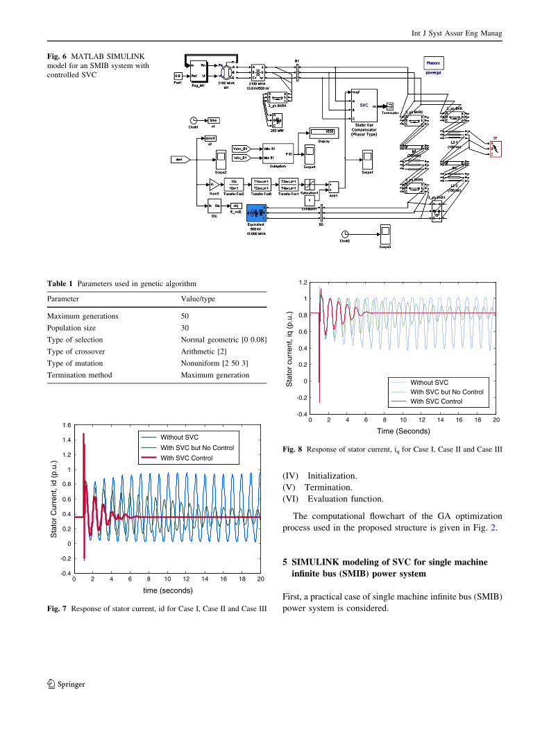
(IV) Initialization.

(V) Termination.

(VI) Evaluation function.

The computational flowchart of the GA optimization

process used in the proposed structure is given in Fig. 2.

5 SIMULINK modeling of SVC for single machine

infinite bus (SMIB) power system

First, a practical case of single machine infinite bus (SMIB)

power system is considered.

0 2 4 6 8 10 12 14 16 18 20-0.4

-0.2

0

0.2

0.4

0.6

0.8

1

1.2

1.4

1.6

time (seconds)

Sta

tor

Cur

rent

, id

(p.u

.)

Without SVC

With SVC but No Control

With SVC Control

Fig. 7 Response of stator current, id for Case I, Case II and Case III

Table 1 Parameters used in genetic algorithm

Parameter Value/type

Maximum generations 50

Population size 30

Type of selection Normal geometric [0 0.08]

Type of crossover Arithmetic [2]

Type of mutation Nonuniform [2 50 3]

Termination method Maximum generation

Fig. 6 MATLAB SIMULINK

model for an SMIB system with

controlled SVC

0 2 4 6 8 10 12 14 16 18 20-0.4

-0.2

0

0.2

0.4

0.6

0.8

1

1.2

Time (Seconds)

Sta

tor

curr

ent,

iq (

p.u.

)

Without SVCWith SVC but No ControlWith SVC Control

Fig. 8 Response of stator current, iq for Case I, Case II and Case III


123

The model of power system shown in Fig. 3 is devel-

oped using SimPowerSystems blockset. There are three

cases:

Case I: SMIB power system without SVC (Fig. 4)

Case II: Model of SMIB power system with SVC but no

control (Fig. 5)

Case III : Model of SMIB power system with SVC

control (Fig. 6)

6 Simulation

The parameters employed for the implementations of real-

coded genetic algorithm (RCGA) in the present study are

given in Table 1.

0 2 4 6 8 10 12 14 16 18 20-0.01

-0.008

-0.006

-0.004

-0.002

0

0.002

0.004

0.006

0.008

0.01

Time (Seconds)

Rot

or s

peed

dev

iatio

ns, d

w (

p.u.

)


Fig. 11 Response of rotor speed deviation, dx for Case I, Case II and

Case III

0 2 4 6 8 10 12 14 16 18 20500

1000

1500

2000

2500

3000

Time (seconds)

Line

pow

er, P

L (M

W)


Fig. 12 Response of line power, PL at bus-1 for Case I, Case II and

Case III

0 2 4 6 8 10 12 14 16 18 200.8

0.85

0.9

0.95

1

1.05

1.1

1.15

1.2

1.25

Time (seconds)

Vre

f (p.

u.)

Fig. 13 SVC reference voltage signal for Case III

0 2 4 6 8 10 12 14 16 18 20-0.2

0

0.2

0.4

0.6

0.8

1

1.2

1.4

Time (Seconds)

Mac

hine

Act

ive

Pow

er O

utpu

t, P

eo (

p.u.

)


Fig. 9 Response of machine active power output, Peo for Case I, Case

II and Case III II and Case III

0 2 4 6 8 10 12 14 16 18 20-1.8

-1.6

-1.4

-1.2

-1

-0.8

-0.6

-0.4

Time (Seconds)

Rot

or a

ngle

dev

iatio

n d

__th

eta

(rad

) Without SVCWith SVC but No ControlWith SVC Control

Fig. 10 Response of rotor angle deviation, dh for Case I, Case II and

Case III


123

Simulations were conducted in the MATLAB 7.7.0

environment and the optimization process is repeated 20

times. As three-phase non-linear models of power system

components are used in the present study, realization of

RCGA optimization process consumes on an average

3,000 s of CPU time. The best final solutions obtained in

the 20 runs are given below (Houari et al. 2007; Oonsivilai

A 2007; Venkateswara Rao et al. 2009).

For SVC controller

Ksvc = 193.3288, T1svc = 0.0538 s, T2svc = 0.2724 s,

T3svc = 0.3507 s, T4svc = 0.8041 s

To assess the effectiveness of the proposed controller

simulation studies are carried out for various models. The

behavior of the power system is analyzed at loading con-

dition P = 0.9 pu under severe disturbance. A 5-cycle,

3-phase fault is applied at the middle of the line at

t = 1.0 s. The original system is restored upon the fault

clearance. The system response under this severe distur-

bance is shown in Figs. 7, 8, 9, 10, 11, 12 and 13.

Case I: Response of SMIB power system without SVC

Case II: Response of SMIB power system with SVC but

no control

2100 MVA13.8KV/500KV

175 Km

SVC

Trfr

CB2100 MVA

M1

Fault

CB

175 Km175 Km

175 Km

100Km1400 MVA

13.8KV/500KV2100 MVA

M34200 MVA

M2

2100 MVA13.8KV/500KV

50 Km

Fig. 14 Multi machine power

system (MMPS) with SVC


MMPS system without SVC


123

Case III: Response of SMIB power system with RCGA

optimized SVC-based controller

7 SIMULINK modeling of SVC for multi-machine

power system

After SMIB power system, a practical case of multi-

machine power system (MMPS) is considered in this paper.

The model of power system shown in Fig. 14 is devel-

oped using SimPowerSystems blockset. There are three

cases:

Case I: Model of MMPS without SVC (Fig. 15)

Case II: Model of MMPS with SVC but no control

(Fig. 16)

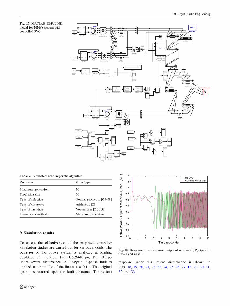
Case III: Model of MMPS with SVC control (Fig. 17)

The system consists of three hydraulic generating units.

Two of 2,100 MVA, 13.8 kV, 60 Hz each and one of 4,200

MVA, 13.8 kV, 60 Hz, three 3-phase 13.8/500 kV step-up

transformer and a 200 MVA SVC. The generators are

equipped with hydraulic turbine and governor (HTG),

excitation system. The HTG represents a nonlinear

hydraulic turbine model, a PID governor system, and a

servomotor. The excitation system consists of a voltage

regulator and DC exciter, without the exciter’s saturation

function (SimPowerSystems 2012).

8 Simulation

The parameters employed for the implementations of

RCGA in the present study are given in Table 2.

Simulations were conducted in the MATLAB 7.7.0

environment and the optimization process is repeated 20

times. As three-phase non-linear models of power system

components are used in the present study, realization of

RCGA optimization process consumes on an average

7,000 s of CPU time. The best final solutions obtained in

the 20 runs are given below.

For SVC controller:

Ksvc = 168.0367, T1svc = 0.9049 s, T2svc = 0.4528 s,

T3svc = 0.8208 s, T4svc = 0.4483 s


MMPS system with SVC

without control


123

9 Simulation results

To assess the effectiveness of the proposed controller

simulation studies are carried out for various models. The

behavior of the power system is analyzed at loading

condition P1 = 0.7 pu, P2 = 0.526687 pu, P3 = 0.7 pu

under severe disturbance. A 12-cycle, 3-phase fault is

applied at the middle of the line at t = 0.1 s. The original

system is restored upon the fault clearance. The system

response under this severe disturbance is shown in

Figs. 18, 19, 20, 21, 22, 23, 24, 25, 26, 27, 18, 29, 30, 31,

32 and 33.

Fig. 17 MATLAB SIMULINK

model for MMPS system with

controlled SVC

Table 2 Parameters used in genetic algorithm

Parameter Value/type

Maximum generations 50

Population size 30

Type of selection Normal geometric [0 0.08]

Type of crossover Arithmetic [2]

Type of mutation Nonuniform [2 50 3]

Termination method Maximum generation

0 1 2 3 4 5 6 7 8 9 10-0.6

-0.4

-0.2

0

0.2

0.4

0.6

0.8

1

1.2

1.4

Time (seconds)

Act

ive

Pow

er O

utpu

t of M

achi

ne-1

, Peo

1 (p

,u.)

No SVCSVC but No Control

Fig. 18 Response of active power output of machine-1, Peo (pu) for

Case I and Case II


123

0 1 2 3 4 5 6 7 8 9 100

0.2

0.4

0.6

0.8

1

1.2

1.4

1.6

1.8

Time (seconds)

Act

ive

Pow

er O

utpu

t of M

achi

ne-2

, Peo

2 (p

.u.)



Case I and Case II

0 1 2 3 4 5 6 7 8 9 10-0.4

-0.2

0

0.2

0.4

0.6

0.8

1

1.2

Time (seconds)

Act

ive

Pow

er O

utpu

t of M

achi

ne-3

,P

eo3

(p.u

.)



Case I and Case II

0 1 2 3 4 5 6 7 8 9 10-5

-4

-3

-2

-1

0

1

2

3x 10

-3

Time (seconds)

Spe

ed v

aria

tions

, dw

1-3

(p.u

.)

No SVC

SVC but No Control

Fig. 21 Response of difference of speed variations of machine-

1(dx1) and machine-3 (dx3), dx13 for Case I and Case II

0 1 2 3 4 5 6 7 8 9 10-0.1

0

0.1

0.2

0.3

0.4

0.5

0.6

0.7

Time (seconds)

dw1-

2 (p

.u.)



1(dx1) and machine-2 (dx2), dx12 for Case I and Case II

0 1 2 3 4 5 6 7 8 9 10-0.1

0

0.1

0.2

0.3

0.4

0.5

0.6

0.7

Time (seconds)

dw3-

2 (p

.u.)


Fig. 23 Response of difference of speed variations of machine-3

(dx3) and machine-2 (dx2), dx32 for Case I and Case II

0 1 2 3 4 5 6 7 8 9 100

1

2

3

4

5

6x 10

4

Time (seconds)

d__t

heta

1-2

(deg

ree)


Fig. 24 Response of difference of rotor angle deviations dh (degree)

of machine-1 and machine-2, dh12 for Case I and Case II


123

0 1 2 3 4 5 6 7 8 9 10-15

-10

-5

0

5

10

Time (seconds)

d__t

heta

1-3

(deg

ree)



of machine-1 and machine-3, dh13 for Case I and Case II

0 1 2 3 4 5 6 7 8 9 10-2000

-1000

0

1000

2000

3000

4000

Time (Seconds)

Act

ive

Pow

er a

t Bus

-1 (

MW

)


Fig. 26 Response of active power at bus-1 or power flow through the

line (MW) for Case I and Case II

0 10 20 30 40 50 600

0.2

0.4

0.6

0.8

1

1.2

1.4

Time (seconds)

Act

ive

Pow

er O

utpu

t of M

achi

ne-1

(p.

u.)

Fig. 27 Response of active power output of machine-1, Peo1 (pu) for

Case III

0 10 20 30 40 50 60-2.5

-2

-1.5

-1

-0.5

0

0.5

1

1.5

2x 10

-3

Time (seconds)

Spe

ed d

evia

tions

, dw

1-3

(p.u

.)


1((dx1) and machine-3 (dx3), dx13 for Case III

0 10 20 30 40 50 60-8

-6

-4

-2

0

2

4

6

8x 10

-3

Time (seconds)

Spe

ed d

evia

tions

, dw

1-2

(p.u

.)


1((dx1) and machine-2 (dx2), dx12 for Case III

0 10 20 30 40 50 6030

40

50

60

70

80

90

100

110

Time (seconds)

d__t

heta

1-2

(deg

ree)


of machine-1 and machine-2, dh12 for Case III


123

Case I: Response of MMPS without SVC

Case II: Response of MMPS with SVC but no control

Case III : Response of MMPS with RCGA optimized

SVC-based controller

10 Conclusions

For designing the controller, a non-linear time-domain

simulation-based objective function is used and RCGA

optimization technique is employed to optimally tune the

parameters of the proposed controller.

The models of SMIB power system and MMPS are

developed using SimPowerSystems blockset. For modeling

SMIB power system and MMPS, different cases are con-

sidered (i) without SVC, (ii) with SVC but no control and

(iii) with genetically optimized SVC controller.

The simulation results show that the power system is

completely unstable without the use of SVC when a three

phase fault occurs on the transmission line. When we use

genetically optimized SVC, the power system becomes

stable after few cycles when fault occurs. Thus the proposed

SVC controller can generate variation of the control signals

and gives efficient damping to system oscillations due to

any disturbance and enhances the power system stability.

Appendix

A complete list of parameters used appears in the default

options of SimPowerSystems in the User’s Manual. All

data are in pu.

Generator 1, M1 SB = 2,100 MVA, H = 3.7 s,

VB = 13.8 kV, f = 60 Hz, RS = 2.8544e-3, Xd = 1.305,

Xd0 = 0.296, Xd

00 = 0.252, Xq = 0.474, Xq0 = 0.243,

Xq00 = 0.18, Td = 1.01 s, Td

0 = 0.053 s, Tqo

00= 0.1 s.,

Pe = 0.7 pu.


VB = 13.8 kV, f = 60 Hz, RS = 2.8544e-3, Xd = 1.305,

Xd0 = 0.296, Xd

00 = 0.252, Xq = 0.474, Xq0 = 0.243,

Xq00 = 0.18, Td = 1.01 s, Td

0 = 0.053 s, Tqo00 = 0.1 s.,

Pe = 0.5267 pu.


VB = 13.8 kV, f = 60 Hz, RS = 2.8544e-3, Xd = 1.305,

Xd0 = 0.296, Xd

00 = 0.252, Xq = 0.474, Xq0 = 0.243,

Xq00 = 0.18, Td = 1.01 s, Td

0 = 0.053 s, Tqo00 = 0.1 s.,

Pe = 0.7 pu.

Load at Bus1 250 MW

Transformer 1 2,100 MVA, 13.8/500 kV, 60 Hz,

R1 = R2 = 0.002, L1 = 0, L2 = 0.12, D1/Yg connection,

Rm = 500, Lm = 500

0 10 20 30 40 50 60-16

-14

-12

-10

-8

-6

-4

-2

Time (seconds)

d__t

heta

1-3

(deg

ree)


of machine-1 and machine-3, dh13 for Case III

0 10 20 30 40 50 60500

1000

1500

2000

2500

3000

Time (seconds)

Act

ive

Pow

er a

t Bus

-1 (

MW

)

Fig. 32 Response of active power at bus-1 or power flow through the

line for Case III

0 10 20 30 40 50 600.8

0.85

0.9

0.95

1

1.05

1.1

1.15

1.2

1.25

Time (seconds)

Vre

f (p.

u.)

Fig. 33 Reference voltage of SVC, Vref for Case III


123



Rm = 500, Lm = 500



Rm = 500, Lm = 500

Transmission lines 3-Ph, 60 Hz, length = 50 km,

100 km, 175/2 km, 175 km, R1 = 0.02546 X/km, R0 =

0.3864 X/km, L1 = 0.9337e-3 H/km, L0 = 4.1264e-

3 H/km, C1 = 12.74e-9 F/km, C0 = 7.751e-9F/km

Hydraulic turbine and governor Ka = 3.33, Ta = 0.07,

Gmin = 0.01, Gmax = 0.97518, Vgmin = 0.1 pu/s, Vgmax =

0.1 pu/s, Rp = 0.05, Kp = 1.163, Ki = 0.105, Kd = 0,

Td = 0.01 s, b = 0, Tw = 2.67 s each

Excitation system: TLP = 0.02 s, Ka = 200, Ta =

0.001 s, Ke = 1, Te = 0, Tb = 0, Tc = 0, Kf = 0.001,

Tf = 0.1 s, Efmin = 0, Efmax = 7, Kp = 0 each

Static var compensator 500 kV, ±200 MVAR, droop =

0.03

References

Chang Y, Xu Z (2007) A novel SVC supplementary controller based

on wide area signals. Electri Power Syst Res 77:1569–1574

Gyugyi L (1988) Power electronics in electric utilities: static var

compensators. IEEE Proc 76(4):483–494

Hingorani NG, Gyugyi L (2001) Understanding FACTS-concepts and

technology of flexible AC transmission systems. IEEE, New

York

Houari B, Gherbi FZ, Hadjeri S, Ghezal F (2007) Modelling and

simulation of static var compensator with Matlab. In: 4th

International Conference on Computer Integrated Manufacturing

CIP’2007

Kundur P (1993) Power system stability and control. McGraw-Hill

Inc., New York

Mathur RM, Varma R (2002) Thyristor-based FACTS controllers for

electrical transmission systems. IEEE, New York

Padiyar KR (2007) FACTS controller in power transmission and

distribution. New Age International (P) Limited, New Delhi

Panda S, Ardil C (2008) Real-coded genetic algorithm for robust

power system stabilizer design. Int J Electr Comput Syst Eng

2(1):6–14

Panda S, Padhy NP (2007) Power system with PSS and FACTS

controller: modeling, simulation and simultaneous tuning

employing genetic algorithm. Int J Electr Comput Syst Eng

1(1):9–18

Panda S, Padhy NP (2008) Comparison of particle swarm optimiza-

tion and genetic algorithm for FACTS-based controller design.

Appl Soft Comput, Elsevier 8(4):1418–1427

Panda S, Patidar NP, Singh R (2008) Simultaneous tuning of static var

compensator and power system stabilizer employing real-coded

genetic algorithm. World Acad Sci Eng Technol 41:1

SimPowerSystems 5.7 User’s Guide (2012) http://www.mathworks.

com/products/simpower/

Somsai K, Oonsivilai A, SRIKAEW A, Kulworawanichpong T

(2007) Optimal PI controller design and simulation of a static var

compensator using MATLAB’s SIMULINK. In: Proceedings of

the 7th WSEAS International Conference on Power Systems,

Beijing, China

Tang Y, Meliopoylos APS (1997) Power systems small signal

stability analysis with FACTS elements. IEEE Power Deliv

12(3):1352

Venkateswara Rao B, Nagesh Kumar GV, Ramya Priya M, Sobhan

PVS (2009) Implementation of static VAR compensator for

improvement of power system stability. In: International Con-

ference on Advances in Computing, Control, and Telecommu-

nication Technologies, pp. 453–457

Zhou EZ (1993) Application of static var compensators to increase

power system damping. IEEE Trans Power Syst 8(2):655


123

http://www.mathworks.com/products/simpower/

http://www.mathworks.com/products/simpower/

Documents

Improvement of power system stability using genetically optimized SVC controller