Embed Size (px)
Citation preview

Improvement of Observation Modeling
for Score Following
Arshia ContMemoire de stage de DEA ATIAM annee 2003-2004
Universite Pierre et Marie Curie, PARIS VI
IRCAM, Real-time Applications Group
Under the supervision ofDiemo Schwarz
andNorbert Schnell
June 30, 2004

ii

Dedicated to my brother, Rama Cont, without whosecourage, I would never find myself in Paris.
– Arshia Cont, , June 2004, Paris.
iii

iv

Abstract
Training the score follower, in the context of musical practice, is to adapt its pa-rameters to improve performance for a certain score. To this aim, every param-eter used in the system has to have direct physical interpretation or correlationwith high-level desired parameters, in order to be trainable and controllable.This criteria has forced us to reconsider the design and approach in one of themain components of the score follower, the probability observation block.
In order to this approach, we developed a criticism based on the notion ofheuristics used in the design of the existing system at the beginning of thisproject with a look at empirical-synthetical sciences which score following re-search is a member. In his respect, we argue that the heuristics used in thedesign of the system has been considered in a late stage during the design andsuggests an alternative approach in which heuristics will be used as the lowest-level of information modeling and higher-level models used in the system wouldbecome an outcome of a series of derivation based on these heuristics modelings.
A novel learning algorithm based on these views called automatic discrim-inative training was implemented which conforms to the practical criteria of ascore following. The novelty of this system lies in the fact that this method,unlike classical methods for HMM training, is not concerned with modeling themusic signal but with correctly choosing the sequence of music events that wasperformed. In this manner, using a discrimination process we attempt to modelclass boundaries rather than constructing an accurate model for each class. Thediscrimination knowledge is provided by an alternative algorithm, namely Yindeveloped by de Cheveigne and Kawahara (2002).
Following the design of the training method, further experiments were un-dertaken to improve the response of system. For this purpose, every feature inthe observation process of the system was studied and examined for correlationwith high-level states and using the analysis results, modifications on the exist-ing feature as well as a totally new feature were introduced to be used in thesystem.
During evaluations, the system proved to be more stable and the resultsare improved compared to the previous system. Moreover, due to our designapproach, the shortcomings of the current system have physical interpretationsin the terms of current design and can be envisioned for further improvements,which was not the case with the previous system.
Finally, the new concepts presented in this work, opens a new and moreflexible view of score following for further research and improvements by arisingan urgent need for a database of aligned sound and other research work whichwould lead the system towards better following.
v

vi

Resume en francais
L’apprentissage du suivi de partition dans le contexte de la pratique musicaleconsiste en une adaptation de parametres permettant d’ameliorer le suivi temps-reel d’une execution d’une partition donnee. Dans cette perspective, chaqueparametre utilise dans le systeme doit avoir une interpretation physique et etrecorrele directement avec des etats haut-niveau desires, pour que le suivi puisseetre entraıne et controle. Ce critere nous a force a reconsiderer la conceptiond’une des composantes principales du suivi de partition: l’observation des prob-abilites.
Dans cette approche, nous avons developpe une critique basee sur la notiond’heuristique utilisee pour la conception du systeme au debut de ce stage. Pourconstruire cette critique, nous regardons les principes des sciences empirique-synthetiques dont le suivi de partition fait partie. Dans cette perspective, nouspretendons que les heuristiques utilisees ont ete considerees dans une etapetardive de la conception et suggerons une approche alternative dans laquelle lesheuristiques entrent dans la conception au plus bas-niveau de la modelisationde l’information. Ainsi, les modeles plus haut-niveau deviennent des resultatsissus de ces modeles bas-niveau.
Une nouvelle approche d’apprentissage basee sur cette perspective nommeeapprentissage discriminatif automatique est implementee. Elle se conforme auxcriteres pratiques d’un suiveur de partition. La nouveaute est que ce systeme,malgre les methodes classiques d’apprentissage des chaınes de Markov cachees,ne prend pas en compte la modelisation des signaux musicaux mais la pertinencedu choix des sequences des evenements musicaux joues. Grace a l’utilisationd’un processus de discrimination, nous tentons de modeliser les marges descategories au lieu de construire un modele precis pour chaque categorie. Ceprocessus de discrimination utilise un algorithme exterieur du suivi de parti-tion, notamment Yin de Alain de Cheveigne et Kawahara (2002). La methoded’apprentissage proposee est independante des parametres de reconnaissance,ce qui est essentiel pour le developpement futur du systeme.
Apres la conception d’une methode d’apprentissage, des experiences plusapprofondies ont ete menees pour ameliorer la reponse du systeme. Pour cela,la correlation entre les parametres du processus d’observation et les etats haut-niveau a ete examinee. En utilisant les resultats de cette analyse, nous avonsmodifie certains parametres et en avons introduit d’autres dans le systeme pourune meilleure reconnaissance.
Pendant l’evaluation, le systeme s’est montre plus stable et les resultatsd’alignement ont ete ameliores comparativement a l’ancien systeme. Ces evaluat-ions sont le resultat d’une simulation sur ordinateur et d’experiences dans unstudio avec des musiciens. Pendant les experiences en temps-reel, le systeme
vii

viii
a obtenu des resultats meilleurs pour certaines phrases qui n’avaient jamaisete reconnues avec le systeme precedent. Grace a notre demarche conception-nelle, les defauts du systeme ont des interpretations physiques permettant desameliorations futures, ce qui n’etait pas le cas avec l’ancien systeme.
Finalement, les nouveaux concepts presentes dans ce travail, ouvrent unenouvelle image plus flexible du suivi de partition pour de futures recherchesen introduisant des nouvelles demandes comme le besoin urgent d’une base dedonnees de sons alignes. Ils ouvrent de nouvelles pistes de recherche qui doiventconduire le systeme a un meilleur suivi.

Acknowledgements
I would like to thank my project directors, Diemo Schwarz and Norbert Schnell,who accepted me to their team and have borne with my sometimes extremeexcitement and too much self-confidence towards research. Much appreciationsto Diemo Schwarz’ patience with my impatience towards research and listeningto my ideas and loud thoughts, and for being a great supervisor.Alain de Cheveigne, whom I had the great opportunity to meet during this work,who spent a considerable amount of time explaining Yin, giving feedbacks onmy approach and widening my horizon of thinking throughout the project.Philippe Manoury, Serge Lemouton and everyone in the ”Suivi Reunion” fortheir practical feedbacks on score following. Specially to Philippe Manoury asone of the only daring composers always eager to test new developments in scorefollowing.Gerard Assayag, Cyrille Defaye and all the coordinators and professors of DEAATIAM, first for accepting me to ATIAM, being at IRCAM as one of my dreamplaces since high-school and second for bearing with my strange situation start-ing from late application and strange requests as the only foreign student in thispromotion of ATIAM.My great ATIAM colleagues, with whom I spent an unforgettable time thisyear, for their understanding and acceptance of this stranger into their group,for helping me with the language, for all the fun and harsh times during exams,for being such an odd mixture of taste and character, and for sharing their vastexperience with me. I will never forget you!My office-mate and colleague, Nicolas Rasamimanana, whom I could never pro-nounce his last name correctly, for his extreme patience during work and bearingwith my harsh humor, for his flexibility after a while and giving me feedbackson my jokes after a while! Nicolas, at last we are good friends!To Thierry Coduys and ”La Kitchen” crews in Paris, for accepting me for apart-time position from the beginning of the DEA and keeping me involvedwith professional music research at all times, without whom I could never man-age my life in Paris.My deepest gratitude to my brother, Rama Cont, and his wife, RokhsanehGhandi, to whom I dedicate this work and without whom I would never hadthe courage to come to Paris and the accident of getting accepted at ATIAMand my one-year stay would never happen.To my parents, Gh. Cont and Mansoureh Daneshkazemi and my dearest twinsister, Mandana Cont.Finally to Marie Vandenbussche for being there, her patience and understandingduring this intense project.
ix

x

Contents
Introduction 1
1 Previous works and Background 31.1 Score Following: A definition in practice . . . . . . . . . . . . . . 31.2 A brief history of Score Following . . . . . . . . . . . . . . . . . . 4
1.2.1 Early Definitions . . . . . . . . . . . . . . . . . . . . . . . 41.2.2 Years of string matching and pitch detection . . . . . . . 61.2.3 The paradigm of the statistical approach . . . . . . . . . 71.2.4 Other approaches . . . . . . . . . . . . . . . . . . . . . . . 81.2.5 Evaluation . . . . . . . . . . . . . . . . . . . . . . . . . . 91.2.6 Training in the context of score following . . . . . . . . . 10
1.3 IRCAM ’s Score Following . . . . . . . . . . . . . . . . . . . . . . 121.3.1 System Overview . . . . . . . . . . . . . . . . . . . . . . . 121.3.2 Features and Observations . . . . . . . . . . . . . . . . . . 141.3.3 HMM based alignment . . . . . . . . . . . . . . . . . . . 19
2 Static Analysis 232.1 A Critic of Pure Heuristics . . . . . . . . . . . . . . . . . . . . . 23
2.1.1 Heuristics in features . . . . . . . . . . . . . . . . . . . . . 242.1.2 Heuristics in Probability Observation modeling . . . . . . 24
2.2 Feature Analysis . . . . . . . . . . . . . . . . . . . . . . . . . . . 252.2.1 ∆Log of Energy . . . . . . . . . . . . . . . . . . . . . . . 262.2.2 ∆PSM . . . . . . . . . . . . . . . . . . . . . . . . . . . . . 27
2.3 New Feature Considerations . . . . . . . . . . . . . . . . . . . . . 282.3.1 Moving Average ∆Log of Energy (mdlog) . . . . . . . . . 282.3.2 Spectral Activity Feature . . . . . . . . . . . . . . . . . . 29
3 Probability Observation Design 313.1 Model basis . . . . . . . . . . . . . . . . . . . . . . . . . . . . . . 313.2 Probability preliminaries . . . . . . . . . . . . . . . . . . . . . . . 323.3 Introducing Discrimination . . . . . . . . . . . . . . . . . . . . . 333.4 Statistical Analysis and Modeling . . . . . . . . . . . . . . . . . . 34
3.4.1 Log of Energy Feature . . . . . . . . . . . . . . . . . . . . 343.4.2 Spectral Balance Feature . . . . . . . . . . . . . . . . . . 353.4.3 PSM feature . . . . . . . . . . . . . . . . . . . . . . . . . 36
3.5 Design Summary and Remarks . . . . . . . . . . . . . . . . . . . 37
xi

xii CONTENTS
4 Training 414.1 Training and Music Tradition . . . . . . . . . . . . . . . . . . . . 414.2 Previous Work . . . . . . . . . . . . . . . . . . . . . . . . . . . . 424.3 The automatic discriminative training . . . . . . . . . . . . . . . 43
4.3.1 Discrimination . . . . . . . . . . . . . . . . . . . . . . . . 444.3.2 Training . . . . . . . . . . . . . . . . . . . . . . . . . . . . 45
4.4 Some results and remarks . . . . . . . . . . . . . . . . . . . . . . 45
5 System Evaluation 47
6 Future Works and Conclusion 516.1 Future Works and Remarks . . . . . . . . . . . . . . . . . . . . . 51
6.1.1 The urge of an aligned database of music . . . . . . . . . 516.1.2 Towards localized probability modeling . . . . . . . . . . 526.1.3 Feature tests . . . . . . . . . . . . . . . . . . . . . . . . . 526.1.4 Temporal Considerations in HMM . . . . . . . . . . . . . 526.1.5 Refining the Music model . . . . . . . . . . . . . . . . . . 526.1.6 Calibration for real-time score following . . . . . . . . . . 53
6.2 Conclusion . . . . . . . . . . . . . . . . . . . . . . . . . . . . . . 53

List of Figures
1.1 Score Following Timeline . . . . . . . . . . . . . . . . . . . . . . 51.2 General overview of IRCAM ’s score following . . . . . . . . . . . 121.3 More detailed general diagram of IRCAM ’s score following . . . 131.4 Feature and Probability Observation Diagram . . . . . . . . . . . 151.5 PSM Trapezoidal filter banks for one sample note . . . . . . . . . 161.6 Upper and lower threshold exponential CDFs . . . . . . . . . . . 181.7 Note Markov Model . . . . . . . . . . . . . . . . . . . . . . . . . 201.8 score parsing visualization . . . . . . . . . . . . . . . . . . . . . . 20
2.1 Discriminated ∆log energy feature observation . . . . . . . . . . 262.2 ∆log energy histogram during sustain states . . . . . . . . . . . . 272.3 Discriminated ∆PSM feature observations . . . . . . . . . . . . . 282.4 Moving Average ∆log energy feature . . . . . . . . . . . . . . . . 292.5 New Spectral Activity Feature observation . . . . . . . . . . . . . 302.6 Spectral Activity Feature histogram during Sustains . . . . . . . 30
3.1 A Gaussian PDF with µ = 0 and σ = 1 . . . . . . . . . . . . . . 323.2 CDF and inverse CDF samples with µ = 0 and σ = 1 . . . . . . . 333.3 Statistics for Log of Energy . . . . . . . . . . . . . . . . . . . . . 353.4 Statistics for Spectral Balance feature . . . . . . . . . . . . . . . 363.5 Histogram of PSM feature non-discriminated (left) and discrim-
inated (right) for all notes in ”Riviere” . . . . . . . . . . . . . . . 373.6 PSM discrimination using Yin . . . . . . . . . . . . . . . . . . . 373.7 New Feature and Probability Observation Diagram (1) . . . . . . 393.8 New Feature and Probability Observation Diagram (2) . . . . . . 40
4.1 HMM for ”Orio training” . . . . . . . . . . . . . . . . . . . . . . 424.2 One iteration of ”Orio training” . . . . . . . . . . . . . . . . . . . 434.3 Automatic Discriminative Training Diagram . . . . . . . . . . . . 444.4 Results of training for LogE feature in ”Rivier” . . . . . . . . . . 46
5.1 Evaluation of different score following systems . . . . . . . . . . . 49
xiii

xiv LIST OF FIGURES

Introduction
This project started with the primary goal of implementing a learning methodfor IRCAM ’s score follower. However, it soon changed its direction towardsdesign considerations of the existing system to have a better following which ledto a novel training method as well as new component designs in the system. Itshould be noted that this work is a result of collaborations with the composerPhilippe Manoury and his musical assistant Serge Lemouton along with AndrewGerzso who organized several sessions with soprano Valerie Philippin for testingthe score following on live and on En Echo.
Before we introduce the contents of each chapter, we would like to emphasizeon some terminologies used throughout this report. To this aim, high-levelstates refer to music symbols modeling the HMM system, which are silenceand note events (attacks, sustains and rests). Features are essentially audiodescriptors marking the first stage of information extraction. Respectively, high-level feature state probabilities correspond to probabilities of high-level statesextracted from audio descriptors.
Chapter 1 marks the early studies towards this project, containing detailedstudies of other similar systems’ implementations followed by a detailed analysisof IRCAM ’s score follower. In his analysis, the author has undertaken a differentview than the articles published in literature on the system in order to emphasizeshortcomings and criticize the concepts behind the design of the existing system.
In Chapter 2, a static analysis is described on the system’s features intro-duced in Chapter 1, trying to analyze features’ behaviors and their correlationswith high-level states. At the same time, a critic on the basis of the existingsystem is developed which results into modifications presented in other chaptersand describes partly the objectives of this project. In this manner, a featuremodification and one totally new feature are introduced for the score follower.
A more general analysis on the probability observation component of thesystem is documented in Chapter 3, which culminates to a redesign and recon-sideration of the probability observation based on critics introduced in Chapter2. The basis of the model and methodology in detail is demonstrated in thischapter.
As a result of the designs and considerations in previous chapters, Chapter 4introduces a novel training algorithm with subsequent results, called automaticdiscriminative training. The novelty lies in the discrimination section in whichwe emphasize on modeling feature boundaries instead of trying to model thefeatures themselves.
Chapter 5 demonstrates some evaluations of the new system and comparisonsbetween the previous system in practice. This is continued in Chapter 6 bylisting future works which are necessary for further developments of the system
1

2 INTRODUCTION
and are in continuation of the current work with a conclusion for this report.

Chapter 1
Previous works andBackground
We need not destroy the past. It is gone.— John Cage
In this first chapter, we aim to give an overview of the previous works whichcount the early studies undertook for this project. As the first attempt, a historyof score following is studied, showing its evolution from the technological andmusical side in time and some reflections on the general notion of score followingand its outcome in the future. It follows with a more elaborated section onIRCAM ’s latest score following system which will be the main ground of thiswork. In studying the IRCAM ’s score follower, the author develops a subjectivescientific view of the topic which would help for understanding the new designsfollowed in the coming chapters.
1.1 Score Following: A definition in practice
Some remarks on the historical definition of score following will be seen in thenext section. However, score following being a medium of interaction betweennew demands from performers and composers at one side and new scientifictechnologies on the other side, has changed and evolved in its definition over 20years. Therefore, a subjective definition can easily loose its account over time.Here we try to define a general definition according to its nature in practice:
Score following serves as a real-time mapping interface from Au-dio abstractions towards Music symbols and from performer(s) liveperformance to the score in question.
The challenge always lies in how this mapping succeeds and engenders differentmusical situations in practice such as errors of the musicians and different styles
3

4 CHAPTER 1. PREVIOUS WORKS AND BACKGROUND
of interpretation. Over about 20 years of score following research, interestingly,the objectives of this technology have been widened through other disciplinessuch as Music Information Retrieval among others. However, in our reportand research, we rest with the score following used in the context of musicperformance.
1.2 A brief history of Score Following
Studying the evolution of score following is essential for this work since at allmoments throughout this report, we encounter how composers’ and musician’sexpectations along with researchers would help evolve this technology. For thispurpose, the author started his work contemplating on the evolution of scorefollowing throughout its history leading to the recent notions of score followingbeing a result of almost 20 years of experience and interaction between musicand sciences.
It should be noted that while this introduction does not include all theresearchers involved in the domain, it tries to lie down most of the main conceptsintroduced into score following along with introducing their innovators. Wehave tried to give the least subjective definition on each approach and all thecomments on each technology is limited to author’s familiarity with the systemas well as the literature available. In this manner, Figure 1.1 shows a scorefollowing timeline which is gathered and mentioned due to their initiatives,original views and importance in the application and history of score following.We will elaborate on different aspects of each system in the following sections.
In our review, we divide the history of score following in four sections:the early definitions which marks the beginning of score following history, theyears of string matching and pitch detection containing systems using those ap-proaches, statistical approaches and other important systems. After the timelineis over, we contemplate on the important subject of system evaluations and givean overview of the training aspects of each mentioned system, if any.
1.2.1 Early Definitions
The history begins officially in 1984 with Roger Dannenberg’s and Barry Ver-coe’s articles appearing in the International Computer Music Conference (ICMC )independently. The two articles mark the first attempts towards real-time scorefollowing and real-time accompaniment which would become a major researchtopic in various research centers and as we will see later, would initiate andmark early attempts for other research topics currently being undertaken inaudio research community.
Barry Vercoe’s 1984 article titled ”The synthetic performer in the contextof live performance” defines the objective as follows:
To understand the dynamics of live ensemble performance well enoughto replace any member of the group by a synthetic performer (i.e.a computer model) so that the remaining live members can not tellthe difference (Vercoe 1984).
While the article describes the system developed in collaboration with LarryBeauregard and for flute, Vercoe pictures the system as having three main ele-ments: LISTEN, PERFORM and LEARN. While he discusses briefly temporal

1.2. A BRIEF HISTORY OF SCORE FOLLOWING 5
Authors Institute Description Year
Barry Vercoe MIT/Ircam First definition, tempo and pitch
considerations, Synthetic performer
1984-
1986
Roger
Dannenberg
Carnegie
Mellon
First definition- String matching
algorithm, Pitch oriented with
heuristics
1984-
1985
Vercoe,
Puckette
MIT/Ircam Training the synthetic performer,
string matching added, ‘cost’.
1987
Puckett Ircam EXPLODE, Pitch oriented 1990
Baird, Belvins,
Zahler
Conneticut
College
String Matching, phrase matching 1990
Vantomme McGill
University
Temporal Patterns 1995
Dannenberg CMU Statistical Modeling 1997
Christopher
Raphael
University
of Amherst
HMM based score following 1999
Loscos, Cano
and Bonada
UPF HMM based score following 1999
Nicola Orio Ircam HMM based score following 2001
Schreck
Ensemble
Schreck
Ensemble
Neural Network Approach, Pitch
based
2001
Pardo,
Birminghm
University
of Michigan
Pitch based, probabilistic ‘cost’ 2002
Christopher
Raphael
University
of Amherst
Bayesian Belief Approach 2001-3
Figure 1.1: Score Following Timeline
modeling of the live performance, his main cue for detection is pitch, whichaccording to the article and the technologies at the time ”implies detection at aspeed almost impossible for audio methods alone” and thus uses fingering infor-mation on the flute. Another interesting contemplation on this early attemptis its author’s considerations for learning or as he puts it, learning to improve.One year later, along with Miller Puckette, he would elaborate more on thistopic (Vercoe and Puckette 1985). The learning aspect of Vercoe and Puckettewill be studied in a later section.
While Vercoe’s approach undertook a ”synthetic performer”, in his 1984article, Roger Dannenberg searches for ”An On-line algorithm for real-time ac-companiment”. In his approach, Dannenberg clearly defines his goals as to firstdetect what the soloist is doing; second, to match the detected input againsta score and third, to produce an accompaniment that follows the soloist (Dan-nenberg 1984). In his approach, he uses dynamic programming to produce thematch and consequently concentrates on the second problem above. In his mod-

6 CHAPTER 1. PREVIOUS WORKS AND BACKGROUND
eling, he considers ”error” cases which consist of omitted notes as well as extranotes in the sequence. In his matching algorithm, while considering events asstring sequences, the best match is defined as ”the longest common subsequenceof the two streams.”(Dannenberg 1984) In this manner, Dannenberg’s approachcan be regarded as a string matching technique. It should be mentioned thatDannenberg’s approach, too, is dependent on pitch in the soloist event detec-tion. Dannenberg’s string matching algorithm ,for which he holds a patent(Dannenberg 1988), is more elaborated in this article by Bloch and Dannenberg(1985).
1.2.2 Years of string matching and pitch detection
The years that follow the early definition of score following mark several im-plementations of score following mainly based on pitch detection and stringmatching as mentioned above and before the next jump to the statistical ap-proach. Also, we would encounter first attempts to the use of score following inmusical composition mainly at IRCAM.
Before 1990, Roger Dannenberg and his students would concentrate on im-proving his string matching algorithm. In (Dannenberg and Mont-Reynaud1987), they expand previous work by addressing the problem of following solosimproved over fixed chord progressions rather than fixed note sequences, leadingto new matching algorithms. In order to make the score following more robust,Dannenberg and Mukaino (1988) introduce the idea of using multiple matcherscentered at different locations. In this version the system can also deal withtrills, glissandi, and grace notes by considering different matching technics foreach event. The main low level changes in this version of Dannenberg’s scorefollowing are the use of multiple matching algorithms at the same time (no-tion of matching objects instead of matching procedure) and the use of delayeddecisions which prevents accidental matching by not trusting all reports fromthe matcher and adding a delay of about 100ms to open more decision makingopportunities.
The year 1990 marks the appearance of Miller Puckette’s EXPLODE article(Puckette 1990). In this article, Puckette defines the interface used for scorefollowing at IRCAM and the score follower itself is more described in (Pucketteand Lippe 1992). Puckette’s EXPLODE marks several pieces written originallywith having score following in mind, particularly Philippe Manoury’s Plutonand Pierre Boulez’ . . . Explosante-fixe. . . . The algorithm consists of pitchrecognition along with a pointer to the ”current” note as well as a set of pointersto prior notes which have not been matched (Puckette and Lippe 1992). In the92 article, Puckette and Lippe give an honest report of their result (which israre in other literatures) noting the weaknesses of the system and when it cannot follow perfectly, adding the following comment:
... Composers are often forced to make compromises so that theirmusic is followed in such a way that the electronic events in the scoreare correctly triggered (Puckette and Lippe 1992).
It should be again noted that this version of IRCAM score following has nodependency on tempo and makes no predictions about the future behavior of themusic to be followed. Rather than use predictions to arrange for the computerand player to act simultaneously (which is Dannenberg’s case), the effort was

1.2. A BRIEF HISTORY OF SCORE FOLLOWING 7
made to make the delay between the musician’s stimulus and the computer’sresponse imperceptibly small (Puckette 1995). This score following had in mindcompositions in the score following repertoire at the time of implementationand its assumptions had to be dropped for new composition demands to come,namely Philippe Manoury’s En Echo for soprano and computer premiered inSummer 1993.
In 1995, Puckette publishes the results of the new approaches to score fol-lowing as a result of the compromise between technology and new composi-tional demands (mostly due to Manoury’s En Echo)(Puckette 1995). Whilethis system, known as F9 in Max/MSP, is still dependent on pitch detection,the instantaneous pitch recognition uses the accelerated constant-Q transformas described in (Brown and Puckette 1992) and (Brown and Puckette 1993).This approach is very similar in its concept to what is being used in the latestHMM Score Following’s PSM (Peak Structure Match) to be elaborated later.In this manner, the best pitch is the instantaneous pitch corresponding to thehighest instantaneous power at which a pitch was present (Puckette 1995). Forscore following, two parallel match signals would be present with different de-lays and the reliable one would be used as the input to a discrete-event scorefollower.
In parallel to the above systems, Baird, Blevins and Zahler have revised anew matching algorithm which was based directly on (Dannenberg 1984) and(Vercoe 1984) with the difference that it is based on the concept of segmentsas opposed to single events. Matching is performed on segments of predefinedlength; that is, segment sizes are not necessarily based on any musical heuristicsor analytic conventions. Comparisons by events and rest positions are performedand stored tentatively until the set of previously heard and unsegmented eventsmatch one of four segment types as described in (Baird et al. 1990) and (Bairdet al. 1993).
1.2.3 The paradigm of the statistical approach
Contemplating on the nature of score following, we encounter that even withperfect feature observations (pitch, temporal patterns) we always remain in arealm of uncertainty due to various types of errors by the musician or the relativenature of a music performance especially in the temporal aspect. Therefore, itis natural to consider probabilistic approaches towards real-time score following.
The pioneering work in this domain belongs to Grubb and Dannenberg(1997b) for which they hold a patent (Grubb and Dannenberg 1997a). In thisapproach, the position in the score is represented by a probability density func-tion. Unlike previous systems, it does not require subjective weighting schemesor heuristics and it can use formally derived or empirically estimated probabil-ities describing the variation of the detected features. In this approach, at anypoint, the position of the performer is represented stochastically as a continuousdensity function over score position. The area under this function between twoscore positions indicates the probability that the performer is actually wherein the score. As the performance progresses and subsequent observations arereported, the score position density is updated to yield a probability distribu-tion describing the performer’s new location. In this manner, for tracking theperformer and to calculate new observation, current score position density andthe observation estimations are used to estimate a new score position density.

8 CHAPTER 1. PREVIOUS WORKS AND BACKGROUND
It is worth to make a comparison between this new paradigm of statisticalapproach and the previous mainly pitch oriented approaches. In this new ap-proach, if pitch detection is applied to the performance, then this informationwould provide a likelihood that the detector will report that pitch conditioned onthe pitch written in the score, despite the previous constraints of score followershighly dependent on the output of the pitch detection.
A simpler statistical approach on the same line as the string matching algo-rithm is reported at (Pardo and Birmingham 2002) and (Pardo and Birmingham2001) from University of Michigan. Their algorithm is based on the same ideasin (Dannenberg 1984) and (Puckette and Lippe 1992) by defining a match scoreand skip penalty with the difference that these ”costs” are modeled by someprobability distribution instead of mere numbers. In this manner, the system istrained off-line and on a date base of sound (not on the music itself), to obtaina match score matrix.
One of the most important works in statistical score following systems hasbeen undertaken by Christopher Raphael in a series of research marking its be-ginning in 1999. The IRCAM Score following system finds its roots in Raphael’s1999 article on ”Automatic Segmentation of Acoustic Musical Signals UsingHidden Markov Models” (Raphael 1999b). In this pioneering work and as hisfirst published experiment with real-time score following, he defines musicalanalogies as Markov models consisting of note models (attack, sustain, durationmodeling) and rest models which would be derived from the score and spectralfeature observations would be used to calculate state probabilities and decodein real-time. Since there is much similarities between Raphael’s system and thesystem in consideration for this report, we would refer the reader to Section 1.2and also to Raphael’s fully documented article in (Raphael 1999b) and (Raphael1999a). One last comment on the difference between Raphael’s system and thatof IRCAM is the way the observation probabilities are calculated. In Raphael’ssystem, there is no such distinction between observation probabilities and theHMM system and his features are statistics over the data frame.
Similar work on the use and consideration of HMM systems for score follow-ing have been published at the same time but for limited applications namelyin (Loscos et al. 1999a) and (Loscos et al. 1999b).
Raphael would continue on his way and explore more models for automaticmusic accompaniment which are crucial in the context of our work. In hismore recent research papers he reports a new approach by coupling the HMMsystem by a Bayesian belief network (Raphael 2001). The basic idea behindthis coupling is HMM ’s famous incapability of handling temporal issues. Heuses the output of the HMM system as onsets of the Bayesian network whichwould train themselves on a performance sample, thus learning some ”interpre-tational” aspects of the performance and using tempo anticipation in triggeringthe accompaniment. This issue will be observed in more details later. It shouldbe noted at this point that Raphael’s system is pointed more towards accom-paniment rather than synchronizing the follower with the performance.
1.2.4 Other approaches
As indicated in the previous subsections, most score following systems describeddo not consider temporal patterns as main cues for recognition. One of the firstattempts to use temporal patterns as the main following cue was done in univer-

1.2. A BRIEF HISTORY OF SCORE FOLLOWING 9
sity of McGill by Vantomme (1990). The main input of the system, however, isthe onset time of each event in MIDI format and there is few discussion of the li-ability of this information for the system. Moreover, the implementation is donein LISP which, despite the insistence of its author on unimportance of real-timeissues surrounding LISP, should limit processing for certain pieces. Following isbased on performer’s rhythms which, again despite the insistence of the authoron the stylistically unbiased system, should limit its usage specially for con-temporary repertoire with non-stationary and complicated rhythmic patterns.However, reports in (Vantomme 1990) indicates that the system is independentof the performer’s errors in pitch and robust enough in rhythm recognition,assuming that everything works.
One completely different approach is the ComParser score following de-veloped by Schreck Ensemble in Netherlands as a free open source software(Schreck Ensemble and Suurmond 2001). Before going into some brief tech-nical details, it should be noted that ComParser has been developed to meetits ensemble’s musical needs. Therefore, it has certain applications which hadnot been visioned in the previously mentioned systems such as following Audioinstead of symbolic musical scores. For this reason, the authors of the systemrefer to their approach as a sonic approach as opposed to ”IRCAM ’s Symbolicapproach.” This system uses the neural network technology for audio recogni-tion with spectrum features as inputs of the network. Although being used inperformances of Schreck Ensemble, ComParser is under development and as oftheir last report, the network architecture used is a modified Avalanche networkas originally introduced in (Grossberg 1982) with the addition of time-delays,weights on forward connections and limited lengths and activities of previousactivity windows. Like most neural network systems, ComParser requires su-pervised training on audio which can be frustrating, but reports indicate thatit is fairly robust. However, use of neural networks technologies introduce prob-lems which would never be encountered in previous ”formalized” systems suchas premature recognition and over-fitting due to the generalization behavior ofthe network. On the other hand, recognition of note onset, release and changeseems to be not much of a problem and is dependent on training issues.
1.2.5 Evaluation
Speaking about 12 different systems in the previous sections, it is evident to askabout the performance evaluation of systems in general and their advantagesand drawbacks among each other. Unfortunately, all the published reports andarticles focus on the scientific aspect of the systems and speak less or not atall on evaluation and comparison. This is mostly due to few musical practicein most institutions and non existence of a data base and unified approach forevaluation. However evaluation of score following was a topic of a panel in theICMC 2003 conference but to this date no action has followed that meeting.
One main important issue, not previously addressed, in evaluation of scorefollowing is the non-unified definition of score following among its authors. Thisissue becomes clear by having a closer look at Section 1.2.1, the early defini-tions. From the beginning we see that the term score following is ambiguousbetween automatic accompaniment and synchronization. Vercoe and Puckette’sapproach (or more precisely IRCAM ’s score following) is dealing with the prob-lem of synchronizing the performer to the score at each instant and on the

10 CHAPTER 1. PREVIOUS WORKS AND BACKGROUND
other hand, Dannenberg and Raphael’s approach is more towards automaticaccompaniment. The difference is that in the first approach, we want exactsynchronization of the performance with the score and the computer does notimpose anything directly on the performer but in the second approach, mostlydue to temporal anticipations, future events might occur before the performer’scues and at those moments, the performer must adapt itself to the accompa-niment(Dannenberg 2004). This ambiguous usage of the term score followingmakes the use of literature more difficult and leads to false expectations andcomments from each side.
On the other hand, it is at IRCAM ’s interest to evaluate score following asan in practice procedure mostly due to its wider repertoire using score followingand musical production environment. In IRCAM ’s case, the user of the scorefollowing is not the developer or researcher and we are always dealing with thetradition of musical practice. Moreover, at IRCAM we are dealing with newmusic repertoire with more demanding and finer score followers than classicalmusic repertoire. Most of the systems described above, besides the IRCAMsystem, are tested and trained using the researchers as musicians and on classi-cal repertoires; thus, not considering their system as an interface dealing withmusicians and more over using simpler musical excerpts for score following.
Recently, the Real-time Applications Group at IRCAM has brought forwardthe issue of evaluation in an article published at the NIME conference (Orioet al. 2003). In that article, they elaborate the issue by discussing objectiveand subjective evaluations, suggesting a framework for evaluation of differentexisting systems. To conclude, evaluating score following is an essential topicwhich should be seriously considered for further progress. We would elaboratemore on its details in the concluding chapter of this report.
1.2.6 Training in the context of score following
Since one of the main objectives of this project is to obtain an automatic trainingof IRCAM ’s score follower, it is worth to look at training in the context ofdifferent score following systems observed before.
The first learning scheme in the context of score following occurred in Ver-coe’s score following and appeared in Vercoe and Puckette (1985). In describingthe objective of training Vercoe’s score following, we quote from the originalarticle:
. . . [speaking about the 84 score follower] there was no performance”memory”, and no facility for the synthetic performer to learn frompast experience. . . since many contemporary scores are only weaklystructured (e.g. unmetered, or multi-branching with free decision), ithas also meant development of score following and learning methodsthat are not necessarily dependent on structure(Vercoe and Puckette1985).
Their learning method, interestingly statistical, allows the synthetic performerto rehearse a work with the live performer and thus provide an effective perfor-mance, called ”post-performance memory messaging.” This non-realtime pro-gram begins by calculating the mean of all onset detections, and subsequentlytempo matching the mean-corrected deviations to the original score. The stan-dard deviation of the original onset regularities is then computed and used to

1.2. A BRIEF HISTORY OF SCORE FOLLOWING 11
weaken the importance of each performed event. When subsequent rehearsaltakes place, the system uses these weighted values to influence the computationof its least-square fit for metrical prediction.
While in Dannenberg’s works before 1997 (or more precisely before the statis-tical system) there is no report of training, in Puckette’s 95 article (F9 system)there are evidences of off-line parameter control in three instances: defining theweights used on each constant-Q filter associated with a partial of a pitch inthe score, the curve-fitting procedure used to obtain a sharper estimate of f0
and threshold used for the input level of the sung voice. According to (Puckette1995), Puckette did not envision any learning methods to obtain the mentionedparameters. In the first two instances he uses trial and error to obtain globalparameters satisfying desired behavior and the threshold is set by hand duringperformance.
By moving to the probabilistic or statistical score followers, the concept oftraining becomes more inherent. In Dannenberg and Grubb’s score follower,the probability density functions should be obtained in advance and are goodcandidates for an automatic learning algorithm. In their article, they reportthree different PDFs in use and they define three alternative methods to obtainthem:
First, one can simply rely on intuition and experience regarding vocalperformances and estimate a density function that seems reasonable.Alternatively, one can conduct empirical investigations of actual vo-cal performances to obtain numerical estimates of these densities.Pursuing this, one might actually attempt to model such data ascontinuous density functions whose parameters vary according tothe conditioning variables (Grubb and Dannenberg 1997b).
Their approach for training the system is a compromise of the three mentionedabove. A total of 20 recorded performances were used and their pitch detectedand hand-parsed time alignment is used to provide an observation distributionfor actual pith given a scored pitch and the required PDF s would be calculatedfrom these hand-discriminated data.
In the HMM score following system of Raphael, where there can be manyparameters to train and there are traditional ways to train the system, he doesnot train the HMM transitional probabilities. For training his statistics (orfeatures in our system’s terminology) he uses the posterior marginal distribu-tion {p(xk|y)} to re-estimate his feature probabilities in an iterative manner(Raphael 1999b). In his iterative training he uses signatures assigned to eachframe for discrimination but it is not clear from the article whether a parsingis applied beforehand to obtain the right behavior or not. In his latest system,incorporating Bayesian Belief Networks (BNN), since the BNN handles tem-poral aspect of the interpretation, several rehearsal run-throughs are used tocompute the means and variances of each event in the score, specific to thatinterpretation.
In the case of Pardo and University of Michigan’s score follower, a trainingis done to obtain the probabilistic costs which is independent of the score andperformance and is obtained by giving the system some musical patterns suchas arpeggios and chromatic scales (Pardo and Birmingham 2002).
For IRCAM ’s score following before this project, training has been doneonce to obtain the global PDF s describing desired behavior and in the context

12 CHAPTER 1. PREVIOUS WORKS AND BACKGROUND
described in (Grubb and Dannenberg 1997b) as empiric and intuitive and in(Orio et al. 2003) as heuristic. That is series of observations were made ondifferent sound files and musical situation, and using ”heuristics” the PDF pa-rameters were chosen to obtain desired behavior. It should be noted that in thatversion of the score following, PDF s were fixed exponential functions. Therehas been no publication to date of an automatic training for this system.
1.3 IRCAM ’s Score Following
This project is done in the context of IRCAM ’s score following system as brieflydescribed before. Therefore, as a prerequisite of this work, the current systemneeds to be studied in depth for further analysis and modification.
In this section we aim to define the architecture which existed upon arrivalof the author in the Real-time Applications Group at IRCAM on March 2004. Itshould be noted that while the system described hereafter is well documented in(Orio and Schwarz 2001), (Orio and Dechelle 2001) and (Orio et al. 2003), theauthor’s view of the system focuses on different aspects than in the mentionedarticles, in order to emphasize more on the learning aspects and shortcomings ofthe system to be considered during the project and design of a new architecturein Chapter 3.
1.3.1 System Overview
Before anything, it should be noted that while the score following runs in real-time and on audio, it prepares itself for following in advance by loading thescore into the system. In general, we can imagine two some-how independentcomponents for the whole system as illustrated in Figure 1.2. In this figure andthereafter, dashed lines refer to information which is processed off-line into thescore following.
Observations
Score
Score cue activation
Decision and Alignment
Parameters
Score
Audio data
Figure 1.2: General overview of IRCAM ’s score following

1.3. IRCAM’S SCORE FOLLOWING 13
In this view, score following consists of two some-how independent com-ponents running in parallel: the Observation and Alignment. To describe thefunctionality of each block, it is natural to vision a human listener. In thiscase, the observation is what is being observed on the raw audio by human earsand alignment is the high-level information deducted from these observations.Score is being pre-processed for both blocks which is basically preparation of ananticipation for observation and preparing the symbolic or high-level targets forthe alignment and parameters are needed for the observation in order to adaptitself to the situation.
Following this introduction, Figure 1.3 reveals the system with more detailson the technologies and terminologies used throughout this report.
Feature Calculation and Probability Observation
Score
......
Audio frame data
Parameters
Feature probabilities
(out of time)
(in time)
Event Following
Hidden Markov Model
Score
Figure 1.3: More detailed general diagram of IRCAM ’s score following
Getting more detailed, the observations are spectral features calculated onaudio frames of about 6ms length and what are actually observed by the align-ment section are feature probabilities and not the features themselves. In thismanner, the observation block in Figure 1.2 consists of both feature calculationand probability mapping of the calculated features at each instant. As seen inFigure 1.3, Hidden Markov Models (HMMs) are used for score modeling andalignment. The score is defined as a Markov model and using feature stateprobabilities, the system decodes this information into the high-level musicalstates in the HMM which in terms, upon the activation cues marked in thescore, triggers outside events.
We can argue that in observation we are handling an acoustic modeling asin the alignment section we are undertaking a music modeling.
The score is loaded beforehand into both blocks to prepare the right featurecalculation and to construct the HMM score model for observation and align-ment respectively. Preparation of a HMM model from the score is called scoreparsing which is studied in Section 1.3.3. At the same time, and again off-line,parameters are needed to define the probability models for each state features

14 CHAPTER 1. PREVIOUS WORKS AND BACKGROUND
to be sent to the HMM system.At this point, we are ready to consider each block in Figure 1.3 in more
details. From now on in this report, the general score following term will referto IRCAM ’s HMM based score following.
1.3.2 Features and Observations
Figure 1.4 shows a detailed diagram of the early Feature Calculation and Proba-bility Observation section of the score following. This figure shows the real-timeprocess of the mentioned block which undertakes feature calculations and theirmapping to high-level state probability observations. Complete lines in the fig-ure refer to number flows as dashed lines refer to vector flows at each instant ofscore following.
First, we need to define the features being used in the mentioned figure. Asis seen, all the features are calculated on the magnitude spectrum or FFT of thepresent frame. In this section we go through each feature and through the end,define the probability observation mapping shown in Figure 1.4.
The main ambition in choosing a feature is that each corresponds to one orseveral high-level states (note sustain, note attack and rest) and that they wouldbe mutually independent among each other. At this point we will not discussthe validity of these features but aim to introduce them for further discussionsfollowed in coming sections. In the score following in question the followingmain features were in use:
Log of Energy feature (loge)
This feature is simply the Log of the energy contained in the FFT frame asshown in Equation 1.1, assuming y to be raw audio signals in a frame. FFT inthis context signifies the magnitude of the FFT of a windowed time frame usinga hamming window. Main characteristic of this feature is that it will help thesystem distinguish between note and non-note events.
LogE = log(∑
FFT(y))
(1.1)
Delta Log of Energy feature (∆log)
The Delta log of energy feature is simply the difference between the currentframe’s log of energy and the previous one as shown in Equation 1.2. It ishoped that this feature would observe less activity during note sustain and restand high activity during attacks.
Dlog(n) = loge(n)− loge(n− 1) (1.2)
Peak Structure Match (PSM)
This feature is handling some notion of pitch and at each moment specifies theenergy contained at a specified peak structure in the spectrum1. More precisely,the pitch is not used as a feature directly but the structure of the peaks in the
1This subsection is mainly adopted from Orio and Schwarz (2001).

1.3. IRCAM’S SCORE FOLLOWING 15
Log
of E
nerg
yD
elta
Log
of E
nerg
yP
SM
Del
ta P
SM
FF
T
LogE
Sus
tain
Pro
babi
lity
min
µ, th
resh
old
LogE
Res
t Pro
babi
lity
max
µ, th
resh
old
LogE
atta
ck P
roba
bilit
y
min
µ, th
resh
old
dLog
Sus
tain
Pro
babi
lity
max
µ, th
resh
old
dLog
Res
t Pro
babi
lity
max
µ, th
resh
old
dLog
atta
ck P
roba
bilit
y
min
µ, th
resh
old
PS
M S
usta
in P
roba
bilit
y
min
µ, th
resh
old
PS
M a
ttack
Pro
babi
lity
min
µ, th
resh
old
dPS
M S
usta
in P
roba
bilit
y
max
µ, th
resh
old
dPS
M a
ttack
Pro
babi
lity
min
µ, th
resh
old
Res
t Sta
te P
roba
bilit
yA
ttack
Sta
te P
roba
bilit
yS
usta
in S
tate
Pro
babi
lity
Abs
olut
e V
alue
Aud
io F
ram
e D
ata
Figure 1.4: Feature and Probability Observation Diagram

16 CHAPTER 1. PREVIOUS WORKS AND BACKGROUND
spectrum given by the harmonic sinusoidal partials. The advantage is that, thisconcept can be easily extended to polyphonic signals.
For this purpose, expected peaks are modeled from the pitches in the score.For each note, 8 harmonic peaks are generated. In the latest version, the peakstake the form of trapezoidal spectral bands with an equal amplitude of 1 andno overlap. Figure 1.5 shows a visualization of a one note PSM with differenttrapezoidal slopes. In the score following, a slope value of 1 is being used withno overlap. Each band has a bandwidth of one half-tone to accommodate forslight tuning differences and vibrato.
0 500 1000 1500 2000 2500 3000 3500 40000
0.1
0.2
0.3
0.4
0.5
0.6
0.7
0.8
0.9
1
Frequency [Hz]
Trapezoidal Harmonic Filter Bands range = 1−189 bins = 21.5332−4069.78 Hz
filter (slope = 0)filter (slope = 0.5)filter (slope = 1)filter (slope = 2)odd bandseven bands
Figure 1.5: PSM Trapezoidal filter banks for one sample note
This generated score spectrum (S ) is multiplied by the Fourier magnitudespectrum (P 2) of one frame of audio during performance. Normalization of theresult is necessary to prevent a loud, noisy frame from matching all generatedbands. Equation 1.3 shows the mathematical analogy of what is described abovewhere m corresponds to the frame number in performance and n is the noteevent number in the score. Thus, PSM is a vector at each instant carryinginformation about all possible notes in the score (the reason for having dashedlines in Figure 1.4).
PSM(m,n) =∑
SiPi2
∑Pi
2 (1.3)

1.3. IRCAM’S SCORE FOLLOWING 17
Delta of Peak Structure Match (∆PSM)
Like Delta log of energy, the ∆PSM reports local bursts for each PSM and itis there to force and help the recognition of attacks and note changes since weexpect to have high rise in PSMs during attacks and also for assuring sustainstates since, by heuristics, we expect to observe low activity of ∆PSM duringsustain. The equation is essentially similar to that of 1.2.
Probability Observation Mapping
After the features are calculated, their values are being used to compute obser-vation probabilities for high-level states in the HMM score model. There arethree high-level states at this moment: Attack, Sustain and Rest. To computethe state probability of the three mentioned states, all or some of the featuresare used. Before we get to the procedure and practical details of the systemas illustrated in Figure 1.4, it is necessary to approach the matter using somemathematics and lie down the assumptions used throughout this process, whichwould eventually help us in redesigning and training the observation block2.
A frame of our data (after the FFT block), lies in a high dimensional space– <J where J=1024 in our experiment. Thus, we can look at the observationblock as a dimension reduction process towards high-level states to make repre-sentation and training possible. In this way, we can consider each feature as avector-valued function, mapping the high dimensional space into a much lowerdimensional space. We can think of the features s(y) as containing all relevantinformation for estimating the desired segmentation, i.e. the alignment l, givenno information but y, that is, we assume s is a sufficient statistic for l, meaningthat p(y|s(y), l) does not depend on l. As a consequence:
p(y|l) = p(y, s(y)|l)= p(y|s(y), l)p(s(y)|l)= p(y|s(y))p(s(y)|l) (1.4)
Since p(y|s(y)) will be constant for each frame we disregard that factor andconcentrate on the way we would be connected to the hidden segmentation l.Adding the assumption of conditional independence of each feature (sd) along,the above equation follows as:
p(y|l) ∝ p(s(y)|l)
=D∏
d=1
p(sd|l) (1.5)
Which is actually why in Figure 1.4 feature probabilities are being multipliedto obtain the high-level state probabilities. In our case, s(y)= [loge(y), ∆log(y),PSM(y), ∆PSM(y)] with D = 2 + 2 · N , N indicating the number of notes inthe score, as our feature space.
Knowing this, we are now ready to contemplate on the calculation of eachprobability density or the details of p(.) functions discussed previously.
2The interpretation demonstrated here is partially inspired by (Raphael 1999b) and (Ra-biner 1989).

18 CHAPTER 1. PREVIOUS WORKS AND BACKGROUND
A key design decision in acoustic modeling (given a decision/training crite-rion such as maximum likelihood) is the choice of functional form for the stateoutput probability density functions. After that we try to adapt these functionsto our application by controlling their parameters.
Most HMM recognition systems use a parametric form of output PDF. Inthis case a particular functional form is chosen for the set of PDF s to be es-timated. Typical choices include Laplacians, Gaussians and mixtures of these.The parameters of the PDF are then estimated so as to optimally model thetraining data. If we are dealing with a family of models within which the correctmodel falls, this is an optimal strategy.
For the score following in question the parametric form of PDFs is chosenas an exponential function with upper or lower thresholds. Documentationsindicate that these functional forms were chosen because they model the a prioribehavior of the features well enough. In order to better understand the nature ofthe heuristics used, we demonstrate a simple case of calculating Rest probabilityfor the Log of Energy feature: In this case, heuristics tell us that the less theenergy, the more the probability of being at rest and after some certain value weare sure we would be at rest. Using this reasoning, a lower bounded exponentialfunction is chosen as the probability mapping function in question.
Following the above heuristics for every feature, two kinds of exponentialprobability mapping is chosen to demonstrate an upper threshold (Eq 1.6) anda lower-threshold (Eq 1.7). As is seen in the corresponding equations, for eachfunction the µ and σ parameters need to be adjusted.
y = e−(σ−x)
µ for (σ − x) > 0 y = 1 for (σ − x) ≤ 0 (1.6)
y = e−(x−σ)
µ for (x− σ) > 0 y = 1 for (x− σ) ≤ 0 (1.7)
Figure 1.6 demonstrates the general forms of the above probability mapswith different parameters.
−10 −8 −6 −4 −2 0 2 4 6 8 100
0.1
0.2
0.3
0.4
0.5
0.6
0.7
0.8
0.9
1
x
y
µ=0.5µ=0.7µ=0.9µ=1.1µ=1.3µ=1.5µ=1.7µ=1.9
−10 −8 −6 −4 −2 0 2 4 6 8 100
0.1
0.2
0.3
0.4
0.5
0.6
0.7
0.8
0.9
1
x
y
µ=0.5µ=0.7µ=0.9µ=1.1µ=1.3µ=1.5µ=1.7µ=1.9
Figure 1.6: Upper (left) and lower (right) threshold exponential CDFs
Looking back into Figure 1.4, the blocks on the second row refer to thementioned probability mappings which means, having five blocks, there are 10parameters to adjust.

1.3. IRCAM’S SCORE FOLLOWING 19
1.3.3 HMM based alignment
As mentioned before, in the HMM system the music model is being handledfrom the observed acoustic model or it can be viewed as the main bridge fromthe audio abstraction to music symbolism. At this point, we describe the processbeing done in the HMM system to align to the right place in the score and themusic model used and how it is being mapped in score following.
Hidden Markov Models
Interested readers in HMM mathematics and its general model are referred tothe historical article of Rabiner (1989). In this section we aim to discuss generalissues of HMM s which are in direct interest of score following applications.
Hidden Markov Models (HMM s) are among the ideal models in literaturefor sequential event recognition. Score following in its nature is a sequentialevent recognizer. In a Hidden Markov modeling of audio or music we assumethat audio is a piecewise stationary process. A HMM is a stochastic automationwith a stochastic output process attached to each state. Thus we have two con-current stochastic processes: a Markov process modeling the temporal structureof music; and a set of state output processes modeling the stationary characterof the music signal. HMMs are ”hidden” because the states of the model, q,are not observed; rather the output of a stochastic process, y, attached to thatstate is observed. This is described by a probability distribution p(y|q).
In the context of our score following, qs correspond to the high-level statefeatures in the music model which will be described in the coming subsectionand probability distributions p(y|q) are the output of our observation block asdescribed previously.
For recognition the probability required is P (Q|Y ). It is not obvious howto estimate P (Q|Y ) directly; however we may reexpress this probability usingBayes’ rule:
P (Q|X) =p(y|q)P (Q)
p(Y )
This separates the probability estimation process into two parts: acoustic mod-eling, in which the data dependent probability p(Y |Q)/p(Y ) is estimated; andmusic modeling in which the prior probabilities of sequence models, P (Q), areestimated (Renals et al. 1993). When we use the maximum likelihood criterion,estimation of the acoustic model is reduced to p(Y |Q) as we assume p(Y ) to beequal across the model and which is the case in our follower.
Therefore, after the observation process described in the previous section, wehave all the probabilities required and at this moment, we choose the sequencethat has a more likely chance of being the current sequence which in terms,reveals the current place in the score.
Music Model
HMM serves as a bridge from audio abstraction to music symbols. Moreover, itis the HMM which handles time evolution of the score during a performance.For this purpose, a music model should be derived using Markov models.
The model used in score following, considers three high-level states as dis-cussed before: Attack state, Sustain state and Rest state, which the first two,

20 CHAPTER 1. PREVIOUS WORKS AND BACKGROUND
obviously are characteristics of a note while the last describes silence and theend of a note. Figure 1.7 shows the Markov model for a single note. It is a left-right model which represents time evolution and to this end, the model consistsof one attack state, several sustain states modeling the note duration and onerest state which models the end of a note which can jump to the next event(silence or note; note in this example) for the case of legato notes.
...a s ss ar
Figure 1.7: Note Markov Model, a=attack s=sustain r=rest
The number of sustain states for a note or the number of rest states for ano-note event as well as the transition probabilities between them models theduration specified in the score. Since this is not the subject of this research,we refer the reader to (Mouillet 2001) which is essentially on the subject of thissystem’s temporal modeling.
Other important parameters in a HMM model are the transition probabili-ties between the states. In the score following, due to the nature of a music per-formance, only transitions to previous and next states as well as self-transitionare allowed which are fixed numbers and assume equal probabilities for eachtransition (except for time modeling which is the issue in (Mouillet 2001)) andessentially assures a temporal left-right flow in the score, which is natural.
Using this Markov model vocabulary and before each performance, the scoreis translated into a left-right chain of Markov models. This process is calledscore parsing which is one of the off-line processes discussed before. Figure 1.8demonstrates a visualization of this process.
... ... ... ...a s ss a sss r rr a s ssr r r
Figure 1.8: score parsing visualization
Sequential recognition and Alignment
So far we have discussed the observation probabilities and the music model.While being used in real-time, the score follower is examining the probabilitythat a sequence of events would occur. In the classical HMM literature anefficient procedure called Forward-Backward procedure computes this variablewhich takes into account both probability of the states before and after a certainstate for computation. Clearly, since we are dealing with real-time situationswe can have no chance of observing the future states and therefore, we use only

1.3. IRCAM’S SCORE FOLLOWING 21
the Forward Procedure which takes into account the observation probabilitiesfor all states from the observation block, transition probabilities obtained fromthe music model and previous sequence probabilities. Classically, this Forwardvariable is referred to as αt which is basically the probability of the partialobservation sequence O = O1O2...Ot (until time t) and state Si at time t, giventhe HMM model λ, as demonstrated in Equation 1.8 (Rabiner 1989).
αt(i) = P (O1O2...Ot−1, qt = Si|λ)
=
[N∑
i=1
αt−1(i)aij
]bj(Ot) (1.8)
Note that in Equation 1.8, aij is the transition probability between stateswhich is obtained from the music model and bj(Ot) is p(Ot|qt = Sj) which is adirect outcome of the observation block computed for every state in the HMMmusic model. Also N is the total number of states available in the HMM score.
After computing all possible α variables for the audio frame in consideration,we can solve for the individually most likely state qt, as
qt = argmax1≤i≤N [αt(i)] (1.9)
Equation 1.9 is referred to as decoding and specifies the most likely high-levelstate depending on previous matches, new observation probabilities as well asthe score and in real-time. At this moment, score following is done!

22 CHAPTER 1. PREVIOUS WORKS AND BACKGROUND

Chapter 2
Static Analysis
A sound does not view itself as thought, as ought, asneeding another sound for its elucidation, as etc.; ithas not time for any consideration–it is occupied withthe performance of its characteristics: before it hasdied away it must have made perfectly exact its fre-quency, its loudness, its length, its overtone structure,the precise morphology of these and of itself.— John Cage, Experimental Music: Doctrine
Experiments with the score following and profound look at the music modelin the alignment section reveals that an important aspect of the score followingis in the observation section. In this manner, we believe that by having a strongobservation we will always be able to pass to the right state in the music model.
In this chapter, we aim to analyze the behavior of features in the observationsection and suggest improvements on the features and probability observationsto better correspond to the musical events we wish to observe.
We start the chapter by a rather epistemological critic on the basis design ofthe existing observation block at the beginning of this project, which reveals ourmethodology in analysis and redesign as well as the approach we believe wouldlead to a stronger observation. It follows by an analysis of existing featuresusing the mentioned approach and new features would be introduced in Section2.3.
2.1 A Critic of Pure Heuristics
Heuristics are the main basis of the probability observation block of the scorefollowing. Although the notion is not quite clear, we try to approach it froma scientific regard and criticize the manner in which it has been used from anepistemological point of view.
In the design of the score following (covered in Section 1.3), the scientific facts
23

24 CHAPTER 2. STATIC ANALYSIS
assumed are based on the reproducibility of measurements and the possibilityof predicting a result, which makes it possible to validate a theory. In the epis-temology literature, this way of integrating scientific data is called Empirical-Logical in which the score following lies in the Empirical-Synthetical categorywhich is founded on systematic synthesis of the empirical data, interpretedwithin the framework of the structural level of organization and the emergentfunctional properties (Castel 1999). This empirical-synthetical method, in epis-temological continuity with experimental sciences has its own methodologicaland scientific validation framework.
In the context of our score following the choice of the probability densityfunctions and features are synthesis of empirical data based on some heuristicsassumed dealing with music information retrieval. While the empirical data hasbeen gathered from a database of music sounds, the decision or the synthesisof these observations which should culminate to a reproducible and predictableresults, based on heuristics, is not clear.
2.1.1 Heuristics in features
The heuristics assumed or forced on features are rather simple and straightfor-ward. First of all we need the features to have correlations with the desiredhigh-level states and second, as discussed in Section 1.3.2 on Page 17, featuresshould be mutually independent with atleast no significant correlations amongeach other so that the multiplication in the last layer of Figure 1.4 on Page 15would make sense.
In analyzing the features, we would base our exploration on evaluating thetwo mentioned assumptions. After having the ”right” features, we need toevaluate and adapt the probability observations on the calculated features.
2.1.2 Heuristics in Probability Observation modeling
Since we are dealing with statistical modeling in the probability observationcalculation and the choice of PDF s, we can evaluate the heuristics used froma statistical point of view which is a wide topic in statistical modeling andestimation of observed data (Pollard 2001).
The dogma used in estimating feature observation probability in the scorefollowing is that each feature is modeled with an exponential probability dis-tribution with µ and σ parameters to control as demonstrated in Section 1.3.2.Two questions arise while studying the behavior of this choice as a probabilitymapping:
• Whether the choice of exponential probability provides enough flexibilityfor high-level state observation and how we have derived this form ofrepresentation?
• How would the parameters µ and σ correspond to physical phenomena foradapting the functionality to a certain performance?
As mentioned before, the choice of the exponential probability mapping isdue to logarithmic descending and ascending probabilities of feature behaviorfollowed from heuristics. While the author of this article does not criticize

2.2. FEATURE ANALYSIS 25
the use of heuristics in the case of an empirical-synthetical implementation, hecriticizes the stage these heuristics are used for the mentioned modeling.
For the score follower in question, heuristics impose the probability modeland the parameters are to be optimized by looking at observations. Withouthesitation, this methodology produces a loop of evaluations on the model sincewe use observations to fit a model which has apparently been derived from con-sidering observations along with heuristics. Moreover, the heuristics in definingthis model have entered in a very high-level stage. The author believes thenatural way of dealing with such empirical-synthetical situation is to imposeheuristics at the lowest-level of information modeling and construct the higher-level models on this ground basis information. In this manner, the probabilitymodel will not be directly a result of any heuristics but a series of derivationswhich in their roots are based on some heuristics.
This argument will become clear when trying to control the µ and σ param-eters as σ clearly signifies the threshold for a certain detection but µ does notfind any clear physical interpretation for training; which simply means that theheuristics in constructing these models have not been well-defined. A suggestedtraining method for exponential PDFs will be covered in Section 4.2.
We have based our redesign of the probability observation block on the abovemethodology which conforms to a empirical-synthetical approach as well as thespecial case of score following.
2.2 Feature Analysis
Training and adapting parameters would make sense when features correspondto the desired high-level states. If we adapt all parameters and the features donot behave as desired, we can not have an acceptable score following. There-fore, eventhough the main objective of this research project was training thescore following, we examined the features at the same time and what is beingpresented are contemplations of the mentioned work.
For this purpose, we examine two features which seemed to be most prob-lematic for certain high-level states1: the Delta Log of Energy and the ∆PSM.
An ideal feature should observe atleast three behaviors:
• High correlation with the appropriate high-level state
• Mutually independent from other features
• Stability in the sense that during the appropriate high-level state event,we should not observe steep changes.
Using the above criteria we examine the two mentioned features. The exper-imental results shown are feature observations on three pieces that use scorefollowing extensively: Phillipe Manoury’s En Echo for soprano and electronics,Pierre Boulez’ . . . Explosante-Fixe . . . and Philippe Manoury’s Pluton for pianoand electronics.
One problem of the score following even with trained probability mappingis that we observe early detections such as jumps to future states at unwanted
1Experience and the ground basis of score following show that the two other features (Logof Energy and PSM) are quite stable and are good candidates for forcing correct passes.

26 CHAPTER 2. STATIC ANALYSIS
times such as during a note sustain. This is because the probability of anothernote’s attack state becomes suddenly higher than the sustain probability atan inappropriate time. Our experience shows that this inconsistency is mainlyproduced because of:
1. Inconsistency of the two delta features with the appropriate feature, and
2. Instability of the two delta features leading to sudden jumps when thereshould not be any.
Here, we demonstrate these inconsistencies of the two delta features:
2.2.1 ∆Log of Energy
From its original conception, we expect that the ∆log energy would observehigh activity for Attack states and low activity during Sustains and Rests.
Figure 2.1 shows the ∆log energy features observed for measure 39 of ”Riv-iere”, the first movement of En Echo for soprano and electronics as one of shortphrase, summarizing most of the score following problems: repeated notes in thebeginning and sudden jumps during the following. The red features correspondto the beginning of a note, extracted with the aid of YIN (de Cheveigne andKawahara 2002).
0 200 400 600 800 1000 1200 1400 1600−2
−1.5
−1
−0.5
0
0.5
1
1.5
2
Figure 2.1: Discriminated ∆log energy feature for measure 39 of RIVIERE
From the figure we can see that large feature changes occurs when there isno attack (in this case sustain). The reader might argue that these changes arenot as large as the ones observed during attacks but we remind that first of all,due to the nature of the feature, the probability model of this feature wouldbe very steep leading to big change in probability by observing a small burst,and secondly, an increase in ∆log energy implies an increase in attack state

2.2. FEATURE ANALYSIS 27
probability and decrease in sustain and rest states at the same time. This ex-periment among with other similar results brings out immediately the questionof stability and right correlation with the high-level states.
In order to make things more clear about the above argument, Figure 2.2shows a histogram of the ∆log features observed on note sustains and only forvalues over 0.4 and on the entire movement of ”Riviere.” As mentioned beforewe expect to observe none or very few high activation of this feature duringsustain states which is clearly not the case.
0.4 0.6 0.8 1 1.2 1.4 1.6 1.8 2 2.2 2.40
5
10
15
20
25
30
35
Figure 2.2: ∆log energy feature histogram during note sustains, for ∆log ≥ 0.4
2.2.2 ∆PSM
Like ∆log energy, the ∆PSM feature helps in differentiating between suddenbursts and mainly signifies note transitions. One quantitative difference betweenthis feature and ∆log energy is that for each analysis frame it is a vector ratherthan a number, representing delta operation applied to each PSM feature ofeach note in the score.
Figure 2.3 on Page 28 shows two instances of ∆PSM feature again on measure39 of ”Riviere.” Here again, the red color represents the beginning of a note andwe expect to observe high activity only during this time and stable low activityat other times.
While the same arguments for ∆log energy hold here, we see that they aremore exaggerated to the extent that we can question the foundation of thisfeature for having the right correspondence with the desired high-level states.Being very unstable, this feature can not be a representative of attack states aswell as sustain states.
Moreover, we can argue on the nature of this feature, being the delta of thePSM representing the pitch structure, that a simple ∆ function and on the samepitch, can in no way represent changes in high-level states for several reasons:

28 CHAPTER 2. STATIC ANALYSIS
0 200 400 600 800 1000 1200 1400 1600−0.6
−0.4
−0.2
0
0.2
0.4
0.6
0.8
frames
ampl
itude
0 200 400 600 800 1000 1200 1400 1600−0.8
−0.6
−0.4
−0.2
0
0.2
0.4
0.6
frames
ampl
itude
Figure 2.3: ∆PSM for note 1 and 2 on measure 39 of RIVIERE
• At each instant during the performance, the presence of partials of othernotes in a harmonic spectrum of a different note would cause changes inPSM and subsequently bursts in ∆PSM.
• On the other hand, in computing a notion of difference in the case of PSMs,it is natural to use some notion of distance between all notes whether herethe difference is being calculated on the PSM in question itself withoutany consideration for PSM values of other notes.
2.3 New Feature Considerations
Following our observations and contemplations on two problematic features, weattempted to refine the features as well as introduce features that would bettermeet the criteria described in Section 2.2. Here we represent a refinement onthe ∆log feature after series of experiments and also a completely new featurewhich so far best meets the criteria mentioned.
2.3.1 Moving Average ∆Log of Energy (mdlog)
As one main problem of the ∆log energy feature is its instability, we try to makethe feature smoother by considering not only the previous frame information forcalculating the delta but a frame window. As a natural choice, we used a movingaverage process which is defined as in Equation 2.1 which can also be regardedas a filtering on the feature.
mdlog[n] =1M
M−1∑
k=1
dlog[n− k] (2.1)
Figure 2.4 shows the moving average ∆log feature that corresponds to thesame sample of Figure 2.1 on Page 26. Comparing the figures would revealimproved stability of the new feature still despite the presence of unwantedpeaks.

2.3. NEW FEATURE CONSIDERATIONS 29
0 200 400 600 800 1000 1200 1400 1600−0.4
−0.3
−0.2
−0.1
0
0.1
0.2
0.3
0.4
0.5
frames
ampl
itude
Figure 2.4: Moving Average ∆log energy for measure 39 of Riviere
One drawback of the moving average filtering is the introduction of delays.In this manner, the discrimination undertaken for Figure 2.4 has a delay ofabout 5 frames compared to the discrimination done for Figure 2.1.
Although the moving average approach has improved the earlier feature,still the same arguments for ∆log energy holds but in a slighter manner. There-fore, some efforts were taken in looking for new features that would resolve theproblems observed with ∆ features.
2.3.2 Spectral Activity Feature
As one of the last attempts in this research project, we tried to implement afeature consistent with the criteria defined in 2.2 to have a more stable, correctand smooth score following. As a result, we introduce a new feature calledSpectral Activity feature as described in Equation 2.2 where it is applied to eachframe’s FFT output and J signifies the number of FFT points.
SpectralActivity(y) =(∑bJ/3c
j=1 y2(j)− 2∑b2J/3cbJ/3c+1 y2(j) +
∑J−1b2J/3c+1 y2(j))
∑J−1j=0 y2(j)
(2.2)From a mathematical point of view, this feature provide us with a measure
of the spectrum’s curvature at that frame and the physical interpretation is ameasurement of spectral burstiness of the signal. A closer look at the equationreveals that we are computing different levels of energy in three spectral bands.
Figure 2.5 shows the spectral activity feature again on the same excerpt usedbefore (measure 39 of ”Riviere”).
The feature’s behavior is much more stable than the delta features discussedbefore and it directly distinguishes attacks, sustains and rests. More interest-ingly, as is demonstrated in Figure 2.5 it has been able to distinguish the re-peated notes (a classic problem of score following since its conception) that YINalgorithm could not recognize. Again in this figure, the red color correspondsto the beginning of the note.
To provide more comparison, Figure 2.6 demonstrates the histogram of thespectral activity features during note sustains. Clearly, the values of this feature

30 CHAPTER 2. STATIC ANALYSIS
Repeated NotesNot found by YIN
Figure 2.5: The new Spectral Activity feature on measure 39 of Riviere
are highly concentrated near 1 which demonstrates the desired stability for scorefollowing as opposed to our previous observations in Figure 2.2.
0 0.1 0.2 0.3 0.4 0.5 0.6 0.7 0.8 0.9 10
0.5
1
1.5
2
2.5
3x 10
4
feature value
occu
renc
e
Figure 2.6: Spectral Activity feature histogram during note sustains on theentire Riviere
Moreover, since the spectral activity feature is strong enough to distinguishbetween the three high-level states, we were able to safely remove the two ∆features from score following, since we doubted their direct correlation withhigh-level states as well as enough stability, without any need for more features.Therefore, in the version of score following using the Spectral Activity feature,the total number of features are reduced to three: Log of Energy, PSM andSpectral Activity features.

Chapter 3
Probability ObservationDesign
One of Mies van der Rohe’s pupils, a girl, came to himand said, ”I have difficulty studying with you becauseyou don’t leave any room for self-expressions.” Heasked her whether she had a pen with her. She did.He said, ”Sign your name,” She did. He said, ”That’swhat I call self-expression.”— John Cage, Indeterminacy
Having acceptable features, we need to have a probability observation thatwould be well-defined on both the features and the high-level states. Havinga well-defined architecture would allow us to better plan a training leading todesired behavior as will be discussed in Chapter 4. In this chapter, we firstgo through the basis of our modeling, describing how our model’s basis beliefsdiverges from that of the previous system. It follows by an overview of theprobability functions used in the design and the notion of discrimination usedwidely in this report. After this introduction, a statistical analysis will studyand model each feature based on the described basis. Finally, the new designsfor Probability Observation block of score following are demonstrated along withsome remarks.
3.1 Model basis
The model basis suggested here is what follows directly from critical thoughtsin Section 2.1.2 on Page 24. In those lines, we envisioned heuristics to enter themodel at a low-level stage in order to have more control over parameters andbehavior of the system.
In the previous model, all probability mappings are modeled by exponential
31

32 CHAPTER 3. PROBABILITY OBSERVATION DESIGN
functions as a result of experience and heuristics and ideally, its parametersshould be controlled to fit to an observed model. But as discussed in Section2.1.2, the insufficient definition of this probability mapping would lead to train-ing algorithms which are mathematically and physically hard to interpret withsuboptimal results in the end as will be demonstrated in Chapter 4.
In our methodology, we force no a priori probability mapping. We believethat in its nature, a probability mapping is a posteriori and should be derivedfrom low-level observations. In this way, our a priori data would be severalobservations on recorded music and we would fit some pre-defined probabilitymodels, obtained from statistical analysis of several observations, and constructthe probability mapping using each feature’s heuristics and in the end of theprocess.
In this manner, the new model requires a statistical analysis of feature ob-servations by synthesizing the empiric data into probability models which weassume would predict and reproduce future events. This way, the probabilitymapping will be constructed as a final outcome rather than an a priori model.
Before we get to the statistical analysis and modeling, we would give a sum-mary of the probability preliminaries used as well as the notion of discriminationwhich is used widely in this report.
3.2 Probability preliminaries
In this section, we give an overview of the probability concepts and functionsin use in the new probability observation block. In general, after statisticalanalysis of features, we would model each high-level feature observation witha gaussian or normal distribution. Equation 3.1 demonstrates the gaussianprobability density function (PDF) which is demonstrated in Figure 3.1.
P = f(x|µ, σ) =1
σ√
2πe−(x−µ)2
2σ2 (3.1)
−5 −4 −3 −2 −1 0 1 2 3 4 50
0.05
0.1
0.15
0.2
0.25
0.3
0.35
0.4
x
Figure 3.1: A Gaussian PDF with µ = 0 and σ = 1
After modeling the feature states, we model the probability mapping for eachhigh-level feature states. For this stage we make use of Cumulative Distribution

3.3. INTRODUCING DISCRIMINATION 33
Function(CDF) and its inverse associated with each modeled gaussian PDF.Equation 3.2 and 3.3 demonstrate the calculation of CDF and inverse CDFrespectively from a PDF. Note that the inverse CDF is simply 1−F (x). Figure3.2 visualizes both functions for the same PDF in Figure 3.1.
F (x) =∫ x
−∞f(t)dt (3.2)
Finv(x) =∫ +∞
x
f(t)dt (3.3)
−5 −4 −3 −2 −1 0 1 2 3 4 50
0.1
0.2
0.3
0.4
0.5
0.6
0.7
0.8
0.9
1
x
CD
F
Sample CDF
−5 −4 −3 −2 −1 0 1 2 3 4 50
0.1
0.2
0.3
0.4
0.5
0.6
0.7
0.8
0.9
1
x
inve
rse
CD
F
Sample inverse CDF
Figure 3.2: CDF and inverse CDF samples with µ = 0 and σ = 1
For choosing the right function for the probability mapping we make use ofthe heuristics associated with each high-level feature states. In this manner, aCDF is chosen for state features which observe high probability for higher values(case of all sustain features) and inverse CDF for state features observing highprobability for lower values (case of rest features) and the gaussian PDF itselfwhen the value should be concentrated around some observations.
To conclude this section, we note that the notion of PDF has been used in theprevious system for probability mapping, but mathematically, the exponentialfunctions used are not PDFs but CDFs. Moreover, use of gaussians rather thanexponential functions leaves us with more physical interpretation of parametersand more precision during training.
3.3 Introducing Discrimination
When trying to model each high-level state in the features, we note that whiledistinguishing note events and rest events are not complicated, distinguishingbetween higher-level note events (that is attack and sustain states) is not thatstraightforward. For this reason, we introduce a process of discrimination onnote states, distinguishing between attacks and sustains whenever there is anote event. We will elaborate more on the foundations of this notion in Section4.3.
For this project, Yin f0 estimator (de Cheveigne and Kawahara 2002) is usedfor discriminating high-level states. At each frame, Yin provides us with an es-timation of the aperiodicity of the time-domain signal as well as an estimation

34 CHAPTER 3. PROBABILITY OBSERVATION DESIGN
of f0. Using this information, we can easily distinguish between rest and noteevents and further more, by putting more constraints on the signal, the attacksand sustain frames. The imposed criteria for discriminating attack is the begin-ning of f0 events which exist in the score with an imposed minimum duration.During our experiments, we have concluded that with our analysis parameters,taking about 15 frames at the beginning of each mentioned f0 would give anacceptable estimation of attack feature values.
We should note that we only need a not-so-precise approximation of featuresout of discrimination since we are working with statistics. That is, eventhoughYin seems to be working very well in our case, introduction of errors in dis-crimination would not harm our modeling. Finally, note that since Yin worksin time-domain, we would adapt its parameters so that there would be a one-to-one correspondence between our feature frames and that of Yin.
3.4 Statistical Analysis and Modeling
As stated, we tend to observe the features for as many musical situations aspossible (empirical) and construct a probabilistic model upon them to reproducedesired behavior and predict future observations (synthetical).
The ideal approach to this empirical-synthetical method is a huge data baseof aligned music files, specially the ones which use score following in perfor-mance. While there is a huge need for such a database, it does not exist upto the time of writing this report. Therefore we have used music files whichexist in the score following database, that is music which uses score followingin performance. While the results are promising and are currently in practice,having such database is necessary for further progress in score following as willbe discussed in Chapter 6.
In this regard, we aim to observe statistical behavior of features in high-level states. That is we observe how each feature reacts during rests, attacksand sustains and decide upon modeling each high-level feature probability mod-eling. After this modeling, using each feature’s heuristics (as demonstrated inSection 3.2) we define the probability mapping associated. For each case, wedemonstrate one or two examples as a report of the entire work.
3.4.1 Log of Energy Feature
Since log of energy feature is directly correlated to the distinction between noteevent and rest event, it can be observed directly without need for further dis-crimination of high-level states in the feature. However, for Attack observationwe would always need discrimination as described in the previous section.
Figure 3.3 on Page 35 shows three instances at which this feature has beencalculated for an entire piece with the histograms produced. We can see that, foreach histogram presented there are two places where population is centered. Thelower value population corresponds to rests in the piece (silence and backgroundnoise) and the higher value population corresponds to note events.
Moreover, by synthesizing this concept and looking further at the shapeand population we can assume to model each high-level event in this case bya Gaussian. By this assumption, we try to fit one gaussian to each population

3.4. STATISTICAL ANALYSIS AND MODELING 35
representing note and rest events as is demonstrated for one histogram in Figure3.3.
For modeling the high-level state probability mapping using the derivedgaussians, we use the same heuristics used in the previous system but in a moremathematical rigor: For rests, an inverse CDF would fit the heuristics that forless energy, the rest probability is here. Conversely, a CDF would model bothsustains and attacks.
0 1 2 3 4 5 60
200
400
600
800
1000
1200
1400
LogE values
occu
renc
e
6 7 8 9 10 11 12 13 140
50
100
150
200
250
LogE values
occu
renc
e
−2 0 2 4 6 8 10 12 140
0.5
1
1.5
2
2.5LogE gaussian modeling − Riviere
LogE values
Den
sity
Estimated DensityLearned GMM Density
0 2 4 6 8 10 12 140
500
1000
1500
LogE values
occu
renc
e
Figure 3.3: Histograms of LogE for ”Riviere” (top-left), ”. . . Explosante Fix. . . ”(top-right) and ”Pluton” (low-right) with estimated gaussians for ”Riviere”(low-right)
3.4.2 Spectral Balance Feature
Looking at the Spectral Balance feature’s histogram, we can still distinguish therests and notes but not higher level note states as is the main job of spectralbalance feature.
Figure 3.4 on Page 36 shows the histogram of spectral balance done on”Riviere” as well as results of discrimination for all three high-level states. Asfor Log Energy feature, we can model each event using a gaussian.
After modeling each high-level feature probability with a gaussian, as before,we model the final probability mapping uing features’ heuristics. In this respect,for rests an inverse CDF would model the right probability as the least activity
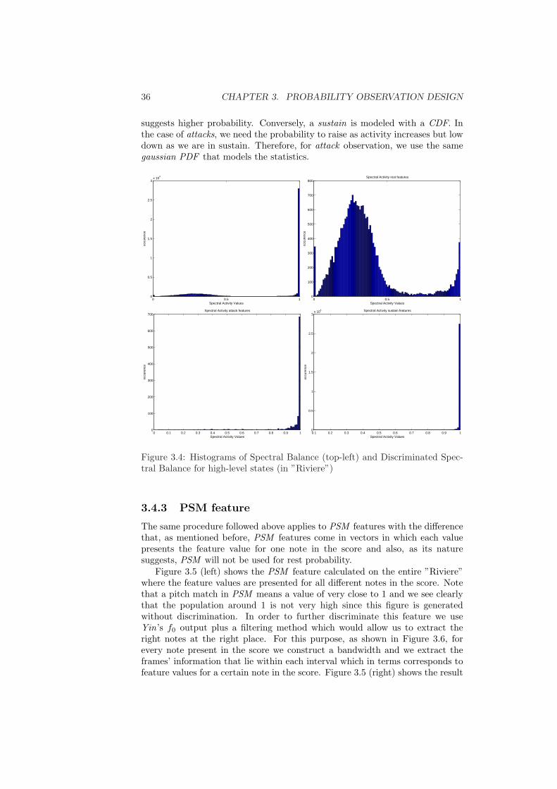
36 CHAPTER 3. PROBABILITY OBSERVATION DESIGN
suggests higher probability. Conversely, a sustain is modeled with a CDF. Inthe case of attacks, we need the probability to raise as activity increases but lowdown as we are in sustain. Therefore, for attack observation, we use the samegaussian PDF that models the statistics.
0 0.5 10
0.5
1
1.5
2
2.5
3x 10
4
Spectral Activity Values
occu
renc
e
0 0.5 10
100
200
300
400
500
600
700
800
Spectral Activity Valuesoc
cure
nce
Spectral Activity rest features
0 0.1 0.2 0.3 0.4 0.5 0.6 0.7 0.8 0.9 10
100
200
300
400
500
600
700
Spectral Activity Values
occu
renc
e
Spectral Activity attack features
0.1 0.2 0.3 0.4 0.5 0.6 0.7 0.8 0.9 10
0.5
1
1.5
2
2.5
3x 10
4
Spectral Activity Values
occu
renc
e
Spectral Activity sustain features
Figure 3.4: Histograms of Spectral Balance (top-left) and Discriminated Spec-tral Balance for high-level states (in ”Riviere”)
3.4.3 PSM feature
The same procedure followed above applies to PSM features with the differencethat, as mentioned before, PSM features come in vectors in which each valuepresents the feature value for one note in the score and also, as its naturesuggests, PSM will not be used for rest probability.
Figure 3.5 (left) shows the PSM feature calculated on the entire ”Riviere”where the feature values are presented for all different notes in the score. Notethat a pitch match in PSM means a value of very close to 1 and we see clearlythat the population around 1 is not very high since this figure is generatedwithout discrimination. In order to further discriminate this feature we useYin’s f0 output plus a filtering method which would allow us to extract theright notes at the right place. For this purpose, as shown in Figure 3.6, forevery note present in the score we construct a bandwidth and we extract theframes’ information that lie within each interval which in terms corresponds tofeature values for a certain note in the score. Figure 3.5 (right) shows the result

3.5. DESIGN SUMMARY AND REMARKS 37
of this discrimination on the same feature values.
0 0.2 0.4 0.6 0.8 10
0.5
1
1.5
2
2.5
3
PSM values
occu
renc
e
fa5si5re6dod6mi6mib6sib5sold5sol6la5fad6fa6sol5do6fad5mib5sold6re5mi5dod5la6
0 0.2 0.4 0.6 0.8 1 1.2 1.40
10
20
30
40
50
60
70
80Discriminrated trapezoidal PSM Energy
PSM values
dens
ity
fa5si5re6dod6mi6mib6sib5sold5sol6la5fad6fa6sol5do6fad5mib5sold6re5mi5dod5la6
Figure 3.5: Histogram of PSM feature non-discriminated (left) and discrimi-nated (right) for all notes in ”Riviere”
215 220 225 230 235 240 245 250 255 260 265
300
400
500
600
700
800
900
frames
f 0, Hz
fa5si5re6dod6mi6mib6sib5sold5sol6la5fad6fa6sol5do6fad5mib5sold6re5mi5dod5la6
Figure 3.6: PSM discrimination using Yin
This discriminated data will be used to model sustains and attacks usingtwo gaussians. In this respect, the probability mapping for both features wouldbe CDFs.
3.5 Design Summary and Remarks
Integrating the suggested models for probability observation and mapping, thenew probability observation block would become as demonstrated in Figures 3.7

38 CHAPTER 3. PROBABILITY OBSERVATION DESIGN
on Page 39 and 3.8 on Page 40 for different feature suggestions. Features usedin each diagram correspond to our discussions in Section 2.3. In Figure 3.7,the Spectal Balance feature has replaced both Delta features and in Figure 3.8,Moving Average ∆log feature has replaced ∆log feature.
In the new system, each probability mapping block (2nd layer) is loadedbefore performance with its appropriate trained gaussian model. We see thatafter this modeling and above discussions, training gains a physical meaningand becomes integrated into the system. Training will be discussed in details inChapter 4.
The two proposed systems are the final outcome of this project and theright choice between the two depends on Robustness results of the two systemsfor which experiments are underway to use in concerts. So far, the system withSpectral Balance feature has proven be more robust and leading to better resultsthan others.

3.5. DESIGN SUMMARY AND REMARKS 39
Log
of
Ene
rgy
Spec
tral
Act
ivity
PSM
FF
T
LogE
Sus
tain
Pro
babi
lity
LogE
Res
t Pro
babi
lity
LogE
atta
ck P
roba
bilit
ySA
Sus
tain
Pro
babi
lity
CD
F
SA R
est P
roba
bilit
y
Inve
rse
CD
F
SA a
ttack
Pro
babi
lity
PD
F
PSM
Sus
tain
Pro
babi
lity
CD
F
PSM
atta
ck P
roba
bilit
y
CD
F
Res
t Sta
te P
roba
bilit
yA
ttack
Sta
te P
roba
bilit
yS
usta
in S
tate
Pro
babi
lity
Aud
io F
ram
e D
ata
Inve
rse
CD
FC
DF
CD
F
Tra
ined
Gau
ssia
n D
atab
ase
Figure 3.7: New Feature and Probability Observation Diagram (1)

40 CHAPTER 3. PROBABILITY OBSERVATION DESIGN
Log
of E
nerg
yM
ovin
g A
vera
ge d
Log
PS
MD
elta
PS
M
FF
T
LogE
Sus
tain
Pro
babi
lity
LogE
Res
t Pro
babi
lity
LogE
atta
ck P
roba
bilit
ydL
og S
usta
in P
roba
bilit
ydL
og R
est P
roba
bilit
y
Inve
rse
CD
F
dLog
atta
ck P
roba
bilit
yP
SM
Sus
tain
Pro
babi
lity
PS
M a
ttack
Pro
babi
lity
dPS
M S
usta
in P
roba
bilit
ydP
SM
atta
ck P
roba
bilit
y
CD
F
Res
t Sta
te P
roba
bilit
yA
ttack
Sta
te P
roba
bilit
yS
usta
in S
tate
Pro
babi
lity
Abs
olut
e V
alue
Aud
io F
ram
e D
ata
CD
FC
DF
CD
FC
DF
CD
FIn
vers
e C
DF
CD
FC
DF
Tra
ined
Gau
ssia
n D
atab
ase
Figure 3.8: New Feature and Probability Observation Diagram (2)

Chapter 4
Training
The principles of form will be our only constant con-nection with the past. Although the great form of thefuture will not be as it was in the past . . . , it will berelated to these as they are to each other: through theprinciple of organization or man’s common ability tothink. — John Cage, Credo
In this chapter, we introduce a training method for IRCAM ’s score followingbased on designs in Chapter 3. Before we enter the training itself, we need todefine the notion of training and also contemplate and differentiate betweenand ideal training and training in the context of music practice, defining theobjectives of training for the score following in question.
4.1 Training and Music Tradition
As discussed before, by training we aim to adapt the observation parametersto a certain piece. Speaking about training for score following, often initiatesfear of system obsolesce and portability for musicians and composers using thesystem. For this reason, we tend to specify what we mean exactly by trainingin our case.
In an ideal training, the system runs on a huge database of aligned soundfiles and adapts its parameters to the performance. In this case, the trainingis usually supervised and is integrated in the system’s practice. However, in amusical situation dealing with traditions of music rehearsals and performances,
• Musicians prefer no additional item added to their practice situation.
• No database of aligned audio exists and moreover, working in the contextof contemporary music limits the availability of different performances andrecordings for a piece.
41

42 CHAPTER 4. TRAINING
s
a
r
Figure 4.1: HMM for ”Orio training”
• Whatever added to the system in general, should not reduce the portabilityof the piece. Musicians travel with the piece!
The above constraints would limit the ideal training to an unsupervised train-ing, having few or just one rehearsal run-throughs to be observed. In this con-text, the training will be off-line and would use the data during rehearsal totrain itself. Atleast for portability issues, training should be automatic.
Also from a developmental point of view, since score following is a work inprogress as composers’ demands increase and change, training should be ideallyindependent of features so that by introducing new features, training does notneed any change.
4.2 Previous Work
The training method discussed here is proposed by Nicola Orio and DiemoSchwarz and marks the beginning of this project. Note that this method wasproposed for the old observation block in Figure 1.4 on Page 15.
In their unsupervised training, Orio has proposed using a simple three-stateHMM, demonstrated in Figure 4.1, with the same transition probabilities andobservation block as the score following. The system would observe and decodethe HMM using Viterbi algorithm at each iteration and the new µ and σ pa-rameters for each exponential probability mapping is found by a curve fittingon the histogram of the feature observation. Figure 4.2 shows one iteration ofthis training for Log of Energy’s sustain feature where the red-line indicated thenewly fitted exponential mapping to be used in the next iteration.
Without going into the evaluation of the score following using the trainedparameters, which were not satisfactory, we can criticize this methodology fromdifferent point of views:
• This training method assumes the same heuristics criticized in Section2.1.2 and therefore fails to construct a basic correspondence between theparameters and high-level states.
• Assuming the training is appropriate, this method experience error prop-agation, that is, if there is a tiny error at one iteration by propagationthrough other iterations it becomes bigger and bigger.
• The curve fitting method is highly dependent on the precision of the his-togram constructed over features which is not fixed for different pieces andfeatures and would highly affect the parameters found.
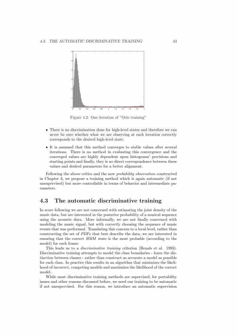
4.3. THE AUTOMATIC DISCRIMINATIVE TRAINING 43
0 0.2 0.4 0.6 0.8 1 1.2 1.4 1.6 1.8 20
1
2
3
4
5
6
Figure 4.2: One iteration of ”Orio training”
• There is no discrimination done for high-level states and therefore we cannever be sure whether what we are observing at each iteration correctlycorresponds to the desired high-level state.
• It is assumed that this method converges to stable values after severaliterations. There is no method in evaluating this convergence and theconverged values are highly dependent upon histograms’ precisions andstarting points and finally, they is no direct correspondence between thesevalues and desired parameters for a better alignment.
Following the above critics and the new probability observation constructedin Chapter 3, we propose a training method which is again automatic (if notunsupervised) but more controllable in terms of behavior and intermediate pa-rameters.
4.3 The automatic discriminative training
In score following we are not concerned with estimating the joint density of themusic data, but are interested in the posterior probability of a musical sequenceusing the acoustic data. More informally, we are not finally concerned withmodeling the music signal, but with correctly choosing the sequence of musicevents that was performed. Translating this concern to a local level, rather thanconstructing the set of PDFs that best describe the data, we are interested inensuring that the correct HMM state is the most probable (according to themodel) for each frame.
This leads us to a discriminative training criterion (Renals et al. 1993).Discriminative training attempts to model the class boundaries - learn the dis-tinction between classes - rather than construct as accurate a model as possiblefor each class. In practice this results in an algorithm that minimizes the likeli-hood of incorrect, competing models and maximizes the likelihood of the correctmodel.
While most discriminative training methods are supervised, for portabilityissues and other reasons discussed before, we need our training to be automaticif not unsupervised. For this reason, we introduce an automatic supervision

44 CHAPTER 4. TRAINING
over training by constructing a discrimination knowledge by an alternative al-gorithm which forces each model to its boundaries and discriminates featureobservations. Yin (de Cheveigne and Kawahara 2002) has been chosen as thisalgorithm to provide discrimination knowledge after several considerations.
Figure 4.3 shows a diagram of different steps of this training. The inputs ofthis training are an audio file plus its score. There are two main cores to thissystem: Discrimination and Training.
Score Audio File
Load Score
score parsing
Discrimination Knowledge
YinFeature Calculation
Discriminate Features
High-level state features
Train Gaussians
EM Algorithm
Construct Structures
StoreStructures
Figure 4.3: Automatic Discriminative Training Diagram
4.3.1 Discrimination
During discrimination, using the discrimination knowledge (provided by Yin),the score information (list of all notes in the score) and audio features, high-levelstate features will be discriminated from each other. For example, the SpectralBalance feature will be discriminated to Spectral Balance - Attacks, SpectralBalance - Sustains and Spectral Balance - Rests. In this manner, we would beready to model the class boundaries and learn the distinction between classes.
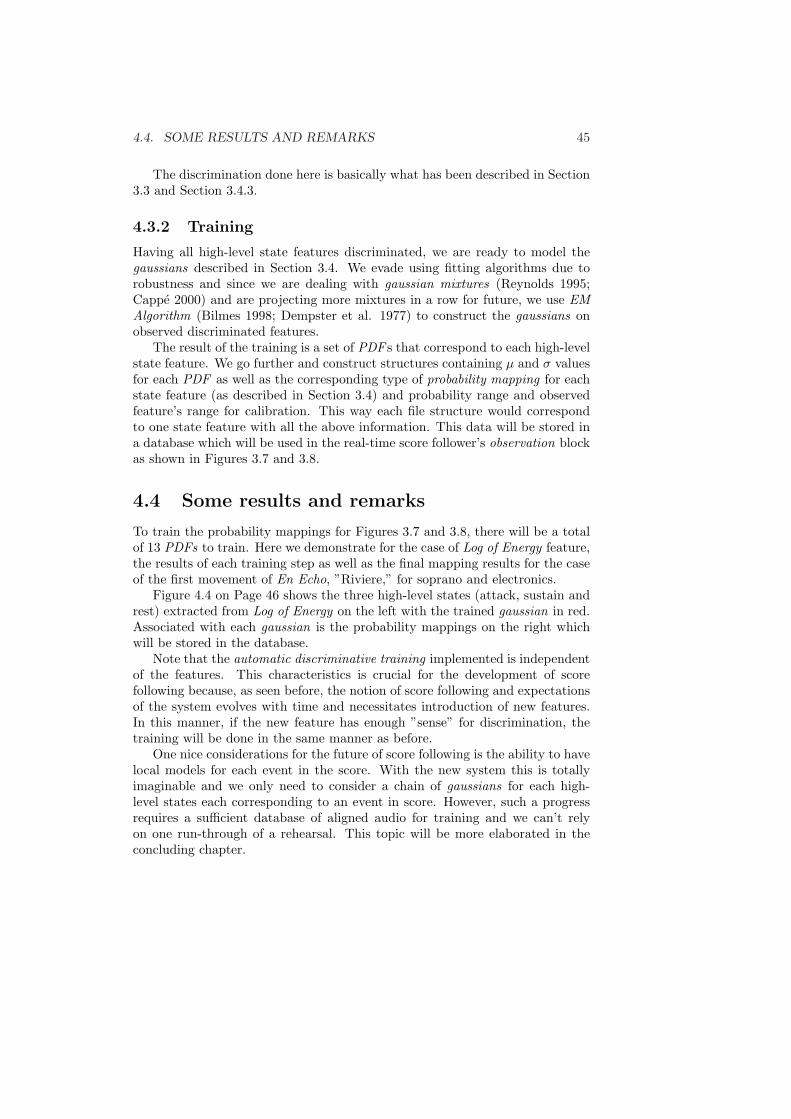
4.4. SOME RESULTS AND REMARKS 45
The discrimination done here is basically what has been described in Section3.3 and Section 3.4.3.
4.3.2 Training
Having all high-level state features discriminated, we are ready to model thegaussians described in Section 3.4. We evade using fitting algorithms due torobustness and since we are dealing with gaussian mixtures (Reynolds 1995;Cappe 2000) and are projecting more mixtures in a row for future, we use EMAlgorithm (Bilmes 1998; Dempster et al. 1977) to construct the gaussians onobserved discriminated features.
The result of the training is a set of PDF s that correspond to each high-levelstate feature. We go further and construct structures containing µ and σ valuesfor each PDF as well as the corresponding type of probability mapping for eachstate feature (as described in Section 3.4) and probability range and observedfeature’s range for calibration. This way each file structure would correspondto one state feature with all the above information. This data will be stored ina database which will be used in the real-time score follower’s observation blockas shown in Figures 3.7 and 3.8.
4.4 Some results and remarks
To train the probability mappings for Figures 3.7 and 3.8, there will be a totalof 13 PDFs to train. Here we demonstrate for the case of Log of Energy feature,the results of each training step as well as the final mapping results for the caseof the first movement of En Echo, ”Riviere,” for soprano and electronics.
Figure 4.4 on Page 46 shows the three high-level states (attack, sustain andrest) extracted from Log of Energy on the left with the trained gaussian in red.Associated with each gaussian is the probability mappings on the right whichwill be stored in the database.
Note that the automatic discriminative training implemented is independentof the features. This characteristics is crucial for the development of scorefollowing because, as seen before, the notion of score following and expectationsof the system evolves with time and necessitates introduction of new features.In this manner, if the new feature has enough ”sense” for discrimination, thetraining will be done in the same manner as before.
One nice considerations for the future of score following is the ability to havelocal models for each event in the score. With the new system this is totallyimaginable and we only need to consider a chain of gaussians for each high-level states each corresponding to an event in score. However, such a progressrequires a sufficient database of aligned audio for training and we can’t relyon one run-through of a rehearsal. This topic will be more elaborated in theconcluding chapter.

46 CHAPTER 4. TRAINING
−2 −1 0 1 2 3 4 50
1
2
3
4
5
6Gaussian modeling for LogE Rest
feature value
PD
F
ksdensityGMM
−2 −1 0 1 2 3 4 50
0.1
0.2
0.3
0.4
0.5
0.6
0.7
0.8
0.9
1LogE Rest inverse CDF
feature value
prob
abili
ty
−2 0 2 4 6 8 10 12 140
0.1
0.2
0.3
0.4
0.5
0.6
0.7Gaussian modeling for LogE Sustain
feature value
PD
F
ksdensityGMM
−2 0 2 4 6 8 10 12 140
0.1
0.2
0.3
0.4
0.5
0.6
0.7
0.8
0.9
1LogE Sustain CDF
feature value
prob
abili
ty
−3 −2 −1 0 1 2 3 4 5 60
0.05
0.1
0.15
0.2
0.25
0.3
0.35
0.4Gaussian modeling for LogE Attack
feature value
PD
F
ksdensityGMM
−3 −2 −1 0 1 2 3 4 50
0.1
0.2
0.3
0.4
0.5
0.6
0.7
0.8
0.9
1LogE Attack CDF
feature value
prob
abili
ty
Figure 4.4: Results of training for LogE feature in ”Rivier”

Chapter 5
System Evaluation
In this chapter we aim to provide a subjective evaluation of systems in Figure1.4 (old system), 3.7 (new probability observation with moving average ∆logfeature) and 3.8 (new probability observation with Spectral Balance feature),with the two latter using the outcome of a training session. The evaluationsshown here are simulations of the score follower on Matlab ran on audio files.However, we tested the system in several test sessions in studios with PhilippeManoury, Serge Lemouton along with soprano Valerie Philippin on En Echowhich we will describe.
For the simulation, we limit our observations on segmentation output of thescore follower, being the main objective of the score following. We demonstratescore following results on short fragments of music which were problematic inthe old system and comment on the output. The examples demonstrated hereare excerpts from Manoury’s first movement of En Echo, ”Riviere,” for sopranoand electronics.
Figure 5.1 demonstrates real-time alignment results for measure 39 and mea-sures 29 − 32 for the three systems mentioned. Observing from the previoussystem to the system using spectral balance as feature (system (2) in figure),we can contemplate on the following remarks:
• The stability of the system has increased, in the sense that we do notobserve jumps to other states during sustains.
• At some instants, specially fast transitions, alignment is improved.
• Even if a high-level state is not recognized, due to the new system design,the system’s behavior can be explained and remarks can be gathered forfurther development of the system (example: first repeated note in mea-sure 39 in system (2) which is not recognized and is because of higherprecision needed in the Spectral Balance feature and finer training.
The real-time tests in the studio, led to similar improvements specially forthe mentioned measures and similar instants in the score where we were notable to detect before. Although the score follower turned out to be almost per-fect on audio recordings of a performance, its performance in real-time was notperfect to that extent. But due to our design approach, every shortcoming of
47

48 CHAPTER 5. SYSTEM EVALUATION
the system encountered a direct physical interpretation which could be over-come by adjusting the parameters during performance; thus, leading to moreconsiderations for future research.
As a conclusion for evaluation, we would like to refer the reader to the generalcontemplations made on the topic of Evaluations of score following in Section1.2.5. An important need for the evaluation of new features and elements aswell as final system’s output evaluation is a database of aligned music files. Thistopic will be addressed in Chapter 6.

49
0.5 1 1.5 2 2.5 3 3.5 4
x 105
−1
−0.8
−0.6
−0.4
−0.2
0
0.2
0.4
0.6
0.8
1
frame number
1 0 1 2 1 2 3 2 3 4 5 6 7 6 7 6 7 8 9 10 1110111011 12
ampl
itude
Measure 39 − Previous system
0.2 0.4 0.6 0.8 1 1.2 1.4 1.6 1.8 2 2.2
x 105
−1
−0.8
−0.6
−0.4
−0.2
0
0.2
0.4
0.6
0.8
1
frame number
1 0 1 2 3 4 3 4 5 4 5 4 5 6
ampl
itude
Measures 29−32 − Previous system
0.5 1 1.5 2 2.5 3 3.5 4
x 105
−1
−0.8
−0.6
−0.4
−0.2
0
0.2
0.4
0.6
0.8
1
frame number
1 0 1 3 4 5 6 7 6 7 8 7 8 7 9 10 11 12
ampl
itude
Measure 39 − system (1)
0.2 0.4 0.6 0.8 1 1.2 1.4 1.6 1.8 2 2.2
x 105
−1
−0.8
−0.6
−0.4
−0.2
0
0.2
0.4
0.6
0.8
1
frame number
1 2 3 4 5 4 5 6
ampl
itude
Measures 29−32 − System (1)
0.5 1 1.5 2 2.5 3 3.5 4
x 105
−1
−0.8
−0.6
−0.4
−0.2
0
0.2
0.4
0.6
0.8
1
frame number
1 2 3 4 5 6 7 8 7 8 9 10 11 12
ampl
itude
Measure 39 − system (2)
0.2 0.4 0.6 0.8 1 1.2 1.4 1.6 1.8 2 2.2
x 105
−1
−0.8
−0.6
−0.4
−0.2
0
0.2
0.4
0.6
0.8
1
frame number
1 2 3 4 5 4 6
ampl
itude
Measures 29−32 − System (2)
Figure 5.1: Evaluation of the three systems on measure 39 (left) and measures29-32 (right) of ”Riviere.” System (1) refers to the observation probability withmoving average ∆ features; System (2) refers to the observation probability withspectral activity feature and no ∆ features.

50 CHAPTER 5. SYSTEM EVALUATION

Chapter 6
Future Works andConclusion
One day down at Black Mountain, David Tudor waseating his lunch. A student came over to his table andbegan asking him questions. David Tudor went oneating his lunch. The student kept asking questions.Finally David Tudor looked at him and said, ”If youdon’t know, why do you ask?”— John Cage, Indeterminacy
6.1 Future Works and Remarks
In this section we summarize our contemplations on future works and consid-erations of score following research. In this manner, we go through each aspectseparately since each define separate issues but at the same time correlatedtowards further progress of score following in general.
6.1.1 The urge of an aligned database of music
Without hesitation, we emphasize on the importance of the availability of adatabase of aligned music files for further progress of score following research.Since we are dealing with a research oriented towards a empirical-syntheticalapproach, it is important to evaluate the changes made in the system on a largedatabase of aligned music to compare the output and see whether it would begood enough to be used for score following in practice. While small changesand improvements are possible without such database, it limits the researchprogress since for many proposed works we would need evaluations to ensurethe robustness of the system as well as training.
51

52 CHAPTER 6. FUTURE WORKS AND CONCLUSION
We note at this point that the speech recognition literature was standing atthe same point in early 80s and important improvements in their systems tookplace by having huge databases of speech available for training and evaluationof competing systems.
6.1.2 Towards localized probability modeling
One comment on further development of our system is to move from fixed, ”outof time” observations to localized observations. At this moment, the systemassumes fixed probability mappings for all high-level states in a score (for exam-ple, one probability mapping for all attacks). This assumption again is based onheuristics which has never been evaluated since we need the mentioned database.Another approach, which seems reasonable after our experience, is to assumelocalized probability mappings for each high-level states in the system. Withthe current system, this means using a mixture of gaussians for each high-levelstate and is completely implementable within our new framework. However,this approach requires the mentioned database for training and evaluations andconsiderations of such approach for practical purposes.
6.1.3 Feature tests
Furthermore, the modified features along with the new suggested feature shouldbe tested for robustness. For this reason, the features need to be run on a largedatabase of sound files and their behavior should be studied which was out ofthe context of this project.
6.1.4 Temporal Considerations in HMM
We believe that with a strong observation, we would always pass to the rightstate. However, a classical problem with the HMM approach lies in its temporalmodeling. While this topic was not an objective of this project, we contemplatedon it since it would lead to improvements of the general systems. There has beenmany approaches in the literature towards solving this classical problem suchas using parallel HMMs and coupling the system with other approaches. As ageneral remark, it seems that in the context of score following where we try tomodel a musical (or virtual) time, the idea of using clock time (i.e. frame byframe analysis and decoding to HMM ) is not a good idea. One famous approachwhich is widely used in music information retrieval is to drop the clock time anduse the onset information as the time triggers of the temporal analysis (Takedaet al. 2003; Takeda et al. 2002).
6.1.5 Refining the Music model
Furthermore, in the HMM Music Model we need to consider adding a releasemodel. At the moment, the release model used is just a rest model added at theend of a note model. With the designed observation block and training method,it is totally possible to extract release features from low-level features and trainthem for detection. This will help for faster and easier recognition of attacks,more cues for special cases such as repeated notes where most features are not

6.2. CONCLUSION 53
changing and also better transition modeling for the cases of legato and staccatonotes.
6.1.6 Calibration for real-time score following
In order to have satisfying results as shown in evaluation during a live perfor-mance, we need to make sure that the feature values produced lie in the samerange as the training samples. In the training literature, this goal is achieved byan automatic (if not unsupervised) on-line learning. However, due to practicalpurposes in a musical situation, this is not possible. One practical solution tothis, after our contemplations is to calibrate the solo input of the system beforeeach live performance which is a simple audio engineering task.
For this purpose, we have included range of each feature in the saved struc-ture after training. The audio engineer can ask the soloist to perform a singlefortissimo note while looking at one or several feature values and by controllingthe tabs on the mixer desk, he can calibrate the values to an approximate valuenear the maximum of the feature range.
This way, we would make sure that during live performance, feature valueswill occur in the same range used during training which in terms assures desiredalignment of real-time score follower.
6.2 Conclusion
The early objective of this project was to implement a training algorithm for theexisting score follower at IRCAM. Such task requires profound understandingof system’s behavior from a control aspect. The project started by studying IR-CAM ’s score following and other systems available in the literature. Throughoutthis process and after several unsuccessful attempts, the author realized that theincapabilities of the score follower in question lies in the concepts used for thecomponent designs and especially in the observation block.
From this moment on, studies and experiments were undertaken to redesignthe observation process of the score follower which resulted in the system in-troduced in Chapter 3. The proposed system adds more flexibility in terms ofdevelopment and physical observation of musical phenomena in score following.In this design, the author emphasizes on critical thinking developed on the basisof use of heuristics in the previous systems from a control aspect.
One major outcome of this new design is an implicit notion of parametercontrol which eases the process of training introduced in Chapter 4. In thisrespect, a new approach to training called automatic discriminative training isintroduced which emphasizes on the alignment goal of score following, being themain objective of the system, rather than adapting a perfect model. Moreover,the proposed method is independent of features which makes it usable andflexible for future developments of score following.
While having adapted parameters out of training and through evaluations ofthe system on several music samples, the author realized that the second stagetowards more precision and perfection in score following is refinement of thefeatures used during observations. In this manner, every feature was analyzedand some refinements as well as new features were introduced as described inChapter 2. The newly introduced Spectral Balance feature, being much more

54 CHAPTER 6. FUTURE WORKS AND CONCLUSION
correlated to high-level states, is currently in use in the score following and hasreplaced two features in the previous system and has proved to be practical forreal-time performance of the system.
Some evaluations of the outputs of the proposed systems were presented inChapter 5 which shows more stability, precision and specially more control overphysical behavior of the new system. Real-time tests of the system have provenimproved results and more control over the behavior of the system, as well asintroducing a way to go for further refinements of score follower.
Moreover, during this work and facing new designs and challenges in thefield the author has gathered several contemplations regarding the future de-velopments of score following in general which was presented in the previoussection.
The field of score following, having almost 20 years of age, has recently gainedmuch attention and feedback from other domains specially the music informationretrieval literature. Saying this and considering recent advancements in fastcomputations, we can argue that the rapid growth of this field in applicationsand development is not quite astonishing and we anticipate more interestingadvancements in its technologies and practical aspects in near future.

Bibliography
Baird, B., D. Blevins, and N. Zahler (1990). The Artificially Intelligent Com-puter Performer: The Second Generation. In Interface – Journal of NewMusic Research, Number 19, pp. 197–204.
Baird, B., D. Blevins, and N. Zahler (1993). Artificial Intelligence and Mu-sic: Implementing an Interactive Computer Performer. Computer MusicJournal 17 (2), 73–79.
Bilmes, J.A. (1998). A Gentle Tutorial of the EM Algorithm and its Applica-tion to Parameter Estimation for Gaussian Mixture and Hidden MarkovModels. ICSI.
Bloch, J. and Roger B. Dannenberg (1985). Real-Time Accompaniment ofPolyphonic Keyboard Performance. In Proceedings of the ICMC, pp. 279–290.
Brown, J.C. and Miller Puckette (1992). An efficient algorithm for the Cal-culation of a Constant Q Transform. In Acoust. Soc. Am., pp. 2698–2701.
Brown, J.C. and Miller Puckette (1993). A high resolution fundamental fre-quency determination based on phase changes of the Fourier transform.In Acoust. Soc. Am., pp. 662–667.
Cappe, Olivier (2000, June). Modeles de melange et modeles de markovcaches pour le traitement automatique de la parole. Web page.http://www.tsi.enst.fr/ cappe/cours/tap.pdf.
Castel, Yohan (1999). Human behaviors and psychobiology. Web page.http://www.psychobiology.org/.
Dannenberg, Roger (1988). Method and apparatus for providing coordinatedaccompaniment for a performance. US Patent No.4745836.
Dannenberg, Roger (2004, June). Private conversation with the author.Hamamatsu, Japan.
Dannenberg, Roger B. (1984). An On-Line Algorithm for Real-Time Accom-paniment. In Proceedings of the ICMC, pp. 193–198.
Dannenberg, Roger B. and B. Mont-Reynaud (1987). Following an Improvi-sation in Real Time. In Proceedings of the ICMC, pp. 241–248.
Dannenberg, Roger B. and Mukaino (1988). New Techniques for EnhancedQuality of Computer Accompaniment. In Proceedings of the ICMC, pp.243–249.
de Cheveigne, Alain and H. Kawahara (2002). YIN, a fundamental frequencyestimator for speech and music. J. Acoust. Soc. Am. 111, 1917–1930.
55

56 BIBLIOGRAPHY
Dempster, A.P., N. M. Laird, and D. B. Rubin (1977). maximum likelihoodfrom incomplete data via the EM algorithm. Journal of Royal StatisticalSociety 39 (B), 1–38.
Grossberg, Stephen (1982). Studies of Mind and Brain, Chapter Learning byNeural Networks, pp. 65–156. D. Reidel Publishing, Boston, MA.
Grubb, Lorin and Roger Dannenberg (1997a). System and method forstochastic score following. US Patent No.5913259.
Grubb, Lorin and Roger B. Dannenberg (1997b). A Stochastic Method ofTracking a Vocal Performer. In Proceedings of the ICMC, pp. 301–308.
Loscos, A., P. Cano, and J. Bonada (1999a). Low-Delay Singing Voice Align-ment to Text. In Proceedings of the ICMC.
Loscos, A., P. Cano, and J. Bonada (1999b). Score-Performance Matchingusing HMMs. In Proceedings of the ICMC, pp. 441–444.
Mouillet, Vincent (2001). Prise en compte des informations temporelles dansles modeles de markov caches. Rapport de stage, IRCAM.
Orio, Nicola and F. Dechelle (2001). Score Following Using Spectral Analysisand Hidden Markov Models. In Proceedings of the ICMC, Havana, Cuba.
Orio, Nicola, Serge Lemouton, Diemo Schwarz, and Norbert Schnell (2003,May). Score Following: State of the Art and New Developments. In Pro-ceedings of the International Conference on New Interfaces for MusicalExpression (NIME), Montreal, Canada.
Orio, Nicola and Diemo Schwarz (2001). Alignment of Monophonic and Poly-pophonic Music to a Score. In Proceedings of the ICMC, Havana, Cuba.
Pardo, Bryan and William Birmingham (2001). Following a musical perfor-mance from a partially specified score. In IEEE Multimedia TechnologyApplications Conference, Irvine, CA.
Pardo, Bryan and William Birmingham (2002). Improved Score Following forAcoustic Performances.
Pollard, David (2001). Paris lectures on le cam theory. Web page.http://www.stat.yale.edu/ pollard/Paris2001/lectures.html.
Puckette, Miller (1990). EXPLODE: A User Interface for Sequencing andScore Following. In Proceedings of the ICMC, pp. 259–261.
Puckette, Miller (1995). Score Following Using the Sung Voice. In Proceedingsof the ICMC, pp. 199–200.
Puckette, Miller and Cort Lippe (1992). Score Following in Practice. In Pro-ceedings of the ICMC, pp. 182–185.
Rabiner, L.R. (1989). A tutorial on hidden markov models and selected ap-plications in speech recognition. Proceedings of the IEEE 77 (2), 257–285.
Raphael, Christopher (1999a). A Probabilistic Expert System for AutomaticMusical Accompaniment. Jour. of Comp. and Graph. Stats 10 (3), 487–512.
Raphael, Christopher (1999b). Automatic Segmentation of Acoustic Musi-cal Signals Using Hidden Markov Models. IEEE Transactions on PatternAnalysis and Machine Intelligence 21 (4), 360–370.

BIBLIOGRAPHY 57
Raphael, Christopher (2001). A Bayesian network for Real-time Musical Ac-companiment. Neural Information Processing Systems (NIPS) 14.
Renals, S., N. Morgan, H. Bourlard, M. Cohen, and H. Franco (1993). Connec-tionist probability estimators in HMM speech recognition. IEEE Trans-actions Speech and Audio Processing .
Reynolds, Douglas A. (1995, August). Speaker identification and verificationusing gaussian mixture speaker models. In Speech Communication, Vol-ume 17, pp. 91–108.
Schreck Ensemble and Pieter Suurmond (2001). ComParser. Web page.http://www.hku.nl/ pieter/SOFT/CMP/.
Takeda, Haruto, Takuya Nishimoto, and Shigeki Sagayama (2003, October).Automatic Rhythm Transcription from Multiphonic MIDI Signals. In 4thInternational Conference on Music Information Retrieval.
Takeda, Haruto, Nakai Saito, Tomoshi Otsuki, Mituru Nakai, Hiroshi Shi-modaira, and Shigeki Sagayama (2002, December). Hidden Markov Modelfor Automatic Transcription of MIDI Signals. In IEEE Workhop on Mul-timedia Signal Processing.
Vantomme, Jason D. (1990). Score Following by Temporal Patterns. Com-puter Music Journal 19 (3), 50–59.
Vercoe, Barry (1984). The Synthetic Performer in the Context of Live Per-formance. In Proceedings of the ICMC, pp. 199–200.
Vercoe, Barry and Miller Puckette (1985). Synthetic Rehearsal: Training theSynthetic Performer. In Proceedings of the ICMC, pp. 275–278.