Embed Size (px)
Citation preview

IMPROVED STEAMFLOOD ANALYTICAL MODEL
A Thesis
by
SUANDY CHANDRA
Submitted to the Office of Graduate Studies of Texas A&M University
in partial fulfillment of the requirements for the degree of
MASTER OF SCIENCE
August 2005
Major Subject: Petroleum Engineering

IMPROVED STEAMFLOOD ANALYTICAL MODEL
A Thesis
by
SUANDY CHANDRA
Submitted to the Office of Graduate Studies of
Texas A&M University in partial fulfillment of the requirements for the degree of
MASTER OF SCIENCE
Approved by : Co-Chairs of Committee, Daulat D. Mamora Robert A. Wattenbarger Committee Member, Luc T. Ikelle Head of Department, Stephen A. Holditch
August 2005
Major Subject: Petroleum Engineering

iii
ABSTRACT
Improved Steamflood Analytical Model.
(August 2005)
Suandy Chandra, B.S., Institut Teknologi Bandung
Co-Chairs of Advisory Committee: Dr. Daulat D. Mamora Dr. Robert A. Wattenbarger
The Jeff Jones steamflood model incorporates oil displacement by steam as described by
Myhill and Stegemeier, and a three-component capture factor based on empirical
correlations. The main drawback of the model however is the unsatisfactory prediction
of the oil production peak: usually significantly lower than the actual. Our study focuses
on improving this aspect of the Jeff Jones model.
In our study, we simulated the production performance of a 5-spot steamflood
pattern unit and compared the results against those based on the Jeff Jones model. Three
reservoir types were simulated using 3-D Cartesian black oil models: Hamaca (9°API),
San Ardo (12°API) and that based on the SPE fourth comparative solution project
(14°API). In the first two field cases, a 45x23x8 model was used that represented 1/8 of
a 10-acre 5-spot pattern unit, using typical rock and reservoir fluid properties. In the SPE
project case, three models were used: 23x12x12 (2.5 ac), 31x16x12 (5 ac) and 45x23x8
(10 ac), that represented 1/8 of a 5-spot pattern unit.
To obtain a satisfactory match between simulation and Jeff Jones analytical model
results of the start and height of the production peak, the following refinements to the Jeff
Jones model were necessary. First, the dimensionless steam zone size AcD was modified
to account for decrease in oil viscosity during steamflood and its dependence on the

iv
steam injection rate. Second, the dimensionless volume of displaced oil produced VoD
was modified from its square-root format to an exponential form.
The modified model gave very satisfactory results for production performance up
to 20 years of simulated steamflood, compared to the original Jeff Jones model.
Engineers will find the modified model an improved and useful tool for prediction of
steamflood production performance.

v
DEDICATION This thesis is dedicated to my family in Indonesia, especially to my mother, Sia Soei Hwa, for her endless love.

vi
ACKNOWLEDGEMENTS
I am deeply grateful to my advisor, Dr. Daulat D. Mamora, who has provided
encouragement and constructive comments and suggestions since the beginning of this
research. I am much honored to be his student.
I would like to convey my sincere thanks to the distinguished professors, Dr
Robert A. Wattenbarger for serving as co-chair of my committee and Dr. Luc. T. Ikelle,
for serving as valuable committee member.
I would like to acknowledge BP MIGAS and Chevron Texaco Exploration and
Production Technology Company for funding my study.
Special thanks go to all the faculty members and staff in the Petroleum Engineering
Department at Texas A&M University for their support and help.

vii
TABLE OF CONTENTS
Page
ABSTRACT………………………………………………………………………… iii
DEDICATION……………………………………………………………………… v
ACKNOWLEDGEMENTS…………………………………………………..…….. vi
TABLE OF CONTENTS……………………………………………………...…..... vii
LIST OF FIGURES……………………………………………………………..….. ix
LIST OF TABLES………………………………………………………………..… xii
CHAPTER
I INTRODUCTION…………………………………………………………..... 1
1.1 Objective of the Study……………………………………….. 2 1.2 Methodology………………………………………………….. 3 1.3 Chapter Organization……………………………….………… 3
II THEORETICAL BACKGROUND……………...…………………………... 5
2.1 Steamflooding Mechanism …………………………………... 5 2.2 Prediction of Steamflood Performance…...…………………... 8 2.3 Literature Review……………………………………………... 11 2.4 Jeff Jones’ Method……………………………………………. 13
III NUMERICAL SIMULATION ………………………….…………………... 17
3.1 Symmetrical Element ………………………………………… 18 3.2 Grid Orientation Effect ………………………………………. 19 3.3 Block Geometry Modifier…………………………………..... 22 3.4 SPE Comparative Case Simulation Model………………….... 24 3.5 San Ardo Simulation Model………………………………….. 30 3.6 Hamaca Simulation Model…………………………………..... 33
IV NEW STEAMFLOOD MODEL………………………..……………….…... 37
4.1 New Model Calculation Steps….…………….……………..... 42 4.1.1 Displacement Calculation…………………………….. 43 4.1.2 Production Calculations……..………………………... 45 4.2 Oil Production Rate Performance..…………………………... 45

viii
CHAPTER Page
4.3 Cumulative Oil Steam Ratio…………………………….…..... 54
V SUMMARY AND CONCLUSIONS………………………………………... 61
5.1 Summary……………………………………………………… 61 5.2 Conclusions…………………………………………………… 62
NOMENCLATURE…………………..…………………………………………….. 63
REFERENCES……..……………………………………………………………….. 67
APPENDIX A JEFF JONES OIL DISPLACEMENT CALCULATION……........ 70
APPENDIX B SIMULATION INPUT FOR FOURTH SPE COMPARATIVE CASE, AREA = 2.5 ACRE, STEAM INJECTION RATE = 400 STB/D……………………..…………………………………….... 72
APPENDIX C SIMULATION INPUT DATA FOR SAN ARDO CASE, AREA = 10 ACRE, STEAM INJECTION RATE = 1600 STB/D...……... 81
APPENDIX D SIMULATION INPUT DATA FOR HAMACA CASE, AREA = 10 ACRE, STEAM INJECTION RATE = 1600 STB/D……….... 90
APPENDIX E VBA PROGRAM OF NEW MODEL…………………………….. 99
VITA………………………………………………………………………………... 106

ix
LIST OF FIGURES
Page
Fig. 2.1 Steamflood typical temperature and saturation profile…………………. 6
Fig. 2.2 Temperature profile of Marx-Langenheim model..…………………….. 11
Fig. 2.3 Three production stages of Jeff Jones’ model………...………………… 14
Fig. 3.1 1/8 element of inverted 5-spot pattern model: (a) plan view; (b) 3D view……………………………………………………………………... 19
Fig. 3.2 Five spot pattern grids: (a) diagonal grid; (b) parallel grid……………... 20
Fig. 3.3 Five and nine-point, finite-difference formulation……………………... 21
Fig. 3.4 Five-point vs nine-point formulation on oil production rate in 1/8 five-spot…………………………………………………………………........ 22
Fig. 3.5 Active and inactive cells in a 1/8 five-spot pattern model……………… 23
Fig. 3.6 Simulation grid for area of 2.5 ac, SPE comparative case model………. 25
Fig. 3.7 Simulation grid for area of 5.0 ac, SPE comparative case model………. 26
Fig. 3.8 Simulation grid for area of 10 ac, SPE comparative case model……….. 26
Fig. 3.9 Relative permeability curve (water/oil system) for SPE comparative case……………………………………………………………………… 29
Fig. 3.10 Relative permeability curve (gas/oil system) for SPE comparative case. 29
Fig. 3.11 Water-oil relative permeability curves with temperature dependence, San Ardo Model………………………………………………………....
32
Fig. 3.12 Gas-oil relative permeability curves with temperature dependence, San Ardo model……………………………………………………………... 33
Fig. 3.13 Water-oil relative permeability, Hamaca model………………………... 36
Fig. 3.14 Gas-oil relative permeability, Hamaca model………………………….. 36
Fig. 4.1 New model: three different stages of oil production under steam drive…………………………………………………………….……….
37

x
Page
Fig. 4.2 α vs injection rate relationship…………………………………………. 39
Fig. 4.3 β vs Nc relationship……………………………………………………... 42
Fig. 4.4 Oil production rate (SPE comparative model, area = 2.5 ac, injection rate = 400 B/D)…………………………………………………………. 47
Fig. 4.5 Oil production rate (SPE comparative model, area = 2.5 ac, injection rate = 600 B/D)…………………………………………………………. 48
Fig. 4.6 Oil production rate (SPE comparative model, area = 2.5 ac, injection rate = 800 B/D)…………………………………………………………. 48
Fig. 4.7 Oil production rate (SPE comparative model, area = 5.0 ac, injection rate = 600 B/D)…………………………………………………………. 49
Fig. 4.8 Oil production rate (SPE comparative model, area = 5.0 ac, injection rate = 800 B/D)…………………………………………………………. 49
Fig. 4.9 Oil production rate (SPE comparative model, area = 5.0 ac, injection rate = 1000 B/D)………………………………………………………. 50
Fig. 4.10 Oil production rate (SPE comparative model, area = 5.0 ac, injection rate = 1200 B/D)…………………..……………………………………. 50
Fig. 4.11 Oil production rate (SPE comparative model, area = 10 ac, injection rate = 1000 B/D)…………………..……………………………………. 51
Fig. 4.12 Oil production rate (SPE comparative model, area = 10 ac, injection rate = 1200 B/D)…………………..……………………………………. 51
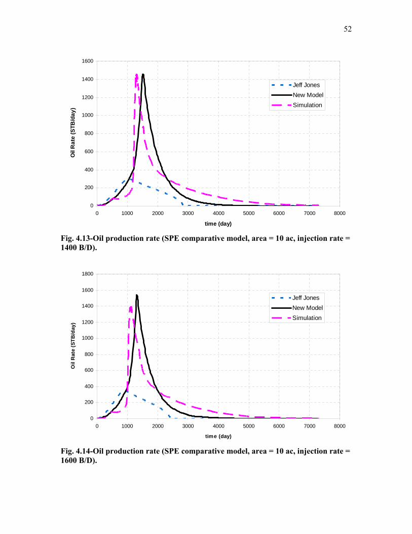
Fig. 4.13 Oil production rate (SPE comparative model, area = 10 ac, injection rate = 1400 B/D)…………………..……………………………………. 52
Fig. 4.14 Oil production rate (SPE comparative model, area = 10 ac, injection rate = 1600 B/D)…………………..……………………………………. 52
Fig. 4.15 Oil production rate (San Ardo model, area = 10 ac, injection rate = 1600 B/D)…………………..………………………...…………………. 53
Fig. 4.16 Oil production rate (Hamaca model, area = 10 ac, injection rate = 1600 B/D)…………………..…………………………………………………. 53
Fig. 4.17 Cumulative oil steam ratio (SPE comparative model, area = 2.5 ac, injection rate = 400 B/D)……………..……………...…………………. 54

xi
Page
Fig. 4.18 Cumulative oil steam ratio (SPE comparative model, area = 2.5 ac, injection rate = 600 B/D)……………..……………...…………………. 55
Fig. 4.19 Cumulative oil steam ratio (SPE comparative model, area = 2.5 ac, injection rate = 800 B/D)……………..……………...…………………. 55
Fig. 4.20 Cumulative oil steam ratio (SPE comparative model, area = 5.0 ac, injection rate = 600 B/D)……………..……………...…………………. 56
Fig. 4.21 Cumulative oil steam ratio (SPE comparative model, area = 5.0 ac, injection rate = 800 B/D)……………..……………...…………………. 56
Fig. 4.22 Cumulative oil steam ratio (SPE comparative model, area = 5.0 ac, injection rate = 1000 B/D)…………………………...…………………. 57
Fig. 4.23 Cumulative oil steam ratio (SPE comparative model, area = 5.0 ac, injection rate = 1200 B/D)…………………………...…………………. 57
Fig. 4.24 Cumulative oil steam ratio (SPE comparative model, area = 10 ac, injection rate = 1000 B/D)…………………………...…………………. 58
Fig. 4.25 Cumulative oil steam ratio (SPE comparative model, area = 10 ac, injection rate = 1200 B/D)…………………………...…………………. 58
Fig. 4.26 Cumulative oil steam ratio (SPE comparative model, area = 10 ac, injection rate = 1400 B/D)…………………………...…………………. 59
Fig. 4.27 Cumulative oil steam ratio (SPE comparative model, area = 10 ac, injection rate = 1600 B/D)…………………………...…………………. 59
Fig. 4.28 Cumulative oil steam ratio (San Ardo model, area = 10 ac, injection rate = 1600 B/D)…………………………...…………………………… 60
Fig. 4.29 Cumulative oil steam ratio (Hamaca model, area = 10 ac, injection rate = 1600 B/D)…………………………...……………………………..…. 60

xii
LIST OF TABLES
Page
Table 2.1 Typical Data Required by Thermal Reservoir Simulators………… 9
Table 3.1 Modification Parameters for Edges and Corner-Grids………….… 24
Table 3.2 Initial Reservoir Properties………………………………………... 25
Table 3.3 Cell Dimensions for SPE Comparative Case Model……………… 27
Table 3.4 Temperature-Viscosity Relationship for SPE Comparative Case…. 27
Table 3.5 Initial Reservoir Properties for San Ardo Model………………….. 30
Table 3.6 Oil Component Properties for San Ardo Model………………....... 31
Table 3.7 Temperature-Viscosity Relationship for San Ardo Oil…..……....... 32
Table 3.8 Initial Reservoir Properties for Hamaca Model…………………… 34
Table 3.9 Temperature-Viscosity Relationship for Hamaca Oil…..…………. 35
Table 4.1 Formula for Capture Factor Components: New Model and Jones Model………………...………………………………...………….. 46

1
CHAPTER I
INTRODUCTION
Steamflooding is a major EOR process applied to heavy oil reservoirs.
Steamflooding uses separate injection and production wells to improve both the rate of
production and the amount of oil that will ultimately be produced. Injected steam heats
the formation around the wellbore and eventually forms a steam zone that grows with
continuous steam injection. Steam reduces the oil viscosity and saturation in the steam
zone to a low value, pushing the mobile oil (i.e. difference between the initial and
residual oil saturations) out of the steam zone. As the steam zone grows, more oil is
moved from the steam zone to the unheated zone ahead of the steam front. Then the oil
accumulates to form an oil bank. The condensed hot water also moves across the steam
front, heating and displacing the accumulated oil. The heated oil with reduced viscosity
moves towards the producing well and is produced usually by artificial lifting.
A steam flood project typically proceeds through four phases of development: (1)
reservoir screening; (2) pilot tests; (3) fieldwide implementation; and (4) reservoir
management. Performance prediction is essential to provide information for proper
execution of each of these development phases. Three different mathematical models
(statistical, numerical, and analytical models) are commonly used to predict steam flood
performance.
This thesis follows the style of Society of Petroleum Engineers Journal.

2
Statistical models are commonly based on the historical data of steamflood
performance from other reservoirs which have similar oil and rock properties. This is the
reason why statistical models do not give a unique result for one particular reservoir.
Numerical models usually require extensive information about the reservoir and lengthy
calculations using computers. They may be extremely comprehensive and better serve as
tools for research or advanced reservoir analysis. Meanwhile, analytical models may be
much more economical at the expense of the accuracy and flexibility and serve as tools
for engineering screening of possible reservoir candidates for field testing.
For many years, attempts1-7 have been made to provide analytical models for
steamflood production performance prediction. One of the most widely-used analytical
models is the Jeff Jones model.7 Jeff Jones model incorporates oil displacement by steam
as described by Myhill and Stagemeier,5 and a three-component capture factor based on
empirical correlations. The main drawback of the model however is the unsatisfactory
prediction of the oil production peak: usually significantly lower than the actual. Our
study focused on improving this aspect of the Jeff Jones model.
1.1 Objective of the Study
The main drawback of the Jeff Jones model is the unsatisfactory prediction of the oil
production peak: usually significantly lower than the actual. The main objective of this
study is therefore to improve this aspect of the Jeff Jones model. The results of the
modified model will be tested against results based on numerical simulation to verify its
accuracy and validity. A more accurate steamflood model will provide engineers with an
improved and useful tool for prediction of steamflood production performance.

3
1.2 Methodology
A series of simulation runs were conducted to simulate the production performance of a
5-spot steamflood pattern unit. The simulation results were then compared against that
based on the Jeff Jones model. CMG STARS Thermal Simulator was used for this
purpose. Three different reservoir types and fluid properties were simulated using 3-D
Cartesian black oil models: Hamaca (9°API), San Ardo (12°API) and that based on the
SPE fourth comparative solution project8 (14°API). In the first two field cases (Hamaca
and San Ardo), a 45x23x8 model was used that represented 1/8 of a 10-acre 5-spot
pattern unit, using typical rock and reservoir fluid properties. In the SPE project case,
three models were used: 23x12x12 (2.5 ac), 31x16x12 (5 ac) and 45x23x8 (10 ac), that
represented 1/8 of a 5-spot pattern unit.
To obtain a satisfactory match between simulation and the Jeff Jones analytical
model results of the start and height of the production peak, the following refinements to
the Jeff Jones model were necessary. First, the dimensionless steam zone size AcD was
modified to account for decrease in oil viscosity during steamflood and its dependence on
the steam injection rate. Second, the dimensionless volume of displaced oil produced VoD
was modified from its square-root format to an exponential form.
1.3 Chapter Organization
This thesis is organized into five chapters. Chapter I (Introduction) provides methodology
used and the objective of the study. Chapter II provides description of the steamflooding
process mechanism, description of methodologies used in steamflooding production
performance prediction and literature review of available analytical methods for

4
steamflooding performance prediction. Chapter III discusses important concepts
generally used in thermal simulation modeling. Simulation models used in this thesis will
be explained in detail in Chapter III. Chapter IV gives a complete explanation of the new
analytical method developed. This chapter also provides comparisons of oil production
rate and cumulative oil steam ratio among the new model, the Jeff Jones model and the
simulation results. Finally, main conclusions of this research are given in Chapter V.

5
CHAPTER II
THEORETICAL BACKGROUND
This chapter consists of four sections. First section of this chapter provides a description
of the reservoir mechanics of steamflooding. Second section of this chapter gives detailed
explanation of the methodologies used in steamflood production performance prediction.
The third section of this chapter is a literature review of currently available analytical
models for steamflood prediction. Since this work is a modification of the Jeff Jones
model, the Jeff Jones model will be discussed in more detail and is given in the fourth
section.
2.1 Steamflooding Mechanism
Steamflooding uses separate injection and production wells to improve both the rate of
production and the amount of oil that will ultimately be produced. Heat from the injected
steam reduces the viscosity of the oil as the injected fluid drives the oil from injector to
producer.
As steam moves through the reservoir between the injector and producer, it
typically creates five regions of different temperatures and fluid saturations.9 All of these
regions are shown in Fig. 2.1.

6
Fig. 2.1–Steamflood typical temperature and saturation profile (after Hong9, 1994).
As steam enters the reservoir, it forms a steam saturated zone around the wellbore. This
zone, at about the temperature of injected steam, expands as more steam is injected.
Ahead of the steam saturated zone (A), steam condenses into water as it loses heat to the
formation and forms a hot condensate zone (B, C). Pushed by continued steam injection,
the hot condensates carries some heat ahead of the steam front into the cooler regions
further from the injector. Eventually, the condensate loses its heat to the formation, and
its temperature is reduced to the initial reservoir temperature.
Because different oil displacement mechanisms are active in each zone, oil
saturation varies between injector and producer. The active mechanism and hence, the
Soi
TR
TS
Te,
per
ature
, oF
Sor
A B C D E
Oil
Sat
ura
tion,
%
From Injection Well to Producing Well
Legend A Steam Zone B Solvent Bank C Hot water Bank D Oil Bank-Cold Condensate zone E Reservoir Fluid Zone TR Reservoir Temperature TS Steam Temperature Soi Initial Oil Saturation Sor Residual Oil Saturation

7
saturation depend mainly on thermal properties of the oil. In the steam zone (A), oil
saturation reaches its lowest value because the oil is subject to the highest temperature.
The actual residual saturation achieved is independent of initial saturation but rather
depends on temperature and crude oil composition. Oil is moved from the steam zone to
the hot condensate zone (B, C) by steam distillation at the steam temperature, creating a
solvent bank (B) of distilled light ends just ahead of the steam front. Gas is also stripped
from the oil in this region.
In the hot condensate zone, the solvent bank (B) generated by the steam zone
extracts additional oil from the formation to form an oil-phase miscible drive. The high
temperature in this zone reduces the oil viscosity and expands the oil to produce
saturations lower than those found in a conventional waterflood.
The mobilized oil is pushed ahead by the advancing steam (A) and hot water (C)
fronts. By the time the injected steam has condensed and cooled to reservoir temperature
(in the cold condensate zone), an oil bank (D) has formed. Thus, oil saturation in this
zone is actually higher than initial oil saturation. Displacement here is representative of a
waterflood. Finally, in the reservoir fluid zone (E), temperature and saturation approach
the initial conditions.
The decrease in oil viscosity (μo) with increasing temperature is the most
important mechanism for recovering heavy oils. As the reservoir temperature increases
during steam injection, the viscosity of oil (μo) decreases. The viscosity of water (μw)
also decreases, but to a lesser degree. The net result of increasing temperature is to
improve the water-oil mobility ratio, M, defined as follows.9
ow
wo
kk
Mμμ
= (2.1)

8
where kw and ko are the effective permeabilities to water and oil respectively.
With lower oil viscosity, the displacement and area sweep efficiencies are
improved. Thus, a hot waterflood will recover more heavy oil than a conventional
waterflood because at high temperatures the heavy oil behaves more like a light oil.
The change in oil viscosity with temperature is usually reversible. In other words,
when the temperature decreases again, the oil viscosity reverts approximately to its
original value.9
This reversible of the change in oil viscosity with temperature may account for oil
banking. When a steam front moves through a reservoir, the temperature immediately
ahead of the front increases, thereby decreasing the oil viscosity. Oil is readily displaced
from the high temperature region to an area where the temperature may be considered
lower. In this low temperature region, the oil viscosity increases again, thus retarding the
oil flow; consequently, a large amount of oil accumulates as on oil bank. This bank, often
observed when steamflooding heavy oil, is responsible for high oil production rates and
low water/oil ratios just prior to or at the time of heat breakthrough at the producing
well.9
2.2 Prediction of Steamflood Performance
Steamflood performance can be predicted using a statistical model, numerical model or
analytical model. Statistical models are commonly based on the historical data of steam
flood performance from other reservoirs which have the same oil and rock properties.
Numerical models require a large amount of data input about the reservoir (geometry and
distribution of properties), its fluids (saturation, pressures, properties, and initial

9
conditions), wells (location, interval opens, skin effect, and well model to be used), and
operational variables (rates, pressures and the constraints of both). Table 2.1 indicates the
amount of information required by a numerical model.10
TABLE 2.1–TYPICAL DATA REQUIRED BY THERMAL RESERVOIR SIMULATORS (AFTER PRATTS10)
Group Property Requirements Reservoir Principal values of the anisotropic
absolute permeability and thermal conductivity, assigned to the directions x, y and z Porosity and heat capacity of reservoir rocks Relative permeabilities for each phase Capillary pressure Reservoir geometry
Three values of permeability and conductivity Two values for each block One relation for each phase at each grid block; each relation is a function of saturations and temperature Two relations as functions of saturations; several pairs allowed. Specify coordinate system to be used and locations of wells and boundaries
Overburden and underburden
Thermal conductivity and heat capacity
At least one of each for both caprock and base rock
Initial values Saturations, pressure, temperature, and composition
One value for each variable at each grid block
Fluids Density and viscosity of each phase; compressibility of the reservoir matrix Component properties and K values (for compositional simulation) Latent heat of vaporization and saturation pressure
One relation for each phase; each relation is a function of temperature, pressure and possibly composition Relations as a function of pressures and temperature Latent heat of vaporization and pressure/temperature relation at saturation for each component that

10
TABLE 2.1 (CONTINUED)
Group Property Requirements Enthalpy and internal energy of
each phase undergoes a phase change A relation for each quantity for each phase as a function of temperature, pressure, and possibly composition
Well and boundary conditions
Rates, pressures, and temperatures Maximum and minimum values, constraints and penalties
Specifically, reservoir properties such as permeability and porosity are required inputs for
each grid block, and several sets of relative permeabilities and capillary pressures usually
can be used to describe the reservoir. In other words, the simulator requires more
information about the distribution of properties in the reservoir than is normally
available.
By contrast, the analytical models generally require the entering of few but
critical data.10 Frequently, displacement is assumed to be piston-like. This means that
there is a sharp drop in the oil saturation across the displacement front, leaving a
uniformly low amount of oil in the swept zone. There are several analytical and semi-
analytical methods for estimating steamflood production rate. In all of these models,
certain simplifying assumptions have to be made to solve the complex heat and fluid flow
equations. In the analytical methods, the reservoir is typically assumed to be
homogenous. Since, it is much faster to obtain results from analytical models than from
simulation, analytical models are still useful tools for preliminary forecasting purposes
and sensitivity studies. In addition, the models provide a better insight than simulation
into the physics of the thermal process.
11
2.3 Literature Review
Several analytical models for steamflood production performance have been published.
In this section, a literature review covering the main analytical models will be presented.
Marx and Langenheim Method (1959).1 Many of currently available simplified
methods are based on the reservoir heating model of Marx and Langenheim (1959). The
Marx and Langenheim (1959) model considers the injection of hot fluid into a well at
constant rate and temperature. The operation element consists of a radial flow system,
concentric about the point of injection. They assumed the temperature of the heated zone
to be uniform at the downhole temperature of the injected fluid (Ts) and the reservoir
temperature outside the heated zone to be at the initial and reference temperature (TR).
Marx-Langenheim’s temperature model is schematically depicted in Fig. 2.2.
Fig. 2.2–Temperature profile of Marx-Langenheim model.
Ts Marx-Langenheim Method
Actual Temperature Distribution
Radial Distance from Injection Well
Tem
per
ature
TR

12
Their model is basically based on a heat balance relationship between the rate of heat
injected, the rate of heat loss to the over and underlying strata and the rate of heat flow
into the reservoir.
Mandl and Volek Method (1969).2 Subsequent to the Marx-Langenheim model,
Mandl and Volek developed a more rigorous reservoir heating model, which considers
hot water transport ahead of the condensing steam front. They introduced a certain
critical time, tc, which depends on reservoir thickness, temperature, and quality of the
steam. The critical time marks an important change in the heat flow across the
condensation front, which are purely conductive during 0 < t < tc, becomes
predominantly convective at t ≥ tc. Convective heat transport from the steam zone into the
liquid zone does not start at the beginning of a steam-drive process, but rather at a later
time, i.e. the critical time. Before the critical time, the Marx-Langenheim model is the
same as that of Mandl and Volek’s model. However, after the critical time, description
for the steam zone growth must be developed by making use of upper and lower bounds
for the exact solution of the problem.
Boberg and Lantz Method (1966).3 The Boberg and Lantz developed a model for
cyclic steam injection, based on the Marx-Langenheim model. Their model assumes that
there is sufficient reservoir energy to produce oil at the initial reservoir temperature (TR)
prior to steam injection. The Boberg and Lantz method works quite well for relatively
thin reservoirs with sufficient energy to produce under unstimulated conditions. But their
method is not satisfactory for thick, low-pressure reservoirs where the bulk of the
produced oil must come from the heated zone.

13
Newman Method (1975).4 The Newman method accounts for steam override.
Model equations developed by Newman enable estimation of the rate of steam zone
thickness increase and areal extent; the volume of oil displaced from the steam zone and
the underlying hot water zone; the reduced injection rate, which will maintain a constant
steam zone area; and the additional oil displaced after steam injection is stopped.
Myhill and Stegemeier Method (1978).5 The Myhill and Stegemeier method is
essentially an energy relationship based on Marx and Langenheim’s model. The steam
zone growth is calculated using a slightly modified version of Mandl and Volek’s
method, so that the steam zone volume would vanish when no steam is injected. The oil
steam ratio is calculated assuming oil produced is equal to steam-zone pore volume times
the change in oil saturation.
Gomma Method (1980).6 The Gomma method is based on oil recovery
correlations for a typical heavy-oil reservoir with an unconsolidated sand matrix. It was
developed by determining the sensitivity of different parameters on a typical heavy oil
project using a numerical steamflood simulator. The simulator was first used to history-
match a Kern River Field steamflood project. It was then used to determine the sensitivity
of oil recovery to several parameters. Based on the results of the sensitivity studies,
correlations were developed for predicting oil recovery performance.
2.4 Jeff Jones’ Method
Jeff Jones Method (1981).7 Jeff Jones presents a model based on work published by Van
Lookeren11 and Myhill-Stegemeier. Jeff Jones’ model is divided into two different parts.
The first part of the model calculates an optimal steam injection rate (to the nearest 5

14
B/D) for a given set of steam and reservoir parameters by the method proposed by Van
Lookeren. The second part of the model uses the optimal steam rate (or a given steam
rate) and related data calculated in the first part in conjunction with additional inputs to
predict the oil production history. Myhill-Stegemeier’s oil displacement rate is converted
to Jeff Jones’ oil production rate based on correlation with 14 different steamflood
projects. The conversion of Myhill-Stegemeier’s displacement rate to the production rate
is done by assuming that steamflooding process has the following three major stages of
production. The first production stage is dominated by initial oil viscosity and possibly is
affected by reservoir fillup if a significant void exists. The second stage of production
normally is dominated by hot oil mobility and reservoir permeability. At the second
stage, the production rate is essentially the displacement rate. The third phase of
production is dominated by the remaining mobile fraction of original oil in place. Fig. 2.3
gives an illustration of these three stages.
Fig. 2.3–Three production stages of Jeff Jones’ model (Jones7, 1981).
0
0.2
0.4
0.6
0.8
0.5 1.0 1.5 2.0 2.5 3.0
0
20
40
60
80
100
120
STAGE 2 STAGE 3 STAGE 1
qod (MYHILL - STEGEMEIER)
MODEL) qo (PRESENT
qo = qod AcD VoD VpD
VoD
AcD VpD
TIME , YEARS
PRO
DU
CTIO
N R
ATE,
BO
PD
DIS
PLA
CEM
EN
T /
PRO
DU
CTIO
N C
ON
VERSIO
N F
ACTO
RS, D
IMEN
SIO
NLE
SS

15
Appendix A gives equations used for oil displacement (qod) calculations. This oil
displacement calculation is essentially the same as in the Myhill-Stegemeier’s method but
with some simplifications. Major simplifications noticed are: (1) Assumption that heat
capacity of the base rock and caprock is 1.2 times heat capacity of reservoir rock, (2)
Simplification of equation used for overall reservoir thermal efficiency (Ehs) calculation,
and (3) using a correlation to calculate dimensionless critical time (tcD). These
simplifications lead to some inaccuracies which are removed in the new model by not
making these simplifications.
Jeff Jones’ “Capture Efficiency” converts Myhill-Stegemeier’s oil displacement
rate (qod) to actual oil production rate. Jeff Jones’ “Capture Efficiency” consists of three
elements, AcD, VoD, VpD. The product of these three elements yields the “Capture
Efficiency”. That is,
pDoDcD VVAEfficiencyCapture ××= (2.2)
Formulas for AcD, VoD and VpD are given in Eq. 2.3, Eq. 2.4 and Eq. 2.5. These formulas
were determined empirically by Jeff Jones using data from numerous steamflooded
fields.
( ){ }.
100ln11.0
2
21 ⎥
⎥⎦
⎤
⎢⎢⎣
⎡=
oi
scD
A
AA
μ (2.3)
(with these limits: 0 ≤ AcD ≤ 1.0 and AcD = 1.0 at µo ≤ 100 cp).
2/1
1 ⎟⎟⎠
⎞⎜⎜⎝
⎛Δ
−=o
oidoD S
SN
NV (2.4)
(with the limits: 0 ≤ VoD ≤ 1.0).

16
2,
436062.5
⎟⎟⎠
⎞⎜⎜⎝
⎛=
gn
injspD ShA
VV
φ (2.5)
(with these limits: 0 ≤ VpD ≤ 1.0 and VpD = 1.0 at Sg = 0).
The area steamed (As) in AcD calculation is from Marx and Langenheim’s model:
( ) ( )1/2560,434 2
1 −+×−
= πDDt
fsh
ninjs tterfce
MttkMhQ
A D , (2.6)
where
( ){ }326.14 −−+××= fwfgsfsinj TChfhiQ , (2.7)
and
2574.091 sf ph ×= . (2.8)
Jeff Jones’ oil production rate is then given as,
EfficiencyCaptureqq odo ×= (2.9)
pDoDcDod VVAq ×××= .

17
CHAPTER III
NUMERICAL SIMULATION
Numerical reservoir simulators for steamflood prediction performance have been
extensively used in the past 20 years. Advances in reservoir simulation techniques have
made it possible to model virtually all the important reservoir phenomena. The
availability of high-speed and low-cost computers in the recent past allowed the use of
more detailed and accurate numerical models at reasonable cost and with reduced
computing time.
Numerical steamflood simulators are similar to other reservoir simulators, with
the exception that thermal effects are considered. They are based on a mathematical
model of steamflooding derived from the basic laws of conservation of mass and energy.
The law of conservation of a quantity states that:
Accumulation = Input – Output + Sources – Sinks (3.1)
Fluid flow in the reservoir associated with production and injection causes the transfer of
mass from one location to another. This is generally modeled with the empirical Darcy’s
law. Heat is also carried with the mass. In addition, conduction causes the transfer of
heat, which is usually modeled with Fourier’s law.10
The simulator used to perform this study was CMG’s STARS version 2003. It is a
three-phase multi-component thermal simulator that can handle a wide range of processes
such as steam drive, cyclic steam injection, in-situ combustion, polymer flooding, foam
18
and emulsion flow. Three simulation concepts used in this study are explained later in
this chapter followed by description of the simulation models for SPE comparison, San
Ardo and Hamaca cases.
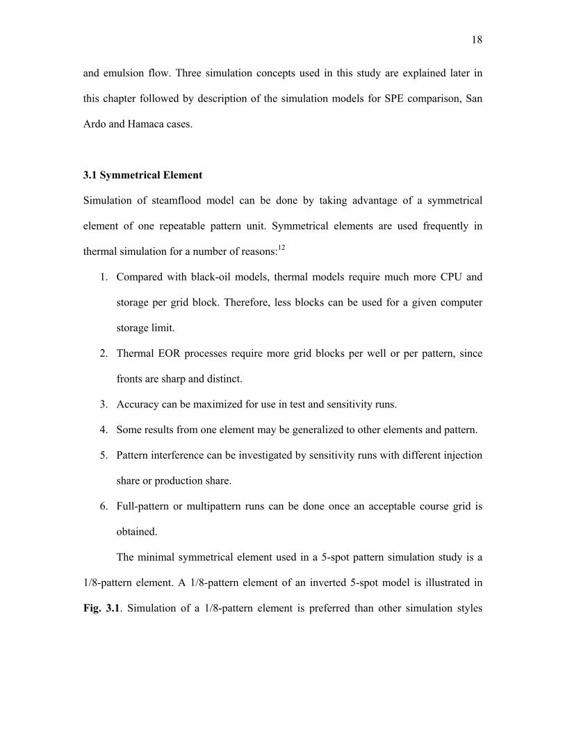
3.1 Symmetrical Element
Simulation of steamflood model can be done by taking advantage of a symmetrical
element of one repeatable pattern unit. Symmetrical elements are used frequently in
thermal simulation for a number of reasons:12
1. Compared with black-oil models, thermal models require much more CPU and
storage per grid block. Therefore, less blocks can be used for a given computer
storage limit.
2. Thermal EOR processes require more grid blocks per well or per pattern, since
fronts are sharp and distinct.
3. Accuracy can be maximized for use in test and sensitivity runs.
4. Some results from one element may be generalized to other elements and pattern.
5. Pattern interference can be investigated by sensitivity runs with different injection
share or production share.
6. Full-pattern or multipattern runs can be done once an acceptable course grid is
obtained.
The minimal symmetrical element used in a 5-spot pattern simulation study is a
1/8-pattern element. A 1/8-pattern element of an inverted 5-spot model is illustrated in
Fig. 3.1. Simulation of a 1/8-pattern element is preferred than other simulation styles

19
(1/4- pattern element or full pattern) because it is less time-consuming and more cost-
efficient than others.
Fig. 3.1–1/8 element of inverted 5-spot pattern model: (a) plan view; (b) 3D view.
3.2 Grid Orientation Effect
This 1/8-pattern element can be simulated using two different approaches of grid
orientation system: (a) diagonal grid and (b) parallel grid, as given in Fig. 3.2.
Production Well
Injection Well
1/8-pattern element
Injector (1/8-Well)
Producer (1/8-Well)
(a) Plan View
(b) 3D View

20
Fig. 3.2–Five spot pattern grids: (a) diagonal grid; (b) parallel grid.
The five-point difference scheme conventionally used in numerical simulation can
introduce significant disparity in results for equivalent parallel and diagonal grids. This
disparity was noted by Todd et al.13 for adverse-mobility ratio waterfloods and later by
Coats et al.14 for steamfloods. Abou-Kasem and Aziz15 reported a detailed comparison of
the nine-point difference and other numerical schemes as remedies to the grid orientation
problem in ¼ of a five-spot steamflood pattern. They concluded that the nine-point
scheme significantly reduces the grid orientation effect.
A schematic diagram of flow directions considered in the five and nine-point,
finite-difference formulations is presented in Fig. 3.3. The five-point formulation only
considers flow between a block and the four blocks that are adjacent to its boundaries.
(a) Diagonal Grid (b) Parallel Grid
Injection Well
Production Well
Center of grid block

21
The nine-point formulation considers this flow as well as the flow between the block and
the four blocks located at its corners.16
Fig. 3.3–Five and nine-point, finite-difference formulation (after Yanosik and McCraken16, 1979).
Fig. 3.4 compares full pattern oil rate results for five-point and nine-point
formulation. It indicates that the nine-point different scheme significantly reduced the
grid orientation effect.17
X X
X
X
X
X X
X
X
X X
X
X
X
(a) Five-Point Formulation (b) Nine-Point Formulation

22
Fig. 3.4–Five-point vs nine-point formulation on oil production rate in 1/8 five-spot (Coats and Ramesh17, 1987).
3.3 Block Geometry Modifier
In order to put grid nodes on injector-producer lines in a block-centered grid system, an
oversized grid must be specified.12 This grid is then modified by using block geometry
modifiers. Fig. 3.5 illustrates this idea for the parallel grid system.

23
Fig. 3.5–Active and inactive cells in a 1/8 five-spot pattern model.
All the grids at the edges and corners of the model are oversized, only half of the
grids at the edges are active and only one-eighth of the grids at the corners are active. In
order to get proper input parameters to be used in simulation, these grids are modified as
given in Table 3.1.
Active cell
Inactive cell
X
Z
(b) X-Z View
1/8 of Injector
1/8 of Producer
X
Y (a) X-Y View

24
TABLE 3.1–MODIFICATION PARAMETERS FOR EDGES AND CORNER-GRIDS
Value for Parameter Grids at Edges Grids at Corners Porosity 1/2 of value at normal grid 1/8 of value at normal grid Transmisibility at z-direction 1/2 of value at normal grid 1/8 of value at normal grid
Grid block rock volume 1/2 of value at normal grid 1/8 of value at normal grid Heat transmissibility at z-direction 1/2 of value at normal grid 1/8 of value at normal grid
Block geometry modifier in CMG STARS is done automatically by using *VAMOD and
*VATYPE keywords.
3.4 SPE Comparative Case Simulation Model
SPE comparative case model is a modified version of Case No. 2a of “Fourth SPE
Comparative Solution Project: Comparison of Steam Injection Simulators” by Azis et.al.8
SPE comparative case model simulates one-eighth of a five-spot repeatable pattern
described as follows.
1. Initial reservoir properties
Initial reservoir properties for SPE Comparative Case are given in Table 3.2.

25
TABLE 3.2–INITIAL RESERVOIR PROPERTIES
Properties Values Units Oil gravity 14 oAPI Initial pressure 75 psia Initial temperature 125 oF Net oil sand thickness 120 ft Initial oil saturation 55 % Initial water saturation 45 % Permeability 1000 md Porosity 30 % In-situ oil viscosity at 125oF 487 cp
2. Simulation model grid
Three simulation grid models are used for SPE comparative case model, depending
on the simulated area. 23x12x12 grid system is used for area of 2.5 ac, 31x16x12 for
area of 5 ac, and 45x23x8 for area of 10 ac. Fig. 3.6 to Fig. 3.8 show these grid
systems.
Fig. 3.6–Simulation grid for area of 2.5 ac, SPE comparative case model.

26
Fig. 3.7–Simulation grid for area of 5.0 ac, SPE comparative case model.
Fig. 3.8–Simulation grid for area of 10 ac, SPE comparative case model.

27
Table 3.3 shows the cell dimensions for each of the area simulated for the SPE
comparative case model.
TABLE 3.3 CELL DIMENSIONS FOR SPE COMPARATIVE CASE MODEL
Cell Dimensions (ft) Area (Acre) i j K 2.5 10.61 10.61 10 5 11 11 10 10 10.607 10.607 15
3. Rock properties
• Thermal conductivity of reservoir = 24 BTU/(ft-D-oF)
• Heat capacity of reservoir = 35 BTU/(ft3 of rock-oF)
• Heat capacity of overburden and underburden = 42 BTU/(ft3 of rock-oF)
4. Fluid properties
Water properties. Pure water is assumed and standard water properties are used.
Oil properties. Density at standard condition is 60.68 lbm/ft3. Compressibility is 5 ×
10-6 psi-1. The molecular weight is 600. Viscosity data is shown in Table 3.4.
TABLE 3.4–TEMPERATURE-VISCOSITY RELATIONSHIP FOR SPE COMPARATIVE CASE
Temperature (oF) Viscosity (cp) 75 5780 100 1380 150 187 200 47 250 17.4 300 8.5 350 5.2 500 2.5

28
5. Relative permeability data
The relative permeability expressions for water/oil system and water/gas system are
based on Corey relationships as follows:
For water/oil system,
,1
5.2
⎟⎟⎠
⎞⎜⎜⎝
⎛−−
−=
wirorw
wirwrwrorw SS
SSkk (3.2)
.11
2
⎟⎟⎠
⎞⎜⎜⎝
⎛−−−−
=iworw
worwroiwrow SS
SSkk (3.3)
For gas/oil system,
,1
12
⎟⎟⎠
⎞⎜⎜⎝
⎛
−−
−−−=
gcwir
gorgwirroiwrog SS
SSSkk (3.4)
.1
5.1
⎟⎟⎠
⎞⎜⎜⎝
⎛
−−
−=
gciw
gcgrgrorg SS
SSkk (3.5)
The residual oil saturation (water/oil system) Sorw = 0.15, the residual oil saturation
(gas oil system), Sorg = 0.10, and the critical gas saturation, Sgc = 0.06. Oil relative
permeability at interstitial water saturation, kroiw ≈ 0.4, water relative permeability at
residual oil saturation (water/oil system) krwro = 0.1, and gas relative permeability at
residual oil saturation (gas/oil system) krgro = 0.2. Fig. 3.9 and Fig. 3.10 show relative
permeability curves for SPE comparative case model.

29
0.00
0.05
0.10
0.15
0.20
0.25
0.30
0.35
0.40
0.45
0 0.2 0.4 0.6 0.8 1S w
k rw/k
row
krwkrow
Fig.3.9–Relative permeability curve (water/oil system) for SPE comparative case.
0.00
0.05
0.10
0.15
0.20
0.25
0.30
0.35
0.40
0.45
0 0.2 0.4 0.6 0.8 1Liquid Saturation
k rg/k
rog
krg
krog
Fig. 3.10–Relative permeability curve (gas/oil system) for SPE comparative case.
6. Operating conditions
Steam is injected at a temperature of 545oF. The quality of the steam at bottom hole
condition is 0.7. Minimum bottom hole pressure at producer is 17 psia.

30
3.5 San Ardo Simulation Model
The San Ardo simulation study was conducted with the available information from
Lombardi reservoir in San Ardo field.18 San Ardo model simulates one-eighth of a 10-
acre five-spot repeatable pattern described as follows.
1. Initial reservoir properties
Initial reservoir properties for San Ardo model are given in Table 3.5.
TABLE 3.5–INITIAL RESERVOIR PROPERTIES FOR SAN ARDO MODEL
Properties Values Units Oil gravity 12 oAPI Formation top 1900 ft. Initial pressure 275 psia Initial temperature 127 oF Net oil sand thickness 115 ft Initial oil saturation 73.3 % Initial water saturation 26.7 % Permeability 6922 md Porosity 34.5 % In-situ oil viscosity at 275 psia 3000 cp
2. Simulation model grid
45x23x8 grid system is used to simulate one-eighth of a 10-acre five-spot
repeatable pattern. Fig. 3.8 shows this grid system. The cell dimensions are i =
10.61 ft, j = 10.61 ft and k = 14.375 ft.
3. Rock properties
• Thermal conductivity of reservoir = 24 BTU/(ft-D-oF)
• Heat capacity of reservoir = 35.02 BTU/(ft3 of rock-oF)
• Heat capacity of overburden and underburden = 60 BTU/(ft3 of rock-oF)

31
4. Fluid properties
A live, black oil model (2 pseudo-components and water) is used for the
simulation.
Water properties. Pure water is assumed and standard water properties are used.
Oil properties. Oil consists of two components: “Oil” and “Gas” with the
properties as given in Table 3.6. Table 3.7 gives dead oil viscosity value for San
Ardo’s oil.
TABLE 3.6–OIL COMPONENT PROPERTIES FOR SAN ARDO MODEL
Component name Oil Gas Molecular weight, (CMM) 456.015 16.7278 Critical pressure (PCRIT), psia 179.02 670.46 Critical temperature (TCRIT), oF 1036.21 -107.35 First coefficient in the correlation for gas-liquid K value (KV1), psi
5.165E+6 1.534E+5
Fourth coefficient in the correlation for gas-liquid K value (KV4), oF
-15362.5 -1914.1
Fifth coefficient in the correlation for gas-liquid K value (KV5), oF
-459.67 -459.67
Partial molar density at reference pressure and temperature (MOLDEN), lbmol/cft
1.356E-01 4.515E-02
Liquid Compressibility at constant temperature (CP), 1/psi
3.805E-06 3.754E-03
First coefficient of the thermal expansion coefficient (CT1), 1/oF
1.660E-04 1.910E-03

32
TABLE 3.7–TEMPERATURE - VISCOSITY RELATIONSHIP FOR SAN ARDO OIL
Temperature (oF) Viscosity (cp) 50 500000 100 20000 150 1500 200 240 250 60 300 20 350 8 400 3.5
5. Relative permeability data
Temperature-dependent relative permeability data is used in San Ardo model. Fig.
3.11 and Fig. 3.12 show water-oil and gas-oil relative permeability plots of San Ardo
oil at four temperatures.
T=50 oF
0
0.2
0.4
0.6
0.8
0.4 0.6 0.8 1Sw
Kr
Krow Krw
T= 110 oF
0
0.2
0.4
0.6
0.8
0.4 0.6 0.8 1Sw
Kr
Krow
Krw
T= 250 oF
0
0.2
0.4
0.6
0.8
0.4 0.6 0.8 1Sw
Kr
Krow
Krw
T=400 oF
0
0.2
0.4
0.6
0.8
0.4 0.6 0.8 1Sw
Kr
Krow
Krw
Fig. 3.11–Water-oil relative permeability curves with temperature dependence, San Ardo model.

33
T= 50 oF
0
0.2
0.4
0.6
0 0.1 0.2 0.3Sg
Kr
Krog Krg
T= 110 oF
0
0.2
0.4
0.6
0 0.1 0.2 0.3Sg
Kr
Krog
Krg
T= 250 oF
0
0.2
0.4
0.6
0 0.1 0.2 0.3Sg
Kr
Krog Krg
T= 400 oF
0
0.2
0.4
0.6
0 0.1 0.2 0.3Sg
Kr
Krog Krg
Fig. 3.12–Gas-oil relative permeability curves with temperature dependence, San Ardo model.
6. Operating conditions
Steam is injected at a temperature of 582.3oF. The quality of the steam at bottom hole
condition is 0.8. Minimum Bottom hole pressure at producer is 15 psia.
3.6 Hamaca Simulation Model
Hamaca model simulates one-eighth of a five-spot repeatable pattern described as
follows.19
1. Initial reservoir properties
Initial reservoir properties for Hamaca model are given in Table 3.8.

34
TABLE 3.8–INITIAL RESERVOIR PROPERTIES FOR HAMACA MODEL
Properties Values Units Initial pressure 275 psia Initial temperature 125 oF Net oil sand thickness 100 ft Initial oil saturation 83.2 % Initial water saturation 16.8 % Permeability 12000 md Porosity 30 % In-situ oil viscosity at 125 oF 25000 cp
2. Simulation model grid
45x23x8 grid system is used to simulate one-eighth of a 10-acre five-spot
repeatable pattern. Fig. 3.8 shows this grid system. The cell dimensions are i =
10.61 ft, j = 10.61 ft and k = 12.5 ft.
3. Rock properties
• Thermal conductivity of reservoir = 24 BTU/(ft-D-oF)
• Heat capacity of reservoir = 35 BTU/(ft3 of rock-oF)
• Heat capacity of overburden and underburden = 60 BTU/(ft3 of rock-oF)
4. Fluid properties
Water properties. Pure water is assumed and standard water properties are used.
Oil properties. Density at standard condition is 63.18 lbm/ft3. Compressibility is 5
× 10-6 psi-1. The molecular weight is 511.78. Table 3.9 gives dead oil viscosity
value for Hamaca’s oil.
35
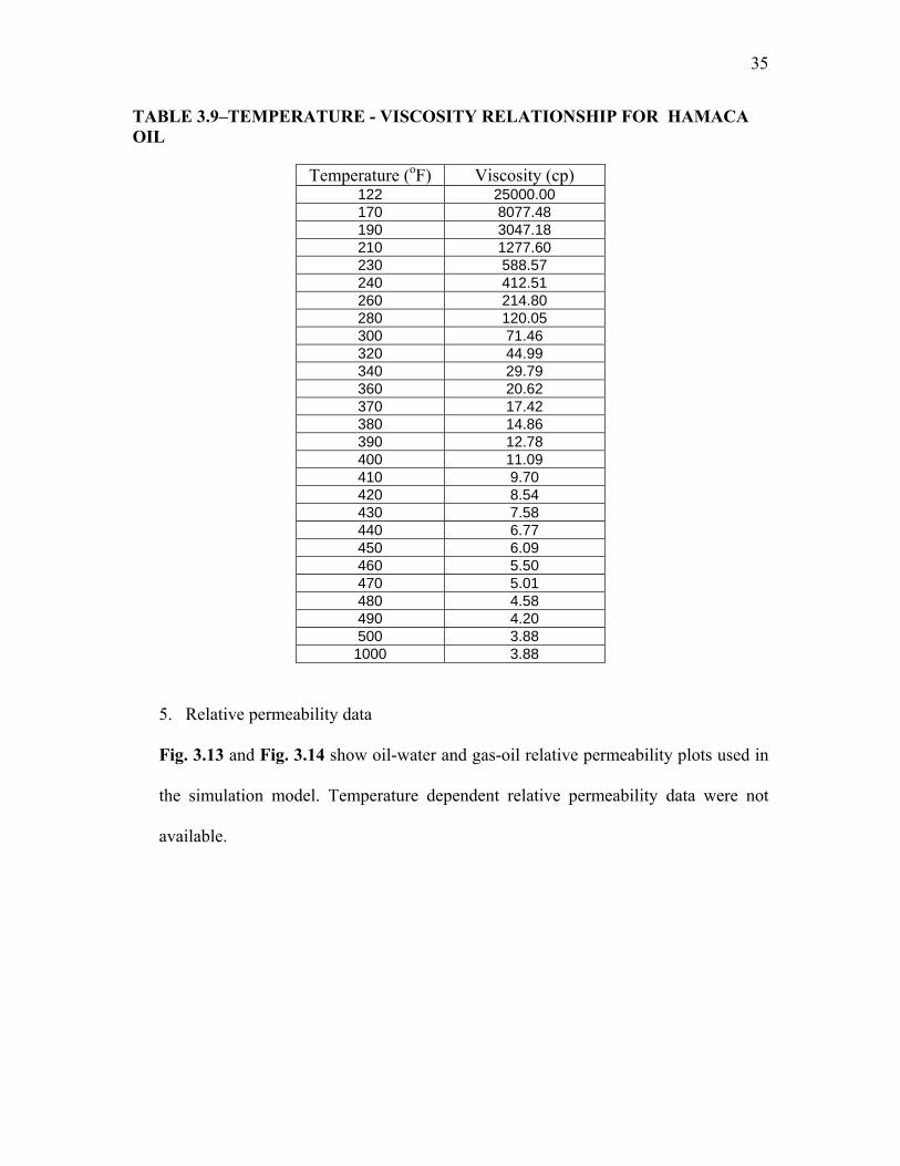
TABLE 3.9–TEMPERATURE - VISCOSITY RELATIONSHIP FOR HAMACA OIL
Temperature (oF) Viscosity (cp) 122 25000.00 170 8077.48 190 3047.18 210 1277.60 230 588.57 240 412.51 260 214.80 280 120.05 300 71.46 320 44.99 340 29.79 360 20.62 370 17.42 380 14.86 390 12.78 400 11.09 410 9.70 420 8.54 430 7.58 440 6.77 450 6.09 460 5.50 470 5.01 480 4.58 490 4.20 500 3.88 1000 3.88
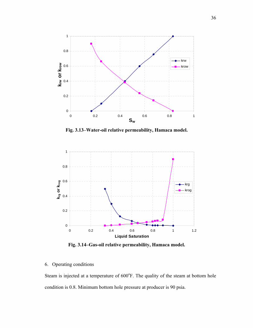
5. Relative permeability data
Fig. 3.13 and Fig. 3.14 show oil-water and gas-oil relative permeability plots used in
the simulation model. Temperature dependent relative permeability data were not
available.
36
0
0.2
0.4
0.6
0.8
1
0 0.2 0.4 0.6 0.8 1Sw
krw
or k
row
krw
krow
Fig. 3.13–Water-oil relative permeability, Hamaca model.
0
0.2
0.4
0.6
0.8
1
0 0.2 0.4 0.6 0.8 1 1.2
Liquid Saturation
k rg
or k
rog
krg
krog
Fig. 3.14–Gas-oil relative permeability, Hamaca model.
6. Operating conditions
Steam is injected at a temperature of 600oF. The quality of the steam at bottom hole
condition is 0.8. Minimum bottom hole pressure at producer is 90 psia.

37
CHAPTER IV
NEW STEAMFLOOD MODEL
As described in section 2.4, in the Jeff Jones model, the capture factor consists of three
components, AcD, VoD and VpD. The first two components had to be modified to obtain
satisfactory match of oil production rate based on the new model and simulation. The
component VoD in the new model is unchanged from that in the Jeff Jones model because
we have only studied the case where initial gas saturation is zero. Modification of AcD
and VoD is described in the following.
First, as in the Jeff Jones model, oil production consists of three stages (Stage I, II
and III) as schematically shown in Fig. 4.1.
Time (day)
Oil
Prod
uctio
n R
ate
(STB
/D)
Fig. 4.1-New model: three different stages of oil production under steam drive.
Stage I
Stage II
Stage III

38
Stage I is related to cold oil production. As described by Jeff Jones, this stage is
dominated by initial oil viscosity and possibly is affected by reservoir fillup if a
significant initial gas saturation exists. During reservoir fillup, free gas initially in the
reservoir is displaced by steam injected. This process ends after all of the moveable gas is
displaced from the reservoir. VpD is the capture factor component that describes this
reservoir fillup phenomenon. This new model uses the same VpD expression as given by
the Jeff Jones model:
.560,43
62.52
,
⎟⎟⎠
⎞⎜⎜⎝
⎛=
gn
injspD ShA
xVV
φ (4.1)
(limits: 0 ≤ VpD ≤ 1.0 and VpD = 1.0 at Sg = 0)
AcD expresses viscosity and area dependence in oil production rate for the Stage I. Based
on Jeff Jones model, AcD is given by
( ){ }.
100ln11.0
2
21 ⎥
⎥⎦
⎤
⎢⎢⎣
⎡=
oi
scD
A
AA
μ (4.2)
(limits: 0 ≤ AcD ≤ 1.0 and AcD = 1.0 at µo ≤ 100 cp)
In this study, we found that steam injection rate has quite a significant effect on oil
production rate in Stage I, and thus on AcD. From Eq. 4.2, it can be seen that the constant
in the denominator, 011, would have to vary with steam injection rate. In the new model,
this constant is replaced by α as follows.
( ){ }.
100ln
2
21
⎥⎥⎦
⎤
⎢⎢⎣
⎡=
oi
scD
A
AA
μα (4.3)
(limits: 0 ≤ AcD ≤ 1.0 and AcD = 1.0 at µo ≤ 100 cp)
Correlation between α and steam injection rate was developed by making several
simulation runs of SPE comparative model, each run with a different steam injection rate.
By trial-and-error, α for each steam injection rate was determined as that which gave the

39
best match of oil production rate based on the new model and simulation. A graph of α
versus steam injection rate is shown in Fig. 4.2, indicating the following linear
relationship:
.05.000015.0 += siα (4.4)
α = 0.00015 i s + 0.05
0
0.05
0.1
0.15
0.2
0.25
0.3
0.35
0 200 400 600 800 1000 1200 1400 1600 1800
Steam Injection Rate, i s (CWEBPD)
α, d
imen
sion
less
Fig. 4.2- α vs injection rate relationship.
Note that, in the new model, calculations of As and Qinj are as in the Jeff Jones
model, as given in Eq. 2.6 and Eq. 2.7.
Stage II is related to the oil bank breakthrough. Oil bank is the region where a
large amount of hot oil with lower viscosity is accumulated. At the beginning of
steamflooding process, the oil bank region is formed near the injector. Producer still
produces cold oil near to it which is not affected by the steam temperature. As the volume
of steam injected increases, the oil bank region is pushed towards the producer. At the

40
same time, the oil viscosity in the reservoir continues to decrease, increasing the oil
production rate.
When the oil bank region arrives at the producer, a large amount of the hot oil
breaks through and results in a sharp increase in oil production. Oil production rate at this
time will be significantly higher than the Myhill-Stegemeier oil displacement rate. This
happens because the oil displaced previously, which is not produced but stored in the oil
bank region, is produced at this time.
To account for the viscosity change due to heating, the viscosity value for AcD in
Stage II is described as an average viscosity between hot oil region and cold oil region as
given in Eq. 4.5.
.)(_
A
AAA sTosoio
steamμμ
μ+−
= (4.5)
With this average viscosity value, the value of AcD will increase faster to properly
describe the oil bank breakthrough. AcD expression for Stage II of the new model is:
.
100ln
4
2/1__
⎥⎥⎥⎥⎥
⎦
⎤
⎢⎢⎢⎢⎢
⎣
⎡
⎭⎬⎫
⎩⎨⎧
⎟⎠⎞
⎜⎝⎛
=
o
scD
A
AA
μα
(4.6)
(limits: 1.0 < AcD ≤ maxcDA and AcD = 1.0 at
__
oμ ≤ 100 cp)
Stage III is dominated by the remaining mobile portion of original oil-in-place as
expressed in VoD. VoD of the Jeff Jones model is given as
.12/1
⎟⎟⎠
⎞⎜⎜⎝
⎛Δ
−=o
oidoD S
SNN
V (4.7)
(limits: 0 ≤ VoD ≤ 1.0)

41
In this study, we observed that the simulation results always gave exponential
trends for oil rate decline in the Stage III. Thus, the Jeff Jones VoD expression was
modified from its square-root format to an exponential form. Also, in the Jeff Jones
model, VoD may decline from a value of 1 in Stage I, while in the new model, VoD starts to
decline only at start of stage III. Thus, in the new model, VoD is expressed as follows.
⎪⎭
⎪⎬⎫
⎪⎩
⎪⎨⎧
⎥⎥⎦
⎤
⎢⎢⎣
⎡⎟⎟⎠
⎞⎜⎜⎝
⎛
Δ−=
o
oioD S
SN
NExpAV D
cDmax
maxβ . (4.8)
(limits: maxcDA ≥ VoD ≥ 0)
where, maxcDA is AcD where oil production rate = injection rate, and
maxDN = ND from Myhill-Stegemeier calculation - ND up to maxcDA .
We found that production decline rate was dependent on the steam injection rate.
Thus, as can be seen in Eq. 4.8, the exponent had to vary with steam injection rate. To do
this, we incorporated the parameter, β, in the exponent. We made several simulation runs
using the SPE comparative solution model. By trial-and-error, we found that β is linearly
dependent on a dimensionless parameter, Nc, as shown in Fig. 4.3 and the following
equation.
.3401.193.17 += cNβ (4.9)
Nc is the ratio of the volume of moveable oil to that of steam injection up to the critical
time, tc, as given in Eq. 4.10:
,365
)1(7758
cs
wcorc ti
SShAN
−−=
φ (4.10)
where
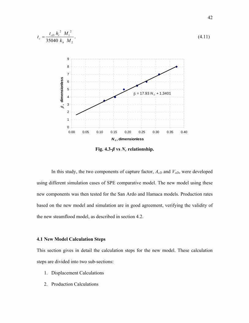
42
.35040 2
21
2
MkMht
th
tcDc = (4.11)
β = 17.93 N c + 1.3401
0
1
2
3
4
5
6
7
8
9
0.00 0.05 0.10 0.15 0.20 0.25 0.30 0.35 0.40
N c , dimensionless
β,
dim
ensi
onle
ss
Fig. 4.3-β vs Nc relationship.
In this study, the two components of capture factor, AcD and VoD, were developed
using different simulation cases of SPE comparative model. The new model using these
new components was then tested for the San Ardo and Hamaca models. Production rates
based on the new model and simulation are in good agreement, verifying the validity of
the new steamflood model, as described in section 4.2.
4.1 New Model Calculation Steps
This section gives in detail the calculation steps for the new model. These calculation
steps are divided into two sub-sections:
1. Displacement Calculations
2. Production Calculations

43
4.1.1 Displacement Calculations
Oil displacement calculations used in the new model is basically the method proposed by
Myhill and Stegemeier.5 In the Myhill-Stegemeier method, the oil displacement rate is a
function of cumulative oil steam ratio (Fos). This cumulative oil steam ratio is then a
function of overall thermal efficiency (Ehs). Overall thermal efficiency can be calculated
by the following formula:
( ) ( ) ( ) ( )[
( ) .
12211
0 ⎪⎭
⎪⎬⎫
⎥⎥⎦
⎤−
−−
⎩⎨⎧
−−−−
−+=
∫cDt
DD
x
cDDhvDcDD
hvDD
hs
tGxt
dxxerfce
ttftttU
ftGt
E
π
π (4.12)
The dimensionless time, tD, is given by
,35040
21
22
MhMtk
tt
hD
×
×××= (4.13)
and the function G (tD) is given by
.12 DtD terfcetG D+−=
π (4.14)
The erfc ( Dt ) term in Eq. 4.12 and Eq. 4.14 can be approximate from Effinger and
Wasson:20
() ,061405429.1453152027.1
421413741.1284496736.0254829592.054
32
Dt
D
eKK
KKKterfc−+−
+−= (4.15)
where
.3275911.01
1
DtK
+= (4.16)
The dimensionless critical time is calculated from the following expression:
44
,1 hvcDt fterfce cD −= (4.17)
where fhv, the fraction of the heat injected in latent form, is given by:
.11−
⎟⎟⎠
⎞⎜⎜⎝
⎛ Δ+=
fgs
whv hf
TCf (4.18)
The unit function, U (x), in Eq. 4.12 is 0 for x < 0 and 1 for x > 0.
Eq. 4.19 gives the relationship between overall thermal efficiency, Ehs, and cumulative
oil steam ratio, Fos:
( ) .11
hshDot
nwwos EFS
hh
MC
F +Δ= φρ
(4.19)
FhD is the dimensionless steam quality:
.TC
hfF
w
fgshD Δ
= (4.20)
Latent heat of vaporization, hfg, is calculated from Ejiogu-Fiori equation21 as follows,
.scsvfg hhh −= (4.21)
Calculation of the enthalpy of condensate, hsc, is divided into two pressure ranges:
,036.77 28302.0ssc ph = (4.22)
where 500 ≤ p ≤ 1500 psia, and
,984.43012038.0 += ssc ph (4.23)
where 1500 ≤ p ≤ 2500 psia.
Enthalpy of vapor, hsv, can be calculated as
( ) .23.453000197697.08.1204 73808.1−−= ssv ph (4.24)
With the preceding information, cumulative oil displacement is calculated as
.,injsosd VFN = (4.25)

45
Oil displacement rate can be estimated from the time derivative of cumulative oil
displacement function:
.1
tNN
q nn ddod Δ
−= − (4.26)
4.1.2 Production Calculations
The oil production rate is derived from the oil displacement rate as follows,
.pDoDcDodo VVAqq = (4.27)
These three factors, AcD, VoD and VpD are the three components of the capture factor. Each
represents a fraction of the displaced oil that will be produced (or “captured”). VpD is
given in Eq. 4.1 , AcD is given in Eq. 4.3 and Eq. 4.6 and VoD is given in Eq. 4.8.
Table 4.1 gives comparisons of AcD, VoD and VpD between new model and Jones model.
Program listing (in MS Visual Basic) of the new model is given in Appendix E.
4.2 Oil Production Rate Performance
13 different cases were conducted to verify the validity of the new model:
1. SPE comparative model, area = 2.5 ac, steam injection rate = 400 B/D.
2. SPE comparative model, area = 2.5 ac, steam injection rate = 600 B/D
3. SPE comparative model, area = 2.5 ac, steam injection rate = 800 B/D
4. SPE comparative model, area = 5.0 ac, steam injection rate = 600 B/D
5. SPE comparative model, area = 5.0 ac, steam injection rate = 800 B/D
6. SPE comparative model, area = 5.0 ac, steam injection rate = 1000 B/D
7. SPE comparative model, area = 5.0 ac. steam injection rate = 1200 B/D

TABLE 4.1-FORMULAS FOR CAPTURE FACTOR COMPONENTS: NEW MODEL AND JONES MODEL
AcD VoD VpD Stage New Model Jones Model New Model Jones Model New Model = Jones Model
I ( ){ }
2
21100ln ⎥⎦
⎤⎢⎣
⎡=
oi
scD A
AAμα
limits: 0 ≤ AcD ≤ 1.0 and AcD = 1.0 at μo ≤ 100 cp. where,
05.000015.0 += siα
( ){ }
2
21100ln11.0 ⎥⎦
⎤⎢⎣
⎡=
oi
scD A
AAμ
limits: 0 ≤ AcD ≤ 1.0 and AcD = 1.0 at μo ≤ 100 cp.
1
21
1 ⎟⎟⎠
⎞⎜⎜⎝
⎛Δ
−=o
oidoD S
SNNV
limit: 0 ≤ VoD ≤ 1.0
2
,
560,4362.5
⎟⎟⎠
⎞⎜⎜⎝
⎛ ×=
gn
injspD SAh
VV
φ
limits: 0 ≤ VpD ≤ 1.0 and VpD = 1.0 at Sg = 0
II
4
21__100ln
⎥⎥⎥⎥⎥
⎦
⎤
⎢⎢⎢⎢⎢
⎣
⎡
⎭⎬⎫
⎩⎨⎧
⎟⎠⎞
⎜⎝⎛
=
o
scD
A
AA
μα
limits: 1.0 < AcD ≤ maxcDA
and AcD = 1.0 at __
oμ ≤ 100 cp. where,
05.000015.0 += siα
1 1
21
1 ⎟⎟⎠
⎞⎜⎜⎝
⎛Δ
−=o
oidoD S
SNNV
limit: 0 ≤ VoD ≤ 1.0
1
III 1 1
⎪⎭
⎪⎬⎫
⎪⎩
⎪⎨⎧
⎥⎥⎦
⎤
⎢⎢⎣
⎡⎟⎟⎠
⎞⎜⎜⎝
⎛Δ
−=o
oiDcDoD S
SN
NExpAV max
maxβ
limit: maxcDA > VoD ≥ 0
where, 3401.193.17 += cNβ
( )cs
wcorc ti
SSAhN365
17758 −−=
21
1 ⎟⎟⎠
⎞⎜⎜⎝
⎛Δ
−=o
oidoD S
SNNV
limit: 0 ≤ VoD ≤ 1.0 1
46

47
8. SPE comparative model, area = 10.0 ac, steam injection rate = 1000 B/D
9. SPE comparative model, area = 10.0 ac, steam injection rate = 1200 B/D
10. SPE comparative model, area = 10.0 ac, steam injection rate = 1400 B/D
11. SPE comparative model, area = 10.0 ac, steam injection rate = 1600 B/D
12. San Ardo model, area = 10.0 ac, steam injection rate = 1600 B/D
13. Hamaca model, area = 10.0 ac, steam injection rate = 1600 B/D.
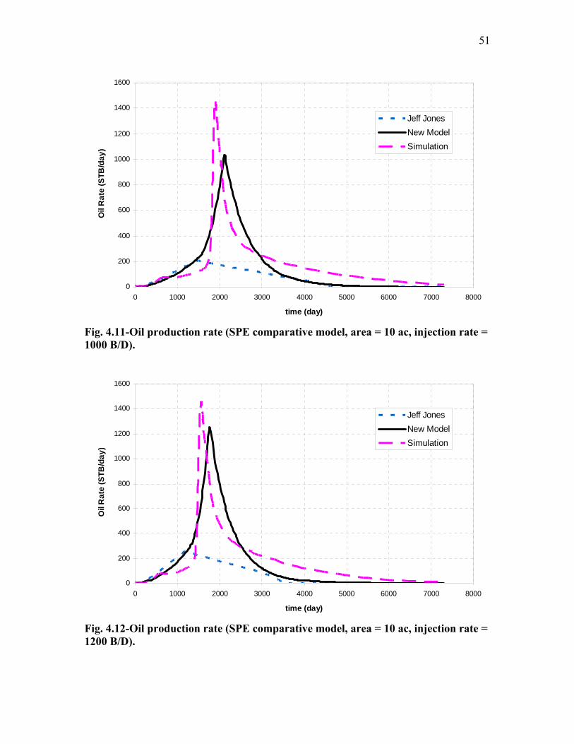
Fig. 4.4 to Fig. 4.16 give oil rate production performances from simulation, the Jeff Jones
model and new model for all of these cases.
0
100
200
300
400
500
600
700
800
0 500 1000 1500 2000 2500 3000 3500 4000
time (day)
Oil
Rat
e (S
TB/d
ay)
Jeff JonesNew ModelSimulation
Fig. 4.4-Oil production rate (SPE comparative model, area = 2.5 ac, injection rate =400 B/D).

48
0
100
200
300
400
500
600
700
800
900
1000
0 500 1000 1500 2000 2500 3000 3500 4000
time (day)
Oil
Rat
e (S
TB/d
ay)
Jeff JonesNew ModelSimulation
Fig. 4.5-Oil production rate (SPE comparative model, area = 2.5 ac, injection rate = 600 B/D).
0
200
400
600
800
1000
1200
0 500 1000 1500 2000 2500 3000 3500 4000
time (day)
Oil
Rat
e (S
TB/d
ay)
Jeff JonesNew ModelSimulation
Fig. 4.6-Oil production rate (SPE comparative model, area = 2.5 ac, injection rate = 800 B/D).

49
0
200
400
600
800
1000
1200
0 1000 2000 3000 4000 5000 6000
time (day)
Oil
Rat
e (S
TB/d
ay)
Jeff JonesNew ModelSimulation
Fig. 4.7-Oil production rate (SPE comparative model, area = 5.0 ac, injection rate = 600 B/D).
0
200
400
600
800
1000
1200
1400
0 1000 2000 3000 4000 5000 6000
time (day)
Oil
Rat
e (S
TB/d
ay)
Jeff JonesNew ModelSimulation
Fig. 4.8-Oil production rate (SPE comparative model, area = 5.0 ac, injection rate = 800 B/D).

50
0
200
400
600
800
1000
1200
1400
0 1000 2000 3000 4000 5000 6000
time (day)
Oil
Rat
e (S
TB/d
ay)
Jeff JonesNew ModelSimulation
Fig. 4.9-Oil production rate (SPE comparative model, area = 5.0 ac, injection rate = 1000 B/D).
0
200
400
600
800
1000
1200
1400
1600
0 1000 2000 3000 4000 5000 6000
time (day)
Oil
Rat
e (S
TB/d
ay)
Jeff JonesNew ModelSimulation
Fig. 4.10-Oil production rate (SPE comparative model, area = 5.0 ac, injection rate = 1200 B/D).
51
0
200
400
600
800
1000
1200
1400
1600
0 1000 2000 3000 4000 5000 6000 7000 8000
time (day)
Oil
Rat
e (S
TB/d
ay)
Jeff JonesNew ModelSimulation
Fig. 4.11-Oil production rate (SPE comparative model, area = 10 ac, injection rate = 1000 B/D).
0
200
400
600
800
1000
1200
1400
1600
0 1000 2000 3000 4000 5000 6000 7000 8000
time (day)
Oil
Rat
e (S
TB/d
ay)
Jeff JonesNew ModelSimulation
Fig. 4.12-Oil production rate (SPE comparative model, area = 10 ac, injection rate = 1200 B/D).
52
0
200
400
600
800
1000
1200
1400
1600
0 1000 2000 3000 4000 5000 6000 7000 8000
time (day)
Oil
Rat
e (S
TB/d
ay)
Jeff JonesNew ModelSimulation
Fig. 4.13-Oil production rate (SPE comparative model, area = 10 ac, injection rate = 1400 B/D).
0
200
400
600
800
1000
1200
1400
1600
1800
0 1000 2000 3000 4000 5000 6000 7000 8000
time (day)
Oil
Rat
e (S
TB/d
ay)
Jeff JonesNew ModelSimulation
Fig. 4.14-Oil production rate (SPE comparative model, area = 10 ac, injection rate = 1600 B/D).

53
0
500
1000
1500
2000
2500
0 1000 2000 3000 4000 5000 6000 7000
time (day)
Oil
Rat
e (S
TB/d
ay)
Jeff JonesNew ModelSimulation
Fig. 4.15-Oil production rate (San Ardo model, area = 10 ac, injection rate = 1600 B/D).
0
500
1000
1500
2000
2500
0 1000 2000 3000 4000 5000 6000 7000
time (day)
Oil
Rat
e (S
TB/d
ay)
Jeff JonesNew ModelSimulation
Fig. 4.16-Oil production rate (Hamaca model, area = 10 ac, injection rate = 1600 B/D).

54
4.3 Cumulative Oil Steam Ratio
Cumulative oil steam ratio (OSR) is defined as cumulative oil produced divided by
cumulative steam injected. Fig. 4.17 until Fig. 4.29 gives cumulative oil steam ratio plots
for all of the cases. It can be seen that cumulative OSR based on the new model are in
good agreement with simulation results.
0
0.05
0.1
0.15
0.2
0.25
0.3
0.35
0.4
0 500 1000 1500 2000 2500 3000 3500 4000 4500
Time (days)
Cum
ulat
ive
Oil
Stea
m R
atio
Simulation
New Model
Fig. 4.17-Cumulative oil steam ratio (SPE comparative model, area = 2.5 ac, injection rate = 400 B/D).

55
0
0.05
0.1
0.15
0.2
0.25
0.3
0.35
0.4
0 500 1000 1500 2000 2500 3000 3500 4000
Time (days)
Cum
ulat
ive
Oil
Stea
m R
atio
Simulation
New Model
Fig. 4.18-Cumulative oil steam ratio (SPE comparative model, area = 2.5 ac, injection rate = 600 B/D).
0
0.05
0.1
0.15
0.2
0.25
0.3
0.35
0.4
0 500 1000 1500 2000 2500 3000 3500 4000
Time (days)
Cum
ulat
ive
Oil
Stea
m R
atio
Simulation
New Model
Fig. 4.19-Cumulative oil steam ratio (SPE comparative model, area = 2.5 ac, injection rate = 800 B/D).

56
0
0.05
0.1
0.15
0.2
0.25
0.3
0.35
0 1000 2000 3000 4000 5000 6000
Time (days)
Cum
ulat
ive
Oil
Stea
m R
atio
Simulation
New Model
Fig. 4.20-Cumulative oil steam ratio (SPE comparative model, area = 5.0 ac, injection rate = 600 B/D).
0
0.05
0.1
0.15
0.2
0.25
0.3
0.35
0.4
0 1000 2000 3000 4000 5000 6000
Time (days)
Cum
ulat
ive
Oil
Stea
m R
atio
Simulation
New Model
Fig. 4.21-Cumulative oil steam ratio (SPE comparative model, area = 5.0 ac, injection rate = 800 B/D).

57
0
0.05
0.1
0.15
0.2
0.25
0.3
0.35
0.4
0 1000 2000 3000 4000 5000 6000
Time (days)
Cum
ulat
ive
Oil
Stea
m R
atio
Simulation
New Model
Fig. 4.22-Cumulative oil steam ratio (SPE comparative model, area = 5.0 ac, injection rate = 1000 B/D).
0
0.05
0.1
0.15
0.2
0.25
0.3
0.35
0.4
0.45
0 1000 2000 3000 4000 5000 6000
Time (days)
Cum
ulat
ive
Oil
Stea
m R
atio
Simulation
New Model
Fig. 4.23-Cumulative oil steam ratio (SPE comparative model, area = 5.0 ac, injection rate = 1200 B/D).

58
0
0.05
0.1
0.15
0.2
0.25
0.3
0.35
0 1000 2000 3000 4000 5000 6000 7000 8000
Time (days)
Cum
ulat
ive
Oil
Stea
m R
atio
Simulation
New Model
Fig. 4.24-Cumulative oil steam ratio (SPE comparative model, area = 10 ac, injection rate = 1000 B/D).
0
0.05
0.1
0.15
0.2
0.25
0.3
0.35
0 1000 2000 3000 4000 5000 6000
Time (days)
Cum
ulat
ive
Oil
Stea
m R
atio
Simulation
New Model
Fig. 4.25-Cumulative oil steam ratio (SPE comparative model, area = 10 ac, injection rate = 1200 B/D).

59
0
0.05
0.1
0.15
0.2
0.25
0.3
0.35
0 1000 2000 3000 4000 5000 6000
Time (days)
Cum
ulat
ive
Oil
Stea
m R
atio
Simulation
New Model
Fig. 4.26-Cumulative oil steam ratio (SPE comparative model, area = 10 ac, injection rate = 1400 B/D).
0
0.05
0.1
0.15
0.2
0.25
0.3
0.35
0 1000 2000 3000 4000 5000 6000
Time (days)
Cum
ulat
ive
Oil
Stea
m R
atio
Simulation
New Model
Fig. 4.27-Cumulative oil steam ratio (SPE comparative model, area = 10 ac, injection rate = 1600 B/D).

60
0
0.05
0.1
0.15
0.2
0.25
0.3
0.35
0 1000 2000 3000 4000 5000 6000
Time (days)
Cum
ulat
ive
Oil
Stea
m R
atio
Simulation
New Model
Fig. 4.28-Cumulative oil steam ratio (San Ardo model, area = 10 ac, injection rate = 1600 B/D).
0
0.05
0.1
0.15
0.2
0.25
0.3
0.35
0 1000 2000 3000 4000 5000 6000
Time (days)
Cum
ulat
ive
Oil
Stea
m R
atio
Simulation
New Model
Fig. 4.29-Cumulative oil steam ratio (Hamaca model, area = 10 ac, injection rate = 1600 B/D).

61
CHAPTER V
SUMMARY AND CONCLUSIONS
5.1 Summary
The main drawback of the Jeff Jones analytical steamflood model is the unsatisfactory
prediction of the oil production peak: usually significantly lower than the actual. The
main objective of this study is therefore to improve this aspect of the Jeff Jones model.
As in the Jeff Jones model, oil production in the new model consists of three
stages. The first production stage is related to cold oil production. The second production
stage describes breakthrough of the oil bank. The third production stage is related to the
production of the remaining mobile portion of original oil-in-place.
Two of the three components of the capture factor, AcD and VoD, given in Jeff
Jones’ model were modified to obtain a satisfactory match of the oil production rate
based on the new model and simulation. In the new model, AcD was modified to account
for effect of steam injection rate on oil production in the first and second stages. In
addition, the oil viscosity value for AcD in the second stage is taken as that at the average
of the steam and initial reservoir temperature. In the third stage, the Jeff Jones VoD
expression was modified from its square-root format to an exponential form, and took
into account the effect of steam injection rate on production rate decline.
Steamflood production performances based on the new model were compared
against simulation results for three cases: San Ardo field (12oAPI), Hamaca field (9oAPI),
and that based on the SPE fourth comparative solution project (14oAPI). In the first two
field cases, a 45x23x8 model was used that represented 1/8 of a 10-acre 5-spot pattern

62
unit, using typical rock and reservoir fluid properties. In the SPE project case, three
models were used: 23x12x12 (2.5 ac), 31x16x12 (5 ac) and 45x23x8 (10 ac), that
represented 1/8 of a 5-spot pattern unit.
Based on oil production rate and cumulative oil steam ratio performances of the
13 different cases investigated, the new model gives good agreement with simulation
results, verifying the validity of the new steamflood model.
5.2 Conclusions
1. Although the Jeff Jones model is commonly used for analytical steamflooding
performance prediction, it gives unsatisfactory prediction of the oil production
peak: usually lower than actual.
2. Simulation results indicate exponential decline trends for oil rate in the third
production stage. This is different from the square-root trend of the Jeff Jones
model.
3. A new analytical model for steamflooding performance prediction has been
developed by modifying the Jeff Jones analytical model.
4. Results based on the modified model agree well with simulation results for
thirteen different cases that includes three different sets of reservoir and fluid
properties: that of the SPE fourth comparative project, San Ardo field and
Hamaca field.
5. Engineers will find the modified model an improved and useful tool for prediction
of steamflood production performance.

63
NOMENCLATURE
ΔSo = change in oil saturation before/after steam front passage, fraction
ΔT = temperature difference = Tf - Ts
φ = porosity, percent
μoi = initial oil viscosity (cp)
μw = water viscosity (cp)
__
oμ = average viscosity defined by Eq. 4.5
μoi = initial reservoir oil viscosity, cp
steamToμ = oil viscosity value at steam temperature condition, cp
ρw = water density, lb/cu-ft
A = effective pattern area, acres
As = steam zone size, acres
AcD = Jeff Jones’ dimensionless steam zone size, dimensionless
maxcDA = maximum AcD value, obtained when oil production rate is equal to steam injection rate, dimensionless
Cw = specific heat of water, Btu/lbm-oF
Ehs = average thermal efficiency of steam zone, dimensionless
fhv = fraction of heat injected in vapor form, fraction
fs = bottomhole injection steam quality, dimensonless
FhD = ratio of enthalpy of vaporization to liquid enthalpy, dimensionless
Fos = cumulative ratio of oil displaced from steam zone to water injected as steam, dimensionless
G = function defined by Eq. 4.14

64
hf = enthalpy of saturated water at steam temperature, Btu/lbm
hfg = latent heat of steam, BTU/lbm
hn = net zone thickness, ft
hs = steam zone thickness, ft
hsc = enthalpy of condensate, BTU/lbm
hsv = enthalpy of vapor, BTU/lbm
ht = gross formation thickness, ft
is = steam injection rate, cold water equivalent, B/D
K = constant defined in Eq. 4.16, dimensionless
kh = bulk thermal conductivity of cap rock and base rock, BTU/ft-hr-oF
ko = oil relative permeability, fraction
krg = gas relative permeability (gas/oil system), fraction
krgro = gas relative permeability at residual oil saturation (gas/oil system), fraction
krog = oil relative permeability (gas/oil system), fraction
kroiw = oil relative permeability at interstitial water saturation, fraction
krow = oil relative permeability (water-oil system), fraction
krw = water relative permeability (water-oil system), fraction
krwro = water relative permeability at residual oil saturation (water/oil system), fraction
kw = water relative permeability, fraction
M = mobility ratio, dimensionless
M1 = average heat capacity of steam zone, BTU/cu ft-oF
M2 = average heat capacity of cap rock and base rock, BTU/cu ft-oF

65
N = oil originally in place, STB
Nc = ratio of the volume of moveable oil to that of steam injection up to the critical time, tc
ND = cumulative oil displacement, RB
maxDN = ND from Myhill-Stegemeier calculation - ND up to maxcDA , RB
ps = steam injection pressure, psia
Q inj = heat injection rate, BTU/hr
qo = oil production rate (STB/D)
qod = oil displacement rate/ Myhill-Stegemeier’s oil production rate (RB/D)
Sg = gas saturation, fraction
Sgc = critical gas saturation, fraction
Siw = interstitial water saturation, fraction
Soi = initial oil saturation, fraction
Sor = residual oil saturation, fraction
Sorg = residual oil saturation (gas/oil system), fraction
Sorw = residual oil saturation (water/oil system), fraction
Sw = water saturation, fraction
Swc = connate water saturation, fraction
Swir = irreducible water saturation, fraction
t = time of steam injection, years
tc = critical time, years
tcD = time of steam injection at onset of convective heat transport through condensation front, dimensionless
tD = time of steam injection, dimensionless

66
tf = initial formation temperature, oF
ts = steam temperature, oF
U(x) = unit function, equals 0 for x < 0, equals 1 for x > 0
VoD = volume of displaced oil produced, fraction
VpD = initial pore void filled with steam as water, fraction
Vs,inj = cumulative steam injection, RB

67
REFERENCES
1. Marx, J.W and Langenheim, R.H.: “Reservoir Heating by Hot Fluid Injection,”
Trans, AIME(1959) 216, 312-314.
2. Mandl, G. and Volek, C.W.: “Heat and Mass Transport in Steam Drive Processes,”
Soc. Pet. Eng. J. (March 1969) 59-79; Trans, AIME, 246.
3. Boberg, T.C. and Lantz, R.B.: “Calculation of the Production Rate of a Thermally
Stimulated Well,” J. Pet. Tech. (December 1966): 1613-23.
4. Neuman, C.H.: “A Mathematical Model of the Steam Drive Process – Applications,”
paper SPE 4757 presented at the 1975 SPE 50th Annual Technical Conference and
Exhibition, Dallas, 28 Sept. – 1 Oct.
5. Myhill, N.A. and Stegemeier, G.L.: “Steam-Drive Correlation and Prediction,” J. Pet.
Tech. (Feb. 1978), 173-182.
6. Gomaa, E.E.: “Correlations for Predicting Oil Recovery by Steamflood,” J.Pet.Tech.
(Feb. 1980), 325-332.
7. Jones, J.: “Steam Drive Model for Hand-Held Programmable Calculators,” J. Pet.
Tech. (September 1981), 1583-1598.
8. Aziz, K., Ramesh, A.B., and Woo. P.T.: “Fourth SPE Comparative Solution Project:
Comparison of Steam Injection Simulators,” J. Pet. Tech. (December 1987), 1576-
1584.
9. Hong, K.C.: Steamflood Reservoir Management, PennWell Books, Tulsa, (1994).
10. Pratts, M.: Thermal Recovery Monograph Vol. 7, Society of Petroleum Engineering,
Houston, (1986).

68
11. Van Lookeren, J.: “Calculation methods for Linear and Radial Steam Flow in Oil
Reservoirs,” paper SPE 6788 presented at the 1977 SPE 52nd Annual Technical
Conference and Exhibition, Denver, 9-12 Oct.
12. User Guide, STARS Advanced Process and Thermal Reservoir Simulator Version
2003, Computer Modeling Group Ltd., Calgary, (2003).
13. Todd, M.R., O’Dell, P.M., and Hirassaki, G.J.: “Methods for Increased Accuracy in
Numerical Reservoir Simulators,” Soc. Pet. Eng. J. (Dec. 1974), 573-92; Trans.,
AIME, 253.
14. Coats, K.H. et al.: “Three-Dimensional Simulation of Steamflooding,” Soc. Pet. Eng.
J. (Dec. 1974), 573-92; Trans., AIME, 257.
15. Abou-Kassem, J.H. and Aziz, K.: “Grid Orientation During Steam Displacement,”
paper SPE 10497 presented at the 1982 SPE Symposium on Reservoir Simulation,
New Orleans, 1-3 Feb.
16. Yanosik, J.L. and McCracken, T.A.: “A Nine-Point, Finite-Difference Reservoir
Simulator for Realistic Prediction of Adverse Mobility Ratio Displacement,” Soc.
Pet. Eng. J. (Aug. 1979), 253-62.
17. Coats, K.H., Ramesh, A.B.: “Effects of Grid Type and Difference Scheme on Pattern
Steamflood Simulation Results,” J. Pet. Tech. (May 1987), 557-569.
18. Sandoval, J.E. (2004): A Simulation Study of Steam and Steam-Propane Injection
Using A Novel Smart Horizontal Producer to Enhance Oil Production, MS Thesis,
Texas A&M University, College Station.
19. Venturini, G.J. (2002): Simulation Studies of Steam-Propane Injection for the
Hamaca Heavy Oil Field, MS Thesis, Texas A&M University, College Station.

69
20. Effinger, A.W. and Wasson, J.A: “Applying Marx and Langenheim Calculations to
the Prediction of Oil Recovery by Steamflooding in Venango Sands,” USBM
Information Circular 8482, U.S. Dept. of Interior (1969).
21. Ejiogu, G.C. and Fiori, M.: “High-Pressure Saturated-Steam Correlations,” J. Pet.
Tech. (December 1987), 1585-1590.

70
APPENDIX A
JEFF JONES OIL DISPLACEMENT CALCULATION
The method used is basically that proposed by Myhill and Stegemeier. The rate of oil
displacement is a function of Fos, which is in turn a function of Ehs or overall reservoir
thermal efficiency. Formula for Ehs calculation:
( )1/21−+= πDD
t
Dhs tterfce
tE D (A.1)
if tD ≤ tcD,
( )
⎥⎥⎦
⎤
⎟⎟⎠
⎞−−
−−
⎢⎢⎣
⎡⎜⎜⎝
⎛+
+−
−−+=
D
cDDD
tcDD
hD
cDDDD
t
Dhs
ttt
terfcett
Ftt
tterfcet
E
D
D
π
ππ
333
111/21
(A.2)
if tD > tcD,
where,
12
048,42Mh
tkt
t
hD = . (A.3)
The constant in Eq. A-3 assumes that heat capacity of the base rock and caprock is 1.2
times that of the reservoir and converts time to a yearly basis. The dimensionless time is
based on correlation:
71.148.0 hDcD Ft = . (A.4)
Dimensionless steam quality:
TChf
Fw
fgshD Δ
= . (A.5)

71
where,
sfg ph 207.0865 −= (A.6)
erfc function can be estimated from Effigner and Wasson equation:
()54
32
061405429.1453152027.1
421413741.1284496736.02548292.0
KK
KKKterfc D
+−
+−= (A.7)
where,
DtK
3275911.011
+= . (A.8)
Cumulative ratio of oil produced to water as steam injected:
( ) hshDot
nwwos EFS
hh
Mc
F +Δ= 1'1
φρ
. (A.9)
With the preceding information, cumulative oil displacement is calculated as:
injsosd VFN ,'= . (A.10)
Oil displacement rate is the time derivative of Nd function:
tNN
q dndno Δ
−= −1 . (A.11)

72
APPENDIX B
SIMULATION INPUT DATA FOR FOURTH SPE COMPARATIVE CASE, AREA = 2.5 ACRE, STEAM INJECTION RATE = 400 STB/D
***************************************************************************** ** Template Fourth SPE Comparative Solution Project 2a ** ***************************************************************************** ************************************************************************************** ** ** ** FILE : SPE4th_2.5ac_400STB-D.DAT ** ** ** ** MODEL: INVERTED 5 SPOT STEAM DRIVE FIELD UNITS 23X12X12 CARTESIAN GRID ** ** AREA AND BLOCK MODIFIERS 1/8 PATTERN ** ** 9 POINT TRANSMISSIBLITY ** ** ** ** ** ** USAGE: SPE COMPARATIVE SOLUTION FOR STEAM DRIVE SIMULATION ** ** ** ************************************************************************************** ************************************************************************************** ** ** ** ** ** This is the STARS data set for modified Problem 2A in "Fourth SPE ** ** Comparative Solution Project - A Comparison of Steam Injection ** ** Simulators", paper SPE 13510, presented at the eighth SPE symposium ** ** on reservoir simulation at Dallas, Texas, Feb 10-13, 1985. ** ** Also published in J. Pet. Tech. (Dec, 1987), pp 1576-1584 ** ** ** ** The problem is oil displacement by steam in an inverted five-spot ** ** pattern. The oil consists of a single 14 deg API pseudo-component. ** ** Steam breakthrough times are sensitive to grid orientation effects. ** ** This problem has the same oil and reservoir properties as problem 1a. ** ** Only the grid and well data are different. ** ** ** ** Features: ** ** ** ** 1) Nine-point discretization in the areal plane. ** ** ** ** 2) Black-oil type treatment of fluids. ** ** ** ** 3) Sharp changes in oil viscosity occur at the steam front ** ** (487 cp at 125 F to 2.5 cp at 545 oF). ** ** ** ** 4) Automatic initial vertical equilibrium calculation. ** ** ** ** 5) Multi-layer well with additional injection and production ** ** operating constraints. ** ** ** ** 6) 1/8 of an inverted five-spot pattern is defined through ** ** grid volume and area modifiers. ** ** **

73
************************************************************************************** ** ============== INPUT/OUTPUT CONTROL ====================== RESULTS SIMULATOR STARS *FILENAME *OUTPUT *INDEX-OUT *MAIN-RESULTS-OUT ** Use default file names **CHECKONLY *INTERRUPT *STOP *TITLE1 'Base Case' *TITLE2 'Modified Fourth SPE Comparative Solution Project' *TITLE3 'Area = 2.5 Acre, Injection Rate = 400 STB/D' *INUNIT *FIELD ** output same as input *OUTPRN *GRID *PRES *SW *SO *SG *TEMP *Y *X *W *SOLCONC *OBHLOSS *VISO *OUTPRN *WELL *ALL *WRST 300 *WPRN *GRID 300 *WPRN *ITER 300 *OUTSRF *WELL *LAYER ALL ** ============== GRID AND RESERVOIR DEFINITION ================= *GRID *CART 23 12 12 *KDIR *DOWN *NINEPOINT *IJ ** The triangular area of 1/8 of five-spot pattern is covered with a ** 23x12 grid with grid lines horizontal to the line linking the injector ** with the producer. These blocks are trimmed using block ** modifiers. ** In addition, a point-distributed grid is required in order to put ** grid nodes on the injector-producer line. To do this, an oversized ** grid is specified, and then trimmed back using block modifiers. ** The interwell distance is divided into 22 equal segments, requiring ** ni = 23. The third corner is a 1/4 block, and is located at j = 12. ** The five-spot pattern is 2.5 acres in area, or 330 ft square. The ** distance between injector and producer is (330/2)*1.414 = ** 233.3 ft, giving a block size of 233.3/22 = 10.6045 ft. *DI *CON 10.6045 *DJ *CON 10.6045 *DK *CON 10 ** Trim grid to 1/8 of an inverted 5-spot pattern *VAMOD 2 0.5 0.5 1.0 0.5 *VAMOD 3 0.5 1.0 1.0 0.5 *9p 0.5 1.0 *VAMOD 4 0.5 1.0 1.0 0.5 *9p 1.0 0.5 *VAMOD 5 0.125 0.5 1.0 0.125 *9p 0.5 1.0

74
*VAMOD 6 0.25 1.0 1.0 0.25 *9p 1.0 0.5 *VATYPE *ALL
5 2 2 2 2 2 2 2 2 2 2 2 2 2 2 2 2 2 2 2 2 2 5 0 3 1 1 1 1 1 1 1 1 1 1 1 1 1 1 1 1 1 1 1 4 0 0 0 3 1 1 1 1 1 1 1 1 1 1 1 1 1 1 1 1 1 4 0 0 0 0 0 3 1 1 1 1 1 1 1 1 1 1 1 1 1 1 1 4 0 0 0 0 0 0 0 3 1 1 1 1 1 1 1 1 1 1 1 1 1 4 0 0 0 0
0 0 0 0 0 3 1 1 1 1 1 1 1 1 1 1 1 4 0 0 0 0 0 0 0 0 0 0 0 3 1 1 1 1 1 1 1 1 1 4 0 0 0 0 0 0
0 0 0 0 0 0 0 3 1 1 1 1 1 1 1 4 0 0 0 0 0 0 0 0 0 0 0 0 0 0 0 3 1 1 1 1 1 4 0 0 0 0 0 0 0 0 0 0 0 0 0 0 0 0 0 3 1 1 1 4 0 0 0 0 0 0 0 0 0 0 0 0 0 0 0 0 0 0 0 3 1 4 0 0 0 0 0 0 0 0 0 0 0 0 0 0 0 0 0 0 0 0 0 6 0 0 0 0 0 0 0 0 0 0 0
5 2 2 2 2 2 2 2 2 2 2 2 2 2 2 2 2 2 2 2 2 2 5 0 3 1 1 1 1 1 1 1 1 1 1 1 1 1 1 1 1 1 1 1 4 0 0 0 3 1 1 1 1 1 1 1 1 1 1 1 1 1 1 1 1 1 4 0 0 0 0 0 3 1 1 1 1 1 1 1 1 1 1 1 1 1 1 1 4 0 0 0 0 0 0 0 3 1 1 1 1 1 1 1 1 1 1 1 1 1 4 0 0 0 0
0 0 0 0 0 3 1 1 1 1 1 1 1 1 1 1 1 4 0 0 0 0 0 0 0 0 0 0 0 3 1 1 1 1 1 1 1 1 1 4 0 0 0 0 0 0
0 0 0 0 0 0 0 3 1 1 1 1 1 1 1 4 0 0 0 0 0 0 0 0 0 0 0 0 0 0 0 3 1 1 1 1 1 4 0 0 0 0 0 0 0 0 0 0 0 0 0 0 0 0 0 3 1 1 1 4 0 0 0 0 0 0 0 0 0 0 0 0 0 0 0 0 0 0 0 3 1 4 0 0 0 0 0 0 0 0 0 0 0 0 0 0 0 0 0 0 0 0 0 6 0 0 0 0 0 0 0 0 0 0 0 5 2 2 2 2 2 2 2 2 2 2 2 2 2 2 2 2 2 2 2 2 2 5 0 3 1 1 1 1 1 1 1 1 1 1 1 1 1 1 1 1 1 1 1 4 0 0 0 3 1 1 1 1 1 1 1 1 1 1 1 1 1 1 1 1 1 4 0 0 0 0 0 3 1 1 1 1 1 1 1 1 1 1 1 1 1 1 1 4 0 0 0 0 0 0 0 3 1 1 1 1 1 1 1 1 1 1 1 1 1 4 0 0 0 0
0 0 0 0 0 3 1 1 1 1 1 1 1 1 1 1 1 4 0 0 0 0 0 0 0 0 0 0 0 3 1 1 1 1 1 1 1 1 1 4 0 0 0 0 0 0
0 0 0 0 0 0 0 3 1 1 1 1 1 1 1 4 0 0 0 0 0 0 0 0 0 0 0 0 0 0 0 3 1 1 1 1 1 4 0 0 0 0 0 0 0 0 0 0 0 0 0 0 0 0 0 3 1 1 1 4 0 0 0 0 0 0 0 0 0 0 0 0 0 0 0 0 0 0 0 3 1 4 0 0 0 0 0 0 0 0 0 0 0 0 0 0 0 0 0 0 0 0 0 6 0 0 0 0 0 0 0 0 0 0 0 5 2 2 2 2 2 2 2 2 2 2 2 2 2 2 2 2 2 2 2 2 2 5 0 3 1 1 1 1 1 1 1 1 1 1 1 1 1 1 1 1 1 1 1 4 0 0 0 3 1 1 1 1 1 1 1 1 1 1 1 1 1 1 1 1 1 4 0 0 0 0 0 3 1 1 1 1 1 1 1 1 1 1 1 1 1 1 1 4 0 0 0 0 0 0 0 3 1 1 1 1 1 1 1 1 1 1 1 1 1 4 0 0 0 0 0 0 0 0 0 3 1 1 1 1 1 1 1 1 1 1 1 4 0 0 0 0 0 0 0 0 0 0 0 3 1 1 1 1 1 1 1 1 1 4 0 0 0 0 0 0 0 0 0 0 0 0 0 3 1 1 1 1 1 1 1 4 0 0 0 0 0 0 0 0 0 0 0 0 0 0 0 3 1 1 1 1 1 4 0 0 0 0 0 0 0 0 0 0 0 0 0 0 0 0 0 3 1 1 1 4 0 0 0 0 0 0 0 0 0 0 0 0 0 0 0 0 0 0 0 3 1 4 0 0 0 0 0 0 0 0 0 0 0 0 0 0 0 0 0 0 0 0 0 6 0 0 0 0 0 0 0 0 0 0 0 5 2 2 2 2 2 2 2 2 2 2 2 2 2 2 2 2 2 2 2 2 2 5

75
0 3 1 1 1 1 1 1 1 1 1 1 1 1 1 1 1 1 1 1 1 4 0 0 0 3 1 1 1 1 1 1 1 1 1 1 1 1 1 1 1 1 1 4 0 0 0 0 0 3 1 1 1 1 1 1 1 1 1 1 1 1 1 1 1 4 0 0 0 0 0 0 0 3 1 1 1 1 1 1 1 1 1 1 1 1 1 4 0 0 0 0 0 0 0 0 0 3 1 1 1 1 1 1 1 1 1 1 1 4 0 0 0 0 0 0 0 0 0 0 0 3 1 1 1 1 1 1 1 1 1 4 0 0 0 0 0 0 0 0 0 0 0 0 0 3 1 1 1 1 1 1 1 4 0 0 0 0 0 0 0 0 0 0 0 0 0 0 0 3 1 1 1 1 1 4 0 0 0 0 0 0 0 0 0 0 0 0 0 0 0 0 0 3 1 1 1 4 0 0 0 0 0 0 0 0 0 0 0 0 0 0 0 0 0 0 0 3 1 4 0 0 0 0 0 0 0 0 0 0 0 0 0 0 0 0 0 0 0 0 0 6 0 0 0 0 0 0 0 0 0 0 0 5 2 2 2 2 2 2 2 2 2 2 2 2 2 2 2 2 2 2 2 2 2 5 0 3 1 1 1 1 1 1 1 1 1 1 1 1 1 1 1 1 1 1 1 4 0 0 0 3 1 1 1 1 1 1 1 1 1 1 1 1 1 1 1 1 1 4 0 0 0 0 0 3 1 1 1 1 1 1 1 1 1 1 1 1 1 1 1 4 0 0 0 0 0 0 0 3 1 1 1 1 1 1 1 1 1 1 1 1 1 4 0 0 0 0 0 0 0 0 0 3 1 1 1 1 1 1 1 1 1 1 1 4 0 0 0 0 0 0 0 0 0 0 0 3 1 1 1 1 1 1 1 1 1 4 0 0 0 0 0 0 0 0 0 0 0 0 0 3 1 1 1 1 1 1 1 4 0 0 0 0 0 0 0 0 0 0 0 0 0 0 0 3 1 1 1 1 1 4 0 0 0 0 0 0 0 0 0 0 0 0 0 0 0 0 0 3 1 1 1 4 0 0 0 0 0 0 0 0 0 0 0 0 0 0 0 0 0 0 0 3 1 4 0 0 0 0 0 0 0 0 0 0 0 0 0 0 0 0 0 0 0 0 0 6 0 0 0 0 0 0 0 0 0 0 0 5 2 2 2 2 2 2 2 2 2 2 2 2 2 2 2 2 2 2 2 2 2 5 0 3 1 1 1 1 1 1 1 1 1 1 1 1 1 1 1 1 1 1 1 4 0 0 0 3 1 1 1 1 1 1 1 1 1 1 1 1 1 1 1 1 1 4 0 0 0 0 0 3 1 1 1 1 1 1 1 1 1 1 1 1 1 1 1 4 0 0 0 0 0 0 0 3 1 1 1 1 1 1 1 1 1 1 1 1 1 4 0 0 0 0 0 0 0 0 0 3 1 1 1 1 1 1 1 1 1 1 1 4 0 0 0 0 0 0 0 0 0 0 0 3 1 1 1 1 1 1 1 1 1 4 0 0 0 0 0 0 0 0 0 0 0 0 0 3 1 1 1 1 1 1 1 4 0 0 0 0 0 0 0 0 0 0 0 0 0 0 0 3 1 1 1 1 1 4 0 0 0 0 0 0 0 0 0 0 0 0 0 0 0 0 0 3 1 1 1 4 0 0 0 0 0 0 0 0 0 0 0 0 0 0 0 0 0 0 0 3 1 4 0 0 0 0 0 0 0 0 0 0 0 0 0 0 0 0 0 0 0 0 0 6 0 0 0 0 0 0 0 0 0 0 0 5 2 2 2 2 2 2 2 2 2 2 2 2 2 2 2 2 2 2 2 2 2 5 0 3 1 1 1 1 1 1 1 1 1 1 1 1 1 1 1 1 1 1 1 4 0 0 0 3 1 1 1 1 1 1 1 1 1 1 1 1 1 1 1 1 1 4 0 0 0 0 0 3 1 1 1 1 1 1 1 1 1 1 1 1 1 1 1 4 0 0 0 0 0 0 0 3 1 1 1 1 1 1 1 1 1 1 1 1 1 4 0 0 0 0 0 0 0 0 0 3 1 1 1 1 1 1 1 1 1 1 1 4 0 0 0 0 0 0 0 0 0 0 0 3 1 1 1 1 1 1 1 1 1 4 0 0 0 0 0 0 0 0 0 0 0 0 0 3 1 1 1 1 1 1 1 4 0 0 0 0 0 0 0 0 0 0 0 0 0 0 0 3 1 1 1 1 1 4 0 0 0 0 0 0 0 0 0 0 0 0 0 0 0 0 0 3 1 1 1 4 0 0 0 0 0 0 0 0 0 0 0 0 0 0 0 0 0 0 0 3 1 4 0 0 0 0 0 0 0 0 0 0 0 0 0 0 0 0 0 0 0 0 0 6 0 0 0 0 0 0 0 0 0 0 0 5 2 2 2 2 2 2 2 2 2 2 2 2 2 2 2 2 2 2 2 2 2 5 0 3 1 1 1 1 1 1 1 1 1 1 1 1 1 1 1 1 1 1 1 4 0 0 0 3 1 1 1 1 1 1 1 1 1 1 1 1 1 1 1 1 1 4 0 0 0 0 0 3 1 1 1 1 1 1 1 1 1 1 1 1 1 1 1 4 0 0 0 0 0 0 0 3 1 1 1 1 1 1 1 1 1 1 1 1 1 4 0 0 0 0

76
0 0 0 0 0 3 1 1 1 1 1 1 1 1 1 1 1 4 0 0 0 0 0 0 0 0 0 0 0 3 1 1 1 1 1 1 1 1 1 4 0 0 0 0 0 0 0 0 0 0 0 0 0 3 1 1 1 1 1 1 1 4 0 0 0 0 0 0 0 0 0 0 0 0 0 0 0 3 1 1 1 1 1 4 0 0 0 0 0 0 0 0 0 0 0 0 0 0 0 0 0 3 1 1 1 4 0 0 0 0 0 0 0 0 0 0 0 0 0 0 0 0 0 0 0 3 1 4 0 0 0 0 0 0 0 0 0 0 0 0 0 0 0 0 0 0 0 0 0 6 0 0 0 0 0 0 0 0 0 0 0 5 2 2 2 2 2 2 2 2 2 2 2 2 2 2 2 2 2 2 2 2 2 5 0 3 1 1 1 1 1 1 1 1 1 1 1 1 1 1 1 1 1 1 1 4 0 0 0 3 1 1 1 1 1 1 1 1 1 1 1 1 1 1 1 1 1 4 0 0 0 0 0 3 1 1 1 1 1 1 1 1 1 1 1 1 1 1 1 4 0 0 0 0 0 0 0 3 1 1 1 1 1 1 1 1 1 1 1 1 1 4 0 0 0 0 0 0 0 0 0 3 1 1 1 1 1 1 1 1 1 1 1 4 0 0 0 0 0 0 0 0 0 0 0 3 1 1 1 1 1 1 1 1 1 4 0 0 0 0 0 0 0 0 0 0 0 0 0 3 1 1 1 1 1 1 1 4 0 0 0 0 0 0 0 0 0 0 0 0 0 0 0 3 1 1 1 1 1 4 0 0 0 0 0 0 0 0 0 0 0 0 0 0 0 0 0 3 1 1 1 4 0 0 0 0 0 0 0 0 0 0 0 0 0 0 0 0 0 0 0 3 1 4 0 0 0 0 0 0 0 0 0 0 0 0 0 0 0 0 0 0 0 0 0 6 0 0 0 0 0 0 0 0 0 0 0 5 2 2 2 2 2 2 2 2 2 2 2 2 2 2 2 2 2 2 2 2 2 5 0 3 1 1 1 1 1 1 1 1 1 1 1 1 1 1 1 1 1 1 1 4 0 0 0 3 1 1 1 1 1 1 1 1 1 1 1 1 1 1 1 1 1 4 0 0 0 0 0 3 1 1 1 1 1 1 1 1 1 1 1 1 1 1 1 4 0 0 0 0 0 0 0 3 1 1 1 1 1 1 1 1 1 1 1 1 1 4 0 0 0 0 0 0 0 0 0 3 1 1 1 1 1 1 1 1 1 1 1 4 0 0 0 0 0 0 0 0 0 0 0 3 1 1 1 1 1 1 1 1 1 4 0 0 0 0 0 0 0 0 0 0 0 0 0 3 1 1 1 1 1 1 1 4 0 0 0 0 0 0 0 0 0 0 0 0 0 0 0 3 1 1 1 1 1 4 0 0 0 0 0 0 0 0 0 0 0 0 0 0 0 0 0 3 1 1 1 4 0 0 0 0 0 0 0 0 0 0 0 0 0 0 0 0 0 0 0 3 1 4 0 0 0 0 0 0 0 0 0 0 0 0 0 0 0 0 0 0 0 0 0 6 0 0 0 0 0 0 0 0 0 0 0 5 2 2 2 2 2 2 2 2 2 2 2 2 2 2 2 2 2 2 2 2 2 5 0 3 1 1 1 1 1 1 1 1 1 1 1 1 1 1 1 1 1 1 1 4 0 0 0 3 1 1 1 1 1 1 1 1 1 1 1 1 1 1 1 1 1 4 0 0 0 0 0 3 1 1 1 1 1 1 1 1 1 1 1 1 1 1 1 4 0 0 0 0 0 0 0 3 1 1 1 1 1 1 1 1 1 1 1 1 1 4 0 0 0 0 0 0 0 0 0 3 1 1 1 1 1 1 1 1 1 1 1 4 0 0 0 0 0 0 0 0 0 0 0 3 1 1 1 1 1 1 1 1 1 4 0 0 0 0 0 0 0 0 0 0 0 0 0 3 1 1 1 1 1 1 1 4 0 0 0 0 0 0 0 0 0 0 0 0 0 0 0 3 1 1 1 1 1 4 0 0 0 0 0 0 0 0 0 0 0 0 0 0 0 0 0 3 1 1 1 4 0 0 0 0 0 0 0 0 0 0 0 0 0 0 0 0 0 0 0 3 1 4 0 0 0 0 0 0 0 0 0 0 0 0 0 0 0 0 0 0 0 0 0 6 0 0 0 0 0 0 0 0 0 0 0 *POR *CON 0.3 *PERMI *CON 1000 *PERMJ *EQUALSI *PERMK *EQUALSI / 10 *END-GRID

77
*CPOR 5e-4 *PRPOR 75 *ROCKCP 35 *THCONR 24 *THCONW 24 *THCONO 24 *THCONG 24 *HLOSSPROP *OVERBUR 42 24 *UNDERBUR 42 24 ** ============== FLUID DEFINITIONS ====================== *MODEL 2 2 2 ** Components are water and dead oil. Most water ** properties are defaulted (=0). Dead oil K values ** are zero, and no gas properties are needed. *COMPNAME 'WATER' 'OIL' ** ----- ------- *CMM 18.02 600 *PCRIT 3206.2 0 ** These four properties *TCRIT 705.4 0 ** are for the gas phase. *AVG 1.13e-5 0 ** The dead oil component does *BVG 1.075 0 ** not appear in the gas phase. *MOLDEN 0 0.10113 *CP 0 5.e-6 *CT1 0 3.8e-4 *CPL1 0 300 *VISCTABLE ** Temp 75 0 5780 100 0 1380 150 0 187 200 0 47 250 0 17.4 300 0 8.5 350 0 5.2 500 0 2.5 800 0 2.5 *PRSR 14.7 *TEMR 60 *PSURF 14.7 *TSURF 60 ** ============== ROCK-FLUID PROPERTIES ====================== *ROCKFLUID *SWT ** Water-oil relative permeabilities

78
** Sw Krw Krow ** ---- -------- ------- 0.45 0.0 0.4 0.47 0.000056 0.361 0.50 0.000552 0.30625 0.55 0.00312 0.225 0.60 0.00861 0.15625 0.65 0.01768 0.1 0.70 0.03088 0.05625 0.75 0.04871 0.025 0.77 0.05724 0.016 0.80 0.07162 0.00625 0.82 0.08229 0.00225 0.85 0.1 0.0 *SLT ** Liquid-gas relative permeabilities ** Sl Krg Krog ** ---- ------- ------- 0.45 0.2 0.0 0.55 0.14202 0.0 0.57 0.13123 0.00079 0.60 0.11560 0.00494 0.62 0.10555 0.00968 0.65 0.09106 0.01975 0.67 0.08181 0.02844 0.70 0.06856 0.04444 0.72 0.06017 0.05709 0.75 0.04829 0.07901 0.77 0.04087 0.09560 0.80 0.03054 0.12346 0.83 0.02127 0.15486 0.85 0.01574 0.17778 0.87 0.01080 0.20227 0.90 0.00467 0.24198 0.92 0.00165 0.27042 0.94 0.0 0.30044 1. 0.0 0.4 ** ============== INITIAL CONDITIONS ====================== *INITIAL ** Automatic static vertical equilibrium *VERTICAL *DEPTH_AVE *REFPRES 75 *REFBLOCK 1 1 1 *TEMP *CON 125

79
** ============== NUMERICAL CONTROL ====================== *NUMERICAL ** All these can be defaulted. The definitions ** here match the previous data. *NORM *PRESS 200 *SATUR 0.2 *TEMP 50 *RUN ** ============== RECURRENT DATA ====================== ** Project starts on January 01, 2004 *DATE 2004 01 01 *DTWELL 1 ** o *WELL 1 'INJECTOR' *VERT 1 1 *FRAC .125 ** o o o *WELL 2 'PRODUCER' *VERT 23 1 *FRAC .125 ** o o o o o ** o o o o o o o ** 1 o o o o o o o 2 *INJECTOR *MOBWEIGHT 'INJECTOR' *INCOMP WATER 1.0 0.0 *TINJW 545 QUAL .7 *OPERATE *BHP 1000 *OPERATE *MAX *STW 400 *PERFV 'INJECTOR' ** k wi ** Inject only in the bottom layer 6 32235.39 ** 2*pi*k*h / ln(cc*sqrt((dx**2+dy**2)/pi)/rw) 7 32235.39 ** k = 1000 md, h = 10 ft, dx = dy = 10.6045 ft, 8 32235.39 ** cc = 0.249, rw = 0.3 ft 9 32235.39 10 32235.39 11 32235.39 12 32235.39 *PRODUCER 'PRODUCER' *OPERATE *BHP 17 *PERFV 'PRODUCER' ** k wi 1 32235.39 2 32235.39 3 32235.39 4 32235.39 5 32235.39 6 32235.39 7 32235.39 8 32235.39 9 32235.39 10 32235.39 11 32235.39

80
12 32235.39 OPEN 'PRODUCER' OPEN 'INJECTOR' *TIME 365 *TIME 730 *TIME 1095 *TIME 1460 *TIME 1825 *TIME 2190 *TIME 2555 *TIME 2920 *TIME 3285 *TIME 3650 *STOP

81
APPENDIX C
SIMULATION INPUT DATA FOR SAN ARDO CASE AREA = 10 ACRE, STEAM INJECTION RATE = 1600 STB/D
***************************************************************************** ** Template San Ardo field – Lombardi Reservoir ** ***************************************************************************** ************************************************************************************** ** ** ** FILE : SanArdo.DAT ** ** ** ** MODEL:INVERTED 5 SPOT STEAM DRIVE FIELD UNITS 45X23X8 CARTESIAN GRID ** ** AREA AND BLOCK MODIFIERS 1/8 PATTERN ** ** 9 POINT TRANSMISSIBLITY ** ** ** ** ** ** USAGE: SAN ARDO FIELD - LOMBARDI RESERVOIR STEAM DRIVE SIMULATION ** ** ** ************************************************************************************** ** ============== INPUT/OUTPUT CONTROL ====================== RESULTS SIMULATOR STARS *FILENAME *OUTPUT *INDEX-OUT *MAIN-RESULTS-OUT ** Use default file names *INTERRUPT *STOP *TITLE1 'San Ardo Case' *TITLE2 ' SanArdo Field Lombardi Reservoir' *TITLE3 'Area = 10 Acre Injection Rate = 1600 STB/D' *INUNIT *FIELD ** output same as input *OUTPRN *GRID *PRES *SW *SO *SG *TEMP *Y *X *W *SOLCONC *OBHLOSS *VISO *OUTPRN *WELL *ALL *WRST 300 *WPRN *GRID 300 *WPRN *ITER 300 *OUTSRF *WELL *LAYER ALL ** ============== GRID AND RESERVOIR DEFINITION ================= *GRID *CART 45 23 8 *KDIR *DOWN *NINEPOINT *IJ ** The triangular area of 1/8 of five-spot pattern is covered with a ** 45x23 grid with grid lines horizontal to the line linking the injector ** with the producer. These blocks are trimmed using block ** modifiers.
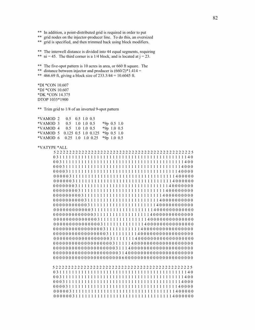
82
** In addition, a point-distributed grid is required in order to put ** grid nodes on the injector-producer line. To do this, an oversized ** grid is specified, and then trimmed back using block modifiers. ** The interwell distance is divided into 44 equal segments, requiring ** ni = 45. The third corner is a 1/4 block, and is located at j = 23. ** The five-spot pattern is 10 acres in area, or 660 ft square. The ** distance between injector and producer is (660/2)*1.414 = ** 466.69 ft, giving a block size of 233.3/44 = 10.6045 ft. *DI *CON 10.607 *DJ *CON 10.607 *DK *CON 14.375 DTOP 1035*1900 ** Trim grid to 1/8 of an inverted 9-spot pattern *VAMOD 2 0.5 0.5 1.0 0.5 *VAMOD 3 0.5 1.0 1.0 0.5 *9p 0.5 1.0 *VAMOD 4 0.5 1.0 1.0 0.5 *9p 1.0 0.5 *VAMOD 5 0.125 0.5 1.0 0.125 *9p 0.5 1.0 *VAMOD 6 0.25 1.0 1.0 0.25 *9p 1.0 0.5 *VATYPE *ALL
5 2 2 2 2 2 2 2 2 2 2 2 2 2 2 2 2 2 2 2 2 2 2 2 2 2 2 2 2 2 2 2 2 2 2 2 2 2 2 2 2 2 2 2 5 0 3 1 1 1 1 1 1 1 1 1 1 1 1 1 1 1 1 1 1 1 1 1 1 1 1 1 1 1 1 1 1 1 1 1 1 1 1 1 1 1 1 1 4 0 0 0 3 1 1 1 1 1 1 1 1 1 1 1 1 1 1 1 1 1 1 1 1 1 1 1 1 1 1 1 1 1 1 1 1 1 1 1 1 1 1 1 4 0 0 0 0 0 3 1 1 1 1 1 1 1 1 1 1 1 1 1 1 1 1 1 1 1 1 1 1 1 1 1 1 1 1 1 1 1 1 1 1 1 1 1 4 0 0 0 0 0 0 0 3 1 1 1 1 1 1 1 1 1 1 1 1 1 1 1 1 1 1 1 1 1 1 1 1 1 1 1 1 1 1 1 1 1 1 1 4 0 0 0 0 0 0 0 0 0 3 1 1 1 1 1 1 1 1 1 1 1 1 1 1 1 1 1 1 1 1 1 1 1 1 1 1 1 1 1 1 1 1 1 4 0 0 0 0 0 0 0 0 0 0 0 3 1 1 1 1 1 1 1 1 1 1 1 1 1 1 1 1 1 1 1 1 1 1 1 1 1 1 1 1 1 1 1 4 0 0 0 0 0 0 0 0 0 0 0 0 0 3 1 1 1 1 1 1 1 1 1 1 1 1 1 1 1 1 1 1 1 1 1 1 1 1 1 1 1 1 1 4 0 0 0 0 0 0 0 0 0 0 0 0 0 0 0 3 1 1 1 1 1 1 1 1 1 1 1 1 1 1 1 1 1 1 1 1 1 1 1 1 1 1 1 4 0 0 0 0 0 0 0 0 0 0 0 0 0 0 0 0 0 3 1 1 1 1 1 1 1 1 1 1 1 1 1 1 1 1 1 1 1 1 1 1 1 1 1 4 0 0 0 0 0 0 0 0 0 0 0 0 0 0 0 0 0 0 0 3 1 1 1 1 1 1 1 1 1 1 1 1 1 1 1 1 1 1 1 1 1 1 1 4 0 0 0 0 0 0 0 0 0 0 0 0 0 0 0 0 0 0 0 0 0 3 1 1 1 1 1 1 1 1 1 1 1 1 1 1 1 1 1 1 1 1 1 4 0 0 0 0 0 0 0 0 0 0 0 0 0 0 0 0 0 0 0 0 0 0 0 3 1 1 1 1 1 1 1 1 1 1 1 1 1 1 1 1 1 1 1 4 0 0 0 0 0 0 0 0 0 0 0 0 0 0 0 0 0 0 0 0 0 0 0 0 0 3 1 1 1 1 1 1 1 1 1 1 1 1 1 1 1 1 1 4 0 0 0 0 0 0 0 0 0 0 0 0 0 0 0 0 0 0 0 0 0 0 0 0 0 0 0 3 1 1 1 1 1 1 1 1 1 1 1 1 1 1 1 4 0 0 0 0 0 0 0 0 0 0 0 0 0 0 0 0 0 0 0 0 0 0 0 0 0 0 0 0 0 3 1 1 1 1 1 1 1 1 1 1 1 1 1 4 0 0 0 0 0 0 0 0 0 0 0 0 0 0 0 0 0 0 0 0 0 0 0 0 0 0 0 0 0 0 0 3 1 1 1 1 1 1 1 1 1 1 1 4 0 0 0 0 0 0 0 0 0 0 0 0 0 0 0 0 0 0 0 0 0 0 0 0 0 0 0 0 0 0 0 0 0 3 1 1 1 1 1 1 1 1 1 4 0 0 0 0 0 0 0 0 0 0 0 0 0 0 0 0 0 0 0 0 0 0 0 0 0 0 0 0 0 0 0 0 0 0 0 3 1 1 1 1 1 1 1 4 0 0 0 0 0 0 0 0 0 0 0 0 0 0 0 0 0 0 0 0 0 0 0 0 0 0 0 0 0 0 0 0 0 0 0 0 0 3 1 1 1 1 1 4 0 0 0 0 0 0 0 0 0 0 0 0 0 0 0 0 0 0 0 0 0 0 0 0 0 0 0 0 0 0 0 0 0 0 0 0 0 0 0 3 1 1 1 4 0 0 0 0 0 0 0 0 0 0 0 0 0 0 0 0 0 0 0 0 0 0 0 0 0 0 0 0 0 0 0 0 0 0 0 0 0 0 0 0 0 3 1 4 0 0 0 0 0 0 0 0 0 0 0 0 0 0 0 0 0 0 0 0 0 0 0 0 0 0 0 0 0 0 0 0 0 0 0 0 0 0 0 0 0 0 0 6 0 0 0 0 0 0 0 0 0 0 0 0 0 0 0 0 0 0 0 0 0 0
5 2 2 2 2 2 2 2 2 2 2 2 2 2 2 2 2 2 2 2 2 2 2 2 2 2 2 2 2 2 2 2 2 2 2 2 2 2 2 2 2 2 2 2 5 0 3 1 1 1 1 1 1 1 1 1 1 1 1 1 1 1 1 1 1 1 1 1 1 1 1 1 1 1 1 1 1 1 1 1 1 1 1 1 1 1 1 1 4 0 0 0 3 1 1 1 1 1 1 1 1 1 1 1 1 1 1 1 1 1 1 1 1 1 1 1 1 1 1 1 1 1 1 1 1 1 1 1 1 1 1 1 4 0 0 0 0 0 3 1 1 1 1 1 1 1 1 1 1 1 1 1 1 1 1 1 1 1 1 1 1 1 1 1 1 1 1 1 1 1 1 1 1 1 1 1 4 0 0 0 0 0 0 0 3 1 1 1 1 1 1 1 1 1 1 1 1 1 1 1 1 1 1 1 1 1 1 1 1 1 1 1 1 1 1 1 1 1 1 1 4 0 0 0 0 0 0 0 0 0 3 1 1 1 1 1 1 1 1 1 1 1 1 1 1 1 1 1 1 1 1 1 1 1 1 1 1 1 1 1 1 1 1 1 4 0 0 0 0 0 0 0 0 0 0 0 3 1 1 1 1 1 1 1 1 1 1 1 1 1 1 1 1 1 1 1 1 1 1 1 1 1 1 1 1 1 1 1 4 0 0 0 0 0 0

83
0 0 0 0 0 0 0 3 1 1 1 1 1 1 1 1 1 1 1 1 1 1 1 1 1 1 1 1 1 1 1 1 1 1 1 1 1 4 0 0 0 0 0 0 0 0 0 0 0 0 0 0 0 3 1 1 1 1 1 1 1 1 1 1 1 1 1 1 1 1 1 1 1 1 1 1 1 1 1 1 1 4 0 0 0 0 0 0 0 0 0 0 0 0 0 0 0 0 0 3 1 1 1 1 1 1 1 1 1 1 1 1 1 1 1 1 1 1 1 1 1 1 1 1 1 4 0 0 0 0 0 0 0 0 0 0 0 0 0 0 0 0 0 0 0 3 1 1 1 1 1 1 1 1 1 1 1 1 1 1 1 1 1 1 1 1 1 1 1 4 0 0 0 0 0 0 0 0 0 0 0 0 0 0 0 0 0 0 0 0 0 3 1 1 1 1 1 1 1 1 1 1 1 1 1 1 1 1 1 1 1 1 1 4 0 0 0 0 0 0 0 0 0 0 0 0 0 0 0 0 0 0 0 0 0 0 0 3 1 1 1 1 1 1 1 1 1 1 1 1 1 1 1 1 1 1 1 4 0 0 0 0 0 0 0 0 0 0 0 0 0 0 0 0 0 0 0 0 0 0 0 0 0 3 1 1 1 1 1 1 1 1 1 1 1 1 1 1 1 1 1 4 0 0 0 0 0 0 0 0 0 0 0 0 0 0 0 0 0 0 0 0 0 0 0 0 0 0 0 3 1 1 1 1 1 1 1 1 1 1 1 1 1 1 1 4 0 0 0 0 0 0 0 0 0 0 0 0 0 0 0 0 0 0 0 0 0 0 0 0 0 0 0 0 0 3 1 1 1 1 1 1 1 1 1 1 1 1 1 4 0 0 0 0 0 0 0 0 0 0 0 0 0 0 0 0 0 0 0 0 0 0 0 0 0 0 0 0 0 0 0 3 1 1 1 1 1 1 1 1 1 1 1 4 0 0 0 0 0 0 0 0 0 0 0 0 0 0 0 0 0 0 0 0 0 0 0 0 0 0 0 0 0 0 0 0 0 3 1 1 1 1 1 1 1 1 1 4 0 0 0 0 0 0 0 0 0 0 0 0 0 0 0 0 0 0 0 0 0 0 0 0 0 0 0 0 0 0 0 0 0 0 0 3 1 1 1 1 1 1 1 4 0 0 0 0 0 0 0 0 0 0 0 0 0 0 0 0 0 0 0 0 0 0 0 0 0 0 0 0 0 0 0 0 0 0 0 0 0 3 1 1 1 1 1 4 0 0 0 0 0 0 0 0 0 0 0 0 0 0 0 0 0 0 0 0 0 0 0 0 0 0 0 0 0 0 0 0 0 0 0 0 0 0 0 3 1 1 1 4 0 0 0 0 0 0 0 0 0 0 0 0 0 0 0 0 0 0 0 0 0 0 0 0 0 0 0 0 0 0 0 0 0 0 0 0 0 0 0 0 0 3 1 4 0 0 0 0 0 0 0 0 0 0 0 0 0 0 0 0 0 0 0 0 0 0 0 0 0 0 0 0 0 0 0 0 0 0 0 0 0 0 0 0 0 0 0 6 0 0 0 0 0 0 0 0 0 0 0 0 0 0 0 0 0 0 0 0 0 0
5 2 2 2 2 2 2 2 2 2 2 2 2 2 2 2 2 2 2 2 2 2 2 2 2 2 2 2 2 2 2 2 2 2 2 2 2 2 2 2 2 2 2 2 5 0 3 1 1 1 1 1 1 1 1 1 1 1 1 1 1 1 1 1 1 1 1 1 1 1 1 1 1 1 1 1 1 1 1 1 1 1 1 1 1 1 1 1 4 0 0 0 3 1 1 1 1 1 1 1 1 1 1 1 1 1 1 1 1 1 1 1 1 1 1 1 1 1 1 1 1 1 1 1 1 1 1 1 1 1 1 1 4 0 0 0 0 0 3 1 1 1 1 1 1 1 1 1 1 1 1 1 1 1 1 1 1 1 1 1 1 1 1 1 1 1 1 1 1 1 1 1 1 1 1 1 4 0 0 0 0 0 0 0 3 1 1 1 1 1 1 1 1 1 1 1 1 1 1 1 1 1 1 1 1 1 1 1 1 1 1 1 1 1 1 1 1 1 1 1 4 0 0 0 0 0 0 0 0 0 3 1 1 1 1 1 1 1 1 1 1 1 1 1 1 1 1 1 1 1 1 1 1 1 1 1 1 1 1 1 1 1 1 1 4 0 0 0 0 0 0 0 0 0 0 0 3 1 1 1 1 1 1 1 1 1 1 1 1 1 1 1 1 1 1 1 1 1 1 1 1 1 1 1 1 1 1 1 4 0 0 0 0 0 0 0 0 0 0 0 0 0 3 1 1 1 1 1 1 1 1 1 1 1 1 1 1 1 1 1 1 1 1 1 1 1 1 1 1 1 1 1 4 0 0 0 0 0 0 0 0 0 0 0 0 0 0 0 3 1 1 1 1 1 1 1 1 1 1 1 1 1 1 1 1 1 1 1 1 1 1 1 1 1 1 1 4 0 0 0 0 0 0 0 0 0 0 0 0 0 0 0 0 0 3 1 1 1 1 1 1 1 1 1 1 1 1 1 1 1 1 1 1 1 1 1 1 1 1 1 4 0 0 0 0 0 0 0 0 0 0 0 0 0 0 0 0 0 0 0 3 1 1 1 1 1 1 1 1 1 1 1 1 1 1 1 1 1 1 1 1 1 1 1 4 0 0 0 0 0 0 0 0 0 0 0 0 0 0 0 0 0 0 0 0 0 3 1 1 1 1 1 1 1 1 1 1 1 1 1 1 1 1 1 1 1 1 1 4 0 0 0 0 0 0 0 0 0 0 0 0 0 0 0 0 0 0 0 0 0 0 0 3 1 1 1 1 1 1 1 1 1 1 1 1 1 1 1 1 1 1 1 4 0 0 0 0 0 0 0 0 0 0 0 0 0 0 0 0 0 0 0 0 0 0 0 0 0 3 1 1 1 1 1 1 1 1 1 1 1 1 1 1 1 1 1 4 0 0 0 0 0 0 0 0 0 0 0 0 0 0 0 0 0 0 0 0 0 0 0 0 0 0 0 3 1 1 1 1 1 1 1 1 1 1 1 1 1 1 1 4 0 0 0 0 0 0 0 0 0 0 0 0 0 0 0 0 0 0 0 0 0 0 0 0 0 0 0 0 0 3 1 1 1 1 1 1 1 1 1 1 1 1 1 4 0 0 0 0 0 0 0 0 0 0 0 0 0 0 0 0 0 0 0 0 0 0 0 0 0 0 0 0 0 0 0 3 1 1 1 1 1 1 1 1 1 1 1 4 0 0 0 0 0 0 0 0 0 0 0 0 0 0 0 0 0 0 0 0 0 0 0 0 0 0 0 0 0 0 0 0 0 3 1 1 1 1 1 1 1 1 1 4 0 0 0 0 0 0 0 0 0 0 0 0 0 0 0 0 0 0 0 0 0 0 0 0 0 0 0 0 0 0 0 0 0 0 0 3 1 1 1 1 1 1 1 4 0 0 0 0 0 0 0 0 0 0 0 0 0 0 0 0 0 0 0 0 0 0 0 0 0 0 0 0 0 0 0 0 0 0 0 0 0 3 1 1 1 1 1 4 0 0 0 0 0 0 0 0 0 0 0 0 0 0 0 0 0 0 0 0 0 0 0 0 0 0 0 0 0 0 0 0 0 0 0 0 0 0 0 3 1 1 1 4 0 0 0 0 0 0 0 0 0 0 0 0 0 0 0 0 0 0 0 0 0 0 0 0 0 0 0 0 0 0 0 0 0 0 0 0 0 0 0 0 0 3 1 4 0 0 0 0 0 0 0 0 0 0 0 0 0 0 0 0 0 0 0 0 0 0 0 0 0 0 0 0 0 0 0 0 0 0 0 0 0 0 0 0 0 0 0 6 0 0 0 0 0 0 0 0 0 0 0 0 0 0 0 0 0 0 0 0 0 0
5 2 2 2 2 2 2 2 2 2 2 2 2 2 2 2 2 2 2 2 2 2 2 2 2 2 2 2 2 2 2 2 2 2 2 2 2 2 2 2 2 2 2 2 5 0 3 1 1 1 1 1 1 1 1 1 1 1 1 1 1 1 1 1 1 1 1 1 1 1 1 1 1 1 1 1 1 1 1 1 1 1 1 1 1 1 1 1 4 0 0 0 3 1 1 1 1 1 1 1 1 1 1 1 1 1 1 1 1 1 1 1 1 1 1 1 1 1 1 1 1 1 1 1 1 1 1 1 1 1 1 1 4 0 0 0 0 0 3 1 1 1 1 1 1 1 1 1 1 1 1 1 1 1 1 1 1 1 1 1 1 1 1 1 1 1 1 1 1 1 1 1 1 1 1 1 4 0 0 0 0 0 0 0 3 1 1 1 1 1 1 1 1 1 1 1 1 1 1 1 1 1 1 1 1 1 1 1 1 1 1 1 1 1 1 1 1 1 1 1 4 0 0 0 0 0 0 0 0 0 3 1 1 1 1 1 1 1 1 1 1 1 1 1 1 1 1 1 1 1 1 1 1 1 1 1 1 1 1 1 1 1 1 1 4 0 0 0 0 0 0 0 0 0 0 0 3 1 1 1 1 1 1 1 1 1 1 1 1 1 1 1 1 1 1 1 1 1 1 1 1 1 1 1 1 1 1 1 4 0 0 0 0 0 0 0 0 0 0 0 0 0 3 1 1 1 1 1 1 1 1 1 1 1 1 1 1 1 1 1 1 1 1 1 1 1 1 1 1 1 1 1 4 0 0 0 0 0 0 0 0 0 0 0 0 0 0 0 3 1 1 1 1 1 1 1 1 1 1 1 1 1 1 1 1 1 1 1 1 1 1 1 1 1 1 1 4 0 0 0 0 0 0 0 0 0 0 0 0 0 0 0 0 0 3 1 1 1 1 1 1 1 1 1 1 1 1 1 1 1 1 1 1 1 1 1 1 1 1 1 4 0 0 0 0 0 0 0 0 0 0 0 0 0 0 0 0 0 0 0 3 1 1 1 1 1 1 1 1 1 1 1 1 1 1 1 1 1 1 1 1 1 1 1 4 0 0 0 0 0 0 0 0 0 0 0 0 0 0 0 0 0 0 0 0 0 3 1 1 1 1 1 1 1 1 1 1 1 1 1 1 1 1 1 1 1 1 1 4 0 0 0 0 0 0 0 0 0 0 0 0 0 0 0 0 0 0 0 0 0 0 0 3 1 1 1 1 1 1 1 1 1 1 1 1 1 1 1 1 1 1 1 4 0 0 0 0 0 0 0 0 0 0 0 0 0 0 0 0 0 0 0 0 0 0 0 0 0 3 1 1 1 1 1 1 1 1 1 1 1 1 1 1 1 1 1 4 0 0 0 0 0 0 0 0 0 0 0 0 0 0 0 0 0 0 0 0 0 0 0 0 0 0 0 3 1 1 1 1 1 1 1 1 1 1 1 1 1 1 1 4 0 0 0 0 0 0 0 0 0 0 0 0 0 0

84
0 0 0 0 0 0 0 0 0 0 0 0 0 0 0 3 1 1 1 1 1 1 1 1 1 1 1 1 1 4 0 0 0 0 0 0 0 0 0 0 0 0 0 0 0 0 0 0 0 0 0 0 0 0 0 0 0 0 0 0 0 3 1 1 1 1 1 1 1 1 1 1 1 4 0 0 0 0 0 0 0 0 0 0 0 0 0 0 0 0 0 0 0 0 0 0 0 0 0 0 0 0 0 0 0 0 0 3 1 1 1 1 1 1 1 1 1 4 0 0 0 0 0 0 0 0 0 0 0 0 0 0 0 0 0 0 0 0 0 0 0 0 0 0 0 0 0 0 0 0 0 0 0 3 1 1 1 1 1 1 1 4 0 0 0 0 0 0 0 0 0 0 0 0 0 0 0 0 0 0 0 0 0 0 0 0 0 0 0 0 0 0 0 0 0 0 0 0 0 3 1 1 1 1 1 4 0 0 0 0 0 0 0 0 0 0 0 0 0 0 0 0 0 0 0 0 0 0 0 0 0 0 0 0 0 0 0 0 0 0 0 0 0 0 0 3 1 1 1 4 0 0 0 0 0 0 0 0 0 0 0 0 0 0 0 0 0 0 0 0 0 0 0 0 0 0 0 0 0 0 0 0 0 0 0 0 0 0 0 0 0 3 1 4 0 0 0 0 0 0 0 0 0 0 0 0 0 0 0 0 0 0 0 0 0 0 0 0 0 0 0 0 0 0 0 0 0 0 0 0 0 0 0 0 0 0 0 6 0 0 0 0 0 0 0 0 0 0 0 0 0 0 0 0 0 0 0 0 0 0
5 2 2 2 2 2 2 2 2 2 2 2 2 2 2 2 2 2 2 2 2 2 2 2 2 2 2 2 2 2 2 2 2 2 2 2 2 2 2 2 2 2 2 2 5 0 3 1 1 1 1 1 1 1 1 1 1 1 1 1 1 1 1 1 1 1 1 1 1 1 1 1 1 1 1 1 1 1 1 1 1 1 1 1 1 1 1 1 4 0 0 0 3 1 1 1 1 1 1 1 1 1 1 1 1 1 1 1 1 1 1 1 1 1 1 1 1 1 1 1 1 1 1 1 1 1 1 1 1 1 1 1 4 0 0 0 0 0 3 1 1 1 1 1 1 1 1 1 1 1 1 1 1 1 1 1 1 1 1 1 1 1 1 1 1 1 1 1 1 1 1 1 1 1 1 1 4 0 0 0 0 0 0 0 3 1 1 1 1 1 1 1 1 1 1 1 1 1 1 1 1 1 1 1 1 1 1 1 1 1 1 1 1 1 1 1 1 1 1 1 4 0 0 0 0 0 0 0 0 0 3 1 1 1 1 1 1 1 1 1 1 1 1 1 1 1 1 1 1 1 1 1 1 1 1 1 1 1 1 1 1 1 1 1 4 0 0 0 0 0 0 0 0 0 0 0 3 1 1 1 1 1 1 1 1 1 1 1 1 1 1 1 1 1 1 1 1 1 1 1 1 1 1 1 1 1 1 1 4 0 0 0 0 0 0 0 0 0 0 0 0 0 3 1 1 1 1 1 1 1 1 1 1 1 1 1 1 1 1 1 1 1 1 1 1 1 1 1 1 1 1 1 4 0 0 0 0 0 0 0 0 0 0 0 0 0 0 0 3 1 1 1 1 1 1 1 1 1 1 1 1 1 1 1 1 1 1 1 1 1 1 1 1 1 1 1 4 0 0 0 0 0 0 0 0 0 0 0 0 0 0 0 0 0 3 1 1 1 1 1 1 1 1 1 1 1 1 1 1 1 1 1 1 1 1 1 1 1 1 1 4 0 0 0 0 0 0 0 0 0 0 0 0 0 0 0 0 0 0 0 3 1 1 1 1 1 1 1 1 1 1 1 1 1 1 1 1 1 1 1 1 1 1 1 4 0 0 0 0 0 0 0 0 0 0 0 0 0 0 0 0 0 0 0 0 0 3 1 1 1 1 1 1 1 1 1 1 1 1 1 1 1 1 1 1 1 1 1 4 0 0 0 0 0 0 0 0 0 0 0 0 0 0 0 0 0 0 0 0 0 0 0 3 1 1 1 1 1 1 1 1 1 1 1 1 1 1 1 1 1 1 1 4 0 0 0 0 0 0 0 0 0 0 0 0 0 0 0 0 0 0 0 0 0 0 0 0 0 3 1 1 1 1 1 1 1 1 1 1 1 1 1 1 1 1 1 4 0 0 0 0 0 0 0 0 0 0 0 0 0 0 0 0 0 0 0 0 0 0 0 0 0 0 0 3 1 1 1 1 1 1 1 1 1 1 1 1 1 1 1 4 0 0 0 0 0 0 0 0 0 0 0 0 0 0 0 0 0 0 0 0 0 0 0 0 0 0 0 0 0 3 1 1 1 1 1 1 1 1 1 1 1 1 1 4 0 0 0 0 0 0 0 0 0 0 0 0 0 0 0 0 0 0 0 0 0 0 0 0 0 0 0 0 0 0 0 3 1 1 1 1 1 1 1 1 1 1 1 4 0 0 0 0 0 0 0 0 0 0 0 0 0 0 0 0 0 0 0 0 0 0 0 0 0 0 0 0 0 0 0 0 0 3 1 1 1 1 1 1 1 1 1 4 0 0 0 0 0 0 0 0 0 0 0 0 0 0 0 0 0 0 0 0 0 0 0 0 0 0 0 0 0 0 0 0 0 0 0 3 1 1 1 1 1 1 1 4 0 0 0 0 0 0 0 0 0 0 0 0 0 0 0 0 0 0 0 0 0 0 0 0 0 0 0 0 0 0 0 0 0 0 0 0 0 3 1 1 1 1 1 4 0 0 0 0 0 0 0 0 0 0 0 0 0 0 0 0 0 0 0 0 0 0 0 0 0 0 0 0 0 0 0 0 0 0 0 0 0 0 0 3 1 1 1 4 0 0 0 0 0 0 0 0 0 0 0 0 0 0 0 0 0 0 0 0 0 0 0 0 0 0 0 0 0 0 0 0 0 0 0 0 0 0 0 0 0 3 1 4 0 0 0 0 0 0 0 0 0 0 0 0 0 0 0 0 0 0 0 0 0 0 0 0 0 0 0 0 0 0 0 0 0 0 0 0 0 0 0 0 0 0 0 6 0 0 0 0 0 0 0 0 0 0 0 0 0 0 0 0 0 0 0 0 0 0
5 2 2 2 2 2 2 2 2 2 2 2 2 2 2 2 2 2 2 2 2 2 2 2 2 2 2 2 2 2 2 2 2 2 2 2 2 2 2 2 2 2 2 2 5 0 3 1 1 1 1 1 1 1 1 1 1 1 1 1 1 1 1 1 1 1 1 1 1 1 1 1 1 1 1 1 1 1 1 1 1 1 1 1 1 1 1 1 4 0 0 0 3 1 1 1 1 1 1 1 1 1 1 1 1 1 1 1 1 1 1 1 1 1 1 1 1 1 1 1 1 1 1 1 1 1 1 1 1 1 1 1 4 0 0 0 0 0 3 1 1 1 1 1 1 1 1 1 1 1 1 1 1 1 1 1 1 1 1 1 1 1 1 1 1 1 1 1 1 1 1 1 1 1 1 1 4 0 0 0 0 0 0 0 3 1 1 1 1 1 1 1 1 1 1 1 1 1 1 1 1 1 1 1 1 1 1 1 1 1 1 1 1 1 1 1 1 1 1 1 4 0 0 0 0 0 0 0 0 0 3 1 1 1 1 1 1 1 1 1 1 1 1 1 1 1 1 1 1 1 1 1 1 1 1 1 1 1 1 1 1 1 1 1 4 0 0 0 0 0 0 0 0 0 0 0 3 1 1 1 1 1 1 1 1 1 1 1 1 1 1 1 1 1 1 1 1 1 1 1 1 1 1 1 1 1 1 1 4 0 0 0 0 0 0 0 0 0 0 0 0 0 3 1 1 1 1 1 1 1 1 1 1 1 1 1 1 1 1 1 1 1 1 1 1 1 1 1 1 1 1 1 4 0 0 0 0 0 0 0 0 0 0 0 0 0 0 0 3 1 1 1 1 1 1 1 1 1 1 1 1 1 1 1 1 1 1 1 1 1 1 1 1 1 1 1 4 0 0 0 0 0 0 0 0 0 0 0 0 0 0 0 0 0 3 1 1 1 1 1 1 1 1 1 1 1 1 1 1 1 1 1 1 1 1 1 1 1 1 1 4 0 0 0 0 0 0 0 0 0 0 0 0 0 0 0 0 0 0 0 3 1 1 1 1 1 1 1 1 1 1 1 1 1 1 1 1 1 1 1 1 1 1 1 4 0 0 0 0 0 0 0 0 0 0 0 0 0 0 0 0 0 0 0 0 0 3 1 1 1 1 1 1 1 1 1 1 1 1 1 1 1 1 1 1 1 1 1 4 0 0 0 0 0 0 0 0 0 0 0 0 0 0 0 0 0 0 0 0 0 0 0 3 1 1 1 1 1 1 1 1 1 1 1 1 1 1 1 1 1 1 1 4 0 0 0 0 0 0 0 0 0 0 0 0 0 0 0 0 0 0 0 0 0 0 0 0 0 3 1 1 1 1 1 1 1 1 1 1 1 1 1 1 1 1 1 4 0 0 0 0 0 0 0 0 0 0 0 0 0 0 0 0 0 0 0 0 0 0 0 0 0 0 0 3 1 1 1 1 1 1 1 1 1 1 1 1 1 1 1 4 0 0 0 0 0 0 0 0 0 0 0 0 0 0 0 0 0 0 0 0 0 0 0 0 0 0 0 0 0 3 1 1 1 1 1 1 1 1 1 1 1 1 1 4 0 0 0 0 0 0 0 0 0 0 0 0 0 0 0 0 0 0 0 0 0 0 0 0 0 0 0 0 0 0 0 3 1 1 1 1 1 1 1 1 1 1 1 4 0 0 0 0 0 0 0 0 0 0 0 0 0 0 0 0 0 0 0 0 0 0 0 0 0 0 0 0 0 0 0 0 0 3 1 1 1 1 1 1 1 1 1 4 0 0 0 0 0 0 0 0 0 0 0 0 0 0 0 0 0 0 0 0 0 0 0 0 0 0 0 0 0 0 0 0 0 0 0 3 1 1 1 1 1 1 1 4 0 0 0 0 0 0 0 0 0 0 0 0 0 0 0 0 0 0 0 0 0 0 0 0 0 0 0 0 0 0 0 0 0 0 0 0 0 3 1 1 1 1 1 4 0 0 0 0 0 0 0 0 0 0 0 0 0 0 0 0 0 0 0 0 0 0 0 0 0 0 0 0 0 0 0 0 0 0 0 0 0 0 0 3 1 1 1 4 0 0 0 0 0 0 0 0 0 0 0 0 0 0 0 0 0 0 0 0 0 0 0 0 0 0 0 0 0 0 0 0 0 0 0 0 0 0 0 0 0 3 1 4 0 0 0 0 0 0 0 0 0 0 0 0 0 0 0 0 0 0 0 0 0 0 0 0 0 0 0 0 0 0 0 0 0 0 0 0 0 0 0 0 0 0 0 6 0 0 0 0 0 0 0 0 0 0 0 0 0 0 0 0 0 0 0 0 0 0

85
5 2 2 2 2 2 2 2 2 2 2 2 2 2 2 2 2 2 2 2 2 2 2 2 2 2 2 2 2 2 2 2 2 2 2 2 2 2 2 2 2 2 2 2 5 0 3 1 1 1 1 1 1 1 1 1 1 1 1 1 1 1 1 1 1 1 1 1 1 1 1 1 1 1 1 1 1 1 1 1 1 1 1 1 1 1 1 1 4 0 0 0 3 1 1 1 1 1 1 1 1 1 1 1 1 1 1 1 1 1 1 1 1 1 1 1 1 1 1 1 1 1 1 1 1 1 1 1 1 1 1 1 4 0 0 0 0 0 3 1 1 1 1 1 1 1 1 1 1 1 1 1 1 1 1 1 1 1 1 1 1 1 1 1 1 1 1 1 1 1 1 1 1 1 1 1 4 0 0 0 0 0 0 0 3 1 1 1 1 1 1 1 1 1 1 1 1 1 1 1 1 1 1 1 1 1 1 1 1 1 1 1 1 1 1 1 1 1 1 1 4 0 0 0 0 0 0 0 0 0 3 1 1 1 1 1 1 1 1 1 1 1 1 1 1 1 1 1 1 1 1 1 1 1 1 1 1 1 1 1 1 1 1 1 4 0 0 0 0 0 0 0 0 0 0 0 3 1 1 1 1 1 1 1 1 1 1 1 1 1 1 1 1 1 1 1 1 1 1 1 1 1 1 1 1 1 1 1 4 0 0 0 0 0 0 0 0 0 0 0 0 0 3 1 1 1 1 1 1 1 1 1 1 1 1 1 1 1 1 1 1 1 1 1 1 1 1 1 1 1 1 1 4 0 0 0 0 0 0 0 0 0 0 0 0 0 0 0 3 1 1 1 1 1 1 1 1 1 1 1 1 1 1 1 1 1 1 1 1 1 1 1 1 1 1 1 4 0 0 0 0 0 0 0 0 0 0 0 0 0 0 0 0 0 3 1 1 1 1 1 1 1 1 1 1 1 1 1 1 1 1 1 1 1 1 1 1 1 1 1 4 0 0 0 0 0 0 0 0 0 0 0 0 0 0 0 0 0 0 0 3 1 1 1 1 1 1 1 1 1 1 1 1 1 1 1 1 1 1 1 1 1 1 1 4 0 0 0 0 0 0 0 0 0 0 0 0 0 0 0 0 0 0 0 0 0 3 1 1 1 1 1 1 1 1 1 1 1 1 1 1 1 1 1 1 1 1 1 4 0 0 0 0 0 0 0 0 0 0 0 0 0 0 0 0 0 0 0 0 0 0 0 3 1 1 1 1 1 1 1 1 1 1 1 1 1 1 1 1 1 1 1 4 0 0 0 0 0 0 0 0 0 0 0 0 0 0 0 0 0 0 0 0 0 0 0 0 0 3 1 1 1 1 1 1 1 1 1 1 1 1 1 1 1 1 1 4 0 0 0 0 0 0 0 0 0 0 0 0 0 0 0 0 0 0 0 0 0 0 0 0 0 0 0 3 1 1 1 1 1 1 1 1 1 1 1 1 1 1 1 4 0 0 0 0 0 0 0 0 0 0 0 0 0 0 0 0 0 0 0 0 0 0 0 0 0 0 0 0 0 3 1 1 1 1 1 1 1 1 1 1 1 1 1 4 0 0 0 0 0 0 0 0 0 0 0 0 0 0 0 0 0 0 0 0 0 0 0 0 0 0 0 0 0 0 0 3 1 1 1 1 1 1 1 1 1 1 1 4 0 0 0 0 0 0 0 0 0 0 0 0 0 0 0 0 0 0 0 0 0 0 0 0 0 0 0 0 0 0 0 0 0 3 1 1 1 1 1 1 1 1 1 4 0 0 0 0 0 0 0 0 0 0 0 0 0 0 0 0 0 0 0 0 0 0 0 0 0 0 0 0 0 0 0 0 0 0 0 3 1 1 1 1 1 1 1 4 0 0 0 0 0 0 0 0 0 0 0 0 0 0 0 0 0 0 0 0 0 0 0 0 0 0 0 0 0 0 0 0 0 0 0 0 0 3 1 1 1 1 1 4 0 0 0 0 0 0 0 0 0 0 0 0 0 0 0 0 0 0 0 0 0 0 0 0 0 0 0 0 0 0 0 0 0 0 0 0 0 0 0 3 1 1 1 4 0 0 0 0 0 0 0 0 0 0 0 0 0 0 0 0 0 0 0 0 0 0 0 0 0 0 0 0 0 0 0 0 0 0 0 0 0 0 0 0 0 3 1 4 0 0 0 0 0 0 0 0 0 0 0 0 0 0 0 0 0 0 0 0 0 0 0 0 0 0 0 0 0 0 0 0 0 0 0 0 0 0 0 0 0 0 0 6 0 0 0 0 0 0 0 0 0 0 0 0 0 0 0 0 0 0 0 0 0 0
5 2 2 2 2 2 2 2 2 2 2 2 2 2 2 2 2 2 2 2 2 2 2 2 2 2 2 2 2 2 2 2 2 2 2 2 2 2 2 2 2 2 2 2 5 0 3 1 1 1 1 1 1 1 1 1 1 1 1 1 1 1 1 1 1 1 1 1 1 1 1 1 1 1 1 1 1 1 1 1 1 1 1 1 1 1 1 1 4 0 0 0 3 1 1 1 1 1 1 1 1 1 1 1 1 1 1 1 1 1 1 1 1 1 1 1 1 1 1 1 1 1 1 1 1 1 1 1 1 1 1 1 4 0 0 0 0 0 3 1 1 1 1 1 1 1 1 1 1 1 1 1 1 1 1 1 1 1 1 1 1 1 1 1 1 1 1 1 1 1 1 1 1 1 1 1 4 0 0 0 0 0 0 0 3 1 1 1 1 1 1 1 1 1 1 1 1 1 1 1 1 1 1 1 1 1 1 1 1 1 1 1 1 1 1 1 1 1 1 1 4 0 0 0 0 0 0 0 0 0 3 1 1 1 1 1 1 1 1 1 1 1 1 1 1 1 1 1 1 1 1 1 1 1 1 1 1 1 1 1 1 1 1 1 4 0 0 0 0 0 0 0 0 0 0 0 3 1 1 1 1 1 1 1 1 1 1 1 1 1 1 1 1 1 1 1 1 1 1 1 1 1 1 1 1 1 1 1 4 0 0 0 0 0 0 0 0 0 0 0 0 0 3 1 1 1 1 1 1 1 1 1 1 1 1 1 1 1 1 1 1 1 1 1 1 1 1 1 1 1 1 1 4 0 0 0 0 0 0 0 0 0 0 0 0 0 0 0 3 1 1 1 1 1 1 1 1 1 1 1 1 1 1 1 1 1 1 1 1 1 1 1 1 1 1 1 4 0 0 0 0 0 0 0 0 0 0 0 0 0 0 0 0 0 3 1 1 1 1 1 1 1 1 1 1 1 1 1 1 1 1 1 1 1 1 1 1 1 1 1 4 0 0 0 0 0 0 0 0 0 0 0 0 0 0 0 0 0 0 0 3 1 1 1 1 1 1 1 1 1 1 1 1 1 1 1 1 1 1 1 1 1 1 1 4 0 0 0 0 0 0 0 0 0 0 0 0 0 0 0 0 0 0 0 0 0 3 1 1 1 1 1 1 1 1 1 1 1 1 1 1 1 1 1 1 1 1 1 4 0 0 0 0 0 0 0 0 0 0 0 0 0 0 0 0 0 0 0 0 0 0 0 3 1 1 1 1 1 1 1 1 1 1 1 1 1 1 1 1 1 1 1 4 0 0 0 0 0 0 0 0 0 0 0 0 0 0 0 0 0 0 0 0 0 0 0 0 0 3 1 1 1 1 1 1 1 1 1 1 1 1 1 1 1 1 1 4 0 0 0 0 0 0 0 0 0 0 0 0 0 0 0 0 0 0 0 0 0 0 0 0 0 0 0 3 1 1 1 1 1 1 1 1 1 1 1 1 1 1 1 4 0 0 0 0 0 0 0 0 0 0 0 0 0 0 0 0 0 0 0 0 0 0 0 0 0 0 0 0 0 3 1 1 1 1 1 1 1 1 1 1 1 1 1 4 0 0 0 0 0 0 0 0 0 0 0 0 0 0 0 0 0 0 0 0 0 0 0 0 0 0 0 0 0 0 0 3 1 1 1 1 1 1 1 1 1 1 1 4 0 0 0 0 0 0 0 0 0 0 0 0 0 0 0 0 0 0 0 0 0 0 0 0 0 0 0 0 0 0 0 0 0 3 1 1 1 1 1 1 1 1 1 4 0 0 0 0 0 0 0 0 0 0 0 0 0 0 0 0 0 0 0 0 0 0 0 0 0 0 0 0 0 0 0 0 0 0 0 3 1 1 1 1 1 1 1 4 0 0 0 0 0 0 0 0 0 0 0 0 0 0 0 0 0 0 0 0 0 0 0 0 0 0 0 0 0 0 0 0 0 0 0 0 0 3 1 1 1 1 1 4 0 0 0 0 0 0 0 0 0 0 0 0 0 0 0 0 0 0 0 0 0 0 0 0 0 0 0 0 0 0 0 0 0 0 0 0 0 0 0 3 1 1 1 4 0 0 0 0 0 0 0 0 0 0 0 0 0 0 0 0 0 0 0 0 0 0 0 0 0 0 0 0 0 0 0 0 0 0 0 0 0 0 0 0 0 3 1 4 0 0 0 0 0 0 0 0 0 0 0 0 0 0 0 0 0 0 0 0 0 0 0 0 0 0 0 0 0 0 0 0 0 0 0 0 0 0 0 0 0 0 0 6 0 0 0 0 0 0 0 0 0 0 0 0 0 0 0 0 0 0 0 0 0 0 *POR *CON 0.345 *PERMI *CON 6922 *PERMJ *EQUALSI *PERMK *EQUALSI / 10

86
*END-GRID *CPOR 8E-04 *PRPOR 275 *ROCKCP 35.02 *THCONR 24 *THCONW 24 *THCONO 24 *THCONG 24 *HLOSSPROP *OVERBUR 60 24 *UNDERBUR 60 24 ** ============== FLUID DEFINITIONS ====================== *MODEL 3 3 3 ** Components are water and live oil (consists of ‘GAS’ and ‘OIL’). COMPNAME 'WATER' 'OIL' 'GAS' ** -------- -------- -------- CMM 0.0000 456.015 16.7278 PCRIT 0.00 179.02 670.46 TCRIT 0.00 1036.21 -107.35 KV1 0.000E+0 5.165E+6 1.534E+5 KV2 0.000E+0 0.000E+0 0.000E+0 KV3 0.000E+0 0.000E+0 0.000E+0 KV4 0.0 -15362.5 -1914.1 KV5 0.00 -459.67 -459.67 MOLDEN 0.000E+00 1.356E-01 4.515E-02 CP 0.000E+00 3.805E-06 3.754E-03 CT1 0.000E+00 1.660E-04 1.910E-03 VISCTABLE ** T, deg F 'WATER' 'OIL' 'GAS' ** -------- ----- -------- 50.000 0.0000E+00 500000 1.1018E-02 100.000 0.0000E+00 20000 1.1882E-02 150.000 0.0000E+00 1500 1.2721E-02 200.000 0.0000E+00 240 1.3536E-02 250.000 0.0000E+00 60 1.4326E-02 300.000 0.0000E+00 20 1.5094E-02 350.000 0.0000E+00 8 1.5840E-02 400.000 0.0000E+00 3.5 1.6566E-02 450.000 0.0000E+00 1.8 1.7273E-02 500.000 0.0000E+00 1 1.7962E-02 550.000 0.0000E+00 0.6 1.8635E-02 600.000 0.0000E+00 0.35 1.9293E-02 650.000 0.0000E+00 0.2 1.9937E-02 700.000 0.0000E+00 0.13 2.0568E-02 PRSR 275.000 ** reference pressure, corresponding to the density TEMR 127.000 ** reference temperature, corresponding to the density PSURF 14.696 ** pressure at surface, for reporting well rates, etc. TSURF 60.000 ** temperature at surface, for reporting well rates, etc.
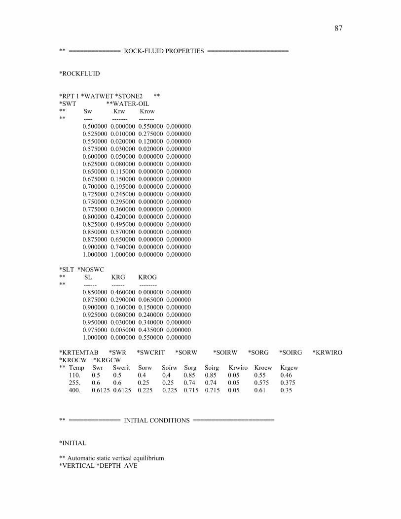
87
** ============== ROCK-FLUID PROPERTIES ====================== *ROCKFLUID *RPT 1 *WATWET *STONE2 ** *SWT **WATER-OIL ** Sw Krw Krow ** ---- ------- -------
0.500000 0.000000 0.550000 0.000000 0.525000 0.010000 0.275000 0.000000 0.550000 0.020000 0.120000 0.000000 0.575000 0.030000 0.020000 0.000000 0.600000 0.050000 0.000000 0.000000 0.625000 0.080000 0.000000 0.000000 0.650000 0.115000 0.000000 0.000000 0.675000 0.150000 0.000000 0.000000 0.700000 0.195000 0.000000 0.000000 0.725000 0.245000 0.000000 0.000000 0.750000 0.295000 0.000000 0.000000 0.775000 0.360000 0.000000 0.000000 0.800000 0.420000 0.000000 0.000000 0.825000 0.495000 0.000000 0.000000 0.850000 0.570000 0.000000 0.000000 0.875000 0.650000 0.000000 0.000000 0.900000 0.740000 0.000000 0.000000 1.000000 1.000000 0.000000 0.000000
*SLT *NOSWC ** SL KRG KROG ** ------ ------ --------
0.850000 0.460000 0.000000 0.000000 0.875000 0.290000 0.065000 0.000000 0.900000 0.160000 0.150000 0.000000 0.925000 0.080000 0.240000 0.000000 0.950000 0.030000 0.340000 0.000000 0.975000 0.005000 0.435000 0.000000 1.000000 0.000000 0.550000 0.000000
*KRTEMTAB *SWR *SWCRIT *SORW *SOIRW *SORG *SOIRG *KRWIRO *KROCW *KRGCW ** Temp Swr Swcrit Sorw Soirw Sorg Soirg Krwiro Krocw Krgcw 110. 0.5 0.5 0.4 0.4 0.85 0.85 0.05 0.55 0.46 255. 0.6 0.6 0.25 0.25 0.74 0.74 0.05 0.575 0.375 400. 0.6125 0.6125 0.225 0.225 0.715 0.715 0.05 0.61 0.35 ** ============== INITIAL CONDITIONS ====================== *INITIAL ** Automatic static vertical equilibrium *VERTICAL *DEPTH_AVE

88
*REFPRES 275 *REFDEPTH 1957.5 SW CON 0.267 SO CON 0.733 *TEMP *CON 127 MFRAC_OIL 'OIL' CON 0.78904 MFRAC_GAS 'GAS' CON 0.21096 ** ============== NUMERICAL CONTROL ====================== *NUMERICAL *NORM *PRESS 200 *SATUR 0.2 *TEMP 50 *RUN ** ============== RECURRENT DATA ====================== ** Project starts on January 01, 2004 *DATE 2004 01 01 *DTWELL 1 ** o *WELL 1 'INJECTOR' *VERT 1 1 *FRAC .125 ** o o o *WELL 2 'PRODUCER' *VERT 45 1 *FRAC .125 ** o o o o o ** o o o o o o o ** 1 o o o o o o o 2 *INJECTOR *MOBWEIGHT 'INJECTOR' *INCOMP WATER 1.0 0.0 0.0 *TINJW 582.3 QUAL .8 *OPERATE *BHP 1350 *OPERATE *MAX *STW 1600 *PERFV 'INJECTOR' ** k wi ** Inject only in the bottom layer ** 2*pi*k*h / ln(cc*sqrt((dx**2+dy**2)/pi)/rw) 5 320715.436 ** k = 6922 md, h = 14.375 ft, dx = dy = 10.607 ft, 6 320715.436 ** cc = 0.249, rw = 0.3 ft 7 320715.436 8 320715.436 *PRODUCER 'PRODUCER' *OPERATE *BHP 15 *OPERATE *MAX *STL 5000 **OPERATE *MAX *STEAM 10 ** Steam CWE in bbl/day *PERFV 'PRODUCER' ** k wi

89
5 320715.436 6 320715.436 7 320715.436 8 320715.436 OPEN 'PRODUCER' OPEN 'INJECTOR' *TIME 365 *TIME 730 *TIME 1095 *TIME 1460 *TIME 1825 *TIME 2190 *TIME 2555 *TIME 2920 *TIME 3285 *TIME 3650 *TIME 4015 *TIME 4380 *TIME 4745 *TIME 5110 *TIME 5475 *TIME 5840 *TIME 6205 *TIME 6570 *TIME 6935 *TIME 7300 *STOP

90
APPENDIX D
SIMULATION INPUT DATA FOR HAMACA CASE AREA = 10 ACRE, STEAM INJECTION RATE = 1600 STB/D
***************************************************************************** ** Template Hamaca Field ** ***************************************************************************** ************************************************************************************** ** ** ** FILE : Hamaca.DAT ** ** ** ** MODEL: INVERTED 5 SPOT STEAM DRIVE FIELD UNITS 45X23X8 CARTESIAN GRID ** ** AREA AND BLOCK MODIFIERS 1/8 PATTERN ** ** 9 POINT TRANSMISSIBLITY ** ** ** ** ** ** USAGE: HAMACA FIELD STEAM DRIVE SIMULATION ** ** ** ************************************************************************************** ** ============== INPUT/OUTPUT CONTROL ====================== RESULTS SIMULATOR STARS *FILENAME *OUTPUT *INDEX-OUT *MAIN-RESULTS-OUT ** Use default file names **CHECKONLY *INTERRUPT *STOP *TITLE1 'Hamaca Case' *TITLE2 'Hamaca Field' *TITLE3 'Area = 10 Acre Injection Rate = 1600 STB/D' *INUNIT *FIELD ** output same as input *OUTPRN *GRID *PRES *SW *SO *SG *TEMP *Y *X *W *SOLCONC *OBHLOSS *VISO *OUTPRN *WELL *ALL *WRST 300 *WPRN *GRID 300 *WPRN *ITER 300 *OUTSRF *WELL *LAYER ALL ** ============== GRID AND RESERVOIR DEFINITION ================= *GRID *CART 45 23 8 *KDIR *DOWN *NINEPOINT *IJ ** The triangular area of 1/8 of five-spot pattern is covered with a ** 45x23 grid with grid lines horizontal to the line linking the injector ** with the producer. These blocks are trimmed using block

91
** modifiers. ** In addition, a point-distributed grid is required in order to put ** grid nodes on the injector-producer line. To do this, an oversized ** grid is specified, and then trimmed back using block modifiers. ** The interwell distance is divided into 44 equal segments, requiring ** ni = 45. The third corner is a 1/4 block, and is located at j = 23. ** The five-spot pattern is 10 acres in area, or 660 ft square. The ** distance between injector and producer is (660/2)*1.414 = ** 466.69 ft, giving a block size of 233.3/44 = 10.6045 ft. *DI *CON 10.607 *DJ *CON 10.607 *DK *CON 12.5 ** Trim grid to 1/8 of an inverted 5-spot pattern *VAMOD 2 0.5 0.5 1.0 0.5 *VAMOD 3 0.5 1.0 1.0 0.5 *9p 0.5 1.0 *VAMOD 4 0.5 1.0 1.0 0.5 *9p 1.0 0.5 *VAMOD 5 0.125 0.5 1.0 0.125 *9p 0.5 1.0 *VAMOD 6 0.25 1.0 1.0 0.25 *9p 1.0 0.5 *VATYPE *ALL
5 2 2 2 2 2 2 2 2 2 2 2 2 2 2 2 2 2 2 2 2 2 2 2 2 2 2 2 2 2 2 2 2 2 2 2 2 2 2 2 2 2 2 2 5 0 3 1 1 1 1 1 1 1 1 1 1 1 1 1 1 1 1 1 1 1 1 1 1 1 1 1 1 1 1 1 1 1 1 1 1 1 1 1 1 1 1 1 4 0 0 0 3 1 1 1 1 1 1 1 1 1 1 1 1 1 1 1 1 1 1 1 1 1 1 1 1 1 1 1 1 1 1 1 1 1 1 1 1 1 1 1 4 0 0 0 0 0 3 1 1 1 1 1 1 1 1 1 1 1 1 1 1 1 1 1 1 1 1 1 1 1 1 1 1 1 1 1 1 1 1 1 1 1 1 1 4 0 0 0 0 0 0 0 3 1 1 1 1 1 1 1 1 1 1 1 1 1 1 1 1 1 1 1 1 1 1 1 1 1 1 1 1 1 1 1 1 1 1 1 4 0 0 0 0
0 0 0 0 0 3 1 1 1 1 1 1 1 1 1 1 1 1 1 1 1 1 1 1 1 1 1 1 1 1 1 1 1 1 1 1 1 1 1 4 0 0 0 0 0 0 0 0 0 0 0 3 1 1 1 1 1 1 1 1 1 1 1 1 1 1 1 1 1 1 1 1 1 1 1 1 1 1 1 1 1 1 1 4 0 0 0 0 0 0
0 0 0 0 0 0 0 3 1 1 1 1 1 1 1 1 1 1 1 1 1 1 1 1 1 1 1 1 1 1 1 1 1 1 1 1 1 4 0 0 0 0 0 0 0 0 0 0 0 0 0 0 0 3 1 1 1 1 1 1 1 1 1 1 1 1 1 1 1 1 1 1 1 1 1 1 1 1 1 1 1 4 0 0 0 0 0 0 0 0 0 0 0 0 0 0 0 0 0 3 1 1 1 1 1 1 1 1 1 1 1 1 1 1 1 1 1 1 1 1 1 1 1 1 1 4 0 0 0 0 0 0 0 0 0 0 0 0 0 0 0 0 0 0 0 3 1 1 1 1 1 1 1 1 1 1 1 1 1 1 1 1 1 1 1 1 1 1 1 4 0 0 0 0 0 0 0 0 0 0 0 0 0 0 0 0 0 0 0 0 0 3 1 1 1 1 1 1 1 1 1 1 1 1 1 1 1 1 1 1 1 1 1 4 0 0 0 0 0 0 0 0 0 0 0
0 0 0 0 0 0 0 0 0 0 0 0 3 1 1 1 1 1 1 1 1 1 1 1 1 1 1 1 1 1 1 1 4 0 0 0 0 0 0 0 0 0 0 0 0 0 0 0 0 0 0 0 0 0 0 0 0 0 3 1 1 1 1 1 1 1 1 1 1 1 1 1 1 1 1 1 4 0 0 0 0 0 0 0 0 0 0 0 0 0
0 0 0 0 0 0 0 0 0 0 0 0 0 0 3 1 1 1 1 1 1 1 1 1 1 1 1 1 1 1 4 0 0 0 0 0 0 0 0 0 0 0 0 0 0 0 0 0 0 0 0 0 0 0 0 0 0 0 0 0 3 1 1 1 1 1 1 1 1 1 1 1 1 1 4 0 0 0 0 0 0 0 0 0 0 0 0 0 0 0
0 0 0 0 0 0 0 0 0 0 0 0 0 0 0 0 3 1 1 1 1 1 1 1 1 1 1 1 4 0 0 0 0 0 0 0 0 0 0 0 0 0 0 0 0 0 0 0 0 0 0 0 0 0 0 0 0 0 0 0 0 0 3 1 1 1 1 1 1 1 1 1 4 0 0 0 0 0 0 0 0 0 0 0 0 0 0 0 0 0
0 0 0 0 0 0 0 0 0 0 0 0 0 0 0 0 0 0 3 1 1 1 1 1 1 1 4 0 0 0 0 0 0 0 0 0 0 0 0 0 0 0 0 0 0 0 0 0 0 0 0 0 0 0 0 0 0 0 0 0 0 0 0 0 3 1 1 1 1 1 4 0 0 0 0 0 0 0 0 0 0 0 0 0 0 0 0 0 0 0 0 0 0 0 0 0 0 0 0 0 0 0 0 0 0 0 0 0 0 0 3 1 1 1 4 0 0 0 0 0 0 0 0 0 0 0 0 0 0 0 0 0 0 0 0 0 0 0 0 0 0 0 0 0 0 0 0 0 0 0 0 0 0 0 0 0 3 1 4 0 0 0 0 0 0 0 0 0 0 0 0 0 0 0 0 0 0 0 0 0 0 0 0 0 0 0 0 0 0 0 0 0 0 0 0 0 0 0 0 0 0 0 6 0 0 0 0 0 0 0 0 0 0 0 0 0 0 0 0 0 0 0 0 0 0 5 2 2 2 2 2 2 2 2 2 2 2 2 2 2 2 2 2 2 2 2 2 2 2 2 2 2 2 2 2 2 2 2 2 2 2 2 2 2 2 2 2 2 2 5 0 3 1 1 1 1 1 1 1 1 1 1 1 1 1 1 1 1 1 1 1 1 1 1 1 1 1 1 1 1 1 1 1 1 1 1 1 1 1 1 1 1 1 4 0 0 0 3 1 1 1 1 1 1 1 1 1 1 1 1 1 1 1 1 1 1 1 1 1 1 1 1 1 1 1 1 1 1 1 1 1 1 1 1 1 1 1 4 0 0 0 0 0 3 1 1 1 1 1 1 1 1 1 1 1 1 1 1 1 1 1 1 1 1 1 1 1 1 1 1 1 1 1 1 1 1 1 1 1 1 1 4 0 0 0 0 0 0 0 3 1 1 1 1 1 1 1 1 1 1 1 1 1 1 1 1 1 1 1 1 1 1 1 1 1 1 1 1 1 1 1 1 1 1 1 4 0 0 0 0
0 0 0 0 0 3 1 1 1 1 1 1 1 1 1 1 1 1 1 1 1 1 1 1 1 1 1 1 1 1 1 1 1 1 1 1 1 1 1 4 0 0 0 0 0

92
0 0 0 0 0 0 3 1 1 1 1 1 1 1 1 1 1 1 1 1 1 1 1 1 1 1 1 1 1 1 1 1 1 1 1 1 1 1 4 0 0 0 0 0 0 0 0 0 0 0 0 0 3 1 1 1 1 1 1 1 1 1 1 1 1 1 1 1 1 1 1 1 1 1 1 1 1 1 1 1 1 1 4 0 0 0 0 0 0 0 0 0 0 0 0 0 0 0 3 1 1 1 1 1 1 1 1 1 1 1 1 1 1 1 1 1 1 1 1 1 1 1 1 1 1 1 4 0 0 0 0 0 0 0 0 0 0 0 0 0 0 0 0 0 3 1 1 1 1 1 1 1 1 1 1 1 1 1 1 1 1 1 1 1 1 1 1 1 1 1 4 0 0 0 0 0 0 0 0 0 0 0 0 0 0 0 0 0 0 0 3 1 1 1 1 1 1 1 1 1 1 1 1 1 1 1 1 1 1 1 1 1 1 1 4 0 0 0 0 0 0 0 0 0 0 0 0 0 0 0 0 0 0 0 0 0 3 1 1 1 1 1 1 1 1 1 1 1 1 1 1 1 1 1 1 1 1 1 4 0 0 0 0 0 0 0 0 0 0 0
0 0 0 0 0 0 0 0 0 0 0 0 3 1 1 1 1 1 1 1 1 1 1 1 1 1 1 1 1 1 1 1 4 0 0 0 0 0 0 0 0 0 0 0 0 0 0 0 0 0 0 0 0 0 0 0 0 0 3 1 1 1 1 1 1 1 1 1 1 1 1 1 1 1 1 1 4 0 0 0 0 0 0 0 0 0 0 0 0 0
0 0 0 0 0 0 0 0 0 0 0 0 0 0 3 1 1 1 1 1 1 1 1 1 1 1 1 1 1 1 4 0 0 0 0 0 0 0 0 0 0 0 0 0 0 0 0 0 0 0 0 0 0 0 0 0 0 0 0 0 3 1 1 1 1 1 1 1 1 1 1 1 1 1 4 0 0 0 0 0 0 0 0 0 0 0 0 0 0 0
0 0 0 0 0 0 0 0 0 0 0 0 0 0 0 0 3 1 1 1 1 1 1 1 1 1 1 1 4 0 0 0 0 0 0 0 0 0 0 0 0 0 0 0 0 0 0 0 0 0 0 0 0 0 0 0 0 0 0 0 0 0 3 1 1 1 1 1 1 1 1 1 4 0 0 0 0 0 0 0 0 0 0 0 0 0 0 0 0 0
0 0 0 0 0 0 0 0 0 0 0 0 0 0 0 0 0 0 3 1 1 1 1 1 1 1 4 0 0 0 0 0 0 0 0 0 0 0 0 0 0 0 0 0 0 0 0 0 0 0 0 0 0 0 0 0 0 0 0 0 0 0 0 0 3 1 1 1 1 1 4 0 0 0 0 0 0 0 0 0 0 0 0 0 0 0 0 0 0 0 0 0 0 0 0 0 0 0 0 0 0 0 0 0 0 0 0 0 0 0 3 1 1 1 4 0 0 0 0 0 0 0 0 0 0 0 0 0 0 0 0 0 0 0 0 0 0 0 0 0 0 0 0 0 0 0 0 0 0 0 0 0 0 0 0 0 3 1 4 0 0 0 0 0 0 0 0 0 0 0 0 0 0 0 0 0 0 0 0 0 0 0 0 0 0 0 0 0 0 0 0 0 0 0 0 0 0 0 0 0 0 0 6 0 0 0 0 0 0 0 0 0 0 0 0 0 0 0 0 0 0 0 0 0 0 5 2 2 2 2 2 2 2 2 2 2 2 2 2 2 2 2 2 2 2 2 2 2 2 2 2 2 2 2 2 2 2 2 2 2 2 2 2 2 2 2 2 2 2 5 0 3 1 1 1 1 1 1 1 1 1 1 1 1 1 1 1 1 1 1 1 1 1 1 1 1 1 1 1 1 1 1 1 1 1 1 1 1 1 1 1 1 1 4 0 0 0 3 1 1 1 1 1 1 1 1 1 1 1 1 1 1 1 1 1 1 1 1 1 1 1 1 1 1 1 1 1 1 1 1 1 1 1 1 1 1 1 4 0 0 0 0 0 3 1 1 1 1 1 1 1 1 1 1 1 1 1 1 1 1 1 1 1 1 1 1 1 1 1 1 1 1 1 1 1 1 1 1 1 1 1 4 0 0 0 0 0 0 0 3 1 1 1 1 1 1 1 1 1 1 1 1 1 1 1 1 1 1 1 1 1 1 1 1 1 1 1 1 1 1 1 1 1 1 1 4 0 0 0 0
0 0 0 0 0 3 1 1 1 1 1 1 1 1 1 1 1 1 1 1 1 1 1 1 1 1 1 1 1 1 1 1 1 1 1 1 1 1 1 4 0 0 0 0 0 0 0 0 0 0 0 3 1 1 1 1 1 1 1 1 1 1 1 1 1 1 1 1 1 1 1 1 1 1 1 1 1 1 1 1 1 1 1 4 0 0 0 0 0 0
0 0 0 0 0 0 0 3 1 1 1 1 1 1 1 1 1 1 1 1 1 1 1 1 1 1 1 1 1 1 1 1 1 1 1 1 1 4 0 0 0 0 0 0 0 0 0 0 0 0 0 0 0 3 1 1 1 1 1 1 1 1 1 1 1 1 1 1 1 1 1 1 1 1 1 1 1 1 1 1 1 4 0 0 0 0 0 0 0 0 0 0 0 0 0 0 0 0 0 3 1 1 1 1 1 1 1 1 1 1 1 1 1 1 1 1 1 1 1 1 1 1 1 1 1 4 0 0 0 0 0 0 0 0 0 0 0 0 0 0 0 0 0 0 0 3 1 1 1 1 1 1 1 1 1 1 1 1 1 1 1 1 1 1 1 1 1 1 1 4 0 0 0 0 0 0 0 0 0 0 0 0 0 0 0 0 0 0 0 0 0 3 1 1 1 1 1 1 1 1 1 1 1 1 1 1 1 1 1 1 1 1 1 4 0 0 0 0 0 0 0 0 0 0 0
0 0 0 0 0 0 0 0 0 0 0 0 3 1 1 1 1 1 1 1 1 1 1 1 1 1 1 1 1 1 1 1 4 0 0 0 0 0 0 0 0 0 0 0 0 0 0 0 0 0 0 0 0 0 0 0 0 0 3 1 1 1 1 1 1 1 1 1 1 1 1 1 1 1 1 1 4 0 0 0 0 0 0 0 0 0 0 0 0 0
0 0 0 0 0 0 0 0 0 0 0 0 0 0 3 1 1 1 1 1 1 1 1 1 1 1 1 1 1 1 4 0 0 0 0 0 0 0 0 0 0 0 0 0 0 0 0 0 0 0 0 0 0 0 0 0 0 0 0 0 3 1 1 1 1 1 1 1 1 1 1 1 1 1 4 0 0 0 0 0 0 0 0 0 0 0 0 0 0 0
0 0 0 0 0 0 0 0 0 0 0 0 0 0 0 0 3 1 1 1 1 1 1 1 1 1 1 1 4 0 0 0 0 0 0 0 0 0 0 0 0 0 0 0 0 0 0 0 0 0 0 0 0 0 0 0 0 0 0 0 0 0 3 1 1 1 1 1 1 1 1 1 4 0 0 0 0 0 0 0 0 0 0 0 0 0 0 0 0 0
0 0 0 0 0 0 0 0 0 0 0 0 0 0 0 0 0 0 3 1 1 1 1 1 1 1 4 0 0 0 0 0 0 0 0 0 0 0 0 0 0 0 0 0 0 0 0 0 0 0 0 0 0 0 0 0 0 0 0 0 0 0 0 0 3 1 1 1 1 1 4 0 0 0 0 0 0 0 0 0 0 0 0 0 0 0 0 0 0 0 0 0 0 0 0 0 0 0 0 0 0 0 0 0 0 0 0 0 0 0 3 1 1 1 4 0 0 0 0 0 0 0 0 0 0 0 0 0 0 0 0 0 0 0 0 0 0 0 0 0 0 0 0 0 0 0 0 0 0 0 0 0 0 0 0 0 3 1 4 0 0 0 0 0 0 0 0 0 0 0 0 0 0 0 0 0 0 0 0 0 0 0 0 0 0 0 0 0 0 0 0 0 0 0 0 0 0 0 0 0 0 0 6 0 0 0 0 0 0 0 0 0 0 0 0 0 0 0 0 0 0 0 0 0 0 5 2 2 2 2 2 2 2 2 2 2 2 2 2 2 2 2 2 2 2 2 2 2 2 2 2 2 2 2 2 2 2 2 2 2 2 2 2 2 2 2 2 2 2 5 0 3 1 1 1 1 1 1 1 1 1 1 1 1 1 1 1 1 1 1 1 1 1 1 1 1 1 1 1 1 1 1 1 1 1 1 1 1 1 1 1 1 1 4 0 0 0 3 1 1 1 1 1 1 1 1 1 1 1 1 1 1 1 1 1 1 1 1 1 1 1 1 1 1 1 1 1 1 1 1 1 1 1 1 1 1 1 4 0 0 0 0 0 3 1 1 1 1 1 1 1 1 1 1 1 1 1 1 1 1 1 1 1 1 1 1 1 1 1 1 1 1 1 1 1 1 1 1 1 1 1 4 0 0 0 0 0 0 0 3 1 1 1 1 1 1 1 1 1 1 1 1 1 1 1 1 1 1 1 1 1 1 1 1 1 1 1 1 1 1 1 1 1 1 1 4 0 0 0 0
0 0 0 0 0 3 1 1 1 1 1 1 1 1 1 1 1 1 1 1 1 1 1 1 1 1 1 1 1 1 1 1 1 1 1 1 1 1 1 4 0 0 0 0 0 0 0 0 0 0 0 3 1 1 1 1 1 1 1 1 1 1 1 1 1 1 1 1 1 1 1 1 1 1 1 1 1 1 1 1 1 1 1 4 0 0 0 0 0 0
0 0 0 0 0 0 0 3 1 1 1 1 1 1 1 1 1 1 1 1 1 1 1 1 1 1 1 1 1 1 1 1 1 1 1 1 1 4 0 0 0 0 0 0 0 0 0 0 0 0 0 0 0 3 1 1 1 1 1 1 1 1 1 1 1 1 1 1 1 1 1 1 1 1 1 1 1 1 1 1 1 4 0 0 0 0 0 0 0 0 0 0 0 0 0 0 0 0 0 3 1 1 1 1 1 1 1 1 1 1 1 1 1 1 1 1 1 1 1 1 1 1 1 1 1 4 0 0 0 0 0 0 0 0 0 0 0 0 0 0 0 0 0 0 0 3 1 1 1 1 1 1 1 1 1 1 1 1 1 1 1 1 1 1 1 1 1 1 1 4 0 0 0 0 0 0 0 0 0 0 0 0 0 0 0 0 0 0 0 0 0 3 1 1 1 1 1 1 1 1 1 1 1 1 1 1 1 1 1 1 1 1 1 4 0 0 0 0 0 0 0 0 0 0 0
0 0 0 0 0 0 0 0 0 0 0 0 3 1 1 1 1 1 1 1 1 1 1 1 1 1 1 1 1 1 1 1 4 0 0 0 0 0 0 0 0 0 0 0 0 0 0 0 0 0 0 0 0 0 0 0 0 0 3 1 1 1 1 1 1 1 1 1 1 1 1 1 1 1 1 1 4 0 0 0 0 0 0 0 0 0 0 0 0 0
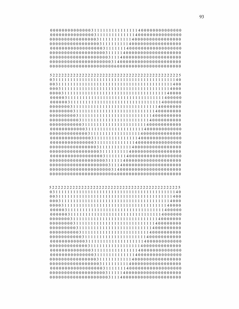
93
0 0 0 0 0 0 0 0 0 0 0 0 0 0 3 1 1 1 1 1 1 1 1 1 1 1 1 1 1 1 4 0 0 0 0 0 0 0 0 0 0 0 0 0 0 0 0 0 0 0 0 0 0 0 0 0 0 0 0 0 3 1 1 1 1 1 1 1 1 1 1 1 1 1 4 0 0 0 0 0 0 0 0 0 0 0 0 0 0 0
0 0 0 0 0 0 0 0 0 0 0 0 0 0 0 0 3 1 1 1 1 1 1 1 1 1 1 1 4 0 0 0 0 0 0 0 0 0 0 0 0 0 0 0 0 0 0 0 0 0 0 0 0 0 0 0 0 0 0 0 0 0 3 1 1 1 1 1 1 1 1 1 4 0 0 0 0 0 0 0 0 0 0 0 0 0 0 0 0 0
0 0 0 0 0 0 0 0 0 0 0 0 0 0 0 0 0 0 3 1 1 1 1 1 1 1 4 0 0 0 0 0 0 0 0 0 0 0 0 0 0 0 0 0 0 0 0 0 0 0 0 0 0 0 0 0 0 0 0 0 0 0 0 0 3 1 1 1 1 1 4 0 0 0 0 0 0 0 0 0 0 0 0 0 0 0 0 0 0 0 0 0 0 0 0 0 0 0 0 0 0 0 0 0 0 0 0 0 0 0 3 1 1 1 4 0 0 0 0 0 0 0 0 0 0 0 0 0 0 0 0 0 0 0 0 0 0 0 0 0 0 0 0 0 0 0 0 0 0 0 0 0 0 0 0 0 3 1 4 0 0 0 0 0 0 0 0 0 0 0 0 0 0 0 0 0 0 0 0 0 0 0 0 0 0 0 0 0 0 0 0 0 0 0 0 0 0 0 0 0 0 0 6 0 0 0 0 0 0 0 0 0 0 0 0 0 0 0 0 0 0 0 0 0 0 5 2 2 2 2 2 2 2 2 2 2 2 2 2 2 2 2 2 2 2 2 2 2 2 2 2 2 2 2 2 2 2 2 2 2 2 2 2 2 2 2 2 2 2 5 0 3 1 1 1 1 1 1 1 1 1 1 1 1 1 1 1 1 1 1 1 1 1 1 1 1 1 1 1 1 1 1 1 1 1 1 1 1 1 1 1 1 1 4 0 0 0 3 1 1 1 1 1 1 1 1 1 1 1 1 1 1 1 1 1 1 1 1 1 1 1 1 1 1 1 1 1 1 1 1 1 1 1 1 1 1 1 4 0 0 0 0 0 3 1 1 1 1 1 1 1 1 1 1 1 1 1 1 1 1 1 1 1 1 1 1 1 1 1 1 1 1 1 1 1 1 1 1 1 1 1 4 0 0 0 0 0 0 0 3 1 1 1 1 1 1 1 1 1 1 1 1 1 1 1 1 1 1 1 1 1 1 1 1 1 1 1 1 1 1 1 1 1 1 1 4 0 0 0 0
0 0 0 0 0 3 1 1 1 1 1 1 1 1 1 1 1 1 1 1 1 1 1 1 1 1 1 1 1 1 1 1 1 1 1 1 1 1 1 4 0 0 0 0 0 0 0 0 0 0 0 3 1 1 1 1 1 1 1 1 1 1 1 1 1 1 1 1 1 1 1 1 1 1 1 1 1 1 1 1 1 1 1 4 0 0 0 0 0 0
0 0 0 0 0 0 0 3 1 1 1 1 1 1 1 1 1 1 1 1 1 1 1 1 1 1 1 1 1 1 1 1 1 1 1 1 1 4 0 0 0 0 0 0 0 0 0 0 0 0 0 0 0 3 1 1 1 1 1 1 1 1 1 1 1 1 1 1 1 1 1 1 1 1 1 1 1 1 1 1 1 4 0 0 0 0 0 0 0 0 0 0 0 0 0 0 0 0 0 3 1 1 1 1 1 1 1 1 1 1 1 1 1 1 1 1 1 1 1 1 1 1 1 1 1 4 0 0 0 0 0 0 0 0 0 0 0 0 0 0 0 0 0 0 0 3 1 1 1 1 1 1 1 1 1 1 1 1 1 1 1 1 1 1 1 1 1 1 1 4 0 0 0 0 0 0 0 0 0 0 0 0 0 0 0 0 0 0 0 0 0 3 1 1 1 1 1 1 1 1 1 1 1 1 1 1 1 1 1 1 1 1 1 4 0 0 0 0 0 0 0 0 0 0 0
0 0 0 0 0 0 0 0 0 0 0 0 3 1 1 1 1 1 1 1 1 1 1 1 1 1 1 1 1 1 1 1 4 0 0 0 0 0 0 0 0 0 0 0 0 0 0 0 0 0 0 0 0 0 0 0 0 0 3 1 1 1 1 1 1 1 1 1 1 1 1 1 1 1 1 1 4 0 0 0 0 0 0 0 0 0 0 0 0 0
0 0 0 0 0 0 0 0 0 0 0 0 0 0 3 1 1 1 1 1 1 1 1 1 1 1 1 1 1 1 4 0 0 0 0 0 0 0 0 0 0 0 0 0 0 0 0 0 0 0 0 0 0 0 0 0 0 0 0 0 3 1 1 1 1 1 1 1 1 1 1 1 1 1 4 0 0 0 0 0 0 0 0 0 0 0 0 0 0 0
0 0 0 0 0 0 0 0 0 0 0 0 0 0 0 0 3 1 1 1 1 1 1 1 1 1 1 1 4 0 0 0 0 0 0 0 0 0 0 0 0 0 0 0 0 0 0 0 0 0 0 0 0 0 0 0 0 0 0 0 0 0 3 1 1 1 1 1 1 1 1 1 4 0 0 0 0 0 0 0 0 0 0 0 0 0 0 0 0 0
0 0 0 0 0 0 0 0 0 0 0 0 0 0 0 0 0 0 3 1 1 1 1 1 1 1 4 0 0 0 0 0 0 0 0 0 0 0 0 0 0 0 0 0 0 0 0 0 0 0 0 0 0 0 0 0 0 0 0 0 0 0 0 0 3 1 1 1 1 1 4 0 0 0 0 0 0 0 0 0 0 0 0 0 0 0 0 0 0 0 0 0 0 0 0 0 0 0 0 0 0 0 0 0 0 0 0 0 0 0 3 1 1 1 4 0 0 0 0 0 0 0 0 0 0 0 0 0 0 0 0 0 0 0 0

94
0 0 0 0 0 0 0 0 0 0 0 0 0 0 0 0 0 0 0 0 0 3 1 4 0 0 0 0 0 0 0 0 0 0 0 0 0 0 0 0 0 0 0 0 0 0 0 0 0 0 0 0 0 0 0 0 0 0 0 0 0 0 0 0 0 0 0 6 0 0 0 0 0 0 0 0 0 0 0 0 0 0 0 0 0 0 0 0 0 0
5 2 2 2 2 2 2 2 2 2 2 2 2 2 2 2 2 2 2 2 2 2 2 2 2 2 2 2 2 2 2 2 2 2 2 2 2 2 2 2 2 2 2 2 5 0 3 1 1 1 1 1 1 1 1 1 1 1 1 1 1 1 1 1 1 1 1 1 1 1 1 1 1 1 1 1 1 1 1 1 1 1 1 1 1 1 1 1 4 0 0 0 3 1 1 1 1 1 1 1 1 1 1 1 1 1 1 1 1 1 1 1 1 1 1 1 1 1 1 1 1 1 1 1 1 1 1 1 1 1 1 1 4 0 0 0 0 0 3 1 1 1 1 1 1 1 1 1 1 1 1 1 1 1 1 1 1 1 1 1 1 1 1 1 1 1 1 1 1 1 1 1 1 1 1 1 4 0 0 0 0 0 0 0 3 1 1 1 1 1 1 1 1 1 1 1 1 1 1 1 1 1 1 1 1 1 1 1 1 1 1 1 1 1 1 1 1 1 1 1 4 0 0 0 0
0 0 0 0 0 3 1 1 1 1 1 1 1 1 1 1 1 1 1 1 1 1 1 1 1 1 1 1 1 1 1 1 1 1 1 1 1 1 1 4 0 0 0 0 0 0 0 0 0 0 0 3 1 1 1 1 1 1 1 1 1 1 1 1 1 1 1 1 1 1 1 1 1 1 1 1 1 1 1 1 1 1 1 4 0 0 0 0 0 0
0 0 0 0 0 0 0 3 1 1 1 1 1 1 1 1 1 1 1 1 1 1 1 1 1 1 1 1 1 1 1 1 1 1 1 1 1 4 0 0 0 0 0 0 0 0 0 0 0 0 0 0 0 3 1 1 1 1 1 1 1 1 1 1 1 1 1 1 1 1 1 1 1 1 1 1 1 1 1 1 1 4 0 0 0 0 0 0 0 0 0 0 0 0 0 0 0 0 0 3 1 1 1 1 1 1 1 1 1 1 1 1 1 1 1 1 1 1 1 1 1 1 1 1 1 4 0 0 0 0 0 0 0 0 0 0 0 0 0 0 0 0 0 0 0 3 1 1 1 1 1 1 1 1 1 1 1 1 1 1 1 1 1 1 1 1 1 1 1 4 0 0 0 0 0 0 0 0 0 0 0 0 0 0 0 0 0 0 0 0 0 3 1 1 1 1 1 1 1 1 1 1 1 1 1 1 1 1 1 1 1 1 1 4 0 0 0 0 0 0 0 0 0 0 0
0 0 0 0 0 0 0 0 0 0 0 0 3 1 1 1 1 1 1 1 1 1 1 1 1 1 1 1 1 1 1 1 4 0 0 0 0 0 0 0 0 0 0 0 0 0 0 0 0 0 0 0 0 0 0 0 0 0 3 1 1 1 1 1 1 1 1 1 1 1 1 1 1 1 1 1 4 0 0 0 0 0 0 0 0 0 0 0 0 0
0 0 0 0 0 0 0 0 0 0 0 0 0 0 3 1 1 1 1 1 1 1 1 1 1 1 1 1 1 1 4 0 0 0 0 0 0 0 0 0 0 0 0 0 0 0 0 0 0 0 0 0 0 0 0 0 0 0 0 0 3 1 1 1 1 1 1 1 1 1 1 1 1 1 4 0 0 0 0 0 0 0 0 0 0 0 0 0 0 0
0 0 0 0 0 0 0 0 0 0 0 0 0 0 0 0 3 1 1 1 1 1 1 1 1 1 1 1 4 0 0 0 0 0 0 0 0 0 0 0 0 0 0 0 0 0 0 0 0 0 0 0 0 0 0 0 0 0 0 0 0 0 3 1 1 1 1 1 1 1 1 1 4 0 0 0 0 0 0 0 0 0 0 0 0 0 0 0 0 0
0 0 0 0 0 0 0 0 0 0 0 0 0 0 0 0 0 0 3 1 1 1 1 1 1 1 4 0 0 0 0 0 0 0 0 0 0 0 0 0 0 0 0 0 0 0 0 0 0 0 0 0 0 0 0 0 0 0 0 0 0 0 0 0 3 1 1 1 1 1 4 0 0 0 0 0 0 0 0 0 0 0 0 0 0 0 0 0 0 0 0 0 0 0 0 0 0 0 0 0 0 0 0 0 0 0 0 0 0 0 3 1 1 1 4 0 0 0 0 0 0 0 0 0 0 0 0 0 0 0 0 0 0 0 0 0 0 0 0 0 0 0 0 0 0 0 0 0 0 0 0 0 0 0 0 0 3 1 4 0 0 0 0 0 0 0 0 0 0 0 0 0 0 0 0 0 0 0 0 0 0 0 0 0 0 0 0 0 0 0 0 0 0 0 0 0 0 0 0 0 0 0 6 0 0 0 0 0 0 0 0 0 0 0 0 0 0 0 0 0 0 0 0 0 0 5 2 2 2 2 2 2 2 2 2 2 2 2 2 2 2 2 2 2 2 2 2 2 2 2 2 2 2 2 2 2 2 2 2 2 2 2 2 2 2 2 2 2 2 5 0 3 1 1 1 1 1 1 1 1 1 1 1 1 1 1 1 1 1 1 1 1 1 1 1 1 1 1 1 1 1 1 1 1 1 1 1 1 1 1 1 1 1 4 0 0 0 3 1 1 1 1 1 1 1 1 1 1 1 1 1 1 1 1 1 1 1 1 1 1 1 1 1 1 1 1 1 1 1 1 1 1 1 1 1 1 1 4 0 0 0 0 0 3 1 1 1 1 1 1 1 1 1 1 1 1 1 1 1 1 1 1 1 1 1 1 1 1 1 1 1 1 1 1 1 1 1 1 1 1 1 4 0 0 0 0 0 0 0 3 1 1 1 1 1 1 1 1 1 1 1 1 1 1 1 1 1 1 1 1 1 1 1 1 1 1 1 1 1 1 1 1 1 1 1 4 0 0 0 0
0 0 0 0 0 3 1 1 1 1 1 1 1 1 1 1 1 1 1 1 1 1 1 1 1 1 1 1 1 1 1 1 1 1 1 1 1 1 1 4 0 0 0 0 0 0 0 0 0 0 0 3 1 1 1 1 1 1 1 1 1 1 1 1 1 1 1 1 1 1 1 1 1 1 1 1 1 1 1 1 1 1 1 4 0 0 0 0 0 0
0 0 0 0 0 0 0 3 1 1 1 1 1 1 1 1 1 1 1 1 1 1 1 1 1 1 1 1 1 1 1 1 1 1 1 1 1 4 0 0 0 0 0 0 0 0 0 0 0 0 0 0 0 3 1 1 1 1 1 1 1 1 1 1 1 1 1 1 1 1 1 1 1 1 1 1 1 1 1 1 1 4 0 0 0 0 0 0 0 0 0 0 0 0 0 0 0 0 0 3 1 1 1 1 1 1 1 1 1 1 1 1 1 1 1 1 1 1 1 1 1 1 1 1 1 4 0 0 0 0 0 0 0 0 0 0 0 0 0 0 0 0 0 0 0 3 1 1 1 1 1 1 1 1 1 1 1 1 1 1 1 1 1 1 1 1 1 1 1 4 0 0 0 0 0 0 0 0 0 0 0 0 0 0 0 0 0 0 0 0 0 3 1 1 1 1 1 1 1 1 1 1 1 1 1 1 1 1 1 1 1 1 1 4 0 0 0 0 0 0 0 0 0 0 0
0 0 0 0 0 0 0 0 0 0 0 0 3 1 1 1 1 1 1 1 1 1 1 1 1 1 1 1 1 1 1 1 4 0 0 0 0 0 0 0 0 0 0 0 0 0 0 0 0 0 0 0 0 0 0 0 0 0 3 1 1 1 1 1 1 1 1 1 1 1 1 1 1 1 1 1 4 0 0 0 0 0 0 0 0 0 0 0 0 0
0 0 0 0 0 0 0 0 0 0 0 0 0 0 3 1 1 1 1 1 1 1 1 1 1 1 1 1 1 1 4 0 0 0 0 0 0 0 0 0 0 0 0 0 0 0 0 0 0 0 0 0 0 0 0 0 0 0 0 0 3 1 1 1 1 1 1 1 1 1 1 1 1 1 4 0 0 0 0 0 0 0 0 0 0 0 0 0 0 0
0 0 0 0 0 0 0 0 0 0 0 0 0 0 0 0 3 1 1 1 1 1 1 1 1 1 1 1 4 0 0 0 0 0 0 0 0 0 0 0 0 0 0 0 0 0 0 0 0 0 0 0 0 0 0 0 0 0 0 0 0 0 3 1 1 1 1 1 1 1 1 1 4 0 0 0 0 0 0 0 0 0 0 0 0 0 0 0 0 0
0 0 0 0 0 0 0 0 0 0 0 0 0 0 0 0 0 0 3 1 1 1 1 1 1 1 4 0 0 0 0 0 0 0 0 0 0 0 0 0 0 0 0 0 0 0 0 0 0 0 0 0 0 0 0 0 0 0 0 0 0 0 0 0 3 1 1 1 1 1 4 0 0 0 0 0 0 0 0 0 0 0 0 0 0 0 0 0 0 0 0 0 0 0 0 0 0 0 0 0 0 0 0 0 0 0 0 0 0 0 3 1 1 1 4 0 0 0 0 0 0 0 0 0 0 0 0 0 0 0 0 0 0 0 0 0 0 0 0 0 0 0 0 0 0 0 0 0 0 0 0 0 0 0 0 0 3 1 4 0 0 0 0 0 0 0 0 0 0 0 0 0 0 0 0 0 0 0 0 0 0 0 0 0 0 0 0 0 0 0 0 0 0 0 0 0 0 0 0 0 0 0 6 0 0 0 0 0 0 0 0 0 0 0 0 0 0 0 0 0 0 0 0 0 0 *POR *CON 0.3 *PERMI *CON 12000 *PERMJ *EQUALSI *PERMK *EQUALSI / 10

95
*END-GRID *CPOR 4e-4 *PRPOR 275 *ROCKCP 35 *THCONR 24 *THCONW 24 *THCONO 24 *THCONG 24 *HLOSSPROP *OVERBUR 60 24 *UNDERBUR 60 24 ** ============== FLUID DEFINITIONS ====================== *MODEL 2 2 2 ** Components are water and dead oil. Most water ** properties are defaulted (=0). Dead oil K values ** are zero, and no gas properties are needed. *COMPNAME 'WATER' 'OIL' ** ----- ------- *CMM 18 511.78 *PCRIT 635 2415.7 *TCRIT 323 2280 *CPG1 0 0 *CPG2 0 0 *CPG3 0 0 *CPG4 0 0 *MASSDEN 62.7401 63.18664 *CP 0 5.e-6 *CT1 0 5.005E-4 *CT2 0 0 *VISCTABLE ** Temp Water Oil 122 0 25000 170 0 8077.48 190 0 3047.18 210 0 1277.603 230 0 588.57 240 0 412.51 260 0 214.801 280 0 120.0453 300 0 71.4554 320 0 44.9924 340 0 29.7859 360 0 20.6202 370 0 17.4199 380 0 14.8553 390 0 12.7812 400 0 11.0892

96
410 0 9.697 420 0 8.5443 430 0 7.5815 440 0 6.7721 450 0 6.0873 460 0 5.5044 470 0 5.0053 480 0 4.5756 490 0 4.2038 500 0 3.8805 1000 0 3.8805 *PRSR 14.7 *TEMR 60 *PSURF 14.7 *TSURF 60 ** ============== ROCK-FLUID PROPERTIES ====================== *ROCKFLUID *SWT ** Water-oil relative permeabilities ** Sw Krw Krow ** ---- -------- ------- 0.168000 0.000000 0.900000 0.250000 0.100000 0.665000 0.440000 0.400000 0.380000 0.560000 0.600000 0.237500 0.672000 0.760000 0.142500 0.830000 1.000000 0.000000 *SLT ** Liquid-gas relative permeabilities ** Sl Krg Krog ** ---- ------- ------- 0.338000 0.500000 0.000000 0.401100 0.300000 0.005670 0.486700 0.125000 0.014400 0.600000 0.062500 0.026700 0.657800 0.037500 0.034400 0.743300 0.012500 0.046700 0.800000 0.005000 0.056700 0.825000 0.002500 0.062222222 0.850000 0.002500 0.067777778 0.900000 0.002500 0.080000 1.000000 0.000000 0.900000 ** ============== INITIAL CONDITIONS ======================

97
*INITIAL ** Automatic static vertical equilibrium *VERTICAL *DEPTH_AVE *REFPRES 275 *REFBLOCK 1 1 1 *TEMP *CON 125 ** ============== NUMERICAL CONTROL ====================== *NUMERICAL ** All these can be defaulted. The definitions ** here match the previous data. *NORM *PRESS 30 *SATUR 0.09 *TEMP 15 *RUN ** ============== RECURRENT DATA ====================== ** Project starts on January 01, 2004 *DATE 2004 01 01 *DTWELL 1 ** o *WELL 1 'INJECTOR' *VERT 1 1 *FRAC .125 ** o o o *WELL 2 'PRODUCER' *VERT 45 1 *FRAC .125 ** o o o o o ** o o o o o o o ** 1 o o o o o o o 2 *INJECTOR *MOBWEIGHT 'INJECTOR' *INCOMP WATER 1.0 0.0 *TINJW 600 QUAL .8 *OPERATE *BHP 1600 *OPERATE *MAX *STW 1600 *PERFV 'INJECTOR' ** k wi ** Inject only in the bottom layer ** 2*pi*k*h / ln(cc*sqrt((dx**2+dy**2)/pi)/rw) 5 483472.39 ** k = 12000 md, h = 12.5 ft, dx = dy = 10.607 ft, 6 483472.39 ** cc = 0.249, rw = 0.3 ft 7 483472.39 8 483472.39 *PRODUCER 'PRODUCER' *OPERATE *BHP 90 *OPERATE *MAX *STL 3500

98
*PERFV 'PRODUCER' ** k wi 5 483472.39 6 483472.39 7 483472.39 8 483472.39 OPEN 'PRODUCER' OPEN 'INJECTOR' *TIME 365 *TIME 730 *TIME 1095 *TIME 1460 *TIME 1825 *TIME 2190 *TIME 3650 *TIME 5475 *STOP

99
APPENDIX E
VBA PROGRAM OF NEW MODEL
'Microsoft Excel Macro Program 'Modified Jeff Jones Model 'Define variables Global limit As Single Dim Acd1 As Double Dim Acd2 As Double Dim Acd3 As Double Dim Acd4 As Double Dim Acd1p2 As Double Dim Acd2p2 As Double Dim Acd3p2 As Double Dim Acd4p2 As Double Dim Vod1 As Double Dim peakoilrate As Double Dim Ms As Double Dim check As Integer Dim maxq As Double Dim maxqnumber As Integer Dim maxiter As Integer Dim NdPartIII As Variant Dim maxAcD As Double 'Define functions Function ERFC(x As Double) y = 1 / (1 + 0.3275911 * x) ERFC = (0.254829592 * y - 0.284496736 * y ^ 2 + 1.421413741 * y ^ 3 - _ 1.453152027 * y ^ 4 + 1.061405429 * y ^ 5) * Exp(-(x ^ 2)) + 0.00000015 End Function Function SQRT(temp As Double) SQRT = temp ^ 0.5 End Function Function Pi() Pi = 3.14159265358979 End Function Function integration(td As Double, tcd As Variant, section As Double) delta = (tcd - 0) / section Start = delta / 2 Sum = 0 For i = 0 To section - 1 Sum = Exp(Start + delta * i) * ERFC(SQRT(Start + delta * i)) / _ SQRT(td - (Start + delta * i)) * delta + Sum Next i integration = Sum End Function Sub JeffJones() 'Initialize value

100
check = 0 maxq = 0 NdPartIII = 0 StartIterVoD = 0 With Sheets("JJ Formula") 'Get data entry a = Worksheets("JJ Formula").Range("A").Value 'Area por = Worksheets("JJ Formula").Range("por").Value 'Porosity Soi = Worksheets("JJ Formula").Range("Soi").Value 'Initial oil saturation Sor = Worksheets("JJ Formula").Range("Sor").Value 'Residual oil saturation Sgi = Worksheets("JJ Formula").Range("Sgi").Value 'Initial gas saturation Oil_viscosity = Worksheets("JJ Formula"). _ Range("oil_viscosity").Value 'Initial Oil viscosity Tres = Worksheets("JJ Formula").Range("Tres").Value 'Reservoir temperature Bo = Worksheets("JJ Formula").Range("Bo").Value 'Oil formation volume factor kh = Worksheets("JJ Formula").Range("kh").Value 'Thermal conductivity of formation Rock_Density = Worksheets("JJ Formula").Range("Rock_Density").Value 'Rock Density Cr = Worksheets("JJ Formula").Range("Cr").Value 'Heat capacity of rock Water_Density = Worksheets("JJ Formula"). _ Range("Water_Density").Value 'Water density Oil_Density = Worksheets("JJ Formula").Range("Oil_Density").Value 'Oil density Cw = Worksheets("JJ Formula").Range("Cw").Value 'Heat capacity of water Co = Worksheets("JJ Formula").Range("Co").Value 'Heat capacity of oil ht = Worksheets("JJ Formula").Range("ht").Value 'Total thickness hn = Worksheets("JJ Formula").Range("hn").Value 'Net thickness M_1Temp = Worksheets("JJ Formula"). _ Range("M_1Temp").Value 'Volumetric heat capacity of rock Irate = Worksheets("JJ Formula").Range("Irate").Value 'Injection rate Ps = Worksheets("JJ Formula").Range("Ps").Value 'Saturated steam pressure fs = Worksheets("JJ Formula").Range("fs").Value 'Steam quality Tinj = Worksheets("JJ Formula").Range("Tinj").Value 'Injection temperature viscosity = Worksheets("JJ Formula"). _ Range("viscosity").Value 'Oil viscosity @ steam temperature Ms = Worksheets("JJ Formula"). _ Range("Ms").Value 'Volumetric heat capacity of overburden and underburden TotalDay = Worksheets("JJ Formula"). _ Range("TotalDay").Value 'Total day of calculations DeltaDay = Worksheets("JJ Formula"). _ Range("DeltaDay").Value 'Delta day of calculations peakoilrate = Irate 'Maximum oil production rate 'Calculate volumetric heat capacity of formation If M_1Temp = 0 Then M_1 = (1 - por) * Rock_Density * Cr + por * Sor * Oil_Density * Co _ + por * (1 - fs) ^ 0.5 * (1 - Sor) * Water_Density * Cw Else M_1 = M_1Temp End If 'Calculate enthalpy of condensate If Ps >= 500 And Ps <= 1500 Then Hsc = 77.036 * Ps ^ 0.28302 ElseIf Ps > 1500 And Ps <= 2500 Then

101
Hsc = 0.12038 * Ps + 430.984 End If 'Calculate enthalpy of vapor Hsv = 1204.8 - 0.000197697 * (Ps - 453.23) ^ 1.73808 'Calculate latent heat of steam hfg = Hsv - Hsc 'Calculate fraction of heat injected in vapor form fhv = 1 / (1 + Cw * (Tinj - Tres) / (fs * hfg)) 'Determine critical dimensionless time Worksheets("JJ Formula").Range("goal").GoalSeek Goal:=fhv, _ ChangingCell:=Worksheets("JJ Formula").Range("ChangingCell") tcd = Worksheets("JJ Formula").Range("ChangingCell") 'Calculate ratio of enthalpy of vaporization to liquid enthalpy fhD = fs * hfg / (Cw * (Tinj - Tres)) 'Calculate dimensionless time constant 'Dimensionless time = tD_multiplier multiply by time tD_multiplier = 35040 * Ms * kh / (ht ^ 2 * M_1 ^ 2) 'Calculate cumulative oil steam ratio constant 'Cumulative oil steam ratio = Fos_multiplier multiply by Ehs Fos_multiplier = Water_Density * Cw / M_1 * hn / ht * _ (Soi - Sor) * por * (1 + fhD) 'Calculate heat injection rate Qinj = 14.6 * Irate * (Hsc + fs * hfg - Cw * (Tres - 32)) 'Calculate oil originally in place N = 43560 * a * hn * por * Soi / (5.62 * Bo) 'Calculate alpha alpha = 0.00015 * Irate + 0.05 'Calculate betha tc = tcd * ht ^ 2 * M_1 ^ 2 / (35040 * kh * Ms) Nc = 7758 * a * hn * por * (Soi - Sor) / (365 * Irate * tc) betha = 17.93 * Nc + 1.3401 '*************************************************************** 'Coefficient for AcD Stage I Acd1 = alpha Acd2 = 100 Acd3 = 0.5 Acd4 = 2 'Coefficient for AcD Stage II Acd1p2 = 0.11 Acd2p2 = 100 Acd3p2 = 0.5 Acd4p2 = 4

102
'Coefficient for VoD Vod1 = betha '**************************************************************** 'Display the calculations result .Cells(36, 3).Value = M_1 .Cells(41, 3).Value = hfg .Cells(40, 7) = Hsv .Cells(41, 7) = Hsc .Cells(47, 3).Value = fhD .Cells(53, 3).Value = tcd .Cells(60, 3).Value = tD_multiplier .Cells(78, 3).Value = Fos_multiplier .Cells(86, 3).Value = Qinj .Cells(125, 3).Value = N .Cells(95, 13).Value = fhv .Cells(54, 13).Value = alpha .Cells(76, 13).Value = alpha .Cells(59, 19).Value = betha 'Iterations for each time step Dim iter As Integer limit = TotalDay / DeltaDay .Range("A134:Z5000").Clear For iter = 1 To limit 'Calculate time in days .Cells(133 + iter, 2).Value = DeltaDay * iter 'Calculate time in years .Cells(133 + iter, 1).Value = .Cells(133 + iter, 2).Value / 365.25 'Calculate dimensionless time .Cells(133 + iter, 3).Value = tD_multiplier * _ .Cells(133 + iter, 1) 'Calculate function G(tD) .Cells(133 + iter, 4) = 2 * SQRT(.Cells(133 + iter, 3) / Pi()) - 1 _ + Exp(.Cells(133 + iter, 3)) * ERFC(SQRT( _ .Cells(133 + iter, 3))) 'Calculate average thermal efficiency of steam zone If .Cells(133 + iter, 3) < tcd Then .Cells(133 + iter, 5) = 1 / .Cells(133 + iter, 3) * _ .Cells(133 + iter, 4) Else .Cells(133 + iter, 5) = 1 / .Cells(133 + iter, 3) * (.Cells(133 + iter, 4) _ + (1 - fhv) * 1 / SQRT(Pi()) * (2 * SQRT(.Cells(133 + iter, 3)) - _ 2 * (1 - fhv) * SQRT(.Cells(133 + iter, 3) - tcd) - _ integration(.Cells(133 + iter, 3), tcd, 5000) _ - SQRT(Pi()) * .Cells(133 + iter, 4))) End If 'Calculate cumulative oil steam ratio .Cells(133 + iter, 6) = Fos_multiplier * .Cells(133 + iter, 5) 'Calculate cumulative steam injection .Cells(133 + iter, 7) = Irate * .Cells(133 + iter, 2).Value 'Calculate cumulative oil displacement .Cells(133 + iter, 8) = .Cells(133 + iter, 6) * .Cells(133 + iter, 7) / Bo

103
'Calculate oil displacement rate If iter = 1 Then .Cells(133 + iter, 9) = (.Cells(133 + iter, 8) - 0) / DeltaDay Else .Cells(133 + iter, 9) = (.Cells(133 + iter, 8) - .Cells(132 + iter, 8)) _ / DeltaDay End If 'Calculate steam zone size .Cells(133 + iter, 10) = Qinj * hn * M_1 / (4 * kh * (Tinj - Tres) _ * Ms * 43560) * (Exp(.Cells(133 + iter, 3).Value) * _ ERFC(SQRT(.Cells(133 + iter, 3).Value)) + 2 * _ SQRT(.Cells(133 + iter, 3).Value / Pi()) - 1) 'Calculate AcD If maxq = 0 Then If check = 0 Then If 132 + iter = 133 Then .Cells(133 + iter, 11) = (.Cells(133 + iter, 10) / (a * (Acd1 * _ Log(Oil_viscosity / Acd2)) ^ Acd3)) ^ Acd4 ElseIf .Cells(132 + iter, 11) < 1 Then .Cells(133 + iter, 11) = (.Cells(133 + iter, 10) / (a * (Acd1 * _ Log((.Cells(133 + iter, 10) * viscosity + _ (a - .Cells(133 + iter, 10)) * Oil_viscosity) / a / _ Acd2)) ^ Acd3)) ^ Acd4 Else check = 1 .Cells(133 + iter, 11) = (.Cells(133 + iter, 10) / (a * (Acd1p2 * _ Log((.Cells(133 + iter, 10) * viscosity + (a - _ .Cells(133 + iter, 10)) * Oil_viscosity) / a / Acd2p2)) _ ^ Acd3p2)) ^ Acd4p2 End If Else If .Cells(132 + iter, 15) < peakoilrate Then .Cells(133 + iter, 11) = (.Cells(133 + iter, 10) / (a * (Acd1p2 * _ Log((.Cells(133 + iter, 10) * viscosity + (a - _ .Cells(133 + iter, 10)) * Oil_viscosity) / _ a / Acd2p2)) ^ Acd3p2)) ^ Acd4p2 Else .Cells(132 + iter, 15) = peakoilrate maxq = .Cells(132 + iter, 15) maxqnumber = 132 + iter maxiter = iter - 1 maxAcD = peakoilrate / (.Cells(132 + iter, 12) * .Cells(132 + iter, 13) _ * .Cells(133 + iter, 9)) .Cells(132 + iter, 11) = maxAcD .Cells(132 + iter, 14) = maxAcD * .Cells(132 + iter, 12) * _ .Cells(132 + iter, 13) NdPartIII = .Cells(132 + iter, 8) .Cells(133 + iter, 11) = 1 End If End If Else .Cells(133 + iter, 11) = 1 End If

104
'Calculate VpD If Sgi = 0 Then .Cells(133 + iter, 12) = 1 Else If (.Cells(133 + iter, 7) * 5.62 / (43560 * a * hn * por * Sgi)) ^ 2 < 1 Then .Cells(133 + iter, 12) = (.Cells(133 + iter, 7) * 5.62 / _ (43560 * a * hn * por * Sgi)) ^ 2 Else .Cells(133 + iter, 12) = 1 End If End If 'Calculate VoD If NdPartIII = 0 Then .Cells(133 + iter, 13) = 1 Else If (1 - (.Cells(133 + iter, 8) - NdPartIII) / N * Soi / (Soi - Sor)) > 0 Then .Cells(133 + iter, 13) = maxAcD * Exp(-Vod1 * _ (.Cells(133 + iter, 8) - NdPartIII) / N * Soi / (Soi - Sor)) Else .Cells(133 + iter, 13) = 0 End If End If 'Calculate Capture Factor .Cells(133 + iter, 14) = .Cells(133 + iter, 11) * .Cells(133 + iter, 12) * _ .Cells(133 + iter, 13) 'Calculate oil rate .Cells(133 + iter, 15) = .Cells(133 + iter, 14) * .Cells(133 + iter, 9) 'Jeff Jones '********************************************************************************* 'Calculate Jeff Jones' AcD If (.Cells(133 + iter, 10) / (a * (0.11 * Log(Oil_viscosity / 100)) ^ 0.5)) _ ^ 2 <= 1 And Oil_viscosity > 100 Then .Cells(133 + iter, 16) = (.Cells(133 + iter, 10) / (a * (0.11 * _ Log(Oil_viscosity / 100)) ^ 0.5)) ^ 2 Else .Cells(133 + iter, 16) = 1 End If 'Calculate Jeff Jones' VpD If Sgi = 0 Then .Cells(133 + iter, 17) = 1 Else If (.Cells(133 + iter, 7) * 5.62 / (43560 * a * hn * por * Sgi)) _ ^ 2 < 1 Then .Cells(133 + iter, 17) = (.Cells(133 + iter, 7) * 5.62 / _ (43560 * a * hn * por * Sgi)) ^ 2 Else .Cells(133 + iter, 17) = 1 End If End If 'Calculate Jeff Jones' VoD If (1 - .Cells(133 + iter, 8) / N * Soi / (Soi - Sor)) > 0 Then .Cells(133 + iter, 18) = (1 - .Cells(133 + iter, 8) / _

105
N * Soi / (Soi - Sor)) ^ 0.5 Else .Cells(133 + iter, 18) = 0 End If 'Calculate Jeff Jones' Capture Factor .Cells(133 + iter, 19) = .Cells(133 + iter, 16) * .Cells(133 + iter, 17) * _ .Cells(133 + iter, 18) 'Calculate Jeff Jones' oil production rate .Cells(133 + iter, 20) = .Cells(133 + iter, 19) * .Cells(133 + iter, 9) '********************************************************************************* Next 'Cell borders Sheets("JJ Formula").Range(Sheets("JJ Formula").Cells(134, 1), _ Sheets("JJ Formula").Cells(133 + limit, 20)).Select Selection.Borders(xlDiagonalDown).LineStyle = xlNone Selection.Borders(xlDiagonalUp).LineStyle = xlNone With Selection.Borders(xlEdgeLeft) .LineStyle = xlContinuous .Weight = xlThin .ColorIndex = xlAutomatic End With With Selection.Borders(xlEdgeTop) .LineStyle = xlContinuous .Weight = xlThin .ColorIndex = xlAutomatic End With With Selection.Borders(xlEdgeBottom) .LineStyle = xlContinuous .Weight = xlThin .ColorIndex = xlAutomatic End With With Selection.Borders(xlEdgeRight) .LineStyle = xlContinuous .Weight = xlThin .ColorIndex = xlAutomatic End With With Selection.Borders(xlInsideVertical) .LineStyle = xlContinuous .Weight = xlThin .ColorIndex = xlAutomatic End With With Selection.Borders(xlInsideHorizontal) .LineStyle = xlContinuous .Weight = xlThin .ColorIndex = xlAutomatic End With Sheets("JJ Formula").Cells(20, 11).Select End With End Sub

106
VITA
Name: Suandy Chandra
Permanent Address: Jln. Samudera No. 6
Medan – 20214
Sumatera Utara, Indonesia
Email: [email protected]
Education: M.S., Petroleum Engineering
Texas A&M University
College Station, TX 77843-3116, U.S.A.
August 2005
B.S., Petroleum Engineering,
Institut Teknologi Bandung
Bandung, Indonesia
March 2003