1

Improved Spectroscopy for Microwave and Infrared Satellite Data Assimilation

Vivienne Payne, Jean-Luc Moncet and Tony Clough*

JCSDA 6th Workshop on Satellite Data AssimilationJune 10-11 2008

*Currently at Clough Associates

2

Acknowledgements

• AER: Mark Shephard, Jennifer Delamere, Karen Cady-Pereira and Eli Mlawer• UMBC: Larrabee Strow, Scott Hannon

• U. Wisconsin: Dave Tobin, Dave Turner

• NASA Langley: Bill Smith’s group

• NASA JPL: TES Algorithm Development Team

• Paris XII, Creteill: Jean Michel Hartmann’s Group

• UMass: Bob Gamache

• ANL: Maria Cadeddu

• Radiometrics: Mike Exner

• University of L’Aquila: Nico Cimini• NOAA: Ed Westwater

3

Overview

• Microwave– MonoRTM– Comparisons with Rosenkranz model– Water vapor continuum validation

• Infrared– Updates to LBLRTM

» General update to latest HITRAN 2004 line parameters• Water vapor line widths

» CO2 line mixing

– Validation against satellite measurements» AIRS/SARTA/LBLRTM comparisons» IASI comparisons

– Validation against ground-based measurements– Future plans

• Summary

4

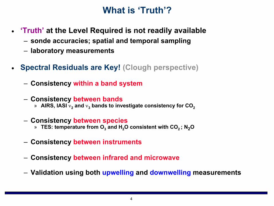
What is ‘Truth’?

• ‘Truth’ at the Level Required is not readily available– sonde accuracies; spatial and temporal sampling– laboratory measurements

• Spectral Residuals are Key! (Clough perspective)

– Consistency within a band system

– Consistency between bands» AIRS, IASI ν2 and ν3 bands to investigate consistency for CO2

– Consistency between species» TES: temperature from O3 and H2O consistent with CO2 ; N2O

– Consistency between instruments

– Consistency between infrared and microwave

– Validation using both upwelling and downwelling measurements

5

Microwave

• MonoRTM• Differences from the Rosenkranz model• Update on line parameters• Ongoing continuum validation

Microwave topics

6

MonoRTM

• Microwave monochromatic radiative transfer model– "laser" - i.e. single frequency - version of LBLRTM

• Developed at AER (Clough et al., 2005)• Useful range: 0-1648 GHz• Spectroscopic parameters from external line file

– HITRAN 2004 with specific updates/modifications» 22 GHz and 183 GHz line intensities from Clough et al (1973)» Other 22 GHz and 183 GHz line parameters from Payne et al. (2008)» Oxygen widths, line coupling parameters from Tretyakov et al (2005)

• Ground-based validation of oxygen parameters in MonoRTM: Cadeddu et al. (2007)

• Latest version: Monortm_v3.3

• Lineshape: Van-Vleck Weisskopf• Continuum: CKD_2.4

7

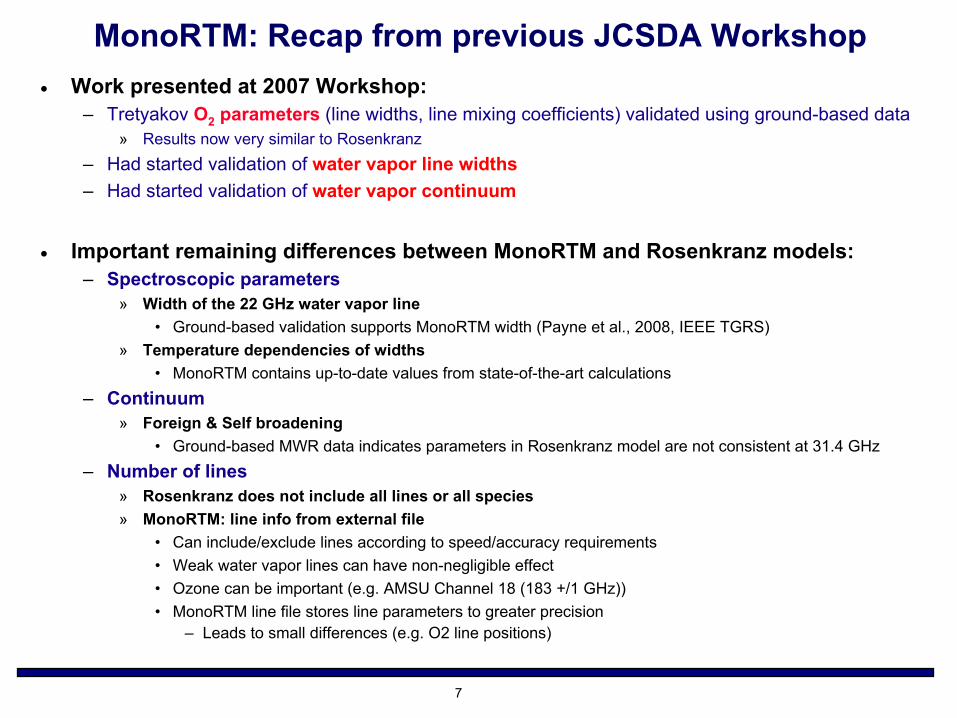
MonoRTM: Recap from previous JCSDA Workshop• Work presented at 2007 Workshop:

– Tretyakov O2 parameters (line widths, line mixing coefficients) validated using ground-based data» Results now very similar to Rosenkranz

– Had started validation of water vapor line widths– Had started validation of water vapor continuum

• Important remaining differences between MonoRTM and Rosenkranz models:– Spectroscopic parameters

» Width of the 22 GHz water vapor line• Ground-based validation supports MonoRTM width (Payne et al., 2008, IEEE TGRS)

» Temperature dependencies of widths• MonoRTM contains up-to-date values from state-of-the-art calculations

– Continuum» Foreign & Self broadening

• Ground-based MWR data indicates parameters in Rosenkranz model are not consistent at 31.4 GHz– Number of lines

» Rosenkranz does not include all lines or all species» MonoRTM: line info from external file

• Can include/exclude lines according to speed/accuracy requirements• Weak water vapor lines can have non-negligible effect• Ozone can be important (e.g. AMSU Channel 18 (183 +/1 GHz))• MonoRTM line file stores line parameters to greater precision

– Leads to small differences (e.g. O2 line positions)

8

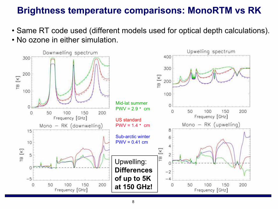
Brightness temperature comparisons: MonoRTM vs RK

• Same RT code used (different models used for optical depth calculations).• No ozone in either simulation.

Mid-lat summerPWV = 2.9 cm

US standardPWV = 1.4 cm

Sub-arctic winterPWV = 0.41 cm

Upwelling:Differences of up to 5K at 150 GHz!

9

Water vapor: Line widths

22.24 GHz23.8 GHz24.5 GHz

Incorrect specification of the 22 GHz width will lead to inconsistency betweeneg AMSU/AMSR-E and SSMIS!

Payne et al., 2008, IEEE TGRS, in press

22 GHz:MonoRTM 5% lower than RK

RK

RK

MonoRTMMonoRTM

183 GHz:MonoRTM ~ same as RK

Additional evidence for lower 22GHz width value from upwelling radiation:

»UK Met Office (W. Bell and P. J. Rayer -lower width improves SSMI biases)»Tom Wilheit (Texas A&M) - TMI and SSMI

10

Water vapor continuumRatios of absorption in models (Rosenkranz=1.0)Thomas Meissner (RSS)

Mean: 0.67 KS.D.: 0.53 K

Foreign broadening(FB)

Self broadening(SB)

Clough and Cady-Pereira

MWR: 31.4 GHz MWR: 31.4 GHz

Extending the SGP MWR analysis Continuum uncertainty

31.4 GHz 150 GHz

∆TB = a∆X frg (PWV ) + b∆X slf (PWV )2

PWV

∆TB

foreign selfWithin green area: Consistency withmeasurements possible

Outside red oval: consistency with measurements impossible

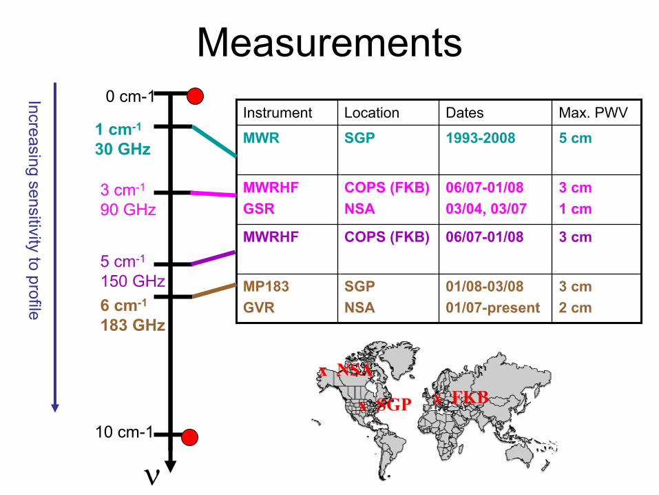
Measurements

3 cm 06/07-01/08COPS (FKB)MWRHF

3 cm2 cm

01/08-03/0801/07-present

SGPNSA

MP183GVR

3 cm1 cm

06/07-01/0803/04, 03/07

COPS (FKB)NSA

MWRHFGSR

5 cm1993-2008SGPMWRMax. PWVDatesLocationInstrument

Increas ing sens itivit y to profi le

1 cm-1

30 GHz

5 cm-1

150 GHz6 cm-1

183 GHz

0 cm-1

10 cm-1

3 cm-1

90 GHz

ν

x NSA

x SGP x FKB

13

Microwave Summary

• Main differences between MonoRTM v3.3 and Rosenkranz (2007):– Width of 22 GHz water vapor line– Water vapor continuum– Number of lines and input format

• Ground-based validation supports MonoRTM 22 GHz line width– Additional evidence from upwelling radiation:

» UK Met Office (W. Bell and P. J. Rayer - lower width value improves SSMI biases)» Tom Wilheit (Texas A&M) - TMI & SSMI

• Ongoing/future work:– Continued validation at ARM sites– “Best fit” water vapor continuum using a range of frequencies– Consistency between microwave and infrared (AERI instrument at NSA)– Zeeman line splitting

14

Infrared

LBLRTMLine-by-line radiative transfer model

• Recent updates to LBLRTM• Validation against satellite data

– AIRS/LBLRTM/SARTA comparisons– IASI/LBLRTM comparisons

• Validation against ground-based data– AERI

• Working closely with Tony Clough

15

LBLRTM: Line parameters

• HITRAN: reference source for ‘AER’ Line Parameters• Substitutions made only for very specific reasons and only with extensive validation

• aer_v_2.0 (0 -22,656 cm-1)

MIPAS vs HITRAN 2004HITRAN 2004MIPAS (Wagner et al., Flaud et al.)

O3

MIPAS CO2 ν3 strengths and widths(S. Tashkun, J-L. Teffo et

al.,J-M. Flaud et al.)Corresponding update to line coupling, chi-factor, CO2continuum

HITRAN 2000(Identical to HITRAN 2004 forν2 and ν3 regions)

Niro et al. line coupling implemented for all CO2bands

HITRAN 2000P&R branch line coupling implemented for strongest bands

(Niro et al., 2005, J-M Hartmann)

CO2

Temperature dependence of widths (R. Gamache)Strengths (L. Coudert)

HITRAN 2004 + updatesUpdated widthsAER co-authors on Gordon et al., 2007

HITRAN 2000H2OUnder investigation20082007

16

LBLRTM: MT_CKD_2.1 Continuum

• Water Vapor- Self / Foreign- Single Line Shape for each

• Carbon Dioxide- Continuing Research Focus- in conjunction with CO2 line parameters, line coupling and lineshape (chi-factor)

• Nitrogen: Collision Induced- 2330 cm-1 Region

• Oxygen: Collision Induced- 1600 cm-1 Region

AIRS/model comparisons

Models• LBLRTM v11.3

– HITRAN 2004 line parameters, except for CO2• Includes water vapor width updates from Gordon et al. (2007)

– CO2• line parameters are HITRAN 2000 (consistency with line mixing)• Q / P&R branch line mixing from Niro et al. (2005)• Chi-factor currently set to 1.0

– Continuum: MT_CKD_2.1

• SARTA v1.05– version 4 of AIRS RTA, January 2004– Line parameters based on HITRAN 2000 (Strow et al. 2006)– Line mixing / chi factors

• Tobin (1996), De Souza-Machado et al. (1999)– H2O continuum loosely based on MT_CKD

• but with large modifications (scaling by up to 10x in selected regions)– Transmittances tuned to agree with the dataset in these comparisons

Measurements

• AIRS validation, phase 1– ARM Tropical Western Pacific at Nauru– Over ocean

• Avoid issues of modeling of land emissivity– Night-time

• Avoid non-LTE effects and reflected solar radiation– “Clear-sky” AIRS overpasses

• Sonde launches within 1 hour, 30km of AIRS measurement• 39 AIRS spectra (multiple AIRS match-ups for each sonde)• 8 distinct radiosonde profiles

– PWV range: 4.0 to 5.6 cm

Specification of atmospheric state

• Layer profiles supplied by L. Strow– Temperature, H2O

• ARM “best estimate” files below 60 mbar (Tobin et al., 2006)– Constructed from sondes launched at times around AIRS

overpasses• AIRS retrieval (uses SARTA) above 60 mbar

– CO2 VMR set to 370 ppmv– Other trace gases

• O3 from ECMWF (Strow et al 2006)• CH4 and CO columns have been fitted• All other molecules from US standard atmosphere

Layering

Fig. 1 from Strow et al. (2003): Mean layer pressures used in the AIRS radiative transfer model

• 100 layers• Layering is fine enough that switching on/off the “linear-in-tau”approximation in LBLRTM has negligible impact

AIRS/model comparisons:Mean differences for 39 AIRS match-ups at ARM TWP

Lower 3 plots: Black dots show subset of 281 channels used by NCEP

23

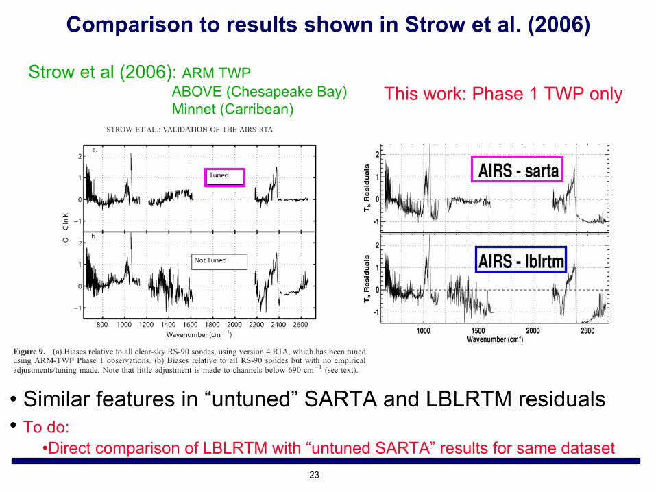
Comparison to results shown in Strow et al. (2006)

• Similar features in “untuned” SARTA and LBLRTM residuals• To do:

•Direct comparison of LBLRTM with “untuned SARTA” results for same dataset

Strow et al (2006): ARM TWPABOVE (Chesapeake Bay)Minnet (Carribean)

This work: Phase 1 TWP only

24

CO2 667 cm-1 Q branch

– LBLRTM currently using 1st order perturbation theory– not sufficient for sharp 667 cm-1 Q-branch

– Exact calculation is very time consuming– Niro et al., 2005

– Approaches to be investigated:– 2nd order perturbation – parameterization of Niro et al.

25

Residuals at 2500 cm-1:“Good” and “bad” ARM TWP Phase 1 cases

“Good”: Case 003 “Bad”: Case 034

• “Bad” case:• Sonde T, H2O profile does not accurately represent atmospheric state observed by AIRS?• Influence of cloud?• Demonstrates importance of careful selection of cases in addition to ensembles for RT model validation

AIRS - lblrtmAIRS - lblrtm

AIRS - sartaAIRS - sarta

sarta - lblrtmsarta - lblrtm

AIRS/model comparisons– CO2 residuals:

•Tropospheric– Sonde provides good estimate of “true” temperature– ν2 region agrees well with sonde in troposphere– ν3 region - issues with modeling outer edges of the band

» Both in LBLRTM and “untuned” SARTA•Stratospheric

– “True” temperature is more difficult to determine– Models essentially not yet validated in the stratosphere– LBLRTM/SARTA agree well (apart from 667cm-1 Q branch)

» LBLRTM uses first order perturbation for line coupling» First order perturbation not enough for 667 cm-1 Q branch

– H2O residuals• Sonde should not be regarded as “truth”

– Sonde biases– Variation of H2O on small temporal and spatial scales

– H2O continuum:» Known to within a few percent at 900 cm-1

» Larger uncertainty at 2500 cm-1

27

Figure from Strow et al (2006)

AERI comparisons also indicate possible evidence of H2O dependence for v > 2385 cm-1 (past CO2 v3 bandhead)

IASI/LBLRTM comparisons

29

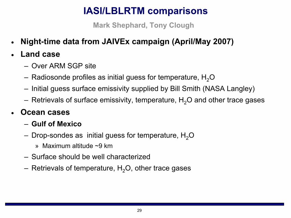
IASI/LBLRTM comparisons

• Night-time data from JAIVEx campaign (April/May 2007)• Land case

– Over ARM SGP site– Radiosonde profiles as initial guess for temperature, H2O– Initial guess surface emissivity supplied by Bill Smith (NASA Langley)– Retrievals of surface emissivity, temperature, H2O and other trace gases

• Ocean cases– Gulf of Mexico– Drop-sondes as initial guess for temperature, H2O

» Maximum altitude ~9 km

– Surface should be well characterized– Retrievals of temperature, H2O, other trace gases

Mark Shephard, Tony Clough

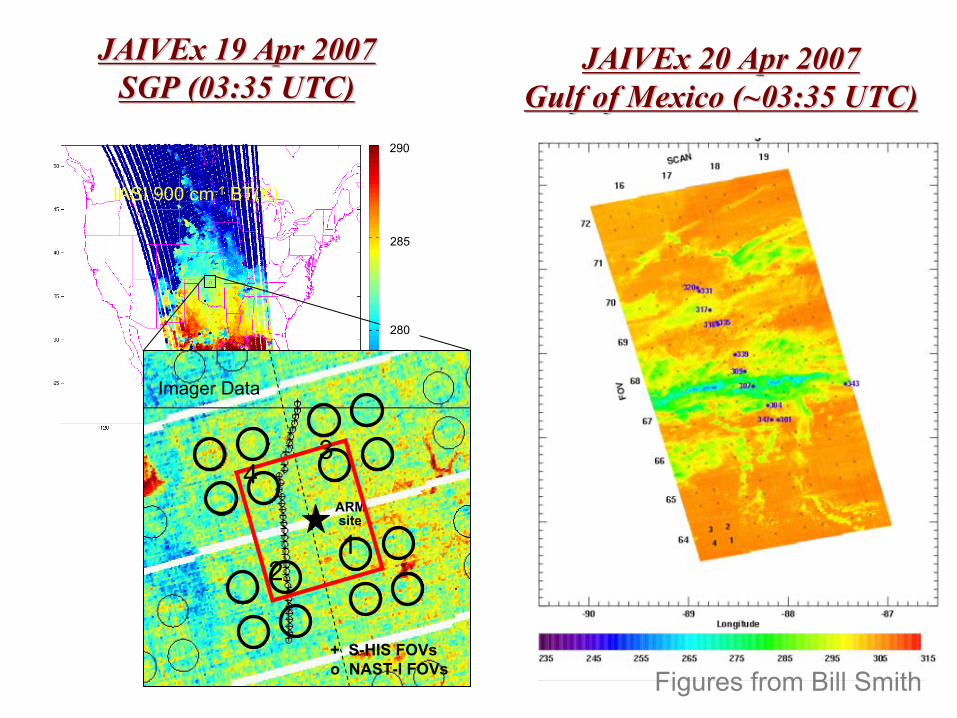
JAIVEx 19 Apr 2007JAIVEx 19 Apr 2007SGPSGP (03:35 UTC)(03:35 UTC)

ARMsite

+ S-HIS FOVso NAST-I FOVs

290

285

280

IASI 900 cm-1 BT(K)

Imager Data

12

34

JAIVExJAIVEx 20 Apr 200720 Apr 2007Gulf of Mexico (~03:35 UTC)Gulf of Mexico (~03:35 UTC)

Figures from Bill Smith

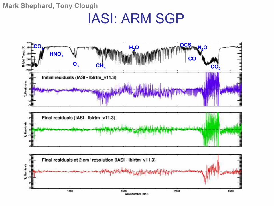
IASI: ARM SGPMark Shephard, Tony Clough

CO2

HNO3

O3 CH4

H2O

CO

N2O

CO2

OCS

Tony Clough, Mark Shephard

IASI: Gulf of MexicoMark Shephard, Tony Clough

PRELIMINARY

34

IASI/LBLRTM comparisons

• IASI measurements are excellent!

• Experience with ocean cases:– “Good” high H2O cases show negative residual at 2500 cm-1

– “Good” low H2O cases show positive residual at 2500 cm-1

– Can’t attribute both to the H2O continuum» Residual contribution due to H2O continuum would go to zero for low PWV profiles

– H2O continuum is not the only piece of the answer at 2500 cm-1……

• Residuals in H2O region remain large after retrieval– Issues with HITRAN H2O line parameters?– Laurent Coudert:

» New measurements indicate HITRAN strengths may be 5% to low for strong lines– Bob Gamache

» Temperature dependences of widths in HITRAN are out of date» Large impact in upper troposphere

35

• LBLRTM:

• Update CO2 ν3 line parameters• HITRAN_MIPAS database: line parameters from Tashkun, Teffo, Flaud et al

• Validated by Flaud et al. using MIPAS spectra

• Update line coupling, continuum and chi-factor accordingly

• Initial validation using laboratory spectra (J. Johns)

• Re-assessment of H2O self continuum in region of 2500 cm-1

• Validation using AIRS, IASI and AERI

• Validation of LBLRTM in the stratosphere

• Comparisons with “untuned” SARTA

• Investigation of alternative sets of ν2 water vapor line parameters

• Line strengths from L. Coudert

• Temperature dependences of widths from R. R. Gamache

Future Plans

Summary of Accomplishments • Microwave

• Publication on water vapor line widths• Validation of water vapor self & foreign H2O continuum using

ground-based measurements• Infrared

• Implementation of P&R branch line coupling for all CO2 bands• Updated water vapor line widths• AIRS/LBLRTM/SARTA comparisons• IASI/LBLRTM comparisons

P.I.: J.-L. Moncet, AER, Inc.

Future Work• Microwave

• Find optimal fit for self and foreign H2O continuum• Zeeman splitting

• Infrared• Update CO2 ν3 line parameters

• Update CO2 line coupling, lineshape and continuum• Validation using up- & down-welling measurements

• Assessment of H2O continuum in 2500 cm-1 region using upwelling, & downwelling measurements

• Validation of LBLRTM in the stratosphere• Comparisons with “untuned SARTA”• Investigate alternative H2O line parameters

Figure 1: Current uncertainty on MW water vapor continuum

Figure 2: AIRS/LBLRTM/SARTA comparisons for ARM TWP

150 GHz31.4 GHz

Improved Spectroscopy for Microwave and Infrared Satellite Data Assimilation