Embed Size (px)
Citation preview

Improved Simplified Methods for
Effective Seismic Analysis and Design
of Isolated and Damped Bridges in
Western and Eastern North America
by
Viacheslav Koval
A thesis submitted in conformity with the requirements for the degree of Degree of Doctor of Philosophy
Department of Civil Engineering University of Toronto
© Copyright by Viacheslav Koval (2015)
ii
Improved Simplified Methods for
Effective Seismic Analysis and Design
of Isolated and Damped Bridges in
Western and Eastern North America
Viacheslav Koval
Degree of Doctor of Philosophy
Department of Civil Engineering University of Toronto
2015
Abstract
The seismic design provisions of the CSA-S6 Canadian Highway Bridge Design Code and the
AASHTO LRFD Seismic Bridge Design Specifications have been developed primarily based on
historical earthquake events that have occurred along the west coast of North America. For the
design of seismic isolation systems, these codes include simplified analysis and design methods.
The appropriateness and range of application of these methods are investigated through extensive
parametric nonlinear time history analyses in this thesis.
It was found that there is a need to adjust existing design guidelines to better capture the
expected nonlinear response of isolated bridges. For isolated bridges located in eastern North
America, new damping coefficients are proposed. The applicability limits of the code-based
simplified methods have been redefined to ensure that the modified method will lead to
conservative results and that a wider range of seismically isolated bridges can be covered by this
method.
The possibility of further improving current simplified code methods was also examined. By
transforming the quantity of allocated energy into a displacement contribution, an idealized
analytical solution is proposed as a new simplified design method. This method realistically
reflects the effects of ground-motion and system design parameters, including the effects of a

iii
drifted oscillation center. The proposed method is therefore more appropriate than current
existing simplified methods and can be applicable to isolation systems exhibiting a wider range
of properties.
A multi-level-hazard performance matrix has been adopted by different seismic provisions
worldwide and will be incorporated into the new edition of the Canadian CSA-S6-14 Bridge
Design code. However, the combined effect and optimal use of isolation and supplemental
damping devices in bridges have not been fully exploited yet to achieve enhanced performance
under different levels of seismic hazard. A novel Dual-Level Seismic Protection (DLSP) concept
is proposed and developed in this thesis which permits to achieve optimum seismic performance
with combined isolation and supplemental damping devices in bridges. This concept is shown to
represent an attractive design approach for both the upgrade of existing seismically deficient
bridges and the design of new isolated bridges.

iv
Acknowledgements I would like to thank my supervisors Professor Constantin Christopoulos and Professor Robert
Tremblay for their valuable guidance and dedication. Their insightful support and steady
feedback over the past five years are directly related to the depth of this research. I have learned
from their endless enthusiasm and strong practical sense, both vital for the successful completion
of this work. It was truly an honor to work with them. I sincerely thank you for giving me this
inspiring opportunity.
The financial support for this research program was provided by the Natural Sciences and
Engineering Research Council of Canada (NSERC). Scholarship for excellence from the FQRNT
(Fonds Québécois de la Recherche sur la Nature et les Technologies) awarded for the highest
level of achievement is gratefully acknowledged.
I wish to express my special gratitude to my family, in particular to my wife Kateryna, my son
Ihor and my daughter Arianne for their love, understanding and encouragement all through.

v
Table of Contents
Acknowledgments .......................................................................................................................... iv
List of Tables .................................................................................................................................x
List of Figures ...............................................................................................................................xiii
Chapter 1: Introduction and Research Objectives ......................................................................... 1
1.1 Problem Definition and Background .................................................................................. 1
1.2 Project Scope and Goals ..................................................................................................... 4
1.3 Project Methodology ........................................................................................................... 6
1.4 Organization of the Thesis ................................................................................................ 10
Chapter 2: Overview of Current Code Analysis and Design Procedures for Isolated Bridges ....................................................................................................................... 12
2.1 Simplified Method in NA Provisions ............................................................................... 12
2.2 Critical Review of Limitations of the Equivalent Linearization Method ......................... 21
2.3 Seismic Protection Mechanism and Devices .................................................................... 27
2.4 Summary ........................................................................................................................... 30
Chapter 3: Analytical Model and Numerical Platform for Nonlinear Time-History Analysis of Isolated and Damped Bridges ................................................................. 32
3.1 Introduction ....................................................................................................................... 32
3.2 Analytical Model for Isolated Bridges .............................................................................. 33
3.3 Model Assumptions for Reference Bridge ....................................................................... 33
3.4 Closed Form Solution and Computation Process ............................................................. 39
3.5 Modeling of Inherent Damping ........................................................................................ 46
3.5.1 Overview of Damping Assumptions ..................................................................... 46
3.5.2 Technique for Modeling Inherent Damping ......................................................... 48
3.6 Model Validation Example ............................................................................................... 50
3.6.1 Modeling Assumptions ......................................................................................... 51

vi
3.6.2 Modeling of Isolation Devices .............................................................................. 54
3.6.3 Time-History Ground Motion ............................................................................... 55
3.6.4 Numerical Modeling with SAP2000 ..................................................................... 55
3.6.5 Results and Comparison ....................................................................................... 57
3.7 Conclusions ....................................................................................................................... 59
Chapter 4: Ground Motion (GM) Selection and Scaling for Time-History Analysis of Isolated Bridges .......................................................................................................... 60
4.1 Introduction ....................................................................................................................... 60
4.2 Overview of Relevant Development in Seismology ......................................................... 61
4.3 Site-Specific Scenarios for ENA and WNA ..................................................................... 64
4.4 Dominant Earthquake Scenarios ....................................................................................... 65
4.5 Directivity Effect on Response Variability ....................................................................... 86
4.6 Ground Motion Scaling ..................................................................................................... 91
4.7 Conclusions on Records Selection and Scaling ................................................................ 99
Chapter 5: Assessment of Damping Coefficients for Seismic Design of Isolated Bridges in Eastern and Western North American Regions ................................................... 100
5.1 Introduction ..................................................................................................................... 100
5.2 Ground Motions Considered for Time-History Analyses ............................................... 101
5.3 Linear Time-History Analyses (LTHA) ......................................................................... 102
5.4 Nonlinear Time-History Analyses (NLTHA) ................................................................. 119
5.4.1 Structural Parameters for Nonlinear Time-History Analyses ............................. 120
5.4.2 General Results from NLTHA ............................................................................ 122
5.4.3 Effects of Ground-Motion Characteristics on Damping Coefficients ................ 126
5.4.4 Comparison of CSA-S6-06 Design Estimates with Results from NLTHA ........ 129
5.5 Proposed Equation for Damping Coefficients, B ............................................................ 136
5.5.1 Calibrating Damping Coefficients, B .................................................................. 136
5.5.2 Validation of the Proposed Damping Coefficients, B ......................................... 138

vii
5.6 Conclusions ..................................................................................................................... 142
Chapter 6: Influence of nonlinear parameters and applicability limits for the code simplified method .................................................................................................... 144
6.1 Introduction ..................................................................................................................... 144
6.2 Influence of System Properties on Damping Coefficients and the Code Simplified Method .......................................................................................................... 145
6.3 Limits of the Equivalent Linearization Method .............................................................. 153
6.3.1 Evaluation of the Equivalence Ratio ................................................................... 153
6.3.2 Results for Equivalence Ratio as a Function of Effective Damping .................. 157
6.3.3 Influence of the System Parameters on Equivalence Ratio ................................ 167
6.4 Applicability Limits for Equivalent Linearization Method ............................................ 170
6.4.1 Limits on Effective Damping, effβ .................................................................... 170
6.4.2 Limits on Effective Period, Teff ........................................................................... 172
6.5 Conclusions ..................................................................................................................... 178
Chapter 7: Basis for Development of New Simplified Method for Estimating the Response of Isolated Bridges ................................................................................... 180
7.1 Introduction ..................................................................................................................... 180
7.2 Equal Displacement and Equal Energy Approximations for Estimating Response of Isolated Bridges .......................................................................................................... 182
7.2.1 Background of Inelastic Response Approximation Concepts ............................ 182
7.2.2 EEA Approach for Bilinear Systems with α > 0 ................................................. 186
7.2.3 EDA and EEA versus Seismic Response of Nonlinear Systems Responding to Seismic Motions ......................................................................... 187
7.3 NL-SDOF Systems Studied through Response Dynamics and Energy Balance ............ 195
7.3.1 Formulation of Energy Balance for Linear and Bilinear SDOF Systems ........... 196
7.3.2 Undamped L-SDOF Response Mechanics: Energy Allocation and Transient Oscillation Center ............................................................................... 201
7.3.3 Transient Response of NL-SDOF Systems to Sinusoidal Loading .................... 214
7.3.4 NL-SDOF Response Mechanics: Results and Discussions ................................ 222

viii
7.4 Conclusions ..................................................................................................................... 237
Chapter 8: Proposed Energy-Based Simplified Analytical Method for Predicting the Response of Isolated Bridges ................................................................................... 239
8.1 Introduction ..................................................................................................................... 239
8.2 Assumptions of New E-R-µ Relationships for the Proposed Energy Formulation for Bilinear Elastoplastic Systems .................................................................................. 240
8.3 Development of New E-R-µ Relationships for the Proposed Energy Formulation for Bilinear Elastoplastic Systems .................................................................................. 243
8.3.1 Development of New E-R-µ Relationships ........................................................ 243
8.3.2 Influence of Ground-Motion and Nonlinear System Parameters ....................... 250
8.4 Design Procedure and Validation ................................................................................... 255
8.4.1 Design Implementation of the Energy-Based E-R-µ Method ............................. 255
8.4.2 Validation of the New Energy-Based Method against NLTHA ......................... 262
8.5 Conclusions ..................................................................................................................... 268
Chapter 9: Design Implications of the Proposed Methods ........................................................ 270
9.1 General ............................................................................................................................ 270
9.2 Proposed Improvements to CSA-S6-06 Simplified Method .......................................... 270
9.3 Proposed New Energy-Based E-R-µ Method ................................................................. 282
9.4 Example of Response Prediction Using Simplified Methods ......................................... 286
9.5 Optimizing Bridge Performance with the New Energy-Based E-R-µ Method .............. 292
9.6 Conclusions ..................................................................................................................... 298
Chapter 10: Dual-Level Seismic Protection Approach for Isolated and Damped Bridge Structures ......... ........................................................................................................299
10.1 Introduction ..................................................................................................................... 299
10.2 Seismic Performance Objectives for Dual-Hazard Level Design of Bridges ................. 301
10.3 DLSP Concept for Seismic Protection Mechanism ........................................................ 303
10.4 Energy-Based E-R-µ Method for Designing a Dual-Level Seismic Protection System for a Bridge Retrofit in Montreal ....................................................................... 309
10.4.1 Defining Bridge and Importance Category ......................................................... 310

ix
10.4.2 Defining Dual-Hazard Performance Objectives ................................................. 312
10.4.3 Assessing Structural Properties using Nonlinear Incremental Analyses ............ 313
10.4.4 Defining Low and Upper Bounds for DLSP System .......................................... 314
10.4.5 Modeling and Basic System Parameters for DLSP Approach ............................ 317
10.4.6 Evaluating the Bridge's Performance Using the New Energy-Based E-R-µ Method ................................................................................................................ 323
10.4.7 Improving the Bridge's Performance Using the New Energy-Based E-R-µ Method ................................................................................................................ 328
10.5 Implementation of a Dual-Level Seismic Protection System for a Bridge Retrofit in Vancouver ................................................................................................................... 332
10.5.1 Defining Bridge and Importance Category ......................................................... 333
10.5.2 Dual-Hazard Performance Objectives ................................................................ 334
10.5.3 Assessing Structural Properties Using Nonlinear Incremental Analyses ........... 335
10.5.4 Time-History Ground Motions Considered for Configuring Optimal Protection System ............................................................................................... 336
10.5.5 Basic System Parameters for DLSP Approach ................................................... 336
10.5.6 Optimization of Isolated Bridges without Added Viscous Dampers .................. 340
10.5.7 Optimization Results for Isolated Bridge with Added Viscous Dampers .......... 344
10.6 Conclusions ..................................................................................................................... 345
Chapter 11: Summary and Conclusions ....................................................................................... 347
11.1 Overview and Project Contributions ............................................................................... 347
11.2 Conclusions ..................................................................................................................... 349
11.3 Recommendations for Future Research .......................................................................... 353
References ...................................................................................................................................354
Appendix A .................................................................................................................................371

x
List of Tables Table 2-1 Values of the damping coefficient B ............................................................................ 16
Table 2-2 Effective formulations for equivalent linearization (compared in Mavronicola and
Komodromos, 2011) ..................................................................................................................... 24
Table 3-1 Pier properties for the model validating example ......................................................... 53
Table 3-2 Modeling parameters: bilinear hysteretic response ...................................................... 54
Table 4-1 Dominant M-R scenarios determined by using the mean and modal techniques for
Montreal, for a probability of exceedance 2% in 50 years (summarized form Halchuk, 2010) ... 71
Table 4-2 Dominant M-R scenarios determined by using the mean and modal techniques for
Vancouver, for a probability of exceedance 2% in 50 years (summarized form Halchuk, 2010) 71
Table 4-3 Magnitude-distance ranges for Step 2 of scenario definition ....................................... 78
Table 4-4 Step 2 - M-R ranges selection approach for Montreal, 2%-50 years ........................... 80
Table 4-5 Step 1 - Boundary selection approach for Montreal, 2%-50 years ............................... 82
Table 4-6 M-R events selected from Steps 1 and 2 – ENA .......................................................... 83
Table 4-7 Distribution and number of records from Step 1 and Step 2 - ENA ............................ 84
Table 4-8 Distribution and number of records from Step 3 - ENA .............................................. 86
Table 4-9 Spectral values from the target UHS NBCC (2005) - 2% in 50 years, site class C ..... 92
Table 4-10 ATK-E 20 Records scaled to the target UHS 2005 NBCC, 2%-50 years, site class C,
city of Montreal (ENA), Sa-targ/Sa-sim computed over 0.2 - 4.0 s ................................................... 96
Table 4-11 MCG-CEUS 20 Records scaled to the target UHS 2005 NBCC, 2%-50 years, site
class C, city of Montreal (ENA) , SA-targ/SA-sim computed over 0.2 - 4.0 s ................................... 97
Table 4-12 ATK-W 20 Records scaled to the target UHS 2005 NBCC, 2%-50 years, site class C,
city of Vancouver (WNA) , SA-targ/SA-sim computed over 0.2 - 4.0 s............................................. 98

xi
Table 5-1 Structural parameters for nonlinear time-history analyses ......................................... 121
Table 5-2 Summary on comparison between individual responses from NLTHA and the
corresponding response estimates according to the code provisions (sample of 1200 values) .. 130
Table 5-3 Statistical assessment for results obtained for ENA using Eq.(2.8) with n=0.2 ......... 138
Table 6-1 Examples of equivalent linearization (ATK-E 20 Records, Te=0.25 s; α=0.01) ........ 157
Table 7-1 Normalized time, kinetic energy, absorbed energy, and displacement at transient OC
for the first half response cycle ................................................................................................... 207
Table 8-1 Direct energy-based E-R-µ design method................................................................. 257
Table 8-2 Procedure for the response estimate using iterative energy-based E-R-µ method ..... 260
Table 9-1 Modified procedure following the Simplified Equivalent Static Force Method
(CAN/CSA-S6) ........................................................................................................................... 273
Table 9-2 Iterative approach for response estimate using current Equation (2.8) with n = 0.3
(where for βeff > 30%, B = 1.7) ................................................................................................... 288
Table 9-3 Iterative approach for response estimate using Equation (2.8) with n = 0.2 .............. 288
Table 9-4 Direct approach for response estimate using new energy-based E-R-µ method ........ 289
Table 9-5 Relative error for response estimates ......................................................................... 289
Table 9-6 Direct approach for response estimate using new energy-based E-R-µ method ........ 296
Table 10-1 Bridge classification performance levels (Huffman et al. 2012) .............................. 301
Table 10-2 Expected bridge functionality levels (summarized from Huffman et al., 2012) ...... 302
Table 10-3 DLSP optimization strategy for seismic protection mechanism .............................. 304
Table 10-4 Dual-level performance objectives for design of isolated bridges ........................... 312
Table 10-5 Original bridge - Substructure parameters ............................................................... 318

xii
Table 10-6 DLSP's responses obtained using the E-R-µ relationship for each performance level
..................................................................................................................................................... 326
Table 10-7 System equivalent parameters for DLSP's stages ..................................................... 330
Table 10-8 Original bridge (m2 = 954 000 kg) - Substructure parameters .................................. 336
Table 10-9 Isolated bridge - Parameters of isolation on piers and abutments ............................ 337
Table 10-10 Activation levels for isolators at the abutments ..................................................... 341

xiii
List of Figures Figure 2.1 Equivalent linearization method: a) transformation of nonlinear system (bilinear
response) to equivalent system (viscoelastic response); b) typical isolated bridge - nonlinear
system; and c) equivalent linearization method ............................................................................ 12
Figure 2.2 Acceleration (SA) and displacement (SD) design spectra in Eurocode 8 ..................... 18
Figure 2.3 Damping coefficient in different seismic codes .......................................................... 19
Figure 2.4 AASHTO equivalent damping ratio as a function of shear displacement ductility ratio
(Hwang and Sheng, 1993) ............................................................................................................. 23
Figure 2.5 Relative errors of the maximum relative displacements at the isolation level
considering the proposed linearized models, varying the post-yielding ratio, under the selected
earthquake excitations scaled to PGA = 0.8 g (Mavronicola and Komodromos, 2011). ............. 25
Figure 2.6 Comparison of responses calculated using various methods, response spectra scaled to
the NEHRP spectrum, and values calculated for the NEHRP spectrum (FEMA 440): a) SDOF
with T = 0.2 s; b) SDOF with T = 0.5 s; SDOF with T = 1.0 s; and d) methods description ........ 27
Figure 2.7 Seismic isolators with restoring force: a) LRB (Buckle et al., 2006); b) FPI (Buckle et
al., 2006); c) FSI with restoring force (Dion et al., 2012); and d) bilinear force-displacement
relationship, 0 < α < 1. .................................................................................................................. 28
Figure 2.8 Flat sliding seismic isolator without restoring force: a) seismic energy products
(www.sepbearings.com); b) bilinear force-displacement relationship, α = 0 ............................... 29
Figure 2.9 Viscous damper .......................................................................................................... 30
Figure 3.1 Kelvin-Voigt solid model and simple oscillator SDOF system .................................. 34
Figure 3.2 Equivalent stiffness for different bridge configurations: a) non-isolated bridge, b)
bridge with isolation atop the piers and c) bridge with isolation atop the piers and abutments ... 35
Figure 3.3 Pier-deck model (Tsopelas et al., 1996) ...................................................................... 37
Figure 3.4 Example of fully equipped bridge ............................................................................... 38

xiv
Figure 3.5 Bridge 2-DOF equivalent model ................................................................................. 38
Figure 3.6 Average acceleration assumed for time step Δt ........................................................... 43
Figure 3.7 Equivalent stiffness correction: Step 1 ........................................................................ 44
Figure 3.8 Equivalent stiffness correction: Step 2 ........................................................................ 44
Figure 3.9 Flowchart of the computation process ......................................................................... 45
Figure 3.10 Bridge elevation ......................................................................................................... 50
Figure 3.11 Bridge cross-section and pier configuration .............................................................. 51
Figure 3.12 Mass assumptions for bridge modelling .................................................................... 51
Figure 3.13 Deck weight and axial loads (idealized geometrical distribution) ............................ 52
Figure 3.14 Pier modeling assumptions for pushover analyses: a) cross-section and sectional
properties, b) material properties, and c) loading and support conditions .................................... 53
Figure 3.15 Protection axial loads distribution ............................................................................. 54
Figure 3.16 Simulated time-history record – M7.0-R70-1 ........................................................... 55
Figure 3.17 Modeling bridge with SAP2000 ................................................................................ 56
Figure 3.18 Hysteretic bridge response from SAP2000 and IS-Bridge ........................................ 57
Figure 3.19 Time histories of bridge responses computed by SAP2000 and IS-Bridge .............. 58
Figure 4.1 The concept of UHS for a location affected by local sources of moderate seismicity
and distant sources (Bommer et al., 2000a and Hancock, 2006 after Reiter, 1990) ..................... 63
Figure 4.2 Hazard curves for Vancouver and Montréal (Adams and Halchuk 2004) .................. 64
Figure 4.3 Earthquake risk distribution in Canada (Adams, 2011) .............................................. 65
Figure 4.4 Hazard deaggregation for SA(0.2) = 0.584 g in Montreal for a probability of
exceedance 2% in 50 years (Halchuk, 2010) ................................................................................ 67

xv
Figure 4.5 Hazard deaggregation for SA(0.5) = 0.289 g in Montreal for a probability of
exceedance 2% in 50 years (Halchuk, 2010) ................................................................................ 67
Figure 4.6 Hazard deaggregation for SA(1.0) = 0.123 g in Montreal for a probability of
exceedance 2% in 50 years (Halchuk, 2010) ................................................................................ 68
Figure 4.7 Hazard deaggregation for SA(2.0) = 0.031 g in Montreal for a probability of
exceedance 2% in 50 years (Halchuk, 2010) ................................................................................ 68
Figure 4.8 Hazard deaggregation for SA(0.2) = 0.931 g in Vancouver for a probability of
exceedance 2% in 50 years (Halchuk, 2010) ................................................................................ 69
Figure 4.9 Hazard deaggregation for SA(0.5) = 0.622 g in Vancouver for a probability of
exceedance 2% in 50 years (Halchuk, 2010) ................................................................................ 69
Figure 4.10 Hazard deaggregation for SA(1.0) = 0.291 g in Vancouver for a probability of
exceedance 2% in 50 years (Halchuk, 2010) ................................................................................ 70
Figure 4.11 Hazard deaggregation for SA(2.0) = 0.132 g in Vancouver for a probability of
exceedance 2% in 50 years (Halchuk, 2010) ................................................................................ 70
Figure 4.12 Modal and mean earthquakes for Montreal, T=2.0 s, 2%-50 years (mean hazard level
is determined over all hazard contributions) ................................................................................. 73
Figure 4.13 Earthquakes covered by Atkinson's M-R ranges and boundary ranges .................... 77
Figure 4.14 Example of selecting earthquake scenarios using Atkinson's M-R ranges (Step 1)
from hazard deaggregated for Montreal, SA(0.5) = 0.289 g, at a probability of exceedance 2% in
50 years (deaggregation by Halchuk, 2010) ................................................................................. 79
Figure 4.15 Example of selecting earthquake scenarios using Boundary M-R ranges (Step 2)
from hazard deaggregated for Montreal, SA(0.5) = 0.289 g, at a probability of exceedance 2% in
50 years (deaggregation by Halchuk, 2010) ................................................................................. 81
Figure 4.16 Dominant earthquake scenario for montreal at 2% in 50 years (0.2 s to 2.0 s) ......... 84
Figure 4.17 Pulse time function .................................................................................................... 87

xvi
Figure 4.18 Plan view of the directivity effect on the ground motion intensity and duration ...... 88
Figure 4.19 Forward and backward rupture directivity from the 1992 Landers earthquake
(Somerville, 1997a) ....................................................................................................................... 89
Figure 4.20 ATK-E 20 Records - Mean and individual 5% damped response spectra scaled to the
target UHS 2005 NBCC ................................................................................................................ 93
Figure 4.21 MCG-CEUS 20 Records - Mean and individual 5% damped response spectra scaled
to the target UHS 2005 NBCC ...................................................................................................... 94
Figure 4.22 ATK-E 20 Records - Mean and individual 5% damped response spectra scaled to the
target UHS 2005 NBCC ................................................................................................................ 95
Figure 5.1 Damped response spectra (Mean of 20 Records) - ATK-W ..................................... 105
Figure 5.2 Damped response spectra (Mean of 20 Records) - ATK-E ....................................... 106
Figure 5.3 Damped response spectra (Mean of 20 Records) - MCG-CEUS .............................. 107
Figure 5.4 Power amplitude with period (Mean of 20 Records) - ATK-W and ATK-E ............ 108
Figure 5.5 Comparison of damping coefficients B for the 0.2 s - 4.0 s period range:
a) )( DSB coefficients and b) )( ASB coefficients ......................................................................... 109
Figure 5.6 Variation of B-Coefficient with damping ratio by period range – Mean of 20 Records
..................................................................................................................................................... 111
Figure 5.7 Damped pseudo velocity response spectra (Mean of 20 Records) ............................ 112
Figure 5.8 Variation of damping coefficients B with period - ATK-W: a) )( ASB coefficients and
b) )( DSB coefficients .................................................................................................................. 113
Figure 5.9 Variation of damping coefficients B with period - ATK-E: a) )( ASB coefficients and
b) )( DSB coefficients .................................................................................................................. 114
Figure 5.10 Variation of damping coefficients B with period - MCG-CEUS:
a) )( ASB coefficients and b) )( DSB coefficients ........................................................................ 115

xvii
Figure 5.11 Idealized factor B(SA) for harmonic response of SDOF systems ............................ 118
Figure 5.12 Idealized factor B(SD) for harmonic response of SDOF systems ............................ 118
Figure 5.13 Structure nonlinear parameters - Bilinear hysteretic ............................................... 121
Figure 5.14 Comparison of B computed for WNA with those specified in the CSA-S6-06 Code
(AASHTO): (a) mean of 20 records, (b) individual records ....................................................... 124
Figure 5.15 Comparison of B computed for ENA with those specified in the CSA-S6-06 Code
(AASHTO): (a) mean of 20 records, (b) individual records ....................................................... 125
Figure 5.16 ENA response spectra for 20 ATK-E records: (a) individual spectra and (b) mean
spectra regrouped according to M-R subsets: E6C1 (6 records), E6C2 (3 records), E7C1 (3
Records), and E7C2 (8 Records) ................................................................................................ 127
Figure 5.17 Effect of ENA M-R distribution on damping coefficients ...................................... 128
Figure 5.18 Frequency of uNLTH/ucode versus normal distribution - WNA Eq.(2.8) with n=0.3 . 131
Figure 5.19 Frequency of uNLTH/ucode versus normal distribution - ENA Eq.(2.8) with n=0.3 ... 132
Figure 5.20 Responses from NLTHA versus code estimate - WNA Eq.(2.8) with n=0.3 .......... 134
Figure 5.21 Responses from NLTHA versus code estimate - ENA Eq.(2.8) with n=0.3 ........... 135
Figure 5.22 One-tailed hypothesis test for the population mean at a 95% confidence level ...... 137
Figure 5.23 Relative errors of the displacement estimate as a function of the effective damping
(Equivalent linearization method and coefficients B from Eq.(2.8) with n = 0.3 for WNA and
n = 0.2 for ENA) ......................................................................................................................... 139
Figure 5.24 Relative errors of the displacement estimate as a function of the effective period
(Equivalent linearization method and coefficients B from Eq.(2.8) with n = 0.3 for WNA and
n = 0.2 for ENA) ......................................................................................................................... 140
Figure 5.25 Comparison of proposed and computed B damping coefficients for ENA ............. 142
Figure 6.1 Bilinear response and equivalent viscoelastic response ............................................ 145
xviii
Figure 6.2 Variation of damping coefficients B in ENA with initial period Te .......................... 147
Figure 6.3 Bilinear response - Influence of the R factor on the hysteretic shape ....................... 148
Figure 6.4 Bilinear response - Response around drifted oscillation center and equivalent response
around original center as prescribed in the CSA-S6-06 simplified method. .............................. 150
Figure 6.5 Variation of damping coefficients B in ENA with effective period Teff for ratios
R = [4, 16, 28, 40, and 52], Te = [0.25, 0.5, 0.75, and 1.0 s] and α = [0.01, 0.05, and 0.1] ........ 152
Figure 6.6 Response of SDOF system from NLTHA and equivalent LTHA ............................ 156
Figure 6.7 Equivalence ratio - WNA ATK-W: α=0.1 ................................................................ 158
Figure 6.8 Equivalence ratio - WNA ATK-W: α=0.05 .............................................................. 159
Figure 6.9 Equivalence ratio - WNA ATK-W: α=0.01 .............................................................. 160
Figure 6.10 Equivalence ratio - ENA ATK-E: α=0.1 ................................................................. 161
Figure 6.11 Equivalence ratio - ENA ATK-E: α=0.05 ............................................................... 162
Figure 6.12 Equivalence ratio - ENA ATK-E: α=0.01 ............................................................... 163
Figure 6.13 Coefficient of variation for equivalence ratio - WNA ATK-W .............................. 165
Figure 6.14 Coefficient of variation for equivalence ratio - ENA ATK-E ................................. 166
Figure 6.15 Distribution of equivalence ratio by R and Te (WNA ATK-W) ............................. 168
Figure 6.16 Distribution of equivalence ratio by R and Te (ENA ATK-E) ................................ 169
Figure 6.17 Equivalent damping ratio with ductility for α =0.01, 0.05, and 0.1 ........................ 171
Figure 6.18 Effective damping with effective period: Equations (6.13) and (6.14) ................... 174
Figure 6.19 Coefficient of variation for equivalence ratio with Teff - ENA ATK-W .................. 175
Figure 6.20 20-Records mean responses versus code estimates with proposed limits on effective
period - WNA Eq.(2.8) with n=0.3 ............................................................................................. 176

xix
Figure 6.21 20-Records mean responses versus code estimates with proposed limits on effective
period - ENA Eq.(2.8) with n=0.2 .............................................................................................. 177
Figure 7.1 EDA and EEA concepts for elastic perfectly-plastic systems: α=0 .......................... 184
Figure 7.2 Inelastic design spectra for earthquakes (Newmark and Hall, 1960) ........................ 185
Figure 7.3 Concept of Equal Energy - Energies absorbed by linear and nonlinear systems: : α>0
..................................................................................................................................................... 186
Figure 7.4 Energy deficit between "exact" response and EEA estimate .................................... 188
Figure 7.5 "Exact" responses and the 5% damped Sa-Sd spectrum (α=0.05, Te=0.25 s and 0.5 s)
..................................................................................................................................................... 190
Figure 7.6 "Exact" responses and the 5% damped Sa-Sd spectrum (α=0.05, Te=0.75 s and 1.0 s)
..................................................................................................................................................... 191
Figure 7.7 Influence of the R-factor and period on the error between "exact" response and Equal
Displacement Approximation (α = 0.05, mean of 20 Atkinson's artificial records - ENA) ....... 192
Figure 7.8 Influence of the R-factor and period on the error between "exact" response and Equal
Energy Approximation (α = 0.05, mean of 20 Atkinson's artificial records - ENA) .................. 193
Figure 7.9 Error between "exact" response and Equal Energy Approximation versus normalized
energy deficit (α = 0.05, mean of 20 Atkinson's artificial records - ENA) ................................. 194
Figure 7.10 SDOF system free-body diagram and energy balance: a) SDOF system model;
b) forced damped dynamic motion ............................................................................................. 200
Figure 7.11 Example of loading frequency ratios ]5.1;0.1;75.0[/ =eg ωω for three different
bridge structures subjected to the same ground motion excitation ............................................. 202
Figure 7.12 Example of loading frequency ratios ]5.1;0.1;75.0[/ =eg ωω for a bridge structure
subjected to three different ground-motion excitations .............................................................. 203
Figure 7.13 Response of elastic SDOF system for ]5.1;0.1;75.0[/ =eg ωω .......................... 205
xx
Figure 7.14 Velocity and displacement of elastic SDOF system for ]5.1;0.1;75.0[/ =eg ωω 206
Figure 7.15 Energy flow, elastic SDOF system for: a) 75.0/ =eg ωω ; b) 0.1/ =eg ωω and
c) 5.1/ =eg ωω ........................................................................................................................... 209
Figure 7.16 Relative complete displacement as a result of transient and steady-state responses 210
Figure 7.17 Relative complete velocity as a result of transient and steady-state responses ....... 210
Figure 7.18 Influence of the frequency ration on normalized kinetic Ek and absorbed EAb energies
at the transient OC for undamped L-SDOF systems .................................................................. 213
Figure 7.19 Cycloidal front pulses: Type A (left) and Type B (right) used by Makris (1997) to
approximate recorded ground motions. ...................................................................................... 216
Figure 7.20 Normalized response of an elastic undamped system (1 cycle at 1/ =eg ωω ) ..... 221
Figure 7.21 Amplitude increase with cycles for an elastic undamped system ( 1/ =eg ωω ) ..... 221
Figure 7.22 Normalized amplitude versus frequency ratio for different R-factors (1 cycle and 10
cycles loadings, 5.0=α ) ........................................................................................................... 224
Figure 7.23 Normalized amplitude versus frequency ratio for different R-factors (1 cycle and 10
cycles loading, 1.0=α ) ............................................................................................................. 225
Figure 7.24 Normalized amplitude versus frequency ratio for different R-factors (1 cycle and 10
cycles loading, 05.0=α ) ........................................................................................................... 226
Figure 7.25 Normalized amplitude versus frequency ratio for different R-factors (1 cycle and 10
cycles loading, 01.0=α ) ........................................................................................................... 227
Figure 7.26 Time histories of velocity and displacement responses for NL-SDOF with
ωg / ωe = 1, α = 0.01 under 10 cycles of sinusoidal loading ........................................................ 229
Figure 7.27 Energy allocation for NL-SDOF system with ωg / ωe = 1, α = 0.01, R = 2, 4 and 16
(input, kinetic, absorbed energies, and power of balanced displacement response) ................... 231

xxi
Figure 7.28 Normalized response with frequency ratio: maximum response and drifted
oscillation center for α = 0.01 and R = 16 ................................................................................... 235
Figure 7.29 Normalized hysteretic response maximum response and drifted oscillation center for
α = 0.01, R = 16, and for: a) eg ωω / = 0.5 ; b) eg ωω / = 1.0. .................................................... 236
Figure 8.1 Idealized response a) input energy, b) kinetic energy, c) absorbed energy,
d) equivalent strain energy as portion of absorbed energy, and e) dissipated portion of absorbed
energy .......................................................................................................................................... 244
Figure 8.2 Characteristics of the ground forcing function .......................................................... 247
Figure 8.3 Concept of energy balance for transient response ..................................................... 249
Figure 8.4 Ductility response with ratio Te / Tg using the E-R-µ relationship with PGD = 72 mm,
Tg = 0.9 s, ue(Te) = 40Te (mean parametres - 20 Atkinson's records) .......................................... 253
Figure 8.5 E-R-µ relationship obtained from Equation (8.20) compared to R-µ expression for
EEA given by Equation (7.7): ENA for 05.0=α ...................................................................... 254
Figure 8.6 Ground-motion characteristics and 5% damped displacement spectra for four M-R
scenario sets (ATK-ENA and ATK-WNA) ................................................................................ 262
Figure 8.7 WNA E-R-µ relationship from analytical estimate and NL SDOF analyses ............ 264
Figure 8.8 ENA E-R-µ relationship from analytical estimate and NL SDOF analyses .............. 265
Figure 8.9 NLTHA versus energy-based E-R-µ approach using Equation (8.20) ...................... 266
Figure 8.10 NLTHA versus energy-based E-R-µ approach using Equation (8.20) and Equal
Energy Approach (EEA) using Equation (7.8) ........................................................................... 267
Figure 9.1 Relative errors in maximum displacements at the isolation level using the code
simplified method compared to NLTHA for WNA and α = 0.1 (ATK-W): a) current CSA-S6-06
method; b) current method with damping coefficients from Eq.(2.8) applicability limits;
c) current method with damping coefficients from Eq.(2.8) and applicability limits based on
effective period. .......................................................................................................................... 276

xxii
Figure 9.2 Relative errors in maximum displacements at the isolation level using the code
simplified method compared to NLTHA for WNA and α = 0.05 (ATK-W): a) current CSA-S6-
06 method; b) current method with damping coefficients from Eq.(2.8) applicability limits;
c) current method with damping coefficients from Eq.(2.8) and applicability limits based on
effective period. .......................................................................................................................... 277
Figure 9.3 Relative errors in maximum displacements at the isolation level using the code
simplified method compared to NLTHA for WNA and α = 0.01 (ATK-W): a) current CSA-S6-
06 method; b) current method with damping coefficients from Eq.(2.8) applicability limits;
c) current method with damping coefficients from Eq.(2.8) and applicability limits based on
effective period. .......................................................................................................................... 278
Figure 9.4 Relative errors in maximum displacements at the isolation level using the code
simplified method compared to NLTHA for ENA and α = 0.1 (ATK-E): a) current CSA-S6-06
method; b) current method with damping coefficients from Eq.(2.8) applicability limits;
c) current method with damping coefficients from Eq.(2.8) and applicability limits based on
effective period. .......................................................................................................................... 279
Figure 9.5 Relative errors in maximum displacements at the isolation level using the code
simplified method compared to NLTHA for ENA and α = 0.05 (ATK-E): a) current CSA-S6-06
method; b) current method with damping coefficients from Eq.(2.8) applicability limits;
c) current method with damping coefficients from Eq.(2.8) and applicability limits based on
effective period. .......................................................................................................................... 280
Figure 9.6 Relative errors in maximum displacements at the isolation level using the code
simplified method compared to NLTHA for ENA and α = 0.01 (ATK-E): a) current CSA-S6-06
method; b) current method with damping coefficients from Eq.(2.8) applicability limits;
c) current method with damping coefficients from Eq.(2.8) and applicability limits based on
effective period. .......................................................................................................................... 281
Figure 9.7 Relative error of the maximum displacements at the isolation level using the new
energy-based E-R-µ method - PGD=337 mm; Tg =1.82 s (mean of 20 Atkinson's records - WNA)
..................................................................................................................................................... 284

xxiii
Figure 9.8 Relative error of the maximum displacements at the isolation level using the new
energy-based E-R-µ method - PGD = 72 mm; Tg =0.89 s (mean of 20 Atkinson's records - ENA)
..................................................................................................................................................... 285
Figure 9.9 Archetype three-span bridge in Montreal .................................................................. 286
Figure 9.10 Response estimates using different methods (Current simplified CSA-S6-06 method;
Modified simplified CSA-S6-06 method; New energy-based E-R-µ method; NLTHA) ........... 289
Figure 9.11 Displacement and force responses with characteristic strength Qd ......................... 294
Figure 9.12 Bridge response with characteristic strength Qd and period Td ............................... 295
Figure 9.13 Peak seismic forces with characteristic strength Qd and period Td ......................... 297
Figure 9.14 Peak seismic forces with response modification factor R ....................................... 297
Figure 10.1 Bridge seismic protection along longitudinal direction of a bridge: a) Combination
..................................................................................................................................................... 303
Figure 10.2 Optimization flowchart for DLSP ........................................................................... 306
Figure 10.3 Response of isolated bridges with response modification factor R in ENA using
Equation (8.20) PGD = 72 mm, Tg = 0.89, Te = 0.5, α = 0.01 .................................................... 307
Figure 10.4 Photo (Google Maps- ©2012 Google), plan and elevation of the two-span bridge in
Montreal ...................................................................................................................................... 311
Figure 10.5 Pier Pushover Analysis - Bridge in Montreal .......................................................... 313
Figure 10.6 Design spectra for SE (10% in 50 years) and DE (2% in 50 years) ........................ 314
Figure 10.7 Response ranges using factor R for bounded analyses ............................................ 316
Figure 10.8 Performance objectives and responses ranges using E-R-μ relationship for two
hazard levels with variation of the isolator’s properties ............................................................. 316
Figure 10.9 Response idealizations for two DLSP’s stages ....................................................... 320

xxiv
Figure 10.10 Responses normalized to elastic response: curve from E-R-µ with respect to
NLTHA (20 Atk-E Records, Montreal) ...................................................................................... 325
Figure 10.11 Bridge's performance obtained using the new energy-based E-R-µ method (ATK-E:
PGD=72 mm, Tg=0.89 s)............................................................................................................ 328
Figure 10.12 Selection of elastic stiffness for isolators at the abutments ................................... 329
Figure 10.13 Performance of the DLSP with reduced stiffness using the new energy-based E-R-µ
method (ATK-E: PGD=72 mm, Tg=0.89 s) ............................................................................... 330
Figure 10.14 Performance of the DLSP with reduced stiffness and adding 5% of viscous
damping using the new energy-based E-R-µ method (ATK-E: PGD = 72 mm, Tg = 0.89 s) ..... 331
Figure 10.15 Photo (Google Maps- ©2012 Google), plan and elevation of the four-span bridge in
Vancouver. .................................................................................................................................. 334
Figure 10.16 Pier pushover analysis - Bridge in Vancouver ...................................................... 335
Figure 10.17 Selection of elastic stiffness for isolators at the abutments ................................... 338
Figure 10.18 Responses of abutment isolators with R-factor (10% in 50 years) ........................ 340
Figure 10.19 Displacement responses for bridge without dampers (20 records - 10%-50 years):
(a) Q3d = 100%, (b) Q3d = 51%, (c) Q3d = 29%, and (d) Q3d = 19% ............................................ 342
Figure 10.20 Displacement responses for bridge without dampers (20 artificial records - 2%-50
years): (a) Q3d = 100%, (b) Q3d = 51%, (c) Q3d = 29%, and (d) Q3d = 19% ................................ 342
Figure 10.21 Isolator forces for bridge without damper (20 artificial records - 2%-50 years):
(a) Q3d = 100%, (b) Q3d = 51%, (c) Q3d = 29%, and (d) Q3d = 19% ............................................ 343
Figure 10.22 Optimizing damper c3 to expansion joints limit (1 record - 10%-50 years) .......... 344
Figure 10.23 Displacement responses for bridge with damper c3 = 0.6 MN-s/m (20 records) ... 345

xxv
List of Symbols and Abbreviations
EATK − artificial time-histories simulated by Atkinson's (2009) for eastern Canada
WATK − artificial time-histories simulated by Atkinson's (2009) for western Canada
CEUS the central-eastern U.S.
DE design earthquake
DLSP Dual-Level Seismic Protection
DOF degree of freedom
EDA equal displacement approximation
EEA equal energy approximation
ENA eastern North America
EQ earthquake
FPI friction pendulum isolator
FSI flat sliding isolator
GM Ground motion
LB low bound
LRB lead rubber bearing
LTH linear time history
CEUSMCG − hybrid time histories produced by McGuire (2001) to reproduce the
seismicity from the central-eastern U.S.
NA North America
NLTH nonlinear time history
OC oscillation centre
SDOF single degree of freedom
SE service earthquake
TH time history
UB upper bound
UHS uniform hazard spectrum
WNA western North America
WUS the western U.S.

xxvi
A constant spectral acceleration
maxA pulse acceleration amplitude
B damping coefficient
SAB damping coefficients defined for spectral acceleration in terms of transmissibility
SDB damping coefficients defined for spectral displacement using response
amplification factor Rd
[ ]C damping matrix
EQCOV coefficients of variation for equivalence ratio in statistical analyses
vC constant of integration for velocity
uC constant of integration for displacement
c damping coefficient
1c damping coefficient for modeling the pier inherent damping or equivalent
damping coefficient in Equation (3.21)
2c damping coefficient for modeling dampers at the pier
3c damping coefficient for modeling dampers at the abutment
crc critical damping
D constant spectral displacement
d displacement estimate of the bridge deck
id displacement estimate of the bridge deck during iterative step i
0d displacement estimate of the bridge deck during iterative step 1−i
AbE absorbed energy
AbLE energy absorbed by elastic system
AbNLE energy absorbed by bilinear system
EqAbE energy absorbed by the equivalent substitute system
dE energy dissipated by viscous damping
hE amount of energy dissipated in one cycle
inE relative input energy
kE relative kinetic energy

xxvii
pE potential energy
F design forces to be resisted by the bridge substructure
aF site amplification factor for short spectral periods
dF damping force
)(1 tFD , )(2 tFD , )(3 tFD damping force at DOF1, DOF2, DOF3 at time t
eF maximum elastic force
iF inertia force
iFi , iFd , iFs inertial, damping and spring forces at the thi time step
1+iFi , 1+iFd , 1+iFs inertial, damping and spring forces at time step 1+i
)(1 tFI , )(2 tFI , )(3 tFI inertia forces at DOF1, DOF2, DOF3 at time t
maxF peak force response
sF spring force
)(1 tFS , )(2 tFS , )(3 tFS spring force at DOF1, DOF2, DOF3 at time t
uF ultimate force
vF site amplification factor for long spectral periods
yF force at elastic limit or activation force
1F forces resisted by the pier structure
2F forces resisted by isolators at the pier
3F forces resisted by isolators at the abutment
yF1 force resisted by the pier structure at elastic limit
yF2 activation force for isolation system located at the bridge piers
yF3 activation force for isolation system located at the bridge abutment
{ }DF damping force vector
{ }IF inertia force vector
{ }SF spring force vector
'cf compressive strength of concrete
tf tensile strength of concrete

xxviii
uf ultimate strength of the rebar
yf yield strength of the rebar
g acceleration of gravity
effK effective stiffness in Equation (3.24)
k stiffness coefficient
abutk stiffness corresponding to the abutment structure
jabutk , stiffness of abutment j
dk post-yielding or post-activation stiffness
ek elastic stiffness
effk effective stiffness
eqk equivalent stiffness
1eqk , 2eqk , 2eqk equivalent stiffness ratios for tri-linear hysteresis
1eeqk − equivalent elastic stiffness during DLSP Stage I
2eeqk − equivalent elastic stiffness during DLSP Stage II
isolk stiffness of isolators
jisolk , stiffness of isolator devices installed on a given abutment j
iisolk , stiffness of isolator devices installed on a given pier i
pierk stiffness corresponding to the pier structure
ipierk , stiffness of pier i
uk initial stiffness of bilinear hysteresis
1k stiffness coefficient for modeling pier
2k stiffness coefficient for modeling isolators at the pier
3k stiffness coefficient for modeling isolators at the abutment
dk1 post-yielding stiffness for modeling pier
dk2 post-activation stiffness of isolators at the pier
dk3 post-activation stiffness of isolators at the abutments
uk1 initial stiffness for modeling pier

xxix
uk2 initial stiffness of isolators at the pier
uk3 initial stiffness of isolators at the abutments
[ ]K stiffness matrix
m mass of SDOF system
1m mass of the pier structure or mass at DOF1
2m mass of the bridge superstructure or mass at DOF2
[ ]M mass matrix
1NF near-fault-factor-1 (Dicleli and Buddaram, 2007)
2NF near-fault-factor-2 (Dicleli and Buddaram, 2007)
n exponential coefficient or number of cycles
P external loading force
PGA peak ground acceleration
PGD peak ground displacement
maxP peak loading force
DPS spectral pseudo-displacement
)(1 tP , )(2 tP , )(3 tP external force acting at DOF1, DOF2, DOF3 at time t
)(tP loading force function
0p amplitude of loading function
{ }P loading force vector
dQ characteristic strength
dQ2 , dQ3 characteristic strength of isolators at the pier and abutment
R response modification factor
crR critical value of the response modification
dR displacement amplification factor
minR , maxR minimum and maximum response modification factors
1minR , 1maxR minimum and maximum response modification factors during DLSP Stage I
2minR , 2maxR minimum and maximum response modification factors during DLSP Stage II
AS spectral acceleration
simaS − actual acceleration of simulated ground motion used in scaling process

xxx
argtaS − target acceleration for ground motion scaling
DS spectral displacement
SF ground motion scaling factor
VS spectral velocity
T fundamental vibration period
dT post-activation vibration period
eT elastic vibration period or initial vibration period of inelastic SDOF system
inheffT , effective period with inherent damping level
%0,effT effective period with 0% of viscous damping
%5,effT effective period with 5% of viscous damping
1eeqT − initial equivalent period during DLSP Stage I
2eeqT − initial equivalent period during DLSP Stage II
gT ground-motion predominant period
limT limit of applicability proposed in this thesis for the code simplified method
TR transmissibility
t time
dt time of fault slip duration
it time step i
1+it time step 1+i
rt time of fault rupture propagation
u relative displacement
cu relative displacement of complementary solution
codeu estimate of displacement response using code simplified method
eu maximum relative displacement of elastic SDOF system
EEAu estimate of displacement response using equal energy approximation
EDAu estimate of displacement response using equal displacement
μERu estimate of displacement response using energy-based E-R-μ method
gu ground displacement

xxxi
iu relative displacement at the thi time step
inu maximum relative displacement of inelastic SDOF system
1+iu relative displacement at time step 1+i
LTHu maximum displacement response from linear time-history analyses
mu maximum displacement in development of the energy-based E-R-μ method
maxu peak displacement response
NLTHu maximum displacement response from nonlinear time-history analyses
pu relative displacement of particular solution
stu static displacement
totu total displacement ( mu + gu )
yu displacement at elastic limit or activation displacement
1u , 2u , 3u relative displacement at DOF1, DOF2, DOF3
yu1 pier displacement at elastic limit
uu1 pier ultimate displacement
yu2 displacement corresponding to the activation of the isolation system located at the
bridge piers
yu3 displacement corresponding to the activation of the isolation system located at the
bridge abutments
u& relative velocity
cu& relative velocity of complementary solution
gu& ground velocity
iu& relative velocity at the thi time step
1+iu& relative velocity at time step 1+i
pu& relative velocity of particular solution
u&& relative acceleration
gu&& ground acceleration
iu&& relative acceleration at the thi time step

xxxii
1+iu&& relative acceleration at time step 1+i
V constant spectral velocity
gV peak pulse velocity
maxV maximum velocity
W dead load of the structure
cW dissipative work
DW energy dissipated by the structure in a complete cycle in Equation (3.24)
x mean value of ratio codeNLTH uu / determined in statistical analyses
x upper bound of confidence interval in statistical analyses or horizontal coordinate
)(1 tx , )(2 tx , )(3 tx horizontal coordinate of DOF1, DOF2, DOF3 at time t
)(1 tx& , )(2 tx& , )(3 tx& velocity at DOF1, DOF2, DOF3 along the x axis at time t
)(1 tx&& , )(2 tx&& , )(3 tx&& acceleration at DOF1, DOF2, DOF3 along the x axis at time t
{ }x displacement vector
{ }x& velocity vector
{ }x&& acceleration vector
{ }gx&& ground acceleration vector

xxxiii
a post-yielding stiffness ratio or post-activation stiffness ratio
1eqα equivalent post-yielding stiffness ratio during DLSP Stage I
2eqα equivalent post-yielding stiffness ratio during DLSP Stage II
varα azimuthal variability of damage indices
β viscous damping in expression for damping coefficient B
eβ elastic damping ratio defined as proportional to elastic stiffness
effβ effective damping
eqβ equivalent damping
max−eqβ maximum equivalent damping
inhβ inherent damping
einh−β inherent damping proportional to the elastic stiffness
effinh−β inherent damping proportional to the effective stiffness
sβ equivalent damping in Equation (3.23)
vβ damping ratio of a viscous damper determined at an elastic period Te in
Equation (3.24)
0β elastic viscous damping ratio
FiΔ difference between inertia forces at time steps i and 1+i
FdΔ difference between damping forces at time steps i and 1+i
FsΔ difference between spring forces at time steps i and 1+i
tΔ time increment
'cε strain at compressive strength of concrete
sε strain of steel
θ azimuthal direction; direction in which the fault rupture propagates toward the site
corresponds to the azimuth °= 0θ
λ system property modification factors
tmin,λ , tmax,λ minimum and maximum system property modification factors - effect of
temperature
amin,λ , amax,λ minimum and maximum system property modification factors - effect of
aging

xxxiv
cmin,λ , cmax,λ minimum and maximum system property modification factors - effect of
contamination
trmin,λ , cmax,λ minimum and maximum system property modification factors - effect of
cumulative movement or travel
minλ , maxλ minimum and maximum system property modification factors
μ ductility ratio
iμ ductility ratio at iterative step i
1μ initial value of ductility used for the iterative step 1=i
ξ viscous damping ratio
eξ viscous damping ratio proportional to elastic stiffness
effξ viscous damping ratio proportional to effective stiffness
inhξ inherent damping which corresponds to the damping level of the design response
spectrum
π dimensionless mathematical constant
σ standard deviation in statistical analyses
τ discrete time
ϕ phase angle
eω angular frequency of elastic SDOF system
effω effective circular frequency
dω post-activation circular frequency
gω ground-motion predominant circular frequency

Introduction and Research Objectives 1
Improved Simplified Methods for Effective Analysis and Design of Isolated and Damped Bridges in Western and Eastern North America
Chapter 1: Introduction and Research Objectives
1.1 Problem Definition and Background
In North America (NA), the seismic design of bridge structures is regulated by the CAN/CSA-
S6-06 Canadian Highway Bridge Design Code (CSA 2006) in Canada and the AASHTO LRFD
Seismic Bridge Design Specifications in the United States (AASHTO 2009, 2010). Seismic
provisions included in these two codes have been essentially developed for ground motions from
historical earthquake events that have occurred along the west coast of North America. One
reason for this was the lack of good historical seismic records or simulated ground motion time
histories representative of the seismological characteristic of eastern North America. The Eastern
North American (ENA) ground motions are very different from those in Western North America
(WNA) (Atkinson, 2009). In contrast to WNA, the ENA ground motions are characterized by
high-frequency content and most of the seismic energy is transmitted to the system in a shorter
period range. This causes concern about the appropriateness of using the same seismic provisions
for ENA and WNA and needs to be validated.
As indicated in the Commentary on CAN/CSA-S6-06, Canadian Highway Bridge Design Code
(CSA 2006), the seismic provisions currently specified in CAN/CSA-S6-06 are mainly based on
the Standard Specifications for Highway Bridges (AASHTO 1994) and mostly reflect state-of-
the-art knowledge dating back to the 1980-90. The upcoming CAN/CSA-S6-14 will make use of
uniform hazard spectra (UHS) developed based on more recent seismic data. A significant
amount of new information has been generated in the last two decades on the characteristics of
the ground motions expected in ENA and WNA. The seismic provisions must be validated to
reflect this updated seismic data.
Over the last two decades, seismic protection techniques incorporating isolation and damping
devices have become increasingly attractive for reducing seismic demand on bridges and
achieving more cost effective designs. A simplified method has been adopted in North American
codes for the analysis and design of seismic isolation systems for bridges. The method relies on
an equivalent effective linearization of the isolated structure and a damping coefficient, or
response reduction factor B, that takes into account the energy dissipation capacity of the
Introduction and Research Objectives 2
Improved Simplified Methods for Effective Analysis and Design of Isolated and Damped Bridges in Western and Eastern North America
nonlinear system assuming equivalent viscous damping. Code-specified damping coefficients
have been established essentially based on the effect of viscous damping on the linear response,
rather than from nonlinear time history analyses accounting for the actual nonlinear response of
actual isolation systems. More specifically, these damping coefficients were estimated from
regression analyses by setting average B values statistically. For instance, code B values vary as
a function of the equivalent added damping but do not vary with the characteristics of the
anticipated ground motions or the effective period of the linear equivalent system. The accuracy
of the approximate simplified method has been extensively investigated worldwide and different
factors of influence have been reported. The appropriateness of using the same damping
coefficients for both western and eastern North American ground motions has been questioned in
past studies (Taylor, 1999; Naumoski et al., 2000). Bommer and Mendis (2005) found that
damping effects may also vary with earthquake magnitude and distance as well as with soil
types. They stated that magnitude and distance effects can be accounted for by applying different
reduction factors. However, there is no consensus on how these parameters can be incorporated
in the simplified method to obtain improved response predictions. Due to the large uncertainty
on the effect of the different parameters, estimating the response of seismically isolated bridges
still represents a challenging task for engineers.
To reduce the parametric uncertainty, the current seismic codes specify limits for the application
of their simplified methods. In particular, the equivalent viscous damping is limited to 30% and
bridge isolators must be provided with minimum recentring capabilities. Although ensuring the
conservative use of the code provisions, these limitations are found to be too restrictive for
certain cases of practical applications (Medeot, 2004; Medeot, 2012).
The current code simplified method is based on the steady-state response of an equivalent linear
system with viscous damper, which may not be representative of the actual response of bridge
isolated structures. In particular, peak displacements are likely to be influenced by transient
response under large acceleration pulses or shifting of the oscillation center (Iwan, 1961;
Kawashima et al., 1998; Graizer, 2010). It confirms that a more refined method accounting for
these effects is needed to improve the accuracy of displacement predictions.
There is a need for an alternative method that could properly take into account the specificity of
the expected seismic ground motions and the nonlinear system parameters in the displacement

Introduction and Research Objectives 3
Improved Simplified Methods for Effective Analysis and Design of Isolated and Damped Bridges in Western and Eastern North America
predictions of isolated and damped bridges such that the current limits can be expanded to allow
a greater choice for design engineers.
A design approach based on two levels of seismic hazard has been incorporated in different NA
performance-based specifications for the seismic design of bridges. Performance objectives in
terms of damage for two hazard levels have been proposed by Huffman et al. (2012) for possible
inclusion in the future edition of the CSA-S6 Canadian Highway Bridge Design Code (CSA
2006). Two hazard levels are considered: the Design (DE: upper-level) and the Service (SE:
lower-level) earthquakes with a probability of exceedance of 2% and 10% in 50 years,
respectively. The use of isolation and damping techniques is an efficient means of achieving the
desired level of earthquake performance and safety. However, it is difficult to achieve target
design objectives at each of the two seismic hazard levels while taking full advantage of the
benefits provided by the isolation and damping systems. When multi-level-hazard performance
objectives are considered, the performance criteria may be satisfied for design parameters under
an upper-level earthquake (DE) and not satisfied under a more frequent and less intensive event
(SE). In practice, the design is carried out for a single-hazard performance level (usually
corresponding to the highest seismic hazard) and the consequences of this design on the
performance for a lower seismic hazard level are just accepted, without any optimization. Such a
design approach usually results in seismic protective solutions that bring no or very limited
improvement to the performance of the bridge structure under the SE event where the isolation
system is unlikely to be activated and therefore the bridge will have to be designed to respond
elastically for this seismic hazard level. If, in contrast, the protection system is designed to fully
engage under the lower-level (SE) event, the bridge is likely to experience excessive
deformations across the isolation system and, thereby, extensive damage or even the possibility
of collapse under a rare, more severe earthquake (DE). Ideally, a bridge protective system based
on isolation and damping should positively impact the seismic performance at both hazard levels.
However, it is still challenging to meet specific performance objectives under different levels of
seismic hazard.
The topic of multi-level hazard design is of growing interest to the scientific and engineering
communities. Different researchers worldwide carry out studies on how to efficiently achieve
target design objectives at multiple hazard levels (Buckle et al. 2006, Morgan and Mahin 2011,
Monzon et al. 2012). Monzon et al. (2012) experimentally studied two different configurations of

Introduction and Research Objectives 4
Improved Simplified Methods for Effective Analysis and Design of Isolated and Damped Bridges in Western and Eastern North America
protective systems, full isolation and hybrid isolation. The systems were designed at a single
level such that the bridge columns remain elastic at a lower-level event which corresponds to
more frequent earthquakes. To outline benefits of using the hybrid isolation in achieving the
multi-level performance goals, the responses of the bridge with full and hybrid isolations were
compared at both lower-level and upper-level events. Morgan and Mahin (2011) have
investigated the possibility of achieving the multi-level performance goals in seismic protection
of isolated buildings using the triple pendulum isolator. The isolation system was examined
through numerical simulations and experiments. The researchers stated that the multi-level-
hazard solution obtained with this device may not be general for a wide-class of structural
systems and further investigations will be needed. The development of a new multi-hazard
protection concept is of significance for achieving optimal designs for the upgrade of existing
seismically deficient bridges and for the design of new isolated bridges.
1.2 Project Scope and Goals The research study presented in this thesis aims to develop enhanced seismic design strategies
for isolated and damped bridges in eastern and western North America. The biggest challenges
faced by engineers in the seismic design of isolated bridges is a high level of uncertainty related
to the seismic randomness (ground-motion parameters) and the effect of nonlinear system
parameters. The resulting inaccuracy in response prediction causes concern on the part of
researchers and practicing engineers. There is a need for improving our understanding of the
sources of the inaccuracy and to provide more reliability for design of isolated and damped
bridges. This is the main motivation for this project. The main purpose of this project hinges
together threefold objectives as follows.
1) Verify and enhance the CAN/CSA-S6-06 Simplified Equivalent Method for isolated bridges for
eastern and western North American regions.
The coefficients B of the CSA-S6 simplified method will be revisited and modified where
necessary for both eastern and western North American regions to reflect the design spectra
and the seismic data that have been generated in the two decades and that will be used in the
upcoming code edition. The limits of application and minimum recentering requirements of
the simplified method will also be revisited and adjusted as needed to ensure reliable
displacement predictions.

Introduction and Research Objectives 5
Improved Simplified Methods for Effective Analysis and Design of Isolated and Damped Bridges in Western and Eastern North America
2) Development of a new simplified method for estimating responses of isolated bridges by
considering ground-motion and nonlinear system parameters.
A new simplified method that will take into account the differences in ground-motion
characteristics and more specific bridge design parameters will be developed with the aim of
extending the range of permissible isolation systems beyond the range of applications of the
current code simplified method. The development of the method will make use of the concept
of energy allocation under transient excitation, which can more accurately account for the
transient response and possible shifting of the oscillation center of nonlinear isolated bridges,
two aspects that are not accounted for in the current code simplified method.
3) Development of an optimum multi-level-hazard seismic protection concept for bridge
structures.
The development of a new multi-level-hazard protection concept is the goal of the third phase
of this research. The method will provide guidance on the selection, combination and sizing
of different isolation and damping systems with the aim of developing a predefined hierarchy
of activation of different protective devices exhibiting complementary properties so that
specific hazard level performance objectives can be met. The method will be developed such
that it can be used for the design of new isolated bridges as well as for the upgrade of existing
seismically deficient bridges.
This research will contribute to the development of next-generation techniques and strategies for
the design of isolated and damped bridges in both eastern and western North American regions.
Satisfying the first two objectives listed above should allow improvement in the accuracy of the
simplified method. Satisfying the third objective should allow achievement of more effective
protection systems that can be exploited at two different hazard levels.
By implementing these innovative techniques and strategies, bridge owners and designers will be
able to determine the optimum bridge protective system in terms of performance and cost-
effectiveness. More realistic response estimates will reduce the impact of the uncertainties
related to the decision on the implementation of different isolation and damping devices for
seismic protection of bridges. The project goals summarized above put in evidence the
significance, originality and contribution to knowledge of this research work.

Introduction and Research Objectives 6
Improved Simplified Methods for Effective Analysis and Design of Isolated and Damped Bridges in Western and Eastern North America
1.3 Project Methodology
The thesis starts with a critical review on the Current Code Analysis and Design Procedures for
Isolated Bridges. Then, the project preliminary phase is presented. This phase precedes the
primary project framework and is dedicated to the development of 1) a numerical analysis tool
and 2) ensembles of ground-motion time histories, both needed to carry out the analyses of the
nonlinear structural behaviour of isolated bridges throughout this research project.
To achieve primary goals of this research, this project is organized around three main phases
defined by their corresponding objectives as stated in the previous section. Each of these phases
can be perceived as an independent work that originally contributes to the main purpose of the
project. However, a higher significance level may be expected when these contributions are put
together in a complementary way as they are presented in this work.
Overview of Current Code Analysis and Design Procedures for Isolated Bridges
A review on the current methodologies and practices for designing Isolated Bridges is
complemented by critical review of the relevant researches. Revising the basic assumptions,
made at the time when the method was developed, led to better understanding of the method
limitations and related accuracy problems. The critical review of the relevant studies made it
possible to select strategies on how to overcome these limitations as well as to establish a project
framework with respect to the state of the art.
Preliminary Phase - Analytical Model and Numerical Platform for Nonlinear Time-History
Analysis of Isolated and Damped Bridges
A new analytical model and methodology were developed for simulating nonlinear structural
behaviour of isolated bridges equipped with different seismic protective devices. The approach
aimed at streamlining the modeling assumptions with the purpose of developing a proper and
effective, yet simple analytical model that can be used at the preliminary design stages for a fully
equipped isolated bridge. The ability of the model to simulate the structural behaviour of
deficient bridges equipped with different seismic protective devices was demonstrated through
bridge retrofit examples. The model allows engineers to determine optimal seismic protection
solution through an iterative optimization design process requiring minimum computational
effort. A numerical analysis tool was programmed in MATLAB and may be widely exploited for

Introduction and Research Objectives 7
Improved Simplified Methods for Effective Analysis and Design of Isolated and Damped Bridges in Western and Eastern North America
teaching-learning process and research purposes due to the possibility of animating seismic
response simulations through a graphical user interface.
Preliminary Phase - Ground motion selection and scaling for time-history analysis of isolated
bridges in ENA and WNA
Site-specific ensembles of ground-motion time histories are defined and scaled to carry out the
analyses of the nonlinear structural behaviour of isolated bridges in eastern and western North
America.
The design spectrum in the Canadian CSA-S6-06 code is no longer up to date and it is expected
that the Uniform Hazard Spectrum (UHS) currently used in NBCC (NRCC, 2005) for buildings
will be adopted as the design spectrum in the next CSA-S6-14. When this study was initiated in
2009, UHS for CSA-S6-14 had not been developed yet and the UHS data specified in NBCC
2005 was adopted as it represented the most recent data available at that time. The UHS data was
modified in the 2010 edition of NBCC (NRCC, 2010) but the changes were small and not likely
to significantly affect the outcome of the study. Hence, the research was completed using the
2005 seismic data.
The technique and methodology proposed in this study intend to select and scale time histories
for dynamic analyses from the perspective of a structural engineer using the available state of the
art in seismology. The proposed approach can be summarized in two main steps as follows:
• Defining a site‐specific earthquake scenario from hazard deaggregation;
• Selecting and scaling ground motion records using linear scaling process over a period range which is
expected to represent the period lengthening during inelastic behaviour of isolated bridges;
Project Phase 1 - Appropriateness of the CSA-S6-06 code simplified method for design of
isolated bridges in ENA and WNA
The first phase of the primary framework aims to examine and enhance the code simplified
method currently specified in CAN/CSA-S6-06.
The approach of assessing the B-coefficients by using linear time-history analyses (LTHA) is
first presented in this study, given that it corresponds well to the state-of-the-art technique of

Introduction and Research Objectives 8
Improved Simplified Methods for Effective Analysis and Design of Isolated and Damped Bridges in Western and Eastern North America
assessing damping coefficients. The coefficients obtained from LTHA in ENA and WNA are
compared to those specified in codes in order to examine the possible influence of the regional
characteristics of the seismicity on the reduction effects of damping. The suitability of using the
same B-coefficient for reducing force and displacement responses is also examined. Based on the
results from LTHA, this study also investigates the dependency of B-coefficients on the effective
period of the structure that has already been identified by other researchers (Atkinson and Pierre,
2004 and Hatzigeorgiou, 2010). The differences observed in the response reduction effects
caused by viscous damping are explained by exploiting the concepts of the force transmissibility
and response amplification respectively for spectral accelerations SA and displacements SD.
Then, an extensive parametric study is carried out using dynamic nonlinear time history analysis
(NLTHA) so that the nonlinear response of the bridge isolation systems is properly accounted
for. The parametric study was carried out by varying several parameters that may be used to
define the system's dynamic properties at the initial design stage. Recommendations are made on
possible modifications to improve the accuracy of the code simplified method. To better assess
the accuracy of the B-coefficients on the seismic displacement response, nonlinear structures
were analyzed following the complete iterative procedure prescribed in the CSA-S6-06
simplified method. This study also examines the need for an upper limit on damping for which
the B-coefficient method can be used in codes.
Given that the sources of the method inaccuracy may be both the local damping reduction effect
and the equivalent linearization method which is an intrinsic part of the code method, the
accuracy of the equivalent linearization method is carefully examined and the influence of the
nonlinear parameters is outlined. Recommendations are made on how to define the range of
parameters for which the equivalent linearization method can provide an accurate response
estimate. The need for a new simplified method that takes into account the differences in ground-
motion characteristics and isolated bridge design parameters is also outlined.
Project Phase 2 - New Energy-Based E-R-µ Simplified Method
In the second phase of this project, a new simplified method that takes into account the
differences in ground-motion characteristics and bridge design parameters is proposed.

Introduction and Research Objectives 9
Improved Simplified Methods for Effective Analysis and Design of Isolated and Damped Bridges in Western and Eastern North America
In order to establish a basis for the development of a new simplified method, two widely adopted
methods in earthquake engineering, the Equal Displacement Approximation (EDA) and the
Equal Energy Approximation (EEA) are first briefly reviewed. The accuracy is characterized in
terms of the relative error in order to determine the limitations that are inherent to the EDA and
EEA. The energy concept used in the EEA is then considered for further development. In such a
way, different system's properties and ground-motion characteristics can then be taken into
account for seismic response prediction.
Special attention is drawn to the effect of the transient phase of loading that occurs at the
beginning of the excitation. Based on the principle of conservation of energy, the energy flow is
examined within the system's motion in the transient phase of the response before reaching peak
displacement. This investigation showed that kinetic energy is a possible key element that must
be considered in the new simplified method.
Then, a more detailed insight on the energy flow1 is gained by studying the effect of the response
modification factor R and the frequency ratio on the energy allocation. Through this study, it is
found that the transition state between limited-nonlinear and highly-nonlinear responses defines
the limit beyond which the kinetic energy has a dominant effect on the response of NL-SDOF
systems.
The transient response and possible shifting of the transient oscillation centre, was taken into
account by applying the concept of energy allocation under transient excitation. Based on this, a
new simplified method is proposed. This method takes into account the differences in ground-
motion characteristics and bridge design parameters and can predict the peak displacement of
bilinear systems. This new energy-based E-R-µ method was developed purely based on
analytical derivations rather than being empirically calibrated. The basis on which the
predictions are made assumes that 1) ground motions are represented by a single sine-wave pulse
defined by the peak ground acceleration (PGA) and peak ground displacement (PGD) and
2) response to that pulse can be predicted using the E-R-μ method.
1. "Energy flow" refers to the transformation of energy transmitted to the system during a ground motion in
different energy forms such as kinetic, absorbed, and dissipated"

Introduction and Research Objectives 10
Improved Simplified Methods for Effective Analysis and Design of Isolated and Damped Bridges in Western and Eastern North America
Project Phase 3 - New Multi-Level-Hazard Seismic Protection Technique
In the phase 3, a novel Dual-Level Seismic Protection (DLSP) design method that relies on the
combination of different isolation and damping systems to achieve a different optimal response
for different seismic hazard levels was proposed. The development of the multi-level-hazard
performance-based design concept was first reviewed. The proposed methodology was described
and an optimization process is then presented.
The DLSP design is based on the selection, combination and sizing of different isolation and
damping systems to develop a predefined hierarchy of activation of different protective devices
exhibiting complementary properties. Accordingly, isolation devices are introduced at all
supports to act as fuses and to control the seismic input in the substructure. At the intermediate
pier support, the horizontal resistance offered by the isolators must not exceed the lateral force
producing yielding of the pier reinforcements. Supplemental damping devices are combined to
the isolation system at the abutments to control the lateral displacement of the superstructure.
A detailed DLSP design was carried out for the structure of deficient bridge with a primary
objective of preventing damage to the bridge substructure under both levels of seismic hazard.
An optimization process was then used to identify the system properties that best meet the
stringent lifeline bridge requirements at these two hazard levels. Results from the optimization
process also provided insight into the influence of the response modification factor R on the
response of the isolated structure. A further optimization of the system that was achieved by
introducing viscous dampers at the abutments was also outlined using new energy-based E-R-µ
method and through time-history analyses.
1.4 Organization of the Thesis The research study presented in this thesis is organized in 11 chapters:
Problem formulation, project scope and detailed methodology are provided in Chapter 1. A
critical review of the current methodology and practice for design of Isolated Bridges are
described in Chapter 2.

Introduction and Research Objectives 11
Improved Simplified Methods for Effective Analysis and Design of Isolated and Damped Bridges in Western and Eastern North America
Chapter 3 presents a new analytical model and methodology developed for simulating nonlinear
structural behaviour of isolated bridges equipped with different seismic protective devices.
Chapter 4 outlines the process of defining earthquake scenario, records selection and scaling for
site-specific suite of time-history records. The importance of considering the effect of seismic
directivity is outlined.
In Chapter 5, the appropriateness of the damping coefficient B for western and eastern North
American ground motions is investigated. A study on the appropriateness of using an equivalent
linear substitute (SDOF system) to estimate responses of NL damped structures is then
presented. New damping coefficients are proposed based on these results.
In Chapter 6, the accuracy of the equivalent linearization method is carefully examined and the
influence of the nonlinear parameters is outlined. This study is used to define the range of
parameters for which the equivalent linearization method can provide an accurate response
estimate.
In Chapter 7, the dynamic behaviour of seismically isolated and damped bridges is studied in
depth to gain a better understanding of the physical phenomena involved in the response of
isolated bridges. In order to establish a basis for the development of the new simplified method,
the energy flow is examined within the system's motion in the transient phase.
In Chapter 8, a new simplified method that takes into account the differences in ground-motion
characteristics and bridge design parameters is proposed. This new energy-based E-R-µ method
was developed purely based on analytical derivations. The effectiveness and accuracy of this
energy-based method for capturing the response of highly-nonlinear systems is then validated.
Chapter 9 summarizes the improvements proposed in this thesis for designing seismically
isolated bridge structures and it also concludes with a discussion of their design implications. A
detailed insight on the use of the new energy-based E-R-µ method for achieving an optimum
isolation solution is provided by studying the effect of the bridge parameters.
Chapter 10 introduces a Dual-Level Seismic Protection (DLSP) design method that relies on the
combination of different isolation and damping systems to achieve a different optimal response

Introduction and Research Objectives 12
Improved Simplified Methods for Effective Analysis and Design of Isolated and Damped Bridges in Western and Eastern North America
under different levels of seismic hazard. The optimal design process of a DLSP is illustrated by
using the energy-based E-R-µ method for the retrofit of actual bridges.
Chapter 11 summarizes the main findings of this study focusing on the contribution to the
development of the next-generation techniques and methodologies to mitigate the high seismic
risk that exists in both eastern and western North American regions.

Overview of Current Code Analysis and Design Procedures for Isolated Bridges 12
Improved Simplified Methods for Effective Seismic Analysis and Design of Isolated and Damped Bridges in Western and Eastern North America
Chapter 2: Overview of Current Code Analysis and Design Procedures for Isolated Bridges
2.1 Simplified Method in NA Provisions
Formulation of Equivalent Linearization
Current North American codes include a simplified equivalent static force method to compute
the seismic response of isolated bridges and displacements across the isolation bearings. The
method is based on the transformation of the actual nonlinear isolated structure into an
equivalent linear system. The transformation is illustrated in Figure 2.1(a) for the case of a
bridge with isolators exhibiting bilinear response which is representative of numerous isolation
systems such as lead-rubber, hysteretic and frictional devices.
Figure 2.1 Equivalent linearization method: a) transformation of nonlinear system (bilinear
response) to equivalent system (viscoelastic response); b) typical isolated bridge - nonlinear
system; and c) equivalent linearization method
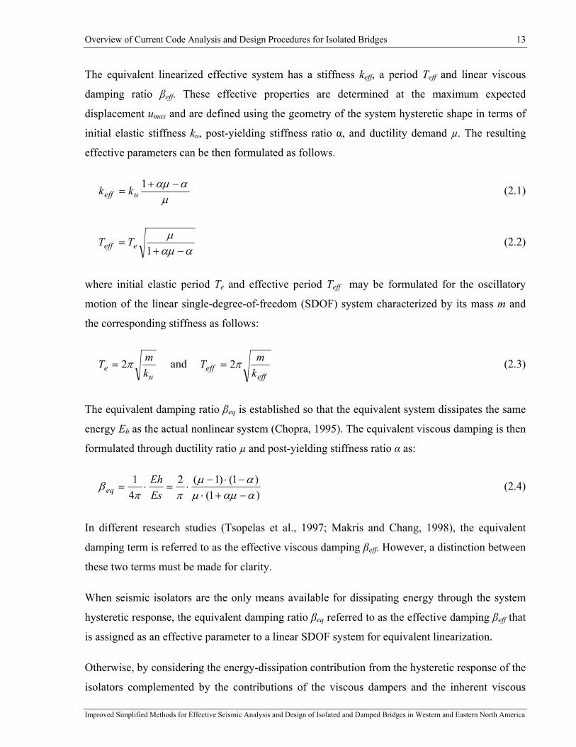
Overview of Current Code Analysis and Design Procedures for Isolated Bridges 13
Improved Simplified Methods for Effective Seismic Analysis and Design of Isolated and Damped Bridges in Western and Eastern North America
The equivalent linearized effective system has a stiffness keff, a period Teff and linear viscous
damping ratio βeff. These effective properties are determined at the maximum expected
displacement umax and are defined using the geometry of the system hysteretic shape in terms of
initial elastic stiffness ku, post-yielding stiffness ratio α, and ductility demand µ. The resulting
effective parameters can be then formulated as follows.
μααμ −+
=1
ueff kk (2.1)
ααμμ
−+=
1eeff TT (2.2)
where initial elastic period Te and effective period Teff may be formulated for the oscillatory
motion of the linear single-degree-of-freedom (SDOF) system characterized by its mass m and
the corresponding stiffness as follows:
ue k
mT π2= and eff
eff kmT π2= (2.3)
The equivalent damping ratio βeq is established so that the equivalent system dissipates the same
energy Eh as the actual nonlinear system (Chopra, 1995). The equivalent viscous damping is then
formulated through ductility ratio µ and post-yielding stiffness ratio α as:
)1()1()1(2
41
ααμμαμ
ππβ
−+⋅−⋅−
⋅=⋅=EsEh
eq (2.4)
In different research studies (Tsopelas et al., 1997; Makris and Chang, 1998), the equivalent
damping term is referred to as the effective viscous damping βeff. However, a distinction between
these two terms must be made for clarity.
When seismic isolators are the only means available for dissipating energy through the system
hysteretic response, the equivalent damping ratio βeq referred to as the effective damping βeff that
is assigned as an effective parameter to a linear SDOF system for equivalent linearization.
Otherwise, by considering the energy-dissipation contribution from the hysteretic response of the
isolators complemented by the contributions of the viscous dampers and the inherent viscous
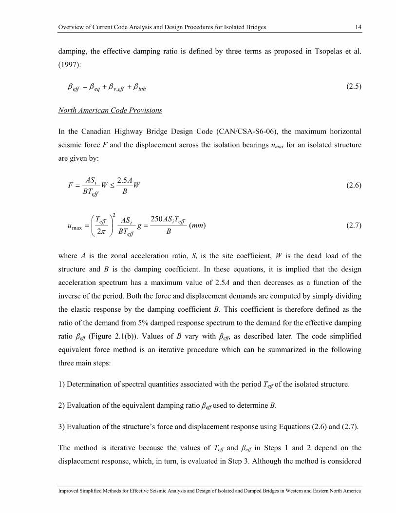
Overview of Current Code Analysis and Design Procedures for Isolated Bridges 14
Improved Simplified Methods for Effective Seismic Analysis and Design of Isolated and Damped Bridges in Western and Eastern North America
damping, the effective damping ratio is defined by three terms as proposed in Tsopelas et al.
(1997):
inheffveqeff ββββ ++= , (2.5)
North American Code Provisions
In the Canadian Highway Bridge Design Code (CAN/CSA-S6-06), the maximum horizontal
seismic force F and the displacement across the isolation bearings umax for an isolated structure
are given by:
WB
AWBTAS
Feff
i 5.2≤= (2.6)
)(250
2
2
max mmB
TASg
BTAST
u effi
eff
ieff =⎟⎟⎠
⎞⎜⎜⎝
⎛=
π (2.7)
where A is the zonal acceleration ratio, Si is the site coefficient, W is the dead load of the
structure and B is the damping coefficient. In these equations, it is implied that the design
acceleration spectrum has a maximum value of 2.5A and then decreases as a function of the
inverse of the period. Both the force and displacement demands are computed by simply dividing
the elastic response by the damping coefficient B. This coefficient is therefore defined as the
ratio of the demand from 5% damped response spectrum to the demand for the effective damping
ratio βeff (Figure 2.1(b)). Values of B vary with βeff, as described later. The code simplified
equivalent force method is an iterative procedure which can be summarized in the following
three main steps:
1) Determination of spectral quantities associated with the period Teff of the isolated structure.
2) Evaluation of the equivalent damping ratio βeff used to determine B.
3) Evaluation of the structure’s force and displacement response using Equations (2.6) and (2.7).
The method is iterative because the values of Teff and βeff in Steps 1 and 2 depend on the
displacement response, which, in turn, is evaluated in Step 3. Although the method is considered

Overview of Current Code Analysis and Design Procedures for Isolated Bridges 15
Improved Simplified Methods for Effective Seismic Analysis and Design of Isolated and Damped Bridges in Western and Eastern North America
a force-based design method, the procedure is in fact used to determine the displacement of the
isolated structure (Equation (2.7)) and the design seismic forces for the substructure are
subsequently determined from the load-displacement response of the actual nonlinear isolation
system.
In the United States, the design procedure in the AASHTO Guide Specification for Seismic
Isolation Design (AASHTO 2010) is identical except that the 5% damped elastic design
spectrum is constructed using a two-point method depending on the site specific design spectral
values SS and S1 at periods of 0.2 and 1.0 s, respectively.
The current seismic design philosophy based on the damped elastic response spectra was
introduced in North America in the late 1970's. In the early 1980's, seismic protection
techniques, incorporating isolation and damping devices, started to draw attention as a possible
effective means of reducing the seismic demand and enhancing the seismic response of
structures. Guidelines for the design of seismic isolation systems were first published by the
Structural Engineers Association of Northern California (SEAONC, 1986). The damping
coefficient B, which reflects the energy dissipation capacity as a function of equivalent damping,
first appeared in the 1991 UBC (ICBO) provisions for base-isolated buildings (Naeim and
Kircher, 2001).
The concept of equivalent damping βeff was introduced by Jacobsen (1930) and formulated as a
function of dissipated energy Eh in 1960. Gulkan and Sozen (1974) used it to define a substitute
linear structure with a fictitious equivalent damper, as presented in Figure 2.1(a), and the concept
was later incorporated in seismic provisions as a simplified design method. The displacement
response of the equivalent system is intended to closely reproduce the inelastic response of a real
nonlinear structure (Figure 2.1(b)). As illustrated in Figure 2.1(c), the elastic 5% damped
spectrum is divided by the damping coefficient B(βeff) to obtain the resulting reduced response as
a function of effective period Teff. The values of B specified in codes have been derived from the
work by Newmark and Hall (1982). In these early studies, spectrum amplification factors were
computed for different damping levels using the elastic response of a viscously damped single-
degree-of-freedom (SDOF) system subjected to the 1940 El Centro earthquake record. These
values were then slightly adjusted over the years. Damping coefficients specified in various
seismic provisions are presented in Table 2.1.

Overview of Current Code Analysis and Design Procedures for Isolated Bridges 16
Improved Simplified Methods for Effective Seismic Analysis and Design of Isolated and Damped Bridges in Western and Eastern North America
Table 2-1 Values of the damping coefficient B
β
CSA-S6 (2006)
AASHTO (1994)
AASHTO (2009)
EC 8: Part 2 (1996)
EC 8: Part 2 (2005)
UBC (1994)
ATC-40 (1996)
Newmark & Hall (1982)
(%) B B 1/η 1/η B B1 A1 Region
V2 Region
2 0.8 0.76 0.82 0.84 0.77 0.81 5 1.0 1.00 1.00 1.00 1.00 1.00 1.00 1.00 10 1.2 1.23 1.21 1.22 1.19 1.22 1.29 1.20 20 1.5 1.52 1.49 1.58 1.56 1.54 1.81 1.53 30 1.7 1.71 1.70 1.87 1.89 1.82 40 1.9 1.87 1.87 2.12 2.08 50 2.0 2.00 2.02 2.35
1. A Region - Acceleration-sensitive region of the response spectrum
2. V Region - Velocity-sensitive region of the response spectrum
In 1999, values of the damping coefficient were introduced in AASHTO LRFD Guide
Specifications for Seismic Isolation Design (AASHTO, 1999). The same values were also
incorporated in the 2000 edition of the Canadian code CSA-S6 and are still in force in CSA-S6-
06. The third edition of the AASHTO Guide Specification for Seismic Isolation Design (2010)
now proposes an exponential equation for the value of B as a function of βeff:
neffB ⎟⎟
⎠
⎞⎜⎜⎝
⎛=
%5β
(2.8)
where the exponent n is set to 0.3. Interpolation between tabulated values is therefore no longer
required.
Codes specify limits for the application of this simplified method. In particular, the effective
viscous damping βeff is limited to a maximum value of 30% and bridge isolators must be
provided with minimum recentring capabilities. The damping limit of 30% was introduced in
AASHTO LRFD Guide Specifications for Seismic Isolation Design (AASHTO, 1999) at the
same time as the damping coefficients. The changes were adopted based on the development of
the NCHRP Project 12-49 provisions (MCEER/ATC-49, 2003). The proposed provisions
intended to develop a new set of seismic design specifications which reflect the latest design
philosophies (Lee Marsh et al. 2001). However, no explicit scientific basis was provided by the
NCHRP Project 12-49 Team to support these changes.

Overview of Current Code Analysis and Design Procedures for Isolated Bridges 17
Improved Simplified Methods for Effective Seismic Analysis and Design of Isolated and Damped Bridges in Western and Eastern North America
In addition to the damping limits, current CSA-S6 and AASHTO codes also have minimum
lateral restoring force criteria to ensure a minimum recentring capability to the system. CSA-S6-
06, clause 4.10.10.2 reads: "… The isolation system shall be configured to produce a lateral
restoring force such that the lateral force at the design displacement is greater than the lateral
force at 50% of the design displacement by at least 0.025W”. In AASHTO (2009, 2010), the
minimum restoring force at 50% of the design displacement is 0.0125W, which is less stringent
than in CSA S6. Unfortunately, the codes do not provide a clear scientific basis for these criteria
although it is speculated that these criteria are intended to result in systems with a non-zero post-
elastic stiffness. As a result of the difference between both codes, the design of isolated bridges
in Canada may be limited more frequently by this requirement when compared to engineering
practice in the US.
European Provisions
In Eurocode 8 (EC8), the fundamental mode method corresponds to the equivalent static force
method found in NA codes. Although the methods are essentially the same, Eurocode 8
incorporates a displacement-based design approach where performance objectives are explicitly
tied to the displacement response. In that approach, the displacement is obtained from the elastic
acceleration spectrum using a pseudo-spectral relation, as in the case in NA codes. However,
EC8 provides displacement spectral data for long period structures which is more appropriate for
the design of seismically isolated structures. The need for a displacement spectrum for long
period structures was highlighted by Tolis and Faccioli (1999), and Bommer et al. (2000b)
proposed a simple method to obtain the required displacement spectrum.
The method, which was later adopted by EC8, is illustrated in Figure 2.2. Up to the corner period
TD, which defines the beginning of the constant displacement plateau, the elastic displacement is
obtained by direct transformation of the elastic acceleration spectrum and the NA codes and EC8
provide identical simplified design approaches.
For the cases where the effective period exceeds 4 s, the plateau of the maximum displacement
response is lengthened to the corner period TE followed by the segment TE-TF which links the
maximum displacement to the peak ground displacement (PGD) plateau. The PGD value is
defined as a function of the peak ground acceleration (PGA). Consequently, the development of

Overview of Current Code Analysis and Design Procedures for Isolated Bridges 18
Improved Simplified Methods for Effective Seismic Analysis and Design of Isolated and Damped Bridges in Western and Eastern North America
spectral segments beyond TD, where the spectrum is capped by the constant displacement plateau
(TD-TE) and PGD, represents a significant difference when compared to the NA codes.
Figure 2.2 Acceleration (SA) and displacement (SD) design spectra in Eurocode 8
Accordingly, the EC8 approach produces less conservative displacement predictions compared
to AASHTO and CSA-S6 for long period structures. Recently, Bommer and Pinho (2006)
emphasized the inconsistency in anchoring TD to a fixed value and suggested that additional
research be performed to consider larger values of TD. Akkar and Bommer (2007) also confirmed
the need to modify the EC8 displacement response spectra because of "a gross underestimation
leading to dangerously low spectral displacements at longer periods".

Overview of Current Code Analysis and Design Procedures for Isolated Bridges 19
Improved Simplified Methods for Effective Seismic Analysis and Design of Isolated and Damped Bridges in Western and Eastern North America
Another difference between the NA and EC8 codes is that EC8 specifies two design spectra to
account for the differences in the effects of large and small-to-moderate earthquake events:
Type 1 spectrum for surface wave magnitudes MS > 5.5 and Type 2 spectrum for MS < 5.5.
Similar to the American codes, Eurocode 8 accounts for the effect of high equivalent damping
resulting from the response of seismic isolation systems by using a damping correction factor η .
This factor corresponds to the inverse of the damping coefficient B (η = 1/ B). In 1996, the EC8
Part 2 draft (CEN, 1996) incorporated the relationship:
35.0
%2%7
⎟⎟⎠
⎞⎜⎜⎝
⎛
+=
effβη (2.9)
As shown in Figure 2.3, Equation (2.9) (CEN, 1996) produces almost identical reduction effects
on spectral values for damping ratios up to 50% damping when compared to Equation (2.8) with
n = 0.3 (AASHTO).
0.0
0.5
1.0
1.5
2.0
2.5
3.0
0% 10% 20% 30% 40% 50% 60%
B
Damping Ratio, βeff
Damping Coefficient
UBC ‐ 1994 ATC‐40EC8‐1996 CSA‐S6 / AASHTOEC8‐2005 Newmark & Hall ‐ 1982
Figure 2.3 Damping coefficient in different seismic codes
In 1999, Tolis and Faccioli, aiming at extending the current code specifications, particularly for
the displacement-based approach in EC8, proposed a new less conservative expression for the
damping correction factor (Equation 2.4). They realized that for displacement response spectra,
specially for periods beyond about 2 s, a larger damping reduction effect may be considered.
However, these observations were mainly based on a set of time histories recorded during the

Overview of Current Code Analysis and Design Procedures for Isolated Bridges 20
Improved Simplified Methods for Effective Seismic Analysis and Design of Isolated and Damped Bridges in Western and Eastern North America
1995 Hyogoken-Nanbu (Kobe, M = 6.9) earthquake where records with fault distances greater
than 35 km were excluded. Only five European records with a fault distance ranging between 2
and 20 km and magnitudes 5.3 ≤ Ms ≤ 6.7 were analysed. Tolis and Faccioli (1999) recognized
that the results provided by their study had a limited background and were subject to the
criticism.
5.0
%10%15
⎟⎟⎠
⎞⎜⎜⎝
⎛
+=
effβη (2.10)
Bommer et al. (2000b) proposed an alternative expression being developed by regression
analyses using a much larger dataset of European ground motions, which were previously used
by Ambraseys et al. (1996), with surface-wave magnitudes from 4.0 to 7.9 and distances up to
260 km. This expression is specified in the current edition of EC8 Part 2 (CEN, 2005):
5.0
%5%10
⎟⎟⎠
⎞⎜⎜⎝
⎛
+=
effβη (2.11)
The intent of Equation (2.11) was to provide values that were more representative of the
European seismicity. With respect to the previous EC8 draft edition (CEN, 1996), these factors
offer more of a reduction effect for damping ratios of 20% and greater. In EC8, Equation (2.11)
is used for both spectra. However, Bommer and Mendis (2005) indicated that damping response
reduction effects for Type 2 spectra could be significantly lower than for Type 1 spectra.
In contrast, in spite of having been recently reexamined, the factors prescribed in both the
AASHTO and CSA-S6 remain unchanged and are the same for all North American regions.
They are also defined as independent of the structure's natural period. However, Atkinson and
Pierre (2002) demonstrated that for a period range of 0.05 - 2.0 s the damping coefficient
decreases with the period of structures. Hatzigeorgiou (2010) drew special attention to flexible
structures with longer periods for which damping coefficients decrease significantly and may
equal almost unity (no reduction effect). These observations are in overall agreement with the
explanation given by Chopra (2007) that spectral values in ranges approaching the peak ground
acceleration and the peak ground displacement are irrespective of damping given that for T → 0,
the structure moves rigidly with the ground and for T → ∞, the structural mass stays still while

Overview of Current Code Analysis and Design Procedures for Isolated Bridges 21
Improved Simplified Methods for Effective Seismic Analysis and Design of Isolated and Damped Bridges in Western and Eastern North America
the ground underneath moves. It is clear that such an explanation has a scarce scientific basis
what confirms the need for a more comprehensive study of the period dependant nature of
damping coefficients.
Bommer and Mendis (2005) demonstrated that the influence of damping on spectral values
increases with increasing earthquake magnitude and distance and decreases for softer site
conditions, also suggesting an increase with ground motion duration. Dependency of the
damping coefficient on seismic characteristics has also been observed in other studies (e.g.,
Atkinson and Pierre, 2004; Cameron and Green, 2007; and Stafford et al., 2008).
These observations suggest that damping coefficients may vary across North America due to the
differences in ground motions from earthquakes occurring in western North America (WNA) and
eastern North America (ENA). In the more active WNA seismic regions, earthquakes occur more
frequently than in the stable continental region of ENA where, accordingly, more energy is
released per unit area (stress drop) when an earthquake occurs. Due to the stiffer, denser, and less
fractured bedrock in ENA, high-frequency seismic waves generated from earthquakes attenuate
more slowly with distance than in WNA. Consequently, seismic records from earthquakes at
same magnitude and distance (M-R) in WNA and ENA exhibit different amplitudes, frequency
content, predominant periods and durations. These differences may impact on structural
response, as observed by Taylor (1999) and Naumoski (2000).
The above discussion demonstrates that there is a need to carefully review the proposed damping
coefficients B for western and eastern North American regions in order to better address the
spectral shape, and different ground-motion characteristics.
2.2 Critical Review of Limitations of the Equivalent Linearization
Method
As discussed in the previous section, the coefficients B on which the code simplified analysis
method relies are derived empirically using the elastic response of a viscously damped SDOF
system. The coefficients B are calibrated so the accuracy of the simplified method is enhanced by
reducing errors in response prediction. The sources of the method inaccuracy may be both the
local damping reduction effect and the equivalent linearization method which is an intrinsic part

Overview of Current Code Analysis and Design Procedures for Isolated Bridges 22
Improved Simplified Methods for Effective Seismic Analysis and Design of Isolated and Damped Bridges in Western and Eastern North America
of the code method. A better understanding of the source of these inaccuracies can be reached by
investigating solely the equivalent linearization method.
Over time various studies have been carried out in order to validate and enhance the method of
equivalent linearization or the substitute-structure method. The technique of defining a linear
system through effective linear parameters as currently specified in AASHTO and CSA-S6-06
(presented previously in this section (Equations 2.1 to 2.4)) has been questioned because of a
limited understanding of the actual sources of errors produced during response estimates. The
accuracy problems related to this method were attributed to different physical phenomena and
various empirical formulae have been proposed to better approximate the inelastic response of
bilinear systems.
Iwan and Gates (1979) proposed an empirical method of linearization for inelastic response
spectra. Their research aimed to address the effects of deterioration, stiffness degradation,
cracking and ductility. The equivalent linear system was defined by equivalent damping and
effective linear period found by optimizing a root mean square (RMS) error between the elastic
and inelastic responses. In 1980, Iwan presented an improved empirical formulation for response
approximation of structures within the mid-period range of 0.4-4.0 s and ductility range of 2-8.
Although the ductility range up to 8 represents severe damage for conventional structures, the
response of seismically isolated structures may be characterized much larger ductility ratios.
Hwang and Sheng (1994) examined the formulation specified in 1991 by AASHTO (same as in
the current AASHTO and CSA S6-06 provisions) for simplified equivalent analyses of isolated
bridges. They claimed that these provisions may not be appropriate given that for higher ductility
ratios, the expression of equivalent damping (Equation 2.4)) results in low damping values. As
shown in Figure 2.4 for post-yielding ratio α > 0, the equivalent damping ratio (Equation 2.4)
decreases with the ductility ratio after the curve peak is reached. Researchers presumed that the
energy dissipated by the isolators becomes larger with increase of the inelastic response and
considering a smaller damping ratio for this case is unrealistic. They used data obtained by Iwan
and Gates (1979) to carry out comparative analyses and proposed an alternate formulation for the
effective period (effective stiffness). With respect to Iwan's model, an exponential function
instead of a power function was adopted.
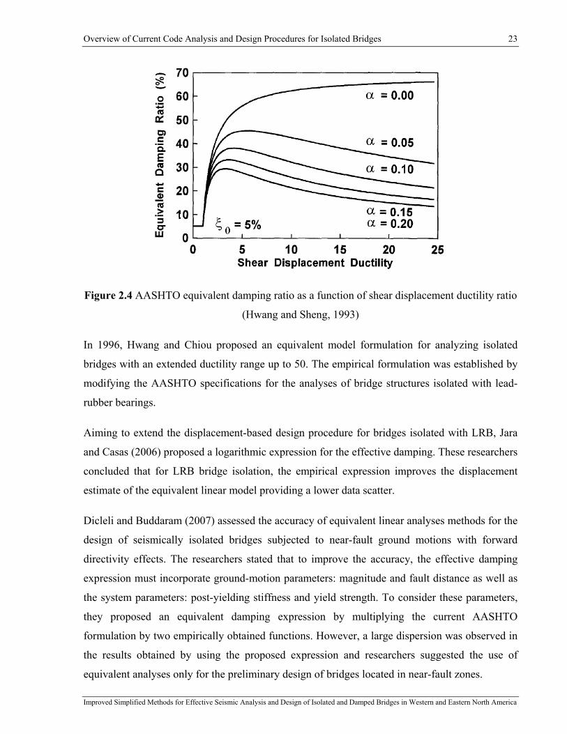
Overview of Current Code Analysis and Design Procedures for Isolated Bridges 23
Improved Simplified Methods for Effective Seismic Analysis and Design of Isolated and Damped Bridges in Western and Eastern North America
Figure 2.4 AASHTO equivalent damping ratio as a function of shear displacement ductility ratio
(Hwang and Sheng, 1993)
In 1996, Hwang and Chiou proposed an equivalent model formulation for analyzing isolated
bridges with an extended ductility range up to 50. The empirical formulation was established by
modifying the AASHTO specifications for the analyses of bridge structures isolated with lead-
rubber bearings.
Aiming to extend the displacement-based design procedure for bridges isolated with LRB, Jara
and Casas (2006) proposed a logarithmic expression for the effective damping. These researchers
concluded that for LRB bridge isolation, the empirical expression improves the displacement
estimate of the equivalent linear model providing a lower data scatter.
Dicleli and Buddaram (2007) assessed the accuracy of equivalent linear analyses methods for the
design of seismically isolated bridges subjected to near-fault ground motions with forward
directivity effects. The researchers stated that to improve the accuracy, the effective damping
expression must incorporate ground-motion parameters: magnitude and fault distance as well as
the system parameters: post-yielding stiffness and yield strength. To consider these parameters,
they proposed an equivalent damping expression by multiplying the current AASHTO
formulation by two empirically obtained functions. However, a large dispersion was observed in
the results obtained by using the proposed expression and researchers suggested the use of
equivalent analyses only for the preliminary design of bridges located in near-fault zones.

Overview of Current Code Analysis and Design Procedures for Isolated Bridges 24
Improved Simplified Methods for Effective Seismic Analysis and Design of Isolated and Damped Bridges in Western and Eastern North America
In 2011, Mavronicola and Komodromos assessed the suitability of the equivalent linear analyses
by comparing different equivalent models proposed in the literature and previously discussed in
this chapter. The six equivalent methods compared by researchers are presented in Table 2-2.
Table 2-2 Effective formulations for equivalent linearization (compared in Mavronicola and
Komodromos, 2011)
Method Effective Formulation for Equivalent Linearization
AASHTO (1991)
μααμ −+
=1
ueff kk
)1()1()1(2
ααμμαμ
πβ
−+⋅−⋅−
⋅=eff
Iwan (1980) [ ] 2939.0)1(121.01−
−⋅+⋅= μeeff kk
371.00 )1(0587.0 −⋅⋅+= μββeff
Hwang and Sheng (1993) [ ]{ } 2137.1)1(13.01ln1−
−⋅++⋅= μeeff kk
371.00 )1(0587.0 −⋅⋅+= μββeff
Hwang and Chiou (1996) 2
2
11737.01
)1(15.01
−−
⎟⎟⎠
⎞⎜⎜⎝
⎛ −⋅−⋅⎥
⎦
⎤⎢⎣
⎡−⋅+
⋅=μ
μμ
μueff kk
[ ] 5.4)1(15.01
117.1 58.0μμπ
μβ ⋅
−⋅+⋅
⎟⎟⎠
⎞⎜⎜⎝
⎛−⋅
=eff
Jara and Casas (2006)
μααμ −+
=1
ueff kk
)(ln05.005.0 μβ ⋅⋅+=eff
Dicleli and Buddaram (2007)
μααμ −+
=1
ueff kk
)1()1()1(2
21 ααμμαμ
πβ
−+⋅−⋅−
⋅⋅⋅= NFNFeff
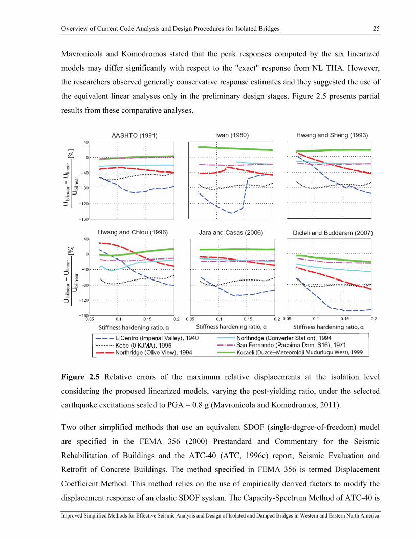
Overview of Current Code Analysis and Design Procedures for Isolated Bridges 25
Improved Simplified Methods for Effective Seismic Analysis and Design of Isolated and Damped Bridges in Western and Eastern North America
Mavronicola and Komodromos stated that the peak responses computed by the six linearized
models may differ significantly with respect to the "exact" response from NL THA. However,
the researchers observed generally conservative response estimates and they suggested the use of
the equivalent linear analyses only in the preliminary design stages. Figure 2.5 presents partial
results from these comparative analyses.
Figure 2.5 Relative errors of the maximum relative displacements at the isolation level
considering the proposed linearized models, varying the post-yielding ratio, under the selected
earthquake excitations scaled to PGA = 0.8 g (Mavronicola and Komodromos, 2011).
Two other simplified methods that use an equivalent SDOF (single-degree-of-freedom) model
are specified in the FEMA 356 (2000) Prestandard and Commentary for the Seismic
Rehabilitation of Buildings and the ATC-40 (ATC, 1996c) report, Seismic Evaluation and
Retrofit of Concrete Buildings. The method specified in FEMA 356 is termed Displacement
Coefficient Method. This method relies on the use of empirically derived factors to modify the
displacement response of an elastic SDOF system. The Capacity-Spectrum Method of ATC-40 is
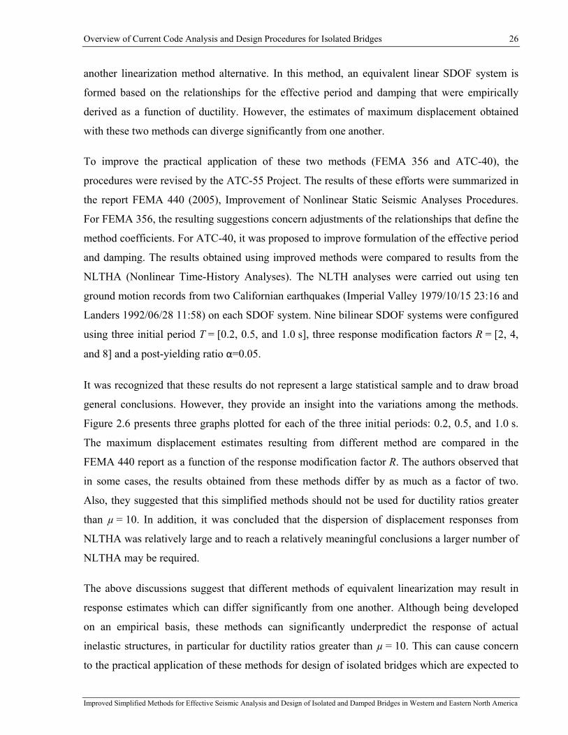
Overview of Current Code Analysis and Design Procedures for Isolated Bridges 26
Improved Simplified Methods for Effective Seismic Analysis and Design of Isolated and Damped Bridges in Western and Eastern North America
another linearization method alternative. In this method, an equivalent linear SDOF system is
formed based on the relationships for the effective period and damping that were empirically
derived as a function of ductility. However, the estimates of maximum displacement obtained
with these two methods can diverge significantly from one another.
To improve the practical application of these two methods (FEMA 356 and ATC-40), the
procedures were revised by the ATC-55 Project. The results of these efforts were summarized in
the report FEMA 440 (2005), Improvement of Nonlinear Static Seismic Analyses Procedures.
For FEMA 356, the resulting suggestions concern adjustments of the relationships that define the
method coefficients. For ATC-40, it was proposed to improve formulation of the effective period
and damping. The results obtained using improved methods were compared to results from the
NLTHA (Nonlinear Time-History Analyses). The NLTH analyses were carried out using ten
ground motion records from two Californian earthquakes (Imperial Valley 1979/10/15 23:16 and
Landers 1992/06/28 11:58) on each SDOF system. Nine bilinear SDOF systems were configured
using three initial period T = [0.2, 0.5, and 1.0 s], three response modification factors R = [2, 4,
and 8] and a post-yielding ratio α=0.05.
It was recognized that these results do not represent a large statistical sample and to draw broad
general conclusions. However, they provide an insight into the variations among the methods.
Figure 2.6 presents three graphs plotted for each of the three initial periods: 0.2, 0.5, and 1.0 s.
The maximum displacement estimates resulting from different method are compared in the
FEMA 440 report as a function of the response modification factor R. The authors observed that
in some cases, the results obtained from these methods differ by as much as a factor of two.
Also, they suggested that this simplified methods should not be used for ductility ratios greater
than µ = 10. In addition, it was concluded that the dispersion of displacement responses from
NLTHA was relatively large and to reach a relatively meaningful conclusions a larger number of
NLTHA may be required.
The above discussions suggest that different methods of equivalent linearization may result in
response estimates which can differ significantly from one another. Although being developed
on an empirical basis, these methods can significantly underpredict the response of actual
inelastic structures, in particular for ductility ratios greater than µ = 10. This can cause concern
to the practical application of these methods for design of isolated bridges which are expected to
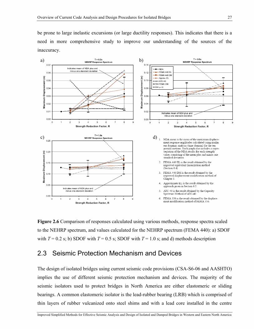
Overview of Current Code Analysis and Design Procedures for Isolated Bridges 27
Improved Simplified Methods for Effective Seismic Analysis and Design of Isolated and Damped Bridges in Western and Eastern North America
be prone to large inelastic excursions (or large ductility responses). This indicates that there is a
need in more comprehensive study to improve our understanding of the sources of the
inaccuracy.
Figure 2.6 Comparison of responses calculated using various methods, response spectra scaled
to the NEHRP spectrum, and values calculated for the NEHRP spectrum (FEMA 440): a) SDOF
with T = 0.2 s; b) SDOF with T = 0.5 s; SDOF with T = 1.0 s; and d) methods description
2.3 Seismic Protection Mechanism and Devices
The design of isolated bridges using current seismic code provisions (CSA-S6-06 and AASHTO)
implies the use of different seismic protection mechanism and devices. The majority of the
seismic isolators used to protect bridges in North America are either elastomeric or sliding
bearings. A common elastomeric isolator is the lead-rubber bearing (LRB) which is comprised of
thin layers of rubber vulcanized onto steel shims and with a lead core installed in the centre
a) b)
c) d)
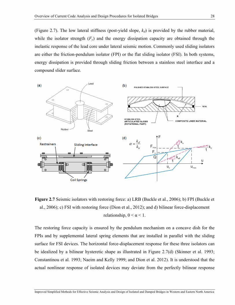
Overview of Current Code Analysis and Design Procedures for Isolated Bridges 28
Improved Simplified Methods for Effective Seismic Analysis and Design of Isolated and Damped Bridges in Western and Eastern North America
(Figure 2.7). The low lateral stiffness (post-yield slope, kd) is provided by the rubber material,
while the isolator strength (Fy) and the energy dissipation capacity are obtained through the
inelastic response of the lead core under lateral seismic motion. Commonly used sliding isolators
are either the friction-pendulum isolator (FPI) or the flat sliding isolator (FSI). In both systems,
energy dissipation is provided through sliding friction between a stainless steel interface and a
compound slider surface.
Figure 2.7 Seismic isolators with restoring force: a) LRB (Buckle et al., 2006); b) FPI (Buckle et
al., 2006); c) FSI with restoring force (Dion et al., 2012); and d) bilinear force-displacement
relationship, 0 < α < 1.
The restoring force capacity is ensured by the pendulum mechanism on a concave dish for the
FPIs and by supplemental lateral spring elements that are installed in parallel with the sliding
surface for FSI devices. The horizontal force-displacement response for these three isolators can
be idealized by a bilinear hysteretic shape as illustrated in Figure 2.7(d) (Skinner et al. 1993;
Constantinou et al. 1993; Naeim and Kelly 1999; and Dion et al. 2012). It is understood that the
actual nonlinear response of isolated devices may deviate from the perfectly bilinear response

Overview of Current Code Analysis and Design Procedures for Isolated Bridges 29
Improved Simplified Methods for Effective Seismic Analysis and Design of Isolated and Damped Bridges in Western and Eastern North America
assumed in this research. The effects of such deviations are not considered in this thesis and
could be examined in a separate study.
FSI devices with no or limited recentring capacity are typically used as fuse elements to limit the
seismic forces transmitted to substructure elements. They are particularly effective when inserted
between the superstructure and the bridge piers, especially in the case of existing bridge columns
having limited lateral capacity. Sliding isolators also usually have a very small activation
displacement uy due to a high pre-yielding stiffness, ku (Zhang et Huo, 2009). However, this very
short range of elastic displacements can be lengthened when the sliding interface is combined in
series with an elastomeric pad as illustrated in Figure 2.8. The added flexibility can be adjusted
as a function of the height of the elastomeric pad.
Figure 2.8 Flat sliding seismic isolator without restoring force: a) seismic energy products
(www.sepbearings.com); b) bilinear force-displacement relationship, α = 0
LRBs inherently exhibit higher restoring forces upon yielding and the system is therefore more
suitable at the abutments where greater lateral resistance can be more easily developed. The
typical post-yielding stiffness ratio is α = 0.1 (http://www.dis-inc.com/technical.html). While
isolators are mainly used to control seismic induced forces, their energy dissipation capacity
contributes in reducing the structure’s relative displacements across the isolation layer. In design,
the effect of this damping is considered in terms of equivalent damping which is added to the
inherent damping of the structure.
The addition of velocity dependent viscous dampers can further enhance the damping of the
system and contribute to the response control of the isolated structure. Both linear (n = 1) or
nonlinear (n < 1) viscous dampers can be used for this purpose (Figure 2.9). Maximum forces
Overview of Current Code Analysis and Design Procedures for Isolated Bridges 30
Improved Simplified Methods for Effective Seismic Analysis and Design of Isolated and Damped Bridges in Western and Eastern North America
from viscous dampers and isolators can occur nearly simultaneously in the inelastic range and it
is more practical to locate dampers at the abutments, rather than at the piers, to limit the forces
on the bridge piers.
Figure 2.9 Viscous damper
2.4 Summary
In this chapter, a review of the simplified code methods for seismic design of isolated bridges in
North American regions was presented. The simplified methods are currently specified in the
CAN/CSA-S6-06 Canadian Highway Bridge Design Code (CSA 2006) in Canada and the
AASHTO LRFD Seismic Bridge Design Specifications in the United States (AASHTO 2009,
2010). These methods rely on damping coefficients B and the technique of equivalent
linearization. The discussion demonstrated that there is a need to carefully review the proposed
damping coefficients B for western and eastern North American regions in order to better address
the spectral shape, and different ground-motion characteristics.
It was also shown that the sources of the method's inaccuracy may be both the local damping
reduction effect and the equivalent linearization method. Different equivalent linearization
methods were then discussed. These discussions suggest that methods of equivalent linearization
may result in response estimates which can differ significantly from one another.
The reviewed studies confirm that the equivalent linearization methods are subject to limitations
that may affect the accuracy in predicting the peak displacement response. These observations
emphasize the concern to cover a broad range of practical applications when bridges are

Overview of Current Code Analysis and Design Procedures for Isolated Bridges 31
Improved Simplified Methods for Effective Seismic Analysis and Design of Isolated and Damped Bridges in Western and Eastern North America
retrofitted using different isolation and damping devices. This indicates that there is a need in a
more comprehensive study to improve our understanding of the sources of the inaccuracy and
how to extend the method's applicability limits.
Finally, isolation and damping devices which are commonly used in North American practice for
seismic protection of bridges are reviewed. The main characteristics and expected performance
of the isolation and damping devices were outlined. These seismic protection devices are further
considered in this research for developing different configurations of isolated bridges.
Analytical Model and Numerical Platform for Nonlinear Time-History Analysis of Isolated and Damped Bridges 32
Improved Simplified Methods for Effective Seismic Analysis and Design of Isolated and Damped Bridges in Western and Eastern North America
Chapter 3: Analytical Model and Numerical Platform for Nonlinear Time-History Analysis of Isolated and Damped Bridges
3.1 Introduction
In this chapter, a new analytical model and a methodology to carry out nonlinear simplified
isolated bridge analysis are presented. The approach aims at streamlining the modeling
assumptions with the purpose of developing a proper and effective, yet simple analytical model
that can be used at the preliminary design stages for a fully equipped isolated bridge. The 2-DOF
model proposed in this study represents a simple two-span bridge in its longitudinal direction.
This is a simplified layout that can be expanded for bridges with more than two spans by making
a few additional assumptions. This 2-DOF model can represent a wide range of bridge
configurations that are typical of thousands of older bridges in North America that need to be
upgraded to meet requirements of current seismic provisions.
Based on this analytical model, a computer program IS-Bridge was written in MATLAB code.
This numerical analysis tool was developed in order to simulate the nonlinear structural
behaviour of isolated bridges equipped with different seismic protective devices. The main
motivation for developing this program was the need to carry out extensive parametric analyses
in the framework of the present research study. While SDOF models were adopted to examine
and enhance the code simplified method currently specified in CAN/CSA-S6-06 (Chapters 5 to
8), the 2-DOF models were employed for developing and validating the dual-level seismic
protection concept (Chapter 10).
After introducing the modelling assumptions and model formulation, a non-iterative direct
solution is proposed to analytically solve this model at each discrete step of time-history analysis
(THA). A less time-consuming computational process makes the program IS-Bridge much more
advantageous with respect to numerous programs which rely on iterative schemes. An important
aspect to be considered in the simulation of nonlinear structural behaviour of isolated bridges is
the modelling of inherent damping. Different techniques of modelling the inherent damping for
Analytical Model and Numerical Platform for Nonlinear Time-History Analysis of Isolated and Damped Bridges 33
Improved Simplified Methods for Effective Seismic Analysis and Design of Isolated and Damped Bridges in Western and Eastern North America
nonlinear THA are discussed. An alternative approach for considering the inherent damping ratio
proportional to the effective stiffness is presented. The ability of the model to simulate the
structural behaviour of isolated bridges was validated through a bridge retrofit example. The IS-
Bridge results from a nonlinear time-history analysis were compared to those obtained using a
SAP2000 (CSI, 2009) model of the same structure.
3.2 Analytical Model for Isolated Bridges
With the exponential increase in computing power over the last two decades, a variety of
numerical models have been developed and implemented for simulating the nonlinear response
of isolated bridges. Increasingly complex and detailed structural models have been developed
and have greatly enhanced our understanding of the response of such structures. Commercial
software used for structural analysis such as, ETABS, SAP2000 and CSiBridge include elements
for modeling damping and isolation devices. Detailed 3-D structural models have been adopted
for a variety of projects (e.g., Zhang et al., 2004; Dicleli, 2006; Zhang and Huo, 2009). By
analyzing a typical highway bridge having no skew, Zhang and Huo concluded that 2-D and 3-D
models yield comparable results while 2-D models are significantly less computationally
expensive. It is also arguable whether the extensive amount of information resulting from
sophisticated 3-D analyses is necessary at the preliminary design stage of a project. The approach
presented in this chapter is therefore aimed at streamlining the modeling assumptions with the
purpose of developing a proper and effective, yet simple analytical model that can be used at the
preliminary design stages. However, this approach can also be adopted for the final design stage
when the code-prescribed criteria are met to use the simplified modeling assumptions.
3.3 Model Assumptions for Reference Bridge
The use of simple equivalent SDOF (single-degree-of-freedom) systems has been recognized for
many decades as the simplest means of obtaining information on the dynamic response of
isolated structures subjected to seismic excitations. For the analysis of bridge structures in the
longitudinal direction, it is common practice to divide the structure into two model elements: the
substructure and the superstructure. Most of the bridge mass is located at the level of the deck
(superstructure), and the effect of the substructure mass is neglected when computing the
dynamic response. Conversely, the stiffness of the substructure has a significant effect on the
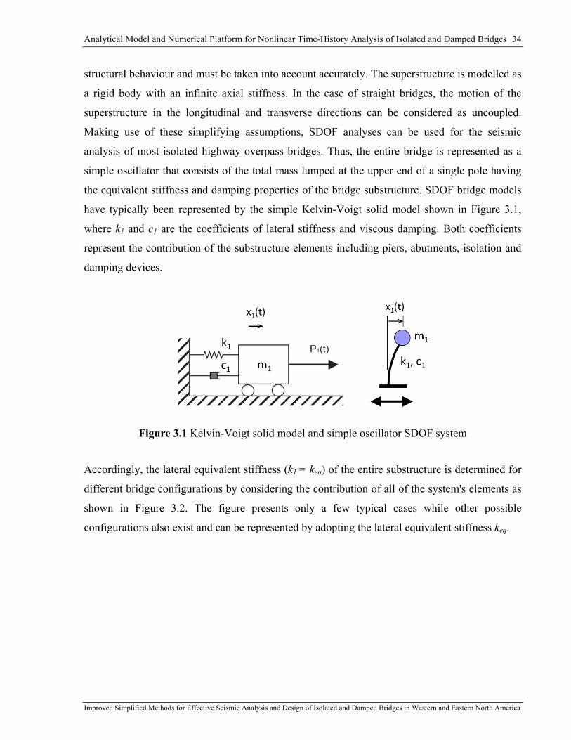
Analytical Model and Numerical Platform for Nonlinear Time-History Analysis of Isolated and Damped Bridges 34
Improved Simplified Methods for Effective Seismic Analysis and Design of Isolated and Damped Bridges in Western and Eastern North America
structural behaviour and must be taken into account accurately. The superstructure is modelled as
a rigid body with an infinite axial stiffness. In the case of straight bridges, the motion of the
superstructure in the longitudinal and transverse directions can be considered as uncoupled.
Making use of these simplifying assumptions, SDOF analyses can be used for the seismic
analysis of most isolated highway overpass bridges. Thus, the entire bridge is represented as a
simple oscillator that consists of the total mass lumped at the upper end of a single pole having
the equivalent stiffness and damping properties of the bridge substructure. SDOF bridge models
have typically been represented by the simple Kelvin-Voigt solid model shown in Figure 3.1,
where k1 and c1 are the coefficients of lateral stiffness and viscous damping. Both coefficients
represent the contribution of the substructure elements including piers, abutments, isolation and
damping devices.
Figure 3.1 Kelvin-Voigt solid model and simple oscillator SDOF system
Accordingly, the lateral equivalent stiffness (k1 = keq) of the entire substructure is determined for
different bridge configurations by considering the contribution of all of the system's elements as
shown in Figure 3.2. The figure presents only a few typical cases while other possible
configurations also exist and can be represented by adopting the lateral equivalent stiffness keq.

Analytical Model and Numerical Platform for Nonlinear Time-History Analysis of Isolated and Damped Bridges 35
Improved Simplified Methods for Effective Seismic Analysis and Design of Isolated and Damped Bridges in Western and Eastern North America
a)
b)
c)
Figure 3.2 Equivalent stiffness for different bridge configurations: a) non-isolated bridge, b)
bridge with isolation atop the piers and c) bridge with isolation atop the piers and abutments
For a simple non-isolated bridge model, the equivalent stiffness is determined as a sum of the
total stiffness of all piers kpier and the total stiffness of the two abutments kabut (Equation (3.1).
This bridge configuration is presented as two parallel springs in Figure 3.2(a).
abutpiereq kkk += (3.1)
For a bridge model with isolation atop the piers, the equivalent stiffness is determined following
Equation (3.2). In this expression, the first term represents two springs placed in series and it
corresponds to the contribution of the piers and their isolators to the global system stiffness. The
parameter kisol,i is the stiffness of all isolator devices installed on a given pier i and n is the
number of piers. This bridge configuration is illustrated in Figure 3.2(b).
eqkpierk
abutk
eqk
eqkpierk
abutk
isolk
isolk
eqk
eqkpierk
abutk
isolkeqk
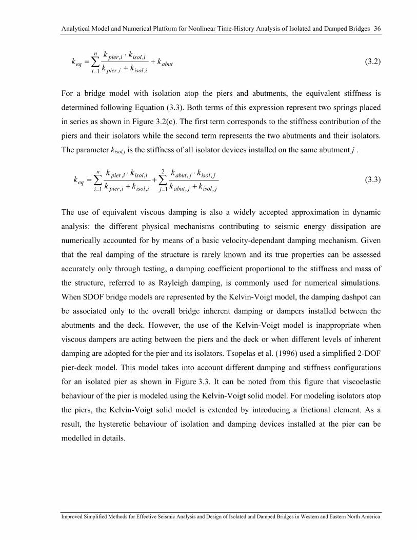
Analytical Model and Numerical Platform for Nonlinear Time-History Analysis of Isolated and Damped Bridges 36
Improved Simplified Methods for Effective Seismic Analysis and Design of Isolated and Damped Bridges in Western and Eastern North America
abut
n
i iisolipier
iisolipiereq k
kkkk
k ++
⋅= ∑
=1 ,,
,,
(3.2)
For a bridge model with isolation atop the piers and abutments, the equivalent stiffness is
determined following Equation (3.3). Both terms of this expression represent two springs placed
in series as shown in Figure 3.2(c). The first term corresponds to the stiffness contribution of the
piers and their isolators while the second term represents the two abutments and their isolators.
The parameter kisol,j is the stiffness of all isolator devices installed on the same abutment j .
∑∑== +
⋅+
+
⋅=
2
1 ,,
,,
1 ,,
,,
j jisoljabut
jisoljabutn
i iisolipier
iisolipiereq kk
kkkkkk
k (3.3)
The use of equivalent viscous damping is also a widely accepted approximation in dynamic
analysis: the different physical mechanisms contributing to seismic energy dissipation are
numerically accounted for by means of a basic velocity-dependant damping mechanism. Given
that the real damping of the structure is rarely known and its true properties can be assessed
accurately only through testing, a damping coefficient proportional to the stiffness and mass of
the structure, referred to as Rayleigh damping, is commonly used for numerical simulations.
When SDOF bridge models are represented by the Kelvin-Voigt model, the damping dashpot can
be associated only to the overall bridge inherent damping or dampers installed between the
abutments and the deck. However, the use of the Kelvin-Voigt model is inappropriate when
viscous dampers are acting between the piers and the deck or when different levels of inherent
damping are adopted for the pier and its isolators. Tsopelas et al. (1996) used a simplified 2-DOF
pier-deck model. This model takes into account different damping and stiffness configurations
for an isolated pier as shown in Figure 3.3. It can be noted from this figure that viscoelastic
behaviour of the pier is modeled using the Kelvin-Voigt solid model. For modeling isolators atop
the piers, the Kelvin-Voigt solid model is extended by introducing a frictional element. As a
result, the hysteretic behaviour of isolation and damping devices installed at the pier can be
modelled in details.
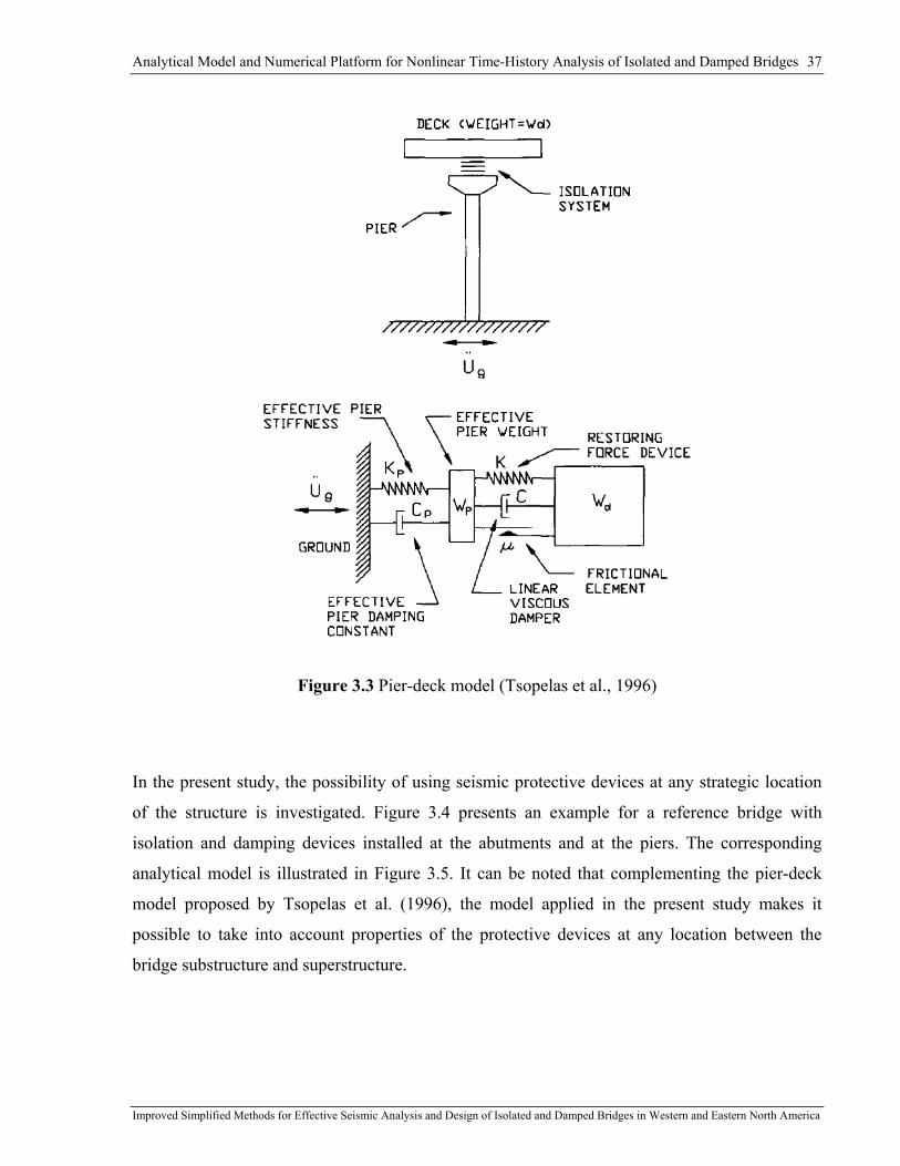
Analytical Model and Numerical Platform for Nonlinear Time-History Analysis of Isolated and Damped Bridges 37
Improved Simplified Methods for Effective Seismic Analysis and Design of Isolated and Damped Bridges in Western and Eastern North America
Figure 3.3 Pier-deck model (Tsopelas et al., 1996)
In the present study, the possibility of using seismic protective devices at any strategic location
of the structure is investigated. Figure 3.4 presents an example for a reference bridge with
isolation and damping devices installed at the abutments and at the piers. The corresponding
analytical model is illustrated in Figure 3.5. It can be noted that complementing the pier-deck
model proposed by Tsopelas et al. (1996), the model applied in the present study makes it
possible to take into account properties of the protective devices at any location between the
bridge substructure and superstructure.
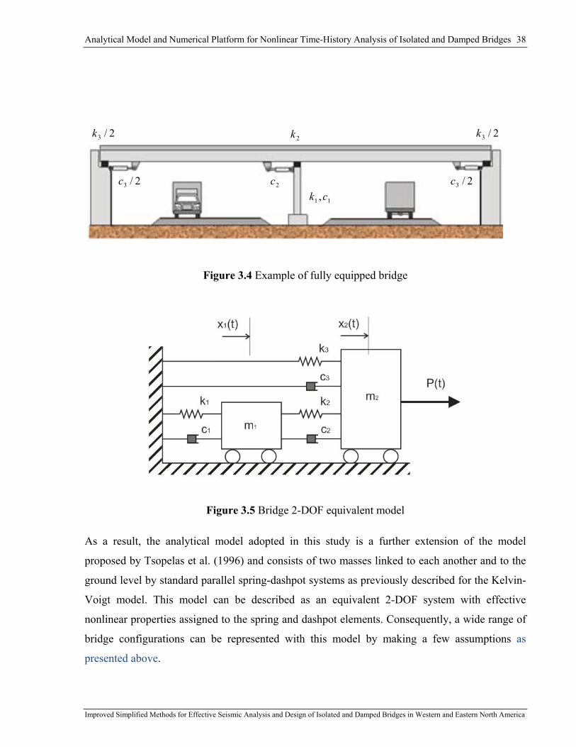
Analytical Model and Numerical Platform for Nonlinear Time-History Analysis of Isolated and Damped Bridges 38
Improved Simplified Methods for Effective Seismic Analysis and Design of Isolated and Damped Bridges in Western and Eastern North America
Figure 3.4 Example of fully equipped bridge
Figure 3.5 Bridge 2-DOF equivalent model
As a result, the analytical model adopted in this study is a further extension of the model
proposed by Tsopelas et al. (1996) and consists of two masses linked to each another and to the
ground level by standard parallel spring-dashpot systems as previously described for the Kelvin-
Voigt model. This model can be described as an equivalent 2-DOF system with effective
nonlinear properties assigned to the spring and dashpot elements. Consequently, a wide range of
bridge configurations can be represented with this model by making a few assumptions as
presented above.
11 ,ck
2k2/3k
2c
2/3k
2/3c 2/3c

Analytical Model and Numerical Platform for Nonlinear Time-History Analysis of Isolated and Damped Bridges 39
Improved Simplified Methods for Effective Seismic Analysis and Design of Isolated and Damped Bridges in Western and Eastern North America
3.4 Closed Form Solution and Computation Process
The dynamic equilibrium for a nonlinear SDOF system is formulated by using Newton's second
law equation of motions (Equation (3.4)) which represents the sum of the forces acting on the
system mass m1 at the time t. The solution for the response of this system is obtained by solving
the equation of motion for the displacement x1 defined as a function of time t.
)()()()( 1111111 txmtxktxctxm g&&&&& −=++ (3.4)
where )(txg&& is the ground-motion acceleration time history. Consequently, the seismic force
induced in the structure is given by )()( 11 txmtP g&&−= . Accordingly, the force balance resulting
from interaction of inertial, damping, spring and induced forces is presented as:
)()()()( 1111 tPtFtFtF SDI =++ (3.5)
In spite of the attractive simplicity of the Kelvin-Voigt solid model, such a model can only be
applied as far as the bridge model incorporates an overall effective level of damping represented
by a dashpot c1 . In the case where different levels of damping must be considered for a more
accurate simulation, the use of a 2-DOF model is essential and the corresponding damping
properties are assigned to dashpots denoted as c1, c2, and c3. This model involves the
participation of two masses denoted as the mass of the substructure, m1, and that of the
superstructure, m2. However, the inertial forces generated by the mass of the substructure m1 are
relatively small compared to those generated by the superstructure mass. Therefore, for this
model, m1 is considered to be a fictitious mass and the corresponding inertial forces generated by
the pier are assumed to be zero. Nonetheless, the term m1 is still kept in further analytical
developments. The model inelastic behaviour is obtained by assigning nonlinear properties to the
springs k1, k2, and k3.
The equations of motion for the 2-DOF model are defined in the following matrix form:
[ ]{ } [ ]{ } [ ]{ } [ ]{ } gxrMxKxCxM &&&&& −=++ (3.6)
where the dynamic coupling vector, mass matrix, damping matrix and stiffness matrix are
defined as follows:

Analytical Model and Numerical Platform for Nonlinear Time-History Analysis of Isolated and Damped Bridges 40
Improved Simplified Methods for Effective Seismic Analysis and Design of Isolated and Damped Bridges in Western and Eastern North America
{ }⎭⎬⎫
⎩⎨⎧
=11
r (3.7)
[ ] ⎥⎦
⎤⎢⎣
⎡=
2
1
00
mm
M (3.8)
[ ] ⎥⎦
⎤⎢⎣
⎡+−
−+=
)()(
322
221
cccccc
C (3.9)
[ ] ⎥⎦
⎤⎢⎣
⎡+−
−+=
)()(
322
221
kkkkkk
K (3.10)
The same equations of motion are rewritten as a force equilibrium matrix:
{ } { } { } { }PFFF SDI =++ (3.11)
with inertial forces:
{ }⎭⎬⎫
⎩⎨⎧
=⎭⎬⎫
⎩⎨⎧
⎥⎦
⎤⎢⎣
⎡=
22
11
2
1
2
1
00
xmxm
xx
mm
FI &&
&&
&&
&& (3.12)
damping forces:
{ }⎭⎬⎫
⎩⎨⎧
+−
=⎭⎬⎫
⎩⎨⎧
+−−−
=⎭⎬⎫
⎩⎨⎧
⎥⎦
⎤⎢⎣
⎡+−
−+=
32
21
23122
12211
2
1
322
221
)()(
)()(
DD
DDD FF
FFxcxxc
xxcxcxx
cccccc
F&&&
&&&
&
& (3.13)
and spring forces:
{ }⎭⎬⎫
⎩⎨⎧
+−
=⎭⎬⎫
⎩⎨⎧
+−−−
=⎭⎬⎫
⎩⎨⎧
⎥⎦
⎤⎢⎣
⎡+−
−+=
32
21
23122
12211
2
1
322
221
)()(
)()(
SS
SSS FF
FFxkxxk
xxkxkxx
kkkkkk
F (3.14)
Substituting the equations defining the forces (3.12), (3.13), and (3.14) in the force equilibrium
Equation (3.11), the following solution is obtained:
⎭⎬⎫
⎩⎨⎧
−−
=⎭⎬⎫
⎩⎨⎧
+−
+⎭⎬⎫
⎩⎨⎧
+−
+⎭⎬⎫
⎩⎨⎧
g
g
SS
SS
DD
DD
I
Ixmxm
FFFF
FFFF
FF
&&
&&
2
1
32
21
32
21
2
1 (3.15)

Analytical Model and Numerical Platform for Nonlinear Time-History Analysis of Isolated and Damped Bridges 41
Improved Simplified Methods for Effective Seismic Analysis and Design of Isolated and Damped Bridges in Western and Eastern North America
gxmxxkxkxxcxcxm &&&&&&& 1122111221111 )()( −=−−+−−+
gxmxkxxkxcxxcxm &&&&&&& 2231222312222 )()( −=+−++−+
Assuming m1 = 0 :
0)()( 1221112211 =−−+−− xxkxkxxcxc &&& (3.16)
gxmxkxxkxcxxcxm &&&&&&& 2231222312222 )()( −=+−++−+
Using Equations (3.16) instead of (3.15), the 2-DOF model is reduced to a SDOF system or,
more precisely, a single-mass 2-DOF system. With this transformation, it is possible to exclude
the acceleration term 1x&& . As a result, an exact analytical solution is obtained for each time step
by simultaneously solving the two Equations (3.16). In this case, there is no need to approximate
the system solution by an iterative method. In turn, the response of DOF 1 (position between the
pier and the isolator) is subsequently solved for using the corresponding displacement, velocity
and acceleration values obtained for DOF 2.
In the above solution, all three dashpots were defined by the equivalent linear damping
mechanism in which the damping force is proportional to the relative velocity. The nonlinear
behaviour of viscous dampers is commonly modeled using an equivalent linear damping model.
This technique is still broadly accepted today when the actual damper properties are unknown or
the dampers are assumed to behave linearly to make the computational process simpler.
However, the real damper properties specified by the manufacturer can be incorporated into the
computational model to obtain more realistic structural behaviour. For this reason, a nonlinear
damping model having damping force FD proportional to the velocity with a constant exponent is
adopted to define the behaviour of viscous dampers in this study:
nD ucusignF &&)(= (3.17)
where u& is the relative velocity between two ends of a damper and α is the velocity exponent
ranging from 0.2 to 2. For the exponent n = 1, the damping model represents a linear response
that is directly proportional to the relative velocity.

Analytical Model and Numerical Platform for Nonlinear Time-History Analysis of Isolated and Damped Bridges 42
Improved Simplified Methods for Effective Seismic Analysis and Design of Isolated and Damped Bridges in Western and Eastern North America
In this study, an equivalent linear damping model is assumed for the inherent damping response
of the pier, while a nonlinear damping behaviour is adopted for each of the two supplemental
dampers located between the piers and the abutments. Consequently, the corresponding damping
forces are determined as:
)()( 111 tuctFD &=
22222 )())(()( n
D tuctusigntF &&= (3.18)
33333 )())(()( n
D tuctusigntF &&=
where, according to the bridge model configuration that is considered in this model, relative
displacements, velocities and accelerations are defined through the corresponding absolute
quantities as:
11 xu = ; 11 xu && = ; 11 xu &&&& =
122 xxu −= ; 122 xxu &&& −= ; 122 xxu &&&&&& −= (3.19)
23 xu = ; 23 xu && = ; 23 xu &&&& =
By rearranging equations (3.16) using (3.18) and (3.19), a more realistic solution for the single-
mass 2-DOF bridge model with added dampers is obtained by solving simultaneously both
equations (3.20) and (3.21).
0)( 22112
22211 =−+− ukukuusigncuc n&&& (3.20)
0)()()( 33223
3332
22232 =+++++ ukukuusigncuusigncuum nng &&&&&&&& (3.21)
To solve this system of equations, Newmark’s constant acceleration method (Newmark, 1959)
was adopted as it represents one of the most robust step-by-step integration methods. As
illustrated in Figure 3.6, a direct solution is computed for )(2 itu&& as long as the model's equivalent
stiffness remains the same during a discrete time step between it and 1+it . Otherwise, if the
equivalent stiffness of the model changes during the evaluated period of time, a stiffness
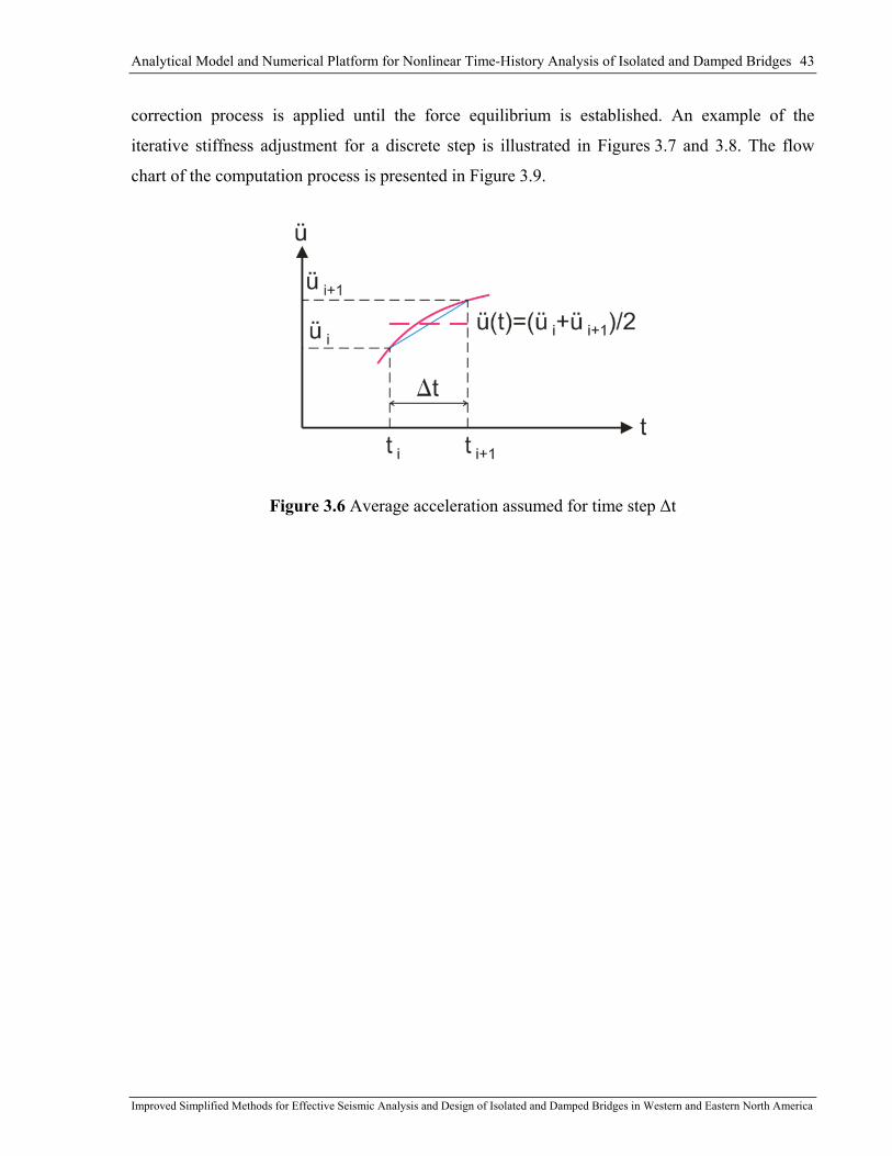
Analytical Model and Numerical Platform for Nonlinear Time-History Analysis of Isolated and Damped Bridges 43
Improved Simplified Methods for Effective Seismic Analysis and Design of Isolated and Damped Bridges in Western and Eastern North America
correction process is applied until the force equilibrium is established. An example of the
iterative stiffness adjustment for a discrete step is illustrated in Figures 3.7 and 3.8. The flow
chart of the computation process is presented in Figure 3.9.
Figure 3.6 Average acceleration assumed for time step Δt
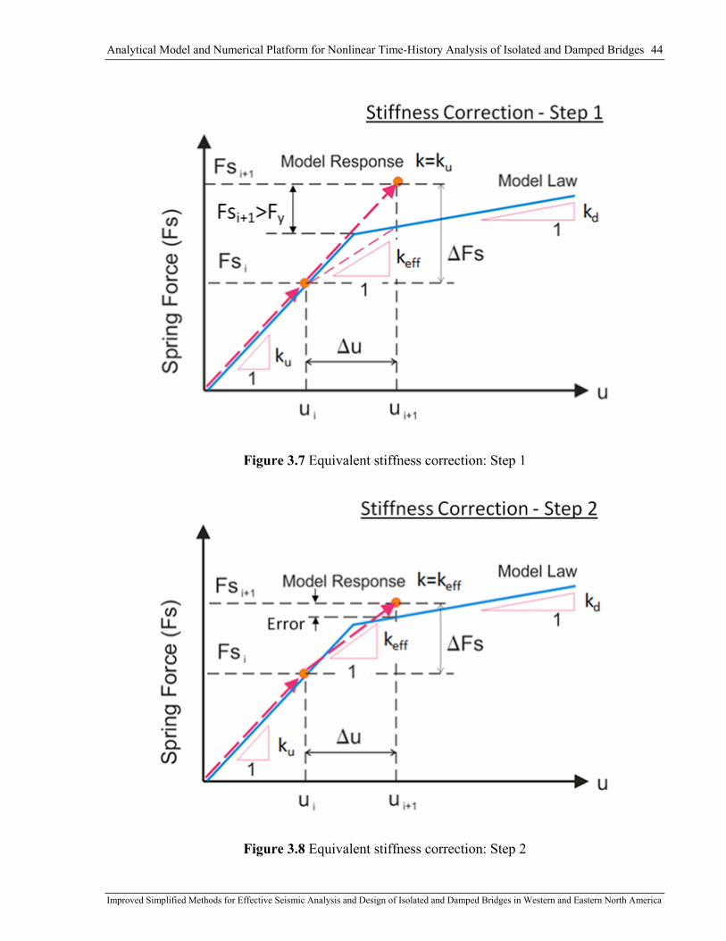
Analytical Model and Numerical Platform for Nonlinear Time-History Analysis of Isolated and Damped Bridges 44
Improved Simplified Methods for Effective Seismic Analysis and Design of Isolated and Damped Bridges in Western and Eastern North America
Figure 3.7 Equivalent stiffness correction: Step 1
Figure 3.8 Equivalent stiffness correction: Step 2
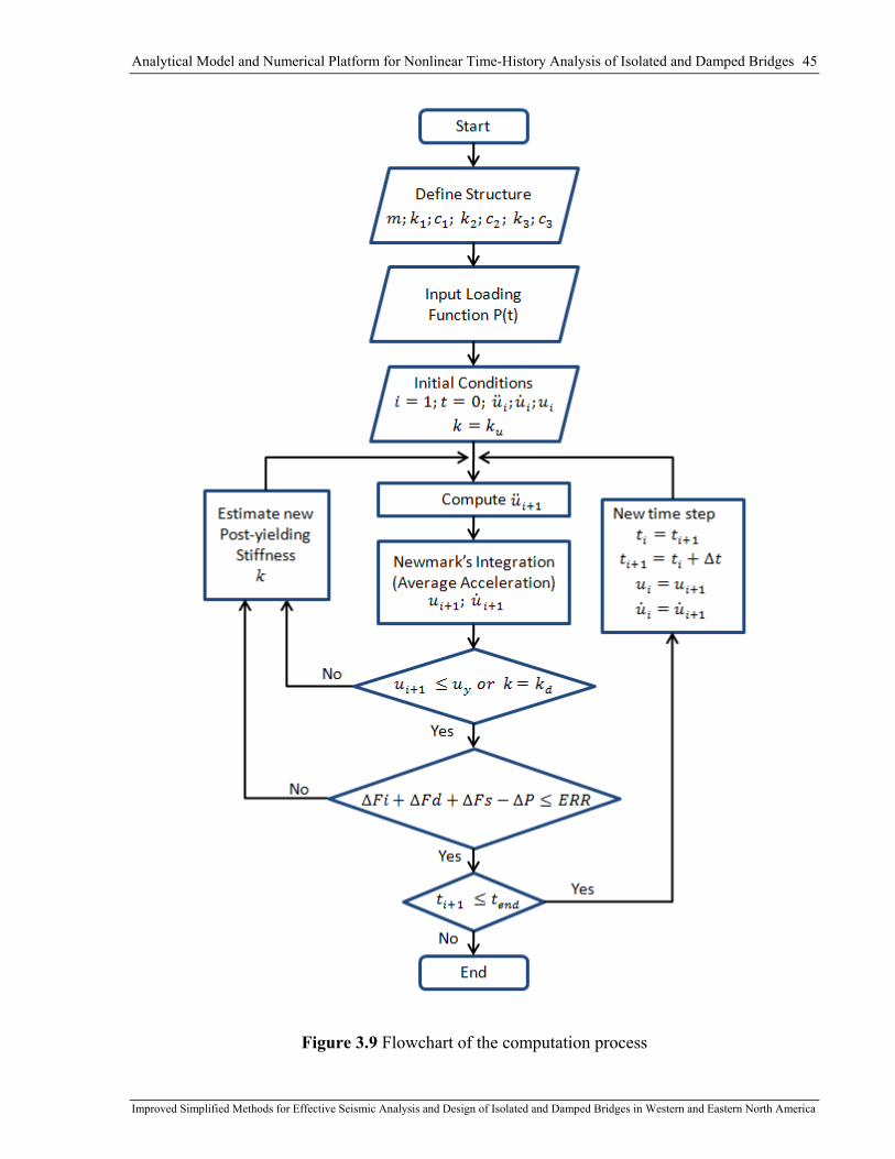
Analytical Model and Numerical Platform for Nonlinear Time-History Analysis of Isolated and Damped Bridges 45
Improved Simplified Methods for Effective Seismic Analysis and Design of Isolated and Damped Bridges in Western and Eastern North America
Figure 3.9 Flowchart of the computation process
Analytical Model and Numerical Platform for Nonlinear Time-History Analysis of Isolated and Damped Bridges 46
Improved Simplified Methods for Effective Seismic Analysis and Design of Isolated and Damped Bridges in Western and Eastern North America
3.5 Modeling of Inherent Damping
In this subsection, different techniques for modeling the inherent damping for nonlinear THA are
presented and discussed. An alternative approach for considering the inherent damping ratio
proportional to effective stiffness is then proposed.
3.5.1 Overview of Damping Assumptions
It is usual practice in seismic resistant design to define the earthquake demand by an elastic
response spectrum. While the damped linear response of a structure is well understood, the
solution for the response of a structure beyond the elastic range is still less well defined due to
the assumptions that are made for modeling the inherent damping during the nonlinear response
of the system. In an actual bridge structure, diverse sources of inherent damping can be
identified: material damping, yielding damping, and interfacial damping. Different physical
mechanisms can be associated with the capacity of inherent damping to dissipate seismic energy.
The dissipative effect of inherent damping on structural responses can be numerically accounted
for by means of an equivalent velocity-dependant damping mechanism.
As discussed earlier in Chapter 2, the concept of equivalent damping was first introduced by
Lydik Jacobsen (Jacobsen, 1930) to represent nonlinear damping by an equivalent viscous
damping model. In his work, an approximate solution was proposed for a SDOF system
undergoing forced steady-state vibration with viscous damping proportional to the first power of
the velocity. The velocity term was defined as a product of the maximum displacement and the
angular velocity under observation. In his simplified solution, Jacobsen assumed that different
damping effects could be reproduced by a linear viscous damping model. His assumptions were
generally based on the equality of energy dissipated throughout the work done by the actual and
the equivalent damping forces of a system over each cycle as presented in Figure 2.1(a). For the
case where the damping force is proportional to the nth power of the velocity, the equivalent
damping coefficient, c1, is determined from the following equality of dissipative work done
during a cycle:
dxdtdxcdx
dtdxc
TT n
n ∫∫ ⎟⎠⎞
⎜⎝⎛⋅=⎟
⎠⎞
⎜⎝⎛⋅
4/
0
1
1
4/
0
44 (3.22)
Analytical Model and Numerical Platform for Nonlinear Time-History Analysis of Isolated and Damped Bridges 47
Improved Simplified Methods for Effective Seismic Analysis and Design of Isolated and Damped Bridges in Western and Eastern North America
Jacobsen compared the responses obtained with the simplified approach to the exact analytical
solution derived by Den Hartog (1930) for four damping configurations and the results showed
close agreement with the minimum error observed at the resonance frequency. Later, in 1960,
Jacobsen expressed the equivalent viscous damping ratio for hysteretic behaviour in terms of the
dissipative work, Wc, done during one cycle and the maximum potential energy Ep as:
p
c
EW
mkc
⋅⋅
=⋅
=π
ξ2
12
(3.23)
where c, k, and m are the damping coefficient, the initial stiffness and the mass of structure,
respectively.
Jacobsen mentioned, however, that his concept becomes almost meaningless when highly
nonlinear systems or large values of non-viscous damping are applied.
Gulkan and Sozen (1974) carried out an experimental study of the dynamic response of
reinforced concrete structures and concluded that the effective natural frequency decreases when
a structure experiences excursions into the inelastic range. They explained this observation by
the reduction in stiffness due to degradation of the structure. Additionally, they also found that an
increase in energy dissipation capacity contributes, in turn, for reducing the acceleration response
below the value expected with constant damping. Thereby, Gulkan and Sozen (1974) proposed to
define an equivalent damping ratio, βs by assuming that the earthquake energy input is entirely
dissipated by a fictitious equivalent damper.
dtuumdtumT
g
T
effs ⋅⋅−=⎥⎦
⎤⎢⎣
⎡⋅⋅ ∫∫ &&&
00
22 ωβ (3.24)
where u is the relative displacement, gu&& is the ground acceleration, effω is the effective angular
frequency and m is the mass of the structure.
Iwan and Gates (1979) proposed an empirical method of linearization for inelastic response
spectra. The equivalent linear system was defined by equivalent damping and effective linear
period found by optimizing a root mean square (RMS) error between elastic and inelastic
responses.

Analytical Model and Numerical Platform for Nonlinear Time-History Analysis of Isolated and Damped Bridges 48
Improved Simplified Methods for Effective Seismic Analysis and Design of Isolated and Damped Bridges in Western and Eastern North America
In 1997, Tsopelas et al. presented a technical report on the methods suggested by FEMA 273
(1997) and FEMA 274 (ATC/BSSC, 1997) for the use of a simplified linear procedure based on
substitute elastic structures with equivalent stiffness and damping properties when the effect of
added damping is considered. They suggested to define the effective damping ratio of an
equivalent linear system using three terms as:
effinhe
effv
eff
Deff T
TDK
W−++= ββ
πβ 22
(3.25)
where WD is the energy dissipated by the structure in a complete cycle, βv is the damping ratio of
a viscous damper determined at an elastic period Te, and βinh-eff is the inherent damping of the
structure, usually set equal to 0.05 (5%) unless a different damping level is specified.
Researchers outlined the importance of defining the inherent damping ratio in relation to the
effective period Teff and not the elastic period as the effect of improperly modeled inherent
damping leads to an unconservative displacement prediction (Tsopelas et al., 1997). As a result,
for modelling highly nonlinear systems in this study, a modified Jacobesn’s equivalent damping
concept has been adopted using the effective period Teff determined by the effective secant
stiffness keff at maximum displacement.
3.5.2 Technique for Modeling Inherent Damping
In engineering practice, the effect of inherent damping is commonly represented by analytical
models using a constant damping ratio with respect to the critical damping proportional to the
stiffness of the system. In this study to comply with equivalent damping concept, the critical
damping proportional to the effective stiffness ( effcr mkc 2= ) is adopted. This damping
approximation is identical to the one given in Equation (3.29). As a result, the viscous damping
coefficient c decreases as the effective period increases.
However, it is understood that the effective period is a function of the maximum displacement
and is unknown before the analysis has been completed. For this reason, the effective damping is
defined in relation to the elastic damping ratio (proportional to the initial elastic period Te) and it
is determined in three steps. In the first two steps, the effective periods are evaluated for elastic
damping ratios βe = 0% and 5%. The second value corresponds to the assumed inherent

Analytical Model and Numerical Platform for Nonlinear Time-History Analysis of Isolated and Damped Bridges 49
Improved Simplified Methods for Effective Seismic Analysis and Design of Isolated and Damped Bridges in Western and Eastern North America
damping βinh = 5%. In the third step, the value of the inherent damping of 5% (this example) at
the elastic period is determined at the effective period by linear interpolation. The damping ratio
βe and the damping coefficient, c, proportional to elastic stiffness are given in Equations (3.26)
and (3.27):
u
e mkc
2=β (3.26)
ue mkc β2= (3.27)
Note that to simplify the step-by-step time-history analysis, the viscous damping coefficient
remains unchanged for the entire ground-motion duration and the corresponding equilibrium of
forces at each time step is given as:
)()()(2)( tumtuktumktum gtueinh &&&&& −=++ −β (3.28)
The damping ratio proportional to the effective stiffness β(keff) is determined as:
effe
effueff mk
cTT
kk2
)()( == ββ (3.29)
Once the responses at β(ku) = 0% and 5% are computed, the value of the elastic damping is
transformed into damping that is proportional to the effective stiffness by using Equation (3.29),
where the effective period Teff for a bilinear hysteretic behaviour is:
ααμμ
−+⋅=
1eeff TT (3.30)
The system response is given in terms of the ductility demand μ and α is a the post-yield stiffness
ratio. Finally, the inherent damping ratio proportional to the elastic stiffness which is required for
the analysis is recalculated using a linear interpolation:
effinheff
effeffeffinheff
TTTT −−
−+= β
β %5,
%5,%0,%0,, 0
(3.31)
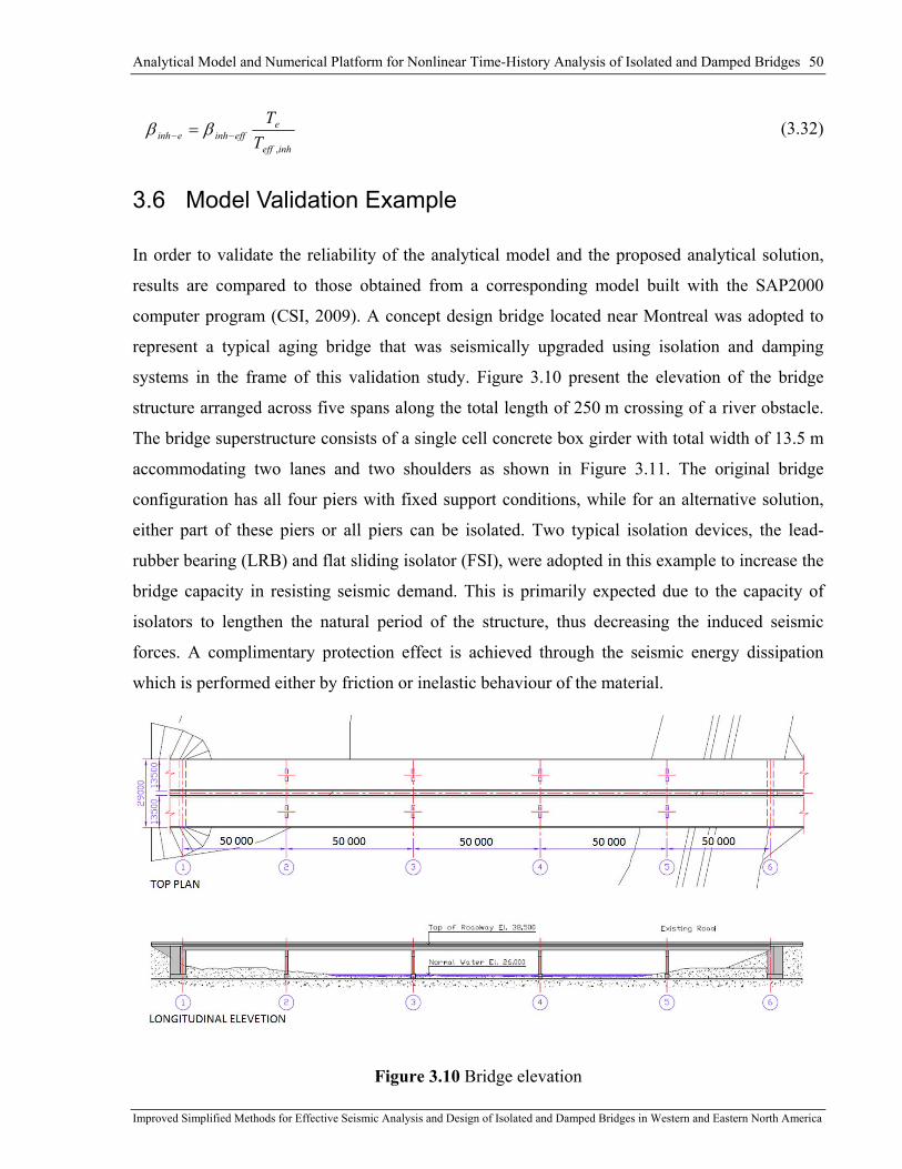
Analytical Model and Numerical Platform for Nonlinear Time-History Analysis of Isolated and Damped Bridges 50
Improved Simplified Methods for Effective Seismic Analysis and Design of Isolated and Damped Bridges in Western and Eastern North America
inheff
eeffinheinh T
T
,−− = ββ (3.32)
3.6 Model Validation Example
In order to validate the reliability of the analytical model and the proposed analytical solution,
results are compared to those obtained from a corresponding model built with the SAP2000
computer program (CSI, 2009). A concept design bridge located near Montreal was adopted to
represent a typical aging bridge that was seismically upgraded using isolation and damping
systems in the frame of this validation study. Figure 3.10 present the elevation of the bridge
structure arranged across five spans along the total length of 250 m crossing of a river obstacle.
The bridge superstructure consists of a single cell concrete box girder with total width of 13.5 m
accommodating two lanes and two shoulders as shown in Figure 3.11. The original bridge
configuration has all four piers with fixed support conditions, while for an alternative solution,
either part of these piers or all piers can be isolated. Two typical isolation devices, the lead-
rubber bearing (LRB) and flat sliding isolator (FSI), were adopted in this example to increase the
bridge capacity in resisting seismic demand. This is primarily expected due to the capacity of
isolators to lengthen the natural period of the structure, thus decreasing the induced seismic
forces. A complimentary protection effect is achieved through the seismic energy dissipation
which is performed either by friction or inelastic behaviour of the material.
Figure 3.10 Bridge elevation
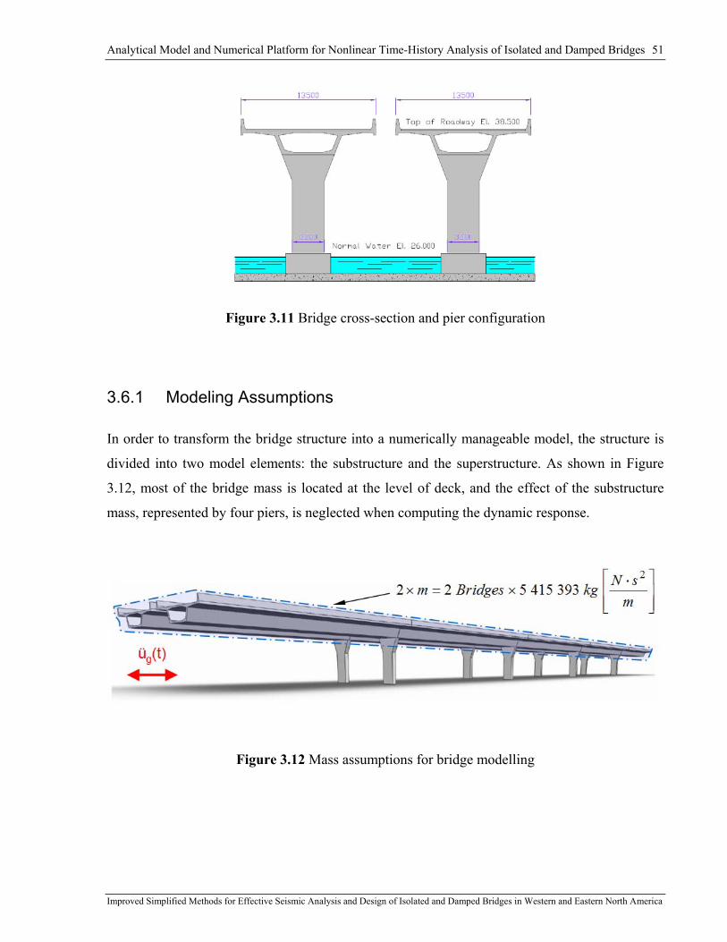
Analytical Model and Numerical Platform for Nonlinear Time-History Analysis of Isolated and Damped Bridges 51
Improved Simplified Methods for Effective Seismic Analysis and Design of Isolated and Damped Bridges in Western and Eastern North America
Figure 3.11 Bridge cross-section and pier configuration
3.6.1 Modeling Assumptions
In order to transform the bridge structure into a numerically manageable model, the structure is
divided into two model elements: the substructure and the superstructure. As shown in Figure
3.12, most of the bridge mass is located at the level of deck, and the effect of the substructure
mass, represented by four piers, is neglected when computing the dynamic response.
Figure 3.12 Mass assumptions for bridge modelling
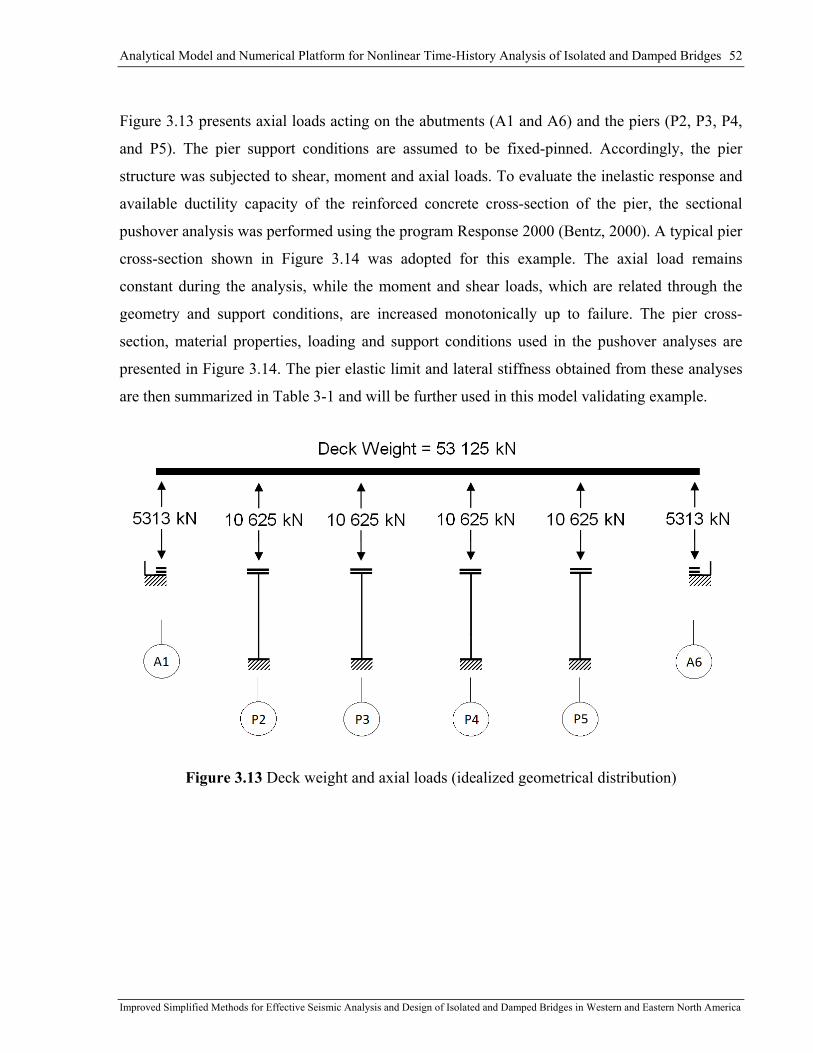
Analytical Model and Numerical Platform for Nonlinear Time-History Analysis of Isolated and Damped Bridges 52
Improved Simplified Methods for Effective Seismic Analysis and Design of Isolated and Damped Bridges in Western and Eastern North America
Figure 3.13 presents axial loads acting on the abutments (A1 and A6) and the piers (P2, P3, P4,
and P5). The pier support conditions are assumed to be fixed-pinned. Accordingly, the pier
structure was subjected to shear, moment and axial loads. To evaluate the inelastic response and
available ductility capacity of the reinforced concrete cross-section of the pier, the sectional
pushover analysis was performed using the program Response 2000 (Bentz, 2000). A typical pier
cross-section shown in Figure 3.14 was adopted for this example. The axial load remains
constant during the analysis, while the moment and shear loads, which are related through the
geometry and support conditions, are increased monotonically up to failure. The pier cross-
section, material properties, loading and support conditions used in the pushover analyses are
presented in Figure 3.14. The pier elastic limit and lateral stiffness obtained from these analyses
are then summarized in Table 3-1 and will be further used in this model validating example.
Figure 3.13 Deck weight and axial loads (idealized geometrical distribution)

Analytical Model and Numerical Platform for Nonlinear Time-History Analysis of Isolated and Damped Bridges 53
Improved Simplified Methods for Effective Seismic Analysis and Design of Isolated and Damped Bridges in Western and Eastern North America
Figure 3.14 Pier modeling assumptions for pushover analyses: a) cross-section and sectional
properties, b) material properties, and c) loading and support conditions
Table 3-1 Pier properties for the model validating example
Pier model parameters P2, P3, P4, and P5
Height of pier without bearing, h (m) 9.70
Axial load (kN) 10 625
Displacement elastic limit, uy (mm) 57
Ultimate displacement, uu (mm) 248
Lateral force elastic limit, Fy (kN) 692
Lateral stiffness (kN/m) 12 140
(Response 2000)
(Response 2000) (Response 2000)

Analytical Model and Numerical Platform for Nonlinear Time-History Analysis of Isolated and Damped Bridges 54
Improved Simplified Methods for Effective Seismic Analysis and Design of Isolated and Damped Bridges in Western and Eastern North America
3.6.2 Modeling of Isolation Devices
Two different isolation systems, lead rubber bearing (LRB) and flat sliding isolation (FSI), were
chosen for this example. FSI devices without recentring capacity are used as fuse elements to
limit the seismic forces transmitted to the piers P2, P3, P4, and P5. LRBs inherently exhibit
higher restoring forces upon yielding and the system is therefore installed at the abutments A1
and A6 where greater lateral resistance can be more easily developed. Figure 3.15 presents the
bridge protection layout, while isolator's modeling parameters are given in Table 3-2.
Figure 3.15 Protection axial loads distribution
Table 3-2 Modeling parameters: bilinear hysteretic response
Isolator model parameters A1 and A6 P2, P3, P4, and P5
Type of Device LRB (DIS) FSI
Total Number 4 Isolators 8 Isolators
Coefficient of Friction, µs N/A 2%
Activation Force (kN) 220 106.3
Post-yielding stiffness, kd (kN/m) 1100 0
Post-yielding stiffness ratio, α 0.1 0
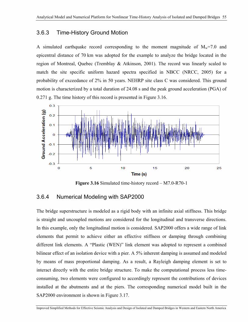
Analytical Model and Numerical Platform for Nonlinear Time-History Analysis of Isolated and Damped Bridges 55
Improved Simplified Methods for Effective Seismic Analysis and Design of Isolated and Damped Bridges in Western and Eastern North America
3.6.3 Time-History Ground Motion
A simulated earthquake record corresponding to the moment magnitude of Mw=7.0 and
epicentral distance of 70 km was adopted for the example to analyze the bridge located in the
region of Montreal, Quebec (Tremblay & Atkinson, 2001). The record was linearly scaled to
match the site specific uniform hazard spectra specified in NBCC (NRCC, 2005) for a
probability of exceedance of 2% in 50 years. NEHRP site class C was considered. This ground
motion is characterized by a total duration of 24.08 s and the peak ground acceleration (PGA) of
0.271 g. The time history of this record is presented in Figure 3.16.
Figure 3.16 Simulated time-history record – M7.0-R70-1
3.6.4 Numerical Modeling with SAP2000
The bridge superstructure is modeled as a rigid body with an infinite axial stiffness. This bridge
is straight and uncoupled motions are considered for the longitudinal and transverse directions.
In this example, only the longitudinal motion is considered. SAP2000 offers a wide range of link
elements that permit to achieve either an effective stiffness or damping through combining
different link elements. A “Plastic (WEN)” link element was adopted to represent a combined
bilinear effect of an isolation device with a pier. A 5% inherent damping is assumed and modeled
by means of mass proportional damping. As a result, a Rayleigh damping element is set to
interact directly with the entire bridge structure. To make the computational process less time-
consuming, two elements were configured to accordingly represent the contributions of devices
installed at the abutments and at the piers. The corresponding numerical model built in the
SAP2000 environment is shown in Figure 3.17.
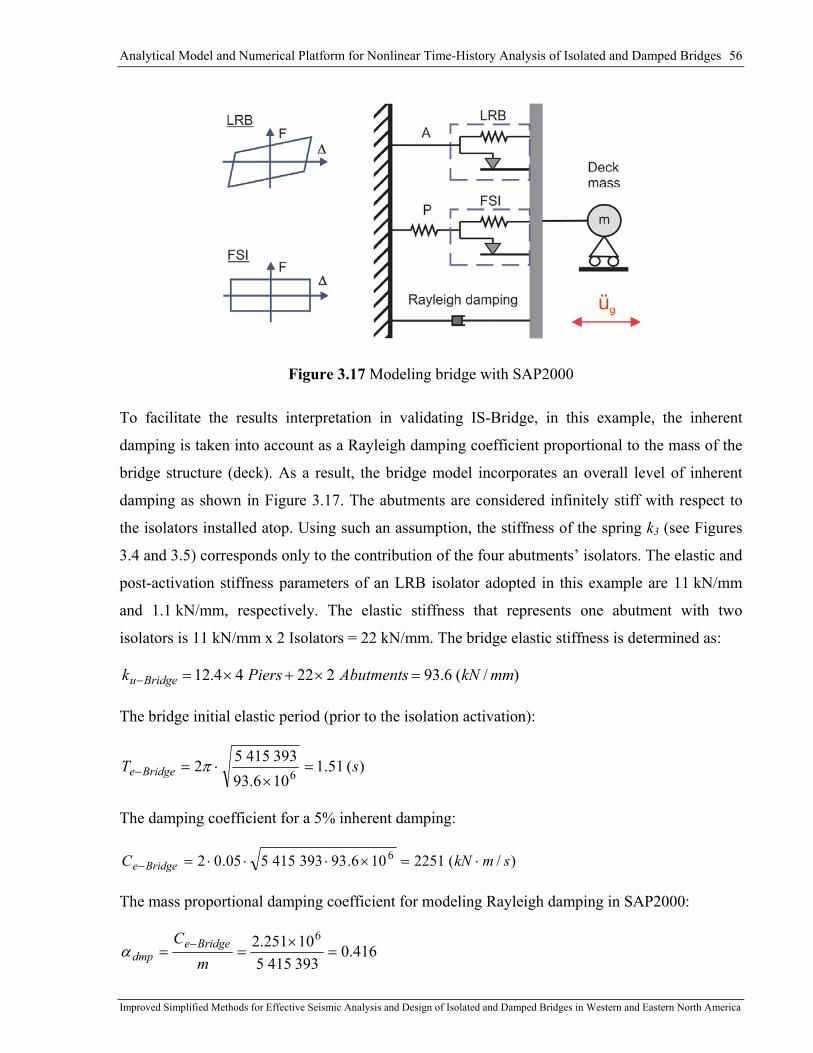
Analytical Model and Numerical Platform for Nonlinear Time-History Analysis of Isolated and Damped Bridges 56
Improved Simplified Methods for Effective Seismic Analysis and Design of Isolated and Damped Bridges in Western and Eastern North America
Figure 3.17 Modeling bridge with SAP2000
To facilitate the results interpretation in validating IS-Bridge, in this example, the inherent
damping is taken into account as a Rayleigh damping coefficient proportional to the mass of the
bridge structure (deck). As a result, the bridge model incorporates an overall level of inherent
damping as shown in Figure 3.17. The abutments are considered infinitely stiff with respect to
the isolators installed atop. Using such an assumption, the stiffness of the spring k3 (see Figures
3.4 and 3.5) corresponds only to the contribution of the four abutments’ isolators. The elastic and
post-activation stiffness parameters of an LRB isolator adopted in this example are 11 kN/mm
and 1.1 kN/mm, respectively. The elastic stiffness that represents one abutment with two
isolators is 11 kN/mm x 2 Isolators = 22 kN/mm. The bridge elastic stiffness is determined as:
)/(6.9322244.12 mmkNAbutmentsPiersk Bridgeu =×+×=−
The bridge initial elastic period (prior to the isolation activation):
)(51.1106.9339341552 6 sT Bridgee =
×⋅=− π
The damping coefficient for a 5% inherent damping:
)/(2251106.93393415505.02 6 smkNC Bridgee ⋅=×⋅⋅⋅=−
The mass proportional damping coefficient for modeling Rayleigh damping in SAP2000:
416.0393415510251.2 6
=×
== −
mC Bridgee
dmpα

Analytical Model and Numerical Platform for Nonlinear Time-History Analysis of Isolated and Damped Bridges 57
Improved Simplified Methods for Effective Seismic Analysis and Design of Isolated and Damped Bridges in Western and Eastern North America
3.6.5 Results and Comparison
The results obtained from the nonlinear time-history analysis carried out using the SAP2000
model are compared to those from the IS-Bridge model. The time step used for the analyses with
both models was set to 0.001 s. The bridge hysteretic responses computed by SAP2000 and by
IS-Bridge are presented in Figure 3.18. Similar hysteretic shapes result from both simulations
thus indicating that the characteristics of the LRB and FSI devices are properly taken into
account by the models (same activation levels, elastic and post-yielding stiffness). The
displacement and force time histories are shown in Figure 3.19. An excellent agreement is
observed between these responses over the entire record duration. Some slight differences in
responses, however, can be noted. The responses from IS-Bridge result in insignificant
overshooting generally due to differences in integrating process which is iterative in SAP2000
and is based on direct solution for a discrete time step in IS-Bridge.
Abutment
Pier
‐600
‐400
‐200
0
200
400
600
‐50 ‐40 ‐30 ‐20 ‐10 0 10 20 30 40 50
Lateral Force (k
N)
Displacement (mm)
SAP2000 Modeling
Abutment
Pier
‐600
‐400
‐200
0
200
400
600
‐50 ‐40 ‐30 ‐20 ‐10 0 10 20 30 40 50
Lateral Force (k
N)
Displacement (mm)
IS‐Bridge Modeling
Figure 3.18 Hysteretic bridge response from SAP2000 and IS-Bridge

Analytical Model and Numerical Platform for Nonlinear Time-History Analysis of Isolated and Damped Bridges 58
Improved Simplified Methods for Effective Seismic Analysis and Design of Isolated and Damped Bridges in Western and Eastern North America
‐50
‐40
‐30
‐20
‐10
0
10
20
30
40
0 1 2 3 4 5 6 7 8 9 10 11 12 13 14 15 16 17 18 19 20 21 22 23 24 25
Deck Displacem
ent (m
m)
Time (s)
IS‐BridgeSAP2000
‐600
‐400
‐200
0
200
400
600
0 1 2 3 4 5 6 7 8 9 10 11 12 13 14 15 16 17 18 19 20 21 22 23 24 25
Abutment Force (kN)
Time (s)
IS‐Bridge SAP2000
‐300
‐200
‐100
0
100
200
300
0 1 2 3 4 5 6 7 8 9 10 11 12 13 14 15 16 17 18 19 20 21 22 23 24 25
Pier Force (kN)
Time (s)
IS‐Bridge SAP2000
Figure 3.19 Time histories of bridge responses computed by SAP2000 and IS-Bridge

Analytical Model and Numerical Platform for Nonlinear Time-History Analysis of Isolated and Damped Bridges 59
Improved Simplified Methods for Effective Seismic Analysis and Design of Isolated and Damped Bridges in Western and Eastern North America
3.7 Conclusions
A new analytical model and methodology to carry out nonlinear simplified isolated bridge
analysis are presented and validated in this chapter. The ability of IS-Bridge to accurately
simulate the structural behaviour of isolated bridges makes this program an useful tool to carry
out the extensive parametric analyses needed to achieve objectives of this research. In addition,
this numerical tool can be used at the preliminary design stage of seismically isolated bridges as
well as it may be widely exploited for teaching-learning process and research purposes due to the
possibility of animating seismic response simulations through a graphical user interface.

Ground Motion (GM) Selection and Scaling for Time-History Analysis of Isolated Bridges 60
Improved Simplified Methods for Effective Seismic Analysis and Design of Isolated and Damped Bridges in Western and Eastern North America
Chapter 4: Ground Motion (GM) Selection and Scaling for Time-History Analysis of Isolated Bridges
4.1 Introduction
In this chapter, site-specific ensembles of ground-motion time histories are defined and scaled to
carry out the analyses of the nonlinear structural behaviour of isolated bridges in Eastern (ENA)
and Western (WNA) North America. In spite of being widely addressed over the last decade by
many research studies, the record selection and scaling process is still challenging to structural
engineers today. There is a variety of approaches that have been developed for specific design
purposes based on either site-specific seismic hazard conditions or properties of structures to be
analyzed.
The current seismic code provisions (CSA-S6-06 and AASHTO), however, do not provide an
explicit procedure on how to select and scale ground-motion records for nonlinear time-history
analyses (THA) of isolated bridges to obtain acceptable response predictions over a wide range
of inelastic excursion (related to period lengthening). The technique and methodology proposed
in this study intend to select and scale time histories for dynamic analyses from the perspective
of a structural engineer using the available state of the art in seismology.
The design spectrum in the Canadian CSA-S6-06 code is no longer up to date and it is expected
that the uniform hazard spectrum (UHS) currently used in NBCC (NRCC, 2005) for buildings
will be adopted as the design spectrum in the next CSA-S6-14. When this study was initiated in
2009, UHS for CSA-S6-14 had not been developed yet and the UHS data specified in NBCC
2005 was adopted as it represented the most recent data available at that time. The UHS data was
modified in the 2010 edition of NBCC (NRCC, 2010) but the changes were small and not likely
to significantly affect the outcome of the study. Hence, the research was completed using the
2005 seismic data.
An overview of recent developments in seismology is presented first. The time histories are then
selected according to magnitude-distance (M-R) scenarios dominating the seismic hazard for two
densely populated Canadian cities: Montreal, Quebec, for ENA, and Vancouver, British

Ground Motion (GM) Selection and Scaling for Time-History Analysis of Isolated Bridges 61
Improved Simplified Methods for Effective Seismic Analysis and Design of Isolated and Damped Bridges in Western and Eastern North America
Columbia, for WNA. The amplitude of the ground motions are linearly scaled to match the site
specific uniform hazard spectra specified in NBCC (NRCC, 2005). The technique for scaling
time histories for a specific period range as proposed by Atkinson (2009) was adopted.
4.2 Overview of Relevant Development in Seismology
Since the 1906 earthquake that devastated San Francisco, scientists and engineers have expressed
the need for a better understanding of seismic events and seismic demand on structures. The
same year, the Seismological Society of America (SSA) was founded and it marked the
beginning of the modern science of seismology in North America. To rebuild San Francisco, the
minimum design wind load of 1.4 kPa (30 psf) requirement was adopted to provide structures
with the capacity to withstand wind lateral forces. Although there was no direct mention of
seismic forces, the increase in structural capacity to resist both wind and earthquakes was
intended (Popov, 1994). Learning from the 1925 Santa Barbara and the 1933 Long Beach
earthquakes, seismic provisions were progressively introduced into design practice. Seismic
forces were then expressed as a percentage of the gravity loads. Several seismological values
were specified to account for different seismic zones and soil types. In addition, it is during the
1933 Long Beach earthquake that acceleration time histories were recorded for a strong motion
for the first time. Since then, the input based on seismological data were considered by engineers
for earthquake resistant design.
During the 1940 El Centro earthquake (Imperial Valley earthquake), sets of detailed strong
motion recordings were obtained. These records have been extensively used since by researchers
and engineers in time-history analyses to validate the reliability of structural designs and develop
new design methods. Through the subsequent decade, seismic design provisions were based on a
qualitative evaluation of hazard (Atkinson, 2004). However, it was recognized that even if being
scaled to a desired ground-motion intensity, a given ground motion (GM) record may be
characterized by magnitude M and distance R parameters that are not necessary representative of
the site-specific seismic hazard.
Different seismic models have then been produced to predict and simulate ground-motion
activity in the regions of interest. Based on these models, seismic hazard maps could be
developed which represented a major improvement for seismic design. In Canada, such a

Ground Motion (GM) Selection and Scaling for Time-History Analysis of Isolated Bridges 62
Improved Simplified Methods for Effective Seismic Analysis and Design of Isolated and Damped Bridges in Western and Eastern North America
national probabilistic seismic hazard map was introduced for the first time in 1970 (Atkinson,
2004).
The current building code in Canada is now based on the fourth generation seismic hazard maps
that have been proposed by Adams and Halchuk (2003). Significant advances in the
understanding of seismicity have been necessary in the development of these maps. Special
efforts have also been devoted to the treatment of uncertainty in hazard analyses and this new
seismic hazard model incorporates aleatory and epistemic uncertainties. Contrary to the aleatory
uncertainty that characterizes inherent physical variability, the epistemic uncertainty results from
the lack of knowledge and can be reduced by collecting and analyzing new ground motion data.
In Canada, epistemic uncertainty is reflected by the use of two probabilistic seismic hazard
models “H” and “R”. The “H” model was created to represent the hazard based on the historical
events that have been observed in the past. It therefore contains only a few seismic sources
located in known seismic active areas. To compensate for the short period of seismic
observation, the “R” model incorporates a larger number of seismic sources that are based on
seismotectonic characteristics reflecting the potential for earthquake activity. For the fourth
generation map, the reliability of the seismic hazard in "stable" regions of Canada was improved
by introducing a third probabilistic seismic model "F" ("floor"). That model is based on the
seismic data obtained worldwide on the earthquake activity in similar continental parts subjected
to low seismic activity and was adopted as a "floor" level of seismic hazard across Canada. In
addition to the first three probabilistic models, a deterministic model "C" was also developed to
include the hazard posed by a realistic scenario generated for a prehistorical great earthquake that
occurred on the Cascadia subduction zone in the 18th century. Adams and Halchuk (2003)
suggested to choose the highest value of seismic hazard (the more conservative result) from the
four models. This approach had been proposed earlier by Adams et al. (1995) and is known as
the "robust" model. However, it has been recognized that by using only the "R" model for eastern
Canada, the seismic protection could be reduced significantly in regions of high historical
seismicity while the protection in other locations would be insignificantly increased (Adams and
Atkinson, 2003).
The implementation of the uniform hazard spectrum (UHS) in seismic design is another major
development in the seismic hazard methodology. In contrast to the previous code maps, the UHS

Ground Motion (GM) Selection and Scaling for Time-History Analysis of Isolated Bridges 63
Improved Simplified Methods for Effective Seismic Analysis and Design of Isolated and Damped Bridges in Western and Eastern North America
provides a constant probability of exceedance for each response spectral ordinates computed at
different structure periods. The contribution of earthquake having various magnitude and
distance characteristics is considered in the evaluation of the seismic hazard at each specific site.
Thus the UHS shape results from the effect of all possible events that can contribute to the site-
specific hazard as illustrated in Figure 4.1 for close (local) and distant seismic events.
Figure 4.1 The concept of UHS for a location affected by local sources of moderate seismicity
and distant sources (Bommer et al., 2000a and Hancock, 2006 after Reiter, 1990)
The fourth generation seismic model (Adams and Halchuk, 2003) provides 5% damped spectral
acceleration values at periods of 0.2, 0.5, 1.0, 2.0 s, and PGA (peak ground acceleration). A
reference ground condition corresponding to the NEHRP site class C has been adopted to
generate the national hazard maps. This ground condition is characterized by an average shear
wave velocity of 360 to 760 m/s over the top 30 m of soil, which corresponds to “very dense soil
and soft rock” ("firm soil"). The site class C is representative of a large number of well recorded
strong ground motions, which minimizes the uncertainty related to site amplification (Adams
and Halchuk, 2004). For other site conditions, two site amplification factors Fa and Fv are
specified for short and long periods, respectively. The spectral acceleration values for a given
site class are obtained by amplifying or de-amplifying the site C value using the corresponding
Fa and Fv factors.
For the fourth generation seismic hazard model, the level of probability of exceedance previously
specified in the Canadian code as 10% in 50 years (0.0021 per annum) was decreased to 2% in

Ground Motion (GM) Selection and Scaling for Time-History Analysis of Isolated Bridges 64
Improved Simplified Methods for Effective Seismic Analysis and Design of Isolated and Damped Bridges in Western and Eastern North America
50 years (0.0004 per annum) (Adams and Halchuk, 2003). This important change aimed to
assure a more uniform level of safety against collapse or failure of structures across all regions of
Canada (Heidebrecht, 2003). The hazard curves across Canada do not have the same slope, as
illustrated in Figure 4.2, and designing for 10% in 50 years hazard level as specified in the
current CSA-S6-06 would not result in the same level of protection against stronger earthquakes
with lower probability of exceedance. Therefore, a probability of exceedance of 2% in 50 years
corresponding to a return period of 2475 years was adopted for the design spectrum in the next
CSA-S6-14. Heidebreht (2003) indicated that the design of common structures for events with
this lower probability level will provide a uniform level of the target reliability across Canada.
Figure 4.2 Hazard curves for Vancouver and Montréal (Adams and Halchuk 2004)
4.3 Site-Specific Scenarios for ENA and WNA
To define earthquake scenarios and select ground motion time histories for the parametric studies
conducted in this project, two locations representative of eastern and western North America
were first selected. Two densely populated cities where a large number of bridges are present
were chosen: Vancouver, British Columbia, for WNA and Montreal, Quebec, for ENA. As
shown in Figure 4.3, these two locations were also selected as they represent the populated
regions with the highest seismic risk in western and eastern Canada (Halchuk et Adams, 2004).

Ground Motion (GM) Selection and Scaling for Time-History Analysis of Isolated Bridges 65
Improved Simplified Methods for Effective Seismic Analysis and Design of Isolated and Damped Bridges in Western and Eastern North America
These two Canadian cities are representative of other large cities such as Boston or New York in
the eastern US and Seattle and Portland in the western US.
Figure 4.3 Earthquake risk distribution in Canada (Adams, 2011)
For reducing epistemic uncertainty that results from the lack of knowledge, the commonly
adopted practice consists in processing a large number of time-history records. However, this
technique provides statistically poor results for regions with scarcity in well-recorded historical
ground motions as in the case of eastern North America. Significant advances in seismology
research made recently suggest the possibility of reducing the number of required records by
considering site-specific records which are selected in terms of magnitude and distance (M-R)
according to the dominant earthquake scenario.
4.4 Dominant Earthquake Scenarios
In this study, the earthquake scenarios are determined from site-specific hazard deaggregations
produced in terms of magnitude and distance (M-R) for a probability of exceedance of 2% in 50
years and NBCC site class C (Halchuk and Adams, 2004, Halchuk, 2009 and Halchuk, 2010).
The deaggregation of seismic hazard is commonly defined as the M-R distribution of the annual
rate of exceedance of a target spectral amplitude SA(T) at a period T. The annual rate of
exceedance accumulated by M-R bins that represent the relative contribution of each of the
earthquake M-R scenarios to the hazard. The deaggregated results are generally presented on the
form of a binned plot from which one can easily determine which earthquake scenario
contributes most to the site-specific seismic hazard at the structure period of interest. The

Ground Motion (GM) Selection and Scaling for Time-History Analysis of Isolated Bridges 66
Improved Simplified Methods for Effective Seismic Analysis and Design of Isolated and Damped Bridges in Western and Eastern North America
dominant earthquakes are then used to select the ground-motion records with comparable seismic
magnitude and source-to-site distance. These records are applied for inelastic time-histories
analyses of structures so that the distribution of delivered energy with time is realistically
represented (McGuire et al. 2001b; McGuire et al. 2002).
Deaggregated hazard plots for the 5% damped spectral acceleration Sa(T) computed at the four
periods T = 0.2, 0.5, 1.0 and 2.0 s are presented in Figures 4.4 to 4.7 for Montreal and in Figures
4.8 to 4.11 for Vancouver. These plots are provided for a probability of exceedance 2% in 50
years (probability of 0.000404 per annum). In these figures, the size of the bins is 20 km in
distance and 0.25 in magnitude.
When examining the plots for Montreal, it is clear that for this probability level, more than one
M-R earthquake scenario may significantly contribute to the hazard. It is also evident that the
dominant scenarios also vary with the period T. For instance, two bins with the maximum
contribution to the hazard of 68/1000 correspond to the events M5.875 at 10 km and M5.875 at
30 km for the period T=0.2 s. For periods of 0.5 and 1.0 s, the hazard is dominated by events
with a greater magnitude M6.875 at 30 km. For period T=2.0 s the maximum contribution to the
hazard comes from the event M6.625 at 30 km, which magnitude is greater than that from
T=0.25 s and smaller than those from T=0.5 and 1.0 s. Moreover, it can be noted that the
contribution to the hazard from distant earthquakes increases with period as those of 1/1000,
4/1000, 11/1000, and 27/1000 for T=0.2 s, 0.5 s, 1.0 s, and 2.0 s, respectively. In contrast to
Montreal, the deaggregation plots for Vancouver present mostly similar shape so that the
maximum contributions correspond to the same event for periods of 0.2 and 0.5 s (M6.875at
70 km) and for periods of 1.0 and 2.0 s (M7.125 at 70 km).
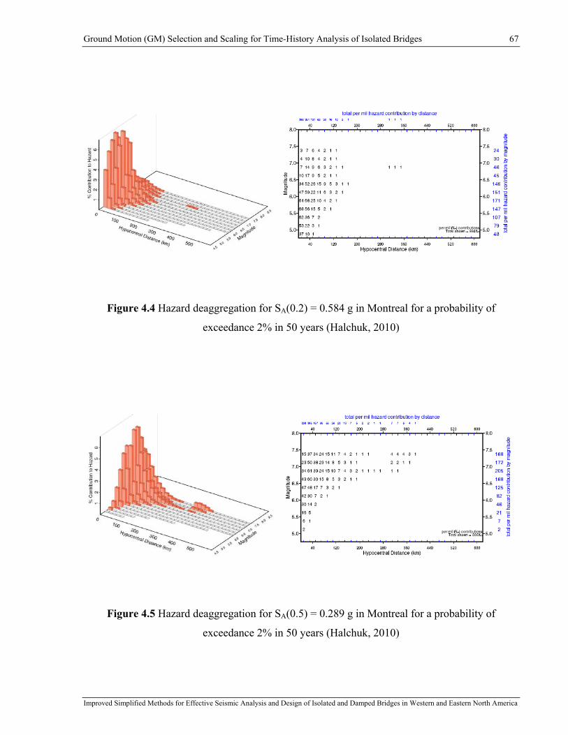
Ground Motion (GM) Selection and Scaling for Time-History Analysis of Isolated Bridges 67
Improved Simplified Methods for Effective Seismic Analysis and Design of Isolated and Damped Bridges in Western and Eastern North America
Figure 4.4 Hazard deaggregation for SA(0.2) = 0.584 g in Montreal for a probability of
exceedance 2% in 50 years (Halchuk, 2010)
Figure 4.5 Hazard deaggregation for SA(0.5) = 0.289 g in Montreal for a probability of
exceedance 2% in 50 years (Halchuk, 2010)
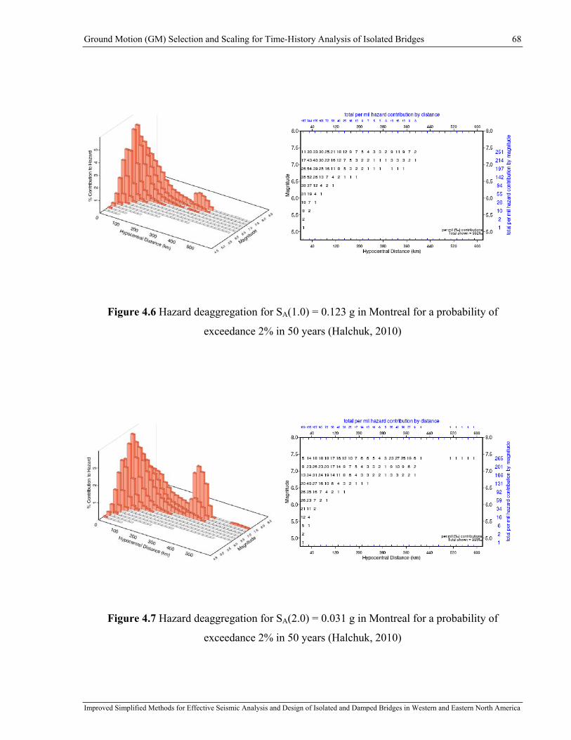
Ground Motion (GM) Selection and Scaling for Time-History Analysis of Isolated Bridges 68
Improved Simplified Methods for Effective Seismic Analysis and Design of Isolated and Damped Bridges in Western and Eastern North America
Figure 4.6 Hazard deaggregation for SA(1.0) = 0.123 g in Montreal for a probability of
exceedance 2% in 50 years (Halchuk, 2010)
Figure 4.7 Hazard deaggregation for SA(2.0) = 0.031 g in Montreal for a probability of
exceedance 2% in 50 years (Halchuk, 2010)
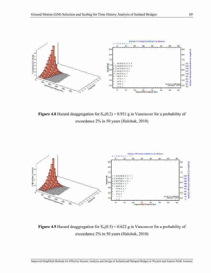
Ground Motion (GM) Selection and Scaling for Time-History Analysis of Isolated Bridges 69
Improved Simplified Methods for Effective Seismic Analysis and Design of Isolated and Damped Bridges in Western and Eastern North America
Figure 4.8 Hazard deaggregation for SA(0.2) = 0.931 g in Vancouver for a probability of
exceedance 2% in 50 years (Halchuk, 2010)
Figure 4.9 Hazard deaggregation for SA(0.5) = 0.622 g in Vancouver for a probability of
exceedance 2% in 50 years (Halchuk, 2010)
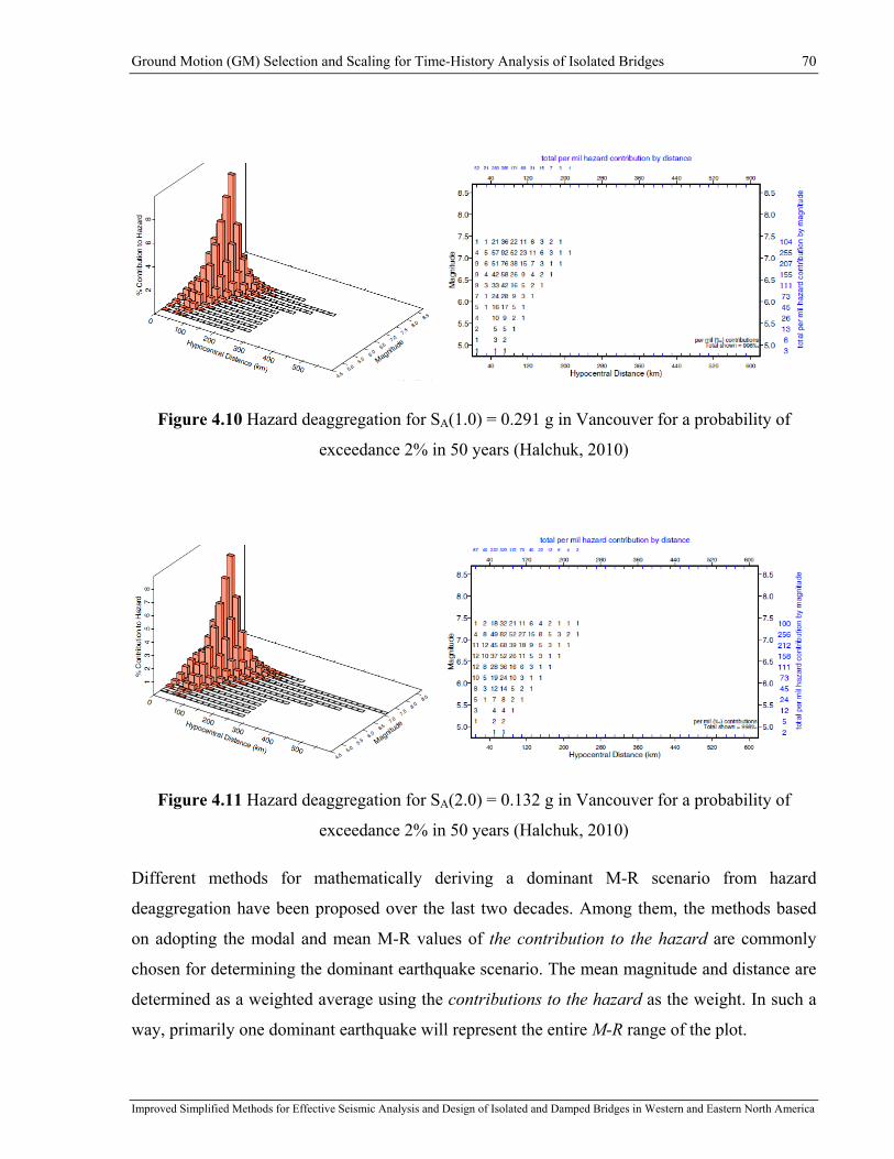
Ground Motion (GM) Selection and Scaling for Time-History Analysis of Isolated Bridges 70
Improved Simplified Methods for Effective Seismic Analysis and Design of Isolated and Damped Bridges in Western and Eastern North America
Figure 4.10 Hazard deaggregation for SA(1.0) = 0.291 g in Vancouver for a probability of
exceedance 2% in 50 years (Halchuk, 2010)
Figure 4.11 Hazard deaggregation for SA(2.0) = 0.132 g in Vancouver for a probability of
exceedance 2% in 50 years (Halchuk, 2010)
Different methods for mathematically deriving a dominant M-R scenario from hazard
deaggregation have been proposed over the last two decades. Among them, the methods based
on adopting the modal and mean M-R values of the contribution to the hazard are commonly
chosen for determining the dominant earthquake scenario. The mean magnitude and distance are
determined as a weighted average using the contributions to the hazard as the weight. In such a
way, primarily one dominant earthquake will represent the entire M-R range of the plot.
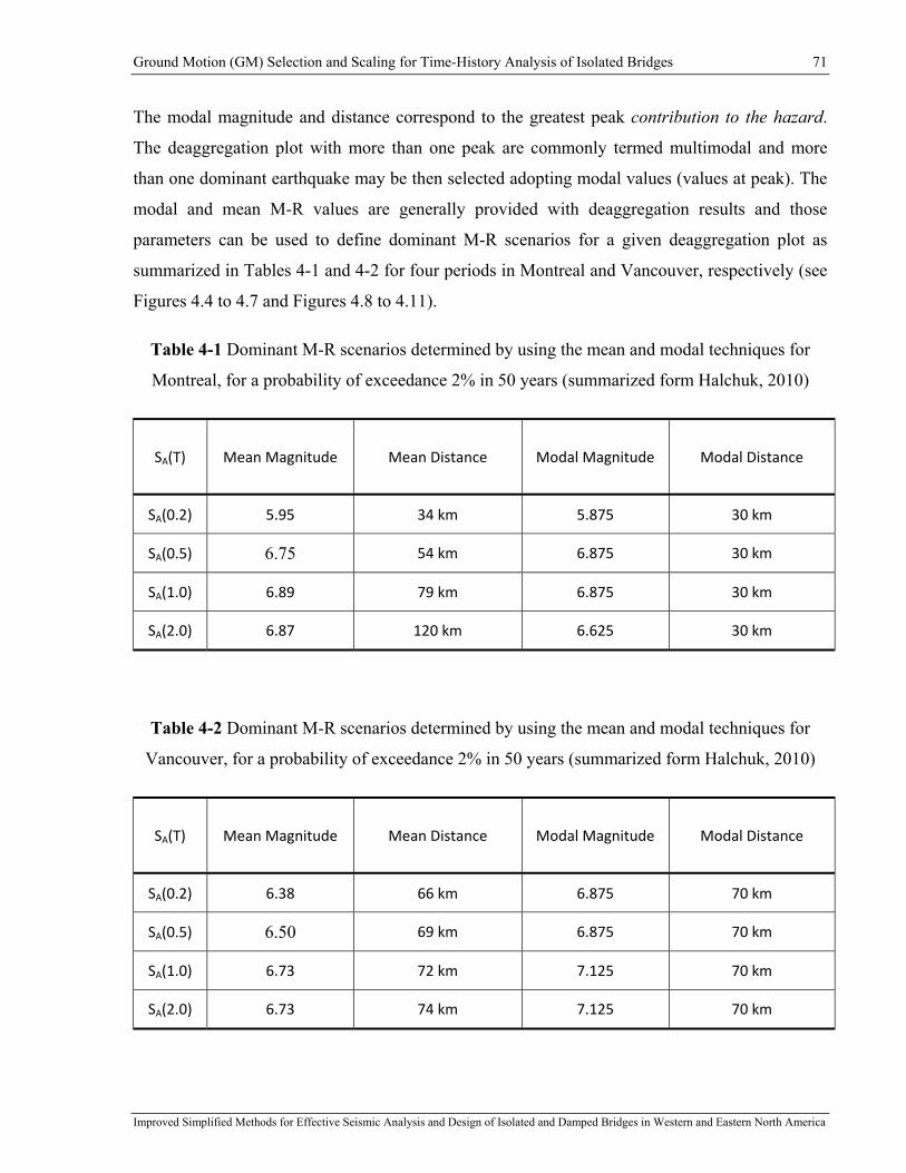
Ground Motion (GM) Selection and Scaling for Time-History Analysis of Isolated Bridges 71
Improved Simplified Methods for Effective Seismic Analysis and Design of Isolated and Damped Bridges in Western and Eastern North America
The modal magnitude and distance correspond to the greatest peak contribution to the hazard.
The deaggregation plot with more than one peak are commonly termed multimodal and more
than one dominant earthquake may be then selected adopting modal values (values at peak). The
modal and mean M-R values are generally provided with deaggregation results and those
parameters can be used to define dominant M-R scenarios for a given deaggregation plot as
summarized in Tables 4-1 and 4-2 for four periods in Montreal and Vancouver, respectively (see
Figures 4.4 to 4.7 and Figures 4.8 to 4.11).
Table 4-1 Dominant M-R scenarios determined by using the mean and modal techniques for
Montreal, for a probability of exceedance 2% in 50 years (summarized form Halchuk, 2010)
SA(T) Mean Magnitude Mean Distance Modal Magnitude Modal Distance
SA(0.2) 5.95 34 km 5.875 30 km
SA(0.5) 6.75 54 km 6.875 30 km
SA(1.0) 6.89 79 km 6.875 30 km
SA(2.0) 6.87 120 km 6.625 30 km
Table 4-2 Dominant M-R scenarios determined by using the mean and modal techniques for
Vancouver, for a probability of exceedance 2% in 50 years (summarized form Halchuk, 2010)
SA(T) Mean Magnitude Mean Distance Modal Magnitude Modal Distance
SA(0.2) 6.38 66 km 6.875 70 km
SA(0.5) 6.50 69 km 6.875 70 km
SA(1.0) 6.73 72 km 7.125 70 km
SA(2.0) 6.73 74 km 7.125 70 km

Ground Motion (GM) Selection and Scaling for Time-History Analysis of Isolated Bridges 72
Improved Simplified Methods for Effective Seismic Analysis and Design of Isolated and Damped Bridges in Western and Eastern North America
The dominant scenarios obtained for Vancouver using the mean and modal values of the
contribution to the hazard, are in close agreement for all four periods. All four deaggregation
plots present a single-mode hazard (single peak) and respective modal and mean values will
correspond to a similar dominant earthquake scenario and the corresponding damage potentiality.
In contrast, by comparing the dominant earthquakes summarized in Table 4.1 (modal and mean
values) for Montreal, it can be noted that the differences in magnitude and distance between the
dominant earthquakes may significantly increase with period. This is primarily because of the
influence of distant earthquakes whose effects increase with periods. For instance in Figure 4.7
(T = 2.0 s), the deaggregation plot clearly presents two modes due to the close and distant
earthquakes.
As it can be observed in Figure 4.12, if only the earthquake with the maximum contribution to
the hazard was selected (as that indicated in Table 4.1 for modal earthquake: M=6.625 and
R=30 km), the effect of the close event will be “fairly” taken into account while from the distant
earthquake will be ignored completely. In contrast, the mean value of the hazard makes it
possible to take into account the contribution of all earthquakes. However, in the case of a multi-
modal hazard, the mean values of the magnitude and distance may point out an event with a
lower hazard and the resulting seismic demand may be non-realistically estimated.

Ground Motion (GM) Selection and Scaling for Time-History Analysis of Isolated Bridges 73
Improved Simplified Methods for Effective Seismic Analysis and Design of Isolated and Damped Bridges in Western and Eastern North America
Figure 4.12 Modal and mean earthquakes for Montreal, T=2.0 s, 2%-50 years (mean hazard
level is determined over all hazard contributions)
The differences in the dominant scenarios between Vancouver and Montreal may be explained
by the effect of different sources that influence the site-specific seismic hazard. For the Western
Canadian shore (Vancouver), the high (quick) attenuation of seismic waves reduces significantly
the effect of distant earthquakes. In contrast, for Eastern Canada (Montreal), due to the low
attenuation, close and distant earthquakes may affect significantly the site-specific hazard.
Ground Motion (GM) Selection and Scaling for Time-History Analysis of Isolated Bridges 74
Improved Simplified Methods for Effective Seismic Analysis and Design of Isolated and Damped Bridges in Western and Eastern North America
McGuire (1995) suggested to keep separate modal M-R scenarios rather than a mean M - R
earthquake whether different seismic sources dominate the hazard at different periods. This
technique makes it possible to reflect different damaging aspects brought by events from
different seismic sources. Aiming at exploring the physical meaning of earthquake scenarios,
McGuire et al. (2001a) has shown that high-frequency responses (around 10Hz) are dominated
by small-magnitude earthquakes occurring at close distances to the site, while low-frequency
responses (around 1Hz) are dominated by larger earthquakes at longer distances.
While such an approach would be appropriate for structures characterized by elastic responses,
several engineers and researchers raise the question whether this technique will realistically
reveal the earthquakes' damage potential for structures that behave within the inelastic range
(Tremblay and Atkinson, 2001; Leger and Tremblay, 2009).
In this study, the results from the deaggregation analyses are used to carry out deterministic time-
history analyses of the nonlinear structural behaviour of isolated bridges. Accordingly, from the
perspective of structural engineering, an earthquake scenario is expected to simulate closely the
damage potential of the earthquakes contributing to the hazard.
Several studies have investigated the effect of different ground-motion characteristic on the
seismic inelastic response and capacity of structures (Jeong and Iwan, 1988; Tremblay, 1998;
Tremblay and Atkinson, 2001; Hancock and Bommer, 2005 and Leger and Tremblay, 2009).
These previous studies suggest that the ultimate capacity can be reached through different
inelastic behaviors. Structures may fail due to excessive peak deformations or as a result of
excessive cumulated inelastic demand (Tremblay and Atkinson, 2001; Hancock, 2006).
In order to account for different damageable effects and evaluate the range of possible responses
of various isolated bridge structures, an ensemble of seismic ground motions is used for each
site. These ground motions result from multiple likely M-R scenarios.
The approach proposed in this chapter consists in considering earthquakes with the greatest
values of the contribution to the hazard referred as modal values or bins. The modal values are
considered within M-R ranges that are likely prone of producing a large demand to structures
(damage to structures).

Ground Motion (GM) Selection and Scaling for Time-History Analysis of Isolated Bridges 75
Improved Simplified Methods for Effective Seismic Analysis and Design of Isolated and Damped Bridges in Western and Eastern North America
This however, requires that the M-R ranges with likely damage potential be established
beforehand. Because of the inherent physical variability of the earthquakes, these M-R ranges
may be individually defined for each of the earthquakes. However, to produce a generalized
strategy that could “robustly” take into account damage potential of different earthquakes, the
proposed technique is primarily based on the extended M-R ranges. The M-R ranges were
proposed by Atkinson (2009) for generating artificial ground-motion records that are compatible
with an UHS determined through probabilistic seismic hazard analyses (PSHA). These M-R
ranges have been primarily defined to make these artificial records easily match the target UHS
from the NBCC 2005 (NRCC, 2005).
The selection of the proper design earthquakes is still challenging given that dynamic
characteristic of the ground motions can vary significantly from one site to another (Anderson
and Bertero, 1987). By considering several possible ground motions makes it possible to reduce
the effect of uncertainty in revealing earthquakes damaging potentiality. In this study, in addition
to the Atkinson’s M-R ranges, boundaries that delimitate hazard contributions are considered. In
this way, the Atkinson’s M-R ranges are complemented so that the damaging earthquakes that
are not necessary covered by them would be definitely considered for time-history analyses. As a
result, a more "robust" technique is adopted as shown in Figure 4.13. It can be seen that in
addition to the Atkinson’s M-R ranges, the boundary ranges are considered. The M-R boundary
ranges cover earthquakes in ranges of the closest distance, greatest magnitude and those from a
group of distant events.
The influence of distance and magnitude on the earthquake damage potentiality has been widely
reported in the past (Anderson and Bertero, 1987; Bommer and Martinez-Pereira, 1999; Liu et
al., 2001, Bommer et al. 2001; Hancock, 2006). Bertero et al. (1978) observed that during the
San Fernando earthquake, long-duration acceleration pulses rather than the high frequency
acceleration spikes were the cause of the most observed structural damages in structures located
close to the earthquake fault. The structures subjected to closer ground motions will most likely
experience failures at the prescribed peak of inelastic deformation.
The distant earthquakes may also produce damaging long-duration pulses as, for example, during
the earthquake at Bucharest, Rumania in 1977 (Anderson and Bertero, 1987). The damaging
long-duration acceleration pulses for sites located at large distance are mostly attributable to soil

Ground Motion (GM) Selection and Scaling for Time-History Analysis of Isolated Bridges 76
Improved Simplified Methods for Effective Seismic Analysis and Design of Isolated and Damped Bridges in Western and Eastern North America
amplification or topographical features (Yamada, 1988; Somerville and Yoshimura, 1990;
Bommer et al., 2001).
The earthquakes from close distances are typically characterized by a wide frequency range and
much shorter duration with respect to that from more distant strong ground motions. For these
distant earthquakes, damaging potentiality is generally due to the low frequency (long period)
seismic waves that attenuate more slowly with distance when compared to the high frequency
waves.
The influence of the ground motion duration on the earthquake damaging effect has been also
reported by many studies (Ambraseys and Srbulov, 1994; Bommer and Martinez-Pereira 1999;
Bommer et al., 2009). Certain studies reported that the ground motion duration may be strongly
influenced by magnitude and distance (Rosenblueth and Bustamante, 1962; Esteva and
Rosenblueth, 1964; Trifunac and Novikova, 1995). Esteva and Rosenblueth (1964) developed
the first equation that expressed duration as a function of magnitude and distance. It was shown
that duration increases exponentially with magnitude and linearly with distance. Trifunac and
Novikova, (1995) carried out regression analyses on the Californian earthquakes at epicentral
distances up to 100 km and with magnitudes in the range 2.5 < M < 7.5. They also observed that
the ground motion duration increases with magnitude. Earthquakes with large magnitude result
in wider response spectra (Kalkan and Chopra, 2010). Their predominant period and duration
will be also increased compared to those having small magnitude (Somerville et al. 1997b;
Somerville, 2000; Bommer et al. 2001).
The damage potential due to accumulation of damage is widely associated with events having
larger pulses and long duration (Nassar and Krawinkler,1991; Hancock, 2006). From an
engineering viewpoint, the accumulation of damage results in the increased drifting of the
seismic protection system and is expected to be accounted in this study by considering the
boundary M-R ranges in addition to those defined by Atkinson (2009). It should be noted that
this technique does not prevent from taking the same event two times if it results the most critical
from the both the Atkinson’s M-R and boundary ranges. As expected, the eventuality of the most
damaging effect will be reiterated thus providing the dominant earthquake scenario with a certain
level of redundancy.
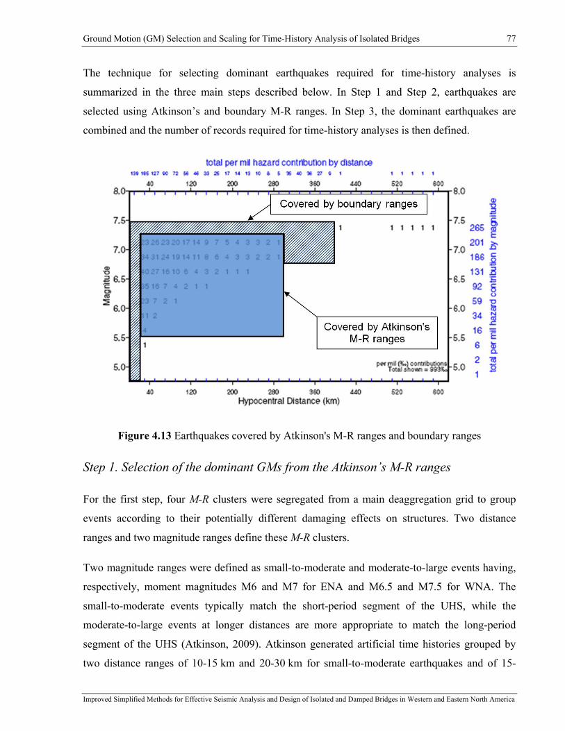
Ground Motion (GM) Selection and Scaling for Time-History Analysis of Isolated Bridges 77
Improved Simplified Methods for Effective Seismic Analysis and Design of Isolated and Damped Bridges in Western and Eastern North America
The technique for selecting dominant earthquakes required for time-history analyses is
summarized in the three main steps described below. In Step 1 and Step 2, earthquakes are
selected using Atkinson’s and boundary M-R ranges. In Step 3, the dominant earthquakes are
combined and the number of records required for time-history analyses is then defined.
Figure 4.13 Earthquakes covered by Atkinson's M-R ranges and boundary ranges
Step 1. Selection of the dominant GMs from the Atkinson’s M-R ranges
For the first step, four M-R clusters were segregated from a main deaggregation grid to group
events according to their potentially different damaging effects on structures. Two distance
ranges and two magnitude ranges define these M-R clusters.
Two magnitude ranges were defined as small-to-moderate and moderate-to-large events having,
respectively, moment magnitudes M6 and M7 for ENA and M6.5 and M7.5 for WNA. The
small-to-moderate events typically match the short-period segment of the UHS, while the
moderate-to-large events at longer distances are more appropriate to match the long-period
segment of the UHS (Atkinson, 2009). Atkinson generated artificial time histories grouped by
two distance ranges of 10-15 km and 20-30 km for small-to-moderate earthquakes and of 15-

Ground Motion (GM) Selection and Scaling for Time-History Analysis of Isolated Bridges 78
Improved Simplified Methods for Effective Seismic Analysis and Design of Isolated and Damped Bridges in Western and Eastern North America
25 km and 50-100 km for moderate-to-large earthquakes that result in four subsets defined in
terms of magnitude and distance. Adopting these M-R ranges for the present study, four suites of
earthquakes were defined as presented in Table 4-3.
Table 4-3 Magnitude-distance ranges for Step 2 of scenario definition
Region
UHS Short-Period Range UHS Long-Period Range
Close Events
R10
(10-15 km)
Distant Events
R30
(20-30 km)
Close Events
R10:R30
(15-25 km)
Distant Events
R50:R110
(50-100 km)
ENA E6C1
M6 at R10
(5.5<M<6.5)
E6C2 M6 at R30
(5.5<M<6.5)
E7C1 M7 R15-R25
(6.5<M<7.5)
E7C2 M7 R50-R110
(6.5<M<7.5)
WNA W6C1
M6.5 at R10
(6.0<M<7.0)
W6C2 M6.5 at R30
(6.0<M<7.0)
W7C1 M7.5 R10-R30
(7.0<M<8.0)
W7C2 M7.5 R50-R110
(7.0<M<8.0)
The corresponding selection process adopted for the second step is presented in Figure 4.14. The
bins with the greatest contribution to the hazard are chosen from the deaggregation plots for each
of above-defined M-R clusters. As a result, four M-R events were selected for each of four
periods as summarized in Table 4-4.

Ground Motion (GM) Selection and Scaling for Time-History Analysis of Isolated Bridges 79
Improved Simplified Methods for Effective Seismic Analysis and Design of Isolated and Damped Bridges in Western and Eastern North America
SA (T)
Short‐Period Range
M6 (5.5 ‐ 6.5)
Long‐Period Range
M7 (6.5 ‐ 7.5)
R10 R30 R10‐R30 R50‐R110
SA(0.5) 47/1000
M6.375‐R10
48/1000
M6.375‐R30
61/1000
M6.875‐R30
39/1000
M6.875‐R50
Figure 4.14 Example of selecting earthquake scenarios using Atkinson's M-R ranges (Step 1)
from hazard deaggregated for Montreal, SA(0.5) = 0.289 g, at a probability of exceedance 2% in
50 years (deaggregation by Halchuk, 2010)
M7‐R10:R30 (0.5s) 61/1000 M6.875R30
M7‐R50:R110 (0.5s) 39/1000 M6.875R50
M6‐R30 (0.5s) 48/1000 M6.375R30
M6‐R10 (0.5s) 47/1000 M6.375R10

Ground Motion (GM) Selection and Scaling for Time-History Analysis of Isolated Bridges 80
Improved Simplified Methods for Effective Seismic Analysis and Design of Isolated and Damped Bridges in Western and Eastern North America
Table 4-4 Step 2 - M-R ranges selection approach for Montreal, 2%-50 years
SA (T)
Short‐Period Range
M6 (5.5 ‐ 6.5)
Long‐Period Range
M7 (6.5 ‐ 7.5)
R10 R30 R10‐R30 R50‐R110
SA(0.2) 68/1000
M5.625‐R10
68/1000
M5.875‐R30
17/1000
M6.625‐R30
8/1000
M6.875‐R50
SA (0.5) 47/1000
M6.375‐R10
48/1000
M6.375‐R30
61/1000
M6.875‐R30
39/1000
M6.875‐R50
SA (1.0) 38/1000
M6.375‐R10
37/1000
M6.375‐R30
54/1000
M6.875‐R30
40/1000
M7.125‐R50
SA (2.0) 26/1000
M6.375‐R10
35/1000
M6.375‐R30
34/1000
M6.875‐R30
31/1000
M6.875‐R50
Step 2. Selection of the dominant GMs from the Boundary M-R ranges
In Figure 4.15, the results of the deaggregation are presented in a summary table that is used in
the second step of the selection process. In the table, the bins with the greatest contributions to
the hazard are chosen from the largest magnitude row, from the shortest distance column, and
from the separate group if any. In this step, the damage potential of the earthquakes with the
closest distance, greatest magnitude and those from a group of distant events is considered for
time-history analyses. As a result, three M-R events are selected for a given period. The M-R
scenarios selected for Montreal using this step are given in Table 4-5 for the four periods.
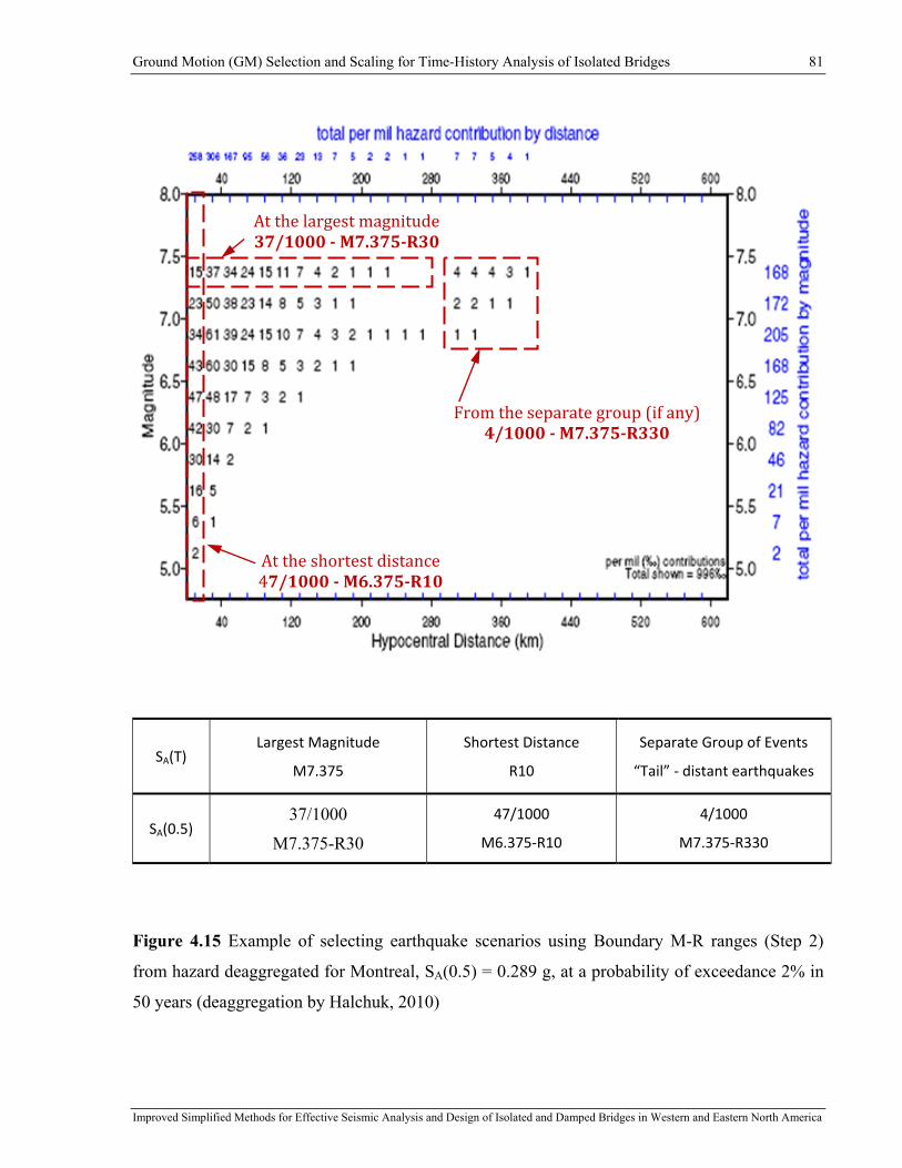
Ground Motion (GM) Selection and Scaling for Time-History Analysis of Isolated Bridges 81
Improved Simplified Methods for Effective Seismic Analysis and Design of Isolated and Damped Bridges in Western and Eastern North America
SA(T) Largest Magnitude
M7.375
Shortest Distance
R10
Separate Group of Events
“Tail” ‐ distant earthquakes
SA(0.5) 37/1000
M7.375-R30
47/1000
M6.375‐R10
4/1000
M7.375‐R330
Figure 4.15 Example of selecting earthquake scenarios using Boundary M-R ranges (Step 2)
from hazard deaggregated for Montreal, SA(0.5) = 0.289 g, at a probability of exceedance 2% in
50 years (deaggregation by Halchuk, 2010)
From the separate group (if any) 4/1000 M7.375R330
At the shortest distance 47/1000 M6.375R10
At the largest magnitude 37/1000 M7.375R30

Ground Motion (GM) Selection and Scaling for Time-History Analysis of Isolated Bridges 82
Improved Simplified Methods for Effective Seismic Analysis and Design of Isolated and Damped Bridges in Western and Eastern North America
Table 4-5 Step 1 - Boundary selection approach for Montreal, 2%-50 years
SA (T) Largest Magnitude
M7.375
Shortest Distance
R10
Separate Group of Events
“Tail” ‐ distant earthquakes
SA (0.2) 7/1000
M7.375‐R30
68/1000
M5.625‐R10
1/1000
M7.375‐R330
SA (0.5) 37/1000
M7.375-R30
47/1000
M6.375‐R10
4/1000
M7.375‐R330
SA (1.0) 33/1000
M7.375‐R30
38/1000
M6.375‐R10
11/1000
M7.375‐R330
SA (2.0) 18/1000
M7.375‐R30
26/1000
M6.375‐R10
27/1000
M7.375‐R330
Step 3. Target Seismic Scenarios and Number of TH Records
The 28 dominant earthquakes obtained as modal values from the previous two steps are then
combined, which resulted in a total number of nine events summarized in Table 4-6. A number
of required records, their M-R characteristics and the contribution to hazard are given in Table
4-7. Figure 4.16 presents the dominant earthquake scenario obtained by compiling the 28
dominant earthquakes. The nine events were distributed within the four Atkinson's M-R ranges
to facilitate the selection of time-history records performed further in this chapter. As presented
in Table 4-7, a number of records was assigned to each of the ranges so the least number of
alternative records would be a number of two. In this study, the two records correspond to the M-
R range with the lowest hazard contribution as that of 161/1000 of E7C2. Note that the level of
hazard contribution associated with each of the remaining M-R ranges is not necessary an exact
multiple of 161/2 as it could be desired. However, the numbers of records were approximated to
be proportionally related to the hazard contribution.

Ground Motion (GM) Selection and Scaling for Time-History Analysis of Isolated Bridges 83
Improved Simplified Methods for Effective Seismic Analysis and Design of Isolated and Damped Bridges in Western and Eastern North America
Table 4-6 M-R events selected from Steps 1 and 2 – ENA
M-R Events Contribution Earthquake Selection Approach
M5.625-R10 (136/1000) 68/1000 68/1000
Step 2: SA(0.2)-Shortest Distance Step 1: SA (0.2)-Short-Period Range / R10
M5.875-R30 (68/1000) 68/1000 Step 1: SA (0.2)-Short-Period Range / R30
M6.375-R10 (222/1000)
47/1000 38/1000 26/1000 47/1000 38/1000 26/1000
Step 2: SA (0.5)-Shortest Distance Step 2: SA (1.0)-Shortest Distance Step 2: SA (2.0)-Shortest Distance Step 1: SA (0.5)‐Short‐Period Range / R10
Step 1: SA (1.0)‐Short‐Period Range / R10
Step 1: SA (2.0)‐Short‐Period Range / R10
M6.375-R30 (120/1000) 48/1000 37/1000 35/1000
Step 1: SA (0.5)-Short-Period Range / R30 Step 1: SA (1.0)-Short-Period Range / R30 Step 1: SA (2.0)-Short-Period Range / R30
M6.625-R30 (17/1000) 17/1000 Step 1: SA (0.2)-Long-Period Range / R10-R30
M6.875-R30 (149/1000) 61/1000 54/1000 34/1000
Step 1: SA (0.5)-Long-Period Range / R10-R30 Step 1: SA (1.0)-Long-Period Range / R10-R30 Step 1: SA (2.0)-Long-Period Range / R10-R30
M6.875-R50 (118/1000)
8/1000 39/1000 40/1000 31/1000
Step 1: SA (0.2)-Long-Period Range / R50-R110 Step 1: SA (0.5)-Long-Period Range / R50-R110 Step 1: SA (1.0)-Long-Period Range / R50-R110 Step 1: SA (2.0)-Long-Period Range / R50-R110
M7.375-R30 (95/1000)
7/1000 37/1000 33/1000 18/1000
Step 2: SA (0.2)- Largest Magnitude Step 2: SA (0.5)- Largest Magnitude Step 2: SA (1.0)- Largest Magnitude Step 2: SA (2.0)- Largest Magnitude
M7.375-R330 (43/1000)
1/1000 4/1000 11/1000 27/1000
Step 2: SA (0.2)- Separate Group Step 2: SA (0.5)- Separate Group Step 1: SA (1.0)- Separate Group Step 1: SA (2.0)- Separate Group

Ground Motion (GM) Selection and Scaling for Time-History Analysis of Isolated Bridges 84
Improved Simplified Methods for Effective Seismic Analysis and Design of Isolated and Damped Bridges in Western and Eastern North America
Table 4-7 Distribution and number of records from Step 1 and Step 2 - ENA
E6C1 M6 at R10
E6C2 M6 at R30
E7C1 M7 R10:R30
E7C2 M7 R50:R110
M5.625-R10 (136/1000)
M6.375-R10 (222/1000)
M5.875-R30 (68/1000)
M6.375-R30 (120/1000)
M6.625-R30 (17/1000)
M6.875-R30 (149/1000)
M7.375-R30 (95/1000)
M6.875-R50 (118/1000)
M7.375-R330 (43/1000)
358/1000 188/1000 261/1000 161/1000
6 Records 3 Records 3 Records 2 Records
Figure 4.16 Dominant earthquake scenario for montreal at 2% in 50 years (0.2 s to 2.0 s)
This dominant earthquake scenario would be adequate for analyses of structures characterized by
a period range for which the deaggregated plots were provided (0.2, 0.5, 1.0, and 2.0 s).
However, an extended period range beyond 2.0 s is necessary to cover a large inelastic excursion

Ground Motion (GM) Selection and Scaling for Time-History Analysis of Isolated Bridges 85
Improved Simplified Methods for Effective Seismic Analysis and Design of Isolated and Damped Bridges in Western and Eastern North America
of isolated bridges. The hazard deaggregation plots for a longer period range are not available
today and there are no studies on how to combine the relative contributions for longer periods.
To overcome these limitations and to represent the damage potential for long-period range as for
example, 4.0 s and 6.0 s, the earthquakes were arbitrary added to the dominant scenario. The
records were added to the suite E7C2 (moderate-to-large events at longer distances) as explained
below.
To evaluate the number of records that are needed to complement the seismic scenario derived in
previous steps, the distribution of the UHS linear segments as provided by the NBCC (NRCC,
2005) code was adopted. In addition to the periods of 0.2, 0.5, 1.0, and 2.0 s (available
deaggregation plots), the period of 4.0 s is specified as a limit beyond which spectral acceleration
values are constant. Accordingly, for the cases where the effective period exceeds 4 s, constant
annual probability of exceedance of a target spectral amplitude Sa(T) are assumed. It has been
recognized that for longer periods, more distant earthquakes with larger magnitudes contribute
more to the hazard (Adams and Halchuk, 2004).
As discussed in Chapter 2, it was shown by different studies (Tolis and Faccioli, 1999; Bommer
et al., 2000b) that acceleration design spectra as specified in the NBCC (2005 and 2010) do not
necessary provide engineers with reliable realistic displacement demand in long periods. It raises
the question as how to reduce the effect of the uncertainty in response of isolated bridges for
which displacement response in long period range is of intrinsic importance.
Aiming to address the effect of the uncertainty in long periods, the extended period range is
defined through six periods as 0.2, 0.5, 1.0, 2.0, 4.0, and 6.0 (any longer than 4 s) and for the last
two periods, only the contributions from the E7C2 (moderate-to-large events at longer distances)
earthquakes are assumed to dominate the contribution to the hazard.
Assuming a proportional distribution of records between the six periods, a number of 14 records
was divided by 4 periods and multiplied by 6 records what yields 21 records. The number was
rounded down to 20 records for simplicity. The ENA earthquake scenario was then
complemented with six records as presented in Table 4-8. Three time histories is a minimum
number of records that was attributed to the suites of E6C2 and E7C1. Three records rather than
one were intentionally adopted to take into account the record-to-record inherent variability.
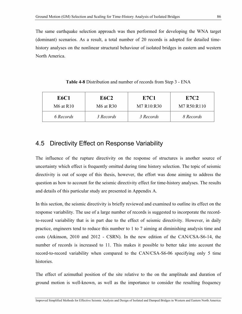
Ground Motion (GM) Selection and Scaling for Time-History Analysis of Isolated Bridges 86
Improved Simplified Methods for Effective Seismic Analysis and Design of Isolated and Damped Bridges in Western and Eastern North America
The same earthquake selection approach was then performed for developing the WNA target
(dominant) scenarios. As a result, a total number of 20 records is adopted for detailed time-
history analyses on the nonlinear structural behaviour of isolated bridges in eastern and western
North America.
Table 4-8 Distribution and number of records from Step 3 - ENA
E6C1 M6 at R10
E6C2 M6 at R30
E7C1 M7 R10:R30
E7C2 M7 R50:R110
6 Records 3 Records 3 Records 8 Records
4.5 Directivity Effect on Response Variability
The influence of the rupture directivity on the response of structures is another source of
uncertainty which effect is frequently omitted during time history selection. The topic of seismic
directivity is out of scope of this thesis, however, the effort was done aiming to address the
question as how to account for the seismic directivity effect for time-history analyses. The results
and details of this particular study are presented in Appendix A.
In this section, the seismic directivity is briefly reviewed and examined to outline its effect on the
response variability. The use of a large number of records is suggested to incorporate the record-
to-record variability that is in part due to the effect of seismic directivity. However, in daily
practice, engineers tend to reduce this number to 1 to 7 aiming at diminishing analysis time and
costs (Atkinson, 2010 and 2012 - CSRN). In the new edition of the CAN/CSA-S6-14, the
number of records is increased to 11. This makes it possible to better take into account the
record-to-record variability when compared to the CAN/CSA-S6-06 specifying only 5 time
histories.
The effect of azimuthal position of the site relative to the on the amplitude and duration of
ground motion is well-known, as well as the importance to consider the resulting frequency
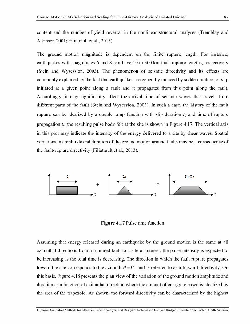
Ground Motion (GM) Selection and Scaling for Time-History Analysis of Isolated Bridges 87
Improved Simplified Methods for Effective Seismic Analysis and Design of Isolated and Damped Bridges in Western and Eastern North America
content and the number of yield reversal in the nonlinear structural analyses (Tremblay and
Atkinson 2001; Filiatrault et al., 2013).
The ground motion magnitude is dependent on the finite rupture length. For instance,
earthquakes with magnitudes 6 and 8 can have 10 to 300 km fault rupture lengths, respectively
(Stein and Wysession, 2003). The phenomenon of seismic directivity and its effects are
commonly explained by the fact that earthquakes are generally induced by sudden rupture, or slip
initiated at a given point along a fault and it propagates from this point along the fault.
Accordingly, it may significantly affect the arrival time of seismic waves that travels from
different parts of the fault (Stein and Wysession, 2003). In such a case, the history of the fault
rupture can be idealized by a double ramp function with slip duration td and time of rupture
propagation tr, the resulting pulse body felt at the site is shown in Figure 4.17. The vertical axis
in this plot may indicate the intensity of the energy delivered to a site by shear waves. Spatial
variations in amplitude and duration of the ground motion around faults may be a consequence of
the fault-rupture directivity (Filiatrault et al., 2013).
Figure 4.17 Pulse time function
Assuming that energy released during an earthquake by the ground motion is the same at all
azimuthal directions from a ruptured fault to a site of interest, the pulse intensity is expected to
be increasing as the total time is decreasing. The direction in which the fault rupture propagates
toward the site corresponds to the azimuth °= 0θ and is referred to as a forward directivity. On
this basis, Figure 4.18 presents the plan view of the variation of the ground motion amplitude and
duration as a function of azimuthal direction where the amount of energy released is idealized by
the area of the trapezoid. As shown, the forward directivity can be characterized by the highest
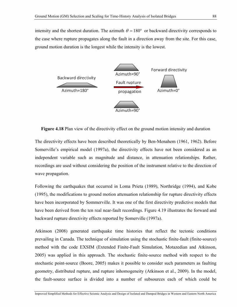
Ground Motion (GM) Selection and Scaling for Time-History Analysis of Isolated Bridges 88
Improved Simplified Methods for Effective Seismic Analysis and Design of Isolated and Damped Bridges in Western and Eastern North America
intensity and the shortest duration. The azimuth °= 180θ or backward directivity corresponds to
the case where rupture propagates along the fault in a direction away from the site. For this case,
ground motion duration is the longest while the intensity is the lowest.
Figure 4.18 Plan view of the directivity effect on the ground motion intensity and duration
The directivity effects have been described theoretically by Ben-Menahem (1961, 1962). Before
Somerville’s empirical model (1997a), the directivity effects have not been considered as an
independent variable such as magnitude and distance, in attenuation relationships. Rather,
recordings are used without considering the position of the instrument relative to the direction of
wave propagation.
Following the earthquakes that occurred in Loma Prieta (1989), Northridge (1994), and Kobe
(1995), the modifications to ground motion attenuation relationship for rupture directivity effects
have been incorporated by Sommerville. It was one of the first directivity predictive models that
have been derived from the ten real near-fault recordings. Figure 4.19 illustrates the forward and
backward rupture directivity effects reported by Somerville (1997a).
Atkinson (2008) generated earthquake time histories that reflect the tectonic conditions
prevailing in Canada. The technique of simulation using the stochastic finite-fault (finite-source)
method with the code EXSIM (Extended Finite-Fault Simulation, Motazedian and Atkinson,
2005) was applied in this approach. The stochastic finite-source method with respect to the
stochastic point-source (Boore, 2005) makes it possible to consider such parameters as faulting
geometry, distributed rupture, and rupture inhomogeneity (Atkinson et al., 2009). In the model,
the fault-source surface is divided into a number of subsources each of which could be

Ground Motion (GM) Selection and Scaling for Time-History Analysis of Isolated Bridges 89
Improved Simplified Methods for Effective Seismic Analysis and Design of Isolated and Damped Bridges in Western and Eastern North America
considered as a small point source of the earthquake ground motion. The entire fault ground
motion is then obtained by summing the calculated subsource effects in the time domain,
activating the point sources with an appropriate time delay in a predetermined fault direction. On
this basis, directivity effects can be taken into consideration by such a finite-fault modeling.
Figure 4.19 Forward and backward rupture directivity from the 1992 Landers earthquake
(Somerville, 1997a)
The significance of considering the rupture directivity effect in terms of the response variability
may be outlined to justify a larger number of time-history records for nonlinear structural
analyses in the time domain. The effect of seismic directivity was investigated to outline its
effect on response variability. The study on directivity effects was carried out using
Atkinson's 2008 artificial ground motions and consists of two main steps: 1) the characterization
of the earthquake records with respect to the ground motion azimuthal direction; and 2) the
assessment of the effect of directivity on the inelastic structural responses.
To examine directivity effects, Atkinson's 2008 ground motions were adopted instead of those
Atkinson's 2009 scaled in the previous subsection. The reason for using the older sets is that they

Ground Motion (GM) Selection and Scaling for Time-History Analysis of Isolated Bridges 90
Improved Simplified Methods for Effective Seismic Analysis and Design of Isolated and Damped Bridges in Western and Eastern North America
formed a complete ensemble in terms of azimuths : 3 different trials x 8 azimuths in 45°
increments for each M-R scenario. Accordingly, this particular ground motion set of artificial
records were analyzed only in this section of this thesis. Two suites of earthquake time-histories
simulated for two moment magnitudes were considered to represent small-to-moderate (short-
period) and moderate-to-large (long-period) seismic events for each location: M6.0 and M7.0 for
ENA and M6.5 and M7.5 for WNA. To reproduce the effect of close and distant events, two
fault-distance ranges were selected. The suites of the small-to-moderate ground motions were
analyzed for distances of 10 and 30 km, while those of the moderate-to-large - for distances of 30
and 50 km. Only the records generated for site class C were analyzed in this study.
This thesis is dedicated to methods for predicting the peak response of isolated bridge. The
seismic directivity is identified as a possible source of the variability in the response estimates.
The details and results of this particular study are presented in Appendix A, while this section
presents the resulting conclusion.
The responses from different azimuthal directions were compared with respect that having
azimuth °= 0θ (forward directivity). The index of azimuthal variability varα was examined to
identify the maximum amplification effect on the earthquake damage potential. The maximum
amplification averaged over the period range 0.5 s - 6.0 s are 45.1)(var =ENAα and
41.1)(var =WNAα . The largest amplifications correspond to the period range 0.5 - 1.0 s
70.1)(var =ENAα and 67.1)(var =WNAα .
A particular variability shape was observed for parameters defined as a function of azimuthal
distribution for the both steps. There is however no definitive evidence found to establish clear
directivity-dependant trends for different M-R suites or hazard-dominant earthquake scenarios.
There is likely a limitation in the finite-fault model utilized by Atkinson (2008) for generating
artificial ground motions since clear geometric sequences of activating the point sources are not
necessary established when rupture effect is simulated.
However, using this available source of time histories generated with azimuthal distribution, the
significance of considering the rupture directivity effect in terms of the variability of the damage
potential is outlined in this section. To account for this variability during the nonlinear time-

Ground Motion (GM) Selection and Scaling for Time-History Analysis of Isolated Bridges 91
Improved Simplified Methods for Effective Seismic Analysis and Design of Isolated and Damped Bridges in Western and Eastern North America
history analyses a large number of time-history records characterized by different azimuthal
directions is justified.
4.6 Ground Motion Scaling
Among the numerous approaches that are commonly adopted to make earthquake records
matching a target UHS, the amplitude-scaling method is the one that makes possible to preserve
the influence of physical characteristics representative of the geological source. The ground-
motion parameters as the frequency content and duration do not change when the spectral
amplitude is linearly scaled. The ground-motion parameters vary significantly across North
America and it was a primary reason for adopting the amplitude-scaling method for investigating
nonlinear behaviour of isolated bridges in ENA and WNA. According to the dominant scenario
derived above, 20 records are required for each locality (Montreal - ENA and Vancouver -
WNA). In this way the site-specific record-to-record variability would be appropriately taken
into consideration. Moreover, to account for the effect of seismic directivity, the time-history
records having different azimuthal directions will be selected for each of the M-R scenarios.
Due to a scarce number of ground motions corresponding to historical events occurred in ENA,
sets of eastern artificial (Atkinson, 2009) and hybrid (McGuire et al., 2001a) ground motions
were adopted for the ENA region. To establish the same comparative basis between ENA and
WNA, only the set of artificial western records (Atkinson, 2009) was selected for parametric
analyses.
The artificial ground motions were generated by Atkinson to match the 2005 NBCC UHS at any
generic regions of eastern and western Canada. These records are freely accessible from
www.seismotoolbox.ca and are provided for the site classes A, C, D and E. A dataset (catalogue)
of 180 records is available for each of these site classes. The records were regrouped by 45 using
two magnitude ranges (small-to-moderate and moderate-to-large events) and two fault-distance
ranges (close and distant events). This M-R distribution are summarized in Table 4.3 for ENA
and WNA and is adopted for the parametric analyses further presented in this thesis.
The database of hybrid time histories was produced by McGuire et al. (2001a) to reproduce the
seismicity from the central-eastern U.S. (CEUS). This database was obtained by processing a
range of historic recordings primarily from the western U.S. (WUS). The WUS records have

Ground Motion (GM) Selection and Scaling for Time-History Analysis of Isolated Bridges 92
Improved Simplified Methods for Effective Seismic Analysis and Design of Isolated and Damped Bridges in Western and Eastern North America
been then modified using spectral matching approach to reflect appropriately the CEUS ground
motion characteristics.
Three ground motions suites were then assembled from records selected from the corresponding
databases (Atkinson, 2009 and McGuire et al., 2001a) according to the dominant M-R earthquake
scenario. Even though the selected time-histories were characteristic of the site-specific
seismicity (ENA and WNA) and the required magnitudes and fault distances, these ground
motions needed to be scaled to the level of earthquake that corresponds to the probability of
exceedance adopted in the NBCC (2005) (2% in 50 years). The scaling process employed in this
study is similar to those described in details by Atkinson (2009) and Guilini Charette (2009).
In engineering practice, a challenging part of the selection and scaling process is still to make the
records match an entire period range. In this study, each time-history record was scaled with a
simple factor so that the area under the response spectrum equals that of the site-specific UHS
specified in NBCC (NRCC, 2005) over the same period range. As proposed by Atkinson (2009),
the records with the lowest standard deviation of SA-targ/SA-sim computed in the 0.2 - 4.0 s period
range were then selected. The resulting suites are denoted as ATK-E and MCG-CEUS for ENA
and ATK-W for WNA. Spectral values from the UHS NBCC (2005) used for scaling are
presented in Table 4-9. Figures from 4.20 to 4.22 present the individual and mean spectra of the
scaled ground motions. The records and scaling factors are listed in Tables from 4-10 to 4-12.
Table 4-9 Spectral values from the target UHS NBCC (2005) - 2% in 50 years, site class C
Period Montreal - ENA Vancouver - WNA
T (s) SA (g) PSD (mm) SA (g) PSD (mm)
0.0 0.690 0.00 0.940 0.00
0.2 0.690 6.86 0.940 9.30
0.5 0.340 21.1 0.640 39.8
1.0 0.140 34.8 0.330 82.0
2.0 0.048 47.7 0.170 169
4.0 0.024 95.4 0.085 338
6.0 0.024 215 0.085 760
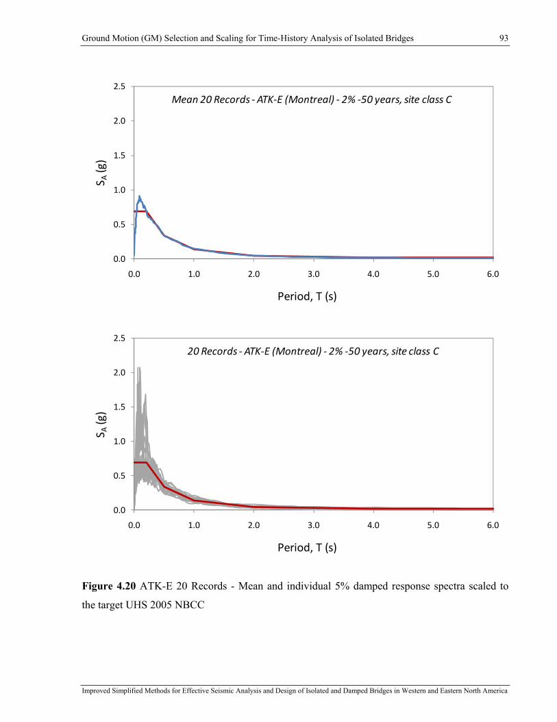
Ground Motion (GM) Selection and Scaling for Time-History Analysis of Isolated Bridges 93
Improved Simplified Methods for Effective Seismic Analysis and Design of Isolated and Damped Bridges in Western and Eastern North America
0.0
0.5
1.0
1.5
2.0
2.5
0.0 1.0 2.0 3.0 4.0 5.0 6.0
S A(g)
Period, T (s)
Mean 20 Records ‐ATK‐E (Montreal) ‐ 2% ‐50 years, site class C
0.0
0.5
1.0
1.5
2.0
2.5
0.0 1.0 2.0 3.0 4.0 5.0 6.0
S A(g)
Period, T (s)
20 Records ‐ATK‐E (Montreal) ‐ 2% ‐50 years, site class C
Figure 4.20 ATK-E 20 Records - Mean and individual 5% damped response spectra scaled to
the target UHS 2005 NBCC

Ground Motion (GM) Selection and Scaling for Time-History Analysis of Isolated Bridges 94
Improved Simplified Methods for Effective Seismic Analysis and Design of Isolated and Damped Bridges in Western and Eastern North America
0.0
0.5
1.0
1.5
2.0
2.5
0.0 1.0 2.0 3.0 4.0 5.0 6.0
S A(g)
Period, T (s)
Mean 20 Records ‐MCG‐CEUS (Montreal) ‐ 2% ‐50 years, site class C
0.0
0.5
1.0
1.5
2.0
2.5
0.0 1.0 2.0 3.0 4.0 5.0 6.0
S A(g)
Period, T (s)
20 Records ‐MCG‐CEUS (Montreal) ‐ 2% ‐50 years, site class C
Figure 4.21 MCG-CEUS 20 Records - Mean and individual 5% damped response spectra scaled
to the target UHS 2005 NBCC
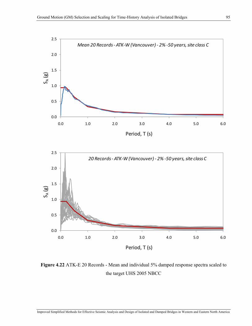
Ground Motion (GM) Selection and Scaling for Time-History Analysis of Isolated Bridges 95
Improved Simplified Methods for Effective Seismic Analysis and Design of Isolated and Damped Bridges in Western and Eastern North America
0.0
0.5
1.0
1.5
2.0
2.5
0.0 1.0 2.0 3.0 4.0 5.0 6.0
S A(g)
Period, T (s)
Mean 20 Records ‐ATK‐W (Vancouver) ‐ 2% ‐50 years, site class C
0.0
0.5
1.0
1.5
2.0
2.5
0.0 1.0 2.0 3.0 4.0 5.0 6.0
S A(g)
Period, T (s)
20 Records ‐ATK‐W (Vancouver) ‐ 2% ‐50 years, site class C
Figure 4.22 ATK-E 20 Records - Mean and individual 5% damped response spectra scaled to
the target UHS 2005 NBCC

Ground Motion (GM) Selection and Scaling for Time-History Analysis of Isolated Bridges 96
Improved Simplified Methods for Effective Seismic Analysis and Design of Isolated and Damped Bridges in Western and Eastern North America
Table 4-10 ATK-E 20 Records scaled to the target UHS 2005 NBCC, 2%-50 years, site class C,
city of Montreal (ENA), Sa-targ/Sa-sim computed over 0.2 - 4.0 s
Record Name M R (km) S.F. T-Range sima
ta
SS
−
− arg ATK-E Earthquake
E6C1
E6C1-9 6.0 12.8 1.114 0.2-6.0s 0.366 east6c1-09-2009
E6C1-12 6.0 12.8 1.252 0.2-6.0s 0.462 east6c1-12-2009
E6C1-33 6.0 17 1.360 0.2-6.0s 0.526 east6c1-33-2009
E6C1-34 6.0 16.6 1.075 0.2-6.0s 0.256 east6c1-34-2009
E6C1-42 6.0 17 1.095 0.2-6.0s 0.550 east6c1-42-2009
E6C1-43 6.0 17 1.539 0.2-6.0s 0.325 east6c1-43-2009
E6C2
E6C2-12 6.0 21.1 2.297 0.2-6.0s 0.763 east6c2-18-2009
E6C2-39 6.0 25.1 2.915 0.2-6.0s 0.966 east6c2-18-2009
E6C2-41 6.0 30.7 3.031 0.2-6.0s 0.568 east6c2-18-2009
E7C1
E7C1-9 7.0 14.2 0.289 0.2-6.0s 0.260 east7c1-18-2009
E7C1-32 7.0 25.8 0.776 0.2-6.0s 0.227 east7c1-18-2009
E7C1-41 7.0 25.6 0.942 0.2-6.0s 0.200 east7c1-18-2009
E7C2
E7C2-8 7.0 45.2 1.410 0.2-6.0s 0.304 east7c2-08-2009
E7C2-18 7.0 62.6 2.385 0.2-6.0s 0.211 east7c2-18-2009
E7C2-23 7.0 69.9 2.287 0.2-6.0s 0.275 east7c2-23-2009
E7C2-26 7.0 70.2 2.162 0.5-1.0s 0.162 east7c2-26-2009
E7C2-40 7.0 94.3 2.152 0.2-6.0s 0.184 east7c2-40-2009
E7C2-42 7.0 94.3 2.242 0.2-6.0s 0.240 east7c2-42-2009
E7C2-43 7.0 98.6 2.547 0.2-6.0s 0.262 east7c2-43-2009
E7C2-45 7.0 98.6 2.512 0.2-6.0s 0.195 east7c2-45-2009
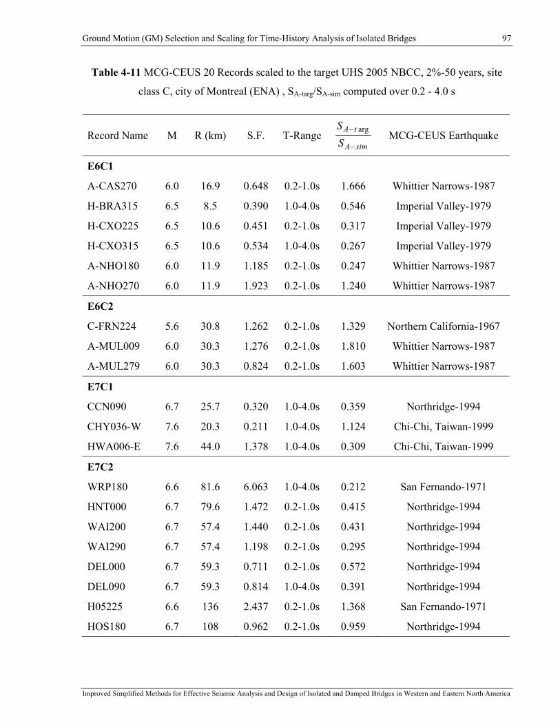
Ground Motion (GM) Selection and Scaling for Time-History Analysis of Isolated Bridges 97
Improved Simplified Methods for Effective Seismic Analysis and Design of Isolated and Damped Bridges in Western and Eastern North America
Table 4-11 MCG-CEUS 20 Records scaled to the target UHS 2005 NBCC, 2%-50 years, site
class C, city of Montreal (ENA) , SA-targ/SA-sim computed over 0.2 - 4.0 s
Record Name M R (km) S.F. T-Range simA
tA
SS
−
− arg MCG-CEUS Earthquake
E6C1
A-CAS270 6.0 16.9 0.648 0.2-1.0s 1.666 Whittier Narrows-1987
H-BRA315 6.5 8.5 0.390 1.0-4.0s 0.546 Imperial Valley-1979
H-CXO225 6.5 10.6 0.451 0.2-1.0s 0.317 Imperial Valley-1979
H-CXO315 6.5 10.6 0.534 1.0-4.0s 0.267 Imperial Valley-1979
A-NHO180 6.0 11.9 1.185 0.2-1.0s 0.247 Whittier Narrows-1987
A-NHO270 6.0 11.9 1.923 0.2-1.0s 1.240 Whittier Narrows-1987
E6C2
C-FRN224 5.6 30.8 1.262 0.2-1.0s 1.329 Northern California-1967
A-MUL009 6.0 30.3 1.276 0.2-1.0s 1.810 Whittier Narrows-1987
A-MUL279 6.0 30.3 0.824 0.2-1.0s 1.603 Whittier Narrows-1987
E7C1
CCN090 6.7 25.7 0.320 1.0-4.0s 0.359 Northridge-1994
CHY036-W 7.6 20.3 0.211 1.0-4.0s 1.124 Chi-Chi, Taiwan-1999
HWA006-E 7.6 44.0 1.378 1.0-4.0s 0.309 Chi-Chi, Taiwan-1999
E7C2
WRP180 6.6 81.6 6.063 1.0-4.0s 0.212 San Fernando-1971
HNT000 6.7 79.6 1.472 0.2-1.0s 0.415 Northridge-1994
WAI200 6.7 57.4 1.440 0.2-1.0s 0.431 Northridge-1994
WAI290 6.7 57.4 1.198 0.2-1.0s 0.295 Northridge-1994
DEL000 6.7 59.3 0.711 0.2-1.0s 0.572 Northridge-1994
DEL090 6.7 59.3 0.814 1.0-4.0s 0.391 Northridge-1994
H05225 6.6 136 2.437 0.2-1.0s 1.368 San Fernando-1971
HOS180 6.7 108 0.962 0.2-1.0s 0.959 Northridge-1994

Ground Motion (GM) Selection and Scaling for Time-History Analysis of Isolated Bridges 98
Improved Simplified Methods for Effective Seismic Analysis and Design of Isolated and Damped Bridges in Western and Eastern North America
Table 4-12 ATK-W 20 Records scaled to the target UHS 2005 NBCC, 2%-50 years, site class C,
city of Vancouver (WNA) , SA-targ/SA-sim computed over 0.2 - 4.0 s
Record Name M R (km) S.F. T-Range simA
tA
SS
−
− arg ATK-W Earthquake
W6C1
W6C1-19 6.5 10.8 1.024 0.2-6.0s 0.311 west6c1-19-2009
W6C1-21 6.5 10.8 1.347 0.2-6.0s 0.421 west6c1-21-2009
W6C1-25 6.5 11.2 1.806 0.2-6.0s 0.297 west6c1-25-2009
W6C1-34 6.5 12.2 1.299 0.2-6.0s 0.430 west6c1-34-2009
W6C1-38 6.5 13.0 1.765 0.2-6.0s 0.413 west6c1-38-2009
W6C1-44 6.5 13.0 1.885 0.2-6.0s 0.389 west6c1-44-2009
W6C2
W6C2-1 6.5 19.7 1.652 0.2-6.0s 0.141 west6c2-1-2009
W6C2-7 6.5 13.2 1.292 0.2-6.0s 0.295 west6c2-7-2009
W6C2-25 6.5 26.3 2.170 0.2-6.0s 0.193 west6c2-25-2009
W7C1
W7C1-11 7.5 17.1 1.051 0.2-6.0s 0.166 west7c1-11-2009
W7C1-17 7.5 21.6 0.973 0.2-6.0s 0.255 west7c1-17-2009
W7C1-26 7.5 18.1 0.725 0.2-6.0s 0.189 west7c1-26-2009
W7C2
W7C2-10 7.5 50.7 2.785 0.2-6.0s 0.182 west7c2-10-2009
W7C2-13 7.5 30.2 1.032 0.2-6.0s 0.422 west7c2-13-2009
W7C2-14 7.5 30.2 1.335 0.2-6.0s 0.198 west7c2-14-2009
W7C2-19 7.5 70.5 3.500 1.0-2.0s 0.207 west7c2-19-2009
W7C2-25 7.5 68.5 2.273 0.2-6.0s 0.281 west7c2-25-2009
W7C2-33 7.5 100.4 3.194 0.2-6.0s 0.503 west7c2-33-2009
W7C2-39 7.5 100.0 2.841 0.2-6.0s 0.446 west7c2-39-2009
W7C2-40 7.5 100.4 4.767 0.2-1.0s 0.288 west7c2-40-2009

Ground Motion (GM) Selection and Scaling for Time-History Analysis of Isolated Bridges 99
Improved Simplified Methods for Effective Seismic Analysis and Design of Isolated and Damped Bridges in Western and Eastern North America
4.7 Conclusions on Records Selection and Scaling
In this chapter, the site-specific ensembles of ground-motion time histories are defined and
scaled to carry out the extensive parametric analyses on the nonlinear structural behaviour of
isolated bridges in eastern and western North America. In spite of a number of existing
approaches that have been developed for specific design purposes, there is no consensus on how
to select and scale ground-motion records for nonlinear time-history analyses (THA) of isolated
bridges. The technique and methodology were proposed in this study aiming to define time-
history records for dynamic analyses from the perspective of a structural engineer using the
available state of the art in seismology and where the data is not available adopting conservative
approaches rather than those statistically supported. As a result, the hazard-dominant earthquake
scenarios were developed for the eastern and western North America. Three suites of 20 time
histories each were assembled according the site-specific hazard scenarios. The records were
then scaled to match the 2005 NBCC UHS for a wide period range required to accommodate
large inelastic excursions prone to the behaviour of isolated bridges. An excellent match was
obtained as a result of the records selection and scaling approaches adopted in this study.
In addition, the effect of seismic directivity was outlined. It was emphasized the importance of
assembling ground motions suites for different M-R earthquakes that may result in different
damage potentials amplified as a function of the azimuthal directivity. The rupture directivity
effect is then considered by selecting the time-history records having different azimuthal
directions for each of the M-R scenarios.

Assessment of Damping Coefficients for Seismic Design of Isolated Bridges in Eastern and Western North American Regions 100
Improved Simplified Methods for Effective Seismic Analysis and Design of Isolated and Damped Bridges in Western and Eastern North America
Chapter 5: Assessment of Damping Coefficients for Seismic Design of Isolated Bridges in Eastern and Western North American Regions
5.1 Introduction
The appropriateness of the damping coefficients B that are currently specified in the CAN/CSA-
S6-06 Canadian Highway Bridge Design Code (CSA, 2006) in Canada and the AASHTO LRFD
Seismic Bridge Design Specifications in the United States (AASHTO, 2009, 2010) for the design
of isolated bridges for both western and eastern North American ground motions is investigated
in this chapter. The coefficients B have been developed based on studying the effects of ground
motions from historical earthquake events that have occurred along the North American west
coast. The appropriateness of using the same damping coefficients for ENA and WNA has been
questioned in past studies (Taylor, 1999; Naumoski, 2000).
The values of B specified in codes have been derived from the work by Newmark and Hall
(1982). In these early studies, spectrum amplification coefficients were computed for different
damping levels using the elastic response of a viscously damped SDOF system to the 1940 El
Centro earthquake record. Similar approaches are widely adopted and reported by the majority of
studies where B-coefficients were evaluated statistically by processing a large number of seismic
records (Tolis and Faccioli, 1999; Bommer et al., 2000b; Lin and Chang, 2003; and
Hatzigeorgiou, 2010).
The approach of assessing the B-coefficients by using linear time-history analyses (LTHA) is
first adopted in this study (Section 5.3), given that it corresponds well to the state of the art. The
coefficients obtained from LTHA in ENA and WNA are compared to those specified in codes in
order to examine the possible influence of the regional characteristics of the seismicity on the
reduction effects of damping. The suitability of using the same B-coefficient for reducing force
and displacement responses is also examined. Based on the results from LTHA, this study also
investigates the dependency of B-coefficients on the effective period of the structure that has
already been identified by other researchers (Atkinson and Pierre, 2004 and Hatzigeorgiou,

Assessment of Damping Coefficients for Seismic Design of Isolated Bridges in Eastern and Western North American Regions 101
Improved Simplified Methods for Effective Seismic Analysis and Design of Isolated and Damped Bridges in Western and Eastern North America
2010). The differences observed in the response reduction effects caused by viscous damping are
explained by exploiting the concepts of the force transmissibility and response amplification
respectively for spectral accelerations SA and spectral displacements SD.
Complementary to the earlier studies that were based on LTHA and to accurately address the
validity of the damping coefficients for the design of isolated bridges, in Section 5.4, an
extensive parametric study is carried out using dynamic nonlinear time history analysis
(NLTHA) so that the nonlinear response of the bridge isolation systems is properly accounted
for. The parametric study was carried out by varying several parameters that may be used to
define the system's dynamic properties at the initial design stage. Based on these results, in
Section 5.5, recommendations are made on possible modifications to improve the accuracy of
current North American simplified design methods. To better assess the accuracy of the
B-coefficients on the seismic displacement response, nonlinear structures were analyzed
following the complete iterative procedure prescribed in the CSA-S6-06 simplified method
(similar to AASHTO 2009, 2010). This study also examines the need for an upper limit on
damping for which the B-coefficient method can be used in codes.
5.2 Ground Motions Considered for Time-History Analyses
As discussed in details in Chapter 4, because of the scarcity of historical ground motions
corresponding to events having occurred in ENA, sets of eastern artificial (Atkinson, 2009) and
hybrid (McGuire et al., 2001a) ground motions were adopted for the ENA regions. To establish
the same comparative basis between ENA and WNA, only the set of artificial western records
(Atkinson, 2009) was analysed. Each of these ground-motion sets were comprised of twenty
records that were selected according to site-specific likely earthquakes scenarios. More details in
how these scenarios were defined are presented in Chapter 4 (Sections 4.3 and 4.4). For analyses
carried out in this parametric study, two densely populated Canadian cities were chosen:
Montreal, Quebec, for eastern Canada, and Vancouver, British Columbia, for western Canada.
Three suites of twenty ground-motion records, denoted as artificial ENA (ATK-E), hybrid ENA
(MCG-CEUS) and artificial WNA (ATK-W), were linearly scaled to the corresponding NBCC
design spectrum (NBCC, 2005).
Assessment of Damping Coefficients for Seismic Design of Isolated Bridges in Eastern and Western North American Regions 102
Improved Simplified Methods for Effective Seismic Analysis and Design of Isolated and Damped Bridges in Western and Eastern North America
5.3 Linear Time-History Analyses (LTHA)
As a first step in this study, the effect of viscous damping on the response of linear elastic SDOF
systems is studied. Such an approach corresponds well to the state of the art in assessing
damping coefficients (Newmark and Hall, 1982; Tolis and Faccioli 1999; Bommer et al., 2000b;
Lin and Chang, 2003; and Hatzigeorgiou, 2010). In this study, the B-coefficients obtained from
LTHA are compared to those specified in codes. One of the aspects that is investigated is the
influence on B-coefficients of the ground motion characteristics such as the ones expected
between ENA and WNA records. These analyses are intended to essentially fill a gap in
knowledge about differences in how the damping reduction may be affected by western and
eastern North American seismicity.
Furthermore, as previously indicated in Equations (2.6) and (2.7) (see Chapter 2), the same
damping coefficient B is used to determine both the statically equivalent seismic force and the
displacement across the isolation bearings as a function of the spectral acceleration AS and
pseudo displacement DPS , respectively. The validity of using this same B-coefficient for both
these calculations is verified and discussed in this section.
The response of L-SDOF systems subjected to twenty time-history records, referred to as linear
"exact", was mathematically averaged over 20 records for each of the three ground-motion
suites. The resulting mean response spectra were constructed for six levels of viscous damping,
β = 5%, 10%, 20%, 30%, 40%, and 50% of critical for both spectral acceleration )(βAS and
spectral displacement )(βDS . These damped response spectra for the three suites of records
defined in Chapter 2 (ATK-W, ATK-E, and MCG-CEUS) are presented in Figures 5.1, 5.2, and
5.3, respectively. It can be noted from these figures that the WNA DS spectra can be
approximated by multiple linear segments (period ranges from 0-1.3, 1.3-2.0, 2.0-3.5, and 3.5-
4.0 s) corresponding to each respective level of damping. A near constant rate of displacement
response indicates that the seismic energy delivered by the WNA ground motions is transmitted
to the system at a wide band of frequencies covering a longer period range as it can be noted in
Figure 5.4. This figure presents power spectra that was obtained from Fast Fourier Transform
(FFT) bringing the amplitude of the ground motion from the time domain to the period (or
frequency) domain. In this way, the time function of the ground-motion excitation is simply
Assessment of Damping Coefficients for Seismic Design of Isolated Bridges in Eastern and Western North American Regions 103
Improved Simplified Methods for Effective Seismic Analysis and Design of Isolated and Damped Bridges in Western and Eastern North America
decomposed into a series of periodic functions (termed Fourier series) and insight into the
seismic energy distribution with respect to period is provided.
In contrast to WNA, the ENA ground motions are characterized by high-frequency content and
most of the seismic energy is transmitted to the system in a shorter period range (see Figure 5.4).
Structures with fundamental periods close to the ground-motion predominant periods attract
more seismic forces because of resonance conditions and structures having longer fundamental
periods are less excited by such ground motions and the resulting responses are less prone to
dynamic amplification. This is further shown in this chapter. The resulting DS spectra (ATK-E
and MCG-CEUS) present significant changes in the spectral shape which is lower for longer
periods.
The damping coefficients B were computed by dividing the site-specific 5% damped response
spectrum by the corresponding response of the L-SDOF system for a given level of viscous
damping β :
)(%)5(
)(βA
AA S
SSB = (5.1)
)(%)5()(βD
DD S
SSB = (5.2)
Values of B(SA) and B(SD) are plotted in Figure 5.5 as a function of β over a period range of 0.2 s
to 4.0 s. These values are compared to the damping coefficients specified in the CSA-S6-06
code. It is noted that in CSA-S6-06, the same values are used to determine the statically
equivalent seismic force (Equation (2.6)) and the displacement across the isolation bearing
(Equation (2.7)) as a function of the spectral acceleration, SA and pseudo displacement, PSD,
respectively, as both parameters are obtained from the site spectral acceleration reduced by a
single B coefficient representing the damping of the isolated system. It is opportune to mention
that for a shorter period range (depending on the earthquake characteristics) the pseudo
displacement PSD and displacement SD spectra may be very close and the use of the code
damping coefficients will be accurate. However, for a range of longer periods, the PSD and SD
spectra diverge given that the PSD spectrum always increases with period, while the SD spectrum
is bounded by the maximum displacement plateau. In such a case, the damping coefficients

Assessment of Damping Coefficients for Seismic Design of Isolated Bridges in Eastern and Western North American Regions 104
Improved Simplified Methods for Effective Seismic Analysis and Design of Isolated and Damped Bridges in Western and Eastern North America
calibrated by using damped SD spectrum, will result in an underestimation displacement demands
on isolated structures.
The results show that the damping coefficients )( DSB , which were assessed using displacement
response spectra )(βDS are higher than those specified in CSA-S6-06, indicating that the code
values result in conservative displacement predictions for all levels of damping and for all three
of the record suites that were considered. Comparing spectral displacements )(βDS rather than
spectral accelerations )(βAS , agrees well with the original method proposed by Newmark and
Hall. Contrary to the results of )( DSB , the )( ASB values determined from damped spectral
accelerations are smaller than the code values, which indicates that the use of the code damping
coefficients will result in an underestimation of force demands on isolated structures, which is
unconservative.
The code provides two methods to determine seismic forces: 1) by applying directly the damping
coefficients in Equation (2.6) and 2) by calculating the forces induced when the isolators reach
umax (Equation (2.7)). The results obtained in this study suggest that only the second method
should be used for evaluating forces as a function of the maximum displacement.
In addition, it is opportune to mention that both sets of ENA ground motions yield results that are
in good agreement with each other. This indicates that these suites have a reasonable level of
compatibility, confirming consistency in the record selection and scaling procedures adopted for
these time-history analyses.
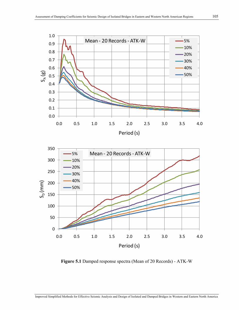
Assessment of Damping Coefficients for Seismic Design of Isolated Bridges in Eastern and Western North American Regions 105
Improved Simplified Methods for Effective Seismic Analysis and Design of Isolated and Damped Bridges in Western and Eastern North America
0.0
0.1
0.2
0.3
0.4
0.5
0.6
0.7
0.8
0.9
1.0
0.0 0.5 1.0 1.5 2.0 2.5 3.0 3.5 4.0
S A(g)
Period (s)
Mean ‐ 20 Records ‐ATK‐W 5%
10%
20%
30%
40%
50%
0
50
100
150
200
250
300
350
0.0 0.5 1.0 1.5 2.0 2.5 3.0 3.5 4.0
S D(m
m)
Period (s)
Mean ‐ 20 Records ‐ATK‐W5%
10%
20%
30%
40%
50%
Figure 5.1 Damped response spectra (Mean of 20 Records) - ATK-W
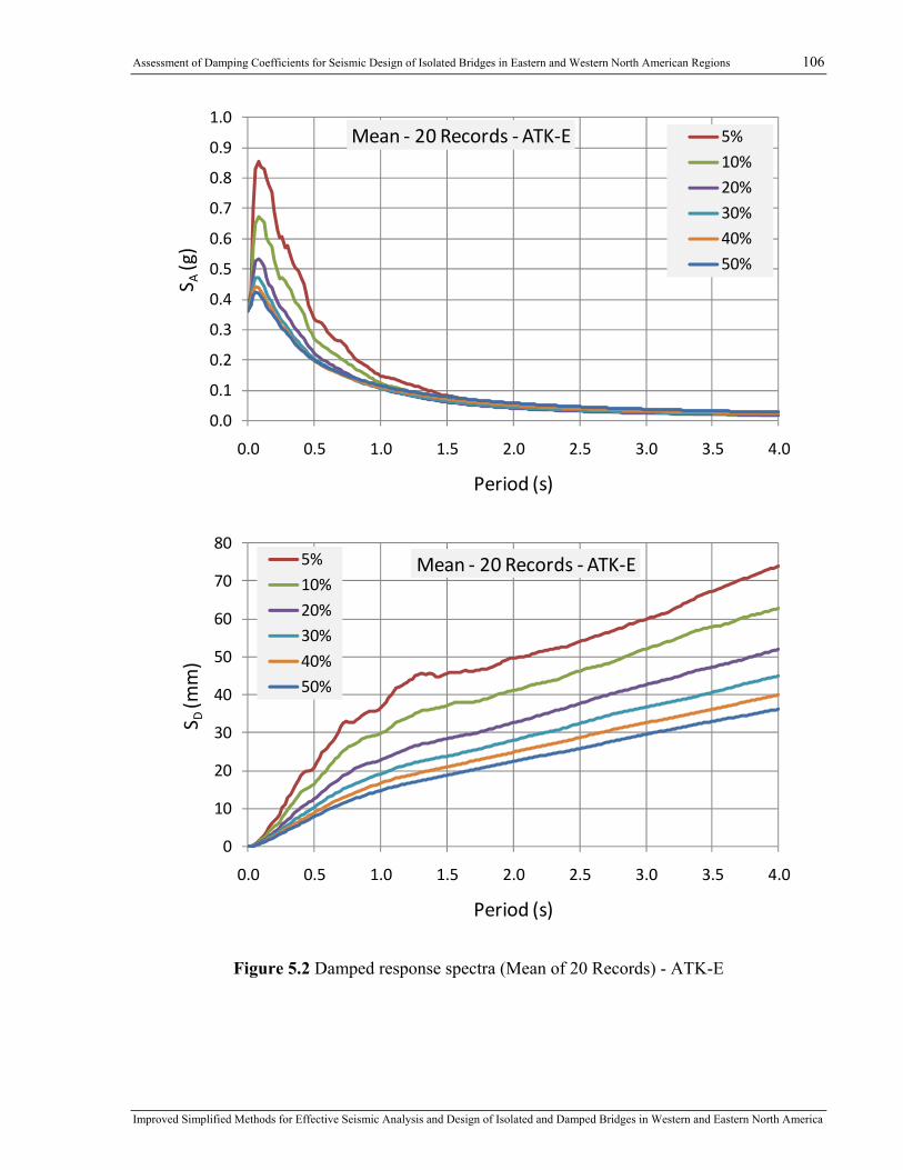
Assessment of Damping Coefficients for Seismic Design of Isolated Bridges in Eastern and Western North American Regions 106
Improved Simplified Methods for Effective Seismic Analysis and Design of Isolated and Damped Bridges in Western and Eastern North America
0.0
0.1
0.2
0.3
0.4
0.5
0.6
0.7
0.8
0.9
1.0
0.0 0.5 1.0 1.5 2.0 2.5 3.0 3.5 4.0
S A(g)
Period (s)
Mean ‐ 20 Records ‐ATK‐E 5%
10%
20%
30%
40%
50%
0
10
20
30
40
50
60
70
80
0.0 0.5 1.0 1.5 2.0 2.5 3.0 3.5 4.0
S D(m
m)
Period (s)
Mean ‐ 20 Records ‐ATK‐E5%
10%
20%
30%
40%
50%
Figure 5.2 Damped response spectra (Mean of 20 Records) - ATK-E

Assessment of Damping Coefficients for Seismic Design of Isolated Bridges in Eastern and Western North American Regions 107
Improved Simplified Methods for Effective Seismic Analysis and Design of Isolated and Damped Bridges in Western and Eastern North America
0.0
0.1
0.2
0.3
0.4
0.5
0.6
0.7
0.8
0.9
1.0
0.0 0.5 1.0 1.5 2.0 2.5 3.0 3.5 4.0
S A(g)
Period (s)
Mean ‐ 20 Records ‐MCG‐CEUS 5%
10%
20%
30%
40%
50%
0
10
20
30
40
50
60
70
80
0.0 0.5 1.0 1.5 2.0 2.5 3.0 3.5 4.0
S D(m
m)
Period (s)
Mean ‐ 20 Records ‐MCG‐CEUS5%
10%
20%
30%
40%
50%
Figure 5.3 Damped response spectra (Mean of 20 Records) - MCG-CEUS
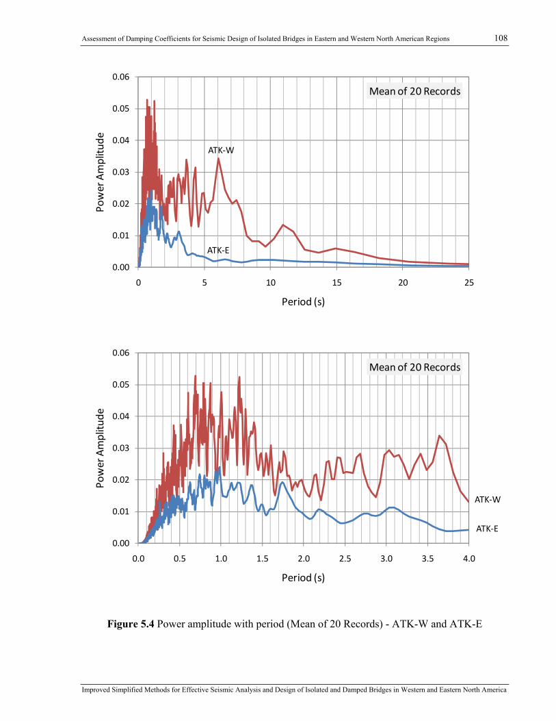
Assessment of Damping Coefficients for Seismic Design of Isolated Bridges in Eastern and Western North American Regions 108
Improved Simplified Methods for Effective Seismic Analysis and Design of Isolated and Damped Bridges in Western and Eastern North America
ATK‐W
ATK‐E
0.00
0.01
0.02
0.03
0.04
0.05
0.06
0 5 10 15 20 25
Power Amplitu
de
Period (s)
Mean of 20 Records
ATK‐W
ATK‐E
0.00
0.01
0.02
0.03
0.04
0.05
0.06
0.0 0.5 1.0 1.5 2.0 2.5 3.0 3.5 4.0
Power Amplitu
de
Period (s)
Mean of 20 Records
Figure 5.4 Power amplitude with period (Mean of 20 Records) - ATK-W and ATK-E
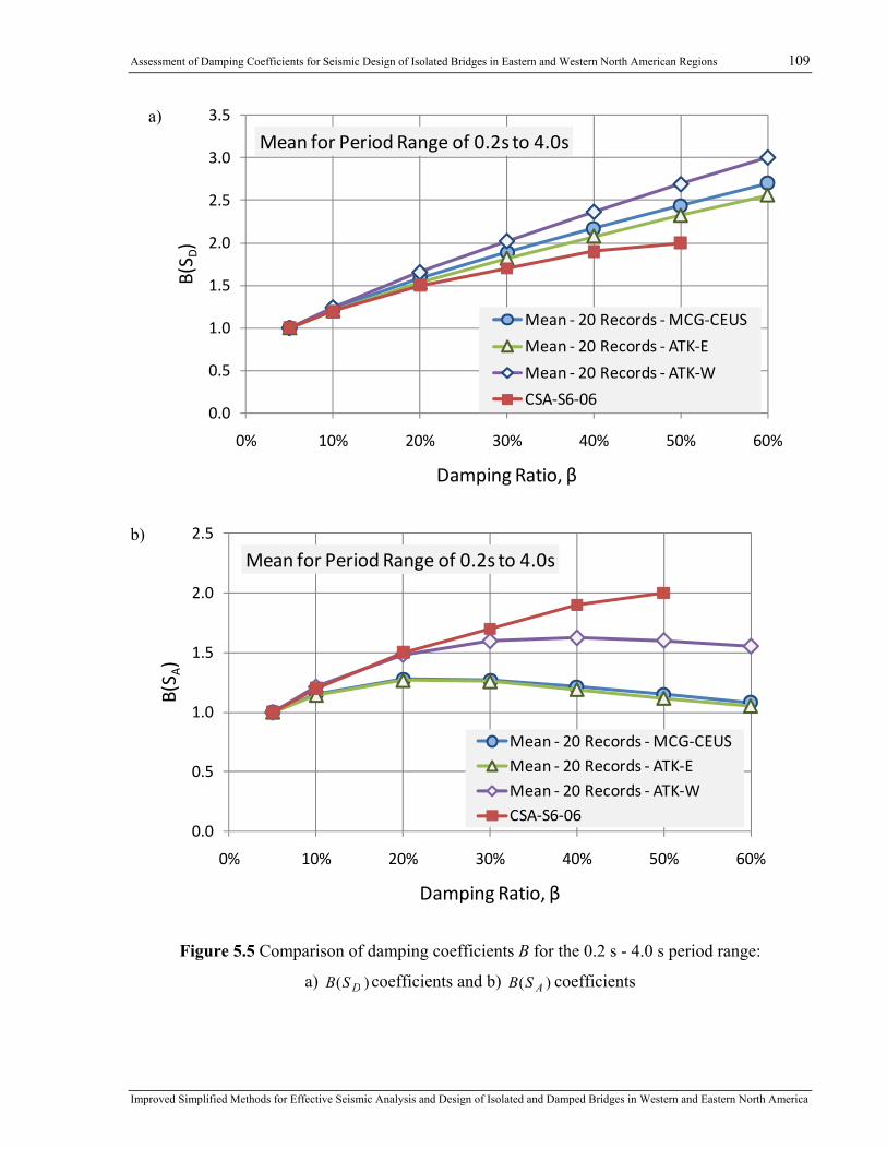
Assessment of Damping Coefficients for Seismic Design of Isolated Bridges in Eastern and Western North American Regions 109
Improved Simplified Methods for Effective Seismic Analysis and Design of Isolated and Damped Bridges in Western and Eastern North America
a)
0.0
0.5
1.0
1.5
2.0
2.5
3.0
3.5
0% 10% 20% 30% 40% 50% 60%
B(S D)
Damping Ratio, β
Mean for Period Range of 0.2s to 4.0s
Mean ‐ 20 Records ‐MCG‐CEUS
Mean ‐ 20 Records ‐ ATK‐E
Mean ‐ 20 Records ‐ ATK‐W
CSA‐S6‐06
b)
0.0
0.5
1.0
1.5
2.0
2.5
0% 10% 20% 30% 40% 50% 60%
B(S A)
Damping Ratio, β
Mean for Period Range of 0.2s to 4.0s
Mean ‐ 20 Records ‐MCG‐CEUSMean ‐ 20 Records ‐ ATK‐EMean ‐ 20 Records ‐ ATK‐WCSA‐S6‐06
Figure 5.5 Comparison of damping coefficients B for the 0.2 s - 4.0 s period range:
a) )( DSB coefficients and b) )( ASB coefficients
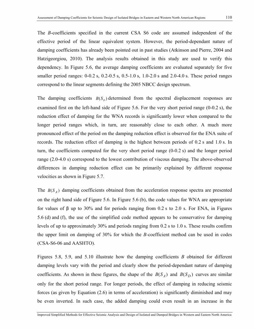
Assessment of Damping Coefficients for Seismic Design of Isolated Bridges in Eastern and Western North American Regions 110
Improved Simplified Methods for Effective Seismic Analysis and Design of Isolated and Damped Bridges in Western and Eastern North America
The B-coefficients specified in the current CSA S6 code are assumed independent of the
effective period of the linear equivalent system. However, the period-dependant nature of
damping coefficients has already been pointed out in past studies (Atkinson and Pierre, 2004 and
Hatzigeorgiou, 2010). The analysis results obtained in this study are used to verify this
dependency. In Figure 5.6, the average damping coefficients are evaluated separately for five
smaller period ranges: 0-0.2 s, 0.2-0.5 s, 0.5-1.0 s, 1.0-2.0 s and 2.0-4.0 s. These period ranges
correspond to the linear segments defining the 2005 NBCC design spectrum.
The damping coefficients )( DSB determined from the spectral displacement responses are
examined first on the left-hand side of Figure 5.6. For the very short period range (0-0.2 s), the
reduction effect of damping for the WNA records is significantly lower when compared to the
longer period ranges which, in turn, are reasonably close to each other. A much more
pronounced effect of the period on the damping reduction effect is observed for the ENA suite of
records. The reduction effect of damping is the highest between periods of 0.2 s and 1.0 s. In
turn, the coefficients computed for the very short period range (0-0.2 s) and the longer period
range (2.0-4.0 s) correspond to the lowest contribution of viscous damping. The above-observed
differences in damping reduction effect can be primarily explained by different response
velocities as shown in Figure 5.7.
The )( ASB damping coefficients obtained from the acceleration response spectra are presented
on the right hand side of Figure 5.6. In Figure 5.6 (b), the code values for WNA are appropriate
for values of β up to 30% and for periods ranging from 0.2 s to 2.0 s. For ENA, in Figures
5.6 (d) and (f), the use of the simplified code method appears to be conservative for damping
levels of up to approximately 30% and periods ranging from 0.2 s to 1.0 s. These results confirm
the upper limit on damping of 30% for which the B-coefficient method can be used in codes
(CSA-S6-06 and AASHTO).
Figures 5.8, 5.9, and 5.10 illustrate how the damping coefficients B obtained for different
damping levels vary with the period and clearly show the period-dependant nature of damping
coefficients. As shown in these figures, the shape of the )( ASB and )( DSB curves are similar
only for the short period range. For longer periods, the effect of damping in reducing seismic
forces (as given by Equation (2.6) in terms of acceleration) is significantly diminished and may
be even inverted. In such case, the added damping could even result in an increase in the

Assessment of Damping Coefficients for Seismic Design of Isolated Bridges in Eastern and Western North American Regions 111
Improved Simplified Methods for Effective Seismic Analysis and Design of Isolated and Damped Bridges in Western and Eastern North America
acceleration and seismic force response of the structure as can be seen for the ENA ground
motions (see Figures 5.9(a) and 5.10(a)).
0.0
0.5
1.0
1.5
2.0
2.5
3.0
3.5
0% 10% 20% 30% 40% 50% 60%
B (S
D)
Damping Ratio, β
Mean ‐ 20 Records ‐ ATK‐W
0.0 ‐ 0.2 s 0.2 ‐ 0.5 s0.5 ‐ 1.0 s 1.0 ‐ 2.0 s2.0 ‐ 4.0 s CSA‐S6‐06
0.0
0.5
1.0
1.5
2.0
2.5
3.0
3.5
0% 10% 20% 30% 40% 50% 60%
B (S
A)
Damping Ratio, β
Mean ‐ 20 Records ‐ ATK‐W
0.0
0.5
1.0
1.5
2.0
2.5
3.0
3.5
0% 10% 20% 30% 40% 50% 60%
B (S
D)
Damping Ratio, β
Mean ‐ 20 Records ‐MCG‐CEUS
0.0 ‐ 0.2 s 0.2 ‐ 0.5 s0.5 ‐ 1.0 s 1.0 ‐ 2.0 s2.0 ‐ 4.0 s CSA‐S6‐06
0.0
0.5
1.0
1.5
2.0
2.5
3.0
3.5
0% 10% 20% 30% 40% 50% 60%
B (S
A)
Damping Ratio, β
Mean ‐ 20 Records ‐MCG‐CEUS
0.0
0.5
1.0
1.5
2.0
2.5
3.0
3.5
0% 10% 20% 30% 40% 50% 60%
B (S
D)
Damping Ratio, β
Mean ‐ 20 Records ‐ ATK‐E
0.0 ‐ 0.2 s 0.2 ‐ 0.5 s0.5 ‐ 1.0 s 1.0 ‐ 2.0 s2.0 ‐ 4.0 s CSA‐S6‐06
0.0
0.5
1.0
1.5
2.0
2.5
3.0
3.5
0% 10% 20% 30% 40% 50% 60%
B (S
A)
Damping Ratio, β
Mean ‐ 20 Records ‐ ATK‐E
Figure 5.6 Variation of B-Coefficient with damping ratio by period range – Mean of 20 Records
)(a )(b
)(c )(d
)(e )( f
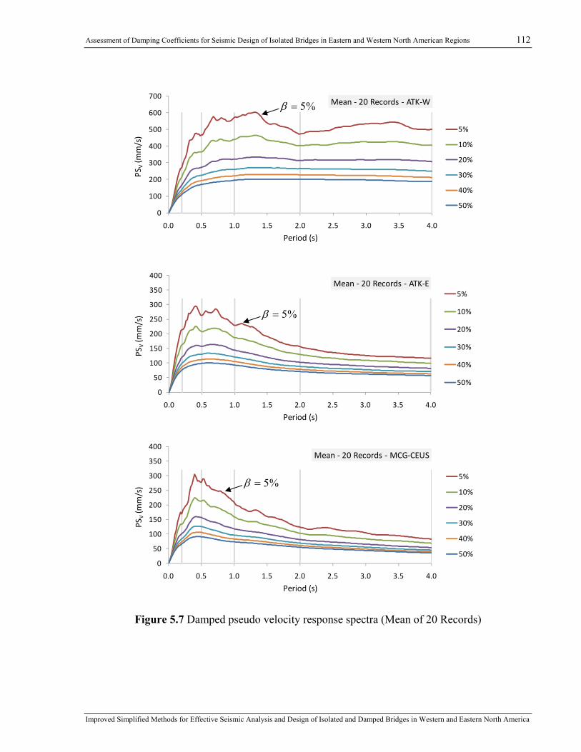
Assessment of Damping Coefficients for Seismic Design of Isolated Bridges in Eastern and Western North American Regions 112
Improved Simplified Methods for Effective Seismic Analysis and Design of Isolated and Damped Bridges in Western and Eastern North America
Figure 5.7 Damped pseudo velocity response spectra (Mean of 20 Records)
0
50
100
150
200
250
300
350
400
0.0 0.5 1.0 1.5 2.0 2.5 3.0 3.5 4.0
PSV(m
m/s)
Period (s)
Mean ‐ 20 Records ‐ ATK‐E5%
10%
20%
30%
40%
50%
%5=β
0
50
100
150
200
250
300
350
400
0.0 0.5 1.0 1.5 2.0 2.5 3.0 3.5 4.0
PSV(m
m/s)
Period (s)
Mean ‐ 20 Records ‐ MCG‐CEUS
5%
10%
20%
30%
40%
50%
%5=β
0
100
200
300
400
500
600
700
0.0 0.5 1.0 1.5 2.0 2.5 3.0 3.5 4.0
PSV(m
m/s)
Period (s)
Mean ‐ 20 Records ‐ ATK‐W
5%
10%
20%
30%
40%
50%
%5=β
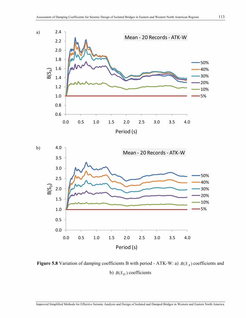
Assessment of Damping Coefficients for Seismic Design of Isolated Bridges in Eastern and Western North American Regions 113
Improved Simplified Methods for Effective Seismic Analysis and Design of Isolated and Damped Bridges in Western and Eastern North America
a)
0.6
0.8
1.0
1.2
1.4
1.6
1.8
2.0
2.2
2.4
0.0 0.5 1.0 1.5 2.0 2.5 3.0 3.5 4.0
B(S A)
Period (s)
Mean ‐ 20 Records ‐ATK‐W
50%40%30%20%10%5%
b)
0.0
0.5
1.0
1.5
2.0
2.5
3.0
3.5
4.0
0.0 0.5 1.0 1.5 2.0 2.5 3.0 3.5 4.0
B(S D)
Period (s)
Mean ‐ 20 Records ‐ATK‐W
50%40%30%20%10%5%
Figure 5.8 Variation of damping coefficients B with period - ATK-W: a) )( ASB coefficients and
b) )( DSB coefficients

Assessment of Damping Coefficients for Seismic Design of Isolated Bridges in Eastern and Western North American Regions 114
Improved Simplified Methods for Effective Seismic Analysis and Design of Isolated and Damped Bridges in Western and Eastern North America
a)
0.6
0.8
1.0
1.2
1.4
1.6
1.8
2.0
2.2
2.4
0.0 0.5 1.0 1.5 2.0 2.5 3.0 3.5 4.0
B(S A)
Period (s)
Mean ‐ 20 Records ‐ATK‐E
50%40%30%20%10%5%
b)
0.0
0.5
1.0
1.5
2.0
2.5
3.0
3.5
4.0
0.0 0.5 1.0 1.5 2.0 2.5 3.0 3.5 4.0
B(S D)
Period (s)
Mean ‐ 20 Records ‐ATK‐E
50%40%30%20%10%5%
Figure 5.9 Variation of damping coefficients B with period - ATK-E: a) )( ASB coefficients and
b) )( DSB coefficients
Assessment of Damping Coefficients for Seismic Design of Isolated Bridges in Eastern and Western North American Regions 115
Improved Simplified Methods for Effective Seismic Analysis and Design of Isolated and Damped Bridges in Western and Eastern North America
a)
0.6
0.8
1.0
1.2
1.4
1.6
1.8
2.0
2.2
2.4
0.0 0.5 1.0 1.5 2.0 2.5 3.0 3.5 4.0
B(S A)
Period (s)
Mean ‐ 20 Records ‐MCG‐CEUS
50%40%30%20%10%5%
b)
0.0
0.5
1.0
1.5
2.0
2.5
3.0
3.5
4.0
0.0 0.5 1.0 1.5 2.0 2.5 3.0 3.5 4.0
B(S D)
Period (s)
Mean ‐ 20 Records ‐MCG‐CEUS
50%40%30%20%10%5%
Figure 5.10 Variation of damping coefficients B with period - MCG-CEUS:
a) )( ASB coefficients and b) )( DSB coefficients

Assessment of Damping Coefficients for Seismic Design of Isolated Bridges in Eastern and Western North American Regions 116
Improved Simplified Methods for Effective Seismic Analysis and Design of Isolated and Damped Bridges in Western and Eastern North America
Insight into the observed amplification of the acceleration response (instead of the expected
reduction) with increased damping may be gained by studying the damped transmissibility of
SDOF systems as a function of the period ratio T / Tg (where T is the structure’s fundamental
period and Tg is the ground-motion’s predominant period). To apply such an analogy, the steady-
state response of a SDOF system is assumed to be representative of the one under seismic
excitation. This analogy is consistent for this study given that the equivalent linearization method
is based on an effective stiffness and damping transformation of nonlinear systems derived from
the system's steady-state response. Based on Newton's second law, the equation of motion for
harmonic base excitation of an SDOF system is defined as:
⎟⎟⎠
⎞⎜⎜⎝
⎛⋅⋅−=⋅+⋅+⋅ t
Tumtuktuctum
gg
π2sin)()()( &&&&& (5.4)
where )(tu is the displacement of the system's mass m relative to its base.
Accordingly, the harmonic loading is defined in terms of the ground acceleration as:
⎟⎟⎠
⎞⎜⎜⎝
⎛⋅⋅⋅−=⎟
⎟⎠
⎞⎜⎜⎝
⎛⋅⋅− t
TPGAmt
Tum
ggg
ππ 2sin2sin&& (5.5)
and the spectral acceleration is determined as:
)()(max tutuS gtA &&&& += (5.6)
The transmissibility is then defined as a ratio of the transmitted peak acceleration ),( βTS A , or
the spectral acceleration, to the peak ground acceleration PGA. Using the formulation proposed
by Chopra (2011) for the harmonic response of an SDOF system, the transmissibility
),( βTTR can be expressed as follows :
222
2
)]/(2[])/(1[
)]/(2[1),(),(gg
gA
TTTT
TTPGA
TSTTR⋅+−
⋅+==
β
βββ (5.7)
The idealized damping coefficient B can be then expressed for harmonic excitation of an SDOF
system in terms of the transmissibility ratio as:
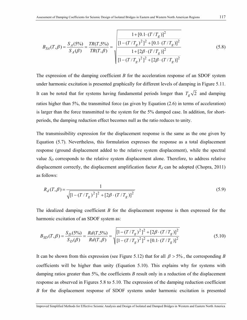
Assessment of Damping Coefficients for Seismic Design of Isolated Bridges in Eastern and Western North American Regions 117
Improved Simplified Methods for Effective Seismic Analysis and Design of Isolated and Damped Bridges in Western and Eastern North America
222
2
222
2
)]/(2[])/(1[
)]/(2[1
)]/(1.0[])/(1[
)]/(1.0[1
),(%)5,(
)(%)5(),(
gg
g
gg
g
A
ASA
TTTT
TT
TTTT
TT
TTRTTR
SSTB
⋅+−
⋅+
⋅+−
⋅+
===
β
ββββ (5.8)
The expression of the damping coefficient B for the acceleration response of an SDOF system
under harmonic excitation is presented graphically for different levels of damping in Figure 5.11.
It can be noted that for systems having fundamental periods longer than 2gT and damping
ratios higher than 5%, the transmitted force (as given by Equation (2.6) in terms of acceleration)
is larger than the force transmitted to the system for the 5% damped case. In addition, for short-
periods, the damping reduction effect becomes null as the ratio reduces to unity.
The transmissibility expression for the displacement response is the same as the one given by
Equation (5.7). Nevertheless, this formulation expresses the response as a total displacement
response (ground displacement added to the relative system displacement), while the spectral
value SD corresponds to the relative system displacement alone. Therefore, to address relative
displacement correctly, the displacement amplification factor Rd can be adopted (Chopra, 2011)
as follows:
222 )]/(2[])/(1[
1),(gg
dTTTT
TR⋅+−
=β
β (5.9)
The idealized damping coefficient B for the displacement response is then expressed for the
harmonic excitation of an SDOF system as:
222
222
)]/(1.0[])/(1[
)]/(2[])/(1[),(
%)5,()(
%)5(),(
gg
gg
D
DSD
TTTT
TTTTTRdTRd
SS
TB⋅+−
⋅+−===
βββ
β (5.10)
It can be shown from this expression (see Figure 5.12) that for all %5>β , the corresponding B
coefficients will be higher than unity (Equation 5.10). This explains why for systems with
damping ratios greater than 5%, the coefficients B result only in a reduction of the displacement
response as observed in Figures 5.8 to 5.10. The expression of the damping reduction coefficient
B for the displacement response of SDOF systems under harmonic excitation is presented
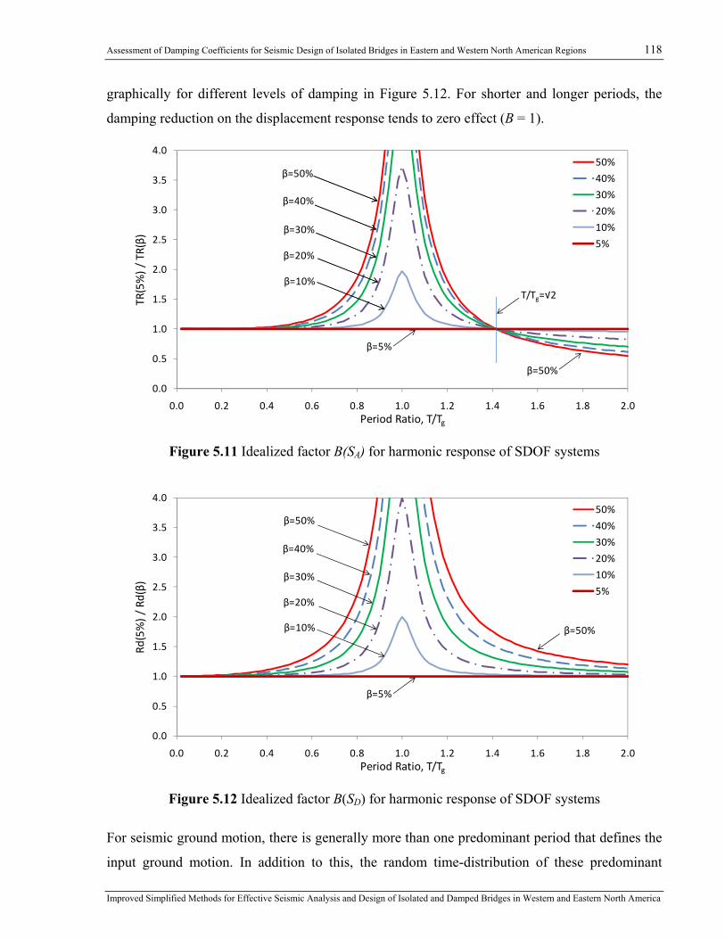
Assessment of Damping Coefficients for Seismic Design of Isolated Bridges in Eastern and Western North American Regions 118
Improved Simplified Methods for Effective Seismic Analysis and Design of Isolated and Damped Bridges in Western and Eastern North America
graphically for different levels of damping in Figure 5.12. For shorter and longer periods, the
damping reduction on the displacement response tends to zero effect (B = 1).
β=50%
β=50%
β=40%
β=30%
β=20%
β=10%
β=5%
0.0
0.5
1.0
1.5
2.0
2.5
3.0
3.5
4.0
0.0 0.2 0.4 0.6 0.8 1.0 1.2 1.4 1.6 1.8 2.0
TR(5%) / TR(β)
Period Ratio, T/Tg
50%
40%
30%
20%
10%
5%
T/Tg=√2
Figure 5.11 Idealized factor B(SA) for harmonic response of SDOF systems
β=50%
β=50%
β=40%
β=30%
β=20%
β=10%
β=5%
0.0
0.5
1.0
1.5
2.0
2.5
3.0
3.5
4.0
0.0 0.2 0.4 0.6 0.8 1.0 1.2 1.4 1.6 1.8 2.0
Rd(5%) / Rd(β)
Period Ratio, T/Tg
50%
40%
30%
20%
10%
5%
Figure 5.12 Idealized factor B(SD) for harmonic response of SDOF systems
For seismic ground motion, there is generally more than one predominant period that defines the
input ground motion. In addition to this, the random time-distribution of these predominant
Assessment of Damping Coefficients for Seismic Design of Isolated Bridges in Eastern and Western North American Regions 119
Improved Simplified Methods for Effective Seismic Analysis and Design of Isolated and Damped Bridges in Western and Eastern North America
periods and the system nonlinear response to non-harmonic ground motion excitations contribute
to the complexity of the damping reduction mechanism. Nevertheless, the formulation of the
damping coefficients (Equations (5.8) and (5.10)) of a linear SDOF system under harmonic
excitations provide an explanation of the physical phenomena leading to the general trends
governing the damping reduction effect of isolated bridge structures. Consequently, as shown
above, the coefficients B(SA) and B(SD) reflect different aspects of the system response (absolute
acceleration and relative displacement). As mentioned previously, the coefficients B(SA) reflect
the relation between the pseudo displacement spectra. Even when the pseudo displacement
spectrum is close to the displacement response spectrum, the use of the coefficients B(SA) may
not be representative of the “real” damping reduction in displacement response. For this reason,
B-coefficients for reducing force and displacement responses must be independently defined and
calibrated. In this study, the focus will be set only on the damping coefficients B that relate
displacement responses of the system to the 5% damped displacement spectra. The reason for
only addressing B(SD) in detail is that, as explained in Chapter 2, the procedure of the simplified
code method (CAN/CSA-S6-06) is used to determine the displacement of the isolated structure.
The design seismic forces are subsequently determined from the load-displacement response of
the actual nonlinear isolation system.
For a more accurate evaluation of the expected displacement across isolation bearings, the
analysis results suggest that the simplified code method should be used to predict displacements
rather than accelerations or forces. For assessing the statically equivalent seismic force using
Equation 2.6 (see Chapter 2), limitations on the effective period range and the effective damping
ratio should also be specified. Otherwise, the use of current code provisions could result in
unconservative response estimates.
5.4 Nonlinear Time-History Analyses (NLTHA)
The results presented in the previous section are applicable to the response of linear systems for
which the response reduction effect is solely due to velocity-dependant viscous damping. For
isolated bridge structures responding nonlinearly, however, the amount of equivalent damping
depends on the hysteretic nature and the maximum displacement response, and the equivalent
damping is no longer a direct function of the velocity. For this reason, a series of nonlinear time-
history (NLTH) analyses were performed for an ensemble of bilinear SDOF systems covering a
Assessment of Damping Coefficients for Seismic Design of Isolated Bridges in Eastern and Western North American Regions 120
Improved Simplified Methods for Effective Seismic Analysis and Design of Isolated and Damped Bridges in Western and Eastern North America
wide range of isolated and damped bridge configurations. The same suites of artificial ground-
motion records (ATK-E and ATK-W) that were used for the study on linear systems were also
adopted for this parametric study.
5.4.1 Structural Parameters for Nonlinear Time-History Analyses
The study was performed on SDOF systems exhibiting the bilinear hysteretic response shown in
Figure 5.13. This response is representative of bridge structures protected with a variety of
seismic isolators commonly used in practice. For such isolated bridge structures, the equivalent
effective period Teff and damping ratio effβ depend on the hysteretic shape and the maximum
displacement (see Equations (2.2) and (2.4), Chapter 2). A wide range of effective parameters
was considered by varying the following system properties: the response modification factor R,
which corresponds to the ratio between the activation lateral force of the isolation system and the
elastic force demand, SA(Te,5%)W, the initial (elastic) structure period, Te, the ratio α between the
post-elastic kd and the initial (elastic) ku structure stiffness, and different levels of viscous
damping related to both the elastic period Te and the effective period Teff.
These parameters were adopted for the present parametric study given that they make it possible
to define the hysteretic properties of the system at the initial design stage. Accordingly, the
structure-earthquake interaction may be characterized through the period ratio Te / Tg and the
response modification factor R. The response modification factor R has a direct implication in the
design process because it relates the isolation activation limit, uy to the UHS spectral value
through the relation:
uy = ue / R = SD (5%, Te) / R. (5.11)
The resulting system configuration, which is defined by uy as a function of R, is constant for all
of the analyses carried out for a given set of 20 records.
Different levels of inherent damping were defined in relation to the elastic and effective periods.
Both are frequently adopted by researchers for NLTH analyses and yield comparable results for
low-ductility responses. However, the use of inherent damping related to the elastic period may
lead to unconservative displacement response for highly nonlinear systems (Jacobsen, 1960). In
this study, the results obtained with inherent damping which is defined in relation to the elastic

Assessment of Damping Coefficients for Seismic Design of Isolated Bridges in Eastern and Western North American Regions 121
Improved Simplified Methods for Effective Seismic Analysis and Design of Isolated and Damped Bridges in Western and Eastern North America
period are nonetheless included as they are relevant in cases where supplemental damping
devices are used in bridges.
Figure 5.13 Structure nonlinear parameters - Bilinear hysteretic
Table 5-1 presents the parameters used for defining the properties of the nonlinear SDOF
systems that were analyzed in this study which resulted in a total of 12 000 time-history analyses
(THA). The parameters were changed one at the time, resulting in 300 isolated bridge
configurations (5 (R) x 4 (Te) x 5 (β) x 3 (α)). These parameters and their respective ranges were
chosen such that an extensive range of isolated and damped bridge configurations was covered.
Each of these isolation systems were analyzed under 20 time-history records for each of the
WNA and ENA regions.
Table 5-1 Structural parameters for nonlinear time-history analyses
Analysis Parameters Eastern North America Western North America
Response modification factor R=[4, 16, 28, 40, 52] R=[4, 16, 28, 40, 52]
Elastic period Te=[0.25, 0.5, 0.75, 1.0 s] Te=[0.25, 0.5, 0.75 1.0 s]
Inherent damping ratio β(Te)= [0%, 2%, 5%];
β(Teff)=[2%, 5%]
β(Te)= [0%, 2%, 5%];
β(Teff)=[2%, 5%]
Post-yield stiffness ratio α=[0.01, 0.05, 0.1] α=[0.01, 0.05, 0.1]
Ground-motions records 20 Atkinson's 2009 (ATK-E) 20 Atkinson's 2009 (ATK-W)
y
e
y
euu
FFR ==
yuumax=μ
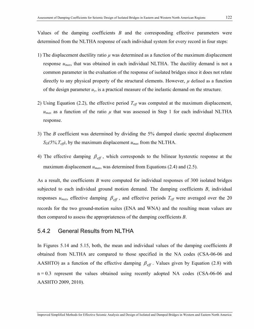
Assessment of Damping Coefficients for Seismic Design of Isolated Bridges in Eastern and Western North American Regions 122
Improved Simplified Methods for Effective Seismic Analysis and Design of Isolated and Damped Bridges in Western and Eastern North America
Values of the damping coefficients B and the corresponding effective parameters were
determined from the NLTHA response of each individual system for every record in four steps:
1) The displacement ductility ratio µ was determined as a function of the maximum displacement
response umax, that was obtained in each individual NLTHA. The ductility demand is not a
common parameter in the evaluation of the response of isolated bridges since it does not relate
directly to any physical property of the structural elements. However, µ defined as a function
of the design parameter uy, is a practical measure of the inelastic demand on the structure.
2) Using Equation (2.2), the effective period Teff was computed at the maximum displacement,
umax as a function of the ratio µ that was assessed in Step 1 for each individual NLTHA
response.
3) The B coefficient was determined by dividing the 5% damped elastic spectral displacement
SD(5%,Teff), by the maximum displacement umax from the NLTHA.
4) The effective damping effβ , which corresponds to the bilinear hysteretic response at the
maximum displacement umax, was determined from Equations (2.4) and (2.5).
As a result, the coefficients B were computed for individual responses of 300 isolated bridges
subjected to each individual ground motion demand. The damping coefficients B, individual
responses umax, effective damping effβ , and effective periods Teff were averaged over the 20
records for the two ground-motion suites (ENA and WNA) and the resulting mean values are
then compared to assess the appropriateness of the damping coefficients B.
5.4.2 General Results from NLTHA
In Figures 5.14 and 5.15, both, the mean and individual values of the damping coefficients B
obtained from NLTHA are compared to those specified in the NA codes (CSA-06-06 and
AASHTO) as a function of the effective damping effβ . Values given by Equation (2.8) with
n = 0.3 represent the values obtained using recently adopted NA codes (CSA-06-06 and
AASHTO 2009, 2010).

Assessment of Damping Coefficients for Seismic Design of Isolated Bridges in Eastern and Western North American Regions 123
Improved Simplified Methods for Effective Seismic Analysis and Design of Isolated and Damped Bridges in Western and Eastern North America
By observing the mean values of the damping coefficients B, presented in Figure 5.14(a) for
WNA, it can be noted that the majority of the plotted dots are above the curve representing the
code-specified damping coefficients, which shows that current code provisions generally result
in conservative (larger) response estimates. Damping coefficients are however underestimated
for effβ values greater than 20% and this aspect is discussed in further details later.
In contrast, for the ENA records in Figure 5.15(a), a considerable number of points are situated
below the curve representing the code prescribed values indicating unconservative predictions
when using the code-defined B coefficients for all damping levels. Therefore, there is a need to
adjust these factors to better predict the expected response of isolated bridges under ENA
earthquake records. The different damping coefficients observed for WNA and ENA responses
are primarily attributed to the differences in the ground motion characteristics that are expected
for seismicity in WNA and in ENA as discussed previously in this chapter.
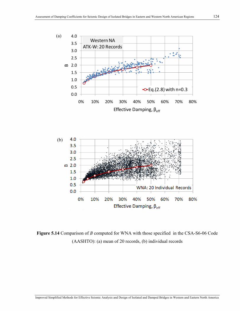
Assessment of Damping Coefficients for Seismic Design of Isolated Bridges in Eastern and Western North American Regions 124
Improved Simplified Methods for Effective Seismic Analysis and Design of Isolated and Damped Bridges in Western and Eastern North America
(a)
0.0
0.5
1.0
1.5
2.0
2.5
3.0
3.5
4.0
0% 10% 20% 30% 40% 50% 60% 70% 80%
B
Effective Damping, βeff
Western NAATK‐W: 20 Records
Eq.(2.8) with n=0.3
(b)
Figure 5.14 Comparison of B computed for WNA with those specified in the CSA-S6-06 Code
(AASHTO): (a) mean of 20 records, (b) individual records
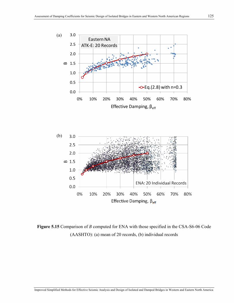
Assessment of Damping Coefficients for Seismic Design of Isolated Bridges in Eastern and Western North American Regions 125
Improved Simplified Methods for Effective Seismic Analysis and Design of Isolated and Damped Bridges in Western and Eastern North America
(a)
0.0
0.5
1.0
1.5
2.0
2.5
3.0
0% 10% 20% 30% 40% 50% 60% 70% 80%
B
Effective Damping, βeff
Eastern NAATK‐E: 20 Records
Eq.(2.8) with n=0.3
(b)
Figure 5.15 Comparison of B computed for ENA with those specified in the CSA-S6-06 Code
(AASHTO): (a) mean of 20 records, (b) individual records
Assessment of Damping Coefficients for Seismic Design of Isolated Bridges in Eastern and Western North American Regions 126
Improved Simplified Methods for Effective Seismic Analysis and Design of Isolated and Damped Bridges in Western and Eastern North America
Figures 5.14(b) and 5.15(b) present individual values of the damping coefficients B, which are
scattered out over the 20 records when compared to the plot of the mean values. These results
provide an overall insight into the variability of the coefficients B within a suite of 20 ground
motions. Despite a very large scatter in the individual points, the same tendencies as for averaged
assessment (Figures 5.14(a) and 5.15(a)) can be easily distinguished from these figures.
To explain the variability of the coefficients B, it should be recalled that the damping coefficient
method is an approximation and it cannot take into account the effect of the record-to-record
variability that may reflect the true random character of the real earthquakes.
5.4.3 Effects of Ground-Motion Characteristics on Damping Coefficients
To gain a better understanding on the variability of the coefficients B, the effects of the ground
motion characteristics on this parameter are further studied by examining damping coefficients
obtained from four different ground motion subsets each representing the ENA suite. These four
subsets are divided by grouping earthquake scenarios in terms of magnitude and distance: E6C1
(M6, 10 to 15 km), E6C2 (M6, 20 to 30 km), E7C1 (M7, 15 to 25 km) and E7C2 (M7, 50 to
100 km) (see for more details Chapter 4). Mean 5% damped displacement spectra are given for
each subset in Figure 5.16. As expected, for longer periods, the smaller earthquakes E6C1 and
E6C2 induce smaller elastic displacement demands when compared to those from the greater
earthquakes E7C1 and E7C2. For a given magnitude range, closer earthquakes E6C1 and E7C1
produce larger elastic displacements.
It can be noted from these figures that the spectra from individual records may deviate
significantly from each other. The reason for this, as explained in Chapter 4, is that the 20
records (ENA or WNA) were scaled over a certain period range so the mean response spectrum
matches the UHS closely (for Montreal and Vancouver). These observations shed light on the
mechanisms contributing to the variability of the coefficients B within a suite of 20 ground
motions.
Figure 5.17 gives the mean damping coefficients computed for each subset. Damping
coefficients that are much smaller than the code-specified values (the code predictions are
unconservative in this case) are obtained for the M6 events. For the two subsets of larger M7
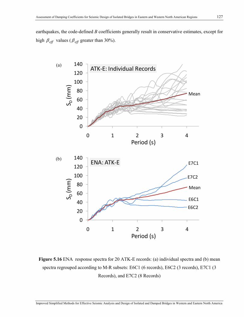
Assessment of Damping Coefficients for Seismic Design of Isolated Bridges in Eastern and Western North American Regions 127
Improved Simplified Methods for Effective Seismic Analysis and Design of Isolated and Damped Bridges in Western and Eastern North America
earthquakes, the code-defined B coefficients generally result in conservative estimates, except for
high effβ values ( effβ greater than 30%).
(a)
Mean
0
20
40
60
80
100
120
140
0 1 2 3 4
S D(m
m)
Period (s)
ATK‐E: Individual Records
(b)
E7C2
E7C1
E6C2
E6C1
Mean
0
20
40
60
80
100
120
140
0 1 2 3 4
S D(m
m)
Period (s)
ENA: ATK‐E
Figure 5.16 ENA response spectra for 20 ATK-E records: (a) individual spectra and (b) mean
spectra regrouped according to M-R subsets: E6C1 (6 records), E6C2 (3 records), E7C1 (3
Records), and E7C2 (8 Records)
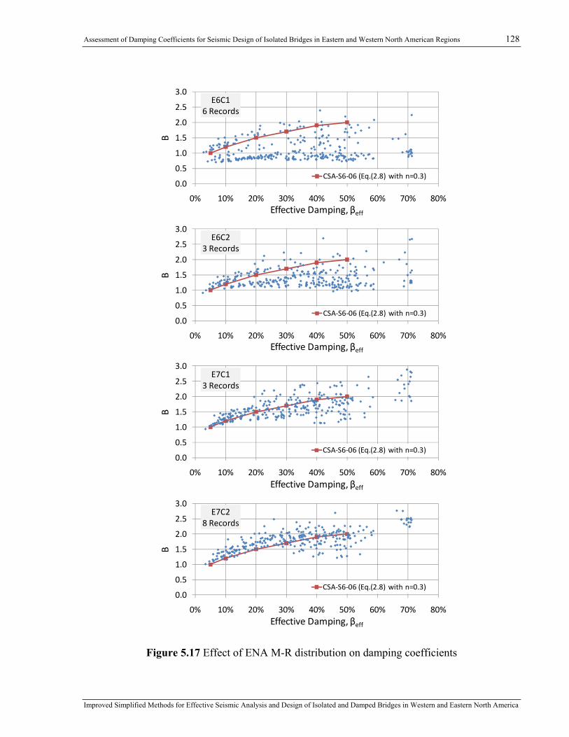
Assessment of Damping Coefficients for Seismic Design of Isolated Bridges in Eastern and Western North American Regions 128
Improved Simplified Methods for Effective Seismic Analysis and Design of Isolated and Damped Bridges in Western and Eastern North America
0.0
0.5
1.0
1.5
2.0
2.5
3.0
0% 10% 20% 30% 40% 50% 60% 70% 80%
B
Effective Damping, βeff
E6C16 Records
CSA‐S6‐06 (Eq.(2.8) with n=0.3)
0.0
0.5
1.0
1.5
2.0
2.5
3.0
0% 10% 20% 30% 40% 50% 60% 70% 80%
B
Effective Damping, βeff
E6C23 Records
CSA‐S6‐06 (Eq.(2.8) with n=0.3)
0.0
0.5
1.0
1.5
2.0
2.5
3.0
0% 10% 20% 30% 40% 50% 60% 70% 80%
B
Effective Damping, βeff
E7C13 Records
CSA‐S6‐06 (Eq.(2.8) with n=0.3)
0.0
0.5
1.0
1.5
2.0
2.5
3.0
0% 10% 20% 30% 40% 50% 60% 70% 80%
B
Effective Damping, βeff
E7C28 Records
CSA‐S6‐06 (Eq.(2.8) with n=0.3)
Figure 5.17 Effect of ENA M-R distribution on damping coefficients

Assessment of Damping Coefficients for Seismic Design of Isolated Bridges in Eastern and Western North American Regions 129
Improved Simplified Methods for Effective Seismic Analysis and Design of Isolated and Damped Bridges in Western and Eastern North America
5.4.4 Comparison of CSA-S6-06 Design Estimates with Results from
NLTHA
To better assess the accuracy of code-specified B-coefficients on the seismic displacement
response, a number of 180 isolated bridge structures (5 (R) x 4 (Te) x 3 (β) x 3 (α)) were analyzed
following the complete iterative procedure prescribed in the CSA-S6-06 simplified method
(similar to AASHTO).
The displacement response was calculated by dividing the 5% damped pseudo-displacement by
the damping coefficient as )(/)%,5( effeffDcode BTPSu β= . The PSD (5%,Teff) value is determined
by transforming the SA (5%,Teff) value from the UHS acceleration spectrum represented by the
20-records mean acceleration response spectrum. The )( effB β value is determined as a function
of the effective damping effβ using Equation (2.8) with n=0.3 (as specified in AASHTO), As
stated in Chapter 2, this expression accurately represents the damping coefficients tabulated in
the CSA-S6-06 code and will be further exploited to enhance the accuracy of the simplified
method.
The displacement response is however defined as a function of the effective period Teff and
effective damping βeff. As a result, the response estimate is obtained by successive iterations
because the values of Teff and βeff depend, in turn, on the displacement response ucode (refer to
Chapter 2, Section 2.1 for more details on the procedure).
Figures 5.18 and 5.19 present probability density functions of the ratios between the peak
displacements from nonlinear time history analyses (NLTHA) and peak displacements obtained
using the CSA-S6-06 simplified method. Values in the plots are computed for a sample of 1200
responses, that correspond to 60 different isolated bridge structures (5 (R) x 4 (Te) x 3 (β))
analyzed under 20 time-history records. Accordingly, there are 20 responses from NLTHA that
correspond to one response estimate using the CSA-S6-06 simplified method. Each plot is
obtained for one site (West vs East) and one value of α (0.1, 0.05, 0.01).
It can be noted from these figures that the probability density is close to a normal distribution:
the distribution pattern is symmetrical; the highest point is close to the center of the distribution;
and the shape of the distribution follows a general "bell" curve. In addition, for the normally
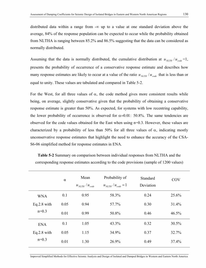
Assessment of Damping Coefficients for Seismic Design of Isolated Bridges in Eastern and Western North American Regions 130
Improved Simplified Methods for Effective Seismic Analysis and Design of Isolated and Damped Bridges in Western and Eastern North America
distributed data within a range from -∞ up to a value at one standard deviation above the
average, 84% of the response population can be expected to occur while the probability obtained
from NLTHA is ranging between 85.2% and 86.5% suggesting that the data can be considered as
normally distributed.
Assuming that the data is normally distributed, the cumulative distribution at codeNLTH uu / =1,
presents the probability of occurrence of a conservative response estimate and describes how
many response estimates are likely to occur at a value of the ratio codeNLTH uu / that is less than or
equal to unity. These values are tabulated and compared in Table 5-2.
For the West, for all three values of α, the code method gives more consistent results while
being, on average, slightly conservative given that the probability of obtaining a conservative
response estimate is greater than 50%. As expected, for systems with low recentring capability,
the lower probability of occurrence is observed for α=0.01: 50.8%. The same tendencies are
observed for the code values obtained for the East when using n=0.3. However, these values are
characterized by a probability of less than 50% for all three values of α, indicating mostly
unconservative response estimates that highlight the need to enhance the accuracy of the CSA-
S6-06 simplified method for response estimates in ENA.
Table 5-2 Summary on comparison between individual responses from NLTHA and the
corresponding response estimates according to the code provisions (sample of 1200 values)
α Mean
codeNLTH uu /
Probability of
1/ =codeNLTH uu Standard
Deviation COV
WNA
Eq.2.8 with
n=0.3
0.1 0.95 58.3% 0.24 25.6%
0.05 0.94 57.7% 0.30 31.4%
0.01 0.99 50.8% 0.46 46.5%
ENA
Eq.2.8 with
n=0.3
0.1 1.05 43.3% 0.32 30.5%
0.05 1.15 34.9% 0.37 32.7%
0.01 1.30 26.9% 0.49 37.4%

Assessment of Damping Coefficients for Seismic Design of Isolated Bridges in Eastern and Western North American Regions 131
Improved Simplified Methods for Effective Seismic Analysis and Design of Isolated and Damped Bridges in Western and Eastern North America
0
20
40
60
80
100
120
140
0.0 0.2 0.4 0.6 0.8 1.0 1.2 1.4 1.6 1.8 2.0
Freq
uency
uNLTH/ucode
NL SDOF (ATK‐W)α=0.1
Eq.(2.8) n=0.3
‐σ +σ
0
20
40
60
80
100
120
140
0.0 0.2 0.4 0.6 0.8 1.0 1.2 1.4 1.6 1.8 2.0
Freq
uency
uNLTH/ucode
NL SDOF (ATK‐W)α=0.05
Eq.(2.8) n=0.3
‐σ +σ
0
20
40
60
80
100
120
140
0.0 0.2 0.4 0.6 0.8 1.0 1.2 1.4 1.6 1.8 2.0
Freq
uency
uNLTH/ucode
NL SDOF (ATK‐W)α=0.01
Eq.(2.8) n=0.3
‐σ +σ
Figure 5.18 Frequency of uNLTH/ucode versus normal distribution - WNA Eq.(2.8) with n=0.3
Probability = 86.5% "Bell" curve
Probability = 86.0%
Probability = 85.2%
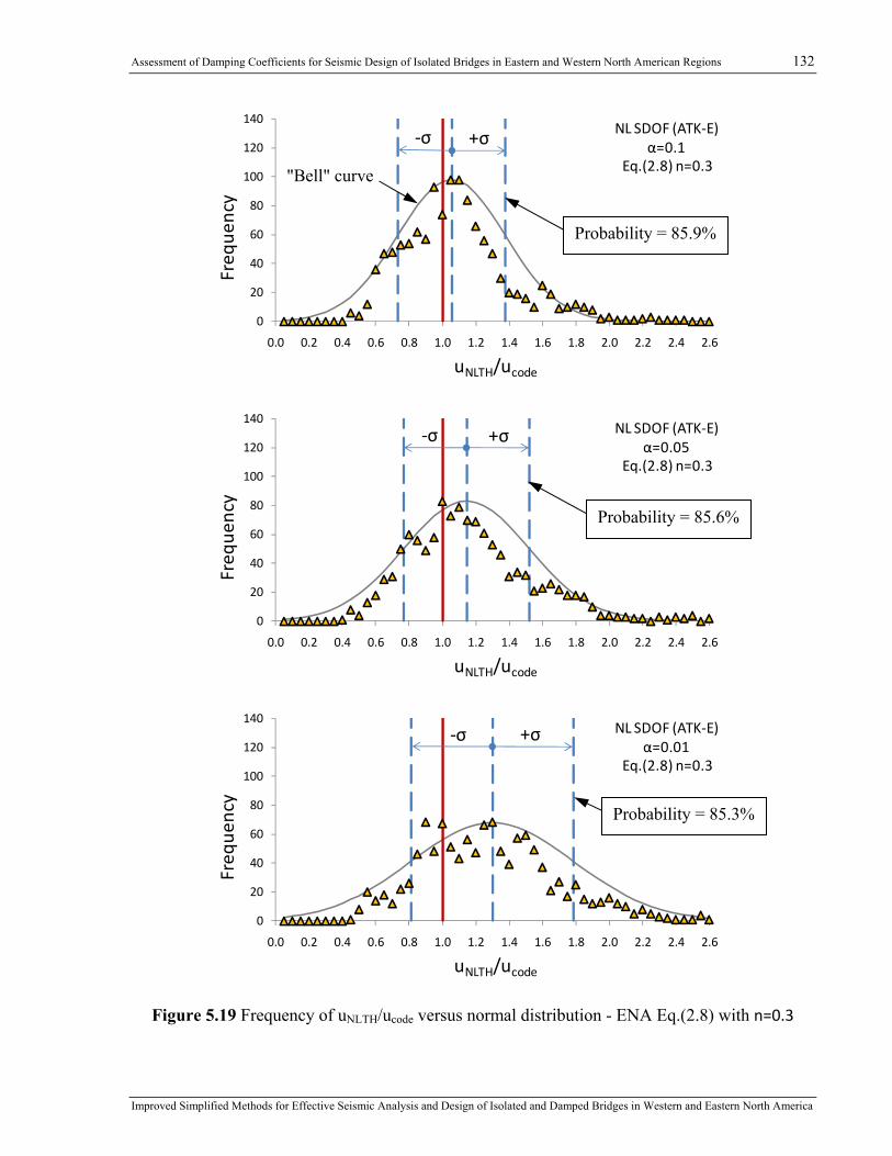
Assessment of Damping Coefficients for Seismic Design of Isolated Bridges in Eastern and Western North American Regions 132
Improved Simplified Methods for Effective Seismic Analysis and Design of Isolated and Damped Bridges in Western and Eastern North America
0
20
40
60
80
100
120
140
0.0 0.2 0.4 0.6 0.8 1.0 1.2 1.4 1.6 1.8 2.0 2.2 2.4 2.6
Freq
uency
uNLTH/ucode
NL SDOF (ATK‐E)α=0.1
Eq.(2.8) n=0.3
‐σ +σ
0
20
40
60
80
100
120
140
0.0 0.2 0.4 0.6 0.8 1.0 1.2 1.4 1.6 1.8 2.0 2.2 2.4 2.6
Freq
uency
uNLTH/ucode
NL SDOF (ATK‐E)α=0.05
Eq.(2.8) n=0.3
‐σ +σ
0
20
40
60
80
100
120
140
0.0 0.2 0.4 0.6 0.8 1.0 1.2 1.4 1.6 1.8 2.0 2.2 2.4 2.6
Freq
uency
uNLTH/ucode
NL SDOF (ATK‐E)α=0.01
Eq.(2.8) n=0.3
‐σ +σ
Figure 5.19 Frequency of uNLTH/ucode versus normal distribution - ENA Eq.(2.8) with n=0.3
Probability = 85.9%
Probability = 85.6%
Probability = 85.3%
"Bell" curve

Assessment of Damping Coefficients for Seismic Design of Isolated Bridges in Eastern and Western North American Regions 133
Improved Simplified Methods for Effective Seismic Analysis and Design of Isolated and Damped Bridges in Western and Eastern North America
Ratios obtained from individual records are presented in Figures 5.20 to 5.21. As mentioned
previously, the observed deviation from the sample mean value is mostly due to the record-to-
record variability including the differences observed between the response spectrum from each
individual record and the corresponding UHS (as shown in Figure 5.16). It should be recalled
that the 20 records (ENA or WNA) are scaled over a certain period range so the mean response
spectrum matches closely the UHS (for Montreal and Vancouver respectively) while individual
records may deviate significantly from each other.
The variability is measured in terms of the standard deviation, which is compared in Tables 5.2
for samples of 1200. As expected for the systems with low recentring capability, which are easily
prone to residual displacements, the variability increases as the value of α decreases. The upper
and lower limits of standard deviations observed for α=0.01 are 0.46 for the West and 0.49 for
the East. The respective coefficients of variation (COV), which describe the standard deviation
as a percentage of the sample mean, are 46.5% and 37.4%. The greater coefficient of variation
can be explained by stronger ground-motion intensities in Western Canadian regions.

Assessment of Damping Coefficients for Seismic Design of Isolated Bridges in Eastern and Western North American Regions 134
Improved Simplified Methods for Effective Seismic Analysis and Design of Isolated and Damped Bridges in Western and Eastern North America
0
50
100
150
200
250
300
350
400
450
500
0 200 400 600 800 1,000
u code(m
m)
uNLTH (mm)
NL SDOF (ATK‐W) ‐ Eq.(2.8) with n=0.3 ‐ α=0.1
‐σ +σ
Mean u/ucodeu/ucode = 1
0
50
100
150
200
250
300
350
400
450
500
0 200 400 600 800 1,000
u code(m
m)
uNLTH (mm)
NL SDOF (ATK‐W) ‐ Eq.(2.8) with n=0.3 ‐ α=0.05
‐σ +σ
Mean u/ucode
u/ucode = 1
0
50
100
150
200
250
300
350
400
450
500
0 200 400 600 800 1,000
u code(m
m)
uNLTH (mm)
NL SDOF (ATK‐W) ‐ Eq.(2.8) with n=0.3 ‐ α=0.01
‐σ +σ
Mean u/ucodeu/ucode = 1
Figure 5.20 Responses from NLTHA versus code estimate - WNA Eq.(2.8) with n=0.3

Assessment of Damping Coefficients for Seismic Design of Isolated Bridges in Eastern and Western North American Regions 135
Improved Simplified Methods for Effective Seismic Analysis and Design of Isolated and Damped Bridges in Western and Eastern North America
0
10
20
30
40
50
60
70
80
90
100
0 20 40 60 80 100 120 140 160 180
u code(m
m)
uNLTH (mm)
NL SDOF (ATK‐E) ‐ Eq.(2.8) with n=0.3 ‐ α=0.1
‐σ +σMean u/ucode
u/ucode = 1
0
10
20
30
40
50
60
70
80
90
100
0 20 40 60 80 100 120 140 160 180
u code(m
m)
uNLTH (mm)
NL SDOF (ATK‐E) ‐ Eq.(2.8) with n=0.3 ‐ α=0.05
‐σ +σ Mean u/ucode
u/ucode = 1
0
10
20
30
40
50
60
70
80
90
100
0 20 40 60 80 100 120 140 160 180
u code(m
m)
uNLTH (mm)
NL SDOF (ATK‐E) ‐ Eq.(2.8) with n=0.3 ‐ α=0.01
Mean u/ucode‐σ +σ
u/ucode = 1
Figure 5.21 Responses from NLTHA versus code estimate - ENA Eq.(2.8) with n=0.3
Assessment of Damping Coefficients for Seismic Design of Isolated Bridges in Eastern and Western North American Regions 136
Improved Simplified Methods for Effective Seismic Analysis and Design of Isolated and Damped Bridges in Western and Eastern North America
5.5 Proposed Equation for Damping Coefficients, B
The analysis results that were presented earlier in this chapter showed that the damping
coefficients specified in NA codes may lead to underestimations of peak isolator displacements
in ENA and, therefore, modified damping coefficient values are required to better predict the
damping reduction effect.
5.5.1 Calibrating Damping Coefficients, B
As previously stated, the most critical value of α for obtaining the conservative response
estimates corresponds to α = 0.01. To improve the accuracy of the simplified method for
estimating the bridge responses in ENA, the damping coefficients were modified so that for ENA
and WNA, the levels of statistical significance for the response estimates are similar for isolated
bridges having α = 0.01. The calibration criteria are based on the confidence interval for a
population mean with a 95% confidence level. Two samples of 1200 results were examined. By
assuming the one-tailed hypothesis test, the sample mean that is greater than the upper bound of
the confidence interval is rejected. As a result, the upper bound for a confidence interval
represents the lower-bound damping coefficients and it is determined as:
1200645.1 σ
+= xx (5.12)
where x corresponds to a codeNLTH uu / mean value obtained for a population with a size of 1200
and a standard deviationσ . The upper critical value for one-tailed standard distribution to
accumulate 95% of probability is accordingly σ645.1 . The corresponding test hypothesis
adopted for this study is presented in Figure 5.22.
There is a probability of 95% that the codeNLTH uu / mean value for a next sample of 1200 results
in WNA will occur within a confidence interval defined from ∞− to x.
01.11200
46.0645.199.0 =+=x (5.13)
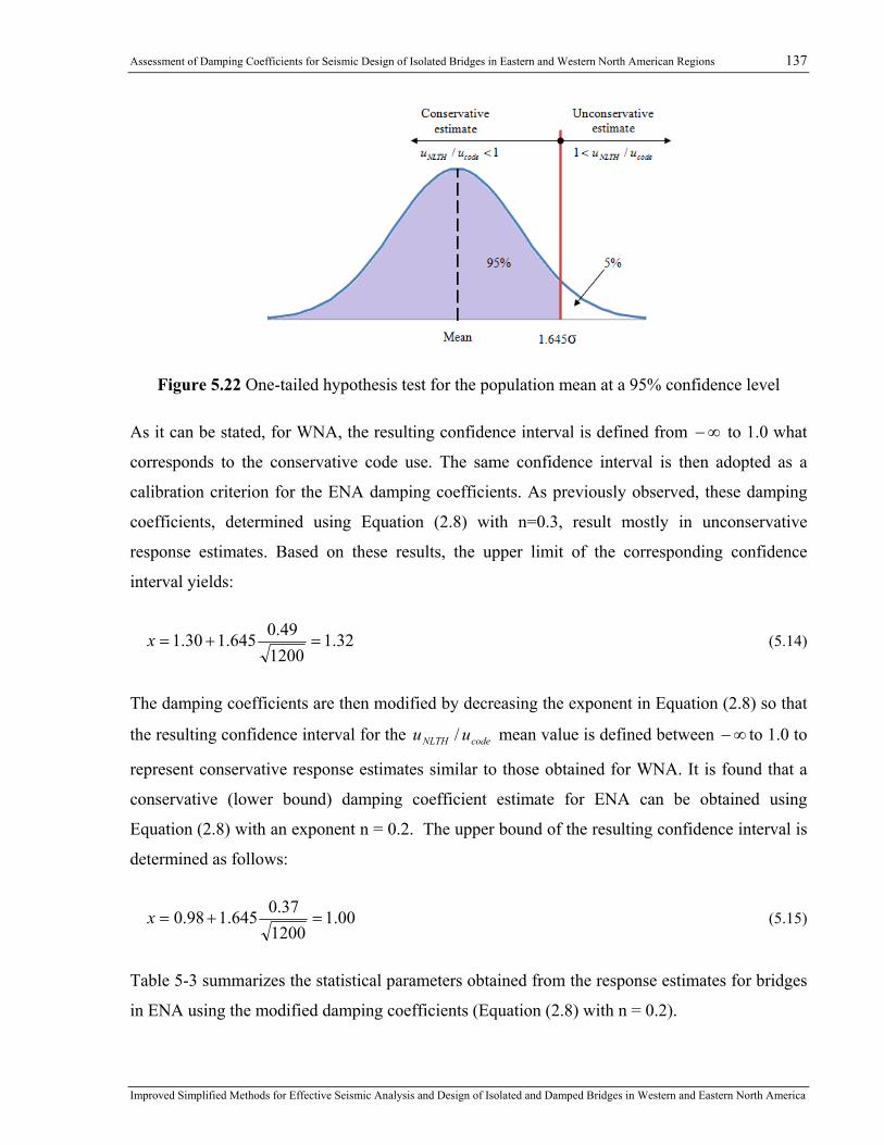
Assessment of Damping Coefficients for Seismic Design of Isolated Bridges in Eastern and Western North American Regions 137
Improved Simplified Methods for Effective Seismic Analysis and Design of Isolated and Damped Bridges in Western and Eastern North America
Figure 5.22 One-tailed hypothesis test for the population mean at a 95% confidence level
As it can be stated, for WNA, the resulting confidence interval is defined from ∞− to 1.0 what
corresponds to the conservative code use. The same confidence interval is then adopted as a
calibration criterion for the ENA damping coefficients. As previously observed, these damping
coefficients, determined using Equation (2.8) with n=0.3, result mostly in unconservative
response estimates. Based on these results, the upper limit of the corresponding confidence
interval yields:
32.11200
49.0645.130.1 =+=x (5.14)
The damping coefficients are then modified by decreasing the exponent in Equation (2.8) so that
the resulting confidence interval for the codeNLTH uu / mean value is defined between ∞− to 1.0 to
represent conservative response estimates similar to those obtained for WNA. It is found that a
conservative (lower bound) damping coefficient estimate for ENA can be obtained using
Equation (2.8) with an exponent n = 0.2. The upper bound of the resulting confidence interval is
determined as follows:
00.11200
37.0645.198.0 =+=x (5.15)
Table 5-3 summarizes the statistical parameters obtained from the response estimates for bridges
in ENA using the modified damping coefficients (Equation (2.8) with n = 0.2).

Assessment of Damping Coefficients for Seismic Design of Isolated Bridges in Eastern and Western North American Regions 138
Improved Simplified Methods for Effective Seismic Analysis and Design of Isolated and Damped Bridges in Western and Eastern North America
Table 5-3 Statistical assessment for results obtained for ENA using Eq.(2.8) with n=0.2
α Mean
codeNLTH uu /
Probability of
1/ =codeNLTH uu
Standard
Deviation COV
ENA
Eq.2.8 with
n=0.2
0.1 0.93 60.3% 0.27 29.2%
0.05 0.95 56.1% 0.31 32.3%
0.01 0.98 51.8% 0.37 37.6%
5.5.2 Validation of the Proposed Damping Coefficients, B
To validate the accuracy of the proposed B-coefficients on the seismic response prediction, the
same 180 isolated bridge structures (5 (R) x 4 (Te) x 3 (β) x 3 (α)) were analyzed following the
complete iterative procedure prescribed in the CSA-S6-06 simplified method using Equation
(2.8) with n=0.2. The results are then validated by comparing the corresponding relative error to
that resulting from the use of Equation (2.8) with n = 0.3 for WNA.
The relative errors were computed for individual responses of 180 isolated bridges undergoing
each individual ground motion demand. Then individual results were averaged over the 20
records for the two ground-motion suites (ENA and WNA) and the resulting mean values are
then compared as a function of the effective period Teff and effective damping effβ both obtained
from the displacement estimate.
As shown in Figures 5.23 and 5.24, for most cases associated to the various effβ and Teff values
obtained in the parametric study, the error ranges from 5% to -50% when using Equation (2.8)
with n = 0.3 for WNA. In the same figures, it is shown that using Equation (2.8) with an
exponent n = 0.2 for ENA results in a comparable relative error range. In this way, the same level
of accuracy would be reached in both parts of the country.
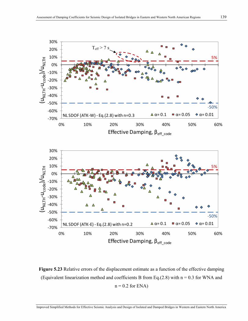
Assessment of Damping Coefficients for Seismic Design of Isolated Bridges in Eastern and Western North American Regions 139
Improved Simplified Methods for Effective Seismic Analysis and Design of Isolated and Damped Bridges in Western and Eastern North America
‐50%
5%
‐70%
‐60%
‐50%
‐40%
‐30%
‐20%
‐10%
0%
10%
20%
30%
0% 10% 20% 30% 40% 50% 60%
(uNLTH‐u
code)/u N
LTH
Effective Damping, βeff_code
NL SDOF (ATK‐E) ‐ Eq.(2.8) with n=0.2 α= 0.1 α= 0.05 α= 0.01
Figure 5.23 Relative errors of the displacement estimate as a function of the effective damping
(Equivalent linearization method and coefficients B from Eq.(2.8) with n = 0.3 for WNA and
n = 0.2 for ENA)
‐50%
5%
‐70%
‐60%
‐50%
‐40%
‐30%
‐20%
‐10%
0%
10%
20%
30%
0% 10% 20% 30% 40% 50% 60%
(uNLTH‐u
code)/u N
LTH
Effective Damping, βeff_code
NL SDOF (ATK‐W) ‐ Eq.(2.8) with n=0.3 α= 0.1 α= 0.05 α= 0.01
Teff > 7 s

Assessment of Damping Coefficients for Seismic Design of Isolated Bridges in Eastern and Western North American Regions 140
Improved Simplified Methods for Effective Seismic Analysis and Design of Isolated and Damped Bridges in Western and Eastern North America
‐50%
5%
‐70%
‐60%
‐50%
‐40%
‐30%
‐20%
‐10%
0%
10%
20%
30%
0 1 2 3 4 5 6 7 8 9 10
(uNLTH‐u
code)/u N
LTH
Effective Period, Teff_code
NL SDOF (ATK‐W) ‐ Eq.(2.8) with n=0.3 α= 0.1 α= 0.05 α= 0.01
‐50%
5%
‐70%
‐60%
‐50%
‐40%
‐30%
‐20%
‐10%
0%
10%
20%
30%
0 1 2 3 4 5 6 7 8 9 10
(uNLTH‐u
code)/u N
LTH
Effective Period, Teff_code
NL SDOF (ATK‐E) ‐ Eq.(2.8) with n=0.2 α= 0.1 α= 0.05 α= 0.01
Figure 5.24 Relative errors of the displacement estimate as a function of the effective period
(Equivalent linearization method and coefficients B from Eq.(2.8) with n = 0.3 for WNA and
n = 0.2 for ENA)
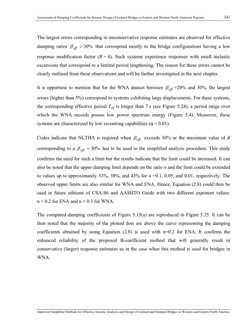
Assessment of Damping Coefficients for Seismic Design of Isolated Bridges in Eastern and Western North American Regions 141
Improved Simplified Methods for Effective Seismic Analysis and Design of Isolated and Damped Bridges in Western and Eastern North America
The largest errors corresponding to unconservative response estimates are observed for effective
damping ratios %30>effβ that correspond mostly to the bridge configurations having a low
response modification factor (R = 4). Such systems experience responses with small inelastic
excursions that correspond to a limited period lengthening. The reason for these errors cannot be
clearly outlined from these observations and will be further investigated in the next chapter.
It is opportune to mention that for the WNA dataset between effβ =20% and 30%, the largest
errors (higher than 5%) correspond to systems exhibiting large displacements. For these systems,
the corresponding effective period Teff is longer than 7 s (see Figure 5.24), a period range over
which the WNA records posses low power spectrum energy (Figure 5.4). Moreover, these
systems are characterized by low recentring capabilities (α = 0.01).
Codes indicate that NLTHA is required when effβ exceeds 30% or the maximum value of B
corresponding to a %30=effβ has to be used in the simplified analysis procedure. This study
confirms the need for such a limit but the results indicate that the limit could be increased. It can
also be noted that the upper damping limit depends on the ratio α and the limit could be extended
to values up to approximately 33%, 38%, and 43% for α =0.1, 0.05, and 0.01, respectively. The
observed upper limits are also similar for WNA and ENA. Hence, Equation (2.8) could then be
used in future editions of CSA-S6 and AASHTO Guide with two different exponent values:
n = 0.2 for ENA and n = 0.3 for WNA.
The computed damping coefficients of Figure 5.15(a) are reproduced in Figure 5.25. It can be
then noted that the majority of the plotted dots are above the curve representing the damping
coefficients obtained by using Equation (2.8) is used with n=0.2 for ENA. It confirms the
enhanced reliability of the proposed B-coefficient method that will generally result in
conservative (larger) response estimates as in the case when this method is used for bridges in
WNA.
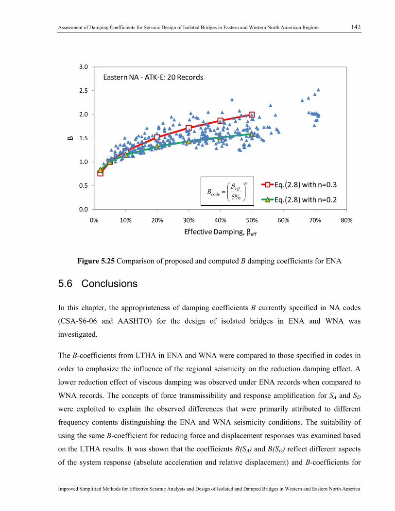
Assessment of Damping Coefficients for Seismic Design of Isolated Bridges in Eastern and Western North American Regions 142
Improved Simplified Methods for Effective Seismic Analysis and Design of Isolated and Damped Bridges in Western and Eastern North America
Figure 5.25 Comparison of proposed and computed B damping coefficients for ENA
5.6 Conclusions
In this chapter, the appropriateness of damping coefficients B currently specified in NA codes
(CSA-S6-06 and AASHTO) for the design of isolated bridges in ENA and WNA was
investigated.
The B-coefficients from LTHA in ENA and WNA were compared to those specified in codes in
order to emphasize the influence of the regional seismicity on the reduction damping effect. A
lower reduction effect of viscous damping was observed under ENA records when compared to
WNA records. The concepts of force transmissibility and response amplification for SA and SD
were exploited to explain the observed differences that were primarily attributed to different
frequency contents distinguishing the ENA and WNA seismicity conditions. The suitability of
using the same B-coefficient for reducing force and displacement responses was examined based
on the LTHA results. It was shown that the coefficients B(SA) and B(SD) reflect different aspects
of the system response (absolute acceleration and relative displacement) and B-coefficients for
0.0
0.5
1.0
1.5
2.0
2.5
3.0
0% 10% 20% 30% 40% 50% 60% 70% 80%
B
Effective Damping, βeff
Eastern NA ‐ ATK‐E: 20 Records
Eq.(2.8) with n=0.3
Eq.(2.8) with n=0.2
neff
codeB ⎟⎟⎠
⎞⎜⎜⎝
⎛=
%5β

Assessment of Damping Coefficients for Seismic Design of Isolated Bridges in Eastern and Western North American Regions 143
Improved Simplified Methods for Effective Seismic Analysis and Design of Isolated and Damped Bridges in Western and Eastern North America
reducing force and displacement responses must be independently calibrated. For a more
accurate evaluation of the displacement across isolation bearings, the analysis results suggest that
for the simplified code method the definition of the B coefficients should be based on spectral
displacements rather than spectral accelerations. The dependency of the B-coefficients on the
effective period was also confirmed.
In this study, complementary to most of previous studies performed worldwide in which LTHA
was used, an extensive parametric study was carried out using dynamic NLTHA so that a series
of nonlinear system parameters was considered to cover a wide range of isolated and damped
bridge configurations. A total of 12 000 NLTHA were carried out on 300 isolated bridge
configurations under 20 time-history records representatively for the WNA and ENA regional
seismicity (40 records in total). Based on the observations made for LTHA, in the parametric
study, the damping coefficients were assessed solely for displacement responses. The damping
coefficients specified in current CSA-S6 and AASHTO codes were found to result mostly in safe
designs for WNA but underestimated the displacement demand of bridges subjected to ENA
seismic ground motions.
Based on these results a new value was proposed for the exponent to be used in the equation
currently specified in the AASHTO specifications for the damping coefficients so that the same
equation can be used with different exponents for WNA and ENA locations. The study also
showed that the current upper limit on the effective damping ratio for the application of the
simplified methods in North America could be relaxed and defined more accurately as a function
of the post-yielding stiffness ratio α.
Despite the improvements made, the simplified method still under predicts the response of
isolated bridges for a number of cases. In particular, systems with low R factors, low α ratios,
with high effective damping ratios or short effective periods were found to be more critical in
this regard. This indicates that there is a need to improve our understanding of the sources of the
inaccuracy that are inherent to the simplified analysis procedure used in design codes. This
aspect is further examined in detail in the following chapters.
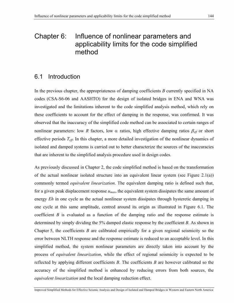
Influence of nonlinear parameters and applicability limits for the code simplified method 144
Improved Simplified Methods for Effective Seismic Analysis and Design of Isolated and Damped Bridges in Western and Eastern North America
Chapter 6: Influence of nonlinear parameters and applicability limits for the code simplified method
6.1 Introduction
In the previous chapter, the appropriateness of damping coefficients B currently specified in NA
codes (CSA-S6-06 and AASHTO) for the design of isolated bridges in ENA and WNA was
investigated and the limitations inherent to the code simplified analysis method, which rely on
these coefficients to account for the effect of damping in the response, was confirmed. It was
observed that the inaccuracy of the simplified code method can be associated to certain ranges of
nonlinear parameters: low R factors, low α ratios, high effective damping ratios βeff or short
effective periods Teff. In this chapter, a more detailed investigation of the nonlinear dynamics of
isolated and damped systems is carried out to better characterize the sources of the inaccuracies
that are inherent to the simplified analysis procedure used in design codes.
As previously discussed in Chapter 2, the code simplified method is based on the transformation
of the actual nonlinear isolated structure into an equivalent linear system (see Figure 2.1(a))
commonly termed equivalent linearization. The equivalent damping ratio is defined such that,
for a given peak displacement response umax, the equivalent system dissipates the same amount of
energy Eh in one cycle as the actual nonlinear system dissipates through hysteretic damping in
one cycle at this same amplitude, centred around its origin as illustrated in Figure 6.1. The
coefficient B is evaluated as a function of the damping ratio and the response estimate is
determined by simply dividing the 5% damped elastic response by the coefficient B. As shown in
Chapter 5, the coefficients B are calibrated empirically for a given regional seismicity so the
error between NLTH response and the response estimate is reduced to an acceptable level. In this
simplified method, the system nonlinear parameters are directly taken into account by the
process of equivalent linearization, while the effect of regional seismicity is expected to be
reflected by applying different coefficients B. The coefficients B are however calibrated so the
accuracy of the simplified method is enhanced by reducing errors from both sources, the
equivalent linearization and the local damping reduction effect.

Influence of nonlinear parameters and applicability limits for the code simplified method 145
Improved Simplified Methods for Effective Seismic Analysis and Design of Isolated and Damped Bridges in Western and Eastern North America
Figure 6.1 Transformation of Actual Nonlinear System (Bilinear Response) to Equivalent
Figure 6.1 Bilinear response and equivalent viscoelastic response
To improve our understanding of the actual sources of inaccuracy that are present in the response
estimates, the influence of the nonlinear parameters that were used in the parametric study that
was carried out in the previous chapter is first discussed. Then, the accuracy of the equivalent
linearization method is carefully examined and the influence of the nonlinear parameters is
outlined. Recommendations are made on how to define the range of parameters for which the
equivalent linearization method can provide an accurate response estimate. The need for a new
simplified method that takes into account the differences in ground-motion characteristics and
isolated bridge design parameters is also outlined in this chapter.
6.2 Influence of System Properties on Damping Coefficients and
the Code Simplified Method
Parameters such as the initial period Te, the post-yield stiffness ratio α, and the response
modification factor R make it possible to define the hysteretic properties of the system at the
initial design stage. These parameters were adopted for the parametric study carried out in the
previous chapter. Their influence on the response of isolated bridges and B coefficients were
presented.
Elastic Te and effective periods Teff
The initial effective period Te interacts with the predominant earthquake period when the system
behaves essentially elastically and is a relevant parameter when using elastic response spectra. In
eT
effk
F
effTeffk
uk
dk
F
maxF
maxu maxuu u
1
1 1
1
Equivalent System Actual Nonlinear System
effT

Influence of nonlinear parameters and applicability limits for the code simplified method 146
Improved Simplified Methods for Effective Seismic Analysis and Design of Isolated and Damped Bridges in Western and Eastern North America
other words, when the time function of the seismic excitation is decomposed into a Fourier
series, the dynamic response amplification may be simply attributed to the resonant interaction
between the structure and time functions of the ground motion. Accordingly, for an elastic
system, the resonant interaction occurs solely at the elastic period Te. For such systems, damping
coefficients for displacement responses tend to unity for very short periods and very long
periods, and maximum damping effects are expected for intermediate periods in the velocity-
sensitive region of the spectrum, especially for periods close to the predominant ground motion
periods (Chopra, 2011). As was discussed in Chapter 5 for harmonic response, the damping
effect varies as a function of the ratio Te / Tg.
For systems responding in the inelastic range, the influence of the effective damping on the
response should depend on the ratio Teff / Tg rather than Te / Tg. However, the initial effective
period Te is a parameter that can be more easily defined at the initial design stage, when the
system response is still unknown. It also clearly defines the lower bound and can be used to
estimate the extent of the likely range of the effective period Teff. The influence of Te on the
damping coefficients B obtained from NLTHA for ENA ground motions is outlined in Figure
6.2. The reduction effect of damping, represented in terms of B, is the highest for structures with
the shortest initial period (Te = 0.25 s). For these structures, NA code damping coefficients will
result in conservative response estimates for most cases. For longer initial periods (Te = 0.5 s to
1.0 s), damping coefficients are smaller and code-prescribed values are unconservative for effβ
greater than the 20-30% range.
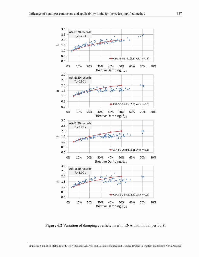
Influence of nonlinear parameters and applicability limits for the code simplified method 147
Improved Simplified Methods for Effective Seismic Analysis and Design of Isolated and Damped Bridges in Western and Eastern North America
0.0
0.5
1.0
1.5
2.0
2.5
3.0
0% 10% 20% 30% 40% 50% 60% 70% 80%
B
Effective Damping, βeff
Atk‐E: 20 recordsTe=0.25 s
CSA‐S6‐06 (Eq.(2.8) with n=0.3)
0.0
0.5
1.0
1.5
2.0
2.5
3.0
0% 10% 20% 30% 40% 50% 60% 70% 80%
B
Effective Damping, βeff
Atk‐E: 20 recordsTe=0.50 s
CSA‐S6‐06 (Eq.(2.8) with n=0.3)
0.0
0.5
1.0
1.5
2.0
2.5
3.0
0% 10% 20% 30% 40% 50% 60% 70% 80%
B
Effective Damping, βeff
Atk‐E: 20 recordsTe=0.75 s
CSA‐S6‐06 (Eq.(2.8) with n=0.3)
0.0
0.5
1.0
1.5
2.0
2.5
3.0
0% 10% 20% 30% 40% 50% 60% 70% 80%
B
Effective Damping, βeff
Atk‐E: 20 recordsTe=1.00 s
CSA‐S6‐06 (Eq.(2.8) with n=0.3)
Figure 6.2 Variation of damping coefficients B in ENA with initial period Te

Influence of nonlinear parameters and applicability limits for the code simplified method 148
Improved Simplified Methods for Effective Seismic Analysis and Design of Isolated and Damped Bridges in Western and Eastern North America
Response modification factor R
The response modification factor R characterizes the response by relating the isolation activation
limit to the elastic demand for a given UHS. Figure 6.3 shows how the system’s hysteretic shape
is defined based on the response modification factor. It can be noted from this figure that systems
designed with low response modification factors R exhibit a limited inelastic response and are
therefore characterized by the elastic properties of the system while the response of systems with
higher R-factors is mostly oriented along the post-activation stiffness kd, resulting in a longer
effective period Teff and larger displacements.
Figure 6.3 Bilinear response - Influence of the R factor on the hysteretic shape
Post-yielding stiffness ratio α
As observed in the previous chapter, larger displacements are observed in systems with a smaller
α ratio (small post-activation stiffness) where the peak response is increased as a result of the
system’s lower recentring capability.

Influence of nonlinear parameters and applicability limits for the code simplified method 149
Improved Simplified Methods for Effective Seismic Analysis and Design of Isolated and Damped Bridges in Western and Eastern North America
The systems with low recentring capability are also more prone to residual displacements. It is
important to take residual displacements into account given that the displacement response to the
subsequent ground motion will start from the position corresponding to the residual displacement
from the previous motion. Similarly, when the ground motion is represented by a series of single-
pulse motions, the initial zero position for each new pulse is the position reached at the end of the
previous one.
Accordingly, the initial equilibrium position may drift during an earthquake motion. In other
words, during inelastic excursions, the system’s oscillation center drifts from its initial zero-
displacement position and the system starts vibrating around a new equilibrium position termed
the transient oscillation center, after large inelastic cycles. A large or a few consecutive smaller
yielding excursions in the same direction produces an inelastic response that is skewed in the
direction of these inelastic excursions.
In such cases, the maximum displacement response will not reflect the real damping that is
associated with the peak response of the system, and which is defined as a portion of the
dissipated hysteretic energy, Eh as illustrated in Figure 6.4. For two systems with the same
properties as elastic initial period Te (or elastic stiffness ku), system activation limit uy (or
response modification factor R), and post-yielding stiffness ratio α (or post-yielding stiffness kd),
the real energy dissipated around a drifted oscillation center may be strongly overestimated by
considering an equivalent response around the original center as prescribed in the CSA-S6-06
code (or AASHTO). It could be noted from Figure 6.4 that the effective stiffness keff (or effective
period Teff) of the equivalent response about the original center misrepresents the real system
behaviour when the system drifts from its initial equilibrium position.
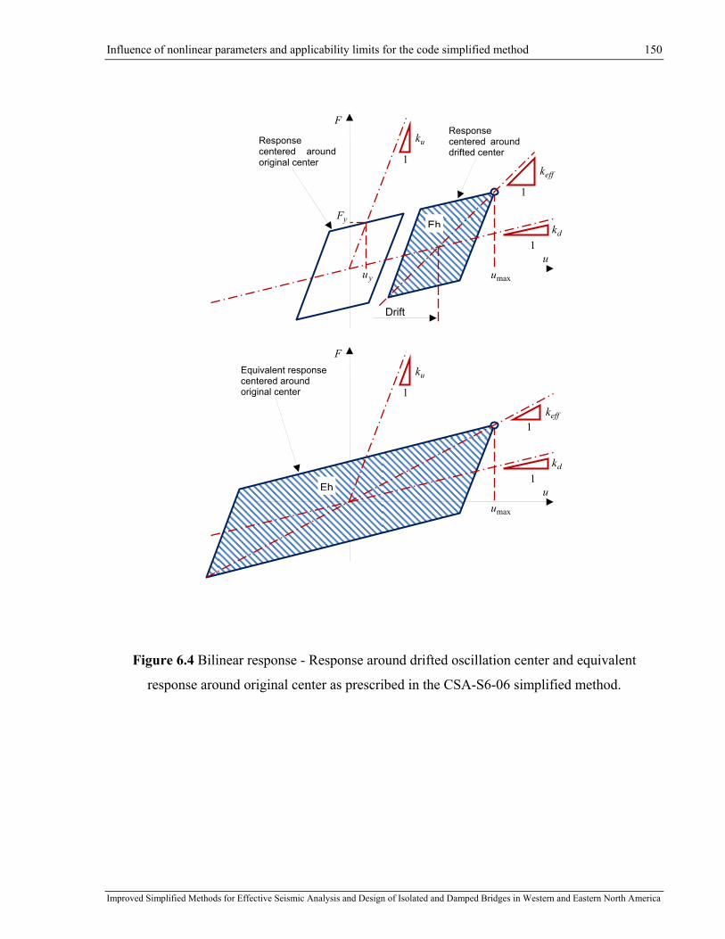
Influence of nonlinear parameters and applicability limits for the code simplified method 150
Improved Simplified Methods for Effective Seismic Analysis and Design of Isolated and Damped Bridges in Western and Eastern North America
Figure 6.4 Bilinear response - Response around drifted oscillation center and equivalent
response around original center as prescribed in the CSA-S6-06 simplified method.
effk
1
F
u
dk1
uk
1
yF
maxuyu
Response centered around original center
Drift
Response centered around drifted center
Eh
F
u
dk1
uk
1
maxu
effk1
Equivalent response centered around original center
Eh

Influence of nonlinear parameters and applicability limits for the code simplified method 151
Improved Simplified Methods for Effective Seismic Analysis and Design of Isolated and Damped Bridges in Western and Eastern North America
B-coefficients with nonlinear system parameters
The damping coefficients obtained through NLTH in the previous chapter for ENA are presented
versus Teff for different R and α parameters in Figure 6.5. Certain trends are outlined by using
second degree polynominal trendlines which put in evidence that the same effective damping for
different period ranges may be characterized by a different damping reduction effect.
It can be observed that for systems with post-activation stiffness ratio α = 0.1 and 0.05, damping
coefficients are larger for elastic periods in the range of Te = 0.25 and 1.0 s when compared to
those obtained in the range of Te = 0.5 and 0.75 s. For the systems with α = 0.01, the largest
damping coefficients are observed for Te = 0.25, while for the three longer elastic periods
(Te = 0.5, 075 and 1.0), the curves describing B-coefficients are similar and differ generally by
the effect of the corresponding period lengthening. As discussed previously, long effective
periods are obtained for systems with large R factors and low α factors. For these systems (e.g.,
α = 0.01), the damping coefficients do not vary much with the effective period after
approximately Teff = 3.7 s.
These observations provide further evidence of the influence of the nonlinear system parameters
on the observed damping coefficients. However, a simple physical explanation on the sources of
this variability, that may account for the inaccuracies that have been observed in the code
simplified methods, has not yet been proposed. This is examined in more detail in the following
sections.
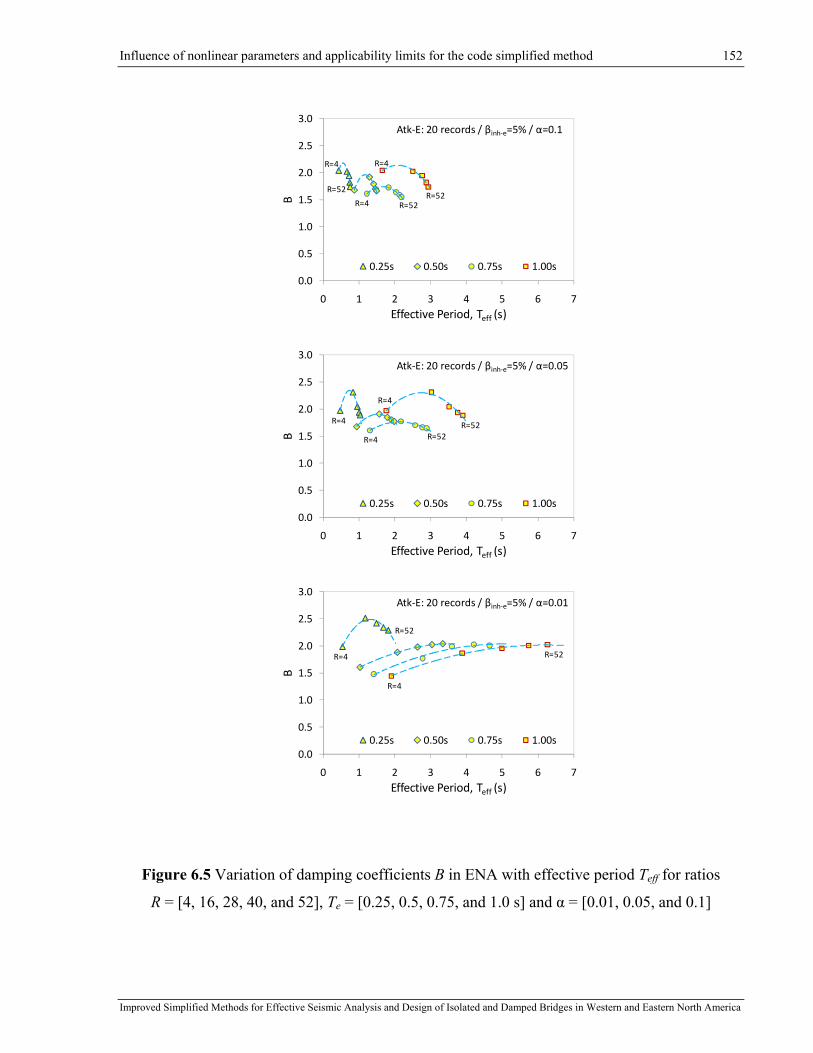
Influence of nonlinear parameters and applicability limits for the code simplified method 152
Improved Simplified Methods for Effective Seismic Analysis and Design of Isolated and Damped Bridges in Western and Eastern North America
R=4
R=52
R=4 R=52
R=4
R=52
0.0
0.5
1.0
1.5
2.0
2.5
3.0
0 1 2 3 4 5 6 7B
Effective Period, Teff (s)
Atk‐E: 20 records / βinh‐e=5% / α=0.1
0.25s 0.50s 0.75s 1.00s
R=4
R=4 R=52
R=4
R=52
0.0
0.5
1.0
1.5
2.0
2.5
3.0
0 1 2 3 4 5 6 7
B
Effective Period, Teff (s)
Atk‐E: 20 records / βinh‐e=5% / α=0.05
0.25s 0.50s 0.75s 1.00s
R=4
R=52
R=4
R=52
0.0
0.5
1.0
1.5
2.0
2.5
3.0
0 1 2 3 4 5 6 7
B
Effective Period, Teff (s)
Atk‐E: 20 records / βinh‐e=5% / α=0.01
0.25s 0.50s 0.75s 1.00s
Figure 6.5 Variation of damping coefficients B in ENA with effective period Teff for ratios
R = [4, 16, 28, 40, and 52], Te = [0.25, 0.5, 0.75, and 1.0 s] and α = [0.01, 0.05, and 0.1]
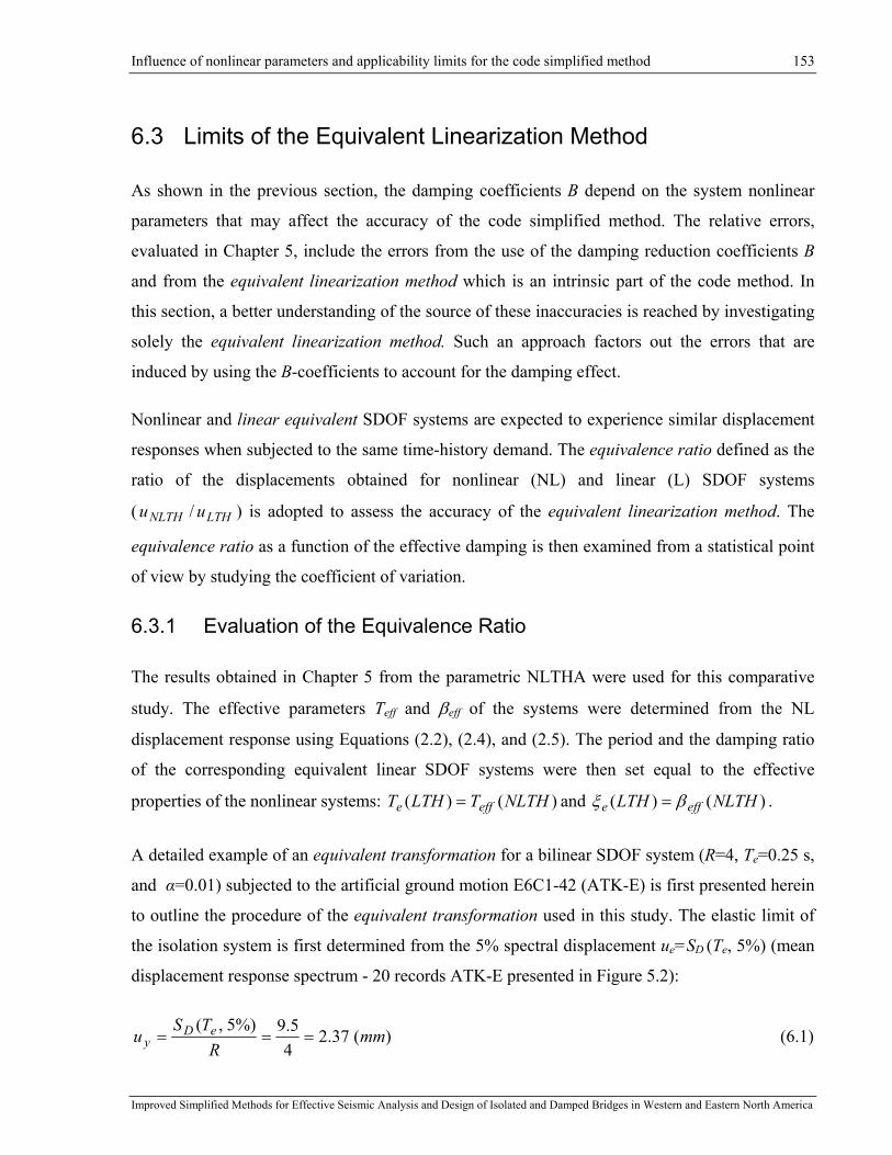
Influence of nonlinear parameters and applicability limits for the code simplified method 153
Improved Simplified Methods for Effective Seismic Analysis and Design of Isolated and Damped Bridges in Western and Eastern North America
6.3 Limits of the Equivalent Linearization Method
As shown in the previous section, the damping coefficients B depend on the system nonlinear
parameters that may affect the accuracy of the code simplified method. The relative errors,
evaluated in Chapter 5, include the errors from the use of the damping reduction coefficients B
and from the equivalent linearization method which is an intrinsic part of the code method. In
this section, a better understanding of the source of these inaccuracies is reached by investigating
solely the equivalent linearization method. Such an approach factors out the errors that are
induced by using the B-coefficients to account for the damping effect.
Nonlinear and linear equivalent SDOF systems are expected to experience similar displacement
responses when subjected to the same time-history demand. The equivalence ratio defined as the
ratio of the displacements obtained for nonlinear (NL) and linear (L) SDOF systems
( LTHNLTH uu / ) is adopted to assess the accuracy of the equivalent linearization method. The
equivalence ratio as a function of the effective damping is then examined from a statistical point
of view by studying the coefficient of variation.
6.3.1 Evaluation of the Equivalence Ratio
The results obtained in Chapter 5 from the parametric NLTHA were used for this comparative
study. The effective parameters Teff and βeff of the systems were determined from the NL
displacement response using Equations (2.2), (2.4), and (2.5). The period and the damping ratio
of the corresponding equivalent linear SDOF systems were then set equal to the effective
properties of the nonlinear systems: )()( NLTHTLTHT effe = and )()( NLTHLTH effe βξ = .
A detailed example of an equivalent transformation for a bilinear SDOF system (R=4, Te=0.25 s,
and α=0.01) subjected to the artificial ground motion E6C1-42 (ATK-E) is first presented herein
to outline the procedure of the equivalent transformation used in this study. The elastic limit of
the isolation system is first determined from the 5% spectral displacement ue=SD (Te, 5%) (mean
displacement response spectrum - 20 records ATK-E presented in Figure 5.2):
)(37.245.9%)5,(
mmR
TSu eD
y === (6.1)

Influence of nonlinear parameters and applicability limits for the code simplified method 154
Improved Simplified Methods for Effective Seismic Analysis and Design of Isolated and Damped Bridges in Western and Eastern North America
The peak displacement from the NLTHA is 12.0 mm and the ductility demand µ is then found
as:
06.537.2
12===
y
NLTHu
uμ (6.2)
The effective period is determined as a function of the ductility using Equation (2.2):
sTT eeff 55.001.006.501.01
06.525.01
=−⋅+
=−+
=ααμ
μ (6.3)
An inherent damping, einh−β , of 2% is assumed for the system. This damping ratio is based on
the elastic period Te=0.25 s. It is transformed into the inherent damping at Teff=0.55 s as:
%4.425.055.0%0.2 =⋅== −−
e
effeinheffinh T
Tββ (6.4)
The equivalent damping ratio eqβ is determined through the system hysteretic response:
%6.48)01.006.501.01(06.5
)01.01()106.5(2)1()1()1(2
=−⋅+⋅
−⋅−⋅=
−+⋅−⋅−
⋅=πααμμ
αμπ
βeq (6.5)
The combined effective damping ratio of the equivalent linear system can be determined from:
%53%4.4%6.48 =+=+= −effinheqeff βββ (6.6)
A linear SDOF system is then defined using the following equivalent effective parameters:
Te=0.55 s and %53=eξ . The peak response of the equivalent linearized system under the same
ground motion E6C1-42 (ATK-E) results in mmuLTH 0.8= . The corresponding equivalence
ratio is determined as:
5.10.80.12
==LTH
NLTHu
u (6.7)
An equivalence ratio higher than 1.0 indicates that the response obtained using the equivalent
linear SDOF system underestimates the "real" displacement demand. The responses from the

Influence of nonlinear parameters and applicability limits for the code simplified method 155
Improved Simplified Methods for Effective Seismic Analysis and Design of Isolated and Damped Bridges in Western and Eastern North America
NLTHA and equivalent LTHA are presented in Figure 6.6. It can be noted that for the nonlinear
(NL-SDOF) and equivalent (L-SDOF) systems, the maximum response amplitudes are reached
in opposite directions. The absolute response values are then compared. However, it is opportune
to note that if the maximum responses for both NLTH and LTH responses occur in the same
direction, the divergence in the peak response is primarily attributed to the drift of the system
oscillation center that leads to the underestimation of the "real" displacement response as shown
in Figure 6.6.
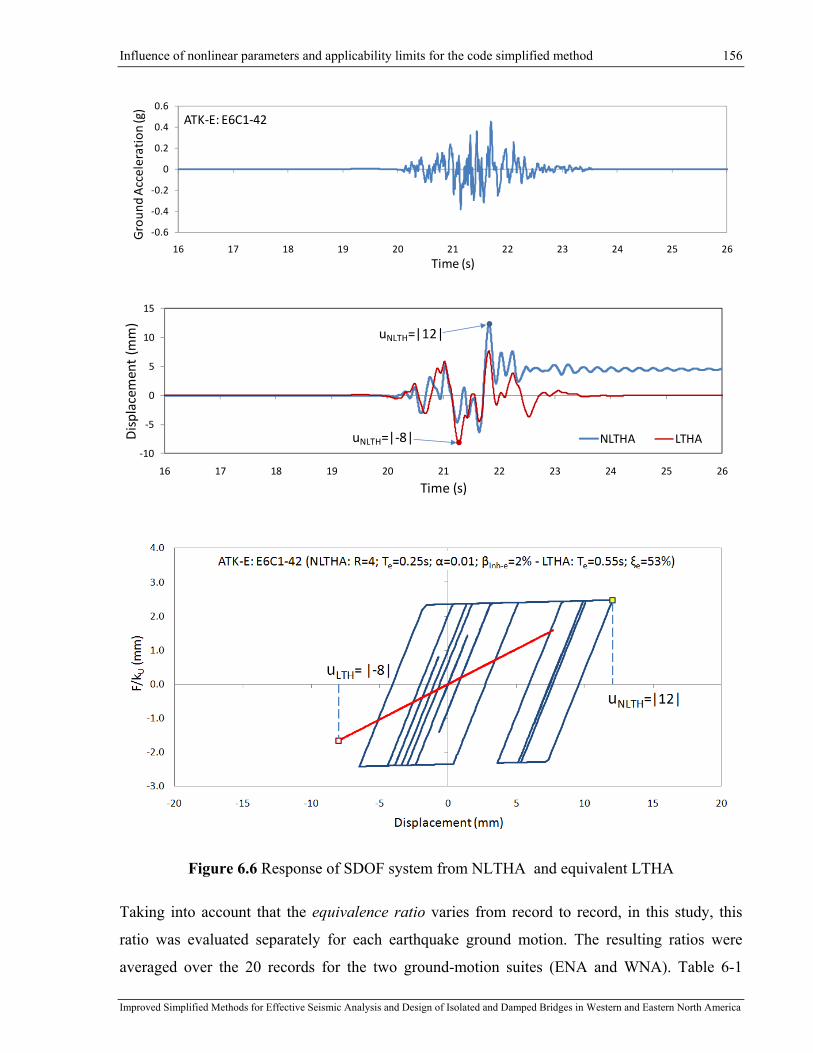
Influence of nonlinear parameters and applicability limits for the code simplified method 156
Improved Simplified Methods for Effective Seismic Analysis and Design of Isolated and Damped Bridges in Western and Eastern North America
‐0.6
‐0.4
‐0.2
0
0.2
0.4
0.6
16 17 18 19 20 21 22 23 24 25 26
Groun
d Acceleration (g)
Time (s)
ATK‐E: E6C1‐42
‐10
‐5
0
5
10
15
16 17 18 19 20 21 22 23 24 25 26
Displacem
ent (m
m)
Time (s)
NLTHA LTHA
uNLTH=|12|
uNLTH=|‐8|
Figure 6.6 Response of SDOF system from NLTHA and equivalent LTHA
Taking into account that the equivalence ratio varies from record to record, in this study, this
ratio was evaluated separately for each earthquake ground motion. The resulting ratios were
averaged over the 20 records for the two ground-motion suites (ENA and WNA). Table 6-1
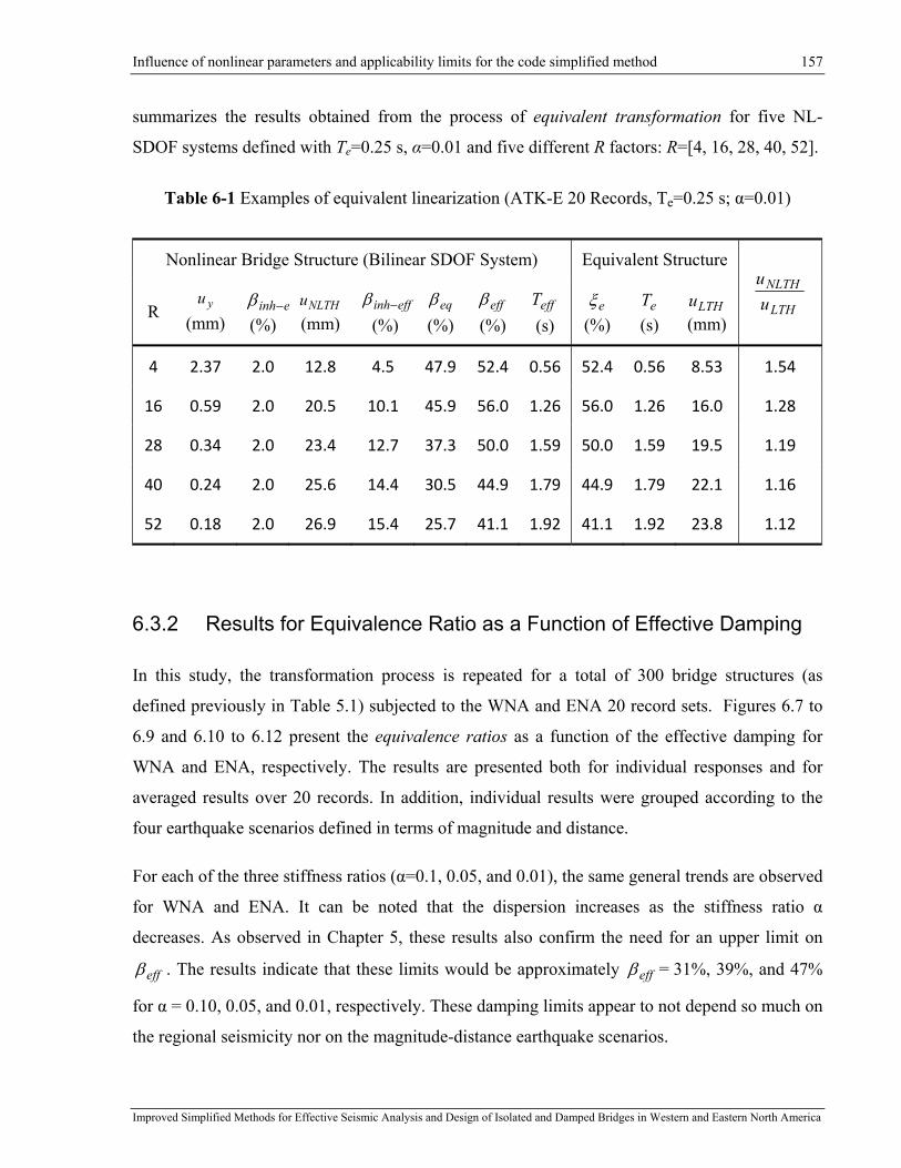
Influence of nonlinear parameters and applicability limits for the code simplified method 157
Improved Simplified Methods for Effective Seismic Analysis and Design of Isolated and Damped Bridges in Western and Eastern North America
summarizes the results obtained from the process of equivalent transformation for five NL-
SDOF systems defined with Te=0.25 s, α=0.01 and five different R factors: R=[4, 16, 28, 40, 52].
Table 6-1 Examples of equivalent linearization (ATK-E 20 Records, Te=0.25 s; α=0.01)
Nonlinear Bridge Structure (Bilinear SDOF System) Equivalent Structure
LTH
NLTHu
u
R yu (mm)
einh−β(%)
NLTHu (mm)
effinh−β (%)
eqβ (%)
effβ (%)
effT (s)
eξ (%)
eT (s)
LTHu (mm)
4 2.37 2.0 12.8 4.5 47.9 52.4 0.56 52.4 0.56 8.53 1.54
16 0.59 2.0 20.5 10.1 45.9 56.0 1.26 56.0 1.26 16.0 1.28
28 0.34 2.0 23.4 12.7 37.3 50.0 1.59 50.0 1.59 19.5 1.19
40 0.24 2.0 25.6 14.4 30.5 44.9 1.79 44.9 1.79 22.1 1.16
52 0.18 2.0 26.9 15.4 25.7 41.1 1.92 41.1 1.92 23.8 1.12
6.3.2 Results for Equivalence Ratio as a Function of Effective Damping
In this study, the transformation process is repeated for a total of 300 bridge structures (as
defined previously in Table 5.1) subjected to the WNA and ENA 20 record sets. Figures 6.7 to
6.9 and 6.10 to 6.12 present the equivalence ratios as a function of the effective damping for
WNA and ENA, respectively. The results are presented both for individual responses and for
averaged results over 20 records. In addition, individual results were grouped according to the
four earthquake scenarios defined in terms of magnitude and distance.
For each of the three stiffness ratios (α=0.1, 0.05, and 0.01), the same general trends are observed
for WNA and ENA. It can be noted that the dispersion increases as the stiffness ratio α
decreases. As observed in Chapter 5, these results also confirm the need for an upper limit on
effβ . The results indicate that these limits would be approximately effβ = 31%, 39%, and 47%
for α = 0.10, 0.05, and 0.01, respectively. These damping limits appear to not depend so much on
the regional seismicity nor on the magnitude-distance earthquake scenarios.

Influence of nonlinear parameters and applicability limits for the code simplified method 158
Improved Simplified Methods for Effective Seismic Analysis and Design of Isolated and Damped Bridges in Western and Eastern North America
0.0
0.5
1.0
1.5
2.0
2.5
3.0
3.5
0% 10% 20% 30% 40% 50%
u NLTH/u
LTH
Effective Damping, βeff
ATK‐W W6C1α=0.1
0.0
0.5
1.0
1.5
2.0
2.5
3.0
3.5
0% 10% 20% 30% 40% 50%
u NLTH/u
LTH
Effective Damping, βeff
ATK‐W W6C2α=0.1
0.0
0.5
1.0
1.5
2.0
2.5
3.0
3.5
0% 10% 20% 30% 40% 50%
u NLTH/u
LTH
Effective Damping, βeff
ATK‐W W7C1α=0.1
0.0
0.5
1.0
1.5
2.0
2.5
3.0
3.5
0% 10% 20% 30% 40% 50%u N
LTH/u
LTH
Effective Damping, βeff
ATK‐W W7C2α=0.1
Figure 6.7 Equivalence ratio - WNA ATK-W: α=0.1

Influence of nonlinear parameters and applicability limits for the code simplified method 159
Improved Simplified Methods for Effective Seismic Analysis and Design of Isolated and Damped Bridges in Western and Eastern North America
0.0
0.5
1.0
1.5
2.0
2.5
3.0
3.5
0% 10% 20% 30% 40% 50% 60%
u NLTH/u
LTH
Effective Damping, βeff
ATK‐W W6C1α=0.05
0.0
0.5
1.0
1.5
2.0
2.5
3.0
3.5
0% 10% 20% 30% 40% 50% 60%
u NLTH/u
LTH
Effective Damping, βeff
ATK‐W W6C2α=0.05
0.0
0.5
1.0
1.5
2.0
2.5
3.0
3.5
0% 10% 20% 30% 40% 50% 60%
u NLTH/u
LTH
Effective Damping, βeff
ATK‐W W7C1α=0.05
0.0
0.5
1.0
1.5
2.0
2.5
3.0
3.5
0% 10% 20% 30% 40% 50% 60%u N
LTH/u
LTH
Effective Damping, βeff
ATK‐W W7C2α=0.05
Figure 6.8 Equivalence ratio - WNA ATK-W: α=0.05

Influence of nonlinear parameters and applicability limits for the code simplified method 160
Improved Simplified Methods for Effective Seismic Analysis and Design of Isolated and Damped Bridges in Western and Eastern North America
0.0
0.5
1.0
1.5
2.0
2.5
3.0
3.5
0% 10% 20% 30% 40% 50% 60% 70% 80%
u NLTH/u
LTH
Effective Damping, βeff
ATK‐W W6C1α=0.01
0.0
0.5
1.0
1.5
2.0
2.5
3.0
3.5
0% 10% 20% 30% 40% 50% 60% 70% 80%
u NLTH/u
LTH
Effective Damping, βeff
ATK‐W W6C2α=0.01
0.0
0.5
1.0
1.5
2.0
2.5
3.0
3.5
0% 10% 20% 30% 40% 50% 60% 70% 80%
u NLTH/u
LTH
Effective Damping, βeff
ATK‐W W7C1α=0.01
0.0
0.5
1.0
1.5
2.0
2.5
3.0
3.5
0% 10% 20% 30% 40% 50% 60% 70% 80%u N
LTH/u
LTH
Effective Damping, βeff
ATK‐W W7C2α=0.01
Figure 6.9 Equivalence ratio - WNA ATK-W: α=0.01

Influence of nonlinear parameters and applicability limits for the code simplified method 161
Improved Simplified Methods for Effective Seismic Analysis and Design of Isolated and Damped Bridges in Western and Eastern North America
0.0
0.5
1.0
1.5
2.0
2.5
3.0
3.5
0% 10% 20% 30% 40% 50%
u NLTH/u
LTH
Effective Damping, βeff
ATK‐E E6C1α=0.1
0.0
0.5
1.0
1.5
2.0
2.5
3.0
3.5
0% 10% 20% 30% 40% 50%
u NLTH/u
LTH
Effective Damping, βeff
ATK‐E E6C2α=0.1
0.0
0.5
1.0
1.5
2.0
2.5
3.0
3.5
0% 10% 20% 30% 40% 50%
u NLTH/u
LTH
Effective Damping, βeff
ATK‐E E7C1α=0.1
0.0
0.5
1.0
1.5
2.0
2.5
3.0
3.5
0% 10% 20% 30% 40% 50%u N
LTH/u
LTH
Effective Damping, βeff
ATK‐E E7C2α=0.1
Figure 6.10 Equivalence ratio - ENA ATK-E: α=0.1
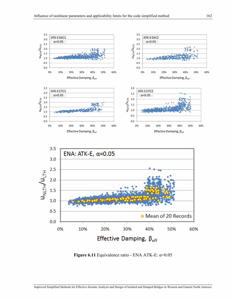
Influence of nonlinear parameters and applicability limits for the code simplified method 162
Improved Simplified Methods for Effective Seismic Analysis and Design of Isolated and Damped Bridges in Western and Eastern North America
0.0
0.5
1.0
1.5
2.0
2.5
3.0
3.5
0% 10% 20% 30% 40% 50% 60%
u NLTH/u
LTH
Effective Damping, βeff
ATK‐E E6C1α=0.05
0.0
0.5
1.0
1.5
2.0
2.5
3.0
3.5
0% 10% 20% 30% 40% 50% 60%
u NLTH/u
LTH
Effective Damping, βeff
ATK‐E E6C2α=0.05
0.0
0.5
1.0
1.5
2.0
2.5
3.0
3.5
0% 10% 20% 30% 40% 50% 60%
u NLTH/u
LTH
Effective Damping, βeff
ATK‐E E7C1α=0.05
0.0
0.5
1.0
1.5
2.0
2.5
3.0
0% 10% 20% 30% 40% 50% 60%u N
LTH/u
LTH
Effective Damping, βeff
ATK‐E E7C2α=0.05
Figure 6.11 Equivalence ratio - ENA ATK-E: α=0.05

Influence of nonlinear parameters and applicability limits for the code simplified method 163
Improved Simplified Methods for Effective Seismic Analysis and Design of Isolated and Damped Bridges in Western and Eastern North America
0.0
0.5
1.0
1.5
2.0
2.5
3.0
3.5
0% 20% 40% 60% 80%
u NLTH/u
LTH
Effective Damping, βeff
ATK‐E E6C1α=0.01
0.0
0.5
1.0
1.5
2.0
2.5
3.0
3.5
0% 20% 40% 60% 80%
u NLTH/u
LTH
Effective Damping, βeff
ATK‐E E6C2α=0.01
0.0
0.5
1.0
1.5
2.0
2.5
3.0
3.5
0% 10% 20% 30% 40% 50% 60% 70% 80%
u NLTH/u
LTH
Effective Damping, βeff
ATK‐E E7C1α=0.01
0.0
0.5
1.0
1.5
2.0
2.5
3.0
3.5
0% 10% 20% 30% 40% 50% 60% 70% 80%u N
LTH/u
LTH
Effective Damping, βeff
ATK‐E E7C2α=0.01
Figure 6.12 Equivalence ratio - ENA ATK-E: α=0.01

Influence of nonlinear parameters and applicability limits for the code simplified method 164
Improved Simplified Methods for Effective Seismic Analysis and Design of Isolated and Damped Bridges in Western and Eastern North America
The variability in the equivalence ratio as a function of the effective damping is characterized in
terms of the coefficients of variation (COV), and is compared in Figures 6.13 and 6.14. Each plot
is obtained for one site (West vs East) and one value of α (0.1, 0.05, 0.01) that correspond,
accordingly, to 100 different isolated bridge structures (5 (R) x 4 (Te) x 5 (β)) analyzed under 20
time-history records.
It can be observed that responses with high effective damping ratios lead to greater coefficients
of variation, indicating that less consistent results are obtained in such cases from the linear
equivalent systems. As previously mentioned, these observations confirm the need for an upper
limit on effective damping defined approximately as effβ = 31%, 39%, and 47% for α = 0.10,
0.05, and 0.01, respectively.
Accordingly, by inspecting these results, it can be stated that the need for upper effective
damping limits to achieve sufficient accuracy originates from limitations of the equivalent
linearization method rather than from the damping coefficients B.
In addition, a more efficient way to ensure stability for response prediction using the equivalent
linearization method would be to express these damping limits as a function of the post-yielding
stiffness ratio α.

Influence of nonlinear parameters and applicability limits for the code simplified method 165
Improved Simplified Methods for Effective Seismic Analysis and Design of Isolated and Damped Bridges in Western and Eastern North America
0.00
0.05
0.10
0.15
0.20
0.25
0.30
0.35
0.40
0% 10% 20% 30% 40% 50% 60% 70% 80%
COV E
Q
Effective Damping, βeff
WNA: ATK‐W, α=0.1
0.00
0.05
0.10
0.15
0.20
0.25
0.30
0.35
0.40
0% 10% 20% 30% 40% 50% 60% 70% 80%
COV E
Q
Effective Damping, βeff
WNA: ATK‐W, α=0.05
0.00
0.05
0.10
0.15
0.20
0.25
0.30
0.35
0.40
0% 10% 20% 30% 40% 50% 60% 70% 80%
COV E
Q
Effective Damping, βeff
WNA: ATK‐W, α=0.01
Figure 6.13 Coefficient of variation for equivalence ratio - WNA ATK-W
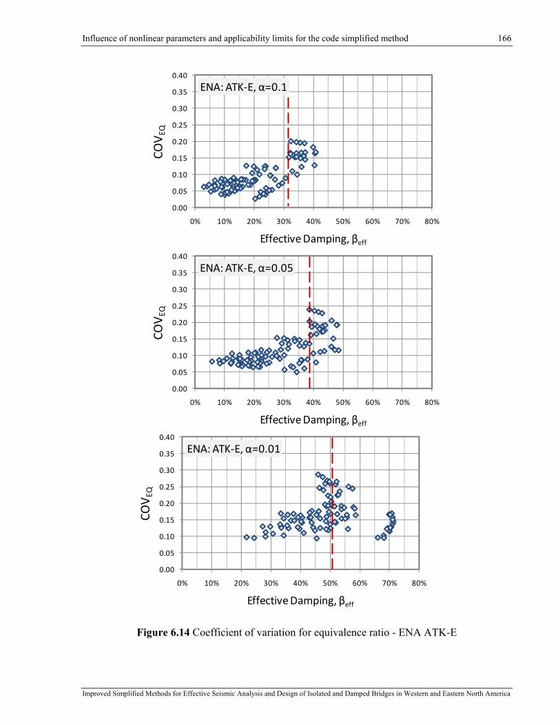
Influence of nonlinear parameters and applicability limits for the code simplified method 166
Improved Simplified Methods for Effective Seismic Analysis and Design of Isolated and Damped Bridges in Western and Eastern North America
0.00
0.05
0.10
0.15
0.20
0.25
0.30
0.35
0.40
0% 10% 20% 30% 40% 50% 60% 70% 80%
COV E
Q
Effective Damping, βeff
ENA: ATK‐E, α=0.1
0.00
0.05
0.10
0.15
0.20
0.25
0.30
0.35
0.40
0% 10% 20% 30% 40% 50% 60% 70% 80%
COV E
Q
Effective Damping, βeff
ENA: ATK‐E, α=0.05
0.00
0.05
0.10
0.15
0.20
0.25
0.30
0.35
0.40
0% 10% 20% 30% 40% 50% 60% 70% 80%
COV E
Q
Effective Damping, βeff
ENA: ATK‐E, α=0.01
Figure 6.14 Coefficient of variation for equivalence ratio - ENA ATK-E
Influence of nonlinear parameters and applicability limits for the code simplified method 167
Improved Simplified Methods for Effective Seismic Analysis and Design of Isolated and Damped Bridges in Western and Eastern North America
6.3.3 Influence of the System Parameters on Equivalence Ratio
In the previous subsection, the equivalence ratio was exploited to identify the range of the
effective damping for which the equivalent linearization method can provide an accurate
response estimate. In this section, the influence of the three system parameters R, Te, and α on the
equivalence ratio is outlined. The equivalence ratios averaged over 20 ground-motion records
are presented in Figures 6.15 and 6.16 as a function of the response modification factor R and
elastic period Te for ENA and WNA, respectively. Results for one value of α (0.1, 0.05, 0.01) are
presented in each three-dimensional bar chart, where each vertical bar corresponds to an
equivalence ratio value averaged over five levels of inherent damping.
In all cases, the equivalence ratio increases as α decreases. When α is reduced from 0.1 to 0.01,
the equivalence ratios may increase by approximately 25% for both WNA and ENA. For all
three α-ratios, it was also observed that the variation of the equivalence ratio as a function of R
and Te is consistent.
As for results presented in Chapter 5, systems with low R factors, which correspond to high
effective damping ratios or short effective periods, are observed to be more critical given that
these systems are characterized by the greatest equivalence ratio. The equivalence ratio
generally decreases when increasing R in the range from R=4 to 28 and then tends to remain
constant for the larger R values of 40 and 52. This indicates that the equivalent linearization
method results in more accurate response estimates for systems with higher R-factors. Such
systems mostly experience responses oriented along the post-activation stiffness kd resulting in
larger displacements (ductility ratios) and lower effective damping ratios (see Figure 6.3).
For ENA, the equivalence ratio increases with Te up to 0.75 s and then decreases for Te = 1.0 s.
In the WNA region, for the four elastic periods, the equivalence ratio increases with the period
Te. This can be explained by the fact that in contrast to ENA, the WNA ground motions transmit
energy to the system at a wider band of frequencies covering longer periods as it was earlier
shown in Figure 5.4.

Influence of nonlinear parameters and applicability limits for the code simplified method 168
Improved Simplified Methods for Effective Seismic Analysis and Design of Isolated and Damped Bridges in Western and Eastern North America
Figure 6.15 Distribution of equivalence ratio by R and Te (WNA ATK-W)
R=4R=16
R=28R=40
R=52
1.01.21.41.61.82.0
1.14
1.20
1.341.36
0.94
0.97
1.051.04
0.95
0.96
1.000.98
0.96
0.97
0.990.97
0.97
0.97
1.000.97
WNA: ATK‐W α=0.10LTH
NLTHu
u
R=4R=16
R=28R=40
R=52
1.01.21.41.61.82.0
1.31
1.49
1.62
1.64
1.07
1.17
1.261.27
1.04
1.09
1.13
1.17
1.01
1.06
1.09
1.14
1.01
1.03
1.06
1.13
WNA: ATK‐W α=0.01LTH
NLTHu
u
R=4R=16
R=28R=40
R=52
1.01.21.41.61.82.0
1.20
1.30
1.451.47
0.96
1.04
1.081.09
0.95
1.011.00
1.03
0.95
1.00
0.981.00
0.96
0.99
0.980.99
WNA: ATK‐W α=0.05LTH
NLTHu
u

Influence of nonlinear parameters and applicability limits for the code simplified method 169
Improved Simplified Methods for Effective Seismic Analysis and Design of Isolated and Damped Bridges in Western and Eastern North America
Figure 6.16 Distribution of equivalence ratio by R and Te (ENA ATK-E)
R=4R=16
R=28R=40
R=52
1.01.21.41.61.82.0
1.54
1.781.81 1.67
1.28
1.401.40
1.33
1.20
1.24
1.251.20
1.15
1.17
1.201.13
1.11
1.13
1.171.10
ENA: ATK‐E α=0.01LTH
NLTHu
u
R=4R=16
R=28R=40
R=52
1.01.21.41.61.82.0
1.30
1.43
1.481.43
0.98
1.06
1.131.10
0.95
1.00
1.061.04
0.95
0.99
1.041.02
0.95
0.98
1.031.01
ENA: ATK‐E α=0.10LTH
NLTHu
u
R=4R=16
R=28R=40
R=52
1.01.21.41.61.82.0
1.38
1.55
1.631.52
1.04
1.19
1.211.19
1.02
1.10
1.111.09
1.00
1.06
1.071.04
0.99
1.04
1.051.02
ENA: ATK‐E α=0.05LTH
NLTHu
u

Influence of nonlinear parameters and applicability limits for the code simplified method 170
Improved Simplified Methods for Effective Seismic Analysis and Design of Isolated and Damped Bridges in Western and Eastern North America
The overall observations, emerging from the results that were obtained from this study,
emphasize the strong dependency of the equivalence ratios on the system parameters. These
results confirm that the limitation in the use of the code simplified method (CSA-S6-06 and
AASHTO) is mostly due to the limited range of system parameters for which the equivalent
linearization method provides sufficient accuracy. Accordingly, an applicability range for the
equivalent linearization method can be established for reducing inaccuracy of the code simplified
method.
6.4 Applicability Limits for Equivalent Linearization Method
The equivalent transformation of the actual nonlinear isolated structure into an equivalent linear
system (see Figure 2.1(a)) is obtained by using only two parameters: the effective damping and
effective period. Both of these parameters depend on the system response in terms of ductility
ratio and they take into account the system’s nonlinear parameters α and Te. The upper limits set
as a function of the effective damping effβ and effective period Teff will be accordingly derived
in this section as they can provide a realistic insight into the applicability ranges.
6.4.1 Limits on Effective Damping, effβ
As observed previously in this study, the damping limits were found not to depend on the
regional seismicity and they are clearly related to the post-yielding stiffness ratio α. Examining
the formulation of the equivalent transformation for the equivalent damping ratio eqβ given by
Equation (6.8), the system parameter that defines eqβ is the ratio α, with the ductility ratio µ
being obtained from the system response.
)1()1()1(2
ααμμαμ
πβ
−+⋅−⋅−
⋅=eq (6.8)
Figure 6.17 shows how the equivalent damping ratio eqβ varies with the ductility ratio µ for
three different α values: 0.01, 0.05, and 0.1.
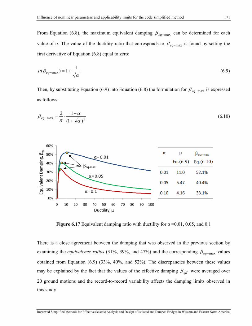
Influence of nonlinear parameters and applicability limits for the code simplified method 171
Improved Simplified Methods for Effective Seismic Analysis and Design of Isolated and Damped Bridges in Western and Eastern North America
From Equation (6.8), the maximum equivalent damping max−eqβ can be determined for each
value of α. The value of the ductility ratio that corresponds to max−eqβ is found by setting the
first derivative of Equation (6.8) equal to zero:
αβμ 11)( max +=−eq (6.9)
Then, by substituting Equation (6.9) into Equation (6.8) the formulation for max−eqβ is expressed
as follows:
2max)1(
12αα
πβ
+
−⋅=−eq (6.10)
Figure 6.17 Equivalent damping ratio with ductility for α =0.01, 0.05, and 0.1
There is a close agreement between the damping that was observed in the previous section by
examining the equivalence ratios (31%, 39%, and 47%) and the corresponding max−eqβ values
obtained from Equation (6.9) (33%, 40%, and 52%). The discrepancies between these values
may be explained by the fact that the values of the effective damping effβ were averaged over
20 ground motions and the record-to-record variability affects the damping limits observed in
this study.
α= 0.01
α= 0.05
α= 0.10%
10%
20%
30%
40%
50%
60%
0 10 20 30 40 50 60 70 80 90 100
Equivalent Dam
ping, β
eq
Ductility, µ
βeq-max

Influence of nonlinear parameters and applicability limits for the code simplified method 172
Improved Simplified Methods for Effective Seismic Analysis and Design of Isolated and Damped Bridges in Western and Eastern North America
The damping formulations based on Equations (6.8) and (6.10) reflect a relation between the
hysteresis shape and dissipated energy and offer a realistic insight into the possible influence of
the ratio α on the observed coefficients of variation (see Figures 6.13 and 6.14) and, thereby, the
required effective damping limits.
However, there is no obvious physical explanation on why the equivalent linearization method
does not provide accurate response estimates when approaching and exceeding these damping
limits. The drift of the oscillation center was however pointed out as a possible reason for the
errors in the response estimates (see Figure 6.6).
6.4.2 Limits on Effective Period, Teff
To determine limits on the effective period, the response-independent relationship between the
effective damping and effective period is first established. Then, the relationship of the effective
damping as a function of the effective period is derived. Similarly to the limit on the effective
damping, the maximum value of the function is assumed to mark a limit for the method’s
applicability range. These limits are validated with results of the parametric study that was
carried-out in Chapter 5.
The formulation for the effective period Teff given by Equation (6.11), is defined by the system's
parameters as the elastic period Te and ratio α, the ductility ratio µ being obtained from the
system response.
ααμμ
−+⋅=
1eeff TT (6.11)
The equivalent viscous damping is formulated through the post-yielding stiffness ratio α and
ductility ratio µ as:
)1()1()1(2
ααμμαμ
πβ
−+⋅−⋅−
⋅=eq (6.8)
As it can be noted from Equations (6.11) and (6.8), the effective period and effective damping
are established as a function of the ductility demand µ. This reflects solely a relationship between
the response shape and the maximum displacement response ( μ⋅= yuumax ).
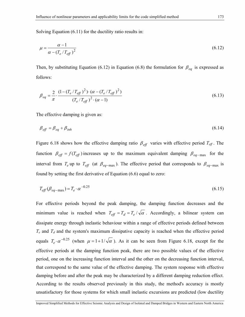
Influence of nonlinear parameters and applicability limits for the code simplified method 173
Improved Simplified Methods for Effective Seismic Analysis and Design of Isolated and Damped Bridges in Western and Eastern North America
Solving Equation (6.11) for the ductility ratio results in:
2)/(1
effe TT−
−=
ααμ (6.12)
Then, by substituting Equation (6.12) in Equation (6.8) the formulation for eqβ is expressed as
follows:
)1()/(
))/(())/(1(22
22
−⋅
−⋅−⋅=
α
απ
βeffe
effeeffeeq
TT
TTTT (6.13)
The effective damping is given as:
inheqeff βββ += (6.14)
Figure 6.18 shows how the effective damping ratio effβ varies with effective period Teff . The
function )( effeff Tf=β increases up to the maximum equivalent damping max−eqβ for the
interval from eT up to effT (at max−eqβ ). The effective period that corresponds to max−eqβ is
found by setting the first derivative of Equation (6.6) equal to zero:
25.0max)( −
− ⋅= αβ eeqeff TT (6.15)
For effective periods beyond the peak damping, the damping function decreases and the
minimum value is reached when α/edeff TTT == . Accordingly, a bilinear system can
dissipate energy through inelastic behaviour within a range of effective periods defined between
Te and Td and the system's maximum dissipative capacity is reached when the effective period
equals 25.0−⋅αeT (when αμ /11+= ). As it can be seen from Figure 6.18, except for the
effective periods at the damping function peak, there are two possible values of the effective
period, one on the increasing function interval and the other on the decreasing function interval,
that correspond to the same value of the effective damping. The system response with effective
damping before and after the peak may be characterized by a different damping reduction effect.
According to the results observed previously in this study, the method's accuracy is mostly
unsatisfactory for those systems for which small inelastic excursions are predicted (low ductility
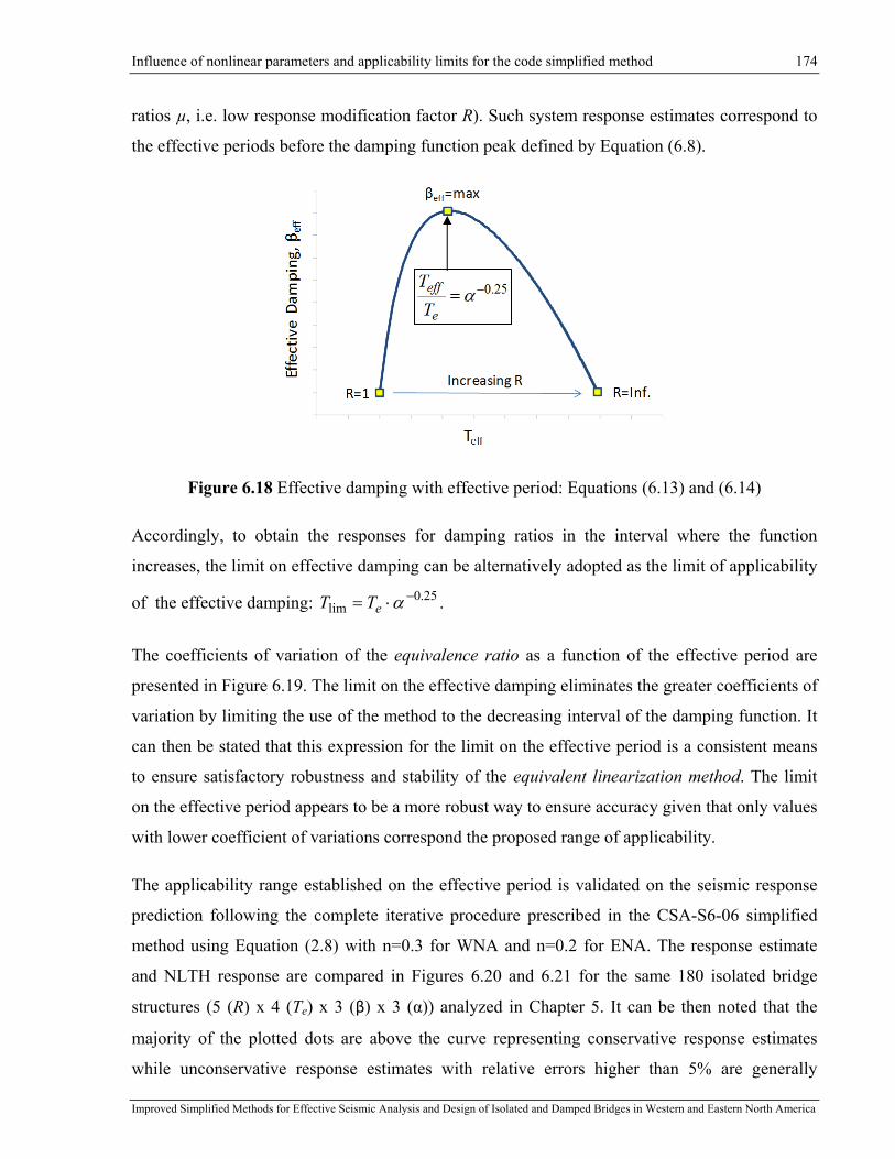
Influence of nonlinear parameters and applicability limits for the code simplified method 174
Improved Simplified Methods for Effective Seismic Analysis and Design of Isolated and Damped Bridges in Western and Eastern North America
ratios µ, i.e. low response modification factor R). Such system response estimates correspond to
the effective periods before the damping function peak defined by Equation (6.8).
Figure 6.18 Effective damping with effective period: Equations (6.13) and (6.14)
Accordingly, to obtain the responses for damping ratios in the interval where the function
increases, the limit on effective damping can be alternatively adopted as the limit of applicability
of the effective damping: 25.0lim
−⋅= αeTT .
The coefficients of variation of the equivalence ratio as a function of the effective period are
presented in Figure 6.19. The limit on the effective damping eliminates the greater coefficients of
variation by limiting the use of the method to the decreasing interval of the damping function. It
can then be stated that this expression for the limit on the effective period is a consistent means
to ensure satisfactory robustness and stability of the equivalent linearization method. The limit
on the effective period appears to be a more robust way to ensure accuracy given that only values
with lower coefficient of variations correspond the proposed range of applicability.
The applicability range established on the effective period is validated on the seismic response
prediction following the complete iterative procedure prescribed in the CSA-S6-06 simplified
method using Equation (2.8) with n=0.3 for WNA and n=0.2 for ENA. The response estimate
and NLTH response are compared in Figures 6.20 and 6.21 for the same 180 isolated bridge
structures (5 (R) x 4 (Te) x 3 (β) x 3 (α)) analyzed in Chapter 5. It can be then noted that the
majority of the plotted dots are above the curve representing conservative response estimates
while unconservative response estimates with relative errors higher than 5% are generally

Influence of nonlinear parameters and applicability limits for the code simplified method 175
Improved Simplified Methods for Effective Seismic Analysis and Design of Isolated and Damped Bridges in Western and Eastern North America
occurring beyond the proposed range of applicability. It confirms the enhanced reliability of the
proposed applicability limits that could then be used in future editions of CSA-S6 for WNA and
ENA.
Figure 6.19 Coefficient of variation for equivalence ratio with Teff - ENA ATK-W

Influence of nonlinear parameters and applicability limits for the code simplified method 176
Improved Simplified Methods for Effective Seismic Analysis and Design of Isolated and Damped Bridges in Western and Eastern North America
0
50
100
150
200
250
300
350
400
450
500
0 50 100 150 200 250 300 350 400 450 500
u code(m
m)
uNLTH (mm)
NL SDOF (ATK‐W) ‐ Eq.(2.8) with n=0.3 ‐ α=0.1
uNLTH/ucode=1.05
0
50
100
150
200
250
300
350
400
450
500
0 50 100 150 200 250 300 350 400 450 500
u code(m
m)
uNLTH (mm)
NL SDOF (ATK‐W) ‐ Eq.(2.8) with n=0.3 ‐ α=0.05
uNLTH/ucode=1.05
0
50
100
150
200
250
300
350
400
450
500
0 50 100 150 200 250 300 350 400 450 500
u code(m
m)
uNLTH (mm)
NL SDOF (ATK‐W) ‐ Eq.(2.8) with n=0.3 ‐ α=0.01
uNLTH/ucode=1.05
Figure 6.20 20-Records mean responses versus code estimates with proposed limits on effective
period - WNA Eq.(2.8) with n=0.3

Influence of nonlinear parameters and applicability limits for the code simplified method 177
Improved Simplified Methods for Effective Seismic Analysis and Design of Isolated and Damped Bridges in Western and Eastern North America
0
20
40
60
80
100
120
0 20 40 60 80 100 120
u code(m
m)
uNLTH (mm)
NL SDOF (ATK‐E) ‐ Eq.(2.8) with n=0.2 ‐ α=0.1
uNLTH/ucode=1.05
0
20
40
60
80
100
120
0 20 40 60 80 100 120
u code(m
m)
uNLTH (mm)
NL SDOF (ATK‐E) ‐ Eq.(2.8) with n=0.2 ‐ α=0.05
uNLTH/ucode=1.05
0
20
40
60
80
100
120
0 20 40 60 80 100 120
u code(m
m)
uNLTH (mm)
NL SDOF (ATK‐E) ‐ Eq.(2.8) with n=0.2 ‐ α=0.01
uNLTH/ucode=1.05
Figure 6.21 20-Records mean responses versus code estimates with proposed limits on effective
period - ENA Eq.(2.8) with n=0.2

Influence of nonlinear parameters and applicability limits for the code simplified method 178
Improved Simplified Methods for Effective Seismic Analysis and Design of Isolated and Damped Bridges in Western and Eastern North America
6.5 Conclusions
In this chapter, the influence of the system nonlinear parameters on the accuracy of the code
simplified method (CSA-S6-06 and AASHTO) was carefully examined. It was confirmed that
there is a certain range of nonlinear parameters for which the code simplified method can provide
an accurate response estimate while inaccuracies are observed outside this range.
It was found that the source of the inaccuracy originates from the equivalent linearization
method rather than from the definition of the damping coefficients B. By examining in details the
process of equivalent linearization, the upper limit for the method applicability range was
derived on the effective damping and effective period. In this way, the influence of the nonlinear
parameters was taken into account to achieve sufficient accuracy in the seismic response
prediction.
The method applicability limits, proposed in this chapter, were validated by comparing NLTH
responses, obtained in Chapter 5, to the response estimates obtained during the design process
following the complete iterative procedure prescribed in the CSA-S6-06 simplified method using
Equation (2.8) with n=0.3 for WNA and n=0.2 for ENA. It was confirmed that the use of the
proposed limits makes it possible to reject responses with unsatisfactory accuracy and these
limits could then be used in future editions of CSA-S6 for both WNA and ENA.
There is no obvious physical explanation on why the equivalent linearization method does not
provide accurate response estimates when approaching and exceeding these limits. The drift of
the oscillation center was however pointed out as a possible reason for these errors. The real
energy dissipated around a drifted oscillation center may be strongly overestimated by
considering an equivalent response around the original center as prescribed in the CSA-S6-06
code (or AASHTO).
In addition, it was observed that the effective damping values before (increasing interval) and
beyond (decreasing interval) its peak may be characterized by different reduction effects.
According to this study, the method accuracy is unsatisfactory mostly for systems that
correspond to the increasing interval of the damping function. Such systems experience small
inelastic excursions and correspond to low response modification factors R. The response

Influence of nonlinear parameters and applicability limits for the code simplified method 179
Improved Simplified Methods for Effective Seismic Analysis and Design of Isolated and Damped Bridges in Western and Eastern North America
modification factor R represents the earthquake-structure interaction and its effect cannot be
captured by the code simplified method.
In light of these findings and observations, it can be stated that for prediction of the seismic
response beyond the limits proposed in this chapter, a new simplified method, which takes into
account the differences in ground-motion characteristics and isolated bridge design parameters,
appears necessary. Several alternatives for developing the new simplified method are further
examined and discussed in the following chapter.

Basis for Development of New Simplified Method for Estimating the Response of Isolated Bridges 180
Improved Simplified Methods for Effective Seismic Analysis and Design of Isolated and Damped Bridges in Western and Eastern North America
Chapter 7: Basis for Development of New Simplified Method for Estimating the Response of Isolated Bridges
7.1 Introduction
In the previous chapter, it was confirmed that the simplified method, currently specified in the
North American codes (CAN/CSA-S6-06 and AASHTO 2009, 2010), is subject to certain
limitations that may significantly affect the accuracy in the response estimate for certain ranges
of structural properties. The drift of the oscillation center was pointed out as a possible reason for
the errors in the response estimates. The real energy dissipated around a drifted oscillation center
may be strongly overestimated by considering an equivalent response around the original center
as prescribed in the CSA-S6-06 code (or AASHTO). In addition, the current code simplified
method (as discussed in Chapter 5 and Chapter 6) does not take into account the complex
relation between the structure’s properties and the different ground-motion characteristics. As
observed in the previous chapters, the parameters as the period ratio Te / Tg, where Te is the
structure’s initial period and Tg is the ground-motion’s predominant period, and the response
modification factor R make it possible to characterize the effect of the structure-earthquake
interaction.
In light of these findings and observations, a new simplified method that takes into account the
differences in ground-motion characteristics and isolated bridge design parameters is necessary.
This chapter aims at examining the potentiality for developing a new method for predicting
isolated bridge response more accurately. The basis for the new method concept and the key
elements that may affect the method's accuracy are identified.
In order to establish a basis for the development of this new method, two widely adopted
methods in earthquake engineering, the Equal Displacement Approximation (EDA) and the
Equal Energy Approximation (EEA) are first briefly reviewed. Then response estimates obtained
using these approaches are compared to the nonlinear “real” responses of the bridge isolation
systems from a limited series of NLTHA presented in Chapter 5. The accuracy is characterized

Basis for Development of New Simplified Method for Estimating the Response of Isolated Bridges 181
Improved Simplified Methods for Effective Seismic Analysis and Design of Isolated and Damped Bridges in Western and Eastern North America
in terms of the relative error in order to determine the limitations that are inherent to the EDA
and EEA. The energy concept used in the EEA is then considered for further development. In
such a way, different system's properties and ground-motion characteristics can then be taken
into account for seismic response prediction.
To gain a better understanding of the physical phenomena involved in the response of isolated
bridges and how the response is related to the structure’s properties and the different ground-
motion characteristics, a comprehensive study on the response of SDOF systems under harmonic
excitation was carried out in this study.
The harmonic steady-state response of SDOF systems exhibiting bilinear hysteretic rule has been
studied in detail by many researchers, as a result, various dynamic aspects of structural response
have already been reported (Caughey 1960, Iwan 1961, Masri 1974, Abé 1996). However, the
steady-state response of a SDOF system is not necessarily representative of the response of
isolated bridges under seismic excitation for all ranges of structural parameters and ground
motion characteristics. The nonlinear response to earthquake is not a steady state. In particular,
peak displacement response of nonlinear systems is typically observed during short time
intervals, ranging from half of a cycle to a maximum of 2 or 3 cycles, each having different
amplitudes. In view of that, this chapter will focus on the transient response to sinusoidal
excitations, not the steady-state response.
For this reason, to better characterize seismic response in the present study, special attention is
drawn to the effect of the transient phase of loading that occurs at the beginning of the excitation.
Based on the principle of conservation of energy, the energy flow is examined within the
system's motion in the transient phase of the response before reaching peak displacement. This
investigation shows that kinetic energy is a possible key element that must be considered in the
new simplified method.
Then, a more detailed insight on the energy flow is gained by studying the effect of the response
modification factor R and the frequency ratio on the energy allocation. Through this study, it is
found that the transition state between limited-nonlinear and highly-nonlinear responses defines
the limit beyond which the kinetic energy has a dominant effect on the response of NL-SDOF
systems.

Basis for Development of New Simplified Method for Estimating the Response of Isolated Bridges 182
Improved Simplified Methods for Effective Seismic Analysis and Design of Isolated and Damped Bridges in Western and Eastern North America
7.2 Equal Displacement and Equal Energy Approximations for
Estimating Response of Isolated Bridges
In this section, we examine the appropriateness and limitations of the Equal Displacement
Approximation (EDA) and the Equal Energy Approximation (EEA) in assessing the inelastic
response of highly-nonlinear systems representative of isolated bridge structures responding to
strong seismic excitations. Both methods are briefly reviewed first. Then, the method EEA is
formulated for application to bilinear SDOF systems having a post-yielding stiffness ratio α
higher than zero (α > 0).
The results obtained from a limited series of NLTHA in Chapter 5 are compared to those
obtained by using EDA and EEA methods. Differences in displacement responses between the
NLTHA results and the EEA approximations are then discussed with respect to the concept of
kinetic energy deficit.
7.2.1 Background of Inelastic Response Approximation Concepts
EDA and EEA form the basis of the seismic provisions of many design codes worldwide. These
empirical approaches have been proposed by Veletsos and Newmark (1960) based on the
observations of the inelastic responses of SDOF systems subjected to the 1940 El Centro and
1933 Vernon earthquake records that both occurred in California. The inelastic responses were
computed using a numerical integration method for elastic perfectly-plastic systems (α = 0) with
three levels of ductility: µ = 1.25, 2 and 4. The results were then compared to those of elastic
systems (µ = 1) having the same elastic stiffness (same initial period Te). For relatively small
levels of damping, less than 5%, the EDA appeared to be reasonably accurate. For larger levels
of damping, an alternative approach was proposed in which the energy absorbed by the inelastic
system under monotonic loading is set equal to the energy absorbed by a corresponding elastic
system under the earthquake excitation. The elastic system is defined by the elastic stiffness of
the inelastic system. The energy absorbed by the inelastic system is equal to the area under the
force-displacement curve at maximum displacement. A similar approach was formulated earlier
by Housner (1956) who suggested to design inelastic structures so that they can absorb the entire
kinetic energy corresponding to an elastic system subjected to the design earthquake. As in EEA,
the elastic system is defined by the pre-yielding stiffness of the inelastic system. In fact,

Basis for Development of New Simplified Method for Estimating the Response of Isolated Bridges 183
Improved Simplified Methods for Effective Seismic Analysis and Design of Isolated and Damped Bridges in Western and Eastern North America
Housner’s method relied on an alternative interpretation of the EEA concept. However, Housner
noted that such a method will overestimate the absorbed energy if the inelastic excursion has a
major effect on the effective stiffness of the structure, i.e., for systems sustaining large ductility
demand. Therefore, there is a concern that a similar overestimation might observed when
applying EEA to highly-nonlinear systems such as isolated bridges, which are intended to
experience significant reductions of their effective stiffness during the seismic response.
According to Housner, for this approximation, the maximum energy input is equal to the kinetic
energy obtained using the damped spectral velocity ),( eeV TS ξ defined at the system's elastic
period Te:
2
21
Vin SmE = (7.1)
Using the pseudo relationship for a steady-state response, eDV TSS /2π⋅= , the input energy can
then be defined in terms of the maximum elastic displacement eu ( ),( eeD TS ξ ) as follows:
( ) 222
21
21/2
21
eeDeeDin ukSkTSmE === π (7.2)
If the structure's response exceeds the elastic limit (Teff > Te), the spectral velocity SV within the
period range between Te and Teff must remain the same in order for the input energy level to be
maintained. This is not always the case in nonlinear response and a lower input energy generally
characterizes the inelastic response, which results in conservative displacement estimates. In
common practice, the energy-equating technique applied for assessing the inelastic displacement
is referred to as the EEA. Both of these approaches were proposed for design and can be
formulated by means of the response modification factors R defined as:
μ=R for EDA (7.3)
12 −= μR for EEA (7.4)
Figure 7.1 presents both the EDA and EEA for the elastic perfectly-plastic system (α=0) as
initially described by Veletsos and Newmark (1960).
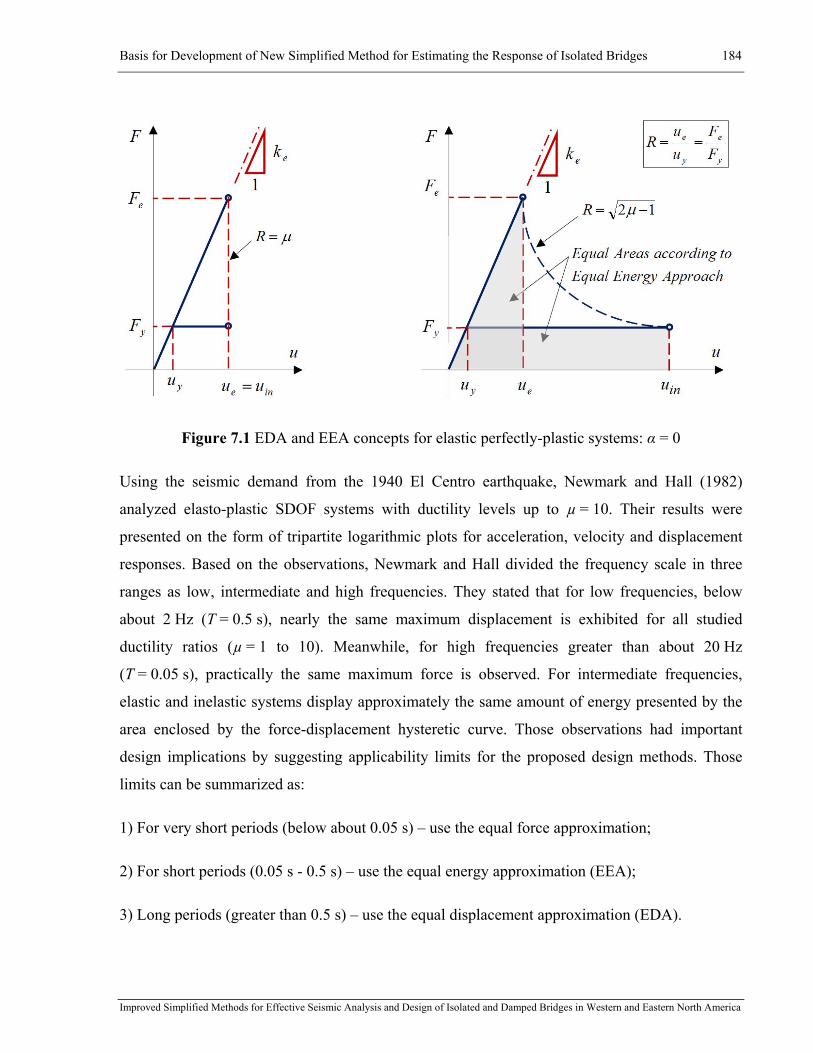
Basis for Development of New Simplified Method for Estimating the Response of Isolated Bridges 184
Improved Simplified Methods for Effective Seismic Analysis and Design of Isolated and Damped Bridges in Western and Eastern North America
Figure 7.1 EDA and EEA concepts for elastic perfectly-plastic systems: α = 0
Using the seismic demand from the 1940 El Centro earthquake, Newmark and Hall (1982)
analyzed elasto-plastic SDOF systems with ductility levels up to µ = 10. Their results were
presented on the form of tripartite logarithmic plots for acceleration, velocity and displacement
responses. Based on the observations, Newmark and Hall divided the frequency scale in three
ranges as low, intermediate and high frequencies. They stated that for low frequencies, below
about 2 Hz (T = 0.5 s), nearly the same maximum displacement is exhibited for all studied
ductility ratios (µ = 1 to 10). Meanwhile, for high frequencies greater than about 20 Hz
(T = 0.05 s), practically the same maximum force is observed. For intermediate frequencies,
elastic and inelastic systems display approximately the same amount of energy presented by the
area enclosed by the force-displacement hysteretic curve. Those observations had important
design implications by suggesting applicability limits for the proposed design methods. Those
limits can be summarized as:
1) For very short periods (below about 0.05 s) – use the equal force approximation;
2) For short periods (0.05 s - 0.5 s) – use the equal energy approximation (EEA);
3) Long periods (greater than 0.5 s) – use the equal displacement approximation (EDA).

Basis for Development of New Simplified Method for Estimating the Response of Isolated Bridges 185
Improved Simplified Methods for Effective Seismic Analysis and Design of Isolated and Damped Bridges in Western and Eastern North America
Typical bridge structures do not fall in the very short period range and in general correspond to
longer period ranges as further used in this study (0.25 to 1.0 s).
In light of these observations, Newmark and Hall proposed to incorporate their findings directly
in the design process by means of inelastic response spectra as shown in Figure 7.2. The elastic
and inelastic response spectra have been presented by the regions of constant displacement,
constant velocity and constant acceleration denoted respectively as D, V and A. Accordingly, the
elastic response spectra built for the selected level of damping and seismic hazard (DVAA0) is
transformed to the inelastic response by using a corresponding aforementioned reduction factor R
being a function of ductility.
Figure 7.2 Inelastic design spectra for earthquakes (Newmark and Hall, 1960)
In turn, in the same work, in order to construct an elastic response spectrum for different
damping levels a series of empirical spectrum amplification factors have been proposed for each
of the D, V and A regions of the spectrum. It has to be recognized that these findings have led to
the incorporation, by different design codes, of the static equivalent force method which takes
into considerations levels of damping greater than 5%. For example, this method is included in
the current Canadian Highway Bridge Design Code (CAN/CSA-S6) for a simplified design
approach.

Basis for Development of New Simplified Method for Estimating the Response of Isolated Bridges 186
Improved Simplified Methods for Effective Seismic Analysis and Design of Isolated and Damped Bridges in Western and Eastern North America
7.2.2 EEA Approach for Bilinear Systems with α > 0
As discussed in Chapter 5, the present research is dedicated to the seismic response of
seismically isolated bridges, where a certain level of restoring force is required to reduce the
system's inelastic excursion and resulting residual displacements. The restoring capabilities of
such isolation systems are commonly presented by the non-zero post-yielding stiffness in terms
of stiffness ratio α. For bilinear systems with a post-yielding stiffness ratio greater than zero
(α > 0), the R-µ relationship aforementioned for the equal energy approximation (elastic
perfectly-plastic system: α = 0) is no longer valid and has to be re-evaluated by equating areas of
the corresponding response shapes as shown in Figure 7.3. The energy absorbed by an elastic
system (EAbL) and that absorbed by a corresponding nonlinear system (EAbNL) are assumed to be
equal and are defined through the area under the force-displacement curve obtained for the first
half cycle of the response.
Figure 7.3 Concept of Equal Energy - Energies absorbed by linear and nonlinear systems: : α>0
The energy absorbed by an elastic system is determined as:
222
21
21 RukukE yeeeAbL == (7.5)
Basis for Development of New Simplified Method for Estimating the Response of Isolated Bridges 187
Improved Simplified Methods for Effective Seismic Analysis and Design of Isolated and Damped Bridges in Western and Eastern North America
The energy absorbed by a corresponding bilinear system (the same elastic stiffness ke) is
expressed as follows:
2222 )1(21)1(
21
−+−+= μαμ yeyeyeAbNL ukukukE
))1()1(21(21 22 −⋅+−⋅+= μαμyeuk (7.6)
Solving both equations for the response modification factor, R results in:
)1()12(2 αμαμ −⋅−+=R (7.7)
Consequently the ductility ratio µ can be written as a function of R and α for α>0 as:
αααμ 1111
2
2−
++−=R (7.8)
Equations (7.7) and (7.8) present formulations of the EEA for bilinear SDOF systems with α>0.
These expressions are based on the same assumption as the one made by Housner (1956), which
states that the input energy remains unchanged for elastic and inelastic systems. It should be
clear, however, that this simplified approximation will overestimate the energy absorbed by
inelastic systems. In addition, it should be mentioned that the EEA formulation is based on the a
steady-state response assumption where the maximum relative velocity, corresponding to the
peak kinetic energy, occurs at the zero displacement position. Accordingly, the effect of the
oscillation center drift (see Chapter 6) is not accounted for in this approach.
7.2.3 EDA and EEA versus Seismic Response of Nonlinear Systems
Responding to Seismic Motions
To better understand the limitations of the EDA and EEA methods in assessing the response of
highly-nonlinear systems, a limited series of NLTHA presented in Chapter 5 is used here for this
comparative study. The nonlinear SDOF systems were subjected to the 20 seismic excitations
presented in Chapter 4 (Atkinson's, 2009). The bilinear system configurations are defined by
varying the initial fundamental period Te and response modification factor R, while the post-
yielding stiffness ratio α = 0.05 remains constant. Four natural periods Te = 0.25, 0.5, 0.75, and
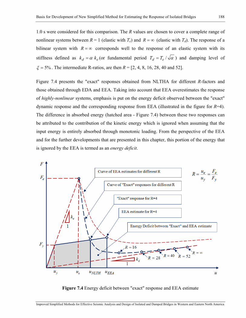
Basis for Development of New Simplified Method for Estimating the Response of Isolated Bridges 188
Improved Simplified Methods for Effective Seismic Analysis and Design of Isolated and Damped Bridges in Western and Eastern North America
1.0 s were considered for this comparison. The R values are chosen to cover a complete range of
nonlinear systems between R = 1 (elastic with Te) and ∞=R (elastic with Td). The response of a
bilinear system with ∞=R corresponds well to the response of an elastic system with its
stiffness defined as ed kk α= (or fundamental period α/ed TT = ) and damping level of
%5=ξ . The intermediate R-ratios, are then R = [2, 4, 8, 16, 28, 40 and 52].
Figure 7.4 presents the "exact" responses obtained from NLTHA for different R-factors and
those obtained through EDA and EEA. Taking into account that EEA overestimates the response
of highly-nonlinear systems, emphasis is put on the energy deficit observed between the "exact"
dynamic response and the corresponding response from EEA (illustrated in the figure for R=4).
The difference in absorbed energy (hatched area - Figure 7.4) between these two responses can
be attributed to the contribution of the kinetic energy which is ignored when assuming that the
input energy is entirely absorbed through monotonic loading. From the perspective of the EEA
and for the further developments that are presented in this chapter, this portion of the energy that
is ignored by the EEA is termed as an energy deficit.
Figure 7.4 Energy deficit between "exact" response and EEA estimate

Basis for Development of New Simplified Method for Estimating the Response of Isolated Bridges 189
Improved Simplified Methods for Effective Seismic Analysis and Design of Isolated and Damped Bridges in Western and Eastern North America
Figure 7.5 and Figure 7.6 compare the "exact" responses computed for different R-ratios to those
obtained through EDA and EEA for each of the four elastic periods Te = 0.25, 0.50, 0.75 and
1.00 s. The comparison is presented on the SA-PSD spectrum to show how the ratio R influences
the systems' responses with respect to the 5% damped elastic response spectra. The responses of
the systems characterized by 1=R and ∞=R are given by the intersection between the 5%
damped SA-PSD spectrum and the lines initiated from the intercept having a system elastic and
post-yielding slope. In the graph, the system slopes are presented in terms of the squared
frequency of vibration 2eω and 2
dω for the elastic and the post-yielding slopes, respectively. In
all cases, the NLTHA “exact” response is situated under the 5% damped spectrum, indicating an
equivalent damping level greater than 5%.
For systems with elastic periods of Te = 0.25 s and 0.5 s, the EDA underestimates the peak
response of the systems for all values of R. When the EDA is applied for the two other systems
with longer elastic period (Te = 0.75 s and 1.0 s), the maximum displacements can be
approximated with a reasonable degree of accuracy for R factors smaller than about R = 8.
Beyond R = 16, the accelerations and, thereby, the forces are nearly the same for systems with
Te = 0.5, 0.75 and 1.0 s. For the shorter elastic period (0.25 s), the lowest force level is obtained
for R = 16 and a slight increase in the force is observed for higher R-ratios.
In these figures, the curves representing EEA predictions overestimate the "exact" responses for
all four elastic periods studied. However, the EEA values appear to be much closer to the "exact"
responses for the shorter elastic period of 0.25 s than for longer periods. This suggests that for
elastic periods shorter than 0.25 s, the "exact" response can be reliably approximated using the
EEA approach. Given that structures having shorter elastic periods (Te < 0.25 s) represent a small
percentage of isolated bridges, this case is of little practical relevance and is therefore not
covered later by this study.

Basis for Development of New Simplified Method for Estimating the Response of Isolated Bridges 190
Improved Simplified Methods for Effective Seismic Analysis and Design of Isolated and Damped Bridges in Western and Eastern North America
Figure 7.5 "Exact" responses and the 5% damped Sa-PSd spectrum (α=0.05, Te=0.25 s and 0.5 s)
0.00
0.10
0.20
0.30
0.40
0.50
0.60
0.70
0 5 10 15 20 25 30 35 40 45
Sa (g)
PSd (mm)
Atkinson's 20 Eastern Records ‐ α=0.05, Te=0.25 s
2eω
1
1=R
4 8 1652
∞=R
2dω
1
"Exact" response (R=4)
Equal energy approach for α>0 ( R=4)
2=R
28 40
0.00
0.05
0.10
0.15
0.20
0.25
0.30
0.35
0.40
0 5 10 15 20 25 30 35 40 45 50 55 60
Sa (g)
PSd (mm)
Atkinson's 20 Eastern Records ‐ α=0.05, Te=0.5 s
2eω
1
1=R
2=R
4
16 28 40
52
∞=R2
dω1
"Exact" response (R=4)
Equal energy approach for α>0 (R=4)
8

Basis for Development of New Simplified Method for Estimating the Response of Isolated Bridges 191
Improved Simplified Methods for Effective Seismic Analysis and Design of Isolated and Damped Bridges in Western and Eastern North America
Figure 7.6 "Exact" responses and the 5% damped Sa-PSd spectrum (α=0.05, Te=0.75 s and 1.0 s)
0.00
0.05
0.10
0.15
0.20
0.25
0.30
0 5 10 15 20 25 30 35 40 45 50 55 60 65 70 75 80
Sa (g)
PSd (mm)
Atkinson's 20 Eastern Records ‐ α=0.05, Te=0.75 s
2eω
1
1=R
2=R
4
8 16 28
40 52
∞=R
"Exact" response (R=4)
Equal energy approach for α>0 (R=4)
0.00
0.02
0.04
0.06
0.08
0.10
0.12
0.14
0.16
0.18
0.20
0 5 10 15 20 25 30 35 40 45 50 55 60 65 70 75 80 85 90
Sa (g)
PSd (mm)
Atkinson's 20 Eastern Records ‐ α=0.05, Te=1.0 s
2eω
1
2dω 1
1=R
2=R
4
8 16 28
40 52
∞=R
"Exact" response (R=4)
Equal energy approach for α>0 (R=4)

Basis for Development of New Simplified Method for Estimating the Response of Isolated Bridges 192
Improved Simplified Methods for Effective Seismic Analysis and Design of Isolated and Damped Bridges in Western and Eastern North America
Figures 7.7 and 7.8 summarize the discrepancies between the "exact" responses and those
estimated through EDA and EEA, respectively. The accuracy is evaluated in terms of the relative
errors:
NLTH
EDANLTH
uuu
Error−
= and NLTH
EEANLTHu
uuError
−= (7.9)
Positive and negative relative errors correspond respectively to underestimated and
overestimated response estimates. For the four examples studied, the EDA (Figure 7.7)
consistently underestimates the "exact" responses. A reasonably accurate estimate (Error < 10%)
is observed for the two systems with longer elastic periods (0.75 and 1.0 s) and for R ≤ 8, which
is in agreement with the observations by Veletsos and Newmark (1960) for ductility levels up to
µ = 4 and Newmark and Hall (1982) for ductility up to µ = 10, where R = µ.
0%
10%
20%
30%
40%
50%
60%
70%
80%
0 5 10 15 20 25 30 35 40 45 50 55 60 65
Error
Response Modification Factor, R
EDA ‐ α=0.05
Te= 1.00
Te= 0.75
Te= 0.50
Te= 0.25
Figure 7.7 Influence of the R-factor and period on the error between "exact" response and Equal
Displacement Approximation (α = 0.05, mean of 20 Atkinson's artificial records - ENA)
Contrary to EDA, the EEA technique (Figure 7.8) overestimates the "exact" responses for all
studied cases. As a result, for the four cases studied herein, the "exact" responses are bounded by
the EDA and EEA response approximating techniques. Another tendency that can be observed in
Figure 7.8 is that the smallest errors for the EEA are obtained for the shortest period of 0.25 s,
while the greatest errors are observed for the period of 0.75 s, not for the longest period of 1.0 s.
This confirms the dependency of the EEA estimate error on the elastic period, as was the case for
the code simplified method observed in Chapter 6 (Figure 6.15).

Basis for Development of New Simplified Method for Estimating the Response of Isolated Bridges 193
Improved Simplified Methods for Effective Seismic Analysis and Design of Isolated and Damped Bridges in Western and Eastern North America
‐250%
‐200%
‐150%
‐100%
‐50%
0%
0 5 10 15 20 25 30 35 40 45 50 55 60 65
Error
Response Modification Factor, R
EEA ‐ α=0.05
Te= 1.00
Te= 0.75
Te= 0.50
Te= 0.25
Figure 7.8 Influence of the R-factor and period on the error between "exact" response and Equal
Energy Approximation (α = 0.05, mean of 20 Atkinson's artificial records - ENA)
To explain the differences observed in response estimates between the EEA and “exact” NLTHA
results, the relation between the relative error and the energy deficit is presented in Figure
7.9.The energy deficit is defined as the difference in the absorbed energy (hatched area - Figure
7.4) between the "exact" dynamic response, ENLTHA, and the absorbed energy assumed in the
EEA, EEEA. These energy quantities are determined using Equation (7.6). For the EEA, the error
in response estimate generally increases with the energy deficit. By examining Equation (7.6),
the energy deficit depends on system’s parameters such as the post-yield stiffness ratio α, the
initial period Te (in terms of ke), and the response modification factor R (in terms of uy).
Given that the "exact" response is overestimated by the EEA, the concept of energy deficit due to
the kinetic energy contribution to the system's response is kept herein for further developing the
concept of energy balance. The concept of energy deficit is proposed and investigated in the
following sections.
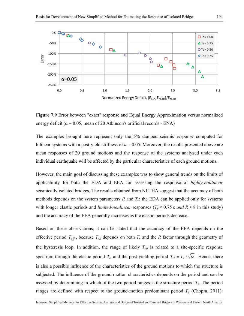
Basis for Development of New Simplified Method for Estimating the Response of Isolated Bridges 194
Improved Simplified Methods for Effective Seismic Analysis and Design of Isolated and Damped Bridges in Western and Eastern North America
‐250%
‐200%
‐150%
‐100%
‐50%
0%
0.0 0.5 1.0 1.5 2.0 2.5 3.0 3.5
Error
Normalized Energy Deficit, (EEEA‐ENLTH)/ENLTH
α=0.05
Te= 1.00
Te= 0.75
Te= 0.50
Te= 0.25
Figure 7.9 Error between "exact" response and Equal Energy Approximation versus normalized
energy deficit (α = 0.05, mean of 20 Atkinson's artificial records - ENA)
The examples brought here represent only the 5% damped seismic response computed for
bilinear systems with a post-yield stiffness of α = 0.05. Moreover, the results presented above are
mean responses of 20 ground motions and the response of the systems analyzed under each
individual earthquake will be affected by the particular characteristics of each ground motions.
However, the main goal of discussing these examples was to show general trends on the limits of
applicability for both the EDA and EEA for assessing the response of highly-nonlinear
seismically isolated bridges. The results obtained from NLTHA suggest that the accuracy of both
methods depends on the system parameters R and Te: the EDA can be applied only for systems
with longer elastic periods and limited-nonlinear responses (Te ≥ 0.75 s and R ≤ 8 in this study)
and the accuracy of the EEA generally increases as the elastic periods decrease.
Based on these observations, it can be stated that the accuracy of the EEA depends on the
effective period effT , because Teff depends on both Te and the R factor through the geometry of
the hysteresis loop. In addition, the range of likely Teff is related to a site-specific response
spectrum through the elastic period eT and the post-yielding period α/ed TT = . Hence, there
is also a possible influence of the characteristics of the ground motions to which the structure is
subjected. The influence of the ground motion characteristics depends on the period and can be
assessed by determining in which of the two period ranges is the structure period Te. The period
ranges are defined with respect to the ground-motion predominant period Tg (Chopra, 2011):

Basis for Development of New Simplified Method for Estimating the Response of Isolated Bridges 195
Improved Simplified Methods for Effective Seismic Analysis and Design of Isolated and Damped Bridges in Western and Eastern North America
"slowly varying force" period range ( gTT < ) and "rapidly varying force” period range
( gTT > ). As a result, the response can be classified into either one of the three cases:
• "slowly" varying force for 1/ <gTT (or "slow" loading);
• forcing period which is close to the fundamental period 1/ ≈gTT ;
• "rapidly" varying force for 1/ >gTT (or "rapid" loading).
The system response depends on which of the three cases applies. The energy distribution and
energy deficit may also vary depending on the period ratio. This is investigated in the following
sections.
7.3 NL-SDOF Systems Studied through Response Dynamics
and Energy Balance
In the previous section, the energy deficit was identified to explain differences in response
estimates between the EEA and "exact" NLTHA results. It was observed that the energy deficit
depends on system parameters (ratio R, elastic period Te, and post-yielding stiffness ratio α) and
the characteristics of the ground motions to which the system is subjected.
A better understanding of the dynamics of nonlinear systems, especially those exhibiting a high
ductility response, is however needed before proposing a new approximate method for design.
This is done in the following sections by studying the transient response dynamics of L-SDOF
and NL-SDOF systems subjected to sinusoidal excitations. Using the principle of conservation of
energy, the focus is put on investigating the energy flow within the system. The energy allocation
(distribution), corresponding to the maximum system displacement and position of the transient
oscillation center for L-SDOF and shifted oscillation center for NL-SDOF, are of special interest
in this study to show how the system's peak response is built and to reveal the source of the
energy deficit.
The study of L-SDOF systems aims at investigating the influence of the frequency ratio eg ωω /
(or period ratio ge TT / ) on the energy allocation (distribution) when the effects of nonlinear

Basis for Development of New Simplified Method for Estimating the Response of Isolated Bridges 196
Improved Simplified Methods for Effective Seismic Analysis and Design of Isolated and Damped Bridges in Western and Eastern North America
system's parameters are neglected. Then, further insight on the energy distribution of a transient
system's response is gained by including nonlinear system parameters.
7.3.1 Formulation of Energy Balance for Linear and Bilinear SDOF
Systems
Two energy formulations can be used to study the seismic response of a structural system:
relative energy formulation and absolute energy formulation. In the relative energy formulation,
the equivalent external dynamic force acts on the mass of the system that is fixed at its base. The
earthquake ground motion at the base of structure is replaced by a "fictitious" dynamic load,
)()( tumtP g&&−= acting on the mass. In the absolute energy formulation, the loading is
considered through the absolute inertia force acting on the system mass. This "real" inertia force
is defined as the product of the system mass and its absolute acceleration. The two energy
formulations have been discussed in detail by Filiatrault and al. (1994) and Christopoulos and
Filiatrault (2003) for a MDOF system. The researchers compared the relative and absolute
formulations proposed by Uang and Bertero (1990) and stated that both formulations are
mathematically equivalent and the resulting sums of the kinetic and input energies are equal.
In this study, the relative energy formulation is adopted to investigate the influence of system
parameters and ground-motion characteristics on the energy flow. The advantage of this
formulation for seismically isolated and damped bridges is that it is directly related to the system
relative velocity and displacement, which explicitly characterizes the devices' response. With
such an approach, a clear insight can therefore be gained into the seismic performance of bridges.
The energy balance for a nonlinear SDOF system is formulated by using Newton's second law
equation of motions which represents the sum of the forces acting on the system mass m at the
time t:
)()()()( tPtFstFdtFi =++ (7.10)
)()()()( tumtuktuctum g&&&&& −=++ (7.11)
These forces are in equilibrium at every instant of time and the corresponding energy quantities,
formulated in terms of the work done by these forces over a distance of the relative displacement

Basis for Development of New Simplified Method for Estimating the Response of Isolated Bridges 197
Improved Simplified Methods for Effective Seismic Analysis and Design of Isolated and Damped Bridges in Western and Eastern North America
u, will be consequently balanced. The energy flow throughout the ground motion can be tracked
by integrating the corresponding contributions to work. When using the relative formulation of
the energy for a nonlinear SDOF system subjected to earthquake ground motions, four energy
terms must be considered: relative kinetic energy, kE , energy dissipated by viscous damping,
dE , absorbed energy, AbE , and relative input energy, inE . The relative formulation of energy
balance for an SDOF system is expressed by:
)()()()( tEtEtEtE inAbdk =++ (7.12)
These energy terms can be further defined as follows::
1) The relative input energy inE is the energy transmitted to the structure during external
mechanical excitation (dynamic loading) represented by a "fictitious external" inertia force,
)()( tumtP g&&−= . It is determined by integrating the inertia force through the relative
displacement from the beginning of the ground motion up to the time t:
∫−= dutumtE gin )()( && (7.13)
Note that under the same base excitation, the displacement response varies from one system to
another and the resulting quantities of induced energy are different for two systems with different
dynamic properties. For the comparative analyses presented in this study, the system mass
remains the same, while different dynamic properties are obtained by changing the system
parameters as ke, α, and R. Therefore, the relative energy input will vary from one bridge to the
next.
2) The relative kinetic energy kE is related to the system mass motion (velocity) with respect to
its base. When the mass position reaches its maximum relative displacement, the relative velocity
becomes equal to zero and the kinetic energy is completely absorbed by the system. In turn,
when the system is in motion, the kinetic energy can be expressed for each discrete time as half
the product of the oscillator mass and its squared relative velocity at time t:
2)(21)( tumtEk &= (7.14)

Basis for Development of New Simplified Method for Estimating the Response of Isolated Bridges 198
Improved Simplified Methods for Effective Seismic Analysis and Design of Isolated and Damped Bridges in Western and Eastern North America
In this approach, the kinetic energy is determined by integrating the "fictitious internal" force,
which is related to the mass acceleration relative to the system base:
∫= dutumtEk )()( && (7.15)
The relative kinetic energy is an absolute input energy fraction which is stored in the oscillator
mass motion. This energy term provides insight into the system capacity to store in motion the
part of induced energy before it is completely absorbed or dissipated by the system. For an
infinitely stiff system (the fundamental period of vibration tends towards zero), this capacity is
null as the system is completely prevented from relative motion. In contrast, a larger amount of
relative kinetic energy is expected for more flexible structures with longer fundamental periods
of vibration. In this way, the relative kinetic energy may directly reflect the effect of seismic
isolation. This concept will be further exploited in this study.
3) The absorbed energy EAb is the mechanical form of the system energy. It is composed of the
elastically stored energy (recoverable) and the energy dissipated during hysteretic behaviour
(unrecoverable). At the maximum displacement, the kinetic energy is fully transformed into the
energy absorbed by the system. This energy is related to the hysteretic shape (bilinear in this
study) and its quantity depends on the relative displacement response. Accordingly, for a
response cycle, the peak of the absorbed energy is reached at the maximum displacement when
the kinetic energy is fully transformed into the energy absorbed by the system. This energy at
time t is determined by integrating the spring force )()( tuktFs ⋅= through the relative
displacement. In this formulation, k is the effective stiffness at time t.
∫= dutuktEAb )()( (7.16)
4.) Part of the induced energy is dissipated through viscous damping. This energy term is
determined by integrating the velocity-proportional damping force )()( tuctFd &= through the
relative displacement from the beginning of the ground motion up to the time t.
∫= dutuctEd )()( & (7.17)

Basis for Development of New Simplified Method for Estimating the Response of Isolated Bridges 199
Improved Simplified Methods for Effective Seismic Analysis and Design of Isolated and Damped Bridges in Western and Eastern North America
The SDOF system adopted in this study for simulating responses of isolated bridges is
represented by the simple Kelvin-Voigt solid model shown in Figure 7.10(a). For the relative
energy formulation, the system base remains fixed and the force equilibrium is established using
Newton's equation of motions. Figure 7.10(b) presents free-body diagrams of the system
subjected to load )()( tumtP g&&−= .
Although all interacting forces contribute to the dynamic equilibrium, the inertia force is of
special interest when defining and distinguishing the different phases of an oscillatory motion.
Changes in motion may by identified using the Newtonian or inertial reference frame which
relies on the well-known Newton's first law. This law was formulated by Newton in Principia in
Latin as:
"Lex I: Corpus omne perseverare in statu suo quiescendi vel movendi uniformiter in directum,
nisi quatenus a viribus impressis cogitur statum illum mutare."
Being translated to English, the law reads as:
"Law I: Every body persists in its state of being at rest or of moving uniformly straight forward,
except insofar as it is compelled to change its state by force impressed." (Isaac Newton (1999)
The Principia, A new translation by I.B. Cohen and A. Whitman, University of California press,
Berkeley 1999).
Formulating this law for the SDOF system studied, it can be stated that the system’s mass will
stay at rest so long as no force acts on it or the mass will stay in constant motion until an external
force acts on it in its motion’s direction. In both cases, the relative velocity is constant when the
mass acceleration relative to the system base equals zero that accordingly corresponds to a zero
inertia force. In other words, inertia force acts in “resisting” any change in the mass motion.
Accordingly, for a system being initially at rest and suddenly subjected to an oscillatory motion,
the change between motion phases occurs when the inertia force reduces to zero.
For a steady-state response of an elastic SDOF system, the inertia force equals zero
( 0== umFi && ) when the system's mass passes through the zero-displacement position ( 0=u )
which is the center of the oscillation motion. At this position, the velocity and the kinetic energy
reach their maximum for a given cycle of motion.
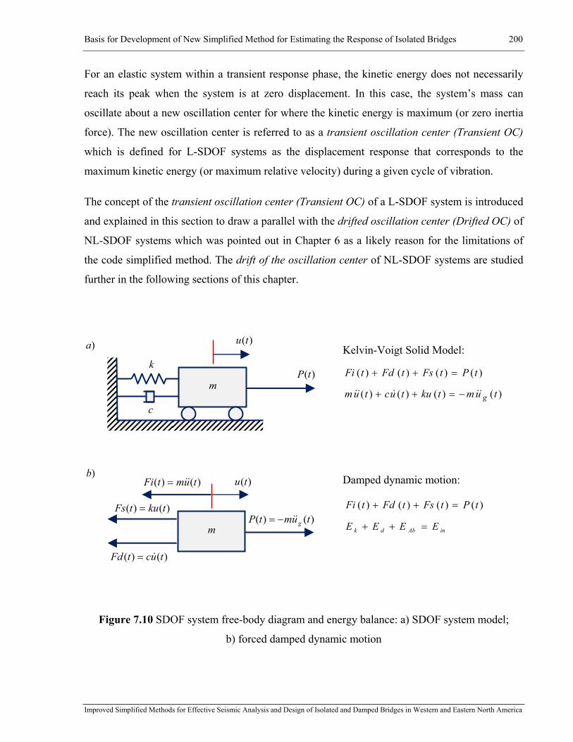
Basis for Development of New Simplified Method for Estimating the Response of Isolated Bridges 200
Improved Simplified Methods for Effective Seismic Analysis and Design of Isolated and Damped Bridges in Western and Eastern North America
For an elastic system within a transient response phase, the kinetic energy does not necessarily
reach its peak when the system is at zero displacement. In this case, the system’s mass can
oscillate about a new oscillation center for where the kinetic energy is maximum (or zero inertia
force). The new oscillation center is referred to as a transient oscillation center (Transient OC)
which is defined for L-SDOF systems as the displacement response that corresponds to the
maximum kinetic energy (or maximum relative velocity) during a given cycle of vibration.
The concept of the transient oscillation center (Transient OC) of a L-SDOF system is introduced
and explained in this section to draw a parallel with the drifted oscillation center (Drifted OC) of
NL-SDOF systems which was pointed out in Chapter 6 as a likely reason for the limitations of
the code simplified method. The drift of the oscillation center of NL-SDOF systems are studied
further in the following sections of this chapter.
Figure 7.10 SDOF system free-body diagram and energy balance: a) SDOF system model;
b) forced damped dynamic motion
)()()()( tPtFstFdtFi =++
inAbdk EEEE =++
Kelvin-Voigt Solid Model:
Damped dynamic motion:
)()()()( tumtkutuctum g&&&&& −=++
)()()()( tPtFstFdtFi =++
)a
)b)(tu
)()( tumtP g&&−=)()( tkutFs =
)()( tuctFd &=
)()( tumtFi &&=
m
)(tu
)(tPk
c
m
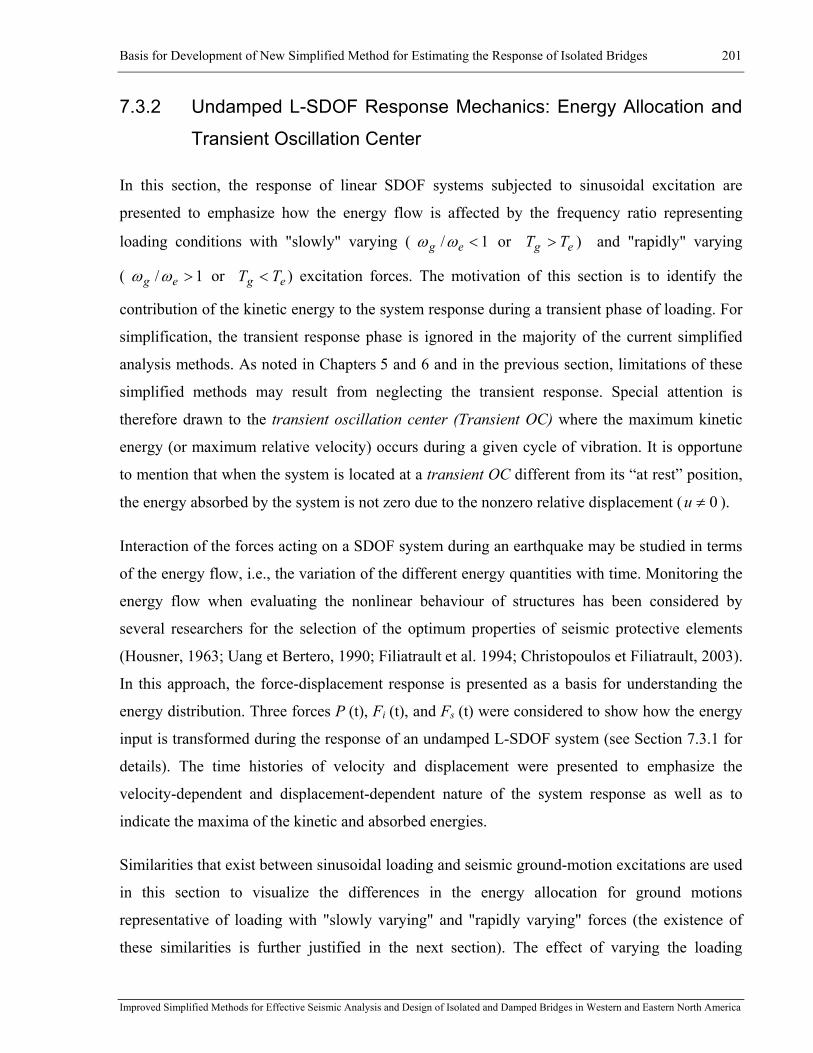
Basis for Development of New Simplified Method for Estimating the Response of Isolated Bridges 201
Improved Simplified Methods for Effective Seismic Analysis and Design of Isolated and Damped Bridges in Western and Eastern North America
7.3.2 Undamped L-SDOF Response Mechanics: Energy Allocation and
Transient Oscillation Center
In this section, the response of linear SDOF systems subjected to sinusoidal excitation are
presented to emphasize how the energy flow is affected by the frequency ratio representing
loading conditions with "slowly" varying ( 1/ <eg ωω or eg TT > ) and "rapidly" varying
( 1/ >eg ωω or eg TT < ) excitation forces. The motivation of this section is to identify the
contribution of the kinetic energy to the system response during a transient phase of loading. For
simplification, the transient response phase is ignored in the majority of the current simplified
analysis methods. As noted in Chapters 5 and 6 and in the previous section, limitations of these
simplified methods may result from neglecting the transient response. Special attention is
therefore drawn to the transient oscillation center (Transient OC) where the maximum kinetic
energy (or maximum relative velocity) occurs during a given cycle of vibration. It is opportune
to mention that when the system is located at a transient OC different from its “at rest” position,
the energy absorbed by the system is not zero due to the nonzero relative displacement ( 0≠u ).
Interaction of the forces acting on a SDOF system during an earthquake may be studied in terms
of the energy flow, i.e., the variation of the different energy quantities with time. Monitoring the
energy flow when evaluating the nonlinear behaviour of structures has been considered by
several researchers for the selection of the optimum properties of seismic protective elements
(Housner, 1963; Uang et Bertero, 1990; Filiatrault et al. 1994; Christopoulos et Filiatrault, 2003).
In this approach, the force-displacement response is presented as a basis for understanding the
energy distribution. Three forces P (t), Fi (t), and Fs (t) were considered to show how the energy
input is transformed during the response of an undamped L-SDOF system (see Section 7.3.1 for
details). The time histories of velocity and displacement were presented to emphasize the
velocity-dependent and displacement-dependent nature of the system response as well as to
indicate the maxima of the kinetic and absorbed energies.
Similarities that exist between sinusoidal loading and seismic ground-motion excitations are used
in this section to visualize the differences in the energy allocation for ground motions
representative of loading with "slowly varying" and "rapidly varying" forces (the existence of
these similarities is further justified in the next section). The effect of varying the loading

Basis for Development of New Simplified Method for Estimating the Response of Isolated Bridges 202
Improved Simplified Methods for Effective Seismic Analysis and Design of Isolated and Damped Bridges in Western and Eastern North America
frequency is therefore examined for an undamped linear elastic system initially at rest and
suddenly subjected to a one-cycle sinusoidal loading. Three frequency ratios are considered:
[ ]5.1;0.1;75.0/ =eg ωω . These three loading cases are respectively representative of a structure
characterized by a fundamental period Te (ωe) subjected to three different ground motions
( eg TT >1 , eg TT =2 , and eg TT <3 ), or a ground motion with predominant period Tg (ωg) that
excites three different structures ( 1eg TT > , 2eg TT = , and 3eg TT < ). This is illustrated in Figures
7.11 and 7.12.
SD
Period, TTe2=Tg
ωg/ωe2=1.0
Te1<Tg
ωg/ωe1=0.75
Tg<Te3
ωg/ωe3=1.5
Figure 7.11 Example of loading frequency ratios ]5.1;0.1;75.0[/ =eg ωω for three different
bridge structures subjected to the same ground motion excitation

Basis for Development of New Simplified Method for Estimating the Response of Isolated Bridges 203
Improved Simplified Methods for Effective Seismic Analysis and Design of Isolated and Damped Bridges in Western and Eastern North America
Figure 7.12 Example of loading frequency ratios ]5.1;0.1;75.0[/ =eg ωω for a bridge structure
subjected to three different ground-motion excitations

Basis for Development of New Simplified Method for Estimating the Response of Isolated Bridges 204
Improved Simplified Methods for Effective Seismic Analysis and Design of Isolated and Damped Bridges in Western and Eastern North America
The loading function considered for the linear time-history analyses on the undamped L-SDOF
systems is given as:
)sin()sin()sin()( 2000 ϕωωϕωϕω +⋅⋅−=+⋅−=+⋅= tumtumtptP gggg && (7.18)
Where the phase angle °= 0ϕ corresponds to the system's initial conditions at rest ( 0)0( =u and
0)0( =u& ).
The energy balance is established through the contribution of the three forces interacting at the
level of the mass:
)()()( tEtEtE inAbk =+ (7.19)
Figures 7.13 and 7.14 compare the responses of the L-SDOF systems undergoing one cycle of
sinusoidal loading from the “at rest” state where the transient portion of the response is
predominant. The results were normalized with respect to the force excitation amplitude 0p , the
base displacement amplitude 0u , and the excitation frequency gω (or period gT ). Key system
and response parameters are presented in Table 7-1. The calculations are performed for ωg / ωe =
0.75, 1.0 and 1.5. The first and third cases are representative of the responses for ωg / ωe < 1.0
and ωg / ωe > 1.0, respectively.
In Figure 7.13, force time-histories and force-displacement responses during the excitation cycle
of the L-SDOF system are presented on the left-hand side (LHS) and right-hand side (RHS) of
the figure, respectively. In the LHS figure, the time history of the elastic force also represents the
relative displacement history as both parameters are proportional to each other. As discussed in
the previous section, in each half-cycle, the inertia force passes by zero ( 0== umFi && ) and the
kinetic energy then reaches its maximum at this point. Accordingly, for the entire cycle, there are
two transient OCs, one in each displacement direction, where kinetic energy is maximum. At
these system positions, because the inertia force is zero, the excitation input force is balanced by
the spring force (P = Fs). From the beginning of the loading, the inertia force Fi was acting in the
opposite direction with respect to the excitation force P. At the transient OC, the inertia force
changes sign and, from this point on, P and Fi act in the same direction, opposite to the direction
of the elastic spring force Fs. For all three frequency ratios, Fi is still acting in the direction

Basis for Development of New Simplified Method for Estimating the Response of Isolated Bridges 205
Improved Simplified Methods for Effective Seismic Analysis and Design of Isolated and Damped Bridges in Western and Eastern North America
opposite to Fs when Fs (and the relative displacement) reaches its maximum. However, the input
(excitation) force P is opposite to Fs for 1 0g e/ .ω ω < and acts in the same direction as Fs
for 1 0g e/ .ω ω > . For 1 0g e/ .ω ω = , P=0 when Fs is maximum and, accordingly, Fs = Fi at this
point. In the figure, the portion of the inertia force in the overall force balance increases with the
frequency ratio. It can also be noted that the L-SDOF system experiences larger displacement
responses for higher frequency ratios. This is due to the greater contribution of the inertia force
and kinetic energy, as explained next.
Figure 7.13 Response of elastic SDOF system for ]5.1;0.1;75.0[/ =eg ωω
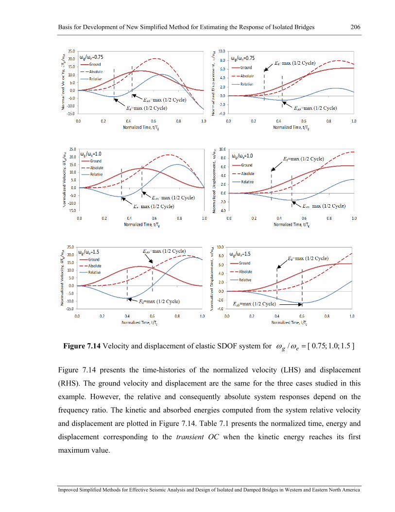
Basis for Development of New Simplified Method for Estimating the Response of Isolated Bridges 206
Improved Simplified Methods for Effective Seismic Analysis and Design of Isolated and Damped Bridges in Western and Eastern North America
Figure 7.14 Velocity and displacement of elastic SDOF system for ]5.1;0.1;75.0[/ =eg ωω
Figure 7.14 presents the time-histories of the normalized velocity (LHS) and displacement
(RHS). The ground velocity and displacement are the same for the three cases studied in this
example. However, the relative and consequently absolute system responses depend on the
frequency ratio. The kinetic and absorbed energies computed from the system relative velocity
and displacement are plotted in Figure 7.14. Table 7.1 presents the normalized time, energy and
displacement corresponding to the transient OC when the kinetic energy reaches its first
maximum value.
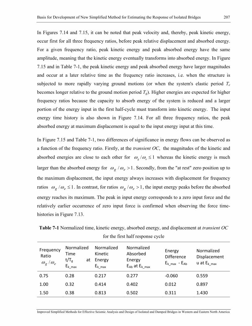
Basis for Development of New Simplified Method for Estimating the Response of Isolated Bridges 207
Improved Simplified Methods for Effective Seismic Analysis and Design of Isolated and Damped Bridges in Western and Eastern North America
In Figures 7.14 and 7.15, it can be noted that peak velocity and, thereby, peak kinetic energy,
occur first for all three frequency ratios, before peak relative displacement and absorbed energy.
For a given frequency ratio, peak kinetic energy and peak absorbed energy have the same
amplitude, meaning that the kinetic energy eventually transforms into absorbed energy. In Figure
7.15 and in Table 7-1, the peak kinetic energy and peak absorbed energy have larger magnitudes
and occur at a later relative time as the frequency ratio increases, i.e. when the structure is
subjected to more rapidly varying ground motions (or when the system's elastic period Te
becomes longer relative to the ground motion period Tg). Higher energies are expected for higher
frequency ratios because the capacity to absorb energy of the system is reduced and a larger
portion of the energy input in the first half-cycle must transform into kinetic energy. The input
energy time history is also shown in Figure 7.14. For all three frequency ratios, the peak
absorbed energy at maximum displacement is equal to the input energy input at this time.
In Figure 7.15 and Table 7-1, two differences of significance in energy flows can be observed as
a function of the frequency ratio. Firstly, at the transient OC, the magnitudes of the kinetic and
absorbed energies are close to each other for 1/ ≤eg ωω whereas the kinetic energy is much
larger than the absorbed energy for 1/ >eg ωω . Secondly, from the "at rest" zero position up to
the maximum displacement, the input energy always increases with displacement for frequency
ratios 1/ ≤eg ωω . In contrast, for ratios 1/ >eg ωω , the input energy peaks before the absorbed
energy reaches its maximum. The peak in input energy corresponds to a zero input force and the
relatively earlier occurrence of zero input force is confirmed when observing the force time-
histories in Figure 7.13.
Table 7-1 Normalized time, kinetic energy, absorbed energy, and displacement at transient OC
for the first half response cycle
Frequency Ratio
eg ωω /
Normalized Time t/Tg at Ek_max
Normalized Kinetic Energy Ek_max
Normalized Absorbed Energy EAb at Ek_max
Energy Difference Ek_max ‐ EAb
Normalized Displacement u at Ek_max
0.75 0.28 0.217 0.277 ‐0.060 0.559
1.00 0.32 0.414 0.402 0.012 0.897
1.50 0.38 0.813 0.502 0.311 1.430
Basis for Development of New Simplified Method for Estimating the Response of Isolated Bridges 208
Improved Simplified Methods for Effective Seismic Analysis and Design of Isolated and Damped Bridges in Western and Eastern North America
Based on these observations, it can be stated that for ratios 1/ >eg ωω , the input energy is
transmitted into the system at a faster rate than the rate of energy absorption of the system. In
other words, the portion of the input energy transformed into the kinetic energy is larger than that
can be transformed into absorbed energy. Accordingly, an excessive amount of energy is stored
within the system’s motion (kinetic energy) that will be absorbed by the system at a later time,
leading to a larger displacement response.
When the system is initially at rest, the first half cycle seems to be crucial from an energy
allocation point of view, and this energy distribution may affect peak displacement demand. The
system response during the transient phase may be represented by the combined effect of the free
vibration and forced steady-state responses. These responses may be solved mathematically as
the sum of the particular solution, up(t), and complementary solution, uc(t), for steady-state and
transient responses, respectively (Chopra, 2011). The complete displacement solution )(tu
characterizes the system's mass position with respect to its “at rest” equilibrium position at the
time t starting “at rest” initial conditions 0)0( =u and 0)0( =u& . Figures 7.16 and 7.17 show
histories of the normalized relative displacement and velocity for transient and steady-state
responses for a high frequency ratio ( 1 5g e/ .=ω ω ). As shown in the figure, higher displacement
demand can occur under this combined effect compared to a steady-state response alone, which
can be missed when using simplified analysis methods that rely only on the steady-state
response.
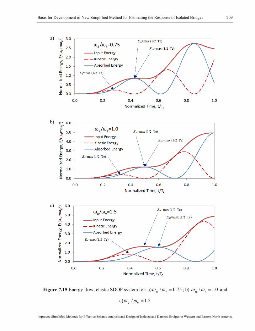
Basis for Development of New Simplified Method for Estimating the Response of Isolated Bridges 209
Improved Simplified Methods for Effective Seismic Analysis and Design of Isolated and Damped Bridges in Western and Eastern North America
a)
b)
c)
Figure 7.15 Energy flow, elastic SDOF system for: a) 75.0/ =eg ωω ; b) 0.1/ =eg ωω and
c) 5.1/ =eg ωω
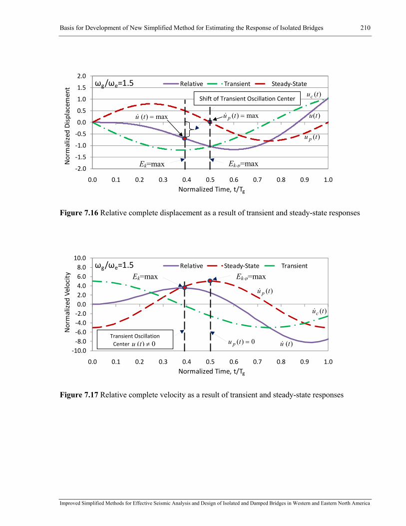
Basis for Development of New Simplified Method for Estimating the Response of Isolated Bridges 210
Improved Simplified Methods for Effective Seismic Analysis and Design of Isolated and Damped Bridges in Western and Eastern North America
Figure 7.16 Relative complete displacement as a result of transient and steady-state responses
Figure 7.17 Relative complete velocity as a result of transient and steady-state responses
‐10.0‐8.0‐6.0‐4.0‐2.00.02.04.06.08.010.0
0.0 0.1 0.2 0.3 0.4 0.5 0.6 0.7 0.8 0.9 1.0
Normalized
Velocity
Normalized Time, t/Tg
ωg/ωe=1.5 Relative Steady‐State Transient
Ek-p=maxEk=max
0)( =tu pTransient Oscillation Center 0)( ≠tu )(tu&
)(tu p&
)(tuc&
‐2.0
‐1.5
‐1.0
‐0.5
0.0
0.5
1.0
1.5
2.0
0.0 0.1 0.2 0.3 0.4 0.5 0.6 0.7 0.8 0.9 1.0
Normalized
Displacem
ent
Normalized Time, t/Tg
ωg/ωe=1.5 Relative Transient Steady‐State
Ek-p=maxEk=max
Shift of Transient Oscillation Center
max)( =tu p&
)(tuc
)(tu p
)(tumax)( =tu&

Basis for Development of New Simplified Method for Estimating the Response of Isolated Bridges 211
Improved Simplified Methods for Effective Seismic Analysis and Design of Isolated and Damped Bridges in Western and Eastern North America
The equation of motion corresponding to the elastic system without damping subjected to
harmonic sinusoidal loading is presented as follows (Chopra, 2011):
tptFtum gs ωsin)()( 0=+&& (7.20)
The particular solution that describes a steady-state motion is given as ( eg ωω ≠ ):
tkp
tu gege
p ωωω
sin/1
1)( 220 ⋅
−⋅= (7.21)
The complementary solution that represents transient response is given as ( eg ωω ≠ ):
tkp
tututu eeg
eg
ee
eec ω
ωω
ωωω
ωω sin
/1
/sin)0(cos)0()( 22
0 ⋅−
⋅−⋅+⋅=&
(7.22)
For the system being at rest at the start of the loading, Equation 7.22 is reduces to:
tkp
tu eeg
eg
ec ω
ωω
ωωsin
/1
/)( 22
0 ⋅−
⋅−= (7.23)
The corresponding complete solution becomes:
⎟⎟⎠
⎞⎜⎜⎝
⎛−⋅
−=+= tt
kptututu e
e
gg
egepc ω
ωω
ωωω
sinsin/1
1)()()( 220 (7.24)
Differentiating Equations 7.21 and 7.22 with respect to time and rewriting for the initial
conditions at rest the velocity particular and complementary solutions are obtained as:
tkptu g
eg
g
ep ω
ωω
ωcos
/1)( 22
0 ⋅−
⋅=& (7.25)
tkp
tu eeg
g
ec ω
ωω
ωcos
/1)( 22
0 ⋅−
⋅−=& (7.26)

Basis for Development of New Simplified Method for Estimating the Response of Isolated Bridges 212
Improved Simplified Methods for Effective Seismic Analysis and Design of Isolated and Damped Bridges in Western and Eastern North America
Similarly, the complete solution for the relative velocity is given as:
)cos(cos/1
)( 220 tt
kp
tu egeg
g
eωω
ωω
ω−⋅
−⋅=& (7.27)
By differentiating Equation 7.27 with respect to time and equating the resulting acceleration to
zero, the time at which the relative velocity (and kinetic energy) reaches its maximum is obtained
from the following equation:
0)sinsin(/1
)( 220 =−⋅
−⋅= tt
kp
tu ggeeeg
g
eωωωω
ωω
ω&& (7.28)
Equation 6.23 is satisfied when:
0sinsin =− tt ge
ge ω
ωω
ω or e
g
g
ett
ωω
ωω
=sinsin
(7.29)
Solving Equation 7.29 for time t and substituting it in Equations 7.22 and 7.27 respectively, the
relative displacement, )( maxuu & and the maximum relative velocity, maxu& at the position of the
transient OC can be calculated. The maximum kinetic energy is then obtained from Equation
7.30 as a function of the relative velocity (complete solution - )(tu& ):
2)(
2))()((
)(22 tumtutum
tE cpk
&&&=
+= (7.30)
The corresponding absorbed energy is determined with the system relative displacement as a
static strain energy stored in the spring, ke:
eAb kuuE 2max 2
1)( =& (7.31)
The kinetic and absorbed energies at the transient OC are plotted in Figure 7.17 for eg ωω /
ranging from 0.2 to 2.0. In this figure, the energies are normalized with respect to ust mωg2. It can
be noted that for frequency ratios up to the resonant state 1/ =eg ωω , the magnitudes of the two
energies are close. Beyond the resonant ratio, the maximum kinetic energy increases with the

Basis for Development of New Simplified Method for Estimating the Response of Isolated Bridges 213
Improved Simplified Methods for Effective Seismic Analysis and Design of Isolated and Damped Bridges in Western and Eastern North America
frequency ratio, while the corresponding absorbed energy remains nearly constant at a level
slightly higher than at resonance. Based on the previous discussion, higher kinetic energy
compared to absorbed energy at the transient OC produces an unbalanced condition at this point:
the system will have to deform to larger peak displacements before it can completely absorb the
excess in kinetic energy. In Figure 7.18, the significant increase in the difference between the
two energies for frequency ratios higher than unity ( 1/ >eg ωω ) suggests that larger peak
displacements can be expected during the transient phase of the response to ground motions
having dominant frequencies higher than that of the bridge structure.
Figure 7.18 Influence of the frequency ration on normalized kinetic Ek and absorbed EAb
energies at the transient OC for undamped L-SDOF systems
In the following sections the similarity between the effect of the frequency ratio on the response
of L-SDOF systems and the influence of the effective stiffness keff for NL-SDOF systems will be
outlined. Isolated bridge structures are typically designed with low lateral resistance at the
activation of the isolation system (high R-ratios), which translates into low effective stiffness
and, possibly, high frequency ratios. This means that transient response may be of importance for
such structures.
Before moving to the response of nonlinear systems, it should be noted that the transient
oscillation center for L-SDOF systems gradually converges to the system's initial zero
deformation position when the transient response gradually diminishes and the system reaches its
0.0
0.2
0.4
0.6
0.8
1.0
1.2
1.4
0.0 0.2 0.4 0.6 0.8 1.0 1.2 1.4 1.6 1.8 2.0
Normalized
Energy
Frequency ratio, ωg/ωe
Kinetic
Absorbed kE
AbE
1/ <eg ωω 1/ >eg ωω

Basis for Development of New Simplified Method for Estimating the Response of Isolated Bridges 214
Improved Simplified Methods for Effective Seismic Analysis and Design of Isolated and Damped Bridges in Western and Eastern North America
steady-state condition. In turn, the transient oscillation center for NL-SDOF systems
corresponds to a permanent residual displacement when the system experiences inelastic
response. It is therefore expected, as will be further investigated in the following sections, that
there is a critical value of the response modification factor R (Rcr) beyond which an excessive
amount of energy amount is allocated to kinetic energy and produces a permanent shift, or drift,
of the oscillation center. In such a case, the total displacement of the nonlinear system is equal to
the sum of the oscillation center drift and the local system response about this new oscillation
center. The effect of the energy excess allocated as kinetic energy and the resulting oscillation
center drift on the responses of NL-SDOF systems are therefore further studied in this chapter.
7.3.3 Transient Response of NL-SDOF Systems to Sinusoidal Loading
In the previous section, the transient oscillation center and the excess of kinetic energy at that
point were outlined for the transient response of L-SDOF systems by examining the energy flow
in the system. Excess of kinetic energy was found to occur for frequency ratios higher than 1.0,
i.e., for "rapidly" varying ( 1/ >eg ωω ) ground motions with respect to the structure frequency.
In this section, the concepts of excess of kinetic energy and the transient oscillation center are
examined for undamped nonlinear (bilinear) systems subjected to harmonic loading.
Contrary to the undamped linear system in which there was no dissipation of energy, the energy
in undamped NL-SDOF systems is dissipated through inelastic behaviour of the system. An
overview of loading assumptions for reproducing seismic response of structures by using
harmonically applied loading is presented first. A sinusoidal function is then defined to excite
structures from their rest conditions. The reference structure and system's nonlinear parameters
are configured so that a wide range of isolated bridges subjected to different earthquake ground
motions are covered.
7.3.3.1 Definition of Loading Function: Assumptions and Parameters
The loading function used for the L-SDOF systems is considered again here for the parametric
study on the NL-SDOF systems:
)sin()sin()sin()( 2000 ϕωωϕωϕω +⋅⋅−=+⋅−=+⋅= tumtumtptP gggg && (7.18)

Basis for Development of New Simplified Method for Estimating the Response of Isolated Bridges 215
Improved Simplified Methods for Effective Seismic Analysis and Design of Isolated and Damped Bridges in Western and Eastern North America
where the phase angle °= 0ϕ corresponds to the system's initial conditions at rest ( 0)0( =u or
0)0( =u& ). These initial conditions were adopted to approximate the system response at the
beginning of the few large amplitude cycles of the strong motion portion of a seismic ground
motion..
In order to approximate seismic response using theoretical closed form solutions, various forcing
functions have been studied by many researchers over the last decades. The response of systems
initially at rest subjected to a series of load-time functions has been discussed by Jacobsen and
Ayre (1958), Housner (1963), and Biggs (1964). Closed-form solutions have been proposed for
the response of linear elastic systems for these loading functions. Iwan (1961) and Masri (1974)
proposed "exact" analytical solutions for a steady-state response of bilinear systems. Despite the
significant effort in developing "exact" solutions for bilinear systems analytically, there seems to
exist no closed-form expression to obtain the transient response of an inelastic bilinear system
subjected to sinusoidal loading.
Hall et al. (1995) introduced two types of simple ground pulses to idealize forward only (non-
reversing) displacement and forward and back (reversing) displacement denoted as Type A and
Type B, respectively. Makris (1997) proposed to approximate pulse-like ground motions with
trigonometric functions having a cycloidal front. He highlighted that the use of such a function
was preferred to the step-pulse loading previously proposed by Hall et al. (1995) since the
possibility of a closed-form solution as well as that the response to this type of loading is not
influenced by infinite accelerations or "jerks". Figure 7.19 presents two pulse motions of type A
and B studied by Makris to simulate ground motions produced, respectively, by the 17 January
1994 Northridge and the 28 June 1992 Landers earthquakes.

Basis for Development of New Simplified Method for Estimating the Response of Isolated Bridges 216
Improved Simplified Methods for Effective Seismic Analysis and Design of Isolated and Damped Bridges in Western and Eastern North America
Figure 7.19 Cycloidal front pulses: Type A (left) and Type B (right) used by Makris (1997) to
approximate recorded ground motions.
To assign the appropriate pulse amplitude and period, Makris (1997) manipulated the peak
ground displacement and the peak ground velocity of the corresponding ground motion, so that
the predominant period can be obtained by dividing the maximum ground displacement by the
maximum ground velocity. While the maximum pulse displacement and velocity were in good
agreement with those of the ground motion, the obtained accelerations underestimated the actual
peak accelerations. As a result, to describe the pulse acceleration amplitude, maxA , the following
expressions have been proposed:
Type A:
2/max ggVA ω= (7.31)
Type B:
ggVA ω=max (7.32)
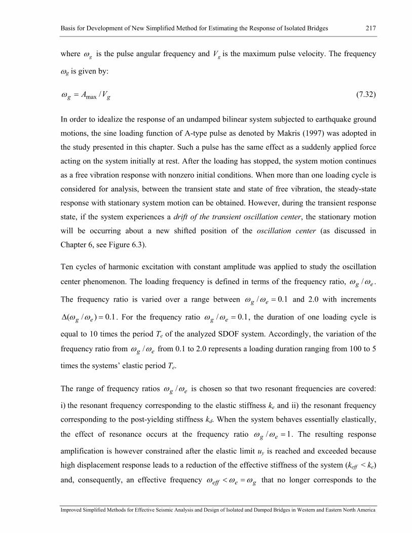
Basis for Development of New Simplified Method for Estimating the Response of Isolated Bridges 217
Improved Simplified Methods for Effective Seismic Analysis and Design of Isolated and Damped Bridges in Western and Eastern North America
where gω is the pulse angular frequency and gV is the maximum pulse velocity. The frequency
ωg is given by:
gg VA /max=ω (7.32)
In order to idealize the response of an undamped bilinear system subjected to earthquake ground
motions, the sine loading function of A-type pulse as denoted by Makris (1997) was adopted in
the study presented in this chapter. Such a pulse has the same effect as a suddenly applied force
acting on the system initially at rest. After the loading has stopped, the system motion continues
as a free vibration response with nonzero initial conditions. When more than one loading cycle is
considered for analysis, between the transient state and state of free vibration, the steady-state
response with stationary system motion can be obtained. However, during the transient response
state, if the system experiences a drift of the transient oscillation center, the stationary motion
will be occurring about a new shifted position of the oscillation center (as discussed in
Chapter 6, see Figure 6.3).
Ten cycles of harmonic excitation with constant amplitude was applied to study the oscillation
center phenomenon. The loading frequency is defined in terms of the frequency ratio, eg ωω / .
The frequency ratio is varied over a range between 1.0/ =eg ωω and 2.0 with increments
1.0)/( =Δ eg ωω . For the frequency ratio 1.0/ =eg ωω , the duration of one loading cycle is
equal to 10 times the period Te of the analyzed SDOF system. Accordingly, the variation of the
frequency ratio from eg ωω / from 0.1 to 2.0 represents a loading duration ranging from 100 to 5
times the systems’ elastic period Te.
The range of frequency ratios eg ωω / is chosen so that two resonant frequencies are covered:
i) the resonant frequency corresponding to the elastic stiffness ke and ii) the resonant frequency
corresponding to the post-yielding stiffness kd. When the system behaves essentially elastically,
the effect of resonance occurs at the frequency ratio 1/ =eg ωω . The resulting response
amplification is however constrained after the elastic limit uy is reached and exceeded because
high displacement response leads to a reduction of the effective stiffness of the system (keff < ke)
and, consequently, an effective frequency geeff ωωω =< that no longer corresponds to the

Basis for Development of New Simplified Method for Estimating the Response of Isolated Bridges 218
Improved Simplified Methods for Effective Seismic Analysis and Design of Isolated and Damped Bridges in Western and Eastern North America
resonance conditions. A sustainable resonance effect can however be anticipated when the
effective frequency approaches the frequency corresponding to the post-yield stiffness (keff →
kd). The frequency ratio for this condition ( deff ωω → ) can be determined as a function of the
post-yield stiffness ratio α as follows:
System's elastic frequency is determined as:
mke
e =ω (7.33)
Post-yielding frequency related to the second slope stiffness α ke :
αωαω eed
d mk
mk
=⋅
== (7.34)
Resonance condition corresponding to the post-yielding stiffness kd when:
dg ωω = (7.35)
By substituting Equation (7.34) in (7.35), the frequency ratio for post-yielding resonance is then
given as:
αωω
=e
g (7.36)
Using Equation (7.36), the frequency ratios for post-yielding resonance are respectively equal to
0.71, 0.32, 0.22 and 0.1 for the selected values of α = 0.5, 0.1, 0.05, and 0.01 (see below).
7.3.3.2 Definition of the Nonlinear Parameters
The parametric study was performed on SDOF systems exhibiting a bilinear hysteretic response.
Viscous damping is not considered in order to isolate the effect of the energy dissipated by a
bilinear system through its hysteretic behaviour.
A range of nonlinear systems was considered by varying the response modification factor R and
the post-yielding stiffness ratio α. Ten response modification factors R = 1.0, 1.25, 1.5, 2, 4, 8,

Basis for Development of New Simplified Method for Estimating the Response of Isolated Bridges 219
Improved Simplified Methods for Effective Seismic Analysis and Design of Isolated and Damped Bridges in Western and Eastern North America
16, 28, 40 and 52 and four post-yield stiffness ratios α = 0.5, 0.1, 0.05 and 0.01 were considered.
While α = 0.1, 0.05 and 0.01 are representative of structures equipped with typical isolation
systems, the case α = 0.5 is used to represent a non-isolated system. As mentioned, the g e/ω ω
ratio was varied from 0.1 to 2.0.
To establish a common comparison basis, a unique peak elastic displacement ue was used to
determine the activation displacement, Ruu ey /= of all nonlinear systems. The displacement ue
was taken equal to the maximum elastic response for a frequency ratio 1 0g e/ .=ω ω . This ratio
was selected because it corresponds to resonance and, therefore, leads to the maximum elastic
displacement among all frequency ratios. However, peak undamped elastic response at resonance
keeps increasing when applying several cycles of loading. For simplicity in this study, the
maximum displacement at the end of the first cycle of loading was selected for ue. The
calculation of ue is discussed next. This elastic displacement ue corresponds to a ratio R = 1 and
the activation displacement, Ruu ey /= , of all nonlinear configurations was defined as a
function of this elastic response, regardless of the frequency ratio. This represents an ensemble of
isolated bridge structures having different activation displacements, each bridge being subjected
to a series of harmonic signals exhibiting different frequencies.
The following paragraphs present the response at resonance of an elastic system subjected to a
sinusoidal excitation. This information is used to determine the reference displacement ue. It is
also used later when defining the critical value of the R factor, Rcr. The equation of motion
corresponding to the response of the undamped system is given as:
tptFtum gs ωsin)()( 0=+&& (7.20)
and the transient and steady-state responses are as follows (Filiatrault, 2008):
∫ −⋅=t
ege
dtmp
tu0
0 )(sinsin)( ττωτωω
(7.37)
Evaluating the integral of Equation (7.37), the response solution at an excitation time, t is:
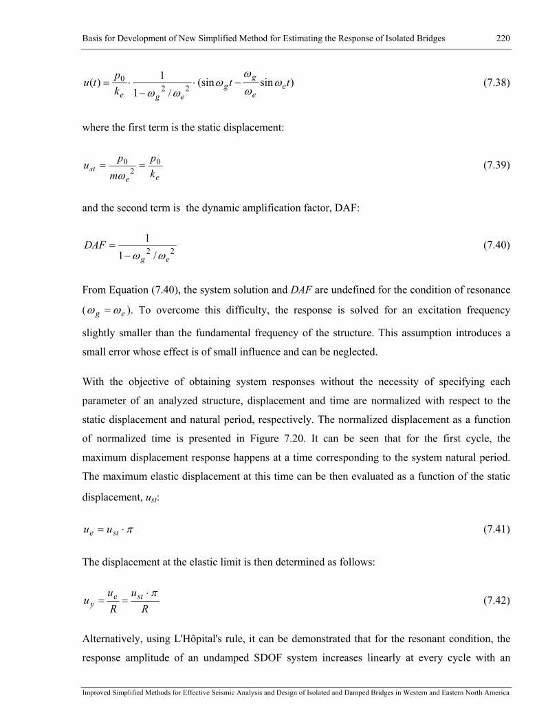
Basis for Development of New Simplified Method for Estimating the Response of Isolated Bridges 220
Improved Simplified Methods for Effective Seismic Analysis and Design of Isolated and Damped Bridges in Western and Eastern North America
)sin(sin/1
1)( 220 tt
kp
tu ee
gg
egeω
ωω
ωωω
−⋅−
⋅= (7.38)
where the first term is the static displacement:
eest k
pm
pu 0
20 ==
ω (7.39)
and the second term is the dynamic amplification factor, DAF:
22 /11
egDAF
ωω−= (7.40)
From Equation (7.40), the system solution and DAF are undefined for the condition of resonance
( eg ωω = ). To overcome this difficulty, the response is solved for an excitation frequency
slightly smaller than the fundamental frequency of the structure. This assumption introduces a
small error whose effect is of small influence and can be neglected.
With the objective of obtaining system responses without the necessity of specifying each
parameter of an analyzed structure, displacement and time are normalized with respect to the
static displacement and natural period, respectively. The normalized displacement as a function
of normalized time is presented in Figure 7.20. It can be seen that for the first cycle, the
maximum displacement response happens at a time corresponding to the system natural period.
The maximum elastic displacement at this time can be then evaluated as a function of the static
displacement, ust:
π⋅= ste uu (7.41)
The displacement at the elastic limit is then determined as follows:
Ru
Ru
u stey
π⋅== (7.42)
Alternatively, using L'Hôpital's rule, it can be demonstrated that for the resonant condition, the
response amplitude of an undamped SDOF system increases linearly at every cycle with an
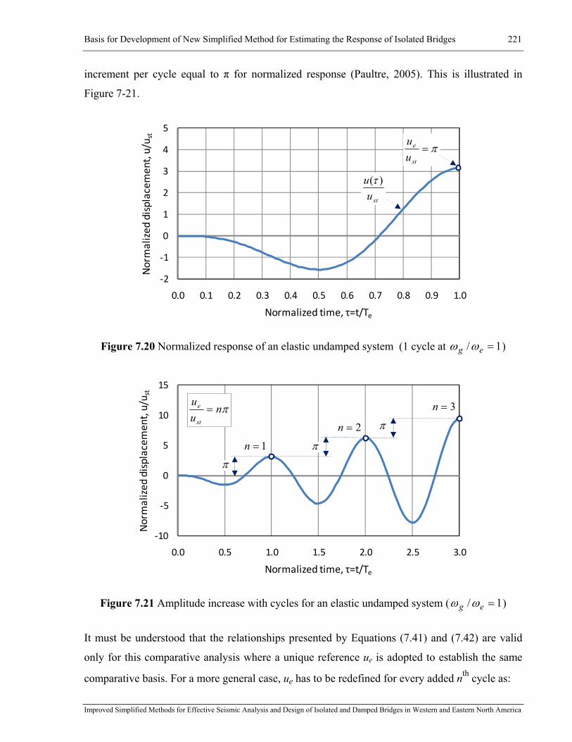
Basis for Development of New Simplified Method for Estimating the Response of Isolated Bridges 221
Improved Simplified Methods for Effective Seismic Analysis and Design of Isolated and Damped Bridges in Western and Eastern North America
increment per cycle equal to π for normalized response (Paultre, 2005). This is illustrated in
Figure 7-21.
Figure 7.20 Normalized response of an elastic undamped system (1 cycle at 1/ =eg ωω )
Figure 7.21 Amplitude increase with cycles for an elastic undamped system ( 1/ =eg ωω )
It must be understood that the relationships presented by Equations (7.41) and (7.42) are valid
only for this comparative analysis where a unique reference ue is adopted to establish the same
comparative basis. For a more general case, ue has to be redefined for every added nth cycle as:
‐10
‐5
0
5
10
15
0.0 0.5 1.0 1.5 2.0 2.5 3.0
Normalized
displacem
ent, u/u s
t
Normalized time, τ=t/Te
πnuu
st
e = 3=n
2=n
π
π
π
1=n
‐2
‐1
0
1
2
3
4
5
0.0 0.1 0.2 0.3 0.4 0.5 0.6 0.7 0.8 0.9 1.0
Normalized
displacem
ent, u/u s
t
Normalized time, τ=t/Te
stuu )(τ
π=st
e
uu
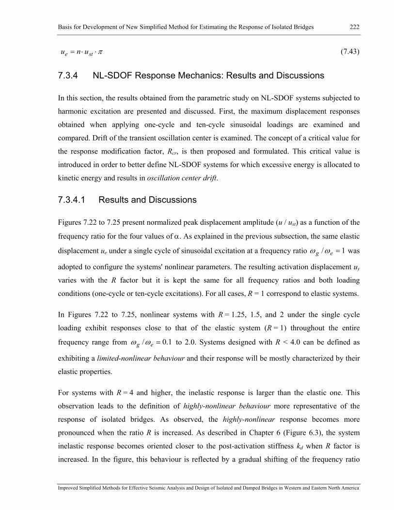
Basis for Development of New Simplified Method for Estimating the Response of Isolated Bridges 222
Improved Simplified Methods for Effective Seismic Analysis and Design of Isolated and Damped Bridges in Western and Eastern North America
π⋅⋅= ste unu (7.43)
7.3.4 NL-SDOF Response Mechanics: Results and Discussions
In this section, the results obtained from the parametric study on NL-SDOF systems subjected to
harmonic excitation are presented and discussed. First, the maximum displacement responses
obtained when applying one-cycle and ten-cycle sinusoidal loadings are examined and
compared. Drift of the transient oscillation center is examined. The concept of a critical value for
the response modification factor, Rcr, is then proposed and formulated. This critical value is
introduced in order to better define NL-SDOF systems for which excessive energy is allocated to
kinetic energy and results in oscillation center drift.
7.3.4.1 Results and Discussions
Figures 7.22 to 7.25 present normalized peak displacement amplitude (u / ust) as a function of the
frequency ratio for the four values of α. As explained in the previous subsection, the same elastic
displacement ue under a single cycle of sinusoidal excitation at a frequency ratio 1/ =eg ωω was
adopted to configure the systems' nonlinear parameters. The resulting activation displacement uy
varies with the R factor but it is kept the same for all frequency ratios and both loading
conditions (one-cycle or ten-cycle excitations). For all cases, R = 1 correspond to elastic systems.
In Figures 7.22 to 7.25, nonlinear systems with R = 1.25, 1.5, and 2 under the single cycle
loading exhibit responses close to that of the elastic system (R = 1) throughout the entire
frequency range from 1.0/ =eg ωω to 2.0. Systems designed with R < 4.0 can be defined as
exhibiting a limited-nonlinear behaviour and their response will be mostly characterized by their
elastic properties.
For systems with R = 4 and higher, the inelastic response is larger than the elastic one. This
observation leads to the definition of highly-nonlinear behaviour more representative of the
response of isolated bridges. As observed, the highly-nonlinear response becomes more
pronounced when the ratio R is increased. As described in Chapter 6 (Figure 6.3), the system
inelastic response becomes oriented closer to the post-activation stiffness kd when R factor is
increased. In the figure, this behaviour is reflected by a gradual shifting of the frequency ratio

Basis for Development of New Simplified Method for Estimating the Response of Isolated Bridges 223
Improved Simplified Methods for Effective Seismic Analysis and Design of Isolated and Damped Bridges in Western and Eastern North America
where maximum response is obtained gradually shifting from the value of 1.0 to the value
associated to the post-yielding resonance conditions defined by Equation (6.31) when increasing
R. This shift from elastic to post-yield resonance is more pronounced when the system is
subjected to the repeated loading of 10 cycles.
Using equations (7.41) and (7.43), the normalized peak displacement amplitude (u / ust) for the
elastic systems (R = 1) with 1/ =eg ωω that are subjected to one-cycle or ten-cycle are 3.14 and
31.4, respectively. The response amplification caused by the elastic resonance is primarily due to
the increase in energy stored within the system with each consecutive cycle. Such a resonance
amplification is unbounded (Iwan, 1961), given that there is an energy excess which is the
difference between the input energy and the energy dissipated by the system in each cycle. No
amplification is observed for systems exhibiting limited-nonlinear responses as those with
R = 1.25, 1.5, and 2.0. For limited-nonlinear response, the energy induced in the system over a
loading cycle is dissipated through the system's inelastic response within the same cycle and the
system generally oscillates about its original equilibrium position.
In contrast, for highly-nonlinear responses (in this study R ≥ 4), the amplitude increase with the
number of cycles is primarily due to the drift of the oscillation center. Such a drift results from
the excess of energy, as was the case in the elastic resonance. However, when the system is in the
highly-nonlinear response range, the energy excess is generated during a transient phase of
loading and can be dissipated through a few consecutive cycles. This resonance amplification is
bounded given that the transient oscillation center shifts gradually in each of these cycles until
the excess of energy is entirely dissipated (as is further shown in this section). Unbounded
resonance is expected, however, when ∞→R because the system cannot dissipate the input
energy completely. Such a system behaves nearly elastically, with deff kk → , rather than
inelastically. The unbounded inelastic behaviour is outside the scope of this study.
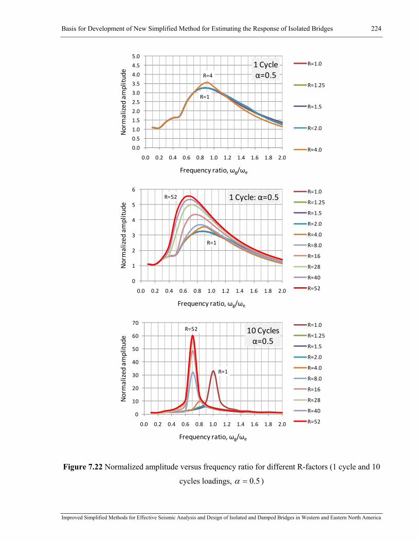
Basis for Development of New Simplified Method for Estimating the Response of Isolated Bridges 224
Improved Simplified Methods for Effective Seismic Analysis and Design of Isolated and Damped Bridges in Western and Eastern North America
R=1
R=4
0.0
0.5
1.0
1.5
2.0
2.5
3.0
3.5
4.0
4.5
5.0
0.0 0.2 0.4 0.6 0.8 1.0 1.2 1.4 1.6 1.8 2.0
Normalized
amplitu
de
Frequency ratio, ωg/ωe
1 Cycleα=0.5
R=1.0
R=1.25
R=1.5
R=2.0
R=4.0
R=1
R=52
0
1
2
3
4
5
6
0.0 0.2 0.4 0.6 0.8 1.0 1.2 1.4 1.6 1.8 2.0
Normalized
amplitu
de
Frequency ratio, ωg/ωe
1 Cycle: α=0.5R=1.0
R=1.25
R=1.5
R=2.0
R=4.0
R=8.0
R=16
R=28
R=40
R=52
R=1
R=52
0
10
20
30
40
50
60
70
0.0 0.2 0.4 0.6 0.8 1.0 1.2 1.4 1.6 1.8 2.0
Normalized
amplitu
de
Frequency ratio, ωg/ωe
10 Cyclesα=0.5
R=1.0
R=1.25
R=1.5
R=2.0
R=4.0
R=8.0
R=16
R=28
R=40
R=52
Figure 7.22 Normalized amplitude versus frequency ratio for different R-factors (1 cycle and 10
cycles loadings, 5.0=α )
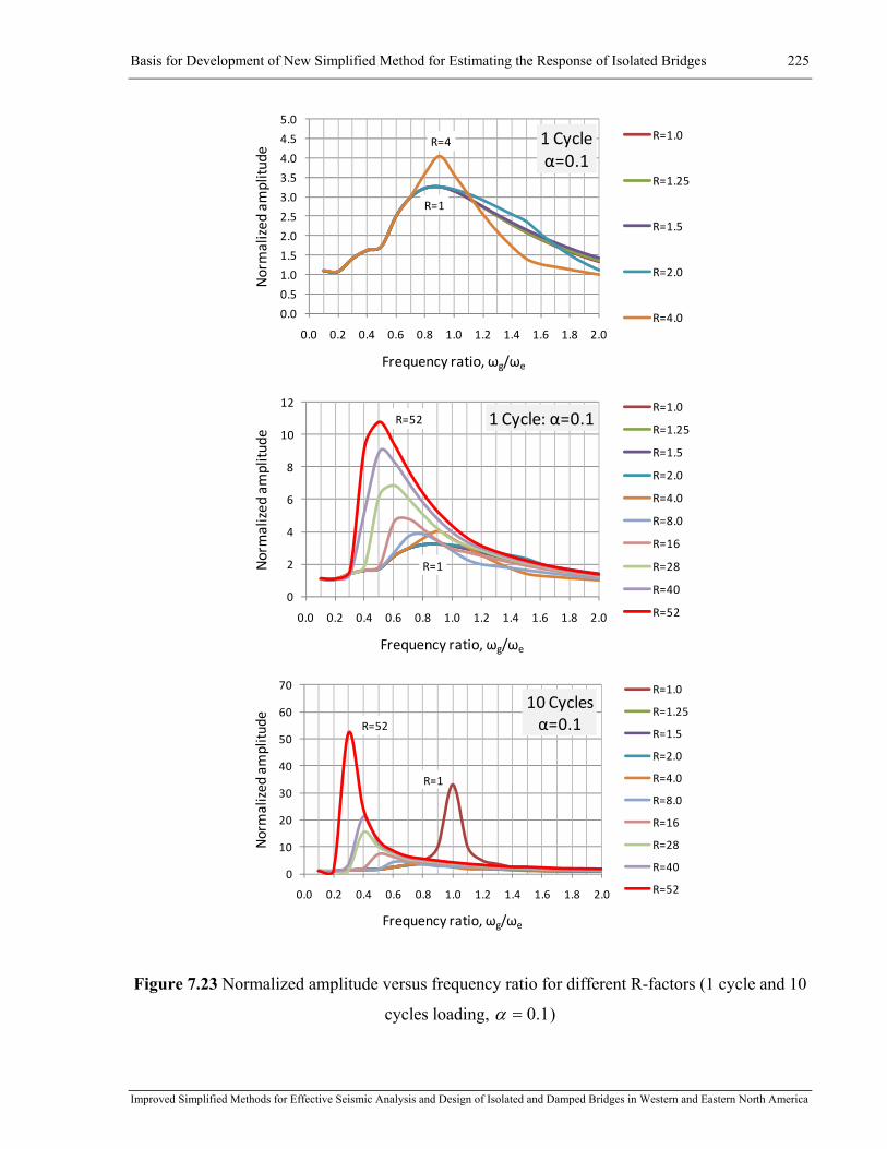
Basis for Development of New Simplified Method for Estimating the Response of Isolated Bridges 225
Improved Simplified Methods for Effective Seismic Analysis and Design of Isolated and Damped Bridges in Western and Eastern North America
R=1
R=4
0.0
0.5
1.0
1.5
2.0
2.5
3.0
3.5
4.0
4.5
5.0
0.0 0.2 0.4 0.6 0.8 1.0 1.2 1.4 1.6 1.8 2.0
Normalized
amplitu
de
Frequency ratio, ωg/ωe
1 Cycleα=0.1
R=1.0
R=1.25
R=1.5
R=2.0
R=4.0
R=1
R=52
0
2
4
6
8
10
12
0.0 0.2 0.4 0.6 0.8 1.0 1.2 1.4 1.6 1.8 2.0
Normalized
amplitu
de
Frequency ratio, ωg/ωe
1 Cycle: α=0.1R=1.0
R=1.25
R=1.5
R=2.0
R=4.0
R=8.0
R=16
R=28
R=40
R=52
R=1
R=52
0
10
20
30
40
50
60
70
0.0 0.2 0.4 0.6 0.8 1.0 1.2 1.4 1.6 1.8 2.0
Normalized
amplitu
de
Frequency ratio, ωg/ωe
10 Cyclesα=0.1
R=1.0
R=1.25
R=1.5
R=2.0
R=4.0
R=8.0
R=16
R=28
R=40
R=52
Figure 7.23 Normalized amplitude versus frequency ratio for different R-factors (1 cycle and 10
cycles loading, 1.0=α )
Basis for Development of New Simplified Method for Estimating the Response of Isolated Bridges 226
Improved Simplified Methods for Effective Seismic Analysis and Design of Isolated and Damped Bridges in Western and Eastern North America
R=1
R=4
0.0
0.5
1.0
1.5
2.0
2.5
3.0
3.5
4.0
4.5
5.0
0.0 0.2 0.4 0.6 0.8 1.0 1.2 1.4 1.6 1.8 2.0
Normalized
amplitu
de
Frequency ratio, ωg/ωe
1 Cycleα=0.05
R=1.0
R=1.25
R=1.5
R=2.0
R=4.0
R=1
R=4R=8
R=52
0
2
4
6
8
10
12
0.0 0.2 0.4 0.6 0.8 1.0 1.2 1.4 1.6 1.8 2.0
Normalized
amplitu
de
Frequency ratio, ωg/ωe
1 Cycle: α=0.05R=1.0
R=1.25
R=1.5
R=2.0
R=4.0
R=8.0
R=16
R=28
R=40
R=52
R=1
R=52
0
5
10
15
20
25
30
35
0.0 0.2 0.4 0.6 0.8 1.0 1.2 1.4 1.6 1.8 2.0
Normalized
amplitu
de
Frequency ratio, ωg/ωe
10 Cyclesα=0.05
R=1.0
R=1.25
R=1.5
R=2.0
R=4.0
R=8.0
R=16
R=28
R=40
R=52
Figure 7.24 Normalized amplitude versus frequency ratio for different R-factors (1 cycle and 10
cycles loading, 05.0=α )
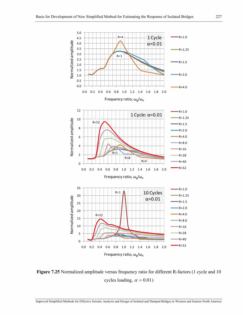
Basis for Development of New Simplified Method for Estimating the Response of Isolated Bridges 227
Improved Simplified Methods for Effective Seismic Analysis and Design of Isolated and Damped Bridges in Western and Eastern North America
R=1
R=4
0.0
0.5
1.0
1.5
2.0
2.5
3.0
3.5
4.0
4.5
5.0
0.0 0.2 0.4 0.6 0.8 1.0 1.2 1.4 1.6 1.8 2.0
Normalized
amplitu
de
Frequency ratio, ωg/ωe
1 Cycleα=0.01
R=1.0
R=1.25
R=1.5
R=2.0
R=4.0
R=1
R=4R=8
R=52
0
2
4
6
8
10
12
0.0 0.2 0.4 0.6 0.8 1.0 1.2 1.4 1.6 1.8 2.0
Normalized
amplitu
de
Frequency ratio, ωg/ωe
1 Cycle: α=0.01R=1.0
R=1.25
R=1.5
R=2.0
R=4.0
R=8.0
R=16
R=28
R=40
R=52
R=1
R=52
0
5
10
15
20
25
30
35
0.0 0.2 0.4 0.6 0.8 1.0 1.2 1.4 1.6 1.8 2.0
Normalized
amplitu
de
Frequency ratio, ωg/ωe
10 Cyclesα=0.01
R=1.0
R=1.25
R=1.5
R=2.0
R=4.0
R=8.0
R=16
R=28
R=40
R=52
Figure 7.25 Normalized amplitude versus frequency ratio for different R-factors (1 cycle and 10
cycles loading, 01.0=α )

Basis for Development of New Simplified Method for Estimating the Response of Isolated Bridges 228
Improved Simplified Methods for Effective Seismic Analysis and Design of Isolated and Damped Bridges in Western and Eastern North America
To provide more insight into these observations, velocity and displacement response time
histories under 10 cycles of sinusoidal loading are presented in Figure 7.25 for ωg / ωe = 1 and
α = 0.01. For the system with R = 2, the velocity response reaches its maximum during the
second half of the first cycle. The same maximum positive and minimum negative velocities are
observed in all subsequent cycles of loading. This highlights that there is a constant level of
kinetic energy that is stored within the system. The peak displacement response is also reached
during the second half of the first cycle. During the first half cycle, the system behaves
elastically and it starts dissipating energy only in the second half cycle. As shown, the maximum
displacement decreases in the subsequent cycles, indicating that the system's capacity to dissipate
energy remains higher than the energy input.
The system with R = 4 also exhibits the maximum velocity level during the second half of the
first cycle. However, lower velocity peaks are observed in the following cycles. The maximum
displacement is observed during the first cycle. In the first half cycle, the system experiences
inelastic excursions with similar maximum negative and the maximum positive displacements.
This represents a balanced displacement response, meaning that the same amount of energy is
dissipated in both directions during the cycle of loading.
Contrary to the balanced displacement response experienced by the system with R = 4, the
systems with R = 8 and 16 exhibit an unbalanced displacement response which is skewed in the
direction of the inelastic negative excursions. The maximum displacement response is observed
during the first and second cycles for the systems with R = 8 and R = 16, respectively. In these
cases, the maximum displacement comprises the oscillation center drift plus the local system
response about the new oscillation center. The peak displacements for subsequent cycles are
lower. The gradual reduction in displacement is attributed to the drift of the transient oscillation
center towards the "at rest" equilibrium position. The initial shifting of the transient oscillation
center results from the transformation of the excess of kinetic energy into the energy absorbed by
the system. It can be observed by comparing systems with R = 8 and R = 16 in Figure 7.26, the
system with the higher peak velocity during the first half cycle experiences the larger shift of the
transient oscillation center.

Basis for Development of New Simplified Method for Estimating the Response of Isolated Bridges 229
Improved Simplified Methods for Effective Seismic Analysis and Design of Isolated and Damped Bridges in Western and Eastern North America
‐80
‐60
‐40
‐20
0
20
40
60
80
0 1 2 3 4 5 6 7 8 9 10
Normalized
Velocity
Normalized Time, t/Tg
R=2 R=4 R=8 R=16
‐6‐5‐4‐3‐2‐1012345
0 1 2 3 4 5 6 7 8 9 10
Normalized
Displacem
ent
Normalized Time, t/Tg
R=2 R=4 R=8 R=16
Figure 7.26 Time histories of velocity and displacement responses for NL-SDOF with
ωg / ωe = 1, α = 0.01 under 10 cycles of sinusoidal loading
The influence of the R factor on the energy flow is illustrated in Figure 7.27 for systems at
resonance with R = 2, 4, and 16. In the figure the energies are normalized with respect to the
common reference ust mωg2 and all energy quantities for the three systems can be directly
compared. In this figure, the straight dash-dotted line indicates an idealized input energy rate at
which the system will exhibit a balanced displacement response. For the system with R = 4, the
energy input is generally follows the straight line indicating that the amount of input energy
induced in the system corresponds well to the system's capacity to absorb and dissipate this

Basis for Development of New Simplified Method for Estimating the Response of Isolated Bridges 230
Improved Simplified Methods for Effective Seismic Analysis and Design of Isolated and Damped Bridges in Western and Eastern North America
energy completely over the same cycle of loading. For the system with R = 2, the energy input is
situated under the straight line of the balanced displacement, which means that the system's
capacity to store the input energy is underused and the system therefore exhibits limited-
nonlinear response. For R = 16, the input energy is situated above the balanced energy straight
line suggesting a highly-nonlinear response. In this case, much higher input and kinetic energies
are developed over the first cycle.
The capacity to absorb energy of the system is reduced when increasing R, so that a larger
portion of the energy input in the first half-cycle must transform into kinetic energy. Higher
kinetic energy also means higher velocity in one direction. The system then has to absorb that
kinetic energy so that the velocity returns to zero at peak displacement. This takes longer in time
because of the limited capacity of the system to absorb energy. The shift in time for the kinetic
energy built-up and transformation into absorbed energy up to peak displacement can be seen in
Figure 7.27 when R is increased from 4 to 16.
The excessive kinetic energy over the first half response cycle can be confirmed by comparing
the peak kinetic energy at the first, second and third transient oscillation centers (transient OC).
This phenomenon is more pronounced in the first half-cycle, because energy dissipation has not
started yet. After peak displacement has been reached, most of the energy stored in the system is
dissipated and is no longer in the system to contribute to the response in the opposite direction.
Energy dissipation, together with the fact that energy input no longer is in phase with points of
system zero velocity, eventually leads to the stabilization of the response in the subsequent
cycles.
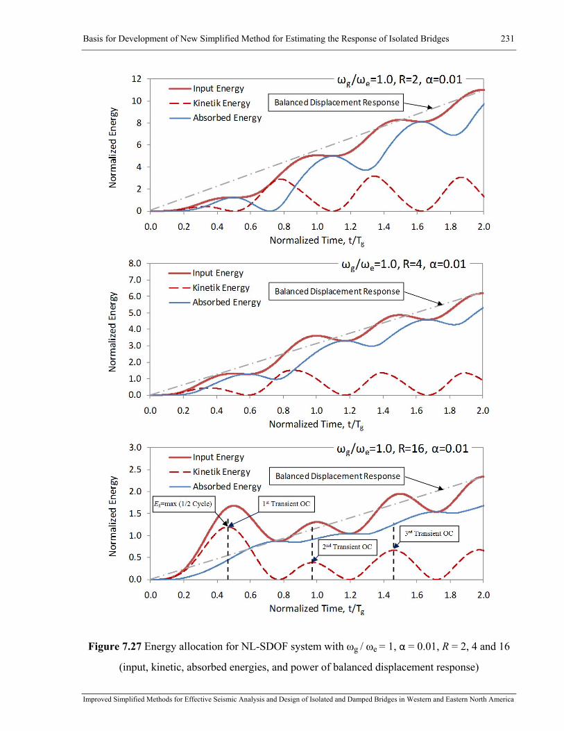
Basis for Development of New Simplified Method for Estimating the Response of Isolated Bridges 231
Improved Simplified Methods for Effective Seismic Analysis and Design of Isolated and Damped Bridges in Western and Eastern North America
Figure 7.27 Energy allocation for NL-SDOF system with ωg / ωe = 1, α = 0.01, R = 2, 4 and 16
(input, kinetic, absorbed energies, and power of balanced displacement response)

Basis for Development of New Simplified Method for Estimating the Response of Isolated Bridges 232
Improved Simplified Methods for Effective Seismic Analysis and Design of Isolated and Damped Bridges in Western and Eastern North America
According to the observations discussed above, the response of the NL-SDOF systems can be
classified as exhibiting either a limited-nonlinear or a highly-nonlinear response, where the
transition between these two response types is defined by the balanced displacement response
(as observed in this study for R = 4).
1) During the limited-nonlinear response, systems oscillate about its "at rest" equilibrium
position and as previously discussed, the energy induced to the system over a loading cycle is
dissipated completely through the system's inelastic response over the same cycle.
2) In turn, during the highly-nonlinear response, the systems experience the oscillation center
drift which results from the kinetic energy excess. In such a case, the maximum displacement
response consists of the oscillation center drift and the local system response about the new
oscillation center. The energy excess generated during a transient phase of loading can be
dissipated through a few consecutive cycles. The transient oscillation center shifts gradually with
each of these cycles until the energy excess is entirely dissipated.
These results make it possible to provide a detailed insight into the response mechanics of the
limited-nonlinear and highly-nonlinear responses from the perspective of the energy allocation.
There appears to exist a limit between the two states of nonlinear behaviour and it is of interest to
express this limit in terms the system's nonlinear parameters. The influence of the R factor on the
energy flow explains why shifting of the OC is mainly observed in the first half-cycle, which is
kept as the basis for the further developments that are presented in this and subsequent chapters.
7.3.4.2 Definition of Critical Response Modification Factor Rcr
As pointed out in the previous discussions, the system inelastic behaviour is characterized as
limited-nonlinear response for low R or highly-nonlinear response for higher R-ratios. The point
of transition between these two response states corresponds to the balanced displacement
response that can be defined by a critical response modification factor Rcr. For R < Rcr, nonlinear
systems generally exhibit a limited-nonlinear response with oscillations about their "at rest"
equilibrium position. The response is therefore mostly characterized by the elastic properties of
the system and. Conversely, for R > Rcr, highly-nonlinear response mostly oriented along the
post-activation (or post-yield) stiffness kd is observed. The systems are prone to oscillation center
drifting that may results in relatively larger displacements (see Chapter 6, Figure 6.3).

Basis for Development of New Simplified Method for Estimating the Response of Isolated Bridges 233
Improved Simplified Methods for Effective Seismic Analysis and Design of Isolated and Damped Bridges in Western and Eastern North America
A system with R = Rcr can absorb exactly the entire amount of input energy in each of the two
directions of motion. This corresponds well to a particular case of the transient response when
the system behaves similarly to the one under a steady-state motion. For such a system, the
energy input in the system within a loading cycle is dissipated completely over the same cycle.
An energy excess on the form of kinetic energy will be absorbed by the system at a later time and
will result in a larger inelastic excursion. Thus, the critical parameter Rcr is defined as the value
of R that leads to the limit case of a balanced displacement response where the energy delivered
by the excitation and the energy dissipated during one inelastic response cycle are equal and
there is no drifting of the oscillation center.
The input energy for an entire cycle of loading is defined as:
μωπμπ yggygin uumuumE 2=⋅⋅⋅⋅= && (7.43)
The energy dissipated by a bilinear system over the entire cycle is determined as:
)1()1(4 2 −−= μαyeAb ukE (7.44)
Solving Equations (7.43) and (7.44) simultaneously for ductility response,
14
1
2
2
−+⋅⋅
−=
αω
ωπ
αμ
e
g
y
g
uu
(7.45)
This is the solution for balanced displacement response, i.e., when the system has sufficient
resistance to exactly absorb the kinetic energy within the same cycle, which leads to a stable
bounded response, without drifting. If the resistance of the system is slightly reduced, drifting of
the oscillation center will occur and the response will be unbounded, eventually resulting in a
ductility that will tend to infinity. The value of Rcr can therefore be defined for the conditions
that lead to ∞=μ , i.e., when the denominator term in Equation (7.45) becomes equal to zero:
014 2
2
=−+⋅⋅ αω
ωπ
e
g
y
g
uu
(7.46)
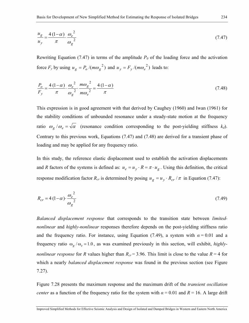
Basis for Development of New Simplified Method for Estimating the Response of Isolated Bridges 234
Improved Simplified Methods for Effective Seismic Analysis and Design of Isolated and Damped Bridges in Western and Eastern North America
2
2)1(4
g
e
y
g
uu
ωω
πα
⋅−
= (7.47)
Rewriting Equation (7.47) in terms of the amplitude P0 of the loading force and the activation
force Fy by using )/( 2gog mPu ω= and )/( 2
eyy mFu ω= leads to:
πα
ω
ω
ωω
πα )1(4)1(4
2
2
2
2 −=⋅⋅
−=
e
g
g
e
y
o
m
mFP (7.48)
This expression is in good agreement with that derived by Caughey (1960) and Iwan (1961) for
the stability conditions of unbounded resonance under a steady-state motion at the frequency
ratio αωω =eg / (resonance condition corresponding to the post-yielding stiffness kd).
Contrary to this previous work, Equations (7.47) and (7.48) are derived for a transient phase of
loading and may be applied for any frequency ratio.
In this study, the reference elastic displacement used to establish the activation displacements
and R factors of the systems is defined as: gye uRuu ⋅=⋅= π . Using this definition, the critical
response modification factor Rcr is determined by posing π/cryg Ruu ⋅= in Equation (7.47):
2
2)1(4
g
ecrR
ωωα ⋅−= (7.49)
Balanced displacement response that corresponds to the transition state between limited-
nonlinear and highly-nonlinear responses therefore depends on the post-yielding stiffness ratio
and the frequency ratio. For instance, using Equation (7.49), a system with α = 0.01 and a
frequency ratio / 1.0g eω ω = , as was examined previously in this section, will exhibit, highly-
nonlinear response for R values higher than Rcr = 3.96. This limit is close to the value R = 4 for
which a nearly balanced displacement response was found in the previous section (see Figure
7.27).
Figure 7.28 presents the maximum response and the maximum drift of the transient oscillation
center as a function of the frequency ratio for the system with α = 0.01 and R = 16. A large drift
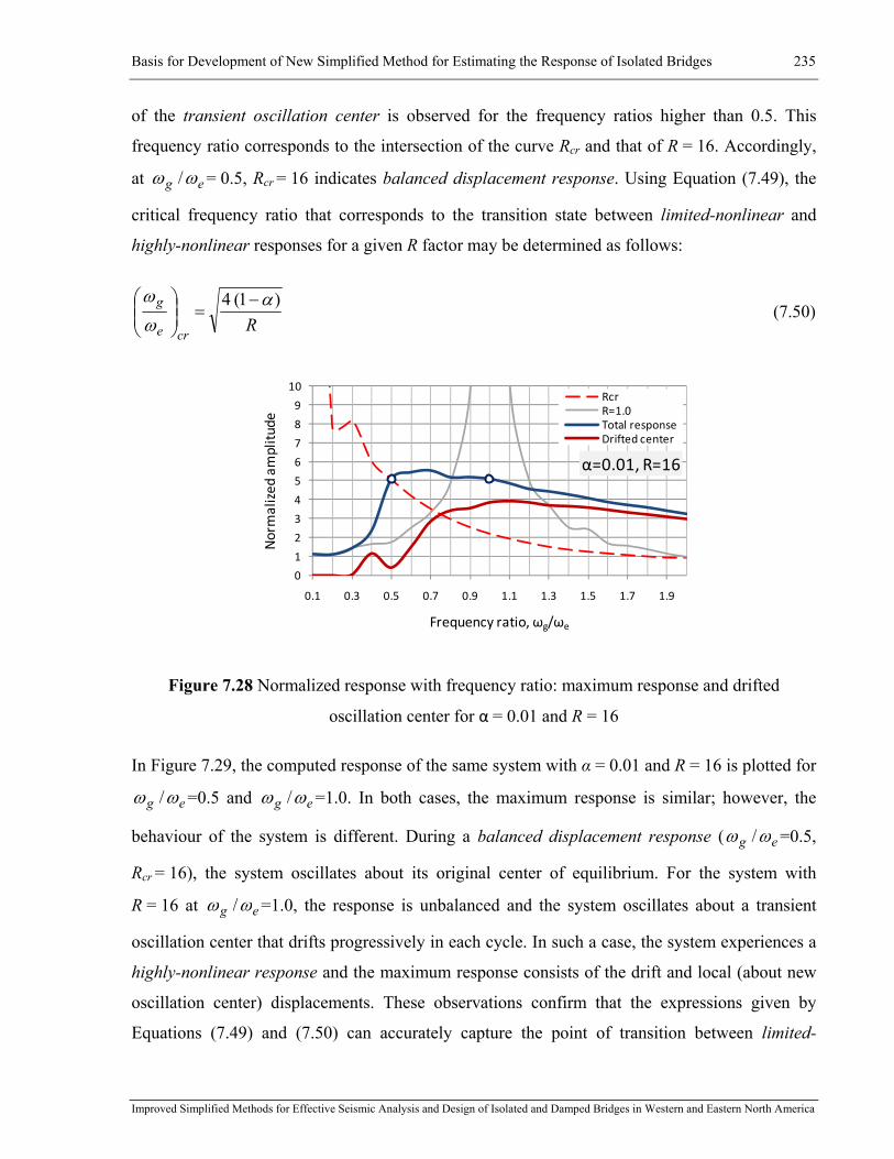
Basis for Development of New Simplified Method for Estimating the Response of Isolated Bridges 235
Improved Simplified Methods for Effective Seismic Analysis and Design of Isolated and Damped Bridges in Western and Eastern North America
of the transient oscillation center is observed for the frequency ratios higher than 0.5. This
frequency ratio corresponds to the intersection of the curve Rcr and that of R = 16. Accordingly,
at eg ωω / = 0.5, Rcr = 16 indicates balanced displacement response. Using Equation (7.49), the
critical frequency ratio that corresponds to the transition state between limited-nonlinear and
highly-nonlinear responses for a given R factor may be determined as follows:
Rcre
g )1(4 αωω −
=⎟⎟⎠
⎞⎜⎜⎝
⎛ (7.50)
Figure 7.28 Normalized response with frequency ratio: maximum response and drifted
oscillation center for α = 0.01 and R = 16
In Figure 7.29, the computed response of the same system with α = 0.01 and R = 16 is plotted for
eg ωω / =0.5 and eg ωω / =1.0. In both cases, the maximum response is similar; however, the
behaviour of the system is different. During a balanced displacement response ( eg ωω / =0.5,
Rcr = 16), the system oscillates about its original center of equilibrium. For the system with
R = 16 at eg ωω / =1.0, the response is unbalanced and the system oscillates about a transient
oscillation center that drifts progressively in each cycle. In such a case, the system experiences a
highly-nonlinear response and the maximum response consists of the drift and local (about new
oscillation center) displacements. These observations confirm that the expressions given by
Equations (7.49) and (7.50) can accurately capture the point of transition between limited-
0
1
2
3
4
5
6
7
8
9
10
0.1 0.3 0.5 0.7 0.9 1.1 1.3 1.5 1.7 1.9
Normalized
amplitu
de
Frequency ratio, ωg/ωe
α=0.01, R=16
RcrR=1.0Total responseDrifted center
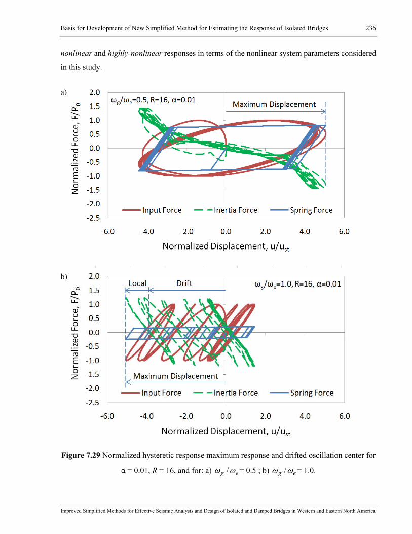
Basis for Development of New Simplified Method for Estimating the Response of Isolated Bridges 236
Improved Simplified Methods for Effective Seismic Analysis and Design of Isolated and Damped Bridges in Western and Eastern North America
nonlinear and highly-nonlinear responses in terms of the nonlinear system parameters considered
in this study.
a)
b)
Figure 7.29 Normalized hysteretic response maximum response and drifted oscillation center for
α = 0.01, R = 16, and for: a) eg ωω / = 0.5 ; b) eg ωω / = 1.0.

Basis for Development of New Simplified Method for Estimating the Response of Isolated Bridges 237
Improved Simplified Methods for Effective Seismic Analysis and Design of Isolated and Damped Bridges in Western and Eastern North America
7.4 Conclusions
In this chapter, the potential for the development of a new energy-based method to predict
isolated bridge response more accurately is studied. Two widely adopted methods in earthquake
engineering, the Equal Displacement (EDA) and the Equal Energy (EEA) approaches, were
briefly reviewed and examined. It was found that the "exact" responses from NLTHA are
confined by that obtained from these two response approximating techniques (EDA and EEA).
The response estimates obtained by using the EEA were found to be conservative for all studied
cases. It was shown that the differences between the response estimates from the EEA and
“exact” NLTHA results may be related to the amount of absorbed energy. It was assumed that
the difference in absorbed energy between these two responses can be attributed to the kinetic
energy which is ignored when assuming that the input energy is absorbed entirely through
monotonic loading. This portion of the energy input that is ignored by the EEA was termed as an
energy deficit.
The energy concept used in the Equal Energy Approach was then considered as a basis for
further development given that this approach relies upon the principle of conservation of energy.
Then, the energy deficit was identified by studying the response of SDOF systems under
harmonic excitation. To better characterize seismic response in the present study, special
attention was drawn to the transient phase of loading that occurs at the beginning of the
excitation.
According to the observations made in this study, bi-linear NL-SDOF systems were classified as
exhibiting either a limited-nonlinear or a highly-nonlinear response. It was confirmed that during
limited-nonlinear response, systems oscillate about their "at rest" equilibrium position and the
energy induced into the systems over a loading cycle is dissipated completely through the
system's inelastic response within the same cycle. In turn, during highly-nonlinear response, the
systems experience a drift of the oscillation center which results from an excess of kinetic energy
compared to the energy absorption capacity of the system. In such a case, the maximum
displacement response consists of the drift of the oscillation center plus the local system response
about the new oscillation center. The energy excess generated during a transient phase of loading
can be dissipated through a few consecutive cycles. The transient oscillation center shifts
gradually in each of these cycles until the energy excess is entirely dissipated.

Basis for Development of New Simplified Method for Estimating the Response of Isolated Bridges 238
Improved Simplified Methods for Effective Seismic Analysis and Design of Isolated and Damped Bridges in Western and Eastern North America
The effect of the kinetic energy on the system behaviour was identified as a key element to be
considered in the development of the new simplified method for complementing the assumptions
of the original EEA. It is postulated that isolated bridge response can probably be predicted more
accurately by using the concept of energy allocation under transient excitation, a concept that
accounts for the transient response and possible shifting of the transient oscillation center, two
aspects that are not accounted for in the current code simplified method. Using this approach, it
was found that different system properties, including the initial elastic period, the post-activation
stiffness and the R factor, as well as ground motion characteristics including amplitude and
frequency content will be taken into account in the seismic response prediction.
Finally, the transition state between limited-nonlinear and highly-nonlinear responses was
defined as the point beyond which the response of a system starts oscillating about a drifted
equilibrium center. The critical parameter Rcr was derived to mark this point of transition.

Proposed Energy-Based Simplified Analytical Method for Predicting the Response of Isolated Bridges 239
Improved Simplified Methods for Effective Seismic Analysis and Design of Isolated and Damped Bridges in Western and Eastern North America
Chapter 8: Proposed Energy-Based Simplified Analytical Method for Predicting the Response of Isolated Bridges
8.1 Introduction
In Chapters 5 and 6, it was shown that the simplified method, currently specified in the North
American codes (CAN/CSA-S6-06 and AASHTO 2009, 2010), is subject to limitations that may
affect the accuracy in predicting the peak response of isolated bridges. As shown in Chapter 7
these limitations are primarily attributed to the fact that the highly nonlinear response of isolated
bridges is better characterized by the nonlinear dynamics of the system’s response to transient
dynamic loading rather than the steady-state loading and the phenomenon of shifting of the
transient oscillation centre during the nonlinear response. These two aspects are not accounted
for in current code simplified methods.
In addition, the previous study indicated that the response of isolated systems is dependent on the
complex relation between the structure’s properties and the ground-motion characteristics. It was
also recognized that the use of the response modification factor R and the ratio between the
structure’s initial period and the ground-motion’s predominant period Te / Tg make it possible to
better characterize the response of the structure to seismic loading.
These observations indicate that a new simplified method is needed that could address the
limitations of current methods in accurately estimating the highly-nonlinear response of isolated
bridges. The development of the new simplified method for predicting isolated bridge response is
the main objective of the study presented in this chapter.
As discussed in the previous chapter, the energy concept used in the Equal Energy Approach
(EEA) could be used as the basis for the development of a simplified analysis method that can be
adopted in design process as an efficient alternative to the currently specified design approach
(CSA-S6-06). The transient response and possible shifting of the transient oscillation centre,
may be taken into account by applying the concept of energy allocation under transient
excitation.

Proposed Energy-Based Simplified Analytical Method for Predicting the Response of Isolated Bridges 240
Improved Simplified Methods for Effective Seismic Analysis and Design of Isolated and Damped Bridges in Western and Eastern North America
Based on this, a new simplified method that takes into account the differences in ground-motion
characteristics and bridge design parameters is proposed. This method can predict the peak
displacement of bilinear systems. This new energy-based E-R-µ method was developed purely
based on analytical derivations rather than being empirically calibrated on a region-by-region
basis to obtain accurate response predictions. The basis on which the predictions are made
assumes that a) ground motions are represented by a single sine-wave pulse defined by PGA and
PGD and b) response to that pulse can be predicted using the E-R-μ method.
In Section 8.2, the main assumptions and fundamentals of the energy-based E-R-µ relationship
are presented. In Section 8.3, the new energy-based E-R-µ relationship is formulated. Given that
this relationship is developed based on an energy formulation, the letter E was added to
differentiate this proposed E-R-µ formulation from a series of existing R-μ relationships that
have been derived empirically based on nonlinear time history analyses or other methods. The
design procedure using this new energy-based E-R-µ relationship is proposed in Section 8.4. In
order to harmonize the use of the proposed method with the design procedure specified in the
CAN/CSA-S6-06, the terms and parameters commonly used in current design practice are
adopted in the formulation of the method.
At the end of Section 8.4, the effectiveness and accuracy of the new energy-based method for
capturing the response of highly-nonlinear systems is validated by comparing the response
estimates against results from dynamic nonlinear time-history analyses (NLTHA) that were
presented in Chapter 5. The results from NLTHA are compared to the response estimates made
for isolated bridges in WNA and ENA by using the proposed method and the EEA.
8.2 Assumptions of New E-R-µ Relationships for the Proposed
Energy Formulation for Bilinear Elastoplastic Systems
This section adapts the theoretical results from Chapter 7 to propose a design method for isolated
bridges exhibiting a highly nonlinear response. The proposed method can predict the peak
displacement of bilinear systems which is defined by structure parameters used in design of
isolated bridges (the response modification factor R, elastic period Te and post-yielding stiffness
ratio α as shown in Figure 5.13). The bridge structure, being initially at rest, is assumed to be
subjected to the ground motion excitation that are represented by a single sine-wave pulse

Proposed Energy-Based Simplified Analytical Method for Predicting the Response of Isolated Bridges 241
Improved Simplified Methods for Effective Seismic Analysis and Design of Isolated and Damped Bridges in Western and Eastern North America
defined by PGA and PGD. To predict the peak displacement response to the pulse loading, an
energy-based method is used. The energy method accounts for the excess in kinetic energy and
shifting of the oscillation centre (OC).
Based on the results obtained in Chapter 7, the following assumptions are made for developing
the new energy-based simplified design method:
1) As discussed in Section 7.3.3, an earthquake loading is not periodic. In order to approximate
the seismic response of a system using theoretical solutions, the excitation is assumed to be a
sinusoidal force function as was done for analyzing linear and nonlinear SDOF systems in
Chapter 7. The same sine loading function (A-type cycloidal pulse) was proposed by Makris
(1997) to idealize excitations representing pulse-like ground motions. The effect of such a
pulse is similar to the effect of a suddenly applied force acting on a system which is initially at
rest. To characterize the acceleration pulse of loading cycle, PGA and PGD values should be
determined. To predict the demand under a specific ground motion, PGA is obtained from
records; for design, PGA is obtained directly from seismic hazard design values provided by
GSC (Geological Survey of Canada). For PGD, spectral displacement values are used for
individual records and for design. The predominant ground-motion period Tg is obtained from
PGA and PGD using Equation 8.1 (based on the assumption that the pulse is a sine wave).
This assumption is similar to that made by Jacobsen and Ayre (1958) for transient responses
to pulse-type excitations.
PGAPGDTg π2= (8.1)
2) As confirmed in Chapter 7, an excess of kinetic energy is produced during a transient phase of
loading when the system exhibits a highly nonlinear response to seismic loading. Such a
response is expected when R is high, as in the case of isolated bridges exhibiting limited
lateral resistance: the kinetic energy induced by large amplitude ground motion cannot be
absorbed and dissipated within the first response cycle. The energy excess generated during a
transient phase of loading can be dissipated through a few subsequent cycles. The transient
oscillation centre shifts gradually with each of these cycles until the energy excess is entirely
dissipated. As shown in Figures 7.26 and 7.29, such a behaviour is characterized by a skewed
response which consists of consecutive drifts of the transient oscillation centre and the local

Proposed Energy-Based Simplified Analytical Method for Predicting the Response of Isolated Bridges 242
Improved Simplified Methods for Effective Seismic Analysis and Design of Isolated and Damped Bridges in Western and Eastern North America
response around new equilibrium position. The sum of consecutive drifts results in a total
drift. It is assumed that the total drift can be approximated by transforming the excess kinetic
energy directly into energy absorbed during the total drift of the oscillation centre. The
maximum displacement is then determined by adding the total drift resulted from this
transformation to the local response around the drifted equilibrium positions.
3) As also pointed out in Chapter 7, the kinetic energy allocation corresponding to the maximum
system displacement and to the position of the transient oscillation centre provides a better
insight into the source of the energy deficit that marks the difference between the "exact"
response and EEA estimate. In the EEA, the energy absorbed by an elastic system and that
absorbed by a corresponding nonlinear system are assumed to be equal and are defined
through the area under the force-displacement curve obtained for the first half cycle of the
response. As a result, the energy absorbed by the nonlinear system under monotonic loading is
assumed be equal to the work done by the excitation (P) and inertia (Fi) forces. The energy
equilibrium is formulated for the first half cycle of the response.
The assumptions adopted for developing the energy-based E-R-µ relationship imply certain
degree of conservatism. The energy transmitted to the isolated system is idealized as being
representative of the system response under a sinusoidal excitation with a sole period Tg which
relates the peak ground displacement and the peak ground acceleration. The response estimates
will correspond to the response of isolated bridges under the most demanding loading conditions
from the strong motion portion of a seismic ground motion.
Makris (1997), however, assumed that the acceleration record contains several random spikes
that must be neglected in deriving a smooth acceleration function. In this way, the maximum
values of Makris' acceleration function are 30% less than the recorded PGA value. This
technique can be considered in the frame of specialized record-to-record analyses with a more
detailed understanding of seismological effects.
The technique that was selected for evaluating PGA, PGD and Tg, and that was assumed for
developing the new energy-based simplified method in the present chapter, is simple enough for
its implementation in a new simplified design approach. In addition, because it utilizes the
recorded PGA value, this new energy-based simplified method will provide engineers mostly
with conservative response estimates which is also desirable for a design procedure.

Proposed Energy-Based Simplified Analytical Method for Predicting the Response of Isolated Bridges 243
Improved Simplified Methods for Effective Seismic Analysis and Design of Isolated and Damped Bridges in Western and Eastern North America
Note that the source of the kinetic energy used to extend the EEA also represents a single
excitation pulse. It is clear that being derived for a single loading pulse, this method has an
inherent limitation to capture the effect of the loading duration or complex irregularity in the
seismic excitation and the structural response. Accordingly, the discrepancies in the response
estimate can be attributed to the effect of multiple oscillation centre drifts that originate from
various loading pulses.
8.3 Development of New E-R-µ Relationships for the Proposed
Energy Formulation for Bilinear Elastoplastic Systems
In this section, the proposed design procedure using a new energy-based E-R-µ relationship is
formulated.
8.3.1 Development of New E-R-µ Relationships
The idealized force-displacement response and the corresponding input and kinetic energies are
presented in Figure 8.1 (a) and (b). The energy that is absorbed during the nonlinear response of
the system is formulated in Figure 8.1 (c). To account for the effect of damping, the dissipated
portion of the absorbed energy is defined through equivalent damping and viscous damping
ratios (βeq and ξ). An equivalent presentation of the energy absorbed by a substitute equivalent
structure is shown in Figures 8.1 (d) and (e) in terms of the strain energy and the portion of
energy dissipated through viscous damping. In this approach, it is assumed that the system
completes a half-cycle between the maximum and minimum displacements. As a result, the first
half cycle is defined from the zero displacement to the maximum displacement um.

Proposed Energy-Based Simplified Analytical Method for Predicting the Response of Isolated Bridges 244
Improved Simplified Methods for Effective Seismic Analysis and Design of Isolated and Damped Bridges in Western and Eastern North America
Figure 8.1 Idealized response a) input energy, b) kinetic energy, c) absorbed energy,
d) equivalent strain energy as portion of absorbed energy, and e) dissipated portion of absorbed
energy
(c)
(b) (a)
(d) (e)

Proposed Energy-Based Simplified Analytical Method for Predicting the Response of Isolated Bridges 245
Improved Simplified Methods for Effective Seismic Analysis and Design of Isolated and Damped Bridges in Western and Eastern North America
The basis for the development of the new E-R-µ relationship is the energy equilibrium of the
system, which is defined as follows:
Abkin EEE += (8.2)
The input energy is defined as a function of the maximum ground acceleration, gu&& and the
maximum inelastic displacement, mu :
mggmgin umuuumE 2
21
21 ω== && (8.3)
where the maximum base acceleration is related to the maximum base displacement, gu by:
2ggg uu ω=&& (8.4)
The kinetic energy at the maximum displacement um, which corresponds to a first half cycle, is
given by:
)(21
21
21 22
gmmgmgtotmk uuumuumuumE +=== ωω&& (8.5)
The energy absorbed by the system in a first half cycle under inelastic behaviour:
))1()1(21(21 22 −+−+= μαμyeAb ukE (8.6)
The energy absorbed by the equivalent substitute system:
effmeffmeffEqAb ukukE βπ 22
41
21
+= (8.7)
where effβ represents both, equivalent and viscous damping ratios at keff ( ξβ +eq (keff)).
The maximum inelastic response, um is presented in terms of the ductility as μym uu = . The
elastic limit, uy is related to R ( Ruu ey /= ), where ue is the maximum elastic response that may

Proposed Energy-Based Simplified Analytical Method for Predicting the Response of Isolated Bridges 246
Improved Simplified Methods for Effective Seismic Analysis and Design of Isolated and Damped Bridges in Western and Eastern North America
be determined as a 5% damped spectral displacement )%,5( eDe TSu = . To make gu and gu&&
representative of a generic seismic excitation, the peak ground displacement and acceleration are
defined as suggested by Jacobsen and Ayre (1958) for transient responses to pulse-type
excitations. The excitation is therefore defined as a sinusoidal force function
)sin()( tumtP gg ω&&−= applied to the system that is initially at rest ( 0)0()0( == uu& ).
The normalized ground acceleration, velocity and displacement as a function of time are shown
in Figure 8.2. These functions were obtained by integrating the ground acceleration with respect
to time and assuming zero initial conditions:
vgg
gt
ggg Ctu
dttutu +−== ∫ )cos()sin()(0
ωω
ω&&
&&& (8.8)
where the arbitrary constant of integration vC can be found by assuming that the ground velocity
at t=0 is zero ( 0)0( =gu& ):
g
g
g
gv
uuC
ωω
&&&&== )0cos( (8.9)
Thus the function of the ground velocity starting at rest yields:
)cos()( tuu
tu gg
g
g
gg ω
ωω
&&&&& −= (8.10)
Integrating Equation (8.10) once, the function of the ground displacement is:
ugg
g
g
gt
gg
g
g
gg Ct
utudtt
uutu +−=−= ∫ )sin()cos()( 2
0
ωωω
ωωω
&&&&&&&& (8.11)
where the integration constant equals zero ( 0=uC ) to satisfy the zero ground displacement at
rest.
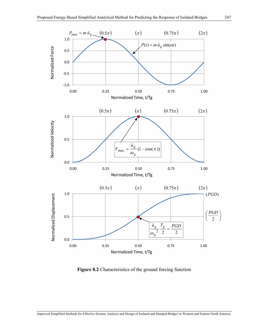
Proposed Energy-Based Simplified Analytical Method for Predicting the Response of Isolated Bridges 247
Improved Simplified Methods for Effective Seismic Analysis and Design of Isolated and Damped Bridges in Western and Eastern North America
Figure 8.2 Characteristics of the ground forcing function
‐1.0
‐0.5
0.0
0.5
1.0
0.00 0.25 0.50 0.75 1.00
Normalized
Force
Normalized Time, t/Tg
( )π( )π5.0 ( )π2( )π75.0gumP &&=max
)sin()( tumtP g ω&&=
0.0
0.5
1.0
0.00 0.25 0.50 0.75 1.00
Normalized
Displacem
ent
Normalized Time, t/Tg
( )π( )π5.0 ( )π2( )π75.0)(PGD
222PGDTu g
g
g =ω
&&
⎟⎠⎞
⎜⎝⎛
2PGD
0.0
0.5
1.0
0.00 0.25 0.50 0.75 1.00
Normalized
Velocity
Normalized Time, t/Tg
( )π( )π5.0 ( )π2( )π75.0
))cos(1(max πω
−=g
guV
&&

Proposed Energy-Based Simplified Analytical Method for Predicting the Response of Isolated Bridges 248
Improved Simplified Methods for Effective Seismic Analysis and Design of Isolated and Damped Bridges in Western and Eastern North America
According to the assumptions in Section 8.2, the maximum ground displacement representative
of a seismic peak ground displacement (PGD) occurs at the end of an entire cycle (t = Tg).
However, the energy equilibrium is formulated for the first half cycle. The ground displacements
at time gT (at π2=twg ) and 2/gT (at π=twg ) can be found by using Equation (8.11) with
0=uC :
PGDTuu
Tu
Tu gg
g
g
gg
g
ggg ==−=
ωπ
ωω
&&&&&&)2sin()( 2 (8.12)
22)sin(
2)2/( 2
PGDTuuTuTu g
g
g
g
gg
g
ggg ==−=
ωπ
ωω
&&&&&& (8.13)
The maximum base displacement gu and acceleration gu&& corresponding to the half cycle that is
used in the analytical formulation are defined as follows:
2/PGDug = and 22 )2/( gggg PGDuu ωω ==&& (8.14)
Substituting equations (8.3), (8.5), and (8.6) in the energy balance equations for the system
without added damping (Ein = Ek + EAb) and solving for R, the E-R-µ relationship is defined as:
( ))2/1()1(2
−−++= μααμωμ
PGAu
PGDu
R eee (8.15)
For the system with added damping, instead of using Equation (8.6), R may be determined with
the equivalent formulation for the absorbed energy (Equation (8.7)):
( )μααμαπβαμαωμ
/)1(22/)1(332
−+−+−−++= effeee
PGAu
PGDu
R (8.16)
In Figure 8.3, the interaction of the input and kinetic energies (Ein-Ek) as a function of ductility is
shown against the corresponding function of the energy absorbed by the system EAb. The energy
Ein-Ek represents the amount to be absorbed by the system at the end of loading in the direction
of the inelastic excursions. It can be noted that the absorbed energy grows with ductility until the
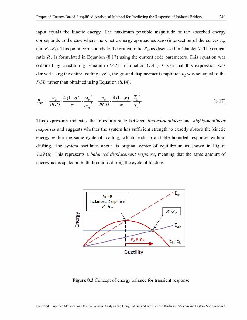
Proposed Energy-Based Simplified Analytical Method for Predicting the Response of Isolated Bridges 249
Improved Simplified Methods for Effective Seismic Analysis and Design of Isolated and Damped Bridges in Western and Eastern North America
input equals the kinetic energy. The maximum possible magnitude of the absorbed energy
corresponds to the case where the kinetic energy approaches zero (intersection of the curves Ein
and Ein-Ek). This point corresponds to the critical ratio Rcr as discussed in Chapter 7. The critical
ratio Rcr is formulated in Equation (8.17) using the current code parameters. This equation was
obtained by substituting Equation (7.42) in Equation (7.47). Given that this expression was
derived using the entire loading cycle, the ground displacement amplitude ug was set equal to the
PGD rather than obtained using Equation (8.14).
2
2
2
2 )1(4)1(4
e
ge
g
eecr
T
TPGDu
PGDu
R ⋅−
⋅=⋅−
⋅=π
αω
ωπ
α (8.17)
This expression indicates the transition state between limited-nonlinear and highly-nonlinear
responses and suggests whether the system has sufficient strength to exactly absorb the kinetic
energy within the same cycle of loading, which leads to a stable bounded response, without
drifting. The system oscillates about its original center of equilibrium as shown in Figure
7.29 (a). This represents a balanced displacement response, meaning that the same amount of
energy is dissipated in both directions during the cycle of loading.
Figure 8.3 Concept of energy balance for transient response

Proposed Energy-Based Simplified Analytical Method for Predicting the Response of Isolated Bridges 250
Improved Simplified Methods for Effective Seismic Analysis and Design of Isolated and Damped Bridges in Western and Eastern North America
Accordingly, the range of applicability for equations (8.15) and (8.16) corresponds to a highly-
nonlinear response which is defined within ∞<< RRcr . When Equation 8.17 yields Rcr ≤ 1.0, a
balanced displacement response is not possible and the structure will experience a highly
nonlinear response as soon as the structure exceeds its elastic limit. For such a case, Rcr is set to
1.0.
For structures with response modification factors greater than Rcr, the capacity to absorb energy
of the system is reduced when increasing R (reducing strength), so that a larger portion of the
energy input Ein in the first half-cycle must transform into kinetic energy Ek. In such a case, the
transient OC shifts gradually with each of consecutive cycles until the energy excess is entirely
dissipated. The energy excess will be absorbed by the system at a later time and will result in a
larger ductility demand. This is illustrated in Figure 8.3 as Ek Effect.
8.3.2 Influence of Ground-Motion and Nonlinear System Parameters
To better understand the influence of different ground-motion and nonlinear system parameters
on the response estimates obtained through the energy-based E-R-µ relationship, Equation (8.15)
is rearranged. After substituting the PGA obtained using the pseudo relationship 2gPGD ω⋅ and
by replacing the frequency terms ( gω and eω ) by the corresponding periods, the solution
becomes:
( ))/12()1(2
2
μααμμ −−++=e
gee
T
TPGDu
PGDu
R (8.18)
The effect of the loading with "slowly" or "rapidly" varying forces which was discussed in detail
in Chapter 7 (see Figure 7.12) is captured by the period ratio eg TT / in the second term of
Equation (8.18). Accordingly, the effect of the kinetic energy excess is taken into account by the
second term in this formulation.
The second term can be reorganized to isolate the effect of the kinetic energy on the sytem
response within its elastic and inelastic ranges as follows:

Proposed Energy-Based Simplified Analytical Method for Predicting the Response of Isolated Bridges 251
Improved Simplified Methods for Effective Seismic Analysis and Design of Isolated and Damped Bridges in Western and Eastern North America
)/12()1(2
2
2
2
μααμμ −−++=e
ge
e
gee
T
TPGDu
T
TPGDu
PGDu
R (8.19)
)/12()1(2
2
2
2
μαμμ −−++=e
ge
d
gee
T
TPGDu
T
TPGDu
PGDu
R (8.20)
For systems with supplemental damping, Equation (8.16) is rearranged to obtain an expression
similar to Eq. 8.18):
( )μααμαπβαμαμ /)1(22/)1(332
2
−+−+−−++= effe
gee
T
TPGDu
PGDu
R (8.21)
For a given response modification factor R, the maximum response is reached when the second
and third terms of Equation (8.20) tend towards zero. As such, the E-R-µ relationship is reduced
to the following form:
μPGDu
R e= (8.22)
and the maximum ductility response is:
ye uPGD
uPGDR
=⋅
=μ (8.23)
As a result, the maximum displacement of the structure equals the peak ground displacement
PGD for a "perfectly" isolated structure for which the motions of the mass and the base of the
system are completely uncoupled (um = PGD). In Equation (8.20), the second and third terms
tend to zero when the periods Td and Te become very large, i.e. for a structure that has an
infinitely small stiffness or an infinitely large mass. When the second and third terms of Equation
(8.20) become less significant, the response is dominated by the first term that represents
isolation effects. The same effect is attained when the ground-motion predominant period is very
short which is representative of a very "rapidly" varying loading force (see Figure 7.12).
The effect of the period ratio Te / Tg on the response amplitude is presented in Figure 8.4. The

Proposed Energy-Based Simplified Analytical Method for Predicting the Response of Isolated Bridges 252
Improved Simplified Methods for Effective Seismic Analysis and Design of Isolated and Damped Bridges in Western and Eastern North America
response amplitude in terms of the ductility ratio was calculated using Equation (8.20) for
different R and α-ratios. It can be observed that the maximum response amplitude corresponds to
the post-yielding resonance defined by Equation (7.36). This resonance condition corresponding
to the post-yielding stiffness kd is met when dg TT = and the ratio
αα === )//(// eedege TTTTTT . It can be noted that for higher period ratios, which
correspond to systems with relatively longer elastic periods, the response amplitude decreases
and tends to the ground displacement or, in terms of ductility, to yuPGD /=μ (see Equation
(8.23)). The tendencies observed from Figure 8.4 are in good agreement with those presented in
Chapter 7 (see Figures 7.22 to 7.24) for the response of NL-SDOF systems under harmonic
excitation. This confirms the ability of the proposed E-R-µ relationship to properly take into
account the complex relation between the structure’s nonlinear response and the ground-motion
characteristics that are not accounted for in the code simplified methods.
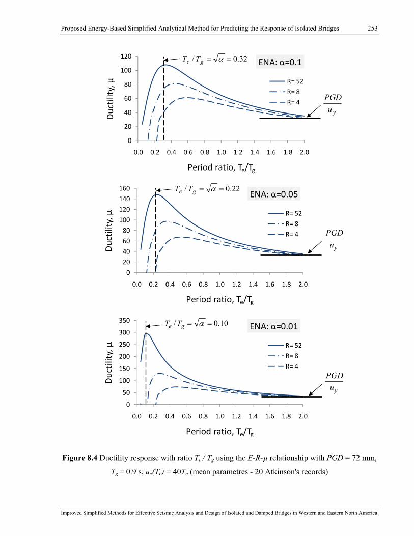
Proposed Energy-Based Simplified Analytical Method for Predicting the Response of Isolated Bridges 253
Improved Simplified Methods for Effective Seismic Analysis and Design of Isolated and Damped Bridges in Western and Eastern North America
Figure 8.4 Ductility response with ratio Te / Tg using the E-R-µ relationship with PGD = 72 mm,
Tg = 0.9 s, ue(Te) = 40Te (mean parametres - 20 Atkinson's records)
0
20
40
60
80
100
120
0.0 0.2 0.4 0.6 0.8 1.0 1.2 1.4 1.6 1.8 2.0
Ductility, µ
Period ratio, Te/Tg
ENA: α=0.1
R= 52R= 8
R= 4
32.0/ == αge TT
yuPGD
0
20
40
60
80
100
120
140
160
0.0 0.2 0.4 0.6 0.8 1.0 1.2 1.4 1.6 1.8 2.0
Ductility, µ
Period ratio, Te/Tg
ENA: α=0.05
R= 52R= 8
R= 4
22.0/ == αge TT
yuPGD
0
50
100
150
200
250
300
350
0.0 0.2 0.4 0.6 0.8 1.0 1.2 1.4 1.6 1.8 2.0
Ductility, µ
Period ratio, Te/Tg
ENA: α=0.01
R= 52R= 8
R= 4
10.0/ == αge TT
yuPGD
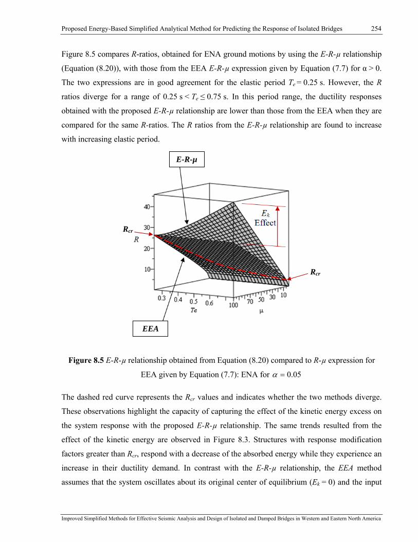
Proposed Energy-Based Simplified Analytical Method for Predicting the Response of Isolated Bridges 254
Improved Simplified Methods for Effective Seismic Analysis and Design of Isolated and Damped Bridges in Western and Eastern North America
Figure 8.5 compares R-ratios, obtained for ENA ground motions by using the E-R-µ relationship
(Equation (8.20)), with those from the EEA E-R-µ expression given by Equation (7.7) for α > 0.
The two expressions are in good agreement for the elastic period Te = 0.25 s. However, the R
ratios diverge for a range of 0.25 s < Te ≤ 0.75 s. In this period range, the ductility responses
obtained with the proposed E-R-µ relationship are lower than those from the EEA when they are
compared for the same R-ratios. The R ratios from the E-R-µ relationship are found to increase
with increasing elastic period.
Figure 8.5 E-R-µ relationship obtained from Equation (8.20) compared to R-µ expression for
EEA given by Equation (7.7): ENA for 05.0=α
The dashed red curve represents the Rcr values and indicates whether the two methods diverge.
These observations highlight the capacity of capturing the effect of the kinetic energy excess on
the system response with the proposed E-R-µ relationship. The same trends resulted from the
effect of the kinetic energy are observed in Figure 8.3. Structures with response modification
factors greater than Rcr, respond with a decrease of the absorbed energy while they experience an
increase in their ductility demand. In contrast with the E-R-µ relationship, the EEA method
assumes that the system oscillates about its original center of equilibrium (Ek = 0) and the input
E-R-µ
Rcr
Rcr
EEA

Proposed Energy-Based Simplified Analytical Method for Predicting the Response of Isolated Bridges 255
Improved Simplified Methods for Effective Seismic Analysis and Design of Isolated and Damped Bridges in Western and Eastern North America
energy Ein is fully transformed into the energy absorbed by the system EAb leading to a larger
displacement response.
8.4 Design Procedure and Validation
In this section, the proposed energy-based E-R-µ relationship is adapted for the design of bridges
equipped with seismic isolation systems. First, the E-R-µ method is formulated as a direct design
procedure. Then, an iterative design procedure is proposed to facilitate the implementation of the
method in current North American design practice. The effectiveness and accuracy of the E-R-µ
method for capturing the response of highly nonlinear systems is validated by comparing the
response estimates against results from dynamic NLTHA.
8.4.1 Design Implementation of the Energy-Based E-R-µ Method
The steps for the design procedure are outlined in Table 8-1.
The ground-motion characteristics for the actual bridge location, importance category and site
are determined first in Step 1. The design response spectrum is selected to represent the
earthquake scenarios for the seismic hazard at the site using the uniform hazard spectrum (UHS)
currently used in NBCC (NRCC, 2005) for buildings that will be adopted as the design spectrum
in the next CSA-S6-14. When a displacement SD design spectrum is not available, the pseudo
displacement PSD spectrum is used instead for the design process. The SA spectrum provides the
peak ground acceleration PGA while the peak ground displacement PGD is determined as the
pseudo-displacement at the longest available spectral period. Alternatively, the displacement
response spectrum SD and the corresponding PGD may be determined using a simple method
specified in Eurocode 8 (EC8) as shown in Figure 2.2. The predominant ground-motion period is
calculated using Equation (8.1) in Step 2.
In Step 3, the properties of the isolated bridge system are determined as follows:
m - mass of the of the bridge superstructure;
Te - initial elastic period:
ee k
mT ⋅= π2 (8.24)

Proposed Energy-Based Simplified Analytical Method for Predicting the Response of Isolated Bridges 256
Improved Simplified Methods for Effective Seismic Analysis and Design of Isolated and Damped Bridges in Western and Eastern North America
where
ke - lateral elastic stiffness represents the contribution of the substructure elements including
piers, abutments, isolation devices and determined using Equations (3.1) to (3.3).
Td – post-yield period of vibration defined using the post-yielding stiffness kd = α ke as follows:
gkWTd
d ⋅⋅= π2 or α/ed TT = (8.25)
uy - deck displacement at activation of the isolation system;
ξinh - inherent damping which corresponds to the damping level of the design response spectrum;
ξel - damping ratio of viscous dampers determined at an elastic period Te.
In Step 4, the maximum elastic displacement ue is determined using the damped design response
spectra as follows:
);( inheDe TSu ξ= (8.26)
In Step 5, the response modification factor R is determined as the ratio between the activation
displacement of the isolation system uy and the maximum elastic displacement ue.
y
euu
R = (8.27)
Equation (8.20) can be used to determine the response modification factor R for a given set of the
isolated structure's properties, ground motion characteristics and a target ductility. Alternatively,
the system's response in terms of ductility can be determined from Equation (8.20) for a given R-
factor by trials and errors in Step 6. In cases where supplemental damping devices are used,
Equation (8.21) can be used instead of Equation (8.20) to determine the system's response.
In Equation (8.21), the effective damping ratio effβ represents both, equivalent and viscous
damping ratios determined at the effective period Teff. The equivalent damping ratio eqβ and
effective period Teff are defined in Chapter 2 using Equations (2.4) and (2.2), respectively. The
effective damping can be then determined as a function of ductility as follows:

Proposed Energy-Based Simplified Analytical Method for Predicting the Response of Isolated Bridges 257
Improved Simplified Methods for Effective Seismic Analysis and Design of Isolated and Damped Bridges in Western and Eastern North America
ααμμξ
ααμμαμ
πξββ
−++
−+⋅−⋅−
⋅=+=1)1(
)1()1(2el
e
effeleqeff T
T (8.28)
Once the solution for the ductility µ is obtained in Step 6, the displacement response of the
bridge deck is calculated in Step 7 using Equation (8.29).
μ⋅=Ru
d e (8.29)
Table 8-1 Direct energy-based E-R-µ design method
Direct Energy-Based E-R-µ Method
Step 1. Determine ground-motion characteristics for seismic hazard and site:
Design Response Spectra ( AS or DS ) for ξinh;
PGD - peak ground displacement;
PGA - peak ground displacement;
Step 2. Calculate predominant period of the ground motion using Equation (8.1):
PGAPGDTg π2=
Step 3. Determine properties of the isolated bridge system:
m -mass of the bridge superstructure;
uy - deck displacement at activation of the isolation system;
α - post-yielding stiffness ratio;
Te - initial elastic period at elastic stiffness ke defined as:
ee k
mT ⋅= π2
Td - period of vibration at the post-yielding stiffness kd = α ke defined as:
α/ed TT = ξinh - inherent damping;
Step 4. Determine displacement of elastic system using Design Response Spectra:
);( inheDe TSu ξ=

Proposed Energy-Based Simplified Analytical Method for Predicting the Response of Isolated Bridges 258
Improved Simplified Methods for Effective Seismic Analysis and Design of Isolated and Damped Bridges in Western and Eastern North America
Step 5. Determine the response modification factor: y
euu
R =
Step 6. Calculate the ductility μ using E-R-µ relationship (Equation (8.20) or Equation (8.21) for supplemental damping):
Step 7. Calculate the displacement: μ⋅=Ru
d e
In order to harmonize the use of the proposed energy-based E-R-µ method with the design
procedure specified in the CAN/CSA-S6-06, the procedure summarized in Table 8-1 was
rewritten using the terms and variables that are commonly used in current North American
design practice. Accordingly, the response modification factor R is expressed as:
d
eQ
FR
)1( α−⋅= (8.30)
where the parameters dQ and α are respectively the characteristic strength and post-yielding
stiffness ratio of the isolation system. These parameters are commonly determined using
technical data specified for a given isolation device by its manufacturer.
The elastic force Fe is determined using the damped design response spectra as follows:
gWTSF inheAe ⋅= );( ξ (8.31)
where
W - dead load of the structure;
g - acceleration due to gravity;
ξinh - inherent damping which corresponds to the damping level of the design response spectrum;
Te - initial elastic period defined at elastic stiffness ke as:

Proposed Energy-Based Simplified Analytical Method for Predicting the Response of Isolated Bridges 259
Improved Simplified Methods for Effective Seismic Analysis and Design of Isolated and Damped Bridges in Western and Eastern North America
gkWTe
e ⋅⋅= π2 (8.32)
Td – post-yield period of vibration defined using the post-yielding stiffness kd = α ke as follows:
gkWTd
d ⋅⋅= π2 or α/ed TT = (8.33)
Although the intent of rearranging Equation (8.20) was to solve for the displacement ductility
ratio µ, the resulting expression was deemed too long and complex for the purposes of a
simplified design method. For this reason, a simpler and more direct expression was derived for
the displacement d as follows:
)(1/12249
2
22
mmT
TW
TQPGDd
d
g
i
gdi ⎟
⎟
⎠
⎞
⎜⎜
⎝
⎛+⎟
⎟
⎠
⎞
⎜⎜
⎝
⎛⎟⎟⎠
⎞⎜⎜⎝
⎛−⋅
⋅⋅−=
μ (8.34)
where the ground-motion characteristics are defined in terms of the peak ground displacement
PGD (mm) and the predominant period Tg determined from Equation (8.1).
It can be noted that the ductility µ, which depends on the displacement response d, is still in the
right side of Equation (8.34). Thus, the solution is obtained through an iterative calculation. The
initial estimate of the ductility 1μ to start the iteration process is given by Equation (8.35) which
was obtained by substituting Equation (8.30) in Equation (7.7) which was derived for the EEA:
αα
ααμ
1)/)1((1112
21−−⋅
++−= de QF (8.35)
Thus, the initial value of ductility 1μ corresponds to the response estimate obtained with the
EEA. This response estimate will be refined in the next iterative steps using the E-R-µ method.
The displacement estimate id obtained from Equation (8.34) during iterative step i must be
compared to the displacement 1−id . For the first iteration (i = 1), the displacement id is checked
against the displacement 0d which is obtained using the initial estimate of the ductility 1μ .

Proposed Energy-Based Simplified Analytical Method for Predicting the Response of Isolated Bridges 260
Improved Simplified Methods for Effective Seismic Analysis and Design of Isolated and Damped Bridges in Western and Eastern North America
110 )1(μ
αμ ⋅
−⋅⋅
=⋅=e
deeF
QuRu
d (8.36)
The iterative steps are repeated until an acceptable displacement error is reached (for example
5%). Once the solution for the displacement is obtained, the design seismic forces for the bridge
substructure are subsequently determined from the load-displacement response of the actual
nonlinear isolation system using Equation (8.37).
id
d dTWQF ⋅+= 24 (8.37)
Table 8-2 provides a summary of the proposed iterative code compatible design procedure for
assessing the response of isolated bridges using the energy-based E-R-µ method. Being
mathematically equivalent, the direct and iterative E-R-µ methods provide the same response
estimates. For this reason their responses do not need to be compared.
Table 8-2 Procedure for the response estimate using iterative energy-based E-R-µ method
Iterative Energy-Based E-R-µ Method
Step 1. Determine ground-motion characteristics for seismic hazard and site:
Design Response Spectra ( AS or DS ) for ξinh;
PGD - peak ground displacement;
PGA - peak ground displacement;
Step 2. Calculate predominant period using Equation (8.1):
PGAPGDTg π2=
Step 3. Determine properties of the bridge system:
W - dead load of the superstructure supported by the isolator device (bearing);
Qd - characteristic strength of the isolation system;
α - post-yielding stiffness ratio
Te - initial elastic period at elastic stiffness ke defined as:

Proposed Energy-Based Simplified Analytical Method for Predicting the Response of Isolated Bridges 261
Improved Simplified Methods for Effective Seismic Analysis and Design of Isolated and Damped Bridges in Western and Eastern North America
gk
WTe
e ⋅⋅= π2
Td - period of vibration at the post-yielding stiffness kd = α ke defined as:
α/ed TT = ξinh - inherent damping,;
Step 4. Determine displacement and force of elastic system using Design Response Spectra:
);( inheDe TSu ξ=
gWTSF inheAe ⋅= );( ξ
Step 5. Calculate initial values of ductility 1μ to be used in an iterative solution for
displacement across the isolation device, Equation (7.7) is rewritten as follows:
αα
ααμ
1)/)1((1112
21−−⋅
++−= de QF
Step 6. Calculate the displacement according to the expression derived from the E-R-µ
relationship ( Equation (8.20)):
⎟⎟
⎠
⎞
⎜⎜
⎝
⎛+⎟
⎟
⎠
⎞
⎜⎜
⎝
⎛⎟⎟⎠
⎞⎜⎜⎝
⎛−⋅
⋅⋅−=
2
22
1/12249
)()(d
g
i
gdi
T
TW
TQmmPGDmmd
μ
check error with respect to 1−id . For i = 1, use 0d determined as:
10 )1(μ
α⋅
−⋅⋅
=e
deF
Qud
Step 7. Calculate the design forces to be resisted by the bridge substructure:
id
d dTWQF ⋅+=
24

Proposed Energy-Based Simplified Analytical Method for Predicting the Response of Isolated Bridges 262
Improved Simplified Methods for Effective Seismic Analysis and Design of Isolated and Damped Bridges in Western and Eastern North America
8.4.2 Validation of the New Energy-Based Method against NLTHA
In contrast to the EEA analytical form originally proposed by Newmark and Hall (1982), the
method proposed in this study takes into account the nonlinear system parameters (Te and α) and
the ground-motion characteristics (Tg, PGA, and PGD). The structure-earthquake interaction is
therefore explicitly accounted for in the method. To demonstrate the capacity of the proposed
energy-based method for capturing the highly-nonlinear response of isolated bridges to different
ground motions, the E-R-µ relationship (Equation (8.20)) is validated against the responses of
isolated bridges located in eastern and western Canada.
The results obtained in Chapter 5 from the parametric NLTHA were used for this comparative
study. The nonlinear responses were investigated under site-specific ground motions anticipated
in ENA and WNA. Each of these ground-motions sets were comprised of twenty records that
were selected according to the site-specific dominant M-R earthquake scenarios. Details on these
scenarios are presented in Chapter 4 (Sections 4.3 and 4.4). Figure 8.6 presents the ground-
motion characteristics and the mean displacement spectra averaged over 20 records and over
each of the four M-R scenario sets.
Figure 8.6 Ground-motion characteristics and 5% damped displacement spectra for four M-R
scenario sets (ATK-ENA and ATK-WNA)
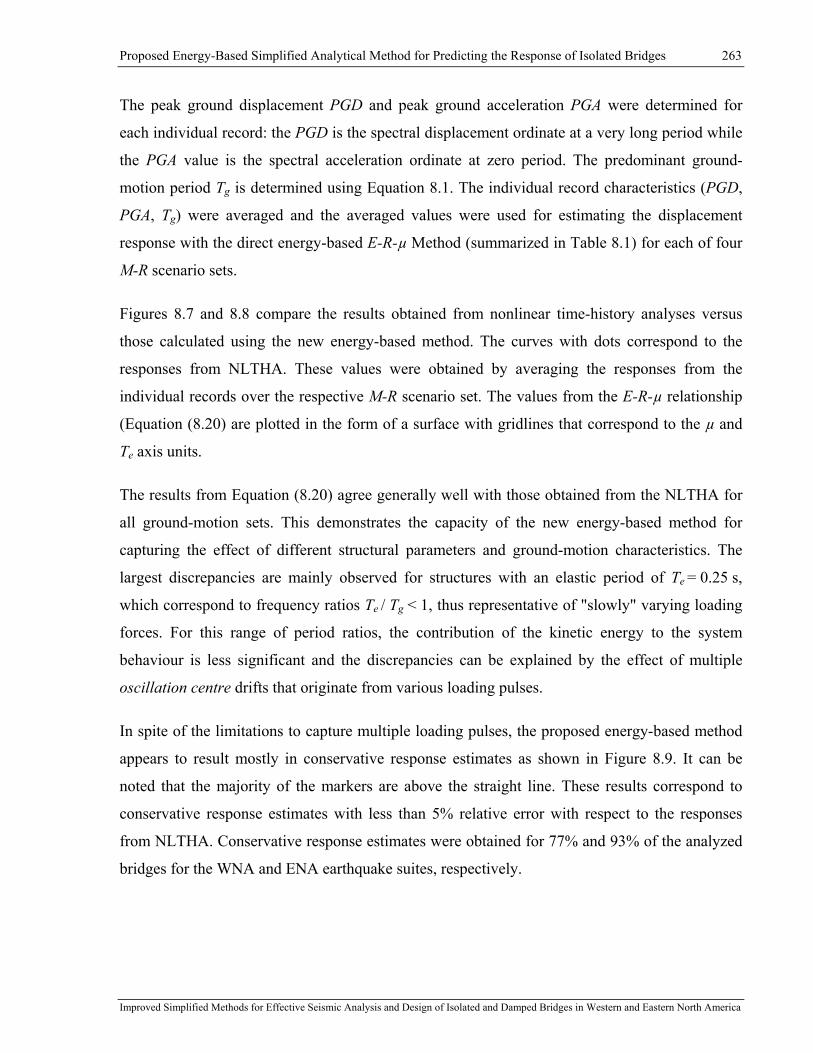
Proposed Energy-Based Simplified Analytical Method for Predicting the Response of Isolated Bridges 263
Improved Simplified Methods for Effective Seismic Analysis and Design of Isolated and Damped Bridges in Western and Eastern North America
The peak ground displacement PGD and peak ground acceleration PGA were determined for
each individual record: the PGD is the spectral displacement ordinate at a very long period while
the PGA value is the spectral acceleration ordinate at zero period. The predominant ground-
motion period Tg is determined using Equation 8.1. The individual record characteristics (PGD,
PGA, Tg) were averaged and the averaged values were used for estimating the displacement
response with the direct energy-based E-R-µ Method (summarized in Table 8.1) for each of four
M-R scenario sets.
Figures 8.7 and 8.8 compare the results obtained from nonlinear time-history analyses versus
those calculated using the new energy-based method. The curves with dots correspond to the
responses from NLTHA. These values were obtained by averaging the responses from the
individual records over the respective M-R scenario set. The values from the E-R-µ relationship
(Equation (8.20) are plotted in the form of a surface with gridlines that correspond to the µ and
Te axis units.
The results from Equation (8.20) agree generally well with those obtained from the NLTHA for
all ground-motion sets. This demonstrates the capacity of the new energy-based method for
capturing the effect of different structural parameters and ground-motion characteristics. The
largest discrepancies are mainly observed for structures with an elastic period of Te = 0.25 s,
which correspond to frequency ratios Te / Tg < 1, thus representative of "slowly" varying loading
forces. For this range of period ratios, the contribution of the kinetic energy to the system
behaviour is less significant and the discrepancies can be explained by the effect of multiple
oscillation centre drifts that originate from various loading pulses.
In spite of the limitations to capture multiple loading pulses, the proposed energy-based method
appears to result mostly in conservative response estimates as shown in Figure 8.9. It can be
noted that the majority of the markers are above the straight line. These results correspond to
conservative response estimates with less than 5% relative error with respect to the responses
from NLTHA. Conservative response estimates were obtained for 77% and 93% of the analyzed
bridges for the WNA and ENA earthquake suites, respectively.

Proposed Energy-Based Simplified Analytical Method for Predicting the Response of Isolated Bridges 264
Improved Simplified Methods for Effective Seismic Analysis and Design of Isolated and Damped Bridges in Western and Eastern North America
Figure 8.7 WNA E-R-µ relationship from analytical estimate and NL SDOF analyses

Proposed Energy-Based Simplified Analytical Method for Predicting the Response of Isolated Bridges 265
Improved Simplified Methods for Effective Seismic Analysis and Design of Isolated and Damped Bridges in Western and Eastern North America
Figure 8.8 ENA E-R-µ relationship from analytical estimate and NL SDOF analyses

Proposed Energy-Based Simplified Analytical Method for Predicting the Response of Isolated Bridges 266
Improved Simplified Methods for Effective Seismic Analysis and Design of Isolated and Damped Bridges in Western and Eastern North America
Figure 8.9 NLTHA versus energy-based E-R-µ approach using Equation (8.20)
The values presented in Figure 8.9 for the new energy-based E-R-µ method are reproduced in
Figure 8.10. In the same figure, the response estimates obtained from the EEA are presented
versus the responses obtained from NLTHA. By comparing these results, it can be noted that
these two methods provide similar response estimates for bridges exhibiting limited nonlinear
responses which are characterized by small inelastic displacements as discussed in Chapter 7.
For structures sustaining larger inelastic displacements, the response estimates from the EEA are
generally much more conservative than those obtained from the proposed E-R-µ method. It
emphasizes the effect of the kinetic energy that was considered in the development of the
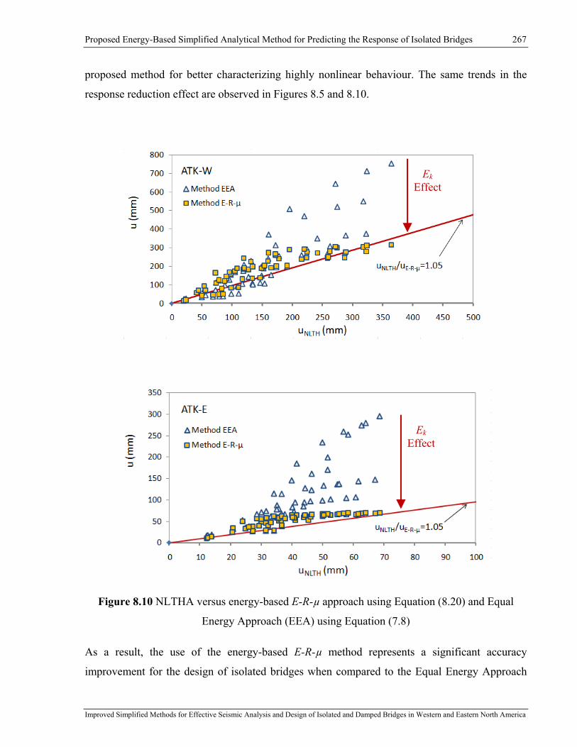
Proposed Energy-Based Simplified Analytical Method for Predicting the Response of Isolated Bridges 267
Improved Simplified Methods for Effective Seismic Analysis and Design of Isolated and Damped Bridges in Western and Eastern North America
proposed method for better characterizing highly nonlinear behaviour. The same trends in the
response reduction effect are observed in Figures 8.5 and 8.10.
Figure 8.10 NLTHA versus energy-based E-R-µ approach using Equation (8.20) and Equal
Energy Approach (EEA) using Equation (7.8)
As a result, the use of the energy-based E-R-µ method represents a significant accuracy
improvement for the design of isolated bridges when compared to the Equal Energy Approach
Ek Effect
Ek Effect

Proposed Energy-Based Simplified Analytical Method for Predicting the Response of Isolated Bridges 268
Improved Simplified Methods for Effective Seismic Analysis and Design of Isolated and Damped Bridges in Western and Eastern North America
(EEA) proposed by Newmark and Hall (1982). The energy-based E-R-µ method may be
incorporated in the current design provisions as an efficient alternative to the currently specified
in the North American codes (CAN/CSA-S6-06 and AASHTO 2009, 2010), which is subject to
certain limitations. The main advantage of the proposed energy-based E-R-µ method with respect
to that currently specified in the code (CSA-S6-06) is that the energy-based E-R-µ method
accounts more explicitly for bilinear response and ground motion properties. The use of the
proposed method for developing effective and optimal seismic protection strategies is another
attractive point which is further studied in the next chapter.
8.5 Conclusions In this chapter, a new energy-based E-R-µ method was developed for predicting the peak
displacement response of isolated bridges. The method assumes that the bridge structure being
initially at rest is subjected to the ground motion excitation that is represented by a single sine-
wave pulse. The response to the pulse loading is solved by making use of the concept of energy
allocation under transient excitation that was derived in chapter 7. The energy concept used in
the Equal Energy Approach (EEA) was adopted as a basis for the development of the new
method. The method's account of the kinetic energy distinguishes it from EEA-based methods
derived solely assuming a steady-state response of the nonlinear structure.
This new energy-based E-R-µ method, was developed purely based on analytical derivations
rather than being empirically calibrated on a region-by-region basis to obtain accurate response
predictions. The ground motion characteristics and the system's nonlinear parameters are taken
into account by the new simplified method. In order to harmonize the use of the proposed
energy-based E-R-µ method with the design procedure specified in the CAN/CSA-S6-06, the
design procedure was formulated by adopting the seismic and structure parameters commonly
used in current design practice.
As was shown in this chapter, the use of the proposed energy-based E-R-µ method represents a
significant accuracy improvement for the design of isolated bridges over the currently used
EEA-based methods (Figure 8.10). The results obtained from NLTHA (Chapter 5) for 120
isolated bridges (60 in WNA and 60 in ENA) were compared to those calculated by the new
energy-based E-R-µ method. The proposed energy-based E-R-µ method appears to result mostly

Proposed Energy-Based Simplified Analytical Method for Predicting the Response of Isolated Bridges 269
Improved Simplified Methods for Effective Seismic Analysis and Design of Isolated and Damped Bridges in Western and Eastern North America
in conservative response prediction. Conservative response estimates were obtained for 77% and
93% of analyzed bridges in WNA and in ENA, respectively.
Being derived for a single loading pulse, this method has an inherent limitation to capture the
effect of the loading duration or irregularity in seismic excitation and structural response that
may be very complex.
The energy-based E-R-µ method may be incorporated into the current design provisions as an
efficient alternative to the currently specified design approach. This method can be applied at a
preliminary design stage. Once the protection strategy is defined, more detailed and time-
consuming analyses can be used to refine preliminary response estimates. This method can be
extended to any SDOF system and it is not limited to bridge applications. The use of the new
energy-based E-R-µ method for developing optimum cost-effective isolation solutions is further
explored in the next chapters.

Design Implications of the Proposed Methods 270
Improved Simplified Methods for Effective Seismic Analysis and Design of Isolated and Damped Bridges in Western and Eastern North America
Chapter 9: Design Implications of the Proposed Methods
9.1 General
This chapter summarizes the improvements proposed in this thesis for designing seismically
isolated bridge structures and it also concludes with a discussion of their design implications.
The first part of this chapter presents the modifications that are proposed, based on this research
thesis (Chapters 5 and 6), to improve the accuracy and extend the applicability of current code
simplified methods. The effect of these modifications is demonstrated for a series of 180 isolated
bridge structures that were analyzed in Chapter 5.
The response of the same isolated bridges is then re-assessed by using the new energy-based
method that was proposed in Chapter 8 as an alternative design approach to account for the
different structural parameters and ground-motion characteristics.
Finally, a bridge retrofit example is presented to compare bridge designs using the current code
provisions and those proposed in this research. The focus is set on assessing the possibility of
using the new energy-based method as an alternative design approach to address the limitations
of the current code methods.
In addition, a detailed insight on the use of the new energy-based E-R-µ method for achieving an
optimum isolation solution is gained by studying the effect of the bridge parameters.
9.2 Proposed Improvements to CSA-S6-06 Simplified Method The observations made in Chapter 5 suggest that the code simplified method results mostly in
safe designs for WNA but underestimates the displacement demand of bridges subjected to ENA
seismic ground motions. It was also observed that the damping limits of the current code
simplified method disqualify a large number of physically achievable and even desirable seismic
protection schemes, including cases where the code method results in conservative response
predictions.

Design Implications of the Proposed Methods 271
Improved Simplified Methods for Effective Seismic Analysis and Design of Isolated and Damped Bridges in Western and Eastern North America
In addition to the damping limits, current CSA-S6 and AASHTO codes also have minimum
lateral restoring force criteria to ensure a minimum recentring capability to the system. CSA-S6-
06, clause 4.10.10.2 reads: "… The isolation system shall be configured to produce a lateral
restoring force such that the lateral force at the design displacement is greater than the lateral
force at 50% of the design displacement by at least 0.025W”. In AASHTO (2009, 2010), the
minimum restoring force at 50% of the design displacement is 0.0125W, which is less stringent
than in CSA S6. Unfortunately, the codes do not provide a clear scientific basis for these criteria
although it is speculated that these criteria are intended to result in systems with a non-zero post-
elastic stiffness. As a result of the difference between both codes, the design of isolated bridges
in Canada may be limited more frequently by this requirement when compared to engineering
practice in the US.
To address the limitations inherent to the current seismic code provisions (CSA-S6-06 and
AASHTO), the modifications are proposed in this research thesis. These modifications could
then be used in future editions of CSA-S6 for both WNA and ENA to improve the accuracy and
to extend the applicability of the current simplified method by superseding the original
requirements for the maximum damping limit and minimum lateral restoring force.
Table 9.1 summarizes a method that follows the framework of the one presented in clause
4.10.6.2.1 of CAN/CSA-S6-06 but with the following proposed revisions:
1) Improving method's accuracy - Damping coefficients B
Damping coefficients B specified in Table 4.8 can be replaced by an exponential equation
between B and βeff (Equation 2.8). Interpolation between tabulated values would therefore no
longer be required.
The same equation can be used with different exponents for WNA and ENA locations to
reflect different damping response reduction effects. The exponents n = 0.3 and 0.2 are
suggested for design of isolated bridges in WNA and ENA, respectively.
2) Extending method's applicability limits
The damping limits can be relaxed and expressed as a function of the post-yielding stiffness
ratio α (Equation (6.10)). This expression reflects a geometrical relation between the

Design Implications of the Proposed Methods 272
Improved Simplified Methods for Effective Seismic Analysis and Design of Isolated and Damped Bridges in Western and Eastern North America
hysteresis shape and dissipated energy and reflects the influence of the ratio α on the
accuracy of the equivalent linearization method that forms the basis of the code-specified
simplified method. The damping limit of 30% currently specified in CAN/CSA-S6-06 has
been established for α = 0.10, a value which is primarily representative of the lead-rubber
bearing (LRB) system. An upper limit greater than %30=effβ can be adopted for α-ratios
lower than 0.10. As further presented in this section, this would allow for a wider range of
seismic protection systems with α ≤ 0.1 such as friction pendulum isolators (FPI) and flat
sliding isolators (FSI) to be efficiently used up to their maximum dissipative capacity.
maximum allowable effective damping effβ is determined using Equation (6.10) and yields
33%, 40%, and 52% for α = 0.10, 0.05, and 0.01, respectively.
• To ensure that the method will lead to conservative results, the method applicability limits
can be established in terms of the effective period Teff (Equation (6.15)). This expression
takes into account the influence of the initial elastic period Te and post-yielding stiffness
ratio α on the accuracy of the code-specified simplified method. As a result, the damping
limits proposed by Equation (6.10) would be automatically satisfied. Responses that are not
sufficiently accurate are automatically rejected when using limits that depend on Teff.

Design Implications of the Proposed Methods 273
Improved Simplified Methods for Effective Seismic Analysis and Design of Isolated and Damped Bridges in Western and Eastern North America
Table 9-1 Modified procedure following the Simplified Equivalent Static Force Method
(CAN/CSA-S6)
CSA-S6 Simplified Method Procedure
Step 1. Ground-motion data required:
5% Damped Response Spectrum
Step 2. System data required:
RT inhe ;;; αβ
For the first iteration, assume inheffeeff TT ββ == ;
Step 3. Determine from spectrum:
%)5;( effD TPS
Step 4. Determine damping coefficient B using Equation 2.8: n
effB ⎟⎟⎠
⎞⎜⎜⎝
⎛=
%5β
with n=0.3 for WNA and 0.2 for ENA
Step 5. Calculate:
)(/%)5;( effeffDi BTPSd β=
Step 6. For iteration 2 and higher, check accuracy:
1 100%i i
i
d derrord
−−= ⋅
if error is acceptable, go to Step 8
Step 7. Calculate and Return to Step 3:
ieD
dTPSR
⋅=%)5;(
μ
ααμμ
−+⋅=
1eeff TT
)1()1()1(2
ααμμπαμβ
−+⋅⋅−⋅−⋅
=eq
inheqeff βββ +=
Step 8. Save and print response:
id

Design Implications of the Proposed Methods 274
Improved Simplified Methods for Effective Seismic Analysis and Design of Isolated and Damped Bridges in Western and Eastern North America
The effects of the proposed modifications can be examined in Figures 9.1 to 9.6, which present
the relative error between the maximum displacements and the isolation level from the code
simplified method, ucode, and the results from nonlinear time-history analyses (uNLTH). The
comparison is performed using the response of 180 isolated bridge structures obtained by varying
the following parameters: for Te = [0.25, 0.5, 0.75, and 1.0 s], R = [4, 16, 28, 40, 52], and
α = [0.1, 0.05, and 0.01]. The bridges have been analyzed in Chapter 5. For the improved code
method, the displacement estimates were obtained by following the complete iterative procedure
shown in Table 9.1. The resulting displacement estimates are the deck displacements which
corresponds to the displacements across the isolation devices located at the abutments. The
displacements across the isolators on the piers must then be determined from that value in
proportion to the relative stiffness of the piers and piers' isolators.
The results are presented in 6 figures (Figures 9.1 to 9.6) to cover the two regions (WNA and
ENA) and three values of α. In each figure, three sub-plots are shown. Figures 9.1(a) to 9.6(a)
give the errors obtained when applying the current code method, without the suggested
modifications. In the plots, the isolated bridges that satisfy the current code applicability limits
are identified. Figures 9.1(b) to 9.6(b) shows the improvement in the method’s accuracy when
using the proposed exponential expression (Equation (2.8)) for the damping coefficient, with the
exponents n=0.3 and 0.2 for WNA and ENA, respectively. Figures 9.1(c) to 9.6(c) shows the
effects of applying the proposed method applicability limits that are function of Teff.
For WNA, the use of Equation (2.8) for the damping coefficients does not affect the response
prediction much because the damping coefficients B from Equation (2.8) with n=0.3 corresponds
well to the originally tabulated values of B in the code provisions, as presented in Table 2-1. By
respectively comparing Figures 9.4(a), 9.5(a) and 9.6(a) to Figures 9.4(b), 9.5(b), and 9.6(b), a
greater improvement is obtained for displacement estimates in ENA. Equation (2.8) with n=0.2
gives more uniform predictions over the possible range of effective damping. The number of
bridges satisfying the conservative response estimates in ENA was accordingly increased from
31% to 89%. This number is close in agreement with 90% of satisfactory estimates in WNA. To
implement the modifications proposed in this thesis, ENA and WNA seismic regions can be
distinguished using the criteria based on the ratio Sa(0.2) / Sa(2.0) > 8.0 and
Sa(0.2) / Sa (2.0) < 8.0 (for ENA and WNA, respectively), as currently specified in the NBCC
(NRCC, 2010).

Design Implications of the Proposed Methods 275
Improved Simplified Methods for Effective Seismic Analysis and Design of Isolated and Damped Bridges in Western and Eastern North America
In the figures, it is noted that applying the current maximum damping limit (30%) and the
minimum lateral restoring force requirement (0.025W at 50% of the design displacement)
ensures that the current method, without revisions, gives conservative predictions. More
importantly, it is also clear from these figures that these limits are excessively stringent because a
large portion of the bridges for which satisfactory (conservative) estimates are obtained are
rejected. For WNA, only 60% of the bridges for which a conservative result was obtained meet
the current code limits. For ENA, this percentage reduces to 36%.
The second proposed improvement aims at extending the percentage of accepted satisfactory
estimates with unconservative relative errors ranging up to 5%. This effect can be outlined by
comparing Figures 9.1(b) - 9.6(b) to Figures 9.1(c) - 9.6(b). As shown, the proposed limits can
be used to identify and reject responses with unsatisfactory accuracy. A comparison of the
response of 180 isolated bridge structures shows that the percentages of cases with satisfactory
predictions increase from 60% to 93% and from 36% to 94% for WNA and ENA, respectively,
when the structures meet the proposed limit set as a function of the effective period (Equation
(6.15)). On this basis, it is believed that the proposed limits could be used in future editions of
CSA-S6 for both WNA and ENA.
Based on the above, it can be stated that the implementation of the modifications proposed in this
research would significantly improve the current code simplified method for estimating
displacement demands, in terms of both the accuracy of the predictions and the number of cases
for which the method can be applied. The modified simplified code method will then result in the
same level of accuracy in WNA and ENA, with relative errors ranging from 5% (unconservative)
to -50% (conservative) in both seismic regions. In addition, a wider choice of market-available
seismic protective devices will be covered by the modified seismic provisions.

Design Implications of the Proposed Methods 276
Improved Simplified Methods for Effective Seismic Analysis and Design of Isolated and Damped Bridges in Western and Eastern North America
a)
b)
c)
Figure 9.1 Relative errors in maximum displacements at the isolation level using the code
simplified method compared to NLTHA for WNA and α = 0.1 (ATK-W): a) current CSA-S6-06
method; b) current method with damping coefficients from Eq.(2.8) applicability limits;
c) current method with damping coefficients from Eq.(2.8) and applicability limits based on
effective period.

Design Implications of the Proposed Methods 277
Improved Simplified Methods for Effective Seismic Analysis and Design of Isolated and Damped Bridges in Western and Eastern North America
a)
b)
c)
Figure 9.2 Relative errors in maximum displacements at the isolation level using the code
simplified method compared to NLTHA for WNA and α = 0.05 (ATK-W): a) current CSA-S6-
06 method; b) current method with damping coefficients from Eq.(2.8) applicability limits;
c) current method with damping coefficients from Eq.(2.8) and applicability limits based on
effective period.

Design Implications of the Proposed Methods 278
Improved Simplified Methods for Effective Seismic Analysis and Design of Isolated and Damped Bridges in Western and Eastern North America
a)
b)
c)
Figure 9.3 Relative errors in maximum displacements at the isolation level using the code
simplified method compared to NLTHA for WNA and α = 0.01 (ATK-W): a) current CSA-S6-
06 method; b) current method with damping coefficients from Eq.(2.8) applicability limits;
c) current method with damping coefficients from Eq.(2.8) and applicability limits based on
effective period.
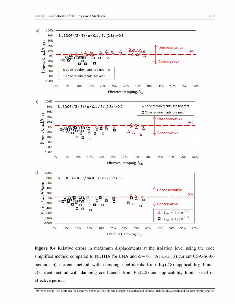
Design Implications of the Proposed Methods 279
Improved Simplified Methods for Effective Seismic Analysis and Design of Isolated and Damped Bridges in Western and Eastern North America
a)
b)
c)
Figure 9.4 Relative errors in maximum displacements at the isolation level using the code
simplified method compared to NLTHA for ENA and α = 0.1 (ATK-E): a) current CSA-S6-06
method; b) current method with damping coefficients from Eq.(2.8) applicability limits;
c) current method with damping coefficients from Eq.(2.8) and applicability limits based on
effective period.
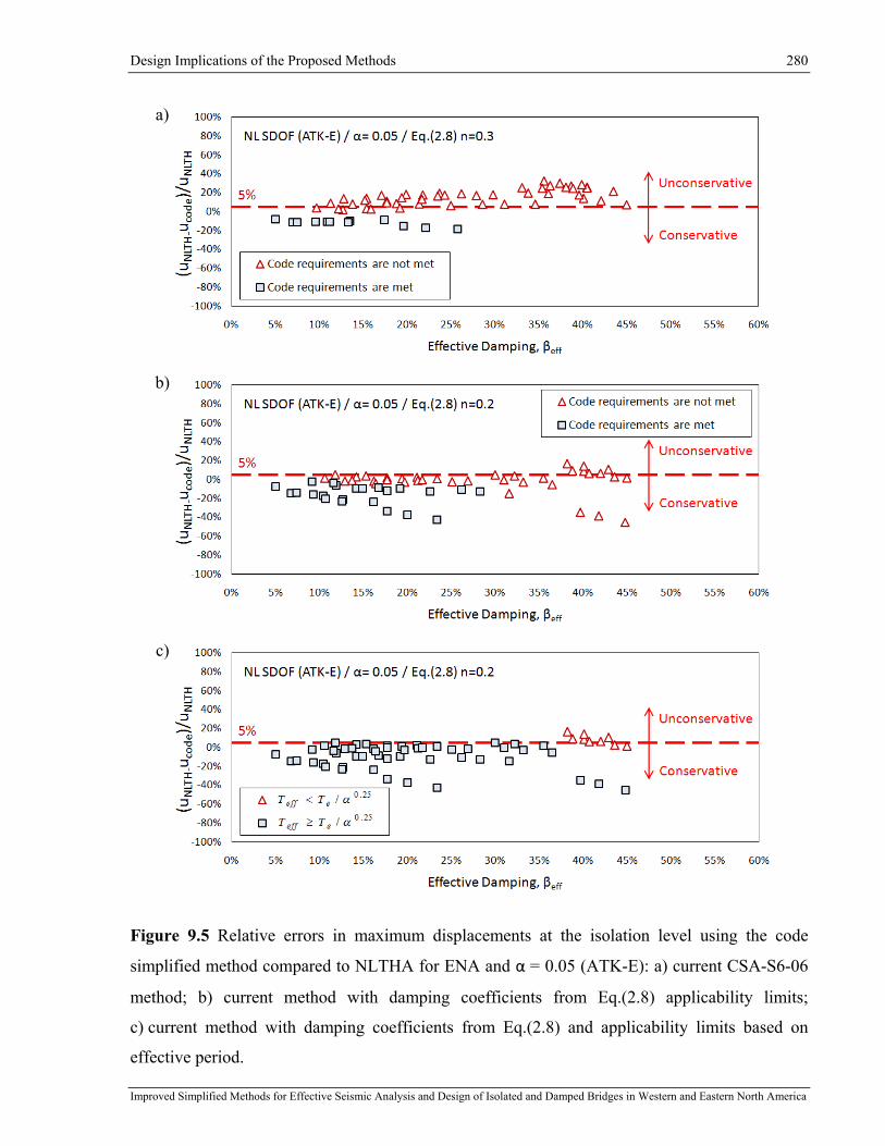
Design Implications of the Proposed Methods 280
Improved Simplified Methods for Effective Seismic Analysis and Design of Isolated and Damped Bridges in Western and Eastern North America
a)
b)
c)
Figure 9.5 Relative errors in maximum displacements at the isolation level using the code
simplified method compared to NLTHA for ENA and α = 0.05 (ATK-E): a) current CSA-S6-06
method; b) current method with damping coefficients from Eq.(2.8) applicability limits;
c) current method with damping coefficients from Eq.(2.8) and applicability limits based on
effective period.
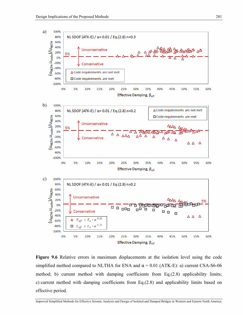
Design Implications of the Proposed Methods 281
Improved Simplified Methods for Effective Seismic Analysis and Design of Isolated and Damped Bridges in Western and Eastern North America
a)
b)
c)
Figure 9.6 Relative errors in maximum displacements at the isolation level using the code
simplified method compared to NLTHA for ENA and α = 0.01 (ATK-E): a) current CSA-S6-06
method; b) current method with damping coefficients from Eq.(2.8) applicability limits;
c) current method with damping coefficients from Eq.(2.8) and applicability limits based on
effective period.
Design Implications of the Proposed Methods 282
Improved Simplified Methods for Effective Seismic Analysis and Design of Isolated and Damped Bridges in Western and Eastern North America
9.3 Proposed New Energy-Based E-R-µ Method
The new energy-based simplified method proposed in this research (Chapter 8) is based on the
E-R-µ relationship. The energy concept used in the Equal Energy Approach (EEA) was adopted
as a basis for the development of the new method. The EEA was extended by considering the
transient response to pulse type loading, which is deemed to better represent the response of an
isolated bridge structure that is subjected to seismic ground motions. The proposed method was
derived based on the concept of energy allocation under transient response.
The method's capability for directly accounting for the kinetic energy differentiates it from the
EEA method derived solely from a steady-state response. The strong ground motion
characteristics and the system's nonlinear parameters are both taken into account in the energy-
based E-R-µ method. This reflects more closely the actual nonlinear response of isolated bridges
to strong ground motions. As a result, it is applicable to a broader range of structures and the
accuracy of the prediction has generally been improved. With the proposed method,
displacement estimates can be obtained directly, without iterations, which represents a significant
advantage compared to linearization approach used in current code simplified methods. This
direct method has been worked into a design procedure that was outlined in detail in Table 8.1.
This design procedure may be used for the preliminary design of isolated bridge structures; it
could also be used as a replacement of the simplified method currently specified in CAN/CSA-
S6.
Figures 9.7 and 9.8 present the errors in response estimates from the proposed method relative to
the results from NLTHA. The response estimates were obtained using mean values of the
ground-motion characteristics. The response spectrum, predominant period Tg and peak ground
displacement PGD were determined by averaging the characteristics of 20 individual time
histories as presented in Figure 8.6 for ATK-W and ATK-E. As shown, the proposed method
generally results in conservative response estimates. The level of conservatism in the response
estimates is comparable to those attained using the different linearization methods that were
compared in Figure 2.5 (Mavronicola and Komodromos, 2011) and Figure 2.6 (FEMA 356,
ATC-40, and FEMA 440). Taking into account that the linearization methods were empirically
calibrated, the level of conservatism from the new energy-based E-R-µ method, which was

Design Implications of the Proposed Methods 283
Improved Simplified Methods for Effective Seismic Analysis and Design of Isolated and Damped Bridges in Western and Eastern North America
developed solely on a theoretical basis without any additional calibration, makes this method an
interesting alternative in the design process.
Contrary to the current simplified code method, the energy-based E-R-µ method is not iterative
and a large number of possible solutions can be obtained directly to evaluate the most
appropriate scheme complying with the design objectives. The proposed method can provide
upper bound displacement predictions that will unlikely be exceeded and will represent useful
information for the design engineers.
It can be noted from Figures 9.7 and 9.8 that the level of conservatism mostly decreases as the
response modification factor R increases. This suggests that the proposed energy-based E-R-µ
method is better suited for bridge structures that exhibit a response of larger displacement
ductility demands (larger R factors). It was also found that the errors increase for structures with
shorter elastic periods.
The conservatism of the proposed method is inherent to the method's assumptions that were
explained in Chapter 8. The energy transmitted to the isolated system is idealized as being the
representative of the system response under a sinusoidal excitation with a sole period Tg which
relates the peak ground displacement and the peak ground acceleration. The response estimates
will correspond to the response of isolated bridges under the most demanding loading conditions
form the strong motion portion of a seismic ground motion.
Providing mainly upper bound displacement estimates, the energy-based E-R-µ method may also
be adopted for complementing the current code method beyond its applicability limits. In this
way, the response estimate may be obtained for a given isolated bridge when the simplified code
method does not provide engineers with reliable response predictions.
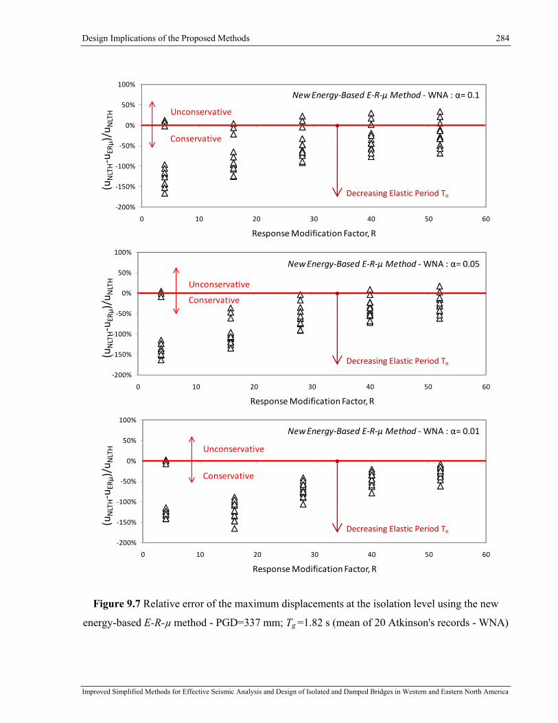
Design Implications of the Proposed Methods 284
Improved Simplified Methods for Effective Seismic Analysis and Design of Isolated and Damped Bridges in Western and Eastern North America
Figure 9.7 Relative error of the maximum displacements at the isolation level using the new
energy-based E-R-µ method - PGD=337 mm; Tg =1.82 s (mean of 20 Atkinson's records - WNA)
‐200%
‐150%
‐100%
‐50%
0%
50%
100%
0 10 20 30 40 50 60
(uNLTH‐u
ERµ)/u
NLTH
Response Modification Factor, R
New Energy‐Based E‐R‐µ Method ‐WNA : α= 0.01
Conservative
Unconservative
Decreasing Elastic Period Te
‐200%
‐150%
‐100%
‐50%
0%
50%
100%
0 10 20 30 40 50 60
(uNLTH‐u
ERµ)/u
NLTH
Response Modification Factor, R
New Energy‐Based E‐R‐µ Method ‐WNA : α= 0.05
Conservative
Unconservative
Decreasing Elastic Period Te
‐200%
‐150%
‐100%
‐50%
0%
50%
100%
0 10 20 30 40 50 60
(uNLTH‐u
ERµ)/u
NLTH
Response Modification Factor, R
New Energy‐Based E‐R‐µ Method ‐WNA : α= 0.1
Conservative
Unconservative
Decreasing Elastic Period Te
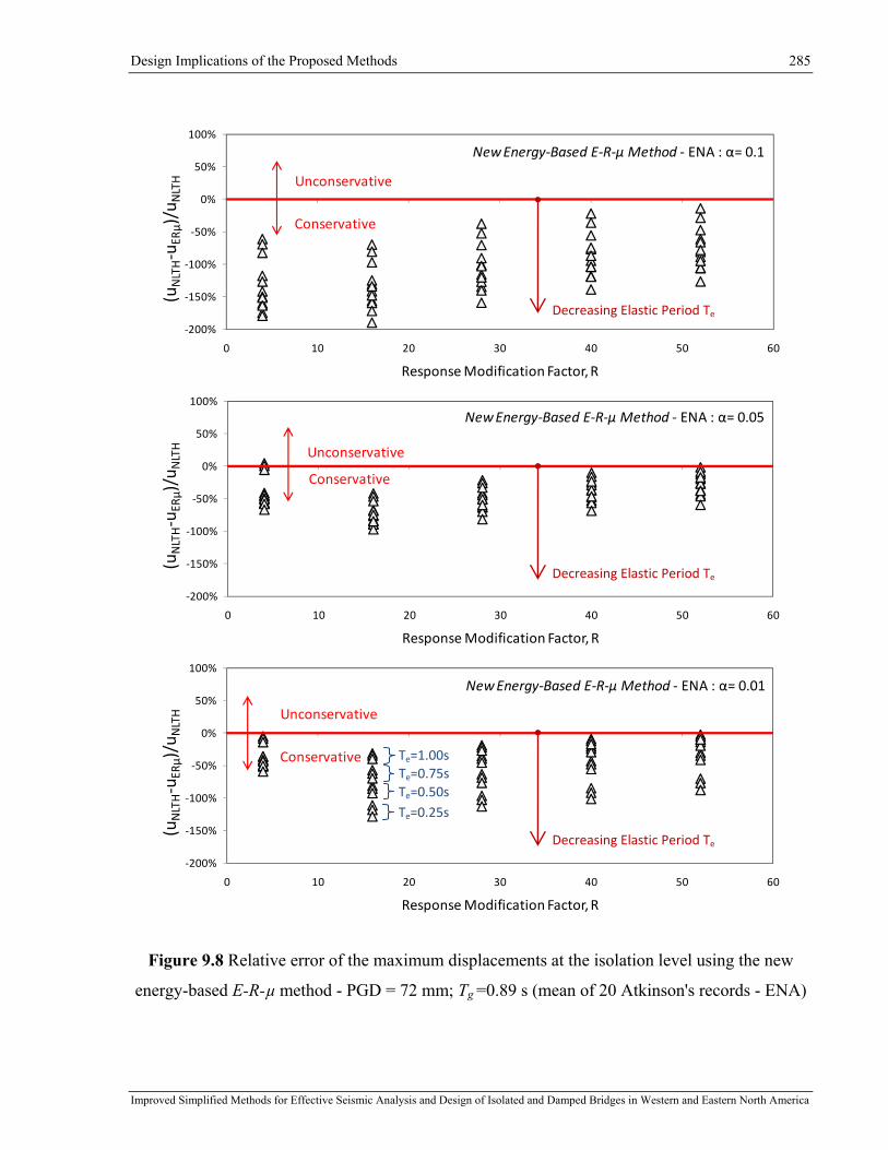
Design Implications of the Proposed Methods 285
Improved Simplified Methods for Effective Seismic Analysis and Design of Isolated and Damped Bridges in Western and Eastern North America
Figure 9.8 Relative error of the maximum displacements at the isolation level using the new
energy-based E-R-µ method - PGD = 72 mm; Tg =0.89 s (mean of 20 Atkinson's records - ENA)
‐200%
‐150%
‐100%
‐50%
0%
50%
100%
0 10 20 30 40 50 60
(uNLTH‐u
ERµ)/u
NLTH
Response Modification Factor, R
New Energy‐Based E‐R‐µ Method ‐ ENA : α= 0.05
Conservative
Unconservative
Decreasing Elastic Period Te
‐200%
‐150%
‐100%
‐50%
0%
50%
100%
0 10 20 30 40 50 60
(uNLTH‐u
ERµ)/u
NLTH
Response Modification Factor, R
New Energy‐Based E‐R‐µ Method ‐ ENA : α= 0.1
Conservative
Unconservative
Decreasing Elastic Period Te
‐200%
‐150%
‐100%
‐50%
0%
50%
100%
0 10 20 30 40 50 60
(uNLTH‐u
ERµ)/u
NLTH
Response Modification Factor, R
New Energy‐Based E‐R‐µ Method ‐ ENA : α= 0.01
Conservative
Unconservative
Te=0.25s Te=0.50sTe=0.75sTe=1.00s
Decreasing Elastic Period Te

Design Implications of the Proposed Methods 286
Improved Simplified Methods for Effective Seismic Analysis and Design of Isolated and Damped Bridges in Western and Eastern North America
9.4 Example of Response Prediction Using Simplified Methods In this section, an example is presented to illustrate the application of the current and modified
simplified methods for the prediction of the response of an isolated bridge. The improvements
achieved when using the modified simplified method are outlined. A bridge located near
Montreal, Quebec, is adopted to represent a typical aging bridge that is seismically upgraded
with an isolation system. Figure 9.9 presents the elevation of the bridge. The structure is 78 m
long and has three equal spans crossing over a river obstacle.
Figure 9.9 Archetype three-span bridge in Montreal

Design Implications of the Proposed Methods 287
Improved Simplified Methods for Effective Seismic Analysis and Design of Isolated and Damped Bridges in Western and Eastern North America
In this example, the bridge is analyzed in the longitudinal direction. In this direction, the bridge
retrofit consists of incorporating isolation devices between the superstructure and both piers.
Frictionless roller supports are considered at both abutments. A typical friction sliding isolation
(FSI) device was adopted to increase the bridge seismic resistance.
The initial elastic period Te of the bridge isolation system in the longitudinal direction is 0.5 s.
The FSI devices have a high initial stiffness before being activated. The activation sliding
strength was set equal to the force corresponding to a value of R equal to 4. Upon sliding, the FSI
units exhibit elastic restoring force characterized by the post-yielding stiffness ratio α = 0.01.
The mean damped response spectrum obtained from the suites of 20 eastern records (ATK-E), as
presented in Figures 5.2, is adopted for design. This ensures consistency between the demand
considered for design and the NLTHA performed later to validate the design. For simplicity, the
inherent damping of the structure is assumed to be equal to 5% of critical based on the effective
structural properties. This is the same as the damping level considered in the design spectrum.
The elastic stiffness of the isolated bridge structure is 169.6 kN/mm and the bridge displacement
at activation is 5.2 mm.
In the example, response estimates are determined using three simplified methods:
1) Current CSA-S6-06 method using Equation (2.8) with n=0.3;
2) Modified CSA-S6-06 method using Equation (2.8) with n=0.2;
3) New energy-based E-R-µ method.
The results from these three approaches are summarized in Tables 9-2 to 9-4. The displacements
shown are those of the superstructure relative to the ground. For the first two methods, the
superstructure displacement is obtained following the iterative code procedure outlined in Table
9-1. For the new energy-based E-R-µ method, the direct method is used as presented in Table
8-1. All three response estimates are compared to the reference response from NLTHA. The
relative errors with respect to the NLTHA are presented in Table 9-5. Positive error values
correspond to unconservative response estimates. The comparison of the response predictions
against the "exact" response from NLTHA is presented in Figure 9.10.

Design Implications of the Proposed Methods 288
Improved Simplified Methods for Effective Seismic Analysis and Design of Isolated and Damped Bridges in Western and Eastern North America
Table 9-2 Iterative approach for response estimate using current Equation (2.8) with n = 0.3
(where for βeff > 30%, B = 1.7)
iteration
Sdi
(mm)
di
(mm)
Error
(%)
μ Teff
(s)
βeq
(%)
βeff
(%)
B
1 20.8 20.8 ‐ 4.01 0.99 45.9 50.9 1.70
2 36.2 21.3 2.24 4.10 1.00 46.2 51.2 1.70
3 36.5 21.5 0.63 4.13 ‐ ‐ ‐ ‐
Table 9-3 Iterative approach for response estimate using Equation (2.8) with n = 0.2
iteration
Sdi
(mm)
di
(mm)
Error
(%)
μ Teff
(s)
βeq
(%)
βeff
(%)
B
1 20.8 20.8 ‐ 4.01 0.99 45.9 50.9 1.59
2 36.2 22.8 8.53 4.38 1.03 47.0 52.0 1.60
3 37.5 23.5 3.02 4.52 1.04 47.4 52.4 1.60
4 38.1 23.8 1.29 4.58 1.05 47.5 52.5 1.60
5 38.6 24.1 1.36 4.64 1.06 47.7 52.7 1.60
6 39.1 24.4 1.15 4.69 1.06 47.8 52.8 1.60
7 39.1 24.4 ‐0.04 ‐ ‐ ‐ ‐ ‐
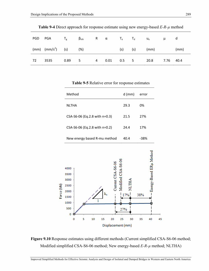
Design Implications of the Proposed Methods 289
Improved Simplified Methods for Effective Seismic Analysis and Design of Isolated and Damped Bridges in Western and Eastern North America
Table 9-4 Direct approach for response estimate using new energy-based E-R-µ method
PGD PGA Tg βinh R α Te Td ue µ d
(mm) (mm/s2) (s) (%) (s) (s) (mm) (mm)
72 3535 0.89 5 4 0.01 0.5 5 20.8 7.76 40.4
Table 9-5 Relative error for response estimates
Method d (mm) error
NLTHA 29.3 0%
CSA‐S6‐06 (Eq.2.8 with n=0.3) 21.5 27%
CSA‐S6‐06 (Eq.2.8 with n=0.2) 24.4 17%
New energy based R‐mu method 40.4 ‐38%
Figure 9.10 Response estimates using different methods (Current simplified CSA-S6-06 method;
Modified simplified CSA-S6-06 method; New energy-based E-R-µ method; NLTHA)

Design Implications of the Proposed Methods 290
Improved Simplified Methods for Effective Seismic Analysis and Design of Isolated and Damped Bridges in Western and Eastern North America
In this example, both approaches using the simplified code method provide unconservative
response estimates. The estimates obtained using the modified code method are more accurate
than that from the current code method. However, both estimates are not close enough to the
“exact” (NLTHA) response to be considered as satisfactory. Equally important is the fact that
this simple structure does not satisfy the limits set in the CSA S6-06 for the current and modified
methods:
i) In Table 9.3, the current CSA-S6-06 method using Equation (2.8) with n=0.3 (d=21.5 mm):
i-1) The effective damping ratio is higher than 30% thus B=1.7 is used according to CSA-S6-
06, Table 4.8.
i-2) The bridge isolation system does not develop a lateral restoring force at least 0.025W
greater than the lateral force at 50% of the design displacement, as required in CSA-S6-
06 Clause 4.10.10.2 Lateral restoring force). The lateral force is verified as follows:
The displacement of the elastic system is given as:
mmsSu De 8.20%)5;5.0( == (9.1)
The elastic limit which corresponds to the displacement at activation is determined using the
response modification factor R as:
mmmmRu
u ey 2.5
48.20
=== (9.2)
The elastic stiffness is given as:
mmkN
mmskN
sm
Tk
eu 6.169074.1
5.022 222
=⋅
⎟⎟⎠
⎞⎜⎜⎝
⎛=⎟⎟
⎠
⎞⎜⎜⎝
⎛=
ππ (9.3)
The ductility demand at 100% of the design displacement d determined in iteration 3 (Table
9.2):
14.42.55.21
%100 ===mmmm
ud
yμ (9.4)

Design Implications of the Proposed Methods 291
Improved Simplified Methods for Effective Seismic Analysis and Design of Isolated and Damped Bridges in Western and Eastern North America
The ductility demand at 50% of the design displacement d is determined as:
07.2%100%50
%100%50 == μμ (9.5)
The effective stiffness at 100% of the design displacement using Equation (2.1) is:
mmkNmmkNkeff /3.4214.4
01.014.401.01/6.169)( %100 =−⋅+
⋅=μ (9.6)
The effective stiffness at 50% of the design displacement using Equation (2.1) is:
mmkNmmkNkeff /8.8207.2
01.007.201.01/6.169)( %50 =−⋅+
⋅=μ (9.7)
The system lateral force at 100% of the design displacement is determined as:
kNmmmmkNF 5.9095.21/3.42)( %100 =⋅=μ (9.8)
The system lateral force at 50% of the design displacement is determined as:
kNmmmmkNF 3.89107.22.5/8.82)( %50 =⋅⋅=μ (9.9)
The difference between the lateral forces at 50% and 100% of the design displacement is:
kNkNkNFF 2.183.8915.909)()( %50%100 =−=− μμ (9.10)
The minimum force to be verified is found as (CSA-S6-06, Cl.4.10.10.2):
kNsmkgW 4.26310/81.91074000025.0025.0 32 =×⋅⋅= − (9.11)
Thus, the minimum lateral restoring force requirement is not satisfied given that:
WFF 025.0)()( %50%100 <− μμ
kNkN 4.2632.18 <
ii) For the modified CSA-S6-06 method using Equation (2.8) with n = 0.2, the effective period
must be longer than the value given by Equation (6.15):

Design Implications of the Proposed Methods 292
Improved Simplified Methods for Effective Seismic Analysis and Design of Isolated and Damped Bridges in Western and Eastern North America
ssTT eeqeff 58.101.0
5.0)( 25.025.0
max ==⋅= −− αβ (9.12)
The ductility demand at 100% of the design displacement determined at iteration 7 (Table 9.3):
69.42.54.24
===mmmm
ud
yμ (9.13)
The effective period is determined using Equation (2.2) as:
ssTeff 06.101.069.401.01
69.45.0 =−⋅+
⋅= (9.14)
Thus, the minimum effective period requirement is not satisfied given that:
effeqeff TT >− )( maxβ
ss 06.158.1 >
Hence, the current and modified methods could not be used for this particular example. The
example therefore highlights how the new energy-based E-R-µ method represents an applicable
alternative simplified approach for cases where the desired seismic protection scheme does not
meet the code methods' limits.
9.5 Optimizing Bridge Performance with the New Energy-Based
E-R-µ Method
The use of current seismic code provisions (CSA-S6-06 and AASHTO) for achieving a cost-
effective isolation solution implies the use of an elaborate iterative analysis and design approach.
The effective properties of a bridge such as the effective period and the effective damping must
be redefined for each iteration, which represents a complex, time-consuming and laborious task.
In this section, it is illustrated how the E-R-µ method can be efficiently used to optimize the
design of bridges with isolation and damping. For the same example presented above, an
optimization design process is performed using the energy-based E-R-µ method.
Design Implications of the Proposed Methods 293
Improved Simplified Methods for Effective Seismic Analysis and Design of Isolated and Damped Bridges in Western and Eastern North America
Figures 9.11 and 9.12 illustrate how the displacement and force vary with the characteristic
strength Qd. In Figure 9.11, the intersection of the displacement and force curves does not
necessary indicate an optimal solution. This point is arbitrary set to represent the bridge
configuration previously adopted in this study. In such a way the tendencies in response of a
bridge structure are outlined providing information needed to find the response that best meets
the performance target.
The optimum displacements and forces can be found by only varying the bridge parameters in
Equations (8.28) and (8.31). For the same Td and α, if the force activation, or characteristic
strength Qd, is reduced, the seismic forces transmitted by the isolators to the bridge substructure
decrease. In such a case, the effective period of the structure lengthens, resulting in larger
displacement response. Target performance objectives for the bridge structure may be achieved
by carefully selecting the activation force of the isolators. For example, in Figure 9.11, it is
shown that Qd = 881 kN is needed to limit the displacement to 40 mm. Using Qd = 400 kN will
result in an increased displacement of 55 mm. For this structure, this would translate in an
increase of the response modification factor from R = 4.0 to 8.74.
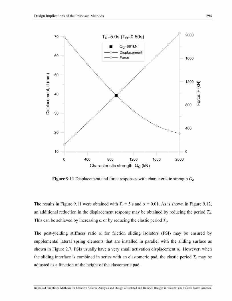
Design Implications of the Proposed Methods 294
Improved Simplified Methods for Effective Seismic Analysis and Design of Isolated and Damped Bridges in Western and Eastern North America
0 400 800 1200 1600 2000
Characteristic strength, Qd (kN)
10
20
30
40
50
60
70
Dis
plac
emen
t, d
(mm
)Qd=881kNDisplacementForce
0
400
800
1200
1600
2000
Forc
e, F
(kN
)
Td=5.0s (Te=0.50s)
Figure 9.11 Displacement and force responses with characteristic strength Qd
The results in Figure 9.11 were obtained with Td = 5 s and α = 0.01. As is shown in Figure 9.12,
an additional reduction in the displacement response may be obtained by reducing the period Td.
This can be achieved by increasing α or by reducing the elastic period Te.
The post-yielding stiffness ratio α for friction sliding isolators (FSI) may be ensured by
supplemental lateral spring elements that are installed in parallel with the sliding surface as
shown in Figure 2.7. FSIs usually have a very small activation displacement uy. However, when
the sliding interface is combined in series with an elastomeric pad, the elastic period Te may be
adjusted as a function of the height of the elastomeric pad.

Design Implications of the Proposed Methods 295
Improved Simplified Methods for Effective Seismic Analysis and Design of Isolated and Damped Bridges in Western and Eastern North America
.0 400 800 1200 1600 2000
Characteristic strength, Qd (kN)
0
10
20
30
40
50
60
70
80
Dis
plac
emen
t, d
(mm
)
Qd=881kN / Td=5.0sTd=10s (Te=1.00s)Td=7.5s (Te=0.75s)Td=5.0s (Te=0.50s)Td=2.5s (Te=0.25s)
0 400 800 1200 1600 2000
Characteristic strength, Qd (kN)
0
500
1000
1500
2000
2500
Forc
e, F
(kN
)
Qd=881kN / Td=5.0sTd=10s (Te=1.00s)Td=7.5s (Te=0.75s)Td=5.0s (Te=0.50s)Td=2.5s (Te=0.25s)
Figure 9.12 Bridge response with characteristic strength Qd and period Td
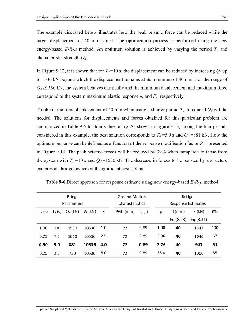
Design Implications of the Proposed Methods 296
Improved Simplified Methods for Effective Seismic Analysis and Design of Isolated and Damped Bridges in Western and Eastern North America
The example discussed below illustrates how the peak seismic force can be reduced while the
target displacement of 40 mm is met. The optimization process is performed using the new
energy-based E-R-µ method. An optimum solution is achieved by varying the period Td and
characteristic strength Qd.
In Figure 9.12, it is shown that for Td =10 s, the displacement can be reduced by increasing Qd up
to 1530 kN beyond which the displacement remains at its minimum of 40 mm. For the range of
Qd ≥1530 kN, the system behaves elastically and the minimum displacement and maximum force
correspond to the system maximum elastic response ue and Fe, respectively.
To obtain the same displacement of 40 mm when using a shorter period Td, a reduced Qd will be
needed. The solutions for displacements and forces obtained for this particular problem are
summarized in Table 9-5 for four values of Td. As shown in Figure 9.13, among the four periods
considered in this example, the best solution corresponds to Td =5.0 s and Qd =881 kN. How the
optimum response can be defined as a function of the response modification factor R is presented
in Figure 9.14. The peak seismic forces will be reduced by 39% when compared to those from
the system with Td =10 s and Qd =1530 kN. The decrease in forces to be resisted by a structure
can provide bridge owners with significant cost saving.
Table 9-6 Direct approach for response estimate using new energy-based E-R-µ method
Bridge
Parameters
Ground Motion
Characteristics
Bridge
Response Estimates
Te (s) Td (s) Qd (kN) W (kN) R PGD (mm) Tg (s) µ d (mm) F (kN) (%)
Eq.(8.28) Eq.(8.31)
1.00 10 1530 10536 1.0 72 0.89 1.00 40 1547 100
0.75 7.5 1010 10536 2.5 72 0.89 2.96 40 1040 67
0.50 5.0 881 10536 4.0 72 0.89 7.76 40 947 61
0.25 2.5 730 10536 8.0 72 0.89 36.8 40 1000 65

Design Implications of the Proposed Methods 297
Improved Simplified Methods for Effective Seismic Analysis and Design of Isolated and Damped Bridges in Western and Eastern North America
Figure 9.13 Peak seismic forces with characteristic strength Qd and period Td
Figure 9.14 Peak seismic forces with response modification factor R
These examples show that the proposed method can be very effective for the selection of an
optimum isolation system. The main reason being that the method is not iterative and a large
number of possible solutions can be obtained directly to evaluate the most appropriate scheme
for the studied structure and design objective.
1547
10409471000
0200400600800
100012001400160018002000
600 800 1000 1200 1400 1600
F (kN)
Qd (kN)
Optimum Solution
1547
10409471000
0200400600800
100012001400160018002000
0 1 2 3 4 5 6 7 8 9 10 11 12
F (kN)
Td (s)
Optimum Solution
1547 kN
1040 kN947 kN 1000 kN
0200400600800
100012001400160018002000
0 1 2 3 4 5 6 7 8 9
F (kN)
Response Modification Factor , R
Optimum Solution
Design Implications of the Proposed Methods 298
Improved Simplified Methods for Effective Seismic Analysis and Design of Isolated and Damped Bridges in Western and Eastern North America
9.6 Conclusions In this chapter, the modifications proposed within this research to improve the accuracy and
extend the applicability of the current code simplified method (CSA-S6-06) were summarized
and discussed. The ability to accurately predict the response of isolated bridges was
demonstrated for a series of 180 isolated bridge structures.
It was shown that the modified simplified code method proposed in this thesis for estimating
displacement demand result in comparable relative errors ranging from 5% (unconservative) to
-50% (conservative) for both WNA and ENA. In addition, a wider choice of the market-available
seismic protective devices can be covered by the modified simplified method.
The displacements of the same 180 isolated bridges were determined using the new energy-based
method proposed in Chapter 8 as an alternative design approach that accounts for different
structure parameters and strong ground motion characteristics. It was confirmed that the
proposed energy-based method results consistently in conservative response prediction. The level
of conservatism generally decreases as the response modification factor R and elastic periods Te
increase, thus suggesting that the proposed energy-based E-R-µ method is an appropriate
approach for designing bridge structures with a high level of isolation.
A bridge retrofit example was presented to compare the current code and proposed simplified
methods. The example showed the possibility of using the new energy-based method as an
alternative design approach when the code methods' requirements are not satisfied.
This new energy-based E-R-µ method can be adopted for preliminary design as a straight-
forward procedure to define an optimum seismic protection strategy. More efficient and reliable
seismic protection systems may be designed providing bridge owners with significant cost
saving. The use of the new energy-based E-R-µ method in the context of developing optimum
cost-effective isolation solutions is further presented in the next chapter.

Dual-Level Seismic Protection Approach for Isolated and Damped Bridge Structures 299
Improved Simplified Methods for Effective Seismic Analysis and Design of Isolated and Damped Bridges in Western and Eastern North America
Chapter 10: Dual-Level Seismic Protection Approach for Isolated and Damped Bridge Structures
10.1 Introduction
The design of isolated brides using current seismic code provisions (CSA-S6-06 and AASHTO)
implies the use of an elaborate iterative analysis and design approach. The effective properties of
the bridge such as the effective period and the effective damping must be redefined for each
iteration. The properties of the seismic isolation devices may vary due to the effects of wear,
aging, and temperature, which introduces an additional degree of complexity for the design of
isolated bridges. Use of such an iterative approach for achieving a cost-effective isolation
solution for different levels of earthquake performance represents for engineers a complex, time-
consuming and laborious task.
The current seismic code provisions (CSA-S6-06 and AASHTO) do not provide an explicit
optimization procedure that allows engineers to fully benefit from the performance
enhancements that can be achieved with isolation and damping. In particular, it is still
challenging to meet specific performance objectives under different levels of seismic hazard by
using a single isolation scheme when its properties are based on a single seismic hazard level.
The possibility of achieving the multi-level performance goals in seismic protection of isolated
buildings has been investigated Morgan and Mahin (2011) using the triple pendulum isolator.
The triple pendulum isolator is capable of exhibiting different hysteretic characteristics under
different hazard levels. The appropriate hysteretic properties must be established for each design
case by carefully selecting the pendulum radii, friction coefficient and dish displacement. As the
three pendulum mechanisms are progressively activated, the response becomes stiffer thus
limiting isolator displacements under rare earthquakes while allowing increase in force demand.
The stiffening effect is particularly efficient for seismic protection of buildings given that the
drift demand in the superstructure is limited. However, the researchers stated that this effect may
not be general for a wide-class of structural systems and further investigations will be needed.
For seismic protection of bridges, the response stiffening is less advantageous given that the

Dual-Level Seismic Protection Approach for Isolated and Damped Bridge Structures 300
Improved Simplified Methods for Effective Seismic Analysis and Design of Isolated and Damped Bridges in Western and Eastern North America
limits in isolator displacement demand may be less stringent than for buildings. It is rather
preferred to limit the displacement demand in the bridge substructure thus limiting the forces
imposed to the piers and abutments. It is apparent that there is no potential in using the triple
pendulum isolators as a force-limiting fuse protection which can be achieved by using
conventional isolators without recentring capability. The development of a new multi-hazard
protection concept is of significance for achieving optimal designs for the upgrade of existing
seismically deficient bridges and for the design of new isolated bridges.
In the previous chapter it was shown that the new energy-based E-R-µ method can be very
effective for the selection of an optimum isolation system. The main reason being that the
method is not iterative when using direct procedure (Table 8-1) and a large number of possible
solutions can be obtained directly from the E-R-µ relationship. This new energy-based E-R-µ
method can therefore be adopted for preliminary design, allowing engineers to rapidly identify
the most appropriate scheme for the structure for multi-level-hazard design objectives.
To fill the gap in the design of isolated bridges for multi-level-hazard objectives, this chapter
introduces a Dual-Level Seismic Protection (DLSP) design method. This method relies on the
combination of different isolation and damping systems to achieve a different optimal response
for different seismic hazard levels. The proposed methodology makes uses of the new energy-
based E-R-µ method presented in Chapter 8. In this chapter, the methodology is first described
and then applied for the seismic retrofit of existing, seismically deficient bridges. Detailed DLSP
designs are carried out for the bridge structures with the primary objective of preventing damage
to the substructure under two different seismic hazard levels. An optimization process is then
used to identify the properties of the system that best meet the stringent lifeline bridge design
objectives at the two hazard levels.
The optimal design process of a DLSP is illustrated by using the energy-based E-R-µ method for
the retrofit of a bridge in Montreal. Then, an optimization process is shown for a bridge in
Vancouver using detailed NLTHA. These two approaches for configuring the DLSP system are
presented to illustrate that the DLSP concept is self-contained and independent from the adopted
design method. The estimates predicted using the new energy-based E-R-µ method are compared
to the response obtained from NLTHA to demonstrate the appropriateness of adopting this
method for preliminary design to define an optimum seismic protection strategy. To enhance the

Dual-Level Seismic Protection Approach for Isolated and Damped Bridge Structures 301
Improved Simplified Methods for Effective Seismic Analysis and Design of Isolated and Damped Bridges in Western and Eastern North America
multi-level-hazard performance, a further optimization of the system that can be achieved by
introducing viscous dampers at the abutments is also investigated through nonlinear time-history
analyses.
10.2 Seismic Performance Objectives for Dual-Hazard Level
Design of Bridges
The concept of performance-based design is based on the ability to realistically evaluate seismic
demands and assess the performance of the structure under such demands. Following the 1989
Loma Prieta and 1994 Northridge earthquakes, performance based design criteria and
recommendations were proposed for the seismic design of bridges (ATC 1996a, 1996b). For the
first time, a design approach based on two levels of seismic hazard, the functional-evaluation
earthquake and the safety-evaluation earthquake, was implemented. This approach was then
incorporated in different performance-based specifications for the seismic design of bridges. The
primary performance objective is to provide for life-safety under an upper-level design seismic
demand that corresponds to ground motion effects with low probabilities of exceedance,
typically in the range of 2% to 10% in 50 years (corresponding to 2,475 and 475 year return
periods, respectively). The implementation of the lower-level design seismic demand was
motivated by the unexpectedly high bridge repair costs resulting from the destructive
earthquakes of 1989 and 1994. Even though the intended goal of preventing the loss of life was
achieved, the extensive damage to bridges was a disappointing aspect that clearly demarked "the
need to consider seismic design in a manner that limits the repair costs and the time needed to
complete the repair" (Itani and Malik, 2000). Table 10-1 presents performance objectives in
terms of damage for two hazard levels that have been proposed for possible inclusion in the
future edition of the CSA-S6 Canadian Highway Bridge Design Code (Huffman et al. 2012).
Two hazard levels are considered: the Design (DE: upper-level) and the Service (SE: lower-
level) earthquakes with a probability of exceedance of 2% and 10% in 50 years, respectively.
The functionality objectives immediately after the DE are summarized in Table 10-2.

Dual-Level Seismic Protection Approach for Isolated and Damped Bridge Structures 302
Improved Simplified Methods for Effective Seismic Analysis and Design of Isolated and Damped Bridges in Western and Eastern North America
Table 10-1 Bridge classification performance levels (Huffman et al. 2012)
Earthquake level Performance level
Other (OR) Major Route (MR) Lifeline (LL)
Design (2% - 50 years) Life Safety Extensive Repairable
Service (10% - 50 years) Extensive Repairable Minimal
Table 10-2 Expected bridge functionality levels (summarized from Huffman et al., 2012)
Performance Level Expected Bridge Functionality
Minimal Fully serviceable for normal traffic
Repairable Can be used for emergency traffic, and repair can be made without closing the entire bridge allowing normal service within a short time
Extensive Can be used for restricted emergency traffic after inspection, and with repair can be restored to full service
Life Safety May be unusable. Persons on the bridge should be able to exit safely
The use of isolation and damping techniques is an efficient means of achieving the desirable
level of earthquake performance and safety. However, it is difficult to achieve the desired design
objectives at each of the two seismic hazard levels while taking full advantage of the benefits
provided by the isolation and damping systems. In practice, the design is carried out for a single-
hazard performance level, usually corresponding to the highest seismic hazard, and the
consequences of this design on the performance for lower seismic hazard levels are accepted,
without any optimization. Such a design approach usually results in seismic protective solutions
that bring no or very limited improvement to the performance of the bridge structure under more
frequent, smaller SE events because the isolation system is unlikely to be activated under such
earthquakes. Prevention of damage under SE events will require that the bridge be designed to
respond elastically for this seismic hazard level. If, in contrast, the protection system is designed
to fully engage under the lower-level (SE) event, the bridge is likely to experience excessive
deformations across the isolation system and, thereby, extensive damage or even the possibility
of collapse under a stronger earthquake (DE). Ideally, a bridge protective system based on
isolation and damping should positively impact the seismic performance at both hazard levels.
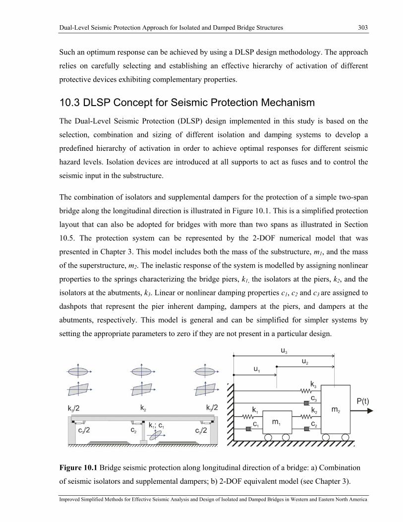
Dual-Level Seismic Protection Approach for Isolated and Damped Bridge Structures 303
Improved Simplified Methods for Effective Seismic Analysis and Design of Isolated and Damped Bridges in Western and Eastern North America
Such an optimum response can be achieved by using a DLSP design methodology. The approach
relies on carefully selecting and establishing an effective hierarchy of activation of different
protective devices exhibiting complementary properties.
10.3 DLSP Concept for Seismic Protection Mechanism The Dual-Level Seismic Protection (DLSP) design implemented in this study is based on the
selection, combination and sizing of different isolation and damping systems to develop a
predefined hierarchy of activation in order to achieve optimal responses for different seismic
hazard levels. Isolation devices are introduced at all supports to act as fuses and to control the
seismic input in the substructure.
The combination of isolators and supplemental dampers for the protection of a simple two-span
bridge along the longitudinal direction is illustrated in Figure 10.1. This is a simplified protection
layout that can also be adopted for bridges with more than two spans as illustrated in Section
10.5. The protection system can be represented by the 2-DOF numerical model that was
presented in Chapter 3. This model includes both the mass of the substructure, m1, and the mass
of the superstructure, m2. The inelastic response of the system is modelled by assigning nonlinear
properties to the springs characterizing the bridge piers, k1, the isolators at the piers, k2, and the
isolators at the abutments, k3. Linear or nonlinear damping properties c1, c2 and c3 are assigned to
dashpots that represent the pier inherent damping, dampers at the piers, and dampers at the
abutments, respectively. This model is general and can be simplified for simpler systems by
setting the appropriate parameters to zero if they are not present in a particular design.
Figure 10.1 Bridge seismic protection along longitudinal direction of a bridge: a) Combination
of seismic isolators and supplemental dampers; b) 2-DOF equivalent model (see Chapter 3).

Dual-Level Seismic Protection Approach for Isolated and Damped Bridge Structures 304
Improved Simplified Methods for Effective Seismic Analysis and Design of Isolated and Damped Bridges in Western and Eastern North America
Typically, some properties of the system can be initially selected based on key performance
objectives. Other properties are subsequently determined by optimizing the bridge response
through a large number of possible solutions obtained directly for each hazard level using the
new energy-based E-R-µ method.
Using the Dual-Level Seismic Protection (DLSP), the optimum solutions are achieved by
defining an effective hierarchy of two activation stages denoted as Stage I and II, respectively.
The hierarchy of activation of the individual components is tailored to form a DLSP system that
effectively meets design objectives corresponding to both seismic hazard levels defined in Table
10-1 as the Design (DE) and the Service (SE) earthquakes. The DLSP optimization concept for
the seismic protection mechanism is summarized in Table 10-3.
Table 10-3 DLSP optimization strategy for seismic protection mechanism
Stage I Longitudinal displacements are controlled by the energy dissipation
mobilized in the isolation and damping devices located at the two
abutments without the activation of the isolation system located at the
bridge piers. In this case, the forces attracted by the piers are kept low
enough to ensure that the piers remain in the elastic range
(F2y > F2(10%-50y.) or u2y > u2(10%-50y.) ).
Stage II The isolation systems at the piers are activated, limiting the forces
imposed to the piers (by setting F2y < F1y). The resulting increase in
displacement in Stage II is mitigated through a higher restraint being
offered by the isolators and dampers positioned at the abutments.
Optimum solution Amongst the various solutions satisfying the pre-defined objectives at the
two seismic hazard levels, the optimum solution is the one inducing the
lowest forces to be resisted by the abutments.

Dual-Level Seismic Protection Approach for Isolated and Damped Bridge Structures 305
Improved Simplified Methods for Effective Seismic Analysis and Design of Isolated and Damped Bridges in Western and Eastern North America
The DLSP system can be configured using different seismic protection devices such as dampers
and isolators. The DLSP concept is independent from the type of adopted isolators. However, the
concept requires that isolators with recentring capability are installed at the abutments while
isolators without recentring capability are installed at the piers. From the capacity perspective,
the abutment structures are typically laterally stiffer and more resistant than the piers due to the
contribution of the wing walls and backfill. For this reason, it would be more cost effective to
concentrate the force restoring capability in a few abutments’ isolators. The isolators on the piers
would dissipate seismic energy while controlling the forces imposed on the piers.
The design optimization flowchart for the DLSP system is presented in Figure 10.2. The bridge
category and corresponding performance objectives are defined in Steps 1 and 2. Then, in Step 3,
the inelastic structural response of the bridge substructure is assessed to explicitly relate the
resulting structural parameters (uy and uu) to the performance objectives. In Steps 4 to 6, the
elements of the DLSP system are selected and configured.
The isolators at the piers are simply selected to act as force-limiting fuse protection in Step 4.
Then, in Step 5, the post-yielding stiffness, kd3 is configured. For the initial design phase, kd3 is
set so that the elastic displacement response, Sd (5%,Te) of the bridge deck, u3, is lower than the
limit umax(10%-50y) under SE. As previously studied in Chapter 7, adopting the Equal Displacement
Approximation (EDA) for structures with low R-ratios and periods longer than 0.5 s, the inelastic
displacement response is assumed to be close to that of an elastic response of the bridge. Thus,
the initial parameter kd3 is configured to start the optimization process. The parameter kd3 can be
adjusted in Step 10 if required for the system to meet the target performance objectives.
The optimization process comprises steps from 6 to 11. The activation limits Q3d of the isolators
located at the abutments (selected in Step 6) is a critical parameter for the reduction of the
maximum force transmitted to the abutments. For convenience in the optimization process, this
limit can be defined as a function of the response modification factor R.

Dual-Level Seismic Protection Approach for Isolated and Damped Bridge Structures 306
Improved Simplified Methods for Effective Seismic Analysis and Design of Isolated and Damped Bridges in Western and Eastern North America
Define Bridge and Importance Category
Define Two‐Hazard Performance Objectives:umax(2%‐50y.); umax (10%‐50y.)
Assess Structural Properties using Nonlinear Incremental Analysis : k1u; k1d; u1y; u1u
Configure Isolators (FSI) on Piers: F2y<F1y
Configure Isolators on Abutments: k3d for SD(5%,Te)< umax (10%‐50y.)
Increase k3dor
Reduce k2u
Start
End
Yes
Yes
No
No
Configure Isolators on Abutments: Q3d for optimum F and u
u2y>u2 (10%‐50y.)
u3<umax (10%‐50y.)
u3<umax (2%‐50y.)
Add Viscous Damping on Abutment
Assess response fortwo hazard levels
Step 1
Step 5
Step 2
Step 3
Step 4
Step 6
Step 7
Step 8
Step 9
Step 10
Step 11
Figure 10.2 Optimization flowchart for DLSP

Dual-Level Seismic Protection Approach for Isolated and Damped Bridge Structures 307
Improved Simplified Methods for Effective Seismic Analysis and Design of Isolated and Damped Bridges in Western and Eastern North America
Figure 10.3 illustrates how the normalized displacement u / ue and normalized force F / Fe vary
with the response modification factor R. The intersection of the displacement and force curves is
arbitrary set at the SE intensity to outline the tendencies in the response of a bridge structure
when the earthquake intensity increases up to the DE level.
For a given bridge structure, the same activation limit Q3d may correspond to different R-factors
being representative of different seismic hazard levels. The response modification factor R
increases with the earthquake intensity and, as shown in Figure 10.3, the factors Rmin and Rmax
correspond to the SE and DE hazard levels, respectively. As the R-factor increases, the
normalized forces F / Fe transmitted by the isolators to the substructure decrease and the
normalized displacements u / ue increase. The DE corresponds to larger displacements and higher
R-ratios when compared to the SE. As shown for the example in Figure 10.3, this would translate
in an increase of the response modification factor from R = 4.0 (SE) to 16 (DE).
Figure 10.3 Response of isolated bridges with response modification factor R in ENA using
Equation (8.20) PGD = 72 mm, Tg = 0.89, Te = 0.5, α = 0.01
For a given hazard level, different R-factors represent different activation limits, thus providing a
range of possible isolation arrangements. The activation limit is selected such that among the
Displacement
Force minR
maxR
Increasing EQ Intensity SE DE

Dual-Level Seismic Protection Approach for Isolated and Damped Bridge Structures 308
Improved Simplified Methods for Effective Seismic Analysis and Design of Isolated and Damped Bridges in Western and Eastern North America
different responses satisfying the target performance objectives, the one optimizing the
displacement and force demands would be selected.
In Step 7, the responses are assessed for the bridge piers, the isolators at the piers, and the
isolators at the abutments. If the isolators at the piers are activated under SE rather than under
DE as suggested in Table 10.3 for Stage II (check in Step 8), the lateral stiffness k2 can be
reduced by adding elastic pads between the pier and the isolators in Step 10 (see discussion in
Chapter 2, Figure 2.7). In Step 9, the displacements of the bridge deck u3 are compared to the
limits umax(10%-50y) and umax(2%-50y) under SE and DE, respectively. If adjustments are necessary to
satisfy the target performance objectives, the displacements are controlled by adding velocity-
dependent damping elements in Step 11.
The DLSP design methodology presented above must be adjusted to take into account the
variability of the system properties due to the effects of wear, aging, and temperature. The exact
properties of the isolation devices can be rarely known over the bridge lifespan. Nevertheless, the
actual properties of the isolation devices subjected to different loading, environmental, and aging
conditions can be evaluated through testing such that maximum and minimum probable values
can be established. The properties that are most likely subject to variations are the stiffness and
the characteristic strength.
To consider the variation in isolator properties, the well known bounded analysis procedure
using lower (LB) and upper (UB) bound property values is considered for every hazard level.
The UB values represent higher activation forces which result in lower R-factors. Conversely, the
LB values result in higher R-factors and are characterized by larger displacement demands. For
each hazard level, the range of responses between the UB and LB values may be assessed as a
function of the response modification factor R. Optimum protection solutions can then be found
though a bounded analysis.
By considering two hazard levels with specific sets of properties for each level, the response
range is defined between the SE-UB (Service Earthquake Upper-Bound) and DE-LB (Design
Earthquake Lower-Bound) thus corresponding to Rmin and Rmax, respectively. The new energy-
based E-R-µ method is applied to evaluate the most appropriate scheme for the studied structure
and design objective. Such an approach provides engineers with the information they need to
establish a range of design displacements. Then, the SE-LB and DE-UB levels should be

Dual-Level Seismic Protection Approach for Isolated and Damped Bridge Structures 309
Improved Simplified Methods for Effective Seismic Analysis and Design of Isolated and Damped Bridges in Western and Eastern North America
checked more carefully after the design is completed. The forces obtained with this technique
correspond to those transmitted to the substructure by the isolation system and, when used, the
dampers.
Although not investigated in this study, the same methodology can be applied for a new bridge to
reduce construction costs for the main structural members in addition to achieving higher
performance at multiple hazard levels.
10.4 Energy-Based E-R-µ Method for Designing a Dual-Level
Seismic Protection System for a Bridge Retrofit in Montreal
In this section, the optimal design process of a DLSP is illustrated by using the energy-based
E-R-µ method developed in Chapter 8. The effects of aging and temperature on the isolator
sliding resistances will be considered.
A simplified procedure for developing an optimum DLSP system is presented and validated
against the results obtained from NLTHA.
The Dual-Level Seismic Protection (DLSP) system developed in this example is based on the
DLSP’s assumptions and methodology described in Section 10.3. Isolation devices are
introduced at all supports to act as fuses and to control the seismic input in the substructure. As
suggested by the DLSP’s concept (Table 10-3) the isolators without recentring capability are
installed at the piers while isolators with recentering capability are installed at the abutments.
The hierarchy of activation is predefined so that isolators located on the abutments are activated
under SE (Stage I) and isolators on the piers are expected to start sliding under DE (Stage II). An
optimization process as specified in Figure 10.2 is then used to identify the properties of the
system that best meet the lifeline bridge design objectives at the SE and DE hazard levels defined
in Table 10-1.
The protection system considered for this example consists of flat sliding isolators (FSI) as
described in Chapter 2. For the FSI isolators, the energy dissipation is provided through sliding
friction between a stainless steel interface and a compound slider surface. The restoring force
capacity is ensured by supplemental lateral spring elements that are installed in parallel with the
sliding surface for FSI devices. The FSI isolators have a very small activation displacement due

Dual-Level Seismic Protection Approach for Isolated and Damped Bridge Structures 310
Improved Simplified Methods for Effective Seismic Analysis and Design of Isolated and Damped Bridges in Western and Eastern North America
to a high pre-activation stiffness. The pre-activation displacement can be increased when the
sliding interface is combined in series with an elastomeric pad as illustrated in Figure 2.7.
10.4.1 Defining Bridge and Importance Category
An existing two-span concrete bridge was used to represent a typical overpass bridge that needs
to be seismically retrofitted. The superstructure is a continuous two-girder concrete post-
tensioned deck spanning a total length of 76 m and being supported at mid-length by a single pier
(Figure 10.4).
As part of the seismic retrofit, the bridge is upgraded from the ordinary Other bridges category to
the Lifeline bridge importance category. A target performance to be achieved with the DLSP
system is defined for the two hazard levels considered and is based on the recommendations
outlined in Table 10-4.

Dual-Level Seismic Protection Approach for Isolated and Damped Bridge Structures 311
Improved Simplified Methods for Effective Seismic Analysis and Design of Isolated and Damped Bridges in Western and Eastern North America
a)
b)
Figure 10.4 Photo (Google Maps- ©2012 Google), plan and elevation of the two-span bridge in
Montreal

Dual-Level Seismic Protection Approach for Isolated and Damped Bridge Structures 312
Improved Simplified Methods for Effective Seismic Analysis and Design of Isolated and Damped Bridges in Western and Eastern North America
Table 10-4 Dual-level performance objectives for design of isolated bridges
Stage Hazard level Performance objectives
Bridge Abutment Pier
I SE
(10% - 50 years)
Functional
No damage
Isolator activated
Elastic response
Isolator not activated
Elastic response
II DE
(2% - 50 years)
Functional
Minor damage
Isolator activated
Elastic response
Isolator activated
Elastic response
10.4.2 Defining Dual-Hazard Performance Objectives
The performance objectives are that the bridge structure (superstructure and substructure)
responds essentially elastically under both hazard levels (u1max < u1y) and is fully serviceable for
normal traffic following both DE and SE events. This is referred as Functional in Table 10.4.
Minor Damage to the bridge is tolerated under DE events as long as it does not impair its normal
operation and its repair does not require total closure of the bridge. Examples of Minor Damage
correspond to the superstructure expansion joints exceeding their displacement limit, cracking or
residual displacement during a DE motion. For this example, a damage threshold of 20 mm is
adopted for the expansion joints.
The isolation and damping devices, in turn, must exhibit adequate performance under the effects
of a main shock and remain functional for possible aftershock motions. The need for explicit
performance criteria for aftershocks is based on observations in past earthquakes such as the
situation that occurred in 2012 in Italy`s Emilia-Romagna region where a M6 main shock (May,
20) was followed by two damaging aftershocks of M5.8 and M5.4 (May, 29) (EQECAT, 2012)).
The total economic losses were greatly increased as a result of the aftershocks. Accordingly, a
limit of 50 mm is adopted in this example to represent the maximum allowable displacement for
the abutment isolators. Exceeding this limit, isolators on the abutments will be damaged.
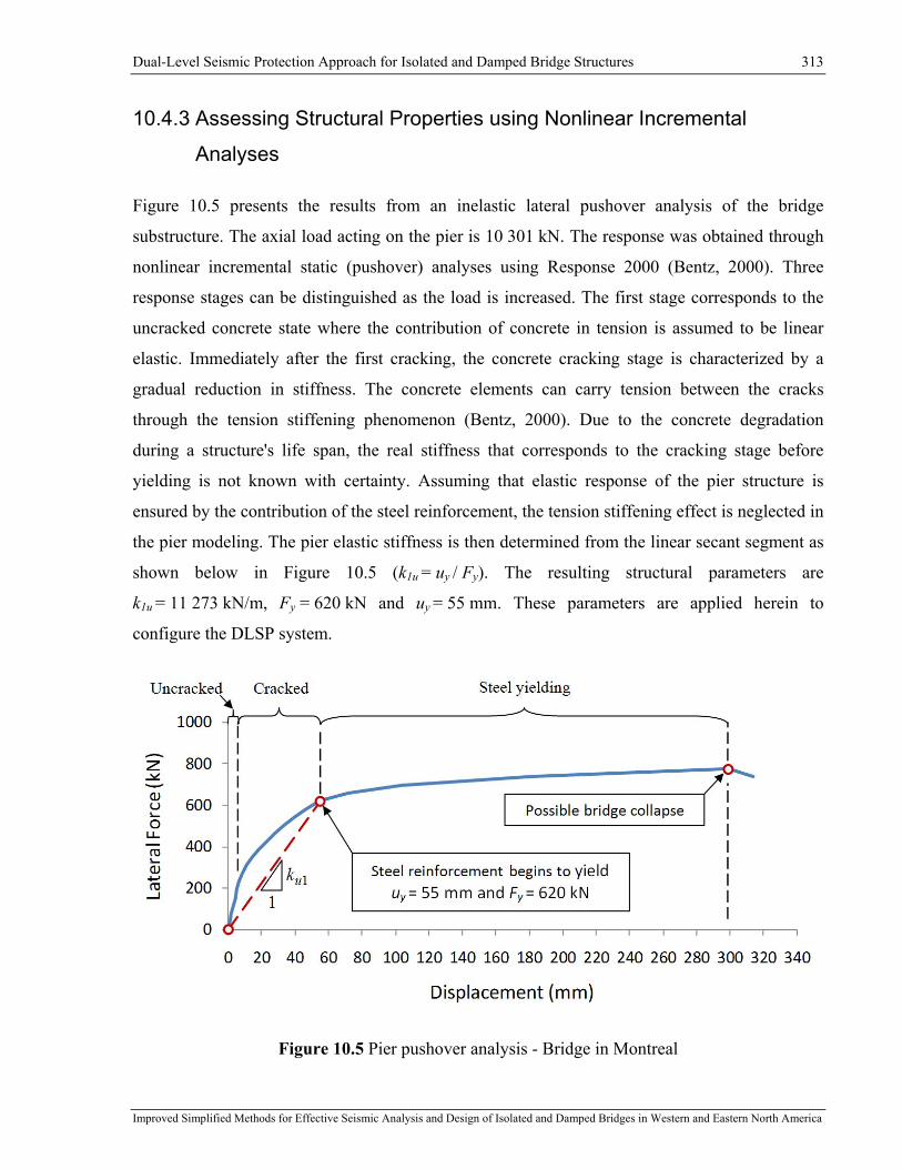
Dual-Level Seismic Protection Approach for Isolated and Damped Bridge Structures 313
Improved Simplified Methods for Effective Seismic Analysis and Design of Isolated and Damped Bridges in Western and Eastern North America
10.4.3 Assessing Structural Properties using Nonlinear Incremental
Analyses
Figure 10.5 presents the results from an inelastic lateral pushover analysis of the bridge
substructure. The axial load acting on the pier is 10 301 kN. The response was obtained through
nonlinear incremental static (pushover) analyses using Response 2000 (Bentz, 2000). Three
response stages can be distinguished as the load is increased. The first stage corresponds to the
uncracked concrete state where the contribution of concrete in tension is assumed to be linear
elastic. Immediately after the first cracking, the concrete cracking stage is characterized by a
gradual reduction in stiffness. The concrete elements can carry tension between the cracks
through the tension stiffening phenomenon (Bentz, 2000). Due to the concrete degradation
during a structure's life span, the real stiffness that corresponds to the cracking stage before
yielding is not known with certainty. Assuming that elastic response of the pier structure is
ensured by the contribution of the steel reinforcement, the tension stiffening effect is neglected in
the pier modeling. The pier elastic stiffness is then determined from the linear secant segment as
shown below in Figure 10.5 (k1u = uy / Fy). The resulting structural parameters are
k1u = 11 273 kN/m, Fy = 620 kN and uy = 55 mm. These parameters are applied herein to
configure the DLSP system.
Figure 10.5 Pier pushover analysis - Bridge in Montreal
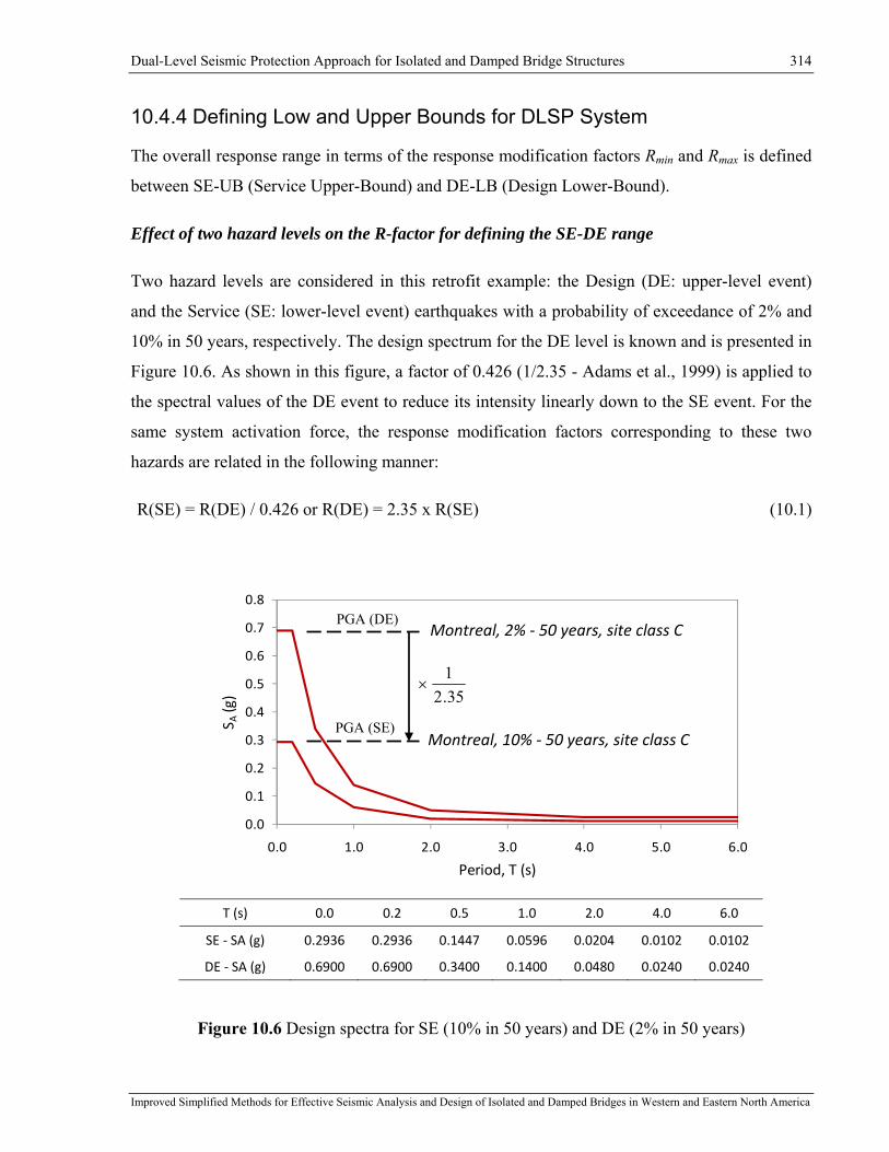
Dual-Level Seismic Protection Approach for Isolated and Damped Bridge Structures 314
Improved Simplified Methods for Effective Seismic Analysis and Design of Isolated and Damped Bridges in Western and Eastern North America
10.4.4 Defining Low and Upper Bounds for DLSP System
The overall response range in terms of the response modification factors Rmin and Rmax is defined
between SE-UB (Service Upper-Bound) and DE-LB (Design Lower-Bound).
Effect of two hazard levels on the R-factor for defining the SE-DE range
Two hazard levels are considered in this retrofit example: the Design (DE: upper-level event)
and the Service (SE: lower-level event) earthquakes with a probability of exceedance of 2% and
10% in 50 years, respectively. The design spectrum for the DE level is known and is presented in
Figure 10.6. As shown in this figure, a factor of 0.426 (1/2.35 - Adams et al., 1999) is applied to
the spectral values of the DE event to reduce its intensity linearly down to the SE event. For the
same system activation force, the response modification factors corresponding to these two
hazards are related in the following manner:
R(SE) = R(DE) / 0.426 or R(DE) = 2.35 x R(SE) (10.1)
T (s) 0.0 0.2 0.5 1.0 2.0 4.0 6.0
SE ‐ SA (g) 0.2936 0.2936 0.1447 0.0596 0.0204 0.0102 0.0102
DE ‐ SA (g) 0.6900 0.6900 0.3400 0.1400 0.0480 0.0240 0.0240
Figure 10.6 Design spectra for SE (10% in 50 years) and DE (2% in 50 years)
0.0
0.1
0.2
0.3
0.4
0.5
0.6
0.7
0.8
0.0 1.0 2.0 3.0 4.0 5.0 6.0
S A(g)
Period, T (s)
PGA (DE)
PGA (SE)
35.21
×
Montreal, 2% ‐ 50 years, site class C
Montreal, 10% ‐ 50 years, site class C

Dual-Level Seismic Protection Approach for Isolated and Damped Bridge Structures 315
Improved Simplified Methods for Effective Seismic Analysis and Design of Isolated and Damped Bridges in Western and Eastern North America
Effect of property modification factors on the R-factor for defining the UB-LB range
The variability of the isolators' properties is quantified by a means of the system property
modification factors λ. The nominal device properties are multiplied by λ to reflect the effect of
the specific conditions to which the isolation system is subjected. The protection system
considered for this example consists of flat sliding isolators (FSI). The FSI isolators with
recentring capability are installed at the abutments while the FSI isolators without recentring
capability are installed at the piers.
The system property modification factors λ for FSIs having stainless steel surface facing
downward and sealed lubricated PTFE (Constantinou et al., 2007) influence the isolators'
activation limits and are determined as follows:
1) Effect of temperature at -30°C and 20°C (Tremblay and Koval, 2008):
0.1min, =tλ at 20°C and 3.1max, =tλ at -30°C (10.2)
2) Effect of aging (Constantinou et al., 2007):
0.1min, =aλ new and 3.1max, =aλ under aging effect (10.3)
3) Effect of contamination (Constantinou et al., 2007):
0.1min, =cλ new and 0.1max, =cλ under contamination effect (10.4)
4) Effect of cumulative movement or travel (Constantinou et al., 2007):
0.1min, =trλ new and 0.1max, =trλ cumulative travel of 2000 m (10.5)
The resulting modification factor to be applied to the nominal value of the coefficient of friction:
0.1min =λ and 69.1max =λ (10.6)
The maximum property modification factor λmax=1.69 relates the UB and LB for each EQ event.
In Figure 10.7, it is shown that the two hazard levels are related through a factor of 2.35 and this
results in a factor of 3.97 between the range limits SE-UB with λmax and Rmin and DE-LB with
λmin and Rmax. The corresponding system displacements are assessed using the E-R-µ
relationship. The range of optimum solutions is then determined by selecting responses
according to the performance objectives. The response ranges for two hazard levels are
illustrated in Figure 10.8. It can be noted from this figure that the deck displacement should
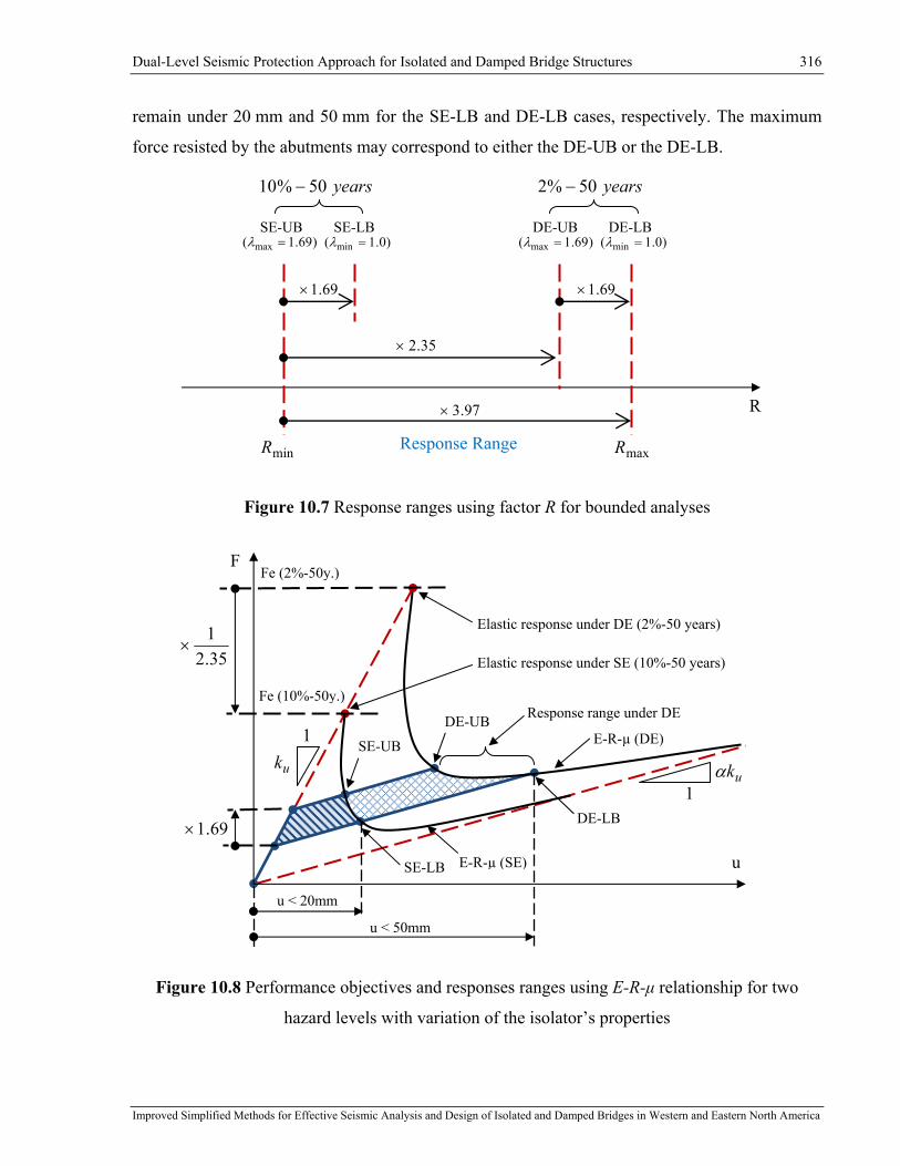
Dual-Level Seismic Protection Approach for Isolated and Damped Bridge Structures 316
Improved Simplified Methods for Effective Seismic Analysis and Design of Isolated and Damped Bridges in Western and Eastern North America
remain under 20 mm and 50 mm for the SE-LB and DE-LB cases, respectively. The maximum
force resisted by the abutments may correspond to either the DE-UB or the DE-LB.
Figure 10.7 Response ranges using factor R for bounded analyses
Figure 10.8 Performance objectives and responses ranges using E-R-μ relationship for two
hazard levels with variation of the isolator’s properties
R
69.1×69.1×
35.2×
DE-LB DE-UB )0.1( min =λ)69.1( max =λ
SE-LB SE-UB )0.1( min =λ)69.1( max =λ
years50%2 −years50%10 −
minR
97.3×
maxRResponse Range
E-R-µ (SE)
1
uk
1ukα
Elastic response under DE (2%-50 years)
Elastic response under SE (10%-50 years)
Response range under DE Fe (10%-50y.)
Fe (2%-50y.)
35.21
×
69.1×
u
F
SE-LB
DE-LB
SE-UB
DE-UBE-R-µ (DE)
u < 20mm
u < 50mm

Dual-Level Seismic Protection Approach for Isolated and Damped Bridge Structures 317
Improved Simplified Methods for Effective Seismic Analysis and Design of Isolated and Damped Bridges in Western and Eastern North America
10.4.5 Modeling and Basic System Parameters for DLSP Approach
In order to adequately simulate the structural behaviour of the bridge, the numerical model
shown in Figure 10.1 included two main parts, one representing the superstructure and one
representing the substructure. Given that most of the bridge mass is located at the level of the
deck, the mass of the substructure m1 was neglected in the dynamic analyses. The total bridge
mass in the analysis m2 was therefore defined using the total dead load situated above the
isolation system interface. In the model presented in Figure 10.1, it is assumed that the deck
element has infinite axial stiffness such that that displacement of the deck is the same at any
point along the bridge length. The parameters of the substructure lateral stiffness (k1 in Figure
10.1) were obtained using Response 2000 analyses as discussed earlier. The design parameters
for the isolator units at the abutments and pier were determined as described in Section 10.3.
Once the pier and isolators parameters have been determined, the equivalent system parameters
were calculated to represent the global bridge behavior. The entire bridge structure was then
represented as a SDOF system.
Table 10-5 summarizes the two sets of design parameters that were considered in this example.
The lower bound (LB) with the nominal system properties λ = λmin = 1.0 is representative of an
isolated bridge at a temperature of +20°C that was recently retrofitted and its isolators are not yet
affected by aging. The upper bound (UB) with λ = λmax = 1.69 corresponds to the behaviour of
the aged isolators at -30C°.
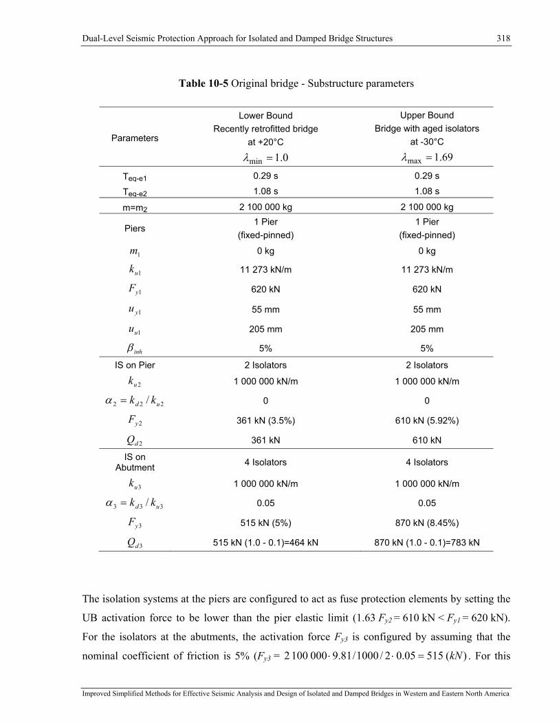
Dual-Level Seismic Protection Approach for Isolated and Damped Bridge Structures 318
Improved Simplified Methods for Effective Seismic Analysis and Design of Isolated and Damped Bridges in Western and Eastern North America
Table 10-5 Original bridge - Substructure parameters
Parameters
Lower Bound Recently retrofitted bridge
at +20°C
0.1min =λ
Upper Bound Bridge with aged isolators
at -30°C
69.1max =λ
Teq-e1 0.29 s 0.29 s
Teq-e2 1.08 s 1.08 s
m=m2 2 100 000 kg 2 100 000 kg
Piers 1 Pier
(fixed-pinned) 1 Pier
(fixed-pinned)
1m 0 kg 0 kg
1uk 11 273 kN/m 11 273 kN/m
1yF 620 kN 620 kN
1yu 55 mm 55 mm
1uu 205 mm 205 mm
inhβ 5% 5%
IS on Pier 2 Isolators 2 Isolators
2uk 1 000 000 kN/m 1 000 000 kN/m
222 / ud kk=α 0 0
2yF 361 kN (3.5%) 610 kN (5.92%)
2dQ 361 kN 610 kN
IS on Abutment 4 Isolators 4 Isolators
3uk 1 000 000 kN/m 1 000 000 kN/m
333 / ud kk=α 0.05 0.05
3yF 515 kN (5%) 870 kN (8.45%)
3dQ 515 kN (1.0 - 0.1)=464 kN 870 kN (1.0 - 0.1)=783 kN
The isolation systems at the piers are configured to act as fuse protection elements by setting the
UB activation force to be lower than the pier elastic limit (1.63 Fy2 = 610 kN < Fy1 = 620 kN).
For the isolators at the abutments, the activation force Fy3 is configured by assuming that the
nominal coefficient of friction is 5% (Fy3 = )(51505.02/1000/81.90001002 kN=⋅⋅ . For this
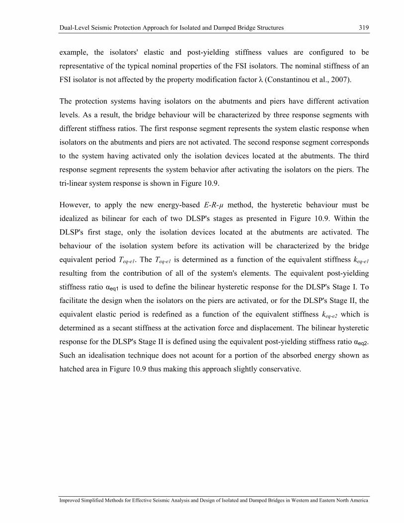
Dual-Level Seismic Protection Approach for Isolated and Damped Bridge Structures 319
Improved Simplified Methods for Effective Seismic Analysis and Design of Isolated and Damped Bridges in Western and Eastern North America
example, the isolators' elastic and post-yielding stiffness values are configured to be
representative of the typical nominal properties of the FSI isolators. The nominal stiffness of an
FSI isolator is not affected by the property modification factor λ (Constantinou et al., 2007).
The protection systems having isolators on the abutments and piers have different activation
levels. As a result, the bridge behaviour will be characterized by three response segments with
different stiffness ratios. The first response segment represents the system elastic response when
isolators on the abutments and piers are not activated. The second response segment corresponds
to the system having activated only the isolation devices located at the abutments. The third
response segment represents the system behavior after activating the isolators on the piers. The
tri-linear system response is shown in Figure 10.9.
However, to apply the new energy-based E-R-µ method, the hysteretic behaviour must be
idealized as bilinear for each of two DLSP's stages as presented in Figure 10.9. Within the
DLSP's first stage, only the isolation devices located at the abutments are activated. The
behaviour of the isolation system before its activation will be characterized by the bridge
equivalent period Teq-e1. The Teq-e1 is determined as a function of the equivalent stiffness keq-e1
resulting from the contribution of all of the system's elements. The equivalent post-yielding
stiffness ratio αeq1 is used to define the bilinear hysteretic response for the DLSP's Stage I. To
facilitate the design when the isolators on the piers are activated, or for the DLSP's Stage II, the
equivalent elastic period is redefined as a function of the equivalent stiffness keq-e2 which is
determined as a secant stiffness at the activation force and displacement. The bilinear hysteretic
response for the DLSP's Stage II is defined using the equivalent post-yielding stiffness ratio αeq2.
Such an idealisation technique does not acount for a portion of the absorbed energy shown as
hatched area in Figure 10.9 thus making this approach slightly conservative.
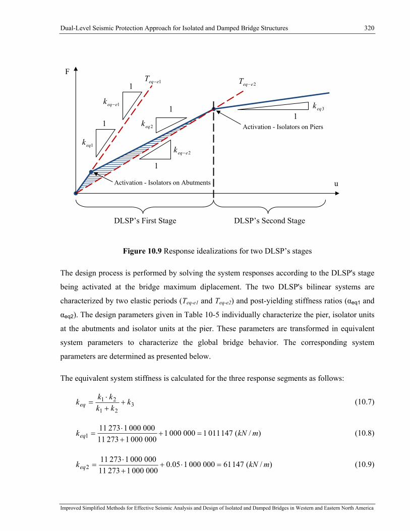
Dual-Level Seismic Protection Approach for Isolated and Damped Bridge Structures 320
Improved Simplified Methods for Effective Seismic Analysis and Design of Isolated and Damped Bridges in Western and Eastern North America
Figure 10.9 Response idealizations for two DLSP’s stages
The design process is performed by solving the system responses according to the DLSP's stage
being activated at the bridge maximum diplacement. The two DLSP's bilinear systems are
characterized by two elastic periods (Teq-e1 and Teq-e2) and post-yielding stiffness ratios (αeq1 and
αeq2). The design parameters given in Table 10-5 individually characterize the pier, isolator units
at the abutments and isolator units at the pier. These parameters are transformed in equivalent
system parameters to characterize the global bridge behavior. The corresponding system
parameters are determined as presented below.
The equivalent system stiffness is calculated for the three response segments as follows:
321
21 kkkkk
keq ++⋅
= (10.7)
)/(14701110000001000000127311000000127311
1 mkNkeq =++⋅
= (10.8)
)/(14761000000105.0000000127311000000127311
2 mkNkeq =⋅++⋅
= (10.9)
3eqk1
1
1eqk
1
2eqk
1
2eeqk −
2eeqT −1
1eeqk −
1eeqT −
Activation - Isolators on Piers
Activation - Isolators on Abutments
DLSP’s First Stage DLSP’s Second Stage
u
F

Dual-Level Seismic Protection Approach for Isolated and Damped Bridge Structures 321
Improved Simplified Methods for Effective Seismic Analysis and Design of Isolated and Damped Bridges in Western and Eastern North America
)/(00050000000105.0027311027311
3 mkNkeq =⋅++⋅
= (10.10)
The deck displacement that is required to activate the isolator at the abutments is determined for
the isolators’ activation force kNFy 5153 = :
)(515.0100000001
515 33 mmu y =⋅= (10.11)
The system total force resisted by the isolators on the abutments and pier is calculated as:
)(7.52010515.01470111)( 33 kNuF y =⋅⋅= − (10.12)
The deck displacement required to activate isolators on the pier is determined for the isolators’
activation force kNFy 3612 = :
)(4.3210000000127311000000127311361 3
2 mmu y =⋅⋅+
⋅= (10.13)
The system total force resisted by the isolators on the abutments and pier is then calculated as:
)(247010)515.04.32(147617.520)( 32 kNuF y =⋅−⋅+= − (10.14)
The effective stiffness at activation of the isolators installed at the pier is determined as:
)/(76235104.32
2470 32 mkNk eeq =⋅=− (10.15)
The equivalent system elastic period for DLSP's first stage ( 1eeqk − = 1eqk ):
)(29.00001470111
0001002221
1 sk
mTeeq
eeq ===−
− ππ (10.16)
The equivalent system elastic period for DLSP's second stage:
)(04.100023576
0001002222
2 sk
mTeeq
eeq ===−
− ππ (10.17)
The post-yielding stiffness ratio for DLSP's first stage:
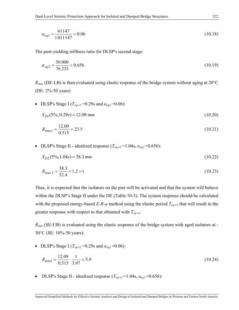
Dual-Level Seismic Protection Approach for Isolated and Damped Bridge Structures 322
Improved Simplified Methods for Effective Seismic Analysis and Design of Isolated and Damped Bridges in Western and Eastern North America
06.01470111
147611 ==eqα (10.18)
The post-yielding stiffness ratio for DLSP's second stage:
656.02357600050
2 ==eqα (10.19)
Rmax (DE-LB) is then evaluated using elastic response of the bridge system without aging at 20°C
(DE: 2%-50 years)
• DLSP's Stage I (Teq-e1 =0.29s and αeq1 =0.06):
mmsSD 09.12)29.0%;5(1 = (10.20)
5.23515.009.12
1max ==R (10.21)
• DLSP's Stage II - idealized response (Teq-e2 =1.04s, αeq2 =0.656):
mmsSD 3.38)04.1%;5(2 = (10.22)
12.14.323.38
2max >==R (10.23)
Thus, it is expected that the isolators on the pier will be activated and that the system will behave
within the DLSP’s Stage II under the DE (Table 10-3). The system response should be calculated
with the proposed energy-based E-R-µ method using the elastic period Teq-e2 that will result in the
greater response with respect to that obtained with Teq-e1.
Rmin (SE-UB) is evaluated using the elastic response of the bridge system with aged isolators at -
30°C (SE: 10%-50 years):
• DLSP's Stage I (Teq-e1 =0.29s and αeq1 =0.06):
9.597.31
515.009.12
1min =⋅=R (10.24)
• DLSP's Stage II - idealized response (Teq-e2 =1.04s, αeq2 =0.656):
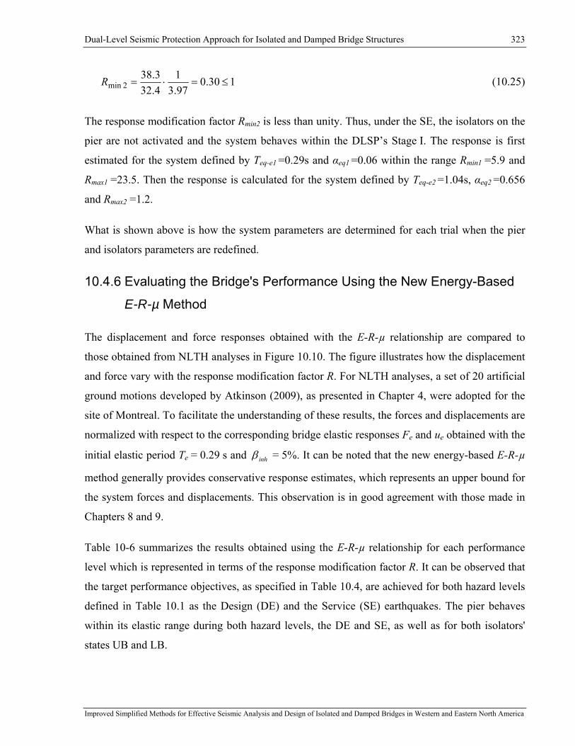
Dual-Level Seismic Protection Approach for Isolated and Damped Bridge Structures 323
Improved Simplified Methods for Effective Seismic Analysis and Design of Isolated and Damped Bridges in Western and Eastern North America
130.097.31
4.323.38
2min ≤=⋅=R (10.25)
The response modification factor Rmin2 is less than unity. Thus, under the SE, the isolators on the
pier are not activated and the system behaves within the DLSP’s Stage I. The response is first
estimated for the system defined by Teq-e1 =0.29s and αeq1 =0.06 within the range Rmin1 =5.9 and
Rmax1 =23.5. Then the response is calculated for the system defined by Teq-e2 =1.04s, αeq2 =0.656
and Rmax2 =1.2.
What is shown above is how the system parameters are determined for each trial when the pier
and isolators parameters are redefined.
10.4.6 Evaluating the Bridge's Performance Using the New Energy-Based
E-R-µ Method
The displacement and force responses obtained with the E-R-µ relationship are compared to
those obtained from NLTH analyses in Figure 10.10. The figure illustrates how the displacement
and force vary with the response modification factor R. For NLTH analyses, a set of 20 artificial
ground motions developed by Atkinson (2009), as presented in Chapter 4, were adopted for the
site of Montreal. To facilitate the understanding of these results, the forces and displacements are
normalized with respect to the corresponding bridge elastic responses Fe and ue obtained with the
initial elastic period Te = 0.29 s and inhβ = 5%. It can be noted that the new energy-based E-R-µ
method generally provides conservative response estimates, which represents an upper bound for
the system forces and displacements. This observation is in good agreement with those made in
Chapters 8 and 9.
Table 10-6 summarizes the results obtained using the E-R-µ relationship for each performance
level which is represented in terms of the response modification factor R. It can be observed that
the target performance objectives, as specified in Table 10.4, are achieved for both hazard levels
defined in Table 10.1 as the Design (DE) and the Service (SE) earthquakes. The pier behaves
within its elastic range during both hazard levels, the DE and SE, as well as for both isolators'
states UB and LB.

Dual-Level Seismic Protection Approach for Isolated and Damped Bridge Structures 324
Improved Simplified Methods for Effective Seismic Analysis and Design of Isolated and Damped Bridges in Western and Eastern North America
During the SE motion, the deck displacement will not exceed the 20 mm limit. The bridge is
operational with no damage to its elements. During the DE motion, the opening of the
superstructure expansion joints will exceed the 20 mm limit while the deck displacement is
smaller than the 50 mm limit. Accordingly, after the DE motion, the bridge is expected to be
operational with minor damage.
It was also found that the system behaves within the DLSP’s first stage for performance levels
SE-UB, SE-LB, and DE-UB. For the DE-LB performance level, the bridge response within the
DLSP's first stage results in the pier force F1 = 448 kN which is below the pier elastic limit of
620 kN. However, for the DE-LB performance level, the DLSP’s second stage is activated
limiting the pier forces at F1 = 361 kN. In such a case, the isolators do not provide an increased
protection to the pier. The use of the pier protective devices would be justified only for the DE-
UB level when the isolators will be limiting the forces imposed to the piers to 610 kN which is
just below the pier elastic limit of 620 kN.
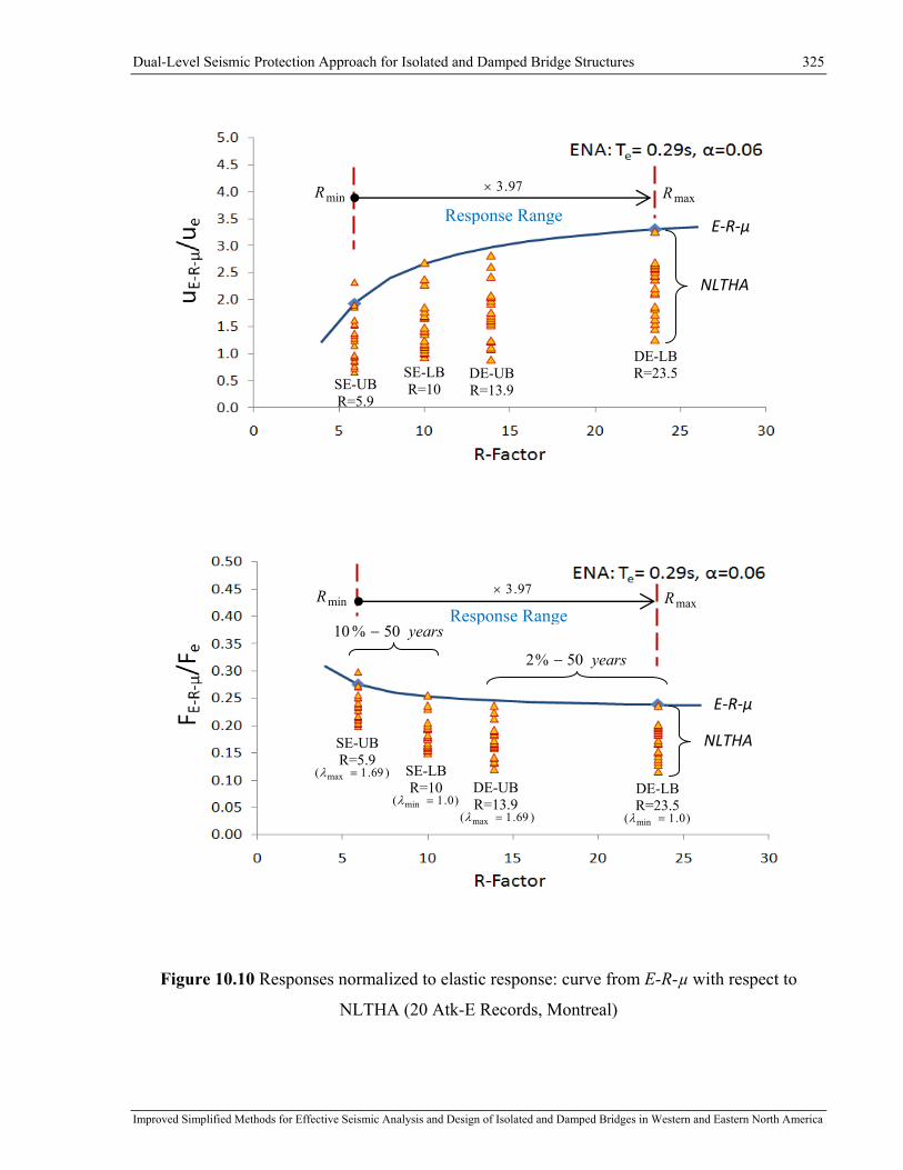
Dual-Level Seismic Protection Approach for Isolated and Damped Bridge Structures 325
Improved Simplified Methods for Effective Seismic Analysis and Design of Isolated and Damped Bridges in Western and Eastern North America
Figure 10.10 Responses normalized to elastic response: curve from E-R-µ with respect to
NLTHA (20 Atk-E Records, Montreal)
SE-UB R=5.9
SE-LB R=10
DE-UB R=13.9
DE-LB R=23.5
97.3×
Response RangeminR maxR
E‐R‐µ
NLTHA
SE-LB R=10
)0.1( min =λ
SE-UB R=5.9
)69.1( max =λDE-UB R=13.9
)69.1( max =λ
DE-LB R=23.5
)0.1( min =λ
minR 97.3×maxR
Response Rangeyears50%10 −
years50%2 −
μ−RE‐R‐µ
NLTHA
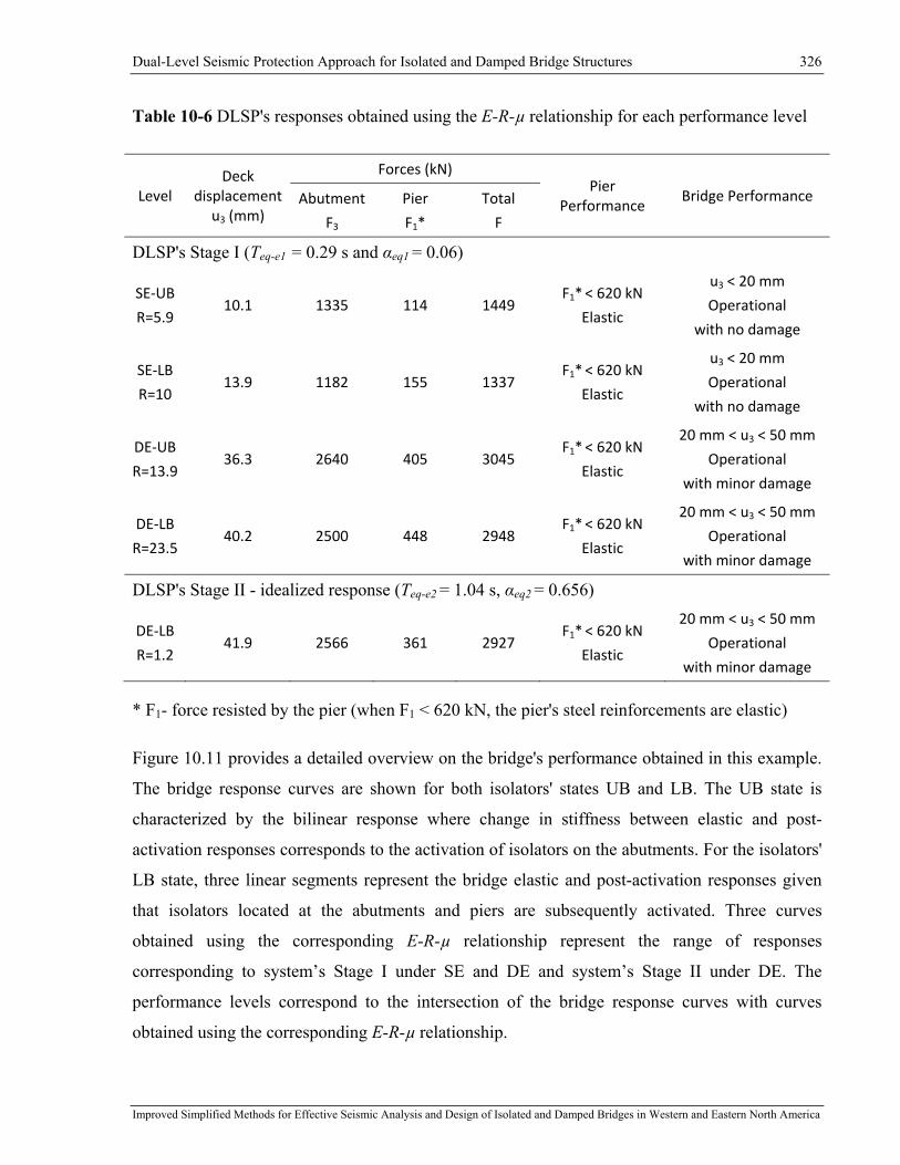
Dual-Level Seismic Protection Approach for Isolated and Damped Bridge Structures 326
Improved Simplified Methods for Effective Seismic Analysis and Design of Isolated and Damped Bridges in Western and Eastern North America
Table 10-6 DLSP's responses obtained using the E-R-µ relationship for each performance level
Level Deck
displacement u3 (mm)
Forces (kN) Pier
Performance Bridge Performance Abutment
F3
Pier
F1*
Total
F
DLSP's Stage I (Teq-e1 = 0.29 s and αeq1 = 0.06)
SE‐UB
R=5.9 10.1 1335 114 1449
F1* < 620 kN
Elastic
u3 < 20 mm
Operational
with no damage
SE‐LB
R=10 13.9 1182 155 1337
F1* < 620 kN
Elastic
u3 < 20 mm
Operational
with no damage
DE‐UB
R=13.9 36.3 2640 405 3045
F1* < 620 kN
Elastic
20 mm < u3 < 50 mm
Operational
with minor damage
DE‐LB
R=23.5 40.2 2500 448 2948
F1* < 620 kN
Elastic
20 mm < u3 < 50 mm
Operational
with minor damage
DLSP's Stage II - idealized response (Teq-e2 = 1.04 s, αeq2 = 0.656)
DE‐LB
R=1.2 41.9 2566 361 2927
F1* < 620 kN
Elastic
20 mm < u3 < 50 mm
Operational
with minor damage
* F1- force resisted by the pier (when F1 < 620 kN, the pier's steel reinforcements are elastic)
Figure 10.11 provides a detailed overview on the bridge's performance obtained in this example.
The bridge response curves are shown for both isolators' states UB and LB. The UB state is
characterized by the bilinear response where change in stiffness between elastic and post-
activation responses corresponds to the activation of isolators on the abutments. For the isolators'
LB state, three linear segments represent the bridge elastic and post-activation responses given
that isolators located at the abutments and piers are subsequently activated. Three curves
obtained using the corresponding E-R-µ relationship represent the range of responses
corresponding to system’s Stage I under SE and DE and system’s Stage II under DE. The
performance levels correspond to the intersection of the bridge response curves with curves
obtained using the corresponding E-R-µ relationship.

Dual-Level Seismic Protection Approach for Isolated and Damped Bridge Structures 327
Improved Simplified Methods for Effective Seismic Analysis and Design of Isolated and Damped Bridges in Western and Eastern North America
The two dashed lines correspond to two post-activation stiffness ratios, thus representing the
response of systems having relatively small resistance (R → ∞). These lines bound the maximum
displacements for the response range represented by the corresponding E-R-µ curve. For this
bridge protection system, the E-R-µ relationship does not provide any solutions for
displacements exceeding the limits of 20 mm and 50 mm for SE and DE motions, respectively.
This indicates that for any R value within the range from R = 1.0 to ∞, the performance
objectives will be met. As specified in Table 10.3, amongst the various solutions satisfying the
pre-defined objectives at the two seismic hazard levels, the optimum solution is the one inducing
the lowest forces to be resisted by the abutments. As shown in Section 9.5, an optimum solution
can be achieved by varying simultaneously the isolator's nominal stiffness (or period) and
activation force (or characteristic strength).
However, the range of possible solutions is subject to physical limitations as for example, the
isolators' minimum activation force. For instance, for a FSI, the minimum activation load is the
force needed to overcome the static friction. This force depends on the applied vertical load, the
type of sliding interface and its condition. In this example for the FSI isolators at the abutments,
the minimum coefficient of friction of 5% is assumed. In practice, the isolator activation force is
specified in the manufacturers' product specifications and should be accurately taken into
account during the design process. Alternatively, to reduce the isolators' minimum activation
force, the vertical force acting on the isolators can be reduced. This can be achieved by
distributing vertical forces between isolators and "frictionless" mechanical bearings: rockers and
rollers. However, such solutions are not covered by the scope of this chapter and alternative
optimization options will be studied in the following subsection.

Dual-Level Seismic Protection Approach for Isolated and Damped Bridge Structures 328
Improved Simplified Methods for Effective Seismic Analysis and Design of Isolated and Damped Bridges in Western and Eastern North America
Figure 10.11 Bridge's performance obtained using the new energy-based E-R-µ method
(ATK-E: PGD=72 mm, Tg=0.89 s)
10.4.7 Improving the Bridge's Performance Using the New Energy-Based
E-R-µ Method
In the previous subsection, the DLSP system was configured to meet design objectives
corresponding to both seismic hazard levels, the DE and SE earthquakes. It was however
assumed that for the isolators at the abutments, the activation force was subject to physical
limitations and was prevented from further reduction needed to take full advantage of the
benefits provided by the isolation system. In this subsection, the optimization process is
performed following the design optimization flowchart for the DLSP system as presented in
Figure 10.2.
Starting from Step 5 (Figure 10.2) as a first phase, the elastic stiffness of the FSI isolators on the
abutments is reduced. By installing an elastomer on top of the sliding interface, the elastic period
may be lengthened such that system forces are further decreased. As a counterpart of the period
lengthening, the increase in displacement is expected. The second optimization phase consists in
0
500
1000
1500
2000
2500
3000
3500
4000
0 5 10 15 20 25 30 35 40 45 50 55 60
Force, F (kN)
Displacement, u (mm)
1eeqT −
2eeqT −
Activation - Isolator on Pier
E-R-µ - Stage I (DE)
E-R-µ - Stage I (SE)
E-R-µ - Stage II (DE)
DE-LB
DE-UB
SE-LB SE-UB
E-R-µ - Stage I (SE) - ∞=R
E-R-µ - Stage II (DE) - ∞=R

Dual-Level Seismic Protection Approach for Isolated and Damped Bridge Structures 329
Improved Simplified Methods for Effective Seismic Analysis and Design of Isolated and Damped Bridges in Western and Eastern North America
adjusting the displacement response so that the target performance objectives are still met. The
damping devices can be then installed at the abutments as suggested in Step 11 (Figure 10.2).
To avoid a complex iterative process, a straightforward approach for selecting ku3 is proposed.
The parameter ku3 is varied such that the corresponding elastic period Te results in the elastic
displacement response ue3=Sd (5%,Te) of the bridge deck that is smaller than 20 mm. As
mentioned in Section 10.4.2, a damage threshold of 20 mm corresponds to the deformation limit
of the expansion joints. As shown in Figure 10.12, a period of Te = 1.12 s was needed to achieve
this objective. The parameter of the post-yield stiffness, kd3 is then determined following
Equations (10.26) to (10.28). The modified system equivalent parameters are summarized in
Table 10.7.
mT
ke
equ 2
2
,4π
= (10.26)
21
21,3
uu
uuequu kk
kkkk+⋅
−= (10.27)
33 ud kk ⋅= α (10.28)
Figure 10.12 Selection of elastic stiffness for isolators at the abutments
0
5
10
15
20
25
30
35
40
0 0.2 0.4 0.6 0.8 1 1.2 1.4 1.6 1.8 2
Sd (m
m)
Period (s)
20 Records ‐ ATK‐Eξ=5%; 10% ‐50 years
Limit of Expansion Joints
Sd(1.12s)=18mm

Dual-Level Seismic Protection Approach for Isolated and Damped Bridge Structures 330
Improved Simplified Methods for Effective Seismic Analysis and Design of Isolated and Damped Bridges in Western and Eastern North America
Table 10-7 System equivalent parameters for DLSP's stages
ku3 (kN/m) keq1 (kN/m) keq2 (kN/m) keq3 (kN/m) Teq-e1 (s) Teq-e1 (s) αeq1 αeq2
54 944 66 091 14 452 2 747 1.12 1.68 0.219 0.093
The performance of the bridge protection system with reduced stiffness is assessed using the new
energy-based E-R-µ method and is presented in Figure 10.13. By comparing this system’s
response to that of the previous example (presented in Figure 10.11 and Table 10.6), it can be
noted that the maximum force obtained for DE-UB was significantly reduced from 3045 kN to
1545 kN. However, as shown, two pre-defined performance objectives are not satisfied with this
design. The displacement under the SE motions exceeds 20 mm for the LB condition, which
indicates that the opening of the expansion joints will exceed the targeted limit. In addition,
under the DE motions, the deck displacement for the LB condition is larger than the specified
limit of 50 mm.
Figure 10.13 Performance of the DLSP with reduced stiffness using the new energy-based
E-R-µ method (ATK-E: PGD=72 mm, Tg=0.89 s)
0
500
1000
1500
2000
2500
3000
3500
4000
0 5 10 15 20 25 30 35 40 45 50 55 60
Force, F (kN)
Displacement, u (mm)
Activation - Isolator on Pier
E-R-µ - Stage I (DE) E-R-µ - Stage II (DE)
SE-LB
DE-LB
SE-UB
DE-UB
E-R-µ - Stage I (SE)

Dual-Level Seismic Protection Approach for Isolated and Damped Bridge Structures 331
Improved Simplified Methods for Effective Seismic Analysis and Design of Isolated and Damped Bridges in Western and Eastern North America
To improve the bridge performance, the increase in the deck displacement is mitigated following
Steps 9 and 11 as specified in the DLSP optimization flowchart (Figure 10.2). In this example,
the displacement is controlled by adding viscous damping. The damping level to be added in
addition to the 5% inherent damping is arbitrary set to 5%. Such an approach is representative of
the selection of damping devices from the manufacturers' product chart which is tailored at a 5%
damping increment. To determine how much damping is needed to comply with the target
displacement, the B-factor relationships (Equation (2.8)) can be adopted.
Figure 10.14 presents the performance of the DLSP with reduced stiffness and added damping.
In this approach, to take into account the added viscous damping, the new energy-based E-R-µ
method is based on Equation (8.16).
The targeted performance levels are satisfied, resulting in an operational bridge and an elastic
substructure after both the SE and DE ground motions. When compared to the performance of
the initial DLSP configuration (Figure 10.11), the maximum system force is reduced by 49.2%
from 3045 kN to 1497 kN. The maximum force to be resisted by the abutments is reduced from
2640 kN to 958 kN which corresponds to a considerable reduction of 63.7%.
Figure 10.14 Performance of the DLSP with reduced stiffness and adding 5% of viscous
damping using the new energy-based E-R-µ method (ATK-E: PGD = 72 mm, Tg = 0.89 s)
0
500
1000
1500
2000
2500
3000
3500
4000
0 5 10 15 20 25 30 35 40 45 50 55 60
Force, F (kN)
Displacement, u (mm)
Activation - Isolator on Pier
E-R-µ - Stage I (DE) E-R-µ - Stage II (DE)
SE-LB DE-LB
SE-UB
DE-UB
E-R-µ - Stage I (SE)

Dual-Level Seismic Protection Approach for Isolated and Damped Bridge Structures 332
Improved Simplified Methods for Effective Seismic Analysis and Design of Isolated and Damped Bridges in Western and Eastern North America
The examples presented above illustrate how the performance of the DLSP system can be
improved using a simple and straight-forward procedure based on the proposed energy-based
E-R-µ method. Although not shown in this section, when using the new energy-based E-R-µ
method, an optimum solution can be directly achieved by varying simultaneously the system
stiffness kd, characteristic strength Qd and damping level effβ . Such an improvement represents
an interesting and cost-effective solution that can be adopted by engineers during preliminary
design to achieve multi-level-hazard design objectives.
10.5 Implementation of a Dual-Level Seismic Protection System
for a Bridge Retrofit in Vancouver
In this section, the optimal design process of a DLSP is illustrated for the case of an existing
bridge that needs to be upgraded to meet the requirements of current seismic provisions. Such a
bridge may be eventually subjected to a seismic demand that is beyond its capacity. A simplified
procedure for developing an optimum DLSP system using detailed NLTH analyses is presented
and validated using this example. The responses from the NLTHA are compared to the estimates
obtained using the energy-based E-R-µ method in order to validate the appropriateness of
adopting this method for preliminary design in the definition of an optimum seismic protection
strategy.
As previously discussed in Section 10.3 for the seismic protection at the pier support, the lateral
resistance provided by the isolators must not exceed the lateral force producing yielding of the
piers. Supplemental damping devices are combined to the isolation system at the abutments to
control the lateral displacement of the superstructure. At the abutments, the isolators are also
designed with a minimum recentring capacity to control displacements and prevent progressive
drifting of the superstructure. The primary objective of such an implementation is to prevent any
damage to the bridge substructure for both seismic hazard levels defined in Table 10-1 as the
Design (DE) and the Service (SE) earthquakes.
The protection system considered for this example consists of the flat sliding isolators (FSI) and
lead rubber bearings (LRB) that are installed at the piers and abutments, respectively. LRBs
inherently exhibit higher restoring forces upon yielding and the system is therefore more suitable
at the abutments where greater lateral resistance can be more easily developed. The energy

Dual-Level Seismic Protection Approach for Isolated and Damped Bridge Structures 333
Improved Simplified Methods for Effective Seismic Analysis and Design of Isolated and Damped Bridges in Western and Eastern North America
dissipation capacity is obtained through the inelastic response of the lead core under lateral
seismic motion.
10.5.1 Defining Bridge and Importance Category
The structure that is studied is located in Vancouver. The bridge is an existing four-span concrete
bridge with a total length of 68 m (Figure 10.15). The bridge is comprised of two independent
structures, one servicing east bound traffic and the other servicing west bound traffic. In this
example, only the eastbound bridge was examined. The superstructure cross-section includes six
AASHTO precast prestressed girders spanning over 18 m. The bridge is skewed but the effects
of the skew angle on the seismic response are deemed to be small and are neglected in this
preliminary DLSP design.
As part of the retrofit, the bridge is upgraded from the Other bridges category to the Lifeline
bridge importance category. A target performance to be achieved with the DLSP system is
defined for the two hazard levels considered and is based on the recommendations outlined in
Table 10-4.

Dual-Level Seismic Protection Approach for Isolated and Damped Bridge Structures 334
Improved Simplified Methods for Effective Seismic Analysis and Design of Isolated and Damped Bridges in Western and Eastern North America
a)
b)
Figure 10.15 Photo (Google Maps- ©2012 Google), plan and elevation of the four-span bridge
in Vancouver.
10.5.2 Dual-Hazard Performance Objectives
As in the previous example, the bridge structure is expected to perform elastically under both
hazard levels (u1max < u1y) and the bridge is to be fully serviceable for normal traffic following

Dual-Level Seismic Protection Approach for Isolated and Damped Bridge Structures 335
Improved Simplified Methods for Effective Seismic Analysis and Design of Isolated and Damped Bridges in Western and Eastern North America
both DE and SE events. A 40 mm limit is defined as the damage threshold for the expansion
joints. The deck displacement between this limit and the maximum allowable displacement
indicates an allowable Minor Damage. The maximum allowable displacement for the abutment
isolators is limited to 120 mm.
10.5.3 Assessing Structural Properties Using Nonlinear Incremental
Analyses
The structural properties of the as-built bridge were determined through nonlinear incremental
static analyses. Sectional analysis of the reinforced concrete piers was performed using Response
2000 (Bentz, 2000) to evaluate their inelastic response and available ductility capacity.
Figure 10.16 presents the computed inelastic response for the bridge piers. Similarly as explained
in the previous example (see Figure 10.5), the pier elastic stiffness is determined from the linear
secant segment as shown below in Figure 10.16 (ku1 = uy / Fy). Table 10-8 summarizes the
original (non-isolated) bridge properties. In this table, uy1 and uu1 represent the pier yielding and
ultimate displacement levels, respectively.
Figure 10.16 Pier pushover analysis - Bridge in Vancouver

Dual-Level Seismic Protection Approach for Isolated and Damped Bridge Structures 336
Improved Simplified Methods for Effective Seismic Analysis and Design of Isolated and Damped Bridges in Western and Eastern North America
Table 10-8 Original bridge (m2 = 954 000 kg) - Substructure parameters
Te (s) ku1 (kN/m) kd1 (kN/m) Fy1 (kN) uy1 (mm) uu1 (mm) βinh (%)
0.82 55 814 5 821 2 292 41 240 5
10.5.4 Time-History Ground Motions Considered for Configuring Optimal
Protection System
In this example, time-history analyses are used both for configuring and for optimizing the basic
system parameters. A set of 20 artificial ground motions developed by Atkinson (2009), as
presented in Chapter 4, were adopted for the site of Vancouver. The motions were selected to
represent the dominant (DE) magnitude-distance earthquake scenarios as determined from
deaggregation of the seismic hazard at the site for a probability of exceedance of 2% in 50 years
(Halchuk and Adams, 2004 and Halchuk, 2009). The records were linearly scaled with respect to
the NBCC design spectrum (NRCC, 2005). To perform the TH analyses for the 10% in 50 years
(SE) hazard level, the same records were used but their intensity was scaled down by a factor of
1.94 according to the hazard curve determined by Adams et al. (1999) for Vancouver.
10.5.5 Basic System Parameters for DLSP Approach
A number of the basic properties of the system can be initially selected to meet specific key
performance objectives for the bridge following Steps 3 to 5 in the optimization flowchart
presented for DLSP in Figure 10.2. The other properties are subsequently determined by
optimizing the bridge response through nonlinear time history analyses using ensembles of
earthquake records representative of each hazard level.
As previously mentioned for this structure, flat sliding isolators (FSI) and lead rubber bearings
(LRB) are installed at the piers and abutments, respectively. For LRB isolators, the properties
that are subject to variations are the stiffness and the characteristic strength. For FSI isolators,
only the characteristic strength is affected by the property modification factor λ (Constantinou et
al., 2007). For simplicity in this example, the effect of property modification factors is not
considered thus assuming λ = 1.0. Despite the apparent simplicity of such an approach it still

Dual-Level Seismic Protection Approach for Isolated and Damped Bridge Structures 337
Improved Simplified Methods for Effective Seismic Analysis and Design of Isolated and Damped Bridges in Western and Eastern North America
provides useful insight into the response of isolated and damped bridges that can then be used in
more comprehensive studies that would include the expected variability of the isolator's
properties. Table 10-9 summarizes the retrofitted bridge properties, including the isolation
system.
Table 10-9 Isolated bridge - Parameters of isolation on piers and abutments
Te (s) ku2 (kN/m) α2=kd2/ku2 Qd2 (kN) ku3 (kN/m) α3=kd3/ku3 Qd3 (kN)
0.70 55 814 0 2 106 48 000 0.1 A
780 B
A Post-yielding stiffness ratio for LBR (www.dis-inc.com/pdf_files/DIS_BASE_ISO.pdf)
B Maximum available characteristic strength from the isolator design properties
Configuring Pier Isolators
For a set of 18 sliding isolators placed at the piers, a total activation force of 2 106 kN is
determined to be lower than the pier elastic limit of 2 292 kN (3 piers). For this example, the
activation force was obtained using an assumed Coulomb`s friction with a constant friction
coefficient of 30% (personal communication with P. Lapalme, Goodco, 2012).
Configuring Abutment Isolators
The isolators located at the abutments (LRB) are expected to be activated at Stage I. They are
configured according to the following two steps:
Step1. The elastic stiffness, ku3 is determined by using a post-yielding stiffness ratio, α (α3 = 0.1,
Table 10.13). Similar to the previous example, the elastic period Te is varied such that the
resulting elastic displacement response ue3 = Sd (5%, Te) of the bridge deck is smaller than
40 mm which corresponds to the damage threshold of expansion joints. Once Te is determined,
the parameter of the post-yield stiffness, kd3 is determined following Equations (10.26) to (10.28)
as illustrated in Figure 10.17. This spectrum corresponds to the SE hazard and represents a mean
response of the 20 ground motions adopted for this example. In such a way, for an elastic

Dual-Level Seismic Protection Approach for Isolated and Damped Bridge Structures 338
Improved Simplified Methods for Effective Seismic Analysis and Design of Isolated and Damped Bridges in Western and Eastern North America
response of the bridge, the performance objective consisting of preventing damage to the
expansion joints is satisfied for Stage I (SE).
Figure 10.17 Selection of elastic stiffness for isolators at the abutments
Step 2. The characteristic strength, Qd3, of the isolators at the abutments is the second design
parameter to be configured. This parameter is defined in terms of the R-factor, which, in turn,
relates the activation limit uy3 to the maximum elastic response, ue3 = Sd (5%, Te). The maximum
available characteristic strength specified by the manufacturer for the isolators used in this
example is 65 kN what results for a group of 12 isolators in kNisolatorskNQd 78012653 =⋅=
or Fy3 = 867 kN (http://www.dis-inc.com/technical.html). As a result, with respect to the
maximum elastic response, the isolator activation force corresponds to the minimum
R = ue3 / (Fy3 / ku3) = 1.85.
Figure 10.18 illustrates the response of the isolators at the abutments as a function of R. Four
ground motions were selected to represent general responses characterizing four magnitude-
distance events denoted as E6C1 (M6.5, 10 to 15 km), E6C2 (M6.5, 20 to 30 km), E7C1 (M7.5,
15 to 25 km) and E7C2 (M7.5, 50 to 100 km). The same decreasing trend in force with
increasing R is observed for all types of events, while each of the displacement curves has a
particular shape.
In addition to the responses obtained using NLTHA for each of the four ground motions, Figure
10.18 presents the response estimates obtained using the energy-based E-R-µ method. It can be
noted that the force curve obtained with the E-R-µ relationship is replicating the shape of the

Dual-Level Seismic Protection Approach for Isolated and Damped Bridge Structures 339
Improved Simplified Methods for Effective Seismic Analysis and Design of Isolated and Damped Bridges in Western and Eastern North America
responses very well while overestimating slightly the NLTH responses (Figure 10.18(a)). The
displacement curve underestimated the NLTHA responses for R = 1.85, provided estimates that
were close to the NLTHA average for R = 3.6 and mostly overestimated the NLTHA responses
for higher R-factors (Figure 10.18(b)). As outlined in the previous section, the straight-forward
procedure of the new energy-based E-R-µ method can be very effective for the selection of the
most appropriate isolation scheme to achieve multi-level-hazard design objectives. For instance,
the NLTH analyses requires certain number of time-history records (20 records in this study, 5
records in CAN/CSA-S6-06 and 11 records in CAN/CSA-S6-14). Previous to carry out the
NLTH analyses, the records must be selected and scaled as well as an appropriate nonlinear
model must be developed. As a result in engineering practice, the NLTH analyses are much more
expensive and time consuming when compared to just a few simple calculations needed to obtain
the same trends with the E-R-µ relationship method.
When considering the NLTHA average responses, the minimum displacement occurs for R = 6.4
which defines an optimum system configuration for an SE event. However, for a DE event, the
R-factor will increase to R ≈ 6.4 x 1.94 = 12.4, and a larger displacement u3 is expected
according to the trends in Figure 10.13. In cases where the limit defining the performance
objective of the DLSP's for Stage II is exceeded, this can be remedied by increasing the strength
and stiffness of the isolators at the abutments or by adding viscous damping. Both approaches are
illustrated in the following sections for protection systems with and without added viscous
dampers.
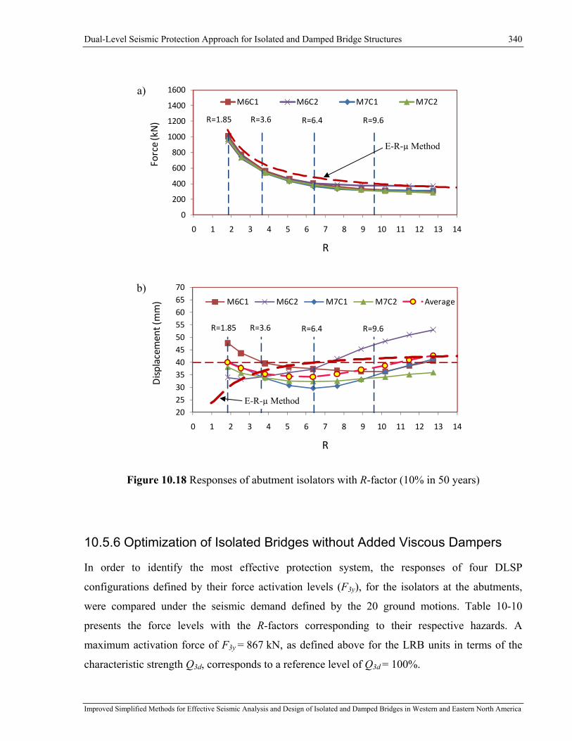
Dual-Level Seismic Protection Approach for Isolated and Damped Bridge Structures 340
Improved Simplified Methods for Effective Seismic Analysis and Design of Isolated and Damped Bridges in Western and Eastern North America
a)
b)
Figure 10.18 Responses of abutment isolators with R-factor (10% in 50 years)
10.5.6 Optimization of Isolated Bridges without Added Viscous Dampers
In order to identify the most effective protection system, the responses of four DLSP
configurations defined by their force activation levels (F3y), for the isolators at the abutments,
were compared under the seismic demand defined by the 20 ground motions. Table 10-10
presents the force levels with the R-factors corresponding to their respective hazards. A
maximum activation force of F3y = 867 kN, as defined above for the LRB units in terms of the
characteristic strength Q3d, corresponds to a reference level of Q3d = 100%.
R=1.85 R=3.6 R=6.4 R=9.6
0
200
400
600
800
1000
1200
1400
1600
0 1 2 3 4 5 6 7 8 9 10 11 12 13 14
Force (kN)
R
M6C1 M6C2 M7C1 M7C2
E-R-µ Method
R=1.85 R=3.6 R=6.4 R=9.6
2025303540455055606570
0 1 2 3 4 5 6 7 8 9 10 11 12 13 14
Displacem
ent (mm)
R
M6C1 M6C2 M7C1 M7C2 Average
E-R-µ Method

Dual-Level Seismic Protection Approach for Isolated and Damped Bridge Structures 341
Improved Simplified Methods for Effective Seismic Analysis and Design of Isolated and Damped Bridges in Western and Eastern North America
Table 10-10 Activation levels for isolators at the abutments
Activation Level
Qd3 (kN) 10% - 50 years 2% - 50 years
100% Q3d_max 780 R=1.85 R=5.6
51% Q3d_max 398 R=3.6 R=7.0
29% Q3d_max 226 R=6.4 R=12.4
19% Q3d_max 148 R=9.6 R=18.6
Figures 10.19 and 10.20 present the responses from nonlinear time history (NLTH) analysis of
the isolated bridges subjected to the SE and DE events, respectively. As noted in Figure 10.19,
the deck and the pier experience the same displacements under these lower amplitude ground
motions. For the first three configurations (Q3d = 100%, 51% and 29%) the SE performance
objective is satisfied. The displacements remain mostly under the 40 mm limit representing the
damage threshold for the expansion joints. For the system with Q3d = 19%, however, this
performance objective is not satisfied (Figure 10.19(d)). For the DE level (2% in 50 years), the
displacements of the pier remain below the pier elastic limit, as intended in the design of the pier
isolators. The deck displacement is significantly affected by the increase in the event intensity
and exceeds the displacement limit for the expansion joints (accepted minor damage). For the
first three configurations (Q3d = 100%, 51% and 29%) under the DE event, the performance
objectives are satisfied. The pier remains below the pier elastic limit and the abutment isolator
limit (u3max = 120 mm) is not exceeded. Although damage will occur to the expansion joint, the
bridge would be expected remain functional, which would be acceptable. As a result, the
performance objectives are not satisfied only for the system configuration having Q3d = 19%
(Figure 10.20(d)).
The displacements from the NLTHA are compared to the estimate obtained using the energy-
based E-R-µ method. The method results in comparable response estimates.

Dual-Level Seismic Protection Approach for Isolated and Damped Bridge Structures 342
Improved Simplified Methods for Effective Seismic Analysis and Design of Isolated and Damped Bridges in Western and Eastern North America
Figure 10.19 Displacement responses for bridge without dampers (20 records - 10%-50 years):
(a) Q3d = 100%, (b) Q3d = 51%, (c) Q3d = 29%, and (d) Q3d = 19%
Figure 10.20 Displacement responses for bridge without dampers (20 artificial records - 2%-50
years): (a) Q3d = 100%, (b) Q3d = 51%, (c) Q3d = 29%, and (d) Q3d = 19%
E‐R‐µ Method 30mm E‐R‐µ Method 36mm
E‐R‐µ Method 40mm E‐R‐µ Method 41mm
E‐R‐µ Method 57mm E‐R‐µ Method 70mm
E‐R‐µ Method 77mm E‐R‐µ Method 80mm

Dual-Level Seismic Protection Approach for Isolated and Damped Bridge Structures 343
Improved Simplified Methods for Effective Seismic Analysis and Design of Isolated and Damped Bridges in Western and Eastern North America
Figure 10.21 presents the maximum forces in the isolators at the piers and at the abutments under
earthquakes representing the 2% in 50 years hazard level. As expected, the percentage of ground
motions that activate the isolators at the piers increases as the activation force at the abutment
isolators decreases (10% for Qd3 = 100%, 25% for Qd3 = 51%, 70% for Qd3 = 29%, and 85% for
Qd3 = 19%).
These results indicate that among the first three configurations (Q3d = 100%, 51% and 29%)
which met the performance objectives, the most effective solution is achieved when the seismic
forces are the lowest for Qd3 = 29%. This confirms that the response tendency as a function of the
R-factor represents good indicators for determining the optimal system parameters.
Figure 10.21 Isolator forces for bridge without damper (20 artificial records - 2%-50 years):
(a) Q3d = 100%, (b) Q3d = 51%, (c) Q3d = 29%, and (d) Q3d = 19%
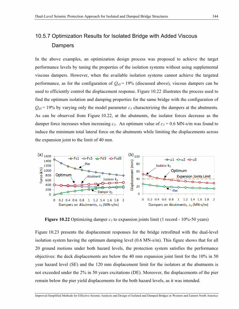
Dual-Level Seismic Protection Approach for Isolated and Damped Bridge Structures 344
Improved Simplified Methods for Effective Seismic Analysis and Design of Isolated and Damped Bridges in Western and Eastern North America
10.5.7 Optimization Results for Isolated Bridge with Added Viscous
Dampers
In the above examples, an optimization design process was proposed to achieve the target
performance levels by tuning the properties of the isolation systems without using supplemental
viscous dampers. However, when the available isolation systems cannot achieve the targeted
performance, as for the configuration of Qd3 = 19% (discussed above), viscous dampers can be
used to efficiently control the displacement response. Figure 10.22 illustrates the process used to
find the optimum isolation and damping properties for the same bridge with the configuration of
Qd3 = 19% by varying only the model parameter c3 characterizing the dampers at the abutments.
As can be observed from Figure 10.22, at the abutments, the isolator forces decrease as the
damper force increases when increasing c3. An optimum value of c3 = 0.6 MN-s/m was found to
induce the minimum total lateral force on the abutments while limiting the displacements across
the expansion joint to the limit of 40 mm.
Figure 10.22 Optimizing damper c3 to expansion joints limit (1 record - 10%-50 years)
Figure 10.23 presents the displacement responses for the bridge retrofitted with the dual-level
isolation system having the optimum damping level (0.6 MN-s/m). This figure shows that for all
20 ground motions under both hazard levels, the protection system satisfies the performance
objectives: the deck displacements are below the 40 mm expansion joint limit for the 10% in 50
year hazard level (SE) and the 120 mm displacement limit for the isolators at the abutments is
not exceeded under the 2% in 50 years excitations (DE). Moreover, the displacements of the pier
remain below the pier yield displacements for the both hazard levels, as it was intended.
Isolator k3

Dual-Level Seismic Protection Approach for Isolated and Damped Bridge Structures 345
Improved Simplified Methods for Effective Seismic Analysis and Design of Isolated and Damped Bridges in Western and Eastern North America
Figure 10.23 Displacement responses for bridge with damper c3 = 0.6 MN-s/m (20 records)
10.6 Conclusions The current seismic code provisions (CSA-S6-06 and AASHTO) do not provide an explicit
optimization procedure that allows engineers to fully benefit from the performance
enhancements at different levels of seismic hazard. To fill the gap in the design of isolated
bridges for multi-level-hazard objectives, a dual-level seismic protection (DLSP) system
involving sequential activation of isolation and supplemental damping devices was introduced in
this chapter.
Through the careful selection of protective devices and the clear definition of a proper hierarchy
of activation, which is related to the two-hazard level performance objectives, the concept of a
dual-level seismic protection system makes it possible to achieve optimum cost-effective
isolation solutions using conventional isolation and damping devices. The ability of the DLSP to
control the structural behaviour of isolated bridges equipped with different seismic protective
devices was demonstrated through a bridge retrofit example.
The proposed methodology was applied using both NLTHA and the proposed energy-based
E-R-µ method, for the retrofit of existing, seismically deficient bridges. The optimal design
process of a DLSP was illustrated for the retrofit of a bridge in Montreal and a bridge in
Vancouver. By comparing the responses from the NLTHA to the estimates obtained using the
E-R-µ method, the appropriateness of adopting the latter for preliminary design to define an
optimum seismic protection strategy was confirmed.

Dual-Level Seismic Protection Approach for Isolated and Damped Bridge Structures 346
Improved Simplified Methods for Effective Seismic Analysis and Design of Isolated and Damped Bridges in Western and Eastern North America
The retrofit designs were further optimized by considering the addition of supplemental viscous
dampers at the abutments. Based on the case studies presented in this chapter it was determined
that the DLSP concept represents a viable approach for achieving optimal performance-based
design of bridges with isolation and damping systems.
Summary and Conclusions 347
Improved Simplified Methods for Effective Seismic Analysis and Design of Isolated and Damped Bridges in Western and Eastern North America
Chapter 11: Summary and Conclusions
11.1 Overview and Project Contributions
The code simplified method currently specified in the Canadian seismic design provisions for
design of isolated bridges (CAN/CSA-S6-06, Section 4.10 Seismic Base Isolation) has been
verified and enhanced. The damping coefficients B, on which the CSA-S6 simplified method
relies, have been revisited for design of isolated bridges in both eastern and western North
American regions. Results of this study incorporate a significant amount of new information that
has been generated in the last two decades on the characteristics of the ground motions expected
in eastern and western North America. This site-specific seismic data, was not available at the
time when the simplified method was developed. Therefore, by addressing concerns about the
appropriateness of using the same seismic provisions for ENA and WNA, the study presented in
this research will fill a gap in the current design provisions. To improve the accuracy of the
simplified method for estimating the bridge responses in ENA, the damping coefficients B were
modified so that the levels of statistical significance for the response estimates are similar for
design of isolated bridges in ENA and WNA.
The limits for the application of the code simplified method have been also examined. It was
found that the source of the inaccuracy originates from the equivalent linearization method rather
than from the definition of the damping coefficients B. To ensure that the method will lead to
conservative results, the method applicability limits can be established in terms of the effective
period. This expression takes into account the influence of the nonlinear parameters. In this way
response estimates that are not sufficiently accurate are automatically rejected and the method
applicability limits are relaxed with respect to those currently set in the code provisions
(CAN/CSA-S6-06). As a result, a much wider choice of the market-available seismic protective
devices can be covered by the modified simplified method.
It was shown that these limits are intrinsic to the assumptions made in developing the simplified
method which relies on a steady-state response of the equivalent linearized system. The
equivalent linearized system oscillates around its original equilibrium position and is naturally

Summary and Conclusions 348
Improved Simplified Methods for Effective Seismic Analysis and Design of Isolated and Damped Bridges in Western and Eastern North America
restrained to capture the drift of the oscillation centre that in turn, results in the problem of the
method accuracy. To overcome these limitations a new energy-based E-R-µ method has been
developed. This method can more accurately account for the transient response and the drift of
the oscillation centre of isolated bridges, two aspects that are not accounted for in the current
code simplified method. The ground motion characteristic and the system's nonlinear parameters
are taken into account by the proposed energy-based E-R-µ method. The capability of this
method to improve, complement and extend the applicability of existing methods is validated
against results from NLTHA. The energy-based E-R-µ method appears to result mostly in
conservative response prediction and may be incorporated into the current design provisions as
an efficient alternative to the currently specified design approach.
The current seismic code provisions (CSA-S6-06) do not provide an explicit optimization
procedure that allows engineers to fully benefit from the performance enhancements at different
levels of seismic hazard. To fill the gap in the design of isolated bridges for multi-level-hazard
objectives, a dual-level seismic protection (DLSP) system involving sequential activation of
isolation and supplemental damping devices has been developed in the present research. The
DLSP system can be configured using different seismic protection devices as dampers and
isolators. The DLSP system can be configured such that it can be used for the design of new
isolated bridges as well as for the upgrade of existing seismically deficient bridges. More
efficient and reliable seismic protection systems may be designed providing bridge owners with
significant cost saving.
This research will contribute to the development of next-generation techniques and strategies for
the design of isolated and damped bridges in both eastern and western North American regions.
The accuracy of the simplified method will be improved and a much wider choice of the market-
available seismic protective devices can be covered by the modified simplified method. The new
energy-based E-R-µ method represents an applicable alternative simplified approach for cases
where the desired seismic protection scheme does not meet the code methods' limits. The dual-
level seismic protection (DLSP) system will allow engineers to fully benefit from the
performance enhancements that can be achieved with isolation and damping to meet specific
performance objectives under different levels of seismic hazard.
By implementing these innovative techniques and strategies, bridge owners and designers will be
able to determine the optimum bridge protective system in terms of performance and cost-

Summary and Conclusions 349
Improved Simplified Methods for Effective Seismic Analysis and Design of Isolated and Damped Bridges in Western and Eastern North America
effectiveness. More realistic response estimates will reduce the impact of the uncertainties
related to the decision on the implementation of different isolation and damping devices for
seismic protection of bridges. The findings and achievements summarized above put in evidence
the significance, originality and contribution to knowledge of this research work.
11.2 Conclusions
Improvement of the CSA-S6-06 code simplified method for design of isolated bridges in ENA
and WNA
In this study, the appropriateness of damping coefficients B currently specified in the NA codes
(CSA-S6-06 and AASHTO) for the design of isolated bridges in ENA and WNA was
investigated by using both LTHA and NLTHA.
The B-coefficients from LTHA in ENA and WNA were compared to those specified in codes in
order to emphasize the influence of the regional seismicity on the reduction damping effect. A
lower reduction effect of viscous damping was observed under ENA records when compared to
WNA records. The concepts of force transmissibility and response amplification for SA and SD
were exploited to explain the observed differences that were primarily attributed to different
frequency contents distinguishing the ENA and WNA seismicity conditions.
The suitability of using the same B-coefficient for reducing force and displacement responses
was examined based on the LTHA results. It was shown that the coefficients B(SA) and B(SD)
reflect different aspects of the system response (absolute acceleration and relative displacement)
and B-coefficients for reducing force and displacement responses must be independently
calibrated. For a more accurate evaluation of the displacement across isolation bearings, the
analysis results suggest that for the simplified code method the definition of the B coefficients
should be based on spectral displacements rather than spectral accelerations. The dependency of
the B-coefficients on the effective period was also confirmed.
In this research, complementary to most of previous studies performed worldwide in which
LTHA was used, an extensive parametric study was carried out using dynamic NLTHA so that a
series of nonlinear system parameters was considered to cover a wide range of isolated and
damped bridge configurations. A total of 12 000 NLTHA were carried out on 300 isolated bridge
Summary and Conclusions 350
Improved Simplified Methods for Effective Seismic Analysis and Design of Isolated and Damped Bridges in Western and Eastern North America
configurations under 20 time-history records representatively for the WNA and ENA regional
seismicity (40 records in total). Based on the observations made for LTHA, in the parametric
study, the damping coefficients were assessed solely for displacement responses. The damping
coefficients specified in current CSA-S6 and AASHTO codes were found to result mostly in safe
designs for WNA but underestimated the displacement demand of bridges subjected to ENA
seismic ground motions.
Based on these results a new value was proposed for the exponent to be used in the equation
currently specified in the AASHTO specifications for the damping coefficients so that the same
equation can be used with different exponents for WNA and ENA locations (Chapter 5). The
modified simplified code method proposed in this thesis for estimating displacement demand
result in comparable relative errors ranging from 5% (unconservative) to -50% (conservative) for
both WNA and ENA. The number of bridges satisfying the conservative response estimates in
ENA was accordingly increased from 31% to 89%. This number is in close agreement with 90%
of satisfactory estimates in WNA. In this way, the same level of accuracy would be reached in
both parts of the country.
The study also showed that the simplified method still underpredicts the response of isolated
bridges for a number of cases. In particular, systems with low R factors, low α ratios, with high
effective damping ratios or short effective periods were found to be more critical in this regard.
The sources of the method inaccuracy may be both the local damping reduction effect and the
equivalent linearization method which is an intrinsic part of the code method. To improve our
understanding of the sources of the method inaccuracy, the accuracy of the equivalent
linearization method is then carefully examined. It was found that the source of the inaccuracy
originates from the equivalent linearization method rather than from the definition of the
damping coefficients B (Chapter 6). By examining in details the process of equivalent
linearization, the upper limit for the method applicability range was derived on the effective
damping and effective period. In this way, the influence of the nonlinear parameters was taken
into account to achieve sufficient accuracy in the seismic response prediction.
The method applicability limits, proposed in this thesis (Chapter 6), were validated by comparing
NLTH responses, obtained in Chapter 5, to the response estimates obtained during the design
process following the complete iterative procedure prescribed in the CSA-S6-06 simplified

Summary and Conclusions 351
Improved Simplified Methods for Effective Seismic Analysis and Design of Isolated and Damped Bridges in Western and Eastern North America
method using damping coefficients B proposed in this thesis for WNA and ENA. It was
confirmed that the use of the proposed limits makes it possible to reject responses with
unsatisfactory accuracy. When comparing the actual code limits (CSA-S6-06) to those proposed
in this thesis, the number of bridges meeting these limits while satisfying the conservative
response estimates was increased from 60% to 93% for WNA and from 36% to 94% for ENA
(Chapter 9). This represents a major improvement thus ensuring a wider choice of the market-
available seismic protective devices that can be covered by the modified simplified method.
These limits could then be used in future editions of CSA-S6 for both WNA and ENA.
To overcome these limitations the need for a new simplified method that takes into account the
differences in ground-motion characteristics and isolated bridge design parameters is also
outlined.
New Energy-Based E-R-µ Simplified Method
In order to establish a basis for the development of a new simplified method, two widely adopted
methods in earthquake engineering, the Equal Displacement (EDA) and the Equal Energy (EEA)
approaches, were briefly reviewed and examined. It was found that the "exact" responses from
NLTHA are confined by that obtained from these two response approximating techniques (EDA
and EEA). The response estimates obtained by using the EEA were found to be conservative for
all studied cases. It was shown that the differences between the response estimates from the EEA
and “exact” NLTHA results may be related to the amount of absorbed energy. It was then shown
that the difference in absorbed energy between these two responses is attributed to the kinetic
energy which is ignored when assuming that the input energy is absorbed entirely through
monotonic loading. This portion of the energy input that is ignored by the EEA was termed as an
energy deficit.
To better characterize seismic response in the present study, special attention was drawn to the
transient phase of loading that occurs at the beginning of the excitation. Through this study, bi-
linear NL-SDOF systems were classified as exhibiting either a limited-nonlinear or a highly-
nonlinear response. It was confirmed that during limited-nonlinear response, systems oscillate
about their "at rest" equilibrium position and the energy induced into the systems over a loading
cycle is dissipated completely through the system's inelastic response within the same cycle. In
turn, during highly-nonlinear response, the systems experience a drift of the oscillation center

Summary and Conclusions 352
Improved Simplified Methods for Effective Seismic Analysis and Design of Isolated and Damped Bridges in Western and Eastern North America
which results from an excess of kinetic energy compared to the energy absorption capacity of the
system. In such a case, the maximum displacement response consists of the drift of the
oscillation center plus the local system response about the new oscillation center. The energy
excess generated during a transient phase of loading can be dissipated through a few consecutive
cycles. The transient oscillation center shifts gradually in each of these cycles until the energy
excess is entirely dissipated.
The transition state between limited-nonlinear and highly-nonlinear responses was defined as the
point beyond which the response of a system starts oscillating about a drifted equilibrium center.
The critical parameter Rcr was derived to mark this point of transition.
The effect of the kinetic energy on the system behaviour was identified as a key element to be
considered in the development of the new simplified method. The transient response and possible
shifting of the transient oscillation centre, was taken into account by applying the concept of
energy allocation under transient excitation. Based on this, a new simplified method was
proposed. This method takes into account the differences in ground-motion characteristics and
bridge design parameters and can predict the peak displacement of bilinear systems. This new
energy-based E-R-µ method was developed purely based on analytical derivations rather than
being empirically calibrated. The basis on which the predictions are made assumes that 1) ground
motions are represented by a single sine-wave pulse defined by the peak ground acceleration
(PGA) and peak ground displacement (PGD) and 2) response to that pulse can be predicted using
the E-R-μ method.
New Multi-Level-Hazard Protection Technique
To fill the gap in the design of isolated bridges for multi-level-hazard objectives, a dual-level
seismic protection (DLSP) system involving sequential activation of isolation and supplemental
damping devices was introduced in this thesis.
Through the careful selection of protective devices and the clear definition of a proper hierarchy
of activation, which is related to the two-hazard level performance objectives, the concept of
dual-level seismic protection system makes it possible to achieve optimum cost-effective
isolation solutions using conventional isolation and damping devices. The ability of the DLSP to
control the structural behaviour of isolated bridges equipped with different seismic protective

Summary and Conclusions 353
Improved Simplified Methods for Effective Seismic Analysis and Design of Isolated and Damped Bridges in Western and Eastern North America
devices was demonstrated through bridge retrofit examples. It was determined that the DLSP
concept represents a viable approach for achieving optimal performance based design of bridges
with isolation and damping systems.
11.3 Recommendations for Future Research
Although the code simplified method (CAN/CSA-S6-06) has been extensively examined and the
proposed modifications will enhance the method's reliability, there are still certain aspects that
can be studied to improve the method accuracy based on the achievements of the present
research.
• The damping coefficients B can be derived as a function of the ground motion characteristics
and system nonlinear parameters using energy concept for transient phase of loading.
• Different formulations of damping coefficients B can be developed for ranges of the limited-
nonlinear and highly-nonlinear responses (defined in Chapter 7).
To improve the accuracy of the energy-based E-R-µ method proposed in this thesis, additional
research is suggested on how to capture the effect of the loading duration or complex irregularity
in the seismic excitation and the structural response. In this way, the method will take into
account the effect of multiple oscillation centre drifts that originate from various successive
loading pulses.
It is recommended to extend the energy-based E-R-µ method to predict the peak displacement of
systems having different hysteresis shapes as for example that flag-shaped or multilinear. As a
result, a much wider choice of the market-available seismic protective devices can be covered by
the proposed energy-based E-R-µ method.
To extend the dual-level seismic protection concept, research studies can be performed on the
development of a number of novel seismic protection devices. Such devices can be designed to
have different activation levels to meet specific performance objectives under different levels of
seismic hazard. Configuring the multilevel protection device to a proper hierarchy of activation
will allow to achieve optimum cost-effective seismic protection.

References 354
Improved Simplified Methods for Effective Seismic Analysis and Design of Isolated and Damped Bridges in Western and Eastern North America
References AASHTO (1991). "Guide specifications for seismic isolation design", American Association of
State Highway and Transportation Officials (AASHTO), Washington, D.C., US.
AASHTO (1994). "AASHTO LRFD Bridge Design Specifications", 1st Edition including
interim revisions for 1996 and 1997, American Association of State Highway and
Transportation Officials (AASHTO), Washington, D.C., US.
AASHTO (1999). "Guide Specifications for Seismic Isolation Design, 2nd Edition", American
Association State and Highway Transportation Officials (AASHTO), Washington, D.C., US.
AASHTO (2009). "Guide Specifications for the LRFD Seismic Bridge Design", American
Association of State Highway and Transportation Officials (AASHTO), Washington, D.C.,
US.
AASHTO (2010). "Guide Specifications for Seismic Isolation Design", 3rd Edition, American
Association of State Highway and Transportation Officials (AASHTO), Washington, D.C.,
US.
Abé, M. (1996). "Tuned Mass Dampers for Structures with Bilinear Hysteresis", Journal of
Engineering Mechanics, 122(8), 797-800.
Abrahamson, N.A. and Silva, W.J. (1997). "Empirical response spectral attenuation relations for
shallow crustal earthquakes", Seismological Research Letters, 68, 94–127.
Abrahamson, N.A. (2000). "Effects of rupture directivity on probabilistic seismic hazard
analysis", Proc. Sixth International Conference on Seismic Zonation, November 12–15,
Palm Springs, California.
Abrahamson, N.A., and Silva, W.J. (2008). "Summary of the Abrahamson & Silva NGA
groundmotion relations", Earthquake Spectra, 24, 67–97.
Adams, J., Basham, P.W., and Halchuk, S. (1995). "Northeastern North American earthquake
potential – new challenges for seismic hazard mapping, In: Current Research 1995-D",
Geological Survey of Canada, 91–99.

References 355
Improved Simplified Methods for Effective Seismic Analysis and Design of Isolated and Damped Bridges in Western and Eastern North America
Adams, J., Weichert, D., and Halchuk, S. (1999). "Lowering the probability level - fourth
generation seismic hazard results for Canada at the 2% in 50 year probability level", Proc. of
Eighth Canadian Conference on Earthquake Engineering, Vancouver, 83-88.
Adams, J. and Atkinson, G. (2003). "Development of seismic hazard maps for the 2003 National
Building Code of Canada", Canadian Journal of Civil Engineering, 30, 255-271.
Adams, J. and Halchuk, S. (2003). "Fourth generation seismic hazard maps of Canada: Values
for over 650 Canadian localities intended for the 2005 National Building Code of Canada",
Geological Survey of Canada, Open File 4459, 150 p.
Adams, J. and Halchuk, S. (2004). "Fourth-generation seismic hazard maps for the 2005 national
building code of Canada", Proceedings of the 13th World Conference on Earthquake
Engineering, Vancouver, Canada. Paper 2502 on CD-ROM.
Adams, J. (2011). "Seismic hazard and seismic risk in Canada perspective for the insurance
industry", Geological Survey of Canada, Natural Resources Canada, Ottawa, Ontario, ICLR
workshop Toronto, ON.
Akkar, S. and Bommer, J.J. (2007). "Prediction of elastic displacement response spectra in
Europe and the Middle East", Earthquake Engineering & Structural Dynamics, 36, 1275-
1301.
Ambraseys, N.N. and Srbulov, M. (1994). "Attenuation of Earthquake-Induced Ground
Displacements", Earthquake Engineering & Structural Dynamics, 23, 467-487.
Ambraseys, N.N., Simpson, K.A. and Bommer, J. J. (1996), "Prediction of Horizontal Response
Spectra in Europe", Earthquake Engineering & Structural Dynamics, 25: 371–400.
Ambraseys, N., Smit, P., Sigbjörnsson, R., Suhadolc, P. and Margaris, B. (2001). Internet-Site
for European Strong-Motion Data. <http://www.isesd.cv.ic.ac.uk>, EVR1-CT-1999-40008,
European Commission, Directorate-General XII, Environmental and Climate Programme,
Bruxelles, Belgium.
American Society of Civil Engineers (2005). "Minimum Design Loads for Buildings", ASCE 7-
05, Reston, Virginia, US.

References 356
Improved Simplified Methods for Effective Seismic Analysis and Design of Isolated and Damped Bridges in Western and Eastern North America
Anderson, J. and Bertero, V. (1987). "Uncertainties in Establishing Design Earthquakes",
Journal of Structural Engineering, 113(8), 1709–1724.
ASCE (2000a). "Prestandard and Commentary for the Seismic Rehabilitation of Buildings",
FEMA 356 Report, American Society of Civil Engineers (ASCE), Federal Emergency
Management Agency (FEMA), Washington, D.C., US.
ASCE (2000b). "Global Topics Report on the Prestandard and Commentary for the Seismic
Rehabilitation of Buildings", FEMA 357 Report, American Society of Civil Engineers
(ASCE), Federal Emergency Management Agency (FEMA), Washington, D.C., US.
ATC (1996a). "Seismic Design Criteria for Highway Structures: Current and Future", Report No.
ATC-18, Applied Technology Council (ATC), Redwood City, California, US.
ATC (1996b). "Improved Seismic Design Criteria for California Bridges: Provisional
Recommendations", Report No. ATC-32, Applied Technology Council (ATC), Redwood
City, California, US.
ATC (1996c). "Seismic Evaluation and Retrofit of Concrete Buildings", Report No. ATC-40,
Volumes 1 and 2, Applied Technology Council (ATC), Redwood City, California, US.
ATC/BSSC (1997). "NEHRP Guidelines for the Seismic Rehabilitation of Buildings", FEMA
273 Report (Guidelines) and FEMA 274 Report (Commentary), Applied Technology Council
(ATC), Federal Emergency Management Agency (FEMA), Washington, D.C., US.
Atkinson, G.M. and Beresnev, I., (1998). "Compatible ground-motion time histories for new
national seismic hazard maps", Canadian Journal of Civil Engineering, 25, 305-318.
Atkinson, G.M. (2004). "An Overview of Developments in Seismic Hazard Analyses", 13th
World Conference on Earthquake Engineering, Vancouver, B.C., Canada
Atkinson, G.M. and Pierre, J.R. (2004). "Ground motion response spectra in Eastern North
America for different critical damping values", Seismological Research Letters, 75(4), 541–
545.

References 357
Improved Simplified Methods for Effective Seismic Analysis and Design of Isolated and Damped Bridges in Western and Eastern North America
Atkinson, G.M. (2005). "Ground Motions for Earthquakes in southwestern British Columbia and
northwestern Washington: Crustal, In-Slab and Offshore Events", Bulletin of the
Seismological Society of America, 95, 1027-1044.
Atkinson, G.M. and Boore, D. (2006). "Ground motion prediction equations for earthquakes in
eastern North America", Bulletin of the Seismological Society of America, 96, 2181-2205.
Atkinson, G.M. (2008). "Earthquake time histories compatible with the 2005 NBCC Uniform
Hazard Spectrum", Canadian Journal of Civil Engineering, Submitted.
Atkinson, G.M. (2009). "Earthquake time histories compatible with the 2005 National Building
Code of Canada uniform hazard spectrum", Canadian Journal of Civil Engineering, 36(6),
991-1000.
Atkinson, G.M., Assatourians, K., Boore, D.M., Campbell, K., and Motazedian, D. (2009). "A
Guide to Differences between Stochastic Point-Source and Stochastic Finite-Fault
Simulations", Bulletin of the Seismological Society of America, 99(6), 3192–3201
Atkinson, G.M. (2010). "Time History modifications – frequency domain approach",
Presentation, CSRN Meeting April 2010.
Ben-Menahem, A. (1961). "Radiation of seismic surface-waves from finite moving sources",
Bulletin of the Seismological Society of America, 51, 401–435.
Ben-Menahem, A. (1962). "Radiation of seismic body-waves from finite moving sources in the
earth", Journal of Geophysical Research, 67, 345–350.
Beresnev, I. and Atkinson, G.M. (1997). "Modeling finite fault radiation from the ω n spectrum",
Bulletin of the Seismological Society of America, 87, 67-84.
Beresnev, I. and Atkinson, G.M. (1998). "Stochastic finite-fault modeling of ground motions
from the 1994 Northridge, California earthquake. I. Validation on rock sites", Bulletin of the
Seismological Society of America, 88, 1392-1401.
Bertero, V.V., Mahin, S.A. and Herrera, R.A. (1978). "Aseismic design implications of near-
fault San Fernando earthquake records", Earthquake Engineering & Structural Dynamics 6,
31-42.
References 358
Improved Simplified Methods for Effective Seismic Analysis and Design of Isolated and Damped Bridges in Western and Eastern North America
Biggs, J.M. (1964). "Introduction to Structural Dynamics", McGraw-Hill.
Bommer, J.J. and Martinez-Pereira, A. (1999). "The Effective Duration of Earthquake Strong
Motion", Journal of Earthquake Engineering, 3(2), 127-172
Bommer, J.J., Scott, S.G., and Sarma, S.K. (2000a). "Hazard-consistent earthquake scenarios",
Soil Dynamics and Earthquake Engineering, 19(4), 219-231.
Bommer, J.J., Elnashai, A.S., and Weir A.G. (2000b). "Compatible acceleration and
displacement spectra for seismic design codes", Proc. 12th World Conference on Earthquake
Engineering, January 30 - February 4, Auckland, New Zeland, Paper No. 0207.
Bommer, J.J., Georgallides, G., and Tromans, I.J. (2001). "Is there a near-field for small-to-
moderate magnitude earthquakes?", Journal of Earthquake Engineering 5(3), 395-423.
Bommer, J.J. and Acevedo, A.B. (2004). "The Use of Real Eathquake Accelerograms as Input to
Dynamic Analysis", Journal of Earthquake Engineering, 8(1), 43-91.
Bommer, J.J. and Mendis, R. (2005). "Scaling of spectral displacement ordinates with damping
ratios", Earthquake Engineering & Structural Dynamics, 34(2): 145-165.
Bommer, J.J. and Pinho, R. (2006). "Adapting earthquake actions in Eurocode 8 for
performance-based seismic design", Earthquake Engineering & Structural Dynamics, 35(1),
39–55.
Bommer, J.J., Stafford, P.J., and Alarcon, J.E. (2009). "Empirical Equations for the Prediction of
the Significant, Bracketed, and Uniform Duration of Earthquake Ground Motion", Bulletin of
the Seismological Society of America, 99, 3217-3233.
Boore, D. and Atkinson, G.M. (2008). "Ground-motion prediction equations for the average
horizontal component of PGA, PGV, and 5%-damped SA at spectral periods between 0.01s
and 10.0 s", Earthquake Spectra, 24(1), 99-138.
Boore, D.M. (2005). SMSIM; Fortran programs for simulating ground motions from
earthquakes: Version 2.3 A revision of OFR 96-80-A, U.S. Geol. Surv. Open-File Rept. (a
modified version of OFR 00-509, describing the program as of 15 August 2005 [version
2.30]).

References 359
Improved Simplified Methods for Effective Seismic Analysis and Design of Isolated and Damped Bridges in Western and Eastern North America
Buckle, I., Friedland, I., Mander, J., Martin, G., Nutt, R. and Power, M (2006). "Seismic
retrofitting manual for highway structures: Part 1-bridges", MCEER Publications, State
University of New York, Buffalo, New York, US.
Cameron, W.I., and Green, R. U. (2007). "Damping correction factors for horizontal ground-
motion response spectra", Bulletin of the Seismological Society of America, 97(3), 934–960.
Cameron, W.I., Green, R.U. (2007). "Damping correction factors for horizontal ground-motion
response spectra." Bulletin of the Seismological Society of America, 97(3) 934–960.
Campbell, K.W., and Bozorgnia, Y., 2003. Updated near-source ground-motion (attenuation)
relations for the horizontal and vertical components of peak ground acceleration and
acceleration response spectra, Bulletin of the Seismological Society of America, 93, 314–331.
CSA (2006). "Canadian Highway Bridge Design Code", CAN/CSA-S6-06, Canadian Standards
Association (CSA), Mississauga, Ontario, Canada.
Caughey, T.K. (1960). "Sinusoidal excitation of a system with bilinear hysteresis", Journal of
Applied Mechanics, 27(4), 640–643.
CEN. (1996) "Eurocode 8: Design Provisions for Earthquake Resistance of Structures. Part 2:
Bridges", ENV 1998-2:1996, Comité européen de normalisation (CEN), Brussels, Belgium.
CEN (2005). "Eurocode 8: Design Provisions for Earthquake Resistance of Structures. Part 2:
Bridges", EN 1998-2:2005, Comité européen de normalisation (CEN), Brussels, Belgium.
Chopra, A.K. (1995). "Dynamics of structures: Theory and applications to earthquake
engineering", Prentice-Hall, New Jersey, US.
Chopra, A.K. (2011). "Dynamics of structures, theory and applications to earthquake
engineering", 4th Edition, Pearson Prentice-Hall, Upper Saddle River, New Jersey, US.
Christopoulos, C. and Filiatrault, A. (2006). “Principles of passive supplemental damping and
seismic isolation”, IUSS Press, Pavia, Italy.
Christopoulos, C., Filiatrault, A., and Folz, B. (2002a). "Seismic response of self-centring
hysteretic SDOF systems", Earthquake Engineering & Structural Dynamics, 31(5), 1131-
1150.

References 360
Improved Simplified Methods for Effective Seismic Analysis and Design of Isolated and Damped Bridges in Western and Eastern North America
Christopoulos, C., Filiatrault, A., Uang, C-M., and Folz, B. (2002b). "Posttensioned Energy
Dissipating Connections for Moment-Resisting Steel Frames", Journal of Structural
Engineering, 128(9), 1111-1120.
Constantinou, M.C., Tsopelas, P., Kim, Y-S., and Okamoto, S. (1993). "NCEER-Taisei
Corporation Research Program on Sliding Isolation Systems for Bridges: Experimental and
Analytical Study of Friction Pendulum System", Report No. 93-0020, National Center for
Earthquake Engineering, State University of New York, Buffalo, New York, US.
Constantinou, M.C., Whittaker, A.S., Kalpakidis, Y., Fenz, D.M., and Warn, G.P. (2007).
"Performance of Seismic Isolation Hardware under Service and Seismic Loading", Technical
Report MCEER-07-0012, Buffalo, New York, US, 469 p.
CSI (2009). SAP2000 [Computer Software] Computers and Structures Inc., Berkeley, California,
US.
CSRN (2012). "Topics related to selecting and scaling ground motions", Workshop related to
CSRN activities - Canadian Seismic Research Network (CSRN), September 17, Montreal,
Quebec, Canada
Den Hartog, J.P. (1930). "Forced Vibrations with Combined Viscous and Coulomb Damping",
The London, Edinbourg, and Dublin Philosophical Magazine, 9(59) 801-817.
Dicleli, M. (2006). "Supplemental elastic stiffness to reduce isolator displacements for seismic-
isolated bridges in near-fault zones", Engineering Structures, 29(5) 763–775.
Dicleli, M. and Buddaram, S (2007). "Equivalent linear analysis of seismic-isolated bridges
subjected to near-fault ground motions with forward rupture directivity effect", Engineering
Structures, 29(1), 21-32
Dion, C., Bouaanani, N., Tremblay, R., and Lamarche, C. (2012). ”Real-Time Dynamic
Substructuring Testing of a Bridge Equipped with Friction-Based Seismic Isolators”, Journal
of Bridge Engineering, 17(1) 4–14.
EN1998-2 (2005). "Design of structures for earthquake resistance - Part 2: Bridges", European
Committee for Standardization, Brussels, Belgium.

References 361
Improved Simplified Methods for Effective Seismic Analysis and Design of Isolated and Damped Bridges in Western and Eastern North America
EQECAT (2012). http://www.eqecat.com/catwatch/damaging-aftershocks-in-northern-italy-
2012-05-29.
Esteva, L. and Rosenblueth, E. (1964). "Espectros de temblores a distancias moderadas y
grandes", Sociedad Mexicana de Ingenieria Sismica, Publ. No.1, vol. II, 1–18.
FEMA (1997). "NEHRP commentary on the guidelines for the seismic rehabilitation of
buildings", FEMA-274, Federal Emergency Management Agency (FEMA), Washington,
D.C., US.
FEMA 273 (1997). "NEHRP Guidelines for the Seismic Rehabilitation of Buildings", Federal
Emergency Management Agency (FEMA), Washington, D.C., US.
FEMA 356 (2000). "Prestandard and Commentary for the Seismic Rehabilitation of Buildings",
American Society of Civil Engineers (ASCE), Federal Emergency Management Agency
(FEMA), Washington, D.C., US.
FEMA 356 (2000). "Prestandard and Commentary for the Seismic Rehabilitation of Buildings",
American Society of Civil Engineers (ASCE), Federal Emergency Management Agency
(FEMA), Washington, D.C., US.
FEMA 440 (2005). "Improvement of nonlinear static seismic analysis procedures", American
Society of Civil Engineers (ASCE), Federal Emergency Management Agency (FEMA),
Washington, D.C., US.
Filiatrault, A., Leger, P., and Tinawi, R. (1994). "On the Computation of Seismic Energy in
Inelastic Structures", Engineering Structures, 16(6), 426-436.
Filiatrault, A. (2008). "Elements of Earthquake Engineering and Structural Dynamics", 2nd
Edition, Presses Internationales Polytechnique, Montreal, Quebec, Canada.
Filiatrault, A., Tremblay, R., Christopoulos, C., Folz, B., and Pettigna, D. (2013). "Elements of
Earthquake Engineering and Structural Dynamics", 3rd Edition, Presses Internationales
Polytechnique, Montreal, Quebec, Canada.

References 362
Improved Simplified Methods for Effective Seismic Analysis and Design of Isolated and Damped Bridges in Western and Eastern North America
Graizer, V. (2010). "Strong Motion Recordings and Residual Displacements: What Are We
Actually Recording in Strong Motion Seismology? ", Seismological Research Letters, 81(4),
635-639.
Guilini Charette, K. (2009). "Effets des Mouvements Sismiques sur les Structures en Acier de la
Catégorie des Constructions Conventionnelles", M.Sc. Thesis, Departement of Civil,
Geological and Mining Engineering, École Polytechnique de Montréal, Montreal, Quebec,
Canada.
Gulkan P, Sozen M. (1974). "Inelastic response of reinforced concrete structures to earthquakes
motions", ACI Journal, 71(12) 604-610.
Halchuk, S. and Adams, J. (2004). "Deaggregation of seismic hazard for selected Canadian
cities", Proc. 13th World Conference on Earthquake Engineering, Vancouver, Canada,
August 1-6, Paper No. 2470.
Halchuk, S. (2009-2010). Personal Communication.
Hall, J.F., Heaton, T.H., Halling, M.W., and Wald, D.J. (1995) "Near-source ground motions and
its effects on flexible buildings", Earthquake Spectra 11(4), 569-605.
Hancock, J. (2006). "The Influence of Duration and the Selection and Scaling of Accelerograms
in Engineering Design and Assessment", Ph.D. Dissertation, Department of Civil and
Environmental Engineering, University of London, London, UK, 442 p.
Hatzigeorgiou, G.D. (2010). "Damping modification factors for SDOF systems subjected to
near-fault, far-fault and artificial earthquakes", Earthquake Eng. Dyn., 39 (11), 1239–1258.
Heidebrecht , A.C. (2003)."Overview of seismic provisions of the proposed 2005 edition of the
National Building Code of Canada", Canadian Journal of Civil Engineering, 30, 241-254.
Housner G.W. (1956). "Limit design of structures to resist earthquakes", Proceedings of the 1st
World Conference on Earthquake Engineering, California, US, 5, 5-1 to 5-13.
Housner, G.W. (1963). "The behavior of inverted pendulum structures during earthquakes",
Bulletin of the Seismological Society of America, 53(2), 403-417.

References 363
Improved Simplified Methods for Effective Seismic Analysis and Design of Isolated and Damped Bridges in Western and Eastern North America
Huang, Y.N., Whittaker, A., and Luco, N. (2008). "Maximum spectral demands in the near-fault
region, Earthquake Engineering Research Institute", Earthquake Spectra, 24(1), 319-341.
Huffman, S., Gillespie, D.G., and Anderson, D.L. (2012). "Performance-based Design (PBD) of
British Columbia Bridges", Proc. of 15th World Conference on Earthquake Engineering,
Lisbon, Portugal, Paper No. 898.
Hwang, J.S. and Chiou, J.M. (1996). "An equivalent linear model of lead-rubber seismic
isolation bearings", Engineering Structures, 18(7), 528-536
Hwang, J.S. and Sheng, L.H. (1994). "Equivalent elastic seismic analysis of base-isolated
bridges with lead-rubber bearings", Engineering Structures, 16(3), 201-209
ICBO (1991). "Uniform Building Code", International Conference of Building Officials,
California, US.
Iervolino, I., Maddaloni, G., Cosenza, E., and Manfredi, G. (2007). "Selection of Time-Histories
for Bridge Design in Eurocode 8", Proc. of 1st US-Italy Seismic Bridge Workshop, 18 - 20
April, EUCENTRE, Pavia, Italy.
Itani, A.M., and Malik, A.H. (2000). "Enhancing Seismic Design Criteria for Our Nation’s
Vulnerable Bridges", CD-ROM, Transportation in the New Millennium: State of the Art and
Future Directions, Perspectives from the Transportation Research Board Standing
Committees, Retrieved from http://onlinepubs.trb.org/onlinepubs/millennium/00034.pdf.
Iwan, W.D. (1961), "The Dynamic Response of Bilinear Hysteretic Systems", Ph.D.
dissertation, Earthquake Engineering Research Laboratory, California Institute of
Technology, California, US, 152 p.
Iwan, W.D. and Gates, N.C. (1979). "Estimating Earthquake Response of Simple Hysteretic
Structures", Journal of Engineering Mechanics Division, ASCE, 105(EM3) 391-405.
Iwan, W.D. (1980). "Estimating inelastic response spectra from elastic spectra", Earthquake
Engineering & Structural Dynamics, 8, 375–388.
Jacobsen, L.S. (1930). "Steady Forced Vibrations as Influenced by Damping", ASME
Transactions, 52, 169-181.

References 364
Improved Simplified Methods for Effective Seismic Analysis and Design of Isolated and Damped Bridges in Western and Eastern North America
Jacobsen, L.S. (1960). "Damping in Composite Structures", Proc. of 2nd World Conference on
Earthquake Engineering, Tokyo and Kyoto, Japan, 1029-1044.
Jacobsen, L.S. and Ayre, R.S. (1958). "Engineering vibrations", McGraw-Hill, New York, New
York, US.
Jara, M. and Casas, J.R. (2006). "A direct displacement-based method for the seismic design of
bridges on bi-linear isolation devices", Engineering Structures, 28(6), 869-879.
Jeong, G.D. and Iwan, W.D. (1988), "The effect of earthquake duration on the damage of
structures", Earthquake Engineering Structural Dynamics, 16, 1201–1211.
Kalkan, E. and Chopra, A.K. (2010). "Practical guidelines to select and scale earthquake records
for nonlinear response history analysis of structures: U.S", Geological Survey Open-File
Report 2010-1068, 124 p.
Kawashima, K., MacRae, G.A., Hoshikuma, J., and Nagaya, K. (1998). "Residual Displacement
Response Spectrum", Journal of Structural Engineering, 124(5), 523-530.
Koval, V., Christopoulos, C., and Tremblay, R. (2012a). "Analytical Model for Optimizing the
Design of Isolated and Damped Bridge Structures", Proc. of 29th International Bridge
Conference, June 10-13, Pittsburgh, Pennsylvania, US, Paper IBC-12-106.
Koval, V., Tremblay, R., and Christopoulos, C. (2012b). "Isolation and Damping Mitigation
Strategies for Bridges in Western and Eastern North America", Proc. of 15th World
Conference on Earthquake Engineering, Lisbon, Portugal, Paper No. 898.
Lapalme, P. (2012). Personal communication. Engineer, Goodco Z-Tech.
Lee Marsh, M., Mayes, R.L., and Friedland, I.M (2001). "Recommended LRFD Guidelines for
the Seismic Design of Highway Bridges", Proceedings of the 17th U.S.-Japan Bridge
Engineering Workshop, November 12,13 and 14, Public Works Research Institute, 14 p.
Leger, P. and Tremblay, R. (2009). "Earthquake Ground Motions for Seismic Damage
Assessment and Re-Evaluation of Existing Buildings and Critical Facilities", Damage
Assessment and Reconstruction After War and Natural Disaster, NATO Science for Peace
and Security Series C: Environmental Security, 193-219.

References 365
Improved Simplified Methods for Effective Seismic Analysis and Design of Isolated and Damped Bridges in Western and Eastern North America
Lin, Y.Y. and Chang, K.C. (2003). " Study on Damping Reduction Factor for Buildings under
Earthquake Ground Motions", Journal of Structural Engineering, 129(2), 206-214.
Liu, A, Stewart, J.P., Abrahamson, N., Moriwaki, Y. (2001). "Equivalent number of uniform
stress cycles for liquefaction analysis". Journal of Geotechnical and Geoenvironmental
Engineering (ASCE), 127(12):1017–1026.
Makris, N. (1997). "Rigidity-plasticity-viscosity: Can electrorheological dampers protect base-
isolated structures from near-source ground motions?", Earthquake Engineering &
Structural Dynamics, 26(5), 571-591.
Makris, N. and Chang, S. P. (1998), "Effect of Damping Mechanisms on the Response of
Seismically Isolated Structures", Technical Report PEER-98/06, University of California,
Berkeley, California, US.
Masri, S.F. (1975). "Forced vibration of the damped bilinear hysteretic oscillator", Journal of the
Acoustical Society of America, 57(1), 106–112.
MATLAB. (2009) MATLAB Version 7.8, The MathWorks, Inc.
Mavronicola, E. and Komodromos, P. (2011). "Assessing the suitability of equivalent linear
elastic analysis of seismically isolated multi-storey buildings", Computers and Structures,
89(21-22), 1920-1231.
MCEER/ATC-49 (2003). "Recommended LRFD guidelines for the seismic design of highway
bridges. Part II: Commentary and Appendices", NCHRP Project 12-49, FY 98.
ATC/MCEER Joint Venture.
McGuire, R.K. (1995). "Probabilistic seismic hazard analysis and design earthquakes: closing the
loop", Bulletin of the Seismological Society of America, 85(5), 1275-1284.
McGuire, R.K., Silva, W.J., and Kenneally, R (2001a). "New seismic design spectra for nuclear
power plants", Nuclear Engineering and Design, 203 (2001) 249–257.
McGuire, R.K., Silva, W.J., and Constantino, C.J. (2001b). "Technical Basis for Revision of
Regulatory Guidance on Design Ground Motions: Hazard- and Risk-consistent Ground

References 366
Improved Simplified Methods for Effective Seismic Analysis and Design of Isolated and Damped Bridges in Western and Eastern North America
Motion Spectra Guidelines", Report No. NUREG/CR-6728 prepared for the U.S. Nuclear
Regulatory Commission, Risk Engineering, Inc., Boulder, CO, 213 p.
McGuire, R.K., Silva, W.J., and Constantino, C.J. (2002). "Technical Basis for Revision of
Regulatory Guidance on Design Ground Motions: Development of Hazard- and Risk-
consistent Seismic Spectra for Two Sites", Report No. NUREG/CR-6769 prepared for the
U.S. Nuclear Regulatory Commission, Risk Engineering, Inc., Boulder, CO, 168 p.
Medeot, R. (2004) "Re-Centring Capability Evaluation of Seismic Isolation Systems Based on
Energy Concepts", 13th World Conference on Earthquake Engineering, Vancouver, B.C.,
Canada.
Medeot, R. (2012). "Re-centring Capability of Seismic Isolation Systems: A controversial matter
moving scarcely towards its settlement", Proc. of 15th World Conference on Earthquake
Engineering, Lisbon, Portugal, Paper No.878.
Monzon, E.V, Wei, C, Buckle, I.G, and Itani, A. (2012). "Seismic Response of Full and Hybrid
Isolated Curved Bridges", Structures Congress 2012, March 29-31, 2012, Chicago, Illinois,
US, 603-612.
Morgan, T.A. and Mahin S.A. (2011). "The Use of Base Isolation Systems to Achieve Complex
Seismic Performance Objectives", PEER Report 2011/06, Pacific Earthquake Engineering
Research Center, College of Engineering, University of California, Berkeley, California, US,
326 p.
Motazedian, D. and Atkinson, G.M. (2005). "Stochastic finite-fault model based on dynamic
corner frequency", Bulletin of the Seismological Society of America, 95, 995-1010.
Naeim, F., and Kelly, J. M. (1999). "Design of seismic isolated structures: From theory to
practice", Wiley, New York, US.
Naeim, F. and Kircher, C.A. (2001). "On the damping adjustment factors for earthquake
response spectra", The Structural Design of Tall Buildings, 10(5), 361-369.
Nassar, A.A. and Krawinkler, H. (1991). "Seismic Deands or SDOF and MDOF Systems",
Report No.95, Department of Civil and Environmental Engineering, Stanford University,
Stanford, California, US, 218 p.

References 367
Improved Simplified Methods for Effective Seismic Analysis and Design of Isolated and Damped Bridges in Western and Eastern North America
Naumoski, N.; Tso, W.K. and Heidebrecht, A.C. (1988). "A selection of representative strong
mtion earthquake records having different A/V ratios". Report No.88-01, Earthquake
Research Group, McMaster University, Hamilton, Ontario, Canada.
Naumoski, N., Cheung, M.S., and Foo, S. (2000). "Evaluation of the seismic response coefficient
introduced in the Canadian Highway Bridge Design Code", Canadian Journal of Civil
Engineering, 27(6), 1183–1191.
Newmark, N.M. (1959). "A method of computation for structural dynamics", Journal of
Engineering Mechanic., 85(3) 67-94.
Newmark, N.M. and Hall, W.J. (1982). "Earthquake spectra and design", Earthquake
Engineering Research Institute, Oakland, California, US.
Newton, I. (1999). "The Principia", A new translation by I.B. Cohen and A. Whitman, University
of California press, Berkeley, California, US.
NRCC. (2005). "National Building Code of Canada, 12th ed., and Commentary", National
Research Council of Canada, Ottawa, Ontario, Canada.
NRCC. (2010). "National Building Code of Canada, 13th ed., and Commentary", National
Research Council of Canada, Ottawa, Ontario, Canada.
Paultre, P. (2005). "Dynamique des structures", Editions Hermes Lavoisier, Paris, France.
Popov, E.P. (1994). "Development of US Seismic Codes", Journal of Constructional Steel
Research, 29(1-3), 191-207
Priestley, M.J.N., Calvi, G.M., and Kowalsky, M.J. (2007). "Displacement-Based Seismic
Design of Structures", IUSS Press, Pavia, Italy.
Reiter L. (1990). "Earthquake hazard analysis: issues and insights", New York: Columbia
University Press.
RESPONSE 2000, Bentz, E.C. (2000). "Sectional analysis of reinforced concrete members",
Ph.D. dissertation, University of Toronto, Toronto, Ontario, Canada.

References 368
Improved Simplified Methods for Effective Seismic Analysis and Design of Isolated and Damped Bridges in Western and Eastern North America
Rowshandel, B. (2010). "Directivity Correction for the Next Generation Attenuation (NGA)
Relations", Earthquake Engineering Research Institute, Earthquake Spectra, 26(2), 525–
559.
SEAOC (1995). "Performance Based Seismic Engineering of Buildings, Vision 2000 Report,
Volumes I and II", Structural Engineers Association of California (SEAOC), Sacramento,
California, US.
SEAONC. (1986). "Tentative Seismic Isolation Design Requirements", Structural Engineers
Association of Northern California (SEAONC), San Francisco, California, US.
Skinner, R.I., Robinson, W.H., and McVerry, G.H. (1991). "Seismic isolation in New Zealand",
Nuclear Engineering and Design, 127(3), 281-289.
Skinner, R.I., Robinson, W.H., and McVerry, G.H. (1993). "An introduction to seismic
isolation", Wiley, Chichester, UK.
Somerville, P.G and Yoshimura, J. (1990). "The influence of critical Moho reflections on strong
ground motions recorded in San Francisco and Oakland during the 1989 Loma Prieta
earthquake", Geophysical Research Letters, 17, 1203-1206.
Somerville, P.G. (1996). "Strong ground motion of the Kobe, Japan earthquake of Jan. 17, 1995,
and development of a model of forward rupture directivity effects applicable in California",
Proceedings of Western Regional Technical Seminar on Earthquake Engineering for Dams,
April 11-12, Association of State Dam Safety Officials, Sacramento, California, US.
Somerville, P.G., Smith, N.F., Graves, R.W, and Abrahamson, N.A. (1997a). "Modification of
empirical strong ground motion attenuation relations to include the amplitude and duration
effects of rupture directivity", Seismological Research Letters, 68(1), 199-222.
Somerville, P., Smith, H., Puriyamurthala, S., and Sun. J. (1997b). "Development of Ground
Motion Time Histories for Phase 2 of the FEMA/SAC Steel Project", SAC Joint Venture
Report SAC/BD 97/04, Sacramento, California, US.
Somerville, P. (2000). "New developments in seismic hazard estimation", Proceedings of the
Sixth International Conference on Seismic Zonation, Palm Springs, California, US.

References 369
Improved Simplified Methods for Effective Seismic Analysis and Design of Isolated and Damped Bridges in Western and Eastern North America
Spudich, P., Chiou, B. S-J., Graves, R., Collins, N., and Somerville, P. G. (2004). "A formulation
of directivity for earthquake sources using isochrone theory", U.S. Geological Survey Open
File Report 2004-1268, http://pubs.usgs.gov/of/2004/1268/.
Spudich, P. and Chiou, B. S-J. (2006). "Directivity in preliminary NGA residuals", Final Project
Report for PEER Lifelines Program Task 1M01, 49 pp.
Stafford, P.J., Mendis, R. and Bommer J.J. (2008). "Dependence of damping correction factors
for response spectra on duration and numbers of cycles", Journal of Structural Engineering,
ASCE, 134(8), 1364-1373.
Stein, S., and Wysession, M. (2003). "An Introduction to Seismology, Earthquakes and Earth
Structures", Wiley-Blackwell Publishers, 498 p.
Taylor, P.R. (1999). "Some thoughts on seismic engineering for bridges seen from a Canadian
perspective", Proc. 8th Canadian Conference on Earthquake Engineering, Vancouver, BC,
Canada, 29–41.
Tolis, S.V. and Faccioli, E. (1999). "Displacement design spectra", Journal of Earthquake
Engineering, 3(1), 107-125.
Tremblay, R. (1998). "Development of design spectra for long-duration ground motions from
Cascadia subduction earthquakes", Canadian Journal of Civil Engineering, 25, 1078-1090.
Tremblay, R. and Atkinson, G.M. (2001). "Comparative Study of the Inelastic Seismic Demand
of Eastern and Western Sites", Earthquake Spectra, 17(2), 333-358.
Tremblay, R. (2003). "Analytical Prediction of the nonlinear Seismic Response of a Two-Storey
Semi-Rigid Steel-Concrete Composite Frame", European Commission Joint Research
Centre, 72 p.
Tremblay, R. and Koval, V. (2008). "Essais de qualification de prototypes d’isolateurs sismiques
IS-1 Goodco Z-Tech - Pont P-05328 sur la rivière Nicolet, Autoroute 20, Saint-Léonard-
D’Aston, QC", Rapport No. ST08-15, Département des génies civil, géologique et des mines,
Groupe de recherche en génie des structures, École Polytechnique, Montreal, Quebec,
Canada, 89 p.

References 370
Improved Simplified Methods for Effective Seismic Analysis and Design of Isolated and Damped Bridges in Western and Eastern North America
Trifunac, M.D. and Novikova, E.I. (1995). "Duration of Earthquake Fault Motion in California",
Earthquake Engineering & Structural Dynamics, 24, 781-799.
Tso, W.K., Zhu, T.J., and Heidebrecht, A.C. (1992). "Engineering implications of ground motion
A/V ratio", Soil Dynamics & Earthquake Engineering, 11(3), 133-144.
Tsopelas P.C., Constantinou M.C., Okamota S., Fujii S, and Ozaki D. (1996). "Experimental
study of bridge seismic sliding isolation systems", Engineering Structures; 18(4) 301–10.
Tsopelas, P., Constantinou, M.C., Kircher, C.A., and Wittaker, A.S. (1997). "Evaluation of
Symplified Methods of Analysis for Yielding Structures", Technical Report NCEER-97-
0012, State University of New York, Buffalo, New York, US, 48 p.
Tsopelas, T., Constantinou, M.C. (1994). "Experimental and Analytical Study of a System
Consisting of Sliding Bearings and Fluid Restoring Force/Damping Devices", Report
NCEER-94-0014, Dept. of Civ. Eng., State University of New York, Buffalo, New York, US.
Uang, C.-M. and Bertero, V. V. (1990). "Evaluation of seismic energy in structures", Earthquake
Engineering & Structural Dynamics, 19, 77–90.
Veletsos, A.S. and Newmark, N.M. (1960). "Effect of Inelastic Behaviour in the Response of
Simple Systems to Earthquake Motions", Proc. of 2nd World Conference on Earthquake
Engineering, Tokyo, Japan, 895–912.
Yamada, M., Kawamura, H., Tani, A., Katsunobu, I., Sakai, Y., Nishikawa, H., Masui, A., and
Yamada, M. (1988). "Fracture ductility of structural elements and of structures",
Proceedings of the 9th World Conference on Earthquake Engineering, IV, Tokyo, Japan,
219-224.
Zhang, J. and Huo, Y. (2009). "Evaluating Effectiveness and Optimum Design of Isolation
Devices for Highway Bridges Using the fragility function method", Engineering Structures,
31(8), 1648-1660.
Zhang, J., Makris, N., and Delis, T. (2004). "Structural Characterization of Modern Highway
Overcrossings—Case Study", Journal of Structural Engineering, 130(6), 846–860.

Appendix A 371
Improved Simplified Methods for Effective Seismic Analysis and Design of Isolated and Damped Bridges in Western and Eastern North America
Appendix A
Directivity Effects on the Inelastic Structural Responses

Appendix A 372
Improved Simplified Methods for Effective Seismic Analysis and Design of Isolated and Damped Bridges in Western and Eastern North America
Appendix A presents details and results on the assessment of the fault rupture directivity effects.
Using artificial time histories (Atkinson, 2008), the effect of seismic directivity was investigated
to outline its effect on response variability.
A1: Presents the characterization of the earthquake records with respect to the ground motion
azimuthal direction.
A2: Presents the assessment of the effect of directivity on the inelastic structural responses. The
effects of the rupture directivity was outlined herein by using different response parameters.
A1 Ground Motion Record Characterization
The parameters chosen for this study aimed to put in evidence possible trends of the seismic
directivity effects on the structural behaviour. Four ground motion parameters adopted for this
assessment are as follows:
1) Arias Duration:
Interval of time corresponding to the accumulation of the total ground motion arias
intensity between 5% and 95%.
2) Arias Intensity, IA:
dttag
It
A ∫=0
2 )(π (A.1)
3) Number of Zero Crossing, NZC;
4) Ratio of Peak Acceleration to Peak Ground Velocity, PGA/ PGV.
PGA/ PGV characterizes the ground motion frequency content (when PGA/ PGV is high,
the frequency content is high) (Naumoski et al., 1988; Leger and Tremblay, 2009).
The characteristics of the time histories were evaluated for each of the 8 azimuth directions: 0°,
45°, 90°, 135°, 180°, 225°, 270° and 315°. The results are presented in Figures B.1 and B.2. To
highlight the effect of directivity, the results are presented on the form of an ratio, αvar(θ), which
is defined as the ratio between the ground motion parameter for a given azimuth Ѳ to the ground
motion parameter for an azimuth of 0°:

Appendix A 373
Improved Simplified Methods for Effective Seismic Analysis and Design of Isolated and Damped Bridges in Western and Eastern North America
( )( )°
=0Parameter
Parameter )(varθθα (A.2)
The trends are outlined by using the polynomial trendline of degree 6. However, the variation is
not clearly defined to distinguish predominant effect of the azimuthal positions between the
forward or backward directivities. The largest variation of the Arias Duration is observed at
°= 270θ for the ENA short-period event at close fault-to-site distance (M6 at 10 km), while the
same event for WNA at the same azimuth shows the shortest Arias Duration. Large variability of
the Arias Intensity is primarily due to the record-to-record differences in the peak ground
acceleration (not shown). The effect of the normal-to-fault rupture directivity ( °= 90θ and
°= 270θ ) is more explicitly prevailing for NZC parameter. There is relatively small variation
observed between PGA/PGV ratios. It can be stated from these results that the effect of the
lateral rupture directivity ( °≤≤° 13545 θ and °≤≤° 315225 θ ) mostly dominate the response
variability. This indicates that a larger damage potential may be expected for inelastic response
of structures to those ground motions.
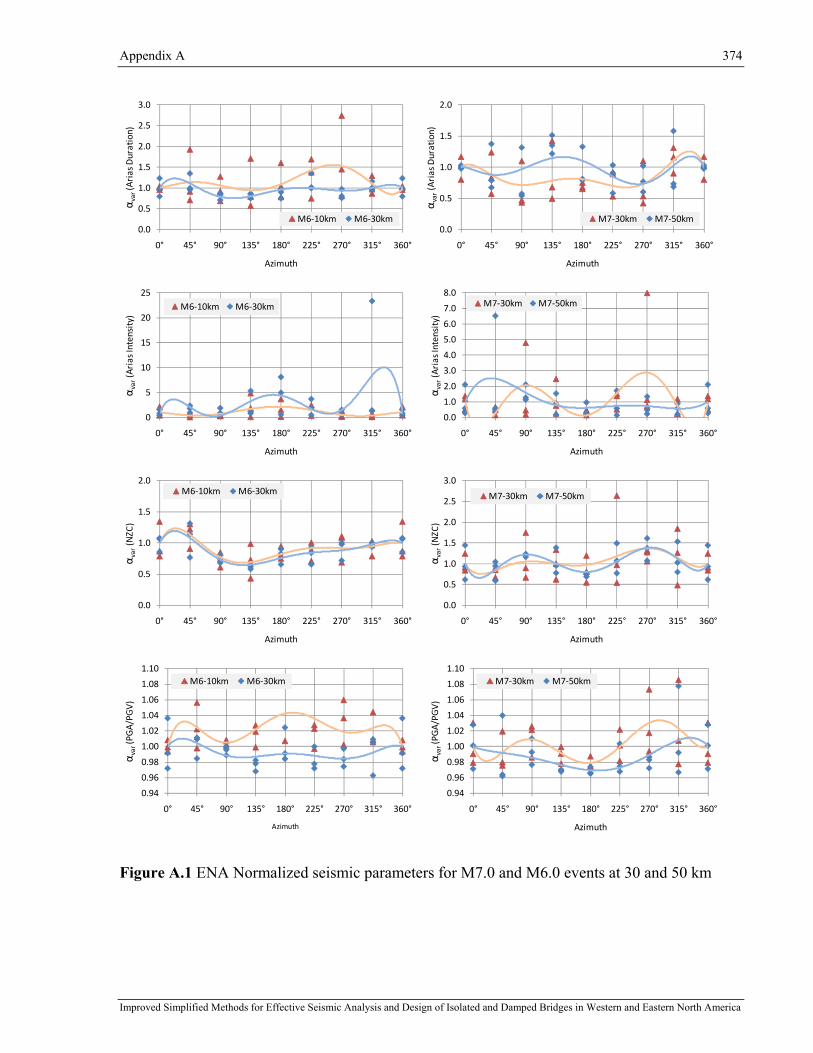
Appendix A 374
Improved Simplified Methods for Effective Seismic Analysis and Design of Isolated and Damped Bridges in Western and Eastern North America
0.0
0.5
1.0
1.5
2.0
2.5
3.0
0° 45° 90° 135° 180° 225° 270° 315° 360°
αvar(Arias Duration)
Azimuth
M6‐10km M6‐30km
0.0
0.5
1.0
1.5
2.0
0° 45° 90° 135° 180° 225° 270° 315° 360°
αvar(Arias Duration)
Azimuth
M7‐30km M7‐50km
0
5
10
15
20
25
0° 45° 90° 135° 180° 225° 270° 315° 360°
αvar(Arias Intensity)
Azimuth
M6‐10km M6‐30km
0.0
1.0
2.0
3.0
4.0
5.0
6.0
7.0
8.0
0° 45° 90° 135° 180° 225° 270° 315° 360°αvar(Arias Intensity)
Azimuth
M7‐30km M7‐50km
0.0
0.5
1.0
1.5
2.0
0° 45° 90° 135° 180° 225° 270° 315° 360°
αvar(NZC
)
Azimuth
M6‐10km M6‐30km
0.0
0.5
1.0
1.5
2.0
2.5
3.0
0° 45° 90° 135° 180° 225° 270° 315° 360°
αvar(NZC
)
Azimuth
M7‐30km M7‐50km
0.94
0.96
0.98
1.00
1.02
1.04
1.06
1.08
1.10
0° 45° 90° 135° 180° 225° 270° 315° 360°
αvar(PGA/PG
V)
Azimuth
M6‐10km M6‐30km
0.94
0.96
0.98
1.00
1.02
1.04
1.06
1.08
1.10
0° 45° 90° 135° 180° 225° 270° 315° 360°
αvar(PGA/PG
V)
Azimuth
M7‐30km M7‐50km
Figure A.1 ENA Normalized seismic parameters for M7.0 and M6.0 events at 30 and 50 km

Appendix A 375
Improved Simplified Methods for Effective Seismic Analysis and Design of Isolated and Damped Bridges in Western and Eastern North America
0.0
0.5
1.0
1.5
2.0
0° 45° 90° 135° 180° 225° 270° 315° 360°
αvar(Arias Duration)
Azimuth
M6.5‐10km M6.5‐30km
0.0
0.5
1.0
1.5
2.0
0° 45° 90° 135° 180° 225° 270° 315° 360°
αvar(Arias Duration)
Azimuth
M7.5‐30km M7.5‐50km
0
10
20
30
40
50
0° 45° 90° 135° 180° 225° 270° 315° 360°
αvar(Arias Intensity)
Azimuth
M6.5‐10km M6.5‐30km
0
10
20
30
40
50
60
0° 45° 90° 135° 180° 225° 270° 315° 360°αvar(Arias Intensity)
Azimuth
M7.5‐30km M7.5‐50km
0.0
1.0
2.0
3.0
4.0
5.0
0° 45° 90° 135° 180° 225° 270° 315° 360°
αvar(NZC
)
Azimuth
M6.5‐10km M6.5‐30km
‐1.0
0.0
1.0
2.0
3.0
4.0
5.0
6.0
7.0
0° 45° 90° 135° 180° 225° 270° 315° 360°
αvar(NZC
)
Azimuth
M7.5‐30km M7.5‐50km
0.94
0.96
0.98
1.00
1.02
1.04
1.06
1.08
1.10
0° 45° 90° 135° 180° 225° 270° 315° 360°
αvar(PGA/PG
V)
Azimuth
M6.5‐10km M6.5‐30km
0.950.970.991.011.031.051.071.091.111.131.15
0° 45° 90° 135° 180° 225° 270° 315° 360°
αvar(PGA/PG
V)
Azimuth
M7.5‐30km M7.5‐50km
Figure A.2 WNA Normalized seismic parameters for M7.5 and M6.5 events at 30 and 50 km

Appendix A 376
Improved Simplified Methods for Effective Seismic Analysis and Design of Isolated and Damped Bridges in Western and Eastern North America
A2 Effect of Directivity on Inelastic Responses
The effects of the rupture directivity was outlined herein by using different response parameters.
The use of damage indices are commonly adopted to evaluate a structure failure potential. The
potential damage as a function of azimuth is determined by using a number of yielding
occurrences as well as the kinematic, hysteretic, and low-cycle fatigue damage indices that are
defined in terms of the ductility ratio µ. Note that no limit was defined for these parameters; only
the values obtained are compared to indicate the failure occurrence in this assessment. These
parameters are explained in details as follows:
1) Number of Yielding Occurrences is determined by counting the number of times the state of
the structure changes from linear elastic to inelastic. The number of yielding occurrences is an
important parameter to emphasize ground motion demand on structure in terms of cumulative
damage. This damage indicator may be of significance for seismic protection systems such as
elastomeric (rubber or lead-rubber) isolation devices or hysteretic energy dissipation devices
made from steel and shape memory alloys.
2) Kinematic Damage Index is critical for any isolation system since it reflects the maximum
displacement demand. It is determined as:
11
, −−
=monu
Dμ
μμ (A.3)
where yΔ
Δ= maxμ ;
μu,mon = maximum ductility capacity under monotonic loading
For this study, only relative values of Dμ are needed for the various azimuth values and μu,mon
was arbitrarily set equal to 12.
3) Hysteretic Damage Index is related to the dissipative capacity of isolation systems and it is
defined as:
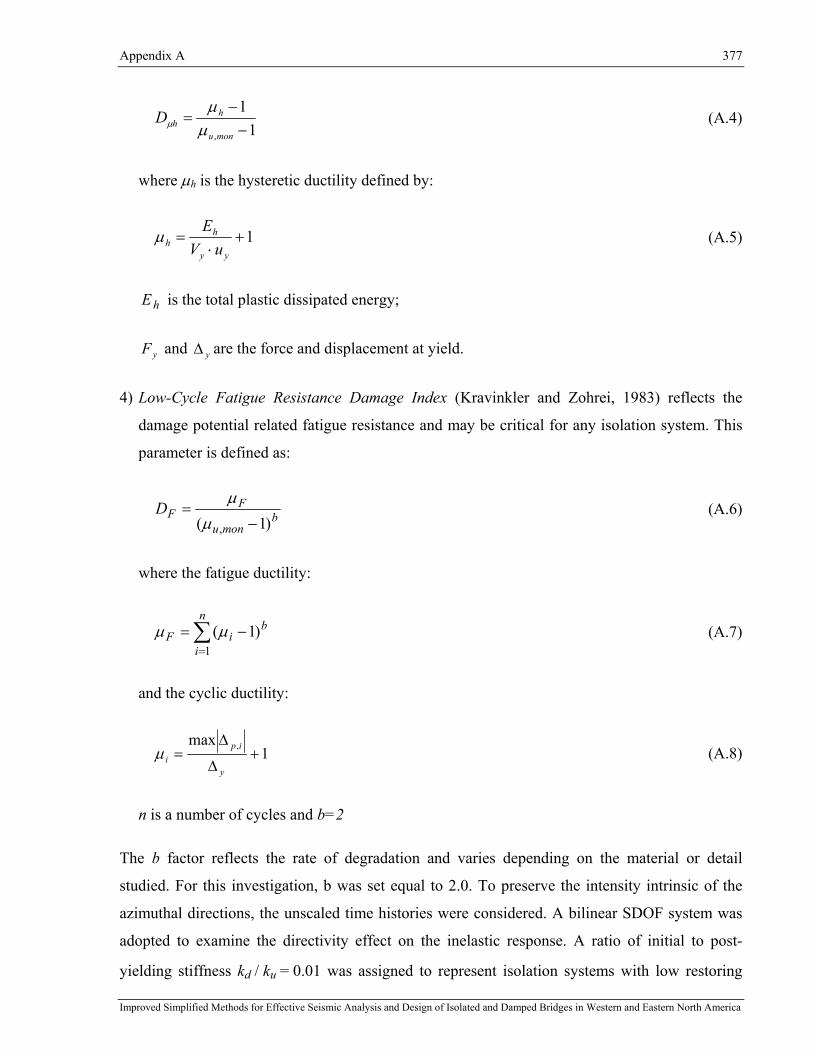
Appendix A 377
Improved Simplified Methods for Effective Seismic Analysis and Design of Isolated and Damped Bridges in Western and Eastern North America
11
, −−
=monu
hhD
μμ
μ (A.4)
where μh is the hysteretic ductility defined by:
1+⋅
=yy
hh uV
Eμ (A.5)
hE is the total plastic dissipated energy;
yF and yΔ are the force and displacement at yield.
4) Low-Cycle Fatigue Resistance Damage Index (Kravinkler and Zohrei, 1983) reflects the
damage potential related fatigue resistance and may be critical for any isolation system. This
parameter is defined as:
bmonu
FFD
)1( , −=
μμ
(A.6)
where the fatigue ductility:
∑=
−=n
i
biF
1)1(μμ (A.7)
and the cyclic ductility:
1max ,
+Δ
Δ=
y
ipiμ (A.8)
n is a number of cycles and b=2
The b factor reflects the rate of degradation and varies depending on the material or detail
studied. For this investigation, b was set equal to 2.0. To preserve the intensity intrinsic of the
azimuthal directions, the unscaled time histories were considered. A bilinear SDOF system was
adopted to examine the directivity effect on the inelastic response. A ratio of initial to post-
yielding stiffness kd / ku = 0.01 was assigned to represent isolation systems with low restoring
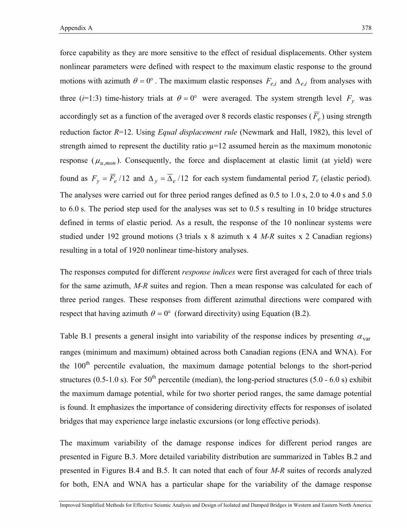
Appendix A 378
Improved Simplified Methods for Effective Seismic Analysis and Design of Isolated and Damped Bridges in Western and Eastern North America
force capability as they are more sensitive to the effect of residual displacements. Other system
nonlinear parameters were defined with respect to the maximum elastic response to the ground
motions with azimuth °= 0θ . The maximum elastic responses ieF , and ie,Δ from analyses with
three (i=1:3) time-history trials at °= 0θ were averaged. The system strength level yF was
accordingly set as a function of the averaged over 8 records elastic responses ( eF ) using strength
reduction factor R=12. Using Equal displacement rule (Newmark and Hall, 1982), this level of
strength aimed to represent the ductility ratio µ=12 assumed herein as the maximum monotonic
response ( monu,μ ). Consequently, the force and displacement at elastic limit (at yield) were
found as 12/ey FF = and 12/ey Δ=Δ for each system fundamental period Te (elastic period).
The analyses were carried out for three period ranges defined as 0.5 to 1.0 s, 2.0 to 4.0 s and 5.0
to 6.0 s. The period step used for the analyses was set to 0.5 s resulting in 10 bridge structures
defined in terms of elastic period. As a result, the response of the 10 nonlinear systems were
studied under 192 ground motions (3 trials x 8 azimuth x 4 M-R suites x 2 Canadian regions)
resulting in a total of 1920 nonlinear time-history analyses.
The responses computed for different response indices were first averaged for each of three trials
for the same azimuth, M-R suites and region. Then a mean response was calculated for each of
three period ranges. These responses from different azimuthal directions were compared with
respect that having azimuth °= 0θ (forward directivity) using Equation (B.2).
Table B.1 presents a general insight into variability of the response indices by presenting varα
ranges (minimum and maximum) obtained across both Canadian regions (ENA and WNA). For
the 100th percentile evaluation, the maximum damage potential belongs to the short-period
structures (0.5-1.0 s). For 50th percentile (median), the long-period structures (5.0 - 6.0 s) exhibit
the maximum damage potential, while for two shorter period ranges, the same damage potential
is found. It emphasizes the importance of considering directivity effects for responses of isolated
bridges that may experience large inelastic excursions (or long effective periods).
The maximum variability of the damage response indices for different period ranges are
presented in Figure B.3. More detailed variability distribution are summarized in Tables B.2 and
presented in Figures B.4 and B.5. It can noted that each of four M-R suites of records analyzed
for both, ENA and WNA has a particular shape for the variability of the damage response

Appendix A 379
Improved Simplified Methods for Effective Seismic Analysis and Design of Isolated and Damped Bridges in Western and Eastern North America
indices. The forward directivity effect ( °= 0θ ) on the amplification of damage potential appears
to be the least frequent, while the amplification of the damage potential observed at °= 90θ is
the most recurrent among the analyzed directions. The azimuth of 90° controls the maximum
damage ( maxvar =α ) in 50% and 58% of the cases analyzed for ENA and WNA, respectively.
The backward directivity ( °= 180θ ) appears to be decisive in 25% of the cases for the ENA
events and it has no critical incidence in the WNA analysis.
Table A.1 Range for the response indices studied (ENA and WNA)
Measures of Position Period Range Variation
50th Percentile
0.5 - 1.0 0.98 - 1.07
2.0 - 4.0 0.95 - 1.06
5.0 - 6.0 1.00 - 1.24
84th Percentile
0.5 - 1.0 1.00 - 1.54
2.0 - 4.0 1.03 - 1.35
5.0 - 6.0 1.05 - 2.26
100th Percentile
0.5 - 1.0 1.03 – 3.87
2.0 - 4.0 1.27 – 2.79
5.0 - 6.0 1.24 – 2.45
The shorter-period structures (0.5 - 1.0 s) subjected to the short-period distant events (M6 -
30 km - ENA and M6.5 - 30 km - WNA) presented the larger damage potential (ENA:
90.2var =α and WNA: 87.3var =α ). For median responses (50th percentile), the maximum
damage potentials are observed from a longer period range (5.0 - 6.0 s) for both ENA and WNA
(ENA - M7 - 30 km: 24.1var =α and WNA - M7 - 50 km: 09.1var =α ). In this case, the damage
potential is by 15% larger in ENA with respect to WNA. These observations put in evidence the
importance of considering for NLTHA different M-R suites that take into account the rupture
directivity effects.

Appendix A 380
Improved Simplified Methods for Effective Seismic Analysis and Design of Isolated and Damped Bridges in Western and Eastern North America
1.03
1.63
1.94
2.90
1.641.72
0.00
0.50
1.00
1.50
2.00
2.50
3.00
3.50
T=0.5‐1.0s T=2.0‐4.0s T=5.0‐6.0s
ENA ‐ M6.0 ‐ Non‐scaled Events
M6.0‐10km
M6.0‐30km
2.14
1.49
2.45
1.90
1.45 1.24
0.00
0.50
1.00
1.50
2.00
2.50
3.00
T=0.5‐1.0s T=2.0‐4.0s T=5.0‐6.0s
ENA ‐ M7.0 ‐ Non‐scaled Events
M7.0‐30km
M7.0‐50km
1.33 1.63 1.42
3.87
2.79
1.94
0.000.501.001.502.002.503.003.504.004.50
T=0.5‐1.0s T=2.0‐4.0s T=5.0‐6.0s
WNA ‐M6.5 ‐ Non‐scaled Events
M6.5‐10km
M6.5‐30km
1.091.27
1.321.29
1.33
1.88
0.00
0.50
1.00
1.50
2.00
T=0.5‐1.0s T=2.0‐4.0s T=5.0‐6.0s
WNA ‐M7.5 ‐ Non‐scaled Events
M7.5‐30km
M7.5‐50km
Figure A.3 Maximum (100th Percentile) variability of the damage response indices

Appendix A 381
Improved Simplified Methods for Effective Seismic Analysis and Design of Isolated and Damped Bridges in Western and Eastern North America
Table A.2 Variability of the damage response indices
Region
Events
Period Range T (s)
Response Variation Index (αvar)
50th 84th 100th
0.5 - 1.0 0.98 1.00 1.03
M6.0-10 km 2.0 - 4.0 1.06 1.33 1.63
5.0 - 6.0 1.06 1.35 1.94
0.5 - 1.0 1.02 1.53 2.90
M6.0-30 km 2.0 - 4.0 1.04 1.28 1.64
ENA 5.0 - 6.0 1.00 1.26 1.72
0.5 - 1.0 1.07 1.39 2.14
M7.0-30 km 2.0 - 4.0 1.00 1.14 1.49
5.0 - 6.0 1.24 2.26 2.45
0.5 - 1.0 1.05 1.54 1.90
M7.0-50 km 2.0 - 4.0 1.00 1.35 1.45
5.0 - 6.0 1.00 1.13 1.24
0.5 - 1.0 0.98 1.07 1.33
M6.5-10 km 2.0 - 4.0 1.04 1.26 1.63
5.0 - 6.0 1.00 1.05 1.42
0.5 - 1.0 1.00 1.27 3.87
M6.5-30 km 2.0 - 4.0 1.00 1.30 2.79
WNA 5.0 - 6.0 1.00 1.22 1.94
0.5 - 1.0 1.00 1.01 1.09
M7.5-30 km 2.0 - 4.0 0.95 1.03 1.27
5.0 - 6.0 1.00 1.27 1.32
0.5 - 1.0 1.00 1.13 1.29
M7.5-50 km 2.0 - 4.0 1.00 1.28 1.33
5.0 - 6.0 1.09 1.52 1.88

Appendix A 382
Improved Simplified Methods for Effective Seismic Analysis and Design of Isolated and Damped Bridges in Western and Eastern North America
Despite these observations, there is no definitive evidence that directivity effect is increasing
with period and magnitude as well as it is decreasing with distance such as it has been reported
by many researchers. This kind of discrepancy could not be explained by a simple effect of the
proximity to fault since the tendencies observed for the long-period distant events are simply
inversed for ENA and WNA.
100th
50th
84th
0.0
0.5
1.0
1.5
2.0
2.5
3.0
3.5
4.0
4.5
Variab
ility Inde
x, α
ENAM6.0‐30km
ENAM6.0‐10km
ENAM7.0‐30km
ENAM7.0‐50km
Figure A.4 ENA - Response Variability Index (αvar)
100th
50th
84th
0.0
0.5
1.0
1.5
2.0
2.5
3.0
3.5
4.0
4.5
Variab
ility Inde
x, α
WNAM6.0‐30km
WNAM6.0‐10km
WNAM7.0‐30km
WNAM7.0‐50km
Figure A.5 WNA - Response Variability Index (αvar)
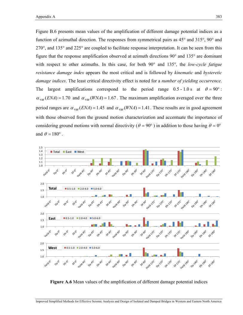
Appendix A 383
Improved Simplified Methods for Effective Seismic Analysis and Design of Isolated and Damped Bridges in Western and Eastern North America
Figure B.6 presents mean values of the amplification of different damage potential indices as a
function of azimuthal direction. The responses from symmetrical pairs as 45° and 315°, 90° and
270°, and 135° and 225° are coupled to facilitate response interpretation. It can be seen from this
figure that the response amplification observed at azimuth directions 90° and 135° are dominant
with respect to other azimuths. In this case, for both 90° and 135°, the low-cycle fatigue
resistance damage index appears the most critical and is followed by kinematic and hysteretic
damage indices. The least critical directivity effect is noted for a number of yielding occurrence.
The largest amplifications correspond to the period range 0.5 - 1.0 s at °= 90θ :
70.1)(var =ENAα and 67.1)(var =WNAα . The maximum amplification averaged over the three
period ranges are 45.1)(var =ENAα and 41.1)(var =WNAα . These results are in good agreement
with those observed from the ground motion characterization and accentuate the importance of
considering ground motions with normal directivity ( °= 90θ ) in addition to those having °= 0θ
and °= 180θ .
1.01.11.21.31.41.5
Total East West
1.0
1.5
2.0
Total 0.5‐1.0 2.0‐4.0 5.0‐6.0
1.0
1.5
2.0
East 0.5‐1.0 2.0‐4.0 5.0‐6.0
1.0
1.5
2.0
West 0.5‐1.0 2.0‐4.0 5.0‐6.0
Figure A.6 Mean values of the amplification of different damage potential indices