Embed Size (px)
Citation preview
IMPROVED LICENSE PLATE LOCALIZATION ALGORITHM BASED ON MORPHOLOGICAL OPERATIONS
A Thesis Submitted to the
College of Graduate and Postdoctoral Studies
in Partial Fulfillment of the Requirements
for the Degree of Master of Science
In the Department of Electrical and Computer Engineering
University of Saskatchewan
Saskatoon
By
Juan Yépez
Juan Yépez, July 2017. All rights reserved.
i
Permission to Use
In presenting this thesis in partial fulfilment of the requirements for a Postgraduate degree
from the University of Saskatchewan, I agree that the Libraries of this University may make
it freely available for inspection. I further agree that permission for copying of this thesis in
any manner, in whole or in part, for scholarly purposes may be granted by the professor or
professors who supervised my thesis work or, in their absence, by the Head of the Department
or the Dean of the College in which my thesis work was done. It is understood that any copying
or publication or use of this thesis or parts thereof for financial gain shall not be allowed
without my written permission. It is also understood that due recognition shall be given to me
and to the University of Saskatchewan in any scholarly use which may be made of any material
in my thesis.
Requests for permission to copy or to make other use of material in this thesis in whole or part
should be addressed to:
Head of the Department of Electrical and Computer Engineering
57 Campus Drive
University of Saskatchewan
Saskatoon, Saskatchewan
Canada
S7N 5A9
ii
Abstract
Automatic License Plate Recognition (ALPR) systems have become an important tool to
track stolen cars, access control, and monitor traffic. ALPR system consists of locating the
license plate in an image, followed by character detection and recognition. Since the license
plate can exist anywhere within an image, localization is the most important part of ALPR and
requires greater processing time. Most ALPR systems are computationally intensive and
require a high-performance computer. The proposed algorithm differs significantly from those
utilized in previous ALPR technologies by offering a fast algorithm, composed of structural
elements which more precisely conducts morphological operations within an image, and can
be implemented in portable devices with low computation capabilities. The proposed
algorithm is able to accurately detect and differentiate license plates in complex images. This
method was first tested through MATLAB with an on-line public database of Greek license
plates which is a popular benchmark used in previous works. The proposed algorithm was
100% accurate in all clear images, and achieved 98.45% accuracy when using the entire
database which included complex backgrounds and license plates obscured by shadow and
dirt. Second, the efficiency of the algorithm was tested in devices with low computational
processing power, by translating the code to Python, and was 300% faster than previous work.

iii
Acknowledgements
The compilation of this thesis would have been impossible without the love and support I
received from my lovely wife, Lucia. She stayed by my side during the many arduous and
sleepless nights. She was always my source of encouragement in difficult situations.
Thanks to God for the gift of life and special thanks for the lovely gift of my first son,
Anthony. He has been my source of motivation and joy each day.
I would also like to acknowledge and appreciate the guidance and constructive role played
by my supervisor, Dr. Seok-Bum Ko. Without his thoughtful insights, comments and patience
with me, this task would have been difficult to accomplish. He assisted me to see many new
perspectives in every draft that I presented to him. This has translated my view and broadened
my scope regarding this area. Thank you.
Sincere thanks to Suganthi, Hao, Zhexin, and Yi for assisting me throughout my Masters
program. I also extend my gratitude to all the ECE faculties for the important lessons regarding
this particular discipline.
I am also indebted to my family and friends who were so helpful. All they did may be too
much to mention on this piece. Special thanks to my mother, Cecilia, my sister, Andrea, and
my brother, Christian for their unwavering support. Last but not least, thanks to my father,
Juan, who is not with me physically but spiritually.
Thank you all so much.
iv
Contents
Permission to Use ................................................................................................................................... i
Abstract ................................................................................................................................................. ii
Acknowledgements ............................................................................................................................... iii
Contents ................................................................................................................................................ iv
List of Tables .......................................................................................................................................... vi
List of Figures ....................................................................................................................................... vii
List of Abbreviations ............................................................................................................................ viii
Chapter 1: Introduction ......................................................................................................................... 1
1.1 Previous Work ....................................................................................................................... 5
1.2 Motivation ............................................................................................................................ 12
1.3 Contribution ......................................................................................................................... 13
1.4 Organization of Thesis ......................................................................................................... 14
Chapter 2: Mathematical Morphology ................................................................................................ 15
2.1 Introduction .......................................................................................................................... 15
2.2 Structuring element .............................................................................................................. 18
2.3 Fundamental Morphological Operators ............................................................................... 19
2.3.1 Binary Dilation and Erosion ......................................................................................... 19
2.3.2 Greyscale Dilation and Erosion .................................................................................... 22
2.4 Morphological Filters .......................................................................................................... 25
2.4.1 Definitions ................................................................................................................... 25
2.4.2 Opening, Closing and Top-hat ..................................................................................... 25
2.4.3 Alternating Sequential Filters ...................................................................................... 32
2.5 Summary .............................................................................................................................. 32
Chapter 3: License Plate Localization Algorithm ............................................................................... 34
3.1. Pre-processing ...................................................................................................................... 35
3.2. License plate enhancement .................................................................................................. 37
3.3. Thresholding or Binarization process .................................................................................. 38
v
3.4. Noise Removal ..................................................................................................................... 42
3.5. Finding Contours ................................................................................................................. 44
3.6. Geometrical conditions ........................................................................................................ 47
3.7. Summary .............................................................................................................................. 49
Chapter 4: Determining the Appropriate Values in the SE ............................................................... 51
4.1 Determining the Appropriate Values in the SE ................................................................... 52
4.2 Analyzing Appropriate SE Values ....................................................................................... 58
4.3 The Appropriate SE Model .................................................................................................. 54
4.4 Conclusion ........................................................................................................................... 60
Chapter 5: Experiment Results .......................................................................................................... 61
5.1 Database ............................................................................................................................... 61
5.2 Appropriate SE results ......................................................................................................... 62
5.3 MATLAB Implementation and Results ............................................................................... 64
5.4 Low-Cost Devices Implementation and Results .................................................................. 66
5.5 Summary .............................................................................................................................. 69
Chapter 6: Conclusion ......................................................................................................................... 70
Chapter 7: Future Work ...................................................................................................................... 72
References .......................................................................................................................................... 73

vi
List of Tables
2.1 The pseudo code of dilation
2.2 The pseudo code of erosion
2.3 The pseudo code of opening
2.4 The pseudo code of closing
2.5 The pseudo code of top-hat
3.1 The pseudo code of threshold segmentation (Otsu’s method)
5.1 MediaLab sample sets and number of images in each set
5.2 Optimal SE for varying resolution images run on a PC.
5.3 Successful LPL rate by different sets
5.4 LPL localization rates and time comparisons
5.5 Average FPS of our algorithm versus that of Weber and Jung
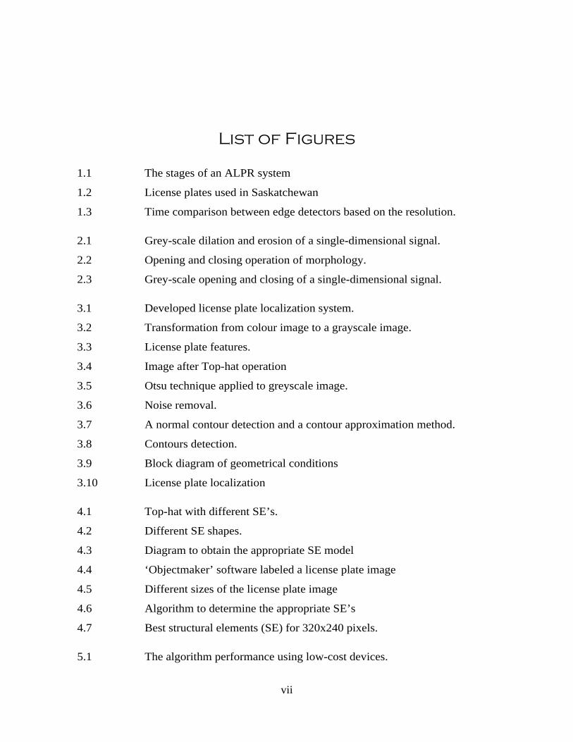
vii
List of Figures
1.1 The stages of an ALPR system
1.2 License plates used in Saskatchewan
1.3 Time comparison between edge detectors based on the resolution.
2.1 Grey-scale dilation and erosion of a single-dimensional signal.
2.2 Opening and closing operation of morphology.
2.3 Grey-scale opening and closing of a single-dimensional signal.
3.1 Developed license plate localization system.
3.2 Transformation from colour image to a grayscale image.
3.3 License plate features.
3.4 Image after Top-hat operation
3.5 Otsu technique applied to greyscale image.
3.6 Noise removal.
3.7 A normal contour detection and a contour approximation method.
3.8 Contours detection.
3.9 Block diagram of geometrical conditions
3.10 License plate localization
4.1 Top-hat with different SE’s.
4.2 Different SE shapes.
4.3 Diagram to obtain the appropriate SE model
4.4 ‘Objectmaker’ software labeled a license plate image
4.5 Different sizes of the license plate image
4.6 Algorithm to determine the appropriate SE’s
4.7 Best structural elements (SE) for 320x240 pixels.
5.1 The algorithm performance using low-cost devices.

viii
List of Abbreviations
ALPR Automatic License Plate Recognition
CCA Connected Component Analysis
ER Extremal region
FPGA Field Programmable Gate Arrays.
FPS Frames per second
FT Fourier Transform
GHz Gigahertz
Hv Horizontal value
LPL License Plate Localization
LNBD Last newly-found border
MSER Maximally Stable Extremal Regions
MM Mathematical Morphology
NBD Newly-found border
NTUA National Technical University of Athens
PASCAL Pattern Analysis, Statistical Modelling and Computational Learning
RAM Random Access Memory
RGB Red, Green and Blue
SE Structural Element
VEDA Vertical Edge Detection Algorithm
Vv Vertical value
WT Wavelet Transform

1
Chapter 1
Introduction
Automatic license plate recognition (ALPR) is a computer technology where an
optical device captures an image and this is then processed to obtain a string from a license
plate. The plate allows the identification of a particular vehicle used on the roads. This
system is significant for traffic and road monitoring systems. When checking the identities
of parties involved in road accidents, for instance, the initial step involves the location
and reading of the vehicle license plates. A suitable license plate localization mechanism
(locating the plate from the whole image) is very important for the efficiency of a fully-
computerized traffic monitoring system. This system mainly comprises of private parking
lot management, toll collection facilities, automatic traffic ticket issuing facilities, traffic
managing system, and security enforcement equipment or mechanism. Upon gathering
the requisite primary data, the system can be used to generate more secondary information
to facilitate more complex actions including vehicle travel time computations and border
control of traffic.
ALPR systems consists of three stages: license plate localization (LPL), character
segmentation, and optical character recognition (OCR) [1], [2]. LPL scans all of the pixels
within an image to detect and localize the position of a license plate. Character
segmentation is the stage where detection and separation of each character on a license
plate occurs. OCR receives the character’s information, validates, and encodes it to an
ASCII symbol as an alphabetic letter or number.
In every stage, there are certain parameters that have to be considered during the
design and preparation of the system. The first stage sees the usage of a camera to localize
the required image. It is however important to consider certain technical parameters when

2
settling on the type of camera to be used. These parameters include the camera resolution,
shutter speed, orientation, and light conditions. The second stage involves the character
segmentation which entails the tasks of projecting the color information of the plates,
labeling them and matching their position with the appropriate templates. Lastly, the
characters are matched with templates or other types of classifiers. Figure 1.1 outlines the
different steps demonstrated in the form of a flowchart. The preparation of an efficient
ALPR system requires the robust function of each step both individually and wholly as a
synchronization of all of the steps.
Figure 1.1 The stages of an ALPR system.
Various regions all over the world may impose certain standards for the vehicle license
plates systems and regulations. In some instances, vehicle owners may order for
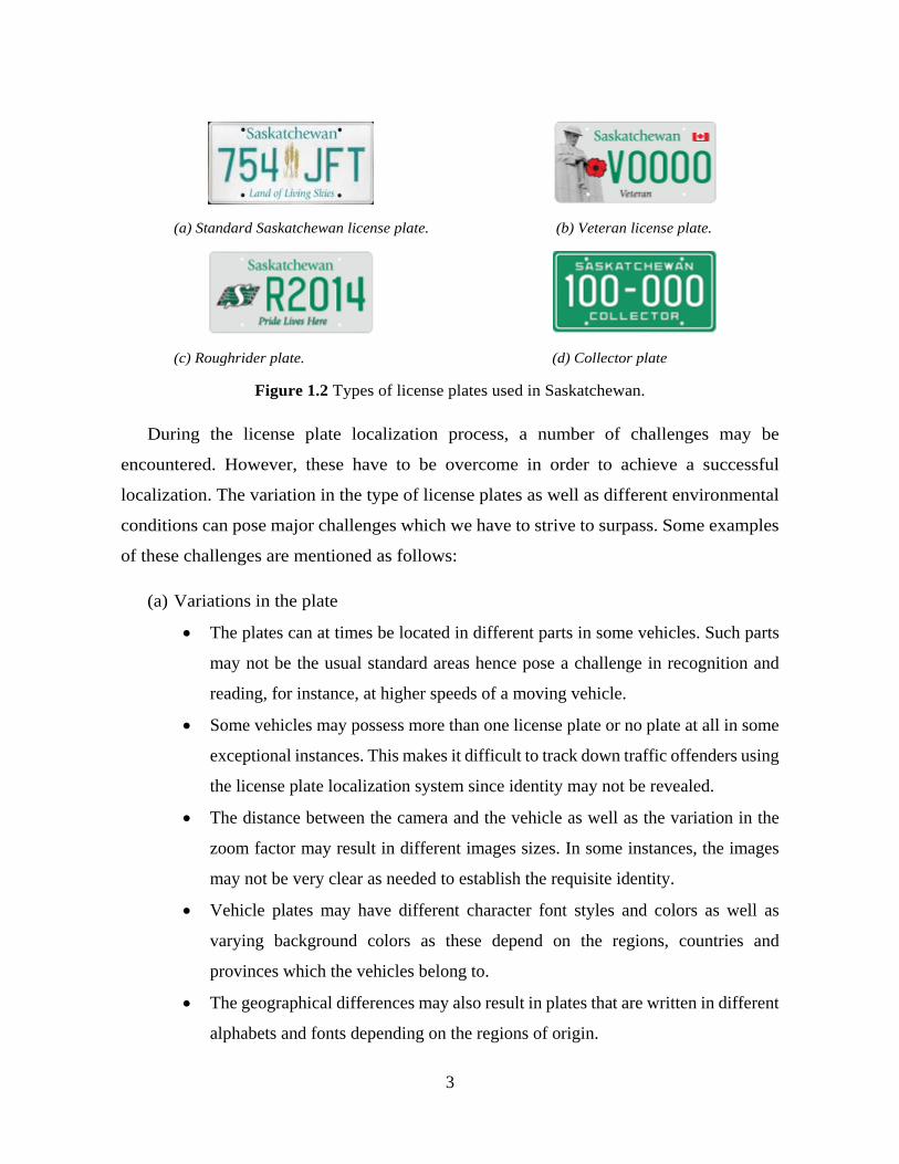
customized license plate that may come with different colours and designs. Figure 1.2
shows different types of license plates that are used in Saskatchewan.
License Plate Localization
Character Segmentation
Optical Character Recognition
3
(a) Standard Saskatchewan license plate. (b) Veteran license plate.
(c) Roughrider plate. (d) Collector plate
Figure 1.2 Types of license plates used in Saskatchewan.
During the license plate localization process, a number of challenges may be
encountered. However, these have to be overcome in order to achieve a successful
localization. The variation in the type of license plates as well as different environmental
conditions can pose major challenges which we have to strive to surpass. Some examples
of these challenges are mentioned as follows:
(a) Variations in the plate
• The plates can at times be located in different parts in some vehicles. Such parts
may not be the usual standard areas hence pose a challenge in recognition and
reading, for instance, at higher speeds of a moving vehicle.
• Some vehicles may possess more than one license plate or no plate at all in some
exceptional instances. This makes it difficult to track down traffic offenders using
the license plate localization system since identity may not be revealed.
• The distance between the camera and the vehicle as well as the variation in the
zoom factor may result in different images sizes. In some instances, the images
may not be very clear as needed to establish the requisite identity.
• Vehicle plates may have different character font styles and colors as well as
varying background colors as these depend on the regions, countries and
provinces which the vehicles belong to.
• The geographical differences may also result in plates that are written in different
alphabets and fonts depending on the regions of origin.
4
• In some states/provinces, we may encounter more than one plate style which also
poses a big challenge in identification.
• Plates may be difficult to read when they are covered with too much dirt. This
hampers the identification process due to lack of clarity
• When the license plates are tilted in some cases, localization proves difficult since
some tilted parts may not be clearly visible.
• Plates may contain additional elements like a frame or screws. These are foreign
elements as far as the localization process is concerned hence may distort the
required identities.
(b) Variation in the environment
• Environmental lighting and vehicle headlights may create varied illuminations
which may result in very different image inputs. This may pose a challenge on
proper identification.
• Presence of other elements similar to the plate patterns, for example, numbers
stamped on a vehicle, bumpers with vertical patterns, and textured backgrounds
may vitiate the image properties and location hence hindering correct
identification.
In order to successfully identify the required region of the image of the license plate,
a still/video camera is used in the capturing of the desired image. The camera should
averagely be able to capture the image at a resolution of 1024 × 768 pixels. The region of
interest which is the license plate area should account for a larger portion of the image,
roughly between 9% and 44% of the total image area. Scanning through the pixels to find
the license plates is a comparatively slower process. The stage which is crucial and takes
the most processing time is that of LPL. This fact of the more time taken to complete
processing motivated the development of the improved LPL algorithm with less
processing time. The algorithm presented in this thesis is therefore based on
morphological operations with a high and accurate detection rate suitable for low-cost
devices such as Raspberry Pi, Odroid or any other embedded platforms that make
localization less costly and also speed up the processing stage. For the foregoing reasons,
this thesis will concentrate on the process of localization which is the initial stage and not

5
the remaining two stages (character segmentation and optical character recognition)
which follows localization for a complete license recognition system. In future, remaining
two stages will be investigated.
1.1 Previous Work
The LPL influences the accuracy of an ALPR system. The input at this stage is a car
image, and the output is a portion of the image containing the potential license plate. The
license plate can be in any part of the image. Instead of processing every pixel of the
image, which increases the processing duration, the license plate can be distinguished by
its features such that the system processes only the pixels that have these distinct features.
These features are derived from the standard license plate format and the constituting
characters. The license plate color is one of the features since some jurisdictions (i.e.,
regions, countries, states, or provinces) have certain colors that are unique for
identification of their license plates. The rectangular shape of the license plate boundary
is another feature that distinguishes the license plate from other parts of the vehicle. The
color difference between the characters and the plate background, also known as the
texture, is also used to clearly separate the license plate region from the rest of the image.
Finally, the existence of the specific plate characters can also be used as a distinguishing
feature for the identification of the license plate region. In the following sections, we
categorize the various applicable LPL methods based on the features they employed in
detecting the license plate regions.
Edge detection algorithms find a rectangular shaped region with a known aspect ratio
and extracts all rectangles from within the image. This technique examines the changes
in pixel amplitudes to transform the grayscale image into an edge image. This method is
simple and fast but fails when challenged with complex images with several rectangular
features. The Sobel operator algorithm [3] is a filter used for edge detection to define the
boundary between two regions in a 2D image, with its kernel scanning in both a vertical
and horizontal axis [4]–[7]. Specifically, Sobel filter detects the transitions and intensities
in colour between a license plate and the car body and thus defines the edges of the license
6
plate. The Sobel filter algorithm can be set up to scan only horizontally, only vertically,
or as is most common, on both axis of an image [4], [6]. But in some cases, the Sobel scan
was in both the vertical and horizontal directions because a license plate exists on both y
and x axis. Some edge detection methods use Sobel operation to extract the license plate
information followed by noise reduction through the use of filters. The Canny operator
[8] uses Gaussian filter for smoothing or convolution and can work with images of varying
environmental conditions, distances and angles [9]. Unfortunately, since Sobel and Canny
are based on matrix multiplication, they need more processing power comparing with
other methods. Researchers and industry are interested in developing new algorithms that
are less complex but just as accurate and can perform on low processing power devices
without sacrificing computation time. For these reasons, a vertical edge detection
algorithm (VEDA) was developed in 2015 for license plate extraction [10]. VEDA is
faster than Sobel and Canny, but fails to detect license plates in blurred image and has not
been tested on low cost devices. A number of morphological detection systems are
presented in [1], and [11]–[17]. In [1], Zhai eliminates non-plate regions thereby selecting
the license plate. This mechanism is faster than the other edge methods. Zhai’s system
uses an open operation, followed by binarization and two morphological filters to enhance
the license plate region and is accurate with relatively clean images. However, there are
several drawbacks in Zhai’s system in that it did not use complex images which challenge
the algorithm. All previous edge detection systems are highly accurate and efficient but
are compromised when presented with complex images and were not designed to be used
in low cost devices.
Global image systems use connected component analysis (CCA) and are often used
for license plate detection in low resolution videos, including live feeds [9], [10], [18].
CCA algorithm scans a binary image and divides it into different components based on
pixel connectivity. A contour detection algorithm is applied to identify connected objects
based on their geometrical and spatial features such as area and aspect ratio, and are used
for license plate extraction. Global image information methods work reliably regardless
of the position of the license plate, but may generate license plates regions that are
7
incomplete because of the lack of pixel connectivity so that only a portion of a license
plate is detected [19].
Another ALPR technology utilizes textual features, which results in significant change
in the grayscale level between characters colour and license plate background colour, for
detecting the license plate. Texture based methods primarily use image transformation
tools because once an image is converted to a grey scale one so that the characters appear
in high density as compared to the background [20]. Gabor filters, which can differentiate
textures in unlimited orientations and scales, is one of the major tool for texture analysis
[21], [22]. However, a major drawback of Gabor filters is that they are time-consuming.
Another popular method is wavelet transform and is based on small wavelets with limited
duration [2], [23]–[25]. In this method, vertical features are extracted using wavelet
transform and the position parameters of the plate are determined by analyzing the
projection features in both the time and frequency domains.
Another texture detecting technology uses Haar-like methods for object detection
[22], [23], [26]. Haar-like methods classify size, colour, brightness and location of license
plates thereby aiding in the detection of characters on a plate. A more complex textural
method is that of the sliding concentric windows (SCW), and can detect the boundary
even if the license plate in the image is deformed [18]. The main disadvantage of textural
methods, however is that they require high computational power and are thus expensive.
Colour features methods exploit the differences in shapes and colour of the text versus
that of the background on a license plate in order to detect the license plate. The colour
modes used are red, green and blue (RGB), hue, lightness, and saturation (HLS), and hue,
saturation and value (HSV). One algorithm uses the RGB colour space to detect a license
plate and the characters on it [27]. In this method, the colour features were joined with
the grayscale features to eliminate the background so that the characters stood out and are
able to be detected. RGB, however, is limited by illumination conditions. HLS has also
been used for ALPR by determining the highest colour density, which typically are the
characters, from the license plate region [28]. A drawback of HLS is that it is
compromised with environmental conditions, such as an image being taken in the dark or
8
a reflection on a license plate. HSV methods are better able to deal with the problem of
illumination conditions and identifies the colour features of a license plate even when the
letter is inclined and deformed [29], [30]. When the colour information is extracted by the
license plate localization system, the average accuracy rate is at about 75%, a value which
is improved with comparison to the 69% accuracy when no plate information is used. A
higher improvement is observed for the green and blue colours. Similar to other colour
methods, HSV is limited by environmental conditions and also requires powerful
processing systems.
Character features methods examine the image for the existence of characters.
Assuming the characters are from the license plate region. These methods search for
characters in the image. If the characters are found, their region is extracted as the license
plate region. In [31], instead of using features of the license plate directly, the algorithm
finds all character-like regions in the image. These methods are robust to the rotation, but
they have to scan through the entire image. The maximally stable extremal regions
(MSER) was pioneered by Matas et al. [32]. According to Matas et al., MSER was applied
for wide baseline-stereo problems. For purposes of detection of license plates and other
traffic symbols, they employed the extremal region (ER) method in 2005 [33]. It can be
observed that the ER method they used is appropriate and stronger against size variations
and multi-orientations. This mechanism was later on improved in form of component trees
by Donoser et al. [34] and Nister et al. [35]. In their method, the duration and cost of
extraction was significantly reduced using the MSER.
Consequently, many researchers have used the MSER based method in the recent past
for detecting text in relatively complex scenes [36]–[38]. MSER is equally utilized by
character feature based algorithms in detection of license plates. This is possible through
its combination with morphology [39], the conditional random field model and minimum
spanning tree [40] or label-moveable clique [41]. Application of these mechanisms is
appropriate for facilitating a higher detection rate in simple scenes. Bai and Li’s method
is however not suitable for usage in more complex scenes because it fails to detect license
plates of multiple sizes. Gu’s method is also unable to discern the correct order of
9
characters in complex scenes [42]. It makes use of edge detection, morphology, and
MSER. It is also popular for its reduction of the computational cost of MSER extraction.
The method however remains sensitive to non-required edges and only deals with small
plate sizes. The foregoing methods are robust and appropriate for rotation although they
have to scan through the entire image. This translates into the disadvantages of time
consumption, and the risk of errors when more text types are present in the image.
A number of the mechanisms used usually look for two or more features of the license
number plate. These extraction mechanisms involved are known as hybrid extraction methods
[2], [28], [43]. Both the colour and texture features are combined in [44]–[47]. A duo-neural
networks in [48] is used to detect the texture feature as well as the colour feature. Each of
these neural networks is trained to perform its function with one detecting the color while the
other detects texture by utilizing the number of edges inside the plate area. Both the neural
networks’ outputs are combined to determine the candidate regions. In [45], only a single
neural network is employed in the process of scanning the image. This kind of scanning is
done using the H ×W window which is the same as license plate size. Subsequently, it is
possible to detect colour and edges within this window so as to come up with a needed
candidate. In [47], the neural network is used in the scanning of the HLS image horizontally
by the usage of a 1×M window. In this scenario, M is approximately the same as the
measurement of the license plate width. Scanning is also done vertically by the N×1 window.
In this case, N has the same measurement similar to that of the license plate height. The hue
value for every pixel represents the color data and the intensity represents the texture data.
Both outputs (the vertical and the horizontal scan) are brought together to enable the
determination of the desired candidate regions.
The time-delay neural network (TDNN), implemented in [46], is employed in the
extraction of plates. Double TDNNs are employed in the analysis of the color and texture of
the license plate through the examination of small windows of vertical and horizontal cross
sections of the image. In [49], the edge and the color data are combined to extract the plate.
High-edge density sections are taken as plates if their pixel values are similar to the license
plate. In [50], extraction through the covariance matrix takes place based on the statistical and
10
the spatial information of the license plate. The single covariance matrix extracted from a
particular region has adequate data which is able to match that region in various views. A
neural network that is trained on the covariance matrix of the license plate and non-license
plate regions is utilized in the detection of the license plate. In [51], the texture, rectangular,
and the colour features are all brought together as a combination to aid in the extraction of the
license plate. In this process, 1176 images were used having been taken from various scenes
and conditions. The success rate amounted to about 97.3%. In [52], a raster scan clip was used
as the input. The video had a low memory utilization. Gabor filter, threshold, and connected
component labeling were employed in the determination of the plate region. In [49], the
wavelet transform was applied in detection of the edges of the image. Upon the edge detection,
the morphology in that particular image was used to analyze the image shape and structure in
order to strengthen the structure so as to locate the license plate.
In [53], the mechanism relied upon used the HL sub-band feature of 2-D DWT twice so
as to substantially highlight the vertical edges of the license plates and to appropriately
suppress the background noise. Subsequently, the promising candidates of the license plates
were extracted. The extraction process saw the application of two methods namely the first-
order local recursive Otsu’s segmentation and orthogonal projection histogram analysis. In
this process, the edge density verification and aspect ratio constraint were used to select the
most probable candidate. In [54], local structure patterns computed from the modified census
transform was applied in detecting the license plate. In the subsequent step, a duo-part post-
processing was applied to minimize false positive rates. One of the duo is the position-based
mechanism which relies on the positional relation between a license plate and a possible false
positive with similar local structure patterns, such as headlights or radiators. The other one,
color-based method, applies the known color information of license plates.
In comparison to classical edge detection operators, the morphological edge detection
methods are the fastest methods for image processing. Therefore, morphological operators
are used for edge detection since they are fast and straightforward. Figure 1.3 shows the
time taken versus the resolution of a greyscale 2D image to detect edges using Top Hat,
Sobel, and the Canny methods. Initially, when the resolution is small the time processing
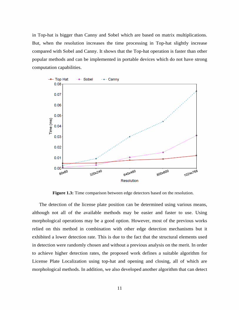
11
in Top-hat is bigger than Canny and Sobel which are based on matrix multiplications.
But, when the resolution increases the time processing in Top-hat slightly increase
compared with Sobel and Canny. It shows that the Top-hat operation is faster than other
popular methods and can be implemented in portable devices which do not have strong
computation capabilities.
Figure 1.3: Time comparison between edge detectors based on the resolution.
The detection of the license plate position can be determined using various means,
although not all of the available methods may be easier and faster to use. Using
morphological operations may be a good option. However, most of the previous works
relied on this method in combination with other edge detection mechanisms but it
exhibited a lower detection rate. This is due to the fact that the structural elements used
in detection were randomly chosen and without a previous analysis on the merit. In order
to achieve higher detection rates, the proposed work defines a suitable algorithm for
License Plate Localization using top-hat and opening and closing, all of which are
morphological methods. In addition, we also developed another algorithm that can detect
12
the best Structural Element (SE) which fits in a specific image resolution and a size of the
license plate image. Using morphological operations makes the system faster. On top of
that, it can also be implemented in any kind of device regardless of the processor or
memory capacities.
1.2 Motivation
The ALPR is an important computer vision technology that can be applied in many
real-life situations. Despite this fact, ALPR surprisingly still remains a private
technological aspect. This is mainly because ALPR fundamentally requires a high-
performance work station to localize and recognize the license plates. Generally, the
servers receive the video from the installed cameras via the network and not in the form
of a photo of the car and the license plate string. Also, to note is the fact that there are few
embedded cameras developed to recognize license plates and most of them only work in
certain geographical jurisdictions and environmental conditions. The cameras also require
a powerful processor to recognize license plates. Another shortcoming is posed by the
fact that there are no open source programs available to download so as to effect a proper
ALPR system. The available ones are commercial solutions which are often extremely
expensive. All these factors limit the usage of ALPR technology only to companies and
government institutions which are endowed with huge resource bases. Our motivation is
to achieve the extension of this technology to the general public and every individual
regardless of their financial situation. In this regard, we have strived to develop a license
plate localization system (which is the first step for ALPR). The system can be installed
on a Computer or any type of embedded devices including low-cost devices with a high
localization rate and exhibits a shorter processing time.
Our proposition is equally motivated by the numerous amounts of research and
recommendations in this area. We therefore strive to keenly address some of these rising
human needs. The proposed algorithm attempts to improve by coming up with a
comprehensive and efficient system that is can be specifically used in carrying out a faster
and affordable localization process. We significantly try to improve the rate of
13
localization. It is undeniable that license plate localization is a very crucial stage in an
ALPR system and it is also computationally intensive. The main motivation in this
connection thus is to develop a low complexity with high detection rate LPL algorithm
based on morphological operations together with an efficient multiplier less architecture
based on that algorithm. We will then try to implement the proposed algorithm on cheaper
devices. In this way, we can efficiently assist real users to track, identify and monitor
moving vehicles by automatically extracting their license plates. In the modern world
today, such systems are rapidly becoming used for a vast number of applications that are
truly important for the general well-being. Some of these applications are automatic
congestion charge systems, access control, tracing of stolen cars, and identification of
dangerous drivers. This research is thus motivated by the fact that such systems are
increasingly significant in law enforcement among other real-life scenarios.
1.3 Contribution
ALPR system is an important technology which is very useful for a variety of
applications. However, the commercial software systems are very expensive and
dependable of high cost computers or server, due to the processing of the video in real
time. LPL is the stage that consumes more processing time. This thesis is focused on LPL
and the main objective is developing a system that can reduce the computational
complexity with increased accuracy despite environmental challenges such as
illumination and plate orientation. The proposed software can highlight the license plate
while the background is removed using morphological operations. The morphological
operations will enhance the license plate and remove the noise in the background and the
noise inside the object.
The operators for a morphological operation are the image and the structural element
(SE). When the operation has the correct SE, the results make the system work with better
detection rate. Hence, we design a novel algorithm to detect the best structural elements
depending on the resolution of the screen. The SE will improve the detection rate on the
LPL algorithm.
14
The proposed algorithm is implemented in MATLAB. It is compared with previous
works for its accuracy and speed. To demonstrate that this system could run in low-cost
devices without issues, the code is rewritten in both Python and OpenCV. It is
subsequently implemented in low-cost devices so that the detection speed could be
measured and compared with other LPL’s in frames per second (FPS). In this process, a
video camera is used. This system allows users to identify vehicles by automatically
extracting their license plates. This is basically due to the fact that such a system is needed
for a vast number of applications including, security, access control, paid parking, tolling
and weight-in-motion industries.
1.4 Organization of Thesis
The subsequent chapters are organized as follows: Chapter 2 discusses mathematical
morphology in order to show the morphological operations that are used in image
processing; Chapter 3 presents the proposed license plate localization algorithm which is
suitable for low-cost devices; Chapter 4 presents a new algorithm that helps to determine
the appropriate values in the SE; Chapter 5 presents the experiment results and makes a
comparison to previous works that used the same database; Chapter 6 provides a
conclusion to the thesis; and finally Chapter 7 presents a proposition of potential future
works based on this thesis.
15
Chapter 2
Mathematical Morphology
The hypothesis and ability employed in the analysis and processing of geometrical
structures on the basis of lattice theory, topology, and random functions can be referred to as
Mathematical Morphology denoted by MM. MM mainly involves the particular shape of a
signal waveform in the time domain rather than the frequency one. This subject matter remains
completely distinct from other techniques which mainly depend upon the integral transform
that includes Wavelet Transform denoted by WT, and Fourier Transform denoted as FT, in
fundamental principles, algorithmic functions, and approach. It is important to note that
Mathematical Morphology is a non-linear theory as opposed to the linear ones of Wavelet
Transform and Fourier Transform. Chapter 2, therefore, introduces morphological operations
as far as signal processing is concerned in line with Mathematical Morphology theory. This
chapter goes further to break down, briefly, the fundamental concepts of this hypothesis, a
number of morphological operators, their characteristics, and functionalities.
2.1 Introduction
A brief historical background of the MM theory dates back to 1964 when it was
initially proposed by Matheron and Serra. These two were French researchers who majored in
solving tasks on petrography and mineralogy [55]. According to these researchers, the criteria
used to provide an analysis of binary images was based on simple operations like intersections,
unions, translations, and complementation. A major breakthrough followed in the year 1975
to further document the MM theory in the book, Random Sets and Integral Geometry [56]. It
is important to note that the development of the Mathematical Morphology theory has taken a
number of years which has ensured that MM becomes greatly significant in the field of image
processing and specifically as a needed tool for geometrical shape analysis.
16
For the past four decades or so, researchers have concentrated on the subject matter of
digital image analysis. The MM theory has consequently grown in terms of techniques and
applications. This has seen the formation of solid mechanisms like image segmentation and
classification, image filtering, pattern recognition, texture analysis and synthesis as well as
image measurements among others. On the other hand, optical character recognition and
document processing, materials science, visual inspection and quality control, life sciences
and geosciences have all formed part of the developed applications. These recognizable
developments have been documented by J. Serra and P. Soille in their milestone monographs
of 1982 [57] and 2003 [58] respectively.
MM is based on a complete lattice due to its mathematical foundations. It is, therefore,
important to understand the meaning of a complete lattice. However, it is worth noting and
expounding the concept of a partly ordered set (poset) before embarking on the former. The
latter can, therefore, be defined as a set that exhibits a binary relation (≤) for some pairs of
elements. This binary relation (≤) over P, therefore, proposes as follows for the elements x, y,
z ϵ P:
1. Reflexive: ∀ x, x ≤ x.
2. Antisymmetry: If x ≤ y and y ≤ x, then x = y.
3. Transitivity: If x ≤ y and y ≤ z, then x ≤ z.
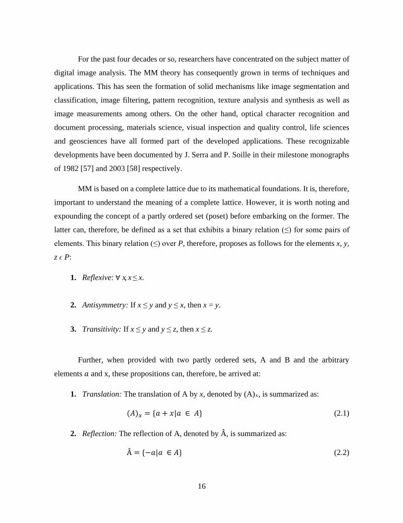
Further, when provided with two partly ordered sets, A and B and the arbitrary
elements 𝑎𝑎 and x, these propositions can, therefore, be arrived at:
1. Translation: The translation of A by x, denoted by (A)x, is summarized as:
(𝐴𝐴)𝑥𝑥 = {𝑎𝑎 + 𝑥𝑥|𝑎𝑎 ∈ 𝐴𝐴} (2.1)
2. Reflection: The reflection of A, denoted by Â, is summarized as:
 = {−𝑎𝑎|𝑎𝑎 ∈ 𝐴𝐴} (2.2)

17
3. Complement: The complement of A, denoted by Ac, is summarized as:
𝐴𝐴𝑐𝑐 = {𝑥𝑥|𝑥𝑥 ∉ 𝐴𝐴} (2.3)
4. Difference: The difference between two set A and B, denoted by A – B, is
summarized as:
𝐴𝐴 − 𝐵𝐵 = {𝑥𝑥|𝑥𝑥 ∈ 𝐴𝐴, 𝑥𝑥 ∉ 𝐵𝐵} = 𝐴𝐴 ∩ 𝐵𝐵𝑐𝑐 (2.4)
Based on the operation above, the complement of set A can also be summarized as:
𝐴𝐴𝑐𝑐 = {𝑥𝑥|𝑥𝑥 ∈ 𝐼𝐼 − 𝐴𝐴}, where I represents the universal set. (2.5)
Note: Reflection is also known as transposition.
Importantly, the set that is partially ordered supports the notion of an ordering relation,
which is a fundamental concept in Mathematical Morphology [58]. Also in existence is a total
ordering relation that has a stronger relation of ‘<’. This proposes that for any two elements x
and y, exactly one of x < y, x = y, x > y. It is equally true to say that the property of transitivity
on a totally ordered set becomes x < y and y < z which generally implies that x < z.
It can thus be concluded that a poset (P, ≤) qualifies to be a lattice where any two
elements of it, x and y, have the most significant lower bound, x ∧ y, and a least upper bound,
x ∨ y. A full lattice will, therefore, fulfill the following propositions for subsets X, Y and Z,
1. Commutativity: change in order of the operands does not change the result:
X ∨ Y = Y ∨ X, X ∧ Y = Y ∧ X (2.6)
2. Associativity: rearrange the parentheses in an expression will not change its value:
(X ∨ Y) ∨ Z = X ∨ (Y ∨ Z), (X ∧ Y) ∧ Z = X ∧ (Y ∧ Z). (2.7)
18
2.2 Structuring Element (SE)
A SE is a simple binary image that defines the neighborhood structures. The SE is used
to probe or interact with a particular image in order to conclude if that shape fits in the image
or otherwise. As a term used in mathematical morphology, it is denoted by SE. Choosing a
given SE will eventually influence the outcome of the affected morphological operation. The
following two major characteristics relate directly to SE:
(a) Shape. The SE may take various shapes. For instance, it may be ball-like or in form
of a line; convex or ring-like et cetera. Selecting a given SE will be able to assist one
to differentiate particular objects either fully or partly from others depending on their
specific shapes or spatial orientation.
(b) Size. Taking SE sizes of 3×3 or 21 ×21 squares for instance, one sets the observation
scale and subsequently determines the criterion for differentiating objects in the image
in terms of their sizes.
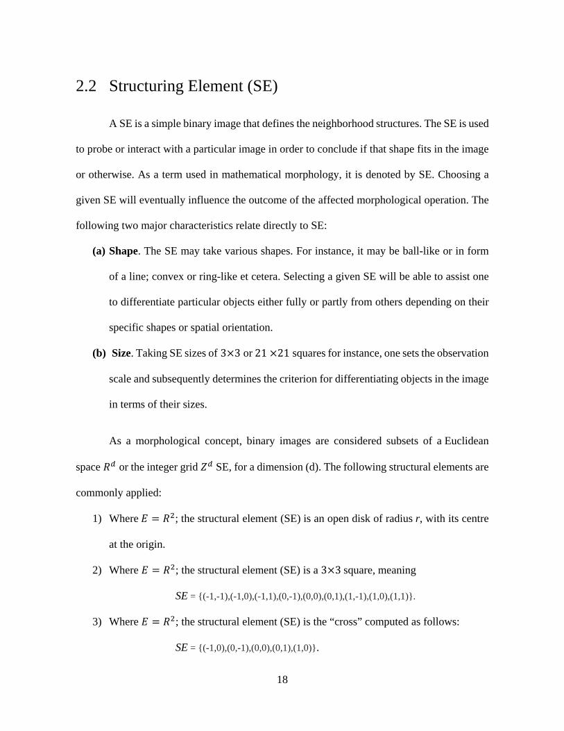
As a morphological concept, binary images are considered subsets of a Euclidean
space 𝑅𝑅𝑑𝑑 or the integer grid 𝑍𝑍𝑑𝑑 SE, for a dimension (d). The following structural elements are
commonly applied:
1) Where 𝐸𝐸 = 𝑅𝑅2; the structural element (SE) is an open disk of radius r, with its centre
at the origin.
2) Where 𝐸𝐸 = 𝑅𝑅2; the structural element (SE) is a 3×3 square, meaning
SE = {(-1,-1),(-1,0),(-1,1),(0,-1),(0,0),(0,1),(1,-1),(1,0),(1,1)}.
3) Where 𝐸𝐸 = 𝑅𝑅2; the structural element (SE) is the “cross” computed as follows:
SE = {(-1,0),(0,-1),(0,0),(0,1),(1,0)}.
19
A structural element can also be provided as a set of pixels on a grid in discrete cases,
assuming the values 1 or 0 where the pixel belongs to the SE or otherwise.
Two simple SEs can be generated through a hit-or-miss transform where the SE is
normally a composite of duo-disjoint sets (one associated to the foreground and the other to
the background of the given image to be probed).
2.3 Fundamental Morphological Operators
As a key role, morphological operators are meant to be applied in the extraction of
relevant structures of a particular set. This process occurs through the interaction of that
specific set with a SE. Here, some a priori information or knowledge concerning the shape of
the signal is used to actually predetermine the shape of the SE. In theory, a basic duo of
morphological operators (dilation and erosion) exists.
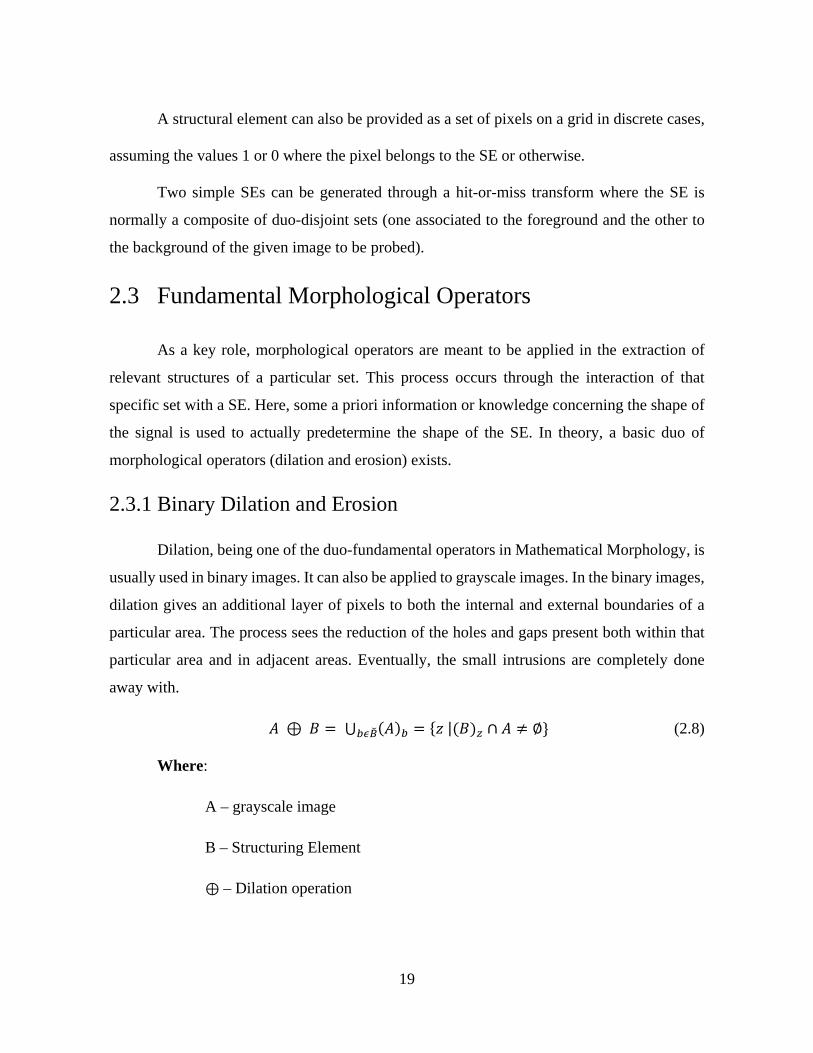
2.3.1 Binary Dilation and Erosion
Dilation, being one of the duo-fundamental operators in Mathematical Morphology, is
usually used in binary images. It can also be applied to grayscale images. In the binary images,
dilation gives an additional layer of pixels to both the internal and external boundaries of a
particular area. The process sees the reduction of the holes and gaps present both within that
particular area and in adjacent areas. Eventually, the small intrusions are completely done
away with.
𝐴𝐴 ⊕ 𝐵𝐵 = ⋃ (𝐴𝐴)𝑏𝑏𝑏𝑏𝑏𝑏𝐵𝐵� = {𝑧𝑧 |(𝐵𝐵)𝑧𝑧 ∩ 𝐴𝐴 ≠ ∅} (2.8)
Where:
A – grayscale image
B – Structuring Element
⊕ – Dilation operation
20
B is subsequently scanned over the image and maximal value extended is calculated, and the
pixels below the anchor point are substituted with the calculated maximum value.
Erosion is the other operator. Similar to dilation, this can be used in both binary and
grayscale images. The operator impact is to use the area boundaries. As a result, these areas
are reduced in size whereas the gaps and holes present in those particular areas are enlarged.
𝐴𝐴 ⊝ 𝐵𝐵 = ⋂ (𝐴𝐴)𝑏𝑏𝑏𝑏𝑏𝑏𝐵𝐵� = {𝑧𝑧 |(𝐵𝐵)𝑧𝑧 ⊆ 𝐴𝐴} (2.9)
Where:
A – grayscale image
B – Structuring Element
⊝ – Erosion operation
Upon scanning the SE over the image, a new image is formed by erosion.
Subsequently, the minimal value overlap calculated and the pixels under the anchor points are
substituted with that value.
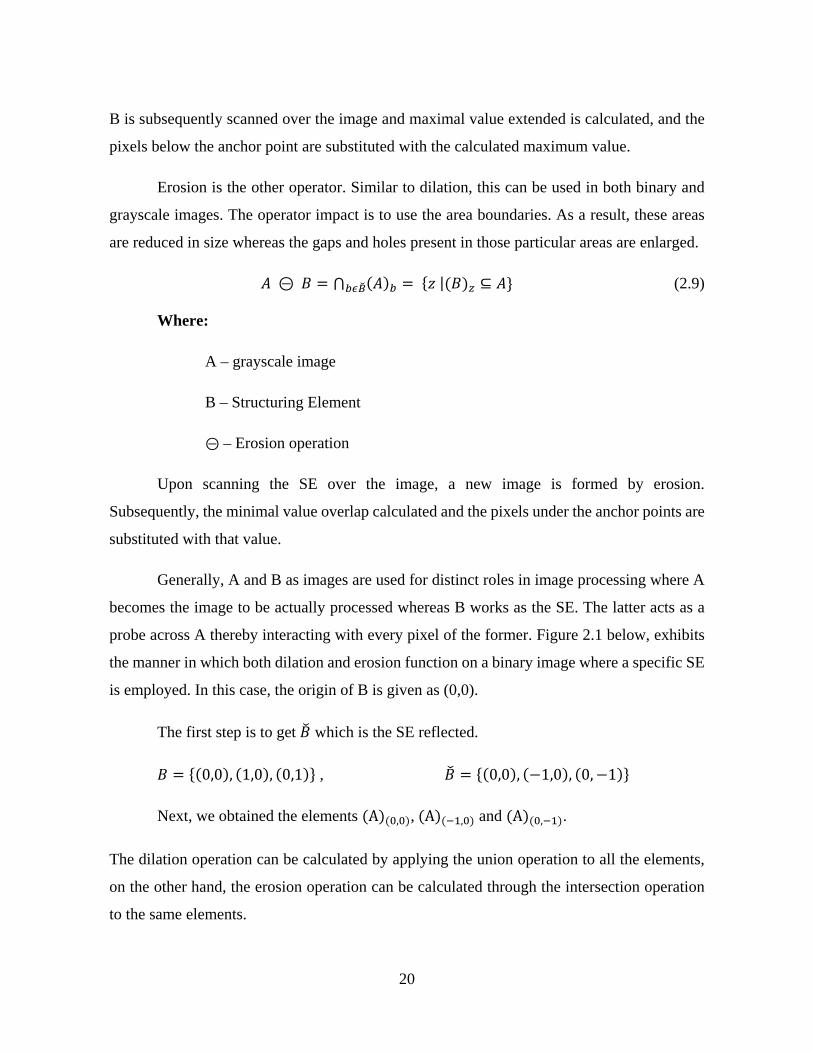
Generally, A and B as images are used for distinct roles in image processing where A
becomes the image to be actually processed whereas B works as the SE. The latter acts as a
probe across A thereby interacting with every pixel of the former. Figure 2.1 below, exhibits
the manner in which both dilation and erosion function on a binary image where a specific SE
is employed. In this case, the origin of B is given as (0,0).
The first step is to get 𝐵𝐵� which is the SE reflected.
𝐵𝐵 = {(0,0), (1,0), (0,1)} , 𝐵𝐵� = {(0,0), (−1,0), (0,−1)}
Next, we obtained the elements (A)(0,0), (A)(−1,0) and (A)(0,−1).
The dilation operation can be calculated by applying the union operation to all the elements,
on the other hand, the erosion operation can be calculated through the intersection operation
to the same elements.
21
Figure 2.1 Binary dilation and erosion of a binary image.
𝐴𝐴 (𝐴𝐴)(0,0)
(𝐴𝐴)(−1,0) (𝐴𝐴)(0,−1)
𝐴𝐴 ⊝ 𝐵𝐵 = (𝐴𝐴)(0,0) ∩ (𝐴𝐴)(−1,0) ∩ (𝐴𝐴)(0,−1) 𝐴𝐴 ⊕ 𝐵𝐵 = (𝐴𝐴)(0,0) ∪ (𝐴𝐴)(−1,0) ∪ (𝐴𝐴)(0,−1)
𝐵𝐵 = {(0,0), (1,0), (0,1)}
𝐵𝐵� = {(0,0), (−1,0), (0,−1)}
22
2.3.2 Greyscale Dilation and Erosion
When employing the theory of Mathematical Morphology in image processing in cases
where a majority of the signals non-binary, there is need to extend morphological operators to
the level of grey-scale. Subsequently, dilation and erosion are both performed through an
algebraic summation and subtraction rather than the union and intersection used for binary
images. Dilation and erosion can thus be summed up as follows:
𝑓𝑓 ⊕ 𝑔𝑔(𝑥𝑥) = max𝑠𝑠
{𝑓𝑓(𝑥𝑥 + 𝑠𝑠) + 𝑔𝑔(𝑠𝑠)|(𝑥𝑥 + 𝑠𝑠) ∈ 𝐷𝐷𝑓𝑓 , 𝑠𝑠 ∈ 𝐷𝐷𝑔𝑔} (2.10)
𝑓𝑓 ⊝ 𝑔𝑔(𝑥𝑥) = max𝑠𝑠
{𝑓𝑓(𝑥𝑥 + 𝑠𝑠) − 𝑔𝑔(𝑠𝑠)|(𝑥𝑥 + 𝑠𝑠) ∈ 𝐷𝐷𝑓𝑓 , 𝑠𝑠 ∈ 𝐷𝐷𝑔𝑔} (2.11)
Where:
f – signal,
g – SE, and the length of g is considerably shorter than that of f
Df, Dg – the definition domains of f and g, respectively.
Instinctively, we can imagine erosion to be a shrinking process whereas, on the other hand,
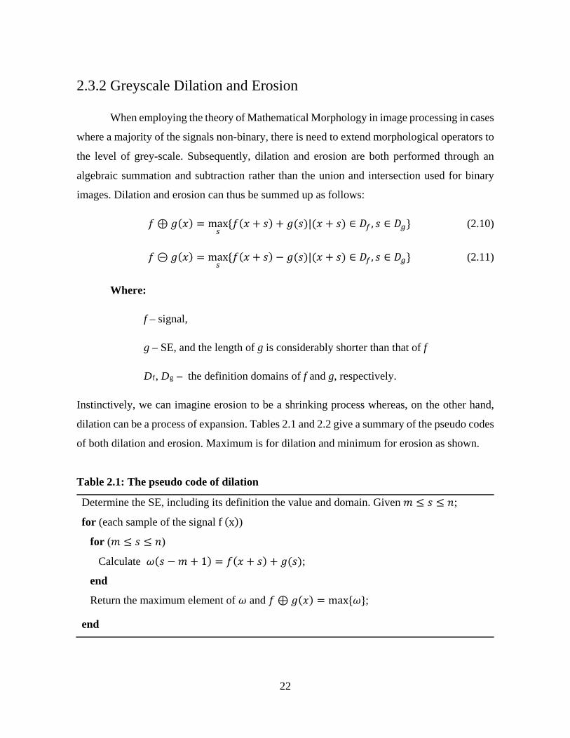
dilation can be a process of expansion. Tables 2.1 and 2.2 give a summary of the pseudo codes
of both dilation and erosion. Maximum is for dilation and minimum for erosion as shown.
Table 2.1: The pseudo code of dilation
Determine the SE, including its definition the value and domain. Given 𝑚𝑚 ≤ 𝑠𝑠 ≤ 𝑛𝑛;
for (each sample of the signal f (x))
for (𝑚𝑚 ≤ 𝑠𝑠 ≤ 𝑛𝑛)
Calculate 𝜔𝜔(𝑠𝑠 − 𝑚𝑚 + 1) = 𝑓𝑓(𝑥𝑥 + 𝑠𝑠) + 𝑔𝑔(𝑠𝑠);
end
Return the maximum element of 𝜔𝜔 and 𝑓𝑓 ⊕ 𝑔𝑔(𝑥𝑥) = max{𝜔𝜔};
end
23
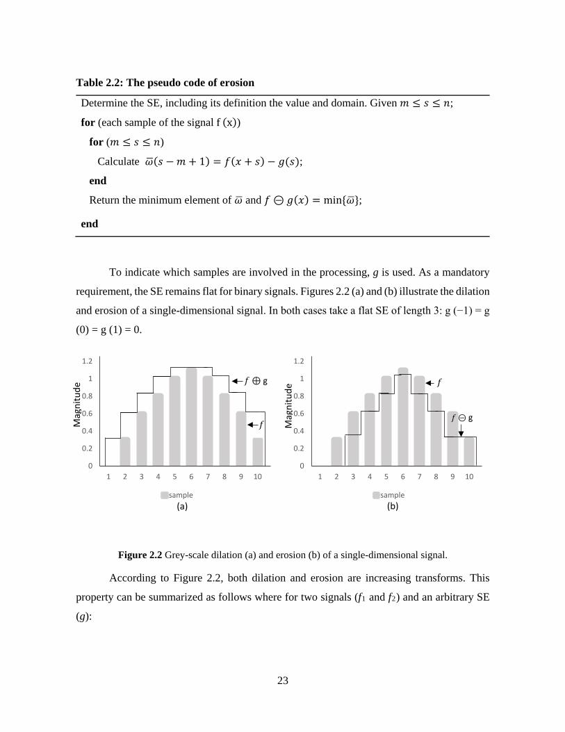
Table 2.2: The pseudo code of erosion
Determine the SE, including its definition the value and domain. Given 𝑚𝑚 ≤ 𝑠𝑠 ≤ 𝑛𝑛;
for (each sample of the signal f (x))
for (𝑚𝑚 ≤ 𝑠𝑠 ≤ 𝑛𝑛)
Calculate 𝜔𝜔�(𝑠𝑠 − 𝑚𝑚 + 1) = 𝑓𝑓(𝑥𝑥 + 𝑠𝑠) − 𝑔𝑔(𝑠𝑠);
end
Return the minimum element of 𝜔𝜔� and 𝑓𝑓 ⊝ 𝑔𝑔(𝑥𝑥) = min{𝜔𝜔�};
end
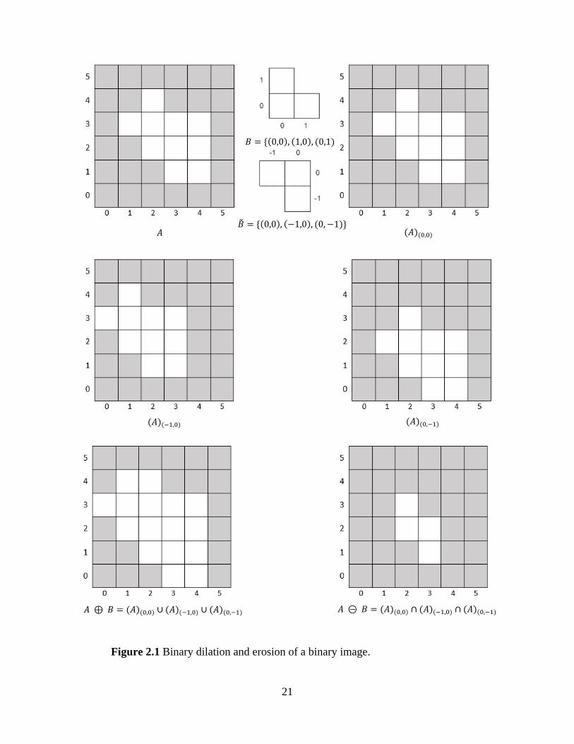
To indicate which samples are involved in the processing, g is used. As a mandatory
requirement, the SE remains flat for binary signals. Figures 2.2 (a) and (b) illustrate the dilation
and erosion of a single-dimensional signal. In both cases take a flat SE of length 3: g (−1) = g
(0) = g (1) = 0.
Figure 2.2 Grey-scale dilation (a) and erosion (b) of a single-dimensional signal.
According to Figure 2.2, both dilation and erosion are increasing transforms. This
property can be summarized as follows where for two signals (f1 and f2) and an arbitrary SE
(g):
0
0.2
0.4
0.6
0.8
1
1.2
1 2 3 4 5 6 7 8 9 10
sample
0
0.2
0.4
0.6
0.8
1
1.2
1 2 3 4 5 6 7 8 9 10
sample
Mag
nitu
de
Mag
nitu
de
(a) (b)
𝑓𝑓 ⊕ g
𝑓𝑓 𝑓𝑓 ⊝ g
𝑓𝑓
24
𝑓𝑓1 ≤ 𝑓𝑓2 → �𝑓𝑓1 ⊕ 𝑔𝑔 ≤ 𝑓𝑓2 ⊕ 𝑔𝑔𝑓𝑓1 ⊝ 𝑔𝑔 ≤ 𝑓𝑓2 ⊝ 𝑔𝑔 (2.12)
Also, the ordering relation between the two morphological operators can be said to be
the erosion of a signal by an SE which is less than or equal to its dilation where the SE remains
constant (f ⊝g ≤ f ⊕ g). In case the SE contains its origin that refers to the processing of a
sample of the signal within a window that contains the sample, the ordering will be expressed
as follows:
𝑓𝑓 ⊝𝑔𝑔 ≤ 𝑓𝑓 ≤ 𝑓𝑓 ⊕ 𝑔𝑔 (2.13)
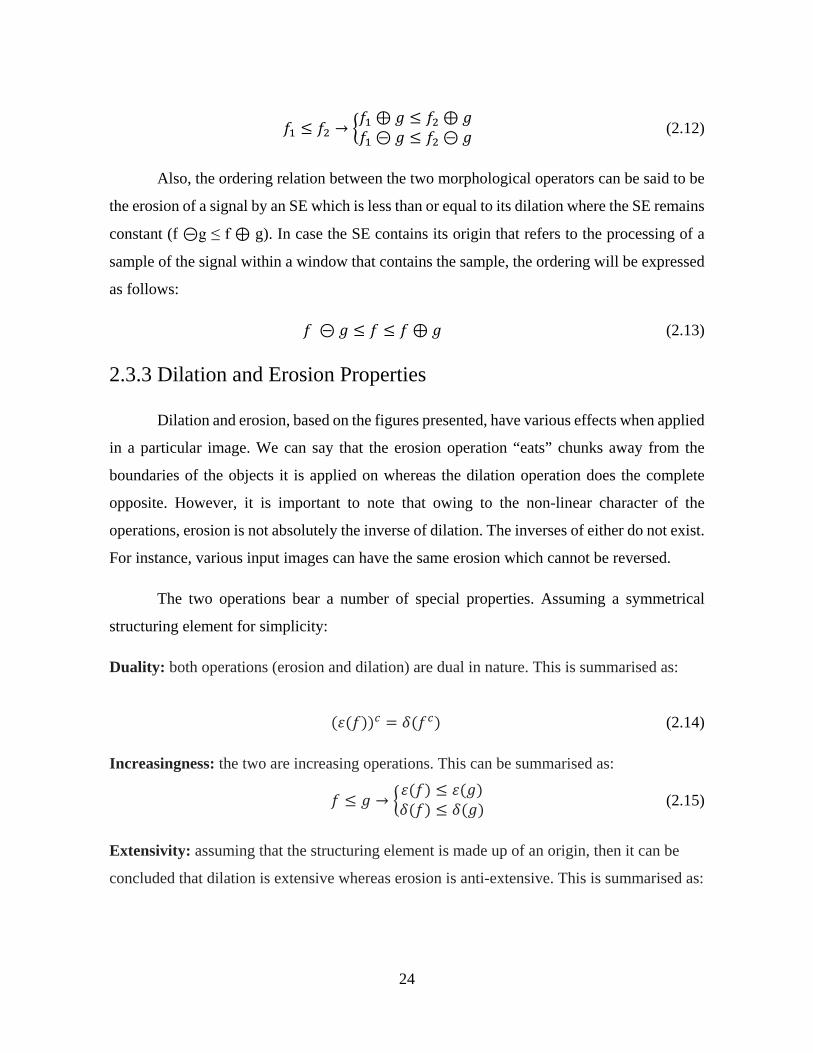
2.3.3 Dilation and Erosion Properties
Dilation and erosion, based on the figures presented, have various effects when applied
in a particular image. We can say that the erosion operation “eats” chunks away from the
boundaries of the objects it is applied on whereas the dilation operation does the complete
opposite. However, it is important to note that owing to the non-linear character of the
operations, erosion is not absolutely the inverse of dilation. The inverses of either do not exist.
For instance, various input images can have the same erosion which cannot be reversed.
The two operations bear a number of special properties. Assuming a symmetrical
structuring element for simplicity:
Duality: both operations (erosion and dilation) are dual in nature. This is summarised as:
(𝜀𝜀(𝑓𝑓))𝑐𝑐 = 𝛿𝛿(𝑓𝑓𝑐𝑐) (2.14)
Increasingness: the two are increasing operations. This can be summarised as:
𝑓𝑓 ≤ 𝑔𝑔 → �𝜀𝜀(𝑓𝑓) ≤ 𝜀𝜀(𝑔𝑔)𝛿𝛿(𝑓𝑓) ≤ 𝛿𝛿(𝑔𝑔) (2.15)
Extensivity: assuming that the structuring element is made up of an origin, then it can be
concluded that dilation is extensive whereas erosion is anti-extensive. This is summarised as:

25
0 ∈ 𝑆𝑆 → �𝜀𝜀(𝑓𝑓) ≤ 𝑓𝑓𝑓𝑓 ≤ 𝛿𝛿(𝑓𝑓) (2.16)
Separability: It is possible to separate the symmetrical structuring element in a single
dimensional part. The operations (erosion or dilation) can be performed using such a one-
dimensional part. This is summarised as:
𝑆𝑆 = 𝛿𝛿𝑆𝑆1(𝑆𝑆2) → �𝜀𝜀𝑆𝑆(𝑓𝑓) = 𝜀𝜀𝑆𝑆1(𝜀𝜀𝑠𝑠2(𝑓𝑓))𝛿𝛿𝑆𝑆(𝑓𝑓) = 𝛿𝛿𝑆𝑆1(𝛿𝛿𝑠𝑠2(𝑓𝑓)) (2.17)
2.4 Morphological Filters
2.4.1 Definitions
Morphological filters can be defined as a signal transformation that is characteristically
non-linear in nature and locally modifies the geometrical aspects of signals or images. It is
agreeable that the idempotence and increasing features are relevantly sufficient requirements
for a transform, ψ, to be a morphological filter thus:
ψ is a morphological filter ⇔ ψ is increasing and idempotent.
In a nutshell, idempotence property means double usage of a morphological filter on a
signal is equivalent to using it only once:
ψ is idempotent ⇔ ψψ =ψ.
It is worth noting that the increasing property guarantees the ordering relation on
signals is maintained after being filtered where the SE is kept constant.
2.4.2 Opening and Closing operations
The opening operator performs dilation on a sigmal eroded by the same structural
element. It is summarized as:

26
𝑓𝑓 ∘ 𝑔𝑔 = (𝑓𝑓 ⊖ 𝑔𝑔) ⊕𝑔𝑔 (2.18)
Where:
f – signal
g – SE, and
◦ is the opening operator.
This operator can recover a majority of the structures lost through erosion. An
exception only exists for those structures that were absolutely erased by erosion. Its
counterpart, Closing can be summarized as follows:
𝑓𝑓 ⦁ 𝑔𝑔 = (𝑓𝑓 ⊕ 𝑔𝑔) ⊖𝑔𝑔 (2.19)
Where:
f – signal
g – SE, and
⦁ is the closing operator.
It is also common to see opening and closing denoted by the operators γ and φ,
respectively. Table 2.3 shows the pseudo code of opening whereas Table 2.4 shows that of
closing.
Table 2.3: The pseudo code of opening
Determine the SE, including its definition the value and domain. Given 𝑚𝑚 ≤ 𝑠𝑠 ≤ 𝑛𝑛;
for (each sample of the signal f (x)) for (𝑚𝑚 ≤ 𝑠𝑠 ≤ 𝑛𝑛) Calculate 𝜔𝜔�(𝑠𝑠 − 𝑚𝑚 + 1) = 𝑓𝑓(𝑥𝑥 + 𝑠𝑠) + 𝑔𝑔(𝑠𝑠); end Return the minimum element of 𝜔𝜔� and 𝜀𝜀(𝑥𝑥) = min{𝜔𝜔�}; end for (each sample of the signal 𝜀𝜀(𝑥𝑥))
27
for (𝑚𝑚 ≤ 𝑠𝑠 ≤ 𝑛𝑛) Calculate 𝜔𝜔(𝑠𝑠 − 𝑚𝑚 + 1) = 𝜀𝜀(𝑥𝑥 + 𝑠𝑠) − 𝑔𝑔(𝑠𝑠); end Return the maximum element of 𝜔𝜔 and 𝛾𝛾(𝑥𝑥) = max{𝜔𝜔}; end
Table 2.4: The pseudo code of closing
Determine the SE, including its definition the value and domain. Given 𝑚𝑚 ≤ 𝑠𝑠 ≤ 𝑛𝑛;
for (each sample of the signal f (x)) for (𝑚𝑚 ≤ 𝑠𝑠 ≤ 𝑛𝑛) Calculate 𝜔𝜔(𝑠𝑠 − 𝑚𝑚 + 1) = 𝑓𝑓(𝑥𝑥 + 𝑠𝑠) + 𝑔𝑔(𝑠𝑠); end Return the maximum element of 𝜔𝜔 and 𝛿𝛿(𝑥𝑥) = max{𝜔𝜔}; end for (each sample of the signal 𝛿𝛿(𝑥𝑥)) for (𝑚𝑚 ≤ 𝑠𝑠 ≤ 𝑛𝑛) Calculate 𝜔𝜔�(𝑠𝑠 − 𝑚𝑚 + 1) = 𝜀𝜀(𝑥𝑥 + 𝑠𝑠) − 𝑔𝑔(𝑠𝑠); end Return the minimum element of 𝜔𝜔� and 𝜑𝜑(𝑥𝑥) = max{𝜔𝜔}; end
Note: Morphological opening and closing are both increasing transforms thus:
𝑓𝑓1 ≤ 𝑓𝑓2 → �𝛾𝛾(𝑓𝑓1) ≤ 𝛾𝛾(𝑓𝑓2)
𝜑𝜑(𝑓𝑓1) ≤ 𝜑𝜑(𝑓𝑓2) (2.20)
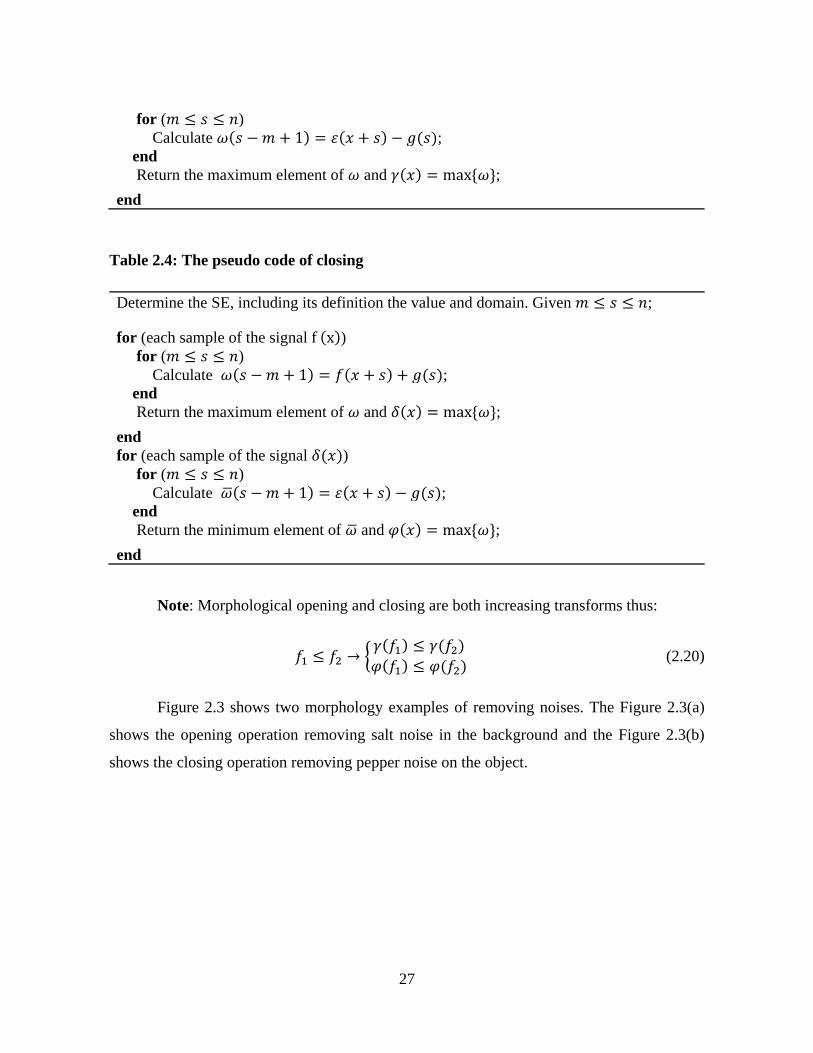
Figure 2.3 shows two morphology examples of removing noises. The Figure 2.3(a)
shows the opening operation removing salt noise in the background and the Figure 2.3(b)
shows the closing operation removing pepper noise on the object.
28
(a) opening operation
(b) closing operation
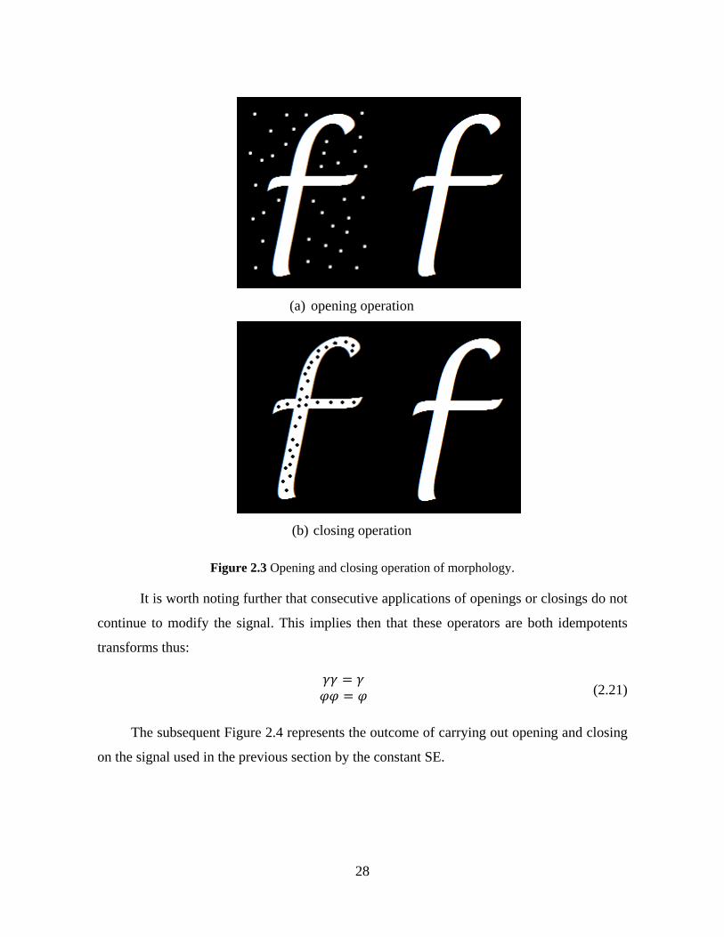
Figure 2.3 Opening and closing operation of morphology.
It is worth noting further that consecutive applications of openings or closings do not
continue to modify the signal. This implies then that these operators are both idempotents
transforms thus:
𝛾𝛾𝛾𝛾 = 𝛾𝛾𝜑𝜑𝜑𝜑 = 𝜑𝜑 (2.21)
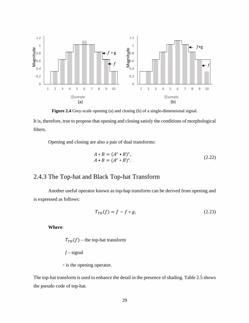
The subsequent Figure 2.4 represents the outcome of carrying out opening and closing
on the signal used in the previous section by the constant SE.
29
Figure 2.4 Grey-scale opening (a) and closing (b) of a single-dimensional signal.
It is, therefore, true to propose that opening and closing satisfy the conditions of morphological
filters.
Opening and closing are also a pair of dual transforms:
𝐴𝐴 ∘ 𝐵𝐵 = (𝐴𝐴𝑐𝑐 ⦁ 𝐵𝐵)𝑐𝑐 ,𝐴𝐴 ⦁ 𝐵𝐵 = (𝐴𝐴𝑐𝑐 ∘ 𝐵𝐵)𝑐𝑐 . (2.22)
2.4.3 The Top-hat and Black Top-hat Transform
Another useful operator known as top-hap transform can be derived from opening and
is expressed as follows:
𝑇𝑇𝑇𝑇𝑇𝑇(𝑓𝑓) = 𝑓𝑓 − 𝑓𝑓 ∘ 𝑔𝑔, (2.23)
Where:
𝑇𝑇𝑇𝑇𝑇𝑇(𝑓𝑓) – the top-hat transform
f – signal
◦ is the opening operator.
The top-hat transform is used to enhance the detail in the presence of shading. Table 2.5 shows
the pseudo code of top-hat.
0
0.2
0.4
0.6
0.8
1
1.2
1 2 3 4 5 6 7 8 9 10
sample
0
0.2
0.4
0.6
0.8
1
1.2
1 2 3 4 5 6 7 8 9 10
sample
𝑓𝑓 ∘ g
𝑓𝑓
𝑓𝑓⦁g
𝑓𝑓 Mag
nitu
de
Mag
nitu
de
(a) (b)

30
Table 2.5: The pseudo code of top-hat
Determine the SE, including its definition the value and domain. Given 𝑚𝑚 ≤ 𝑠𝑠 ≤ 𝑛𝑛;
for (each sample of the signal f (x)) for (𝑚𝑚 ≤ 𝑠𝑠 ≤ 𝑛𝑛) Calculate 𝜔𝜔�(𝑠𝑠 − 𝑚𝑚 + 1) = 𝑓𝑓(𝑥𝑥 + 𝑠𝑠) + 𝑔𝑔(𝑠𝑠); end Return the minimum element of 𝜔𝜔� and 𝜀𝜀(𝑥𝑥) = min{𝜔𝜔�}; end for (each sample of 𝜀𝜀(𝑥𝑥)) for (𝑚𝑚 ≤ 𝑠𝑠 ≤ 𝑛𝑛) Calculate 𝜔𝜔(𝑠𝑠 − 𝑚𝑚 + 1) = 𝜀𝜀(𝑥𝑥 + 𝑠𝑠) − 𝑔𝑔(𝑠𝑠); end Return the maximum element of 𝜔𝜔 and 𝛾𝛾(𝑥𝑥) = max{𝜔𝜔}; end Calculate and return 𝑇𝑇𝑇𝑇𝑇𝑇(𝑓𝑓) = 𝑓𝑓(𝑥𝑥) − 𝛾𝛾(𝑥𝑥)
Figure 2.3 shows examples of top-hat morphology where the SE is a small circle.
Subsequently, all the small circles are maintained within the image.
Figure 2.3 Top-hat operation of morphology.
The top-hat transform has an operator counterpart which is known as the black top-hat
filter (T∗ (f)). The black top-hat filter is defined by the residue of closing and the original:
𝑇𝑇𝐵𝐵𝑇𝑇𝑇𝑇(𝑓𝑓) = (𝑓𝑓 ⦁ 𝑔𝑔) − 𝑓𝑓, (2.24)

31
Whereas the top-hat transform is useful for the process of extracting small “white”
structures with relatively larger grey values compared to the background, the black top-hat
filter is significant for the extraction of small darker structures which may be mainly holes and
cavities. It is important to note that the top-hat transform and the black top-hat filters are both
idempotent.
Figure 2.4 Black Top-hat operation of morphology.
Table 2.6: The pseudo code of black top-hat
Determine the SE, including its definition the value and domain. Given 𝑚𝑚 ≤ 𝑠𝑠 ≤ 𝑛𝑛;
for (each sample of the signal f (x)) for (𝑚𝑚 ≤ 𝑠𝑠 ≤ 𝑛𝑛) Calculate 𝜔𝜔(𝑠𝑠 − 𝑚𝑚 + 1) = 𝑓𝑓(𝑥𝑥 + 𝑠𝑠) + 𝑔𝑔(𝑠𝑠); end Return the maximum element of 𝜔𝜔 and 𝛿𝛿(𝑥𝑥) = max{𝜔𝜔}; end for (each sample of the signal 𝛿𝛿(𝑥𝑥)) for (𝑚𝑚 ≤ 𝑠𝑠 ≤ 𝑛𝑛) Calculate 𝜔𝜔�(𝑠𝑠 − 𝑚𝑚 + 1) = 𝜀𝜀(𝑥𝑥 + 𝑠𝑠) − 𝑔𝑔(𝑠𝑠); End Return the minimum element of 𝜔𝜔� and 𝜑𝜑(𝑥𝑥) = max{𝜔𝜔}; end Calculate and return 𝑇𝑇𝐵𝐵𝑇𝑇𝑇𝑇(𝑓𝑓) = 𝜑𝜑(𝑥𝑥) − 𝑓𝑓(𝑥𝑥)
32
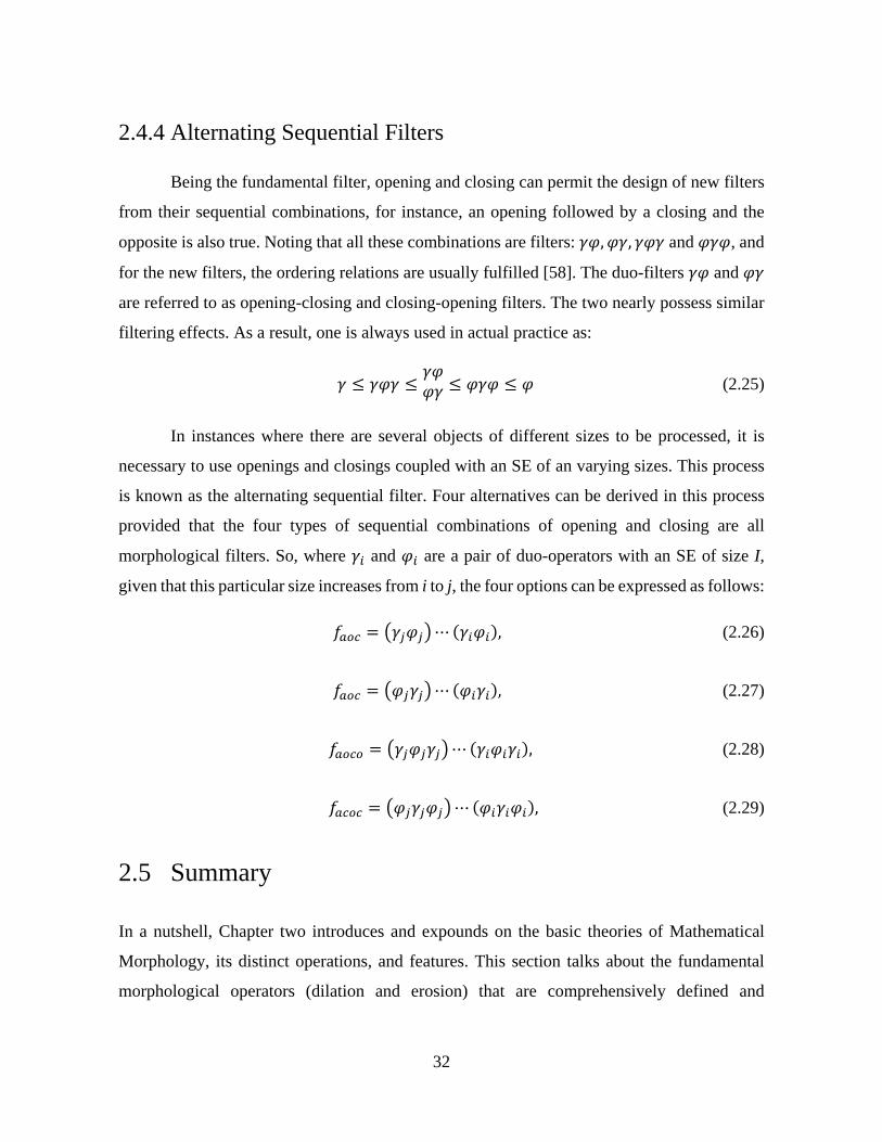
2.4.4 Alternating Sequential Filters
Being the fundamental filter, opening and closing can permit the design of new filters
from their sequential combinations, for instance, an opening followed by a closing and the
opposite is also true. Noting that all these combinations are filters: 𝛾𝛾𝜑𝜑,𝜑𝜑𝛾𝛾, 𝛾𝛾𝜑𝜑𝛾𝛾 and 𝜑𝜑𝛾𝛾𝜑𝜑, and
for the new filters, the ordering relations are usually fulfilled [58]. The duo-filters 𝛾𝛾𝜑𝜑 and 𝜑𝜑𝛾𝛾
are referred to as opening-closing and closing-opening filters. The two nearly possess similar
filtering effects. As a result, one is always used in actual practice as:
𝛾𝛾 ≤ 𝛾𝛾𝜑𝜑𝛾𝛾 ≤𝛾𝛾𝜑𝜑𝜑𝜑𝛾𝛾 ≤ 𝜑𝜑𝛾𝛾𝜑𝜑 ≤ 𝜑𝜑 (2.25)
In instances where there are several objects of different sizes to be processed, it is
necessary to use openings and closings coupled with an SE of an varying sizes. This process
is known as the alternating sequential filter. Four alternatives can be derived in this process
provided that the four types of sequential combinations of opening and closing are all
morphological filters. So, where 𝛾𝛾𝑖𝑖 and 𝜑𝜑𝑖𝑖 are a pair of duo-operators with an SE of size I,
given that this particular size increases from i to j, the four options can be expressed as follows:
𝑓𝑓𝑎𝑎𝑎𝑎𝑐𝑐 = �𝛾𝛾𝑗𝑗𝜑𝜑𝑗𝑗�⋯ (𝛾𝛾𝑖𝑖𝜑𝜑𝑖𝑖), (2.26)
𝑓𝑓𝑎𝑎𝑎𝑎𝑐𝑐 = �𝜑𝜑𝑗𝑗𝛾𝛾𝑗𝑗�⋯ (𝜑𝜑𝑖𝑖𝛾𝛾𝑖𝑖), (2.27)
𝑓𝑓𝑎𝑎𝑎𝑎𝑐𝑐𝑎𝑎 = �𝛾𝛾𝑗𝑗𝜑𝜑𝑗𝑗𝛾𝛾𝑗𝑗�⋯ (𝛾𝛾𝑖𝑖𝜑𝜑𝑖𝑖𝛾𝛾𝑖𝑖), (2.28)
𝑓𝑓𝑎𝑎𝑐𝑐𝑎𝑎𝑐𝑐 = �𝜑𝜑𝑗𝑗𝛾𝛾𝑗𝑗𝜑𝜑𝑗𝑗�⋯ (𝜑𝜑𝑖𝑖𝛾𝛾𝑖𝑖𝜑𝜑𝑖𝑖), (2.29)
2.5 Summary
In a nutshell, Chapter two introduces and expounds on the basic theories of Mathematical
Morphology, its distinct operations, and features. This section talks about the fundamental
morphological operators (dilation and erosion) that are comprehensively defined and
33
explained in two phases (binary and in greyscale). The operators are broken down in complete
detail to bring a succinct understanding of their properties and be able to apply this knowledge
further in the concept of morphological filtering (opening and closing). As per this chapter’s
contents, the computation involved in morphological operations are only limited to addition
and subtraction, and maximum and minimum operations. It is important to keenly note that no
multiplication or division exists. Comparatively, MM uses a significantly smaller size of the
sampling window in actual real-time signal processing. This relatively differs from integral
transform-based algorithms which will need a longer period of the signal in order to secure
distinct features. MM is consequently applicable to non-periodic transient and is not only
limited to periodic signals.
34
Chapter 3
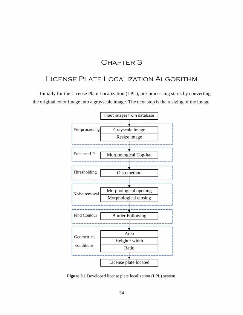
License Plate Localization Algorithm
Initially for the License Plate Localization (LPL), pre-processing starts by converting
the original color image into a grayscale image. The next step is the resizing of the image.
Figure 3.1 Developed license plate localization (LPL) system.
Input images from database
Grayscale image Resize image
Morphological Top-hat
Otsu method
Morphological opening Morphological closing
Border Following
Area Height / width
Ratio
License plate located
Pre-processing
Enhance LP
Thresholding
Noise removal
Find Contour
Geometrical
conditions
35
This is then followed by enhancing the license plate through the Top-hat morphology
transformation. Then, binary thresholding is applied by employing the Otsu method. The
next step is noise removal using closing and opening morphology features. Finally, the
last step sees the extraction of the license plate candidates by finding appropriate contours
and validating them against geometrical conditions. The overview of the developed LPL
method is summarized in Figure 3.1.
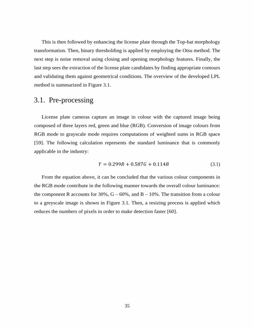
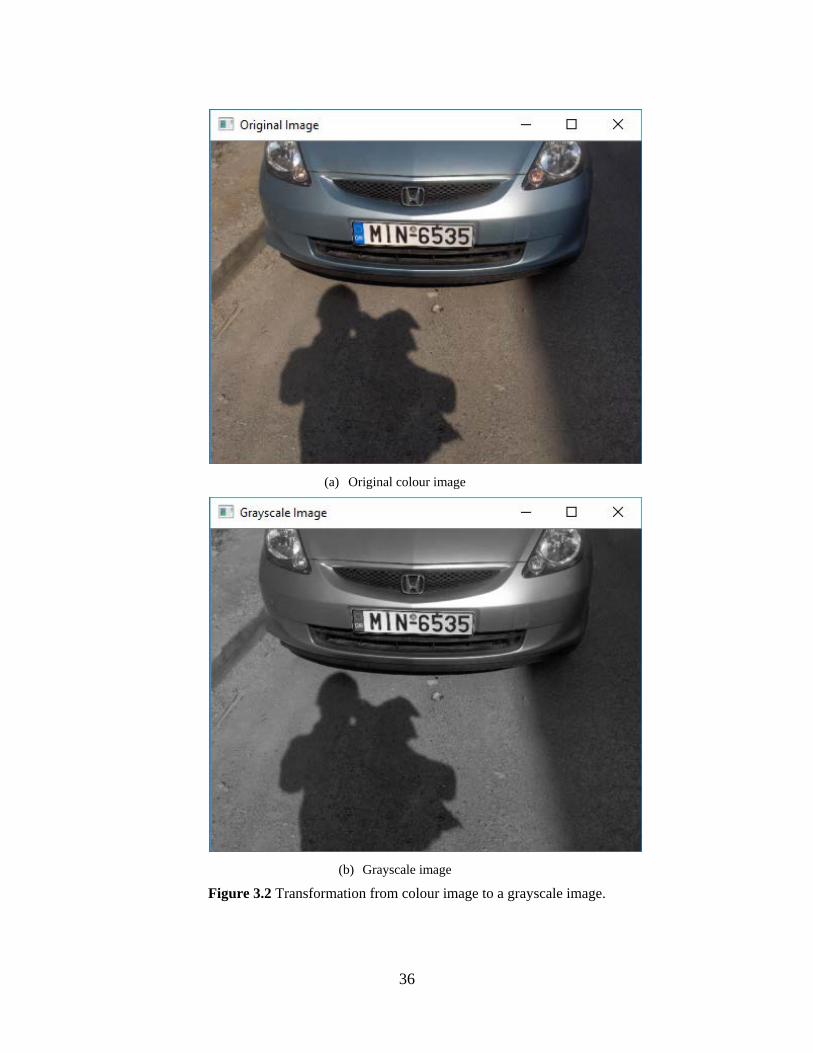
3.1. Pre-processing
License plate cameras capture an image in colour with the captured image being
composed of three layers red, green and blue (RGB). Conversion of image colours from
RGB mode to grayscale mode requires computations of weighted sums in RGB space
[59]. The following calculation represents the standard luminance that is commonly
applicable in the industry:
𝑌𝑌 = 0.299𝑅𝑅 + 0.587𝐺𝐺 + 0.114𝐵𝐵 (3.1)
From the equation above, it can be concluded that the various colour components in
the RGB mode contribute in the following manner towards the overall colour luminance:
the component R accounts for 30%, G – 60%, and B – 10%. The transition from a colour
to a greyscale image is shown in Figure 3.1. Then, a resizing process is applied which
reduces the numbers of pixels in order to make detection faster [60].
36
(a) Original colour image
(b) Grayscale image
Figure 3.2 Transformation from colour image to a grayscale image.
37
3.2. License plate enhancement
The functions of the Top-hat transformation are to remove shapes which do not fit
with the SE, suppress the background, and enhance the license plate region based on the
shape and size parameters defined within the SE. Therefore, a small SE is necessary to
achieve the objective of removing most of the background, still our purpose is maintained
in the license plate region. It is possible that the SE is slightly larger than the distance
between characters and borders. The license plate features are explained as follows:
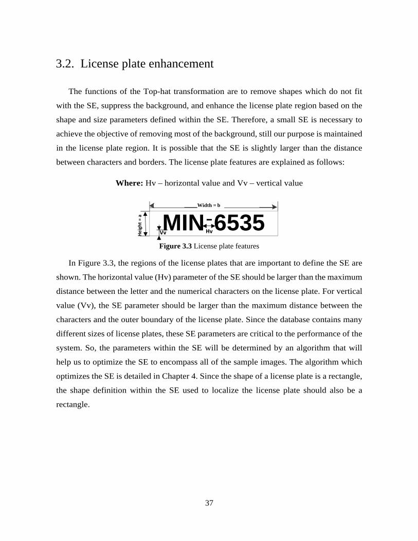
Where: Hv – horizontal value and Vv – vertical value
Figure 3.3 License plate features
In Figure 3.3, the regions of the license plates that are important to define the SE are
shown. The horizontal value (Hv) parameter of the SE should be larger than the maximum
distance between the letter and the numerical characters on the license plate. For vertical
value (Vv), the SE parameter should be larger than the maximum distance between the
characters and the outer boundary of the license plate. Since the database contains many
different sizes of license plates, these SE parameters are critical to the performance of the
system. So, the parameters within the SE will be determined by an algorithm that will
help us to optimize the SE to encompass all of the sample images. The algorithm which
optimizes the SE is detailed in Chapter 4. Since the shape of a license plate is a rectangle,
the shape definition within the SE used to localize the license plate should also be a
rectangle.
_____Width = b ______
MIN ̄ 6535
Hei
ght =
a
Hv Vv
38
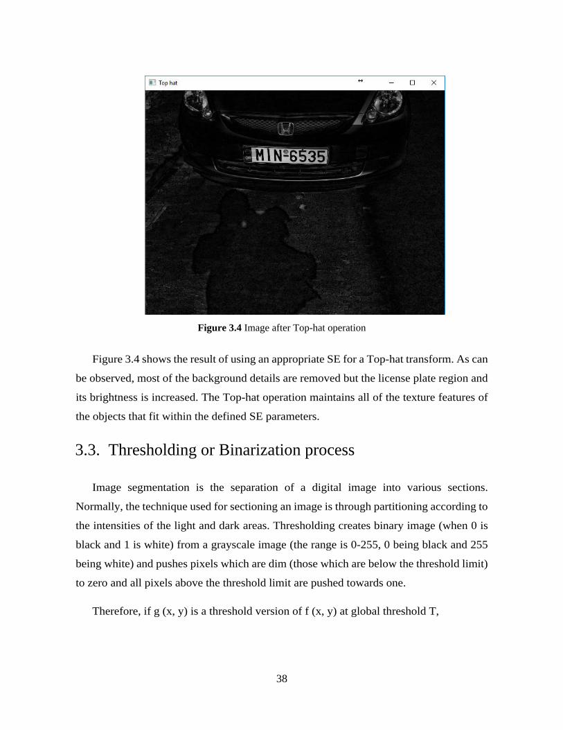
Figure 3.4 Image after Top-hat operation
Figure 3.4 shows the result of using an appropriate SE for a Top-hat transform. As can
be observed, most of the background details are removed but the license plate region and
its brightness is increased. The Top-hat operation maintains all of the texture features of
the objects that fit within the defined SE parameters.
3.3. Thresholding or Binarization process
Image segmentation is the separation of a digital image into various sections.
Normally, the technique used for sectioning an image is through partitioning according to
the intensities of the light and dark areas. Thresholding creates binary image (when 0 is
black and 1 is white) from a grayscale image (the range is 0-255, 0 being black and 255
being white) and pushes pixels which are dim (those which are below the threshold limit)
to zero and all pixels above the threshold limit are pushed towards one.
Therefore, if g (x, y) is a threshold version of f (x, y) at global threshold T,
39
𝑔𝑔(𝑥𝑥, 𝑦𝑦) = �1, 𝑖𝑖𝑓𝑓 (𝑥𝑥,𝑦𝑦) < 𝑇𝑇0, 𝑜𝑜𝑜𝑜ℎ𝑒𝑒𝑒𝑒𝑒𝑒𝑖𝑖𝑠𝑠𝑒𝑒 (3.2)
However, the major issue with thresholding is that it considers only the intensity and
not the connections between adjacent pixels. Thus, there is no assurance that the pixels
recognized by the thresholding procedures are adjoining. The thresholding procedure
simply disconnects pixels inside the locale. Thresholding is often subjective so that in one
instance, we may lose areas by moving too much towards zero, or gain unnecessary details
by moving towards 1 or 255.
Otsu’s method, named after Nobuyuki Otsu, is a global image thresholding algorithm
usually employed for thresholding, binarization and segmentation [61]. It is utilized to
differentiate between two types of relatively homogenous things such as the foreground
versus background [62]. When an image is converted to its greyscale form, this single-
band image has a bimodal (black and white) pixel distribution. Otsu’s technique performs
a duo-class segmentation by automatically finding an optimal threshold based on the
observed distribution of pixel values thereby separating the two classes (license plate and
background).
The method employed by Otsu investigates the threshold which least reduces the
variance within the particular class, expressed as a weighted sum of variances of the two
classes as follows:
𝜎𝜎𝜔𝜔2(𝑜𝑜) = 𝜔𝜔0(𝑜𝑜)𝜎𝜎02(𝑜𝑜) + 𝜔𝜔1(𝑜𝑜)𝜎𝜎12(𝑜𝑜) (3.3)
From the expression above, 𝜔𝜔0 and 𝜔𝜔1represent the probabilities of both classes used.
These two classes are distinguished by a threshold which is denoted by 𝑜𝑜. The variances
of these two classes are represented by 𝜎𝜎02 and 𝜎𝜎12.
The class probability represented by 𝜔𝜔0,1(𝑜𝑜) is calculated from the L histograms as
expressed below:
(3.4)
40
𝜔𝜔0(𝑜𝑜) = �𝑝𝑝(𝑖𝑖)𝑡𝑡−1
𝑖𝑖=0
𝜔𝜔1(𝑜𝑜) = �𝑝𝑝(𝑖𝑖)𝐿𝐿−1
𝑖𝑖=𝑡𝑡
According to Otsu, we can conclude that it is a similar process to minimize the intra-
class variance or maximize the inter-class variance. This also means that as the inter-class
variance is maximized, the intra-class variance is also simultaneously minimized. The
following expressions explain this as shown:
𝜎𝜎𝑏𝑏2(𝑜𝑜) = 𝜎𝜎2 − 𝜎𝜎𝜔𝜔2(𝑜𝑜) (3.5)
= 𝜔𝜔0(𝜇𝜇0 − 𝜇𝜇𝑇𝑇)2 + 𝜔𝜔1(𝜇𝜇1 − 𝜇𝜇𝑇𝑇)2
= 𝜔𝜔0(𝑜𝑜)𝜔𝜔1(𝑜𝑜)[𝜇𝜇0(𝑜𝑜)− 𝜇𝜇1(𝑜𝑜)]2
Where: 𝜔𝜔 – Class probabilities
𝜇𝜇 – Class means
𝜎𝜎𝑏𝑏2 and 𝜎𝜎𝜔𝜔2 – Class variances
𝑜𝑜 – Threshold
Therefore, the class mean 𝜇𝜇0,1,𝑇𝑇(𝑜𝑜) can be expressed as follows:
𝜇𝜇0(𝑜𝑜) = ∑ 𝑖𝑖 𝑝𝑝(𝑖𝑖)𝜔𝜔0
𝑡𝑡−1𝑖𝑖=0
𝜇𝜇1(𝑜𝑜) = �𝑖𝑖𝑝𝑝(𝑖𝑖)𝜔𝜔1
𝐿𝐿−1
𝑖𝑖=𝑡𝑡
𝜇𝜇𝑇𝑇 = ∑ 𝑖𝑖𝑝𝑝(𝑖𝑖)𝐿𝐿−1𝑖𝑖=0
Table 3.1 shows how the class probabilities and class means can be calculated generally.
The class probabilities are denoted by 𝜔𝜔, 𝜇𝜇 represents the class means, 𝑜𝑜 – threshold
(3.6)
41
whereas the class variances are denoted by 𝜎𝜎𝑏𝑏2 and 𝜎𝜎𝜔𝜔2 . The table explains that the desired
threshold will be equivalent to the maximum element.
Table 3.1: The pseudo code of threshold segmentation (Otsu’s method)
In determining the intensity level;
Calulate the histogram and probabilities of every intensity level;
Set up initial 𝜔𝜔𝑖𝑖(0) and 𝜇𝜇𝑖𝑖(0);
for (each threshold t to maximun intensity)
Update 𝜔𝜔𝑖𝑖 and 𝜇𝜇𝑖𝑖;
Calculate 𝜎𝜎𝑏𝑏2(𝑜𝑜) = 𝜔𝜔0(𝑜𝑜)𝜔𝜔1(𝑜𝑜)[𝜇𝜇0(𝑜𝑜) − 𝜇𝜇1(𝑜𝑜)]2;
The desired threshold will correspond to the maximum element 𝜎𝜎𝑏𝑏2(𝑜𝑜).
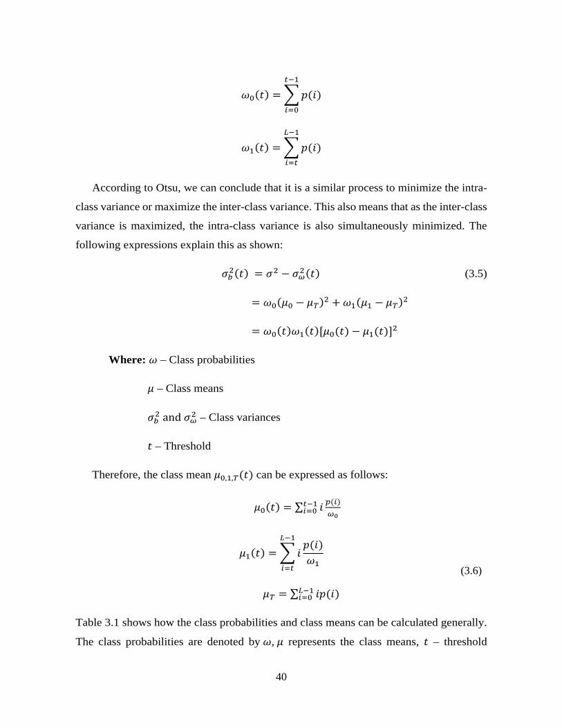
Figure 3.5 shown below reflects the result of a binarized image after employing Otsu’s
method.
Figure 3.5 Otsu technique applied to greyscale image.

42
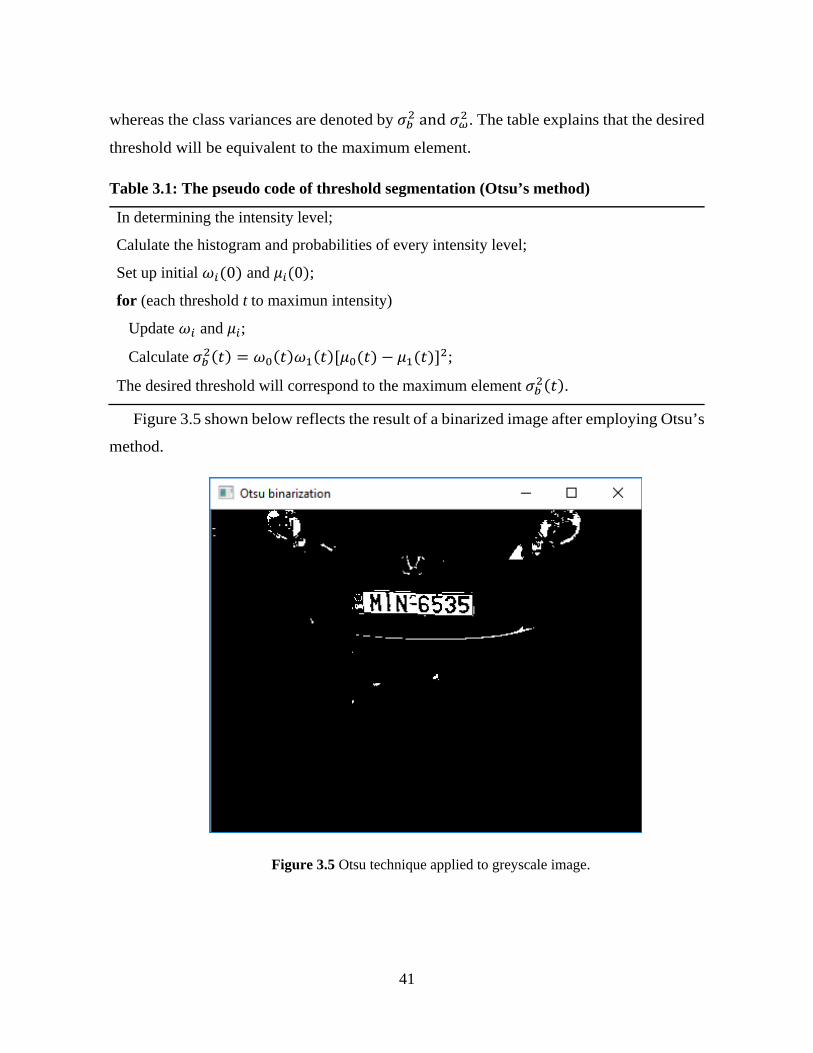
3.4. Noise Removal
As illustrated by Figure 3.5, the license plate is visible and the background is greatly
reduced. However, even though we are able to eliminate a large portion of the background,
some white regions remain and these may cause false positives. To eliminate these areas,
a filtering strategy based on morphology operations is designed within the system. In this
case, the algorithm applies a morphological opening (that eliminates the noise in
background) followed by closing (that eliminates the noise inside the region of interest)
to the binary image. The dimension and the shape within the two SE’s (one for opening
and another for closing) are not randomly chosen but are determined on an algorithm
which obtains the best shape fit in order to achieve high accuracy.
As described in Chapter 2, morphological opening is very useful for removing small
objects when the objects are white on a dark background. In Figure 3.6(a), when the binary
image is applied in the opening operation, most of the noise information is removed and
the characters on the license plate are maintained. It is important to keep the characters to
preserve the license plate region otherwise the contour function would divide the plate
region into multiple parts.
The next step is to remove the characters and delineate the license plate region based
on its rectangular shape. For the closing operation, our system focuses on the delineated
rectangular shape. Morphological closing is used to remove small black holes in a white
region. The condition to remove the characters from the license plate region is done by
ensuring that that the dimensions are wider and longer than the line of the characters.
These dimensions are determined by the algorithm detailed in section 4.3.
Figure 3.6(b) shows the result of applying the closing operation after the opening
operation. As can be seen, most of the characters have been removed, and the license plate
region is a big rectangle that could be easily identified through pixel connectivity
methods.
43
(a) Image after opening operation
(b) Image after closing operation
Figure 3.6 Noise removal.
44
3.5. Finding Contours
After applying noise removal, the resultant image consists of groups of white objects.
Contour detection methodology is used to identify the location of the white objects.
Contour detection is a technique applied to digital images to outline their external
boundaries. This technique is very useful for shape analysis and object recognition. It can
be explained as a curve joining all the continuous points which have the same color or
intensity. In the developed work, contour detection is used with the binary image after
applying noise removal. Our goal is to apply it to the image with a black background
which has only a few white objects thereby making detection simple and fast.
Using the theory of Suzuki and Abe, we can determine the candidates of license plate.
Consequently, the extracted objects are expressed as trees. From this, the root will be a
sequence representing the outer contour in every tree. The sub-trees form sequences
which represent inner contours of successive depth levels.
Suzuki and Abe’s algorithm has its foundational basis supported two principle
identifies represented as NBD (sequential number of the newly-found border) and LNBD
(sequential number of the border recently encountered during the search process). This
therefore means that the LNBD-identified border will either form part of the parent border
of the newly-found border or it will share a common parent with the newly-found border.
In order to carry out the searching process, scanning is done. This is performed through
the scanning of the image input 𝐹𝐹 = {𝑓𝑓𝑖𝑖𝑗𝑗} using a given raster beginning with NBD set to
1. Each time a new row of the image is to be scanned, LNBD is reset to 1. In this process,
the steps below are carried out on each pixel such that 𝑓𝑓𝑖𝑖𝑗𝑗 ≠ 0.
(1) Choose any of the following:
a. Where 𝑓𝑓𝑖𝑖𝑗𝑗 = 1 and 𝑓𝑓𝑖𝑖,𝑗𝑗−1 = 0 make the pixel (i, j) the border and the starting point
of an outer border, increment NBD to be expressed as (𝑖𝑖2, 𝑗𝑗2) ← (𝑖𝑖, 𝑗𝑗 − 1).
45
b. Alternatively, where 𝑓𝑓𝑖𝑖𝑗𝑗 ≥ 1 and 𝑓𝑓𝑖𝑖,𝑗𝑗+1 = 0, make pixel (i, j) the border following
the starting point of a hole border, increment NBD to be expressed as (𝑖𝑖2, 𝑗𝑗2) ←
(𝑖𝑖, 𝑗𝑗 + 1), and LNBD ← 𝑓𝑓𝑖𝑖𝑗𝑗 where 𝑓𝑓𝑖𝑖𝑗𝑗 > 1.
c. If not, and neither (a) nor (b) is employed, proceed to (4).
(2) Use step (1) to determine the parent of the current border. Remember, this is done
depending on the type of the newly-found border and that with a sequential number
LNBD to mean the last border met on the current row.
(3) Sub-steps 3.1 – 3.5 guide in detecting this border from the starting point (i, j):
(3.1) Beginning from (𝑖𝑖2, 𝑗𝑗2), study the pixels in a clockwise manner within the
neighborhood of (i, j) and find a nonzero pixel. Make (𝑖𝑖1, 𝑗𝑗1) the first nonzero pixel.
Where there is no nonzero pixel found, make – NBD to 𝑓𝑓𝑖𝑖𝑗𝑗 and proceed to (4).
(3.2) Let (𝑖𝑖2, 𝑗𝑗2) ← (𝑖𝑖1, 𝑗𝑗1) and(𝑖𝑖3, 𝑗𝑗3) ← (𝑖𝑖, 𝑗𝑗).
(3.3) In an anti-clockwise manner, examine the pixels within the neighborhood of the
current pixel (𝑖𝑖3, 𝑗𝑗3) to find a nonzero pixel and let the first one be (𝑖𝑖4, 𝑗𝑗4). Perform
this beginning from the next element of the pixel (𝑖𝑖2, 𝑗𝑗2).
(3.4) Vary the value 𝑓𝑓𝑖𝑖3,𝑗𝑗3 of the pixel (𝑖𝑖3, 𝑗𝑗3) as shown in (a) and (b):
(a) Where the pixel (𝑖𝑖3, 𝑗𝑗3 + 1) is a 0-pixel as per the results of the examination
in sub-step (3.3), then 𝑓𝑓𝑖𝑖3,𝑗𝑗3 ← -NBD.
(b) Where the pixel (𝑖𝑖3, 𝑗𝑗3 + 1) is not a 0-pixel from the results of examination
in sub-step (3.3) and 𝑓𝑓𝑖𝑖3,𝑗𝑗3 = 1, then 𝑓𝑓𝑖𝑖3,𝑗𝑗3 ←-NBD.
(c) Or else, do not vary 𝑓𝑓𝑖𝑖3,𝑗𝑗3.
(3.5) Where (𝑖𝑖4, 𝑗𝑗4) = (𝑖𝑖, 𝑗𝑗) and (𝑖𝑖3, 𝑗𝑗3) = (𝑖𝑖1, 𝑗𝑗1) from the starting point, then
proceed to (4); if not,(𝑖𝑖2, 𝑗𝑗2) ← (𝑖𝑖3, 𝑗𝑗3), (𝑖𝑖3, 𝑗𝑗3) ← (𝑖𝑖4, 𝑗𝑗4) and go back to sub-step
(3.3).
(4) Where 𝑓𝑓𝑖𝑖𝑗𝑗 ≠ 1, then LNBD ← �𝑓𝑓𝑖𝑖𝑗𝑗� and resume the raster scan from pixel (𝑖𝑖, 𝑗𝑗 + 1).
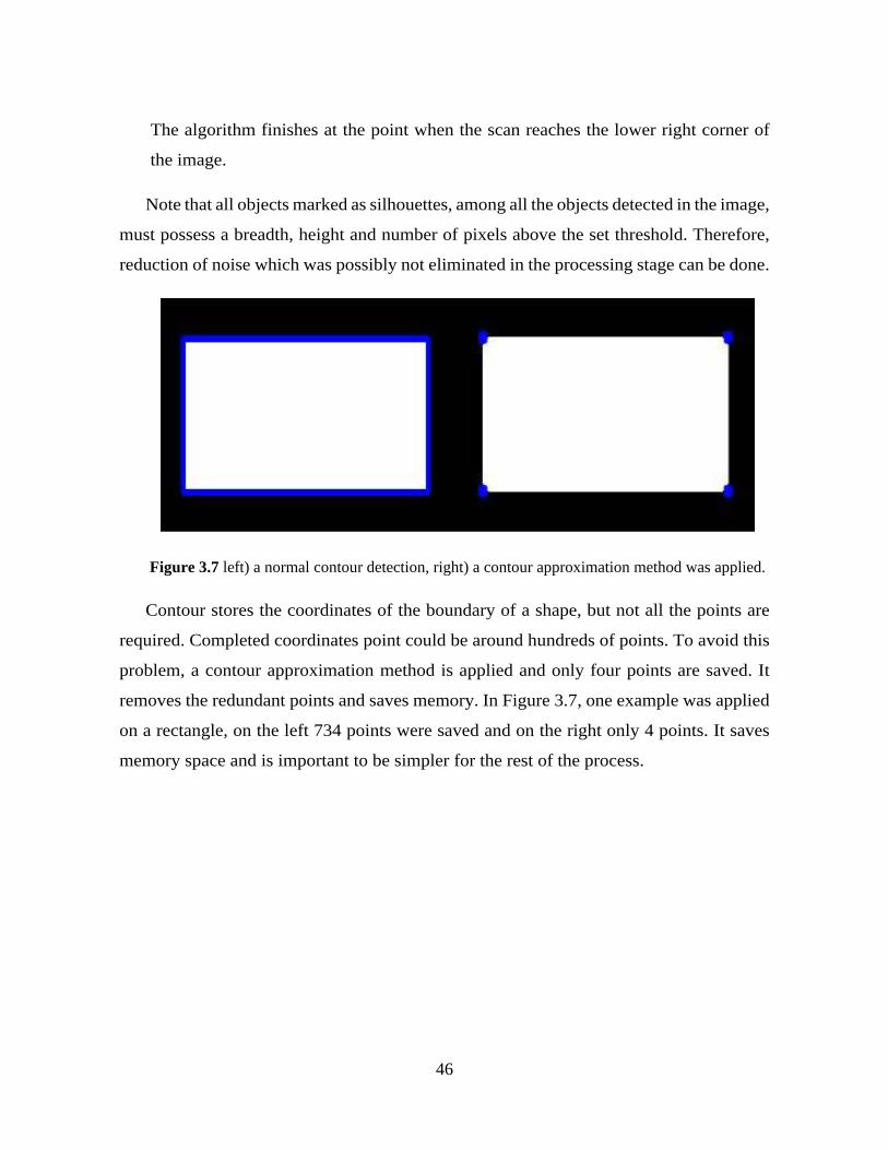
46
The algorithm finishes at the point when the scan reaches the lower right corner of
the image.
Note that all objects marked as silhouettes, among all the objects detected in the image,
must possess a breadth, height and number of pixels above the set threshold. Therefore,
reduction of noise which was possibly not eliminated in the processing stage can be done.
Figure 3.7 left) a normal contour detection, right) a contour approximation method was applied.
Contour stores the coordinates of the boundary of a shape, but not all the points are
required. Completed coordinates point could be around hundreds of points. To avoid this
problem, a contour approximation method is applied and only four points are saved. It
removes the redundant points and saves memory. In Figure 3.7, one example was applied
on a rectangle, on the left 734 points were saved and on the right only 4 points. It saves
memory space and is important to be simpler for the rest of the process.

47
Figure 3.8 Contours detection.
Figure 3.8 above shows the result of applying a contour detection technique. As can
be seen, the license plate and a few additional objects are detected. Because the license
plates have geometrical features which are unique from the other objects, this can be used
to differentiate between them.
3.6. Geometrical conditions
Once the contour detector finds the candidate objects, the candidates can be selected
using the following geometrical conditions: area, inclination angle, ratio, width and
height.
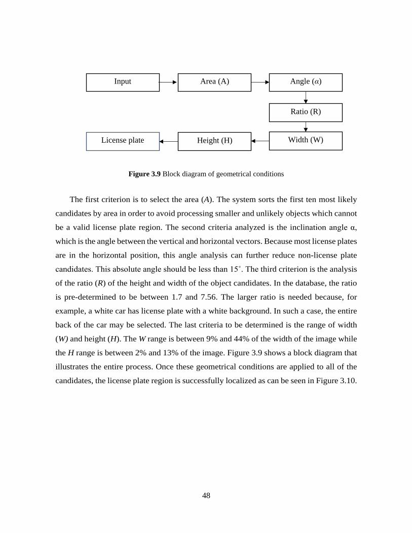
48
Figure 3.9 Block diagram of geometrical conditions
The first criterion is to select the area (A). The system sorts the first ten most likely
candidates by area in order to avoid processing smaller and unlikely objects which cannot
be a valid license plate region. The second criteria analyzed is the inclination angle α,
which is the angle between the vertical and horizontal vectors. Because most license plates
are in the horizontal position, this angle analysis can further reduce non-license plate
candidates. This absolute angle should be less than 15˚. The third criterion is the analysis
of the ratio (R) of the height and width of the object candidates. In the database, the ratio
is pre-determined to be between 1.7 and 7.56. The larger ratio is needed because, for
example, a white car has license plate with a white background. In such a case, the entire
back of the car may be selected. The last criteria to be determined is the range of width
(W) and height (H). The W range is between 9% and 44% of the width of the image while
the H range is between 2% and 13% of the image. Figure 3.9 shows a block diagram that
illustrates the entire process. Once these geometrical conditions are applied to all of the
candidates, the license plate region is successfully localized as can be seen in Figure 3.10.
Input Area (A)
Ratio (R)
Width (W) License plate Height (H)
Angle (α)
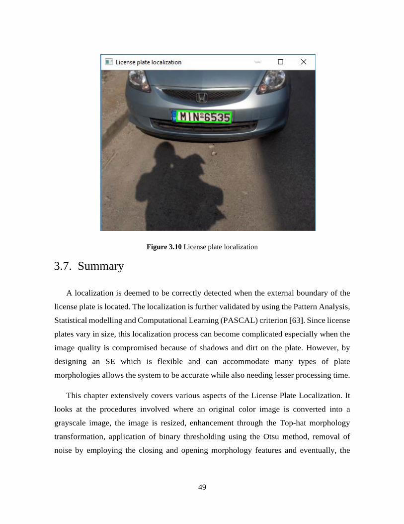
49
Figure 3.10 License plate localization
3.7. Summary
A localization is deemed to be correctly detected when the external boundary of the
license plate is located. The localization is further validated by using the Pattern Analysis,
Statistical modelling and Computational Learning (PASCAL) criterion [63]. Since license
plates vary in size, this localization process can become complicated especially when the
image quality is compromised because of shadows and dirt on the plate. However, by
designing an SE which is flexible and can accommodate many types of plate
morphologies allows the system to be accurate while also needing lesser processing time.
This chapter extensively covers various aspects of the License Plate Localization. It
looks at the procedures involved where an original color image is converted into a
grayscale image, the image is resized, enhancement through the Top-hat morphology
transformation, application of binary thresholding using the Otsu method, removal of
noise by employing the closing and opening morphology features and eventually, the
50
extraction of the license plate candidates process. All these steps are diagrammatically
condensed to aid finer understanding.
We observe that in pre-processing, the capturing of a fully-colored image with the
RGB layers. Mathematical processes are subsequently applied to combine all these layers
into one single grayscale image. The license plate enhancement sees the process of
transformation by the top-hat transformation to ensure shapes and background fit with the
SE. when we get to threshold which is also referred to as the binarization process, the
digital image is separated into various segments depending on the darkness or lightness
of the areas. Otsu’s method is therefore applied to achieve this. After this, morphological
opening and closing are used in performing noise removal and later contours are
determined through Otsu and Abe’s theory.

51
Chapter 4
Determining the Appropriate Values in the SE
MM uses a set of different operators based on the SE. Hence, designing an appropriate
SE is crucial. Figure 4.1 shows the difference between choosing a SE with 40 × 40 pixel
parameters versus an SE with pixel parameters of 5 × 5. As can be seen, when the SE is too
large, the background is not completely removed. On the other hand, when the SE is too small,
the background and most of the object of interest merge and cannot be defined. This is because
a small change in a regions dimension can significantly affect the performance and utility of
an SE, which may overlook a license plate if it does not meet the parameters defined in the
SE.
(a) Top-hat with SE 40×40

52
(b) Top-hat with SE 5×5
Figure 4.1 Top-hat with different SE’s.
4.1 Determining the Appropriate Values in the SE
Defining a suitable a suitable structural element is key for the process of license plate
localization. The SE determines the pixels that are classified as ‘neighbours’ in every
particular morphological method. It also dictates the size and shape of this
‘neighbourhood’ thereby clearly separating whatever you need to extract off the image.
Different examples of SEs that have undergone conversion into images are shown in
Figure 4.2 below. These show the ‘neighbourhoods’ around a central pixel known as the
‘origin.’
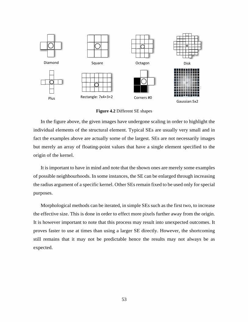
53
Figure 4.2 Different SE shapes
In the figure above, the given images have undergone scaling in order to highlight the
individual elements of the structural element. Typical SEs are usually very small and in
fact the examples above are actually some of the largest. SEs are not necessarily images
but merely an array of floating-point values that have a single element specified to the
origin of the kernel.
It is important to have in mind and note that the shown ones are merely some examples
of possible neighbourhoods. In some instances, the SE can be enlarged through increasing
the radius argument of a specific kernel. Other SEs remain fixed to be used only for special
purposes.
Morphological methods can be iterated, in simple SEs such as the first two, to increase
the effective size. This is done in order to effect more pixels further away from the origin.
It is however important to note that this process may result into unexpected outcomes. It
proves faster to use at times than using a larger SE directly. However, the shortcoming
still remains that it may not be predictable hence the results may not always be as
expected.
Diamond Square Octagon Disk
Plus Rectangle: 7x4+3+2 Corners #0 Gaussian:5x2
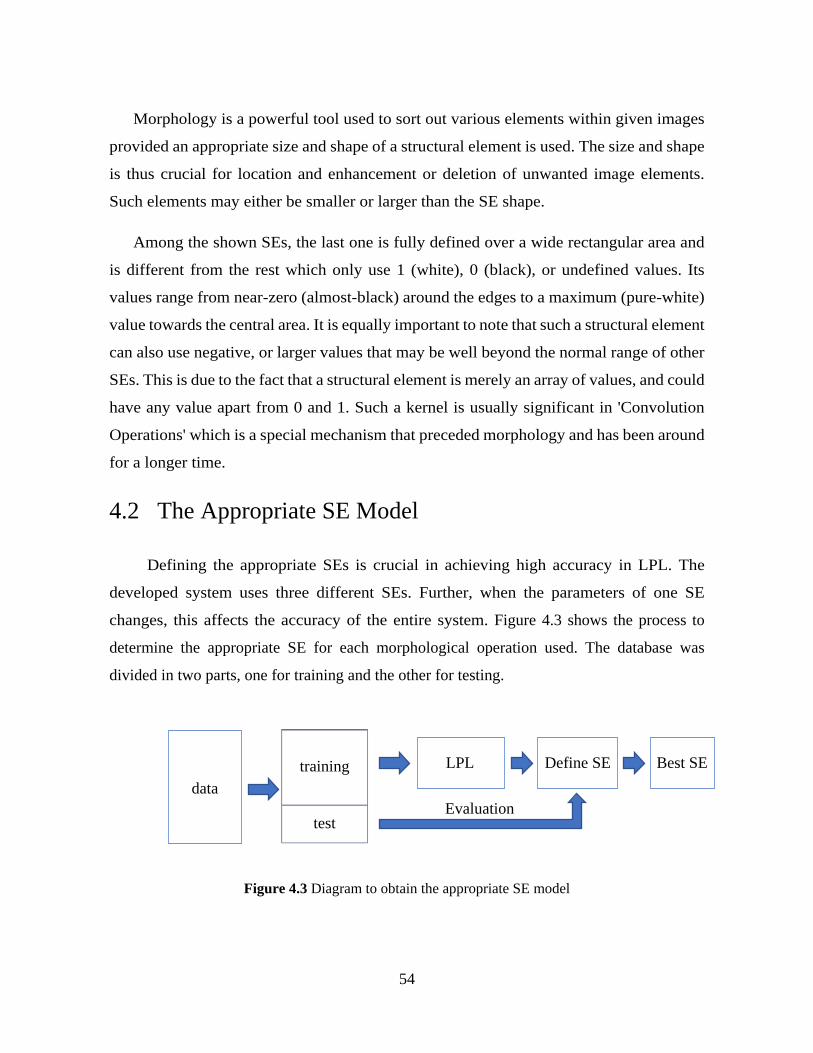
54
Morphology is a powerful tool used to sort out various elements within given images
provided an appropriate size and shape of a structural element is used. The size and shape
is thus crucial for location and enhancement or deletion of unwanted image elements.
Such elements may either be smaller or larger than the SE shape.
Among the shown SEs, the last one is fully defined over a wide rectangular area and
is different from the rest which only use 1 (white), 0 (black), or undefined values. Its
values range from near-zero (almost-black) around the edges to a maximum (pure-white)
value towards the central area. It is equally important to note that such a structural element
can also use negative, or larger values that may be well beyond the normal range of other
SEs. This is due to the fact that a structural element is merely an array of values, and could
have any value apart from 0 and 1. Such a kernel is usually significant in 'Convolution
Operations' which is a special mechanism that preceded morphology and has been around
for a longer time.
4.2 The Appropriate SE Model
Defining the appropriate SEs is crucial in achieving high accuracy in LPL. The
developed system uses three different SEs. Further, when the parameters of one SE
changes, this affects the accuracy of the entire system. Figure 4.3 shows the process to
determine the appropriate SE for each morphological operation used. The database was
divided in two parts, one for training and the other for testing.
Figure 4.3 Diagram to obtain the appropriate SE model
data
training
test
LPL Define SE Best SE
Evaluation
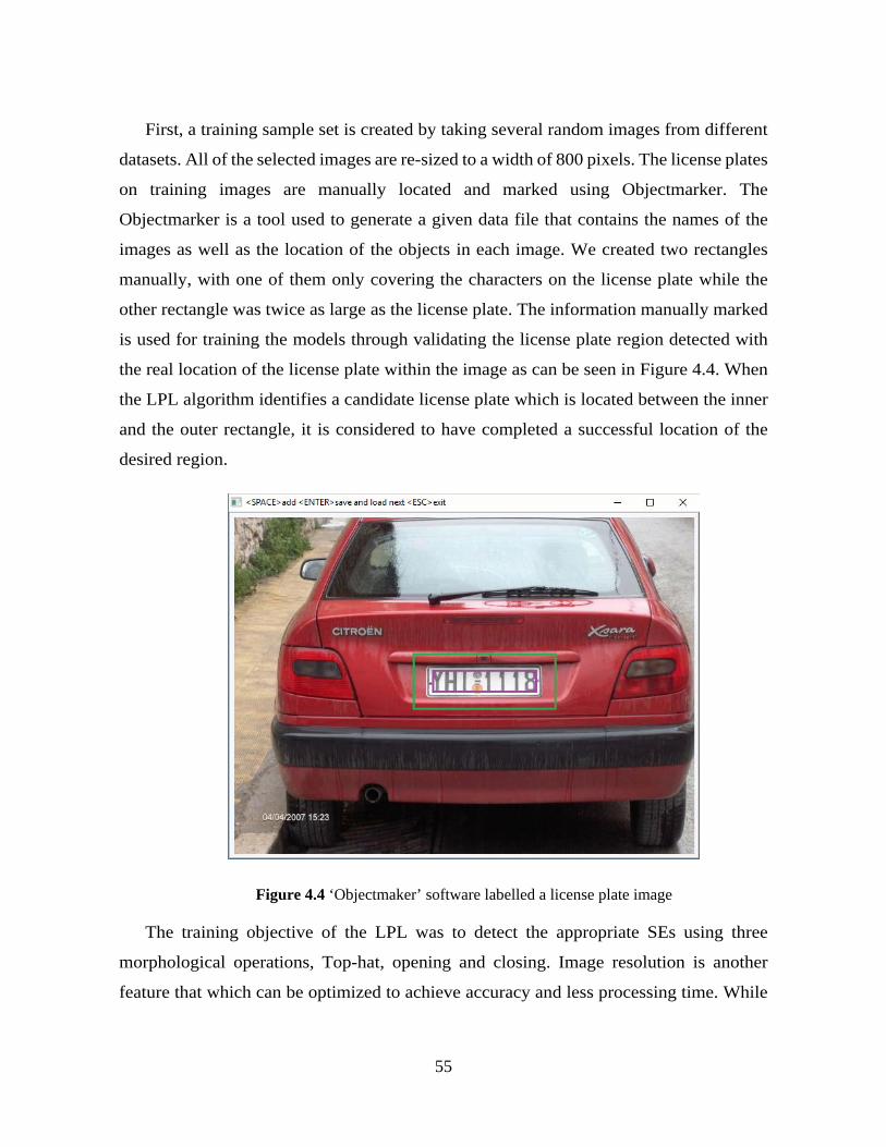
55
First, a training sample set is created by taking several random images from different
datasets. All of the selected images are re-sized to a width of 800 pixels. The license plates
on training images are manually located and marked using Objectmarker. The
Objectmarker is a tool used to generate a given data file that contains the names of the
images as well as the location of the objects in each image. We created two rectangles
manually, with one of them only covering the characters on the license plate while the
other rectangle was twice as large as the license plate. The information manually marked
is used for training the models through validating the license plate region detected with
the real location of the license plate within the image as can be seen in Figure 4.4. When
the LPL algorithm identifies a candidate license plate which is located between the inner
and the outer rectangle, it is considered to have completed a successful location of the
desired region.
Figure 4.4 ‘Objectmaker’ software labelled a license plate image
The training objective of the LPL was to detect the appropriate SEs using three
morphological operations, Top-hat, opening and closing. Image resolution is another
feature that which can be optimized to achieve accuracy and less processing time. While
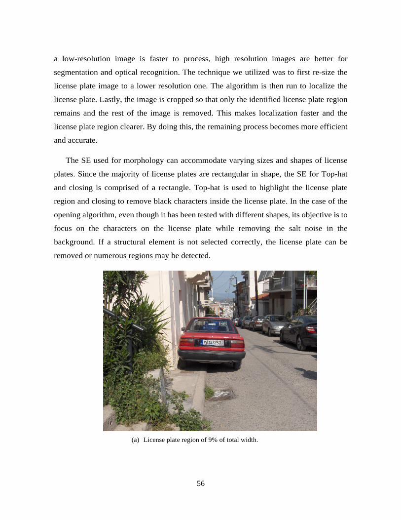
56
a low-resolution image is faster to process, high resolution images are better for
segmentation and optical recognition. The technique we utilized was to first re-size the
license plate image to a lower resolution one. The algorithm is then run to localize the
license plate. Lastly, the image is cropped so that only the identified license plate region
remains and the rest of the image is removed. This makes localization faster and the
license plate region clearer. By doing this, the remaining process becomes more efficient
and accurate.
The SE used for morphology can accommodate varying sizes and shapes of license
plates. Since the majority of license plates are rectangular in shape, the SE for Top-hat
and closing is comprised of a rectangle. Top-hat is used to highlight the license plate
region and closing to remove black characters inside the license plate. In the case of the
opening algorithm, even though it has been tested with different shapes, its objective is to
focus on the characters on the license plate while removing the salt noise in the
background. If a structural element is not selected correctly, the license plate can be
removed or numerous regions may be detected.
(a) License plate region of 9% of total width.
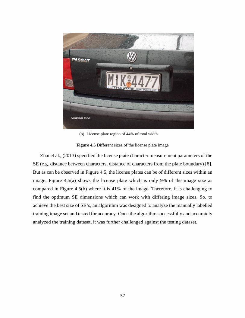
57
(b) License plate region of 44% of total width.
Figure 4.5 Different sizes of the license plate image
Zhai et al., (2013) specified the license plate character measurement parameters of the
SE (e.g. distance between characters, distance of characters from the plate boundary) [8].
But as can be observed in Figure 4.5, the license plates can be of different sizes within an
image. Figure 4.5(a) shows the license plate which is only 9% of the image size as
compared in Figure 4.5(b) where it is 41% of the image. Therefore, it is challenging to
find the optimum SE dimensions which can work with differing image sizes. So, to
achieve the best size of SE’s, an algorithm was designed to analyze the manually labelled
training image set and tested for accuracy. Once the algorithm successfully and accurately
analyzed the training dataset, it was further challenged against the testing dataset.
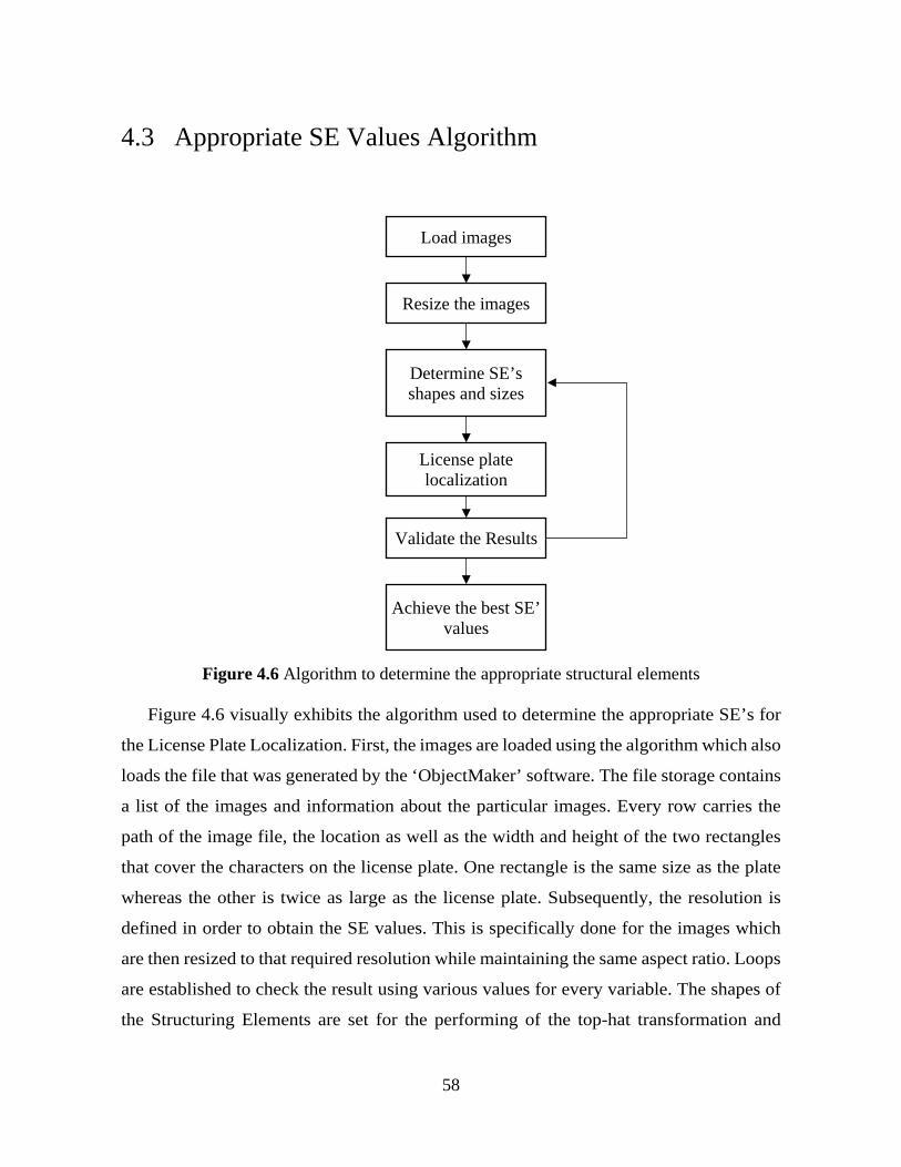
58
4.3 Appropriate SE Values Algorithm
Figure 4.6 Algorithm to determine the appropriate structural elements
Figure 4.6 visually exhibits the algorithm used to determine the appropriate SE’s for
the License Plate Localization. First, the images are loaded using the algorithm which also
loads the file that was generated by the ‘ObjectMaker’ software. The file storage contains
a list of the images and information about the particular images. Every row carries the
path of the image file, the location as well as the width and height of the two rectangles
that cover the characters on the license plate. One rectangle is the same size as the plate
whereas the other is twice as large as the license plate. Subsequently, the resolution is
defined in order to obtain the SE values. This is specifically done for the images which
are then resized to that required resolution while maintaining the same aspect ratio. Loops
are established to check the result using various values for every variable. The shapes of
the Structuring Elements are set for the performing of the top-hat transformation and
Load images
Resize the images
Determine SE’s shapes and sizes
License plate localization
Validate the Results
Achieve the best SE’ values
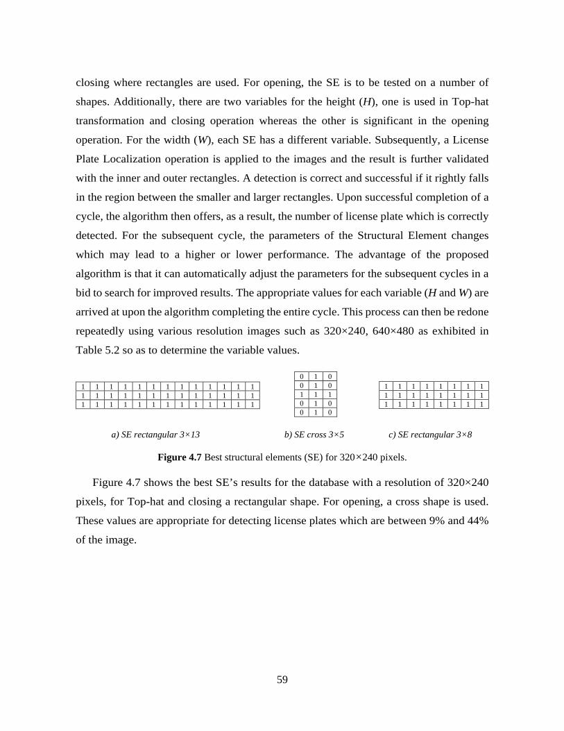
59
closing where rectangles are used. For opening, the SE is to be tested on a number of
shapes. Additionally, there are two variables for the height (H), one is used in Top-hat
transformation and closing operation whereas the other is significant in the opening
operation. For the width (W), each SE has a different variable. Subsequently, a License
Plate Localization operation is applied to the images and the result is further validated
with the inner and outer rectangles. A detection is correct and successful if it rightly falls
in the region between the smaller and larger rectangles. Upon successful completion of a
cycle, the algorithm then offers, as a result, the number of license plate which is correctly
detected. For the subsequent cycle, the parameters of the Structural Element changes
which may lead to a higher or lower performance. The advantage of the proposed
algorithm is that it can automatically adjust the parameters for the subsequent cycles in a
bid to search for improved results. The appropriate values for each variable (H and W) are
arrived at upon the algorithm completing the entire cycle. This process can then be redone
repeatedly using various resolution images such as 320×240, 640×480 as exhibited in
Table 5.2 so as to determine the variable values.
a) SE rectangular 3×13 b) SE cross 3×5 c) SE rectangular 3×8
Figure 4.7 Best structural elements (SE) for 320×240 pixels.
Figure 4.7 shows the best SE’s results for the database with a resolution of 320×240
pixels, for Top-hat and closing a rectangular shape. For opening, a cross shape is used.
These values are appropriate for detecting license plates which are between 9% and 44%
of the image.
1 1 1 1 1 1 1 1 1 1 1 1 1 1 1 1 1 1 1 1 1 1 1 1 1 1 1 1 1 1 1 1 1 1 1 1 1 1 1
0 1 0 0 1 0 1 1 1 0 1 0 0 1 0
1 1 1 1 1 1 1 1 1 1 1 1 1 1 1 1 1 1 1 1 1 1 1 1

60
4.4 Conclusion
This section concentrates on determining the appropriate values in the SE. Thus, it is
correctly observed that the parameters set with the SE are crucial in achieving a high
accuracy in LPL. Important to note also is the fact that when the parameters of one SE
changes, the entire system’s accuracy is affected. To simplify the process of obtaining the
best parameters, a suitable algorithm designed to measure accuracy of the localization
process is employed.
61
Chapter 5
Experiment Results
The developed approach was tested in MATLAB on a PC with a 2.7 GHz core i7 and
8 GB of RAM. Further, it was implemented in Python on a low-cost Raspberry Pi device
with a 700 MHz processor and 256 MB of RAM. The algorithm was first tested by
challenging it against the public MediaLab database. We then compared our results, for
both the PC and Raspberry Pi, with that of previous works which had used the same
database for accuracy and processing times.
5.1 Database
The LPR database used for testing the algorithm is provided by MediaLab of the
National Technical University of Athens (NTUA) [64]. The database contains images with
different background scenes which show the front or back of vehicles. The database has
images in JPEG format with different resolutions such as 1792×1312, 800×600, and
640×480 pixels. The width of the license plates in the database images vary from 9% to
44% of the width of the image. The license plates are from Europe and have black colour
characters on a white background. The license plates have two or three alphabetic
characters on the left-hand side, followed by a dash and four numerical characters on the
right-hand side. The files within the dataset are composed of three categories: still images,
difficult cases, and videos. Previous researchers who employed the MediaLab database
used only the still images for their work. However, in our work both still and difficult
cases images were used.
The image database contains eight different cases and are the following:
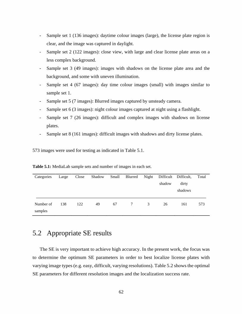
62
- Sample set 1 (136 images): daytime colour images (large), the license plate region is
clear, and the image was captured in daylight.
- Sample set 2 (122 images): close view, with large and clear license plate areas on a
less complex background.
- Sample set 3 (49 images): images with shadows on the license plate area and the
background, and some with uneven illumination.
- Sample set 4 (67 images): day time colour images (small) with images similar to
sample set 1.
- Sample set 5 (7 images): Blurred images captured by unsteady camera.
- Sample set 6 (3 images): night colour images captured at night using a flashlight.
- Sample set 7 (26 images): difficult and complex images with shadows on license
plates.
- Sample set 8 (161 images): difficult images with shadows and dirty license plates.
573 images were used for testing as indicated in Table 5.1.
Table 5.1: MediaLab sample sets and number of images in each set.
Categories Large Close Shadow Small Blurred Night Difficult
shadow
Difficult,
dirty
shadows
Total
Number of
samples
138 122 49 67 7 3 26 161 573
5.2 Appropriate SE results
The SE is very important to achieve high accuracy. In the present work, the focus was
to determine the optimum SE parameters in order to best localize license plates with
varying image types (e.g. easy, difficult, varying resolutions). Table 5.2 shows the optimal
SE parameters for different resolution images and the localization success rate.
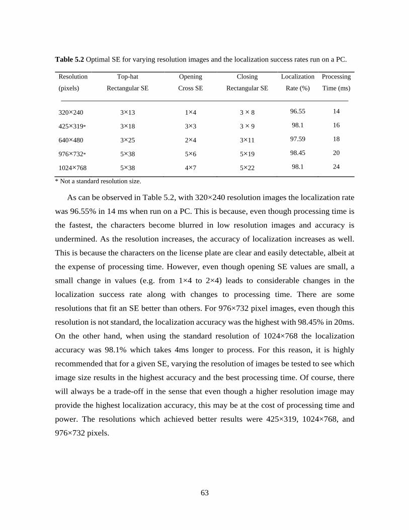
63
Table 5.2 Optimal SE for varying resolution images and the localization success rates run on a PC.
Resolution
(pixels)
Top-hat
Rectangular SE
Opening
Cross SE
Closing
Rectangular SE
Localization
Rate (%)
Processing
Time (ms)
320×240 3×13 1×4 3 × 8 96.55 14
425×319* 3×18 3×3 3 × 9 98.1 16
640×480 3×25 2×4 3×11 97.59 18
976×732* 5×38 5×6 5×19 98.45 20
1024×768 5×38 4×7 5×22 98.1 24
* Not a standard resolution size.
As can be observed in Table 5.2, with 320×240 resolution images the localization rate
was 96.55% in 14 ms when run on a PC. This is because, even though processing time is
the fastest, the characters become blurred in low resolution images and accuracy is
undermined. As the resolution increases, the accuracy of localization increases as well.
This is because the characters on the license plate are clear and easily detectable, albeit at
the expense of processing time. However, even though opening SE values are small, a
small change in values (e.g. from 1×4 to 2×4) leads to considerable changes in the
localization success rate along with changes to processing time. There are some
resolutions that fit an SE better than others. For 976×732 pixel images, even though this
resolution is not standard, the localization accuracy was the highest with 98.45% in 20ms.
On the other hand, when using the standard resolution of 1024×768 the localization
accuracy was 98.1% which takes 4ms longer to process. For this reason, it is highly
recommended that for a given SE, varying the resolution of images be tested to see which
image size results in the highest accuracy and the best processing time. Of course, there
will always be a trade-off in the sense that even though a higher resolution image may
provide the highest localization accuracy, this may be at the cost of processing time and
power. The resolutions which achieved better results were 425×319, 1024×768, and
976×732 pixels.
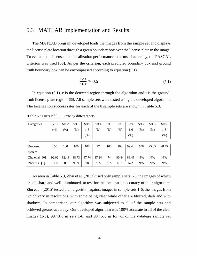
64
5.3 MATLAB Implementation and Results
The MATLAB program developed loads the images from the sample set and displays
the license plate location through a green boundary box over the license plate in the image.
To evaluate the license plate localization performance in terms of accuracy, the PASCAL
criterion was used [65]. As per the criterion, each predicted boundary box and ground
truth boundary box can be encompassed according to equation (5.1).
𝑐𝑐 ∩ t𝑐𝑐 ∪ 𝑡𝑡
≥ 0.5 (5.1)
In equation (5.1), c is the detected region through the algorithm and t is the ground-
truth license plate region [66]. All sample sets were tested using the developed algorithm.
The localization success rates for each of the 8 sample sets are shown in Table 5.3.
Table 5.3 Successful LPL rate by different sets
Categories Set 1
(%)
Set 2
(%)
Set 3
(%)
Sets
1-3
(%)
Set 4
(%)
Set 5
(%)
Set 6
(%)
Sets
1-6
(%)
Set 7
(%)
Set 8
(%)
Sets
1-8
(%)
Proposed
system
100 100 100 100 97 100 100 99.48 100 95.65 98.45
Zhu et al.[60] 92.02 82.48 88.73 87.74 87.24 74 90.84 89.45 N/A N/A N/A
Zhai et al.[1] 97.8 98.3 97.9 98 N/A N/A N/A N/A N/A N/A N/A
As seen in Table 5.3, Zhai et al. (2013) used only sample sets 1-3, the images of which
are all sharp and well illuminated, to test for the localization accuracy of their algorithm.
Zhu et al. (2015) tested their algorithm against images in sample sets 1-6, the images from
which vary in resolutions, with some being clear while other are blurred, dark and with
shadows. In comparison, our algorithm was subjected to all of the sample sets and
achieved greater accuracy. Our developed algorithm was 100% accurate in all of the clear
images (1-3), 99.48% in sets 1-6, and 98.45% in for all of the database sample set
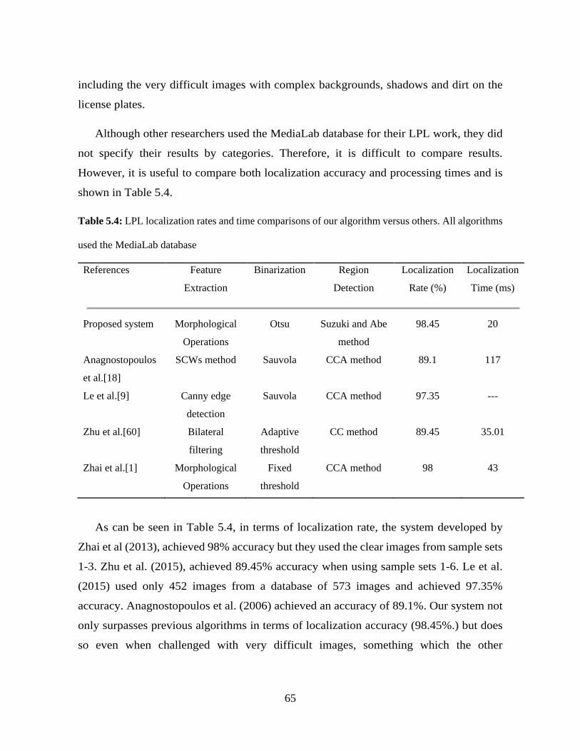
65
including the very difficult images with complex backgrounds, shadows and dirt on the
license plates.
Although other researchers used the MediaLab database for their LPL work, they did
not specify their results by categories. Therefore, it is difficult to compare results.
However, it is useful to compare both localization accuracy and processing times and is
shown in Table 5.4.
Table 5.4: LPL localization rates and time comparisons of our algorithm versus others. All algorithms
used the MediaLab database
References Feature
Extraction
Binarization Region
Detection
Localization
Rate (%)
Localization
Time (ms)
Proposed system Morphological
Operations
Otsu Suzuki and Abe
method
98.45 20
Anagnostopoulos
et al.[18]
SCWs method Sauvola CCA method 89.1 117
Le et al.[9] Canny edge
detection
Sauvola CCA method 97.35 ---
Zhu et al.[60] Bilateral
filtering
Adaptive
threshold
CC method 89.45 35.01
Zhai et al.[1] Morphological
Operations
Fixed
threshold
CCA method 98 43
As can be seen in Table 5.4, in terms of localization rate, the system developed by
Zhai et al (2013), achieved 98% accuracy but they used the clear images from sample sets
1-3. Zhu et al. (2015), achieved 89.45% accuracy when using sample sets 1-6. Le et al.
(2015) used only 452 images from a database of 573 images and achieved 97.35%
accuracy. Anagnostopoulos et al. (2006) achieved an accuracy of 89.1%. Our system not
only surpasses previous algorithms in terms of localization accuracy (98.45%.) but does
so even when challenged with very difficult images, something which the other

66
algorithms did not. It is likely that if the other algorithms were challenged against the
difficult images, they would have achieved lower accuracy rates.
In terms of processing time, the data in Table 5.4 provides the average run times for
processing a 640×480 image. As can be seen, our approach was the fastest requiring only
20 ms for LPL. The times of the other researchers varied from 35.01 to 117 ms, with the
caveat that one of the authors did not report the processing time.
5.4 Low-Cost Devices Implementation and Results
Our ultimate goal was to create a system which could run on a low-cost and low
processing power portable devices. With this in mind, our system was implemented in a
Raspberry Pi device. Since MATLAB software runs slower in a Raspberry Pi when
compared to other platforms, our system was rewritten in Python 2.7 and OpenCV 3.1
using the same architecture. Linux Raspbian 3.18 operating system was installed in the
Raspberry Pi. In addition, a USB camera was connected to the computer board. The
developed Raspberry Pi system works as follows:
- The system captures video frames from the camera.
- The frames are processed with the LPL algorithm.
- The license plate is located and its location shown as a green boundary box.
A video frame is one of the many still images which comprises the complete video.
Humans can process and individually perceive 10 to 12 images per second. A rate higher
than 10-12 is perceived as motion. Frame per second (FPS), is a useful measurement to
show how many video frames a system can process per second. The higher the FPS rate,
the faster the image processing. The results compare with a previous works as shown in
Table 5.5.
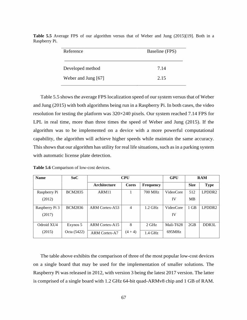
67
Table 5.5 Average FPS of our algorithm versus that of Weber and Jung (2015)[19]. Both in a Raspberry Pi.
Reference Baseline (FPS)
Developed method 7.14
Weber and Jung [67] 2.15
Table 5.5 shows the average FPS localization speed of our system versus that of Weber
and Jung (2015) with both algorithms being run in a Raspberry Pi. In both cases, the video
resolution for testing the platform was 320×240 pixels. Our system reached 7.14 FPS for
LPL in real time, more than three times the speed of Weber and Jung (2015). If the
algorithm was to be implemented on a device with a more powerful computational
capability, the algorithm will achieve higher speeds while maintain the same accuracy.
This shows that our algorithm has utility for real life situations, such as in a parking system
with automatic license plate detection.
Table 5.6 Comparison of low-cost devices.
Name SoC CPU GPU RAM
Architecture Cores Frequency Size Type
Raspberry Pi
(2012)
BCM2835 ARM11 1 700 MHz VideoCore
IV
512
MB
LPDDR2
Raspberry Pi 3
(2017)
BCM2836 ARM Cortex-A53 4 1.2 GHz VideoCore
IV
1 GB LPDDR2
Odroid XU4
(2015)
Exynos 5
Octa (5422)
ARM Cortex-A15 8
(4 + 4)
2 GHz Mali-T628
695MHz
2GB DDR3L
ARM Cortex-A7 1.4 GHz
The table above exhibits the comparison of three of the most popular low-cost devices
on a single board that may be used for the implementation of smaller solutions. The
Raspberry Pi was released in 2012, with version 3 being the latest 2017 version. The latter
is comprised of a single board with 1.2 GHz 64-bit quad-ARMv8 chip and 1 GB of RAM.
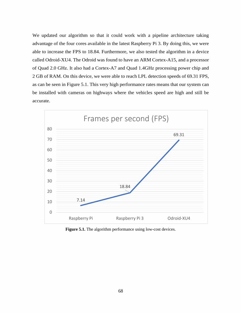
68
We updated our algorithm so that it could work with a pipeline architecture taking
advantage of the four cores available in the latest Raspberry Pi 3. By doing this, we were
able to increase the FPS to 18.84. Furthermore, we also tested the algorithm in a device
called Odroid-XU4. The Odroid was found to have an ARM Cortex-A15, and a processor
of Quad 2.0 GHz. It also had a Cortex-A7 and Quad 1.4GHz processing power chip and
2 GB of RAM. On this device, we were able to reach LPL detection speeds of 69.31 FPS,
as can be seen in Figure 5.1. This very high performance rates means that our system can
be installed with cameras on highways where the vehicles speed are high and still be
accurate.
Figure 5.1. The algorithm performance using low-cost devices.
7.14
18.84
69.31
0
10
20
30
40
50
60
70
80
Raspberry Pi Raspberry Pi 3 Odroid-XU4
Frames per second (FPS)

69
5.5 Summary
Chapter Five analyses various statistical data and experiments. Here, the MATLAB
approach is used. The chapter goes further ahead to account for the implementation of the
test and scrutinizes the results. The outcome is specifically analyzed and presented in
graphs and tables. The initial test sample for the algorithm was through challenging it
against the public MediaLab database. The results were then compared against previous
works which had used the same database for accuracy and processing times.
70
Chapter 6
Conclusion
Owing to the importance of LPL in an ALPR system, an improved algorithm based
on morphological operations was developed. In this study, the LPR algorithm developed
involves the use of only three morphologic operations which reduces the computational
complexity compared to other methods. Thus, license plate enhancement, thresholding,
noise reduction, and contour detection were utilized during experiments. Initial license
plate enhancement by Top-hat operations reduced the background and highlighted the
license plate region. Otsu threshold reduced the impact of uneven luminance regions
through a binarization process. Discontinuous and salt and pepper noise are filtered
through opening and closing operations.
It is therefore concluded that in order for a localization to be deemed as correctly
detected, the external boundary of the license plate is located. The procedure involved in
localization can thus be summarized more to include conversion of original color image
into a grayscale image, resizing, enhancement through the Top-hat morphology
transformation, application of binary thresholding using the Otsu method, removal of
noise by employing the closing and opening morphology features and eventually, the
extraction process.
We observe various important areas to note, for instance that in pre-processing, the
colored image bears three distinguishable RGB layers. Computation is done to
subsequently combine all layers into one single grayscale image. The license plate
enhancement stage witnesses the top-hat transformation to ensure shapes and background
fit with the SE. The digital image is separated into various segments depending on the
darkness or lightness of the areas in the binarization or thresholding process by the Otsu’s
71
method. Morphological opening and closing are employed for noise removal and
afterwards, contours are determined through Otsu and Abe’s theory. It is also correctly
observed that the parameters set with the SE are crucial in achieving a high accuracy in
LPL. When the parameters of one SE changes, the entire system’s accuracy is interfered
with. This is however cured through a simplification process that involves obtaining a
suitable algorithm designed to measure accuracy of the localization process.
A method to determine the best SE dimensions for the morphological operations is
used for optimization purposes. A contour method determines regions and using
geometrical conditions the license plate regions are located. The MediaLab license plate
image database was used for training and testing the system. The developed method
achieved 98.28% accuracy of LPL even when challenged with very complex images.
Moreover, the MATLAB processing rates were 20 ms and were much faster than those of
other algorithms. In addition, the system was implemented in a few different low-cost,
low processing power devices. The algorithm was able to locate license plates at 7.14 FPS
on a Raspberry Pi version B, 18.84 FPS on a Raspberry Pi version 3, and 69.31 FPS on a
Odroid-XU4 devices. As demonstrated, the developed algorithm is able to work on both
a computer and a low processing power portable device with high accuracy and low
processing time.
72
Chapter 7
Future Work
The license plate recognition system should be installed on multiple types of devices,
for example in smartphones, tablets, in embedded devices, among others and tested for its
accuracy and processing speeds. There are many algorithms, for instance for detecting the
license plate of a moving vehicle, that have been developed but this keeps on changing.
Image processing plays a very crucial role in license plate detection and should therefore
be enhanced. Since the morphological operation with an appropriate SE is highly accurate
only within a certain range of license plate sizes as compared to the image (e.g. 9-44%),
future work should try to expand this limitation. One option could be to use multiple
structural elements simultaneously, which can fit specific license plate dimensions for
easier detection. Thereafter, while relying on a suitable comparison block, we would be
able to detect which license plates regions have a higher probability to be successfully
located. Furthermore, an added development is to find a formula which can automatically
calculate the optimum SE instead of manually having to train and test a database. Also,
there is added scope to complete the other parts of the algorithm which recognize and
define the characters. Some algorithm may not work suitably in particular environmental
conditions. This depends on the image quality; thus, improvements can be done by using
high resolution cameras, and increasing illumination so as to counter the shadow effect
and ensure the correct intensity of the image is processed.
In the coming future, we intend to work on the remaining aspects of license plate
recognition so as to come up with a conclusive and comprehensive system. This thesis
has majorly concentrated on the localization process. The remaining stages are character
segmentation and optical character recognition. These two will form the base of our future
73
works in order to realize a complete and exhaustive license plate recognition system that
can be actualized and fully implemented for usage in the real-life scenarios. These stages
can also be optimized for low-capability devices so as to obtain a suitable license plate
system that can be used in any situation. Based on the amounts of research and
recommendations in this area, the future works will also be keen to address some of these
rising concerns. Generally, the future propositions will improve more on coming up with
comprehensive and efficient systems that significantly reduce the rate of localization. LPL
is a very important stage in an ALPR system and is computationally intensive. The future
works can present a low complexity with high detection rate LPL based on morphological
operations together with an efficient multiplier less architecture based on that algorithm.
We will try to implement the proposed architecture on more devices such as a Mentor
Graphics RC240 FPGA (Field Programmable Gate Arrays). Such a system will be able to
efficiently allow real users to track, identify and monitor moving vehicles by
automatically extracting their license plates.
In a nutshell, in order to complete our proposed algorithm’s function in the future, it
must have all the stages which involve the computationally intensive tasks. This is
motivated by the fact that such systems are increasingly significant in law enforcement
among other real-life scenarios.
74
References
[1] X. Zhai, S. Ramalingam, and F. Bensaali, “Improved number plate localisation
algorithm and its efficient field programmable gate arrays implementation,” IET
Circuits, Devices Syst., vol. 7, no. 2, pp. 93–103, 2013.
[2] S. K. Jitendra Sharma, Amit Mishra, Khushboo Saxera, “A hybrid technique for
License Plate Recognition based on feature selection of wavelet transform and
artificial neural network,” 2014 Int. Conf. Reliab. Optim. Inf. Technol., pp. 347–352,
2014.
[3] I. Sobel and G. Feldman, “A 3x3 isotropic gradient operator for image processing.,”
Hart, P. E. Duda R. O. Pattern Classif. Scene Anal., pp. 271–272, 1973.
[4] A. D. X, “License Plate Localization by Sobel Vertical Edge Detection Method,” Int.
J. Emerg. Technol. Eng. Res., vol. 4, no. 6, pp. 48–53, 2016.
[5] M. Salahshoor, A. Broumandnia, and M. Rastgarpour, “Application of intelligent
systems for Iranian License Plate Recognition,” Intell. Syst. (ICIS), 2014 Iran. Conf.,
pp. 1–6, 2014.
[6] Q. Feng and T. Qin, “A Novel License Plate Recognition and Character Segmentation
Algorithm Based on Sobel Operator,” in 2011 International Conference in Electrics,
Communication and Automatic Control Proceedings, R. Chen, Ed. New York, NY:
Springer New York, 2012, pp. 1615–1623.
[7] V. Abolghasemi and A. Ahmadyfard, “A Fast Algorithm for License Plate Detection,”
in Advances in Visual Information Systems: 9th International Conference, VISUAL
2007 Shanghai, China, June 28-29, 2007 Revised Selected Papers, G. Qiu, C. Leung,
X. Xue, and R. Laurini, Eds. Berlin, Heidelberg: Springer Berlin Heidelberg, 2007,
pp. 468–477.
[8] J. Canny, “A computational approach to edge detection.,” IEEE Trans. Pattern Anal.
Mach. Intell., vol. 8, no. 6, pp. 679–698, 1986.
[9] T. S. Le, V. N. Tran, and K. Hamamoto, “A robust and flexible license plate detection

75
method,” Int. Conf. Adv. Technol. Commun., pp. 326–331, 2015.
[10] A. M. Davis, “Automatic License Plate Detection using Vertical Edge Detection
Method,” Int. Conf. Innov. Inf. Embed. Commun. Syst., pp. 1–6, 2015.
[11] N. Ukani and H. Mehta, “An accurate method for license plate localization using
morphological operations and edge processing,” Proc. - 2010 3rd Int. Congr. Image
Signal Process. CISP 2010, vol. 5, pp. 2488–2491, 2010.
[12] J. Hsieh, S. Yu, and Y. Chen, “Morphology-based license plate detection from
complex scenes,” Object Recognit. Support. by user Interact. Serv. Robot., vol. 3, pp.
176–179, 2002.
[13] “LICENSE PLATE LOCALIZATION BASED ON EDGE-GEOMETRICAL
FEATURES USING MORPHOLOGICAL APPROACH Jinn-Li Tan , Syed A . R
Abu-Bakar and Musa M . Mokji Computer Vision , Video and Image Processing Lab ,
ECE Department , Universiti Teknologi Malaysia,” pp. 4549–4553, 2013.
[14] Y. Sun, “A morphological license plate locating method in complex background,”
Proc. - 1st Int. Conf. Robot. Vis. Signal Process. RVSP 2011, pp. 216–219, 2011.
[15] X. Zhai, F. Benssali, and S. Ramalingam, “License plate localisation based on
morphological operations,” 11th Int. Conf. Control. Autom. Robot. Vision, ICARCV
2010, no. December, pp. 1128–1132, 2010.
[16] X. Chun-rong, C. Tie-jun, and L. Jie, “Algorithm of License Plate Location Based on
Morphological Multi-Structural Elements *,” vol. 2010, no. 20901, pp. 487–493,
2012.
[17] I. Ullah and H. J. Lee, “An Approach of Locating Korean Vehicle License Plate
Based on Mathematical Morphology and Geometrical Features,” 2016 Int. Conf.
Comput. Sci. Comput. Intell., pp. 836–840, 2016.
[18] C.-N. E. Anagnostopoulos, I. E. Anagnostopoulos, I. D. Psoroulas, V. Loumos, and E.
Kayafas, “License Plate Recognition From Still Images and Video Sequences: A
Survey,” Intell. Transp. Syst. IEEE Trans., vol. 9, no. 3, pp. 377–391, 2008.
[19] S. Du, M. Ibrahim, M. Shehata, and W. Badawy, “Automatic license plate recognition
(ALPR): A state-of-the-art review,” IEEE Trans. Circuits Syst. Video Technol., vol.
23, no. 2, pp. 311–325, 2013.
76
[20] K. I. Kim, K. Jung, and J. H. Kim, “Color Texture-Based Object Detection: An
Application to License Plate Localization,” in Pattern Recognition with Support
Vector Machines: First International Workshop, SVM 2002 Niagara Falls, Canada,
August 10, 2002 Proceedings, S.-W. Lee and A. Verri, Eds. Berlin, Heidelberg:
Springer Berlin Heidelberg, 2002, pp. 293–309.
[21] V. Tadi, Ž. Trpovski, and P. Odry, “License Plate Detection using Gabor Filter Banks
and Texture Analysis,” Int. Symp. Intell. Syst. Informatics, pp. 381–386, 2011.
[22] H. Han, “Method of License Plate Location Based on Edge Detection and Color
Information,” Int. Conf. Transp. Mech. Electr. Eng., pp. 1477–1480, 2011.
[23] M. Zhao, C. Zhao, and X. Qi, “Comparative analysis of several vehicle detection
methods in urban traffic scenes,” Int. Conf. Sens. Technol., pp. 0–3, 2016.
[24] S. Phule, “License Plate Identification Using Artificial Neural Network and Wavelet
Transformed Feature Selection,” Int. Conf. Pervasive Comput., pp. 3–7, 2015.
[25] P. Kanani, A. Gupta, D. Yadav, R. Bodade, and R. B. Pachori, “Vehicle License Plate
Localization Using Wavelets,” IEEE Conf. Inf. Commun. Technol., no. Ict, pp. 1160–
1164, 2013.
[26] K. Zheng, Y. Zhao, J. Gu, and Q. Hu, “License plate detection using Haar-like
features and histogram of oriented gradients,” IEEE Int. Symp. Ind. Electron., pp.
1502–1505, 2012.
[27] S. Yu, Z. Xu, B. Zhang, L. Meng, and K. Du, “A Novel Algorithm for License Plate
Location Based on the RGB Features and the Texture Features,” Int. Conf. Biomed.
Eng. Informatics, pp. 156–159, 2012.
[28] B. H. B. Hongliang and L. C. L. Changping, “A hybrid license plate extraction
method based on edge statistics and morphology,” Proc. 17th Int. Conf. Pattern
Recognition, 2004. ICPR 2004., pp. 2–5, 2004.
[29] Y. Dong, M. Pei, and X. Qin, “Vehicle color recognition based on license plate
color,” Proc. - 2014 10th Int. Conf. Comput. Intell. Secur. CIS 2014, pp. 264–267,
2015.
[30] Q. Yan, “Method of License Plate Location based on License Plate Texture and HSV
Color Space,” in Information Engineering and Applications: International Conference
77
on Information Engineering and Applications (IEA 2011), R. Zhu and Y. Ma, Eds.
London: Springer London, 2012, pp. 962–970.
[31] Y. Liu and J. Yang, “Research of license plate character features extraction and
recognition,” Proc. 2nd Int. Conf. Comput. Sci. Netw. Technol., pp. 2154–2157, 2012.
[32] J. Matas, O. Chum, M. Urban, and T. Pajdla, “Robust Wide Baseline Stereo from
Maximally Stable Extremal Regions,” Br. Mach. Vis. Conf., pp. 384–393, 2002.
[33] J. Matas and K. Zimmermann, “Unconstrained licence plate and text localization and
recognition,” IEEE Conf. Intell. Transp. Syst. Proceedings, ITSC, vol. 2005, pp. 572–
577, 2005.
[34] M. Donoser and H. Bischof, “Efficient Maximally Stable Extremal Region (MSER)
Tracking,” 2006 IEEE Comput. Soc. Conf. Comput. Vis. Pattern Recognit., pp. 553–
560, 2006.
[35] D. Nistér and H. Stewénius, “Linear Time Maximally Stable Extremal Regions,” in
Computer Vision -- ECCV 2008: 10th European Conference on Computer Vision,
Marseille, France, October 12-18, 2008, Proceedings, Part II, D. Forsyth, P. Torr,
and A. Zisserman, Eds. Berlin, Heidelberg: Springer Berlin Heidelberg, 2008, pp.
183–196.
[36] L. Neumann and J. Matas, “Efficient Scene text localization and recognition with
local character refinement,” Proc. Int. Conf. Doc. Anal. Recognition, ICDAR, vol.
2015–Novem, pp. 746–750, 2015.
[37] Q. Ye and D. Doermann, “Text Detection and Recognition in Imagery: A Survey,”
IEEE Trans. Pattern Anal. Mach. Intell., vol. 37, no. 7, pp. 1480–1500, 2015.
[38] Xu-Cheng Yin, Xuwang Yin, Kaizhu Huang, and Hong-Wei Hao, “Robust Text
Detection in Natural Scene Images,” IEEE Trans. Pattern Anal. Mach. Intell., vol. 36,
no. 5, pp. 970–983, 2014.
[39] D. Li and Z. Wang, “A Character-Based Method for License Plate Detection in
Complex Scenes,” in Pattern Recognition: 7th Chinese Conference, CCPR 2016,
Chengdu, China, November 5-7, 2016, Proceedings, Part II, T. Tan, X. Li, X. Chen,
J. Zhou, J. Yang, and H. Cheng, Eds. Singapore: Springer Singapore, 2016, pp. 576–
587.
78
[40] B. Li, B. Tian, Y. Li, and D. Wen, “Component-Based License Plate Detection Using
Conditional Random Field Model,” Trans. Intell. Transp. Sys., vol. 14, no. 4, pp.
1690–1699, Dec. 2013.
[41] Q. Gu, J. Yang, L. Kong, and G. Cui, “Multi-scaled license plate detection based on
the label-moveable maximal MSER clique,” Opt. Rev., vol. 22, no. 4, pp. 669–678,
2015.
[42] C. Gou, K. Wang, Y. Yao, and Z. Li, “Vehicle License Plate Recognition Based on
Extremal Regions and Restricted Boltzmann Machines,” vol. 17, no. 4, pp. 1–12,
2015.
[43] W. Le and S. Li, “A Hybrid License Plate Extraction Method for Complex Scenes,”
18th Int. Conf. Pattern Recognit., no. 1, pp. 324–327, 2006.
[44] J. A. G. Nijhuis et al., “Car license plate recognition with neural networks and fuzzy
logic,” Proc. ICNN’95 - Int. Conf. Neural Networks, vol. 5, pp. 2–6, 1995.
[45] Jian-Feng Xu, Shao-Fa Li, and Mian-Shui Yu, “Car license plate extraction using
color and edge information,” Proc. 2004 Int. Conf. Mach. Learn. Cybern. (IEEE Cat.
No.04EX826), vol. 6, no. August, pp. 3904–3907, 2004.
[46] K. K. Kim, K. I. Kim, J. B. Kim, and H. J. Kim, “Learning-based approach for license
plate recognition,” Neural Networks Signal Process. X. Proc. 2000 IEEE Signal
Process. Soc. Work. (Cat. No.00TH8501), vol. 2, no. C, pp. 614–623, 2000.
[47] S. H. Park, K. I. Kim, K. Jung, and H. J. Kim, “Locating car license plates using
neural networks,” Electron. Lett., vol. 35, no. 17, p. 14751477, 1999.
[48] “License Plate Recognition Using DTCNNs,” no. April, pp. 14–17, 1998.
[49] M.-L. Wang, Y.-H. Liu, B.-Y. Liao, Y.-S. Lin, and M.-F. Horng, “A Vehicle License
Plate Recognition System Based on Spatial/Frequency Domain Filtering and Neural
Networks,” in Computational Collective Intelligence. Technologies and Applications:
Second International Conference, ICCCI 2010, Kaohsiung, Taiwan, November 10-12,
2010. Proceedings, Part III, J.-S. Pan, S.-M. Chen, and N. T. Nguyen, Eds. Berlin,
Heidelberg: Springer Berlin Heidelberg, 2010, pp. 63–70.
[50] F. Porikli and T. Kocak, “Robust license plate detection using covariance descriptor in
a neural network framework,” Proc. - IEEE Int. Conf. Video Signal Based Surveill.
79
2006, AVSS 2006, 2006.
[51] Z. X. Chen, C. Y. Liu, F. L. Chang, and G. Y. Wang, “Automatic license-plate
location and recognition based on feature salience,” IEEE Trans. Veh. Technol., vol.
58, no. 7, pp. 3781–3785, 2009.
[52] H. Caner, H. S. Gecim, and A. Z. Alkar, “Efficient embedded neural-network-based
license plate recognition system,” IEEE Trans. Veh. Technol., vol. 57, no. 5, pp.
2675–2683, 2008.
[53] M. K. Wu, J. S. Wei, H. C. Shih, and C. C. Ho, “License plate detection based on 2-
level 2D Haar wavelet transform and edge density verification,” IEEE Int. Symp. Ind.
Electron., no. ISlE, pp. 1699–1704, 2009.
[54] Y. L. Y. Lee, T. S. T. Song, B. K. B. Ku, S. J. S. Jeon, D. K. Han, and H. K. H. Ko,
“License Plate Detection Using Local Structure Patterns,” Adv. Video Signal Based
Surveill. (AVSS), 2010 Seventh IEEE Int. Conf., pp. 574–579, 2010.
[55] J. Serra, “Stereology and structuring elements,” J. Microsc., vol. 95, no. 1, pp. 93–
103, Feb. 1972.
[56] G. Matheron, Random Sets and Integral Geometry [By] G. Matheron. Wiley, 1974.
[57] I. T. Young, “Image analysis and mathematical morphology, by J. Serra. Academic
Press, London, 1982, xviii + 610 p. $90.00,” Cytometry, vol. 4, no. 2, pp. 184–185,
Sep. 1983.
[58] P. Soille, Morphological Image Analysis: Principles and Applications, 2nd ed.
Secaucus, NJ, USA: Springer-Verlag New York, Inc., 2003.
[59] C. Saravanan, “Color image to grayscale image conversion,” in 2010 2nd
International Conference on Computer Engineering and Applications, ICCEA 2010,
2010, vol. 2, pp. 196–199.
[60] S. Zhu, S. Dianat, and L. K. Mestha, “End-to-end system of license plate localization
and recognition,” J. Electron. Imaging, vol. 24, no. 2, p. 23020, 2015.
[61] N. Otsu, “A threshold selection method from gray-level histograms,” IEEE Trans.
Syst. Man. Cybern., vol. 9, no. 1, pp. 62–66, 1979.
[62] Z. Zhi-Yong and S. Yang, “The License Plate Image Binarization Based on Otsu
Algorithm and MATLAB Realize,” Int. Conf. Ind. Control Electron. Eng., pp. 1657–
80
1659, 2012.
[63] M. Everingham, L. Van Gool, C. K. I. Williams, J. Winn, and A. Zisserman, “The
pascal visual object classes (VOC) challenge,” Int. J. Comput. Vis., vol. 88, no. 2, pp.
303–338, 2010.
[64] MediaLab of National Technical University of Athens, “Medialab Lpr Database.”
[Online]. Available: http://www.medialab.ntua.gr/research/LPRdatabase.html.
[65] K. H. Lin, H. Tang, and T. S. Huang, “Robust license plate detection using image
saliency,” Proc. - Int. Conf. Image Process. ICIP, vol. 2, no. 1, pp. 3945–3948, 2010.
[66] Y. Yuan, W. Zou, Y. Zhao, X. Wang, X. Hu, and N. Komodakis, “A Robust and
Efficient Approach to License Plate Detection,” vol. 26, no. 3, pp. 1102–1114, 2017.
[67] H. Weber and C. R. Jung, “Low-cost plate detection using a calibrated camera,” Int.
Conf. Image Process., pp. 4763–4767, 2015.