Embed Size (px)
Citation preview
ISSN 1055-1425
March 2005
This work was performed as part of the California PATH Program of the University of California, in cooperation with the State of California Business, Transportation, and Housing Agency, Department of Transportation; and the United States Department of Transportation, Federal Highway Administration.
The contents of this report reflect the views of the authors who are responsible for the facts and the accuracy of the data presented herein. The contents do not necessarily reflect the official views or policies of the State of California. This report does not constitute a standard, specification, or regulation.
Final Report for Task Order 4138
CALIFORNIA PATH PROGRAMINSTITUTE OF TRANSPORTATION STUDIESUNIVERSITY OF CALIFORNIA, BERKELEY
Improved Grade Crossing Safety with In-Pavement Warning Lights
UCB-ITS-PRR-2005-10California PATH Research Report
Theodore E. CohnUniversity of California, Berkeley
CALIFORNIA PARTNERS FOR ADVANCED TRANSIT AND HIGHWAYS

Improved Grade Crossing Safety with In-Pavement Warning Lights Contract #65A0071
2
Final Report Improved Grade Crossing Safety with In-Pavement Warning Lights Contract #65A0071
Principal Investigator: Theodore E. Cohn, Professor
School of Optometry and Department of Bioengineering
Visual Detection Laboratory
Institute of Transportation Studies
University of California, Berkeley 360 Minor Hall Berkeley, CA 94720-2020 Phone: 510-642-5076; Fax: 510-643-5109
E-mail: [email protected]


Abstract
The focus of this project is the modification of a commercially available in-pavement warning
signal that was evolved from one originally designed to indicate the presence of pedestrians in a
crosswalk. We have proposed use of a similar device to provide warning to vehicles approaching
a railroad grade crossing, and we have tested a variety of illumination patterns in order to provide
an optimal implementation of such a warning device. Our laboratory tests demonstrate an
improvement in visual response, as evidenced by a lowered reaction time, to a pattern that
incorporates alternating groups of spatially-separated flashed LEDs in order to stimulate
perception of movement. We have also completed preparations, including installation, for a
future field test to study vehicle behavior in the presence of embedded warning lights
incorporating this modified firing pattern.
Keywords:
Railroad, Grade Crossing, Safety, Vision


Improved Grade Crossing Safety with In-Pavement Warning Lights Contract #65A0071
3
TABLE OF CONTENTS Research Summary 4
Task 1. Assemble Expert Panel 6
Introduction 6
Task 2. Selecting the Field Test Site 6
Laboratory Test 7
Task 3. Modify Signals to Allow Testing 7
Task 4. Measure Speed of Response 14
“True Standard” Pattern 14
“Alternating Flashed Pair” Pattern 16
“Revised Standard” Pattern 17
Laboratory Test Results and Data Analysis 17
Task 5. Final Design of Signal, Construct Prototype 25
Field Test 25
Task 6. Develop “Groundhog” System for Traffic Monitoring 33
Task 7. Employ “Groundhog/97” System 35
Task 8. Deploy Signals at Test Site 35
Field Test Results 35
Task 9. Monitor Vehicle Behavior 35
Task 10. Analyze Recorded Data 35
Task 11. Assemble Expert Panel 36
Potential for Deployment and Implementation 36
Acknowledgements 36
Appendix. Statistical Analysis Methodology 37


Improved Grade Crossing Safety with In-Pavement Warning Lights Contract #65A0071
4
“Improved Grade Crossing Safety with In-Pavement Warning Devices" PATH Task Order No. TO-4138 RESEARCH SUMMARY 1. Why was this Research undertaken? Rail crossing collisions continue to occur in California. While their number has been reduced over the past decade (2909 in 2003) principally due to the elimination of at-grade crossings, or due to street furniture upgrades, collisions still occur and their elimination is a necessary precondition before train speeds can be upgraded in a given rail corridor. This project has examined means of improving commercial off-the-shelf in-pavement signals and their suitability for use at grade crossings. 2. What was done? A kick-off meeting was held in Berkeley in February, 2002. Attendees from Caltrans included Tori Kanzler, Katie Benouar, and Ken Galt; Peter Lai of the CA-PUC was unable to attend as was Peter Molenda, a signal expert from Union Pacific. (1) We studied different means of monitoring traffic behavior at a rail crossing.
• EVT-300 radar units as used in other PATH projects (Eaton-Vorad) • NC-97 magnetometer on-road units (Nu-Metrics). • PTS (Groundhog) a wireless magnetometer (Nu-Metrics) • We concluded that the on-pavement magnetometer would be less subject to vandalism
and more robust. • Testing of the magnetometer provided evidence of its reliability and calibration. • The magnetometer could also be used to monitor train passage if placed adjacent to
tracks.
(2) We designed a new controller for in-pavement lights. The controller allows different light on-off patterns and can be switched on site for testing purposes. (3) We explored the statistics of measured reaction times in order to understand how to interpret this measure of human performance, how many measurements to make, and what kind of analyses would be most robust in the face of human variability and small effects. (4) We measured subjective preference for several different on-off configurations of in-pavement lights. (5) We calculated the advantage of using “sudden onset” LEDs for signaling in comparison to incandescent lamps as used in flashing signals. By themselves, they improve signal visibility. (6) We measured reaction times for different on-off configurations of in-pavement lights in worst-case viewing conditions. An alternating flashed pair mode gave superior results to the off-the-shelf simultaneous illumination mode. (7) We worked with the California Public Utilities Commission to develop a field testing plan, contributing our expertise on vehicle monitoring and arranging for a flexible installation that would allow PUC tests of the off-the-shelf in-pavement system followed by our own tests of the improved on-off configuration at the same location. A test location in Kern Co. has been identified and the system is installed and ready for a field operational test pending extension of electrical power to the system. (8) We worked with local, county, state and federal agencies to secure permission to conduct our testing. This work included testifying before the California Traffic Control Devices Committee (CTCDC).

Improved Grade Crossing Safety with In-Pavement Warning Lights Contract #65A0071
5
3. What can be concluded from the Research? Traffic speed, number, vehicle length can all be robustly recorded using a magnetometric on-pavement device positioned in the center of a traffic lane. This type of device is unobtrusive from the perspective of passing motorists and thus does not present a target for vandals. Commercial off-the-shelf in-pavement lights for use at pedestrian crosswalks can be easily modified (beyond color requirements) to yield superior visibility and salience at no additional expense in terms of power used. A modified controller can supply the benefits but additional wiring is also required. On-off configurations that lead to the impression of movement across the field of view are more rapidly visible than the off-the-shelf configuration in which all lights are illuminated simultaneously. The intertwined responsibilities of the rail property, the local, state and federal officials and the Public Utilities Commission give a daunting array of hurdles to surmount for even testing of a new crossing signal concept. In the present case, the rail union, a sixth entity, has not agreed to permit the use of railroad power to power the in-pavement signals and so the field test, as well as the test of the companion PUC project, is temporarily stalled. 4. What do the Researchers recommend? We strongly recommend that field operational testing, poised to occur, be conducted once the rail property allows use of its power. We recommend that the on-off configuration which we view as superior to that of the off-the-shelf system be described to the CTCDC to seek their reaction and analysis (presently, the MUTCD does not explicitly prohibit the proposed configuration, but rules could be read in such a way as to discourage it). Criteria for the deployment of spatially varying signals are largely unaddressed in the MUTCD. We recommend that motorist reaction to the preferred configuration, and to the off-the-shelf configuration be studied (the CA-PUC study is poised to do the latter). 5. Implementation strategies. The in-pavement system is installed and ready for operation at the Poplar Street Crossing of the BNSF main line in Kern Co, California. Several steps remain prior to implementation. One needs permission to gain power to the system from the BNSF railroad. True standard and alternating flashed pair signaling can be tested at this installation. Available on-road magnetometers can quantify vehicle behavior for analysis. Observation in both modes by experienced traffic authorities will enable subjective comparison. Roadside survey of drivers can supply input from representative motorists. 6. List of contacts. LED controller for optimal space-time configuration and statistical analysis of reaction-time frequency distributions Kent Christianson, 510-642-2966; Visual Detection Lab, 360 Minor Hall, UC Berkeley, 94720-2020; [email protected]
Overview of project Daniel Greenhouse or Ted Cohn: 510-642-2966; Visual Detection Lab, 360 Minor Hall, UC Berkeley, 94720-2020; [email protected]; [email protected]
LED time-course and human visual response Joseph E. Barton, Daniel Greenhouse, or Ted Cohn: 510-642-2966; Visual Detection Lab, 360 Minor Hall, UC Berkeley, 94720-2020; [email protected]; [email protected]; [email protected]
Improved Grade Crossing Safety with In-Pavement Warning Lights Contract #65A0071
6
FINAL REPORT Task 1. Assemble Expert Panel A kick-off meeting was held in Berkeley in February, 2002. Attendees from Caltrans included Tori Kanzler, Katie Benouar, and Ken Galt; Peter Lai of the CA-PUC was unable to attend as was Peter Molenda, a signal expert from Union Pacific.
Introduction Rail is an increasingly important component of surface transportation in California. A significant impediment to increased use of rail resources is the large number of collisions (nearly 3000 nationwide annually) at grade crossings1. Over 350 persons die each year from this cause with many more injured and consequent damage to the efficiency of this transportation modality. Many such collisions occur at crossings with active motorist warnings (e.g. flashing red lights and bells). This raises the question as to whether crossing collisions can be meaningfully prevented. The present project set out to study a novel active warning system that may have the capability of improving the communication to motorists thereby lessening the number of incursions in front of trains. The focus of the project is the modification of a commercially available in-pavement warning signal that was evolved from one originally designed to indicate the presence of pedestrians in a crosswalk. The warning lights (MUTCD compliant) are embedded in the roadway ahead of the railroad grade crossing. Thus they are approximately in the direction where the driver is generally looking, more nearly so than with present flashing signals which are at the side of the road. The question was whether this technology would be capable of supplying an effective visual barrier at a railroad crossing where no gate exists. In particular, the Visual Detection Laboratory was charged with trying to optimize the effectiveness of such a warning signal. Our experimental efforts consisted of two parts: (a) laboratory testing to determine an optimal pattern(s) for the warning signal and (b) testing the pattern(s) in the field at a railroad grade crossing. This report includes a full description and results of all laboratory tests, plus a full description of the field test instrumentation, installation and procedure. We are submitting this report in advance of the final field test results, which have been delayed due to administrative factors beyond our control, fully described herein. Field test results will be submitted as an addendum to the Final Report.
Task 2. Selecting the Field Test Site We selected a test site at the Poplar Avenue Crossing No. 2-907.20 in Kern County, California. This was chosen because we were performing this experiment in collaboration with an FHWA-approved project,“4-237 (Ex)-In-Roadway Lights for Highway-Rail Grade Crossings—Kern County.” The principal investigator of that project is Mr. Peter Lai of the California Public Utilities Commission (CPUC). This site is fully described later in this report.
1 Federal Railroad Administration, Office of Safety Analysis, data for calendar 2003 (refer: http://safetydata.fra.dot.gov/OfficeofSafety/Default.asp?page=summary.asp )
Improved Grade Crossing Safety with In-Pavement Warning Lights Contract #65A0071
7
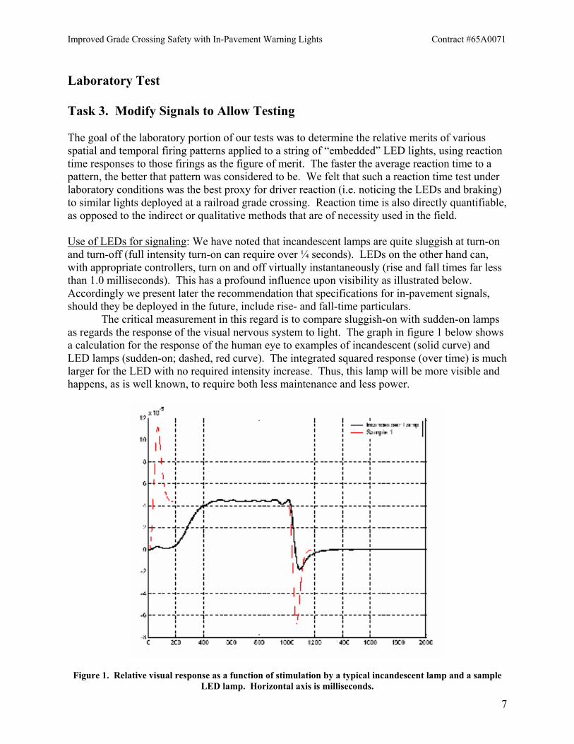
Laboratory Test Task 3. Modify Signals to Allow Testing The goal of the laboratory portion of our tests was to determine the relative merits of various spatial and temporal firing patterns applied to a string of “embedded” LED lights, using reaction time responses to those firings as the figure of merit. The faster the average reaction time to a pattern, the better that pattern was considered to be. We felt that such a reaction time test under laboratory conditions was the best proxy for driver reaction (i.e. noticing the LEDs and braking) to similar lights deployed at a railroad grade crossing. Reaction time is also directly quantifiable, as opposed to the indirect or qualitative methods that are of necessity used in the field. Use of LEDs for signaling: We have noted that incandescent lamps are quite sluggish at turn-on and turn-off (full intensity turn-on can require over ¼ seconds). LEDs on the other hand can, with appropriate controllers, turn on and off virtually instantaneously (rise and fall times far less than 1.0 milliseconds). This has a profound influence upon visibility as illustrated below. Accordingly we present later the recommendation that specifications for in-pavement signals, should they be deployed in the future, include rise- and fall-time particulars. The critical measurement in this regard is to compare sluggish-on with sudden-on lamps as regards the response of the visual nervous system to light. The graph in figure 1 below shows a calculation for the response of the human eye to examples of incandescent (solid curve) and LED lamps (sudden-on; dashed, red curve). The integrated squared response (over time) is much larger for the LED with no required intensity increase. Thus, this lamp will be more visible and happens, as is well known, to require both less maintenance and less power.
Figure 1. Relative visual response as a function of stimulation by a typical incandescent lamp and a sample LED lamp. Horizontal axis is milliseconds.
Improved Grade Crossing Safety with In-Pavement Warning Lights Contract #65A0071
8
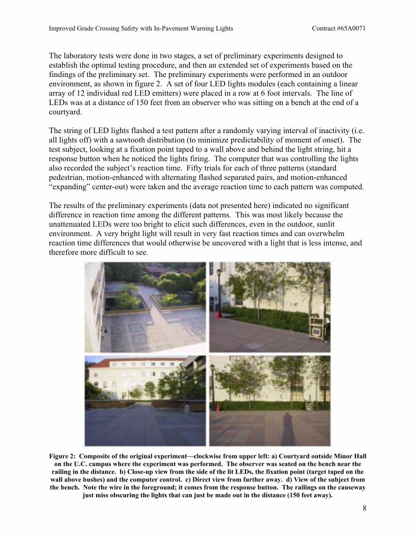
The laboratory tests were done in two stages, a set of preliminary experiments designed to establish the optimal testing procedure, and then an extended set of experiments based on the findings of the preliminary set. The preliminary experiments were performed in an outdoor environment, as shown in figure 2. A set of four LED lights modules (each containing a linear array of 12 individual red LED emitters) were placed in a row at 6 foot intervals. The line of LEDs was at a distance of 150 feet from an observer who was sitting on a bench at the end of a courtyard. The string of LED lights flashed a test pattern after a randomly varying interval of inactivity (i.e. all lights off) with a sawtooth distribution (to minimize predictability of moment of onset). The test subject, looking at a fixation point taped to a wall above and behind the light string, hit a response button when he noticed the lights firing. The computer that was controlling the lights also recorded the subject’s reaction time. Fifty trials for each of three patterns (standard pedestrian, motion-enhanced with alternating flashed separated pairs, and motion-enhanced “expanding” center-out) were taken and the average reaction time to each pattern was computed. The results of the preliminary experiments (data not presented here) indicated no significant difference in reaction time among the different patterns. This was most likely because the unattenuated LEDs were too bright to elicit such differences, even in the outdoor, sunlit environment. A very bright light will result in very fast reaction times and can overwhelm reaction time differences that would otherwise be uncovered with a light that is less intense, and therefore more difficult to see.
Figure 2: Composite of the original experiment—clockwise from upper left: a) Courtyard outside Minor Hall
on the U.C. campus where the experiment was performed. The observer was seated on the bench near the railing in the distance. b) Close-up view from the side of the lit LEDs, the fixation point (target taped on the wall above bushes) and the computer control. c) Direct view from further away. d) View of the subject from the bench. Note the wire in the foreground; it comes from the response button. The railings on the causeway
just miss obscuring the lights that can just be made out in the distance (150 feet away).
Improved Grade Crossing Safety with In-Pavement Warning Lights Contract #65A0071
9
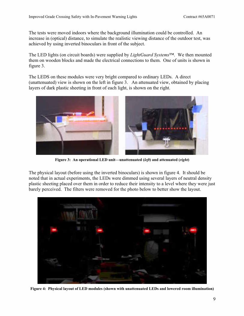
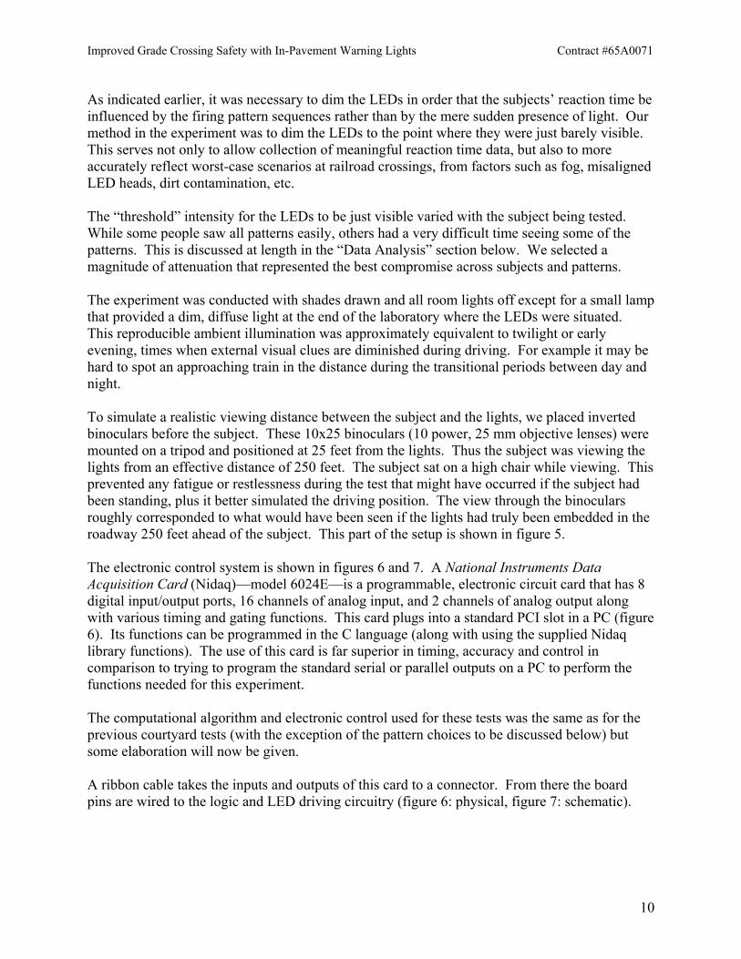
The tests were moved indoors where the background illumination could be controlled. An increase in (optical) distance, to simulate the realistic viewing distance of the outdoor test, was achieved by using inverted binoculars in front of the subject. The LED lights (on circuit boards) were supplied by LightGuard Systems™. We then mounted them on wooden blocks and made the electrical connections to them. One of units is shown in figure 3. The LEDS on these modules were very bright compared to ordinary LEDs. A direct (unattenuated) view is shown on the left in figure 3. An attenuated view, obtained by placing layers of dark plastic sheeting in front of each light, is shown on the right.
Figure 3: An operational LED unit—unattenuated (left) and attenuated (right)
The physical layout (before using the inverted binoculars) is shown in figure 4. It should be noted that in actual experiments, the LEDs were dimmed using several layers of neutral density plastic sheeting placed over them in order to reduce their intensity to a level where they were just barely perceived. The filters were removed for the photo below to better show the layout.
Figure 4: Physical layout of LED modules (shown with unattenuated LEDs and lowered room illumination)
Improved Grade Crossing Safety with In-Pavement Warning Lights Contract #65A0071
10
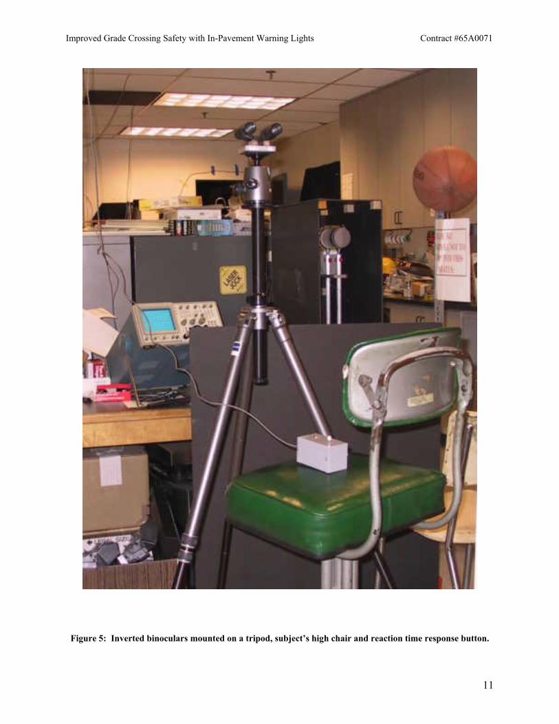
As indicated earlier, it was necessary to dim the LEDs in order that the subjects’ reaction time be influenced by the firing pattern sequences rather than by the mere sudden presence of light. Our method in the experiment was to dim the LEDs to the point where they were just barely visible. This serves not only to allow collection of meaningful reaction time data, but also to more accurately reflect worst-case scenarios at railroad crossings, from factors such as fog, misaligned LED heads, dirt contamination, etc. The “threshold” intensity for the LEDs to be just visible varied with the subject being tested. While some people saw all patterns easily, others had a very difficult time seeing some of the patterns. This is discussed at length in the “Data Analysis” section below. We selected a magnitude of attenuation that represented the best compromise across subjects and patterns. The experiment was conducted with shades drawn and all room lights off except for a small lamp that provided a dim, diffuse light at the end of the laboratory where the LEDs were situated. This reproducible ambient illumination was approximately equivalent to twilight or early evening, times when external visual clues are diminished during driving. For example it may be hard to spot an approaching train in the distance during the transitional periods between day and night. To simulate a realistic viewing distance between the subject and the lights, we placed inverted binoculars before the subject. These 10x25 binoculars (10 power, 25 mm objective lenses) were mounted on a tripod and positioned at 25 feet from the lights. Thus the subject was viewing the lights from an effective distance of 250 feet. The subject sat on a high chair while viewing. This prevented any fatigue or restlessness during the test that might have occurred if the subject had been standing, plus it better simulated the driving position. The view through the binoculars roughly corresponded to what would have been seen if the lights had truly been embedded in the roadway 250 feet ahead of the subject. This part of the setup is shown in figure 5. The electronic control system is shown in figures 6 and 7. A National Instruments Data Acquisition Card (Nidaq)—model 6024E—is a programmable, electronic circuit card that has 8 digital input/output ports, 16 channels of analog input, and 2 channels of analog output along with various timing and gating functions. This card plugs into a standard PCI slot in a PC (figure 6). Its functions can be programmed in the C language (along with using the supplied Nidaq library functions). The use of this card is far superior in timing, accuracy and control in comparison to trying to program the standard serial or parallel outputs on a PC to perform the functions needed for this experiment. The computational algorithm and electronic control used for these tests was the same as for the previous courtyard tests (with the exception of the pattern choices to be discussed below) but some elaboration will now be given. A ribbon cable takes the inputs and outputs of this card to a connector. From there the board pins are wired to the logic and LED driving circuitry (figure 6: physical, figure 7: schematic).
Improved Grade Crossing Safety with In-Pavement Warning Lights Contract #65A0071
11
Figure 5: Inverted binoculars mounted on a tripod, subject’s high chair and reaction time response button.
Improved Grade Crossing Safety with In-Pavement Warning Lights Contract #65A0071
12
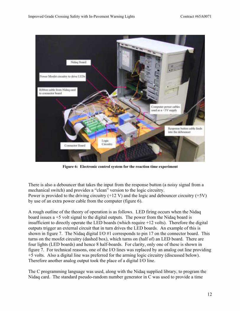
Figure 6: Electronic control system for the reaction time experiment
There is also a debouncer that takes the input from the response button (a noisy signal from a mechanical switch) and provides a “clean” version to the logic circuitry. Power is provided to the driving circuitry (+12 V) and the logic and debouncer circuitry (+5V) by use of an extra power cable from the computer (figure 6). A rough outline of the theory of operation is as follows. LED firing occurs when the Nidaq board issues a +5 volt signal to the digital outputs. The power from the Nidaq board is insufficient to directly operate the LED boards (which require +12 volts). Therefore the digital outputs trigger an external circuit that in turn drives the LED boards. An example of this is shown in figure 7. The Nidaq digital I/O #1 corresponds to pin 17 on the connector board. This turns on the mosfet circuitry (dashed box), which turns on (half of) an LED board. There are four lights (LED boards) and hence 8 half-boards. For clarity, only one of these is shown in figure 7. For technical reasons, one of the I/O lines was replaced by an analog out line providing +5 volts. Also a digital line was preferred for the arming logic circuitry (discussed below). Therefore another analog output took the place of a digital I/O line. The C programming language was used, along with the Nidaq supplied library, to program the Nidaq card. The standard pseudo-random number generator in C was used to provide a time
Improved Grade Crossing Safety with In-Pavement Warning Lights Contract #65A0071
13
delay between pattern firings. A random delay is needed because the subject can “learn” what the time delay is and anticipate (perhaps without realizing it) the firing rather than reacting to it.
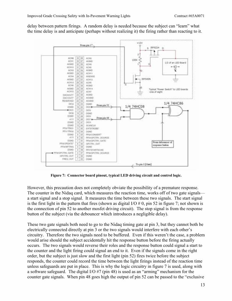
Figure 7: Connector board pinout, typical LED driving circuit and control logic.
However, this precaution does not completely obviate the possibility of a premature response. The counter in the Nidaq card, which measures the reaction time, works off of two gate signals—a start signal and a stop signal. It measures the time between these two signals. The start signal is the first light in the pattern that fires (shown as digital I/O # 0, pin 52 in figure 7; not shown is the connection of pin 52 to another mosfet driving circuit). The stop signal is from the response button of the subject (via the debouncer which introduces a negligible delay). These two gate signals both need to go to the Nidaq timing gate at pin 3, but they cannot both be electrically connected directly at pin 3 or the two signals would interfere with each other’s circuitry. Therefore the two signals need to be buffered. Even if this weren’t the case, a problem would arise should the subject accidentally hit the response button before the firing actually occurs. The two signals would reverse their roles and the response button could signal a start to the counter and the light firing could signal an end to it. Even if the signals come in the right order, but the subject is just slow and the first light (pin 52) fires twice before the subject responds, the counter could record the time between the light firings instead of the reaction time unless safeguards are put in place. This is why the logic circuitry in figure 7 is used, along with a software safeguard. The digital I/O #7 (pin 48) is used as an “arming” mechanism for the counter gate signals. When pin 48 goes high the output of pin 52 can be passed to the “exclusive
Improved Grade Crossing Safety with In-Pavement Warning Lights Contract #65A0071
14
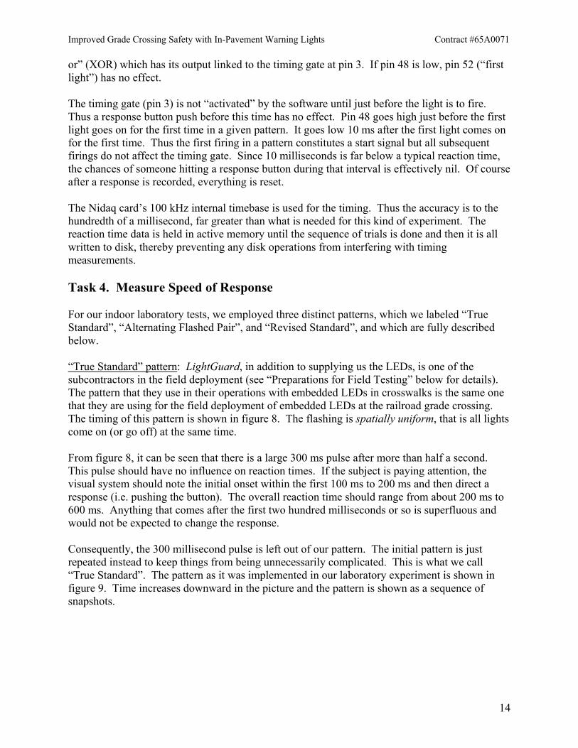
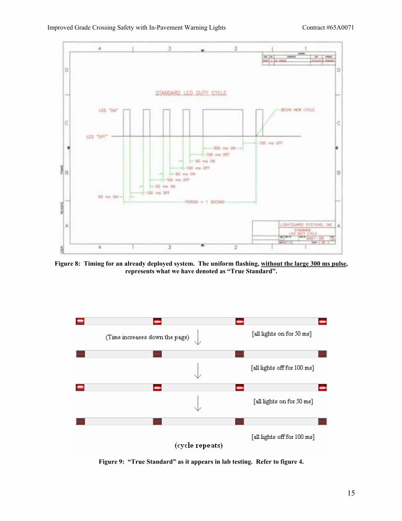
or” (XOR) which has its output linked to the timing gate at pin 3. If pin 48 is low, pin 52 (“first light”) has no effect. The timing gate (pin 3) is not “activated” by the software until just before the light is to fire. Thus a response button push before this time has no effect. Pin 48 goes high just before the first light goes on for the first time in a given pattern. It goes low 10 ms after the first light comes on for the first time. Thus the first firing in a pattern constitutes a start signal but all subsequent firings do not affect the timing gate. Since 10 milliseconds is far below a typical reaction time, the chances of someone hitting a response button during that interval is effectively nil. Of course after a response is recorded, everything is reset. The Nidaq card’s 100 kHz internal timebase is used for the timing. Thus the accuracy is to the hundredth of a millisecond, far greater than what is needed for this kind of experiment. The reaction time data is held in active memory until the sequence of trials is done and then it is all written to disk, thereby preventing any disk operations from interfering with timing measurements. Task 4. Measure Speed of Response For our indoor laboratory tests, we employed three distinct patterns, which we labeled “True Standard”, “Alternating Flashed Pair”, and “Revised Standard”, and which are fully described below. “True Standard” pattern: LightGuard, in addition to supplying us the LEDs, is one of the subcontractors in the field deployment (see “Preparations for Field Testing” below for details). The pattern that they use in their operations with embedded LEDs in crosswalks is the same one that they are using for the field deployment of embedded LEDs at the railroad grade crossing. The timing of this pattern is shown in figure 8. The flashing is spatially uniform, that is all lights come on (or go off) at the same time. From figure 8, it can be seen that there is a large 300 ms pulse after more than half a second. This pulse should have no influence on reaction times. If the subject is paying attention, the visual system should note the initial onset within the first 100 ms to 200 ms and then direct a response (i.e. pushing the button). The overall reaction time should range from about 200 ms to 600 ms. Anything that comes after the first two hundred milliseconds or so is superfluous and would not be expected to change the response. Consequently, the 300 millisecond pulse is left out of our pattern. The initial pattern is just repeated instead to keep things from being unnecessarily complicated. This is what we call “True Standard”. The pattern as it was implemented in our laboratory experiment is shown in figure 9. Time increases downward in the picture and the pattern is shown as a sequence of snapshots.
Improved Grade Crossing Safety with In-Pavement Warning Lights Contract #65A0071
15
Figure 8: Timing for an already deployed system. The uniform flashing, without the large 300 ms pulse,
represents what we have denoted as “True Standard”.
Figure 9: “True Standard” as it appears in lab testing. Refer to figure 4.
Improved Grade Crossing Safety with In-Pavement Warning Lights Contract #65A0071
16
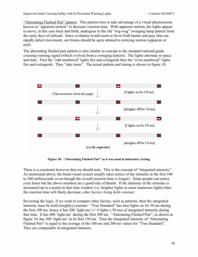
“Alternating Flashed Pair” pattern: This pattern tries to take advantage of a visual phenomenon known as “apparent motion” to decrease reaction time. With apparent motion, the lights appear to move, in this case back and forth, analogous to the old “wig-wag” swinging lamp pattern from the early days of railroad. Since evolution would seem to favor both hunter and prey that can rapidly detect movement, our brains should be quite attuned to noticing motion (apparent or real).
The alternating flashed pair pattern is also similar in concept to the standard railroad grade crossing warning signal (which evolved from a swinging lantern). The lights alternate in space and time. First the “odd numbered” lights fire and extinguish then the “even numbered” lights fire and extinguish. They “take turns”. The actual pattern and timing is shown in figure 10.
Figure 10: “Alternating Flashed Pair” as it was used in laboratory testing.
There is a constraint however that we should note. This is the concept of “integrated intensity”. As mentioned above, the brain/visual system usually takes notice of the stimulus in the first 100 to 200 milliseconds (even though the overall reaction time is longer). Some people can notice even faster but the above numbers are a good rule of thumb. If the intensity of the stimulus is increased (up to a point) in that time window (i.e. brighter lights or more numerous lights) then the reaction time will likely decrease, other factors being held constant. Reversing the logic, if we want to compare other factors, such as patterns, then the integrated intensity must be held (roughly) constant. “True Standard” has four lights on for 50 ms during the first 100 ms; hence it has 200 ‘light-ms’ (= 4 lights x 50 ms) of integrated intensity during that time. It has 400 ‘light-ms’ during the first 200 ms. “Alternating Flashed Pair”, as shown in figure 10, has 300 ‘light-ms’ in its first 150 ms. Thus the integrated intensity of “Alternating Flashed Pair” is equal to the average of the 100 ms and 200 ms values for “True Standard”. They are comparable in integrated intensity.
Improved Grade Crossing Safety with In-Pavement Warning Lights Contract #65A0071
17
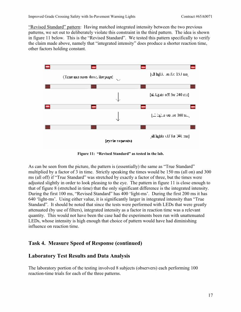
“Revised Standard” pattern: Having matched integrated intensity between the two previous patterns, we set out to deliberately violate this constraint in the third pattern. The idea is shown in figure 11 below. This is the “Revised Standard”. We tested this pattern specifically to verify the claim made above, namely that “integrated intensity” does produce a shorter reaction time, other factors holding constant.
Figure 11: “Revised Standard” as tested in the lab.
As can be seen from the picture, the pattern is (essentially) the same as “True Standard” multiplied by a factor of 3 in time. Strictly speaking the times would be 150 ms (all on) and 300 ms (all off) if “True Standard” was stretched by exactly a factor of three, but the times were adjusted slightly in order to look pleasing to the eye. The pattern in figure 11 is close enough to that of figure 8 (stretched in time) that the only significant difference is the integrated intensity. During the first 100 ms, “Revised Standard” has 400 ‘light-ms’. During the first 200 ms it has 640 ‘light-ms’. Using either value, it is significantly larger in integrated intensity than “True Standard”. It should be noted that since the tests were performed with LEDs that were greatly attenuated (by use of filters), integrated intensity as a factor in reaction time was a relevant quantity. This would not have been the case had the experiments been run with unattenuated LEDs, whose intensity is high enough that choice of pattern would have had diminishing influence on reaction time.
Task 4. Measure Speed of Response (continued) Laboratory Test Results and Data Analysis The laboratory portion of the testing involved 8 subjects (observers) each performing 100 reaction-time trials for each of the three patterns.
Improved Grade Crossing Safety with In-Pavement Warning Lights Contract #65A0071
18
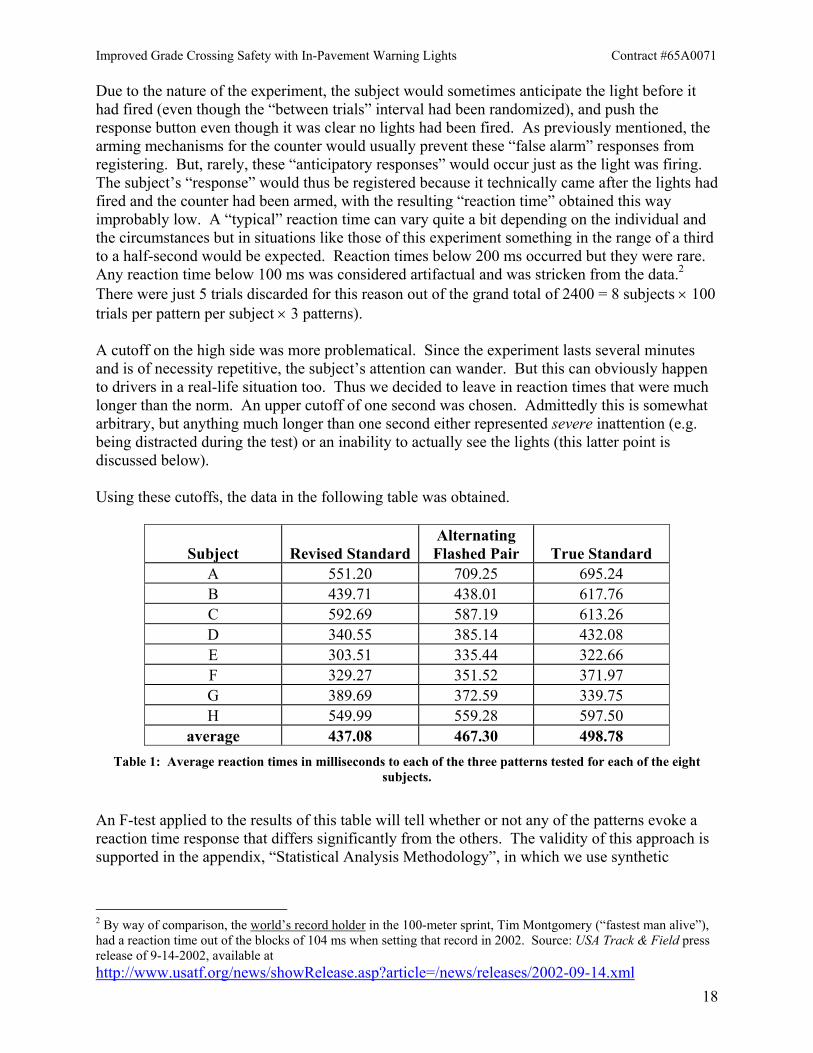
Due to the nature of the experiment, the subject would sometimes anticipate the light before it had fired (even though the “between trials” interval had been randomized), and push the response button even though it was clear no lights had been fired. As previously mentioned, the arming mechanisms for the counter would usually prevent these “false alarm” responses from registering. But, rarely, these “anticipatory responses” would occur just as the light was firing. The subject’s “response” would thus be registered because it technically came after the lights had fired and the counter had been armed, with the resulting “reaction time” obtained this way improbably low. A “typical” reaction time can vary quite a bit depending on the individual and the circumstances but in situations like those of this experiment something in the range of a third to a half-second would be expected. Reaction times below 200 ms occurred but they were rare. Any reaction time below 100 ms was considered artifactual and was stricken from the data.2 There were just 5 trials discarded for this reason out of the grand total of 2400 = 8 subjects × 100 trials per pattern per subject × 3 patterns). A cutoff on the high side was more problematical. Since the experiment lasts several minutes and is of necessity repetitive, the subject’s attention can wander. But this can obviously happen to drivers in a real-life situation too. Thus we decided to leave in reaction times that were much longer than the norm. An upper cutoff of one second was chosen. Admittedly this is somewhat arbitrary, but anything much longer than one second either represented severe inattention (e.g. being distracted during the test) or an inability to actually see the lights (this latter point is discussed below). Using these cutoffs, the data in the following table was obtained.
Subject Revised StandardAlternating Flashed Pair True Standard
A 551.20 709.25 695.24 B 439.71 438.01 617.76 C 592.69 587.19 613.26 D 340.55 385.14 432.08 E 303.51 335.44 322.66 F 329.27 351.52 371.97 G 389.69 372.59 339.75 H 549.99 559.28 597.50
average 437.08 467.30 498.78 Table 1: Average reaction times in milliseconds to each of the three patterns tested for each of the eight
subjects.
An F-test applied to the results of this table will tell whether or not any of the patterns evoke a reaction time response that differs significantly from the others. The validity of this approach is supported in the appendix, “Statistical Analysis Methodology”, in which we use synthetic
2 By way of comparison, the world’s record holder in the 100-meter sprint, Tim Montgomery (“fastest man alive”), had a reaction time out of the blocks of 104 ms when setting that record in 2002. Source: USA Track & Field press release of 9-14-2002, available at http://www.usatf.org/news/showRelease.asp?article=/news/releases/2002-09-14.xml

Improved Grade Crossing Safety with In-Pavement Warning Lights Contract #65A0071
19
reaction time data to examine the validity of applying certain statistical testing procedures. If there is a difference then pair-wise t-tests can find which of the patterns is the best. The F-test is not crucial in the present circumstances because there were only three patterns tested. But if one were testing a wide variety of patterns and one suspected that no significant reaction time differences among the patterns was a strong possibility (i.e. the Null Hypothesis is likely to hold), then a pair-wise t-test of the various combinations could end up being a tedious and needless expenditure of time; a preliminary F-test could tell the experimenter if “something is there” worth further investigation. It should be noted that a two-factor F-test is the correct one to apply. An F-test for one-factor experiments is likely to give incorrect results. This seems obvious given the fact that large variation between subjects is highly likely. This is, in fact, the case and can be “proven” by doing a Monte Carlo simulation of reaction time testing. If “subject” variation is put into the simulation as well as “pattern” variation (by appropriate shifting and scaling of the random number distributions that represent reaction time responses) and only a one-factor F-test is applied to the results, the test can fail to find (statistically significant) pattern variation even though that was deliberately put into the simulation (see appendix). Carrying forward the two-factor (pattern and subject) F-test then, the needed numbers are calculated from the previous table:
.54.968,29 variationerror)or (random residual30.239,342subjectsbetween variation
13.230,15tternsbetween pavariation 98.437,387variation total
72.467 meangrand
====
====
=
e
s
p
vv
vv
There are a = 3 patterns and b = 8 subjects. The resulting table,
Variation Degrees of
Freedom (unbiased) Mean Variance F statistic
13.230,15=pv 21 =−a 06.615,7
1ˆ2 =
−=
av
s pp 56.3
ˆˆ
2
2
=e
p
ss
with
( )( )( ) )14,2(11,1 =−−− baa degrees of freedom
30.239,342=sv 71 =−b 33.891,48
1ˆ2 =
−=
bv
s ss 84.22
ˆˆ
2
2
=e
s
ss
with
( )( )( ) )14,7(11,1 =−−− bab degrees of freedom
54.968,29=ev ( )( ) 1411 =−− ba ( )( ) 61.140,2
11ˆ2 =
−−=
bav
s ee
Table 2: Applying the F-test.
Improved Grade Crossing Safety with In-Pavement Warning Lights Contract #65A0071
20
allows comparison to the critical F values. For subjects, the critical F value3 at the 95th percentile for 7 and 14 degrees of freedom is 2.76. For the 99th percentile the value is 4.28. Therefore since,
76.284.22 95.0 =>=subjects
s FF
and 28.484.22 99.0 =>=
subjectss FF ,
the subject variation is, as one would suspect, not consistent with the null hypothesis. The variation is almost surely not due to chance. This is consistent with the earlier argument that the two-factor F test had to be used since subject variation could not be ignored. The reaction time variation due to the firing patterns is a much closer call. The critical F value at the 95th percentile is 3.74 for 2 and 14 degrees of freedom. Thus,
74.356.3 95.0 =<=patterns
p FF
is consistent with the null hypothesis. But at the 90th percentile,
73.256.3 90.0 =>=patterns
p FF
it is statistically significant. At what percentile level does the F statistic for patterns reach equality with the critical F value? Numerical integration of the central F distribution shows that,
.463.394.0 =patterns
F
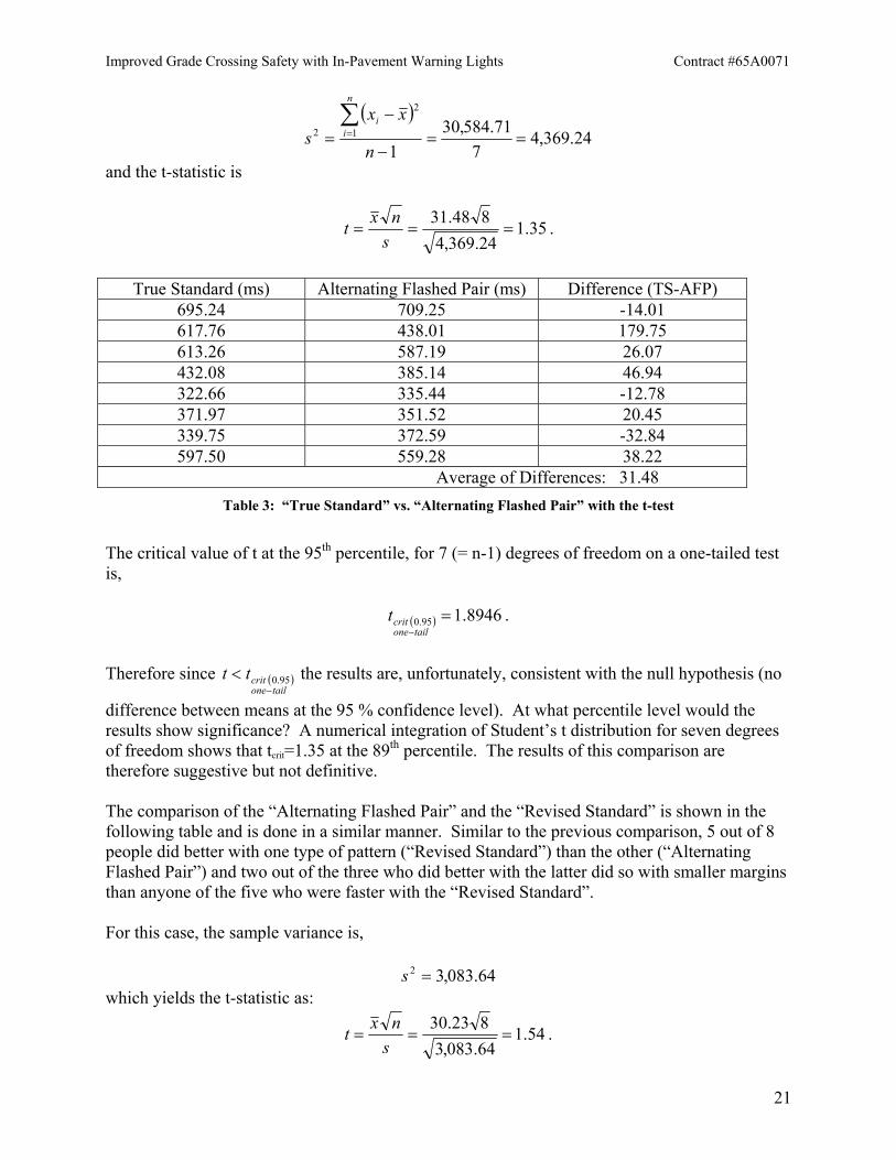
Thus the null hypothesis can be rejected at the 94 % confidence level but not the 95 % level. (In fact, Fp = 3.56 corresponds to about the 94.4 percentile.) With the statistic being “right on the cusp” as it were, further investigation is warranted. Closer examination can be done with the t-test on pair-wise differences (“Two-sample paired t-test”). The “True Standard” and “Alternating Flashed Pair” are compared in the following table. The “Alternating Flashed Pair” produced a faster reaction time in 5 out of the 8 subjects. Furthermore, in two of the three cases where the “True Standard” produced a faster average reaction time, the margin of superiority was smaller (in absolute value) than that of all five cases where “Alternating Flashed Pair” prevailed. The average paired difference is 31.48 ms. Denoting this by x and the individual time differences by xi along with the number of subjects by n (= 8), the sample variance is:
3 Appendix F of Probability and Statistics (1st Ed.), by Murray R. Spiegel in Schaum’s Outline Series [McGraw-Hill Book Company].
Improved Grade Crossing Safety with In-Pavement Warning Lights Contract #65A0071
21
( )24.369,4
771.584,30
11
2
2 ==−
−=∑=
n
xxs
n
ii
and the t-statistic is
.35.124.369,4848.31
===s
nxt
True Standard (ms) Alternating Flashed Pair (ms) Difference (TS-AFP)
695.24 709.25 -14.01 617.76 438.01 179.75 613.26 587.19 26.07 432.08 385.14 46.94 322.66 335.44 -12.78 371.97 351.52 20.45 339.75 372.59 -32.84 597.50 559.28 38.22 Average of Differences: 31.48
Table 3: “True Standard” vs. “Alternating Flashed Pair” with the t-test
The critical value of t at the 95th percentile, for 7 (= n-1) degrees of freedom on a one-tailed test is,
( ) .8946.195.0 =−tailone
critt
Therefore since ( )
tailonecrittt
−< 95.0 the results are, unfortunately, consistent with the null hypothesis (no
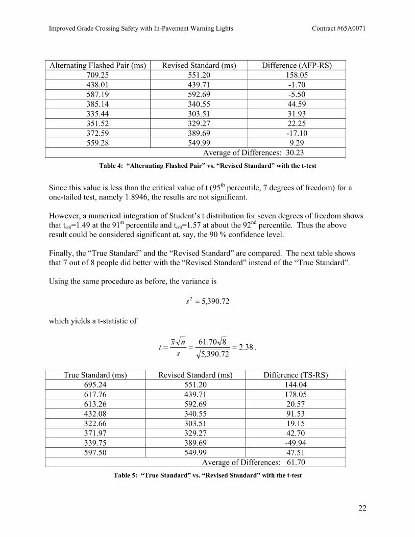
difference between means at the 95 % confidence level). At what percentile level would the results show significance? A numerical integration of Student’s t distribution for seven degrees of freedom shows that tcrit=1.35 at the 89th percentile. The results of this comparison are therefore suggestive but not definitive. The comparison of the “Alternating Flashed Pair” and the “Revised Standard” is shown in the following table and is done in a similar manner. Similar to the previous comparison, 5 out of 8 people did better with one type of pattern (“Revised Standard”) than the other (“Alternating Flashed Pair”) and two out of the three who did better with the latter did so with smaller margins than anyone of the five who were faster with the “Revised Standard”. For this case, the sample variance is,
64.083,32 =s which yields the t-statistic as:
.54.164.083,3823.30
===s
nxt
Improved Grade Crossing Safety with In-Pavement Warning Lights Contract #65A0071
22
Alternating Flashed Pair (ms) Revised Standard (ms) Difference (AFP-RS)
709.25 551.20 158.05 438.01 439.71 -1.70 587.19 592.69 -5.50 385.14 340.55 44.59 335.44 303.51 31.93 351.52 329.27 22.25 372.59 389.69 -17.10 559.28 549.99 9.29 Average of Differences: 30.23
Table 4: “Alternating Flashed Pair” vs. “Revised Standard” with the t-test
Since this value is less than the critical value of t (95th percentile, 7 degrees of freedom) for a one-tailed test, namely 1.8946, the results are not significant. However, a numerical integration of Student’s t distribution for seven degrees of freedom shows that tcrit=1.49 at the 91st percentile and tcrit=1.57 at about the 92nd percentile. Thus the above result could be considered significant at, say, the 90 % confidence level. Finally, the “True Standard” and the “Revised Standard” are compared. The next table shows that 7 out of 8 people did better with the “Revised Standard” instead of the “True Standard”. Using the same procedure as before, the variance is
72.390,52 =s
which yields a t-statistic of
.38.272.390,5870.61
===s
nxt
True Standard (ms) Revised Standard (ms) Difference (TS-RS)
695.24 551.20 144.04 617.76 439.71 178.05 613.26 592.69 20.57 432.08 340.55 91.53 322.66 303.51 19.15 371.97 329.27 42.70 339.75 389.69 -49.94 597.50 549.99 47.51 Average of Differences: 61.70
Table 5: “True Standard” vs. “Revised Standard” with the t-test
Improved Grade Crossing Safety with In-Pavement Warning Lights Contract #65A0071
23
This time the value of the t-statistic is greater than the critical value:
.8946.138.2 )95.0( =>=−tailone
crittt
(The t-statistic of 2.38 corresponds to about the 97.5 percentile.) The “Revised Standard” can thus be said to definitively elicit faster reaction times than the “True Standard” (at least as “definitively” as statistics allows). This result makes sense from a psychophysical viewpoint: It is known that longer duration visual stimuli evoke faster reaction times4 (obviously only up to a point). The same is true of auditory stimuli.5 Since the “Revised Standard” is the same spatial pattern as the “True Standard” but is (essentially) 3 times as long, the former would be expected to do better than the latter. It can now be seen that the previous results from the F-test are consistent. The F-test is used to decide if any of a series of tests differ (significantly) from the others. In particular it tests whether or not the proposition holds that all the test results could have come from populations with the same mean; either it is likely that all the test means are the same within statistical fluctuation or it is not. In the present setting there are only three cases. One can imagine the means of, say, ten cases being “clustered” or “spread out” but these adjectives wouldn’t have as much meaning for only two cases. For three cases the situation is only a little better. Only the two extremes “Revised Standard” and “True Standard” showed a statistically significant difference when doing the pairwise comparisons (t-test). Thus if, in the case of the F-test, the null hypothesis held and there were no difference between the means one can imagine that the “true” mean was near that of the “Alternating Flashed Pair” with the means of “Revised Standard” and “True Standard” falling on either side due to statistical fluctuations. Each result would be (statistically) near enough the “true” mean that the null hypothesis for the F-test would hold but the two results on the “wings” might be just far enough apart to show statistical significance under a pairwise comparison. Despite the three paired t-tests giving only one result of statistical significance, the results are actually better than that for two reasons, one quantitative and one qualitative. Quantitative. The quantitative reason is that the non-significant results are close enough to the threshold of significance that an increase in the number of subjects tested might cross that threshold. This is supposition of course, but it is not supposition without a basis. The “Alternating Flashed Pair” was faster than the “True Standard” by an average of 31 ms. This difference just fell a little shy of statistical significance at the 95 % confidence level. The fact that it was faster is consistent with the notion that apparent motion produces a faster response, other factors being held constant (see earlier discussion). This has practical significance, as outlined below.
4 Froeberg, S. [1907]. The relation between magnitude of stimulus and the time of reaction. Archives of Psychology, No. 8 5 Wells, G. R. [1913]. The influence of stimulus duration on RT. Psychological Monographs 15: 1066

Improved Grade Crossing Safety with In-Pavement Warning Lights Contract #65A0071
24
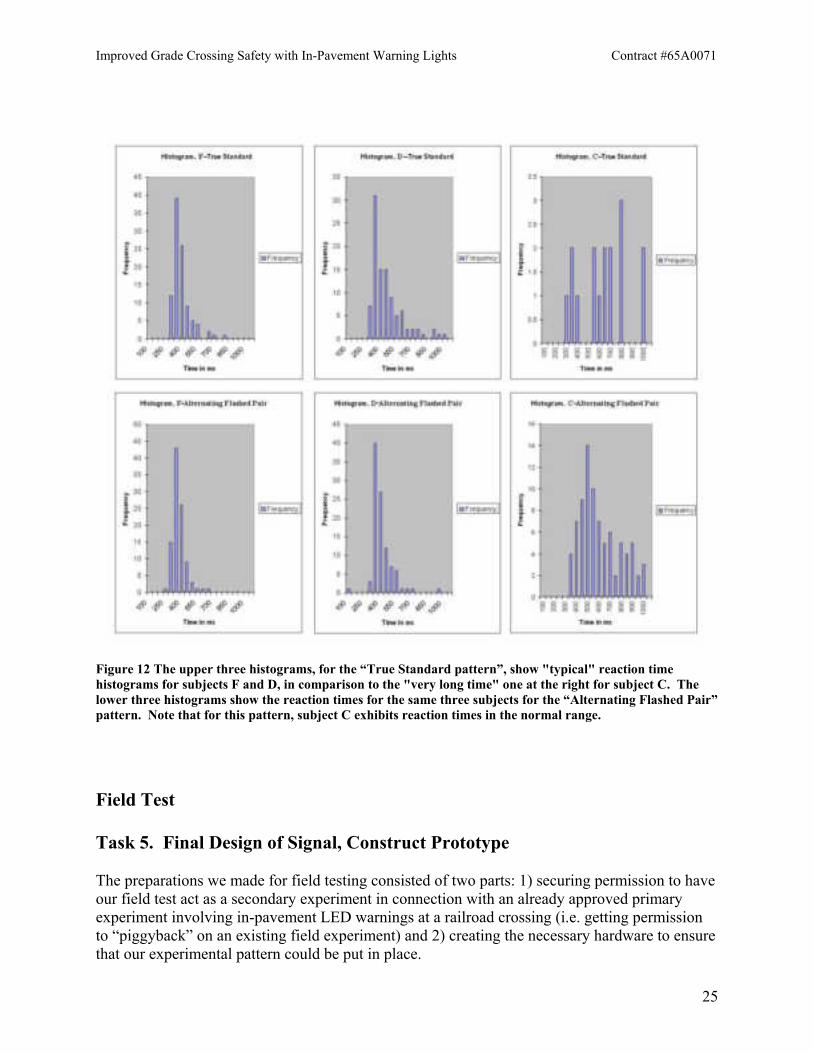
Statistical analysis above supplies some reason to think that different signaling strategies supply different outcomes as regards how long it takes an observer to react to a signal. The average reaction time differences are slight (just over 30 milliseconds). This amount corresponds to a stop location that is under a meter further advanced toward a crossing at 60 MPH. That magnitude of difference would be only marginally important but the average difference is not a good way to characterize the difference between these two illumination strategies. In fact, contributing to the 30 milliseconds average difference are a number of rather large delays, as may be seen in figure 12. For example, 20% of the reaction times for subject “D” to the “True Standard” pattern are greater than 700 milliseconds, while only 1.5% of the reaction times for the same subject to the “Alternating Flashed Pair” pattern are greater than 700 milliseconds. The increased number of relatively long reaction times for the “True Standard” pattern would be very significant in the real world setting of braking/slowing for a signal. They don't occur often, but they occur often enough to predict an important advantage for the strategy of alternating signaling. The experimental design (number of trials, number of subjects) was based on the results of a Monte Carlo simulation of reaction time testing but for a smaller number of subjects. Since it is an experiment and one does not know the outcome, the best that can be done in experimental design is to estimate what is likely to occur (given, say, a hypothetical positive result) and incorporate that estimate in such a way as to generate sufficient statistics should that scenario occur. That was the course followed here but the subject variation that was assumed in the simulation was much less than occurred in the actual experiment. Thus if a larger pool of subjects was tested it is quite possible that the same (average) reaction time differentials may have been seen but that the statistics would pass into the realm of significance. Qualitative. The qualitative reason is the reports of some of our subjects. Three of our subjects remarked that the “True Standard” was very difficult to see in comparison to the other two patterns. One of those two (subject “C”) reported barely being able to see the pattern at all. The histogram of his reaction times for this pattern plainly backs him up as can be seen in the comparison in figure 12. The vast bulk of the responses were beyond one second (not shown in histogram). On the other hand, with the “Alternating Flashed Pair” pattern, all subjects exhibited reaction times in the normal range. As mentioned previously, the data was cutoff above one second for consistency of treatment. If C’s (and for that matter B’s and A’s) data above one second were included in a reanalysis, the “True Standard” would fare even worse than it did. In trying to make the patterns “just barely noticeable”, the “True Standard” obviously fell below this threshold for a couple of subjects. Rather than apply a reanalysis with no upper data cutoff (when it is clear that the pattern “True Standard” may not have even been seen in some cases), or redo the entire experiment until all subjects can unequivocally see all patterns (but “just barely”), or throw out some patterns for some subjects and reanalyze the data with an unequal number of pairwise comparisons, it seems more straightforward to just note this, quite strong, qualitative evidence that the “True Standard” pattern was more difficult to see for two of the three observers.
Improved Grade Crossing Safety with In-Pavement Warning Lights Contract #65A0071
25
Figure 12 The upper three histograms, for the “True Standard pattern”, show "typical" reaction time histograms for subjects F and D, in comparison to the "very long time" one at the right for subject C. The lower three histograms show the reaction times for the same three subjects for the “Alternating Flashed Pair” pattern. Note that for this pattern, subject C exhibits reaction times in the normal range.
Field Test Task 5. Final Design of Signal, Construct Prototype The preparations we made for field testing consisted of two parts: 1) securing permission to have our field test act as a secondary experiment in connection with an already approved primary experiment involving in-pavement LED warnings at a railroad crossing (i.e. getting permission to “piggyback” on an existing field experiment) and 2) creating the necessary hardware to ensure that our experimental pattern could be put in place.
Improved Grade Crossing Safety with In-Pavement Warning Lights Contract #65A0071
26
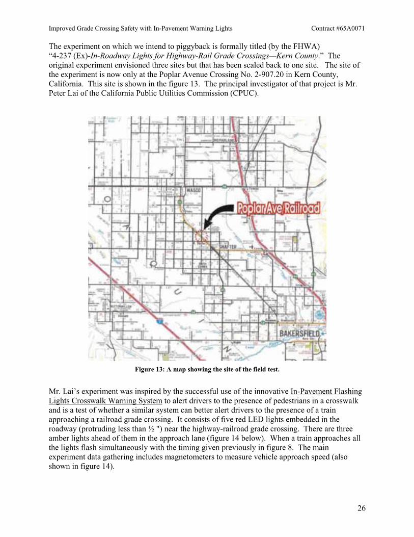
The experiment on which we intend to piggyback is formally titled (by the FHWA) “4-237 (Ex)-In-Roadway Lights for Highway-Rail Grade Crossings—Kern County.” The original experiment envisioned three sites but that has been scaled back to one site. The site of the experiment is now only at the Poplar Avenue Crossing No. 2-907.20 in Kern County, California. This site is shown in the figure 13. The principal investigator of that project is Mr. Peter Lai of the California Public Utilities Commission (CPUC).
Figure 13: A map showing the site of the field test.
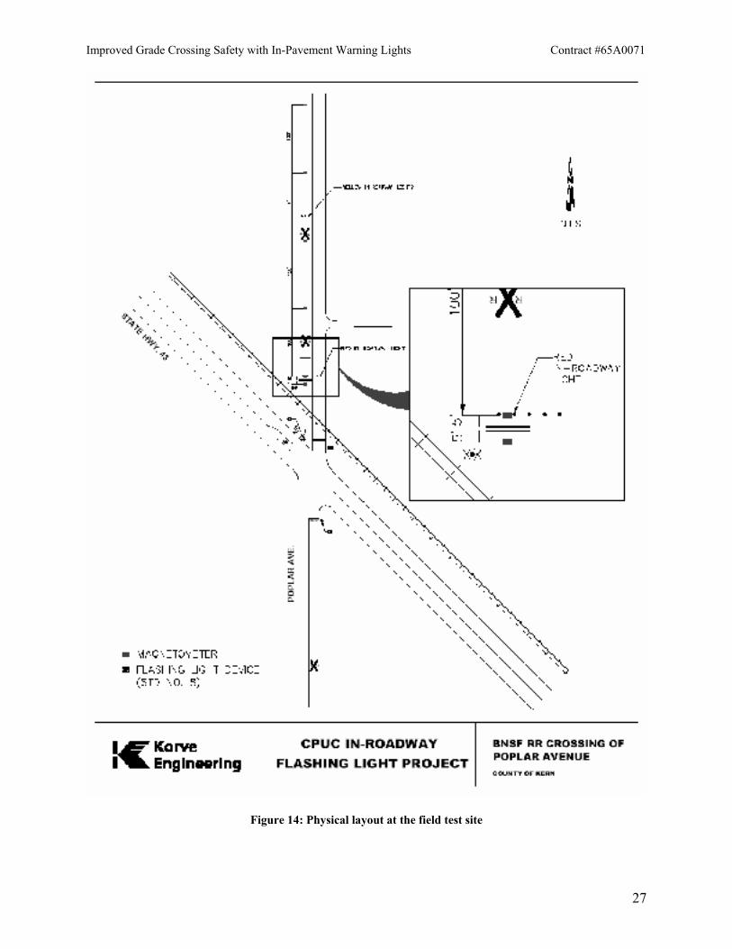
Mr. Lai’s experiment was inspired by the successful use of the innovative In-Pavement Flashing Lights Crosswalk Warning System to alert drivers to the presence of pedestrians in a crosswalk and is a test of whether a similar system can better alert drivers to the presence of a train approaching a railroad grade crossing. It consists of five red LED lights embedded in the roadway (protruding less than ½ ") near the highway-railroad grade crossing. There are three amber lights ahead of them in the approach lane (figure 14 below). When a train approaches all the lights flash simultaneously with the timing given previously in figure 8. The main experiment data gathering includes magnetometers to measure vehicle approach speed (also shown in figure 14).
Improved Grade Crossing Safety with In-Pavement Warning Lights Contract #65A0071
27
Figure 14: Physical layout at the field test site
Improved Grade Crossing Safety with In-Pavement Warning Lights Contract #65A0071
28
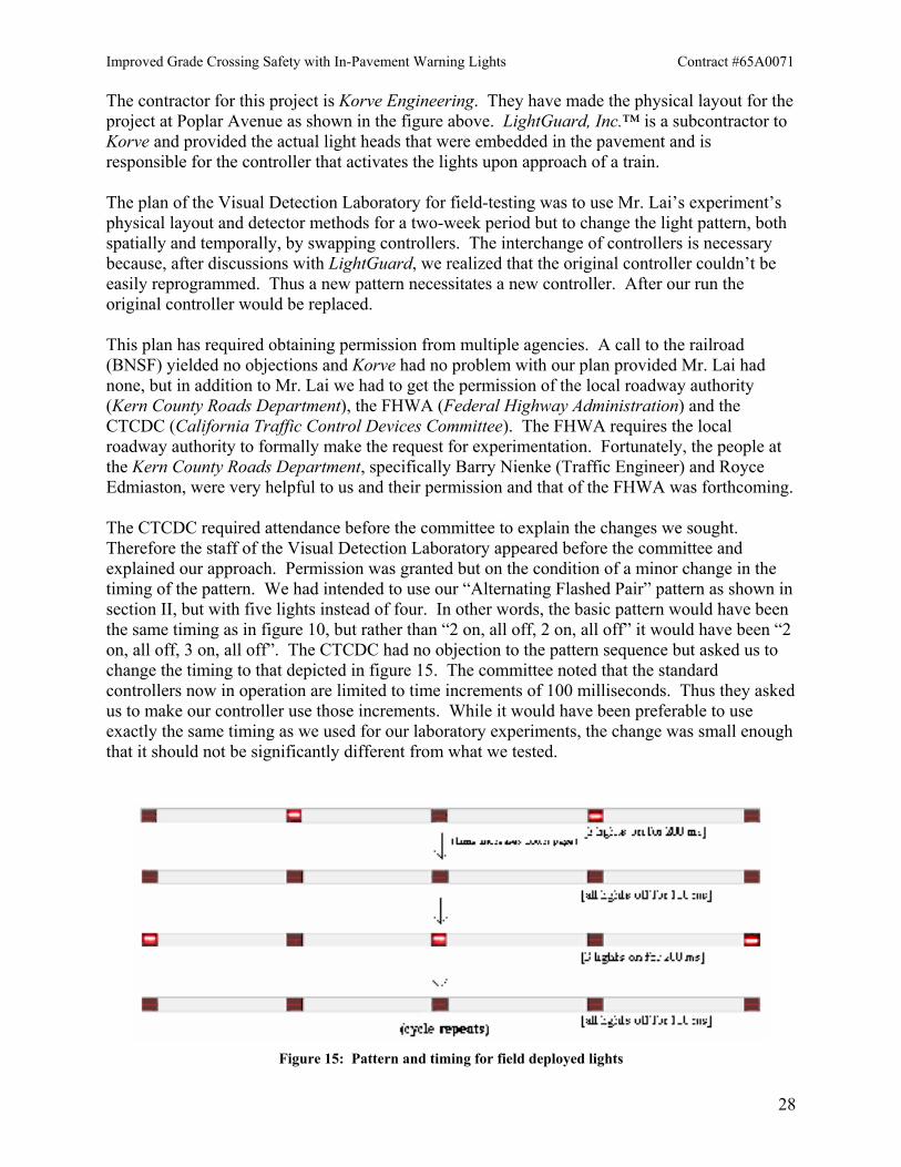
The contractor for this project is Korve Engineering. They have made the physical layout for the project at Poplar Avenue as shown in the figure above. LightGuard, Inc.™ is a subcontractor to Korve and provided the actual light heads that were embedded in the pavement and is responsible for the controller that activates the lights upon approach of a train. The plan of the Visual Detection Laboratory for field-testing was to use Mr. Lai’s experiment’s physical layout and detector methods for a two-week period but to change the light pattern, both spatially and temporally, by swapping controllers. The interchange of controllers is necessary because, after discussions with LightGuard, we realized that the original controller couldn’t be easily reprogrammed. Thus a new pattern necessitates a new controller. After our run the original controller would be replaced. This plan has required obtaining permission from multiple agencies. A call to the railroad (BNSF) yielded no objections and Korve had no problem with our plan provided Mr. Lai had none, but in addition to Mr. Lai we had to get the permission of the local roadway authority (Kern County Roads Department), the FHWA (Federal Highway Administration) and the CTCDC (California Traffic Control Devices Committee). The FHWA requires the local roadway authority to formally make the request for experimentation. Fortunately, the people at the Kern County Roads Department, specifically Barry Nienke (Traffic Engineer) and Royce Edmiaston, were very helpful to us and their permission and that of the FHWA was forthcoming. The CTCDC required attendance before the committee to explain the changes we sought. Therefore the staff of the Visual Detection Laboratory appeared before the committee and explained our approach. Permission was granted but on the condition of a minor change in the timing of the pattern. We had intended to use our “Alternating Flashed Pair” pattern as shown in section II, but with five lights instead of four. In other words, the basic pattern would have been the same timing as in figure 10, but rather than “2 on, all off, 2 on, all off” it would have been “2 on, all off, 3 on, all off”. The CTCDC had no objection to the pattern sequence but asked us to change the timing to that depicted in figure 15. The committee noted that the standard controllers now in operation are limited to time increments of 100 milliseconds. Thus they asked us to make our controller use those increments. While it would have been preferable to use exactly the same timing as we used for our laboratory experiments, the change was small enough that it should not be significantly different from what we tested.
Figure 15: Pattern and timing for field deployed lights
Improved Grade Crossing Safety with In-Pavement Warning Lights Contract #65A0071
29
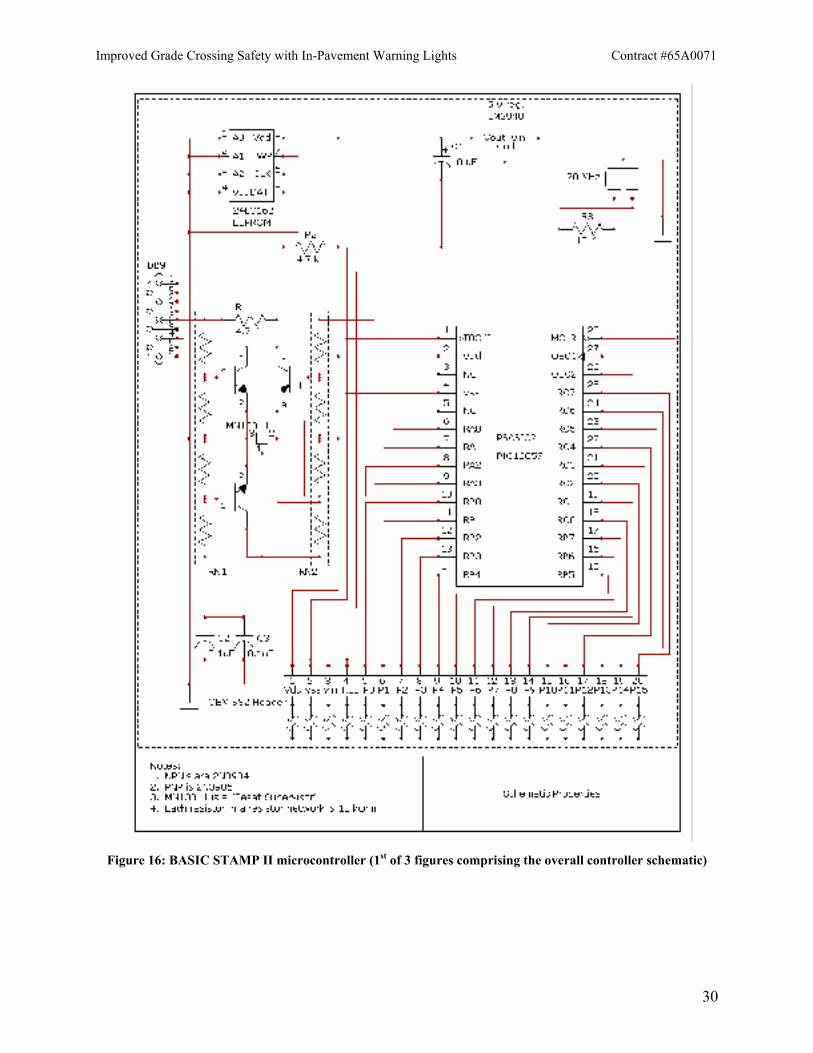
Since the Lai experiment has the lights and magnetometers in place, the essential hardware aspect that the Visual Detection Laboratory had to create was the controller. As mentioned above, a new controller for the lights had to be created because the original one was unsuitable for anything beyond what was needed for the (spatially) uniform flashing of the original experiment by Mr. Lai. Since the pattern is relatively uncomplicated, the controller does not need extensive programming. The Visual Detection Laboratory made the decision to use a BASIC STAMP II, a controller made by Parallax, Inc. This controller can be programmed in BASIC and also has the virtue of being reprogrammable from a portable computer using a serial cable with a DB9 connector. Thus it could be reprogrammed in the field if necessary. The only question was whether the use of a high-level programming language made the controller too slow. This seemed very doubtful because included among the documented commands was a “waiting” command that had increments of 1 ms. Nonetheless, to ensure there would be no problem, we tested the hardware by measuring the timing intervals using LEDs, a light detector and a storage oscilloscope with a better than 1 ms resolution. The tests confirmed that the controller had at least a 1 ms resolution, much better than is needed for our purposes. The schematic for this microcontroller is shown in figure 16.
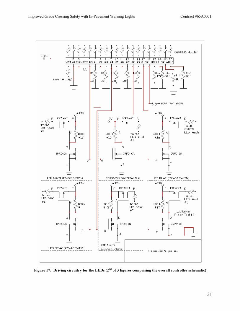
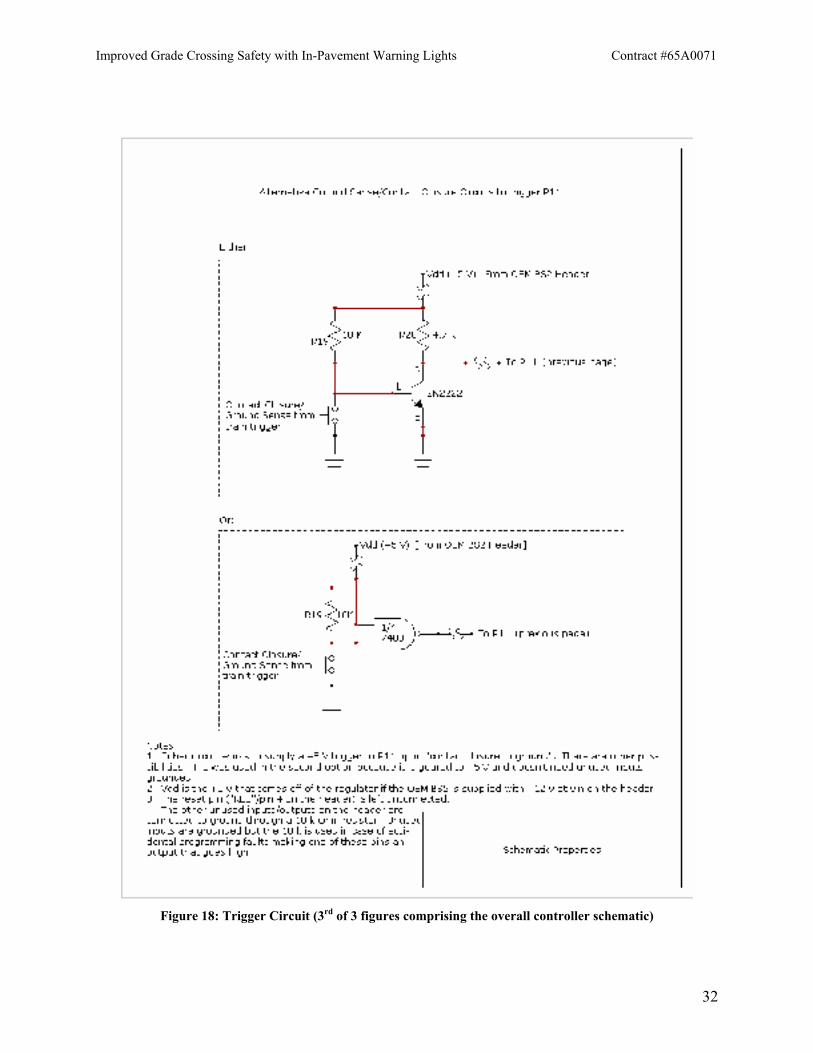
Figures 17 and 18 show the driving circuitry for the in-pavement LEDs (needed because the lights operate at a different voltage and take more power than the microcontroller can deliver) and the trigger circuitry that commands the microcontroller to run the light pattern because a train is coming.
Although the Visual Detection Laboratory designed the alternate controller circuitry, LightGuard was the company contracted to supply the controller to the Lai experiment. They were gracious enough to not only check our work but to build the actual device so that it would be compatible with their equipment when the controllers are swapped.
Improved Grade Crossing Safety with In-Pavement Warning Lights Contract #65A0071
30
Figure 16: BASIC STAMP II microcontroller (1st of 3 figures comprising the overall controller schematic)
Improved Grade Crossing Safety with In-Pavement Warning Lights Contract #65A0071
31
Figure 17: Driving circuitry for the LEDs (2nd of 3 figures comprising the overall controller schematic)
Improved Grade Crossing Safety with In-Pavement Warning Lights Contract #65A0071
32
Figure 18: Trigger Circuit (3rd of 3 figures comprising the overall controller schematic)
Improved Grade Crossing Safety with In-Pavement Warning Lights Contract #65A0071
33
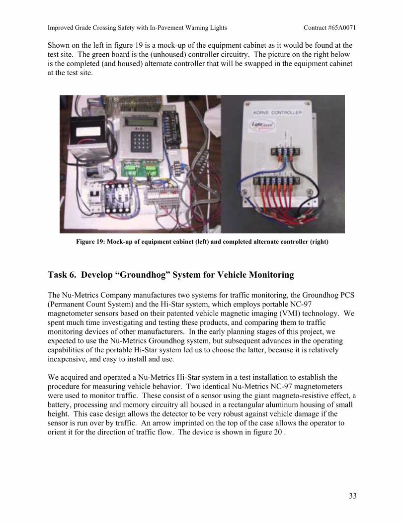
Shown on the left in figure 19 is a mock-up of the equipment cabinet as it would be found at the test site. The green board is the (unhoused) controller circuitry. The picture on the right below is the completed (and housed) alternate controller that will be swapped in the equipment cabinet at the test site.
Figure 19: Mock-up of equipment cabinet (left) and completed alternate controller (right)
Task 6. Develop “Groundhog” System for Vehicle Monitoring The Nu-Metrics Company manufactures two systems for traffic monitoring, the Groundhog PCS (Permanent Count System) and the Hi-Star system, which employs portable NC-97 magnetometer sensors based on their patented vehicle magnetic imaging (VMI) technology. We spent much time investigating and testing these products, and comparing them to traffic monitoring devices of other manufacturers. In the early planning stages of this project, we expected to use the Nu-Metrics Groundhog system, but subsequent advances in the operating capabilities of the portable Hi-Star system led us to choose the latter, because it is relatively inexpensive, and easy to install and use. We acquired and operated a Nu-Metrics Hi-Star system in a test installation to establish the procedure for measuring vehicle behavior. Two identical Nu-Metrics NC-97 magnetometers were used to monitor traffic. These consist of a sensor using the giant magneto-resistive effect, a battery, processing and memory circuitry all housed in a rectangular aluminum housing of small height. This case design allows the detector to be very robust against vehicle damage if the sensor is run over by traffic. An arrow imprinted on the top of the case allows the operator to orient it for the direction of traffic flow. The device is shown in figure 20 .

Improved Grade Crossing Safety with In-Pavement Warning Lights Contract #65A0071
34
Figure 20: Nu-Metrics, Inc magnetometer (Hi-Star® NC-97)
In operation the detector is charged and programmed through small jacks on its side before deployment. At deployment the sensor is positioned on the roadway in such a way as to have vehicle bodies pass directly over it. Of course, vehicle wheels sometimes directly run over it, hence the need for a small profile and physical robustness. The detector is held in place by a disposable epoxy mat that adheres to the roadway and covers the detector. The detector is primarily designed for vehicle counts but can be programmed to record vehicle speed and a “time stamp” (the time at which the vehicle passed over the detector). This “long sequential” mode was used in the present test. Raw data include a time stamp, vehicle speed, vehicle length and whether the roadway was wet or dry. The downloaded data was then converted from the native format of the software that is used with the detectors to a more widely used format, that of Microsoft’s Excel. For this test run, we installed two sensors at positions along the roadway, one approximately 50 meters in advance of, and the second approximately 5 meters beyond the position of a roadway warning sign. The purpose was to be able to test our ability to coordinate readings at two sensors for the purpose of estimating average deceleration. We measured vehicle speeds for a period of 24 hours, acquiring records for approximately 5000 vehicles. We then downloaded the data, and acquired data for another 24-hour period. The data was separated into separate bins for daytime and nighttime conditions. Also, outlier data points that were obviously erroneous were removed. Table 6 shows the analyzed data for the two conditions. From the vehicle speed at each detector and the associated time stamp average deceleration is easily calculated (not shown here). Average observed speed, s.e. [mph] Detector A Detector B (55 m beyond A) Sample 1 Sample 2 Sample 1 Sample 2 Day 28.4; 0.1 29.1; 0.1 25.1; 0.1 26.3; 0.1 Night 31.6; 0.3 30.6; 0.4 29.2; 0.3 28.5; 0.3
Table 6. Sample data obtained with the Hi-Star system. This demonstrates the utility and ease of use of the Hi-Star NC-97 system for purposes of monitoring traffic flow and compiling vehicle speed statistics.
Improved Grade Crossing Safety with In-Pavement Warning Lights Contract #65A0071
35
Task 7. Employ “Groundhog/97” System at Test Site During the course of this project, our field test strategy evolved to that of “piggybacking” on another project (see Task 5), and therefore using the other project’s system for traffic monitoring, which, as became evident, employed similar NC-97 equipment. The only modifications resulted from Korve Engineering working with Nu-Metrics to increase the memory and extend the battery life of the NC-97. For the Lai project, the NC-97 is placed inside a shallow box whose upper surface is flush with the roadway (thus eliminating the need for an epoxy mat). Since the Lai project put all this in place, there was no need for us to duplicate it as long as it was compatible with our needs, which was assured by our previous testing (described in Task 6). Field Test Results Task 8. Deploy Signals at Test Site Task 9. Monitor Vehicle Behavior Task 10. Analyze Recorded Data The Visual Detection Laboratory agreed to “piggyback” on Mr. Lai’s project (see Task 5) for the field test portion of our experiment in order to conserve resources. We felt that duplicating all the conditions of that experiment, save the patterns, would require more funding than allowable in the project budget. Since Mr. Lai had already received permission to implant the lights, install magnetometer detectors in the roadway, and connect his controller to the railroad train-approach trigger, and since he already had begun implementing these steps, our decision seemed a wise and efficient use of resources. All that remained for us to do was develop a controller to enable a change of the light pattern. Unfortunately, this decision meant that the field portion of our experiment was no longer completely under our control. While, at the time of this writing, the Lai project has the magnetometers, lights and controller in place, an issue has arisen as to how to provide power to both his and to this project’s equipment. As of October, 2004, Mr. Lai reported that he was still in discussions to resolve the power issue. Even though the period of performance for this project has officially ended, the Visual Detection Lab is committed to completing the field deployment and conducting the field test experiments, using alternative resources. The field test results will be reported as an addendum to this Final Report.
Improved Grade Crossing Safety with In-Pavement Warning Lights Contract #65A0071
36
Task 11. Assemble Expert Panel The expert panel, to be convened, will consist of Tori Kanzler, Katie Benouar, Ken Galt, and Michael Samadian of Caltrans, Peter Lai of the CA-PUC, Peter Molenda, a signal expert from Union Pacific, Matt Schmitz of the FHWA, and Gerry Meis of Caltrans and the CTCDC. Potential for Deployment and Implementation In the laboratory tests, we compared reaction times of human observers to three different pattern/timing combinations of embedded LED lights. By a combination of statistical analysis and qualitative means, we demonstrated that the “Revised Standard” pattern is more effective than the “Alternating Flashed Pair” which is turn more effective than the “True Standard”. Even though the “Revised Standard” fared better than “Alternating Flashed Pair”, we have argued that this is likely due to the former pattern having a greater integrated intensity. Therefore, we selected the “Alternating Flashed Pair” and “True Standard” patterns to be compared in the field deployment (using vehicle behavior as the dependent variable). Because of delays in field deployment owing to circumstances beyond the control of the Visual Detection Laboratory, we will report the results of the field tests later as an addendum to this report. The experimental results combined with the relative ease of constructing a new controller show that marginal costs for a more effective pattern choice are very small. We therefore recommend changing from the standard, spatially uniform, flashed pattern in figure 8, which is currently employed in embedded LED lights serving as pedestrian crosswalk warning devices, to “Alternating Flashed Pair” for any likely permanent deployment of this system. Because this pattern generates the perception of movement, the human visual system responds faster, allowing a shorter overall reaction time, and thus an increased safety factor. We further recommend that the full benefit of LEDs be protected by ensuring, in specifications, that rise and fall times for light intensity be restricted to less than 10 milliseconds. Implicit in our recommendations that a pattern that generates apparent movement be adopted is that the MUTCD and other agencies should incorporate rules for spatially varying signals in addition to the current rules governing strictly temporally varying signals (flashing). Acknowledgements We would like to thank the personnel at LightGuard Systems, Inc.™, especially Jeremy Greenburg, Dave Michaelson and Bill Parry, who have provided considerable assistance by building the modified controller from the design we provided, and making sure it was compatible with their equipment. Mr. Peter Lai of the CPUC deserves special thanks for letting us piggyback our project onto his. Ali Banava of Korve Engineering and Joaquin Siques, formerly of that firm, helped make sure that our project could mesh with Mr. Lai’s project. We would also like to thank Barry Nienke and Royce Edmiaston of the Kern County Roads Department and Matthew Schmitz of the FHWA for their help in obtaining the multiple agency permissions that this project has required.
Improved Grade Crossing Safety with In-Pavement Warning Lights Contract #65A0071
37
Appendix: Statistical Analysis Methodology
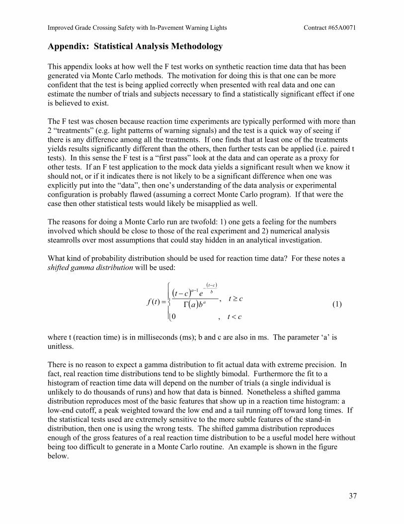
This appendix looks at how well the F test works on synthetic reaction time data that has been generated via Monte Carlo methods. The motivation for doing this is that one can be more confident that the test is being applied correctly when presented with real data and one can estimate the number of trials and subjects necessary to find a statistically significant effect if one is believed to exist. The F test was chosen because reaction time experiments are typically performed with more than 2 “treatments” (e.g. light patterns of warning signals) and the test is a quick way of seeing if there is any difference among all the treatments. If one finds that at least one of the treatments yields results significantly different than the others, then further tests can be applied (i.e. paired t tests). In this sense the F test is a “first pass” look at the data and can operate as a proxy for other tests. If an F test application to the mock data yields a significant result when we know it should not, or if it indicates there is not likely to be a significant difference when one was explicitly put into the “data”, then one’s understanding of the data analysis or experimental configuration is probably flawed (assuming a correct Monte Carlo program). If that were the case then other statistical tests would likely be misapplied as well. The reasons for doing a Monte Carlo run are twofold: 1) one gets a feeling for the numbers involved which should be close to those of the real experiment and 2) numerical analysis steamrolls over most assumptions that could stay hidden in an analytical investigation. What kind of probability distribution should be used for reaction time data? For these notes a shifted gamma distribution will be used:
( )
( )
( )
<
≥Γ
−=
−−−
ct
ctbaect
tf a
bct
a
,0
,)(1
(1)
where t (reaction time) is in milliseconds (ms); b and c are also in ms. The parameter ‘a’ is unitless. There is no reason to expect a gamma distribution to fit actual data with extreme precision. In fact, real reaction time distributions tend to be slightly bimodal. Furthermore the fit to a histogram of reaction time data will depend on the number of trials (a single individual is unlikely to do thousands of runs) and how that data is binned. Nonetheless a shifted gamma distribution reproduces most of the basic features that show up in a reaction time histogram: a low-end cutoff, a peak weighted toward the low end and a tail running off toward long times. If the statistical tests used are extremely sensitive to the more subtle features of the stand-in distribution, then one is using the wrong tests. The shifted gamma distribution reproduces enough of the gross features of a real reaction time distribution to be a useful model here without being too difficult to generate in a Monte Carlo routine. An example is shown in the figure below.
Improved Grade Crossing Safety with In-Pavement Warning Lights Contract #65A0071
38
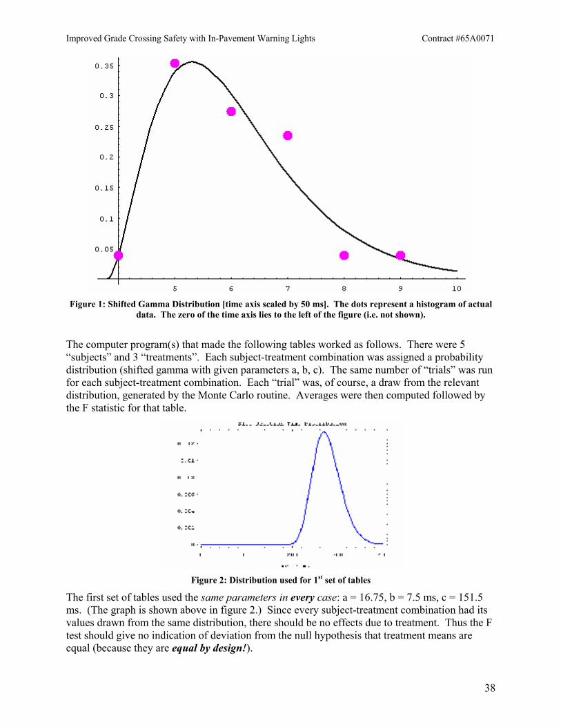
Figure 1: Shifted Gamma Distribution [time axis scaled by 50 ms]. The dots represent a histogram of actual
data. The zero of the time axis lies to the left of the figure (i.e. not shown).
The computer program(s) that made the following tables worked as follows. There were 5 “subjects” and 3 “treatments”. Each subject-treatment combination was assigned a probability distribution (shifted gamma with given parameters a, b, c). The same number of “trials” was run for each subject-treatment combination. Each “trial” was, of course, a draw from the relevant distribution, generated by the Monte Carlo routine. Averages were then computed followed by the F statistic for that table.
Figure 2: Distribution used for 1st set of tables
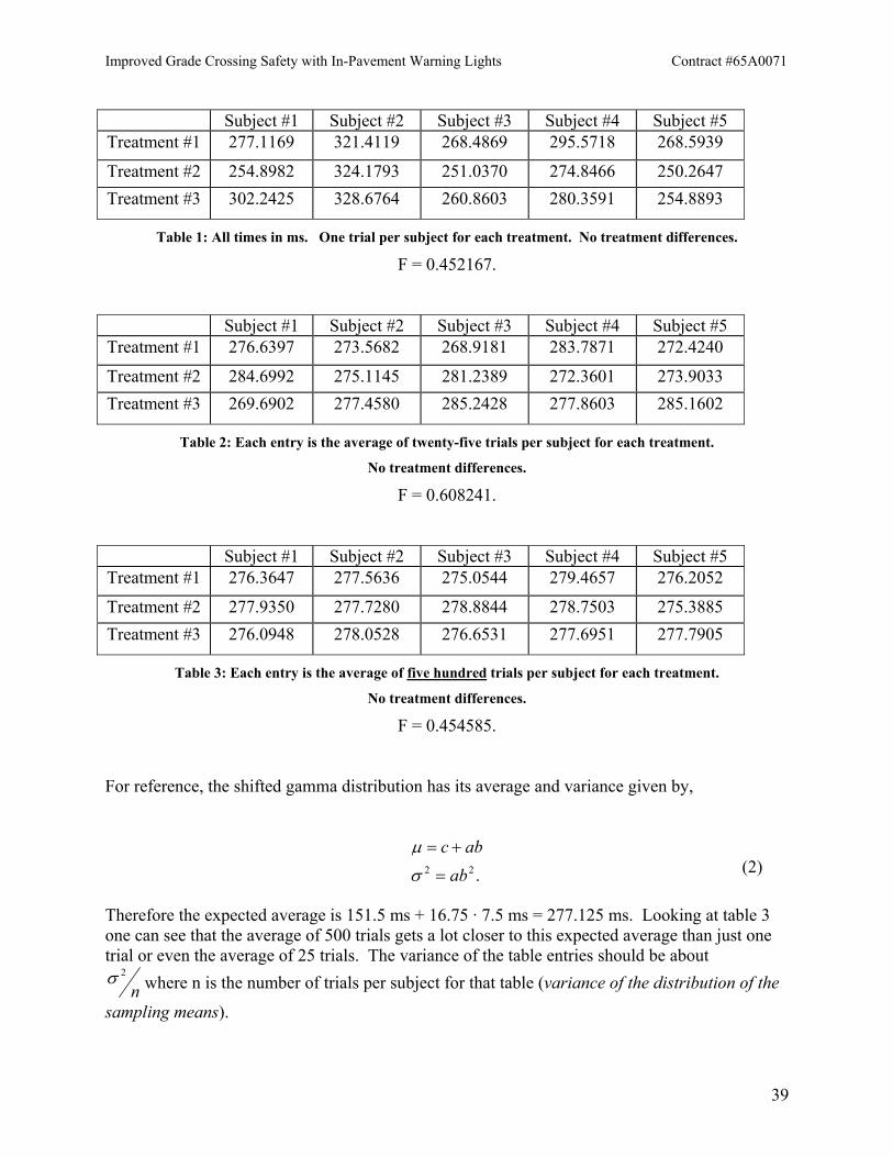
The first set of tables used the same parameters in every case: a = 16.75, b = 7.5 ms, c = 151.5 ms. (The graph is shown above in figure 2.) Since every subject-treatment combination had its values drawn from the same distribution, there should be no effects due to treatment. Thus the F test should give no indication of deviation from the null hypothesis that treatment means are equal (because they are equal by design!).
Improved Grade Crossing Safety with In-Pavement Warning Lights Contract #65A0071
39
Subject #1 Subject #2 Subject #3 Subject #4 Subject #5
Treatment #1 277.1169 321.4119 268.4869 295.5718 268.5939
Treatment #2 254.8982 324.1793 251.0370 274.8466 250.2647 Treatment #3 302.2425 328.6764 260.8603 280.3591 254.8893
Table 1: All times in ms. One trial per subject for each treatment. No treatment differences.
F = 0.452167.
Subject #1 Subject #2 Subject #3 Subject #4 Subject #5 Treatment #1 276.6397 273.5682 268.9181 283.7871 272.4240
Treatment #2 284.6992 275.1145 281.2389 272.3601 273.9033 Treatment #3 269.6902 277.4580 285.2428 277.8603 285.1602
Table 2: Each entry is the average of twenty-five trials per subject for each treatment.
No treatment differences.
F = 0.608241.
Subject #1 Subject #2 Subject #3 Subject #4 Subject #5
Treatment #1 276.3647 277.5636 275.0544 279.4657 276.2052
Treatment #2 277.9350 277.7280 278.8844 278.7503 275.3885 Treatment #3 276.0948 278.0528 276.6531 277.6951 277.7905
Table 3: Each entry is the average of five hundred trials per subject for each treatment.
No treatment differences.
F = 0.454585.
For reference, the shifted gamma distribution has its average and variance given by,
.22 ababc
=
+=
σ
µ
(2)
Therefore the expected average is 151.5 ms + 16.75 · 7.5 ms = 277.125 ms. Looking at table 3 one can see that the average of 500 trials gets a lot closer to this expected average than just one trial or even the average of 25 trials. The variance of the table entries should be about
n2σ where n is the number of trials per subject for that table (variance of the distribution of the
sampling means).
Improved Grade Crossing Safety with In-Pavement Warning Lights Contract #65A0071
40
Since there are 3 treatments and 5 subjects, the degrees of freedom are 3 – 1 = 2 and 3(5 – 1) = 12. The critical F value at the 95th percentile, for 2 and 12 degrees of freedom is 3.89 [Schaum’s Outline: Probability and Statistics 2nd Ed. p. 396].
.]..12&2[89.395.0 fodF = (3)
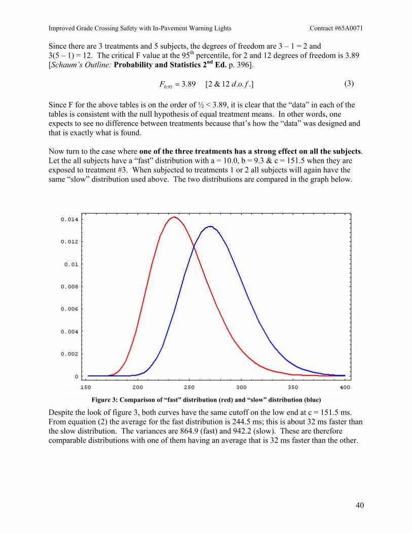
Since F for the above tables is on the order of ½ < 3.89, it is clear that the “data” in each of the tables is consistent with the null hypothesis of equal treatment means. In other words, one expects to see no difference between treatments because that’s how the “data” was designed and that is exactly what is found. Now turn to the case where one of the three treatments has a strong effect on all the subjects. Let the all subjects have a “fast” distribution with a = 10.0, b = 9.3 & c = 151.5 when they are exposed to treatment #3. When subjected to treatments 1 or 2 all subjects will again have the same “slow” distribution used above. The two distributions are compared in the graph below.
Figure 3: Comparison of “fast” distribution (red) and “slow” distribution (blue)
Despite the look of figure 3, both curves have the same cutoff on the low end at c = 151.5 ms. From equation (2) the average for the fast distribution is 244.5 ms; this is about 32 ms faster than the slow distribution. The variances are 864.9 (fast) and 942.2 (slow). These are therefore comparable distributions with one of them having an average that is 32 ms faster than the other.
Improved Grade Crossing Safety with In-Pavement Warning Lights Contract #65A0071
41
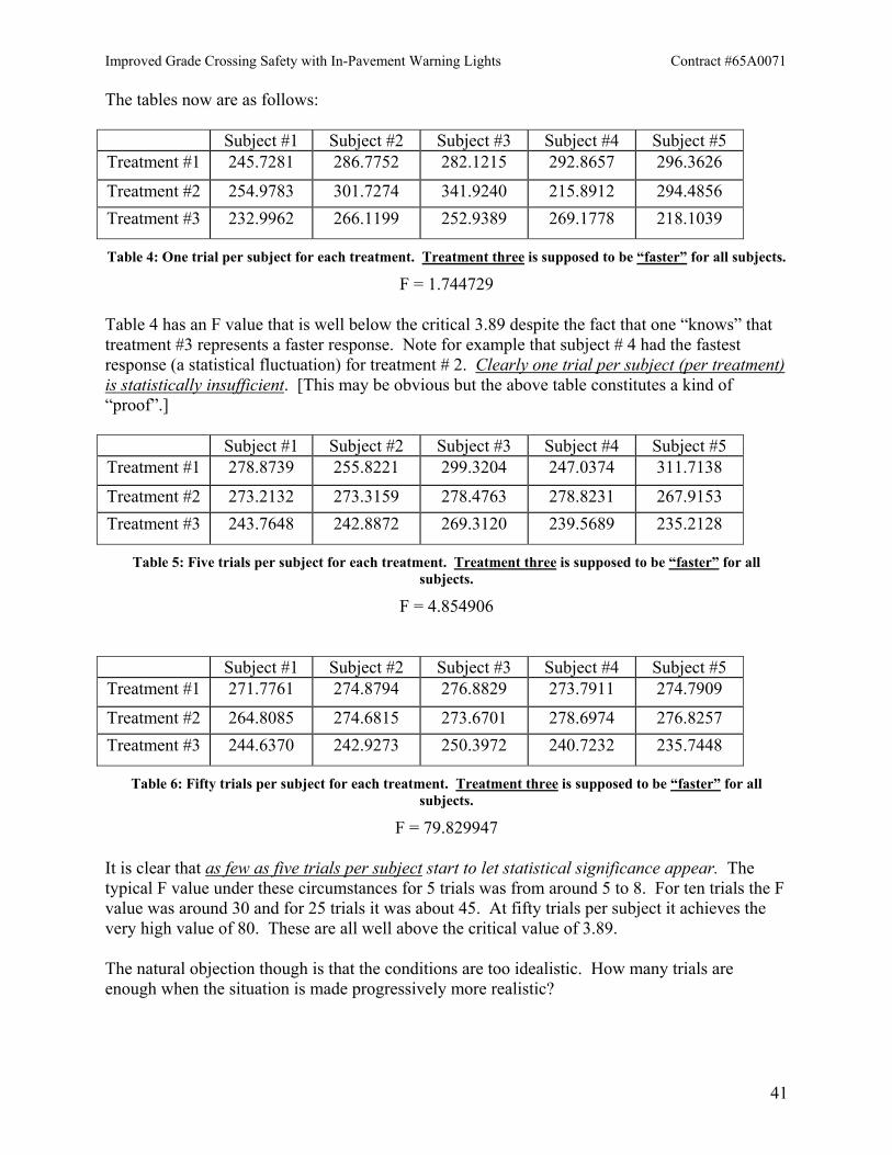
The tables now are as follows:
Subject #1 Subject #2 Subject #3 Subject #4 Subject #5 Treatment #1 245.7281 286.7752 282.1215 292.8657 296.3626
Treatment #2 254.9783 301.7274 341.9240 215.8912 294.4856 Treatment #3 232.9962 266.1199 252.9389 269.1778 218.1039
Table 4: One trial per subject for each treatment. Treatment three is supposed to be “faster” for all subjects.
F = 1.744729
Table 4 has an F value that is well below the critical 3.89 despite the fact that one “knows” that treatment #3 represents a faster response. Note for example that subject # 4 had the fastest response (a statistical fluctuation) for treatment # 2. Clearly one trial per subject (per treatment) is statistically insufficient. [This may be obvious but the above table constitutes a kind of “proof”.]
Subject #1 Subject #2 Subject #3 Subject #4 Subject #5 Treatment #1 278.8739 255.8221 299.3204 247.0374 311.7138
Treatment #2 273.2132 273.3159 278.4763 278.8231 267.9153 Treatment #3 243.7648 242.8872 269.3120 239.5689 235.2128
Table 5: Five trials per subject for each treatment. Treatment three is supposed to be “faster” for all subjects.
F = 4.854906
Subject #1 Subject #2 Subject #3 Subject #4 Subject #5 Treatment #1 271.7761 274.8794 276.8829 273.7911 274.7909
Treatment #2 264.8085 274.6815 273.6701 278.6974 276.8257 Treatment #3 244.6370 242.9273 250.3972 240.7232 235.7448
Table 6: Fifty trials per subject for each treatment. Treatment three is supposed to be “faster” for all subjects.
F = 79.829947
It is clear that as few as five trials per subject start to let statistical significance appear. The typical F value under these circumstances for 5 trials was from around 5 to 8. For ten trials the F value was around 30 and for 25 trials it was about 45. At fifty trials per subject it achieves the very high value of 80. These are all well above the critical value of 3.89. The natural objection though is that the conditions are too idealistic. How many trials are enough when the situation is made progressively more realistic?
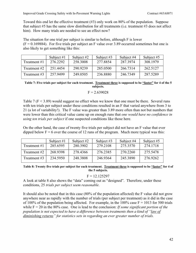
Improved Grade Crossing Safety with In-Pavement Warning Lights Contract #65A0071
42
Toward this end let the effective treatment (#3) only work on 80% of the population. Suppose that subject #5 has the same slow distribution for all treatments (i.e. treatment #3 does not affect him). How many trials are needed to see an effect now? The situation for one trial per subject is similar to before, although F is lower (F = 0.169884). For five trials per subject an F value over 3.89 occurred sometimes but one is also likely to get something like this:
Subject #1 Subject #2 Subject #3 Subject #4 Subject #5 Treatment #1 276.2292 258.3008 277.8854 287.3974 308.1979
Treatment #2 251.4454 290.9239 285.0500 266.7314 262.5127 Treatment #3 257.9499 249.0505 236.8880 246.7349 287.5289
Table 7: Five trials per subject for each treatment. Treatment three is supposed to be “faster” for 4 of the 5 subjects.
F = 2.639028
Table 7 (F < 3.89) would suggest no effect when we know that one must be there. Several runs with ten trials per subject under these conditions resulted in an F that varied anywhere from 3 to 21 (a lot of variability!). The F value was greater than 3.89 more often than not but numbers that were lower than this critical value came up on enough runs that one would have no confidence in using ten trials per subject if one suspected conditions like those here. On the other hand, the case of twenty five trials per subject did not have an F value that ever dipped below F = 6 over the course of 12 runs of the program. Much more typical was this:
Subject #1 Subject #2 Subject #3 Subject #4 Subject #5 Treatment #1 285.6595 280.3902 279.2108 275.3570 274.1718
Treatment #2 268.9398 278.4366 276.2385 270.2260 275.5478 Treatment #3 234.5950 248.3808 246.9364 245.3890 276.9262
Table 8: Twenty five trials per subject for each treatment. Treatment three is supposed to be “faster” for 4 of the 5 subjects.
F = 12.125297 A look at table 8 also shows the “data” coming out as “designed”. Therefore, under these conditions, 25 trials per subject seem reasonable. It should also be noted that in this case (80% of the population affected) the F value did not grow anywhere near as rapidly with the number of trials (per subject per treatment) as it did in the case of 100% of the population being affected. For example, in the 100% case F = 1013 for 500 trials while F = 20 in the 80% case. One is lead to the conclusion: If some significant portion of the population is not expected to have a difference between treatments then a kind of “law of diminishing returns” for statistics sets in regarding an ever greater number of trials.
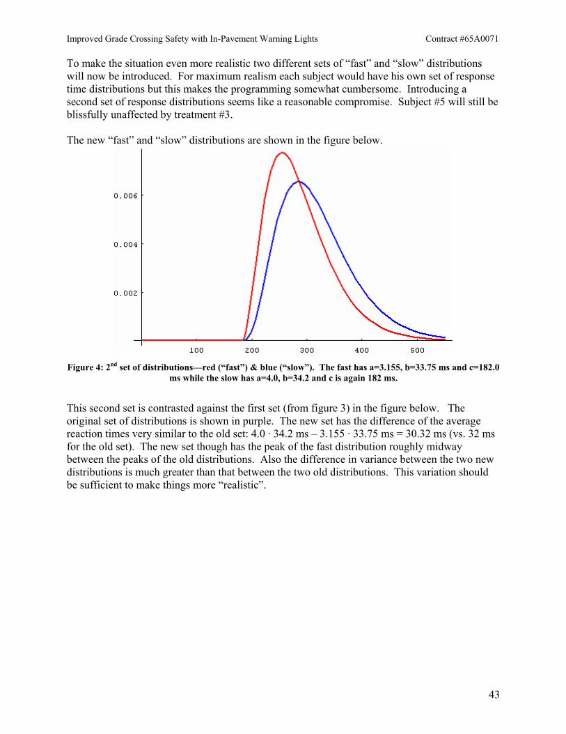
Improved Grade Crossing Safety with In-Pavement Warning Lights Contract #65A0071
43
To make the situation even more realistic two different sets of “fast” and “slow” distributions will now be introduced. For maximum realism each subject would have his own set of response time distributions but this makes the programming somewhat cumbersome. Introducing a second set of response distributions seems like a reasonable compromise. Subject #5 will still be blissfully unaffected by treatment #3. The new “fast” and “slow” distributions are shown in the figure below.
Figure 4: 2nd set of distributions—red (“fast”) & blue (“slow”). The fast has a=3.155, b=33.75 ms and c=182.0
ms while the slow has a=4.0, b=34.2 and c is again 182 ms.
This second set is contrasted against the first set (from figure 3) in the figure below. The original set of distributions is shown in purple. The new set has the difference of the average reaction times very similar to the old set: 4.0 · 34.2 ms – 3.155 · 33.75 ms = 30.32 ms (vs. 32 ms for the old set). The new set though has the peak of the fast distribution roughly midway between the peaks of the old distributions. Also the difference in variance between the two new distributions is much greater than that between the two old distributions. This variation should be sufficient to make things more “realistic”.
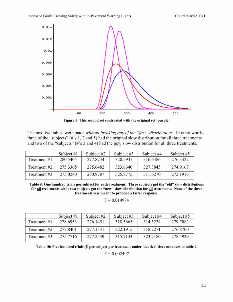
Improved Grade Crossing Safety with In-Pavement Warning Lights Contract #65A0071
44
Figure 5: This second set contrasted with the original set [purple]
The next two tables were made without invoking any of the “fast” distributions. In other words, three of the “subjects” (#’s 1, 2 and 5) had the original slow distribution for all three treatments and two of the “subjects” (#’s 3 and 4) had the new slow distribution for all three treatments.
Subject #1 Subject #2 Subject #3 Subject #4 Subject #5 Treatment #1 280.5404 277.8734 320.5947 316.6386 276.3422
Treatment #2 275.3365 275.6482 323.8640 327.3845 274.9167 Treatment #3 273.0240 280.9787 325.8775 311.6270 272.1916
Table 9: One hundred trials per subject for each treatment. Three subjects got the “old” slow distributions for all treatments while two subjects got the “new” slow distribution for all treatments. None of the three
treatments was meant to produce a faster response.
F = 0.014984
Subject #1 Subject #2 Subject #3 Subject #4 Subject #5 Treatment #1 278.6953 276.1451 318.3665 314.5224 279.7082
Treatment #2 277.8401 277.1531 322.1915 318.2271 276.8700 Treatment #3 275.7716 277.2539 315.7143 323.2180 278.5929
Table 10: Five hundred trials (!) per subject per treatment under identical circumstances to table 9.
F = 0.002407
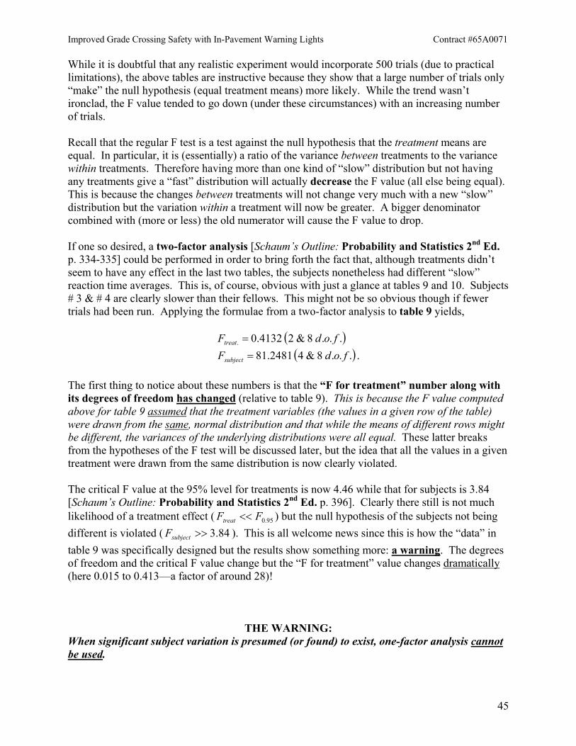
Improved Grade Crossing Safety with In-Pavement Warning Lights Contract #65A0071
45
While it is doubtful that any realistic experiment would incorporate 500 trials (due to practical limitations), the above tables are instructive because they show that a large number of trials only “make” the null hypothesis (equal treatment means) more likely. While the trend wasn’t ironclad, the F value tended to go down (under these circumstances) with an increasing number of trials. Recall that the regular F test is a test against the null hypothesis that the treatment means are equal. In particular, it is (essentially) a ratio of the variance between treatments to the variance within treatments. Therefore having more than one kind of “slow” distribution but not having any treatments give a “fast” distribution will actually decrease the F value (all else being equal). This is because the changes between treatments will not change very much with a new “slow” distribution but the variation within a treatment will now be greater. A bigger denominator combined with (more or less) the old numerator will cause the F value to drop. If one so desired, a two-factor analysis [Schaum’s Outline: Probability and Statistics 2nd Ed. p. 334-335] could be performed in order to bring forth the fact that, although treatments didn’t seem to have any effect in the last two tables, the subjects nonetheless had different “slow” reaction time averages. This is, of course, obvious with just a glance at tables 9 and 10. Subjects # 3 & # 4 are clearly slower than their fellows. This might not be so obvious though if fewer trials had been run. Applying the formulae from a two-factor analysis to table 9 yields,
( )( ) ....8&42481.81
...8&24132.0.
fodFfodF
subject
treat
==
The first thing to notice about these numbers is that the “F for treatment” number along with its degrees of freedom has changed (relative to table 9). This is because the F value computed above for table 9 assumed that the treatment variables (the values in a given row of the table) were drawn from the same, normal distribution and that while the means of different rows might be different, the variances of the underlying distributions were all equal. These latter breaks from the hypotheses of the F test will be discussed later, but the idea that all the values in a given treatment were drawn from the same distribution is now clearly violated. The critical F value at the 95% level for treatments is now 4.46 while that for subjects is 3.84 [Schaum’s Outline: Probability and Statistics 2nd Ed. p. 396]. Clearly there still is not much likelihood of a treatment effect ( 95.0FFtreat << ) but the null hypothesis of the subjects not being different is violated ( 84.3>>subjectF ). This is all welcome news since this is how the “data” in table 9 was specifically designed but the results show something more: a warning. The degrees of freedom and the critical F value change but the “F for treatment” value changes dramatically (here 0.015 to 0.413—a factor of around 28)!
THE WARNING: When significant subject variation is presumed (or found) to exist, one-factor analysis cannot be used.
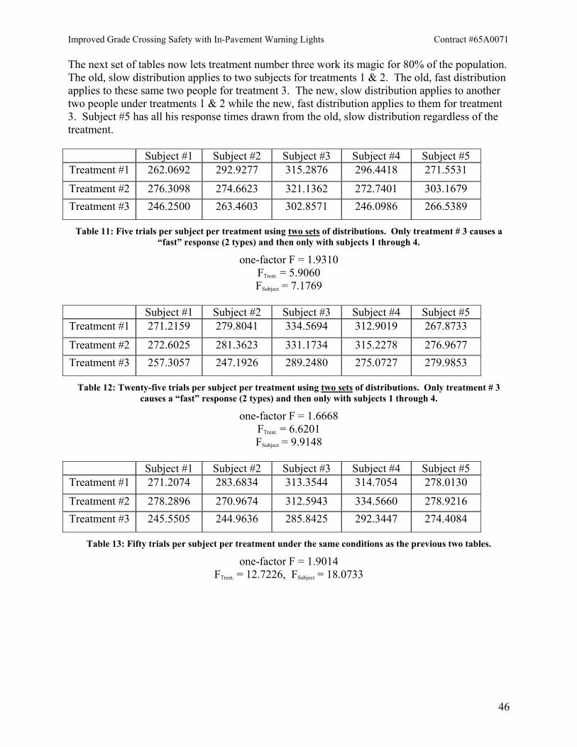
Improved Grade Crossing Safety with In-Pavement Warning Lights Contract #65A0071
46
The next set of tables now lets treatment number three work its magic for 80% of the population. The old, slow distribution applies to two subjects for treatments 1 & 2. The old, fast distribution applies to these same two people for treatment 3. The new, slow distribution applies to another two people under treatments 1 & 2 while the new, fast distribution applies to them for treatment 3. Subject #5 has all his response times drawn from the old, slow distribution regardless of the treatment.
Subject #1 Subject #2 Subject #3 Subject #4 Subject #5 Treatment #1 262.0692 292.9277 315.2876 296.4418 271.5531
Treatment #2 276.3098 274.6623 321.1362 272.7401 303.1679 Treatment #3 246.2500 263.4603 302.8571 246.0986 266.5389
Table 11: Five trials per subject per treatment using two sets of distributions. Only treatment # 3 causes a “fast” response (2 types) and then only with subjects 1 through 4.
one-factor F = 1.9310 FTreat. = 5.9060 FSubject = 7.1769
Subject #1 Subject #2 Subject #3 Subject #4 Subject #5
Treatment #1 271.2159 279.8041 334.5694 312.9019 267.8733
Treatment #2 272.6025 281.3623 331.1734 315.2278 276.9677 Treatment #3 257.3057 247.1926 289.2480 275.0727 279.9853
Table 12: Twenty-five trials per subject per treatment using two sets of distributions. Only treatment # 3 causes a “fast” response (2 types) and then only with subjects 1 through 4.
one-factor F = 1.6668 FTreat. = 6.6201 FSubject = 9.9148
Subject #1 Subject #2 Subject #3 Subject #4 Subject #5
Treatment #1 271.2074 283.6834 313.3544 314.7054 278.0130
Treatment #2 278.2896 270.9674 312.5943 334.5660 278.9216 Treatment #3 245.5505 244.9636 285.8425 292.3447 274.4084
Table 13: Fifty trials per subject per treatment under the same conditions as the previous two tables.
one-factor F = 1.9014 FTreat. = 12.7226, FSubject = 18.0733
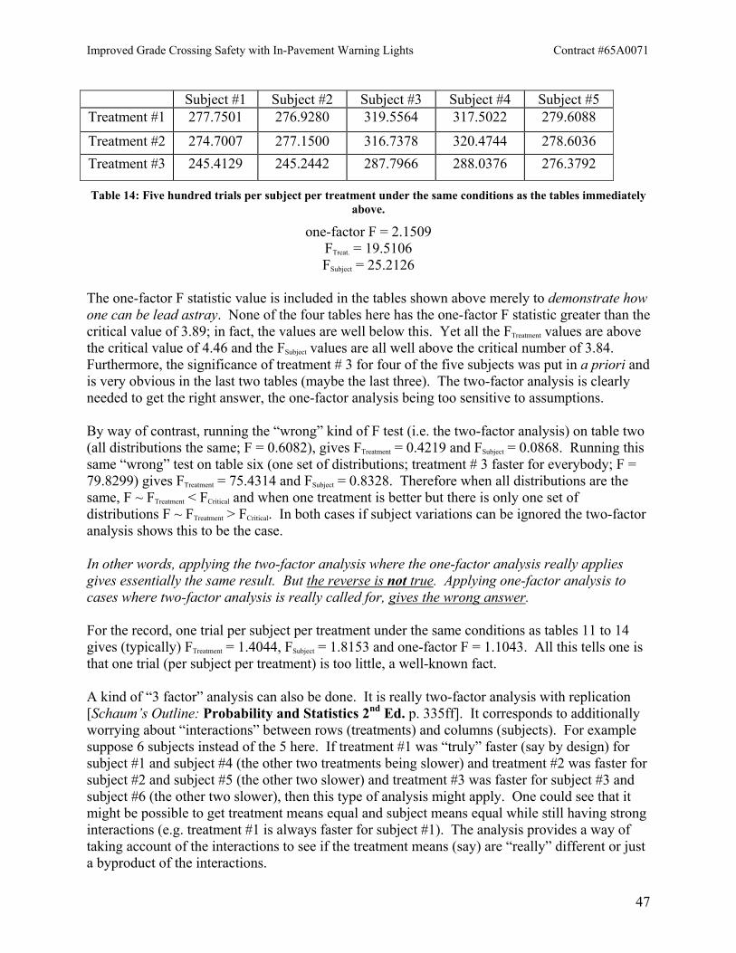
Improved Grade Crossing Safety with In-Pavement Warning Lights Contract #65A0071
47
Subject #1 Subject #2 Subject #3 Subject #4 Subject #5
Treatment #1 277.7501 276.9280 319.5564 317.5022 279.6088
Treatment #2 274.7007 277.1500 316.7378 320.4744 278.6036 Treatment #3 245.4129 245.2442 287.7966 288.0376 276.3792
Table 14: Five hundred trials per subject per treatment under the same conditions as the tables immediately above.
one-factor F = 2.1509 FTreat. = 19.5106 FSubject = 25.2126
The one-factor F statistic value is included in the tables shown above merely to demonstrate how one can be lead astray. None of the four tables here has the one-factor F statistic greater than the critical value of 3.89; in fact, the values are well below this. Yet all the FTreatment values are above the critical value of 4.46 and the FSubject values are all well above the critical number of 3.84. Furthermore, the significance of treatment # 3 for four of the five subjects was put in a priori and is very obvious in the last two tables (maybe the last three). The two-factor analysis is clearly needed to get the right answer, the one-factor analysis being too sensitive to assumptions. By way of contrast, running the “wrong” kind of F test (i.e. the two-factor analysis) on table two (all distributions the same; F = 0.6082), gives FTreatment = 0.4219 and FSubject = 0.0868. Running this same “wrong” test on table six (one set of distributions; treatment # 3 faster for everybody; F = 79.8299) gives FTreatment = 75.4314 and FSubject = 0.8328. Therefore when all distributions are the same, F ~ FTreatment < FCritical and when one treatment is better but there is only one set of distributions F ~ FTreatment > FCritical. In both cases if subject variations can be ignored the two-factor analysis shows this to be the case. In other words, applying the two-factor analysis where the one-factor analysis really applies gives essentially the same result. But the reverse is not true. Applying one-factor analysis to cases where two-factor analysis is really called for, gives the wrong answer. For the record, one trial per subject per treatment under the same conditions as tables 11 to 14 gives (typically) FTreatment = 1.4044, FSubject = 1.8153 and one-factor F = 1.1043. All this tells one is that one trial (per subject per treatment) is too little, a well-known fact. A kind of “3 factor” analysis can also be done. It is really two-factor analysis with replication [Schaum’s Outline: Probability and Statistics 2nd Ed. p. 335ff]. It corresponds to additionally worrying about “interactions” between rows (treatments) and columns (subjects). For example suppose 6 subjects instead of the 5 here. If treatment #1 was “truly” faster (say by design) for subject #1 and subject #4 (the other two treatments being slower) and treatment #2 was faster for subject #2 and subject #5 (the other two slower) and treatment #3 was faster for subject #3 and subject #6 (the other two slower), then this type of analysis might apply. One could see that it might be possible to get treatment means equal and subject means equal while still having strong interactions (e.g. treatment #1 is always faster for subject #1). The analysis provides a way of taking account of the interactions to see if the treatment means (say) are “really” different or just a byproduct of the interactions.
Improved Grade Crossing Safety with In-Pavement Warning Lights Contract #65A0071
48
Even though the last few tables had an “interaction” term with subject number 5 consistently being unfazed by treatment three, this type of “two-factor analysis with replication” is not too useful under the present circumstances. This is because a) it is complicated and “plain vanilla” two-factor analysis seems to handle the job reasonably well, as demonstrated above; b) a situation requiring such interaction terms [such as 20% of the population being affected strongly by only one treatment, another 20% being affected by the next treatment and so on for five different treatments] wouldn’t be likely to be of interest for most of the real-life reaction time applications; c) the assumptions for this type of analysis are typically violated by reaction time experiments. Indeed almost all kinds of statistical tests applied to almost all kinds of experiments have to be done under conditions that violate the assumptions of the tests! Statistical tests usually have to be done under such violations; the question is how well they hold up! An important reason for making all these tables in the first place is to see just how well statistical tests hold up under mild but realistic violation of those assumptions. Typically the Central Limit Theorem comes to the rescue. It does so here in the case of the one-factor F test (provided other assumptions hold—not likely in practice as shown above) and it does so in the case of the two-factor F tests. It does not do so in the case of “two-factor analysis with replication” (at least intuitively; this should probably be proven). The average of trials from a reaction time distribution with finite variance (e.g. a shifted gamma here or the real-life more bimodal distribution) will tend, asymptotically, to a Gaussian distribution. Therefore a “few” trials (say 10) from a shifted gamma will produce a sample mean that is approximately (but not exactly!) normally distributed. This number is then fed into the one and two factor F tests, which assume normal distributions. But the “two-factor analysis with replication” tests use the original draws (before averaging) from the non-normal parent population. Since reaction time distributions are definitely non-normal, taking n = 1 as a substitute for n → ∞ hardly seems likely to give a beneficial result. Turning to t tests, it is quite unlikely that the assumptions for these types of tests strictly hold up against the reaction time data; again the real question is how robust the tests are—do they hold up with violations of their assumptions? One assumption is normality of the distributions from which the treatment values (i.e. a row from the above tables) are drawn. This is almost surely violated. Even though the average of several trials for a given subject under a given treatment will be a sample mean that is approximately normally distributed (thanks to the Central Limit Theorem), the combination of a small number of subjects under a given treatment will not. The distribution of values in a given row will be a (weighted) combination of the individual subject distributions. This is not a combination of the independent random variables (because a linear combination of Gaussian random variables is a Gaussian random variable); rather it is a combination of the distributions themselves. When only a small number of normal distributions combine (i.e. a handful of subjects) the result can be distinctly non-normal. For example, height in a given race of people generally follows a normal distribution. If one measures the heights of a population consisting of many races then that too would probably be close to normal. But if one measures the heights in a population consisting only of unusually small and unusually large people, the resulting histogram will surely be bimodal even though the two races might individually have their heights following a bell curve. In the same vein, if the reaction time distributions for each subject (for a given treatment) have widely spaced means then the distribution for that treatment might have several peaks.

Improved Grade Crossing Safety with In-Pavement Warning Lights Contract #65A0071
49
There are three saving graces though. 1) The t test that would be used here is the paired sample t test because the same subjects undergo the different treatments. Therefore only the differences between treatments on the subjects need be normally distributed. This is much more likely to be true. 2) The reaction time distributions are not as widely spaced (in terms of σ’s) as say the weight distributions of football players and ballerinas. The distribution for a given treatment would then have “ripples” around the peak rather than a few distinct humps. 3) The t tests are apparently fairly robust against non-normality in practice. In fact with regard to this last point, a brief search of the Internet turned up these rules of thumb (albeit for the t test for independent samples): [By Gerard E. Dallal, Chief of the Biostatistics Unit at the Jean Mayer USDA Human Nutrition
Research Center on Aging at Tufts University, writing in his “Little Handbook of Statistical Practice” at http://www.tufts.edu/~gdallal/STUDENT.HTM]
Formal analysis and simulations offer the following guidelines describing extent to which the assumptions of normality and equal population variances be violated without affecting the validity of Student's test for independent samples. [see Rupert Miller, Jr., (1986) Beyond ANOVA, Basics of Applied Statistics, New York: John Wiley & Sons]
• If sample sizes are equal, (a) nonnormality is not a problem and (b) the t test can tolerate population standard deviation ratios of 2 without showing any major ill effect. (For equal sample sizes, the two test statistics are equal.) The worst situation occurs when one sample has both a much larger variance and a much smaller sample size than the other. For example, if the variance ratio is 5 and the sample size ratio is 1/5, a nominal P value of 0.05 is actually 0.22.
• Serious distortion of the P value can occur when the skewness of the two populations is different. • Outliers can distort the mean difference and the t statistic. They tend to inflate the
variance and depress the value and corresponding statistical significance of the t statistic.
Preliminary tests for normality and equality of variances--using Student's t test only if these preliminary tests fail to achieve statistical significance--should be avoided [my emphasis]. These preliminary tests often detect differences too small to affect Student's t test. Since the test is such a convenient way to compare two populations, it should not be abandoned without good cause. Important violations of the requirements will be detectable to the naked eye without a formal significance test.
Additional cursory searches seemed to back this up. The abstract of a report (The Effects of Non-normality on Student’s Two-Sample T-test (April, 2000)—a published report on a Monte Carlo study. Journal and author information was not posted at the website!) basically said that the t test gave acceptable Type I error rates even with skewed distributions, provided they were skewed in the same direction. Therefore a paired t test on these “data” ought to work and one shouldn’t have to resort to data transformation to achieve quasi-normality nor abandon them altogether in favor of non-parametric tests. The latter it should be noted are not truly “distribution free” as is sometimes claimed; there are assumptions about the underlying distributions (such as unimodality). The assumptions are just less rigid.
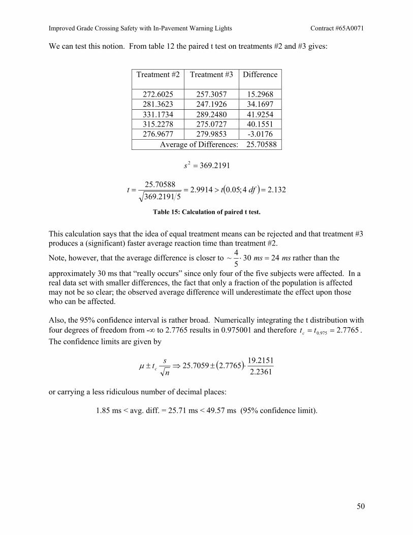
Improved Grade Crossing Safety with In-Pavement Warning Lights Contract #65A0071
50
We can test this notion. From table 12 the paired t test on treatments #2 and #3 gives:
Treatment #2 Treatment #3 Difference
272.6025 257.3057 15.2968 281.3623 247.1926 34.1697 331.1734 289.2480 41.9254 315.2278 275.0727 40.1551 276.9677 279.9853 -3.0176
Average of Differences: 25.70588
369.21912 =s
( ) 132.24;05.09914.252191.369
70588.25=>== dftt
Table 15: Calculation of paired t test.
This calculation says that the idea of equal treatment means can be rejected and that treatment #3 produces a (significant) faster average reaction time than treatment #2.
Note, however, that the average difference is closer to msms 243054~ =⋅ rather than the
approximately 30 ms that “really occurs” since only four of the five subjects were affected. In a real data set with smaller differences, the fact that only a fraction of the population is affected may not be so clear; the observed average difference will underestimate the effect upon those who can be affected. Also, the 95% confidence interval is rather broad. Numerically integrating the t distribution with four degrees of freedom from -∞ to 2.7765 results in 0.975001 and therefore 7765.2975.0 == ttc . The confidence limits are given by
( )2361.22151.197765.27059.25 ⋅±⇒±
nstcµ
or carrying a less ridiculous number of decimal places:
1.85 ms < avg. diff. = 25.71 ms < 49.57 ms (95% confidence limit).
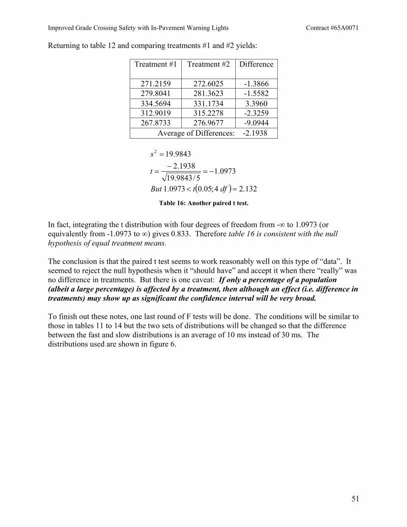
Improved Grade Crossing Safety with In-Pavement Warning Lights Contract #65A0071
51
Returning to table 12 and comparing treatments #1 and #2 yields:
Treatment #1 Treatment #2 Difference
271.2159 272.6025 -1.3866 279.8041 281.3623 -1.5582 334.5694 331.1734 3.3960 312.9019 315.2278 -2.3259 267.8733 276.9677 -9.0944
Average of Differences: -2.1938
( ) 132.24;05.00973.1
0973.15/9843.19
1938.29843.192
=<
−=−
=
=
dftBut
t
s
Table 16: Another paired t test.
In fact, integrating the t distribution with four degrees of freedom from -∞ to 1.0973 (or equivalently from -1.0973 to ∞) gives 0.833. Therefore table 16 is consistent with the null hypothesis of equal treatment means. The conclusion is that the paired t test seems to work reasonably well on this type of “data”. It seemed to reject the null hypothesis when it “should have” and accept it when there “really” was no difference in treatments. But there is one caveat: If only a percentage of a population (albeit a large percentage) is affected by a treatment, then although an effect (i.e. difference in treatments) may show up as significant the confidence interval will be very broad. To finish out these notes, one last round of F tests will be done. The conditions will be similar to those in tables 11 to 14 but the two sets of distributions will be changed so that the difference between the fast and slow distributions is an average of 10 ms instead of 30 ms. The distributions used are shown in figure 6.
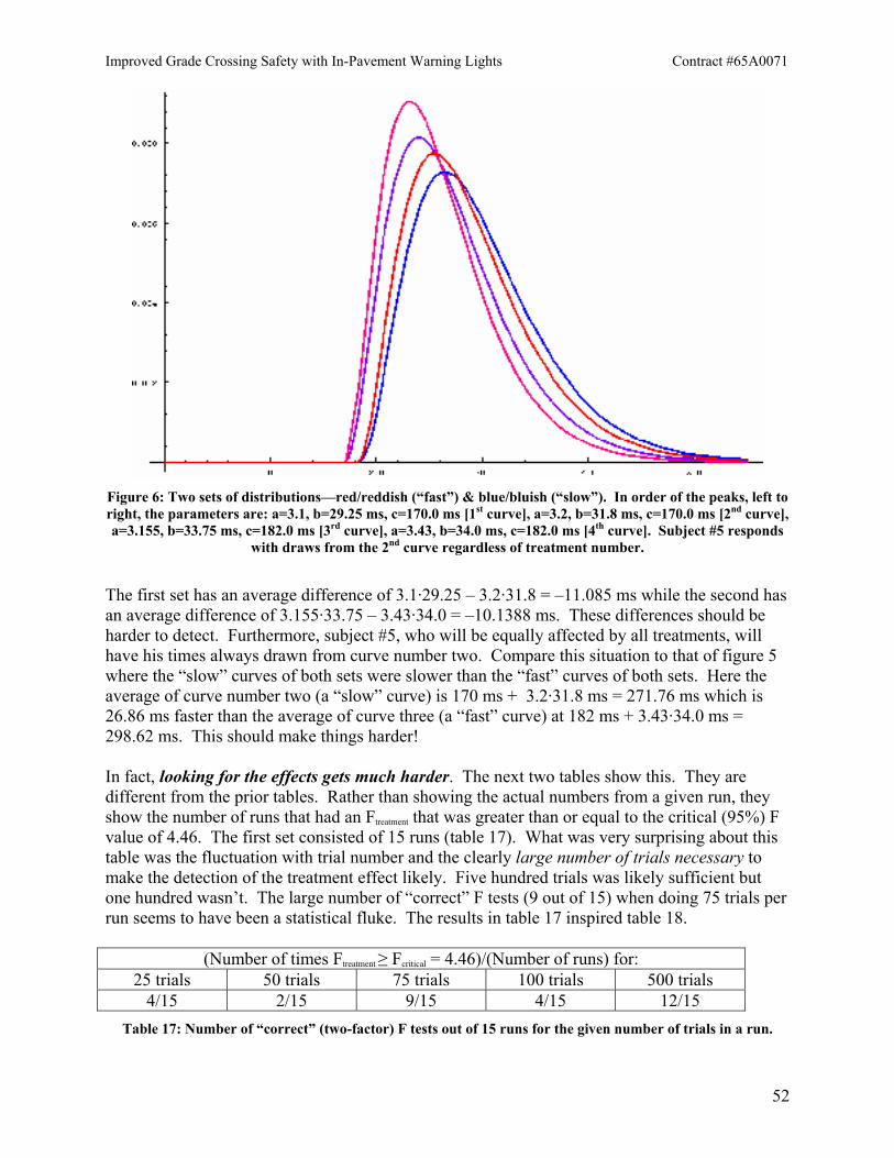
Improved Grade Crossing Safety with In-Pavement Warning Lights Contract #65A0071
52
Figure 6: Two sets of distributions—red/reddish (“fast”) & blue/bluish (“slow”). In order of the peaks, left to right, the parameters are: a=3.1, b=29.25 ms, c=170.0 ms [1st curve], a=3.2, b=31.8 ms, c=170.0 ms [2nd curve], a=3.155, b=33.75 ms, c=182.0 ms [3rd curve], a=3.43, b=34.0 ms, c=182.0 ms [4th curve]. Subject #5 responds
with draws from the 2nd curve regardless of treatment number.
The first set has an average difference of 3.1·29.25 – 3.2·31.8 = –11.085 ms while the second has an average difference of 3.155·33.75 – 3.43·34.0 = –10.1388 ms. These differences should be harder to detect. Furthermore, subject #5, who will be equally affected by all treatments, will have his times always drawn from curve number two. Compare this situation to that of figure 5 where the “slow” curves of both sets were slower than the “fast” curves of both sets. Here the average of curve number two (a “slow” curve) is 170 ms + 3.2·31.8 ms = 271.76 ms which is 26.86 ms faster than the average of curve three (a “fast” curve) at 182 ms + 3.43·34.0 ms = 298.62 ms. This should make things harder! In fact, looking for the effects gets much harder. The next two tables show this. They are different from the prior tables. Rather than showing the actual numbers from a given run, they show the number of runs that had an Ftreatment that was greater than or equal to the critical (95%) F value of 4.46. The first set consisted of 15 runs (table 17). What was very surprising about this table was the fluctuation with trial number and the clearly large number of trials necessary to make the detection of the treatment effect likely. Five hundred trials was likely sufficient but one hundred wasn’t. The large number of “correct” F tests (9 out of 15) when doing 75 trials per run seems to have been a statistical fluke. The results in table 17 inspired table 18.
(Number of times Ftreatment ≥ Fcritical = 4.46)/(Number of runs) for: 25 trials 50 trials 75 trials 100 trials 500 trials
4/15 2/15 9/15 4/15 12/15 Table 17: Number of “correct” (two-factor) F tests out of 15 runs for the given number of trials in a run.
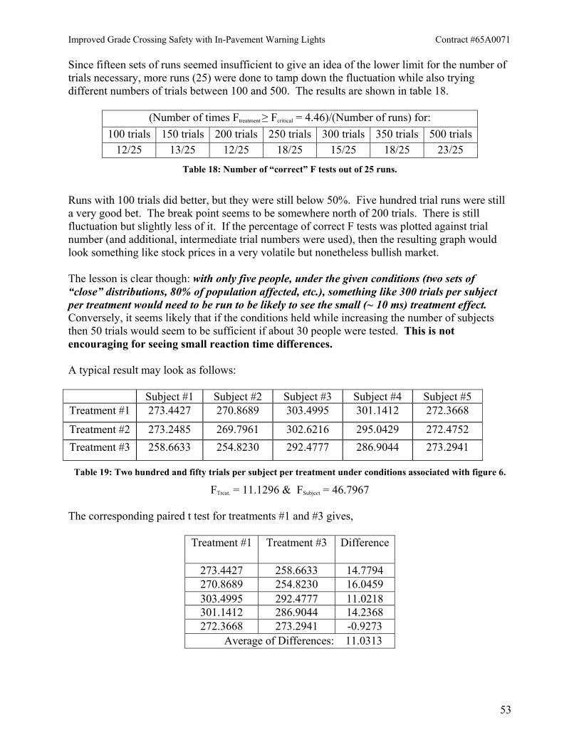
Improved Grade Crossing Safety with In-Pavement Warning Lights Contract #65A0071
53
Since fifteen sets of runs seemed insufficient to give an idea of the lower limit for the number of trials necessary, more runs (25) were done to tamp down the fluctuation while also trying different numbers of trials between 100 and 500. The results are shown in table 18.
(Number of times Ftreatment ≥ Fcritical = 4.46)/(Number of runs) for:
100 trials 150 trials 200 trials 250 trials 300 trials 350 trials 500 trials12/25 13/25 12/25 18/25 15/25 18/25 23/25
Table 18: Number of “correct” F tests out of 25 runs.
Runs with 100 trials did better, but they were still below 50%. Five hundred trial runs were still a very good bet. The break point seems to be somewhere north of 200 trials. There is still fluctuation but slightly less of it. If the percentage of correct F tests was plotted against trial number (and additional, intermediate trial numbers were used), then the resulting graph would look something like stock prices in a very volatile but nonetheless bullish market. The lesson is clear though: with only five people, under the given conditions (two sets of “close” distributions, 80% of population affected, etc.), something like 300 trials per subject per treatment would need to be run to be likely to see the small (~ 10 ms) treatment effect. Conversely, it seems likely that if the conditions held while increasing the number of subjects then 50 trials would seem to be sufficient if about 30 people were tested. This is not encouraging for seeing small reaction time differences. A typical result may look as follows:
Subject #1 Subject #2 Subject #3 Subject #4 Subject #5 Treatment #1 273.4427 270.8689 303.4995 301.1412 272.3668
Treatment #2 273.2485 269.7961 302.6216 295.0429 272.4752 Treatment #3 258.6633 254.8230 292.4777 286.9044 273.2941
Table 19: Two hundred and fifty trials per subject per treatment under conditions associated with figure 6.
FTreat. = 11.1296 & FSubject = 46.7967
The corresponding paired t test for treatments #1 and #3 gives,
Treatment #1 Treatment #3 Difference
273.4427 258.6633 14.7794 270.8689 254.8230 16.0459 303.4995 292.4777 11.0218 301.1412 286.9044 14.2368 272.3668 273.2941 -0.9273
Average of Differences: 11.0313
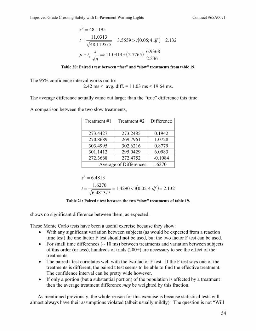
Improved Grade Crossing Safety with In-Pavement Warning Lights Contract #65A0071
54
( )
( )2361.29368.67765.20313.11
132.24;05.05559.35/1195.48
0313.111195.482
⋅±⇒±
=>==
=
nst
dftt
s
cµ
Table 20: Paired t test between “fast” and “slow” treatments from table 19.
The 95% confidence interval works out to:
2.42 ms < avg. diff. = 11.03 ms < 19.64 ms.
The average difference actually came out larger than the “true” difference this time. A comparison between the two slow treatments,
Treatment #1 Treatment #2 Difference
273.4427 273.2485 0.1942 270.8689 269.7961 1.0728 303.4995 302.6216 0.8779 301.1412 295.0429 6.0983 272.3668 272.4752 -0.1084
Average of Differences: 1.6270
( ) 132.24;05.04290.15/4813.6
6270.14813.62
=<==
=
dftt
s
Table 21: Paired t test between the two “slow” treatments of table 19.
shows no significant difference between them, as expected. These Monte Carlo tests have been a useful exercise because they show:
• With any significant variation between subjects (as would be expected from a reaction time test) the one factor F test should not be used, but the two factor F test can be used.
• For small time differences (~ 10 ms) between treatments and variation between subjects of this order (or less), hundreds of trials (200+) are necessary to see the effect of the treatments.
• The paired t test correlates well with the two factor F test. If the F test says one of the treatments is different, the paired t test seems to be able to find the effective treatment. The confidence interval can be pretty wide however.
• If only a portion (but a substantial portion) of the population is affected by a treatment then the average treatment difference may be weighted by this fraction.
As mentioned previously, the whole reason for this exercise is because statistical tests will
almost always have their assumptions violated (albeit usually mildly). The question is not “Will

Improved Grade Crossing Safety with In-Pavement Warning Lights Contract #65A0071
55
there be a violation of the assumptions for this test?” but rather “How well does the test hold up under those violations?”. These notes were meant to provide some insight into this latter question for the case of reaction time testing.