Embed Size (px)
Citation preview

DE-EE0002961 Final Report Executive Summary 1
Improved Design Tools for Surface Water and Standing Column Well Heat Pump Systems (DE-EE0002961)
Final Report November 2012
Oklahoma State University J.D. Spitler, Principal Investigator
Graduate research assistants: J.R. Cullin, K. Conjeevaram, M. Ramesh, M. Selvakumar
Distribution Notice The following sections of the report contain protected data: N/A
Shortwave radiation
EvaporationConvection
Net long wave radiation
Attenuation of shortwave radiation
Surface wind stress
River/stream inflow Surface outflow
Internal waves
Sediment
Sheltered regionExposed region
Surface mixing
Turbulent mixing
Sediment heat flux
Heat exchanger
Heat exchanger heat flux
DE-EE0002961 Final Report Executive Summary 2
Executive Summary Ground-source heat pump (GSHP) systems are perhaps the most widely used “sustainable” heating and cooling systems, with an estimated 1.7 million installed units with total installed heating capacity on the order of 18 GW. They are widely used in residential, commercial, and institutional buildings. Standing column wells (SCW) are one form of ground heat exchanger that, under the right geological conditions, can provide excellent energy efficiency at a relatively low capital cost. Closed-loop surface water heat pump (SWHP) systems utilize surface water heat exchangers (SWHE) to reject or extract heat from nearby surface water bodies. For building near surface water bodies, these systems also offer a high degree of energy efficiency at a low capital cost. However, there have been few design tools available for properly sizing standing column wells or surface water heat exchangers. Nor have tools for analyzing the energy consumption and supporting economics-based design decisions been available. The main contributions of this project lie in providing new tools that support design and energy analysis. These include a design tool for sizing surface water heat exchangers, a design tool for sizing standing column wells, a new model of surface water heat pump systems implemented in EnergyPlus and a new model of standing column wells implemented in EnergyPlus. These tools will better help engineers design these systems and determine the economic and technical feasibility.
Report Organization This report contains the following sections:
• Project Summary – An expanded version of the executive summary. • Task-by-task summary; compares actual accomplishments to goals and objectives and
summarizes project activities for the entire period of funding. • Products developed • Computer modeling • References

DE-EE0002961 Final Report Executive Summary 3
Project Summary This report describes a project aimed at developing validated models and improved design tools for both surface water heat pump and standing column well systems. The most important project results are summarized in this Project Summary as follows for the two technologies.
Surface Water Heat Pump (SWHP) systems For buildings where surface water, e.g. lakes, ponds, reservoirs, rivers, or the ocean, is nearby, surface water heat pump (SWHP) systems are efficient means of providing heating or cooling. However, neither design tools nor energy analysis tools have been readily available for design of surface water heat exchangers (SWHE) or analysis of SWHP systems. This project developed and validated a lake model that includes stratification and SWHE models. These are combined together and implemented in both a design tool and in EnergyPlus. The main contributions of this part of the project are summarized in the following points:
• A one-dimensional, daily time step lake model was developed to predict water temperatures varying with depth and time. The lake model accounts for 1) all relevant heat transfer mechanisms at the lake surface - convection, evaporation, shortwave radiation, longwave radiation, formation of ice, accumulation of snow, and melting of ice, 2) stratification of the water column, turnover and energy transfer in the water column with an eddy diffusion model and 3) sediment-water heat transfer. The lake model is more fully described in Appendix 6.1.
• A range of models for surface convection, surface evaporation and eddy diffusion have previously been proposed in the literature. Based on validation results for 14 different lakes with surface areas ranging between 3 acres and 21,500 acres, the recommended combination of sub-models for each lake category have been identified. These recommended model combinations for each lake category have been encapsulated in EnergyPlus as defaults. The recommended model combinations for each lake category are summarized in Table 1. The model selection process is described more fully in Appendix 6.1.
DE-EE0002961 Final Report Executive Summary 4
Table 1: Recommended sub- models for based on lake size
Recommended models
Lake category
Surface area
Ha(acres)
Surface
convection/evaporation Eddy diffusion
Small shallow ponds
≤ 5 (12)
Molineaux et al. (1994)
(Molineaux, Lachal et al.
1994)
Gu and Stefan
(1995)
Small lakes 5(12) - 100 (250) Molineaux et al. (1994) Imberger et al.
(1978)
Medium sized
lakes
100(250) -
1000(2500) Molineaux et al. (1994)
Rohden et al.
(2007)
(Rohden,
Wunderle et al.
2007)
Large lakes >1000(2500) Molineaux et al. (1994) McCormick and
Scavia (1981)
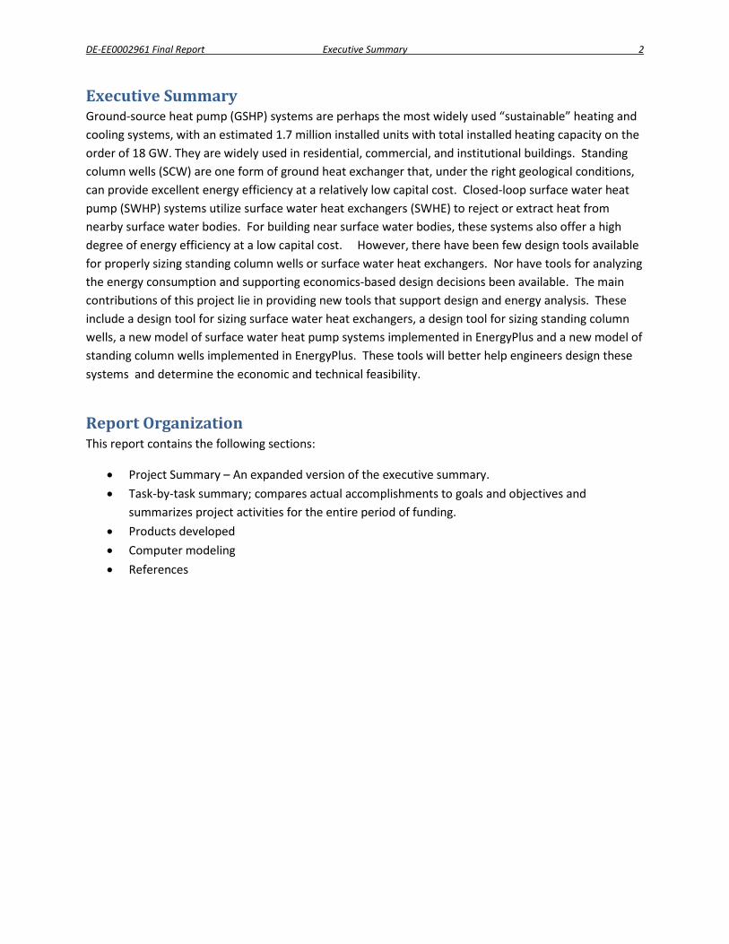
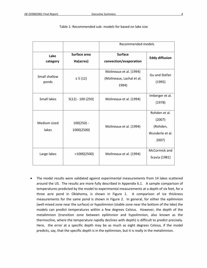
• The model results were validated against experimental measurements from 14 lakes scattered around the US. The results are more fully described in Appendix 6.1. A sample comparison of temperatures predicted by the model to experimental measurements at a depth of six feet, for a three acre pond in Oklahoma, is shown in Figure 1. A comparison of ice thickness measurements for the same pond is shown in Figure 2. In general, for either the epilimnion (well-mixed zone near the surface) or hypolimnion (stable zone near the bottom of the lake) the models can predict temperatures within a few degrees Celsius. However, the depth of the metalimnion (transition zone between epilimnion and hypolimnion, also known as the thermocline, where the temperature rapidly declines with depth) is difficult to predict precisely. Here, the error at a specific depth may be as much as eight degrees Celsius, if the model predicts, say, that the specific depth is in the epilimnion, but it is really in the metalimnion.
DE-EE0002961 Final Report Executive Summary 5
Figure 1. Water temperature comparison between the model and experiment at a depth of 1.7 m (6 ft)
Figure 2. Surface ice thickness comparison between the model and experiment
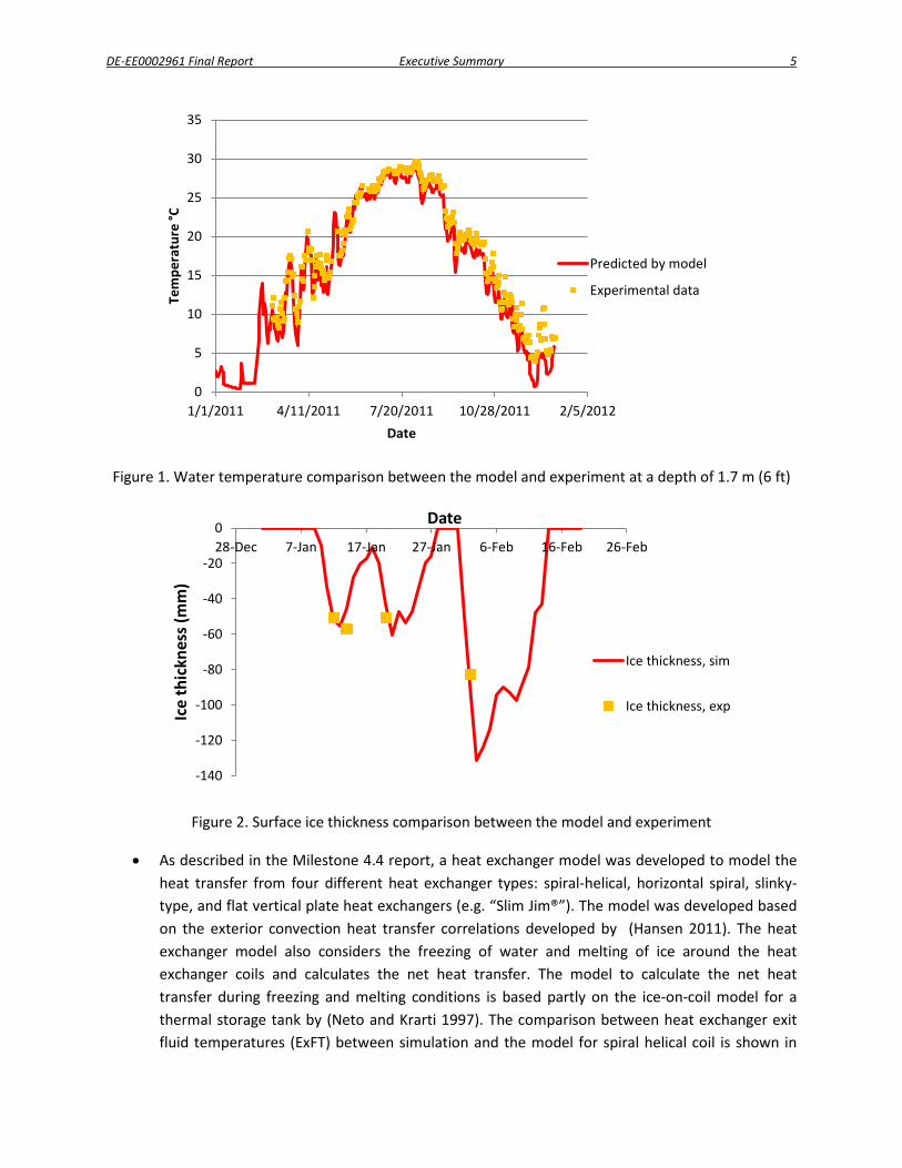
• As described in the Milestone 4.4 report, a heat exchanger model was developed to model the heat transfer from four different heat exchanger types: spiral-helical, horizontal spiral, slinky-type, and flat vertical plate heat exchangers (e.g. “Slim Jim®”). The model was developed based on the exterior convection heat transfer correlations developed by (Hansen 2011). The heat exchanger model also considers the freezing of water and melting of ice around the heat exchanger coils and calculates the net heat transfer. The model to calculate the net heat transfer during freezing and melting conditions is based partly on the ice-on-coil model for a thermal storage tank by (Neto and Krarti 1997). The comparison between heat exchanger exit fluid temperatures (ExFT) between simulation and the model for spiral helical coil is shown in
0
5
10
15
20
25
30
35
1/1/2011 4/11/2011 7/20/2011 10/28/2011 2/5/2012
Tem
pera
ture
°C
Date
Predicted by model
Experimental data
-140
-120
-100
-80
-60
-40
-20
028-Dec 7-Jan 17-Jan 27-Jan 6-Feb 16-Feb 26-Feb
Ice
thic
knes
s (m
m)
Date
Ice thickness, sim
Ice thickness, exp
DE-EE0002961 Final Report Executive Summary 6
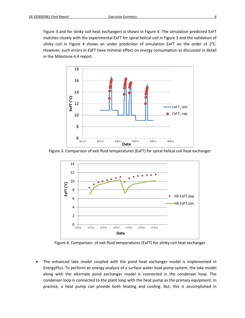
Figure 3 and for slinky coil heat exchangers is shown in Figure 4. The simulation predicted ExFT matches closely with the experimental ExFT for spiral helical coil in Figure 3 and the validation of slinky coil in Figure 4 shows an under prediction of simulation ExFT on the order of 2°C. However, such errors in ExFT have minimal effect on energy consumption as discussed in detail in the Milestone 4.4 report.
Figure 3. Comparison of exit fluid temperatures (ExFT) for spiral helical coil heat exchanger
Figure 4. Comparison of exit fluid temperatures (ExFT) for slinky coil heat exchanger
• The enhanced lake model coupled with the pond heat exchanger model is implemented in EnergyPlus. To perform an energy analysis of a surface water heat pump system, the lake model along with the alternate pond exchanger model is connected in the condenser loop. The condenser loop is connected to the plant loop with the heat pump as the primary equipment. In practice, a heat pump can provide both heating and cooling. But, this is accomplished in
0
2
4
6
8
10
12
14
1/7/11 1/7/11 1/7/11 1/7/11 1/7/11 1/7/11 1/7/11
ExFT
(°C)
Date
HX ExFT,exp
HX ExFT,sim
DE-EE0002961 Final Report Executive Summary 7
EnergyPlus by connecting two virtual heat pump models - one for cooling in the chiller water plant loop and the other one for heating in the hot water plant loop. More information regarding the EnergyPlus implementation are documented in the Input/output reference (Appendix 4.2.1), Engineering reference (Appendix 4.2.2), and in an example simulation (Appendix 4.2.3).
• The EnergyPlus model results are validated against experimental measurements. This includes comparison of simulation-predicted pond temperatures and heat exchanger exit fluid temperatures against experimental results collected from the OSU research pond. The comparison of pond temperatures predicted from EnergyPlus with the experimental temperatures is similar to the results of standalone FORTRAN model. The validation of heat exchanger exit fluid temperatures predicted by the EnergyPlus model is discussed in detail in the Milestone 4.4 report.
• A design tool has been implemented using Microsoft® Excel and a separate Fortran executable simulation engine. The designer provides inputs such as:
o Hourly building heating and cooling loads. These would be obtained from an energy analysis program such as EnergyPlus.
o Weather data that corresponds to the weather used to generate the building heating and cooling loads. This would typically be the same EPW file as used in EnergyPlus.
o Heat pump performance information. o Working fluid – pure water or water/antifreeze mixture. o Lake surface area and depth. Alternatively, more detailed bathymetric information can
be specified. o Heat exchanger type and depth.
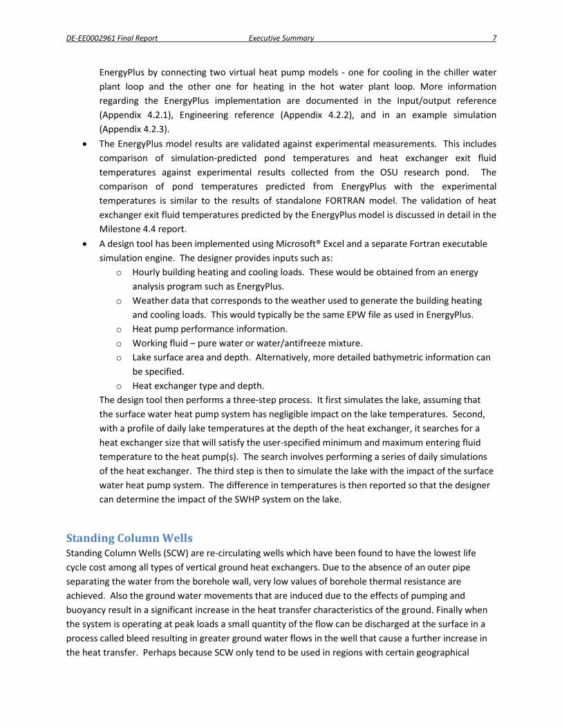
The design tool then performs a three-step process. It first simulates the lake, assuming that the surface water heat pump system has negligible impact on the lake temperatures. Second, with a profile of daily lake temperatures at the depth of the heat exchanger, it searches for a heat exchanger size that will satisfy the user-specified minimum and maximum entering fluid temperature to the heat pump(s). The search involves performing a series of daily simulations of the heat exchanger. The third step is then to simulate the lake with the impact of the surface water heat pump system. The difference in temperatures is then reported so that the designer can determine the impact of the SWHP system on the lake.
Standing Column Wells Standing Column Wells (SCW) are re-circulating wells which have been found to have the lowest life cycle cost among all types of vertical ground heat exchangers. Due to the absence of an outer pipe separating the water from the borehole wall, very low values of borehole thermal resistance are achieved. Also the ground water movements that are induced due to the effects of pumping and buoyancy result in a significant increase in the heat transfer characteristics of the ground. Finally when the system is operating at peak loads a small quantity of the flow can be discharged at the surface in a process called bleed resulting in greater ground water flows in the well that cause a further increase in the heat transfer. Perhaps because SCW only tend to be used in regions with certain geographical
DE-EE0002961 Final Report Executive Summary 8
features1, there have been relatively few models or design tools that have been developed to support design of SCW. This report describes the work done to improve and identify and overcome the limitations of the existing SCW models and incorporate the revised model into design tools (GLHEPRO) and in energy analysis software (EnergyPlus).
• The first task was improvement of the bleed control in the existing SCW model. Improvements were made such that three different bleed strategies could be used. The three strategies included constant bleed throughout, constant bleed between specified temperature limits and variable bleed for domestic purposes. Details of these strategies can be found in the Milestone 1.1 report.
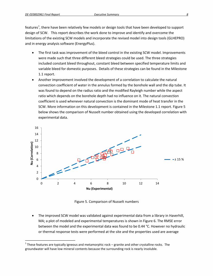
• Another improvement involved the development of a correlation to calculate the natural convection coefficient of water in the annulus formed by the borehole wall and the dip tube. It was found to depend on the radius ratio and the modified Rayleigh number while the aspect ratio which depends on the borehole depth had no influence on it. The natural convection coefficient is used whenever natural convection is the dominant mode of heat transfer in the SCW. More information on this development is contained in the Milestone 1.1 report. Figure 5 below shows the comparison of Nusselt number obtained using the developed correlation with experimental data.
Figure 5. Comparison of Nusselt numbers
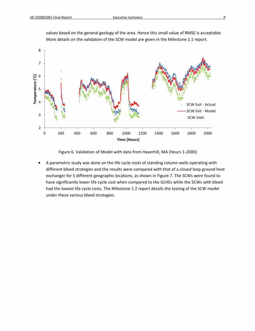
• The improved SCW model was validated against experimental data from a library in Haverhill, MA; a plot of modeled and experimental temperatures is shown in Figure 6. The RMSE error between the model and the experimental data was found to be 0.44 °C. However no hydraulic or thermal response tests were performed at the site and the properties used are average
1 These features are typically igneous and metamorphic rock – granite and other crystalline rocks. The groundwater will have low mineral contents because the surrounding rock is nearly insoluble.
0
2
4
6
8
10
12
14
16
0 2 4 6 8 10 12 14
Nu
(Cor
rela
tion)
Nu (Experimental)
± 15 %
DE-EE0002961 Final Report Executive Summary 9
values based on the general geology of the area. Hence this small value of RMSE is acceptable. More details on the validation of the SCW model are given in the Milestone 1.1 report.
Figure 6. Validation of Model with data from Haverhill, MA (Hours 1-2000)
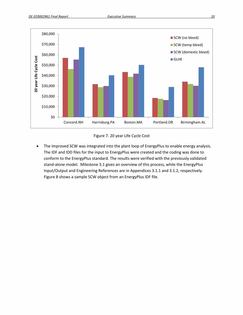
• A parametric study was done on the life cycle costs of standing column wells operating with different bleed strategies and the results were compared with that of a closed loop ground heat exchanger for 5 different geographic locations, as shown in Figure 7. The SCWs were found to have significantly lower life cycle cost when compared to the GLHEs while the SCWs with bleed had the lowest life cycle costs. The Milestone 1.2 report details the testing of the SCW model under these various bleed strategies.
2
3
4
5
6
7
8
0 200 400 600 800 1000 1200 1400 1600 1800 2000
Tem
pera
ture
(°C)
Time (Hours)
SCW Exit - ActualSCW Exit - Model SCW Inlet
DE-EE0002961 Final Report Executive Summary 10
Figure 7. 20 year Life Cycle Cost
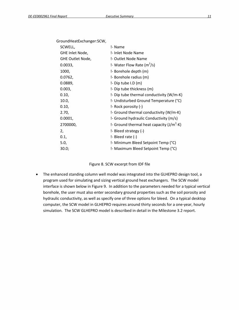
• The improved SCW was integrated into the plant loop of EnergyPlus to enable energy analysis. The IDF and IDD files for the input to EnergyPlus were created and the coding was done to conform to the EnergyPlus standard. The results were verified with the previously validated stand-alone model. Milestone 3.1 gives an overview of this process, while the EnergyPlus Input/Output and Engineering References are in Appendices 3.1.1 and 3.1.2, respectively. Figure 8 shows a sample SCW object from an EnergyPlus IDF file.
$0
$10,000
$20,000
$30,000
$40,000
$50,000
$60,000
$70,000
$80,000
Concord.NH Harrisburg.PA Boston.MA Portland.OR Birmingham.AL
20 y
ear L
ife C
ycle
Cos
t SCW (no bleed)
SCW (temp bleed)
SCW (domestic bleed)
GLHE
DE-EE0002961 Final Report Executive Summary 11
GroundHeatExchanger:SCW, SCWELL, !- Name GHE Inlet Node, !- Inlet Node Name GHE Outlet Node, !- Outlet Node Name 0.0033, !- Water Flow Rate (m3/s) 1000, !- Borehole depth (m) 0.0762, !- Borehole radius (m) 0.0889, !- Dip tube I.D (m) 0.003, !- Dip tube thickness (m) 0.10, !- Dip tube thermal conductivity (W/m-K) 10.0, !- Undisturbed Ground Temperature (°C) 0.10, !- Rock porosity (-) 2.70, !- Ground thermal conductivity (W/m-K) 0.0001, !- Ground hydraulic Conductivity (m/s) 2700000, !- Ground thermal heat capacity (J/m3-K) 2, !- Bleed strategy (-) 0.1, !- Bleed rate (-) 5.0, !- Minimum Bleed Setpoint Temp (°C) 30.0; !- Maximum Bleed Setpoint Temp (°C)
Figure 8. SCW excerpt from IDF file
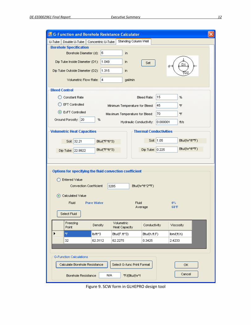
• The enhanced standing column well model was integrated into the GLHEPRO design tool, a program used for simulating and sizing vertical ground heat exchangers. The SCW model interface is shown below in Figure 9. In addition to the parameters needed for a typical vertical borehole, the user must also enter secondary ground properties such as the soil porosity and hydraulic conductivity, as well as specify one of three options for bleed. On a typical desktop computer, the SCW model in GLHEPRO requires around thirty seconds for a one-year, hourly simulation. The SCW GLHEPRO model is described in detail in the Milestone 3.2 report.
DE-EE0002961 Final Report Executive Summary 12
Figure 9. SCW form in GLHEPRO design tool
DE-EE0002961 Final Report Executive Summary 13
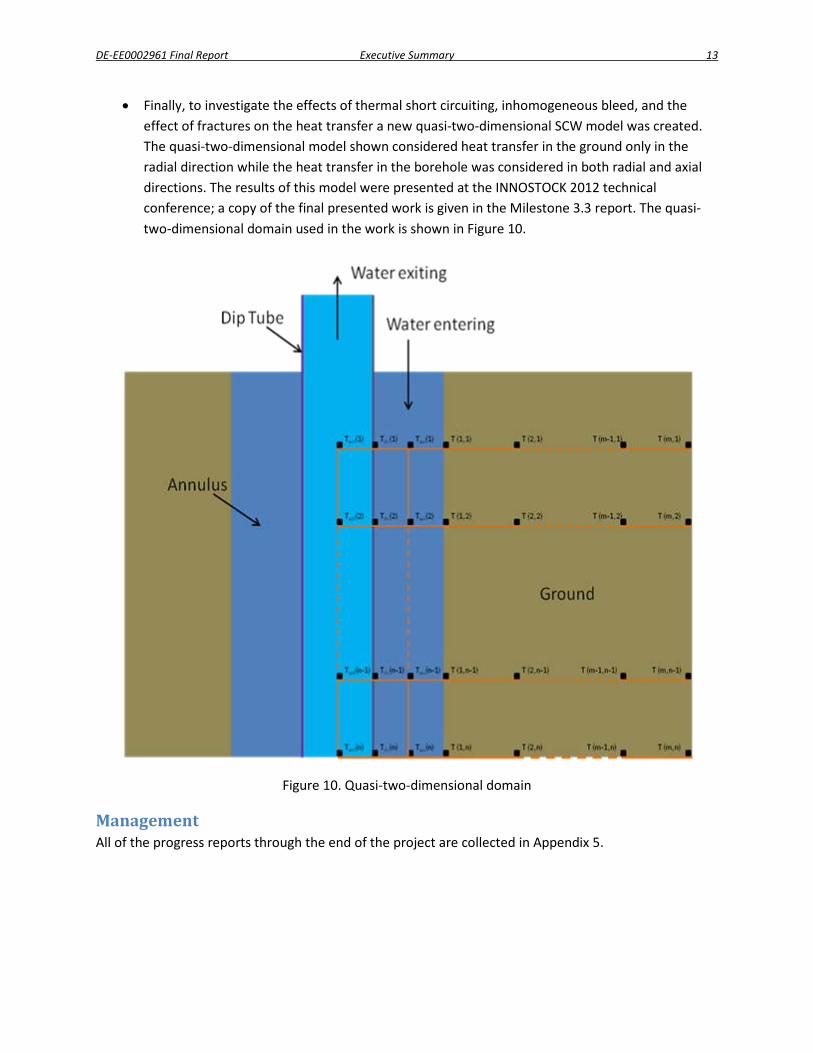
• Finally, to investigate the effects of thermal short circuiting, inhomogeneous bleed, and the effect of fractures on the heat transfer a new quasi-two-dimensional SCW model was created. The quasi-two-dimensional model shown considered heat transfer in the ground only in the radial direction while the heat transfer in the borehole was considered in both radial and axial directions. The results of this model were presented at the INNOSTOCK 2012 technical conference; a copy of the final presented work is given in the Milestone 3.3 report. The quasi-two-dimensional domain used in the work is shown in Figure 10.
Figure 10. Quasi-two-dimensional domain
Management All of the progress reports through the end of the project are collected in Appendix 5.

DE-EE0002961 Final Report Executive Summary 14
Task-by-Task Summary This section provides a comparison of the actual accomplishments with the goals and objectives of the project on a task-by-task basis. It also summarizes the project activities for the entire period of funding. It is organized as an overview with a brief summary here in this section, with pointers to the appendices where more detailed information is given. There are four types of appendices:
• Regular appendices, which are referred to, for example, as Appendix 3.1.2. This would be the 2nd appendix related to Task 3, Subtask 3.1. The appendices are provided both as separate PDF files called, for example, “Appendix_3.1.2.pdf” and as sections of the full final project report, “DE-EE0002961_full.pdf”
• Milestone reports, which are referred to, for example, as Milestone 2.1 Report. This would be the milestone report for Task 2, Subtask 2.1. It will also be provided in a PDF file called “Milestone_2.1.pdf” and as a section of the full final project report, “DE-EE0002961_full.pdf”
• Source code is provided two different ways. For the one task where the source code is relatively short, it is provided as a PDF called “SourceCode_3.2.pdf” and it also appears in the full final project report.
• For EnergyPlus source code and standalone models that consist of multiple Fortran 90 modules in multiple files, the working directory including project files have been zipped up into single files such as “Source_4.2.zip”
Task 1: Enhancement of Existing Standing Column Well Model Task 1 represents the first year of the project’s work standing column wells. The main work was development and testing of an enhanced standing column well model. Table 2 contains summaries for each of the subtasks, pointing to a more detailed report found in the appendices.
Table 1 Subtask Summaries for Task 1
Subtask Accomplishments
Subtask 1.1. Development and validation of SCW model with separate bleed control.
Done. The Milestone 1.1 report explains both the starting point and the revisions to the model, as well as validation against experimental data.
Subtask 1.2. Testing of model with various bleed control strategies.
Done. The Milestone 1.2 report describes a parametric study utilizing various bleed control strategies.

DE-EE0002961 Final Report Executive Summary 15
Task 2: Enhancement of Existing Pond Model Task 2 represents the first year of the project’s work on development of a lake model and a surface water heat exchanger model for surface water heat pump systems. Before the project started, we envisioned adding new features to an existing model previously developed by Chiasson, et al. (2000). However, because prediction of stratification required substantial restructuring of the model, we changed our plan and just developed a new model. Table 2 contains summaries for each of the subtasks, pointing to a more detailed report found in the appendices.
Table 2 Subtask Summaries for Task 2
Subtask Accomplishments
Subtask 2.1. Modeling of stratification. Done. Modeling of stratification is described in
the Milestone2.1 report.
Subtask 2.2. Modeling of ice-on-coil. Done. Modeling of ice-on-coil is described in the
Milestone2.2 report.
Subtask 2.3. Modeling of ice-on-surface. Done. Modeling of ice-on-surface is described in the
Milestone2.3 report.

DE-EE0002961 Final Report Executive Summary 16
Task 3: Implementation of Enhanced Standing Column Well Model Task 3 involved implementation of the enhanced model in two environments: EnergyPlus and a standalone design tool. Table 3 contains summaries for each of the subtasks, pointing to a more detailed report found in the appendices.
Table 3 Subtask Summaries for Task 3
Subtask Appendices
Subtask 3.1. Implementation of enhanced SCW model in EnergyPlus. Done. The EnergyPlus input documentation is given in
Appendix 3.1.1. The EnergyPlus Engineering
Reference documentation is given in Appendix 3.1.2.
Subtask 3.2. Implementation of enhanced SCW model in design tool. Done. The implementation of the model in the stand-alone design tool is described in the
Milestone 3.2 report.
Subtask 3.3. Technology transfer. Mostly done. This model has been described in a paper presented at the Innostock
2012 conference sponsored by the International Energy
Agency, Energy Conservation through Energy Storage
Working Agreement. The paper is contained in the
Milestone 3.3 report. A journal paper is still in the works.

DE-EE0002961 Final Report Executive Summary 17
Task 4: Implementation of Enhanced Pond Model This task involved further improvements to the pond model, by way of adding models of additional heat exchanger types; documentation of the model in EnergyPlus; implementation of the model in a design tool; and validation of the model.
Table 4 contains summaries for each of the subtasks, pointing to a more detailed report found in the appendices.
Table 4 Subtask Summaries for Task 4
Subtask Appendices
Subtask 4.1. Modeling of alternate pond heat exchanger types. Done. The models of the alternate pond heat exchanger
types are described in the Milestone 4.1 report.
Subtask 4.2. Documentation of enhanced pond model in EnergyPlus. Done. The EnergyPlus documentation is contained in 3 appendices. Appendix 4.2.1
contains the Input Output Reference. Appendix 4.2.2 contains the Engineering
Reference. Appendix 4.2.3 contains the example.
Subtask 4.3. Implementation of enhanced pond model in design tool. Done. The Milestone 4.3.1 report contains the
documentation for the design tool. The Milestone 4.3.2
report contains an example of using the design tool.
Subtask 4.4. Validation of pond model. Done. The Milestone 4.4 report describes the
validation.
Subtask 4.5. Technology transfer. Partially done. Several papers are under development, but not yet finished. There is a
complete draft of one paper and a “70% draft” of the other
paper.
Task 5: Project Management and Reporting In addition to this final report, 10 quarterly progress reports and two annual reports were prepared. All of the quarterly progress reports are contained in Appendix 5, in the file Appendix5_Progress_Reports.pdf.
DE-EE0002961 Final Report Executive Summary 18
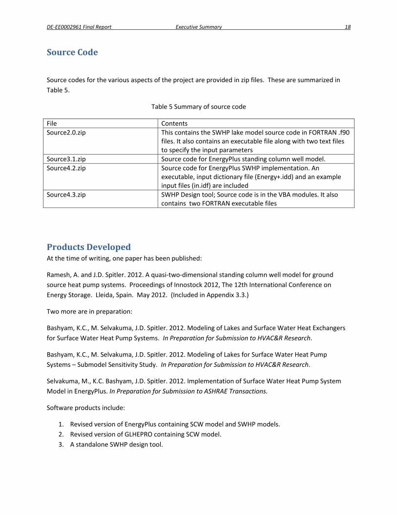
Source Code
Source codes for the various aspects of the project are provided in zip files. These are summarized in Table 5.
Table 5 Summary of source code
File Contents Source2.0.zip This contains the SWHP lake model source code in FORTRAN .f90
files. It also contains an executable file along with two text files to specify the input parameters
Source3.1.zip Source code for EnergyPlus standing column well model. Source4.2.zip Source code for EnergyPlus SWHP implementation. An
executable, input dictionary file (Energy+.idd) and an example input files (in.idf) are included
Source4.3.zip SWHP Design tool; Source code is in the VBA modules. It also contains two FORTRAN executable files
Products Developed At the time of writing, one paper has been published:
Ramesh, A. and J.D. Spitler. 2012. A quasi-two-dimensional standing column well model for ground source heat pump systems. Proceedings of Innostock 2012, The 12th International Conference on Energy Storage. Lleida, Spain. May 2012. (Included in Appendix 3.3.)
Two more are in preparation:
Bashyam, K.C., M. Selvakuma, J.D. Spitler. 2012. Modeling of Lakes and Surface Water Heat Exchangers for Surface Water Heat Pump Systems. In Preparation for Submission to HVAC&R Research.
Bashyam, K.C., M. Selvakuma, J.D. Spitler. 2012. Modeling of Lakes for Surface Water Heat Pump Systems – Submodel Sensitivity Study. In Preparation for Submission to HVAC&R Research.
Selvakuma, M., K.C. Bashyam, J.D. Spitler. 2012. Implementation of Surface Water Heat Pump System Model in EnergyPlus. In Preparation for Submission to ASHRAE Transactions.
Software products include:
1. Revised version of EnergyPlus containing SCW model and SWHP models. 2. Revised version of GLHEPRO containing SCW model. 3. A standalone SWHP design tool.

DE-EE0002961 Final Report Executive Summary 19
Computer Modeling The DOE has requested that we provide information related to the computer modeling in this project. From the Federal Assistance Reporting Instructions:
a. Model description, key assumptions, version, source and intended use;
b. Performance criteria for the model related to the intended use;
c. Test results to demonstrate the model performance criteria were met (e.g., code verification/validation, sensitivity analyses, history matching with lab or field data, as appropriate);
d. Theory behind the model, expressed in non-mathematical terms;
e. Mathematics to be used, including formulas and calculation methods;
f. Whether or not the theory and mathematical algorithms were peer reviewed, and, if so, include a summary of theoretical strengths and weaknesses;
Reports covering this information are contained in Appendix 6.1 (SWHP Systems) and Appendix 6.2 (SCW).

DE-EE0002961 Final Report Executive Summary 20
References
Chiasson, A. D., J. D. Spitler, et al. (2000). "A Model For Simulating The Performance Of A Shallow Pond As A Supplemental Heat Rejecter With Closed-Loop Ground-Source Heat Pump Systems." ASHRAE Transactions 106(2): 107-121.
Hansen, G. M. (2011). Experimental testing and analysis of spiral-helical surface water heat exchanger configurations. Masters Masters thesis, Oklahoma State University.
Molineaux, B., B. Lachal, et al. (1994). "Thermal analysis of five outdoor swimming pools heated by unglazed solar collectors." Solar Energy 53(1): 21-26.
Neto, J. H. M. and M. Krarti (1997). "Deterministic model for an internal melt ice-on-coil thermal storage tank." ASHRAE Transactions 103(1): 113-124.
Rohden, C. v., K. Wunderle, et al. (2007). "Parameterisation of the vertical transport in a small thermally stratified lake." Aquatic Sciences - Research Across Boundaries 69(1): 129-137.

DE-EE0002961 Final Report Appendix 3.1.1 1
Appendix 3.1.1
Standing Column Well EnergyPlus Input/Output Reference
Malai Ramesh
Oklahoma State University
DE-EE0002961 Final Report Appendix 3.1.1 2 GroundHeatExchanger:SCW
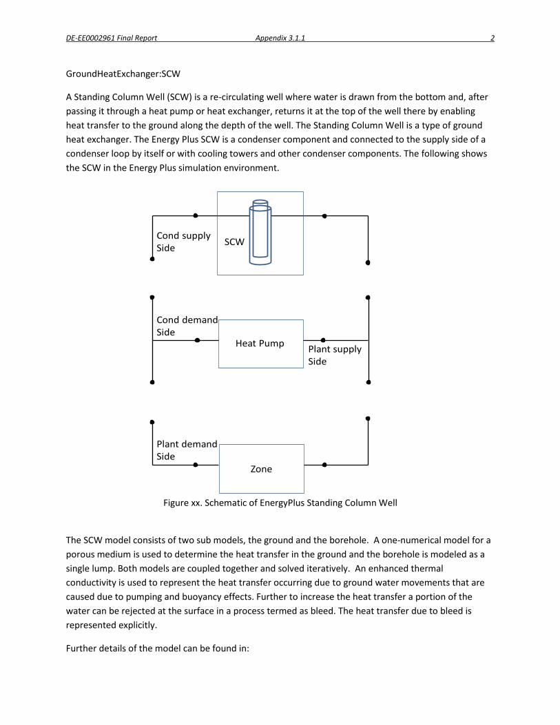
A Standing Column Well (SCW) is a re-circulating well where water is drawn from the bottom and, after passing it through a heat pump or heat exchanger, returns it at the top of the well there by enabling heat transfer to the ground along the depth of the well. The Standing Column Well is a type of ground heat exchanger. The Energy Plus SCW is a condenser component and connected to the supply side of a condenser loop by itself or with cooling towers and other condenser components. The following shows the SCW in the Energy Plus simulation environment.
SCWCond supply Side
Heat Pump
Cond demand Side
Plant supply Side
Plant demand Side
Zone
Figure xx. Schematic of EnergyPlus Standing Column Well
The SCW model consists of two sub models, the ground and the borehole. A one-numerical model for a porous medium is used to determine the heat transfer in the ground and the borehole is modeled as a single lump. Both models are coupled together and solved iteratively. An enhanced thermal conductivity is used to represent the heat transfer occurring due to ground water movements that are caused due to pumping and buoyancy effects. Further to increase the heat transfer a portion of the water can be rejected at the surface in a process termed as bleed. The heat transfer due to bleed is represented explicitly.
Further details of the model can be found in:

DE-EE0002961 Final Report Appendix 3.1.1 3 Deng,Z. Modeling of Standing Column Wells in Ground Source Heat Pump Systems. Ph.D. Thesis, Oklahoma State University, Stillwater, OK. December 2005.
The data definition for the Groundheatexchanger:SCW from the Energy+.idd file is shown below.
Field: Name
This alpha field contains the identifying name for the Standing Column Well (SCW).
Field: Inlet Node Name
This alpha field contains the SCW inlet node name.
Field: Outlet Node Name
This alpha field contains the SCW outlet node name.
Field: Maximum Flow Rate
This numeric field contains the SCW maximum design flow rate in m3/s.
Field: Borehole Depth
The numeric field contains the depth of the borehole in meters {m}.
Field: Borehole Radius
This numeric field contains the radius of the borehole in meters {m}.
Field: Dip Tube I.D
This numeric field contains the inner diameter of the dip tube in meters {m}.
Field: Dip Tube Thickness
This numeric field contains the thickness of the dip tube material in meters {m}.
Field: Dip Tube Thermal Conductivity
This numeric field contains the thermal conductivity of the dip tube material in W/m-K.
Field: Undisturbed Ground Temperature
This numeric field contains the undisturbed ground temperature in °C.
Field: Rock porosity
This numeric field contains the porosity of the surrounding ground {-}.
Field: Ground Thermal Conductivity

DE-EE0002961 Final Report Appendix 3.1.1 4 This numeric field contains the thermal conductivity of the surrounding ground in W/m-K.
Field: Ground Hydraulic Conductivity
This numeric field contains the hydraulic conductivity of the surrounding ground in m/s.
Field: Ground Thermal Heat Capacity
This numeric field contains the volumetric heat capacity of the surround ground in J/m3-K
Field: Bleed Strategy
This numeric field contains the bleed strategy that is to be used {-}.
1 – This indicates a constant bleed rate for the entire duration of the simulation
2- This indicates that a constant bleed rate will only be used when the entering water temperature falls below or above specified values.
0 – or any other value will result in the SCW operating without any bleed.
Field: Bleed Rate
This numeric field contains the percentage of the total flow rate that will be bled off (0 to 1) {-}.
Field: Minimum Bleed Setpoint Temperature
This numeric field contains the temperature limit below which bleed will be activated in °C.
Field: Maximum Bleed Setpoint Temperature
This numeric field contains the temperature limit above which bleed will be activated in °C.

DE-EE0002961 Final Report Appendix 3.1.1 5 The following is an example input:
GroundHeatExchanger:SCW, SCWELL, !- Name GHE Inlet Node, !- Inlet Node Name GHE Outlet Node, !- Outlet Node Name 0.0033, !- Water Flow Rate {m3/s} 1000, !- Borehole depth {m} 0.0762, !- Borehole radius {m} 0.0889, !- Dip tube I.D {m} 0.003, !- Dip tube thickness {m} 0.10, !- Dip tube thermal conducitvity {W/m-K} 10.0, !- Undisturbed Ground Temperature {°C} 0.10, !- Rock porosity {-} 2.70, !- Ground thermal conducivity {W/m-K} 0.0001, !- Ground hydraulic Conductivity {m/s} 2700000, !- Ground thermal heat capacity {J/m3-K} 2, !- Bleed strategy {-} 0.1, !- Bleed rate {-} 5.0, !- Minimum Bleed Setpoint Temp {°C} 30.0; !- Maximum Bleed Setpoint Temp {°C}

DE-EE0002961 Final Report Appendix 3.1.2 1
Appendix 3.1.2
Standing Column Well EnergyPlus Engineering Reference
Malai Ramesh
Oklahoma State University
DE-EE0002961 Final Report Appendix 3.1.2 2
Plant Loop Standing Column Well (SCW) Ground Heat Exchanger
The documentation for the base SCW model is derived from the Phd. Thesis of Zheng Deng, which is
available on the website of the Building and Environmental Thermal Systems Research Group at
Oklahoma State University:
http://www.hvac.okstate.edu/research/Documents/Deng_Thesis.pdf
However some improvements have been made to the model and they will be documented in another
Phd. Thesis that is yet to be published.
An SCW is a re-circulating well where water is drawn from the bottom and, after passing it through a
heat pump or heat exchanger, returns it at the top of the well there by enabling heat transfer to the
ground along the depth of the well. In locations where it is permissible to bleed off some of the water
drawn from the well, the induced flow of groundwater into the borehole significantly enhances the heat
transfer. The borehole of the SCW is modeled as a single lump and the heat transfer is calculated using a
thermal network approach. Based on a value of entering water temperature to the SCW from the heat
pump and a constant heat flux at the borehole wall this model calculates the temperature of water
leaving the SCW. The surrounding ground is modeled as a homogenous isotropic aquifer with no vertical
heat or water flow. Geothermal gradients are not considered and there is no explicit consideration for
density dependent flow. The heat transfer in the surrounding ground is considered to be one-
dimensional in the radial direction.
A typical SCW is shown below:
DE-EE0002961 Final Report Appendix 3.1.2 3
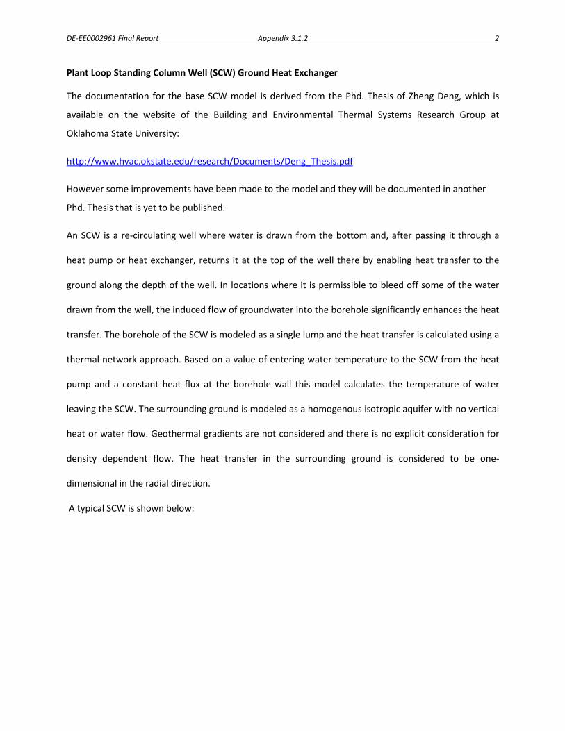
Figure xx. Typical SCW
Description of borehole model:
In the borehole model the heat transfer is due to the temperature difference between the average
water temperature in the borehole and the borehole wall. The expression for average temperature
considering bleed based on an assumption of linear variation of water temperature with depth is given
by the following Equation:
𝑇𝑓 =(1 − 𝑟)𝑇𝑓𝑖 + 𝑟𝑇𝑏 + 𝑇𝑓𝑜
2
Since the borehole is assumed to be a single lump the water in it can be considered to be well mixed. A
heat balance on the borehole is given by :
Borehole Wall
Dip Tube
Water entering From heat pump
Water exiting To heat pump
Submersible Pump
Discharge tube
Porter shroud
DE-EE0002961 Final Report Appendix 3.1.2 4
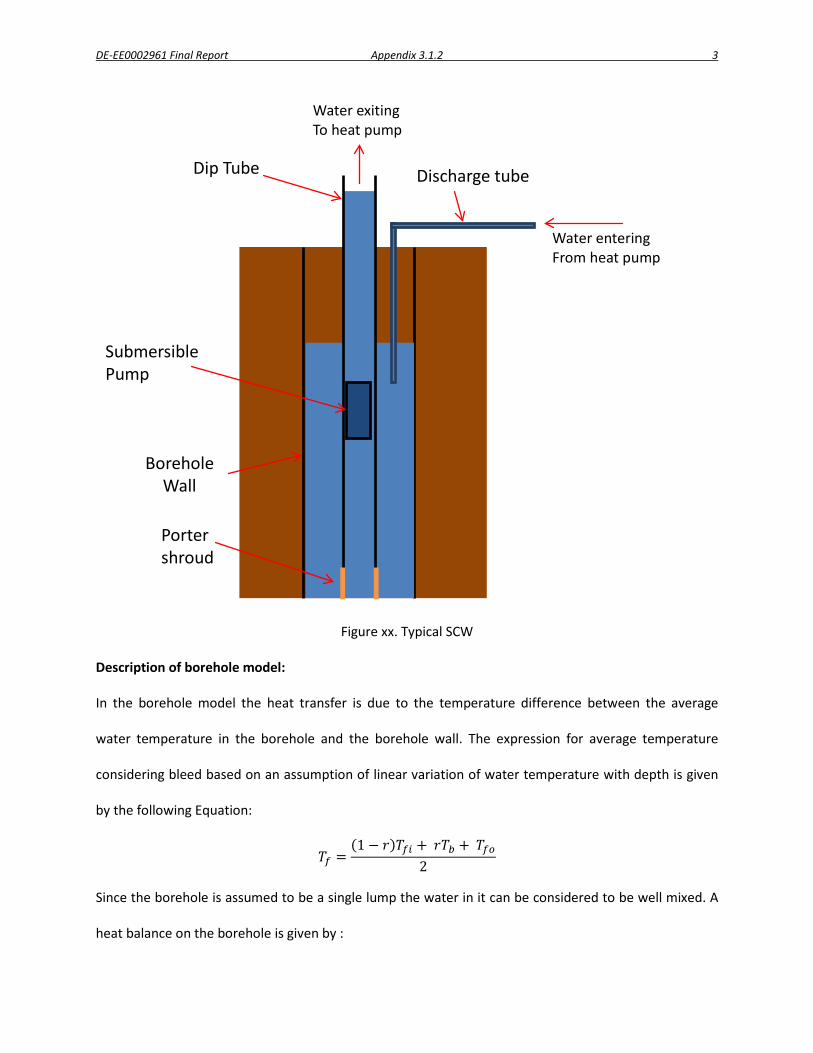
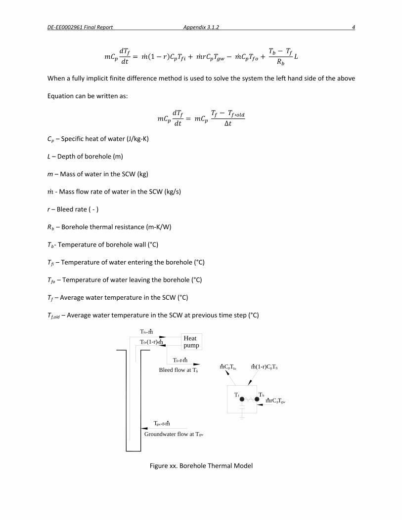
𝑚𝐶𝑝𝑑𝑇𝑓𝑑𝑡
= �̇�(1− 𝑟)𝐶𝑝𝑇𝑓𝑖 + �̇�𝑟𝐶𝑝𝑇𝑔𝑤 − �̇�𝐶𝑝𝑇𝑓𝑜 + 𝑇𝑏 − 𝑇𝑓𝑅𝑏
𝐿
When a fully implicit finite difference method is used to solve the system the left hand side of the above
Equation can be written as:
𝑚𝐶𝑝𝑑𝑇𝑓𝑑𝑡
= 𝑚𝐶𝑝 𝑇𝑓 − 𝑇𝑓 ,𝑜𝑙𝑑
∆𝑡
Cp – Specific heat of water (J/kg-K)
L – Depth of borehole (m)
m – Mass of water in the SCW (kg)
�̇� - Mass flow rate of water in the SCW (kg/s)
r – Bleed rate ( - )
Rb – Borehole thermal resistance (m-K/W)
Tb- Temperature of borehole wall (°C)
Tfi – Temperature of water entering the borehole (°C)
Tfo – Temperature of water leaving the borehole (°C)
Tf – Average water temperature in the SCW (°C)
Tf,old – Average water temperature in the SCW at previous time step (°C)
Figure xx. Borehole Thermal Model
T m
Bleed flow at T
Groundwater flow at T
gwT r m
T
Tfi
m
fo
fi (1-r)
m(1-r)C T
gw
fT
mr
fi
Heat pump
fopmC T
mrC TbT
p gw
p fi
DE-EE0002961 Final Report Appendix 3.1.2 5
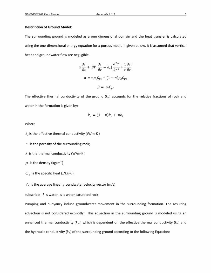
Description of Ground Model:
The surrounding ground is modeled as a one dimensional domain and the heat transfer is calculated
using the one-dimensional energy equation for a porous medium given below. It is assumed that vertical
heat and groundwater flow are negligible.
𝛼𝜕𝑇𝜕𝑡
+ 𝛽𝑉𝑟𝜕𝑇𝜕𝑟
= 𝑘𝑒[ 𝜕2𝑇𝜕𝑟2
+1𝑟𝜕𝑇𝜕𝑟
]
𝛼 = 𝑛𝜌𝑙𝐶𝑝𝑙 + (1 − 𝑛)𝜌𝑠𝐶𝑝𝑠
𝛽 = 𝜌𝑙𝐶𝑝𝑙
The effective thermal conductivity of the ground (ke) accounts for the relative fractions of rock and
water in the formation is given by:
𝑘𝑒 = (1 − 𝑛)𝑘𝑟 + 𝑛𝑘𝑙
Where
ek is the effective thermal conductivity (W/m-K )
n is the porosity of the surrounding rock;
k is the thermal conductivity (W/m-K )
ρ is the density (kg/m3 )
pC is the specific heat (J/kg-K )
rV is the average linear groundwater velocity vector (m/s)
subscripts: l is water , s is water saturated rock
Pumping and buoyancy induce groundwater movement in the surrounding formation. The resulting
advection is not considered explicitly. This advection in the surrounding ground is modeled using an
enhanced thermal conductivity (ken) which is dependent on the effective thermal conductivity (ke) and
the hydraulic conductivity (kh) of the surrounding ground according to the following Equation:
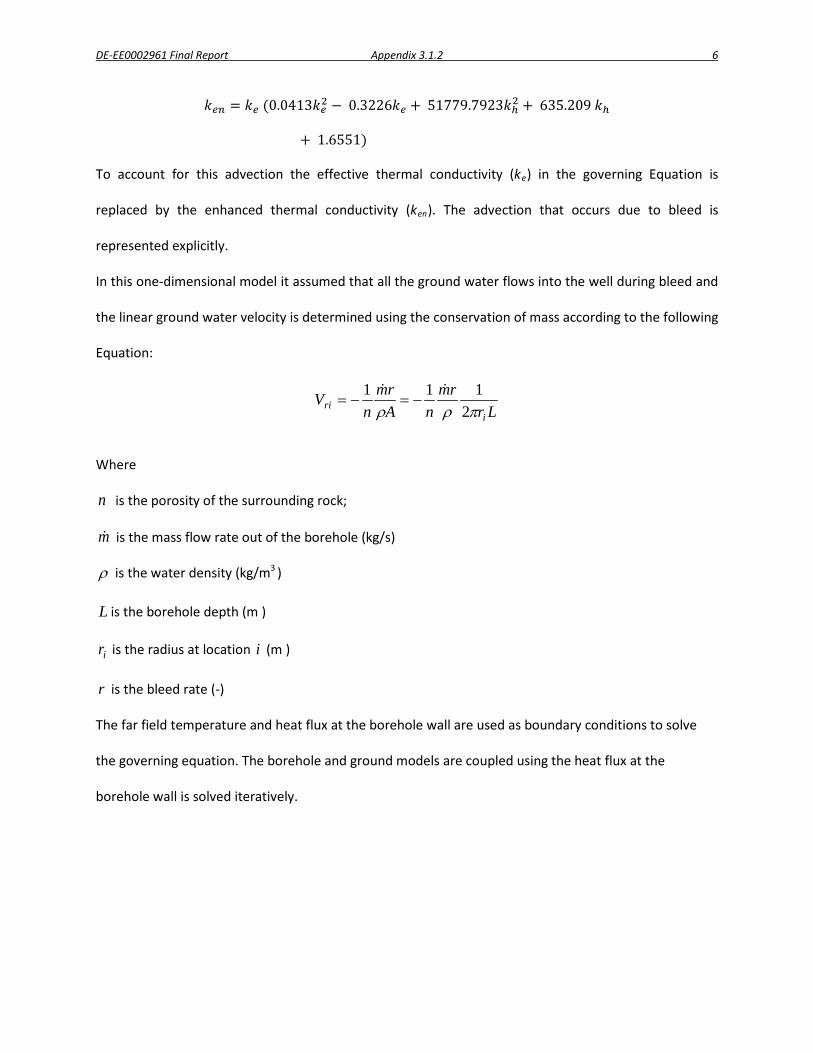
DE-EE0002961 Final Report Appendix 3.1.2 6
𝑘𝑒𝑛 = 𝑘𝑒 (0.0413𝑘𝑒2 − 0.3226𝑘𝑒 + 51779.7923𝑘ℎ2 + 635.209 𝑘ℎ
+ 1.6551)
To account for this advection the effective thermal conductivity (ke) in the governing Equation is
replaced by the enhanced thermal conductivity (ken). The advection that occurs due to bleed is
represented explicitly.
In this one-dimensional model it assumed that all the ground water flows into the well during bleed and
the linear ground water velocity is determined using the conservation of mass according to the following
Equation:
Lrrm
nArm
nV
iri πρρ 2
111 −=−=
Where
n is the porosity of the surrounding rock;
m is the mass flow rate out of the borehole (kg/s)
ρ is the water density (kg/m3 )
L is the borehole depth (m )
ir is the radius at location i (m )
r is the bleed rate (-)
The far field temperature and heat flux at the borehole wall are used as boundary conditions to solve
the governing equation. The borehole and ground models are coupled using the heat flux at the
borehole wall is solved iteratively.

DE-EE0002961 Final Report Appendix 4.2.1 1
Appendix 4.2.1
Surface Water Heat Pump Systems EnergyPlus Input Output Reference
Manojkumar Selvakumar
Oklahoma State University

DE-EE0002961 Final Report Appendix 4.2.1 2
SWHP: Pond
The SWHP pond model simulates a pond or lake of any size with submerged hydronic tubes or flat plates through which the heat transfer fluid is circulated. The model considers the effects of stratification as observed in deeper lakes and calculates the ice and snow thickness formed at the pond/lake surface. The model can be simulated with four different types of heat exchanger coils such as spiral helical coils, flat spiral coils, vertical or horizontal slinky coils and flat plate heat exchangers (SlimJim®). The model also considers the effect of heat transfer due to the ice formation on the heat exchanger coils.
Field: Lake Name
This is the identifying name for the pond
Field: Lake Surface Area
This field contains the top surface area of the lake [m2].
Field: Maximum Lake Depth This field contains the maximum depth exhibited by the lake [m] Field: Volume development parameter This field contains Volume Development parameter (Vd) - a constant which defines the bathymetry profile of the lake [-] It characterizes the shape of the lake basin. This constant is used to model the variations in area and volume along depth. This constant value is highly important in accurate temperature prediction. More details to determine this constant are described in the Engineering Reference. If you know lake surface area, maximum depth and the lake volume it is very easy to calculate Vd from the formula described in Engineering Reference. Field: Secchi Depth This alpha field contains secchi depth of the lake - the measure of clarity of water [m] High secchi depth indicates more clear water whereas low secchi depth indicates cloudy or turbid water. Secchi depth is measured using Secchi disk. If your lake is maintained by any federal or state agencies, then the value of secchi depth can be retrieved from their online resources. Since secchi depth varies with time for respective lake, you should specify the value of secchi depth which is averaged over many months or years. Increase in secchi depth increases the solar penetration in the lake. Field: Grid Size This numeric field contains the vertical grid size for simulating the temperatures [m] It determines the thickness of model water layers in the lake. The minimum value of grid size is 0.1m which is set as a default option. High value reduces the simulation time but accuracy will be compromised. Field: Initial Water Temperature This numeric field is to initialize the linear temperature profile of the lake [°C]. The default option makes the initial linear temperature to be at 4°C. Field: Initial Ground Temperature This numeric field is to initialize temperature profile of lake sediment [°C]. The ground temperature varies with time and the place where the lake is located. It is the averaged value for a year. Field: Eddy Diffusion Model Type This field allows the user to select the ‘Eddy Diffusion Model Type’. The types of eddy diffusion model implemented in the lake model are GuandStefan, Banks, HondzoandStefan, HendersonSellers, Senuguptaetal, Imbergeretal, McormicandScavia, JassbyandPowell,

DE-EE0002961 Final Report Appendix 4.2.1 3
TuckerandGreen, Ellisetal and Rohdenetal. The model names indicate the author names of the paper from which this sub-model is adopted. If you are not sure of choosing the correct eddy diffusion model type for your lake bathymetry, then choose automatic. The model will select the best eddy diffusion model according to the depth and surface area of your lake. (See Engineering Reference) Field: Maximum Eddy Diffusion Coefficient This numeric field allows the option for you to put in your own maximum eddy diffusion coefficient [m2/day]. This value will replace the calculated value in the model. However, user-defined eddy diffusion coefficient is not appreciable. If you choose automatic, then the maximum eddy diffusion coefficient will be calculated by the model itself Field: Surface Convection Model Type This field allows the user to select the ‘Surface Convection Model Type’. The types of surface convection model implemented in the lake model are Molineauxetal, LosordoandPiedrahita, FrieheandSchmitt, Czarnecki, Chiassonetal, Saloranta and BrancoandTorgersen. The model names indicate the author names of the paper from which this sub-model is adopted. If you are not sure of choosing the correct surface convection model type for your lake bathymetry, then choose automatic. The model will select the best surface convection model according to the depth and surface area of your lake. (See Engineering Reference) Field: HX Fluid Inlet Node Name This numeric field contains the name of heat exchanger inlet node (condenser supply side inlet node)
Field: HX Fluid Outlet Node Name
This numeric field contains the name of heat exchanger outlet node (condenser supply side outlet node)
Field: Pond Heat Exchanger Type
This field allows the option for you to select the heat exchanger type you need to simulate with lake model. The lake model contains five different heat exchanger model Spiral helical, Flat spiral, Slinky, Helical and Flat plate. Once the HX type is selected, then corresponding dimensions go in the fields below.
Field: Outside coil diameter This numeric field contains the outside diameter of the heat exchanger coil [m] If you are selecting spiral helical or flat spiral or slinky you must specify the corresponding coil diameter in this field. The diagram showing the coil diameter for different heat exchanger types are shown in Engineering Reference.
Field: Horizontal spacing of a coil This numeric field contains the horizontal spacing in the bound up coil [m] If you are selecting spiral helical or flat spiral you must specify the corresponding horizontal spacing value. The diagram showing the horizontal spacing for different heat exchanger types are shown in Engineering Reference.
Field: Vertical spacing of a coil This numeric field contains the vertical spacing in the bound up coil [m] If you are selecting spiral helical you must specify the corresponding vertical spacing value. The diagram showing the vertical spacing for spiral helical heat exchanger type is shown in Engineering Reference.

DE-EE0002961 Final Report Appendix 4.2.1 4
Field: Height of the flat plate This numeric field contains the height of the flat plat heat exchanger [m]. The diagram is shown in Engineering Reference
.Field: Length of the flat plate
This numeric field contains the length of the flat plat heat exchanger [m].. The diagram is shown in Engineering Reference.
Field: Thickness of the flat plate
This numeric field contains the thickness of the flat plat heat exchanger [m].. The diagram is shown in Engineering Reference.
Field: Number of passes
This numeric field contains the number of channels in the flat plat heat exchanger [-]. The diagram is shown in Engineering Reference.
Field: Hydronic Tubing Outside Diameter This numeric field contains the pipe outside diameter [m]. For example, if you use HDPE SDR 11 ¾” nominal diameter, then the outside diameter is 1.05”
Field: Hydronic Tubing Inside Diameter This numeric field contains the pipe outside diameter [m]. For example, if you use HDPE SDR 11 ¾” nominal diameter, then the outside diameter is 0.86”
Field: Number of Tubing Circuits This numeric field contains the total number of heat exchanger coils placed in the lake [-].
Field: Length of the Tubing Circuit This numeric field contains length of the hydronic tubing circuit used [m].
Field: Depth of Heat Exchanger Placement – Top of the Heat Exchanger
This numeric field contains the depth at which the top of the heat exchanger is located from the lake surface [m]. Detailed diagram is shown in engineering reference
Field: Depth of Heat Exchanger Placement – Bottom of the Heat Exchanger
This numeric field contains the depth at which the bottom of the heat exchanger is located from the lake surface [m]. Detailed diagram is shown in engineering reference
DE-EE0002961 Final Report Appendix 4.2.1 5
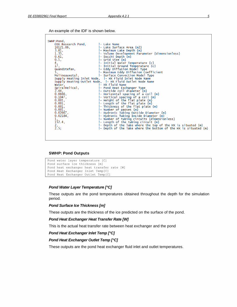
An example of the IDF is shown below.
SWHP: Pond Outputs
Pond water layer temperature [C] Pond surface ice thickness [m] Pond heat exchanger heat transfer rate [W] Pond Heat Exchanger Inlet Temp[C] Pond Heat Exchanger Outlet Temp[C]
Pond Water Layer Temperature [°C]
These outputs are the pond temperatures obtained throughout the depth for the simulation period.
Pond Surface Ice Thickness [m]
These outputs are the thickness of the ice predicted on the surface of the pond.
Pond Heat Exchanger Heat Transfer Rate [W]
This is the actual heat transfer rate between heat exchanger and the pond
Pond Heat Exchanger Inlet Temp [°C]
Pond Heat Exchanger Outlet Temp [°C]
These outputs are the pond heat exchanger fluid inlet and outlet temperatures.

DE-EE0002961 Final Report Appendix 4.2.2 1
Appendix 4.2.2
Surface Water Heat Pump Systems EnergyPlus Engineering Reference
Manojkumar Selvakumar
Oklahoma State University
DE-EE0002961 Final Report Appendix 4.2.2 2
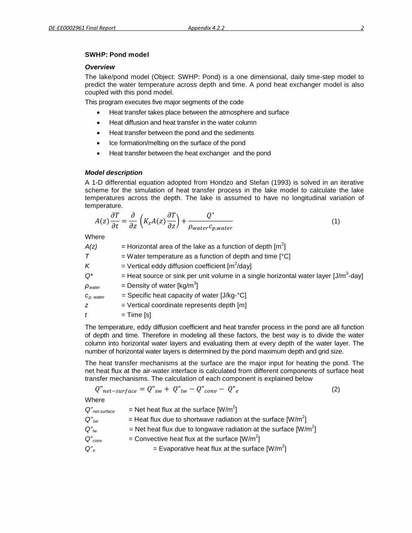
SWHP: Pond model
Overview The lake/pond model (Object: SWHP: Pond) is a one dimensional, daily time-step model to predict the water temperature across depth and time. A pond heat exchanger model is also coupled with this pond model. This program executes five major segments of the code
• Heat transfer takes place between the atmosphere and surface • Heat diffusion and heat transfer in the water column • Heat transfer between the pond and the sediments • Ice formation/melting on the surface of the pond • Heat transfer between the heat exchanger and the pond
Model description A 1-D differential equation adopted from Hondzo and Stefan (1993) is solved in an iterative scheme for the simulation of heat transfer process in the lake model to calculate the lake temperatures across the depth. The lake is assumed to have no longitudinal variation of temperature.
𝐴(𝑧)𝜕𝑇𝜕𝑡
=𝜕𝜕𝑧
�𝐾𝑧𝐴(𝑧)𝜕𝑇𝜕𝑧� +
𝑄∗
𝜌𝑤𝑎𝑡𝑒𝑟𝑐𝑝,𝑤𝑎𝑡𝑒𝑟 (1)
Where A(z) = Horizontal area of the lake as a function of depth [m2] T = Water temperature as a function of depth and time [°C] K = Vertical eddy diffusion coefficient [m2/day] Q* = Heat source or sink per unit volume in a single horizontal water layer [J/m3-day] ρwater = Density of water [kg/m3] cp, water = Specific heat capacity of water [J/kg-°C] z = Vertical coordinate represents depth [m] t = Time [s]
The temperature, eddy diffusion coefficient and heat transfer process in the pond are all function of depth and time. Therefore in modeling all these factors, the best way is to divide the water column into horizontal water layers and evaluating them at every depth of the water layer. The number of horizontal water layers is determined by the pond maximum depth and grid size.
The heat transfer mechanisms at the surface are the major input for heating the pond. The net heat flux at the air-water interface is calculated from different components of surface heat transfer mechanisms. The calculation of each component is explained below 𝑄"𝑛𝑒𝑡−𝑠𝑢𝑟𝑓𝑎𝑐𝑒 = 𝑄"𝑠𝑤 + 𝑄"𝑙𝑤 − 𝑄"𝑐𝑜𝑛𝑣 − 𝑄"𝑒 (2) Where Q”net-surface = Net heat flux at the surface [W/m2] Q”sw = Heat flux due to shortwave radiation at the surface [W/m2] Q”lw = Net heat flux due to longwave radiation at the surface [W/m2] Q”conv = Convective heat flux at the surface [W/m2] Q”e = Evaporative heat flux at the surface [W/m2]
DE-EE0002961 Final Report Appendix 4.2.2 3
Here, the shortwave and longwave radiative heat flux are calculated from Chiasson et al. (2000) and the pond model contains various sub-models to calculate the surface convective and evaporative fluxes. Mixing of water layers due to the wind stress at the surface is the significant factor which determines the depth of the epilimnion in the lakes. Ford and Stefan (1980) explained the algorithm for this process by calculating the depth of the water layer where the turbulent kinetic energy (TKE) caused in the surface by the wind is balanced by the potential energy (PE) of the water layer. The equations for TKE and PE are adopted from Saloranta and Andersen (2004). Also, energy transfer between the water layers is by turbulent diffusion process which is determined by various eddy diffusion sub-models built in this pond model. These eddy diffusion sub-models calculate eddy diffusion coefficient (Kz) which is a function of wind speed, depth and density gradients in the water column. The pond model also accounts for the heat transfer between the water and the sediment layers. The sediment heat transfer acts as a significant source of heat gain to the lake during ice cover period (Gu and Stefan (1990)). Lake simulation model incorporates the theory of sediment heat transfer from Fang and Stefan (1996) and calculation is based on implicit numerical method given by Saloranta and Andersen (2004). Modeling ice on the surface of the lake is by developing individual sub-models for ice formation, ice growth and ice melting. If the surface water temperature goes below freezing temperature then the ice formation is triggered. Due to congelation of ice, ice thickness gets increased if there is a continuous ice formation on the surface. The newly formed ice for the current day will be added to the previous day ice thickness to get the total amount. The ice formed on the surface gets melted from the top by the short wave heat flux and melted from the bottom by conductive heat flux from water layers. Hansen (2011) obtained correlations for outside Nusselt number for five different pond heat exchangers based on the experiments on OSU research pond. The correlations developed are used in the heat exchanger modeling.
Algorithm to handle daily time step pond model in EnergyPlus environment The pond heat exchanger implemented in EnergyPlus is connected to the supply side of a condenser loop and it can be used with any type of plant loop. Since the pond model is a daily time step model, it is triggered only once per day during the first hour of a day. However, the pond HX model runs according to the system time step. Initially at the start of day, the pond model simulates the pond temperatures and calculates the average temperature near the place where the HX is submerged for current day. The pond HX model takes in the current day average pond temperature and calculates the heat transfer rate to/from the pond and HX ExFT for every hour. Then, the pond model calculates temperatures for the next day by utilizing the total amount of heat rejected/extracted for a current day. In short, we set the pond simulation to lag by one day. Model input parameters The different sets of input needed to simulate the pond model with a pond heat exchanger are listed below in Figure 1 followed by a discussion about inputs and selecting sub models.
DE-EE0002961 Final Report Appendix 4.2.2 4
Figure 1 Sets of model input parameters
Bathymetry input The user must input surface area, maximum depth of the lake and volume development parameter to define the bathymetry of the lake. In this, Volume Development parameter (Vd) is a constant which characterizes the shape of the lake basin. This constant is necessary to model the variations in area and volume with depth, which is very significant in modeling the temperature along the depth of the lake. This kind of approach in modeling lake bathymetry is adopted from Johansson et al. (2007). To calculate this parameter two possibilities have been identified. Possibility 1: Lake surface area, maximum depth and volume are known If lake surface area, maximum depth and maximum volume are known to the user then Vd can be calculated from the following equation
𝑉𝑑 =𝑀𝑎𝑥𝑖𝑚𝑢𝑚 𝑉𝑜𝑙𝑢𝑚𝑒
𝑆𝑢𝑟𝑓𝑎𝑐𝑒 𝑎𝑟𝑒𝑎 ∗ 𝑀𝑎𝑥 𝑑𝑒𝑝𝑡ℎ3
(3)
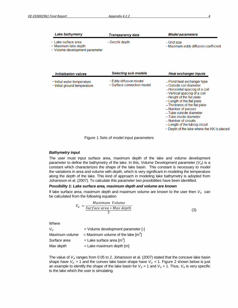
Where Vd = Volume development parameter [-] Maximum volume = Maximum volume of the lake [m3] Surface area = Lake surface area [m2] Max depth = Lake maximum depth [m] The value of Vd ranges from 0.05 to 2. Johansson et al. (2007) stated that the concave lake basin shape have Vd > 1 and the convex lake basin shape have Vd < 1. Figure 2 shown below is just an example to identify the shape of the lake basin for Vd > 1 and Vd < 1. Thus, Vd is very specific to the lake which the user is simulating.
DE-EE0002961 Final Report Appendix 4.2.2 5
Figure 2 Concave and convex lakes basin shapes and their corresponding Vd
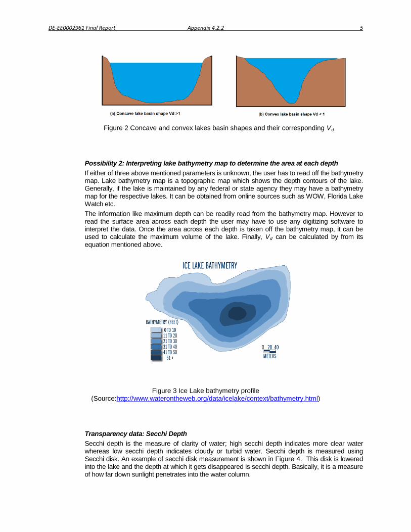
Possibility 2: Interpreting lake bathymetry map to determine the area at each depth If either of three above mentioned parameters is unknown, the user has to read off the bathymetry map. Lake bathymetry map is a topographic map which shows the depth contours of the lake. Generally, if the lake is maintained by any federal or state agency they may have a bathymetry map for the respective lakes. It can be obtained from online sources such as WOW, Florida Lake Watch etc. The information like maximum depth can be readily read from the bathymetry map. However to read the surface area across each depth the user may have to use any digitizing software to interpret the data. Once the area across each depth is taken off the bathymetry map, it can be used to calculate the maximum volume of the lake. Finally, Vd can be calculated by from its equation mentioned above.
Figure 3 Ice Lake bathymetry profile (Source:http://www.waterontheweb.org/data/icelake/context/bathymetry.html)
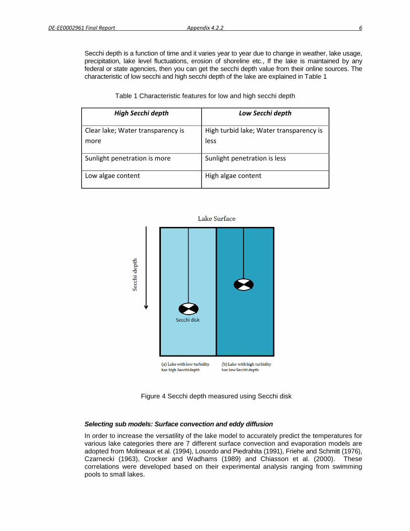
Transparency data: Secchi Depth Secchi depth is the measure of clarity of water; high secchi depth indicates more clear water whereas low secchi depth indicates cloudy or turbid water. Secchi depth is measured using Secchi disk. An example of secchi disk measurement is shown in Figure 4. This disk is lowered into the lake and the depth at which it gets disappeared is secchi depth. Basically, it is a measure of how far down sunlight penetrates into the water column.
DE-EE0002961 Final Report Appendix 4.2.2 6
Secchi depth is a function of time and it varies year to year due to change in weather, lake usage, precipitation, lake level fluctuations, erosion of shoreline etc., If the lake is maintained by any federal or state agencies, then you can get the secchi depth value from their online sources. The characteristic of low secchi and high secchi depth of the lake are explained in Table 1
Table 1 Characteristic features for low and high secchi depth
High Secchi depth Low Secchi depth
Clear lake; Water transparency is more
High turbid lake; Water transparency is less
Sunlight penetration is more Sunlight penetration is less
Low algae content High algae content
Figure 4 Secchi depth measured using Secchi disk
Selecting sub models: Surface convection and eddy diffusion
In order to increase the versatility of the lake model to accurately predict the temperatures for various lake categories there are 7 different surface convection and evaporation models are adopted from Molineaux et al. (1994), Losordo and Piedrahita (1991), Friehe and Schmitt (1976), Czarnecki (1963), Crocker and Wadhams (1989) and Chiasson et al. (2000). These correlations were developed based on their experimental analysis ranging from swimming pools to small lakes.
DE-EE0002961 Final Report Appendix 4.2.2 7
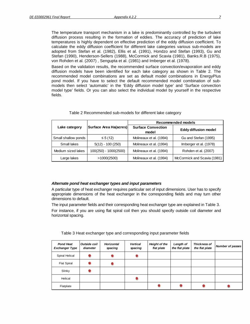
The temperature transport mechanism in a lake is predominantly controlled by the turbulent diffusion process resulting in the formation of eddies. The accuracy of prediction of lake temperatures is highly dependent on effective prediction of the eddy diffusion coefficient. To calculate the eddy diffusion coefficient for different lake categories various sub-models are adopted from Stefan et al. (1982), Ellis et al. (1991), Hondzo and Stefan (1993), Gu and Stefan (1990), Henderson-Sellers (1988), McCormick and Scavia (1981), Banks.R.B (1975), von Rohden et al. (2007) , Sengupta et al. (1981) and Imberger et al. (1978). Based on the validation results, the recommended surface convection/evaporation and eddy diffusion models have been identified for each lake category as shown in Table 2. The recommended model combinations are set as default model combinations in EnergyPlus pond model. If you have to select the default recommended model combination of sub-models then select ‘automatic’ in the ‘Eddy diffusion model type’ and ‘Surface convection model type’ fields. Or you can also select the individual model by yourself in the respective fields.
Table 2 Recommended sub-models for different lake category
Alternate pond heat exchanger types and input parameters A particular type of heat exchanger requires particular set of input dimensions. User has to specify appropriate dimensions of the heat exchanger in the corresponding fields and may turn other dimensions to default. The input parameter fields and their corresponding heat exchanger type are explained in Table 3. For instance, if you are using flat spiral coil then you should specify outside coil diameter and horizontal spacing.
Table 3 Heat exchanger type and corresponding input parameter fields
Surface Convection model Eddy diffusion model
Small shallow ponds ≤ 5 (12) Molineaux et al. (1994) Gu and Stefan (1995)
Small lakes 5(12) - 100 (250) Molineaux et al. (1994) Imberger et al. (1978)
Medium sized lakes 100(250) - 1000(2500) Molineaux et al. (1994) Rohden et al. (2007)
Large lakes >1000(2500) Molineaux et al. (1994) McCormick and Scavia (1981)
Recommended modelsLake category Surface Area Ha(acres)
Pond Heat Exchanger Type
Outside coil diameter
Horizontal spacing
Vertical spacing
Height of the flat plate
Length of the flat plate
Thickness of the flat plate Number of passes
Spiral Helical
Flat Spiral
Slinky
Helical
Flatplate

DE-EE0002961 Final Report Appendix 4.2.2 8
Spiral helical coil The coil outside diameter, horizontal spacing and vertical spacing as shown in Figure 5 are the required inputs to simulate spiral helical coil
Figure 5 Spiral helical coil input dimensions
Flat spiral coil The coil outside diameter and horizontal spacing shown in Figure 6 are the required inputs to simulate flat spiral coil.
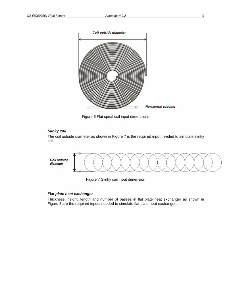
DE-EE0002961 Final Report Appendix 4.2.2 9
Figure 6 Flat spiral coil input dimensions
Slinky coil The coil outside diameter as shown in Figure 7 is the required input needed to simulate slinky coil.
Figure 7 Slinky coil input dimension
Flat plate heat exchanger Thickness, height, length and number of passes in flat plate heat exchanger as shown in Figure 8 are the required inputs needed to simulate flat plate heat exchanger.
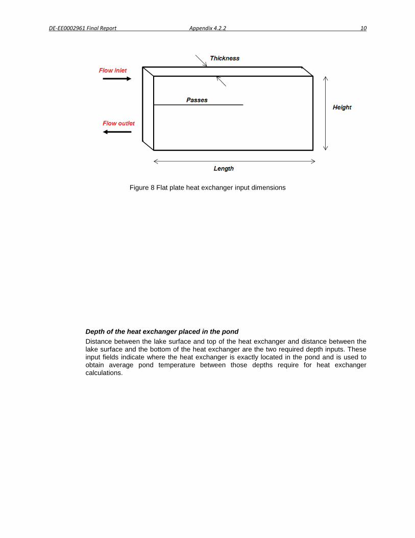
DE-EE0002961 Final Report Appendix 4.2.2 10
Figure 8 Flat plate heat exchanger input dimensions
Depth of the heat exchanger placed in the pond Distance between the lake surface and top of the heat exchanger and distance between the lake surface and the bottom of the heat exchanger are the two required depth inputs. These input fields indicate where the heat exchanger is exactly located in the pond and is used to obtain average pond temperature between those depths require for heat exchanger calculations.
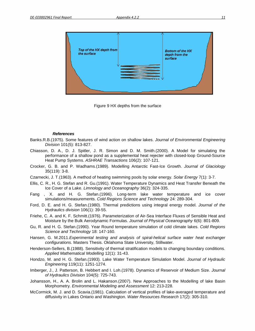
DE-EE0002961 Final Report Appendix 4.2.2 11
Figure 9 HX depths from the surface
References
Banks.R.B.(1975). Some features of wind action on shallow lakes. Journal of Environmental Engineering Division 101(5): 813-827.
Chiasson, D. A., D. J. Spitler, J. R. Simon and D. M. Smith.(2000). A Model for simulating the performance of a shallow pond as a supplemental heat rejecter with closed-loop Ground-Source Heat Pump Systems. ASHRAE Transactions 106(2): 107-121.
Crocker, G. B. and P. Wadhams.(1989). Modelling Antarctic Fast-Ice Growth. Journal of Glaciology 35(119): 3-8.
Czarnecki, J. T.(1963). A method of heating swimming pools by solar energy. Solar Energy 7(1): 3-7. Ellis, C. R., H. G. Stefan and R. Gu.(1991). Water Temperature Dynamics and Heat Transfer Beneath the
Ice Cover of a Lake. Limnology and Oceanography 36(2): 324-335. Fang , X. and H. G. Stefan.(1996). Long-term lake water temperature and ice cover
simulations/measurements. Cold Regions Science and Technology 24: 289-304. Ford, D. E. and H. G. Stefan.(1980). Thermal predictions using integral energy model. Journal of the
Hydraulics division 106(1): 39-55. Friehe, C. A. and K. F. Schmitt.(1976). Parameterization of Air-Sea Interface Fluxes of Sensible Heat and
Moisture by the Bulk Aerodynamic Formulas. Journal of Physical Oceanography 6(6): 801-809. Gu, R. and H. G. Stefan.(1990). Year Round temperature simulation of cold climate lakes. Cold Regions
Science and Technology 18: 147-160. Hansen, G. M.2011.Experimental testing and analysis of spiral-helical surface water heat exchanger
configurations. Masters Thesis. Oklahoma State University, Stillwater. Henderson-Sellers, B.(1988). Sensitivity of thermal stratification models to changing boundary conditions.
Applied Mathematical Modelling 12(1): 31-43. Hondzo, M. and H. G. Stefan.(1993). Lake Water Temperature Simulation Model. Journal of Hydraulic
Engineering 119(11): 1251-1274. Imberger, J., J. Patterson, B. Hebbert and I. Loh.(1978). Dynamics of Reservoir of Medium Size. Journal
of Hydraulics Division 104(5): 725-743. Johansson, H., A. A. Brolin and L. Hakanson.(2007). New Approaches to the Modelling of lake Basin
Morphometry. Environmental Modeling and Assessment 12: 213-228. McCormick, M. J. and D. Scavia.(1981). Calculation of vertical profiles of lake-averaged temperature and
diffusivity in Lakes Ontario and Washington. Water Resources Research 17(2): 305-310.

DE-EE0002961 Final Report Appendix 4.2.2 12 Molineaux, B., B. Lachal and O. Guisan.(1994). Thermal analysis of five outdoor swimming pools heated
by unglazed solar collectors. Solar Energy 53(1): 21-26. Saloranta and Andersen. (2004). My lake (v.1.1): Technical model documentation and users guide. Oslo,
Norway, Norweigian Institute for Water Research: 44. Sengupta, S., E. Nwadike and S. S. Lee.(1981). Long term simulation of stratification in cooling lakes.
Applied Mathematical Modelling 5(5): 313-320. Stefan, H. G., J. J. Cardoni and A. W. Fu. (1982). Resqual 2: A dynamic water quality simulation program
for a stratified shallow lake or reservoir: application to Lake Chicot, Arkansas. Minneapolis, St Anthony Falls Laboratory: 154.
von Rohden, C., K. Wunderle and J. Ilmberger.(2007). Parameterisation of the vertical transport in a small thermally stratified lake. Aquatic Sciences - Research Across Boundaries 69(1): 129-137.
.
DE-EE0002961 Final Report Appendix 4.2.3 1
Appendix 4.2.3
Surface Water Heat Pump Systems EnergyPlus Example of Usage
Manojkumar Selvakumar
Oklahoma State University
DE-EE0002961 Final Report Appendix 4.2.3 2
Example for running SWHP: Pond model in EnergyPlus
This document is intended to give you a start on using SWHP: Pond model. The example presented here is about model inputs parameters needed for Ice Lake, MN and using it as a heat source/sink for a commercial building - Strip Mall one of the EnergyPlus reference building. Overview
• Strip Mall Reference Building
• Rectangular one story building with 10 thermal zones
• 2 large stores and 8 small stores
• Total floor area of 2090 m2 • Building coupled with Ice Lake, MN with a surface area of 166000 m2 and maximum
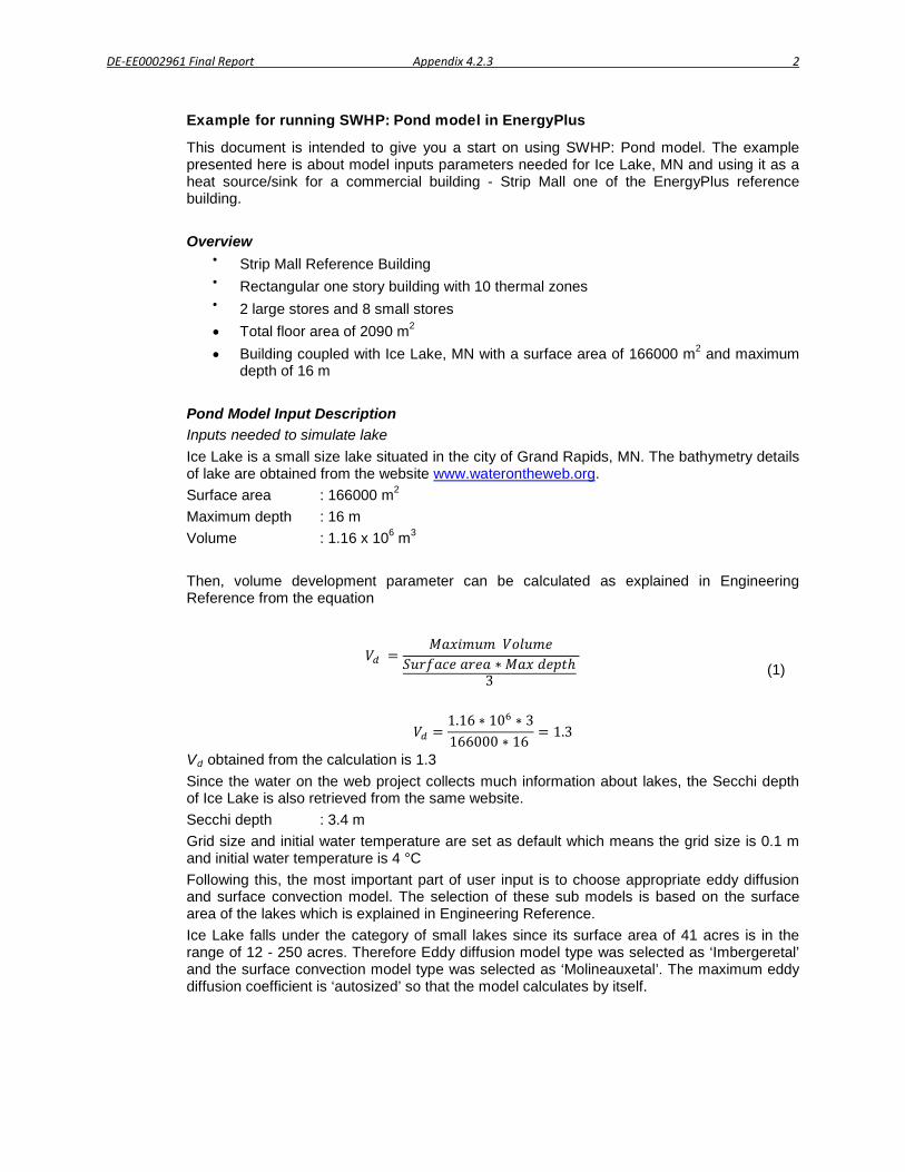
depth of 16 m Pond Model Input Description Inputs needed to simulate lake Ice Lake is a small size lake situated in the city of Grand Rapids, MN. The bathymetry details of lake are obtained from the website www.waterontheweb.org. Surface area : 166000 m2 Maximum depth : 16 m Volume : 1.16 x 10⁶ m3
Then, volume development parameter can be calculated as explained in Engineering Reference from the equation
𝑉𝑑 =𝑀𝑎𝑥𝑖𝑚𝑢𝑚 𝑉𝑜𝑙𝑢𝑚𝑒
𝑆𝑢𝑟𝑓𝑎𝑐𝑒 𝑎𝑟𝑒𝑎 ∗ 𝑀𝑎𝑥 𝑑𝑒𝑝𝑡ℎ3
(1)
𝑉𝑑 =1.16 ∗ 106 ∗ 3166000 ∗ 16
= 1.3
Vd obtained from the calculation is 1.3 Since the water on the web project collects much information about lakes, the Secchi depth of Ice Lake is also retrieved from the same website. Secchi depth : 3.4 m Grid size and initial water temperature are set as default which means the grid size is 0.1 m and initial water temperature is 4 °C Following this, the most important part of user input is to choose appropriate eddy diffusion and surface convection model. The selection of these sub models is based on the surface area of the lakes which is explained in Engineering Reference. Ice Lake falls under the category of small lakes since its surface area of 41 acres is in the range of 12 - 250 acres. Therefore Eddy diffusion model type was selected as ‘Imbergeretal’ and the surface convection model type was selected as ‘Molineauxetal’. The maximum eddy diffusion coefficient is ‘autosized’ so that the model calculates by itself.

DE-EE0002961 Final Report Appendix 4.2.3 3
Inputs needed to simulate heat exchanger Spiral helical coil was selected as a surface water heat exchanger to be placed in a lake at the depth of ~ 10 m. The dimensions of the coil are shown in Figure 1. The inputs of spiral helical coil are as listed below Outside coil diameter : 2.44 m Horizontal spacing of a coil : 0.1047 m Vertical spacing of a coil : 0.0666 m Hydronic tube outside diameter : 0.02667 m Hydronic tube inside diameter : 0.02184 m Length of the tubing circuit : 875.6 m Depth of the lake where the top of the HX is situated : 10 m Depth of the lake where the bottom of the HX is situated : 10.5 m The other inputs which are related to other heat exchanger types are set to minimum value of 0.01.
Figure 1 Spiral Helical Coil Dimensions
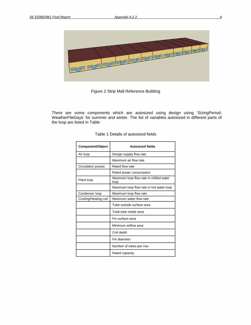
Building and HVAC Description
The building shown in Figure 1 is a rectangular one story Strip Mall reference building is used along with the lake model. It consists of 2 large stores and 8 small stores with total building floor area of 2090 m2. Thus this building is divided into 10 thermal zones. The building has internal gains such as lights, people and electric equipment given as schedules. Space Conditioning Heating setpoints: 21 °C occupied, 15.6 °C unoccupied Cooling setpoints: 24 °C occupied, 30 °C unoccupied Environment Location: Phoenix, Arizona, USA Annual simulation period: Jan 1 – Dec 31
DE-EE0002961 Final Report Appendix 4.2.3 4
Figure 2 Strip Mall Reference Building
There are some components which are autosized using design using ‘SizingPeriod: WeatherFileDays’ for summer and winter. The list of variables autosized in different parts of the loop are listed in Table
Table 1 Details of autosized fields
Component/Object Autosized fields
Air loop Design supply flow rate
Maximum air flow rate
Circulation pumps Rated flow rate
Rated power consumption
Plant loop Maximum loop flow rate in chilled water loop
Maximum loop flow rate in hot water loop
Condenser loop Maximum loop flow rate Cooling/Heating coil Maximum water flow rate
Tube outside surface area
Total tube inside area
Fin surface area
Minimum airflow area
Coil depth
Fin diameter
Number of tubes per row
Rated capacity
DE-EE0002961 Final Report Appendix 4.2.3 5
Air loop The type of air system distribution terminal is constant volume single duct reheat air
terminal. This system consists of an air loop which has cooling coil (Coil:Cooling:Water:DetailedGeometry) and the fan (Fan:ConstantVolume) also each zone has a separate reheat coil (Coil: Heating:Water). Plant loop
The building is served by two separate water-to-water heat pumps one for heating and one for cooling (HeatPump:WaterToWater:EquationFit: Cooling/Heating) connected with two plant loops, chilled water plant loop and hot water plant loop. Each have separate constant speed circulation pump. Climate Master GSW120 heat pump was selected and the coefficient are generated using manufacturers data. Condenser loop
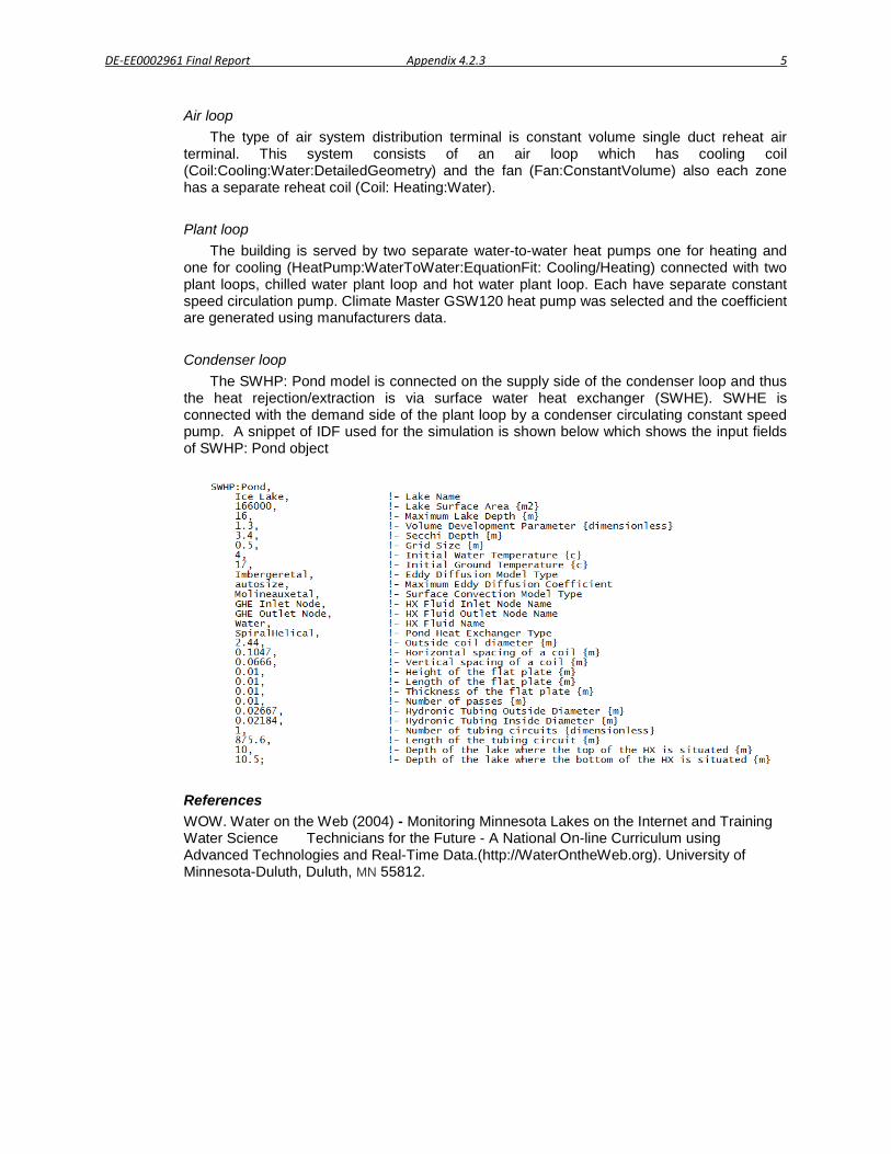
The SWHP: Pond model is connected on the supply side of the condenser loop and thus the heat rejection/extraction is via surface water heat exchanger (SWHE). SWHE is connected with the demand side of the plant loop by a condenser circulating constant speed pump. A snippet of IDF used for the simulation is shown below which shows the input fields of SWHP: Pond object
References WOW. Water on the Web (2004) - Monitoring Minnesota Lakes on the Internet and Training Water Science Technicians for the Future - A National On-line Curriculum using Advanced Technologies and Real-Time Data.(http://WaterOntheWeb.org). University of Minnesota-Duluth, Duluth, MN 55812.

Progress Report
DE‐EE0002961/001 ‐ Recovery Act:
Improved Design Tools for Surface Water and Standing Column Well Heat Pump Systems
Quarter 1 (1/1/2010‐3/31/2010)
Principal Investigator: Jeffrey D. Spitler ([email protected]), Oklahoma State University
Effort this quarter has primarily been aimed at developing a model of lakes and ponds that accounts for stratification, so as to accurately predict the water temperature surrounding the surface water heat exchangers. This model is under development and partly complete. This quarter, the following features have been developed:
• The one dimensional advection‐diffusion equation is solved with a finite difference approach to predict water temperatures as a function of depth in the lake or pond. We are currently working with a cell size (depth) of 0.25 m or about 10 inches and a time step of one day. The finite difference equations are solved implicitly with a tri‐diagonal matrix algorithm.
• A full surface energy balance is incorporated which includes solar radiation, long‐wave radiation, evaporation and convection.
• Solar radiation is transmitted and absorbed below the surface. Turbidity is treated as an input parameter.
• The eddy diffusivity coefficients for the epilimnion (well‐mixed region near the surface) are computed based on wind speed. The epilimnion depth is computed by balancing the potential energy due to temperature difference and the kinetic energy due to wind shear. The eddy diffusivity coefficients for the lower layers are currently fixed.
• The bottom boundary condition is currently adiabatic.
Some sample results for a lake in Stillwater are shown for this spring in Figures 1 and 2. These have not been validated against measured data yet, and there are a number of features missing from the program, so the results should not be misconstrued as being accurate representations. Having said that, the water surface temperature was checked at the local lake on one day and the simulation results were within 0.5⁰C of the measured value. That may, of course, just have been luck!
Features that will be added in the near future include:
• The lake bottom will be modeled with a quasi one‐dimensional conduction model coupled by convection to the water.
• Modeling seasonal lake turnover requires an algorithm to detect the transition.
• Addition of a pond heat exchanger model.
• Addition of freezing and thawing on the surfaces of the pond heat exchanger.
• Freezing and thawing at the lake surface, as well as snow accumulation.
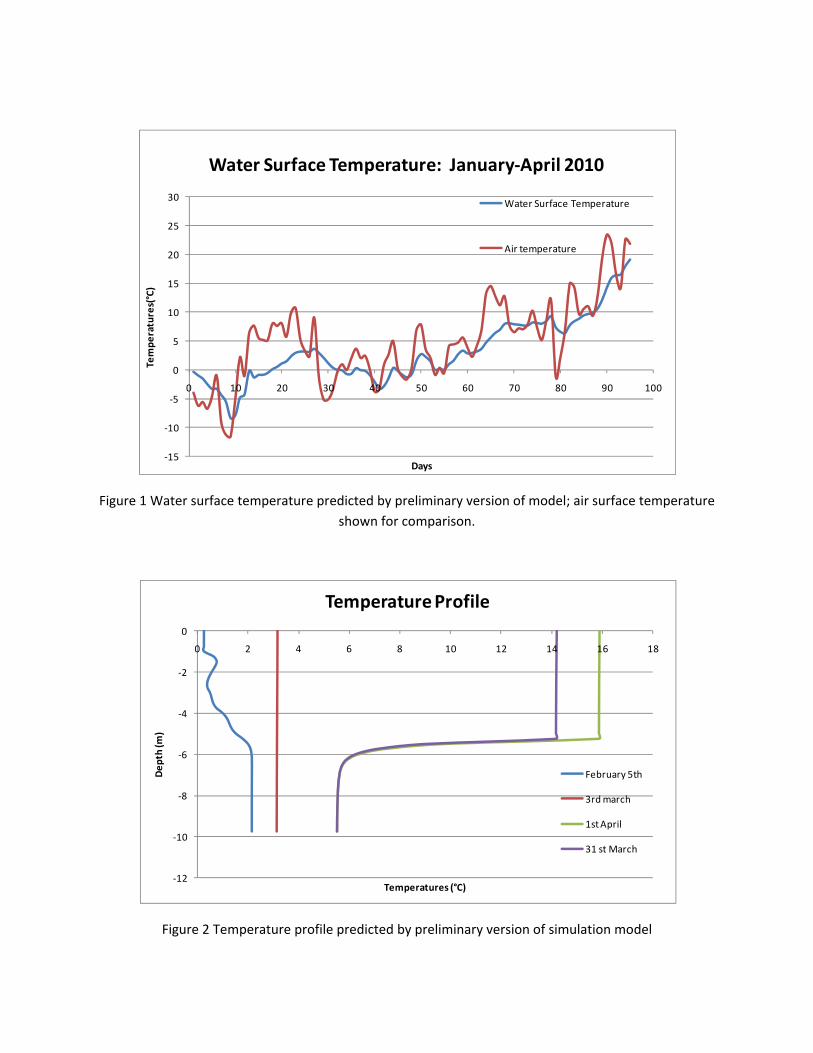
Figure 1 Water surface temperature predicted by preliminary version of model; air surface temperature shown for comparison.
Figure 2 Temperature profile predicted by preliminary version of simulation model
‐15
‐10
‐5
0
5
10
15
20
25
30
0 10 20 30 40 50 60 70 80 90 100
Tempe
ratures(°C)
Days
Water Surface Temperature: January‐April 2010
Water Surface Temperature
Air temperature
‐12
‐10
‐8
‐6
‐4
‐2
0
0 2 4 6 8 10 12 14 16 18
Dep
th (m
)
Temperatures (°C)
Temperature Profile
February 5th
3rd march
1st April
31 st March

Progress Report
DE-EE0002961/001 - Recovery Act:
Improved Design Tools for Surface Water and Standing Column Well Heat Pump Systems
Quarter 2 (4/1/2010-6/30/2010)
Principal Investigator: Jeffrey D. Spitler ([email protected]), Oklahoma State University
Task 1 Enhancement of Existing Standing Column Well Models
This part of the project is behind schedule due to difficulty in finding a student to work on it. However, one of our graduates from the MSME program is starting a PhD and has begun work on the project, as of June 1. The very first step is an improvement to the model used to estimate convection heat transfer coefficients at the borehole wall and the outer wall of the well intake tube. Regrettably, there is no published experimental research which has led to convection correlations for the geometry and high Rayleigh numbers that occur within a standing column well. An alternative approach is to use measurements made by other researchers in a similar type of ground heat exchanger commonly used in Sweden. There, a common configuration involves suspending a U-tube in a groundwater-filled borehole. Several researchers e.g. Gustafsson and Westerlund (2010) have reported measurements of borehole resistance from which we might back out convection coefficients. This is currently being explored.
In the next two quarters, our existing model will be modified to incorporate new convection coefficients and separate out the bleed control.
Task 2 Enhancement of Existing Pond Model
Effort this quarter has primarily been aimed at developing a model of lakes and ponds that accounts for stratification, so as to accurately predict the water temperature surrounding the surface water heat exchangers. This model is under development and partly complete.
Last quarter, the model had the following features which have been retained:
• The one dimensional advection-diffusion equation is solved with a finite difference approach to predict water temperatures as a function of depth in the lake or pond. We are currently working with a cell size (depth) of 0.25 m or about 10 inches and a time step of one day. The finite difference equations are solved implicitly with a tri-diagonal matrix algorithm.
• A full surface energy balance is incorporated which includes solar radiation, long-wave radiation, evaporation and convection.
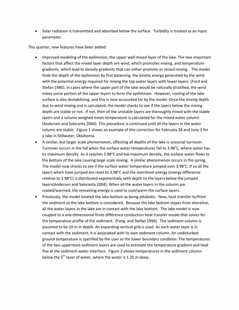
• Solar radiation is transmitted and absorbed below the surface. Turbidity is treated as an input parameter.
This quarter, new features have been added:
• Improved modeling of the epilimnion, the upper well-mixed layer of the lake. The two important factors that affect the mixed layer depth are wind, which promotes mixing, and temperature gradients, which lead to density gradients that can either promote or retard mixing. The model finds the depth of the epilimnion by first balancing the kinetic energy generated by the wind with the potential energy required for mixing the top water layers with lower layers. (Ford and Stefan 1980). In cases where the upper part of the lake would be naturally stratified, the wind mixes some portion of the upper layers to form the epilimnion. However, cooling of the lake surface is also destabilizing, and this is now accounted for by the model. Once the mixing depth due to wind mixing and is calculated, the model checks to see if the layers below the mixing depth are stable or not. If not, then all the unstable layers are thoroughly mixed with the stable layers and a volume weighed mean temperature is calculated for the mixed water column (Andersen and Saloranta 2004). This procedure is continued until all the layers in the water column are stable. Figure 1 shows an example of this correction for February 28 and June 3 for a lake in Stillwater, Oklahoma.
• A similar, but larger scale phenomenon, affecting all depths of the lake is seasonal turnover. Turnover occurs in the fall when the surface water temperatures fall to 3.98°C, where water has its maximum density. As it reaches 3.98°C and has maximum density, the surface water flows to the bottom of the lake causing large scale mixing. A similar phenomenon occurs in the spring. The model now checks to see if the surface water temperature jumped over 3.98°C. If so all the layers which have jumped are reset to 3.98°C and the overshoot energy (energy difference relative to 3.98°C) is distributed exponentially with depth to the layers below the jumped layers(Andersen and Saloranta 2004). When all the water layers in the column are cooled/warmed, the remaining energy is used to cool/warm the surface layers.
• Previously, the model treated the lake bottom as being adiabatic. Now, heat transfer to/from the sediment at the lake bottom is considered. Because the lake bottom slopes from shoreline, all the water layers in the lake are in contact with the lake bottom. The lake model is now coupled to a one-dimensional finite difference conduction heat transfer model that solves for the temperature profile of the sediment. (Fang and Stefan 1996). The sediment column is assumed to be 10 m in depth. An expanding vertical grid is used. As each water layer is in contact with the sediment, it is associated with its own sediment column. An undisturbed ground temperature is specified by the user as the lower boundary condition. The temperatures of the two uppermost sediment layers are used to estimate the temperature gradient and heat flux at the sediment-water interface. Figure 2 shows temperatures in the sediment column below the 5th layer of water, where the water is 1.25 m deep.
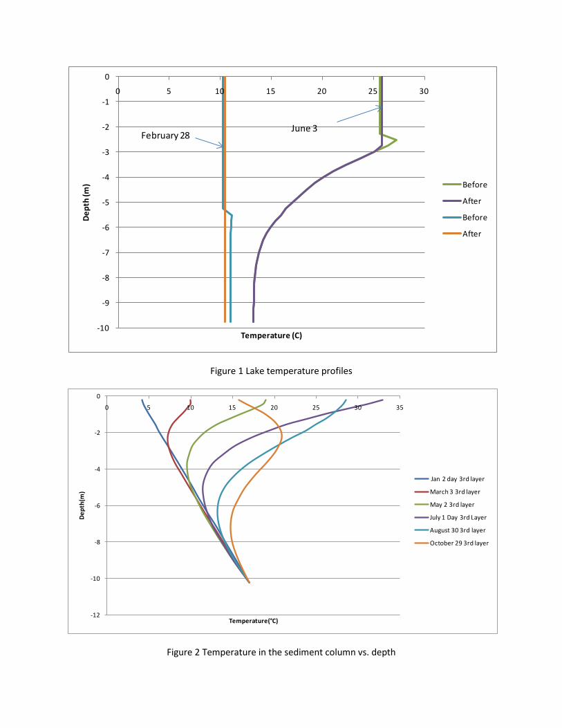
Figure 1 Lake temperature profiles
Figure 2 Temperature in the sediment column vs. depth
-10
-9
-8
-7
-6
-5
-4
-3
-2
-1
0
0 5 10 15 20 25 30De
pth
(m)
Temperature (C)
Before
After
Before
After
February 28June 3
-12
-10
-8
-6
-4
-2
0
0 5 10 15 20 25 30 35
Dept
h(m
)
Temperature(°C)
Jan 2 day 3rd layer
March 3 3rd layer
May 2 3rd layer
July 1 Day 3rd Layer
August 30 3rd layer
October 29 3rd layer

Features that will be added in the next two quarters include:
• Addition of a pond heat exchanger model. • Addition of freezing and thawing on the surfaces of the pond heat exchanger. • Freezing and thawing at the lake surface, as well as snow accumulation.
References
Andersen and Saloranta (2004). My Lake(v.1.1):Technical model documentation and users guide. Oslo, Norway, Norwegian Institute for water research 44. Fang , X. and H. G. Stefan (1996). "Long-term lake water temperature and ice cover simulations/measurements." Cold regions science and technology 24: 289-304. Ford, D. E. and H. G. Stefan (1980). "Thermal predictions using integral energy model." Journal of the Hydraulics Division 106(1): 39-55. Gustafsson, A. M. and L. Westerlund. 2010. Multi-injection rate thermal response test in groundwater filled borehole heat exchanger. Renewable Energy 35(5): 1061-1070.
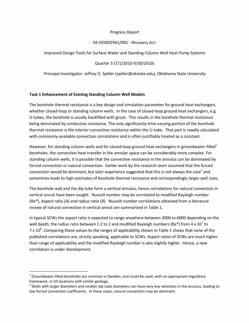
Progress Report
DE-EE0002961/001 - Recovery Act:
Improved Design Tools for Surface Water and Standing Column Well Heat Pump Systems
Quarter 3 (7/1/2010-9/30/2010)
Principal Investigator: Jeffrey D. Spitler ([email protected]), Oklahoma State University
Task 1 Enhancement of Existing Standing Column Well Models
The borehole thermal resistance is a key design and simulation parameter for ground heat exchangers,
whether closed-loop or standing column wells. In the case of closed-loop ground heat exchangers, e.g.
U-tubes, the borehole is usually backfilled with grout. This results in the borehole thermal resistance
being dominated by conductive resistance. The only significantly time-varying portion of the borehole
thermal resistance is the interior convective resistance within the U-tube. That part is readily calculated
with commonly-available convection correlations and is often justifiably treated as a constant.
However, for standing column wells and for closed-loop ground heat exchangers in groundwater-filled1
boreholes, the convection heat transfer in the annular space can be considerably more complex. For
standing column wells, it is possible that the convective resistance in the annulus can be dominated by
forced convection or natural convection. Earlier work by the research team assumed that the forced
convection would be dominant, but later experience suggested that this is not always the case2 and
sometimes leads to high estimates of borehole thermal resistance and correspondingly larger well sizes.
The borehole wall and the dip tube form a vertical annulus; hence correlations for natural convection in
vertical annuli have been sought. Nusselt number may be correlated to modified Rayleigh number
(Ra*), Aspect ratio (A) and radius ratio (R). Nusselt number correlations obtained from a literature
review of natural convection in vertical annuli are summarized in Table 1.
In typical SCWs the aspect ratio is expected to range anywhere between 3000 to 6000 depending on the
well depth, the radius ratio between 1.2 to 2 and modified Rayleigh numbers (Ra*) from 4 x 10⁷ to
7 x 10⁸. Comparing these values to the ranges of applicability shown in Table 1 shows that none of the
published correlations are, strictly speaking, applicable to SCWs. Aspect ratios of SCWs are much higher
than range of applicability and the modified Rayleigh number is also slightly higher. Hence, a new
correlation is under development.
1 Groundwater-filled boreholes are common in Sweden, and could be used, with an appropriate regulatory
framework, in US locations with similar geology. 2 Wells with larger diameters and smaller dip tube diameters can have very low velocities in the annulus, leading to
low forced convection coefficients. In these cases, natural convection may be dominant.
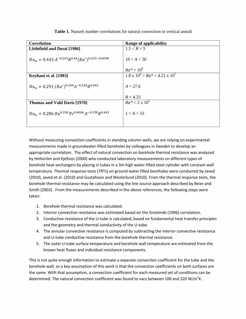
Table 1. Nusselt number correlations for natural convection in vertical annuli
Correlation Range of applicability
Littlefield and Desai [1986]
1.5 < R < 5
10 < A < 50
Ra* < 108
Keyhani et al. [1983]
1.8 x 10⁴ < Ra* < 4.21 x 10
7
A = 27.6
R = 4.33
Thomas and Vahl Davis [1970]
Ra* < 2 x 10⁵
1 < A < 33
Without measuring convection coefficients in standing column wells, we are relying on experimental
measurements made in groundwater-filled boreholes by colleagues in Sweden to develop an
appropriate correlation. The effect of natural convection on borehole thermal resistance was analyzed
by Hellström and Kjellson (2000) who conducted laboratory measurements on different types of
borehole heat exchangers by placing U-tubes in a 3m high water-filled steel cylinder with constant wall
temperature. Thermal response tests (TRTs) on ground water filled boreholes were conducted by Javed
(2010), Javed et al. (2010) and Gustafsson and Westerlund (2010). From the thermal response tests, the
borehole thermal resistance may be calculated using the line source approach described by Beier and
Smith (2002). From the measurements described in the above references, the following steps were
taken:
1. Borehole thermal resistance was calculated.
2. Interior convective resistance was estimated based on the Gnielinski (1996) correlation.
3. Conductive resistance of the U-tube is calculated, based on fundamental heat transfer principles
and the geometry and thermal conductivity of the U-tube.
4. The annular convective resistance is computed by subtracting the interior convective resistance
and U-tube conductive resistance from the borehole thermal resistance.
5. The outer U-tube surface temperature and borehole wall temperature are estimated from the
known heat fluxes and individual resistance components.
This is not quite enough information to estimate a separate convection coefficient for the tube and the
borehole wall, so a key assumption of this work is that the convection coefficients on both surfaces are
the same. With that assumption, a convection coefficient for each measured set of conditions can be
determined. The natural convection coefficient was found to vary between 100 and 320 W/m2K.
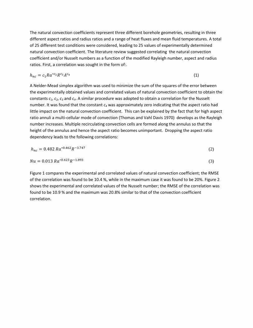
The natural convection coefficients represent three different borehole geometries, resulting in three
different aspect ratios and radius ratios and a range of heat fluxes and mean fluid temperatures. A total
of 25 different test conditions were considered, leading to 25 values of experimentally determined
natural convection coefficient. The literature review suggested correlating the natural convection
coefficient and/or Nusselt numbers as a function of the modified Rayleigh number, aspect and radius
ratios. First, a correlation was sought in the form of:.
(1)
A Nelder-Mead simplex algorithm was used to minimize the sum of the squares of the error between
the experimentally obtained values and correlated values of natural convection coefficient to obtain the
constants c1, c2, c3 and c4. A similar procedure was adopted to obtain a correlation for the Nusselt
number. It was found that the constant c4 was approximately zero indicating that the aspect ratio had
little impact on the natural convection coefficient. This can be explained by the fact that for high aspect
ratio annuli a multi-cellular mode of convection (Thomas and Vahl Davis 1970) develops as the Rayleigh
number increases. Multiple recirculating convection cells are formed along the annulus so that the
height of the annulus and hence the aspect ratio becomes unimportant. Dropping the aspect ratio
dependency leads to the following correlations:
(2)
(3)
Figure 1 compares the experimental and correlated values of natural convection coefficient; the RMSE
of the correlation was found to be 10.4 %, while in the maximum case it was found to be 20%. Figure 2
shows the experimental and correlated values of the Nusselt number; the RMSE of the correlation was
found to be 10.9 % and the maximum was 20.8% similar to that of the convection coefficient
correlation.
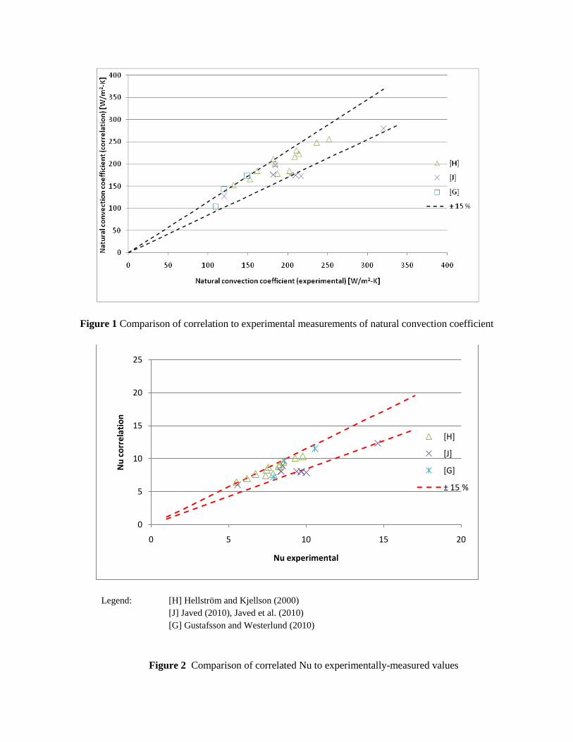
Figure 1 Comparison of correlation to experimental measurements of natural convection coefficient
Legend: [H] Hellström and Kjellson (2000)
[J] Javed (2010), Javed et al. (2010)
[G] Gustafsson and Westerlund (2010)
Figure 2 Comparison of correlated Nu to experimentally-measured values
0
5
10
15
20
25
0 5 10 15 20
Nu
co
rre
lati
on
Nu experimental
[H]
[J]
[G]
± 15 %
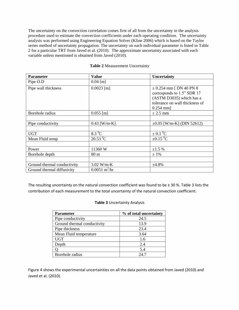
The uncertainty on the convection correlation comes first of all from the uncertainty in the analysis
procedure used to estimate the convection coefficients under each operating condition. The uncertainty
analysis was performed using Engineering Equation Solver (Kline 2006) which is based on the Taylor
series method of uncertainty propagation. The uncertainty on each individual parameter is listed in Table
2 for a particular TRT from Javed et al. (2010). The approximate uncertainty associated with each
variable unless mentioned is obtained from Javed (2010).
Table 2 Measurement Uncertainty
Parameter Value Uncertainty
Pipe O.D 0.04 [m]
Pipe wall thickness 0.0023 [m] ± 0.254 mm [ DN 40 PN 8
corresponds to 1.5” SDR 17
(ASTM D3035) which has a
tolerance on wall thickness of
0.254 mm]
Borehole radius 0.055 [m] ± 2.5 mm
Pipe conductivity 0.43 [W/m-K] ±0.05 [W/m-K] (DIN 52612)
UGT 8.3 0C ± 0.1
0C
Mean Fluid temp 20.53 0C ±0.15
0C
Power 11360 W ±1.5 %
Borehole depth 80 m ± 1%
Ground thermal conductivity 3.02 W/m-K ±4.8%
Ground thermal diffusivity 0.0051 m2/hr
The resulting uncertainty on the natural convection coefficient was found to be ± 30 %. Table 3 lists the
contribution of each measurement to the total uncertainty of the natural convection coefficient.
Table 3 Uncertainty Analysis
Parameter % of total uncertainty
Pipe conductivity 24.5
Ground thermal conductivity 13.9
Pipe thickness 23.4
Mean Fluid temperature 3.64
UGT 1.6
Depth 2.4
Q 5.4
Borehole radius 24.7
Figure 4 shows the experimental uncertainties on all the data points obtained from Javed (2010) and
Javed et al. (2010).
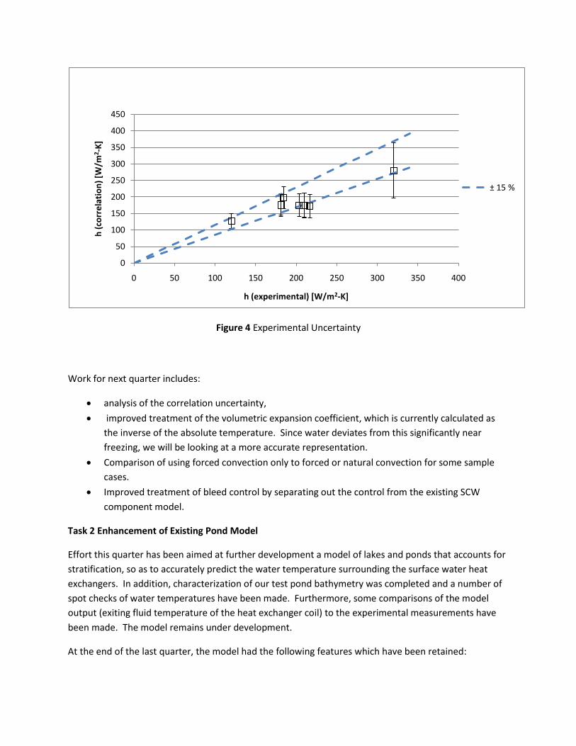
Figure 4 Experimental Uncertainty
Work for next quarter includes:
analysis of the correlation uncertainty,
improved treatment of the volumetric expansion coefficient, which is currently calculated as
the inverse of the absolute temperature. Since water deviates from this significantly near
freezing, we will be looking at a more accurate representation.
Comparison of using forced convection only to forced or natural convection for some sample
cases.
Improved treatment of bleed control by separating out the control from the existing SCW
component model.
Task 2 Enhancement of Existing Pond Model
Effort this quarter has been aimed at further development a model of lakes and ponds that accounts for
stratification, so as to accurately predict the water temperature surrounding the surface water heat
exchangers. In addition, characterization of our test pond bathymetry was completed and a number of
spot checks of water temperatures have been made. Furthermore, some comparisons of the model
output (exiting fluid temperature of the heat exchanger coil) to the experimental measurements have
been made. The model remains under development.
At the end of the last quarter, the model had the following features which have been retained:
0
50
100
150
200
250
300
350
400
450
0 50 100 150 200 250 300 350 400
h (
corr
ela
tio
n)
[W/m
2-K
]
h (experimental) [W/m2-K]
± 15 %
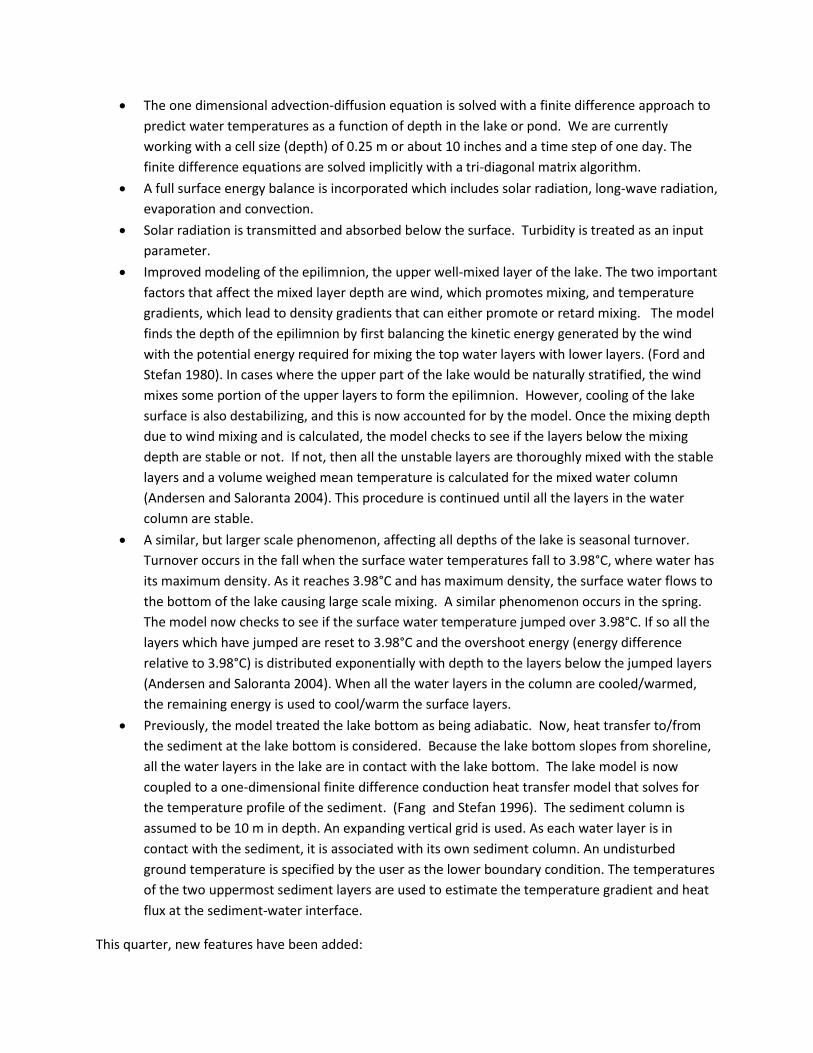
The one dimensional advection-diffusion equation is solved with a finite difference approach to
predict water temperatures as a function of depth in the lake or pond. We are currently
working with a cell size (depth) of 0.25 m or about 10 inches and a time step of one day. The
finite difference equations are solved implicitly with a tri-diagonal matrix algorithm.
A full surface energy balance is incorporated which includes solar radiation, long-wave radiation,
evaporation and convection.
Solar radiation is transmitted and absorbed below the surface. Turbidity is treated as an input
parameter.
Improved modeling of the epilimnion, the upper well-mixed layer of the lake. The two important
factors that affect the mixed layer depth are wind, which promotes mixing, and temperature
gradients, which lead to density gradients that can either promote or retard mixing. The model
finds the depth of the epilimnion by first balancing the kinetic energy generated by the wind
with the potential energy required for mixing the top water layers with lower layers. (Ford and
Stefan 1980). In cases where the upper part of the lake would be naturally stratified, the wind
mixes some portion of the upper layers to form the epilimnion. However, cooling of the lake
surface is also destabilizing, and this is now accounted for by the model. Once the mixing depth
due to wind mixing and is calculated, the model checks to see if the layers below the mixing
depth are stable or not. If not, then all the unstable layers are thoroughly mixed with the stable
layers and a volume weighed mean temperature is calculated for the mixed water column
(Andersen and Saloranta 2004). This procedure is continued until all the layers in the water
column are stable.
A similar, but larger scale phenomenon, affecting all depths of the lake is seasonal turnover.
Turnover occurs in the fall when the surface water temperatures fall to 3.98°C, where water has
its maximum density. As it reaches 3.98°C and has maximum density, the surface water flows to
the bottom of the lake causing large scale mixing. A similar phenomenon occurs in the spring.
The model now checks to see if the surface water temperature jumped over 3.98°C. If so all the
layers which have jumped are reset to 3.98°C and the overshoot energy (energy difference
relative to 3.98°C) is distributed exponentially with depth to the layers below the jumped layers
(Andersen and Saloranta 2004). When all the water layers in the column are cooled/warmed,
the remaining energy is used to cool/warm the surface layers.
Previously, the model treated the lake bottom as being adiabatic. Now, heat transfer to/from
the sediment at the lake bottom is considered. Because the lake bottom slopes from shoreline,
all the water layers in the lake are in contact with the lake bottom. The lake model is now
coupled to a one-dimensional finite difference conduction heat transfer model that solves for
the temperature profile of the sediment. (Fang and Stefan 1996). The sediment column is
assumed to be 10 m in depth. An expanding vertical grid is used. As each water layer is in
contact with the sediment, it is associated with its own sediment column. An undisturbed
ground temperature is specified by the user as the lower boundary condition. The temperatures
of the two uppermost sediment layers are used to estimate the temperature gradient and heat
flux at the sediment-water interface.
This quarter, new features have been added:
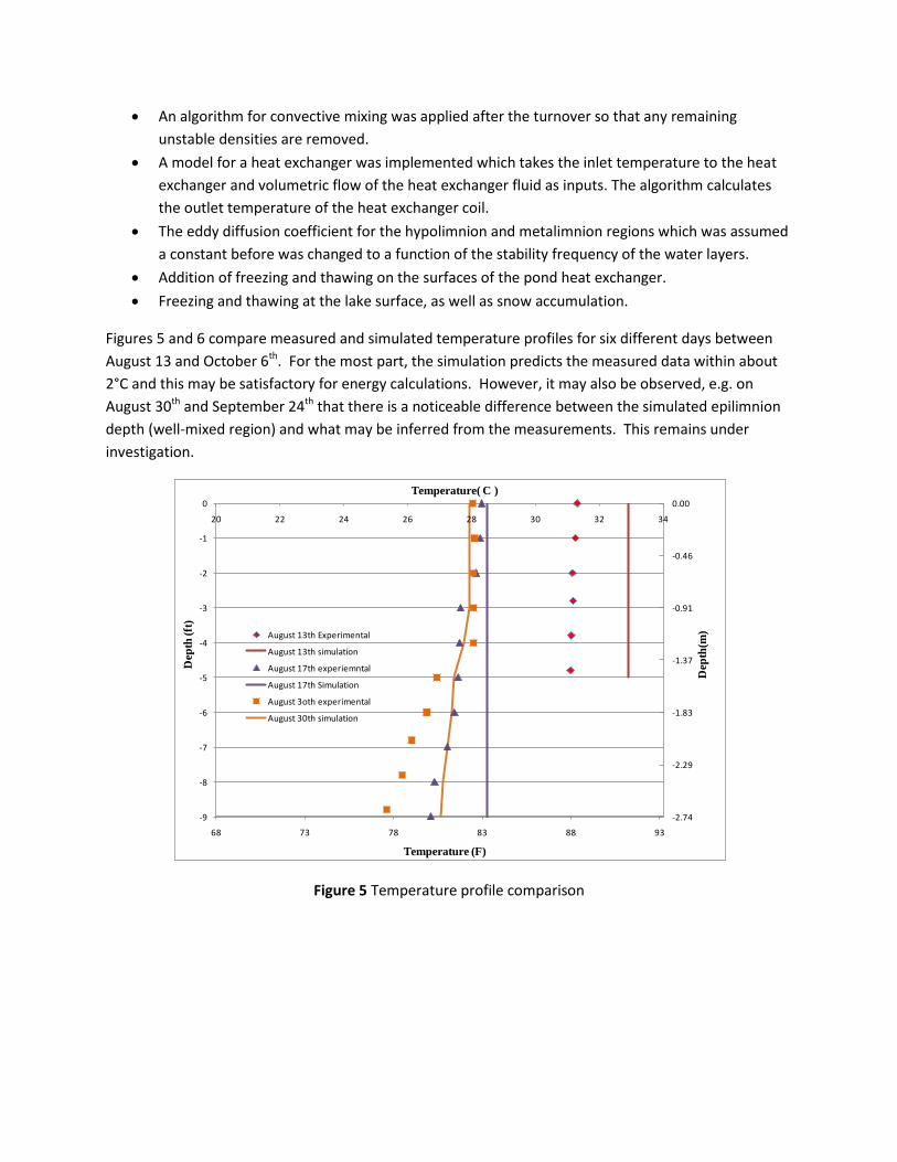
An algorithm for convective mixing was applied after the turnover so that any remaining
unstable densities are removed.
A model for a heat exchanger was implemented which takes the inlet temperature to the heat
exchanger and volumetric flow of the heat exchanger fluid as inputs. The algorithm calculates
the outlet temperature of the heat exchanger coil.
The eddy diffusion coefficient for the hypolimnion and metalimnion regions which was assumed
a constant before was changed to a function of the stability frequency of the water layers.
Addition of freezing and thawing on the surfaces of the pond heat exchanger.
Freezing and thawing at the lake surface, as well as snow accumulation.
Figures 5 and 6 compare measured and simulated temperature profiles for six different days between
August 13 and October 6th. For the most part, the simulation predicts the measured data within about
2°C and this may be satisfactory for energy calculations. However, it may also be observed, e.g. on
August 30th and September 24th that there is a noticeable difference between the simulated epilimnion
depth (well-mixed region) and what may be inferred from the measurements. This remains under
investigation.
Figure 5 Temperature profile comparison
68 73 78 83 88 93
-2.74
-2.29
-1.83
-1.37
-0.91
-0.46
0.00
-9
-8
-7
-6
-5
-4
-3
-2
-1
0
20 22 24 26 28 30 32 34
Temperature( C )
Dep
th(m
)
Dep
th (ft
)
Temperature (F)
August 13th Experimental
August 13th simulation
August 17th experiemntal
August 17th Simulation
August 3oth experimental
August 30th simulation
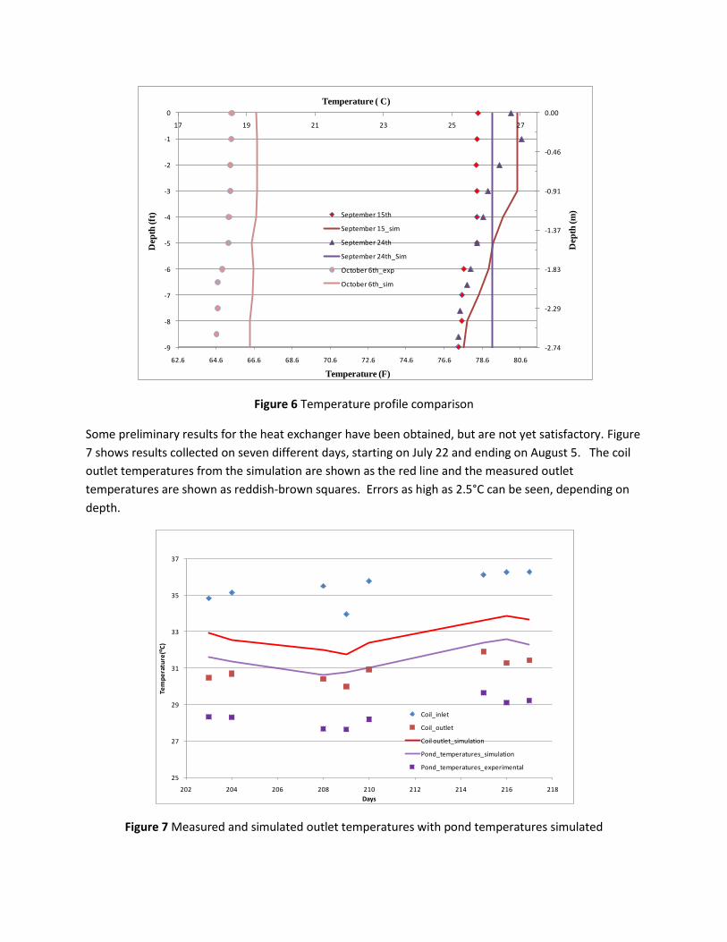
Figure 6 Temperature profile comparison
Some preliminary results for the heat exchanger have been obtained, but are not yet satisfactory. Figure
7 shows results collected on seven different days, starting on July 22 and ending on August 5. The coil
outlet temperatures from the simulation are shown as the red line and the measured outlet
temperatures are shown as reddish-brown squares. Errors as high as 2.5°C can be seen, depending on
depth.
Figure 7 Measured and simulated outlet temperatures with pond temperatures simulated
62.6 64.6 66.6 68.6 70.6 72.6 74.6 76.6 78.6 80.6
-2.74
-2.29
-1.83
-1.37
-0.91
-0.46
0.00
-9
-8
-7
-6
-5
-4
-3
-2
-1
0
17 19 21 23 25 27
Temperature ( C)
Dep
th (
m)
Dep
th (ft
)
Temperature (F)
September 15th
September 15_sim
September 24th
September 24th_Sim
October 6th_exp
October 6th_sim
25
27
29
31
33
35
37
202 204 206 208 210 212 214 216 218
Temperatu
re(⁰C)
Days
Coil_inlet
Coil_outlet
Coil outlet_simulation
Pond_temperatures_simulation
Pond_temperatures_experimental
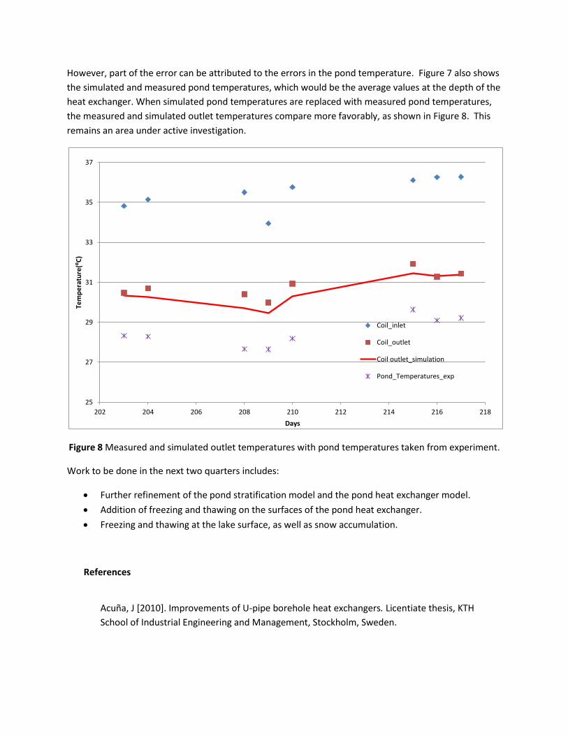
However, part of the error can be attributed to the errors in the pond temperature. Figure 7 also shows
the simulated and measured pond temperatures, which would be the average values at the depth of the
heat exchanger. When simulated pond temperatures are replaced with measured pond temperatures,
the measured and simulated outlet temperatures compare more favorably, as shown in Figure 8. This
remains an area under active investigation.
Figure 8 Measured and simulated outlet temperatures with pond temperatures taken from experiment.
Work to be done in the next two quarters includes:
Further refinement of the pond stratification model and the pond heat exchanger model.
Addition of freezing and thawing on the surfaces of the pond heat exchanger.
Freezing and thawing at the lake surface, as well as snow accumulation.
References
Acuña, J [2010]. Improvements of U-pipe borehole heat exchangers. Licentiate thesis, KTH
School of Industrial Engineering and Management, Stockholm, Sweden.
25
27
29
31
33
35
37
202 204 206 208 210 212 214 216 218
Temperature(⁰C)
Days
Coil_inlet
Coil_outlet
Coil outlet_simulation
Pond_Temperatures_exp

Andersen and Saloranta (2004). My Lake(v.1.1):Technical model documentation and users guide. Oslo, Norway, Norwegian Institute for water research 44. Beier, R.A and Smith, M.D. [2002]. Borehole thermal resistance from line-source model of in-situ
tests. ASHRAE Transactions, 108(2): 212-219.
Deng, Z. [2004]. Modeling of Standing Column Wells in Ground Source Heat Pump Systems.
Ph.D. Thesis, Oklahoma State University, Stillwater, OK.
Fang , X. and H. G. Stefan (1996). "Long-term lake water temperature and ice cover simulations/measurements." Cold regions science and technology 24: 289-304. Ford, D. E. and H. G. Stefan (1980). "Thermal predictions using integral energy model." Journal of the Hydraulics Division 106(1): 39-55. Gnielinski, V. [1976]. New equations for heat and mass transfer in turbulent pipe and channel
flow. International Chemical Engineering, 16: 359-368.
Gustafsson, A. M. and L. Westerlund. 2010. Multi-injection rate thermal response test in groundwater filled borehole heat exchanger. Renewable Energy 35(5): 1061-1070.
Hellström, G. and Kjellsson, E. [2000]. Laboratory measurements of heat transfer properties of
different types of borehole heat exchangers. Proc. of Terrastock 2000, Stuttgart, Germany.
Javed, S. [2010]. Design of ground source heat pump systems, Thermal modeling and evaluation
of boreholes. Licentiate thesis, Chalmers University of Technology, Göteborg, Sweden.
Javed,S., Spitler.J.D. and Fahlén,P. [2010]. An experimental investigation of the accuracy of
thermal response tests used to measure ground thermal properties. ASHRAE Transactions ,
116(2) In Press
Keyhani,M., Kulacki,F.A and R.N.Christensen. [1983]. Free convection in a vertical annulus with
constant heat flux on the inner wall. Journal of Heat Transfer, 105: 454-459.
Klein. S. A.. (2006). "Engineering Equation Solver," V7.723-3D ed, Madison, WI, USA: F-Chart
Software.
Littlefield, D. and P. Desai, [1986]. Buoyant laminar thermal convection in a vertical annulus.
Journal of Heat Transfer, 108: 814-821.
Spitler, J., L. Xing, J. Cullin, D. Fisher, J. Shonder, and P. Im. 2010. Residential Ground Source Heat
Pump Systems Utilizing Foundation Heat Exchangers. Proceedings of Clima 2010, Antalya,
Turkey. May 9-12.

Thomas, R.W and de Vahl Davis, G. [1970]. Natural convection in annular and rectangular
cavities. Proceedings fourth international heat transfer conference, Paris, 4: Paper NC 2.4.
Young, R. [2004]. Development, Verification, and Design Analysis of the Borehole Fluid Thermal
Mass Model for Approximating Short Term Borehole Thermal Response. M.S. Thesis, Oklahoma
State University, Stillwater, OK.
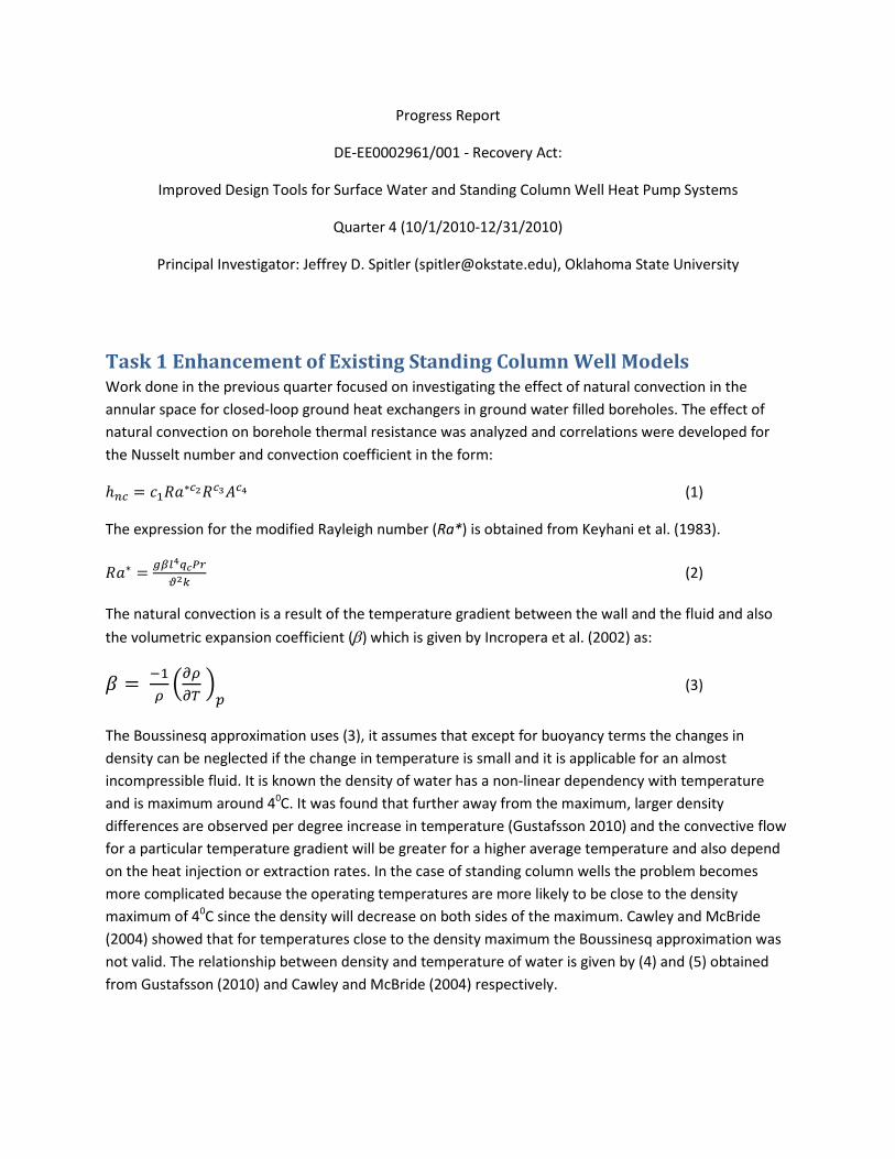
Progress Report
DE-EE0002961/001 - Recovery Act:
Improved Design Tools for Surface Water and Standing Column Well Heat Pump Systems
Quarter 4 (10/1/2010-12/31/2010)
Principal Investigator: Jeffrey D. Spitler ([email protected]), Oklahoma State University
Task 1 Enhancement of Existing Standing Column Well Models Work done in the previous quarter focused on investigating the effect of natural convection in the annular space for closed-loop ground heat exchangers in ground water filled boreholes. The effect of natural convection on borehole thermal resistance was analyzed and correlations were developed for the Nusselt number and convection coefficient in the form:
ℎ𝑛𝑐 = 𝑐1𝑅𝑎∗𝑐2𝑅𝑐3𝐴𝑐4 (1)
The expression for the modified Rayleigh number (Ra*) is obtained from Keyhani et al. (1983).
𝑅𝑎∗ = 𝑔𝛽𝑙4𝑞𝑐𝑃𝑟𝜗2𝑘
(2)
The natural convection is a result of the temperature gradient between the wall and the fluid and also the volumetric expansion coefficient (β) which is given by Incropera et al. (2002) as:
𝛽 = −1𝜌�𝜕𝜌𝜕𝑇
�𝑝
(3)
The Boussinesq approximation uses (3), it assumes that except for buoyancy terms the changes in density can be neglected if the change in temperature is small and it is applicable for an almost incompressible fluid. It is known the density of water has a non-linear dependency with temperature and is maximum around 40C. It was found that further away from the maximum, larger density differences are observed per degree increase in temperature (Gustafsson 2010) and the convective flow for a particular temperature gradient will be greater for a higher average temperature and also depend on the heat injection or extraction rates. In the case of standing column wells the problem becomes more complicated because the operating temperatures are more likely to be close to the density maximum of 40C since the density will decrease on both sides of the maximum. Cawley and McBride (2004) showed that for temperatures close to the density maximum the Boussinesq approximation was not valid. The relationship between density and temperature of water is given by (4) and (5) obtained from Gustafsson (2010) and Cawley and McBride (2004) respectively.
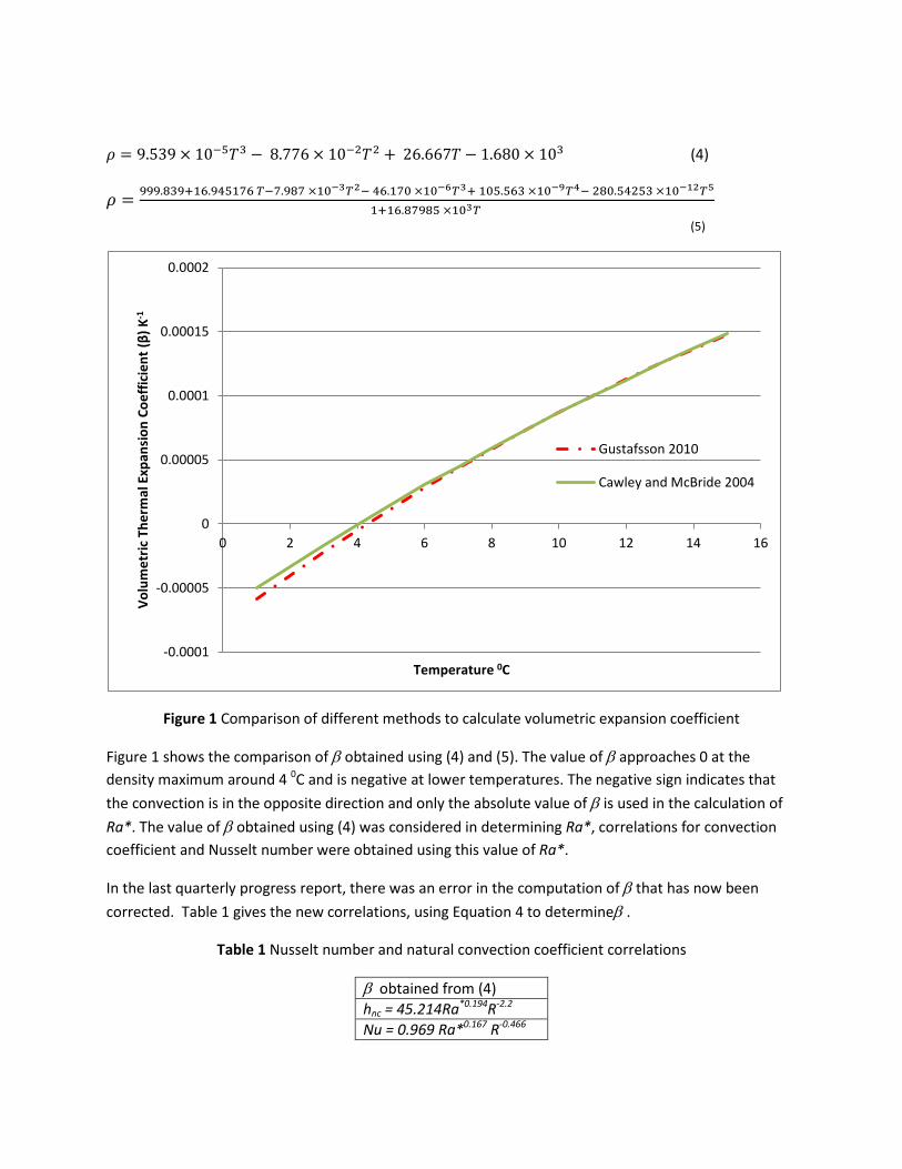
𝜌 = 9.539 × 10⁻⁵𝑇3 − 8.776 × 10⁻²𝑇2 + 26.667𝑇 − 1.680 × 10³ (4)
𝜌 = 999.839+16.945176 𝑇−7.987 ×10⁻³𝑇2− 46.170 ×10⁻⁶𝑇3+ 105.563 ×10⁻⁹𝑇4− 280.54253 ×10⁻¹²𝑇5
1+16.87985 ×10³𝑇
(5)
Figure 1 Comparison of different methods to calculate volumetric expansion coefficient
Figure 1 shows the comparison of β obtained using (4) and (5). The value of β approaches 0 at the density maximum around 4 0C and is negative at lower temperatures. The negative sign indicates that the convection is in the opposite direction and only the absolute value of β is used in the calculation of Ra*. The value of β obtained using (4) was considered in determining Ra*, correlations for convection coefficient and Nusselt number were obtained using this value of Ra*.
In the last quarterly progress report, there was an error in the computation of β that has now been corrected. Table 1 gives the new correlations, using Equation 4 to determineβ .
Table 1 Nusselt number and natural convection coefficient correlations
β obtained from (4) hnc = 45.214Ra*0.194R-2.2 Nu = 0.969 Ra*0.167 R-0.466
-0.0001
-0.00005
0
0.00005
0.0001
0.00015
0.0002
0 2 4 6 8 10 12 14 16
Volu
met
ric T
herm
al E
xpan
sion
Coe
ffici
ent (
β) K
-1
Temperature 0C
Gustafsson 2010
Cawley and McBride 2004
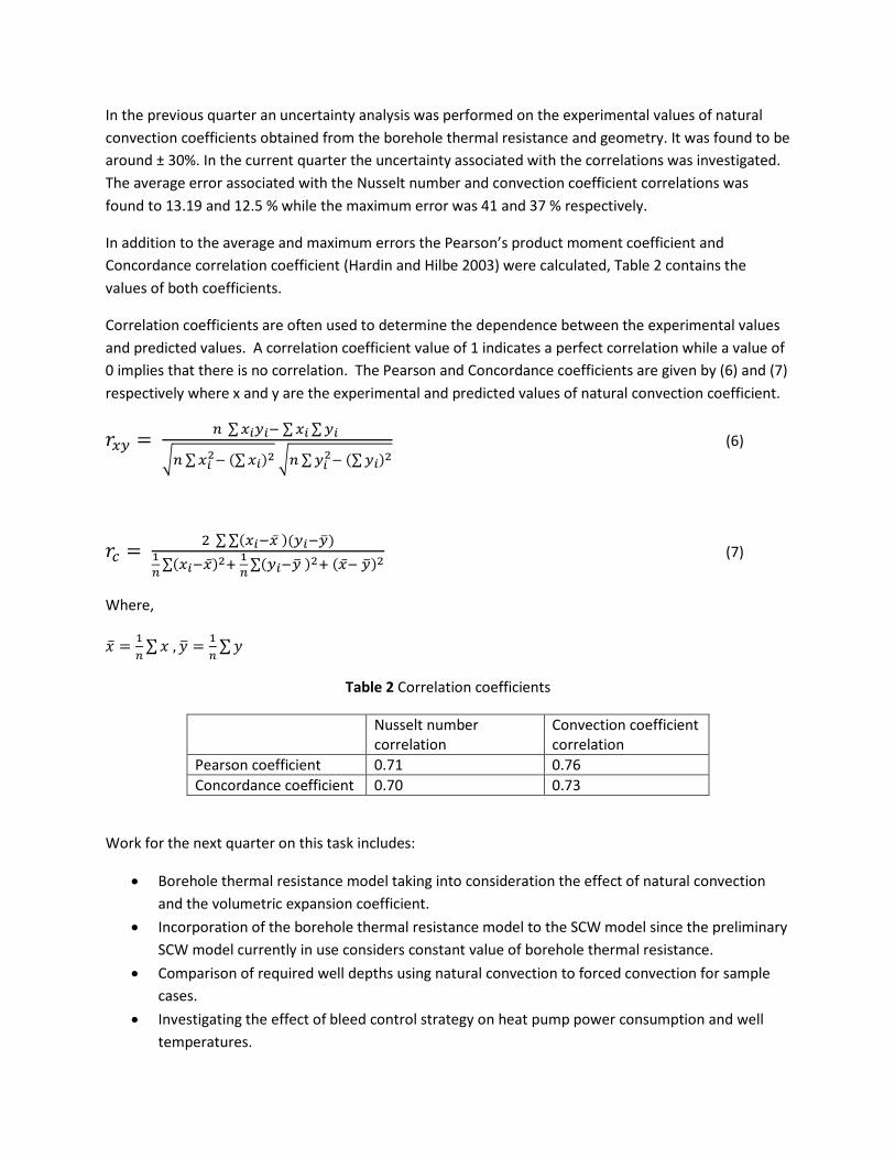
In the previous quarter an uncertainty analysis was performed on the experimental values of natural convection coefficients obtained from the borehole thermal resistance and geometry. It was found to be around ± 30%. In the current quarter the uncertainty associated with the correlations was investigated. The average error associated with the Nusselt number and convection coefficient correlations was found to 13.19 and 12.5 % while the maximum error was 41 and 37 % respectively.
In addition to the average and maximum errors the Pearson’s product moment coefficient and Concordance correlation coefficient (Hardin and Hilbe 2003) were calculated, Table 2 contains the values of both coefficients.
Correlation coefficients are often used to determine the dependence between the experimental values and predicted values. A correlation coefficient value of 1 indicates a perfect correlation while a value of 0 implies that there is no correlation. The Pearson and Concordance coefficients are given by (6) and (7) respectively where x and y are the experimental and predicted values of natural convection coefficient.
𝑟𝑥𝑦 = 𝑛 ∑𝑥𝑖𝑦𝑖− ∑𝑥𝑖 ∑𝑦𝑖
�𝑛∑𝑥𝑖2− (∑𝑥𝑖)2 �𝑛∑𝑦𝑖
2− (∑𝑦𝑖)2 (6)
𝑟𝑐 = 2 ∑∑(𝑥𝑖−�̅� )(𝑦𝑖−𝑦�)1𝑛∑(𝑥𝑖−�̅�)2+ 1𝑛∑(𝑦𝑖−𝑦� )2+ (�̅�− 𝑦�)2
(7)
Where,
�̅� = 1𝑛∑𝑥 ,𝑦� = 1
𝑛∑𝑦
Table 2 Correlation coefficients
Nusselt number correlation
Convection coefficient correlation
Pearson coefficient 0.71 0.76 Concordance coefficient 0.70 0.73
Work for the next quarter on this task includes:
• Borehole thermal resistance model taking into consideration the effect of natural convection and the volumetric expansion coefficient.
• Incorporation of the borehole thermal resistance model to the SCW model since the preliminary SCW model currently in use considers constant value of borehole thermal resistance.
• Comparison of required well depths using natural convection to forced convection for sample cases.
• Investigating the effect of bleed control strategy on heat pump power consumption and well temperatures.
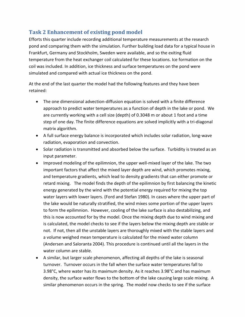
Task 2 Enhancement of existing pond model Efforts this quarter include recording additional temperature measurements at the research pond and comparing them with the simulation. Further building load data for a typical house in Frankfurt, Germany and Stockholm, Sweden were available, and so the exiting fluid temperature from the heat exchanger coil calculated for these locations. Ice formation on the coil was included. In addition, ice thickness and surface temperatures on the pond were simulated and compared with actual ice thickness on the pond.
At the end of the last quarter the model had the following features and they have been retained:
• The one dimensional advection-diffusion equation is solved with a finite difference approach to predict water temperatures as a function of depth in the lake or pond. We are currently working with a cell size (depth) of 0.3048 m or about 1 foot and a time step of one day. The finite difference equations are solved implicitly with a tri-diagonal matrix algorithm.
• A full surface energy balance is incorporated which includes solar radiation, long-wave radiation, evaporation and convection.
• Solar radiation is transmitted and absorbed below the surface. Turbidity is treated as an input parameter.
• Improved modeling of the epilimnion, the upper well-mixed layer of the lake. The two important factors that affect the mixed layer depth are wind, which promotes mixing, and temperature gradients, which lead to density gradients that can either promote or retard mixing. The model finds the depth of the epilimnion by first balancing the kinetic energy generated by the wind with the potential energy required for mixing the top water layers with lower layers. (Ford and Stefan 1980). In cases where the upper part of the lake would be naturally stratified, the wind mixes some portion of the upper layers to form the epilimnion. However, cooling of the lake surface is also destabilizing, and this is now accounted for by the model. Once the mixing depth due to wind mixing and is calculated, the model checks to see if the layers below the mixing depth are stable or not. If not, then all the unstable layers are thoroughly mixed with the stable layers and a volume weighed mean temperature is calculated for the mixed water column (Andersen and Saloranta 2004). This procedure is continued until all the layers in the water column are stable.
• A similar, but larger scale phenomenon, affecting all depths of the lake is seasonal turnover. Turnover occurs in the fall when the surface water temperatures fall to 3.98°C, where water has its maximum density. As it reaches 3.98°C and has maximum density, the surface water flows to the bottom of the lake causing large scale mixing. A similar phenomenon occurs in the spring. The model now checks to see if the surface
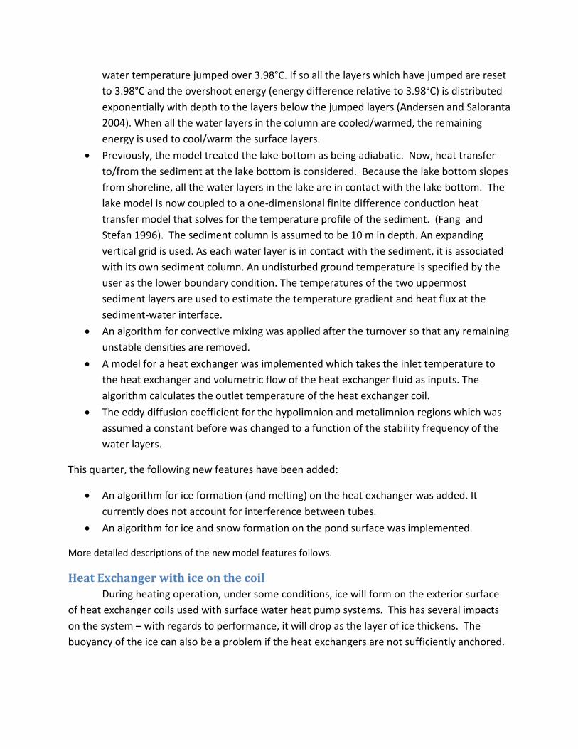
water temperature jumped over 3.98°C. If so all the layers which have jumped are reset to 3.98°C and the overshoot energy (energy difference relative to 3.98°C) is distributed exponentially with depth to the layers below the jumped layers (Andersen and Saloranta 2004). When all the water layers in the column are cooled/warmed, the remaining energy is used to cool/warm the surface layers.
• Previously, the model treated the lake bottom as being adiabatic. Now, heat transfer to/from the sediment at the lake bottom is considered. Because the lake bottom slopes from shoreline, all the water layers in the lake are in contact with the lake bottom. The lake model is now coupled to a one-dimensional finite difference conduction heat transfer model that solves for the temperature profile of the sediment. (Fang and Stefan 1996). The sediment column is assumed to be 10 m in depth. An expanding vertical grid is used. As each water layer is in contact with the sediment, it is associated with its own sediment column. An undisturbed ground temperature is specified by the user as the lower boundary condition. The temperatures of the two uppermost sediment layers are used to estimate the temperature gradient and heat flux at the sediment-water interface.
• An algorithm for convective mixing was applied after the turnover so that any remaining unstable densities are removed.
• A model for a heat exchanger was implemented which takes the inlet temperature to the heat exchanger and volumetric flow of the heat exchanger fluid as inputs. The algorithm calculates the outlet temperature of the heat exchanger coil.
• The eddy diffusion coefficient for the hypolimnion and metalimnion regions which was assumed a constant before was changed to a function of the stability frequency of the water layers.
This quarter, the following new features have been added:
• An algorithm for ice formation (and melting) on the heat exchanger was added. It currently does not account for interference between tubes.
• An algorithm for ice and snow formation on the pond surface was implemented.
More detailed descriptions of the new model features follows.
Heat Exchanger with ice on the coil During heating operation, under some conditions, ice will form on the exterior surface of heat exchanger coils used with surface water heat pump systems. This has several impacts on the system – with regards to performance, it will drop as the layer of ice thickens. The buoyancy of the ice can also be a problem if the heat exchangers are not sufficiently anchored.

Therefore, a model was developed for ice formation on heat exchanger coils. The model is loosely based on the model presented by Neto and Krari (1997) for ice storage tanks. The present model considers a single heat exchanger coil, and currently does not account for interference between ice layers formed on adjacent pipe segments. The model calculates ice formation with variable thickness along the length of the coil, which is currently divided into 50 segments. For test purposes to date, a coil length of 500 feet (152.4 meters) has been assumed.
The model accounts for convection from the working fluid (water-antifreeze mixture also referred to as brine) to the interior pipe surface, conduction through the pipe, convection from the pipe surface or ice surface to the pond, formation of ice on the pipe surface, and melting of ice from the outer surface. Unlike an ice storage tank, ice is expected to melt from the outside of the ice towards the pipe surface.
For purposes of preliminary testing, building loads for a well-insulated house (Spitler et al. 2010) and TMY weather files were used to simulate a pond heat exchanger in Frankfurt, Germany and Stockholm, Sweden. Figures 2 and 3 show the resulting entering and exiting fluid temperatures for a typical year in Frankfurt, Germany and Stockholm, Sweden. The pond temperatures at the heat exchanger depths are also plotted.
Figures 4 and 5 show the calculated amount of ice formation, i.e thickness on the coils at different distances from the origin of the coil for Frankfurt and Stockholm.
It should be emphasized that the results shown here are preliminary and have not been validated by experiment. Published experimental data will be sought.
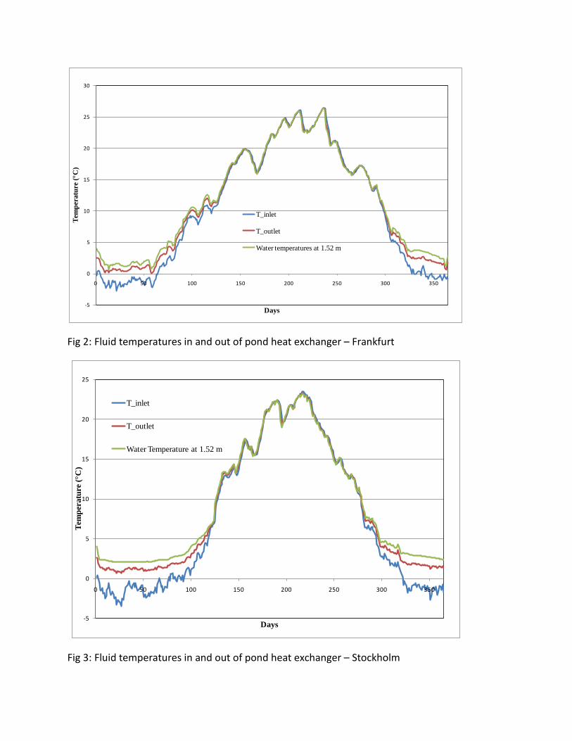
Fig 2: Fluid temperatures in and out of pond heat exchanger – Frankfurt
Fig 3: Fluid temperatures in and out of pond heat exchanger – Stockholm
-5
0
5
10
15
20
25
30
0 50 100 150 200 250 300 350
Tem
pera
ture
(°C
)
Days
T_inlet
T_outlet
Water temperatures at 1.52 m
-5
0
5
10
15
20
25
0 50 100 150 200 250 300 350
Tem
pera
ture
(°C
)
Days
T_inlet
T_outlet
Water Temperature at 1.52 m
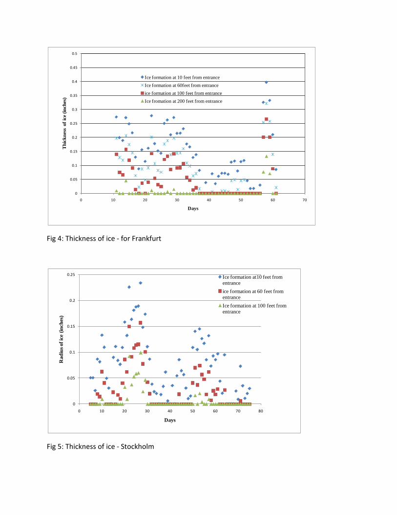
Fig 4: Thickness of ice - for Frankfurt
Fig 5: Thickness of ice - Stockholm
0
0.05
0.1
0.15
0.2
0.25
0.3
0.35
0.4
0.45
0.5
0 10 20 30 40 50 60 70
Thi
ckne
ss o
f ice
(inc
hes)
Days
Ice formation at 10 feet from entranceIce formation at 60feet from entranceice formation at 100 feet from entranceIce fromation at 200 feet from entrance
0
0.05
0.1
0.15
0.2
0.25
0 10 20 30 40 50 60 70 80
Rad
ius o
f ice
(inc
hes)
Days
Ice formation at10 feet from entranceice formation at 60 feet from entranceIce formation at 100 feet from entrance
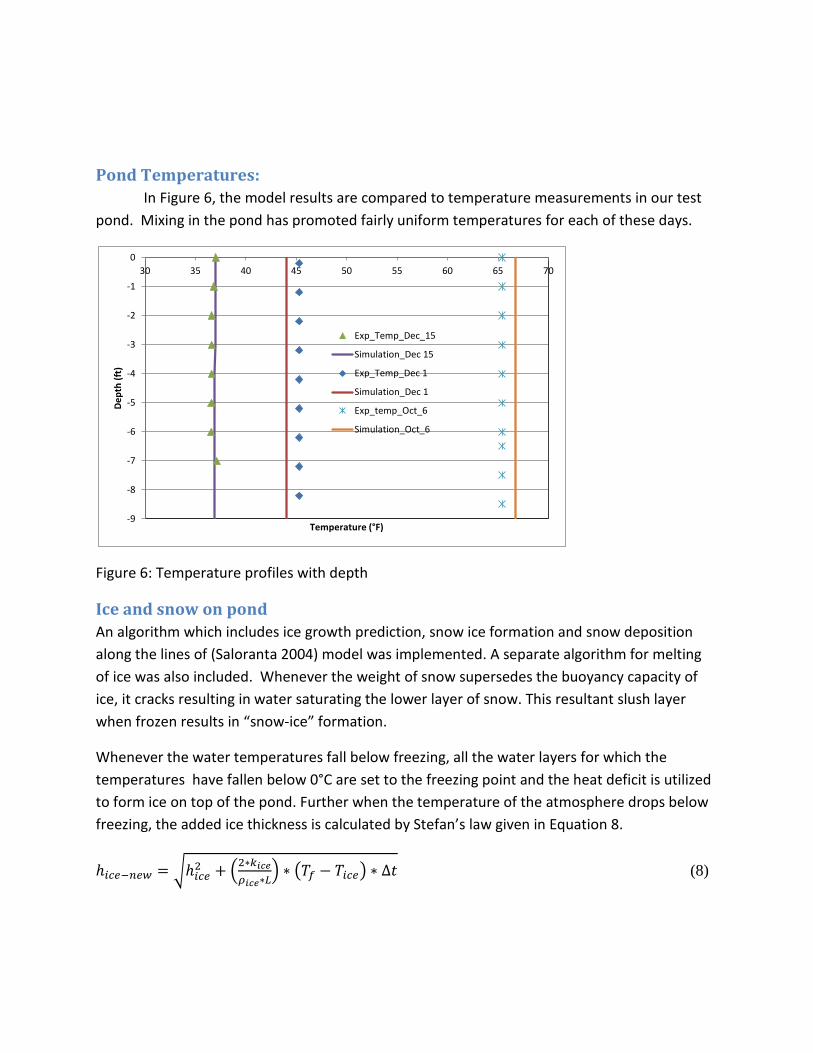
Pond Temperatures: In Figure 6, the model results are compared to temperature measurements in our test pond. Mixing in the pond has promoted fairly uniform temperatures for each of these days.
Figure 6: Temperature profiles with depth
Ice and snow on pond An algorithm which includes ice growth prediction, snow ice formation and snow deposition along the lines of (Saloranta 2004) model was implemented. A separate algorithm for melting of ice was also included. Whenever the weight of snow supersedes the buoyancy capacity of ice, it cracks resulting in water saturating the lower layer of snow. This resultant slush layer when frozen results in “snow-ice” formation.
Whenever the water temperatures fall below freezing, all the water layers for which the temperatures have fallen below 0°C are set to the freezing point and the heat deficit is utilized to form ice on top of the pond. Further when the temperature of the atmosphere drops below freezing, the added ice thickness is calculated by Stefan’s law given in Equation 8.
ℎ𝑖𝑐𝑒−𝑛𝑒𝑤 = �ℎ𝑖𝑐𝑒2 + �2∗𝑘𝑖𝑐𝑒𝜌𝑖𝑐𝑒∗𝐿
� ∗ �𝑇𝑓 − 𝑇𝑖𝑐𝑒� ∗ ∆𝑡 (8)
-9
-8
-7
-6
-5
-4
-3
-2
-1
030 35 40 45 50 55 60 65 70
Dept
h (ft
)
Temperature (°F)
Exp_Temp_Dec_15
Simulation_Dec 15
Exp_Temp_Dec 1
Simulation_Dec 1
Exp_temp_Oct_6
Simulation_Oct_6
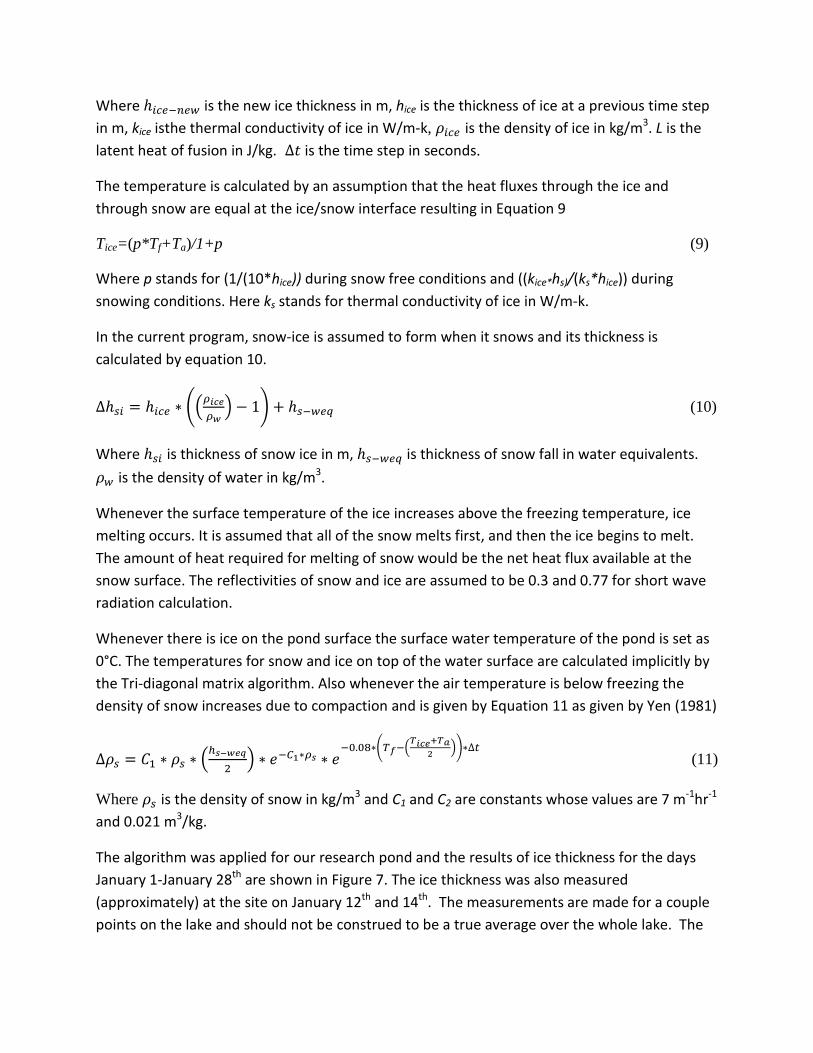
Where ℎ𝑖𝑐𝑒−𝑛𝑒𝑤 is the new ice thickness in m, hice is the thickness of ice at a previous time step in m, kice isthe thermal conductivity of ice in W/m-k, 𝜌𝑖𝑐𝑒 is the density of ice in kg/m3. L is the latent heat of fusion in J/kg. ∆𝑡 is the time step in seconds.
The temperature is calculated by an assumption that the heat fluxes through the ice and through snow are equal at the ice/snow interface resulting in Equation 9
Tice=(p*Tf+Ta)/1+p (9)
Where p stands for (1/(10*hice)) during snow free conditions and ((kice*hs)/(ks*hice)) during snowing conditions. Here ks stands for thermal conductivity of ice in W/m-k.
In the current program, snow-ice is assumed to form when it snows and its thickness is calculated by equation 10.
∆ℎ𝑠𝑖 = ℎ𝑖𝑐𝑒 ∗ ��𝜌𝑖𝑐𝑒𝜌𝑤� − 1� + ℎ𝑠−𝑤𝑒𝑞 (10)
Where ℎ𝑠𝑖 is thickness of snow ice in m, ℎ𝑠−𝑤𝑒𝑞 is thickness of snow fall in water equivalents. 𝜌𝑤 is the density of water in kg/m3.
Whenever the surface temperature of the ice increases above the freezing temperature, ice melting occurs. It is assumed that all of the snow melts first, and then the ice begins to melt. The amount of heat required for melting of snow would be the net heat flux available at the snow surface. The reflectivities of snow and ice are assumed to be 0.3 and 0.77 for short wave radiation calculation.
Whenever there is ice on the pond surface the surface water temperature of the pond is set as 0°C. The temperatures for snow and ice on top of the water surface are calculated implicitly by the Tri-diagonal matrix algorithm. Also whenever the air temperature is below freezing the density of snow increases due to compaction and is given by Equation 11 as given by Yen (1981)
∆𝜌𝑠 = 𝐶1 ∗ 𝜌𝑠 ∗ �ℎ𝑠−𝑤𝑒𝑞
2� ∗ 𝑒−𝐶1∗𝜌𝑠 ∗ 𝑒
−0.08∗�𝑇𝑓−�𝑇𝑖𝑐𝑒+𝑇𝑎
2 ��∗∆𝑡 (11)
Where 𝜌𝑠 is the density of snow in kg/m3 and C1 and C2 are constants whose values are 7 m-1hr-1 and 0.021 m3/kg.
The algorithm was applied for our research pond and the results of ice thickness for the days January 1-January 28th are shown in Figure 7. The ice thickness was also measured (approximately) at the site on January 12th and 14th. The measurements are made for a couple points on the lake and should not be construed to be a true average over the whole lake. The
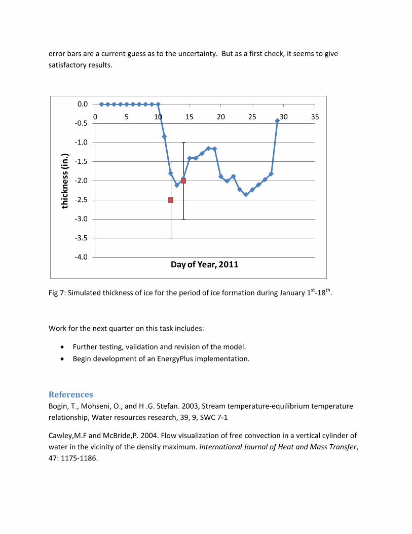
error bars are a current guess as to the uncertainty. But as a first check, it seems to give satisfactory results.
Fig 7: Simulated thickness of ice for the period of ice formation during January 1st-18th.
Work for the next quarter on this task includes:
• Further testing, validation and revision of the model. • Begin development of an EnergyPlus implementation.
References Bogin, T., Mohseni, O., and H .G. Stefan. 2003, Stream temperature-equilibrium temperature relationship, Water resources research, 39, 9, SWC 7-1
Cawley,M.F and McBride,P. 2004. Flow visualization of free convection in a vertical cylinder of water in the vicinity of the density maximum. International Journal of Heat and Mass Transfer, 47: 1175-1186.
-4.0
-3.5
-3.0
-2.5
-2.0
-1.5
-1.0
-0.5
0.0
0 5 10 15 20 25 30 35
thic
knes
s (in
.)
Day of Year, 2011
Edinger, J.E., Duttweiler, D.W. and J.C. Geyer. 1968, The response of water temperatures to meteorological conditions, Water resources research, 4, 5, 1109-1115.
Gustafsson, A.M. 2010. Thermal Response Tests: influence of convective flow in ground water filled heat exchangers. PhD thesis. Luleå University of Technology, Sweden.
Hardin,J.W and Hilbe, J.M. 2003. Generalized Estimating Equations. New York: Chapman and Hall / CRC
Incropera, F.P., DeWitt, D.P., 2002. Fundamentals of Heat and Mass Transfer, fifth ed. New Jersey: John Wiley & Sons
Incropera, Dewitt. 2007 Introduction to Heat Transfer, 5th Edition, chapter 9, Valerie A Vargas, Hoboken, NJ, John Wiley and Sons Inc., 523-581
Mohseni, O., Stefan, H.G. and T.R. Erickson. 1998, A Non-linear regression model for weekly stream temperatures, Water resources research, 34, 10, 2685-2693.
Neto, J.H.M. and M.Krarti. 1997, Deterministic model for an internal melt ice-on coil thermal storage tank. ASHRAE Transactions, 106, 1, 113-124.
Saloranta and Andersen. 2004, My lake (v.1.1): Technical model documentation and users guide. Oslo, Norway, Norweigian Institute for Water Research: 44.
Yen, Y. C. 1981, Review of thermal properties of snow, ice and sea-ice. Hanover,NH,USA, US Army Cold Regions Research and Engineering Laboratory.
Nomenclature:
Nua – Nusselt number based on annulus gap (hnc [ro –ri] / kw) R – radius ratio (r0/ri) Pr – Prandtl number Ra* - modified Rayleigh number q – heat flux (W/m2-K) ν – kinematic viscosity (m2/s) β – volumetric coefficient of expansion = (K-1) k – conductivity (W/m-K) g – acceleration due to gravity (m/s2) D – diameter (m) r – radius (m) h – natural convection coefficient (W/m2-K) c – constant

T – temperature (K) rc – concordance coefficient rxy – Pearson’s coefficient n – number of data points Subscripts o – outer i – inner nc – natural convection Abbreviations SCW – standing column well

Progress Report: Quarter 5 DE-EE0002961 1
Progress Report
DE-EE0002961/001 - Recovery Act:
Improved Design Tools for Surface Water and Standing Column Well Heat Pump Systems
Quarter 5 (1/1/2011-3/31/2011)
Principal Investigator: Jeffrey D. Spitler ([email protected]), Oklahoma State University
Task 1: Enhancement of Existing Standing Column Well Models
The work done in the previous quarter focused on the development of a correlation which could be used to calculate the convection coefficient due to natural convection in the well based on the temperature difference between the fluid and the borehole wall. This correlation was implemented in a borehole thermal resistance model, which calculates the borehole thermal resistance iteratively at each time step based on the fluid and wall temperatures. The borehole thermal resistance model was then incorporated into the standing column well (SCW) model; previously the borehole thermal resistance was assumed to be a constant value and considered as a parameter in the SCW model. In addition to the borehole thermal resistance model, further improvements to the SCW model include the calculation of short circuiting flux within the model itself using the method described in Deng (2004). Previously it was assumed to be constant and calculated from a value of short circuiting resistance which was considered a parameter.
Experimental Validation
The improved model was then validated against data collected from a SCW in Haverhill, MA. The key parameters involved in this validation are the rock properties. According to Domenico and Schwartz (1990) the Haverhill area is composed of rocks from the Cambrian and Ordovician period which primarily consist of sandstone, limestone and dolomite having a porosity ranging from 0.001 – 0.1. The other properties are the rock specific heat capacity, thermal conductivity and hydraulic conductivity which are listed in Table1.
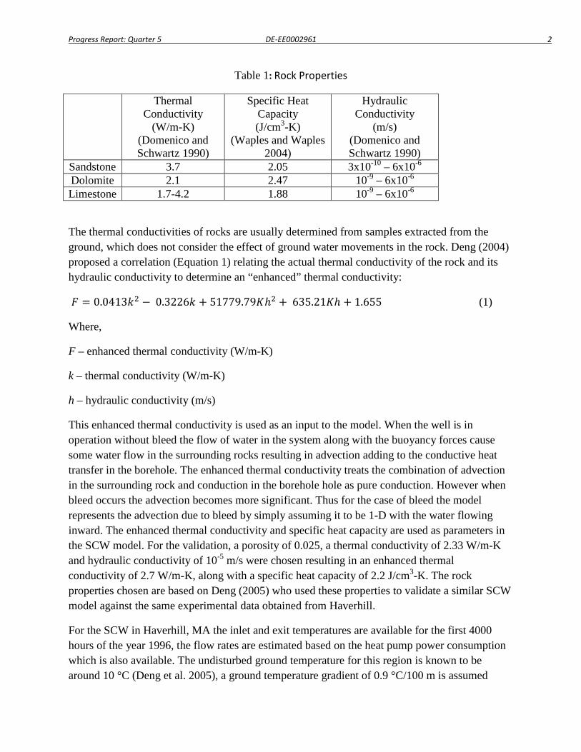
Progress Report: Quarter 5 DE-EE0002961 2
Table 1: Rock Properties
Thermal Conductivity
(W/m-K) (Domenico and Schwartz 1990)
Specific Heat Capacity (J/cm3-K)
(Waples and Waples 2004)
Hydraulic Conductivity
(m/s) (Domenico and Schwartz 1990)
Sandstone 3.7 2.05 3x10⁻¹⁰ – 6x10⁻⁶ Dolomite 2.1 2.47 10-9 – 6x10⁻⁶ Limestone 1.7-4.2 1.88 10-9 – 6x10⁻⁶
The thermal conductivities of rocks are usually determined from samples extracted from the ground, which does not consider the effect of ground water movements in the rock. Deng (2004) proposed a correlation (Equation 1) relating the actual thermal conductivity of the rock and its hydraulic conductivity to determine an “enhanced” thermal conductivity:
𝐹 = 0.0413𝑘2 − 0.3226𝑘 + 51779.79𝐾ℎ2 + 635.21𝐾ℎ + 1.655 (1)
Where,
F – enhanced thermal conductivity (W/m-K)
k – thermal conductivity (W/m-K)
h – hydraulic conductivity (m/s)
This enhanced thermal conductivity is used as an input to the model. When the well is in operation without bleed the flow of water in the system along with the buoyancy forces cause some water flow in the surrounding rocks resulting in advection adding to the conductive heat transfer in the borehole. The enhanced thermal conductivity treats the combination of advection in the surrounding rock and conduction in the borehole hole as pure conduction. However when bleed occurs the advection becomes more significant. Thus for the case of bleed the model represents the advection due to bleed by simply assuming it to be 1-D with the water flowing inward. The enhanced thermal conductivity and specific heat capacity are used as parameters in the SCW model. For the validation, a porosity of 0.025, a thermal conductivity of 2.33 W/m-K and hydraulic conductivity of 10-5 m/s were chosen resulting in an enhanced thermal conductivity of 2.7 W/m-K, along with a specific heat capacity of 2.2 J/cm3-K. The rock properties chosen are based on Deng (2005) who used these properties to validate a similar SCW model against the same experimental data obtained from Haverhill.
For the SCW in Haverhill, MA the inlet and exit temperatures are available for the first 4000 hours of the year 1996, the flow rates are estimated based on the heat pump power consumption which is also available. The undisturbed ground temperature for this region is known to be around 10 °C (Deng et al. 2005), a ground temperature gradient of 0.9 °C/100 m is assumed
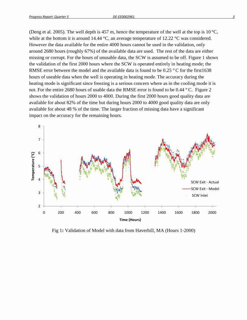
Progress Report: Quarter 5 DE-EE0002961 3
(Deng et al. 2005). The well depth is 457 m, hence the temperature of the well at the top is 10 °C, while at the bottom it is around 14.44 °C, an average temperature of 12.22 °C was considered. However the data available for the entire 4000 hours cannot be used in the validation, only around 2680 hours (roughly 67%) of the available data are used. The rest of the data are either missing or corrupt. For the hours of unusable data, the SCW is assumed to be off. Figure 1 shows the validation of the first 2000 hours where the SCW is operated entirely in heating mode; the RMSE error between the model and the available data is found to be 0.25 ° C for the first1638 hours of useable data when the well is operating in heating mode. The accuracy during the heating mode is significant since freezing is a serious concern where as in the cooling mode it is not. For the entire 2680 hours of usable data the RMSE error is found to be 0.44 ° C. Figure 2 shows the validation of hours 2000 to 4000. During the first 2000 hours good quality data are available for about 82% of the time but during hours 2000 to 4000 good quality data are only available for about 48 % of the time. The larger fraction of missing data have a significant impact on the accuracy for the remaining hours.
Fig 1: Validation of Model with data from Haverhill, MA (Hours 1-2000)
2
3
4
5
6
7
8
0 200 400 600 800 1000 1200 1400 1600 1800 2000
Tem
pera
ture
(°C)
Time (Hours)
SCW Exit - Actual
SCW Exit - Model
SCW Inlet
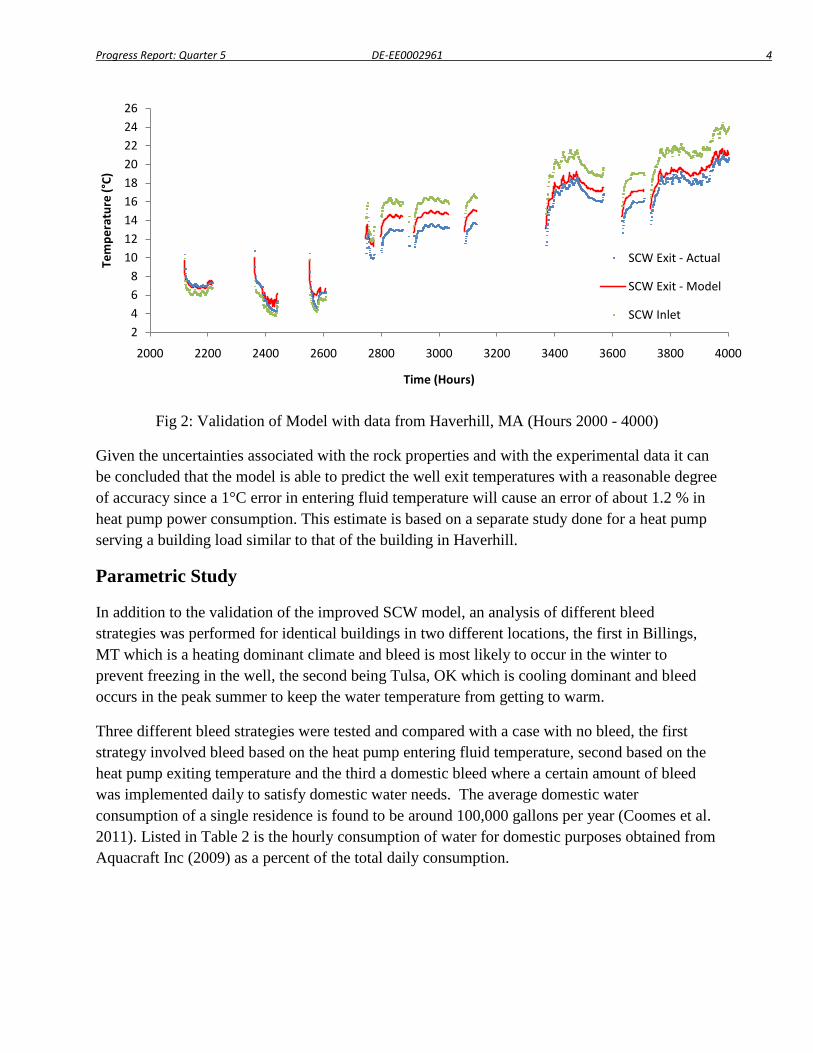
Progress Report: Quarter 5 DE-EE0002961 4
Fig 2: Validation of Model with data from Haverhill, MA (Hours 2000 - 4000)
Given the uncertainties associated with the rock properties and with the experimental data it can be concluded that the model is able to predict the well exit temperatures with a reasonable degree of accuracy since a 1°C error in entering fluid temperature will cause an error of about 1.2 % in heat pump power consumption. This estimate is based on a separate study done for a heat pump serving a building load similar to that of the building in Haverhill.
Parametric Study
In addition to the validation of the improved SCW model, an analysis of different bleed strategies was performed for identical buildings in two different locations, the first in Billings, MT which is a heating dominant climate and bleed is most likely to occur in the winter to prevent freezing in the well, the second being Tulsa, OK which is cooling dominant and bleed occurs in the peak summer to keep the water temperature from getting to warm.
Three different bleed strategies were tested and compared with a case with no bleed, the first strategy involved bleed based on the heat pump entering fluid temperature, second based on the heat pump exiting temperature and the third a domestic bleed where a certain amount of bleed was implemented daily to satisfy domestic water needs. The average domestic water consumption of a single residence is found to be around 100,000 gallons per year (Coomes et al. 2011). Listed in Table 2 is the hourly consumption of water for domestic purposes obtained from Aquacraft Inc (2009) as a percent of the total daily consumption.
2468
101214161820222426
2000 2200 2400 2600 2800 3000 3200 3400 3600 3800 4000
Tem
pera
ture
(°C)
Time (Hours)
SCW Exit - Actual
SCW Exit - Model
SCW Inlet
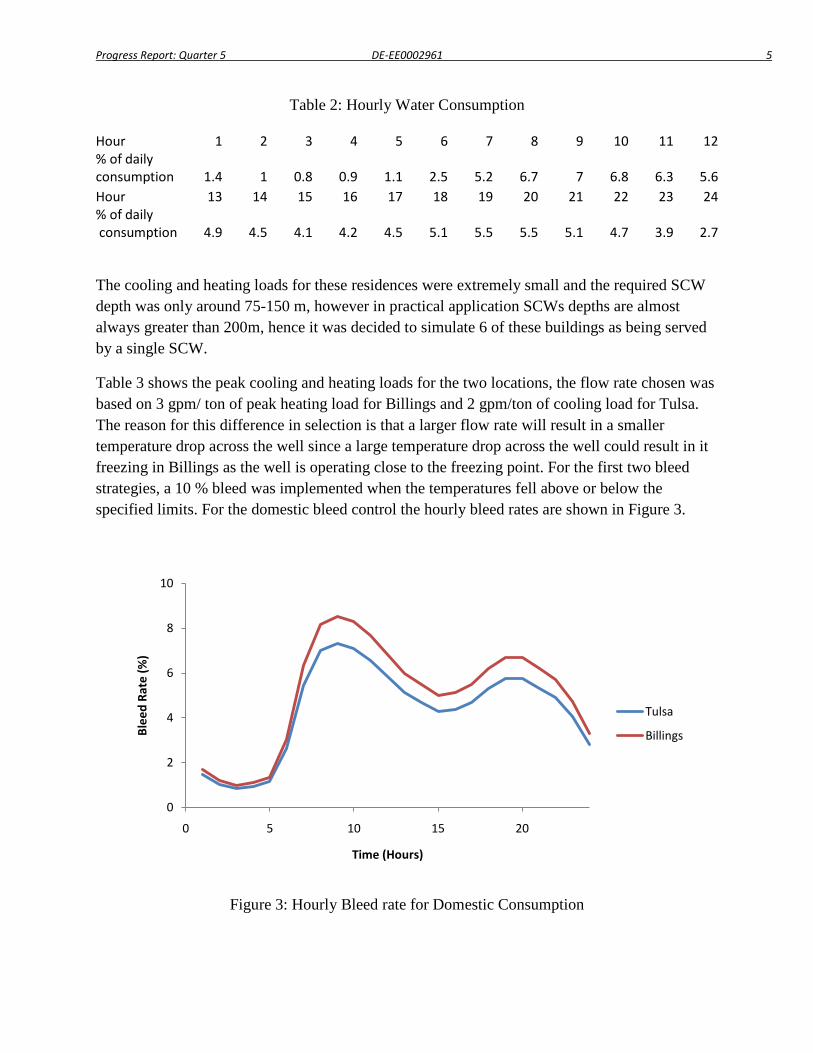
Progress Report: Quarter 5 DE-EE0002961 5
Table 2: Hourly Water Consumption
Hour 1 2 3 4 5 6 7 8 9 10 11 12 % of daily consumption 1.4 1 0.8 0.9 1.1 2.5 5.2 6.7 7 6.8 6.3 5.6 Hour 13 14 15 16 17 18 19 20 21 22 23 24 % of daily consumption 4.9 4.5 4.1 4.2 4.5 5.1 5.5 5.5 5.1 4.7 3.9 2.7
The cooling and heating loads for these residences were extremely small and the required SCW depth was only around 75-150 m, however in practical application SCWs depths are almost always greater than 200m, hence it was decided to simulate 6 of these buildings as being served by a single SCW.
Table 3 shows the peak cooling and heating loads for the two locations, the flow rate chosen was based on 3 gpm/ ton of peak heating load for Billings and 2 gpm/ton of cooling load for Tulsa. The reason for this difference in selection is that a larger flow rate will result in a smaller temperature drop across the well since a large temperature drop across the well could result in it freezing in Billings as the well is operating close to the freezing point. For the first two bleed strategies, a 10 % bleed was implemented when the temperatures fell above or below the specified limits. For the domestic bleed control the hourly bleed rates are shown in Figure 3.
Figure 3: Hourly Bleed rate for Domestic Consumption
0
2
4
6
8
10
0 5 10 15 20
Blee
d Ra
te (%
)
Time (Hours)
Tulsa
Billings
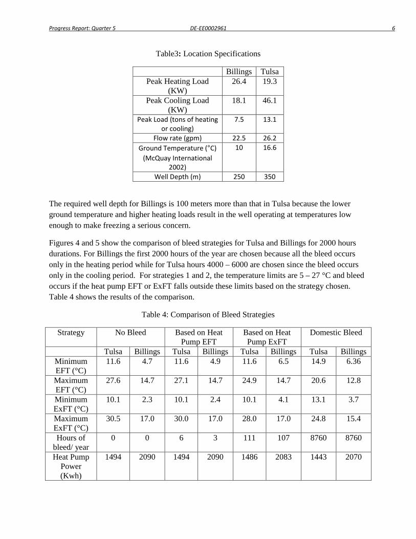
Progress Report: Quarter 5 DE-EE0002961 6
Table3: Location Specifications
Billings Tulsa Peak Heating Load
(KW) 26.4 19.3
Peak Cooling Load (KW)
18.1 46.1
Peak Load (tons of heating or cooling)
7.5 13.1
Flow rate (gpm) 22.5 26.2 Ground Temperature (°C)
(McQuay International 2002)
10 16.6
Well Depth (m) 250 350
The required well depth for Billings is 100 meters more than that in Tulsa because the lower ground temperature and higher heating loads result in the well operating at temperatures low enough to make freezing a serious concern.
Figures 4 and 5 show the comparison of bleed strategies for Tulsa and Billings for 2000 hours durations. For Billings the first 2000 hours of the year are chosen because all the bleed occurs only in the heating period while for Tulsa hours 4000 – 6000 are chosen since the bleed occurs only in the cooling period. For strategies 1 and 2, the temperature limits are 5 – 27 °C and bleed occurs if the heat pump EFT or ExFT falls outside these limits based on the strategy chosen. Table 4 shows the results of the comparison.
Table 4: Comparison of Bleed Strategies
Strategy No Bleed Based on Heat Pump EFT
Based on Heat Pump ExFT
Domestic Bleed
Tulsa Billings Tulsa Billings Tulsa Billings Tulsa Billings Minimum EFT (°C)
11.6 4.7 11.6 4.9 11.6 6.5 14.9 6.36
Maximum EFT (°C)
27.6 14.7 27.1 14.7 24.9 14.7 20.6 12.8
Minimum ExFT (°C)
10.1 2.3 10.1 2.4 10.1 4.1 13.1 3.7
Maximum ExFT (°C)
30.5 17.0 30.0 17.0 28.0 17.0 24.8 15.4
Hours of bleed/ year
0 0 6 3 111 107 8760 8760
Heat Pump Power (Kwh)
1494 2090 1494 2090 1486 2083 1443 2070
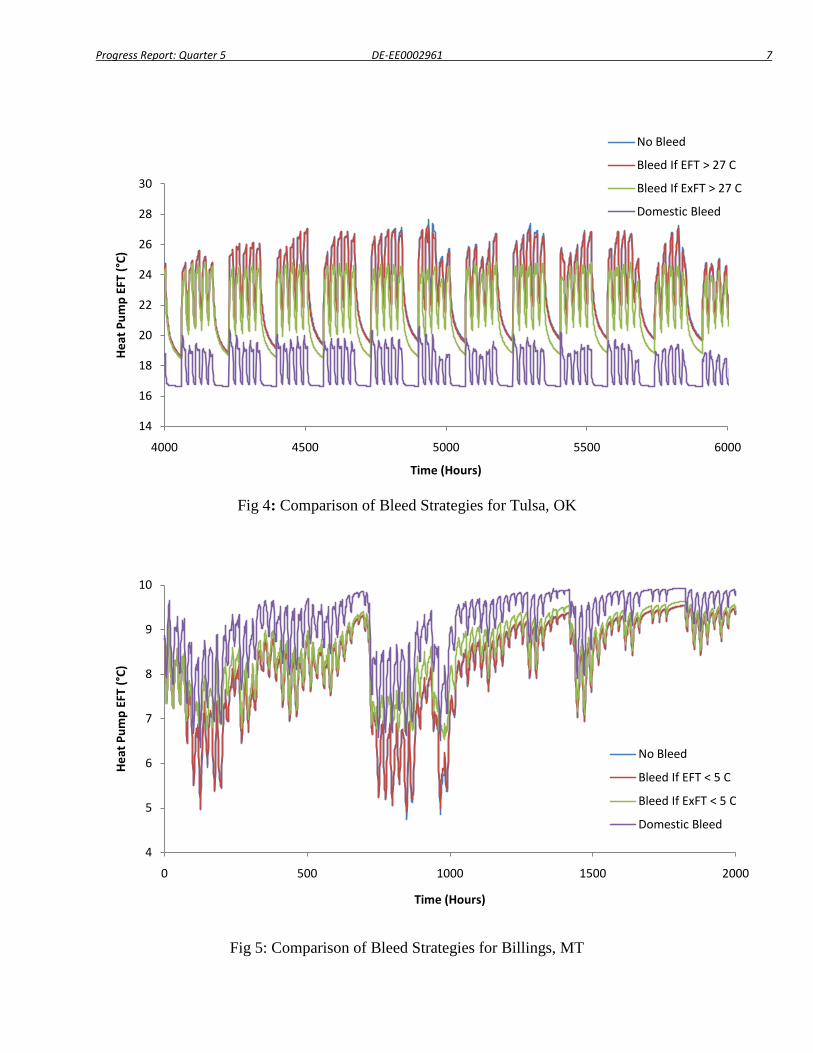
Progress Report: Quarter 5 DE-EE0002961 7
Fig 4: Comparison of Bleed Strategies for Tulsa, OK
Fig 5: Comparison of Bleed Strategies for Billings, MT
14
16
18
20
22
24
26
28
30
4000 4500 5000 5500 6000
Heat
Pum
p EF
T (°
C)
Time (Hours)
No Bleed
Bleed If EFT > 27 C
Bleed If ExFT > 27 C
Domestic Bleed
4
5
6
7
8
9
10
0 500 1000 1500 2000
Heat
Pum
p EF
T (°
C)
Time (Hours)
No Bleed
Bleed If EFT < 5 C
Bleed If ExFT < 5 C
Domestic Bleed
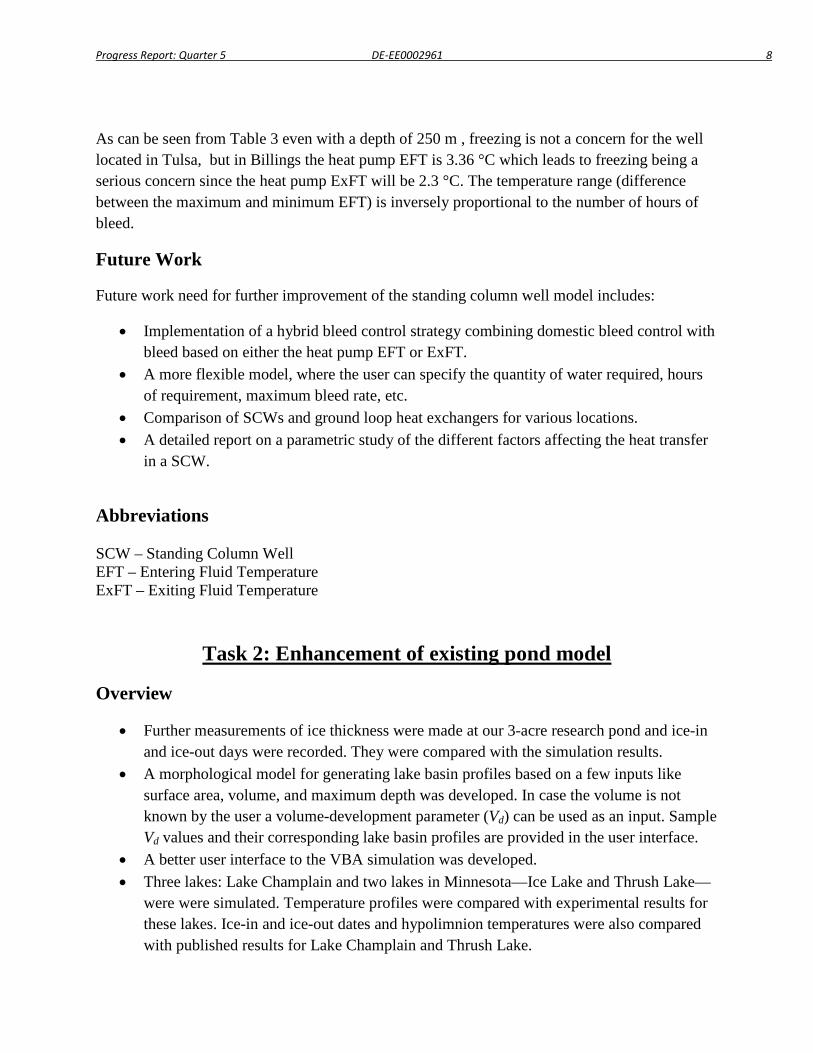
Progress Report: Quarter 5 DE-EE0002961 8
As can be seen from Table 3 even with a depth of 250 m , freezing is not a concern for the well located in Tulsa, but in Billings the heat pump EFT is 3.36 °C which leads to freezing being a serious concern since the heat pump ExFT will be 2.3 °C. The temperature range (difference between the maximum and minimum EFT) is inversely proportional to the number of hours of bleed.
Future Work
Future work need for further improvement of the standing column well model includes:
• Implementation of a hybrid bleed control strategy combining domestic bleed control with bleed based on either the heat pump EFT or ExFT.
• A more flexible model, where the user can specify the quantity of water required, hours of requirement, maximum bleed rate, etc.
• Comparison of SCWs and ground loop heat exchangers for various locations. • A detailed report on a parametric study of the different factors affecting the heat transfer
in a SCW.
Abbreviations SCW – Standing Column Well EFT – Entering Fluid Temperature ExFT – Exiting Fluid Temperature
Task 2: Enhancement of existing pond model
Overview
• Further measurements of ice thickness were made at our 3-acre research pond and ice-in and ice-out days were recorded. They were compared with the simulation results.
• A morphological model for generating lake basin profiles based on a few inputs like surface area, volume, and maximum depth was developed. In case the volume is not known by the user a volume-development parameter (Vd) can be used as an input. Sample Vd values and their corresponding lake basin profiles are provided in the user interface.
• A better user interface to the VBA simulation was developed. • Three lakes: Lake Champlain and two lakes in Minnesota—Ice Lake and Thrush Lake—
were were simulated. Temperature profiles were compared with experimental results for these lakes. Ice-in and ice-out dates and hypolimnion temperatures were also compared with published results for Lake Champlain and Thrush Lake.
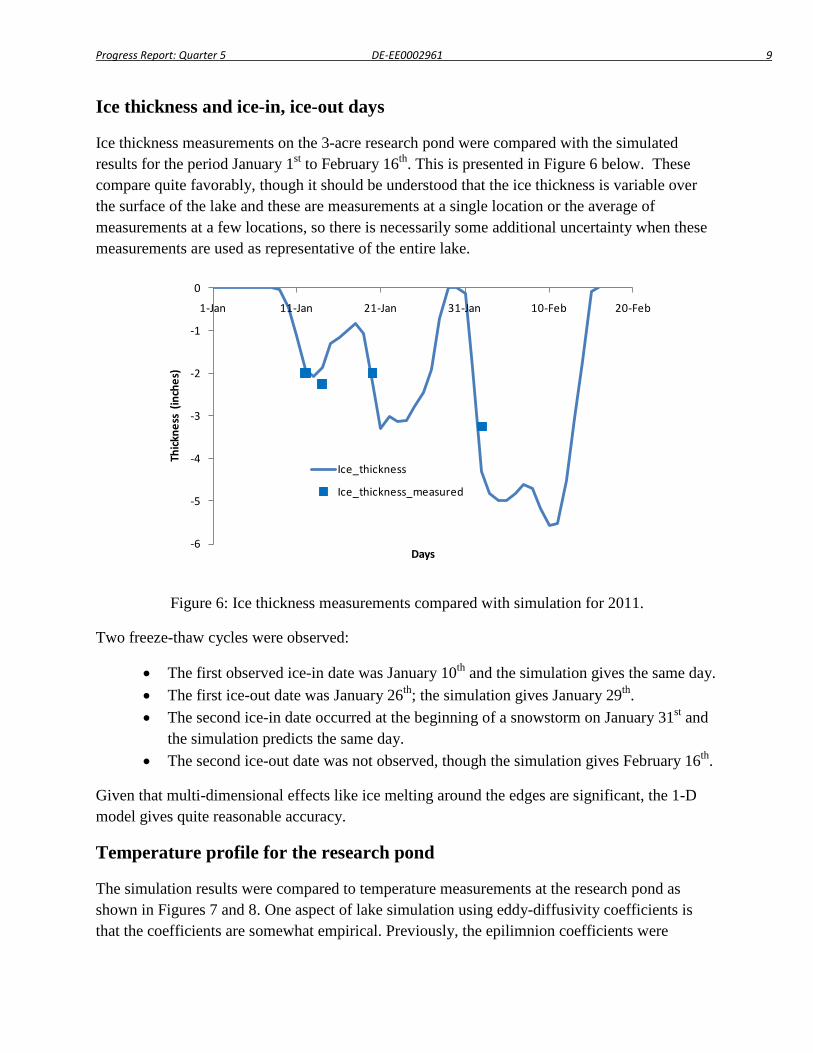
Progress Report: Quarter 5 DE-EE0002961 9
Ice thickness and ice-in, ice-out days
Ice thickness measurements on the 3-acre research pond were compared with the simulated results for the period January 1st to February 16th. This is presented in Figure 6 below. These compare quite favorably, though it should be understood that the ice thickness is variable over the surface of the lake and these are measurements at a single location or the average of measurements at a few locations, so there is necessarily some additional uncertainty when these measurements are used as representative of the entire lake.
Figure 6: Ice thickness measurements compared with simulation for 2011.
Two freeze-thaw cycles were observed:
• The first observed ice-in date was January 10th and the simulation gives the same day. • The first ice-out date was January 26th; the simulation gives January 29th. • The second ice-in date occurred at the beginning of a snowstorm on January 31st and
the simulation predicts the same day. • The second ice-out date was not observed, though the simulation gives February 16th.
Given that multi-dimensional effects like ice melting around the edges are significant, the 1-D model gives quite reasonable accuracy.
Temperature profile for the research pond
The simulation results were compared to temperature measurements at the research pond as shown in Figures 7 and 8. One aspect of lake simulation using eddy-diffusivity coefficients is that the coefficients are somewhat empirical. Previously, the epilimnion coefficients were
-6
-5
-4
-3
-2
-1
0
1-Jan 11-Jan 21-Jan 31-Jan 10-Feb 20-Feb
Thick
ness
(in
ches
)
Days
Ice_thickness
Ice_thickness_measured
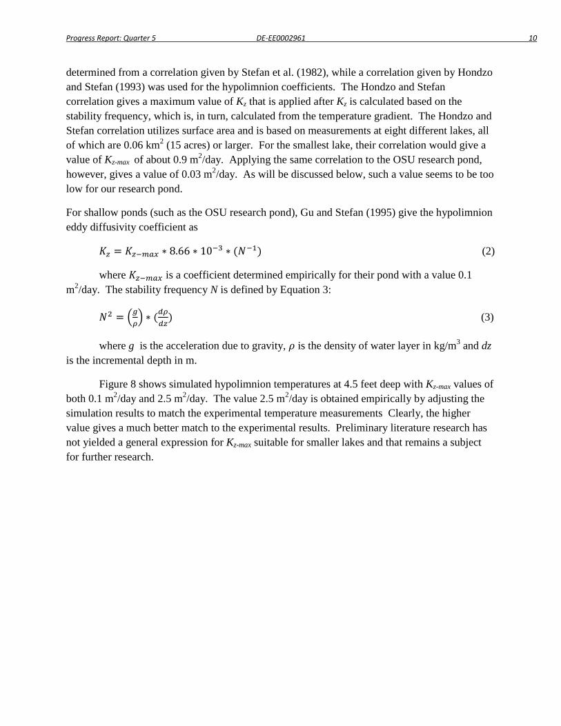
Progress Report: Quarter 5 DE-EE0002961 10
determined from a correlation given by Stefan et al. (1982), while a correlation given by Hondzo and Stefan (1993) was used for the hypolimnion coefficients. The Hondzo and Stefan correlation gives a maximum value of Kz that is applied after Kz is calculated based on the stability frequency, which is, in turn, calculated from the temperature gradient. The Hondzo and Stefan correlation utilizes surface area and is based on measurements at eight different lakes, all of which are 0.06 km2 (15 acres) or larger. For the smallest lake, their correlation would give a value of Kz-max of about 0.9 m2/day. Applying the same correlation to the OSU research pond, however, gives a value of 0.03 m2/day. As will be discussed below, such a value seems to be too low for our research pond.
For shallow ponds (such as the OSU research pond), Gu and Stefan (1995) give the hypolimnion eddy diffusivity coefficient as
𝐾𝑧 = 𝐾𝑧−𝑚𝑎𝑥 ∗ 8.66 ∗ 10−3 ∗ (𝑁−1) (2)
where 𝐾𝑧−𝑚𝑎𝑥 is a coefficient determined empirically for their pond with a value 0.1 m2/day. The stability frequency N is defined by Equation 3:
𝑁2 = �𝑔𝜌� ∗ (𝑑𝜌
𝑑𝑧) (3)
where g is the acceleration due to gravity, 𝜌 is the density of water layer in kg/m3 and dz is the incremental depth in m.
Figure 8 shows simulated hypolimnion temperatures at 4.5 feet deep with Kz-max values of both 0.1 m2/day and 2.5 m2/day. The value 2.5 m2/day is obtained empirically by adjusting the simulation results to match the experimental temperature measurements Clearly, the higher value gives a much better match to the experimental results. Preliminary literature research has not yielded a general expression for Kz-max suitable for smaller lakes and that remains a subject for further research.
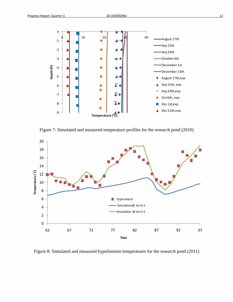
Progress Report: Quarter 5 DE-EE0002961 11
Figure 7: Simulated and measured temperature profiles for the research pond (2010)
Figure 8: Simulated and measured hypolimnion temperatures for the research pond (2011)
-9
-8
-7
-6
-5
-4
-3
-2
-1
0
0 10 20 30 40
Dept
h (ft
)
Temperature (⁰C)
August 17th
Sep 15th
Sep 24th
October 6th
December 1st
December 15th
August 17th,exp
Sep 15th, exp
Sep 24th,exp
Oct 6th, exp
Dec 1st,exp
Dec 15th,exp
0
2
4
6
8
10
12
14
16
18
20
62 67 72 77 82 87 92 97
Tem
pera
ture
(˚C)
Days
Experiment
Simulation@ Kz=0.1
Simulation @ kz=2.5
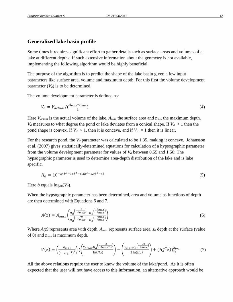
Progress Report: Quarter 5 DE-EE0002961 12
Generalized lake basin profile
Some times it requires significant effort to gather details such as surface areas and volumes of a lake at different depths. If such extensive information about the geometry is not available, implementing the following algorithm would be highly beneficial.
The purpose of the algorithm is to predict the shape of the lake basin given a few input parameters like surface area, volume and maximum depth. For this first the volume development parameter (Vd) is to be determined.
The volume development parameter is defined as:
𝑉𝑑 = 𝑉𝑎𝑐𝑡𝑢𝑎𝑙/(𝐴𝑚𝑎𝑥∗𝑧𝑚𝑎𝑥3
) (4)
Here Vactual is the actual volume of the lake, Amax the surface area and zmax the maximum depth. Vd measures to what degree the pond or lake deviates from a conical shape. If Vd < 1 then the pond shape is convex. If Vd > 1, then it is concave, and if Vd = 1 then it is linear.
For the research pond, the Vd parameter was calculated to be 1.35, making it concave. Johansson et al. (2007) gives statistically-determined equations for calculation of a hypsographic parameter from the volume development parameter for values of Vd between 0.55 and 1.50: The hypsographic parameter is used to determine area-depth distribution of the lake and is lake specific.
𝐻𝑑 = 10−34𝑏5−18𝑏4−6.3𝑏3−1.9𝑏2−4𝑏 (5)
Here b equals log10(Vd).
When the hypsographic parameter has been determined, area and volume as functions of depth are then determined with Equations 6 and 7.
𝐴(𝑧) = 𝐴𝑚𝑎𝑥 �𝐻𝑑
�− 𝑧𝑧𝑚𝑎𝑥
�−𝐻𝑑
�−𝑧𝑚𝑎𝑥𝑧𝑚𝑎𝑥
�
𝐻𝑑�− 𝑧0𝑧𝑚𝑎𝑥
�−𝐻𝑑
�−𝑧𝑚𝑎𝑥𝑧𝑚𝑎𝑥
�� (6)
Where A(z) represents area with depth, Amax represents surface area, z0 depth at the surface (value of 0) and zmax is maximum depth.
𝑉(𝑧) = � 𝐴𝑚𝑎𝑥
�1−𝐻𝑑−1�2� (�2𝑧𝑚𝑎𝑥𝐻𝑑
�− 𝑧𝑧𝑚𝑎𝑥−1
�
ln(𝐻𝑑) � − �𝑧𝑚𝑎𝑥𝐻𝑑�− 2𝑧𝑧𝑚𝑎𝑥
�
2 ln(𝐻𝑑) � + (𝐻𝑑−2𝑧))𝑧𝑖𝑧𝑖+1 (7)
All the above relations require the user to know the volume of the lake/pond. As it is often expected that the user will not have access to this information, an alternative approach would be
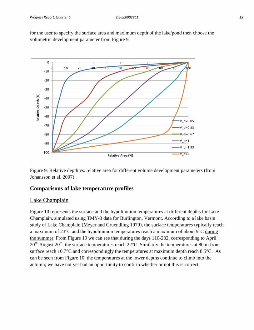
Progress Report: Quarter 5 DE-EE0002961 13
for the user to specify the surface area and maximum depth of the lake/pond then choose the volumetric development parameter from Figure 9.
Figure 9: Relative depth vs. relative area for different volume development parameters (from Johansson et al. 2007)
Comparisons of lake temperature profiles
Lake Champlain
Figure 10 represents the surface and the hypolimnion temperatures at different depths for Lake Champlain, simulated using TMY-3 data for Burlington, Vermont. According to a lake basin study of Lake Champlain (Meyer and Gruendling 1979), the surface temperatures typically reach a maximum of 23°C and the hypolimnion temperatures reach a maximum of about 9°C during the summer. From Figure 10 we can see that during the days 110-232, corresponding to April 20th-August 20th, the surface temperatures reach 22°C. Similarly the temperatures at 80 m from surface reach 10.7°C and correspondingly the temperatures at maximum depth reach 8.5°C. As can be seen from Figure 10, the temperatures at the lower depths continue to climb into the autumn; we have not yet had an opportunity to confirm whether or not this is correct.
-100
-90
-80
-70
-60
-50
-40
-30
-20
-10
0
0 10 20 30 40 50 60 70 80 90 100
Rela
tive
Dept
h (%
)
Relative Area (%)
V_d=0.05
V_d=0.33
V_d=0.67
V_d=1
V_d=1.33
V_d=2
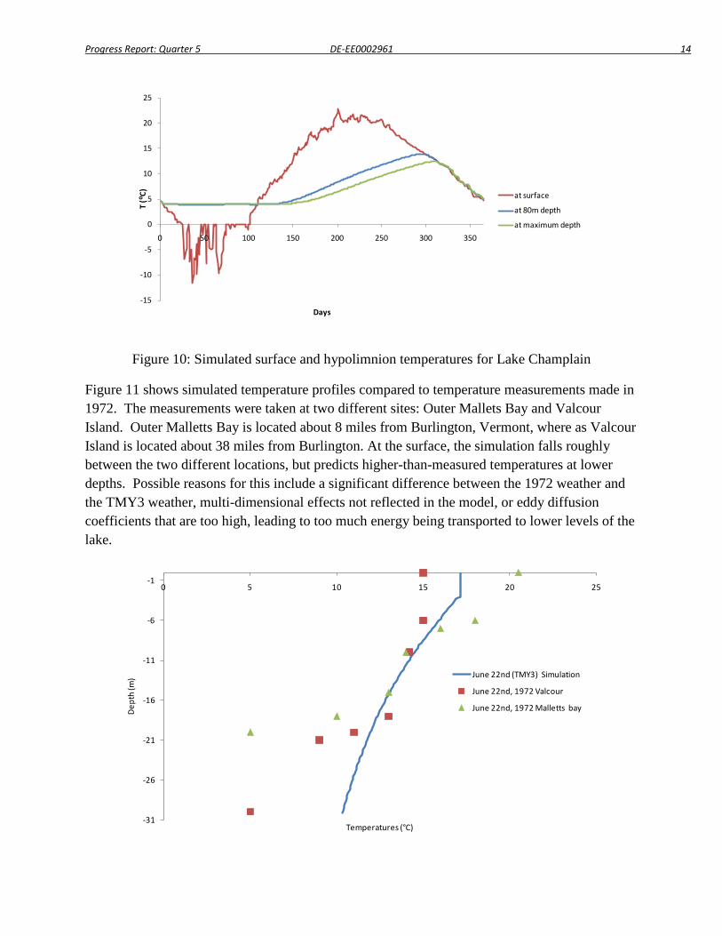
Progress Report: Quarter 5 DE-EE0002961 14
Figure 10: Simulated surface and hypolimnion temperatures for Lake Champlain
Figure 11 shows simulated temperature profiles compared to temperature measurements made in 1972. The measurements were taken at two different sites: Outer Mallets Bay and Valcour Island. Outer Malletts Bay is located about 8 miles from Burlington, Vermont, where as Valcour Island is located about 38 miles from Burlington. At the surface, the simulation falls roughly between the two different locations, but predicts higher-than-measured temperatures at lower depths. Possible reasons for this include a significant difference between the 1972 weather and the TMY3 weather, multi-dimensional effects not reflected in the model, or eddy diffusion coefficients that are too high, leading to too much energy being transported to lower levels of the lake.
-15
-10
-5
0
5
10
15
20
25
0 50 100 150 200 250 300 350
T (⁰C)
Days
at surface
at 80m depth
at maximum depth
-31
-26
-21
-16
-11
-6
-10 5 10 15 20 25
Dept
h (m
)
Temperatures (°C)
June 22nd (TMY3) Simulation
June 22nd, 1972 Valcour
June 22nd, 1972 Malletts bay
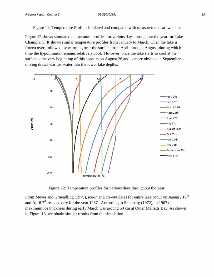
Progress Report: Quarter 5 DE-EE0002961 15
Figure 11: Temperature Profile simulated and compared with measurements at two sites
Figure 12 shows simulated temperature profiles for various days throughout the year for Lake Champlain. It shows similar temperature profiles from January to March, when the lake is frozen over, followed by warming near the surface from April through August, during which time the hypolimnion remains relatively cool. However, once the lake starts to cool at the surface – the very beginning of this appears on August 26 and is more obvious in September – mixing draws warmer water into the lower lake depths.
Figure 12: Temperature profiles for various days throughout the year.
From Meyer and Gruendling (1979), ice-in and ice-out dates for entire lake occur on January 19th and April 7th respectively for the year 1967. According to Sundberg (1972), in 1967 the maximum ice thickness during early March was around 50 cm at Outer Malletts Bay. As shown in Figure 13, we obtain similar results from the simulation.
-120
-100
-80
-60
-40
-20
0
-5 0 5 10 15 20
Dept
h (m
)
Temperatures (⁰C)
Jan 30th
Feb 27th
March 29th
April 28th
June 27th
July 27th
August 26th
Oct 25th
Nov 24th
Dec 24th
September 25th
May 27th
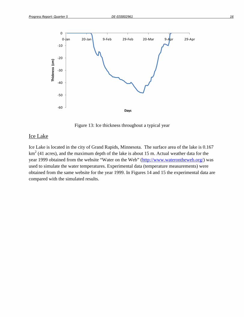
Progress Report: Quarter 5 DE-EE0002961 16
Figure 13: Ice thickness throughout a typical year
Ice Lake
Ice Lake is located in the city of Grand Rapids, Minnesota. The surface area of the lake is 0.167 km2 (41 acres), and the maximum depth of the lake is about 15 m. Actual weather data for the year 1999 obtained from the website “Water on the Web” (http://www.waterontheweb.org/) was used to simulate the water temperatures. Experimental data (temperature measurements) were obtained from the same website for the year 1999. In Figures 14 and 15 the experimental data are compared with the simulated results.
-60
-50
-40
-30
-20
-10
0
0-Jan 20-Jan 9-Feb 29-Feb 20-Mar 9-Apr 29-Apr
Thick
ness
(cm
)
Days
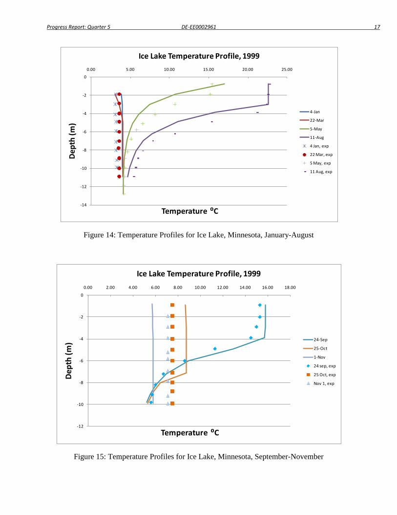
Progress Report: Quarter 5 DE-EE0002961 17
Figure 14: Temperature Profiles for Ice Lake, Minnesota, January-August
Figure 15: Temperature Profiles for Ice Lake, Minnesota, September-November
-14
-12
-10
-8
-6
-4
-2
0
0.00 5.00 10.00 15.00 20.00 25.00De
pth
(m)
Temperature ⁰C
Ice Lake Temperature Profile, 1999
4-Jan
22-Mar
5-May
11-Aug
4 Jan, exp
22 Mar, exp
5 May, exp
11 Aug, exp
-12
-10
-8
-6
-4
-2
0
0.00 2.00 4.00 6.00 8.00 10.00 12.00 14.00 16.00 18.00
Dept
h (m
)
Temperature ⁰C
Ice Lake Temperature Profile, 1999
24-Sep
25-Oct
1-Nov
24 sep, exp
25 Oct, exp
Nov 1, exp
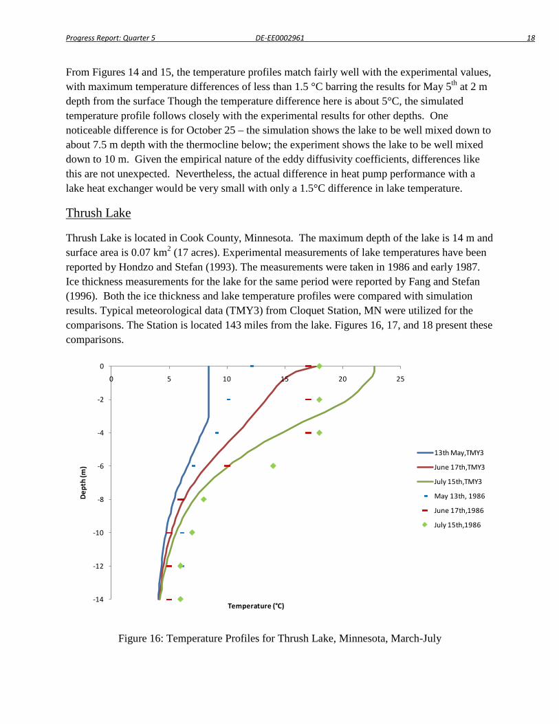
Progress Report: Quarter 5 DE-EE0002961 18
From Figures 14 and 15, the temperature profiles match fairly well with the experimental values, with maximum temperature differences of less than 1.5 °C barring the results for May 5th at 2 m depth from the surface Though the temperature difference here is about 5°C, the simulated temperature profile follows closely with the experimental results for other depths. One noticeable difference is for October 25 – the simulation shows the lake to be well mixed down to about 7.5 m depth with the thermocline below; the experiment shows the lake to be well mixed down to 10 m. Given the empirical nature of the eddy diffusivity coefficients, differences like this are not unexpected. Nevertheless, the actual difference in heat pump performance with a lake heat exchanger would be very small with only a 1.5°C difference in lake temperature.
Thrush Lake
Thrush Lake is located in Cook County, Minnesota. The maximum depth of the lake is 14 m and surface area is 0.07 km2 (17 acres). Experimental measurements of lake temperatures have been reported by Hondzo and Stefan (1993). The measurements were taken in 1986 and early 1987. Ice thickness measurements for the lake for the same period were reported by Fang and Stefan (1996). Both the ice thickness and lake temperature profiles were compared with simulation results. Typical meteorological data (TMY3) from Cloquet Station, MN were utilized for the comparisons. The Station is located 143 miles from the lake. Figures 16, 17, and 18 present these comparisons.
Figure 16: Temperature Profiles for Thrush Lake, Minnesota, March-July
-14
-12
-10
-8
-6
-4
-2
0
0 5 10 15 20 25
Dept
h (m
)
Temperature (°C)
13th May,TMY3
June 17th,TMY3
July 15th,TMY3
May 13th, 1986
June 17th,1986
July 15th,1986
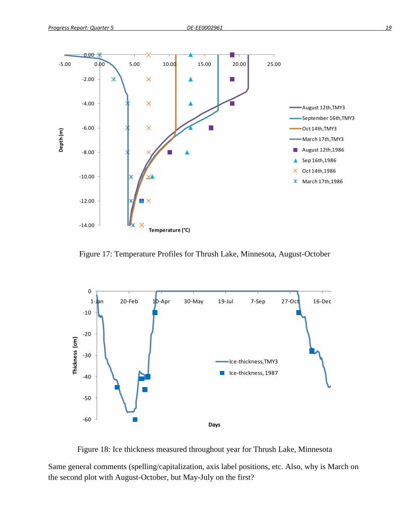
Progress Report: Quarter 5 DE-EE0002961 19
Figure 17: Temperature Profiles for Thrush Lake, Minnesota, August-October
Figure 18: Ice thickness measured throughout year for Thrush Lake, Minnesota
Same general comments (spelling/capitalization, axis label positions, etc. Also, why is March on the second plot with August-October, but May-July on the first?
-14.00
-12.00
-10.00
-8.00
-6.00
-4.00
-2.00
0.00
-5.00 0.00 5.00 10.00 15.00 20.00 25.00De
pth
(m)
Temperature (°C)
August 12th,TMY3
September 16th,TMY3
Oct 14th,TMY3
March 17th,TMY3
August 12th,1986
Sep 16th,1986
Oct 14th,1986
March 17th,1986
-60
-50
-40
-30
-20
-10
0
1-Jan 20-Feb 10-Apr 30-May 19-Jul 7-Sep 27-Oct 16-Dec
Thick
ness
(cm
)
Days
Ice-thickness,TMY3
Ice-thickness, 1987
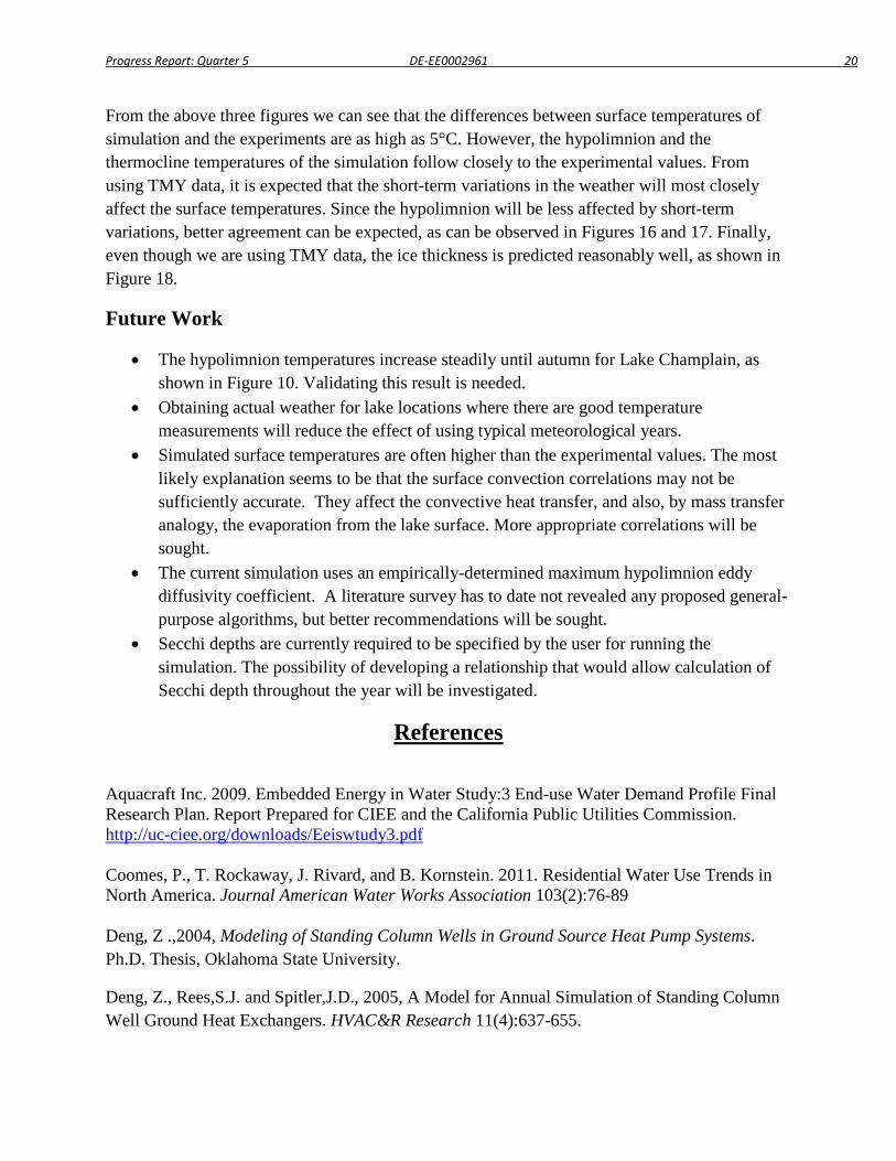
Progress Report: Quarter 5 DE-EE0002961 20
From the above three figures we can see that the differences between surface temperatures of simulation and the experiments are as high as 5°C. However, the hypolimnion and the thermocline temperatures of the simulation follow closely to the experimental values. From using TMY data, it is expected that the short-term variations in the weather will most closely affect the surface temperatures. Since the hypolimnion will be less affected by short-term variations, better agreement can be expected, as can be observed in Figures 16 and 17. Finally, even though we are using TMY data, the ice thickness is predicted reasonably well, as shown in Figure 18.
Future Work
• The hypolimnion temperatures increase steadily until autumn for Lake Champlain, as shown in Figure 10. Validating this result is needed.
• Obtaining actual weather for lake locations where there are good temperature measurements will reduce the effect of using typical meteorological years.
• Simulated surface temperatures are often higher than the experimental values. The most likely explanation seems to be that the surface convection correlations may not be sufficiently accurate. They affect the convective heat transfer, and also, by mass transfer analogy, the evaporation from the lake surface. More appropriate correlations will be sought.
• The current simulation uses an empirically-determined maximum hypolimnion eddy diffusivity coefficient. A literature survey has to date not revealed any proposed general-purpose algorithms, but better recommendations will be sought.
• Secchi depths are currently required to be specified by the user for running the simulation. The possibility of developing a relationship that would allow calculation of Secchi depth throughout the year will be investigated.
References
Aquacraft Inc. 2009. Embedded Energy in Water Study:3 End-use Water Demand Profile Final Research Plan. Report Prepared for CIEE and the California Public Utilities Commission. http://uc-ciee.org/downloads/Eeiswtudy3.pdf Coomes, P., T. Rockaway, J. Rivard, and B. Kornstein. 2011. Residential Water Use Trends in North America. Journal American Water Works Association 103(2):76-89 Deng, Z .,2004, Modeling of Standing Column Wells in Ground Source Heat Pump Systems. Ph.D. Thesis, Oklahoma State University.
Deng, Z., Rees,S.J. and Spitler,J.D., 2005, A Model for Annual Simulation of Standing Column Well Ground Heat Exchangers. HVAC&R Research 11(4):637-655.
Progress Report: Quarter 5 DE-EE0002961 21
Domenico, P.A., and F.W. Schwartz., 1990, Physical and Chemical Hydrogeology. NewYork: John Wiley & Sons, Inc. Fang , X. and H. G. Stefan.,1996, "Long-term lake water temperature and ice cover simulations/measurements." Cold Regions Science and Technology 24: 289-304.
Gu, R. and Heinz.G.Stefan.,1995, "Stratification Dynamics in Wastewater Stabilization Ponds." Water Research 29(8): 1909-1923.
Hondzo, M. and H. G. Stefan.,1993, "Lake water temperature simulation model." Journal of Hydraulic Engineering 119: 1251-1273.
Johansson, H., A. A. Brolin., et al, 2007, "New Approaches to the Modelling of lake Basin Morphometry." Environmental Modeling and Assessment 12: 213-228.
McQuay International. 2002. Geothermal Heat Pump Design Manual. Application Guide AG 31-008. Minneapolis: McQuay International, Inc
http://www.mcquay.com/mcquaybiz/literature/lit_systems/AppGuide/AG_31-008_Geothermal_021607b.pdf
Meyer, G. E. and G. K. Gruendling., 1979, Limnology of Lake Champlain. New York, State University of New York: 395.
Sundberg, S.E.,1972,"Thermal Properties of Malletts Bay, Lake Champlain." PhD. University of Vermont. (as described by Meyer and Gruendling (1979)).
Waples, D.W and Waples,J.S. 2004. A review and evaluation of specific heat capacities of rocks, minerals and subsurface fluids. Part 1:Minerals and nonporous rocks. Natual Resources Research, 13:(2) 97-121.

Progress Report: Quarter 6 DE-EE0002961 1
Progress Report
DE-EE0002961/001 - Recovery Act:
Improved Design Tools for Surface Water and Standing Column Well Heat Pump
Systems
Quarter 6 (4/1/2011-6/30/2011)
Principal Investigator: Jeffrey D. Spitler ([email protected]),
Oklahoma State University
Task 1: Enhancement of Existing Standing Column Well Models
In the previous quarter a preliminary investigation was done on the effect of bleed on required
borehole depths for a fictitious small residential building in two different locations, Tulsa, OK
and Billings, MT. The fictitious building was very well insulated and hence the loads associated
with it were rather small. The parametric analysis done in the current quarter involves a typical
small office building in 5 different locations, Concord, NH; Boston, Ma; Harrisburg, Pa;
Portland, OR and Birmingham, AL. Different bleed strategies were investigated and an
economic analysis was performed to determine the life cycle costs of the SCWs with different
bleed strategies and drawdown levels and compare it with a convection closed loop GLHE.
Comparative Performance Analysis of SCW and GLHE
A performance analysis of ground source heat pump systems using either standing column wells
(SCW) or ground loop heat exchanger (GLHE) was done in the HVACSIM+ environment using
a system simulation approach. The individual component models for the SCW system are a
building model, an SCW model and a heat pump model. For the system with a GLHE, the SCW
model is replaced with a GLHE model.
The building that is used in this analysis represents a small commercial facility that has been
used in other energy studies (Yavuzturk 1999). The total floor area of the building is
approximately 1,320 m2. The building loads were determined using building energy simulation
software (BLAST 1986). The occupancy was set to one person per 9.3 m2 with a heat gain of
131.9 W, equipment and lighting loads were set to 12.2 and 11.1 W/m2 respectively. During the
day time the temperature is set at 20 °C and during nights heating is provided if the temperature
falls below 14.4 °C. The building loads were determined using building energy simulation
software (BLAST 1986) with Typical Meteorological Year (TMY) Weather files for five
different locations, Boston, MA; Harrisburg, PA; Concord, NH; Portland, OR and Birmingham,
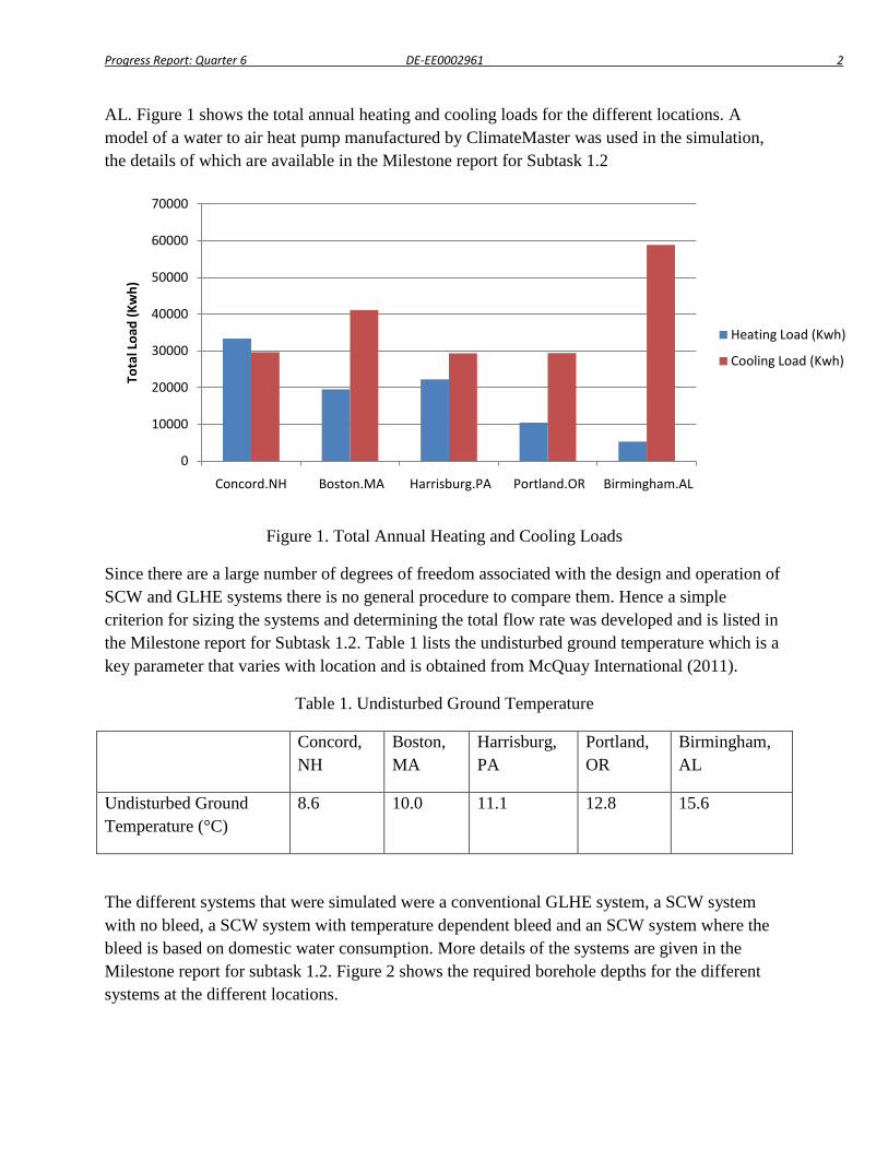
Progress Report: Quarter 6 DE-EE0002961 2
AL. Figure 1 shows the total annual heating and cooling loads for the different locations. A
model of a water to air heat pump manufactured by ClimateMaster was used in the simulation,
the details of which are available in the Milestone report for Subtask 1.2
Figure 1. Total Annual Heating and Cooling Loads
Since there are a large number of degrees of freedom associated with the design and operation of
SCW and GLHE systems there is no general procedure to compare them. Hence a simple
criterion for sizing the systems and determining the total flow rate was developed and is listed in
the Milestone report for Subtask 1.2. Table 1 lists the undisturbed ground temperature which is a
key parameter that varies with location and is obtained from McQuay International (2011).
Table 1. Undisturbed Ground Temperature
Concord,
NH
Boston,
MA
Harrisburg,
PA
Portland,
OR
Birmingham,
AL
Undisturbed Ground
Temperature (°C)
8.6 10.0 11.1 12.8 15.6
The different systems that were simulated were a conventional GLHE system, a SCW system
with no bleed, a SCW system with temperature dependent bleed and an SCW system where the
bleed is based on domestic water consumption. More details of the systems are given in the
Milestone report for subtask 1.2. Figure 2 shows the required borehole depths for the different
systems at the different locations.
0
10000
20000
30000
40000
50000
60000
70000
Concord.NH Boston.MA Harrisburg.PA Portland.OR Birmingham.AL
Tota
l Lo
ad (
Kw
h)
Heating Load (Kwh)
Cooling Load (Kwh)
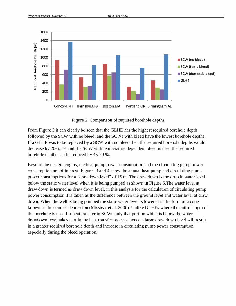
Progress Report: Quarter 6 DE-EE0002961 3
Figure 2. Comparison of required borehole depths
From Figure 2 it can clearly be seen that the GLHE has the highest required borehole depth
followed by the SCW with no bleed, and the SCWs with bleed have the lowest borehole depths.
If a GLHE was to be replaced by a SCW with no bleed then the required borehole depths would
decrease by 20-55 % and if a SCW with temperature dependent bleed is used the required
borehole depths can be reduced by 45-70 %.
Beyond the design lengths, the heat pump power consumption and the circulating pump power
consumption are of interest. Figures 3 and 4 show the annual heat pump and circulating pump
power consumptions for a “drawdown level” of 15 m. The draw down is the drop in water level
below the static water level when it is being pumped as shown in Figure 5.The water level at
draw down is termed as draw down level, in this analysis for the calculation of circulating pump
power consumption it is taken as the difference between the ground level and water level at draw
down. When the well is being pumped the static water level is lowered in the form of a cone
known as the cone of depression (Misstear et al. 2006). Unlike GLHEs where the entire length of
the borehole is used for heat transfer in SCWs only that portion which is below the water
drawdown level takes part in the heat transfer process, hence a large draw down level will result
in a greater required borehole depth and increase in circulating pump power consumption
especially during the bleed operation.
0
200
400
600
800
1000
1200
1400
1600
Concord.NH Harrisburg.PA Boston.MA Portland.OR Birmingham.AL
Re
qu
ire
d B
ore
ho
le D
ep
th (
m)
SCW (no bleed)
SCW (temp bleed)
SCW (domestic bleed)
GLHE
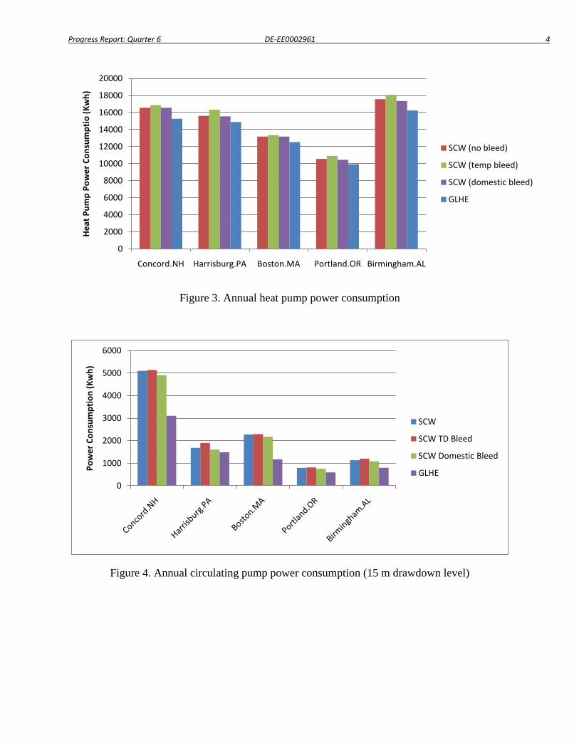
Progress Report: Quarter 6 DE-EE0002961 4
Figure 3. Annual heat pump power consumption
Figure 4. Annual circulating pump power consumption (15 m drawdown level)
0
2000
4000
6000
8000
10000
12000
14000
16000
18000
20000
Concord.NH Harrisburg.PA Boston.MA Portland.OR Birmingham.AL
He
at P
um
p P
ow
er
Co
nsu
mp
tio
(K
wh
)
SCW (no bleed)
SCW (temp bleed)
SCW (domestic bleed)
GLHE
0
1000
2000
3000
4000
5000
6000
Po
we
r C
on
sum
pti
on
(K
wh
)
SCW
SCW TD Bleed
SCW Domestic Bleed
GLHE
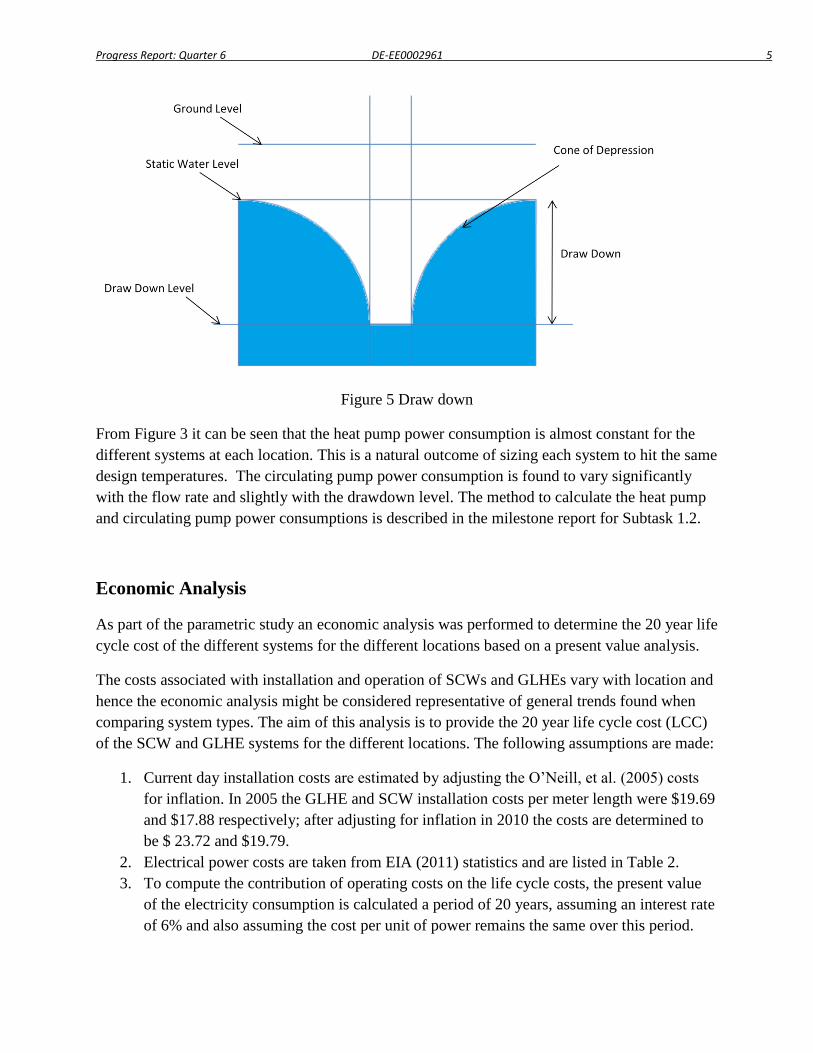
Progress Report: Quarter 6 DE-EE0002961 5
Figure 5 Draw down
From Figure 3 it can be seen that the heat pump power consumption is almost constant for the
different systems at each location. This is a natural outcome of sizing each system to hit the same
design temperatures. The circulating pump power consumption is found to vary significantly
with the flow rate and slightly with the drawdown level. The method to calculate the heat pump
and circulating pump power consumptions is described in the milestone report for Subtask 1.2.
Economic Analysis
As part of the parametric study an economic analysis was performed to determine the 20 year life
cycle cost of the different systems for the different locations based on a present value analysis.
The costs associated with installation and operation of SCWs and GLHEs vary with location and
hence the economic analysis might be considered representative of general trends found when
comparing system types. The aim of this analysis is to provide the 20 year life cycle cost (LCC)
of the SCW and GLHE systems for the different locations. The following assumptions are made:
1. Current day installation costs are estimated by adjusting the O’Neill, et al. (2005) costs
for inflation. In 2005 the GLHE and SCW installation costs per meter length were $19.69
and $17.88 respectively; after adjusting for inflation in 2010 the costs are determined to
be $ 23.72 and $19.79.
2. Electrical power costs are taken from EIA (2011) statistics and are listed in Table 2.
3. To compute the contribution of operating costs on the life cycle costs, the present value
of the electricity consumption is calculated a period of 20 years, assuming an interest rate
of 6% and also assuming the cost per unit of power remains the same over this period.

Progress Report: Quarter 6 DE-EE0002961 6
4. Maintenance and disposal costs are not included, since they are assumed to be the same
for all systems.
5. Heat pump EFT will vary from year to year, and hence heat pump energy consumption
will vary from year to year. But for this analysis, we assumed that the heat pump energy
consumption for outlying years may be adequately approximated by the heat pump
energy consumption for the first year.
Table 2. Electric Utility Costs
Concord,
NH
Boston,
MA
Harrisburg,
PA
Portland,
OR
Birmingham,
AL
Price/ Kwh
($)
0.144 0.139 0.0977 0.083 0.104
Figure 6 is based on drawdown level of 15 m and it shows the total life cycle costs (LCC) for 20
years for the different cases that were analyzed.
Figure 6. 20 year Life Cycle Cost based on Drawdown Level of 15 m
Figure 7 shows a breakdown of the contributions to LCC for Boston with a drawdown level of
15 meters. Of the total LCC the installation accounts for about 30 %, the heat pump power
consumption 60 % and the circulating pump power consumption around 10 % for a typical SCW
with no bleed at Boston. The SCWs with temperature dependent bleed and domestic bleed have
the lowest LCC, around 13 % lower than the SCW with no bleed and 26 % lower than the
GLHE. Based on all the cases analyzed the SCW with no bleed has a LCC 10 - 40 % lower than
a GLHE and for an SCW with bleed it can be lower by 25 -70 %.
$0
$10,000
$20,000
$30,000
$40,000
$50,000
$60,000
$70,000
Concord.NH Harrisburg.PA Boston.MA Portland.OR Birmingham.AL
20
ye
ar L
ife
Cyc
le C
ost
SCW (no bleed)
SCW (temp bleed)
SCW (domestic bleed)
GLHE
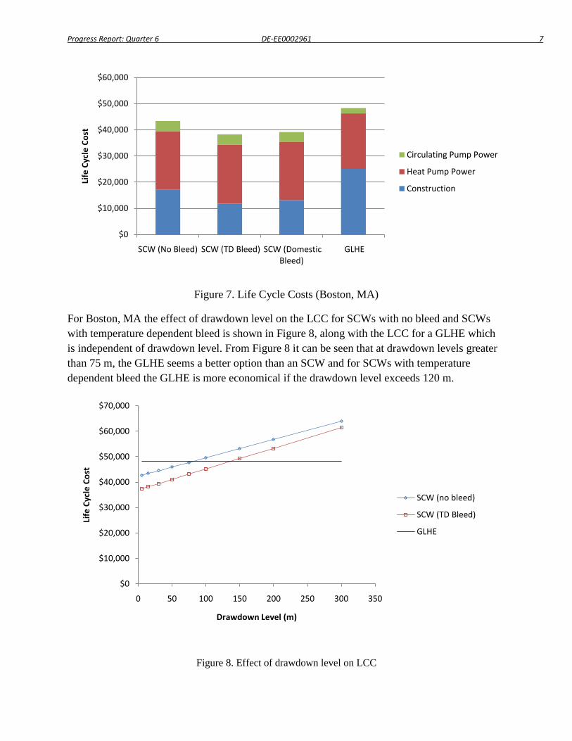
Progress Report: Quarter 6 DE-EE0002961 7
Figure 7. Life Cycle Costs (Boston, MA)
For Boston, MA the effect of drawdown level on the LCC for SCWs with no bleed and SCWs
with temperature dependent bleed is shown in Figure 8, along with the LCC for a GLHE which
is independent of drawdown level. From Figure 8 it can be seen that at drawdown levels greater
than 75 m, the GLHE seems a better option than an SCW and for SCWs with temperature
dependent bleed the GLHE is more economical if the drawdown level exceeds 120 m.
Figure 8. Effect of drawdown level on LCC
$0
$10,000
$20,000
$30,000
$40,000
$50,000
$60,000
SCW (No Bleed) SCW (TD Bleed) SCW (Domestic Bleed)
GLHE
Life
Cyc
le C
ost
Circulating Pump Power
Heat Pump Power
Construction
$0
$10,000
$20,000
$30,000
$40,000
$50,000
$60,000
$70,000
0 50 100 150 200 250 300 350
Life
Cyc
le C
ost
Drawdown Level (m)
SCW (no bleed)
SCW (TD Bleed)
GLHE
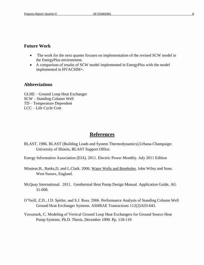
Progress Report: Quarter 6 DE-EE0002961 8
Future Work
The work for the next quarter focuses on implementation of the revised SCW model in
the EnergyPlus environment.
A comparison of results of SCW model implemented in EnergyPlus with the model
implemented in HVACSIM+.
Abbreviations
GLHE – Ground Loop Heat Exchanger
SCW – Standing Column Well
TD – Temperature Dependent
LCC – Life Cycle Cost
References
BLAST. 1986. BLAST (Building Loads and System Thermodynamics).Urbana-Champaign:
University of Illinois, BLAST Support Office.
Energy Information Association (EIA). 2011. Electric Power Monthly. July 2011 Edition
Misstear,B., Banks,D, and L.Clark. 2006. Water Wells and Boreholes. John Wiley and Sons.
West Sussex, England.
McQuay International. 2011. Geothermal Heat Pump Design Manual. Application Guide, AG
31-008.
O’Neill, Z.D., J.D. Spitler, and S.J. Rees. 2006. Performance Analysis of Standing Column Well
Ground Heat Exchanger Systems. ASHRAE Transactions 112(2):633-643.
Yavuzturk, C. Modeling of Vertical Ground Loop Heat Exchangers for Ground Source Heat
Pump Systems. Ph.D. Thesis, December 1999. Pp. 118-119
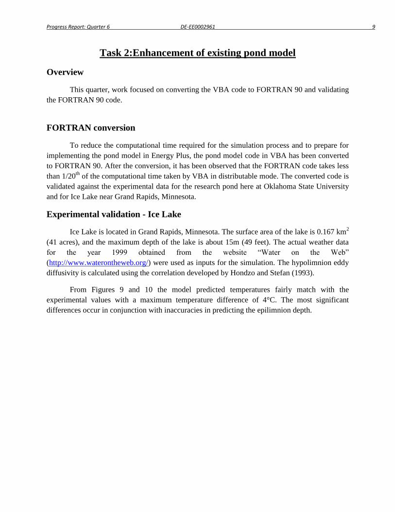
Progress Report: Quarter 6 DE-EE0002961 9
Task 2:Enhancement of existing pond model
Overview
This quarter, work focused on converting the VBA code to FORTRAN 90 and validating
the FORTRAN 90 code.
FORTRAN conversion
To reduce the computational time required for the simulation process and to prepare for
implementing the pond model in Energy Plus, the pond model code in VBA has been converted
to FORTRAN 90. After the conversion, it has been observed that the FORTRAN code takes less
than 1/20th
of the computational time taken by VBA in distributable mode. The converted code is
validated against the experimental data for the research pond here at Oklahoma State University
and for Ice Lake near Grand Rapids, Minnesota.
Experimental validation - Ice Lake
Ice Lake is located in Grand Rapids, Minnesota. The surface area of the lake is 0.167 km2
(41 acres), and the maximum depth of the lake is about 15m (49 feet). The actual weather data
for the year 1999 obtained from the website “Water on the Web”
(http://www.waterontheweb.org/) were used as inputs for the simulation. The hypolimnion eddy
diffusivity is calculated using the correlation developed by Hondzo and Stefan (1993).
From Figures 9 and 10 the model predicted temperatures fairly match with the
experimental values with a maximum temperature difference of 4°C. The most significant
differences occur in conjunction with inaccuracies in predicting the epilimnion depth.
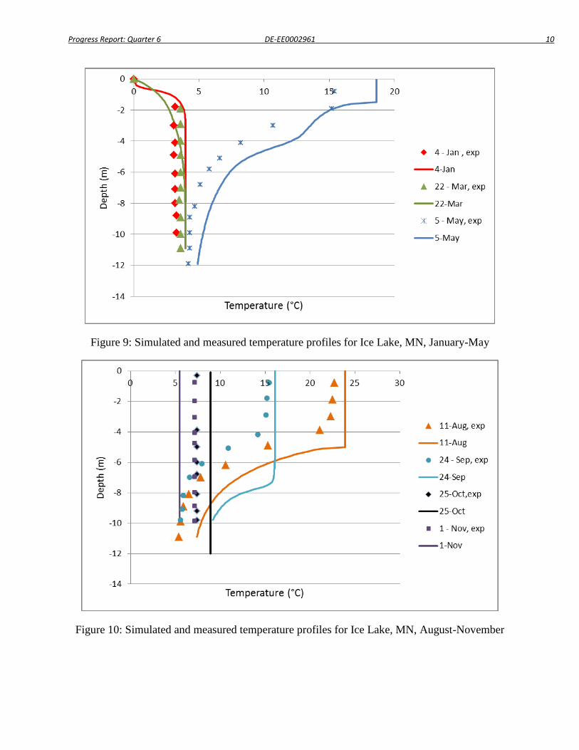
Progress Report: Quarter 6 DE-EE0002961 10
Figure 9: Simulated and measured temperature profiles for Ice Lake, MN, January-May
Figure 10: Simulated and measured temperature profiles for Ice Lake, MN, August-November
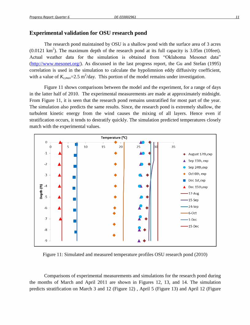
Progress Report: Quarter 6 DE-EE0002961 11
Experimental validation for OSU research pond
The research pond maintained by OSU is a shallow pond with the surface area of 3 acres
(0.0121 km2). The maximum depth of the research pond at its full capacity is 3.05m (10feet).
Actual weather data for the simulation is obtained from “Oklahoma Mesonet data”
(http://www.mesonet.org/). As discussed in the last progress report, the Gu and Stefan (1995)
correlation is used in the simulation to calculate the hypolimnion eddy diffusivity coefficient,
with a value of Kz,max=2.5 m2/day. This portion of the model remains under investigation.
Figure 11 shows comparisons between the model and the experiment, for a range of days
in the latter half of 2010. The experimental measurements are made at approximately midnight.
From Figure 11, it is seen that the research pond remains unstratified for most part of the year.
The simulation also predicts the same results. Since, the research pond is extremely shallow, the
turbulent kinetic energy from the wind causes the mixing of all layers. Hence even if
stratification occurs, it tends to destratify quickly. The simulation predicted temperatures closely
match with the experimental values.
Figure 11: Simulated and measured temperature profiles OSU research pond (2010)
Comparisons of experimental measurements and simulations for the research pond during
the months of March and April 2011 are shown in Figures 12, 13, and 14. The simulation
predicts stratification on March 3 and 12 (Figure 12) , April 5 (Figure 13) and April 12 (Figure
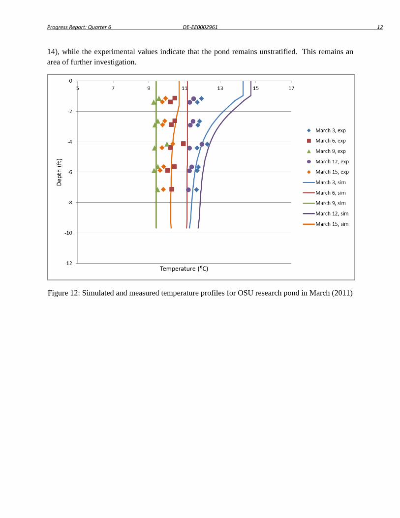
Progress Report: Quarter 6 DE-EE0002961 12
14), while the experimental values indicate that the pond remains unstratified. This remains an
area of further investigation.
Figure 12: Simulated and measured temperature profiles for OSU research pond in March (2011)
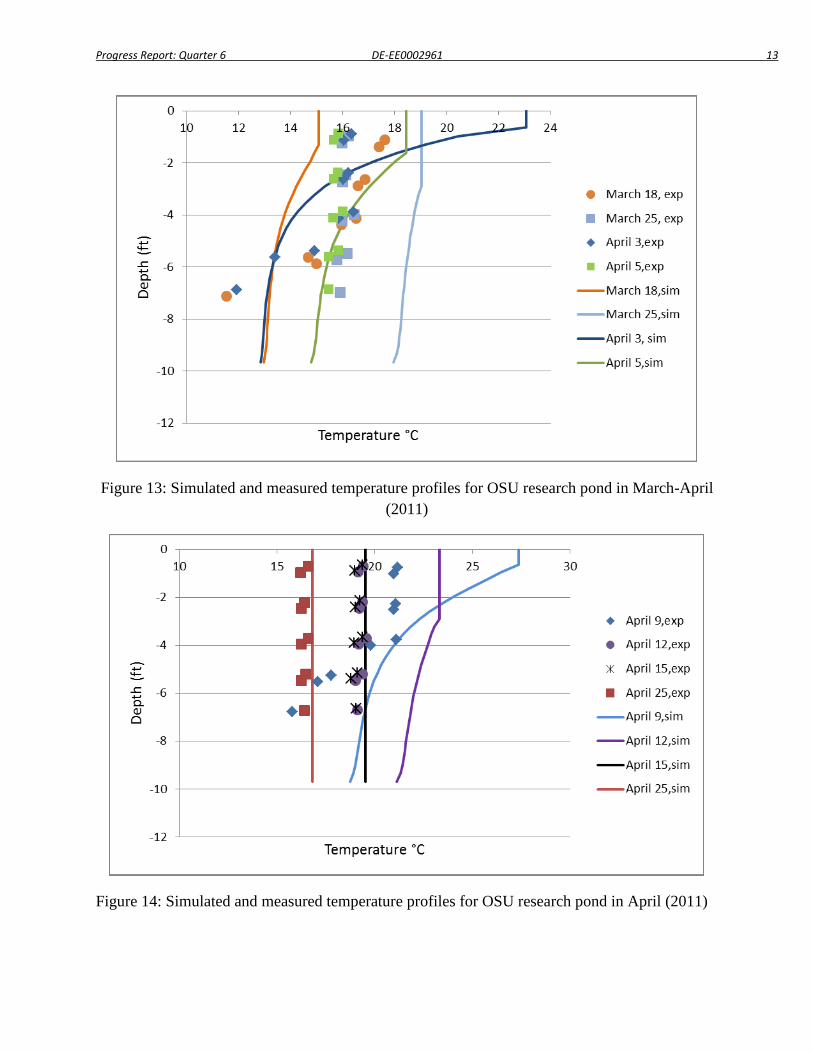
Progress Report: Quarter 6 DE-EE0002961 13
Figure 13: Simulated and measured temperature profiles for OSU research pond in March-April
(2011)
Figure 14: Simulated and measured temperature profiles for OSU research pond in April (2011)
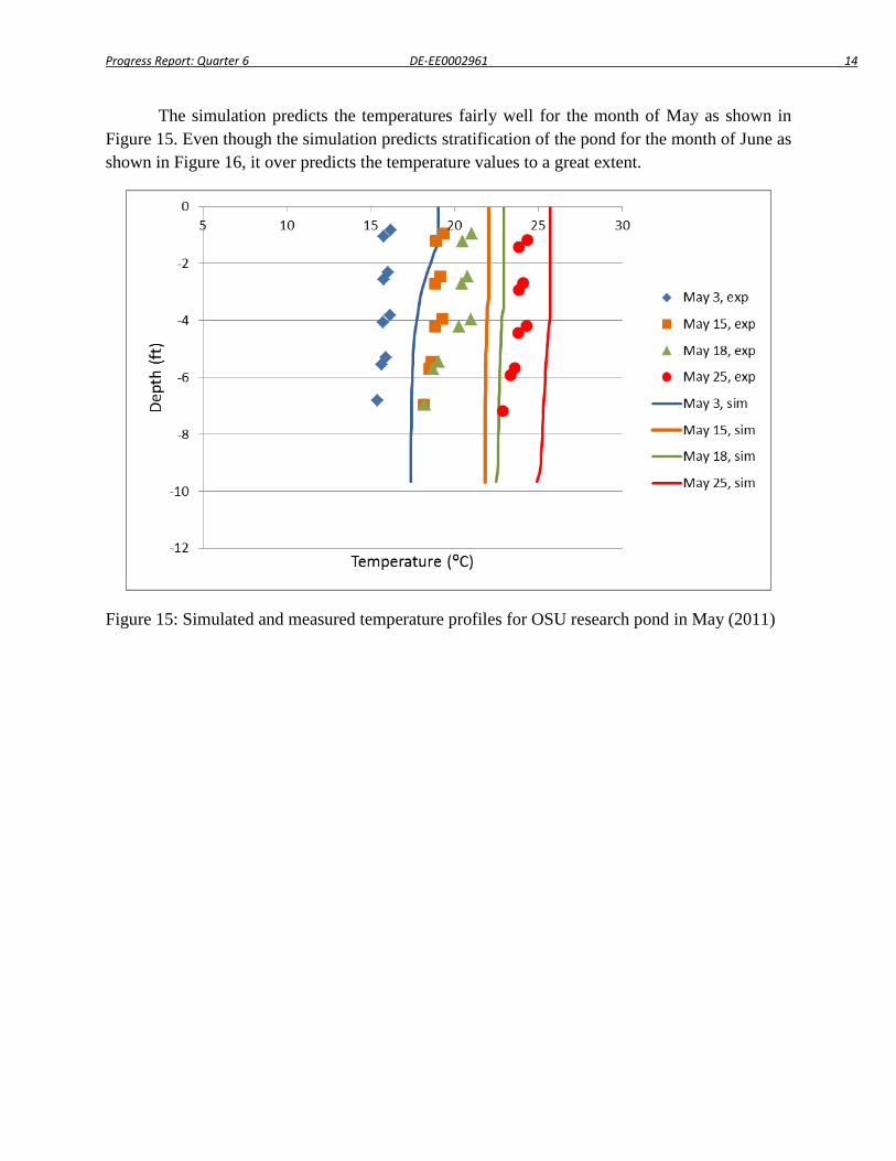
Progress Report: Quarter 6 DE-EE0002961 14
The simulation predicts the temperatures fairly well for the month of May as shown in
Figure 15. Even though the simulation predicts stratification of the pond for the month of June as
shown in Figure 16, it over predicts the temperature values to a great extent.
Figure 15: Simulated and measured temperature profiles for OSU research pond in May (2011)
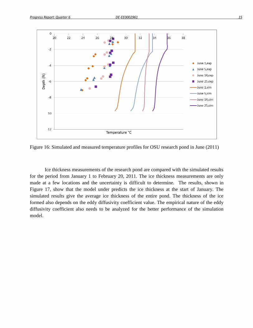
Progress Report: Quarter 6 DE-EE0002961 15
Figure 16: Simulated and measured temperature profiles for OSU research pond in June (2011)
Ice thickness measurements of the research pond are compared with the simulated results
for the period from January 1 to February 20, 2011. The ice thickness measurements are only
made at a few locations and the uncertainty is difficult to determine. The results, shown in
Figure 17, show that the model under predicts the ice thickness at the start of January. The
simulated results give the average ice thickness of the entire pond. The thickness of the ice
formed also depends on the eddy diffusivity coefficient value. The empirical nature of the eddy
diffusivity coefficient also needs to be analyzed for the better performance of the simulation
model.
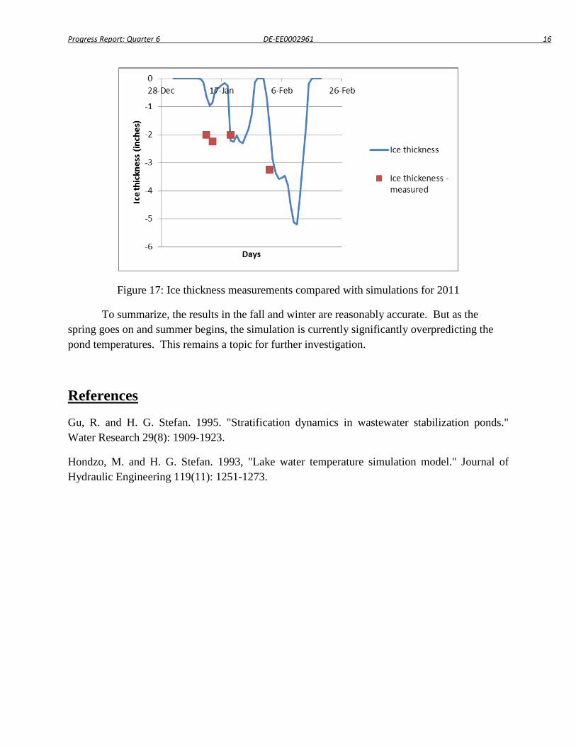
Progress Report: Quarter 6 DE-EE0002961 16
Figure 17: Ice thickness measurements compared with simulations for 2011
To summarize, the results in the fall and winter are reasonably accurate. But as the
spring goes on and summer begins, the simulation is currently significantly overpredicting the
pond temperatures. This remains a topic for further investigation.
References
Gu, R. and H. G. Stefan. 1995. "Stratification dynamics in wastewater stabilization ponds."
Water Research 29(8): 1909-1923.
Hondzo, M. and H. G. Stefan. 1993, "Lake water temperature simulation model." Journal of
Hydraulic Engineering 119(11): 1251-1273.
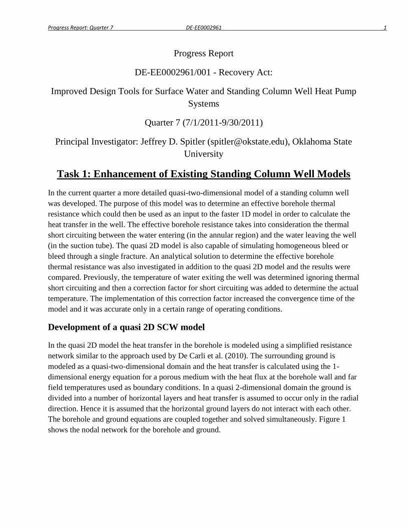
Progress Report: Quarter 7 DE-EE0002961 1
Progress Report
DE-EE0002961/001 - Recovery Act:
Improved Design Tools for Surface Water and Standing Column Well Heat Pump
Systems
Quarter 7 (7/1/2011-9/30/2011)
Principal Investigator: Jeffrey D. Spitler ([email protected]), Oklahoma State
University
Task 1: Enhancement of Existing Standing Column Well Models
In the current quarter a more detailed quasi-two-dimensional model of a standing column well
was developed. The purpose of this model was to determine an effective borehole thermal
resistance which could then be used as an input to the faster 1D model in order to calculate the
heat transfer in the well. The effective borehole resistance takes into consideration the thermal
short circuiting between the water entering (in the annular region) and the water leaving the well
(in the suction tube). The quasi 2D model is also capable of simulating homogeneous bleed or
bleed through a single fracture. An analytical solution to determine the effective borehole
thermal resistance was also investigated in addition to the quasi 2D model and the results were
compared. Previously, the temperature of water exiting the well was determined ignoring thermal
short circuiting and then a correction factor for short circuiting was added to determine the actual
temperature. The implementation of this correction factor increased the convergence time of the
model and it was accurate only in a certain range of operating conditions.
Development of a quasi 2D SCW model
In the quasi 2D model the heat transfer in the borehole is modeled using a simplified resistance
network similar to the approach used by De Carli et al. (2010). The surrounding ground is
modeled as a quasi-two-dimensional domain and the heat transfer is calculated using the 1-
dimensional energy equation for a porous medium with the heat flux at the borehole wall and far
field temperatures used as boundary conditions. In a quasi 2-dimensional domain the ground is
divided into a number of horizontal layers and heat transfer is assumed to occur only in the radial
direction. Hence it is assumed that the horizontal ground layers do not interact with each other.
The borehole and ground equations are coupled together and solved simultaneously. Figure 1
shows the nodal network for the borehole and ground.
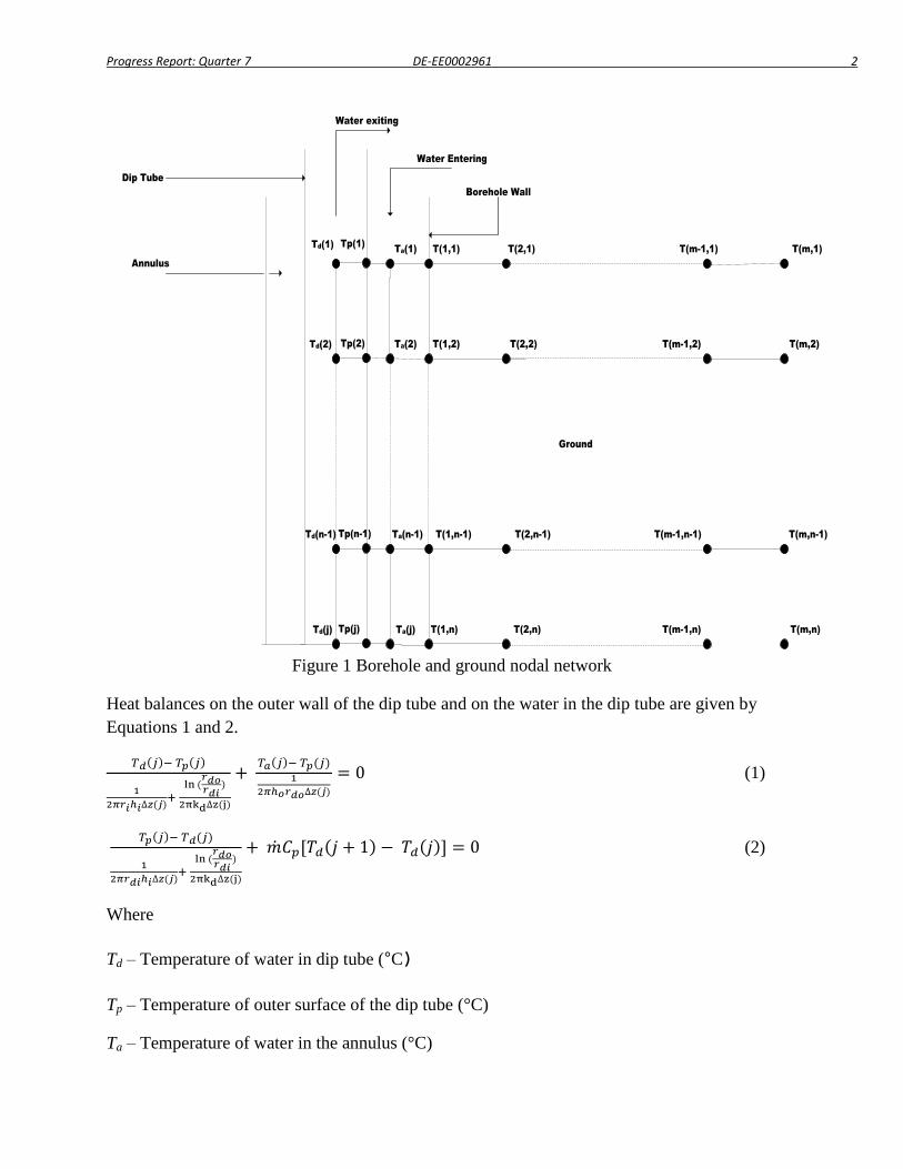
Progress Report: Quarter 7 DE-EE0002961 2
Dip Tube
Annulus
Borehole Wall
Water exiting
Water Entering
Ground
Td(1)T(1,1)
Td(j)
Td(n-1)
Td(2)
Ta(j)
Ta(n-1)
Ta(2)
Ta(1)
T(1,n)
T(1,n-1)
T(1,2)
T(2,1)
T(m-1,n-1)T(2,n-1)
T(2,2)
T(2,n)
T(m-1,2)
T(m-1,1)
T(m-1,n)
T(m,1)
T(m,2)
T(m,n-1)
T(m,n)
Tp(1)
Tp(2)
Tp(n-1)
Tp(j)
Figure 1 Borehole and ground nodal network
Heat balances on the outer wall of the dip tube and on the water in the dip tube are given by
Equations 1 and 2.
(1)
(2)
Where
Td – Temperature of water in dip tube (°C)
Tp – Temperature of outer surface of the dip tube (°C)
Ta – Temperature of water in the annulus (°C)
Progress Report: Quarter 7 DE-EE0002961 3
ri – Dip tube inner radius (m)
ro – Dip tube outer radius (m)
hi – Convection coefficient of water inside the dip tube (W/m2-K)
ho – Convection coefficient of water in the annulus (W/m2-K)
kd – Dip tube thermal conductivity (W/m-K)
Cp – Specific heat of water (J/kg-K)
- Mass flow rate in the system (kg/s)
Δz – Grid spacing in the vertical direction (m)
j – Node number (-)
A heat balance on the fluid in the annular region is given by Equation 3. It is more complicated
because there are different quantities of water entering from 2 directions (top and side) at
different temperatures during bleed. The water entering from the top is at the temperature of the
previous node and that entering from the side during bleed is at the borehole wall temperature.
= 0 (3)
Where,
T(1,j) – Borehole wall temperature (°C)
rb – Borehole radius (m)
– Quantity of water entering the borehole at node j in the annulus from the ground (kg/s)
- Quantity of water entering node j in the annulus from the previous node (kg/s)
The term refers to the sum of the quantity of water entering the well from the heat pump and
the quantity of water that has entered the well from the ground at all the previous nodes during
bleed operation. In the case of homogenous bleed the term has a constant value at all nodes
while in the case of bleed through a single fracture its value is zero at all nodes except the node
representing the fracture in the ground.
Progress Report: Quarter 7 DE-EE0002961 4
Equation 4 represents the coupling between the borehole and the ground and the 1D energy
equation for a porous medium used to determine the heat transfer in the ground is given by
Equation 5.
(4)
(5)
(6)
(7)
(8)
Where,
q” – Heat flux at the borehole wall (W/m2)
n – Porosity (-)
α – Volumetric heat capacity of the ground (J/m3-K)
β – Volumetric heat capacity of water (J/m3-K)
Vr – Linear ground water velocity during bleed at node (i,j) in the ground (m/s)
keff – Effective thermal conductivity of ground (W/m-K)
r - Radius measured from center of borehole (m)
Cps – Specific heat capacity of ground (J/kg-K)
ρs – Density of ground (kg/m3)
kl, ks – Thermal conductivity of water and ground, respectively (W/m-K)
Equation 5 is solved for each horizontal ground layer using a fully implicit finite difference
method. The heat flux is used as a boundary condition at the borehole wall and the far field
temperature is used as the other boundary condition. The domain size (180 m) and grid spacing
are based on the sensitivity analysis done by Deng (2004). The effective borehole thermal
resistance (Rb) is determined using Equation 9.
(9)
Where,
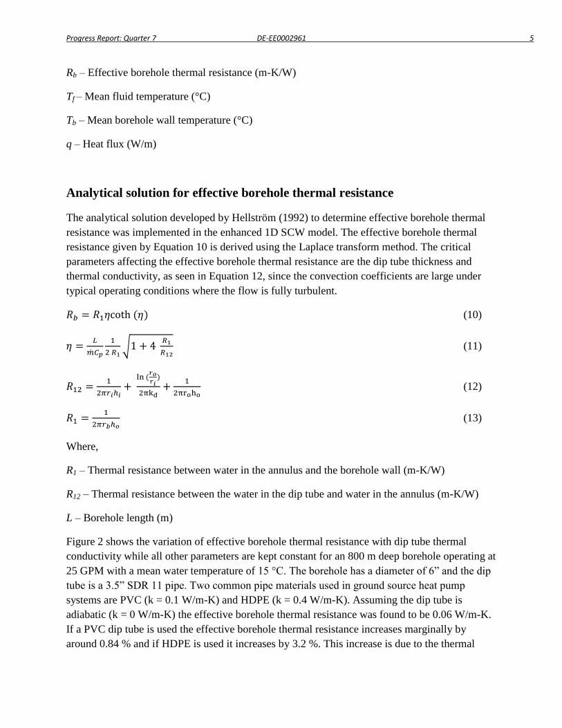
Progress Report: Quarter 7 DE-EE0002961 5
Rb – Effective borehole thermal resistance (m-K/W)
Tf – Mean fluid temperature (°C)
Tb – Mean borehole wall temperature (°C)
q – Heat flux (W/m)
Analytical solution for effective borehole thermal resistance
The analytical solution developed by Hellström (1992) to determine effective borehole thermal
resistance was implemented in the enhanced 1D SCW model. The effective borehole thermal
resistance given by Equation 10 is derived using the Laplace transform method. The critical
parameters affecting the effective borehole thermal resistance are the dip tube thickness and
thermal conductivity, as seen in Equation 12, since the convection coefficients are large under
typical operating conditions where the flow is fully turbulent.
(10)
(11)
(12)
(13)
Where,
R1 – Thermal resistance between water in the annulus and the borehole wall (m-K/W)
R12 – Thermal resistance between the water in the dip tube and water in the annulus (m-K/W)
L – Borehole length (m)
Figure 2 shows the variation of effective borehole thermal resistance with dip tube thermal
conductivity while all other parameters are kept constant for an 800 m deep borehole operating at
25 GPM with a mean water temperature of 15 °C. The borehole has a diameter of 6” and the dip
tube is a 3.5” SDR 11 pipe. Two common pipe materials used in ground source heat pump
systems are PVC (k = 0.1 W/m-K) and HDPE (k = 0.4 W/m-K). Assuming the dip tube is
adiabatic (k = 0 W/m-K) the effective borehole thermal resistance was found to be 0.06 W/m-K.
If a PVC dip tube is used the effective borehole thermal resistance increases marginally by
around 0.84 % and if HDPE is used it increases by 3.2 %. This increase is due to the thermal
Progress Report: Quarter 7 DE-EE0002961 6
short-circuiting caused due to the heat transfer between the water in the dip tube and water in the
annulus. Hence it is concluded that when a PVC dip tube is used thermal short circuiting is not
significant. This is also verified using the quasi 2D SCW model.
Figure 2. Effective borehole thermal resistance vs Dip tube thermal conductivity
Comparison of quasi 2D SCW model and analytical solution
For a ground source heat pump system operating in heating mode the first 1000 hours of exiting
water temperatures obtained using the 1D SCW model with the analytical solution to determine
effective borehole thermal resistance and the quasi 2D model are shown in Figure 3. It can be
seen that the 1D SCW Model has a slightly higher exiting water temperatures than the quasi 2D
model. The RMSE error was found to be approximately 0.4 °C. Although the differences are
fairly small, understanding the causes is important to our research and further investigation is
underway.
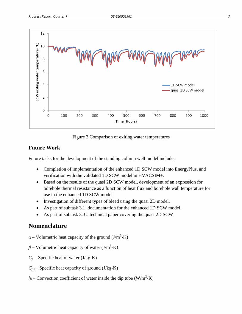
Progress Report: Quarter 7 DE-EE0002961 7
Figure 3 Comparison of exiting water temperatures
Future Work
Future tasks for the development of the standing column well model include:
Completion of implementation of the enhanced 1D SCW model into EnergyPlus, and
verification with the validated 1D SCW model in HVACSIM+.
Based on the results of the quasi 2D SCW model, development of an expression for
borehole thermal resistance as a function of heat flux and borehole wall temperature for
use in the enhanced 1D SCW model.
Investigation of different types of bleed using the quasi 2D model.
As part of subtask 3.1, documentation for the enhanced 1D SCW model.
As part of subtask 3.3 a technical paper covering the quasi 2D SCW
Nomenclature
α – Volumetric heat capacity of the ground (J/m3-K)
β – Volumetric heat capacity of water (J/m3-K)
Cp – Specific heat of water (J/kg-K)
Cps – Specific heat capacity of ground (J/kg-K)
hi – Convection coefficient of water inside the dip tube (W/m2-K)
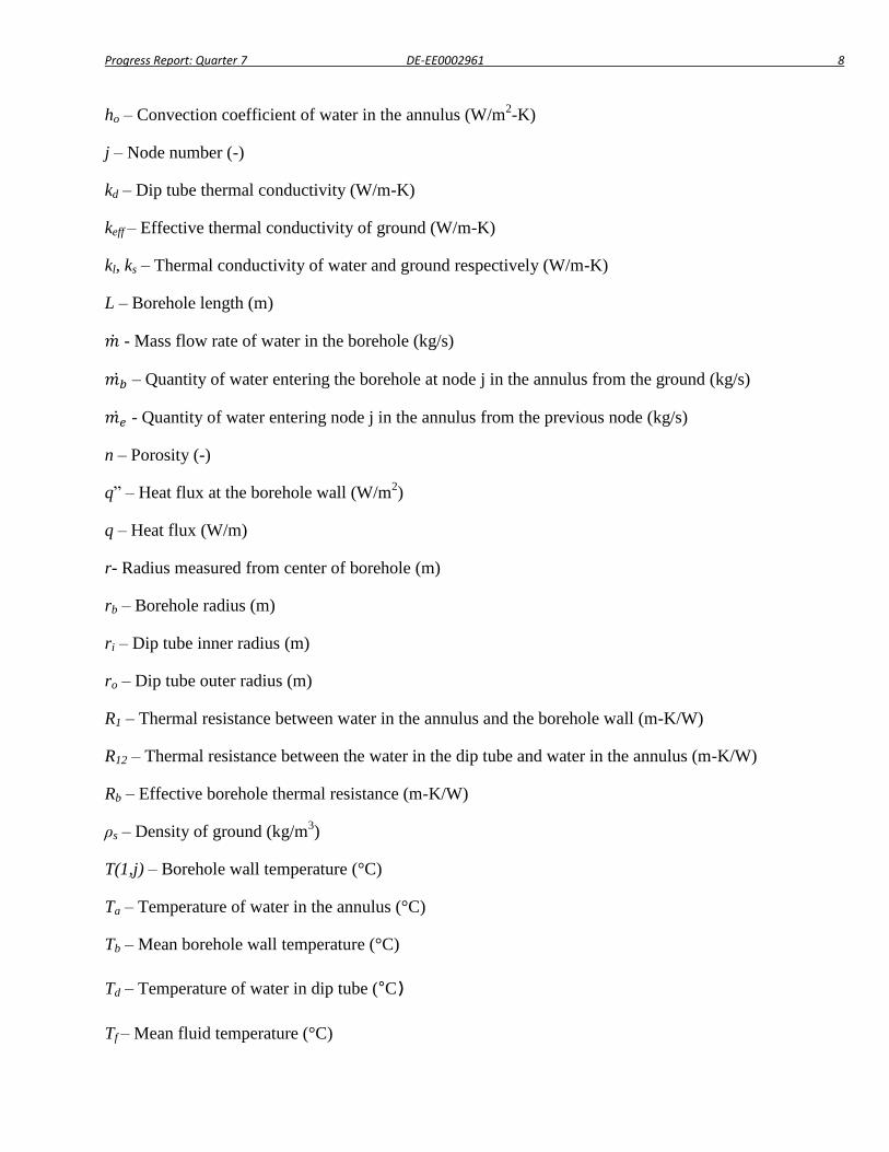
Progress Report: Quarter 7 DE-EE0002961 8
ho – Convection coefficient of water in the annulus (W/m2-K)
j – Node number (-)
kd – Dip tube thermal conductivity (W/m-K)
keff – Effective thermal conductivity of ground (W/m-K)
kl, ks – Thermal conductivity of water and ground respectively (W/m-K)
L – Borehole length (m)
- Mass flow rate of water in the borehole (kg/s)
– Quantity of water entering the borehole at node j in the annulus from the ground (kg/s)
- Quantity of water entering node j in the annulus from the previous node (kg/s)
n – Porosity (-)
q” – Heat flux at the borehole wall (W/m2)
q – Heat flux (W/m)
r- Radius measured from center of borehole (m)
rb – Borehole radius (m)
ri – Dip tube inner radius (m)
ro – Dip tube outer radius (m)
R1 – Thermal resistance between water in the annulus and the borehole wall (m-K/W)
R12 – Thermal resistance between the water in the dip tube and water in the annulus (m-K/W)
Rb – Effective borehole thermal resistance (m-K/W)
ρs – Density of ground (kg/m3)
T(1,j) – Borehole wall temperature (°C)
Ta – Temperature of water in the annulus (°C)
Tb – Mean borehole wall temperature (°C)
Td – Temperature of water in dip tube (°C)
Tf – Mean fluid temperature (°C)
Progress Report: Quarter 7 DE-EE0002961 9
Tp – Temperature of outer surface of the dip tube (°C)
Vr – Linear ground water velocity during bleed at node (i,j) in the ground (m/s)
Δz – Grid spacing in the vertical direction (m)
References
De Carli, M., M.Tonon, A.Zarrella, and R.Zecchin. 2010. A computational capacity resistance
model (CaRM) for vertical ground-coupled heat exchangers. Renewable Energy
35(7):1537-1550.
Deng, Z. 2004. Modeling of standing column wells in ground source heat pump systems. Ph.D.
thesis, Oklahoma State University, Stillwater, OK.
Hellström, G. 1991. Ground Heat Storage: Thermal analysis of duct storage systems- I. Theory.
University of Lund, Sweden.
Task 2 : Enhancement of existing pond model and implementation
in EnergyPlus
Overview
In this quarter work on the pond model focused on enhancing the accuracy of the model by
restructuring the code to calculate the water temperatures iteratively and also for implementation
in EnergyPlus.
Iterative temperature calculation
The model predicts the water temperature profiles by solving the one-dimensional heat transfer
equation given by Hondzo and Stefan (1993):
(14)
Where
A is the horizontal area of the lake as a function of the depth (z) [m2]
T is the water temperature as a function of the depth (z) and time (t) [°C]
K is the vertical eddy diffusion coefficient [m2/day]
Q is the internal distribution of heat to each water layer due to the absorption of
solar radiation in the water column. It is a function of both depth (z) and time (t)
[J/m3-day].
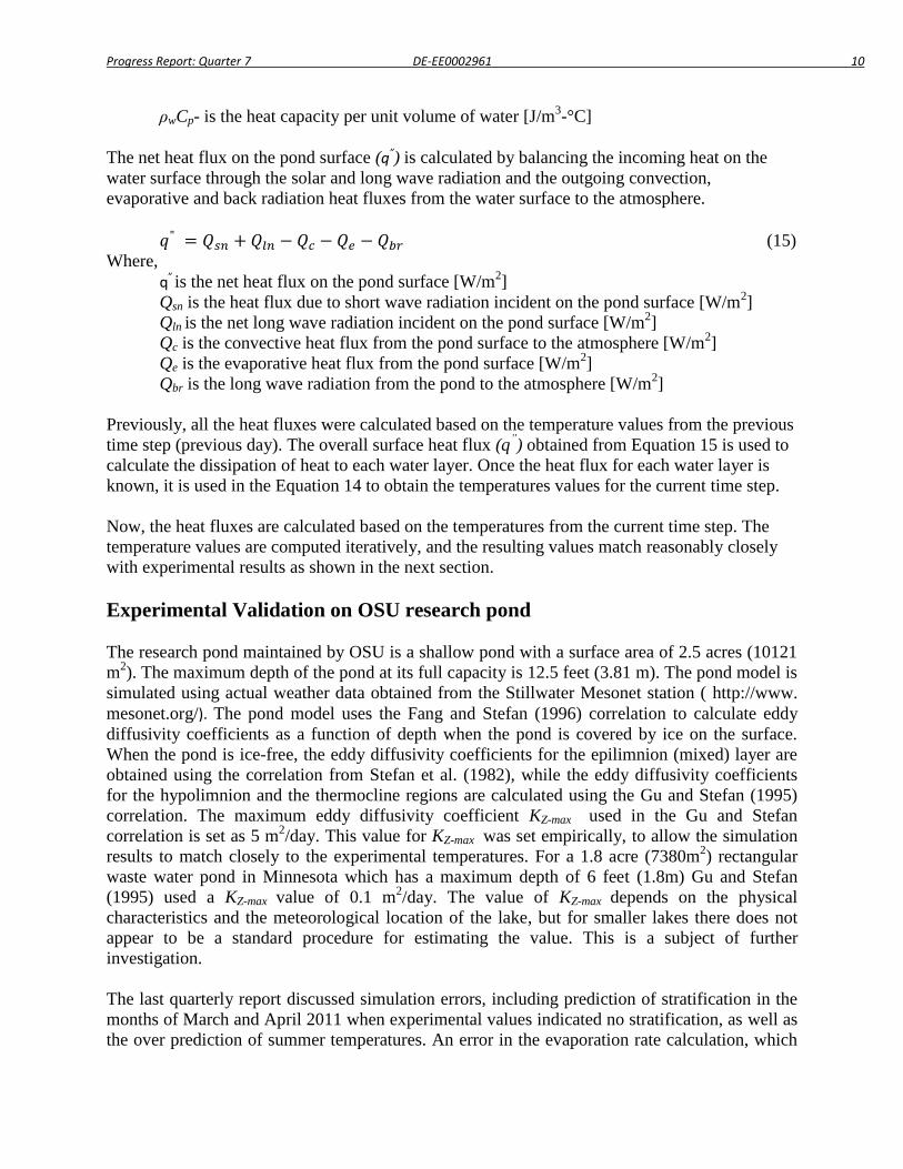
Progress Report: Quarter 7 DE-EE0002961 10
ρwCp- is the heat capacity per unit volume of water [J/m3-°C]
The net heat flux on the pond surface (q”) is calculated by balancing the incoming heat on the
water surface through the solar and long wave radiation and the outgoing convection,
evaporative and back radiation heat fluxes from the water surface to the atmosphere.
(15)
Where,
q” is the net heat flux on the pond surface [W/m2]
Qsn is the heat flux due to short wave radiation incident on the pond surface [W/m2]
Qln is the net long wave radiation incident on the pond surface [W/m2]
Qc is the convective heat flux from the pond surface to the atmosphere [W/m2]
Qe is the evaporative heat flux from the pond surface [W/m2]
Qbr is the long wave radiation from the pond to the atmosphere [W/m2]
Previously, all the heat fluxes were calculated based on the temperature values from the previous
time step (previous day). The overall surface heat flux (q”) obtained from Equation 15 is used to
calculate the dissipation of heat to each water layer. Once the heat flux for each water layer is
known, it is used in the Equation 14 to obtain the temperatures values for the current time step.
Now, the heat fluxes are calculated based on the temperatures from the current time step. The
temperature values are computed iteratively, and the resulting values match reasonably closely
with experimental results as shown in the next section.
Experimental Validation on OSU research pond
The research pond maintained by OSU is a shallow pond with a surface area of 2.5 acres (10121
m2). The maximum depth of the pond at its full capacity is 12.5 feet (3.81 m). The pond model is
simulated using actual weather data obtained from the Stillwater Mesonet station ( http://www.
mesonet.org/). The pond model uses the Fang and Stefan (1996) correlation to calculate eddy
diffusivity coefficients as a function of depth when the pond is covered by ice on the surface.
When the pond is ice-free, the eddy diffusivity coefficients for the epilimnion (mixed) layer are
obtained using the correlation from Stefan et al. (1982), while the eddy diffusivity coefficients
for the hypolimnion and the thermocline regions are calculated using the Gu and Stefan (1995)
correlation. The maximum eddy diffusivity coefficient KZ-max used in the Gu and Stefan
correlation is set as 5 m2/day. This value for KZ-max was set empirically, to allow the simulation
results to match closely to the experimental temperatures. For a 1.8 acre (7380m2) rectangular
waste water pond in Minnesota which has a maximum depth of 6 feet (1.8m) Gu and Stefan
(1995) used a KZ-max value of 0.1 m2/day. The value of KZ-max depends on the physical
characteristics and the meteorological location of the lake, but for smaller lakes there does not
appear to be a standard procedure for estimating the value. This is a subject of further
investigation.
The last quarterly report discussed simulation errors, including prediction of stratification in the
months of March and April 2011 when experimental values indicated no stratification, as well as
the over prediction of summer temperatures. An error in the evaporation rate calculation, which
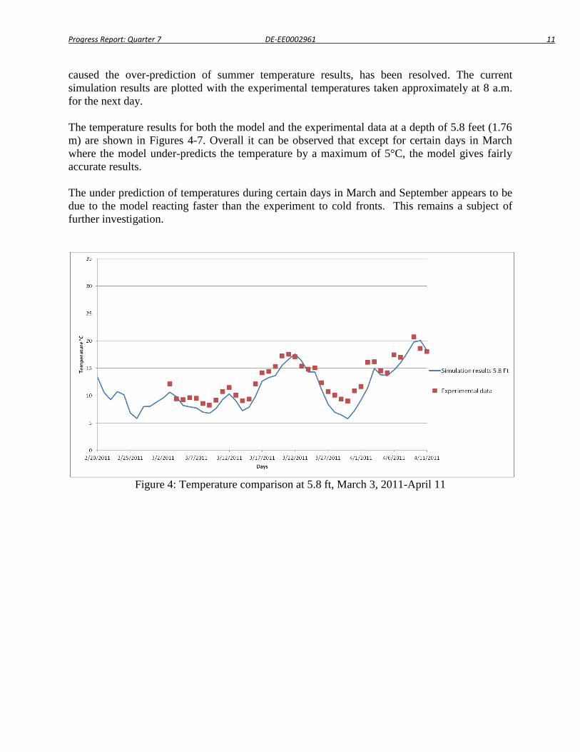
Progress Report: Quarter 7 DE-EE0002961 11
caused the over-prediction of summer temperature results, has been resolved. The current
simulation results are plotted with the experimental temperatures taken approximately at 8 a.m.
for the next day.
The temperature results for both the model and the experimental data at a depth of 5.8 feet (1.76
m) are shown in Figures 4-7. Overall it can be observed that except for certain days in March
where the model under-predicts the temperature by a maximum of 5°C, the model gives fairly
accurate results.
The under prediction of temperatures during certain days in March and September appears to be
due to the model reacting faster than the experiment to cold fronts. This remains a subject of
further investigation.
Figure 4: Temperature comparison at 5.8 ft, March 3, 2011-April 11
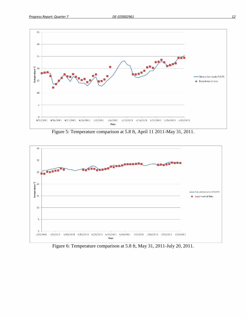
Progress Report: Quarter 7 DE-EE0002961 12
Figure 5: Temperature comparison at 5.8 ft, April 11 2011-May 31, 2011.
Figure 6: Temperature comparison at 5.8 ft, May 31, 2011-July 20, 2011.
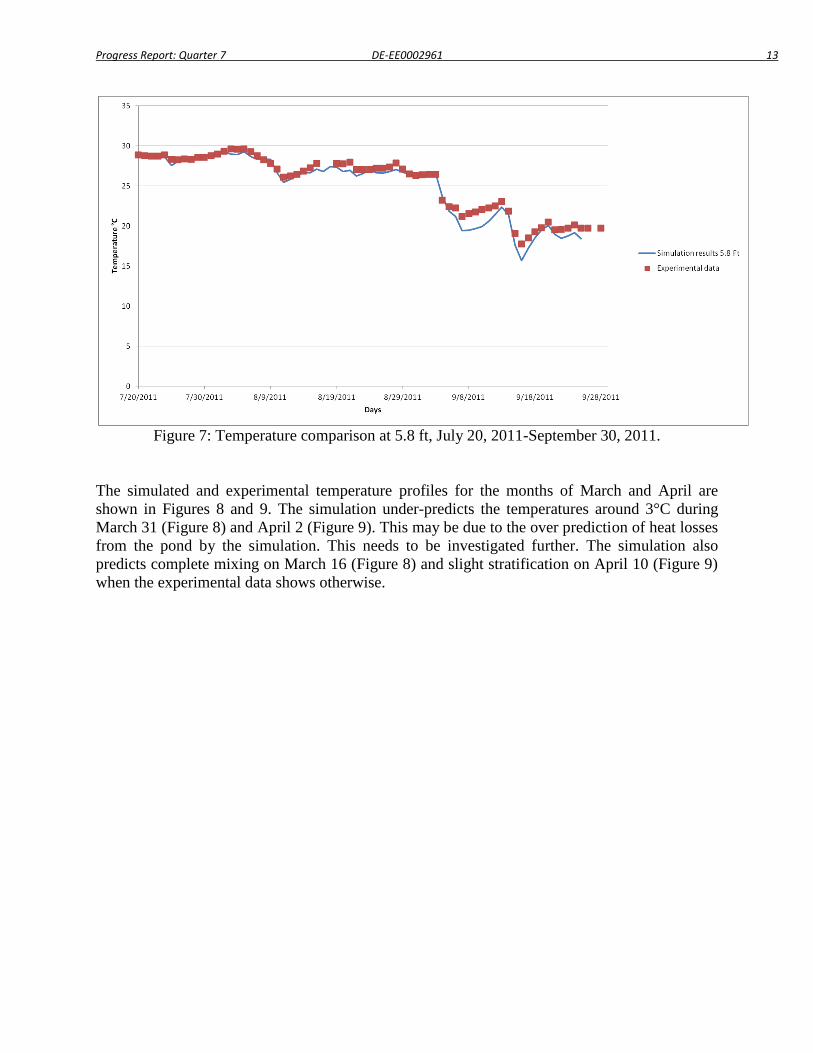
Progress Report: Quarter 7 DE-EE0002961 13
Figure 7: Temperature comparison at 5.8 ft, July 20, 2011-September 30, 2011.
The simulated and experimental temperature profiles for the months of March and April are
shown in Figures 8 and 9. The simulation under-predicts the temperatures around 3°C during
March 31 (Figure 8) and April 2 (Figure 9). This may be due to the over prediction of heat losses
from the pond by the simulation. This needs to be investigated further. The simulation also
predicts complete mixing on March 16 (Figure 8) and slight stratification on April 10 (Figure 9)
when the experimental data shows otherwise.
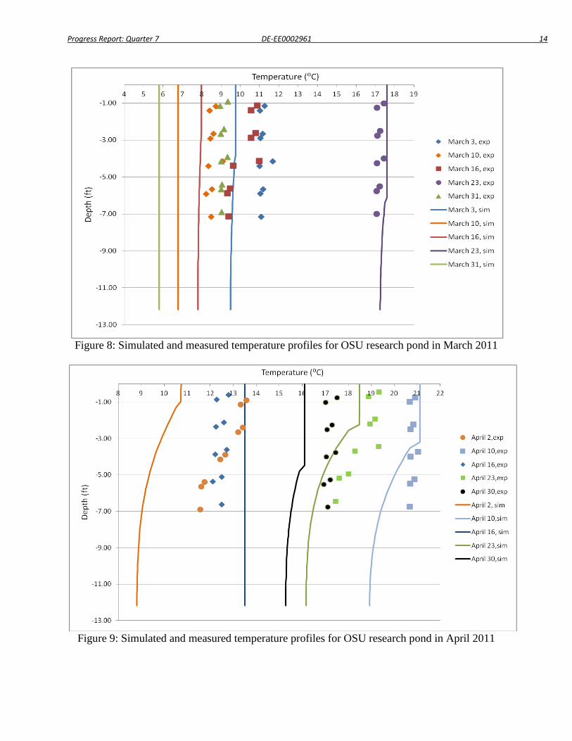
Progress Report: Quarter 7 DE-EE0002961 14
Figure 8: Simulated and measured temperature profiles for OSU research pond in March 2011
Figure 9: Simulated and measured temperature profiles for OSU research pond in April 2011
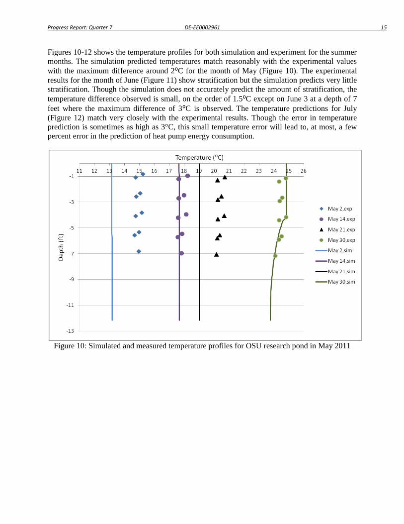
Progress Report: Quarter 7 DE-EE0002961 15
Figures 10-12 shows the temperature profiles for both simulation and experiment for the summer
months. The simulation predicted temperatures match reasonably with the experimental values
with the maximum difference around 2⁰C for the month of May (Figure 10). The experimental
results for the month of June (Figure 11) show stratification but the simulation predicts very little
stratification. Though the simulation does not accurately predict the amount of stratification, the
temperature difference observed is small, on the order of 1.5⁰C except on June 3 at a depth of 7
feet where the maximum difference of 3⁰C is observed. The temperature predictions for July
(Figure 12) match very closely with the experimental results. Though the error in temperature
prediction is sometimes as high as 3°C, this small temperature error will lead to, at most, a few
percent error in the prediction of heat pump energy consumption.
Figure 10: Simulated and measured temperature profiles for OSU research pond in May 2011
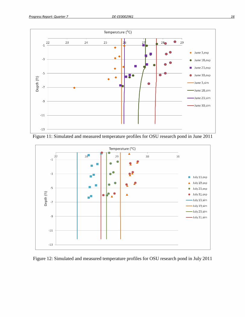
Progress Report: Quarter 7 DE-EE0002961 16
Figure 11: Simulated and measured temperature profiles for OSU research pond in June 2011
Figure 12: Simulated and measured temperature profiles for OSU research pond in July 2011
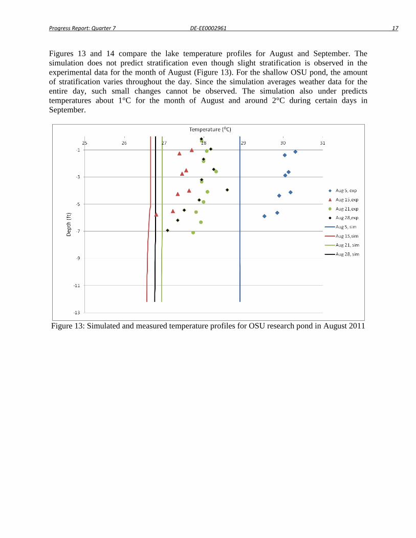
Progress Report: Quarter 7 DE-EE0002961 17
Figures 13 and 14 compare the lake temperature profiles for August and September. The
simulation does not predict stratification even though slight stratification is observed in the
experimental data for the month of August (Figure 13). For the shallow OSU pond, the amount
of stratification varies throughout the day. Since the simulation averages weather data for the
entire day, such small changes cannot be observed. The simulation also under predicts
temperatures about 1°C for the month of August and around 2°C during certain days in
September.
Figure 13: Simulated and measured temperature profiles for OSU research pond in August 2011
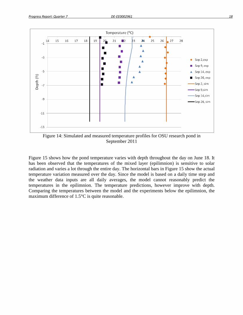
Progress Report: Quarter 7 DE-EE0002961 18
Figure 14: Simulated and measured temperature profiles for OSU research pond in
September 2011
Figure 15 shows how the pond temperature varies with depth throughout the day on June 18. It
has been observed that the temperatures of the mixed layer (epilimnion) is sensitive to solar
radiation and varies a lot through the entire day. The horizontal bars in Figure 15 show the actual
temperature variation measured over the day. Since the model is based on a daily time step and
the weather data inputs are all daily averages, the model cannot reasonably predict the
temperatures in the epilimnion. The temperature predictions, however improve with depth.
Comparing the temperatures between the model and the experiments below the epilimnion, the
maximum difference of 1.5°C is quite reasonable.
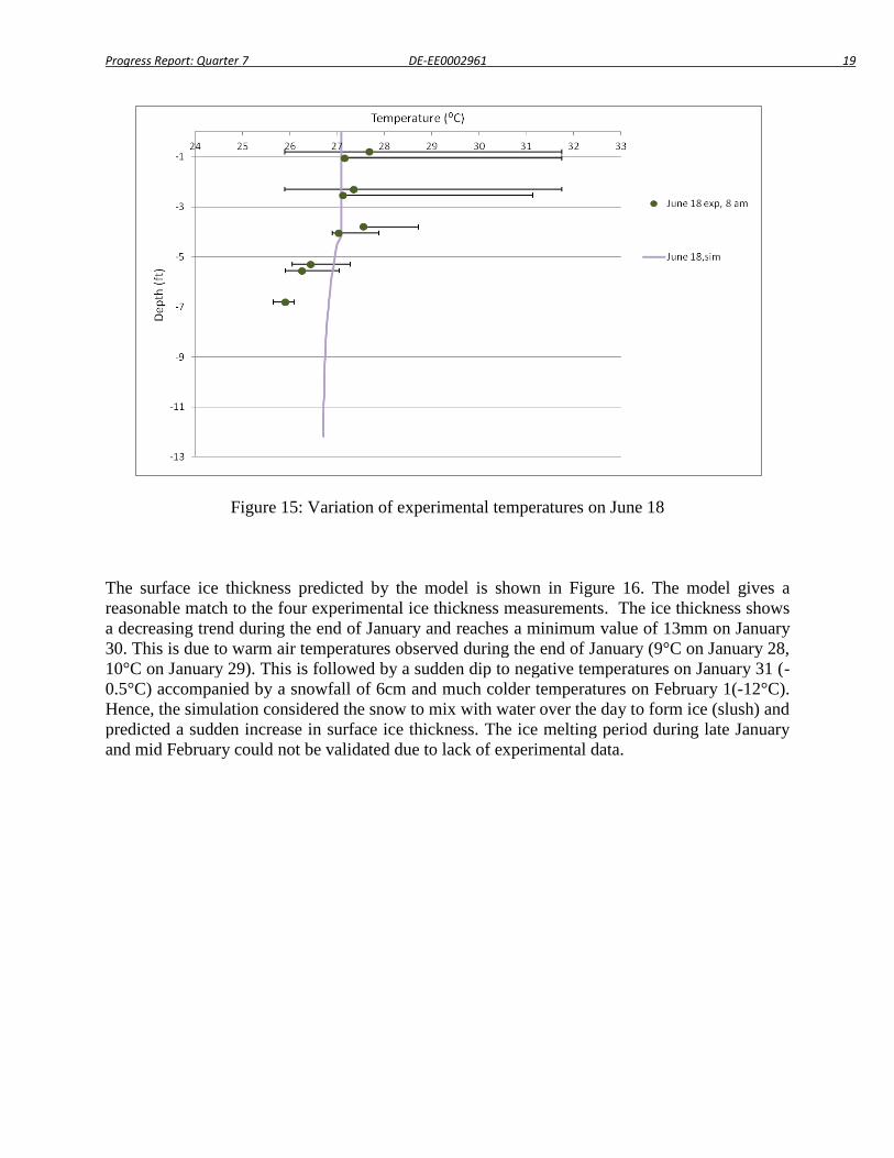
Progress Report: Quarter 7 DE-EE0002961 19
Figure 15: Variation of experimental temperatures on June 18
The surface ice thickness predicted by the model is shown in Figure 16. The model gives a
reasonable match to the four experimental ice thickness measurements. The ice thickness shows
a decreasing trend during the end of January and reaches a minimum value of 13mm on January
30. This is due to warm air temperatures observed during the end of January (9°C on January 28,
10°C on January 29). This is followed by a sudden dip to negative temperatures on January 31 (-
0.5°C) accompanied by a snowfall of 6cm and much colder temperatures on February 1(-12°C).
Hence, the simulation considered the snow to mix with water over the day to form ice (slush) and
predicted a sudden increase in surface ice thickness. The ice melting period during late January
and mid February could not be validated due to lack of experimental data.
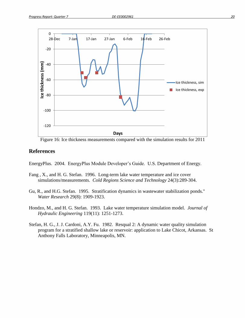
Progress Report: Quarter 7 DE-EE0002961 20
Figure 16: Ice thickness measurements compared with the simulation results for 2011
References
EnergyPlus. 2004. EnergyPlus Module Developer’s Guide. U.S. Department of Energy.
Fang , X., and H. G. Stefan. 1996. Long-term lake water temperature and ice cover
simulations/measurements. Cold Regions Science and Technology 24(3):289-304.
Gu, R., and H.G. Stefan. 1995. Stratification dynamics in wastewater stabilization ponds."
Water Research 29(8): 1909-1923.
Hondzo, M., and H. G. Stefan. 1993. Lake water temperature simulation model. Journal of
Hydraulic Engineering 119(11): 1251-1273.
Stefan, H. G., J. J. Cardoni, A.Y. Fu. 1982. Resqual 2: A dynamic water quality simulation
program for a stratified shallow lake or reservoir: application to Lake Chicot, Arkansas. St
Anthony Falls Laboratory, Minneapolis, MN.
-120
-100
-80
-60
-40
-20
0
28-Dec 7-Jan 17-Jan 27-Jan 6-Feb 16-Feb 26-Feb Ic
e t
hic
knes
s (m
m)
Days
Ice thickness, sim
Ice thickness, exp

DE-EE0002961
Oklahoma State University
FY2012, Q8
Page 1 of 45
Quarterly Research Performance Progress Report
Federal Agency and Organization: DOE EERE – Geothermal Technologies Program
Recipient Organization: Oklahoma State University
DUNS Number: 049987720
Recipient Address: Stillwater, OK 74078
Award Number: DE-EE0002961/001
Project Title: Improved Design Tools for Surface Water and Standing Column Well Heat Pump
Systems
Project Period: October 1, 2010 to February 28, 2012
Principal Investigator: Jeffrey D. Spitler
Regents Professor and C.M. Leonard Professor
405-744-5900
Date of Report Submission: Jan 30, 2012
Reporting Period: October 1, 2011 to December 31, 2011
Report Frequency: Quarterly
Project Partners: n/a
DOE Project Team: DOE Contracting Officer – Genevieve Wozniak
DOE Project Officer – Ava Coy
Project Monitor – Sara Gonnion

DE-EE0002961
Oklahoma State University
FY2012, Q8
Page 2 of 45
STATUS / ACCOMPLISHMENTS
Project Status Summary: The project is divided into the Standing Column Well (SCW) and
Surface Water (SW) tracks. In the SCW track the main objectives are the enhancement of an
existing 1D SCW model and implementation of the enhanced model in EnergyPlus and in a
design tool. The enhancements to the model involved implementing a separate bleed control
strategy and developing a suitable model to account for the effects of natural convection. The
model was then validated against experimental data from a public library in Haverhill, MA.
During the current reporting period a quasi 2D SCW model was developed to investigate thermal
short circuiting and effects of different types of bleed on the heat transfer. The results of the
quasi 2D SCW model will be presented in a technical conference in May 2012. Additionally,
input files were developed for the implementation of the 1D SCW model in EnergyPlus and,
integration of the model into the plant loop is currently in progress. In order to be implemented
in a design tool the 1D SCW model is currently being modified to run in the VisualBasic
programming environment.
The main objectives of the SW track are to enhance the existing pond model and to implement it
in both EnergyPlus and a ground heat exchanger design tool. The existing pond model in
EnergyPlus was enhanced by including the effects of stratification and modeling both the ice
formation on the heat exchanger coils and on the pond surface. During this quarter, the enhanced
pond model code has been restructured in order to fit into EnergyPlus and implementation was
completed. The model was validated using 11 months of depth-varying temperatures from the
Oklahoma State University research pond. Additionally, the pond model was further enhanced
by including a robust model to determine the heat transfer for various shapes of heat exchangers.
Work this quarter also focused on implementing the enhanced pond model into a design tool for
ground heat exchangers.
Task 1.0 – Enhancement of Existing Standing Column Well Model
1. Planned Activities:
Subtask 1.1: Development and validation of SCW model with separate bleed control
Last quarter‟s planned activity was to develop a quasi 2D model to investigate thermal
short circuiting and possible non-homogeneous bleed.
Subtask 1.2: Testing of SCW model with various bleed control strategies
Last quarter‟s planned activity was to investigate the effects of non-homogeneous bleed
on a constant bleed case.
2. Actual Accomplishments:
Subtask 1.1: Development and validation of SCW model with separate bleed control
One of the main reasons for the development of a quasi 2D model was to investigate the
effect of thermal short circuiting between the water in the dip tube and the water in the
annulus. The short circuiting analysis was done for three different dip tube thermal
conductivities. The conductivities chosen were 0.1, 0.4 and 16 W/m-K corresponding to
pipe materials of PVC, HDPE and stainless steel. Though a stainless steel dip tube is
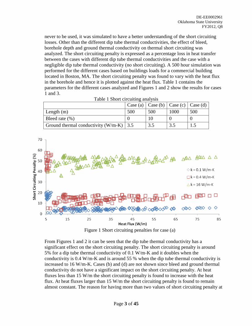
DE-EE0002961
Oklahoma State University
FY2012, Q8
Page 3 of 45
never to be used, it was simulated to have a better understanding of the short circuiting
losses. Other than the different dip tube thermal conductivities, the effect of bleed,
borehole depth and ground thermal conductivity on thermal short circuiting was
analyzed. The short circuiting penalty is expressed as a percentage loss in heat transfer
between the cases with different dip tube thermal conductivities and the case with a
negligible dip tube thermal conductivity (no short circuiting). A 500 hour simulation was
performed for the different cases based on buildings loads for a commercial building
located in Boston, MA. The short circuiting penalty was found to vary with the heat flux
in the borehole and hence it is plotted against the heat flux. Table 1 contains the
parameters for the different cases analyzed and Figures 1 and 2 show the results for cases
1 and 3.
Table 1 Short circuiting analysis
Case (a) Case (b) Case (c) Case (d)
Length (m) 500 500 1000 500
Bleed rate (%) 0 10 0 0
Ground thermal conductivity (W/m-K) 3.5 3.5 3.5 1.5
Figure 1 Short circuiting penalties for case (a)
From Figures 1 and 2 it can be seen that the dip tube thermal conductivity has a
significant effect on the short circuiting penalty. The short circuiting penalty is around
5% for a dip tube thermal conductivity of 0.1 W/m-K and it doubles when the
conductivity is 0.4 W/m-K and is around 55 % when the dip tube thermal conductivity is
increased to 16 W/m-K. Cases (b) and (d) are not shown since bleed and ground thermal
conductivity do not have a significant impact on the short circuiting penalty. At heat
fluxes less than 15 W/m the short circuiting penalty is found to increase with the heat
flux. At heat fluxes larger than 15 W/m the short circuiting penalty is found to remain
almost constant. The reason for having more than two values of short circuiting penalty at
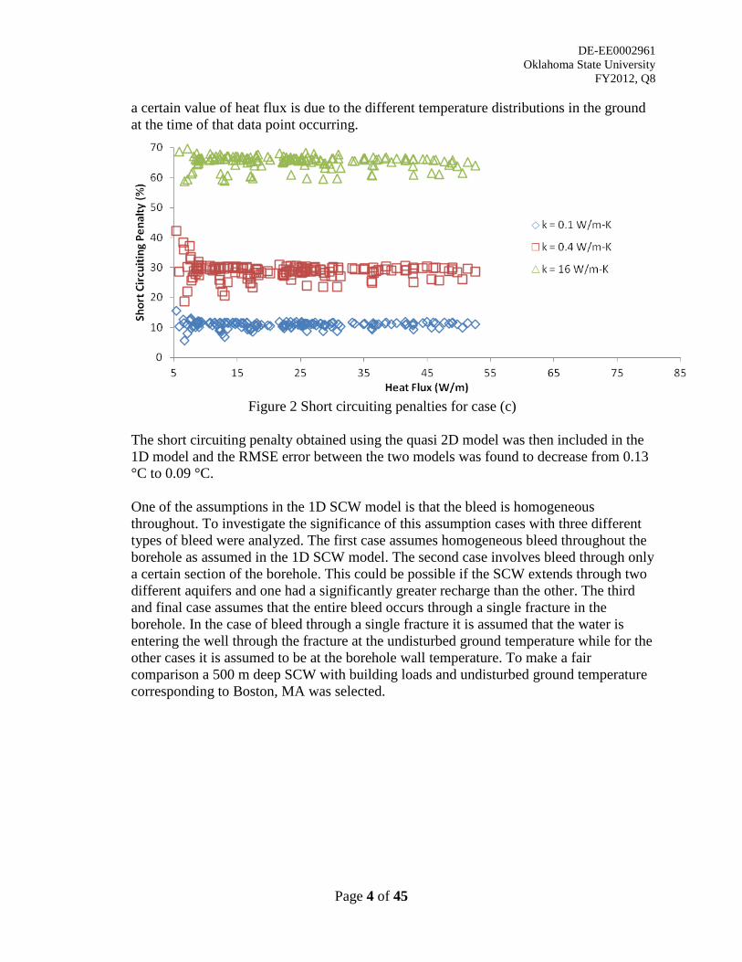
DE-EE0002961
Oklahoma State University
FY2012, Q8
Page 4 of 45
a certain value of heat flux is due to the different temperature distributions in the ground
at the time of that data point occurring.
Figure 2 Short circuiting penalties for case (c)
The short circuiting penalty obtained using the quasi 2D model was then included in the
1D model and the RMSE error between the two models was found to decrease from 0.13
°C to 0.09 °C.
One of the assumptions in the 1D SCW model is that the bleed is homogeneous
throughout. To investigate the significance of this assumption cases with three different
types of bleed were analyzed. The first case assumes homogeneous bleed throughout the
borehole as assumed in the 1D SCW model. The second case involves bleed through only
a certain section of the borehole. This could be possible if the SCW extends through two
different aquifers and one had a significantly greater recharge than the other. The third
and final case assumes that the entire bleed occurs through a single fracture in the
borehole. In the case of bleed through a single fracture it is assumed that the water is
entering the well through the fracture at the undisturbed ground temperature while for the
other cases it is assumed to be at the borehole wall temperature. To make a fair
comparison a 500 m deep SCW with building loads and undisturbed ground temperature
corresponding to Boston, MA was selected.
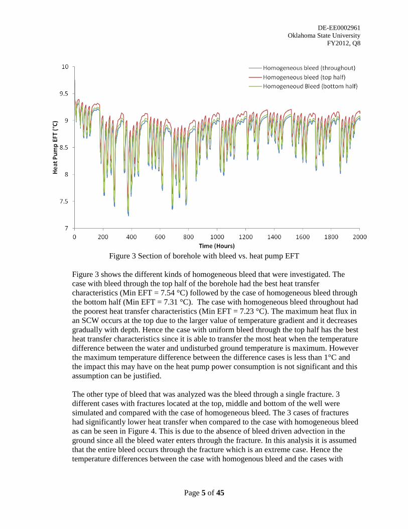
DE-EE0002961
Oklahoma State University
FY2012, Q8
Page 5 of 45
Figure 3 Section of borehole with bleed vs. heat pump EFT
Figure 3 shows the different kinds of homogeneous bleed that were investigated. The
case with bleed through the top half of the borehole had the best heat transfer
characteristics (Min EFT = 7.54 °C) followed by the case of homogeneous bleed through
the bottom half (Min EFT = 7.31 °C). The case with homogeneous bleed throughout had
the poorest heat transfer characteristics (Min EFT = 7.23 °C). The maximum heat flux in
an SCW occurs at the top due to the larger value of temperature gradient and it decreases
gradually with depth. Hence the case with uniform bleed through the top half has the best
heat transfer characteristics since it is able to transfer the most heat when the temperature
difference between the water and undisturbed ground temperature is maximum. However
the maximum temperature difference between the difference cases is less than 1°C and
the impact this may have on the heat pump power consumption is not significant and this
assumption can be justified.
The other type of bleed that was analyzed was the bleed through a single fracture. 3
different cases with fractures located at the top, middle and bottom of the well were
simulated and compared with the case of homogeneous bleed. The 3 cases of fractures
had significantly lower heat transfer when compared to the case with homogeneous bleed
as can be seen in Figure 4. This is due to the absence of bleed driven advection in the
ground since all the bleed water enters through the fracture. In this analysis it is assumed
that the entire bleed occurs through the fracture which is an extreme case. Hence the
temperature differences between the case with homogenous bleed and the cases with
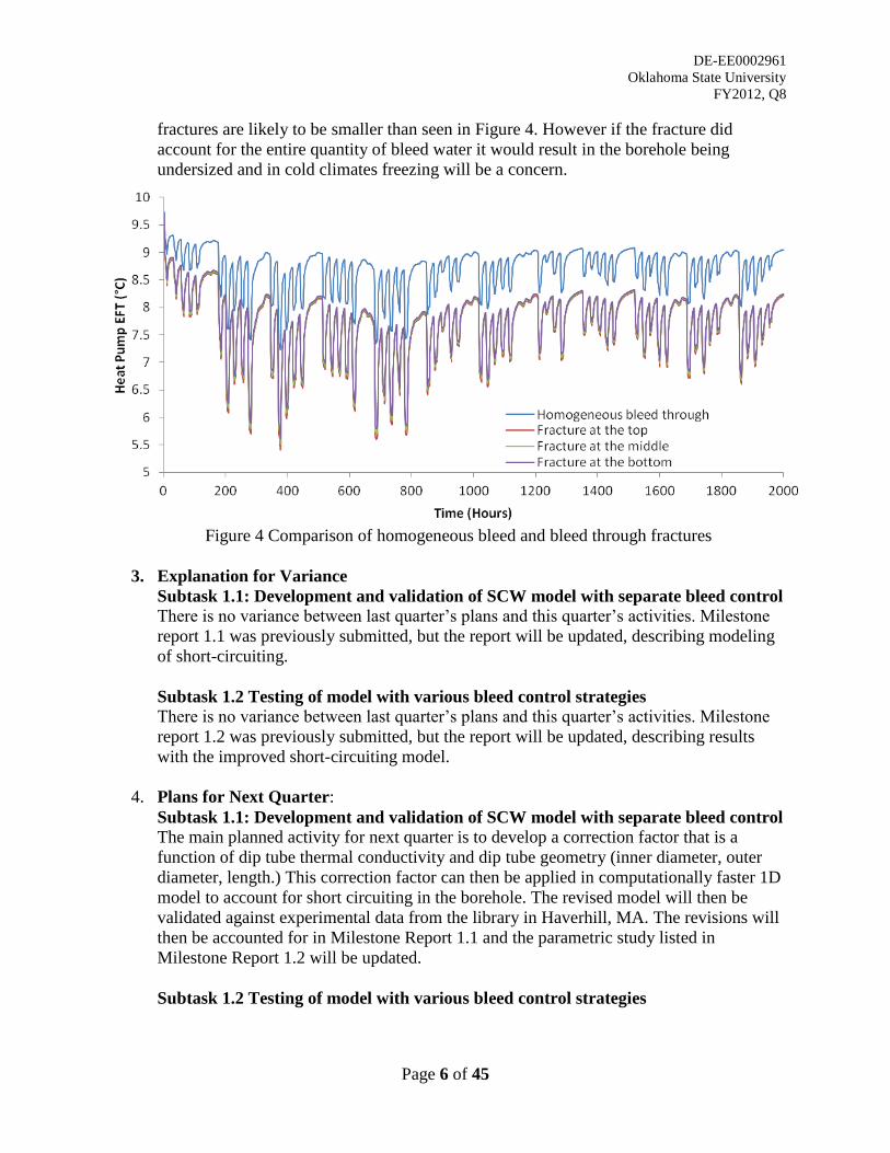
DE-EE0002961
Oklahoma State University
FY2012, Q8
Page 6 of 45
fractures are likely to be smaller than seen in Figure 4. However if the fracture did
account for the entire quantity of bleed water it would result in the borehole being
undersized and in cold climates freezing will be a concern.
Figure 4 Comparison of homogeneous bleed and bleed through fractures
3. Explanation for Variance
Subtask 1.1: Development and validation of SCW model with separate bleed control
There is no variance between last quarter‟s plans and this quarter‟s activities. Milestone
report 1.1 was previously submitted, but the report will be updated, describing modeling
of short-circuiting.
Subtask 1.2 Testing of model with various bleed control strategies
There is no variance between last quarter‟s plans and this quarter‟s activities. Milestone
report 1.2 was previously submitted, but the report will be updated, describing results
with the improved short-circuiting model.
4. Plans for Next Quarter:
Subtask 1.1: Development and validation of SCW model with separate bleed control
The main planned activity for next quarter is to develop a correction factor that is a
function of dip tube thermal conductivity and dip tube geometry (inner diameter, outer
diameter, length.) This correction factor can then be applied in computationally faster 1D
model to account for short circuiting in the borehole. The revised model will then be
validated against experimental data from the library in Haverhill, MA. The revisions will
then be accounted for in Milestone Report 1.1 and the parametric study listed in
Milestone Report 1.2 will be updated.
Subtask 1.2 Testing of model with various bleed control strategies
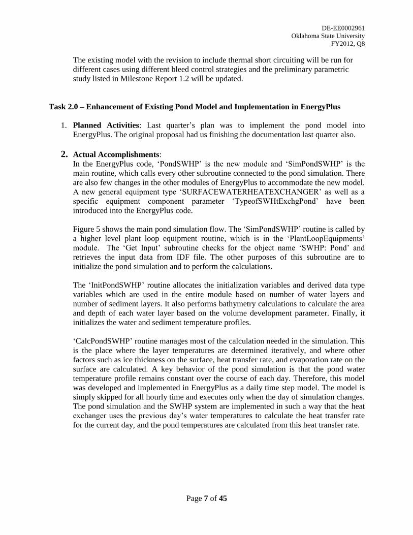
DE-EE0002961
Oklahoma State University
FY2012, Q8
Page 7 of 45
The existing model with the revision to include thermal short circuiting will be run for
different cases using different bleed control strategies and the preliminary parametric
study listed in Milestone Report 1.2 will be updated.
Task 2.0 – Enhancement of Existing Pond Model and Implementation in EnergyPlus
1. Planned Activities: Last quarter‟s plan was to implement the pond model into
EnergyPlus. The original proposal had us finishing the documentation last quarter also.
2. Actual Accomplishments: In the EnergyPlus code, „PondSWHP‟ is the new module and „SimPondSWHP‟ is the
main routine, which calls every other subroutine connected to the pond simulation. There
are also few changes in the other modules of EnergyPlus to accommodate the new model.
A new general equipment type „SURFACEWATERHEATEXCHANGER‟ as well as a
specific equipment component parameter „TypeofSWHtExchgPond‟ have been
introduced into the EnergyPlus code.
Figure 5 shows the main pond simulation flow. The „SimPondSWHP‟ routine is called by
a higher level plant loop equipment routine, which is in the „PlantLoopEquipments‟
module. The „Get Input‟ subroutine checks for the object name „SWHP: Pond‟ and
retrieves the input data from IDF file. The other purposes of this subroutine are to
initialize the pond simulation and to perform the calculations.
The „InitPondSWHP‟ routine allocates the initialization variables and derived data type
variables which are used in the entire module based on number of water layers and
number of sediment layers. It also performs bathymetry calculations to calculate the area
and depth of each water layer based on the volume development parameter. Finally, it
initializes the water and sediment temperature profiles.
„CalcPondSWHP‟ routine manages most of the calculation needed in the simulation. This
is the place where the layer temperatures are determined iteratively, and where other
factors such as ice thickness on the surface, heat transfer rate, and evaporation rate on the
surface are calculated. A key behavior of the pond simulation is that the pond water
temperature profile remains constant over the course of each day. Therefore, this model
was developed and implemented in EnergyPlus as a daily time step model. The model is
simply skipped for all hourly time and executes only when the day of simulation changes.
The pond simulation and the SWHP system are implemented in such a way that the heat
exchanger uses the previous day‟s water temperatures to calculate the heat transfer rate
for the current day, and the pond temperatures are calculated from this heat transfer rate.
DE-EE0002961
Oklahoma State University
FY2012, Q8
Page 8 of 45
Figure 5 Flow of the main routine
Validation of EnergyPlus results:
To confirm the accuracy of the EnergyPlus model, the simulation results are compared
with the experimental results obtained for OSU research pond. Validation here is
presented using experimental data from March through November.
The OSU research is a shallow pond with a surface area of 2.5 acres (10,000 m2) with the
maximum depth of the pond is 12.5 feet (3.81 m). The pond model uses the Fang and
Stefan (1996) correlation to calculate eddy diffusivity coefficients as a function of depth
when the pond is covered by ice on the surface. When the pond is ice-free, the eddy
diffusivity coefficients for the epilimnion (mixed) layer are obtained using the correlation
from Stefan et al. (1982), while the eddy diffusivity coefficients for the hypolimnion and
the thermocline regions are calculated using the Gu and Stefan (1995) correlation. The
maximum eddy diffusivity coefficient, KZ-max, used in the Gu and Stefan correlation is
set as 5 m2/day. This value for KZ-max was set empirically, to allow the simulation results
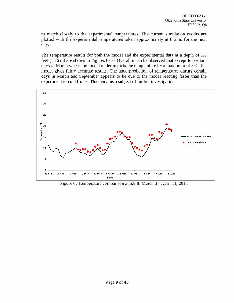
DE-EE0002961
Oklahoma State University
FY2012, Q8
Page 9 of 45
to match closely to the experimental temperatures. The current simulation results are
plotted with the experimental temperatures taken approximately at 8 a.m. for the next
day.
The temperature results for both the model and the experimental data at a depth of 5.8
feet (1.76 m) are shown in Figures 6-10. Overall it can be observed that except for certain
days in March where the model underpredicts the temperature by a maximum of 5°C, the
model gives fairly accurate results. The underprediction of temperatures during certain
days in March and September appears to be due to the model reacting faster than the
experiment to cold fronts. This remains a subject of further investigation
Figure 6: Temperature comparison at 5.8 ft, March 3 - April 11, 2011
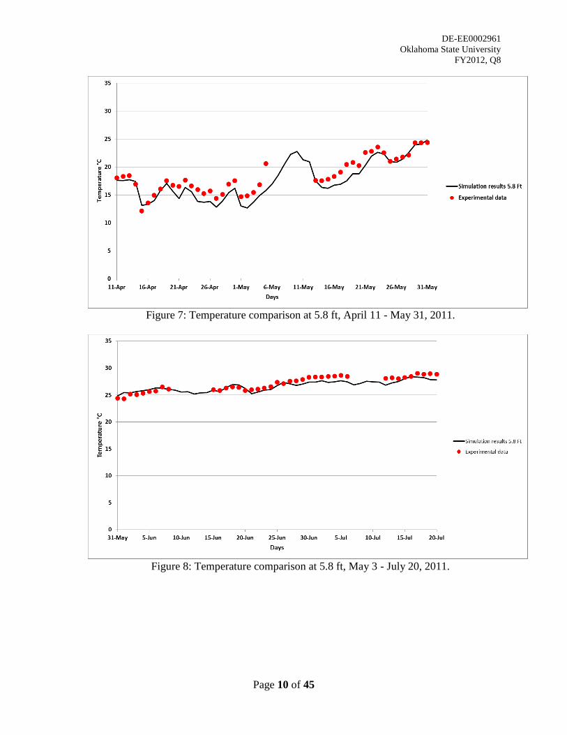
DE-EE0002961
Oklahoma State University
FY2012, Q8
Page 10 of 45
Figure 7: Temperature comparison at 5.8 ft, April 11 - May 31, 2011.
Figure 8: Temperature comparison at 5.8 ft, May 3 - July 20, 2011.
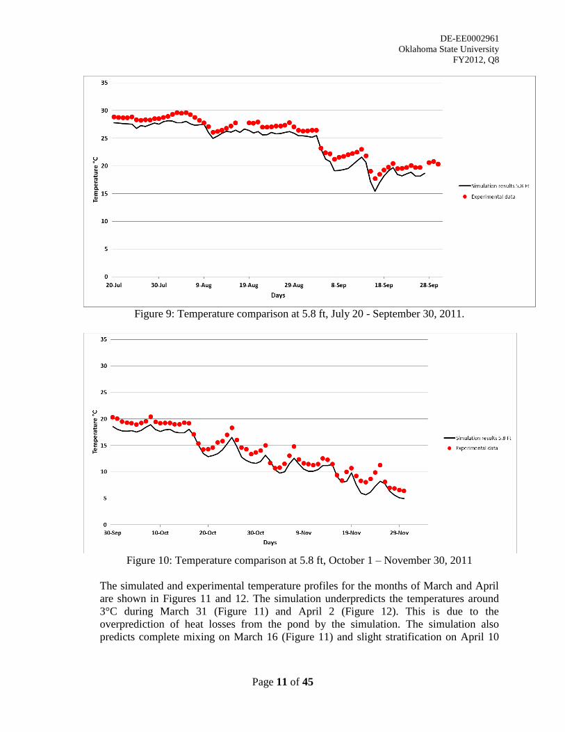
DE-EE0002961
Oklahoma State University
FY2012, Q8
Page 11 of 45
Figure 9: Temperature comparison at 5.8 ft, July 20 - September 30, 2011.
Figure 10: Temperature comparison at 5.8 ft, October 1 – November 30, 2011
The simulated and experimental temperature profiles for the months of March and April
are shown in Figures 11 and 12. The simulation underpredicts the temperatures around
3°C during March 31 (Figure 11) and April 2 (Figure 12). This is due to the
overprediction of heat losses from the pond by the simulation. The simulation also
predicts complete mixing on March 16 (Figure 11) and slight stratification on April 10
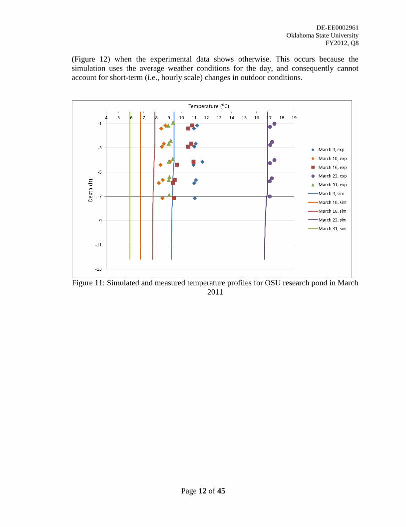
DE-EE0002961
Oklahoma State University
FY2012, Q8
Page 12 of 45
(Figure 12) when the experimental data shows otherwise. This occurs because the
simulation uses the average weather conditions for the day, and consequently cannot
account for short-term (i.e., hourly scale) changes in outdoor conditions.
Figure 11: Simulated and measured temperature profiles for OSU research pond in March
2011
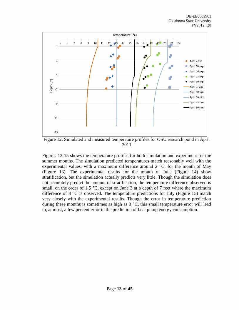
DE-EE0002961
Oklahoma State University
FY2012, Q8
Page 13 of 45
Figure 12: Simulated and measured temperature profiles for OSU research pond in April
2011
Figures 13-15 shows the temperature profiles for both simulation and experiment for the
summer months. The simulation predicted temperatures match reasonably well with the
experimental values, with a maximum difference around 2 °C, for the month of May
(Figure 13). The experimental results for the month of June (Figure 14) show
stratification, but the simulation actually predicts very little. Though the simulation does
not accurately predict the amount of stratification, the temperature difference observed is
small, on the order of 1.5 °C, except on June 3 at a depth of 7 feet where the maximum
difference of 3 °C is observed. The temperature predictions for July (Figure 15) match
very closely with the experimental results. Though the error in temperature prediction
during these months is sometimes as high as 3 °C, this small temperature error will lead
to, at most, a few percent error in the prediction of heat pump energy consumption.
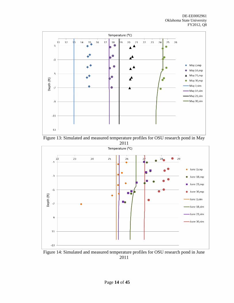
DE-EE0002961
Oklahoma State University
FY2012, Q8
Page 14 of 45
Figure 13: Simulated and measured temperature profiles for OSU research pond in May
2011
Figure 14: Simulated and measured temperature profiles for OSU research pond in June
2011
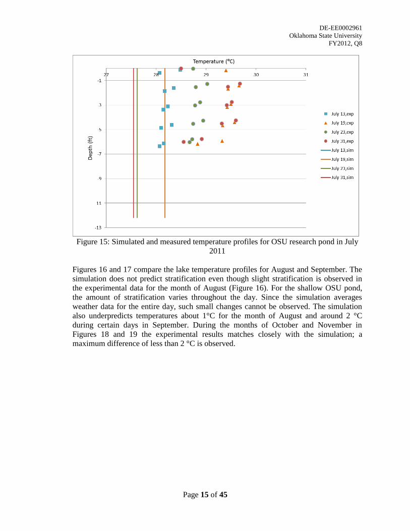
DE-EE0002961
Oklahoma State University
FY2012, Q8
Page 15 of 45
Figure 15: Simulated and measured temperature profiles for OSU research pond in July
2011
Figures 16 and 17 compare the lake temperature profiles for August and September. The
simulation does not predict stratification even though slight stratification is observed in
the experimental data for the month of August (Figure 16). For the shallow OSU pond,
the amount of stratification varies throughout the day. Since the simulation averages
weather data for the entire day, such small changes cannot be observed. The simulation
also underpredicts temperatures about 1°C for the month of August and around 2 °C
during certain days in September. During the months of October and November in
Figures 18 and 19 the experimental results matches closely with the simulation; a
maximum difference of less than 2 °C is observed.
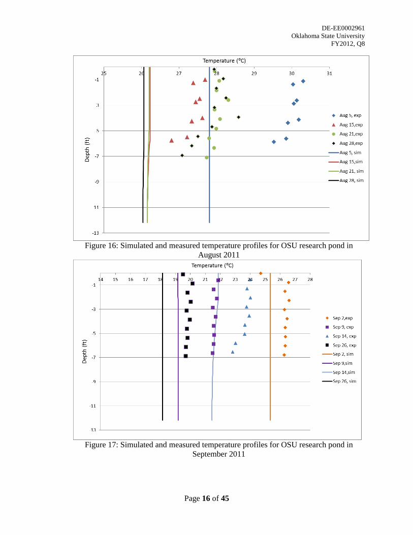
DE-EE0002961
Oklahoma State University
FY2012, Q8
Page 16 of 45
Figure 16: Simulated and measured temperature profiles for OSU research pond in
August 2011
Figure 17: Simulated and measured temperature profiles for OSU research pond in
September 2011
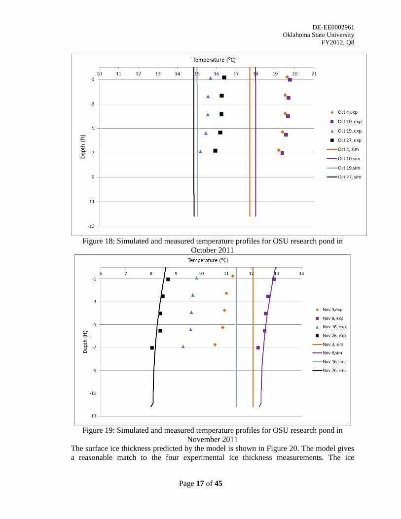
DE-EE0002961
Oklahoma State University
FY2012, Q8
Page 17 of 45
Figure 18: Simulated and measured temperature profiles for OSU research pond in
October 2011
Figure 19: Simulated and measured temperature profiles for OSU research pond in
November 2011
The surface ice thickness predicted by the model is shown in Figure 20. The model gives
a reasonable match to the four experimental ice thickness measurements. The ice
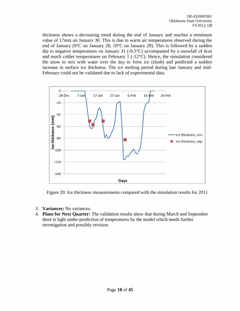
DE-EE0002961
Oklahoma State University
FY2012, Q8
Page 18 of 45
thickness shows a decreasing trend during the end of January and reaches a minimum
value of 17mm on January 30. This is due to warm air temperatures observed during the
end of January (9°C on January 28, 10°C on January 29). This is followed by a sudden
dip to negative temperatures on January 31 (-0.5°C) accompanied by a snowfall of 6cm
and much colder temperatures on February 1 (-12°C). Hence, the simulation considered
the snow to mix with water over the day to form ice (slush) and predicted a sudden
increase in surface ice thickness. The ice melting period during late January and mid-
February could not be validated due to lack of experimental data.
Figure 20: Ice thickness measurements compared with the simulation results for 2011
3. Variances: No variances.
4. Plans for Next Quarter: The validation results show that during March and September
there is light under-prediction of temperatures by the model which needs further
investigation and possibly revision.

DE-EE0002961
Oklahoma State University
FY2012, Q8
Page 19 of 45
Task 3.0 – Implementation of Enhanced SCW Model
1. Planned Activities:
Subtask 3.1 Implementation of Enhanced SCW Model in EnergyPlus
The plans for last quarter were to implement the enhanced SCW model in EnergyPlus,
including development of the input files (IDD and IDF) that describe the SCW model.
Subtask 3.2 Implementation of Enhanced SCW Model in Design Tool
The plans for last quarter were to begin implementation of the enhanced SCW model in
the design tool GLHEPRO.
Subtask 3.3 Technology Transfer
n/a.
2. Actual Accomplishments:
Subtask 3.1 Implementation of Enhanced SCW Model in EnergyPlus
Work done on the EnergyPlus implementation involved modifications to the input files
(IDD and IDF) to include the standing column well model. The model is currently being
integrated into the plant loop as a type of ground heat exchanger. The model is in the
debugging phase and once complete an intermodel verification will be done against the
SCW model in HVACSIM+, which has already been validated.
Subtask 3.2 Implementation of Enhanced SCW Model in Design Tool
In support of the design tool, some documentation to help users determine hydraulic
properties has been drafted. The first two sections are drafts of the documentation and
the following sections describe implementation of the enhanced SCS model..
Documentation of hydraulic properties for design tool:
If the SCW model is to be used in a design tool or in EnergyPlus then the designer must
have a reasonable understanding of the hydraulic properties of the ground and its impact
on the heat transfer. A brief description of the hydraulic properties is provided and typical
values for different rock types are suggested. The methods to determine them are also
provided.
A parameter significantly influencing the heat transfer in the SCW model is the enhanced
thermal conductivity. The enhanced thermal conductivity is an effective thermal
conductivity for the ground taking into consideration heat transfer by conduction and
advection. The heat transfer due to conduction depends on the actual thermal
conductivity of the ground. Considerable research has been done to determine this ground
thermal conductivity and the ground source heat pump designer is likely to be familiar
with the in-situ methods used. However the heat transfer due to advection depends on the
hydraulic properties of the ground such as the hydraulic conductivity, porosity,
transmissivity and storativity which a GSHP designer is less likely to be familiar with.
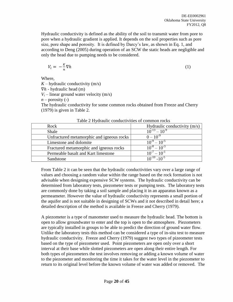
DE-EE0002961
Oklahoma State University
FY2012, Q8
Page 20 of 45
Hydraulic conductivity is defined as the ability of the soil to transmit water from pore to
pore when a hydraulic gradient is applied. It depends on the soil properties such as pore
size, pore shape and porosity. It is defined by Darcy‟s law, as shown in Eq. 1, and
according to Deng (2005) during operation of an SCW the static heads are negligible and
only the head due to pumping needs to be considered.
(1)
Where,
K – hydraulic conductivity (m/s)
- hydraulic head (m)
Vi – linear ground water velocity (m/s)
n – porosity (-)
The hydraulic conductivity for some common rocks obtained from Freeze and Cherry
(1979) is given in Table 2.
Table 2 Hydraulic conductivities of common rocks
Rock Hydraulic conductivity (m/s)
Shale 10-13
– 10-9
Unfractured metamorphic and igneous rocks 0 – 10-9
Limestone and dolomite 10-9
– 10-5
Fractured metamorphic and igneous rocks 10-8
– 10-3
Permeable basalt and Kart limestone 10-7
– 10-1
Sandstone 10-10
-10-5
From Table 2 it can be seen that the hydraulic conductivities vary over a large range of
values and choosing a random value within the range based on the rock formation is not
advisable when designing expensive SCW systems. The hydraulic conductivity can be
determined from laboratory tests, piezometer tests or pumping tests. The laboratory tests
are commonly done by taking a soil sample and placing it in an apparatus known as a
permeameter. However the value of hydraulic conductivity represents a small portion of
the aquifer and is not suitable in designing of SCWs and it not described in detail here; a
detailed description of the method is available in Freeze and Cherry (1979).
A piezometer is a type of manometer used to measure the hydraulic head. The bottom is
open to allow groundwater to enter and the top is open to the atmosphere. Piezometers
are typically installed in groups to be able to predict the direction of ground water flow.
Unlike the laboratory tests this method can be considered a type of in-situ test to measure
hydraulic conductivity. Freeze and Cherry (1979) suggest two types of pizeometer tests
based on the type of piezometer used. Point piezometers are open only over a short
interval at their base while slotted piezometers are open along their entire length. For
both types of piezometers the test involves removing or adding a known volume of water
to the piezometer and monitoring the time it takes for the water level in the piezometer to
return to its original level before the known volume of water was added or removed. The
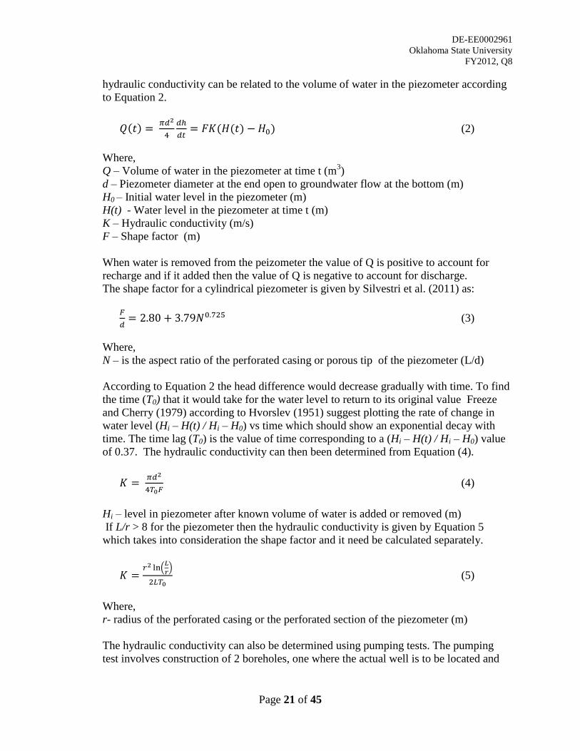
DE-EE0002961
Oklahoma State University
FY2012, Q8
Page 21 of 45
hydraulic conductivity can be related to the volume of water in the piezometer according
to Equation 2.
(2)
Where,
Q – Volume of water in the piezometer at time t (m3)
d – Piezometer diameter at the end open to groundwater flow at the bottom (m)
H0 – Initial water level in the piezometer (m)
H(t) - Water level in the piezometer at time t (m)
K – Hydraulic conductivity (m/s)
F – Shape factor (m)
When water is removed from the peizometer the value of Q is positive to account for
recharge and if it added then the value of Q is negative to account for discharge.
The shape factor for a cylindrical piezometer is given by Silvestri et al. (2011) as:
(3)
Where,
N – is the aspect ratio of the perforated casing or porous tip of the piezometer (L/d)
According to Equation 2 the head difference would decrease gradually with time. To find
the time (T0) that it would take for the water level to return to its original value Freeze
and Cherry (1979) according to Hvorslev (1951) suggest plotting the rate of change in
water level (Hi – H(t) / Hi – H0) vs time which should show an exponential decay with
time. The time lag (T0) is the value of time corresponding to a (Hi – H(t) / Hi – H0) value
of 0.37. The hydraulic conductivity can then been determined from Equation (4).
(4)
Hi – level in piezometer after known volume of water is added or removed (m)
If L/r > 8 for the piezometer then the hydraulic conductivity is given by Equation 5
which takes into consideration the shape factor and it need be calculated separately.
(5)
Where,
r- radius of the perforated casing or the perforated section of the piezometer (m)
The hydraulic conductivity can also be determined using pumping tests. The pumping
test involves construction of 2 boreholes, one where the actual well is to be located and
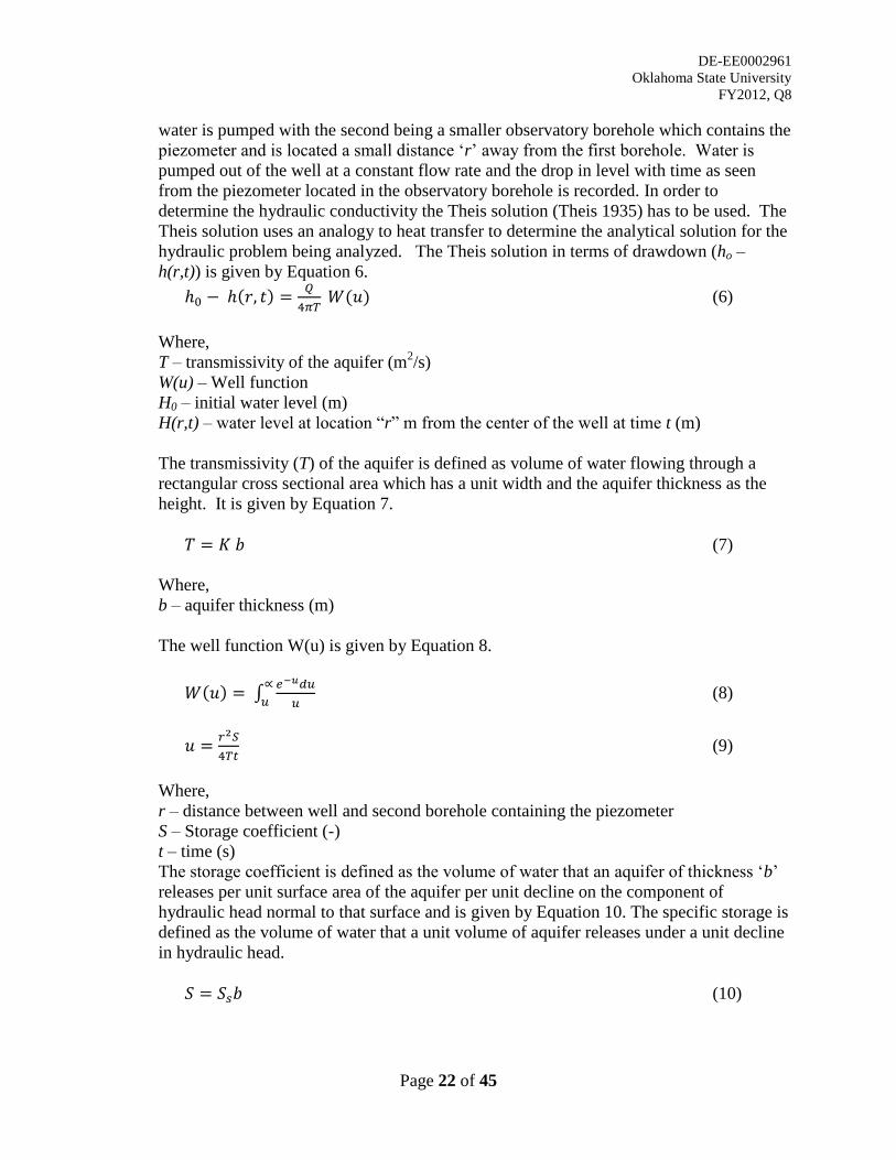
DE-EE0002961
Oklahoma State University
FY2012, Q8
Page 22 of 45
water is pumped with the second being a smaller observatory borehole which contains the
piezometer and is located a small distance „r‟ away from the first borehole. Water is
pumped out of the well at a constant flow rate and the drop in level with time as seen
from the piezometer located in the observatory borehole is recorded. In order to
determine the hydraulic conductivity the Theis solution (Theis 1935) has to be used. The
Theis solution uses an analogy to heat transfer to determine the analytical solution for the
hydraulic problem being analyzed. The Theis solution in terms of drawdown (ho –
h(r,t)) is given by Equation 6.
(6)
Where,
T – transmissivity of the aquifer (m2/s)
W(u) – Well function
H0 – initial water level (m)
H(r,t) – water level at location “r” m from the center of the well at time t (m)
The transmissivity (T) of the aquifer is defined as volume of water flowing through a
rectangular cross sectional area which has a unit width and the aquifer thickness as the
height. It is given by Equation 7.
(7)
Where,
b – aquifer thickness (m)
The well function W(u) is given by Equation 8.
(8)
(9)
Where,
r – distance between well and second borehole containing the piezometer
S – Storage coefficient (-)
t – time (s)
The storage coefficient is defined as the volume of water that an aquifer of thickness „b‟
releases per unit surface area of the aquifer per unit decline on the component of
hydraulic head normal to that surface and is given by Equation 10. The specific storage is
defined as the volume of water that a unit volume of aquifer releases under a unit decline
in hydraulic head.
(10)

DE-EE0002961
Oklahoma State University
FY2012, Q8
Page 23 of 45
Where,
Ss – specific storage (m-1
)
If the aquifer thickness is not known it can be taken as the difference between the water
table and the bottom of the borehole. This assumption is based on the well being part of a
single homogenous isotropic aquifer.
When a pumping test is performed the drop in water level with time at the observatory
borehole is noted and the hydraulic conductivity (K) and specific storage (Ss) can be
obtained from Equation 6 -10 using a Nelder-Mead simplex algorithm with reasonable
guess values to minimize the error between the observed and predicted values. Figures 21
and 22 shows the ideal curves for the different cases listed in Table 3 that were simulated
for a period of 30 hours. Case A can be considered as a base case and all other cases are
compared with it. Analyzing the hydraulic properties will also enable the designer to
choose between closed and open loop system since poor hydraulic properties would result
in the advection being insignificant thereby disabling the possibility of bleed operation
and making the closed loop system more feasible. Since the effect of hydraulic
conductivity on the change in water level was large Figure 21 is plotted on a logarithmic
scale. The value of hydraulic conductivity obtained from the pumping test is averaged
over a larger region then that obtained from a piezometer test and is the preferable
method when designing systems with multiple SCWs.
Table 3 Hydraulic properties test cases
Case A B C D E F G H I J K
Flow rate , Q gpm 10 10 10 10 10 20 30 10 10 10 10
Depth, b (m) 100 100 100 200 300 100 100 100 100 100 100
Hydraulic
conductivity, k (m/s) 10-4
10-5
10-6
10-4
10-4
10-4
10-4
10-4
10-4
10-4
10-4
Distance between
borehole centers, r
(m) 10 10 10 10 10 10 10 20 30 10 10
Specific storage Ss
(m-1
) 10-4
10-4
10-4
10-4
10-4
10-4
10-4
10-4
10-4
10-5
10-6
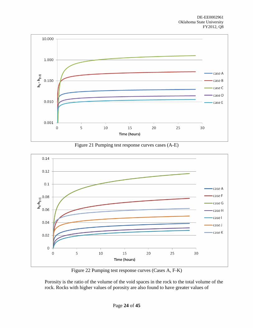
DE-EE0002961
Oklahoma State University
FY2012, Q8
Page 24 of 45
Figure 21 Pumping test response curves cases (A-E)
Figure 22 Pumping test response curves (Cases A, F-K)
Porosity is the ratio of the volume of the void spaces in the rock to the total volume of the
rock. Rocks with higher values of porosity are also found to have greater values of
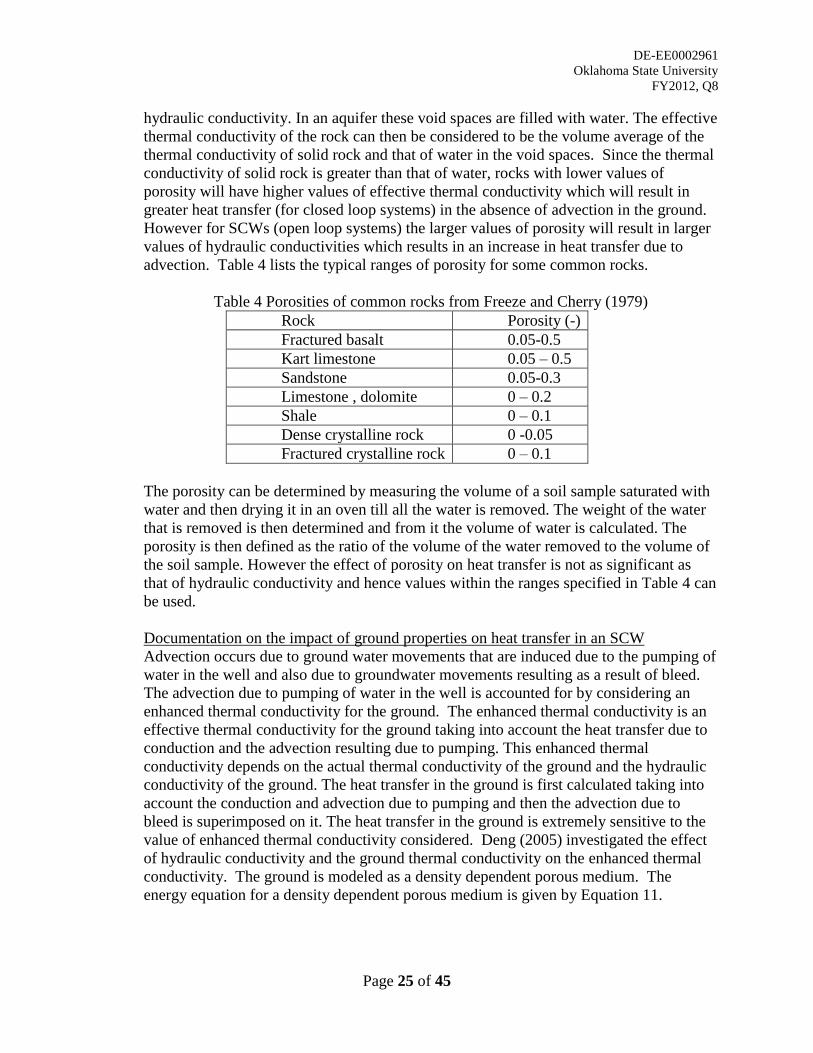
DE-EE0002961
Oklahoma State University
FY2012, Q8
Page 25 of 45
hydraulic conductivity. In an aquifer these void spaces are filled with water. The effective
thermal conductivity of the rock can then be considered to be the volume average of the
thermal conductivity of solid rock and that of water in the void spaces. Since the thermal
conductivity of solid rock is greater than that of water, rocks with lower values of
porosity will have higher values of effective thermal conductivity which will result in
greater heat transfer (for closed loop systems) in the absence of advection in the ground.
However for SCWs (open loop systems) the larger values of porosity will result in larger
values of hydraulic conductivities which results in an increase in heat transfer due to
advection. Table 4 lists the typical ranges of porosity for some common rocks.
Table 4 Porosities of common rocks from Freeze and Cherry (1979)
Rock Porosity (-)
Fractured basalt 0.05-0.5
Kart limestone 0.05 – 0.5
Sandstone 0.05-0.3
Limestone , dolomite 0 – 0.2
Shale 0 – 0.1
Dense crystalline rock 0 -0.05
Fractured crystalline rock 0 – 0.1
The porosity can be determined by measuring the volume of a soil sample saturated with
water and then drying it in an oven till all the water is removed. The weight of the water
that is removed is then determined and from it the volume of water is calculated. The
porosity is then defined as the ratio of the volume of the water removed to the volume of
the soil sample. However the effect of porosity on heat transfer is not as significant as
that of hydraulic conductivity and hence values within the ranges specified in Table 4 can
be used.
Documentation on the impact of ground properties on heat transfer in an SCW
Advection occurs due to ground water movements that are induced due to the pumping of
water in the well and also due to groundwater movements resulting as a result of bleed.
The advection due to pumping of water in the well is accounted for by considering an
enhanced thermal conductivity for the ground. The enhanced thermal conductivity is an
effective thermal conductivity for the ground taking into account the heat transfer due to
conduction and the advection resulting due to pumping. This enhanced thermal
conductivity depends on the actual thermal conductivity of the ground and the hydraulic
conductivity of the ground. The heat transfer in the ground is first calculated taking into
account the conduction and advection due to pumping and then the advection due to
bleed is superimposed on it. The heat transfer in the ground is extremely sensitive to the
value of enhanced thermal conductivity considered. Deng (2005) investigated the effect
of hydraulic conductivity and the ground thermal conductivity on the enhanced thermal
conductivity. The ground is modeled as a density dependent porous medium. The
energy equation for a density dependent porous medium is given by Equation 11.
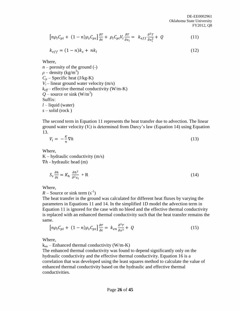
DE-EE0002961
Oklahoma State University
FY2012, Q8
Page 26 of 45
(11)
(12)
Where,
n – porosity of the ground (-)
ρ – density (kg/m3)
Cp – Specific heat (J/kg-K)
Vi – linear ground water velocity (m/s)
keff – effective thermal conductivity (W/m-K)
Q – source or sink (W/m3)
Suffix:
l – liquid (water)
s – solid (rock )
The second term in Equation 11 represents the heat transfer due to advection. The linear
ground water velocity (Vi) is determined from Darcy‟s law (Equation 14) using Equation
13.
(13)
Where,
K – hydraulic conductivity (m/s)
- hydraulic head (m)
+ R (14)
Where,
R – Source or sink term (s-1
)
The heat transfer in the ground was calculated for different heat fluxes by varying the
parameters in Equations 11 and 14. In the simplified 1D model the advection term in
Equation 11 is ignored for the case with no bleed and the effective thermal conductivity
is replaced with an enhanced thermal conductivity such that the heat transfer remains the
same.
(15)
Where,
ken – Enhanced thermal conductivity (W/m-K)
The enhanced thermal conductivity was found to depend significantly only on the
hydraulic conductivity and the effective thermal conductivity. Equation 16 is a
correlation that was developed using the least squares method to calculate the value of
enhanced thermal conductivity based on the hydraulic and effective thermal
conductivities.
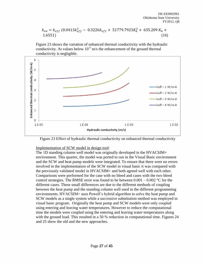
DE-EE0002961
Oklahoma State University
FY2012, Q8
Page 27 of 45
(16)
Figure 23 shows the variation of enhanced thermal conductivity with the hydraulic
conductivity. At values below 10-5
m/s the enhancement of the ground thermal
conductivity is negligible.
Figure 23 Effect of hydraulic thermal conductivity on enhanced thermal conductivity
Implementation of SCW model in design tool:
The 1D standing column well model was originally developed in the HVACSIM+
environment. This quarter, the model was ported to run in the Visual Basic environment
and the SCW and heat pump models were integrated. To ensure that there were no errors
involved in the implementation of the SCW model in visual basic it was compared with
the previously validated model in HVACSIM+ and both agreed well with each other.
Comparisons were performed for the case with no bleed and cases with the two bleed
control strategies. The RMSE error was found to be between 0.001 – 0.002 °C for the
different cases. These small differences are due to the different methods of coupling
between the heat pump and the standing column well used in the different programming
environments. HVACSIM+ uses Powell‟s hybrid algorithm to solve the heat pump and
SCW models as a single system while a successive substitution method was employed in
visual basic program. Originally the heat pump and SCW models were only coupled
using entering and leaving water temperatures. However to reduce the computational
time the models were coupled using the entering and leaving water temperatures along
with the ground load. This resulted in a 50 % reduction in computational time. Figures 24
and 25 show the old and the new approaches.
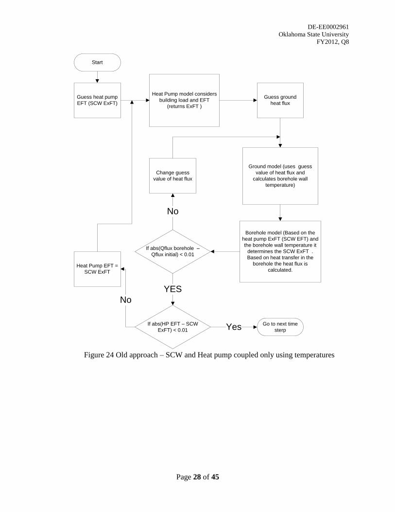
DE-EE0002961
Oklahoma State University
FY2012, Q8
Page 28 of 45
Start
Guess heat pump EFT (SCW ExFT)
Heat Pump model considers building load and EFT
(returns ExFT )
Ground model (uses guess value of heat flux and
calculates borehole wall temperature)
Borehole model (Based on the heat pump ExFT (SCW EFT) and the borehole wall temperature it
determines the SCW ExFT . Based on heat transfer in the
borehole the heat flux is calculated.
If abs(HP EFT – SCW ExFT) < 0.01
Go to next time sterpYes
Heat Pump EFT = SCW ExFT
No
Guess ground heat flux
If abs(Qflux borehole – Qflux initial) < 0.01
YES
Change guess value of heat flux
No
Figure 24 Old approach – SCW and Heat pump coupled only using temperatures
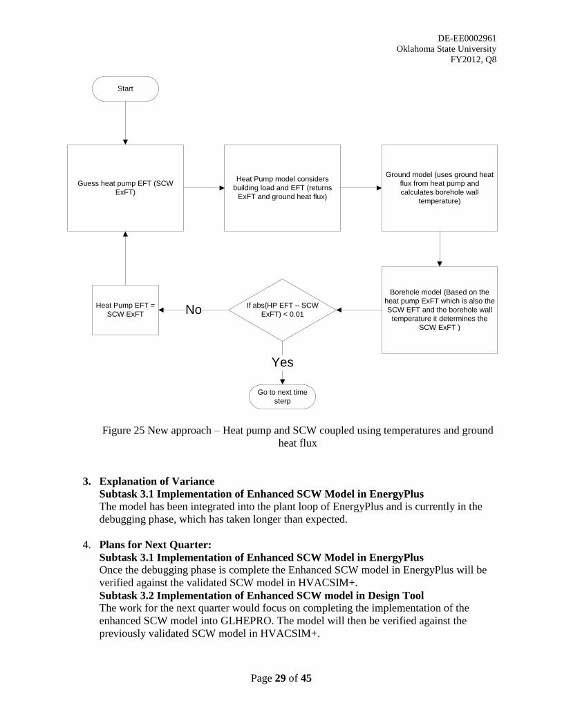
DE-EE0002961
Oklahoma State University
FY2012, Q8
Page 29 of 45
Start
Guess heat pump EFT (SCW ExFT)
Heat Pump model considers building load and EFT (returns
ExFT and ground heat flux)
Ground model (uses ground heat flux from heat pump and calculates borehole wall
temperature)
Borehole model (Based on the heat pump ExFT which is also the SCW EFT and the borehole wall
temperature it determines the SCW ExFT )
If abs(HP EFT – SCW ExFT) < 0.01
Go to next time sterp
Yes
Heat Pump EFT = SCW ExFT No
Figure 25 New approach – Heat pump and SCW coupled using temperatures and ground
heat flux
3. Explanation of Variance
Subtask 3.1 Implementation of Enhanced SCW Model in EnergyPlus
The model has been integrated into the plant loop of EnergyPlus and is currently in the
debugging phase, which has taken longer than expected.
4. Plans for Next Quarter:
Subtask 3.1 Implementation of Enhanced SCW Model in EnergyPlus
Once the debugging phase is complete the Enhanced SCW model in EnergyPlus will be
verified against the validated SCW model in HVACSIM+.
Subtask 3.2 Implementation of Enhanced SCW model in Design Tool
The work for the next quarter would focus on completing the implementation of the
enhanced SCW model into GLHEPRO. The model will then be verified against the
previously validated SCW model in HVACSIM+.

DE-EE0002961
Oklahoma State University
FY2012, Q8
Page 30 of 45
Subtask 3.3 Technology Transfer
A draft of a technical paper describing the quasi 2D SCW model will be written and
submitted for presentation at a conference.

DE-EE0002961
Oklahoma State University
FY2012, Q8
Page 31 of 45
Task 4: Enhancement, Implementation and Validation of Enhanced Pond Model
1. Planned Activities:
Subtask 4.1 Modeling of alternate pond heat exchanger types Plans for last quarter were to implement exterior convection correlations for different
pond heat exchanger types.
Subtask 4.2 Documentation of enhanced pond model in EnergyPlus
The enhanced pond model implemented in EnergyPlus was planned to be completely
documented with some examples.
Subtask 4.3 Implementation of enhanced pond model in design tool
Work on this quarter was also focused on implementing the enhanced pond model as part
of the design tool for ground heat exchangers (GLHEPRO).A milestone report containing
the documentation of the design tool with some examples was planned to be submitted in
this quarter.
Subtask 4.4 Validation of pond model
The pond model integrated with the heat exchanger model in EnergyPlus was to be
validated against the experimental results obtained for different heat exchanger types
from the OSU research pond.
Subtask 4.5 Technology Transfer
No plans for last quarter.
2. Actual Accomplishments:
Subtask 4.1 Modeling of alternate pond heat exchanger types
Hansen (2011) conducted a total of 119 tests on 5 different heat exchanger coil types in
the 3 acre (12,000 m2) OSU research pond and arrived with three correlations to calculate
the outside Nusselt number and hence the outside convection heat transfer coefficient for
five types of heat exchanger coils namely spiral-helical, spiral, slinky-type, loose bundled
and flat plate heat exchangers (e.g. “SlimJim®”). The breakdown of the tests and the
parameters varied in the tests are shown in Table 5 below
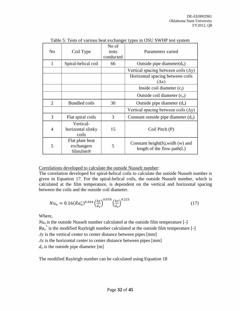
DE-EE0002961
Oklahoma State University
FY2012, Q8
Page 32 of 45
Table 5: Tests of various heat exchanger types in OSU SWHP test system
No Coil Type
No of
tests
conducted
Parameters varied
1 Spiral-helical coil 66 Outside pipe diameter(do)
Vertical spacing between coils (Δy)
Horizontal spacing between coils
(Δx)
Inside coil diameter (ci)
Outside coil diameter (co)
2 Bundled coils 30 Outside pipe diameter (do)
Vertical spacing between coils (Δy)
3 Flat spiral coils 3 Constant outside pipe diameter (do)
4
Vertical-
horizontal slinky
coils
15 Coil Pitch (P)
5
Flat plate heat
exchangers
SlimJim®
5 Constant height(h),widh (w) and
length of the flow path(L)
Correlations developed to calculate the outside Nusselt number:
The correlation developed for spiral-helical coils to calculate the outside Nusselt number is
given in Equation 17. For the spiral-helical coils, the outside Nusselt number, which is
calculated at the film temperature, is dependent on the vertical and horizontal spacing
between the coils and the outside coil diameter.
(17)
Where,
Nuo is the outside Nusselt number calculated at the outside film temperature [-]
Rao* is the modified Rayleigh number calculated at the outside film temperature [-]
Δy is the vertical center to center distance between pipes [mm]
Δx is the horizontal center to center distance between pipes [mm]
do is the outside pipe diameter [m]
The modified Rayleigh number can be calculated using Equation 18
DE-EE0002961
Oklahoma State University
FY2012, Q8
Page 33 of 45
(18)
Where,
g is the acceleration due to gravity [m/s2]
β is the thermal expansion coefficient calculated at the outside film temperature [1/K]
Qc is the coil heat flux [W]
L is the characteristic length [m]
Pr is the Prandtl number [-]
k is the thermal conductivity of the pond calculated at the film temperature [W/m-K]
υ is the kinematic viscosity calculated at the outside film temperature [m2/s]
In the case of flat spiral and vertical and horizontal slinky type coils the correlation for
calculating the outside Nusselt number is given in Equation 19
(19)
Finally, the outside Nusselt number correlation for flat plate heat exchanger is given as
(20)
Current structure of the heat exchanger model:
The heat exchanger model takes in the average lake temperature, building heating/cooling
loads and heat exchanger information as inputs. The building loads are given as inputs to
the Heat pump model to calculate the load on the heat exchanger coils. This load
experienced by the heat exchanger coils is calculated based on the performance of the heat
pump. The heat pump model is explained in detail in subtask 4.3. The values of the
entering fluid temperature (EFT) and the exiting fluid temperature (ExFT) to the heat
exchanger are assumed initially. The schematic of the heat exchanger model is shown in
Figure 26 below.
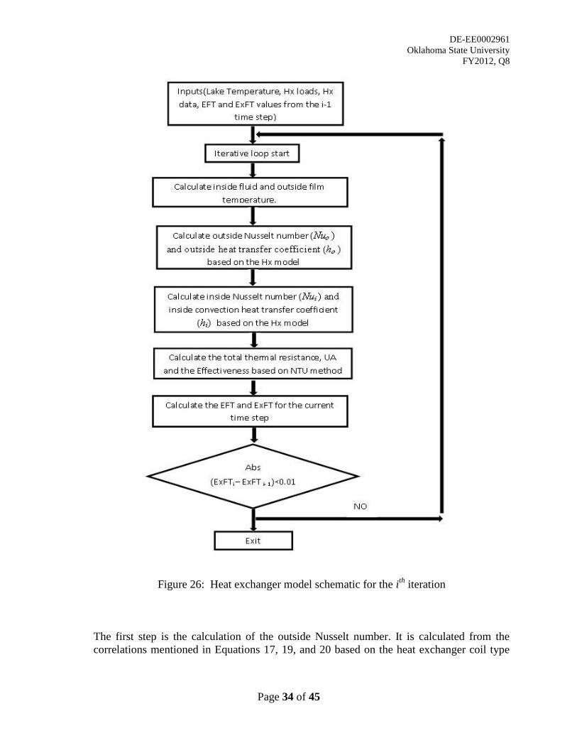
DE-EE0002961
Oklahoma State University
FY2012, Q8
Page 34 of 45
Figure 26: Heat exchanger model schematic for the i
th iteration
The first step is the calculation of the outside Nusselt number. It is calculated from the
correlations mentioned in Equations 17, 19, and 20 based on the heat exchanger coil type
DE-EE0002961
Oklahoma State University
FY2012, Q8
Page 35 of 45
and the film temperature. The outside convection coefficient is calculated by multiplying
the outside Nusselt number with the thermal conductivity of the pond and dividing by the
outside pipe diameter:
(21)
Next, the inside Nusselt number is calculated. Similar to the outside Nusselt number
calculation, the inside Nusselt number is calculation depends on the type of the heat
exchanger coil used. For spiral-helical and helical coils the correlation obtained by
Salimpour (2009) is used.
(22)
(23)
(24)
Where,
NuI is the inside Nusselt number calculated at the inside fluid temperature [-]
Pr is Prandtl number calculated at the inside fluid temperature [-]
De is the Dean number [-]
γ is the dimensionless pitch ratio [-]
di is the inside pipe diameter [m]
Dc is the coil diameter [m]
Re is the Reynolds number [-]
In the case of flat spiral and vertical-horizontal slinky coils, the inside Nusselt number is
calculated based on Rogers and Mayhew (1964) correlation for curved pipes.
(25)
For flat plate heat exchangers the inside Nusselt number is calculated based on the Dittus-
Boelter (Sleicher and Rouse 1975) correlation for straight pipes, shown in Equation 26.
More literature search is currently needed to find an acceptable correlation for the inside
Nusselt number for flat plate heat exchanger.
(26)
Where,
n = 0.3 for fluid cooling and 0.4 for fluid heating process.
DE-EE0002961
Oklahoma State University
FY2012, Q8
Page 36 of 45
Once the inside Nusselt number is calculated, the inside convection coefficient is calculated
by multiplying the inside Nusselt number with the thermal conductivity of the fluid and
dividing it by the pipe diameter.
(27)
The outside convection resistance (Ro) is calculated by taking the inverse of the outside
convection coefficient multiplied by the outside pipe surface area (Ao)
(28)
Similarly, the inside convection resistance (Ri) is calculated by taking the inverse of the
inside convection coefficient multiplied by the inside pipe surface area (Ai)
(29)
The conductive thermal resistance of the HDPE pipe is calculated via Equation 30:
(30)
Where,
kpipe is the thermal conductivity of the pipe [W/m-K]
Lpipe is the length of the heat exchanger pipe [m]
The UA of the heat exchanger can then be found using Equation 31.
(31)
Next, the effectiveness (ε) of the heat exchanger is calculated based on the NTU
formulation
(32)
(33)
(34)
Where,
mf is the fluid mass flow rate [Kg/s]
is the fluid heat capacity [J/kg-K]
DE-EE0002961
Oklahoma State University
FY2012, Q8
Page 37 of 45
The heat exchanger entering and exiting fluid temperatures are calculated by the following
equations
(35)
(36)
Where,
EFTi is the heat exchanger entering fluid temperature in the i‟th iteration [°C]
ExFTi is the heat exchanger exiting fluid temperature in the ith
iteration [°C]
Ql is the load on each heat exchanger coil [W]
Verification of results from the heat exchanger model:
The heat exchanger model was verified with the experimental results from a spiral-helical
heat exchanger coil placed in the OSU research pond. A time-dependent load was given to
the heat exchanger coils and the EFT and ExFT of the heat exchanger were calculated at 10
second intervals. The duration of the experiment done was approximately 3 hours. The
dimensions of the spiral-helical heat exchanger are as follows:
Pipe inner diameter - 1” (0.0254 m)
Coil outer diameter – 6‟6” (1.98 m)
Coil inner diameter – 4‟0” (1.22 m)
Horizontal spacing between coils – 2.625” (0.066 m)
Vertical spacing between coils – 2.625” (0.066m)
The model was simulated with the same heat exchanger loads and the ExFT from the
model was compared with the ExFT measured experimentally. Figure 27 shows the
comparison between the simulated ExFT and the experimental ExFT of the heat exchanger
coil for the experiment conducted on September 7, 2011. The simulation under predicts the
ExFT by approximately 1 °C. The reason for the difference in temperature is still under
investigation.

DE-EE0002961
Oklahoma State University
FY2012, Q8
Page 38 of 45
Figure 27: Comparison between experimental and model ExFT on September 7, 2011
Subtask 4.3 Implementation of Enhanced Pond Model in Design Tool:
In this quarter, the implementation of the enhanced pond model in design tool has focused
on building up the structure of the code and beginning some basic testing. The design tool
is based on the existing pond model, coupled with surface water heat exchangers and heat
pump simulation.
Current Structure of the Design Tool:
The Surface Water Heat Exchanger (SWHE) design tool currently operates as a Microsoft
Excel spreadsheet, with Visual Basic for Applications handling the simulation. The
spreadsheet interface requires inputs such as lake geometry, heat exchanger information,
heat pump specification, building heating and cooling loads, and weather data. It then calls
the existing pond model to calculate the lake temperatures in the heat exchanger immersion
range. Finally, the design tool calculates the heat exchanger entering and exiting fluid
temperature (EFT and ExFT) iteratively, along with estimated lake temperatures. A
schematic of the program is as shown in Figure 28, including various inputs and outputs.
15
17
19
21
23
25
27
29
0 2000 4000 6000 8000 10000 12000 14000
Tem
per
atu
re (
°C)
Timestep (s)
EFT(Exp)
ExFT(Exp)
ExFT(sim)
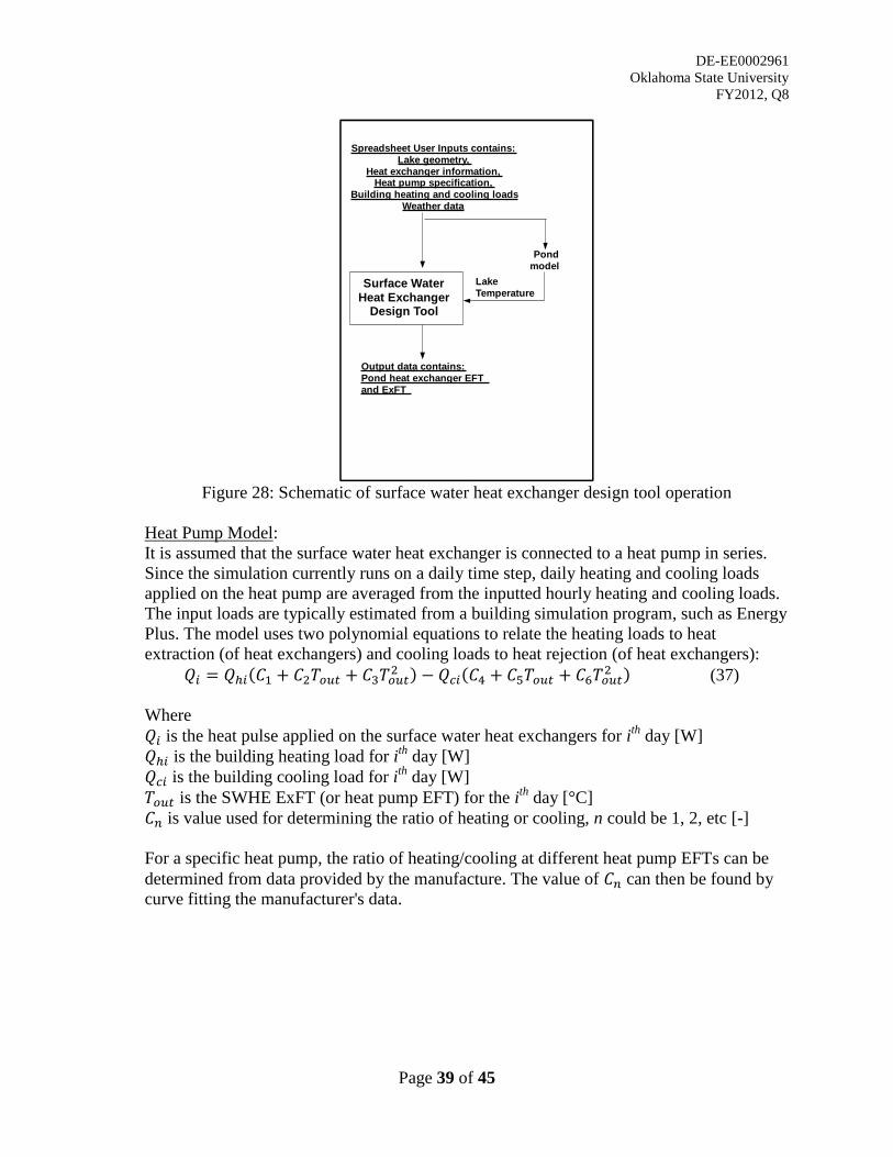
DE-EE0002961
Oklahoma State University
FY2012, Q8
Page 39 of 45
Figure 28: Schematic of surface water heat exchanger design tool operation
Heat Pump Model:
It is assumed that the surface water heat exchanger is connected to a heat pump in series.
Since the simulation currently runs on a daily time step, daily heating and cooling loads
applied on the heat pump are averaged from the inputted hourly heating and cooling loads.
The input loads are typically estimated from a building simulation program, such as Energy
Plus. The model uses two polynomial equations to relate the heating loads to heat
extraction (of heat exchangers) and cooling loads to heat rejection (of heat exchangers):
(37)
Where
is the heat pulse applied on the surface water heat exchangers for ith
day [W]
is the building heating load for ith
day [W]
is the building cooling load for ith
day [W]
is the SWHE ExFT (or heat pump EFT) for the ith
day [°C]
is value used for determining the ratio of heating or cooling, n could be 1, 2, etc [-]
For a specific heat pump, the ratio of heating/cooling at different heat pump EFTs can be
determined from data provided by the manufacture. The value of can then be found by
curve fitting the manufacturer's data.
Spreadsheet User Inputs contains:Lake geometry,
Heat exchanger information,Heat pump specification,
Building heating and cooling loadsWeather data
Surface Water
Heat Exchanger Design Tool
Pond model
Lake Temperature
Output data contains:Pond heat exchanger EFT and ExFT
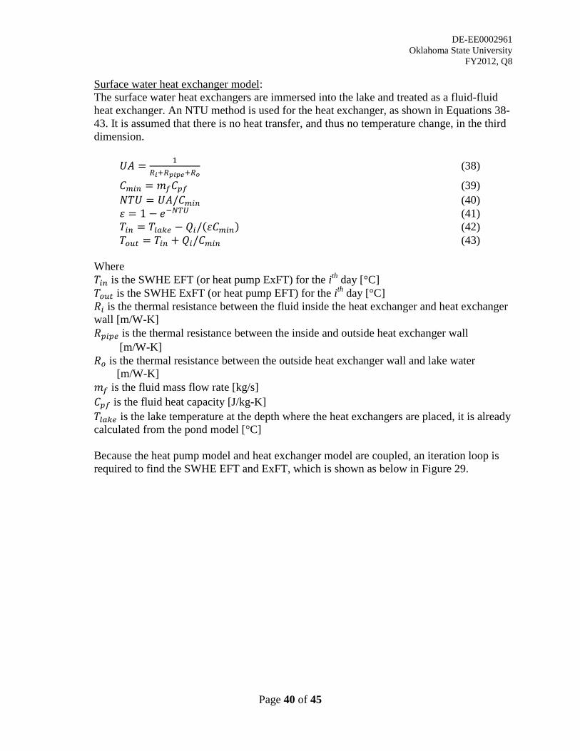
DE-EE0002961
Oklahoma State University
FY2012, Q8
Page 40 of 45
Surface water heat exchanger model:
The surface water heat exchangers are immersed into the lake and treated as a fluid-fluid
heat exchanger. An NTU method is used for the heat exchanger, as shown in Equations 38-
43. It is assumed that there is no heat transfer, and thus no temperature change, in the third
dimension.
(38)
(39)
(40)
(41)
(42)
(43)
Where
is the SWHE EFT (or heat pump ExFT) for the ith
day [°C]
is the SWHE ExFT (or heat pump EFT) for the ith
day [°C]
is the thermal resistance between the fluid inside the heat exchanger and heat exchanger
wall [m/W-K]
is the thermal resistance between the inside and outside heat exchanger wall
[m/W-K]
is the thermal resistance between the outside heat exchanger wall and lake water
[m/W-K]
is the fluid mass flow rate [kg/s]
is the fluid heat capacity [J/kg-K]
is the lake temperature at the depth where the heat exchangers are placed, it is already
calculated from the pond model [°C]
Because the heat pump model and heat exchanger model are coupled, an iteration loop is
required to find the SWHE EFT and ExFT, which is shown as below in Figure 29.
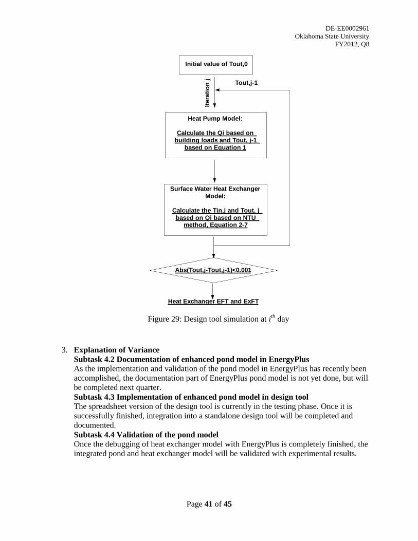
DE-EE0002961
Oklahoma State University
FY2012, Q8
Page 41 of 45
Figure 29: Design tool simulation at i
th day
3. Explanation of Variance
Subtask 4.2 Documentation of enhanced pond model in EnergyPlus
As the implementation and validation of the pond model in EnergyPlus has recently been
accomplished, the documentation part of EnergyPlus pond model is not yet done, but will
be completed next quarter.
Subtask 4.3 Implementation of enhanced pond model in design tool
The spreadsheet version of the design tool is currently in the testing phase. Once it is
successfully finished, integration into a standalone design tool will be completed and
documented.
Subtask 4.4 Validation of the pond model
Once the debugging of heat exchanger model with EnergyPlus is completely finished, the
integrated pond and heat exchanger model will be validated with experimental results.
Initial value of Tout,0
Heat Pump Model:
Calculate the Qi based on building loads and Tout, j-1
based on Equation 1
Surface Water Heat Exchanger Model:
Calculate the Tin,j and Tout, j based on Qi based on NTU
method, Equation 2-7
Tout,j-1
Ite
rati
on
j
Abs(Tout,j-Tout,j-1)<0.001
Heat Exchanger EFT and ExFT
DE-EE0002961
Oklahoma State University
FY2012, Q8
Page 42 of 45
4. Plans for Next Quarter:
Subtask 4.1 Modeling of alternate pond heat exchanger types
The accuracy of the heat exchanger model developed will be validated with the
experimental data for all the five heat exchanger types. The current difference between
the model and the experimental ExFT for the spiral-coil heat exchanger needs to be
examined so that it may be reduced further. Once the debugging of EnergyPlus model is
complete, it will be documented.
Subtask 4.2 Documentation of enhanced pond model in EnergyPlus
The milestone report containing the documentation of the EnergyPlus model with
examples of usage will be prepared.
Subtask 4.3 Implementation of the enhanced pond model in design tool
The design tool developed will also be tested and validated against the available
experimental data. Additionally, the design tool should include the capability to size the
heat exchanger based on a specified maximum and minimum heat pump entering fluid
temperature. A GLHEPRO version of the design tool will be created and documented.
Subtask 4.4 Validation of the pond model
The EnergyPlus pond model will be completely validated with experimental results from
different heat exchanger types.
References
Deng, Z. 2004. Modeling of Standing Column Wells in Ground Source Heat Pump Systems
Ph.D.Thesis, Oklahoma State University.
Freeze, R.A and J.A Cherry. 1979. Groundwater. Prentice-Hall, Inc. Englewood Cliffs, NJ 0762.
Hvorslev, M.J. 1951. Time lag and soil permeability in ground water observations. Bulletin no
36, Waterways Experiment Station Corps of Engineers, U.S. Army Vicksburg, MI.
Hansen, G.M. 2011. Experimental testing and analysis of spiral-helical surface water heat
exchanger configurations Masters Thesis, Oklahoma State University.
Rogers, G.F.C and Y.R. Mayhew 1964. Heat transfer and pressure loss in helically coiled tubes
with turbulent flow. International Journal of Heat and Mass Transfer 7(11): 1207-1216.
Salimpour, M.R. 2009. Heat transfer coefficients of shell and coiled tube heat exchangers.
Experimental Thermal and Fluid Science 33(2):203-207.
Sleicher,C.A. and M.W. Rouse 1975. A convenient correlation for heat transfer to constant and
variable property fluids in turbulent pipe flow. International Journal of Heat and Mass
Transfer 18(5): 677-683.

DE-EE0002961
Oklahoma State University
FY2012, Q8
Page 43 of 45
Theis, C.V. 1935. The relation between the lowering of the piezometric surface and the rate and
duration of discharge of well using groundwater storage. Transactions of American
Geophysics Union, 2: 519-524.
Sleicher,C.A. and M.W. Rouse 1975. A convenient correlation for heat transfer to constant and
variable property fluids in turbulent pipe flow. International Journal of Heat and Mass
Transfer 18(5): 677-683.

DE-EE0002961
Oklahoma State University
FY2012, Q8
Page 44 of 45
PRODUCTS / DELIVERABLES
Training and Professional Development: n/a
Publications, Conference Papers, and Presentations: n/a
Patents and IP: n/a
Other Products / Deliverables: n/a

DE-EE0002961
Oklahoma State University
FY2012, Q8
Page 45 of 45
BUDGETARY AND OTHER INFORMATION
Complete the following tables in the Excel Progress Report accordingly:
Budget by Task – “QuarterlySumRpt” Tab
Financial and Spend Plan Data – “Financial Data” Tab
To insert this document into the Excel Progress Report:
A cell is provided in the Excel Progress Report (BP/BQ 10) to insert this Project Narrative. To
insert your narrative file into this cell, employ the "Insert" function from the excel tool bar.
Select "Insert Object" and select the "Create from File" tab. Use the "Browse" option to locate
the file you wish to insert. Check the "Display as Icon" box and select "OK".
Recipient Requests for DOE Attention: n/a

DE-EE0002961 Oklahoma State University
FY2012, Q9
Page 1 of 22
Quarterly Research Performance Progress Report Federal Agency and Organization: DOE EERE – Geothermal Technologies Program Recipient Organization: Oklahoma State University DUNS Number: 049987720 Recipient Address: Stillwater, OK 74078 Award Number: DE-EE0002961/001 Project Title: Improved Design Tools for Surface Water and Standing Column Well Heat Pump Systems Project Period: October 1, 2010 to August 31, 2012 Principal Investigator: Jeffrey D. Spitler
Regents Professor and C.M. Leonard Professor [email protected] 405-744-5900
Date of Report Submission: Apr 30, 2012 Reporting Period: January 1, 2012 to March 31, 2012 Report Frequency: Quarterly Project Partners: n/a DOE Project Team: DOE Contracting Officer – Genevieve Wozniak DOE Project Officer – Ava Coy Project Monitor – Sara Gonnion
DE-EE0002961 Oklahoma State University
FY2012, Q9
Page 2 of 22
STATUS / ACCOMPLISHMENTS Project Status Summary: The project is divided into the Standing Column Well (SCW) and Surface Water (SW) tracks. In the SCW track the main objectives are the enhancement of an existing 1D SCW model and implementation of the enhanced model in EnergyPlus and in a design tool. The enhancements to the model involved implementing a separate bleed control strategy and developing a suitable model to account for the effects of natural convection. During the current reporting period a technical paper was submitted to a conference on thermal energy storage, INNOSTOCK 2012, describing the quasi-two-dimensional SCW model developed in the previous quarter. Additionally, to account for thermal short circuiting in the SCW the results of the quasi-two-dimensional model were analyzed using the line source approach to generate an effective borehole thermal resistance which could be used in a more computationally efficient 1D SCW model that will be implemented in EnergyPlus and in the design tool. The main objectives of the SW track are to enhance the existing pond model and to implement it in both EnergyPlus and a ground heat exchanger design tool. In this reporting period, efforts focused on further improvements to the accuracy of the pond model via improved surface convection and evaporation models. This improves results during the shoulder seasons. Additionally, the EnergyPlus model documentation has been completed, and work continues on the stand-alone design tool. Task 1.0 – Enhancement of Existing Standing Column Well Model
1. Planned Activities: Subtask 1.1: Development and validation of SCW model with separate bleed control The one-dimensional SCW model requires a better analysis of the short-circuiting resistance. A correction factor or effective resistance term will be developed using the quasi-2D SCW model. Subtask 1.2: Testing of model with various bleed control strategies After correcting the 1D model to include thermal short-circuiting, different bleed control strategies will be tested.
2. Actual Accomplishments:
Subtask 1.1: Development and validation of SCW model with separate bleed control To be able to develop an effective borehole thermal resistance to be used for the one-dimensional SCW model the results of the quasi-two-dimensional model were analyzed using the line source method to generate an effective borehole resistance. The line source approach was developed by Lord Kelvin; it considered the ground and the line source to be infinite mediums. It was first to applied to ground heat exchangers by Ingersoll and Plass (1948) according to Equation 1.
𝑇(𝑟, 𝑡) − 𝑇𝑖 = 𝑞′4𝜋𝑘 ∫
𝑒−𝐵2
𝐵∞𝑟
2√𝛼𝑡𝑑𝐵 (1)
Where,
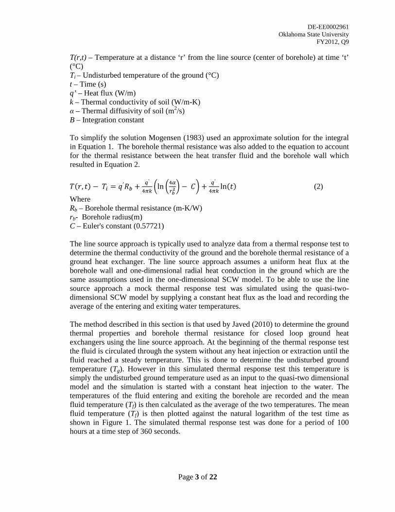
DE-EE0002961 Oklahoma State University
FY2012, Q9
Page 3 of 22
T(r,t) – Temperature at a distance ‘r’ from the line source (center of borehole) at time ‘t’ (°C) Ti – Undisturbed temperature of the ground (°C) t – Time (s) q’ – Heat flux (W/m) k – Thermal conductivity of soil (W/m-K) α – Thermal diffusivity of soil (m2/s) B – Integration constant To simplify the solution Mogensen (1983) used an approximate solution for the integral in Equation 1. The borehole thermal resistance was also added to the equation to account for the thermal resistance between the heat transfer fluid and the borehole wall which resulted in Equation 2.
𝑇(𝑟, 𝑡) − 𝑇𝑖 = 𝑞′𝑅𝑏 + 𝑞′
4𝜋𝑘�ln �4𝛼
𝑟𝑏2� − 𝐶� + 𝑞′
4𝜋𝑘ln(𝑡) (2)
Where Rb – Borehole thermal resistance (m-K/W) rb- Borehole radius(m) C – Euler's constant (0.57721) The line source approach is typically used to analyze data from a thermal response test to determine the thermal conductivity of the ground and the borehole thermal resistance of a ground heat exchanger. The line source approach assumes a uniform heat flux at the borehole wall and one-dimensional radial heat conduction in the ground which are the same assumptions used in the one-dimensional SCW model. To be able to use the line source approach a mock thermal response test was simulated using the quasi-two-dimensional SCW model by supplying a constant heat flux as the load and recording the average of the entering and exiting water temperatures.
The method described in this section is that used by Javed (2010) to determine the ground thermal properties and borehole thermal resistance for closed loop ground heat exchangers using the line source approach. At the beginning of the thermal response test the fluid is circulated through the system without any heat injection or extraction until the fluid reached a steady temperature. This is done to determine the undisturbed ground temperature (Tg). However in this simulated thermal response test this temperature is simply the undisturbed ground temperature used as an input to the quasi-two dimensional model and the simulation is started with a constant heat injection to the water. The temperatures of the fluid entering and exiting the borehole are recorded and the mean fluid temperature (Tf) is then calculated as the average of the two temperatures. The mean fluid temperature (Tf) is then plotted against the natural logarithm of the test time as shown in Figure 1. The simulated thermal response test was done for a period of 100 hours at a time step of 360 seconds.
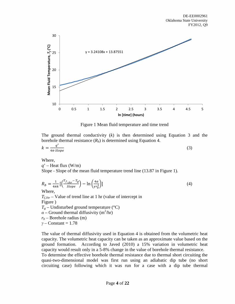
DE-EE0002961 Oklahoma State University
FY2012, Q9
Page 4 of 22
Figure 1 Mean fluid temperature and time trend
The ground thermal conductivity (k) is then determined using Equation 3 and the borehole thermal resistance (Rb) is determined using Equation 4. 𝑘 = 𝑞′
4𝜋∙𝑆𝑙𝑜𝑝𝑒 (3)
Where, q’ – Heat flux (W/m) Slope - Slope of the mean fluid temperature trend line (13.87 in Figure 1).
𝑅𝑏 = 14𝜋𝑘
[�𝑇𝑓1ℎ𝑟− 𝑇𝑔𝑆𝑙𝑜𝑝𝑒
� − ln � 4𝛼𝛾𝑟𝑏
2�] (4)
Where, Tf,1hr – Value of trend line at 1 hr (value of intercept in Figure ) Tg – Undisturbed ground temperature (°C) α – Ground thermal diffusivity (m2/hr) rb – Borehole radius (m) γ – Constant = 1.78 The value of thermal diffusivity used in Equation 4 is obtained from the volumetric heat capacity. The volumetric heat capacity can be taken as an approximate value based on the ground formation. According to Javed (2010) a 15% variation in volumetric heat capacity would result only in a 5-8% change in the value of borehole thermal resistance. To determine the effective borehole thermal resistance due to thermal short circuiting the quasi-two-dimensional model was first run using an adiabatic dip tube (no short circuiting case) following which it was run for a case with a dip tube thermal
y = 3.24108x + 13.87551
10
15
20
25
30
0 0.5 1 1.5 2 2.5 3 3.5 4 4.5 5
Mea
n Fl
uid
Tem
pera
ture
, Tf (
°C)
ln [time] (hours)
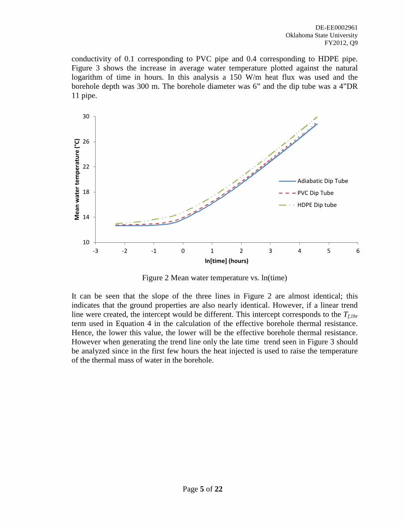
DE-EE0002961 Oklahoma State University
FY2012, Q9
Page 5 of 22
conductivity of 0.1 corresponding to PVC pipe and 0.4 corresponding to HDPE pipe. Figure 3 shows the increase in average water temperature plotted against the natural logarithm of time in hours. In this analysis a 150 W/m heat flux was used and the borehole depth was 300 m. The borehole diameter was 6” and the dip tube was a 4”DR 11 pipe.
Figure 2 Mean water temperature vs. ln(time) It can be seen that the slope of the three lines in Figure 2 are almost identical; this indicates that the ground properties are also nearly identical. However, if a linear trend line were created, the intercept would be different. This intercept corresponds to the Tf,1hr term used in Equation 4 in the calculation of the effective borehole thermal resistance. Hence, the lower this value, the lower will be the effective borehole thermal resistance. However when generating the trend line only the late time trend seen in Figure 3 should be analyzed since in the first few hours the heat injected is used to raise the temperature of the thermal mass of water in the borehole.
10
14
18
22
26
30
-3 -2 -1 0 1 2 3 4 5 6
Mea
n w
ater
tem
pera
ture
(°C)
ln[time] (hours)
Adiabatic Dip Tube
PVC Dip Tube
HDPE Dip tube
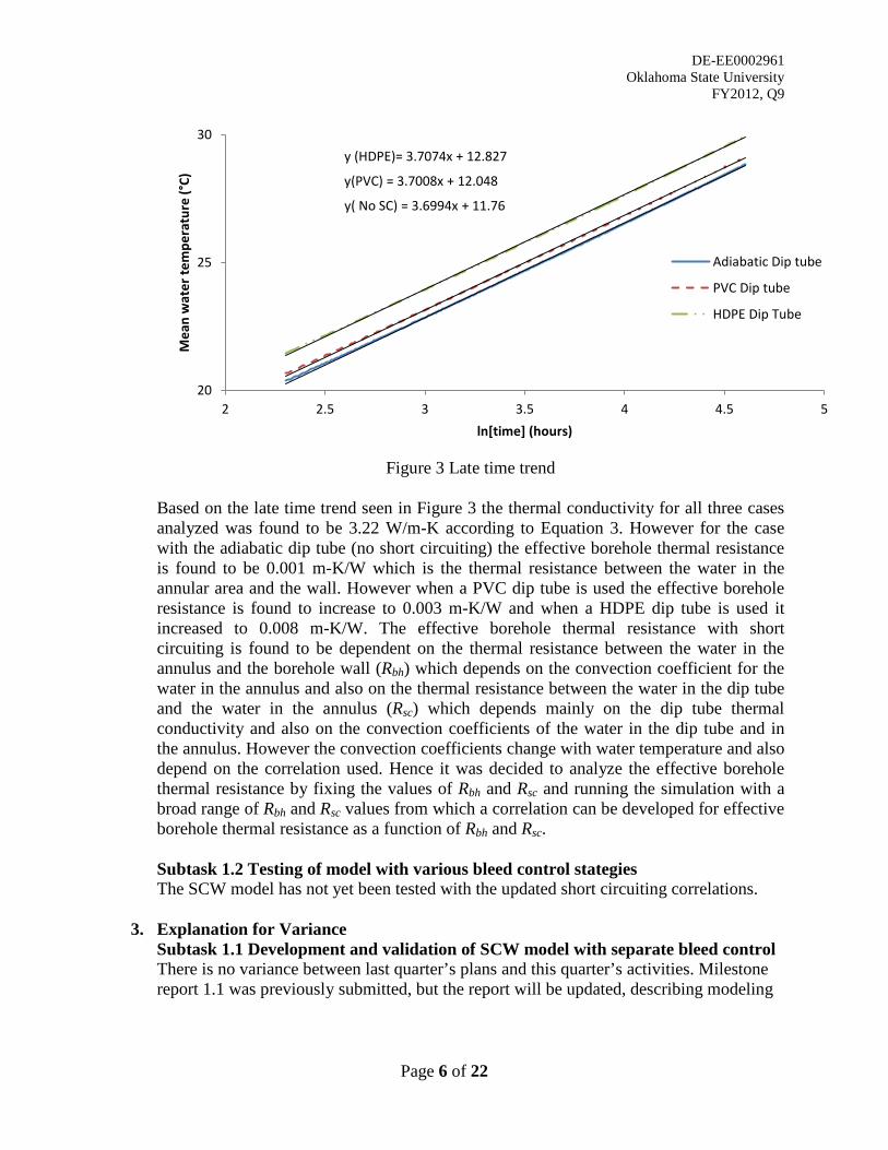
DE-EE0002961 Oklahoma State University
FY2012, Q9
Page 6 of 22
Figure 3 Late time trend Based on the late time trend seen in Figure 3 the thermal conductivity for all three cases analyzed was found to be 3.22 W/m-K according to Equation 3. However for the case with the adiabatic dip tube (no short circuiting) the effective borehole thermal resistance is found to be 0.001 m-K/W which is the thermal resistance between the water in the annular area and the wall. However when a PVC dip tube is used the effective borehole resistance is found to increase to 0.003 m-K/W and when a HDPE dip tube is used it increased to 0.008 m-K/W. The effective borehole thermal resistance with short circuiting is found to be dependent on the thermal resistance between the water in the annulus and the borehole wall (Rbh) which depends on the convection coefficient for the water in the annulus and also on the thermal resistance between the water in the dip tube and the water in the annulus (Rsc) which depends mainly on the dip tube thermal conductivity and also on the convection coefficients of the water in the dip tube and in the annulus. However the convection coefficients change with water temperature and also depend on the correlation used. Hence it was decided to analyze the effective borehole thermal resistance by fixing the values of Rbh and Rsc and running the simulation with a broad range of Rbh and Rsc values from which a correlation can be developed for effective borehole thermal resistance as a function of Rbh and Rsc. Subtask 1.2 Testing of model with various bleed control stategies The SCW model has not yet been tested with the updated short circuiting correlations.
3. Explanation for Variance Subtask 1.1 Development and validation of SCW model with separate bleed control There is no variance between last quarter’s plans and this quarter’s activities. Milestone report 1.1 was previously submitted, but the report will be updated, describing modeling
y( No SC) = 3.6994x + 11.76
y(PVC) = 3.7008x + 12.048
y (HDPE)= 3.7074x + 12.827
20
25
30
2 2.5 3 3.5 4 4.5 5
Mea
n w
ater
tem
pera
ture
(°C)
ln[time] (hours)
Adiabatic Dip tube
PVC Dip tube
HDPE Dip Tube
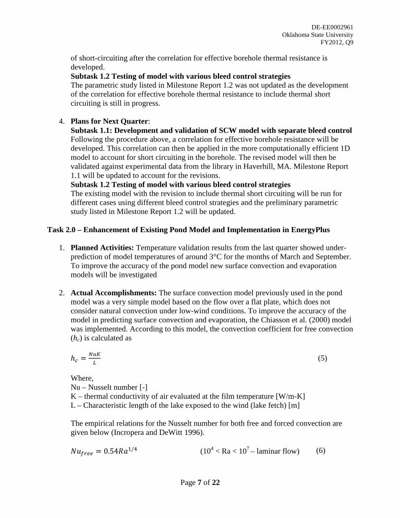
DE-EE0002961 Oklahoma State University
FY2012, Q9
Page 7 of 22
of short-circuiting after the correlation for effective borehole thermal resistance is developed. Subtask 1.2 Testing of model with various bleed control strategies The parametric study listed in Milestone Report 1.2 was not updated as the development of the correlation for effective borehole thermal resistance to include thermal short circuiting is still in progress.
4. Plans for Next Quarter:
Subtask 1.1: Development and validation of SCW model with separate bleed control Following the procedure above, a correlation for effective borehole resistance will be developed. This correlation can then be applied in the more computationally efficient 1D model to account for short circuiting in the borehole. The revised model will then be validated against experimental data from the library in Haverhill, MA. Milestone Report 1.1 will be updated to account for the revisions. Subtask 1.2 Testing of model with various bleed control strategies The existing model with the revision to include thermal short circuiting will be run for different cases using different bleed control strategies and the preliminary parametric study listed in Milestone Report 1.2 will be updated.
Task 2.0 – Enhancement of Existing Pond Model and Implementation in EnergyPlus
1. Planned Activities: Temperature validation results from the last quarter showed under-prediction of model temperatures of around 3°C for the months of March and September. To improve the accuracy of the pond model new surface convection and evaporation models will be investigated
2. Actual Accomplishments: The surface convection model previously used in the pond model was a very simple model based on the flow over a flat plate, which does not consider natural convection under low-wind conditions. To improve the accuracy of the model in predicting surface convection and evaporation, the Chiasson et al. (2000) model was implemented. According to this model, the convection coefficient for free convection (hc) is calculated as ℎ𝑐 = 𝑁𝑢𝐾
𝐿 (5)
Where, Nu – Nusselt number [-] K – thermal conductivity of air evaluated at the film temperature [W/m-K] L – Characteristic length of the lake exposed to the wind (lake fetch) [m] The empirical relations for the Nusselt number for both free and forced convection are given below (Incropera and DeWitt 1996). 𝑁𝑢𝑓𝑟𝑒𝑒 = 0.54𝑅𝑎1/4 (104 < Ra < 107 – laminar flow) (6)
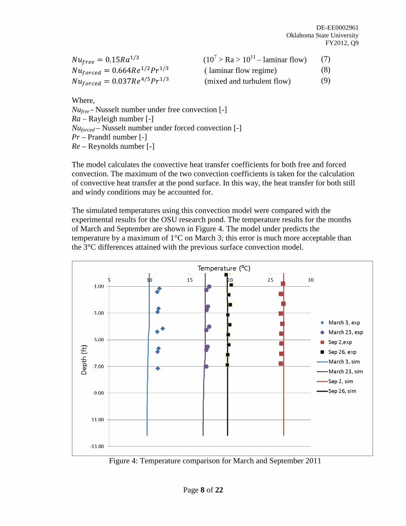
DE-EE0002961 Oklahoma State University
FY2012, Q9
Page 8 of 22
𝑁𝑢𝑓𝑟𝑒𝑒 = 0.15𝑅𝑎1/3 (107 > Ra > 1011 – laminar flow) (7) 𝑁𝑢𝑓𝑜𝑟𝑐𝑒𝑑 = 0.664𝑅𝑒1/2𝑃𝑟1/3 ( laminar flow regime) (8) 𝑁𝑢𝑓𝑜𝑟𝑐𝑒𝑑 = 0.037𝑅𝑒4/5𝑃𝑟1/3 (mixed and turbulent flow) (9) Where, Nufree - Nusselt number under free convection [-] Ra – Rayleigh number [-] Nuforced – Nusselt number under forced convection [-] Pr – Prandtl number [-] Re – Reynolds number [-] The model calculates the convective heat transfer coefficients for both free and forced convection. The maximum of the two convection coefficients is taken for the calculation of convective heat transfer at the pond surface. In this way, the heat transfer for both still and windy conditions may be accounted for. The simulated temperatures using this convection model were compared with the experimental results for the OSU research pond. The temperature results for the months of March and September are shown in Figure 4. The model under predicts the temperature by a maximum of 1°C on March 3; this error is much more acceptable than the 3°C differences attained with the previous surface convection model.
Figure 4: Temperature comparison for March and September 2011

DE-EE0002961 Oklahoma State University
FY2012, Q9
Page 9 of 22
3. Plans for Next Quarter: This task, including all subtasks, is now complete.
Task 3.0 – Implementation of Enhanced SCW Model
1. Planned Activities: Subtask 3.1 Implementation of Enhanced SCW Model in EnergyPlus The SCW model in EnergyPlus is to be debugged and verified against the validated HVACSIM+ model of the SCW. Subtask 3.2 Implementation of Enhanced SCW Model in Design Tool An SCW model based on this work will be added to a stand-alone ground heat exchanger design tool. Subtask 3.3 Technology Transfer A technical paper was written and submitted to the INNOSTOCK 2012 conference.
2. Actual Accomplishments: Subtask 3.1 Implementation of Enhanced SCW Model in EnergyPlus The implementation of the enhanced SCW model in Energy Plus is continuing. Once the correlation for effective borehole resistance to include thermal short circuiting is developed it will be included in the EnergyPlus model. Subtask 3.2 Implementation of Enhanced SCW Model in Design Tool The SCW model has been added to the ground heat exchanger design tool GLHEPRO. The model (and the program itself) are currently in the debug phase. Subtask 3.3 Technology Transfer A paper describing the quasi-two-dimensional SCW model developed in the previous quarter was submitted to an international conference on thermal energy storage, INNOSTOCK 2012. This paper will be presented in Lleida, Spain, in May. A copy of the paper is attached with this report.
3. Explanation of Variance Subtask 3.1 Implementation of Enhanced SCW Model in EnergyPlus The model has been integrated into the plant loop of EnergyPlus. The inclusion of the correlation for effective borehole thermal resistance is pending. Subtask 3.2 Implementation of Enhanced SCW Model in Design Tool Several substantial issues have been encountered during the debugging of the design tool, some of which stem from a migration to the VB.Net platform.
4. Plans for Next Quarter: Subtask 3.1 Implementation of Enhanced SCW Model in EnergyPlus Once the correlation for effective borehole thermal resistance is developed it will be implemented in the enhanced EnergyPlus model and the Enhanced SCW model in EnergyPlus will be validated against experimental data from the Haverhill library. Subtask 3.2 Implementation of Enhanced SCW model in Design Tool The design tool program will continue to be debugged; once debugging is complete, the model will be rigorously tested.

DE-EE0002961 Oklahoma State University
FY2012, Q9
Page 10 of 22
Subtask 3.3 Technology Transfer This subtask is now complete.
Task 4.0 – Enhancement, Implementation, and Validation of Enhanced Pond Model
1. Planned Activities: Subtask 4.1 Modeling of alternate pond heat exchanger types A milestone report documenting the algorithms used in the alternate pond heat exchanger model will be submitted. Subtask 4.2 Documentation of enhanced pond model in EnergyPlus The enhanced pond model implemented in EnergyPlus will be completely documented, including Engineering Reference, Input/Output, and examples. Subtask 4.3 Implementation of enhanced pond model in design tool The enhanced pond model will be implemented into a standalone design tool for ground heat exchangers. Accompanying documentation will be written. Subtask 4.4 Validation of pond model The pond model integrated with the heat exchanger model in EnergyPlus will be validated against the experimental results obtained for different heat exchanger types from the OSU research pond. Subtask 4.5 Technology Transfer Several technical papers will be planned and developed.
2. Actual Accomplishments: Subtask 4.1 Modeling of alternate pond heat exchanger types Five different pond heat exchanger types have been modeled. Details on each of the models can be found in Milestone Report 4.1, which accompanies this report. Subtask 4.2 Documentation of Enhanced Pond model in Energy Plus The enhanced pond model is currently being fully integrated into EnergyPlus. The creation of EnergyPlus documentation, including Engineering Reference, Input/Output, and example files, has begun.
Subtask 4.3 Implementation of Enhanced Pond Model in Design Tool The enhanced pond model, including the effects of ice-on-coil, has been developed into an Excel spreadsheet design tool, using Visual Basic for Applications to run the simulations. This model is a modified version of the model for ice on coil for ice storage tank by Neto and Krarti (1997). A full description of the ice-on-coil model is given in Milestone Report 2.3. The design tool has been validated against experimental data from the OSU research pond for four heat exchanger types (spiral-helical coil, flat spiral coil, horizontal slinky coil and flat plate heat exchangers). For the validation, the design tool used actual weather data to compute the pond temperature, which was then used in the calculation of the heat exchanger EFT and ExFT. Table 1 lists information regarding the experiment for the spiral-helical coil, including heat exchanger dimensions.
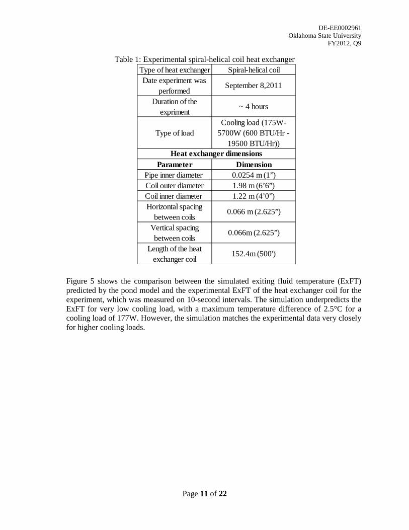
DE-EE0002961 Oklahoma State University
FY2012, Q9
Page 11 of 22
Table 1: Experimental spiral-helical coil heat exchanger
Figure 5 shows the comparison between the simulated exiting fluid temperature (ExFT) predicted by the pond model and the experimental ExFT of the heat exchanger coil for the experiment, which was measured on 10-second intervals. The simulation underpredicts the ExFT for very low cooling load, with a maximum temperature difference of 2.5°C for a cooling load of 177W. However, the simulation matches the experimental data very closely for higher cooling loads.
Type of heat exchanger Spiral-helical coilDate experiment was
performedSeptember 8,2011
Duration of the expriment
~ 4 hours
Type of loadCooling load (175W-
5700W (600 BTU/Hr - 19500 BTU/Hr))
Parameter DimensionPipe inner diameter 0.0254 m (1”)Coil outer diameter 1.98 m (6’6”)Coil inner diameter 1.22 m (4’0”)Horizontal spacing
between coils 0.066 m (2.625”)
Vertical spacing between coils
0.066m (2.625”)
Length of the heat exchanger coil
152.4m (500')
Heat exchanger dimensions
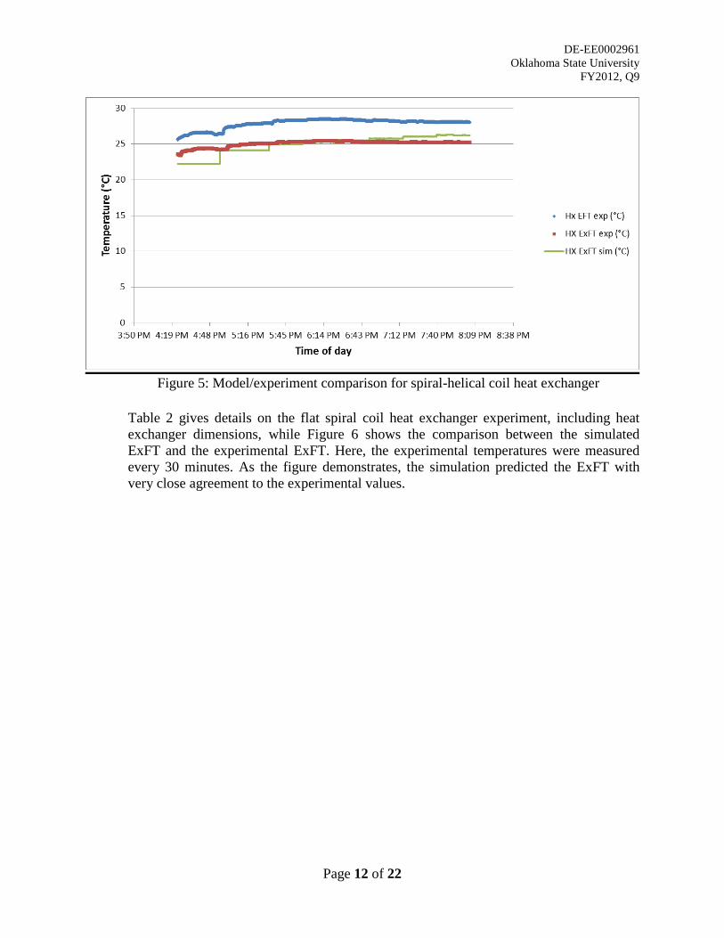
DE-EE0002961 Oklahoma State University
FY2012, Q9
Page 12 of 22
Figure 5: Model/experiment comparison for spiral-helical coil heat exchanger
Table 2 gives details on the flat spiral coil heat exchanger experiment, including heat exchanger dimensions, while Figure 6 shows the comparison between the simulated ExFT and the experimental ExFT. Here, the experimental temperatures were measured every 30 minutes. As the figure demonstrates, the simulation predicted the ExFT with very close agreement to the experimental values.
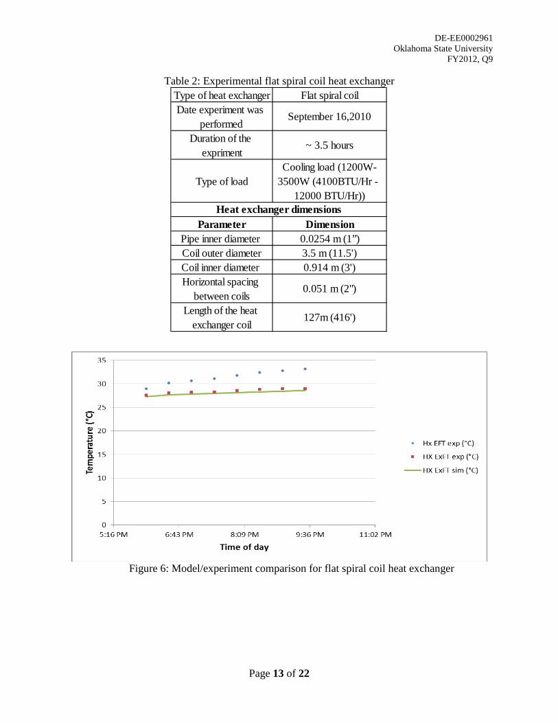
DE-EE0002961 Oklahoma State University
FY2012, Q9
Page 13 of 22
Table 2: Experimental flat spiral coil heat exchanger
Figure 6: Model/experiment comparison for flat spiral coil heat exchanger
Type of heat exchanger Flat spiral coilDate experiment was
performedSeptember 16,2010
Duration of the expriment
~ 3.5 hours
Type of loadCooling load (1200W-
3500W (4100BTU/Hr - 12000 BTU/Hr))
Parameter DimensionPipe inner diameter 0.0254 m (1”)Coil outer diameter 3.5 m (11.5')Coil inner diameter 0.914 m (3')Horizontal spacing
between coils 0.051 m (2")
Length of the heat exchanger coil
127m (416')
Heat exchanger dimensions
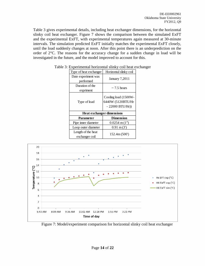
DE-EE0002961 Oklahoma State University
FY2012, Q9
Page 14 of 22
Table 3 gives experimental details, including heat exchanger dimensions, for the horizontal slinky coil heat exchanger. Figure 7 shows the comparison between the simulated ExFT and the experimental ExFT, with experimental temperatures again measured at 30-minute intervals. The simulation predicted ExFT initially matches the experimental ExFT closely, until the load suddenly changes at noon. After this point there is an underprediction on the order of 2°C. The reasons for the accuracy change for a sudden change in load will be investigated in the future, and the model improved to account for this.
Table 3: Experimental horizontal slinky coil heat exchanger
Figure 7: Model/experiment comparison for horizontal slinky coil heat exchanger
Type of heat exchanger Horizontal slinky coilDate experiment was
performedJanuary 7,2011
Duration of the expriment
~ 7.5 hours
Type of loadCooling load (1500W-6440W (5120BTU/Hr
- 22000 BTU/Hr))
Parameter DimensionPipe inner diameter 0.0254 m (1”)Loop outer diameter 0.91 m (3')Length of the heat
exchanger coil152.4m (500')
Heat exchanger dimensions
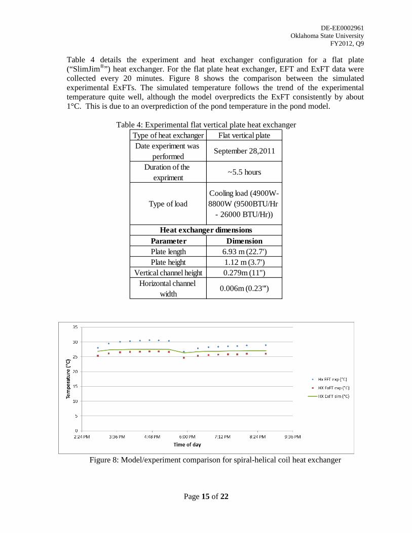
DE-EE0002961 Oklahoma State University
FY2012, Q9
Page 15 of 22
Table 4 details the experiment and heat exchanger configuration for a flat plate (“SlimJim®”) heat exchanger. For the flat plate heat exchanger, EFT and ExFT data were collected every 20 minutes. Figure 8 shows the comparison between the simulated experimental ExFTs. The simulated temperature follows the trend of the experimental temperature quite well, although the model overpredicts the ExFT consistently by about 1°C. This is due to an overprediction of the pond temperature in the pond model.
Table 4: Experimental flat vertical plate heat exchanger
Figure 8: Model/experiment comparison for spiral-helical coil heat exchanger
Type of heat exchanger Flat vertical plateDate experiment was
performedSeptember 28,2011
Duration of the expriment
~5.5 hours
Type of loadCooling load (4900W-8800W (9500BTU/Hr
- 26000 BTU/Hr))
Parameter DimensionPlate length 6.93 m (22.7')Plate height 1.12 m (3.7')
Vertical channel height 0.279m (11'')Horizontal channel
width0.006m (0.23"')
Heat exchanger dimensions
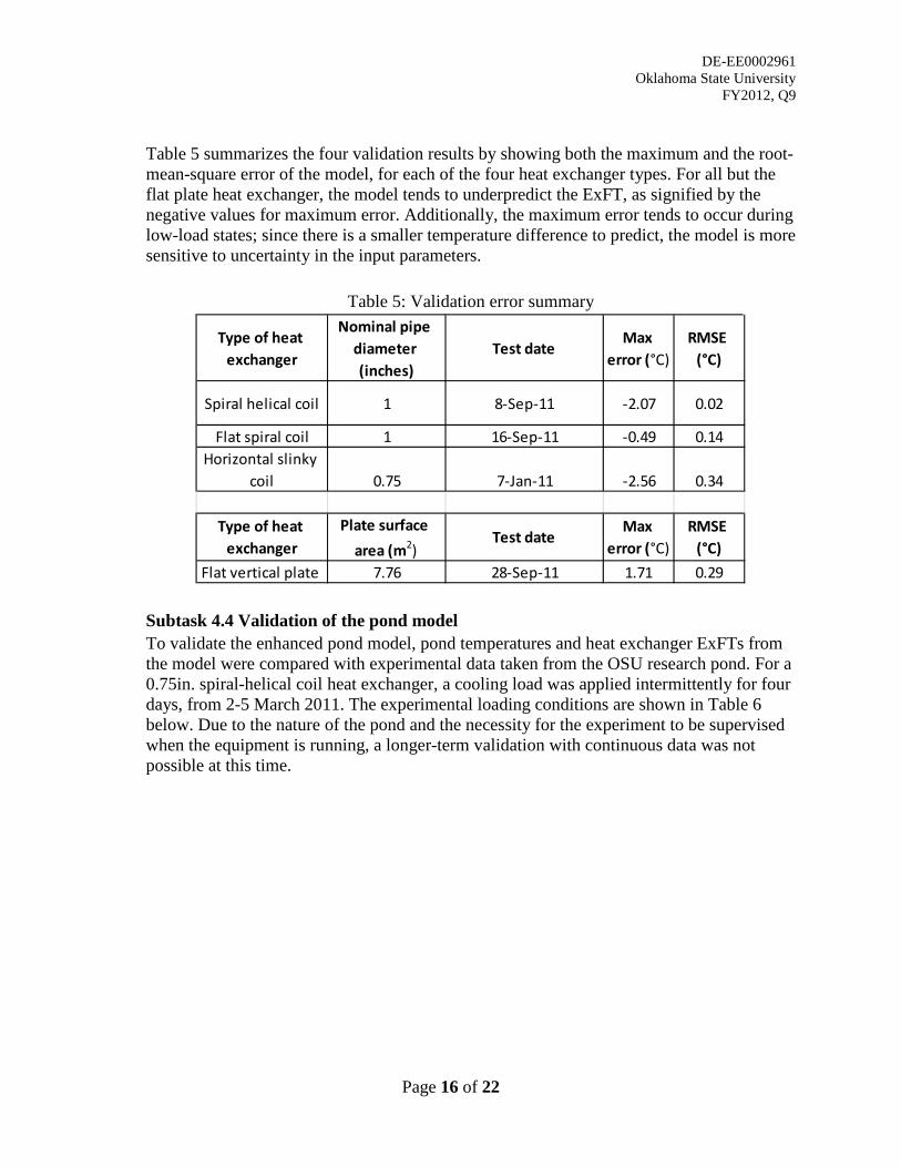
DE-EE0002961 Oklahoma State University
FY2012, Q9
Page 16 of 22
Table 5 summarizes the four validation results by showing both the maximum and the root-mean-square error of the model, for each of the four heat exchanger types. For all but the flat plate heat exchanger, the model tends to underpredict the ExFT, as signified by the negative values for maximum error. Additionally, the maximum error tends to occur during low-load states; since there is a smaller temperature difference to predict, the model is more sensitive to uncertainty in the input parameters.
Table 5: Validation error summary
Subtask 4.4 Validation of the pond model To validate the enhanced pond model, pond temperatures and heat exchanger ExFTs from the model were compared with experimental data taken from the OSU research pond. For a 0.75in. spiral-helical coil heat exchanger, a cooling load was applied intermittently for four days, from 2-5 March 2011. The experimental loading conditions are shown in Table 6 below. Due to the nature of the pond and the necessity for the experiment to be supervised when the equipment is running, a longer-term validation with continuous data was not possible at this time.
Type of heat exchanger
Nominal pipe diameter (inches)
Test dateMax
error (°C)RMSE
(°C)
Spiral helical coil 1 8-Sep-11 -2.07 0.02
Flat spiral coil 1 16-Sep-11 -0.49 0.14Horizontal slinky
coil 0.75 7-Jan-11 -2.56 0.34
Type of heat exchanger
Plate surface area (m2)
Test dateMax
error (°C)RMSE
(°C)Flat vertical plate 7.76 28-Sep-11 1.71 0.29
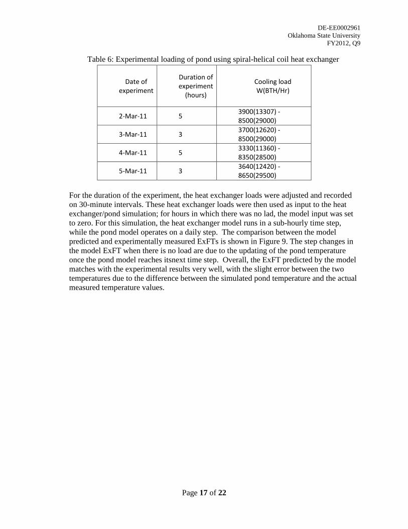
DE-EE0002961 Oklahoma State University
FY2012, Q9
Page 17 of 22
Table 6: Experimental loading of pond using spiral-helical coil heat exchanger
Date of experiment
Duration of experiment
(hours)
Cooling load W(BTH/Hr)
2-Mar-11 5 3900(13307) - 8500(29000)
3-Mar-11 3 3700(12620) - 8500(29000)
4-Mar-11 5 3330(11360) - 8350(28500)
5-Mar-11 3 3640(12420) - 8650(29500)
For the duration of the experiment, the heat exchanger loads were adjusted and recorded on 30-minute intervals. These heat exchanger loads were then used as input to the heat exchanger/pond simulation; for hours in which there was no lad, the model input was set to zero. For this simulation, the heat exchanger model runs in a sub-hourly time step, while the pond model operates on a daily step. The comparison between the model predicted and experimentally measured ExFTs is shown in Figure 9. The step changes in the model ExFT when there is no load are due to the updating of the pond temperature once the pond model reaches itsnext time step. Overall, the ExFT predicted by the model matches with the experimental results very well, with the slight error between the two temperatures due to the difference between the simulated pond temperature and the actual measured temperature values.
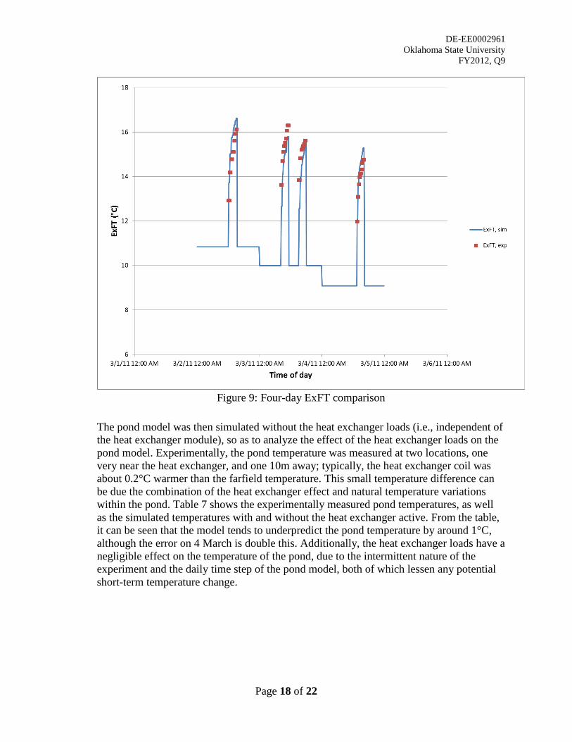
DE-EE0002961 Oklahoma State University
FY2012, Q9
Page 18 of 22
Figure 9: Four-day ExFT comparison
The pond model was then simulated without the heat exchanger loads (i.e., independent of the heat exchanger module), so as to analyze the effect of the heat exchanger loads on the pond model. Experimentally, the pond temperature was measured at two locations, one very near the heat exchanger, and one 10m away; typically, the heat exchanger coil was about 0.2°C warmer than the farfield temperature. This small temperature difference can be due the combination of the heat exchanger effect and natural temperature variations within the pond. Table 7 shows the experimentally measured pond temperatures, as well as the simulated temperatures with and without the heat exchanger active. From the table, it can be seen that the model tends to underpredict the pond temperature by around 1°C, although the error on 4 March is double this. Additionally, the heat exchanger loads have a negligible effect on the temperature of the pond, due to the intermittent nature of the experiment and the daily time step of the pond model, both of which lessen any potential short-term temperature change.
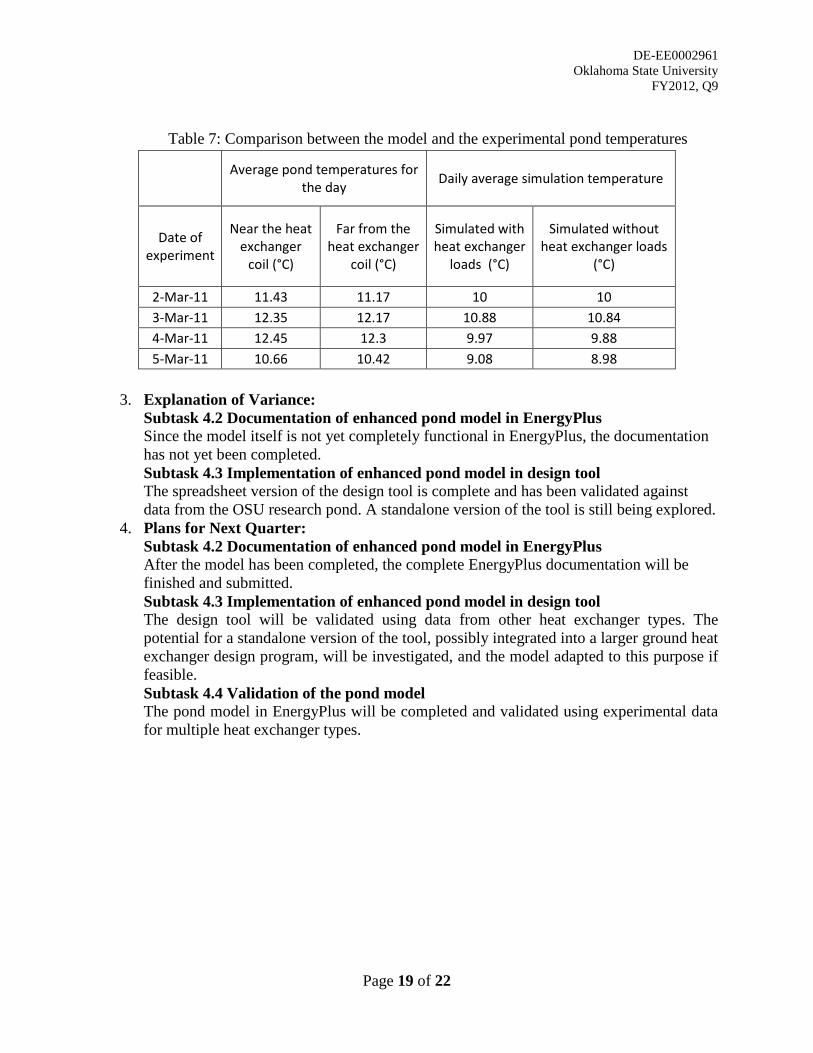
DE-EE0002961 Oklahoma State University
FY2012, Q9
Page 19 of 22
Table 7: Comparison between the model and the experimental pond temperatures
Average pond temperatures for
the day Daily average simulation temperature
Date of experiment
Near the heat exchanger
coil (°C)
Far from the heat exchanger
coil (°C)
Simulated with heat exchanger
loads (°C)
Simulated without heat exchanger loads
(°C)
2-Mar-11 11.43 11.17 10 10 3-Mar-11 12.35 12.17 10.88 10.84 4-Mar-11 12.45 12.3 9.97 9.88 5-Mar-11 10.66 10.42 9.08 8.98
3. Explanation of Variance:
Subtask 4.2 Documentation of enhanced pond model in EnergyPlus Since the model itself is not yet completely functional in EnergyPlus, the documentation has not yet been completed. Subtask 4.3 Implementation of enhanced pond model in design tool The spreadsheet version of the design tool is complete and has been validated against data from the OSU research pond. A standalone version of the tool is still being explored.
4. Plans for Next Quarter: Subtask 4.2 Documentation of enhanced pond model in EnergyPlus After the model has been completed, the complete EnergyPlus documentation will be finished and submitted. Subtask 4.3 Implementation of enhanced pond model in design tool The design tool will be validated using data from other heat exchanger types. The potential for a standalone version of the tool, possibly integrated into a larger ground heat exchanger design program, will be investigated, and the model adapted to this purpose if feasible. Subtask 4.4 Validation of the pond model The pond model in EnergyPlus will be completed and validated using experimental data for multiple heat exchanger types.

DE-EE0002961 Oklahoma State University
FY2012, Q9
Page 20 of 22
References Chiasson, A.D., J.D. Spitler, S.J. Rees, and M.D. Smith. 2000. A Model for Simulating the
Performance of a Shallow Pond as a Supplemental Heat Rejector with Closed-Loop Ground-Source Heat Pump Systems. ASHRAE Transcations 106(2): 107-121.
Incropera, F.P., and D.P. DeWitt. 1996. Introduction to heat transfer. New York: John Wiley and Sons.
Ingersoll, L.R., and H.J. Plass. 1948. Theory of the Ground Pipe Heat Source for the Heat Pump. Heating, Piping & Air Conditioning.
Javed, S. 2010. Design of ground source heat pump systems. Licentiate Thesis. Chalmers University of Technology, Göteborg, Sweden.
Mogensen, P. 1983. Fluid to Duct Wall Heat Transfer in Duct System Heat Storages. Proceedings of the International Conference on Subsurface Heat Storage in Theory and Practice, Sweden, Swedish Council for Building Research.
Neto, J. H. M. and M. Krarti. 1997. Deterministic model for an internal melt ice-on-coil thermal storage tank. ASHRAE Transactions 103(1): 113-124.

DE-EE0002961 Oklahoma State University
FY2012, Q9
Page 21 of 22
PRODUCTS / DELIVERABLES
Training and Professional Development: n/a Publications, Conference Papers, and Presentations: See attached paper: Ramesh, A., J.D. Spitler. 2012. A quasi-two-dimensional standing column well model for ground source heat pump systems. Accepted for publication in the proceedings of Innostock 2012, The 12th International Conference on Energy Storage. Patents and IP: n/a Other Products / Deliverables: n/a

DE-EE0002961 Oklahoma State University
FY2012, Q9
Page 22 of 22
BUDGETARY AND OTHER INFORMATION Complete the following tables in the Excel Progress Report accordingly:
• Budget by Task – “QuarterlySumRpt” Tab • Financial and Spend Plan Data – “Financial Data” Tab
To insert this document into the Excel Progress Report: A cell is provided in the Excel Progress Report (BP/BQ 10) to insert this Project Narrative. To insert your narrative file into this cell, employ the "Insert" function from the excel tool bar. Select "Insert Object" and select the "Create from File" tab. Use the "Browse" option to locate the file you wish to insert. Check the "Display as Icon" box and select "OK". Recipient Requests for DOE Attention: n/a

Milestone report: Modeling of alternate pond heat exchanger types DE-EE0002961 1
Milestone Report
Task 4.1- Modeling of alternate pond heat exchanger types
DE-EE0002961/001 - Recovery Act:
Improved Design Tools for Surface Water and Standing Column Well Heat Pump
Systems
Krishna Conjeevaram Bashyam, ([email protected]), Research Associate,
Professor Jeffrey D Spitler, ([email protected]), Principal Investigator,
Oklahoma State University
Introduction
In practice, there are several types of pond heat exchangers and the amount of heat
transfer varies between heat exchanger types even with identical geometric conditions. Based on
his experiments at the OSU research pond, Hansen (2011) obtained outside Nusselt number
correlations for five different types of pond heat exchangers. These correlations are implemented
in the heat exchanger module of the enhanced pond model.
Methodology
Hansen (2011) conducted a total of 119 tests on five different heat exchanger coil types
in the 3 acre (12,000 m2) OSU research pond and developed three correlations to calculate the
outside Nusselt number and hence the outside convection heat transfer coefficient. The heat
exchanger types tested were spiral-helical, spiral, slinky-type, loose bundled, and flat vertical
plate heat exchangers (e.g. “SlimJim®”). The breakdown of the tests and the parameters varied in
the tests are shown in Table 1 below.
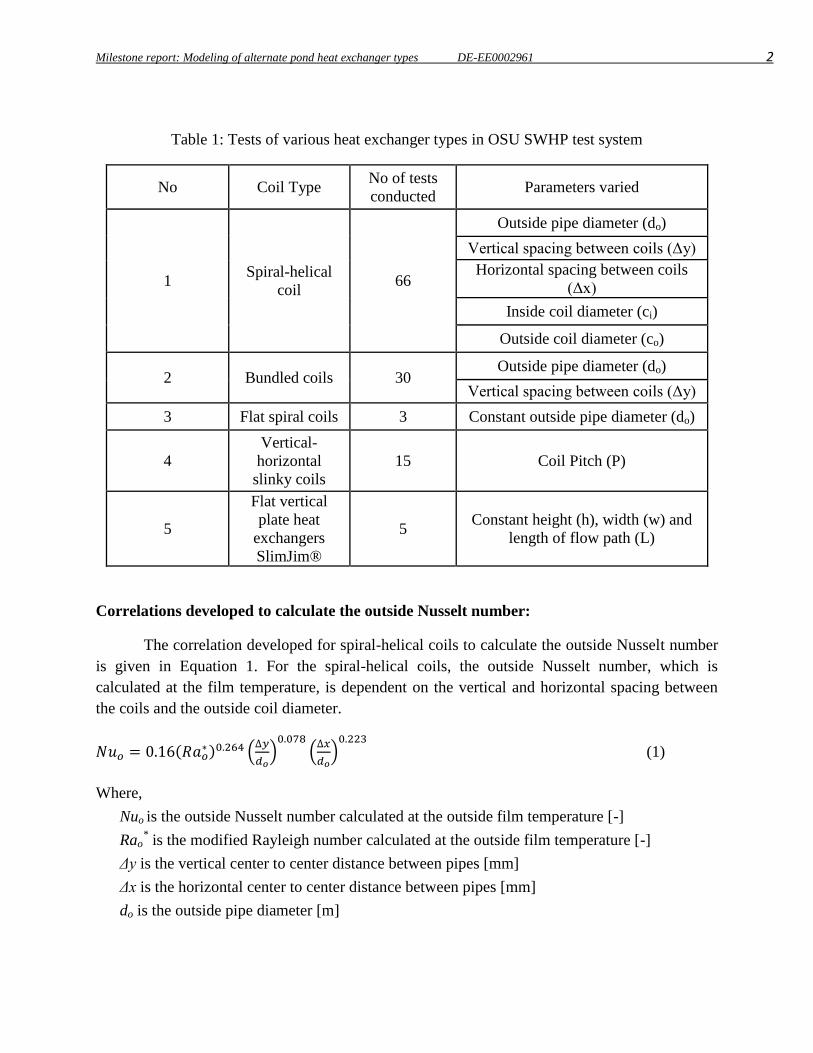
Milestone report: Modeling of alternate pond heat exchanger types DE-EE0002961 2
Table 1: Tests of various heat exchanger types in OSU SWHP test system
No Coil Type No of tests
conducted Parameters varied
1 Spiral-helical
coil 66
Outside pipe diameter (do)
Vertical spacing between coils (Δy)
Horizontal spacing between coils
(Δx)
Inside coil diameter (ci)
Outside coil diameter (co)
2 Bundled coils 30 Outside pipe diameter (do)
Vertical spacing between coils (Δy)
3 Flat spiral coils 3 Constant outside pipe diameter (do)
4
Vertical-
horizontal
slinky coils
15 Coil Pitch (P)
5
Flat vertical
plate heat
exchangers
SlimJim®
5 Constant height (h), width (w) and
length of flow path (L)
Correlations developed to calculate the outside Nusselt number:
The correlation developed for spiral-helical coils to calculate the outside Nusselt number
is given in Equation 1. For the spiral-helical coils, the outside Nusselt number, which is
calculated at the film temperature, is dependent on the vertical and horizontal spacing between
the coils and the outside coil diameter.
( ) (
)
(
)
(1)
Where,
Nuo is the outside Nusselt number calculated at the outside film temperature [-]
Rao* is the modified Rayleigh number calculated at the outside film temperature [-]
Δy is the vertical center to center distance between pipes [mm]
Δx is the horizontal center to center distance between pipes [mm]
do is the outside pipe diameter [m]
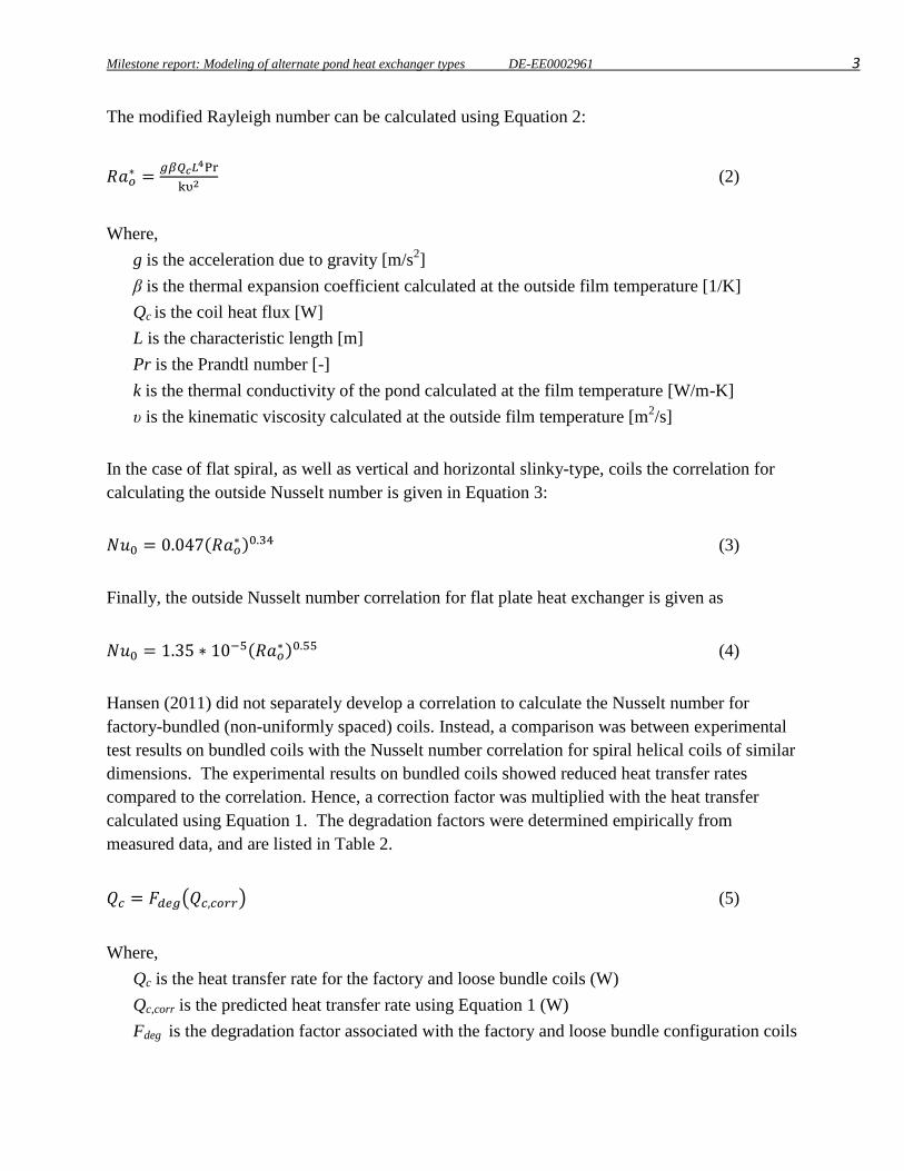
Milestone report: Modeling of alternate pond heat exchanger types DE-EE0002961 3
The modified Rayleigh number can be calculated using Equation 2:
(2)
Where,
g is the acceleration due to gravity [m/s2]
β is the thermal expansion coefficient calculated at the outside film temperature [1/K]
Qc is the coil heat flux [W]
L is the characteristic length [m]
Pr is the Prandtl number [-]
k is the thermal conductivity of the pond calculated at the film temperature [W/m-K]
υ is the kinematic viscosity calculated at the outside film temperature [m2/s]
In the case of flat spiral, as well as vertical and horizontal slinky-type, coils the correlation for
calculating the outside Nusselt number is given in Equation 3:
( ) (3)
Finally, the outside Nusselt number correlation for flat plate heat exchanger is given as
(
) (4)
Hansen (2011) did not separately develop a correlation to calculate the Nusselt number for
factory-bundled (non-uniformly spaced) coils. Instead, a comparison was between experimental
test results on bundled coils with the Nusselt number correlation for spiral helical coils of similar
dimensions. The experimental results on bundled coils showed reduced heat transfer rates
compared to the correlation. Hence, a correction factor was multiplied with the heat transfer
calculated using Equation 1. The degradation factors were determined empirically from
measured data, and are listed in Table 2.
( ) (5)
Where,
Qc is the heat transfer rate for the factory and loose bundle coils (W)
Qc,corr is the predicted heat transfer rate using Equation 1 (W)
Fdeg is the degradation factor associated with the factory and loose bundle configuration coils
Milestone report: Modeling of alternate pond heat exchanger types DE-EE0002961 4
The degradation factor for different bundle coil configurations is given in the following table
Table 2: Degradation factors for different bundled coil configurations
Degradation factor (Fdeg)
Tube diameter mm(inches)
Loose bundles
Factory bundles
19(0.75) 0.7 0.4
25.4(1) 0.7 0.45
31.75(1.25) 0.85 0.6
Current structure of the heat exchanger model:
The heat exchanger model takes in the average lake temperature, building heating/cooling
loads and heat exchanger information as inputs. The building loads are given as inputs to the heat
pump model to calculate the load on the heat exchanger coils. The load experienced by the heat
exchanger coils are calculated from the building loads based on the type and performance of the
heat pump. The values of the entering fluid temperature (EFT) and the exiting fluid temperature
(ExFT) to the heat exchanger are assumed initially. The schematic of the heat exchanger model
is shown in Figure 1 below.
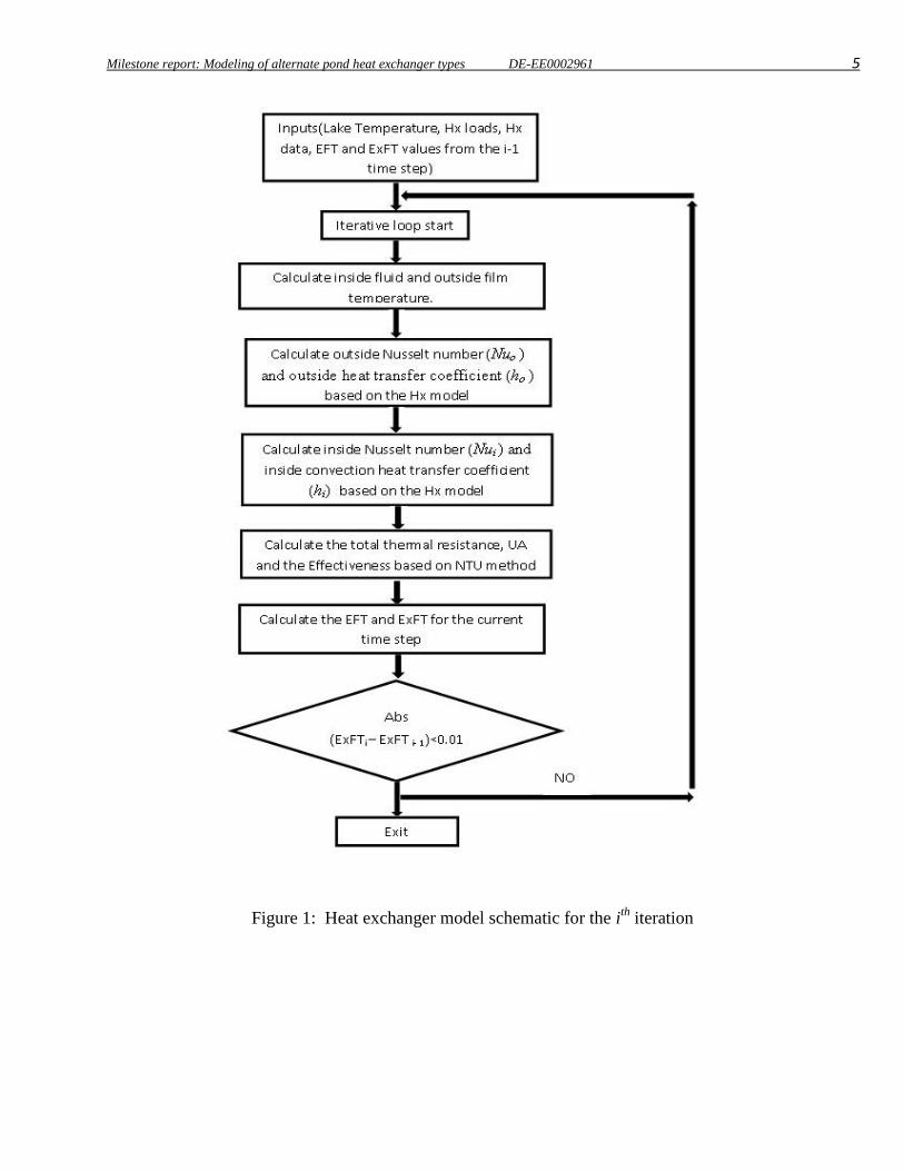
Milestone report: Modeling of alternate pond heat exchanger types DE-EE0002961 5
Figure 1: Heat exchanger model schematic for the ith
iteration
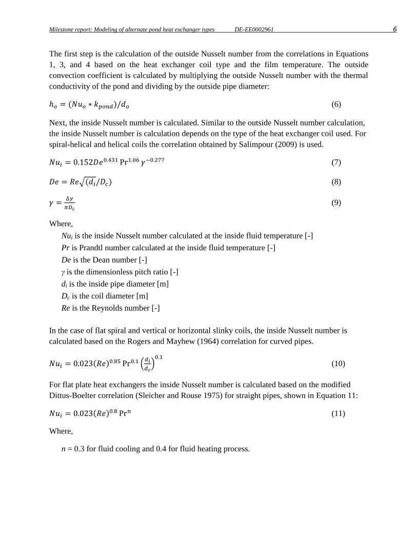
Milestone report: Modeling of alternate pond heat exchanger types DE-EE0002961 6
The first step is the calculation of the outside Nusselt number from the correlations in Equations
1, 3, and 4 based on the heat exchanger coil type and the film temperature. The outside
convection coefficient is calculated by multiplying the outside Nusselt number with the thermal
conductivity of the pond and dividing by the outside pipe diameter:
( ) (6)
Next, the inside Nusselt number is calculated. Similar to the outside Nusselt number calculation,
the inside Nusselt number is calculation depends on the type of the heat exchanger coil used. For
spiral-helical and helical coils the correlation obtained by Salimpour (2009) is used.
(7)
√( ) (8)
(9)
Where,
Nui is the inside Nusselt number calculated at the inside fluid temperature [-]
Pr is Prandtl number calculated at the inside fluid temperature [-]
De is the Dean number [-]
γ is the dimensionless pitch ratio [-]
di is the inside pipe diameter [m]
Dc is the coil diameter [m]
Re is the Reynolds number [-]
In the case of flat spiral and vertical or horizontal slinky coils, the inside Nusselt number is
calculated based on the Rogers and Mayhew (1964) correlation for curved pipes.
( ) (
)
(10)
For flat plate heat exchangers the inside Nusselt number is calculated based on the modified
Dittus-Boelter correlation (Sleicher and Rouse 1975) for straight pipes, shown in Equation 11:
( ) (11)
Where,
n = 0.3 for fluid cooling and 0.4 for fluid heating process.
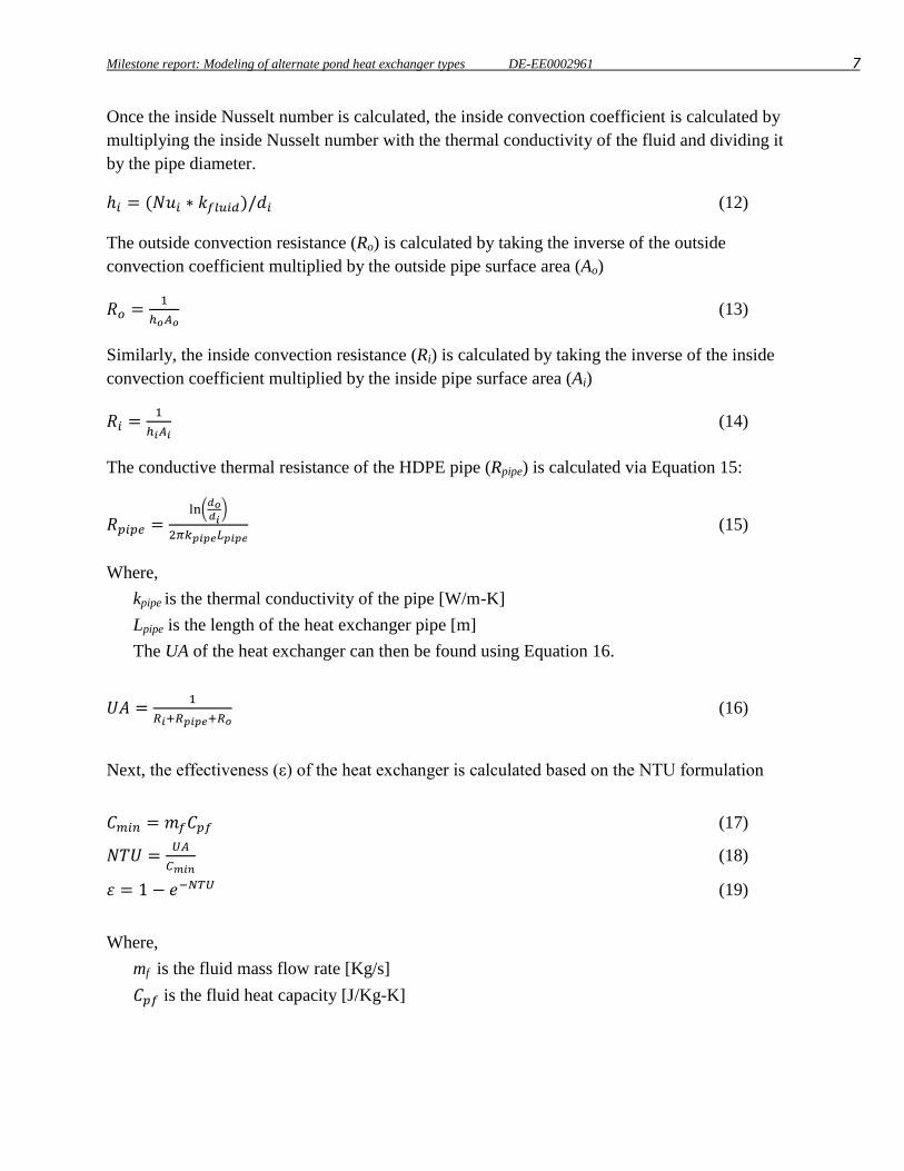
Milestone report: Modeling of alternate pond heat exchanger types DE-EE0002961 7
Once the inside Nusselt number is calculated, the inside convection coefficient is calculated by
multiplying the inside Nusselt number with the thermal conductivity of the fluid and dividing it
by the pipe diameter.
( ) (12)
The outside convection resistance (Ro) is calculated by taking the inverse of the outside
convection coefficient multiplied by the outside pipe surface area (Ao)
(13)
Similarly, the inside convection resistance (Ri) is calculated by taking the inverse of the inside
convection coefficient multiplied by the inside pipe surface area (Ai)
(14)
The conductive thermal resistance of the HDPE pipe (Rpipe) is calculated via Equation 15:
(
)
(15)
Where,
kpipe is the thermal conductivity of the pipe [W/m-K]
Lpipe is the length of the heat exchanger pipe [m]
The UA of the heat exchanger can then be found using Equation 16.
(16)
Next, the effectiveness (ε) of the heat exchanger is calculated based on the NTU formulation
(17)
(18)
(19)
Where,
mf is the fluid mass flow rate [Kg/s]
is the fluid heat capacity [J/Kg-K]
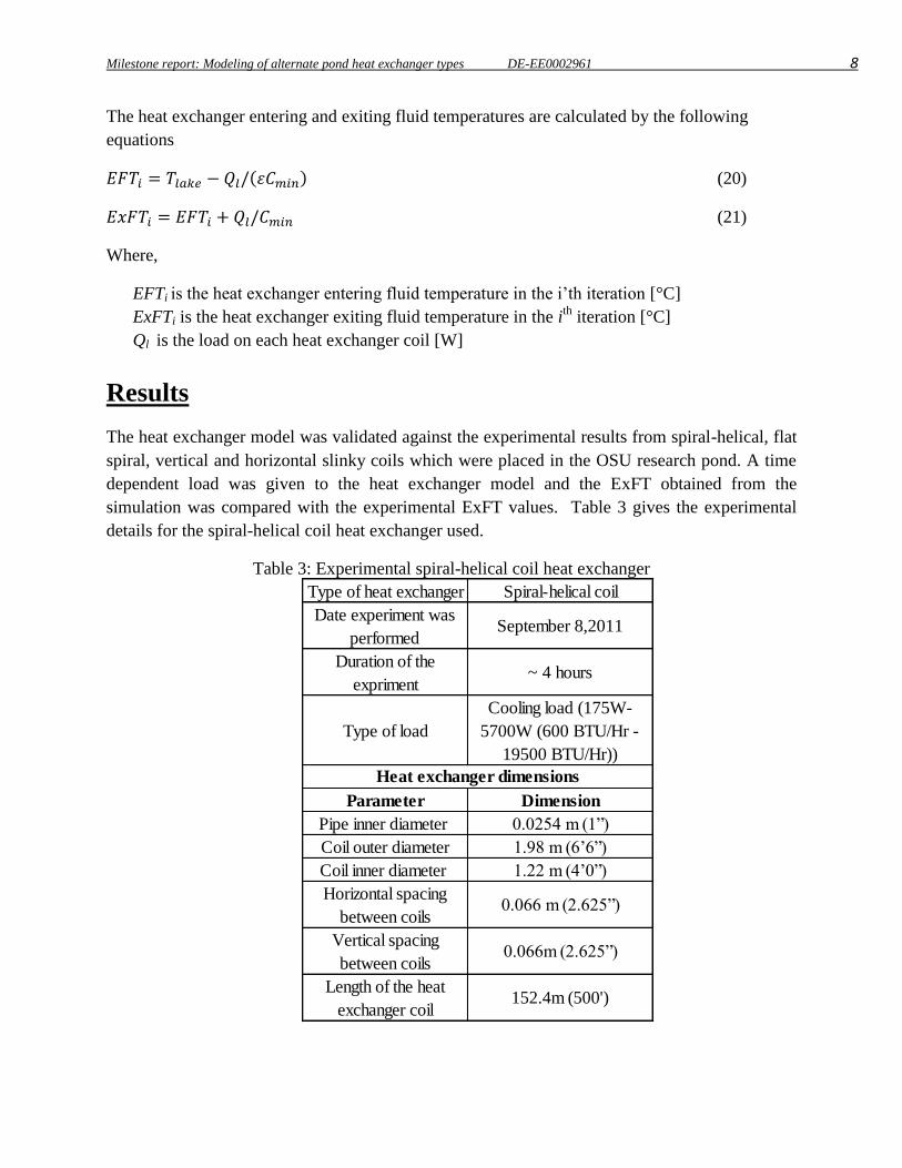
Milestone report: Modeling of alternate pond heat exchanger types DE-EE0002961 8
The heat exchanger entering and exiting fluid temperatures are calculated by the following
equations
( ) (20)
(21)
Where,
EFTi is the heat exchanger entering fluid temperature in the i’th iteration [°C]
ExFTi is the heat exchanger exiting fluid temperature in the ith
iteration [°C]
Ql is the load on each heat exchanger coil [W]
Results
The heat exchanger model was validated against the experimental results from spiral-helical, flat
spiral, vertical and horizontal slinky coils which were placed in the OSU research pond. A time
dependent load was given to the heat exchanger model and the ExFT obtained from the
simulation was compared with the experimental ExFT values. Table 3 gives the experimental
details for the spiral-helical coil heat exchanger used.
Table 3: Experimental spiral-helical coil heat exchanger
Type of heat exchanger Spiral-helical coil
Date experiment was
performedSeptember 8,2011
Duration of the
expriment~ 4 hours
Type of load
Cooling load (175W-
5700W (600 BTU/Hr -
19500 BTU/Hr))
Parameter Dimension
Pipe inner diameter 0.0254 m (1”)
Coil outer diameter 1.98 m (6’6”)
Coil inner diameter 1.22 m (4’0”)
Horizontal spacing
between coils 0.066 m (2.625”)
Vertical spacing
between coils 0.066m (2.625”)
Length of the heat
exchanger coil152.4m (500')
Heat exchanger dimensions
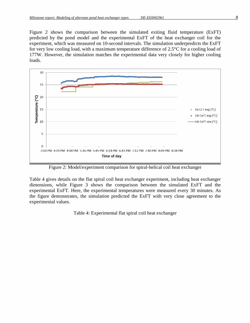
Milestone report: Modeling of alternate pond heat exchanger types DE-EE0002961 9
Figure 2 shows the comparison between the simulated exiting fluid temperature (ExFT)
predicted by the pond model and the experimental ExFT of the heat exchanger coil for the
experiment, which was measured on 10-second intervals. The simulation underpredicts the ExFT
for very low cooling load, with a maximum temperature difference of 2.5°C for a cooling load of
177W. However, the simulation matches the experimental data very closely for higher cooling
loads.
Figure 2: Model/experiment comparison for spiral-helical coil heat exchanger
Table 4 gives details on the flat spiral coil heat exchanger experiment, including heat exchanger
dimensions, while Figure 3 shows the comparison between the simulated ExFT and the
experimental ExFT. Here, the experimental temperatures were measured every 30 minutes. As
the figure demonstrates, the simulation predicted the ExFT with very close agreement to the
experimental values.
Table 4: Experimental flat spiral coil heat exchanger
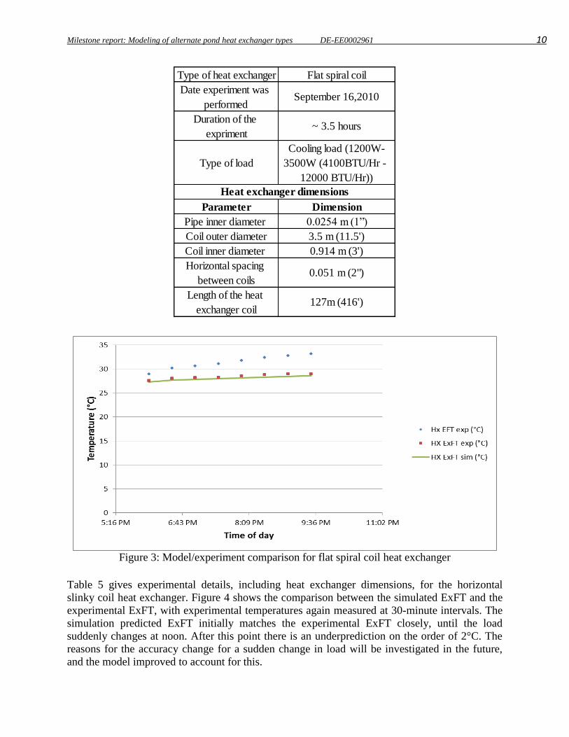
Milestone report: Modeling of alternate pond heat exchanger types DE-EE0002961 10
Figure 3: Model/experiment comparison for flat spiral coil heat exchanger
Table 5 gives experimental details, including heat exchanger dimensions, for the horizontal
slinky coil heat exchanger. Figure 4 shows the comparison between the simulated ExFT and the
experimental ExFT, with experimental temperatures again measured at 30-minute intervals. The
simulation predicted ExFT initially matches the experimental ExFT closely, until the load
suddenly changes at noon. After this point there is an underprediction on the order of 2°C. The
reasons for the accuracy change for a sudden change in load will be investigated in the future,
and the model improved to account for this.
Type of heat exchanger Flat spiral coil
Date experiment was
performedSeptember 16,2010
Duration of the
expriment~ 3.5 hours
Type of load
Cooling load (1200W-
3500W (4100BTU/Hr -
12000 BTU/Hr))
Parameter Dimension
Pipe inner diameter 0.0254 m (1”)
Coil outer diameter 3.5 m (11.5')
Coil inner diameter 0.914 m (3')
Horizontal spacing
between coils 0.051 m (2")
Length of the heat
exchanger coil127m (416')
Heat exchanger dimensions
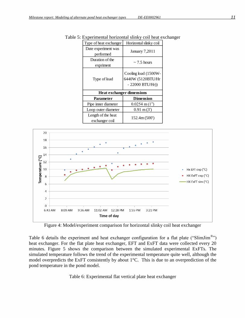
Milestone report: Modeling of alternate pond heat exchanger types DE-EE0002961 11
Table 5: Experimental horizontal slinky coil heat exchanger
Figure 4: Model/experiment comparison for horizontal slinky coil heat exchanger
Table 6 details the experiment and heat exchanger configuration for a flat plate (“SlimJim®”)
heat exchanger. For the flat plate heat exchanger, EFT and ExFT data were collected every 20
minutes. Figure 5 shows the comparison between the simulated experimental ExFTs. The
simulated temperature follows the trend of the experimental temperature quite well, although the
model overpredicts the ExFT consistently by about 1°C. This is due to an overprediction of the
pond temperature in the pond model.
Table 6: Experimental flat vertical plate heat exchanger
Type of heat exchanger Horizontal slinky coil
Date experiment was
performedJanuary 7,2011
Duration of the
expriment~ 7.5 hours
Type of load
Cooling load (1500W-
6440W (5120BTU/Hr
- 22000 BTU/Hr))
Parameter Dimension
Pipe inner diameter 0.0254 m (1”)
Loop outer diameter 0.91 m (3')
Length of the heat
exchanger coil152.4m (500')
Heat exchanger dimensions
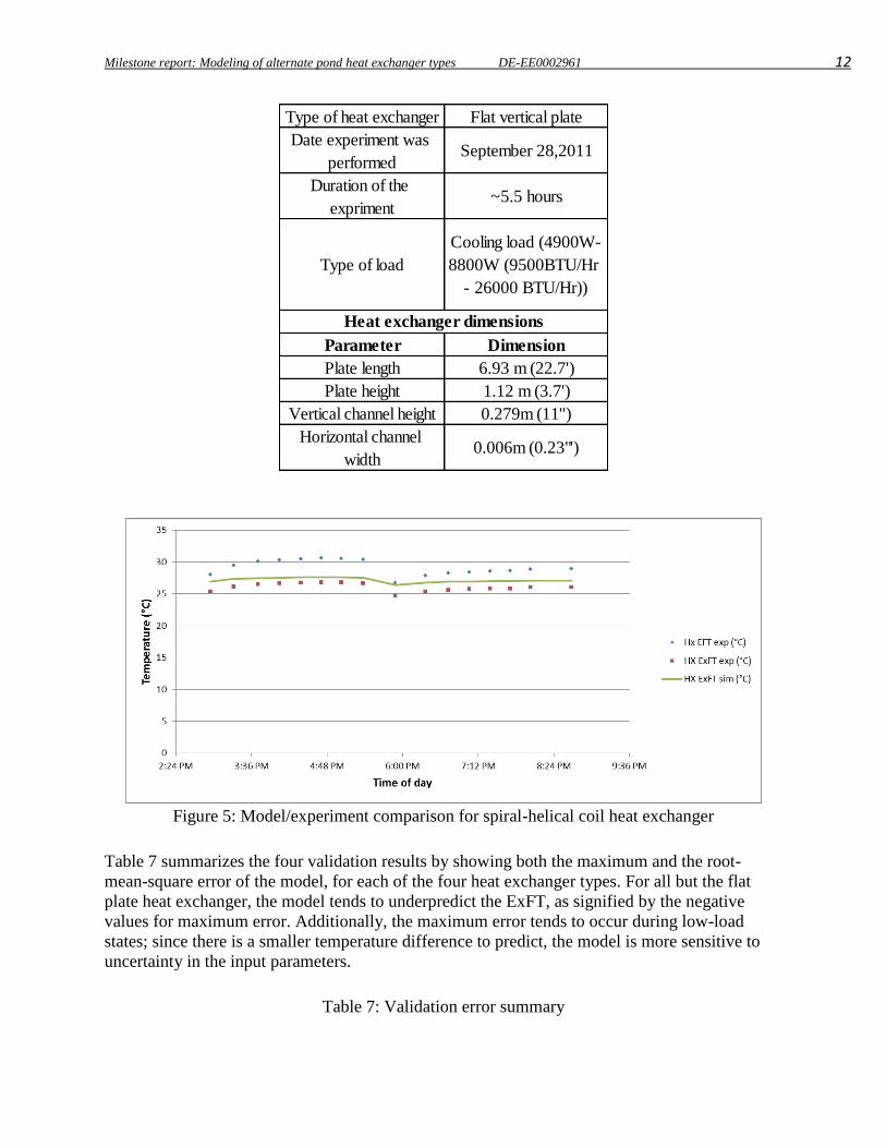
Milestone report: Modeling of alternate pond heat exchanger types DE-EE0002961 12
Figure 5: Model/experiment comparison for spiral-helical coil heat exchanger
Table 7 summarizes the four validation results by showing both the maximum and the root-
mean-square error of the model, for each of the four heat exchanger types. For all but the flat
plate heat exchanger, the model tends to underpredict the ExFT, as signified by the negative
values for maximum error. Additionally, the maximum error tends to occur during low-load
states; since there is a smaller temperature difference to predict, the model is more sensitive to
uncertainty in the input parameters.
Table 7: Validation error summary
Type of heat exchanger Flat vertical plate
Date experiment was
performedSeptember 28,2011
Duration of the
expriment~5.5 hours
Type of load
Cooling load (4900W-
8800W (9500BTU/Hr
- 26000 BTU/Hr))
Parameter Dimension
Plate length 6.93 m (22.7')
Plate height 1.12 m (3.7')
Vertical channel height 0.279m (11'')
Horizontal channel
width0.006m (0.23"')
Heat exchanger dimensions
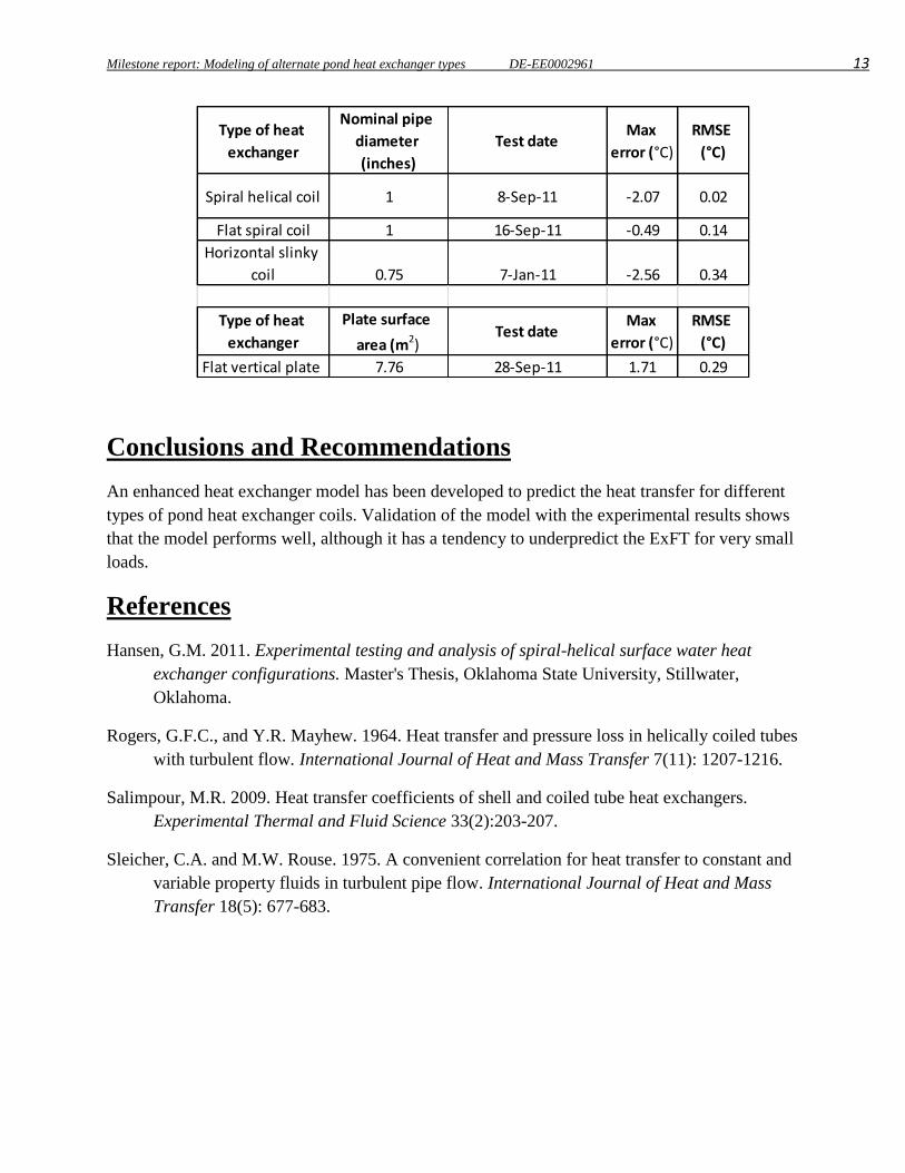
Milestone report: Modeling of alternate pond heat exchanger types DE-EE0002961 13
Conclusions and Recommendations
An enhanced heat exchanger model has been developed to predict the heat transfer for different
types of pond heat exchanger coils. Validation of the model with the experimental results shows
that the model performs well, although it has a tendency to underpredict the ExFT for very small
loads.
References
Hansen, G.M. 2011. Experimental testing and analysis of spiral-helical surface water heat
exchanger configurations. Master's Thesis, Oklahoma State University, Stillwater,
Oklahoma.
Rogers, G.F.C., and Y.R. Mayhew. 1964. Heat transfer and pressure loss in helically coiled tubes
with turbulent flow. International Journal of Heat and Mass Transfer 7(11): 1207-1216.
Salimpour, M.R. 2009. Heat transfer coefficients of shell and coiled tube heat exchangers.
Experimental Thermal and Fluid Science 33(2):203-207.
Sleicher, C.A. and M.W. Rouse. 1975. A convenient correlation for heat transfer to constant and
variable property fluids in turbulent pipe flow. International Journal of Heat and Mass
Transfer 18(5): 677-683.
Type of heat
exchanger
Nominal pipe
diameter
(inches)
Test dateMax
error (°C)
RMSE
(°C)
Spiral helical coil 1 8-Sep-11 -2.07 0.02
Flat spiral coil 1 16-Sep-11 -0.49 0.14
Horizontal slinky
coil 0.75 7-Jan-11 -2.56 0.34
Type of heat
exchanger
Plate surface
area (m2)Test date
Max
error (°C)
RMSE
(°C)
Flat vertical plate 7.76 28-Sep-11 1.71 0.29

Innostock 2012 The 12th International Conference on Energy Storage
1
INNO-XX-YYY
A quasi-two-dimensional standing column well model for ground source heat pump systems
Annamalai Ramesh1, Jeffrey D. Spitler2
1School of Mechanical and Aerospace Engineering, Oklahoma State University, Stillwater, OK 74078, USA, Phone: 405-744-0389, Fax: 405-744-7873, e-mail: [email protected]
2School of Mechanical and Aerospace Engineering, Oklahoma State University, Stillwater, OK 74078, USA, Phone: 405-744-5900, Fax: 405-744-7873, e-mail: [email protected]
1. Introduction
Standing column wells (SCW) are a type of ground heat exchanger (GHE) that may be used with ground source heat pump (GSHP) or underground thermal energy storage (UTES) systems. SCWs are “open-loop” ground heat exchangers that draw ground water from the bottom of the well and, after passing it through a heat pump or heat exchanger, return it at the top of the well. Water circulating down the borehole wall exchanges heat with the surrounding ground.
Compared to closed-loop ground heat exchangers, standing column wells have three important advantages that allow for increased heat transfer and, consequently, less required borehole length and lower first cost. First, standing column wells have lower borehole thermal resistance than closed-loop ground heat exchangers because the working fluid is in direct contact with the borehole wall. Typical values for borehole resistance of closed-loop grouted heat exchangers are on the order of 0.1-0.3 m-K/W. In SCWs, fully turbulent flow results in values of borehole thermal resistance around 0.0005-0.005 m-K/W. Second, they benefit from groundwater flow in and out of the surrounding formation that is induced by pumping and density differences between the groundwater in the well and that in the surrounding ground. Third, in locations where it is permissible to bleed off some of the water drawn from the well, the induced flow of groundwater into the borehole significantly enhances the heat transfer.
Though SCWs have been in operation since the 1970s, there is relatively little published research on this type of GHE. SCW models are needed to support design software and energy calculation software. But only a few SCW models have been developed and several of these are too computationally expensive to be directly useful for design or energy calculations.
One of the first SCW models (Yuill and Mikler 1995) utilized a simple groundwater flow model to estimate the groundwater flow induced by pumping in and out of the borehole. Then a one-dimensional finite difference model which accounted for heat conduction and advection was used to analyze the heat transfer. As presented, the model did not account for bleed or convective resistances inside the borehole. Rees et al. (2004) developed a two-dimensional finite volume model and Ng et al. (2010) developed a three-dimensional finite volume model. Both models are capable of modeling bleed and accounting for convective resistances inside the borehole. Both models used separate grids to model the heat transfer in the borehole and the surrounding ground; the two solution domains are coupled together and solved iteratively. The grid size and iteratively coupled solution technique requires significant computational time, making either model too computationally intensive for direct use in either design software or energy calculation software.
A computationally efficient model which is more suited to be used in design tools or energy analysis programs is the one-dimensional SCW model developed by Deng et al. (2005). Though it is computationally efficient, there are some aspects of the model that have not been thoroughly investigated. These include its assumption of isotropic aquifers with homogeneous
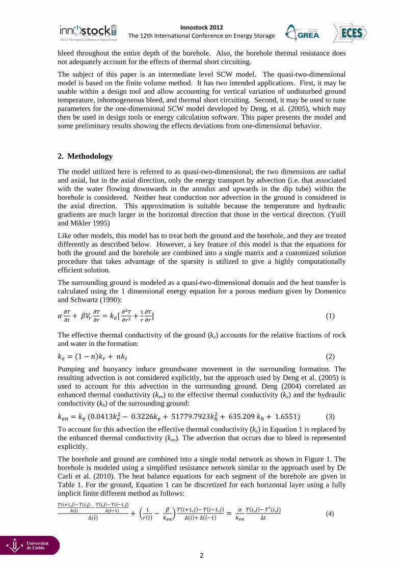
Innostock 2012 The 12th International Conference on Energy Storage
2
bleed throughout the entire depth of the borehole. Also, the borehole thermal resistance does not adequately account for the effects of thermal short circuiting.
The subject of this paper is an intermediate level SCW model. The quasi-two-dimensional model is based on the finite volume method. It has two intended applications. First, it may be usable within a design tool and allow accounting for vertical variation of undisturbed ground temperature, inhomogeneous bleed, and thermal short circuiting. Second, it may be used to tune parameters for the one-dimensional SCW model developed by Deng, et al. (2005), which may then be used in design tools or energy calculation software. This paper presents the model and some preliminary results showing the effects deviations from one-dimensional behavior.
2. Methodology
The model utilized here is referred to as quasi-two-dimensional; the two dimensions are radial and axial, but in the axial direction, only the energy transport by advection (i.e. that associated with the water flowing downwards in the annulus and upwards in the dip tube) within the borehole is considered. Neither heat conduction nor advection in the ground is considered in the axial direction. This approximation is suitable because the temperature and hydraulic gradients are much larger in the horizontal direction that those in the vertical direction. (Yuill and Mikler 1995)
Like other models, this model has to treat both the ground and the borehole, and they are treated differently as described below. However, a key feature of this model is that the equations for both the ground and the borehole are combined into a single matrix and a customized solution procedure that takes advantage of the sparsity is utilized to give a highly computationally efficient solution.
The surrounding ground is modeled as a quasi-two-dimensional domain and the heat transfer is calculated using the 1 dimensional energy equation for a porous medium given by Domenico and Schwartz (1990):
𝛼 𝜕𝑇𝜕𝑡
+ 𝛽𝑉𝑟𝜕𝑇𝜕𝑟
= 𝑘𝑒[ 𝜕2𝑇𝜕𝑟2
+ 1𝑟𝜕𝑇𝜕𝑟
] (1)
The effective thermal conductivity of the ground (ke) accounts for the relative fractions of rock and water in the formation:
𝑘𝑒 = (1 − 𝑛)𝑘𝑟 + 𝑛𝑘𝑙 (2)
Pumping and buoyancy induce groundwater movement in the surrounding formation. The resulting advection is not considered explicitly, but the approach used by Deng et al. (2005) is used to account for this advection in the surrounding ground. Deng (2004) correlated an enhanced thermal conductivity (ken) to the effective thermal conductivity (ke) and the hydraulic conductivity (kh) of the surrounding ground:
𝑘𝑒𝑛 = 𝑘𝑒 (0.0413𝑘𝑒2 − 0.3226𝑘𝑒 + 51779.7923𝑘ℎ2 + 635.209 𝑘ℎ + 1.6551) (3)
To account for this advection the effective thermal conductivity (ke) in Equation 1 is replaced by the enhanced thermal conductivity (ken). The advection that occurs due to bleed is represented explicitly.
The borehole and ground are combined into a single nodal network as shown in Figure 1. The borehole is modeled using a simplified resistance network similar to the approach used by De Carli et al. (2010). The heat balance equations for each segment of the borehole are given in Table 1. For the ground, Equation 1 can be discretized for each horizontal layer using a fully implicit finite different method as follows: 𝑇(𝑖+1,𝑗)− 𝑇(𝑖,𝑗)
∆(𝑖) − 𝑇(𝑖,𝑗)− 𝑇(𝑖−1,𝑗)∆(𝑖−1)
∆(𝑖)+ � 1
𝑟(𝑖)− 𝛽
𝑘𝑒𝑛� 𝑇(𝑖+1,𝑗)− 𝑇(𝑖−1,𝑗)
∆(𝑖)+ ∆(𝑖−1) = 𝛼𝑘𝑒𝑛
𝑇(𝑖,𝑗)− 𝑇′(𝑖,𝑗)∆𝑡
(4)

Innostock 2012 The 12th International Conference on Energy Storage
3
Table 1 Heat balance equations in the borehole
1. Heat balance on the outer surface of the dip tube (Tds)
𝑇𝑤𝑑 (𝑗) − 𝑇𝑑𝑠(𝑗)
12𝜋𝑟𝑑𝑖ℎ𝑖∆𝑧
+ln (𝑟𝑑𝑜𝑟𝑑𝑖
)2𝜋𝑘𝑑∆𝑧
+ 𝑇𝑤𝑎(𝑗) − 𝑇𝑑𝑠(𝑗)
12𝜋𝑟𝑑𝑜ℎ𝑜∆𝑧
= 0
2. Heat balance on the
water in the dip tube (Twd)
𝑇𝑑𝑠(𝑗) − 𝑇𝑤𝑑(𝑗)
12𝜋𝑟𝑑𝑖ℎ𝑖∆𝑧
+ln (𝑟𝑑𝑜𝑟𝑑𝑖
)2𝜋𝑘𝑑∆𝑧
+ 𝑇𝑤𝑑(𝑗 + 1) − 𝑇𝑤𝑑(𝑗)
�̇�𝐶𝑝= 0
3. Heat balance on the water in the annulus (Twa)
𝑇𝑤𝑎(𝑗 − 1) − 𝑇𝑤𝑎(𝑗)�̇�(𝑗)𝐶𝑝
+ 𝑇𝑑𝑠(𝑗) − 𝑇𝑤𝑎(𝑗)
12𝜋𝑟𝑑𝑜ℎ𝑜∆𝑧
+ 𝑇(1, 𝑗) − 𝑇𝑤𝑎(𝑗)
12𝜋𝑟𝑏ℎ𝑜∆𝑧
+ �̇�𝑏(𝑗)𝐶𝑝= 0
T(1,j) – Borehole wall temperature
4. Coupling between borehole and ground
𝑇(1, 𝑗) − 𝑇𝑤𝑎(𝑗)1
2𝜋𝑟𝑏ℎ𝑜∆𝑧+ 2𝜋𝑟𝑏∆𝑧 𝑞"(𝑗) = 0
5. Boundary nodes Top layer: Set 𝑇𝑤𝑎(0) to be equal to the inlet temperature Bottom layer: Set 𝑇𝑤𝑑(𝑛 + 1) = 𝑇𝑤𝑎(𝑛)
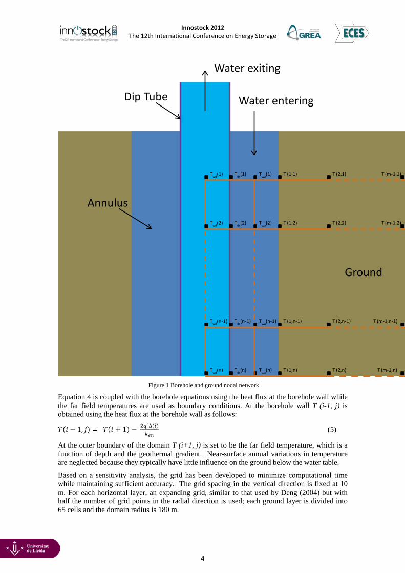
Innostock 2012 The 12th International Conference on Energy Storage
4
Figure 1 Borehole and ground nodal network
Equation 4 is coupled with the borehole equations using the heat flux at the borehole wall while the far field temperatures are used as boundary conditions. At the borehole wall T (i-1, j) is obtained using the heat flux at the borehole wall as follows:
𝑇(𝑖 − 1, 𝑗) = 𝑇(𝑖 + 1) − 2𝑞"∆(𝑖)𝑘𝑒𝑛
(5)
At the outer boundary of the domain T (i+1, j) is set to be the far field temperature, which is a function of depth and the geothermal gradient. Near-surface annual variations in temperature are neglected because they typically have little influence on the ground below the water table.
Based on a sensitivity analysis, the grid has been developed to minimize computational time while maintaining sufficient accuracy. The grid spacing in the vertical direction is fixed at 10 m. For each horizontal layer, an expanding grid, similar to that used by Deng (2004) but with half the number of grid points in the radial direction is used; each ground layer is divided into 65 cells and the domain radius is 180 m.
Ground
Water entering
Water exiting
Dip Tube
Twd(1) Tds(1)
Twd(n-1)
Twd(n)
Twd(2)
Tds(n)
Tds(n-1)
Tds(2)
Twa(n)
Twa(n-1)
Twa(2)
Twa(1)
T (1,2)
T (1,1) T (2,1) T (m-1,1)
T (2,2) T (m-1,2)
T (m-1,n-1)
T (m-1,n)
T (1,n-1) T (2,n-1)
T (2,n) T (1,n)
Annulus
Innostock 2012 The 12th International Conference on Energy Storage
5
Thus for each horizontal segment there are three equations representing the heat transfer in the borehole, one equation for the coupling between the borehole and ground and 65 equations for the heat transfer in the ground. Thus a 500 m deep SCW with a grid spacing of 10 m in the vertical direction will have a total of 3450 equations. Though there are 3450 equations, each equation has no more than five non-zero coefficients. Hence to save memory they are stored in a (3450, 5) array and are solved using a customized decomposition method to maximize computational efficiency. Temperature dependent bleed control strategies have also been incorporated in the model where the user can specify minimum and maximum heat pump entering or leaving water temperatures below and above which bleed can be activated.
During bleed the linear ground water velocity (Vr) in each ground node is obtained using Equation 6.
𝑉𝑟(𝑖, 𝑗) = − 1𝑛
𝑚𝑏̇ (𝑗)2𝜋𝑟(𝑖)∆𝑧(𝑗)𝜌𝑤
(6)
In a particular horizontal layer j the 𝑚𝑏̇ term is constant throughout and the value of Vr(i,j) decreases as the radius increases according to Equation 6. In the case of homogeneous bleed the 𝑚𝑏̇ term is uniform for all the horizontal layers. However in the case of bleed through a single fracture the 𝑚𝑏̇ term has a value of zero for all the horizontal layers except the layer representing the fracture. In the case where bleed occurs only in a certain section of the borehole, the 𝑚𝑏̇ term has a uniform value for all the horizontal layers representing that section and a value of 0 for the rest. Initially this model assumes a homogenous and isotropic aquifer. However if the properties such as porosities, thermal conductivities and hydraulic conductivities are available for anisotropic and heterogeneous aquifers this model can be easily modified to simulate it.
3. Results and Discussion
The quasi-two-dimensional model was validated against data obtained from a 467 m deep SCW in Haverhill, MA. See Deng (2004) for further description of the data set. The ground properties are chosen based on the geology of the area since a thermal response test was not performed. Figure 2 shows the comparison of the exiting water temperatures for the available experimental data and the model. The RMSE error between the model and the available data was found to be around 0.4 °C which is acceptable considering the uncertainties associated with the ground properties.
One objective of the model was to have a run time that would be reasonable for use in a design tool or to estimate parameters for a faster one-dimensional model. The detailed fully-two-dimensional model used by Rees, et al. (2004) took weeks to run on a (circa 2001) fast desktop computer when implemented in Fortran. For the current model, implemented in an interpreted language (Visual Basic for Applications), a typical annual simulation with hourly time steps for a 500 m deep SCW coupled with a heat pump using a successive substitution method takes approximately 4.5 minutes to run on a fast desktop computer that is a few years old. If the SCW model is run as a standalone model the computational time is around two minutes. For comparison, the one-dimensional model, also implemented in the same interpreted language, takes about 10 seconds to run when coupled with a heat pump model.
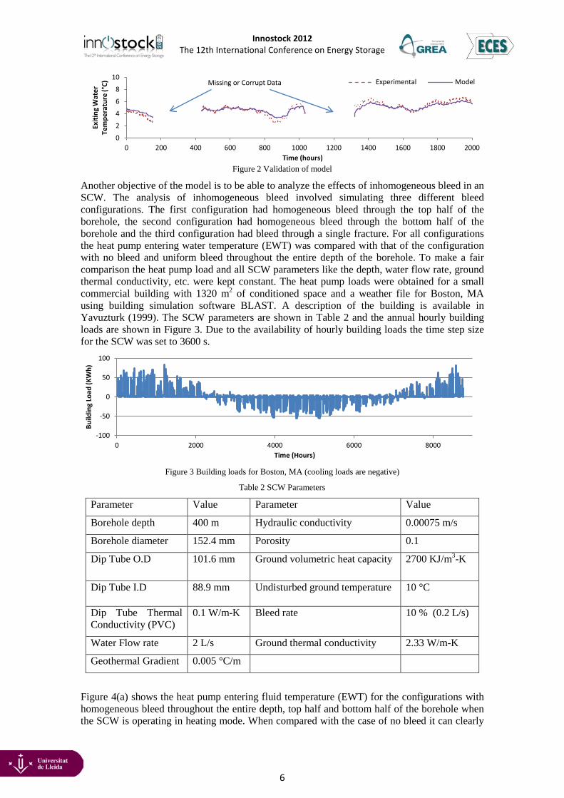
Innostock 2012 The 12th International Conference on Energy Storage
6
Figure 2 Validation of model Another objective of the model is to be able to analyze the effects of inhomogeneous bleed in an SCW. The analysis of inhomogeneous bleed involved simulating three different bleed configurations. The first configuration had homogeneous bleed through the top half of the borehole, the second configuration had homogeneous bleed through the bottom half of the borehole and the third configuration had bleed through a single fracture. For all configurations the heat pump entering water temperature (EWT) was compared with that of the configuration with no bleed and uniform bleed throughout the entire depth of the borehole. To make a fair comparison the heat pump load and all SCW parameters like the depth, water flow rate, ground thermal conductivity, etc. were kept constant. The heat pump loads were obtained for a small commercial building with 1320 m2 of conditioned space and a weather file for Boston, MA using building simulation software BLAST. A description of the building is available in Yavuzturk (1999). The SCW parameters are shown in Table 2 and the annual hourly building loads are shown in Figure 3. Due to the availability of hourly building loads the time step size for the SCW was set to 3600 s.
Figure 3 Building loads for Boston, MA (cooling loads are negative)
Table 2 SCW Parameters
Parameter Value Parameter Value
Borehole depth 400 m Hydraulic conductivity 0.00075 m/s
Borehole diameter 152.4 mm Porosity 0.1
Dip Tube O.D 101.6 mm Ground volumetric heat capacity 2700 KJ/m3-K
Dip Tube I.D 88.9 mm Undisturbed ground temperature 10 °C
Dip Tube Thermal Conductivity (PVC)
0.1 W/m-K Bleed rate 10 % (0.2 L/s)
Water Flow rate 2 L/s Ground thermal conductivity 2.33 W/m-K
Geothermal Gradient 0.005 °C/m
Figure 4(a) shows the heat pump entering fluid temperature (EWT) for the configurations with homogeneous bleed throughout the entire depth, top half and bottom half of the borehole when the SCW is operating in heating mode. When compared with the case of no bleed it can clearly
0
2
4
6
8
10
0 200 400 600 800 1000 1200 1400 1600 1800 2000
Exiti
ng W
ater
Te
mpe
ratu
re (°
C)
Time (hours)
Experimental ModelMissing or Corrupt Data
-100
-50
0
50
100
0 2000 4000 6000 8000
Build
ing
Load
(KW
h)
Time (Hours)
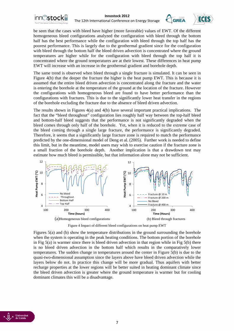
Innostock 2012 The 12th International Conference on Energy Storage
7
be seen that the cases with bleed have higher (more favorable) values of EWT. Of the different homogeneous bleed configurations analyzed the configuration with bleed through the bottom half has the best performance while the configuration with bleed through the top half has the poorest performance. This is largely due to the geothermal gradient since for the configuration with bleed through the bottom half the bleed driven advection is concentrated where the ground temperatures are higher while for the configuration with bleed through the top half it is concentrated where the ground temperatures are at their lowest. These differences in heat pump EWT will increase with an increase in the geothermal gradient and borehole depth.
The same trend is observed when bleed through a single fracture is simulated. It can be seen in Figure 4(b) that the deeper the fracture the higher is the heat pump EWT. This is because it is assumed that the entire bleed driven advection is concentrated along the fracture and the water is entering the borehole at the temperature of the ground at the location of the fracture. However the configurations with homogeneous bleed are found to have better performance than the configurations with fractures. This is due to the significantly lower heat transfer in the regions of the borehole excluding the fracture due to the absence of bleed driven advection.
The results shown in Figures 4(a) and 4(b) have several important practical implications. The fact that the “bleed throughout” configuration lies roughly half way between the top-half bleed and bottom-half bleed suggests that the performance is not significantly degraded when the bleed comes through only half of the borehole. Yet, when it is reduced to the extreme case of the bleed coming through a single large fracture, the performance is significantly degraded. Therefore, it seems that a significantly large fracture zone is required to match the performance predicted by the one-dimensional model of Deng et al. (2005). Further work is needed to define this limit, but in the meantime, model users may wish to exercise caution if the fracture zone is a small fraction of the borehole depth. Another implication is that a drawdown test may estimate how much bleed is permissible, but that information alone may not be sufficient.
(a)Homogeneous bleed configurations (b) Bleed through fractures
Figure 4 Impact of different bleed configurations on heat pump EWT
Figures 5(a) and (b) show the temperature distributions in the ground surrounding the borehole when the system is operating in the peak heating conditions. The bottom portion of the borehole in Fig 5(a) is warmer since there is bleed driven advection in that region while in Fig 5(b) there is no bleed driven advection in the bottom half which results in the comparatively lower temperatures. The sudden change in temperatures around the center in Figure 5(b) is due to the quasi-two-dimensional assumption since the layers above have bleed driven advection while the layers below do not. In practice this change will be more gradual. Thus aquifers with better recharge properties at the lower regions will be better suited in heating dominant climate since the bleed driven advection is greater where the ground temperature is warmer but for cooling dominant climates this will be a disadvantage.
4
6
8
10
12
100 200 300 400
Heat
Pum
p EW
T (°
C)
Time (hours)
No bleed ThroughoutBottom HalfTop Half
4
6
8
10
12
100 200 300 400
Heat
Pum
p EW
T (°
C)
Time (Hours)
Fracture @ 10 mFracture @ 200 mNo BleedFracture @ 400 m
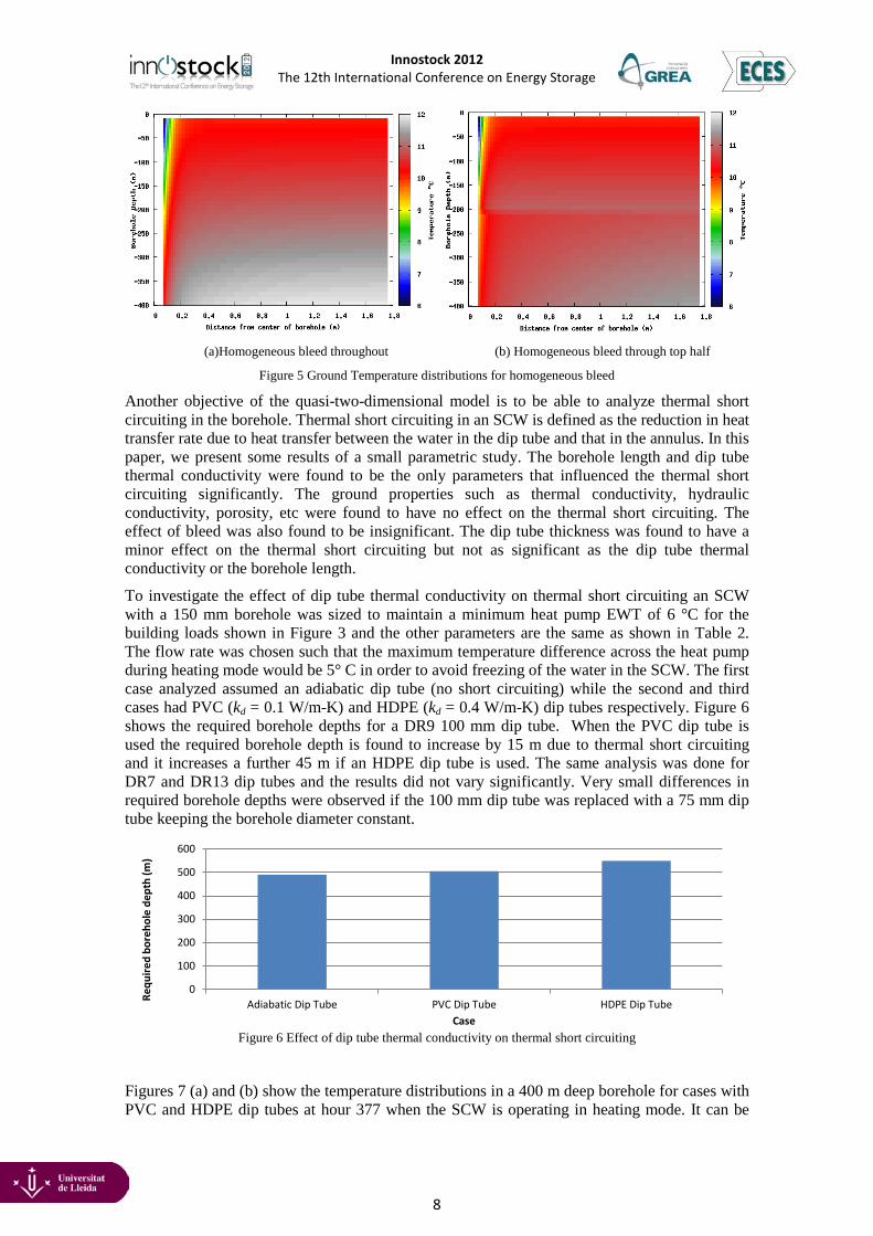
Innostock 2012 The 12th International Conference on Energy Storage
8
(a)Homogeneous bleed throughout (b) Homogeneous bleed through top half
Figure 5 Ground Temperature distributions for homogeneous bleed
Another objective of the quasi-two-dimensional model is to be able to analyze thermal short circuiting in the borehole. Thermal short circuiting in an SCW is defined as the reduction in heat transfer rate due to heat transfer between the water in the dip tube and that in the annulus. In this paper, we present some results of a small parametric study. The borehole length and dip tube thermal conductivity were found to be the only parameters that influenced the thermal short circuiting significantly. The ground properties such as thermal conductivity, hydraulic conductivity, porosity, etc were found to have no effect on the thermal short circuiting. The effect of bleed was also found to be insignificant. The dip tube thickness was found to have a minor effect on the thermal short circuiting but not as significant as the dip tube thermal conductivity or the borehole length.
To investigate the effect of dip tube thermal conductivity on thermal short circuiting an SCW with a 150 mm borehole was sized to maintain a minimum heat pump EWT of 6 °C for the building loads shown in Figure 3 and the other parameters are the same as shown in Table 2. The flow rate was chosen such that the maximum temperature difference across the heat pump during heating mode would be 5° C in order to avoid freezing of the water in the SCW. The first case analyzed assumed an adiabatic dip tube (no short circuiting) while the second and third cases had PVC (kd = 0.1 W/m-K) and HDPE (kd = 0.4 W/m-K) dip tubes respectively. Figure 6 shows the required borehole depths for a DR9 100 mm dip tube. When the PVC dip tube is used the required borehole depth is found to increase by 15 m due to thermal short circuiting and it increases a further 45 m if an HDPE dip tube is used. The same analysis was done for DR7 and DR13 dip tubes and the results did not vary significantly. Very small differences in required borehole depths were observed if the 100 mm dip tube was replaced with a 75 mm dip tube keeping the borehole diameter constant.
Figure 6 Effect of dip tube thermal conductivity on thermal short circuiting
Figures 7 (a) and (b) show the temperature distributions in a 400 m deep borehole for cases with PVC and HDPE dip tubes at hour 377 when the SCW is operating in heating mode. It can be
0
100
200
300
400
500
600
Adiabatic Dip Tube PVC Dip Tube HDPE Dip TubeRequ
ired
bore
hole
dep
th (m
)
Case
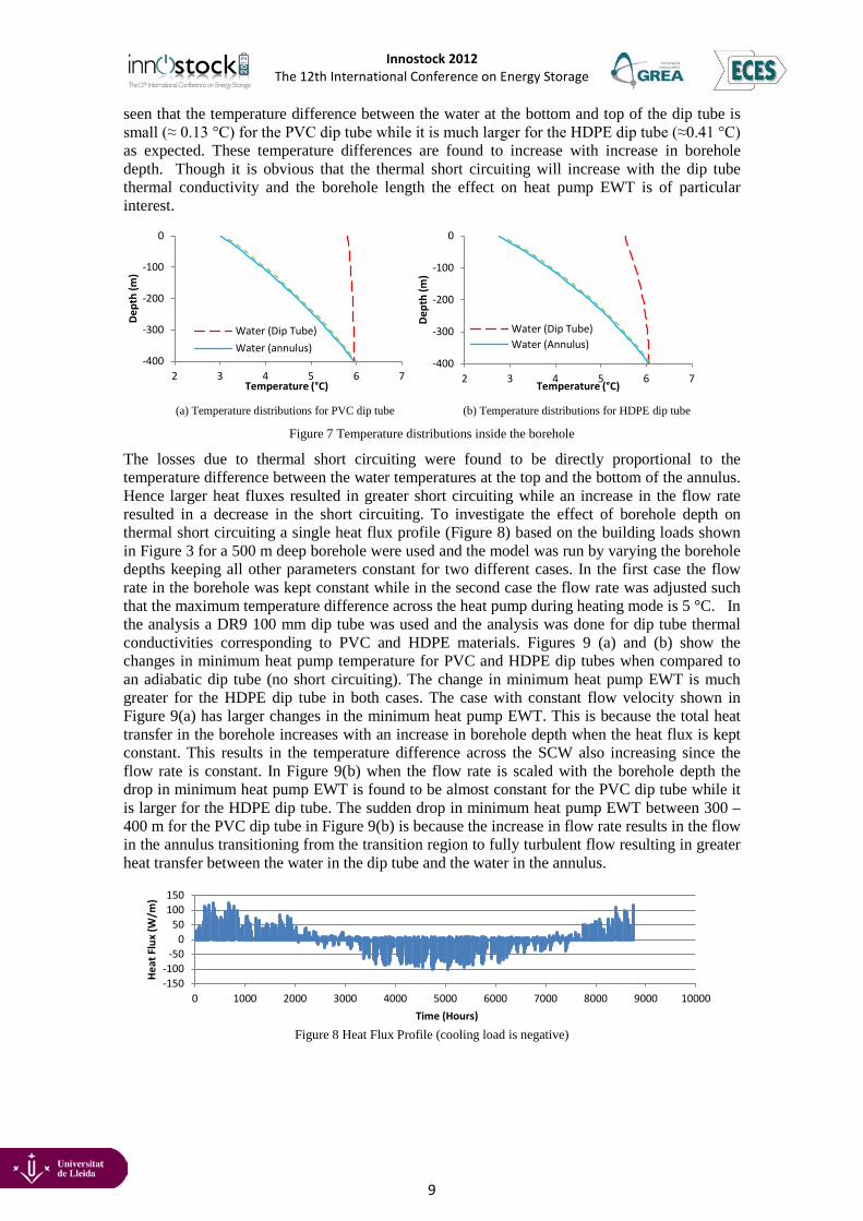
Innostock 2012 The 12th International Conference on Energy Storage
9
seen that the temperature difference between the water at the bottom and top of the dip tube is small (≈ 0.13 °C) for the PVC dip tube while it is much larger for the HDPE dip tube (≈0.41 °C) as expected. These temperature differences are found to increase with increase in borehole depth. Though it is obvious that the thermal short circuiting will increase with the dip tube thermal conductivity and the borehole length the effect on heat pump EWT is of particular interest.
(a) Temperature distributions for PVC dip tube (b) Temperature distributions for HDPE dip tube
Figure 7 Temperature distributions inside the borehole
The losses due to thermal short circuiting were found to be directly proportional to the temperature difference between the water temperatures at the top and the bottom of the annulus. Hence larger heat fluxes resulted in greater short circuiting while an increase in the flow rate resulted in a decrease in the short circuiting. To investigate the effect of borehole depth on thermal short circuiting a single heat flux profile (Figure 8) based on the building loads shown in Figure 3 for a 500 m deep borehole were used and the model was run by varying the borehole depths keeping all other parameters constant for two different cases. In the first case the flow rate in the borehole was kept constant while in the second case the flow rate was adjusted such that the maximum temperature difference across the heat pump during heating mode is 5 °C. In the analysis a DR9 100 mm dip tube was used and the analysis was done for dip tube thermal conductivities corresponding to PVC and HDPE materials. Figures 9 (a) and (b) show the changes in minimum heat pump temperature for PVC and HDPE dip tubes when compared to an adiabatic dip tube (no short circuiting). The change in minimum heat pump EWT is much greater for the HDPE dip tube in both cases. The case with constant flow velocity shown in Figure 9(a) has larger changes in the minimum heat pump EWT. This is because the total heat transfer in the borehole increases with an increase in borehole depth when the heat flux is kept constant. This results in the temperature difference across the SCW also increasing since the flow rate is constant. In Figure 9(b) when the flow rate is scaled with the borehole depth the drop in minimum heat pump EWT is found to be almost constant for the PVC dip tube while it is larger for the HDPE dip tube. The sudden drop in minimum heat pump EWT between 300 – 400 m for the PVC dip tube in Figure 9(b) is because the increase in flow rate results in the flow in the annulus transitioning from the transition region to fully turbulent flow resulting in greater heat transfer between the water in the dip tube and the water in the annulus.
Figure 8 Heat Flux Profile (cooling load is negative)
-400
-300
-200
-100
0
2 3 4 5 6 7
Dept
h (m
)
Temperature (°C)
Water (Dip Tube)Water (annulus)
-400
-300
-200
-100
0
2 3 4 5 6 7
Dept
h (m
)
Temperature (°C)
Water (Dip Tube)Water (Annulus)
-150-100
-500
50100150
0 1000 2000 3000 4000 5000 6000 7000 8000 9000 10000
Heat
Flu
x (W
/m)
Time (Hours)
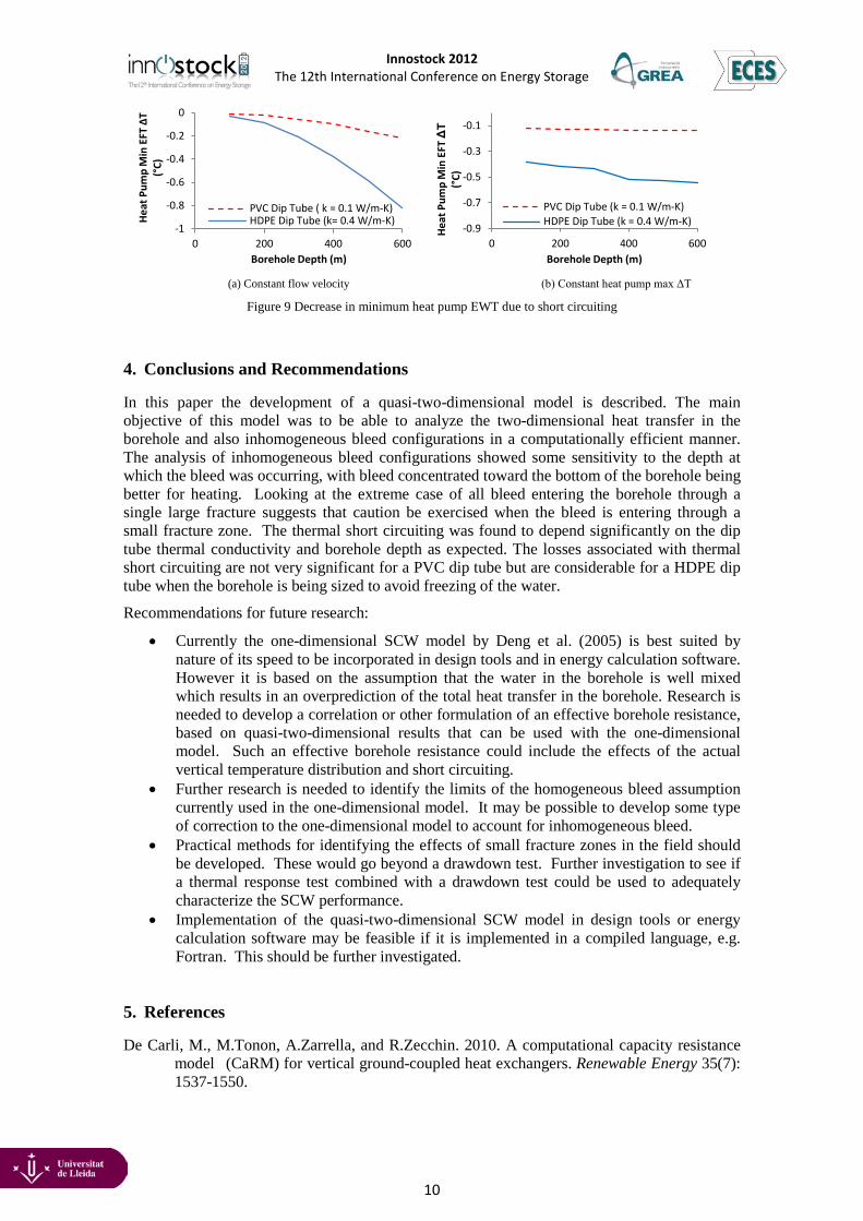
Innostock 2012 The 12th International Conference on Energy Storage
10
(a) Constant flow velocity (b) Constant heat pump max ΔT Figure 9 Decrease in minimum heat pump EWT due to short circuiting
4. Conclusions and Recommendations
In this paper the development of a quasi-two-dimensional model is described. The main objective of this model was to be able to analyze the two-dimensional heat transfer in the borehole and also inhomogeneous bleed configurations in a computationally efficient manner. The analysis of inhomogeneous bleed configurations showed some sensitivity to the depth at which the bleed was occurring, with bleed concentrated toward the bottom of the borehole being better for heating. Looking at the extreme case of all bleed entering the borehole through a single large fracture suggests that caution be exercised when the bleed is entering through a small fracture zone. The thermal short circuiting was found to depend significantly on the dip tube thermal conductivity and borehole depth as expected. The losses associated with thermal short circuiting are not very significant for a PVC dip tube but are considerable for a HDPE dip tube when the borehole is being sized to avoid freezing of the water.
Recommendations for future research:
• Currently the one-dimensional SCW model by Deng et al. (2005) is best suited by nature of its speed to be incorporated in design tools and in energy calculation software. However it is based on the assumption that the water in the borehole is well mixed which results in an overprediction of the total heat transfer in the borehole. Research is needed to develop a correlation or other formulation of an effective borehole resistance, based on quasi-two-dimensional results that can be used with the one-dimensional model. Such an effective borehole resistance could include the effects of the actual vertical temperature distribution and short circuiting.
• Further research is needed to identify the limits of the homogeneous bleed assumption currently used in the one-dimensional model. It may be possible to develop some type of correction to the one-dimensional model to account for inhomogeneous bleed.
• Practical methods for identifying the effects of small fracture zones in the field should be developed. These would go beyond a drawdown test. Further investigation to see if a thermal response test combined with a drawdown test could be used to adequately characterize the SCW performance.
• Implementation of the quasi-two-dimensional SCW model in design tools or energy calculation software may be feasible if it is implemented in a compiled language, e.g. Fortran. This should be further investigated.
5. References
De Carli, M., M.Tonon, A.Zarrella, and R.Zecchin. 2010. A computational capacity resistance model (CaRM) for vertical ground-coupled heat exchangers. Renewable Energy 35(7): 1537-1550.
-1
-0.8
-0.6
-0.4
-0.2
0
0 200 400 600
Heat
Pum
p M
in E
FT Δ
T (°
C)
Borehole Depth (m)
PVC Dip Tube ( k = 0.1 W/m-K)HDPE Dip Tube (k= 0.4 W/m-K)
-0.9
-0.7
-0.5
-0.3
-0.1
0 200 400 600
Heat
Pum
p M
in E
FT Δ
T (°
C)
Borehole Depth (m)
PVC Dip Tube (k = 0.1 W/m-K)HDPE Dip Tube (k = 0.4 W/m-K)
Innostock 2012 The 12th International Conference on Energy Storage
11
Deng, Z. 2004. Modeling of Standing Column Wells in Ground Source Heat Pump Systems. Ph.D. Thesis, Oklahoma State University.
Deng, Z., S.J. Rees, and J.D. Spitler. 2005. A Model for Annual Simulation of Standing Column Well Ground Heat Exchangers. HVAC&R Research 11(4):637-655.
Domenico, P.A., and F.W. Schwartz, 1990. Physical and Chemical Hydrogeology. New York: John Wiley & Sons, Inc.
Ng, B.M., C.Underwood, and S.Walker. 2009. Numerical modeling of multiple standing column wells for heating and cooling buildings. Proceedings of the Eleventh International IBPSA Conference, Glasgow, Scotland, July 27-30.
Rees, S.J., J.D. Spitler, Z. Deng, C.D. Orio, and C.N. Johnson. 2004. A Study Of Geothermal Heat Pump And Standing Column Well Performance. ASHRAE Transactions 110(1):3- 13.
Yavuzturk, C. 1999. Modeling of vertical ground loop heat exchangers for ground source heat pump systems. PhD dissertation, Oklahoma State University.
Yuill, G.K. and V. Mikler, 1995. Analysis of the effect of induced groundwater flow on heat transfer from a vertical open-hole concentric-tube thermal well. ASHRAE Transactions. 101(1): 173-185.
6. Acknowledgements The work described in this paper was funded by the U.S Department of Energy through Award
# DE-EE000296.
Nomenclature: Cp – Specific heat of water (J/kg-K) i – Node number in radial direction j – Node number in vertical direction ke– Effective thermal conductivity of ground (W/m-K) ken – Enhanced thermal conductivity (W/m-K) kd – Dip tube thermal conductivity (W/m-K) kh – Hydraulic conductivity (m/s) kr – Thermal conductivity of solid rock (W/m-K) kl – Thermal conductivity of water (W/m-K) hi – Convection coefficient in the dip tube (W/m2-K) ho – Convection coefficient in the annulus (W/m2-K) n – Ground porosity (-) q” – Heat flux at the borehole wall (W/m2) r(i)- Radius at node i measured from center of borehole (m) rdi – Dip tube inner radius (m) rdo – Dip tube outer radius (m) rb –Borehole radius (m)
Vr – Linear ground water velocity (m/s) T’ – Temeprature at previous time step (°C) Twd – Temperature of water in the dip tube (°C) Twa – Temperature of water in the annulus (°C) Tds – Dip tube outer surface temperature (°C) �̇� - Total mass flow rate (kg/s) �̇�(𝑗)- Mass flow rate entering node j from previous node in the annulus �̇�𝑏(𝑗) - Mass flow rate of water entering node j in the annulus due to bleed (kg/s) Greek symbols α – Volumetric heat capacity of the ground (J/m3-K) β – Volumetric heat capacity of water (J/m3-K) ρs – Density of rock (kg/m3) ρw – Density of water (kg/m3) Δ – Grid spacing in radial direction (m) Δz – Grid spacing in the vertical direction (m)

DE-EE0002961 Oklahoma State University
FY2012, Q10
Page 1 of 24
Quarterly Research Performance Progress Report Federal Agency and Organization: DOE EERE – Geothermal Technologies Program Recipient Organization: Oklahoma State University DUNS Number: 049987720 Recipient Address: Stillwater, OK 74078 Award Number: DE-EE0002961/001 Project Title: Improved Design Tools for Surface Water and Standing Column Well Heat Pump Systems Project Period: January 1, 2010 to August 31, 2012 Principal Investigator: Jeffrey D. Spitler
Regents Professor and C.M. Leonard Professor [email protected] 405-744-5900
Date of Report Submission: July 16, 2012 Reporting Period: April 1, 2012 to June 30, 2012 Report Frequency: Quarterly Project Partners: n/a DOE Project Team: DOE Contracting Officer – Genevieve Wozniak DOE Project Officer – Steve Palmeri Project Monitor – N/A (As of 5/16/2012, Sara Gonnion communicated
that as the project was being moved to the Buildings Technology team, she would no longer be our Project Monitor. We have not received news of any replacement.)
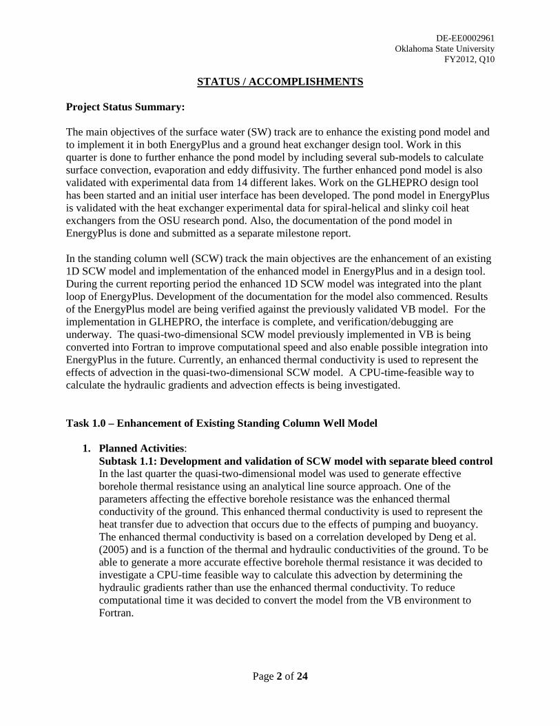
DE-EE0002961 Oklahoma State University
FY2012, Q10
Page 2 of 24
STATUS / ACCOMPLISHMENTS Project Status Summary: The main objectives of the surface water (SW) track are to enhance the existing pond model and to implement it in both EnergyPlus and a ground heat exchanger design tool. Work in this quarter is done to further enhance the pond model by including several sub-models to calculate surface convection, evaporation and eddy diffusivity. The further enhanced pond model is also validated with experimental data from 14 different lakes. Work on the GLHEPRO design tool has been started and an initial user interface has been developed. The pond model in EnergyPlus is validated with the heat exchanger experimental data for spiral-helical and slinky coil heat exchangers from the OSU research pond. Also, the documentation of the pond model in EnergyPlus is done and submitted as a separate milestone report. In the standing column well (SCW) track the main objectives are the enhancement of an existing 1D SCW model and implementation of the enhanced model in EnergyPlus and in a design tool. During the current reporting period the enhanced 1D SCW model was integrated into the plant loop of EnergyPlus. Development of the documentation for the model also commenced. Results of the EnergyPlus model are being verified against the previously validated VB model. For the implementation in GLHEPRO, the interface is complete, and verification/debugging are underway. The quasi-two-dimensional SCW model previously implemented in VB is being converted into Fortran to improve computational speed and also enable possible integration into EnergyPlus in the future. Currently, an enhanced thermal conductivity is used to represent the effects of advection in the quasi-two-dimensional SCW model. A CPU-time-feasible way to calculate the hydraulic gradients and advection effects is being investigated. Task 1.0 – Enhancement of Existing Standing Column Well Model
1. Planned Activities: Subtask 1.1: Development and validation of SCW model with separate bleed control In the last quarter the quasi-two-dimensional model was used to generate effective borehole thermal resistance using an analytical line source approach. One of the parameters affecting the effective borehole resistance was the enhanced thermal conductivity of the ground. This enhanced thermal conductivity is used to represent the heat transfer due to advection that occurs due to the effects of pumping and buoyancy. The enhanced thermal conductivity is based on a correlation developed by Deng et al. (2005) and is a function of the thermal and hydraulic conductivities of the ground. To be able to generate a more accurate effective borehole thermal resistance it was decided to investigate a CPU-time feasible way to calculate this advection by determining the hydraulic gradients rather than use the enhanced thermal conductivity. To reduce computational time it was decided to convert the model from the VB environment to Fortran.
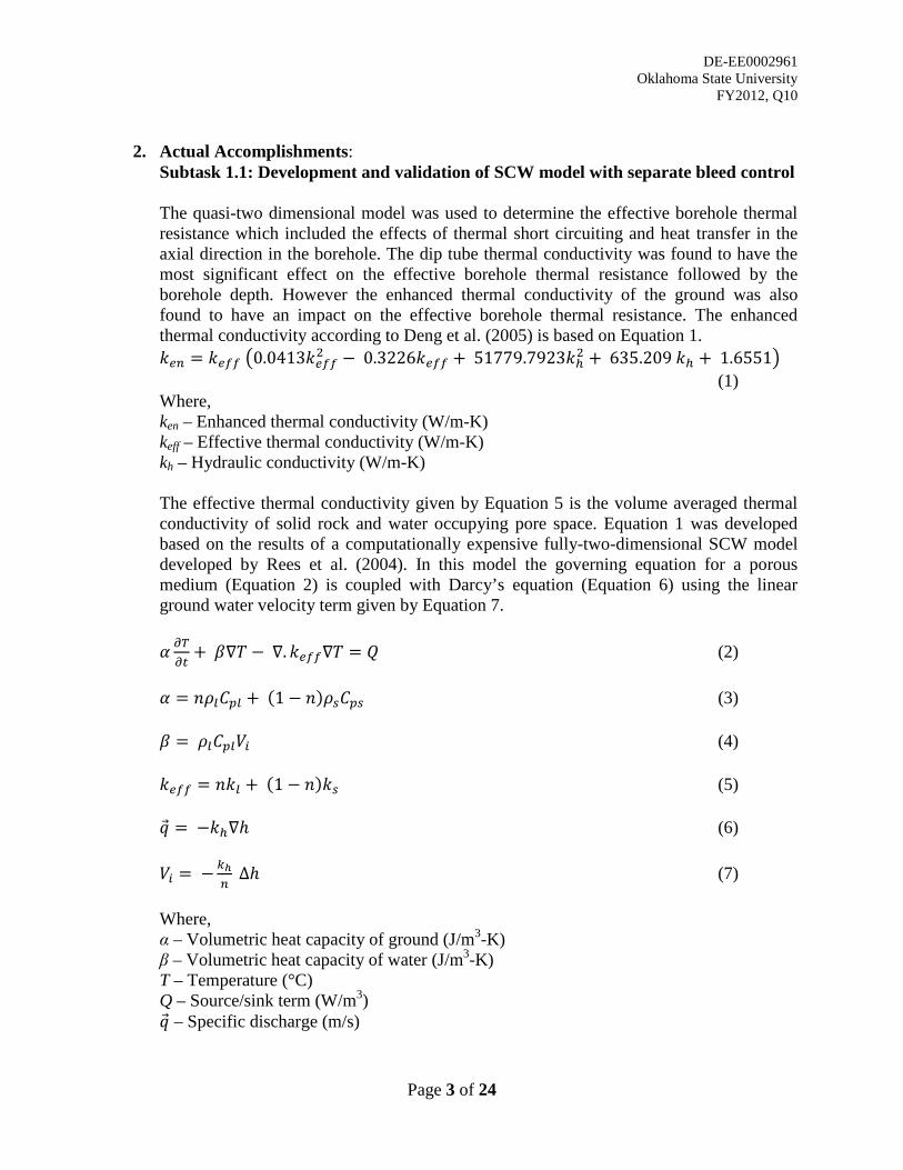
DE-EE0002961 Oklahoma State University
FY2012, Q10
Page 3 of 24
2. Actual Accomplishments:
Subtask 1.1: Development and validation of SCW model with separate bleed control
The quasi-two dimensional model was used to determine the effective borehole thermal resistance which included the effects of thermal short circuiting and heat transfer in the axial direction in the borehole. The dip tube thermal conductivity was found to have the most significant effect on the effective borehole thermal resistance followed by the borehole depth. However the enhanced thermal conductivity of the ground was also found to have an impact on the effective borehole thermal resistance. The enhanced thermal conductivity according to Deng et al. (2005) is based on Equation 1. 𝑘𝑒𝑛 = 𝑘𝑒𝑓𝑓 �0.0413𝑘𝑒𝑓𝑓2 − 0.3226𝑘𝑒𝑓𝑓 + 51779.7923𝑘ℎ2 + 635.209 𝑘ℎ + 1.6551� (1) Where, ken – Enhanced thermal conductivity (W/m-K) keff – Effective thermal conductivity (W/m-K) kh – Hydraulic conductivity (W/m-K) The effective thermal conductivity given by Equation 5 is the volume averaged thermal conductivity of solid rock and water occupying pore space. Equation 1 was developed based on the results of a computationally expensive fully-two-dimensional SCW model developed by Rees et al. (2004). In this model the governing equation for a porous medium (Equation 2) is coupled with Darcy’s equation (Equation 6) using the linear ground water velocity term given by Equation 7. 𝛼 𝜕𝑇𝜕𝑡
+ 𝛽∇𝑇 − ∇.𝑘𝑒𝑓𝑓∇𝑇 = 𝑄 (2) 𝛼 = 𝑛𝜌𝑙𝐶𝑝𝑙 + (1 − 𝑛)𝜌𝑠𝐶𝑝𝑠 (3) 𝛽 = 𝜌𝑙𝐶𝑝𝑙𝑉𝑖 (4) 𝑘𝑒𝑓𝑓 = 𝑛𝑘𝑙 + (1 − 𝑛)𝑘𝑠 (5) �⃗� = −𝑘ℎ∇ℎ (6) 𝑉𝑖 = −𝑘ℎ
𝑛 ∆ℎ (7)
Where, α – Volumetric heat capacity of ground (J/m3-K) β – Volumetric heat capacity of water (J/m3-K) T – Temperature (°C) Q – Source/sink term (W/m3) �⃗� – Specific discharge (m/s)
DE-EE0002961 Oklahoma State University
FY2012, Q10
Page 4 of 24
∇ℎ - Hydraulic gradient (m/m) keff – Effective thermal conductivity (W/m-K) n – Rock porosity (-) ρ – Density (kg/m3) Cp – specific heat (J/kg-K) Vi – linear ground water velocity (m/s) k – Thermal conductivity (W/m-K) l – Water s – Solid rock
The Rees et al. (2004) model considered the thermal and hydraulic gradients in the ground in both radial and axial directions thereby making it computationally expensive. However Yuill and Mikler (1995) suggest that these gradients are significant only in the radial direction when the borehole depth is much greater than its diameter. Hence the quasi-two-dimensional approach may be a reasonably accurate comparatively computationally efficient method to determine the thermal and hydraulic gradients only in the radial direction while at the same time considering heat transfer in the borehole in the axial direction.
Currently the Darcy Equation (Equation 6) and the equation to determine the linear velocity are being integrated into the model and a customized solution procedure for the particular set of equations is being developed to increase computational efficiency. This solution procedure takes advantage of the sparsity of the coefficient matrix. In addition the model also takes the water flow rate and ground storage coefficient as inputs which are then used in calculating the hydraulic head according to Equation 8.
𝑆𝑠𝜕ℎ𝜕𝑡
= 𝑘ℎ𝜕2ℎ𝜕𝑥
+ 𝑅 (8)
Where,
Ss – Specific storage
R – source/sink term
The specific storage is defined as the volume of water a unit volume of aquifer releases due to changes in the compression of the fluid and medium caused by a unit decline in hydraulic head.
3. Explanation of Variance Subtask 1.1: Development and validation of SCW model with separate bleed control The plan for the last quarter was to develop a correlation for effective borehole thermal resistance using the analytical line source to analyze the results of the quasi-two-dimensional model. However to get more accurate results it was decided to make
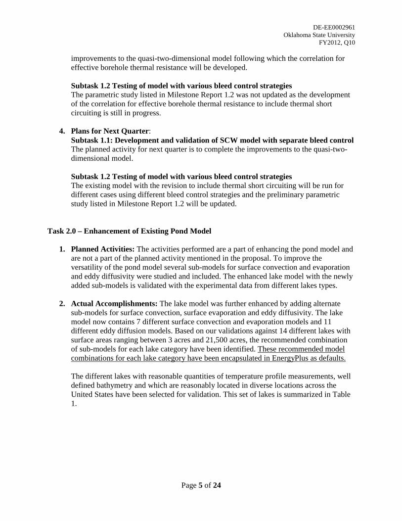
DE-EE0002961 Oklahoma State University
FY2012, Q10
Page 5 of 24
improvements to the quasi-two-dimensional model following which the correlation for effective borehole thermal resistance will be developed. Subtask 1.2 Testing of model with various bleed control strategies The parametric study listed in Milestone Report 1.2 was not updated as the development of the correlation for effective borehole thermal resistance to include thermal short circuiting is still in progress.
4. Plans for Next Quarter:
Subtask 1.1: Development and validation of SCW model with separate bleed control The planned activity for next quarter is to complete the improvements to the quasi-two-dimensional model. Subtask 1.2 Testing of model with various bleed control strategies The existing model with the revision to include thermal short circuiting will be run for different cases using different bleed control strategies and the preliminary parametric study listed in Milestone Report 1.2 will be updated.
Task 2.0 – Enhancement of Existing Pond Model
1. Planned Activities: The activities performed are a part of enhancing the pond model and are not a part of the planned activity mentioned in the proposal. To improve the versatility of the pond model several sub-models for surface convection and evaporation and eddy diffusivity were studied and included. The enhanced lake model with the newly added sub-models is validated with the experimental data from different lakes types.
2. Actual Accomplishments: The lake model was further enhanced by adding alternate sub-models for surface convection, surface evaporation and eddy diffusivity. The lake model now contains 7 different surface convection and evaporation models and 11 different eddy diffusion models. Based on our validations against 14 different lakes with surface areas ranging between 3 acres and 21,500 acres, the recommended combination of sub-models for each lake category have been identified. These recommended model combinations for each lake category have been encapsulated in EnergyPlus as defaults. The different lakes with reasonable quantities of temperature profile measurements, well defined bathymetry and which are reasonably located in diverse locations across the United States have been selected for validation. This set of lakes is summarized in Table 1.
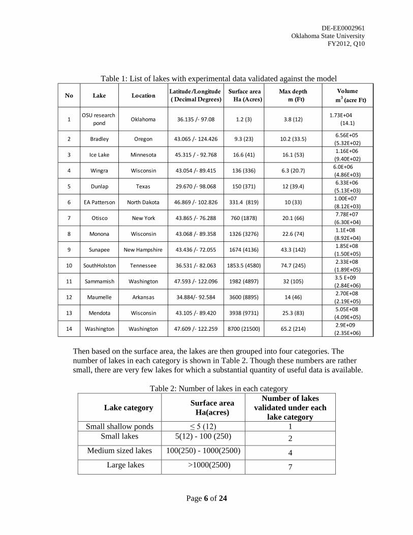
DE-EE0002961 Oklahoma State University
FY2012, Q10
Page 6 of 24
Table 1: List of lakes with experimental data validated against the model
Then based on the surface area, the lakes are then grouped into four categories. The number of lakes in each category is shown in Table 2. Though these numbers are rather small, there are very few lakes for which a substantial quantity of useful data is available.
Table 2: Number of lakes in each category
Lake category Surface area Ha(acres)
Number of lakes validated under each
lake category Small shallow ponds ≤ 5 (12) 1
Small lakes 5(12) - 100 (250) 2 Medium sized lakes 100(250) - 1000(2500) 4
Large lakes >1000(2500) 7
No Lake LocationLatitude/Longitude ( Decimal Degrees)
Surface area Ha (Acres)
Max depth m (Ft)
Volume
m3 (acre Ft)
1OSU research
pond Oklahoma 36.135 /- 97.08 1.2 (3) 3.8 (12)1.73E+04
(14.1)
2 Bradley Oregon 43.065 /- 124.426 9.3 (23) 10.2 (33.5) 6.56E+05 (5.32E+02)
3 Ice Lake Minnesota 45.315 / - 92.768 16.6 (41) 16.1 (53) 1.16E+06 (9.40E+02)
4 Wingra Wisconsin 43.054 /- 89.415 136 (336) 6.3 (20.7) 6.0E+06 (4.86E+03)
5 Dunlap Texas 29.670 /- 98.068 150 (371) 12 (39.4) 6.33E+06 (5.13E+03)
6 EA Patterson North Dakota 46.869 /- 102.826 331.4 (819) 10 (33) 1.00E+07 (8.12E+03)
7 Otisco New York 43.865 /- 76.288 760 (1878) 20.1 (66) 7.78E+07 (6.30E+04)
8 Monona Wisconsin 43.068 /- 89.358 1326 (3276) 22.6 (74) 1.1E+08 (8.92E+04)
9 Sunapee New Hampshire 43.436 /- 72.055 1674 (4136) 43.3 (142) 1.85E+08 (1.50E+05)
10 SouthHolston Tennessee 36.531 /- 82.063 1853.5 (4580) 74.7 (245) 2.33E+08 (1.89E+05)
11 Sammamish Washington 47.593 /- 122.096 1982 (4897) 32 (105) 3.5 E+09 (2.84E+06)
12 Maumelle Arkansas 34.884/- 92.584 3600 (8895) 14 (46) 2.70E+08 (2.19E+05)
13 Mendota Wisconsin 43.105 /- 89.420 3938 (9731) 25.3 (83) 5.05E+08 (4.09E+05)
14 Washington Washington 47.609 /- 122.259 8700 (21500) 65.2 (214) 2.9E+09 (2.35E+06)
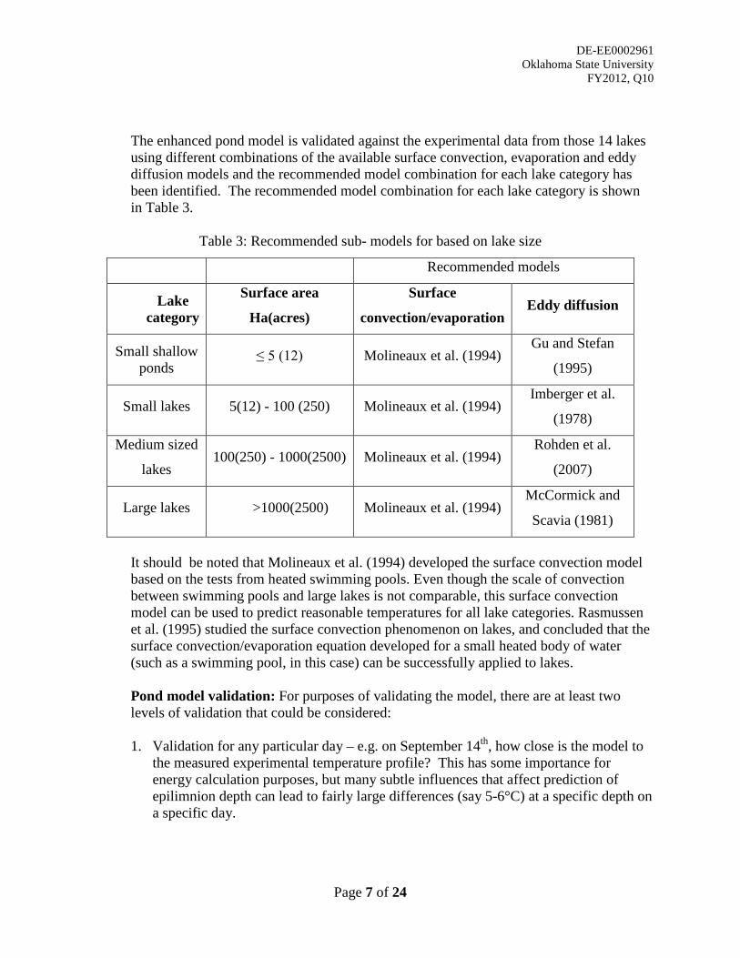
DE-EE0002961 Oklahoma State University
FY2012, Q10
Page 7 of 24
The enhanced pond model is validated against the experimental data from those 14 lakes using different combinations of the available surface convection, evaporation and eddy diffusion models and the recommended model combination for each lake category has been identified. The recommended model combination for each lake category is shown in Table 3.
Table 3: Recommended sub- models for based on lake size
Recommended models
Lake category
Surface area
Ha(acres)
Surface
convection/evaporation Eddy diffusion
Small shallow ponds
≤ 5 (12) Molineaux et al. (1994) Gu and Stefan
(1995)
Small lakes 5(12) - 100 (250) Molineaux et al. (1994) Imberger et al.
(1978)
Medium sized
lakes 100(250) - 1000(2500) Molineaux et al. (1994)
Rohden et al.
(2007)
Large lakes >1000(2500) Molineaux et al. (1994) McCormick and
Scavia (1981)
It should be noted that Molineaux et al. (1994) developed the surface convection model based on the tests from heated swimming pools. Even though the scale of convection between swimming pools and large lakes is not comparable, this surface convection model can be used to predict reasonable temperatures for all lake categories. Rasmussen et al. (1995) studied the surface convection phenomenon on lakes, and concluded that the surface convection/evaporation equation developed for a small heated body of water (such as a swimming pool, in this case) can be successfully applied to lakes. Pond model validation: For purposes of validating the model, there are at least two levels of validation that could be considered: 1. Validation for any particular day – e.g. on September 14th, how close is the model to
the measured experimental temperature profile? This has some importance for energy calculation purposes, but many subtle influences that affect prediction of epilimnion depth can lead to fairly large differences (say 5-6°C) at a specific depth on a specific day.
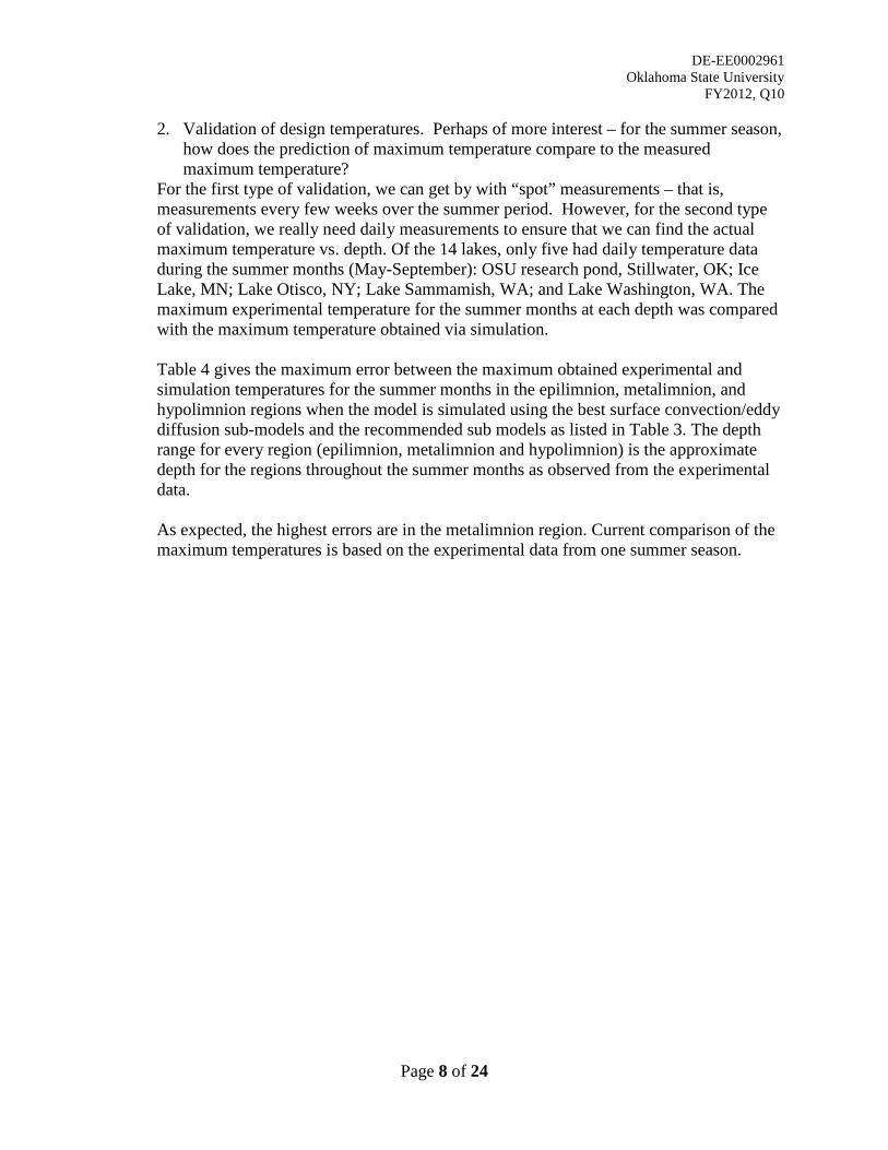
DE-EE0002961 Oklahoma State University
FY2012, Q10
Page 8 of 24
2. Validation of design temperatures. Perhaps of more interest – for the summer season, how does the prediction of maximum temperature compare to the measured maximum temperature?
For the first type of validation, we can get by with “spot” measurements – that is, measurements every few weeks over the summer period. However, for the second type of validation, we really need daily measurements to ensure that we can find the actual maximum temperature vs. depth. Of the 14 lakes, only five had daily temperature data during the summer months (May-September): OSU research pond, Stillwater, OK; Ice Lake, MN; Lake Otisco, NY; Lake Sammamish, WA; and Lake Washington, WA. The maximum experimental temperature for the summer months at each depth was compared with the maximum temperature obtained via simulation. Table 4 gives the maximum error between the maximum obtained experimental and simulation temperatures for the summer months in the epilimnion, metalimnion, and hypolimnion regions when the model is simulated using the best surface convection/eddy diffusion sub-models and the recommended sub models as listed in Table 3. The depth range for every region (epilimnion, metalimnion and hypolimnion) is the approximate depth for the regions throughout the summer months as observed from the experimental data. As expected, the highest errors are in the metalimnion region. Current comparison of the maximum temperatures is based on the experimental data from one summer season.
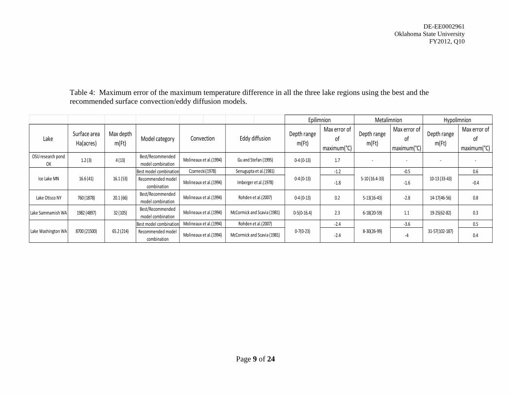
DE-EE0002961 Oklahoma State University
FY2012, Q10
Page 9 of 24
Table 4: Maximum error of the maximum temperature difference in all the three lake regions using the best and the recommended surface convection/eddy diffusion models.
Lake Surface area
Ha(acres)Max depth
m(Ft) Model categoryDepth range
m(Ft)
Max error of of
maximum(°C)
Depth range m(Ft)
Max error of of
maximum(°C)
Depth range m(Ft)
Max error of of
maximum(°C)OSU research pond
OK1.2 (3) 4 (13)
Best/Recommended model combination
0-4 (0-13) 1.7 - - - -
Best model combination -1.2 -0.5 0.6Recommended model
combination-1.8 -1.6 -0.4
Lake Otisco NY 760 (1878) 20.1 (66)Best/Recommended model combination
0-4 (0-13) 0.2 5-13(16-43) -2.8 14-17(46-56) 0.8
Lake Sammamish WA 1982 (4897) 32 (105)Best/Recommended model combination
0-5(0-16.4) 2.3 6-18(20-59) 1.1 19-25(62-82) 0.3
Best model combination -2.4 -3.6 0.5Recommended model
combination-2.4 -4 0.4
0-7(0-23) 8-30(26-99) 31-57(102-187)Molineaux et al.(1994) Rohden et al.(2007)
Lake Washington WA 8700 (21500) 65.2 (214)
Molineaux et al.(1994) McCormick and Scavia (1981)
Molineaux et al.(1994) McCormick and Scavia (1981)
Molineaux et al.(1994) Rohden et al.(2007)
Molineaux et al.(1994) Imberger et al.(1978)0-4 (0-13) 10-13 (33-43)
Molineaux et al.(1994) Gu and Stefan (1995)
Czarnecki(1978) Senugupta et al.(1981)Ice Lake MN 16.6 (41) 16.1 (53)
Epilimnion Metalimnion
5-10 (16.4-33)
Hypolimnion
Convection Eddy diffusion
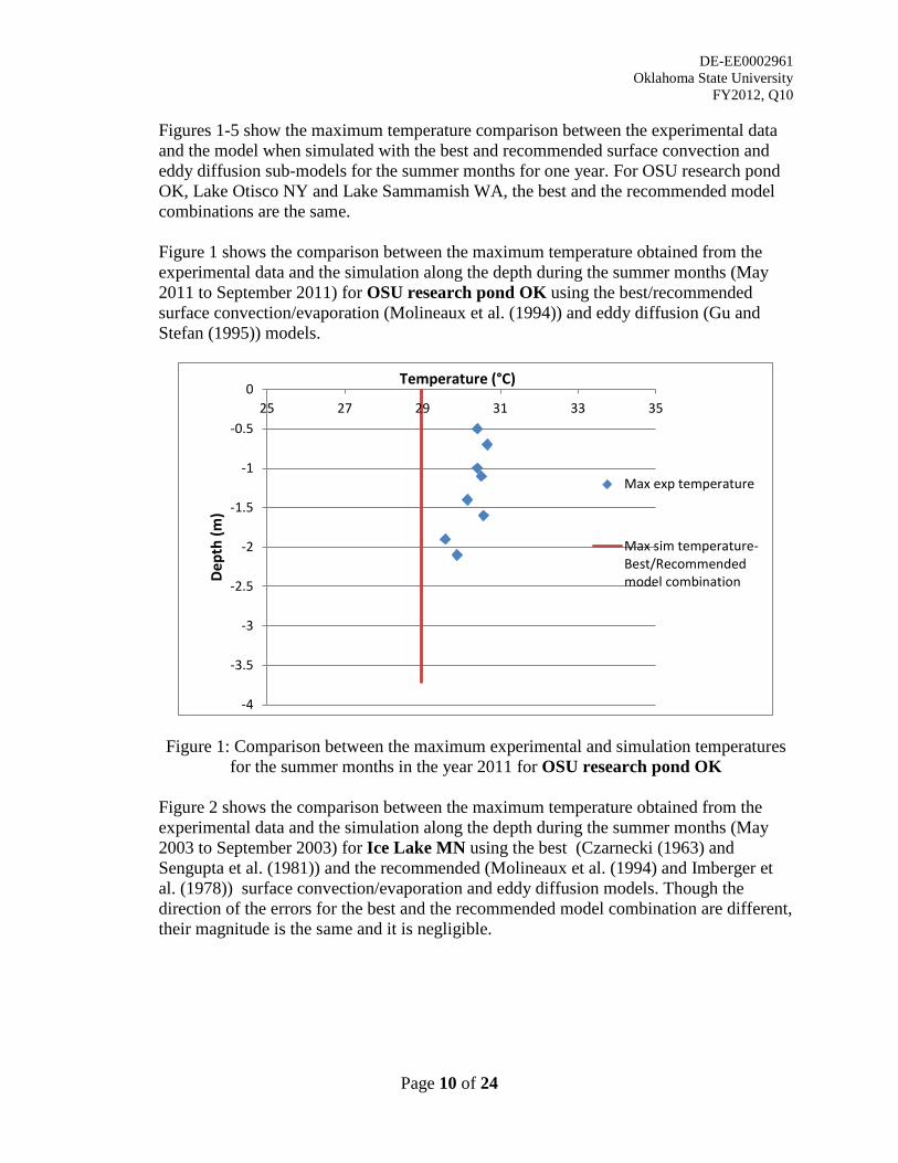
DE-EE0002961 Oklahoma State University
FY2012, Q10
Page 10 of 24
Figures 1-5 show the maximum temperature comparison between the experimental data and the model when simulated with the best and recommended surface convection and eddy diffusion sub-models for the summer months for one year. For OSU research pond OK, Lake Otisco NY and Lake Sammamish WA, the best and the recommended model combinations are the same.
Figure 1 shows the comparison between the maximum temperature obtained from the experimental data and the simulation along the depth during the summer months (May 2011 to September 2011) for OSU research pond OK using the best/recommended surface convection/evaporation (Molineaux et al. (1994)) and eddy diffusion (Gu and Stefan (1995)) models.
Figure 1: Comparison between the maximum experimental and simulation temperatures for the summer months in the year 2011 for OSU research pond OK
Figure 2 shows the comparison between the maximum temperature obtained from the experimental data and the simulation along the depth during the summer months (May 2003 to September 2003) for Ice Lake MN using the best (Czarnecki (1963) and Sengupta et al. (1981)) and the recommended (Molineaux et al. (1994) and Imberger et al. (1978)) surface convection/evaporation and eddy diffusion models. Though the direction of the errors for the best and the recommended model combination are different, their magnitude is the same and it is negligible.
-4
-3.5
-3
-2.5
-2
-1.5
-1
-0.5
025 27 29 31 33 35
Dept
h (m
)
Temperature (°C)
Max exp temperature
Max sim temperature-Best/Recommendedmodel combination
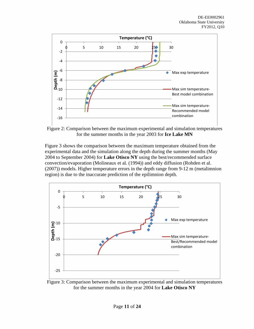
DE-EE0002961 Oklahoma State University
FY2012, Q10
Page 11 of 24
Figure 2: Comparison between the maximum experimental and simulation temperatures
for the summer months in the year 2003 for Ice Lake MN
Figure 3 shows the comparison between the maximum temperature obtained from the experimental data and the simulation along the depth during the summer months (May 2004 to September 2004) for Lake Otisco NY using the best/recommended surface convection/evaporation (Molineaux et al. (1994)) and eddy diffusion (Rohden et al. (2007)) models. Higher temperature errors in the depth range from 9-12 m (metalimnion region) is due to the inaccurate prediction of the epilimnion depth.
Figure 3: Comparison between the maximum experimental and simulation temperatures
for the summer months in the year 2004 for Lake Otisco NY
-16
-14
-12
-10
-8
-6
-4
-2
00 5 10 15 20 25 30
Dept
h (m
)
Temperature (°C)
Max exp temperature
Max sim temperature-Best model combination
Max sim temperature-Recommended modelcombination
-25
-20
-15
-10
-5
00 5 10 15 20 25 30
Dept
h (m
)
Temperature (°C)
Max exp temperature
Max sim temperature-Best/Recommended modelcombination
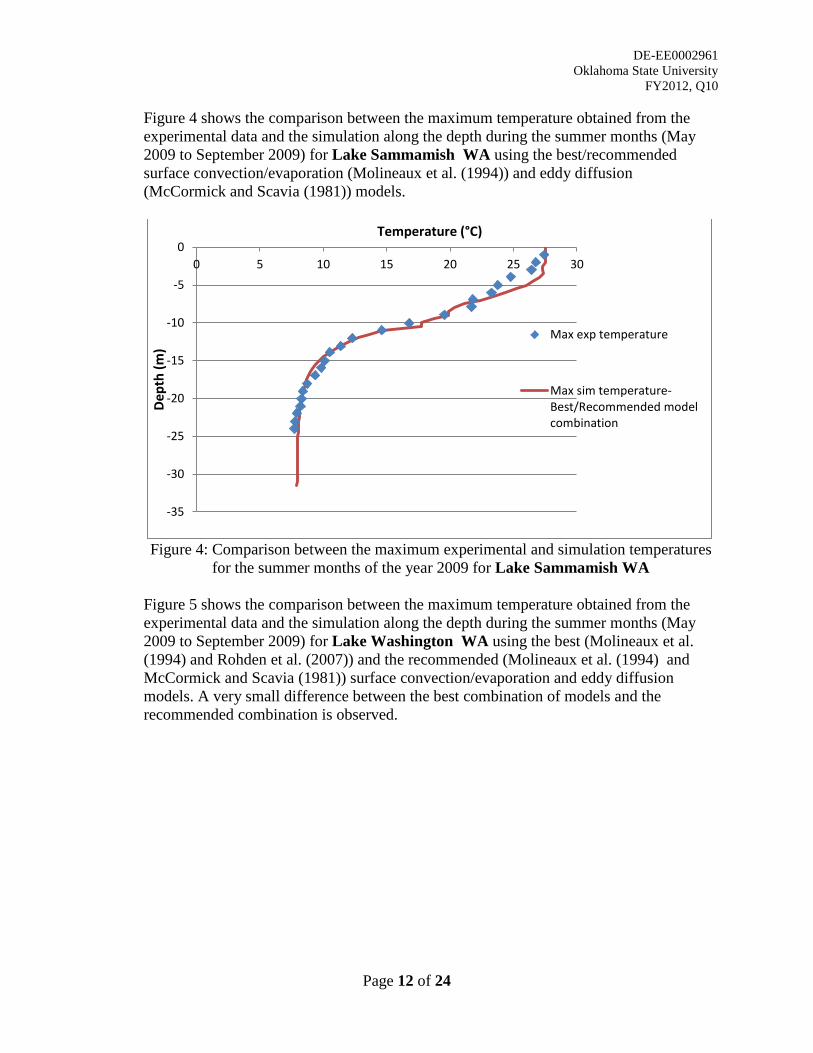
DE-EE0002961 Oklahoma State University
FY2012, Q10
Page 12 of 24
Figure 4 shows the comparison between the maximum temperature obtained from the experimental data and the simulation along the depth during the summer months (May 2009 to September 2009) for Lake Sammamish WA using the best/recommended surface convection/evaporation (Molineaux et al. (1994)) and eddy diffusion (McCormick and Scavia (1981)) models.
Figure 4: Comparison between the maximum experimental and simulation temperatures
for the summer months of the year 2009 for Lake Sammamish WA
Figure 5 shows the comparison between the maximum temperature obtained from the experimental data and the simulation along the depth during the summer months (May 2009 to September 2009) for Lake Washington WA using the best (Molineaux et al. (1994) and Rohden et al. (2007)) and the recommended (Molineaux et al. (1994) and McCormick and Scavia (1981)) surface convection/evaporation and eddy diffusion models. A very small difference between the best combination of models and the recommended combination is observed.
-35
-30
-25
-20
-15
-10
-5
00 5 10 15 20 25 30
Dept
h (m
)
Temperature (°C)
Max exp temperature
Max sim temperature-Best/Recommended modelcombination
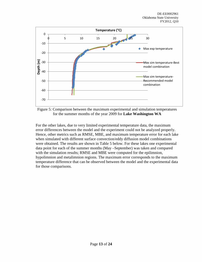
DE-EE0002961 Oklahoma State University
FY2012, Q10
Page 13 of 24
Figure 5: Comparison between the maximum experimental and simulation temperatures
for the summer months of the year 2009 for Lake Washington WA
For the other lakes, due to very limited experimental temperature data, the maximum error differences between the model and the experiment could not be analyzed properly. Hence, other metrics such as RMSE, MBE, and maximum temperature error for each lake when simulated with different surface convection/eddy diffusion model combinations were obtained. The results are shown in Table 5 below. For these lakes one experimental data point for each of the summer months (May –September) was taken and compared with the simulation results; RMSE and MBE were computed for the epilimnion, hypolimnion and metalimnion regions. The maximum error corresponds to the maximum temperature difference that can be observed between the model and the experimental data for those comparisons.
-70
-60
-50
-40
-30
-20
-10
00 5 10 15 20 25 30
Dept
h (m
)
Temperature (°C)
Max exp temperature
Max sim temperature-Bestmodel combination
Max sim temperature-Recommended modelcombination
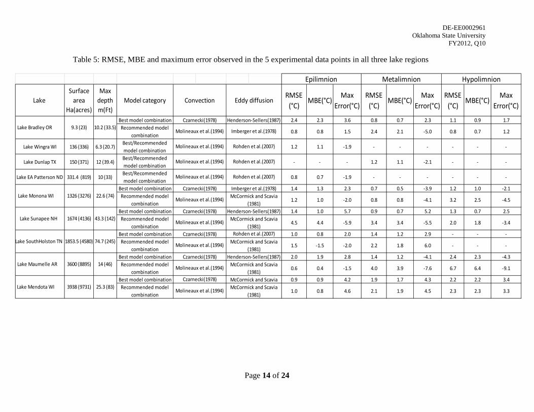
DE-EE0002961 Oklahoma State University
FY2012, Q10
Page 14 of 24
Table 5: RMSE, MBE and maximum error observed in the 5 experimental data points in all three lake regions
Lake Surface
area Ha(acres)
Max depth m(Ft)
Model categoryRMSE
(°C)MBE(°C)
Max Error(°C)
RMSE (°C)
MBE(°C)Max
Error(°C)RMSE
(°C)MBE(°C)
Max Error(°C)
Best model combination 2.4 2.3 3.6 0.8 0.7 2.3 1.1 0.9 1.7Recommended model
combination0.8 0.8 1.5 2.4 2.1 -5.0 0.8 0.7 1.2
Lake Wingra WI 136 (336) 6.3 (20.7)Best/Recommended model combination
1.2 1.1 -1.9 - - - - - -
Lake Dunlap TX 150 (371) 12 (39.4)Best/Recommended model combination
- - - 1.2 1.1 -2.1 - - -
Lake EA Patterson ND 331.4 (819) 10 (33)Best/Recommended model combination
0.8 0.7 -1.9 - - - - - -
Best model combination 1.4 1.3 2.3 0.7 0.5 -3.9 1.2 1.0 -2.1Recommended model
combination1.2 1.0 -2.0 0.8 0.8 -4.1 3.2 2.5 -4.5
Best model combination 1.4 1.0 5.7 0.9 0.7 5.2 1.3 0.7 2.5Recommended model
combination4.5 4.4 -5.9 3.4 3.4 -5.5 2.0 1.8 -3.4
Best model combination 1.0 0.8 2.0 1.4 1.2 2.9 - - -Recommended model
combination1.5 -1.5 -2.0 2.2 1.8 6.0 - - -
Best model combination 2.0 1.9 2.8 1.4 1.2 -4.1 2.4 2.3 -4.3Recommended model
combination0.6 0.4 -1.5 4.0 3.9 -7.6 6.7 6.4 -9.1
Best model combination 0.9 0.9 4.2 1.9 1.7 4.3 2.2 2.2 3.4Recommended model
combination1.0 0.8 4.6 2.1 1.9 4.5 2.3 2.3 3.3
McCormick and Scavia (1981)
Lake SouthHolston TN 1853.5 (4580) 74.7 (245)Molineaux et al.(1994) McCormick and Scavia
(1981)
Lake Maumelle AR 3600 (8895) 14 (46)Czarnecki(1978) Henderson-Sellers(1987)
Molineaux et al.(1994) McCormick and Scavia (1981)
Czarnecki(1978) Rohden et al.(2007)
Lake Mendota WI 3938 (9731) 25.3 (83)Czarnecki(1978) McCormick and Scavia
Molineaux et al.(1994)
Lake Sunapee NH 1674 (4136) 43.3 (142)Czarnecki(1978) Henderson-Sellers(1987)
Molineaux et al.(1994) McCormick and Scavia (1981)
Lake Monona WI 1326 (3276) 22.6 (74)Czarnecki(1978) Imberger et al.(1978)
Molineaux et al.(1994) McCormick and Scavia (1981)
Molineaux et al.(1994) Rohden et al.(2007)
Molineaux et al.(1994) Rohden et al.(2007)
Molineaux et al.(1994) Rohden et al.(2007)
Lake Bradley OR 9.3 (23) 10.2 (33.5)Czarnecki(1978) Henderson-Sellers(1987)
Molineaux et al.(1994) Imberger et al.(1978)
Epilimnion Metalimnion Hypolimnion
Convection Eddy diffusion

DE-EE0002961 Oklahoma State University
FY2012, Q10
Page 15 of 24
3. Explanation of Variance : No variances 4. Plans for Next Quarter: All the subtasks under this task are completed and the
milestones were submitted. No plans for the next quarter.
Task 3.0 – Implementation of Enhanced SCW Model
1. Planned Activities: Subtask 3.1 Implementation of Enhanced SCW Model in EnergyPlus The plans for last quarter were to complete the implementation of the enhanced SCW model in EnergyPlus and continue with the development of the documentation. Subtask 3.2 Implementation of Enhanced SCW Model in Design Tool The GLHEPRO SCW design tool was to be debugged prior to rigorous testing.
2. Actual Accomplishments: Subtask 3.1 Implementation of Enhanced SCW Model in EnergyPlus The implementation of the enhanced SCW model in Energy Plus is complete. The results of the model are currently being verified against the previously validated model in VB. Any further improvements that are made to the model such as the correlation can easily be integrated into the model at a later stage. The structure of the model was modified to conform to other ground heat exchanger models in the plant loop of EnergyPlus. Warnings were incorporated into the model to alert the user when inputs to the idf file were incorrect. For example the SCW uses only water as the working fluid while the other ground exchangers may use antifreeze, if the user specifies a working fluid other than water a warning is displayed. Though the SCW model is programmed to only calculate the properties of water this warning is incorporated since other components in the plant loop calculate the fluid properties based on the input from the idf file. Currently the documentation for the SCW model is being modified to conform to the documentation of the other ground heat exchangers. Subtask 3.2 Implementation of Enhanced SCW Model in Design Tool Debugging of the SCW model in GLHEPRO has continued. The interface is now complete and functioning properly; a screenshot showing the SCW interface is shown in Figure 6. The simulation itself is now being debugged, using a side-by-side comparison with the standalone VB model.
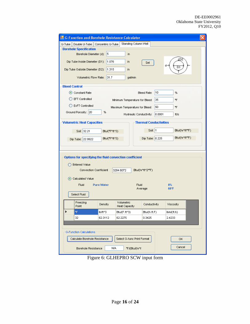
DE-EE0002961 Oklahoma State University
FY2012, Q10
Page 16 of 24
Figure 6: GLHEPRO SCW input form

DE-EE0002961 Oklahoma State University
FY2012, Q10
Page 17 of 24
3. Plans for Next Quarter:
Subtask 3.1 Implementation of Enhanced SCW Model in EnergyPlus Completion of the documentation and verification of model. Further changes to the code to conform with the other ground heat models in EnergyPlus. Subtask 3.2 Implementation of Enhanced SCW model in Design Tool Debugging of the GLHEPRO model will be completed, and the model verified against the standalone VB implementation. User documentation will be created.
Task 4.0 – Enhancement, Implementation and Validation of Enhanced Pond Model
1. Planned Activities : Subtask 4.1 Modeling of alternate pond heat exchanger types No plans for this quarter. Subtask 4.2 Documentation of enhanced pond model in EnergyPlus The enhanced pond model implemented in EnergyPlus was planned to be completely documented with some examples. Subtask 4.3 Implementation of enhanced pond model in design tool Plans for last quarter were to implement the enhanced pond model as a part of the design tool for ground heat exchangers (GLHEPRO) and submit a milestone containing the documentation of the design tool with some examples. Subtask 4.4 Validation of pond model The pond model integrated with the heat exchanger model in EnergyPlus was planned to be validated against the experimental results obtained for different heat exchanger types from the OSU research pond. A milestone report showing the validation of the enhanced pond model is also planned for this quarter. Subtask 4.5 Technology Transfer Plans for the last quarter was to submit several technical papers covering the surface water track and prepare milestone report containing a copy of the submitted papers.
2. Actual Accomplishments: Subtask 4.2 Documentation of Enhanced Pond model in Energy Plus The enhanced pond model developed in EnergyPlus during Phase 1 of this project is completely documented and attached as a milestone report.
Subtask 4.3 Implementation of Enhanced Pond Model in Design Tool The Surface Water Heat Exchanger (SWHE) design tool is currently operated in Microsoft Excel spreadsheet. GLHEPRO is currently being modified to transfer the necessary parameters to Excel, so that the SWHE code can use them in its simulation. Subtask 4.4 Validation of the pond model The pond heat exchanger implemented in EnergyPlus is connected to the supply side of a condenser loop and can be used with any type of plant loop. Since the pond model is a daily time step model, it is triggered only once per day during the first hour of the day.
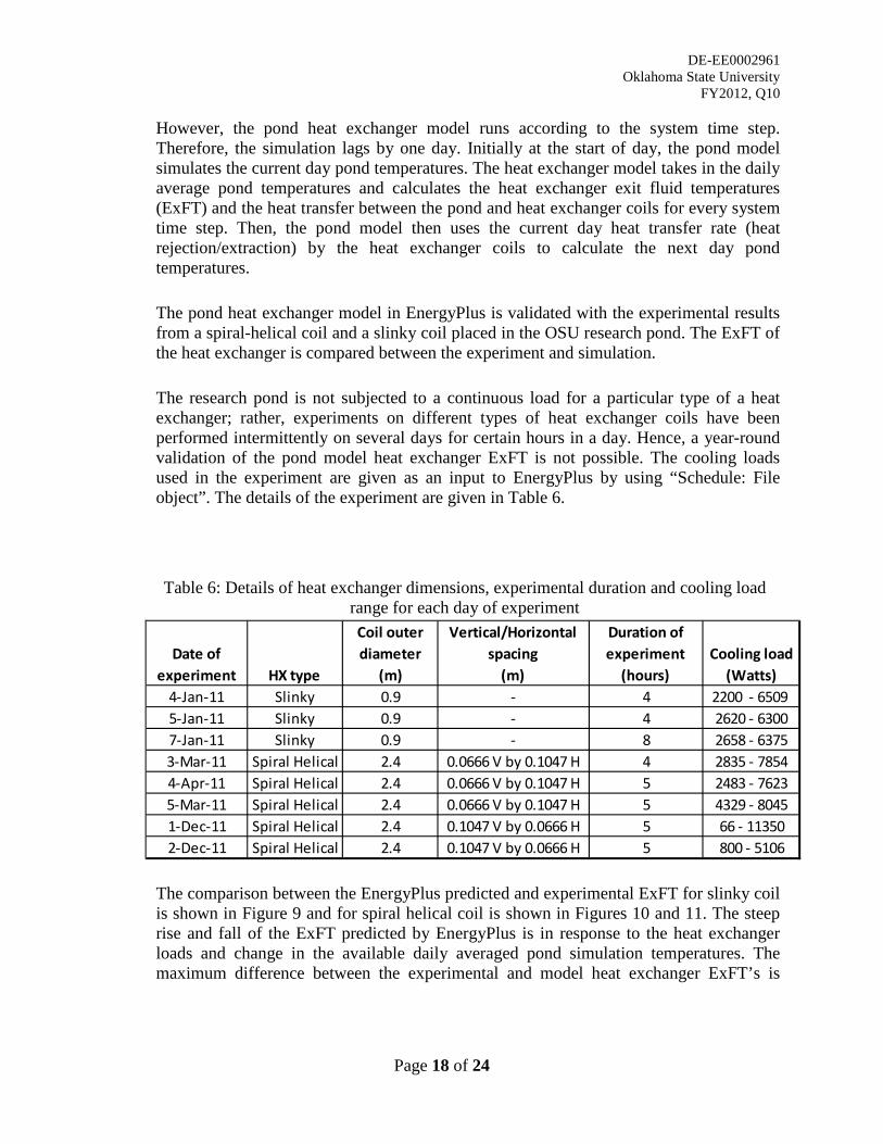
DE-EE0002961 Oklahoma State University
FY2012, Q10
Page 18 of 24
However, the pond heat exchanger model runs according to the system time step. Therefore, the simulation lags by one day. Initially at the start of day, the pond model simulates the current day pond temperatures. The heat exchanger model takes in the daily average pond temperatures and calculates the heat exchanger exit fluid temperatures (ExFT) and the heat transfer between the pond and heat exchanger coils for every system time step. Then, the pond model then uses the current day heat transfer rate (heat rejection/extraction) by the heat exchanger coils to calculate the next day pond temperatures. The pond heat exchanger model in EnergyPlus is validated with the experimental results from a spiral-helical coil and a slinky coil placed in the OSU research pond. The ExFT of the heat exchanger is compared between the experiment and simulation. The research pond is not subjected to a continuous load for a particular type of a heat exchanger; rather, experiments on different types of heat exchanger coils have been performed intermittently on several days for certain hours in a day. Hence, a year-round validation of the pond model heat exchanger ExFT is not possible. The cooling loads used in the experiment are given as an input to EnergyPlus by using “Schedule: File object”. The details of the experiment are given in Table 6.
Table 6: Details of heat exchanger dimensions, experimental duration and cooling load range for each day of experiment
The comparison between the EnergyPlus predicted and experimental ExFT for slinky coil is shown in Figure 9 and for spiral helical coil is shown in Figures 10 and 11. The steep rise and fall of the ExFT predicted by EnergyPlus is in response to the heat exchanger loads and change in the available daily averaged pond simulation temperatures. The maximum difference between the experimental and model heat exchanger ExFT’s is
Date of experiment HX type
Coil outer diameter
(m)
Vertical/Horizontal spacing
(m)
Duration of experiment
(hours)Cooling load
(Watts)4-Jan-11 Slinky 0.9 - 4 2200 - 6509 5-Jan-11 Slinky 0.9 - 4 2620 - 63007-Jan-11 Slinky 0.9 - 8 2658 - 63753-Mar-11 Spiral Helical 2.4 0.0666 V by 0.1047 H 4 2835 - 78544-Apr-11 Spiral Helical 2.4 0.0666 V by 0.1047 H 5 2483 - 76235-Mar-11 Spiral Helical 2.4 0.0666 V by 0.1047 H 5 4329 - 80451-Dec-11 Spiral Helical 2.4 0.1047 V by 0.0666 H 5 66 - 113502-Dec-11 Spiral Helical 2.4 0.1047 V by 0.0666 H 5 800 - 5106
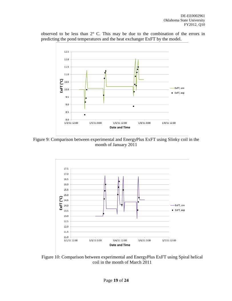
DE-EE0002961 Oklahoma State University
FY2012, Q10
Page 19 of 24
observed to be less than 2° C. This may be due to the combination of the errors in predicting the pond temperatures and the heat exchanger ExFT by the model.
Figure 9: Comparison between experimental and EnergyPlus ExFT using Slinky coil in the
month of January 2011
Figure 10: Comparison between experimental and EnergyPlus ExFT using Spiral helical
coil in the month of March 2011
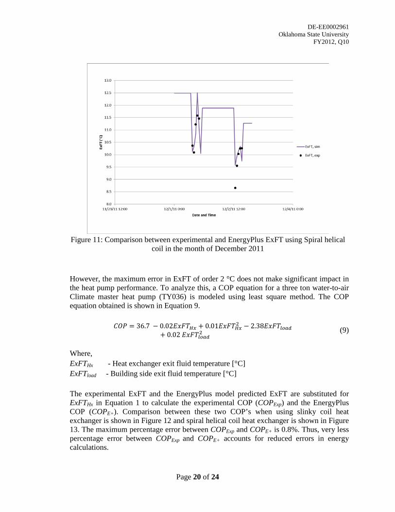
DE-EE0002961 Oklahoma State University
FY2012, Q10
Page 20 of 24
Figure 11: Comparison between experimental and EnergyPlus ExFT using Spiral helical
coil in the month of December 2011 However, the maximum error in ExFT of order 2 °C does not make significant impact in the heat pump performance. To analyze this, a COP equation for a three ton water-to-air Climate master heat pump (TY036) is modeled using least square method. The COP equation obtained is shown in Equation 9.
𝐶𝑂𝑃 = 36.7 − 0.02𝐸𝑥𝐹𝑇𝐻𝑥 + 0.01𝐸𝑥𝐹𝑇𝐻𝑥2 − 2.38𝐸𝑥𝐹𝑇𝑙𝑜𝑎𝑑+ 0.02 𝐸𝑥𝐹𝑇𝑙𝑜𝑎𝑑2 (9)
Where, ExFTHx - Heat exchanger exit fluid temperature [°C] ExFTload - Building side exit fluid temperature [°C] The experimental ExFT and the EnergyPlus model predicted ExFT are substituted for ExFTHx in Equation 1 to calculate the experimental COP (COPExp) and the EnergyPlus COP (COPE+). Comparison between these two COP’s when using slinky coil heat exchanger is shown in Figure 12 and spiral helical coil heat exchanger is shown in Figure 13. The maximum percentage error between COPExp and COPE+ is 0.8%. Thus, very less percentage error between COPExp and COPE+ accounts for reduced errors in energy calculations.
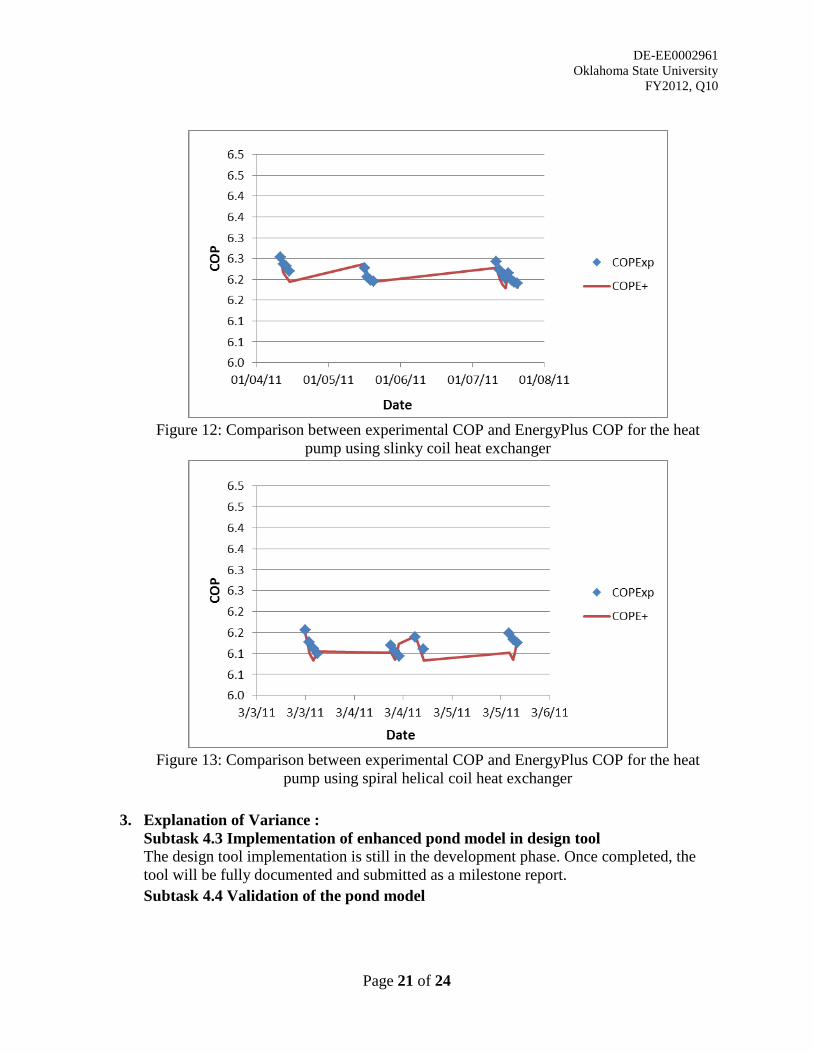
DE-EE0002961 Oklahoma State University
FY2012, Q10
Page 21 of 24
Figure 12: Comparison between experimental COP and EnergyPlus COP for the heat
pump using slinky coil heat exchanger
Figure 13: Comparison between experimental COP and EnergyPlus COP for the heat
pump using spiral helical coil heat exchanger
3. Explanation of Variance : Subtask 4.3 Implementation of enhanced pond model in design tool The design tool implementation is still in the development phase. Once completed, the tool will be fully documented and submitted as a milestone report. Subtask 4.4 Validation of the pond model
DE-EE0002961 Oklahoma State University
FY2012, Q10
Page 22 of 24
Validation is yet to be performed for the flat spiral or flat plate heat exchanger types. Once completed, the full validation effort will be packaged into a milestone report.
4. Plans for Next Quarter: Subtask 4.3 Implementation of enhanced pond model in design tool The design tool user interface is planned to be completed and the work for linking the design tool with the GLHPRO would be underway. Subtask 4.4 Validation of the pond model Validation of the EnergyPlus pond model with the experimental results from other heat exchanger types will be done, and the milestone report submitted.
References
Gu, R., and H. G. Stefan. 1995. Stratification dynamics in wastewater stabilization ponds. Water Research 29(8): 1909-1923.
Imberger, J., J. Patterson, B. Hebbert, and I. Loh. 1978. Dynamics of Reservoir of Medium Size. Journal of Hydraulics Division 104(5): 725-743.
Ingersoll, L. R., and H. J. Plass. 1948. Theory of the Ground Pipe Heat Source for the Heat Pump. Heating, Piping & Air conditioning
Javed, S. 2010. Design of ground source heat pump systems. Licentiate Thesis. Chalmers University of Technology, Göteborg, Sweden.
McCormick, M. J., and D. Scavia. 1981. Calculation of vertical profiles of lake-averaged temperature and diffusivity in Lakes Ontario and Washington. Water Resources Research 17(2): 305-310.
Mogensen, P. 1983. Fluid to Duct Wall Heat Transfer in Duct System Heat Storages. Proceedings of the International Conference on Subsurface Heat Storage in Theory and Practice, Sweden, Swedish Council for Building Research.
Molineaux, B., B. Lachal, and O. Guisan. 1994. Thermal analysis of five outdoor swimming pools heated by unglazed solar collectors. Solar Energy 53(1): 21-26.
Rasmussen, A. H., M. Hondzo, and H. G. Stefan. 1995. A test of several evaporation equations for water temperature simulations in lakes. Journal of the American Water Resources Association 31(6): 1023-1028.
Rohden, C. V., K. Wunderle, and J. Ilmberger. 2007. Parameterisation of the vertical transport in a small thermally stratified lake. Aquatic Sciences - Research Across Boundaries 69(1): 129-137.
Sengupta, S., E. Nwadike, and S. S. Lee. 1981. Long term simulation of stratification in cooling lakes. Applied Mathematical Modelling 5(5): 313-320.

DE-EE0002961 Oklahoma State University
FY2012, Q10
Page 23 of 24
PRODUCTS / DELIVERABLES
Training and Professional Development: n/a Publications, Conference Papers, and Presentations: This paper was presented on May 18, 2012:
Ramesh, A. and J.D. Spitler. 2012. A quasi-two-dimensional standing column well model for ground source heat pump systems. Proceedings of Innostock 2012, The 12th International Conference on Energy Storage. Lleida, Spain. May 2012.
Patents and IP: n/a Other Products / Deliverables: n/a

DE-EE0002961 Oklahoma State University
FY2012, Q10
Page 24 of 24
BUDGETARY AND OTHER INFORMATION Complete the following tables in the Excel Progress Report accordingly:
• Budget by Task – “QuarterlySumRpt” Tab • Financial and Spend Plan Data – “Financial Data” Tab
To insert this document into the Excel Progress Report: A cell is provided in the Excel Progress Report (BP/BQ 10) to insert this Project Narrative. To insert your narrative file into this cell, employ the "Insert" function from the excel tool bar. Select "Insert Object" and select the "Create from File" tab. Use the "Browse" option to locate the file you wish to insert. Check the "Display as Icon" box and select "OK". Recipient Requests for DOE Attention: n/a

DE-EE0002961 Final Report Appendix 6.1 1
Computer Modeling: SWHP Systems
Krishna Conjeevaram Bashyam
Manojkumar Selvakumar
Oklahoma State University
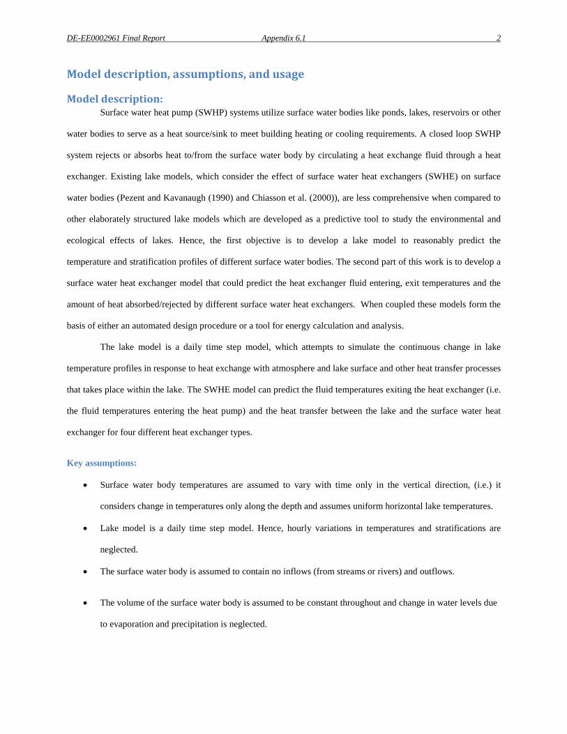
DE-EE0002961 Final Report Appendix 6.1 2
Model description, assumptions, and usage
Model description: Surface water heat pump (SWHP) systems utilize surface water bodies like ponds, lakes, reservoirs or other
water bodies to serve as a heat source/sink to meet building heating or cooling requirements. A closed loop SWHP
system rejects or absorbs heat to/from the surface water body by circulating a heat exchange fluid through a heat
exchanger. Existing lake models, which consider the effect of surface water heat exchangers (SWHE) on surface
water bodies (Pezent and Kavanaugh (1990) and Chiasson et al. (2000)), are less comprehensive when compared to
other elaborately structured lake models which are developed as a predictive tool to study the environmental and
ecological effects of lakes. Hence, the first objective is to develop a lake model to reasonably predict the
temperature and stratification profiles of different surface water bodies. The second part of this work is to develop a
surface water heat exchanger model that could predict the heat exchanger fluid entering, exit temperatures and the
amount of heat absorbed/rejected by different surface water heat exchangers. When coupled these models form the
basis of either an automated design procedure or a tool for energy calculation and analysis.
The lake model is a daily time step model, which attempts to simulate the continuous change in lake
temperature profiles in response to heat exchange with atmosphere and lake surface and other heat transfer processes
that takes place within the lake. The SWHE model can predict the fluid temperatures exiting the heat exchanger (i.e.
the fluid temperatures entering the heat pump) and the heat transfer between the lake and the surface water heat
exchanger for four different heat exchanger types.
Key assumptions:
• Surface water body temperatures are assumed to vary with time only in the vertical direction, (i.e.) it
considers change in temperatures only along the depth and assumes uniform horizontal lake temperatures.
• Lake model is a daily time step model. Hence, hourly variations in temperatures and stratifications are
neglected.
• The surface water body is assumed to contain no inflows (from streams or rivers) and outflows.
• The volume of the surface water body is assumed to be constant throughout and change in water levels due
to evaporation and precipitation is neglected.
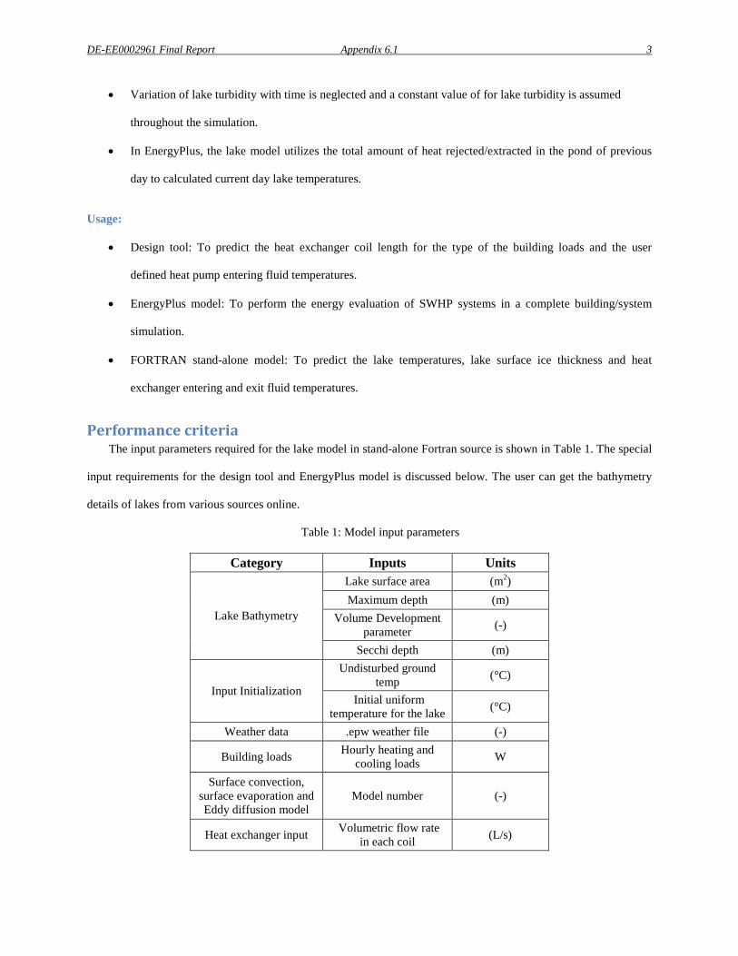
DE-EE0002961 Final Report Appendix 6.1 3
• Variation of lake turbidity with time is neglected and a constant value of for lake turbidity is assumed
throughout the simulation.
• In EnergyPlus, the lake model utilizes the total amount of heat rejected/extracted in the pond of previous
day to calculated current day lake temperatures.
Usage:
• Design tool: To predict the heat exchanger coil length for the type of the building loads and the user
defined heat pump entering fluid temperatures.
• EnergyPlus model: To perform the energy evaluation of SWHP systems in a complete building/system
simulation.
• FORTRAN stand-alone model: To predict the lake temperatures, lake surface ice thickness and heat
exchanger entering and exit fluid temperatures.
Performance criteria The input parameters required for the lake model in stand-alone Fortran source is shown in Table 1. The special
input requirements for the design tool and EnergyPlus model is discussed below. The user can get the bathymetry
details of lakes from various sources online.
Table 1: Model input parameters
Category Inputs Units
Lake Bathymetry
Lake surface area (m2) Maximum depth (m)
Volume Development parameter (-)
Secchi depth (m)
Input Initialization
Undisturbed ground temp (°C)
Initial uniform temperature for the lake (°C)
Weather data .epw weather file (-)
Building loads Hourly heating and cooling loads W
Surface convection, surface evaporation and Eddy diffusion model
Model number (-)
Heat exchanger input Volumetric flow rate in each coil (L/s)
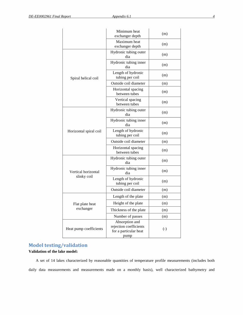
DE-EE0002961 Final Report Appendix 6.1 4
Minimum heat exchanger depth (m)
Maximum heat exchanger depth (m)
Spiral helical coil
Hydronic tubing outer dia (m)
Hydronic tubing inner dia (m)
Length of hydronic tubing per coil (m)
Outside coil diameter (m) Horizontal spacing
between tubes (m)
Vertical spacing between tubes (m)
Horizontal spiral coil
Hydronic tubing outer dia (m)
Hydronic tubing inner dia (m)
Length of hydronic tubing per coil (m)
Outside coil diameter (m) Horizontal spacing
between tubes (m)
Vertical horizontal slinky coil
Hydronic tubing outer dia (m)
Hydronic tubing inner dia (m)
Length of hydronic tubing per coil (m)
Outside coil diameter (m)
Flat plate heat exchanger
Length of the plate (m)
Height of the plate (m)
Thickness of the plate (m) Number of passes (m)
Heat pump coefficients
Absorption and rejection coefficients for a particular heat
pump
(-)
Model testing/validation Validation of the lake model:
A set of 14 lakes characterized by reasonable quantities of temperature profile measurements (includes both
daily data measurements and measurements made on a monthly basis), well characterized bathymetry and
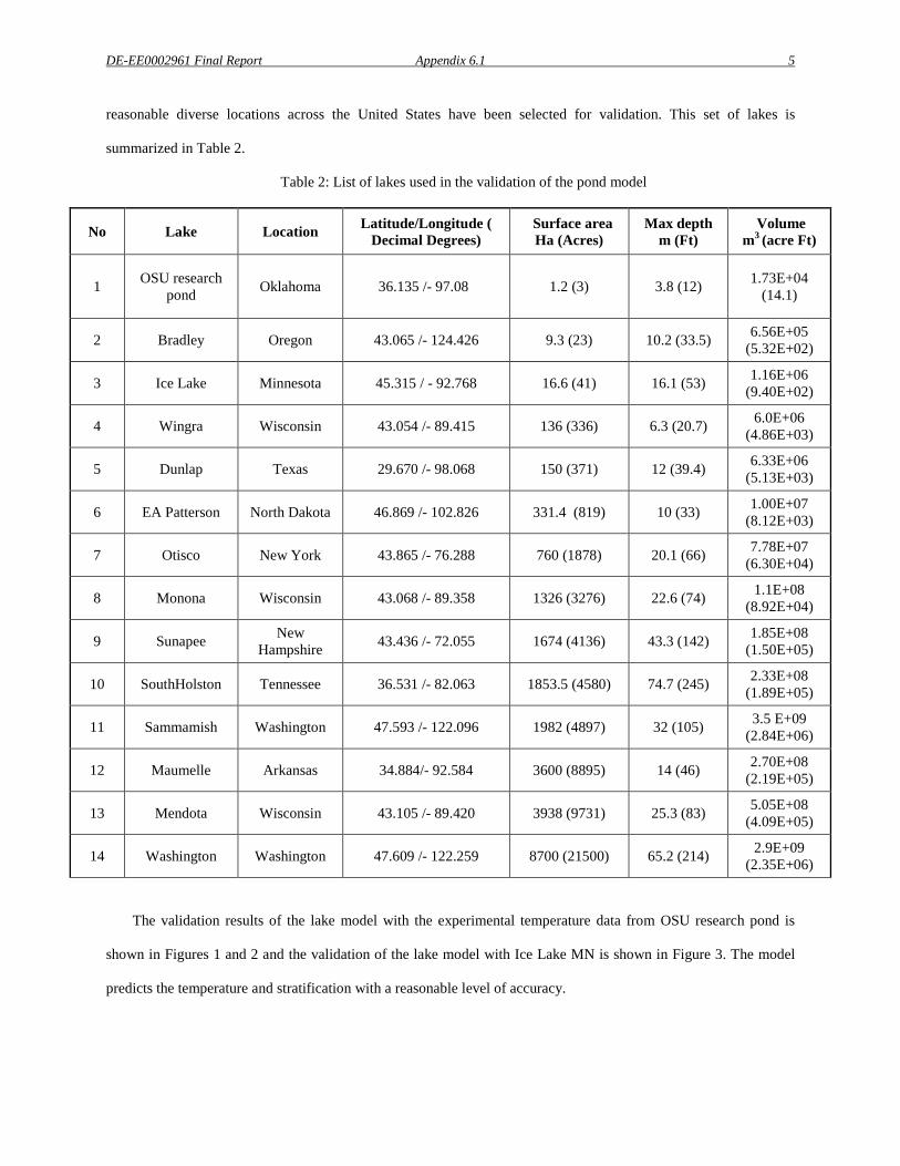
DE-EE0002961 Final Report Appendix 6.1 5 reasonable diverse locations across the United States have been selected for validation. This set of lakes is
summarized in Table 2.
Table 2: List of lakes used in the validation of the pond model
No Lake Location Latitude/Longitude ( Decimal Degrees)
Surface area Ha (Acres)
Max depth m (Ft)
Volume m3 (acre Ft)
1 OSU research pond Oklahoma 36.135 /- 97.08 1.2 (3) 3.8 (12) 1.73E+04
(14.1)
2 Bradley Oregon 43.065 /- 124.426 9.3 (23) 10.2 (33.5) 6.56E+05 (5.32E+02)
3 Ice Lake Minnesota 45.315 / - 92.768 16.6 (41) 16.1 (53) 1.16E+06 (9.40E+02)
4 Wingra Wisconsin 43.054 /- 89.415 136 (336) 6.3 (20.7) 6.0E+06 (4.86E+03)
5 Dunlap Texas 29.670 /- 98.068 150 (371) 12 (39.4) 6.33E+06 (5.13E+03)
6 EA Patterson North Dakota 46.869 /- 102.826 331.4 (819) 10 (33) 1.00E+07 (8.12E+03)
7 Otisco New York 43.865 /- 76.288 760 (1878) 20.1 (66) 7.78E+07 (6.30E+04)
8 Monona Wisconsin 43.068 /- 89.358 1326 (3276) 22.6 (74) 1.1E+08 (8.92E+04)
9 Sunapee New Hampshire 43.436 /- 72.055 1674 (4136) 43.3 (142) 1.85E+08
(1.50E+05)
10 SouthHolston Tennessee 36.531 /- 82.063 1853.5 (4580) 74.7 (245) 2.33E+08 (1.89E+05)
11 Sammamish Washington 47.593 /- 122.096 1982 (4897) 32 (105) 3.5 E+09 (2.84E+06)
12 Maumelle Arkansas 34.884/- 92.584 3600 (8895) 14 (46) 2.70E+08 (2.19E+05)
13 Mendota Wisconsin 43.105 /- 89.420 3938 (9731) 25.3 (83) 5.05E+08 (4.09E+05)
14 Washington Washington 47.609 /- 122.259 8700 (21500) 65.2 (214) 2.9E+09 (2.35E+06)
The validation results of the lake model with the experimental temperature data from OSU research pond is
shown in Figures 1 and 2 and the validation of the lake model with Ice Lake MN is shown in Figure 3. The model
predicts the temperature and stratification with a reasonable level of accuracy.
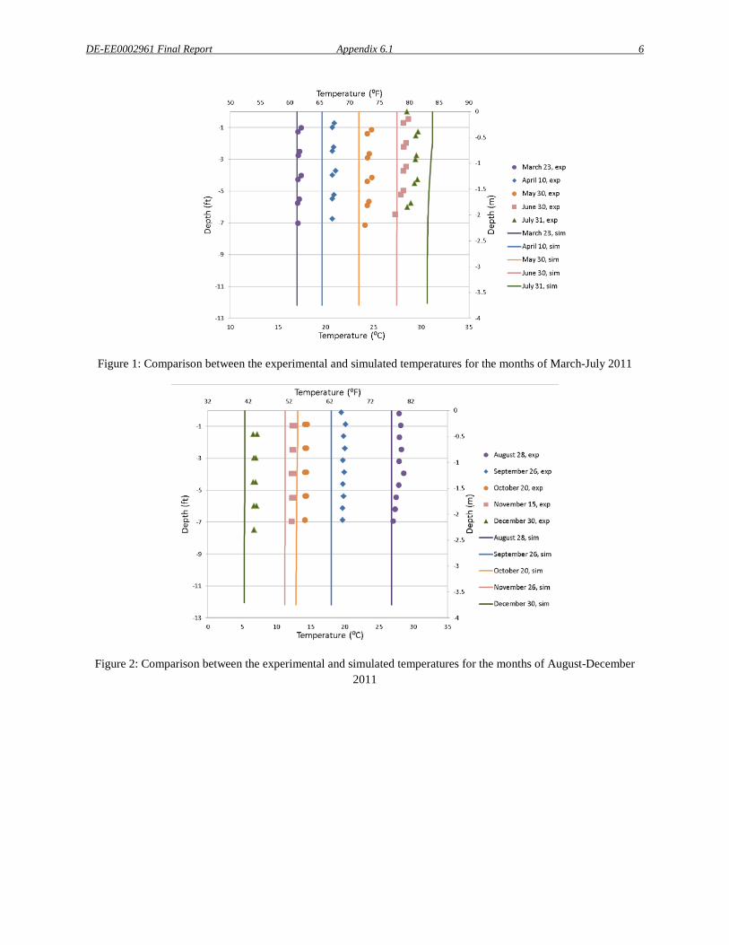
DE-EE0002961 Final Report Appendix 6.1 6
Figure 1: Comparison between the experimental and simulated temperatures for the months of March-July 2011
Figure 2: Comparison between the experimental and simulated temperatures for the months of August-December 2011
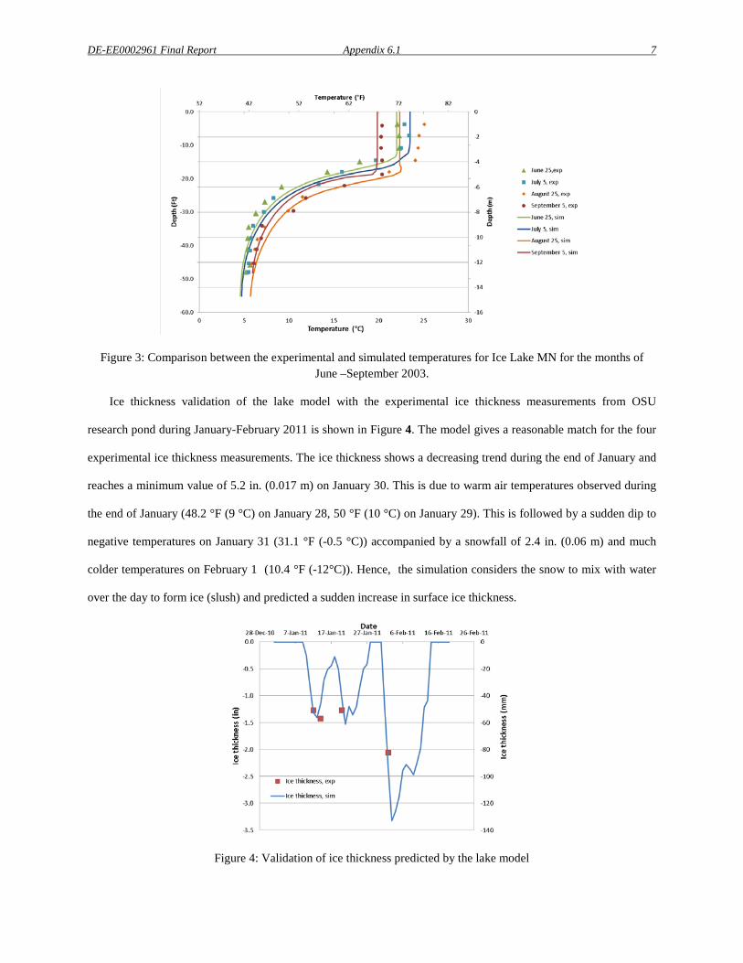
DE-EE0002961 Final Report Appendix 6.1 7
Figure 3: Comparison between the experimental and simulated temperatures for Ice Lake MN for the months of June –September 2003.
Ice thickness validation of the lake model with the experimental ice thickness measurements from OSU
research pond during January-February 2011 is shown in Figure 4. The model gives a reasonable match for the four
experimental ice thickness measurements. The ice thickness shows a decreasing trend during the end of January and
reaches a minimum value of 5.2 in. (0.017 m) on January 30. This is due to warm air temperatures observed during
the end of January (48.2 °F (9 °C) on January 28, 50 °F (10 °C) on January 29). This is followed by a sudden dip to
negative temperatures on January 31 (31.1 °F (-0.5 °C)) accompanied by a snowfall of 2.4 in. (0.06 m) and much
colder temperatures on February 1 (10.4 °F (-12°C)). Hence, the simulation considers the snow to mix with water
over the day to form ice (slush) and predicted a sudden increase in surface ice thickness.
Figure 4: Validation of ice thickness predicted by the lake model
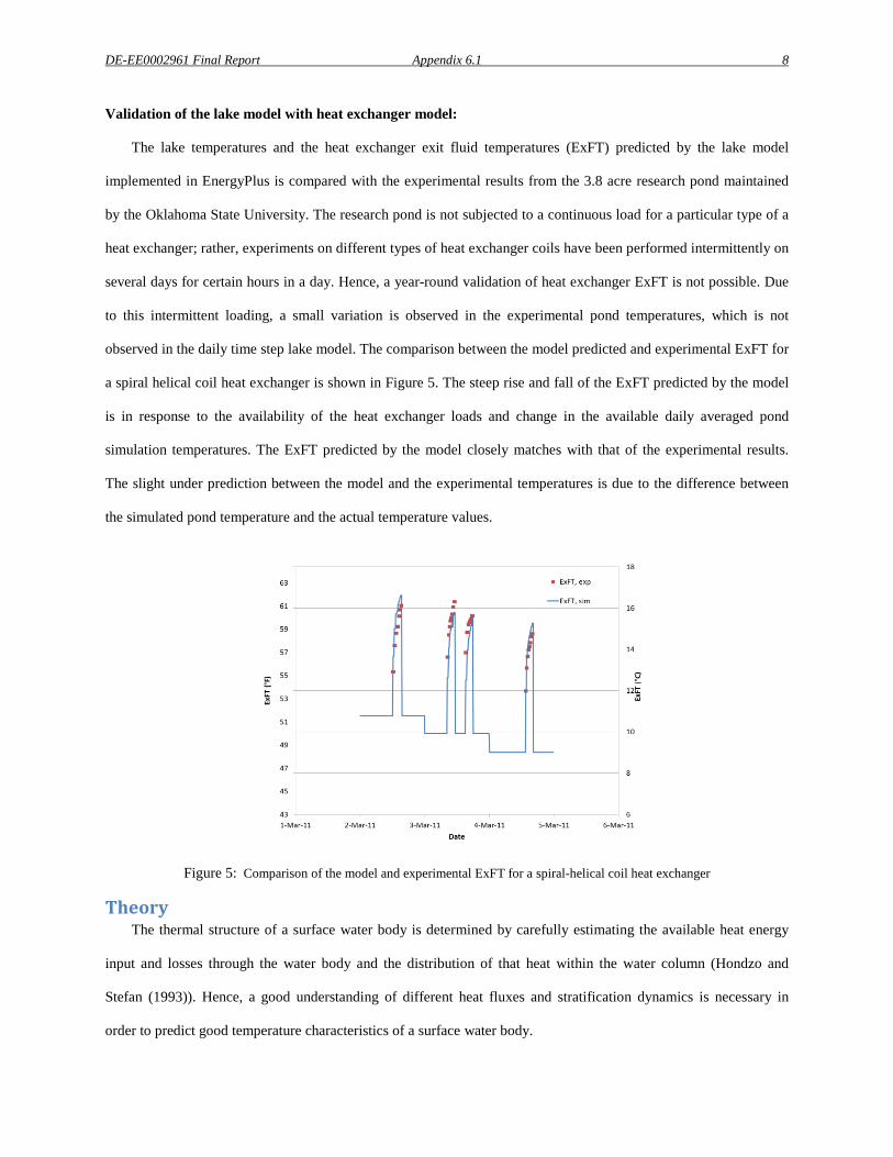
DE-EE0002961 Final Report Appendix 6.1 8 Validation of the lake model with heat exchanger model:
The lake temperatures and the heat exchanger exit fluid temperatures (ExFT) predicted by the lake model
implemented in EnergyPlus is compared with the experimental results from the 3.8 acre research pond maintained
by the Oklahoma State University. The research pond is not subjected to a continuous load for a particular type of a
heat exchanger; rather, experiments on different types of heat exchanger coils have been performed intermittently on
several days for certain hours in a day. Hence, a year-round validation of heat exchanger ExFT is not possible. Due
to this intermittent loading, a small variation is observed in the experimental pond temperatures, which is not
observed in the daily time step lake model. The comparison between the model predicted and experimental ExFT for
a spiral helical coil heat exchanger is shown in Figure 5. The steep rise and fall of the ExFT predicted by the model
is in response to the availability of the heat exchanger loads and change in the available daily averaged pond
simulation temperatures. The ExFT predicted by the model closely matches with that of the experimental results.
The slight under prediction between the model and the experimental temperatures is due to the difference between
the simulated pond temperature and the actual temperature values.
Figure 5: Comparison of the model and experimental ExFT for a spiral-helical coil heat exchanger
Theory The thermal structure of a surface water body is determined by carefully estimating the available heat energy
input and losses through the water body and the distribution of that heat within the water column (Hondzo and
Stefan (1993)). Hence, a good understanding of different heat fluxes and stratification dynamics is necessary in
order to predict good temperature characteristics of a surface water body.

DE-EE0002961 Final Report Appendix 6.1 9 The major heat transfer and transport mechanisms, which affect the thermal structure of a surface water body are,
• Heat balance between the incoming shortwave, long wave radiative heat fluxes to the lake surface from the
atmosphere and the outgoing surface convection and evaporation heat fluxes from the lake surface to the
atmosphere
• Vertical transport of heat through turbulent diffusion
• Internal distribution of heat within the water body through attenuation of incoming shortwave radiation
• Heat transfer between the surface water body and the ground below the bottom of the water body
• Heat transfer between the surface water body and the SWHE
• Ice formation, growth and melting on the water body surface
Figure 6 illustrates some of the heat transfer and mixing mechanisms for a typical surface water body with a
heat exchanger installation.
Figure 6: Heat and temperature transport mechanism for a typical surface water body with heat exchanger
Solar energy is the main heating mechanism in ponds and lakes. Incident solar radiation is partly absorbed
at the water body surface; some of the remaining energy is transmitted through the water body, where it is absorbed.
Penetration of the solar radiation through the depth depends on the transmissivity of the water body, which again
depends on its turbidity. Evaporation is the main cooling mechanism for ponds and lakes. It occurs when the lake
Shortwave radiation
EvaporationConvection
Net long wave radiation
Attenuation of shortwave radiation
Surface wind stress
River/stream inflow Surface outflow
Internal waves
Sediment
Sheltered regionExposed region
Surface mixing
Turbulent mixing
Sediment heat flux
Heat exchanger
Heat exchanger heat flux
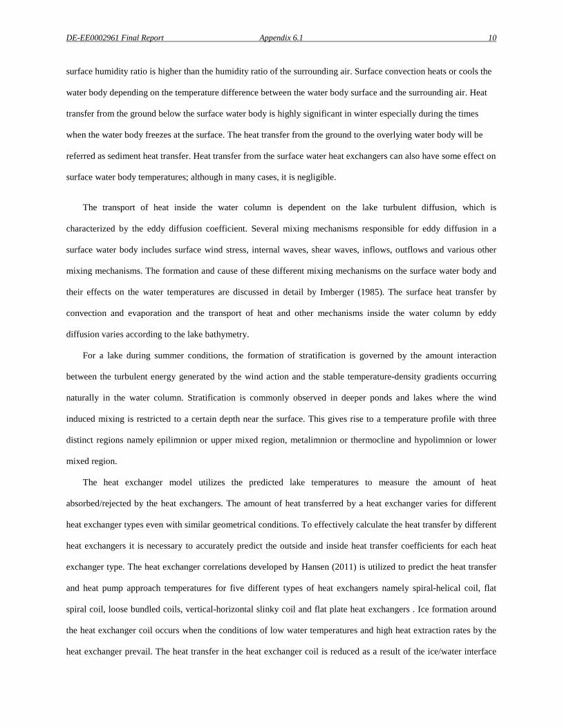
DE-EE0002961 Final Report Appendix 6.1 10 surface humidity ratio is higher than the humidity ratio of the surrounding air. Surface convection heats or cools the
water body depending on the temperature difference between the water body surface and the surrounding air. Heat
transfer from the ground below the surface water body is highly significant in winter especially during the times
when the water body freezes at the surface. The heat transfer from the ground to the overlying water body will be
referred as sediment heat transfer. Heat transfer from the surface water heat exchangers can also have some effect on
surface water body temperatures; although in many cases, it is negligible.
The transport of heat inside the water column is dependent on the lake turbulent diffusion, which is
characterized by the eddy diffusion coefficient. Several mixing mechanisms responsible for eddy diffusion in a
surface water body includes surface wind stress, internal waves, shear waves, inflows, outflows and various other
mixing mechanisms. The formation and cause of these different mixing mechanisms on the surface water body and
their effects on the water temperatures are discussed in detail by Imberger (1985). The surface heat transfer by
convection and evaporation and the transport of heat and other mechanisms inside the water column by eddy
diffusion varies according to the lake bathymetry.
For a lake during summer conditions, the formation of stratification is governed by the amount interaction
between the turbulent energy generated by the wind action and the stable temperature-density gradients occurring
naturally in the water column. Stratification is commonly observed in deeper ponds and lakes where the wind
induced mixing is restricted to a certain depth near the surface. This gives rise to a temperature profile with three
distinct regions namely epilimnion or upper mixed region, metalimnion or thermocline and hypolimnion or lower
mixed region.
The heat exchanger model utilizes the predicted lake temperatures to measure the amount of heat
absorbed/rejected by the heat exchangers. The amount of heat transferred by a heat exchanger varies for different
heat exchanger types even with similar geometrical conditions. To effectively calculate the heat transfer by different
heat exchangers it is necessary to accurately predict the outside and inside heat transfer coefficients for each heat
exchanger type. The heat exchanger correlations developed by Hansen (2011) is utilized to predict the heat transfer
and heat pump approach temperatures for five different types of heat exchangers namely spiral-helical coil, flat
spiral coil, loose bundled coils, vertical-horizontal slinky coil and flat plate heat exchangers . Ice formation around
the heat exchanger coil occurs when the conditions of low water temperatures and high heat extraction rates by the
heat exchanger prevail. The heat transfer in the heat exchanger coil is reduced as a result of the ice/water interface
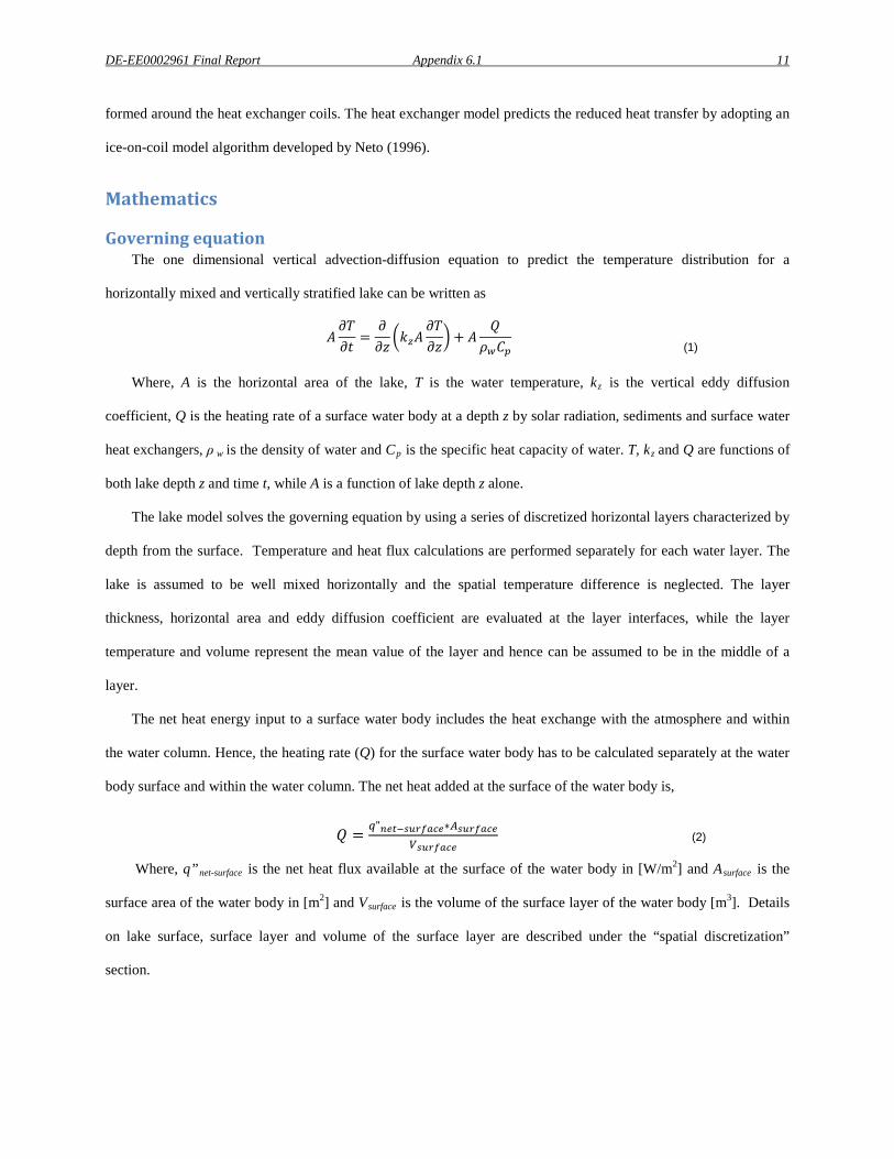
DE-EE0002961 Final Report Appendix 6.1 11 formed around the heat exchanger coils. The heat exchanger model predicts the reduced heat transfer by adopting an
ice-on-coil model algorithm developed by Neto (1996).
Mathematics
Governing equation The one dimensional vertical advection-diffusion equation to predict the temperature distribution for a
horizontally mixed and vertically stratified lake can be written as
𝐴𝜕𝑇𝜕𝑡
=𝜕𝜕𝑧�𝑘𝑧𝐴
𝜕𝑇𝜕𝑧� + 𝐴
𝑄𝜌𝑤𝐶𝑝
(1)
Where, A is the horizontal area of the lake, T is the water temperature, kz is the vertical eddy diffusion
coefficient, Q is the heating rate of a surface water body at a depth z by solar radiation, sediments and surface water
heat exchangers, ρ w is the density of water and Cp is the specific heat capacity of water. T, kz and Q are functions of
both lake depth z and time t, while A is a function of lake depth z alone.
The lake model solves the governing equation by using a series of discretized horizontal layers characterized by
depth from the surface. Temperature and heat flux calculations are performed separately for each water layer. The
lake is assumed to be well mixed horizontally and the spatial temperature difference is neglected. The layer
thickness, horizontal area and eddy diffusion coefficient are evaluated at the layer interfaces, while the layer
temperature and volume represent the mean value of the layer and hence can be assumed to be in the middle of a
layer.
The net heat energy input to a surface water body includes the heat exchange with the atmosphere and within
the water column. Hence, the heating rate (Q) for the surface water body has to be calculated separately at the water
body surface and within the water column. The net heat added at the surface of the water body is,
𝑄 = 𝑞"𝑛𝑒𝑡−𝑠𝑢𝑟𝑓𝑎𝑐𝑒∗𝐴𝑠𝑢𝑟𝑓𝑎𝑐𝑒𝑉𝑠𝑢𝑟𝑓𝑎𝑐𝑒
(2)
Where, q”net-surface is the net heat flux available at the surface of the water body in [W/m2] and Asurface is the
surface area of the water body in [m2] and Vsurface is the volume of the surface layer of the water body [m3]. Details
on lake surface, surface layer and volume of the surface layer are described under the “spatial discretization”
section.
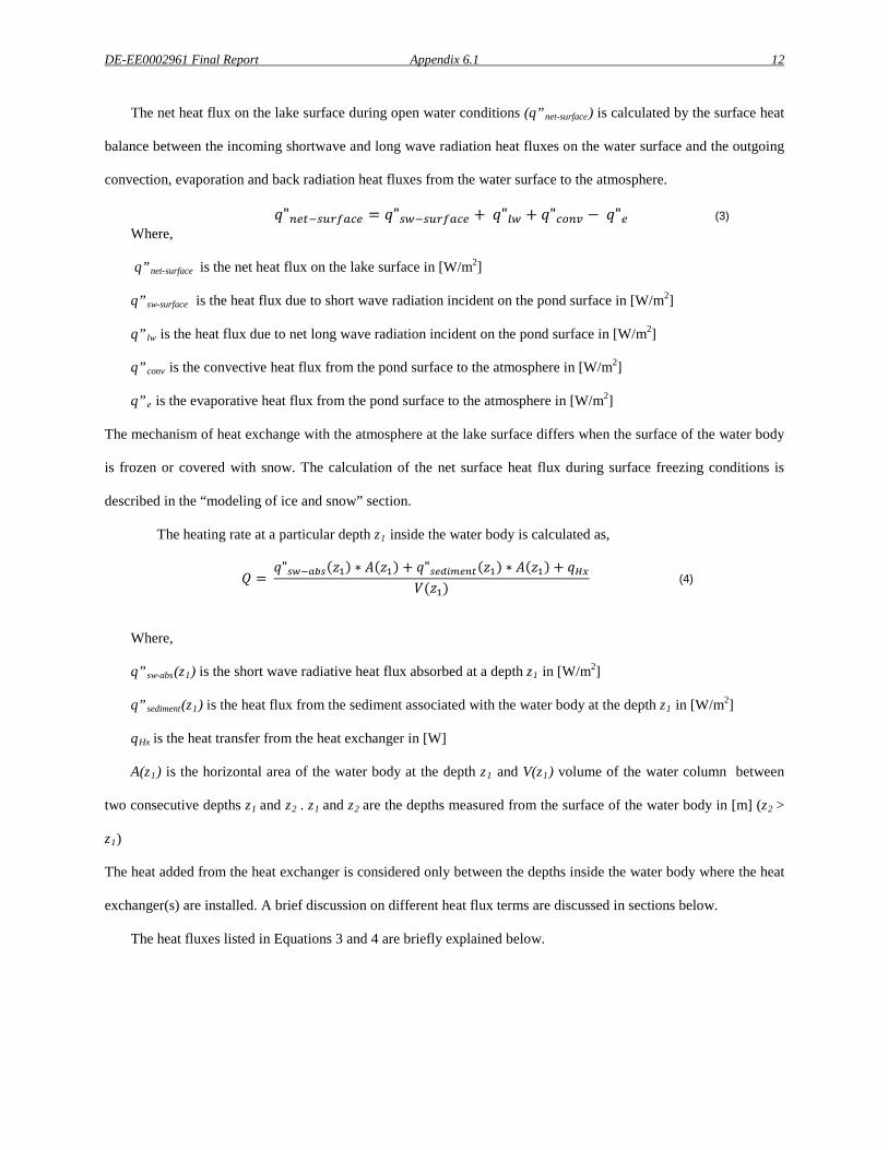
DE-EE0002961 Final Report Appendix 6.1 12
The net heat flux on the lake surface during open water conditions (q”net-surface) is calculated by the surface heat
balance between the incoming shortwave and long wave radiation heat fluxes on the water surface and the outgoing
convection, evaporation and back radiation heat fluxes from the water surface to the atmosphere.
𝑞"𝑛𝑒𝑡−𝑠𝑢𝑟𝑓𝑎𝑐𝑒 = 𝑞"𝑠𝑤−𝑠𝑢𝑟𝑓𝑎𝑐𝑒 + 𝑞"𝑙𝑤 + 𝑞"𝑐𝑜𝑛𝑣 − 𝑞"𝑒 (3) Where,
q”net-surface is the net heat flux on the lake surface in [W/m2]
q”sw-surface is the heat flux due to short wave radiation incident on the pond surface in [W/m2]
q”lw is the heat flux due to net long wave radiation incident on the pond surface in [W/m2]
q”conv is the convective heat flux from the pond surface to the atmosphere in [W/m2]
q”e is the evaporative heat flux from the pond surface to the atmosphere in [W/m2]
The mechanism of heat exchange with the atmosphere at the lake surface differs when the surface of the water body
is frozen or covered with snow. The calculation of the net surface heat flux during surface freezing conditions is
described in the “modeling of ice and snow” section.
The heating rate at a particular depth z1 inside the water body is calculated as,
𝑄 = 𝑞"𝑠𝑤−𝑎𝑏𝑠(𝑧1) ∗ 𝐴(𝑧1) + 𝑞"𝑠𝑒𝑑𝑖𝑚𝑒𝑛𝑡(𝑧1) ∗ 𝐴(𝑧1) + 𝑞𝐻𝑥
𝑉(𝑧1) (4)
Where,
q”sw-abs(z1) is the short wave radiative heat flux absorbed at a depth z1 in [W/m2]
q”sediment(z1) is the heat flux from the sediment associated with the water body at the depth z1 in [W/m2]
qHx is the heat transfer from the heat exchanger in [W]
A(z1) is the horizontal area of the water body at the depth z1 and V(z1) volume of the water column between
two consecutive depths z1 and z2 . z1 and z2 are the depths measured from the surface of the water body in [m] (z2 >
z1)
The heat added from the heat exchanger is considered only between the depths inside the water body where the heat
exchanger(s) are installed. A brief discussion on different heat flux terms are discussed in sections below.
The heat fluxes listed in Equations 3 and 4 are briefly explained below.
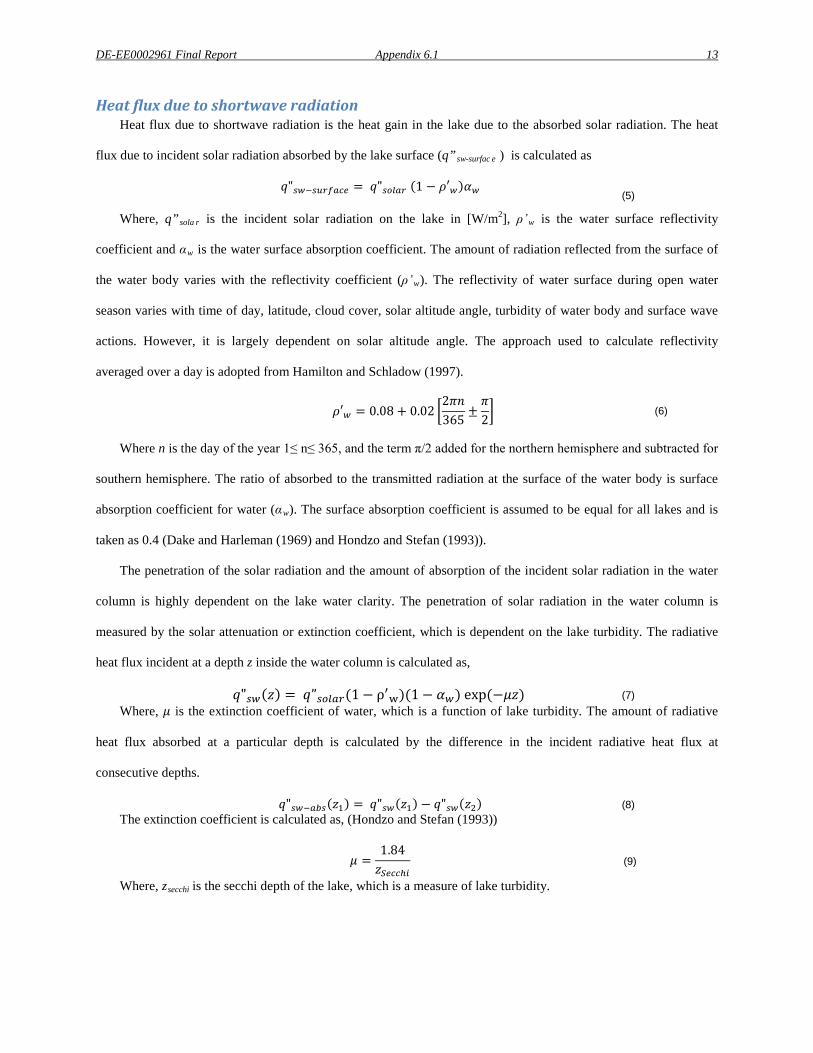
DE-EE0002961 Final Report Appendix 6.1 13
Heat flux due to shortwave radiation Heat flux due to shortwave radiation is the heat gain in the lake due to the absorbed solar radiation. The heat
flux due to incident solar radiation absorbed by the lake surface (q”sw-surfac e ) is calculated as
𝑞"𝑠𝑤−𝑠𝑢𝑟𝑓𝑎𝑐𝑒 = 𝑞"𝑠𝑜𝑙𝑎𝑟 (1 − 𝜌′𝑤)𝛼𝑤 (5)
Where, q”sola r is the incident solar radiation on the lake in [W/m2], ρ’w is the water surface reflectivity
coefficient and αw is the water surface absorption coefficient. The amount of radiation reflected from the surface of
the water body varies with the reflectivity coefficient (ρ’w). The reflectivity of water surface during open water
season varies with time of day, latitude, cloud cover, solar altitude angle, turbidity of water body and surface wave
actions. However, it is largely dependent on solar altitude angle. The approach used to calculate reflectivity
averaged over a day is adopted from Hamilton and Schladow (1997).
𝜌′𝑤 = 0.08 + 0.02 �2𝜋𝑛365
±𝜋2� (6)
Where n is the day of the year 1≤ n≤ 365, and the term π/2 added for the northern hemisphere and subtracted for
southern hemisphere. The ratio of absorbed to the transmitted radiation at the surface of the water body is surface
absorption coefficient for water (αw). The surface absorption coefficient is assumed to be equal for all lakes and is
taken as 0.4 (Dake and Harleman (1969) and Hondzo and Stefan (1993)).
The penetration of the solar radiation and the amount of absorption of the incident solar radiation in the water
column is highly dependent on the lake water clarity. The penetration of solar radiation in the water column is
measured by the solar attenuation or extinction coefficient, which is dependent on the lake turbidity. The radiative
heat flux incident at a depth z inside the water column is calculated as,
𝑞"𝑠𝑤(𝑧) = 𝑞”𝑠𝑜𝑙𝑎𝑟(1− ρ′w)(1− 𝛼𝑤) exp (−𝜇𝑧) (7) Where, 𝜇 is the extinction coefficient of water, which is a function of lake turbidity. The amount of radiative
heat flux absorbed at a particular depth is calculated by the difference in the incident radiative heat flux at
consecutive depths.
𝑞"𝑠𝑤−𝑎𝑏𝑠(𝑧1) = 𝑞"𝑠𝑤(𝑧1) − 𝑞"𝑠𝑤(𝑧2) (8) The extinction coefficient is calculated as, (Hondzo and Stefan (1993))
𝜇 =1.84𝑧𝑆𝑒𝑐𝑐ℎ𝑖
(9)
Where, zsecchi is the secchi depth of the lake, which is a measure of lake turbidity.
DE-EE0002961 Final Report Appendix 6.1 14
Heat flux due to long wave radiation The long wave radiation incident on the lake surface is assumed to be totally absorbed by the surface layer. The
approach to calculate the amount of net heat transfer on the lake surface due to long wave radiation using a
linearized radiation coefficient (hl w) is based on Chiasson et al. (2000). The net long wave radiative heat flux on the
lake surface (Q”l w) is calculated as
𝑞"𝑙𝑤 = ℎ𝑙𝑤(𝑇𝑠𝑘𝑦 − 𝑇𝑠𝑢𝑟𝑓𝑎𝑐𝑒) (10)
Where, hlw is the linearized radiation coefficient, Tsky is the sky temperature in absolute units, Tsurface is the lake
surface temperature in absolute units. Tsky is computed from the relationship given by Swinbank (1963).The
linearized radiation coefficient is calculated using Equation 11.
ℎ𝑙𝑤 = 4𝜀𝑤𝑎𝑡𝑒𝑟𝜎 �𝑇𝑠𝑢𝑟𝑓𝑎𝑐𝑒 + 𝑇𝑠𝑘𝑦
2�3
(11)
Where, εwater is the emissivity coefficient of water taken as 0.97 (Omstedt (1990)) and σ is the Stefan-
Boltzmann constant.
Heat flux due to convection and evaporation at the lake surface Convective heat flux or sensible heat flux on the lake surface accounts for heat transfer due to wind (forced
convection) and air-surface water temperature difference (free convection). Heat transfer due to evaporation is the
major mechanism, which contributes to lake cooling.
The convective heat flux can be computed by
𝑞”𝑐𝑜𝑛𝑣 = ℎ𝑐(𝑇𝑎𝑖𝑟 − 𝑇𝑠𝑢𝑟𝑓𝑎𝑐𝑒) (12)
Where, hc is the convective heat transfer coefficient in [W/m2. °C], Asurface is the surface area of the lake in [m2]
and Tair is the ambient air and Tsurface is the water body surface temperature in [°C].
Several empirical correlations exist to determine the convective heat transfer coefficient and hence to calculate
the convective and evaporative heat flux over the lake surface. Those correlations are based on the experimental
results from swimming pools, cooling ponds, small lakes and horizontal flat plates. The lake model contains seven
different correlations to calculate the surface convective and evaporative heat fluxes.
1. Molineaux et al. (1994)
Molineaux et al. (1994) obtained the correlation for convective heat transfer coefficient based on
experimental analysis from five outdoor swimming pools. The surface area of those swimming pools varies
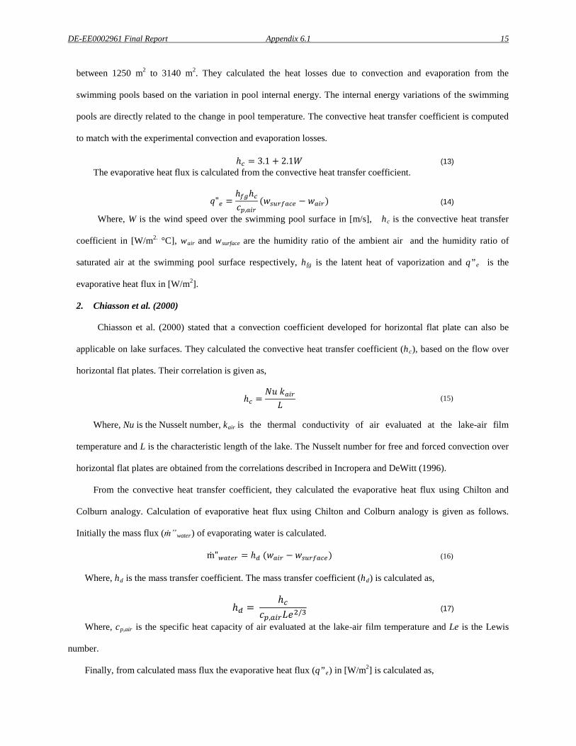
DE-EE0002961 Final Report Appendix 6.1 15
between 1250 m2 to 3140 m2. They calculated the heat losses due to convection and evaporation from the
swimming pools based on the variation in pool internal energy. The internal energy variations of the swimming
pools are directly related to the change in pool temperature. The convective heat transfer coefficient is computed
to match with the experimental convection and evaporation losses.
ℎ𝑐 = 3.1 + 2.1𝑊 (13) The evaporative heat flux is calculated from the convective heat transfer coefficient.
𝑞"𝑒 =ℎ𝑓𝑔ℎ𝑐𝑐𝑝,𝑎𝑖𝑟
(𝑤𝑠𝑢𝑟𝑓𝑎𝑐𝑒 − 𝑤𝑎𝑖𝑟) (14)
Where, W is the wind speed over the swimming pool surface in [m/s], hc is the convective heat transfer
coefficient in [W/m2. °C], wair and wsurface are the humidity ratio of the ambient air and the humidity ratio of
saturated air at the swimming pool surface respectively, hfg is the latent heat of vaporization and q”e is the
evaporative heat flux in [W/m2].
2. Chiasson et al. (2000)
Chiasson et al. (2000) stated that a convection coefficient developed for horizontal flat plate can also be
applicable on lake surfaces. They calculated the convective heat transfer coefficient (hc), based on the flow over
horizontal flat plates. Their correlation is given as,
ℎ𝑐 =𝑁𝑢 𝑘𝑎𝑖𝑟
𝐿 (15)
Where, Nu is the Nusselt number, kair is the thermal conductivity of air evaluated at the lake-air film
temperature and L is the characteristic length of the lake. The Nusselt number for free and forced convection over
horizontal flat plates are obtained from the correlations described in Incropera and DeWitt (1996).
From the convective heat transfer coefficient, they calculated the evaporative heat flux using Chilton and
Colburn analogy. Calculation of evaporative heat flux using Chilton and Colburn analogy is given as follows.
Initially the mass flux (ṁ”water) of evaporating water is calculated.
ṁ"𝑤𝑎𝑡𝑒𝑟 = ℎ𝑑 (𝑤𝑎𝑖𝑟 − 𝑤𝑠𝑢𝑟𝑓𝑎𝑐𝑒) (16)
Where, hd is the mass transfer coefficient. The mass transfer coefficient (hd) is calculated as,
ℎ𝑑 = ℎ𝑐
𝑐𝑝,𝑎𝑖𝑟𝐿𝑒2/3 (17)
Where, cp,air is the specific heat capacity of air evaluated at the lake-air film temperature and Le is the Lewis
number.
Finally, from calculated mass flux the evaporative heat flux (q”e) in [W/m2] is calculated as,
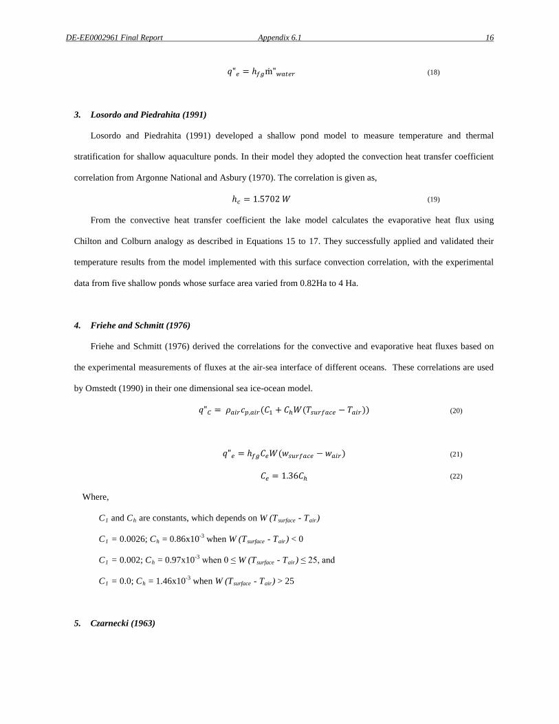
DE-EE0002961 Final Report Appendix 6.1 16
𝑞"𝑒 = ℎ𝑓𝑔ṁ"𝑤𝑎𝑡𝑒𝑟 (18)
3. Losordo and Piedrahita (1991)
Losordo and Piedrahita (1991) developed a shallow pond model to measure temperature and thermal
stratification for shallow aquaculture ponds. In their model they adopted the convection heat transfer coefficient
correlation from Argonne National and Asbury (1970). The correlation is given as,
ℎ𝑐 = 1.5702 𝑊 (19)
From the convective heat transfer coefficient the lake model calculates the evaporative heat flux using
Chilton and Colburn analogy as described in Equations 15 to 17. They successfully applied and validated their
temperature results from the model implemented with this surface convection correlation, with the experimental
data from five shallow ponds whose surface area varied from 0.82Ha to 4 Ha.
4. Friehe and Schmitt (1976)
Friehe and Schmitt (1976) derived the correlations for the convective and evaporative heat fluxes based on
the experimental measurements of fluxes at the air-sea interface of different oceans. These correlations are used
by Omstedt (1990) in their one dimensional sea ice-ocean model.
𝑞"𝐶 = 𝜌𝑎𝑖𝑟𝑐𝑝,𝑎𝑖𝑟(𝐶1 + 𝐶ℎ𝑊(𝑇𝑠𝑢𝑟𝑓𝑎𝑐𝑒 − 𝑇𝑎𝑖𝑟)) (20)
𝑞"𝑒 = ℎ𝑓𝑔𝐶𝑒𝑊(𝑤𝑠𝑢𝑟𝑓𝑎𝑐𝑒 − 𝑤𝑎𝑖𝑟) (21)
𝐶𝑒 = 1.36𝐶ℎ (22)
Where,
C1 and Ch are constants, which depends on W (Tsurface - Tair)
C1 = 0.0026; Ch = 0.86x10⁻³ when W (Tsurface - Tair) < 0
C1 = 0.002; Ch = 0.97x10⁻³ when 0 ≤ W (Tsurface - Tair) ≤ 25, and
C1 = 0.0; Ch = 1.46x10⁻³ when W (Tsurface - Tair) > 25
5. Czarnecki (1963)
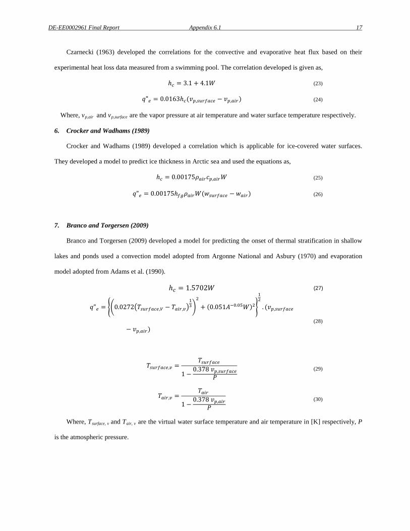
DE-EE0002961 Final Report Appendix 6.1 17
Czarnecki (1963) developed the correlations for the convective and evaporative heat flux based on their
experimental heat loss data measured from a swimming pool. The correlation developed is given as,
ℎ𝑐 = 3.1 + 4.1𝑊 (23)
𝑞"𝑒 = 0.0163ℎ𝑐(𝑣𝑝,𝑠𝑢𝑟𝑓𝑎𝑐𝑒 − 𝑣𝑝,𝑎𝑖𝑟) (24)
Where, vp,air and vp,surface are the vapor pressure at air temperature and water surface temperature respectively.
6. Crocker and Wadhams (1989)
Crocker and Wadhams (1989) developed a correlation which is applicable for ice-covered water surfaces.
They developed a model to predict ice thickness in Arctic sea and used the equations as,
ℎ𝑐 = 0.00175𝜌𝑎𝑖𝑟𝑐𝑝,𝑎𝑖𝑟𝑊 (25)
𝑞"𝑒 = 0.00175ℎ𝑓𝑔𝜌𝑎𝑖𝑟𝑊(𝑤𝑠𝑢𝑟𝑓𝑎𝑐𝑒 − 𝑤𝑎𝑖𝑟) (26)
7. Branco and Torgersen (2009)
Branco and Torgersen (2009) developed a model for predicting the onset of thermal stratification in shallow
lakes and ponds used a convection model adopted from Argonne National and Asbury (1970) and evaporation
model adopted from Adams et al. (1990).
ℎ𝑐 = 1.5702𝑊 (27)
𝑞"𝑒 = ��0.0272�𝑇𝑠𝑢𝑟𝑓𝑎𝑐𝑒,𝑉 − 𝑇𝑎𝑖𝑟,𝑣�13�
2
+ (0.051𝐴−0.05𝑊)2�
12
. (𝑣𝑝,𝑠𝑢𝑟𝑓𝑎𝑐𝑒
− 𝑣𝑝,𝑎𝑖𝑟)
(28)
𝑇𝑠𝑢𝑟𝑓𝑎𝑐𝑒,𝑣 =𝑇𝑠𝑢𝑟𝑓𝑎𝑐𝑒
1 −0.378 𝑣𝑝,𝑠𝑢𝑟𝑓𝑎𝑐𝑒
𝑃
(29)
𝑇𝑎𝑖𝑟,𝑣 =𝑇𝑎𝑖𝑟
1 −0.378 𝑣𝑝,𝑎𝑖𝑟
𝑃
(30)
Where, Tsurface, v and Tair, v are the virtual water surface temperature and air temperature in [K] respectively, P
is the atmospheric pressure.
DE-EE0002961 Final Report Appendix 6.1 18
Sediment heat flux Heat transfer from the sediment is the significant source of heat gain to the lake during ice cover period (Gu and
Stefan (1990)). Lake simulation model incorporates the theory of sediment heat transfer from Fang and Stefan
(1996) and calculation based on the implicit numerical method given by Saloranta and Andersen (2004). A one-
dimensional, unsteady heat conduction equation to calculate the sediment temperatures is given in Equation 29. The
sediment and the water column are discretized into a number of layers and the partial differential equation is solved
by implicit finite difference method using Tri-diagonal matrix algorithm (TDMA). The procedure for solving the
one-dimensional sediment heat conduction equation is similar to the solution methodology of the one-dimensional
temperature transport equation discussed in “Formulation of TDMA coefficients” section.
𝜕𝑇𝑠𝑒𝑑𝜕𝑡
= 𝛼𝑠𝑒𝑑𝜕2𝑇𝑠𝑒𝑑𝜕𝑧2
(31)
Where, Tsed is the sediment temperature and αsed is the thermal diffusivity of the sediments. The temperature of
the sediment layer in contact with the water layer (topmost sediment layer) is assumed to be in the same temperature
as the water layer. The heat flux between the water and the sediment interface (ws) is determined from the
temperature gradient between the water-sediment layers �𝜕𝑇𝑠𝑒𝑑𝜕𝑧𝑠𝑒𝑑
�𝑤𝑠
and the interface area,
𝑞"𝑠𝑒𝑑𝑖𝑚𝑒𝑛𝑡(𝑧1) = −𝑘𝑠𝑒𝑑 �𝜕𝑇𝑠𝑒𝑑𝜕𝑧𝑠𝑒𝑑
�𝑤𝑠�𝐴𝑠𝑒𝑑(𝑧1)𝐴(𝑧1)
� (32)
Where, ksed is the thermal conductivity of the sediments = 1.01 W/m.K (Fang and Stefan (1996)), A(z1) is the
horizontal area of the surface water body at depth z1, Ased(z1) is the water-sediment interface area. The water-
sediment interface area at a particular depth is approximately calculated from the difference in the horizontal area of
the surface water body at consecutive depths.
Heat flux due to the heat exchanger The amount of heat transferred to the surface water body from the heat exchanger depends on the thermal load
supplied to the surface water heat exchangers, type of the heat exchanger, temperature of the surface water body at
the depth where the heat exchanger is placed and the mass flow rate of the heat exchanger fluid. The heat exchanger
fluid is usually water or an antifreeze mixture. The calculation of heat transfer due to the heat exchanger is explained
in detail in “Heat exchanger model” section.
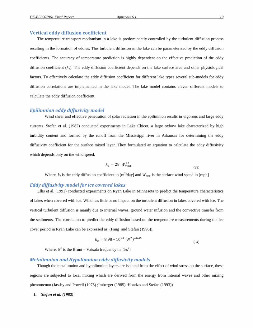
DE-EE0002961 Final Report Appendix 6.1 19
Vertical eddy diffusion coefficient The temperature transport mechanism in a lake is predominantly controlled by the turbulent diffusion process
resulting in the formation of eddies. This turbulent diffusion in the lake can be parameterized by the eddy diffusion
coefficients. The accuracy of temperature prediction is highly dependent on the effective prediction of the eddy
diffusion coefficient (kz). The eddy diffusion coefficient depends on the lake surface area and other physiological
factors. To effectively calculate the eddy diffusion coefficient for different lake types several sub-models for eddy
diffusion correlations are implemented in the lake model. The lake model contains eleven different models to
calculate the eddy diffusion coefficient.
Epilimnion eddy diffusivity model Wind shear and effective penetration of solar radiation in the epilimnion results in vigorous and large eddy
currents. Stefan et al. (1982) conducted experiments in Lake Chicot, a large oxbow lake characterized by high
turbidity content and formed by the runoff from the Mississippi river in Arkansas for determining the eddy
diffusivity coefficient for the surface mixed layer. They formulated an equation to calculate the eddy diffusivity
which depends only on the wind speed.
𝑘𝑧 = 28 𝑊𝑚𝑝ℎ1.3
(33)
Where, kz is the eddy diffusion coefficient in [m2/day] and Wmph is the surface wind speed in [mph]
Eddy diffusivity model for ice covered lakes Ellis et al. (1991) conducted experiments on Ryan Lake in Minnesota to predict the temperature characteristics
of lakes when covered with ice. Wind has little or no impact on the turbulent diffusion in lakes covered with ice. The
vertical turbulent diffusion is mainly due to internal waves, ground water infusion and the convective transfer from
the sediments. The correlation to predict the eddy diffusion based on the temperature measurements during the ice
cover period in Ryan Lake can be expressed as, (Fang and Stefan (1996)).
𝑘𝑧 = 8.98 ∗ 10−4 (𝑁2)−0.43 (34)
Where, N2 is the Brunt – Vaisala frequency in [1/s2]
Metalimnion and Hypolimnion eddy diffusivity models Though the metalimnion and hypolimnion layers are isolated from the effect of wind stress on the surface, these
regions are subjected to local mixing which are derived from the energy from internal waves and other mixing
phenomenon (Jassby and Powell (1975) ;Imberger (1985) ;Hondzo and Stefan (1993))
1. Stefan et al. (1982)
DE-EE0002961 Final Report Appendix 6.1 20
Stefan et al. (1982) also formulated the eddy diffusivity coefficient for the layers below the mixed layer
(thermocline and the hypolimnion) as,
𝑘𝑧 = 0.1 ∗ (𝑊)1.3 (35)
2. Hondzo and Stefan (1993)
Hondzo and Stefan (1993) formulated a correlation to predict the eddy diffusivity coefficients based on their
temperature results from four different lakes in northern Minnesota whose areas range from 15 acres to 1830 acres.
They expressed their correlation based on the surface area of the lake and the Brunt- Vaisala frequency.
𝑘𝑧 = 8.17 ∗ 10−4 𝐴𝑠𝑢𝑟𝑓𝑎𝑐𝑒,𝑘𝑚0.56 (𝑁2)−0.43 ∗ 8.64 (36)
Where, Where, N is the stability frequency or Brunt-Vaisala frequency in [1/s] is a measure of stability of an
oscillating water particle, which oscillates due to the presence of temperature-density gradient and buoyancy fluxes
inside the water column and Asurface, k m is surface area of the lake in [Km2]. The Brunt-Vaisala frequency can be
calculated by the following equation.
𝑁2 =𝑔𝜌𝑑𝜌𝑑𝑧
(37)
Where, g is the acceleration due to gravity, ρ is the density of water and z is the depth of the water column.
3. Gu and Stefan (1995)
The eddy diffusion coefficient determined by Gu and Stefan (1995) for shallow wastewater ponds is
𝑘𝑧 = min [𝑘𝑧𝑚𝑎𝑥 , 𝑘𝑧𝑚𝑎𝑥𝐶𝑁−1] (38)
Where, kzmax is the maximum hypolimnion eddy diffusion coefficient, N is the stability or the Brunt Vaisala
frequency, C is a constant taken as 8.66*10-3 (s-1)(Jassby and Powell (1975)).
The maximum hypolimnion eddy diffusion coefficient (kzmax) represents the maximum diffusion that can
occur in a lake as a result of turbulent action. The maximum eddy diffusion coefficient can be observed in a lake
during weakly stratified conditions as a result of extensive turbulent mixing of water layers due to strong wind
action. kzmax is dependent on the physical and physiological characteristics of the lake. Hondzo and Stefan (1993)
derived the relationship between kzmax and the surface area of the lake as,
𝑘𝑧𝑚𝑎𝑥 = 0.048�𝐴𝑠𝑢𝑟𝑓𝑎𝑐𝑒,𝑘𝑚�0.56 (39)
DE-EE0002961 Final Report Appendix 6.1 21
The expression for kzmax holds good for large ponds and lakes. In case of shallow ponds, which tend to stratify
and de-stratify many times in a day, there does not appear to be a standard procedure to estimate the value of
kzmax. Gu and Stefan (1995) estimated the kzmax value of 0.1m2/day for their 1.8 acre rectangular waste water pond
in Minnesota which has a maximum depth of 1.8 m subjected to inflows to match the experimental temperature
profiles.
McCormick and Scavia (1981) and Henderson-Sellers (1985) expressed the vertical eddy diffusivity
coefficient as a non- linear function of wind strength with depth and stratification stability.
4. McCormick and Scavia (1981)
McCormick and Scavia (1981) obtained a correlation of eddy diffusivity coefficient by the statistical analysis of
temperature observations in Lake Ontario (surface area 4685118 acres) and Lake Washington (surface area 21745
acres), the behavior of eddy diffusivity coefficients in the hypolimnion is predicted. The model can be given as,
𝐾𝑧 =𝑢∗
1𝑐 + �𝜎𝑐�𝑅𝑖
(40)
Where, u* is the surface wind friction velocity caused by the wind stress on the lake surface, σ and c – are
constants proportional to the lake size and structure.
5. Henderson-Sellers (1988)
Henderson-Sellers (1985) formulated a theoretical eddy diffusion model which also depends on the latitude of
the location of the lake. Henderson-Sellers (1988) expressed the vertical eddy diffusivity coefficient as a non- linear
function of wind speed and depth. The author took into consideration the effect of the Earth’s Coriolis force on the
lake by considering the latitude of the position of the lake. This Coriolis force can only be effective for water bodies
with huge surface area.
𝑘𝑧 =𝑉𝑘 𝑢∗ 𝑧𝑃0
𝑒𝑥𝑝(−𝑘∗ 𝑧) 𝑓(𝑅𝑖) (41)
Where, k* is a non-linear function of wind speed and Vk is the Von Karmon constant = 0.4,
𝑘∗ = 6.6 𝑠𝑖𝑛𝜃12 𝑊−1.84 (42)
Where, W is the wind speed and θ is the latitude of the location of the lake [Radians]
6. Banks.R.B (1975)
DE-EE0002961 Final Report Appendix 6.1 22
Banks (1975) obtained an eddy diffusivity correlation which is directly proportional to the wind velocity. The
correlation calculates the eddy diffusivity based on the amount of wind shear experienced on the lake at every depth.
Banks (1975) correlation can be expressed as,
𝑘𝑧 = 14𝛽� 𝜌𝑎𝑖𝑟𝜌𝑤𝑎𝑡𝑒𝑟
� 𝐶𝑓1/2𝑧 𝑊 * 86400
(43)
Where, β is a constant = 0.55, Cf is the wind shear stress coefficient, ρair and ρwater are the densities of air and
water in [Kg/m3] respectively.
7. Rohden et al. (2007)
Rohden et al. (2007) analyzed the vertical diffusion in small lake with surface area of 49 acres. The lake is
characterized by strong stratification. They suggested a relation between eddy diffusion coefficients with the
molecular diffusion of heat. The equation formulated is given as,
𝐾𝑧 =𝑐𝑅𝑖
+ 𝐾𝑏 (44)
Where, c is the molecular diffusion coefficient = 6*10-6 [m2/s], and Kb is the molecular diffusivity of heat in
[m2/day]
8. Sengupta et al. (1981)
Sengupta et al. (1981) considered the effects of area, wind generated turbulence, heat transfer by radiation,
and the effect of thermal discharges due to inflow in the hypolimnion layer in their correlation. The effect of this
correlation was tested on Lake Keowee a large reservoir with surface area of 18,372 acres. The correlation is
given by,
𝑘𝑧 = 𝑘𝑧𝑚𝑎𝑥(1 + 𝜎𝑅𝑖)−1 (45)
Where, σ is a semi empirical constant = 0.1 obtained from the study in Lake Keowee.
9. Imberger et al. (1978)
Imberger et al. (1978) made a field study on Wellington reservoir a medium sized reservoir with an area of
2470 acres and has a maximum depth of 30 m. Imberger et al. (1978) considered both the effects of wind stresses
and the energy from the river to formulate the eddy diffusion coefficients.
𝑘𝑧 =0.048 𝑧2
𝑡𝑚 𝑠 (46)
DE-EE0002961 Final Report Appendix 6.1 23
Where, z is the depth of the lake, tm is the time taken for mixing in the hypolimnion layer [s] and s is the
stability of the hypolimnion layer [-]
𝑡𝑚 =𝑃𝐸
𝐾𝐸𝑖𝑛𝑓𝑙𝑜𝑤 + 𝐾𝐸𝑤𝑖𝑛𝑑 (47)
Where, PE is the potential energy of the particular layer, KEinflow is the kinetic energy from the inflowing
streams and KEwind is the effect of wind energy on the reservoir.
The stability of the particular layer is given by the equation
𝑠 =𝑑𝜌𝑑𝑧
�𝑧
𝜌(0) − 𝜌(𝑧)� (48)
This model was validated with the experimental data from the Wellington reservoir and good temperature
results were obtained which is largely due to the consideration of the kinetic energy from the river inflow.
10. Tucker and Green (1977)
Kullenberg (1971) based on their experimental results from Lake Kattegat proposed the eddy diffusion
coefficient in the form,
𝑘𝑧 = 𝑐𝑤2𝑁−2 �𝜕𝑢𝜕𝑧� (49)
Where, c is a constant = 0.1, �𝜕𝑢𝜕𝑧� = vertical shear caused by the horizontal wind action.
Tucker and Green (1977) approximated the value for vertical shear which is a function of Richardson number. It
is given by the following equation,
�𝜕𝑢𝜕𝑧� =
𝑢∗
𝑘𝑧(1 + 10𝑅𝑖)1/2 (50)
Equation 49 is substituted in Kullenberg (1971) correlation to get the eddy diffusion coefficient.
Formulation of TDMA coefficients The discretization of the lake into set of one-dimensional layers results in a set of linear equations, one for each
layer. Since the concentration of a variable in a layer is dependent on its concentration in the adjacent layers, the set
of equations are arranged in a tri-diagonal matrix form and solved simultaneously. Integrating the one dimensional
advection diffusion equation (Equation 1) between zi and zi+1, where i is the layer number, gives
� 𝐴𝜕𝑇𝜕𝑡
𝑧𝑖+1
𝑧𝑖𝑑𝑧 = �
𝜕𝜕𝑧�𝑘𝑧𝐴
𝜕𝑇𝜕𝑡�
𝑧𝑖+1
𝑧𝑖𝑑𝑧 + � 𝐴
𝑄𝜌𝑤𝐶𝑝
𝑧𝑖+1
𝑧𝑖𝑑𝑧 (51)
DE-EE0002961 Final Report Appendix 6.1 24
𝑉𝑖𝑑𝑇𝑖∗
𝑑𝑡= �𝑘𝑧𝐴
𝜕𝑇𝜕𝑡�𝑧𝑖+1
− �𝑘𝑧𝐴𝜕𝑇𝜕𝑡�𝑧𝑖
+ 𝑉𝑖𝑄𝑖∗
𝜌𝑤𝐶𝑝
(52)
Where, Vi is the volume of the layer i, 𝑇𝑖∗ = 𝑉𝑖−1 ∫ 𝐴𝑇𝑑𝑧 is the volume averaged temperature for the layer i,
and 𝑄𝑖∗ = 𝑉𝑖−1 ∫ 𝐴𝑄𝑑𝑧 is the layer averaged heating rate. Since, the lake model operates on a daily time step the time
increment Δt is taken to be 24 hours.
𝑉𝑖∆𝑡
[𝑇𝑖∗(𝑡) − 𝑇𝑖∗(𝑡 − ∆𝑡)]
= 𝑘𝑧(𝑖+1)𝐴𝑖+11∆𝑧
[𝑇𝑖+1∗ (𝑡) − 𝑇𝑖∗(𝑡)]
− 𝑘𝑧(𝑖)𝐴𝑖1∆𝑧
[𝑇𝑖∗(𝑡) − 𝑇𝑖−1∗ (𝑡)] + 𝑉𝑖𝑄𝑖∗
𝜌𝑤𝐶𝑝
(53)
Simplifying the equation by dividing with Vi/Δt and introducing the notations
𝛼𝑖 =∆𝑡∆𝑧
𝐴𝑖𝑉𝑖𝑘𝑧(𝑖)
𝛽𝑖 =∆𝑡∆𝑧
𝐴𝑖+1𝑉𝑖
𝑘𝑧(𝑖+1)
𝛾𝑖 = 1 + 𝛼𝑖+𝛽𝑖
Equation 52 can be rearranged to get a generalized TDMA equation for a layer i.
−𝛼𝑖𝑇𝑖∗(𝑡) + 𝛾𝑖𝑇𝑖∗(𝑡) − 𝛽𝑖𝑇𝑖+1∗ (𝑡) = 𝑇𝑖∗(𝑡 − ∆𝑡) +𝑄𝑖∗
𝜌𝑤𝐶𝑝∆𝑡
(54)
Assuming zero diffusion between the air-water interface and zero bottom area of the lowermost layer we get
α1=βn=0. Therefore for the surface layer the TDMA equation transforms into
(1 + 𝛽1)𝑇1∗(𝑡) − 𝛽𝑖𝑇2∗(𝑡) = 𝑇1∗(𝑡 − ∆𝑡) +𝑄𝑠𝑢𝑟𝑓𝑎𝑐𝑒∗
𝜌𝑤𝐶𝑝∆𝑡
(55)
Where, Q*surface is the heat added at the surface layer from the surface heat flux terms. The lake model uses the
temperature of the previous time step and the local heating of the layers of the current time step to calculate the
current time step temperature values.
Since, many of the terms in the heat flux equations require the water temperature term for the current time step
to be known, an iterative method is employed to calculate the water layer temperatures. At the start of every time
step the lake model assumes the previous day temperature profile and surface ice thickness value (if ice is predicted
on the lake surface) to calculate the current day heat flux terms. From the heat flux terms, the current day
DE-EE0002961 Final Report Appendix 6.1 25 temperature profiles and surface ice thickness are calculated. Once again, the heat flux terms for the current time
step are computed from the calculated temperature profiles and ice thickness values. This procedure is repeated until
both the temperature and ice thickness values of the current time step converges. Separate convergence criteria are
set up for water layer temperature and surface ice thickness terms.
Formulation of convective mixing and wind induced mixing Once the water temperatures are calculated, the lake model checks for the presence of unstable density layers
(i.e.) the presence of higher density water layer(s) above the lower density layers. If such a case occurs, the groups
of water layer(s) with unstable density profiles are completely mixed with the first stable layer below the unstable
layers. The complete mixing is achieved by calculating the volume weighted average temperature for the unstable
water column. This procedure is repeated until the temperatures in the water column becomes neutral or stable.
Wind induced stress on the lake surface is mainly responsible for the complete mixing of surface layers
resulting in the formation of epilimnion region. The lake model calculates this epilimnion layer thickness by
performing an energy balance between the available total kinetic energy from the wind with the potential energy of
each layer. The total kinetic energy of the wind (TKE) is calculated as,
𝑇𝐾𝐸 = 𝑊𝑠𝑡𝑟𝐴𝑠𝑢𝑟𝑓𝑎𝑐𝑒�𝜏3
𝜌𝑤 ∆𝑡 (56)
Where, τ is the wind stress and Wstr is the wind sheltering coefficient.
𝜏 = 𝜌𝑎𝑖𝑟 ∗ 𝑐𝑑 ∗ 𝑊2 (57)
𝑊𝑠𝑡𝑟 = 1.0 − exp (−0.3𝐴𝑠𝑢𝑟𝑓𝑎𝑐𝑒) (58)
Where, Cd is the drag coefficient which is dependent of the surface wind speed. During the period of ice cover
on the surface of the lake, the effect of wind on the lake surface is neglected and hence, the total kinetic energy
(TKE) is taken as zero. The algorithm to calculate the epilimnion layer thickness is based on Ford and Stefan (1980)
and Saloranta and Andersen (2004). The surface layer is always assumed to be well mixed it is considered to the
first epilimnion layer. The potential energy (PE) required for lifting the immediate water layer below the epilimnion
to the center of the epilimnion layer is calculated.
𝑃𝐸 = 𝑔∆𝜌𝑤𝑉𝑒𝑝𝑖𝑉𝑧𝑉𝑒𝑝𝑖 + 𝑉𝑧
(𝑧𝑒𝑝𝑖 + ∆𝑧𝑀−𝑧 − 𝑧𝑀−𝑒𝑝𝑖) (59)
DE-EE0002961 Final Report Appendix 6.1 26
Where, g is the acceleration due to gravity, Δρw is the density difference between the layer and the epilimnion
layer, zepi is the thickness of the epilimnion layer, ΔzM-z is the distance from the layer’s center of mass to the bottom
of the epilimnion layer, and zM-epi is the depth where the center of mass of the epilimnion layer is present. Vepi is the
volume of the epilimnion layer and is calculated by adding the volume of the current layer (Vz) with the total
volume of the above mixed layers. The TKE available is compared with the PE of the layer. If TKE ≥ PE of the
water layer, it is completely mixed with the above epilimnion layers and the next water layer is checked thus
increasing the epilimnion depth. The total PE to lift the water layer is subtracted from the available TKE. Now the
PE of the next layer is compared with the resultant TKE, and the procedure is repeated until the net resultant TKE is
less than the PE required for new layer to mix with the epilimnion.
Modeling of turnover During spring/autumn seasons, a lake undergoes a large-scale inversion of water mass from the surface until the
lake bottom, which destroys the existing stratification. This phenomenon is called as turnover and the number
occurrence of lake turnover in a year varies for different lakes. The lake model follows the algorithm given by
Saloranta and Andersen (2004) to handle the turnover conditions. Turnover algorithm is initiated whenever the
surface temperature crosses the temperature of maximum density (Tmaxrho = 3.98 °C). The water layers including the
surface layer that has crossed Tmaxrho, are set to Tmaxrho. The energy gained by this temperature difference (i.e. the
energy difference relative to Tmaxrho ) is exponentially distributed to cool/warm the water column to Tmaxrho. The
surface temperature is maintained at Tmaxrho until the entire water column has been cooled/warmed to Tmaxrho. If the
entire water column is cooled/warmed to Tmaxrho the remaining energy is used to cool/warm the surface layers.
Modeling of ice and snow cover There are three processes involved in modeling of ice cover on the lake surface.
a. Ice formation on the lake surface during the start of the freeze-up period.
b. Congelation of ice due to continuous freezing
c. Melting of ice during warm-up period
Ice formation in the lake model is triggered when the calculated water temperatures are below the freezing
point. The sub-cooled water layers are set to water freezing point temperature (Tfreez e) and the resultant heat deficit
in water is converted to latent heat of ice.
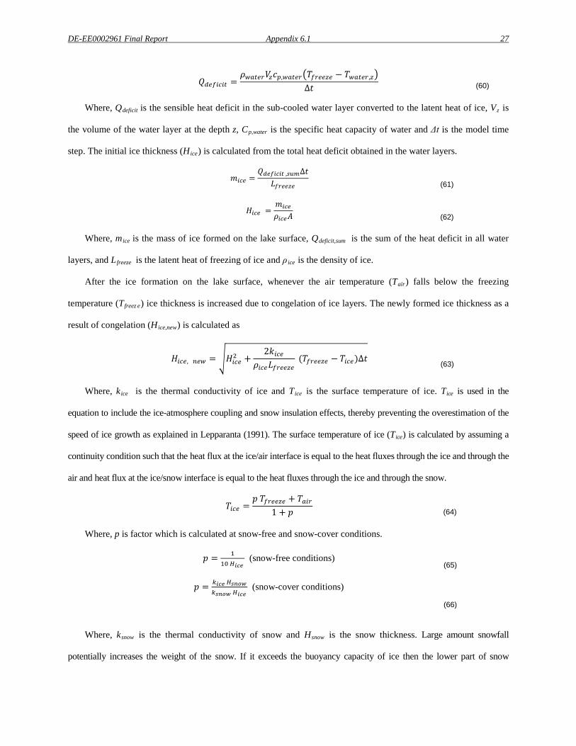
DE-EE0002961 Final Report Appendix 6.1 27
𝑄𝑑𝑒𝑓𝑖𝑐𝑖𝑡 =𝜌𝑤𝑎𝑡𝑒𝑟𝑉𝑧𝑐𝑝,𝑤𝑎𝑡𝑒𝑟�𝑇𝑓𝑟𝑒𝑒𝑧𝑒 − 𝑇𝑤𝑎𝑡𝑒𝑟,𝑧�
∆𝑡 (60)
Where, Qdeficit is the sensible heat deficit in the sub-cooled water layer converted to the latent heat of ice, Vz is
the volume of the water layer at the depth z, Cp,water is the specific heat capacity of water and Δt is the model time
step. The initial ice thickness (Hice) is calculated from the total heat deficit obtained in the water layers.
𝑚𝑖𝑐𝑒 =𝑄𝑑𝑒𝑓𝑖𝑐𝑖𝑡 ,𝑠𝑢𝑚∆𝑡
𝐿𝑓𝑟𝑒𝑒𝑧𝑒
(61)
𝐻𝑖𝑐𝑒 =𝑚𝑖𝑐𝑒
𝜌𝑖𝑐𝑒𝐴
(62)
Where, mice is the mass of ice formed on the lake surface, Qdeficit,sum is the sum of the heat deficit in all water
layers, and Lfreeze is the latent heat of freezing of ice and ρ ice is the density of ice.
After the ice formation on the lake surface, whenever the air temperature (Tair) falls below the freezing
temperature (Tfreez e) ice thickness is increased due to congelation of ice layers. The newly formed ice thickness as a
result of congelation (Hice,new) is calculated as
𝐻𝑖𝑐𝑒, 𝑛𝑒𝑤 = �𝐻𝑖𝑐𝑒2 +2𝑘𝑖𝑐𝑒
𝜌𝑖𝑐𝑒𝐿𝑓𝑟𝑒𝑒𝑧𝑒 (𝑇𝑓𝑟𝑒𝑒𝑧𝑒 − 𝑇𝑖𝑐𝑒)∆𝑡
(63)
Where, kice is the thermal conductivity of ice and Tice is the surface temperature of ice. Tice is used in the
equation to include the ice-atmosphere coupling and snow insulation effects, thereby preventing the overestimation of the
speed of ice growth as explained in Lepparanta (1991). The surface temperature of ice (Tice) is calculated by assuming a
continuity condition such that the heat flux at the ice/air interface is equal to the heat fluxes through the ice and through the
air and heat flux at the ice/snow interface is equal to the heat fluxes through the ice and through the snow.
𝑇𝑖𝑐𝑒 =𝑝 𝑇𝑓𝑟𝑒𝑒𝑧𝑒 + 𝑇𝑎𝑖𝑟
1 + 𝑝
(64)
Where, p is factor which is calculated at snow-free and snow-cover conditions.
𝑝 = 110 𝐻𝑖𝑐𝑒
(snow-free conditions) (65)
𝑝 = 𝑘𝑖𝑐𝑒 𝐻𝑠𝑛𝑜𝑤
𝑘𝑠𝑛𝑜𝑤 𝐻𝑖𝑐𝑒 (snow-cover conditions)
(66)
Where, ksnow is the thermal conductivity of snow and Hsnow is the snow thickness. Large amount snowfall
potentially increases the weight of the snow. If it exceeds the buoyancy capacity of ice then the lower part of snow
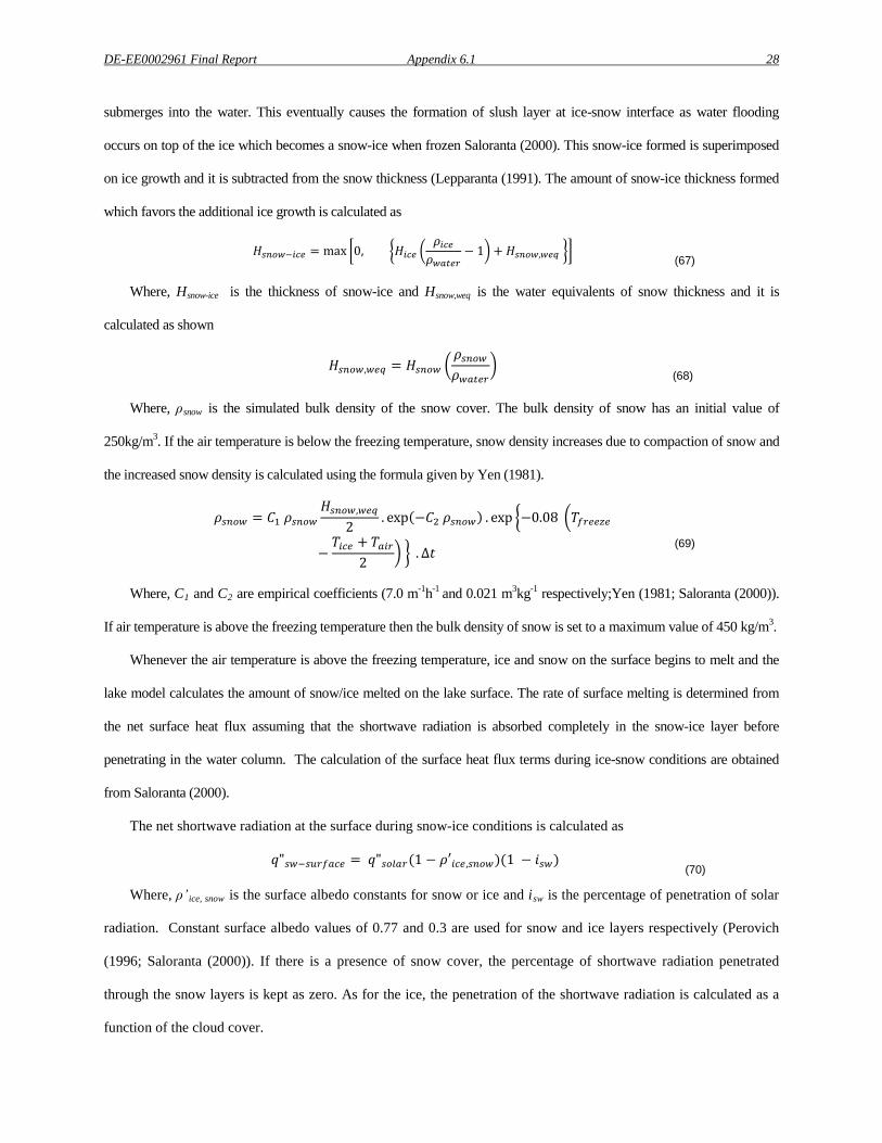
DE-EE0002961 Final Report Appendix 6.1 28 submerges into the water. This eventually causes the formation of slush layer at ice-snow interface as water flooding
occurs on top of the ice which becomes a snow-ice when frozen Saloranta (2000). This snow-ice formed is superimposed
on ice growth and it is subtracted from the snow thickness (Lepparanta (1991). The amount of snow-ice thickness formed
which favors the additional ice growth is calculated as
𝐻𝑠𝑛𝑜𝑤−𝑖𝑐𝑒 = max �0, �𝐻𝑖𝑐𝑒 �𝜌𝑖𝑐𝑒𝜌𝑤𝑎𝑡𝑒𝑟
− 1� + 𝐻𝑠𝑛𝑜𝑤,𝑤𝑒𝑞 �� (67)
Where, Hsnow-ice is the thickness of snow-ice and Hsnow,weq is the water equivalents of snow thickness and it is
calculated as shown
𝐻𝑠𝑛𝑜𝑤,𝑤𝑒𝑞 = 𝐻𝑠𝑛𝑜𝑤 �𝜌𝑠𝑛𝑜𝑤𝜌𝑤𝑎𝑡𝑒𝑟
� (68)
Where, ρsnow is the simulated bulk density of the snow cover. The bulk density of snow has an initial value of
250kg/m3. If the air temperature is below the freezing temperature, snow density increases due to compaction of snow and
the increased snow density is calculated using the formula given by Yen (1981).
𝜌𝑠𝑛𝑜𝑤 = 𝐶1 𝜌𝑠𝑛𝑜𝑤
𝐻𝑠𝑛𝑜𝑤,𝑤𝑒𝑞
2. exp(−𝐶2 𝜌𝑠𝑛𝑜𝑤) . exp �−0.08 �𝑇𝑓𝑟𝑒𝑒𝑧𝑒
−𝑇𝑖𝑐𝑒 + 𝑇𝑎𝑖𝑟
2� � .∆𝑡
(69)
Where, C1 and C2 are empirical coefficients (7.0 m-1h-1 and 0.021 m3kg-1 respectively;Yen (1981; Saloranta (2000)).
If air temperature is above the freezing temperature then the bulk density of snow is set to a maximum value of 450 kg/m3.
Whenever the air temperature is above the freezing temperature, ice and snow on the surface begins to melt and the
lake model calculates the amount of snow/ice melted on the lake surface. The rate of surface melting is determined from
the net surface heat flux assuming that the shortwave radiation is absorbed completely in the snow-ice layer before
penetrating in the water column. The calculation of the surface heat flux terms during ice-snow conditions are obtained
from Saloranta (2000).
The net shortwave radiation at the surface during snow-ice conditions is calculated as
𝑞"𝑠𝑤−𝑠𝑢𝑟𝑓𝑎𝑐𝑒 = 𝑞"𝑠𝑜𝑙𝑎𝑟(1 − 𝜌′𝑖𝑐𝑒,𝑠𝑛𝑜𝑤)(1 − 𝑖𝑠𝑤) (70)
Where, ρ’ ice, snow is the surface albedo constants for snow or ice and isw is the percentage of penetration of solar
radiation. Constant surface albedo values of 0.77 and 0.3 are used for snow and ice layers respectively (Perovich
(1996; Saloranta (2000)). If there is a presence of snow cover, the percentage of shortwave radiation penetrated
through the snow layers is kept as zero. As for the ice, the penetration of the shortwave radiation is calculated as a
function of the cloud cover.
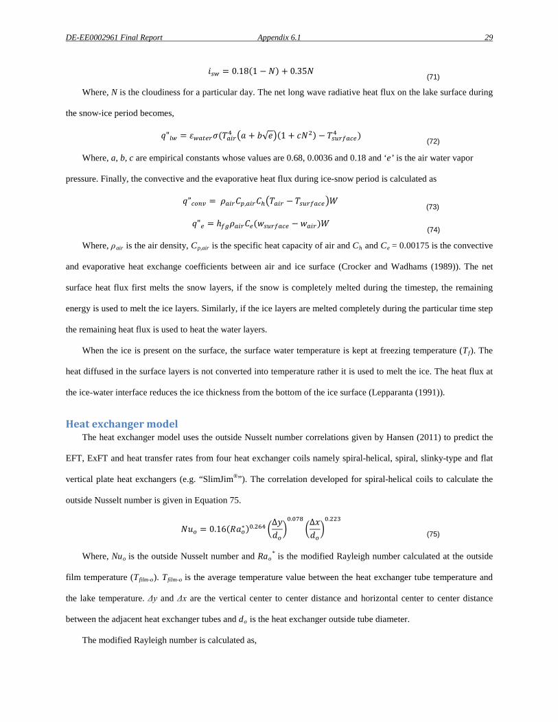
DE-EE0002961 Final Report Appendix 6.1 29
𝑖𝑠𝑤 = 0.18(1 −𝑁) + 0.35𝑁 (71)
Where, N is the cloudiness for a particular day. The net long wave radiative heat flux on the lake surface during
the snow-ice period becomes,
𝑞"𝑙𝑤 = 𝜀𝑤𝑎𝑡𝑒𝑟𝜎(𝑇𝑎𝑖𝑟4 �𝑎 + 𝑏√𝑒�(1 + 𝑐𝑁2) − 𝑇𝑠𝑢𝑟𝑓𝑎𝑐𝑒4 ) (72)
Where, a, b, c are empirical constants whose values are 0.68, 0.0036 and 0.18 and ‘e’ is the air water vapor
pressure. Finally, the convective and the evaporative heat flux during ice-snow period is calculated as
𝑞”𝑐𝑜𝑛𝑣 = 𝜌𝑎𝑖𝑟𝐶𝑝,𝑎𝑖𝑟𝐶ℎ�𝑇𝑎𝑖𝑟 − 𝑇𝑠𝑢𝑟𝑓𝑎𝑐𝑒�𝑊 (73)
𝑞"𝑒 = ℎ𝑓𝑔𝜌𝑎𝑖𝑟𝐶𝑒(𝑤𝑠𝑢𝑟𝑓𝑎𝑐𝑒 − 𝑤𝑎𝑖𝑟)𝑊 (74)
Where, ρair is the air density, Cp,air is the specific heat capacity of air and Ch and Ce = 0.00175 is the convective
and evaporative heat exchange coefficients between air and ice surface (Crocker and Wadhams (1989)). The net
surface heat flux first melts the snow layers, if the snow is completely melted during the timestep, the remaining
energy is used to melt the ice layers. Similarly, if the ice layers are melted completely during the particular time step
the remaining heat flux is used to heat the water layers.
When the ice is present on the surface, the surface water temperature is kept at freezing temperature (Tf). The
heat diffused in the surface layers is not converted into temperature rather it is used to melt the ice. The heat flux at
the ice-water interface reduces the ice thickness from the bottom of the ice surface (Lepparanta (1991)).
Heat exchanger model The heat exchanger model uses the outside Nusselt number correlations given by Hansen (2011) to predict the
EFT, ExFT and heat transfer rates from four heat exchanger coils namely spiral-helical, spiral, slinky-type and flat
vertical plate heat exchangers (e.g. “SlimJim®”). The correlation developed for spiral-helical coils to calculate the
outside Nusselt number is given in Equation 75.
𝑁𝑢𝑜 = 0.16(𝑅𝑎𝑜∗)0.264 �∆𝑦𝑑𝑜�0.078
�∆𝑥𝑑𝑜�0.223
(75)
Where, Nuo is the outside Nusselt number and Rao* is the modified Rayleigh number calculated at the outside
film temperature (Tfilm-o). Tfilm-o is the average temperature value between the heat exchanger tube temperature and
the lake temperature. Δy and Δx are the vertical center to center distance and horizontal center to center distance
between the adjacent heat exchanger tubes and do is the heat exchanger outside tube diameter.
The modified Rayleigh number is calculated as,
DE-EE0002961 Final Report Appendix 6.1 30
𝑅𝑎𝑜∗ =𝑔𝛽𝑄𝑐𝐿4𝑃𝑟𝑘𝑝𝑜𝑛𝑑𝜐2
(76)
Where, g is the acceleration due to gravity, β is the thermal expansion coefficient, kpond is the thermal
conductivity of the pond and υ is the kinematic viscosity, all calculated at the outside film temperature (Tfilm-o), Qc is
the coil heat flux, L is the characteristic length of the heat exchanger coil and Pr is the Prandtl number.
The outside convection coefficient is calculated based on the outside Nusselt number.
ℎ𝑜 = (𝑁𝑢𝑜 ∗ 𝑘𝑝𝑜𝑛𝑑)/𝑑𝑜 (77)
The inside Nusselt number correlation for spiral-helical, horizontal spiral and vertical-horizontal slinky coils are
obtained from Salimpour (2009). The thermal parameters are calculated based on the inside fluid temperature (Tfluid)
which is the average temperature value between the EFT and ExFT for the time step.
𝑁𝑢𝑖 = 0.152 𝐷𝑒0.431 Pr1.06 𝑃𝑖𝑡𝑐ℎ𝑟𝑎𝑡𝑖𝑜−0.277 (78)
𝐷𝑒 = 𝑅𝑒�𝑑𝑖𝑑𝑐𝑜
(79)
𝑃𝑖𝑡𝑐ℎ𝑟𝑎𝑡𝑖𝑜 =∆𝑦𝜋𝑑𝑐𝑜
(80)
Where, Nui is the inside Nusselt number, De is the Dean number, Pitchratio is the dimensionless pitch ratio, di is
the inside tube diameter, 𝑑𝑐𝑜 is the heat exchanger outside coil diameter and Re is the Reynolds number.
The inside Nusselt number correlation for flat plate heat exchangers is obtained from the inside Nusselt number
correlation developed for a serpentine channel by Snyder et al. (1993).
𝑁𝑢𝑖 = 4 + 29.2ln [(𝑅𝑒 Pr0.4 + 1000)/1200] (81)
The inside convection coefficient is calculated from the inside Nusselt number.
ℎ𝑖 = (𝑁𝑢𝑖 ∗ 𝑘𝑓𝑙𝑢𝑖𝑑)/𝑑𝑖 (82)
The global heat transfer coefficient (UAHx) for the heat exchanger is then calculated.
𝑈𝐴𝐻𝑥 =1
𝑅𝑖 + 𝑅𝑡𝑢𝑏𝑒 + 𝑅𝑜
(83)
The thermal resistances are calculated as follows,
DE-EE0002961 Final Report Appendix 6.1 31
𝑅𝑖 =1
ℎ𝑖𝐴𝑖
(84)
𝑅𝑡𝑢𝑏𝑒 =ln �𝑑𝑜𝑑𝑖
�
2𝜋𝑘𝑡𝑢𝑏𝑒𝐿𝑡𝑢𝑏𝑒 (85)
𝑅𝑜 =1
ℎ𝑜𝐴𝑜
(86)
Where, Ri, Rtube and Ro are the inside, heat exchanger tube and outside convection resistances respectively, ktube
is the tube thermal conductivity, Ai, Ao and Ltube are the heat exchanger tube inside surface area, outside surface area
and length respectively.
The effectiveness (ε) of the heat exchanger is calculated based on the NTU formulation
𝐶𝑚𝑖𝑛 = 𝑚𝑓𝑙𝑢𝑖𝑑𝑐𝑝,𝑓𝑙𝑢𝑖𝑑 (87)
𝑁𝑇𝑈 =𝑈𝐴𝐶𝑚𝑖𝑛
(88)
𝜀 = 1 − 𝑒−𝑁𝑇𝑈 (89)
Where, mfluid is the mass flow rate and cp,fluid is the specific heat capacity of the heat exchanger fluid
The heat exchanger entering and exiting fluid temperatures for the i’th timestep are calculated by the following
equations
𝐸𝐹𝑇𝑖 = 𝑇𝑙𝑎𝑘𝑒 − 𝑄𝐻𝑥/(𝜀𝐶𝑚𝑖𝑛) (90)
𝐸𝑥𝐹𝑇𝑖 = 𝐸𝐹𝑇𝑖 + 𝑄𝐻𝑥/𝐶𝑚𝑖𝑛 (91)
Where, Tlake is the daily average lake temperature for the depth range where the heat exchangers are placed in
the lake.
The heat transfer between the heat exchangers and the lake is calculated as,
𝑄ℎ𝑥 = 𝜀𝐶𝑚𝑖𝑛(𝐸𝐹𝑇𝑖 − 𝑇𝑙𝑎𝑘𝑒)(𝑁𝑐𝑖𝑟𝑐𝑢𝑖𝑡𝑠) (92)
Where, Ncircuits is the number of SWHE circuits placed in the lake. All the heat exchanger circuits are assumed
to be in parallel arrangement. The calculation of the EFT and ExFT is iterative and uses an assumed initial value for
the first time step and converged values of the previous time step as initial values for consecutive time steps.
Ice-on-coil model
DE-EE0002961 Final Report Appendix 6.1 32
During cold climatic conditions with low lake water temperatures and with heat exchangers operating in heat
extraction mode, the film of water around the heat exchanger coils tends to freeze and form layer(s) of ice around
the coils. The ice thickness tends to grow as this condition prevails and melting of ice around the coil takes place as
the condition changes. The heat transfer rate of the heat exchanger is affected by the presence of ice around the
coils. The numerical model to simulate the freezing of water and melting of ice around the heat exchanger coils and
thereby calculate the net heat transfer during freezing and melting conditions is based on the ice-on-coil model for a
thermal storage tank by Neto and Krarti (1997).
Since the rate of ice formation and growth varies along the length of the coil, the total length of the heat
exchanger coil is divided into many small segments and the heat transfer of each segment is calculated individually
by calculating the individual segment thermal resistances. The ice-on-coil model calculates the radius of ice and the
heat transfer in each coil segment using an iterative procedure. The following governing equation is applied to each
segment ‘i’.
𝑄𝑐𝑜𝑖𝑙,𝑖 = 𝑄𝑤𝑎𝑡𝑒𝑟,𝑖 + 𝑄𝑙𝑎𝑡,𝑓,𝑖 + 𝑄𝑠𝑐,𝑖 (93)
Where, Qcoil,i is the heat transfer between the heat exchanger fluid and the ice/water interface, Qwater,i is the heat
transfer between water surrounding the heat exchanger segments and the ice/water interface on the heat exchanger,
Qlat,f,i is the latent heat to freeze the water or melt the ice formed at each segment, Qsc,i is the sensible heat to sub
cool the ice during freezing at each segment.
During initial freezing period or during the cool down period when the heat exchanger tube segments are free
from ice, the heat transfer from the heat exchanger coil segments are calculated as
𝑄𝑐𝑜𝑖𝑙,𝑖 = 𝑈𝐴𝑜,𝑖(0°𝐶 − 𝐸𝐹𝑇𝑖) (94)
Where, EFTi is the entering fluid temperature for the i’th segment. It should be noted that the exiting fluid
temperature of the i’th is the entering fluid temperature of the i+1’th segment. UAo,i is the overall heat transfer
coefficient for the segment with no ice formation.
𝑈𝐴𝑜,𝑖 =1
(𝑅𝑒𝑠𝑓𝑙𝑢𝑖𝑑 + 𝑅𝑒𝑠𝑡𝑢𝑏𝑒 + 𝑅𝑒𝑠𝑤𝑎𝑡𝑒𝑟)
(95)
The thermal resistances are given by the following equations.
𝑅𝑒𝑠𝑓𝑙𝑢𝑖𝑑 =1
�(2𝜋 − 𝜃𝑖)𝑟𝑖 𝐿𝑡𝑢𝑏𝑒 ℎ𝑓𝑙𝑢𝑖𝑑�
(96)
DE-EE0002961 Final Report Appendix 6.1 33
𝑅𝑒𝑠𝑡𝑢𝑏𝑒 =𝑙𝑛 𝑟𝑜𝑟𝑖
(2𝜋 − 𝜃𝑖)𝑘𝑡𝑢𝑏𝑒𝐿𝑡𝑢𝑏𝑒 (97)
𝑅𝑒𝑠𝑤𝑎𝑡𝑒𝑟 =1
[(2𝜋 − 𝜃𝑖)𝑟𝑜 𝐿𝑡𝑢𝑏𝑒 ℎ𝑤𝑎𝑡𝑒𝑟] (98)
Where Resfluid, Restube and Resice are the thermal resistances of the heat exchanger fluid, tube and the
surrounding ice respectively, ri, ro and rice are the inside radius of the tube, outside radius of the tube and radius of
the ice respectively, hfluid is the fluid convective heat transfer coefficient, hwater is the convective heat transfer
coefficient when the tubes are free from ice and θ is the overlapping angle of ice between the two tubes which are
adjacent to each other. If overlapping of ice between the tubes occur “0 < θ i < 2π” else “θ i = 0°”.
During the freezing period the heat transfer between the ice/water interface and the heat exchanger fluid is
given by,
𝑄𝑐𝑜𝑖𝑙,𝑖 = 𝑈𝐴𝑓,𝑖(0°𝐶 − 𝐸𝐹𝑇𝑖) (99)
UAf is the overall heat transfer coefficient for the segment, which is defined as,
𝑈𝐴𝑓,𝑖 =1
(𝑅𝑒𝑠𝑓𝑙𝑢𝑖𝑑 + 𝑅𝑒𝑠𝑡𝑢𝑏𝑒 + 𝑅𝑒𝑠𝑖𝑐𝑒)
(100)
𝑅𝑒𝑠𝑖𝑐𝑒 =𝑙𝑛 𝑟𝑖𝑐𝑒𝑟𝑜
(2𝜋 − 𝜃𝑖)𝑘𝑖𝑐𝑒𝐿𝑡𝑢𝑏𝑒 (101)
Resice is the thermal resistance of the ice surrounding the heat exchanger segment and rice is the radius of the ice
During ice formation the heat transfer between the surrounding water around the ice to the ice/water interface, Qwat,i
can be calculated as
𝑄𝑤𝑎𝑡,𝑖 = (2𝜋 − 𝜃𝑖)𝑟𝑖𝑐𝑒𝐿𝑡𝑢𝑏𝑒ℎ𝑤𝑎𝑡−𝑖𝑐𝑒(𝑇𝑤𝑎𝑡,𝑖 − 0℃) (102)
Where, hwat-ice is the convective heat transfer coefficient at the ice/water interface, Twat,i is the water temperature
surrounding each coil segment.
The latent heat to freeze the water around the coils Qlat,f,i is given by,
𝑄𝑙𝑎𝑡,𝑓,𝑖 = ∆𝑀𝑖𝑐𝑒,𝑖
∆𝑡𝐻𝐹𝑖𝑐𝑒 (103)
Where, ΔM ice,i is the mass of ice formed at each segment during the time step Δt is calculated using Equation
104 and HFice is the latent heat of freezing of ice.
DE-EE0002961 Final Report Appendix 6.1 34
∆𝑀𝑖𝑐𝑒,𝑖 = 𝜌𝑖𝑐𝑒(2𝜋 − 𝜃𝑖)
2�𝑟𝑖𝑐𝑒,𝑖
2 − 𝑟𝑖𝑐𝑒,𝑜𝑙𝑑 ,𝑖2 �𝐿𝑠𝑒𝑔 (104)
Where, ρ ice is the density of ice, rice,i and rice,old,i are the radius of ice formed for a segment during the current
and previous time steps respectively and Lseg is the length of each coil segment.
The heat transfer to sub-cool the ice Qsc,i is
𝑄𝑠𝑐,𝑖 =∆𝑀𝑖𝑐𝑒,𝑖
∆𝑡𝐶𝑝,𝑖𝑐𝑒(0℃ − 𝑇𝑏𝑢𝑙𝑘) (105)
Where, Cp,ice is the specific heat capacity of ice and Tbulk is the ice bulk temperature. The ice bulk temperature
Tbulk , convective heat transfer coefficient at the ice/water interface hwat-ice and the fluid convective heat transfer
coefficient hfluid can be calculated based on the correlations given in Neto and Krarti (1997).
The algorithm to calculate the ice thickness and the heat transfer by the coil is described.
1. An initial ice thickness is assumed and the individual heat transfer terms are calculated.
2. If Qcoil,i ≥ (Qwater,i + Qlat,f,i + Qsc,i), then the ice thickness of the coil is increased and new heat transfer
terms are calculated.
3. If Qcoil,i < (Qwater,i + Qlat,f,,i + Qsc,i), then the ice thickness of the segment is decreased and the new heat
transfer terms are calculated.
4. Convergence of ice thickness is achieved only when Qcoil,i = (Qwater,i + Qlat,f,i + Qsc,i) and the final
segment radius and segment heat transfer rate is calculated.
Finally the heat exchanger ExFT for every segment is calculated as
𝐸𝑥𝐹𝑇𝑖 = 𝐸𝐹𝑇𝑖 +𝑄𝑐𝑜𝑖𝑙,𝑖
𝑚𝑓𝑙𝑢𝑖𝑑𝐶𝑝,𝑓𝑙𝑢𝑖𝑑
(106)
The correlations to calculate the rwater,rice and θ i are described in detail in Neto (1996). The heat transfer from each
tube segment Qcoil,i is summed up to calculate the overall heat transfer of the heat exchanger coils QHx.
Peer review status Yes, all the references used to develop the model are peer reviewed.
Hardware requirements This model's only requirements are those needed to run the governing programs (EnergyPlus or standalone
FORTRAN): a standard personal computer running on Windows XP or later.
Documentation

DE-EE0002961 Final Report Appendix 6.1 35
Document Description of the task
Milestone2.1 Development of lake model stratification
Milestone2.2 Development of ice-on-coil model for heat exchangers
Milestone2.3 Development of model to predict ice/snow formation on lake surface
Milestone4.1 Development of alternate pond heat exchanger types
Appendix4.2.1 EnergyPlus Input/output reference
Appendix4.2.2 EnergyPlus Engineering reference
Appendix4.2.3 EnergyPlus example file
Millstone4.3.1 Design tool documentation
Milestone4.3.2 Design tool example file
Milestone4.4 Validation results of lake model implemented in EnergyPlus
NOMENCLATURE:
A = lake horizontal area, [m2]
Cd = drag coefficient [-]
Cp = specific heat capacity, [J/kg .°C]
d = heat exchanger tube diameter, [m]
𝑑𝑐𝑜 = heat exchanger outside coil diameter, [m]
De = Dean number [-]
EFT = heat exchanger entering fluid temperature, [°C]
ExFT = heat exchanger exit fluid temperature, [°C]
g = acceleration due to gravity, [m/s2]
Hice = ice thickness, [m]

DE-EE0002961 Final Report Appendix 6.1 36
Hice, new = New ice thickness due to congelation ice growth, [m]
Hsnow = Snow thickness, [m]
Hsnow-ice = Thickness of snow ice, [m]
hc = surface convective heat transfer coefficient, [W/m2. °C]
hfg = Latent heat of vaporization, [J/kg]
hlw = longwave radiative heat transfer coefficient, [W/m2. °C]
K = thermal conductivity, [W/m. °C]
kz = vertical eddy diffusion coefficient, [m2/day]
kzmax = the maximum hypolimnion eddy diffusion coefficient, [m2/day]
Lfreeze = latent heat of freezing of ice, [J/kg]
m = mass flow rate, [Kg/s]
mice = mass of ice surrounding the heat exchanger tube, [Kg]
mwater = mass of water melted from ice surrounding the heat exchanger tube, [Kg]
N = stability frequency or the Brunt Vaisala frequency, [s-1]
Ncircuit = the number of heat exchanger circuits placed in the lake [-]
Nu = Nusselt number [-]
PE = Potential energy, [J]
Pitchratio = Coil pitch ratio [-]
Pr = Prandtl number [-]
Q = internal distribution of heat to each water layer due to the absorption of solar radiation in the
water column, [J/m3.day]
Qcoil = heat transfer between the heat exchanger fluid and ice/water interface, [W]
Qdeficit = sensible heat deficit in the sub-cooled water layer converted into latent heat of ice, [W]
Qlat = latent heat to freeze the water or melt the ice formed at each segment [W]
Qsc = sensible heat to sub-cool the ice during freezing at each segment, [W]
Qsh = sensible heat to superheat the water during the melting period at each segment, [W]
Qwat = heat transfer between the surrounding lake water and the ice/water interface, [W]
q”c = convective heat flux from the lake surface to the atmosphere, [W/m2]

DE-EE0002961 Final Report Appendix 6.1 37
q”e = evaporative heat flux from the lake surface, [W/m2]
qhx(zhx) = heat flux due to the heat exchanger at the depth of the lake where the heat exchanger is placed
(zhx), [W/m2]
q”lw = net long wave radiation incident on the lake surface, [W/m2]
q”net-surface = net heat flux on the lake surface, [W/m2]
q”net(z) = net heat flux at the depth z, [W/m2]
qsediment = heat flux from sediment to water, [W/m2]
q”sw(z) = incoming short wave radiative heat flux absorbed at the depth z, [W/m2]
q”sw-surface = heat flux due to short wave radiation incident on the lake surface, [W/m2]
r = radius of the heat exchanger tube, [m]
R, Res = Thermal resistances, [1/K]
Ra* = modified Rayleigh number [-]
Ri = Richardson number [-]
t = time, [s]
T = temperature, [°C]
TKE = Total kinetic energy, [J]
UA = global heat transfer coefficient, [W/K]
Vepi = Volume of the epilimnion, [m3]
Vz = Volume of the layer below the epilimnion, [m3]
W = Wind speed, [m/s]
Wstr = Wind sheltering coefficient [-]
wair = humidity ratio of air, [kg water/kg dry air]
wsurface = humidity ratio of saturated air at the lake surface, [kg water/kg dry air]
z = lake depth, [m]
zepi = Thickness of the epilimnion layer, [m]
zM, epi = Depth of the center of mass of the epilimnion, [m]
∆zM, z = Distance from the layers center of mass to the bottom of the epilimnion, [m]
Δx = horizontal center to center distance between adjacent heat exchanger tubes, [m]

DE-EE0002961 Final Report Appendix 6.1 38
Δy = vertical center to center distance between adjacent heat exchanger tubes, [m]
αsed = sediment thermal diffusivity, [m2/day]
β = thermal expansion coefficient, [K-1]
βw = water surface absorption coefficient = 0.4 [-]
ε = effectiveness of the heat exchanger [-]
εwater = emissivity coefficient of water = 0.97 [-]
σ = Stefan Boltzmann constant, [5.67 * 10-8 W/m2.K4]
μ = extinction coefficient of water, [m-1]
ρ = density, [Kg/m3]
ρ’water = water surface reflectivity coefficient [-]
ρ’ ice,snow = surface ice or snow reflectivity coefficient [-]
θ = ice/water overlapping angle, [radians]
τ = Wind shear stress, [N/m2]
Subscripts
fluid = heat exchanger fluid
freeze = freezing point
Hx = Heat exchanger
i = inside
o = outside
sed = sediment
weq = water equivalent
ws = water-sediment layer
References Adams, E. E., D. J. Cosler and K. R. Helfrich.(1990). Evaporation from heated water bodies: Predicting combined
forced plus free convection. Water Resour. Res. 26(3): 425-435. Argonne National, L. and J. G. Asbury. (1970). Effects of thermal discharges on the mass/energy balance of Lake
Michigan. Argonne, Ill., The Laboratory. Banks, R. B.(1975). Some features of wind action on shallow lakes. Journal of Environmental Engineering Division
101(5): 813-827.

DE-EE0002961 Final Report Appendix 6.1 39 Banks.R.B.(1975). Some features of wind action on shallow lakes. Journal of Environmental Engineering Division
101(5): 813-827. Branco, B. and T. Torgersen.(2009). Predicting the onset of thermal stratification in shallow inland waterbodies.
Aquatic Sciences - Research Across Boundaries 71(1): 65-79. Chiasson, A. D., J. D. Spitler, S. J. Rees and M. D. Smith.(2000). A Model for Simulating the Performance of a
Shallow Pond as a Supplemental Heat Rejector with Closed-Loo[ Ground-Source Heat Pump Systems. ASHRAE Transcations 106(2): 107-121.
Chiasson, A. D., J. D. Spitler, S. J. Rees and M. D. Smith.(2000). A Model for Simulating the Performance of a Shallow Pond as a Supplemental Heat Rejector with Closed-Loop Ground-Source Heat Pump Systems. ASHRAE Transcations 106(2): 107-121.
Chiasson, D. A., D. J. Spitler, J. R. Simon and D. M. Smith.(2000). A Model for simulating the performance of a shallow pond as a supplemental heat rejecter with closed-loop Ground-Source Heat Pump Systems. ASHRAE Transactions 106(2): 107-121.
Crocker, G. B. and P. Wadhams.(1989). Modelling Antarctic Fast-Ice Growth. Journal of Glaciology 35(119): 3-8. Czarnecki, J. T.(1963). A method of heating swimming pools by solar energy. Solar Energy 7(1): 3-7. Dake, J. M. K. and D. R. F. Harleman.(1969). Thermal stratification in lakes: Analytical and laboratory studies.
Water Resources Research 5(2): 484-495. Ellis, C. R., H. G. Stefan and R. Gu.(1991). Water Temperature Dynamics and Heat Transfer Beneath the Ice Cover
of a Lake. Limnology and Oceanography 36(2): 324-335. Fang , X. and H. G. Stefan.(1996). Long-term lake water temperature and ice cover simulations/measurements. Cold
Regions Science and Technology 24: 289-304. Ford, D. E. and H. G. Stefan.(1980). Themal predictions using integral energy model. Journal of the Hydraulics
Division 106(1): 39-55. Friehe, C. A. and K. F. Schmitt.(1976). Parameterization of Air-Sea Interface Fluxes of Sensible Heat and Moisture
by the Bulk Aerodynamic Formulas. Journal of Physical Oceanography 6(6): 801-809. Gu, R. and H. G. Stefan.(1990). Year Round temperature simulation of cold climate lakes. Cold Regions Science
and Technology 18: 147-160. Gu, R. and H. G. Stefan.(1995). Stratification dynamics in wastewater stabilization ponds. Water Research 29(8):
1909-1923. Hamilton, D. P. and S. Schladow, G (1997). Prediction of water quality in lakes and reservoirs. Part I - Model
description. Ecological Modelling 96: 91-110. Hansen, G. M.2011.Experimental testing and analysis of spiral-helical surface water heat exchanger configurations.
Masters thesis. Oklahoma State University, Stillwater. Henderson-Sellers, B.(1985). New formulation of eddy diffusion thermocline models. Applied Mathematical
Modelling 9(6): 441-446. Henderson-Sellers, B.(1988). Sensitivity of thermal stratification models to changing boundary conditions. Applied
Mathematical Modelling 12(1): 31-43. Hondzo, M. and H. G. Stefan.(1993). Lake water temperature simulation model. Journal of Hydraulic Engineering
119(11): 1251-1274. Hondzo, M. and H. G. Stefan.(1993). Regional water temperature characteristics of lakes subjected to climate
change. Climatic Change 24(3): 187-211. Imberger, J.(1985). Thermal characteristics of standing waters: an illustration of dynamic processes. Hydrobiologia
125(1): 7-29. Imberger, J., I. Loh, B. Hebbert and J. Patterson.(1978). Dynamics of reservoir of medium size. Journal of
Hydraulics Division 104(5): 725-743. Imberger, J., J. Patterson, B. Hebbert and I. Loh.(1978). Dynamics of Reservoir of Medium Size. Journal of
Hydraulics Division 104(5): 725-743. Incropera, F. P. and D. P. DeWitt. (1996). Introduction to heat transfer. New York, John Wiley and Sons. Jassby, A. and T. Powell.(1975). Vertical patterns of eddy diffusion during stratification in Castle Lake, California.
Limnology and Oceanography 20(4): 530-543. Kullenberg, G.(1971). Vertical Diffusion in Shallow Waters. Tellus 23(2): 129-135. Lepparanta, M.(1991). A review of analytical models of sea-ice growth. Atmosphere-Ocean 31: 123-138. Losordo, T. M. and R. H. Piedrahita.(1991). Modelling temperature variation and thermal stratification in shallow
aquaculture ponds. Ecological Modelling 54(3–4): 189-226. McCormick, M. J. and D. Scavia.(1981). Calculation of vertical profiles of lake-averaged temperature and
diffusivity in Lakes Ontario and Washington. Water Resources Research 17(2): 305-310.

DE-EE0002961 Final Report Appendix 6.1 40 Molineaux, B., B. Lachal and O. Guisan.(1994). Thermal analysis of five outdoor swimming pools heated by
unglazed solar collectors. Solar Energy 53(1): 21-26. Neto, J. H. M.1996.Deterministic model for an indirect ice-storage tank. Ph.D. thesis. University of Colorado
Boulder, Colorado. Neto, J. H. M. and M. Krarti.(1997). Deterministic model for an internal melt ice-on-coil thermal storage tank.
ASHRAE Transactions 103(1): 113-124. Omstedt, A.(1990). A coupled one-dimensional sea ice–ocean model applied to a semi-enclosed basin. Tellus A
42(5): 568-582. Perovich, D. K. (1996). The optical properties of sea ice / Donald K. Perovich ; prepared for Office of Naval
Research. [Hanover, N.H.] :, US Army Corps of Engineers, Cold Regions Research & Engineering Laboratory ; [Springfield, Va. : Available from National Technical Information Service.
Pezent, M. C. and S. P. Kavanaugh.(1990). Development and verification of a thermal model of lakes used with water source heat pumps. ASHRAE Transactions 96(1): 574-582.
Rohden, C. v., K. Wunderle and J. Ilmberger.(2007). Parameterisation of the vertical transport in a small thermally stratified lake. Aquatic Sciences - Research Across Boundaries 69(1): 129-137.
Salimpour, M. R.(2009). Heat Transfer Coefficients of Shell and Coiled Tube Heat Exchangers. Experimental Thermal and Fluid Science 33(2): 203-207.
Saloranta, T. M.(2000). Modeling the evolution of snow, snow ice and ice in the Baltic Sea. Tellus A 52(1): 93-108. Saloranta, T. M. and T. Andersen. (2004). Mylake (v.1.1): Technical model documentation and user's guide. NIVA-
report 4838. Olso,Norway, Norwegian Institute for Water Research. 44. Sengupta, S., E. Nwadike and S. S. Lee.(1981). Long term simulation of stratification in cooling lakes. Applied
Mathematical Modelling 5(5): 313-320. Snyder, B., K. T. Li and R. A. Wirtz.(1993). Heat transfer enhancement in a serpentine channel. International
Journal of Heat and Mass Transfer 36(12): 2965-2976. Stefan, H. G., J. J. Cardoni and A. W. Fu. (1982). Resqual 2: A dynamic water quality simulation program for a
stratified shallow lake or reservoir: application to Lake Chicot, Arkansas. Minneapolis, St Anthony Falls Laboratory: 154.
Swinbank, W. C.(1963). Long-wave radiation from clear skies. Quarterly Journal of the Royal Meteorological Society 89(381): 339-348.
Tucker, W. A. and A. W. Green.(1977). A Time-Dependent Model of the Lake-Averaged, Vertical Temperature Distribution of Lakes. Limnology and Oceanography 22(4): 687-699.
Yen, Y. C. (1981). Review of thermal properties of snow, ice and sea-ice. Hanover,NH,USA, US Army Cold Regions Research and Engineering Laboratory.

DE-EE0002961 Final Report Appendix 6.2 1
Appendix 6.2
Computer Modeling: SCW
Annamalai Ramesh
Oklahoma State University
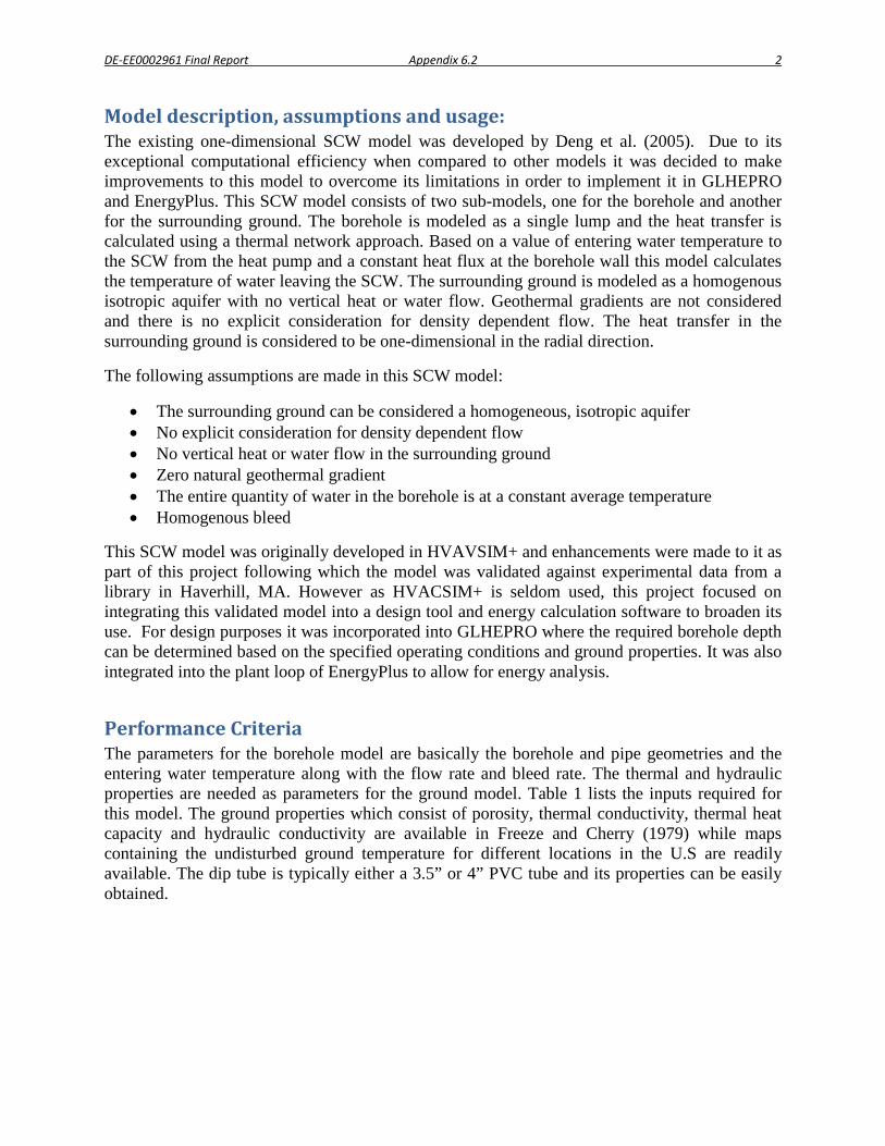
DE-EE0002961 Final Report Appendix 6.2 2
Model description, assumptions and usage: The existing one-dimensional SCW model was developed by Deng et al. (2005). Due to its exceptional computational efficiency when compared to other models it was decided to make improvements to this model to overcome its limitations in order to implement it in GLHEPRO and EnergyPlus. This SCW model consists of two sub-models, one for the borehole and another for the surrounding ground. The borehole is modeled as a single lump and the heat transfer is calculated using a thermal network approach. Based on a value of entering water temperature to the SCW from the heat pump and a constant heat flux at the borehole wall this model calculates the temperature of water leaving the SCW. The surrounding ground is modeled as a homogenous isotropic aquifer with no vertical heat or water flow. Geothermal gradients are not considered and there is no explicit consideration for density dependent flow. The heat transfer in the surrounding ground is considered to be one-dimensional in the radial direction.
The following assumptions are made in this SCW model:
• The surrounding ground can be considered a homogeneous, isotropic aquifer • No explicit consideration for density dependent flow • No vertical heat or water flow in the surrounding ground • Zero natural geothermal gradient • The entire quantity of water in the borehole is at a constant average temperature • Homogenous bleed
This SCW model was originally developed in HVAVSIM+ and enhancements were made to it as part of this project following which the model was validated against experimental data from a library in Haverhill, MA. However as HVACSIM+ is seldom used, this project focused on integrating this validated model into a design tool and energy calculation software to broaden its use. For design purposes it was incorporated into GLHEPRO where the required borehole depth can be determined based on the specified operating conditions and ground properties. It was also integrated into the plant loop of EnergyPlus to allow for energy analysis.
Performance Criteria The parameters for the borehole model are basically the borehole and pipe geometries and the entering water temperature along with the flow rate and bleed rate. The thermal and hydraulic properties are needed as parameters for the ground model. Table 1 lists the inputs required for this model. The ground properties which consist of porosity, thermal conductivity, thermal heat capacity and hydraulic conductivity are available in Freeze and Cherry (1979) while maps containing the undisturbed ground temperature for different locations in the U.S are readily available. The dip tube is typically either a 3.5” or 4” PVC tube and its properties can be easily obtained.
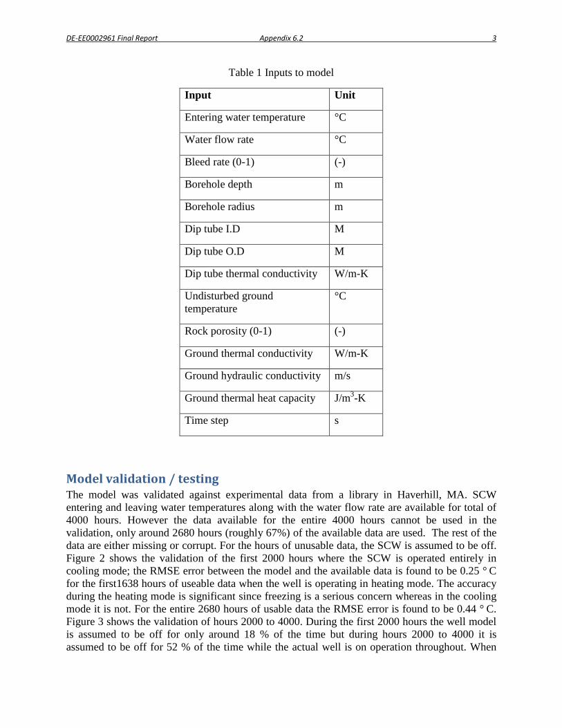
DE-EE0002961 Final Report Appendix 6.2 3
Table 1 Inputs to model
Input Unit
Entering water temperature °C
Water flow rate °C
Bleed rate (0-1) (-)
Borehole depth m
Borehole radius m
Dip tube I.D M
Dip tube O.D M
Dip tube thermal conductivity W/m-K
Undisturbed ground temperature
°C
Rock porosity (0-1) (-)
Ground thermal conductivity W/m-K
Ground hydraulic conductivity m/s
Ground thermal heat capacity J/m3-K
Time step s
Model validation / testing The model was validated against experimental data from a library in Haverhill, MA. SCW entering and leaving water temperatures along with the water flow rate are available for total of 4000 hours. However the data available for the entire 4000 hours cannot be used in the validation, only around 2680 hours (roughly 67%) of the available data are used. The rest of the data are either missing or corrupt. For the hours of unusable data, the SCW is assumed to be off. Figure 2 shows the validation of the first 2000 hours where the SCW is operated entirely in cooling mode; the RMSE error between the model and the available data is found to be 0.25 ° C for the first1638 hours of useable data when the well is operating in heating mode. The accuracy during the heating mode is significant since freezing is a serious concern whereas in the cooling mode it is not. For the entire 2680 hours of usable data the RMSE error is found to be 0.44 ° C. Figure 3 shows the validation of hours 2000 to 4000. During the first 2000 hours the well model is assumed to be off for only around 18 % of the time but during hours 2000 to 4000 it is assumed to be off for 52 % of the time while the actual well is on operation throughout. When
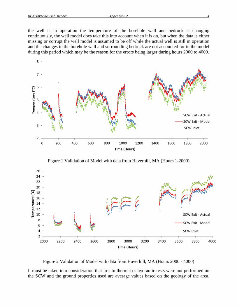
DE-EE0002961 Final Report Appendix 6.2 4
the well is in operation the temperature of the borehole wall and bedrock is changing continuously, the well model does take this into account when it is on, but when the data is either missing or corrupt the well model is assumed to be off while the actual well is still in operation and the changes in the borehole wall and surrounding bedrock are not accounted for in the model during this period which may be the reason for the errors being larger during hours 2000 to 4000.
Figure 1 Validation of Model with data from Haverhill, MA (Hours 1-2000)
Figure 2 Validation of Model with data from Haverhill, MA (Hours 2000 - 4000)
It must be taken into consideration that in-situ thermal or hydraulic tests were not performed on the SCW and the ground properties used are average values based on the geology of the area.
2
3
4
5
6
7
8
0 200 400 600 800 1000 1200 1400 1600 1800 2000
Tem
pera
ture
(°C)
Time (Hours)
SCW Exit - Actual
SCW Exit - Model
SCW Inlet
2468
101214161820222426
2000 2200 2400 2600 2800 3000 3200 3400 3600 3800 4000
Tem
pera
ture
(°C)
Time (Hours)
SCW Exit - Actual
SCW Exit - Model
SCW Inlet
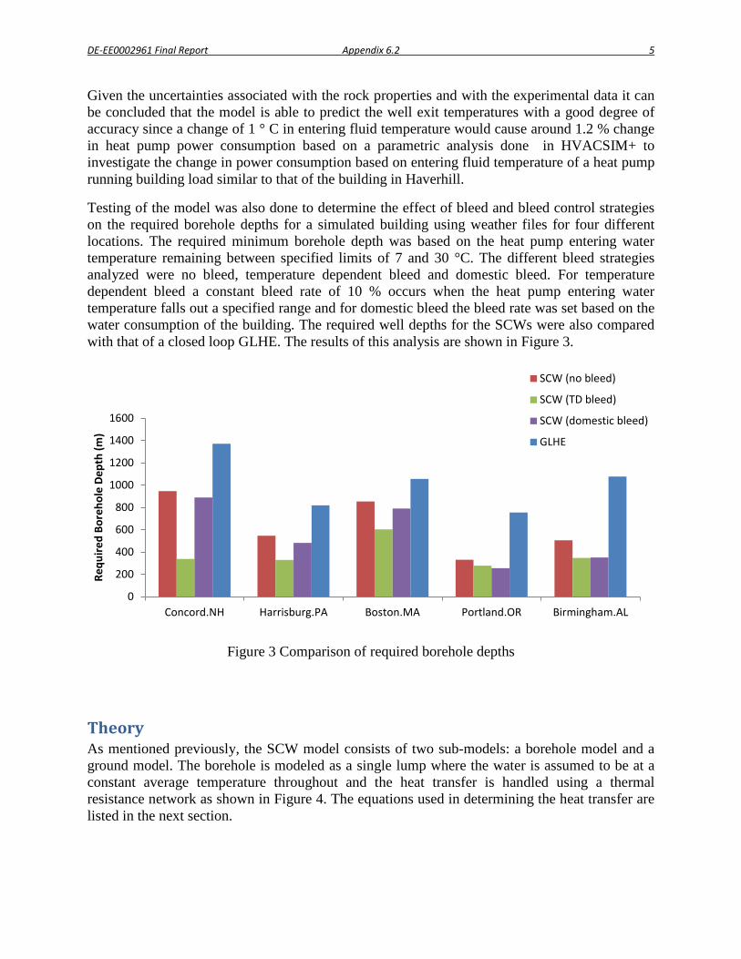
DE-EE0002961 Final Report Appendix 6.2 5
Given the uncertainties associated with the rock properties and with the experimental data it can be concluded that the model is able to predict the well exit temperatures with a good degree of accuracy since a change of 1 ° C in entering fluid temperature would cause around 1.2 % change in heat pump power consumption based on a parametric analysis done in HVACSIM+ to investigate the change in power consumption based on entering fluid temperature of a heat pump running building load similar to that of the building in Haverhill.
Testing of the model was also done to determine the effect of bleed and bleed control strategies on the required borehole depths for a simulated building using weather files for four different locations. The required minimum borehole depth was based on the heat pump entering water temperature remaining between specified limits of 7 and 30 °C. The different bleed strategies analyzed were no bleed, temperature dependent bleed and domestic bleed. For temperature dependent bleed a constant bleed rate of 10 % occurs when the heat pump entering water temperature falls out a specified range and for domestic bleed the bleed rate was set based on the water consumption of the building. The required well depths for the SCWs were also compared with that of a closed loop GLHE. The results of this analysis are shown in Figure 3.
Figure 3 Comparison of required borehole depths
Theory As mentioned previously, the SCW model consists of two sub-models: a borehole model and a ground model. The borehole is modeled as a single lump where the water is assumed to be at a constant average temperature throughout and the heat transfer is handled using a thermal resistance network as shown in Figure 4. The equations used in determining the heat transfer are listed in the next section.
0
200
400
600
800
1000
1200
1400
1600
Concord.NH Harrisburg.PA Boston.MA Portland.OR Birmingham.AL
Requ
ired
Bore
hole
Dep
th (m
)
SCW (no bleed)
SCW (TD bleed)
SCW (domestic bleed)
GLHE
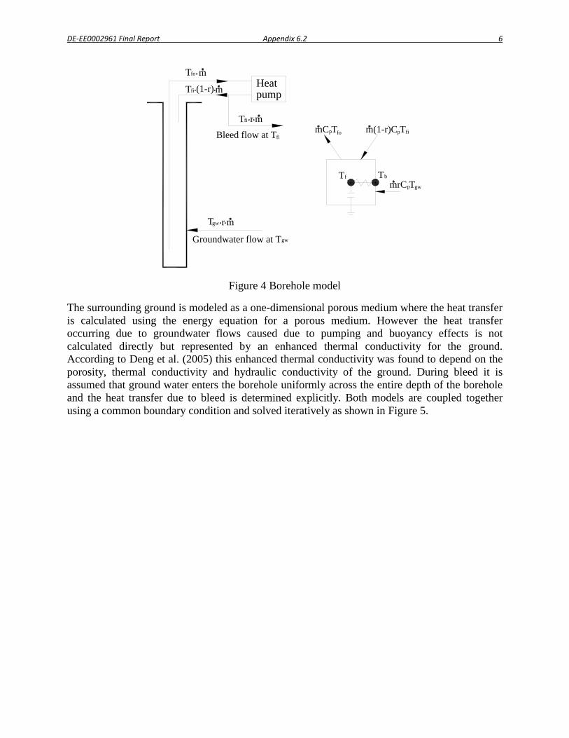
DE-EE0002961 Final Report Appendix 6.2 6
Figure 4 Borehole model
The surrounding ground is modeled as a one-dimensional porous medium where the heat transfer is calculated using the energy equation for a porous medium. However the heat transfer occurring due to groundwater flows caused due to pumping and buoyancy effects is not calculated directly but represented by an enhanced thermal conductivity for the ground. According to Deng et al. (2005) this enhanced thermal conductivity was found to depend on the porosity, thermal conductivity and hydraulic conductivity of the ground. During bleed it is assumed that ground water enters the borehole uniformly across the entire depth of the borehole and the heat transfer due to bleed is determined explicitly. Both models are coupled together using a common boundary condition and solved iteratively as shown in Figure 5.
T m
Bleed flow at T
Groundwater flow at T
gwT r m
T
Tfi
m
fo
fi (1-r)
m(1-r)C T
gw
fT
mr
fi
Heat pump
fopmC T
mrC TbT
p gw
p fi
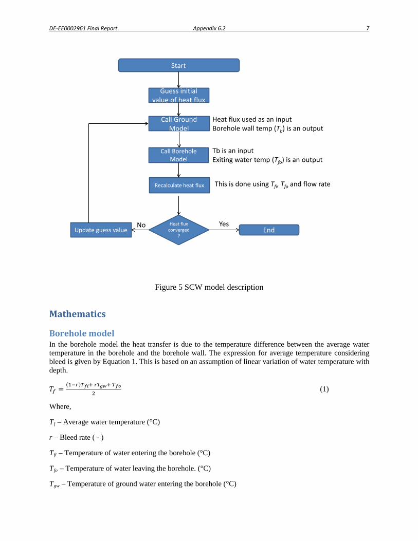
DE-EE0002961 Final Report Appendix 6.2 7
Start
Call Ground Model
Call Borehole Model
Recalculate heat flux
End
Guess initial value of heat flux
Heat flux converged
?Update guess value
No Yes
Heat flux used as an inputBorehole wall temp (Tb) is an output
Tb is an inputExiting water temp (Tfo) is an output
This is done using Tfi, Tfo and flow rate
Figure 5 SCW model description
Mathematics
Borehole model In the borehole model the heat transfer is due to the temperature difference between the average water temperature in the borehole and the borehole wall. The expression for average temperature considering bleed is given by Equation 1. This is based on an assumption of linear variation of water temperature with depth.
𝑇𝑓 =(1−𝑟)𝑇𝑓𝑖+ 𝑟𝑇𝑔𝑤+ 𝑇𝑓𝑜
2 (1)
Where,
Tf – Average water temperature (°C)
r – Bleed rate ( - )
Tfi – Temperature of water entering the borehole (°C)
Tfo – Temperature of water leaving the borehole. (°C)
Tgw – Temperature of ground water entering the borehole (°C)
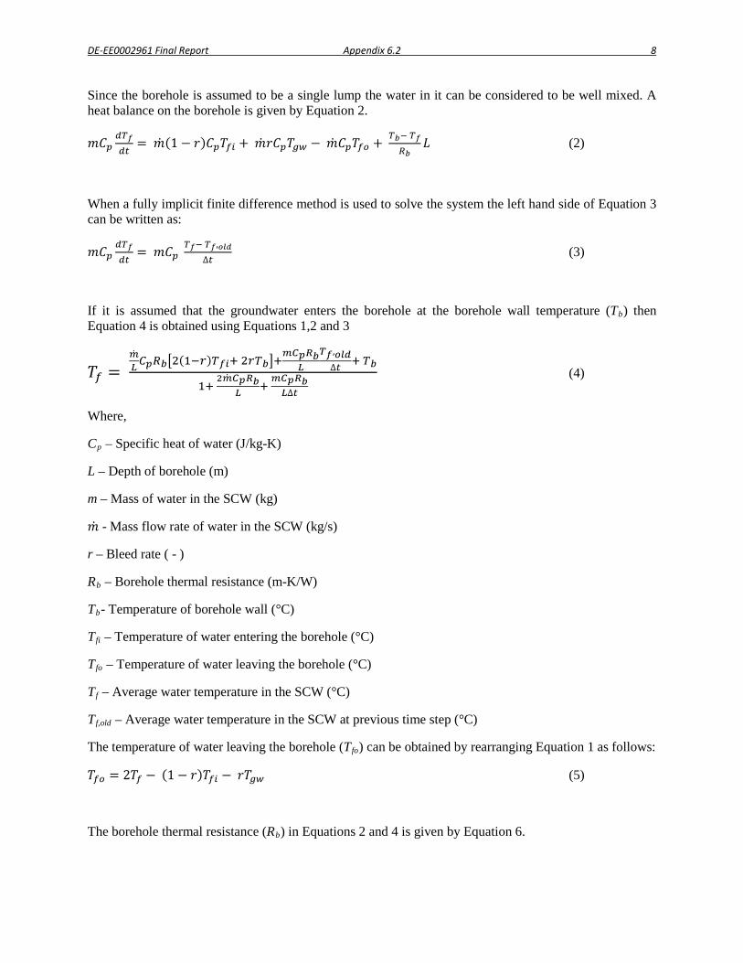
DE-EE0002961 Final Report Appendix 6.2 8
Since the borehole is assumed to be a single lump the water in it can be considered to be well mixed. A heat balance on the borehole is given by Equation 2.
𝑚𝐶𝑝𝑑𝑇𝑓𝑑𝑡
= �̇�(1 − 𝑟)𝐶𝑝𝑇𝑓𝑖 + �̇�𝑟𝐶𝑝𝑇𝑔𝑤 − �̇�𝐶𝑝𝑇𝑓𝑜 + 𝑇𝑏− 𝑇𝑓𝑅𝑏
𝐿 (2)
When a fully implicit finite difference method is used to solve the system the left hand side of Equation 3 can be written as:
𝑚𝐶𝑝𝑑𝑇𝑓𝑑𝑡
= 𝑚𝐶𝑝 𝑇𝑓− 𝑇𝑓,𝑜𝑙𝑑∆𝑡
(3)
If it is assumed that the groundwater enters the borehole at the borehole wall temperature (Tb) then Equation 4 is obtained using Equations 1,2 and 3
𝑇𝑓 = �̇�𝐿 𝐶𝑝𝑅𝑏�2(1−𝑟)𝑇𝑓𝑖+ 2𝑟𝑇𝑏�+
𝑚𝐶𝑝𝑅𝑏𝐿
𝑇𝑓,𝑜𝑙𝑑∆𝑡 + 𝑇𝑏
1+ 2�̇�𝐶𝑝𝑅𝑏
𝐿 + 𝑚𝐶𝑝𝑅𝑏𝐿∆𝑡
(4)
Where,
Cp – Specific heat of water (J/kg-K)
L – Depth of borehole (m)
m – Mass of water in the SCW (kg)
�̇� - Mass flow rate of water in the SCW (kg/s)
r – Bleed rate ( - )
Rb – Borehole thermal resistance (m-K/W)
Tb- Temperature of borehole wall (°C)
Tfi – Temperature of water entering the borehole (°C)
Tfo – Temperature of water leaving the borehole (°C)
Tf – Average water temperature in the SCW (°C)
Tf,old – Average water temperature in the SCW at previous time step (°C)
The temperature of water leaving the borehole (Tfo) can be obtained by rearranging Equation 1 as follows:
𝑇𝑓𝑜 = 2𝑇𝑓 − (1 − 𝑟)𝑇𝑓𝑖 − 𝑟𝑇𝑔𝑤 (5)
The borehole thermal resistance (Rb) in Equations 2 and 4 is given by Equation 6.
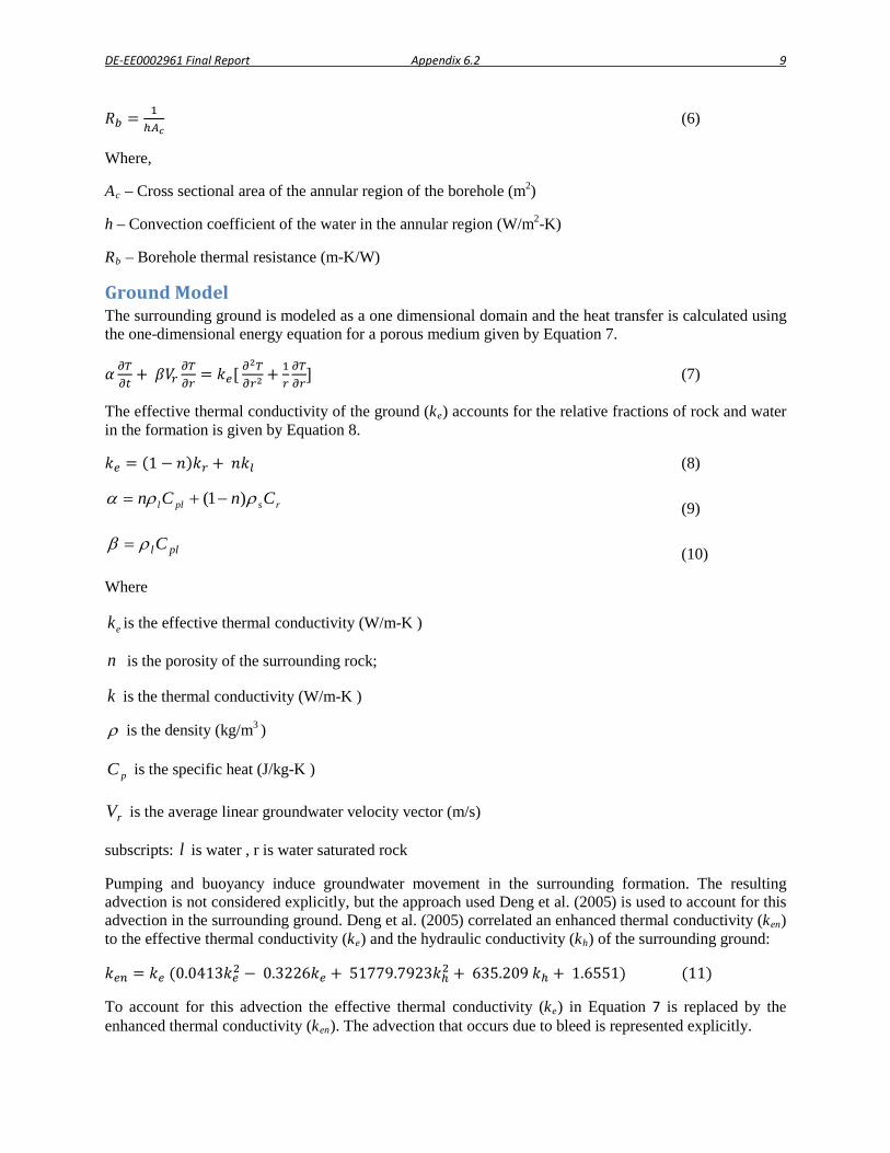
DE-EE0002961 Final Report Appendix 6.2 9
𝑅𝑏 = 1ℎ𝐴𝑐
(6)
Where,
Ac – Cross sectional area of the annular region of the borehole (m2)
h – Convection coefficient of the water in the annular region (W/m2-K)
Rb – Borehole thermal resistance (m-K/W)
Ground Model The surrounding ground is modeled as a one dimensional domain and the heat transfer is calculated using the one-dimensional energy equation for a porous medium given by Equation 7.
𝛼 𝜕𝑇𝜕𝑡
+ 𝛽𝑉𝑟𝜕𝑇𝜕𝑟
= 𝑘𝑒[ 𝜕2𝑇𝜕𝑟2
+ 1𝑟𝜕𝑇𝜕𝑟
] (7)
The effective thermal conductivity of the ground (ke) accounts for the relative fractions of rock and water in the formation is given by Equation 8.
𝑘𝑒 = (1 − 𝑛)𝑘𝑟 + 𝑛𝑘𝑙 (8)
rspll CnCn ρρα )1( −+= (9)
pllCρβ = (10)
Where
ek is the effective thermal conductivity (W/m-K )
n is the porosity of the surrounding rock;
k is the thermal conductivity (W/m-K )
ρ is the density (kg/m3 )
pC is the specific heat (J/kg-K )
rV is the average linear groundwater velocity vector (m/s)
subscripts: l is water , r is water saturated rock
Pumping and buoyancy induce groundwater movement in the surrounding formation. The resulting advection is not considered explicitly, but the approach used Deng et al. (2005) is used to account for this advection in the surrounding ground. Deng et al. (2005) correlated an enhanced thermal conductivity (ken) to the effective thermal conductivity (ke) and the hydraulic conductivity (kh) of the surrounding ground:
𝑘𝑒𝑛 = 𝑘𝑒 (0.0413𝑘𝑒2 − 0.3226𝑘𝑒 + 51779.7923𝑘ℎ2 + 635.209 𝑘ℎ + 1.6551) (11)
To account for this advection the effective thermal conductivity (ke) in Equation 7 is replaced by the enhanced thermal conductivity (ken). The advection that occurs due to bleed is represented explicitly.
DE-EE0002961 Final Report Appendix 6.2 10
In this one-dimensional model it assumed that all the ground water flows into the well during bleed and the linear ground water velocity is determined using the conservation of mass according to Equation 12.
Lrrm
nArm
nV
iri πρρ 2
111 −=−=
(12)
Where
n is the porosity of the surrounding rock;
m is the mass flow rate out of the borehole (kg/s)
ρ is the water density (kg/m3 )
L is the borehole depth (m )
ir is the radius at location i (m )
r is the bleed rate (-)
The governing equation is solved using a fully implicit finite difference method using an expanding grid which is 180 m in the radial direction consisting of 130 segments. The description of the grid spacing can be found in Deng (2004).
Peer review status The development of this model was presented in Deng et al. (2005) while the results of this model were presented in O’Neill et al. (2006). A detailed description of this model is presented in Deng (2004).
Hardware requirements This model's only requirements are those needed to run the governing programs (EnergyPlus or GLHEPRO): a standard personal computer running Windows XP or later.
Documentation The description of this model is presented in Milestone 1.1, while a parametric study using it is presented in Milestone 1.2. The EnergyPlus documentation for this model is listed in Appendix 3.1.1 (Input/Output Reference) and Appendix 3.1.2 (Engineering Reference) while the integration of this model into the plant loop of EnergyPlus is described in Milestone 3.1. The use of this model in a design tool (GLHEPRO) is described in Milestone 3.2.

DE-EE0002961 Final Report Appendix 6.2 11
References Freeze, R. A. and J. A. Cherry. 1979. Groundwater. Prentice-Hall, Inc.: Eaglewood Cliffs, NJ.
Deng, Z. 2004. Modeling of Standing Column Wells in Ground Source Heat Pump Systems.
Ph.D. Dissertation. Oklahoma State University, Stillwater, OK.
Deng, Z., S.J. Rees, and J.D. Spitler. 2005. A model for annual simulation of standing column
well ground heat exchangers. HVAC&R Research 11(4): 637-655.
DE-EE0002961 Final Report Milestone report 1.1 1
Milestone Report 1.1
Development and validation of revised SCW model
Annamalai Ramesh
Oklahoma State University

DE-EE0002961 Final Report Milestone report 1.1 2
Milestone Progress Report
Task 1.1-Development and validation of revised SCW model
DE-EE0002961/001 - Recovery Act:
Improved Design Tools for Surface Water and Standing Column Well Heat Pump Systems
Annamalai Ramesh, ([email protected]), Research Associate
Professor Jeffrey D. Spitler, ([email protected]), Principal Investigator Oklahoma State University
Revisions to model
To get a better understanding of the revisions done to the existing SCW model, it is necessary to have an understanding of the original model. The main features of this model are:
1. One-dimensional 2. Numerical solution: finite difference method 3. Solves advection-diffusion problem for bleed case 4. Uses enhanced thermal conductivity to represent pumping and buoyancy effects 5. Induced groundwater velocity in the bleed case is calculated using a simplified formula
The main focus was on modifying the bleed control, the initial model had the bleed rate as a parameter, which when implemented in the HVACSIM+ environment would limit the flexibility to the user. Figure 1 shows the inputs, outputs and parameters of the initial model. In HVACSIM+ the parameters need to be specified at the beginning and remain constant throughout the simulation while inputs can be changed at each time step.
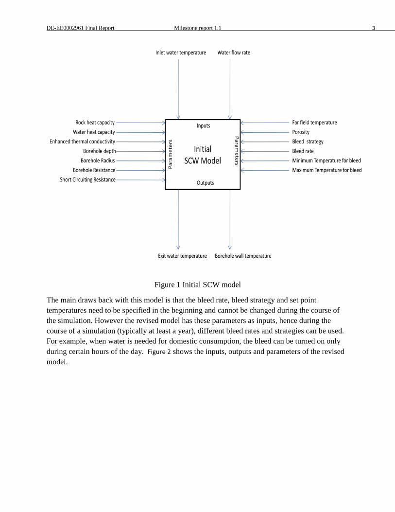
DE-EE0002961 Final Report Milestone report 1.1 3
Figure 1 Initial SCW model
The main draws back with this model is that the bleed rate, bleed strategy and set point temperatures need to be specified in the beginning and cannot be changed during the course of the simulation. However the revised model has these parameters as inputs, hence during the course of a simulation (typically at least a year), different bleed rates and strategies can be used. For example, when water is needed for domestic consumption, the bleed can be turned on only during certain hours of the day. Figure 2 shows the inputs, outputs and parameters of the revised model.
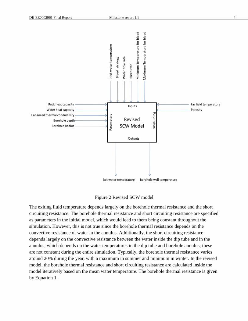
DE-EE0002961 Final Report Milestone report 1.1 4
Figure 2 Revised SCW model
The exiting fluid temperature depends largely on the borehole thermal resistance and the short circuiting resistance. The borehole thermal resistance and short circuiting resistance are specified as parameters in the initial model, which would lead to them being constant throughout the simulation. However, this is not true since the borehole thermal resistance depends on the convective resistance of water in the annulus. Additionally, the short circuiting resistance depends largely on the convective resistance between the water inside the dip tube and in the annulus, which depends on the water temperatures in the dip tube and borehole annulus; these are not constant during the entire simulation. Typically, the borehole thermal resistance varies around 20% during the year, with a maximum in summer and minimum in winter. In the revised model, the borehole thermal resistance and short circuiting resistance are calculated inside the model iteratively based on the mean water temperature. The borehole thermal resistance is given by Equation 1.
DE-EE0002961 Final Report Milestone report 1.1 5
𝑅𝑏 = 12𝜋𝑟𝑏ℎ𝑚𝑎𝑥
(1)
ℎ𝑚𝑎𝑥 = 𝑀𝐴𝑋 (ℎ𝑛𝑎𝑡𝑢𝑟𝑎𝑙,ℎ𝑓𝑜𝑟𝑐𝑒𝑑) (2)
The Nusselt number for forced convection is given by Equation 3 (Gnielinski correlation) and is applicable for values of Reynolds number greater than 2300 where the Reynolds number is based on the annulus gap.
𝑁𝑢 = �𝑓2�(𝑅𝑒−1000)𝑃𝑟
1+12.7 �𝑓2�0.5
(𝑃𝑟23− 1)
(3)
The Nusselt number based on annulus gap for natural convection is given by Equation 4. Equation 4 is obtained using a regression analysis from the experimentally determined values of borehole thermal resistance for GLHEs in ground water filled boreholes. The detailed procedure is listed in Appendix A.
𝑁𝑢 = 0.969 𝑅𝑎∗0.167𝑅−0.466 (4)
However in SCWs due to the high values of heat transfer coefficient in the annulus it was found that the heat transfer depends mainly on the enhanced thermal conductivity of the ground as the thermal resistance of the ground is much greater than the thermal resistance of the water in the annulus under nearly all practical operating conditions.
The SCW model consists of two sub models: a borehole model and a ground model which are coupled together using the heat flux at the borehole wall and solved iteratively. Initially a heat flux (q) is set at the borehole wall. This heat flux is then used as one of the boundary conditions along with the far field temperature to solve the 1-D energy equation for the ground (in radial direction) in a porous medium to determine the borehole wall temperature (Tb) according to Deng (2004).
For the borehole model it is assumed that the water in the borehole is well mixed and that there is only one lump in the borehole which includes water inside the dip tube an energy balance on the borehole can be performed. Equation 5 gives the energy balance on the borehole.
LR
TTTCmTrCmTCrm
dtdT
mCb
fbfopgwpfip
fp ⋅
−+−+−= )1( (5)
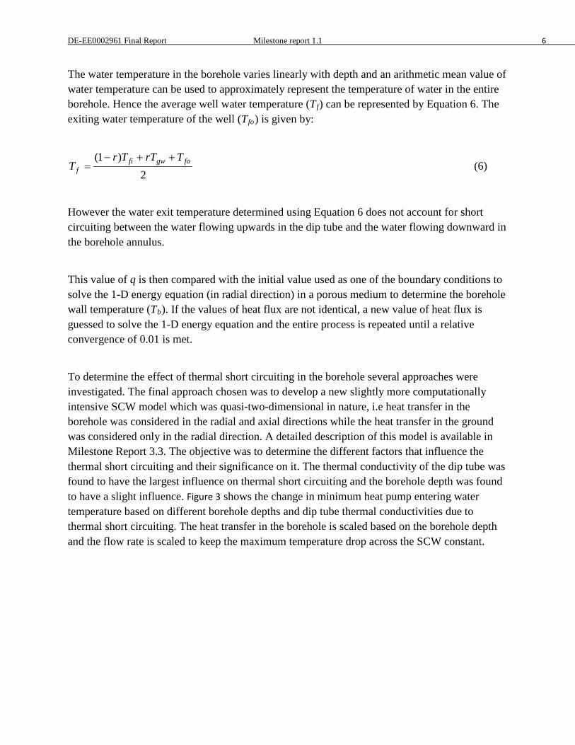
DE-EE0002961 Final Report Milestone report 1.1 6
The water temperature in the borehole varies linearly with depth and an arithmetic mean value of water temperature can be used to approximately represent the temperature of water in the entire borehole. Hence the average well water temperature (Tf) can be represented by Equation 6. The exiting water temperature of the well (Tfo) is given by:
2)1( fogwfi
fTrTTr
T++−
= (6)
However the water exit temperature determined using Equation 6 does not account for short circuiting between the water flowing upwards in the dip tube and the water flowing downward in the borehole annulus.
This value of q is then compared with the initial value used as one of the boundary conditions to solve the 1-D energy equation (in radial direction) in a porous medium to determine the borehole wall temperature (Tb). If the values of heat flux are not identical, a new value of heat flux is guessed to solve the 1-D energy equation and the entire process is repeated until a relative convergence of 0.01 is met.
To determine the effect of thermal short circuiting in the borehole several approaches were investigated. The final approach chosen was to develop a new slightly more computationally intensive SCW model which was quasi-two-dimensional in nature, i.e heat transfer in the borehole was considered in the radial and axial directions while the heat transfer in the ground was considered only in the radial direction. A detailed description of this model is available in Milestone Report 3.3. The objective was to determine the different factors that influence the thermal short circuiting and their significance on it. The thermal conductivity of the dip tube was found to have the largest influence on thermal short circuiting and the borehole depth was found to have a slight influence. Figure 3 shows the change in minimum heat pump entering water temperature based on different borehole depths and dip tube thermal conductivities due to thermal short circuiting. The heat transfer in the borehole is scaled based on the borehole depth and the flow rate is scaled to keep the maximum temperature drop across the SCW constant.
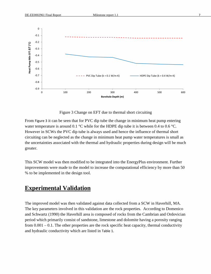
DE-EE0002961 Final Report Milestone report 1.1 7
Figure 3 Change on EFT due to thermal short circuiting
From Figure 3 it can be seen that for PVC dip tube the change in minimum heat pump entering water temperature is around 0.1 °C while for the HDPE dip tube it is between 0.4 to 0.6 °C. However in SCWs the PVC dip tube is always used and hence the influence of thermal short circuiting can be neglected as the change in minimum heat pump water temperatures is small as the uncertainties associated with the thermal and hydraulic properties during design will be much greater.
This SCW model was then modified to be integrated into the EnergyPlus environment. Further improvements were made to the model to increase the computational efficiency by more than 50 % to be implemented in the design tool.
Experimental Validation
The improved model was then validated against data collected from a SCW in Haverhill, MA. The key parameters involved in this validation are the rock properties. According to Domenico and Schwartz (1990) the Haverhill area is composed of rocks from the Cambrian and Ordovician period which primarily consist of sandstone, limestone and dolomite having a porosity ranging from 0.001 – 0.1. The other properties are the rock specific heat capacity, thermal conductivity and hydraulic conductivity which are listed in Table 1.
-0.9
-0.8
-0.7
-0.6
-0.5
-0.4
-0.3
-0.2
-0.1
0
0 100 200 300 400 500 600
Heat
Pum
p M
in E
FT Δ
T (°
C)
Borehole Depth (m)
PVC Dip Tube (k = 0.1 W/m-K) HDPE Dip Tube (k = 0.4 W/m-K)
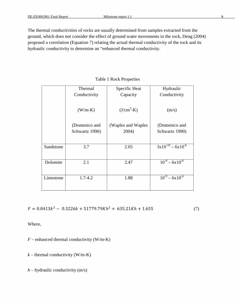
DE-EE0002961 Final Report Milestone report 1.1 8
The thermal conductivities of rocks are usually determined from samples extracted from the ground, which does not consider the effect of ground water movements in the rock, Deng (2004) proposed a correlation (Equation 7) relating the actual thermal conductivity of the rock and its hydraulic conductivity to determine an “enhanced thermal conductivity.
Table 1 Rock Properties
Thermal Conductivity
(W/m-K)
(Domenico and Schwartz 1990)
Specific Heat Capacity
(J/cm3-K)
(Waples and Waples 2004)
Hydraulic Conductivity
(m/s)
(Domenico and Schwartz 1990)
Sandstone 3.7 2.05 3x10⁻¹⁰ – 6x10⁻⁶
Dolomite 2.1 2.47 10-9 – 6x10⁻⁶
Limestone 1.7-4.2 1.88 10-9 – 6x10⁻⁶
𝐹 = 0.0413𝑘2 − 0.3226𝑘 + 51779.79𝐾ℎ2 + 635.21𝐾ℎ + 1.655 (7)
Where,
F – enhanced thermal conductivity (W/m-K)
k – thermal conductivity (W/m-K)
h – hydraulic conductivity (m/s)
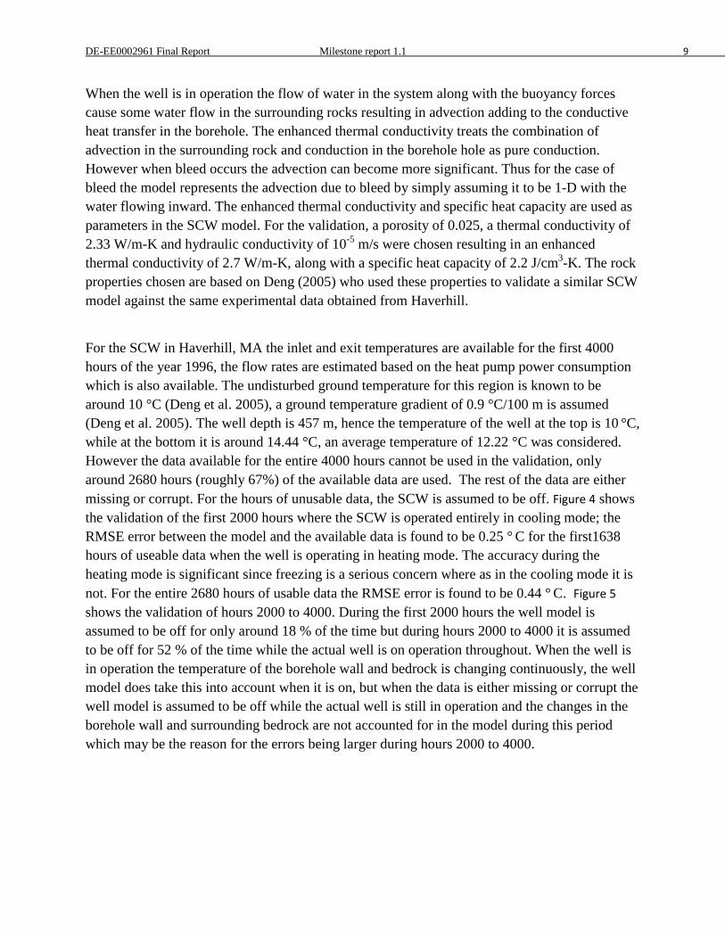
DE-EE0002961 Final Report Milestone report 1.1 9
When the well is in operation the flow of water in the system along with the buoyancy forces cause some water flow in the surrounding rocks resulting in advection adding to the conductive heat transfer in the borehole. The enhanced thermal conductivity treats the combination of advection in the surrounding rock and conduction in the borehole hole as pure conduction. However when bleed occurs the advection can become more significant. Thus for the case of bleed the model represents the advection due to bleed by simply assuming it to be 1-D with the water flowing inward. The enhanced thermal conductivity and specific heat capacity are used as parameters in the SCW model. For the validation, a porosity of 0.025, a thermal conductivity of 2.33 W/m-K and hydraulic conductivity of 10-5 m/s were chosen resulting in an enhanced thermal conductivity of 2.7 W/m-K, along with a specific heat capacity of 2.2 J/cm3-K. The rock properties chosen are based on Deng (2005) who used these properties to validate a similar SCW model against the same experimental data obtained from Haverhill.
For the SCW in Haverhill, MA the inlet and exit temperatures are available for the first 4000 hours of the year 1996, the flow rates are estimated based on the heat pump power consumption which is also available. The undisturbed ground temperature for this region is known to be around 10 °C (Deng et al. 2005), a ground temperature gradient of 0.9 °C/100 m is assumed (Deng et al. 2005). The well depth is 457 m, hence the temperature of the well at the top is 10 °C, while at the bottom it is around 14.44 °C, an average temperature of 12.22 °C was considered. However the data available for the entire 4000 hours cannot be used in the validation, only around 2680 hours (roughly 67%) of the available data are used. The rest of the data are either missing or corrupt. For the hours of unusable data, the SCW is assumed to be off. Figure 4 shows the validation of the first 2000 hours where the SCW is operated entirely in cooling mode; the RMSE error between the model and the available data is found to be 0.25 ° C for the first1638 hours of useable data when the well is operating in heating mode. The accuracy during the heating mode is significant since freezing is a serious concern where as in the cooling mode it is not. For the entire 2680 hours of usable data the RMSE error is found to be 0.44 ° C. Figure 5 shows the validation of hours 2000 to 4000. During the first 2000 hours the well model is assumed to be off for only around 18 % of the time but during hours 2000 to 4000 it is assumed to be off for 52 % of the time while the actual well is on operation throughout. When the well is in operation the temperature of the borehole wall and bedrock is changing continuously, the well model does take this into account when it is on, but when the data is either missing or corrupt the well model is assumed to be off while the actual well is still in operation and the changes in the borehole wall and surrounding bedrock are not accounted for in the model during this period which may be the reason for the errors being larger during hours 2000 to 4000.
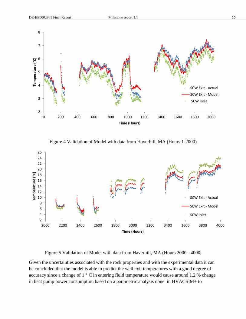
DE-EE0002961 Final Report Milestone report 1.1 10
Figure 4 Validation of Model with data from Haverhill, MA (Hours 1-2000)
Figure 5 Validation of Model with data from Haverhill, MA (Hours 2000 - 4000)
Given the uncertainties associated with the rock properties and with the experimental data it can be concluded that the model is able to predict the well exit temperatures with a good degree of accuracy since a change of 1 ° C in entering fluid temperature would cause around 1.2 % change in heat pump power consumption based on a parametric analysis done in HVACSIM+ to
2
3
4
5
6
7
8
0 200 400 600 800 1000 1200 1400 1600 1800 2000
Tem
pera
ture
(°C)
Time (Hours)
SCW Exit - Actual
SCW Exit - Model
SCW Inlet
2468
101214161820222426
2000 2200 2400 2600 2800 3000 3200 3400 3600 3800 4000
Tem
pera
ture
(°C)
Time (Hours)
SCW Exit - Actual
SCW Exit - Model
SCW Inlet

DE-EE0002961 Final Report Milestone report 1.1 11
investigate the change in power consumption based on entering fluid temperature of a heat pump running building load similar to that of the building in Haverhill. The results of this validated HCACSIM+ model were then used to verify the results of the model implanted in the design tool and in EnergyPlus.
Nomenclature:
A – aspect ratio
α – thermal diffusivity in m2/s
β – volumetric expansion coefficient in 1/K
Cp = specific heat of water in J/kg-K
C1 = specific heat of the fluid in the annulus in J/kg-K
C2 = specific heat of the fluid in the annulus in J/kg-K
Di – U-pipe inner diameter in m
Do – U-pipe outer diameter in m
Db – borehole diameter in m
F = surface area of the dip tube in m2 , dipdip LrF π2=
f – friction factor
g – acceleration due to gravity in m/s2
hnatural = convection coefficient due to natural convection in W/m2-K

DE-EE0002961 Final Report Milestone report 1.1 12
hforced = convection coefficient due to forced convection in W/m2-K
hmax = maximum value of convection coefficient in the well W/m2-K
hin – convection coefficient inside U-pipe in W/m2-K
hnc – natural convection coefficient in W/m2-K
k – thermal conductivity in W/m-K
L - borehole depth in m
Lc – characteristic length (annulus gap) in m
m = mass of water in the standing column well in kg
m = the mass flow rate of water through the heat pump system in kg/s
M1 = mass flow rate in the annulus in kg/s
M2 = mass flow rate in the dip tube in kg/s
Nu – Nusselt number
ν – kinematic viscosity in m2/s
Pr – Prandtl number
qpo – heat flux at pipe wall in W/m2
Qsc = short circuiting heat transfer rate in W

DE-EE0002961 Final Report Milestone report 1.1 13
Q = ground load in W
q = heat flux at borehole wall in W/m2
rb = borehole radius in m
r = bleed rate (-)
R – radius Ratio
bR = borehole resistance in K/(W/m)
Rin – convective resistance inside U-pipe in m-K/w
Rpipe – conductive resistance of U-pipe in m-K/W
Rnc – convective resistance die to natural convection in m-K/W
ρ – density in kg/m3
rbhw – borehole radius in m
rpo – outer radius of pipe in m
Ra – Rayleigh number = 𝑔𝛽𝛥𝑇 𝐿𝐶3
𝛼𝜈2
Ra* - modified Rayleigh number = 𝑔𝛽𝑞 𝐿𝐶4
𝛼𝜈2
Re – Reynolds number
br = the borehole radius in m
DE-EE0002961 Final Report Milestone report 1.1 14
t∆ = time increment in seconds
foT = water temperature leaving the well in ºC
fiT = water temperature entering to the well in ºC
fT = average water temperature at the time step tt ∆+ in ºC
oldfT _ = average water temperature at the previous time step in ºC
bT = borehole wall temperature in ºC
gwT = temperature of groundwater entering into the well in ºC in this model, this temperature is
set to be bT
Tfosc = water temperature exiting the well after taking short circuiting into consideration
U = overall heat transfer coefficient between water in the dip tube and the annulus in W/m2-K
V – flow velocity (m/s)
ABBREVIATIONS:
GLHE – Ground Loop Heat Exchanger
SCW – Standing Column Well
TRT – Thermal Response Test
DE-EE0002961 Final Report Milestone report 1.1 15
References:
Austin III, W.A. 1998. Development of an In Situ system for Measuring Ground Thermal Properties. M.S. Thesis, Oklahoma State University.
Deng, Z. 2004. Modeling of Standing Column Wells in Ground Source Heat Pump Systems. Ph.D. Thesis, Oklahoma State University.
Deng, Z., Rees,S.J. and Spitler, J.D. 2005. A Model for Annual Simulation of Standing Column Well Ground Heat Exchangers. HVAC&R Research 11(4):637-655.
Domenico, P.A., and F.W. Schwartz. 1990. Physical and Chemical Hydrogeology. NewYork: John Wiley & Sons, Inc.
Gustafsson, A. M. and L. Westerlund. 2010. Multi-injection rate thermal response test in groundwater filled borehole heat exchanger. Renewable Energy 35(5): 1061-1070.
Hellström, G. and Kjellsson, E. 2000. Laboratory measurements of heat transfer properties of different types of borehole heat exchangers. Proc. of Terrastock 2000, Stuttgart, Germany. Javed, S. 2010. Design of ground source heat pump systems, Thermal modeling and evaluation of boreholes. Licentiate thesis, Chalmers University of Technology, Göteborg, Sweden. Javed,S., Spitler.J.D. and Fahlén,P.2010. An experimental investigation of the accuracy of thermal response tests used to measure ground thermal properties. ASHRAE Transactions , 116(2) In Press McQuay International. 2011. Geothermal Heat Pump Design Manual. Application Guide, AG 31-008.
Thomas, R.W and de Vahl Davis,G. 1970 Natural Convection in Annular and Rectangular Cavities. Journal of Heat Transfer, Vol 4, Paper NC 2.4.

DE-EE0002961 Final Report Milestone report 1.1 16
Waples, D.W and Waples, J.S. 2004. A review and evaluation of specific heat capacities of rocks, minerals and subsurface fluids. Part 1: Minerals and nonporous rocks. Natural Resources Research 13(2): 97-121.
Young, R. 2004. Development, Verification, and Design Analysis of the Borehole Fluid Thermal Mass Model for Approximating Short Term Borehole Thermal Response. M.S. Thesis, Oklahoma State University, Stillwater, OK.
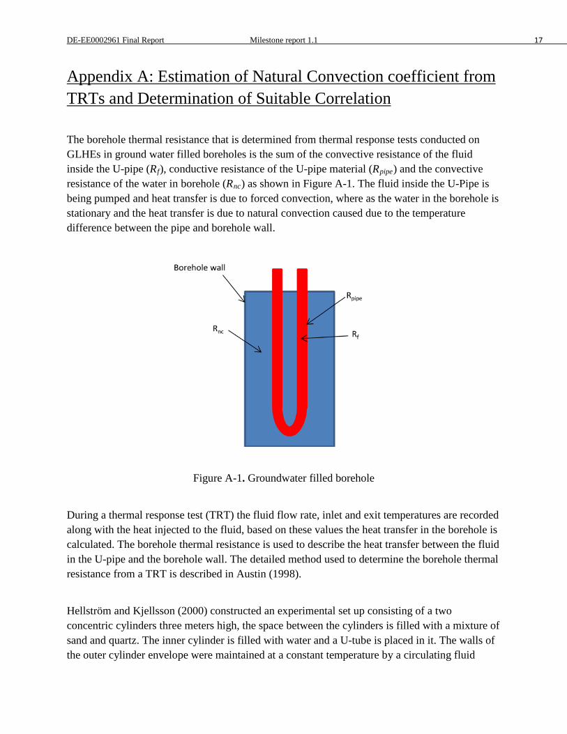
DE-EE0002961 Final Report Milestone report 1.1 17
Appendix A: Estimation of Natural Convection coefficient from TRTs and Determination of Suitable Correlation
The borehole thermal resistance that is determined from thermal response tests conducted on GLHEs in ground water filled boreholes is the sum of the convective resistance of the fluid inside the U-pipe (Rf), conductive resistance of the U-pipe material (Rpipe) and the convective resistance of the water in borehole (Rnc) as shown in Figure A-1. The fluid inside the U-Pipe is being pumped and heat transfer is due to forced convection, where as the water in the borehole is stationary and the heat transfer is due to natural convection caused due to the temperature difference between the pipe and borehole wall.
Figure A-1. Groundwater filled borehole
During a thermal response test (TRT) the fluid flow rate, inlet and exit temperatures are recorded along with the heat injected to the fluid, based on these values the heat transfer in the borehole is calculated. The borehole thermal resistance is used to describe the heat transfer between the fluid in the U-pipe and the borehole wall. The detailed method used to determine the borehole thermal resistance from a TRT is described in Austin (1998).
Hellström and Kjellsson (2000) constructed an experimental set up consisting of a two concentric cylinders three meters high, the space between the cylinders is filled with a mixture of sand and quartz. The inner cylinder is filled with water and a U-tube is placed in it. The walls of the outer cylinder envelope were maintained at a constant temperature by a circulating fluid
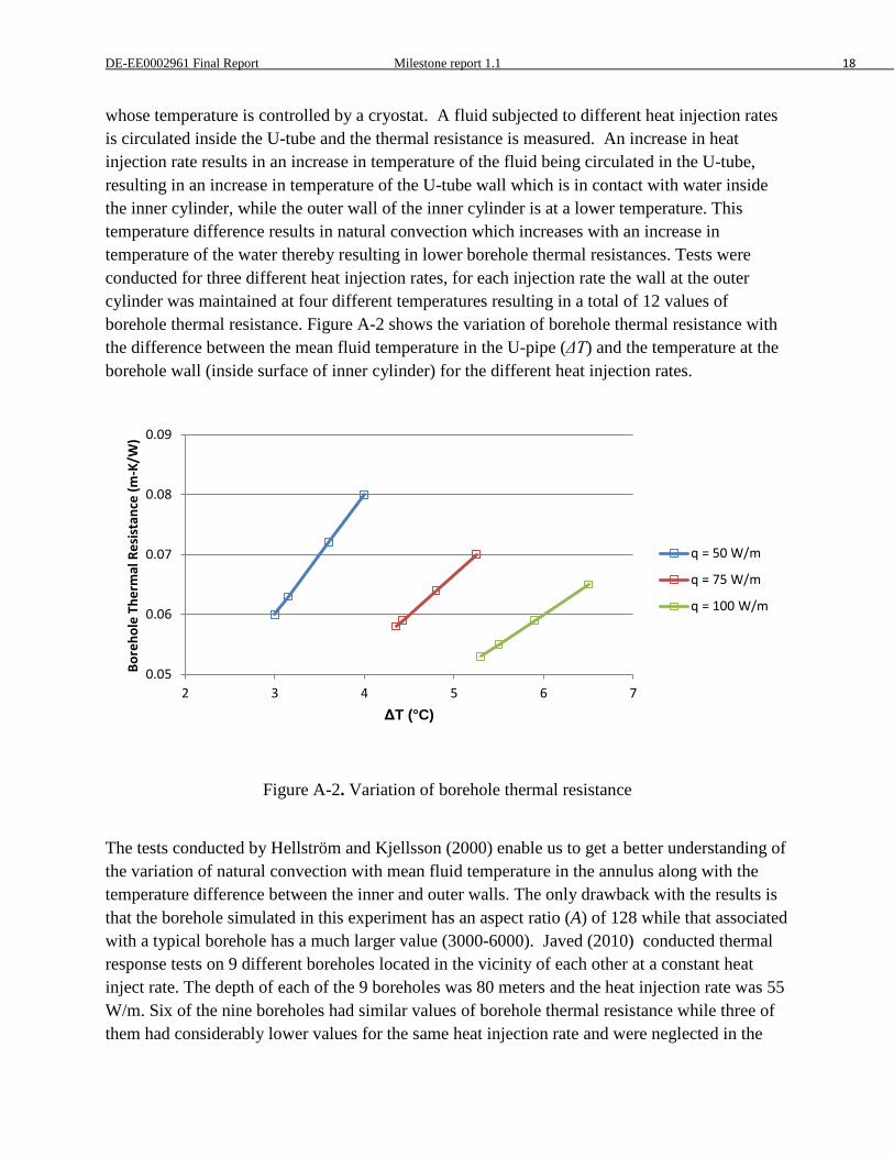
DE-EE0002961 Final Report Milestone report 1.1 18
whose temperature is controlled by a cryostat. A fluid subjected to different heat injection rates is circulated inside the U-tube and the thermal resistance is measured. An increase in heat injection rate results in an increase in temperature of the fluid being circulated in the U-tube, resulting in an increase in temperature of the U-tube wall which is in contact with water inside the inner cylinder, while the outer wall of the inner cylinder is at a lower temperature. This temperature difference results in natural convection which increases with an increase in temperature of the water thereby resulting in lower borehole thermal resistances. Tests were conducted for three different heat injection rates, for each injection rate the wall at the outer cylinder was maintained at four different temperatures resulting in a total of 12 values of borehole thermal resistance. Figure A-2 shows the variation of borehole thermal resistance with the difference between the mean fluid temperature in the U-pipe (ΔT) and the temperature at the borehole wall (inside surface of inner cylinder) for the different heat injection rates.
Figure A-2. Variation of borehole thermal resistance
The tests conducted by Hellström and Kjellsson (2000) enable us to get a better understanding of the variation of natural convection with mean fluid temperature in the annulus along with the temperature difference between the inner and outer walls. The only drawback with the results is that the borehole simulated in this experiment has an aspect ratio (A) of 128 while that associated with a typical borehole has a much larger value (3000-6000). Javed (2010) conducted thermal response tests on 9 different boreholes located in the vicinity of each other at a constant heat inject rate. The depth of each of the 9 boreholes was 80 meters and the heat injection rate was 55 W/m. Six of the nine boreholes had similar values of borehole thermal resistance while three of them had considerably lower values for the same heat injection rate and were neglected in the
0.05
0.06
0.07
0.08
0.09
2 3 4 5 6 7
Bore
hole
The
rmal
Res
ista
nce
(m-K
/W)
ΔT (°C)
q = 50 W/m
q = 75 W/m
q = 100 W/m
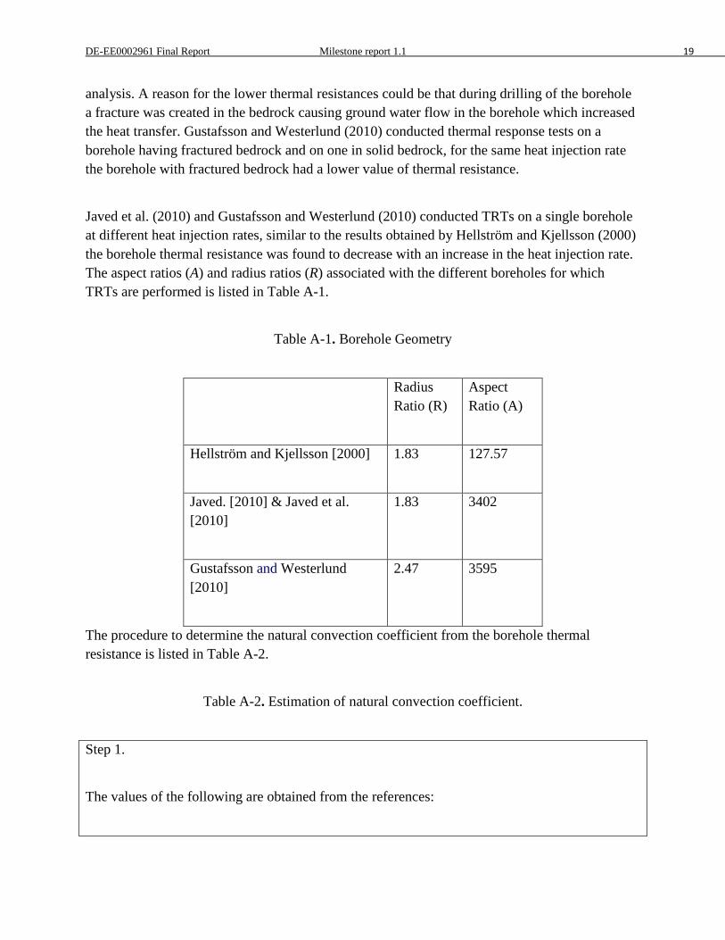
DE-EE0002961 Final Report Milestone report 1.1 19
analysis. A reason for the lower thermal resistances could be that during drilling of the borehole a fracture was created in the bedrock causing ground water flow in the borehole which increased the heat transfer. Gustafsson and Westerlund (2010) conducted thermal response tests on a borehole having fractured bedrock and on one in solid bedrock, for the same heat injection rate the borehole with fractured bedrock had a lower value of thermal resistance.
Javed et al. (2010) and Gustafsson and Westerlund (2010) conducted TRTs on a single borehole at different heat injection rates, similar to the results obtained by Hellström and Kjellsson (2000) the borehole thermal resistance was found to decrease with an increase in the heat injection rate. The aspect ratios (A) and radius ratios (R) associated with the different boreholes for which TRTs are performed is listed in Table A-1.
Table A-1. Borehole Geometry
Radius Ratio (R)
Aspect Ratio (A)
Hellström and Kjellsson [2000] 1.83 127.57
Javed. [2010] & Javed et al. [2010]
1.83 3402
Gustafsson and Westerlund [2010]
2.47 3595
The procedure to determine the natural convection coefficient from the borehole thermal resistance is listed in Table A-2.
Table A-2. Estimation of natural convection coefficient.
Step 1.
The values of the following are obtained from the references:
DE-EE0002961 Final Report Milestone report 1.1 20
1. Borehole thermal resistance , Rb (m-K/W) 2. Inside and outside diameters of U-pipe, Di & Do (m) 3. Mean temperature of circulating fluid temperature in the U-Pipe, Tf (°C) 4. Flow velocity of circulating fluid in U-pipe, V (m/s) 5. Thermal conductivity of the U-pipe, k (W/m-K) 6. Heat flux, q (W/m) 7. Borehole diameter, Db (m)
Step 2.
The convection coefficient of the circulating fluid inside the U-pipe (hin) is obtained using the Gnielinski correlation (Gnielinski 1976).
𝑁𝑢 =ℎ𝑖𝑛 ∗ 𝐷𝑖
𝑘
𝑁𝑢 =�𝑓8� (𝑅𝑒 − 1000)𝑃𝑟
1 + 12.7 �𝑓8�12
(𝑃𝑟23 − 1)
The friction factor (f) is given by:
f = (0.79 ln (Re) – 1.64)-2
The Reynolds number is based on the U-pipe inside diameter (Di) and the fluid properties are evaluated at the mean fluid temperature (Tf).
Finally the convective resistance (Rin) of the fluid is given by:
𝑅𝑖𝑛 = 1ℎ𝑖𝑛𝐴𝑖𝑛
(m-K/W)
Where, Ain is the surface area of the U-pipe / meter length.

DE-EE0002961 Final Report Milestone report 1.1 21
Step 3:
The conductive resistance due to the material of the U-pipe is given by:
𝑅𝑝 =𝑙𝑛�𝐷𝑜𝐷𝑖
�
2𝜋𝑘𝑝 (m-K/W)
Where, kp is the thermal conductivity of the pipe material (W/m-K)
Step 4:
The resistance due to natural convection (Rnc) in the borehole annulus is then given by:
𝑅𝑛𝑐 = 𝑅𝑏 + (𝑅𝑝+ 𝑅𝑖𝑛2
) (m-K/W)
The reason for considering only half the value of Rp and Rin is bacuse the U-pipe has 2 legs (Young 2004)
Step 5:
A key assumption in this procedure is that the value of convection coefficient (hnc) is the same at the pipe wall at the borehole wall. Therefore hnc is calculated from the following equation:
𝑅𝑛𝑐 =1
ℎ𝑛𝑐𝐴𝑏ℎ+
1ℎ𝑛𝑐𝐴𝑝
Where,
Abh – surface area of the borehole wall (ΠDb) per meter borehole length
Ap – surface area of two legs of the U-tube per meter length (2ΠDo)
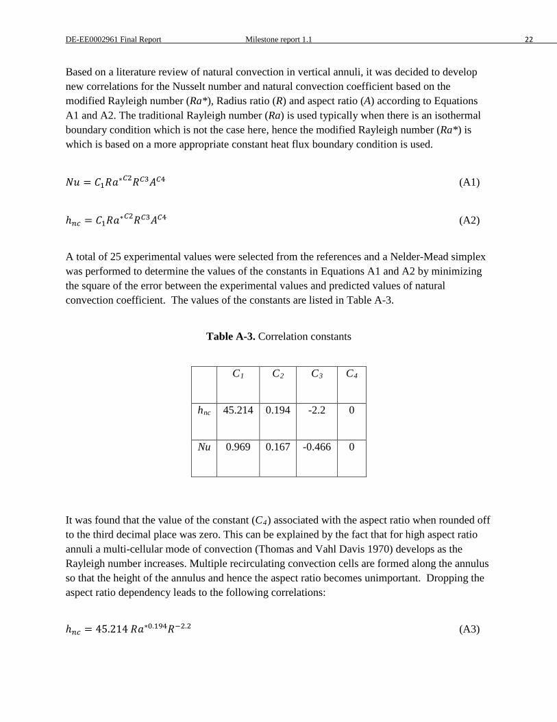
DE-EE0002961 Final Report Milestone report 1.1 22
Based on a literature review of natural convection in vertical annuli, it was decided to develop new correlations for the Nusselt number and natural convection coefficient based on the modified Rayleigh number (Ra*), Radius ratio (R) and aspect ratio (A) according to Equations A1 and A2. The traditional Rayleigh number (Ra) is used typically when there is an isothermal boundary condition which is not the case here, hence the modified Rayleigh number (Ra*) is which is based on a more appropriate constant heat flux boundary condition is used.
𝑁𝑢 = 𝐶1𝑅𝑎∗𝐶2𝑅𝐶3𝐴𝐶4 (A1)
ℎ𝑛𝑐 = 𝐶1𝑅𝑎∗𝐶2𝑅𝐶3𝐴𝐶4 (A2)
A total of 25 experimental values were selected from the references and a Nelder-Mead simplex was performed to determine the values of the constants in Equations A1 and A2 by minimizing the square of the error between the experimental values and predicted values of natural convection coefficient. The values of the constants are listed in Table A-3.
Table A-3. Correlation constants
C1 C2 C3 C4
hnc 45.214 0.194 -2.2 0
Nu 0.969 0.167 -0.466 0
It was found that the value of the constant (C4) associated with the aspect ratio when rounded off to the third decimal place was zero. This can be explained by the fact that for high aspect ratio annuli a multi-cellular mode of convection (Thomas and Vahl Davis 1970) develops as the Rayleigh number increases. Multiple recirculating convection cells are formed along the annulus so that the height of the annulus and hence the aspect ratio becomes unimportant. Dropping the aspect ratio dependency leads to the following correlations:
ℎ𝑛𝑐 = 45.214 𝑅𝑎∗0.194𝑅−2.2 (A3)
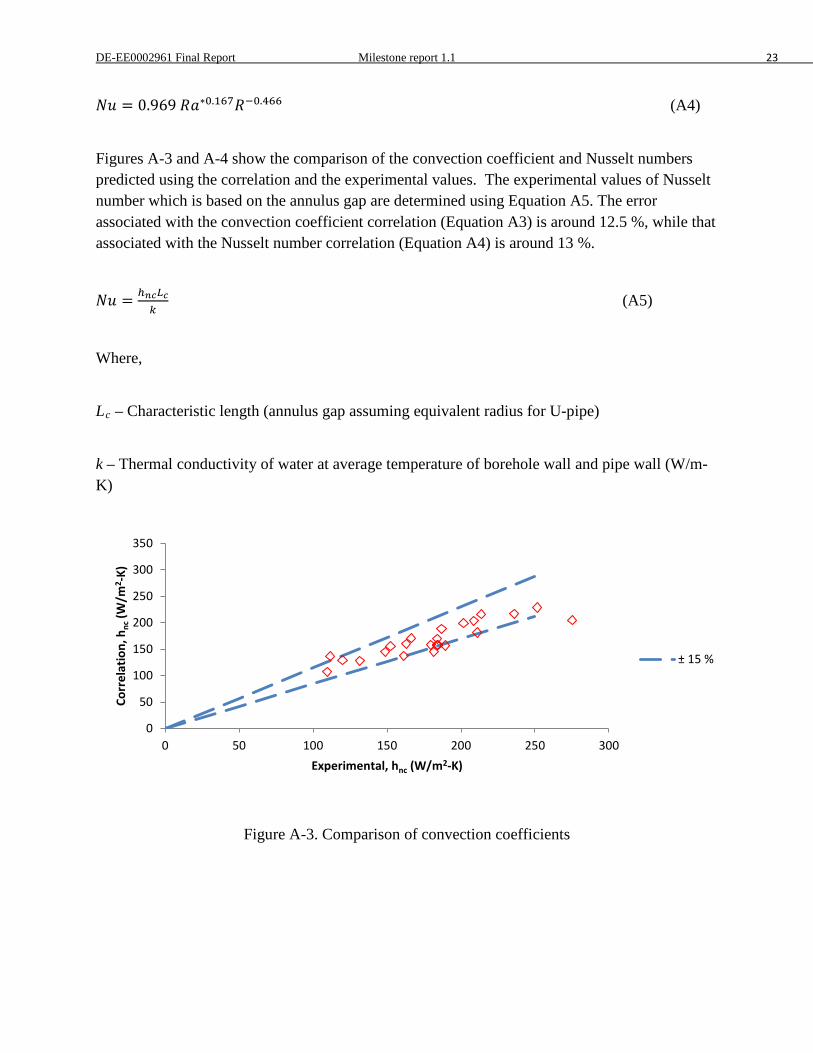
DE-EE0002961 Final Report Milestone report 1.1 23
𝑁𝑢 = 0.969 𝑅𝑎∗0.167𝑅−0.466 (A4)
Figures A-3 and A-4 show the comparison of the convection coefficient and Nusselt numbers predicted using the correlation and the experimental values. The experimental values of Nusselt number which is based on the annulus gap are determined using Equation A5. The error associated with the convection coefficient correlation (Equation A3) is around 12.5 %, while that associated with the Nusselt number correlation (Equation A4) is around 13 %.
𝑁𝑢 = ℎ𝑛𝑐𝐿𝑐𝑘
(A5)
Where,
Lc – Characteristic length (annulus gap assuming equivalent radius for U-pipe)
k – Thermal conductivity of water at average temperature of borehole wall and pipe wall (W/m-K)
Figure A-3. Comparison of convection coefficients
0
50
100
150
200
250
300
350
0 50 100 150 200 250 300
Corr
elat
ion,
hnc
(W/m
2 -K)
Experimental, hnc (W/m2-K)
± 15 %
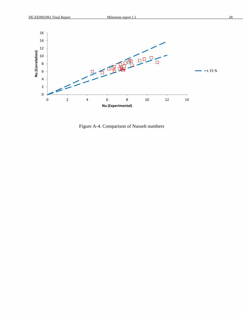
DE-EE0002961 Final Report Milestone report 1.1 24
Figure A-4. Comparison of Nusselt numbers
0
2
4
6
8
10
12
14
16
0 2 4 6 8 10 12 14
Nu
(Cor
rela
tion)
Nu (Experimental)
± 15 %

DE-EE0002961 Final Report Milestone report 1.2 1
Milestone Report 1.2
Testing of model with various bleed control strategies
Annamalai Ramesh
Oklahoma State University

DE-EE0002961 Final Report Milestone report 1.2 2
Milestone Progress Report
Task 1.2-Testing of model with various bleed control strategies
DE-EE0002961/001 - Recovery Act:
Improved Design Tools for Surface Water and Standing Column Well Heat Pump Systems
Annamalai Ramesh, ([email protected]), Research Associate
Professor Jeffrey D. Spitler, ([email protected]), Principal Investigator Oklahoma State University
Introduction In a standard SCW system the water is recirculated between the well and the heat pump. In SCW systems that operate with bleed a portion of the water is discarded after it passes through the heat pump and is not returned to the well, this causes surrounding ground water to enter into the well, since the surrounding ground water is warmer than the water already in the well during winter and cooler during summer, it results in an increased heat transfer in the system which leads to smaller required well depths. Work done as part of Subtask 1.1 listed in the milestone report for it involved making significant improvements regarding bleed control to a pre existing 1-D SCW model (Deng 2004). However when the SCW is operating with bleed, the circulating pump needs to provide the lift that is necessary in transporting the water to the surface which results in increased power consumption.
As part of this study various bleed strategies and their impact on required well depths, heat pump power consumption and circulating pump power consumption are investigated and compared with the case of an SCW with no bleed and a closed GLHE for a commercial building at five different locations in the United States. The different bleed strategies under investigation are:
1. Temperature dependent bleed – Here when the temperature of water entering the heat pump falls below or above minimum (8 °C) and maximum (28.5 °C) set points a constant bleed rate (10% of total flow) is used.
2. Domestic bleed – Here the bleed is operated for a specified duration and the bleed rate depends on the domestic water consumption of the building.
Another factor involving SCWs which is investigated in this study is the well draw down. The draw down is the drop in water level below the static water level when it is being pumped as
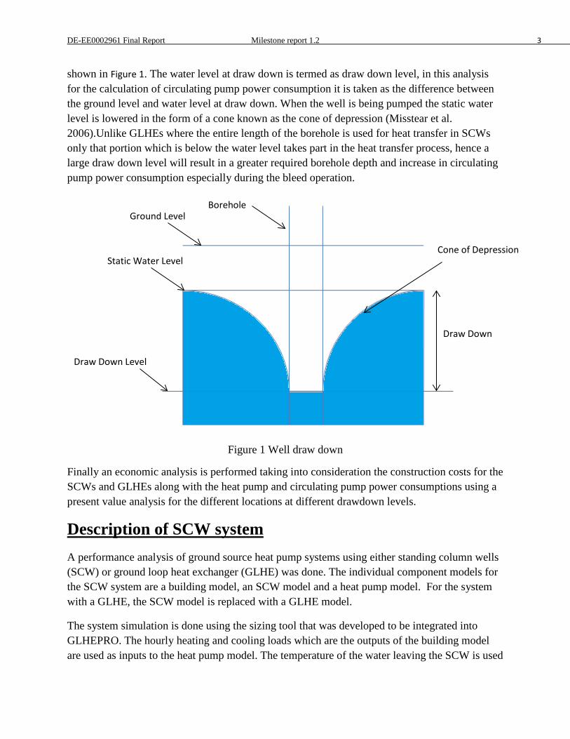
DE-EE0002961 Final Report Milestone report 1.2 3
shown in Figure 1. The water level at draw down is termed as draw down level, in this analysis for the calculation of circulating pump power consumption it is taken as the difference between the ground level and water level at draw down. When the well is being pumped the static water level is lowered in the form of a cone known as the cone of depression (Misstear et al. 2006).Unlike GLHEs where the entire length of the borehole is used for heat transfer in SCWs only that portion which is below the water level takes part in the heat transfer process, hence a large draw down level will result in a greater required borehole depth and increase in circulating pump power consumption especially during the bleed operation.
Figure 1 Well draw down
Finally an economic analysis is performed taking into consideration the construction costs for the SCWs and GLHEs along with the heat pump and circulating pump power consumptions using a present value analysis for the different locations at different drawdown levels.
Description of SCW system A performance analysis of ground source heat pump systems using either standing column wells (SCW) or ground loop heat exchanger (GLHE) was done. The individual component models for the SCW system are a building model, an SCW model and a heat pump model. For the system with a GLHE, the SCW model is replaced with a GLHE model.
The system simulation is done using the sizing tool that was developed to be integrated into GLHEPRO. The hourly heating and cooling loads which are the outputs of the building model are used as inputs to the heat pump model. The temperature of the water leaving the SCW is used
Cone of Depression
Ground Level
Static Water Level
Draw Down Level
Draw Down
Borehole
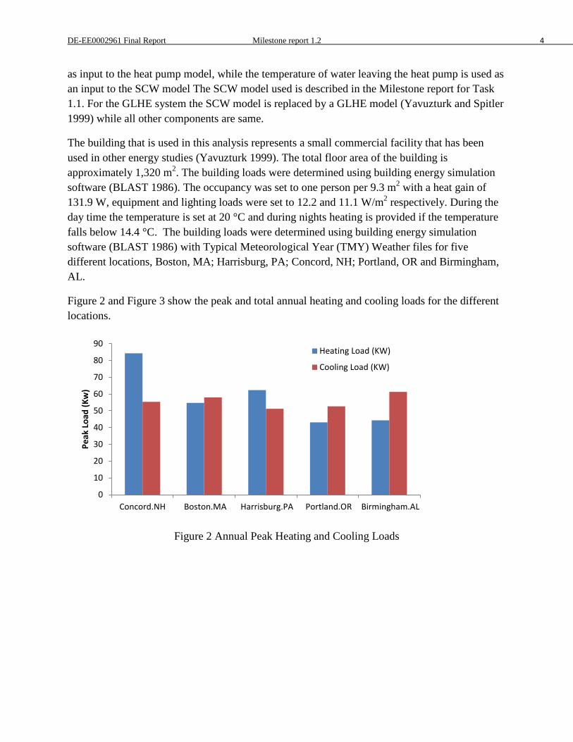
DE-EE0002961 Final Report Milestone report 1.2 4
as input to the heat pump model, while the temperature of water leaving the heat pump is used as an input to the SCW model The SCW model used is described in the Milestone report for Task 1.1. For the GLHE system the SCW model is replaced by a GLHE model (Yavuzturk and Spitler 1999) while all other components are same.
The building that is used in this analysis represents a small commercial facility that has been used in other energy studies (Yavuzturk 1999). The total floor area of the building is approximately 1,320 m2. The building loads were determined using building energy simulation software (BLAST 1986). The occupancy was set to one person per 9.3 m2 with a heat gain of 131.9 W, equipment and lighting loads were set to 12.2 and 11.1 W/m2 respectively. During the day time the temperature is set at 20 °C and during nights heating is provided if the temperature falls below 14.4 °C. The building loads were determined using building energy simulation software (BLAST 1986) with Typical Meteorological Year (TMY) Weather files for five different locations, Boston, MA; Harrisburg, PA; Concord, NH; Portland, OR and Birmingham, AL.
Figure 2 and Figure 3 show the peak and total annual heating and cooling loads for the different locations.
Figure 2 Annual Peak Heating and Cooling Loads
0
10
20
30
40
50
60
70
80
90
Concord.NH Boston.MA Harrisburg.PA Portland.OR Birmingham.AL
Peak
Loa
d (K
w)
Heating Load (KW)
Cooling Load (KW)
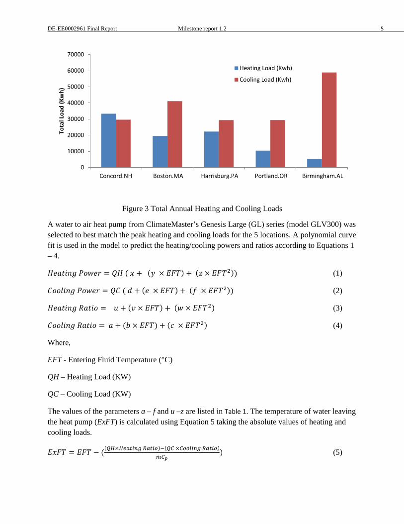
DE-EE0002961 Final Report Milestone report 1.2 5
Figure 3 Total Annual Heating and Cooling Loads
A water to air heat pump from ClimateMaster’s Genesis Large (GL) series (model GLV300) was selected to best match the peak heating and cooling loads for the 5 locations. A polynomial curve fit is used in the model to predict the heating/cooling powers and ratios according to Equations 1 – 4.
𝐻𝑒𝑎𝑡𝑖𝑛𝑔 𝑃𝑜𝑤𝑒𝑟 = 𝑄𝐻 ( 𝑥 + (𝑦 × 𝐸𝐹𝑇) + (𝑧 × 𝐸𝐹𝑇2)) (1)
𝐶𝑜𝑜𝑙𝑖𝑛𝑔 𝑃𝑜𝑤𝑒𝑟 = 𝑄𝐶 ( 𝑑 + (𝑒 × 𝐸𝐹𝑇) + (𝑓 × 𝐸𝐹𝑇2)) (2)
𝐻𝑒𝑎𝑡𝑖𝑛𝑔 𝑅𝑎𝑡𝑖𝑜 = 𝑢 + (𝑣 × 𝐸𝐹𝑇) + (𝑤 × 𝐸𝐹𝑇2) (3)
𝐶𝑜𝑜𝑙𝑖𝑛𝑔 𝑅𝑎𝑡𝑖𝑜 = 𝑎 + (𝑏 × 𝐸𝐹𝑇) + (𝑐 × 𝐸𝐹𝑇2) (4)
Where,
EFT - Entering Fluid Temperature (°C)
QH – Heating Load (KW)
QC – Cooling Load (KW)
The values of the parameters a – f and u –z are listed in Table 1. The temperature of water leaving the heat pump (ExFT) is calculated using Equation 5 taking the absolute values of heating and cooling loads.
𝐸𝑥𝐹𝑇 = 𝐸𝐹𝑇 − ((𝑄𝐻×𝐻𝑒𝑎𝑡𝑖𝑛𝑔 𝑅𝑎𝑡𝑖𝑜)−(𝑄𝐶 ×𝐶𝑜𝑜𝑙𝑖𝑛𝑔 𝑅𝑎𝑡𝑖𝑜)�̇�𝐶𝑝
) (5)
0
10000
20000
30000
40000
50000
60000
70000
Concord.NH Boston.MA Harrisburg.PA Portland.OR Birmingham.AL
Tota
l Loa
d (K
wh)
Heating Load (Kwh)
Cooling Load (Kwh)
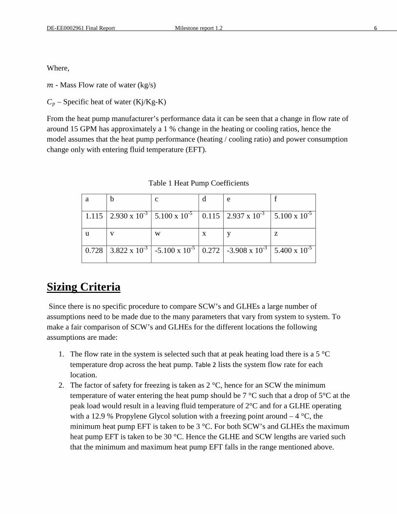
DE-EE0002961 Final Report Milestone report 1.2 6
Where,
𝑚 - Mass Flow rate of water (kg/s)
Cp – Specific heat of water (Kj/Kg-K)
From the heat pump manufacturer’s performance data it can be seen that a change in flow rate of around 15 GPM has approximately a 1 % change in the heating or cooling ratios, hence the model assumes that the heat pump performance (heating / cooling ratio) and power consumption change only with entering fluid temperature (EFT).
Table 1 Heat Pump Coefficients
a b c d e f
1.115 2.930 x 10⁻³ 5.100 x 10⁻⁵ 0.115 2.937 x 10⁻³ 5.100 x 10⁻⁵
u v w x y z
0.728 3.822 x 10⁻³ -5.100 x 10⁻⁵ 0.272 -3.908 x 10⁻³ 5.400 x 10⁻⁵
Sizing Criteria Since there is no specific procedure to compare SCW’s and GLHEs a large number of assumptions need to be made due to the many parameters that vary from system to system. To make a fair comparison of SCW’s and GLHEs for the different locations the following assumptions are made:
1. The flow rate in the system is selected such that at peak heating load there is a 5 °C temperature drop across the heat pump. Table 2 lists the system flow rate for each location.
2. The factor of safety for freezing is taken as 2 °C, hence for an SCW the minimum temperature of water entering the heat pump should be 7 °C such that a drop of 5°C at the peak load would result in a leaving fluid temperature of 2°C and for a GLHE operating with a 12.9 % Propylene Glycol solution with a freezing point around – 4 °C, the minimum heat pump EFT is taken to be 3 °C. For both SCW’s and GLHEs the maximum heat pump EFT is taken to be 30 °C. Hence the GLHE and SCW lengths are varied such that the minimum and maximum heat pump EFT falls in the range mentioned above.
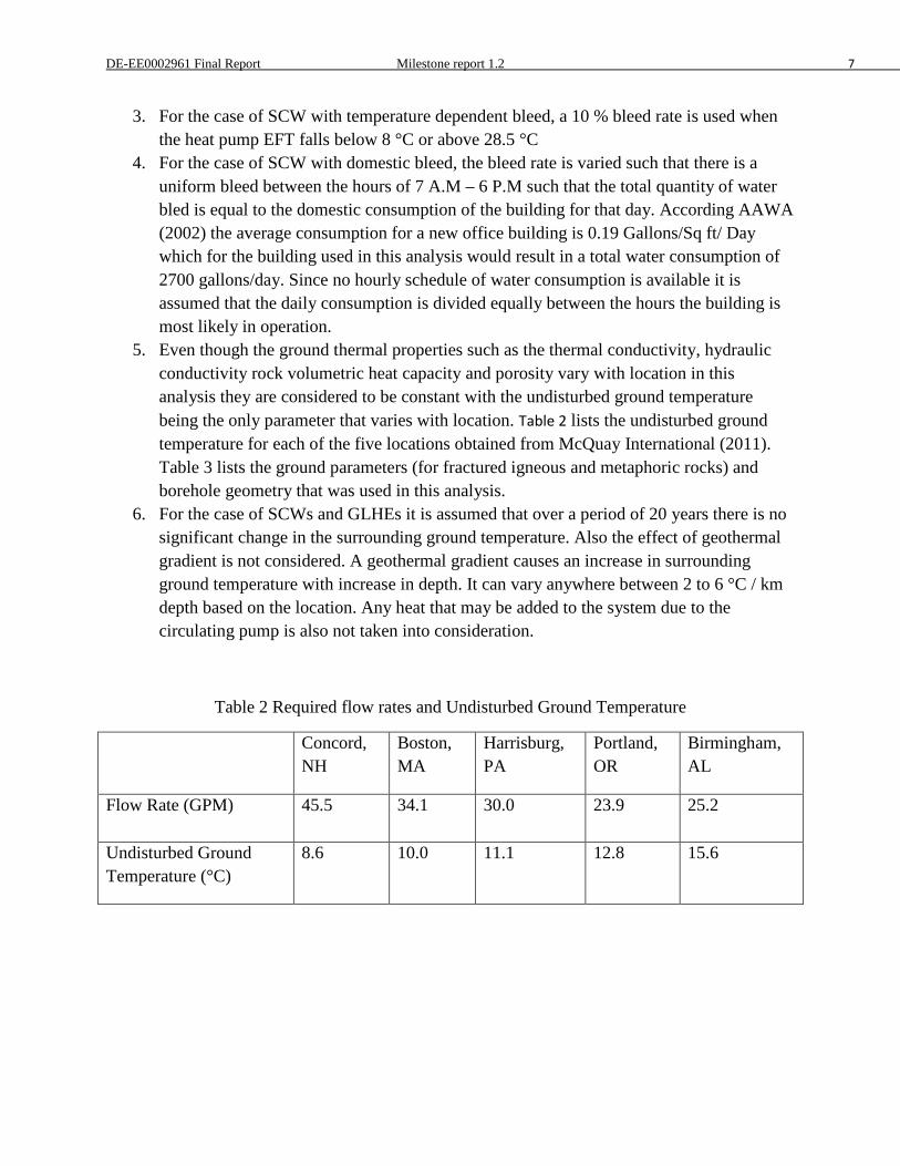
DE-EE0002961 Final Report Milestone report 1.2 7
3. For the case of SCW with temperature dependent bleed, a 10 % bleed rate is used when the heat pump EFT falls below 8 °C or above 28.5 °C
4. For the case of SCW with domestic bleed, the bleed rate is varied such that there is a uniform bleed between the hours of 7 A.M – 6 P.M such that the total quantity of water bled is equal to the domestic consumption of the building for that day. According AAWA (2002) the average consumption for a new office building is 0.19 Gallons/Sq ft/ Day which for the building used in this analysis would result in a total water consumption of 2700 gallons/day. Since no hourly schedule of water consumption is available it is assumed that the daily consumption is divided equally between the hours the building is most likely in operation.
5. Even though the ground thermal properties such as the thermal conductivity, hydraulic conductivity rock volumetric heat capacity and porosity vary with location in this analysis they are considered to be constant with the undisturbed ground temperature being the only parameter that varies with location. Table 2 lists the undisturbed ground temperature for each of the five locations obtained from McQuay International (2011). Table 3 lists the ground parameters (for fractured igneous and metaphoric rocks) and borehole geometry that was used in this analysis.
6. For the case of SCWs and GLHEs it is assumed that over a period of 20 years there is no significant change in the surrounding ground temperature. Also the effect of geothermal gradient is not considered. A geothermal gradient causes an increase in surrounding ground temperature with increase in depth. It can vary anywhere between 2 to 6 °C / km depth based on the location. Any heat that may be added to the system due to the circulating pump is also not taken into consideration.
Table 2 Required flow rates and Undisturbed Ground Temperature
Concord, NH
Boston, MA
Harrisburg, PA
Portland, OR
Birmingham, AL
Flow Rate (GPM) 45.5 34.1 30.0 23.9 25.2
Undisturbed Ground Temperature (°C)
8.6 10.0 11.1 12.8 15.6
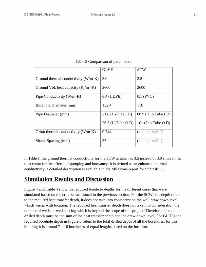
DE-EE0002961 Final Report Milestone report 1.2 8
Table 3 Comparison of parameters
GLHE SCW
Ground thermal conductivity (W/m-K) 3.0 3.5
Ground Vol. heat capacity (Kj/m3-K) 2600 2600
Pipe Conductivity (W/m-K) 0.4 (HDPE) 0.1 (PVC)
Borehole Diameter (mm) 152.4 110
Pipe Diameter (mm) 21.8 (U-Tube I.D)
26.7 (U-Tube O.D)
88.9 ( Dip Tube I.D)
101 (Dip Tube O.D)
Grout thermal conductivity (W/m-K) 0.744 (not applicable)
Shank Spacing (mm) 37 (not applicable)
In Table 3, the ground thermal conductivity for the SCW is taken as 3.5 instead of 3.0 since it has to account for the effects of pumping and buoyancy, it is termed as an enhanced thermal conductivity, a detailed description is available in the Milestone report for Subtask 1.1.
Simulation Results and Discussion Figure 4 and Table 4 show the required borehole depths for the different cases that were simulated based on the criteria mentioned in the previous section. For the SCWs the depth refers to the required heat transfer depth, it does not take into consideration the well draw down level which varies with location. The required heat transfer depth does not take into consideration the number of wells or well spacing which is beyond the scope of this project. Therefore the total drilled depth must be the sum of the heat transfer depth and the draw down level. For GLHEs the required borehole depth in Figure 3 refers to the total drilled depth of all the boreholes, for this building it is around 7 – 10 boreholes of equal lengths based on the location.
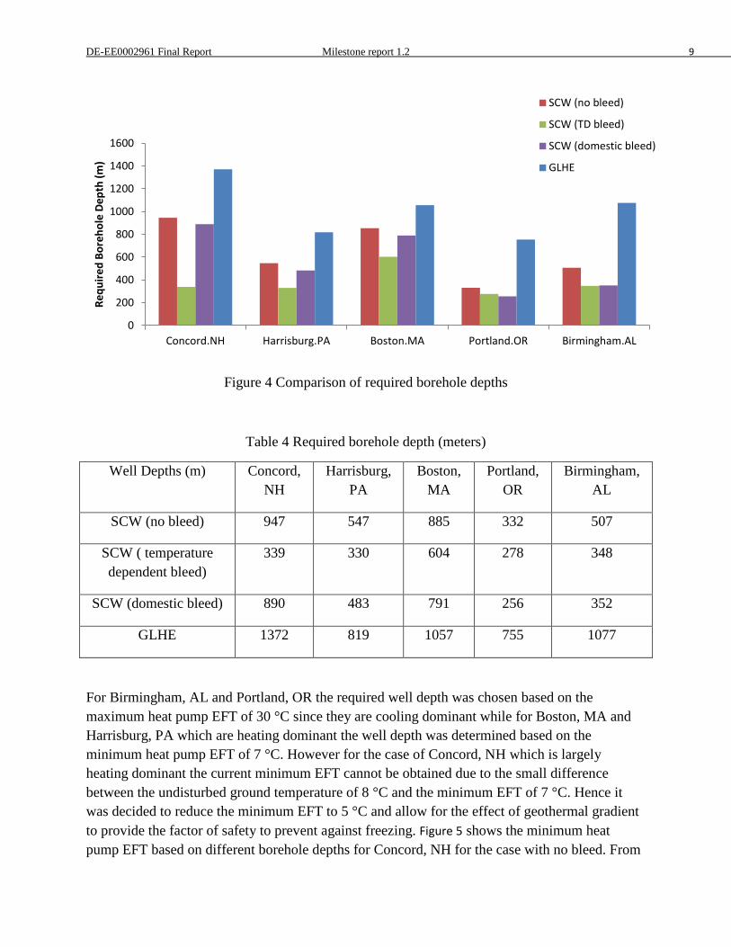
DE-EE0002961 Final Report Milestone report 1.2 9
Figure 4 Comparison of required borehole depths
Table 4 Required borehole depth (meters)
Well Depths (m) Concord, NH
Harrisburg, PA
Boston, MA
Portland, OR
Birmingham, AL
SCW (no bleed) 947 547 885 332 507
SCW ( temperature dependent bleed)
339 330 604 278 348
SCW (domestic bleed) 890 483 791 256 352
GLHE 1372 819 1057 755 1077
For Birmingham, AL and Portland, OR the required well depth was chosen based on the maximum heat pump EFT of 30 °C since they are cooling dominant while for Boston, MA and Harrisburg, PA which are heating dominant the well depth was determined based on the minimum heat pump EFT of 7 °C. However for the case of Concord, NH which is largely heating dominant the current minimum EFT cannot be obtained due to the small difference between the undisturbed ground temperature of 8 °C and the minimum EFT of 7 °C. Hence it was decided to reduce the minimum EFT to 5 °C and allow for the effect of geothermal gradient to provide the factor of safety to prevent against freezing. Figure 5 shows the minimum heat pump EFT based on different borehole depths for Concord, NH for the case with no bleed. From
0
200
400
600
800
1000
1200
1400
1600
Concord.NH Harrisburg.PA Boston.MA Portland.OR Birmingham.AL
Requ
ired
Bore
hole
Dep
th (m
) SCW (no bleed)
SCW (TD bleed)
SCW (domestic bleed)
GLHE
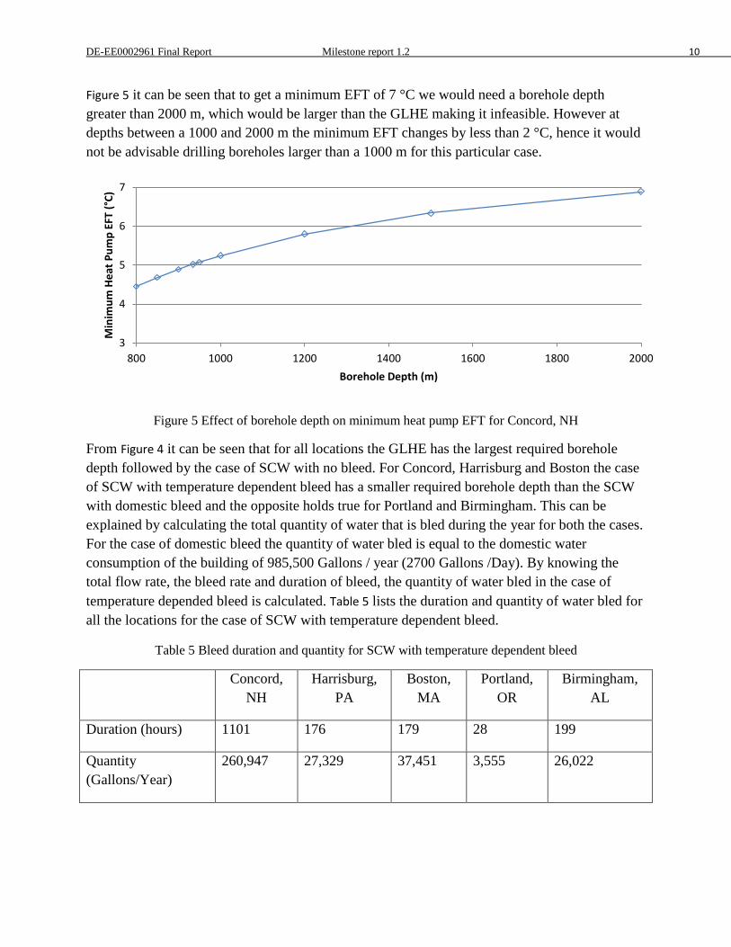
DE-EE0002961 Final Report Milestone report 1.2 10
Figure 5 it can be seen that to get a minimum EFT of 7 °C we would need a borehole depth greater than 2000 m, which would be larger than the GLHE making it infeasible. However at depths between a 1000 and 2000 m the minimum EFT changes by less than 2 °C, hence it would not be advisable drilling boreholes larger than a 1000 m for this particular case.
Figure 5 Effect of borehole depth on minimum heat pump EFT for Concord, NH
From Figure 4 it can be seen that for all locations the GLHE has the largest required borehole depth followed by the case of SCW with no bleed. For Concord, Harrisburg and Boston the case of SCW with temperature dependent bleed has a smaller required borehole depth than the SCW with domestic bleed and the opposite holds true for Portland and Birmingham. This can be explained by calculating the total quantity of water that is bled during the year for both the cases. For the case of domestic bleed the quantity of water bled is equal to the domestic water consumption of the building of 985,500 Gallons / year (2700 Gallons /Day). By knowing the total flow rate, the bleed rate and duration of bleed, the quantity of water bled in the case of temperature depended bleed is calculated. Table 5 lists the duration and quantity of water bled for all the locations for the case of SCW with temperature dependent bleed.
Table 5 Bleed duration and quantity for SCW with temperature dependent bleed
Concord, NH
Harrisburg, PA
Boston, MA
Portland, OR
Birmingham, AL
Duration (hours) 1101 176 179 28 199
Quantity (Gallons/Year)
260,947 27,329 37,451 3,555 26,022
3
4
5
6
7
800 1000 1200 1400 1600 1800 2000
Min
imum
Hea
t Pum
p EF
T (°
C)
Borehole Depth (m)
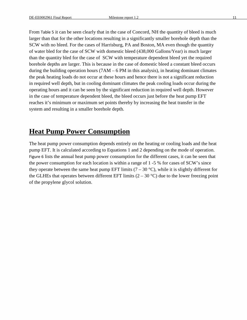
DE-EE0002961 Final Report Milestone report 1.2 11
From Table 5 it can be seen clearly that in the case of Concord, NH the quantity of bleed is much larger than that for the other locations resulting in a significantly smaller borehole depth than the SCW with no bleed. For the cases of Harrisburg, PA and Boston, MA even though the quantity of water bled for the case of SCW with domestic bleed (438,000 Gallons/Year) is much larger than the quantity bled for the case of SCW with temperature dependent bleed yet the required borehole depths are larger. This is because in the case of domestic bleed a constant bleed occurs during the building operation hours (7AM – 6 PM in this analysis), in heating dominant climates the peak heating loads do not occur at these hours and hence there is not a significant reduction in required well depth, but in cooling dominant climates the peak cooling loads occur during the operating hours and it can be seen by the significant reduction in required well depth. However in the case of temperature dependent bleed, the bleed occurs just before the heat pump EFT reaches it’s minimum or maximum set points thereby by increasing the heat transfer in the system and resulting in a smaller borehole depth.
Heat Pump Power Consumption The heat pump power consumption depends entirely on the heating or cooling loads and the heat pump EFT. It is calculated according to Equations 1 and 2 depending on the mode of operation. Figure 6 lists the annual heat pump power consumption for the different cases, it can be seen that the power consumption for each location is within a range of 1 -5 % for cases of SCW’s since they operate between the same heat pump EFT limits (7 – 30 °C), while it is slightly different for the GLHEs that operates between different EFT limits (2 – 30 °C) due to the lower freezing point of the propylene glycol solution.
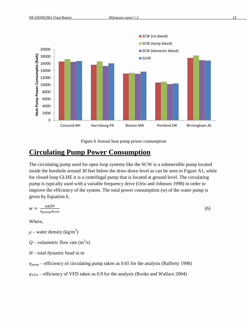
DE-EE0002961 Final Report Milestone report 1.2 12
Figure 6 Annual heat pump power consumption
Circulating Pump Power Consumption The circulating pump used for open loop systems like the SCW is a submersible pump located inside the borehole around 30 feet below the draw down level as can be seen in Figure A1, while for closed loop GLHE it is a centrifugal pump that is located at ground level. The circulating pump is typically used with a variable frequency drive (Orio and Johnson 1998) in order to improve the efficiency of the system. The total power consumption (w) of the water pump is given by Equation 6.
𝑤 = 𝜌𝑔𝑄𝐻𝜂𝑝𝑢𝑚𝑝𝜂𝑉𝐹𝐷
(6)
Where,
ρ – water density (kg/m3)
Q – volumetric flow rate (m3/s)
H – total dynamic head in m
ηpump – efficiency of circulating pump taken as 0.65 for the analysis (Rafferty 1998)
ηVFD – efficiency of VFD taken as 0.9 for the analysis (Rooks and Wallace 2004)
0
2000
4000
6000
8000
10000
12000
14000
16000
18000
20000
Concord.NH Harrisburg.PA Boston.MA Portland.OR Birmingham.AL
Heat
Pum
p Po
wer
Con
sum
ptio
(Kw
h)
SCW (no bleed)
SCW (temp bleed)
SCW (domestic bleed)
GLHE
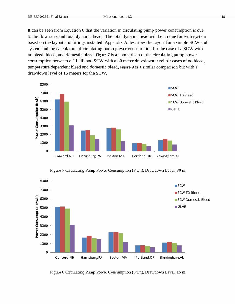
DE-EE0002961 Final Report Milestone report 1.2 13
It can be seen from Equation 6 that the variation in circulating pump power consumption is due to the flow rates and total dynamic head. The total dynamic head will be unique for each system based on the layout and fittings installed. Appendix A describes the layout for a simple SCW and system and the calculation of circulating pump power consumption for the case of a SCW with no bleed, bleed, and domestic bleed. Figure 7 is a comparison of the circulating pump power consumption between a GLHE and SCW with a 30 meter drawdown level for cases of no bleed, temperature dependent bleed and domestic bleed, Figure 8 is a similar comparison but with a drawdown level of 15 meters for the SCW.
Figure 7 Circulating Pump Power Consumption (Kwh), Drawdown Level, 30 m
Figure 8 Circulating Pump Power Consumption (Kwh), Drawdown Level, 15 m
0
1000
2000
3000
4000
5000
6000
7000
8000
Concord.NH Harrisburg.PA Boston.MA Portland.OR Birmingham.AL
Pow
er C
onsu
mpt
ion
(Kw
h)
SCW
SCW TD Bleed
SCW Domestic Bleed
GLHE
0
1000
2000
3000
4000
5000
6000
7000
8000
Concord.NH Harrisburg.PA Boston.MA Portland.OR Birmingham.AL
Pow
er C
onsu
mpt
ion
(Kw
h)
SCW
SCW TD Bleed
SCW Domestic Bleed
GLHE
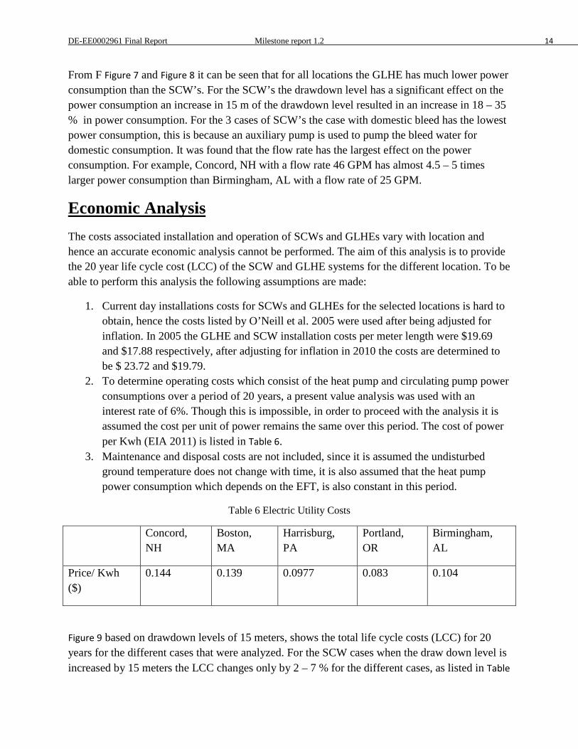
DE-EE0002961 Final Report Milestone report 1.2 14
From F Figure 7 and Figure 8 it can be seen that for all locations the GLHE has much lower power consumption than the SCW’s. For the SCW’s the drawdown level has a significant effect on the power consumption an increase in 15 m of the drawdown level resulted in an increase in 18 – 35 % in power consumption. For the 3 cases of SCW’s the case with domestic bleed has the lowest power consumption, this is because an auxiliary pump is used to pump the bleed water for domestic consumption. It was found that the flow rate has the largest effect on the power consumption. For example, Concord, NH with a flow rate 46 GPM has almost 4.5 – 5 times larger power consumption than Birmingham, AL with a flow rate of 25 GPM.
Economic Analysis The costs associated installation and operation of SCWs and GLHEs vary with location and hence an accurate economic analysis cannot be performed. The aim of this analysis is to provide the 20 year life cycle cost (LCC) of the SCW and GLHE systems for the different location. To be able to perform this analysis the following assumptions are made:
1. Current day installations costs for SCWs and GLHEs for the selected locations is hard to obtain, hence the costs listed by O’Neill et al. 2005 were used after being adjusted for inflation. In 2005 the GLHE and SCW installation costs per meter length were $19.69 and $17.88 respectively, after adjusting for inflation in 2010 the costs are determined to be $ 23.72 and $19.79.
2. To determine operating costs which consist of the heat pump and circulating pump power consumptions over a period of 20 years, a present value analysis was used with an interest rate of 6%. Though this is impossible, in order to proceed with the analysis it is assumed the cost per unit of power remains the same over this period. The cost of power per Kwh (EIA 2011) is listed in Table 6.
3. Maintenance and disposal costs are not included, since it is assumed the undisturbed ground temperature does not change with time, it is also assumed that the heat pump power consumption which depends on the EFT, is also constant in this period.
Table 6 Electric Utility Costs
Concord, NH
Boston, MA
Harrisburg, PA
Portland, OR
Birmingham, AL
Price/ Kwh ($)
0.144 0.139 0.0977 0.083 0.104
Figure 9 based on drawdown levels of 15 meters, shows the total life cycle costs (LCC) for 20 years for the different cases that were analyzed. For the SCW cases when the draw down level is increased by 15 meters the LCC changes only by 2 – 7 % for the different cases, as listed in Table
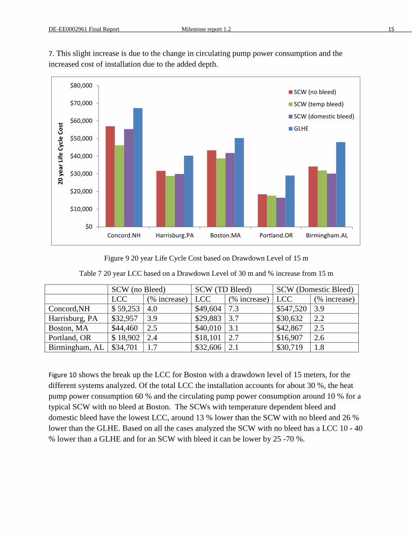
DE-EE0002961 Final Report Milestone report 1.2 15
7. This slight increase is due to the change in circulating pump power consumption and the increased cost of installation due to the added depth.
Figure 9 20 year Life Cycle Cost based on Drawdown Level of 15 m
Table 7 20 year LCC based on a Drawdown Level of 30 m and % increase from 15 m
SCW (no Bleed) SCW (TD Bleed) SCW (Domestic Bleed) LCC (% increase) LCC (% increase) LCC (% increase) Concord,NH $ 59,253 4.0 $49,604 7.3 $547,520 3.9 Harrisburg, PA $32,957 3.9 $29,883 3.7 $30,632 2.2 Boston, MA $44,460 2.5 $40,010 3.1 $42,867 2.5 Portland, OR $ 18,902 2.4 $18,101 2.7 $16,907 2.6 Birmingham, AL $34,701 1.7 $32,606 2.1 $30,719 1.8
Figure 10 shows the break up the LCC for Boston with a drawdown level of 15 meters, for the different systems analyzed. Of the total LCC the installation accounts for about 30 %, the heat pump power consumption 60 % and the circulating pump power consumption around 10 % for a typical SCW with no bleed at Boston. The SCWs with temperature dependent bleed and domestic bleed have the lowest LCC, around 13 % lower than the SCW with no bleed and 26 % lower than the GLHE. Based on all the cases analyzed the SCW with no bleed has a LCC 10 - 40 % lower than a GLHE and for an SCW with bleed it can be lower by 25 -70 %.
$0
$10,000
$20,000
$30,000
$40,000
$50,000
$60,000
$70,000
$80,000
Concord.NH Harrisburg.PA Boston.MA Portland.OR Birmingham.AL
20 y
ear L
ife C
ycle
Cos
t
SCW (no bleed)
SCW (temp bleed)
SCW (domestic bleed)
GLHE
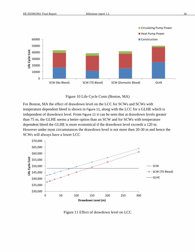
DE-EE0002961 Final Report Milestone report 1.2 16
Figure 10 Life Cycle Costs (Boston, MA)
For Boston, MA the effect of drawdown level on the LCC for SCWs and SCWs with temperature dependent bleed is shown in Figure 11, along with the LCC for a GLHE which is independent of drawdown level. From Figure 11 it can be seen that at drawdown levels greater than 75 m, the GLHE seems a better option than an SCW and for SCWs with temperature dependent bleed the GLHE is more economical if the drawdown level exceeds a 120 m. However under most circumstances the drawdown level is not more then 20-30 m and hence the SCWs will always have a lower LCC
Figure 11 Effect of drawdown level on LCC
0
10000
20000
30000
40000
50000
60000
SCW (No Bleed) SCW (TD Bleed) SCW (Domestic Bleed) GLHE
Life
Cyc
le C
ost
Circulating Pump Power
Heat Pump Power
Construction
$30,000
$35,000
$40,000
$45,000
$50,000
$55,000
$60,000
$65,000
$70,000
0 50 100 150 200 250 300
Life
Cyc
le C
ost
Drawdown Level (m)
SCW
SCW (TD Bleed)
GLHE

DE-EE0002961 Final Report Milestone report 1.2 17
Nomenclature: Cp – Specific heat of water in Kj/kg-K
ηpump – Pump Efficiency
ηVFD – VFD Efficiency
g – acceleration due to gravity in m/s2
H – Total Dynamic Head in m
lf – frictional losses in system in m
m – Mass flow rate of water in kg/s
P – static pressure in Pa
QH – Heating Load in W
QC – Cooling Load in W
Q – Volumetric flow rate in m3/s
Qt – Total volumetric flow rate in m3/s
Qb – Bleed flow rate in m3/s
ρ – Density if water in kg/m3
V – Flow velocity in m.s
w – Pumping power in W
z – Elevation head in m
DE-EE0002961 Final Report Milestone report 1.2 18
ABBREVIATIONS: EFT –Entering Fluid Temperature
ExFT – Exiting Fluid Temperature
FCV – Flow control valve
GLHE – Ground Loop Heat Exchanger
LCC – Life Cycle Cost
SCW – Standing Column Well
TD – Temperature Dependent
TRT – Thermal Response Test
VFD – Variable Frequency Drive
DE-EE0002961 Final Report Milestone report 1.2 19
References: AAWA. 2002. Commercial and Institutional End Uses of Water. AAWA Research Foundation
and the American Water Works Association.
BLAST. 1986. BLAST (Building Loads and System Thermodynamics).Urbana-Champaign: University of Illinois, BLAST Support Office.
Deng, Z. 2004. Modeling of Standing Column Wells in Ground Source Heat Pump Systems. Ph.D. Thesis, Oklahoma State University.
Energy Information Association (EIA). 2011. Electric Power Monthly. July 2011 Edition Misstear,B., Banks,D, and L.Clark. 2006. Water Wells and Boreholes. John Wiley and Sons. West Sussex, England. McQuay International. 2011. Geothermal Heat Pump Design Manual. Application Guide, AG 31-008. O’Neill, Z.D., J.D. Spitler, and S.J. Rees. 2006. Performance Analysis of Standing Column Well Ground Heat Exchanger Systems. ASHRAE Transactions 112(2):633-643. Orio, C.D and C.Johnson. 1999. Reducing GHP Well Water Pumping Costs. GeoExchange Technical Conference and Expo.
Rafferty, K.D. 1998. Well-pumping issues in commercial groundwater heat pump system. ASHRAE Transactions 104(1B):927–31.
Rooks, J.A and A.K.Wallace. 2004. Energy Efficiency of Variable Speed Drive Systems. Electrical Apparatus Service Association (EASA).
Varanasi, A. 2002. Development of a Visual Tool for HVACSIM+. M.S. Thesis, Oklahoma State University
Yavuzturk, C. Modeling of Vertical Ground Loop Heat Exchangers for Ground Source Heat Pump Systems. Ph.D. Thesis, December 1999. 118-119
Yavuzturk, C., and J.D. Spitler. 1999. A Short Time Step Response Factor Model for Vertical Ground Loop Heat Exchangers. ASHRAE Transactions 105(2):475-485.
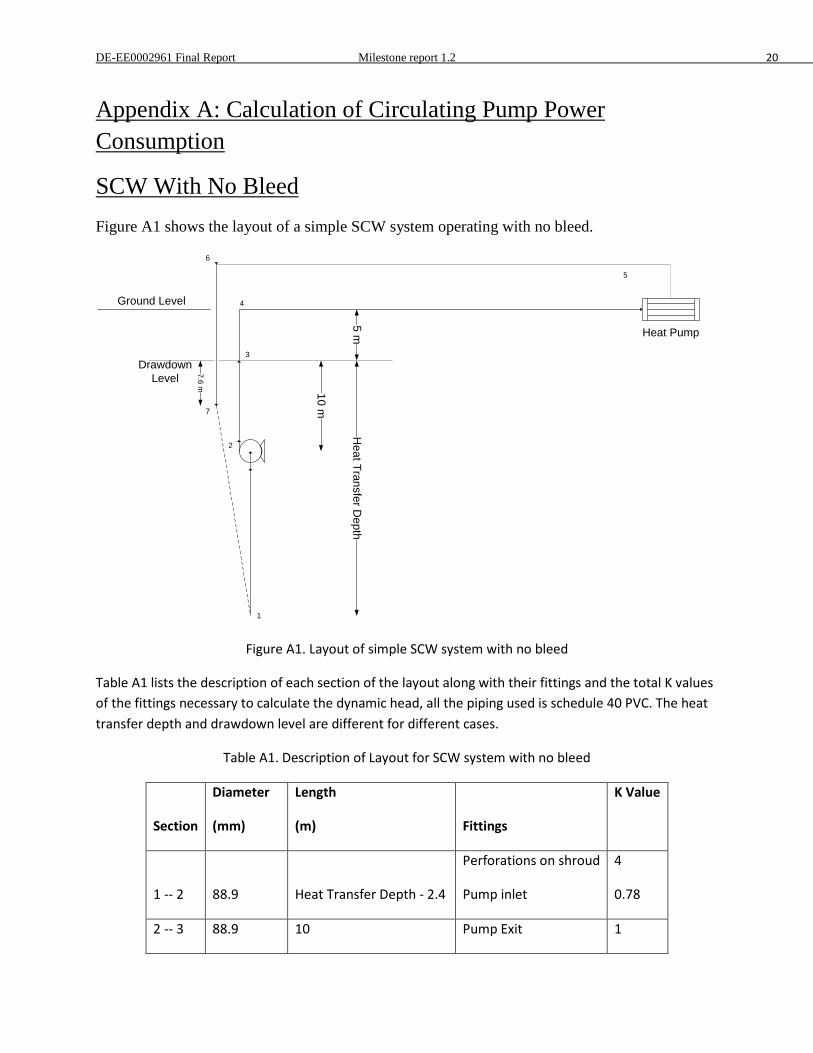
DE-EE0002961 Final Report Milestone report 1.2 20
Appendix A: Calculation of Circulating Pump Power Consumption
SCW With No Bleed Figure A1 shows the layout of a simple SCW system operating with no bleed.
Drawdown Level
10 m
Heat Transfer D
epth
Heat Pump
5 m
7.6 m1
2
3
5
4Ground Level
6
7
Figure A1. Layout of simple SCW system with no bleed
Table A1 lists the description of each section of the layout along with their fittings and the total K values of the fittings necessary to calculate the dynamic head, all the piping used is schedule 40 PVC. The heat transfer depth and drawdown level are different for different cases.
Table A1. Description of Layout for SCW system with no bleed
Section
Diameter
(mm)
Length
(m) Fittings
K Value
1 -- 2 88.9 Heat Transfer Depth - 2.4
Perforations on shroud
Pump inlet
4
0.78
2 -- 3 88.9 10 Pump Exit 1
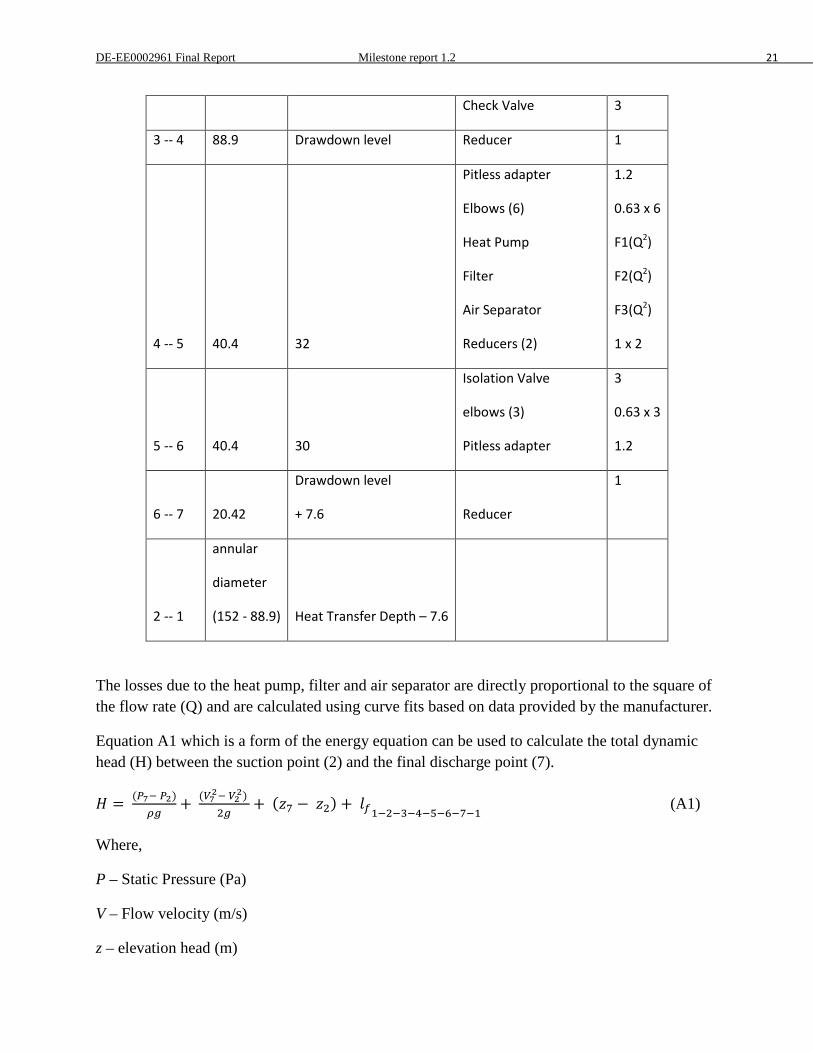
DE-EE0002961 Final Report Milestone report 1.2 21
Check Valve 3
3 -- 4 88.9 Drawdown level Reducer 1
4 -- 5 40.4 32
Pitless adapter
Elbows (6)
Heat Pump
Filter
Air Separator
Reducers (2)
1.2
0.63 x 6
F1(Q2)
F2(Q2)
F3(Q2)
1 x 2
5 -- 6 40.4 30
Isolation Valve
elbows (3)
Pitless adapter
3
0.63 x 3
1.2
6 -- 7 20.42
Drawdown level
+ 7.6 Reducer
1
2 -- 1
annular
diameter
(152 - 88.9) Heat Transfer Depth – 7.6
The losses due to the heat pump, filter and air separator are directly proportional to the square of the flow rate (Q) and are calculated using curve fits based on data provided by the manufacturer.
Equation A1 which is a form of the energy equation can be used to calculate the total dynamic head (H) between the suction point (2) and the final discharge point (7).
𝐻 = (𝑃7− 𝑃2)𝜌𝑔
+ (𝑉72− 𝑉22) 2𝑔
+ (𝑧7 − 𝑧2) + 𝑙𝑓1−2−3−4−5−6−7−1 (A1)
Where,
P – Static Pressure (Pa)
V – Flow velocity (m/s)
z – elevation head (m)
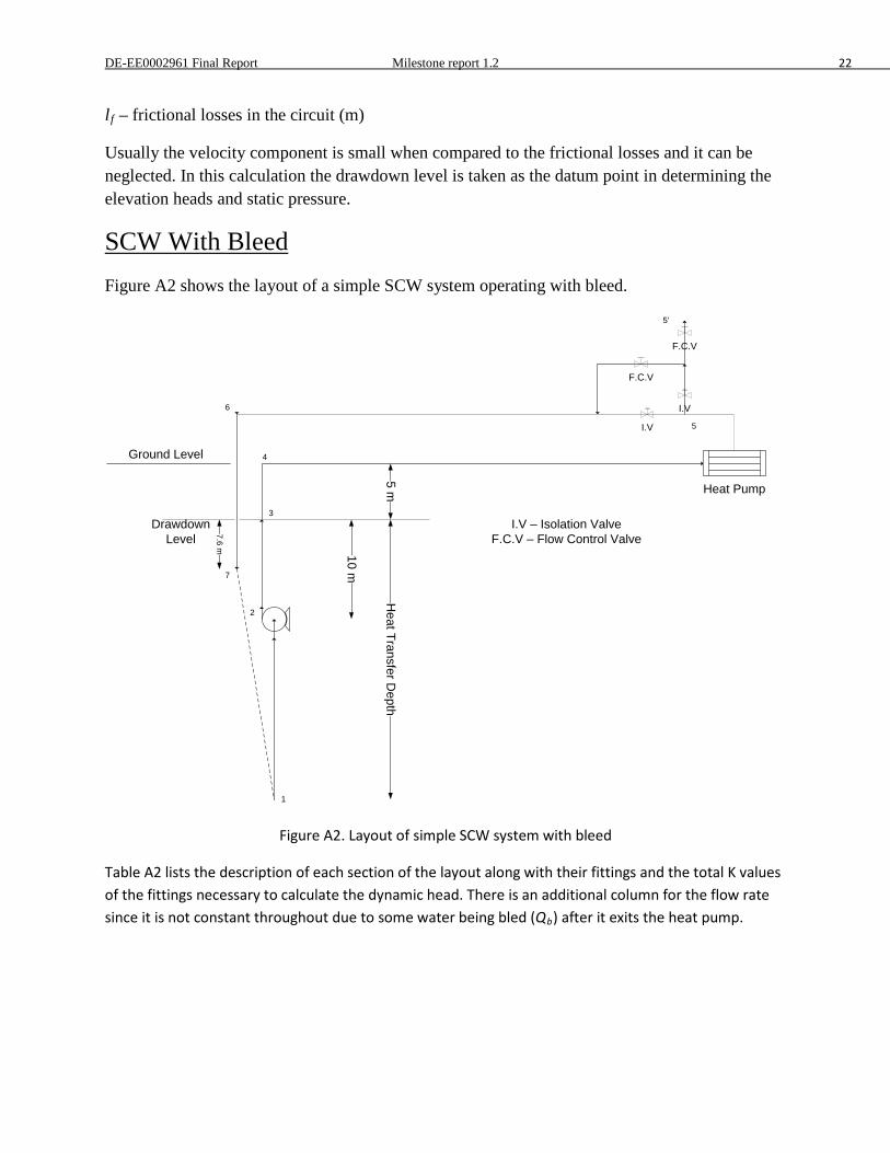
DE-EE0002961 Final Report Milestone report 1.2 22
lf – frictional losses in the circuit (m)
Usually the velocity component is small when compared to the frictional losses and it can be neglected. In this calculation the drawdown level is taken as the datum point in determining the elevation heads and static pressure.
SCW With Bleed Figure A2 shows the layout of a simple SCW system operating with bleed.
Drawdown Level
10 m
Heat Transfer D
epth Heat Pump
5 m
7.6 m
1
2
3
5
4Ground Level
6
7
5'
I.V
I.V
F.C.V
I.V – Isolation ValveF.C.V – Flow Control Valve
F.C.V
Figure A2. Layout of simple SCW system with bleed
Table A2 lists the description of each section of the layout along with their fittings and the total K values of the fittings necessary to calculate the dynamic head. There is an additional column for the flow rate since it is not constant throughout due to some water being bled (Qb) after it exits the heat pump.
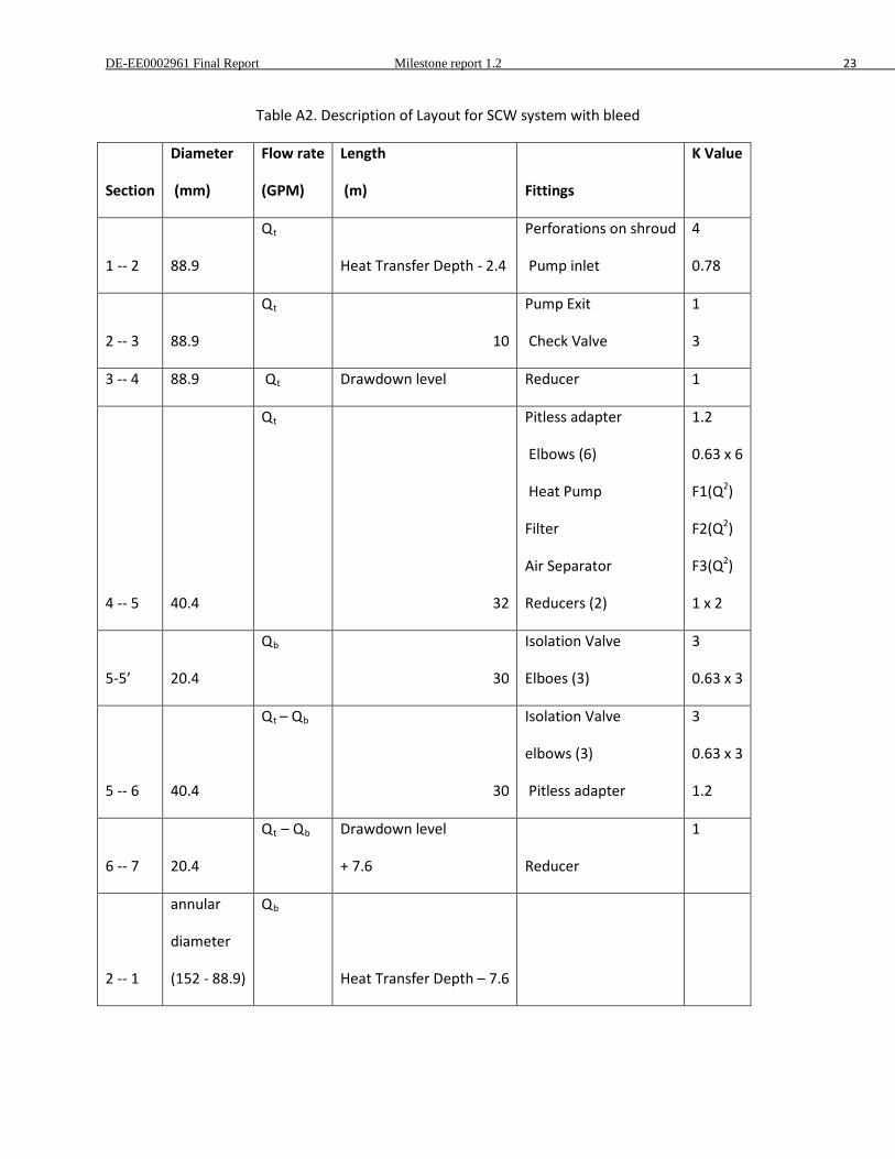
DE-EE0002961 Final Report Milestone report 1.2 23
Table A2. Description of Layout for SCW system with bleed
Section
Diameter
(mm)
Flow rate
(GPM)
Length
(m) Fittings
K Value
1 -- 2 88.9
Qt
Heat Transfer Depth - 2.4
Perforations on shroud
Pump inlet
4
0.78
2 -- 3 88.9
Qt
10
Pump Exit
Check Valve
1
3
3 -- 4 88.9 Qt Drawdown level Reducer 1
4 -- 5 40.4
Qt
32
Pitless adapter
Elbows (6)
Heat Pump
Filter
Air Separator
Reducers (2)
1.2
0.63 x 6
F1(Q2)
F2(Q2)
F3(Q2)
1 x 2
5-5’ 20.4
Qb
30
Isolation Valve
Elboes (3)
3
0.63 x 3
5 -- 6 40.4
Qt – Qb
30
Isolation Valve
elbows (3)
Pitless adapter
3
0.63 x 3
1.2
6 -- 7 20.4
Qt – Qb Drawdown level
+ 7.6 Reducer
1
2 -- 1
annular
diameter
(152 - 88.9)
Qb
Heat Transfer Depth – 7.6
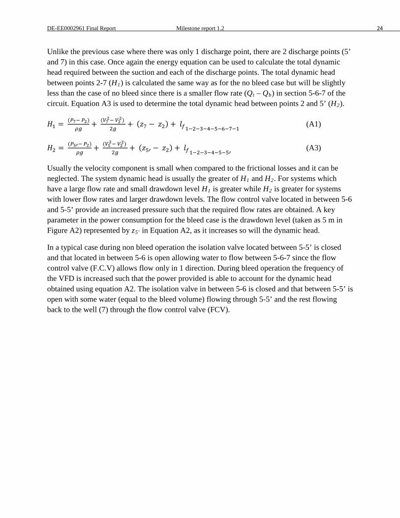
DE-EE0002961 Final Report Milestone report 1.2 24
Unlike the previous case where there was only 1 discharge point, there are 2 discharge points (5’ and 7) in this case. Once again the energy equation can be used to calculate the total dynamic head required between the suction and each of the discharge points. The total dynamic head between points 2-7 (H1) is calculated the same way as for the no bleed case but will be slightly less than the case of no bleed since there is a smaller flow rate (Qt – Qb) in section 5-6-7 of the circuit. Equation A3 is used to determine the total dynamic head between points 2 and 5’ (H2).
𝐻1 = (𝑃7− 𝑃2)𝜌𝑔
+ (𝑉72− 𝑉22) 2𝑔
+ (𝑧7 − 𝑧2) + 𝑙𝑓1−2−3−4−5−6−7−1 (A1)
𝐻2 = (𝑃5′− 𝑃2)𝜌𝑔
+ (𝑉52− 𝑉22) 2𝑔
+ (𝑧5′ − 𝑧2) + 𝑙𝑓1−2−3−4−5−5′ (A3)
Usually the velocity component is small when compared to the frictional losses and it can be neglected. The system dynamic head is usually the greater of H1 and H2. For systems which have a large flow rate and small drawdown level H1 is greater while H2 is greater for systems with lower flow rates and larger drawdown levels. The flow control valve located in between 5-6 and 5-5’ provide an increased pressure such that the required flow rates are obtained. A key parameter in the power consumption for the bleed case is the drawdown level (taken as 5 m in Figure A2) represented by z5’ in Equation A2, as it increases so will the dynamic head.
In a typical case during non bleed operation the isolation valve located between 5-5’ is closed and that located in between 5-6 is open allowing water to flow between 5-6-7 since the flow control valve (F.C.V) allows flow only in 1 direction. During bleed operation the frequency of the VFD is increased such that the power provided is able to account for the dynamic head obtained using equation A2. The isolation valve in between 5-6 is closed and that between 5-5’ is open with some water (equal to the bleed volume) flowing through 5-5’ and the rest flowing back to the well (7) through the flow control valve (FCV).
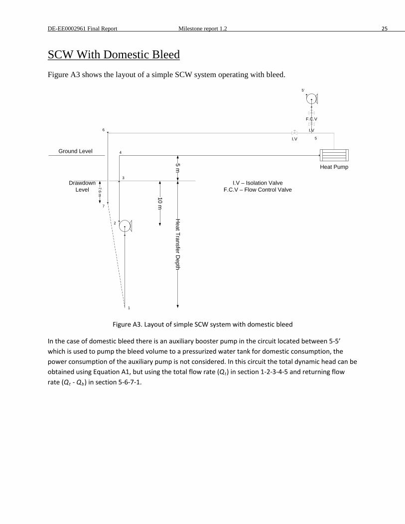
DE-EE0002961 Final Report Milestone report 1.2 25
SCW With Domestic Bleed Figure A3 shows the layout of a simple SCW system operating with bleed.
Drawdown Level
10 m
Heat Transfer D
epth
Heat Pump
5 m
7.6 m1
2
3
5
4Ground Level
6
7
5'
I.V
I.V
F.C.V
I.V – Isolation ValveF.C.V – Flow Control Valve
Figure A3. Layout of simple SCW system with domestic bleed
In the case of domestic bleed there is an auxiliary booster pump in the circuit located between 5-5’ which is used to pump the bleed volume to a pressurized water tank for domestic consumption, the power consumption of the auxiliary pump is not considered. In this circuit the total dynamic head can be obtained using Equation A1, but using the total flow rate (Qt) in section 1-2-3-4-5 and returning flow rate (Qt - Qb) in section 5-6-7-1.

DE-EE0002961 Final Report Milestone 2.1 1
Milestone 2.1
Pond Stratification
Venkata Satish Bhattiprolu
Krishna Conjeevaram Bashyam
Manojkumar Selvakumar
Oklahoma State University
DE-EE0002961 Final Report Milestone 2.1 2
Milestone Report
Task 2.1-Pond Stratification
DE-EE0002961/001 - Recovery Act:
Improved Design Tools for Surface Water and Standing Column Well Heat Pump Systems
Venkata Satish Bhattiprolu, ([email protected]), Research Assistant, Krishna Conjeevaram Bashyam, ([email protected]), Research Assistant, Manojkumar Selvakumar ([email protected]), Research Assistant, Professor Jeffrey D. Spitler, ([email protected]), Principal Investigator, Oklahoma State University
Introduction Stratification in lakes occurs due to the change in the lake temperatures at different depths. During the summer, top layers of water are at a higher temperature compared to the bottom layers. This result in the top layers being lighter and they float on the relatively denser water.
Similarly, during winter, the top layers are at temperatures lower than 4 degrees and this again results in lighter water floating on denser water due to the property of water where in the density decreases with temperature decrease below 4 degrees and temperature increase above 4 degrees. Temperature stratification with depth is observed during the summer and winter periods due to the above phenomenon. However, during the fall and spring a phenomenon known as turnover occurs in the lake. The water reaches its maximum density and starts to displace the lower layers, which are at temperatures above or below 4°C, whenever the surface temperature starts increasing and reaches 4 degrees. This results in the mixing of water temperatures to reach uniform temperature. This is also an important phenomenon as it distributes the oxygen to lowers layers during fall turnover Lot of turbulence is created in the water layers near the surface due to wind. The heat transfer is parameterized by eddy diffusivity in these layers. “Eddy diffusivities include turbulent heat transfer by a variety of processes, including surface and internal waves, seiches and internal seiches, currents, and Langmuir circulation” Stefan and Ford (1975). In other words, this term includes the heat transfer caused by the advection (horizontal movement) of water layers and molecular diffusion. An algorithm for mixing is included in such a way, that the shear wind energy on the water surface due to the wind speed is compared with the available potential energy for
DE-EE0002961 Final Report Milestone 2.1 3
displacing a lighter dense water layer by a heavier water layer below it. The wind energy is utilized and converted in to potential energy until there is no more left. The depth below the water surface when this occurs is called the mixing depth. The eddy diffusivity coefficients formulations until this depth are influenced by the wind energy. The surface temperatures start decreasing after summer resulting in density instabilities which is the primary cause for fall turnover, when the lake surface starts cooling. The phenomenon occurs due to convection currents generated in these layers. The density instabilities are removed by mixing all the unstable water layers with the next stable water layer and accommodating a volume weighed average of temperature throughout the new mixing depth.
All the water layers are assumed to be in contact with their own corresponding sediment layers. A one dimensional heat equation is solved for calculating the sediment temperatures from the lake bottom.
Methodology A one-dimensional advection diffusion equation as given by Ford and Stefan (1980) is
used to predict the temperature distribution for a horizontally mixed and vertically stratified lake. The equation can be written as,
𝐴𝜕𝑇𝜕𝑡
=𝜕𝜕𝑧�𝑘𝑧𝐴
𝜕𝑇𝜕𝑧� +
𝑄𝜌𝑤𝐶𝑝
(1)
Where, A is the horizontal area of the lake in m2, T is the water temperature in °C, kz is the vertical eddy diffusion coefficient in m2/day, Q is the internal distribution of heat in the water column in J/m3day, ρ w is the water density in kg/m3 and Cp is the specific heat of water in J/kgK. T, kz and Q are functions of both lake depth z and time t,while A is a function of lake depth z alone.
The lake model solves the governing equation by using a series of discretized horizontal layers characterized by depth from the surface. The layer thickness, horizontal area and eddy diffusion coefficient are evaluated at the layer interfaces, while the layer temperature and volume represent the mean value of the layer and hence can be assumed to be in the middle of a layer.
The net heat flux on the lake surface (Q”net-surface ) is calculated by the surface heat balance between the incoming shortwave and long wave radiation heat fluxes on the water surface and the outgoing convection, evaporation and back radiation heat fluxes from the water surface to the atmosphere.
𝑄"𝑛𝑒𝑡−𝑠𝑢𝑟𝑓𝑎𝑐𝑒 = 𝑄"𝑠𝑤−𝑠𝑢𝑟𝑓𝑎𝑐𝑒 + 𝑄"𝑙𝑤 − 𝑄"𝑐𝑜𝑛𝑣 − 𝑄"𝑒 (2)
DE-EE0002961 Final Report Milestone 2.1 4
Where,
Q”net-surface is the net heat flux on the lake surface [W/m2]
Q”sw-surface is the heat flux due to short wave radiation incident on the pond surface [W/m2]
Q”lw is the heat flux due to net long wave radiation incident on the pond surface [W/m2]
Q”conv is the convective heat flux from the pond surface to the atmosphere [W/m2]
Q”e is the evaporative heat flux from the pond surface to the atmosphere [W/m2]
The equations used in the calculation of different surface heat fluxes are given below.
𝑄"𝑠𝑤−𝑠𝑢𝑟𝑓𝑎𝑐𝑒 = 𝑄"𝑠𝑜𝑙𝑎𝑟 (1 − 𝑎𝑙𝑏𝑒𝑑𝑜𝑤𝑎𝑡𝑒𝑟)𝛽𝑤 (3) 𝑄"𝑙𝑤 = ℎ𝑙𝑤(𝑇𝑠𝑘𝑦 − 𝑇𝑠𝑢𝑟𝑓𝑎𝑐𝑒) (4) 𝑄”𝑐𝑜𝑛𝑣 = ℎ𝑐𝐴𝑠𝑢𝑟𝑓𝑎𝑐𝑒(𝑇𝑎𝑖𝑟 − 𝑇𝑠𝑢𝑟𝑓𝑎𝑐𝑒) (5)
𝑄"𝑒 =ℎ𝑓𝑔ℎ𝑐𝑐𝑝,𝑎𝑖𝑟
(𝑤𝑠𝑢𝑟𝑓𝑎𝑐𝑒 − 𝑤𝑎𝑖𝑟) (6)
Where, Q”solar is the incident solar radiation on the lake surface [W/m2] , albedowater is the water surface reflectivity coefficient and βw is the water surface absorption coefficient, hc and hlw are the surface convection and linearized longwave radiation coefficients in [W/m2-K] respectively, Tsky, Tsurface and Tair are the sky, lake surface and air temperatures respectively, Asurface is the lake surface area [m2], hfg is the latent heat of vaporization [J/kg], wair is the humidity ratio of the ambient air, wsurface is the humidity ratio of the saturated air at the lake surface.
Dake and Harleman (1969) showed that the reflectivity coefficent of water (albedowater) could vary from 0.03 to 0.1 and the absorption coefficient (βw)interpreted from their measurements in Lake Tahoe and Castle lake was 0.4. The amount of reflection for the current model is fixed at 0.04 and the absorption coefficient is taken as 0.4.
The linearized radiation coefficient is calculated using the following equation,
ℎ𝑙𝑤 = 4𝜀𝑤𝑎𝑡𝑒𝑟𝜎 �𝑇𝑠𝑢𝑟𝑓𝑎𝑐𝑒 + 𝑇𝑠𝑘𝑦
2�3
(7)
Where, εwater is the emissivity coefficient of water taken as 0.97 (Omstedt (1990)) and σ is the Stefan-Boltzmann constant.
The amount of heat transferred by a lake through surface convection and evaporation varies according to the lake size and surface area. Several empirical correlations exist to determine the convective heat transfer coefficient and hence to calculate the convective heat flux over the lake surface. Seven correlations to calculate the convective heat transfer coefficeint are identified and included in the lake model. The correlation to calculate the convective heat transfer coefficient by Molineaux et al. (1994) is given below,
DE-EE0002961 Final Report Milestone 2.1 5
ℎ𝑐 = 3.1 + 2.1𝑊 (8)
Where, W is the wind speed over the lake surface [m/s].
The penetration of solar radiation in the water column is measured by the solar attenuation or extinction coefficient, which is dependent on the lake turbidity content. The radiative heat flux at the depth z is calculated as
𝑄"𝑠𝑤(𝑧) = 𝑄”𝑠𝑤−𝑠𝑢𝑟𝑓𝑎𝑐𝑒(1 − 𝛽𝑤) exp (−𝜇𝑧) (9)
Where, 𝜇 is the extinction coefficient of water which is a function of lake turbidity. The lake turbidity is measured by secchi depth (zsecchi). The extinction coefficient is calculated using Equation 10.
𝜇 =1.86𝑧𝑆𝑒𝑐𝑐ℎ𝑖
(10)
Heat transfer from sediments is a significant source of heat gain for a lake during ice cover periods (Gu and Stefan (1990)). Lake simulation model incorporates the theory of sediment heat transfer from Fang and Stefan (1996). . The heat flux between the water and the sediments is determined from the temperature gradient between the water-sediment (ws) layer
�𝜕𝑇𝑠𝑒𝑑𝜕𝑧
�𝑤𝑠
as,
𝑄𝑠𝑒𝑑𝑖𝑚𝑒𝑛𝑡 = 𝛼𝑠𝑒𝑑𝜌𝑠𝑒𝑑𝑐𝑝,𝑠𝑒𝑑 �𝜕𝑇𝑠𝑒𝑑𝜕𝑧
�𝑤𝑠
(11)
Where, αsed is the thermal diffusivity of the sediments [m2/day], ρsed is the density of the sediments [Kg/m3] and cp,sed is the specific heat capacity of the sediment [J/kg -°C]. Each water layer is in contact with a set of sediment layers. The sediment temperatures of the two uppermost sediment layers are used to calculate the temperature gradients in the sediment-water interface.
The temperature transport mechanism in a lake is predominantly controlled by the turbulent diffusion process resulting in the formation of eddies. This turbulent diffusion in the lake can be parameterized by the eddy diffusion coefficients. The accuracy of temperature prediction is highly dependent on the effective prediction of the eddy diffusion coefficient (kz). The eddy diffusion coefficient depends on the lake surface area and other physiological factors. The lake model contains 11 different eddy diffusion models to predict the eddy diffusion coefficeint for different lake types. The eddy diffusion coefficient determined by Gu and Stefan (1995) for shallow wastewater ponds is
𝑘𝑧 = min [𝑘𝑧𝑚𝑎𝑥,𝑘𝑧𝑚𝑎𝑥𝐶𝑁−1] (12)
Where, kzmax is the maximum hypolimnion eddy diffusion coefficient, N is the stability or the Brunt Vaisala frequency, C is a constant taken as 8.66*10-3 (s-1) (Jassby and Powell (1975)). The stability frequency is estimated by Hondzo and Stefan (1993) as,
DE-EE0002961 Final Report Milestone 2.1 6
𝑁 = ��𝑔𝜌𝑤� �𝜕𝜌𝑤𝜕𝑧
� (13)
Where, ∂ρw is the density difference between the two water layers separated by a distance ∂z. The maximum hypolimnion eddy diffusion coefficient (kzmax) represents the maximum diffusion that can occur in a lake as a result of turbulent action. The maximum eddy diffusion coefficient can be observed in a lake during weakly stratified conditions as a result of extensive turbulent mixing of water layers due to strong wind action. kzmax is dependent on the physical and physiological characteristics of the lake. Hondzo and Stefan (1993) derived the relationship between kzmax and the surface area of the lake as,
𝑘𝑧𝑚𝑎𝑥 = 0.048�𝐴𝑠𝑢𝑟𝑓𝑎𝑐𝑒�0.56
(14)
The expression for kzmax holds good for large ponds and lakes. In case of shallow ponds, which tend to stratify and destratify many times in a day, there does not appear to be a standard procedure to estimate the value of kzmax. Gu and Stefan (1995) estimated the kzmax value of 0.1m2/day for their 1.8 acre (7400 m2) rectangular waste water pond in Minnesota with a maximum depth of 6ft (1.8 m). For OSU research pond in Oklahoma, which has a surface area of 3acres (12140 m2) and a maximum depth of 12.5 ft (3.81 m) the kzmax value of 5 m2/day was estimated.
Since, many of the quantities in the heat transfer equations require the temperature term for the current time step to be known, iterative method is employed to calculate the water layer temperatures. The lake model thus runs iteratively for every time step until a converged temperature value is obtained. With the calculation of all the heat flux terms and eddy diffusion coefficeints, a preliminary lake temperature profile with depth is obtained by solving the governing equation (Equation 1) using Tri-diagonal matrix algorithm (TDMA).
Once the water temperatures are calculated, the lake model checks for the presence of unstable density layers (i.e.) the presence of higher density water layer(s) above the lower density layers. If such a case occurs, the groups of water layer(s) with unstable density profiles are completely mixed with the first stable layer below the unstable layers. Now a mixing algorithm is applied to determine the stratification in the lake. First, the kinetic energy generated on the lake surface by wind shear is calculated. This is given by equation 15.
𝑇𝐾𝐸 = 𝑊𝑠𝑡𝑟𝐴𝑠𝑢𝑟𝑓𝑎𝑐𝑒�𝜏3
𝜌𝑤 ∆𝑡 (15)
Where, τ is the wind stress [N/m2] and Wstr is the wind sheltering coefficient and ∆𝑡 is the time step, in our case 1 day or 86400 seconds.
𝜏 = 𝜌𝑎𝑖𝑟 ∗ 𝑐𝑑 ∗ 𝑊2 (16) 𝑊𝑠𝑡𝑟 = 1.0− exp (−0.3𝐴𝑠𝑢𝑟𝑓𝑎𝑐𝑒) (17)
DE-EE0002961 Final Report Milestone 2.1 7
Where, Cd is the drag coefficient which is dependent of the surface wind speed.
The algorithm to calculate the epilimnion layer thickness (i.e.) the depth of the water layer from the surface which is completely mixed is based on Ford and Stefan (1980) and Saloranta and Andersen (2004). The surface layer is always assumed to be well mixed it is considered to the first epilimnion layer. The potential energy (PE) required for lifting the immediate water layer below the epilimnion to the centre of the epilimnion layer is calculated.
𝑃𝐸 = 𝑔∆𝜌𝑤𝑉𝑒𝑝𝑖𝑉𝑧𝑉𝑒𝑝𝑖 + 𝑉𝑧
(𝑧𝑒𝑝𝑖 + ∆𝑧𝑀−𝑧 − 𝑧𝑀−𝑒𝑝𝑖) (18)
Where, g is the acceleration due to gravity, Δρw is the density difference between the layer and the epilimnion layer, zepi is the thickness of the epilimnion layer, ΔzM-z is the distance from the layer’s centre of mass to the bottom of the epilimnion layer, and zM-epi is the depth where the centre of mass of the epilimnion layer is present. Vepi is the volume of the epilimnion layer and is calculated by adding the volume of the current layer (Vz) with the total volume of the above mixed layers. The TKE available is compared with the PE of the layer. If TKE ≥ PE of the water layer, it is completely mixed with the above epilimnion layers and the next water layer is checked thus increasing the epilimnion depth. The total PE to lift the water layer is subtracted from the available TKE. Now the PE of the next layer is compared with the resultant TKE, and the procedure is repeated until the net resultant TKE is less than the PE required for new layer to mix with the epilimnion.
During spring/autumn seasons a lake undergoes a large scale inversion of water mass from the surface till the lake bottom which completely destroys the existing stratification. This phenomenon is called as turnover and it occurs once or twice annually in a lake. The lake model follows the algorithm given by Saloranta and Andersen (2004) to handle the turnover conditions. Turnover algorithm is initiated whenever the surface temperature crosses the temperature of maximum density (Tmaxrho = 3.98 °C). The water layers including the surface layer that has crossed Tmaxrho, are set to Tmaxrho. The energy gained by this temperature difference (i.e. the energy difference relative to Tmaxrho ) is exponentially distributed to cool/warm the water column to Tmaxrho. The surface temperature is maintained at Tmaxrho until the entire water column has been cooled/warmed to Tmaxrho. If the entire water column is cooled/warmed to Tmaxrho the remaining energy is used to cool/warm the surface layers.
The presence of any unstable layers is removed and the modified lake temperature profiles are again estimated using the TDMA.
Validation Temperature Measurements were taken at the research pond located north of the
Oklahoma State university campus. The validataion of the lake model with the experimental
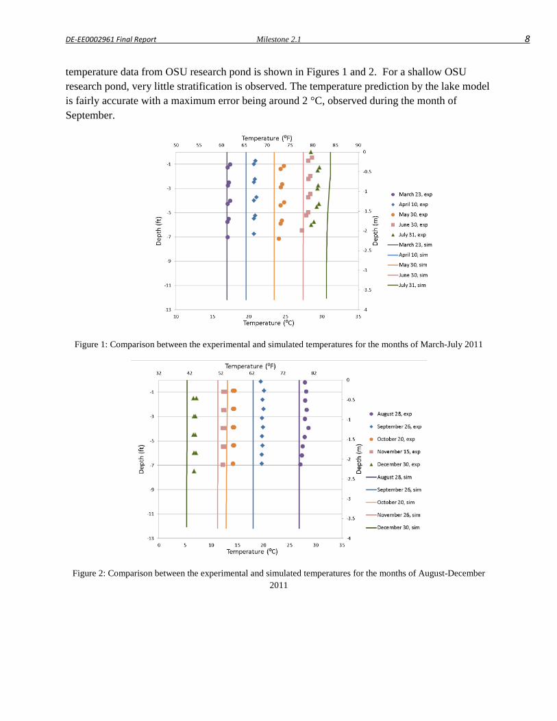
DE-EE0002961 Final Report Milestone 2.1 8
temperature data from OSU research pond is shown in Figures 1 and 2. For a shallow OSU research pond, very little stratification is observed. The temperature prediction by the lake model is fairly accurate with a maximum error being around 2 °C, observed during the month of September.
Figure 1: Comparison between the experimental and simulated temperatures for the months of March-July 2011
Figure 2: Comparison between the experimental and simulated temperatures for the months of August-December 2011
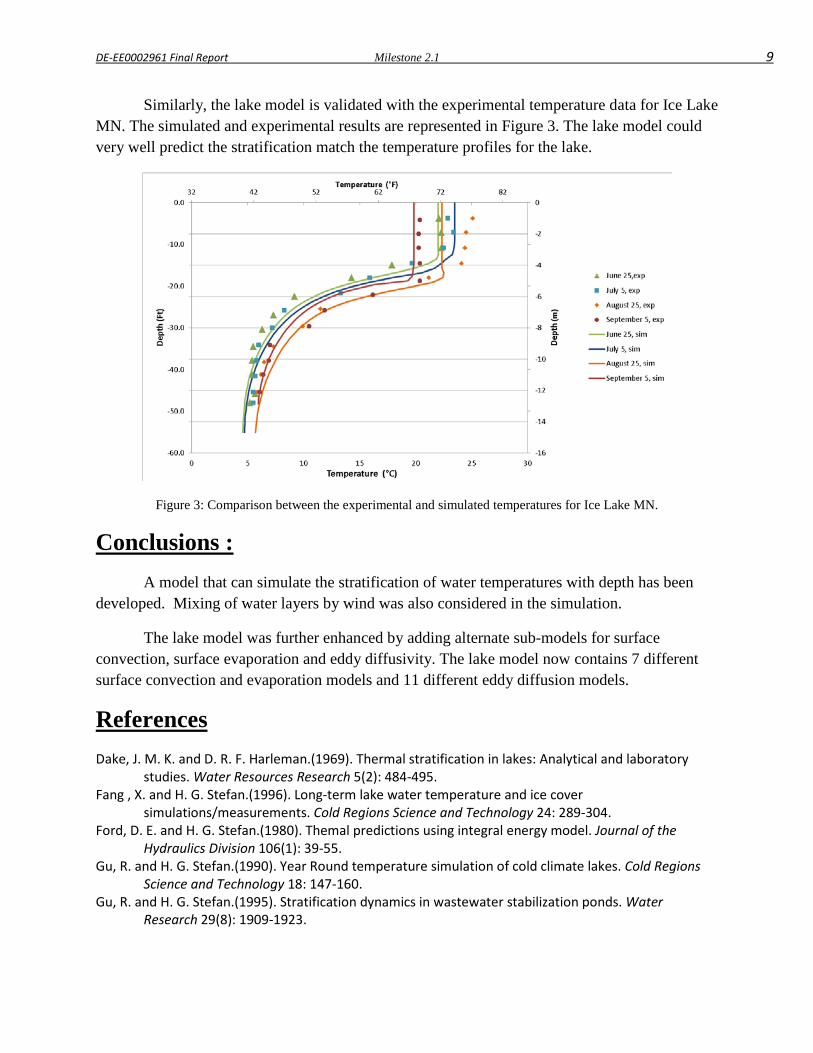
DE-EE0002961 Final Report Milestone 2.1 9
Similarly, the lake model is validated with the experimental temperature data for Ice Lake MN. The simulated and experimental results are represented in Figure 3. The lake model could very well predict the stratification match the temperature profiles for the lake.
Figure 3: Comparison between the experimental and simulated temperatures for Ice Lake MN.
Conclusions : A model that can simulate the stratification of water temperatures with depth has been
developed. Mixing of water layers by wind was also considered in the simulation.
The lake model was further enhanced by adding alternate sub-models for surface convection, surface evaporation and eddy diffusivity. The lake model now contains 7 different surface convection and evaporation models and 11 different eddy diffusion models.
References Dake, J. M. K. and D. R. F. Harleman.(1969). Thermal stratification in lakes: Analytical and laboratory
studies. Water Resources Research 5(2): 484-495. Fang , X. and H. G. Stefan.(1996). Long-term lake water temperature and ice cover
simulations/measurements. Cold Regions Science and Technology 24: 289-304. Ford, D. E. and H. G. Stefan.(1980). Themal predictions using integral energy model. Journal of the
Hydraulics Division 106(1): 39-55. Gu, R. and H. G. Stefan.(1990). Year Round temperature simulation of cold climate lakes. Cold Regions
Science and Technology 18: 147-160. Gu, R. and H. G. Stefan.(1995). Stratification dynamics in wastewater stabilization ponds. Water
Research 29(8): 1909-1923.

DE-EE0002961 Final Report Milestone 2.1 10
Hondzo, M. and H. G. Stefan.(1993). Lake water temperature simulation model. Journal of Hydraulic Engineering 119(11): 1251-1274.
Jassby, A. and T. Powell.(1975). Vertical patterns of eddy diffusion during stratification in Castle Lake, California. Limnology and Oceanography 20(4): 530-543.
Molineaux, B., B. Lachal and O. Guisan.(1994). Thermal analysis of five outdoor swimming pools heated by unglazed solar collectors. Solar Energy 53(1): 21-26.
Omstedt, A.(1990). A coupled one-dimensional sea ice–ocean model applied to a semi-enclosed basin. Tellus A 42(5): 568-582.
Saloranta, T. M. and T. Andersen. (2004). Mylake (v.1.1): Technical model documentation and user's guide. NIVA-report 4838. Olso,Norway, Norwegian Institute for Water Research. 44.
Stefan, H. and D. E. Ford. (1975). Mixed layer depth and temperature dynamics in temperate lakes. A. Minesotta, St Anthony Falls Laboratory: 149-157.

DE-EE0002961 Final Report Milestone 2.2 1
Milestone 2.2
Modeling of ice on coil
Venkata Satish Bhattiprolu
Oklahoma State University

DE-EE0002961 Final Report Milestone 2.2 2
Milestone Report
Task 2.2- Modeling of ice on coil
DE-EE0002961/001 - Recovery Act:
Improved Design Tools for Surface Water and Standing Column Well Heat Pump Systems
Venkata Satish Bhattiprolu, ([email protected]), Research Assistant, Professor Jeffrey D Spitler, ([email protected]), Principal Investigator, Oklahoma State University
Introduction The model for ice on Heat exchanger coil is a modified version of the model for ice storage tank using network method Neto and Krarti (1997).The present model considers a single spiral shaped heat exchanger coil. For simplicity in analysis currently the intersection between adjacent ice layers on the coil was not considered. The total coil of length 152.4 meters is divided in to 50 small segments.
Differences between the Pond HX and Ice Storage Tank
• In the current pond heat exchanger, a single spiral coil is used whereas the ice storage tank consists of multiple parallel circuits of spiral coils
• Volume of water in the storage tank is finite and capacity of water need to be accounted for heat transfer analysis whereas in the current heat exchanger model infinite capacity of pond is assumed and the whole pond volume is considered. This results in very small changes in the pond temperature with heat transfer from or to the pond by the heat exchanger
• No analysis between the environment and the tank wall is considered for the pond heat exchanger.
• Since multiple parallel circuits are present in the ice storage tank, thermal conductivity decreases and to accommodate this, the distances need to be reduced for high thermal performance. This increases the pressure drop and they need to be accounted for in the ice storage tank whereas they are not considered for the pond heat exchanger
Methodology The different heat transfer processes involved include heat transfer by convection inside
the coil from the brine to the surface of the coil, amount of the cooling utilized for ice formation and the heat transfer outside the coil from the surface and the pond .
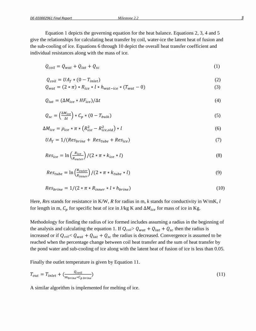
DE-EE0002961 Final Report Milestone 2.2 3
Equation 1 depicts the governing equation for the heat balance. Equations 2, 3, 4 and 5 give the relationships for calculating heat transfer by coil, water-ice the latent heat of fusion and the sub-cooling of ice. Equations 6 through 10 depict the overall heat transfer coefficient and individual resistances along with the mass of ice.
𝑄𝑐𝑜𝑖𝑙 = 𝑄𝑤𝑎𝑡 + 𝑄𝑙𝑎𝑡 + 𝑄𝑠𝑐 (1) 𝑄𝑐𝑜𝑖𝑙 = 𝑈𝐴𝑓 ∗ (0 − 𝑇𝑖𝑛𝑙𝑒𝑡) (2) 𝑄𝑤𝑎𝑡 = (2 ∗ 𝜋) ∗ 𝑅𝑖𝑐𝑒 ∗ 𝑙 ∗ ℎ𝑤𝑎𝑡−𝑖𝑐𝑒 ∗ (𝑇𝑤𝑎𝑡 − 0) (3) 𝑄𝑙𝑎𝑡 = (∆𝑀𝑖𝑐𝑒 ∗ 𝐻𝐹𝑖𝑐𝑒)/∆𝑡 (4)
𝑄𝑠𝑐 = �∆𝑀𝑖𝑐𝑒∆𝑡
� ∗ 𝐶𝑝 ∗ (0 − 𝑇𝑏𝑢𝑙𝑘) (5)
∆𝑀𝑖𝑐𝑒 = 𝜌𝑖𝑐𝑒 ∗ 𝜋 ∗ �𝑅𝑖𝑐𝑒2 − 𝑅𝑖𝑐𝑒,𝑜𝑙𝑑2 � ∗ 𝑙 (6)
𝑈𝐴𝑓 = 1/(𝑅𝑒𝑠𝑏𝑟𝑖𝑛𝑒 + 𝑅𝑒𝑠𝑡𝑢𝑏𝑒 + 𝑅𝑒𝑠𝑖𝑐𝑒) (7)
𝑅𝑒𝑠𝑖𝑐𝑒 = ln � 𝑅𝑖𝑐𝑒𝑅𝑜𝑢𝑡𝑒𝑟
� /(2 ∗ 𝜋 ∗ 𝑘𝑖𝑐𝑒 ∗ 𝑙) (8)
𝑅𝑒𝑠𝑡𝑢𝑏𝑒 = ln �𝑅𝑜𝑢𝑡𝑒𝑟𝑅𝑖𝑛𝑛𝑒𝑟
� /(2 ∗ 𝜋 ∗ 𝑘𝑡𝑢𝑏𝑒 ∗ 𝑙) (9)
𝑅𝑒𝑠𝑏𝑟𝑖𝑛𝑒 = 1/(2 ∗ 𝜋 ∗ 𝑅𝑖𝑛𝑛𝑒𝑟 ∗ 𝑙 ∗ ℎ𝑏𝑟𝑖𝑛𝑒) (10)
Here, Res stands for resistance in K/W, R for radius in m, k stands for conductivity in W/mK, l for length in m, 𝐶𝑝 for specific heat of ice in J/kg K and ∆𝑀𝑖𝑐𝑒 for mass of ice in Kg. Methodology for finding the radius of ice formed includes assuming a radius in the beginning of the analysis and calculating the equation 1. If Qcoil> 𝑄𝑤𝑎𝑡 + 𝑄𝑙𝑎𝑡 + 𝑄𝑠𝑐 then the radius is increased or if Qcoil< 𝑄𝑤𝑎𝑡 + 𝑄𝑙𝑎𝑡 + 𝑄𝑠𝑐 the radius is decreased. Convergence is assumed to be reached when the percentage change between coil heat transfer and the sum of heat transfer by the pond water and sub-cooling of ice along with the latent heat of fusion of ice is less than 0.05. Finally the outlet temperature is given by Equation 11.
𝑇𝑜𝑢𝑡 = 𝑇𝑖𝑛𝑙𝑒𝑡 + ( 𝑄𝑐𝑜𝑖𝑙𝑚𝑏𝑟𝑖𝑛𝑒∗𝐶𝑝 𝑏𝑟𝑖𝑛𝑒
) (11)
A similar algorithm is implemented for melting of ice.
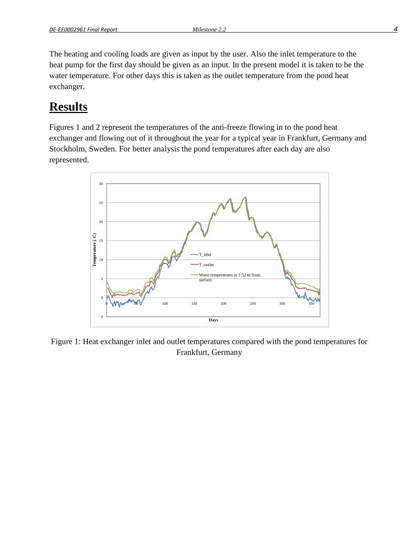
DE-EE0002961 Final Report Milestone 2.2 4
The heating and cooling loads are given as input by the user. Also the inlet temperature to the heat pump for the first day should be given as an input. In the present model it is taken to be the water temperature. For other days this is taken as the outlet temperature from the pond heat exchanger.
Results Figures 1 and 2 represent the temperatures of the anti-freeze flowing in to the pond heat exchanger and flowing out of it throughout the year for a typical year in Frankfurt, Germany and Stockholm, Sweden. For better analysis the pond temperatures after each day are also represented.
Figure 1: Heat exchanger inlet and outlet temperatures compared with the pond temperatures for
Frankfurt, Germany
-5
0
5
10
15
20
25
30
0 50 100 150 200 250 300 350
Tem
pera
ture
(C
)
Days
T_inlet
T_outlet
Water temperatures at 1.52 m from surface
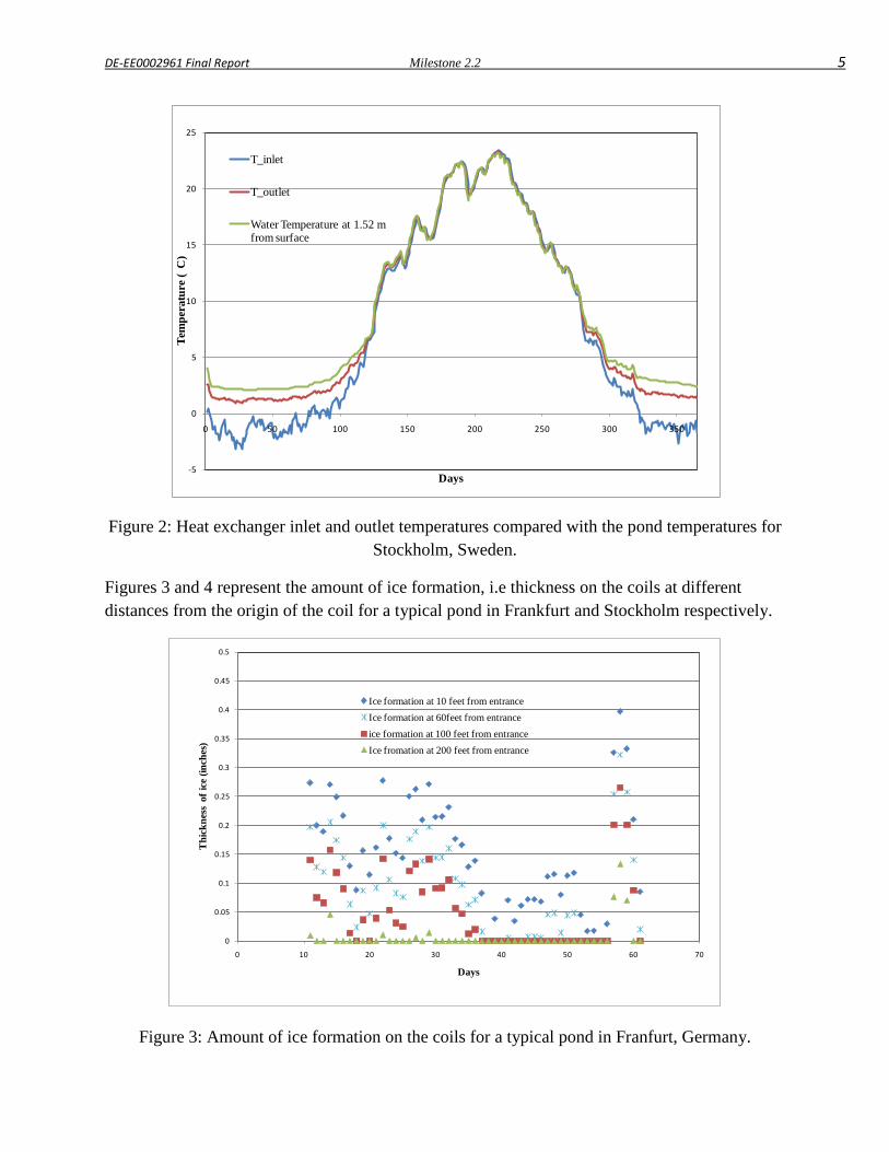
DE-EE0002961 Final Report Milestone 2.2 5
Figure 2: Heat exchanger inlet and outlet temperatures compared with the pond temperatures for Stockholm, Sweden.
Figures 3 and 4 represent the amount of ice formation, i.e thickness on the coils at different distances from the origin of the coil for a typical pond in Frankfurt and Stockholm respectively.
Figure 3: Amount of ice formation on the coils for a typical pond in Franfurt, Germany.
-5
0
5
10
15
20
25
0 50 100 150 200 250 300 350
Tem
pera
ture
(C
)
Days
T_inlet
T_outlet
Water Temperature at 1.52 m from surface
0
0.05
0.1
0.15
0.2
0.25
0.3
0.35
0.4
0.45
0.5
0 10 20 30 40 50 60 70
Thi
ckne
ss o
f ice
(inc
hes)
Days
Ice formation at 10 feet from entranceIce formation at 60feet from entranceice formation at 100 feet from entranceIce fromation at 200 feet from entrance
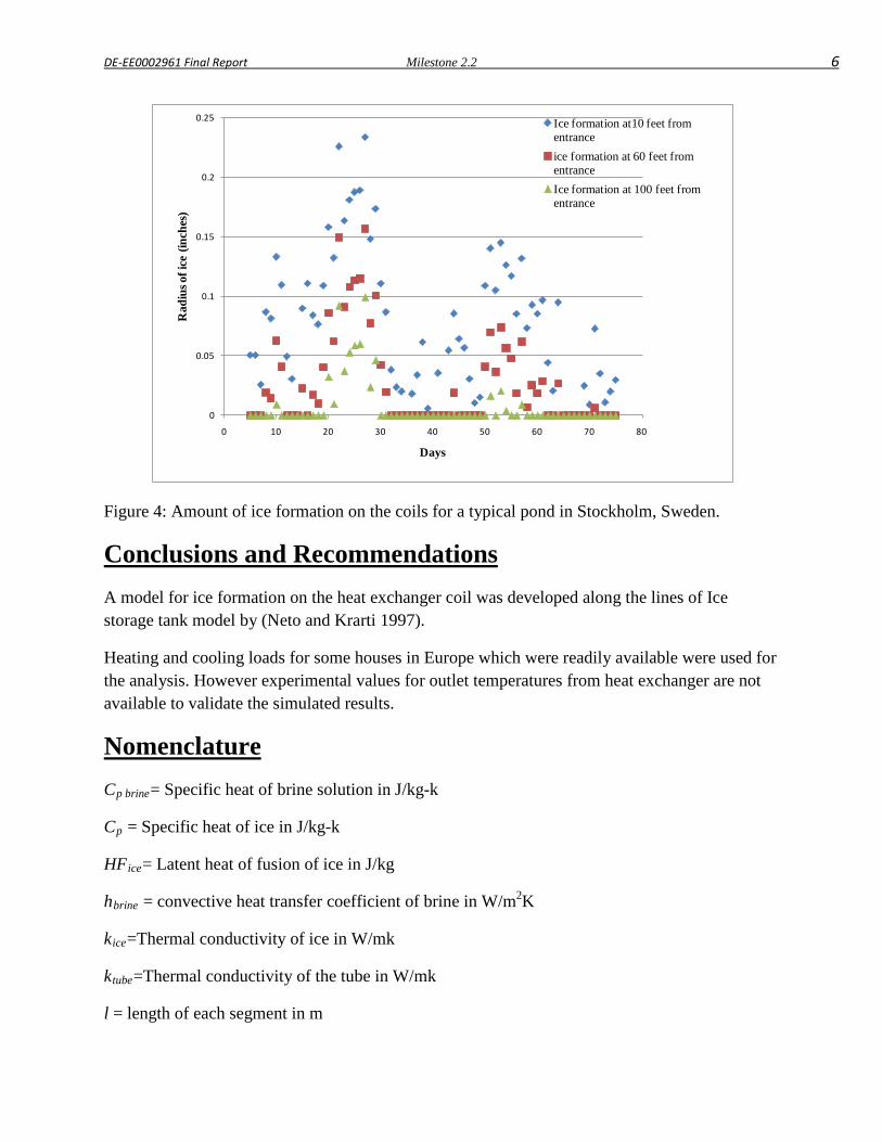
DE-EE0002961 Final Report Milestone 2.2 6
Figure 4: Amount of ice formation on the coils for a typical pond in Stockholm, Sweden.
Conclusions and Recommendations A model for ice formation on the heat exchanger coil was developed along the lines of Ice storage tank model by (Neto and Krarti 1997).
Heating and cooling loads for some houses in Europe which were readily available were used for the analysis. However experimental values for outlet temperatures from heat exchanger are not available to validate the simulated results.
Nomenclature Cp brine= Specific heat of brine solution in J/kg-k
Cp = Specific heat of ice in J/kg-k
HFice= Latent heat of fusion of ice in J/kg
hbrine = convective heat transfer coefficient of brine in W/m2K
kice=Thermal conductivity of ice in W/mk
ktube=Thermal conductivity of the tube in W/mk
l = length of each segment in m
0
0.05
0.1
0.15
0.2
0.25
0 10 20 30 40 50 60 70 80
Rad
ius o
f ice
(inc
hes)
Days
Ice formation at10 feet from entranceice formation at 60 feet from entranceIce formation at 100 feet from entrance
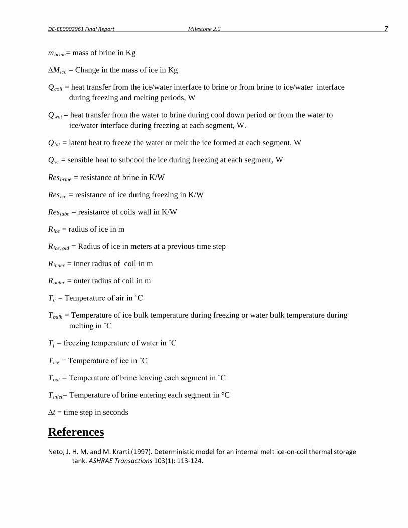
DE-EE0002961 Final Report Milestone 2.2 7
mbrine= mass of brine in Kg
∆Mice = Change in the mass of ice in Kg
Qcoil = heat transfer from the ice/water interface to brine or from brine to ice/water interface during freezing and melting periods, W
Qwat = heat transfer from the water to brine during cool down period or from the water to ice/water interface during freezing at each segment, W.
Qlat = latent heat to freeze the water or melt the ice formed at each segment, W
Qsc = sensible heat to subcool the ice during freezing at each segment, W
Resbrine = resistance of brine in K/W
Resice = resistance of ice during freezing in K/W
Restube = resistance of coils wall in K/W
Rice = radius of ice in m
Rice, old = Radius of ice in meters at a previous time step
Rinner = inner radius of coil in m
Router = outer radius of coil in m
Ta = Temperature of air in ˚C
Tbulk = Temperature of ice bulk temperature during freezing or water bulk temperature during melting in ˚C
Tf = freezing temperature of water in ˚C
Tice = Temperature of ice in ˚C
Tout = Temperature of brine leaving each segment in ˚C
Tinlet= Temperature of brine entering each segment in °C
∆t = time step in seconds
References
Neto, J. H. M. and M. Krarti.(1997). Deterministic model for an internal melt ice-on-coil thermal storage tank. ASHRAE Transactions 103(1): 113-124.

DE-EE0002961 Final Report Milestone 2.3 1
Milestone 2.3
Ice and snow on pond surface
Venkata Satish Bhattiprolu
Oklahoma State University
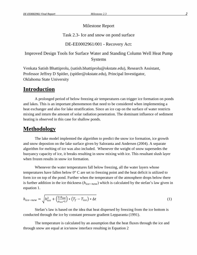
DE-EE0002961 Final Report Milestone 2.3 2
Milestone Report
Task 2.3- Ice and snow on pond surface
DE-EE0002961/001 - Recovery Act:
Improved Design Tools for Surface Water and Standing Column Well Heat Pump Systems
Venkata Satish Bhattiprolu, ([email protected]), Research Assistant, Professor Jeffrey D Spitler, ([email protected]), Principal Investigator, Oklahoma State University
Introduction A prolonged period of below freezing air temperatures can trigger ice formation on ponds and lakes. This is an important phenomenon that need to be considered when implementing a heat exchanger and also for lake stratification. Since an ice cap on the surface of water restricts mixing and inturn the amount of solar radiation penetration. The dominant influence of sediment heating is observed in this case for shallow ponds.
Methodology The lake model implemted the algorithm to predict the snow ice formation, ice growth
and snow depostion on the lake surface given by Saloranta and Andersen (2004). A separate algorithm for melting of ice was also included. Whenever the weight of snow supersedes the buoyancy capacity of ice, it breaks resulting in snow mixing with ice. This resultant slush layer when frozen results in snow ice formation.
Whenever the water temperatures fall below freezing, all the water layers whose temperatures have fallen below 0° C are set to freezing point and the heat deficit is utilized to form ice on top of the pond. Further when the temperature of the atmosphere drops below there is further addition in the ice thickness (ℎ𝑖𝑐𝑒−𝑛𝑒𝑤) which is calculated by the stefan’s law given in equation 1.
ℎ𝑖𝑐𝑒−𝑛𝑒𝑤 = �ℎ𝑖𝑐𝑒2 + �2∗𝑘𝑖𝑐𝑒𝜌𝑖𝑐𝑒∗𝐿
� ∗ �𝑇𝑓 − 𝑇𝑖𝑐𝑒� ∗ ∆𝑡 (1)
Stefan’s law is based on the idea that heat dispersed by freezing from the ice bottom is conducted through the ice by constant pressure gradient Lepparanta (1991).
The temperature is calculated by an assumption that the heat fluxes through the ice and through snow are equal at ice/snow interface resulting in Equation 2
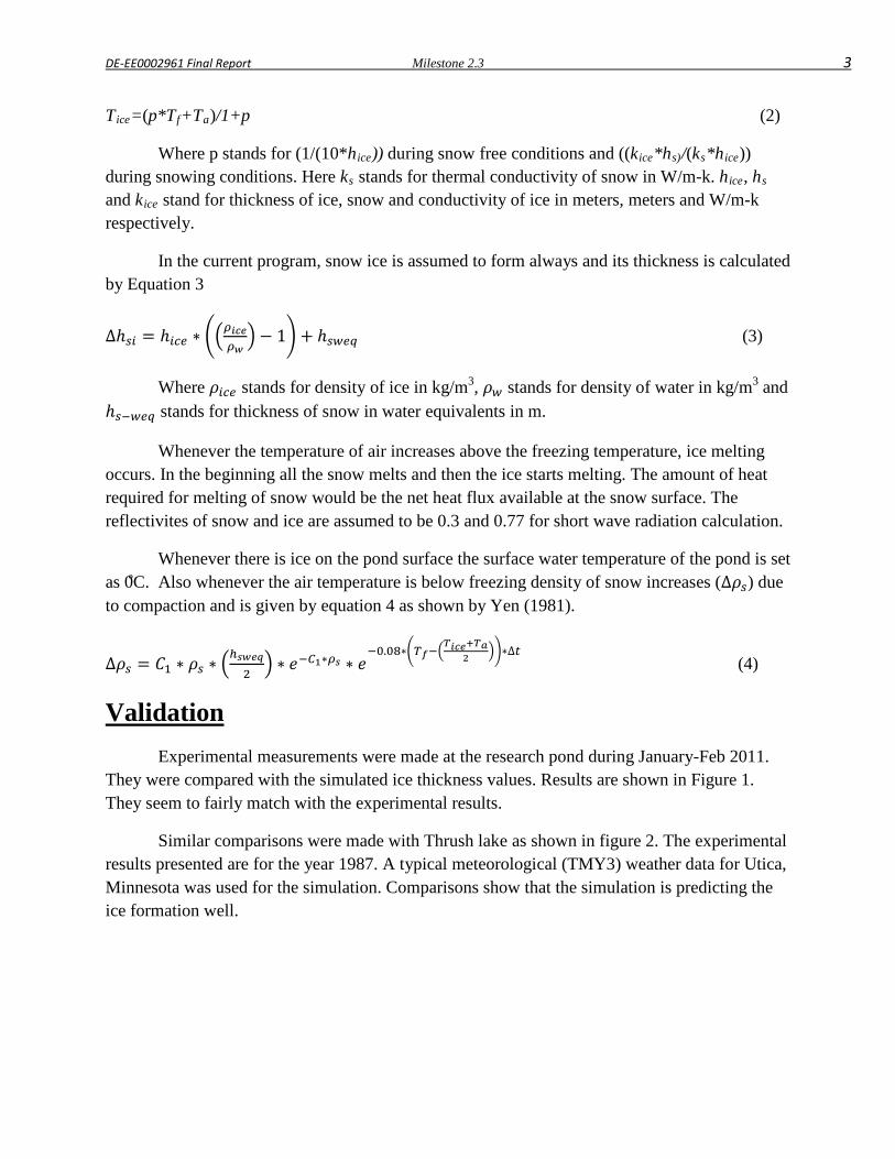
DE-EE0002961 Final Report Milestone 2.3 3
Tice=(p*Tf+Ta)/1+p (2)
Where p stands for (1/(10*hice)) during snow free conditions and ((kice*hs)/(ks*hice)) during snowing conditions. Here ks stands for thermal conductivity of snow in W/m-k. hice, hs and kice stand for thickness of ice, snow and conductivity of ice in meters, meters and W/m-k respectively.
In the current program, snow ice is assumed to form always and its thickness is calculated by Equation 3
∆ℎ𝑠𝑖 = ℎ𝑖𝑐𝑒 ∗ ��𝜌𝑖𝑐𝑒𝜌𝑤� − 1� + ℎ𝑠𝑤𝑒𝑞 (3)
Where 𝜌𝑖𝑐𝑒 stands for density of ice in kg/m3, 𝜌𝑤 stands for density of water in kg/m3 and ℎ𝑠−𝑤𝑒𝑞 stands for thickness of snow in water equivalents in m.
Whenever the temperature of air increases above the freezing temperature, ice melting occurs. In the beginning all the snow melts and then the ice starts melting. The amount of heat required for melting of snow would be the net heat flux available at the snow surface. The reflectivites of snow and ice are assumed to be 0.3 and 0.77 for short wave radiation calculation.
Whenever there is ice on the pond surface the surface water temperature of the pond is set as 0̊C. Also whenever the air temperature is below freezing density of snow increases (∆𝜌𝑠) due to compaction and is given by equation 4 as shown by Yen (1981).
∆𝜌𝑠 = 𝐶1 ∗ 𝜌𝑠 ∗ �ℎ𝑠𝑤𝑒𝑞2� ∗ 𝑒−𝐶1∗𝜌𝑠 ∗ 𝑒
−0.08∗�𝑇𝑓−�𝑇𝑖𝑐𝑒+𝑇𝑎
2 ��∗∆𝑡 (4)
Validation Experimental measurements were made at the research pond during January-Feb 2011. They were compared with the simulated ice thickness values. Results are shown in Figure 1. They seem to fairly match with the experimental results.
Similar comparisons were made with Thrush lake as shown in figure 2. The experimental results presented are for the year 1987. A typical meteorological (TMY3) weather data for Utica, Minnesota was used for the simulation. Comparisons show that the simulation is predicting the ice formation well.
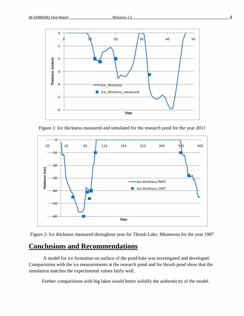
DE-EE0002961 Final Report Milestone 2.3 4
Figure 1: Ice thickness measured and simulated for the research pond for the year 2011
Figure 2: Ice thickness measured throughout year for Thrush Lake, Minnesota for the year 1987
Conclusions and Recommendations A model for ice formation on surface of the pond/lake was investigated and developed. Comparisions with the ice measurements at the research pond and for thrush pond show that the simulation matches the experimental values fairly well.
Further comparisions with big lakes would better solidify the authenticity of the model.
-6
-5
-4
-3
-2
-1
0
0 10 20 30 40 50
Thick
ness
(in
ches
)
Days
Ice_thickness
Ice_thickness_measured
-60
-50
-40
-30
-20
-10
0
-35 15 65 115 165 215 265 315 365
thick
ness
(cm
)
Days
Ice-thickness,TMY3
Ice-thickness, 1987
DE-EE0002961 Final Report Milestone 2.3 5
Nomenclature C1 = 7 m-1hr-1; coefficient used in the calculation of density of snow due to compaction
C2 = 0.021 m3/kg; coefficient used in the calculation of density of snow due to compaction
hice= Thickness of ice in m
hs= Thickness of snow in m
hsi = Thickness of snow-ice in m
hs weq= Thickness of snow in water equivalents in m
ks= Thermal conductivity of snow in W/mk
kice=Thermal conductivity of ice in W/mk
L = latent heat of fusion of ice in J/kg
p = a constant used in the calculation of temperature of ice
Ta = Temperature of air in ˚C
Tf = freezing temperature of water in ˚C
Tice = Temperature of ice in ˚C
∆t = time step in seconds
ρice = density of ice in kg/m3
ρs = density of snow in kg/m3
References Lepparanta, M.(1991). A review of analytical models of sea-ice growth. Atmosphere-Ocean 31: 123-138. Saloranta, T. M. and T. Andersen. (2004). Mylake (v.1.1): Technical model documentation and user's
guide. NIVA-report 4838. Olso,Norway, Norwegian Institute for Water Research. 44. Yen, Y. C. (1981). Review of thermal properties of snow, ice and sea-ice. Hanover,NH,USA, US Army Cold
Regions Research and Engineering Laboratory.
DE-EE0002961 Final Report Milestone report 3.1
Milestone Report 1.1
Implementation of Enhanced SCW Model in EnergyPlus
Annamalai Ramesh
Oklahoma State University
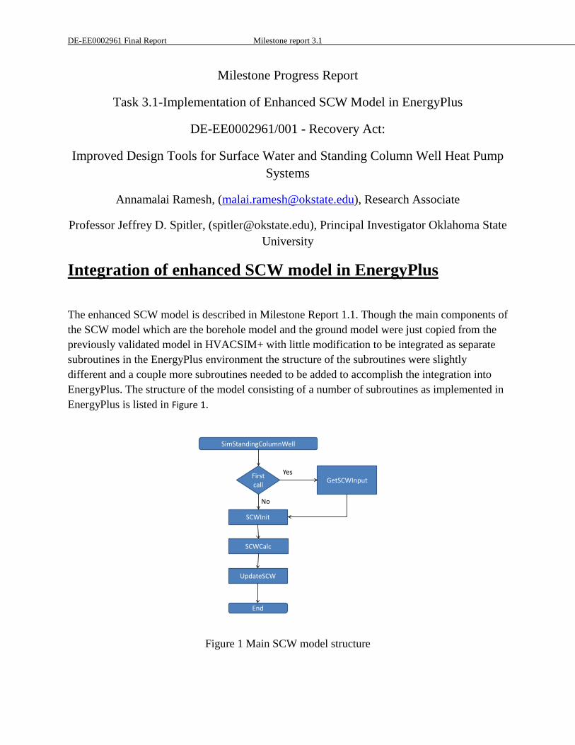
DE-EE0002961 Final Report Milestone report 3.1
Milestone Progress Report
Task 3.1-Implementation of Enhanced SCW Model in EnergyPlus
DE-EE0002961/001 - Recovery Act:
Improved Design Tools for Surface Water and Standing Column Well Heat Pump Systems
Annamalai Ramesh, ([email protected]), Research Associate
Professor Jeffrey D. Spitler, ([email protected]), Principal Investigator Oklahoma State University
Integration of enhanced SCW model in EnergyPlus
The enhanced SCW model is described in Milestone Report 1.1. Though the main components of the SCW model which are the borehole model and the ground model were just copied from the previously validated model in HVACSIM+ with little modification to be integrated as separate subroutines in the EnergyPlus environment the structure of the subroutines were slightly different and a couple more subroutines needed to be added to accomplish the integration into EnergyPlus. The structure of the model consisting of a number of subroutines as implemented in EnergyPlus is listed in Figure 1.
SimStandingColumnWell
First call GetSCWInput
SCWInit
SCWCalc
UpdateSCW
End
Yes
No
Figure 1 Main SCW model structure
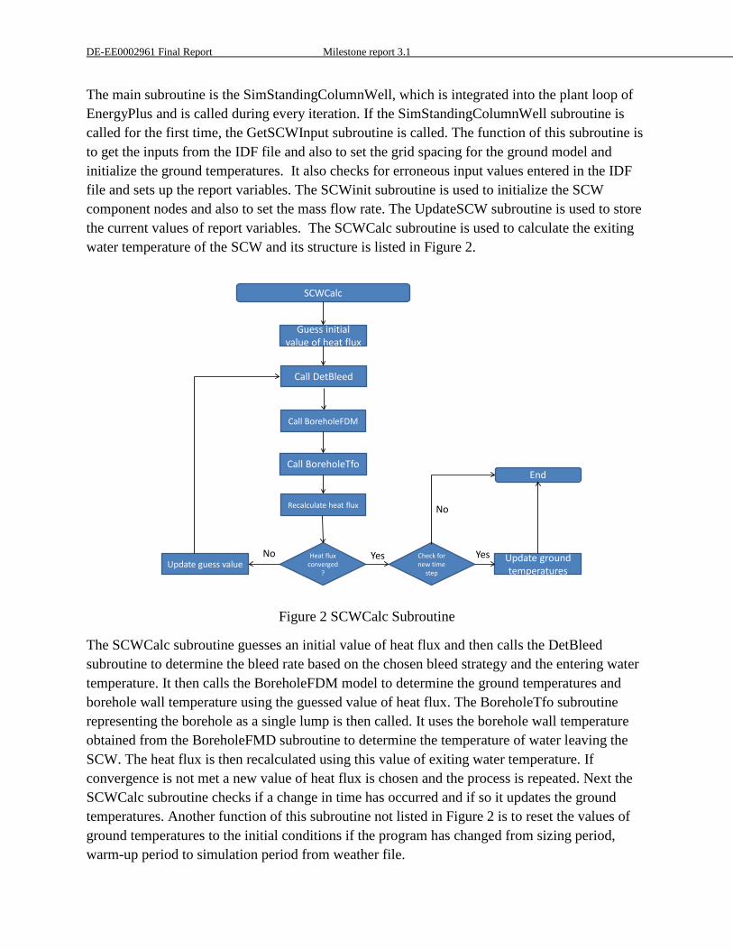
DE-EE0002961 Final Report Milestone report 3.1
The main subroutine is the SimStandingColumnWell, which is integrated into the plant loop of EnergyPlus and is called during every iteration. If the SimStandingColumnWell subroutine is called for the first time, the GetSCWInput subroutine is called. The function of this subroutine is to get the inputs from the IDF file and also to set the grid spacing for the ground model and initialize the ground temperatures. It also checks for erroneous input values entered in the IDF file and sets up the report variables. The SCWinit subroutine is used to initialize the SCW component nodes and also to set the mass flow rate. The UpdateSCW subroutine is used to store the current values of report variables. The SCWCalc subroutine is used to calculate the exiting water temperature of the SCW and its structure is listed in Figure 2.
SCWCalc
Call DetBleed
Call BoreholeFDM
Call BoreholeTfo
Recalculate heat flux
End
Guess initial value of heat flux
Heat flux converged
?Update guess value
No Check for new time
step
Update ground temperatures
Yes Yes
No
Figure 2 SCWCalc Subroutine
The SCWCalc subroutine guesses an initial value of heat flux and then calls the DetBleed subroutine to determine the bleed rate based on the chosen bleed strategy and the entering water temperature. It then calls the BoreholeFDM model to determine the ground temperatures and borehole wall temperature using the guessed value of heat flux. The BoreholeTfo subroutine representing the borehole as a single lump is then called. It uses the borehole wall temperature obtained from the BoreholeFMD subroutine to determine the temperature of water leaving the SCW. The heat flux is then recalculated using this value of exiting water temperature. If convergence is not met a new value of heat flux is chosen and the process is repeated. Next the SCWCalc subroutine checks if a change in time has occurred and if so it updates the ground temperatures. Another function of this subroutine not listed in Figure 2 is to reset the values of ground temperatures to the initial conditions if the program has changed from sizing period, warm-up period to simulation period from weather file.
DE-EE0002961 Final Report Milestone report 3.1
Development of input files
The two input files associated with EnergyPlus are the IDD and IDF files. The IDD file consists of all the parameters that are required for the model. It also specifies which parameters are compulsory, which are optional and their minimum and maximum values if required. An excerpt from the IDD file containing the input variables for the SCW model is listed in Appendix 3.1.1. The IDF file consists of the actual values of the input parameters of not only the SCW but of all the components in the plant and in the zone. Currently an existing input file “GSHP-GHLE.idf” is available in the EnergyPlus data base of input files. It uses a vertical ground heat exchanger as part of the plant condenser loop. Since the operation of the vertical ground heat exchanger are similar as both use the ground as a heat source/sink it was decided to use the same example file but replace the vertical ground heat exchanger with an SCW with all other components remaining the same rather than develop a new IDF file. An excerpt of the IDF file containing the input values for the SCW is listed in Appendix 3.1.2 along with a detailed description of each input parameter. One common error that the user is likely to make is to select an anti-freeze as the working fluid for the plant loop; however this should be avoided as the SCW can only operate with water. A warning or error will be displayed to the user if any fluid other than water is specified in the plant loop. The output report variables that can be generated are the flow rate, heat transfer, bleed rate, inlet temperature and exit temperature.
Verification of SCW model
The results of the SCW model for cases with no bleed and temperature dependent bleed generated using EnergyPlus were compared with the results of the previously validated model. The previously validated model and the validation are described in Milestone Report 1.1. The input parameters used in the IDF file and the SCW entering water temperature at each hour obtained from the EnergyPlus output file were used as inputs to the previously validated SCW model. However some small differences are likely to occur as EnergyPlus uses a variable time step and the hourly output values are averaged duration. For the case with no bleed and the case with bleed the RMSE between the validated SCW model and the SCW model in EnergyPlus was found to be between 0.004-0.006 °C.
DE-EE0002961 Final Report Milestone 3.2 1
Milestone 3.2
Implementation of enhanced SCW model in design tool
James Cullin
Oklahoma State University

DE-EE0002961 Final Report Milestone 3.2 2
Milestone Progress Report
Task 3.2 - Implementation of enhanced SCW model in design tool
DE-EE0002961/001 - Recovery Act:
Improved Design Tools for Surface Water and Standing Column Well Heat Pump Systems
James Cullin ([email protected]), Ph.D. Student
Oklahoma State University
Design Tool Implementation The standing column well (SCW) model has been previously described as part of subtasks 1.1 and 1.2. For this subtask, the model has been incorporated into the GLHEPRO ground heat exchanger design tool. The main screen of the GLHEPRO tool is shown below in Figure 1. From this main screen, the general borehole parameters, ground parameters, and heat pump specification. For an SCW system, since the operating fluid is groundwater, no separate fluid selection is necessary. At the moment, only one SCW is assumed in each system.
By selecting the "Calculate borehole thermal resistance" option, the window in Figure 2 appears. From this screen, the dip tube size can be chosen. Additionally, the bleed rate and other parameters associated with the SCW bleed may be set here. Once all the values have been entered, the "Calculate borehole resistance" button at the bottom is clicked, and the user will be returned to the main screen.
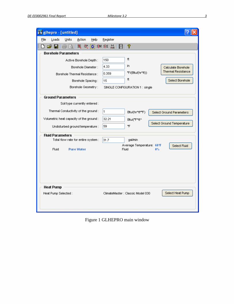
DE-EE0002961 Final Report Milestone 3.2 3
Figure 1 GLHEPRO main window
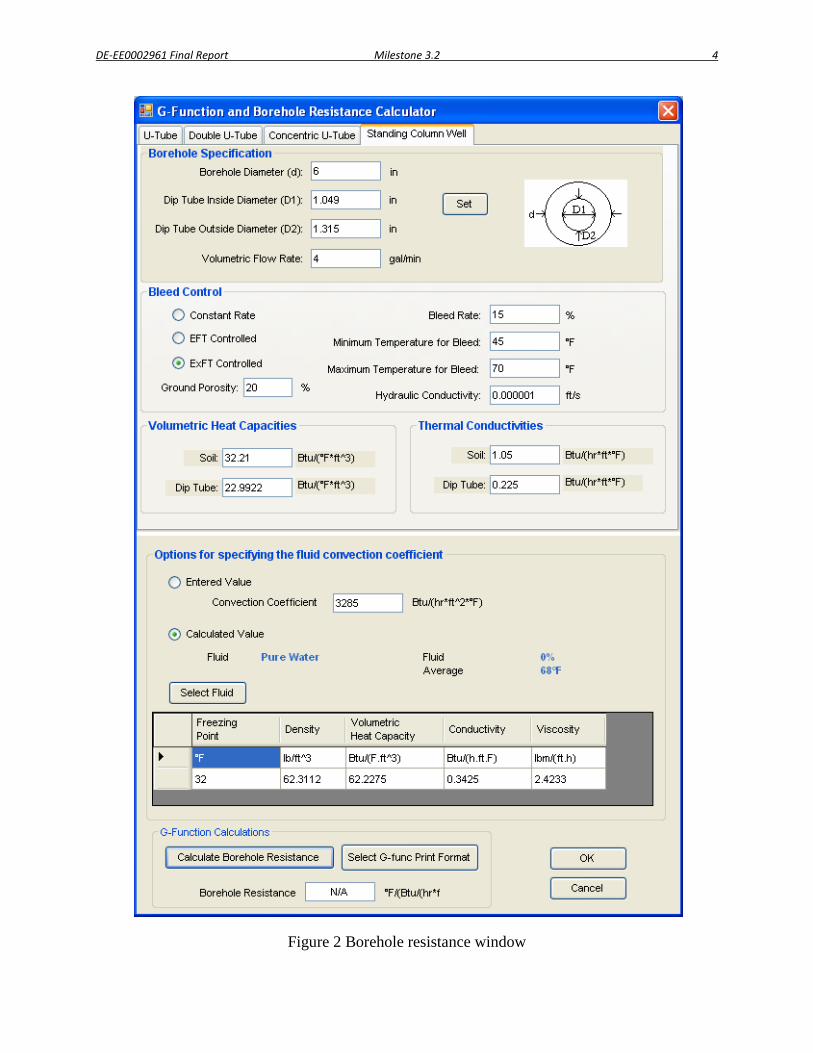
DE-EE0002961 Final Report Milestone 3.2 4
Figure 2 Borehole resistance window
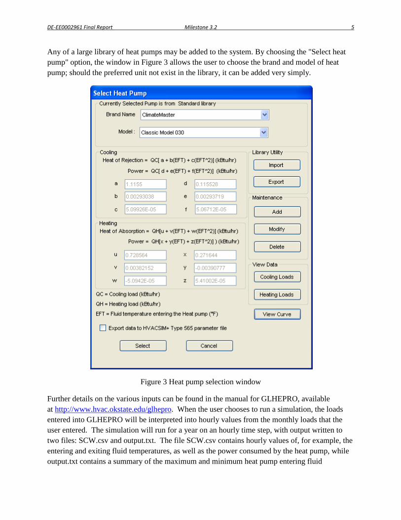
DE-EE0002961 Final Report Milestone 3.2 5
Any of a large library of heat pumps may be added to the system. By choosing the "Select heat pump" option, the window in Figure 3 allows the user to choose the brand and model of heat pump; should the preferred unit not exist in the library, it can be added very simply.
Figure 3 Heat pump selection window
Further details on the various inputs can be found in the manual for GLHEPRO, available at http://www.hvac.okstate.edu/glhepro. When the user chooses to run a simulation, the loads entered into GLHEPRO will be interpreted into hourly values from the monthly loads that the user entered. The simulation will run for a year on an hourly time step, with output written to two files: SCW.csv and output.txt. The file SCW.csv contains hourly values of, for example, the entering and exiting fluid temperatures, as well as the power consumed by the heat pump, while output.txt contains a summary of the maximum and minimum heat pump entering fluid
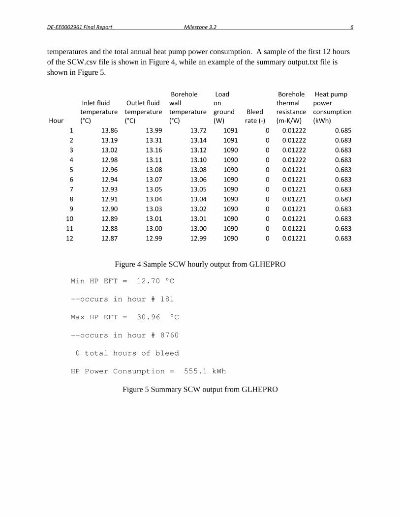
DE-EE0002961 Final Report Milestone 3.2 6
temperatures and the total annual heat pump power consumption. A sample of the first 12 hours of the SCW.csv file is shown in Figure 4, while an example of the summary output.txt file is shown in Figure 5.
Hour
Inlet fluid temperature (°C)
Outlet fluid temperature (°C)
Borehole wall temperature (°C)
Load on ground (W)
Bleed rate (-)
Borehole thermal resistance (m-K/W)
Heat pump power consumption (kWh)
1 13.86 13.99 13.72 1091 0 0.01222 0.685 2 13.19 13.31 13.14 1091 0 0.01222 0.683 3 13.02 13.16 13.12 1090 0 0.01222 0.683 4 12.98 13.11 13.10 1090 0 0.01222 0.683 5 12.96 13.08 13.08 1090 0 0.01221 0.683 6 12.94 13.07 13.06 1090 0 0.01221 0.683 7 12.93 13.05 13.05 1090 0 0.01221 0.683 8 12.91 13.04 13.04 1090 0 0.01221 0.683 9 12.90 13.03 13.02 1090 0 0.01221 0.683
10 12.89 13.01 13.01 1090 0 0.01221 0.683 11 12.88 13.00 13.00 1090 0 0.01221 0.683 12 12.87 12.99 12.99 1090 0 0.01221 0.683
Figure 4 Sample SCW hourly output from GLHEPRO
Min HP EFT = 12.70 °C
--occurs in hour # 181
Max HP EFT = 30.96 °C
--occurs in hour # 8760
0 total hours of bleed
HP Power Consumption = 555.1 kWh
Figure 5 Summary SCW output from GLHEPRO
DE-EE0002961 Final Report Milestone 3.2 1
Milestone 3.3
Implementation of enhanced SCW model – Technology Transfer
Annamalai Ramesh, Jeffrey Spitler
Oklahoma State University
This report contains a copy of the paper:
Ramesh, A. and J.D. Spitler. 2012. A quasi-two-dimensional standing column well model for ground source heat pump systems. Proceedings of Innostock 2012, The 12th International Conference on Energy Storage. Lleida, Spain. May 2012.
Innostock 2012 The 12th International Conference on Energy Storage
1
INNO-U-39
A quasi-two-dimensional standing column well model for ground source heat pump systems
Annamalai Ramesh1, Jeffrey Spitler2
1School of Mechanical and Aerospace Engineering, Oklahoma State University, Stillwater, OK 74078, USA, Phone: 405-744-0389, Fax: 405-744-7873, e-mail: [email protected]
2School of Mechanical and Aerospace Engineering, Oklahoma State University, Stillwater, OK 74078, USA, Phone: 405-744-5900, Fax: 405-744-7873, e-mail: [email protected]
1. Introduction
Standing column wells (SCW) are a type of ground heat exchanger (GHE) that may be used with ground source heat pump (GSHP) or underground thermal energy storage (UTES) systems. SCWs are “open-loop” ground heat exchangers that draw ground water from the bottom of the well and, after passing it through a heat pump or heat exchanger, return it at the top of the well. Water circulating down the borehole wall exchanges heat with the surrounding ground.
Compared to closed-loop ground heat exchangers, standing column wells have three important advantages that allow for increased heat transfer and, consequently, less required borehole length and lower first cost. First, standing column wells have lower borehole thermal resistance than closed-loop ground heat exchangers because the working fluid is in direct contact with the borehole wall. Typical values for borehole resistance of closed-loop grouted heat exchangers are on the order of 0.1-0.3 m-K/W. In SCWs, fully turbulent flow results in values of borehole thermal resistance around 0.0005-0.005 m-K/W. Second, they benefit from groundwater flow in and out of the surrounding formation that is induced by pumping and density differences between the groundwater in the well and that in the surrounding ground. Third, in locations where it is permissible to bleed off some of the water drawn from the well, the induced flow of groundwater into the borehole significantly enhances the heat transfer.
Though SCWs have been in operation since the 1970s, there is relatively little published research on this type of GHE. SCW models are needed to support design software and energy calculation software. But only a few SCW models have been developed and several of these are too computationally expensive to be directly useful for design or energy calculations.
One of the first SCW models (Yuill and Mikler 1995) utilized a simple groundwater flow model to estimate the groundwater flow induced by pumping in and out of the borehole. Then a one-dimensional finite difference model which accounted for heat conduction and advection was used to analyze the heat transfer. As presented, the model did not account for bleed or convective resistances inside the borehole. Rees et al. (2004) developed a two-dimensional finite volume model and Ng et al. (2010) developed a three-dimensional finite volume model. Both models are capable of modeling bleed and accounting for convective resistances inside the borehole. Both models used separate grids to model the heat transfer in the borehole and the surrounding ground; the two solution domains are coupled together and solved iteratively. The grid size and iteratively coupled solution technique requires significant computational time, making either model too computationally intensive for direct use in either design software or energy calculation software.
A computationally efficient model which is more suited to be used in design tools or energy analysis programs is the one-dimensional SCW model developed by Deng et al. (2005). Though it is computationally efficient, there are some aspects of the model that have not been thoroughly investigated. These include its assumption of isotropic aquifers with homogeneous
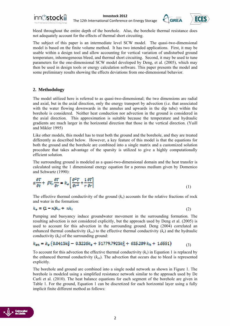
Innostock 2012 The 12th International Conference on Energy Storage
2
bleed throughout the entire depth of the borehole. Also, the borehole thermal resistance does not adequately account for the effects of thermal short circuiting.
The subject of this paper is an intermediate level SCW model. The quasi-two-dimensional model is based on the finite volume method. It has two intended applications. First, it may be usable within a design tool and allow accounting for vertical variation of undisturbed ground temperature, inhomogeneous bleed, and thermal short circuiting. Second, it may be used to tune parameters for the one-dimensional SCW model developed by Deng, et al. (2005), which may then be used in design tools or energy calculation software. This paper presents the model and some preliminary results showing the effects deviations from one-dimensional behavior.
2. Methodology
The model utilized here is referred to as quasi-two-dimensional; the two dimensions are radial and axial, but in the axial direction, only the energy transport by advection (i.e. that associated with the water flowing downwards in the annulus and upwards in the dip tube) within the borehole is considered. Neither heat conduction nor advection in the ground is considered in the axial direction. This approximation is suitable because the temperature and hydraulic gradients are much larger in the horizontal direction that those in the vertical direction. (Yuill and Mikler 1995)
Like other models, this model has to treat both the ground and the borehole, and they are treated differently as described below. However, a key feature of this model is that the equations for both the ground and the borehole are combined into a single matrix and a customized solution procedure that takes advantage of the sparsity is utilized to give a highly computationally efficient solution.
The surrounding ground is modeled as a quasi-two-dimensional domain and the heat transfer is calculated using the 1 dimensional energy equation for a porous medium given by Domenico and Schwartz (1990):
(1)
The effective thermal conductivity of the ground (ke) accounts for the relative fractions of rock and water in the formation:
(2)
Pumping and buoyancy induce groundwater movement in the surrounding formation. The resulting advection is not considered explicitly, but the approach used by Deng et al. (2005) is used to account for this advection in the surrounding ground. Deng (2004) correlated an enhanced thermal conductivity (ken) to the effective thermal conductivity (ke) and the hydraulic conductivity (kh) of the surrounding ground:
(3)
To account for this advection the effective thermal conductivity (ke) in Equation 1 is replaced by the enhanced thermal conductivity (ken). The advection that occurs due to bleed is represented explicitly.
The borehole and ground are combined into a single nodal network as shown in Figure 1. The borehole is modeled using a simplified resistance network similar to the approach used by De Carli et al. (2010). The heat balance equations for each segment of the borehole are given in Table 1. For the ground, Equation 1 can be discretized for each horizontal layer using a fully implicit finite different method as follows:
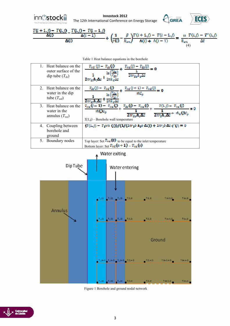
Innostock 2012 The 12th International Conference on Energy Storage
3
(4)
Table 1 Heat balance equations in the borehole
1. Heat balance on the outer surface of the dip tube (Tds)
2. Heat balance on the water in the dip tube (Twd)
3. Heat balance on the
water in the annulus (Twa)
T(1,j) – Borehole wall temperature
4. Coupling between borehole and ground
5. Boundary nodes Top layer: Set to be equal to the inlet temperature
Bottom layer: Set =
Figure 1 Borehole and ground nodal network
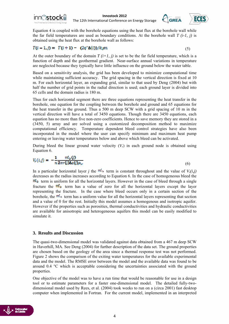
Innostock 2012 The 12th International Conference on Energy Storage
4
Equation 4 is coupled with the borehole equations using the heat flux at the borehole wall while the far field temperatures are used as boundary conditions. At the borehole wall T (i-1, j) is obtained using the heat flux at the borehole wall as follows:
(5)
At the outer boundary of the domain T (i+1, j) is set to be the far field temperature, which is a function of depth and the geothermal gradient. Near-surface annual variations in temperature are neglected because they typically have little influence on the ground below the water table.
Based on a sensitivity analysis, the grid has been developed to minimize computational time while maintaining sufficient accuracy. The grid spacing in the vertical direction is fixed at 10 m. For each horizontal layer, an expanding grid, similar to that used by Deng (2004) but with half the number of grid points in the radial direction is used; each ground layer is divided into 65 cells and the domain radius is 180 m.
Thus for each horizontal segment there are three equations representing the heat transfer in the borehole, one equation for the coupling between the borehole and ground and 65 equations for the heat transfer in the ground. Thus a 500 m deep SCW with a grid spacing of 10 m in the vertical direction will have a total of 3450 equations. Though there are 3450 equations, each equation has no more than five non-zero coefficients. Hence to save memory they are stored in a (3450, 5) array and are solved using a customized decomposition method to maximize computational efficiency. Temperature dependent bleed control strategies have also been incorporated in the model where the user can specify minimum and maximum heat pump entering or leaving water temperatures below and above which bleed can be activated.
During bleed the linear ground water velocity (Vr) in each ground node is obtained using Equation 6.
(6)
In a particular horizontal layer j the term is constant throughout and the value of Vr(i,j) decreases as the radius increases according to Equation 6. In the case of homogeneous bleed the
term is uniform for all the horizontal layers. However in the case of bleed through a single fracture the term has a value of zero for all the horizontal layers except the layer representing the fracture. In the case where bleed occurs only in a certain section of the borehole, the term has a uniform value for all the horizontal layers representing that section and a value of 0 for the rest. Initially this model assumes a homogenous and isotropic aquifer. However if the properties such as porosities, thermal conductivities and hydraulic conductivities are available for anisotropic and heterogeneous aquifers this model can be easily modified to simulate it.
3. Results and Discussion
The quasi-two-dimensional model was validated against data obtained from a 467 m deep SCW in Haverhill, MA. See Deng (2004) for further description of the data set. The ground properties are chosen based on the geology of the area since a thermal response test was not performed. Figure 2 shows the comparison of the exiting water temperatures for the available experimental data and the model. The RMSE error between the model and the available data was found to be around 0.4 °C which is acceptable considering the uncertainties associated with the ground properties.
One objective of the model was to have a run time that would be reasonable for use in a design tool or to estimate parameters for a faster one-dimensional model. The detailed fully-two-dimensional model used by Rees, et al. (2004) took weeks to run on a (circa 2001) fast desktop computer when implemented in Fortran. For the current model, implemented in an interpreted
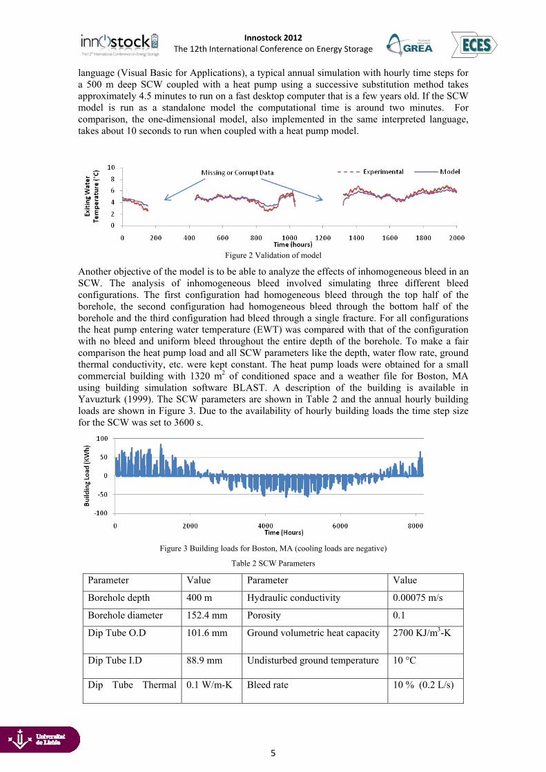
Innostock 2012 The 12th International Conference on Energy Storage
5
language (Visual Basic for Applications), a typical annual simulation with hourly time steps for a 500 m deep SCW coupled with a heat pump using a successive substitution method takes approximately 4.5 minutes to run on a fast desktop computer that is a few years old. If the SCW model is run as a standalone model the computational time is around two minutes. For comparison, the one-dimensional model, also implemented in the same interpreted language, takes about 10 seconds to run when coupled with a heat pump model.
Figure 2 Validation of model
Another objective of the model is to be able to analyze the effects of inhomogeneous bleed in an SCW. The analysis of inhomogeneous bleed involved simulating three different bleed configurations. The first configuration had homogeneous bleed through the top half of the borehole, the second configuration had homogeneous bleed through the bottom half of the borehole and the third configuration had bleed through a single fracture. For all configurations the heat pump entering water temperature (EWT) was compared with that of the configuration with no bleed and uniform bleed throughout the entire depth of the borehole. To make a fair comparison the heat pump load and all SCW parameters like the depth, water flow rate, ground thermal conductivity, etc. were kept constant. The heat pump loads were obtained for a small commercial building with 1320 m2 of conditioned space and a weather file for Boston, MA using building simulation software BLAST. A description of the building is available in Yavuzturk (1999). The SCW parameters are shown in Table 2 and the annual hourly building loads are shown in Figure 3. Due to the availability of hourly building loads the time step size for the SCW was set to 3600 s.
Figure 3 Building loads for Boston, MA (cooling loads are negative)
Table 2 SCW Parameters
Parameter Value Parameter Value
Borehole depth 400 m Hydraulic conductivity 0.00075 m/s
Borehole diameter 152.4 mm Porosity 0.1
Dip Tube O.D 101.6 mm Ground volumetric heat capacity 2700 KJ/m3-K
Dip Tube I.D 88.9 mm Undisturbed ground temperature 10 °C
Dip Tube Thermal 0.1 W/m-K Bleed rate 10 % (0.2 L/s)
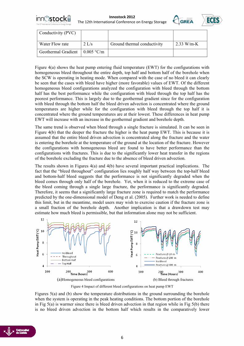
Innostock 2012 The 12th International Conference on Energy Storage
6
Conductivity (PVC)
Water Flow rate 2 L/s Ground thermal conductivity 2.33 W/m-K
Geothermal Gradient 0.005 °C/m
Figure 4(a) shows the heat pump entering fluid temperature (EWT) for the configurations with homogeneous bleed throughout the entire depth, top half and bottom half of the borehole when the SCW is operating in heating mode. When compared with the case of no bleed it can clearly be seen that the cases with bleed have higher (more favorable) values of EWT. Of the different homogeneous bleed configurations analyzed the configuration with bleed through the bottom half has the best performance while the configuration with bleed through the top half has the poorest performance. This is largely due to the geothermal gradient since for the configuration with bleed through the bottom half the bleed driven advection is concentrated where the ground temperatures are higher while for the configuration with bleed through the top half it is concentrated where the ground temperatures are at their lowest. These differences in heat pump EWT will increase with an increase in the geothermal gradient and borehole depth.
The same trend is observed when bleed through a single fracture is simulated. It can be seen in Figure 4(b) that the deeper the fracture the higher is the heat pump EWT. This is because it is assumed that the entire bleed driven advection is concentrated along the fracture and the water is entering the borehole at the temperature of the ground at the location of the fracture. However the configurations with homogeneous bleed are found to have better performance than the configurations with fractures. This is due to the significantly lower heat transfer in the regions of the borehole excluding the fracture due to the absence of bleed driven advection.
The results shown in Figures 4(a) and 4(b) have several important practical implications. The fact that the “bleed throughout” configuration lies roughly half way between the top-half bleed and bottom-half bleed suggests that the performance is not significantly degraded when the bleed comes through only half of the borehole. Yet, when it is reduced to the extreme case of the bleed coming through a single large fracture, the performance is significantly degraded. Therefore, it seems that a significantly large fracture zone is required to match the performance predicted by the one-dimensional model of Deng et al. (2005). Further work is needed to define this limit, but in the meantime, model users may wish to exercise caution if the fracture zone is a small fraction of the borehole depth. Another implication is that a drawdown test may estimate how much bleed is permissible, but that information alone may not be sufficient.
(a)Homogeneous bleed configurations (b) Bleed through fractures
Figure 4 Impact of different bleed configurations on heat pump EWT
Figures 5(a) and (b) show the temperature distributions in the ground surrounding the borehole when the system is operating in the peak heating conditions. The bottom portion of the borehole in Fig 5(a) is warmer since there is bleed driven advection in that region while in Fig 5(b) there is no bleed driven advection in the bottom half which results in the comparatively lower
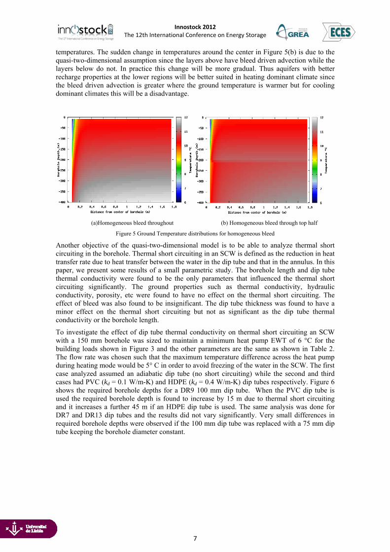
Innostock 2012 The 12th International Conference on Energy Storage
7
temperatures. The sudden change in temperatures around the center in Figure 5(b) is due to the quasi-two-dimensional assumption since the layers above have bleed driven advection while the layers below do not. In practice this change will be more gradual. Thus aquifers with better recharge properties at the lower regions will be better suited in heating dominant climate since the bleed driven advection is greater where the ground temperature is warmer but for cooling dominant climates this will be a disadvantage.
(a)Homogeneous bleed throughout (b) Homogeneous bleed through top half
Figure 5 Ground Temperature distributions for homogeneous bleed
Another objective of the quasi-two-dimensional model is to be able to analyze thermal short circuiting in the borehole. Thermal short circuiting in an SCW is defined as the reduction in heat transfer rate due to heat transfer between the water in the dip tube and that in the annulus. In this paper, we present some results of a small parametric study. The borehole length and dip tube thermal conductivity were found to be the only parameters that influenced the thermal short circuiting significantly. The ground properties such as thermal conductivity, hydraulic conductivity, porosity, etc were found to have no effect on the thermal short circuiting. The effect of bleed was also found to be insignificant. The dip tube thickness was found to have a minor effect on the thermal short circuiting but not as significant as the dip tube thermal conductivity or the borehole length.
To investigate the effect of dip tube thermal conductivity on thermal short circuiting an SCW with a 150 mm borehole was sized to maintain a minimum heat pump EWT of 6 °C for the building loads shown in Figure 3 and the other parameters are the same as shown in Table 2. The flow rate was chosen such that the maximum temperature difference across the heat pump during heating mode would be 5° C in order to avoid freezing of the water in the SCW. The first case analyzed assumed an adiabatic dip tube (no short circuiting) while the second and third cases had PVC (kd = 0.1 W/m-K) and HDPE (kd = 0.4 W/m-K) dip tubes respectively. Figure 6 shows the required borehole depths for a DR9 100 mm dip tube. When the PVC dip tube is used the required borehole depth is found to increase by 15 m due to thermal short circuiting and it increases a further 45 m if an HDPE dip tube is used. The same analysis was done for DR7 and DR13 dip tubes and the results did not vary significantly. Very small differences in required borehole depths were observed if the 100 mm dip tube was replaced with a 75 mm dip tube keeping the borehole diameter constant.
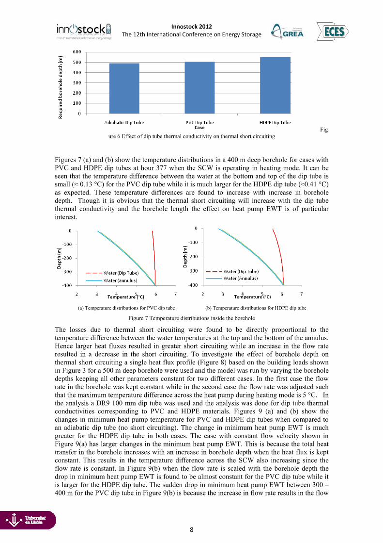
Innostock 2012 The 12th International Conference on Energy Storage
8
Figure 6 Effect of dip tube thermal conductivity on thermal short circuiting
Figures 7 (a) and (b) show the temperature distributions in a 400 m deep borehole for cases with PVC and HDPE dip tubes at hour 377 when the SCW is operating in heating mode. It can be seen that the temperature difference between the water at the bottom and top of the dip tube is small (≈ 0.13 °C) for the PVC dip tube while it is much larger for the HDPE dip tube (≈0.41 °C) as expected. These temperature differences are found to increase with increase in borehole depth. Though it is obvious that the thermal short circuiting will increase with the dip tube thermal conductivity and the borehole length the effect on heat pump EWT is of particular interest.
(a) Temperature distributions for PVC dip tube (b) Temperature distributions for HDPE dip tube
Figure 7 Temperature distributions inside the borehole
The losses due to thermal short circuiting were found to be directly proportional to the temperature difference between the water temperatures at the top and the bottom of the annulus. Hence larger heat fluxes resulted in greater short circuiting while an increase in the flow rate resulted in a decrease in the short circuiting. To investigate the effect of borehole depth on thermal short circuiting a single heat flux profile (Figure 8) based on the building loads shown in Figure 3 for a 500 m deep borehole were used and the model was run by varying the borehole depths keeping all other parameters constant for two different cases. In the first case the flow rate in the borehole was kept constant while in the second case the flow rate was adjusted such that the maximum temperature difference across the heat pump during heating mode is 5 °C. In the analysis a DR9 100 mm dip tube was used and the analysis was done for dip tube thermal conductivities corresponding to PVC and HDPE materials. Figures 9 (a) and (b) show the changes in minimum heat pump temperature for PVC and HDPE dip tubes when compared to an adiabatic dip tube (no short circuiting). The change in minimum heat pump EWT is much greater for the HDPE dip tube in both cases. The case with constant flow velocity shown in Figure 9(a) has larger changes in the minimum heat pump EWT. This is because the total heat transfer in the borehole increases with an increase in borehole depth when the heat flux is kept constant. This results in the temperature difference across the SCW also increasing since the flow rate is constant. In Figure 9(b) when the flow rate is scaled with the borehole depth the drop in minimum heat pump EWT is found to be almost constant for the PVC dip tube while it is larger for the HDPE dip tube. The sudden drop in minimum heat pump EWT between 300 – 400 m for the PVC dip tube in Figure 9(b) is because the increase in flow rate results in the flow
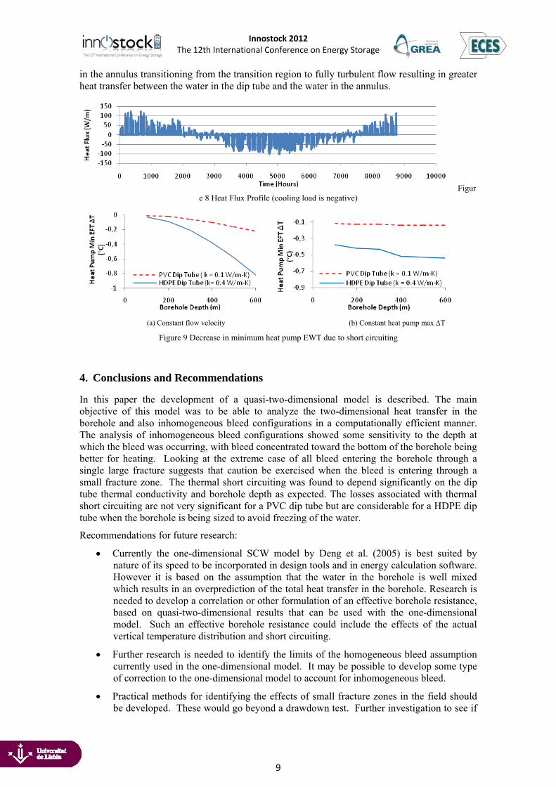
Innostock 2012 The 12th International Conference on Energy Storage
9
in the annulus transitioning from the transition region to fully turbulent flow resulting in greater heat transfer between the water in the dip tube and the water in the annulus.
Figure 8 Heat Flux Profile (cooling load is negative)
(a) Constant flow velocity (b) Constant heat pump max ΔT
Figure 9 Decrease in minimum heat pump EWT due to short circuiting
4. Conclusions and Recommendations
In this paper the development of a quasi-two-dimensional model is described. The main objective of this model was to be able to analyze the two-dimensional heat transfer in the borehole and also inhomogeneous bleed configurations in a computationally efficient manner. The analysis of inhomogeneous bleed configurations showed some sensitivity to the depth at which the bleed was occurring, with bleed concentrated toward the bottom of the borehole being better for heating. Looking at the extreme case of all bleed entering the borehole through a single large fracture suggests that caution be exercised when the bleed is entering through a small fracture zone. The thermal short circuiting was found to depend significantly on the dip tube thermal conductivity and borehole depth as expected. The losses associated with thermal short circuiting are not very significant for a PVC dip tube but are considerable for a HDPE dip tube when the borehole is being sized to avoid freezing of the water.
Recommendations for future research:
Currently the one-dimensional SCW model by Deng et al. (2005) is best suited by nature of its speed to be incorporated in design tools and in energy calculation software. However it is based on the assumption that the water in the borehole is well mixed which results in an overprediction of the total heat transfer in the borehole. Research is needed to develop a correlation or other formulation of an effective borehole resistance, based on quasi-two-dimensional results that can be used with the one-dimensional model. Such an effective borehole resistance could include the effects of the actual vertical temperature distribution and short circuiting.
Further research is needed to identify the limits of the homogeneous bleed assumption currently used in the one-dimensional model. It may be possible to develop some type of correction to the one-dimensional model to account for inhomogeneous bleed.
Practical methods for identifying the effects of small fracture zones in the field should be developed. These would go beyond a drawdown test. Further investigation to see if
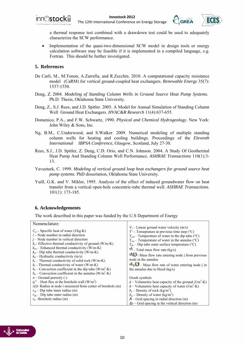
Innostock 2012 The 12th International Conference on Energy Storage
10
a thermal response test combined with a drawdown test could be used to adequately characterize the SCW performance.
Implementation of the quasi-two-dimensional SCW model in design tools or energy calculation software may be feasible if it is implemented in a compiled language, e.g. Fortran. This should be further investigated.
5. References
De Carli, M., M.Tonon, A.Zarrella, and R.Zecchin. 2010. A computational capacity resistance model (CaRM) for vertical ground-coupled heat exchangers. Renewable Energy 35(7): 1537-1550.
Deng, Z. 2004. Modeling of Standing Column Wells in Ground Source Heat Pump Systems. Ph.D. Thesis, Oklahoma State University.
Deng, Z., S.J. Rees, and J.D. Spitler. 2005. A Model for Annual Simulation of Standing Column Well Ground Heat Exchangers. HVAC&R Research 11(4):637-655.
Domenico, P.A., and F.W. Schwartz, 1990. Physical and Chemical Hydrogeology. New York: John Wiley & Sons, Inc.
Ng, B.M., C.Underwood, and S.Walker. 2009. Numerical modeling of multiple standing column wells for heating and cooling buildings. Proceedings of the Eleventh International IBPSA Conference, Glasgow, Scotland, July 27-30.
Rees, S.J., J.D. Spitler, Z. Deng, C.D. Orio, and C.N. Johnson. 2004. A Study Of Geothermal Heat Pump And Standing Column Well Performance. ASHRAE Transactions 110(1):3- 13.
Yavuzturk, C. 1999. Modeling of vertical ground loop heat exchangers for ground source heat pump systems. PhD dissertation, Oklahoma State University.
Yuill, G.K. and V. Mikler, 1995. Analysis of the effect of induced groundwater flow on heat transfer from a vertical open-hole concentric-tube thermal well. ASHRAE Transactions. 101(1): 173-185.
6. Acknowledgements The work described in this paper was funded by the U.S Department of Energy
Nomenclature:
Cp – Specific heat of water (J/kg-K) i – Node number in radial direction j – Node number in vertical direction ke– Effective thermal conductivity of ground (W/m-K) ken – Enhanced thermal conductivity (W/m-K) kd – Dip tube thermal conductivity (W/m-K) kh – Hydraulic conductivity (m/s) kr – Thermal conductivity of solid rock (W/m-K) kl – Thermal conductivity of water (W/m-K) hi – Convection coefficient in the dip tube (W/m2-K) ho – Convection coefficient in the annulus (W/m2-K) n – Ground porosity (-) q” – Heat flux at the borehole wall (W/m2) r(i)- Radius at node i measured from center of borehole (m) rdi – Dip tube inner radius (m) rdo – Dip tube outer radius (m) rb –Borehole radius (m)
Vr – Linear ground water velocity (m/s) T’ – Temeprature at previous time step (°C) Twd – Temperature of water in the dip tube (°C) Twa – Temperature of water in the annulus (°C) Tds – Dip tube outer surface temperature (°C)
- Total mass flow rate (kg/s)
- Mass flow rate entering node j from previous node in the annulus
- Mass flow rate of water entering node j in the annulus due to bleed (kg/s) Greek symbols á – Volumetric heat capacity of the ground (J/m3-K) â – Volumetric heat capacity of water (J/m3-K) ñs – Density of rock (kg/m3) ñw – Density of water (kg/m3) Ä – Grid spacing in radial direction (m) ∆z – Grid spacing in the vertical direction (m)

DE-EE0002961 Final Report Milestone 4.1 1
Milestone 4.1
Modeling of alternate pond heat exchanger types
Krishna Conjeevaram Bashyam
Oklahoma State University
DE-EE0002961 Final Report Milestone 4.1 2
Milestone Report
Task 4.1- Modeling of alternate pond heat exchanger types
DE-EE0002961/001 - Recovery Act:
Improved Design Tools for Surface Water and Standing Column Well Heat Pump Systems
Krishna Conjeevaram Bashyam, ([email protected]), Research Assistant, Professor Jeffrey D Spitler, ([email protected]), Principal Investigator,
Oklahoma State University
Introduction In practice there are several types of pond heat exchangers and the amount of heat transfer varies between heat exchanger types even with identical geometric conditions. Based on his experiments in OSU research pond Hansen (2011) obtained correlations for outside Nusset number calculation for five different types of pond heat exchangers. These correlations are implemented in the heat exchanger module of the enhanced pond model.
Methodology Hansen (2011) conducted a total of 119 tests on 5 different heat exchanger coil types in
the 3 acre (12,000 m2) OSU research pond and arrived with three correlations to calculate the outside Nusselt number and hence the outside convection heat transfer coefficient for five types of heat exchanger coils namely spiral-helical, spiral, slinky-type, loose bundled and flat vertical plate heat exchangers (e.g. “SlimJim®”). The breakdown of the tests and the parameters varied in the tests are shown in Table 1 below
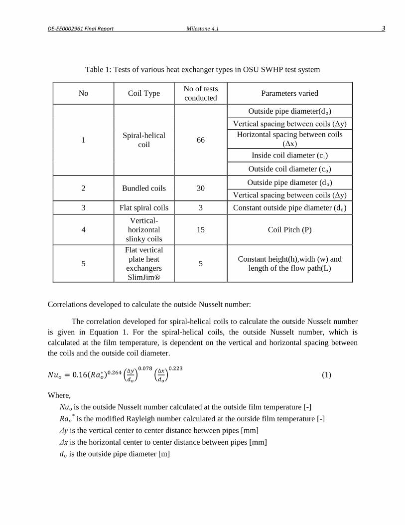
DE-EE0002961 Final Report Milestone 4.1 3
Table 1: Tests of various heat exchanger types in OSU SWHP test system
No Coil Type No of tests conducted Parameters varied
1 Spiral-helical coil 66
Outside pipe diameter(do) Vertical spacing between coils (Δy) Horizontal spacing between coils
(Δx) Inside coil diameter (ci)
Outside coil diameter (co)
2 Bundled coils 30 Outside pipe diameter (do)
Vertical spacing between coils (Δy) 3 Flat spiral coils 3 Constant outside pipe diameter (do)
4 Vertical-horizontal
slinky coils 15 Coil Pitch (P)
5
Flat vertical plate heat
exchangers SlimJim®
5 Constant height(h),widh (w) and length of the flow path(L)
Correlations developed to calculate the outside Nusselt number:
The correlation developed for spiral-helical coils to calculate the outside Nusselt number is given in Equation 1. For the spiral-helical coils, the outside Nusselt number, which is calculated at the film temperature, is dependent on the vertical and horizontal spacing between the coils and the outside coil diameter.
𝑁𝑢𝑜 = 0.16(𝑅𝑎𝑜∗)0.264 �∆𝑦𝑑𝑜�0.078
�∆𝑥𝑑𝑜�0.223
(1)
Where, Nuo is the outside Nusselt number calculated at the outside film temperature [-] Rao
* is the modified Rayleigh number calculated at the outside film temperature [-] Δy is the vertical center to center distance between pipes [mm] Δx is the horizontal center to center distance between pipes [mm] do is the outside pipe diameter [m]
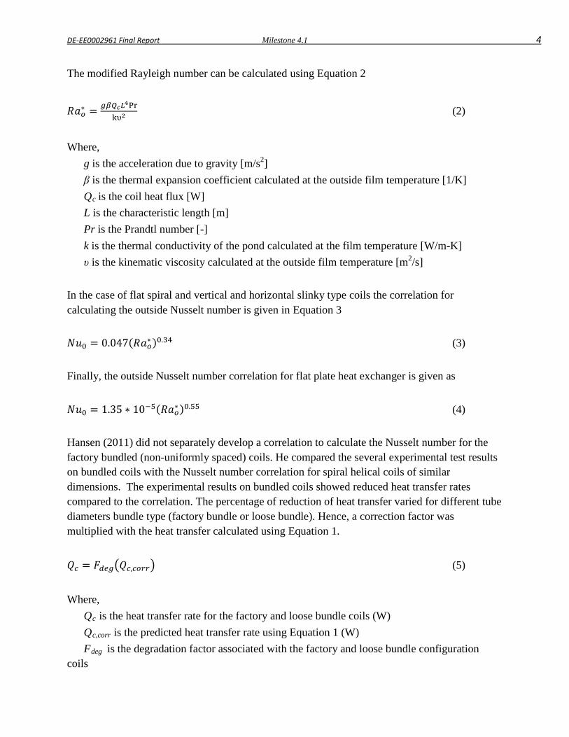
DE-EE0002961 Final Report Milestone 4.1 4
The modified Rayleigh number can be calculated using Equation 2
𝑅𝑎𝑜∗ = 𝑔𝛽𝑄𝑐𝐿4Prkυ2
(2)
Where,
g is the acceleration due to gravity [m/s2] β is the thermal expansion coefficient calculated at the outside film temperature [1/K] Qc is the coil heat flux [W] L is the characteristic length [m] Pr is the Prandtl number [-] k is the thermal conductivity of the pond calculated at the film temperature [W/m-K] υ is the kinematic viscosity calculated at the outside film temperature [m2/s]
In the case of flat spiral and vertical and horizontal slinky type coils the correlation for calculating the outside Nusselt number is given in Equation 3 𝑁𝑢0 = 0.047(𝑅𝑎𝑜∗)0.34 (3) Finally, the outside Nusselt number correlation for flat plate heat exchanger is given as 𝑁𝑢0 = 1.35 ∗ 10−5(𝑅𝑎𝑜∗)0.55 (4) Hansen (2011) did not separately develop a correlation to calculate the Nusselt number for the factory bundled (non-uniformly spaced) coils. He compared the several experimental test results on bundled coils with the Nusselt number correlation for spiral helical coils of similar dimensions. The experimental results on bundled coils showed reduced heat transfer rates compared to the correlation. The percentage of reduction of heat transfer varied for different tube diameters bundle type (factory bundle or loose bundle). Hence, a correction factor was multiplied with the heat transfer calculated using Equation 1. 𝑄𝑐 = 𝐹𝑑𝑒𝑔�𝑄𝑐,𝑐𝑜𝑟𝑟� (5) Where,
Qc is the heat transfer rate for the factory and loose bundle coils (W) Qc,corr is the predicted heat transfer rate using Equation 1 (W) Fdeg is the degradation factor associated with the factory and loose bundle configuration
coils
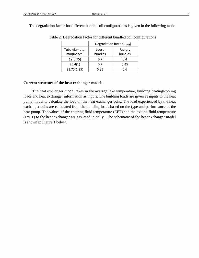
DE-EE0002961 Final Report Milestone 4.1 5
The degradation factor for different bundle coil configurations is given in the following table
Table 2: Degradation factor for different bundled coil configurations
Degradation factor (Fdeg)
Tube diameter mm(inches)
Loose bundles
Factory bundles
19(0.75) 0.7 0.4 25.4(1) 0.7 0.45
31.75(1.25) 0.85 0.6
Current structure of the heat exchanger model:
The heat exchanger model takes in the average lake temperature, building heating/cooling loads and heat exchanger information as inputs. The building loads are given as inputs to the heat pump model to calculate the load on the heat exchanger coils. The load experienced by the heat exchanger coils are calculated from the building loads based on the type and performance of the heat pump. The values of the entering fluid temperature (EFT) and the exiting fluid temperature (ExFT) to the heat exchanger are assumed initially. The schematic of the heat exchanger model is shown in Figure 1 below.

DE-EE0002961 Final Report Milestone 4.1 6
Figure 1: Heat exchanger model schematic for the ith iteration
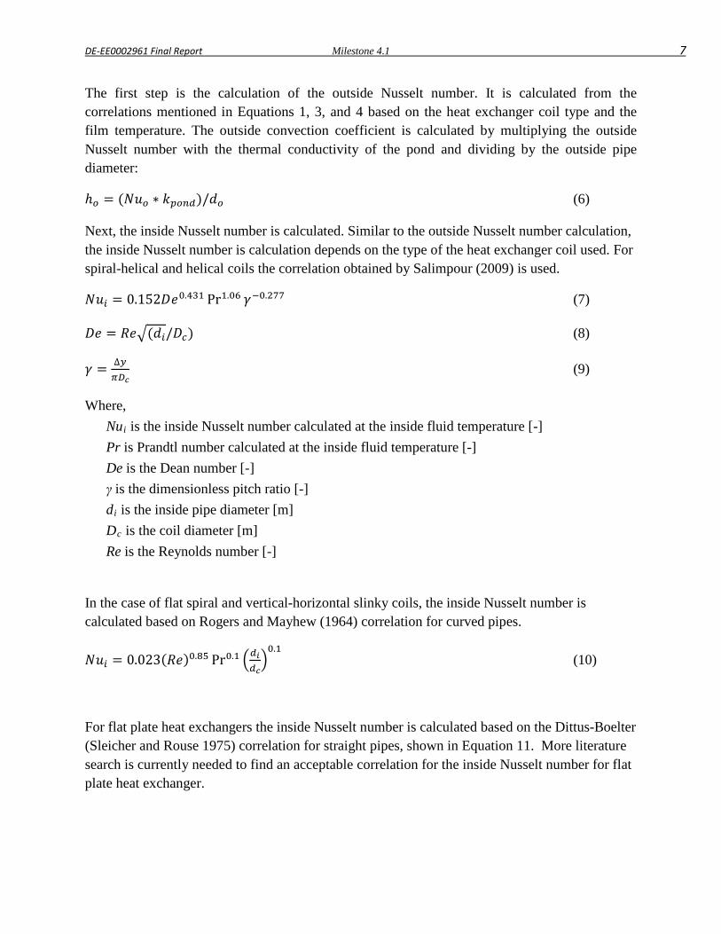
DE-EE0002961 Final Report Milestone 4.1 7
The first step is the calculation of the outside Nusselt number. It is calculated from the correlations mentioned in Equations 1, 3, and 4 based on the heat exchanger coil type and the film temperature. The outside convection coefficient is calculated by multiplying the outside Nusselt number with the thermal conductivity of the pond and dividing by the outside pipe diameter:
ℎ𝑜 = (𝑁𝑢𝑜 ∗ 𝑘𝑝𝑜𝑛𝑑)/𝑑𝑜 (6)
Next, the inside Nusselt number is calculated. Similar to the outside Nusselt number calculation, the inside Nusselt number is calculation depends on the type of the heat exchanger coil used. For spiral-helical and helical coils the correlation obtained by Salimpour (2009) is used.
𝑁𝑢𝑖 = 0.152𝐷𝑒0.431 Pr1.06 𝛾−0.277 (7)
𝐷𝑒 = 𝑅𝑒�(𝑑𝑖/𝐷𝑐) (8)
𝛾 = ∆𝑦𝜋𝐷𝑐
(9)
Where, Nui is the inside Nusselt number calculated at the inside fluid temperature [-] Pr is Prandtl number calculated at the inside fluid temperature [-] De is the Dean number [-] γ is the dimensionless pitch ratio [-] di is the inside pipe diameter [m] Dc is the coil diameter [m] Re is the Reynolds number [-]
In the case of flat spiral and vertical-horizontal slinky coils, the inside Nusselt number is calculated based on Rogers and Mayhew (1964) correlation for curved pipes.
𝑁𝑢𝑖 = 0.023(𝑅𝑒)0.85 Pr0.1 �𝑑𝑖𝑑𝑐�0.1
(10)
For flat plate heat exchangers the inside Nusselt number is calculated based on the Dittus-Boelter (Sleicher and Rouse 1975) correlation for straight pipes, shown in Equation 11. More literature search is currently needed to find an acceptable correlation for the inside Nusselt number for flat plate heat exchanger.
DE-EE0002961 Final Report Milestone 4.1 8
𝑁𝑢𝑖 = 0.023(𝑅𝑒)0.8 Prn (11)
Where,
n = 0.3 for fluid cooling and 0.4 for fluid heating process.
Once the inside Nusselt number is calculated, the inside convection coefficient is calculated by multiplying the inside Nusselt number with the thermal conductivity of the fluid and dividing it by the pipe diameter.
ℎ𝑖 = (𝑁𝑢𝑖 ∗ 𝑘𝑓𝑙𝑢𝑖𝑑)/𝑑𝑖 (12)
The outside convection resistance (Ro) is calculated by taking the inverse of the outside convection coefficient multiplied by the outside pipe surface area (Ao)
𝑅𝑜 = 1ℎ𝑜𝐴𝑜
(13)
Similarly, the inside convection resistance (Ri) is calculated by taking the inverse of the inside convection coefficient multiplied by the inside pipe surface area (Ai)
𝑅𝑖 = 1ℎ𝑖𝐴𝑖
(14)
The conductive thermal resistance of the HDPE pipe (Rpipe) is calculated via Equation 15:
𝑅𝑝𝑖𝑝𝑒 =ln�𝑑𝑜𝑑𝑖
�
2𝜋𝑘𝑝𝑖𝑝𝑒𝐿𝑝𝑖𝑝𝑒 (15)
Where, kpipe is the thermal conductivity of the pipe [W/m-K] Lpipe is the length of the heat exchanger pipe [m] The UA of the heat exchanger can then be found using Equation 16.
𝑈𝐴 = 1𝑅𝑖+𝑅𝑝𝑖𝑝𝑒+𝑅𝑜
(16)
Next, the effectiveness (ε) of the heat exchanger is calculated based on the NTU formulation 𝐶𝑚𝑖𝑛 = 𝑚𝑓𝐶𝑝𝑓 (17)
𝑁𝑇𝑈 = 𝑈𝐴𝐶𝑚𝑖𝑛
(18)
𝜀 = 1 − 𝑒−𝑁𝑇𝑈 (19)
DE-EE0002961 Final Report Milestone 4.1 9
Where,
mf is the fluid mass flow rate [Kg/s] 𝐶𝑝𝑓 is the fluid heat capacity [J/Kg-K]
The heat exchanger entering and exiting fluid temperatures are calculated by the following equations
𝐸𝐹𝑇𝑖 = 𝑇𝑙𝑎𝑘𝑒 − 𝑄𝑙/(𝜀𝐶𝑚𝑖𝑛) (20)
𝐸𝑥𝐹𝑇𝑖 = 𝐸𝐹𝑇𝑖 + 𝑄𝑙/𝐶𝑚𝑖𝑛 (21)
Where,
EFTi is the heat exchanger entering fluid temperature in the i’th iteration [°C] ExFTi is the heat exchanger exiting fluid temperature in the ith iteration [°C] Ql is the load on each heat exchanger coil [W]
Results The heat exchanger model is validated against the experimental results from spiral-helical, flat spiral, vertical and horizontal slinky coils which were placed in the OSU research pond. A time dependent load was given to the heat exchanger model and the ExFT obtained from the simulation is compared with the experimental ExFT values. Table 3, gives the experimental details for the spiral helical coil heat exchanger used.
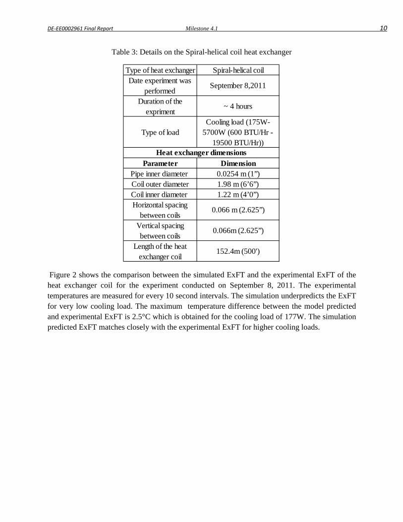
DE-EE0002961 Final Report Milestone 4.1 10
Table 3: Details on the Spiral-helical coil heat exchanger
Figure 2 shows the comparison between the simulated ExFT and the experimental ExFT of the heat exchanger coil for the experiment conducted on September 8, 2011. The experimental temperatures are measured for every 10 second intervals. The simulation underpredicts the ExFT for very low cooling load. The maximum temperature difference between the model predicted and experimental ExFT is 2.5°C which is obtained for the cooling load of 177W. The simulation predicted ExFT matches closely with the experimental ExFT for higher cooling loads.
Type of heat exchanger Spiral-helical coilDate experiment was
performedSeptember 8,2011
Duration of the expriment
~ 4 hours
Type of loadCooling load (175W-
5700W (600 BTU/Hr - 19500 BTU/Hr))
Parameter DimensionPipe inner diameter 0.0254 m (1”)Coil outer diameter 1.98 m (6’6”)Coil inner diameter 1.22 m (4’0”)Horizontal spacing
between coils 0.066 m (2.625”)
Vertical spacing between coils
0.066m (2.625”)
Length of the heat exchanger coil
152.4m (500')
Heat exchanger dimensions
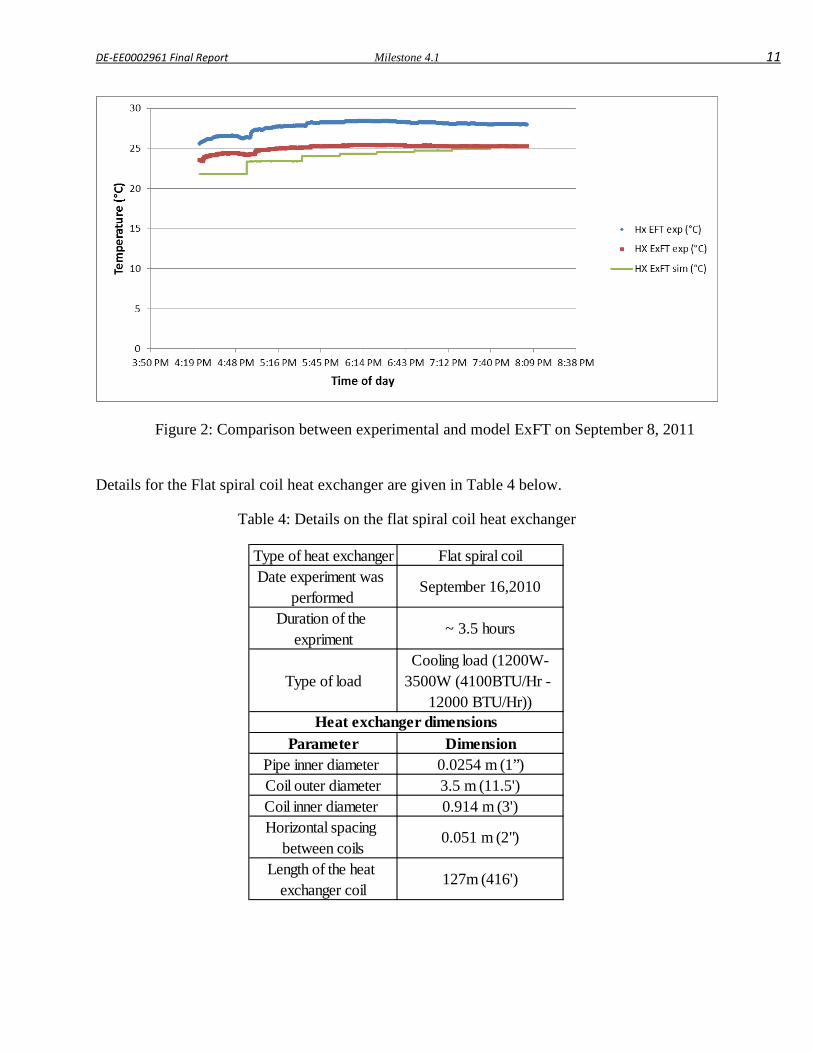
DE-EE0002961 Final Report Milestone 4.1 11
Figure 2: Comparison between experimental and model ExFT on September 8, 2011
Details for the Flat spiral coil heat exchanger are given in Table 4 below.
Table 4: Details on the flat spiral coil heat exchanger
Type of heat exchanger Flat spiral coilDate experiment was
performedSeptember 16,2010
Duration of the expriment
~ 3.5 hours
Type of loadCooling load (1200W-
3500W (4100BTU/Hr - 12000 BTU/Hr))
Parameter DimensionPipe inner diameter 0.0254 m (1”)Coil outer diameter 3.5 m (11.5')Coil inner diameter 0.914 m (3')Horizontal spacing
between coils 0.051 m (2")
Length of the heat exchanger coil
127m (416')
Heat exchanger dimensions
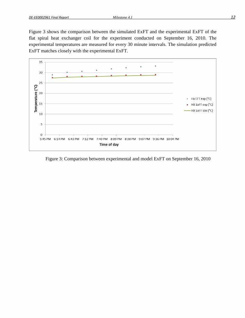
DE-EE0002961 Final Report Milestone 4.1 12
Figure 3 shows the comparison between the simulated ExFT and the experimental ExFT of the flat spiral heat exchanger coil for the experiment conducted on September 16, 2010. The experimental temperatures are measured for every 30 minute intervals. The simulation predicted ExFT matches closely with the experimental ExFT.
Figure 3: Comparison between experimental and model ExFT on September 16, 2010
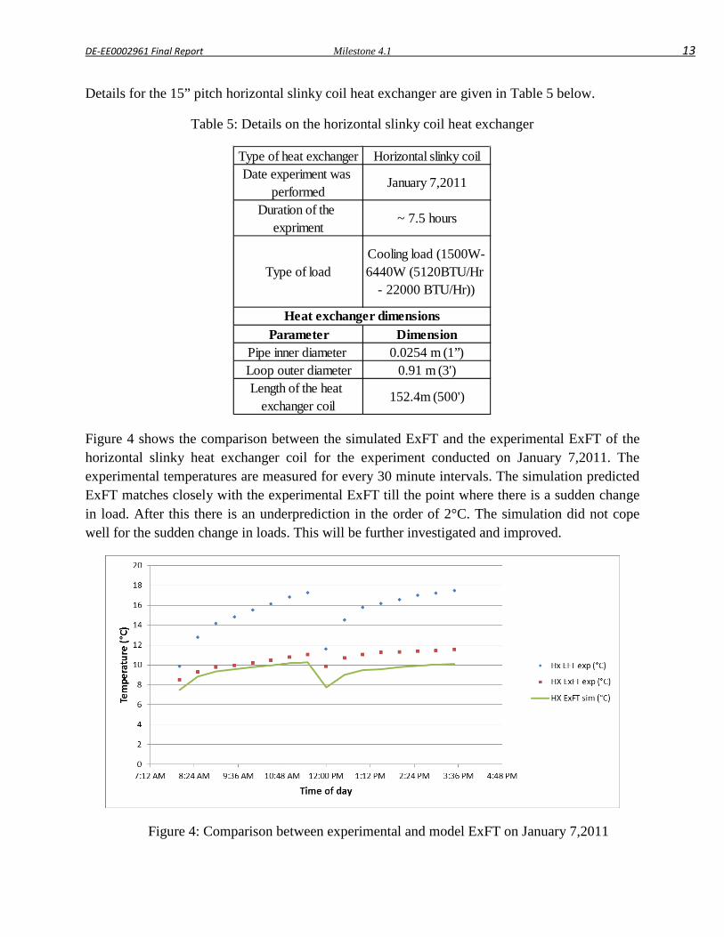
DE-EE0002961 Final Report Milestone 4.1 13
Details for the 15” pitch horizontal slinky coil heat exchanger are given in Table 5 below.
Table 5: Details on the horizontal slinky coil heat exchanger
Figure 4 shows the comparison between the simulated ExFT and the experimental ExFT of the horizontal slinky heat exchanger coil for the experiment conducted on January 7,2011. The experimental temperatures are measured for every 30 minute intervals. The simulation predicted ExFT matches closely with the experimental ExFT till the point where there is a sudden change in load. After this there is an underprediction in the order of 2°C. The simulation did not cope well for the sudden change in loads. This will be further investigated and improved.
Figure 4: Comparison between experimental and model ExFT on January 7,2011
Type of heat exchanger Horizontal slinky coilDate experiment was
performedJanuary 7,2011
Duration of the expriment
~ 7.5 hours
Type of loadCooling load (1500W-6440W (5120BTU/Hr
- 22000 BTU/Hr))
Parameter DimensionPipe inner diameter 0.0254 m (1”)Loop outer diameter 0.91 m (3')Length of the heat
exchanger coil152.4m (500')
Heat exchanger dimensions
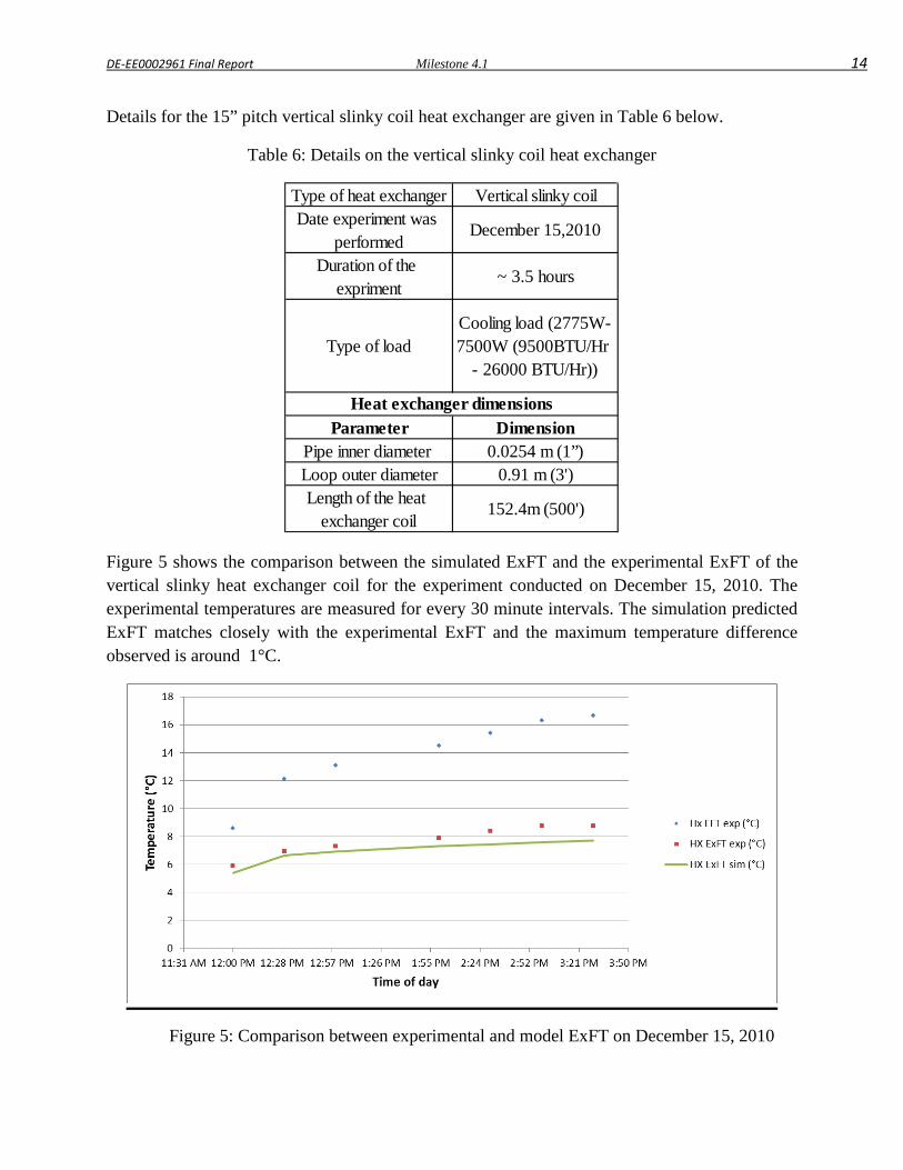
DE-EE0002961 Final Report Milestone 4.1 14
Details for the 15” pitch vertical slinky coil heat exchanger are given in Table 6 below.
Table 6: Details on the vertical slinky coil heat exchanger
Figure 5 shows the comparison between the simulated ExFT and the experimental ExFT of the vertical slinky heat exchanger coil for the experiment conducted on December 15, 2010. The experimental temperatures are measured for every 30 minute intervals. The simulation predicted ExFT matches closely with the experimental ExFT and the maximum temperature difference observed is around 1°C.
Figure 5: Comparison between experimental and model ExFT on December 15, 2010
Type of heat exchanger Vertical slinky coilDate experiment was
performedDecember 15,2010
Duration of the expriment
~ 3.5 hours
Type of loadCooling load (2775W-7500W (9500BTU/Hr
- 26000 BTU/Hr))
Parameter DimensionPipe inner diameter 0.0254 m (1”)Loop outer diameter 0.91 m (3')Length of the heat
exchanger coil152.4m (500')
Heat exchanger dimensions
DE-EE0002961 Final Report Milestone 4.1 15
Conclusions and Recommendations An enhanced heat exchanger model to predict the heat transfer for different types of heat exchanger coils has been developed.
Validation of the model with the experimental results shows that the model generally under predicts the ExFT for very small loads. This needs to be investigated further so as to improve the accuracy of the model.
References Hansen, G.M. 2011. Experimental testing and analysis of spiral-helical surface water heat
exchanger configurations Masters Thesis, Oklahoma State University.
Rogers, G.F.C and Y.R. Mayhew 1964. Heat transfer and pressure loss in helically coiled tubes with turbulent flow. International Journal of Heat and Mass Transfer 7(11): 1207-1216.
Salimpour, M.R. 2009. Heat transfer coefficients of shell and coiled tube heat exchangers. Experimental Thermal and Fluid Science 33(2):203-207.
Sleicher,C.A. and M.W. Rouse 1975. A convenient correlation for heat transfer to constant and variable property fluids in turbulent pipe flow. International Journal of Heat and Mass Transfer 18(5): 677-683.

DE-EE0002961 Final Report Milestone 4.3.1 1
Milestone 4.3.1
Implementation of Enhanced Pond Model in Design Tool
Krishna Conjeevaram Bashyam
Oklahoma State University

DE-EE0002961 Final Report Milestone 4.3.1 2
Milestone Report
Task 4.3.1- Implementation of Enhanced Pond Model in Design Tool
DE-EE0002961/001 - Recovery Act:
Improved Design Tools for Surface Water and Standing Column Well Heat Pump Systems
Krishna Conjeevaram Bashyam, ([email protected]), Research Assistant, Professor Jeffrey D Spitler, ([email protected]), Principal Investigator,
Oklahoma State University
Design Tool Inputs
Following inputs are required for this design tool
1 Lake Bathymetry details
2 EnergyPlus weather file
3 Hourly building heating and cooling loads
4 Heat exchanger type and heat exchanger inputs
5 Type and percentage of antifreeze used
6 Heat pump coefficients during heating and cooling mode
General instructions for using this design tool:
1. Select Metric or IP version option button depending on the input format from the "GetInputParameters" sheet.
2. Enter the required inputs. All items highlighted in yellow, including loads, may be obtained from GLHEPRO. In GLHEPRO, generate the "LakeModelInputs.dat" file by selecting the option from the File menu. Then click the "Get Inputs from GLHEPRO" button on the main screen. You may need to move the input file from your GLHEPRO directory to the directory that this spreadsheet is stored in, if those directory paths are different.
3. The definition about secchi depth and volume development parameter is mentioned below.
4. Advanced options button a. If the area of the lake at particular depths and/or the initial temperatures of the lake at
particular depths are known they can be entered by clicking the advanced options button.

DE-EE0002961 Final Report Milestone 4.3.1 3
b. Each advanced option button will highlight the region where the data needs to be entered. c. Area of lake at particular depths --> Bathymetry profile option button; d. Temperature of lake at particular depths --> Initial water temperature profile option button e. Please click the respected option button to specify the number of area/temperature along the
depth pairs. f. The reset button clears of the entered data and resets the option button. g. If the option button for Bathymetry profiles and Initial water temperature profiles are
clicked, the volume development parameter and the Initial uniform temperature of the lake values will be set as "--" which for the simulation purposes
5. Read .epw file a. Please provide the file path for the .epw file in the dialogue box shown
6. Once the "Run Simulation" button is clicked, the design tool runs the Fortran executable file
based on the input provided and gives the actual size of the coil to be used in the "WriteOutput" page.
7. All the option buttons will be unselected automatically after the end of the simulation.
Please ensure to select the option buttons every time before the simulation starts.
Documentation
I. Lake geometry 1. Input the surface area and the maximum depth of the lake/pond . 2. Secchi depth refers to the depth from the surface where the secchi disc becomes completely
invisible ( gives the turbidity of the lake/pond) . 3. Volume development parameter predicts the shape of the lake basin. It can be defined as
Where Vd - Volume development parameter
Vactual - Actual volume of lake in m3 (Ft3)
Amax - Surface area of the lake in m2 (Ft2)
zmax - Maximum depth of the lake in m (Ft)
If the areas of the lake/pond at some particular depths are known, they can be entered seperately by clicking the advanced options tab
𝑉𝑑 =𝑉𝑎𝑐𝑡𝑢𝑎𝑙
𝐴𝑚𝑎𝑥 ∗ 𝑧𝑚𝑎𝑥3
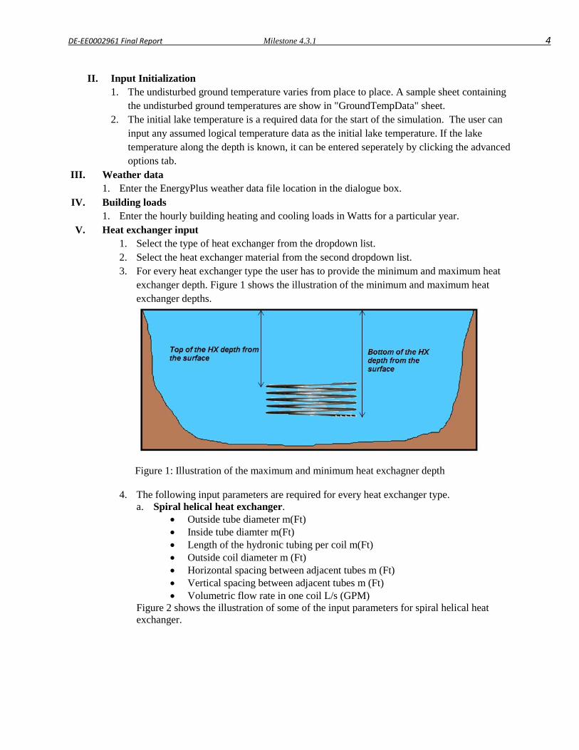
DE-EE0002961 Final Report Milestone 4.3.1 4
II. Input Initialization 1. The undisturbed ground temperature varies from place to place. A sample sheet containing
the undisturbed ground temperatures are show in "GroundTempData" sheet. 2. The initial lake temperature is a required data for the start of the simulation. The user can
input any assumed logical temperature data as the initial lake temperature. If the lake temperature along the depth is known, it can be entered seperately by clicking the advanced options tab.
III. Weather data 1. Enter the EnergyPlus weather data file location in the dialogue box.
IV. Building loads 1. Enter the hourly building heating and cooling loads in Watts for a particular year.
V. Heat exchanger input 1. Select the type of heat exchanger from the dropdown list. 2. Select the heat exchanger material from the second dropdown list. 3. For every heat exchanger type the user has to provide the minimum and maximum heat
exchanger depth. Figure 1 shows the illustration of the minimum and maximum heat exchanger depths.
Figure 1: Illustration of the maximum and minimum heat exchagner depth
4. The following input parameters are required for every heat exchanger type. a. Spiral helical heat exchanger.
• Outside tube diameter m(Ft) • Inside tube diamter m(Ft) • Length of the hydronic tubing per coil m(Ft) • Outside coil diameter m (Ft) • Horizontal spacing between adjacent tubes m (Ft) • Vertical spacing between adjacent tubes m (Ft) • Volumetric flow rate in one coil L/s (GPM)
Figure 2 shows the illustration of some of the input parameters for spiral helical heat exchanger.
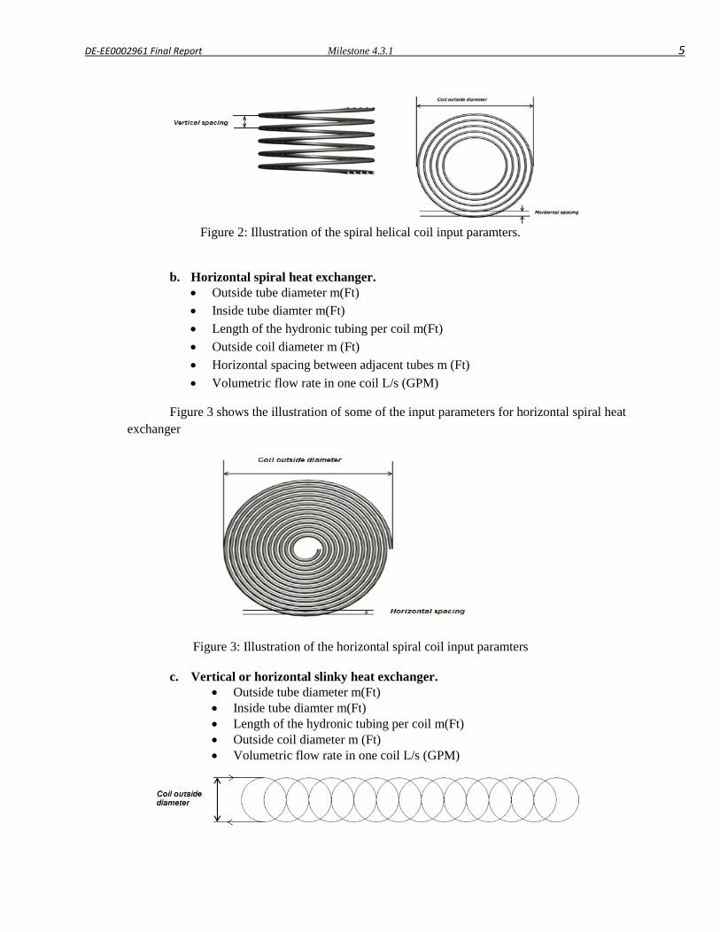
DE-EE0002961 Final Report Milestone 4.3.1 5
Figure 2: Illustration of the spiral helical coil input paramters.
b. Horizontal spiral heat exchanger. • Outside tube diameter m(Ft) • Inside tube diamter m(Ft) • Length of the hydronic tubing per coil m(Ft) • Outside coil diameter m (Ft) • Horizontal spacing between adjacent tubes m (Ft) • Volumetric flow rate in one coil L/s (GPM)
Figure 3 shows the illustration of some of the input parameters for horizontal spiral heat exchanger
Figure 3: Illustration of the horizontal spiral coil input paramters
c. Vertical or horizontal slinky heat exchanger. • Outside tube diameter m(Ft) • Inside tube diamter m(Ft) • Length of the hydronic tubing per coil m(Ft) • Outside coil diameter m (Ft) • Volumetric flow rate in one coil L/s (GPM)
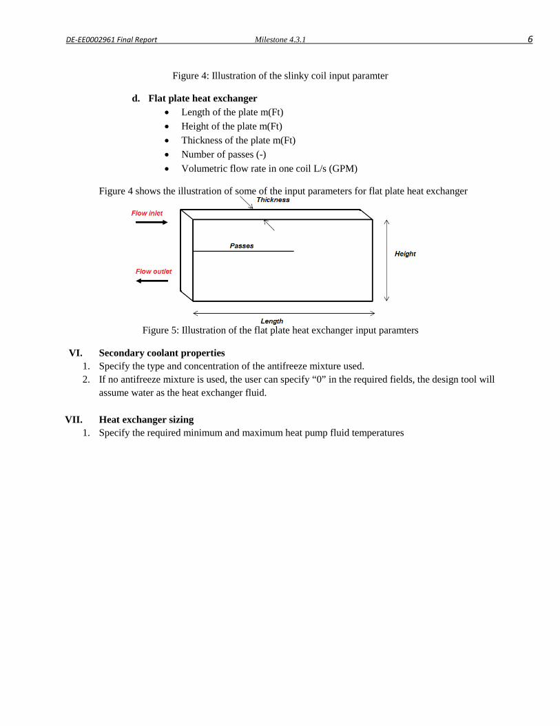
DE-EE0002961 Final Report Milestone 4.3.1 6
Figure 4: Illustration of the slinky coil input paramter
d. Flat plate heat exchanger • Length of the plate m(Ft) • Height of the plate m(Ft) • Thickness of the plate m(Ft) • Number of passes (-) • Volumetric flow rate in one coil L/s (GPM)
Figure 4 shows the illustration of some of the input parameters for flat plate heat exchanger
Figure 5: Illustration of the flat plate heat exchanger input paramters
VI. Secondary coolant properties 1. Specify the type and concentration of the antifreeze mixture used. 2. If no antifreeze mixture is used, the user can specify “0” in the required fields, the design tool will
assume water as the heat exchanger fluid.
VII. Heat exchanger sizing 1. Specify the required minimum and maximum heat pump fluid temperatures

DE-EE0002961 Final Report Milestone 4.3.2 1
Milestone 4.3.2
Implementation of Enhanced Pond Model in Design Tool - Example
Krishna Conjeevaram Bashyam
Oklahoma State University

DE-EE0002961 Final Report Milestone 4.3.2 2
Milestone Report
Task 4.3.2- Implementation of Enhanced Pond Model in Design Tool – Design Tool Example of Usage
DE-EE0002961/001 - Recovery Act:
Improved Design Tools for Surface Water and Standing Column Well Heat Pump Systems
Krishna Conjeevaram Bashyam, ([email protected]), Research Assistant, Professor Jeffrey D Spitler, ([email protected]), Principal Investigator,
Oklahoma State University
Introduction:
This document provides an example of usage of the Microsoft excel version of the design tool. The example presented here is about using the design tool to size a spiral helical coil heat exchanger placed in Ice Lake MN and simulated for the loads from a small office building.
Design Tool Inputs
Following inputs are required for this design tool
1 Lake Bathymetry details
2 EnergyPlus weather file
3 Hourly building heating and cooling loads
4 Heat exchanger type and heat exchanger inputs
5 Type and percentage of antifreeze used
6 Heat pump coefficients during heating and cooling mode
7 Heat exchanger sizing parameters
The user can enter the inputs in SI (metric) units or IP (English) units after selecting the appropriate radio buttons.
All highlighted inputs may be obtained from the GLHEPRO ground heat exchanger design tool by selecting the “WriteLakeModelInputs.dat” option from the File menu in GLHEPRO. The user has to make sure that the generated .dat file is in the same directory as the SWHP tool. The .dat file is read by pressing the “Get GLHEPRO Inputs” button on the spreadsheet.
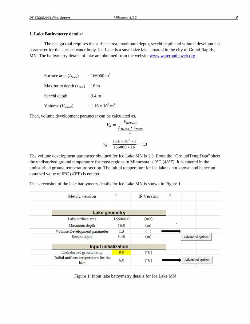
DE-EE0002961 Final Report Milestone 4.3.2 3 1. Lake Bathymetry details:
The design tool requires the surface area, maximum depth, secchi depth and volume development parameter for the surface water body. Ice Lake is a small size lake situated in the city of Grand Rapids, MN. The bathymetry details of lake are obtained from the website www.waterontheweb.org.
Surface area (Amax) : 166000 m2
Maximum depth (zmax) : 16 m
Secchi depth : 3.4 m
Volume (Vactual) : 1.16 x 10⁶ m3
Then, volume development parameter can be calculated as,
𝑉𝑑 =𝑉𝑎𝑐𝑡𝑢𝑎𝑙
𝐴𝑚𝑎𝑥 ∗ 𝑧𝑚𝑎𝑥3
𝑉𝑑 =1.16 ∗ 106 ∗ 3166000 ∗ 16
= 1.3
The volume development parameter obtained for Ice Lake MN is 1.3. From the “GroundTempData” sheet the undisturbed ground temperature for most regions in Minnesota is 9°C (48°F). It is entered in the undisturbed ground temperature section. The initial temperature for Ice lake is not known and hence an assumed value of 6°C (43°F) is entered.
The screenshot of the lake bathymetry details for Ice Lake MN is shown in Figure 1.
Figure 1: Input lake bathymetry details for Ice Lake MN

DE-EE0002961 Final Report Milestone 4.3.2 4 2. EnergyPlus weather file:
To input the EnergyPlus weather file the user has to click the “Read .epw file” button and needs to specify the path of the .epw file when the dialogue box appears. Figure 2 shows the screenshot of the dialogue box which appears when the “Read .epw file” button is selected.
Figure 2: Input the .epw weather file
3. Hourly building heating and cooling loads:
The hourly building heating and cooling loads can be entered by clicking on the “Input Building Loads” button. A new sheet “GetInputBuildingLoads” is opened and the user can enter the hourly heating and cooling load values. Both the building loads needs to be positive and should be inputted in Watts.
4. Heat exchanger type and heat exchanger inputs:
The design tool can perfom sizing on four heat exchanger types namely spiral helical, horizontal spiral, vertical – horizontal slinky and flat plat plate heat exchangers. The heat exchagner type and materical can be selected from the dropdown menu. Once the heat exchanger type is selected, the required inputs need to be entered as shown in Figure 3. For this example, a spiral helical coil heat exchanger is used. It is assumed that the heat exchanger is placed in Ice Lake between 5-6m (16.4 – 19.7 Ft) depths from the surface. The user should input the length of a single heat exchanger coil. Here, the initial coil length is assumed to be150m (492 Ft).

DE-EE0002961 Final Report Milestone 4.3.2 5
Figure 3: Heat exchanger inputs
5. Type and percentage of antifreeze used:
The user needs to specify the type and percentage of concentraion of antifreeze used in the heat exchanger fluid. For this example, the heat exchagner fluid is assumed to be just water. Hence, the value “0” is entered in both the fileds as shown in Figure 4.
Figure 4: Secondary coolant inputs
6. Heat pump coefficients during heating and cooling mode:
GLHEPRO includes a large library of heat pump models that may be selected with the heat pump coefficients already computed. The user can select the required heat pump type in GLHEPRO and generate the “WriteLakeModelInputs.dat” file. The heat pump coefficients are automatically filled in the required input locations by pressing the “Get GLHEPRO Inputs” button.
Figure 5: Heat pump coefficient inputs
Heat exchanger type (m)
Heat exchanger material (m)
Hydronic tubing outer dia 0.02656 (m) Hydronic tubing inner dia 0.02072 (m)
Length of hydronic tubing per coil 150 (m) Outside coil diameter 1.67 (m)
Horizontal spacing between tubes 0.0665 (m) Vertical spacing between tubes 0.0665 (m)
Volumetric flow rate in each coil 3.3 (L/s) Minimum heat exchanger depth 5 (m) Maximum heat exchanger depth 6 (m)
Heat exchanger input
Spiral-helical coil
HDPE
Type of antifreeze 0 0: None, 1: Propylene glycol, 2: Ethylene glycol, 3: Methyl alcohol, 4: Ethyl alcoholPercentage of Concentration 0 %
Secondary coolant properties
i CABS,i CREJ,i
1 0.503 1.1452 0.006 -0.0023 0.000 0.000
Heat pump Coefficients

DE-EE0002961 Final Report Milestone 4.3.2 6 7. Heat exchanger sizing:
For this example, the heat exchanger coil is sized for the design minimum and maximum heat exchanger exit fluid temperatures of 3°C (37.4°F) and 20°C (68°F) respectively.
OUTPUT:
When all the input parameters are provided, the “Run Simulation” button should be pressed to begin the simulation. The required heat exchagner coil length in will be shown in the “WriteOutput” sheet.
DE-EE0002961 Final Report Milestone 4.4 1
Milestone 4.4
Validation of Pond Model
Manojkumar Selvakumar
Oklahoma State University
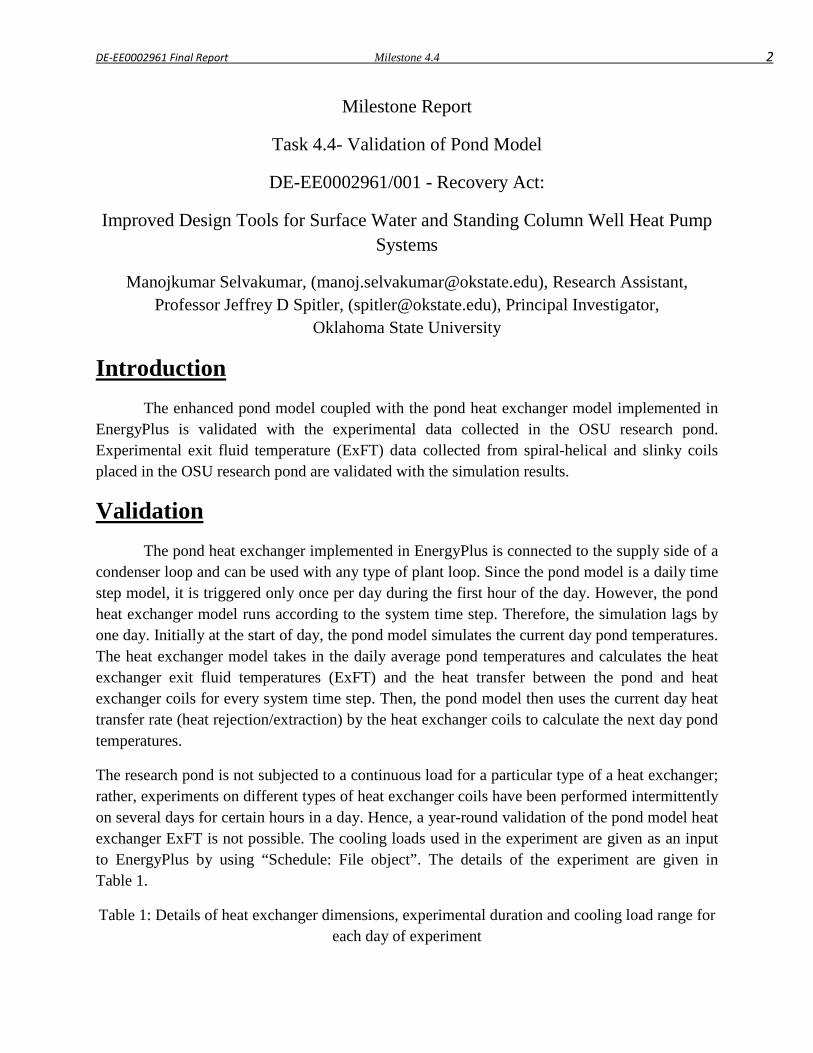
DE-EE0002961 Final Report Milestone 4.4 2
Milestone Report
Task 4.4- Validation of Pond Model
DE-EE0002961/001 - Recovery Act:
Improved Design Tools for Surface Water and Standing Column Well Heat Pump Systems
Manojkumar Selvakumar, ([email protected]), Research Assistant, Professor Jeffrey D Spitler, ([email protected]), Principal Investigator,
Oklahoma State University
Introduction
The enhanced pond model coupled with the pond heat exchanger model implemented in EnergyPlus is validated with the experimental data collected in the OSU research pond. Experimental exit fluid temperature (ExFT) data collected from spiral-helical and slinky coils placed in the OSU research pond are validated with the simulation results.
Validation The pond heat exchanger implemented in EnergyPlus is connected to the supply side of a condenser loop and can be used with any type of plant loop. Since the pond model is a daily time step model, it is triggered only once per day during the first hour of the day. However, the pond heat exchanger model runs according to the system time step. Therefore, the simulation lags by one day. Initially at the start of day, the pond model simulates the current day pond temperatures. The heat exchanger model takes in the daily average pond temperatures and calculates the heat exchanger exit fluid temperatures (ExFT) and the heat transfer between the pond and heat exchanger coils for every system time step. Then, the pond model then uses the current day heat transfer rate (heat rejection/extraction) by the heat exchanger coils to calculate the next day pond temperatures.
The research pond is not subjected to a continuous load for a particular type of a heat exchanger; rather, experiments on different types of heat exchanger coils have been performed intermittently on several days for certain hours in a day. Hence, a year-round validation of the pond model heat exchanger ExFT is not possible. The cooling loads used in the experiment are given as an input to EnergyPlus by using “Schedule: File object”. The details of the experiment are given in Table 1.
Table 1: Details of heat exchanger dimensions, experimental duration and cooling load range for each day of experiment
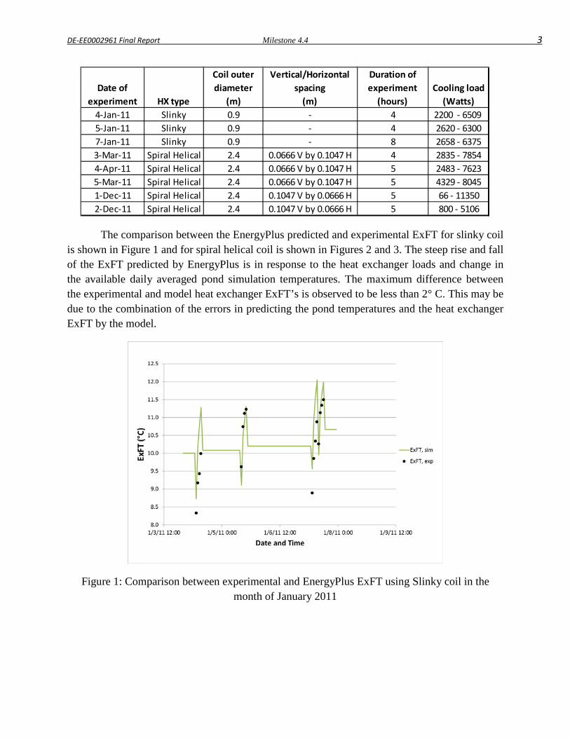
DE-EE0002961 Final Report Milestone 4.4 3
The comparison between the EnergyPlus predicted and experimental ExFT for slinky coil is shown in Figure 1 and for spiral helical coil is shown in Figures 2 and 3. The steep rise and fall of the ExFT predicted by EnergyPlus is in response to the heat exchanger loads and change in the available daily averaged pond simulation temperatures. The maximum difference between the experimental and model heat exchanger ExFT’s is observed to be less than 2° C. This may be due to the combination of the errors in predicting the pond temperatures and the heat exchanger ExFT by the model.
Figure 1: Comparison between experimental and EnergyPlus ExFT using Slinky coil in the month of January 2011
Date of experiment HX type
Coil outer diameter
(m)
Vertical/Horizontal spacing
(m)
Duration of experiment
(hours)Cooling load
(Watts)4-Jan-11 Slinky 0.9 - 4 2200 - 6509 5-Jan-11 Slinky 0.9 - 4 2620 - 63007-Jan-11 Slinky 0.9 - 8 2658 - 63753-Mar-11 Spiral Helical 2.4 0.0666 V by 0.1047 H 4 2835 - 78544-Apr-11 Spiral Helical 2.4 0.0666 V by 0.1047 H 5 2483 - 76235-Mar-11 Spiral Helical 2.4 0.0666 V by 0.1047 H 5 4329 - 80451-Dec-11 Spiral Helical 2.4 0.1047 V by 0.0666 H 5 66 - 113502-Dec-11 Spiral Helical 2.4 0.1047 V by 0.0666 H 5 800 - 5106
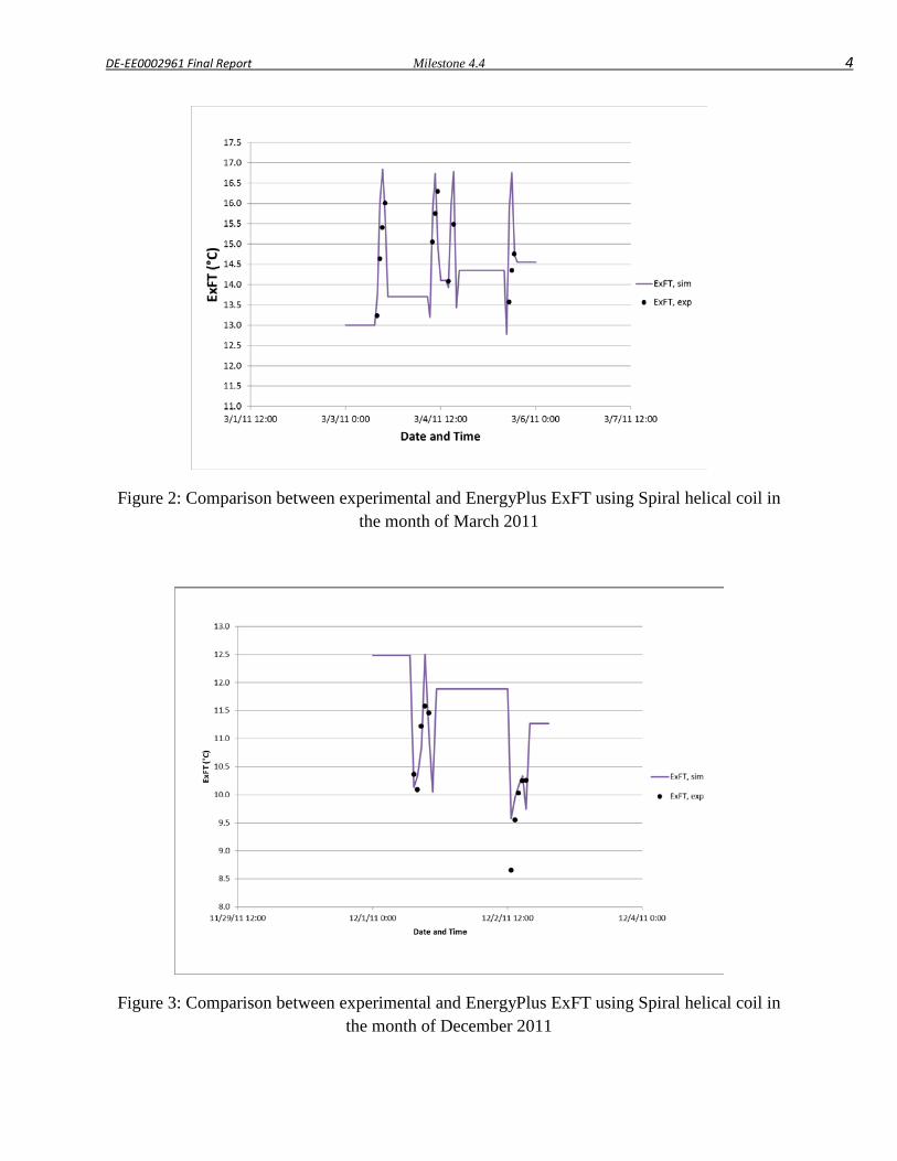
DE-EE0002961 Final Report Milestone 4.4 4
Figure 2: Comparison between experimental and EnergyPlus ExFT using Spiral helical coil in the month of March 2011
Figure 3: Comparison between experimental and EnergyPlus ExFT using Spiral helical coil in the month of December 2011
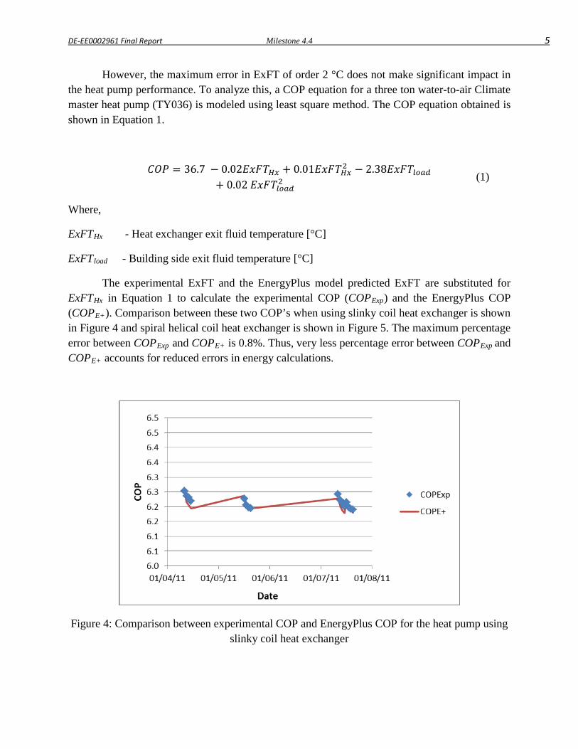
DE-EE0002961 Final Report Milestone 4.4 5
However, the maximum error in ExFT of order 2 °C does not make significant impact in the heat pump performance. To analyze this, a COP equation for a three ton water-to-air Climate master heat pump (TY036) is modeled using least square method. The COP equation obtained is shown in Equation 1.
𝐶𝑂𝑃 = 36.7 − 0.02𝐸𝑥𝐹𝑇𝐻𝑥 + 0.01𝐸𝑥𝐹𝑇𝐻𝑥2 − 2.38𝐸𝑥𝐹𝑇𝑙𝑜𝑎𝑑
+ 0.02 𝐸𝑥𝐹𝑇𝑙𝑜𝑎𝑑2 (1)
Where,
ExFTHx - Heat exchanger exit fluid temperature [°C]
ExFTload - Building side exit fluid temperature [°C]
The experimental ExFT and the EnergyPlus model predicted ExFT are substituted for ExFTHx in Equation 1 to calculate the experimental COP (COPExp) and the EnergyPlus COP (COPE+). Comparison between these two COP’s when using slinky coil heat exchanger is shown in Figure 4 and spiral helical coil heat exchanger is shown in Figure 5. The maximum percentage error between COPExp and COPE+ is 0.8%. Thus, very less percentage error between COPExp and COPE+ accounts for reduced errors in energy calculations.
Figure 4: Comparison between experimental COP and EnergyPlus COP for the heat pump using slinky coil heat exchanger
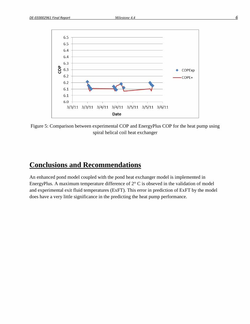
DE-EE0002961 Final Report Milestone 4.4 6
Figure 5: Comparison between experimental COP and EnergyPlus COP for the heat pump using spiral helical coil heat exchanger
Conclusions and Recommendations An enhanced pond model coupled with the pond heat exchanger model is implemented in EnergyPlus. A maximum temperature difference of 2° C is obseved in the validation of model and experimental exit fluid temperatures (ExFT). This error in prediction of ExFT by the model does have a very little significance in the predicting the heat pump performance.

DE-EE0002961 Final Report Source Code 3.2 1
Source Code 3.2
SCW design tool source code
James Cullin
Oklahoma State University

DE-EE0002961 Final Report Source Code 3.2 2
Option Strict Off Option Explicit On Imports System.Math Imports VB = Microsoft.VisualBasic Module SCWell Public Sub Scw_Run_Click() Dim SCW_L As Double ' Borehole depth (m) Dim SCW_db, SCW_rb As Double ' Borehole diameter and radius (m) Dim SCW_Dtid As Double ' Dip tube inside diameter as Double Dim SCW_dtir As Double ' Dip tube inside radius (m) Dim SCW_Dtod As Double ' Dip tube outside diameter (m) Dim SCW_dtor As Double ' Dip tube outside diameter (m) Dim SCW_dtk As Double ' Dip tube thermal conductivity (m) Dim SCW_EHT As Double ' Ground enhanced thermal conductivity (W/m-K) Dim SCW_keff As Double ' Effective soil thermal conductivity (W/m-K) Dim SCW_porosity As Double ' Ground porosity (0-1) Dim SCW_hydcond As Double ' Hydraulic conductivity (m/s) Dim SCW_UGT As Double ' Undisturbed ground temperature Dim SCW_bstrat As Integer ' Bleed strategy (0,1,2) Dim SCW_brate As Double ' Bleed rate (0-1) Dim SCW_tstep As Double ' Time step (seconds) Dim SCW_duration As Integer ' Number of time steps to run simulation (-) Dim SCW_Tp() As Double ' Temperature of nodes in radial direction in the ground (°C) Dim SCW_T() As Double ' Temperature of nodes in radial direction in the ground (°C) after iterations converged Dim SCW_nr As Integer ' Number of nodes in ground (-) Dim SCW_Tfi As Double ' SCW entering water temperature at each time step (°C) Dim SCW_itime As Integer ' Current time step (-) Dim SCW_qflux1 As Double ' Heat flux used for convergence (W/m2) Dim SCW_qflux2 As Double ' Heat flux used for convergence (W/m2) Dim SCW_convergence As Double ' convergence criteria for heat fluxes (-) Dim SCW_deli() As Double ' Grid spacing in the radial direction (m) Dim SCW_vert() As Double ' Coordiantes of each ground node in radial direction (m) Dim SCW_Tb As Double ' Borehole wall temperature (°C)
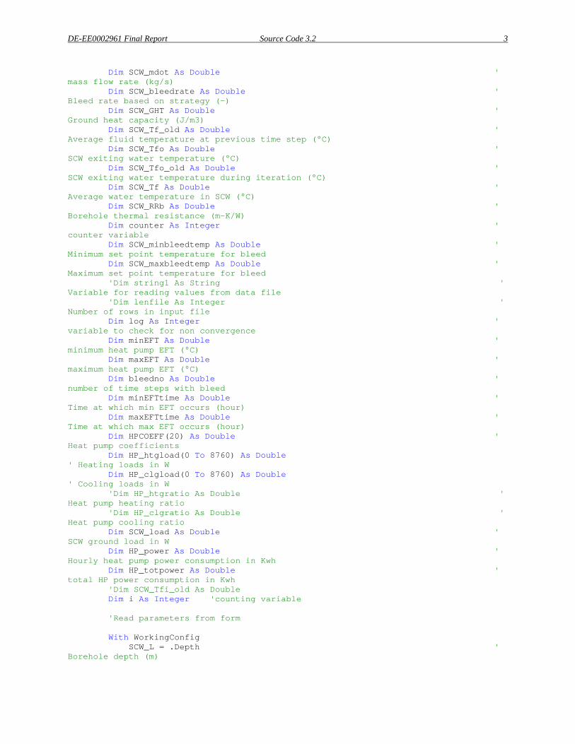
DE-EE0002961 Final Report Source Code 3.2 3
Dim SCW_mdot As Double ' mass flow rate (kg/s) Dim SCW_bleedrate As Double ' Bleed rate based on strategy (-) Dim SCW_GHT As Double ' Ground heat capacity (J/m3) Dim SCW_Tf_old As Double ' Average fluid temperature at previous time step (°C) Dim SCW_Tfo As Double ' SCW exiting water temperature (°C) Dim SCW_Tfo_old As Double ' SCW exiting water temperature during iteration (°C) Dim SCW_Tf As Double ' Average water temperature in SCW (°C) Dim SCW_RRb As Double ' Borehole thermal resistance (m-K/W) Dim counter As Integer ' counter variable Dim SCW_minbleedtemp As Double ' Minimum set point temperature for bleed Dim SCW_maxbleedtemp As Double ' Maximum set point temperature for bleed 'Dim string1 As String ' Variable for reading values from data file 'Dim lenfile As Integer ' Number of rows in input file Dim log As Integer ' variable to check for non convergence Dim minEFT As Double ' minimum heat pump EFT (°C) Dim maxEFT As Double ' maximum heat pump EFT (°C) Dim bleedno As Double ' number of time steps with bleed Dim minEFTtime As Double ' Time at which min EFT occurs (hour) Dim maxEFTtime As Double ' Time at which max EFT occurs (hour) Dim HPCOEFF(20) As Double ' Heat pump coefficients Dim HP_htgload(0 To 8760) As Double ' Heating loads in W Dim HP_clgload(0 To 8760) As Double ' Cooling loads in W 'Dim HP_htgratio As Double ' Heat pump heating ratio 'Dim HP_clgratio As Double ' Heat pump cooling ratio Dim SCW_load As Double ' SCW ground load in W Dim HP_power As Double ' Hourly heat pump power consumption in Kwh Dim HP_totpower As Double ' total HP power consumption in Kwh 'Dim SCW_Tfi_old As Double Dim i As Integer 'counting variable 'Read parameters from form With WorkingConfig SCW_L = .Depth ' Borehole depth (m)
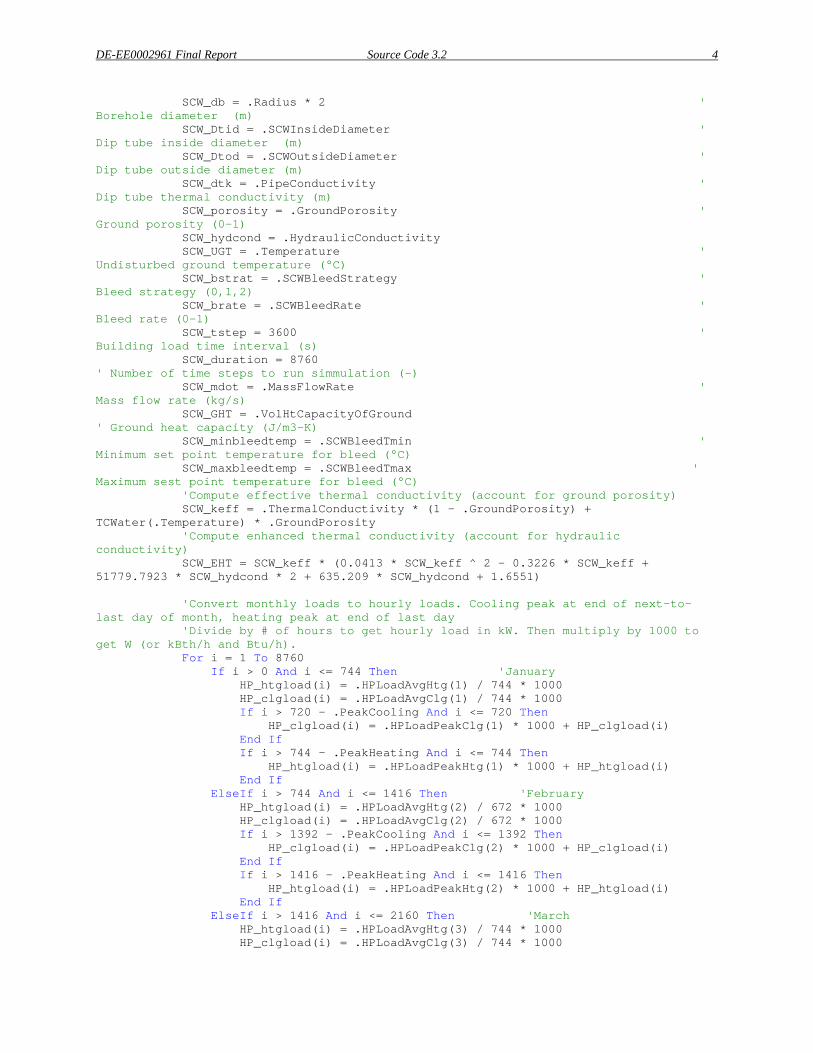
DE-EE0002961 Final Report Source Code 3.2 4
SCW_db = .Radius * 2 ' Borehole diameter (m) SCW_Dtid = .SCWInsideDiameter ' Dip tube inside diameter (m) SCW_Dtod = .SCWOutsideDiameter ' Dip tube outside diameter (m) SCW_dtk = .PipeConductivity ' Dip tube thermal conductivity (m) SCW_porosity = .GroundPorosity ' Ground porosity (0-1) SCW_hydcond = .HydraulicConductivity SCW_UGT = .Temperature ' Undisturbed ground temperature (°C) SCW_bstrat = .SCWBleedStrategy ' Bleed strategy (0,1,2) SCW_brate = .SCWBleedRate ' Bleed rate (0-1) SCW_tstep = 3600 ' Building load time interval (s) SCW_duration = 8760 ' Number of time steps to run simmulation (-) SCW_mdot = .MassFlowRate ' Mass flow rate (kg/s) SCW_GHT = .VolHtCapacityOfGround ' Ground heat capacity (J/m3-K) SCW_minbleedtemp = .SCWBleedTmin ' Minimum set point temperature for bleed (°C) SCW_maxbleedtemp = .SCWBleedTmax ' Maximum sest point temperature for bleed (°C) 'Compute effective thermal conductivity (account for ground porosity) SCW_keff = .ThermalConductivity * (1 - .GroundPorosity) + TCWater(.Temperature) * .GroundPorosity 'Compute enhanced thermal conductivity (account for hydraulic conductivity) SCW_EHT = SCW_keff * (0.0413 * SCW_keff ^ 2 - 0.3226 * SCW_keff + 51779.7923 * SCW_hydcond * 2 + 635.209 * SCW_hydcond + 1.6551) 'Convert monthly loads to hourly loads. Cooling peak at end of next-to-last day of month, heating peak at end of last day 'Divide by # of hours to get hourly load in kW. Then multiply by 1000 to get W (or kBth/h and Btu/h). For i = 1 To 8760 If i > 0 And i <= 744 Then 'January HP_htgload(i) = .HPLoadAvgHtg(1) / 744 * 1000 HP_clgload(i) = .HPLoadAvgClg(1) / 744 * 1000 If i > 720 - .PeakCooling And i <= 720 Then HP_clgload(i) = .HPLoadPeakClg(1) * 1000 + HP_clgload(i) End If If i > 744 - .PeakHeating And i <= 744 Then HP_htgload(i) = .HPLoadPeakHtg(1) * 1000 + HP_htgload(i) End If ElseIf i > 744 And i <= 1416 Then 'February HP_htgload(i) = .HPLoadAvgHtg(2) / 672 * 1000 HP_clgload(i) = .HPLoadAvgClg(2) / 672 * 1000 If i > 1392 - .PeakCooling And i <= 1392 Then HP_clgload(i) = .HPLoadPeakClg(2) * 1000 + HP_clgload(i) End If If i > 1416 - .PeakHeating And i <= 1416 Then HP_htgload(i) = .HPLoadPeakHtg(2) * 1000 + HP_htgload(i) End If ElseIf i > 1416 And i <= 2160 Then 'March HP_htgload(i) = .HPLoadAvgHtg(3) / 744 * 1000 HP_clgload(i) = .HPLoadAvgClg(3) / 744 * 1000
DE-EE0002961 Final Report Source Code 3.2 5
If i > 2134 - .PeakCooling And i <= 2134 Then HP_clgload(i) = .HPLoadPeakClg(3) * 1000 + HP_clgload(i) End If If i > 2160 - .PeakHeating And i <= 2160 Then HP_htgload(i) = .HPLoadPeakHtg(3) * 1000 + HP_htgload(i) End If ElseIf i > 2160 And i <= 2880 Then 'April HP_htgload(i) = .HPLoadAvgHtg(4) / 720 * 1000 HP_clgload(i) = .HPLoadAvgClg(4) / 720 * 1000 If i > 2856 - .PeakCooling And i <= 2856 Then HP_clgload(i) = .HPLoadPeakClg(4) * 1000 + HP_clgload(i) End If If i > 2880 - .PeakHeating And i <= 2880 Then HP_htgload(i) = .HPLoadPeakHtg(4) * 1000 + HP_htgload(i) End If ElseIf i > 2880 And i <= 3624 Then 'May HP_htgload(i) = .HPLoadAvgHtg(5) / 744 * 1000 HP_clgload(i) = .HPLoadAvgClg(5) / 744 * 1000 If i > 3600 - .PeakCooling And i <= 3600 Then HP_clgload(i) = .HPLoadPeakClg(5) * 1000 + HP_clgload(i) End If If i > 3624 - .PeakHeating And i <= 3624 Then HP_htgload(i) = .HPLoadPeakHtg(5) * 1000 + HP_htgload(i) End If ElseIf i > 3624 And i <= 4344 Then 'June HP_htgload(i) = .HPLoadAvgHtg(6) / 720 * 1000 HP_clgload(i) = .HPLoadAvgClg(6) / 720 * 1000 If i > 4320 - .PeakCooling And i <= 4320 Then HP_clgload(i) = .HPLoadPeakClg(6) * 1000 + HP_clgload(i) End If If i > 4344 - .PeakHeating And i <= 4344 Then HP_htgload(i) = .HPLoadPeakHtg(6) * 1000 + HP_htgload(i) End If ElseIf i > 4344 And i <= 5088 Then 'July HP_htgload(i) = .HPLoadAvgHtg(7) / 744 * 1000 HP_clgload(i) = .HPLoadAvgClg(7) / 744 * 1000 If i > 5064 - .PeakCooling And i <= 5064 Then HP_clgload(i) = .HPLoadPeakClg(7) * 1000 + HP_clgload(i) End If If i > 5088 - .PeakHeating And i <= 5088 Then HP_htgload(i) = .HPLoadPeakHtg(7) * 1000 + HP_htgload(i) End If ElseIf i > 5088 And i <= 5832 Then 'August HP_htgload(i) = .HPLoadAvgHtg(8) / 744 * 1000 HP_clgload(i) = .HPLoadAvgClg(8) / 744 * 1000 If i > 5808 - .PeakCooling And i <= 5808 Then HP_clgload(i) = .HPLoadPeakClg(8) * 1000 + HP_clgload(i) End If If i > 5832 - .PeakHeating And i <= 5832 Then HP_htgload(i) = .HPLoadPeakHtg(8) * 1000 + HP_htgload(i) End If ElseIf i > 5832 And i <= 6552 Then 'September HP_htgload(i) = .HPLoadAvgHtg(9) / 720 * 1000 HP_clgload(i) = .HPLoadAvgClg(9) / 720 * 1000 If i > 6528 - .PeakCooling And i <= 6528 Then HP_clgload(i) = .HPLoadPeakClg(9) * 1000 + HP_clgload(i) End If If i > 6552 - .PeakHeating And i <= 6552 Then HP_htgload(i) = .HPLoadPeakHtg(9) * 1000 + HP_htgload(i) End If ElseIf i > 6552 And i <= 7296 Then 'October HP_htgload(i) = .HPLoadAvgHtg(10) / 744 * 1000 HP_clgload(i) = .HPLoadAvgClg(10) / 744 * 1000
DE-EE0002961 Final Report Source Code 3.2 6
If i > 7272 - .PeakCooling And i <= 7272 Then HP_clgload(i) = .HPLoadPeakClg(10) * 1000 + HP_clgload(i) End If If i > 7296 - .PeakHeating And i <= 7296 Then HP_htgload(i) = .HPLoadPeakHtg(10) * 1000 + HP_htgload(i) End If ElseIf i > 7296 And i <= 8016 Then 'November HP_htgload(i) = .HPLoadAvgHtg(11) / 720 * 1000 HP_clgload(i) = .HPLoadAvgClg(11) / 720 * 1000 If i > 7992 - .PeakCooling And i <= 7992 Then HP_clgload(i) = .HPLoadPeakClg(11) * 1000 + HP_clgload(i) End If If i > 8016 - .PeakHeating And i <= 8016 Then HP_htgload(i) = .HPLoadPeakHtg(11) * 1000 + HP_htgload(i) End If ElseIf i > 8016 And i <= 8760 Then 'December HP_htgload(i) = .HPLoadAvgHtg(12) / 744 * 1000 HP_clgload(i) = .HPLoadAvgClg(12) / 744 * 1000 If i > 8736 - .PeakCooling And i <= 8736 Then HP_clgload(i) = .HPLoadPeakClg(12) * 1000 + HP_clgload(i) End If If i > 8760 - .PeakHeating And i <= 8760 Then HP_htgload(i) = .HPLoadPeakHtg(12) * 1000 + HP_htgload(i) End If End If Next HP_htgload(0) = HP_htgload(8760) 'Do this for modulo calculations (later, not used now) HP_clgload(0) = HP_clgload(8760) End With With WorkingHP HPCOEFF(1) = .u HPCOEFF(2) = .v HPCOEFF(3) = .w HPCOEFF(6) = .x HPCOEFF(7) = .y HPCOEFF(8) = .z HPCOEFF(11) = .a HPCOEFF(12) = .b HPCOEFF(13) = .c HPCOEFF(16) = .d HPCOEFF(17) = .e HPCOEFF(18) = .f End With Dim iter_writer As New IO.StreamWriter("SCW.csv") 'Output per iteration 'Initial line for column headings iter_writer.WriteLine("Hour, Inlet fluid temperature (°C), Outlet fluid temperature (°C), Borehole wall temperature (°C), Load on ground (W), Bleed rate (-), Borehole thermal resistance (m-K/W), Heat pump power consumption (kWh)") ' Calculate borehole and dip tube radius SCW_rb = SCW_db / 2 ' Borehole diameter (m) SCW_dtir = SCW_Dtid / 2 ' Dip tube inside diameter (m) SCW_dtor = SCW_Dtod / 2 ' Dip tube outside diameter (m) SCW_nr = 131 ' Number of nodes in the ground
DE-EE0002961 Final Report Source Code 3.2 7
' Redimension array based on maximum nodes ReDim SCW_Tp(SCW_nr) ReDim SCW_T(SCW_nr) ReDim SCW_vert(SCW_nr) ReDim SCW_deli(SCW_nr - 1) SCW_convergence = 0.01 ' Set convergence criteria for heat fluxes Call SCW_initialize(SCW_deli, SCW_vert, SCW_Tp, SCW_T, SCW_nr, SCW_rb, SCW_UGT) ' Get the grid spacing and vertices coordinates and initialize temperatures SCW_qflux1 = 50.0# ' Set initial guess value of heat flux at the borehole wall (W/m2) SCW_Tf_old = SCW_UGT ' Set initial value of average SCW_RRb = 0.05 ' Set initial guess value minEFT = SCW_UGT ' Set initial value maxEFT = SCW_UGT ' Set initial value SCW_Tfi = SCW_UGT SCW_Tfo = SCW_UGT SCW_Tfo_old = SCW_UGT ' Start simulation For SCW_itime = 1 To SCW_duration If ((HP_htgload(SCW_itime) + HP_clgload(SCW_itime)) < 0.1) Then HP_clgload(SCW_itime) = 0.01 End If counter = 0 ' Set counter variable ' iterative loop to check convegence of borehole and ground of the SCW Do log = log + 1 counter = counter + 1 Call HP_ExFT(SCW_Tfo, SCW_mdot, HP_htgload(SCW_itime), HP_clgload(SCW_itime), HPCOEFF, SCW_Tfi, SCW_load, HP_power) ' Calculate heat flux at the borehole wall in W/m2 SCW_qflux1 = SCW_load / (3.14159 * SCW_db * SCW_L) ' Determine whether to bleed or not Call Detbleed(SCW_brate, SCW_bleedrate, SCW_bstrat, SCW_Tfi, SCW_Tfo, SCW_minbleedtemp, SCW_maxbleedtemp) ' Calculate borehole wall temperature using guess value of heat flux Call BoreholeFDM(SCW_Tp, SCW_T, SCW_qflux1, SCW_Tb, SCW_nr, SCW_vert, SCW_deli, SCW_L, SCW_porosity, SCW_mdot, SCW_bleedrate, SCW_EHT, SCW_tstep, SCW_GHT, SCW_UGT)
DE-EE0002961 Final Report Source Code 3.2 8
' Calculate exiting water temeprature based on borehole wall temperature Call BoreholeTfo(SCW_qflux1, SCW_Tb, SCW_Dtid, SCW_Dtod, SCW_rb, SCW_Tf_old, SCW_Tfo, SCW_mdot, SCW_Tf, SCW_L, SCW_RRb, SCW_bleedrate, SCW_Tfi, SCW_tstep, SCW_dtk) 'Calculate the heat flux based on the guessed value of Tfo SCW_qflux2 = SCW_mdot * (cpWater(SCW_Tf) * 1000) * ((((1 - SCW_bleedrate) * (SCW_Tfo - SCW_Tfi)) + (SCW_bleedrate * (SCW_Tfo - SCW_Tb)))) / (SCW_L * 2 * 3.14159 * SCW_rb) SCW_convergence = Abs(SCW_Tfo - SCW_Tfo_old) 'Abs((SCW_qflux2 - SCW_qflux1) * 100 / SCW_qflux2) 'SCW_qflux1 = (0.8 * SCW_qflux2) + (0.2 * SCW_qflux1) If (SCW_convergence < 0.01) Then Exit Do End If If (counter > 50) Then Exit Do End If SCW_Tfo_old = SCW_Tfo Loop ' Tp saves the values after the convergence is met, T is the value based on each iteration SCW_Tp = SCW_T ' Save the mean fluid temperature for the next time step SCW_Tf_old = SCW_Tf HP_totpower = HP_totpower + HP_power 'Print #2, SCW_itime, SCW_Tfi, SCW_Tfo, SCW_Tb, SCW_load, SCW_bleedrate, SCW_RRb, HP_power iter_writer.WriteLine(String.Join(",", New String() {SCW_itime, SCW_Tfi, SCW_Tfo, SCW_Tb, SCW_load, SCW_bleedrate, SCW_RRb, HP_power})) ' Check for max EFT If (SCW_Tfo > maxEFT) Then maxEFT = SCW_Tfo maxEFTtime = SCW_itime * SCW_tstep / 3600 ' Calculate time at which max EFT occurs End If ' Check for min EFT If (SCW_Tfo < minEFT) Then minEFT = SCW_Tfo minEFTtime = SCW_itime * SCW_tstep / 3600 ' Calculate time at which min EFT occurs End If ' Calculate hours of bleed If (SCW_bleedrate > 0) Then bleedno = bleedno + (SCW_tstep / 3600) End If
DE-EE0002961 Final Report Source Code 3.2 9
Next SCW_itime 'Close #2 ' Close the log file iter_writer.Close() 'Write output file Dim summ_writer As New IO.StreamWriter("output.txt") summ_writer.WriteLine("Min HP EFT = " & Str(minEFT) & " °C") summ_writer.WriteLine("--occurs in hour #" & Str(minEFTtime)) summ_writer.WriteLine("Max HP EFT = " & Str(maxEFT) & " °C") summ_writer.WriteLine("--occurs in hour #" & Str(maxEFTtime)) summ_writer.WriteLine(Str(bleedno) & " total hours of bleed") summ_writer.WriteLine("HP Power Consumption = " & Str(HP_totpower) & " kWh") summ_writer.Close() End Sub ' This subroutine calculates the radial coordiantes of the ground nodes and the grid spacing and also initializes the ground temperature Private Sub SCW_initialize(ByVal deli() As Double, ByVal vert() As Double, ByVal Tp() As Double, ByVal t() As Double, ByVal nr As Integer, ByVal Rb As Double, ByVal Farfield As Double) Dim i, j As Integer Dim alfa(4) As Double ' GRid spacing and vertices based on Deng (2004) Thesis ' Calculate vertice positions ' Parameters for grid distribution alfa(1) = 1.685 alfa(2) = -3.657 alfa(3) = -1.701 alfa(4) = -0.783 ' Fixed vertices vert(1) = Rb vert(61) = 1.5 vert(101) = 15 vert(111) = 50 vert(nr) = 180 ' Calculate intermediate vertices For i = 2 To 60 j = i - 1 vert(i) = Rb + (tanhdist(60, alfa(1), j) * (1.5 - Rb)) Next i For i = 62 To 100 j = i - 61 vert(i) = 1.5 + (sinhdist(40, alfa(2), j) * (15 - 1.5)) Next i
DE-EE0002961 Final Report Source Code 3.2 10
For i = 102 To 110 j = i - 101 vert(i) = 15 + (sinhdist(10, alfa(3), j) * (50 - 15)) Next i For i = 112 To nr - 1 j = i - 111 vert(i) = 50 + sinhdist(20, alfa(4), j) * (180 - 50) Next i ' Calculate grid spacing For i = 1 To nr - 1 deli(i) = vert(i + 1) - vert(i) Next i ' Set ground temperatures For i = 1 To nr Tp(i) = Farfield ' Set all ground nodes to the UGT t(i) = Farfield Next i End Sub ' This subroutine uses a finite difference method to calculate temperatures in the ground based on a heat flux and borehole wall temperature Private Sub BoreholeFDM(ByVal Tp() As Double, ByVal t() As Double, ByVal qflux As Double, ByRef TTb As Double, ByVal nr As Integer, ByVal vert() As Double, ByVal del() As Double, ByVal L As Double, ByVal porosity As Double, ByVal massflow As Double, ByVal bleedrate As Double, ByVal gamma As Double, ByVal deltat As Double, ByVal alpha As Double, ByVal Tfar As Double) Dim A11, A12, a2, a3, ri As Double ' Constants in TDMA Dim i As Integer Dim IMAX As Integer ' Maximum nodes in the radial direction Dim beta As Double ' Water volumetric heat capacity (J/m3-K) ' variables used in TDMA Dim P(), Q() As Double Dim denom As Double Dim Ai, bi, ci, Di As Double Dim vr As Double ' Linear ground water velocity (m/s) ' Allocate array space IMAX = nr ReDim P(IMAX) ReDim Q(IMAX) beta = 4190000 ' Volumetric heat capacity of water in J/m3-K '==============Begin Tridiagnonal Matrix Algorithm (Thomas Algorithm) procedure to calculate the temperature============= For i = 1 To IMAX P(i) = 0.0# Q(i) = 0.0# Next i
DE-EE0002961 Final Report Source Code 3.2 11
For i = 1 To IMAX ri = vert(i) vr = -(1 / porosity) * (massflow / 998) * bleedrate / (2 * 3.141596 * ri * L) ' For bleed case If (i = 1) Then del(i - 1) = del(i) A11 = gamma * deltat / alpha / (del(i) ^ 2) A12 = gamma * deltat / alpha / (del(i) * del(i - 1)) a2 = beta * deltat / alpha / (del(i) + del(i - 1)) a3 = gamma * deltat / alpha / (del(i) + del(i - 1)) Ai = (1 + A11 + A12) bi = (A11 + a3 / ri - a2 * vr) + (A12 - a3 / ri + a2 * vr) ci = 0 Di = Tp(i) - (A12 - a3 / ri + a2 * vr) * 2 * qflux * del(i) / gamma ElseIf (i = IMAX) Then Ai = 1 bi = 0 ci = 0 Di = Tfar ' according to haverhill data Else A11 = gamma * deltat / alpha / (del(i) ^ 2) A12 = gamma * deltat / alpha / (del(i) * del(i - 1)) a2 = beta * deltat / alpha / (del(i) + del(i - 1)) a3 = gamma * deltat / alpha / (del(i) + del(i - 1)) Ai = (1 + A11 + A12) bi = (A11 + a3 / ri - a2 * vr) ci = (A12 - a3 / ri + a2 * vr) Di = Tp(i) End If 'Forward substitution denom = Ai - ci * P(i - 1) P(i) = bi / denom Q(i) = (Di + ci * Q(i - 1)) / denom Next i ' Start back Substitution t(IMAX) = (IMAX) For i = IMAX - 1 To 1 Step -1 t(i) = P(i) * t(i + 1) + Q(i) Next i 'Set borehole wall temperature TTb = t(1) End Sub ' this subroutine calcuates the exit water temperature Private Sub BoreholeTfo(ByVal qflux As Double, ByVal Tb As Double, ByVal Di As Double, ByVal Dout As Double, ByVal Rb As Double, ByVal Tf_old As Double, ByRef Tfo As Double, ByVal massflow As Double, ByRef Tf As Double, ByVal L As Double, ByRef RRb As
DE-EE0002961 Final Report Source Code 3.2 12
Double, ByVal bleedrate As Double, ByVal Tfi As Double, ByVal deltat As Double, ByVal kpipe As Double) Dim counter As Integer Dim relax As Double ' Relaxation factor Dim rough As Double ' Borehole roughness (m) Dim difference As Double ' Convergence variable Dim V1, V2 As Double ' Flow velocity in annulus and dip tube resp (m/s) Dim CSA1, CSA2 As Double ' Cross section area of annulus and dip tube resp (m2) Dim R1 As Double ' Convection resistancec inside dip tube (K/w) Dim R2 As Double ' Conductive resistance of dip tube (K/W) Dim R3 As Double ' Convecction resistance on inside of dip tube (K/W) Dim Rtot As Double ' Total resistance between fluid in dip tube and annulus (K/W) Dim HR12 As Double ' Short circuiting resistance according to Hellstrom (m-K/w) Dim HR1 As Double ' convection resistance between water in annulus and borehole wall according to Hellstrom (m-K/W) Dim Ai As Double ' Inner surface area of dip tube (m2) Dim Ao As Double ' Outer surface area of dip tube (m2) Dim hi As Double ' Convection coefficient on inner surface of dip tube (W/m2-K) 'Dim ho As Double ' Convection coeffieient on outer surface of dip tube (W/m2-K) Dim hwall_free As Double ' Convection coefficient at borehole wall due to natural convection (W/m2-K) Dim hwall_forced As Double ' Convection coefficient at borehole wall due to forced convection (W/m2-K) Dim hmax As Double ' Maximum convection coefficient at borehole wall (W/m2-K) Dim e As Double ' Borehole roughness in m Dim Dh As Double ' Hydraulic diameter in , Dim dens As Double ' Density of water at average tempertaure Tf (kg/m3) Dim Cp As Double ' Specific heat of water in J/kg-K at Tf Dim Rbore As Double ' Borehole thermal resistance in m-K/W Dim C1 As Double ' Specific heat of water in J/kg-K Dim eta As Double ' Constant in Hellstrom analytical expression for effective thermal resistance e = 0.00015 ' borehole roughness in m Dh = Rb - (Dout / 2) ' hydraulic diameter in m relax = 0.15 ' relaxation factor
DE-EE0002961 Final Report Source Code 3.2 13
Cp = cpWater(Tf) * 1000 ' added by malai, Cp in J/kg-K dens = densWater(Tf) * 1000 ' added by malai rough = 0.0015 ' borehole roughness in m Ai = 3.141596 * (Di * L) ' Area of inner surface of dip tube in m2 Ao = 3.141596 * (Dout * L) ' Area of outer surface of dip tube in m2 CSA1 = 3.141596 * ((Rb ^ 2) - ((Dout ^ 2) / 4)) ' CSA of annulus in m2 CSA2 = 3.141596 * (Di ^ 2) / 4 ' CSA of dip tube in m2 V1 = massflow / (dens * CSA1) ' Flow velocity in annulus V2 = massflow / (dens * CSA2) ' Flow velocity in dip tube counter = 0 difference = 100 Do 'Convergence criteria satisfied If (difference <= 1) Then Exit Do End If ' No convegence If (counter >= 200) Then Exit Do End If counter = counter + 1 'Expression to calculate mean fluid temperature in borehole Tf = ((RRb * Cp * massflow / L * (2 * (1 - bleedrate) * Tfi + 2 * bleedrate * Tb) + Tb + 3.141596 * (Rb ^ 2) * L * dens * RRb * Cp / L * Tf_old / deltat) / (3.141596 * (Rb ^ 2) * L * dens * RRb * Cp / L / deltat + 2 * RRb * Cp * massflow / L + 1)) ' Calculation of borehole resistance hi = h_in(Tf, Dout, V2) ' inside convection coefficient using Gnielnski correlation hwall_free = natconv(Tf, Dout, (2 * Rb), qflux) ' Natural convection coefficient using my own correlation hwall_forced = Bhatti_Shah(massflow, Tf, e, CSA1, Dh, V1) ' Forced convection coefficient obtained using Bhatti and Shah correlation If (hwall_free > hwall_forced) Then hmax = hwall_free Else hmax = hwall_forced End If R1 = 1 / (hi * Ai) ' Resistance on inner surface of dip tube R2 = Log(Dout / Di) / (2 * 3.141596 * kpipe * L) ' Resistance due to dip tube R3 = 1 / (hmax * Ao) ' Resistance on outer surface of dip tube
DE-EE0002961 Final Report Source Code 3.2 14
Rtot = R1 + R2 + R3 ' total thermal resistance K/W HR12 = Rtot * L ' R12 in hellstrom or sc resistance in m-K/W HR1 = 1 / (2 * 3.141592654 * Rb * hmax) ' R1 in hellstrom m-K/W or resistance between water in annulus and borehole wall C1 = cpWater(Tf) * 1000 ' Specific heat of water eta = (L / (massflow * C1 * 2 * HR1)) * ((1 + (4 * HR1 / HR12)) ^ 0.5) ' Intermediate term Rbore = HR1 * eta / TanH(eta) ' Effective borehole resistance (m-K/W) according to Hellstrom difference = 100 * Abs(RRb - Rbore) / RRb ' Difference between sucessive guesses RRb = Rbore Loop Tfo = (2 * Tf) - ((1 - bleedrate) * Tfi) - (bleedrate * Tb) ' Exiting water temperature (°C) End Sub ' This subroutine calculates the exiting temperature and heat pump power consumption Private Sub HP_ExFT(ByVal EFT As Double, ByVal m_dot As Double, ByVal htgload As Double, ByVal clgload As Double, ByVal C() As Double, ByRef ExWT As Double, ByRef groundload As Double, ByRef hppower As Double) Dim Cp As Double Dim htgratio As Double ' heating ratio Dim clgratio As Double ' cooling ratio Dim htgpower As Double ' heating power Dim clgpower As Double ' cooling power With WorkingHP ' heating ratio htgratio = .a + (.b * EFT) + (.c * (EFT ^ 2)) 'cooling ratio clgratio = .d + (.e * EFT) + (.f * (EFT ^ 2)) ' specific heat in J/kg-K Cp = cpWater(EFT) * 1000 ' Exiting water temperature ExWT = EFT - (htgload * htgratio - clgload * clgratio) / (m_dot * Cp) ' Calculate ground load in W groundload = (htgload * htgratio) - (clgload * clgratio) htgpower = htgload * (.u + (.v * EFT) + (.w * (EFT ^ 2))) clgpower = clgload * (.x + (.y * EFT) + (.z * (EFT ^ 2))) hppower = (htgpower + clgpower) / 1000 ' in kW-hr End With End Sub ' this subroutine determines the bleed rate based on the strategy 'JRC note: this really should be a function that returns 'bleedrate'.
DE-EE0002961 Final Report Source Code 3.2 15
Private Sub Detbleed(ByVal brate As Double, ByRef bleedrate As Double, ByVal bstrat As Integer, ByVal Tfi As Double, ByVal Tfo As Double, ByVal minbleedtemp As Double, ByVal maxbleedtemp As Double) 'constant bleed rate If (bstrat = 1) Then bleedrate = brate ' bleed rate based on heat pump EFT ElseIf (bstrat = 2) Then If (Tfo < minbleedtemp) Then bleedrate = brate ElseIf (Tfo > maxbleedtemp) Then bleedrate = brate Else bleedrate = 0 End If ' bleed strategy based on heat pump ExFT ElseIf (bstrat = 3) Then If (Tfi < minbleedtemp) Then bleedrate = brate ElseIf (Tfi > maxbleedtemp) Then bleedrate = brate Else bleedrate = 0 End If End If End Sub End Module Option Strict Off Option Explicit On Imports System.Math Module SCW_functions 'This function returns the hyperpolic tangent grid distribution Function tanhdist(ByVal n As Integer, ByVal alfa As Double, ByVal j As Integer) As Double Dim r As Double If (alfa > 0) Then r = j / n tanhdist = 1 + TanH(alfa * (r - 1)) / TanH(alfa) Else r = (n - j) / n tanhdist = -TanH(alfa * (r - 1)) / TanH(alfa) End If End Function ' This function returns the hyperbolic sine grid distribution Function sinhdist(ByVal n As Integer, ByVal alfa As Double, ByVal j As Integer) As Double Dim r As Double
DE-EE0002961 Final Report Source Code 3.2 16
If (alfa > 0) Then r = j / n sinhdist = 1 - SinH(alfa * (1 - r)) / SinH(alfa) Else r = (n - j) / n sinhdist = SinH(alfa * (1 - r)) / SinH(alfa) End If End Function ' hyperbolic sine Function SinH(ByVal value As Double) As Double Dim temp As Double temp = Exp(value) SinH = (temp - 1 / temp) / 2 End Function ' hyperbolic tangent Function TanH(ByVal value As Double) As Double Dim temp As Double temp = Exp(value) TanH = (temp - 1 / temp) / (temp + 1 / temp) End Function Function h_in(ByVal V As Double, ByVal Tf As Double, ByVal d As Double) As Double ' Calculates the convection coefficient inside the U-tube ' V - fluid flow velocity in m/s ' Tf - mean fluid temperature ' ISECC - fluid 1 - Pg, 4 - Ethanol, ' Conc - concentration ' D - tube diameter in m Dim Cp, k, mu, nu, Re, F, Nusselt_no, Pr As Double Dim rho As Double rho = densWater(Tf) * 1000 ' density of fluid in kg/m^3 Cp = cpWater(Tf) * 1000 ' Specific heat in J/kg-K k = TCWater(Tf) ' thermal conductivity in W/m-K mu = muWater(Tf) / 1000 ' dynamic viscosity in kg/m-s nu = mu / rho ' kinematic viscosity in m/s Pr = mu * Cp / k Re = V * d / nu ' Reynolds number F = (1.7372 * Log(Re / ((1.964 * Log(Re)) - 3.8215))) ^ (-2) If (Re > 1300) Then Nusselt_no = ((F / 2) * (Re - 1000) * Pr) / (1 + (12.7 * ((F / 2) ^ 0.5) * ((Pr ^ (2 / 3)) - 1))) ' nusselt number using gnielinski correlation Else Nusselt_no = 3.66 End If h_in = Nusselt_no * k / d End Function Function Bhatti_Shah(ByVal mdot As Double, ByVal Tfin As Double, ByVal e As Double, ByVal Ac As Double, ByVal Dh As Double, ByVal V As Double) As Double
DE-EE0002961 Final Report Source Code 3.2 17
' This function returns the convection coefficient based on the correlation proposed by Bhatti and Shah Dim rho, Cp, mew, k, Pr, Prt, F, Re_e, Re, nu, RR As Double rho = densWater(Tfin) * 1000 Cp = (cpWater(Tfin) * 1000) mew = muWater(Tfin) / 1000 k = TCWater(Tfin) Pr = mew * Cp / k Prt = 1.01 - (0.09 * (Pr ^ 0.36)) Re = rho * V * Dh / mew RR = e / Dh ' friction factor for rough pipes according to chen's correlation F = fchen(RR, Re) Re_e = Re * RR * ((F / 2) ^ 0.5) If (Re > 2100) Then nu = ((Re - 1000) * Pr * (F / 2)) / (1 + (((F / 2) ^ 0.5) * (((17.42 - (13.77 * (Prt ^ 0.8))) * (Re_e ^ 0.5)) - 8.48))) Else nu = 3.66 End If Bhatti_Shah = nu * k / (Dh) End Function ' This function calcuates the natural convection coefficient Function natconv(ByVal Tfin As Double, ByVal Di As Double, ByVal Dout As Double, ByVal qflux As Double) As Double Dim rho, Cp, mew, k, nu, alfa, g, ro, ri, r, beta, Ra As Double rho = densWater(Tfin) * 1000 Cp = cpWater(Tfin) * 1000 mew = muWater(Tfin) / 1000 k = TCWater(Tfin) nu = mew / rho ' dynamic viscosity m2/s alfa = k / (rho * Cp) ' thermal diffusivity m2/s g = 9.81 'acceleration due to gravity m/s2 ro = Dout / 2 ri = Di / 2 r = Dout / Di ' First derivate of density function beta = betaG(Tfin) Ra = g * beta * Abs(qflux) * ((ro - ri) ^ 4) / (k * nu * alfa) natconv = 45.214 * (Ra ^ 0.194) * (r ^ -2.2) End Function Function betaG(ByVal t As Double) As Double ' This function calculates the volumetric expansion coefficient Dim a1, a2, a3, a4, dens, temp As Double 'gustafsson density function temp = t + 273
DE-EE0002961 Final Report Source Code 3.2 18
a1 = 9.539937 * (10 ^ -5) a2 = -8.776513 * (10 ^ -2) a3 = 26.66709 a4 = -1.680288 * 1000 dens = (a1 * (temp ^ 3)) + (a2 * (temp ^ 2)) + (a3 * temp) + a4 betaG = Abs(((-1 / dens) * ((a1 * (temp ^ 2) * 3) + (a2 * 2 * temp) + a3))) End Function ' this function calculates the friction factor for rough pipes based on Chen's correlation Function fchen(ByVal RR As Double, ByVal Re As Double) As Double Dim a2 As Double a2 = ((RR ^ 1.1098) / 6.0983) + ((7.149 / Re) ^ 0.8981) fchen = (3.48 - (1.7372 * Log(RR - ((16.2446 / Re) * Log(a2))))) ^ (-2) End Function End Module