Embed Size (px)
Citation preview
DOE/SC-ARM/TR-009
Improved Correction of IR Loss in Diffuse Shortwave Measurements: An ARM Value-Added Product November 2003 K. Younkin and C. N. Long Pacific Northwest National Laboratory Richland, Washington Work supported by the U.S. Department of Energy, Office of Energy Research, Office of Health and Environmental Research
K. Younkin and C. N. Long, November 2003, ARM TR-009
Contents 1. Introduction ............................................................................................................................................ 1 2. The Input Data........................................................................................................................................ 2
2.1 SGP Site ........................................................................................................................................ 2 2.2 TWP and NSA Sites...................................................................................................................... 2
3. Algorithm ............................................................................................................................................... 3 3.1 IR Loss Correction Fitting ............................................................................................................ 3
3.1.1 Organize Input Data .............................................................................................................. 3 3.1.2 Prepare Nighttime Data......................................................................................................... 5 3.1.3 Calculate Bimodal Correction Coefficients .......................................................................... 8 3.1.4 Save Detector Only and Full Correction Coefficients in a Configuration File ................... 12
3.2 Applying Correction Coefficients ............................................................................................... 12 3.2.1 Organize Input Data ............................................................................................................ 12 3.2.2 Calculate SZA..................................................................................................................... 12 3.2.3 Calculate Down-welling Broadband IR Brightness Temperature....................................... 12 3.2.4 Rayleigh Limit Calculations ............................................................................................... 13 3.2.5 Calculate Longwave Irradiance .......................................................................................... 17 3.2.6 Adjusted Daylight Correction ............................................................................................. 17 3.2.7 Apply Detector Only Correction Coefficients .................................................................... 19 3.2.8 Apply Full Correction Coefficients..................................................................................... 21
4. Data QC................................................................................................................................................ 23 4.1 Compare the Difference Between Calculated PIR and Original PIR.......................................... 23 4.2 Compare Case and Dome PIR Temperatures.............................................................................. 24 4.3 Compare IR Brightness Temperature with the Ambient Air Temperature ................................. 25 4.4 Compare Corrected Diffuse SW with Rayleigh Limit Calculation............................................. 27 4.5 Compare Corrected Shaded PSP with Uncorrected PSP ............................................................ 27 4.6 PIR Case Temperature Testing Using Running Standard Deviation .......................................... 28 4.7 Check Calculated PIR Detector Flux .......................................................................................... 31
5. Calculate the Best Estimate of the Down-welling Shortwave Diffuse................................................. 31 6. Calculate Shortwave Sum..................................................................................................................... 32 7. Output Data .......................................................................................................................................... 32 8. Summary .............................................................................................................................................. 33 9. References ............................................................................................................................................ 34
iii
K. Younkin and C. N. Long, November 2003, ARM TR-009
Figures 1 Flow diagram of nighttime fitting process. ........................................................................................... 4 2 About 1.5 years worth of data from the ARM SGP Central Facility showing
the PSP nighttime offset due to IR loss versus the corresponding PIR detector flux loss. ................... 9 3 Relationship between PIR detector flux and the case-dome temperature term
expressed as black body flux for the same data as that in Figure 2. ................................................... 10 4 Flow diagram of shortwave measurement correction. ........................................................................ 13 5 Model Rayleigh limit calculations for SGP and 5th order polynomial fit. .......................................... 14 6 Difference between shaded and unshaded PSPs for sub-Rayleigh diffuse SW. ................................. 15 7 Average barometric pressure at SGP site by month............................................................................ 16 8 Yearly average barometric pressure at TWP by site. .......................................................................... 17 9 Day and night relationships between the PIR detector flux, and the
PSP IR loss for the detector only correction moist mode and dry mode. ........................................... 18 10 Residual differences between corrected PSP diffuse values and those from co-located
Eppley 8-48 B&Ws for bi-mode and adjusted bi-mode methods for SGP data, by cosine of the SZA (CosZ). ............................................................................................................. 20
11 Same as Figure 10, but Full correction only, for the NOAA/ARL SURFRAD sites located at Desert Rock, Nevada and Rock Springs Research site at Penn State University.......................................................................................................................... 21
12 Frequency of residual differences between PSP diffuse measurements and co-located Eppley B&W for daylight corrections using detector only and full correction methodology. ........... 22
13 Night and day difference between original and 20-sec calculated PIR for 15-min average data. ...... 24 14 Night and day difference between PIR Case and Dome Temperature for 15-min average data......... 25 15 Night and day difference between Air and IR Brightness Temperature for 15-min average data. ..... 26 16 SIROS June 7, 1995, example of noisy pyrgeometer flux problem causing the majority
of diffuse full corrected data to be rejected......................................................................................... 29 17 SIROS July 25, 1995, example showing standard deviations used for testing data
for noise problem. ............................................................................................................................... 30
Tables 1 QC Flags Summary............................................................................................................................. 31 2 Output File Combinations................................................................................................................... 33 3 SIRS Input Files and Variables........................................................................................................... 35 4 SIROS Input Files and Variables ........................................................................................................ 36 5 “BRS” Input Files and Variables ........................................................................................................ 36 6 SKYRAD Input Files and Variables ................................................................................................... 37
iv
K. Younkin and C. N. Long, November 2003, ARM TR-009
1. Introduction Simple single black detector pyranometers, such as the Eppley Precision Spectral Pyranometer (PSP) used by the Atmospheric Radiation Measurement (ARM) Program, are known to lose energy via infrared (IR) emission to the sky. This is especially a problem when making clear-sky diffuse shortwave (SW) measurements, which are inherently of low magnitude and suffer the greatest IR loss. Dutton et al. (2001) proposed a technique using information from collocated pyrgeometers to help compensate for this IR loss. The technique uses an empirically derived relationship between the pyrgeometer detector data (and alternatively the detector data plus the difference between the pyrgeometer case and dome temperatures) and the nighttime pyranometer IR loss data. This relationship is then used to apply a correction to the diffuse SW data during daylight hours. We developed an ARM value-added product (VAP) called the SW DIFF CORR 1DUTT VAP to apply the Dutton et al. correction technique to ARM PSP diffuse SW measurements. Subsequent research and analysis has shown that there are actually two modes of behavior in the relationship between the co-located pyrgeometer and pyranometer pair. The two modes are characterized to some extent by the ambient relative humidity (Long et al. 2003), thus have been dubbed the “dry” and “moist” modes. The current SW DIFF CORR 1DUTT VAP uses testing of data to detect the occurrence of these two modes, and subsequently both performs fitting of nighttime data, and applies corrections to the daylight data, based on the separated modes. In addition, the portion of the correction associated with the pyrgeometer detector data is enhanced by a multiplicative factor. The need for this enhanced correction was determined through comparison of shaded PSP data to co-located shaded Eppley model 8-48 “Black and White” data (Long et al. 2003) which is inherently resistant to IR loss (Dutton et al. 2001). The VAP also includes some quality assessment of the input data, particularly the pyrgeometer data, as well as two forms of the corrected diffuse SW output. The “detector only correction” uses only one independent variable: a relationship between the pyrgeometer detector and the pyranometer nighttime IR loss. The “full correction” uses two independent variables: the pyrgeometer detector, plus a term for the difference between the pyrgeometer case and dome temperatures converted into flux units via the Stephen-Boltzman relation. Our analysis has shown that the “full correction” is likely the better quantity (Younkin and Long 2002), and we recommend this as the preferred corrected diffuse value for use if available. In 2001, the ARM Program converted to using Eppley model 8-48 “Black and White” pyranometers for diffuse SW measurements. Studies have shown (Dutton et al. 2001; Long et al. 2001; Michalsky et al. 2002) that the 8-48 does not appreciably suffer from IR loss, and thus does not need IR loss correction. This being the case, the Diffuse Correction VAP series ends at each site when the 8-48s were installed. One word of caution: the results presented here, including the limits established for the QC testing, specifically apply only to co-located ventilated and shaded Eppley PSPs and Precision Infrared Radiometers (PIR). They do not necessarily apply to other instrument makes/models or operational configurations, for example for unventilated and/or unshaded pyrgeometer data.
1
K. Younkin and C. N. Long, November 2003, ARM TR-009
2. The Input Data The input files for this VAP are the standard ARM netcdf file formats. In order to properly run this VAP we need the following input files and data for the Southern Great Plains (SGP), Tropical Western Pacific (TWP) and North Slope of Alaska (NSA) sites: 2.1 SGP Site SIRS instruments: sgpsirsXX.a0 and sgpsirsXX.a1, sgp1smosXX.a0 or sgp5ebbrXX.a0 Where:
sgpsirsXX.a0 - 20 second data sgpsirsXX.a1 - 60 second
sgp1smosXX.a0 - 60 second data OR sgp5ebbrXX.a0 - 60 second data
NOTE: For details of the input variables see Appendix A. SIROS instruments: sgpsirosXX.a1, sgp1smosXX.a0 or sgp5ebbrXX.a0 Where:
sgpsirosXX.a1 - 20 second data sgp1smosXX.a0 - 60 second data OR sgp5ebbrXX.a0 - 60 second data
NOTE: For details of the input variables see Appendix A.
“BRS” platform instruments:
sgp”bsrn”XX.a0 and sgp”bsrn”XX.a1, sgp1smosXX.a0 or sgp5ebbrXX.a0 Where:
sgp”BSRN”XX.a0 - 20 second data sgp”BSRN”XX.a1 - 60 second data gp1smosXX.a0 - 60 second data OR sgp5ebbrXX.a0 - 60 second data
NOTE: For details of the input variables see Appendix A.
2.2 TWP and NSA Sites SKYRAD instruments: twpskyrad60sXX.b1, twpskyrad20sXX.a1, twpgndrad60sXX.b1, twpsmet60sXX.b1
2
K. Younkin and C. N. Long, November 2003, ARM TR-009
Where: twpskyrad60sXX.b1 - 60 second data twpskyrad20sXX.a1 - 20 second data twpgndrad60sXX.b1 - 60 second data twpsmet60sXX.b1 - 60 second data
NOTE: For details of the input variables see Appendix A. 3. Algorithm 3.1 IR Loss Correction Fitting The first part of the DIFFCORR1DUTT VAP organizes and processes all the input data in order to calculate Detector only and Full correction coefficients. The VAP goes thru the several stages of the input data organization. In order to use the input data in correction fitting algorithms we need to calculate several variables: case and dome PIR temperature and PIR detector flux. Only the night data are used as an input to the fitting algorithm and therefore we need to extract only 6 hours of night data, from 3 hours either side of the local midnight. Once nighttime data is separated we need to perform a collection of qc checks to guarantee that only correct data are used for fitting routines. First we calculate the bimodal Detector only correction coefficients by using the method of least absolute deviations. Second we calculate the bimodal Full correction coefficients by using the criterion of the weighted mean absolute deviation calculated by using the median. Once the correction coefficients are calculated we store the results in the diffcorr1dutt_corrections.cdf file so we can use it to correct SW measurements in the second stage of processing. Figure 1 outlines the general process of the input data organization for calculating the correction coefficients. 3.1.1 Organize Input Data SIRS instruments: We use data from SIRS a0 data stream. Variables that are needed are Down-welling pyrgeometer dome thermistor resistance in Ratio form, Down-welling pyrgeometer case thermistor resistance in Ratio form, and Down-welling pyrgeometer thermopile voltage in mV units.
“BRS” instruments: We use data from “BRS” a0 data stream. Variables that are needed are Average pyrgeometer dome thermistor resistance in Ohms, Average pyrgeometer case thermistor resistance in Ohms and Average pyrgeometer thermopile voltage in mV units.
SIROS instruments: We use data from SIROS a1 data stream. Variables that are needed are Ventilated pyrgeometer dome temperature in C°, Ventilated pyrgeometer case temperature in C°, Down-welling Longwave Diffuse Hemispheric Irradiance, and Ventilated Pyrgeometer in Wm-2 units.
3
K. Younkin and C. N. Long, November 2003, ARM TR-009
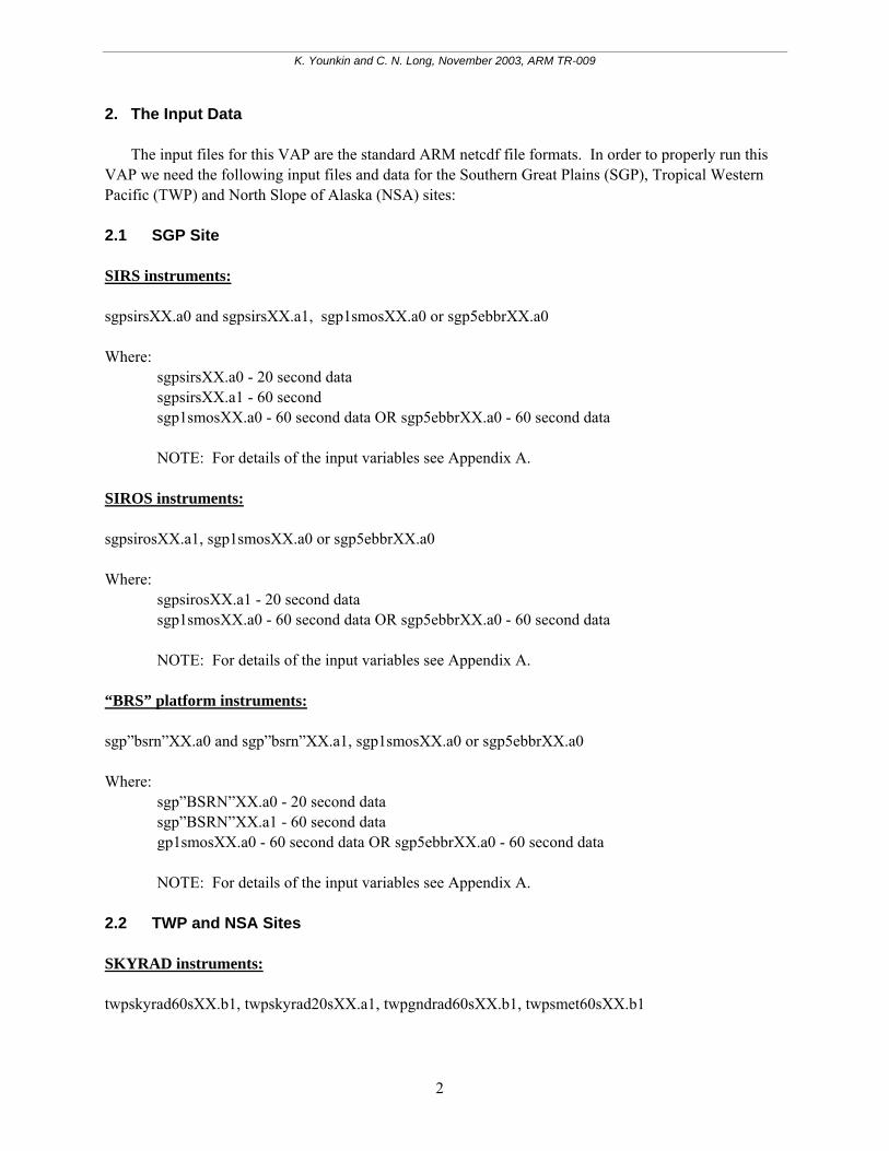
Figure 1. Flow diagram of nighttime fitting process. SKYRAD instruments: We use data from SKYRAD 20s a1 data stream. Variables that are needed are Instantaneous PIR2 case thermistor in Ohms, Instantaneous PIR2 dome thermistor in Ohms and Instantaneous PIR2 uncorrected irradiance in Wm-2 units. Due to the format and nature of the stored information, we must calculate the case and dome temperatures from information about the thermistors resistance (For details see Appendix B). In addition, the detector flux itself must also be calculated (for details see Appendix C). 3.1.1.1 Average Case and Dome PIR Temperature and PIR Detector Flux The PIR case and dome temperatures and PIR Detector Flux, taken at 20 second intervals, are averaged into 60 second time interval since we need to use this data with time coherence with the SMOS a0, EBBR a0 or SMET b1 data stream that have a 60 second time interval. The averaging is done so that
4
K. Younkin and C. N. Long, November 2003, ARM TR-009
all data are averaged to 1-minute data and time stamped with the end of the time interval. The MISSING (-9999) values are excluded from the averaging algorithm. 3.1.2 Prepare Nighttime Data As detailed in Dutton et al. (2001), the diffuse SW IR loss correction is based on collocated pyrgeometer data. At night, when there is no solar irradiance input to the pyranometer, a relationship is determined between the pyrgeometer detector flux (and the pyrgeometer case and dome temperatures in the case of the “full” correction), and the nighttime negative values from the pyranometer. For the SW DIFF CORR 1DUTT VAP, we use 6 hours of data each night, from 3 hours either side of local midnight far away from sunrise and sunset when there might possibly be instrument equilibrium concerns. For example, for SGP data we use data from 0300 Universal Time Coordinates (UTC) to 0900 UTC each night. For mid- and lower latitudes, we do not adjust this nightly time range for the longer nights of winter, because that would then bias the fitting toward winter by default due to the increased number of values each night. For the NSA site we are not able to use an hourly nighttime boundary for inclusion for fitting due to exaggerated seasonal changes in day length. For the NSA site rather than using 3 hours either side of local midnight, we instead use a cosine of solar zenith angle (µ0) limit to determine the nighttime data. Specifically, we include all data for which µ0 < -0.2. Regardless of these differences, once it is determined what data will be included, all the night data is then used to calculate the correction fit coefficients. To prepare nighttime data we need averaged variables:
Case and Dome PIR Temperature, PIR Detector Flux and uncorrected SW diffuse irradiance. In the case of SIRS, “BRS”, SKYRAD instrument, Case and Dome PIR Temperature and PIR Detector Flux are taken from the corresponding 20s data stream. Uncorrected SW diffuse IR is taken from corresponding 60s (a1) data stream. For SIROS instrument all the data is taken from 60s (a1) data stream.
All the variables are at this point averaged at 60 seconds time interval. Several QC checks are performed to make sure that only good data is used for IR Loss correction fitting algorithms. 3.1.2.1 Nighttime QC Checks 3.1.2.1.1 Compare Case and Dome PIR Temperatures Theoretically, the PIR case temperature should always be greater than or equal to the Dome PIR Temperature. After extensive analysis of the average case dome temperature differences, and allowing for thermistor uncertainties, we accept data that fall within the ranges: IR Loss Detector only correction fit
Td >= (Tc – 2.0 K)
5
K. Younkin and C. N. Long, November 2003, ARM TR-009
IR Loss Full correction fit
(Tc + 0.5 K) >= Td >= (Tc – 2.0 K) Where: Td = Dome PIR Temperature (K) Tc = Case PIR Temperature (K)
NOTE: All data that falls in the acceptable range of these limits are included in calculating night-time corrections, else the data are rejected. (See Section 4.2 for used limit specifications.)
3.1.2.1.2 Compare the Difference Between Calculated PIR and Original PIR SIRS, “BRS,” SKYRAD instruments: This check primarily tests the data to ensure that gross errors, such as application of an erroneous calibration coefficient, have not occurred. First we calculate the Longwave Irradiance from the a0 PIR values (see Appendix D for details). Second we accept data that fall within the range:
Abs(PIR_orig – PIR_calc) <= 2.0 Wm-2 Where: PIR_orig = Longwave Irradiance present in SIRS/BRS a1, SKYRAD b1 (60s) data
stream (Wm-2) PIR_calc = Longwave Irradiance calculated from SIRS/BRS a0, SKYRAD a1 (20s)
data stream (Wm-2)
NOTE: If the data agrees to within this limit, we include the sample time for the detector only and full-correction fitting algorithm. We also note here that the PIR case and dome temperature data for site E25 historically has been consistently “noisy,” as reported in ARM Data Quality reports. This noise precluded much of the data from being used for applying a full correction, and caused much of the PIR data to be rejected by this particular test. But extensive analysis of the data shows that the thermistor noise is random in nature. Thus, we have applied an 11-minute running mean to “smooth” the data from E25 (discussed in detail later), which then precludes using this particular test on the E25 data.
SIROS instrument: For the SIROS instrument we cannot perform this check since we have only SIROS a1 20-second data available. We are missing the SIROS a0 data stream from which the PIR is calculated by using the thermopile voltage.
NOTE: See Section 4.1 for used limit specifications.
6
K. Younkin and C. N. Long, November 2003, ARM TR-009
3.1.2.1.3 Check PIR Detector Flux Min Max Value This qc check puts a limit on allowable PIR Detector Flux. This limit is important for the bimodal distribution for calculating correction coefficients. The limits are based on climatologically reasonable expectations for overall pyrgeometer measurements. Data falling outside these limits are rejected (See Section 4.7 for explanation).
-300.0 Wm-2 <= DF <= 0.0 Wm-2 Where: Df = PIR Detector Flux (Wm-2) 3.1.2.1.4 Compare IR Brightness Temperature with the Ambient Air Temperature This qc check eliminates erroneous data, such as abnormally high values that can occur when the instrument is first exposed to rainfall or other thermal shock conditions. First we calculate the down-welling broadband IR brightness temperature using the Stephan-Boltzman relation (see Appendix E for details). Second we accept all data that fall in the range:
Te <= (Ta + 1.5 K) Where: Te = Down-welling Broadband IR Brightness Temperature (K) Ta = Ambient Air Temperature (K) – SMOS, EBBR, SMET instrument
NOTE: Generally the ambient air temperature should be greater than the IR brightness temperature except under rare circumstances (humid overcast conditions with a temperature inversion). If the calculated Te is greater than Ta plus 1.5 K, we exclude the sample time from the detector only and full-correction fitting algorithm. (See Section 4.3 for used limit specifications.)
For some instrument/facility combinations at SGP there is no SMOS/EBBR instrument located at the same facility (e.g., for SIRS (E10, E16) or SIROS (E2, E10, E16, E18). In those instances we substitute the PIR Case Temperature in place of the Ambient Air Temperature and proceed with the QC check. This substitution is also done if there is a missing data sample of Ambient Air Temperature. 3.1.2.1.5 PIR Case Temperature Testing Using Running Standard Deviation Due to the sampling strategy of the data, and the tendency for the 20-second samples to sometimes be “noisy” in these data streams, we calculate the 11-minute running standard deviation for the PIR Case Temperature and the 11-minute running standard deviation of the 11-minutes running average of the PIR Case Temperature as an additional data QC check. The 11-minute running standard deviation and 11-minutes running standard deviation of the 11-minutes running averages are calculated for every 1-minute sample of the Case PIR Temperature. The data of interest is in the middle of the 11-minute period, with 5 data points on each side.
7
K. Younkin and C. N. Long, November 2003, ARM TR-009
QC check:
Tc_sdev – Tc_avg_sdev <= 0.1 Where: Tc_stdev = 11-minute running standard deviation of the Case PIR
Temperature (K) Tc_avg_stdev = 11-minute running standard deviation of the 11-minute running
averages of the Case PIR Temperature (K)
NOTE: If the data point of interest has a standard deviation difference larger than 0.1, we exclude the sample time from the full correction fitting algorithm, but do calculate the detector-only correction which is not significantly affected by this noise problem. (For the description of the noise problem see Section 4.6)
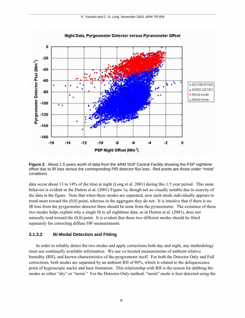
3.1.3 Calculate Bimodal Correction Coefficients Long et al. (2001) and Younkin and Long (2002) tested the Dutton et al. (2001) correction method using collocated shaded Eppley models PSP and 8-48 “Black and White” (B&W) data from the ARM Southern Great Plains (SGP) Central Facility in Oklahoma. These two studies show a number of results, including demonstrating that a relationship linking the pyranometer nighttime offset to the temperature difference of the pyrgeometer case and dome, expressed in terms of flux via the Stephan-Boltzman relation, has more tendency toward the (0,0) intercept than a detector flux relationship as suggested by Dutton et al. (2001). As a result of this “better behavior,” Younkin and Long (2002) recommend a “full” correction method that includes a 3D fitting with the pyrgeometer detector, and the case-dome temperature difference factor, as two independent variables. Regardless of whether the Dutton et al. (2001) “detector only” or the Younkin and Long (2002) “full” recommended corrections are used; Long et al. (2001) show that both correction methodologies completely eliminate the sub-Rayleigh behavior in ARM Oklahoma data noted by Cess et al. (2000). But while the empirical relationships derived using nighttime data do an excellent job of correcting for IR loss at night, they tend to under compensate for pyranometer IR loss when applied during daylight (Long et al. 2001). This tendency is hinted at in Dutton et al (2001) in their Table 2, and in their statement regarding the single black detector corrected diffuse having a tendency to be less than that obtained from a B&W. Philipona (2002) also noted that daytime negative offsets were larger than those at night, and appeared to be larger than those that would result from a nighttime offset versus pyrgeometer detector relationship. 3.1.3.1 Bi-Modal Behavior Long et al. (2001) noted a bimodal behavior between the pyranometer nighttime offset and the corresponding pyrgeometer detector flux. Figure 2 shows this bimodal behavior for about 18 months of data from the ARM SGP Central Facility, here showing the relationship between the nighttime pyranometer offset and the corresponding pyrgeometer detector flux for the six hours each night centered on local midnight. The red points in Figure 2 are data that have been separated using the simple criteria wherein the sky equivalent blackbody radiating temperature (from the Stephan-Boltzman relation) calculated from the down-welling longwave measurement is within 6°C of the pyrgeometer case temperature, and the ambient relative humidity is greater than 80%. Analysis shows that these separated
8
K. Younkin and C. N. Long, November 2003, ARM TR-009
Figure 2. About 1.5 years worth of data from the ARM SGP Central Facility showing the PSP nighttime offset due to IR loss versus the corresponding PIR detector flux loss. Red points are those under “moist” conditions. data occur about 13 to 14% of the time at night (Long et al. 2001) during this 1.5 year period. This same behavior is evident in the Dutton et al. (2001) Figure 1a, though not as visually notable due to scarcity of the data in the figure. Note that when these modes are separated, now each mode individually appears to trend more toward the (0,0) point, whereas in the aggregate they do not. It is intuitive that if there is no IR loss from the pyrgeometer detector there should be none from the pyranometer. The existence of these two modes helps explain why a single fit to all nighttime data, as in Dutton et al. (2001), does not naturally tend toward the (0,0) point. It is evident that these two different modes should be fitted separately for correcting diffuse SW measurements. 3.1.3.2 Bi-Modal Detection and Fitting In order to reliably detect the two modes and apply corrections both day and night, any methodology must use continually available information. We use co-located measurements of ambient relative humidity (RH), and known characteristics of the pyrgeometer itself. For both the Detector Only and Full corrections, both modes are separated by an ambient RH of 80%, which is related to the deliquescence point of hygroscopic nuclei and haze formation. This relationship with RH is the reason for dubbing the modes as either “dry” or “moist.” For the Detector-Only method, “moist” mode is best detected using the
9
K. Younkin and C. N. Long, November 2003, ARM TR-009
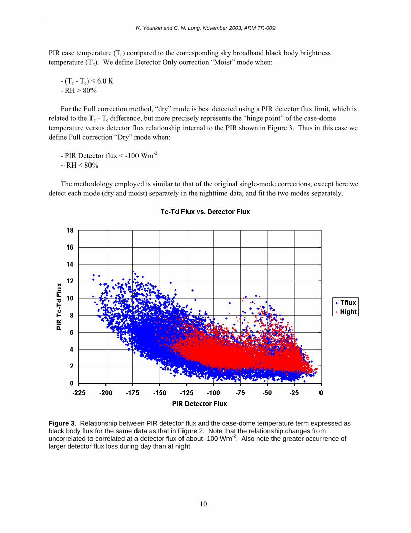
PIR case temperature (Tc) compared to the corresponding sky broadband black body brightness temperature (Te). We define Detector Only correction “Moist” mode when: - (Tc - Te) < 6.0 K - RH > 80% For the Full correction method, “dry” mode is best detected using a PIR detector flux limit, which is related to the Tc - Te difference, but more precisely represents the “hinge point” of the case-dome temperature versus detector flux relationship internal to the PIR shown in Figure 3. Thus in this case we define Full correction “Dry” mode when: - PIR Detector flux < -100 Wm-2 ~ RH < 80% The methodology employed is similar to that of the original single-mode corrections, except here we detect each mode (dry and moist) separately in the nighttime data, and fit the two modes separately.
Figure 3. Relationship between PIR detector flux and the case-dome temperature term expressed as black body flux for the same data as that in Figure 2. Note that the relationship changes from uncorrelated to correlated at a detector flux of about -100 Wm-2. Also note the greater occurrence of larger detector flux loss during day than at night
10
K. Younkin and C. N. Long, November 2003, ARM TR-009
3.1.3.3 Calculate Detector Only Bi-Modal Correction Coefficients At this point we have 2 sample sets (“dry” and “moist”). Each sample set contains the night data for the pyranometer irradiance loss and pyrgeometer detector flux. The Detector only correction coefficients are calculated for both sets. To calculate Detector only bi-modal correction coefficients we use formula:
PSP = b0 + b1*Df Where: PSP = Precision Spectral Pyranometer nighttime Irradiance Loss (Wm-2) b0 = intercept = 0 b1 = regression coefficient (Detector only correction coefficient) Df = PIR Detector Flux (Wm-2)
NOTE: This equation is calculated twice. First time with a “dry” mode sample set and second time with a “moist” mode sample set. To determine the regression coefficient we use a method of least absolute deviations.
3.1.3.4 Calculate Full Bi-Modal Correction Coefficients At this point we have 2 sample sets (“dry” and “moist”). Each sample set contains the night data for the pyranometer irradiance loss and pyrgeometer detector flux, PIR Case Temperature and PIR Dome Temperature. The Full correction coefficients are calculated for both sets. To calculate Full bi-modal correction coefficients we use formula:
PSP = b0 + b1*Df + b2*Sig*(Td4 – Tc4) Where: PSP = Precision Spectral Pyranometer nighttime Irradiance Loss (Wm-2) b0 = intercept = 0 b1, b2 = regression coefficients Df = PIR Detector Flux (Wm-2) Sig = Stephan-Boltzman Constant = 5.67E-08 W/(m2 K4) Tc = PIR Case Temperature (K) Td = PIR Dome Temperature (K)
NOTE: This equation is calculated twice. First time with a “dry” mode sample set and second time with a “moist” mode sample set. To determine the regression coefficients we use the criterion of mean absolute deviation. However, for the TWP site we are not able to detect any “dry mode” data at night. The relative humidity remains above the set limit (80%) during the years that we are correcting for IR loss. Therefore the Full correction “dry mode” coefficients are not calculated, and we use the “moist mode” full correction coefficients to correct all the diffuse SW data. It should also be noted that the tropical atmosphere is moist enough that IR loss is a minimum.
11
K. Younkin and C. N. Long, November 2003, ARM TR-009
3.1.4 Save Detector Only and Full Correction Coefficients in a Configuration File Once the correction coefficients are calculated we record them in the configuration file called diffcor1dutt_corrections.cdf. This file contains the entire set of Detector only and Full correction coefficients that had been calculated for the site, facility, instrument, and time period between replacements of the Eppley PSP pyranometers. This file is essential to apply correction coefficients to the SW measurements. Detector only and Full correction coefficients must be calculated prior to the attempt to correct SW data for the specific site, facility, instrument and time combination. 3.2 Applying Correction Coefficients The second part of the DIFFCORR1DUTT VAP organizes and processes all the input data in order to correct the diffuse SW measurements by using the previously calculated Detector only and Full correction coefficients. The VAP goes thru several stages of input data organization. In order to apply correction coefficients and perform appropriate QC checks we need to calculate several variables: case and dome PIR temperature, PIR detector flux, IR brightness temperature, Rayleigh limit and solar zenith angle (SZA). Once the variables are calculated we apply the bi-modal Detector only correction coefficient and bi-modal Full correction coefficients to the SW measurements and perform a series of QC checks to assure data quality. The final output files are then produced containing all the input and calculated variables used in the process (see Table 7 in Appendix F). Figure 4 outlines the general process of the input data organization and SW measurement correction. 3.2.1 Organize Input Data Calculation of the PIR case and dome temperatures has been described in Section 3.1.1.1. Similarly, see Section 3.1.1.2 for information on the calculation of PIR detector flux, and Section 3.1.1.3 for the averaging details for these variables. 3.2.2 Calculate SZA We calculate the SZA for every data point in the input a1 file (i.e., for every minute that the data is recorded). Solar zenith angle and Cosine of the SZA (µ0) are calculated using the ephemeris routine of Nels Larson (1992), with site latitude and longitude, and date and time as inputs. The SZA is needed since we need to estimate the Rayleigh limit, which is limited to SZA <= 90 degrees. 3.2.3 Calculate Down-welling Broadband IR Brightness Temperature
NOTE: See Appendix E for details.
12
K. Younkin and C. N. Long, November 2003, ARM TR-009
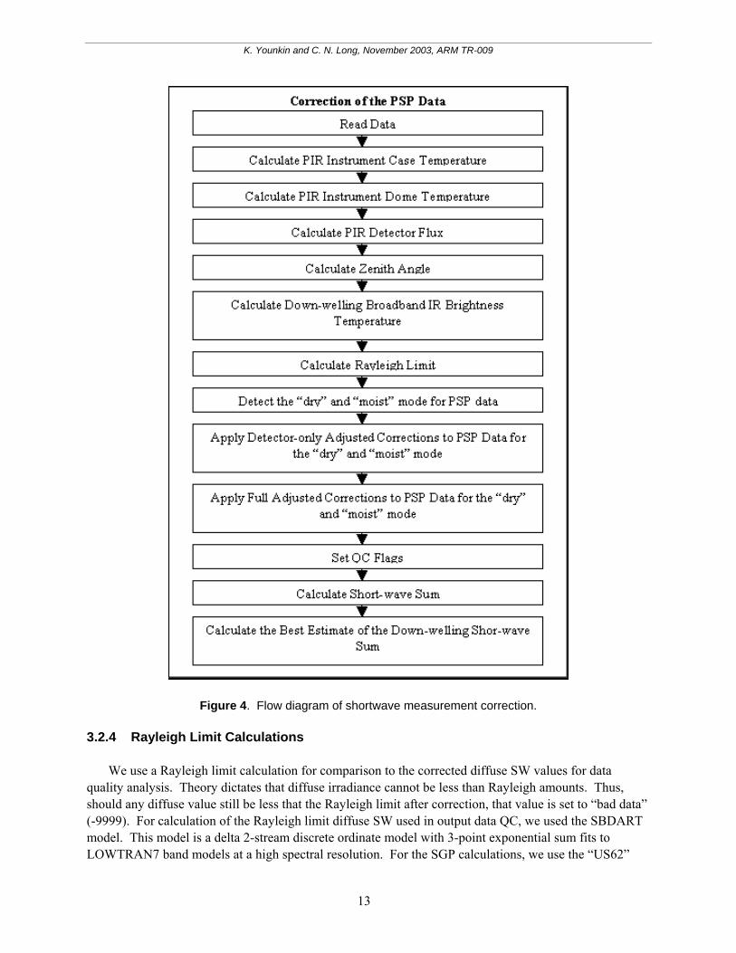
Figure 4. Flow diagram of shortwave measurement correction. 3.2.4 Rayleigh Limit Calculations We use a Rayleigh limit calculation for comparison to the corrected diffuse SW values for data quality analysis. Theory dictates that diffuse irradiance cannot be less than Rayleigh amounts. Thus, should any diffuse value still be less that the Rayleigh limit after correction, that value is set to “bad data” (-9999). For calculation of the Rayleigh limit diffuse SW used in output data QC, we used the SBDART model. This model is a delta 2-stream discrete ordinate model with 3-point exponential sum fits to LOWTRAN7 band models at a high spectral resolution. For the SGP calculations, we use the “US62”
13
K. Younkin and C. N. Long, November 2003, ARM TR-009
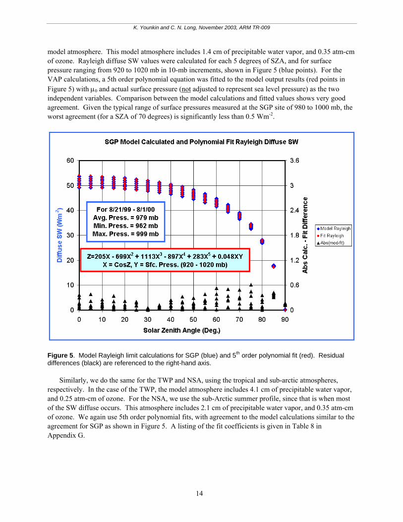
model atmosphere. This model atmosphere includes 1.4 cm of precipitable water vapor, and 0.35 atm-cm of ozone. Rayleigh diffuse SW values were calculated for each 5 degrees of SZA, and for surface pressure ranging from 920 to 1020 mb in 10-mb increments, shown in Figure 5 (blue points). For the VAP calculations, a 5th order polynomial equation was fitted to the model output results (red points in Figure 5) with µ0 and actual surface pressure (not adjusted to represent sea level pressure) as the two independent variables. Comparison between the model calculations and fitted values shows very good agreement. Given the typical range of surface pressures measured at the SGP site of 980 to 1000 mb, the worst agreement (for a SZA of 70 degrees) is significantly less than 0.5 Wm-2.
Figure 5. Model Rayleigh limit calculations for SGP (blue) and 5th order polynomial fit (red). Residual differences (black) are referenced to the right-hand axis. Similarly, we do the same for the TWP and NSA, using the tropical and sub-arctic atmospheres, respectively. In the case of the TWP, the model atmosphere includes 4.1 cm of precipitable water vapor, and 0.25 atm-cm of ozone. For the NSA, we use the sub-Arctic summer profile, since that is when most of the SW diffuse occurs. This atmosphere includes 2.1 cm of precipitable water vapor, and 0.35 atm-cm of ozone. We again use 5th order polynomial fits, with agreement to the model calculations similar to the agreement for SGP as shown in Figure 5. A listing of the fit coefficients is given in Table 8 in Appendix G.
14
K. Younkin and C. N. Long, November 2003, ARM TR-009
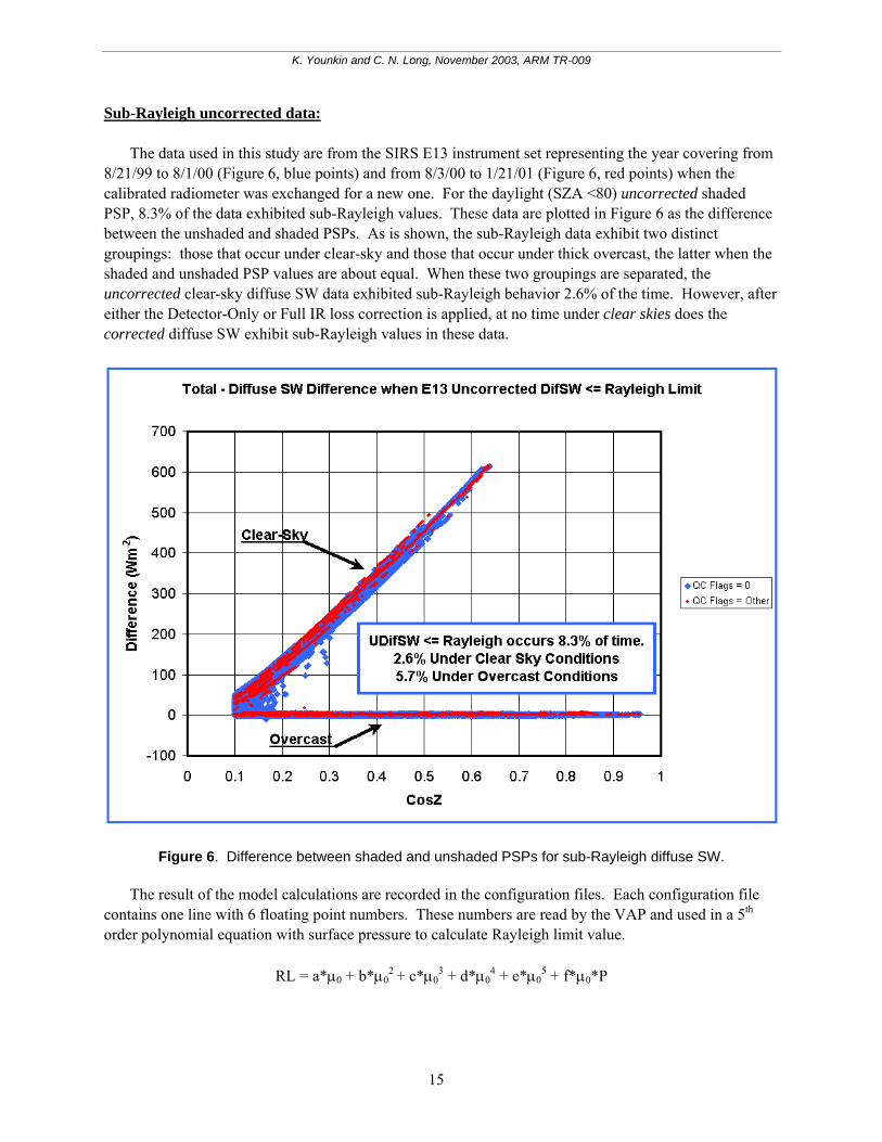
Sub-Rayleigh uncorrected data: The data used in this study are from the SIRS E13 instrument set representing the year covering from 8/21/99 to 8/1/00 (Figure 6, blue points) and from 8/3/00 to 1/21/01 (Figure 6, red points) when the calibrated radiometer was exchanged for a new one. For the daylight (SZA <80) uncorrected shaded PSP, 8.3% of the data exhibited sub-Rayleigh values. These data are plotted in Figure 6 as the difference between the unshaded and shaded PSPs. As is shown, the sub-Rayleigh data exhibit two distinct groupings: those that occur under clear-sky and those that occur under thick overcast, the latter when the shaded and unshaded PSP values are about equal. When these two groupings are separated, the uncorrected clear-sky diffuse SW data exhibited sub-Rayleigh behavior 2.6% of the time. However, after either the Detector-Only or Full IR loss correction is applied, at no time under clear skies does the corrected diffuse SW exhibit sub-Rayleigh values in these data.
Figure 6. Difference between shaded and unshaded PSPs for sub-Rayleigh diffuse SW. The result of the model calculations are recorded in the configuration files. Each configuration file contains one line with 6 floating point numbers. These numbers are read by the VAP and used in a 5th order polynomial equation with surface pressure to calculate Rayleigh limit value.
RL = a*µ0 + b*µ02 + c*µ0
3 + d*µ04 + e*µ0
5 + f*µ0*P
15
K. Younkin and C. N. Long, November 2003, ARM TR-009
Where: RL = Rayleigh limit (Wm-2) a, b, c, d, e, f = Rayleigh model calculation coefficients (see Appendix G for
details) µ0 = cosine of SZA P = barometric pressure from SMOS, EBBR or SMET
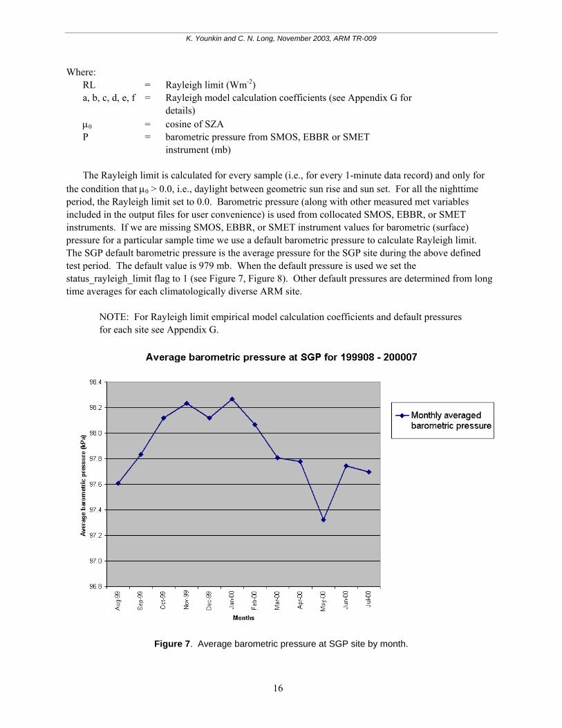
instrument (mb) The Rayleigh limit is calculated for every sample (i.e., for every 1-minute data record) and only for the condition that µ0 > 0.0, i.e., daylight between geometric sun rise and sun set. For all the nighttime period, the Rayleigh limit set to 0.0. Barometric pressure (along with other measured met variables included in the output files for user convenience) is used from collocated SMOS, EBBR, or SMET instruments. If we are missing SMOS, EBBR, or SMET instrument values for barometric (surface) pressure for a particular sample time we use a default barometric pressure to calculate Rayleigh limit. The SGP default barometric pressure is the average pressure for the SGP site during the above defined test period. The default value is 979 mb. When the default pressure is used we set the status_rayleigh_limit flag to 1 (see Figure 7, Figure 8). Other default pressures are determined from long time averages for each climatologically diverse ARM site.
NOTE: For Rayleigh limit empirical model calculation coefficients and default pressures for each site see Appendix G.
Figure 7. Average barometric pressure at SGP site by month.
16
K. Younkin and C. N. Long, November 2003, ARM TR-009
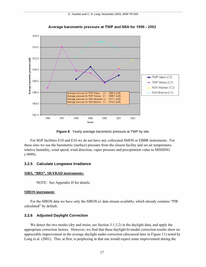
Figure 8. Yearly average barometric pressure at TWP by site. For SGP facilities E10 and E16 we do not have any collocated SMOS or EBBR instruments. For these sites we use the barometric (surface) pressure from the closest facility and set air temperature, relative humidity, wind speed, wind direction, vapor pressure and precipitation value to MISSING (-9999). 3.2.5 Calculate Longwave Irradiance SIRS, “BRS”, SKYRAD instruments:
NOTE: See Appendix D for details. SIROS instrument: For the SIROS data we have only the SIROS a1 data stream available, which already contains “PIR calculated” by default. 3.2.6 Adjusted Daylight Correction We detect the two modes (dry and moist, see Section 3.1.3.2) in the daylight data, and apply the appropriate correction factors. However, we find that these daylight bi-modal correction results show no appreciable improvement in the average daylight under-correction (discussed later in Figure 11) noted by Long et al. (2001). This, at first, is perplexing in that one would expect some improvement during the
17
K. Younkin and C. N. Long, November 2003, ARM TR-009
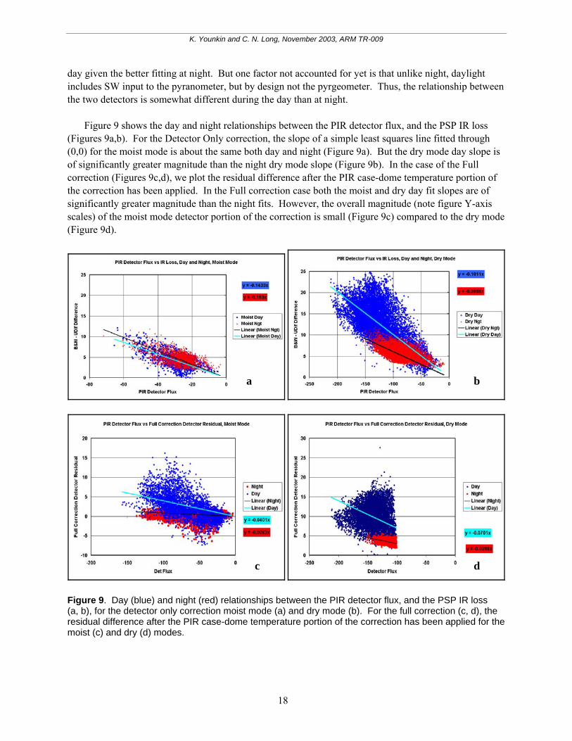
day given the better fitting at night. But one factor not accounted for yet is that unlike night, daylight includes SW input to the pyranometer, but by design not the pyrgeometer. Thus, the relationship between the two detectors is somewhat different during the day than at night. Figure 9 shows the day and night relationships between the PIR detector flux, and the PSP IR loss (Figures 9a,b). For the Detector Only correction, the slope of a simple least squares line fitted through (0,0) for the moist mode is about the same both day and night (Figure 9a). But the dry mode day slope is of significantly greater magnitude than the night dry mode slope (Figure 9b). In the case of the Full correction (Figures 9c,d), we plot the residual difference after the PIR case-dome temperature portion of the correction has been applied. In the Full correction case both the moist and dry day fit slopes are of significantly greater magnitude than the night fits. However, the overall magnitude (note figure Y-axis scales) of the moist mode detector portion of the correction is small (Figure 9c) compared to the dry mode (Figure 9d).
a b
c d
Figure 9. Day (blue) and night (red) relationships between the PIR detector flux, and the PSP IR loss (a, b), for the detector only correction moist mode (a) and dry mode (b). For the full correction (c, d), the residual difference after the PIR case-dome temperature portion of the correction has been applied for the moist (c) and dry (d) modes.
18
K. Younkin and C. N. Long, November 2003, ARM TR-009
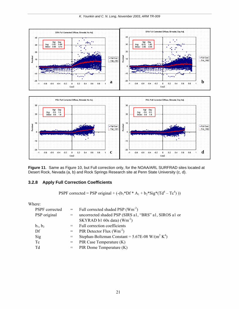
The day-night difference does not affect the pyrgeometer case-dome temperature flux-to-pyranometer-IR-loss relationship, but is related to the detector term only. So for both the Full and Detector Only corrections, we apply an adjustment factor during daylight, but only for the detector portion of the correction. Iteration of the available data sets (results shown below) to achieve the best results for both the mean and standard deviation of residuals between corrected values and co-located Eppley 8-48 B&Ws yields the adjustment factors:
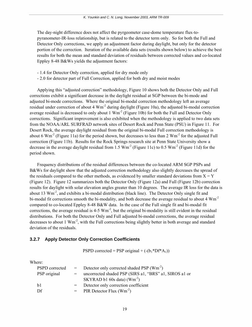
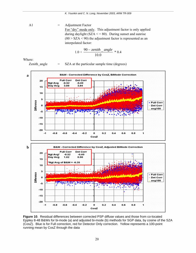
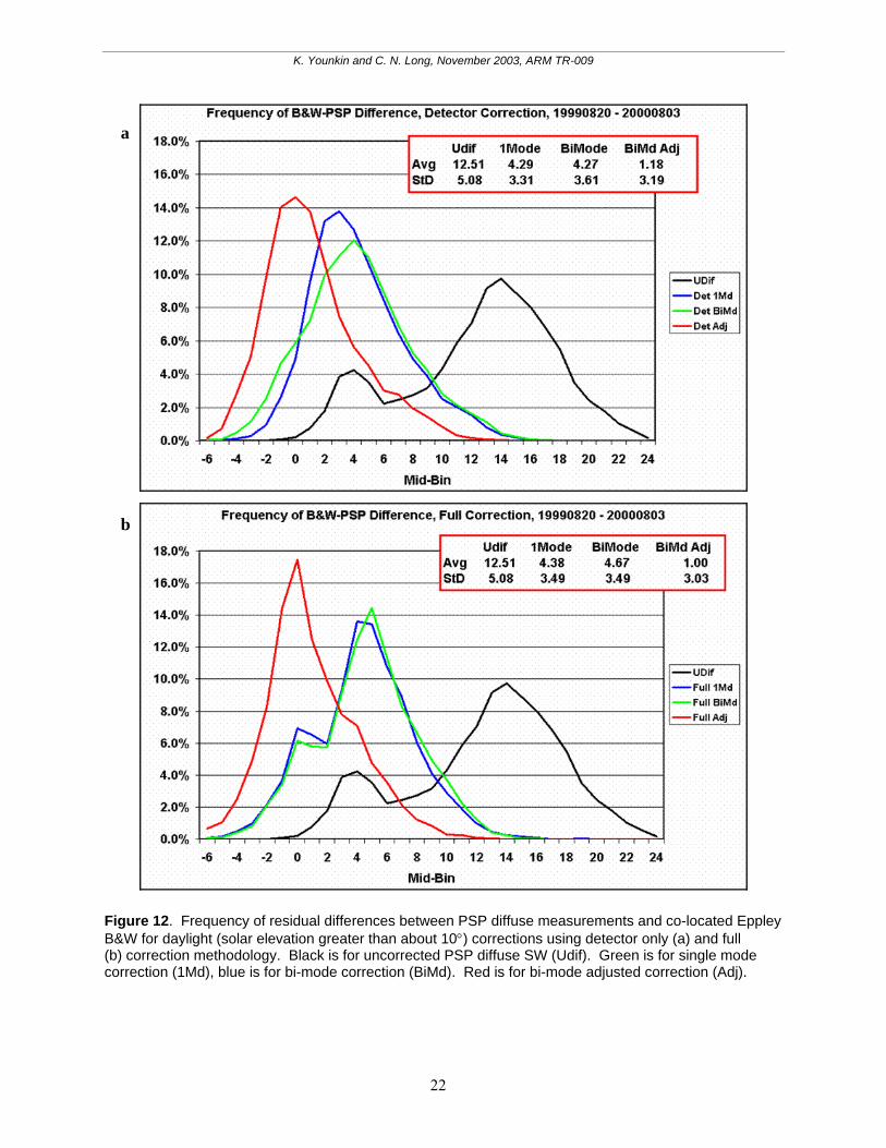
- 1.4 for Detector Only correction, applied for dry mode only - 2.0 for detector part of Full Correction, applied for both dry and moist modes Applying this “adjusted correction” methodology, Figure 10 shows both the Detector Only and Full corrections exhibit a significant decrease in the daylight residual at SGP between the bi-mode and adjusted bi-mode corrections. Where the original bi-modal correction methodology left an average residual under correction of about 4 Wm-2 during daylight (Figure 10a), the adjusted bi-modal correction average residual is decreased to only about 1 Wm-2 (Figure 10b) for both the Full and Detector Only corrections. Significant improvement is also exhibited when the methodology is applied to two data sets from the NOAA/ARL SURFRAD network sites of Desert Rock and Penn State (PSU) in Figure 11. For Desert Rock, the average daylight residual from the original bi-modal Full correction methodology is about 6 Wm-2 (Figure 11a) for the period shown, but decreases to less than 2 Wm-2 for the adjusted Full correction (Figure 11b). Results for the Rock Springs research site at Penn State University show a decrease in the average daylight residual from 1.5 Wm-2 (Figure 11c) to 0.5 Wm-2 (Figure 11d) for the period shown. Frequency distributions of the residual differences between the co-located ARM SGP PSPs and B&Ws for daylight show that the adjusted correction methodology also slightly decreases the spread of the residuals compared to the other methods, as evidenced by smaller standard deviations from X = Y (Figure 12). Figure 12 summarizes both the Detector Only (Figure 12a) and Full (Figure 12b) correction results for daylight with solar elevation angles greater than 10 degrees. The average IR loss for the data is about 13 Wm-2, and exhibits a bi-modal distribution (black line). The Detector Only single fit and bi-modal fit corrections smooth the bi-modality, and both decrease the average residual to about 4 Wm-2 compared to co-located Eppley 8-48 B&W data. In the case of the Full single fit and bi-modal fit corrections, the average residual is 4-5 Wm-2, but the original bi-modality is still evident in the residual distributions. For both the Detector Only and Full adjusted bi-modal corrections, the average residual decreases to about 1 Wm-2, with the Full corrections being slightly better in both average and standard deviation of the residuals. 3.2.7 Apply Detector Only Correction Coefficients
PSPD corrected = PSP original + (-(b1*Df*A1)) Where: PSPD corrected = Detector only corrected shaded PSP (Wm-2) PSP original = uncorrected shaded PSP (SIRS a1, “BRS” a1, SIROS a1 or
SKYRAD b1 60s data) (Wm-2) b1 = Detector only correction coefficient Df = PIR Detector Flux (Wm-2)
19
K. Younkin and C. N. Long, November 2003, ARM TR-009
A1 = Adjustment Factor For “dry” mode only. This adjustment factor is only applied during daylight (SZA < = 80). During sunset and sunrise (80 > SZA < 90) the adjustment factor is represented as an interpolated factor:
1.0 + 0.10_90 anglezenith−
* 0.4
Where: Zenith_angle = SZA at the particular sample time (degrees)
a
b
Figure 10. Residual differences between corrected PSP diffuse values and those from co-located Eppley 8-48 B&Ws for bi-mode (a) and adjusted bi-mode (b) methods for SGP data, by cosine of the SZA (CosZ). Blue is for Full correction, red for Detector Only correction. Yellow represents a 100-point running mean by CosZ through the data
20
K. Younkin and C. N. Long, November 2003, ARM TR-009
a b
c d
Figure 11. Same as Figure 10, but Full correction only, for the NOAA/ARL SURFRAD sites located at Desert Rock, Nevada (a, b) and Rock Springs Research site at Penn State University (c, d). 3.2.8 Apply Full Correction Coefficients
PSPF corrected = PSP original + (-(b1*Df * A1 + b2*Sig*(Td4 – Tc4) )) Where: PSPF corrected = Full corrected shaded PSP (Wm-2) PSP original = uncorrected shaded PSP (SIRS a1, “BRS” a1, SIROS a1 or
SKYRAD b1 60s data) (Wm-2) b1, b2 = Full correction coefficients Df = PIR Detector Flux (Wm-2) Sig = Stephan-Boltzman Constant = 5.67E-08 W/(m2 K4) Tc = PIR Case Temperature (K) Td = PIR Dome Temperature (K)
21
K. Younkin and C. N. Long, November 2003, ARM TR-009
a
b
Figure 12. Frequency of residual differences between PSP diffuse measurements and co-located Eppley B&W for daylight (solar elevation greater than about 10°) corrections using detector only (a) and full (b) correction methodology. Black is for uncorrected PSP diffuse SW (Udif). Green is for single mode correction (1Md), blue is for bi-mode correction (BiMd). Red is for bi-mode adjusted correction (Adj).
22
K. Younkin and C. N. Long, November 2003, ARM TR-009
A1 = Adjustment Factor For “dry” and “moist” mode. This adjustment factor is only applied during daylight (SZA < = 80). During sunset and sunrise (80 > SZA < 90) the adjustment factor is represented as an interpolated factor:
1.0 + 0.10_90 anglezenith−
* 1.0
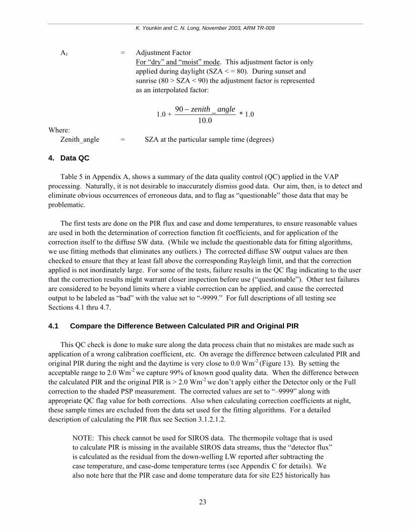
Where: Zenith_angle = SZA at the particular sample time (degrees) 4. Data QC Table 5 in Appendix A, shows a summary of the data quality control (QC) applied in the VAP processing. Naturally, it is not desirable to inaccurately dismiss good data. Our aim, then, is to detect and eliminate obvious occurrences of erroneous data, and to flag as “questionable” those data that may be problematic. The first tests are done on the PIR flux and case and dome temperatures, to ensure reasonable values are used in both the determination of correction function fit coefficients, and for application of the correction itself to the diffuse SW data. (While we include the questionable data for fitting algorithms, we use fitting methods that eliminates any outliers.) The corrected diffuse SW output values are then checked to ensure that they at least fall above the corresponding Rayleigh limit, and that the correction applied is not inordinately large. For some of the tests, failure results in the QC flag indicating to the user that the correction results might warrant closer inspection before use (“questionable”). Other test failures are considered to be beyond limits where a viable correction can be applied, and cause the corrected output to be labeled as “bad” with the value set to “-9999.” For full descriptions of all testing see Sections 4.1 thru 4.7. 4.1 Compare the Difference Between Calculated PIR and Original PIR This QC check is done to make sure along the data process chain that no mistakes are made such as application of a wrong calibration coefficient, etc. On average the difference between calculated PIR and original PIR during the night and the daytime is very close to 0.0 Wm-2 (Figure 13). By setting the acceptable range to 2.0 Wm-2 we capture 99% of known good quality data. When the difference between the calculated PIR and the original PIR is > 2.0 Wm-2 we don’t apply either the Detector only or the Full correction to the shaded PSP measurement. The corrected values are set to “–9999” along with appropriate QC flag value for both corrections. Also when calculating correction coefficients at night, these sample times are excluded from the data set used for the fitting algorithms. For a detailed description of calculating the PIR flux see Section 3.1.2.1.2.
NOTE: This check cannot be used for SIROS data. The thermopile voltage that is used to calculate PIR is missing in the available SIROS data streams, thus the “detector flux” is calculated as the residual from the down-welling LW reported after subtracting the case temperature, and case-dome temperature terms (see Appendix C for details). We also note here that the PIR case and dome temperature data for site E25 historically has
23
K. Younkin and C. N. Long, November 2003, ARM TR-009
been consistently “noisy”, as reported in ARM Data Quality reports. This noise precluded much of the data from being used for applying a full correction, and caused much of the PIR data to be rejected by this particular test. But extensive analysis of the data shows that the thermistor noise is random in nature. Thus, we have applied an 11-minute running mean to “smooth” the data from E25 (discussed in detail later), which then precludes using this particular test on the E25 data.
Figure 13. Night and day difference between original and 20-sec calculated PIR for 15-min average data.
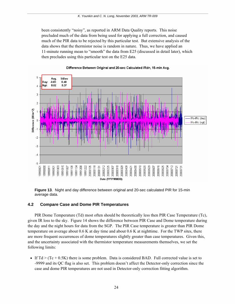
4.2 Compare Case and Dome PIR Temperatures PIR Dome Temperature (Td) most often should be theoretically less then PIR Case Temperature (Tc), given IR loss to the sky. Figure 14 shows the difference between PIR Case and Dome temperature during the day and the night hours for data from the SGP. The PIR Case temperature is greater than PIR Dome temperature on average about 0.6 K at day time and about 0.6 K at nighttime. For the TWP sites, there are more frequent occurrences of dome temperatures slightly greater than case temperatures. Given this, and the uncertainty associated with the thermistor temperature measurements themselves, we set the following limits: • If Td > (Tc + 0.5K) there is some problem. Data is considered BAD. Full corrected value is set to
-9999 and its QC flag is also set. This problem doesn’t affect the Detector-only correction since the case and dome PIR temperatures are not used in Detector-only correction fitting algorithm.
24
K. Younkin and C. N. Long, November 2003, ARM TR-009
Figure 14. Night and day difference between PIR Case and Dome Temperature for 15-min average data.
• If Td < Tc but within 1.5 K (more than 4.0 standard deviations). Data is considered GOOD. The
Detector-only and Full correction are applied. No QC flags are set. • If Td < Tc, but is 1.5 – 2.0K. Data is considered QUESTIONABLE. This state can be generally
caused by a thermal shock, like at start of rainfall. The Detector and Full corrections are applied but both QC flags are set as “questionable.”
• If Td is more than 2.0 < Tc. Data is considered BAD. This state represent ‘beyond clear-sky loss.’
The Detector and Full corrections are not applied (set to –9999) and both QC flags are set.
NOTE: For a detailed description of the calculated PIR case and dome temperature see Section 3.1.2.1.1.
4.3 Compare IR Brightness Temperature with the Ambient Air Temperature It would be extremely rare at SGP for conditions to occur that would produce a sky IR Brightness Temperature (Te) that is greater than the Ambient Air Temperature (Ta). However, there is uncertainty associated with both the PIR and Ta measurements. Thus, we allow a 1.5K “uncertainty range” for this test.
25
K. Younkin and C. N. Long, November 2003, ARM TR-009
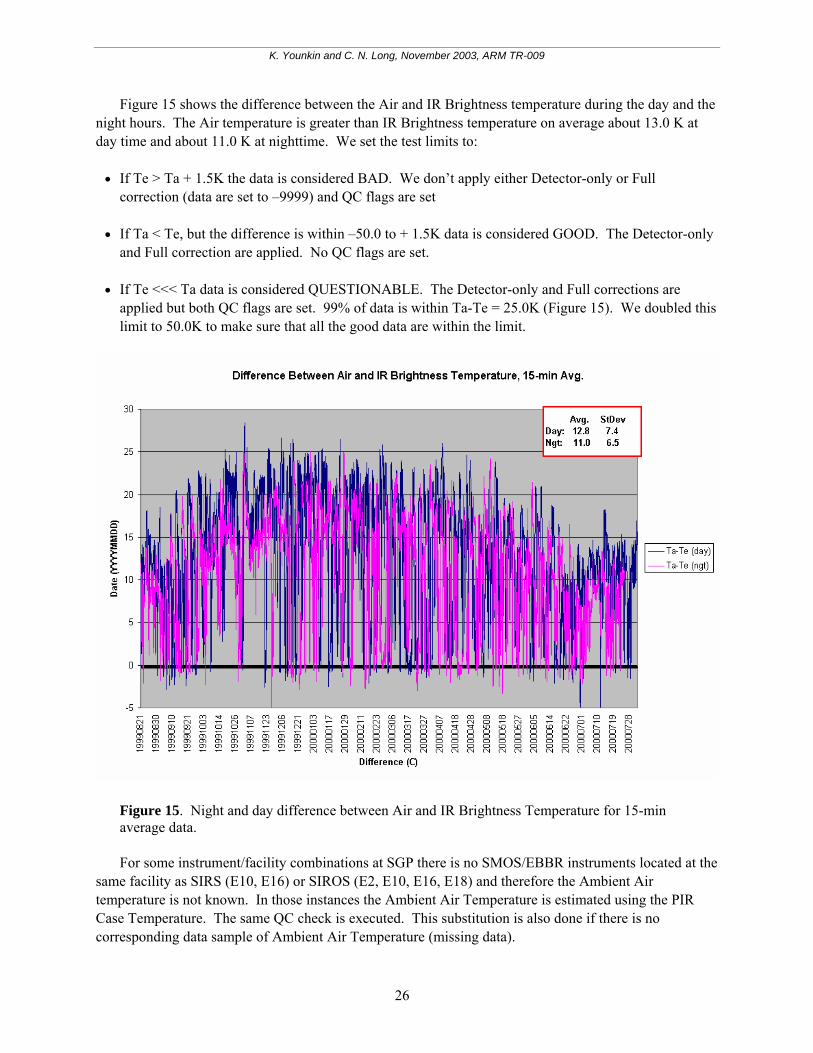
Figure 15 shows the difference between the Air and IR Brightness temperature during the day and the night hours. The Air temperature is greater than IR Brightness temperature on average about 13.0 K at day time and about 11.0 K at nighttime. We set the test limits to: • If Te > Ta + 1.5K the data is considered BAD. We don’t apply either Detector-only or Full
correction (data are set to –9999) and QC flags are set • If Ta < Te, but the difference is within –50.0 to + 1.5K data is considered GOOD. The Detector-only
and Full correction are applied. No QC flags are set. • If Te <<< Ta data is considered QUESTIONABLE. The Detector-only and Full corrections are
applied but both QC flags are set. 99% of data is within Ta-Te = 25.0K (Figure 15). We doubled this limit to 50.0K to make sure that all the good data are within the limit.
Figure 15. Night and day difference between Air and IR Brightness Temperature for 15-min average data.
For some instrument/facility combinations at SGP there is no SMOS/EBBR instruments located at the same facility as SIRS (E10, E16) or SIROS (E2, E10, E16, E18) and therefore the Ambient Air temperature is not known. In those instances the Ambient Air Temperature is estimated using the PIR Case Temperature. The same QC check is executed. This substitution is also done if there is no corresponding data sample of Ambient Air Temperature (missing data).
26
K. Younkin and C. N. Long, November 2003, ARM TR-009
NOTE: For a detailed description of the calculated Broadband IR temperature and the Ambient Air temperature see Section 3.1.2.1.4.
4.4 Compare Corrected Diffuse SW with Rayleigh Limit Calculation For the detail description of Rayleigh limit calculation and study see Section 3.2.4. • If the corrected PSP > Rayleigh limit + 1.0 Wm-2 data is GOOD. It means that the corrected IR is
above the corresponding Rayleigh value, plus twice the maximum “error” due to the polynomial fit shown in Figure 6. In this case the calculated corrected PSP is considered “good” and no QC flag is set.
• If the corrected PSP = Rayleigh limit +/- 1 Wm-2 data is QUESTIONABLE. We allow for 1 Wm-2
uncertainty. In this case the calculated corrected PSP is considered “questionable” and the QC flag is set accordingly.
• If the corrected PSP < Rayleigh limit –1 Wm-2 data is considered BAD for clear skies. This means
that the corrected PSP is well under the corresponding Rayleigh model minimum value. This can also occur under the thick overcast condition. (See Figure 6 in Section 3.2.4) To check if the sky is overcast we perform the following test: If unshaded PSP – shaded PSP > 20 Wm-2 it means that the sky is not overcast. In this case we set corrected PSP to “–9999” and the QC flag is set to “bad.” If the sky is overcast we set the corrected PSP to its calculated value, no QC flag is set and data is not BAD.
NOTE: All the Rayleigh limit tests are applied to Detector only and Full corrected PSP only for (SZA < 80°).
4.5 Compare Corrected Shaded PSP with Uncorrected PSP Figure 12 shows the frequency of occurrence of the difference between the daylight diffuse SW irradiance measured by a shaded B&W and the co-located shaded PSP. The B&W is designed so that IR loss is minimal (Dutton et al. 2001). The uncorrected PSP data (black line) shows a distinct bias compared to the B&W, on average an all-sky IR loss of about 13 Wm-2, and a bimodal distribution. The bias is reduced to about 1 Wm-2 for the adjusted corrected data (red lines) for all-sky conditions. Under clear skies, the diffuse SW is inherently of low magnitude, while at the same time the IR loss is greatest. Long et al. (2001) note that for clear skies, 39% of the time the PSP uncorrected IR loss is 15 Wm-2 or greater with some occurrences of up to 30 Wm-2 of IR loss! Thus we set a limit on the amount of expected correction as: • If the shaded corrected PSP – shaded uncorrected PSP > 30.0 Wm-2 the data is QUESTIONABLE and
the QC flag is set to QUESTIONABLE.
NOTE: Shaded PSP tests are applied to both Detector only and Full corrected diffuse data.
27
K. Younkin and C. N. Long, November 2003, ARM TR-009
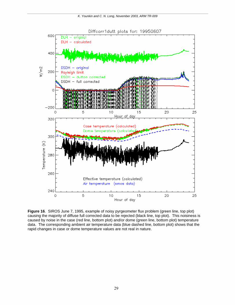
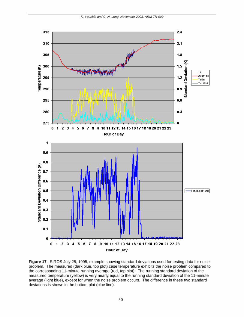
4.6 PIR Case Temperature Testing Using Running Standard Deviation In the early days of the ARM Program, the radiometers in the SGP network of sites were connected to the co-located Multi-Frequency Rotating Shadowband Radiometer (MFRSR) data loggers. Because of the operational constraints of the MFRSR, these radiometer data consist of “instantaneous” samples taken at 20-second resolution. These are the SIROS data streams. At the time, the commercial MFRSR was a relatively new instrument, and as with all new instrument packages sometimes suffered “bugs” in the design. One such “bug” manifested itself occasionally as a significant level of “noise” in some of the data logger channels. This noise had an adverse effect on the data being collected by these loggers, which was exaggerated (for 1-minute averages) due to the limited sampling. Such a case is shown in Figure 16, where the PIR down-welling LW irradiance data (green line, top plot) is extremely “noisy” between the hours of 1 and about 18. The bottom plot in Figure 16 shows that the noise manifested itself primarily in the PIR case and dome temperature data, but has little effect on the PIR detector flux (not shown). Since the calculation of LW irradiance has a fourth power dependence, particularly on the case temperature (see Section 3.2.5), the noise is exaggerated in the irradiance values. However, by comparison, the corresponding ambient air temperature data (blue dashed line, bottom plot) is “smooth” showing that the rapid changes in case or dome temperature values are not real in nature. The air temperature data was collected as part of the meteorological package served by a different data logger. The noise then affects the full correction application, since it also includes a case-dome temperature term with fourth power dependence (see Section 3.2.7), as can be seen by all the “bad” occurrences in the top plot (vertical lines) when the “full corrected” diffuse failed the various QC testing. Yet some data did pass the QC tests, but might be considered “questionable” at best. To test for the occurrence of noisy data, we analyze the case temperature time series. As illustrated in Figure 17, we calculate the 11-minute running average (red line, top plot) and standard deviation (yellow line) centered on the 1-minute data point of interest. Then we calculate the running 11-minute standard deviation of the 11-minute running average (light blue line). We compare the difference between the two standard deviations, subtracting the 11-minute running standard deviation from the 11-minute standard deviation of the 11-minute running average (blue line, bottom plot). Given the highly sensitive fourth power dependence of the full correction on the PIR case and dome temperatures, we must strive to ensure that no questionable data are used for the correction. Since the detector only correction is not appreciably affected by this noise problem, we still calculate a detector-only correction during these “noisy” periods. Thus, we err on the side of caution, and set a limit of 0.1 for the standard deviation difference, based again on extensive analysis of data. This limit does occasionally eliminate some small percentage of “good” data from applying the full correction, but does ensure that the vast majority of “bad” data are eliminated. For a detailed description of the running standard deviation comparison test see Section 3.1.2.1.5.
Tc_sdev – Tc_avg_sdev > 0.1 data is BAD Where: Tc_stdev = 11-minute running standard deviation of the Case PIR Temperature (K) Tc_avg_stdev = 11-minute running standard deviation of the 11-minute running average of the
Case PIR Temperature (K)
28
K. Younkin and C. N. Long, November 2003, ARM TR-009
Figure 16. SIROS June 7, 1995, example of noisy pyrgeometer flux problem (green line, top plot) causing the majority of diffuse full corrected data to be rejected (black line, top plot). This noisiness is caused by noise in the case (red line, bottom plot) and/or dome (green line, bottom plot) temperature data. The corresponding ambient air temperature data (blue dashed line, bottom plot) shows that the rapid changes in case or dome temperature values are not real in nature.
29
K. Younkin and C. N. Long, November 2003, ARM TR-009
Figure 17. SIROS July 25, 1995, example showing standard deviations used for testing data for noise problem. The measured (dark blue, top plot) case temperature exhibits the noise problem compared to the corresponding 11-minute running average (red, top plot). The running standard deviation of the measured temperature (yellow) is very nearly equal to the running standard deviation of the 11-minute average (light blue), except for when the noise problem occurs. The difference in these two standard deviations is shown in the bottom plot (blue line).
30
K. Younkin and C. N. Long, November 2003, ARM TR-009
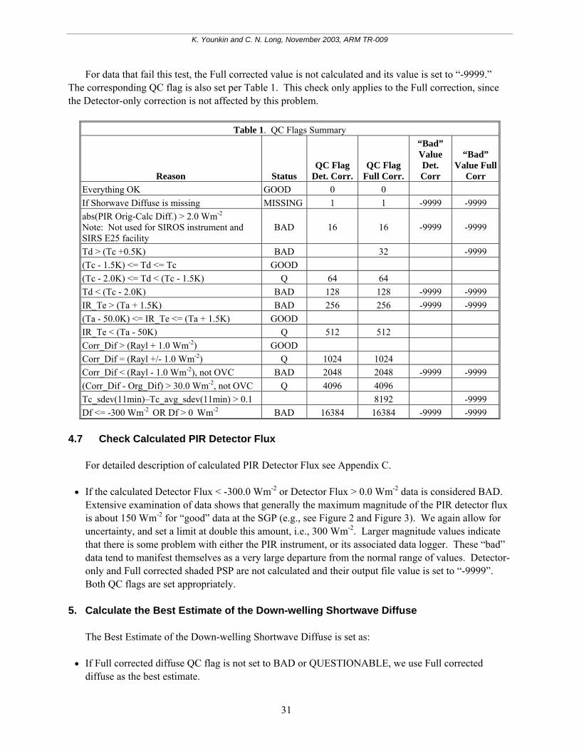
For data that fail this test, the Full corrected value is not calculated and its value is set to “-9999.” The corresponding QC flag is also set per Table 1. This check only applies to the Full correction, since the Detector-only correction is not affected by this problem.
Table 1. QC Flags Summary
Reason Status QC Flag
Det. Corr. QC Flag
Full Corr.
“Bad” Value Det. Corr
“Bad” Value Full
Corr Everything OK GOOD 0 0 If Shorwave Diffuse is missing MISSING 1 1 -9999 -9999 abs(PIR Orig-Calc Diff.) > 2.0 Wm-2 Note: Not used for SIROS instrument and SIRS E25 facility
BAD 16 16 -9999 -9999
Td > (Tc +0.5K) BAD 32 -9999 (Tc - 1.5K) <= Td <= Tc GOOD (Tc - 2.0K) <= Td < (Tc - 1.5K) Q 64 64 Td < (Tc - 2.0K) BAD 128 128 -9999 -9999 IR_Te > (Ta + 1.5K) BAD 256 256 -9999 -9999 (Ta - 50.0K) <= IR_Te <= (Ta + 1.5K) GOOD IR_Te < (Ta - 50K) Q 512 512 Corr_Dif > (Rayl + 1.0 Wm-2) GOOD Corr_Dif = (Rayl +/- 1.0 Wm-2) Q 1024 1024 Corr_Dif < (Rayl - 1.0 Wm-2), not OVC BAD 2048 2048 -9999 -9999 (Corr_Dif - Org_Dif) > 30.0 Wm-2, not OVC Q 4096 4096 Tc_sdev(11min)–Tc_avg_sdev(11min) > 0.1 8192 -9999 Df <= -300 Wm-2 OR Df > 0 Wm-2 BAD 16384 16384 -9999 -9999
4.7 Check Calculated PIR Detector Flux For detailed description of calculated PIR Detector Flux see Appendix C. • If the calculated Detector Flux < -300.0 Wm-2 or Detector Flux > 0.0 Wm-2 data is considered BAD.
Extensive examination of data shows that generally the maximum magnitude of the PIR detector flux is about 150 Wm-2 for “good” data at the SGP (e.g., see Figure 2 and Figure 3). We again allow for uncertainty, and set a limit at double this amount, i.e., 300 Wm-2. Larger magnitude values indicate that there is some problem with either the PIR instrument, or its associated data logger. These “bad” data tend to manifest themselves as a very large departure from the normal range of values. Detector-only and Full corrected shaded PSP are not calculated and their output file value is set to “-9999”. Both QC flags are set appropriately.
5. Calculate the Best Estimate of the Down-welling Shortwave Diffuse The Best Estimate of the Down-welling Shortwave Diffuse is set as: • If Full corrected diffuse QC flag is not set to BAD or QUESTIONABLE, we use Full corrected
diffuse as the best estimate.
31
K. Younkin and C. N. Long, November 2003, ARM TR-009
• If Full corrected diffuse is MISSING or BAD, then we need to check Detector corrected diffuse. If it is not MISSING or QUESTIONABLE we use it as the best estimate.
• If the Full corrected diffuse flag is set to QUESTIONABLE, then we check the Detector corrected
diffuse flag. If the Detector corrected diffuse flag is not set to BAD or QUESTIONABLE, we use the Detector corrected diffuse as the best estimate. If the Detector corrected diffuse flag is set to QUESTIONABLE, we use the Full corrected diffuse as the best estimate.
• If Full corrected diffuse is MISSING or BAD and Detector corrected is MISSING or BAD, we check
if the uncorrected diffuse is MISSING. If the uncorrected diffuse is not MISSING we use it as the best estimate.
• If Full corrected diffuse is MISSING, Detector corrected is MISSING and uncorrected diffuse is
MISSING the Best Estimate Diffuse is set to MISSING as well. 6. Calculate Shortwave Sum The Shortwave sum is calculated as:
SW_sum = (SDN *µ0) + BEDiff Where: SW_sum = Down-welling Shortwave Hemispheric Irradiance, Best Estimate (Wm-2) SDN = Shortwave Direct Normal Irradiance (Wm-2) µ0 = cosine of SZA BEDiff = Best Estimate Diffuse Shortwave (Wm-2) • If either the SDN or the BEDiff are MISSING or BAD, the SW_sum cannot be calculated, but rather
is assigned the value of the unshaded down-welling shortwave hemispheric measurement. 7. Output Data The DIFFCORR1DUTT VAP produces one output file. The name of the output file varies dependent upon the processed input file. The name of the output file: SSSNNNNNN1duttXX.c1.YYYYMMDD.hhmmss Where: SSS – the site of the instrument (Example: sgp) NNNNN – the main instrument name (Example: sirs) 1dutt – identifies that this is DIFFCORR1DUTT VAP XX – facility YYYY – year, MM - month of the year, DD - day of the month, hh - hour of the day,
mm - minute of the hour, ss - second of the minute of data start
32
K. Younkin and C. N. Long, November 2003, ARM TR-009
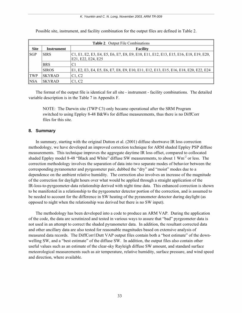
Possible site, instrument, and facility combination for the output files are defined in Table 2.
Table 2. Output File Combinations Site Instrument Facility
SIRS C1, E1, E2, E3, E4, E5, E6, E7, E8, E9, E10, E11, E12, E13, E15, E16, E18, E19, E20, E21, E22, E24, E25
BRS C1
SGP
SIROS E1, E2, E3, E4, E5, E6, E7, E8, E9, E10, E11, E12, E13, E15, E16, E18, E20, E22, E24 TWP SKYRAD C1, C2 NSA SKYRAD C1, C2 The format of the output file is identical for all site - instrument - facility combinations. The detailed variable description is in the Table 7 in Appendix F.
NOTE: The Darwin site (TWP C3) only became operational after the SRM Program switched to using Eppley 8-48 B&Ws for diffuse measurements, thus there is no DiffCorr files for this site.
8. Summary In summary, starting with the original Dutton et al. (2001) diffuse shortwave IR loss correction methodology, we have developed an improved correction technique for ARM shaded Eppley PSP diffuse measurements. This technique improves the aggregate daytime IR loss offset, compared to collocated shaded Eppley model 8-48 “Black and White” diffuse SW measurements, to about 1 Wm-2 or less. The correction methodology involves the separation of data into two separate modes of behavior between the corresponding pyranometer and pyrgeometer pair, dubbed the “dry” and “moist” modes due to a dependence on the ambient relative humidity. The correction also involves an increase of the magnitude of the correction for daylight hours over what would be applied through a straight application of the IR-loss-to-pyrgeometer-data relationship derived with night time data. This enhanced correction is shown to be manifested in a relationship to the pyrgeometer detector portion of the correction, and is assumed to be needed to account for the difference in SW heating of the pyranometer detector during daylight (as opposed to night when the relationship was derived but there is no SW input). The methodology has been developed into a code to produce an ARM VAP. During the application of the code, the data are scrutinized and tested in various ways to assure that “bad” pyrgeometer data is not used in an attempt to correct the shaded pyranometer data. In addition, the resultant corrected data and other ancillary data are also tested for reasonable magnitudes based on extensive analysis of measured data records. The DiffCorr1Dutt VAP output files contain both a “best estimate” of the down-welling SW, and a “best estimate” of the diffuse SW. In addition, the output files also contain other useful values such as an estimate of the clear-sky Rayleigh diffuse SW amount, and standard surface meteorological measurements such as air temperature, relative humidity, surface pressure, and wind speed and direction, where available.
33
K. Younkin and C. N. Long, November 2003, ARM TR-009
9. References Cess, R. D., T. T. Qian, and M. G. Sun, 2000: Consistency tests applied to the measurement of total, direct, and diffuse shortwave radiation at the surface. J. Geophys. Res., 105 (D20), 24,881–24,887. Dutton, E. G., J. J. Michalsky, T. Stoffel, B. W. Forgan, J. Hickey, D. W. Nelson, T. L. Alberta, and I. Reda, 2001: Measurement of broadband diffuse solar irradiance using current commercial instrumentation with a correction for thermal offset errors. J. Atmos. and Ocean. Tech., 18(3), 297–314. Long, C. N., K. Younkin, and D. M. Powell, 2001: Analysis of the Dutton et al. IR loss correction technique applied to ARM diffuse SW measurements. In Proceedings of the Eleventh Atmospheric Radiation Measurement (ARM) Science Team Meeting, ARM-CONF-2001. U.S. Department of Energy, Washington, D.C. Available URL: http://www.arm.gov/docs/documents/technical/conf_0103/long-cn.pdf Long, C. N., K. L. Gaustad, K. Younkin, and J. A. Augustine, 2003: An improved daylight correction for IR loss in ARM diffuse SW measurements. In Proceedings of the Thirteenth Atmospheric Radiation Measurement (ARM) Science Team Meeting, ARM-CONF-2003. U.S. Department of Energy, Washington, D.C. Available URL: http://www.arm.gov/docs/documents/technical/conf_0304/long-cn.pdf Philipona, R., 2002: Underestimation of solar global and diffuse radiation measured at Earth’s surface. J. Geophys. Res., 107(D22), 4654 Michalsky, J. J., et al., 2002: Comparison of diffuse shortwave irradiance measurements. In Proceedings of the Twelfth Atmospheric Radiation Measurement (ARM) Science Team Meeting, ARM-CONF-2002. U.S. Department of Energy, Washington, D.C. Available URL: http://www.arm.gov/docs/documents/technical/conf_0204/michalsky(2)-jj.pdf Younkin, K., and C. N. Long, 2002: Results of the Dutton at al. IR loss correction VAP: Statistical Analysis of Corrected and Uncorrected SW Measurements. In Proceedings of the Twelfth Atmospheric Radiation Measurement (ARM) Science Team Meeting, ARM-CONF-2002. U.S. Department of Energy, Washington, D.C. Available URL: http://www.arm.gov/docs/documents/technical/conf_0204/ younkin-k.pdf Nels Larson, 1992: Solarposition: Integer function for calculating the position of the Sun as seen from a place on Earth at a specific time, Pacific Northwest Laboratory, Richland, Washington.
34
K. Younkin and C. N. Long, November 2003, ARM TR-009
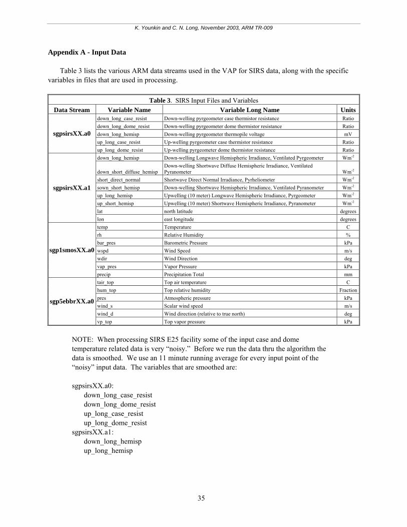
Appendix A - Input Data Table 3 lists the various ARM data streams used in the VAP for SIRS data, along with the specific variables in files that are used in processing.
Table 3. SIRS Input Files and Variables Data Stream Variable Name Variable Long Name Units
down_long_case_resist Down-welling pyrgeometer case thermistor resistance Ratio down_long_dome_resist Down-welling pyrgeometer dome thermistor resistance Ratio down_long_hemisp Down-welling pyrgeometer thermopile voltage mV up_long_case_resist Up-welling pyrgeometer case thermistor resistance Ratio
sgpsirsXX.a0
up_long_dome_resist Up-welling pyrgeometer dome thermistor resistance Ratio down_long_hemisp Down-welling Longwave Hemispheric Irradiance, Ventilated Pyrgeometer Wm-2
down_short_diffuse_hemisp Down-welling Shortwave Diffuse Hemispheric Irradiance, Ventilated Pyranometer Wm-2
short_direct_normal Shortwave Direct Normal Irradiance, Pyrheliometer Wm-2 sown_short_hemisp Down-welling Shortwave Hemispheric Irradiance, Ventilated Pyranometer Wm-2 up_long_hemisp Upwelling (10 meter) Longwave Hemispheric Irradiance, Pyrgeometer Wm-2 up_short_hemisp Upwelling (10 meter) Shortwave Hemispheric Irradiance, Pyranometer Wm-2 lat north latitude degrees
sgpsirsXX.a1
lon east longitude degrees temp Temperature C rh Relative Humidity % bar_pres Barometric Pressure kPa wspd Wind Speed m/s wdir Wind Direction deg vap_pres Vapor Pressure kPa
sgp1smosXX.a0
precip Precipitation Total mm tair_top Top air temperature C hum_top Top relative humidity Fractionpres Atmospheric pressure kPa wind_s Scalar wind speed m/s wind_d Wind direction (relative to true north) deg
sgp5ebbrXX.a0
vp_top Top vapor pressure kPa
NOTE: When processing SIRS E25 facility some of the input case and dome temperature related data is very “noisy.” Before we run the data thru the algorithm the data is smoothed. We use an 11 minute running average for every input point of the “noisy” input data. The variables that are smoothed are:
sgpsirsXX.a0:
down_long_case_resist down_long_dome_resist up_long_case_resist up_long_dome_resist
sgpsirsXX.a1: down_long_hemisp
up_long_hemisp
35
K. Younkin and C. N. Long, November 2003, ARM TR-009
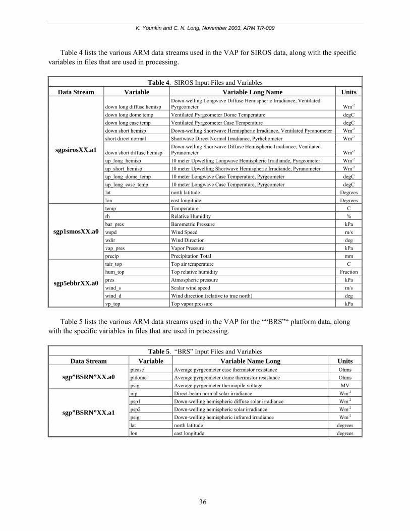
Table 4 lists the various ARM data streams used in the VAP for SIROS data, along with the specific variables in files that are used in processing.
Table 4. SIROS Input Files and Variables Data Stream Variable Variable Long Name Units
down long diffuse hemisp Down-welling Longwave Diffuse Hemispheric Irradiance, Ventilated Pyrgeometer Wm-2
down long dome temp Ventilated Pyrgeometer Dome Temperature degC down long case temp Ventilated Pyrgeometer Case Temperature degC down short hemisp Down-welling Shortwave Hemispheric Irradiance, Ventilated Pyranometer Wm-2 short direct normal Shortwave Direct Normal Irradiance, Pyrheliometer Wm-2
down short diffuse hemisp Down-welling Shortwave Diffuse Hemispheric Irradiance, Ventilated Pyranometer Wm-2
up_long_hemisp 10 meter Upwelling Longwave Hemispheric Irradiande, Pyrgeometer Wm-2 up_short_hemisp 10 meter Upwelling Shortwave Hemispheric Irradiande, Pyranometer Wm-2 up_long_dome_temp 10 meter Longwave Case Temperature, Pyrgeometer degC up_long_case_temp 10 meter Longwave Case Temperature, Pyrgeometer degC lat north latitude Degrees
sgpsirosXX.a1
lon east longitude Degrees temp Temperature C rh Relative Humidity % bar_pres Barometric Pressure kPa wspd Wind Speed m/s wdir Wind Direction deg vap_pres Vapor Pressure kPa
sgp1smosXX.a0
precip Precipitation Total mm tair_top Top air temperature C hum_top Top relative humidity Fraction pres Atmospheric pressure kPa wind_s Scalar wind speed m/s wind_d Wind direction (relative to true north) deg
sgp5ebbrXX.a0
vp_top Top vapor pressure kPa
Table 5 lists the various ARM data streams used in the VAP for the ““BRS”“ platform data, along with the specific variables in files that are used in processing.
Table 5. “BRS” Input Files and Variables Data Stream Variable Variable Name Long Units
ptcase Average pyrgeometer case thermistor resistance Ohms ptdome Average pyrgeometer dome thermistor resistance Ohms sgp”BSRN”XX.a0 psig Average pyrgeometer thermopile voltage MV nip Direct-beam normal solar irradiance Wm-2 psp1 Down-welling hemispheric diffuse solar irradiance Wm-2 psp2 Down-welling hemispheric solar irradiance Wm-2 psig Down-welling hemispheric infrared irradiance Wm-2 lat north latitude degrees
sgp”BSRN”XX.a1
lon east longitude degrees
36
K. Younkin and C. N. Long, November 2003, ARM TR-009
Table 5. (contd) Data Stream Variable Variable Name Long Units
temp Temperature C rh Relative Humidity % bar_pres Barometric Pressure kPa wspd Wind Speed m/s wdir Wind Direction deg vap_pres Vapor Pressure kPa
sgp1smosXX.a0
precip Precipitation Total mm tair_top Top air temperature C hum_top Top relative humidity Fraction pres Atmospheric pressure kPa wind_s Scalar wind speed m/s wind_d Wind direction (relative to true north) deg
sgp5ebbrXX.a0
vp_top Top vapor pressure kPa
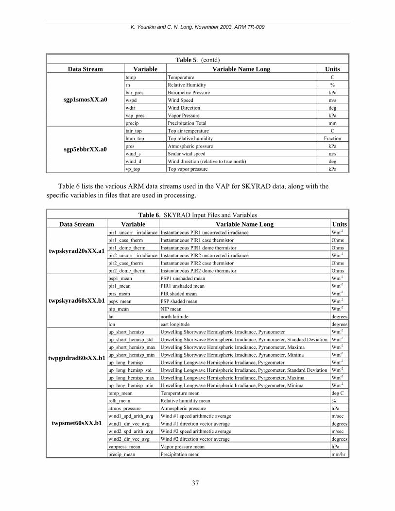
Table 6 lists the various ARM data streams used in the VAP for SKYRAD data, along with the specific variables in files that are used in processing.
Table 6. SKYRAD Input Files and Variables Data Stream Variable Variable Name Long Units
pir1_uncorr _irradiance Instantaneous PIR1 uncorrected irradiance Wm-2 pir1_case_therm Instantaneous PIR1 case thermistor Ohms pir1_dome_therm Instantaneous PIR1 dome thermistor Ohms pir2_uncorr _irradiance Instantaneous PIR2 uncorrected irradiance Wm-2 pir2_case_therm Instantaneous PIR2 case thermistor Ohms
twpskyrad20sXX.a1
pir2_dome_therm Instantaneous PIR2 dome thermistor Ohms psp1_mean PSP1 unshaded mean Wm-2 pir1_mean PIR1 unshaded mean Wm-2 pirs_mean PIR shaded mean Wm-2 psps_mean PSP shaded mean Wm-2 nip_mean NIP mean Wm-2 lat north latitude degrees
twpskyrad60sXX.b1
lon east longitude degreesup_short_hemisp Upwelling Shortwave Hemispheric Irradiance, Pyranometer Wm-2 up_short_hemisp_std Upwelling Shortwave Hemispheric Irradiance, Pyranometer, Standard Deviation Wm-2 up_short_hemisp_max Upwelling Shortwave Hemispheric Irradiance, Pyranometer, Maxima Wm-2 up_short_hemisp_min Upwelling Shortwave Hemispheric Irradiance, Pyranometer, Minima Wm-2 up_long_hemisp Upwelling Longwave Hemispheric Irradiance, Pyrgeometer Wm-2 up_long_hemisp_std Upwelling Longwave Hemispheric Irradiance, Pyrgeometer, Standard Deviation Wm-2 up_long_hemisp_max Upwelling Longwave Hemispheric Irradiance, Pyrgeometer, Maxima Wm-2
twpgndrad60sXX.b1
up_long_hemisp_min Upwelling Longwave Hemispheric Irradiance, Pyrgeometer, Minima Wm-2 temp_mean Temperature mean deg C relh_mean Relative humidity mean % atmos_pressure Atmospheric pressure hPa wind1_spd_arith_avg Wind #1 speed arithmetic average m/sec wind1_dir_vec_avg Wind #1 direction vector average degreeswind2_spd_arith_avg Wind #2 speed arithmetic average m/sec wind2_dir_vec_avg Wind #2 direction vector average degreesvappress_mean Vapor pressure mean hPa
twpsmet60sXX.b1
precip_mean Precipitation mean mm/hr
37
K. Younkin and C. N. Long, November 2003, ARM TR-009
Appendix B – Calculation of PIR Case and Dome Temperatures SIRS instruments: We need to calculate the pyrgeometer case and dome temperatures by converting the resistance (in Ratio) to the temperature in Kelvin.
T = 1/(A + B*X + C*X3) Where: T = Temperature (Deg K) A = 10.295E-04 B = 2.391E-04 C = 0.001568E-04 X = 5 * Ln(10) + Ln(R/100) R = Thermistor Resistance (Ratio)
NOTE: A, B, & C are Steinheart coefficients for fitting resistance-to-temperature data from YSI Precision Thermistor 44031 used in the PIR. (10,000 Ohms at +25 deg C)
If the Thermistor Resistance is MISSING (-9999) we don’t calculate the Temperature value but rather set the Temperature value to MISSING (-9999) as well. “BRS”, SKYRAD platform instruments: We need to calculate the pyrgeometer case and dome temperatures by converting the resistance (in Ohms) to the temperature in Kelvin.
T = 1*105/(A + B*X + C*X2 + D*X3) Where: T = Temperature (Deg K) A = 273.09 B = 26.3198 C = 0.278237 D = 0.0196739 X = Ln(R * 10-3) R = Thermistor Resistance (Ohms)
NOTE: The A, B, C, and D coefficients are based on a simple cubic-fit of the resistance and corresponding temperature data as published by YSI. The data logger was configured based on a fixed resistor in series with the PIR thermistors. (Personal communication with Tom Stoffel.)
If the Thermistor Resistance is MISSING (-9999) we don’t calculate the Temperature value but rather set the Temperature value to MISSING (-9999) as well.
38
K. Younkin and C. N. Long, November 2003, ARM TR-009
SIROS instruments: In the SIROS a1 file we already have the pyrgeometer case and dome temperature calculated in Co. We need to convert the case and dome temperature into Deg K (C° + 273.15 = DegK).
39
K. Younkin and C. N. Long, November 2003, ARM TR-009
Appendix C – Calculation of PIR Detector Flux SIROS instruments: PIR Detector Flux needs to be calculated from the PIR thermopile voltage in the SIRS a0 files.
Df = Tp*C1 Where: Df = PIR Detector Flux (Wm-2) Tp = Down-welling pyrgeometer (PIR) thermopile voltage (mV) C1 = PIR Calibration Factor (Wm-2 per mV)
NOTE: C1 values are taken from the header of the SIRS a0 netcdf file. It is a global attribute “calib-coeff” and marked as “PIR-DIR”.
If the PIR thermopile voltage is MISSING (-9999) we don’t calculate the PIR Detector Flux value but rather set the PIR Detector Flux value to MISSING (-9999) as well. “BRS” instruments: PIR Detector Flux needs to be calculated from the PIR thermopile voltage in the “BRS” a0 files.
Df = (Tp*103)/C1 Where: Df = PIR Detector Flux (Wm-2) Tp = Down-welling pyrgeometer (PIR) thermopile voltage (mV) C1 = PIR Calibration Factor (Wm-2 per mV)
NOTE: C1 values are taken from the header of the “BRS” a0 netcdf file. It is a global attribute “calib-coeff” and marked as “PYRGEOMETER(Shaded)”.
If the PIR thermopile voltage is MISSING (-9999) we don’t calculate the PIR Detector Flux value but rather set the PIR Detector Flux value to MISSING (-9999) as well. SIROS instruments: PIR Detector Flux needs to be calculated from the Down-welling longwave diffuse hemispheric irradiance in the SIROS a1 files.
Df = PIR – Sig*Tc4 + C2*Sig*(Td4 – Tc4) Where: Df = PIR Detector Flux (Wm-2) PIR = Longwave Irradiance (Wm-2)
40
K. Younkin and C. N. Long, November 2003, ARM TR-009
Sig = Stephan-Boltzman Constant = 5.67E-08 W/(m2 K4) Tc = PIR Case Temperature (K) Td = PIR Dome Temperature (K) C2 = PIR Dome Correction Factor = 4.0 (fixed value for ALL SIROS PIRs) If the PIR irradiance is MISSING (-9999) we don’t calculate the PIR Detector Flux value but rather set the PIR Detector Flux value to MISSING (-9999) as well. SKYRAD Instrument: The Detector Flux value is already present in SKYRAD a1 (20s) data stream and therefore doesn’t need to be calculated.
41
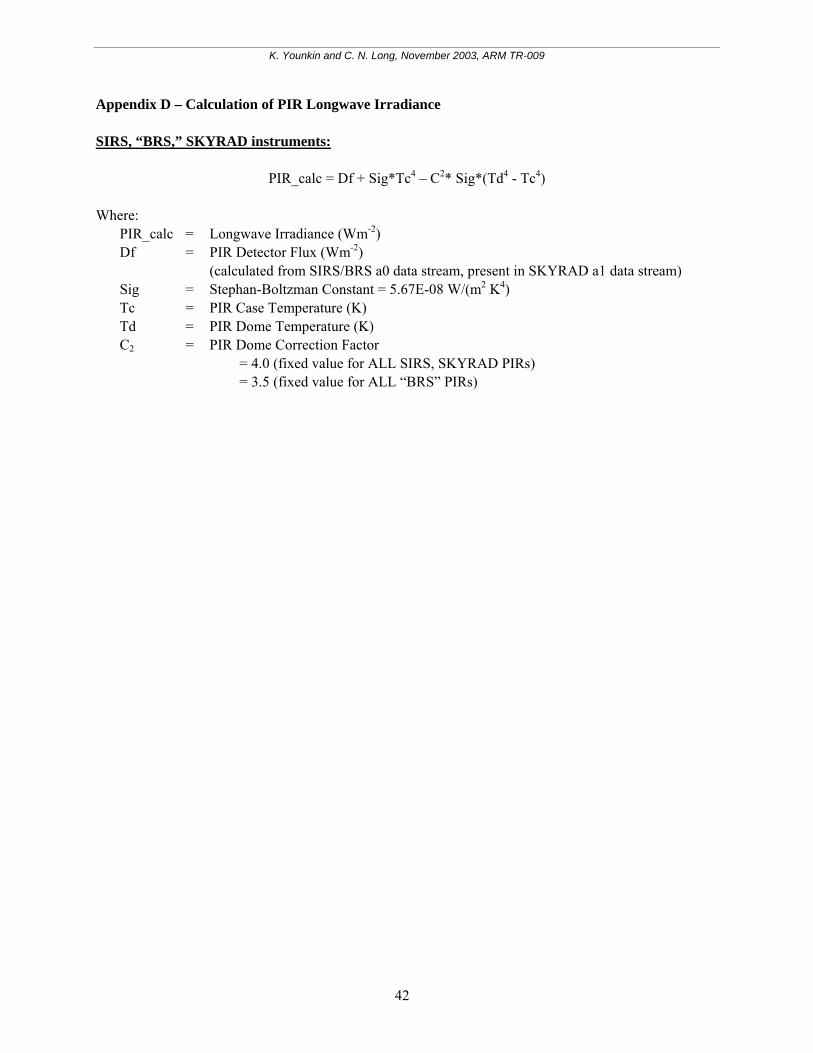
K. Younkin and C. N. Long, November 2003, ARM TR-009
Appendix D – Calculation of PIR Longwave Irradiance SIRS, “BRS,” SKYRAD instruments:
PIR_calc = Df + Sig*Tc4 – C2* Sig*(Td4 - Tc4) Where: PIR_calc = Longwave Irradiance (Wm-2) Df = PIR Detector Flux (Wm-2) (calculated from SIRS/BRS a0 data stream, present in SKYRAD a1 data stream) Sig = Stephan-Boltzman Constant = 5.67E-08 W/(m2 K4) Tc = PIR Case Temperature (K) Td = PIR Dome Temperature (K) C2 = PIR Dome Correction Factor = 4.0 (fixed value for ALL SIRS, SKYRAD PIRs) = 3.5 (fixed value for ALL “BRS” PIRs)
42
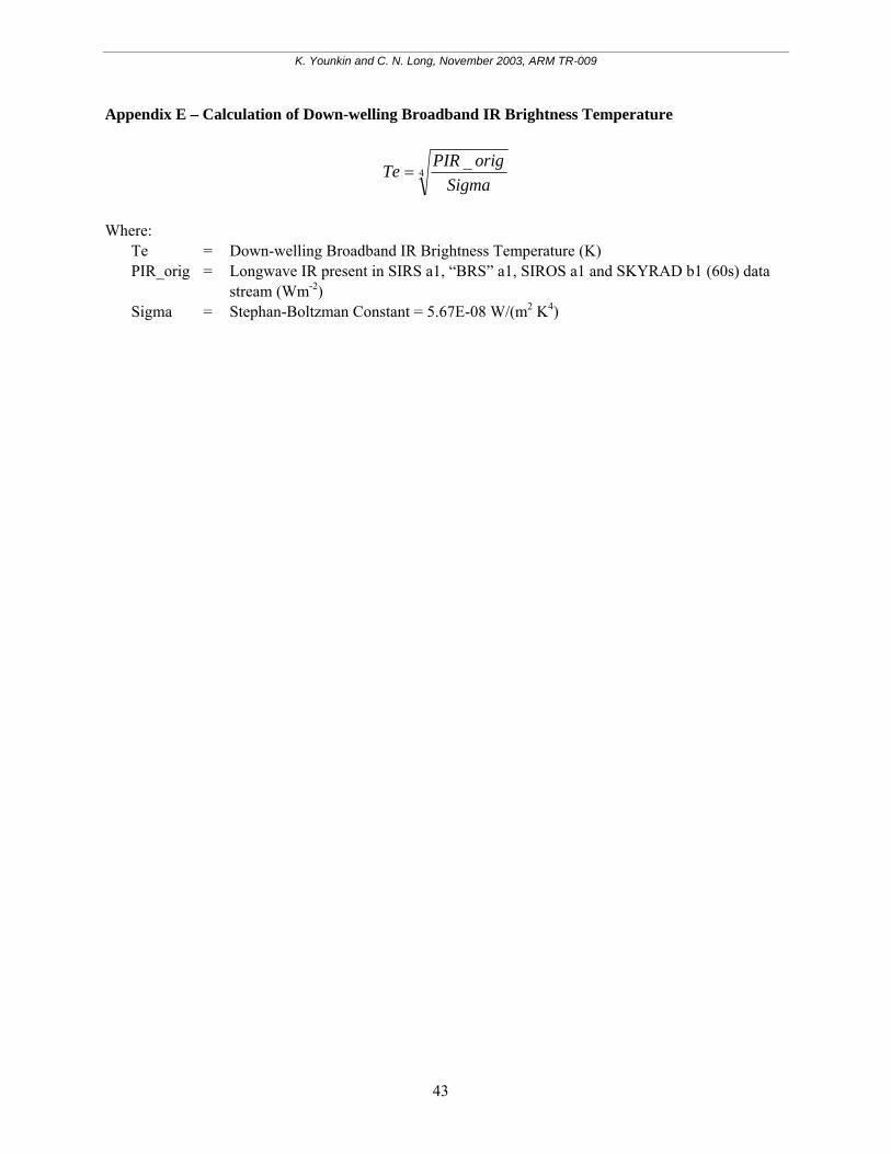
K. Younkin and C. N. Long, November 2003, ARM TR-009
Appendix E – Calculation of Down-welling Broadband IR Brightness Temperature
4_
SigmaorigPIRTe =
Where: Te = Down-welling Broadband IR Brightness Temperature (K) PIR_orig = Longwave IR present in SIRS a1, “BRS” a1, SIROS a1 and SKYRAD b1 (60s) data
stream (Wm-2) Sigma = Stephan-Boltzman Constant = 5.67E-08 W/(m2 K4)
43
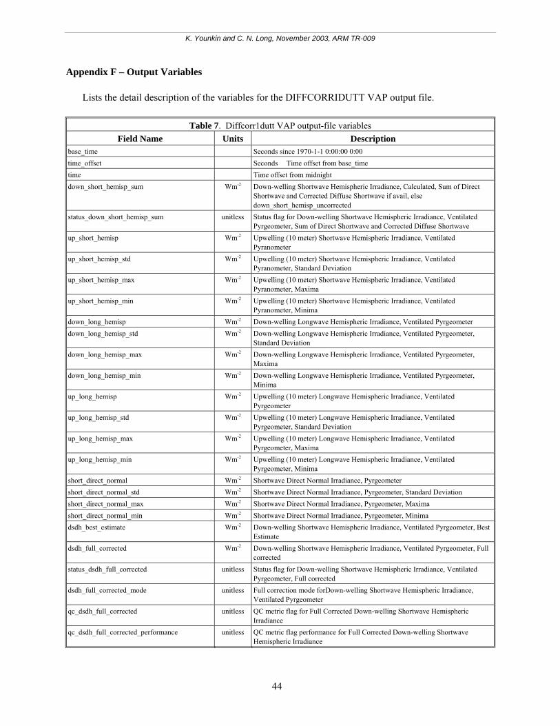
K. Younkin and C. N. Long, November 2003, ARM TR-009
Appendix F – Output Variables Lists the detail description of the variables for the DIFFCORRIDUTT VAP output file.
Table 7. Diffcorr1dutt VAP output-file variables Field Name Units Description
base_time Seconds since 1970-1-1 0:00:00 0:00 time_offset Seconds Time offset from base_time time Time offset from midnight down_short_hemisp_sum Wm-2 Down-welling Shortwave Hemispheric Irradiance, Calculated, Sum of Direct
Shortwave and Corrected Diffuse Shortwave if avail, else down_short_hemisp_uncorrected
status_down_short_hemisp_sum unitless Status flag for Down-welling Shortwave Hemispheric Irradiance, Ventilated Pyrgeometer, Sum of Direct Shortwave and Corrected Diffuse Shortwave
up_short_hemisp Wm-2 Upwelling (10 meter) Shortwave Hemispheric Irradiance, Ventilated Pyranometer
up_short_hemisp_std Wm-2 Upwelling (10 meter) Shortwave Hemispheric Irradiance, Ventilated Pyranometer, Standard Deviation
up_short_hemisp_max Wm-2 Upwelling (10 meter) Shortwave Hemispheric Irradiance, Ventilated Pyranometer, Maxima
up_short_hemisp_min Wm-2 Upwelling (10 meter) Shortwave Hemispheric Irradiance, Ventilated Pyranometer, Minima
down_long_hemisp Wm-2 Down-welling Longwave Hemispheric Irradiance, Ventilated Pyrgeometer down_long_hemisp_std Wm-2 Down-welling Longwave Hemispheric Irradiance, Ventilated Pyrgeometer,
Standard Deviation down_long_hemisp_max Wm-2 Down-welling Longwave Hemispheric Irradiance, Ventilated Pyrgeometer,
Maxima down_long_hemisp_min Wm-2 Down-welling Longwave Hemispheric Irradiance, Ventilated Pyrgeometer,
Minima up_long_hemisp Wm-2 Upwelling (10 meter) Longwave Hemispheric Irradiance, Ventilated
Pyrgeometer up_long_hemisp_std Wm-2 Upwelling (10 meter) Longwave Hemispheric Irradiance, Ventilated
Pyrgeometer, Standard Deviation up_long_hemisp_max Wm-2 Upwelling (10 meter) Longwave Hemispheric Irradiance, Ventilated
Pyrgeometer, Maxima up_long_hemisp_min Wm-2 Upwelling (10 meter) Longwave Hemispheric Irradiance, Ventilated
Pyrgeometer, Minima short_direct_normal Wm-2 Shortwave Direct Normal Irradiance, Pyrgeometer short_direct_normal_std Wm-2 Shortwave Direct Normal Irradiance, Pyrgeometer, Standard Deviation short_direct_normal_max Wm-2 Shortwave Direct Normal Irradiance, Pyrgeometer, Maxima short_direct_normal_min Wm-2 Shortwave Direct Normal Irradiance, Pyrgeometer, Minima dsdh_best_estimate Wm-2 Down-welling Shortwave Hemispheric Irradiance, Ventilated Pyrgeometer, Best
Estimate dsdh_full_corrected Wm-2 Down-welling Shortwave Hemispheric Irradiance, Ventilated Pyrgeometer, Full
corrected status_dsdh_full_corrected unitless Status flag for Down-welling Shortwave Hemispheric Irradiance, Ventilated
Pyrgeometer, Full corrected dsdh_full_corrected_mode unitless Full correction mode forDown-welling Shortwave Hemispheric Irradiance,
Ventilated Pyrgeometer qc_dsdh_full_corrected unitless QC metric flag for Full Corrected Down-welling Shortwave Hemispheric
Irradiance qc_dsdh_full_corrected_performance unitless QC metric flag performance for Full Corrected Down-welling Shortwave
Hemispheric Irradiance
44
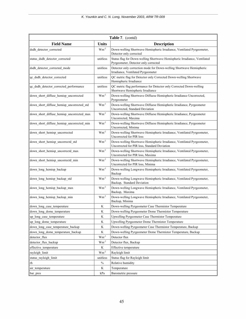
K. Younkin and C. N. Long, November 2003, ARM TR-009
Table 7. (contd) Field Name Units Description
dsdh_detector_corrected Wm-2 Down-welling Shortwave Hemispheric Irradiance, Ventilated Pyrgeometer, Detector only corrected
status_dsdh_detector_corrected unitless Status flag for Down-welling Shortwave Hemispheric Irradiance, Ventilated Pyrgeometer, Detector only corrected
dsdh_detector_corrected_mode unitless Detector only correction mode for Down-welling Shortwave Hemispheric Irradiance, Ventilated Pyrgeometer
qc_dsdh_detector_corrected unitless QC metric flag for Detector only Corrected Down-welling Shortwave Hemispheric Irradiance
qc_dsdh_detector_corrected_performance unitless QC metric flag performance for Detector only Corrected Down-welling Shortwave Hemispheric Irradiance
down_short_diffuse_hemisp_uncorrected Wm-2 Down-welling Shortwave Diffuese Hemispheric Irradiance Uncorrected, Pyrgeometer
down_short_diffuse_hemisp_uncorrected_std Wm-2 Down-welling Shortwave Diffuese Hemispheric Irradiance, Pyrgeometer Uncorrected, Standard Deviation
down_short_diffuse_hemisp_uncorrected_max Wm-2 Down-welling Shortwave Diffuese Hemispheric Irradiance, Pyrgeometer Uncorrected, Maxima
down_short_diffuse_hemisp_uncorrected_min Wm-2 Down-welling Shortwave Diffuese Hemispheric Irradiance, Pyrgeometer Uncorrected, Minima
down_short_hemisp_uncorrected Wm-2 Down-welling Shortwave Hemispheric Irradiance, Ventilated Pyrgeometer, Uncorrected for PIR loss
down_short_hemisp_uncorrectd_std Wm-2 Down-welling Shortwave Hemispheric Irradiance, Ventilated Pyrgeometer, Uncorrected for PIR loss, Standard Deviation
down_short_hemisp_uncorrectd_max Wm-2 Down-welling Shortwave Hemispheric Irradiance, Ventilated Pyrgeometer, Uncorrected for PIR loss, Maxima
down_short_hemisp_uncorrectd_min Wm-2 Down-welling Shortwave Hemispheric Irradiance, Ventilated Pyrgeometer, Uncorrected for PIR loss, Minima
down_long_hemisp_backup Wm-2 Down-welling Longwave Hemispheric Irradiance, Ventilated Pyrgeometer, Backup
down_long_hemisp_backup_std Wm-2 Down-welling Longwave Hemispheric Irradiance, Ventilated Pyrgeometer, Backup, Standard Deviation
down_long_hemisp_backup_max Wm-2 Down-welling Longwave Hemispheric Irradiance, Ventilated Pyrgeometer, Backup, Maxima
down_long_hemisp_backup_min Wm-2 Down-welling Longwave Hemispheric Irradiance, Ventilated Pyrgeometer, Backup, Minima
down_long_case_temperature K Down-welling Pyrgeometer Case Thermistor Temperature down_long_dome_temperature K Down-welling Pyrgeometer Dome Thermistor Temperature up_long_case_temperature K Upwelling Pyrgeometer Case Thermistor Temperature up_long_dome_temperature K Upwelling Pyrgeometer Dome Thermistor Temperature down_long_case_temperature_backup K Down-welling Pyrgeometer Case Thermistor Temperature, Backup down_long_dome_temperature_backup K Down-welling Pyrgeometer Dome Thermistor Temperature, Backup detector_flux Wm-2 Detector flux detector_flux_backup Wm-2 Detector flux, Backup effective_temperature K Effective temperature rayleigh_limit Wm-2 Rayleigh limit status_rayleigh_limit unitless Status flag for Rayleigh limit rh % Relative humidity air_temperature K Temperature bar_pres kPa Barometric pressure
45
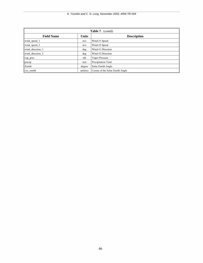
K. Younkin and C. N. Long, November 2003, ARM TR-009
Table 7. (contd) Field Name Units Description
wind_speed_1 m/s Wind #1 Speed wind_speed_2 m/s Wind #2 Speed wind_direction_1 deg Wind #1 Direction wind_direction_2 deg Wind #2 Direction vap_pres mb Vapor Pressure precip mm Precipitation Total Zenith degree Solar Zenith Angle cos_zenith unitless Cosine of the Solar Zenith Angle
46
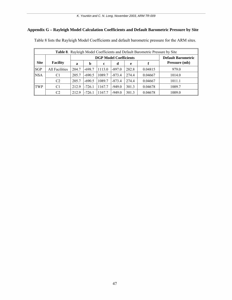
K. Younkin and C. N. Long, November 2003, ARM TR-009
Appendix G – Rayleigh Model Calculation Coefficients and Default Barometric Pressure by Site Table 8 lists the Rayleigh Model Coefficients and default barometric pressure for the ARM sites.
Table 8. Rayleigh Model Coefficients and Default Barometric Pressure by Site DGP Model Coefficients
Site Facility a b c d e f Default Barometric
Pressure (mb)
SGP All Facilities 204.7 -698.7 1113.0 -897.0 282.8 0.04815 979.0 C1 205.7 -690.5 1089.7 -873.4 274.4 0.04667 1014.0 NSA C2 205.7 -690.5 1089.7 -873.4 274.4 0.04667 1011.1 C1 212.9 -726.1 1167.7 -949.0 301.3 0.04678 1009.7 TWP C2 212.9 -726.1 1167.7 -949.0 301.3 0.04678 1009.0
47