Improved Compressive Sensing of Natural Scenes Using Localized RandomSampling

Victor J. Barranca1, Gregor Kovacic2 Douglas Zhou3, David Cai3,4,51Department of Mathematics and Statistics, Swarthmore College

2Department of Mathematical Sciences, Rensselaer Polytechnic Institute3Department of Mathematics, MOE-LSC, and Institute of Natural Sciences, Shanghai Jiao Tong University

4Courant Institute of Mathematical Sciences & Center for Neural Science, New York University5NYUAD Institute, New York University Abu Dhabi∗

(Dated: July 18, 2016)

Compressive sensing (CS) theory demonstrates that by using uniformly-random sampling, ratherthan uniformly-spaced sampling, higher quality image reconstructions are often achievable. Consid-ering that the structure of sampling protocols has such a profound impact on the quality of imagereconstructions, we formulate a new sampling scheme motivated by physiological receptive fieldstructure, localized random sampling, which yields significantly improved CS image reconstructions.For each set of localized image measurements, our sampling method first randomly selects an imagepixel and then measures its nearby pixels with probability depending on their distance from theinitially selected pixel. We compare the uniformly-random and localized random sampling methodsover a large space of sampling parameters, and show that, for the optimal parameter choices, higherquality image reconstructions can be consistently obtained by using localized random sampling. Inaddition, we argue that the localized random CS optimal parameter choice is stable with respect todiverse natural images, and scales with the number of samples used for reconstruction. We expectthat the localized random sampling protocol helps to explain the evolutionarily advantageous natureof receptive field structure in visual systems and suggests several future research areas in CS theoryand its application to brain imaging.

∗ Correspondence and requests for materials should be addressed to V.J.B. (vbarran1@swarthmore.edu), G.K. (ko-vacg@rpi.edu), D.Z. (zdz@sjtu.edu.cn), and D.C. (cai@cims.nyu.edu).

INTRODUCTION

Sampling protocols have drastically changed with the discovery of compressive sensing (CS) data acqui-sition and signal recovery [1, 2]. Prior to the development of CS theory, the Shannon-Nyquist theoremdetermined the majority of sampling procedures for both audio signals and images, dictating the minimumrate, the Nyquist rate, with which a signal must be uniformly sampled to guarantee successful reconstruction[3]. Since the theorem specifically addresses minimal sampling rates corresponding to uniformly-spaced mea-surements, signals were typically sampled at equally-spaced intervals in space or time before the discoveryof CS. However, using CS-type data acquisition, it is possible to reconstruct a broad class of sparse signals,containing a small number of dominant components in some domain, by employing a sub-Nyquist samplingrate [2]. Instead of applying uniformly-spaced signal measurements, CS theory demonstrates that severaltypes of uniformly-random sampling protocols will yield successful reconstructions with high probability[4–6].

While CS signal recovery is relatively accurate for sufficiently high sampling rates, we demonstrate that, forthe recovery of natural scenes, reconstruction quality can be further improved via localized random sampling.In this new protocol, each signal sample consists of a randomly centered local cluster of measurements, inwhich the probability of measuring a given pixel decreases with its distance from the cluster center. Weshow that the localized random sampling protocol consistently produces more accurate CS reconstructions ofnatural scenes than the uniformly-random sampling procedure using the same number of samples. For imagescontaining a relatively large spread of dominant frequency components, the improvement is most pronounced,with localized random sampling yielding a higher fidelity representation of both low and moderate frequencycomponents containing the majority of image information. Moreover, the reconstruction improvementsgarnered by localized random sampling also extend to images with varying size and spectrum distribution,affording improved reconstruction of a broad range of images. Likewise, we verify that the associatedoptimal sampling parameters are scalable with the number of samples utilized, allowing for easy adjustmentdepending on specific user requirements on the computational cost of data acquisition and the accuracy ofthe recovered signal.

Considering CS has accumulated numerous applications in diverse disciplines, including biology, astronomy,and image processing [7–11], the reconstruction improvements offered by our localized random sampling mayhave potentially significant consequences in multiple fields. We expect that the simplicity of this new CSsampling protocol will allow for relatively easy implementation in newly engineered sampling devices, such asthose used in measuring brain activity. In addition, our work addresses the important theoretical questionof how novel sampling methodologies can be developed to take advantage of signal structures while stillmaintaining the randomness associated with CS theory, thereby improving the quality of reconstructedimages.

Outside the scope of engineered devices, it is important to emphasize that we find forms of localizedrandom sampling in natural systems. Most notably, the receptive fields of many sensory systems are muchakin to this sampling protocol. In the visual system, retinal ganglion cells exhibit a center-surround-typearchitecture, such that the output of local groups of photoreceptors is sampled by downstream ganglioncells, stimulating ganglion cell activity in on-center locations and inhibiting activity in off-surround locations[12, 13]. In this way, the size of the receptive field controls the spatial frequency of the information processedand the center-surround architecture allows for enhanced contrast detection. Considering the improvementsin image reconstructions garnered by more biologically plausible sampling schemes, such as localized randomsampling, we suggest this to be demonstration of how visual image processing may be optimized throughevolution.

CONVENTIONAL COMPRESSIVE SENSING BACKGROUND

Due to the sparsity of natural images [14], CS sampling, i.e., uniformly-random sampling, is typically anattractive alternative to uniformly-spaced sampling because CS renders an accurate image reconstructionusing a relatively small number of samples [1, 2, 4]. According to the Shannon-Nyquist sampling theorem,the bandwidth of an image, which is the difference between its maximum and minimum frequencies, should

2

determine the minimum sampling rate necessary for a successful reconstruction employing uniformly-spacedsamples. The theorem demonstrates that a sampling rate greater than twice the bandwidth is in generalsufficient for the reconstruction of any image [3].

If a signal has a sparse representation in some domain, say the frequency domain, then the magnitudeof many frequency components within the signal bandwidth is too small to contribute to the overall signalrepresentation. Thus, CS theory shows that, for such sparse signals, a successful reconstruction can beachieved by using a sampling rate which is much lower than the Nyquist rate. For signals with a k-sparserepresentation in some domain, composed of a total of k nonzero components, CS theory shows that thesampling rate should be determined by k rather than the full bandwidth of the signal [1, 2]. Since naturalimages are typically sparse in certain domains, a variety of coordinate transforms can be used to obtain anappropriate sparse representation viable for CS reconstruction [15, 16].

Since a signal is not necessarily measured in the domain in which it has sparse representation nor is therealways complete a priori knowledge of the distribution of dominant signal components, it is first necessary toidentify a sparse representation of a given signal before formulating a CS reconstruction method that utilizesits sparsity. The problem of recovering a sparse signal using very few measurements takes the form of a largeunderdetermined system. In the language of CS theory, this is a problem of recovering an n-component signal,x, using only m samples, with m� n, represented by an m×n sampling matrix, A. Each of the m samplesis composed of various weighted measurements of the n signal components. Therefore, a given sample isrepresented by a row of the sampling matrix with each row entry containing the weight of the measurementcorresponding to a specific signal component. A total of m such samples yields an m-component measuredsignal, b, which can then be used to recover the full signal. If x is sparse under transform, T , then the sparsesignal representation x = Tx can be recovered first and then inverted to reconstruct x. Therefore, to recoverx from b, it is necessary to solve the linear system

φx = b, (1)

where φ = AT−1, and then compute x = T−1x.While there are infinitely many solutions we can choose from in solving the underdetermined system

(1), through adding the constraint that the solution must be sparse, CS theory aims to make this problem

well-posed. By computing the solution that minimizes |x|`1 =

n∑i=1

|xi| while satisfying φx = b, a successful

reconstruction is obtainable with high probability assuming x is sufficiently sparse and the sampling matrix,A, is appropriately chosen [1, 6]. This is identical to solving the linear programming problem

minimize y1 + · · ·+ yn

given − yi ≤ xi ≤ yi, i = 1, . . . , n,(2)

under constraint (1) [17].In choosing sampling protocol, a key point in CS theory is that the sampling should not be uniformly-

spaced. Specifically, a broad class of sampling matrices obeying the restricted isometry property (RIP)will yield a successful CS reconstruction with near certainty [4–6]. The sampling matrix, A, is said tosatisfy the RIP property if (1 − δk)||x||22 ≤ ||Ax||22 ≤ (1 + δk)||x||22 for all k-sparse x and some smallδk ∈ (0, 1). For sufficiently sparse x and small δk, CS theory proves that the solution to (2) is an accuraterepresentation of x [1, 4]. Intuitively speaking, sampling matrices satisfying this condition preserve signalsize and therefore do not distort the measured signal such that the reconstruction is inaccurate. A host ofsampling matrices with independent identically distributed random variables entries, including Gaussian andBernoulli distributed random variables, can be shown to satisfy the RIP and act as successful CS samplingprotocols [1, 4]. Intuitively, for matrices with such a random construction, a sufficient number of randommeasurements will lead to a relatively uncorrelated measured signal, and therefore may recover the dominantsignal components with high probability. Thus, it is possible in principle to recover sparse signals since theirdominant components contain the majority of information characterizing them. Measurement devices usingCS-type random sampling are therefore relatively easy to design in practice and quite successful in recoveringmany signals [18].

3

METHODS

The discovery of CS suggests that sampling protocols for natural images should shift from uniformly-spacedto random-like measurements. Are there any other sampling schemes with which we can obtain higher fidelityCS reconstructions? In the human visual system, for example, spatially nearby image features are typicallyprocessed together through neuronal receptive-fields [12, 13, 19, 20]. Motivated by this structure, we considerthe viability and advantage of a sampling scheme incorporating both randomness and spatial clustering, i.e.,localized random sampling, in CS image reconstructions.

FIG. 1. Graphical depiction of localized random sampling. Each row of the m× n2 sampling matrix, A, correspondsto localized random measurements taken by a sampling unit located at random coordinates on the [1, n] × [1, n]Cartesian grid covering the n × n pixel image. The sampling unit (located at the center of the transparent redcircle) probabilistically measures nearby pixels (green dots) with sampling probability decaying with distance fromits location according to Eq. (3). The sampling matrix is composed of m sampling units. Sampling weights are takento be 1

n2 for both the localized random sampling and uniformly-random sampling protocols. Courtesy of the Signaland Image Processing Institute at the University of Southern California.

In formulating our localized random sampling methodology, we seek to recover the dominant frequencycomponents, which capture the most relevant information regarding a natural image. To add a sufficientdegree of randomness akin to conventional CS data acquisition, we first place sampling units on randomlychosen pixels composing a given image. For an n× n pixel image, choosing the location of a sampling unitis equivalent to randomly choosing coordinates on a [1, n]× [1, n] Cartesian grid, with each pair of integercoordinates corresponding to a different pixel location. Then, to obtain relevant information regarding localimage features, for a given sampling unit, we measure the pixels composing the image with decreasingprobability as a function of their distance from the sampling unit on the grid of coordinates partitioningthe image. Thus, with respect to the sampling matrix defining the image sampling protocol, A, the set ofmeasurements taken by each sampling unit corresponds to a different row of A with each set of spatially-clustered weighted measurements composing a row. In the case of uniformly-random sampling, however,a sampling unit instead corresponds to a row of independent identically distributed random entries in A,where each entry has equal probability and weight of measurement. Localized random sampling in particularprescribes that if the coordinates of the ith sampling unit are (xi, yi), then the probability, P , to sample apixel with coordinates (xj , yj) is given by

P = ρ exp(−[(xi − xj)2 + (yi − yj)2]/[2σ2]), (3)

4

where ρ represents the sampling probability if (xi, yi) = (xj , yj), i.e., when the location of the sampling unitmatches the location of a given pixel, and σ determines the radius in which the sampling unit is likely tomeasure image pixels. In this way, ρ prescribes the overall density of measurements taken by each samplingunit and σ specifies how closely clustered the measurements will be around the location of the samplingunit. Therefore, the location of a given sampling unit is uniformly-random, analogous to conventional CSsampling, whereas the corresponding localized pixel measurement probabilities depend on the distance ofeach pixel location from the sampling unit and are determined by Eq. (3). We note that, for each samplingunit and pixel location pair, P defines the success probability for a Bernoulli random variable determining thelikelihood of pixel measurement, which is independent of all other measurements taken by the sampling unit.An illustration of the localized random sampling framework is depicted in Fig. 1. In the following sections,we demonstrate that this novel CS sampling captures both dominant low and certain moderate frequencyinformation with a high degree of accuracy, thereby yielding significantly improved reconstructions comparedwith conventional uniformly-random CS sampling for a broad class of images.

Upon sampling a given n×n image using our localized random protocol with m sampling units, representedby m× n2 sampling matrix A, we obtain an m-component measurement, b, which we use to reconstruct theoriginal image with n2 components. To do so, we first compute a sparse representation of the original image,e.g., the two-dimensional discrete-cosine transform. We compute the vectorization of the two-dimensionaltransform of the image, v = (v1, . . . , vn2) = (C ⊗ C)v, where v is the vectorization of the original image, ⊗denotes the n2 × n2 Kronecker product

C ⊗ C =

C11C · · · C1nC...

. . ....

Cn1C · · · CnnC

,C is the n× n, one-dimensional discrete-cosine transform matrix with entries

Cij = (C−1)Tij = ω(i) cos

((i− 1)(2j − 1)π

2n

),

ω(1) = (1/n)1/2, and ω(i 6= 1) = (2/n)1/2.Next, we solve the CS optimization problem of recovering v by considering the underdetermined linear

system resulting from our sampling choice and sparsifying transform,

A(C ⊗ C)−1v = b. (4)

Using CS reconstruction theory, the problem of solving for v can be cast as an L1 optimization problem(2) with xi = vi under the constraint (4). Using the Orthogonal Matching Pursuit algorithm [21], we thenrecover v. Finally, we invert the two-dimensional discrete-cosine transform and the vectorization to obtainthe n × n image reconstruction. As will be shown in the subsequent section, similar results are achievableby computing the sparse image representation with the two-dimensional discrete-wavelet transform andalternative L1 optimization algorithms [22–25].

In Fig. 2, we reconstruct three 100 × 100 pixel images of varying complexity, as well as several squareimages of higher resolution. To quantify the reconstruction accuracy, we compute the relative error of thereconstructed image, precon, compared with the 100× 100 pixel matrix representation of the original image,p, defined by

‖p− precon‖F /‖p‖F , (5)

using the Frobenius matrix norm ‖p‖F =√∑

i

∑j p

2ij . For each image, we compare the optimal CS recon-

structions using uniformly-random sampling and localized random sampling, listing the associated relativereconstruction error for each protocol in the caption of Fig. 2. Specifically, for uniformly-random sampling,we investigate the P parameter space and for localized random sampling, we explore the (ρ, σ) parame-ter space, seeking the parameter regime which yields minimal relative reconstruction error. In the case ofuniformly-random sampling, each element of the sampling matrix is an independent identically distributed

5

FIG. 2. Reconstruction comparison. (a)-(c) 1002, (d) 2502, (e) 4002 pixel images. (f)-(j) Uniformly-random sam-pling CS reconstructions. (k)-(o) Localized random sampling CS reconstructions. For each n2 pixel image, recon-structions use m = n2/10 sampling units. The relative reconstruction errors via uniformly-random sampling are1.0 × 10−14, 0.26, 0.40, 0.22, and 0.12 for (f)-(j). The relative reconstruction errors via localized random samplingare 1.3 × 10−15, 0.14, 0.21, 0.10, and 0.05 for (k)-(o). Courtesy of the Signal and Image Processing Institute at theUniversity of Southern California.

Bernoulli random variable with probability P of having a nonzero value [26]. Thus, P gives an indication ofthe density of samples taken by each sampling unit, with more measurements taken by each sampling unitfor higher P . For both sampling matrices, we choose each nonzero entry to have magnitude 1/n2, so as toscale well with image size. Furthermore, for each 100×100 pixel image, we choose to use m = 1000 samplingunits for both sampling protocols, yielding a large, factor of 10, reduction in the number of samples (numberof rows in the sampling matrix, A) compared to the number of pixels composing the original image. Wesimilarly use a factor of 10 reduction in reconstructing the higher resolution images.

We note that for the simple striped image in Fig. 2 (a), the reconstruction quality yielded by each methodis quite similar and nearly perfect, i.e., very small reconstruction error, since there are relatively few dominantfrequencies to recover in this case. For the more complicated disk image in Fig. 2 (b), we notice a more

6

sizeable difference in the reconstruction results corresponding to the two sampling protocols. The localizedrandom sampling yields a reconstruction with more well-defined edges along the disk and also less noise bothinside as well as outside of the disk. This noise takes the form of small areas of incorrect shade that appearin the reconstructions due to pixel (frequency) blurring, such as small white dots inside of the disk apparentin the reconstruction using uniformly-random sampling. Finally, for the most complex and natural imageof Lena in Fig. 2 (c), the improvement in reconstruction quality using localized random sampling is evenmore pronounced. While the uniformly-random sampling CS reconstruction is quite noisy and bears littleresemblance to the original image, the localized random sampling yields a relatively smooth reconstructioncapturing large-scale, low-frequency characteristics well. The localized random sampling reconstruction alsocaptures some small-scale details completely missing from the uniformly-random sampling reconstruction,such as the eye of Lena and the edge of her hat. As we will show in our discussion of stability, we see evenfurther improvements in the reconstruction quality using localized random sampling with the inclusion ofhigher resolution images, such as in Fig. 2 (d)-(e), and also more sampling units. Increasing the imageresolution up to 400 × 400 pixels, as in Fig. 2 (e), we observe the highest quality reconstruction, withlocalized random sampling yielding a reconstructed image nearly indistinguishable from the original image,which holds even for detailed features and edges.

COMPARISON AND ANALYSIS OF COMPRESSIVE SENSING SAMPLING SCHEMES

Comparing the optimal CS image reconstructions using localized random sampling and conventionaluniformly-random sampling, we observed that CS using localized random sampling does indeed yield signif-icantly more accurate image reconstructions, especially for natural images. In this section, we investigatethe underlying reasons for the disparity between the two sampling methods and how they perform over awide range of sampling parameter choices.

In Fig. 3, we compare the reconstruction error in recovering the images in Fig. 2 (a)-(c) using CS withuniformly-random sampling for a wide range of sampling probabilities, P . Before analyzing the dependenceof the reconstruction quality on P , it is important to remark that for all three images, as P closely approaches0 or 1, the reconstruction error rapidly increases, since there are too few or too many measurements, respec-tively, to properly detect variations in pixel intensities of the image. Intuitively, for the very under-measuredcase, i.e., P is close to 0, only very few frequencies may be detected, failing to give sufficient informationabout the image. Likewise, when too many measurements are taken, i.e., P is close to 1, the average pixelvalue will primarily be detected, thereby concentrating most frequency energy near the 0-frequency. In Fig.3, we do not plot the rapid increases in error when P is near 0 or 1 to focus on error trends in more reasonableparameter regimes.

In Fig. 3 (a), corresponding to the stripe image, we note a slowly increasing error for larger P with allerrors very small regardless of P . Since there are very few frequencies to measure it is more advantageous inthis case to take fewer measurements per sampling unit, and thereby avoid averaging pixel values over thecourse of multiple stripes. Considering the image is simple, though, these small increases in error for largerP are relatively undetectable by sight.

More complicated images, such as typical natural scenes, are typically composed of many more nonzerofrequency components, resulting in a very different CS error dependence than for the simple stripes image.For comparison, we plot in Figs. 4 (a)-(c) the frequency-domain representation of the images in Figs. 2(a)-(c), respectively, observing a much wider spread of dominant frequencies for the disk and Lena images.With respect to the CS reconstruction relative errors for the disk and Lena images, depicted in Figs. 3 (b)and (c), respectively, there is largely a random spread of reconstruction errors across P values. For theseimages, since there are many more dominant frequency-components than in the case of the stripes image,taking additional measurements may capture novel frequency contributions at the cost of losing informationregarding other frequency components. Hence, in this case, the density of measurements taken by eachsampling unit has little effect on reconstruction quality. In fact, the maximal difference in reconstructionerror is only approximately 15% across all choices of P and corresponding realizations of the sampling matrix.Therefore, we see that for such complicated images, the reconstruction error appears to have weak dependenceon P as long as P is not near 0 or 1. Note that, for each plot in Fig. 3, the mean error is depicted over anensemble of 10 realizations of the sampling matrix with error bars representing the standard deviation in the

7

0 0.2 0.4 0.6 0.8 10

2

4

6

8x 10

−13

P

Err

or

(a)

0 0.2 0.4 0.6 0.8 1

0.24

0.26

0.28

0.3

P

Err

or

(b)

0 0.2 0.4 0.6 0.8 10.35

0.4

0.45

P

Err

or

(c)

FIG. 3. CS reconstruction relative error using uniformly-random sampling. (a)-(c) Reconstruction relative errordependence on measurement probability, P , using CS with uniformly-random sampling for the images in Fig. 2(a)-(c), respectively. Each reconstruction uses m = 1000 sampling units to recover n2 = 10000 pixel images. In eachcase, we do not plot the reconstruction errors near P = 0 or near P = 1 in order to accentuate error trends usingmore reasonable and successful sampling methodologies. For each plot, the mean relative error over an ensemble of10 realizations of the sampling matrix for each P is depicted, with error bars corresponding to the standard deviationof the relative error across realizations. The parameter choices yielding minimal error are P = 0.02, P = 0.3, andP = 0.84 for (a)-(c), respectively. The mean standard deviation across realizations is 7.9× 10−15, 0.0091, and 0.014for (a)-(c), respectively. We note that for Figs. 3 (b) and (c), the mean relative error is quite insensitive to changesin P . The minimal error corresponds to the particular P and corresponding sampling matrix realization for whichthe CS reconstruction error is lowest.

error. With small error bars of quite uniform size for each choice of P , it is clear that the CS reconstructionquality is quite stable across both realizations of sampling matrix A and variations in P .

We similarly compute the reconstruction error dependence for the same image set using localized randomsampling in Fig. 5. In each case, we vary sampling parameters defined in Eq. (3), ρ and σ, plotting theassociated reconstruction error for each parameter choice. For the disk and Lena images corresponding toFigs. 5 (b) and (c) respectively, we observe a relatively narrow area of small error, i.e., close to the minimalvalue, for moderately sized σ and high ρ. On the other hand, the stripes image, corresponding to Fig.5 (a), yields a relatively broad area in which the reconstruction error is close to the minimal value. It isimportant to note that in general the profiles of the error surfaces for images with a sufficiently high degree offrequency variation are quite similar, as we observe in comparing the example disk and Lena reconstructionerrors shown in Figs. 5 (b) and (c). Only in the case of relatively simple images, with significantly fewerdominant frequencies, do we observe relatively little variation in error across much of the (ρ, σ) space. Forthese simple images, as we have noted, the CS reconstruction using uniformly-random sampling can reachthe same high accuracy as achieved with our localized random sampling scheme.

It is also worth noting the behavior of the localized random CS reconstruction for extreme parametervalues. In all three cases, we note a rapid increase in error for extreme values of ρ, as in the case of samplingprobability P for the uniformly-random sampling in Fig. 3. In the large σ limit with moderate ρ, as any pixelbecomes equally likely to be sampled, we see small variation in error as the sampling procedure becomes

8

(a) (d) (g)

(b) (h)(e)

(c) (f) (i)

10

-8

1

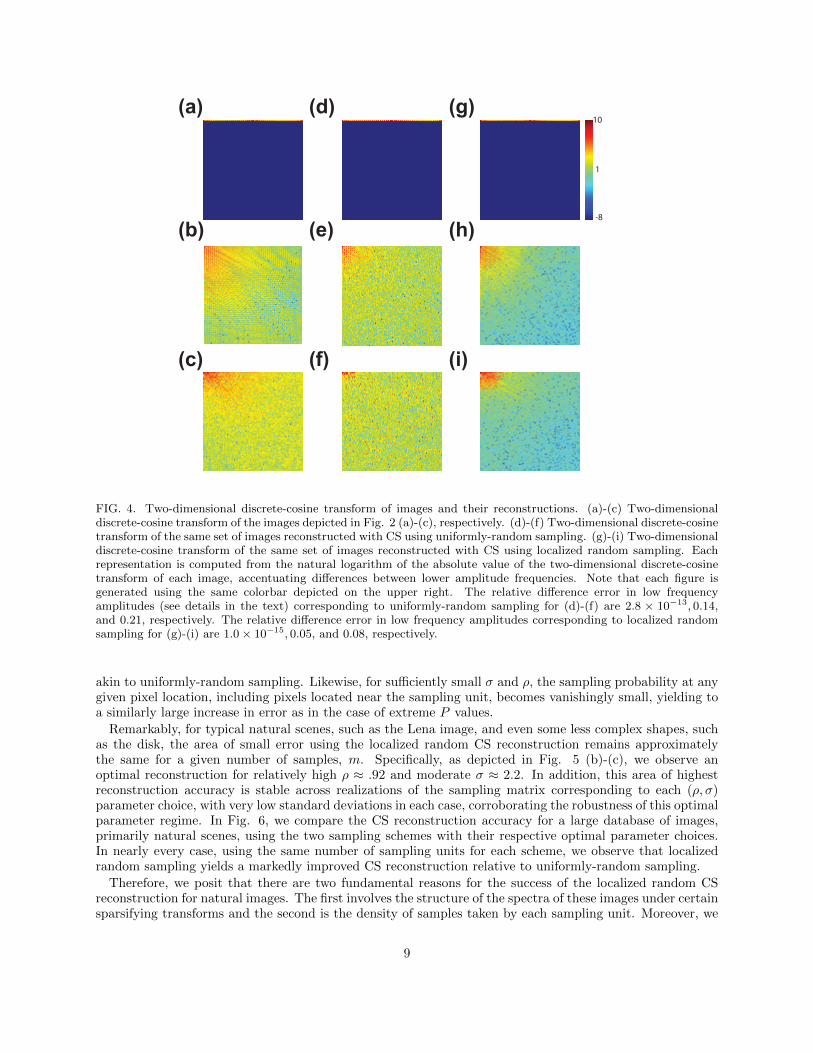
FIG. 4. Two-dimensional discrete-cosine transform of images and their reconstructions. (a)-(c) Two-dimensionaldiscrete-cosine transform of the images depicted in Fig. 2 (a)-(c), respectively. (d)-(f) Two-dimensional discrete-cosinetransform of the same set of images reconstructed with CS using uniformly-random sampling. (g)-(i) Two-dimensionaldiscrete-cosine transform of the same set of images reconstructed with CS using localized random sampling. Eachrepresentation is computed from the natural logarithm of the absolute value of the two-dimensional discrete-cosinetransform of each image, accentuating differences between lower amplitude frequencies. Note that each figure isgenerated using the same colorbar depicted on the upper right. The relative difference error in low frequencyamplitudes (see details in the text) corresponding to uniformly-random sampling for (d)-(f) are 2.8 × 10−13, 0.14,and 0.21, respectively. The relative difference error in low frequency amplitudes corresponding to localized randomsampling for (g)-(i) are 1.0× 10−15, 0.05, and 0.08, respectively.

akin to uniformly-random sampling. Likewise, for sufficiently small σ and ρ, the sampling probability at anygiven pixel location, including pixels located near the sampling unit, becomes vanishingly small, yielding toa similarly large increase in error as in the case of extreme P values.

Remarkably, for typical natural scenes, such as the Lena image, and even some less complex shapes, suchas the disk, the area of small error using the localized random CS reconstruction remains approximatelythe same for a given number of samples, m. Specifically, as depicted in Fig. 5 (b)-(c), we observe anoptimal reconstruction for relatively high ρ ≈ .92 and moderate σ ≈ 2.2. In addition, this area of highestreconstruction accuracy is stable across realizations of the sampling matrix corresponding to each (ρ, σ)parameter choice, with very low standard deviations in each case, corroborating the robustness of this optimalparameter regime. In Fig. 6, we compare the CS reconstruction accuracy for a large database of images,primarily natural scenes, using the two sampling schemes with their respective optimal parameter choices.In nearly every case, using the same number of sampling units for each scheme, we observe that localizedrandom sampling yields a markedly improved CS reconstruction relative to uniformly-random sampling.

Therefore, we posit that there are two fundamental reasons for the success of the localized random CSreconstruction for natural images. The first involves the structure of the spectra of these images under certainsparsifying transforms and the second is the density of samples taken by each sampling unit. Moreover, we

9

0.2 0.4 0.6 0.81

2

3

4

ρ

σ

2

4

6

x 10-15

0.2 0.4 0.6 0.81

2

3

4

ρ

σ

0.15

0.2

0.25

0.2 0.4 0.6 0.81

2

3

4

ρ

σ

0.25

0.3

0.35

(a)

(b)

(c)

FIG. 5. Reconstruction relative error using CS with localized random sampling. (a)-(c) CS reconstruction errordependence on (ρ, σ) parameter choice sets corresponding to localized random sampling of the images depicted inFig. 2 (a)-(c), respectively. Each reconstruction uses m = 1000 sampling units to recover n2 = 10000 pixel images.For each plot, the mean error over an ensemble of 10 realizations of the sampling matrix for each (ρ, σ) parameterchoice set is depicted. The parameter choices yielding minimal error are (ρ, σ) = (0.88, 0.8), (ρ, σ) = (0.92, 2.2),and (ρ, σ) = (0.92, 2.2) for (a)-(c), respectively. The mean standard deviation across realizations in the intervalsρ ∈ [0.2, 0.85] and σ ∈ [1, 4.5] is 3.2× 10−16, 0.0057, and 0.0069 for (a)-(c), respectively.

will show in the next section that these results generalize to images of alternative resolutions and alsoreconstructions utilizing different numbers of sampling units.

We emphasize that the results of this work are generalizable to other sparsifying transformations andalternate L1 optimization algorithms. For example, in Fig. 7 (a) and (b), we consider image reconstructionsusing the two-dimensional discrete-wavelet transformation, comparing the CS reconstruction errors usinglocalized random sampling and uniformly-random sampling, respectively [22, 23]. As in the case of the two-dimensional discrete-cosine transformation, we observe that localized random sampling yields a higher qualityoptimal CS reconstruction than uniformly-random sampling. In addition, the optimal parameter choice inthe localized random CS reconstruction using the two-dimensional discrete-wavelet transformation is quite

10

FIG. 6. Comparison of sampling schemes over image database. (a) Each data point corresponds to the CS recon-struction of an image using localized random sampling (ordinate) and uniformly-random sampling (abscissa). Eachlocalized random sampling CS reconstruction uses parameter choice (ρ, σ) = (0.92, 2.2) and each uniformly-randomsampling CS reconstruction uses parameter choice P = 0.84. Each reconstruction uses m = 1000 sampling units torecover n2 = 10000 pixel images. The dashed identity line is plotted for visual comparison. There are 44 imagesconsidered, composing the University of Southern California Signal and Image Processing Institute Miscellaneousvolume of images (http://sipi.usc.edu/database/database.php?volume=misc), which were processed at the 100× 100pixel resolution and converted to gray-scale images. (b) and (e) Example 100 × 100 pixel images in database. (c)and (f) Reconstruction of images in Fig. 6 (b) and (e), respectively, using localized random sampling. (d) and(g) Reconstruction of images in Fig. 6 (b) and (e), respectively, using uniformly-random sampling. The relativereconstruction errors via localized random sampling are 0.13 and 0.15 for reconstructions (c) and (f), respectively.The relative reconstruction errors via uniformly-random sampling are 0.24 and 0.29 for reconstructions (d) and (g),respectively. Courtesy of the Signal and Image Processing Institute at the University of Southern California.

close to that using the two-dimensional discrete-cosine transformation considered previously. Similarly, inFigs. 7 (e) and (f), we consider the CS reconstruction results using the homotopy method, rather than theorthogonal matching pursuit, to solve the resultant L1 optimization problem [24, 25]. While using a differentoptimization algorithm may result in alternate optimal parameter choices, we see that localized randomsampling again yields improved reconstruction quality.

To investigate the reasons underlying the success of the localized random sampling, we analyze the spectraof the images in Fig. 2 (a)-(c) and their reconstructions using each sampling method in Fig. 4. We depictin Fig. 4 (a)-(c) the spectra of the images in Fig. 2 (a)-(c) by taking the two-dimensional discrete-cosinetransform of each image. In the case of the stripes image, we observe that the spectrum is composedof several large-amplitude frequency components in the horizontal direction, corresponding to multiplesof the fundamental frequency of the stripes, whereas the remaining frequencies primarily have near-zeroamplitudes. In contrast, we see that for the disk and Lena images, the spectra contain great diversity indominant frequency-components, with varying amplitudes. As in the case of typical natural scenes, thereis a high concentration of large-amplitude low-frequency components, corresponding to large-scale imagecharacteristics, and a scatter of small-amplitude high-frequency components, corresponding to small-scaleimage details. It is important to note that the higher frequencies generally display lower amplitudes, andthereby typically contribute less to characterizing images.

One way to quantify the dispersion of amplitudes among the various image frequency components is to

11

FIG. 7. Dependence of CS reconstruction on sparsifying transformation and L1 optimization algorithm. (a) CSreconstruction relative error dependence on (ρ, σ) parameter choice sets corresponding to localized random sampling ofFig. 2 (c) using the two-dimensional discrete-wavelet transformation. (b) CS reconstruction relative error dependenceon measurement probability, P , corresponding to uniformly-random sampling for the image in Fig. 2 (c) using thetwo-dimensional discrete-wavelet transformation. (c) Reconstruction of the image in Fig. 2 (c) using localizedrandom sampling and the two-dimensional discrete-wavelet transformation with the optimal sampling parameterchoice. (d) Reconstruction of the image in Fig. 2 (c) using uniformly-random sampling and the two-dimensionaldiscrete-wavelet transformation with the optimal sampling parameter choice. (e) CS reconstruction relative errordependence on (ρ, σ) parameter choice sets corresponding to localized random sampling of Fig. 2 (c) using thehomotopy L1 optimization algorithm. (f) CS reconstruction relative error dependence on measurement probability,P , corresponding to uniformly-random sampling for the image in Fig. 2 (c) using the homotopy L1 optimizationalgorithm. (g) Reconstruction of the image in Fig. 2 (c) using localized random sampling and the homotopyalgorithm with the optimal sampling parameter choice. (h) Reconstruction of the image in Fig. 2 (c) using uniformly-random sampling and the homotopy algorithm with the optimal sampling parameter choice. Each reconstructionuses m = 1000 sampling units to recover an n2 = 10000 pixel image. In (a) and (e), the mean error over anensemble of 10 realizations of the sampling matrix for each (ρ, σ) parameter choice set is depicted. In (b) and (f),the mean relative error over an ensemble of 10 realizations of the sampling matrix for each P is depicted, with errorbars corresponding to the standard deviation of the error across realizations. The minimal reconstruction error in(a) is 0.21 with (ρ, σ) = (0.92, 1.9). The minimal reconstruction error in (b) is 0.37 with P = .04. The minimalreconstruction error in (e) is 0.27 with (ρ, σ) = (0.48, 4.5). The minimal reconstruction error in (f) is 0.35 withP = 0.12. The minimal error corresponds to the particular sampling parameter choice and corresponding samplingmatrix realization for which the CS reconstruction error is lowest. The mean standard deviation across realizationsin the intervals ρ ∈ [0.2, 0.85] and σ ∈ [1, 4.5] is 0.0089 and 0.032 for (a) and (e), respectively. The mean standarddeviation across realizations is 0.0102 and 0.0257 in (b) and (f), respectively.

compute the image entropy, H, defined by

H = −∑i

gi log2 gi, (6)

where gi denotes the probability of observing the ith frequency-component amplitude, computed over theset of all frequency components composing an image [27]. With their relatively wide-spread large-amplitudecomponents, natural images should intuitively have larger image entropies than typical simpler images withonly a particularly small number of dominant frequency components. In the case of the stripes image, forexample, the image entropy is only 0.1418, whereas the image entropies for the disk and Lena images are4.8996 and 5.4389, respectively. Hence, with the natural-like images having an image entropy of at least anorder of magnitude greater than the simple stripes image, it is clear that such natural scenes should havesignificantly more diverse dominant frequencies. However, such natural images should also be distinguished

12

from white-noise-type images, which also have high image entropy, in the sense that natural images stillexhibit a concentration of image energy at lower frequencies. Images with both sufficiently high imageentropies and energy concentrated in low frequency components, therefore, appear to be good candidates forthe large improvements in reconstruction quality yielded via localized random sampling.

In Fig. 4 (d)-(f), we plot the two-dimensional discrete-cosine transform of the same respective imagesreconstructed using uniformly-random sampling CS reconstructions. We note that, for the simple stripesimage, the spectrum in Fig. 4 (d) is nearly identical to the spectrum of the original image. In addition, asdisplayed in Fig. 2 (f), the corresponding image reconstruction in the space domain is also highly accurate.For the other images, we observe larger differences in the transforms of the reconstructions, plotted inFigs. 4 (e) and (f), relative to the original image transforms. While the relative amplitudes of the low andhigh frequency components in Figs. 4 (e) and (f) are similar with respect to the original images, the clearpatterning in the amplitudes of the higher frequency components is lost in the uniformly-random samplingCS reconstructions. In addition, especially in Fig. 4 (f), the distribution of several large-amplitude low-frequency components appears slightly distorted, contributing to errors in resolving certain large-scale imagefeatures. These spectral differences correspond to a lack of accurate higher-order image information, whichmay cause the graininess observed in the images reconstructed in Figs. 2 (g) and (h).

For comparison we plot in Fig. 4 (g)-(i) the corresponding two-dimensional discrete-cosine transform ofthe CS reconstructions using localized random sampling. Again, we note nearly perfect recovery of thespectrum for the stripes image in Fig. 4 (g). For the transforms of the reconstructed disk and Lena imagesdisplayed in Figs. 4 (h) and (i) respectively, we note a patterning of the dominant frequency-componentamplitudes relatively similar to the corresponding original images yet distinct from the transforms of thereconstructions using uniformly-random sampling. Comparing the spectra of the Lena image, for example,the frequency-components of the CS reconstruction using uniformly-random sampling depicted in Fig. 4 (f)are less dominant in the vertical direction than the same components corresponding to both the originalimage and localized random sampling CS reconstruction in Figs. 4 (c) and (i), respectively. Likewise, inthe case of the disk image, the contribution of several low-frequency components dominant in the originalimage and localized random sampling CS reconstruction are instead diminished in the uniformly-randomsampling CS reconstruction. We also note that the higher-frequency components have primarily near-zeroamplitudes in the localized random sampling CS reconstructions, typically yielding sparse representations inthe two-dimensional discrete-cosine transform domain.

Overall, we observe especially good agreement between the localized random sampling CS reconstructionsand original images for low and moderately-high frequency components. We quantify this agreement in thespectra by using the Frobenius norm relative error in frequency amplitudes, as analogously defined in Eq.(5) in the case of image pixel matrices. We compute this relative error for the frequency-amplitude matrixrepresentations of the images and their reconstructions. In making the comparison, to better quantify agree-ment in the relative distribution of the frequency amplitudes, we first normalize the frequency amplitudes ofthe compared images by their respective maximum frequency-amplitudes. Computing this relative spectraldifference for the 20× 20 submatrix of amplitudes corresponding to combinations of the 20 smallest positivex and y frequency components, we observe closer spectral agreement between the original images and theirCS reconstructions for both the disk and Lena images by using localized random sampling. The exact valuesof these relative differences, using uniformly-random and localized random sampling, can be found in thecaption of Fig. 4. Since the highest frequency components make little contribution to the overall image fea-tures, improved agreement in the lower frequencies via localized random sampling typically results in muchgreater improvement of the image reconstruction than a comparable improved agreement in high-frequencycontributions.

Considering each sampling unit will generally measure groups of spatially nearby pixels via localizedrandom sampling, the approximate average pixel intensity in the region of each sampling unit and thecorresponding frequency information characterizing the variation among those pixels should be well captured.Also, since the sampling units are each randomly placed on the image, the groups of spatially nearby pixelsmeasured by the sampling units are expected to be uniformly spread across the image. Additional frequencyinformation may thus be acquired through the difference in intensities between distinct clusters of measuredpixels. With respect to the highest frequency component contributions, we observe much lower amplitudesin the spectra of the localized random sampling CS reconstructions relative to the corresponding uniformly-random sampling CS reconstructed image spectra in Fig. 4. By utilizing localized random sampling, we

13

0.99 0.995 10

0.5

1

1.5

x 10−14

Sparsity

Err

or

0.99 0.995 1

0.2

0.4

0.6

Sparsity

Err

or

0.99 0.995 10.2

0.3

0.4

0.5

Sparsity

Err

or

(a)

(b)

(c)

0 1 2 3 4 5 60.2

0.3

0.4

0.5

D

Err

or

(d)

FIG. 8. Impact of measurement sparsity on reconstruction relative error. (a)-(c) Dependence of the CS reconstructionrelative error on sampling matrix sparsity using localized random sampling for the images depicted in Fig. 2(a)-(c),respectively. Plots (a)-(c) depict reconstruction errors corresponding to each of the (ρ, σ) parameter choices andresultant sampling matrix sparsities used in Fig. 5 (a)-(c), respectively. For each plot, the mean error and meansparsity over an ensemble of 10 realizations of the sampling matrix for each (ρ, σ) parameter choice set is depicted asa point. The sparsity values corresponding to the minimal reconstruction errors for Fig. 2(a)-(c) are 0.9996, 0.9973,and 0.9973, respectively. (d) CS reconstruction relative error as a function of the expected distance between samplingunits and sampled pixels, D, defined by Eq. (7), for each (ρ, σ) parameter choice using localized random samplingin reconstructing Fig. 2 (c). The mean relative error over an ensemble of 10 realizations of the sampling matrix foreach (ρ, σ) parameter choice set is plotted as a point for each corresponding value of D. The expected distance thatcorresponds to the minimal reconstruction error plotted in (d) is D = 2.71. We note that multiple (ρ, σ) parameterchoices may yield the same sparsity or expected distance, but generate quite different reconstruction errors.

expect that a lack of intersections between clusters of measured pixels may cause high-frequency contributionsto be missed as the price for better resolution of lower frequencies, which we will later discuss further withrespect to the density of samples taken by the sampling units.

Overall, we see that localized random sampling yields a better reconstruction of low and moderately-highfrequency components, which contribute most to the overall image features and reconstruction accuracy.Similarly, in pixel space, capturing these dominant frequencies well corresponds to improved resolution ofsmall-scale features and abrupt transitions in pixel intensity, which are often missed through uniformly-random sampling with the same number of sampling units, as evidenced in Fig. 2.

In addressing the question of what determines the success of localized random sampling, we now investigatehow dense the measurements of each sampling unit should be for a natural image. While sampling densitydid not appear to impact the success of CS reconstructions using uniformly-random sampling for moderatevalues of P , as shown in Fig. 3, we observe a clear dependence on sampling probability parameter, ρ, in thelocalized random sampling scheme, as shown in Fig. 5. To quantify the number of measurements taken byeach sampling unit, we measure the sparsity of each sampling matrix. We define the sparsity of a matrix tobe the percentage of zero-component entries that are contained in the matrix. Thus, sampling units taking

14

very few measurements will have a sparsity near 1.In Fig. 8 (a)-(c), we plot the dependence of the reconstruction relative error on sampling matrix sparsity

for each of the (ρ, σ) parameter choices used in Fig. 5. For each image, the minimal errors are clustered neara sparsity of 0.999, with increasingly large errors in both the low and high sparsity limits. In the extremelylow and high sparsity regimes, low quality reconstructions are yielded for similar reasons as previouslysummarized in the discussion of extreme parameter choices for localized random sampling. However, whatis significant is that the optimal sparsity values approximately correspond to 1 − 1/m, where m is thenumber of utilized sampling units. Since the total number of elements in the m × n2 sampling matrixis mn2, if the fraction of nonzero elements is 1/m, then the expected number of total pixels measured ismn2(1/m) = n2, which exactly equals the total number of pixels in the image. In this particular case,each pixel is sampled approximately once. Hence, there is statistically little over-sampling across samplingunits, such that the contributions of measured pixels (frequencies) blur, and also little under-sampling, suchthat the contribution of specific pixels (frequencies) are missing. For example, in the case of the previousreconstructions with m = 1000 sampling units used to reconstruct n2 = 10000 pixel images, the optimalsparsity is near 1− 1/m = 0.999.

We note that over-sampling in this sense is distinct from adding rows (sampling units) to the samplingmatrix, which would be expected to improve the image reconstruction. Here, over-sampling refers to the rowsof the sampling matrix A having too many non-zero entries, and thus each sampling unit takes too manymeasurements, such that there tends to be redundancy in the spectral information yielded by each samplingunit. Likewise, if too few measurements are taken by each sampling unit, certain pixels (frequencies) maynever be measured and thus less information will be available for reconstruction. In contrast, given theoptimal sparsity of the sampling matrix A, since each pixel is expected to be sampled only once, it is mostlikely for each sampling unit to collect sufficient but not redundant image information.

For more dense measurements, i.e., large σ for fixed ρ, in which the localized clusters of pixels corre-sponding to each sampling unit tend to have more overlap, the spectra of the reconstructions using localizedrandom sampling CS become more similar to the spectra of reconstructions using uniformly-random sam-pling. In the extreme case that σ →∞, localized random sampling reduces to uniformly-random sampling,and thus the spectra of the reconstructions become the same as in the uniformly-random sampling case. Wesuspect that by using localized random sampling with more dense measurements, the overlaps between clus-ters of measured pixels may resolve a few higher frequencies at the price of missing low-frequency componentcontributions, which are typically more significant. In the case of the optimal sparsity, however, the ex-pected lack of localized pixel cluster intersections likely corresponds to less resolution of higher frequencies,but improved resolution of lower frequencies through distinct local measurements. Since lower frequencycomponents contain the most vital image information, improving their resolution produces higher qualityreconstructions corresponding to the minima in Figs. 5 (b) and (c). We demonstrate this by determining theexpected distance between a given sampling unit and a sampled pixel for each localized random samplingCS reconstruction parameter choice. When this distance is greater, it is clearly more likely that the clustersof measured pixels corresponding to each sampling unit will intersect. Averaging across all sampling unitlocations and possible sampled pixels, we compute for each (ρ, σ) parameter choice the expected distancebetween the sampling units and sampled pixels, D, given by

D(ρ, σ) =

⟨ n2∑j=1

Pjdj

/

n2∑j=1

Pj

⟩ , (7)

where the probability of connection, P , is determined by Eq. (3), index j corresponds to the jth possiblepixel location on the image lattice, d gives the Euclidean distance between a sampling unit and pixel tobe measured, and 〈·〉 corresponds to the expectation over all possible sampling unit locations on the imagelattice. In Fig. 8 (d), we plot the CS reconstruction errors displayed in Fig. 5 (c) as a function of D foreach (ρ, σ) parameter choice. We observe a clear minimal error for intermediate D, giving evidence for anoptimal cluster size, corresponding to the optimal sampling matrix sparsity at which each pixel is expectedto be sampled approximately once.

In summary, both the distribution of dominant frequencies in image spectra and the sparsity of mea-surements taken by sampling units play a fundamental role in the success of image reconstructions using

15

localized random sampling. For natural images, in which there is sufficient variation in dominant frequencies,localized random sampling resolves low and moderately-high frequency information especially well, charac-terizing the majority of image features. Likewise, when the sparsity of the sampling matrix is approximately1 − 1/m, there is little overlap between clusters of sampled pixels, allowing most sampling resources to beused towards resolving lower frequency information while still containing some high-frequency informationfrom measurements within clusters of measured pixels.

STABILITY OF LOCALIZED RANDOM SAMPLING

The analysis thus far has focused on pixel images of the same 100 × 100 resolution reconstructed usinga constant number of m = 1000 total samples. We conclude by studying how well our results generalizeto images of other resolutions and also CS reconstructions using different numbers of sampling units. Inparticular, we identify and explain differences in reconstruction quality and optimal parameter choices thatmay arise in each of these alternative scenarios.

(a) (c) (d)

(e) (f)

0.2 0.4 0.6 0.81

2

3

4

ρ

σ

0.15

0.2

0.25

0 0.2 0.4 0.6 0.8 10.27

0.28

0.29

0.3

0.31

P

Err

or

(b)10

1

-8

FIG. 9. CS reconstructions for larger images. (a) 200 × 200 pixel image of Lena. (b) Two-dimensional discrete-cosine transform of image (a). This representation is computed from the natural logarithm of the absolute valueof the two-dimensional discrete-cosine transform of image (a). (c) Optimal CS reconstruction of image (a) usinglocalized random sampling. (d) Optimal CS reconstruction of image (a) using uniformly-random sampling and thesame number of sampling units as in (c). (e) CS reconstruction relative error dependence on (ρ, σ) parameter choicesets corresponding to localized random sampling of image (a). (f) CS reconstruction relative error dependence onmeasurement probability, P , using uniformly-random sampling of image (a). Each reconstruction uses 4000 samplingunits to recover a 40000 pixel image. In reconstruction (c), a minimal reconstruction relative error of 0.14 is achievedusing the parameter choice (ρ, σ) = (0.96, 2.5). In reconstruction (d), a minimal reconstruction relative error of 0.28is achieved using P = 0.6. In (e), the mean relative error over an ensemble of 10 realizations of the sampling matrixfor each (ρ, σ) parameter choice set is depicted. The mean standard deviation across realizations in the intervalsρ ∈ [0.2, 0.85] and σ ∈ [1, 4.5] is 0.0026. In (f), the mean relative error over an ensemble of 10 realizations of thesampling matrix for each P is depicted, with error bars corresponding to the standard deviation of the error acrossrealizations. The mean standard deviation across realizations in (f) is 0.0055.

To address the issue of image resolution, we consider a 200 × 200 pixel image of Lena in Fig. 9 (a)analogous to the 100 × 100 pixel version depicted in Fig. 2 (c). In Figs. 9 (c) and (d), we reconstruct

16

this larger image with m = 4000 sampling units using localized random sampling and uniformly-randomsampling, respectively. Note that we use the same factor of 10 fewer sampling units than total pixels we seekto recover, as in the previous analysis.

For both sampling protocols, we observe a significant improvement in reconstruction quality relative tothe corresponding 100× 100 pixel image reconstruction. The reason for this improvement can be explainedby comparing the spectra of the different-sized Lena images. First, it is clear that the two-dimensionaldiscrete-cosine transform of this larger Lena image, depicted in Fig. 9 (b), is very similar in overall structureto the transform corresponding to the smaller Lena image, depicted in Fig. 4 (c). We observe in Fig. 9 (b)that while some higher-frequency components are introduced in the higher-resolution image, the distributionof amplitudes in the dominant low-frequency components is nearly indistinguishable from that of the lower-resolution Lena image. In particular, the relative frequency amplitude difference between the low frequencycomponents for the two images, as defined previously, is only 0.002. For comparison, we note that thefrequency amplitude difference in the case of two completely different images of the same resolution isseveral orders of magnitude larger. For example, the frequency amplitude difference between the Lena anddisk images in Figs. 2 (b) and (c) has a value of 1.01. As shown in Fig. 9 (b), the newly introduced high-frequency components have very small amplitudes and thus have relatively little impact on the overall imagefeatures compared to the lower frequency components. Since maintaining the same ratio of sampling units torecovered pixels for higher resolution images requires increasing the total number of sampling units utilized,these additional sampling units may greatly increase the accuracy of image reconstructions, especially if thenew samples resolve the dominant low-frequency-component contributions well. We see from Fig. 9 (c) thatthe improved resolution of low-frequency contributions utilizing these additional localized random samplesdoes indeed greatly improve the quality of the recovered image.

Comparing the optimal reconstructions using localized random and uniformly-random sampling in Figs. 9(c) and (d), respectively, we still observe a much higher degree of accuracy is achieved via localized randomsampling for the 200×200 pixel image. Localized random sampling allows for the resolution of even smaller-scale details than in the case of the corresponding smaller Lena image reconstructed in Fig. 2 (m), capturingfeatures as fine as the nose and mouth of Lena, which were mostly missing in the smaller image recovery. Wecompare the reconstruction errors over a range of sampling parameter choices in Figs. 9 (e) and (f) usinglocalized random and uniformly-random sampling, respectively. In the case of uniformly-random sampling,the distribution of errors is again quite unaffected by variations in sampling probability P . Using insteadlocalized random sampling, the smallest reconstruction errors are yielded by utilizing approximately the samesampling parameters as in the case of the smaller 100 × 100 pixel image. Specifically, (ρ, σ) = (0.96, 2.5)and (ρ, σ) = (0.92, 2.2) yield minimal reconstruction relative errors for the 200 × 200 and 100 × 100 pixelimages, respectively, with nearby parameter choices producing quite high reconstruction quality for naturalimages of either resolution. Thus, for natural scenes varying in resolution, the characteristics of the localizedrandom sampling protocol are closely related.

With respect to the number of samples (number of rows in the sampling matrix A) utilized, we considerthe cases in which m = 2000 and m = 500 sampling units are used, doubling and halving, respectively,the number of sampling units employed in the previous section. In Fig. 10 (a) and (b), we plot the CSreconstruction error using localized random sampling of the small 100 × 100 pixel Lena image depictedin Fig. 2 (c) over a wide range of (ρ, σ) parameter choices. We again note a distinct region of minimalreconstruction error, but the minimum is slightly shifted with varying choices of m. We hypothesize thatthe reason for this small shift is because with larger numbers of samples, there is the opportunity to identify,without loss, higher, less dominant, frequency components. Thus, as the number of sampling units increases,the optimal radius in which pixels should be sampled, corresponding to the size of parameter σ, shoulddecrease to avoid overlap between distinct clusters of measured pixels. While the limit of this case will bethe same as the uniformly-random sampling with sufficient number of sampling units, using such a largenumber of samples diminishes the sampling efficiency garnered by CS theory.

To demonstrate the relationship between the number of sampling units and recovered image frequencies,we plot in Figs. 10 (c) and (d) the optimal image reconstructions and their associated two-dimensionaldiscrete-cosine transforms in Figs. 10 (e) and (f), using localized random sampling with m = 2000 andm = 500 sampling units, respectively. It is clear that the transform corresponding to the larger number ofsampling units contains a broader distribution of large-amplitude components, including higher frequencies.Moreover, more sampling units also yields more accurate resolution of low-frequency amplitudes. Thus, in

17

FIG. 10. Dependence of CS reconstruction quality on number of sampling units. (a)-(b) CS reconstruction errordependence on (ρ, σ) parameter choice sets corresponding to localized random sampling of the 10000 pixel imagein Fig. 2 (c) using m = 2000 and m = 500 sampling units, respectively. (c) Optimal CS reconstruction usinglocalized random sampling with m = 2000 sampling units. (d) Optimal CS reconstruction using localized randomsampling with m = 500 sampling units. (e)-(f) Two-dimensional discrete-cosine transform of the reconstructionsin (c)-(d), respectively. (g)-(h) CS reconstruction relative error dependence on measurement probability, P , usinguniformly-random sampling for the image in Fig. 2 (c) with m = 2000 and m = 500 sampling units, respectively.Each transform is computed from the natural logarithm of the absolute value of the two-dimensional discrete-cosinetransform of each image. The relative reconstruction errors corresponding to (c) and (d) are 0.17 and 0.25, respectively.The corresponding optimal parameter choices are (ρ, σ) = (0.96, 1.75) and (ρ, σ) = (0.92, 4.5), respectively. We notethat the minimal reconstruction errors using uniformly-random sampling corresponding to m = 2000 and m = 500sampling units are 0.30 using P = 0.84 and 0.50 using P = 0.96, respectively. In (a) and (b), the mean relative errorover an ensemble of 10 realizations of the sampling matrix for each (ρ, σ) parameter choice set is depicted. The meanstandard deviation across realizations in the intervals ρ ∈ [0.2, 0.85] and σ ∈ [1, 4.5] is 0.0049 and 0.0086 for (a)-(b),respectively. In (g) and (h), the mean relative error over an ensemble of 10 realizations of the sampling matrix foreach P is depicted, with error bars corresponding to the standard deviation of the error across realizations. Themean standard deviation across realizations is 0.0076 and 0.023 in (g) and (h), respectively.

pixel space, there is a marked improvement in reconstruction quality by using more sampling units. Inpractice, depending on the available computing resources and desired reconstruction quality, the number ofutilized sampling units can be adjusted accordingly. For comparison, we plot in Figs. 10 (g) and (h) theCS reconstruction error using uniformly-random sampling over the sampling probability parameter spacecorresponding to the same respective numbers of sampling units. As in the previous cases, the optimal CSreconstruction quality is greatly improved by utilizing localized random sampling.

It is important to note that for an appropriately chosen σ, a high ρ of approximately 0.9 will typicallyyield an accurate reconstruction using image sizes for which available computing resources allow recovery.We expect that for increasingly large numbers of sampling units utilized, σ should be appropriately adjustedso as to maintain the optimal measurement rate such that each pixel is approximately sampled once. Whilewe see that the optimal σ decreases with the number of sampling units used, further research is necessary toquantitatively describe this trend in more general cases. However, if too many sampling units are utilized, itis clear that the benefits of reduced sampling rates garnered by CS are diminished, making such a scenarioless useful to consider. Likewise, if too few sampling units are used, then the expected cluster size will needto be quite large, giving reconstruction results similar to the uniformly-random sampling CS reconstruction.Hence, as demonstrated in Fig. 10 (b), when particularly few sampling units are used, larger σ values typicallyyield improved reconstructions. Overall, utilizing a particularly small number of samples of natural image

18

pixels, the localized random sampling protocol demonstrates a relatively stable dependence on parameterchoices and reconstruction algorithms, and therefore is quite robust in suiting diverse applications.

DISCUSSION

In this work, we have formulated and analyzed a new sampling methodology, motivated by the structureof sensory systems, which is viable for improved CS image reconstructions. Using our localized randomsampling, consisting of sets of randomly chosen local groups of sampled pixels, we recovered a variety ofimages using compressive sensing techniques. We demonstrate that, especially for natural scenes, this newsampling protocol yields remarkably higher quality image reconstructions than more conventional uniformly-random pixel sampling. Using spectral analysis, we conclude that sampling localization better resolves lower-frequency components, which contain more information regarding image features, while retaining some higherfrequency information. Moreover, we also showed that the optimal parameter choices corresponding to thisnew sampling protocol are stable with respect to variations in natural image sizes and may be slightlyadjusted according to the number of samples utilized. Relatively easy to adjust and implement, we expectthat the reconstruction improvements garnered with localized random sampling have high potential for futureapplication in engineered sampling devices crucial to brain imaging or more general image processing.

In terms of both theoretical implications and directions for future study, the results presented in thispaper have several interesting consequences. It would be informative, for example, to derive theoretical errorbounds on the reconstruction quality corresponding to different numbers of sampling units and the sparsitystructure of the image. On a similar note, extending theoretical arguments regarding the probability ofsuccessful reconstruction from simpler independent identically distributed random variable-type sampling tosampling protocols analogous to localized random sampling may signify a useful new direction for CS theory.This may also help to further address the question of to what extent image measurements need to be randomfor successful CS reconstructions.

With respect to sensory systems, we hypothesize that evolution has selected for sensory sampling schemesanalogous to localized random sampling. Given the same number of neurons in the visual system, for example,this work suggests that image information can be encoded more accurately by using sampling protocolsalternative to uniformly-random sampling. The center-surround receptive field architecture, prominent inthe visual, somatosensory, auditory, and olfactory systems, is akin to localized random sampling in the sensethat neurons are most stimulated by a particular range of similar stimuli [12, 13, 28–32]. In the visualsystem, this translates to a given ganglion cell sampling spatially clustered image features, with the responsedepending on where the light falls in the receptive field, i.e., in the center or surround area, as well asthe light intensity. Moreover, the size of receptive fields varies widely within a given sensory system and,depending on the receptive field size, details of various scales are measured, just as in the case of varyingthe σ parameter in our localized random sampling protocol [33–35]. Together, the receptive fields of neuronsin some layers of the visual system have been shown to form a rough map of visual space, with regionsof overlap between the receptive fields varying in size [36–38]. It would be interesting to further extendour localized random sampling by incorporating more specific, detailed structure embedded in the receptivefields of neurons, such as center-surround antagonism and the alignment of receptive fields across differentneurons to achieve certain functions, e.g., orientation selectivity.

In many sensory system areas, the number of downstream neurons is significantly less than the numberof upstream neurons, such as in the case of downstream ganglion cells and upstream photoreceptors in theretina [39, 40]. For successful preservation of sensory information across such highly convergent pathways, itis necessary for neuronal network architecture to facilitate efficient signal processing. It is hypothesized thatthe sparsity of natural scenes combined with the efficiency of localized receptive field sampling may allow forcompression of stimulus information along convergent downstream sensory pathways [19, 20]. This suggeststhat sampling schemes more precisely resembling these biological architectures may yield further improvedinformation acquisition and retention, which may help to guide future enhancements in efficient imageprocessing. In downstream layers of the visual system, such as the visual cortex, receptive field structurebecomes more complex, as input from neurons in upstream layers are integrated, facilitating sensitivity tomore complicated characteristics, including feature orientation and direction of motion [33, 41, 42]. Thus,

19

multi-layer sampling, yielding more complicated receptive field structures as found in the visual system, mayfurther improve upon CS reconstruction quality.

While we have analyzed the consequences of localized random sampling in particular, similar analysis maybe used to understand alternative sampling procedures and their implications on the CS reconstructions. Forspecific classes of images exhibiting a particular set of features, specialized sampling protocols may also bedeveloped and optimized to yield high quality reconstructions. We expect that localized random samplingin particular may also be useful in reconstructing color images and other classes of sparse signals as well.

[1] Candes, E. J., Romberg, J. K. & Tao, T. Stable signal recovery from incomplete and inaccurate measurements.Communications on Pure and Applied Mathematics 59, 1207–1223 (2006).

[2] Donoho, D. L. Compressed sensing. IEEE Trans. Inform. Theory 52, 1289–1306 (2006).[3] Shannon, C. E. Communication in the Presence of Noise. Proceedings of the IRE 37, 10–21 (1949).[4] Candes, E. J. & Wakin, M. B. An Introduction To Compressive Sampling. Signal Processing Magazine, IEEE

25, 21–30 (2008).[5] Baraniuk, R. Compressive sensing. IEEE Signal Processing Mag 118–120 (2007).[6] Bruckstein, A. M., Donoho, D. L. & Elad, M. From sparse solutions of systems of equations to sparse modeling

of signals and images. SIAM Review 51, 34–81 (2009).[7] Mishchenko, Y. & Paninski, L. A bayesian compressed-sensing approach for reconstructing neural connectivity

from subsampled anatomical data. Journal of Computational Neuroscience 33, 371–388 (2012).[8] Gross, D., Liu, Y. K., Flammia, S. T., Becker, S. & Eisert, J. Quantum state tomography via compressed

sensing. Phys. Rev. Lett. 105, 150401 (2010).[9] Lustig, M., Donoho, D. & Pauly, J. M. Sparse MRI: The application of compressed sensing for rapid MR imaging.

Magn. Reson. Med. 58, 1182–1195 (2007).[10] Dai, W., Sheikh, M. A., Milenkovic, O. & Baraniuk, R. G. Compressive sensing DNA microarrays. J. Bioinform.

Syst. Biol. 162824 (2009).[11] Bobin, J., Starck, J.-L. & Ottensamer, R. Compressed sensing in astronomy. J. Sel. Topics Signal Processing 2,

718–726 (2008).[12] Wiesel, T. N. Receptive fields of ganglion cells in the cat’s retina. J Physiol 153, 583–594 (1960).[13] Hubel, D. H. & Wiesel, T. N. Receptive fields of optic nerve fibres in the spider monkey. J Physiol 154, 572–580

(1960).[14] Field, D. J. What is the goal of sensory coding? Neural Computation 6, 559–601 (1994).[15] Tolhurst, D. J., Tadmor, Y. & Chao, T. Amplitude spectra of natural images. Ophthalmic. Physiol. Opt. 12,

229–232 (1992).[16] Olshausen, B. A. & Field, D. J. Natural image statistics and efficient coding. Network 7, 333–339 (1996).[17] Donoho, D. L. & Tsaig, Y. Fast solution of l1-norm minimization problems when the solution may be sparse.

IEEE Transactions on Information Theory 54, 4789–4812 (2008).[18] Duarte, M. F. et al. Single-Pixel Imaging via Compressive Sampling. Signal Processing Magazine, IEEE 25,

83–91 (2008).[19] Barranca, V. J., Kovacic, G., Zhou, D. & Cai, D. Sparsity and compressed coding in sensory systems. PLoS

Comput. Biol. 10, e1003793 (2014).[20] Barranca, V. J., Kovacic, G., Zhou, D. & Cai, D. Network dynamics for optimal compressive-sensing input-signal

recovery. Phys. Rev. E 90, 042908 (2014).[21] Tropp, J. A. & Gilbert, A. C. Signal Recovery From Random Measurements Via Orthogonal Matching Pursuit.

IEEE Transactions on Information Theory 53, 4655–4666 (2007).[22] Haar, A. Zur Theorie der orthogonalen Funktionensysteme. Mathematische Annalen 69, 331–371 (1910).[23] Heil, C. E. & Walnut, D. F. Continuous and discrete wavelet transforms. SIAM review 31, 628–666 (1989).[24] Yang, A. Y., Zhou, Z., Balasubramanian, A. G., Sastry, S. S. & Ma, Y. Fast-minimization algorithms for robust

face recognition. IEEE Transactions on Image Processing 22, 3234–3246 (2013).[25] Donoho, D. L. & Tsaig, Y. Fast solution of-norm minimization problems when the solution may be sparse. IEEE

Transactions on Information Theory 54, 4789–4812 (2008).[26] Feller, W. An Introduction to Probability Theory and Its Applications (John Wiley, New York, 1968).[27] Rieke, F., Warland, D., van Steveninck, R. R. & Bialek, W. Spikes: Exploring the Neural Code. (MIT Press,

Cambridge, 1996).[28] Graziano, M. S. & Gross, C. G. A bimodal map of space: somatosensory receptive fields in the macaque putamen

with corresponding visual receptive fields. Exp Brain Res 97, 96–109 (1993).

20

[29] Wilson, D. A. Receptive fields in the rat piriform cortex. Chem. Senses 26, 577–584 (2001).[30] Welker, C. Receptive fields of barrels in the somatosensory neocortex of the rat. J. Comp. Neurol. 166, 173–189

(1976).[31] Mori, K., Nagao, H. & Yoshihara, Y. The olfactory bulb: coding and processing of odor molecule information.

Science 286, 711–715 (1999).[32] Knudsen, E. I. & Konishi, M. Center-surround organization of auditory receptive fields in the owl. Science 202,

778–780 (1978).[33] Hubel, D. Eye, Brain, and Vision. Scientific American Library Series (Henry Holt and Company, New York,

1995).[34] Sceniak, M. P., Ringach, D. L., Hawken, M. J. & Shapley, R. Contrast’s effect on spatial summation by macaque

V1 neurons. Nat. Neurosci. 2, 733–739 (1999).[35] Desimone, R., Albright, T. D., Gross, C. G. & Bruce, C. Stimulus-selective properties of inferior temporal

neurons in the macaque. J. Neurosci. 4, 2051–2062 (1984).[36] Balasubramanian, V. & Sterling, P. Receptive fields and functional architecture in the retina. J. Physiol. (Lond.)

587, 2753–2767 (2009).[37] Brewer, A. A., Liu, J., Wade, A. R. & Wandell, B. A. Visual field maps and stimulus selectivity in human ventral

occipital cortex. Nat. Neurosci. 8, 1102–1109 (2005).[38] Silver, M. A. & Kastner, S. Topographic maps in human frontal and parietal cortex. Trends Cogn. Sci. (Regul.

Ed.) 13, 488–495 (2009).[39] Barlow, H. B. The ferrier lecture, 1980. critical limiting factors in the design of the eye and visual cortex. Proc

R Soc Lond B Biol Sci 212, 1–34 (1981).[40] Buck, L. B. Information coding in the vertebrate olfactory system. Annu Rev Neurosci 19, 517–544 (1996).[41] Dobbins, A., Zucker, S. W. & Cynader, M. S. Endstopped neurons in the visual cortex as a substrate for

calculating curvature. Nature 329, 438–441 (1987).[42] Barlow, H. B. & Levick, W. R. The mechanism of directionally selective units in rabbit’s retina. J. Physiol.

(Lond.) 178, 477–504 (1965).

ACKNOWLEDGEMENTS

This work was supported by NYU Abu Dhabi Institute G1301 (V.B., G.K., D.Z., D.C.), NSFC-91230202,Shanghai Rising-Star Program-15QA1402600 (D.Z.), Shanghai 14JC1403800, 15JC1400104, NSFC-31571071and SJTU-UM Collaborative Research Program (D.C., D.Z.), and by NSF DMS-1009575 (D.C.).

AUTHOR CONTRIBUTIONS

All four authors (V.J.B., G.K, D.Z., D.C.) contributed in equal measure in the derivation of the resultsand preparation of the manuscript.

AUTHOR INFORMATION

The authors declare no competing financial interests.

21