Embed Size (px)
Citation preview
Improved Approximations for the Erlang Loss Model
J. Anselmi∗
INRIA and LIG LaboratoryMontBonnot Saint-Martin, 38330, FR
Y. Lu, M. Sharma, M.S. SquillanteMathematical Sciences Department
IBM Thomas J. Watson Research CenterYorktown Heights, NY 10598, USA
{yingdong,mxsharma,mss}@us.ibm.com
Abstract
Stochastic loss networks are often a very effective model for studying the random dynamics of systems requiringsimultaneous resource possession. Given a stochastic network and a multi-class customer workload, the classicalErlang model renders the stationary probability that a customer will be lost due to insufficient capacity for at leastone required resource type. Recently a novel family ofslicemethods has been proposed by Junget al to approximatethe stationary loss probabilities in the Erlang model, and has been shown to provide better performance than theclassical Erlang fixed point approximation in many regimes of interest. In this paper, we propose some new methodsfor loss probability calculation. We propose a refinement ofthe 3-point slice method of Junget al which exhibitsimproved accuracy especially when heavily loaded networksare considered, at comparable computational cost. Nextwe exploit the structure of the stationary distribution to propose randomized algorithms to approximate both thestationary distribution and the loss probabilities. Whereas our refined slice method is exact in a certain scaling regimeand is therefore ideally suited to the asymptotic analysis of large networks, the latter algorithms borrow from volumecomputation methods for convex polytopes to provide approximations for the unscaled network with error bounds asa function of the computational costs.
1 Introduction
Starting with the seminal work of Erlang [4], stochastic loss networks (SLNs) have been applied to the study of
many diverse communication and computer systems. In general, a SLN can be used as a model for any system
which allocates non-idling resource capacities to fulfill various classes of requests if possible, each class requiring
simultaneous possession of resources for a random durationfrom a pool of different types of resources. And quite
often a SLN is able to effectively capture the dynamics and uncertainty of the computer/communication system being
modeled. Examples include telephone networks, communication networks, distributed computing systems, database
systems, data centers, wireless networks, and multi-item inventory systems; see, e.g., [16, 7, 21, 8, 9, 10, 18, 15, 22,
17].
An important performance measure arising in the analysis ofsuch loss networks is the stationary loss probability
for each customer class. Given a stochastic network and a multi-class customer workload, the classical Erlang model
renders the stationary probability that a customer will be lost due to insufficient capacity for at least one required
resource type. While the initial results of Erlang [4] were for the particular case of Poisson arrivals and exponential
service times, Sevastyanov [19] demonstrates that the Erlang formula holds under general finite-mean distributions for
∗This work is supported by the Conseil Regional Rhone-Alpes, Global competitiveness cluster Minalogic contract SCEPTRE.
1
the customer service times. Subsequently the formula has been shown to hold under more general conditions [3, 2].
A multi-period version of the loss network has also been recently studied [1].
Unfortunately, the problem of evaluating the exact (multi-dimensional) Erlang formula is known to be♯P -complete1
in the size of the network [12], thus rendering the exact formula of limited use for many large networks in practice.
The well-known Erlang fixed-point approximation (EFPA) hasbeen developed and extensively used and studied as
a tractable approach for calculating the stationary loss probabilities. The method assumes that customer losses are
caused by independent blocking events on each of the resources used by that customer. Estimates of the blocking
probabilities of the individual resources are in turn calculated using the one-dimensional Erlang formula with argu-
ments that are functions of the blocking probabilities of other resources. Surprisingly, the EFPA has been shown to
be asymptotically exact in the limiting regime where arrival rates grow in proportion to the resource capacities [8].
Roughly speaking, this result holds true because in that limiting regime the mean number of calls in the system can be
well approximated by the mode of the stationary distribution of the network states.
The popularity of the EFPA can be attributed to the fact that,in addition to its favorable theoretical properties, the
estimates provided by the method have been found to be remarkably accurate in traditional application areas such as
large communication networks. Recently, SLNs have been used for resource planning within the context of workforce
management in the information technology (IT) services industry, where a collection of IT service products are offered
each requiring a set of resources with certain capabilities[1, 14]. In such applications, one is frequently confronted
with critically loaded workload processes for which the EFPA performs poorly [6]. A novel family ofslicemethods
has been proposed in [6] to compute the stationary loss probabilities using Little’s law and a decomposition of the
computation along hyperplane sections that are parallel tothe route axes (called slices), i.e., subsets of the network
states where the number of calls on a given route is kept fixed.It is shown that the idea of approximating the probability
content of each slice by its mode indeed yields more accurateresults, especially in critically loaded situations [5]. The
general slice method solves a strictly convex program alongeach slice of each route; thus its computational complexity
depends on the resource capacities. A 3-point slice method is also proposed in [6] which uses a suitable interpolation
scheme to reduce computational complexity at a small loss ofaccuracy.
In this paper, we propose some new methods for loss probability calculation. First we present a refinement of
the 3-point slice method which provides improved accuracy especially when heavily loaded networks are considered.
This new approach has nearly the same computational complexity of the 3-point slice method. Next we exploit the
structure of the stationary distribution to propose randomizedcontouralgorithms to approximate both the stationary
distribution and the loss probabilities. The contour algorithms borrow from volume computation methods for convex
polytopes to approximate the probability content of carefully chosen contours. The two sets of proposed algorithms
differ in their applicability: whereas the refined slice method is asymptotically exact in a certain scaling regime and is
therefore ideally suited to the asymptotic analysis of large networks, the contour algorithms provide approximations
corresponding to the unscaled network with error bounds as afunction of the computational cost. Hence, there is
a tradeoff between computational complexity and (probabilistic) accuracy guarantees in choosing among our refined
slice method and our contour methods.1Refer to [20] for details on the♯P -complete complexity class.
2

2 Preliminaries
2.1 Erlang Loss Model
Consider a SLN withJ links, labeled1, 2, . . . , J , and a set ofK fixed routes, denoted byR = {1, . . . , K}, where
each linkj hasCj units of capacity andC = (C1, . . . , CJ ) denotes the vector of link capacities. Calls on router
arrive according to an independent Poisson process of rateνr, with ν = (ν1, . . . , νK) denoting the vector of these
rates, and requireAjr units of capacity on linkj, Ajr ≥ 0. An arriving call on router is admitted to the network if
sufficient capacity is available on all links used by router; otherwise, the call is lost. The call service times are i.i.d.
and follow a general distribution with unit mean.
Let n(t) = (n1(t), . . . , nK(t)) ∈ ZK+ be the vector of the number of active calls in the network at time t. By
definition,n(t) ∈ S(C) where
S(C) ={
n ∈ ZK+ : An ≤ C
}
.
As Erlang originally established, followed by extensions of various researchers, it is well known that there is a unique
stationary distributionπ on the state spaceS(C) such that forn ∈ S(C)
π(n) = G(C)−1∏
r∈R
νnrr
nr!,
whereG(C) is the normalizing constant
G(C) =∑
n∈S(C)
∏
r∈R
νnrr
nr!. (1)
The stationary probability that a call on router is lost can be expressed as
Lr = 1 − G(C)−1
G(C − Aer),
whereer is the unit vector corresponding to a single active call on router.
2.2 Erlang Fixed-Point Approximation
Due to the computational complexity of (1), which is known tobe ♯P -complete in the size of the network [12], the
EFPA has been long used as a more efficient alternative to the exact Erlang loss formula. The EFPA is based on
approximating the stationary blocking probabilities of the individual links, denoted byEj , by the following set of
equations:
Ej = E(ρj , Cj) =ρ
Cj
j
Cj !
Cj∑
i=0
ρij
i!
−1
where ρj =1
1 − Ej
[
∑
r
νrAjr
∏
i
(1 − Ei)Air
]
.
Then the stationary loss probability for router can be approximated in terms of the per-link blocking probabilities as
Lr ≈ 1 −∏
j
(1 − Ej)Ajr .
3

The approximation assumes that lost calls are caused by independent blocking events on each of the links used by the
routes, and uses the one-dimensional Erlang loss formula for each link with an appropriately thinned arrival rate.
The EFPA can provide relatively poor estimates for the per-route loss probabilitiesLr in various model instances.
In [6], it is shown that this is particularly the case when thenetwork is operating in the critically loaded regime [5].
This motivated the authors to investigate alternative approximation algorithms for the exact loss probabilities and to
develop the family of slice methods.
2.3 Slice Methods
The Erlang loss model can be thought of as a stable system where admitted calls experience an average delay of1 and
lost calls experience a delay of0. Hence, the average delay experienced by calls on router is given by
Dr = (1 − Lr) × 1 + Lr × 0 = (1 − Lr),
which together with Little’s law [11] yields
1 − Lr =E[nr]
νr, (2)
and thereforeLr can be obtained throughE[nr]. By definition,
E[nr] =∞∑
k=0
k Pr[nr = k]
and thusE[nr] can be obtained through approximations ofPr[nr = k]. Note thatPr[nr = k] corresponds to the
probability mass along the “slice” of the polytope defined bynr = k. An exact solution forE[nr] can be obtained
by using the exact values ofPr[nr = k], but obtaining the probability mass along a “slice” can be ascomputationally
hard as the original problem. The family of slice methods introduced in [6] is therefore based on approximations for
Pr[nr = k] which assume that the mass along each slice is concentrated around the mode of the distribution restricted
to the slice.
From the definition of the stationary distributionπ(·), the moden∗ corresponds to a solution of the optimization
problem
max∑
r
nr log νr − log nr!
s.t. n ∈ S(C).
A natural continuous relaxation of the state spacen ∈ S(C) is
S(C) ={
x ∈ RK+ : Ax ≤ C
}
, (3)
for which we obtain the corresponding optimization problem(P1):
max∑
r
xr log νr − log Γ(xr + 1)
s.t. x ∈ S(C),
4

where the Gamma function is an extension of the factorial function to real numbers,
Γ(x + 1) =
∫ ∞
0
e−ttxdt, Γ(n + 1) = n!.
For each value ofk ∈ {nr : n ∈ S(C)} that is along eachslice, we definex∗(k, r) to be the solution of the
optimization problem (P2):
max∑
r
xr log νr − log Γ(xr + 1) (4)
s.t. x ∈ Sk,r(C) ≡ S(C) ∩ {x : xr = k}.
A computationally implementable version of the primal problems (P1) and (P2) can be obtained by using Stirling’s
approximation,log Γ(xr + 1) = xr log xr − xr + O(log xr), and ignoring theO(log nr) term. In particular, this
respectively yields the following convex relaxations for (P1) and (P2):
max∑
r
xr log νr + xr − xr log xr (5)
s.t. x ∈ S(C)
and
max∑
r
xr log νr + xr − xr log xr (6)
s.t. x ∈ Sk,r(C).
In the general slice method [6], for each router, the optimization problem (5) is solved for the mode of the
distributionx∗ and the optimization problem (6) is solved for each slice defined bynr = k, k ∈ {nr : n ∈ S(C)}. To
obtain a variation of the general slice method that reduces this computational complexity and provides computational
complexity similar to that of the EFPA, a 3-point slice method is presented in [6]. Instead of computingx∗(k, r) for all
k ∈ {nr : n ∈ S(C)}, the 3-point slice algorithm consists of solving the optimization problem (6) fork = 0 and the
maximum value ofk, and also obtaining the mode of the distributionx∗ by solving (5). Thenx∗(k, r) is approximated
for all other values ofk by linear interpolation between pairs of the 3 computed modes. Formally, the interpolation
scheme to calculatex∗(k, r) is as follows:
(a) If k ≤ x∗r , then
x∗(k, r) = x∗ · k
x∗r
+ x∗(0, r) · x∗r − k
x∗r
.
That is,x∗(k, r) is the point of intersection (in the spaceRK+ ) of the slicexr = k with the line passing through
the two pointsx∗ andx∗(0, r).
(b) Forx∗r < k ≤ nmax
r , wherenmax(r) = max{nr : n ∈ S(C)}, set
x∗(k, r) = x∗(nmax(r), r) · k − x∗r
nmax(r) − x∗r
+ x∗ · nmax(r) − k
nmax(r) − x∗r
.
5

Finally, let us denote the objective function from (5) of theStirling approximated primal problem (P1) (also (P2)) by
q(x) =∑
r
xr log νr + xr − xr log xr.
The estimate ofE[nr] is then obtained as
E[nr] =
∑
k k exp(q(x∗(k, r)))∑
k exp(q(x∗(k, r))),
from which, using (2), we calculateLr = 1 − E[nr]/νr.
2.4 Asymptotic Optimality
Kelly [8, 9] established that the EFPA is asymptotically exact in a large network limiting regime where the traffic
intensities and resource capacities are increased in a proportional manner. More formally, given a SLN with parameters
C andν, a scaled version of the system is defined by the scaled capacities
CN = NC = (NC1, . . . , NCK)
and the scaled arrival rates
νN = Nν = (Nν1, . . . , NνK),
whereN ∈ N is the system scaling parameter. The corresponding feasible region of calls is given byS(NC). Notice
that a normalized version of this region, defined as
SN (C) =
{
1
Nn : n ∈ S(NC)
}
,
tends in the largeN limit to the continuous relaxation(3), that is,S(C) = {x ∈ RK+ : Ax ≤ C}.
In [6], it is shown that the slice method is also asymptotically exact in the above large network limiting regime.
The slice method is further established to provide improvedaccuracy over the EFPA in the critically loaded regime [5].
Numerical results presented in [6] provide additional evidence that the slice methods produce better results than the
EFPA.
3 Refined Slice Method
In this section, we present a refinement to the 3-point slice method which computes approximations for the stationary
loss probabilitiesL using pointsx∗(k, r) that have higher probability content than the points used bythe 3-point slice
method. Before introducing the method, we present some notation and results that will be used below.
Consider the unnormalized stationary probability distribution
π(n) = π(n)G(C), (7)
6
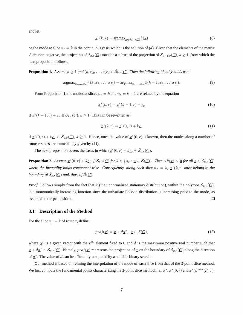
and let
x∗(k, r) = argmaxx∈Sk,r(C)π(x) (8)
be the mode at slicenr = k in the continuous case, which is the solution of (4). Given that the elements of the matrix
A are non-negative, the projection ofSk,r(C) must be a subset of the projection ofSk−1,r(C), k ≥ 1, from which the
next proposition follows.
Proposition 1. Assumek ≥ 1 and(k, x2, . . . , xK) ∈ Sk,r(C). Then the following identity holds true
argmaxx2,...,xKπ(k, x2, . . . , xK) = argmaxx2,...,xK
π(k − 1, x2, . . . , xK). (9)
From Proposition 1, the modes at slicesnr = k andnr = k − 1 are related by the equation
x∗(k, r) = x∗(k − 1, r) + er (10)
if x∗(k − 1, r) + er ∈ Sk,r(C), k ≥ 1. This can be rewritten as
x∗(k, r) = x∗(0, r) + ker (11)
if x∗(0, r) + ker ∈ Sk,r(C), k ≥ 1. Hence, once the value ofx∗(0, r) is known, then the modes along a number of
route-r slices are immediately given by (11).
The next proposition covers the cases in whichx∗(0, r) + ker /∈ Sk,r(C).
Proposition 2. Assumex∗(0, r) + ker /∈ Sk,r(C) for k ∈ {nr : n ∈ S(C)}. Then▽π(x) > 0 for all x ∈ Sk,r(C)
where the inequality holds component-wise. Consequently,along each slicenr = k, x∗(k, r) must belong to the
boundary ofSk,r(C) and, thus, ofS(C).
Proof. Follows simply from the fact thatπ (the unnormalized stationary distribution), within the polytope Sk,r(C),
is a monotonically increasing function since the univariate Poisson distribution is increasing prior to the mode, as
assumed in the proposition.
3.1 Description of the Method
For the slicenr = k of router, define
proj(x) = x + dαr, x ∈ S(C), (12)
whereαr is a given vector with therth element fixed to 0 andd is the maximum positive real number such that
x + dαr ∈ Sk,r(C). Namely,proj(x) represents the projection ofx on the boundary ofSk,r(C) along the direction
of αr. The value ofd can be efficiently computed by a suitable binary search.
Our method is based on refining the interpolation of the mode of each slice from that of the 3-point slice method.
We first compute the fundamental points characterizing the 3-point slice method, i.e.,x∗, x∗(0, r) andx∗(nmax(r), r),
7
as described in [6]. Next, denote byk∗ the positive integer such thatx∗(k∗, r) ∈ S(C) andx∗(k∗, r) + er /∈ S(C).
Then, fork = 1, . . . , k∗, compute the modes at slicenr = k as
x∗(k, r) = x∗(k − 1, r) + er. (13)
Proposition 1 ensures that the modes computed through (13) are exact.
Now, turning to the case wherek > k∗, the mode at slicenr = k must belong to the boundary ofSk,r(C) by
Proposition 2. There are two cases to consider:
1. If k∗ > x∗r , then fork = k∗ + 1, . . . , nmax(r), approximatex∗(k, r) by interpolation using the formula
x∗(k, r) = proj
(
x∗(nmax(r), r)k − k∗
nmax(r) − k∗+ x∗(k∗, r)
nmax(r) − k
nmax(r) − k∗
)
, (14)
which represents the projection to the boundary ofS(C) of the line segment connecting pointsx∗(k∗, r) and
x∗(nmax(r), r), i.e.,αr in (12) is given byx∗(k∗, r) − x∗(nmax(r), r) and setting therth component to 0.
2. If k∗ ≤ x∗r , then
(a) Fork = k∗ + 1, . . . , ⌊x∗r⌋, approximatex∗(k, r) by interpolation as follows
x∗(k, r) = proj
(
x∗ k − k∗
x∗r − k∗
+ x∗(k∗, r)x∗
r − k
x∗r − k∗
)
, (15)
which represents the projection to the boundary ofS(C) of the line segment connecting pointsx∗(k∗, r)
andx∗, i.e.,αr in (12) is given byx∗(k∗, r) − x∗ and setting therth component to 0.
(b) Fork = ⌊x∗r⌋ + 1, . . . , nmax(r), interpolatex∗(k, r) using the formula
x∗(k, r) = proj
(
x∗(nmax(r), r)k − x∗
r
nmax(r) − x∗r
+ x∗ nmax(r) − k
nmax(r) − x∗r
)
, (16)
which represents the projection to the boundary ofS(C) of the line segment connecting pointsx∗ and
x∗(nmax(r), r), i.e.,αr in (12) is given byx∗ − x∗(nmax(r), r) and setting therth component to 0.
Thus, whenk∗ ≤ x∗r , the refined method interpolates the modes at different slices among thefour pointsx∗(0, r),
x∗(k∗, r), x∗ andx∗(nmax(r), r). On the other hand, whenk∗ > x∗r the refined method interpolates among the
threepointsx∗(0, r), x∗(k∗, r) andx∗(nmax(r), r). Notice that in this case by definition, the modex∗ belongs to the
interpolation line (13). We further remark that (14), (15) and (16) provide approximations of the mode for each slice.
Once the pointsx∗(k, r) are computed, the mean number of route-r calls is given by
E[nr] =
∑nmax(r)k=0 k π(x∗(k, r))∑nmax(r)
k=0 π(x∗(k, r))(17)
and the stationary loss probability of route-r calls is obtained from (2).
8
3.2 Comparison with the Original 3-Point Slice Method
Denoting the unconstrained mode ofπ(·) by
ν = argmaxx∈RK+
π(x), (18)
we have the following comparison between the original 3-point slice method and our refinement of this method.
Theorem 1. The points identified by the refined method have higher probability than those identified by the 3-point
slice method when
1. ν ∈ S(C) andx∗r 6= x∗
r(nmax(r), r),
2. ν /∈ S(C) andx∗r 6= x∗
r(0, r).
In all other cases, both methods are equivalent.
Proof. In the first case, we note that the interpolation line segmentconnecting pointsx∗ andx∗(nmax, r) is in general
not on the boundary ofS(C). However, the refined method chooses the line segment along therth dimension accord-
ing to (13), and then chooses a line segment belonging to the boundary ofS(C). Within a given slice, the fact that
the points (13) have higher probability is implied by Proposition 1 and the fact that the boundary points have higher
probability is implied by the monotonically increasing behavior of π for statesn such thatns ≤ x∗s , ∀s 6= r.
In the second case, we note that the interpolation line segment connecting pointsx∗(0, r) andx∗ cannot be on the
boundary ofS(C). However, the refined method always chooses a line segment belonging to the boundary ofS(C).
The fact that these boundary points have higher probabilityis implied by the monotonically increasing behavior ofπ
for statesn such thatns ≤ x∗s, ∀s 6= r.
Finally, the equivalence of the two methods in all other cases follows by definition.
As will be demonstrated in Section 5, instances belonging toeither one of cases1 or 2 of Theorem 1 occur
quite frequently in practice (recall that the refined slice method and the 3-point slice method are identical when these
cases do not occur). Moreover, the refined slice method is computationally comparable to the original 3-point slice
method. In particular, we observe that once the value ofk∗ is known, the firstk∗ terms appearing in the numerator
and denominator ofE[nr] in (17) respectively sum to12k∗(k∗ + 1)π(x(0, r)) and(k∗ + 1)π(x(0, r)). The efficient
computation ofE[nr] is facilitated by obtaining the value ofk∗ using binary search between0 andnmax(r). Finally,
if T (x∗) andT (x∗(k, r)) are the (polynomial-time) costs of computing the modesx∗ andx∗(k, r) using a standard
convex programming solver, then the computational complexity of the refined slice method is given by
O
(
T (x∗) +
K∑
r=1
[T (x∗(0, r)) + T (x∗(nmax(r), r)) + nmax(r)]
)
. (19)
9
4 Contour Method
Our refined slice method provides an efficient means to approximate the stationary loss probabilitiesL. However,
it does not adequately exploit geometric properties of the multidimensional Poisson distribution with respect to the
underlying polytope. To address this, we propose randomized approximation algorithms that are essentially based
on a piece-wise approximation ofπ and on the volume computation of convex bodies. Approximations are provided
for both the normalizing constantG(C) and the loss probabilitiesLr for each router = 1, 2, . . . , K. While these
contour-based methods have a polynomial computational complexity and thus require a greater computational effort
than our refined slice method, they generate sample estimation of the desired quantities with probabilistic guarantees
on estimation accuracy. In addition, we establish expliciterror bounds on the piece-wise approximation ofπ. Hence,
there is a tradeoff between computational complexity and (probabilistic) accuracy guarantees in choosing among our
refined slice method and our contour methods.
4.1 Normalizing Constant Algorithm
By definition, estimating the normalizing constantG(C) is equivalent to estimating a summation over a subset of the
high dimensional latticeZK+ . To be more precise,
G(C) =∑
n∈S(C)
π(n).
For anyǫ > 0, select an integerM > 0 andi, i = 0, 1, . . . , M + 1 such that∆i = i+1 − i are sufficiently
small so that
∣
∣G(C) −∑
i
(i+1 − i)|χi|∣
∣ <ǫ
2,
where
χi = {n ∈ S(C) : π(n) ≥ i} , i = 0, 1, . . . , M,
partitionsS(C) into M disjoint subsetsχ1 − χ0, . . . , χM − χM−1. Meanwhile, define
Hi = {x ∈ S(C) :∑
r
xr log νr + xr − xr log xr ≥ log i},
i.e., the polytope that roughly contains all the points inχi. We know that the only difference between|χi| andV ol(Hi)
occurs for some integer points around the boundary, so
∣
∣|χi| − V ol(Hi)∣
∣ = o(V ol(Hi)).
Hence, we can refine the selection ofM andi to make∆i sufficiently small such that
∣
∣
∣G(C) −∑
i
(i+1 − i)V ol(Hi)∣
∣
∣ <ǫ
2.
10
Therefore, the key task is to calculate the volumes ofHi for i = 1, 2, . . . , M . For this purpose, we adapt a multi-
phase Monte-Carlo based volume calculation algorithm of Lovasz and Vempala [13]. The basic idea is to calculate a
sequence of multivariate integrations through Monte-Carlo methods.
First, we need to apply an affine transformation to make sure that the image of eachHi contains the unit ball
B(0, 1) in RK and is contained inB(0, D) whereD = O(
√K log(1/ǫ)). Second, for eachHi, define
H ′i = ([0, 2D] × Hi) ∩ F,
where
F =
x = (x0, x1, . . . , xK) ∈ RK+1 : 2
√
√
√
√
K∑
i=1
x2i ≤ x0
.
Lovasz and Vempala [13] note that, for anya ≤ ǫ/D, the quantity
Zi(a) =
∫
H′
i
e−ax0dx
serves as a good approximation forV ol(Hi). Now, consider a sequence of positive numbersa0 > a1 > . . . > am for
m = 2⌈√
K log Kǫ ⌉, satisfyinga0 > 2K andam ≤ ǫ2/D. Then the volume ofHi can be approximated by
Zi = Zi(a0)
m−1∏
i=0
Z(ai+1)
Z(ai).
At each stepi = 1, 2, . . . , m of the algorithm,k = 8ǫ2
√K log(K
ǫ ) samplesX1i , X2
i , . . . , Xki will be drawn from
the distribution ofe−aix0/ZM (ai). Then for eachj = 1, 2, . . . , M , those samples that belong toHj can be treated as
samples drawn from the distributione−aix0/Zj(ai). This feature of the algorithm enables us to adapt the algorithm to
estimate the volumes ofM convex bodies together, instead of running the original algorithmM times. Therefore, our
contour algorithm has the same complexity as the volume calculation algorithm in [13]. (We note that this is the only
part of our algorithm which is different from that of Lovaszand Vempala [13].) As for the output, the quantity
W ji =
1
m
m∑
ℓ=1
e(ai−ai+1)(Xℓi )0
can serve as an unbiased estimator ofZj(ai+1)/Zj(ai). The output of the algorithm then will be a vector(Z1, Z2, . . . , ZM ),
where
Zj = K!Ka−(K+1)m W j
1 . . . W jm, j = 1, 2, . . . , M.
Note that the vector(Z1, Z2, . . . , ZM ) is a probabilistic estimation of the volumes ofH1, H2, . . . , HM that satisfy,
with probability at least1 − δ,
|Zi − V ol(Hi)|V ol(Hi)
<ǫ
2.
11
Therefore,
∣
∣
∣G(C) −∑
i
(i+1 − i)Zi
∣
∣
∣ < ǫ.
The variance and covariance of the sequence of random samplings have been calculated, or estimated, by Lovasz
and Vempala [13]. All of those results can be directly applied here to guarantee the accuracy and complexity of our
algorithm. In summary, we have
Theorem 2. For anyǫ > 0 andδ > 0, then, with probability at least1 − δ, G(C) can be approximated with error no
more thanǫ by an algorithm whose complexity is
O
(
K4M
ǫ2log7 K
ǫδ
)
. (20)
.
4.2 Loss Probability Algorithm
4.2.1 Algorithm Description
Our algorithm computes the loss probabilityLr through the following macro steps:
1. For each slicenr = k, chooseM points on the segment connectingerk andx∗(k, r). Let pm
= pm
(k, r), 1 ≤
m ≤ M , denote these points such thatπ(pm
) ≤ π(pm+1
), 1 ≤ m < M . Also letp0
= argminn∈Sk,r(C)π(n)
andpM+1
= x∗(k, r).
2. ComputeE[nr] as
E[nr] =
∑nmax(r)k=0 k
∑Mm=0 |Φ(m, k, r)| (π(p
m) + π(p
m+1))
∑nmax(r)k=0
∑Mm=0 |Φ(m, k, r)| (π(p
m) + π(p
m+1))
(21)
where|Φ(m, k, r)| is the cardinality of the set
Φ(m, k, r) ={
n ∈ S(C) : nr = k, π(pm
) < π(n) ≤ π(pm+1
)}
. (22)
The stationary loss probabilityLr is obtained from (2).
Along each slice, in Step 1 the algorithm initially selects anumber of points on the segments connecting ther-axis
and the modesx∗(k, r). The details of such selection will be discussed below. Then, in Step 2, our algorithm computes
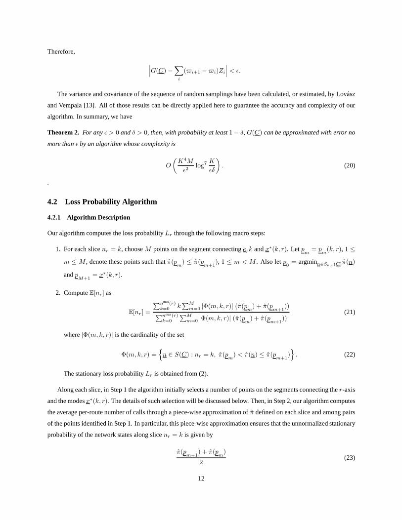
the average per-route number of calls through a piece-wise approximation ofπ defined on each slice and among pairs
of the points identified in Step 1. In particular, this piece-wise approximation ensures that the unnormalized stationary
probability of the network states along slicenr = k is given by
π(pm−1
) + π(pm
)
2(23)
12
for all n ∈ Φ(m, k, r), 0 < m ≤ M . The rationale behind approximation (23) is to take the average value between
two piece-wise functions representing an upper and a lower bound ofπ. These bounds are respectively given by
πupper(n) = π(pm
) iff n ∈ Φ(m, k, r) (24)
and
πlower(n) = π(pm−1
) iff n ∈ Φ(m, k, r). (25)
For a two-route network and a given slice, Figure 1 depicts anexample of such piece-wise functions with respect to the
continuous representation ofπ and assumingM = 2. With approximation (23), several pointsn ∈ S(C) are charac-
π(p1)
π(p2)
p1 p2
πupper
πlower
Figure 1: Graphical representation ofπlower andπupperin the single-route case.
terized by the same value of (23) (see, e.g., Figure 1) and these are captured by the cardinalities of the setsΦ(m, k, r).
In fact, these sets can be interpreted as the inverse images of π associated with the subsets[π(pm
), π(pm+1
)]. For-
mula (21) is then obtained by the exact definition ofE[nr], which can be expressed as
E[nr] =
∑nmax(r)k=0 k
∑
n∈Sk,r(C) π(n)∑nmax(r)
k=0
∑
n∈Sk,r(C) π(n), (26)
and grouping together all statesn having the same value of (23). This allows us to significantlyspeed up the compu-
tation of (26).
We now focus on two remaining issues concerning our algorithm, with the first being the selection of the pointsp1, . . . , p
M.
The simplest approach one can choose is to distribute the points on such segments in a balanced manner, i.e., choosing
the points
m · x∗(k, r)
M + 1, (27)
13
1 ≤ m ≤ M . Given that the structure of the polytopeSk,r(C) is in general different fromSk+1,r(C), even the
arrangement of points at different slices are different. Such arrangements are efficient and in the experimental results
section we show that they yield very accurate results.
The second issue is the computation of the number of elementsin Φ(m, k, r). By the same arguments as those
in Section 4.1, such a task can be achieved with high accuracyby computing the volume of the body defined by
Φ(m, k, r). To determine the volume ofΦ(m, k, r), we again exploit the randomized algorithm of Lovasz and Vempala
[13] which computes the volume of convex bodies in polynomial time and within a given precision threshold. However,
Φ(m, k, r) is in general not convex and, thus, we solve this issue with auxiliary sets.
For router, slicenr = k and pointpm
, consider the set
Φ′(m, k, r) ={
n ∈ S(C) : nr = k, π(pm
) < π(n)}
. (28)
The following relations are straightforward:
Φ(m, k, r) = Φ′(m, k, r) \ Φ′(m + 1, k, r), 0 ≤ m < M ; (29)
Φ(M, k, r) = Φ′(M, k, r). (30)
We further note that all setsΦ′(m, k, r) are convex because they represent the inner points of contours of π, and
Φ′(m+1, k, r) ⊆ Φ′(m, k, r) for eachm = 0, . . . , M−1. Hence, to compute the volume ofΦ(m, k, r), 0 ≤ m ≤ M ,
we first compute the volume ofΦ′(m, k, r) and then we exploit relations (29) and (30).
Once again, adapting the algorithm in [13], the volume ofΦ′(m, k, r) can be approximated within a relative error
of ǫ with probability at least1 − δ and with (polynomial) computational complexity
O
(
K4M
ǫ2log7 K
ǫδ
)
. (31)
4.2.2 Analysis of the Algorithm
Computational Complexity
In summary, for anyǫ > 0 andδ > 0, to obtain the stationary loss probabilities of all routes within a relative error of
ǫ with probability at least1 − δ, the computational complexity of our contour method is
O
K∑
r=1
nmax(r)∑
k=0
[T (x∗(k, r)) + T (Φ(0, k, r), ..., Φ(M, k, r))]
(32)
whereT (x∗(k, r)) is the cost of computing the modex∗(k, r) andT (Φ(0, k, r), ..., Φ(M, k, r)) is the cost of comput-
ing the cardinalities for the vector(Φ(0, k, r), ..., Φ(M, k, r)) with the randomized algorithm. Thus, the computational
requirement is polynomial with respect to the input parameters.
14
Error Analysis
Another source of error of the algorithm comes from the selection of M andp1, . . . , pM . It is evident that the approx-
imation (23) converges toπ (in the continuous case) whenM → ∞. Hence, the choice of whichM must be used is
related to the computational costs that we are willing to incur to solve SLN models. We now explicitly compute such
costs. In what follows, we establish error bounds for the contour method as a function of the number of pointsM to
distribute on each slice. From this error bound, we can conclude that the error decays exponentially asM grows.
Let us consider the unnormalized distributionπ in the continuous case. From its definition, we know that there are
positive constantsc1 andc2 determined only byS(C) andνr such that
c1 ≤ dπ
dx≤ c2, (33)
i.e., the likelihood ratio betweenπ and the Lebesgue measure is bounded from below and above. Since the approxima-
tion (23) converges toπ asM → ∞, the error of the contour method approaches zero asM → ∞ (in the continuous
case). We now evaluate the rate of such convergence.
Within slicenr = k, let
Errk,r(M) =
∣
∣
∣
∣
∣
∫
Sk,r(C)
1
2(πupper(x) + πlower(x)) − π(x) dx
∣
∣
∣
∣
∣
(34)
be the error of the proposed piece-wise approximation whereπupperandπlower are given by (24) and (25). Given that
the average distance betweenπ(x) and (23) is never greater than the distance betweenπupper(x) andπlower(x) (see,
for instance, Figure 1), we must have
Errk,r(M) ≤ G+k,r(M) − G−
k,r(M) = Err∗k,r(M), (35)
where
G+k,r(M) =
∫
Sk,r(C)
πupper(x) dx =
M∑
m=1
|Φ(m, k, r)|π(pm
), (36)
G−k,r(M) =
∫
Sk,r(C)
πlower(x) dx =
M∑
m=1
|Φ(m, k, r)|π(pm−1
). (37)
We now focus on Err∗k,r(M) to determine its rate of convergence asM increases.
It is easy to see from (33) that
|Φ(m, k, r)| ≈ αm1
M + 1. (38)
15

Hence, we have
Err∗k,r(M) ≤ maxm≤M∗
αm
M
M∗
∑
m=0
π(pm+1
) − π(pm
) + minm>M∗
αm
M
M−1∑
m=M∗+1
π(pm+1
) − π(pm
)
= O(
maxm
π(pm+1
) − π(pm
))
= O
(
maxm
∏
r
νpmr+βr/Mr
(pmr + βr/M)!− νpmr
r
pmr!
)
= O
(
maxm
∏
r
νpmrr
pmr!
(
νβr/Mr
pmr!
(pmr − βr/M)!− 1
)
)
≈ O
(
∏
r
(νβr/Mr − 1)
)
(39)
whereβr = x∗r(k, r)/(M + 1) is obtained from (27) andM∗ is such thatπ(p
M∗+1)− π(p
M∗) ≥ 0 andπ(p
M∗+2)−
π(pM∗+1
) < 0 if it exists, otherwise it isM . This means that the error on each slice approaches zero exponentially.
5 Experimental Results
In this section, we numerically assess the accuracy of the refined slice method and of both contour methods. Our
approximations are validated against exact solutions, andthe refined slice method is also compared with the 3-point
slice method [6]. Numerical results are presented relativeto two different sets of experiments: first, we perform a
validation against a small canonical network to emphasize the fundamental properties of the proposed solutions, and
then we focus on a wide test-bed of randomly generated modelsto assess the general quality of the relative error
percentages.
5.1 A Canonical Network
Consider first a small network characterized by
A =
1 01 10 1
, C =
575
, (40)
i.e., link 2 is shared by both routes while links1 and3 are dedicated to route1 and2, respectively. Without loss of
generality, we focus on the average number of calls of route1, i.e.,E[n1]. To quantify the benefits of the refined slice
method, we consider the following cases for the value ofν:
• Stress case 1: ν /∈ S(C) andx∗1 6= x∗
1(0, 1), e.g.,ν = (6, 8);
• Stress case 2: ν ∈ S(C) andx∗1 6= x∗
1(nmax(1), 1), e.g.,ν = (1, 5).
Note that for an evaluation of two-route networks, these classes of values ofν suffice since outside this load region the
3-point slice method and the refined slice method are identical.
16
1 3 5 7 9 11 13 15 17 190
1
2
3
4
5
6
7
8
9
10
N
Pe
rce
nta
ge
re
lative
err
or
(%)
3−point slice methodRefined slice method
(a)
1 3 5 7 9 11 13 15 17 190
1
2
3
4
5
6
7
N
Pe
rce
nta
ge
re
lative
err
or
(%)
3−point slice methodRefined slice method
(b)
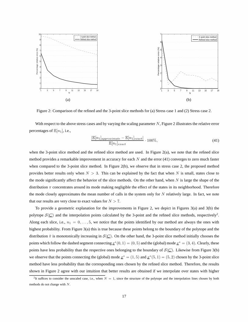
Figure 2: Comparison of the refined and the 3-point slice methods for (a) Stress case 1 and (2) Stress case 2.
With respect to the above stress cases and by varying the scaling parameterN , Figure 2 illustrates the relative error
percentages ofE[n1], i.e.,
|E[n1]approximate − E[n1]exact|E[n1]exact
· 100%, (41)
when the 3-point slice method and the refined slice method areused. In Figure 2(a), we note that the refined slice
method provides a remarkable improvement in accuracy for eachN and the error (41) converges to zero much faster
when compared to the 3-point slice method. In Figure 2(b), weobserve that in stress case 2, the proposed method
provides better results only whenN > 3. This can be explained by the fact that whenN is small, states close to
the mode significantly affect the behavior of the slice methods. On the other hand, whenN is large the shape of the
distributionπ concentrates around its mode making negligible the effect of the states in its neighborhood. Therefore
the mode closely approximates the mean number of calls in thesystem only forN relatively large. In fact, we note
that our results are very close to exact values forN > 7.
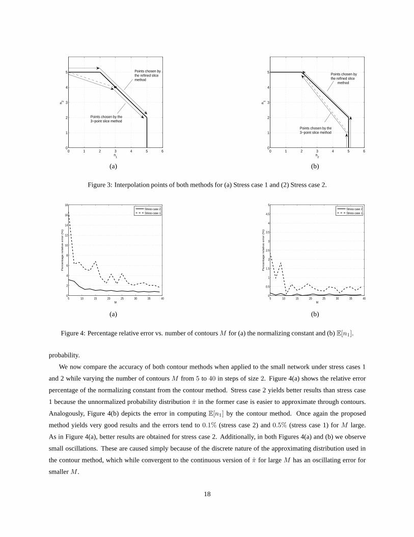
To provide a geometric explanation for the improvements in Figure 2, we depict in Figures 3(a) and 3(b) the
polytopeS(C) and the interpolation points calculated by the 3-point and the refined slice methods, respectively2.
Along each slice, i.e.,n1 = 0, . . . , 5, we notice that the points identified by our method are alwaysthe ones with
highest probability. From Figure 3(a) this is true because these points belong to the boundary of the polytope and the
distributionπ is monotonically increasing inS(C). On the other hand, the 3-point slice method initially chooses the
points which follow the dashed segment connectingx∗(0, 1) = (0, 5) and the (global) modex∗ = (3, 4). Clearly, these
points have less probability than the respective ones belonging to the boundary ofS(C). Likewise from Figure 3(b)
we observe that the points connecting the (global) modex∗ = (1, 5) andx∗(5, 1) = (5, 2) chosen by the 3-point slice
method have less probability than the corresponding ones chosen by the refined slice method. Therefore, the results
shown in Figure 2 agree with our intuition that better results are obtained if we interpolate over states with higher
2It suffices to consider the unscaled case, i.e., whenN = 1, since the structure of the polytope and the interpolation lines chosen by both
methods do not change withN .
17
0 1 2 3 4 5 60
1
2
3
4
5
n1
n2
Points chosen by the3−point slice method
Points chosen bythe refined slicemethod
(a)
0 1 2 3 4 5 60
1
2
3
4
5
n2
n1
Points chosen by the3−point slice method
Points chosen bythe refined slice method
(b)
Figure 3: Interpolation points of both methods for (a) Stress case 1 and (2) Stress case 2.
5 10 15 20 25 30 35 400
2
4
6
8
10
12
14
16
18
M
Pe
rce
nta
ge
re
lative
err
or
(%)
Stress case 2Stress case 1
(a)
5 10 15 20 25 30 35 400
0.5
1
1.5
2
2.5
3
3.5
4
4.5
5
M
Pe
rce
nta
ge
re
lative
err
or
(%)
Stress case 2Stress case 1
(b)
Figure 4: Percentage relative error vs. number of contoursM for (a) the normalizing constant and (b)E[n1].
probability.
We now compare the accuracy of both contour methods when applied to the small network under stress cases 1
and 2 while varying the number of contoursM from 5 to 40 in steps of size2. Figure 4(a) shows the relative error
percentage of the normalizing constant from the contour method. Stress case 2 yields better results than stress case
1 because the unnormalized probability distributionπ in the former case is easier to approximate through contours.
Analogously, Figure 4(b) depicts the error in computingE[n1] by the contour method. Once again the proposed
method yields very good results and the errors tend to0.1% (stress case 2) and0.5% (stress case 1) forM large.
As in Figure 4(a), better results are obtained for stress case 2. Additionally, in both Figures 4(a) and (b) we observe
small oscillations. These are caused simply because of the discrete nature of the approximating distribution used in
the contour method, which while convergent to the continuous version ofπ for largeM has an oscillating error for
smallerM .
18

0.5 1 1.5 2 2.5 50
1
2
3
4
5
6
7
8
9
10
N
Per
cent
age
rela
tive
erro
r (%
)
3−point slice methodRefined slice method
Figure 5: Comparison between the error in computingE[n1] for the refined and the 3-point slice methods.
5.2 Random Models
To assess the accuracy of the proposed methods in a more general setting, we consider a test-bed of thousands of
randomly-generated models larger than the canonical example discussed in the previous section. The input parameters
used to validate our methods are shown in Table 1. We compare the quality of the refined slice method and of both
IntervalNumber of routes {2, 3, 4}Number of links {3, . . . , 10}Links capacities {20, . . . , 50}Arrival rates [1, 50]
Table 1: Input parameters used in the validation.
contour methods with the exact results which we obtain by brute-force enumeration over the set of feasible states, i.e.,
S(C), for each random model. We do not consider networks with larger capacities or a larger number of routes because
of the prohibitively expensive computational effort required to obtain the exact solution and the consequent cost of
calculating robust accuracy results for the large number oftest cases. Further, we consider only random instances such
that no single link simultaneously limits the maximum number of calls onall routes. In fact, in this particular case the
normalizing constant admits a very efficient expression by means of Newton’s multinomial theorem.
In Figure 5 we compare the accuracies of the refined and 3-point slice methods for different values of the scaling
parameterN = 0.5, . . . , 2.5 in steps of size0.5 and, to emphasize the trend of the slice methods, forN = 5. Each
point in the graphs of Figure 5 represents the average of the errors (41) over 3,000 models. Even though the errors of
both methods are small and converge to zero asN increases, we observe that the refined slice method providesmore
accurate results for eachN . In the worst case, i.e.,N = 0.5, our results have an average error of2.2%.
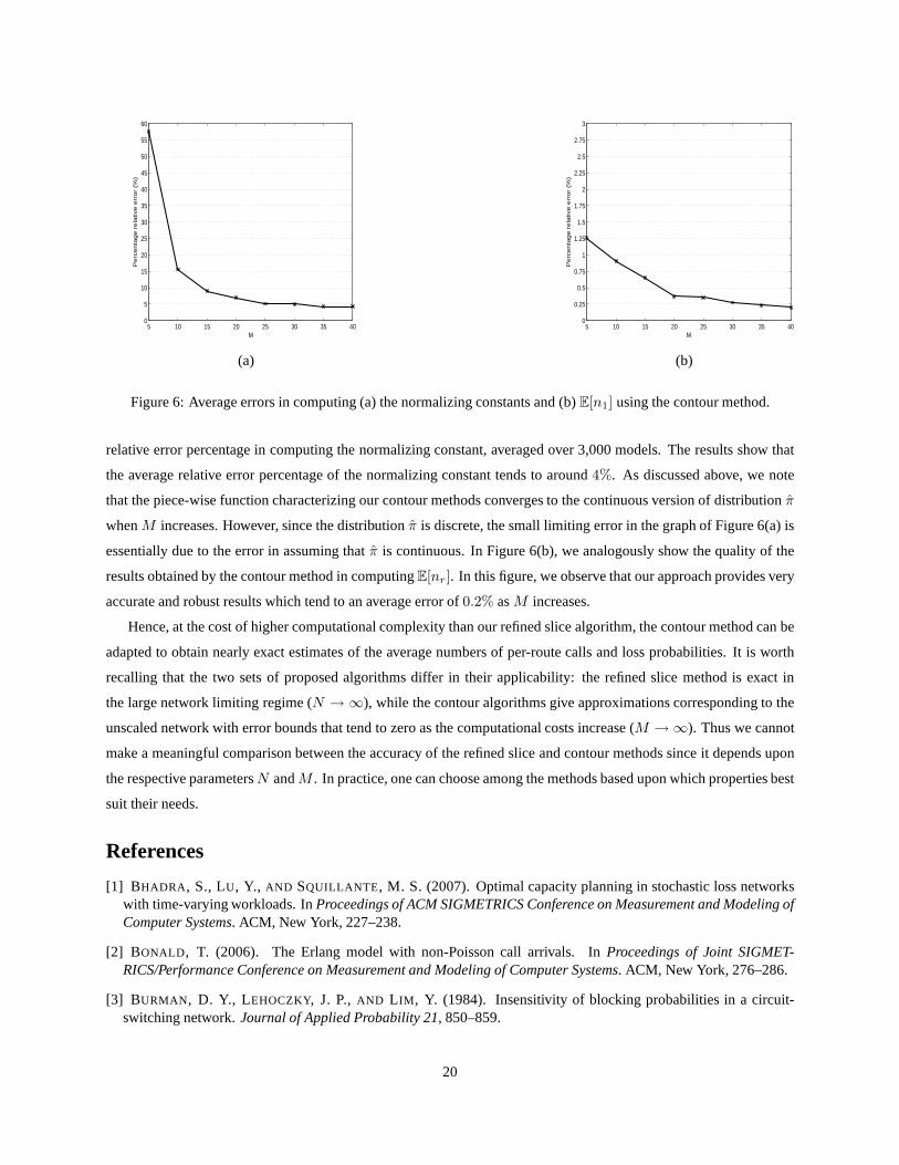
In Figure 6(a), we show the quality of the results obtained bythe contour method which computes the normalizing
constant by varying the number of contoursM from 5 to 40 in steps of size5. In the figure, each point represents the
19
5 10 15 20 25 30 35 400
5
10
15
20
25
30
35
40
45
50
55
60
M
Pe
rce
nta
ge
re
lative
err
or
(%)
(a)
5 10 15 20 25 30 35 400
0.25
0.5
0.75
1
1.25
1.5
1.75
2
2.25
2.5
2.75
3
M
Pe
rce
nta
ge
re
lative
err
or
(%)
(b)
Figure 6: Average errors in computing (a) the normalizing constants and (b)E[n1] using the contour method.
relative error percentage in computing the normalizing constant, averaged over 3,000 models. The results show that
the average relative error percentage of the normalizing constant tends to around4%. As discussed above, we note
that the piece-wise function characterizing our contour methods converges to the continuous version of distributionπ
whenM increases. However, since the distributionπ is discrete, the small limiting error in the graph of Figure 6(a) is
essentially due to the error in assuming thatπ is continuous. In Figure 6(b), we analogously show the quality of the
results obtained by the contour method in computingE[nr]. In this figure, we observe that our approach provides very
accurate and robust results which tend to an average error of0.2% asM increases.
Hence, at the cost of higher computational complexity than our refined slice algorithm, the contour method can be
adapted to obtain nearly exact estimates of the average numbers of per-route calls and loss probabilities. It is worth
recalling that the two sets of proposed algorithms differ intheir applicability: the refined slice method is exact in
the large network limiting regime (N → ∞), while the contour algorithms give approximations corresponding to the
unscaled network with error bounds that tend to zero as the computational costs increase (M → ∞). Thus we cannot
make a meaningful comparison between the accuracy of the refined slice and contour methods since it depends upon
the respective parametersN andM . In practice, one can choose among the methods based upon which properties best
suit their needs.
References
[1] BHADRA , S., LU, Y., AND SQUILLANTE , M. S. (2007). Optimal capacity planning in stochastic lossnetworkswith time-varying workloads. InProceedings of ACM SIGMETRICS Conference on Measurement and Modeling ofComputer Systems. ACM, New York, 227–238.
[2] BONALD , T. (2006). The Erlang model with non-Poisson call arrivals. In Proceedings of Joint SIGMET-RICS/Performance Conference on Measurement and Modeling of Computer Systems. ACM, New York, 276–286.
[3] BURMAN , D. Y., LEHOCZKY, J. P.,AND L IM , Y. (1984). Insensitivity of blocking probabilities in a circuit-switching network.Journal of Applied Probability 21, 850–859.
20

[4] ERLANG, A. K. (1948). Solution of some problems in the theory of probabilities of significance in automatictelephone exchanges. InThe Life and Works of A. K. Erlang, E. Brockmeyer, H. L. Halstrom, and A. Jensen, Eds.Academy of Technical Sciences, Copenhagen. Paper first published in 1917.
[5] HUNT, P. J.AND KELLY, F. P. (1989). On critically loaded loss networks.Advances in Applied Probability21, 4,831–841.
[6] JUNG, K., LU, Y., SHAH , D., SHARMA , M., AND SQUILLANTE , M. S. (2008). Revisiting stochastic lossnetworks: Structures and algorithms. InProceedings of ACM SIGMETRICS Conference on Measurement andModeling of Computer Systems. ACM, New York, 407–418.
[7] K ELLY, F. P. (1985). Stochastic models of computer communicationsystems.Journal of the Royal StatisticalSociety, Series B 47, 379–395.
[8] K ELLY, F. P. (1986). Blocking probabilities in large circuit-switched networks.Advances in Applied Probabil-ity 18, 2, 473–505.
[9] K ELLY, F. P. (1988). Routing in circuit-switched networks: Optimization, shadow prices and decentralization.Advances in Applied Probability20, 1, 112–144.
[10] KELLY, F. P. (1991). Loss networks.Annals of Applied Probability1, 3, 319–378.
[11] L ITTLE , J. D. C. (1961). A proof of the queuing formulaL = λW . Operations Research 9, 383–387.
[12] LOUTH, G., MITZENMACHER, M., AND KELLY, F. (1994). Computational complexity of loss networks.Theo-retical Computer Science125, 1, 45–59.
[13] LOVASZ, L. AND VEMPALA , S. (2006). Simulated annealing in convex bodies and an O*(n4) volume algorithm.Journal of Computer and System Sciences72, 2, 392–417.
[14] LU, Y., RADOVANOVI C, A., AND SQUILLANTE , M. S. (2007). Optimal capacity planning in stochastic lossnetworks.Performance Evaluation Review35, 2.
[15] M ITRA , D., MORRISON, J. A.,AND RAMAKRISHNAN , K. G. (1996). ATM network design and optimization:A multirate loss network framework.IEEE/ACM Transactions on Networking4, 4, 531–543.
[16] M ITRA , D. AND WEINBERGER, P. J. (1984). Probabilistic models of database locking: Solutions, computa-tional algorithms and asymptotics.Journal of the ACM 31, 855–878.
[17] MOMCILOVIC , P.AND SQUILLANTE , M. S. (2008). On throughput in linear wireless networks. InProceedingsof ACM Symposium on Mobile Ad Hoc Networking and Computing. ACM, New York.
[18] ROSS, K. W. (1995).Multiservice Loss Models for Broadband TelecommunicationNetworks. Springer-Verlag,New York.
[19] SEVASTYANOV, B. A. (1957). An ergodic theorem for Markov processes and its application to telephone systemswith refusals.Theoretical Probability Applications 2, 104–112.
[20] VALIANT , L. (1979). The complexity of computing the permanent.Theoretical Computer Science 8, 189–201.
[21] WHITT, W. (1985). Blocking when service is required from several facilities simultaneously.AT&T Bell Labo-ratories Technical Journal64, 8, 1807–1856.
[22] XU, S., SONG, J. S.,AND L IU , B. (1999). Order fulfillment performance measures in an assemble-to-ordersystem with stochastic leadtime.Operations Research47, 1, 131–149.
21