Embed Size (px)
Citation preview

IMPRECISION IN ENGINEERING DESIGN


IMPRECISION IN ENGINEERING DESIGN
Edited by
ERIK K. ANTONSSON, Ph.D., P.E.Executive Officer and Professor of Mechanical Engineering
Engineering Design Research LaboratoryDivision of Engineering & Applied ScienceCalifornia Institute of TechnologyPasadena, California, U.S.A.
Erik K. Antonsson, Ph.D., P.E.
Reference as:
Antonsson, Erik K., ed. (2001) Imprecision in Engineering Design. Engineer-ing Design Research Laboratory, Division of Engineering and Applied Science,California Institute of Technology, Pasadena, California 91125-4400, U.S.A.
Any opinions, findings, conclusions, or recommendations expressed in this pub-lication are those of the author(s) and do not necessarily reflect the views ofthe sponsor(s) or the California Institute of Technology.
Copyright c© 2001 by Erik K. Antonsson
All rights reserved. No part of this publication may be reproduced, stored ina retrieval system or transmitted in any form or by any means, mechanical,photocopying, recording, or otherwise, without the prior written permissionof the publisher, Erik K. Antonsson, 1200 E. California Blvd., Pasadena, CA91125-4400
Printed on acid-free paper.Formatted in LATEX2e using Times-Roman fonts.
Printed in the United States of America
Distributed by:
Engineering Design Research LaboratoryDepartment of Mechanical EngineeringDivision of Engineering and Applied ScienceCalifornia Institute of Technology1200 East California BoulevardPasadena, California 91125-4400U.S.A.
Contents
Preface viiNiccolo Machiavelli
Dedication ixAlbert Einstein
Contributing Authors ix
Introduction xiErik Antonsson
1Computations with Imprecise Parameters in Engineering Design:
Background and Theory1
Kristin L. Wood and Erik K. Antonsson
2Trade-Off Strategies in Engineering Design 31Kevin N. Otto and Erik K. Antonsson
3Design Parameter Selection in the Presence of Noise 65Kevin N. Otto and Erik K. Antonsson
4Tuning Parameters in Engineering Design 99Kevin N. Otto and Erik K. Antonsson
5Imprecision in Engineering Design 115Erik K. Antonsson and Kevin N. Otto
v
vi IMPRECISION IN ENGINEERING DESIGN
6Aggregation Functions For Engineering Design Trade-offs 139Michael J. Scott and Erik K. Antonsson
7Formalisms for Negotiation in Engineering Design 165Michael J. Scott and Erik K. Antonsson
8Preliminary Vehicle Structure Design Application 183Michael J. Scott and Erik K. Antonsson
9Arrow’s Theorem and Engineering Design Decision Making 205Michael J. Scott and Erik K. Antonsson
10Using Indifference Points in Engineering Decisions 225Michael J. Scott and Erik K. Antonsson

Preface
It must be considered that there is nothing more difficult to carry out, nor moredangerous to conduct, nor more doubtful in its success, than an attempt tointroduce changes. For the innovator will have for his enemies all those whoare well off under the existing order of things, and only lukewarm supportersin those who might be better off under the new.
-- NICCOLO MACHIAVELLI
THE PRINCE AND THE DISCOURSES, 1513CHAPTER 6
vii

“Scientists investigatethat which already is;
Engineers create thatwhich has never been.”
Albert Einstein

Contributing Authors
Erik K. Antonsson is Professor and Executive Officer (Dept. Chair) of Me-chanical Engineering at the California Institute of Technology in Pasadena,CA, U.S.A., where he founded and supervises the Engineering Design ResearchLaboratory, and has been a member of the faculty since 1984.
William S. Law is an employee of Function, Palo Alto, California, U.S.A.
Kevin N. Otto is an Associate Professor of Mechanical Engineering at theMassachusetts Institute of Technology, Cambridge, Massachusetts, U.S.A.
Michael J. Scott is an Assistant Professor of Mechanical Engineering at theUniversity of Illinois, Chicago, Illinois, U.S.A.
Kristin L. Wood is a Professor of Mechanical Engineering at the University ofTexas, Austin, Texas, U.S.A.
ix

IntroductionErik Antonsson
T his book is a collection of publications produced from research con-ducted in the Engineering Design Research Laboratory at the Califor-nia Institute of Technology. The research thread, to which all of these
papers are related, is the notion of Imprecision in Engineering Design.Research over the past 17 years has demonstrated that information with a
range of precisions is an essential component of engineering design, and thatformal methods can be developed to represent and manipulate this impreciseinformation. The goal of this volume is to collect into one place a set of relevantpublications describing the results of research in this area.
The ChaptersThis volume begins with a chapter introducing the notion of imprecision
in engineering design, and motivating the research to follow. Chapter 2 in-troduces strategies for trade-offs among multiple incommensurate attributes ofengineering designs. Chapter 3 introduces a method for incorporating uncon-trolled variations (noise) into design decision-making. Chapter 4 extends thenotion of noise to include tuning parameters: those aspects of a design thatare adjusted to compensate for uncontrolled variations. Chapter 5 providesan overview of the Method of Imprecision, and a review of and comparisonwith other methods. Chapter 6 develops the mathematics of aggregation ofincommensurate attributes for design decisions. Chapter 7 extends the aggre-gation methods to negotiation among multiple people or groups involved in anengineering design. Chapter 8 demonstrates the Method of Imprecision on anautomobile structure design problem. Chapter 9 shows that methods for eco-nomic decision-making or social choice do not necessarily apply to engineeringdesign. Finally, Chapter 10 presents a method for determining how to aggregatemultiple incommensurate attributes of an engineering design.
xi

xii IMPRECISION IN ENGINEERING DESIGN
References
[1] WOOD, K. L., AND ANTONSSON, E. K. Computations with Impre-cise Parameters in Engineering Design: Background and Theory.ASMEJournal of Mechanisms, Transmissions, and Automation in Design 111, 4(Dec. 1989), 616–625.
[2] OTTO, K. N., AND ANTONSSON, E. K. Trade-Off Strategies in Engi-neering Design.Research in Engineering Design 3, 2 (1991), 87–104.
[3] OTTO, K. N., AND ANTONSSON, E. K. Design Parameter Selection inthe Presence of Noise.Research in Engineering Design 6, 4 (1994), 234–246.
[4] OTTO, K. N., AND ANTONSSON, E. K. Tuning Parameters in Engineer-ing Design. ASME Journal of Mechanical Design 115, 1 (Mar. 1993),14–19.
[5] A NTONSSON, E. K., AND OTTO, K. N. Imprecision in Engineering De-sign. ASME Journal of Mechanical Design 117(B) (Special CombinedIssue of the Transactions of the ASME commemorating the 50th anniver-sary of the Design Engineering Division of the ASME.)(June 1995), 25–32. Invited paper.
[6] SCOTT, M. J., AND ANTONSSON, E. K. Aggregation Functions for En-gineering Design Trade-offs.Fuzzy Sets and Systems 99, 3 (1998), 253–264.
[7] SCOTT, M. J., AND ANTONSSON, E. K. Formalisms for Negotiation inEngineering Design. In8th International Conference on Design Theoryand Methodology(Aug. 1996), ASME.
[8] SCOTT, M. J., AND ANTONSSON, E. K. Preliminary Vehicle StructureDesign: An Industrial Application of Imprecision in Engineering Design.In 10th International Conference on Design Theory and Methodology(Sept. 1998), ASME.
[9] SCOTT, M. J., AND ANTONSSON, E. K. Arrow’s Theorem and Engi-neering Design Decision Making.Research in Engineering Design 11, 4(2000), 218–228.
[10] SCOTT, M. J., AND ANTONSSON, E. K. Using Indifference Points inEngineering Decisions. In11th International Conference on Design The-ory and Methodology(Sept. 2000), ASME.

INTRODUCTION xiii
Erik K. Antonsson is Executive Officer (Dept. Chair) and Professor of Me-chanical Engineering at the California Institute of Technology in Pasadena,CA, U.S.A., where he organized the Engineering Design Research Labora-tory and has conducted research and taught since 1984.
He earned a B.S. degree in Mechanical Engineering with distinction fromCornell University in 1976, and a Ph.D. in Mechanical Engineering fromMassachusetts Institute of Technology in 1982 under the supervision of Prof.Robert W. Mann.
In 1983 he joined the Mechanical Engineering faculty at the University of Utah, as an Assis-tant Professor. In 1984 he became the Technical Director of the Pediatric Mobility and GaitLaboratory, and an Assistant in Bioengineering (Orthopaedic Surgery), at the MassachusettsGeneral Hospital. He also simultaneously joined the faculty of the Harvard University MedicalSchool as an Assistant Professor of Orthopaedics (Bioengineering).
He was an NSF Presidential Young Investigator from 1986 to 1992, and won the 1995 RichardP. Feynman Prize for Excellence in Teaching.
Dr. Antonsson is a Fellow of the ASME, and a member of the IEEE, SME, ACM, ASEE,IFSA, and NAFIPS.
He teaches courses in engineering design, computer aided engineering design, machine de-sign, mechanical systems, and kinematics. His research interests include formal methods forengineering design, design synthesis, representing and manipulating imprecision in preliminaryengineering design, rapid assessment of early designs (RAED), structured design synthesis ofmicro-electro-mechanical systems (MEMS), and digital micropropulsion microthrusters.
Dr. Antonsson is currently on the editorial board of the International Journals:Research in En-gineering Design, andFuzzy Sets and Systems, and from 1989 to 1993 served as an AssociateTechnical Editor of the ASME Journal of Mechanical Design, (formerly theJournal of Mech-anisms, Transmissions and Automation in Design), with responsibility for the Design Researchand the Design Theory and Methodology area. He serves as a member of the Engineering andApplied Science Division Advisory Group, and as Chairman of the Engineering ComputingFacility at Caltech. He was a member of the Caltech Faculty Committee on Patents and Rela-tions with Industry from 1992 to 1999, and since 1990 has been a member of the CALSTARTTechnical Advisory Committee. He has published over 95 scholarly papers in the engineeringdesign research literature, and holds 4 U.S. Patents. He is a Registered Professional Engineerin California, and serves as an engineering design consultant to industry, research laboratories(including NASA’s Jet Propulsion Laboratory and the 10 meter W. M. Keck Telescope), and theIntellectual Property bar.

Chapter 1
COMPUTATIONS WITHIMPRECISE PARAMETERS INENGINEERING DESIGN:BACKGROUND AND THEORY
Kristin L. Wood and Erik K. Antonsson
ASME Journal of Mechanisms, Transmissions, and Automation in DesignVolume 111, Number 4 (December 1989), pages 616-625.
AbstractA technique to perform design calculations on imprecise representations of
parameters has been developed and is presented. The level of imprecision inthe description of design elements is typically high in the preliminary phaseof engineering design. This imprecision is represented using the fuzzy calcu-lus. Calculations can be performed using this method, to produce (imprecise)performance parameters from imprecise (input) design parameters. The FuzzyWeighted Average technique is used to perform these calculations. A new met-ric, called theγ-level measure, is introduced to determine the relative couplingbetween imprecise inputs and outputs. The background and theory supportingthis approach are presented, along with one example.
1. IntroductionEngineering design, both in practice and research, is evolving rapidly, espe-
cially in the development of computer-based tools. Emphasis is moving fromthe later stages of design, to computational tools for preliminary design. Inan earlier paper [33], a general approach to computational tools in preliminaryengineering design and a model of the design process was described. The pri-mary aim of this model is to provide a structure for the development of tools toassist the designer in: managing the large amount of information encounteredin the design process; determining a design’s functional requirements and con-
1
2 IMPRECISION IN ENGINEERING DESIGN
straints; evaluating the coupling between the design parameters; and carryingout the process of choosing between alternative design concepts.
We are particularly interested in developing tools to assist the designer in thepreliminary phase of engineering design, by making more information avail-able on the performance of design alternatives than is available using conven-tional design techniques. The most important design decisions (and potentiallythe most costly, if wrong) are made at the preliminary stage. Our hypothesis isthat increased information, over what is available by traditional design meth-ods, will enable these decisions to be made with greater confidence and re-duced risk. The effect will be greater, the earlier in the design cycle additionalinformation can be made available.
The preliminary phase of the engineering design process is one that em-bodies many functions: concept generation; evaluation of imprecise descrip-tions of simplified versions of the design; judgement of design feasibility;etc. [26, 15, 28]. The concept generation and simplification processes willnot be addressed by the research reported here, rather our aim is to provide atechnique for representing, manipulating, and evaluating the approximate, orimprecise, parametric descriptions of the (preliminary) design artifact.
Typical examples of imprecise descriptions in preliminary design include:an irregular cross-section structural member may be represented by a rectangu-lar section for the purposes of initial evaluation; a gear set may be representedby a pair of circles rolling on each other (without slip), and an approximatespeed ratio; a length of shaft may be represented as “about 25 cm”; etc. Theseare approximate, orimprecise, descriptions of the design artifact, not incom-plete descriptions. The gear set, imprecisely represented above, has all of thefunctionalattributes of a gear set, but none of the detail.
As the design process proceeds from the preliminary stage to more detaileddesign and analysis, the level of imprecision in the description of the designartifact is reduced. Naturally at the end of the design cycle, the level of impre-cision is very small, although uncertainties (e.g., tolerances) remain. It is thisspectrum of levels of precision that characterizes progress through the designprocess, from a description of a need, to a (precise) description of a device tofulfill that need.
Unfortunately it has been difficult to provide computational tools for the pre-liminary phase of the design process, largely because of the relative paucity ofalgorithms and techniques that can operate on imprecise data. Solid modeling,optimization, mechanism analysis, and other CAD methods all require a highlyprecise representation of the objects being designed. This paper presents anovel (to the engineering design process) application of a method for represent-
Computations with Imprecise Parameters in Engineering Design 3
ing and manipulating imprecision.1 This technique calculates the approximateoutput quantities from the imprecise input parameters for each of the designalternatives, and determines the qualitative relations between the input param-eters and the performance parameters (outputs). The designer is able to rankthe input parameters according to their impact on the performance parameters,and to rate a design alternative according to its merit in relation to the othersunder consideration.
These computational tools are for use in the preliminary and conceptual syn-thesis stages of design, but do not attempt to supplant the designer. The ideais not to fully automate the design process, nor to automatically generate de-sign alternatives, rather it is to make it easier for the designer to evaluate morealternatives in less time, and to provide more information on the performanceof each of those alternatives. These developments form asemi-automatedap-proach to design.
Terminology used to describe the design process will be defined first, back-ground and theory as it is applied to engineering design will be presented next,followed by an example.
2. Terminology
2.1 Design DefinitionsParameter: A variable or quantity used in the design process.
Design Parameter [DP]: Any free or independent parameter whose value isdetermined during the design process.(synonyms: Design Variable, Input Parameter).
Performance Parameter [PP]: Any parameter used in the design process thathas a specified value [FR] determined independent of (and usually in ad-vance of) the design process. The performance parameters [PPs] areusually dependent on the design parameters [DPs], and possibly someother PPs.
Output Parameter [OP]: Any parameter used in the design process that isdependent on the design parameters [DPs], and possibly some perfor-mance parameters [PPs], but has no specified functional requirement[FR] value.
Functional Requirement [FR]: A value, or range of values, or fuzzy numberthat is the specified value for a Performance Parameter [PP].
1Fuzzy sets have been applied to other domains including: seismic risk analysis [8, 6, 7, 9, 18], optimiza-tion [13, 29], reliability [24, 37], expert systems [25], logic and decision support [1, 2, 3, 4, 17, 19, 36, 41,39], language and grammar [17, 21, 42], and others.
4 IMPRECISION IN ENGINEERING DESIGN
This value is determined independent of (and usually in advance of) thedesign process. Each Performance Parameter has a FR.(synonyms: Performance Specification, Constraint).(Note that this distinction between the Performance Parameter and itsspecified value [Functional Requirement] is to permit a Performance Pa-rameter not to be identically equal to its specified Functional Require-ment value at all times during the design process.)
Performance Parameter Expression [PPE]:An expression, relationship, orequation relating some or all of the Design Parameters to a PerformanceParameter. Each PP has a PPE.
2.2 Fuzzy Set Implementation DefinitionsSupport: A crisp set of all values of a fuzzy set where the membership is
greater than zero. Alternatively: The range of parameter values overwhich the fuzzy set membership is greater than zero.
Imprecision: The range (support) or spread of values about the peak [prefer-ence of one (1)] of a parameter’s fuzzy set. The greater the imprecision,the greater the spread on the left or right (or both) sides of the preferencefunction. This is loosely analogous to variance in the stochastic sense.2
The interpretation of Imprecision, as used in design, will be discussed inthe next section.
3. BackgroundMost of engineering, particularly design, can best be represented with some
level of imprecision or approximation. According to Goguen [20]:
“Fuzziness is more than the exception in engineering design problems: usuallythere is no well-defined best solution or design.”
The imprecision that is being represented and manipulated by the techniquereported here is meant to capture the approximations made during the earlyphases of engineering design.
2The mathematics of fuzzy sets are different from the mathematics of probability, and we find fuzzinessmore well suited to solvingimprecise(i.e., “uncertainty in choosing among alternatives”) problems in thepreliminary phase of design. Probability continues to be most appropriate for representing and manipulatingthe uncertainty in truthaspects of design problems. A comparison of probabilistic and fuzzy methods indesign will be the subject of a later publication. Many design problems will require both methods.
Computations with Imprecise Parameters in Engineering Design 5
3.1 Representation and Interpretation ofImprecision
A simple range might be used to represent the imprecision for a parame-ter. This is the technique used in interval analysis [27]. Instead of a range,we represent the imprecise parameter by a range and a preference function todescribe the desirability of using that particular value within the range. Thispreference function is similar to the notion of afuzzy set, or more specificallya fuzzy number which is restricted to the set of real numbers.
A fuzzy set(as developed by Zadeh [38]) is a set with boundaries which arenot sharply defined. Membership in the set is not the customary 0 or 1, but canbe described by a continuum of grades of membership. In the approach de-scribed here we use preference values, analogous to membership, to representimprecision or approximation of engineering design parameters. For example,a designer may want to represent a dimension of “about 25 cm”. He or shewould do so by specifying a preference function to represent that approximateparameter.
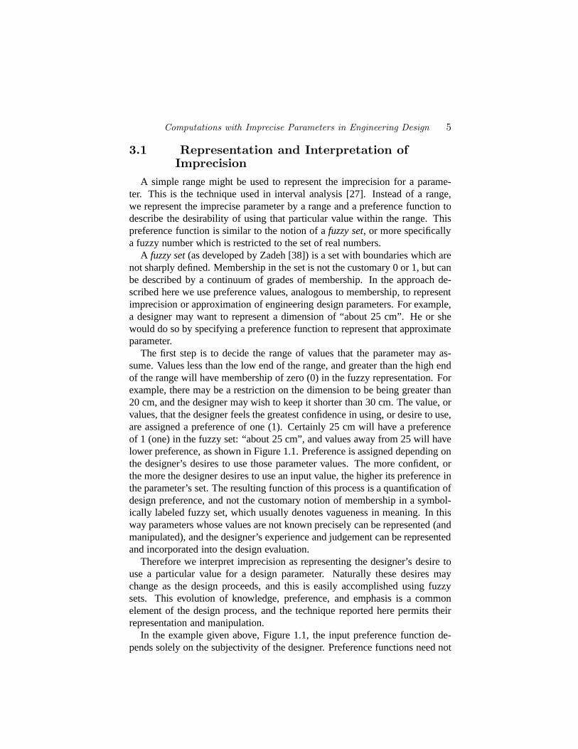
The first step is to decide the range of values that the parameter may as-sume. Values less than the low end of the range, and greater than the high endof the range will have membership of zero (0) in the fuzzy representation. Forexample, there may be a restriction on the dimension to be being greater than20 cm, and the designer may wish to keep it shorter than 30 cm. The value, orvalues, that the designer feels the greatest confidence in using, or desire to use,are assigned a preference of one (1). Certainly 25 cm will have a preferenceof 1 (one) in the fuzzy set: “about 25 cm”, and values away from 25 will havelower preference, as shown in Figure 1.1. Preference is assigned depending onthe designer’s desires to use those parameter values. The more confident, orthe more the designer desires to use an input value, the higher its preference inthe parameter’s set. The resulting function of this process is a quantification ofdesign preference, and not the customary notion of membership in a symbol-ically labeled fuzzy set, which usually denotes vagueness in meaning. In thisway parameters whose values are not known precisely can be represented (andmanipulated), and the designer’s experience and judgement can be representedand incorporated into the design evaluation.
Therefore we interpret imprecision as representing the designer’s desire touse a particular value for a design parameter. Naturally these desires maychange as the design proceeds, and this is easily accomplished using fuzzysets. This evolution of knowledge, preference, and emphasis is a commonelement of the design process, and the technique reported here permits theirrepresentation and manipulation.
In the example given above, Figure 1.1, the input preference function de-pends solely on the subjectivity of the designer. Preference functions need not
6 IMPRECISION IN ENGINEERING DESIGN
15 20 25 30 35
length (cm)
0.0
0.5
1.0
α
.................................................................................................................................................................................................................................................................................................................................................................................................................................................................................................................................................................................................................................................................................................................................................................................
.......................................................................................................................................................................................................................................................................................................................................................................................................................................................................................................................................................................................................................................................................................................................................................................................................................................................................................
............. ............. ............. ............. ............. ............. ............. ............. ............. ............. ............. ............. ............. ............. ............. .........◦ ◦
Figure 1.1 Imprecise Representation of “About 25 cm”,α-cut at 0.5.
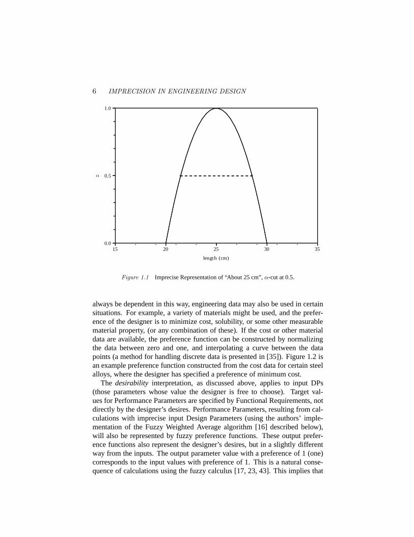
always be dependent in this way, engineering data may also be used in certainsituations. For example, a variety of materials might be used, and the prefer-ence of the designer is to minimize cost, solubility, or some other measurablematerial property, (or any combination of these). If the cost or other materialdata are available, the preference function can be constructed by normalizingthe data between zero and one, and interpolating a curve between the datapoints (a method for handling discrete data is presented in [35]). Figure 1.2 isan example preference function constructed from the cost data for certain steelalloys, where the designer has specified a preference of minimum cost.
The desirability interpretation, as discussed above, applies to input DPs(those parameters whose value the designer is free to choose). Target val-ues for Performance Parameters are specified by Functional Requirements, notdirectly by the designer’s desires. Performance Parameters, resulting from cal-culations with imprecise input Design Parameters (using the authors’ imple-mentation of the Fuzzy Weighted Average algorithm [16] described below),will also be represented by fuzzy preference functions. These output prefer-ence functions also represent the designer’s desires, but in a slightly differentway from the inputs. The output parameter value with a preference of 1 (one)corresponds to the input values with preference of 1. This is a natural conse-quence of calculations using the fuzzy calculus [17, 23, 43]. This implies that
Computations with Imprecise Parameters in Engineering Design 7
0.0 0.5 1.0 1.5
Tensile Strength,St (GPa)
0.0
0.5
1.0
α
.................
.................
.................
.................
.................
.................
.................
.................
.................
.................
.................
.................
.................
.................
.................
.................
.................
.................
.................
.................
.................
.................
.................
.................
.................
.................
.................
.................
.................
.................
.................
.................
.................
.................
.................
.................
.................
.................
.................
.................
.................
.................
.................
.................
.................
.................
.................
...........................................................................................................................................................................................................................................................................................................................................................................................................................................................................................................................................................................................................................................................................................................................................................................................................................................................................................................................................................................................................................................................................................................................................................................................................................
Figure 1.2 Preference Function: Steel Alloy Data
8 IMPRECISION IN ENGINEERING DESIGN
if the designer’s desires are met (inputs with preference of 1), then the perfor-mance will be the output value with preference of 1. Correspondingly, if theperformance parameter output value with preference of 1 satisfies the Func-tional Requirement(s), then the designer can use the input Design Parametervalues with preference of 1. If it is required to use an off-peak value for theperformance (to satisfy a Functional Requirement), then either the designer’sdesires must be adjusted, or input values other than the most desirable must beused. This will be discussed in detail below.
3.2 Existing TechniquesThere exists a variety of means by which imprecise parameters can be rep-
resented and manipulated in engineering design calculations. The most basicapproach is to choose single (crisp, non-fuzzy) values for each of the parame-ters, substitute these into the governing equations, and record the crisp single-valued output. This method benefits from simplicity, but suffers from the timerequired to “explore” any real design space.
Optimization schemes potentially provide a means for handling impreciseparameters. These methods include direct search methods such as Simplex andthree-point equal-interval search, gradient methods such as Newton’s and theConjugate Gradient search [30]. However, conventional optimization methodsrequire precise representations and analyses, and are therefore most useful inthe latter stages of design. A. Diaz [13, 14] is developing an optimization tech-nique using imprecise (fuzzy) constraints. This method will be useful for solv-ing imprecise optimization problems, but will not provide as much informationon the performance of a design operating over a range of design parameters asthe method reported here.
Interval analysis [27] is another method for carrying out computations withimprecise parameters. In this technique an interval (a range of numbers repre-sented by its boundaries) is used to represent a DP in the design calculations.The output (PP) is similarly represented by the two numbers at the end pointsof an interval. This method has some similarity to the method developed bythe authors in that it indicates ranges of possible values for inputs and outputs.Interval analysis, however, provides no information on the performance of adesignwithin the interval. All that can be said, when interpreting a Perfor-mance Parameter output, is that the design will perform somewhere betweenthe boundaries of the interval. Furthermore, the input values which contributedto any one particular value of the output cannot be directly determined (exceptat the boundaries). As the number of intervals used to represent DPs increases(e.g. a succession of decreasing interval sizes may be used to cause a PP toapproach a desired value), interval analysis approaches the method reportedhere.
Computations with Imprecise Parameters in Engineering Design 9
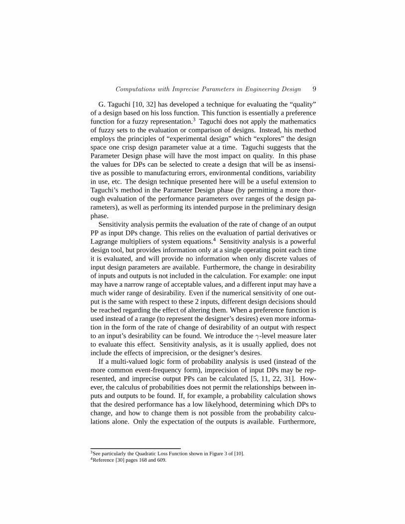
G. Taguchi [10, 32] has developed a technique for evaluating the “quality”of a design based on his loss function. This function is essentially a preferencefunction for a fuzzy representation.3 Taguchi does not apply the mathematicsof fuzzy sets to the evaluation or comparison of designs. Instead, his methodemploys the principles of “experimental design” which “explores” the designspace one crisp design parameter value at a time. Taguchi suggests that theParameter Design phase will have the most impact on quality. In this phasethe values for DPs can be selected to create a design that will be as insensi-tive as possible to manufacturing errors, environmental conditions, variabilityin use, etc. The design technique presented here will be a useful extension toTaguchi’s method in the Parameter Design phase (by permitting a more thor-ough evaluation of the performance parameters over ranges of the design pa-rameters), as well as performing its intended purpose in the preliminary designphase.
Sensitivity analysis permits the evaluation of the rate of change of an outputPP as input DPs change. This relies on the evaluation of partial derivatives orLagrange multipliers of system equations.4 Sensitivity analysis is a powerfuldesign tool, but provides information only at a single operating point each timeit is evaluated, and will provide no information when only discrete values ofinput design parameters are available. Furthermore, the change in desirabilityof inputs and outputs is not included in the calculation. For example: one inputmay have a narrow range of acceptable values, and a different input may have amuch wider range of desirability. Even if the numerical sensitivity of one out-put is the same with respect to these 2 inputs, different design decisions shouldbe reached regarding the effect of altering them. When a preference function isused instead of a range (to represent the designer’s desires) even more informa-tion in the form of the rate of change of desirability of an output with respectto an input’s desirability can be found. We introduce theγ-level measure laterto evaluate this effect. Sensitivity analysis, as it is usually applied, does notinclude the effects of imprecision, or the designer’s desires.
If a multi-valued logic form of probability analysis is used (instead of themore common event-frequency form), imprecision of input DPs may be rep-resented, and imprecise output PPs can be calculated [5, 11, 22, 31]. How-ever, the calculus of probabilities does not permit the relationships between in-puts and outputs to be found. If, for example, a probability calculation showsthat the desired performance has a low likelyhood, determining which DPs tochange, and how to change them is not possible from the probability calcu-lations alone. Only the expectation of the outputs is available. Furthermore,
3See particularly the Quadratic Loss Function shown in Figure 3 of [10].4Reference [30] pages 168 and 609.

10 IMPRECISION IN ENGINEERING DESIGN
some probability calculations (on imprecise parameters rather than uncertainparameters) can produce unexpected results.5
The method presented here, based on a fuzzy representation of imprecision,extends the capabilities of the methods described above by permitting: repre-sentation of imprecise input Design Parameters; calculation of resulting Per-formance Parameters (with corresponding levels of imprecision); evaluation ofDesign Parameters to attain a desired Performance Parameter; and estimatesthe relationship between DPs and PPs over a wide range of values.
4. ApproachAs described in the previous section, we have adopted the fuzzy calculus
as a mathematical representation of imprecision in engineering design. Thearithmetic and calculus of fuzzy sets and fuzzy numbers provides us with amethod for manipulating these imprecise representations.
Fuzzy numbers and their associated arithmetic and calculus are the subjectof many publications and several textbooks [17, 23, 43] and will not be pre-sented here.
In brief, fuzzy arithmetic is based on Zadeh’s extension principle [40]. Kauf-man and Gupta [23] have shown analytically that this is equivalent to anα-cutform of the mathematics [23]. Theα-cut form of some simple mathemati-cal operations are shown in the Appendix.6 Finally, a discrete version of themathematics utilizing interval analysis at discreteα-cuts has been developedby Wong and Dong [16] utilizing their Fuzzy Weighted Average (FWA) algo-rithm.7
Figure 1.1 shows anα-cut at preference 0.5. The discrete FWA algorithmtreats eachα-cut as an interval, and performs interval analysis to calculateeach output preference interval [16]. The important addition to interval anal-ysis, however, is the preference value associated with each value in the fuzzynumber. It can be seen that as successively smaller intervals are used in acalculation, interval analysis approaches fuzzy set mathematics.
One important ramification of fuzzy mathematics is that once a forward cal-culation is made (operating on inputs to determine an output fuzzy function),
5For example:y = mx + b wherem, x, andb have probabilistic representations centered at a value of 3.0,produces an output with a peak likelyhood aty = 11.6 rather than the value12. A detailed comparison ofprobability analysis and the authors’ technique is the subject of a later publication.6A discussion of the Extension principle andα-cuts can be found in Dubois and Prade [17], Chapter 2,pages 36-67 and page 19 respectively.7The analytical method of calculating a fuzzy output from imprecise inputs is infeasible for computer-assisted design applications. Wong and Dong’s FWA algorithm is used here, in a computationally efficientimplementation developed by the authors. This algorithm has computational complexity of order:M ·2(N−1) ·κ, whereM = the number ofα-cuts for each parameter,N = the number of parameters, andκ =the number of (combinatorial interval-analysis) operations for oneα-cut. Example fuzzy-set calculationsare shown in the Appendix.
Computations with Imprecise Parameters in Engineering Design 11
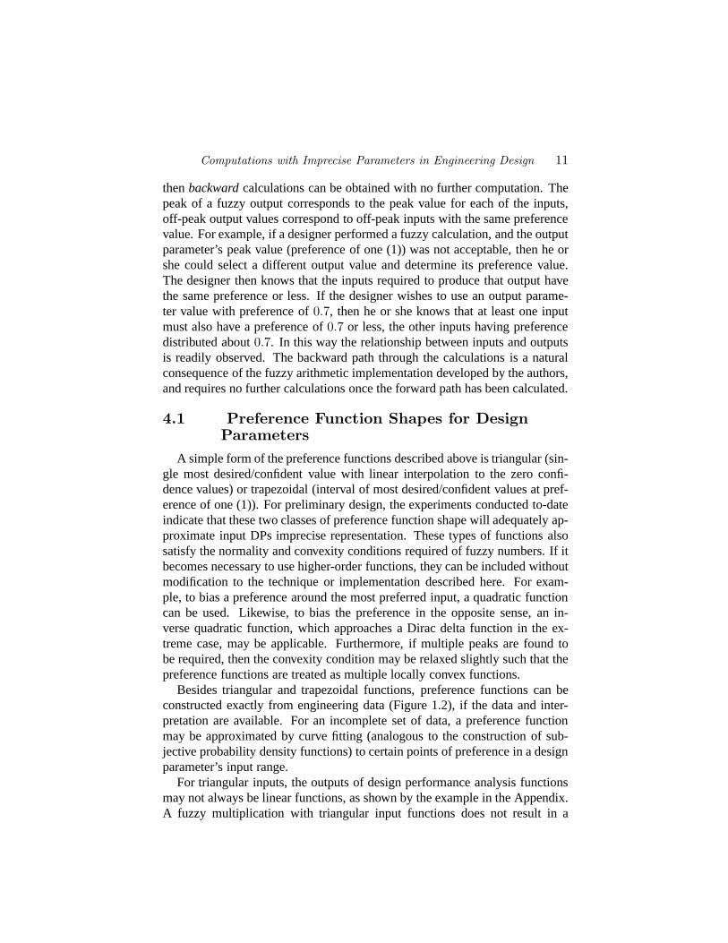
thenbackwardcalculations can be obtained with no further computation. Thepeak of a fuzzy output corresponds to the peak value for each of the inputs,off-peak output values correspond to off-peak inputs with the same preferencevalue. For example, if a designer performed a fuzzy calculation, and the outputparameter’s peak value (preference of one (1)) was not acceptable, then he orshe could select a different output value and determine its preference value.The designer then knows that the inputs required to produce that output havethe same preference or less. If the designer wishes to use an output parame-ter value with preference of0.7, then he or she knows that at least one inputmust also have a preference of0.7 or less, the other inputs having preferencedistributed about0.7. In this way the relationship between inputs and outputsis readily observed. The backward path through the calculations is a naturalconsequence of the fuzzy arithmetic implementation developed by the authors,and requires no further calculations once the forward path has been calculated.
4.1 Preference Function Shapes for DesignParameters
A simple form of the preference functions described above is triangular (sin-gle most desired/confident value with linear interpolation to the zero confi-dence values) or trapezoidal (interval of most desired/confident values at pref-erence of one (1)). For preliminary design, the experiments conducted to-dateindicate that these two classes of preference function shape will adequately ap-proximate input DPs imprecise representation. These types of functions alsosatisfy the normality and convexity conditions required of fuzzy numbers. If itbecomes necessary to use higher-order functions, they can be included withoutmodification to the technique or implementation described here. For exam-ple, to bias a preference around the most preferred input, a quadratic functioncan be used. Likewise, to bias the preference in the opposite sense, an in-verse quadratic function, which approaches a Dirac delta function in the ex-treme case, may be applicable. Furthermore, if multiple peaks are found tobe required, then the convexity condition may be relaxed slightly such that thepreference functions are treated as multiple locally convex functions.
Besides triangular and trapezoidal functions, preference functions can beconstructed exactly from engineering data (Figure 1.2), if the data and inter-pretation are available. For an incomplete set of data, a preference functionmay be approximated by curve fitting (analogous to the construction of sub-jective probability density functions) to certain points of preference in a designparameter’s input range.
For triangular inputs, the outputs of design performance analysis functionsmay not always be linear functions, as shown by the example in the Appendix.A fuzzy multiplication with triangular input functions does not result in a
12 IMPRECISION IN ENGINEERING DESIGN
0.0 0.2 0.4 0.6 0.8 1.0
X, Output
0.0
0.5
1.0
α
← ~D
← θ1(l)
θ2(E )
← θ3(n )
...................................................................................................................................................................................................................................................................................................................................................................................................................................................................................................................................................................................................................................................................................................................................................................................................................................................................................................................................................................................................................................................................................................................................................................................................................................................................................................................................................................................................................................................................................................................................................................................................................................................................................................................................................................................................................
..............................................................................................................................................................................................................................................................................................................................................................................................................................................................................................................................................................................................................................................................................................................................................................................................................................................................................................................................................................................................................................................................................................................................................................................................................................................................................................
.........................
.......................
.....................
....................
...................
....................................................................................................................................................................................................................................................................................................................................................................................................................................................................
..............................................................................................................................................................................................................................................................................................................................................................................................................................................................................................................................................................................................................................................................................................................................................................................................................................................................................................................................................
...............................................................................................................................................................................................................................................................................................................................................................................................................................................................................................................................................................................................................................................................................................................................................................................................................................................................................................................................................................................................................................................................................................................................................................................................
Figure 1.3 Measure of Fuzziness Example
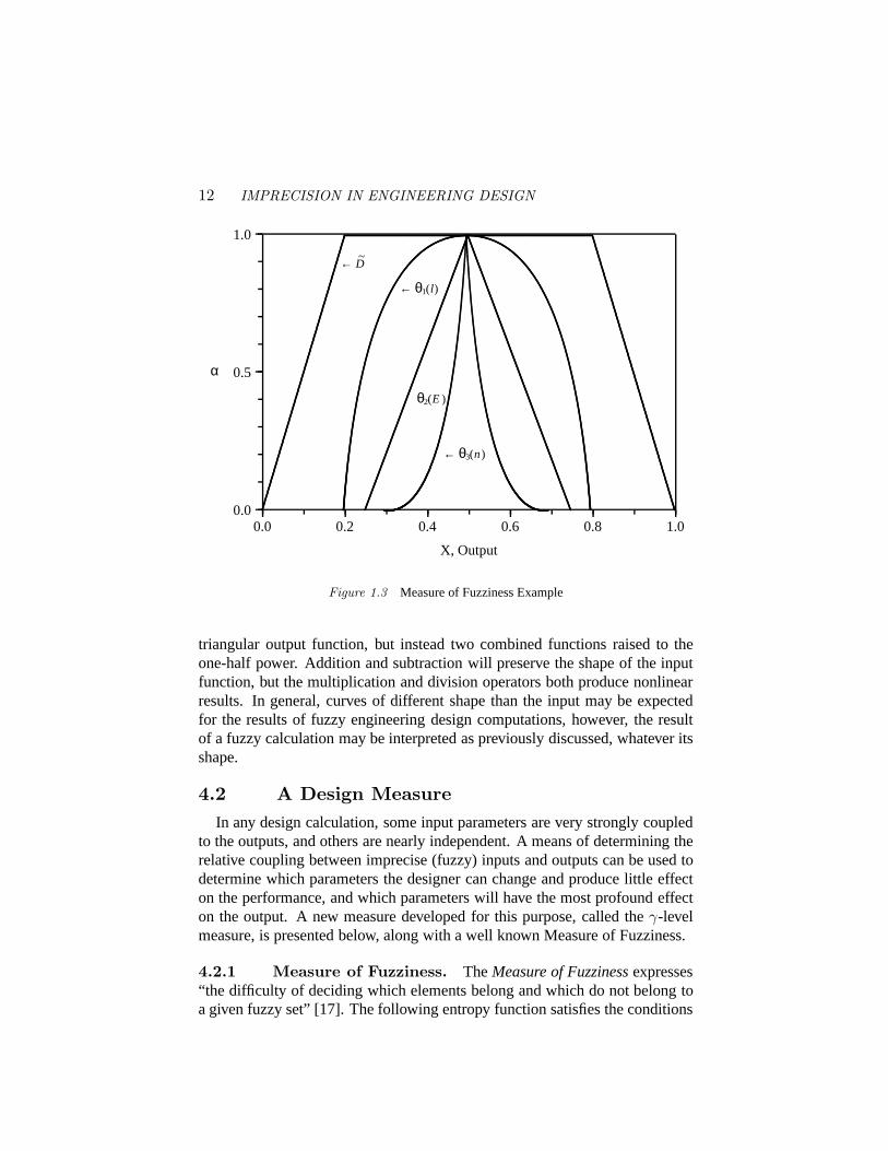
triangular output function, but instead two combined functions raised to theone-half power. Addition and subtraction will preserve the shape of the inputfunction, but the multiplication and division operators both produce nonlinearresults. In general, curves of different shape than the input may be expectedfor the results of fuzzy engineering design computations, however, the resultof a fuzzy calculation may be interpreted as previously discussed, whatever itsshape.
4.2 A Design MeasureIn any design calculation, some input parameters are very strongly coupled
to the outputs, and others are nearly independent. A means of determining therelative coupling between imprecise (fuzzy) inputs and outputs can be used todetermine which parameters the designer can change and produce little effecton the performance, and which parameters will have the most profound effecton the output. A new measure developed for this purpose, called theγ-levelmeasure, is presented below, along with a well known Measure of Fuzziness.
4.2.1 Measure of Fuzziness. TheMeasure of Fuzzinessexpresses“the difficulty of deciding which elements belong and which do not belong toa given fuzzy set” [17]. The following entropy function satisfies the conditions

Computations with Imprecise Parameters in Engineering Design 13
required of a measure of fuzziness [12]:
d(C) = K
|X|∑i=1
Ψ(αC(xi)), (1.1)
where:Ψ(y) = −y ln(y) − (1 − y) ln(1 − y),
αC is the membership function of the fuzzy setC, | X | is the length of thediscretized support (region of non-zero membership) ofC, andK is an integer.
Unfortunately the entropy function as defined in Equation 1.1 measures val-ues centered onαC = 1
2 . A membership value of one-half has the highestdegree of “difficulty of deciding” whether it is a member of the set or not.Memberships close to one (1) are closer to being in the set, memberships closeto zero (0) are closer to being out of the set. Thus this measure indicates howmuch of the membership function is close to one-half. In design, the engineerneeds a measure of the values centered onαC = 1, indicating the “spread” ofthe preference function (near 1), not the steepness of the bounding curves (formembership functions). Figure 1.3 illustrates the difference. TheMeasure ofFuzzinesswill have the same value for membership functionsC1 andC2 sincethese two curves have the same amount ofx nearα = 0.5, however,C1 hasmuch greater imprecision (in the preference function interpretation) thanC2 (amuch larger amount ofx nearα = 1.0). To avoid this difficulty, a new measurehas been developed by the authors.
4.2.2 The γ-Level Measure. We have developed a new measurewhich we will call theγ-level measure. We define this measure in the followingmanner:
D(C) =|X|∑i=1
(eβ(xi) − 1)m, (1.2)
where
β(xi) =
αC(xi)γ if αC ≤ γ
2γ−αC(xi)γ if αC ≥ γ,
0 < γ ≤ 1,
andm is an integer such that asm increases, the measure becomes more con-centrated for values aboutαC = γ. The value ofγ may be set so thatD(C)measures values in the support centered about it. Forγ = 1
2 theγ-levelmea-sure satisfies the conditions for theMeasure of Fuzziness[12]. We will useγ = 1.0 andm = 1.0 in Equation 1.2.
An outline of the process by which thisγ-level measure can be used as aqualitative measure of the relationship between input design parameters and
14 IMPRECISION IN ENGINEERING DESIGN
x
0.0
0.5
1.0
α
~C1 →
~C2 →
............................................................................................................................................................................................................................................................................................................................................................................................................................................................................................................................................................................................
..........................................................................................................................................................................................................................................................................................................................................................................................................................................................................................................................................................................................................................................................
.....................................................................................................................................................................................................................................................................................................................................................................................................................................................................................................................................................................................................................................................................................................................
...............................................................................................................................................................................................................................................................................................................................................................................................................................................................................................................................................................................
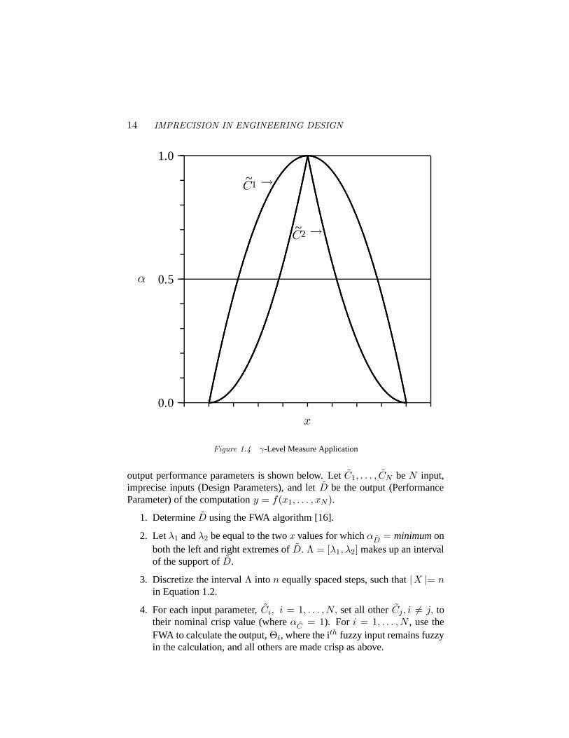
Figure 1.4 γ-Level Measure Application
output performance parameters is shown below. LetC1, . . . , CN beN input,imprecise inputs (Design Parameters), and letD be the output (PerformanceParameter) of the computationy = f(x1, . . . , xN ).
1. DetermineD using the FWA algorithm [16].
2. Letλ1 andλ2 be equal to the twox values for whichαD = minimumonboth the left and right extremes ofD. Λ = [λ1, λ2] makes up an intervalof the support ofD.
3. Discretize the intervalΛ into n equally spaced steps, such that|X |= nin Equation 1.2.
4. For each input parameter,Ci, i = 1, . . . ,N, set all otherCj, i 6= j, totheir nominal crisp value (whereαC = 1). For i = 1, . . . ,N , use theFWA to calculate the output,Θi, where the ith fuzzy input remains fuzzyin the calculation, and all others are made crisp as above.
Computations with Imprecise Parameters in Engineering Design 15
5. Calculate theγ-levelmeasure (γ = 1) for D and allΘi.
6. Normalize theD(Θi)’s with respect toD(D). The result is an order-ing of the inputs according to importance (relative measure), giving aqualitative relationship of inputs to the output.
For the engineer who utilizes fuzzy preference functions in the descriptionof design and performance parameters, this new measure provides the abilityto determine some information on the coupling between the inputs and outputsof design calculations. The measure can also be used to determine which pa-rameters the designer can change and produce little or no effect on the perfor-mance, and which parameters will alter the output the most. Those parameterswith small influence may be fixed to the most-desired value by the engineer,resulting in a simplification of the design problem. The coupling informationnot only includes the rate of change of an output with respect to an input (overthe range of acceptable values), but also includes the change in desirability ofthe parameters. If a small change of an input produces a large change in anoutput, but a small change in the desirability of the output, theγ-level measurewill be small (even though thesensitivityof the output to that input is large).Similarly, if a large change of an input produces a small change in an output,but a large change in the desirability of the output, theγ-level measure will belarge.
Figure 1.4 illustrates an example application of theγ-levelmeasure.D is theoutput fuzzy set of some performance parameter which is functionally relatedthrough a PPE to three imprecise input parametersE, n, andl. TheΘi setsmake up fuzzy outputs for only one fuzzy input parameter (and the other inputsheld at their crisp value). After applying theγ-level measure to each of theseoutput sets, the results may be ordered from largest to smallest. In this case,the ordering consists of the following:D(D), D(Θ1), D(Θ2), D(Θ3). Nor-malizing the output measuresD(Θi) with respect toD(D) shows thatD(Θ1)is much greater than forD(Θ3). The parameter forΘ3 (n) contributes verylittle to the preliminary design analysis when compared to the parameter forΘ1 (l). Thus, the input parametern might be fixed to its crisp value (where itspreference equals one (1)).
5. ExampleA simple mechanical design example using the approach described in the
previous section is presented here. The problem is to design a mechanicalstructure, attached to a wall at one end, which will support an overhangingvertical point load. Constraints on the problem include: the distance the loadis from the wall; the total width of the supporting structure; and the mate-rials used for the structural elements. One possible configuration, shown in
16 IMPRECISION IN ENGINEERING DESIGN
.
. .l/3
60
t
t
A
B D
W
C
l
E
E
Section E-E
t
w
.
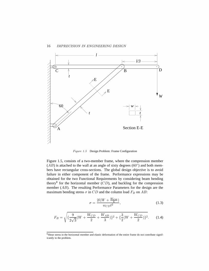
Figure 1.5 Design Problem: Frame Configuration
Figure 1.5, consists of a two-member frame, where the compression member(AB) is attached to the wall at an angle of sixty degrees (60◦) and both mem-bers have rectangular cross-sections. The global design objective is to avoidfailure in either component of the frame. Performance expressions may beobtained for the two Functional Requirements by considering beam bendingtheory8 for the horizontal member (CD), and buckling for the compressionmember (AB). The resulting Performance Parameters for the design are themaximum bending stressσ in CD and the column loadFB onAB:
σ =2l(W + WCD
6 )wCDt2
, (1.3)
FB =
√{ 92√
3(W +
WCD
2+
WAB
3)}2 + {3
2(W +
WCD
2)}2. (1.4)
8Shear stress in the horizontal member and elastic deformation of the entire frame do not contribute signif-icantly to the problem.
Computations with Imprecise Parameters in Engineering Design 17
The design parameters for this example are as follows: the applied loadW ;the length of memberCD l; the width of the compression memberwAB ; andthe thicknesst. If a different material is used, or a range of material propertiesare available,E andρ may also be included as imprecise DPs. The relation-ships for the weight of the two members, and a constraint on width (w) are:
WCD = ρgwCDtl, (1.5)
WAB = ρgwABt(4√
3l
9), (1.6)
wCD = wAB − 2.5 cm. (1.7)
5.1 Performance SpecificationsIn this design,σ must be less than the maximum bending stress before yield.
This example assumes that the material has been specified to be steel. Thus,the functional requirement for maximum bending stress is:
σ ≤ σr = 225 MPa,
where the superscriptr denotes “requirement.”For simplicity, we will only consider the Functional Requirement on bend-
ing stressσ in memberCD in the example shown here. Future publicationswill demonstrate the technique with examples containing more realistic designcomplexities, and comparisons of design alternatives. In the actual design of aframe, such as the one used in this example, buckling of memberAB wouldneed to be included in the analysis.
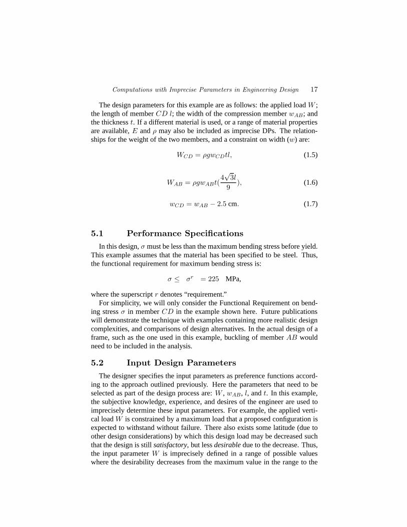
5.2 Input Design ParametersThe designer specifies the input parameters as preference functions accord-
ing to the approach outlined previously. Here the parameters that need to beselected as part of the design process are:W , wAB , l, andt. In this example,the subjective knowledge, experience, and desires of the engineer are used toimprecisely determine these input parameters. For example, the applied verti-cal loadW is constrained by a maximum load that a proposed configuration isexpected to withstand without failure. There also exists some latitude (due toother design considerations) by which this design load may be decreased suchthat the design is stillsatisfactory, but lessdesirabledue to the decrease. Thus,the input parameterW is imprecisely defined in a range of possible valueswhere the desirability decreases from the maximum value in the range to the
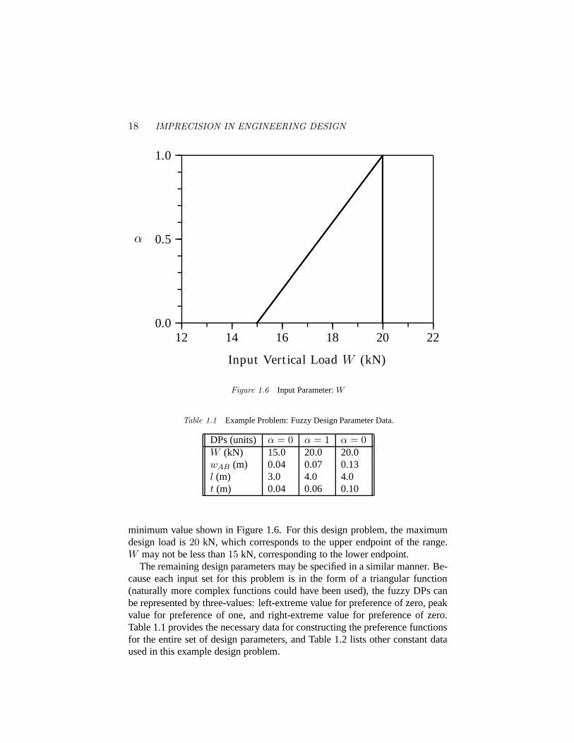
18 IMPRECISION IN ENGINEERING DESIGN
12 14 16 18 20 22
Input Vert ical Load W (kN)
0.0
0.5
1.0
α
..............................................................................................................................................................................................................................................................................................................................................................................................................................................................................................................................................................................................................................................................................................................................................................................................................................................
Figure 1.6 Input Parameter:W
Table 1.1 Example Problem: Fuzzy Design Parameter Data.
DPs (units) α = 0 α = 1 α = 0W (kN) 15.0 20.0 20.0wAB (m) 0.04 0.07 0.13l (m) 3.0 4.0 4.0t (m) 0.04 0.06 0.10
minimum value shown in Figure 1.6. For this design problem, the maximumdesign load is20 kN, which corresponds to the upper endpoint of the range.W may not be less than15 kN, corresponding to the lower endpoint.
The remaining design parameters may be specified in a similar manner. Be-cause each input set for this problem is in the form of a triangular function(naturally more complex functions could have been used), the fuzzy DPs canbe represented by three-values: left-extreme value for preference of zero, peakvalue for preference of one, and right-extreme value for preference of zero.Table 1.1 provides the necessary data for constructing the preference functionsfor the entire set of design parameters, and Table 1.2 lists other constant dataused in this example design problem.
Computations with Imprecise Parameters in Engineering Design 19
Table 1.2 Design Example: “Constant” Data.
Constant (units) ValueE (GPa) 207.0ρ (kg/m3) 7830.0g (m/sec2) 9.81
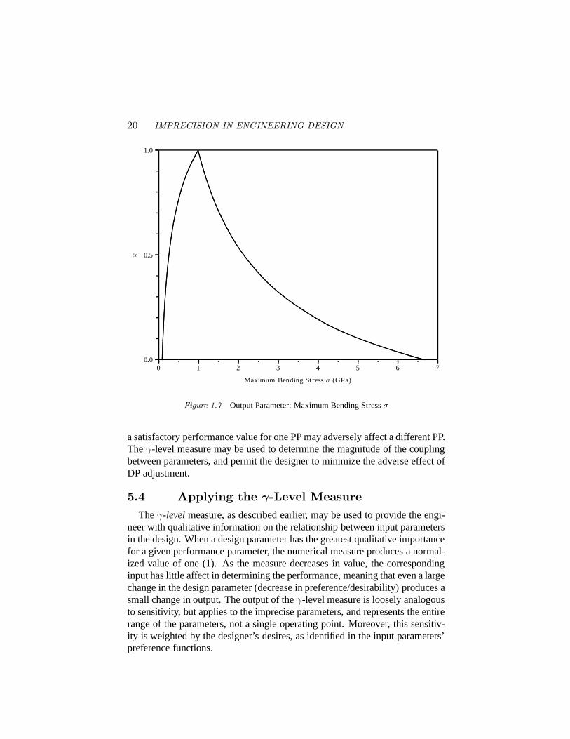
5.3 Output Performance ParametersThe fuzzy output for the performance parameterσ may be obtained by use
of Equation 1.3 and the application of the FWA algorithm described earlier.The results are shown in Figure 1.7.
After the calculations have been performed to produce the output, the nextstep is to compare the output set with the performance criterion. Figure 1.7shows the imprecise performance parameter results for the maximum bendingstress of memberCD (Equation 1.3). The output at the peak ofσ( at α=1) isequal to 994 MPa. This peak output does not satisfy the functional require-mentσr = 225 MPa. To satisfy the requirementσr, the input parameters mustdeviate from the peak (most desired) values. At least one design parametermust decrease in preference, to the left of the peak, by between 0.5 and 0.6(σ( at α=0.5) = 259 MPa andσ( at α=0.4) = 206 MPa), in order to meet the re-quirement onσ. (If a factor of safety is desired, a further decrease in preferencewill be required.)
The backward path of the imprecise calculation may be applied at this pointto determine the effect of changing the preference of any one input designparameter. Data from the solution forσ shows that the input parameters ofWand l could be decreased to the left of their peak values (atα = 1) so thatσ will meet its Functional Requirement, whereas the inputswAB andt mustbe decreased to the right of their peak values. This result cannot easily beobtained from inspection of the governing equation sincewAB and t appearin the denominatorand the numerator of Equation 1.3 when combined withEquation 1.6. While this same result could be obtained through calculationof partial derivatives of the output with respect to each of the inputs, it wasinstead found by use of stored values calculated during the solution of the(imprecise) performance parameter by use of the authors’ implementation ofthe FWA algorithm. No additional calculations were required. These resultsshow thatσr may be satisfied by the frame configuration, but only with a largechange in preference of the DPs from the most desired input peak values. Ifother PPs were part of this design analysis (in addition toσ), care must betaken when adjusting the DPs (which are coupled toσ) to obtain acceptableperformance values in those other PPs. A small adjustment of one DP to obtain
20 IMPRECISION IN ENGINEERING DESIGN
0 1 2 3 4 5 6 7
Maximum Bending Stress σ (GPa)
0.0
0.5
1.0
α
................
................
................
................
................
................
................
................
................
................
................
................
................
................
................
................
................
................
................
................
................
................
................
............................................................................................................................................................................................................................................................................................................................................................................................................................................................................................................................................................................................................................................................................................................................................................................................................................................................................................................................................................................................................................................................................................................................................................................................................................................................................................................................................................................................................................................................................................................................................................................................................................................................................................................................................................................................................
Figure 1.7 Output Parameter: Maximum Bending Stressσ
a satisfactory performance value for one PP may adversely affect a different PP.Theγ-level measure may be used to determine the magnitude of the couplingbetween parameters, and permit the designer to minimize the adverse effect ofDP adjustment.
5.4 Applying the γ-Level MeasureTheγ-levelmeasure, as described earlier, may be used to provide the engi-
neer with qualitative information on the relationship between input parametersin the design. When a design parameter has the greatest qualitative importancefor a given performance parameter, the numerical measure produces a normal-ized value of one (1). As the measure decreases in value, the correspondinginput has little affect in determining the performance, meaning that even a largechange in the design parameter (decrease in preference/desirability) produces asmall change in output. The output of theγ-level measure is loosely analogousto sensitivity, but applies to the imprecise parameters, and represents the entirerange of the parameters, not a single operating point. Moreover, this sensitiv-ity is weighted by the designer’s desires, as identified in the input parameters’preference functions.

Chapter 2
TRADE-OFF STRATEGIES INENGINEERING DESIGN
Kevin N. Otto and Erik K. Antonsson
Research in Engineering DesignVolume 3, Number 2 (1991), pages 87-104.
AbstractA formal method to allow designers to explicitly make trade-off decisions is
presented. The methodology can be used when an engineer wishes to rate thedesign by the weakest aspect, or by cooperatively considering the overall perfor-mance, or a combination of thesestrategies. The design problem is formulatedwith preference rankings, similar to a utility theory or fuzzy sets approach. Thisapproach separates the designtrade-off strategyfrom the performance expres-sions. The details of the mathematical formulation are presented and discussed,along with two design examples: one from the preliminary design domain, andone from the parameter design domain.
1. IntroductionFor a robust automation, design decision making methods need to be ad-
vanced to represent and manipulate a design’s different concerns and uncer-tainties. This development is crucial, since the preliminary decision makingprocess of any design cycle has the greatest effect on overall cost [3, 6, 14]. In adesign decision making process, engineers must trade-off widely differing con-cepts to realize a result which maximizes theiroverall preference for a design.These concepts are usually incommensurate: for example, they could be as dif-ferent as cost, degree of safety, degree of manufacturability, or amount of var-ious performance indicators: stress, heat dissipation, etc. This paper presentsdesign metricsto represent and manipulate these concerns. These metrics takethe form of formal design strategies to permit the designer to trade-off one (ormore) parameter(s) against others, and to implement an overall approach to
31
Computations with Imprecise Parameters in Engineering Design 21
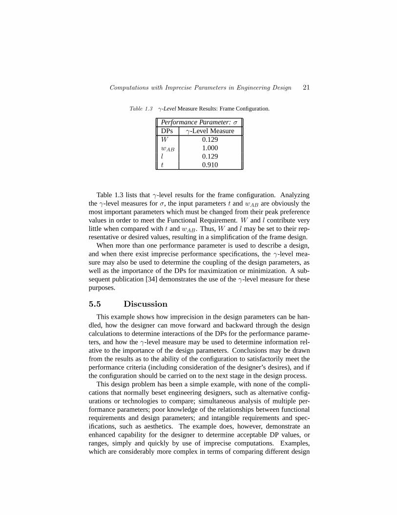
Table 1.3 γ-LevelMeasure Results: Frame Configuration.
Performance Parameter:σDPs γ-Level MeasureW 0.129wAB 1.000l 0.129t 0.910
Table 1.3 lists thatγ-level results for the frame configuration. Analyzingtheγ-level measures forσ, the input parameterst andwAB are obviously themost important parameters which must be changed from their peak preferencevalues in order to meet the Functional Requirement.W andl contribute verylittle when compared witht andwAB . Thus,W andl may be set to their rep-resentative or desired values, resulting in a simplification of the frame design.
When more than one performance parameter is used to describe a design,and when there exist imprecise performance specifications, theγ-level mea-sure may also be used to determine the coupling of the design parameters, aswell as the importance of the DPs for maximization or minimization. A sub-sequent publication [34] demonstrates the use of theγ-level measure for thesepurposes.
5.5 DiscussionThis example shows how imprecision in the design parameters can be han-
dled, how the designer can move forward and backward through the designcalculations to determine interactions of the DPs for the performance parame-ters, and how theγ-level measure may be used to determine information rel-ative to the importance of the design parameters. Conclusions may be drawnfrom the results as to the ability of the configuration to satisfactorily meet theperformance criteria (including consideration of the designer’s desires), and ifthe configuration should be carried on to the next stage in the design process.
This design problem has been a simple example, with none of the compli-cations that normally beset engineering designers, such as alternative config-urations or technologies to compare; simultaneous analysis of multiple per-formance parameters; poor knowledge of the relationships between functionalrequirements and design parameters; and intangible requirements and spec-ifications, such as aesthetics. The example does, however, demonstrate anenhanced capability for the designer to determine acceptable DP values, orranges, simply and quickly by use of imprecise computations. Examples,which are considerably more complex in terms of comparing different design
22 IMPRECISION IN ENGINEERING DESIGN
alternatives and in terms of including uncertainty effects, in addition to impre-cision, will be presented in later publications.
6. ConclusionsOne of the goals of the research reported here is to increase the amount
of information available to engineering designers regarding the performanceof design alternatives, over that available with conventional design analyses.The effect will be greater, the earlier in the design process the informationis made available. Ultimately the most important (and costly) decisions inthe design cycle are made in the very early stages. Engineering designs aretypically represented imprecisely at the early, conceptual (preliminary) stage ofdesign. Computational tools for this area of the design process are rare, largelybecause of the scarcity of techniques capable of handling imprecise data. Oneof the central hypotheses of the research reported here is that representing andmanipulating imprecise descriptions of design artifacts during the preliminaryphase (and hence increasing the information available to the designer) willenable design decisions to be made with greater confidence and reduced risk,and that this will ultimately result in better designs.
The technique and implementation reported here represents a new applica-tion (to the engineering design process) of a powerful approach to representand manipulate imprecise engineering design data. The example shown heredemonstrates that it can be applied to engineering design problems, and pro-vide the ability to perform design calculations on a variety of imprecise param-eters. The (correspondingly) imprecise-calculation results provide more infor-mation to the designer than conventional single-valued design analyses. Thetechnique used is a modified implementation of the Fuzzy Weighted Averageoperating on fuzzy representations of design parameters. Preference functionsare used here to represent the designer’s desire to use particular values for theseparameters.
Additional useful information that this method can provide, through the useof the γ-level measure, is the coupling between imprecise representations ofdesign parameters (inputs) and the performance parameter results. This cou-pling information can be used to focus the engineer’s resources on those as-pects of the design problem with the largest effect on the resulting perfor-mance.
Subsequent publications will compare this method with probability analysis,as well as develop additional examples.
7. AcknowledgementsThis material is based upon work supported, in part, by: The National Sci-
ence Foundation under a Presidential Young Investigator Award, Grant No. DMC-

Computations with Imprecise Parameters in Engineering Design 23
8552695; The Caltech Program in Advanced Technologies, sponsored by Aero-jet General, General Motors, and TRW; and an IBM Faculty DevelopmentAward. Mr. Wood is currently an AT&T-Bell Laboratories Ph.D. scholar, spon-sored by the AT&T foundation. Any opinions, findings, conclusions or recom-mendations expressed in this publication are those of the authors and do notnecessarily reflect the views of the sponsors.

24 IMPRECISION IN ENGINEERING DESIGN
A Appendix: Fuzzy Arithmetic
A.1 Operations for Fuzzy NumbersZadeh [40] introduced the extension principle as one of the fundamental
ideas of fuzzy set theory. Using this idea, classical mathematics may be ex-tended to the fuzzy domain. Specifically, let the fuzzy sets (or fuzzy numbers)C1, C2, . . . , CN be defined in the universesX1,X2, . . . ,XN , respectively. Themapping fromX1 × · · · × XN to a universeY may be defined as a functionfsuch thaty = f(x1, . . . , xN ). The extension principle then gives that a fuzzyset (or number)D onY may be induced fromC1, C2, . . . , CN throughf suchthat the resulting membership function is:
µD(y) = supx1,···,xNmin(µC1
, · · · , µCN)
wherey = f(x1, . . . , xN ). The ordinary binary operations may then becomeextended operations in the fuzzy domain (extended addition, extended multi-plication, etc.).
Even though the development of these extended operations may be com-pleted rigorously using the extension principle approach, interval operationsfor α-level sets will be presented instead, as this method is used in the com-puter implementation.
DEFINITIONS. Some aspects of Fuzzy arithmetic are presented below basedon the material in Kaufmann and Gupta [23].
a. α - Level-Set The discussion of a fuzzy number with respect to its member-ship values leads directly to the idea of defining crisp sets (or intervalsof confidence) for each level,α. Specifically, anα -level-set,Cα, is acrisp set taken from the fuzzy setC such that
Cα = {x|µC(x) ≥ α}, α ∈ [0, 1]. (A.1)
b. Addition and Subtraction Two fuzzy numbers,E andF , may be summedor subtracted level by level (α ∈ [0, 1]) according to the following for-mulas:9
Eα ⊕ Fα = [eαl + fα
l , eαr + fα
r ],Eα Fα = [eα
l − fαr , eα
r − fαl ]
whereEα = [eα
l , eαr ], Fα = [fα
l , fαr ].
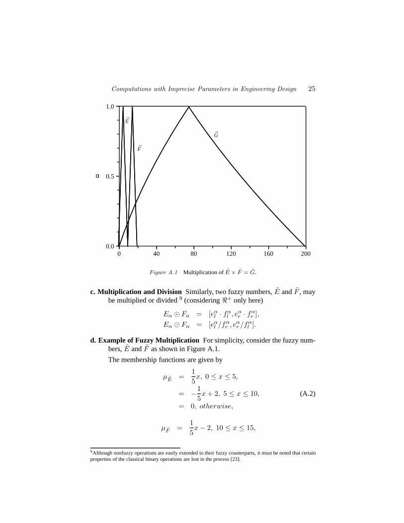
Computations with Imprecise Parameters in Engineering Design 25
0 40 80 120 160 2000.0
0.5
1.0
α
~E
~F
~G
.....................................................................................................................................................................................................................................................................................................................................................................................................................................................................................................................................................................................................................................................................................................................................................................................................................................................................................................................................................................................................................................................................................................................................................................................................................................................................................................................................................................................................................................................................................................................................................................................................................................................................
.................
.................
..................
.................
.................
.................
..................
.................
.................
.................
..................
.................
.................
.................
..................
.................
.................
.................
..................
.................
.................
..................
.................
.................
.................
..................
.................
.................
.................
..................
.................
.................
.................
..................
.................
.................
.................
.................................................................................................................................................................................................................................................................................................................................................................................................................................................................................................................................................................................................................................................................................................................................................................................................................................................................................................................................................................................................................................................................................................................................................................................................................................................................................................................................................................................................................................................................................................................................................................................................................................................................................................................................................................................................................................................................................................................................................................................................................................................................
Figure A.1 Multiplication of E × F = G.
c. Multiplication and Division Similarly, two fuzzy numbers,E andF , maybe multiplied or divided9 (considering<+ only here)
Eα � Fα = [eαl · fα
l , eαr · fα
r ],Eα � Fα = [eα
l /fαr , eα
r /fαl ].
d. Example of Fuzzy Multiplication For simplicity, consider the fuzzy num-bers,E andF as shown in Figure A.1.
The membership functions are given by
µE =15x, 0 ≤ x ≤ 5,
= −15x + 2, 5 ≤ x ≤ 10, (A.2)
= 0, otherwise,
µF =15x − 2, 10 ≤ x ≤ 15,
9Although nonfuzzy operations are easily extended to their fuzzy counterparts, it must be noted that certainproperties of the classical binary operations are lost in the process [23].
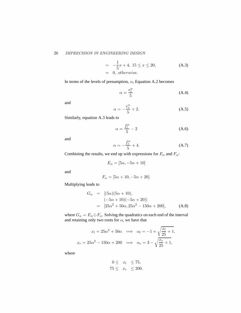
26 IMPRECISION IN ENGINEERING DESIGN
= −15x + 4, 15 ≤ x ≤ 20, (A.3)
= 0, otherwise.
In terms of the levels of presumption,α, Equation A.2 becomes
α =eαl
5(A.4)
and
α = −eαr
5+ 2. (A.5)
Similarly, equation A.3 leads to
α =fα
l
5− 2 (A.6)
and
α = −fαr
5+ 4. (A.7)
Combining the results, we end up with expressions forEα andFα:
Eα = [5α,−5α + 10]
andFα = [5α + 10,−5α + 20].
Multiplying leads to
Gα = [(5α)(5α + 10),(−5α + 10)(−5α + 20)]
= [25α2 + 50α, 25α2 − 150α + 200], (A.8)
whereGα = Eα�Fα. Solving the quadratics on each end of the intervaland retaining only two roots forα, we have that
xl = 25α2 + 50α =⇒ αl = −1 +√
xl
25+ 1,
xr = 25α2 − 150α + 200 =⇒ αr = 3 −√
xr
25+ 1,
where
0 ≤ xl ≤ 75,75 ≤ xr ≤ 200.
Computations with Imprecise Parameters in Engineering Design 27
References
[1] BALDWIN , J. F. A model of fuzzy reasoning and fuzzy logic. Researchem/fs10, University of Bristol, Eng. Math. Dept., 1978.
[2] BALDWIN , J. F., AND GUILD , N. C. F. Feasible algorithms for ap-proximate reasoning using a fuzzy logic. Research em/fs8, University ofBristol, Eng. Math. Dept., 1978.
[3] BALDWIN , J. F.,AND GUILD , N. C. F. A model of multicriteria decisionmaking using fuzzy logic. Research em/fs12, University of Bristol, Eng.Math. Dept., 1978.
[4] BALDWIN , J. F.,AND PILSWORTH, B. W. Axiomatic approach to im-plication for approximate reasoning using fuzzy logic. Research em/fs6,University of Bristol, Eng. Math. Dept., 1978.
[5] BECK, J. V.,AND ARNOLD, K. J. Parameter Estimation in Engineeringand Science. John Wiley and Sons, New York, 1977.
[6] BLOCKLEY, D. I. Predicting the likelihood of structural accidents. InProceedings Institute Civil Engineers(Dec. 1975), pp. 659–668.
[7] BLOCKLEY, D. I. The role of fuzzy sets in civil engineering.Fuzzy Setsand Systems 2(1979), 267–278.
[8] BLOCKLEY, D. I. The Nature of Structural Design and Safety. EllisNorwood Limited, Chichester, 1980.
[9] BROWN, C. B. A fuzzy safety measure.ASCE Journal of the Engineer-ing Mechanics Division(Oct. 1980), 855–872.
[10] BYRNE, D. M., AND TAGUCHI, S. The Taguchi approach to parameterdesign. InQuality Congress Transaction – Anaheim(May 1986), ASQC,pp. 168–177.
[11] COX, R. T. The Algebra of Probable Inference. Johns-Hopkins Univer-sity Press, Baltimore, MD, 1961.
[12] DELUCA, A., AND TERMINI, S. A definition of a nonprobabilisticentropy in the setting of fuzzy set theory.Information and Control 20(1972).
[13] DIAZ , A. R. Fuzzy set based models in design optimization. InAdvancesin Design Automation - 1988(New York, NY, Sept. 1988), S. S. Rao, Ed.,vol. DE-14, ASME, pp. 477–485.
[14] DIAZ , A. R. Modeling of computer-based decisions and optimization inthe design process. InDesign Theory ’88(RPI, Troy, NY, June 1988),S. L. Newsome and W. R. Spillers, Eds., NSF, pp. 286–295. 1988 NSFGrantee Workshop on Design Theory and Methodology.
[15] DIXON, J. R., DUFFEY, M. R., IRANI, R. K., MEUNIER, K. L., AND
ORELUP, M. F. A proposed taxonomy of mechanical design problems.

28 IMPRECISION IN ENGINEERING DESIGN
In Computers in Engineering 1988(New York, NY, June 1988), V. A.Tipnis and E. M. Patton, Eds., ASME, pp. 41–46.
[16] DONG, W. M., AND WONG, F. S. Fuzzy weighted averages and imple-mentation of the extension principle.Fuzzy Sets and Systems 21, 2 (Feb.1987), 183–199.
[17] DUBOIS, D., AND PRADE, H. Fuzzy Sets and Systems: Theory and Ap-plications. Academic Press, New York, 1980.
[18] FUTURA, H., ET AL. Optimum aseismic design using fuzzy sets andempirical connectives. Communication with Dr. Yao Purdue, 1986.
[19] FUTURA, H., AND NARUHITO, S. Fuzzy importance in fault tree analy-sis. Fuzzy Sets and Systems 12(1984), 205–213.
[20] GOGUEN, J. A. L-fuzzy sets.Journal Mathematical Analysis and Ap-plications 18(1967), 145–174.
[21] GUPTA, M. M., SARIDIS, G. N., AND GAINES, B. R., Eds.Fuzzy Au-tomata and Decision Processes. North-Holland Publishers, Amsterdam,1977.
[22] HAUGEN, E. B. Probabilistic Mechanical Design. John Wiley and Sons,New York, NY, 1980.
[23] KAUFMANN , A., AND GUPTA, M. M. Introduction to Fuzzy Arithmetic:Theory and Applications. Electrical/Computer Science and EngineeringSeries. Van Nostrand Reinhold Company, New York, 1985.
[24] KUBIC, W. L., AND STEIN, F. P. A theory of design reliability usingprobability and fuzzy sets.AIChE Journal 34, 4 (Apr. 1988), 583–601.
[25] LEUNG, K. S., AND LAM , W. Fuzzy concepts in expert systems.Com-puter 21, 9 (Sept. 1988), 43–56.
[26] MEUNIER, K. L., AND DIXON, J. R. Iterative respecification: A compu-tational model for hierarchical mechanical system design. InComputersin Engineering 1988(New York, NY, June 1988), V. A. Tipnis and E. M.Patton, Eds., ASME, pp. 25–32.
[27] MOORE, R. E. Methods and Applications of Interval Analysis. Societyfor Industrial and Applied Mathematics, Philadelphia, PA, 1979.
[28] PAHL , G., AND BEITZ, W. Engineering Design. The Design Council,Springer-Verlag, New York, NY, 1984.
[29] RAO, S. S. Description and optimum design of fuzzy mechanical sys-tems. ASME Journal of Mechanisms, Transmissions, and Automation inDesign(1986), 1–7.
[30] REKLAITIS , G. V., RAVINDRAN , A., AND RAGSDELL, K. M. Engi-neering Optimization, Methods and Applications. Wiley, New York, NY,1983.
Computations with Imprecise Parameters in Engineering Design 29
[31] SIDDALL , J. N. Probabilistic Engineering Design; Principles and Ap-plications. Marcel Dekker, New York, NY, 1983.
[32] TAGUCHI, G. Introduction to Quality Engineering. Asian ProductivityOrganization, Unipub, White Plains, NY, 1986.
[33] WOOD, K. L., AND ANTONSSON, E. K. A Fuzzy Sets Approach toComputational Tools for Preliminary Engineering Design. InAdvancesin Design Automation - 1987, Volume One: Design Methods, ComputerGraphics, and Expert Systems – DE-Vol. 10-1(New York, Sept. 1987),S. S. Rao, Ed., ASME, pp. 263–271.
[34] WOOD, K. L., AND ANTONSSON, E. K. Computations with Impre-cise Parameters in Engineering Design: Application and Example.ASMEJournal of Mechanisms, Transmissions, and Automation in Design(June1988).
[35] WOOD, K. L., ANTONSSON, E. K., AND BECK, J. L. Comparing Fuzzyand Probability Calculus for Representing Imprecision in PreliminaryEngineering Design. InDesign Theory and Methodology - 1989(NewYork, Sept. 1989), W. P. Seering, Ed., ASME, pp. 99–105. Presented atthe First International ASMEDesign Theory and Methodology Confer-ence(DTM ’89), September 18-19, 1989, Montr´eal, Canada.
[36] YAGER, R. Satisfaction and fuzzy decision functions. InTheory andApplications to Policy Analysis and Information Systems, P. P. Wang andS. K. Chang, Eds. Plenum Press, New York, 1980.
[37] YAO, J. T. P. Application of fuzzy sets in fatigue and fracture reliability.Communication Dr. Housner Caltech, 1979.
[38] ZADEH, L. A. Fuzzy sets.Information and Control 8(1965), 338–353.
[39] ZADEH, L. A. Outline of a new approach to the analysis of complexsystems and decision processes.IEEE Transactions on Systems, Man,and Cybernetics 3, 1 (1973), 29–44.
[40] ZADEH, L. A. The concept of a linguistic variable and its application toapproximate reasoning – I.Information Sciences 8(1975), 199–249.
[41] ZADEH, L. A. Fuzzy logic and approximate reasoning.Synthese 30(1975), 407–428.
[42] ZADEH, L. A., FU, K. S., TANAKA , K., AND SHIMURA , M., Eds.Fuzzy Sets and their Applications to Cognitive and Decision Processes.Academic Press, New York, NY, 1975.
[43] ZIMMERMANN , H.-J. Fuzzy Set Theory - and Its Applications. Manage-ment Science/Operations Research. Kluwer-Nijhoff Publishing, Boston,MA, 1985.
32 IMPRECISION IN ENGINEERING DESIGN
design trade-offs: either conservative, aggressive, or a combination of the two.The terms: conservative and aggressive are defined in the next section. A for-mal mathematics will be presented to allow designers to explicitly make suchtrade-off decisions.
This approach can help designers observe, justify, and direct their decisionmaking processes. In any design scenario, there are multiple goals which needto be achieved [32]. Designers restrict and choose parameter values based ona combination of these concerns. This work will permit designers to directlyspecify a design goaltrade-off strategyto specify how to trade-off different de-sign goals, and thus allow observation, justification, and recording of decisionsmade.
1.1 Design Trade-Off StrategiesDesign trade-off strategies are always present in the design process. For
example, in the design of a spacecraft solar power cell, a strategy might be totrade-off the performance gains of some goals (like available power output) toincrease the level of other aspects deemed marginal (like stress), to ensure thecell will always function. We will use the term “conservative” design strategy,or also “non-cooperating” or “non-compensatory” strategy, to describe a de-sign strategy of trading off to improve the lower performing goals. A design’soverall preference will be based on the attribute with the lowest preference.Other attributes with higher preference do not compensate for the attribute(s)with lower preference.
On the other hand, a designer may wish to slightly reduce some of theweaker goals in a design if large gains can be made in the other goals, whichwould more than compensate for the slight loss. For example, in the designof a sports car, the designer might reduce the safety margin of some variables(like stress) to gain in performance of other variables (like horsepower), eventhough the stress may already be quite high. We will use the term “aggres-sive” design strategy, or “cooperating” or “compensatory” strategy, to describea design strategy of always cooperatively trading off the goals to improve thedesign. Obviously, hybrid forms of these approaches exist and are used, wheresome portions of a device are designed conservatively, and other portions ag-gressively. We will use the terms: conservative and aggressive design strategiesthroughout this paper.
1.2 Designer PreferencesA method for representing and manipulating uncertainties in preliminary
design, to formalize the process of making these trade-off decisions, has beenintroduced and developed by Wood and Antonsson, [34, 35, 36], called themethod of imprecision. It is used to compare and contrast different objectives
Trade-Off Strategies in Engineering Design 33
within a proposed design and among different design alternatives. The intentis to determine proposed candidates’ feasibility and limitations, even with un-certainty in the variables used.
This paper will incorporate the concepts of imprecision, and a brief reviewwill be presented here. Imprecision indicates a designer’s uncertainty in se-lecting a value for a parameter, in the form of a zero to one rank. If a designerprefers to use a value for a parameter, it will be ranked high, near one. On theother hand, if a designer does not prefer a parameter’s value, it will be rankedlow, near zero. Depending on the domain, the preferences are specified onactual physical variables (such as model dimensions, or calculable quantitiessuch as stress), or, in the preliminary design domain (for example), on featuresin the design. The parameters (on which the preferences are placed) dependon the domain of the design. The discussion presented in the paper will beappropriate for any stage of the design process, from the early planning stagesthrough production. Examples from both the preliminary and a latter stage ofthe design process will be presented. In all cases, the scheme is to place prefer-ences on the candidate model features, with the aim of determining an overallpreference for each candidate model to determine which to pursue. The readeris referred to [20, 21, 22, 33, 34, 35, 36] for a discussion on how to specifypreferences; this paper will not discuss this aspect of the problem. Rather,this paper will focus on the task of combining these individual preferences (ofthe different parameters’ values) to obtain a preference rank for the vector ofdesign parameter values.
The method of imprecision as developed to date used the mathematics offuzzy sets to perform this combination [34]. The primary objective of this pa-per is to introduce different methods for combining these preferences, and toshow that these different methods effectively represent different design strate-gies the designer may adopt.
1.3 Related WorkThere has been some progress in the development of optimization methods
with preference functions. Diaz [7, 8, 9], Rao [20, 21, 22], and Sakawa andYano [24, 25, 26] have advanced the use of “fuzzy goals” where the objectivefunctions and constraints consist of fuzzy preference functions on different per-formance parameters. This paper will illustrate the implications on the choiceof the form of the fuzzy mathematics used. That is, if conventional fuzzy math-ematics is used, it will be demonstrated that this combination corresponds tousing a conservative design strategy.
Parallel work by Dubois and Prade considers trading-off multiple goals withpreference functions [11]. In [11], they review connectives which could beused to combine goals. However, they provide no compelling reason for se-
34 IMPRECISION IN ENGINEERING DESIGN
lecting any of the possible candidates (as is done here: by specifying a designtrade-off strategy). Also, the candidates they propose for combining prefer-ences on incommensurate goals have too many restrictions for the purposesof engineering design. Their developments are derived from the realm of un-certain logic. As such, they are primarily interested in uncertain versions ofconjunction and disjunction. In classical logic, these operations are commuta-tive and associative, which Dubois and Prade assume for all of their develop-ments. In general, engineering design connectives should not be commutative.It makes no sense, for example, to require one goal’s weighting to be appli-cable to a different goal, which is as commutativity requires. Yager, in [37],introduces some of the mathematics that we present here, in the context of se-lecting from a finite set of alternatives. The relationship of his developmentsto ours will be discussed below.
An alternative to the use of imprecision is utility theory [15, 29]. Utility the-ory trades off goals by specifying utility curves on each goal, and then maxi-mizes overall utility by aggressively combining the goals. Doing so eliminatesthe conservative design strategy from consideration, which could be the designstrategy of choice in some cases.
In domains involving goals with explicit expressions, one could formu-late the design problem using an optimization methodology [17]. Such sin-gle objective formulations have been argued to be constraining for actual de-sign problems [32]. Instead, multi-objective function formulations could beused [12, 28, 32]. The methodology presented here is compatible with thesemulti-objective function algorithms, in that one can use them to solve the for-mulations presented here, when the domain has sufficient formalization (per-formance parameter equations) [28]. The focus of this paper is on formallyspecifying the multi-criteria objective function, not methods for finding itsglobal peak.
In the preliminary design domain, the degree of specification of candidatemodels is usually incomplete. The method of imprecision can still be used,however, to determine which candidate models offer the most promise. Tra-ditional methods used in this stage of design are matrix methods [2]. Currentadvanced versions are QFD [1, 13] and Pugh’s method [18]. The basis for thecombination procedure of such matrix methods will be discussed in an exam-ple below.
2. Design ImprecisionIn the method of imprecision, designer preferences (µ) are represented on a
scale from zero to one, with preferences placed individually on each parameter.We shall denotedesign parameters(DP ) as those parameters whose values areto be determined as the objective of the current design process,e.g., lengths,
Trade-Off Strategies in Engineering Design 35
materials, etc. We shall denoteperformance parameters(PP ) as those pa-rameters whose values depend on the design parameter values, and which giveindications of performance,e.g., stress, horsepower, etc. This paper presents
a method to determine an overall rank for avectorof design parameters (−→DP )
given the individual preference information. The preference information isspecified both on the design parameters and on the various performance pa-rameters in the form of specifications or requirements.
Section 2.1 will present axioms governing any preference combination met-ric. Sections 2.2 through 2.5 will discuss different functions to use as globaldesign metrics, and their relation to design strategies. The discussion will bein the context of parametric design; however, the developments apply to anydesign stage, as the examples will demonstrate.
2.1 Global PreferencesThe objective of this paper is to formalize an approach to define and identify
a “best” engineering design. However, the various parameters in the designusually reflect incommensurate concepts, and therefore should be combinedusing a construct that they share: designer preference. This means that prefer-ence information on the design parameters (DPs) and requirement preferenceson the the performance parameters (PPs) must be combined into an overall
preference rating (P) for that design parameter set (−→DP ). Therefore, to com-
bine designer preferences, a global design connective, or metric, is defined,expressed as a function of the known preferences of the goals:
µ(−→DP ) = P
[µ(DP1), ..., µ(DPn), µ(PP1(
−→DP )), ..., µ(PPq(
−→DP ))
](2.1)
This statement implies that the choice of a design parameter set is based oncombining (in a yet to be determined fashion) the preferences of the designparameters and performance parameters. It is a formalization of the idea thatdesigners combine incommensurate parameters based on how much each pa-rameter satisfies them.
The design problem is then to find the design parameter set which maxi-mizes the overall preference:1
µ(−→
DP ∗) = maxDPS
[P[µ(DP1), ..., µ(DPn), µ(PP1(
−→DP )), ..., µ(PPq(
−→DP ))
]](2.2)
The most preferred design parameter set−→
DP ∗ is the one which maximizesP across the design parameter space (DPS), which is the set of all design
1Throughout the papermax is used to to meansupor least upper bound, andmin is used to meaninf orgreatest lower bound.
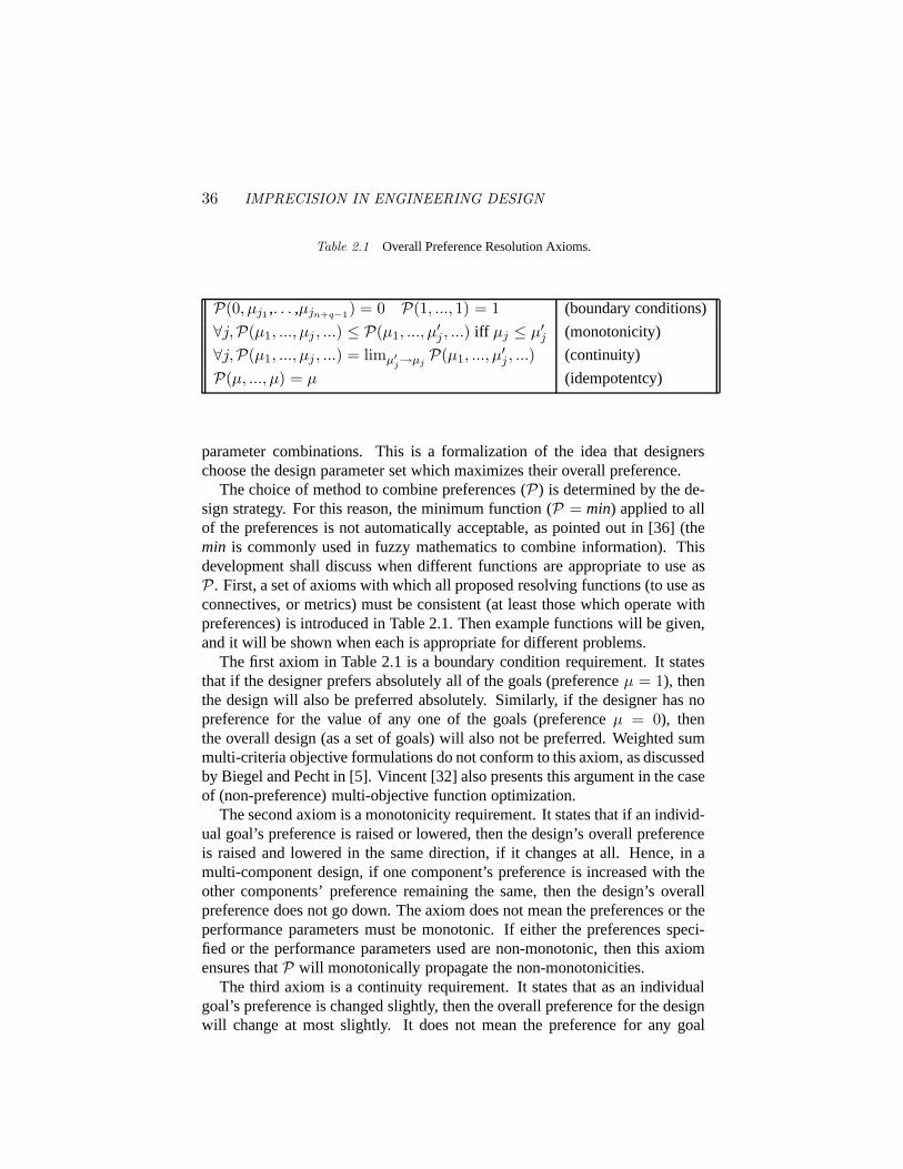
36 IMPRECISION IN ENGINEERING DESIGN
Table 2.1 Overall Preference Resolution Axioms.
P(0, µj1 ,. . . ,µjn+q−1) = 0 P(1, ..., 1) = 1 (boundary conditions)
∀j,P(µ1, ..., µj , ...) ≤ P(µ1, ..., µ′j , ...) iff µj ≤ µ′
j (monotonicity)
∀j,P(µ1, ..., µj , ...) = limµ′j→µj
P(µ1, ..., µ′j , ...) (continuity)
P(µ, ..., µ) = µ (idempotentcy)
parameter combinations. This is a formalization of the idea that designerschoose the design parameter set which maximizes their overall preference.
The choice of method to combine preferences (P) is determined by the de-sign strategy. For this reason, the minimum function (P = min) applied to allof the preferences is not automatically acceptable, as pointed out in [36] (themin is commonly used in fuzzy mathematics to combine information). Thisdevelopment shall discuss when different functions are appropriate to use asP. First, a set of axioms with which all proposed resolving functions (to use asconnectives, or metrics) must be consistent (at least those which operate withpreferences) is introduced in Table 2.1. Then example functions will be given,and it will be shown when each is appropriate for different problems.
The first axiom in Table 2.1 is a boundary condition requirement. It statesthat if the designer prefers absolutely all of the goals (preferenceµ = 1), thenthe design will also be preferred absolutely. Similarly, if the designer has nopreference for the value of any one of the goals (preferenceµ = 0), thenthe overall design (as a set of goals) will also not be preferred. Weighted summulti-criteria objective formulations do not conform to this axiom, as discussedby Biegel and Pecht in [5]. Vincent [32] also presents this argument in the caseof (non-preference) multi-objective function optimization.
The second axiom is a monotonicity requirement. It states that if an individ-ual goal’s preference is raised or lowered, then the design’s overall preferenceis raised and lowered in the same direction, if it changes at all. Hence, in amulti-component design, if one component’s preference is increased with theother components’ preference remaining the same, then the design’s overallpreference does not go down. The axiom does not mean the preferences or theperformance parameters must be monotonic. If either the preferences speci-fied or the performance parameters used are non-monotonic, then this axiomensures thatP will monotonically propagate the non-monotonicities.
The third axiom is a continuity requirement. It states that as an individualgoal’s preference is changed slightly, then the overall preference for the designwill change at most slightly. It does not mean the preference for any goal

Trade-Off Strategies in Engineering Design 37
Design 2Design 1
DP2 DP2DP1DP1
Figure 2.1 Two designs which have the same low preference for a componentDP1, anddifferent (higher) preference for a different componentDP2.
must be continuous. It states only that as any individual goal’s preferenceis continuously changed, the method of combining all the goals’ preferences(that is,P) will induce only continuous changes in the overall preference, if itchanges at all. If some parameters have preference discontinuities, the methodof combining them will continuously propagate the discontinuities. Thereforea design will not be abruptly preferred by slight changes in values, unless theparameterizing expressions dictate this.
These first three axioms present nothing new in terms of inferencing mecha-nisms under uncertainty. Probability and Bayesian inferencing [31], Dempster-Shafer theory [27], fuzzy sets and triangular norms in general [10], and finallyutility theory [15] all conform to these axioms, with slight variations on bound-ary conditions. The subsequent discussion, however, indicates where thesetheories diverge among themselves and with the development presented here.
The last axiom in Table 2.1 is an idempotentcy restriction. It states that if adesigner has the same preference for all individual concerns in a design, thenthe overall preference must have this degree of preference as well. This con-dition must be considered closely, for it is a statement related to rationality.A definition of irrational behavior is to act in a manner which is against one’sobjectives [31]. In the context of preference, this linguistic definition translatesinto meaning that an irrational method is to reduce or increase the overall pref-erence beyond what the parameters specify. Formalization of this definition,however, has many possibilities (among which, for example, is probability, orevenP as so far specified) since this definition is linguistic and non-formal.
The last axiom of idempotentcy eliminates any functions which combinepreferences in an inherently pessimistic or optimistic manner. Methods whichcombine individual preferences and artificially reduce or increase the overall
38 IMPRECISION IN ENGINEERING DESIGN
preference rank should not be considered:e.g., some of the various triangularnorms [10] and power methods [8]. For example, if a design had two goals,each with preference0.8, one would not expect an overall rating of0.2, or1.0, since these results are irrational: they reduced or increased the overallpreference beyond what the parameters specified. Idempotentcy eliminatesthese possibilities.
One axiom absent from the list is strictness:
∀j,P(µ1, ..., µj , ...) < P(µ1, ..., µ′j , ...) iff µj < µ′
j (2.3)
The strictness requirement is unacceptable asalwaysbeing required foranydesign metric. For some design strategies, strictness may be acceptable; forothers not. For example, consider one parameter in two different designs whichhas a low preference of0.4. The two designs differ only in that a second pa-rameter (different from the one ranked at0.4) has a preference of0.6 and0.8in the two designs respectively. See Figure 2.1. It is not clear that the designershouldalwaysdistinguish between these two designs, which the strictness re-quirement requires. Both designs have equally bad components at0.4, and sothe designer may decide to rank both designs as equally poor overall, with apreference of0.4. Alternatively, the designer may see the first parameter asirrelevant, and rank the second design as better overall. This decision dependson the strategy employed. However, attempting toalwaysinclude the strictnessrequirement eliminates valid strategies from consideration by always differen-tiating between Design 1 and 2 in Figure 2.1. The strictness requirement isdiscussed in [10].
Table 2.1 is a list of necessary requirements to which any global com-bination design metric which uses preferences must conform. Using fewerconstraints on the design metric permits irrational and non-intuitive prefer-ence combination functions to be used, based on the informal comparison ofthese axioms with design decision making. Additional constraints will nowbe placed on the metric, where these additional constraints imply a particulardesign strategy.
2.2 Conservative DesignSuppose the designer wishes to trade off to improve the lower performing
goals (in terms of preference) when selecting a design parameter set−→DP . Also,
assume for the moment that all of the individual goals are equal causes ofconcern to the designer. This implies that, to improve a design, there mustbe an increase in the preference level of the goal whose preference is lowest.We refer to this as a conservative design strategy, and the method to use for
Trade-Off Strategies in Engineering Design 39
combining the multiple preferences isP = min. That is,
µ(−→
DP ∗) = maxDPS
[min[µ(DP1), ..., µ(DPn), µ(PP1), ..., µ(PPq)]] (2.4)
where−→
DP ∗ is the most preferred design parameter solution set. Using themin as a design metric always improves a design’s worst aspect, meaning thataspect with the lowest preference. Whichever parameter has the lowest pref-erence dictates the overall preference. If the designer can improve the design,this parameter will change. Of course, the goal which is the “weakest link”
changes with changes in−→DP (changes of position in the design space). There-
fore this metric trades off to improve the lower performing goals.Finally, Equation 2.4 is exactly the fuzzy set formulation of the design prob-
lem [8, 20]. Therefore, using a fuzzy set resolution in the design domainreflects trading off goals conservatively, and without considering importanceweightings.
2.3 Aggressive DesignThemin resolution of Equation 2.4 is not always appropriate, however. If
the resulting design is drastically hindered by one parameter and relaxing it abit greatly increases the others’ preference, then the modified design may beconsidered to produce a higher “overall” performance, even though the lowerperforming goal was slightly reduced even further. In this case, the hinderingparameter should be relaxed and thereby allow other parameters to substan-tially increase their preference.
This can be accomplished with the use of a product:
µ(−→
DP ∗) = maxDPS
q+n∏
j=1µj
1q+n
(2.5)
wheren is the number of design parameters andq is the number of perfor-mance parameters.
This resolution reflects a different design strategy than themin resolutionpresented earlier. Specifically, Equation 2.5 allows higher performing goals tocompensate for lower performing goals (in terms of preference). This metrictrades off the goals to cooperatively improve the design. We refer to this as anaggressive (or cooperative) trade-off strategy.
2.4 Importance RatingsBoth strategy formalizations presented in the previous two sections assumed
all goals were equally important. The formalization of the conservative de-sign strategy as reflected by Equation 2.4 traded off the overall performance
40 IMPRECISION IN ENGINEERING DESIGN
to gain in the lower performing goals, as if each were equally important to thedesigner. The formalization of the aggressive design strategy as reflected byEquation 2.5 did the reverse (traded off the lower performing goals to gain inoverall performance), as if each goal were equally important. Yet, in the gen-eral case, each goal will not hold equal importance. In this more general case,factors must be included to allow the designer to specify how much concern(or weight) should be allocated to each goal.
The reader is referred to [23, 28] for methods on how to specify weights; thispaper will not discuss this aspect of the problem. However, it is noted that thereare several reasons why weighting functions present difficulty [28, 30]. Weconcur, and adopt the standard solution to the problem of specifying weights:iteration. That is, it is not assumed the designer can,a priori, specify the finalgoal weights, only preliminary estimates. The designer then gains insight onhow to specify weights through iteration. In any case, techniques for specify-ing weights from pairwise comparisons of goals are the Analytical HierarchyProcess [23], or the marginal rate of substitution [28]. It is noted that, thoughtheoretical issues remain with weighting functions, they are commonly used inpractice [1, 2, 13, 19].
Assigning importance factors to goals is a relative measure: a goal’s impor-tance is ranked relative to the rest of the goals in a design. The importance ofgoalj (either a design parameter or a performance parameter) shall be denotedωj. Since importance is a relative measure, the importance factors should al-ways be normalized by their sum;i.e., theωj must be such that
q+n∑j=1
ωj(~p) = 1 (2.6)
where~p is the vector composed of the design and performance parameters.This allows for non-normalized weights; for example,ωj might be fuzzy. Ateach point, the non-normal weights must be normalized.
There is another observation on the importance factors: since it is assumedthat no goals are trivial or absolutely dominant, the normalizedωj must besuch that
0 < ωj(~p) < 1 for all j (2.7)
The0 lower boundary condition is actually not strict: the particular goalj thensimply drops out of the consideration (µ
ωj
j becomes1). Further, the1 upperboundary condition is always ensured by the previous normalization require-ment.
A final observation is that importance factors are functions: they can changewith changes in the design. If a goal’s preference is low, perhaps a designermay wish to change the goal’s importance. It is assumed that slight changes ina goal’s value do not induce drastic changes in the goal’s importance. This is a
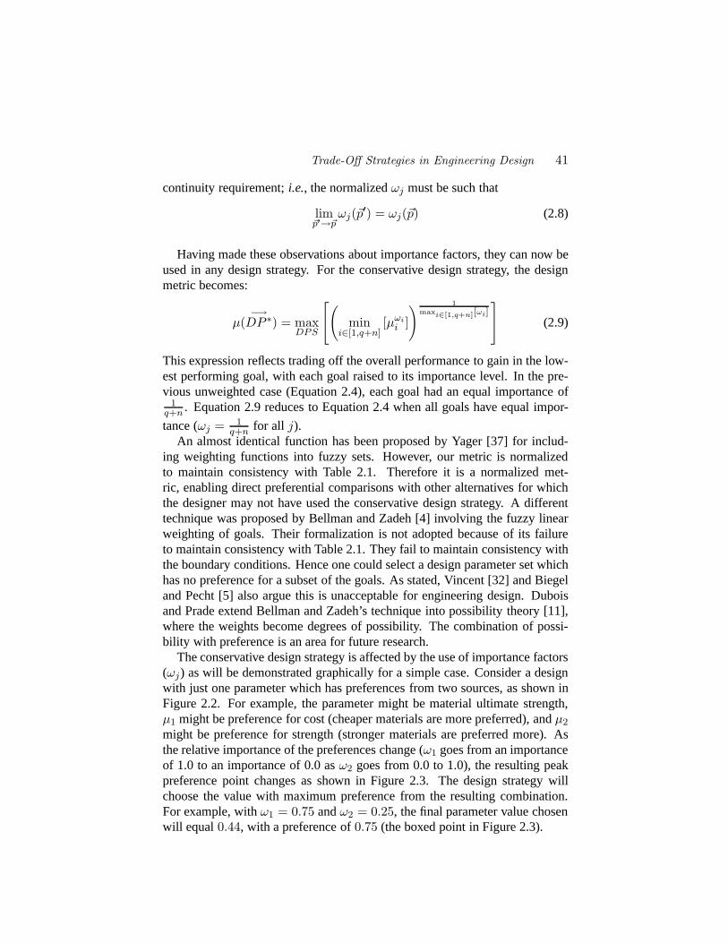
Trade-Off Strategies in Engineering Design 41
continuity requirement;i.e., the normalizedωj must be such that
lim~p′→~p
ωj(~p′) = ωj(~p) (2.8)
Having made these observations about importance factors, they can now beused in any design strategy. For the conservative design strategy, the designmetric becomes:
µ(−→
DP ∗) = maxDPS
( min
i∈[1,q+n][µωi
i ]
) 1maxi∈[1,q+n][ωi]
(2.9)
This expression reflects trading off the overall performance to gain in the low-est performing goal, with each goal raised to its importance level. In the pre-vious unweighted case (Equation 2.4), each goal had an equal importance of
1q+n . Equation 2.9 reduces to Equation 2.4 when all goals have equal impor-
tance (ωj = 1q+n for all j).
An almost identical function has been proposed by Yager [37] for includ-ing weighting functions into fuzzy sets. However, our metric is normalizedto maintain consistency with Table 2.1. Therefore it is a normalized met-ric, enabling direct preferential comparisons with other alternatives for whichthe designer may not have used the conservative design strategy. A differenttechnique was proposed by Bellman and Zadeh [4] involving the fuzzy linearweighting of goals. Their formalization is not adopted because of its failureto maintain consistency with Table 2.1. They fail to maintain consistency withthe boundary conditions. Hence one could select a design parameter set whichhas no preference for a subset of the goals. As stated, Vincent [32] and Biegeland Pecht [5] also argue this is unacceptable for engineering design. Duboisand Prade extend Bellman and Zadeh’s technique into possibility theory [11],where the weights become degrees of possibility. The combination of possi-bility with preference is an area for future research.
The conservative design strategy is affected by the use of importance factors(ωj) as will be demonstrated graphically for a simple case. Consider a designwith just one parameter which has preferences from two sources, as shown inFigure 2.2. For example, the parameter might be material ultimate strength,µ1 might be preference for cost (cheaper materials are more preferred), andµ2might be preference for strength (stronger materials are preferred more). Asthe relative importance of the preferences change (ω1 goes from an importanceof 1.0 to an importance of 0.0 asω2 goes from 0.0 to 1.0), the resulting peakpreference point changes as shown in Figure 2.3. The design strategy willchoose the value with maximum preference from the resulting combination.For example, withω1 = 0.75 andω2 = 0.25, the final parameter value chosenwill equal 0.44, with a preference of0.75 (the boxed point in Figure 2.3).
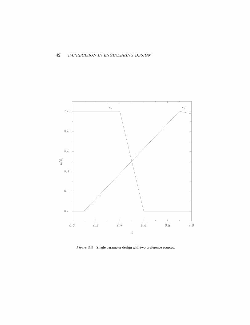
42 IMPRECISION IN ENGINEERING DESIGN
Figure 2.2 Single parameter design with two preference sources.
Trade-Off Strategies in Engineering Design 43
Figure 2.3 Weighted conservative design strategy results.
44 IMPRECISION IN ENGINEERING DESIGN
For the aggressive (cooperating) design strategy case, the design metric willuse a variation from the previous unweighted case (Equation 2.5):
µ(−→
DP ∗) = maxDPS
[q+n∏i=1
µωii
](2.10)
This expression reflects trading off the goals cooperatively to gain in the overallperformance, with each goal raised to its importance level. In the previousunweighted case (Equation 2.5), each goal had an equal importance of1
q+n .Equation 2.10 reduces to Equation 2.5 when all goals have equal importance(ωj = 1
q+n for all j).Yager presents this resolution in [37] as a method to select a proper course of
action based on a set of objectives. We, however, present a justification for itsuse as reflecting a design trade-off strategy, and apply the method to problemsbeyond selection from a finite set of alternatives, the thrust of Yager’s work.
The aggressive design strategy is also affected by the use of importancefactors (ωj) as will be demonstrated graphically for the same simple example(Figure 2.2). As the relative importance of the preferences change (ω1 goesfrom an importance of 1.0 to an importance of 0.0 asω2 goes from 0.0 to1.0), the resulting peak preference point changes as shown in Figure 2.4. Theaggressive design strategy will choose the value with maximum preferencefrom the resulting combination. For example, withω1 = 0.75 andω2 = 0.25,the final parameter value chosen will equal0.4, with a preference of0.78 (theboxed point in Figure 2.4).
Note that, for the same problem with the same preferences and importancefactors, the two design strategies selected different peak points. The two strate-gies traded off the goals in different fashions: conservatively or aggressively.In either case, a goal’s importance can be handled within the design strategies.
2.5 Hybrid Design StrategiesGenerally, a designer may not wish to exclusively trade-off every design
component aggressively or conservatively. A subsystem may need to have itsweakest goals maximized, but a different subsystem may need to be cooper-atively maximized. For these more general cases, a combination of the twomethods (themin and theproduct) can be performed, and this is consistentwith Table 2.1’s axioms. The sub-design would use themincombination of itspreference rankings, and this sub-result would use theproductto be combinedwith rest of the design.
In the general case, an entire hierarchy of the parameters’ preferences wouldbe constructed into the overall metric. This construction could be aided byusing theγ-level measure [34] to determine which parameters are critical tothe design. Theγ-levelmeasure provides an indication of how sensitive each
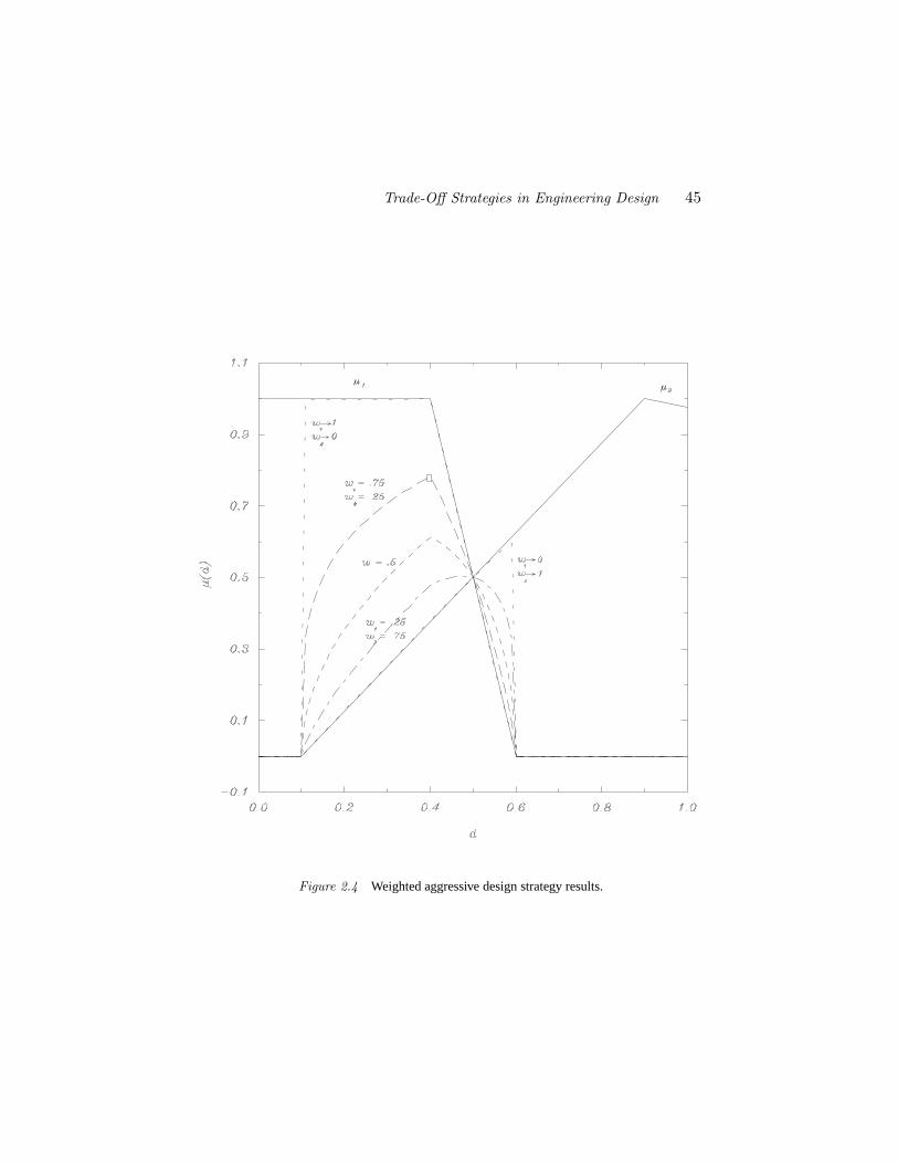
Trade-Off Strategies in Engineering Design 45
Figure 2.4 Weighted aggressive design strategy results.
46 IMPRECISION IN ENGINEERING DESIGN
design parameter is to each performance parameter, based on their relation andthe specified preferences. If theγ-level measure indicates a particular designparameter is critical to different performance parameters, the designer couldthen take extra care when specifying that design parameter’s importance. Alsonote that the importance weightings might also change as the design processprogresses to reflect the addition of more information.
2.6 Discussion: What is a Design Strategy?The term “strategy” has many meanings, both in the research literature, and
in engineering practice. This paper has introduced a formalization of one as-pect of design strategies: how to make trade off decisions among differentgoals. Design strategies might also include considerations of performance,safety, importance, or noise variations. They also usually include considera-tions of the design problem solving methodology or approach. This paper’suse of the term “strategy” therefore includes only one aspect: how to maketrade-off decisions among multiple, incommensurate goals in a design.
A related question is how to determine what goals should be included in aproblem’s formalization. This question cannot be answereda priori, but willevolve with the design. A preliminary indication of whether a parameter needsconsideration can be determined in the same manner as developed for utilitytheory: using Ellis’ “test of importance” [15]. In this method, before deter-mining how the overall metric is to be formulated, the designer asks whethera parameter’s inclusion could change the choice of the others. If so, this addi-tional parameter should be included in the formalization. Hence every possiblyimportant parameter in a design is included. This would likely lead to overlycomplicated forms. Therefore, theγ-levelmeasure [34] could be used to elim-inate those which are shown to have little consequence.
Another concern involves practically evaluating (or searching for) the mostpreferred design parameter set, once a strategy has been used to formally spec-ify the multi-criteria objective function. This aspect of the problem will not beelaborated; it is a problem and processor dependent consideration. For exam-ple, when the design space is a list of alternative configurations and the goalsare features of the design, the problem can be formulated in a matrix format(even for designs involving hundreds of variables) with preferences entered inthe matrix. Search is then simply selecting the alternative with maximumP ofthe feature preferences, as will be shown in Example 1. In such a case, for ahuman “processor”, theminconservative strategy is easier to evaluate than theproductaggressive strategy.
A different problem may involve goals with explicit performance parameterexpressions, as will be shown in Example 2. Here optimization methods [17]can be invoked to search across the design parameter space for the maximum

Trade-Off Strategies in Engineering Design 47
Table 2.2 Raw designer rankings.
Criteria Importance Mechanism RobotEase to get design to satisfy quantity rate 4 5 −1
Ease to ensure operator safety 4 −1 0Development cost 5 −1 3
Ease to ensure production reliability 5 3 0Ease to ensure size constraints 2 4 2
Ease to do design by production time 3 0 4Ease to ensure production quality 4 5 4
preference point, possibly involving penalty methods [17] to ease the search.Here theproductaggressive strategy may be easier to evaluate due to differen-tiability. Theminconservative strategy becomes a traditionalmaximinmultiplegoal optimization formulation [16]. In any case, iteration will almost certainlybe required to ensure the final preferences and weights. Formal iterative meth-ods (see Steuer [28] for a review) could be used.
3. ExamplesThe first example presented will be in the preliminary design domain. The
task is to determine which of two candidate models to pursue into the latterdesign stages. The second example will be in the parametric design domain.The task is to determine which of two air tanks to manufacture, and whichparametric design parameter values to use.
3.1 Example 1: Preliminary DesignConsider the design task involving a selection between two candidate con-
cepts. The candidates are to be used for assembling items in a manufacturingproduction line. The first candidate design is a special purpose mechanism, theother is a general purpose robotic arm.
The decision criteria for determining which candidate to pursue into thesubsequent design stages are listed in Table 2.2. As well, each criterion’s im-portance (on a scale of0 to 5), and each candidate’s ability to satisfy the crite-rion (on a scale from−5 to 5) is tabulated. Background and details of matrixmethods are discussed in [2, 18].
Using the standard weighted sum matrix analysis [2], the mechanism candi-date produces an overall rank of54, and the robot candidate produces an overallrank of43. This technique guides the designer to pursue the mechanism.
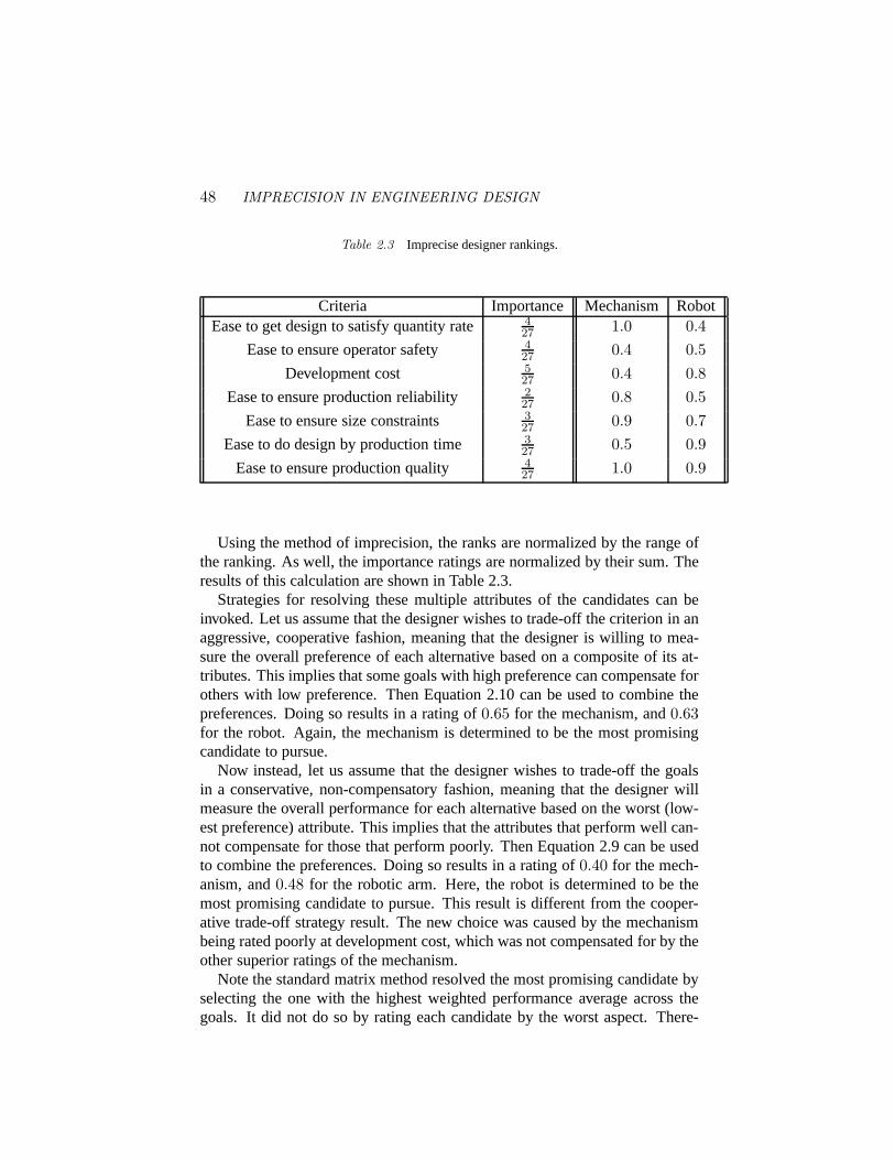
48 IMPRECISION IN ENGINEERING DESIGN
Table 2.3 Imprecise designer rankings.
Criteria Importance Mechanism RobotEase to get design to satisfy quantity rate 4
27 1.0 0.4Ease to ensure operator safety 4
27 0.4 0.5Development cost 5
27 0.4 0.8Ease to ensure production reliability 2
27 0.8 0.5Ease to ensure size constraints 3
27 0.9 0.7Ease to do design by production time 3
27 0.5 0.9Ease to ensure production quality 4
27 1.0 0.9
Using the method of imprecision, the ranks are normalized by the range ofthe ranking. As well, the importance ratings are normalized by their sum. Theresults of this calculation are shown in Table 2.3.
Strategies for resolving these multiple attributes of the candidates can beinvoked. Let us assume that the designer wishes to trade-off the criterion in anaggressive, cooperative fashion, meaning that the designer is willing to mea-sure the overall preference of each alternative based on a composite of its at-tributes. This implies that some goals with high preference can compensate forothers with low preference. Then Equation 2.10 can be used to combine thepreferences. Doing so results in a rating of0.65 for the mechanism, and0.63for the robot. Again, the mechanism is determined to be the most promisingcandidate to pursue.
Now instead, let us assume that the designer wishes to trade-off the goalsin a conservative, non-compensatory fashion, meaning that the designer willmeasure the overall performance for each alternative based on the worst (low-est preference) attribute. This implies that the attributes that perform well can-not compensate for those that perform poorly. Then Equation 2.9 can be usedto combine the preferences. Doing so results in a rating of0.40 for the mech-anism, and0.48 for the robotic arm. Here, the robot is determined to be themost promising candidate to pursue. This result is different from the cooper-ative trade-off strategy result. The new choice was caused by the mechanismbeing rated poorly at development cost, which was not compensated for by theother superior ratings of the mechanism.
Note the standard matrix method resolved the most promising candidate byselecting the one with the highest weighted performance average across thegoals. It did not do so by rating each candidate by the worst aspect. There-
Trade-Off Strategies in Engineering Design 49
fore the standard weighted sum matrix technique invokes a compensating goaltrade-off strategy, informally similar to our aggressive trade-off strategy. Thedevelopments described here allow for a variety of design strategies. Com-binations of conservative and aggressive strategies could be used for differ-ent sub-arrangements of the goals, and then these sub-arrangements combinedwith either a conservative or aggressive strategy, depending on the designer’sjudgments.
3.2 Example 2: Parametric DesignThe example presented below considers a pressurized air tank design, and
is the same problem as presented in Papalambros and Wilde [17], page 217.The reader is referred to the reference [17] to see the restrictions applied tothe problem to permit it to be solved using crisp constraints and various op-timization techniques (monotonicity analysis, non-linear programming). Theexample is simple and was chosen for that reason, and also the ability of itspreferences to be represented on a plane for a visual interpretation.
The design problem is to determine length and radius values in an air tankwith two different choices of head configuration: flat or hemispherical. SeeFigure 2.5.
There are four performance parameters in the design. The first is the metalvolumem:
m = 2πKsr2l + 2πChKhr3 + πK2
s r2l (2.11)
This parameter is proportional to the cost, and the preference ranks are setbecause of this concern. Another performance parameter is the tank capacityv:
v = πr2l + πKvr3 (2.12)
This parameter is an indicator of the design’s principle objective: to hold air.This parameter’s aspiration level ranks the preference for values. Another pa-rameter is an overall height restrictionL0, which is imprecise:
l + 2(Kl + Kh)r ≤ L0 (2.13)
Finally, there is an overall radius restrictionR0, which is also imprecise:
(Ks + 1)r ≤ R0 (2.14)
The last two performance parameters have their preference ranks set by spatialconstraints.
The coefficientsK are from the ASME code for unfired pressure vessels.S is the maximal allowed stress,P is the atmospheric pressure,E is the jointefficiency, andCh is the head volume coefficient.
Kh =
{2√
CP/S flatP
2S−.2P hemi(2.15)
50 IMPRECISION IN ENGINEERING DESIGN
r
l
r
l
Figure 2.5 Hemispherical and flat head air tank designs.
Trade-Off Strategies in Engineering Design 51
µ
l
r
0
1
625 0
125
Figure 2.6 Lengthl preference.
Kl ={
0 flat4/3 hemi
(2.16)
Ks =P
2SE − .6P(2.17)
Kv ={
0 flat1 hemi
(2.18)
This example’s design space is spanned by 2 design parametersl andr. Thepreferences for values of these design parameters and the four performanceparameters are shown in Figures 2.6 through 2.11 for the hemispherical design;the flat head design space is similar.
The problem is to find the values forl andr which maximize overall pref-erence. For comparison, both a conservative and an aggressive strategy will bepresented and contrasted below. Both consider all goals to be equally impor-tant.
For the conservative design strategy,l∗ andr∗ are to be found, where
µ(l∗, r∗) = maxl,r
[min[µl, µr, µv(l,r), µm(l,r), µL0(l,r), µR0(l,r)]
](2.19)
This will find the l∗ and r∗ by trading off the goals to improve the lowestperforming goal (in terms of preference), even though the design parametersand performance parameters are incommensurate with each other.

52 IMPRECISION IN ENGINEERING DESIGN
µ
0
l
r
1
625
125
Figure 2.7 Radiusr preference.
µ
0
1
l
r
6250
125
Figure 2.8 Metal volumem preference.
Trade-Off Strategies in Engineering Design 53
µ
r
l
0
1
625
125
Figure 2.9 Capacityv preference.
µ1
0
l625 0
125
r
Figure 2.10 Outer radiusR0 preference.

54 IMPRECISION IN ENGINEERING DESIGN
µ
1
0
l
625 0
125
r
Figure 2.11 Outer lengthL0 preference.
For the aggressive design strategy, the problem to be solved is to findl∗ andr∗ where
µ(l∗, r∗) = maxl,r
[µl × µr × µv(l,r) × µm(l,r) × µL0(l,r) × µR0(l,r)
]1/6
(2.20)This will find the l∗ andr∗ by trading off the goals cooperatively among eachother, allowing the higher performing goals to compensate for the lower per-forming goals (in terms of preference), even though the design parameters andperformance parameters are incommensurate with each other.
The preference combination results can be seen graphically in Figures 2.12through 2.15. For the conservative design strategy, themin of each individ-ual preference across the design space is the resulting surface shown. Thisis shown in Figures 2.12 and 2.13. The surface’s maximum value inµ is thesolution point to use (the most preferredl andr). For the aggressive designstrategy, the individual preference surfaces are multiplied together as a prod-uct of powers for all points on thel, r plane. This is shown in Figures 2.14and 2.15. These overall preference surfaces should be compared with the in-dividual goals’ preferences shown in Figures 2.6 through 2.11 to observe therelations between individual goals’ preferences over the design space, and theend resulting preference surface.
As can been seen, the aggressive strategy will produce higher overall prefer-ence than a conservative strategy, and the two strategies will result in differentsolution design parameter values for the design: differentl∗,r∗ have the highestµ on the overall preference surfaces of Figures 2.13 and 2.15 (hemispherical

Trade-Off Strategies in Engineering Design 55
r
0
1
625
125
µ
Figure 2.12 Flat head tank design: conservative design strategy results.
56 IMPRECISION IN ENGINEERING DESIGN
l
625
r125
0
1
µ
Figure 2.13 Hemi head tank design: conservative design strategy results.
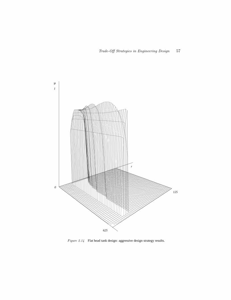
Trade-Off Strategies in Engineering Design 57
r
0
1
625
125
µ
Figure 2.14 Flat head tank design: aggressive design strategy results.

58 IMPRECISION IN ENGINEERING DESIGN
µ
0
1
r
125
0
l
625
Figure 2.15 Hemi head tank design: aggressive design strategy results.
Trade-Off Strategies in Engineering Design 59
head design), and likewise for Figures 2.12 and 2.14 (flat head design). Theconservative design strategy sacrificed the cost (m) to ensure the capacity (v).Designing aggressively did the reverse: reduced the cost (m) at expense of thecapacity (v). Observe that, from an optimization viewpoint, both solutions arein the Pareto-optimal solution set, since both require a reduction in preferenceof a goal to increase another.
This differs from the results of the various problem formulations presentedin Papalambros and Wilde [17]. For example, the non-linear programmingformulation solves the problem by minimizing the metal volume with the restof the goals as crisp constraints. Our formulation allows the constraints to beelastic, as shown in Figures 2.6 through 2.11, so the final design parametervalues determined are different than if crisp constraints had been used. If theexample had selected step functions for preference curves on the constraintperformance parameters, the imprecision results would reduce to the non-linearprogramming solution for any strategy. This is because, with step functions forthe constraint parameters, only one parameter (m) dictates the preference, andso the issue of trade-off between goals is not applicable: there is only onegoal. The point of this example is to visually demonstrate the differing overallpreference (shown here as surfaces) over the design space, and to demonstratethat different design trade-off strategies can entirely change the solution.
4. ConclusionThis paper presents a method for trading off multiple, incommensurate goals.
The definition of “best” in light of the incommensurate goals is determined byspecifying a formal, explicit design trade-off strategy.
This work permits direct comparisons of different design configuration al-ternatives in a formal sense: by comparing their respective overall preferenceratings. This is true even if the different alternatives have vastly differentphysical forms, or even if the different configurations have different param-eters. Further, the formalization of these strategies, introduced here, showsthat strategies can guide design decisions. Two simple examples were pre-sented to demonstrate the methodology in familiar domains. It was shown thatcurrent matrix method formalizations for preliminary design (such as Pugh’smethod [18], and QFD [1, 13]) use a compensating design strategy to trade-offthe different features of alternative configurations. This is because they selecta configuration based on the net sum of designer rankings, rather than on worstcase. This research will allow designers to apply the same techniques, but withdifferent design strategies, as appropriate.
This new methodology permits the designer to formally implement a designtrade-off strategy, and incorporate subjective knowledge and experience (viapreference and imprecision). This makes the designer’s prejudices and strategy

60 IMPRECISION IN ENGINEERING DESIGN
explicit, which can be used to help make, observe, justify, and record designdecisions.
AcknowledgmentsThis research is supported, in part, by: The National Science Foundation
under a Presidential Young Investigator Award, Grant No. DMC-8552695.Mr. Otto is an AT&T-Bell Laboratories Ph.D. scholar, sponsored by the AT&Tfoundation. Any opinions, findings, conclusions or recommendations expressedin this publication are those of the authors and do not necessarily reflect theviews of the sponsors. The past work of Dr. Kris Wood, now at the Universityof Texas at Austin, is also gratefully acknowledged.
Trade-Off Strategies in Engineering Design 61
References
[1] A KAO, Y. Quality Function Deployment: Integrating Customer Require-ments into Product Design. Productivity Press, Cambridge, 1990.
[2] A LGER, J., AND HAYS, C. Creative Synthesis in Design. Prentice Hall,Englewood Cliffs, 1964.
[3] A SHLEY, S. The battle to build better products.Mechanical Engineering109(Nov. 1990), 34–38.
[4] BELLMAN , R. E.,AND ZADEH, L. A. Decision-making in a fuzzy en-vironment.Management Science 17, 4 (Dec. 1970), B–141–163.
[5] BIEGEL, P., AND PECHT, M. Design trade-offs made easy.ConcurrentEngineering 1, 3 (May/June 1991), 29–40.
[6] COLTON, J., AND DESCANIO, J. An integrated, intelligent design envi-ronment.Engineering with Computers 7(1991), 11–22.
[7] DIAZ , A. R. Fuzzy set based models in design optimization. InAdvancesin Design Automation - 1988(New York, NY, Sept. 1988), S. S. Rao, Ed.,vol. DE-14, ASME, pp. 477–485.
[8] DIAZ , A. R. Modeling of computer-based decisions and optimization inthe design process. InDesign Theory ’88(RPI, Troy, NY, June 1988),S. L. Newsome and W. R. Spillers, Eds., NSF, pp. 286–295. 1988 NSFGrantee Workshop on Design Theory and Methodology.
[9] DIAZ , A. R. A strategy for optimal design of hierarchical systems us-ing fuzzy sets. InThe 1989 NSF Engineering Design Research Con-ference(College of Engineering, University of Massachusetts, Amherst,June 1989), J. R. Dixon, Ed., NSF, pp. 537–547.
[10] DUBOIS, D., AND PRADE, H. A class of fuzzy measures based on trian-gular norms.International Journal of General Systems 8(1982), 43–61.
[11] DUBOIS, D., AND PRADE, H. A review of fuzzy set aggregation con-nectives.Information Sciences 36(1985), 85–121.
[12] FREIHEIT, T., AND RAO, S. S. A modified game theory approach tomulti-objective optimization. InAdvances in Design Automation - 1988(New York, NY, Sept. 1988), S. S. Rao, Ed., vol. DE-14, ASME, pp. 107–114.
[13] HAUSER, J.,AND CLAUSING, D. The House of Quality.Harvard Busi-ness Review 66, 3 (May/June 1988), 63–73.
[14] HOLMES, M. F. Machine dynamics, The need for greater productivity.In Research Needs in Mechanical Systems(New York, NY, 1984), K. N.Reid, Ed., ASME, pp. 140–159.
[15] KEENEY, R.,AND RAIFFA, H. Decisions with Multiple Objectives: Pref-erences and Value Tradeoffs. Wiley, New York, NY, 1976.
62 IMPRECISION IN ENGINEERING DESIGN
[16] OSYCSKA, A. Multi-Criterion Optimization in Engineering with FortranExamples. Halstad Press, New York, NY, 1984.
[17] PAPALAMBROS, P., AND WILDE, D. Principles of Optimal Design.Cambridge University Press, New York, NY, 1988.
[18] PUGH, S. Total Design. Addison-Wesley, New York, NY, 1990.
[19] PUTRUS, R. Non-traditional approach in justifying computer integratedmanufacturing systems. InAutofact ’89 Conference Proceedings(De-troit, MI, Oct. 1989), SME, pp. 8.1–8.26.
[20] RAO, S. S. Description and optimum design of fuzzy mechanical sys-tems. ASME Journal of Mechanisms, Transmissions, and Automation inDesign 109(Mar. 1987), 126–132.
[21] RAO, S. S.,AND DHINGRA, A. K. Integrated optimal design of planarmechanisms using fuzzy theories. InAdvances in Design Automation -1989(New York, NY, Sept. 1989), vol. DE-15-2, ASME, pp. 161–168.
[22] RAO, S. S.,AND DHINGRA, A. K. Applications of fuzzy theories tomulti-objective system optimization. NASA Contractor Report 177573,NASA Ames Research Center, 1991.
[23] SAATY, T. L. Exploring the interface between hierarchies, multiple ob-jectives, and fuzzy sets.Fuzzy Sets and Systems 1(1978), 57–68.
[24] SAKAWA , M., AND YANO, H. Interactive decision making for multiob-jective nonlinear programming problems with fuzzy parameters.FuzzySets and Systems 29(1989), 315–326.
[25] SAKAWA , M., AND YANO, H. Interactive fuzzy decision making formultiobjective nonlinear programming problems with fuzzy parameters.Fuzzy Sets and Systems 32(1989), 245–261.
[26] SAKAWA , M., AND YANO, H. An interactive fuzzy satisficing methodfor multiobjective nonlinear programming problems with fuzzy parame-ters.Fuzzy Sets and Systems 30(1989), 221–238.
[27] SMETS, P. Belief functions. InNon-Standard Logics for AutomatedReasoning(1988), P. Smets, E. Mamdani, D. Dubois, and H. Prade, Eds.,Academic Press, pp. 254–286.
[28] STEUER, R. Multiple Criteria Optimization: Theory, Computation, andApplication. J. Wiley, New York, NY, 1986.
[29] THURSTON, D. L., AND TIAN , Y. A method for integrating utility anal-ysis into an expert system for design evaluation under uncertainty. InProceedings of the Seventh Uncertainty in Artificial Intelligence Confer-ence(San Mateo, CA, 1991), B. D’Ambrosio, Ed., Morgan KaufmannPublishers, pp. 398–405.
Trade-Off Strategies in Engineering Design 63
[30] TRIANTAPHYLLOU , E., AND MANN, S. An evaluation of the eigenvalueapproach for determining the membership values in fuzzy sets.Fuzzy Setsand Systems 35(1990), 295–301.
[31] TRIBUS, M. Rational Descriptions, Decisions, and Designs. PergamonPress, New York, NY, 1969.
[32] VINCENT, T. Game theory as a design tool.ASME Journal of Mecha-nisms, Transmissions, and Automation in Design 105(June 1983), 165–170.
[33] WOOD, K. L. A Method for Representing and Manipulating Uncertain-ties in Preliminary Engineering Design. PhD thesis, California Instituteof Technology, Pasadena, CA, 1989.
[34] WOOD, K. L., AND ANTONSSON, E. K. Computations with Impre-cise Parameters in Engineering Design: Background and Theory.ASMEJournal of Mechanisms, Transmissions, and Automation in Design 111,4 (Dec. 1989), 616–625.
[35] WOOD, K. L., AND ANTONSSON, E. K. Modeling Imprecision and Un-certainty in Preliminary Engineering Design.Mechanism and MachineTheory 25, 3 (Feb. 1990), 305–324. Invited paper.
[36] WOOD, K. L., OTTO, K. N., AND ANTONSSON, E. K. A FormalMethod for Representing Uncertainties in Engineering Design. InFirstInternational Workshop on Formal Methods in Engineering Design(FortCollins, Colorado, Jan. 1990), P. Fitzhorn, Ed., Colorado State University,pp. 202–246.
[37] YAGER, R. Fuzzy decision making including unequal objectives.FuzzySets and Systems 1(1978), 87–95.
Chapter 3
DESIGN PARAMETER SELECTIONIN THE PRESENCE OF NOISE
Kevin N. Otto and Erik K. Antonsson
Research in Engineering DesignVolume 6, Number 4 (1994), pages 234-246.
AbstractThe method of imprecisionis a design method whereby a multi-objective
design problem is resolved by maximizing the overall degree ofdesigner prefer-ence: values are iteratively selected based on combining the degree of preferenceplaced on them. Consider, however, design problems that exhibit multiple un-certainty forms (noise). In addition to degrees of preference (imprecision) thereareprobabilisticuncertainties caused by, for example, measuring and fabricationlimitations. There are also parameters that can take on any valuepossiblewithina specified range, such as a manufacturing or tuning adjustment. Finally, theremay be parameters which mustnecessarilysatisfy all values within the rangeover which they vary, such as a horsepower requirement over a motor’s differentspeeds. This paper defines a “best” set of design parameters for design problemswith such multiple uncertainty forms and requirements.
1. IntroductionMuch of the process of formalizing design decision making has yet to be
understood. Rigorous methods for representing and manipulating the concernsand unknowns of a design need to be advanced for a robust automation. Theability to make such decisions, however, is hampered by uncertainties (noise)in the variables used, both in their values and in the manner in which theyshould be manipulated. This paper will introduce methods that appropriatelymodel the various forms of uncertainty to define an overall “best” set of pa-rameters for use.
65
66 IMPRECISION IN ENGINEERING DESIGN
Parameter types are broken down by characterizing some model variables asdesign parameters, or those parameters in the engineering model for which thedesigner must select values, such as geometric sizes.Performance parametersare those the designer uses to indicate a design’s ability to satisfyfunctionalrequirements, such as stress or deflection. Finally, there are usuallynoise pa-rametersthat introduce uncertainty in the designer’s ability to measure, suchas manufacturing errors. Note this use of the termparameteris therefore dif-ferent from its usage in statistics, where it is used to describe a entire set ofnoise values in some respect, usually with a single number (e.g., an expectedvalue).
Initially, design parameter values are uncertain: the designer does not knowwhat values to use. Consequently, the performance parameter values are alsouncertain. As a design process proceeds, values are determined more and moreprecisely in an iterative test and refine fashion. Noise parameter uncertainty,however, always exists, and requires changes in measuring and manufacturingprocesses to improve.
In addition to these basic uncertainties, there are several different types ofdesign parameters [21]. Some parameters may have absolute, rigid functionalrequirements. Others may be flexible; targets only express what is desired, notrequired. Similarly, tolerances may have strict limits placed on them; failureto be within the tolerances is a failed design. Other tolerances may be flexible.This paper introduces a modeling scheme for both parameter types, and definesmethods for selecting an overall best design parameter set with such influences.Those parameters that have strict requirements are termednecessary parame-ters, and may be of the design, performance, or noise variety. The mathematicsof necessity was introduced to engineering design by Ward and Seering [20]for interval mathematics. The concept is extended here to different uncertaintyforms.
Modeling of UncertaintyEvery uncertainty form discussed above shall be directly modeled. That is,
the initial design parameter uncertainty shall be modeled usingthe method ofimprecision[8, 22] where each design parameter value is given a rank fromzero to one to indicate degree of preference. This forms a preference functionµ over each design parameter and performance parameter indicating degree ofpreference for values. Co-dependencies are possible, see [8].
Similarly, probabilistic noise parameters [10] shall have their values rankedwith degrees of probability. Finally, possibilistic noise parameters [10] shallhave their values ranked with degrees of possibility. All these uncertainties re-flect different phenomena, and consequently will have different derived math-

Design Parameter Selection in the Presence of Noise 67
ematics. Of course, these uncertainties can interact. A design parameter mayhave both a preference function and a probability density function.
This paper focuses on making the determination of the “best” overall de-sign parameter set given such influences, and presents a method which can beused to solve for the maximum overall preference for a design parameter set,even with confounding probabilistic and possibilistic uncertainties, as well asnecessary requirements.
Section 2.1 briefly reviews a metric to define the highest preference, see [8]for a complete discussion of its iterative specification. The effects of uncer-tainty on the highest overall preference concept are discussed in Section 2.2for individual forms of confounding influences. Section 3. discusses incorpo-ration of necessary parameters. Finally, Section 4. discusses design problemswith combinations of these effects.
2. Parameter Selection in the Design Process
2.1 Global Preference Functions and DesignStrategies
This work addresses the stage of the engineering design process where thedesigner is selecting a configuration. Therefore, the designer has developeda formal design parameter space (DPS) consisting of alternative configura-tions to choose among. The DPS will be characterized bydesign parameters,d1, . . . , dn. For a design process of selection among alternatives, eachdi rep-resents an alternative, so the DPS' ZZn (the finite set of integers up ton).For determination of values in a design model, there are usually multiple pa-rameters each of which could be thought of as a continuum, and so eachdi
might thought of as a value of a vector within a DPS' IRn, where the DPS isrepresented in some basis with coordinatesdi, for example.
Given that an overall best design parameter set is to be found, the “best” con-cept must be defined. Unfortunately, the various performance parameters usu-ally involve incommensurate concepts. A traditional approach to combiningincommensurate parameters is to use a normalization and a weighting. Instead,incommensurate parameters can be combined more usefully using a commontrait: designer preference. This means that preference information (µ) on thedesign parameters (di) and requirement preferences on the the performanceparameters (fj(~d)) must be combined into an overall preference rating for thatdesign parameter set (~d). The vector notation is meant to suggest the typicaldesign scenario of a multi-component design, but this development is applica-ble to singleton designs.
To reflect the designer’s overall preference, a globaldesign metric(whichranks each combination of possible design parameter arrangements) must ex-ist across the design parameter space, expressed as a function of the known
68 IMPRECISION IN ENGINEERING DESIGN
preferences of the design:
µ(~d) = P(µ(d1), . . . , µ(dn), µ(f1(~d)), . . . , µ(fq(~d))
)(3.1)
where ~d is a design parameter arrangement, andf1 throughfq are the per-formance parameters. This definition is the least possibly restrictive methodof combining incommensurate concepts. It is a formalization of the notion ofcombining incommensurate parameters based on the degree that each parame-ter satisfies the designer. Hence the best design parameter set to use is definedby the maximum of this preference function:
µ(~d∗) = sup{
P(µ(d1), . . . , µ(dn), µ(f1(~d)), . . . , µ(fq(~d)))∣∣∣∣ ~d ∈ DPS
}(3.2)
The multi-objective design problem with multiple constraints then becomes tofind ~d∗ as reflected in Equation 3.2, by maximizing the design metricP overthe design space (DPS).
This problem statement, however, is incomplete:P is unspecified. Thechoice of atrade-off strategydesired to be used by the designer will specifyP.Formal trade-off strategies for engineering design are introduced in [8]. Forexample, use of the minimum function (P ≡ min) reflects aconservativeornon-compensatingstrategy of the designer to improve the design by always im-proving the weakest design aspect. Use of a normalized multiplication reflectsanaggressiveor compensatingstrategy of the designer to develop a maximallyperforming design. Of course, non-compensating and compensating strategyhybridization for different aspects of the design are possible [8].
2.2 Uncertainty EffectsHaving formulated the overall preference function, there may still be uncer-
tainties to confound the search for the design parameter set which provide thehighest global preference. This will be resolved, however, by assuming thatthe designer wants the design parameter set that provides the best “quality” inlight of the possible variations, using the following interpretation of quality:overall preference despite variations. This is similar to the view of quality thatTaguchi uses [17], where he instead applies the view on a single performanceparameter, rather than on preference over many parameters [9].
Confounding InfluencesIn an engineering design problem, noise is typically characterized bynoise
parameters, n1, . . . , nk, . . . , nq. A noise parameternk might be the possiblepositioning of an operator switch, and so the alternatives may be finite. Alter-natively,nk might be a value of a manufacturing error on a design parameter,
Design Parameter Selection in the Presence of Noise 69
and so the NPS may have a continuum of possibilities. In this case,nk mightbe thought of as a value of a vector within an NPS' IRq represented withcoordinatesnκ in some basis, for example.
Though these specific, simple examples illustrate the concept of noise, thestructure needed to model noise can be developed more generally. Thus, theNPS is defined to be anuncertainty measure space (NPS,B, g), which is a setNPS of elementsn, a σ-algebraB of sets over the NPS (also called aBorelfield), and an uncertainty measureg : B → [0, 1]. Notice thatB is a set ofsets.N ∈ B is an event: a set of possible valuesn. This is in keeping withthe historical development of statistical noise, where an event is a possibleoutcome or outcomes.
An uncertainty measure is different from a Lebesgue measure [6] or a fuzzymeasure [4, 5, 14, 15]. An uncertainty measure is a functiong : B → [0, 1]intended to measure the effects of noise. Three specific measures will be devel-oped: the probability measurePr, the possibility measureΠ, and a necessitymeasureNα.
In keeping with the terminology of probability, an element ofB is called anevent. The measureg is to be interpreted as a formalization of the ability of anevent to occur.
Theσ-algebraB is determined by the designer.B characterizes the ability ofthe designer to make statements about the NPS. The number of subsets withinB is determined by the designer’s ability to characterize the NPS.
That events in the NPS have the structure of aσ-algebra must be justified.Formally, this means the NPS has an associated collection of subsetsB thatsatisfy,∀ Ni, Nj ∈ B:
i) Nj = NPS\Nj ∈ Bii)
⋃j∈J Nj ∈ B (3.3)
whereJ is an index set. Thus,i) states that for all eventsNj in the setB,not-an-event (Nj) is equal to the Noise Parameter Space with the event (Nj)removed. It also states that if eventNj can occur, thenNj can also occur (or,stated differently:Nj can not occur). Also,ii) states that the union of all eventsNj (wherej is in the index setJ) are in the setB. If index setJ contains1and2, andN1 andN2 are contained inB (which means thatN1 andN2 canoccur separately), then the union ofN1 andN2 can occur. Stated differently:eitherN1 or N2, or both can occur. These are true for any sequence of events.DeMorgan’s laws also hold on subsets:
iii) (Ni ∪ Nj) = (Ni) ∩ (Nj)
iv) (Ni ∩ Nj) = (Ni) ∪ (Nj).(3.4)
70 IMPRECISION IN ENGINEERING DESIGN
Thusiii) states that the complement (negation) of the union ofNi andNj isthe same as the intersection of not-Ni and not-Nj . Stated differently: if eitherNi or Nj do not occur, then bothNi andNj do not occur. Finally,iv) statesthat the complement (negation) of the intersection ofNi andNj is the sameas the union of not-Ni and not-Nj . Stated differently: if neitherNi or Nj canoccur together, then eitherNi or Nj can not occur.
These assumptions are sufficient to show the collectionB forms an algebraover the subsets [6]. Thus, events inB also satisfy:
ii)⋃
j∈J Nj ∈ Bv)
⋂j∈J Nj ∈ B (3.5)
whereJ is an index set. The algebraic structure of a noise space is not new tothis work, it is historically well developed [6] (for probability).
Given an uncertain space (NPS,B,g), the NPS is characterized. What is de-sired is to rate a design configuration, given these noise effects. To do so, adisjoint collection of subsets whose union is the entire NPS, or apartition, isneeded. On each subset in the partition, the effects of the noise will be deter-mined, and then each rating on each subset in the partition will be incorporatedinto an overall rating across the partition (across the NPS). Not just any par-tition is used, but the limit in refinement of any sequence of partitions withinB. Thus, the most accurate rating of the noise is used, given what the designercan state about the noise.
Probabilistic Uncertainty A particular uncertainty form that can beused to model the NPS occurs when the events are random. For example,inaccuracies in measurements and manufacturing are usually modeled as ran-dom. Such inaccuracies form what is now termed aprobability space. Theprobability space will be denoted NPS, meaning all uncertainties in the NPSare now considered probabilistic, for this section.
Given the probability space, an uncertainty measureg is constructed, anddenotedPr. Pr measures the probability of an event occurring. A restrictionof thePr measure is that the probability of an event occurring and not occur-ring must equal the probability of the certainty event (assumed to be 1) underreal addition. Further, the probability of either of two disjoint events occurringmust equal the real additive probability of the two events. These restrictionsare sufficient to derive an uncertainty measurePr [2, 3, 4, 7, 18].
Thus, for eventsNj , Nk ∈ B such thatNj ∩ Nk = ∅, if g is restricted toobey:
g(Nj) + g(NPS\Nj) = 1
g(Nj) + g(Nk) = g(Nj ∪ Nk)(3.6)
theng is a probability measure of classical probability theory [2, 7, 18].
Design Parameter Selection in the Presence of Noise 71
If uncertainty information is included in design decision making, it is be-cause the variational effects are to be minimized by proper selection of thenominal value of the imprecise variables. This is determined by weighting thepreference of a design parameter set by its probability of occurring through theprobabilistic uncertainty. This implies that given a probability space(NPS,B, P r),the preferential performance of a pointd ∈ DPS is defined by
µ(d) =∫
NPSµ(d, n) dPr (3.7)
whereµ(d, n) = P(µ1, . . . , µN). This integral is the standard Lebesgue inte-
gral from measure theory [6, 12]. Thus,µ(d) is the probabilistic expectationof µ(d, n) across the probability space with respect to the probability mea-surePr. The design configurationd∗ to use is the one which maximizes theexpected performance of Equation 3.7 across the DPS.
If the NPS is a discrete NPS' ZZq, then each of the individual events{nj}forms a suitable partition, where each has an associated discretePr({nj}).The integral of Equation 3.7 then becomes a simple finite sum. If the NPS'IR, then a partition of the form[n, n + dn) might be used. This can usually becharacterized by a probability density functionpdf(n). The integral of Equa-tion 3.7 then becomes
µ(d) =∫
NPS|dµ(d, n) pdf(n|d) d(n|d) (3.8)
a Riemann integral over the NPS. Since the distributions overn can, as before,vary withd, we here use the notationn|d. Of course the PPS, preferences, anddensity functions must all be Riemann integrable for this to hold.
This definition will produce a change in the “best” overall solution from thecase without probabilistic uncertainty. Consider a one parameter design, witha preferenceµ and apdf probability density as shown in Figure 3.1. Thepdfis the same for all design parameter values. The maximalexpectedpreference,i.e., the maximum of theE[µ] curve (which is the result of applying Equa-tion 3.7), not theµ maximum, is found. This set (d∗) is shown on the designparameter axis.
The resultingµ(d) determined from the integral will be the expected valueof preference given the probabilistic uncertainty. One could also evaluate thehigher moments of this relation to determine the standard deviation, skew, andkurtosis. Indeed, one could perform a Monte-Carlo simulation for each designparameter setd ∈ DPS or, if possible, analytically determine the probabilisticuncertainty distribution of theµ(d). This additional information, however, isusually less important and is computationally expensive.
For designs with no probabilistic uncertainty, the parameters in the designmodel that are not design parameters are all crisp numbers. In such circum-stances, Equation 3.7 reduces to Equation 3.1, since the probability density
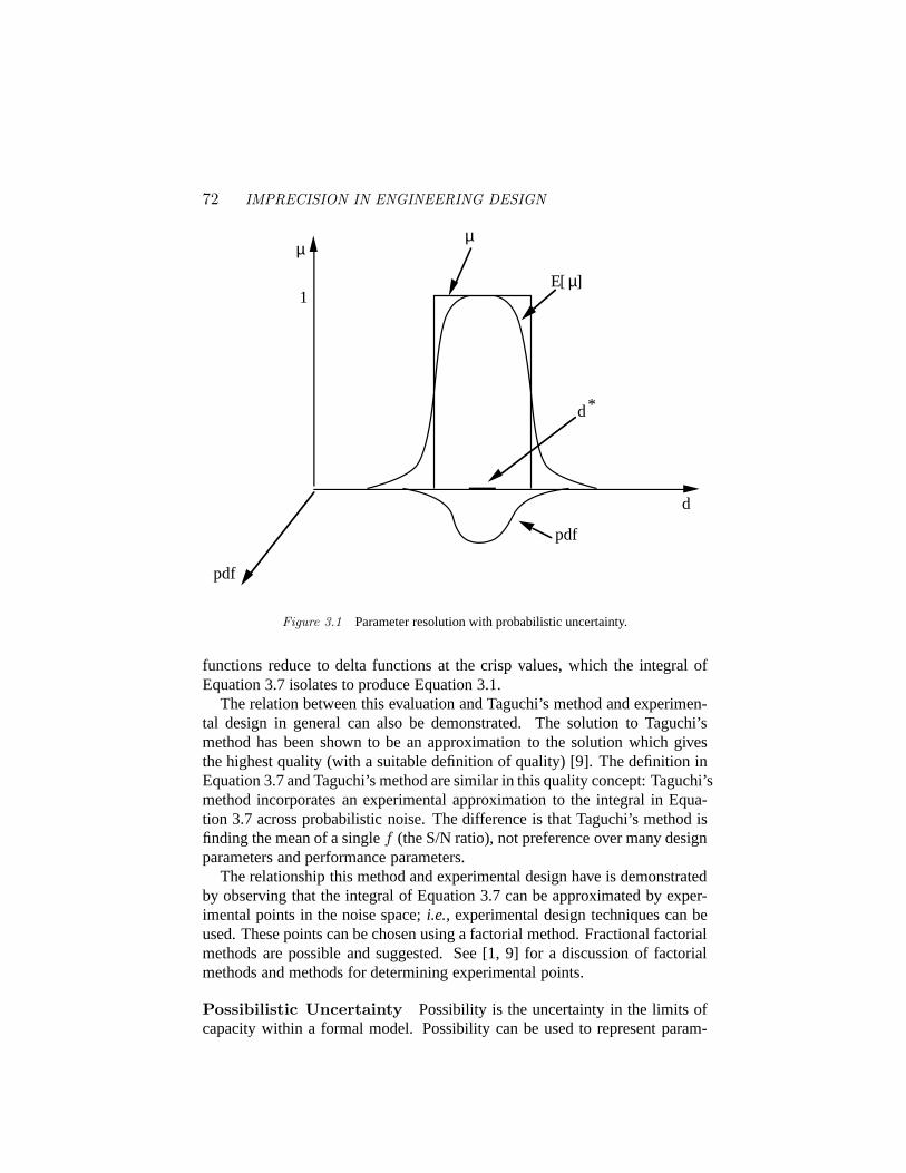
72 IMPRECISION IN ENGINEERING DESIGN
µ
d
µ
µE[ ]
1
d*
Figure 3.1 Parameter resolution with probabilistic uncertainty.
functions reduce to delta functions at the crisp values, which the integral ofEquation 3.7 isolates to produce Equation 3.1.
The relation between this evaluation and Taguchi’s method and experimen-tal design in general can also be demonstrated. The solution to Taguchi’smethod has been shown to be an approximation to the solution which givesthe highest quality (with a suitable definition of quality) [9]. The definition inEquation 3.7 and Taguchi’s method are similar in this quality concept: Taguchi’smethod incorporates an experimental approximation to the integral in Equa-tion 3.7 across probabilistic noise. The difference is that Taguchi’s method isfinding the mean of a singlef (the S/N ratio), not preference over many designparameters and performance parameters.
The relationship this method and experimental design have is demonstratedby observing that the integral of Equation 3.7 can be approximated by exper-imental points in the noise space;i.e., experimental design techniques can beused. These points can be chosen using a factorial method. Fractional factorialmethods are possible and suggested. See [1, 9] for a discussion of factorialmethods and methods for determining experimental points.
Possibilistic Uncertainty Possibility is the uncertainty in the limits ofcapacity within a formal model. Possibility can be used to represent param-
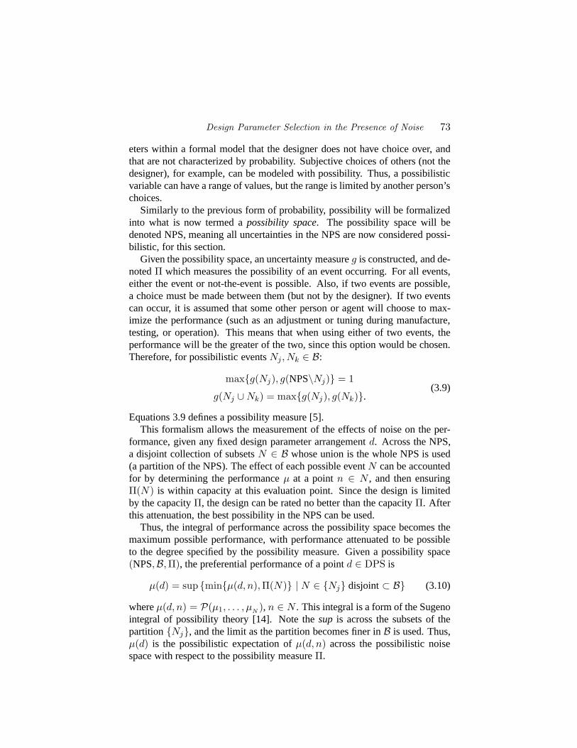
Design Parameter Selection in the Presence of Noise 73
eters within a formal model that the designer does not have choice over, andthat are not characterized by probability. Subjective choices of others (not thedesigner), for example, can be modeled with possibility. Thus, a possibilisticvariable can have a range of values, but the range is limited by another person’schoices.
Similarly to the previous form of probability, possibility will be formalizedinto what is now termed apossibility space. The possibility space will bedenoted NPS, meaning all uncertainties in the NPS are now considered possi-bilistic, for this section.
Given the possibility space, an uncertainty measureg is constructed, and de-notedΠ which measures the possibility of an event occurring. For all events,either the event or not-the-event is possible. Also, if two events are possible,a choice must be made between them (but not by the designer). If two eventscan occur, it is assumed that some other person or agent will choose to max-imize the performance (such as an adjustment or tuning during manufacture,testing, or operation). This means that when using either of two events, theperformance will be the greater of the two, since this option would be chosen.Therefore, for possibilistic eventsNj ,Nk ∈ B:
max{g(Nj), g(NPS\Nj)} = 1
g(Nj ∪ Nk) = max{g(Nj), g(Nk)}.(3.9)
Equations 3.9 defines a possibility measure [5].This formalism allows the measurement of the effects of noise on the per-
formance, given any fixed design parameter arrangementd. Across the NPS,a disjoint collection of subsetsN ∈ B whose union is the whole NPS is used(a partition of the NPS). The effect of each possible eventN can be accountedfor by determining the performanceµ at a pointn ∈ N , and then ensuringΠ(N) is within capacity at this evaluation point. Since the design is limitedby the capacityΠ, the design can be rated no better than the capacityΠ. Afterthis attenuation, the best possibility in the NPS can be used.
Thus, the integral of performance across the possibility space becomes themaximum possible performance, with performance attenuated to be possibleto the degree specified by the possibility measure. Given a possibility space(NPS,B,Π), the preferential performance of a pointd ∈ DPS is
µ(d) = sup {min{µ(d, n),Π(N)} | N ∈ {Nj} disjoint ⊂ B} (3.10)
whereµ(d, n) = P(µ1, . . . , µN), n ∈ N . This integral is a form of the Sugeno
integral of possibility theory [14]. Note thesup is across the subsets of thepartition{Nj}, and the limit as the partition becomes finer inB is used. Thus,µ(d) is the possibilistic expectation ofµ(d, n) across the possibilistic noisespace with respect to the possibility measureΠ.
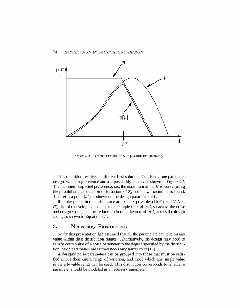
74 IMPRECISION IN ENGINEERING DESIGN
d
µ π
µ
π
[µ]E
d *
1
Figure 3.2 Parameter resolution with possibilistic uncertainty.
This definition resolves a different best solution. Consider a one parameterdesign, with aµ preference and aπ possibility density as shown in Figure 3.2.The maximum expected preference,i.e., the maximum of theE[µ] curve (usingthe possibilistic expectation of Equation 3.10), not theµ maximum, is found.This set is a point (d∗) as shown on the design parameter axis.
If all the points in the noise space are equally possible, (Π(N) = 1 ∀ N ∈B), then the development reduces to a simple max ofµ(d, n) across the noiseand design space,i.e., this reduces to finding the max ofµ(d) across the designspace, as shown in Equation 3.1.
3. Necessary ParametersSo far this presentation has assumed that all the parameters can take on any
value within their distribution ranges. Alternatively, the design may need tosatisfyeveryvalue of a noise parameter to the degree specified by the distribu-tion. Such parameters are termednecessary parameters[19].
A design’s noise parameters can be grouped into those that must be satis-fied across their entire range of variation, and those which any single valuein the allowable range can be used. This distinction corresponds to whether aparameter should be modeled as a necessary parameter.
Design Parameter Selection in the Presence of Noise 75
Two forms of necessary parameters are recognized: probabilistic necessityand possibilistic necessity. Probabilistic necessity arises when a parametervaries probabilistically and the designer wishes to ensure the design will func-tion for the entire range of variation. Possibilistic necessity arises in a similarsituation, but when the parameter varies possibilistically.
When using necessity, the degree of satisfaction desired for a necessary pa-rameter must be specified, and shall be denotedα. α is therefore a number in[0, 1], it is not a distribution, and reflects the domain percentage, as measuredby the underlying uncertainty measure (eitherPr or Π), that the designer feelsmust be ensured.α will be termed theconfidence factor. If α = 0, thenonly the most likely value is considered. Ifα = 1, then all values in the NPSmust be satisfied. For some design problems,α might need to be expressedabsolutely,i.e.,α = 0.999999 to satisfy designs to six standard deviations. Forothers,α might be made a function of the preferenceµ, so when the achievablepreference is high, the necessity range is increased (α is increased); when theachievable preference is low, the necessity range is decreased (α is decreased),easing the degree of difficulty in satisfying the design.
Thus, there is a requirement of determining the domain (NPS) percentagerequired to be satisfied. A subsetNα ∈ B, called thenecessary set, is definedas the subset of the NPS that is desired to be satisfied.
Given the necessary subsetNα, any other subsetN in B can be identified asnecessary. IfN lies within Nα, then the subsetN is necessary, otherwise it isnot. Thus, a necessity measure of each subsetN can be constructed given thenecessary subsetNα. This measure can be defined by
Nα(N) =
{0 N ⊆ Nα
1 N 6⊆ Nα.(3.11)
Any measureg satisfying Equation 3.11 will be called anecessity measure,and is denoted byNα. Thus, only if all points within a setN are necessarydoes the setN become necessary.
The necessity measure is a{0, 1} placed measure. The designer uncertaintywill be incorporated intoα ∈ [0, 1], to determine the extent ofNα. Thus theuncertainty is incorporated into specification ofNα (the necessary set), not inNα (the measure of a set inB).
An uncertainty integral can be constructed with the necessity measure. Theintegral of performance becomes the worst case performance across the ne-cessity space, as measured by the necessity measure. Given a necessity space(NPS,B,Nα), the preferential performance of a pointd ∈ DPS is defined by
µα(d) = inf {max{µ(d, n),Nα(N)} | N ∈ {Nj} disjoint ∈ B} (3.12)
76 IMPRECISION IN ENGINEERING DESIGN
whereµ(d, n) = P(µ1, . . . , µN ), n ∈ N . Again, the limit as the partitionbecomes finer inB is used. Thus,µα(d) is the necessary expectation ofµ(d, n)across the necessary space with respect to the necessary measureNα.
The problem is thus well formed, provided the setNα can be identified.How much of the NPS should be ensured? For an NPS' IRq independent,this has typically been done withconfidence intervals[16]. This formalism,however, assumes that the underlying uncertainty measure (Pr or Π) is con-structed from a density function (pdf or π), which requires an ordering on theNPS. In any case, the portion of the uncertainty space to be satisfied is identi-fied as theconfidence factor: α.
3.1 Probabilistic Necessary ParametersWhen the underlying uncertainty is probabilistic, the density function that
can be used to partition an ordered NPS is the probability density function,pdf : NPS→ IR+ ∪ {0}. Thepdf can be used to define the necessary subsetof the NPS, for any confidence factorα:
Nα = {n ∈ NPS| pdf(n) ≥ Θ} (3.13)
where
Θ = inf{
θ
∣∣∣∣ pdf(n) ≥ θ and∫
NPSχ{pdf(n)≥θ}(n) dPr ≤ α
}. (3.14)
Thus,Θ is the lowest levelpdf value withα equal to thePr of all n whosepdf ≥ Θ. This forms the set of elementsn whose totalPr = α, and whosenall havepdf ≥ Θ.
For example, in the case of NPS' IR, andpdf as the normal distribution,Nα becomes a class interval:
Nα = [E − r,E + r]
whereE is the expected value, andr is a radial distance from the expectedvalue such thatPr([E − r,E + r]) = α.
The most preferred design parameter set and the maximal preference in lightof probabilistic necessary parametersn then becomes:
d∗ : µα(d∗) = sup {inf {µ(d, n) | n ∈ Nα} | d ∈ DPS} . (3.15)
To see this definition’s meaning, consider a one variable design with a prob-abilistic necessary distribution, as shown in Figure 3.3. Each value along thedesign parameter axis is uncertain because of the normal probabilistic varia-tion as shown. Therefore the preference curveµ must be reduced at each point
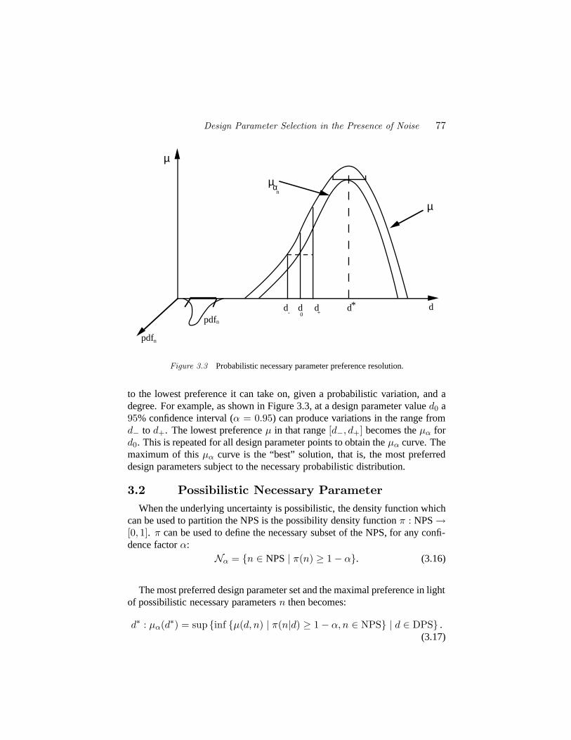
Design Parameter Selection in the Presence of Noise 77
µ
µ
µn
pdfn
pdfn
d* d
α
0d dd
- +
Figure 3.3 Probabilistic necessary parameter preference resolution.
to the lowest preference it can take on, given a probabilistic variation, and adegree. For example, as shown in Figure 3.3, at a design parameter valued0 a95% confidence interval (α = 0.95) can produce variations in the range fromd− to d+. The lowest preferenceµ in that range[d−, d+] becomes theµα ford0. This is repeated for all design parameter points to obtain theµα curve. Themaximum of thisµα curve is the “best” solution, that is, the most preferreddesign parameters subject to the necessary probabilistic distribution.
3.2 Possibilistic Necessary ParameterWhen the underlying uncertainty is possibilistic, the density function which
can be used to partition the NPS is the possibility density functionπ : NPS→[0, 1]. π can be used to define the necessary subset of the NPS, for any confi-dence factorα:
Nα = {n ∈ NPS| π(n) ≥ 1 − α}. (3.16)
The most preferred design parameter set and the maximal preference in lightof possibilistic necessary parametersn then becomes:
d∗ : µα(d∗) = sup {inf {µ(d, n) | π(n|d) ≥ 1 − α, n ∈ NPS} | d ∈ DPS} .(3.17)
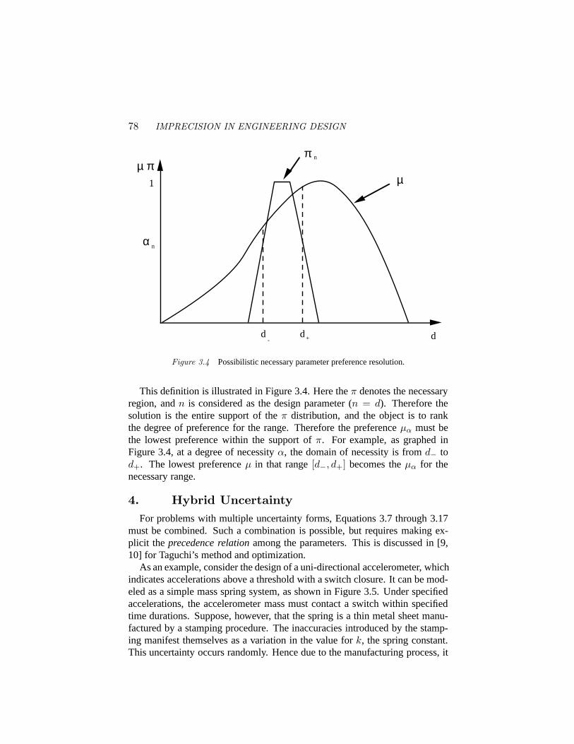
78 IMPRECISION IN ENGINEERING DESIGN
µ πµ
α n
π n
1
dd d- +
Figure 3.4 Possibilistic necessary parameter preference resolution.
This definition is illustrated in Figure 3.4. Here theπ denotes the necessaryregion, andn is considered as the design parameter (n = d). Therefore thesolution is the entire support of theπ distribution, and the object is to rankthe degree of preference for the range. Therefore the preferenceµα must bethe lowest preference within the support ofπ. For example, as graphed inFigure 3.4, at a degree of necessityα, the domain of necessity is fromd− tod+. The lowest preferenceµ in that range[d−, d+] becomes theµα for thenecessary range.
4. Hybrid UncertaintyFor problems with multiple uncertainty forms, Equations 3.7 through 3.17
must be combined. Such a combination is possible, but requires making ex-plicit the precedence relationamong the parameters. This is discussed in [9,10] for Taguchi’s method and optimization.
As an example, consider the design of a uni-directional accelerometer, whichindicates accelerations above a threshold with a switch closure. It can be mod-eled as a simple mass spring system, as shown in Figure 3.5. Under specifiedaccelerations, the accelerometer mass must contact a switch within specifiedtime durations. Suppose, however, that the spring is a thin metal sheet manu-factured by a stamping procedure. The inaccuracies introduced by the stamp-ing manifest themselves as a variation in the value fork, the spring constant.This uncertainty occurs randomly. Hence due to the manufacturing process, it
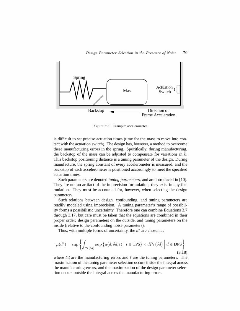
Design Parameter Selection in the Presence of Noise 79
Mass
Spring
ActuationSwitch
Backstop Direction of Frame Acceleration
Figure 3.5 Example: accelerometer.
is difficult to set precise actuation times (time for the mass to move into con-tact with the actuation switch). The design has, however, a method to overcomethese manufacturing errors in the spring. Specifically, during manufacturing,the backstop of the mass can be adjusted to compensate for variations ink.This backstop positioning distance is a tuning parameter of the design. Duringmanufacture, the spring constant of every accelerometer is measured, and thebackstop of each accelerometer is positioned accordingly to meet the specifiedactuation times.
Such parameters are denotedtuning parameters, and are introduced in [10].They are not an artifact of the imprecision formulation, they exist in any for-mulation. They must be accounted for, however, when selecting the designparameters.
Such relations between design, confounding, and tuning parameters arereadily modeled using imprecision. A tuning parameter’s range of possibil-ity forms a possibilistic uncertainty. Therefore one can combine Equations 3.7through 3.17, but care must be taken that the equations are combined in theirproper order: design parameters on the outside, and tuning parameters on theinside (relative to the confounding noise parameters).
Thus, with multiple forms of uncertainty, thed∗ are chosen as
µ(d∗) = sup
{∫Pr(δd)
sup {µ(d, δd, t) | t ∈ TPS} × dPr(δd)∣∣∣∣ d ∈ DPS
}
(3.18)whereδd are the manufacturing errors andt are the tuning parameters. Themaximization of the tuning parameter selection occurs inside the integral acrossthe manufacturing errors, and the maximization of the design parameter selec-tion occurs outside the integral across the manufacturing errors.
80 IMPRECISION IN ENGINEERING DESIGN
It is not always true that possibilistic uncertainty has its evaluation insidethe probabilistic integral. If there had been possibilistic uncertainty associatedwith the design parametersd to limit the designer’s choice, then this combina-tion occurs outside the manufacturing error integral. Similarly, if the designerhad particular preferences for tuning parameter values, then this combinationoccurs inside the integral. The precedence relation among the variables is de-termined by the variable type (design, noise, and tuning parameters) not onthe uncertainty forms associated with each parameter (imprecision, probabil-ity, and possibility).
For a general design problem, the evaluation order of the maximizations,minimizations, and integrals will depend on the precedence relation among thevariables. This is not an artifact of the imprecision formulation. The sameproblem occurs with any other formulation (such as probabilistic optimizationor an extended form of Taguchi’s method); the reader is referred to [10] fordemonstration of the precedence relation ordering in these other formulations.Imprecision simply sets the metric across the space to be preference (µ) ratherthan, for example, a single performance parameter expression.
Finally, the tuning parameter’s value is a possibilistic uncertainty from thedesign engineer’s perspective. It has a range of possible values and the valuethat should be used cannot be set by the design engineer, since it will dependon the manufacturing errors. But the expected value of the probabilistic man-ufacturing error can be determined. Since the possibilistic tuning parameter’svalues depend on the probabilistic manufacturing error, then from the designengineer’s viewpoint (pre-manufacturing) the tuning parameter expected valuecan also be found. That is, the possibilistic tuning parameter will adjust itsvalue based on the probabilistic manufacturing error. Hence, there will be,from the design engineer’s viewpoint, a probabilistic distribution for the tun-ing parameter as well, even though it has no probability aspect associated withit at all. Taking a view of the tuning parameter before the noise occurs, it canbe said to have a distribution. But, inherent in the parameter itself (i.e., fromthe manufacturing engineer’s perspective who must actually set the variable’svalue after the noise has occurred), the parameter has absolutely nothing to dowith probability.
5. ExampleThe example presented herein considers the design of a pressurized air tank,
and is the same problem as presented in Papalambros and Wilde [11], page217. The reader is referred to reference [11] to see the restrictions applied tothe problem to permit it to be solved using crisp constraints and an optimiza-tion methodology. The same problem is considered in a previous paper withno uncertainty, only imprecision and preferences [8]. The example is simple
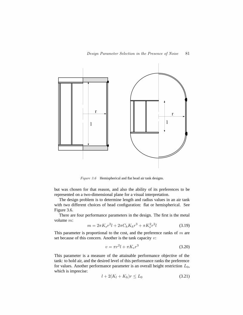
Design Parameter Selection in the Presence of Noise 81
r
l
r
l
Figure 3.6 Hemispherical and flat head air tank designs.
but was chosen for that reason, and also the ability of its preferences to berepresented on a two-dimensional plane for a visual interpretation.
The design problem is to determine length and radius values in an air tankwith two different choices of head configuration: flat or hemispherical. SeeFigure 3.6.
There are four performance parameters in the design. The first is the metalvolumem:
m = 2πKsr2l + 2πChKhr3 + πK2
s r2l (3.19)
This parameter is proportional to the cost, and the preference ranks ofm areset because of this concern. Another is the tank capacityv:
v = πr2l + πKvr3 (3.20)
This parameter is a measure of the attainable performance objective of thetank: to hold air, and the desired level of this performance ranks the preferencefor values. Another performance parameter is an overall height restrictionL0,which is imprecise:
l + 2(Kl + Kh)r ≤ L0 (3.21)
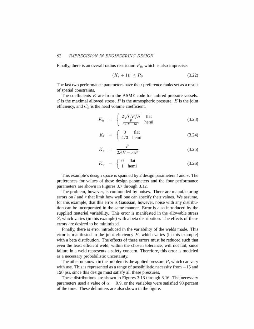
82 IMPRECISION IN ENGINEERING DESIGN
Finally, there is an overall radius restrictionR0, which is also imprecise:
(Ks + 1)r ≤ R0 (3.22)
The last two performance parameters have their preference ranks set as a resultof spatial constraints.
The coefficientsK are from the ASME code for unfired pressure vessels.S is the maximal allowed stress,P is the atmospheric pressure,E is the jointefficiency, andCh is the head volume coefficient.
Kh =
{2√
CP/S flatP
2SE−.6P hemi(3.23)
Kl ={
0 flat4/3 hemi
(3.24)
Ks =P
2SE − .6P(3.25)
Kv ={
0 flat1 hemi
(3.26)
This example’s design space is spanned by 2 design parametersl andr. Thepreferences for values of these design parameters and the four performanceparameters are shown in Figures 3.7 through 3.12.
The problem, however, is confounded by noises. There are manufacturingerrors onl andr that limit how well one can specify their values. We assume,for this example, that this error is Gaussian, however, noise with any distribu-tion can be incorporated in the same manner. Error is also introduced by thesupplied material variability. This error is manifested in the allowable stressS, which varies (in this example) with a beta distribution. The effects of theseerrors are desired to be minimized.
Finally, there is error introduced in the variability of the welds made. Thiserror is manifested in the joint efficiencyE, which varies (in this example)with a beta distribution. The effects of these errors must be reduced such thateven the least efficient weld, within the chosen tolerance, will not fail, sincefailure in a weld represents a safety concern. Therefore, this error is modeledas a necessary probabilistic uncertainty.
The other unknown in the problem is the applied pressureP , which can varywith use. This is represented as a range of possibilistic necessity from−15 and120 psi, since this design must satisfy all these pressures.
These distributions are shown in Figures 3.13 through 3.16. The necessaryparameters used a value ofα = 0.9, or the variables were satisfied90 percentof the time. These delimiters are also shown in the figure.

Design Parameter Selection in the Presence of Noise 83
Figure 3.7 Lengthl preference.
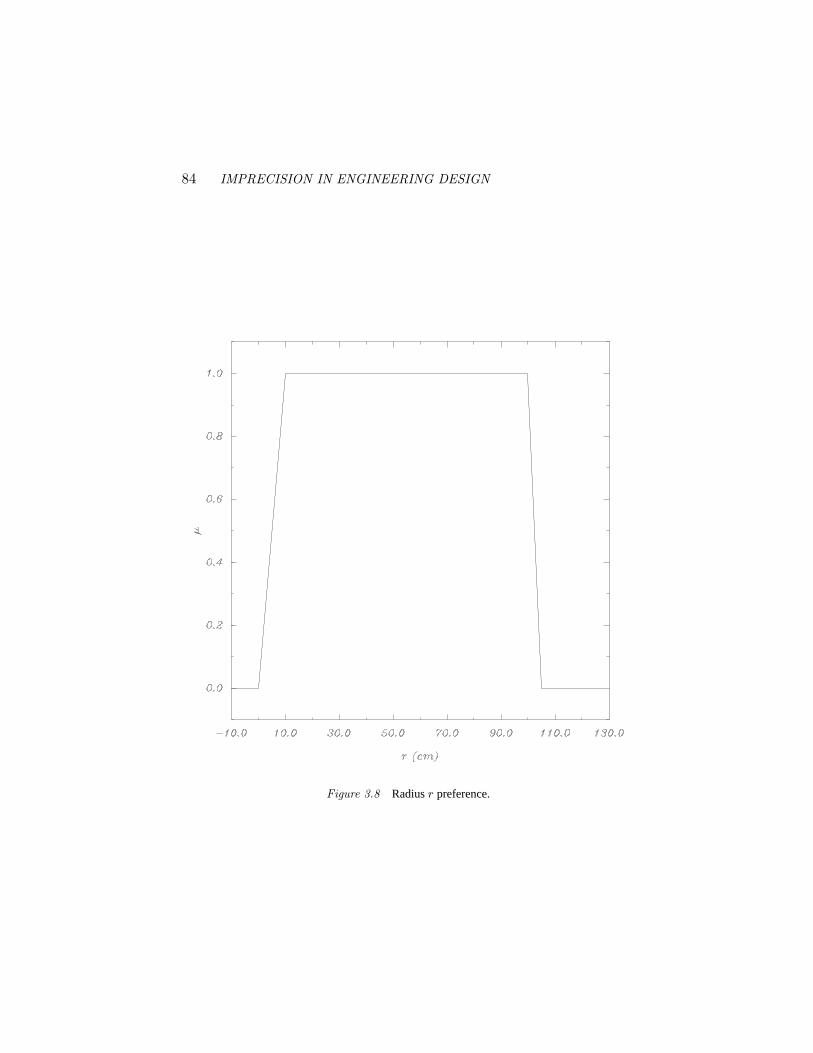
84 IMPRECISION IN ENGINEERING DESIGN
Figure 3.8 Radiusr preference.
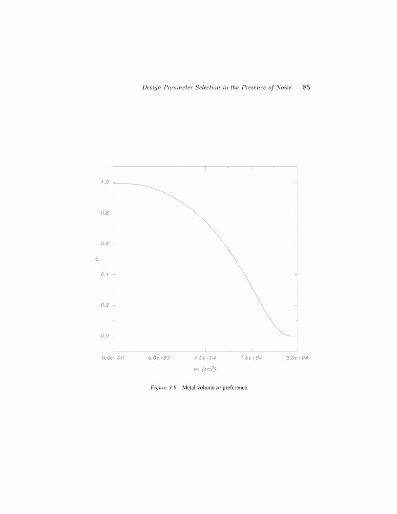
Design Parameter Selection in the Presence of Noise 85
Figure 3.9 Metal volumem preference.

86 IMPRECISION IN ENGINEERING DESIGN
Figure 3.10 Capacityv preference.
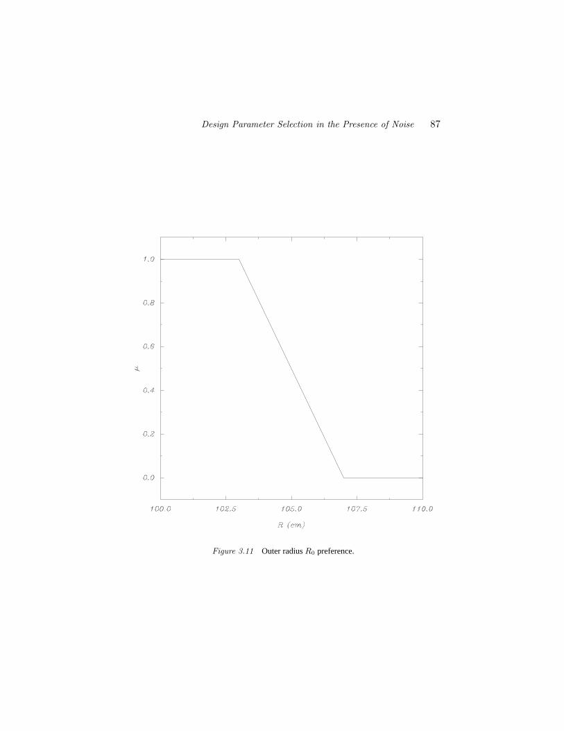
Design Parameter Selection in the Presence of Noise 87
Figure 3.11 Outer radiusR0 preference.
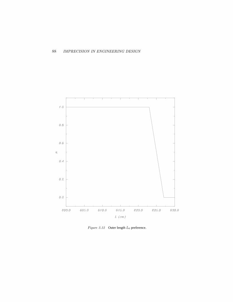
88 IMPRECISION IN ENGINEERING DESIGN
Figure 3.12 Outer lengthL0 preference.
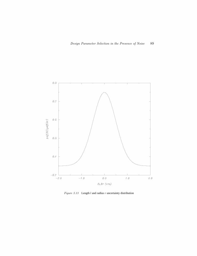
Design Parameter Selection in the Presence of Noise 89
Figure 3.13 Lengthl and radiusr uncertainty distribution

90 IMPRECISION IN ENGINEERING DESIGN
Figure 3.14 Allowable stressS uncertainty distribution
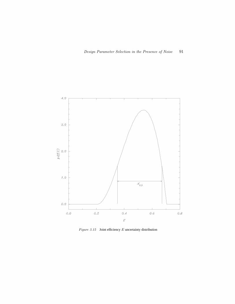
Design Parameter Selection in the Presence of Noise 91
Figure 3.15 Joint efficiencyE uncertainty distribution
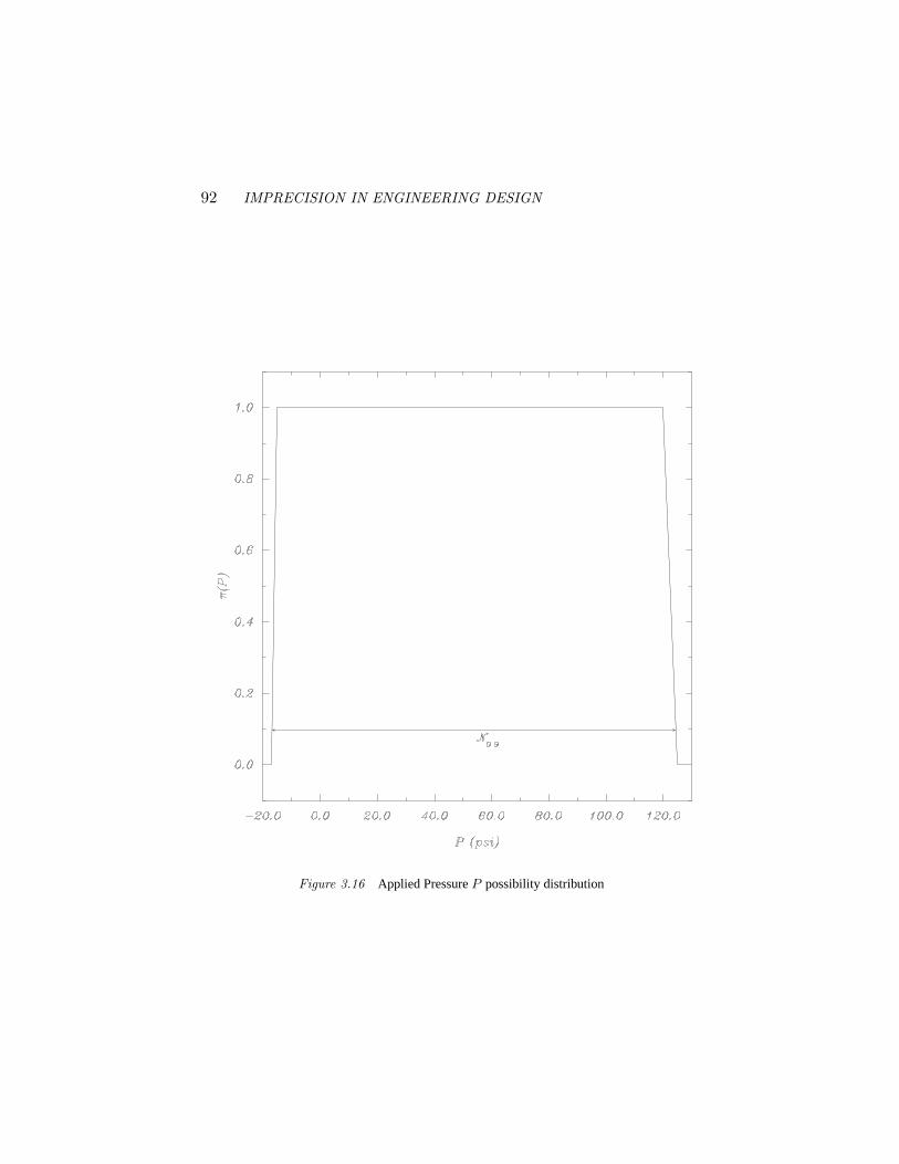
92 IMPRECISION IN ENGINEERING DESIGN
Figure 3.16 Applied PressureP possibility distribution
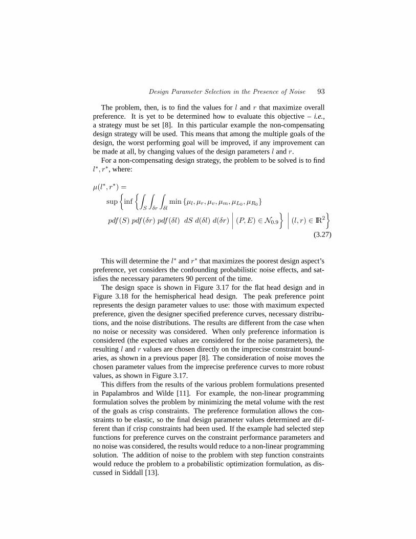
Design Parameter Selection in the Presence of Noise 93
The problem, then, is to find the values forl andr that maximize overallpreference. It is yet to be determined how to evaluate this objective –i.e.,a strategy must be set [8]. In this particular example the non-compensatingdesign strategy will be used. This means that among the multiple goals of thedesign, the worst performing goal will be improved, if any improvement canbe made at all, by changing values of the design parametersl andr.
For a non-compensating design strategy, the problem to be solved is to findl∗, r∗, where:
µ(l∗, r∗) =
sup{
inf{∫
S
∫δr
∫δl
min {µl, µr, µv, µm, µL0 , µR0}
pdf(S) pdf(δr) pdf(δl) dS d(δl) d(δr)∣∣∣∣ (P,E) ∈ N0.9
} ∣∣∣∣ (l, r) ∈ IR2}
(3.27)
This will determine thel∗ andr∗ that maximizes the poorest design aspect’spreference, yet considers the confounding probabilistic noise effects, and sat-isfies the necessary parameters 90 percent of the time.
The design space is shown in Figure 3.17 for the flat head design and inFigure 3.18 for the hemispherical head design. The peak preference pointrepresents the design parameter values to use: those with maximum expectedpreference, given the designer specified preference curves, necessary distribu-tions, and the noise distributions. The results are different from the case whenno noise or necessity was considered. When only preference information isconsidered (the expected values are considered for the noise parameters), theresultingl andr values are chosen directly on the imprecise constraint bound-aries, as shown in a previous paper [8]. The consideration of noise moves thechosen parameter values from the imprecise preference curves to more robustvalues, as shown in Figure 3.17.
This differs from the results of the various problem formulations presentedin Papalambros and Wilde [11]. For example, the non-linear programmingformulation solves the problem by minimizing the metal volume with the restof the goals as crisp constraints. The preference formulation allows the con-straints to be elastic, so the final design parameter values determined are dif-ferent than if crisp constraints had been used. If the example had selected stepfunctions for preference curves on the constraint performance parameters andno noise was considered, the results would reduce to a non-linear programmingsolution. The addition of noise to the problem with step function constraintswould reduce the problem to a probabilistic optimization formulation, as dis-cussed in Siddall [13].
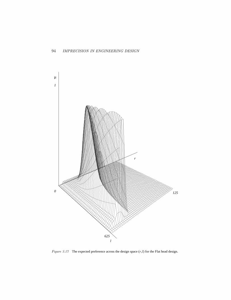
94 IMPRECISION IN ENGINEERING DESIGN
µ
1
0
l625
r
125
Figure 3.17 The expected preference across the design space (r,l) for the Flat head design.
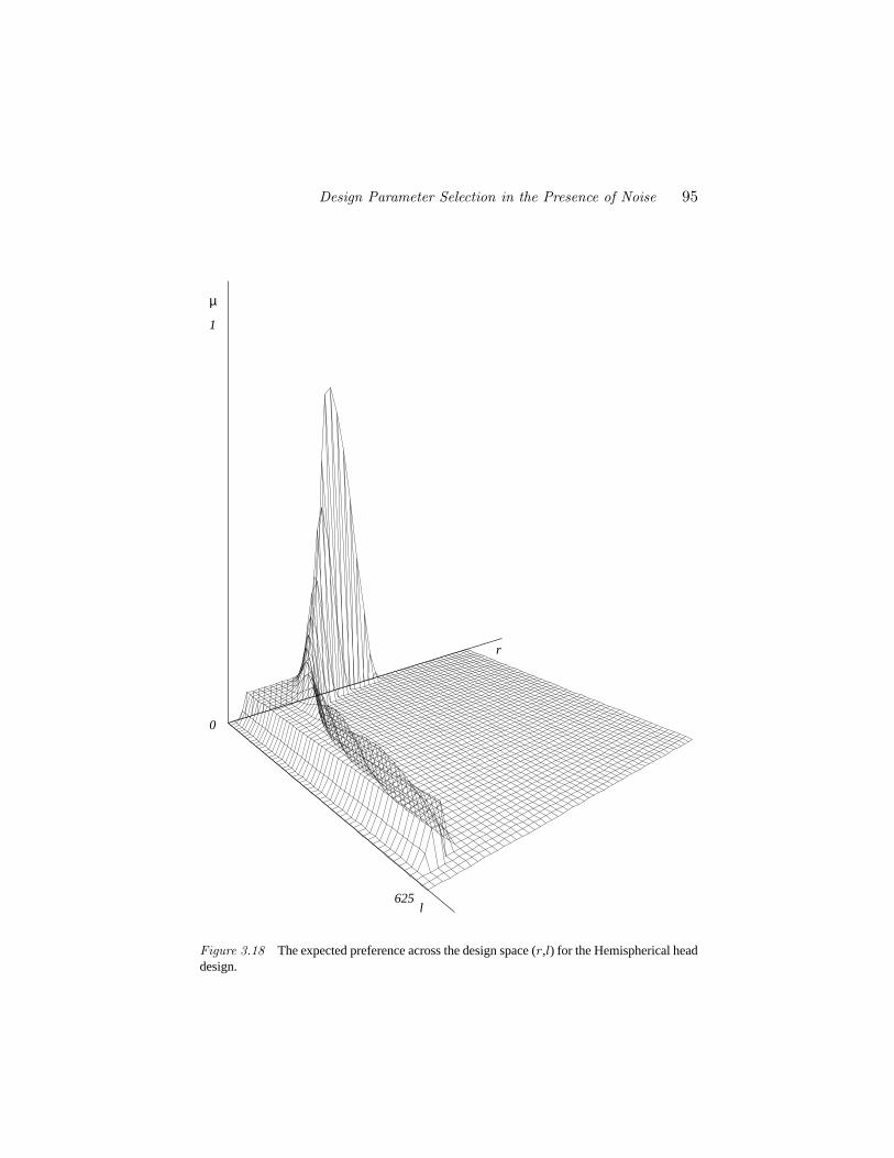
Design Parameter Selection in the Presence of Noise 95
µ
1
0
l625
r
Figure 3.18 The expected preference across the design space (r,l) for the Hemispherical headdesign.
96 IMPRECISION IN ENGINEERING DESIGN
6. ConclusionImprecise preference functions have been used to solve design problems
with multiple, incommensurate goals. A global metric is constructed acrossthe design space from the preference rankings of the parameters. The result ofapplying the design’s global metric has a simple interpretation as the overallpreference for the design.
The imprecision methodology of resolving design parameter values is ex-tended to include different confounding noise forms. Probabilistic noise re-quires the use of the probabilistic expectation process. This allows for thedetermination of the design parameter values that produce the highest overallquality. Possibilistic uncertainties, on the other hand, require the use of thepossibilistic mathematics to confine the design to select the best value amongonly those that are possible.
The formulation is also extended to include necessary requirement forms.Necessary parameters can be either probabilistic or possibilistic in nature, andthe parameter’s necessity range is determined accordingly. Non-linear formu-lations are possible that tieα to µ. Such a formulation will permit trade-offsbetween preference and degree of necessity.
Design problems that have different variable types (design parameters, noiseparameters, and tuning parameters) can now be solved. This work allows thedesigner to determine the “best” design parameter set to use, given uncertaindesign specifications and uncertainty in manufacturing processes.
AcknowledgmentsThis material is based upon work supported, in part, by: The National Sci-
ence Foundation under a Presidential Young Investigator Award, Grant No. DMC-8552695. During this research Professor Otto was an AT&T-Bell LaboratoriesPh.D. scholar, sponsored by the AT&T foundation. Any opinions, findings,conclusions or recommendations expressed in this publication are those of theauthors and do not necessarily reflect the views of the sponsors.
Design Parameter Selection in the Presence of Noise 97
References
[1] BOX, G. E. Statistics for Experimenters. J. Wiley and Sons, New York,1978.
[2] COX, R. T. The Algebra of Probable Inference. Johns-Hopkins Univer-sity Press, Baltimore, MD, 1961.
[3] DUBOIS, D., AND PRADE, H. Fuzzy Sets and Systems: Theory and Ap-plications. Academic Press, New York, 1980.
[4] DUBOIS, D., AND PRADE, H. A class of fuzzy measures based on trian-gular norms.International Journal of General Systems 8(1982), 43–61.
[5] DUBOIS, D., AND PRADE, H. Possibility Theory: An Approach tothe Computerized Processing of Information. Plenum Press, New York,1988.
[6] HALMOS, P. Measure Theory. Springer-Verlag, New York, 1974.
[7] K RANTZ, D., LUCE, R., SUPPES, P., AND TVERSKY, A. Foundationsof Measurement, vol. I. Academic Press, New York, NY, 1971.
[8] OTTO, K. N., AND ANTONSSON, E. K. Trade-Off Strategies in Engi-neering Design.Research in Engineering Design 3, 2 (1991), 87–104.
[9] OTTO, K. N., AND ANTONSSON, E. K. Extensions to the TaguchiMethod of Product Design.ASME Journal of Mechanical Design 115,1 (Mar. 1993), 5–13.
[10] OTTO, K. N., AND ANTONSSON, E. K. Tuning Parameters in Engineer-ing Design. ASME Journal of Mechanical Design 115, 1 (Mar. 1993),14–19.
[11] PAPALAMBROS, P., AND WILDE, D. Principles of Optimal Design.Cambridge University Press, New York, NY, 1988.
[12] ROYDEN, H. Real Analysis. Macmillan, New York, 1988.
[13] SIDDALL , J. N. Probabilistic Engineering Design; Principles and Ap-plications. Marcel Dekker, New York, NY, 1983.
[14] SUGENO, M. Theory of fuzzy integrals and its applications. PhD thesis,Tokyo Institute of Technology, 1974.
[15] SUGENO, M. Fuzzy measures and fuzzy integrals – a survey. InFuzzyAutomata and Decision Processes(New York, 1977), M. Gupta et al.,Eds., North-Holland, pp. 89–102.
[16] SVESHNIKOV, A. Problems in Probability Theory, Mathematical Statis-tics, and the Theory of Random Functions. Dover Publications, NewYork, 1968.
[17] TAGUCHI, G. Introduction to Quality Engineering. Asian ProductivityOrganization, Unipub, White Plains, NY, 1986.
98 IMPRECISION IN ENGINEERING DESIGN
[18] TRIBUS, M. Rational Descriptions, Decisions, and Designs. PergamonPress, New York, NY, 1969.
[19] WARD, A. C. A Theory of Quantitative Inference for Artifact Sets, Ap-plied to a Mechanical Design Compiler. PhD thesis, MIT, 1989.
[20] WARD, A. C., LOZANO-PEREZ, T., AND SEERING, W. P. Extendingthe constraint propagation of intervals.Artificial Intelligence in Engi-neering Design and Manufacturing 4, 1 (1990), 47–54.
[21] WILSON, I., AND WILSON, M. From Idea to Working Model. J. Wileyand Sons, New York, NY, 1970.
[22] WOOD, K. L., AND ANTONSSON, E. K. Computations with Impre-cise Parameters in Engineering Design: Background and Theory.ASMEJournal of Mechanisms, Transmissions, and Automation in Design 111,4 (Dec. 1989), 616–625.

Chapter 4
TUNING PARAMETERSIN ENGINEERING DESIGN
Kevin N. Otto and Erik K. Antonsson
ASME Journal of Mechanical DesignVolume 115, Number 1 (1993), pages 14-19.
AbstractIn the design and manufacture of mechanical devices, there are parameters
whose values are determined by the manufacturing process in response to er-rors introduced in the device’s manufacture or operating environment. Suchparameters are termedtuning parameters, and are distinct fromdesign parame-terswhich the designer selects values for as a part of the design process. Thispaper introduces tuning parameters into the design methods of: optimization,Taguchi’s method, and the method of imprecision [10]. The details of the math-ematical formulation, along with a design example, are presented and discussed.Including tuning parameters in thedesign processcan result in designs that aremore tolerant of variational noise.
1. IntroductionIn the design, development, and manufacture of mechanical devices, param-
eter values are determined by different mechanisms. The device’s geometry,power, etc. are chosen during the design process. However, there are usuallyvariations on these values which are determined by mechanisms such as ran-dom manufacturing errors. There are also variations in the device’s operatingenvironment which are operator induced. But there are also parameters whosevalues are set during the manufacturing process in response to the previousvariations. We denote these parameters astuning parameters. Though they arecommon to the practicing industrial engineering community, we have found noformal models which incorporate their behavior.
99
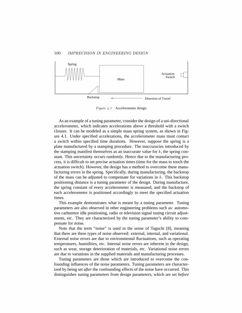
100 IMPRECISION IN ENGINEERING DESIGN
Direction of TravelBackstop
SwitchActuation
Mass
Spring
Figure 4.1 Accelerometer design.
As an example of a tuning parameter, consider the design of a uni-directionalaccelerometer, which indicates accelerations above a threshold with a switchclosure. It can be modeled as a simple mass spring system, as shown in Fig-ure 4.1. Under specified accelerations, the accelerometer mass must contacta switch within specified time durations. However, suppose the spring is aplate manufactured by a stamping procedure. The inaccuracies introduced bythe stamping manifest themselves as an inaccurate value fork, the spring con-stant. This uncertainty occurs randomly. Hence due to the manufacturing pro-cess, it is difficult to set precise actuation times (time for the mass to touch theactuation switch). However, the design has a method to overcome these manu-facturing errors in the spring. Specifically, during manufacturing, the backstopof the mass can be adjusted to compensate for variations ink. This backstoppositioning distance is a tuning parameter of the design. During manufacture,the spring constant of every accelerometer is measured, and the backstop ofeach accelerometer is positioned accordingly to meet the specified actuationtimes.
This example demonstrates what is meant by a tuning parameter. Tuningparameters are also observed in other engineering problems such as: automo-tive carburetor idle positioning, radio or television signal tuning circuit adjust-ments, etc. They are characterized by the tuning parameter’s ability to com-pensate for noise.
Note that the term “noise” is used in the sense of Taguchi [8], meaningthat there are three types of noise observed: external, internal, and variational.External noise errors are due to environmental fluctuations, such as operatingtemperatures, humidities, etc. Internal noise errors are inherent in the design,such as wear, storage deterioration of materials, etc. Variational noise errorsare due to variations in the supplied materials and manufacturing processes.
Tuning parameters are those which are introduced to overcome the con-founding influences of the noise parameters. Tuning parameters are character-ized by being setafter the confounding effects of the noise have occurred. Thisdistinguishes tuning parameters from design parameters, which are setbefore
Tuning Parameters in Engineering Design 101
the noise has occurred. Hence design engineers do not set the values of tun-ing parameters, the manufacturing engineer (or even the customer) sets theirvalues. But when the design parameter values are chosen, the design engineershould take into consideration that a tuning parameter can later be adjusted.
Given such an inherently common concept of engineering, it is surprisingthat none of the formal techniques of engineering design incorporate tuningparameters. It is the objective of this paper to introduce tuning parameters,and to demonstrate how they can be modeled in various existing formalizedmethods of engineering design. We will demonstrate how optimization [4],Taguchi’s method [1], and the method of imprecision [10, 11] can incorporatetuning parameters.
2. Modeling Tuning ParametersIn addition to tuning parameters, two other types of parameters are used in
the design process: design parameters and noise parameters. Design param-eters are those for which the designer selects values as a part of the designprocess. When the design is finished, exact nominal values are specified fordesign parameters. Noise parameters, on the other hand, confound the abil-ity of the designer to specify nominal values for the design parameters. Asstated earlier, noise parameters model uncertainty in the design, they behaverandomly. Typically, parameters in a design will have both a design and a noiseparameter aspect. That is, a designer will specify a nominal value, and therewill be (manufacturing) noise associated with trying to achieve the specifiedvalue.
In the design process, the design parameter values are chosen such thatthe design goals are maximized despite the noise parameter actions. In theaccelerometer example, the design parameters (the nominal spring constantK and the massM ) would be chosen such that the desired performance isachieved as often as possible. This is the extent to which formal techniquessuch as Taguchi’s method [1] and probabilistic optimization [6] currently modelparameter types: select the design parameter values which maximize the outputdespite the noise.
With tuning parameters, however, more freedom is provided to the designer.The above techniques choose the design parameters to maximize the outputdespite the expected noise. Tuning parameters, however, are set after the noisehas occurred, and are set to overcome the noise parameters’ influences.
Utilizing this observation, we can introduce tuning parameters into threecurrent formal methods of engineering design: optimization, Taguchi’s method,and the method of imprecision. The first requirement is to establish (or deter-mine) the order in which the various parameters are fixed. We refer to thisorder as theprecedence relationbetween tuning and noise parameters. This
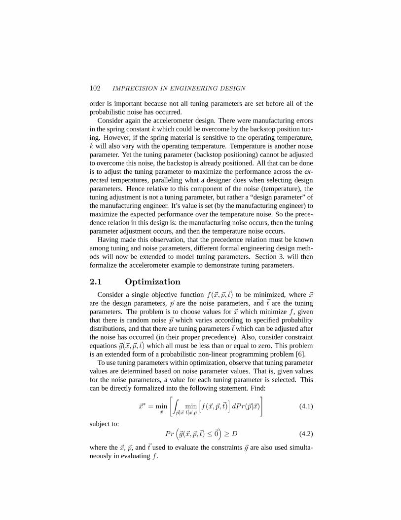
102 IMPRECISION IN ENGINEERING DESIGN
order is important because not all tuning parameters are set before all of theprobabilistic noise has occurred.
Consider again the accelerometer design. There were manufacturing errorsin the spring constantk which could be overcome by the backstop position tun-ing. However, if the spring material is sensitive to the operating temperature,k will also vary with the operating temperature. Temperature is another noiseparameter. Yet the tuning parameter (backstop positioning) cannot be adjustedto overcome this noise, the backstop is already positioned. All that can be doneis to adjust the tuning parameter to maximize the performance across theex-pectedtemperatures, paralleling what a designer does when selecting designparameters. Hence relative to this component of the noise (temperature), thetuning adjustment is not a tuning parameter, but rather a “design parameter” ofthe manufacturing engineer. It’s value is set (by the manufacturing engineer) tomaximize the expected performance over the temperature noise. So the prece-dence relation in this design is: the manufacturing noise occurs, then the tuningparameter adjustment occurs, and then the temperature noise occurs.
Having made this observation, that the precedence relation must be knownamong tuning and noise parameters, different formal engineering design meth-ods will now be extended to model tuning parameters. Section 3. will thenformalize the accelerometer example to demonstrate tuning parameters.
2.1 OptimizationConsider a single objective functionf(~x, ~p,~t) to be minimized, where~x
are the design parameters,~p are the noise parameters, and~t are the tuningparameters. The problem is to choose values for~x which minimizef , giventhat there is random noise~p which varies according to specified probabilitydistributions, and that there are tuning parameters~t which can be adjusted afterthe noise has occurred (in their proper precedence). Also, consider constraintequations~g(~x, ~p,~t) which all must be less than or equal to zero. This problemis an extended form of a probabilistic non-linear programming problem [6].
To use tuning parameters within optimization, observe that tuning parametervalues are determined based on noise parameter values. That is, given valuesfor the noise parameters, a value for each tuning parameter is selected. Thiscan be directly formalized into the following statement. Find:
~x∗ = min~x
[∫~p|~x
min~t|~x,~p
[f(~x, ~p,~t)
]dPr(~p|~x)
](4.1)
subject to:Pr(~g(~x, ~p,~t) ≤ ~0
)≥ D (4.2)
where the~x, ~p, and~t used to evaluate the constraints~g are also used simulta-neously in evaluatingf .
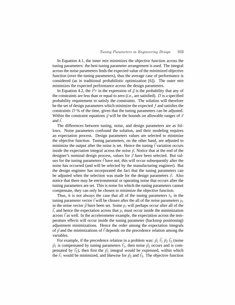
Tuning Parameters in Engineering Design 103
In Equation 4.1, the innermin minimizes the objective function across thetuning parameters: the best tuning parameter arrangement is used. The integralacross the noise parameters finds the expected value of the minimized objectivefunction (over the tuning parameters), thus the average case of performance isconsidered (as in traditional probabilistic optimization [6]). The outerminminimizes the expected performance across the design parameters.
In Equation 4.2, thePr in the expression of~g is the probability that any ofthe constraints are less than or equal to zero (i.e., are satisfied).D is a specifiedprobability requirement to satisfy the constraints. The solution will thereforebe the set of design parameters which minimize the expectedf and satisfies theconstraintsD % of the time, given that the tuning parameters can be adjusted.Within the constraint equations~g will be the bounds on allowable ranges of~xand~t.
The differences between tuning, noise, and design parameters are as fol-lows. Noise parameters confound the solution, and their modeling requiresan expectation process. Design parameters values are selected to minimizethe objective function. Tuning parameters, on the other hand, are adjusted tominimize the output after the noise is set. Hence the tuning~t variation occursinside the expectation integral across the noise~p. Notice that at the end of thedesigner’s nominal design process, values for~x have been selected. But val-ues for the tuning parameters~t have not; this will occur subsequently after thenoise has occurred (and will be selected by the manufacturing engineer). Butthe design engineer has incorporated the fact that the tuning parameters canbe adjusted when the selection was made for the design parameters~x. Alsonotice that there may be environmental or operating noise that occurs after thetuning parameters are set. This is noise for which the tuning parameters cannotcompensate, they can only be chosen to minimize the objective function.
Thus, it is not always the case that all of the tuning parameterstk in thetuning parameter vector~t will be chosen after the all of the noise parameterspi
in the noise vector~p have been set. Somepi will perhaps occur after all of the~t, and hence the expectation across thatpi must occur inside the minimizationacross~t as well. In the accelerometer example, the expectation across the tem-perature effects will occur inside the tuning parameter (backstop positioning)adjustment minimizations. Hence the order among the expectation integralsof ~p and the minimizations of~t depends on the precedence relation among thevariables.
For example, if the precedence relation in a problem was:~p1 ~t1 ~p2 ~t2 (noise~p1 is compensated by tuning parameters~t1, then noise~p2 occurs and is com-pensated by~t2), then first the~p1 integral would be expressed, within whichthe~t1 would be minimized, and likewise for~p2 and~t2. The objective function
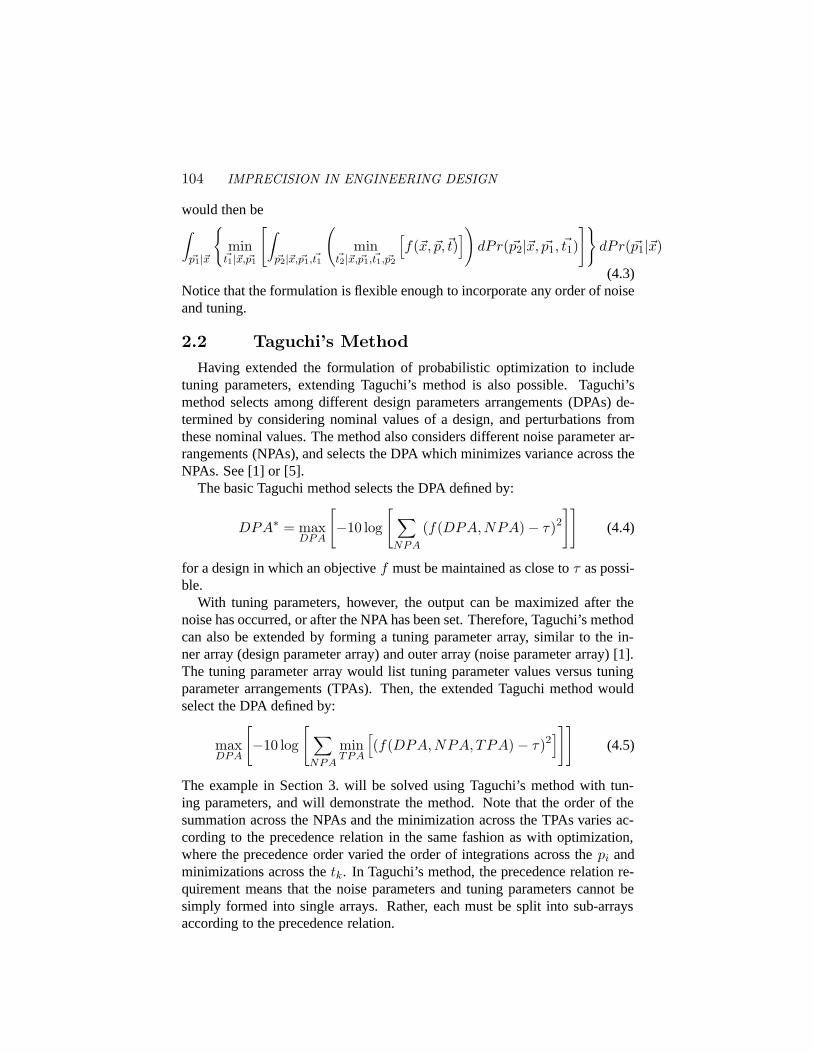
104 IMPRECISION IN ENGINEERING DESIGN
would then be∫~p1|~x
{min~t1|~x, ~p1
[∫~p2|~x, ~p1,~t1
(min
~t2|~x, ~p1,~t1, ~p2
[f(~x, ~p,~t)
])dPr(~p2|~x, ~p1, ~t1)
]}dPr(~p1|~x)
(4.3)Notice that the formulation is flexible enough to incorporate any order of noiseand tuning.
2.2 Taguchi’s MethodHaving extended the formulation of probabilistic optimization to include
tuning parameters, extending Taguchi’s method is also possible. Taguchi’smethod selects among different design parameters arrangements (DPAs) de-termined by considering nominal values of a design, and perturbations fromthese nominal values. The method also considers different noise parameter ar-rangements (NPAs), and selects the DPA which minimizes variance across theNPAs. See [1] or [5].
The basic Taguchi method selects the DPA defined by:
DPA∗ = maxDPA
[−10 log
[ ∑NPA
(f(DPA,NPA) − τ)2]]
(4.4)
for a design in which an objectivef must be maintained as close toτ as possi-ble.
With tuning parameters, however, the output can be maximized after thenoise has occurred, or after the NPA has been set. Therefore, Taguchi’s methodcan also be extended by forming a tuning parameter array, similar to the in-ner array (design parameter array) and outer array (noise parameter array) [1].The tuning parameter array would list tuning parameter values versus tuningparameter arrangements (TPAs). Then, the extended Taguchi method wouldselect the DPA defined by:
maxDPA
[−10 log
[∑NPA
minTPA
[(f(DPA,NPA, TPA) − τ)2
]]](4.5)
The example in Section 3. will be solved using Taguchi’s method with tun-ing parameters, and will demonstrate the method. Note that the order of thesummation across the NPAs and the minimization across the TPAs varies ac-cording to the precedence relation in the same fashion as with optimization,where the precedence order varied the order of integrations across thepi andminimizations across thetk. In Taguchi’s method, the precedence relation re-quirement means that the noise parameters and tuning parameters cannot besimply formed into single arrays. Rather, each must be split into sub-arraysaccording to the precedence relation.
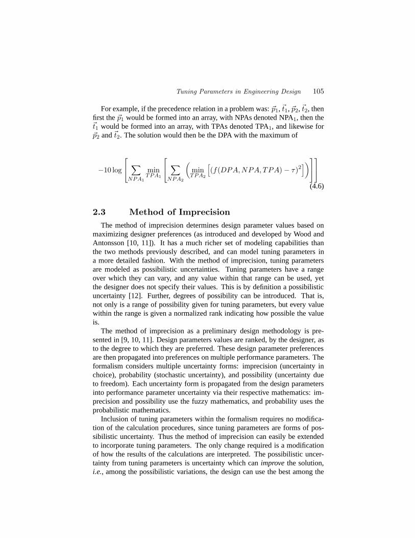
Tuning Parameters in Engineering Design 105
For example, if the precedence relation in a problem was:~p1,~t1, ~p2,~t2, thenfirst the~p1 would be formed into an array, with NPAs denoted NPA1, then the~t1 would be formed into an array, with TPAs denoted TPA1, and likewise for~p2 and~t2. The solution would then be the DPA with the maximum of
−10 log
∑
NPA1
minTPA1
∑
NPA2
(minTPA2
[(f(DPA,NPA, TPA) − τ)2
])
(4.6)
2.3 Method of ImprecisionThe method of imprecision determines design parameter values based on
maximizing designer preferences (as introduced and developed by Wood andAntonsson [10, 11]). It has a much richer set of modeling capabilities thanthe two methods previously described, and can model tuning parameters ina more detailed fashion. With the method of imprecision, tuning parametersare modeled as possibilistic uncertainties. Tuning parameters have a rangeover which they can vary, and any value within that range can be used, yetthe designer does not specify their values. This is by definition a possibilisticuncertainty [12]. Further, degrees of possibility can be introduced. That is,not only is a range of possibility given for tuning parameters, but every valuewithin the range is given a normalized rank indicating how possible the valueis.
The method of imprecision as a preliminary design methodology is pre-sented in [9, 10, 11]. Design parameters values are ranked, by the designer, asto the degree to which they are preferred. These design parameter preferencesare then propagated into preferences on multiple performance parameters. Theformalism considers multiple uncertainty forms: imprecision (uncertainty inchoice), probability (stochastic uncertainty), and possibility (uncertainty dueto freedom). Each uncertainty form is propagated from the design parametersinto performance parameter uncertainty via their respective mathematics: im-precision and possibility use the fuzzy mathematics, and probability uses theprobabilistic mathematics.
Inclusion of tuning parameters within the formalism requires no modifica-tion of the calculation procedures, since tuning parameters are forms of pos-sibilistic uncertainty. Thus the method of imprecision can easily be extendedto incorporate tuning parameters. The only change required is a modificationof how the results of the calculations are interpreted. The possibilistic uncer-tainty from tuning parameters is uncertainty which canimprovethe solution,i.e., among the possibilistic variations, the design can use the best among the
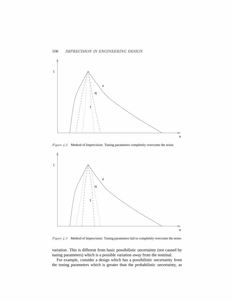
106 IMPRECISION IN ENGINEERING DESIGN
1
u
a
π
f
Figure 4.2 Method of Imprecision: Tuning parameters completely overcome the noise.
1
u
a
π
f
Figure 4.3 Method of Imprecision: Tuning parameters fail to completely overcome the noise.
variation. This is different from basic possibilistic uncertainty (not caused bytuning parameters) which is a possible variationawayfrom the nominal.
For example, consider a design which has a possibilistic uncertainty fromthe tuning parameters which is greater than the probabilistic uncertainty, as
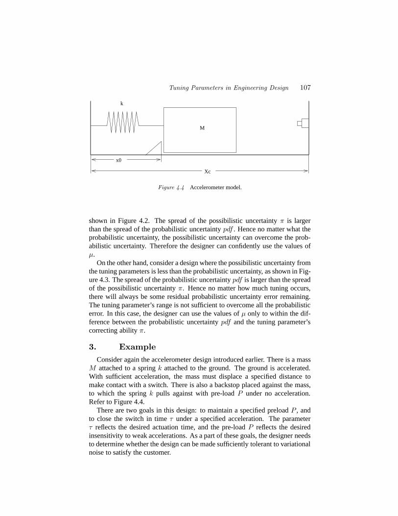
Tuning Parameters in Engineering Design 107
M
k
Xc
x0
Figure 4.4 Accelerometer model.
shown in Figure 4.2. The spread of the possibilistic uncertaintyπ is largerthan the spread of the probabilistic uncertaintypdf . Hence no matter what theprobabilistic uncertainty, the possibilistic uncertainty can overcome the prob-abilistic uncertainty. Therefore the designer can confidently use the values ofµ.
On the other hand, consider a design where the possibilistic uncertainty fromthe tuning parameters is less than the probabilistic uncertainty, as shown in Fig-ure 4.3. The spread of the probabilistic uncertaintypdf is larger than the spreadof the possibilistic uncertaintyπ. Hence no matter how much tuning occurs,there will always be some residual probabilistic uncertainty error remaining.The tuning parameter’s range is not sufficient to overcome all the probabilisticerror. In this case, the designer can use the values ofµ only to within the dif-ference between the probabilistic uncertaintypdf and the tuning parameter’scorrecting abilityπ.
3. ExampleConsider again the accelerometer design introduced earlier. There is a mass
M attached to a springk attached to the ground. The ground is accelerated.With sufficient acceleration, the mass must displace a specified distance tomake contact with a switch. There is also a backstop placed against the mass,to which the springk pulls against with pre-loadP under no acceleration.Refer to Figure 4.4.
There are two goals in this design: to maintain a specified preloadP , andto close the switch in timeτ under a specified acceleration. The parameterτ reflects the desired actuation time, and the pre-loadP reflects the desiredinsensitivity to weak accelerations. As a part of these goals, the designer needsto determine whether the design can be made sufficiently tolerant to variationalnoise to satisfy the customer.
108 IMPRECISION IN ENGINEERING DESIGN
There are two design parameters, massM and spring constantK. There is,however, uncertainty in the manufacture of the spring: a random variation onK, denotedδk. Finally, to assist in maintaining the targets on the goals, themanufacturing line can position the backstop based on measurements made ofthe total spring constant (k = K + δk) of each accelerometer. This backstopdistance is denotedx0, and is a tuning parameter. The switch distance is de-notedxc. The position of the mass at any given time is denotedx. The mass isto make contact with the switch when subjected to accelerationa.
To determine the time to actuate the switch, the differential equation of mo-tion of the mass must be solved. It is:
M(d2x
dt2+ a) × H(x − x0) + kx = P × H(x0 − x) (4.7)
whereH is a step function,x(0) = x0, andx(0) = 0. This can be solved forthe time to actuation:
τ =
√M
k× arccos
(Ma − (xc − x0)k
Ma
)(4.8)
This solution assumes, of course,a is sufficiently large to move the mass (i.e.,thearccosis defined). The other goal is the pre-loadP , whose equation is:
P = kx0 (4.9)
Maintaining a specific pre-load helps eliminate spurious switch closures.
3.1 Optimization Solution FormulationHaving formulated the problem, it can now be solved by optimization meth-
ods. The problem shall be formulated using an objective function consistingof a weighted sum of the two goals: time to actuation and spring pre-load.Both the target actuation time variation and the target pre-load variation shallbe simultaneously minimized, and hence there is a relative coefficient neededbetween the two goals to ensure the variances are of the same order. Therelative weighting coefficient used here was
√5. Determining weighted sum
coefficients is incidental to the tuning parameter formulation, refer to [2, 7]for multi-objective function optimization formulations. Substituting Equations(4.8) and (4.9) into (4.1) produces the problem to be solved as:
M∗,K∗ = minM,K
[∫δk
minx0
[ |τ − τs|τs
+√
5 × |P − Ps|Ps
]× pdf(δk)dδk
](4.10)
subject to:
0.0135 ≤ x0 ≤ 0.0165 (4.11)
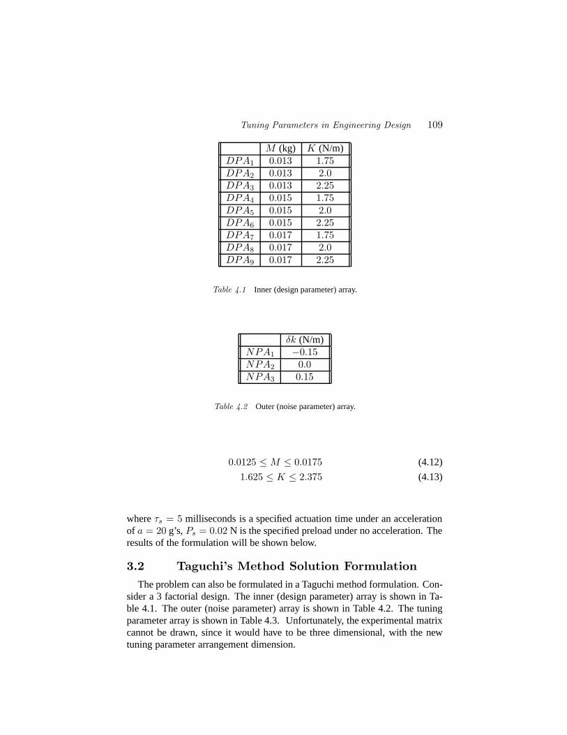
Tuning Parameters in Engineering Design 109
M (kg) K (N/m)DPA1 0.013 1.75DPA2 0.013 2.0DPA3 0.013 2.25DPA4 0.015 1.75DPA5 0.015 2.0DPA6 0.015 2.25DPA7 0.017 1.75DPA8 0.017 2.0DPA9 0.017 2.25
Table 4.1 Inner (design parameter) array.
δk (N/m)NPA1 −0.15NPA2 0.0NPA3 0.15
Table 4.2 Outer (noise parameter) array.
0.0125 ≤ M ≤ 0.0175 (4.12)
1.625 ≤ K ≤ 2.375 (4.13)
whereτs = 5 milliseconds is a specified actuation time under an accelerationof a = 20 g’s, Ps = 0.02 N is the specified preload under no acceleration. Theresults of the formulation will be shown below.
3.2 Taguchi’s Method Solution FormulationThe problem can also be formulated in a Taguchi method formulation. Con-
sider a 3 factorial design. The inner (design parameter) array is shown in Ta-ble 4.1. The outer (noise parameter) array is shown in Table 4.2. The tuningparameter array is shown in Table 4.3. Unfortunately, the experimental matrixcannot be drawn, since it would have to be three dimensional, with the newtuning parameter arrangement dimension.
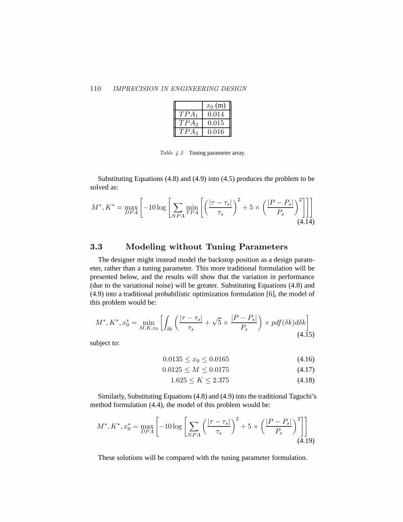
110 IMPRECISION IN ENGINEERING DESIGN
x0 (m)TPA1 0.014TPA2 0.015TPA3 0.016
Table 4.3 Tuning parameter array.
Substituting Equations (4.8) and (4.9) into (4.5) produces the problem to besolved as:
M∗,K∗ = maxDPA
[−10 log
[ ∑NPA
minTPA
[( |τ − τs|τs
)2
+ 5 ×( |P − Ps|
Ps
)2]]]
(4.14)
3.3 Modeling without Tuning ParametersThe designer might instead model the backstop position as a design param-
eter, rather than a tuning parameter. This more traditional formulation will bepresented below, and the results will show that the variation in performance(due to the variational noise) will be greater. Substituting Equations (4.8) and(4.9) into a traditional probabilistic optimization formulation [6], the model ofthis problem would be:
M∗,K∗, x∗0 = min
M,K,x0
[∫δk
( |τ − τs|τs
+√
5 × |P − Ps|Ps
)× pdf(δk)dδk
](4.15)
subject to:
0.0135 ≤ x0 ≤ 0.0165 (4.16)
0.0125 ≤ M ≤ 0.0175 (4.17)
1.625 ≤ K ≤ 2.375 (4.18)
Similarly, Substituting Equations (4.8) and (4.9) into the traditional Taguchi’smethod formulation (4.4), the model of this problem would be:
M∗,K∗, x∗0 = max
DPA
[−10 log
[ ∑NPA
( |τ − τs|τs
)2
+ 5 ×( |P − Ps|
Ps
)2]]
(4.19)
These solutions will be compared with the tuning parameter formulation.
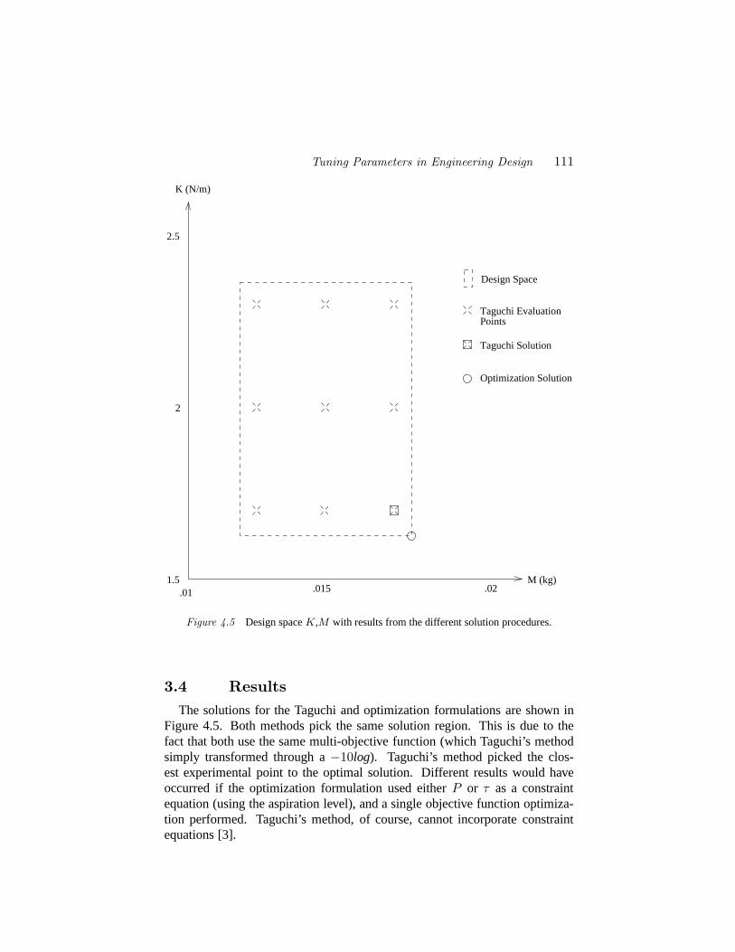
Tuning Parameters in Engineering Design 111
Design Space
Taguchi EvaluationPoints
Taguchi Solution
Optimization Solution
M (kg)
K (N/m)
.015
2
.011.5
2.5
.02
Figure 4.5 Design spaceK,M with results from the different solution procedures.
3.4 ResultsThe solutions for the Taguchi and optimization formulations are shown in
Figure 4.5. Both methods pick the same solution region. This is due to thefact that both use the same multi-objective function (which Taguchi’s methodsimply transformed through a−10log). Taguchi’s method picked the clos-est experimental point to the optimal solution. Different results would haveoccurred if the optimization formulation used eitherP or τ as a constraintequation (using the aspiration level), and a single objective function optimiza-tion performed. Taguchi’s method, of course, cannot incorporate constraintequations [3].
112 IMPRECISION IN ENGINEERING DESIGN
But one additional important question is the tolerance of the device to vari-ational noise. Modeling with tuning parameters allows for more variability inδk, sincex0 can be tuned to keepP andτ on target. Modelingx0 as a tun-ing parameter shows that with±0.2 N/m variation inδk, the pre-loadP waswithin 0.006 N, and that the time to actuationτ was within 5 milliseconds. Atraditional model in whichx0 is treated as a design parameter showed that thepre-loadP was within0.008 N, and that the time to actuationτ was within 6milliseconds. Therefore a traditional model without tuning parameters resultsin a needlessly tight tolerance onδk.
4. ConclusionThis paper has introduced a formalization of tuning parameters common
in engineering design. Tuning parameters are characterized by being set af-ter the effects of noise have occurred. Tuning parameters are set to overcomethese noise effects. The formal models of optimization and Taguchi’s methodhave been extended to include tuning parameters. The method of imprecisioninherently incorporates a modeling scheme for tuning parameters (using pos-sibility).
One important observation regarding tuning parameters is that they are notunder the direct control of the designer. Their values are, in the case of man-ufacturing noise, set by the manufacturing engineer. Therefore care mustbe used by the designer when incorporating tuning parameters into a designmodel.
In the case of variational noise (noise due to variations in supplied material,manufacturing, etc.), the use of tuning parameters is justifiable – the designercan ensure that tuning will occur, and the assumption of finding the best perfor-mance across the tuning parameters’ ranges is correct. In the case of externalnoise (noise due to environmental or user fluctuations) and internal noise (noisedue to wear or storage deterioration), the modeling of tuning parameters whichcan overcome these noises may not be justifiable (in general). The tuningmustoccur for the tuning parameter model to be correct. In the case of a closed loopcontroller, for example, the control response is a valid tuning parameter. Oper-ator adjustment variables, on the other hand, perhaps should not be modeled astuning parameters, even though they can be adjusted to increase performance.The designer cannot ensure that tuning will occur. Hence adjustment variablesshould only be modeled as tuning parameters when the designer is certain theadjustment will occur.
A final point should also be made with respect to modeling tuning parame-ters in Taguchi’s method. Doing so is counter to the Taguchi philosophy, whichstates that one should eliminate tuning parameters altogether (by proper selec-tion of the design parameters), since these are aspects of tolerancing design [8]
Tuning Parameters in Engineering Design 113
and increase cost. This is indeed true; tuning parameters do increase cost. Itis almost always the case that the manufacturing process should be kept assimple as possible,i.e., that one should not use tuning parameters. However,if it is known that the design goals cannot be achieved by proper selection ofthe design parameter values and that tuning parameters will be required, thenthis fact should be incorporated into the design process. Doing so can allowfor the selection of less expensive design parameters and tolerances, given thatthe design will be tuned during manufacture. Hence this is a more completeformulation of Taguchi’s method, incorporating into the method the effects oftolerancing design on the design parameter selection.
This paper has introduced tuning parameters into formal methods of engi-neering design. Including tuning parameters in the design process can result indesigns that are more tolerant of variational noise.
AcknowledgmentsThis material is based upon work supported, in part, by The National Sci-
ence Foundation under a Presidential Young Investigator Award, Grant No. DMC-8552695. Mr. Otto is an AT&T-Bell Laboratories Ph.D. scholar, sponsored bythe AT&T foundation. Any opinions, findings, conclusions or recommenda-tions expressed in this publication are those of the authors and do not neces-sarily reflect the views of the sponsors.
114 IMPRECISION IN ENGINEERING DESIGN
References
[1] BYRNE, D. M., AND TAGUCHI, S. The Taguchi approach to parameterdesign. InQuality Congress Transaction – Anaheim(May 1986), ASQC,pp. 168–177.
[2] OSYCSKA, A. Multi-Criterion Optimization in Engineering with FortranExamples. Halstad Press, New York, NY, 1984.
[3] OTTO, K. N., AND ANTONSSON, E. K. Extensions to the TaguchiMethod of Product Design.ASME Journal of Mechanical Design 115,1 (Mar. 1993), 5–13.
[4] PAPALAMBROS, P., AND WILDE, D. Principles of Optimal Design.Cambridge University Press, New York, NY, 1988.
[5] PHADKE, M. Quality Engineering Using Robust Design. Prentice Hall,Englewood Cliffs, NJ, 1989.
[6] SIDDALL , J. N. Probabilistic Engineering Design; Principles and Ap-plications. Marcel Dekker, New York, NY, 1983.
[7] STEUER, R. Multiple Criteria Optimization: Theory, Computation, andApplication. J. Wiley, New York, NY, 1986.
[8] TAGUCHI, G. Introduction to Quality Engineering. Asian ProductivityOrganization, Unipub, White Plains, NY, 1986.
[9] WOOD, K. L. A Method for Representing and Manipulating Uncertain-ties in Preliminary Engineering Design. PhD thesis, California Instituteof Technology, Pasadena, CA, 1989.
[10] WOOD, K. L., AND ANTONSSON, E. K. Computations with Impre-cise Parameters in Engineering Design: Background and Theory.ASMEJournal of Mechanisms, Transmissions, and Automation in Design 111,4 (Dec. 1989), 616–625.
[11] WOOD, K. L., AND ANTONSSON, E. K. Modeling Imprecision and Un-certainty in Preliminary Engineering Design.Mechanism and MachineTheory 25, 3 (Feb. 1990), 305–324. Invited paper.
[12] ZADEH, L. A. Fuzzy sets as a basis for a theory of possibility.FuzzySets and Systems 1(1978), 3–28.
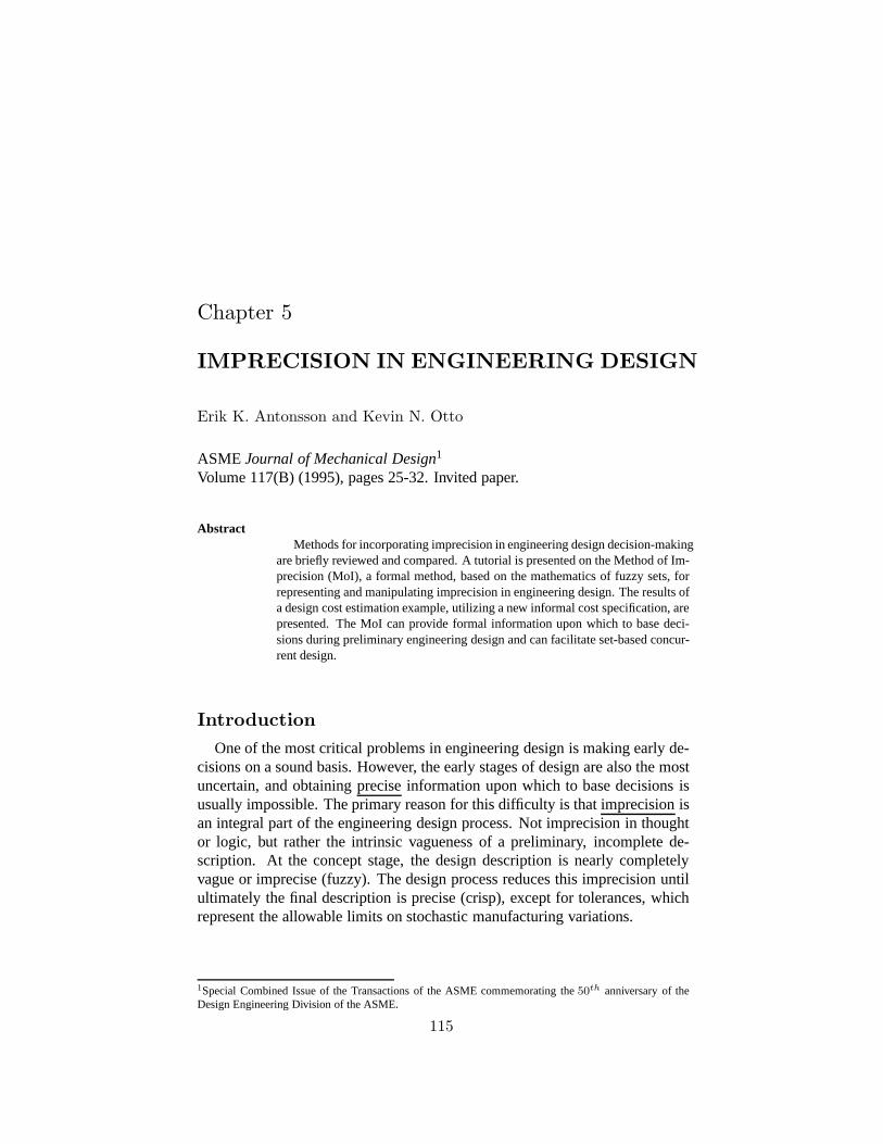
Chapter 5
IMPRECISION IN ENGINEERING DESIGN
Erik K. Antonsson and Kevin N. Otto
ASME Journal of Mechanical Design1
Volume 117(B) (1995), pages 25-32. Invited paper.
AbstractMethods for incorporating imprecision in engineering design decision-making
are briefly reviewed and compared. A tutorial is presented on the Method of Im-precision (MoI), a formal method, based on the mathematics of fuzzy sets, forrepresenting and manipulating imprecision in engineering design. The results ofa design cost estimation example, utilizing a new informal cost specification, arepresented. The MoI can provide formal information upon which to base deci-sions during preliminary engineering design and can facilitate set-based concur-rent design.
IntroductionOne of the most critical problems in engineering design is making early de-
cisions on a sound basis. However, the early stages of design are also the mostuncertain, and obtaining preciseinformation upon which to base decisions isusually impossible. The primary reason for this difficulty is that imprecisionisan integral part of the engineering design process. Not imprecision in thoughtor logic, but rather the intrinsic vagueness of a preliminary, incomplete de-scription. At the concept stage, the design description is nearly completelyvague or imprecise (fuzzy). The design process reduces this imprecision untilultimately the final description is precise (crisp), except for tolerances, whichrepresent the allowable limits on stochastic manufacturing variations.
1Special Combined Issue of the Transactions of the ASME commemorating the50th anniversary of theDesign Engineering Division of the ASME.
115
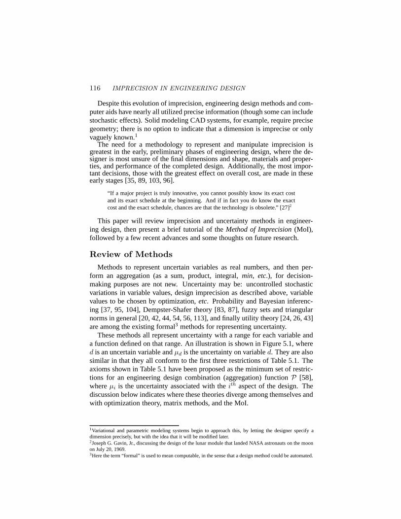
116 IMPRECISION IN ENGINEERING DESIGN
Despite this evolution of imprecision, engineering design methods and com-puter aids have nearly all utilized precise information (though some can includestochastic effects). Solid modeling CAD systems, for example, require precisegeometry; there is no option to indicate that a dimension is imprecise or onlyvaguely known.1
The need for a methodology to represent and manipulate imprecision isgreatest in the early, preliminary phases of engineering design, where the de-signer is most unsure of the final dimensions and shape, materials and proper-ties, and performance of the completed design. Additionally, the most impor-tant decisions, those with the greatest effect on overall cost, are made in theseearly stages [35, 89, 103, 96].
“If a major project is truly innovative, you cannot possibly know its exact costand its exact schedule at the beginning. And if in fact you do know the exactcost and the exact schedule, chances are that the technology is obsolete.” [27]2
This paper will review imprecision and uncertainty methods in engineer-ing design, then present a brief tutorial of theMethod of Imprecision(MoI),followed by a few recent advances and some thoughts on future research.
Review of MethodsMethods to represent uncertain variables as real numbers, and then per-
form an aggregation (as a sum, product, integral,min, etc.), for decision-making purposes are not new. Uncertainty may be: uncontrolled stochasticvariations in variable values, design imprecision as described above, variablevalues to be chosen by optimization,etc. Probability and Bayesian inferenc-ing [37, 95, 104], Dempster-Shafer theory [83, 87], fuzzy sets and triangularnorms in general [20, 42, 44, 54, 56, 113], and finally utility theory [24, 26, 43]are among the existing formal3 methods for representing uncertainty.
These methods all represent uncertainty with a range for each variable anda function defined on that range. An illustration is shown in Figure 5.1, whered is an uncertain variable andµd is the uncertainty on variabled. They are alsosimilar in that they all conform to the first three restrictions of Table 5.1. Theaxioms shown in Table 5.1 have been proposed as the minimum set of restric-tions for an engineering design combination (aggregation) functionP [58],whereµi is the uncertainty associated with theith aspect of the design. Thediscussion below indicates where these theories diverge among themselves andwith optimization theory, matrix methods, and the MoI.
1Variational and parametric modeling systems begin to approach this, by letting the designer specify adimension precisely, but with the idea that it will be modified later.2Joseph G. Gavin, Jr., discussing the design of the lunar module that landed NASA astronauts on the moonon July 20, 1969.3Here the term “formal” is used to mean computable, in the sense that a design method could be automated.
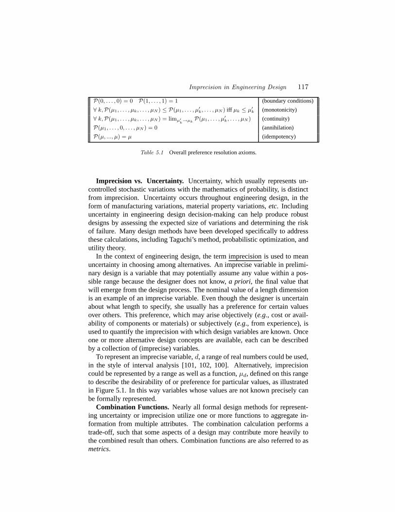
Imprecision in Engineering Design 117
P(0, . . . , 0) = 0 P(1, . . . , 1) = 1 (boundary conditions)
∀ k, P(µ1, . . . , µk, . . . , µN ) ≤ P(µ1, . . . , µ′k, . . . , µN ) iff µk ≤ µ′
k (monotonicity)
∀ k, P(µ1, . . . , µk, . . . , µN ) = limµ′k
→µkP(µ1, . . . , µ
′k, . . . , µN ) (continuity)
P(µ1, . . . , 0, . . . , µN ) = 0 (annihilation)
P(µ, ..., µ) = µ (idempotency)
Table 5.1 Overall preference resolution axioms.
Imprecision vs. Uncertainty. Uncertainty, which usually represents un-controlled stochastic variations with the mathematics of probability, is distinctfrom imprecision. Uncertainty occurs throughout engineering design, in theform of manufacturing variations, material property variations,etc. Includinguncertainty in engineering design decision-making can help produce robustdesigns by assessing the expected size of variations and determining the riskof failure. Many design methods have been developed specifically to addressthese calculations, including Taguchi’s method, probabilistic optimization, andutility theory.
In the context of engineering design, the term imprecisionis used to meanuncertainty in choosing among alternatives. An imprecise variable in prelimi-nary design is a variable that may potentially assume any value within a pos-sible range because the designer does not know,a priori, the final value thatwill emerge from the design process. The nominal value of a length dimensionis an example of an imprecise variable. Even though the designer is uncertainabout what length to specify, she usually has a preference for certain valuesover others. This preference, which may arise objectively (e.g., cost or avail-ability of components or materials) or subjectively (e.g., from experience), isused to quantify the imprecision with which design variables are known. Onceone or more alternative design concepts are available, each can be describedby a collection of (imprecise) variables.
To represent an imprecise variable,d, a range of real numbers could be used,in the style of interval analysis [101, 102, 100]. Alternatively, imprecisioncould be represented by a range as well as a function,µd, defined on this rangeto describe the desirability of or preference for particular values, as illustratedin Figure 5.1. In this way variables whose values are not known precisely canbe formally represented.
Combination Functions. Nearly all formal design methods for represent-ing uncertainty or imprecision utilize one or more functions to aggregate in-formation from multiple attributes. The combination calculation performs atrade-off, such that some aspects of a design may contribute more heavily tothe combined result than others. Combination functions are also referred to asmetrics.
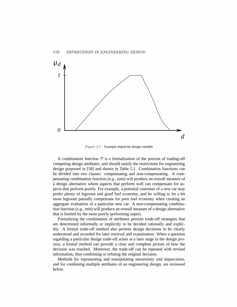
118 IMPRECISION IN ENGINEERING DESIGN
0
1
d
µd
Figure 5.1 Example imprecise design variable
A combination functionP is a formalization of the process of trading-offcompeting design attributes, and should satisfy the restrictions for engineeringdesign proposed in [58] and shown in Table 5.1. Combination functions canbe divided into two classes: compensating and non-compensating. A com-pensating combination function (e.g., sum) will produce an overall measure ofa design alternative where aspects that perform well can compensate for as-pects that perform poorly. For example, a potential customer of a new car mayprefer plenty of legroom and good fuel economy, and be willing to let a bitmore legroom partially compensate for poor fuel economy when creating anaggregate evaluation of a particular new car. A non-compensating combina-tion function (e.g., min) will produce an overall measure of a design alternativethat is limited by the most poorly performing aspect.
Formalizing the combination of attributes permits trade-off strategies thatare determined informally or implicitly to be decided rationally and explic-itly. A formal trade-off method also permits design decisions to be clearlyunderstood and recorded for later retrieval and examination. When a questionregarding a particular design trade-off arises at a later stage in the design pro-cess, a formal method can provide a clear and complete picture of how thedecision was reached. Moreover, the trade-off can be repeated with revisedinformation, thus confirming or refuting the original decision.
Methods for representing and manipulating uncertainty and imprecision,and for combining multiple attributes of an engineering design, are reviewedbelow.
Imprecision in Engineering Design 119
Utility Theory. Utility theory [24, 26, 43] was developed to assist in select-ing among a choice of distinct actions, given uncertainty (noise) in the outcomeof each action. In utility theory, each aspect of a decision (e.g., each designvariable) is assigned a function representing utility, as illustrated in Figure 5.1.The utilities for the individual aspects are aggregated to determine the overallutility, and the combination of variable values that maximizes the overall utilityis used.
Utility theory is restricted to decision problems in which the individual pref-erences can be modeled as additive, either with a weighted sum, or with a“multiplicative” form which is also additive but includes nonlinear terms [26].Since the overall metric is additive, utility theory always reflects a compensat-ing strategy, allowing the higher preference of some goals to offset the lowerpreference of others.
Because utility theory is additive, it fails the annihilation restriction shownin Table 5.1. This means that the utility of one aspect of an alternative can bezero, but the overall utility of the alternative will be non-zero. To surmountthis difficulty, Thurston has applied utility theory to design by dividing thecomplete set of goals into two classes: objective constraints and subjectivegoals [94, 92, 93]. Objective constraints have crisp achievement levels thatmust be satisfied, and thus become standard constraints as in non-linear pro-gramming formulations. Subjective goals are those which can be traded-off,and are modeled using standard utility theory. The subjective goals are traded-off among themselves in a compensating manner (using either of the formula-tions of utility theory), and the objective constraints are traded-off informally(by iteratively refining the constraint values). The overall strategy, therefore,remains informal.
Utility theory was originally developed for management decisions, not forengineering design, and requires that all attributes be aggregated into a sin-gle goal (utility). Economists generally believe every aspect of a decision canalways be translated into a monetary cost. Monetary costs are additive. As-pects which are not additive, or which cannot be “bought off”, are not deemedpossible. The axiom of utility theory which creates the demand that a gain inany aspect must be able to compensate for any loss in any other aspect is theArchimedian property. This restriction requires that any decrease in overallpreference caused by changes in the performance of one variable mustalwaysbe able to be balanced by an increase in performance in any of the other vari-ables. Clearly this is not the case in engineering design, as others have ar-gued [11, 97]. For example, given a fixed material, the tensile strength limitscannot be exceeded no matter the reduction in the design’s cost. Material stresssimply cannot always be traded-off in a compensating fashion. The Archime-dian property and annihilation cannot be simultaneously satisfied. This implies
120 IMPRECISION IN ENGINEERING DESIGN
that utility theory will not permit a worst case analysis, which is required inmany instances in engineering design [33, 49].
Fuzzy Sets. Fuzzy sets have been used to represent imprecision in (non-design) decision-making [20, 42, 44, 54, 56, 113]. Fuzzy sets are intended tomodel subjective uncertainty for use in logic, constructing subjectively uncer-tain versions of “and” and “or” of classical logic. In the first paper describingthe use of fuzzy sets for decision-making [9], a decision was defined as a con-volution of the constraints and goals, usingminas a non-compensating metric.They also suggested that at other times simple multiplication of the individualpreferences might be appropriate.
The overall metrics ofmin and multiplication have been expanded to themore general class oft-norms, first proposed by Menger [51], and reviewed inDubois and Prade [21].T-normsare bounded above bymin, and are the uncer-tain version of conjunction.T-normsare not appropriate as an overall designmetric because they do not, in general, satisfy the restrictions of Table 5.1.Probabilistic reasoning, Dempster-Shafer theory, and fuzzy sets all employt-norms [21]. Related to eacht-norm is an associatedt-conorm (or s-norm),which is the uncertain version of disjunction.T-conormsare bounded belowby max. The set of functions betweent-normsand t-conormsare themixedconnectives, bounded betweenmaxandmin, and are the class of combinationfunctions used by the MoI and utility theory.
Using fuzzy sets for decision-making has received further attention. [22,38, 109, 110, 111, 112], for example, all discuss converting linguistic expres-sions into fuzzy sets, and then using the fuzzy mathematics to make decisions.An excellent review of fuzzy multiple attribute decision-making is presentedin [14]. Bellman and Zadeh suggested using a weighted sum of the preferences.[39] and [7] also develop additive metrics using fuzzy sets beyond Bellmanand Zadeh’s original work. [110] observed the “softness” of multiplication asa connective, and proposed it (andmin) in conjunction with weights.
Completely independent of fuzzy set formulations, [32] (the same year asZadeh’s initial paper on fuzzy sets) proposed a product of powers as a “desir-ability function” in chemical process problems. He observed that the annihila-tion condition is required for engineering design.
[15, 16] and [69, 70, 71, 72, 73] have applied fuzzy set formulations to de-sign optimization problems in mechanical engineering. [55] has applied fuzzysets to nuclear radiation cover design. All have used only a non-compensatingtrade-off strategy for making decisions. Other applications of fuzzy optimiza-tion are reviewed by [50].
Optimization. Other design methodologies exist that do not explicitly rep-resent uncertainty or preferences on variables. For example, optimization for-mulations (linear, non-linear, integer, and mixed integer programming) [1, 4,65, 66, 74] assume a relationship between preference and the objective func-
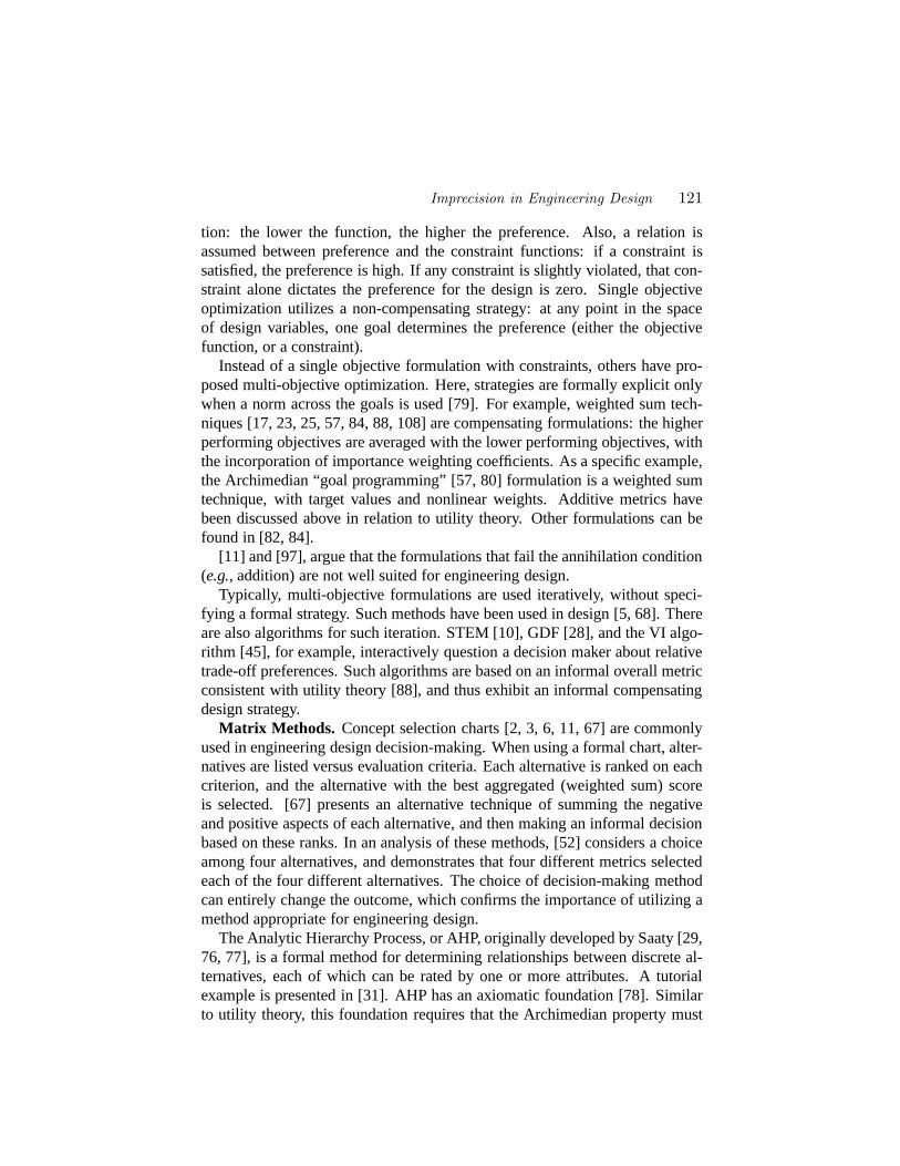
Imprecision in Engineering Design 121
tion: the lower the function, the higher the preference. Also, a relation isassumed between preference and the constraint functions: if a constraint issatisfied, the preference is high. If any constraint is slightly violated, that con-straint alone dictates the preference for the design is zero. Single objectiveoptimization utilizes a non-compensating strategy: at any point in the spaceof design variables, one goal determines the preference (either the objectivefunction, or a constraint).
Instead of a single objective formulation with constraints, others have pro-posed multi-objective optimization. Here, strategies are formally explicit onlywhen a norm across the goals is used [79]. For example, weighted sum tech-niques [17, 23, 25, 57, 84, 88, 108] are compensating formulations: the higherperforming objectives are averaged with the lower performing objectives, withthe incorporation of importance weighting coefficients. As a specific example,the Archimedian “goal programming” [57, 80] formulation is a weighted sumtechnique, with target values and nonlinear weights. Additive metrics havebeen discussed above in relation to utility theory. Other formulations can befound in [82, 84].
[11] and [97], argue that the formulations that fail the annihilation condition(e.g., addition) are not well suited for engineering design.
Typically, multi-objective formulations are used iteratively, without speci-fying a formal strategy. Such methods have been used in design [5, 68]. Thereare also algorithms for such iteration. STEM [10], GDF [28], and the VI algo-rithm [45], for example, interactively question a decision maker about relativetrade-off preferences. Such algorithms are based on an informal overall metricconsistent with utility theory [88], and thus exhibit an informal compensatingdesign strategy.
Matrix Methods. Concept selection charts [2, 3, 6, 11, 67] are commonlyused in engineering design decision-making. When using a formal chart, alter-natives are listed versus evaluation criteria. Each alternative is ranked on eachcriterion, and the alternative with the best aggregated (weighted sum) scoreis selected. [67] presents an alternative technique of summing the negativeand positive aspects of each alternative, and then making an informal decisionbased on these ranks. In an analysis of these methods, [52] considers a choiceamong four alternatives, and demonstrates that four different metrics selectedeach of the four different alternatives. The choice of decision-making methodcan entirely change the outcome, which confirms the importance of utilizing amethod appropriate for engineering design.
The Analytic Hierarchy Process, or AHP, originally developed by Saaty [29,76, 77], is a formal method for determining relationships between discrete al-ternatives, each of which can be rated by one or more attributes. A tutorialexample is presented in [31]. AHP has an axiomatic foundation [78]. Similarto utility theory, this foundation requires that the Archimedian property must

122 IMPRECISION IN ENGINEERING DESIGN
be satisfied, which dictates that the annihilation condition is not satisfied. Sincethe AHP’s ratings are derived from a linear weighted sum, it only implementsa compensating trade-off.
AHP can only consider discrete alternatives; no continuous variations canbe incorporated. Additionally, all alternatives are compared to the lowest per-forming alternative; AHP includes no ability to indicate that one (or more)alternatives are completely unacceptable, or have violated one or more con-straint(s). However, AHP is one of the few methodologies that can incorporatehierarchical objective criteria.
Finally, “Quality Function Deployment,” or QFD [2, 34] begins by listingthe customer requirements for a design on one axis of a chart and the perfor-mance metrics for the design on the other axis. Ratings are performed by usinga transformation to convert symbols to numerical equivalents, and summing.This summation has the difficulties of the additive metrics discussed above.
Probability Methods. In Taguchi’s method [13, 36, 41, 75, 86, 90, 91], the“quality” of a design variable set~d is defined by the expected variation of a sin-gle performance variablep from a target valueτ due to uncontrolled stochasticnoise. Thus, Taguchi’s method finds the mean of a single performance vari-able (variation ofp from τ ), not preference over many design variables andperformance variables [59].
Experimental design techniques can also be used to determine experimentalpoints in the noise space. See [8, 12, 40] for a discussion of factorial meth-ods for determining experimental points. Alternatively, Monte Carlo simula-tion [30] could be used for more accuracy.
Probabilistic optimization methods can be used to evaluate a solution whennoise is present, by evaluating the expected value of the objective function, aspresented by [85, Chapter 13]. The discussion on optimization methods aboveapplies to probabilistic optimization methods as well.
Necessity Methods.Necessity determines the probability (α) of a designoperating successfully despite uncontrolled variations in one or more parame-ters over a range (confidence interval). This approach can account for the worstcase of random disturbances. [98] and [100] have developed a “Labeled Inter-val Calculus” that consists of interval mathematics with associated “only” or“every” labels. [99] have shown that a set-based approach to design decision-making (using intervals) can facilitate concurrent engineering.
Noise can be rated by the expected value, or by the worst case scenario (us-ing necessity). [85, Appendix C] and [81] reject using confidence intervals.Siddall argues that one has difficulty determining the density functionpdf andthe confidence levelα. Savage argues against the use of confidence informa-tion since he feels one is still obliged to choose the expected value. However,confidence intervals are widely used in practice [33, 49], as is modeling toconsider the worst case noise [19].
Imprecision in Engineering Design 123
Fuzzy Design Methods.Fuzzy design methods combine many of the valu-able attributes of the methods described above. They are formal (computable)methods for representing and manipulating design imprecision (uncertainty inchoosing among alternatives) using the mathematics of fuzzy sets. Severalgroups are applying fuzzy methods to engineering design problems [105, 58,53, 114, 115].
Imprecision is represented by a range, and a function defined on this range(µd), to describe the desirability of or preference for particular values, and toincorporate the designer’s experience and judgement into the design evalua-tion. Non-parametric attributes (such as material choice, color, style,etc.) aswell as real-valued attributes (such as physical dimensions, material properties,cost,etc.) can be used.
In the Method of Imprecision (MoI) [105, 106, 63], constraints can be simi-larly imprecise, permitting the customer to specify preferences over a rangeof values, rather than a crisp constraint that may be moved by negotiationlater in the design process. Because the method was developed specificallyfor engineering design, the trade-off combination functions meet the restric-tions shown in Table 5.1 [58]. A choice of two basic combination functionsis available to aggregate the preferences for the attributes of the design: the(non-compensating)minand a (compensating) product of powers.
Because the MoI does not require all attributes to be aggregated into oneevaluation metric, evaluations of the various aspects of a design can be madein a hierarchy. For example, safety margin might be traded-off in a non-compensating way among several parts of the design that are subject to loading,and weight and cost might be traded-off in a compensating way. The results ofthose two trade-offs then might be traded-off with a non-compensating com-bination function. Because importance weighting can be readily applied, therelative weight of each aspect of the decision can be incorporated into the hi-erarchy [48].
Finally, stochastic uncertainty (such as uncontrolled manufacturing varia-tions) and possibilistic uncertainty and necessity (such as post-manufacturingtuning adjustments) can be incorporated into the design decision-making byutilizing well known expectation calculations [62].
Utility theory and the MoI are strongly similar when there is only one goal,and a compensating strategy is used [60]. When goals are traded-off in a non-compensating manner, and without considering importance weightings, theMoI reduces to a convolution of the constraints and goals used in fuzzy setsfor decision-making [9].
124 IMPRECISION IN ENGINEERING DESIGN
The Method of ImprecisionThe following sections will present a brief tutorial on how imprecision is
used to facilitate decision-making in engineering design using the MoI.Definitions and Notation. Design variablesare denoteddi, and the valid
design variable values within thedesign variable space(DVS) form a subsetX . The set of valid values fordi is denotedXi. The preference that a designerhas for values ofdi, the ith design variable, is represented by a preferencefunction onXi, called thedesign preference: µdi
(di).Performance variablesare denotedpj. For each performance variablepj
there must be a mappingfj such thatpj = fj(~d). The mappingsfj can beany calculation or procedure to measure the performance of a design, includ-ing closed-form equations (e.g., for stress, weight, speed, cost,etc.), iterativesolutions, heuristic methods, “black box” calculations, testing of prototypes,or consumer evaluations. The subset of valid performance variable valuesY ismapped fromX and the set of valid values forpj is denotedYj . Theperfor-mance variable space(PVS) is the dependent set of performances evaluated foreach design in the DVS. In order to compare design alternatives, design pref-erences are mapped onto the PVS via the extension principle [111], discussedbelow.
Specifications and requirements also embody design imprecision, even thoughmost are written as if they were crisp,e.g., “This device must have a range ofat least 250 km.” Such a requirement implies that given two designs arbitrarilyclose together, one with a range of 250 km and one just below, the first wouldbe acceptable but not the second, as shown by the dashed line in Figure 5.2.Specifications and requirements in the real world are commonly fuzzy. Oftenthe designer must ask questions to distinguish the underlying fuzzy constraintso that the final design will satisfy the customer’s actual requirements eventhough it may violate the crisp constraint initially given. The fuzziness of con-straints and the fuzziness of preliminary design variables are both forms ofdesign imprecision and can be represented in exactly the same way. The cus-tomer’s preference (requirements) for values ofpj, thejth performance vari-able, is represented by a preference function called thefunctional requirement:µpj(pj). The solid line in Figure 5.2 shows the fuzzy functional requirement.
Trade-Off Strategies. The combined preference of the designer and cus-tomer for a particular design~d is represented by an overall preferenceµo(~d),which is a function of the design preferencesµdi
(di), and the functional re-quirementsµpj(pj):
µo(~d) = P[µd1(d1), . . . , µdn(dn), µp1(f1(~d)), . . . , µpq(fq(~d))
]. (5.1)
Two combination functions (P) that satisfy the restrictions of Table 5.1 havebeen identified:min and a product of powers. Figure 5.3 shows the overall
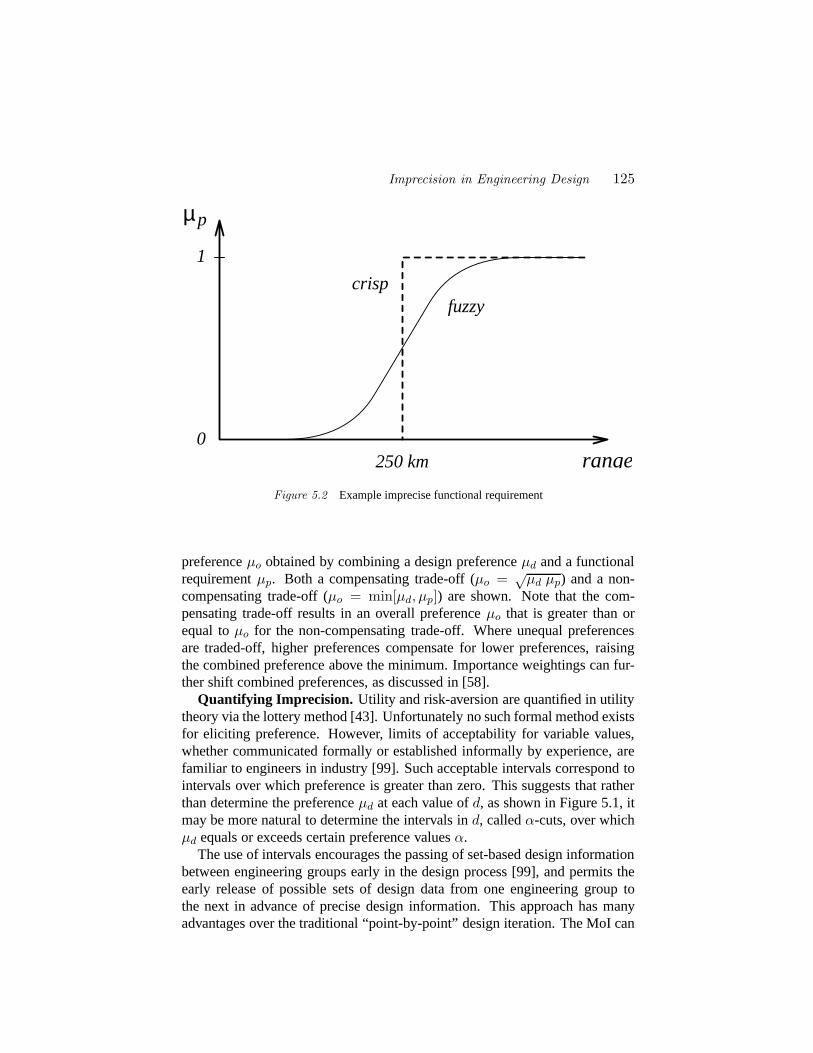
Imprecision in Engineering Design 125
0
1
µp
250 km
fuzzycrisp
range
Figure 5.2 Example imprecise functional requirement
preferenceµo obtained by combining a design preferenceµd and a functionalrequirementµp. Both a compensating trade-off (µo = √
µd µp) and a non-compensating trade-off (µo = min[µd, µp]) are shown. Note that the com-pensating trade-off results in an overall preferenceµo that is greater than orequal toµo for the non-compensating trade-off. Where unequal preferencesare traded-off, higher preferences compensate for lower preferences, raisingthe combined preference above the minimum. Importance weightings can fur-ther shift combined preferences, as discussed in [58].
Quantifying Imprecision. Utility and risk-aversion are quantified in utilitytheory via the lottery method [43]. Unfortunately no such formal method existsfor eliciting preference. However, limits of acceptability for variable values,whether communicated formally or established informally by experience, arefamiliar to engineers in industry [99]. Such acceptable intervals correspond tointervals over which preference is greater than zero. This suggests that ratherthan determine the preferenceµd at each value ofd, as shown in Figure 5.1, itmay be more natural to determine the intervals ind, calledα-cuts, over whichµd equals or exceeds certain preference valuesα.
The use of intervals encourages the passing of set-based design informationbetween engineering groups early in the design process [99], and permits theearly release of possible sets of design data from one engineering group tothe next in advance of precise design information. This approach has manyadvantages over the traditional “point-by-point” design iteration. The MoI can
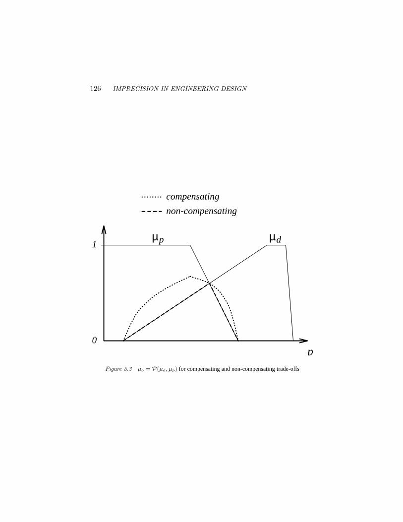
126 IMPRECISION IN ENGINEERING DESIGN
µp
0
1µd
compensating
non-compensating
pFigure 5.3 µo = P(µd, µp) for compensating and non-compensating trade-offs
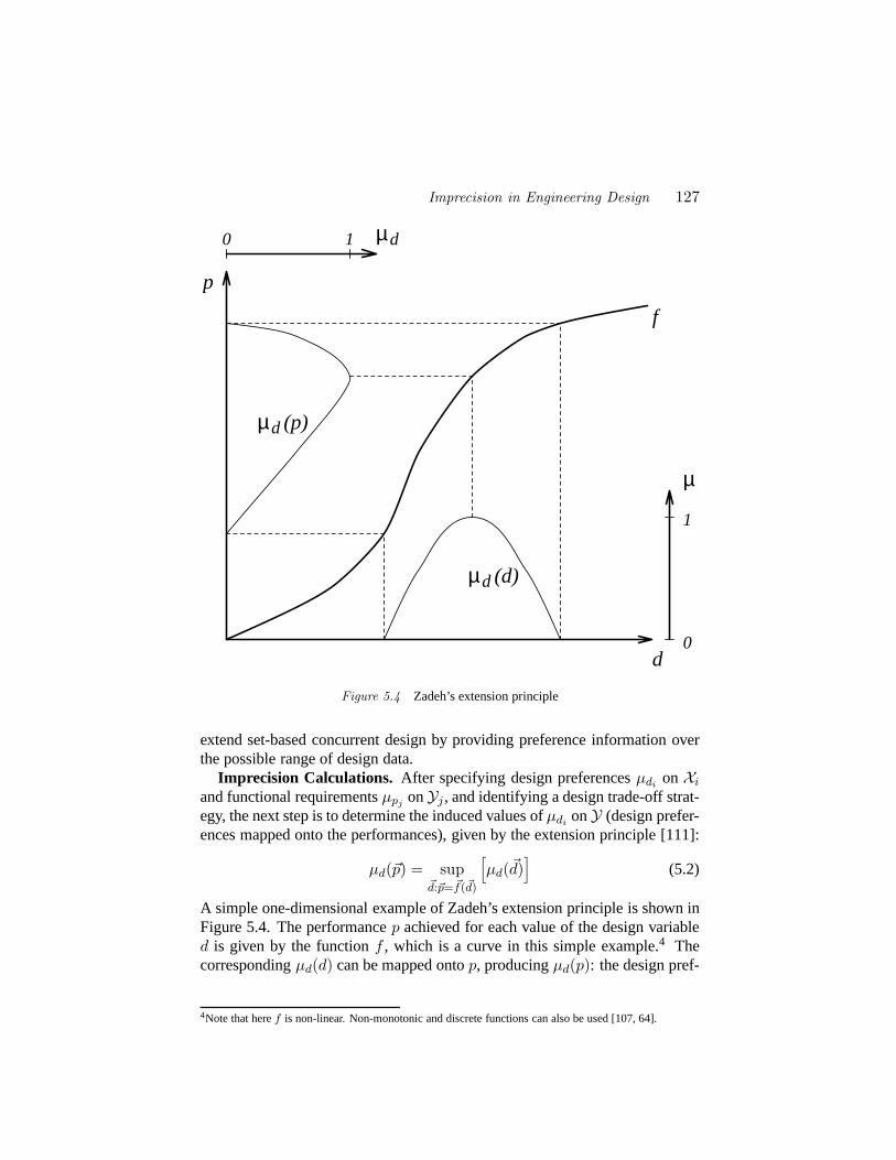
Imprecision in Engineering Design 127
µ
µd (d)
µd
d
p
f
0
0
1
1 µd
(p)
Figure 5.4 Zadeh’s extension principle
extend set-based concurrent design by providing preference information overthe possible range of design data.
Imprecision Calculations. After specifying design preferencesµdion Xi
and functional requirementsµpj onYj , and identifying a design trade-off strat-egy, the next step is to determine the induced values ofµdi
onY (design prefer-ences mapped onto the performances), given by the extension principle [111]:
µd(~p) = sup~d:~p=~f(~d)
[µd(~d)
](5.2)
A simple one-dimensional example of Zadeh’s extension principle is shown inFigure 5.4. The performancep achieved for each value of the design variabled is given by the functionf , which is a curve in this simple example.4 Thecorrespondingµd(d) can be mapped ontop, producingµd(p): the design pref-
4Note that heref is non-linear. Non-monotonic and discrete functions can also be used [107, 64].
128 IMPRECISION IN ENGINEERING DESIGN
erence mapped onto the performance space (as illustrated by the dashed linesin Figure 5.4). For more realistic design problems, eachp will be a function ofmanyd’s, and each functionf will be a hyper-surface.
An algorithm to compute Zadeh’s extension principle (and thus to calculateµd(~p)) is the Level Interval Algorithm(LIA), first proposed by [18] as the“Fuzzy Weighted Average” algorithm and also called the “Vertex Method”,and extended by [107, 64].
Once the imprecision on each design variable (µd(~d)) is induced onto thePVS, the induced preferences are combined with the functional requirements(µp(~p)) to obtain an overall preference (µo(~p)). The point (or points) withthe highest preference correspond to the performance of the overall most pre-ferred design(s). The design problem is to find the corresponding set of designvariables (µd(~d∗)) that produce the maximum overall preference (µ∗
o). In thetypical engineering design case, where the inverse mapping (~f−1 : Y → X )doesn’t exist,µo(~d) can still be obtained point by point [46].
ExampleAn industrial example of cost estimation for aircraft engine design, utiliz-
ing the Engine Development Cost Estimator developed by General ElectricAircraft Engines [47, 46], shows how a crisp design cost estimator can be in-tegrated with the MoI. This permits imprecise cost estimates to be developedwhen only imprecise design data is available. The original example included aformal, and imprecise, functional requirement (µp). The example has recentlybeen extended to include more informal functional requirements.
Figure 5.5 shows the results of the MoI applied to the engine developmentcost estimator, using a compensating strategy. Two different design optionswere simultaneously explored, and are both shown on the figure. Option 1 isto develop the new engine from an existing turbojet design by the addition of afront fan with matching shaft and low pressure turbine. Option 2 is to modifyan existing, but dated, turbofan design. The two curves are the designers’preferences (for a range of each design variable) induced onto the performancespace (here: cost). Each point on the curves in Figure 5.5 corresponds to (atleast) one design.
In comparing the cost specifications to the calculated imprecise design costs,if the customer has imposed a strict limit on the development cost, it may beapplied by choosing the point with highest preference below this limit. If a for-mal, and imprecise, functional requirement for cost is available, the customer’spreference and the designer’s preference (induced onto the cost variable) canbe traded-off, as described above. However, if the customer can only provide“cheaper is better” as an informal cost specification, an informal trade-off canstill be made. Let~dref be the design with the least cost among the highest
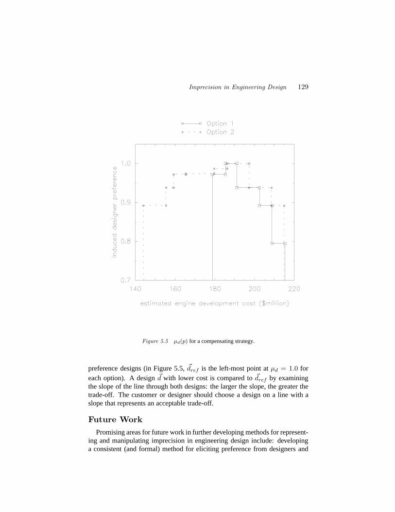
Imprecision in Engineering Design 129
Figure 5.5 µd(p) for a compensating strategy.
preference designs (in Figure 5.5,~dref is the left-most point atµd = 1.0 foreach option). A design~d with lower cost is compared to~dref by examiningthe slope of the line through both designs: the larger the slope, the greater thetrade-off. The customer or designer should choose a design on a line with aslope that represents an acceptable trade-off.
Future WorkPromising areas for future work in further developing methods for represent-
ing and manipulating imprecision in engineering design include: developinga consistent (and formal) method for eliciting preference from designers and

130 IMPRECISION IN ENGINEERING DESIGN
customers, and refinement of the weighting methods. Noise (meaning prob-abilistic uncertainty) has been thoroughly included in the MoI [62, 61], butan application to a commercially relevant industrial problem has not yet beenmade. The MoI was developed to permit hierarchical design decision-making,but a scheme to represent the hierarchy is lacking. Incorporating preference tocreate fuzzy-set based concurrent design methods appears to have significantpromise, and is presently an active area of research. One area of future workthat seems especially interesting is the notion of a fuzzy solid modeling sys-tem. Imprecise physical dimensions can be represented mathematically, but auseful display of this information has not yet been developed.
ConclusionImprecision and uncertainty occur throughout the engineering design pro-
cess. Many methods for incorporating uncertainty (e.g., utility theory, proba-bility methods, Taguchi’s method,etc.) are in common use and are reviewedhere, but methods to represent imprecision in engineering design are few. TheMethod of Imprecision (MoI) is a formal method for incorporating the naturallevel of imprecision that occurs throughout the engineering design process, andcan include: many incommensurate aspects of a design, imprecise constraints,compensating and non-compensating trade-offs, hierarchical trade-offs, andimportance weightings. Uncontrolled variations (noise) can also be incorpo-rated so that the design with the greatest overall preference and most robustnessto the noise can be found.
Furthermore, by encouraging the designer and customer to specify prefer-ences on design and performance variables, design communication will evolvefrom individual “point” designs to (fuzzy) sets of designs. Since a range of pos-sible design variable values can be released to down-stream design processesearlier than a completed individual design, the MoI can facilitate (fuzzy) set-based concurrent design.
AcknowledgmentsThis material is based upon work supported, in part, by: The National Science Founda-
tion under a Presidential Young Investigator Award, Grant No. DMC-8552695, and NSF Grant
No. DDM-9201424. Significant contributions were made to this work by previous graduate stu-
dents: Kristin L. Wood, and Kevin N. Otto. The Review of Methods section was derived from
a portion of Prof. Otto’s Ph.D. thesis. William Law, contributed the informal cost specification
example. Michael Scott and the anonymous reviewers contributed many thoughtful remarks
that greatly improved the paper.

Imprecision in Engineering Design 131
References
[1] A DBY, P.,AND DEMPSTER, M. Introduction to Optimization Methods.Chapman and Hall, London, 1974.
[2] A KAO, Y. Quality Function Deployment: Integrating Customer Re-quirements into Product Design. Productivity Press, Cambridge, 1990.
[3] A LGER, J.,AND HAYS, C. Creative Synthesis in Design. Prentice Hall,Englewood Cliffs, 1964.
[4] A RORA, J. S. Introduction to Optimum Design. McGraw-Hill BookCompany, New York, NY, 1989.
[5] A SHLEY, S. Engineous explores the design space.Mechanical Engi-neering(Feb. 1992), 49–52.
[6] A SIMOW, M. Introduction to Design. Prentice-Hall, Inc., EnglewoodCliffs, N. J., 1962.
[7] BAAS, S., AND KWAKERNAAK , H. Rating and ranking of multiple-aspect alternatives using fuzzy sets.Automatica 13(1977), 47–48.
[8] BARKER, T. Quality by Experimental Design. Marcel Dekker, Inc.,New York, 1985.
[9] BELLMAN , R. E., AND ZADEH, L. A. Decision-making in a fuzzyenvironment.Management Science 17, 4 (Dec. 1970), B–141–163.
[10] BENAYOUN, R., DE MONTGOLFIER, J., TERGNY, J., AND LAR-ITCHEV, O. Linear programming with multiple objective functions:Step method (STEM).Mathematical Programming 1, 3 (1971), 366–375.
[11] BIEGEL, P.,AND PECHT, M. Design trade-offs made easy.ConcurrentEngineering 1, 3 (May/June 1991), 29–40.
[12] BOX, G. E. Statistics for Experimenters. J. Wiley and Sons, New York,1978.
[13] BYRNE, D. M., AND TAGUCHI, S. The Taguchi approach to param-eter design. InQuality Congress Transaction – Anaheim(May 1986),ASQC, pp. 168–177.
[14] CHEN, S.-J.,AND HWANG, C.-L. Fuzzy Multiple Attribute DecisionMaking: Methods and Applications, vol. 375 ofLecture Notes in Eco-nomics and Mathematical Systems. Springer-Verlag, New York, NY,1992. In collaboration with Frank P. Hwang.
[15] DIAZ , A. R. Fuzzy set based models in design optimization. InAd-vances in Design Automation - 1988(New York, NY, Sept. 1988), S. S.Rao, Ed., vol. DE-14, ASME, pp. 477–485.
132 IMPRECISION IN ENGINEERING DESIGN
[16] DIAZ , A. R. A strategy for optimal design of hierarchical systems usingfuzzy sets. InThe 1989 NSF Engineering Design Research Conference(College of Engineering, University of Massachusetts, Amherst, June1989), J. R. Dixon, Ed., NSF, pp. 537–547.
[17] DLESK, D. C., AND LIEBMAN , J. S. Multiple objective engineeringoptimization.Engineering Optimization 6(1983), 161–175.
[18] DONG, W. M., AND WONG, F. S. Fuzzy weighted averages and im-plementation of the extension principle.Fuzzy Sets and Systems 21, 2(Feb. 1987), 183–199.
[19] DOYLE, J., FRANCIS, B., AND TANNENBAUM , A. Feedback ControlTheory. MacMillan Publishing Co., 1990.
[20] DUBOIS, D., AND PRADE, H. Fuzzy Sets and Systems: Theory andApplications. Academic Press, New York, 1980.
[21] DUBOIS, D., AND PRADE, H. A class of fuzzy measures based ontriangular norms.International Journal of General Systems 8(1982),43–61.
[22] EFSTATHIOU, J.,AND RAJKOVIC. Multiattribute decisionmaking usinga fuzzy heuristic approach.IEEE Transactions on Systems, Man andCybernetics 9, 6 (1979), 326–333.
[23] ESCHENAUER, H., KOSKI, J., AND OSYCZKA, A., Eds.MulticriteriaDesign Optimization. Springer-Verlag, Berlin, 1990.
[24] FISHBURN, P. Foundations of Expected Utility. D. Reidel, 1982.
[25] FREIHEIT, T., AND RAO, S. S. A modified game theory approachto multi-objective optimization. InAdvances in Design Automation -1988(New York, NY, Sept. 1988), S. S. Rao, Ed., vol. DE-14, ASME,pp. 107–114.
[26] FRENCH, S. Decision Theory: An Introduction to the Mathematics ofRationality. Ellis Horwood, Chichester, 1988.
[27] GAVIN , JR., J. G. Fly me to the Moon: An interview with Joseph G.Gavin, Jr.Technology Review 97, 5 (July 1994), 61–68.
[28] GEOFFRION, A., DYER, J., AND FEINBERG, A. An interactive ap-proach for multicriterion optimization, with an application to the oper-ation of an academic department.Management Science 19, 4 (1972),357–368.
[29] GOLDEN, B., WASIL, E., AND HARKER, P., Eds.The Analytic Hier-archy Process: Applications and Studies. Springer-Verlag, New York,NY, 1989.
[30] HAMMERSLEY, J., AND HANDSCOMB, D. Monte Carlo Methods.Methuen, London, 1964.
Imprecision in Engineering Design 133
[31] HARKER, P. T. The art and science of decision making: The AnalyticHierarchy Process. InThe Analytic Hierarchy Process: Applicationsand Studies, B. Golden, E. Wasil, and P. Harker, Eds. Springer-Verlag,New York, NY, 1989, pp. 3–36.
[32] HARRINGTON, E. The desirability function.Industrial Quality Control(1965), 494–498.
[33] HARRY, M. J. The nature of six sigma quality. Tech. rep., GovernmentElectronics Group, Motorola, Inc., 1991.
[34] HAUSER, J., AND CLAUSING, D. The House of Quality.HarvardBusiness Review 66, 3 (May/June 1988), 63–73.
[35] HOLMES, M. F. Machine dynamics, The need for greater productivity.In Research Needs in Mechanical Systems(New York, NY, 1984), K. N.Reid, Ed., ASME, pp. 140–159.
[36] HUNTER, J. S. Statistical design applied to product design.Journal ofQuality Technology 17, 4 (Oct. 1985), 210–221.
[37] IVERSEN, G. R.Bayesian Statistical Inference. Series no. 07-043. SagePublications, Beverly Hills and London, 1984.
[38] JAIN , R. Decisionmaking in the presence of fuzzy variables.IEEETransactions on Systems, Man, and Cybernetics(1976), 698–703.
[39] JAIN , R. A procedure for multiple-aspect decision making using fuzzysets.International Journal of System Science 8, 1 (1977), 1–7.
[40] JOHN, P. W.Statistical Design and Analysis of Experiments. MacmillanCo., 1971.
[41] KACKAR, R. N. Off-line quality control, parameter design, and theTaguchi approach.Journal of Quality Technology 17, 4 (Oct. 1985).
[42] KAUFMANN , A., AND GUPTA, M. M. Fuzzy Mathematical Modelsin Engineering and Management Science. North Holland, Amsterdam,1988.
[43] KEENEY, R., AND RAIFFA, H. Decisions with Multiple Objectives:Preferences and Value Tradeoffs. Cambridge University Press, Cam-bridge, U.K., 1993.
[44] KLIR, G. J.,AND FOLGER, T. A. Fuzzy Sets, Uncertainty, and Infor-mation. Prentice Hall, Englewood Cliffs, New Jersey, 1988.
[45] KORHONEN, P.,AND LAASKO, J. A visual interactive method for solv-ing the multiple criteria problem.European Journal of Operations Re-search(1985).
[46] LAW, W. S., AND ANTONSSON, E. K. Implementing the Method ofImprecision: An Engineering Design Example. InProceedings of the
134 IMPRECISION IN ENGINEERING DESIGN
Third IEEE International Conference on Fuzzy Systems (FUZZ-IEEE’94) (June 1994), vol. 1, IEEE, pp. 358–363. Invited paper.
[47] LAW, W. S., AND ANTONSSON, E. K. Including Imprecision in En-gineering Design Calculations. InDesign Theory and Methodology –DTM ’94 (Sept. 1994), vol. DE-68, ASME, pp. 109–114.
[48] LAW, W. S.,AND ANTONSSON, E. K. Hierarchical Imprecise Designwith Weights. InProceedings of the Fourth IEEE International Con-ference on Fuzzy Systems (FUZZ-IEEE/IFES’95)(Mar. 1995), vol. 1,IEEE, pp. 383–388.
[49] LUCAS, A. Motorola’s kaizen brigade.Design News 48, 3 (Feb. 1992),98–101.
[50] LUHANDJULA, M. Fuzzy optimization: An appraisal.Fuzzy Sets andSystems 30(1989), 257–282.
[51] MENGER, K. Statistical metrics.Proceedings of the National Academyof Sciences 28(1942), 535–537.
[52] MILNOR, J. Games against nature. InDecision Processes(New York,NY, 1957), R. Thrall et al., Eds., J. Wiley and Sons, pp. 49–59.
[53] MULLER, K., AND THARIGEN, M. Applications of fuzzy hierarchiesand fuzzy MADM methods to innovative system design. InProceed-ings of the Third IEEE International Conference on Fuzzy Systems(June1994), vol. 1, IEEE, pp. 364–367.
[54] NEGOITA , C. V., AND RALESCU, D. A. Applications of Fuzzy Sets toSystems Analysis. Halsted Press, New York, 1975.
[55] NISHIWAKI , Y. Fuzzy optimization of radiation protection and nuclearsafety. InCombining Fuzzy Imprecision with Probabilistic Uncertaintyin Decision Making(New York, 1988), J. Kacprzyk and M. Fedrizzi,Eds., Spring-Verlag, pp. 353–273.
[56] NOVAK , V. Fuzzy Sets and Their Applications. Adam Hilger, Philadel-phia, 1989. Published in English by IOP Publishing Ltd.
[57] OSYCSKA, A. Multi-Criterion Optimization in Engineering with For-tran Examples. Halstad Press, New York, NY, 1984.
[58] OTTO, K. N., AND ANTONSSON, E. K. Trade-Off Strategies in Engi-neering Design.Research in Engineering Design 3, 2 (1991), 87–104.
[59] OTTO, K. N., AND ANTONSSON, E. K. Extensions to the TaguchiMethod of Product Design.ASME Journal of Mechanical Design 115,1 (Mar. 1993), 5–13.
[60] OTTO, K. N., AND ANTONSSON, E. K. The Method of ImprecisionCompared to Utility Theory for Design Selection Problems. InDesignTheory and Methodology – DTM ’93(Sept. 1993), ASME, pp. 167–173.
Imprecision in Engineering Design 135
[61] OTTO, K. N., AND ANTONSSON, E. K. Tuning Parameters in En-gineering Design.ASME Journal of Mechanical Design 115, 1 (Mar.1993), 14–19.
[62] OTTO, K. N., AND ANTONSSON, E. K. Design Parameter Selectionin the Presence of Noise.Research in Engineering Design 6, 4 (1994),234–246.
[63] OTTO, K. N., AND ANTONSSON, E. K. Modeling Imprecision in Prod-uct Design. InProceedings of the Third IEEE International Conferenceon Fuzzy Systems (FUZZ-IEEE ’94)(June 1994), vol. 1, IEEE, pp. 346–351. Invited paper.
[64] OTTO, K. N., LEWIS, A. D., AND ANTONSSON, E. K. Approximatingα-cuts with the Vertex Method.Fuzzy Sets and Systems 55, 1 (Apr.1993), 43–50.
[65] PAPALAMBROS, P., AND WILDE, D. Principles of Optimal Design.Cambridge University Press, New York, NY, 1988.
[66] PIERRE, D. Optimization Theory with Applications. Dover Press, NewYork, NY, 1986.
[67] PUGH, S. Total Design. Addison-Wesley, New York, NY, 1990.
[68] RAMASWAMY, R., ULRICH, K., KISHI, N., AND TOMIKASHI , M.Solving parametric design problems requiring configuration choices. InAdvances in Design Automation(New York, NY, Sept. 1991), L. Stauf-fer, Ed., ASME, pp. 103–110. Volume DE-31.
[69] RAO, S. S. Description and optimum design of fuzzy mechanical sys-tems.ASME Journal of Mechanisms, Transmissions, and Automation inDesign 109(Mar. 1987), 126–132.
[70] RAO, S. S.,AND DHINGRA, A. K. Integrated optimal design of planarmechanisms using fuzzy theories. InAdvances in Design Automation -1989(New York, NY, Sept. 1989), vol. DE-15-2, ASME, pp. 161–168.
[71] RAO, S. S.,AND DHINGRA, A. K. Applications of fuzzy theories tomulti-objective system optimization. NASA Contractor Report 177573,NASA Ames Research Center, 1991.
[72] RAO, S. S., DHINGRA, A. K., AND KUMAR, V. Nonlinear member-ship functions in the fuzzy optimization of mechanical and structuralsystems. Tech. Rep. 90-1175-CP, AIAA, New York, NY, 1990.
[73] RAO, S. S., SUNDARARAJU, K., PRAKASH, B., AND BALAKRISHNA ,C. Multiobjective fuzzy optimization techniques for engineering design.Computers and Structures 42, 1 (1992), 37–44.
[74] REKLAITIS , G. V., RAVINDRAN , A., AND RAGSDELL, K. M. En-gineering Optimization, Methods and Applications. Wiley, New York,NY, 1983.
136 IMPRECISION IN ENGINEERING DESIGN
[75] ROSS, P. Taguchi Techniques for Quality Engineering. McGraw Hill,New York, NY, 1988.
[76] SAATY, T. L. Exploring the interface between hierarchies, multipleobjectives, and fuzzy sets.Fuzzy Sets and Systems 1(1978), 57–68.
[77] SAATY, T. L. The Analytic Hierarchy Process: Planning, Priority Set-ting, Resource Allocation. McGraw Hill, New York, NY, 1980.
[78] SAATY, T. L. Axiomatic foundation of the analytic hierarchy process.Management Science 32(1986), 841–855.
[79] SALUKVADZE , M. Vector-Valued Optimization Problems in ControlTheory. Academic Press, New York, NY, 1979.
[80] SANDGREN, E. A multi-objective design tree approach for the op-timization of mechanisms.Mechanisms and Machine Theory 25, 3(1990), 257–272.
[81] SAVAGE, J. L. The Foundations of Statistics. (Revised Edition, DoverPublication, 1972). Wiley, New York, 1954.
[82] SEINFELD, J., AND MCBRIDE, W. Optimization with multiple per-formance criteria.Ind. Eng. Chem. Process Des. Develop. 9, 1 (1970),53–57.
[83] SHAFER, S. A Mathematical Theory of Evidence. Princeton UniversityPress, 1976.
[84] SIDDALL , J. N. Analytical Decision Making in Engineering Design.Prentice-Hall, 1972.
[85] SIDDALL , J. N. Probabilistic Engineering Design; Principles and Ap-plications. Marcel Dekker, New York, NY, 1983.
[86] SINGPURWALLA, N. D. Design by decision theory: A unifying perspec-tive on Taguchi’s approach to quality engineering. InNSF Design andManufacturing Systems Grantees Conference(Tempe Arizona, 1990),NSF. In the supplement to the Proceedings.
[87] SMETS, P. Belief functions. InNon-Standard Logics for AutomatedReasoning(1988), P. Smets, E. Mamdani, D. Dubois, and H. Prade,Eds., Academic Press, pp. 254–286.
[88] STEUER, R. Multiple Criteria Optimization: Theory, Computation, andApplication. J. Wiley, New York, NY, 1986.
[89] SULLIVAN , L. P. Quality function deployment.Quality Progress 19, 6(June 1986), 39–50.
[90] TAGUCHI, G. Introduction to Quality Engineering. Asian ProductivityOrganization, Unipub, White Plains, NY, 1986.
[91] TAGUCHI, G., AND PHADKE, M. Quality engineering through designoptimization. IEEE (1984), 1106–1113.
Imprecision in Engineering Design 137
[92] THURSTON, D. L. A formal method for subjective design evaluationwith multiple attributes.Research in Engineering Design 3, 2 (1991),105–122.
[93] THURSTON, D. L., AND ESSINGTON, S. K. A tool for optimal man-ufacturing design decisions.Manufacturing Review 6, 1 (Mar. 1993),48–59.
[94] THURSTON, D. L., AND TIAN , Y. A method for integrating utility anal-ysis into an expert system for design evaluation under uncertainty. InProceedings of the Seventh Uncertainty in Artificial Intelligence Confer-ence(San Mateo, CA, 1991), B. D’Ambrosio, Ed., Morgan KaufmannPublishers, pp. 398–405.
[95] TRIBUS, M. Rational Descriptions, Decisions, and Designs. PergamonPress, New York, NY, 1969.
[96] ULRICH, K. T., AND PEARSON, S. A. Does product design reallydetermine 80% of manufacturing cost? Working Paper MSA 3601-93,MIT, Sloan School of Management, Cambridge, MA, Aug. 1993.
[97] VINCENT, T. Game theory as a design tool.ASME Journal of Mecha-nisms, Transmissions, and Automation in Design 105(June 1983), 165–170.
[98] WARD, A. C. A Theory of Quantitative Inference for Artifact Sets,Applied to a Mechanical Design Compiler. PhD thesis, MIT, 1989.
[99] WARD, A. C., LIKER, J. K., SOBEK, D. K., AND CRISTIANO, J. J.Set-based concurrent engineering and Toyota. InDesign Theory andMethodology – DTM ’94(Sept. 1994), vol. DE68, ASME, pp. 79–90.
[100] WARD, A. C., LOZANO-PEREZ, T., AND SEERING, W. P. Extendingthe constraint propagation of intervals.Artificial Intelligence in Engi-neering Design and Manufacturing 4, 1 (1990), 47–54.
[101] WARD, A. C., AND SEERING, W. P. The performance of a mechanicaldesign compiler. memo 1084, MIT Artificial Intelligence Laboratory,1989.
[102] WARD, A. C., AND SEERING, W. P. Quantitative inference in a me-chanical design compiler. memo 1062, MIT Artificial Intelligence Lab-oratory, 1989.
[103] WHITNEY, D. E. Manufacturing by design.Harvard Business Review66, 4 (July 1988), 83–91.
[104] WINKLER, R. L. An Introduction to Bayesian Inference and Decision.Holt, Rinehart and Winston Inc., 1972.
[105] WOOD, K. L., AND ANTONSSON, E. K. Computations with Impre-cise Parameters in Engineering Design: Background and Theory.ASME
138 IMPRECISION IN ENGINEERING DESIGN
Journal of Mechanisms, Transmissions, and Automation in Design 111,4 (Dec. 1989), 616–625.
[106] WOOD, K. L., AND ANTONSSON, E. K. Modeling Imprecision andUncertainty in Preliminary Engineering Design.Mechanism and Ma-chine Theory 25, 3 (Feb. 1990), 305–324. Invited paper.
[107] WOOD, K. L., OTTO, K. N., AND ANTONSSON, E. K. EngineeringDesign Calculations with Fuzzy Parameters.Fuzzy Sets and Systems 52,1 (Nov. 1992), 1–20.
[108] WOODSON, T. Introduction to Engineering Design. McGraw-Hill, NewYork, NY, 1966.
[109] YAGER, R. Decision making with fuzzy sets.Decision Sciences 6, 3(1975), 590–600.
[110] YAGER, R. Fuzzy decision making including unequal objectives.FuzzySets and Systems 1(1978), 87–95.
[111] ZADEH, L. A. Fuzzy sets.Information and Control 8(1965), 338–353.
[112] ZADEH, L. A. Fuzzy sets as a basis for a theory of possibility.FuzzySets and Systems 1(1978), 3–28.
[113] ZIMMERMANN , H.-J. Fuzzy Set Theory - and Its Applications.Management Science/Operations Research. Kluwer-Nijhoff Publishing,Boston, MA, 1985.
[114] ZIMMERMANN , H.-J., AND SEBASTIAN, H.-J. Optimization andfuzziness in problems of design and configuration. InProceedings ofthe Second IEEE International Conference on Fuzzy Systems(San Fran-cisco, CA, June 1993), IEEE, Pergamon Press, pp. 1237–1240.
[115] ZIMMERMANN , H.-J., AND SEBASTIAN, H.-J. Fuzzy design - Inte-gration of fuzzy theory with knowledge-based system-design. InPro-ceedings of the Third IEEE International Conference on Fuzzy Systems(June 1994), vol. 1, IEEE, pp. 352–357.
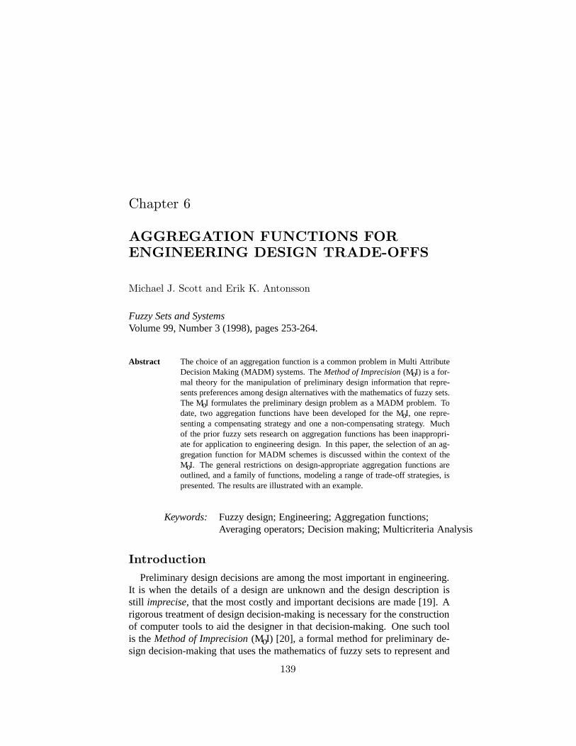
Chapter 6
AGGREGATION FUNCTIONS FORENGINEERING DESIGN TRADE-OFFS
Michael J. Scott and Erik K. Antonsson
Fuzzy Sets and SystemsVolume 99, Number 3 (1998), pages 253-264.
Abstract The choice of an aggregation function is a common problem in Multi AttributeDecision Making (MADM) systems. TheMethod of Imprecision(MoI) is a for-mal theory for the manipulation of preliminary design information that repre-sents preferences among design alternatives with the mathematics of fuzzy sets.The MoI formulates the preliminary design problem as a MADM problem. Todate, two aggregation functions have been developed for the MoI, one repre-senting a compensating strategy and one a non-compensating strategy. Muchof the prior fuzzy sets research on aggregation functions has been inappropri-ate for application to engineering design. In this paper, the selection of an ag-gregation function for MADM schemes is discussed within the context of theMoI. The general restrictions on design-appropriate aggregation functions areoutlined, and a family of functions, modeling a range of trade-off strategies, ispresented. The results are illustrated with an example.
Keywords: Fuzzy design; Engineering; Aggregation functions;Averaging operators; Decision making; Multicriteria Analysis
IntroductionPreliminary design decisions are among the most important in engineering.
It is when the details of a design are unknown and the design description isstill imprecise, that the most costly and important decisions are made [19]. Arigorous treatment of design decision-making is necessary for the constructionof computer tools to aid the designer in that decision-making. One such toolis theMethod of Imprecision(MoI) [20], a formal method for preliminary de-sign decision-making that uses the mathematics of fuzzy sets to represent and
139
140 IMPRECISION IN ENGINEERING DESIGN
manipulate imprecise design information. The MoI casts the design decision-making problem as a Multi Attribute Decision Making (MADM) or Multi Ob-jective Decision Making (MODM) problem [4, 24].
The choice of an aggregation function is a crucial part of any MADM orMODM scheme. The MoI has attempted to approach this choice axiomat-ically. The axioms of the MoI restrict the choice of candidate aggregationfunctions so as to reflect the natural structure of the design decision-makingprocess [10, 11]. Within the axiomatic framework of the MoI, a designer cancombine preliminary design information using different trade-off strategies. Inparticular, two aggregation functions have been used for multi-attribute deci-sion making, one which provides a compensation between the criteria, and onewhich does not compensate.
Many different aggregation functions for fuzzy sets have been proposed andstudied. Much fuzzy set research has focused ont-normsand t-conorms[5].T-norms are bounded above by themin function, and are the appropriate modelfor extensions of the logical AND to fuzzy sets, while t-conorms are boundedbelow by themaxfunction and are an extension of the logical OR. Both classesof functions have been studied in detail, and research is on-going (e.g., [14]).MADM schemes have applied a wide range of t-norms and other operators todecision problems. While averaging operators, which fall betweenmin andmax, have been acknowledged for some time [5, 22, 23], comparatively lit-tle study has been devoted to these connectives. Averaging operators are notappropriate for binary logic, but they are well suited to engineering design de-cisions: indeed, the axioms of the MoI require its aggregation functions to fallbetweenminandmax[10]. This paper will offer a more thorough treatment ofaveraging operators than has been presented previously.
This paper discusses the problem of choosing an aggregation function formultiple criteria decision making. The results are presented within the con-text of the MoI, but they have general applicability in MADM and MODMapproaches. The axioms of the MoI and the reasons for their use in model-ing engineering design decisions will be presented. In the context of theseaxioms, potential aggregation functions will be discussed. The MoI presentlyuses two different aggregation functions to model two different design trade-offstrategies. This paper will explore the range of possible aggregation functionssuitable for such decision-making. A parameterized family of functions thatsatisfies all the axioms for design and that models a continuum of strategiesbetween the two existing strategies of the MoI will be presented. The possibil-ity of suitable aggregation functions outside this range will be discussed, andan example of an application will be given.
The organization of the paper is as follows. The first section presents theissue of uncertainty in engineering design and introduces the MoI. The secondsection discusses the axioms of the MoI in more detail. The third section covers
Aggregation Functions For Engineering Design Trade-offs 141
some of the prior research on fuzzy MADM systems. In the fourth section, aparameterized family of aggregation functions is presented. The fifth sectioncontains some philosophical remarks on the implications of this paper. Finally,the sixth section illustrates the application of the result with an example.
1. Uncertainty in Engineering DesignIn preliminary engineering design, the final values ofdesign variablesare
uncertain. As this uncertainty is not probabilistic, but will be resolved by fur-ther refinement and specification later in the design process, it is appropriatelymodeled using the mathematics of fuzzy sets [20, 21]. The Method of Impre-cision is a formal system for the representation and manipulation of such im-precise design data. When a design is finalized, standard analysis tools (e.g.,finite element analysis,etc.) serve to calculate the performance of a design.These standard analysis tools do not operate on the imprecise information thatis available during preliminary design, and designers rely on experience andintuition in this early stage. In the MoI, designers represent their preferencesfor different values of a design variable using fuzzy sets: each value of a de-sign variable is assigned a preference between zero (totally unacceptable) andone (completely acceptable). Design variables can take on discrete, contin-uous, or linguistic values. The designer’s preferences create a fuzzy set thatcould be called “Values of design variabled preferred by the designer”; themembership in this set of a particular value ofd is the designer’s preferencefor that value. In this way, the designers’ judgment and experience are for-mally incorporated into the preliminary problem. The designers’ preferences,expressed on the design variables, are mapped to the performance space wherethey become preferences on theperformance variables[8]. Preferences arealso specified directly on performance variables by designers or others, andrepresent the functional requirements for the design. Whether calculated orexpressed directly, these performance variables are likewise represented withfuzzy sets. Since a design’s performance is usually described by several dif-ferent performance variables, reconciliation of competing aspects of a design’sperformance forms an important part of the MoI.
The general problem is thus a Multiple Attribute Decision Making (MADM)problem: the designer is to choose the highest performing design configurationfrom an available design space, when each design is to be judged by several,perhaps competing, performance criteria (variables). These performance vari-ables may have different levels of importance, orweights. The MADM prob-lem is one of the aggregation of weighted fuzzy sets. The goal is to choose anaggregation functionthat properly models the concerns of a designer evaluat-ing a design.
142 IMPRECISION IN ENGINEERING DESIGN
A few points of notation: preferences are denoted byµ, indexed asµi, andtheir attendant weights are denoted byωi. The overall preferenceµo is calcu-lated using an aggregation functionP:
µo = P((µ1, ω1), · · · , (µn, ωn))
If it is convenient to ignore the weights, as in the common case of equal weightsfor all objectives, the function can be written simply
µo = P(µ1, · · · , µn)
The MoI has previously used two different aggregation functions to modeltwo different situations in decision-making in design. When the overall pref-erence for the performance of a design is limited by the attribute with the low-est performance, the decision-making problem is said to benon-compensating,and the aggregation function used is the simple minimum. In this case, weightsare immaterial, and are not included in the calculations. When good perfor-mance on one attribute is perceived to partially compensate for lower per-formance on another, the problem is calledcompensating, and the geometricweighted mean or product of powers has been used.1 Which aggregation func-tions are appropriate for design decision-making is the subject of this paper.
2. The Axioms of the MoIIn any MADM system, it is desirable that the aggregation functions used be
justifiable models for decision-making behavior. The choice of an aggregationfunction may be justified in several ways. Empirical tests, such as those con-ducted by other researchers [15] can help determine which aggregation func-tions best model human decision-making in various contexts. (The study men-tioned supports the aggregation functions used by the MoI.) Computationalsimplicity is often used as a basis for the choice of an aggregation function,however inappropriate that may be. The development of the MoI has been toappeal to intuitive notions of rational human behavior [16], and to formalizethis rationality in a set of axioms that the aggregation functions must follow.The axioms of the MoI (see Table 6.1) [10] are a formal description of restric-tions on any aggregation function for (rational) engineering design.
The axioms of monotonicity, commutativity and continuity are common tomany multi-attribute decision making schemes, and they are uncontroversial.Also uncontroversial is the idea that an attribute with zero weight should con-tribute nothing to the overall performance. Self-scaling weights are convenient
1Both of these aggregations are analogous to Pareto-optimal solutions in game theory [9, 18], and theproduct of powers is analogous to a Nash solution. However, neither correspondence is mathematicallyprecise, since preferences are not equivalent to utilities.

Aggregation Functions For Engineering Design Trade-offs 143
Monotonicity:P((µ1, ω1), · · · , (µn, ωn)) ≤ P((µ1, ω1), · · · , (µ′
n, ωn))for µn ≤ µ′
n
P((µ1, ω1), · · · , (µn, ωn)) ≤ P((µ1, ω1), · · · , (µn, ω′n))
for ωn ≤ ω′n; µi < µn ∀i < n
Commutativity:P((µ1, ω1), · · · , (µi, ωi), · · · , (µj , ωj), · · · , (µn, ωn)) =
P((µ1, ω1), · · · , (µj , ωj), · · · , (µi, ωi), · · · , (µn, ωn)) ∀i, j
Continuity: P((µ1, ω1), · · · , (µk, ωk), · · · , (µn, ωn)) =limµ′
k→µk
P((µ1, ω1), · · · , (µ′k, ωk), · · · , (µn, ωn)) ∀k
P((µ1, ω1), · · · , (µk, ωk), · · · , (µn, ωn)) =limω′
k→ωk
P((µ1, ω1), · · · , (µk, ω′k), · · · , (µn, ωn)) ∀k
Idempotency:P((µ, ω1), · · · , (µ, ωn)) = µ
for ω1, · · · , ωn ≥ 0; ω1 + · · · + ωn > 0Annihilation:P((µ1, ω1), · · · , (0, ω), · · · , (µn, ωn)) = 0 for ω 6= 0Self-scaling weights:P((µ1, ω1t), · · · , (µn, ωnt)) = P((µ1, ω1), · · · , (µn, ωn))
∀ ω1, · · · , ωn ≥ 0; ω1 + · · · + ωn, t > 0Zero weights:P((µ1, ω1), · · · , (µk, 0), · · · , (µn, ωn))
= P((µ1, ω1), · · · , (µk−1, ωk−1), (µk+1, ωk+1), · · · , (µn, ωn))
Table 6.1 Axioms of the MoI
144 IMPRECISION IN ENGINEERING DESIGN
for the hierarchical combination of an arbitrary number of attributes. Two ofthe axioms, however, idempotency and annihilation, are fundamental to theMoI and are particularly relevant here.
The idempotency axiom appeals to a notion of rational behavior. It statesthat if several variables with identical preferences are combined, the overallpreference must be the same as the (identical) preferences on the individualvariables. Idempotency reflects the constraint that the overall preference fora design should never exceed the preference of the highest-ranked attribute,nor fall below the preference of the lowest-ranked attribute. Idempotency andmonotonicity together lead to the requirement thatmin≤ P ≤ max.
The annihilation axiom is specific to engineering design, and others haveargued its validity [3, 12, 17]. It states that if the preference for any one at-tribute of the design sinks to zero (unacceptable) then the overall preferencefor the design is zero. For example, given a fixed material, the tensile strengthlimit cannot be exceeded no matter the reduction in the design’s cost or weight.This is in contrast to a decision-making situation in which all performances canbe converted into monetary units; in the latter case, two goals can always betraded, or bought, off.
One axiom that isnot necessary for design-compatible aggregation func-tions is an axiom of strict monotonicity, and such a requirement would beincompatible with annihilation. The non-compensating functionmin is an ex-ample of a function that fulfills all of the axioms of the MoI and is not strictlymonotonic.
The axioms of idempotency and annihilation set the MoI apart from othermulti-attribute decision making systems. The reader is referred to [10] for amore detailed discussion of the motivation for this particular set of axioms.This paper posits the axioms of the MoI as reasonable for design, and askswhat can be said about the functions that satisfy these axioms. Such functionswill be known asdesign-appropriate. This paper does not directly addressthose decision-making problems, outside of the field of engineering design,for which these axioms do not supply a reasonable model, though many of theideas discussed here will be relevant to other non-design MADM schemes.
3. Fuzzy Multi Attribute Decision MakingIn their recent book on the subject, Chen and Hwang [4] identify 18 fuzzy
MADM methods, which they systematically classify into eight categories: sim-ple additive weighting methods, the Analytic Hierarchy Process (AHP), theConjunction/Disjunction method, MAUF, the General MADM method, theoutranking method, maximin, and their own proposed MADM method. In theirsurvey, Chen and Hwang do not draw the distinction observed by Zimmer-mann [24] between continuous Multi Objective Decision Making (MODM)
Aggregation Functions For Engineering Design Trade-offs 145
problems and discrete Multi Attribute Decision Making (MADM) problems.This paper shall follow Chen and Hwang and use MADM to refer to the gen-eral problem, whether continuous or discrete.
Several of the methods surveyed by Chen and Hwang are similar to the MoI.In addition, the application of utility theory [7] to decision problems bearssome similarity to the MoI and to the methods listed above. The possible appli-cation of utility theory to engineering design has been considered previously,and shown to be problematic [12]. Matrix methods such as QFD [6] and Pughcharts [13] also support decision making by simple additive aggregation overseveral requirements.
Aggregation operators are important in all MADM methods, from the mostformal to the most casual. The arithmetic mean or weighted sum is popularin matrix methods and elsewhere, as it is simple to calculate. Themin en-joys considerable popularity as well. Chen and Hwang provide an overviewof commonly used aggregation operators; themin and the product operatorspresently in use in the MoI appear in their list, as do weighted sums. However,the general weighted means discussed in this paper do not.
4. Weighted MeansFuzzy set researchers have productively applied the study of functional equa-
tions [1] to explore t-norms and t-conorms. This section applies the samegeneral approach to design-appropriate aggregation functions: an intuitivelyreasonable set of axioms is translated into a set of functional equations, andthese equations are then solved.
A promising class of functions is the class of weighted means. The proper-ties that define weighted means are listed in Table 6.2. While weighted meansare defined here as functions of two arguments, they can be extended to severalarguments.
The properties of the weighted mean include all of the properties of design-appropriate aggregation functions with the exception of annihilation; a compar-ison of these properties with the axioms of the MoI shows thatany weightedmean that satisfies annihilation is design-appropriate.The properties ofthe weighted mean also include conditions that are not explicitly design ax-ioms; nevertheless, these conditions are consistent with the axioms of theMoI. The bisymmetry condition is a surrogate for commutativity and asso-ciativity, and assures thatP can be consistently defined for more than twoarguments. Weighted means are strictly monotonic, which is a stronger con-dition than the monotonicity of the design axioms.Any strictly monotonicdesign-appropriate aggregation function must be a weighted mean.Thereare design-appropriate functions that are not weighted means, since they aremonotonic but fail to satisfy strict monotonicity. Such operators are often
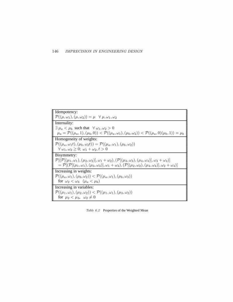
146 IMPRECISION IN ENGINEERING DESIGN
Idempotency:P((µ, ω1), (µ, ω2)) = µ ∀ µ, ω1, ω2
Internality:∃ µa < µb such that ∀ ω1, ω2 > 0µa = P((µa, 1), (µb, 0)) < P((µa, ω1), (µb, ω2)) < P((µa, 0)(µb, 1)) = µb
Homogeneity of weights:P((µa, ω1t), (µb, ω2t)) = P((µa, ω1), (µb, ω2))
∀ ω1, ω2 ≥ 0; ω1 + ω2, t > 0Bisymmetry:P[(P[(µ1, ω1), (µ2, ω2)], ω1 + ω2), (P[(µ3, ω3), (µ4, ω4)], ω3 + ω4)]
= P[(P[(µ1, ω1), (µ3, ω3)], ω1 + ω3), (P[(µ2, ω2), (µ4, ω4)], ω2 + ω4)]Increasing in weights:P((µa, ω1), (µb, ω2)) < P((µa, ω1), (µb, ω3))
for ω2 < ω3 (µa < µb)Increasing in variables:P((µ1, ω1), (µ2, ω2)) < P((µ1, ω1), (µ3, ω2))
for µ2 < µ3, ω2 6= 0
Table 6.2 Properties of the Weighted Mean
Aggregation Functions For Engineering Design Trade-offs 147
conditional rather than algebraic; themin is but one example. The class ofweighted means will not encompass any of these aggregation functions thatare only weakly monotonic. However, we shall see that the weak monotonicoperators presently used for design can be approximated arbitrarily closely bystrictly monotonic operators.
The structure of the class of weighted means is described completely in thefollowing theorem, proven in [1]:
Theorem 1 The properties of the weighted mean are necessary and sufficientfor the functionP((µ1, ω1), (µ2, ω2)) to be of the form
P((µ1, ω1), (µ2, ω2)) = f
(ω1f
−1(µ1) + ω2f−1(µ2)
ω1 + ω2
)
whereµa ≤ µ1, µ2 ≤ µb ; ω1, ω2 ≥ 0 ;ω1 + ω2 > 0 and f is a strictlymonotonic, continuous function with inversef−1.
It follows that any strictly monotonic design-compatible function must havea generating functionf . For example,f(t) = et (with µa = 1 andµb = e)generates the familiar weighted product of powers, denotedPΠ and also knownas the geometric mean:
PΠ((µ1, ω1), (µ2, ω2)) = (µ1ω1µ2
ω2)1
ω1+ω2
This function only satisfies the properties of the weighted mean forµi > 0,but it satisfies all of the design axioms, including annihilation, on the closedinterval [0, 1].
A parameterized family of equations of particular interest for design is gen-erated by the functionsf(t) = t
1s , wheres is a real number. The aggregation
function so generated is
Ps((µ1, ω1), (µ2, ω2)) =(
ω1µ1s + ω2µ2
s
ω1 + ω2
) 1s
Note that a weighted mean satisfies annihilation if and only iff−1(0) is un-bounded for that function. Fors < 0, f−1(t) = ts is unbounded att = 0andPs satisfies annihilation. Similarly,PΠ satisfies annihilation, asf−1(t) =ln(t) is unbounded att = 0. Figure 6.1 shows the behavior ofPs for severalnegative values of the parameters, and for equal weights (ω1 = ω2). In thisgraph,µ2 = 0.5 is fixed andµ1 varies from 0 to 1 along thex-axis. It is graphi-cally evident, and easily shown analytically, thatP0 is identical to the weightedproduct of powersPΠ. Thus the generating function for the geometric mean isnot unique. Furthermore, ass tends to−∞, Ps tends tomin(µ1, µ2), regard-less of the weights.
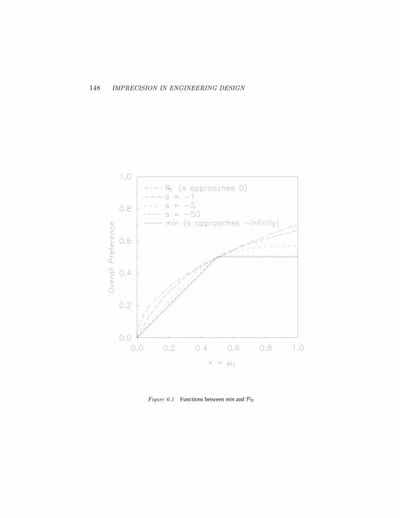
148 IMPRECISION IN ENGINEERING DESIGN
Figure 6.1 Functions betweenminandPΠ
Aggregation Functions For Engineering Design Trade-offs 149
Claim 1 P0 is identical to the weighted product of powersPΠ:
lims→0
Ps((µ1, ω1), (µ2, ω2)) = PΠ((µ1, ω1), (µ2, ω2))
Proof 1
lims→0
Ps((µ1, ω1), (µ2, ω2))
= lims→0
(ω1µ1
s + ω2µ2s
ω1 + ω2
) 1s
= explims→0 ln
(ω1µ1
s+ω2µ2s
ω1+ω2
) 1s
= explims→0
1s
ln(
ω1µ1s+ω2µ2
s
ω1+ω2
)(6.1)
Note that, by the definition of the derivative,
lims→0
1s
ln(
ω1µ1s + ω2µ2
s
ω1 + ω2
)
=d
ds
[ln(
ω1µ1s + ω2µ2
s
ω1 + ω2
)]s=0
=ω1 ln µ1 + ω2 ln µ2
ω1 + ω2
Thus, proceeding from (1), it follows that
lims→0
Ps((µ1, ω1), (µ2, ω2))
= expω1 ln µ1+ω2 ln µ2
ω1+ω2
= (µ1ω1µ2
ω2)1
ω1+ω2
= PΠ((µ1, ω1), (µ2, ω2))
which proves the claim.
In light of the preceding claim, the geometric meanPΠ will also be referredto asP0.
Claim 2 Ass → −∞, Ps tends to min:
lims→−∞ Ps((µ1, ω1), (µ2, ω2)) = min(µ1, µ2)
150 IMPRECISION IN ENGINEERING DESIGN
Proof 2
lims→−∞
(ω1µ1
s + ω2µ2s
ω1 + ω2
) 1s
= lims→−∞
(ω1
ω1 + ω2
) 1s(
µ1s +
ω2
ω1µ2
s) 1
s
= limt→+∞
(1
µ1t+
ω2
ω1µ2t
) 1−t
= limt→+∞
µ2
t(µ2µ1
)t+ ω2
ω1
1t
= limt→+∞
µ2((µ2µ1
)t+ ω2
ω1
) 1t
Note that ifµ2 ≤ µ1, then the denominator tends to one and the limit isµ2; ifµ1 < µ2, then the denominator tends toµ2
µ1and the limit isµ1. This proves the
claim.
Thus the two functions originally proposed as aggregation functions for theMoI, the min and the product of powers, turn out to be two limiting cases of aparameterized family of weighted means. EachPs, s ≤ 0, models a point on acontinuum of trade-off strategies between the original non-compensating andcompensating functions.
5. Application to designIn multi-attribute decision making, aggregation functions should provide a
useful, justifiable model of the design decision process. The parameterizedfamily Ps provides a continuum of weighted means between the two exist-ing functions of the MoI. While this family of functions is useful for designdecision-making, it is not exhaustive. Other generating functions give rise toother aggregation functions that satisfy all the axioms of the MoI but behavedifferently from any of thePs.
Themin is the least compensating possible design-appropriate function. Nodesign aggregation function can take on values less than themin at any pointin a design space. Themin function defines a boundary not only of a certainfamily of weighted means, but also of design-compatible functions in general.The product of powersPΠ is a pivotal example among weighted means, but itis not so clear that it is maximal among design-compatible functions. Indeed,
Aggregation Functions For Engineering Design Trade-offs 151
a maximal design-compatible function is problematic: such a functionPmaxwould satisfy
Pmax(0, µ) = 0 ∀ µ
but also satisfy
Pmax(ε, µ) = µ ∀ µ > ε > 0
for all non-zero weights.Pmax so defined takes on the largest possible valuewhile satisfying both idempotency and annihilation, but it fails another designaxiom: it is discontinuous at zero. It is clear that there is no maximal designfunction corresponding to themin.
It was noted above that the arithmetic mean is an aggregation function com-monly used in multi-attribute decision making. Yet the arithmetic mean doesnot satisfy all of the axioms of the MoI, as it fails annihilation. The arithmeticmean is the aggregation functionP1, and allows goals to compensate morestrongly than the geometric mean. Indeed,Ps, for s > 0, always fails anni-hilation, and the level of compensation between goals increases withs all theway toP+∞ = max. If the arithmetic mean is only chosen for computationalsimplicity, then its use must be questioned.
The family of weighted means that formed a continuum between theminandPΠ was found by varying the parameters in Ps between−∞ and 0. Itis interesting to examine what happens if the parameter is varied between 0and+∞. In this case a family of aggregation functions betweenP0 = PΠ andP∞ = maxis generated. These functions do not satisfy annihilation, so they donot appear to be appropriate for design. As long as no preference approacheszero, however, these functions satisfy all the axioms of the MoI. Figure 6.2showsPs plotted for several positive values ofs. As s → ∞, Ps → max. The“multi-linear” function of utility theory is also shown, though it fails idempo-tency as well as annihilation.
In practice, the MoI is always implemented using discrete functions. This ispartly an artifact of computer implementation, but more fundamentally arisesfrom the fact that some changes in preference are too small to be distinguished.A designer does not actually specify a continuous preference function on theinterval [0, 1], but rather gives the values for each variable on several differentα-cuts [2]. For example, for a particular design variable, the designer mayspecify which values correspond toµ = 0, µ = 0.25, µ = 0.5, µ = 0.75, andµ = 1.
The discontinuous manner in which preferences are specified provides somejustification for allowing the use ofPs with s > 0, or even themaxoperator, asan aggregation function when all of the preferences achieve some level. Thisseems to model the design process, as well: when all attributes are performingto some acceptable standard, a designer may choose to allow the highest pref-
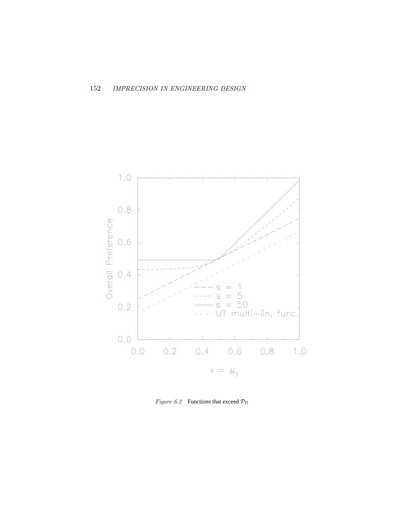
152 IMPRECISION IN ENGINEERING DESIGN
Figure 6.2 Functions that exceedPΠ
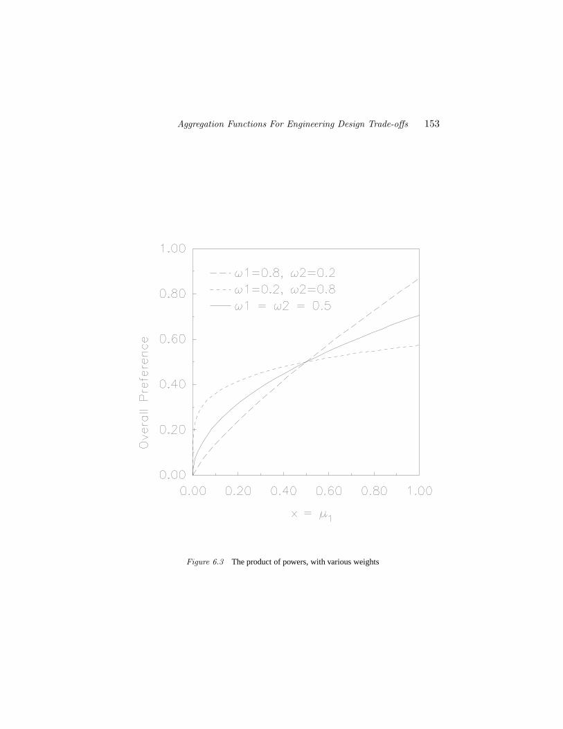
Aggregation Functions For Engineering Design Trade-offs 153
Figure 6.3 The product of powers, with various weights
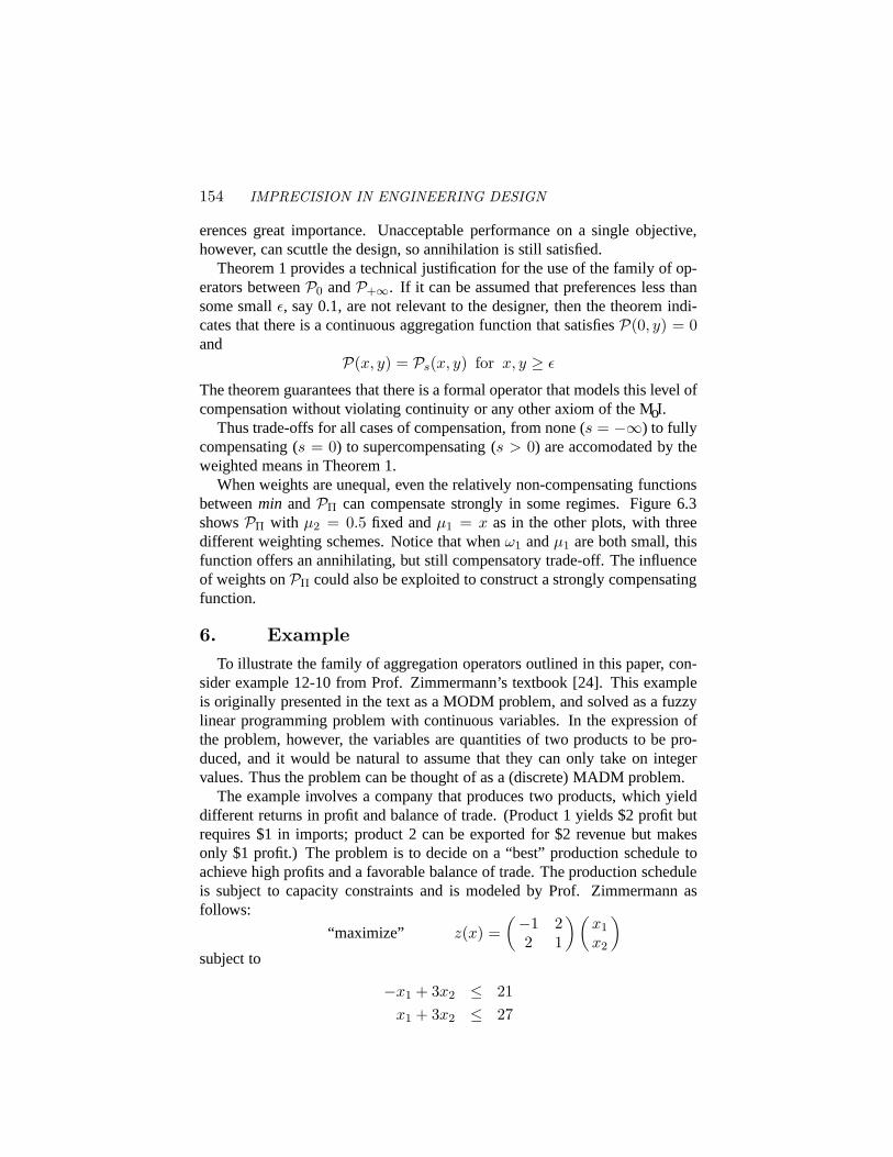
154 IMPRECISION IN ENGINEERING DESIGN
erences great importance. Unacceptable performance on a single objective,however, can scuttle the design, so annihilation is still satisfied.
Theorem 1 provides a technical justification for the use of the family of op-erators betweenP0 andP+∞. If it can be assumed that preferences less thansome smallε, say 0.1, are not relevant to the designer, then the theorem indi-cates that there is a continuous aggregation function that satisfiesP(0, y) = 0and
P(x, y) = Ps(x, y) for x, y ≥ ε
The theorem guarantees that there is a formal operator that models this level ofcompensation without violating continuity or any other axiom of the MoI.
Thus trade-offs for all cases of compensation, from none (s = −∞) to fullycompensating (s = 0) to supercompensating (s > 0) are accomodated by theweighted means in Theorem 1.
When weights are unequal, even the relatively non-compensating functionsbetweenmin andPΠ can compensate strongly in some regimes. Figure 6.3showsPΠ with µ2 = 0.5 fixed andµ1 = x as in the other plots, with threedifferent weighting schemes. Notice that whenω1 andµ1 are both small, thisfunction offers an annihilating, but still compensatory trade-off. The influenceof weights onPΠ could also be exploited to construct a strongly compensatingfunction.
6. ExampleTo illustrate the family of aggregation operators outlined in this paper, con-
sider example 12-10 from Prof. Zimmermann’s textbook [24]. This exampleis originally presented in the text as a MODM problem, and solved as a fuzzylinear programming problem with continuous variables. In the expression ofthe problem, however, the variables are quantities of two products to be pro-duced, and it would be natural to assume that they can only take on integervalues. Thus the problem can be thought of as a (discrete) MADM problem.
The example involves a company that produces two products, which yielddifferent returns in profit and balance of trade. (Product 1 yields $2 profit butrequires $1 in imports; product 2 can be exported for $2 revenue but makesonly $1 profit.) The problem is to decide on a “best” production schedule toachieve high profits and a favorable balance of trade. The production scheduleis subject to capacity constraints and is modeled by Prof. Zimmermann asfollows:
“maximize” z(x) =(−1 2
2 1
)(x1x2
)subject to
−x1 + 3x2 ≤ 21x1 + 3x2 ≤ 27
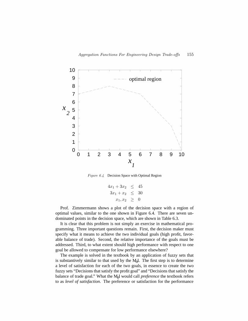
Aggregation Functions For Engineering Design Trade-offs 155
0 1 2 3 4 5 6 7 8 9 10x
0
1
2
3
4
5
6
7
8
9
10
x
optimal region
2
1
Figure 6.4 Decision Space with Optimal Region
4x1 + 3x2 ≤ 453x1 + x2 ≤ 30
x1, x2 ≥ 0
Prof. Zimmermann shows a plot of the decision space with a region ofoptimal values, similar to the one shown in Figure 6.4. There are seven un-dominated points in the decision space, which are shown in Table 6.3.
It is clear that this problem is not simply an exercise in mathematical pro-gramming. Three important questions remain. First, the decision maker mustspecify what it means to achieve the two individual goals (high profit, favor-able balance of trade). Second, the relative importance of the goals must beaddressed. Third, to what extent should high performance with respect to onegoal be allowed to compensate for low performance elsewhere?
The example is solved in the textbook by an application of fuzzy sets thatis substantively similar to that used by the MoI. The first step is to determinea level of satisfaction for each of the two goals, in essence to create the twofuzzy sets “Decisions that satisfy the profit goal” and “Decisions that satisfy thebalance of trade goal.” What the MoI would call preferencethe textbook refersto aslevel of satisfaction. The preference or satisfaction for the performance
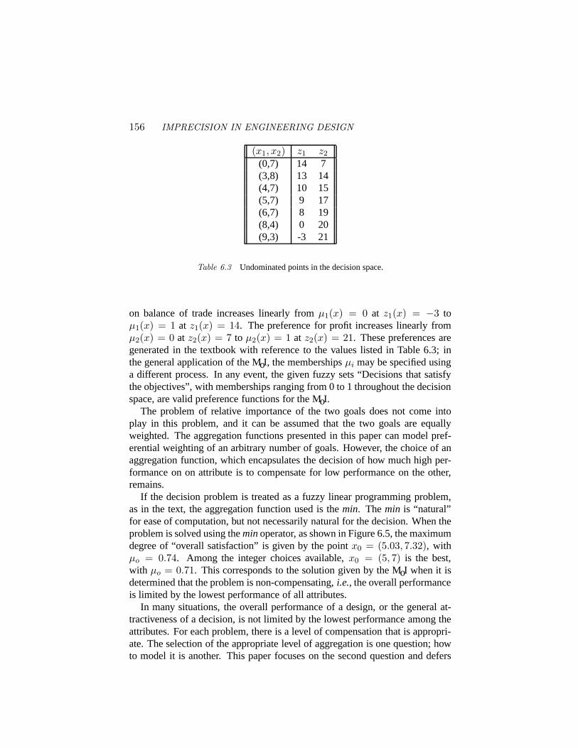
156 IMPRECISION IN ENGINEERING DESIGN
(x1, x2) z1 z2(0,7) 14 7(3,8) 13 14(4,7) 10 15(5,7) 9 17(6,7) 8 19(8,4) 0 20(9,3) -3 21
Table 6.3 Undominated points in the decision space.
on balance of trade increases linearly fromµ1(x) = 0 at z1(x) = −3 toµ1(x) = 1 at z1(x) = 14. The preference for profit increases linearly fromµ2(x) = 0 at z2(x) = 7 to µ2(x) = 1 at z2(x) = 21. These preferences aregenerated in the textbook with reference to the values listed in Table 6.3; inthe general application of the MoI, the membershipsµi may be specified usinga different process. In any event, the given fuzzy sets “Decisions that satisfythe objectives”, with memberships ranging from 0 to 1 throughout the decisionspace, are valid preference functions for the MoI.
The problem of relative importance of the two goals does not come intoplay in this problem, and it can be assumed that the two goals are equallyweighted. The aggregation functions presented in this paper can model pref-erential weighting of an arbitrary number of goals. However, the choice of anaggregation function, which encapsulates the decision of how much high per-formance on on attribute is to compensate for low performance on the other,remains.
If the decision problem is treated as a fuzzy linear programming problem,as in the text, the aggregation function used is themin. Themin is “natural”for ease of computation, but not necessarily natural for the decision. When theproblem is solved using theminoperator, as shown in Figure 6.5, the maximumdegree of “overall satisfaction” is given by the pointx0 = (5.03, 7.32), withµo = 0.74. Among the integer choices available,x0 = (5, 7) is the best,with µo = 0.71. This corresponds to the solution given by the MoI when it isdetermined that the problem is non-compensating,i.e., the overall performanceis limited by the lowest performance of all attributes.
In many situations, the overall performance of a design, or the general at-tractiveness of a decision, is not limited by the lowest performance among theattributes. For each problem, there is a level of compensation that is appropri-ate. The selection of the appropriate level of aggregation is one question; howto model it is another. This paper focuses on the second question and defers
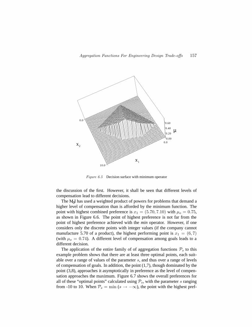
Aggregation Functions For Engineering Design Trade-offs 157
0.0
10.0
x20.0
x1
0.00
0.20
0.40
0.60
µ
Figure 6.5 Decision surface with minimum operator
the discussion of the first. However, it shall be seen that different levels ofcompensation lead to different decisions.
The MoI has used a weighted product of powers for problems that demand ahigher level of compensation than is afforded by the minimum function. Thepoint with highest combined preference isx1 = (5.70, 7.10) with µo = 0.75,as shown in Figure 6.6. The point of highest preference is not far from thepoint of highest preference achieved with themin operator. However, if oneconsiders only the discrete points with integer values (if the company cannotmanufacture 5.70 of a product), the highest performing point isx1 = (6, 7)(with µo = 0.74). A different level of compensation among goals leads to adifferent decision.
The application of the entire family of of aggregation functionsPs to thisexample problem shows that there are at least three optimal points, each suit-able over a range of values of the parameters, and thus over a range of levelsof compensation of goals. In addition, the point (1,7), though dominated by thepoint (3,8), approaches it asymptotically in preference as the level of compen-sation approaches the maximum. Figure 6.7 shows the overall preferences forall of these “optimal points” calculated usingPs, with the parameters rangingfrom -10 to 10. WhenPs = min (s → −∞), the point with the highest pref-
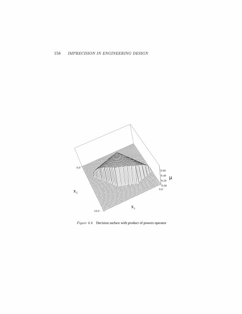
158 IMPRECISION IN ENGINEERING DESIGN
0.0
10.0
x20.0
x1
0.00
0.20
0.40
0.60
µ
Figure 6.6 Decision surface with product of powers operator
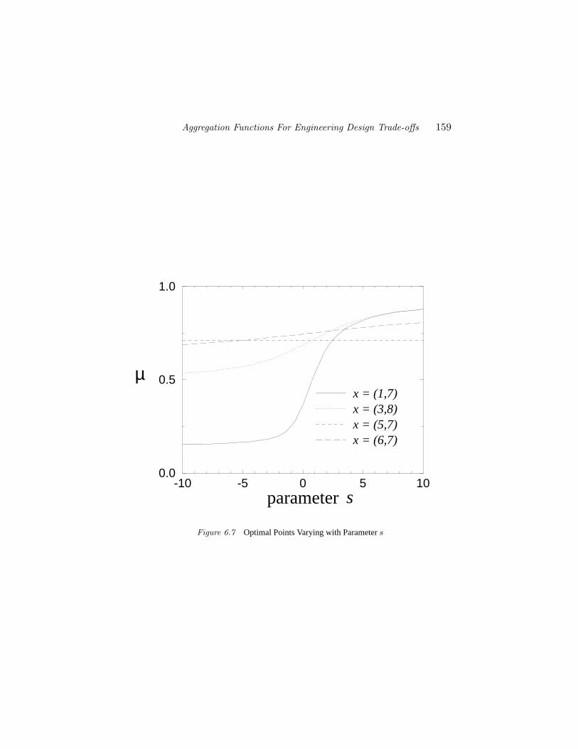
Aggregation Functions For Engineering Design Trade-offs 159
-10 -5 0 5 10parameter
0.0
0.5
1.0
µ x = (1,7)x = (3,8)x = (5,7)x = (6,7)
s
Figure 6.7 Optimal Points Varying with Parameters
160 IMPRECISION IN ENGINEERING DESIGN
erence isx = (5, 7), the textbook answer. Ass grows andPs becomes morecompensating, the preference for other points grows stronger. Ass crosses−5.25, x = (6, 7) overtakesx = (5, 7) and remains the most preferred pointthrough approximatelys = 2.25. This region includes two common aggrega-tion functions: the weighted product of powers or geometric mean (s = 0),and the classical weighted sum or arithmetic mean (s = 1). Values ofs greaterthan 2.25, corresponding to even stronger levels of compensation, lead to anoverall preference for the point (3,8), and ass → +∞, the preference for thedominated pointx = (1, 7) approaches the preference forx = (3, 8) asymp-totically. The limitss = 10 ands = −10 were chosen to show the full rangeof behavior of this problem; values ofs outside this range are certainly permis-sible.
The functions discussed in this paper provide models for a continuum oftrade-offs ranging from the non-compensatingmin to the compensatingPΠ allthe way to themaxoperator. Instead of two aggregation functions, there is aparameterized family of functions ranging from themin to PΠ, and anotherfrom PΠ to themax.
ConclusionThis paper has discussed the selection of an aggregation function for Multi
Attribute Decision Making. The problem was investigated within the contextof the Method of Imprecision, a formal system, based on the mathematics offuzzy sets, for the representation and manipulation of imprecise design infor-mation through the specification of preferences on design and performancevariables. The MoI casts the preliminary design decision problem as a MADMproblem, and uses different aggregation functions to formally model differenttrade-off strategies. The class of functions appropriate for the aggregation ofthese preferences has been explored in this paper. While they are directly ap-plicable to decision making in engineering design, the results of this paper arealso relevant to other MADM schemes.
This paper has presented a complete characterization of aggregation func-tions that satisfy the axioms of the MoI. The class of functional equationsknown as quasi-linear weighted means was shown to be crucial. It was demon-strated that any strictly monotonic design-compatible aggregation function isgenerated by a generating function as detailed in Theorem 1. The condi-tional operators in use, while not weighted means, were shown to be limitsof sequences of such functions. A parameterized family of functions was de-tailed, spanning two continua of possible design strategies, one between thenon-compensatingminand the compensatingPΠ, the two original aggregationfunctions of the MoI, and one betweenPΠ and themax.
Aggregation Functions For Engineering Design Trade-offs 161
Many MADM systems use aggregation functions, such as the arithmeticmean, that compensate between goals more aggressively than the existing func-tions of the MoI. These highly compensating functions may seem to be in con-flict with the axioms of the MoI. This paper has assessed the possibility of usingthese common aggregation functions in design decision-making problems.
There are an infinite number of aggregation operators that are suitable forengineering design. In particular, the parameterized familyPs is a range offunctions that models a broad spectrum of design decision-making situations,with the parameters indicating the degree of compensation permitted amongperformance criteria. The appropriate choice of the parameters is problem-specific and is a matter for further investigation.
The use of an aggregation function in any MADM system may be justifiedon empirical as well as rational grounds. It is not within the scope of this paperto provide empirical studies of designers’ decision making behavior. The de-velopment here has focused on a rational basis for the choice of an aggregationfunction. More empirical studies are needed to confirm in practice the resultsin this paper.
AcknowledgmentsThis material is based upon work supported, in part, by the National Sci-
ence Foundation under NSF Grant No. DMI-9523232. Any opinions, findings,conclusions, or recommendations expressed in this publication are those of theauthors and do not necessarily reflect the views of the sponsor. The authorsexpress their appreciation to the anonymous reviewer whose thoughtful com-ments greatly improved this paper.
162 IMPRECISION IN ENGINEERING DESIGN
References
[1] ACZEL, J. Lectures on Functional Equations and their Applications.Academic Press, New York, 1966.
[2] A NTONSSON, E. K., AND OTTO, K. N. Imprecision in Engineering De-sign. ASME Journal of Mechanical Design 117(B) (Special CombinedIssue of the Transactions of the ASME commemorating the 50th anniver-sary of the Design Engineering Division of the ASME.)(June 1995), 25–32. Invited paper.
[3] BIEGEL, P., AND PECHT, M. Design trade-offs made easy.ConcurrentEngineering 1, 3 (May/June 1991), 29–40.
[4] CHEN, S.-J.,AND HWANG, C.-L. Fuzzy Multiple Attribute DecisionMaking: Methods and Applications, vol. 375 ofLecture Notes in Eco-nomics and Mathematical Systems. Springer-Verlag, New York, NY,1992. In collaboration with Frank P. Hwang.
[5] DUBOIS, D., AND PRADE, H. A review of fuzzy set aggregation con-nectives.Information Sciences 36(1985), 85–121.
[6] HAUSER, J.,AND CLAUSING, D. The House of Quality.Harvard Busi-ness Review 66, 3 (May/June 1988), 63–73.
[7] K EENEY, R.,AND RAIFFA, H. Decisions with Multiple Objectives: Pref-erences and Value Tradeoffs. Cambridge University Press, Cambridge,U.K., 1993.
[8] L AW, W. S., AND ANTONSSON, E. K. Hierarchical Imprecise Designwith Weights. InProceedings of the Fourth IEEE International Confer-ence on Fuzzy Systems (FUZZ-IEEE/IFES’95)(Mar. 1995), vol. 1, IEEE,pp. 383–388.
[9] L UCE, R., AND RAIFFA, H. Games and Decisions. J. Wiley and Sons,New York, NY, 1957. Dover Edition, 1985.
[10] OTTO, K. N. A Formal Representational Theory for Engineering Design.PhD thesis, California Institute of Technology, Pasadena, CA, June 1992.
[11] OTTO, K. N., AND ANTONSSON, E. K. Trade-Off Strategies in Engi-neering Design.Research in Engineering Design 3, 2 (1991), 87–104.
[12] OTTO, K. N., AND ANTONSSON, E. K. The Method of ImprecisionCompared to Utility Theory for Design Selection Problems. InDesignTheory and Methodology – DTM ’93(Sept. 1993), ASME, pp. 167–173.
[13] PUGH, S. Total Design. Addison-Wesley, New York, NY, 1990.
[14] ROYCHOWDHURY, S., AND WANG, B. H. Composite generalizationof dombi class and a new family of t-operators using additive-productconnective generator.Fuzzy Sets and Systems 66, 3 (Sept. 1994), 329–346.
Aggregation Functions For Engineering Design Trade-offs 163
[15] THOLE, U., ZIMMERMAN , H.-J.,AND ZYSNO, P. On the suitability ofminimum and product operators for the intersection of fuzzy sets.FuzzySets and Systems 2, 2 (1979), 167–180.
[16] TRIBUS, M. Rational Descriptions, Decisions, and Designs. PergamonPress, New York, NY, 1969.
[17] VINCENT, T. Game theory as a design tool.ASME Journal of Mecha-nisms, Transmissions, and Automation in Design 105(June 1983), 165–170.
[18] VON NEUMANN, J., AND MORGENSTERN, O. Theory of Games andEconomic Behavior, 2nd ed. Princeton University Press, Princeton, NJ,1953.
[19] WHITNEY, D. E. Manufacturing by design.Harvard Business Review66, 4 (July 1988), 83–91.
[20] WOOD, K. L., AND ANTONSSON, E. K. Computations with Impre-cise Parameters in Engineering Design: Background and Theory.ASMEJournal of Mechanisms, Transmissions, and Automation in Design 111,4 (Dec. 1989), 616–625.
[21] WOOD, K. L., ANTONSSON, E. K., AND BECK, J. L. Comparing Fuzzyand Probability Calculus for Representing Imprecision in PreliminaryEngineering Design. InDesign Theory and Methodology - 1989(NewYork, Sept. 1989), W. P. Seering, Ed., ASME, pp. 99–105. Presented atthe First International ASMEDesign Theory and Methodology Confer-ence(DTM ’89), September 18-19, 1989, Montr´eal, Canada.
[22] YAGER, R. Decision making with fuzzy sets.Decision Sciences 6, 3(1975), 590–600.
[23] YAGER, R. Fuzzy decision making including unequal objectives.FuzzySets and Systems 1(1978), 87–95.
[24] ZIMMERMANN , H.-J. Fuzzy Set Theory - and Its Applications. Manage-ment Science/Operations Research. Kluwer-Nijhoff Publishing, Boston,MA, 1985.


Chapter 7
FORMALISMS FOR NEGOTIATIONIN ENGINEERING DESIGN
Michael J. Scott and Erik K. Antonsson
Proceedings of the8th International Conference on Design Theory and MethodologyASME, Paper Number 96-DETC/DTM-1525, (August, 1996)
Abstract Engineering projects often undergo several design iterations before being com-pleted. Information received from other groups working on a project (analysis,manufacturing, marketing, sales) will often necessitate changes in a design. Theinteraction between different groups associated with a design project often takesthe form of informal “negotiation.” This form of interaction commonly ariseswhen engineering information is imprecise. The Method of Imprecision (MoI)is a formal method for the representation and manipulation of preliminary andimprecise design information. It provides a mechanism for the formalization ofthese informal negotiations. The nature and scope of informal negotiation inengineering is explored and discussed, and application of the MoI is illustratedwith an example.
IntroductionEngineering design projects in industry commonly involve many different
work groups or individuals. In addition to a division of labor by subsystems,there is a division of labor by engineering task. For example, the solid mod-eling and finite element analysis of an artifact may be handled by differentengineers. Production engineers form a group with its own set of concerns,reflected in the considerable literature on the importance of design for manu-facture (see [5] for a good bibliography). Finally, design engineers are ulti-mately responsible to their customers. The customers’ concerns are typicallyrepresented by management or marketing, who form yet another group with aninterest in the design process. The groups within an organization that partici-
165
166 IMPRECISION IN ENGINEERING DESIGN
pate in a project, who are not necessarily all engineers, will be referred to hereasworking groups.
Interest in the issues that arise when so many different groups share thedesign task has led other researchers to explore concurrent engineering. [16],in particular, have pointed out the importance of the communication of set-based information between downstream and upstream processes. In this paper,we deal with situations ofnegotiationbetween working groups that arise in thecourse of a shared design task. Negotiation occurs whenever one workinggroup desires a change in work done by another working group. Often, adefining feature of a negotiation situation is that the two groups have differentviews of the design object or process. It is possible, however, for situationsthat are appropriately modeled as negotiation to arise where there is a single,agreed-upon view of the design. In general, this negotiation is highly informal.
Other researchers, particularly in the artificial intelligence community, haveseen conflict and negotiation between agents as a crucial part of the design pro-cess. Several systems have been developed that attempt to model, incorporate,or handle conflict in design [2, 3, 6, 9, 13]. These projects will be discussedbelow.
This paper was motivated by work done by the authors in collaboration witha US auto manufacturer and a material manufacturing research center. Wefound that the informal negotiations described above are common, so com-mon that informal negotiation appears nearly an automatic part of any designprocess. In most cases, it is not even recognized as negotiation, yet in someinstances the culture of negotiation is so highly developed that parties “cometo the bargaining table” with exaggerated estimates because they expect to be“bargained down.”
Why is this sort of negotiation so prevalent? One reason is the fundamentalimprecision inherent in engineering design. Final designs are exact (includ-ing manufacturing tolerances), yet such precision is present only at the end ofthe design process. Engineers (and managers) routinely conduct analyses andmake decisions with imprecise quantities. As a design progresses, informationbecomes more precise, and it may become necessary to revise earlier estimates.Yet the preliminary decisions account for an overwhelming fraction of the totalcost of a design, with some studies citing figures up to 70% [17].
Despite the ubiquity of imprecision in engineering design, there are fewtools for dealing with imprecise information. One such tool is theMethodof Imprecision(MoI) [18], a formal method for representing and manipulatinguncertainty in engineering design employing the mathematics of fuzzy sets.It has been shown that the MoI can be used to combine design informationusing a variety of different trade-off strategies [11, 15]. Other references havedeveloped the MoI for industrial application [8].

Formalisms for Negotiation in Engineering Design 167
Current work undertakes to use the structure of the MoI to formalize thepresently informal negotiation process. The mechanisms employed by the MoIfor the representation of uncertain or imprecise information are particularlywell-suited to the formal representation of the negotiation process. By for-malizing the negotiation process, design teams can promote a more completeexchange of information and have a mechanism to trace the history of a designthrough its iterations. The existence of a formal negotiation tool may facili-tate the inclusion of important performance goal and market information, thusallowing the incorporation of more relevant information into the early designstages.
This paper discusses the context and importance of design negotiation inindustry, and demonstrates the application of the MoI to place negotiations ona formal basis.
Examples of Negotiation in DesignThe following examples are not exhaustive, but they indicate the wide range
of design negotiation situations:
Unreachable target performance valuesOne example of design negotiation occurs when an engineer or engineering
group is given the task of designing a product to a target performance specifi-cation. When the product is a newer model of an existing product, the targetis often an incremental improvement over last year’s model. As an example,consider an automobile chassis, where an existing model has a torsional stiff-ness of 12,000 ft.-lbs./degree and this year’s requirement is to exceed that by10%. If the engineers are unable to reach the fixed target easily, they will re-turn to the manager who set the task and begin a negotiation process (indeed,this meeting may be scheduled long before any potential problems are known).The engineers may ask for more resources, for a relaxation of other targets, orfor a compromise on the original target. Targets are almost never immovable,and managers are commonly willing to negotiate.
Here, negotiation serves to address an inadequacy in the original descriptionof the problem: the ostensibly exact (orcrisp) requirement is in fact fuzzy, andthrough negotiation the two groups (in this case, chassis designers and theirmanagers) explore the nature of the “constraints.” To formalize this negotia-tion and reduce pre-distorted bargaining positions, it is important to be able torepresent the inherent fuzziness in the constraint. The MoI uses fuzzy sets torepresent such imprecision, as will be shown further below.
168 IMPRECISION IN ENGINEERING DESIGN
Trade-offs between facets of performanceAn additional layer of complication is added when several target perfor-
mances are considered at once; here, negotiation can occur even when all spec-ifications are met. In fact, there are usually at least two specifications, sincecost of engineering and production resources is almost always a factor. In theexample of the chassis design, the designers’ position may be to offer the man-ager a choice between a 6% improvement at a production cost slightly lowerthan the present model’s, or an 11% improvement at a substantially higher cost.To this, the managers may well counter that the new target is 8% improvement,as cheaply as possible.
The trade-off between cost and performance is one of many conflicts thatare resolved through negotiation. A typical project will have an array of per-formance targets. The chassis example mentioned above will also have bend-ing stiffness, weight, noise, and vibrational targets in addition to the torsionalstiffness. The overall performance of the design depends on the individual per-formances, but the exact nature of the dependence varies greatly with the par-ticular problem. The negotiation process is a means by which the true measure(and compromise) of overall performance is uncovered. A method to formal-ize negotiation may provide quicker and more complete information about theoverall performance relationship.
Conflicts between design and manufacturingThe problem of design for manufacturability has been addressed by oth-
ers [5], but it has not previously been noted that conflicts between design andmanufacturing are often resolved through a negotiation process. Sometimesthe issue is the rejection of an unmanufacturable design by the production en-gineer. In many cases, a production engineer suggests changes that will makemanufacture simpler, and negotiates with the design engineer for a compro-mise that will give the most satisfactory overall performance when productioncost and reliability are taken into account. In the most optimistic case, a man-ufacturing group may suggest changes that improve the overall design perfor-mance. In a worst-case scenario, poor or no negotiation can lead to spectacularfailures. The infamous 1981 collapse of the Hyatt Regency walkway in KansasCity, Missouri, the deadliest engineering disaster in U.S. history, has been at-tributed to miscommunication between designers and fabricators [14]. A for-malism for negotiation can help to facilitate the resolution of these conflicts,and can at the same time provide an unambiguous record of decisions that aremade at each step of the design process.
Formalisms for Negotiation in Engineering Design 169
Conflicts between engineering groupsWhen different working groups have responsibility for different subsystems,
or for different aspects, of a design, the requirements of one group may conflictwith the requirements of another. Stiffeners added to improve the structuralrigidity of a frame might eliminate space that the fuel system group was count-ing on for the fuel tank. While in mature designs a structural part may well bedescribed by a volume envelope and a few immutable points of contact, thereare many situations in which the interaction between parts is not so rigidlydescribed. Even when constraints are imposed in an attempt to avoid conflictbetween working groups, points of intersection between subsystems are oftennegotiated.
The incorporation of unquantifiable performancesMany design problems include performance criteria that are difficult, if not
impossible, to measure, yet these criteria can be so important as to drive adesign. Aesthetic and emotional concerns are certainly of great importance inthe auto industry [4], and they also play a surprisingly significant role in otherfields, from heavy machinery to military aircraft.
Style, beauty, appearance of solidity, color, image, are all examples of im-measurable attributes that can play a substantial role in the desirability of anengineered object. The fact that they are not easily quantified can lead to ei-ther underestimation or overestimation of their role in a design. An engineerdesigning for more concrete performance specifications may ignore them alto-gether, yet that same engineer may be working within strict geometrical con-straints dictated by a stylist’s vision.
Immeasurable performances present the greatest challenge in the formaliza-tion of design negotiation as presented in this paper. Still, steps can be takento formalize this part of the design process, and this formalization can lead toa clearer picture of true overall design requirements.
These examples are meant to convey the nature of the problem of informalnegotiation in engineering design. The following section describes a formalsystem to conduct negotiation more rigorously.
Prior Research on NegotiationOther researchers have also recognized the importance of negotiation in de-
sign. Some take the point of view that any contradiction that arises in thedesign process is a conflict to be resolved by negotiation. This paper takes aless inclusive view of negotiation, but points out that the formal representa-tion of any trade-off is realized in the same way as a negotiation between twoparties.
170 IMPRECISION IN ENGINEERING DESIGN
Researchers in artificial intelligence have noted that conflict is an integralpart of the design process. A few are mentioned here: [9] present a more com-prehensive bibliography of current research and a thoughtful list of potentialsources of conflict in addition to their own work on a design support environ-ment called Schemebuilder. [2] have approached conflict from a utility theorypoint of view; their work is perhaps the most comparable to the research di-rection outlined in this paper, but they have focused on a computer implemen-tation of the decision and have limited themselves to a linear weighted summodel and fairly restrictive representations for goals. The work accomplishedpreviously with the MoI, and the applications proposed in this paper, offer morepossibilities for the modeling of the design but less automation of the decisions.Some interesting work has been done on a design support system using Paretooptimality by [13]. The system does not calculate optimal solutions, but rathertracks a history of design decisions and automatically notifies agents when itseems that a better design might be overlooked.
These approaches to managing conflict in design, and others from the arti-ficial intelligence community [3, 6], have concentrated on environments thatmodel the design process itself, with the idea that such a model will be ap-plicable in any design situation, thus approaching the design problem fromabove. The act of negotiation is seen as an entity to be modeled. The researchdiscussed here approaches the design problem from below, where the crucialproblem is to model the imprecision inherent in design information, and to usethat model of design imprecision to guide negotiation.
Imprecision in the Design ProcessThe following is a brief review of the Method of Imprecision and some
necessary definitions. The reader is referred to [1, 10, 12], and [18] for moredetails.
The MoI formalizes design decision making in the presence of uncertaintyby the specification ofpreferencesondesignandperformance variables. Vari-ables are sometimes referred to asparameters. Design variables are denoteddi, wherei ranges from 1 ton. The set of design variable values under con-sideration fordi is denotedXi. The preference that a designer has for valuesof di, the ith design variable, is represented by a preference function onXi,termed thedesign preference:
µdi(di) : Xi → [0, 1]
A preference of 1 denotes a completely satisfactory value of the variable, apreference of 0 denotes an unacceptable value, and values in between representintermediate levels of satisfaction. By treating the preferencesµ as a member-ship function, the MoI can employ the mathematics of fuzzy sets [7, 19] toperform calculations on the uncertain variables.
Formalisms for Negotiation in Engineering Design 171
Performance variablesare denotedpj, with j ranging from 1 toq, and theset of possible values ofpj is denotedYj. The customer’s1 preference forvalues ofpj, thejth performance variable, is called afunctional requirementand is represented by a preference function onYj :
µpj(pj) : Yj → [0, 1]
The set of all performance variables can be represented as a vector~p ∈ Y,and the set of all design variables as~d ∈ X . Each performance variablepj isdefined by a mappingfj such thatpj = fj(~d). The mappingsfj can be anycalculation or procedure to measure the performance of a design, includingclosed-form equations, iterative and heuristic methods, “black box” functions,experiments, and consumer evaluations. When performance and design vari-ables are not all of equal importance, each can be assigned aweight, ωpj orωdi
.The individual preferences on variables are combined into an overall pref-
erenceµo by the use of anaggregation functionP:
µo = P (µd1 , ωd1 , ..., µdn , ωdn , µp1, ωp1 , ..., µpq , ωpq
).
This overall preference is a measure of the overall performance of the designwhen all criteria are considered. The design problem is thus to identify designconfigurations that maximizeµo, i.e., designs~d∗ such that:
µo(~d∗) = µ∗o = sup{µo(~d) | ~d ∈ X}.
The aggregation functionP reflects the design or trade-off strategy, whichindicates to what degree competing attributes of the design should be traded-off against each other [11, 15]. The appropriate design strategy is dictated bythe design problem. A design problem will in general require a hierarchy ofdifferent trade-off strategies which successively aggregate design attributes.
Formalizing NegotiationThe MoI has been applied previously as a decision support tool for self-
contained design problems. Its extension to facilitate negotiation betweenworking groups in engineering design entails a broader perspective on the de-sign problem.
The first step in any application of the MoI is the identification of design andperformance variables. Variables may be continuous or discrete, numericalor represented by linguistic terms. The model used by the MoI will employ
1The functional requirementµpj is called the customer’s preference for values ofpj , even if it is thedesigner who estimatesµpj .
172 IMPRECISION IN ENGINEERING DESIGN
the most important variables. An advantage of formalizing decisions is that itallows the timely incorporation of information that hitherto was not considereduntil after the end of a design iteration (when redesign is often the only option).
The second step is the specification of preferences over the values of thevariables. By treating the specified preferences on these variables as member-ship functions, the MoI can use the mathematics of fuzzy sets to make calcu-lations on these imprecise variables. The imprecision that arises here isun-certaintyas to the (best) final value—this imprecision will be lessened as thedesign progresses until the final design is precisely described. The specifica-tion of preference on performance variables logically precedes preferences ondesign variables. Preferences on performance variables represent targets, andare, at least at the outset, independent requirements. Preferences on designvariables are likely to change if there is a change in the functional require-ments.
The performance variables embody the design task: a designer must createplans for a device that will satisfy given values of a number of performancemeasures. Some performance variables arise because of a particular choice ofdesign solution. For example, in the course of performing its specified task(providing rotational power), an internal combustion engine generates heat, soheat dissipation becomes a performance parameter, although it is incidentalto the primary function of the automobile, which is to carry a load from onepoint to another. Responsibility for providing preferences on the performancevariables will depend on the structure of the company. Ultimately, it is thecustomer who has preferences for performance, though the customer is oftennot polled directly. (This paper suggests, but does not explore, the possibilitiesoffered by the MoI in market research.) Typically, market analysts and manage-ment teams are responsible for providing detailed information as to customers’desires. Simply formalizing the preferences can resolve many confusions. Thefuzzy preferences contain much more information than a simple list of targetvalues. They show a full range of acceptable values, and the relative desirabil-ity of values over that range. Together with weighting and trade-off strategyinformation, they can tell how much a change in one performance variable isworth in terms of another variable. Details of the specification of preferencehave been presented previously [10].
Design engineers then specify preferences on the design variables. Thesedesign preferences embody everything that is not explicitly represented in thecalculation of the performances. The design preferences may thus contain theengineers’ intuition about such concerns as manufacturability; in the exampledetailed below, style is taken into account as a design preference.
Preferences alone provide only a portion of the relevant information. Vari-ables are assigned weights that reflect their relative importance. Trade-off com-bination strategies [11, 15] must be determined, indicating to what extent su-

Formalisms for Negotiation in Engineering Design 173
perior performance in one aspect is to compensate for lower performance else-where. There can be more than one trade-off strategy in a design with manyvariables: for example, one might allow significant trade-off between cost andweight, but insist on considering safety independently. Even in cases wheretwo variables can trade-off strongly, an unacceptable preference (µ = 0) inone variable can never be overcome. The preferences, weights, and trade-offstrategy are used to calculate overall preference for the designs in the designspace [11, 15].
A complete specification of preferences on all performance variables wouldeliminate the need for negotiation whose sole purpose is to clarify the func-tional requirements. Design engineers are generally qualified to calculate thevalues of the performance variablespj; what they lack is complete informationas to which performance vectors~p are to be preferred if one performance vari-able comes in above or below target. It is not just in situations where targetsare unreachable that negotiation ensues; negotiation can also be required be-cause an engineering group finds one target particularly easy to meet and wantsto know where to spread around the extra slack that variable provides. If alldesign variables were simply quantifiable, as are cost, weight, stiffness, and soforth, the task of formalization would be more straightforward. The incorpora-tion of unquantifiable performances presents a particular difficulty. Managersor customers may find it difficult to describe their global preferences for theseunquantifiable variables, and a design may have to be seen for a level of sat-isfaction to be determined. This difficulty can be partially surmounted by theuse of linguistic variables, which fuzzy mathematics handles naturally [20].
In situations in which it is unreasonable to expect one group to be expert inanother’s field, such as the cases mentioned earlier of conflicts between designand manufacturing, or between different design groups, the MoI can providea common language for the resolution of contradictions. Two working groupswith radically different concerns can use the formalism of preference as a start-ing point, so that the issues that one group addresses can be taken into accountby another group. More detailed formalisms, such as those to represent par-ticular manufacturing issues, will need to be developed in knowledge-specificcontexts. The formalism of preference by the MoI provides a common languagefor discourse.
At each stage or iteration of the design process, the formalization of decision-making documents the process. In many cases, the decision will include a re-design, with perhaps a modification of preferences on performance variables.In the redesign, with greater information and more analysis, preferences ondesign variables are likely to change as well. As working groups familiarizethemselves with the method, the results of the informal negotiation can be com-pared to the formal answer produced by the analysis of the MoI. With greaterfamiliarity, the calculations of the MoI serve as decision support. One of the
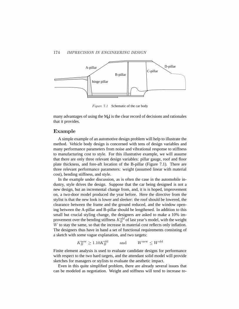
174 IMPRECISION IN ENGINEERING DESIGN
A-pillar D-pillar
B-pillar
hinge pillar
C-pillar
Figure 7.1 Schematic of the car body
many advantages of using the MoI is the clear record of decisions and rationalesthat it provides.
ExampleA simple example of an automotive design problem will help to illustrate the
method. Vehicle body design is concerned with tens of design variables andmany performance parameters from noise and vibrational response to stiffnessto manufacturing cost to style. For this illustrative example, we will assumethat there are only three relevant design variables: pillar gauge, roof and floorplate thickness, and fore-aft location of the B-pillar (Figure 7.1). There arethree relevant performance parameters: weight (assumed linear with materialcost), bending stiffness, and style.
In the example under discussion, as is often the case in the automobile in-dustry, style drives the design. Suppose that the car being designed is not anew design, but an incremental change from, and, it is is hoped, improvementon, a two-door model produced the year before. Here the directive from thestylist is that the new look is lower and sleeker: the roof should be lowered, theclearance between the frame and the ground reduced, and the window open-ing between the A-pillar and B-pillar should be lengthened. In addition to thissmall but crucial styling change, the designers are asked to make a 10% im-provement over the bending stiffnessKold
B of last year’s model, with the weightW to stay the same, so that the increase in material cost reflects only inflation.The designers thus have in hand a set of functional requirements consisting ofa sketch with some vague explanation, and two targets:
KnewB ≥ 1.10Kold
B and W new ≤ W old
Finite element analysis is used to evaluate candidate designs for performancewith respect to the two hard targets, and the attendant solid model will providesketches for managers or stylists to evaluate the aesthetic impact.
Even in this quite simplified problem, there are already several issues thatcan be modeled as negotiation. Weight and stiffness will tend to increase to-
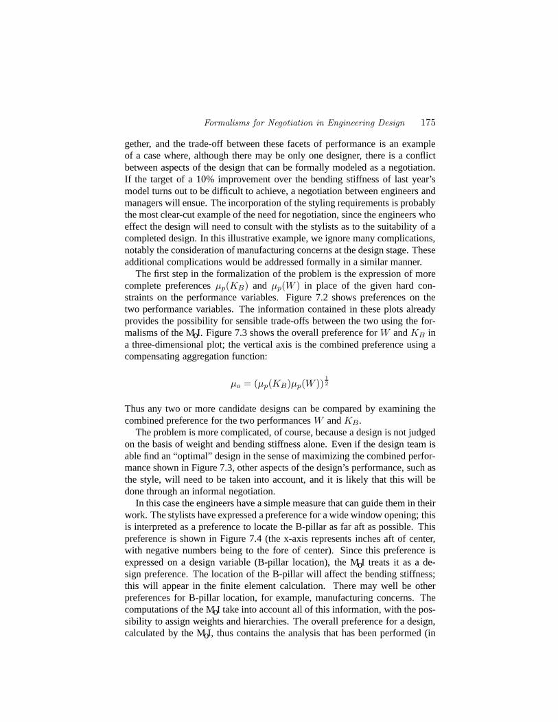
Formalisms for Negotiation in Engineering Design 175
gether, and the trade-off between these facets of performance is an exampleof a case where, although there may be only one designer, there is a conflictbetween aspects of the design that can be formally modeled as a negotiation.If the target of a 10% improvement over the bending stiffness of last year’smodel turns out to be difficult to achieve, a negotiation between engineers andmanagers will ensue. The incorporation of the styling requirements is probablythe most clear-cut example of the need for negotiation, since the engineers whoeffect the design will need to consult with the stylists as to the suitability of acompleted design. In this illustrative example, we ignore many complications,notably the consideration of manufacturing concerns at the design stage. Theseadditional complications would be addressed formally in a similar manner.
The first step in the formalization of the problem is the expression of morecomplete preferencesµp(KB) and µp(W ) in place of the given hard con-straints on the performance variables. Figure 7.2 shows preferences on thetwo performance variables. The information contained in these plots alreadyprovides the possibility for sensible trade-offs between the two using the for-malisms of the MoI. Figure 7.3 shows the overall preference forW andKB ina three-dimensional plot; the vertical axis is the combined preference using acompensating aggregation function:
µo = (µp(KB)µp(W ))12
Thus any two or more candidate designs can be compared by examining thecombined preference for the two performancesW andKB .
The problem is more complicated, of course, because a design is not judgedon the basis of weight and bending stiffness alone. Even if the design team isable find an “optimal” design in the sense of maximizing the combined perfor-mance shown in Figure 7.3, other aspects of the design’s performance, such asthe style, will need to be taken into account, and it is likely that this will bedone through an informal negotiation.
In this case the engineers have a simple measure that can guide them in theirwork. The stylists have expressed a preference for a wide window opening; thisis interpreted as a preference to locate the B-pillar as far aft as possible. Thispreference is shown in Figure 7.4 (the x-axis represents inches aft of center,with negative numbers being to the fore of center). Since this preference isexpressed on a design variable (B-pillar location), the MoI treats it as a de-sign preference. The location of the B-pillar will affect the bending stiffness;this will appear in the finite element calculation. There may well be otherpreferences for B-pillar location, for example, manufacturing concerns. Thecomputations of the MoI take into account all of this information, with the pos-sibility to assign weights and hierarchies. The overall preference for a design,calculated by the MoI, thus contains the analysis that has been performed (in
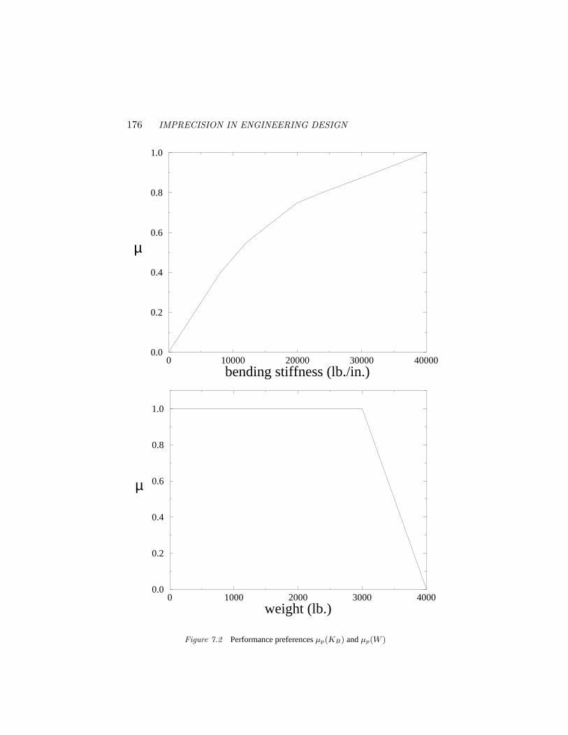
176 IMPRECISION IN ENGINEERING DESIGN
0 10000 20000 30000 40000bending stiffness (lb./in.)
0.0
0.2
0.4
0.6
0.8
1.0
µ
0 1000 2000 3000 4000weight (lb.)
0.0
0.2
0.4
0.6
0.8
1.0
µ
Figure 7.2 Performance preferencesµp(KB) andµp(W )
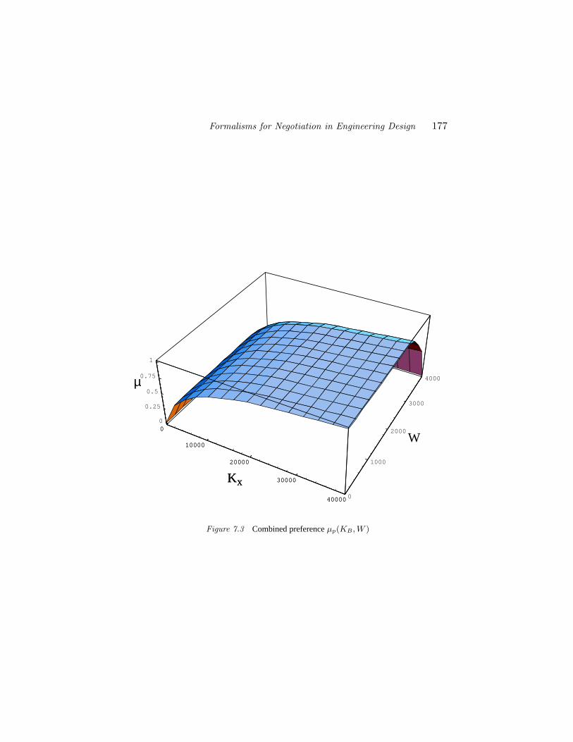
Formalisms for Negotiation in Engineering Design 177
0
10000
20000
30000
40000
Kx0
1000
2000
3000
4000
W
0
0.25
0.5
0.75
1
µ
0
10000
20000
30000
40000
Kx
Figure 7.3 Combined preferenceµp(KB, W )
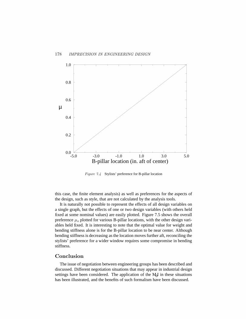
178 IMPRECISION IN ENGINEERING DESIGN
-5.0 -3.0 -1.0 1.0 3.0 5.0B-pillar location (in. aft of center)
0.0
0.2
0.4
0.6
0.8
1.0
µ
Figure 7.4 Stylists’ preference for B-pillar location
this case, the finite element analysis) as well as preferences for the aspects ofthe design, such as style, that are not calculated by the analysis tools.
It is naturally not possible to represent the effects of all design variables ona single graph, but the effects of one or two design variables (with others heldfixed at some nominal values) are easily plotted. Figure 7.5 shows the overallpreferenceµo plotted for various B-pillar locations, with the other design vari-ables held fixed. It is interesting to note that the optimal value for weight andbending stiffness alone is for the B-pillar location to be near center. Althoughbending stiffness is decreasing as the location moves further aft, reconciling thestylists’ preference for a wider window requires some compromise in bendingstiffness.
ConclusionThe issue of negotiation between engineering groups has been described and
discussed. Different negotiation situations that may appear in industrial designsettings have been considered. The application of the MoI in these situationshas been illustrated, and the benefits of such formalism have been discussed.
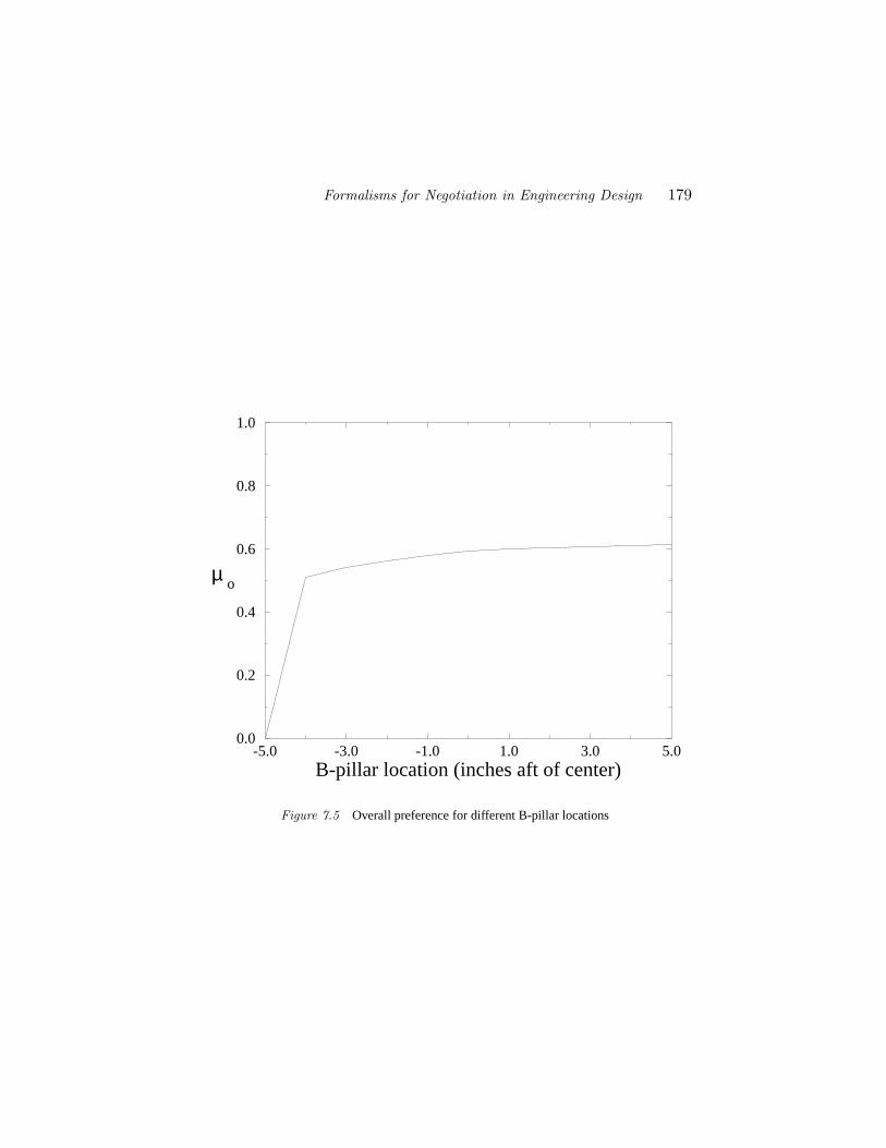
Formalisms for Negotiation in Engineering Design 179
-5.0 -3.0 -1.0 1.0 3.0 5.0B-pillar location (inches aft of center)
0.0
0.2
0.4
0.6
0.8
1.0
µ o
Figure 7.5 Overall preference for different B-pillar locations

180 IMPRECISION IN ENGINEERING DESIGN
The MoI has been developed previously for engineering design applications.This paper has suggested the extension of the method to encompass the do-mains of management and marketing, thus pointing out the possibilities forusing the formalism of uncertainty in the entire design process.
AcknowledgmentThis material is based upon work supported, in part, by the National Science Foundation
under NSF Grant Numbers DDM-9201424 and DMI-9523232. Any opinions, findings, con-
clusions, or recommendations expressed in this publication are those of the authors and do not
necessarily reflect the views of the sponsor.
Formalisms for Negotiation in Engineering Design 181
References
[1] A NTONSSON, E. K., AND OTTO, K. N. Imprecision in Engineering De-sign. ASME Journal of Mechanical Design 117(B) (Special CombinedIssue of the Transactions of the ASME commemorating the 50th anniver-sary of the Design Engineering Division of the ASME.)(June 1995), 25–32. Invited paper.
[2] BAHLER, D., DUPONT, C., AND BOWEN, J. Mixed quantita-tive/qualitative method for evaluating compromise solutions to conflictsin collaborative design.Artificial Intelligence for Engineering Design,Analysis and Manufacturing 9, 4 (September 1995), 325–336.
[3] BRAZIER, F. M. T., VAN LANGEN, P. H. G.,AND TREUR, J. Mod-elling conflict management in design: An explicit approach.ArtificialIntelligence for Engineering Design, Analysis and Manufacturing 9, 4(September 1995), 353–366.
[4] CLARK , K. B., AND FUJIMOTO, T. Product Development Performance:Strategy, Organization and Management in the World Auto Industry. Har-vard Business School Press, Boston, MA, 1991.
[5] FINGER, S., AND DIXON, J. R. A review of research in mechanicalengineering design. part ii: Representations, analysis and design for thelife cycle. Research in Engineering Design 1, 2 (1989), 121–137.
[6] HAROUD, D., BOULANGER, S., GELLE, E., AND SMITH , I. Manage-ment of conflicts for preliminary engineering design tasks.ArtificialIntelligence for Engineering Design, Analysis and Manufacturing 9, 4(September 1995), 313–323.
[7] K LIR, G. J.,AND FOLGER, T. A. Fuzzy Sets, Uncertainty, and Informa-tion. Prentice Hall, Englewood Cliffs, New Jersey, 1988.
[8] L AW, W. S., AND ANTONSSON, E. K. Implementing the Method ofImprecision: An Engineering Design Example. InProceedings of theThird IEEE International Conference on Fuzzy Systems (FUZZ-IEEE’94) (June 1994), vol. 1, IEEE, pp. 358–363. Invited paper.
[9] OH, V., AND SHARPE, J. Conflict management in an interdisciplinarydesign environment.Artificial Intelligence for Engineering Design, Anal-ysis and Manufacturing 9, 4 (September 1995), 247–258.
[10] OTTO, K. N. A Formal Representational Theory for Engineering Design.PhD thesis, California Institute of Technology, Pasadena, CA, June 1992.
[11] OTTO, K. N., AND ANTONSSON, E. K. Trade-Off Strategies in Engi-neering Design.Research in Engineering Design 3, 2 (1991), 87–104.
[12] OTTO, K. N., AND ANTONSSON, E. K. Modeling Imprecision in Prod-uct Design. InProceedings of the Third IEEE International Conference
182 IMPRECISION IN ENGINEERING DESIGN
on Fuzzy Systems (FUZZ-IEEE ’94)(June 1994), vol. 1, IEEE, pp. 346–351. Invited paper.
[13] PETRIE, C. J., WEBSTER, T. A., AND CUTKOSKY, M. R. Using paretooptimality to coordinate distributed agents.Artificial Intelligence for En-gineering Design, Analysis and Manufacturing 9, 4 (September 1995),313–323.
[14] RODDIS, W. M. K. Structural failures and engineering ethics.ASCEJournal of Structural Engineering 119, 5 (May 1993), 1539–1555.
[15] SCOTT, M. J., AND ANTONSSON, E. K. Aggregation Functions for En-gineering Design Trade-offs. In9th International Conference on DesignTheory and Methodology(Sept. 1995), vol. 2, ASME, pp. 389–396.
[16] WARD, A. C., LIKER, J. K., SOBEK, D. K., AND CRISTIANO, J. J. Set-based concurrent engineering and Toyota. InDesign Theory and Method-ology – DTM ’94(Sept. 1994), vol. DE68, ASME, pp. 79–90.
[17] WHITNEY, D. E. Manufacturing by design.Harvard Business Review66, 4 (July 1988), 83–91.
[18] WOOD, K. L., AND ANTONSSON, E. K. Computations with Impre-cise Parameters in Engineering Design: Background and Theory.ASMEJournal of Mechanisms, Transmissions, and Automation in Design 111,4 (Dec. 1989), 616–625.
[19] ZADEH, L. A. Fuzzy sets.Information and Control 8(1965), 338–353.
[20] ZADEH, L. A. The concept of a linguistic variable and its application toapproximate reasoning – I.Information Sciences 8(1975), 199–249.
Chapter 8
PRELIMINARY VEHICLE STRUCTUREDESIGN APPLICATION
Michael J. Scott and Erik K. Antonsson
Proceedings of the10th International Conference on Design Theory and MethodologyASME, Paper Number DETC98/DTM-5646, (September, 1998)
Abstract The Method of Imprecision, or MoI, is a formal method for incorporating im-precise information into a design process. This methodology has been exercisedon a problem in preliminary vehicle structure design in collaboration with VWWolfsburg. Results show that the method is useful in trading off multiple con-flicting attributes, including styling preferences and engineering requirements.
Keywords:Industrial Applications of DTM; Vehicle Structure Design; Design Meth-
ods and Models; Design Representations; Computational Methods of Design;Fuzzy Sets
IntroductionPreliminary design is inherently imprecise [3, 4, 12, 40], and many prelim-
inary design decisions are made informally. Preliminary design has enormouseconomic importance, as much of the cost of a design is determined by these(often informal) preliminary decisions [37]. A further complication is the dif-ficulty of communicating imprecise information between different members orgroups involved in the design process. Many “interface” decisions are madeafter design analysis is complete; thesepost hocdecisions can result in costlyredesigns.
The Method of Imprecision, or MoI [39, 1] has been developed to formallyincorporate imprecise information into the engineering design process. In thesummer of 1997, an application of the MoI to preliminary vehicle structure
183
184 IMPRECISION IN ENGINEERING DESIGN
design was demonstrated for Volkswagen Wolfsburg. The application servesboth to demonstrate the capabilities of the method, and as an introduction tosome of the underlying concepts.
A brief introduction to the Method of Imprecision is followed by a descrip-tion of the demonstration project. The application of the MoI to the problem isthen described in detail, and the implications of the results are discussed.
The Method of ImprecisionThis introduction is necessarily brief; the application serves as a further
tutorial to explicate the ideas reviewed here.The original work on the MoI [38, 39] formulated the design problem as
a decision problem: given a set of candidate designs, identified by vectors~dof design variablesin a Design Variable Space (DVS), a set of performances,described by vectors~p of performance variablesin a Performance VariableSpace (PVS), and a mappingf : ~d 7→ ~p, choose the candidate design~d∗ whichmaps to the “best” possible performance~p∗ = f(~d∗). So stated, there is in-sufficient information to determine what constitutes a “best” performance, andhence a “best” design. On the one hand, requirements are imprecise, whileon the other hand, there is no obvious way to compare different performancevariables which are usually not expressed in the same units.
The need to include imprecision in engineering design can be illustrated by asimple example. Figure 8.1 shows a specification for one performance variable(pj), with theperformance preferenceµp on the vertical axis. As specificationsare commonly written,pj ≥ 500 km would be represented by the dashed line(the sharp-edged rectangular step), whereµp = 1 in the acceptable region,and µp = 0 for unacceptable values. However, this crisp specification (orrequirement) indicates that two different designs, one withdj = 500 − ε, andanother withdj = 500 + ε, would have completely different acceptabilities,no matter how smallε becomes. Thus two designs, indistinguishably differentin dj (as ε → 0), have completely different preferences: one is completelyacceptable and one is unacceptable. This situation makes no sense.
Alternatively, the solid line shown in Figure 8.1 indicates a smooth transi-tion of acceptability of performances from unacceptable (µp = 0) to accept-able (µp = 1), and thus reflects a more realistic specification. The range overwhich the transition from unacceptable performance to most desired perfor-mance takes place will depend on the particular design problem, and may bemore or less steep, and smooth or faceted.
Thus the MoI introduces the notion ofpreferences, denoted byµ ∈ [0, 1],both to represent the imprecision inherent in the preliminary design problem,and to provide a basis for comparison between different attributes. Perfor-mance preferencesµp on thePVSexpress the requirements more completely
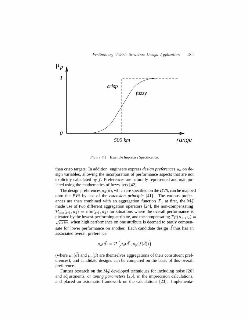
Preliminary Vehicle Structure Design Application 185
0
1
µp
500 km
fuzzycrisp
range
Figure 8.1 Example Imprecise Specification.
than crisp targets. In addition, engineers expressdesign preferencesµd on de-sign variables, allowing the incorporation of performance aspects that are notexplicitly calculated byf . Preferences are naturally represented and manipu-lated using the mathematics of fuzzy sets [42].
The design preferencesµd(~d), which are specified on theDVS, can be mappedonto thePVS by use of theextension principle[41]. The various prefer-ences are then combined with an aggregation functionP; at first, the MoImade use of two different aggregation operators [24], the non-compensatingPmin(µ1, µ2) = min(µ1, µ2) for situations where the overall performance isdictated by the lowest-performing attribute, and the compensatingPΠ(µ1, µ2) =√
µ1µ2, when high performance on one attribute is deemed to partly compen-
sate for lower performance on another. Each candidate design~d thus has anassociated overall preference:
µo(~d) = P(µd(~d), µp(f(~d))
)
(whereµd(~d) andµp(~p) are themselves aggregations of their constituent pref-erences), and candidate designs can be compared on the basis of this overallpreference.
Further research on the MoI developed techniques for including noise [26]and adjustments, ortuning parameters[25], in the imprecision calculations,and placed an axiomatic framework on the calculations [23]. Implementa-
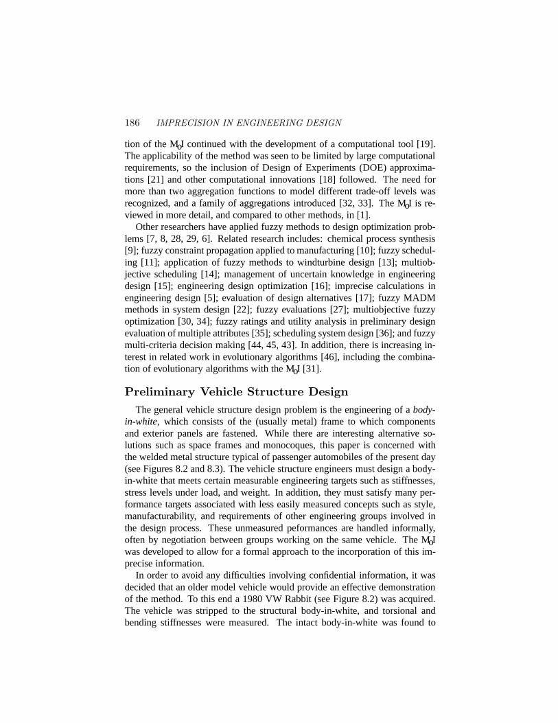
186 IMPRECISION IN ENGINEERING DESIGN
tion of the MoI continued with the development of a computational tool [19].The applicability of the method was seen to be limited by large computationalrequirements, so the inclusion of Design of Experiments (DOE) approxima-tions [21] and other computational innovations [18] followed. The need formore than two aggregation functions to model different trade-off levels wasrecognized, and a family of aggregations introduced [32, 33]. The MoI is re-viewed in more detail, and compared to other methods, in [1].
Other researchers have applied fuzzy methods to design optimization prob-lems [7, 8, 28, 29, 6]. Related research includes: chemical process synthesis[9]; fuzzy constraint propagation applied to manufacturing [10]; fuzzy schedul-ing [11]; application of fuzzy methods to windturbine design [13]; multiob-jective scheduling [14]; management of uncertain knowledge in engineeringdesign [15]; engineering design optimization [16]; imprecise calculations inengineering design [5]; evaluation of design alternatives [17]; fuzzy MADMmethods in system design [22]; fuzzy evaluations [27]; multiobjective fuzzyoptimization [30, 34]; fuzzy ratings and utility analysis in preliminary designevaluation of multiple attributes [35]; scheduling system design [36]; and fuzzymulti-criteria decision making [44, 45, 43]. In addition, there is increasing in-terest in related work in evolutionary algorithms [46], including the combina-tion of evolutionary algorithms with the MoI [31].
Preliminary Vehicle Structure DesignThe general vehicle structure design problem is the engineering of abody-
in-white, which consists of the (usually metal) frame to which componentsand exterior panels are fastened. While there are interesting alternative so-lutions such as space frames and monocoques, this paper is concerned withthe welded metal structure typical of passenger automobiles of the present day(see Figures 8.2 and 8.3). The vehicle structure engineers must design a body-in-white that meets certain measurable engineering targets such as stiffnesses,stress levels under load, and weight. In addition, they must satisfy many per-formance targets associated with less easily measured concepts such as style,manufacturability, and requirements of other engineering groups involved inthe design process. These unmeasured peformances are handled informally,often by negotiation between groups working on the same vehicle. The MoIwas developed to allow for a formal approach to the incorporation of this im-precise information.
In order to avoid any difficulties involving confidential information, it wasdecided that an older model vehicle would provide an effective demonstrationof the method. To this end a 1980 VW Rabbit (see Figure 8.2) was acquired.The vehicle was stripped to the structural body-in-white, and torsional andbending stiffnesses were measured. The intact body-in-white was found to

Preliminary Vehicle Structure Design Application 187
Figure 8.2 1980 VW Rabbit in Stiffness Testing
have a torsional stiffness of approximately 4900 N-m/degree and a bendingstiffness of approximately 2500 N/mm. Tables of data from some of the loadtests are shown in the Appendix. In addition, geometric data were gathered andused to create a solid model (Figure 8.3). The solid model and the structuralstiffness information together were used to create and calibrate a finite elementmodel (Figure 8.4).
The finite element model was parameterized with five1 design variables:
1. A-pillar thickness (mm)
2. B-pillar thickness (mm)
3. floor pan thickness (mm)
4. floor rail thickness (mm)
5. B-pillar location (mm aft of a nominal point chosen by stylists)
and the performance was assessed with three measures:
1The demonstration here was conducted using a subset of the design variables; the method can be applieddirectly to a larger set of variables.
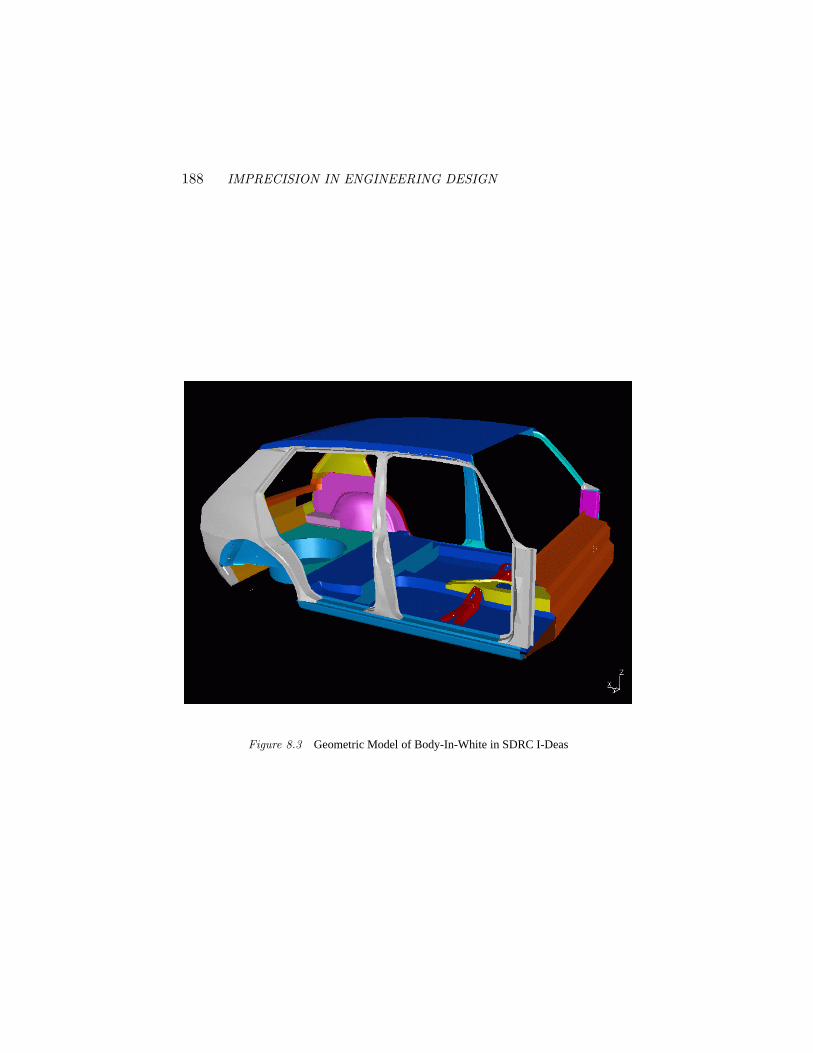
188 IMPRECISION IN ENGINEERING DESIGN
Figure 8.3 Geometric Model of Body-In-White in SDRC I-Deas
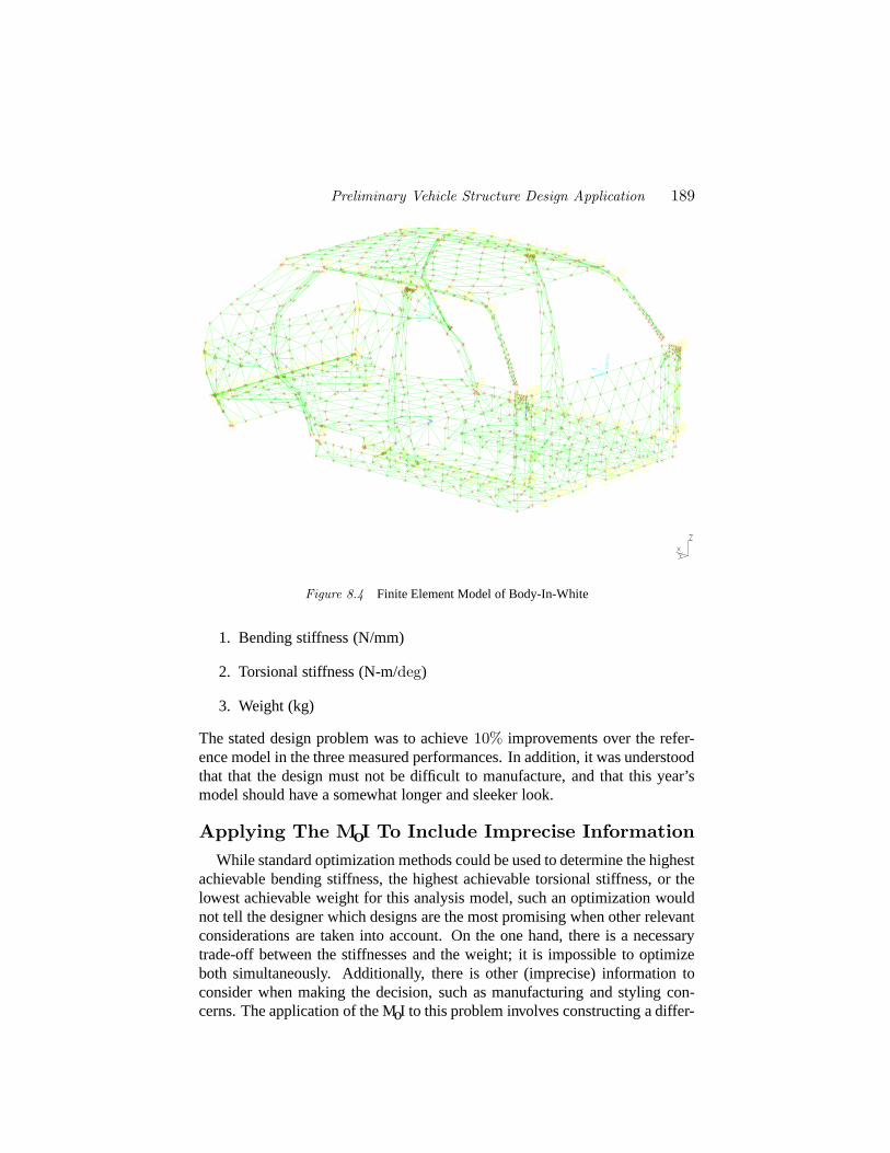
Preliminary Vehicle Structure Design Application 189
Figure 8.4 Finite Element Model of Body-In-White
1. Bending stiffness (N/mm)
2. Torsional stiffness (N-m/deg)
3. Weight (kg)
The stated design problem was to achieve10% improvements over the refer-ence model in the three measured performances. In addition, it was understoodthat that the design must not be difficult to manufacture, and that this year’smodel should have a somewhat longer and sleeker look.
Applying The MoI To Include Imprecise InformationWhile standard optimization methods could be used to determine the highest
achievable bending stiffness, the highest achievable torsional stiffness, or thelowest achievable weight for this analysis model, such an optimization wouldnot tell the designer which designs are the most promising when other relevantconsiderations are taken into account. On the one hand, there is a necessarytrade-off between the stiffnesses and the weight; it is impossible to optimizeboth simultaneously. Additionally, there is other (imprecise) information toconsider when making the decision, such as manufacturing and styling con-cerns. The application of the MoI to this problem involves constructing a differ-
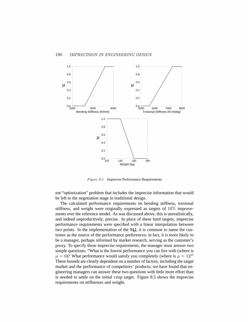
190 IMPRECISION IN ENGINEERING DESIGN
2000 3000 4000Bending Stiffness (N/mm)
0.0
0.2
0.4
0.6
0.8
1.0
µ
5000 6000 7000 8000Torsional Stiffness (N-m/deg)
0.0
0.2
0.4
0.6
0.8
1.0
µ
120 140 160 180Weight (kg)
0.0
0.2
0.4
0.6
0.8
1.0
µ
Figure 8.5 Imprecise Performance Requirements
ent “optimization” problem that includes the imprecise information that wouldbe left to the negotiation stage in traditional design.
The calculated performance requirements on bending stiffness, torsionalstiffness, and weight were originally expressed as targets of10% improve-ments over the reference model. As was discussed above, this is unrealistically,and indeed unproductively, precise. In place of these hard targets, impreciseperformance requirements were specified with a linear interpolation betweentwo points. In the implementation of the MoI, it is common to name the cus-tomer as the source of the performance preferences; in fact, it is more likely tobe a manager, perhaps informed by market research, serving as the customer’sproxy. To specify these imprecise requirements, the manager must answer twosimple questions: “What is the lowest performance you can live with (where isµ = 0)? What performance would satisfy you completely (where isµ = 1)?”These bounds are clearly dependent on a number of factors, including the targetmarket and the performance of competitors’ products; we have found that en-gineering managers can answer these two questions with little more effort thanis needed to settle on the initial crisp target. Figure 8.5 shows the impreciserequirements on stiffnesses and weight.

Preliminary Vehicle Structure Design Application 191
To include requirements on manufacturing, availability, style, and otherthings which are not calculated in the finite element analysis, designer prefer-ences are specified on the design variables. As with the imprecise performancerequirements, they range fromµ = 0 at the unacceptable limit toµ = 1 atthe most preferred. A preference is defined on each of the five design vari-ables, as shown in Figure 8.6. Each preference is representative of impreciseinformation that can be incorporated using the MoI:
1. The sheet steel for stamping the A-pillar is only available in certain in-crements, so this plot is discrete rather than continuous. The manufac-turing engineer has a higher preference for thinner sheets, since they areeasier to form; this is a design preference for manufacturability.
2. The B-pillar thickness is continuous and more complicated than the lin-ear performance preferences. This preference doesnot indicate that thephysical B-pillar might be 1.113 or 1.114 mm thick; rather it means thatthe designer knows that the finite element model is simplified, and that ahigh number for B-pillar thickness means that more reinforcing featureswill need to be added to the B-pillar. The designer would like to keepthe B-pillar as simple as possible.
3. The floor pan thickness is preferred thicker by the designer for ease ofattachments and for durability.
4. The floor rail thickness preference is an example of a sourcing, or avail-ability preference; it states that some thicknesses are more easily ob-tained than others.
5. The design preference for B-pillar location comes from the stylists, andcaptures the directive for a longer, sleeker look for this year’s model. Ithas been specified differently from the other design preferences, usingα-cuts [1], so that the stylists have given a range of perfectly accept-able values, a range of barely acceptable values, and a range of valuesthat fall in the middle. This method of specifying preferences can havecomputational advantages.
In addition to these preferences, each attribute is assigned a weight indicat-ing its relative importance, and the way in which attributes trade-off againsteach other must also be specified. In this test example, it was determined thatbending and torsional stiffness traded-off in a non-compensating manner —the lowest preference is maximized. Together they traded-off with weight in acompensating manner, so that high performance on stiffness could partly makeup for low performance on weight, and vice versa. The designer preferencesall traded-off in a compensating manner as well, with the styling preference

192 IMPRECISION IN ENGINEERING DESIGN
0.6 0.7 0.8 0.9 1.0 1.1A-pillar thickness (mm)
0.0
0.2
0.4
0.6
0.8
1.0
µ
0.8 1.0 1.2 1.4 1.6B-pillar thickness (mm)
0.0
0.2
0.4
0.6
0.8
1.0
µ
0.9 1.0 1.1 1.2 1.3 1.4Floor thickness (mm)
0.0
0.2
0.4
0.6
0.8
1.0
µ
0.7 0.8 0.9 1.0 1.1 1.2 1.3Floor rail thickness (mm)
0.0
0.2
0.4
0.6
0.8
1.0
µ
-50 0 50 100 150 200B-pillar location (mm aft of nominal)
0.0
0.2
0.4
0.6
0.8
1.0
µ
Figure 8.6 Designer Preferences
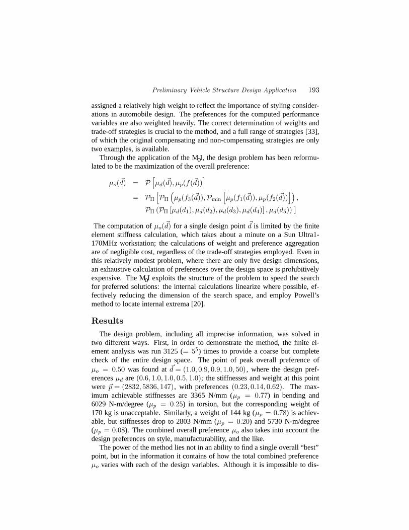
Preliminary Vehicle Structure Design Application 193
assigned a relatively high weight to reflect the importance of styling consider-ations in automobile design. The preferences for the computed performancevariables are also weighted heavily. The correct determination of weights andtrade-off strategies is crucial to the method, and a full range of strategies [33],of which the original compensating and non-compensating strategies are onlytwo examples, is available.
Through the application of the MoI, the design problem has been reformu-lated to be the maximization of the overall preference:
µo(~d) = P[µd(~d), µp(f(~d))
]= PΠ
[PΠ
(µp(f3(~d)),Pmin
[µp(f1(~d)), µp(f2(~d))
]),
PΠ (PΠ [µd(d1), µd(d2), µd(d3), µd(d4)] , µd(d5)) ]
The computation ofµo(~d) for a single design point~d is limited by the finiteelement stiffness calculation, which takes about a minute on a Sun Ultra1-170MHz workstation; the calculations of weight and preference aggregationare of negligible cost, regardless of the trade-off strategies employed. Even inthis relatively modest problem, where there are only five design dimensions,an exhaustive calculation of preferences over the design space is prohibitivelyexpensive. The MoI exploits the structure of the problem to speed the searchfor preferred solutions: the internal calculations linearize where possible, ef-fectively reducing the dimension of the search space, and employ Powell’smethod to locate internal extrema [20].
ResultsThe design problem, including all imprecise information, was solved in
two different ways. First, in order to demonstrate the method, the finite el-ement analysis was run 3125 (= 55) times to provide a coarse but completecheck of the entire design space. The point of peak overall preference ofµo = 0.50 was found at~d = (1.0, 0.9, 0.9, 1.0, 50), where the design pref-erencesµd are(0.6, 1.0, 1.0, 0.5, 1.0); the stiffnesses and weight at this pointwere ~p = (2832, 5836, 147), with preferences(0.23, 0.14, 0.62). The max-imum achievable stiffnesses are 3365 N/mm (µp = 0.77) in bending and6029 N-m/degree (µp = 0.25) in torsion, but the corresponding weight of170 kg is unacceptable. Similarly, a weight of 144 kg (µp = 0.78) is achiev-able, but stiffnesses drop to 2803 N/mm (µp = 0.20) and 5730 N-m/degree(µp = 0.08). The combined overall preferenceµo also takes into account thedesign preferences on style, manufacturability, and the like.
The power of the method lies not in an ability to find a single overall “best”point, but in the information it contains of how the total combined preferenceµo varies with each of the design variables. Although it is impossible to dis-
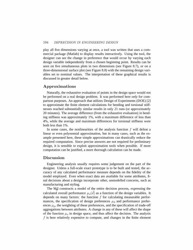
194 IMPRECISION IN ENGINEERING DESIGN
play all five dimensions varying at once, a tool was written that uses a com-mercial package (Matlab) to display results interactively. Using the tool, thedesigner can see the change in preference that would occur by varying eachdesign variable independently from a chosen beginning point. Results can beseen on five simultaneous plots in two dimensions (see Figure 8.7), or on athree-dimensional surface plot (see Figure 8.8) with the remaining design vari-ables set to nominal values. The interpretation of these graphical results isdiscussed in greater detail below.
ApproximationsNaturally, the exhaustive evaluation of points in the design space would not
be performed on a real design problem. It was performed hereonly for com-parison purposes. An approach that utilizes Design of Experiments (DOE) [2]to approximate the finite element calculations for bending and torsional stiff-nesses reached substantially similar results in only 21 runs (or approximately20 minutes). The average difference (from the exhaustive evaluation) in bend-ing stiffness was approximately 1%, with a maximum difference of less than4%, while the average and maximum differences for torsional stiffness wereboth less than 1%.
In some cases, the nonlinearities of the analysis functionf will defeat alinear or even polynomial approximation, but in many cases, such as the ex-ample presented here, these simple approximations can drastically reduce therequired computation. Since precise answers are not required for preliminarydesign, it is sensible to exploit approximation tools when possible. If morecomputation can be justified, a more thorough calculation can be made.
DiscussionEngineering analysis usually requires some judgement on the part of the
designer. Unless a full-scale exact prototype is to be built and tested, the ac-curacy of any calculated performance measure depends on the fidelity of themodel employed. Even when exact data are available for some attributes, fi-nal decisions about a design incorporate other, unmodelled concerns, such asmanufacturing and styling.
The MoI constructs a model of the entire decision process, expressing thecalculated overall performanceµo(~d) as a function of the design variables. Itdepends on many factors: the functionf for calculating measurable perfor-mances, the specification of design preferencesµd and performance prefer-encesµp, the weighting of these preferences, and the specification of trade-offaggregations between attributes. A change in any of these will affect the shapeof the functionµo in design space, and thus affect the decision. The analysisf is here relatively expensive to compute, and changes in the finite element
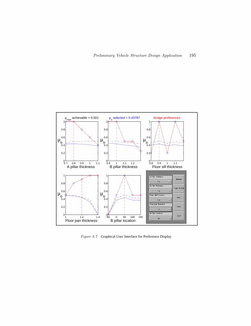
Preliminary Vehicle Structure Design Application 195
0.7 0.8 0.9 1 1.10
0.2
0.4
0.6
0.8
1
A pillar thickness
µo
µmax
achievable = 0.501
0.9 1 1.1 1.20
0.2
0.4
0.6
0.8
1
B pillar thickness
µo
µo selected = 0.43787
0.8 0.9 1 1.10
0.2
0.4
0.6
0.8
1
Floor sill thickness
µo
design preferences
1 1.2 1.40
0.2
0.4
0.6
0.8
1
Floor pan thickness
µo
−50 0 50 100 1500
0.2
0.4
0.6
0.8
1
B pillar location
µo
Figure 8.7 Graphical User Interface for Preference Display
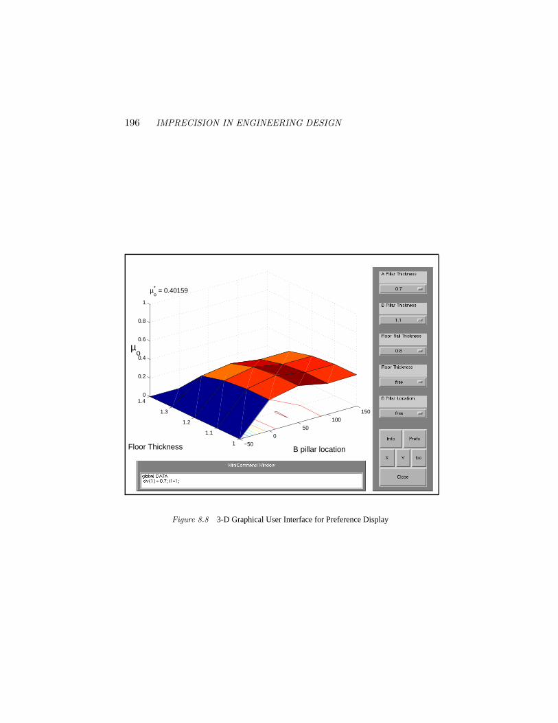
196 IMPRECISION IN ENGINEERING DESIGN
−50
0
50
100
150
1
1.1
1.2
1.3
1.40
0.2
0.4
0.6
0.8
1
B pillar location Floor Thickness
µo* = 0.40159
µo
Figure 8.8 3-D Graphical User Interface for Preference Display
Preliminary Vehicle Structure Design Application 197
model are costly to propagate to overall preference. Changes in the other fac-tors, on the other hand, are easily incorporated, as finite element resultsf(~d)are stored so that the same design point need never be analyzed more than once.This allows the MoI to support an iterative decision process, when the informa-tion from the first round of calculations inspires a change in the preferencestructure.
In the example shown in this paper, the shape of the functionµo(~d) is sensi-tive to changes in the styling preferenceµd(d5), which is not surprising, sincethis preference is accorded a large weight. This and other features of the de-sign problem can be seen in the advanced interface shown in Figure 8.7. Thevertical dashed (red) lines indicate the selected values of the design variables.In this figure, ~d = (0.8, 1, 0.9, 1.2, 50), a point which is representative, notoptimal. The solid (blue) lines indicate how the overall preferenceµo wouldchange by varying that design variable while holding the other four fixed attheir current values. For instance, decreasing the floor pan thicknessd4 willresult in a more preferred design. The dashed (black) lines show the maximumachievableµo for each value of each design variable. Finally, the solid (red)lines joining the circles are the specified preferences on design variables.
In this example, the desired improvements in performance were achievedby small changes to the sheet-metal thicknesses and B-pillar location. Visuallythe improved structure would appear quite similar to that shown in Figure 8.3.No change in vehicle structure configuration was required here.
Figure 8.7 shows that the overall preferenceµo varies qualitatively, thoughnot quantitatively, with four of the five design variables; the exception isd4,floor pan thickness. The variation of the overall preferenceµo with respect tod4 shows a conflict between the calculated stiffness and weight requirementsµp and the provisions for attachment and durability captured by the designerpreferenceµd(d4). This indicatesd4 as a likely candidate for change in apotential redesign. The resolution of the conflict would be achieved by a choiceof d4 that provides the best overall trade-off between the competing attributes.Designers can interact with the preference display to examine trends in thestructure of the overall preference.
ConclusionsIn preliminary vehicle structure design, as in preliminary engineering design
in general, many important decisions are made informally on the basis of im-precise information. Concerns of styling and manufacturability, for instance,can carry great weight in the design process although they are not modelled byany formal analysis. The MoI is a tool to formally incorporate such impreciseinformation into the design process, and thus to make decisions on a soundbasis. In a demonstration of the MoI prepared for VW Wolfsburg, concerns of

198 IMPRECISION IN ENGINEERING DESIGN
manufacturing, styling, parts availability, and design were incorporated withthe engineering analysis of the structural stiffness of a VW Rabbit. The resultsshow the usefulness of the method in trading off these conflicting attributes.
Any analysis involving more than two design variables must contend withtwo difficulties, the exploding need for computation, and the problems of dis-playing results in several dimensions. The MoI uses approximations, whenfeasible, to address the first difficulty, and an interactive graphical tool for pref-erence display was developed and applied here to address the second.
AcknowledgementsVolkswagen Wolfsburg, and particularly Mr. W. Lange, and Dr. O. Tegel
(presently Chief Engineer of the Institut f¨ur Maschinenkonstruktion at the Tech-nical University in Berlin), were indispensable in the development of this project.
The authors would like express their appreciation to Zee Khoo and JuanNuno for their many hours of work stripping and load-testing the Rabbit, andbuilding the solid model, and to Mike Gerfen, manager of Caltech’s CentralEngineering Shop, for his generous help in providing space and equipment.
This material is based upon work supported, in part, by the National ScienceFoundation under NSF Grant Number DMI-9523232. Any opinions, findings,conclusions, or recommendations expressed in this publication are those of theauthors and do not necessarily reflect the views of the sponsors.
Preliminary Vehicle Structure Design Application 199
References
[1] A NTONSSON, E. K., AND OTTO, K. N. Imprecision in Engineering De-sign. ASME Journal of Mechanical Design 117(B) (Special CombinedIssue of the Transactions of the ASME commemorating the 50th anniver-sary of the Design Engineering Division of the ASME.)(June 1995), 25–32. Invited paper.
[2] BARKER, T. Quality by Experimental Design. Marcel Dekker, Inc., NewYork, 1985.
[3] BECKER, J. M. A Structural Design Process Philosophy and Methodol-ogy. PhD thesis, University of California, Berkeley, 1973.
[4] BLOCKLEY, D. I. The Nature of Structural Design and Safety. EllisNorwood Limited, Chichester, 1980.
[5] CHEN, J. E., AND OTTO, K. N. A tool for imprecise calculations inengineering design. InProceedings of the Fourth IEEE InternationalConference on Fuzzy Systems (FUZZ-IEEE/IFES’95)(Mar. 1995), vol. 1,IEEE, pp. 389–394.
[6] DHINGRA, A. K. Multiple objective design optimization. InFuzzy Setsin Engineering Design and Configuration, H.-J. Sebastian and E. K. An-tonsson, Eds. Kluwer, 1996, pp. 53–88.
[7] DIAZ , A. R. Fuzzy set based models in design optimization. InAdvancesin Design Automation - 1988(New York, NY, Sept. 1988), S. S. Rao, Ed.,vol. DE-14, ASME, pp. 477–485.
[8] DIAZ , A. R. A strategy for optimal design of hierarchical systems us-ing fuzzy sets. InThe 1989 NSF Engineering Design Research Con-ference(College of Engineering, University of Massachusetts, Amherst,June 1989), J. R. Dixon, Ed., NSF, pp. 537–547.
[9] DJOUAD, S., FLOQUET, P., DOMENECH, S., AND PIBOULEAU, L.Fuzzy set methods in separation process synthesis. InFuzzy Informa-tion Engineering: A Guided Tour of Applications, D. Dubois, H. Prade,and R. R. Yager, Eds. John Wiley & Sons, 1996.
[10] DUBOIS, D. Tuning the cutting edge conditions on a machining transferline using fuzzy constraint propagation. InFuzzy Information Engineer-ing: A Guided Tour of Applications, D. Dubois, H. Prade, and R. R. Yager,Eds. John Wiley & Sons, 1996.
[11] FARGIER, H. Fuzzy scheduling: Principles and experiments. InFuzzyInformation Engineering: A Guided Tour of Applications, D. Dubois,H. Prade, and R. R. Yager, Eds. John Wiley & Sons, 1996.
[12] GAVIN , JR., J. G. Fly me to the Moon: An interview with Joseph G.Gavin, Jr.Technology Review 97, 5 (July 1994), 61–68.
200 IMPRECISION IN ENGINEERING DESIGN
[13] GERHART, V. Uncertainty within the design of a wind turbine. Workingpaper or, RWTH Aachen, Templergraben 64, 52062 Aachen, Germany,1997.
[14] GRABOT, B., GENESTE, L., AND DUPEUX, A. Tuning of fuzzy rules formultiobjective scheduling. InFuzzy Information Engineering: A GuidedTour of Applications, D. Dubois, H. Prade, and R. R. Yager, Eds. JohnWiley & Sons, 1996.
[15] HAMBURG, I., AND HAMBURG, P. Fuzzy logic, A user friendly technol-ogy for the management of uncertain knowledge in engineering designprocess. InModelling Uncertain Data(Berlin, Mar. 1993), H. Bande-mer, Ed., Akademie Verlag, pp. 153–157. Mathematical Research series,Volume 68, Lectures from the GAMM-Workshop: Modelling UncertainData, held in Freiberg from March 21-24, 1992.
[16] HSU, Y.-L., L IN, Y.-F., AND SUN, T.-L. Engineering design optimiza-tion as a fuzzy control process. InProceedings of the Fourth IEEE In-ternational Conference on Fuzzy Systems (FUZZ-IEEE/IFES’95)(Mar.1995), vol. 4, IEEE, pp. 2001–2008.
[17] KNOSALA, R., AND PEDRYCZ, W. Evaluation of design alternatives inmechanical engineering.Fuzzy Sets and Systems 47, 3 (1992), 269–280.
[18] LAW, W. S. Evaluating Imprecision in Engineering Design. PhD thesis,California Institute of Technology, Pasadena, CA, June 1996.
[19] LAW, W. S., AND ANTONSSON, E. K. Including Imprecision in En-gineering Design Calculations. InDesign Theory and Methodology –DTM ’94 (Sept. 1994), vol. DE-68, ASME, pp. 109–114.
[20] LAW, W. S.,AND ANTONSSON, E. K. Optimization Methods for Cal-culating Design Imprecision. InAdvances in Design Automation - 1995(Sept. 1995), vol. 1, ASME, pp. 471–476.
[21] LAW, W. S., AND ANTONSSON, E. K. Multi-dimensional Mapping ofDesign Imprecision. In8th International Conference on Design Theoryand Methodology(Aug. 1996), ASME.
[22] MULLER, K., AND THARIGEN, M. Applications of fuzzy hierarchiesand fuzzy MADM methods to innovative system design. InProceed-ings of the Third IEEE International Conference on Fuzzy Systems(June1994), vol. 1, IEEE, pp. 364–367.
[23] OTTO, K. N. A Formal Representational Theory for Engineering Design.PhD thesis, California Institute of Technology, Pasadena, CA, June 1992.
[24] OTTO, K. N., AND ANTONSSON, E. K. Trade-Off Strategies in Engi-neering Design.Research in Engineering Design 3, 2 (1991), 87–104.
Preliminary Vehicle Structure Design Application 201
[25] OTTO, K. N., AND ANTONSSON, E. K. Tuning Parameters in Engineer-ing Design. ASME Journal of Mechanical Design 115, 1 (Mar. 1993),14–19.
[26] OTTO, K. N., AND ANTONSSON, E. K. Design Parameter Selectionin the Presence of Noise.Research in Engineering Design 6, 4 (1994),234–246.
[27] POSTHOFF, C., AND SCHLOSSER, M. Learning from examples for theconstruction of fuzzy evaluations. InProceedings of the Third IEEEInternational Conference on Fuzzy Systems(June 1994), vol. 1, IEEE,pp. 368–371.
[28] RAO, S. S.,AND DHINGRA, A. K. Applications of fuzzy theories tomulti-objective system optimization. NASA Contractor Report 177573,NASA Ames Research Center, 1991.
[29] RAO, S. S., SUNDARARAJU, K., PRAKASH, B., AND BALAKRISHNA ,C. Multiobjective fuzzy optimization techniques for engineering design.Computers and Structures 42, 1 (1992), 37–44.
[30] SAKAWA , M., AND KATO, K. An interactive fuzzy satisficing methodsfor large-scale multiobjective linear programs with fuzzy numbers. InProceedings of the Fourth IEEE International Conference on Fuzzy Sys-tems (FUZZ-IEEE/IFES’95)(Mar. 1995), vol. 3, IEEE, pp. 1155–1162.
[31] SCHLEIFFER, R. Fuzzy engineering design. RWTH Aachen, 1998.Diplomarbeit.
[32] SCOTT, M. J., AND ANTONSSON, E. K. Aggregation Functions for En-gineering Design Trade-offs. In9th International Conference on DesignTheory and Methodology(Sept. 1995), vol. 2, ASME, pp. 389–396.
[33] SCOTT, M. J., AND ANTONSSON, E. K. Aggregation Functions forEngineering Design Trade-offs.Fuzzy Sets and Systems 99, 3 (1998),253–264.
[34] SHIH, C. J., AND WANGSAWIDJAJA, R. A. S. Multiobjective fuzzyoptimization with random variables in a mix of fuzzy and probabilisticenvironment. InProceedings of the Fourth IEEE International Confer-ence on Fuzzy Systems (FUZZ-IEEE/IFES’95)(Mar. 1995), vol. 3, IEEE,pp. 1163–1170.
[35] THURSTON, D. L., AND CARNAHAN , J. Fuzzy ratings and utility analy-sis in preliminary design evaluation of multiple attributes.ASME Journalof Mechanical Design 114, 4 (Dec. 1992), 648–658.
[36] TURKSEN, I. B. Scheduling system design: Three fuzzy theory ap-proaches. InFuzzy Information Engineering: A Guided Tour of Appli-cations, D. Dubois, H. Prade, and R. R. Yager, Eds. John Wiley & Sons,1996.
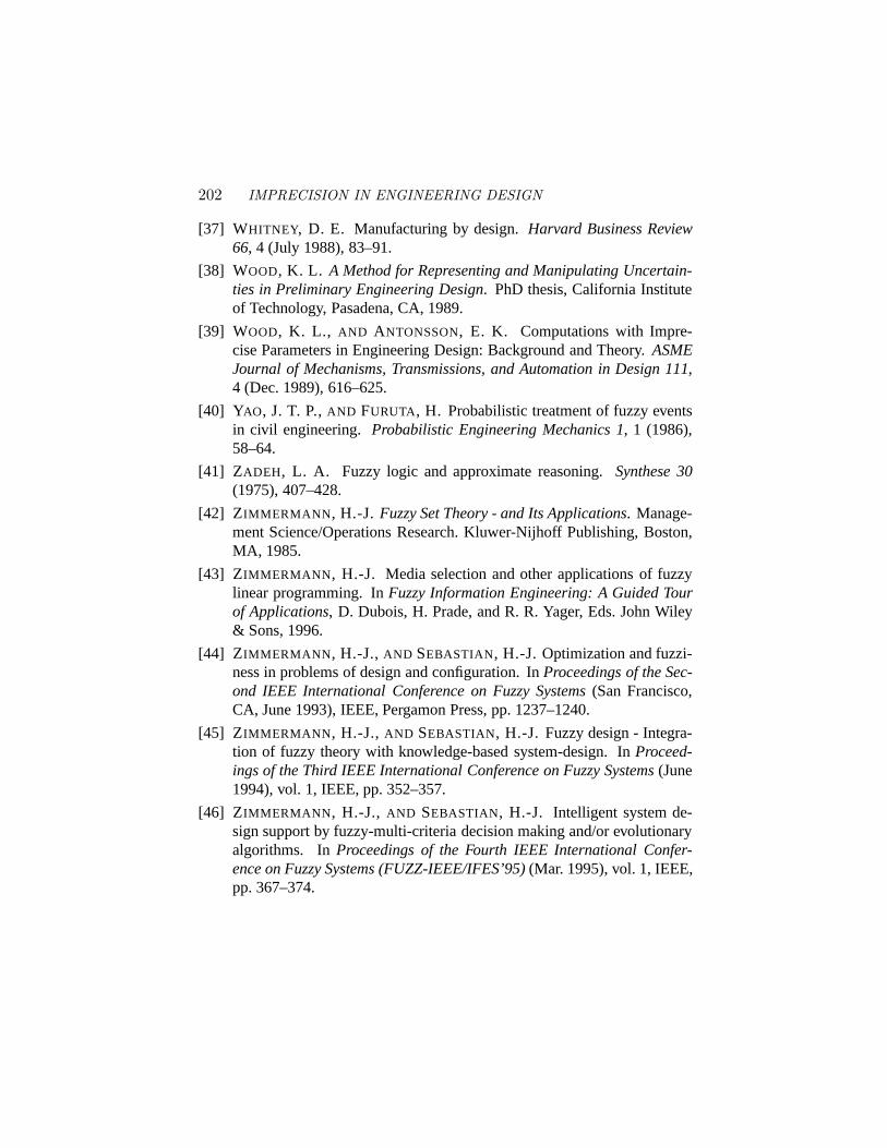
202 IMPRECISION IN ENGINEERING DESIGN
[37] WHITNEY, D. E. Manufacturing by design.Harvard Business Review66, 4 (July 1988), 83–91.
[38] WOOD, K. L. A Method for Representing and Manipulating Uncertain-ties in Preliminary Engineering Design. PhD thesis, California Instituteof Technology, Pasadena, CA, 1989.
[39] WOOD, K. L., AND ANTONSSON, E. K. Computations with Impre-cise Parameters in Engineering Design: Background and Theory.ASMEJournal of Mechanisms, Transmissions, and Automation in Design 111,4 (Dec. 1989), 616–625.
[40] YAO, J. T. P.,AND FURUTA, H. Probabilistic treatment of fuzzy eventsin civil engineering. Probabilistic Engineering Mechanics 1, 1 (1986),58–64.
[41] ZADEH, L. A. Fuzzy logic and approximate reasoning.Synthese 30(1975), 407–428.
[42] ZIMMERMANN , H.-J. Fuzzy Set Theory - and Its Applications. Manage-ment Science/Operations Research. Kluwer-Nijhoff Publishing, Boston,MA, 1985.
[43] ZIMMERMANN , H.-J. Media selection and other applications of fuzzylinear programming. InFuzzy Information Engineering: A Guided Tourof Applications, D. Dubois, H. Prade, and R. R. Yager, Eds. John Wiley& Sons, 1996.
[44] ZIMMERMANN , H.-J.,AND SEBASTIAN, H.-J. Optimization and fuzzi-ness in problems of design and configuration. InProceedings of the Sec-ond IEEE International Conference on Fuzzy Systems(San Francisco,CA, June 1993), IEEE, Pergamon Press, pp. 1237–1240.
[45] ZIMMERMANN , H.-J.,AND SEBASTIAN, H.-J. Fuzzy design - Integra-tion of fuzzy theory with knowledge-based system-design. InProceed-ings of the Third IEEE International Conference on Fuzzy Systems(June1994), vol. 1, IEEE, pp. 352–357.
[46] ZIMMERMANN , H.-J., AND SEBASTIAN, H.-J. Intelligent system de-sign support by fuzzy-multi-criteria decision making and/or evolutionaryalgorithms. InProceedings of the Fourth IEEE International Confer-ence on Fuzzy Systems (FUZZ-IEEE/IFES’95)(Mar. 1995), vol. 1, IEEE,pp. 367–374.
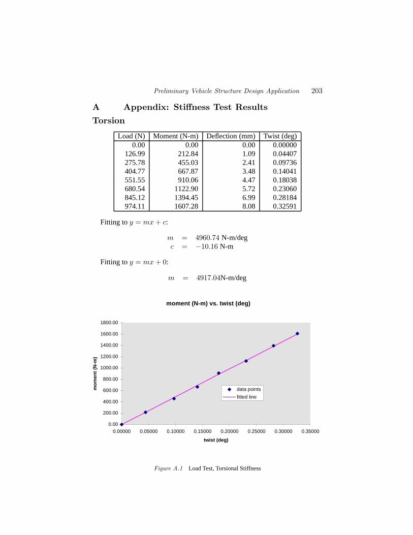
Preliminary Vehicle Structure Design Application 203
A Appendix: Stiffness Test Results
Torsion
Load (N) Moment (N-m) Deflection (mm) Twist (deg)0.00 0.00 0.00 0.00000
126.99 212.84 1.09 0.04407275.78 455.03 2.41 0.09736404.77 667.87 3.48 0.14041551.55 910.06 4.47 0.18038680.54 1122.90 5.72 0.23060845.12 1394.45 6.99 0.28184974.11 1607.28 8.08 0.32591
Fitting toy = mx + c:
m = 4960.74 N-m/degc = −10.16 N-m
Fitting toy = mx + 0:
m = 4917.04N-m/deg
moment (N-m) vs. twist (deg)
0.00
200.00
400.00
600.00
800.00
1000.00
1200.00
1400.00
1600.00
1800.00
0.00000 0.05000 0.10000 0.15000 0.20000 0.25000 0.30000 0.35000
twist (deg)
mom
ent (
N-m
)
data points
fitted line
Figure A.1 Load Test, Torsional Stiffness
204 IMPRECISION IN ENGINEERING DESIGN
BendingLoad (N) Deflection (mm)
0.00 0.00000284.67 0.101060551.55 0.17780836.22 0.33020
2001.60 0.787402286.27 0.914402837.82 1.16840
Fitting toy = mx + c:
m = 2426.16N/mmc = 51.79N
Fitting toy = mx + 0:
m = 2484.80N/mm
load (N) vs. deflection (mm)
0.00
500.00
1000.00
1500.00
2000.00
2500.00
3000.00
3500.00
0.00000 0.20000 0.40000 0.60000 0.80000 1.00000 1.20000 1.40000
deflection (mm)
load
(N
)
data points
fitted line
Figure A.2 Load Test, Torsional Stiffness

Chapter 9
ARROW’S THEOREM ANDENGINEERING DESIGN DECISION MAKING
Michael J. Scott and Erik K. Antonsson
Research in Engineering DesignVolume 11, Number 4 (2000), pages 218-228.
Abstract This article establishes that Arrow’s General Possibility Theorem has only indi-rect application to engineering design. Arrow’s Theorem states that there can beno consistent, equitable method for social choice. Many engineering design de-cisions are based on the aggregation of preferences. The foundation of many en-gineering decision methods is the explicit comparison of degrees of preference,a comparison that is not available in the social choice problem. This explicitcomparison of preference levels is coupled with the choice of an aggregationmethod, and some forms of aggregation may be inadequate or inappropriate inengineering design.
Keywords: Design decision-making; Engineering design; Multi-criteriaanalysis
1. IntroductionImportant tasks in engineering design are to generate and refine design al-
ternatives, and then to select a single design, or a set of designs, to fulfill aparticular need. In informal terms, the latter problem may be stated, “Findthe best alternative(s).” Sometimes the determination of “best” is relativelystraightforward and unambiguous, as in: “Find the lightest alternative,” or,“Find the stiffest alternative.” Sometimes it is less so, as in: “Find the light-est, stiffest alternative.” This simple directive is inadequate to choose betweenone alternative that is stiff but heavy, and another alternative that is light butcompliant.
This engineering design decision problem is a problem of decision withmultiple criteria, and can be stated as follows:
205
206 IMPRECISION IN ENGINEERING DESIGN
Given several performance criteria which are to be simultaneously optimized,determine a method for comparing any two design alternatives that dependsonly the values of the individual criteria for each alternative.
The multiple criteria engineering design decision problem has been addressedby various decision-making systems, such as Quality Function Deployment(QFD) [6], the Analytic Hierarchy Process (AHP) [13], Pugh charts [12], andmulti-criteria optimization [11], all of which help guide designers in choos-ing designs to meet a global performance criterion based on the aggregationof performances on distinct criteria. It is generally assumed that evaluationon the basis of any of the individual criteria is straightforward. In practice,the calculation of the individual criteria may require considerable engineer-ing judgement or resources. It is also assumed that any two alternatives couldbe compared directly, without resorting to individual criteria. In practice, engi-neers working on the designs do not make these direct comparisons, but insteadwork to meet performance specifications. The expertise to assess individualperformance criteria is often distributed throughout an engineering enterprise.A method to compare alternatives based on separate criteria is an efficient andfeasible alternative to direct comparison.
In addition to the engineering decision methods listed above, there is anextensive literature in decision theory on the topic of multiple criteria decision-making by an individual decision maker (see, for instance, [10], [4], [8]). Theidealized decision maker of decision theory need not be an individual person.Rather, it is assumed that there is a single entity that renders decisions; theinner workings of that entity may safely be ignored.
The problem of decision with multiple criteria is similar to the problemof social choice, or group decision-making, in which the rankings of severalalternatives by individuals are to be combined into a single, “social,” ranking(e.g., selecting candidates in a multi-party election). In social choice, of course,there is no longer a single decision maker, and the goal is to arrive at rationaldecisions that respect the sovereignty of the individual citizens involved in thedecision. In the theory of group decision-making, a well-known objection tothe validity of combining separate weak orders into a single social order isKenneth J. Arrow’s General Possibility Theorem [1, 2].
Various engineering design decision methods, such as those mentioned above,depend on the aggregation of several weak orders into a single order. Further-more, it is common for many individuals to participate in an engineering designdecision. Recent discussions in the design research community have raised thequestion of the applicability of Arrow’s Theorem to decision-making in en-gineering design [7]. The relevance of Arrow’s Theorem to the engineeringdesign decision problem depends on whether making a decision in engineer-ing design is sufficiently similar to a social choice problem, or to a decisionwith a single decision maker but with multiple objectives.
Arrow’s Theorem and Engineering Design Decision Making 207
This paper shows how Arrow’s Theorem does not apply to the multi-criteriaengineering decision problem. It further shows that, despite the common par-ticipation of many individuals in engineering design decisions, engineeringdesign is closer to multiple criteria decision-making than it is to social choice.Thus, engineering design decision-making occupies a middle ground betweendecision with an idealized decision maker and decision by groups of fully au-tonomous citizens, and on this middle ground Arrow’s Theorem has no detri-mental consequences.
Also related to multiple criteria analysis is decision under uncertainty, inwhich the problem is to determine the best alternative when the consequencesof each alternative are probability distributions over possible outcomes (e.g.,investment decisions). Both multiple criteria analysis and decision under un-certainty usually overlay the weak ordering of alternatives with a numericalscale.
1.1 Preliminaries: Notation and DefinitionsDesign alternatives are distinguished by uppercase Roman characters:
A, B, C, . . .
Design criteria are denoted by lowercase italics:x, y, z, . . .
Individuals or voters are denoted by Arabic numerals: 1, 2, 3,. . .
The most basic concept in the ranking of alternatives is simple comparison,in which there is no association of numbers with alternatives, but only thenotion that one alternativeA is preferred to another alternativeB. A rankingthat depends only upon simple comparison is called aweak order:
Definition 1 A weak orderon a set of alternatives~X = {A,B,C, . . .} is atransitive binary relation� such that for any two elementsA and B, eitherA � B (A is at least as preferable asB), or B � A (B is at least as preferableasA). Indifference is possible: ifA � B andB � A, then one writesA ∼ B(A is indifferent toB). If A � B butB �/ A, thenA is (strictly) preferred toB,writtenA � B.
A weak order is an ordinal ranking: it orders the alternatives without assign-ing numerical values. Any computational method for decision-making requiresthe further structure of a numerical scale that ranks alternatives. Such a numer-ical scale is called avalue function. The familiar> and≥ on the real numbersof the value function correspond to the preference relations� and� amongalternatives:
Definition 2 A value functionis an assignment of real numbers to alternativesthat preserves a weak order of acceptability of those alternatives. A value
208 IMPRECISION IN ENGINEERING DESIGN
function maps a set together with a weak order{ ~X,�} to the real numberswith its usual ordering{IR,≥}. For a value functionv, v(A) ≥ v(B) iff.A � B, with equality for indifference.
While it is always possible to construct a value function from a weak order(see [9]), the mere assignment of a value function does not imply a measureof degreeof acceptability. A value function is of greater use in a computa-tional decision method if the numerical scale can be used to compare levelsof acceptability. The weak orderA � B � C is captured both byv1, wherev1(A) = 10, v1(B) = 9, andv1(C) = 1, and byv2, wherev2(A) = 10,v2(B) = 2, andv2(C) = 1, but the relative preference forA, B, andC impliedby the two value functions is quite different. It shall be shown below that thecorrect specification of the numerical scale is crucial to the satisfactory reso-lution of both the multi-criteria decision problem and the problem of decisionunder uncertainty.
2. Arrow’s Impossibility Theorem and itsimplications for the aggregation of preference
Kenneth J. Arrow’s General Possibility Theorem, now commonly known asArrow’s Impossibility Theorem or simply Arrow’s Theorem, is an importantand powerful result in the theory of social choice. For that reason, and becausea thorough understanding of Arrow’s Theorem will facilitate a comparison be-tween the social choice and multi-criteria decision problems, the ImpossibilityTheorem will be presented here. The treatment refers mainly to [1] and [2].
2.1 The motivating paradoxThe context of Arrow’s work is politico-economic. Political scientists are
interested in determining a “fair” method of reconciling the potentially con-flicting interests of individuals in a society. Economists seek the most “satis-factory” distribution of a set of commodities throughout a society. The similar-ities between the two problems are evident, and indeed both can be formalizedin the same way; the notions of “fair” and “satisfactory” are explored throughthis formalization.
Themajority method of decision-makingis one possible answer to the looselyformulated question of fair social choice, and one that is sufficiently obviousthat a contradiction that arises from its employment motivates the Impossibil-ity Theorem. For an odd number of people and two options to choose among,a simple vote is guaranteed to satisfy the most people. But when there arethree alternatives, a paradox arises: say that there are three voters, one whoorders the optionsA � B � C, another who holdsB � C � A, and a thirdwho holdsC � A � B. These preferences are shown in Table 9.1. All three
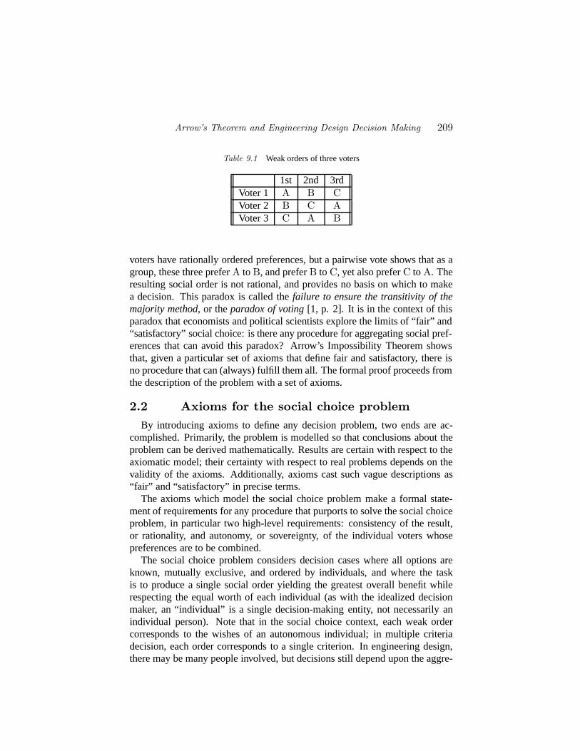
Arrow’s Theorem and Engineering Design Decision Making 209
Table 9.1 Weak orders of three voters
1st 2nd 3rdVoter 1 A B CVoter 2 B C AVoter 3 C A B
voters have rationally ordered preferences, but a pairwise vote shows that as agroup, these three preferA to B, and preferB to C, yet also preferC to A. Theresulting social order is not rational, and provides no basis on which to makea decision. This paradox is called thefailure to ensure the transitivity of themajority method, or theparadox of voting[1, p. 2]. It is in the context of thisparadox that economists and political scientists explore the limits of “fair” and“satisfactory” social choice: is there any procedure for aggregating social pref-erences that can avoid this paradox? Arrow’s Impossibility Theorem showsthat, given a particular set of axioms that define fair and satisfactory, there isno procedure that can (always) fulfill them all. The formal proof proceeds fromthe description of the problem with a set of axioms.
2.2 Axioms for the social choice problemBy introducing axioms to define any decision problem, two ends are ac-
complished. Primarily, the problem is modelled so that conclusions about theproblem can be derived mathematically. Results are certain with respect to theaxiomatic model; their certainty with respect to real problems depends on thevalidity of the axioms. Additionally, axioms cast such vague descriptions as“fair” and “satisfactory” in precise terms.
The axioms which model the social choice problem make a formal state-ment of requirements for any procedure that purports to solve the social choiceproblem, in particular two high-level requirements: consistency of the result,or rationality, and autonomy, or sovereignty, of the individual voters whosepreferences are to be combined.
The social choice problem considers decision cases where all options areknown, mutually exclusive, and ordered by individuals, and where the taskis to produce a single social order yielding the greatest overall benefit whilerespecting the equal worth of each individual (as with the idealized decisionmaker, an “individual” is a single decision-making entity, not necessarily anindividual person). Note that in the social choice context, each weak ordercorresponds to the wishes of an autonomous individual; in multiple criteriadecision, each order corresponds to a single criterion. In engineering design,there may be many people involved, but decisions still depend upon the aggre-

210 IMPRECISION IN ENGINEERING DESIGN
gation of engineeringcriteria. To formalize a desirable decision situation forsocial choice, Arrow introduces five axioms [1, pp. 24-30]:
Axiom 1 (unrestricted domain) Each individual is free to order the alterna-tives in any way.
Restricting Axiom 1 is one way to address the paradox, and methods that guar-antee the transitivity of the majority method can be ranked by how severelythey restrict this freedom. It is not at all obvious that Axiom 1 is reasonablefor design decisions, as will be discussed below.
Axiom 2 (positive response)If a set of orders ranksA beforeB and a secondset of orders is identical except that individuals who rankedB beforeA areentitled to switch, thenA is beforeB in the second set of orders.
Axiom 2 is an ordinal version of monotonicity, and is a consistency or ratio-nality requirement.
Axiom 3 (independence of irrelevant alternatives)If A is beforeB in a so-cial order, thenA is still beforeB if a third alternativeC is ignored or added.
Note that Axiom 3 is violated in the motivating paradox, where the relativerankings ofA and B are influenced by the addition of the alternative C. Thus,this axiom implicitly enforces the transitivity of the social order.
Axiom 4 (not imposed) An order is calledimposedif someA is before someB in all possible social orders. The social choice problem must not be imposed.
As Axiom 1 states that individuals can hold any preferences they like, Axiom 4says that they have a reasonable expectation that their preferences are not ex-cluded from being chosen as the social order. This is a fairness requirement.
Axiom 5 (not dictatorial) An order is calleddictatorial if there is one indi-vidual whose decisions dictate the social order. This is likewise not allowed.
Perhaps the simplest way to guarantee consistency of results is to violate Ax-iom 5: by choosing an individual whose preferences exactly determine thesocial order, the other four axioms are trivially satisfied. Such a solution isintuitively unfair in a social choice context, and is not allowed. While thereis no need in engineering to respect all attributes equally, it is wasteful at bestto evaluate attributes that have no impact on the decision. Dictatorship by oneevaluationcriterion is not a rational solution for engineering design. Someengineering cultures may appear to have a dictator in the form of a single de-cision maker, perhaps a manager with ultimate responsibility for all decisions;however, decisions will still be made by considering several criteria. Ratherthan violating Axiom 5, this changes the problem to decision with multiplecriteria and a single decision maker.
Arrow’s Theorem and Engineering Design Decision Making 211
In addition to these five axioms, there are implicit assumptions. Some aremerely technical: there are at least three alternatives, and there is an odd andfinite number of alternatives. One assumption, however, is substantive and cru-cial. The social order must be chosen based only on the weak orders suppliedby the individuals; it is not permitted to ask for any further information to de-termine strength of preference, as any comparison between individuals is heldto be meaningless.
2.3 The resulting contradictionArrow’s Theorem shows that a social choice function satisfying all five con-
ditions is an impossibility:
Theorem 1 Any social choice function satisfying Axioms 1–3 must be eitherimposed or dictatorial.
The reader is referred to [1, pp. 51-59] or [2, pp. 20-21] for details of the proof,but the basic line of reasoning is as follows. Adecisiveset of individuals forA overB is a set who guarantee thatA will be preferred toB whenever theyunanimously agree so; any decisive set must contain a smaller decisive set;there is always a decisive set; any set that is decisive forA overB is decisivefor A over anything else and for anything else overB, and thus for allA overall B; thus there must be a dictator. The only way to avoid this dictatorship isto impose some preferences, violating Axiom 4.
Thus, the paradox of the intransitivity of the majority method is a manifesta-tion of a difficulty so deeply embedded in the social choice problem that it can-not be resolved without compromising the defining axioms. It is an intuition-building exercise to take the three orders shown in Table 9.1, and attempt tocombine them using a general procedure. It quickly becomes clear that transi-tivity can be insured by dictatorship. Arrow’s Theorem proves essentially thattransitivity can only be insured by dictatorship.
2.4 Ways around the contradictionArrow’s Theorem shows that there is no method of aggregating social choice
that is guaranteed to satisfy all five axioms. Are all socio-political systems thenfundamentally irrational? Or are there systems that, implicitly or explicitly,operate with restricted versions of one or more of the axioms, and thus avoidgross inconsistency?
Arrow and others have attempted to resolve the paradox by weakening thefirst condition, arguing that in real political, economic, and even moral1 sys-tems participants tacitly agree to structure their choices in a “logical” way,i.e.,
1Arrow goes so far as to quote Kant [1, pp. 81–82]
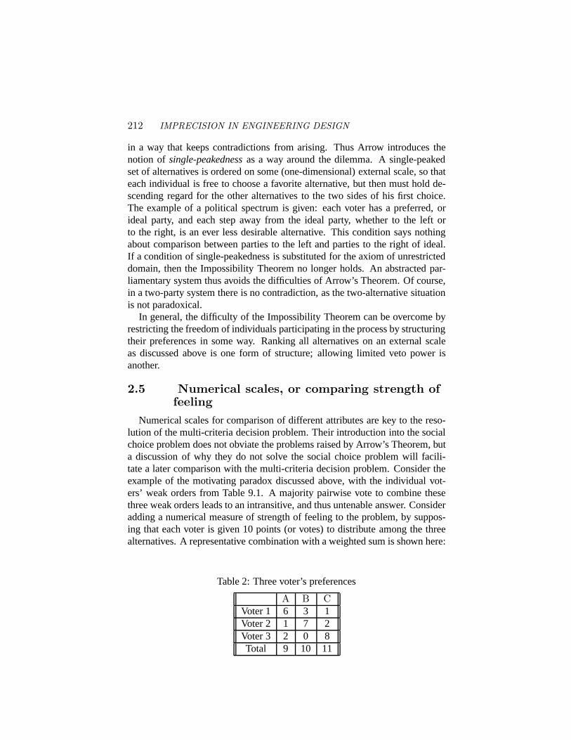
212 IMPRECISION IN ENGINEERING DESIGN
in a way that keeps contradictions from arising. Thus Arrow introduces thenotion of single-peakednessas a way around the dilemma. A single-peakedset of alternatives is ordered on some (one-dimensional) external scale, so thateach individual is free to choose a favorite alternative, but then must hold de-scending regard for the other alternatives to the two sides of his first choice.The example of a political spectrum is given: each voter has a preferred, orideal party, and each step away from the ideal party, whether to the left orto the right, is an ever less desirable alternative. This condition says nothingabout comparison between parties to the left and parties to the right of ideal.If a condition of single-peakedness is substituted for the axiom of unrestricteddomain, then the Impossibility Theorem no longer holds. An abstracted par-liamentary system thus avoids the difficulties of Arrow’s Theorem. Of course,in a two-party system there is no contradiction, as the two-alternative situationis not paradoxical.
In general, the difficulty of the Impossibility Theorem can be overcome byrestricting the freedom of individuals participating in the process by structuringtheir preferences in some way. Ranking all alternatives on an external scaleas discussed above is one form of structure; allowing limited veto power isanother.
2.5 Numerical scales, or comparing strength offeeling
Numerical scales for comparison of different attributes are key to the reso-lution of the multi-criteria decision problem. Their introduction into the socialchoice problem does not obviate the problems raised by Arrow’s Theorem, buta discussion of why they do not solve the social choice problem will facili-tate a later comparison with the multi-criteria decision problem. Consider theexample of the motivating paradox discussed above, with the individual vot-ers’ weak orders from Table 9.1. A majority pairwise vote to combine thesethree weak orders leads to an intransitive, and thus untenable answer. Consideradding a numerical measure of strength of feeling to the problem, by suppos-ing that each voter is given 10 points (or votes) to distribute among the threealternatives. A representative combination with a weighted sum is shown here:
Table 2: Three voter’s preferences
A B CVoter 1 6 3 1Voter 2 1 7 2Voter 3 2 0 8Total 9 10 11
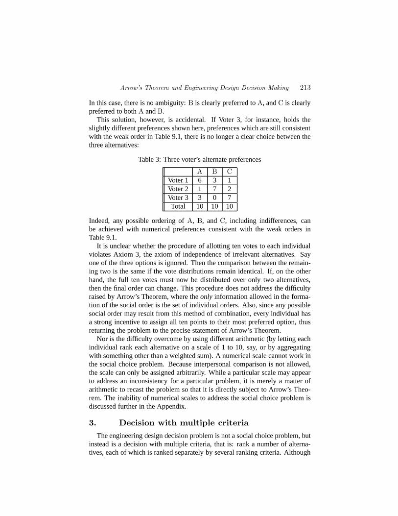
Arrow’s Theorem and Engineering Design Decision Making 213
In this case, there is no ambiguity:B is clearly preferred toA, andC is clearlypreferred to bothA andB.
This solution, however, is accidental. If Voter 3, for instance, holds theslightly different preferences shown here, preferences which are still consistentwith the weak order in Table 9.1, there is no longer a clear choice between thethree alternatives:
Table 3: Three voter’s alternate preferences
A B CVoter 1 6 3 1Voter 2 1 7 2Voter 3 3 0 7Total 10 10 10
Indeed, any possible ordering ofA, B, andC, including indifferences, canbe achieved with numerical preferences consistent with the weak orders inTable 9.1.
It is unclear whether the procedure of allotting ten votes to each individualviolates Axiom 3, the axiom of independence of irrelevant alternatives. Sayone of the three options is ignored. Then the comparison between the remain-ing two is the same if the vote distributions remain identical. If, on the otherhand, the full ten votes must now be distributed over only two alternatives,then the final order can change. This procedure does not address the difficultyraised by Arrow’s Theorem, where theonly information allowed in the forma-tion of the social order is the set of individual orders. Also, since any possiblesocial order may result from this method of combination, every individual hasa strong incentive to assign all ten points to their most preferred option, thusreturning the problem to the precise statement of Arrow’s Theorem.
Nor is the difficulty overcome by using different arithmetic (by letting eachindividual rank each alternative on a scale of 1 to 10, say, or by aggregatingwith something other than a weighted sum). A numerical scale cannot work inthe social choice problem. Because interpersonal comparison is not allowed,the scale can only be assigned arbitrarily. While a particular scale may appearto address an inconsistency for a particular problem, it is merely a matter ofarithmetic to recast the problem so that it is directly subject to Arrow’s Theo-rem. The inability of numerical scales to address the social choice problem isdiscussed further in the Appendix.
3. Decision with multiple criteriaThe engineering design decision problem is not a social choice problem, but
instead is a decision with multiple criteria, that is: rank a number of alterna-tives, each of which is ranked separately by several ranking criteria. Although
214 IMPRECISION IN ENGINEERING DESIGN
this problem appears superficially similar to the social choice problem, since itseeks to combine several individual rankings into one, it is a distinct problem.Two differences are:
In the social choice problem, all orderings are accorded equal worth.In the multiple criteria problem, it is desirable to be able to assign im-portance weightings to criteria. While it is natural to accord all humanvoters equal worth, there is no obvious reason to require equal weightingof the different engineering criteria that describe a device or system.
This difference may disappear if the weighted problem can be recast asan unweighted problem with more individuals.
The social choice problem permits no interpersonal comparison of pref-erences, and is thus limited to the discussion of weak orders. The heartof the multi-criteria engineering problem is the inter-attribute compari-son of preferences. When considering many design goals, it is crucialto understand their relative importance and the way in which they inter-act. Again, what is natural to require when modelling the sovereignty ofindividual citizens is not necessarily applicable to separate engineeringdesign criteria.
This difference makes decision with multiple criteria structurally differ-ent from social choice, and has deep implications for the applicability ofthe Impossibility Theorem to engineering design decision-making.
Even the informal motivating paradox for the Impossibility Theorem (where amajority vote rankedA beforeB beforeC beforeA) loses much of its powerif cast in the framework of multi-criteria decision-making. Consider the anal-ogous example of a design or a product that is to be judged on the basis ofthree criteria:x, y, andz. It is certainly plausible to assume that the designermay be faced with a choice of three candidate designs, A, B, andC, such thatA is better thanB is better thanC with respect to criterionx, B is better thanC is better than A with respect toy, andC is better than A is better thanBwith respect toz. The analogous “paradox” here is that givingx, y, andz onevote each as a method to determine the best design yields no obvious answer.In other words, if all that is known about a design is a weak order among al-ternatives for each of the three criteriax, y, andz, then there is not enoughinformation to decide upon an overall best design. This “paradox” is resolvedin the multi-criteria problem by more careful consideration of preferences forx, y, andz, and consideration of how those preferences interact. Note thateven if this decision is made by a group of three individuals, each responsiblefor one criterion, there is still no paradox; the involvement of more than oneperson does not by itself make group decision-making.
Arrow’s Theorem and Engineering Design Decision Making 215
A crucial assumption was made at the outset about the engineering designdecision problem. In general, in a real design situation, thereis a rational weakorder amongA, B, andC.2 Furthermore, that order could in principle be founddirectly. The “paradox” is merely that additional information beyond the weakorders onx, y, andz is required to recognize the overall order. The questionasked here is whether and when it is possible to find consistent, rational tech-niques to discover the ranking amongA, B, andC. If so, it will necessarily bewith a slightly different set of assumptions from the ones of the ImpossibilityTheorem, assumptions more appropriate for engineering decision-making thanfor social choice.
3.1 Comparison of axioms for the two decisionproblems
A careful examination of the axioms is necessary before considering theImpossibility Theorem in the context of the design decision problem. Whencombining engineering criteria (the multi-criteria problem), rather than indi-vidual orderings (the social choice problem), the axioms of positive response,independence of irrelevant alternatives, and inadmissibility of dictatorial so-lutions still appear to hold. However, it is not obvious that domains must beunrestricted or that orders must not be imposed.
The social choice problem must respect individuals by affording them thefreedom to order alternatives as they choose; in a design situation, cultural,customer, or managerial structure is almost always imposed on the orders. Forinstance, if the three candidate vehicle structure designsA, B, andC havebending stiffnesses of 3000, 3200, and 3400 N/mm respectively, Axiom 1states that any individual is free to express the preferenceC � A � B. Avehicle structures group, however, which proposed this order to management,would be criticized for “irrational” preferencesover bending stiffness. Theorder that ranksC � A � B is transitive, and any transitive order must beconsidered rational in the social choice problem; it would be an acceptablefinal order of candidate designs. With respect to the particular evaluation cri-terion of bending stiffness, however, it is not rational; many such transitiveorders would be considered irrational in an engineering context. No individ-ual is given veto power in the social choice context; almost any attribute of anengineered design has a level so unacceptable as to veto the entire design.
Recall that Arrow proposedsingle-peakedpreferences as a way to resolvethe contradictions of the Impossibility Theorem: preferences are single-peaked
2This does not mean that there is one optimal solution that fits all situations; a design situation includesthe attitudes and preferences of the people and corporate entities involved. Given the need for personaltransportation, some auto manufacturers choose to make luxury cars, while others choose to make economycars.
216 IMPRECISION IN ENGINEERING DESIGN
when all options are ordered on an external scale, and each individual has onepreferred option and holds descending regard for alternatives to the two sidesof that preferred option. Engineering variables are almost always ordered onan external scale, and preferences for engineering requirements are commonlysingle-peaked around an ideal target. Indeed, nearly all engineering require-ments are of one of three forms: less is better, more is better, or closer to aparticular target is better [3]. All three of these forms are single-peaked.
There are (rare) evaluation criteria that do not behave in a single-peakedmanner. A design preference for availability of a particular material stock maybe one criterion for a design, and it may change over time and take on anyorder. The preference for the frequency of the first acoustic mode is often toavoida particular unpleasant range. However, designers can and do restrict cri-teria that are not globally single-peaked to regions of local single-peakedness.The vehicle structure designer seeking to avoid a particular range of frequen-cies of the first acoustic mode, for example, chooses to target either higher orlower frequencies, thus considering only a range over which the criterion issingle-peaked. Thus, while the completely generic design decision problemshould obey Arrow’s axiom of unrestricted domain, designers strive to avoidthe generic problem, and rather to cast each problem so that domains, ratherthan being unrestricted, are single-peaked along the obvious external scalesprovided by the design parameterization. Indeed, in terms of the decisionproblem, the parameterization of a design serves to restrict domains. For themulti-criteria decision problem, the axiom of unrestricted domain is replacedby an exhortation to the designer to verify that criteria are single-peaked, orrestrict the problem until they are. It is understood that this may not always bepossible, but when it is not, the designer realizes that the design problem is notcompletely well-conditioned. Such problems are difficult for formal methodsand informal methods alike.
The axioms of the multi-criteria decision problem are thus not identical tothose of the social choice problem. Axiom 1 is crucial to the social choiceproblem, while in the engineering design problem, it appears in a modifiedform that is known to overcome Arrow’s Theorem. This difference in Ax-iom 1 allows multi-criteria methods to operate on some large classes of prob-lems without violating Arrow’s Theorem, even without the use of a numericalscale to compare preferences across attributes. However, the differences inaxiomatic structure are minor compared to the difference in one fundamentalassumption: the social choice problem does not admit interpersonal compari-son, while the multi-criteria decision problem would be meaningless withoutinter-attribute comparisons. The next section will discuss how a numericalscale for the inter-attribute comparison of preference is used in two contexts:the aforementioned multi-criteria decision problem, and the related problem ofdecision-making under uncertainty.
Arrow’s Theorem and Engineering Design Decision Making 217
There is a further, practical, difference between social choice and engineer-ing design: designs have constraints. A maximum stress indicates the point atwhich a design breaks and fails; government regulations must be fulfilled or adesign is not allowed on the market. However, it is usually far from obvious,a priori, which candidate designs violate constraints, and the engineer mustbe free to consider all potentially viable candidates. In decision theory, thedecision maker chooses among a neatly defined set of viable alternatives; inengineering design, deciding which are the viable alternatives is a major task,often involving considerably more resources than the final decision. Further-more, the early consideration of infeasible designs is often a crucial part of therefinement process.
A decision method that captures this special feature of engineering designwould, in principle, violate Axiom 4. The positions of alternatives that failon the basis of a single criterion could be seen as imposed (to be last) in anyaggregated order. Constraints in engineering design, if translated into socialchoice terms, are a sort of veto that individual criteria may exercise over theentire decision, and thus violate the axiom of no imposed orders. However,when the design is acceptable on the basis of each individual criterion, there isno reason to abandon the axiom of no imposed orders. For the multi-criteriaengineering decision problem, the axiom of no imposed orders is weakened:
Axiom 4.4a (limited imposed orders)Axiom 4 holds, with the exception thatsome alternatives may be declared unacceptable, and thus last in any com-bined order, on the basis of an unacceptable ranking on a single criterion. Allunacceptable alternatives are equally unacceptable.
This modification of Axiom 4 is not a significant theoretical objection to theapplication of Arrow’s Theorem in engineering design, as the same end can beachieved by simply removing alternatives, after analysis, from consideration.It does, however, provide a framework for decision methods for engineeringdesign that are capable of considering alternatives that may turn out later to beinfeasible.
4. Inter-attribute comparison of preferenceDecision with multiple criteria differs empirically from social choice in an
important way. In the former, there is always a well-defined aggregated orderamong alternatives, which is available to anyone with the time and resources toquery a decision maker directly about all possible combinations; in the latter,Arrow’s Theorem calls into question the very existence of a well-defined ag-gregated order. A direct specification of preference in many dimensions in themulti-criteria problem presents no more theoretical difficulties than a direct
218 IMPRECISION IN ENGINEERING DESIGN
specification of preferences in one dimension; the practical implementation,however, can present great difficulty.
There is more than one way to assign a value function when a weak orderamong alternatives is given. In this section, two distinct approaches to theassignment of a value function are discussed: theutilities (or von Neumann–Morgenstern utilities) [14, 8] that are used for decision-making under uncer-tainty, and directly specifiedpreferencessuch as those used in many multi-criteria decision systems. Both techniques use inter-attribute comparison toguarantee consistency (and avoid the pitfalls of the Impossibility Theorem),but the emphasis in each is different.
4.1 UtilityThe specification of utility depends upon a weak order among alternatives,
and on the mathematics of expectation. To determine a utility function, the so-called lottery questionmust have an answer: “Given thatA is preferred toB,andB is preferred toC, at which probabilityp is there indifference between thetwo choices ‘B with probability1’ and ‘a lottery that yieldsA with probabilityp andC with probability (1 − p)’?” (Note that the question need not have adirect answer; see [15], for instance, for a discussion of the elicitation of vonNeumann–Morgenstern utilities with little or no probability information.) VonNeumann and Morgenstern [14] show that, given the assumption that utilitiescombine with the mathematics of expectation, the numerical utility scale isdetermined up to an affine transformation.
The assumption of the use of mathematical expectation arises because util-ity theory is intended to treat questions of decision-making under probabilis-tic uncertainty, such as those that are germane to gambling. This makes thespecification ofrelativeutilities with probabilities natural. The lottery methodprovides an elegant method to determine not only thatA is preferred toB andB is preferred toC, but also how great the preference is forA overB relativeto the preference forB overC.
However, the development of utility specifically excluded the notion of in-terpersonal comparison of utility as too difficult to address:
We do not undertake to fix an absolute zero and an absolute unit of utility. [14,footnote, p. 25]
Utility theory is intended for use in decision-making under uncertainty or risk,rather than as a solution of the multi-criteria decision-making problem. Deci-sion under uncertainty is often required in multi-criteria settings. [8] presentconditions under which a decision maker’s overall utility is a simple functionof individual, independent utility functions. The overall utility function is de-termined by direct comparison of several alternatives in order to determineappropriate weighting factors for the individual utility scales determined withregard to the separate attributes. Arrow’s Theorem presents no difficulty what-
Arrow’s Theorem and Engineering Design Decision Making 219
soever to this sort of calculation; even if several people are involved in thedecision, there is an idealized single decision maker.
The success of the von Neumann–Morgenstern utility paradigm, and theease of its application in terms of quantified risk, have led to a situation inwhich many decision problems are treated as problems of (economic) decision-making under uncertainty. The lottery question seems natural, and so it is as-sumed that the lottery question is the right way to impose a numerical scaleon preferences. Nevertheless, engineering design maynot be best classified asdecision-making under risk and uncertainty. Utility theory is one paradigm fordecision-making, appropriate for a particular set of problems, those where the“estimation of expectations for each option” is the most pertinent information.When design reaches the manufacturing stage, and probability distributionsover manufacturing variations are usually the most relevant uncertainties, thedesign decision problem is indeed similar to the problem addressed by util-ity theory. Earlier in the design process, where uncertainty will be resolvedby refinement of a design alternative, rather than by random selection from aperceived distribution among alternatives, a utility model is less appropriate.Direct preference specification, for uncertainty other than quantified risk, willbe discussed in the next section.
From the point of view of classical utility theory, the design decision prob-lem examined here is a case of decision-making under certainty. In the classicalutility theory view, the construction of the utility function and the choice of a“best” solution with limited computation are uninteresting problems. The con-struction of the utility function is only support for the subsequent question ofwhich course of action to select in the face of uncertain consequences.
4.2 Direct specification of preferenceThe engineering design decision problem that is the subject of this paper is
not primarily a problem of decision-making under uncertainty. While methodssuch as those proposed by [8] could be applied to the problem, and the result-ing utility function would indeed provide a basis for comparison of any twoalternatives, the relative complexity of these methods is not justified in caseswhen no probabilistic uncertainty is to be incorporated in the problem. Thisis particularly true as the number of individual performance criteria increases(the number of coefficients to be determined is2n−1, wheren is the number ofcriteria). Thus methods intended to solve the multi-criteria decision problem asstated at the beginning of this paper, without the incorporation of uncertainty,commonly use direct specification of preference (e.g., QFD [6], AHP [13]).Direct preferences, unlike utilities, are expressed on an absolute scale. For ex-ample, a preference ofµ = 1 could indicate a completely acceptable value, andµ = 0 a completely unacceptable value. Alternatively, each criterion may be
220 IMPRECISION IN ENGINEERING DESIGN
judged on a discrete scale (such as1–3–9). The individual numerical orderingsassociated with each criterion are then aggregated into an overall numericalordering of all alternatives based on all criteria simultaneously. The functionsused for aggregation of the orderings vary; a weighted arithmetic mean is acommon choice.
It was made clear earlier that Arrow’s Theorem does not apply to the en-gineering design decision problem, whose chief concern is to compare prefer-ences based on multiple attributes. Nevertheless, Arrow’s Theorem does bearindirectly on the legitimacy of these methods: if the comparison of preferencesis effected by the arbitrary assignment of numbers to alternatives, then thosepreferences contain no more information than weak orders, as discussed inSection 2.5 and the Appendix. In that case no aggregation method is adequate.A method that delivers an overall preference as a function of individual prefer-ences must explicitly, and justifiably, compare individual preference values.
The individual preference orders may be generated by, or associated with,different people or groups involved in a design. One of the motivations for theengineering design decision problem as described in this paper is the need toassess design alternatives for overall worthiness when the most readily acces-sible information comes from many independent performance measures, eachof which is the responsibility of a different portion of a design team. If thesegroups or individuals must be treated as autonomous citizens, then there is nofair and rational way to combine their preferences. However, team design isnot driven by the need to respect the sovereignty of the individuals involved,but rather by a desire to create superior products.
The team engineering decision problem thus has two aspects: the multiplecriteria problem, to which Arrow’s Theorem does not apply, and the problem ofcollaboration, to which Arrow’s Theorem would apply if it were necessary toguarantee sovereignty of team members. The mere involvement of groups doesnot make it group decision making; in engineering, rather than social systems,attributes, not people, must be reconciled. There are certainly difficult andinteresting issues in the management of groups in an engineering context, butArrow’s Theorem does not make such management impossible.
5. ConclusionsThis paper establishes the legitimacy of constructing aggregated preferences
in engineering design, even though such aggregation is not permissible in thesocial choice problem. It does so by a thorough examination of the contextand results of Kenneth J. Arrow’s General Possibility Theorem. The designdecision problem has structural (axiomatic) peculiarities which make compar-isons in the manner of social choice acceptable in engineering design; morefundamentally, however, the aggregation relies on a procedure for comparing
Arrow’s Theorem and Engineering Design Decision Making 221
the relative importance and interaction of individual preferences that violatesan assumption of citizens’ sovereignty in the social choice milieu.
Decision with multiple criteria and a single, idealized decision maker isone problem in decision theory; social choice, in which each idealized indi-vidual’s sovereignty must be guaranteed, is another. Engineering design oftenfalls somewhere in the middle, but even when many people are involved, thegroup nature of the decision is subordinate to the multi-criteria aspect, as thesovereignty of individuals is not necessary. Interesting parallels are evidentbetween the ideas expressed in this paper and different management styles [5].A top-down management style would correspond to forcing a single decisionmaker on the problem, whereas distributed control would correspond to thegroup decision environment described here; in either case, the decision prob-lem is framed in terms of engineering requirements rather than individuals’desires.
The aggregation of preference in engineering design is often discussed asthe assessment of a utility function, though utility is a particular form of pref-erence assessment that is useful in decision under uncertainty and risk. Themulti-criteria decision problem discussed in this paper does not include the in-corporation of probabilistic uncertainty. The specification of a multi-attributeutility function for decision under uncertainty, and the use of direct specifica-tion of preferences for the resolution of the multi-criteria decision problem,both avoid the problems raised by Arrow’s Theorem, but their emphases aredifferent.
While Arrow’s Theorem does not prove that the engineering design decisionproblem treated here cannot have a rational answer, it does offer a caution tomethods that attempt to solve the multi-criteria decision problem: comparisonof preferences must be made explicit. The arbitrary assignment of numbers toalternatives can lead to undesired conclusions. Similarly, the arbitrary assign-ment of an aggregation method can lead to undesired conclusions. A decisionmethod must have an explicit procedure for assigning values to alternatives,and for combining those values into a single performance function, and thetwo must agree. If a decision method gives inadequate answers, it is not be-cause Arrow’s Theorem declares that comparison is impossible; it is becausethe particular implementation is flawed — the representation and comparisonof preferences in the method are insufficiently rich.
Finally, the need in engineering design to consider and evaluate alternativesthat may turn out to be infeasible is not well captured by the classic formulationof the decision problem, where only feasible alternatives are considered. Thisdifficulty can be overcome by reformulating the decision problem whenever aninfeasible candidate arises. Alternatively, a decision methodology can handlesuch constraints by a modification of the underlying decision axioms.

222 IMPRECISION IN ENGINEERING DESIGN
AcknowledgementsThis material is based upon work supported, in part, by the National Science
Foundation under NSF Grant Numbers DMI-9523232 and DMI-9813121. Anyopinions, findings, conclusions, or recommendations expressed in this publi-cation are those of the authors and do not necessarily reflect the views of thesponsors.
Arrow’s Theorem and Engineering Design Decision Making 223
References
[1] A RROW, K. J. Social Choice and Individual Values, 1st ed. J. Wiley,New York, NY, 1951.
[2] A RROW, K. J., AND RAYNAUD , H. Social Choice and MulticriterionDecision-Making. The MIT Press, Cambridge, MA, 1986.
[3] BYRNE, D. M., AND TAGUCHI, S. The Taguchi approach to parameterdesign. InQuality Congress Transaction – Anaheim(May 1986), ASQC,pp. 168–177.
[4] FRENCH, S. Decision Theory: An Introduction to the Mathematics ofRationality. Ellis Horwood, Chichester, 1988.
[5] GOOLD, M., AND CAMPBELL, A. Many best ways to make strategy.Harvard Business Review 65, 6 (November-December 1987), 70–76.
[6] HAUSER, J.,AND CLAUSING, D. The House of Quality.Harvard Busi-ness Review 66, 3 (May/June 1988), 63–73.
[7] HAZELRIGG, G. A. The implication of arrow’s impossibility theorem onapproaches to optimal engineering design.ASME Journal of MechanicalDesign 118, 2 (jun 1996), 161–164.
[8] K EENEY, R.,AND RAIFFA, H. Decisions with Multiple Objectives: Pref-erences and Value Tradeoffs. Cambridge University Press, Cambridge,U.K., 1993.
[9] K RANTZ, D., LUCE, R., SUPPES, P., AND TVERSKY, A. Foundationsof Measurement, vol. I. Academic Press, New York, NY, 1971.
[10] LUCE, R., AND RAIFFA, H. Games and Decisions. J. Wiley and Sons,New York, NY, 1957. Dover Edition, 1985.
[11] PAPALAMBROS, P., AND WILDE, D. Principles of Optimal Design.Cambridge University Press, New York, NY, 1988.
[12] PUGH, S. Total Design. Addison-Wesley, New York, NY, 1990.
[13] SAATY, T. L. The Analytic Hierarchy Process: Planning, Priority Set-ting, Resource Allocation. McGraw Hill, New York, NY, 1980.
[14] VON NEUMANN, J., AND MORGENSTERN, O. Theory of Games andEconomic Behavior, 2nd ed. Princeton University Press, Princeton, NJ,1953.
[15] WAKKER, P., AND DENEFFE, D. Eliciting von Neumann-Morgensternutilities when probabilities are distorted or unknown.Management Sci-ence 42, 8 (Aug. 1996), 1131–1150.
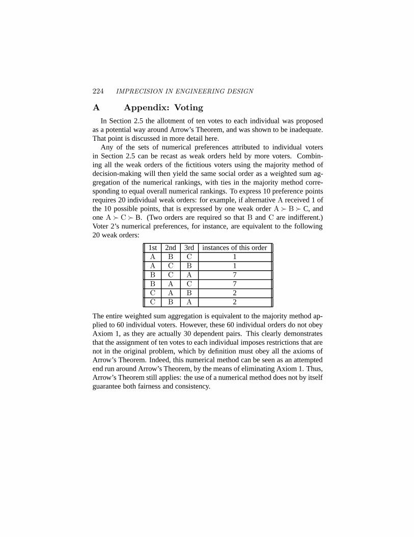
224 IMPRECISION IN ENGINEERING DESIGN
A Appendix: VotingIn Section 2.5 the allotment of ten votes to each individual was proposed
as a potential way around Arrow’s Theorem, and was shown to be inadequate.That point is discussed in more detail here.
Any of the sets of numerical preferences attributed to individual votersin Section 2.5 can be recast as weak orders held by more voters. Combin-ing all the weak orders of the fictitious voters using the majority method ofdecision-making will then yield the same social order as a weighted sum ag-gregation of the numerical rankings, with ties in the majority method corre-sponding to equal overall numerical rankings. To express 10 preference pointsrequires 20 individual weak orders: for example, if alternativeA received 1 ofthe 10 possible points, that is expressed by one weak orderA � B � C, andoneA � C � B. (Two orders are required so thatB andC are indifferent.)Voter 2’s numerical preferences, for instance, are equivalent to the following20 weak orders:
1st 2nd 3rd instances of this orderA B C 1A C B 1B C A 7B A C 7C A B 2C B A 2
The entire weighted sum aggregation is equivalent to the majority method ap-plied to 60 individual voters. However, these 60 individual orders do not obeyAxiom 1, as they are actually 30 dependent pairs. This clearly demonstratesthat the assignment of ten votes to each individual imposes restrictions that arenot in the original problem, which by definition must obey all the axioms ofArrow’s Theorem. Indeed, this numerical method can be seen as an attemptedend run around Arrow’s Theorem, by the means of eliminating Axiom 1. Thus,Arrow’s Theorem still applies: the use of a numerical method does not by itselfguarantee both fairness and consistency.
Chapter 10
USING INDIFFERENCE POINTSIN ENGINEERING DECISIONS
Michael J. Scott and Erik K. Antonsson
Proceedings of the11th International Conference on Design Theory and MethodologyASME, Paper Number DETC2000/DTM-14559, (September, 2000)
Abstract Multi-criteria decision support methods are common in engineering design. Thesemethods typically rely on the specification of importance weights to accomplishtrade-offs among competing objectives. Such methods can have difficulties,however: they may not be able to select all possible Pareto optima, and the directspecification of importance weights can be arbitrary andad hoc. The inabilityto reach all Pareto optima is shown to be surmountable by the consideration oftrade-off strategyas an additional parameter of a decision. The use ofindiffer-ence pointsto select a best solution, as an alternative to direct specification ofimportance weights, is presented, and a simple truss design example is used toillustrate the concepts.
Keywords:multicriteria analysis, engineering design, design decision-making,aggregation functions, trade-offs, strategies
1. IntroductionMulti-criteria decision making is an important part of design. There are
many methods, both informal and formal, that support such design decisionmaking, such as Pugh charts [5], QFD [3], and the Analytic Hierarchy Process,or AHP [6]. These design decision methods share several key features. All relyon the aggregation of preferences to choose among designs, and most methodsallow for the assignment of importance to individual attributes through theuse of weights. These importance weights are meant to allow for meaningfulcomparison of many options when two or more attributes must be traded-offagainst each other. Among decision methods, weighted-sum aggregation ofpreferences is common, as is direct specification of importance weights.
225
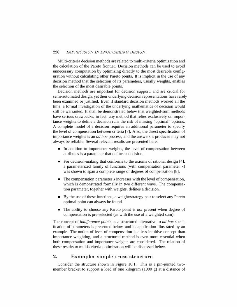
226 IMPRECISION IN ENGINEERING DESIGN
Multi-criteria decision methods are related to multi-criteria optimization andthe calculation of the Pareto frontier. Decision methods can be used to avoidunnecessary computation by optimizing directly to the most desirable config-uration without calculating other Pareto points. It is implicit in the use of anydecision method that the selection of its parameters, usually weights, enablesthe selection of the most desirable points.
Decision methods are important for decision support, and are crucial forsemi-automated design, yet their underlying decision representations have rarelybeen examined or justified. Even if standard decision methods worked all thetime, a formal investigation of the underlying mathematics of decision wouldstill be warranted. It shall be demonstrated below that weighted-sum methodshave serious drawbacks; in fact, any method that relies exclusively on impor-tance weights to define a decision runs the risk of missing “optimal” options.A complete model of a decision requires an additional parameter to specifythe level of compensation between criteria [7]. Also, the direct specification ofimportance weights is anad hocprocess, and the answers it produces may notalways be reliable. Several relevant results are presented here:
In addition to importance weights, the level of compensation betweenattributes is a parameter that defines a decision.
For decision-making that conforms to the axioms of rational design [4],a parameterized family of functions (with compensation parameters)was shown to span a complete range of degrees of compensation [8].
The compensation parameters increases with the level of compensation,which is demonstrated formally in two different ways. The compensa-tion parameter, together with weights, defines a decision.
By the use of these functions, a weight/strategy pair to select any Paretooptimal point can always be found.
The ability to choose any Pareto point isnot present when degree ofcompensation is pre-selected (as with the use of a weighted sum).
The concept ofindifference pointsas a structured alternative toad hocspeci-fication of parameters is presented below, and its application illustrated by anexample. The notion of level of compensation is a less intuitive concept thanimportance weighting, and a structured method is even more essential whenboth compensation and importance weights are considered. The relation ofthese results to multi-criteria optimization will be discussed below.
2. Example: simple truss structureConsider the structure shown in Figure 10.1. This is a pin-jointed two-
member bracket to support a load of one kilogram (1000 g) at a distance of

Using Indifference Points in Engineering Decisions 227
w
h
t
y=0.5
x
L=1
Figure 10.1 Example: a simple truss structure.
1 meter from a wall (L = 1). The positions of the wall mounts are fixed, withthe lower support one half meter below the upper support (y = 0.5). Bothmembers are made of aluminum (6061-T6). The designer controls four designvariables:
x ∈ [0.1 m, 0.9 m] distance from wall to pint ∈ [5 mm, 20 mm] thickness of bending memberh ∈ [5 mm, 20 mm] height of bending memberw ∈ [5 mm, 20 mm] width of (square) compression member
For this example, the performance measures to consider are the mass (M)of the structure, and the safety factor (S). The example is simple enough thatboth can be expressed analytically, but let us start by treating the performancecalculation as a black box. The details of the calculations are presented in theAppendix. For purposes of this paper, the design problem is to minimize themass of the structure while maximizing the factor of safety.
Further suppose that no additional advantage is gained from factors of safetyabove ten. Also, designs with safety factors below one should not be consid-ered. Using optimization or other means, it can be determined that the min-imum mass achievable with a factor of safety of one is 123 grams, while the
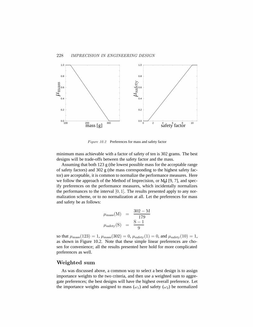
228 IMPRECISION IN ENGINEERING DESIGN
100 200 3000.0
0.2
0.4
0.6
0.8
1.0
µm
ass
mass [g]0 2 4 6 8 10
0.0
0.2
0.4
0.6
0.8
1.0
safety factor
µsa
fety
Figure 10.2 Preferences for mass and safety factor
minimum mass achievable with a factor of safety of ten is 302 grams. The bestdesigns will be trade-offs between the safety factor and the mass.
Assuming that both 123 g (the lowest possible mass for the acceptable rangeof safety factors) and 302 g (the mass corresponding to the highest safety fac-tor) are acceptable, it is common to normalize the performance measures. Herewe follow the approach of the Method of Imprecision, or MoI [9, 7], and spec-ify preferences on the performance measures, which incidentally normalizesthe performances to the interval[0, 1]. The results presented apply to any nor-malization scheme, or to no normalization at all. Let the preferences for massand safety be as follows:
µmass(M) =302 − M
179
µsafety(S) =S − 1
9
so thatµmass(123) = 1, µmass(302) = 0, µsafety(1) = 0, andµsafety(10) = 1,as shown in Figure 10.2. Note that these simple linear preferences are cho-sen for convenience; all the results presented here hold for more complicatedpreferences as well.
Weighted sumAs was discussed above, a common way to select a best design is to assign
importance weights to the two criteria, and then use a weighted sum to aggre-gate preferences; the best designs will have the highest overall preference. Letthe importance weights assigned to mass (ω1) and safety (ω2) be normalized
Using Indifference Points in Engineering Decisions 229
0.0 0.2 0.4 0.6 0.8 1.00.0
0.2
0.4
0.6
0.8
1.0
µmass
µsa
fety
ω1 > 0.6580.492 < ω1 < 0.658ω1 < 0.492
Figure 10.3 Three “best” points found using weighted sum exploration
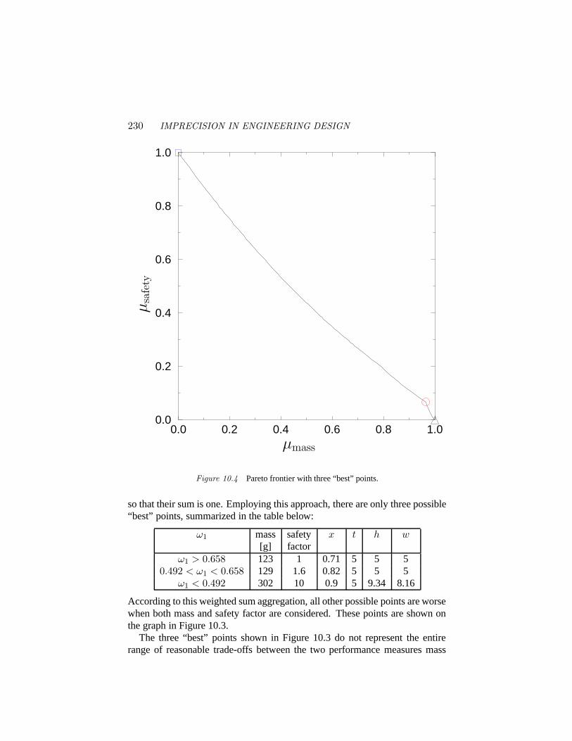
230 IMPRECISION IN ENGINEERING DESIGN
0.0 0.2 0.4 0.6 0.8 1.00.0
0.2
0.4
0.6
0.8
1.0
µmass
µsa
fety
Figure 10.4 Pareto frontier with three “best” points.
so that their sum is one. Employing this approach, there are only three possible“best” points, summarized in the table below:
ω1 mass safety x t h w[g] factor
ω1 > 0.658 123 1 0.71 5 5 50.492 < ω1 < 0.658 129 1.6 0.82 5 5 5
ω1 < 0.492 302 10 0.9 5 9.34 8.16
According to this weighted sum aggregation, all other possible points are worsewhen both mass and safety factor are considered. These points are shown onthe graph in Figure 10.3.
The three “best” points shown in Figure 10.3 do not represent the entirerange of reasonable trade-offs between the two performance measures mass
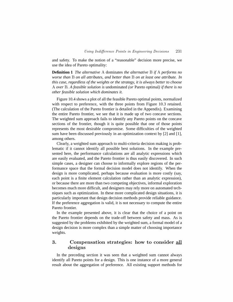
Using Indifference Points in Engineering Decisions 231
and safety. To make the notion of a “reasonable” decision more precise, weuse the idea of Pareto optimality:
Definition 1 The alternativeA dominatesthe alternativeB if A performs noworse thanB on all attributes, and better thanB on at least one attribute. Inthis case, regardless of the weights or the strategy, it is always better to chooseA overB. A feasible solution isundominated(or Pareto optimal) if there is noother feasible solution which dominates it.
Figure 10.4 shows a plot of all the feasible Pareto optimal points, normalizedwith respect to preference, with the three points from Figure 10.3 retained.(The calculation of the Pareto frontier is detailed in the Appendix). Examiningthe entire Pareto frontier, we see that it is made up of two concave sections.The weighted sum approach fails to identify any Pareto points on the concavesections of the frontier, though it is quite possible that one of those pointsrepresents the most desirable compromise. Some difficulties of the weightedsum have been discussed previously in an optimization context by [2] and [1],among others.
Clearly, a weighted sum approach to multi-criteria decision making is prob-lematic if it cannot identify all possible best solutions. In the example pre-sented here, the performance calculations are all analytic expressions whichare easily evaluated, and the Pareto frontier is thus easily discovered. In suchsimple cases, a designer can choose to informally explore regions of the per-formance space that the formal decision model does not identify. When thedesign is more complicated, perhaps because evaluation is more costly (say,each point is a finite element calculation rather than an analytic expression),or because there are more than two competing objectives, informal explorationbecomes much more difficult, and designers may rely more on automated tech-niques such as optimization. In these more complicated design situations, it isparticularly important that design decision methods provide reliable guidance.If the preference aggregation is valid, it is not necessary to compute the entirePareto frontier.
In the example presented above, it is clear that the choice of a point onthe Pareto frontier depends on the trade-off between safety and mass. As issuggested by the problems exhibited by the weighted sum, a formal model of adesign decision is more complex than a simple matter of choosing importanceweights.
3. Compensation strategies: how to consider alldesigns
In the preceding section it was seen that a weighted sum cannot alwaysidentify all Pareto points for a design. This is one instance of a more generalresult about the aggregation of preference. All existing support methods for
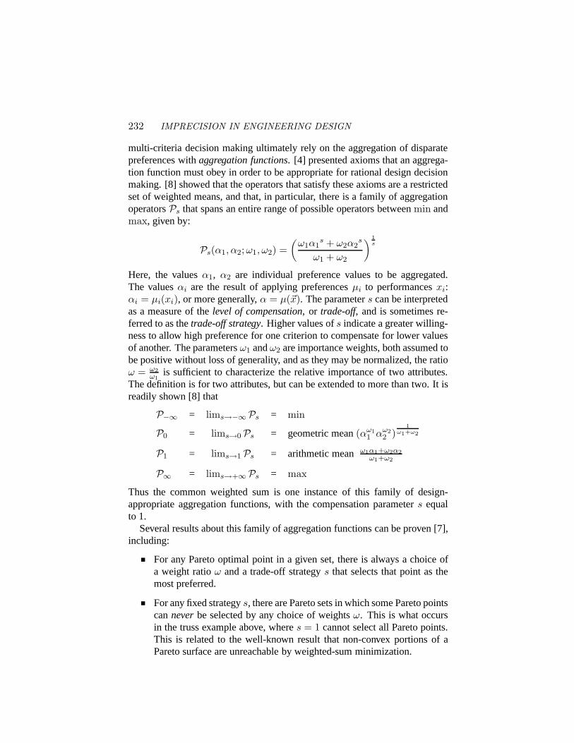
232 IMPRECISION IN ENGINEERING DESIGN
multi-criteria decision making ultimately rely on the aggregation of disparatepreferences withaggregation functions. [4] presented axioms that an aggrega-tion function must obey in order to be appropriate for rational design decisionmaking. [8] showed that the operators that satisfy these axioms are a restrictedset of weighted means, and that, in particular, there is a family of aggregationoperatorsPs that spans an entire range of possible operators betweenmin andmax, given by:
Ps(α1, α2;ω1, ω2) =(
ω1α1s + ω2α2
s
ω1 + ω2
) 1s
Here, the valuesα1, α2 are individual preference values to be aggregated.The valuesαi are the result of applying preferencesµi to performancesxi:αi = µi(xi), or more generally,α = µ(~x). The parameters can be interpretedas a measure of thelevel of compensation, or trade-off, and is sometimes re-ferred to as thetrade-off strategy. Higher values ofs indicate a greater willing-ness to allow high preference for one criterion to compensate for lower valuesof another. The parametersω1 andω2 are importance weights, both assumed tobe positive without loss of generality, and as they may be normalized, the ratioω = ω2
ω1is sufficient to characterize the relative importance of two attributes.
The definition is for two attributes, but can be extended to more than two. It isreadily shown [8] that
P−∞ = lims→−∞ Ps = min
P0 = lims→0 Ps = geometric mean(αω11 αω2
2 )1
ω1+ω2
P1 = lims→1 Ps = arithmetic meanω1α1+ω2α2ω1+ω2
P∞ = lims→+∞ Ps = max
Thus the common weighted sum is one instance of this family of design-appropriate aggregation functions, with the compensation parameters equalto 1.
Several results about this family of aggregation functions can be proven [7],including:
For any Pareto optimal point in a given set, there is always a choice ofa weight ratioω and a trade-off strategys that selects that point as themost preferred.
For any fixed strategys, there are Pareto sets in which some Pareto pointscanneverbe selected by any choice of weightsω. This is what occursin the truss example above, wheres = 1 cannot select all Pareto points.This is related to the well-known result that non-convex portions of aPareto surface are unreachable by weighted-sum minimization.
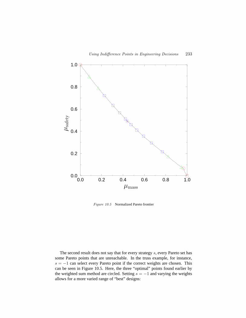
Using Indifference Points in Engineering Decisions 233
0.0 0.2 0.4 0.6 0.8 1.00.0
0.2
0.4
0.6
0.8
1.0
µmass
µsa
fety
Figure 10.5 Normalized Pareto frontier
The second result does not say that for every strategys, every Pareto set hassome Pareto points that are unreachable. In the truss example, for instance,s = −1 can select every Pareto point if the correct weights are chosen. Thiscan be seen in Figure 10.5. Here, the three “optimal” points found earlier bythe weighted sum method are circled. Settings = −1 and varying the weightsallows for a more varied range of “best” designs:
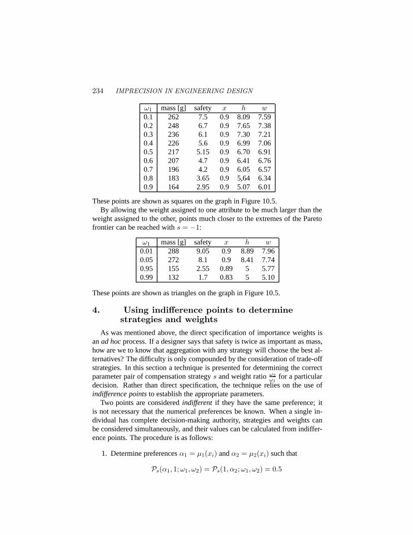
234 IMPRECISION IN ENGINEERING DESIGN
ω1 mass [g] safety x h w0.1 262 7.5 0.9 8.09 7.590.2 248 6.7 0.9 7.65 7.380.3 236 6.1 0.9 7.30 7.210.4 226 5.6 0.9 6.99 7.060.5 217 5.15 0.9 6.70 6.910.6 207 4.7 0.9 6.41 6.760.7 196 4.2 0.9 6.05 6.570.8 183 3.65 0.9 5,64 6.340.9 164 2.95 0.9 5.07 6.01
These points are shown as squares on the graph in Figure 10.5.By allowing the weight assigned to one attribute to be much larger than the
weight assigned to the other, points much closer to the extremes of the Paretofrontier can be reached withs = −1:
ω1 mass [g] safety x h w0.01 288 9.05 0.9 8.89 7.960.05 272 8.1 0.9 8.41 7.740.95 155 2.55 0.89 5 5.770.99 132 1.7 0.83 5 5.10
These points are shown as triangles on the graph in Figure 10.5.
4. Using indifference points to determinestrategies and weights
As was mentioned above, the direct specification of importance weights isanad hocprocess. If a designer says that safety is twice as important as mass,how are we to know that aggregation with any strategy will choose the best al-ternatives? The difficulty is only compounded by the consideration of trade-offstrategies. In this section a technique is presented for determining the correctparameter pair of compensation strategys and weight ratioω2
ω1for a particular
decision. Rather than direct specification, the technique relies on the use ofindifference pointsto establish the appropriate parameters.
Two points are consideredindifferent if they have the same preference; itis not necessary that the numerical preferences be known. When a single in-dividual has complete decision-making authority, strategies and weights canbe considered simultaneously, and their values can be calculated from indiffer-ence points. The procedure is as follows:
1. Determine preferencesα1 = µ1(xi) andα2 = µ2(xi) such that
Ps(α1, 1;ω1, ω2) = Ps(1, α2;ω1, ω2) = 0.5
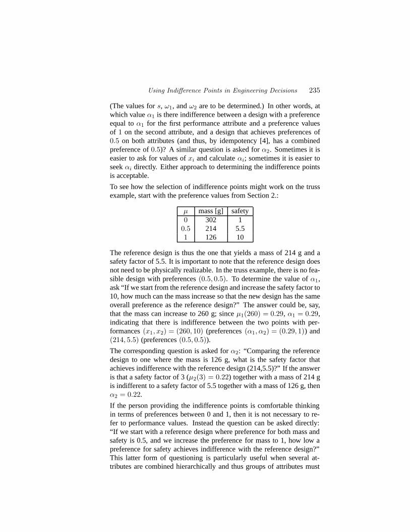
Using Indifference Points in Engineering Decisions 235
(The values fors, ω1, andω2 are to be determined.) In other words, atwhich valueα1 is there indifference between a design with a preferenceequal toα1 for the first performance attribute and a preference valuesof 1 on the second attribute, and a design that achieves preferences of0.5 on both attributes (and thus, by idempotency [4], has a combinedpreference of0.5)? A similar question is asked forα2. Sometimes it iseasier to ask for values ofxi and calculateαi; sometimes it is easier toseekαi directly. Either approach to determining the indifference pointsis acceptable.
To see how the selection of indifference points might work on the trussexample, start with the preference values from Section 2.:
µ mass [g] safety0 302 1
0.5 214 5.51 126 10
The reference design is thus the one that yields a mass of 214 g and asafety factor of 5.5. It is important to note that the reference design doesnot need to be physically realizable. In the truss example, there is no fea-sible design with preferences(0.5, 0.5). To determine the value ofα1,ask “If we start from the reference design and increase the safety factor to10, how much can the mass increase so that the new design has the sameoverall preference as the reference design?” The answer could be, say,that the mass can increase to 260 g; sinceµ1(260) = 0.29, α1 = 0.29,indicating that there is indifference between the two points with per-formances(x1, x2) = (260, 10) (preferences(α1, α2) = (0.29, 1)) and(214, 5.5) (preferences(0.5, 0.5)).The corresponding question is asked forα2: “Comparing the referencedesign to one where the mass is 126 g, what is the safety factor thatachieves indifference with the reference design (214,5.5)?” If the answeris that a safety factor of 3 (µ2(3) = 0.22) together with a mass of 214 gis indifferent to a safety factor of 5.5 together with a mass of 126 g, thenα2 = 0.22.
If the person providing the indifference points is comfortable thinkingin terms of preferences between 0 and 1, then it is not necessary to re-fer to performance values. Instead the question can be asked directly:“If we start with a reference design where preference for both mass andsafety is 0.5, and we increase the preference for mass to 1, how low apreference for safety achieves indifference with the reference design?”This latter form of questioning is particularly useful when several at-tributes are combined hierarchically and thus groups of attributes must

236 IMPRECISION IN ENGINEERING DESIGN
be compared. It is always possible, even in hierarchical aggregation, tospecify particular values of all performance attributes in order to specifyindifference points.
2. Letω = ω2ω1
.
3. If α1 = α2, thenω = 1:
(a) If α1 = 0.5, thens = −∞.
(b) If α1 = 0.25, thens = 0.
(c) If α1 > 0.25, thens ∈ (−∞, 0). Solveα1s + 1 = 2(0.5)s numer-
ically.
(d) If α1 < 0.25, thens ∈ (0,∞). Solveα1s + 1 = 2(0.5)s numeri-
cally.
4. If α1 6= α2, thenω 6= 1. Note that ifs = 0:
α1m = 0.5 = α2
1−m ⇒ α21−logα1
0.5 = 0.5
Thus:
(a) If α21−logα1
0.5 = 0.5, thens = 0, andb =1−logα1
0.5logα1
0.5
(b) If α21−logα1
0.5 > 0.5, thens < 0.If α2
1−logα10.5 < 0.5, thens > 0.
Solve numerically fors from
(1 + ωα2
s
1 + b
) 1s
=(
α1s + ω
1 + ω
) 1s
= 0.5
which reduces to
(α1s − 0.5s) (α2
s − 0.5s) = (1 − 0.5s)2
Once this is solved numerically fors, thenω can also be deter-mined.
Applying steps 2–4 to the indifference valuesα1 = 0.29 andα2 = 0.22 de-termined above, the parameters that determine the aggregation are found tobe:
s∗ = −0.5 ω∗ = 1.23, or (ω1, ω2) = (0.45, 0.55)
The best point on the Pareto frontier for that trade-off is:
mass [g] safety α1 α2 x t h w223 5.45 0.44 0.49 0.9 5 6.90 7.01
Using Indifference Points in Engineering Decisions 237
Note that this best point depends only on the preferences for safety and mass,and on the answers given above to the two indifference questions. Also notethat this point, which is shown as a star on the graph in Figure 10.5, is in-tuitively appealing as an overall optimum, while the points provided by theweighted sum method are not.
It should be noted that if eitherα1 or α2 is close to0, then the(s, ω) pairis quite sensitive to small differences inα1 andα2. In these cases, it might bepreferable to elicit other indifference points to determines andω. In the pro-cedure described above, points that are equivalent to(0.5, 0.5) are chosen; theprocedure can easily be modified to consider indifference to some other refer-ence point. Indeed, if the procedure is applied more than once with differentreference points, the redundant information serves as a check on the accuracyof the specification.
5. ConclusionWeighted sum aggregation with importance weights is common to many
methods for engineering design decision making. Two important difficul-ties with these methods are the inability of weighted-sum methods to selectall Pareto points, and the arbitrary nature of direct assignment of importanceweights.
It is shown here that a complete model of an engineering decision dependsnot only on the importance weights, but also on the level of compensation, ortrade-off strategy. A weighted sum, or any other pre-determined aggregationprocedure, is overly and inappropriately constraining. The appropriate strategy(or degree of compensation among attributes) is situation-dependent, and a“one-size-fits-all” decision method that dictates an aggregation method canlead to incorrect results. An easily computed family of preference aggregationfunctions is completely determined by two parameters that represent the trade-off strategy (degree of compensation) and the importance weighting.
The choice of strategy and importance weights, or even the choice of im-portance weights alone, can bead hocand arbitrary if accomplished by directspecification. A simple procedure is presented, along with straightforward cal-culations, to establish the proper importance weights and degree of compensa-tion to reach rational engineering decisions.
The results in this paper regarding decision methods are related to previ-ously known results about multi-criteria optimization [2, 1]. The preferenceaggregation operators presented here could be used to explore a non-convexPareto frontier. From an optimization point of view, once an aggregated pref-erence function (or utility function) is determined, locating the optimum isstraightforward. If some point lies on a non-convex region of a Pareto frontier,and a utility function is constructed using a weighted sum, then that point is an

238 IMPRECISION IN ENGINEERING DESIGN
inferior point. From a design decision point of view, however, it is appropri-ate to question the choice of a weighted sum to aggregate the preferences. Themethod presented in this paper, unlike a weighted sum, has the great advantagethat it does nota priori exclude any Pareto points from consideration. Thus,if the aggregated preference is optimized, the selected “optimum” is actuallywhat the designer desires, and is not artificially constrained by the geometry ofthe design and performance spaces.
AcknowledgementsThis material is based upon work supported, in part, by the National Science
Foundation under NSF Grant Number DMI-9813121. Any opinions, findings,conclusions, or recommendations expressed in this publication are those of theauthors and do not necessarily reflect the views of the sponsors.
Using Indifference Points in Engineering Decisions 239
References
[1] CHEN, W., WIECEK, M., AND ZHANG, J. Quality utility - a compromiseprogramming approach to robust design.ASME Journal of MechanicalDesign 121, 2 (1999), 179–187.
[2] DAS, I., AND DENNIS, J. A closer look at drawbacks of minimizingweighted sums of objectives for pareto set generation in multicriteria opti-mization problems.Structural Optimization 14, 1 (1997), 63–69.
[3] HAUSER, J., AND CLAUSING, D. The House of Quality.Harvard Busi-ness Review 66, 3 (May/June 1988), 63–73.
[4] OTTO, K. N., AND ANTONSSON, E. K. Trade-Off Strategies in Engi-neering Design.Research in Engineering Design 3, 2 (1991), 87–104.
[5] PUGH, S. Total Design. Addison-Wesley, New York, NY, 1990.
[6] SAATY, T. L. The Analytic Hierarchy Process: Planning, Priority Setting,Resource Allocation. McGraw Hill, New York, NY, 1980.
[7] SCOTT, M. J. Formalizing Negotiation in Engineering Design. PhD thesis,California Institute of Technology, Pasadena, CA, June 1999.
[8] SCOTT, M. J.,AND ANTONSSON, E. K. Aggregation Functions for Engi-neering Design Trade-offs.Fuzzy Sets and Systems 99, 3 (1998), 253–264.
[9] WOOD, K. L., AND ANTONSSON, E. K. Computations with ImpreciseParameters in Engineering Design: Background and Theory.ASME Jour-nal of Mechanisms, Transmissions, and Automation in Design 111, 4 (Dec.1989), 616–625.

240 IMPRECISION IN ENGINEERING DESIGN
A Appendix: Details of the Truss ExampleHere are the details for the example of the bracket shown in Figure 10.1.
Material properties and performance measuresThe material is aluminum (6061-T6), which has the following relevant ma-
terial properties:
Young’s modulus (E) 69 · 109 PaDensity (ρ) 2660 kg/m3
Yield stress (σ) 275 · 106 Pa
There are four design variables:
x ∈ [0.1 m, 0.9 m] distance from wall to pint ∈ [5 mm, 20 mm] thickness of bending memberh ∈ [5 mm, 20 mm] height of bending memberw ∈ [5 mm, 20 mm] width of (square) compression member
The first performance measure is total mass (in kilograms, here, so the loadP below is equal to 1):
M = ρ
(htL + w2
√x2 + y2
)= 2660
(ht + w2
√x2 + 0.25
)
The safety factorS has two components, the safety factor for the bending mem-berSb , and the safety factor for the compression memberSc. Since the yieldstress in the bending member isσ, and the maximum stress in the bendingmember is12P (L−x)
th2 , the factor of safety in bending is the ratio:
Sb =σth2
12P (L − x)=
σth2
120(1 − x)
Similarly, using the Euler buckling load, the safety factor in the compressionmember is:
Sc =π2Exyw4
12PL(x2 + y2)1.5 =π2Exyw4
120(x2 + 0.25)1.5
The safety factor for the entire design is defined to be the minimum of the two:
S = min
(σth2
120(1 − x),
π2Exyw4
120(x2 + 0.25)1.5
)

Using Indifference Points in Engineering Decisions 241
100 150 200 250 300 3501
2
3
4
5
6
7
8
9
10
infeasibleregion
feasibleregion
mass [g]
safe
tyfa
cto
r
Figure A.1 Pareto frontier of best performances

242 IMPRECISION IN ENGINEERING DESIGN
Calculation of the Pareto frontierThe design problem is to minimize the mass while maximizing the factor
of safety; both are analytic expressions. First, note that mass is linear in botht andh, while the factor of safety in bending is linear int but quadratic inh. Thus, as long as no other design variables reach the maximum acceptabledimensions, it will always be preferable to increaseh rather thant. Settingt = tmin = 5 mm reduces the problem to the three design variablesx, h, andw. Bothh andw can be expressed as functions ofx and a safety factor, and thusfinding the minimum possible mass for a given safety factor requires solving arational equation inx. These solutions yield a Pareto frontier of designs, whichis shown in Figure A.1.
The values ofx, h, andw which generate these optimal designs are includedin Figure A.2. It can be seen from Figure A.2 that at each Pareto point, at leastone domain constraint is active: in particular, for low mass,h takes its mini-mum acceptable value of 5 mm, while for higher mass,x takes its maximumacceptable value of 0.9 m. Nevertheless, along most of the Pareto frontier twodesign variables are changing as the frontier is traversed.
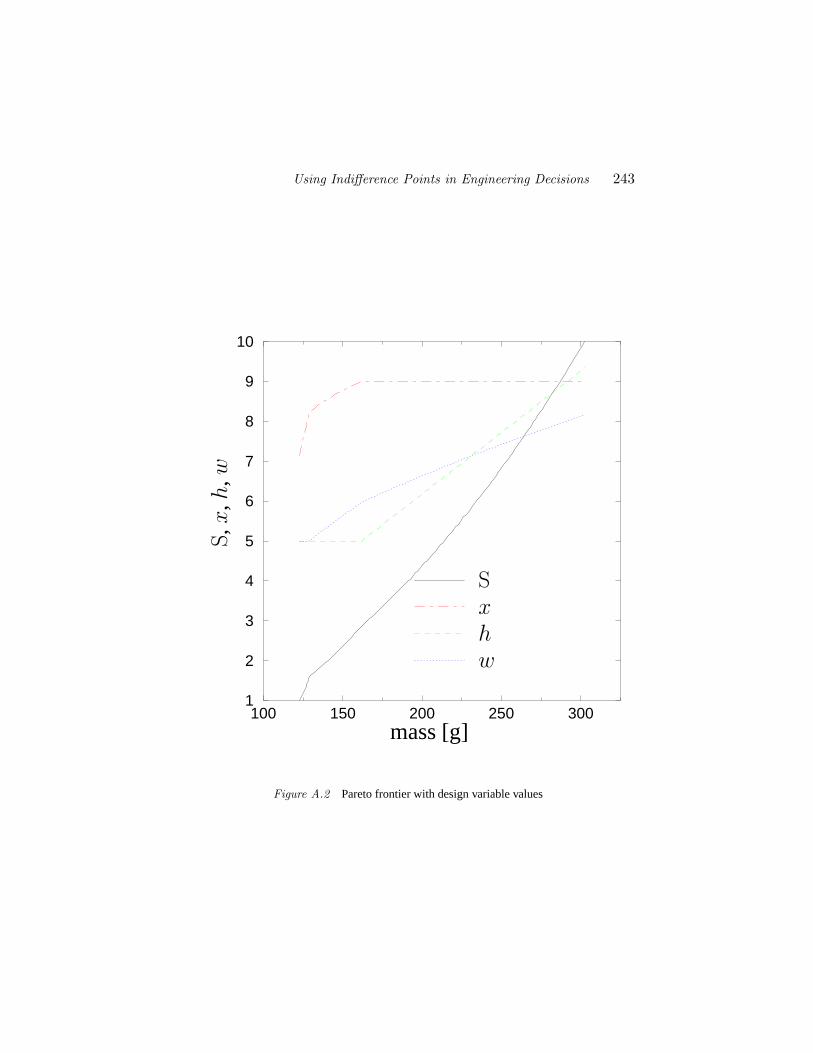
Using Indifference Points in Engineering Decisions 243
100 150 200 250 3001
2
3
4
5
6
7
8
9
10
mass [g]
Sxhw
S,x
,h,w
Figure A.2 Pareto frontier with design variable values