Embed Size (px)
Citation preview
Instructions for use
Title Importance of outer reef slopes for commercially important fishes: implications for designing a marine protected area inthe Philippines
Author(s) Honda, Kentaro; Uy, Wilfredo H.; Baslot, Darwin I.; Pantallano, Allyn Duvin S.; Sato, Masaaki; Nakamura, Yohei;Nakaoka, Masahiro
Citation Fisheries science, 83(4), 523-535https://doi.org/10.1007/s12562-017-1082-4
Issue Date 2017-07
Doc URL http://hdl.handle.net/2115/71161
Rights The final publication is available at www.springerlink.com via http://dx.doi.org/10.1007/s12562-017-1082-4
Type article (author version)
File Information Fisheries science_83 (4)_523-535.pdf
Hokkaido University Collection of Scholarly and Academic Papers : HUSCAP

1
Importance of outer reef slopes for commercially important fishes: implications for designing a marine
protected area in the Philippines
Kentaro Honda1, 2,*, Wilfredo H. Uy3, Darwin I. Baslot3, Allyn Duvin S. Pantallano3, 4, Masaaki Sato1, 5,
Yohei Nakamura4, and Masahiro Nakaoka1
1 Akkeshi Marine Station, Field Science Center for Northern Biosphere, Hokkaido University; Aikappu, Akkeshi,
Hokkaido 088-1114, Japan
2 Present address: Hokkaido National Fisheries Research Institute, Japan Fisheries Research and Education
Agency; 2-2 Nakanoshima, Toyohira-ku, Sapporo, Hokkaido 062-0922, Japan
3Institute of Fisheries Research and Development, Mindanao State University at Naawan; 9023 Naawan, Misamis
Oriental, Philippines
4 Graduate School of Kuroshio Science, Kochi University; 200 Monobe, Nankoku, Kochi 783-8502, Japan
(Present address of Pantallano ADS)
5 Present address: National Research Institute of Fisheries and Environment of Inland Sea, Japan Fisheries
Research and Education Agency; Maruishi 2-17-5, Hatsukaichi-shi, Hiroshima 739-0452, Japan
*Corresponding author: [email protected]
2
Abstract A passive acoustic telemetry survey was conducted to determine occurrence patterns of commercially
important fishes on a steep reef slope along a marine protected area (MPA) in the southern Philippines, where the
outer reef edge is often set as an offshore MPA boundary. Based on 4–61 days of tracking data from 21 detected
individuals from five species (Lutjanus argentimaculatus, Lutjanus monostigma, Lethrinus atkinsoni, Lethrinus
obsoletus, and Siganus guttatus; 20.7–69.2 cm fork length) caught near the reef slope of the MPA, S. guttatus
occurred most frequently on the reef flat of the MPA, whereas all individuals of the four lutjanid and lethrinid
species were primarily (99.4–100%) detected near the reef slope, and nine individuals (56.3% of the four species)
belonging to three species (other than L. obsoletus) most likely used the shallow (≤10 m) and deep (≥20 m) layers
and thus, those middle layer of the slope. These findings indicate that commercially important lutjanid and
lethrinid species predominantly and vertically used the areas near the reef slope, suggesting the importance of
fully including reef slopes in MPAs to enhance their effectiveness by conserving such fishes.
Keywords Acoustic telemetry, Commercially important fish, Coral reef, Depth use, Marine protected area, Reef
slope,
3
Introduction
A fringing coral reef is generally composed of an inner reef flat and an outer reef edge and slope. Offshore
boundaries of marine protected areas (MPAs) established on fringing reefs are often set along outer reef edges
(e.g., [1–3]) without exception in the Philippines (Philippine MPA Database: www.mpa.msi.upd.edu.ph,
Accessed January 2016). Thus, deeper areas of the reef slope are not included in such MPAs and have been used
by fishermen as fishing grounds (e.g., [4–6]). The boundary is set along the outer reef edge because the edges are
easily recognized navigational landmarks used by fishermen [7] and because conservation benefits to mobile
species are expected to be enhanced by limiting “spillover” [8, 9] into unprotected areas if the habitat is restricted
by a natural MPA boundary such as a reef edge [10–12].
However, the negative effect of intensive fishing along the MPA boundary known as “fishing the line”
is a concern on conservation of fisheries resources [13–16]. In the Philippines, deeper areas of reef slope just
outside the MPA boundary are often used by fishermen as fishing grounds and such fishing the line is suggested
to decrease MPA effectiveness [17]. Therefore, if many commercially important fishes frequently move between
inner shallow reefs (inside MPAs) and outer deep reef slopes (outside MPAs) or if such fishes only use the slopes
as their main habitat, fully including slopes inside the MPAs would help conservation efforts. However, little is
known about the occurrence patterns of fishes along reef slopes (but see [18–20]).
In this study, we targeted five commercially important and mobile reef-associated fishes (members of
the families Lutjanidae, Lethrinidae, and Siganidae) captured near the reef edge of a no-take MPA in the southern
Philippines, where the edge contains a steep reef slope and is set as an offshore MPA boundary. We assessed their
occurrence patterns near the slope using passive acoustic telemetry, particularly focusing on their vertical depth
use.
4
Materials and methods
Study site and acoustic receiver array
The field survey was conducted from August 2012 to October 2013 on a fringing reef with the reef flat zone facing
the open sea off Laguindingan, northern Mindanao Island, the Philippines (Fig. 1). Here, a no-take MPA with a
total area of 0.31 km2 (length from shore side to offshore side: ca. 760 m, width: 360–450 m) has been allocated
since 2002. The seascape composition of the MPA included near-shore mangroves, a seagrass bed, and an offshore
coral reef. The coral reef was composed of hermatypic corals, such as tabular and branching Acropora (living
coral coverage >80%). The seagrass bed and mangroves at the site have been described in Honda et al. [21]. The
offshore boundary of the MPA is set along the reef edge consisting of a steep reef slope, with bottom depth along
the slope of 20–30 m. The horizontal distance between the shallowest and deepest parts along the slope was
generally <5 m. This MPA has been strictly regulated since its establishment in 2002 through an installation of a
watchtower. Fishing the line by hook-and-line is operated legally and regularly along the reef edge of this MPA
(authors’ pers. comm., 2011; Fig. 1b).
Twelve acoustic receivers (VR2W; Vemco, Shad Bay, NS, Canada) were deployed at 12 stations located
on the coral reef (on a reef flat and the top and bottom of a reef slope) inside or outside the MPA, as shown in Fig.
1. The stations where receivers were deployed on the reef flat are described from west to east as flat1–flat4,
whereas stations at the top and bottom along the reef slope are described as shallow1–shallow4 and deep1–deep4,
respectively. Flat2, flat3, shallow2, and shallow3 were located inside the MPA, whereas the remaining stations
were located outside the MPA (Fig. 1). Bottom depths at the “flat” stations were 1.0–1.5 m at low tide and 2.0–

5
2.5 m at high tide. When deployed, those at the “shallow” stations (shallow1–shallow4) were 6, 9, 5, and 10 m
whereas those at the “deep” stations (deep1–deep4) were 23, 26, 29, and 29 m. However, depth fluctuated
depending on the tide. Receivers were deployed in small sandy patches at the flat stations using a concrete anchor,
rope, and a buoy. The bottom of each receiver was placed 0.5 m away from the anchor, and the buoy was placed
1 m away from the tip of the receiver. Receivers at the shallow and deep stations were deployed using aluminum
cable and two buoys. The cable was locked to coral or rocks at the shallow stations or to a concrete anchor at the
deep stations. The bottom of each receiver was placed 1.5 m away from the locked point (shallow stations) or the
anchor (deep stations), and the buoys were placed at least 2 m away from the tip of the receiver. All receivers
were deployed from 25 August to 26 November 2012 and from 22 May to 10 October 2013.
The detection ranges of the receivers fluctuated depending on bottom topography and sea conditions,
such as depth, tide, wave action, and wind speed (e.g., [22–24]). Based on the results of Honda et al. [25], who
studied the same site using passive acoustic telemetry and real-time detection, the detection ranges of the receivers
were in a radius of 40–120 m at the flat stations, 50–150 m at the shallow stations, and 60–180 m at the deep
stations.
Fish capture and tagging
All fish were caught inside or along the offshore boundary (reef slope) of the MPA. The target species were
Lutjanus argentimaculatus, Lutjanus monostigma (Lutjanidae), Lethrinus atkinsoni, Lethrinus obsoletus
(Lethrinidae), and Siganus guttatus (Siganidae). These species are listed as “commercial fish” on FishBase
(www.fishbase.org, Accessed January 2016) and are regarded as common commercial targets at our study site
(authors’ pers. comm., 2011).
6
We used hook-and-line and box-shaped fish traps, locally called bubo. Five S. guttatus [20.7–27.9 cm
fork length (FL)] were caught by the former method on reef flats and shallow reef slope inside the MPA, whereas
the remaining four species were caught in traps [two Lutjanus argentimaculatus (34.2 and 69.2 cm FL), 15 L.
monostigma (24.5–41.4 cm FL), five Lethrinus atkinsoni (21.6–24.8 cm FL), and one L. obsoletus (27.9 cm FL);
Table 1]. All traps were located on the sandy bottom next to the reef slope of the MPA, at depths of 25–30 m, and
were retrieved after 7–14 days of deployment. Traps that contained fish were not recovered immediately but were
transferred to shallower depths for 2–3 days to allow the fish to decompress. The captured fish were placed
immediately in an aerated tub on the boat before being carried to a fish cage (ca. 1.5 m long × 1.5 m wide × 1.5
m high) installed near the watchtower (Fig. 1a). To allow the fish to recover from the stress of being caught, the
fish-tagging operation started 1 h after the fish were caged. Fish were transferred to a tank before tagging and
treated with an anesthetic mixture of 0.012‰ eugenol and seawater. After immobilization, a latex-covered coded
acoustic transmitter (V8-4L, V9-2H, V9P-6L, or V13-1L; Vemco) was implanted surgically into the abdominal
cavity of each fish (Table 1). The V8, V9, V9P, and V13 transmitters were 8, 9, 9, and 13 mm in diameter and
20.5, 29.0, 39.0, and 36.0 mm in length and weighed 2.0, 4.7, 4.6, and 11.0 g, respectively. The expected battery
lives were 47, 53, 48, and 339 days and their power outputs were 146 (for the V8) and 147 dB (for others) re 1μPa
at 1 m. Fish with a lower power transmitter might have potentially been less detected than fish with higher power
tags. The frequency for all transmitter types was 69 kHz, and they randomly transmitted a set of six coded pulses
once every 20–40 s. Only the V9P transmitter had a pressure (depth) sensor and transmitted depth data as well.
Of all 28 tagged individuals, 25 fish were equipped with a transmitter without a depth sensor, while the remaining
three were equipped with the V9P transmitter. After the transmitter was implanted, the fish were sutured with
biodegradable silk, and an antibiotic ointment was applied to the incision. The size of each fish was measured
before being placed back in the cage. The proportion of transmitter weight to fish body weight was 0.10–1.96%
7
(Table 1). After all fish recovered from the tagging operation for ca. 30 min, they were released near the
watchtower at depths of 1–2 m (Fig. 1).
Individual fish were given identifiers based on their abbreviated species name and replicate fish number
continued from Honda et al. [25] (see Table 1). Moreover, two L. monostigma [Lu-mo5 and Lu-mo7 (37.3 and
41.4 cm FL, respectively when tagged on 10 and 19 May 2012)] tracked in Honda et al. [25] were included
because the batteries in their attached transmitters remained active.
Data analyses
In this study, considering the negative effect of tagging stress, detection data obtained within 24 h after release
were excluded from analyses. Simultaneous detections by multiple receivers (e.g., flat1 and flat2, shallow3 and
deep3) were counted as one detection. The individual residence index [26], defined as the quotient between the
number of days detected and the period between 1 day after release and the last detection date (tracking period),
was calculated to determine how frequently each tracked fish was certainly present in the fixed array [27].
The detections were grouped into five categories based on locational characteristics: 1. reef flat inside
the MPA (flatIN: detections by flat2 or flat3 and simultaneous detections between these two stations and between
flat2 or flat3 and shallow2 or shallow3); 2. reef slope near the MPA (slopeIN: detections by shallow2, shallow3,
deep2, or deep3 and simultaneous detections among these four stations); 3. reef flat outside the MPA (flatOUT:
detections by flat1 or flat4 and simultaneous detections between flat1 and shallow1 and between flat4 and
shallow4); 4. reef slope outside the MPA (slopeOUT: detections by shallow1, deep1, shallow4, or deep4 and
simultaneous detections between the former two stations and between the latter two stations); and 5. others
[simultaneous detections between stations inside and outside the MPA (e.g., shallow1 and deep2)]. This
8
categorization was adopted because accurate fish home ranges could not be estimated using our study design (i.e.,
fish full home ranges were not encompassed by the receivers’ array), and thus we aimed to grasp their approximate
horizontal occurrence pattern by calculating individual detection frequencies of these five categories.
Depths ≤10 m were defined as the shallow layer because the depth of the reef edge was 5–10 m; thus,
fish at these depths were assumed to occur near or on the edge. Depths ≥20 m were defined as the deep layer
because the bottom depth along the reef slope was 20–30 m; thus, fish at depths ≥20 m were assumed to occur
along the reef slope or on the bottom off the slope. If a tagged fish was detected at flatIN and/or flatOUT two or
more times (considering the false detections [28]), such a fish was defined to be using shallow layer.
For the three fish equipped with a V9P transmitter (henceforth, fish with a depth sensor), time-series
detected depths dividing them into slopeIN and other four categories were shown. Individual vertical kernel
utilization distributions (vKUDs) were estimated in each time period (day, twilight, and night) using ks package
[29] in R version 3.3.1. Here, twilight duration was regarded as 4 h (2 h each around sunrise and sunset), and day
and night comprised the remainder of the day. Sunrise and sunset were determined from Sunrise, sunset, moonrise
and moonset times (www.sunrisesunsetmap.com, Accessed September 2015). The vKUDs were illustrated in a
linear two-dimensional space to determine the vertical use along the reef slope using average positions [30]. The
average positions were calculated every 10 min interval for vertical space use following Currey et al. [18]. In this
analysis, we only used detections obtained at shallow and deep stations. The number of movements between the
shallow and deep layers (N of shallow-deep movement) were counted individually, and the daily mean values
were calculated. Here, shallow-deep movement was defined as ascending or descending between the last detected
station in the deep (shallow) layer and the first detected next station in the shallow (deep) layer within 24 h, and
the time of the shallow-deep movement was defined as the intermediate value of the movement. The daily mean
N of shallow-deep movement was defined as the quotient between total N of shallow-deep movements and the
9
number of days detected. Time-length frequency of ascents and descents and their hourly frequencies using only
<1 h time-length data were calculated to examine diel vertical-movement patterns. Difference in detectability in
receivers at different times of the day (see [31]) might have affected on the N of shallow-deep movements.
Use of shallow and/or deep depth layers by the 25 fish without a depth sensor was estimated in the
following manner. First, the 10-m interval detection frequencies of each receiver at each pair of shallow and deep
stations (e.g., shallow1 and deep1) and those of their simultaneous detections (by the same fish) were calculated
using the detection data of three fish with a depth sensor. Here, because only one fish with a depth sensor was
detected once at >60 m depth according to the results, we defined 60 m as the maximum detectable practical depth
in this analysis. Second, if there was a trend that fish at shallower depths were detected more frequently by a
shallow receiver and vice versa for fish at deeper depths, detection probabilities at three depth layers (0–10 m,
10–20 m, and 20–60 m) at each shallow and deep station and by their simultaneous detections by each pair of
stations were calculated based on the detection frequencies. Third, if the detection probability by shallow or deep
receivers at shallow (0–10 m) or deep (20–60 m) depth layers was high (>80%), respectively, fish in the
corresponding depth layer were considered to be detected with high likelihood at the station. We counted the total
number of detections by each individual only at such stations. Finally, if the summed numbers of detections by a
fish at the shallow or deep stations exceeded 50 (liberal estimate), such a fish was considered to have occurred
one or more times at the shallow or deep depth layer. All of our target species were visually observed at <10 m
depth on the coral reef inside the MPA [21, 25, Honda, personal observation].
Results
10
A total of 160,371 detections originating from 21 of the 28 tagged fish were recorded during the study (Table 1).
Although the tracking periods of six fish (Lu-mo5, Lu-mo11, Le-at8, Si-gu9, Si-gu10, and Si-gu11) lasted 10 or
less days, 11 fish from four lutjanid and lethrinid species were tracked for 30 or more days (Table 1). The mean
residence index (± standard deviation) of all tracked fish was 0.75 ± 0.29, and the indices of 13 (61.9% of all
tracked fish) individuals were 0.75–1.00 (Table 1).
Although Lu-ar6, Lu-mo19, and Le-ob3 were observed at very low detection rates [0.04% (n = 15),
0.02% (n = 1), and 0.61% (n = 63) of all detections, respectively] at flat stations, no other individuals, except
Siganus guttatus, was detected at those stations. In contrast, although Si-gu10 was detected at deep stations [1.92%
(n = 7)], no other S. guttatus individuals were detected at those stations. The detection frequencies of all tracked
lutjanid and lethrinid individuals mostly (98.5–100%) consisted of slopeIN and slopeOUT (Fig. 2). The mean (±
standard deviation) frequency at the former was 69.5 ± 35.4%, and the frequency for 10 fish (62.5%) exceeded
80%. Whereas those of S. guttatus were mostly (99.8–100%) consisting of flatIN and slopeIN, and its frequency
at the former for three fish (Sigu7, Si-gu8, and Si-gu11) were high (97.9%, 92.5%, and 93.5%, respectively; Fig.
2).
Depth-use patterns by fish with a depth sensor
Each fish showed distinct and wide-ranging depth-use patterns (Fig. 3). Lu-ar6 gradually shifted to deeper layers
between 10 and 30 m as the 14 days (26 May–8 June 2013) elapsed soon after tracking started (Fig. 3, upper).
Then, the fish stayed mainly at ≤10 m depth and occasionally descended to 30–50 m. The shallowest and deepest
depths recorded by Lu-ar6 were 0.0 and 48.4 m, respectively. For this fish, the vertical core area (50% vKUD)
and its extent (95% vKUD) ranged mainly 0–10 m and 0–25 m depths, respectively, regardless of time periods
11
(Fig. 4, upper). The 50% vKUD only ranged near the reef slope along the MPA during the day and twilight,
whereas during the night that also ranged outside the MPA. The total N of shallow-deep movements by Lu-ar6
was 120, and its mean daily N was 2.55. Time-length frequencies of both ascents and descents were the highest
in 0–5 min, and those within 1 h occupied 84.2% and 77.1%, respectively (Fig. 5a, upper). Hourly movement
frequencies became higher during 3:00–5:00 and 12:00–13:00 regardless of ascent or descent and any other
remarkable trends were not observed during other time periods (Fig. 5b, upper).
Lu-mo19 exhibited wide-ranging vertical movements between the surface and ca. 60 m depth over 6
days (9–14 June 2013) soon after tracking started (Fig. 3, lower-left). Then, the fish was detected continuously
only in the shallow layer for 11 days (15–25 June), followed by depth-use patterns similar to those observed
during the first 6 days. The shallowest and deepest depths recorded were 0.6 and 58.2 m, respectively. This fish
exhibited similar vertical space use patterns during the day and twilight as those by Lu-ar6 although the 50%
vKUD was relatively wider and deeper (Fig. 4, middle). However, both the 50% and 95% vKUDs during the night
showed distinct patterns that the former was separated into two areas either one above 30 m depth and the other
at 40–50 m and that the latter ranged widely from surface to 60 m. Nonetheless, the 50% vKUDs were mostly
distributed near the slope along the MPA in any of time periods. Total and daily mean N values of shallow-deep
movements by Lu-mo19 were 148 and 3.08, respectively. Similar to Lu-ar6, high frequencies of ascents (88.9%)
and descents (76.7%) were recorded within 1 h (Fig. 5a, middle). The peak of descents was observed during
18:00–21:00 and was five hours earlier than that of ascents (i.e., 23:00–2:00; Fig. 5b, middle). Both ascents and
descents were less observed during daytime; in particular, no movement was recorded from 13:00 to 18:00.
Lu-mo20 did not occur near the surface (0–5 m depth) at all and mainly occurred at 10–30 m (Fig. 3,
right). The fish descended to deeper layers (>40 m) several times, and the shallowest and deepest depths recorded
were 8.5 and 61.3 m, respectively. Unlike Lu-ar6 or Lu-mo19, vertical space use by Lu-mo20 was almost limited
12
to near deep1 (Fig. 4, lower) although the 95% vKUD tended to become larger as it became darker. Total N of
shallow-deep movements by Lu-mo20 was 14, which was much lower than that of Lu-ar6 or Lu-mo19, although
the number of days detected did not differ among the three fish (47, 48, and 50 days for Lu-ar6, Lu-mo19, and
Lu-mo20, respectively). The daily mean N of shallow-deep movements was 0.28, and most of them were recorded
during daytime (Fig. 5b, lower).
Estimate of depth use by fish without a depth sensor
The 10-m detection frequency of each receiver at each pair of stations near the slope and that of simultaneous
detections by each pair of receivers obtained by the three fish with a depth sensor is shown on Fig. 6a. Fish that
occurred in the 0–10 m depth layer were detected with high frequency by shallow1 and shallow2, and fish at 20–
60 m depth layer were mainly detected by deep1 and deep2. This trend was also true for each individual to a
greater or lesser extent (Online Resource 1). In contrast, shallow3 and shallow4 detected fish with high frequency
not only at 0–10 m depth layer but also at 30–60 m (Fig. 6a). The probabilities that shallow1 and shallow2 detected
fish at 0–10 m depth layer were 93.7% and 82.7%, respectively (Fig. 6b), whereas deep1 and deep2 detected fish
at 20–60 m with 83.1% and 80.7% probabilities, respectively.
Lu-ar6, Le-ob3, and all S. guttatus were detected two or more times at flatIN and/or flatOUT (Table 2).
Except for fish with a depth sensor, six fish (Lu-mo3, Lu-mo9, Lu-mo11, Lu-mo16, Lu-mo18, and Le-at10) were
detected more than 50 times at shallow1 and/or shallow2 and deep1 and/or deep2. Thus, nine individuals (56.3%
of four lutjanid and lethrinid species), including three fish with a depth sensor belonging to two lutjanid and one
lethrinid species, were likely to use both the shallow and deep layers (Table 2). S. guttatus used only the shallow
layer (Table 2).
13
Discussion
According to the residence indices of tracked individuals, 61.9% of them occurred in the study area during >75%
of their tracking periods, indicating that they used the area frequently. We also found that all individuals of the
four lutjanid and lethrinid species were most often (99.4–100%) detected near the reef slope and more than half
of the individuals of the four species and one or more individuals of the three species (other than Lethrinus
obsoletus) were likely to use the shallow and deep layers along the steep reef slope of the MPA. Moreover,
although all lutjanid and lethrinid fishes were captured by fish traps located on the bottom next to the reef slope,
considering that we did not bait any of the traps, it was unlikely that the trap itself triggered movement of fish
toward a deep layer. Thus, Le-ob3, which was detected at flatIN but not at deep1 or deep2, may also have used
both depth layers. Further, two of the three fish with a depth sensor exhibited frequent shallow-deep movements
near the slope. These findings suggest that not a few individuals of the four species used the slope vertically.
Siganus guttatus caught from the MPA were assumed to occur mostly inside the MPA, as suggested by Honda et
al. [25]. However, the detection ranges of the receivers in the MPA did not cover the entire MPA.
In this study, the shallow3 and shallow4 stations tended to detect fish in the 30–60 m depth layer with
higher frequency than shallow1 and shallow2. However, the trend in the detection frequency at the 0–30 m depth
layer did not differ much among the four receivers (Fig. 6a). Because depth >30 m indicates a sandy bottom area
off the reef slope, it was possible that shallow3 and shallow4 were located under a specific topographic condition
that made it easy to detect fish at such place (e.g., fewer coral barriers between the receiver and fish at >30 m
depth).
14
The three fish with a depth sensor showed distinct vertical space use patterns among individuals,
indicating that these patterns differed among individuals and between species. In particular, Lu-mo19 (37.8 cm
FL) and Lu-mo20 (32.8 cm FL) showed completely different patterns within the same species, although they were
of similar sizes. These vertical space use variations among individuals have been reported in some reef fishes
(e.g., [19, 20, 32]). For example, Currey et al. [33] acoustically tracked 26 Lethrinus miniatus (37.2–48.6 cm FL)
implanted with a depth sensor in the southern Great Barrier Reef and reported that their depth use varied highly
among individuals regardless of differences in size. Thus, considering our small sample size, we cannot conclude
that the trends we observed represented all individuals of the two species. Moreover, it should be noted that
vertical space use outside the detection range of our receivers’ array was not estimated.
Nevertheless, Lu-ar6 mainly occurred at the shallow layer regardless of time period. Lu-mo19 utilized
the area along the reef slope (0–20 m depth) in any of time period and also used at 40–50 m as a core area during
the night. Because some reef fishes move toward sandy areas far from reefs during the night to feed [34], detecting
Lu-mo19 and two other fish (Lu-ar6 and Lu-mo20) at >30 m may have been due to their movement toward
offshore sandy areas or coral bommies to forage. The daily mean N of shallow-deep movements by Lu-mo6 and
Lu-mo19 exceeded 2.5, indicating that those fish practiced ca. one shuttle shallow-deep movement per day.
Although Lutjanidae species are generally known to be nocturnal [35], only Lu-mo19 showed a nocturnal
movement pattern. The peak of hourly frequency of descents for Lu-mo19 was ca. five hours earlier than that of
ascents during the night, indicating that the fish stayed in deep during the periods of the time gap. Meanwhile,
most shallow-deep movements were observed during daytime by Lu-mo20 although the total number of
movements was small. These suggest that large variabilities in diel activity as well as the depth-use patterns may
have occurred among individuals and species. On the other hand, most shallow-deep movements were completed
15
within 1 h and those modes for Lu-ar6 and Lu-mo19 ranged within 10 min (Fig. 5a), suggesting such movements
were triggered by some purpose, such as feeding or resting.
The triggers for the irregular depth-use patterns by Lu-ar6 during the 2 weeks after tracking started and
the finding that we only detected Lu-mo19 in the shallow layer during the 11 days are unclear, although these
behaviors may have been related to capturing or tagging stressors (e.g., [36]). Currey et al. [37] reported that the
abovementioned 26 acoustically tracked Lethrinus miniatus tended to occur more often on the southern Great
Barrier Reef slope when water temperature was cooler. Further study is needed to reveal their depth-use patterns
in more detail by increasing the number of tracked fish and by specifying the purpose for visiting deeper (>30 m)
areas.
This study demonstrated that the four lutjanid and lethrinid species mainly used the area near the steep
reef slope of the MPA, and that three of the four species most likely used the slope vertically. Therefore,
conservation benefits may only be minimal unless fishing the line along the reef edge is restricted (Fig. 1b). In
fact, the core ranges of two fish with a depth sensor used in this study were mostly distributed along the slope of
the MPA. We propose that MPA boundaries in this country should be moved to >50 m on the offshore side to
cover the entire outer reef slope. Otherwise, we propose no or restricted fishing activities along offshore MPA
boundaries consisting of the reef edges.
Acknowledgments We thank the local government unit and fisherfolk of Barangay Tubajon, Laguindingan,
particularly D.M. Gonzaga and J. Magdugo, E. Pajaron and M. Pajaron of Mantangale Alibuag Dive Resort, Inc.
and T.G. Genovia of the Mindanao State University at Naawan for their collaborative efforts during the fieldwork.
We are grateful to K. Nadaoka and E. Tsukamoto of the Tokyo Institute of Technology, M.D. Fortes of the

16
University of the Philippines-Diliman, Y. Nagahama, Y. Geroleo, and S. Liong of the Japan International
Cooperation Agency for their cooperation and assistance, and to the Mindanao State University at Naawan for the
laboratory and technical support. We would also like to thank L.M. Currey of Australian Institute of Marine
Science and K. Suzuki of Hokkaido National Fisheries Research Institute for their helpful advice. This study was
supported by the Japan Science and Technology Agency/Japan International Cooperation Agency, Science and
Technology Research Partnership for Sustainable Development, as part of the Integrated Coastal Ecosystem
Conservation and Adaptive Management under Local and Global Environmental Impacts in the Philippines
(CECAM) project.
References
1. Eristhee N, Oxenford HA (2001) Home range size and use of space by Bermuda chub Kyphosus sectatrix (L.)
in two marine reserves in the Soufriere Marine Management Area, St Lucia, West Indies. J Fish Biol 59:129–
151
2. Kaunda-Arara B, Rose GA. (2004) Out-migration of tagged fishes from marine Reef National Parks to fisheries
in coastal Kenya. Environ Biol Fishes 70:363–372
3. Tupper MH (2007) Spillover of commercially valuable reef fishes from marine protected areas in Guam,
Micronesia. Fish Bull 105:527–537
4. Roberts CM, Polunin NVC (1993) Marine reserves: Simple solutions to managing complex fisheries? Ambio
22:363–368
5. Teh LCL, Teh LSL, Starkhouse B, Sumaila UR (2009) An overview of socio-economic and ecological
perspectives of Fiji’ s inshore reef fisheries. Mar Policy 33:807–817

17
6. Kittinger JN (2013) Participatory fishing community assessments to support coral reef fisheries
comanagement. Pacific Sci 67:361–381
7. Cinner JE, Wamukota A, Randriamahazo H, Rabearisoa A (2009) Toward institutions for community-based
management of inshore marine resources in the Western Indian Ocean. Mar Policy 33:489–496
8. Rowley RJ (1994) Marine reserves in fisheries management. Aquat Conserv Mar Freshwat Ecosyst 4:233–254
9. Halpern BS, Warner RR (2003) Matching marine reserve design to reserve objectives. Proc R Soc Lond B Biol
Sci 270:1871–1878
10. Lowe CG, Topping DT, Cartamil DP, Papastamatiou YP (2003) Movement patterns, home range, and habitat
utilization of adult kelp bass Paralabrax clathratus in a temperate no-take marine reserve. Mar Ecol Prog Ser
256:205-216
11. Popple ID, Hunte W (2005) Movement patterns of Cephalopholis cruentata in a marine reserve in St Lucia,
Wl, obtained from ultrasonic telemetry. J Fish Biol 67:981-992
12. Gaines SD, White C, Carr MH, Palumbi SR (2010) Designing marine reserve networks for both conservation
and fisheries management. Proc Natl Acad Sci 107:18286–18293
13. McClanahan TR, Kaunda-Arara B (1996) Fishery recovery in a coral-reef marine park and its effect on the
adjacent fishery. Conserv Biol 10:1187–1199
14. McClanahan TR, Mangi S (2000) Spillover of exploitable fishes from a marine park and its effect on the
adjacent fishery. Ecol Appl 10:1792–1805
15. Willis TJ, Millar RB, Babcock RC (2003) Protection of exploited fish in temperate regions: high density and
biomass of snapper Pagrus auratus (Sparidae) in northern New Zealand marine reserves. J Appl Ecol 40:214–
227
18
16. Kellner JB, Tetreault I, Gaines SD, Nisbet RM (2007) Fishing the line near marine reserves in single and
multispecies fisheries. Ecol Appl 17:1039–1054
17. Januchowski-Hartley FA, Graham NAJ, Cinner JE, Russ GR (2013) Spillover of fish naïveté from marine
reserves. Ecol Lett 16:191–197
18. Currey LM, Heupel MR, Simpfendorfer CA, Williams AJ (2015) Assessing fine-scale diel movement patterns
of an exploited coral reef fish. Anim Biotelemetry 3:41
19. Matley JK, Heupel MR, Simpfendorfer CA (2015) Depth and space use of leopard coralgrouper Plectropomus
leopardus using passive acoustic tracking. Mar Ecol Prog Ser 521:201–216
20. Matley JK, Tobin AJ, Lédée EJI, Heupel MR, Simpfendorfer CA (2016) Contrasting patterns of vertical and
horizontal space use of two exploited and sympatric coral reef fish. Mar Biol 163:253
21. Honda K, Nakamura Y, Nakaoka M, Uy WH, Fortes MD (2013) Habitat use by fishes in coral reef, seagrass
bed and mangrove habitats in the Philippines. PLoS ONE 8:e65735
22. Farmer NA, Ault JS, Smith SG, Franklin EC (2013) Methods for assessment of short-term coral reef fish
movements within an acoustic array. Movement Ecol 1:7
23. Kessel ST, Cooke SJ, Heupel MR, Hussey NE, Simpfendorfer CA, Vagle S, Fisk AT (2014) A review of
detection range testing in aquatic passive acoustic telemetry studies. Rev Fish Biol Fisheries 24:199–218
24. Stocks JR, Gray CA, Taylor MD (2014) Testing the Effects of Near-Shore Environmental Variables on
Acoustic Detections : Implications on Telemetry Array Design and Data Interpretation. Mar Technol Soc J
48:28–35
25. Honda K, Uy WH, Baslot DI, Pantallano ADS, Nakamura Y, Nakaoka M (2016) Diel habitat-use patterns of
commercially important fishes in a marine protected area in the Philippines. Aquat Biol 24:163–174

19
26. Alós J, March D, Palmer M, Grau A, Morales-Nin B (2011) Spatial and temporal patterns in Serranus cabrilla
habitat use in the NW Mediterranean by acoustic telemetry. Mar Ecol Prog Ser 427:173–186
27. Collins AB, Heupel MR, Motta PJ (2007) Residence and movement patterns of cownose rays Rhinoptera
bonasus within a south-west Florida estuary. J Fish Biol 71:1159 –1178
28. Pincock DG (2008) False detections: what they are and how to remove them from detection data. Vemco,
Amirix System Inc. Doc-004691-08. Halifax, Nova Scotia, Canada
29. Duong T (2007) ks: Kernel density estimation and kernel discriminant analysis for multivariate data in R. J
Stat Softw 21:1–16
30. Simpfendorfer CA, Heupel MR, Hueter RE (2002) Estimation of short-term centers of activity from an array
of omnidirectional hydrophones and its use in studying animal movements. Can J Fish Aquat Sci 59:23–32
31. Payne NL, Gillanders BM, Webber DM, Semmens JM (2010) Interpreting diel activity patterns from
acoustic telemetry: the need for controls. Mar Ecol Prog Ser 419:295–301
32. Aspillaga E, Bartumeus F, Linares C, Starr RM, López-Sanz À, Díaz D, Zabala M, Hereu B (2016)
Ordinary and extraordinary movement behaviour of small resident fish within a mediterranean marine
protected area. PLoS ONE 11:1–19
33. Currey LM, Heupel MR, Simpfendorfer CA., Williams AJ (2014) Sedentary or mobile? Variability in space
and depth use of an exploited coral reef fish. Mar Biol 161: 2155–2166
34. Hobson ES (1973). Diel feeding migrations in tropical reef fishes. Helgoländer Wissenschaftliche
Meeresuntersuchungen 24:361–370
35. Krumme U (2009) Diel and tidal movements by fish and decapods linking tropical coastal ecosystems. In:
Nagelkerken I (ed) Ecological connectivity among tropical coastal ecosystems. Springer Science and Business
Media, Dordrecht, pp 271–324
20
36. Pichon C Le, Coustillas J, Rochard E (2015) Using a multi-criteria approach to assess post-release recovery
periods in behavioural studies: study of a fish telemetry project in the Seine Estuary. Anim Biotelemetry 3:30
37. Currey LM, Heupel MR, Simpfendorfer CA., Williams AJ (2015) Assessing environmental correlates of fish
movement on a coral reef. Coral Reefs 34:1267–1277
21
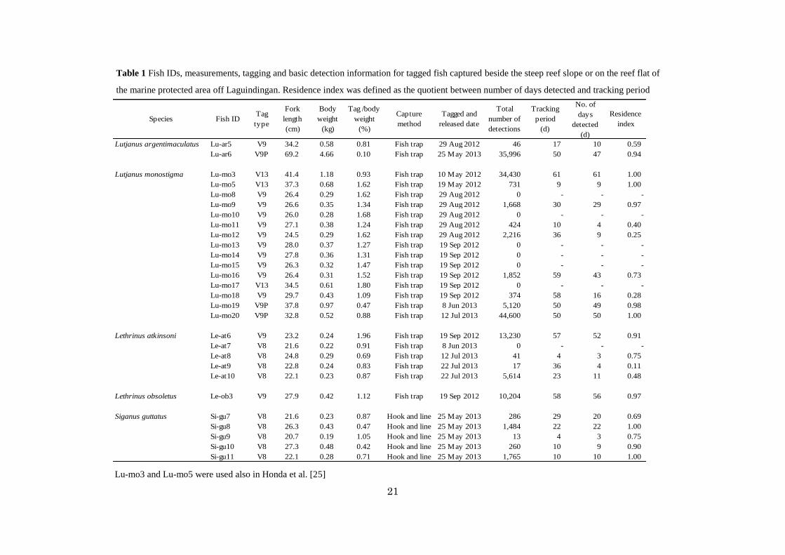
Table 1 Fish IDs, measurements, tagging and basic detection information for tagged fish captured beside the steep reef slope or on the reef flat of
the marine protected area off Laguindingan. Residence index was defined as the quotient between number of days detected and tracking period
Lutjanus argentimaculatus Lu-ar5 V9 34.2 0.58 0.81 Fish trap 29 Aug 2012 46 17 10 0.59
Lu-ar6 V9P 69.2 4.66 0.10 Fish trap 25 May 2013 35,996 50 47 0.94
Lutjanus monostigma Lu-mo3 V13 41.4 1.18 0.93 Fish trap 10 May 2012 34,430 61 61 1.00
Lu-mo5 V13 37.3 0.68 1.62 Fish trap 19 May 2012 731 9 9 1.00
Lu-mo8 V9 26.4 0.29 1.62 Fish trap 29 Aug 2012 0 - - -
Lu-mo9 V9 26.6 0.35 1.34 Fish trap 29 Aug 2012 1,668 30 29 0.97
Lu-mo10 V9 26.0 0.28 1.68 Fish trap 29 Aug 2012 0 - - -
Lu-mo11 V9 27.1 0.38 1.24 Fish trap 29 Aug 2012 424 10 4 0.40
Lu-mo12 V9 24.5 0.29 1.62 Fish trap 29 Aug 2012 2,216 36 9 0.25
Lu-mo13 V9 28.0 0.37 1.27 Fish trap 19 Sep 2012 0 - - -
Lu-mo14 V9 27.8 0.36 1.31 Fish trap 19 Sep 2012 0 - - -
Lu-mo15 V9 26.3 0.32 1.47 Fish trap 19 Sep 2012 0 - - -
Lu-mo16 V9 26.4 0.31 1.52 Fish trap 19 Sep 2012 1,852 59 43 0.73
Lu-mo17 V13 34.5 0.61 1.80 Fish trap 19 Sep 2012 0 - - -
Lu-mo18 V9 29.7 0.43 1.09 Fish trap 19 Sep 2012 374 58 16 0.28
Lu-mo19 V9P 37.8 0.97 0.47 Fish trap 8 Jun 2013 5,120 50 49 0.98
Lu-mo20 V9P 32.8 0.52 0.88 Fish trap 12 Jul 2013 44,600 50 50 1.00
Lethrinus atkinsoni Le-at6 V9 23.2 0.24 1.96 Fish trap 19 Sep 2012 13,230 57 52 0.91
Le-at7 V8 21.6 0.22 0.91 Fish trap 8 Jun 2013 0 - - -
Le-at8 V8 24.8 0.29 0.69 Fish trap 12 Jul 2013 41 4 3 0.75
Le-at9 V8 22.8 0.24 0.83 Fish trap 22 Jul 2013 17 36 4 0.11
Le-at10 V8 22.1 0.23 0.87 Fish trap 22 Jul 2013 5,614 23 11 0.48
Lethrinus obsoletus Le-ob3 V9 27.9 0.42 1.12 Fish trap 19 Sep 2012 10,204 58 56 0.97
Siganus guttatus Si-gu7 V8 21.6 0.23 0.87 Hook and line 25 May 2013 286 29 20 0.69
Si-gu8 V8 26.3 0.43 0.47 Hook and line 25 May 2013 1,484 22 22 1.00
Si-gu9 V8 20.7 0.19 1.05 Hook and line 25 May 2013 13 4 3 0.75
Si-gu10 V8 27.3 0.48 0.42 Hook and line 25 May 2013 260 10 9 0.90
Si-gu11 V8 22.1 0.28 0.71 Hook and line 25 May 2013 1,765 10 10 1.00
SpeciesTagged and
released date
Capture
method
Tag /body
weight
(%)
Body
weight
(kg)
Fork
length
(cm)
Tag
type
Residence
index
No. of
days
detected
(d)
Tracking
period
(d)
Total
number of
detections
Fish ID
Lu-mo3 and Lu-mo5 were used also in Honda et al. [25]
22
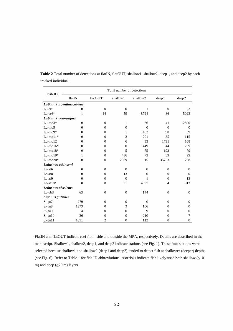
Table 2 Total number of detections at flatIN, flatOUT, shallow1, shallow2, deep1, and deep2 by each
tracked individual
FlatIN and flatOUT indicate reef flat inside and outside the MPA, respectively. Details are described in the
manuscript. Shallow1, shallow2, deep1, and deep2 indicate stations (see Fig. 1). These four stations were
selected because shallow1 and shallow2 (deep1 and deep2) tended to detect fish at shallower (deeper) depths
(see Fig. 6). Refer to Table 1 for fish ID abbreviations. Asterisks indicate fish likely used both shallow (≤10
m) and deep (≥20 m) layers
flatIN flatOUT shallow1 shallow2 deep1 deep2
Lutjanus argentimaculatus
Lu-ar5 0 0 0 1 0 23
Lu-ar6* 1 14 59 8724 86 5023
Lutjanus monostigma
Lu-mo3* 0 0 1 66 41 2590
Lu-mo5 0 0 0 0 0 0
Lu-mo9* 0 0 1 1462 90 69
Lu-mo11* 0 0 2 201 35 115
Lu-mo12 0 0 6 33 1791 108
Lu-mo16* 0 0 0 449 44 239
Lu-mo18* 0 0 5 75 193 79
Lu-mo19* 1 0 436 73 39 99
Lu-mo20* 0 0 2029 15 35733 268
Lethrinus atkinsoni
Le-at6 0 0 0 0 0 0
Le-at8 0 0 13 0 0 0
Le-at9 0 0 0 1 0 13
Le-at10* 0 0 31 4597 4 912
Lethrinus obsoletus
Le-ob3 63 0 0 144 0 0
Siganus guttatus
Si-gu7 279 0 0 0 0 0
Si-gu8 1373 0 3 106 0 0
Si-gu9 4 0 0 9 0 0
Si-gu10 36 0 0 210 0 7
Si-gu11 1651 2 0 112 0 0
Total number of detectionsFish ID
23
Figure Captions
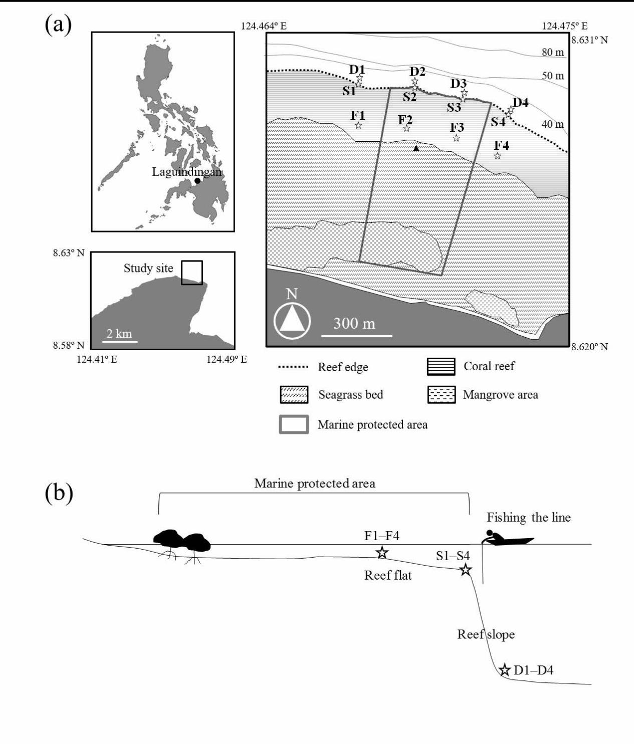
Fig. 1 (a) Geographic location of the study site, Laguindingan, northern Mindanao Island, the Philippines.
Stars and a solid triangle indicate the receivers’ deployment stations and the watchtower, respectively. F1–F4
(1.0–2.5 m bottom depth), S1–S4 (5–10 m), and D1–D4 (23–29 m) indicate each station. Capital letters “F”,
“S”, and “D” indicate reef Flat, Shallow, and Deep, respectively. Depth contour was made using bathymetry
data (LPC. Bernardo, Tokyo Institute of Technology; unpubl. data). (b) Vertical schematic view of the study
site. Intensive fishing operations along the boundary of the marine protected area known as “fishing the line”
operate legally and regularly
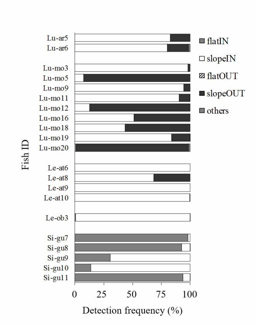
Fig. 2 Detection frequency in each location type used by the tracked fish during the study period. FlatIN,
slopeIN, flatOUT, slopeOUT, and others indicate reef flat inside the marine protected area (MPA), reef slope
near the MPA, reef flat outside the MPA, reef slope outside the MPA, and remaining detections,
respectively. Details are described in the manuscript. Refer to Table 1 for fish ID abbreviations
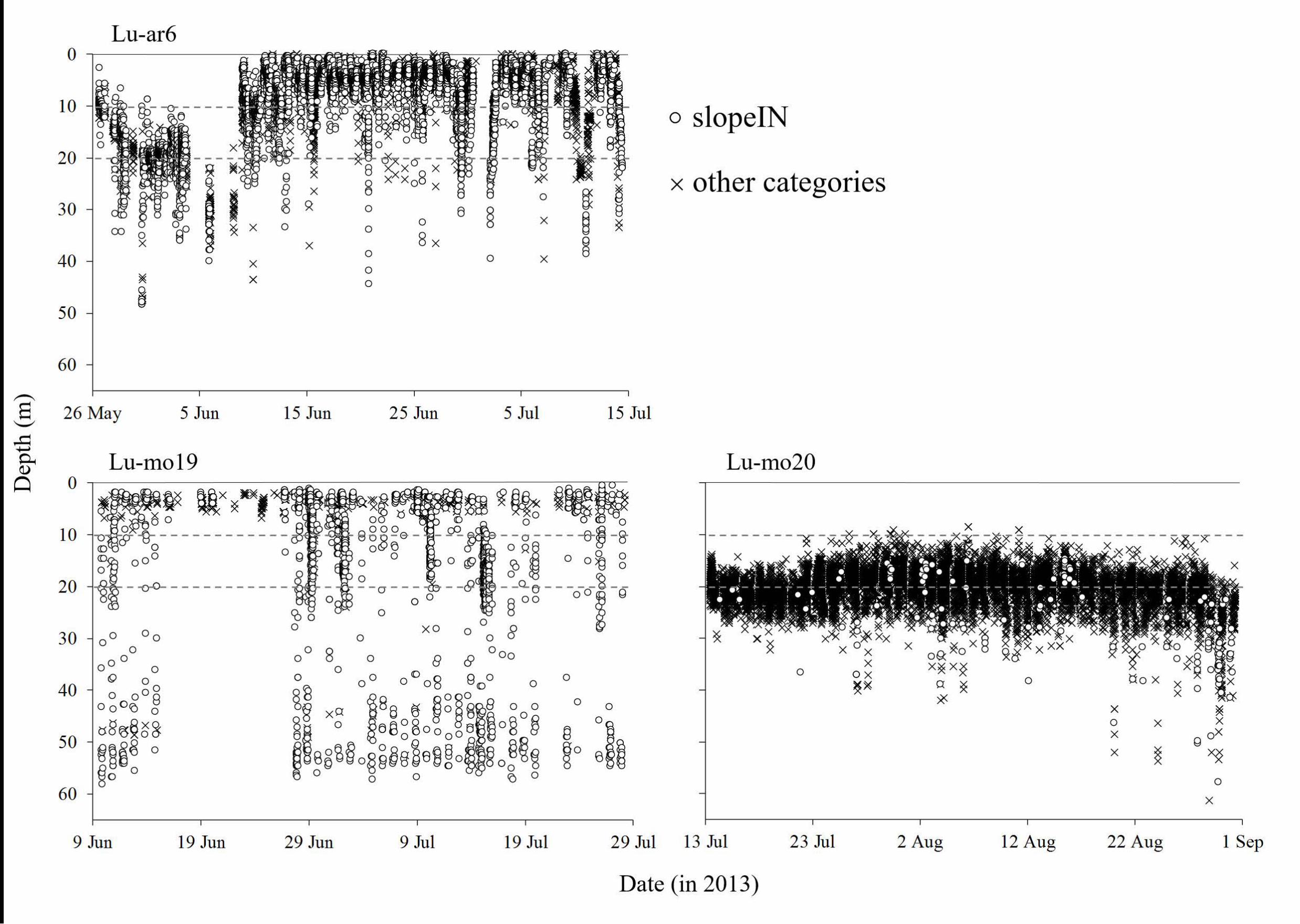
Fig. 3 Time series of the depths detected for the three fish equipped with a depth sensor (fish ID: Lu-ar6, Lu-
mo19, and Lu-mo20) by all 12 acoustic receivers during the study period. Grey dotted lines indicate 10 and
20 m depths. SlopeIN and other categories indicate reef slope near the MPA and remaining detections,
respectively. Details are described in the manuscript
Fig. 4 Vertical space use (kernel utilization distributions, KUDs) along the reef slope in each time period by
the three fish equipped with a depth sensor (fish ID: Lu-ar6, Lu-mo19, and Lu-mo20), represented as mean
depth by mean reef distance (setting shallow1&deep1 as 0 m). Solid and grey colors indicate 50% and 95%
KUDs, respectively, Receiver positions are shown by triangles (shallow1&deep1–shallow4&deep4 locates
form left to right). Two dotted lines indicate western (left) and eastern (right) borders of the marine protected
area
Fig. 5 Time-length frequencies of ascents and descents between shallow (≤10 m) and deep (≥20 m) layers for
the three fish equipped with a depth sensor (fish ID: Lu-ar6, Lu-mo19, and Lu-mo20) (a) and their hourly
24
frequencies only using <1 h time-length movements (b). Grey shaded areas indicate average periods from
sunset to sunrise of days recorded movements
Fig. 6 Detection frequencies in each 10-m depth range (0–60 m) at each pair of shallow and deep stations
(e.g., S1 and D1) by three tagged fish equipped with a depth sensor (a), and detection probabilities in the 0–
10, 10–20, and 20–60 m depth ranges at each pair of stations based on detection frequency (b). The
probabilities at the stations were calculated only when there was a tendency that fish in a shallow (deep) area
were detected more frequently at a shallow (deep) station. S&D in the figures indicates simultaneous
detections by S and D receivers. S1–S4 and D1–D4 indicate station locations (see Fig. 1)


Journal: Fisheries Science
Title: Importance of outer reef slopes for commercially important fishes: implications for designing
a marine protected area in the Philippines
Authors: Kentaro Honda1, 2,*, Wilfredo H. Uy3, Darwin I. Baslot3, Allyn Duvin S. Pantallano3, 4,
Masaaki Sato1, 5, Yohei Nakamura4, and Masahiro Nakaoka1
1 Akkeshi Marine Station, Field Science Center for Northern Biosphere, Hokkaido University; Aikappu,
Akkeshi, Hokkaido 088-1114, Japan
2 Present address: Hokkaido National Fisheries Research Institute, Japan Fisheries Research and Education
Agency; 2-2 Nakanoshima, Toyohira-ku, Sapporo, Hokkaido 062-0922, Japan
3Institute of Fisheries Research and Development, Mindanao State University at Naawan; 9023 Naawan,
Misamis Oriental, Philippines
4 Graduate School of Kuroshio Science, Kochi University; 200 Monobe, Nankoku, Kochi 783-8502, Japan
(Present address of Pantallano ADS)
5 Present address: National Research Institute of Fisheries and Environment of Inland Sea, Japan Fisheries
Research and Education Agency; Maruishi 2-17-5, Hatsukaichi-shi, Hiroshima 739-0452, Japan
*Corresponding author: [email protected]

Online Resource 1. Detection frequencies in each 10-m depth range (0–60 m) at two pairs of shallow and deep stations (i.e., S1 and D1, or S2 and D2) by each of three tagged fish equipped with a depth sensor (fish ID: Lu-ar6, Lu-mo19, and Lu-mo20). S&D in the figures indicates simultaneous detections by S and D receivers. S1, D1, S2, and D2 indicate station locations (see Fig. 1)
Dep
th (m
)
S1 and D1 S2 and D2
Lu-m
o19
Lu-m
o20
Detection frequency (%)
Lu-a
r6
0 20 40 60 80 100
0–10
10–20
20–30
30–40
40–50
50–60
0 20 40 60 80 100
0 20 40 60 80 100
0–10
10–20
20–30
30–40
40–50
50–60
0 20 40 60 80 100
0 20 40 60 80 100
0–10
10–20
20–30
30–40
40–50
50–60
0 20 40 60 80 100
N
64
15
2
0
0
0
S S&D D
235
11
3
0
0
0
11
14,190
10,111
97
18
6
N
8,487
1,576
256
3
0
0
100
35
5
0
0
0
0
40
45
56
4
1