Importance of borehole deviation surveys for monitoring of

Geophysical Prospecting, 2007, 55, 891–899 doi:10.1111/j.1365-2478.2007.00654.x

Importance of borehole deviation surveys for monitoring of hydraulicfracturing treatments

Petr Bulant1∗, Leo Eisner2, Ivan Psencık3 and Joel Le Calvez4

1Charles University in Prague, Czech Republic, 2Schlumberger Cambridge Research, UK, 3Geophysical Institute of the Academy of Sciencesof the Czech Republic, Czech Republic, and 4Schlumberger Data Consulting Services, Houston, USA

Received November 2006, revision accepted April 2007

ABSTRACTDuring seismic monitoring of hydraulic fracturing treatment, it is very common to ig-nore the deviations of the monitoring or treatment wells from their assumed positions.For example, a well is assumed to be perfectly vertical, but in fact, it deviates fromverticality. This can lead to significant errors in the observed azimuth and other pa-rameters of the monitored fracture-system geometry derived from microseismic eventlocations. For common hydraulic fracturing geometries, a 2◦ deviation uncertainty onthe positions of the monitoring or treatment well survey can cause a more than 20◦

uncertainty of the inverted fracture azimuths. Furthermore, if the positions of boththe injection point and the receiver array are not known accurately and the velocitymodel is adjusted to locate perforations on the assumed positions, several-milliseconddiscrepancies between measured and modeled SH-P traveltime differences may appearalong the receiver array. These traveltime discrepancies may then be misinterpretedas an effect of anisotropy, and the use of such anisotropic model may lead to themislocation of the detected fracture system. The uncertainty of the relative positionsbetween the monitoring and treatment wells can have a cumulative, nonlinear effecton inverted fracture parameters. We show that incorporation of borehole deviationsurveys allows reasonably accurate positioning of the microseismic events. In thisstudy, we concentrate on the effects of horizontal uncertainties of receiver and perfo-ration positions. Understanding them is sufficient for treatment of vertical wells, andalso necessary for horizontal wells.

I N T R O D U C T I O N

In oil and gas production, a process known as hydraulic frac-turing is often used to increase the productivity of hydrocar-bon reservoirs. Hydraulic fracturing involves pumping varioustypes of fluids under pressure down a treatment well into thereservoir. The pressurized fluid enters the reservoir and frac-tures the reservoir rock. These fractures increase permeabil-ity and conductivity, and ultimately production. To keep thesefractures highly conductive, solid particles known as proppantare pumped with the fluid into the created fractures. Creation

∗E-mail: [email protected]

of fractures and opening of pre-existing fractures generatesmicroseismic events observed by geophones located in a mon-itoring borehole. The fracture geometry is then determinedfrom locations of these events. For the sake of brevity, we aregoing to use the term “microseismic monitoring” through-out the paper. When using it, we keep in mind that we meanmonitoring of induced microseisms generated in relation tohydraulic fracturing treatment.

Over the years, a large number of hydraulic fracturingtreatments have been monitored to determine fracture geome-tries (e.g., Warpinski et al. 1998; Rutledge and Phillips 2003;Berumen et al. 2004). Usually, only a single (very often, theclosest) monitoring borehole is used, since other boreholesare too distant and signals reaching them are considerablyattenuated. The treatment may be performed in a vertical or a

C© 2007 European Association of Geoscientists & Engineers 891

892 P. Bulant et al.

horizontal well, while the monitoring is commonly performedin a vertical section of a monitoring well. When the moni-toring or the treatment wells are assumed to be vertical, of-ten no borehole deviation survey (i.e., the measurements ofthe borehole inclination and azimuth, which are then used tocalculate the borehole trajectory) is done and the wells arethen treated as perfectly vertical. Commonly, orientation ofthe monitoring geophones is determined from back azimuthsof P-waves generated by the perforation shots located in thetreatment well, assuming isotropy and lateral homogeneityof the medium between wells. Therefore, the orientation ofthe geophones in the monitoring well is determined relativelywith respect to the position of the treatment well at depthscorresponding to the perforations. The orientation (in a geo-graphical coordinate system) of the monitoring array and ofthe observed microseismic event hypocenters can, however,be obtained only from the positions of the receivers and theperforations. Therefore, any error in the positioning of themonitoring array or of the perforations is directly projectedinto the error of the fracture-system position. We show thatthe effects on the fracture-system azimuth may be consider-able, even for wells only slightly deviating from their expectedpositions. Fracture-system geometry (position, azimuth andlength) obtained from microseismic monitoring is used, forexample, as a guide for an “infill drilling” program, duringwhich new wells are drilled into unfractured (and hopefullyundrained) parts of the reservoir. Wrongly estimated fractureazimuth and fracture position may lead to financial losses andan uneconomical infill drilling program.

Additionally, the borehole deviations affect not only the de-termination of the fracture azimuth, but also the distance be-tween the treatment and monitoring wells. Typically, the ini-tial isotropic velocity model is built from sonic logs and/orvertical seismic profiling (VSP) data in microseismic fracturemonitoring. Commonly, the velocity model is then adjusted tolocate perforation shots to their assumedly correct positions(Maxwell, Shemeta and House 2006). The velocity model ad-justment can be realized in a number of ways but it usuallyinvolves fitting S-P-wave traveltime differences. The S-P-wavetraveltime differences that cannot be explained by an isotropicmodel are then fitted by a VTI (transverse isotropy with ver-tical axis of symmetry) velocity model. We show that such aprocedure may lead to a quite strong artificial anisotropy. Theartificial anisotropy will cause distorted locations of the micro-seismic events and thus will distort the shape of the observedhydraulic fracture.

To assess the effects of the borehole deviation uncertaintieson fracture azimuth and anisotropic model building, we start

by estimation of the borehole deviation uncertainty from sev-eral nearly vertical boreholes. We then show how the bore-hole deviation uncertainty relates to fracture azimuth andanisotropic model building. Finally, we discuss the relation ofthe borehole deviation uncertainty and the fracture azimuthuncertainty for an assumed statistical distribution of the bore-hole deviations.

Throughout the paper, we focus on the case of a verticalmonitoring array and a single perforation position. In our il-lustrative figures we assume the case of two nearly verticalwells, but the results concerning the horizontal uncertaintieswould also be the same for the case of perforation in a hor-izontal treatment well. The effects caused by the vertical un-certainties are not studied in this paper. Our results apply todeep as well as shallow boreholes.

B O R E H O L E D E V I AT I O N U N C E RTA I N T I E S

Drillers often quote the angular deviation accuracy of an av-erage “vertical” borehole as being 5◦. One of the “vertical”wells in a recent monitoring campaign shown in Fig. 1 devi-ated at the measured (treatment) depth of 1500 m by morethan 8◦. Figure 1 also shows six other wells in which micro-seismic monitoring took place and for which deviation sur-veys were performed. For these wells, the deviation values aremostly within 2◦. In the following, we shall thus consider thevalue of the deviation uncertainty of “vertical” wells with nodeviation survey to be 2◦, which seems to be a conservative es-timate. Note that, with exception of two wells shown in pinkand violet in Fig. 1, azimuths of the wells are uncorrelated,i.e., boreholes do not generally deviate in the same direction.

To assess uncertainty in deviation survey measurements, wecompared two deviation surveys carried out by two differentcompanies for the same well, and found out that the averagedifference between the two independent measurements of theborehole deviation was 0.18◦. High-quality deviation surveysclaim even higher accuracy. To be conservative, and to takeinto account a systematic error (see, e.g., Williamson 2000),we consider the value of deviation uncertainty of wells with adeviation survey to be 0.5◦.

For nearly vertical wells, the deviation uncertainties resultmainly in horizontal uncertainty of the positions of the per-forations or of the geophones. For simplicity, the vertical un-certainty in their positions will be neglected throughout thispaper. Assuming an average deviation uncertainty ω of a nearlyvertical well, the horizontal uncertainty y of the well at a mea-sured depth (cable length) h is then y = h tan(ω). Consideringa typical depth of hydrofracture experiments to be around

C© 2007 European Association of Geoscientists & Engineers, Geophysical Prospecting, 55, 891–899

Importance of borehole deviation surveys 893

Figure 1 Deviations of seven real wells, where microseismic monitoring of hydraulic fracturing took place, and for which the deviation surveysare available. Left plot shows deviations from vertical, right plot shows azimuths of these deviations. Note that the deviation is unpredictableand may change rapidly in a very short depth range.

Table 1 Horizontal uncertainty, y = h tan(ω), at depth h caused bythe well deviation uncertainty ω

Depth h (m) Well deviation uncertainty ω (deg)

5 2 0.5 0.2

Horizontal uncertainty y = h tan(ω) (m)

500 43.74 17.46 4.36 1.751000 87.49 34.92 8.73 3.491500 131.23 52.38 13.09 5.242000 174.98 69.84 17.45 6.982500 218.72 87.30 21.82 8.73

2000 m, we arrive at a horizontal uncertainty of about 70 mfor wells with no deviation survey (ω = 2◦), and about 17 mfor wells with a deviation survey (ω = 0.5◦). For other ex-amples, refer to Table 1. The horizontal uncertainty y has acumulative effect with measured depth. For shallower depthsthe uncertainty y is smaller, for greater depths it is larger.

Eisner and Bulant (2006) and Bulant et al. (2006) show theeffects of neglecting deviation surveys for particular choicesof the borehole deviation uncertainty and measured depths. Inthis study we generalize their specific choices (suitable for di-rect applications in engineering) and display the resulting frac-ture azimuth uncertainty and apparent anisotropy as functionsof the ratio of the horizontal uncertainty y and the assumedhorizontal distance H of the wells, or as a ratio of the truehorizontal distance x and the assumed horizontal distance H.As the typical values of H for microseismic monitoring exper-iments are between 100 and 500 m, we consider the values ofy/H to be between 0 and 0.5 (for values of y see Table 1), andthe values of x/H to be between 0 and 2, respectively.

F R A C T U R E A Z I M U T H

Let us first examine the effect of the borehole deviation onthe fracture azimuth. As described in the Introduction, thefracture azimuth �0 is determined relatively with respect tothe assumed positions of the perforation and of the monitoring



Figure 2 Plan view of a vertical monitor-ing array (“Well 1”) and a perforation(“Well 2”). The blue dashed circles around“Well 1” and “Well 2” denote maximum de-viations from points “Well 1” and “Well 2”in the horizontal plane, respectively. Twogreen dashed lines tangent to these circlesshow limiting back azimuths �1 and �2 ofa perforation with respect to the monitor-ing array. ��L is the maximum fracture az-imuth error due to the uncertainty in the po-sitioning of the monitoring array and of theperforation.

array, and any error in the positioning of the monitoring arrayor of the perforation causes the fracture azimuth error ��.The actual fracture azimuth � in a geographical coordinatesystem is thus given as � = �0 + �SR ± ��, where �SR is theazimuth of the perforation-to-receiver direction.

We assume that the monitoring array is vertical. Figure 2shows a sketch of a plan view of a hydraulic fracture monitor-ing. The blue point “Well 1” denotes the assumed position ofa monitoring array and the other blue point “Well 2” denotesthe assumed position of the perforation. H is the horizon-tal distance between these points. For simplicity, we assumethat both wells have the same average deviation uncertaintyω along the entire borehole, and that the perforation and re-ceivers are situated at measured depth h. Generalization ofthe estimates of the fracture-azimuth error for the case of twodifferent average deviation uncertainties is straightforward.

The blue dashed circles in Fig. 2 show the representativeuncertainty of the horizontal positions of the perforation andreceivers at the depth h. The two green dashed lines show thelimits of the relative back azimuths of the perforation withrespect to the monitoring array. The uncertainty �� in theback azimuths of the perforation causes the fracture azimuthuncertainty ��, no matter what the angle between the frac-ture and the source-receiver direction is, i.e., regardless of therelative fracture azimuth �0. If the borehole trajectories arelimited by the deviation uncertainty ω (dashed blue circles inFig. 2), then the uncertainty �� is limited by the value of ��L,|��| ≤ |��L|.

We shall now evaluate the uncertainty ��L in the back az-imuth of the fracture for the two limiting cases of the backazimuths shown by dashed green lines in Fig. 2. The relationbetween this uncertainty and the uncertainty for an assumed

statistical distribution of perforation and monitoring array po-sitions can be found in the Discussion. The simple geometricalsketch shown in Fig. 2 allows us to estimate the nonlinear de-pendency of the fracture azimuth uncertainty

��L = arcsin

(h tan(ω)

H/2

)= arcsin

(2

yH

). (1)

Figure 3 illustrates the fracture azimuth uncertainty (1) as afunction of y/H. Note, that the fracture azimuth uncertaintycan be more than 20◦ for an average deviation uncertainty of2◦ at measured depths below 1500 m and a wellhead separa-tion of less than 300 m. This is a common scenario for currentmicroseismic monitoring campaigns in North America. SeeTable 1, where ω = 2◦ and h = 1500 m yield y ∼ 50 m andy/H ∼ 0.17. Such uncertainty severely limits the use of the frac-ture geometry for infill drilling decisions. On the other hand, ifthe average deviation uncertainty ω in the deviation survey isonly 0.5◦, the ratio y/H is less than 0.074 for H ≥ 300 m for alldepths listed in Table 1. Thus the fracture azimuth is well con-strained to less than 7.5◦, which is a value rarely achieved fromlocations of microseismic events. Note that for the values ofy/H between 0 and 0.3 the fracture azimuth uncertainty variesapproximately linearly, yielding about 11.5◦ for each 10% in-crease of y with respect to H. For y/H higher than 0.5, i.e.,for possibly crossed borehole trajectories, the fracture azimuthuncertainty is always more than 90◦, the fracture azimuth isthus completely undeterminable. Let us also mention that thefracture azimuth uncertainty does not influence the relativelocations between individual microearthquakes (the shape ofthe fracture) but it influences the absolute position and orien-tation of the fracture as shown in Fig. 5 of Bulant et al. (2006).



Figure 3 The fracture azimuth uncertainty ��L in degrees as a func-tion of the ratio of the horizontal uncertainty y and the horizontaldistance of wellheads H. For the values of y/H between 0 and 0.3 thefracture azimuth uncertainty is approximately linear, yielding about11.5◦ for each 10% increase of y with respect to H. For y/H higherthan 0.5, the fracture azimuth uncertainty always exceeds 90◦.

A P PA R E N T A N I S O T R O P Y

As explained in the Introduction, it is common to adjust thestarting velocity model, obtained from sonic logs and/or VSP,in such a way that the adjusted model yields observed SH-Ptraveltime differences for the assumed positions of perfora-tions. This is often done by using a VTI model, where verticalvelocities match velocities from sonic logs or VSP, and hori-zontal velocities match the observed SH-P perforation travel-time differences (or P, SH, SV traveltimes if the origin timesof perforations are known, Maxwell et al. 2006). Such ve-locity model adjustments are affected by the accuracy of themonitoring and perforation geometry.

To estimate the effects of incorrect perforation-receiver ge-ometry on velocity model adjustment, we numerically analyzea simple example. Let us consider two almost vertical wellsdeviating from the vertical by an average deviation ω (dashedlines in Fig. 4), and let us investigate traveltime errors causedby treating the wells as perfectly vertical (solid lines in Fig. 4).Let us try to explain the traveltime errors of SH-P by assumingthat the homogeneous medium surrounding the boreholes isnot isotropic, but a weakly VTI medium. Note that an aver-

Figure 4 A schematic side-view of two nearly vertical wells (dashedlines) with an average deviation ω from their assumed vertical position(solid lines). H is the assumed horizontal distance of perforation andreceiver.

age uncertainty of the well deviation is considered in Fig. 4.Examples of real deviations are shown in Fig. 1.

The difference in traveltimes between true and assumed wellpositions in a homogenous isotropic medium can be deducedfrom Fig. 4:

�TSH−P (�) =(

1vSH

− 1vP

)(√cos2 � + x2

H2sin2

�

)H

sin �.(2)

Here x is the true horizontal distance, while H is the assumedhorizontal distance of perforation to receiver array illustratedin Fig. 4. � is an angle between vertical and perforation-receiver direction shown by the dashed line in Fig. 4, � =90◦ thus corresponds to horizontal propagation. We do notconsider the vertical shift of the perforation and of the re-ceiver, since it is negligible in the case of vertical wells; see theDiscussion for more details. vP and vSH are P- and SH-wave ve-locities. For a given uncertainty of the horizontal well positions(e.g., values y in Table 1), we can estimate H−2y < x < H+2y;see Fig. 4. The analysis for an assumed statistical distribution



of perforation and monitoring array positions is detailed inthe Discussion.

The traveltime difference (2) can be explained as an effect ofa homogeneous weakly VTI medium. P- and SH-wave phasevelocities in a weakly VTI medium are given by the followingapproximate (first-order with respect to the deviations of theVTI medium from isotropic one) formulae:

vP (�) = vP [1 + δ sin2� + (ε − δ) sin4

�],

vSH(�) = vSH[1 + γ sin2�]. (3)

Equations (3) are equivalent to equations (16a) and (16c) ofThomsen (1986), respectively. In (3), ε, δ and γ are linearizeddimensionless Thomsen’s parameters, ε = (A11 − v2

P)/(2v2P),

δ = (A13 + 2A55 − v2P)/v2

P, and γ = (A66 − v2SH)/v2

SH, Aij

denoting density-normalized elastic moduli in the Voigt no-tation. The parameters ε, δ, and γ together with vP and vSH

specify the VTI medium. The parameters ε, δ, and γ charac-terize deviations of a weakly VTI medium from an isotropicone. If multiplied by 100%, ε and γ can be used to estimatethe strength of P- and SH-wave anisotropy in %, respectively,δ controls curvature of the P-wave phase-velocity surfacearound the axis of symmetry (Tsvankin 2001). vP and vSH rep-resent vertical P- and SH-wave phase velocities, respectively.The first-order (linearized) P- and SH-wave traveltimes TP

and TSH, respectively, between perforation and receiver can bedetermined from Eqs. (3):

TP (�) = 1vP

[1 − δ sin2� − (ε − δ) sin4

�]H

sin �,

TSH(�) = 1vSH

[1 − γ sin2�]

Hsin �

. (4)

Traveltime difference �TSH−P of the SH- and P-wave in ahomogeneous weakly VTI medium then reads

�TSH−P (�) =[(

1vSH

− 1vP

)−

(1

vSHγ − 1

vPδ

)sin2

�

+ 1vP

(ε − δ) sin4�

]H

sin �. (5)

Equation (5) does not allow independent determination ofall 3 parameters of the VTI medium (γ , δ, and ε) as thereare only two terms of angular dependency of the traveltimedifference. Thus we introduce two coefficients, G and E:

G = γ − vSH

vPδ and E = (ε − δ), (6)

Figure 5 Best fitted VTI anisotropic parameters that would compen-sate the traveltime difference caused by geometrical error due to un-known deviation survey. The blue and green curves represent twocoefficients G and E defined in equation (6). The values of coeffi-cients G and E were obtained by least-square fitting of equation (7) tothe traveltime differences calculated from equation (2) at 8 receiverswith vertical spacing of 30 m and assumed source-receiver horizon-tal distance H = 500 m in the homogenous isotropic model (vP =4400 m/s, vSH = 2600 m/s). For an example of the traveltime differ-ences compensation, refer to Fig. 6.

and rewrite equation (5) as

�TSH−P (�) =[(

1vSH

− 1vP

)− G

vSHsin2

� + EvP

sin4�

]H

sin �.

(7)

If the parameter δ is zero, G = γ and E = ε.The traveltime difference (7) can be matched to the trav-

eltime difference due to incorrect geometry in equation (2).Note that the ratio, x/H, of the assumed to the true distancecontrols the �TSH−P delay in equation (2), thus this ratio con-trols the strength of apparent anisotropy induced by incorrectgeometry.

Figure 5 shows results of the least square inversion of equa-tion (7) for traveltime differences computed from equation (2)at 8 receivers (30 m vertical spacing, centered on the depthof the perforation) in a homogeneous isotropic velocity model(vP = 4400 m/s, vSH = 2600 m/s). Note that G = E = 0 forx/H = 1, i.e., if the true and assumed horizontal distancesare equal, the inversion yields the true isotropic model. Forx/H > 0.5 the inversion is not sensitive to a chosen veloc-ity model, assumed distance H, or number of receivers ortheir spacing. Traveltime differences in equation (2) increasewith increasing deviation from 1 of the ratio between the real



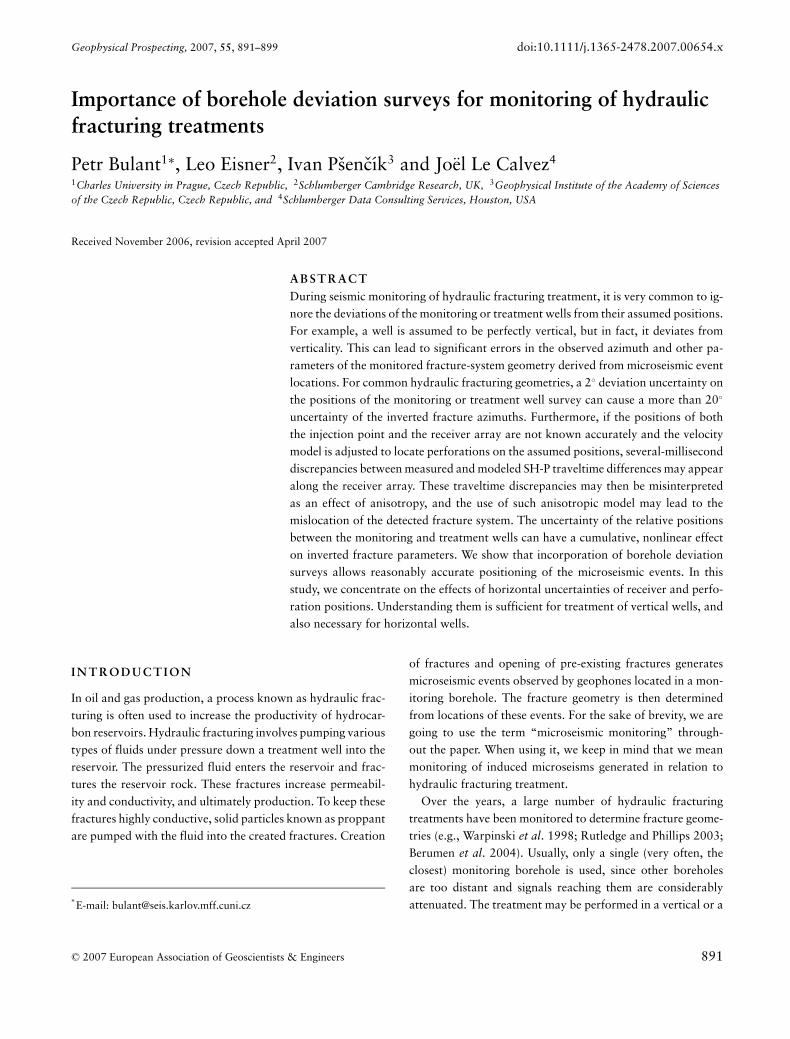
Figure 6 SH-P-wave traveltime differences computed at 8 receiversin a homogeneous isotropic model used for generation of Fig. 5, forperforations 500 m away (assumed horizontal distance: green dots)and 300 m away (true horizontal distance: blue dots). The red circlesrepresent SH-P traveltime differences computed at 8 receivers in thehomogeneous anisotropic model with G = 0.11 and E = −0.09 forperforation 500 m away. Note that the values of G = 0.11 and E =−0.09 correspond to x/H = 0.6 from Fig. 5, i.e., to the true horizon-tal distance 300 m and the assumed horizontal distance 500 m. Theanisotropic model perfectly explains the traveltime discrepancy dueto incorrect assumed geometry.

distance x and the assumed distance (wellhead spacing) H. Fora fixed wellhead spacing H this ratio increases with measureddepth, as the uncertainty in H is linearly proportional to themeasured depth (Bulant et al. 2006). Note that both G andE are negative if the assumed distance between the perfora-tion and the receivers is shorter than the true distance, i.e., ifx/H > 1 in equation (2). Let us emphasize that the approxi-mate formulas (3), (4), (5), and (7), used for the estimates ofthe coefficients (6), work reliably for anisotropy up to approx-imately 20%. Possible stronger anisotropy resulting from theabove formulae thus only indicates strong distortions in thewell geometry. Let us also note that if the average deviation un-certainty ω is only 0.5◦, i.e., deviation surveys are performed,the ratio x/H is limited in the interval 0.86 < x/H < 1.14 forH ≥ 300 m for all depths listed in Table 1. The absolute valuesof parameters G and E are thus less than 0.07.

Figure 6 shows traveltime differences between true andassumed geometry in isotropic medium used for genera-tion of Fig. 5, and assumed geometry with the best fittedanisotropic model. Note that the anisotropic model perfectlyexplains the traveltime discrepancy due to incorrect assumedgeometry.

D I S C U S S I O N

The goal of this article is to present evidence that deviation sur-veys are important for monitoring induced microseisms gen-erated in relation to hydraulic fracturing treatment. We haveanalyzed the uncertainty in the fracture azimuth and the pos-sibility of introducing artificial anisotropy due to geometricaleffects caused by uncertainty in deviation surveys. However,there are numerous other reasons why accurate deviation sur-veys are necessary. For example, Fig. 5 of Bulant et al. (2006)illustrates that deviation-survey uncertainty is the main causeof uncertainty in the location of microseismic events. Devia-tion surveys are necessary for velocity model building frommultiple sonic log measurements, for geometrical relationshipbetween injection points and fracture, etc.

In this study, we have assumed two nearly vertical wells,both with the same average deviation ω from the vertical caus-ing an uncertainty y in the horizontal positions of the sourceand receivers located deep in the boreholes. We then stud-ied the effects of the horizontal uncertainty on the retrievedfracture azimuth, and estimated the ’maximum’ fracture az-imuth uncertainty ��L corresponding to the extreme casedisplayed in Fig. 2. We have shown that in this case everypercentage point of the horizontal position uncertainty meansapproximately 1◦ uncertainty in the azimuth of the fracture;see Fig. 3.

To evaluate the fracture azimuth uncertainty statistically,we need to assume a statistical distribution of the boreholedeviations and a relation between deviations of the two con-sidered wells. The seven borehole trajectories shown in Fig. 1do not allow such a study. Thus, we assume Gaussian distri-bution of the horizontal positions of both monitoring arrayand perforation shot, and mutually uncorrelated deviationsof the two wells. Analytical evaluation of standard deviationof back azimuths ��S requires double-integration of compli-cated elliptical integrals which, to the best of our knowledge,do not have analytical solutions. For two sufficiently distantwells, i.e., for the case of σ � H, we can use Taylor expansionof (�)2 with respect to Cartesian coordinates of perforationand monitoring array, and the first-order term of the expan-sion yields ��S ≈ 1/

√2 arcsin( σ

H/2 ) (L. Klimes, pers. comm.2006). Here, σ is the standard deviation of the selected Gaus-sian distributions for both monitoring and treatment wells.From numerical tests we found that the above approximaterelation is sufficiently accurate for σ/H < 0.3. This meansthat for σ/H < 0.3, ��S as a function of σ/H behaves inthe same way as ��L as a function of y/H, multiplied by1/

√2 ∼= 0.7; see equation (1). Dependence of ��S on σ/H



can be thus illustrated by the curve in Fig. 3 if we substitutey/H by σ/H and ��L by ��S/0.7.

Analogously, we could discuss appropriate choice of the pa-rameter x in equation (2) under the assumption of Gaussiandistribution of horizontal positions of both monitoring arrayand perforation shot. The parameter x then would be in aninterval (H - 1.4σ , H + 1.4σ ) for σ/H < 0.3.

In this study we neglected vertical shifts due to uncertaintyin the deviation surveys. The reasons to neglect the verticalshifts are twofold. For nearly vertical boreholes,� the vertical shift due to unknown deviation surveys always

reduces the assumed depth, both of the monitoring appara-tus as well as the perforation. Thus the corrections in verticaldirection for monitoring and treatment wells are correlated.

� the vertical shift is negligible relative to the horizontal ones.For a deviated straight well, the horizontal shift is h sin(ω),while the vertical shift is h [1-cos(ω)], where h is the mea-sured depth. For the examples given in Table 1, the verticalshift ranges from 9.5 m to 1 cm while the horizontal shiftranges from 218 to 5 m.The average uncertainty (deviated straight wells) may

slightly underestimate the vertical shift. However, even for thedeviations of the real wells (Fig. 1) the horizontal shifts areorders of magnitude larger than the vertical ones. Let us alsopoint out that the vertical shifts do not affect the uncertaintyon the azimuth of the fracture. Significant (comparable to thereceiver spacing) vertical shifts between perforations and mon-itoring arrays due to unknown deviation surveys may causeapparent tilted VTI anisotropy.

Without accurate deviation surveys, considerably distortedresults can be obtained. Assuming we have not adjusted thevelocity model using erroneous geometry, the relative locationsamong microseismic events do not change (see Fig. 5 of Bulantet al. 2006). However, if we adjust the velocity model usingerroneous geometry and introduce artificial anisotropy, eventhe relative locations are distorted. The relative positions ofthe perforation shots (or injection points) and of microseismicevents are in such cases also distorted.

Finally, we would like to mention that in the case of micro-seismic monitoring in horizontal wells, the presented resultsshould be generalized, especially by including vertical as wellas horizontal uncertainty. Horizontal wells are usually longer.Thus, even for a horizontal well with a measured deviationsurvey, the uncertainty in perforation shot position may besignificant. However, the effects of the incorrect position aregeometry-dependent and should be evaluated on a case-by-case basis.

C O N C L U S I O N S

The presented results show that the applicability of the resultsof monitoring of induced microseisms generated in relationto hydraulic fracturing treatment is severely limited if bore-hole deviation surveys of treatment or monitoring wells arenot performed. Deviation surveys are an important factor af-fecting the quality of the information that can be obtainedfrom microseismic monitoring of hydraulic fracturing. Theimportance of the deviation-surveys accuracy increases withthe measured length of the wells and with the length of themonitoring array. It also increases as spacing between moni-toring and treatment wells decreases. Horizontal uncertaintiesof receiver or perforation positions need to be considered formicroseimic monitoring in vertical wells, and they are alsonecessary for horizontal wells. For horizontal wells, the ver-tical uncertainties also play important role. Estimation of theeffects caused by the vertical uncertainties may be done fol-lowing similar steps to those in this study.

Microseismic monitoring with deviation surveys of bothmonitoring and treatment wells reduces uncertainty in the ob-served locations of microseismic events and provides accurateand reliable information.

A C K N O W L E D G E M E N T S

The authors are grateful to Ludek Klimes, Chris Chia, IanBradford and Scott Leanney for useful and stimulating discus-sions. We would also like to thank the anonymous reviewerfor useful recommendations and the European Union for fund-ing the IMAGES Transfer of Knowledge project (MTKI-CT-2004-517242). This research has been partially supportedby the Grant Agency of the Czech Republic under Contract205/07/0032.

R E F E R E N C E S

Berumen S., Gachuz H., Rodriguez J.M., Lapierre Bovier T. and KaiserP. 2004. Hydraulic fracture mapping in treated well channelizedreservoirs development optimization in Mexico. 66th EAGE meet-ing, Paris, France, Extended Abstracts, H027.

Bulant P., Eisner L., Psencık I. and Le Calvez J. 2006. Borehole de-viation surveys are necessary for hydraulic fracture monitoring.Abstracts of SPE Annual Technical Conference, San Antonio, SPE102788, Society of Petroleum Engineers.

Eisner L. and Bulant P. 2006. Borehole deviation surveys are neces-sary for hydraulic fracture monitoring. 68th EAGE meeting, Vienna,Austria, Extended Abstracts, P305.



Maxwell S.C., Shemeta J. and House N. 2006. Integrated anisotropicvelocity modeling using perforation shots, passive seismic and VSPdata. 68th EAGE meeting, Vienna, Austria, Extended Abstracts,A046.

Rutledge J.T. and Phillips W.S. 2003. Hydraulic stimulation of nat-ural fractures as revealed by induced microearthquakes, CarthageCotton Valley gas field, east Texas. Geophysics 68, 441–452.

Thomsen L. 1986. Weak elastic anisotropy. Geophysics 51, 1954–1966.

Tsvankin I. 2001. Seismic Signatures and Analysis of Reflection Datain Anisotropic Media. Elsevier Science.

Warpinski N.R., Branagan P.T., Peterson R.E., Wolhart S.L. and UhlJ.E. 1998. Mapping hydraulic fracture growth and geometry usingmicroseismic events detected by a wireline retrievable accelerometerarray. Abstracts of SPE Gas Technology Symposium, SPE 40014-MS, Society of Petroleum Engineers.

Williamson H.S. 2000. Accuracy prediction for directional measure-ment while drilling. SPE Drilling & Completion 15, 221–233.


Documents

Importance of borehole deviation surveys for monitoring of