Implicit Fairing of Irregular Meshes using Diffusion and Curvature Flow

Mathieu Desbrun Mark Meyer Peter Schr¨oder Alan H. Barr

Caltech∗

AbstractIn this paper, we develop methods to rapidly remove rough featuresfrom irregularly triangulated data intended to portray a smooth sur-face. The main task is to remove undesirable noise and unevenedges while retaining desirable geometric features. The problemarises mainly when creating high-fidelity computer graphics objectsusing imperfectly-measured data from the real world.

Our approach contains three novel features: animplicit integra-tion method to achieve efficiency, stability, and large time-steps; ascale-dependent Laplacian operator to improve the diffusion pro-cess; and finally, a robust curvature flow operator that achieves asmoothing of the shape itself, distinct from any parameterization.Additional features of the algorithm include automatic exact vol-ume preservation, and hard and soft constraints on the positions ofthe points in the mesh.

We compare our method to previous operators and related algo-rithms, and prove that our curvature and Laplacian operators haveseveral mathematically-desirable qualities that improve the appear-ance of the resulting surface. In consequence, the user can easilyselect the appropriate operator according to the desired type of fair-ing. Finally, we provide a series of examples to graphically andnumerically demonstrate the quality of our results.

1 IntroductionWhile the mainstream approach in mesh fairing has been to enhancethe smoothness of triangulated surfaces by minimizing computa-tionally expensive functionals, Taubin [Tau95] proposed in 1995 asignal processing approach to the problem of fairing arbitrary topol-ogy surface triangulations. This method is linear in the number ofvertices in both time and memory space; large arbitrary connectiv-ity meshes can be handled quite easily and transformed into visuallyappealing models. Such meshes appear more and more frequentlydue to the success of 3D range sensing approaches for creating com-plex geometry [CL96].

Taubin based his approach on defining a suitable generalizationof frequency to the case of arbitrary connectivity meshes. Usinga discrete approximation to the Laplacian, its eigenvectors becomethe “frequencies” of a given mesh. Repeated application of the re-sulting linear operator to the mesh was then employed to tailor thefrequency content of a given mesh.

Closely related is the approach of Kobbelt [Kob97], who consid-ered similar discrete approximations of the Laplacian in the con-struction of fair interpolatory subdivision schemes. In later workthis was extended to the arbitrary connectivity setting for purposesof multiresolution editing [KCVS98].

The success of these techniques is largely based on their sim-ple implementation and the increasing need for algorithms whichcan process the ever larger meshes produced by range sensing tech-

∗mathieu|mmeyer|ps|barr @cs.caltech.edu.

(a) (b)Figure 1: (a): Original 3D photography mesh (41,000 vertices).(b): Smoothed version with the scale-dependent operator in twointegration step withλdt = 5 · 10−5, the iterative linear solver(PBCG) converges in 10 iterations. All the images in this paperare flat-shaded to enhance the faceting effect.niques. However, a number of issues in their application remainopen problems in need of a more thorough examination.

The simplicity of the underlying algorithms is based on very ba-sic, uniform approximations of the Laplacian. For irregular con-nectivity meshes this leads to a variety of artifacts such as geomet-ric distortion during smoothing, numerical instability, problems ofslow convergence for large meshes, and insufficient control overglobal behavior. The latter includes shrinkage problems and moreprecise shaping of the frequency response of the algorithms.

In this paper we consider more carefully the question of numeri-cal stability by observing that Laplacian smoothing can be thoughtof as time integration of the heat equation on an irregular mesh.This suggests the use ofimplicit integration schemes which leadto unconditionally stable algorithms allowing for very large timesteps. At the same time the necessary linear system solvers runfaster than explicit approaches for large meshes. We also considerthe question of mesh parameterization more carefully and proposethe use of discretizations of the Laplacian which take the underly-ing parameterization into account. The resulting algorithms avoidmany of the distortion artifacts resulting from the application ofprevious methods. We demonstrate that this can be done at only amodest increase in computing time and results in smoothing algo-rithms with considerably higher geometric fidelity. Finally a morecareful analysis of the underlying discrete differential geometry isused to derive a curvature flow approach which satisfies crucial ge-ometric properties. We detail how these different operators act onmeshes, and how users can then decide which one is appropriate intheir case. If the user wants to, at the same time, smooth the shapeof an object and equalize its triangulation, a scale-dependent diffu-sion must be used. On the other hand, if only the shape must befiltered without affecting the sampling rate, then curvature flow hasall the desired properties. This allows us to propose a novel class ofefficient smoothing algorithms for arbitrary connectivity meshes.

2 Implicit fairingIn this section, we introduceimplicit fairing, an implicit integra-tion of the diffusion equation for the smoothing of meshes. We willdemonstrate several advantages of this approach over the usual ex-

plicit methods. While this section is restricted to the use of a linearapproximation of the diffusion term, implicit fairing will be used asa robust and efficient numerical method throughout the paper, evenfor non-linear operators. We start by setting up the framework anddefining our notation.

2.1 Notation and definitionsIn the remainder of this paper,X will denote a mesh,xi a vertex ofthis mesh, andei j the edge (if existing) connectingxi to xj . We willcall N1(i) the “neighbors” (or 1-ring neighbors) ofxi , i.e., all theverticesxj such that there exists an edgeei j betweenxi andxj (seeFigure 9(a)).

In the surface fairing literature, most techniques use constrainedenergy minimization. For this purpose, different fairness function-als have been used. The most frequent functional is the total curva-ture of a surfaceS :

E(S) =∫

Sκ2

1 +κ22 dS . (1)

This energy can be estimated on discrete meshes [WW94, Kob97]by fitting local polynomial interpolants at vertices. However, prin-cipal curvaturesκ1 andκ2 depend non-linearly on the surfaceS .Therefore, many practical fairing methods prefer the membranefunctional or the thin-plate functional of a meshX:

Emembrane(X) =12

∫Ω

X2u +X2

v dudv (2)

Ethin plate(X) =12

∫Ω

X2uu+2X2

uv+X2vv dudv. (3)

Note that the thin-plate energy turns out to be equal to the totalcurvature only when the parameterization(u,v) is isometric. Theirrespective variational derivatives corresponds to the Laplacian andthe second Laplacian:

L(X) = Xuu+Xvv (4)

L2(X) = L L(X) = Xuuuu+2Xuuvv+Xvvvv. (5)

For smooth surface reconstruction in vision, a weighted aver-age of these derivatives has been used to fair surfaces [Ter88].For meshes, Taubin [Tau95] used signal processing analysis toshow that a combination of these two derivatives of the form:(λ + µ)L − λµL2 can provide a Gaussian filtering that minimizesshrinkage. The constantsλ andµ must be tuned by the user to ob-tain this non-shrinking property. We will refer to this technique astheλ|µ algorithm.

2.2 Diffusion equation for mesh fairingAs we just pointed out, one common way to attenuate noise in amesh is through adiffusion process:

∂X∂t

= λL(X). (6)

By integrating equation 6 over time, a small disturbance will dis-perse rapidly in its neighborhood, smoothing the high frequencies,while the main shape will be only slightly degraded. The Lapla-cian operator can be linearly approximated at each vertex by theumbrella operator (we will use this approximation in the currentsection for the sake of simplicity, but will discuss its validity insection 4), as used in [Tau95, KCVS98]:

L(xi) =1m ∑

j∈N1(i)

xj −xi (7)

wherexj are the neighbors of the vertexxi , andm = #N1(i) is thenumber of these neighbors (valence). A sequence of meshes(Xn)

can be constructed by integrating the diffusion equation with a sim-pleexplicit Eulerscheme, yielding:

Xn+1 = (I +λdtL)Xn. (8)

With the umbrella operator, the stability criterion requiresλdt < 1.If the time step does not satisfy this criterion, ripples appear on thesurface, and often end up creating oscillations of growing magni-tude over the whole surface. On the other hand, if this criterion ismet, we get smoother and smoother versions of the initial mesh asn grows.

2.3 Time-shifted evaluationThe implementation of this previous explicit method, calledfor-ward Euler method, is very straightforward [Tau95] and has niceproperties such as linear time and linear memory size for each fil-tering pass. Unfortunately, when the mesh is large, the time steprestriction results in the need to perform hundreds of integrations toproduce a noticeable smoothing, as mentioned in [KCVS98].

Implicit integration offers a way to avoid this time step limi-tation. The idea is simple: if we approximate the derivative us-ing the new mesh (instead of using the old mesh as done in ex-plicit methods), we will get to the equilibrium state of the PDEfaster. As a result of this time-shifted evaluation, stability is ob-tained unconditionally [PTVF92]. The integration is now:Xn+1 =Xn + λdtL(Xn+1). Performing an implicit integration, this timecalledbackward Euler method, thus means solving the followinglinear system:

(I −λdtL)Xn+1 = Xn. (9)

This apparently minor change allows the user not to worry aboutpractical limitations on the time step. Consequent smoothing willthen be obtained safely by increasing the valueλdt. But solving alinear system is the price to pay.

2.4 Solving the sparse linear systemFortunately, this linear system can be solved efficiently as the ma-trix A = I − λdtL is sparse: each line contains approximately sixnon-zero elements if the Laplacian is expressed using Equ. (7) sincethe average number of neighbors on a typical triangulated mesh issix. We can use a preconditioned bi-conjugate gradient (PBCG) toiteratively solve this system with great efficiency1. The PBCG isbased on matrix-vector multiplies [PTVF92], which only requirelinear time computation in our case thanks to the sparsity of thematrixA. We review in Appendix A the different options we chosefor the PBCG in order to have an efficient implementation for ourpurposes.

2.5 Interpretation of the implicit integrationAlthough this implicit integration for diffusion is sound as is, thereare useful connections with other prior work. We review the analo-gies with signal processing approaches and physical simulation.

2.5.1 Signal processingIn [Tau95], Taubin presents the explicit integration of diffusion witha signal processing point of view. Indeed, ifX is a 1D signal of agiven frequencyω: X = eiω, thenL(X) =−ω2X. Thus, the transferfunction for Equ. (8) is 1−λdtω2, as displayed in Figure 2(a) as asolid line. We can see that the higher the frequencyω, the strongerthe attenuation will be, as expected.

The previous filter is called FIR (for Finite Impulse Response)in signal processing. When the diffusion process is integrated usingimplicit integration, the filter in Equ. (9) turns out to be an InfiniteImpulse Response filter. Its transfer function is now 1/(1+λdtω2),depicted in Figure 2(a) as a dashed line. Because this filter is alwaysin [0,1], we have unconditional stability.

1We use a bi-conjugate gradient method to be able to handle non sym-metric matrices, to allow the inclusion of constraints (see Section 2.7).

0

0.2

0.4

0.6

0.8

3

Frequency

Explicit filter

Implicit filter

Attenuation

2.5

1

0 0.5 1 1.5 20

0.2

0.4

0.6

1

Filter for ten implicit integrations

Filter for ten explicit integrations

Frequency

Attenuation

0.8

0.8

1

0 0.2 0.4 0.6

(a) (b)

Figure 2:Comparison between (a) the explicit and implicit transferfunction forλdt = 1, and (b) their resulting transfer function after10 integrations.

By rewriting Equ. (9) as:Xn+1 = (I −λdtL)−1Xn, we also notethat our implicit filtering is equivalent toI +λdtL +(λdt)2L2 + ...,i.e., standard explicit filtering plus an infinite sequence of higherorder filtering. Contrary to the explicit approach, one single implicitfiltering step performs global filtering.

2.5.2 Mass-spring networkSmoothing a mesh by minimizing the membrane functional can beseen as a physical simulation of a mass-spring network with zero-rest length springs that will shrink to a single point in the limit.Recently, Baraff and Witkin [BW98] presented an implicit methodto allow large time steps in cloth simulation. They found that theuse of an implicit solver instead of the traditional explicit Euler in-tegration considerably improves computational time while still be-ing stable for very stiff systems. Our method compares exactly totheirs, but used for meshes and for a different PDE. We thereforehave the same advantages of using an implicit solver over the usualexplicit type: stability and efficiencywhen significant filtering iscalled for.

2.6 Filter improvementNow that the method has been set up for the usual diffusion equa-tion, we can consider other equations that may be more appropriateor may give better visual results for smoothing when we use im-plicit integration.

We have seen in Section 2.1 that bothL andL2 have been usedwith success in prior work [Ter88, Tau95, KCVS98]. When we useimplicit integration, as Figure 3(a) shows, the higher the power ofthe Laplacian, the closer to alow-pass filterwe get. In terms offrequency analysis, it is a better filter. Unfortunately, the matrixbecomes less and less sparse as more and more neighbors are in-volved in the computation. In practice, we find thatL2 is a verygood trade-off between efficiency and quality. Using higher ordersaffects the computational time significantly, while not always pro-ducing significant improvements. We therefore recommend using(I +λdtL2)Xn+1 = Xn for implicit smoothing (a precise definitionof the umbrella-like operator forL2 can be found in [KCVS98]).

0

0.2

0.4

0.6

0.8

1

0 0.5

-1

(I-L ) -1

(I-L )23

4(I-L )

1 1.5 2 2.5

-1

-1(I-L)

30

0.2

0.4

2 2.5 3

Implicit filterConstant filter

Resulting convolution

1.5

0.6

0.8

1

1.2

0 0.5 1

(a) (b)Figure 3: (a): Comparison between filters usingL, L2, L3, andL4. (b): The scaling to preserve volume creates an amplificationof all frequencies; but the resulting filter (diffusion+scaling) onlyamplifies low frequencies to compensate for the shrinking of thediffusion.

We also tried to use a linear combination of bothL andL2. Weobtained interesting results like, for instance, amplification of lowor middle frequencies to exaggerate large features (refer to [GSS99]for a complete study of feature enhancement). It is not appropriate

in the context of a fixed mesh, though: amplifying frequencies re-quires refinement of the mesh to offer a good discretization.

2.7 ConstraintsWe can put hard and soft constraints on the mesh vertex positionsduring the diffusion. For the user, it means that a vertex or a set ofvertices can be fixed so that the smoothing happens only on the restof the mesh. This can be very useful to retain certain details in themesh.

A vertexxi will stay fixed if we imposeL(xi) = 0. More compli-cated constraints are also possible [BW98]. For example, verticescan be constrained along an axis or on a plane by modifying thePBCG to keep these constraints enforced during the linear solveriterations.

We can also easily implementsoft constraints: each vertex canbe weighted according to the desired smoothing that we want. Forinstance, the user may want to smooth a part of a mesh less thananother one, in order to keep desirable features while getting asmoother version. We allow the assignment of a smoothing valuebetween 0 and 1 to attenuate the smoothing spatially: this is equiv-alent to choosing a variableλ factor on the mesh, and happens tobe very useful in practice. Entire regions can be “spray painted”interactively to easily assign this special factor.

2.8 DiscussionEven if adding a linear solver step to the integration of the diffusionequation seems to slow down the problem at first glance, it turnsout that we gain significantly by doing so. For instance, the implicitintegration can be performed with an arbitrary time step. Sincethe matrix of the system is very sparse, we actually obtain com-putational time similar or better than the explicit methods. In thefollowing table, we indicate the number of iterations of the PBCGmethod for different meshes and it can be seen that the PBCG ismore efficient when the smoothing is high. These timings were per-formed on an SGI High Impact Indigo2 175MHz R10000 processorwith 128M RAM.

Mesh Nb of faces λdt = 10 λdt = 100

Horse 42,000 8 iterations (2.86s) 37 iterations (12.6s)Dragon 42,000 8 iterations (2.98s) 39 iterations (13.82s)Isis 50,000 9 iterations (3.84s) 37 iterations (15.09s)Bunny 66,000 7 iterations (4.53s) 35 iterations (21.34s)Buddha 290,000 5 iterations (13.78s) 28 iterations (69.93s)

To be able to compare the results with the explicit method, onehas to notice that one iteration of the PBCG is only slightly moretime consuming than one integration step using an explicit method.Therefore, we can see in the following results that our implicit fair-ing takes about 60% less time than the explicit fairing for a filteringof λdt = 100, as we get about 33 iterations compared to the 100 in-tegration steps required in the explicit case. We have found this be-havior to be true for all the other meshes as well. The advantage ofthe implicit method in terms of computational speed becomes moreobvious forlarge meshesand/orhigh smoothingvalue. In terms ofquality, Figure 4(b) and 4(c) demonstrate that both implicit and ex-plicit methods produce about the same visual results, with a slightlybetter smoothness for the implicit fairing. Note that we use 10 ex-plicit integrations of the umbrella operator withλdt = 1, and 1 inte-gration using the implicit integration withλdt = 10 to approximatethe same results. Therefore, there is a definite advantage in the useof implicit fairing over the previous explicit methods. Moreover,the remainder of this paper will make heavy use of this method andits stability properties.

3 Automatic anti-shrinking fairingPure diffusion will, by nature, induce shrinkage. This is inconve-nient as this shrinking may be significant for aggressive smooth-ing. Taubin proposed to use a linear combination ofL andL Lto amplify low frequencies in order to balance the natural shrink-ing. Unfortunately, the linear combination depends heavily on themesh in practice, and this requires fine tuning to ensure both stable

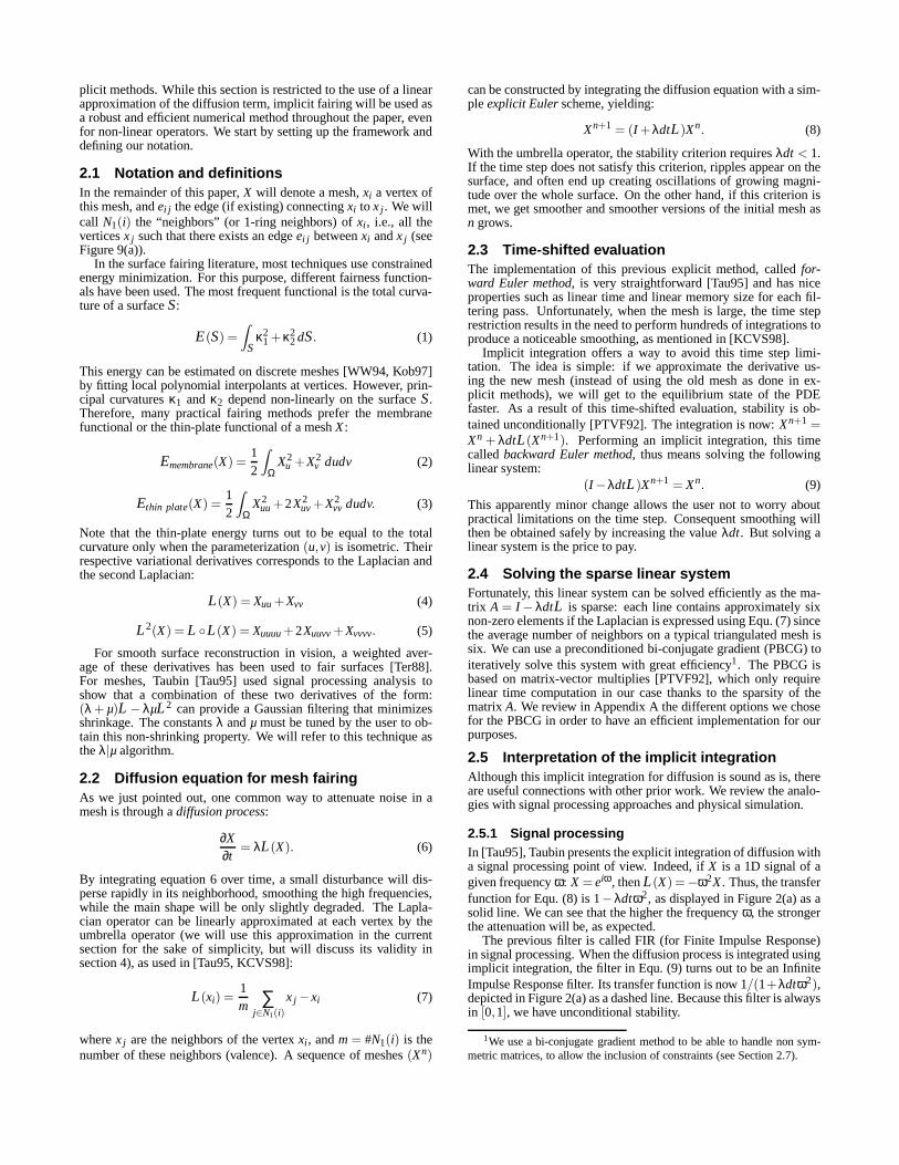
(a) (b) (c) (d)Figure 4:Stanford bunnies: (a) The original mesh, (b) 10 explicit integrations withλdt = 1, (c) 1 implicit integration withλdt = 10 that takesonly 7 PBCG iterations (30% faster), and (d) 20 passes of theλ|µ algorithm, withλ = 0.6307and µ= −0.6732. The implicit integrationresults in better smoothing than the explicit one for the same, or often less, computing time. If volume preservation is called for, our techniquethen requires many fewer iterations to smooth the mesh than theλ|µ algorithm.

and non-shrinking results. In this section, we propose an automaticsolution to avoid this shrinking. We preserve the zeroth moment,i.e., the volume, of the object. Without any other information onthe mesh, we feel it is the most reasonable invariant to preserve,although surface area or other invariants can be used.

3.1 Volume computationAs we have a mesh given in terms of triangles, it is easy to computethe interior volume. This can be done by summing the volumes ofall the oriented pyramids centered at a point in space (the origin, forinstance) and with a triangle of the mesh as a base. This computa-tion has a linear complexity in the number of triangles [LK84]. Forthe reader’s convenience, we give the expression of the volume ofa mesh in the following equation, wherex1

k,x2k andx3

k are the threevertices of thekth triangle:

V =16

nbFaces

∑k=1

gk ·Nk (10)

whereg = (x1k +x2

k +x3k)/3 andNk = ~x1

kx2k∧

~x1kx3

k

3.2 Exact volume preservationAfter an integration step, the mesh will have a new volumeVn. Wethen want to scale it back to its original volumeV0 to cancel theshrinking effect. We apply a simple scale on the vertices to achievethis. By multiplying all the vertex positions byβ = (V0/Vn)1/3,the volume is guaranteed to go back to its original value. As thisis a simple scaling, it is harmless in terms of frequencies. To put itdifferently, this scaling corresponds to a convolution with a scaledDirac in the frequency domain, hence it amplifies all the frequen-cies in the same way to change the volume back. The resultingfilter, after the implicit smoothing and the constant amplificationfilter, amplifies the low frequencies of the original mesh toexactlycompensate for the attenuation of the high frequencies, as sketchedon Figure 3(b).

The overall complexity for volume preservation is then linear.With such a process, we do not need to tweak parameters: theanti-shrinking filter isautomaticallyadapted to the mesh and tothe smoothing, contrary to previous approaches. Note that hardconstraints defined in the previous section are applied before thescaling and do not result in fixed points anymore: scaling alters theabsolute, but not the relative position.

We can generalize this re-scaling phase to different invariants.For instance, if we have to smooth height fields, it is more appropri-ate to take the invariant as being the volume enclosed between theheight field and a reference plane, which changes the computationsonly slightly. Likewise, for surfaces of revolution, we may changethe way the scaling is computed to exploit this special property. Wecan also preserve the surface area if the mesh is a non-closed sur-face. However, in the absence of specific characteristics, preservingthe volume gives nice results. According to specific needs, the usercan select the appropriate type of invariant to be used.

3.3 DiscussionWhen we combine both methods of implicit integration and anti-shrinking convolution, we obtain an automatic and efficient method

for fairing. Indeed, no parameters need be tuned to ensure stabilityor to have exact volume preservation. This is a major advantageover previous techniques. Yet, we retain all of the advantages ofprevious methods, such as constraints [Tau95] and the possibilityof accelerating the fairing via multigrid [KCVS98], while addition-ally offering stability and efficiency. This technique also dramati-cally reduces the computing time over Taubin’s anti-shrinking al-gorithm: as demonstrated in Figure 4(c) and 4(d), using theλ|µalgorithm may preserve the volume after fine tuning, but one itera-tion will only slightly smooth the mesh. The rest of this paper ex-ploits both automatic anti-shrinking and implicit fairing techniquesto offer more accurate tools for fairing.

4 An accurate diffusion processUp to this section, we have relied on the umbrella operator(Equ. (7)) to approximate the Laplacian on a vertex of the mesh.This particular operator does not truly represent a Laplacian in thephysical meaning of this term as we are about to see. Moreover,simple experiments on smooth meshes show that this operator, us-ing explicit or implicit integration, can create bumps or “pimples”on the surface, instead of smoothing it. This section proposes asounder simulation of the diffusion process, by defining a new ap-proximation for the Laplacian and by taking advantage of the im-plicit integration.

4.1 Inadequacy of the umbrella operatorThe umbrella operator, used in the previous sections correspondsto an approximation of the Laplacian in the case of a specific pa-rameterization [KCVS98]. This means that the mesh is supposedto have edges of length 1 and all the angles between two adjacentedges around a vertex should be equal. This is of course far frombeing true in actual meshes, which contain a variety of triangles ofdifferent sizes.

Treating all edges as if they had equal length has significant un-desired consequences for the smoothing. For example, the Lapla-cian can be the same for two very different configurations, corre-sponding to different frequencies as depicted in Figure 5. This dis-torts the filtering significantly, as high frequencies may be consid-ered as low ones, and vice-versa. Nevertheless, the advantage ofthe umbrella operator is that it is normalized: the time step for inte-gration is always 1, which is very convenient. But we want a moreaccurate diffusion process to smooth meshes consistently, in orderto more carefully separate high from low frequencies.

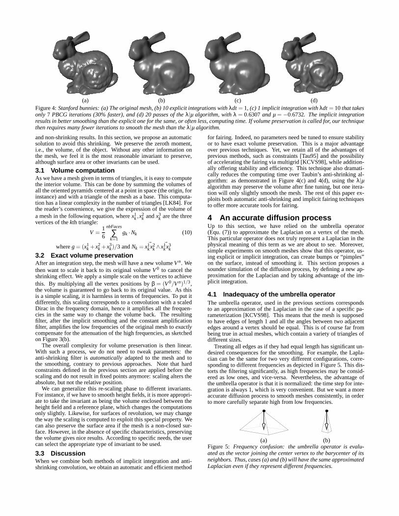
(a) (b)Figure 5: Frequency confusion: the umbrella operator is evalu-ated as the vector joining the center vertex to the barycenter of itsneighbors. Thus, cases (a) and (b) will have the same approximatedLaplacian even if they represent different frequencies.

We need to define a discrete Laplacian which is scale dependent,to better approximate diffusion. However, if we use explicit inte-gration [Tau95], we will suffer from a very restricted stability crite-rion. It is well known [PTVF92] that the time step for a parabolicPDE like Equ. (6) depends on the square of the smallest length scale(here, the smallest edge lengthmin(|e|)):

dt ≤ min(|e|)2

2 λ

This limitation is a real concern for large meshes with small de-tails, since an enormous number of integration steps will have tobe performed to obtain noticeable smoothing. This isintractableinpractice.

With implicit integration explained in Section 2, we can over-come this restriction and use a much larger time step while stillachieving good smoothing, saving considerable computation. Inthe next two paragraphs we present one design of a good approxi-mation for the Laplacian.

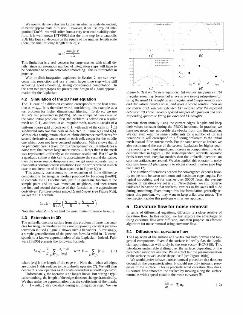
4.2 Simulation of the 1D heat equationThe 1D case of a diffusion equation corresponds to the heat equa-tion xt = xuu. It is therefore worth considering this example as atest problem for higher dimensional filtering. To do so, we useMilne’s test presented in [Mil95]. Milne compared two cases ofthe same initial problem: first, the problem is solved on a regularmesh on[0,1], and then on an irregular mesh, taken to consist of auniform coarse grid of cells on[0,1] with each of the cells in[ 1

2 ,1]subdivided into two fine cells as depicted in Figure 6(a) and 6(b).With such a configuration, classical finite difference coefficients forsecond derivatives can be used on each cell, except for the middleone which does not have centered neighbors. Milne shows that ifno particular care is taken for this “peripheral” cell, it introduces anoise termthat creates large inaccuracies — larger than if the meshwas represented uniformly at the coarser resolution! But if we fita quadratic spline at this cell to approximate the second derivative,then the noise source disappears and we get more accurate resultsthan with a constant coarse resolution (see the errors created in eachcase in one iteration of the heat equation in Figure 6(c)).

This actually corresponds to the extension of finite differencecomputations for irregular meshes proposed by Fornberg [For88]:to compute the FD coefficients, just fit a quadratic function at thesample point and its two immediate neighbors, and then returnthe first and second derivative of that function as the approximatederivatives. For three points spaced∆ andδ apart (see Figure 6(d)),we get the 1D formula:

(xuu)i =2

δ +∆

(xi−1−xi

δ+

xi+1−xi

∆

).

Note that when∆ = δ, we find the usual finite difference formula.

4.3 Extension to 3DThe umbrella operator suffers from this problem of large inaccura-cies for irregular meshes as the same supposedly constant parame-terization is used (Figure 7 shows such a behavior). Surprisingly,a simple generalization of the previous formula valid in 1D corre-sponds to a known approximation of the Laplacian. Indeed, Fuji-wara [Fuj95] presents the following formula:

L(xi) =2E ∑

j∈N1(i)

xj −xi

|ei j |, with E = ∑

j∈N1(i)

|ei j |. (11)

where|ei j | is the length of the edgeei j . Note that, when all edgesare of size 1, this reduces to the umbrella operator (7). We will thendenote this new operator as thescale-dependent umbrella operator.

Unfortunately, the operator is no longer linear. But during a typi-cal smoothing, the length of the edges does not change dramatically.We thus make the approximation that the coefficients of the matrixA = (I − λdtL) stay constant during an integration step. We can

0.6

0.4

0.2

0

0.8

π

Samples on grid A

x0

y

2π

0.8

0.6

0.4

0.2

0

y

x2π

Samples of grid B

π0

(a) (b)

0

5e-07

1e-06

1.5e-06

2e-06

2.5 3 x

Grid A, regular FD

Grid B, extended FD

Grid B, regular FD

Error

2

2.5e-06

3e-06

3.5e-06

0 0.5 1 1.5

X

iX

Xi-1

u

i+1

u

X

δ ∆i+1ii-1u u

(c) (d)Figure 6: Test on the heat equation: (a) regular sampling vs. (b)irregular sampling. Numerical errors in one step of integration (c):using the usual FD weight on an irregular grid to approximate sec-ond derivatives creates noise, and gives a worse solution than onthe coarse grid, whereas extended FD weights offer the expectedbehavior. (d) Three unevenly spaced samples of a function and cor-responding quadratic fitting for extended FD weights.

compute them initially using the current edges’ lengths and keeptheir values constant during the PBCG iterations. In practice, wehave not noted any noticeable drawbacks from this linearization.We can even keep the same coefficients for a number of (or all)iterations: it will correspond to a filtering “relative” to the initialmesh instead if the current mesh. For the same reason as before, wealso recommend the use of the second Laplacian for higher qual-ity smoothing without significant increase in computation time. Asdemonstrated in Figure 7, the scale-dependent umbrella operatordeals better with irregular meshes than the umbrella operator: nospurious artifacts are created. We also applied this operator to noisydata sets from 3D photography to obtain smooth meshes (see Fig-ure 1 and 12).

The number of iterations needed for convergence depends heav-ily on the ratio between minimum and maximum edge lengths. Fortypical smoothing and for meshes over 50000 faces, the averagenumber of iterations we get is 20. Nevertheless, we still observeundesired behavior on flat surfaces: vertices in flat areas still slideduring smoothing. Even though this last formulation generally re-duces this problem, we may want to keep a flat areaintact. Thenext section tackles this problem with a new approach.

5 Curvature flow for noise removalIn terms of differential equations, diffusion is a close relative ofcurvature flow. In this section, we first explore the advantages ofusing curvature flow over diffusion, and then propose an efficientalgorithm for noise removal using curvature flow.

5.1 Diffusion vs. curvature flowThe Laplacian of the surface at a vertex has both normal and tan-gential components. Even if the surface is locally flat, the Lapla-cian approximation will rarely be the zero vector [KCVS98]. Thisintroduces undesirable drifting over the surface, depending on theparameterization we assume. We in effect fair the parameterizationof the surface as well as the shape itself (see Figure 10(b)).

We would prefer to have a noise removal procedure that does notdepend on the parameterization. It should use onlyintrinsic prop-ertiesof the surface. This is precisely what curvature flow does.Curvature flow smoothes the surface by moving along the surfacenormaln with a speed equal to the mean curvatureκ:

∂xi

∂t=−κi ni . (12)

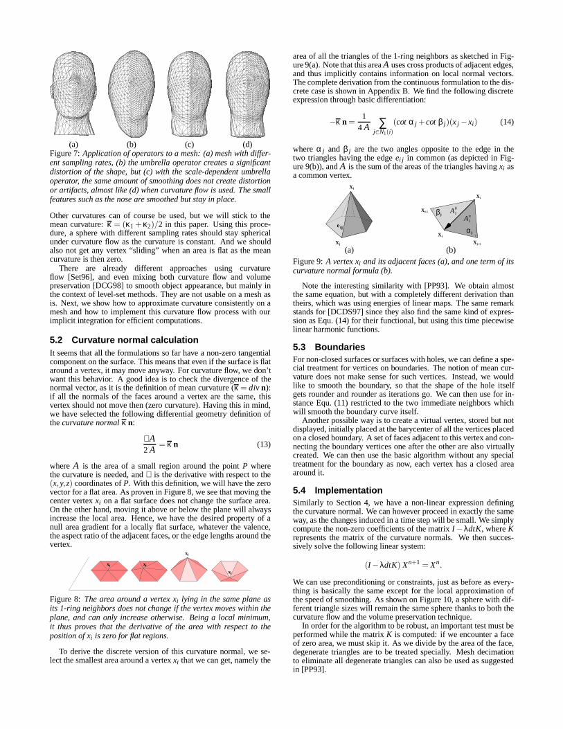
(a) (b) (c) (d)Figure 7:Application of operators to a mesh: (a) mesh with differ-ent sampling rates, (b) the umbrella operator creates a significantdistortion of the shape, but (c) with the scale-dependent umbrellaoperator, the same amount of smoothing does not create distortionor artifacts, almost like (d) when curvature flow is used. The smallfeatures such as the nose are smoothed but stay in place.

Other curvatures can of course be used, but we will stick to themean curvature:κ = (κ1 + κ2)/2 in this paper. Using this proce-dure, a sphere with different sampling rates should stay sphericalunder curvature flow as the curvature is constant. And we shouldalso not get any vertex “sliding” when an area is flat as the meancurvature is then zero.

There are already different approaches using curvatureflow [Set96], and even mixing both curvature flow and volumepreservation [DCG98] to smooth object appearance, but mainly inthe context of level-set methods. They are not usable on a mesh asis. Next, we show how to approximate curvature consistently on amesh and how to implement this curvature flow process with ourimplicit integration for efficient computations.

5.2 Curvature normal calculationIt seems that all the formulations so far have a non-zero tangentialcomponent on the surface. This means that even if the surface is flataround a vertex, it may move anyway. For curvature flow, we don’twant this behavior. A good idea is to check the divergence of thenormal vector, as it is the definition of mean curvature (κ = div n):if all the normals of the faces around a vertex are the same, thisvertex should not move then (zero curvature). Having this in mind,we have selected the following differential geometry definition ofthecurvature normalκ n:

∇A2 A

= κ n (13)

whereA is the area of a small region around the pointP wherethe curvature is needed, and∇ is the derivative with respect to the(x,y,z) coordinates ofP. With this definition, we will have the zerovector for a flat area. As proven in Figure 8, we see that moving thecenter vertexxi on a flat surface does not change the surface area.On the other hand, moving it above or below the plane will alwaysincrease the local area. Hence, we have the desired property of anull area gradient for a locally flat surface, whatever the valence,the aspect ratio of the adjacent faces, or the edge lengths around thevertex.

x

ix

ix

ixi

Figure 8: The area around a vertex xi lying in the same plane asits 1-ring neighbors does not change if the vertex moves within theplane, and can only increase otherwise. Being a local minimum,it thus proves that the derivative of the area with respect to theposition of xi is zero for flat regions.

To derive the discrete version of this curvature normal, we se-lect the smallest area around a vertexxi that we can get, namely the

area of all the triangles of the 1-ring neighbors as sketched in Fig-ure 9(a). Note that this areaA uses cross products of adjacent edges,and thus implicitly contains information on local normal vectors.The complete derivation from the continuous formulation to the dis-crete case is shown in Appendix B. We find the following discreteexpression through basic differentiation:

−κ n =1

4 A ∑j∈N1(i)

(cot α j +cot β j )(xj −xi) (14)

whereα j and β j are the two angles opposite to the edge in thetwo triangles having the edgeei j in common (as depicted in Fig-ure 9(b)), andA is the sum of the areas of the triangles havingxi asa common vertex.

X

ij

j

e

Xi

Aβ

jj

j+1

jj

jαA

βj-1

X

i

α

X

X

X

(a) (b)Figure 9:A vertex xi and its adjacent faces (a), and one term of itscurvature normal formula (b).

Note the interesting similarity with [PP93]. We obtain almostthe same equation, but with a completely different derivation thantheirs, which was using energies of linear maps. The same remarkstands for [DCDS97] since they also find the same kind of expres-sion as Equ. (14) for their functional, but using this time piecewiselinear harmonic functions.

5.3 BoundariesFor non-closed surfaces or surfaces with holes, we can define a spe-cial treatment for vertices on boundaries. The notion of mean cur-vature does not make sense for such vertices. Instead, we wouldlike to smooth the boundary, so that the shape of the hole itselfgets rounder and rounder as iterations go. We can then use for in-stance Equ. (11) restricted to the two immediate neighbors whichwill smooth the boundary curve itself.

Another possible way is to create a virtual vertex, stored but notdisplayed, initially placed at the barycenter of all the vertices placedon a closed boundary. A set of faces adjacent to this vertex and con-necting the boundary vertices one after the other are also virtuallycreated. We can then use the basic algorithm without any specialtreatment for the boundary as now, each vertex has a closed areaaround it.

5.4 ImplementationSimilarly to Section 4, we have a non-linear expression definingthe curvature normal. We can however proceed in exactly the sameway, as the changes induced in a time step will be small. We simplycompute the non-zero coefficients of the matrixI −λdtK, whereKrepresents the matrix of the curvature normals. We then succes-sively solve the following linear system:

(I −λdtK) Xn+1 = Xn.

We can use preconditioning or constraints, just as before as every-thing is basically the same except for the local approximation ofthe speed of smoothing. As shown on Figure 10, a sphere with dif-ferent triangle sizes will remain the same sphere thanks to both thecurvature flow and the volume preservation technique.

In order for the algorithm to be robust, an important test must beperformed while the matrixK is computed: if we encounter a faceof zero area, we must skip it. As we divide by the area of the face,degenerate triangles are to be treated specially. Mesh decimationto eliminate all degenerate triangles can also be used as suggestedin [PP93].

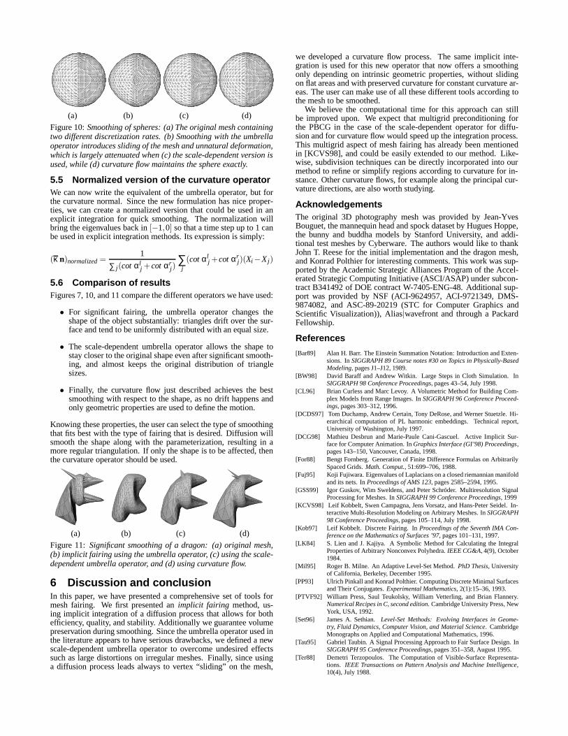
(a) (b) (c) (d)

Figure 10:Smoothing of spheres: (a) The original mesh containingtwo different discretization rates. (b) Smoothing with the umbrellaoperator introduces sliding of the mesh and unnatural deformation,which is largely attenuated when (c) the scale-dependent version isused, while (d) curvature flow maintains the sphere exactly.

5.5 Normalized version of the curvature operatorWe can now write the equivalent of the umbrella operator, but forthe curvature normal. Since the new formulation has nice proper-ties, we can create a normalized version that could be used in anexplicit integration for quick smoothing. The normalization willbring the eigenvalues back in[−1,0] so that a time step up to 1 canbe used in explicit integration methods. Its expression is simply:

(κ n)normalized=1

∑ j (cot αlj +cot αr

j )∑

j(cot αl

j +cot αrj)(Xi−Xj)

5.6 Comparison of resultsFigures 7, 10, and 11 compare the different operators we have used:

• For significant fairing, the umbrella operator changes theshape of the object substantially: triangles drift over the sur-face and tend to be uniformly distributed with an equal size.

• The scale-dependent umbrella operator allows the shape tostay closer to the original shape even after significant smooth-ing, and almost keeps the original distribution of trianglesizes.

• Finally, the curvature flow just described achieves the bestsmoothing with respect to the shape, as no drift happens andonly geometric properties are used to define the motion.

Knowing these properties, the user can select the type of smoothingthat fits best with the type of fairing that is desired. Diffusion willsmooth the shape along with the parameterization, resulting in amore regular triangulation. If only the shape is to be affected, thenthe curvature operator should be used.

(a) (b) (c) (d)

Figure 11: Significant smoothing of a dragon: (a) original mesh,(b) implicit fairing using the umbrella operator, (c) using the scale-dependent umbrella operator, and (d) using curvature flow.

6 Discussion and conclusionIn this paper, we have presented a comprehensive set of tools formesh fairing. We first presented animplicit fairing method, us-ing implicit integration of a diffusion process that allows for bothefficiency, quality, and stability. Additionally we guarantee volumepreservation during smoothing. Since the umbrella operator used inthe literature appears to have serious drawbacks, we defined a newscale-dependent umbrella operator to overcome undesired effectssuch as large distortions on irregular meshes. Finally, since usinga diffusion process leads always to vertex “sliding” on the mesh,

we developed a curvature flow process. The same implicit inte-gration is used for this new operator that now offers a smoothingonly depending on intrinsic geometric properties, without slidingon flat areas and with preserved curvature for constant curvature ar-eas. The user can make use of all these different tools according tothe mesh to be smoothed.

We believe the computational time for this approach can stillbe improved upon. We expect that multigrid preconditioning forthe PBCG in the case of the scale-dependent operator for diffu-sion and for curvature flow would speed up the integration process.This multigrid aspect of mesh fairing has already been mentionedin [KCVS98], and could be easily extended to our method. Like-wise, subdivision techniques can be directly incorporated into ourmethod to refine or simplify regions according to curvature for in-stance. Other curvature flows, for example along the principal cur-vature directions, are also worth studying.

AcknowledgementsThe original 3D photography mesh was provided by Jean-YvesBouguet, the mannequin head and spock dataset by Hugues Hoppe,the bunny and buddha models by Stanford University, and addi-tional test meshes by Cyberware. The authors would like to thankJohn T. Reese for the initial implementation and the dragon mesh,and Konrad Polthier for interesting comments. This work was sup-ported by the Academic Strategic Alliances Program of the Accel-erated Strategic Computing Initiative (ASCI/ASAP) under subcon-tract B341492 of DOE contract W-7405-ENG-48. Additional sup-port was provided by NSF (ACI-9624957, ACI-9721349, DMS-9874082, and ASC-89-20219 (STC for Computer Graphics andScientific Visualization)), Alias|wavefront and through a PackardFellowship.

References

[Bar89] Alan H. Barr. The Einstein Summation Notation: Introduction and Exten-sions. InSIGGRAPH 89 Course notes #30 on Topics in Physically-BasedModeling, pages J1–J12, 1989.

[BW98] David Baraff and Andrew Witkin. Large Steps in Cloth Simulation. InSIGGRAPH 98 Conference Proceedings, pages 43–54, July 1998.

[CL96] Brian Curless and Marc Levoy. A Volumetric Method for Building Com-plex Models from Range Images. InSIGGRAPH 96 Conference Proceed-ings, pages 303–312, 1996.

[DCDS97] Tom Duchamp, Andrew Certain, Tony DeRose, and Werner Stuetzle. Hi-erarchical computation of PL harmonic embeddings. Technical report,University of Washington, July 1997.

[DCG98] Mathieu Desbrun and Marie-Paule Cani-Gascuel. Active Implicit Sur-face for Computer Animation. InGraphics Interface (GI’98) Proceedings,pages 143–150, Vancouver, Canada, 1998.

[For88] Bengt Fornberg. Generation of Finite Difference Formulas on ArbitrarilySpaced Grids.Math. Comput., 51:699–706, 1988.

[Fuj95] Koji Fujiwara. Eigenvalues of Laplacians on a closed riemannian manifoldand its nets. InProceedings of AMS 123, pages 2585–2594, 1995.

[GSS99] Igor Guskov, Wim Sweldens, and Peter Schr¨oder. Multiresolution SignalProcessing for Meshes. InSIGGRAPH 99 Conference Proceedings, 1999

[KCVS98] Leif Kobbelt, Swen Campagna, Jens Vorsatz, and Hans-Peter Seidel. In-teractive Multi-Resolution Modeling on Arbitrary Meshes. InSIGGRAPH98 Conference Proceedings, pages 105–114, July 1998.

[Kob97] Leif Kobbelt. Discrete Fairing. InProceedings of the Seventh IMA Con-ference on the Mathematics of Surfaces ’97, pages 101–131, 1997.

[LK84] S. Lien and J. Kajiya. A Symbolic Method for Calculating the IntegralProperties of Arbitrary Nonconvex Polyhedra.IEEE CG&A, 4(9), October1984.

[Mil95] Roger B. Milne. An Adaptive Level-Set Method.PhD Thesis, Universityof California, Berkeley, December 1995.

[PP93] Ulrich Pinkall and Konrad Polthier. Computing Discrete Minimal Surfacesand Their Conjugates.Experimental Mathematics, 2(1):15–36, 1993.

[PTVF92] William Press, Saul Teukolsky, William Vetterling, and Brian Flannery.Numerical Recipes in C, second edition. Cambridge University Press, NewYork, USA, 1992.

[Set96] James A. Sethian.Level-Set Methods: Evolving Interfaces in Geome-try, Fluid Dynamics, Computer Vision, and Material Science. CambridgeMonographs on Applied and Computational Mathematics, 1996.

[Tau95] Gabriel Taubin. A Signal Processing Approach to Fair Surface Design. InSIGGRAPH 95 Conference Proceedings, pages 351–358, August 1995.

[Ter88] Demetri Terzopoulos. The Computation of Visible-Surface Representa-tions. IEEE Transactions on Pattern Analysis and Machine Intelligence,10(4), July 1988.

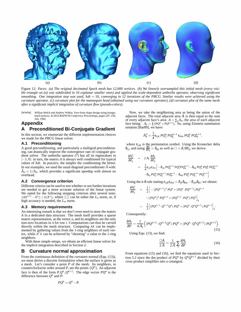
(a) (b) (c) (d)

Figure 12:Faces: (a) The original decimated Spock mesh has 12,000 vertices. (b) We linearly oversampled this initial mesh (every visi-ble triangle on (a) was subdivided in 16 coplanar smaller ones) and applied the scale-dependent umbrella operator, observing significantsmoothing. One integration step was used,λdt = 10, converging in 12 iterations of the PBCG. Similar results were achieved using thecurvature operator. (c) curvature plot for the mannequin head (obtained using our curvature operator), (d) curvature plot of the same meshafter a significant implicit integration of curvature flow (pseudo-colors).

[WW94] Willian Welch and Andrew Witkin. Free-form shape design using triangu-lated surfaces. InSIGGRAPH 94 Conference Proceedings, pages 247–256,July 1994.

AppendixA Preconditioned Bi-Conjugate GradientIn this section, we enumerate the different implementation choiceswe made for the PBCG linear solver.

A.1 PreconditioningA good preconditioning, and particularly a multigrid precondition-ing, can drastically improve the convergence rate of conjugate gra-dient solver. The umbrella operator (7) has all its eigenvalues in[−1,0]: in turn, the matrixA is always well conditioned for typicalvalues ofλdt. In practice, the simpler the conditioning the better.In our examples, we used the usual diagonal preconditionerA with:Aii = 1/Aii , which provides a significant speedup with almost nooverhead.

A.2 Convergence criterionDifferent criteria can be used to test whether or not further iterationsare needed to get a more accurate solution of the linear system.We opted for the following stopping criterion after several tests:||AXn+1−Xn|| < ε||Xn||, where||.|| can be either theL2 norm, or, ifhigh accuracy is needed, theL∞ norm.

A.3 Memory requirementsAn interesting remark is that we don’t even need to store the matrixA in a dedicated data structure. The mesh itself provides a sparsematrix representation, as the vertexxi and its neighbors are the onlynon-zero locations inA for row i. Computations can thus be carrieddirectly within the mesh structure. ComputingAX can be imple-mented by gathering values from the 1-ring neighbors of each ver-tex, whileATX can be achieved by “shooting” a value to the 1-ringneighbors.

With these simple setups, we obtain an efficient linear solver forthe implicit integration described in Section 2.

B Curvature normal approximationFrom the continuous definition of the curvature normal (Equ. (13)),we must derive a discrete formulation when the surface is given asa mesh. Let’s consider a pointP of the mesh. Its neighbors, incounterclockwise order aroundP, are the pointsQn. An adjacentface is then of the formP,Qn,Qn+1. The edge vectorPQn is thedifference betweenQn andP:

PQn = Qn−P.

Now, we take the neighboring area as being the union of theadjacent faces. The total adjacent areaA is then equal to the sumof every adjacent face’s area:A = ∑n An, the area of each adjacentface being: An = 1

2 ||PQn×PQn+1||. So, using Einstein summationnotation [Bar89], we have:

A2n =

14

εi jk PQnj PQn+1

k εilm PQnl PQn+1

m ,

whereεi jk is the permutation symbol. Using the Kronecker deltaδi j , and using∂Pi

∂Pq= δiq as well as∇ = ∂/∂Pq, we derive:

∂A2i

∂Pq= 2 Ai

∂Ai

∂Pq

=14

εi jkεilm

[−δ jq PQn+1

k PQnl PQn+1

m −δkq PQnj PQn

l PQn+1m

−δlq PQnj PQn+1

k PQn+1m −δmq PQn

j PQn+1k PQn+1

l

]Using theε-δ rule statingεi jkεilm = δ jl δkm−δ jmδkl , we obtain:

∂A2i

∂Pq=

12

[−||PQn+1||2 PQn +(PQn ·PQn+1) PQn+1

−||PQn||2 PQn+1 +(PQn+1 ·PQn) PQn]

q

=12

[(PQn+1 ·Qn+1Qn) PQn +(PQn ·QnQn+1) PQn+1

]q.

Consequently:

∂Ai

∂P=

14 Ai

((PQn+1 ·Qn+1Qn) PQn +(PQn ·QnQn+1) PQn+1

).

(15)Using Equ. (13), we find:

∇A2 A

=1

2 A ∑i

∂Ai

∂P(16)

From equations (15) and (16), we find the equations used in Sec-tion 5.2 since the dot product ofPQn by QnQn+1 divided by theircross product simplifies into a cotangent.