Implications of Optimal Investment Policies for Hybrid Pension Plans: Sponsor and Member Perspectives

Peter Albrecht*

Joachim Coche ** Raimond Maurer*** Ralph Rogalla****

Abstract

This paper analyzes pension plan costs and investment strategies in the context of alternative hy-brid pension plans which are optimal either from the perspective of the plan sponsor or the bene-ficiaries. The focus is in particular on how the introduction of minimum and maximum limits for pension benefits as well as minimum guarantees and caps on the return of the members’ individ-ual investment accounts affect investment decisions and plan costs. Within a comparative static analysis framework, it is shown that for low to medium risk portfolios, minimum benefit guaran-tees tend to be more expensive than minimum return guarantees while for the latter costs in-crease exponentially with investment risk. The study also finds that portfolio choices of the sponsor and the beneficiaries show substantial differences depending on the exact plan design and the beneficiaries’ risk aversion. Combining minimum return guarantees and caps on invest-ment returns emerged as a possible means to reduce such differences, to share investment risks and returns more equally between sponsor and beneficiaries, and to keep pension pla n costs un-der control.

*) University of Mannheim Professor of Risk Theory, Portfolio Management, and Insurance Schloss 68131 Mannheim, Germany Telephone: +49 (0)621 181 1680 Facsimile: +49 (0)621 181 1681 E-mail: p.albrecht@bwl.uni-mannheim.de

**) European Central Bank Senior Economist P.O. Box 16 03 19 60066 Frankfurt am Main, Germany Telephone: +49 (0)69 1344 6891 Facsimile: +49 (0)69 1344 6231 E-mail: Joachim.coche@ecb.int

***) Johann Wolfgang Goethe-University of Frankfurt Professor of Investment, Portfolio Management, and Pension Finance Department of Finance Senckenberganlage 31-33 (Uni-PF 58) 60054 Frankfurt am Main, Germany Telephone: ++ 49 69 798 25227 Facsimile: ++ 49 69 798 25228 E-mail: RMaurer@wiwi.uni-frankfurt.de

****) Johann Wolfgang Goethe-University of Frankfurt Department of Finance Senckenberganlage 31-33 (Uni-PF 58) 60054 Frankfurt am Main, Germany Telephone: ++ 49 69 798 25227 Facsimile: ++ 49 69 798 25228 E-mail: rogalla@wiwi.uni-frankfurt.de

Implications of Optimal Investment Policies for Hybrid Pension Plans: Sponsor and Member Perspectives

Introduction

First introduced in the United States by the Bank of America in 1985, hybrid types of

pension plans altered the traditional form of pension plan design.1 The term “hybrid ” pension

plan subsumes plans with elements of both defined contribution (DC) and defined benefit (DB)

plans. The motivation for hybrid plans is to combine the best characteristics of DB and DC plans

while circumventing their major disadvantages. Most hybrid plans include a DC-type individual

account, but also provide minimum and/or maximum annuity benefits at retirement using a DB-

type formula. Additionally, investment returns credited to the individual accounts may be subject

to return guarantees and/or return caps.2

When setting up and running a pension plan, the costs implied by the specific plan de-

sign, as well as the asset allocation decision for the accumulated funds, are of major importance.

In a pure DC plan, plan members have extensive control over the ir accounts’ investment strategy

(usually subject to the investment menu they are offered). This enables participants to shape

their portfolio’s risk/return profile to their individual risk preferences. The sponsor only promises

to make a certain contribution to the account, so the investment risk is therefore completely

borne by the members; consequently, the plan sponsor tends to be rather indifferent toward the

individual’s investment policy, as it poses no cost implications . By contrast, in a pure DB plan,

the sponsor is obliged to provide adequate funds to cover the plan liabilities, so he is fully ex-

posed to capital market risk. The asset allocation decision has direct cost implications for his

funding situation. In a hybrid pension plan, both parties have an interest in influencing the plan’s

investment policy. This can result in a conflict of interest, which is the object of investigation of

this chapter. At the same time, we scrutinize the costs inherent in different DB-type elements.

2

To do so, we construct several hypothetical hybrid pension plans, make assumptions

about key parameters, and derive optimal investment strategies for particular objective functions.

Objective functions analyzed include cost minimization from the perspective of plan sponsor

versus maximizing risk adjusted pension benefits from the perspective of plan members. Al-

though the design of the plan and the assumed parameters do not exactly match a particular pen-

sion plan, the models draw on real-world elements. In particular, the ones presented in this chap-

ter draw on prior analysis of the European Central Bank’s retirement plan,3 though the model

plan developed here has different characteristics and is in particular less complex.4

This paper is organized as follows. First we discuss the main elements of the hybrid plans

evaluated including a minimum pension guarantee, maximum pension limits, a minimum return

guarantee, and a maximum return cap. Next, we focus on technical aspects of the model and the

decision-making process assumed. Finally we analyze the optimal investment strategy, both from

the perspective of the plan sponsor as well as plan members.

Designing a Hybrid Pension Plan

The pension arrangement analyzed in this study is taken to be a mandatory plan whose

members do not contribute to any other public or private pension scheme. It is a non-contributory

funded pension plan, consisting of two types of accounts. First, every plan member owns an in-

dividual account endowed by the plan sponsor with an assumed payment of 17 percent of the

members’ annual salary,5 representing the employer’s regular plan contributions. In addition to

this, the plan sponsor owns a separate account, called the contingency reserve, which plays the

role of a settlement account for transfers to or from the individual accounts. The funds in both

the individual accounts as well as the contingency reserve represent total plan assets. All plan

3

funds must be invested in the same asset allocation, and the return on this portfolio is credited

pro rata to the individual accounts and the contingency reserve.

Complementary to the plan sponsor’s pledge to finance the individual accounts with

regular contributions, the plan design includes a combination of additional guarantees and/or

limits. These are related to the level of benefits at retirement and/or to the asset return credited to

the individual accounts. Incorporating these elements affects plan liabilities, and may require

additional payments from the sponsor (in addition to regular contributions ). These supplementary

contributions may be triggered in two cases. First, when guaranteeing a minimum return on the

plan assets, the plan sponsor must cover shortfalls below the target return by replenishing the in-

dividual accounts through supplementary contributions. Second, supplementary contributions

may be needed if there are guaranteed minimum pension benefits. Specifically, we posit that if

the market value of the total plan assets falls below 90 percent of the actuarial present value of

the plan liabilities (i.e. the solvency ratio falls below 0.9), the plan sponsor must immediately

endow the contingency reserve with enough funds to re-establish a solvency ratio of one.

In this plan, participants cannot withdraw funds during the accumulation phase. Mem-

bers leaving the plan before retirement (e.g. due to workforce turnover) may either leave their

funds in the plan, or receive the balance of their individual account as a lump sum payment (lim-

ited to the actuarial value of the maximum pension where applicable ). At the retirement age of

65, the available funds are converted into a life annuity. This conversion may be subject to the

guaranteed minimum pension benefits and to maximum pension limits, depending on the exact

design of the benefit structure, to be discussed subsequently.

Benefit Structure. In what follows, six distinct hybrid pension plan benefit designs are scrut i-

nized. Every plan is characterized by a unique combination of the elements mentioned earlier.

4

The reason to compare these designs is to investigate their differential effects on plan costs and

pension benefit levels, and implications for optimal plan asset allocation.

In Case I, which we term the “benchmark” design, the pension plan consists of an ind i-

vidual account for every plan member endowed by the plan sponsor with regular contributions of

17 percent of the current salary. These funds are invested in the capital markets. Beneficiaries are

protected from return shortfalls by an annual capital guarantee, i.e. a guaranteed yearly minimum

return of 0 percent.6 In case the funds earn less than 0 percent in any given year, the sponsor

must make additional contributions. If the funds accumulated over a plan member’s career are

insufficient to pay for an adequate pension, this plan also guarantees a minimum level of pension

benefits, corresponding to two percent of the career-average salary per year of service. Further-

more, this plan limits the maximum level of benefits to two percent of the beneficiaries’ final

salary per year of service.7 In the event of a member either leaving the plan or retiring, any funds

in the individual account that exceed the actuarial value of the maximum benefits are transferred

to the contingency reserve.

The subsequent Cases II to V are constructed by eliminating certain plan elements, com-

pared to the benchmark case. Case II excludes the capital guarantee, and in Case III the maxi-

mum benefits are also removed. Case IV eliminates the minimum bene fit from the benchmark

case, while Case V only includes the annual capital guarantee. Case VI includes the annual capi-

tal guarantee alongside a return cap of 10 percent per year, but provides no further benefit ele-

ments relating to salary and years of service. If the asset return on the funds in the individual ac-

counts in any year exceeds the 10 percent level, the excess return will be credited to the contin-

gency reserve. Case VII does not include any guarantees or caps and, therefore, can be inter-

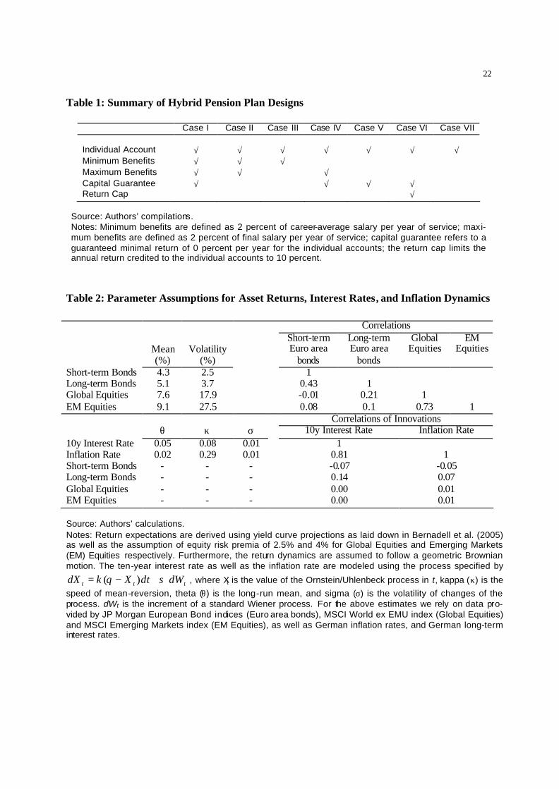
preted as a pure defined contribution plan. Table 1 summarizes the various plan designs.

Table 1 here

5

The minimum rate of return guarantee increases the complexity of the pension plan sub-

stantially. More specifically, the minimum rate of return guarantee may introduce an asymmetric

dependency between assets and liabilities. Suppose in Case I, the value of a given investment

account corresponds to a pension payment in-between the minimum and the maximum pension

limit. In this situation, a high asset return in any given year permanently increases the sponsors’

liabilities for the current and future years. Negative returns in subsequent years do not decrease

the liability as the minimum rate of return guarantee requires the sponsor to replenish the in-

vestment account. Thus the high asset return in the first year had a permanent effect on the li-

abilities.8 However in a situation where the investment account corresponds to a pension pay-

ment either below the minimum pension guarantee or above the maximum pension limit, asset

returns do not have an immediate effect on the sponsor’s liabilities.

Asset Liability Modeling and the Pension Decision-Making Process. Next we evaluate the

asset liability model and decision making process needed to determine the fund’s investment

strategy. For that purpose, we describe the key assumptions on how assets and liabilities are pro-

jected forward, and subsequently specify decision rules used either by the plan sponsor or by the

beneficiaries to identify the optimal asset allocation. Regardless of whether the asset allocation

decision is made by the sponsor or by the beneficiaries, a two-step heuristic method is applied,

which is often found in practical decision-making formats. In the first step, the set of mean-

variance efficient asset allocations is determined using a standard Markowitz-type portfolio op-

timization. In the second step, all portfolios from the efficient frontier are assessed against a pro-

jection of asset and liabilities over a horizon of 30 years.

To project the return and risk effects of a certain asset allocation over time, it is neces-

sary to specify the stochastic processes governing asset class returns, the long-term interest rate

(10 years), as well as the inflation rate. The difference between the nominal 10 year interest rate

6

and the inflation rate (i.e. the real 10-year interest rate) is used to discount future pension liabili-

ties. The stochastic dynamics of the (uncertain) market values of the assets are modeled as geo-

metric Brownian motion, which implies that the log return of every asset is independent and

identically normally distributed. The long -term interest rate as well as the inflation rate are mod-

eled using the multi-dimensional Ornstein/Uhlenbeck process, to cover the empirically obser v-

able mean reversion characteristics in these time series.9

The investment universe comprises the broad asset classes, long and short-term euro

area bonds, world-wide diversified equities, and emerging market equities. A regime-switching

model is used to derive expected returns for the fixed income asset classes. This technique allows

consistent generation of yield curve projections contingent on expectations about economic ac-

tivity (Bernadell et al., 2005). In the long-term projection of the macro economic environment,

we rely on the Economist Intelligence Unit (EIU) as an external provider of forecasts for the

Euro area, the US and Japan. 10 Expected returns on equity investments are approximated by add-

ons to the long-term yields on government bonds. In the analysis the equity risk premium is fixed

at 2.5 percent annually for world-wide diversified equity. Reflecting higher risk of emerging

market investments we assume an equity risk premium of 4 percent for this asset class. All asset

classes are subject to short selling constraints and, in addition, the investment in emerging mar-

ket equity is restricted to a maximum of 5 percent of overall investments.

Table 2 here

The projection of liabilities is based on a discontinuance valuation method usually ap-

plied by plan actuaries; this relies on the assumption that service of each participant ceases on the

respective valuation date. It assumes that at a given valuation date the individual investment ac-

counts are translated into a (usually deferred) life annuity with inflation-adjusted payme nts,

whereby the minimum and maximum pension limits laid out earlier are applied. The real dis-

7

count rates used fo r this exercise are the real 10-year interest rates determined by the asset

model. Discontinuance valuation is performed for each year over the 30-year analysis horizon

(Bacinello, 2000). The valuation of liabilities requires projecting population dynamics compris-

ing the evolution of the number and composition of staff, salaries, number of retirees and de-

pendents. For this purpose a hypothetical population comprising initially of 1000 staff members

is constructed. The population is evolved forward on the basis of an inhomogeneous, discrete-

time Markov chain. Transition probabilities and parameters are derived using assumptions for

the company’s recruitment, promotion and turnover patterns, evolution of salaries as a function

of consumer price inflation, and mortality rates.

Comparing the value of liabilities with the projected value of assets at the respective

valuation date allows for the evolution of the plan’s solvency ratio to be determined and supple-

mentary contributions to be made by the sponsor and average benefits received by the beneficiar-

ies. Given the complexity of the plan design, solutions are determined using Monte Carlo simula-

tion over 1000 simulation runs. In the process, we make a number of specific assumptions about

selection criteria used to determine the plan’s optimal asset allocation. To this end, two different

regimes are introduced. Under the first regime, arguably the standard for hybrid pension plans,

the plan sponsor is solely responsible for the investment strategy. Correspondingly, the second

regime assumes that decisions are made by the beneficiaries. In both cases, investment decisions

apply simultaneously to all individual investment accounts and the contingency reserve.

For the sponsor, we assume that the objective is to minimize the costs of running the

plan. More specifically the sponsor’s behavior is modeled as minimizing the worst-case value of

discounted supplementary contributions, where the worst-case value is defined as the five per-

cent quantile of the distribution of the sum of discounted supplementary contributions over the

30-year investment horizon. Thus, decision criteria other than costs (such as plan solvency) are

8

not considered explicitly. Plan funding is accounted for by the solvency rule, according to which

the funding ratio cannot fall short of 90 percent in any single year. More formally, let SCt be the

total amount of supplementary contributions to be made by the plan sponsor in period t and r the

appropriate discount rate, then the objective function is given by:

( )

+∑

=

30

1%5

1min

tt

t

r

SCVaR (1)

For the beneficiaries, investment decisions for the plan are made collaboratively for all

investment accounts. These decisions may be made in the context of an investment committee

composed of staff representatives. Such a body is assumed to maximize the expected value of the

constant-relative-risk-aversion (CRRA) utility function )(PBFu with risk aversion parameter

0>γ , which is assumed to be equal for all beneficiaries.

( )[ ]

−

=−

γ

γ

1maxmax

1PBFEPBFuE (2)

Utility is defined over the pension benefit factor PBF which refers to pension payments per year

service expressed as the percentage of final salary at time of retirement. Factor PBF comprises

all simulation runs and all plan members retiring over the 30-year investment horizon.

The Plan Sponsor’s Investment Decision

We next take the perspective of the plan sponsor, to evaluate the interrelation between

asset allocation in the individual pension accounts and the resulting plan costs measured in terms

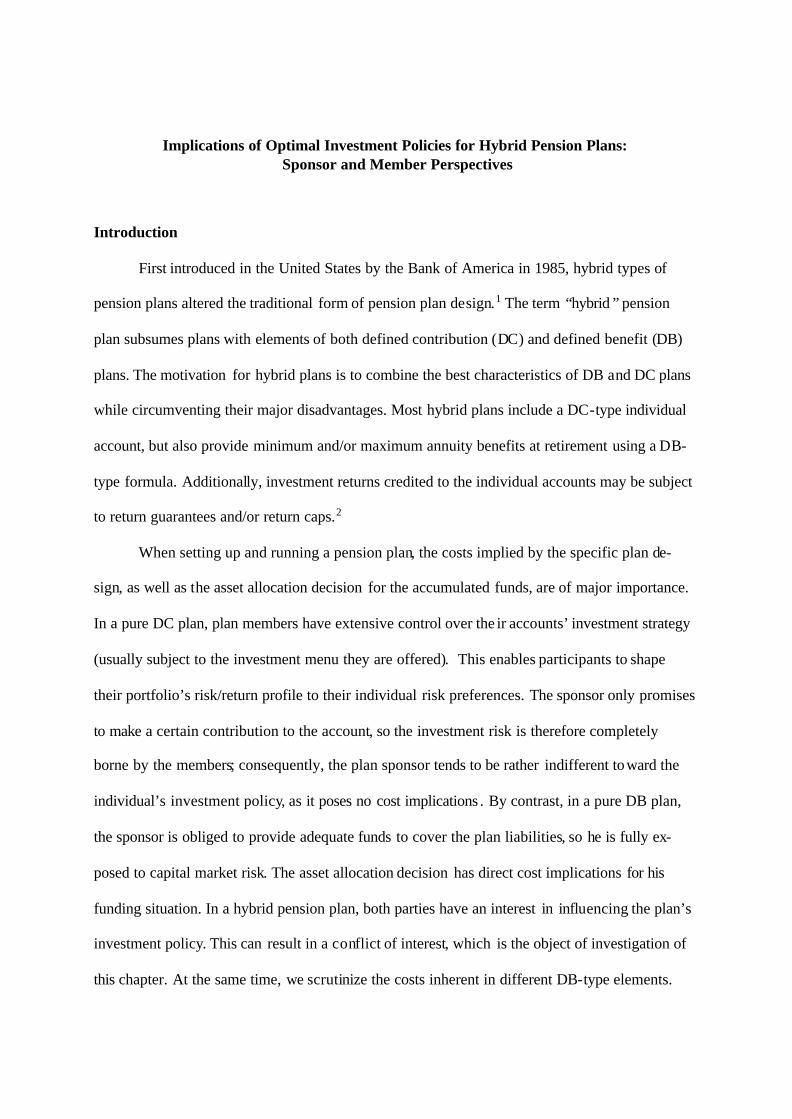
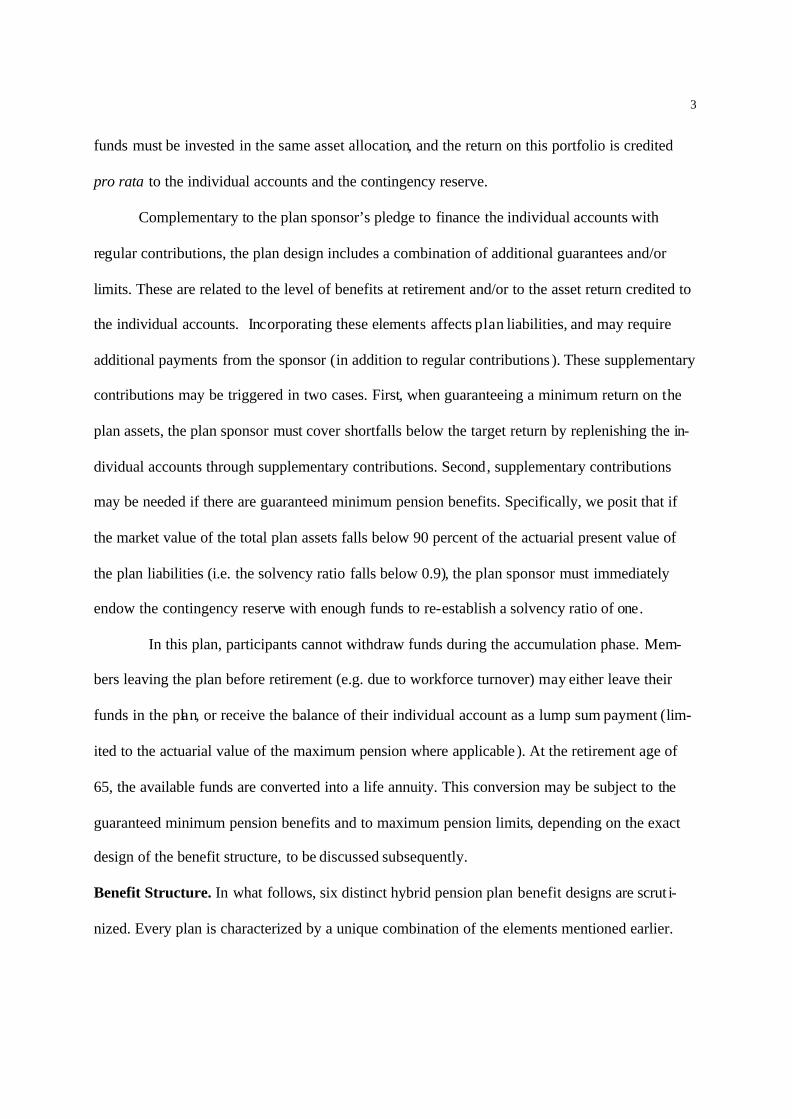
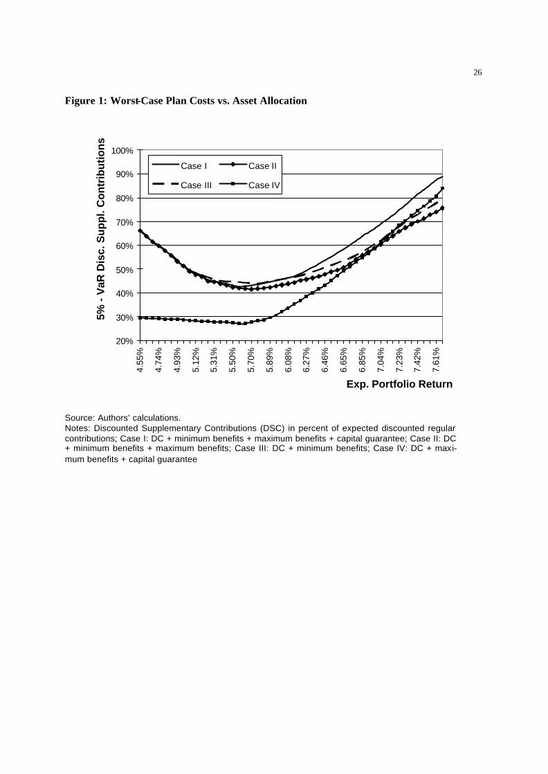
of supplementary contributions by the plan sponsor. Figure 1 depicts the worst-case supplemen-

tary contributions for Cases I to IV for different portfolio allocations, and Figure 2 for Cases V

and VI. Worst-case costs are measured as the five percent value at risk of the supplementary con-

tributions, i.e. the present value of contributions by the plan sponsor exceeding the regular pay-

ments of 17 percent of the salaries. Portfolio allocations are represented by the mean-variance

9

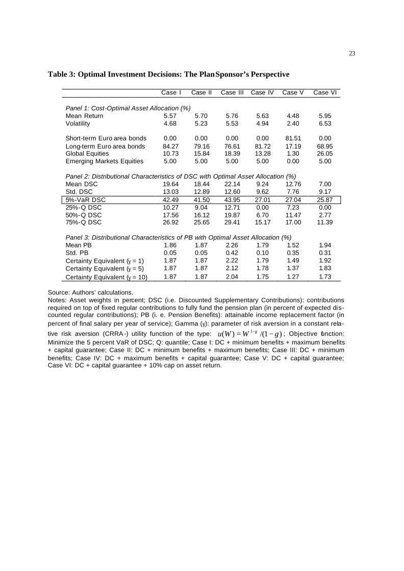
efficient portfolio returns. Details of the cost-optimal asset allocations, including the asset

weights for short- and long-term euro area bonds, global and emerging market equities appear in

Panel 1 of Table 3. Panel 2 contains the distributional characteristics of the discounted supple-

mentary contributions for the cost-optimal asset allocations. Finally, Panel 3 reports the pension

benefits for these allocations in terms of certainty equivalents.11 These certainty equivalents are

calculated according to the utility function stated above and for four different parameters of rela-

tive risk aversion, gamma=0 (i.e. mean pension benefits), gamma=1, 5, and 10.

Table 3 here

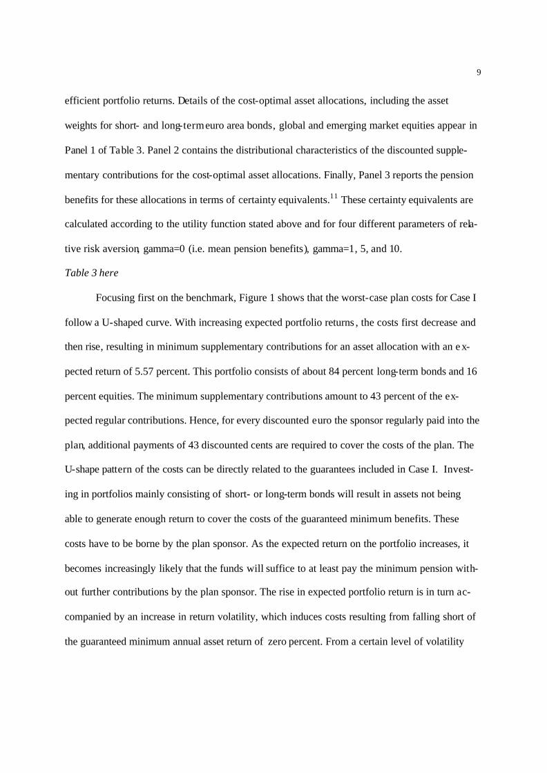
Focusing first on the benchmark, Figure 1 shows that the worst-case plan costs for Case I

follow a U-shaped curve. With increasing expected portfolio returns , the costs first decrease and

then rise, resulting in minimum supplementary contributions for an asset allocation with an e x-

pected return of 5.57 percent. This portfolio consists of about 84 percent long-term bonds and 16

percent equities. The minimum supplementary contributions amount to 43 percent of the ex-

pected regular contributions. Hence, for every discounted euro the sponsor regularly paid into the

plan, additional payments of 43 discounted cents are required to cover the costs of the plan. The

U-shape pattern of the costs can be directly related to the guarantees included in Case I. Invest-

ing in portfolios mainly consisting of short- or long-term bonds will result in assets not being

able to generate enough return to cover the costs of the guaranteed minimum benefits. These

costs have to be borne by the plan sponsor. As the expected return on the portfolio increases, it

becomes increasingly likely that the funds will suffice to at least pay the minimum pension with-

out further contributions by the plan sponsor. The rise in expected portfolio return is in turn ac-

companied by an increase in return volatility, which induces costs resulting from falling short of

the guaranteed minimum annual asset return of zero percent. From a certain level of volatility

10

onwards, these newly induced costs overcompensate the cost savings related to the minimum

pension benefits and the overall costs increase again.

Figure 1 here

Changing the design of the plan has some interesting effects. Eliminating the annual re-

turn guarantee for the individual accounts in Case II cuts the amount of supplementary contrib u-

tions, especially in the case of a more risky asset allocation. However the asset allocation which

minimizes costs is only slightly different compared to Case I (i.e. about five percent less bonds

and more equities). The minimum worst-case costs decrease marginally from 43 to 42 percent of

regular contributions. This can be attributed to the fact that for a low risk asset allocation the

costs from the annual return guarantee are relatively low.12

In Case III, not only the capital guarantee but also the maximum pension regulation is

eliminated; now the plan is basically DC but the beneficiaries are protected by a DB minimum

pension benefit in the event of adverse capital market developments. Therefore the amount of

supplementary contributions increases compared to Case II, as there are no longer funds in ex-

cess of those needed to provide maximum pension benefits which could be credited to the plan

sponsor. Looking at the cost minimizing asset allocation, the equity exposure is slightly further

increased to about 23 percent with overall worst case supplementary contributions of 44 percent.

Case IV shows a quite different cost function. The previously observed U-shape form is

maintained showing a minimum of supplementary contributions at a portfolio return of 5.6 per-

cent, which corresponds to an asset allocation of 82 percent bonds and 18 percent equities. While

the asset allocation is comparable to Cases I to III, the level of supplementary contributions with

27 percent of regular contributions is substantially lower than in the previous cases. Additionally,

the left branch of the cost function (low risk portfolios) is nearly flat while the right branch

(more risky portfolios) shows a strong increase. Economically, this can be explained as follows.

11

As discussed for Case I, the predominant source of costs, especially when investing in low risk

allocations, is the minimum benefit guarantee. This guarantee is not included in Case IV, leading

to substantially lower costs compared to Case I. Increasing the expected return and the volatility

of the portfolio now has two opposing effects. The higher the (expected) portfolio return, the

more often the plan sponsor will profit from cashing in funds from the individual retirement ac-

counts that exceed the amount necessary to cover the maximum pension benefits. Contrarily, the

higher the return volatility, the more often supplementary contributions will be triggered due to

the annual capital guarantee. Since the former effect dominates the latter for less risky portfolios,

the overall costs first decrease with increasing expected portfolio return. For more risky alloca-

tions the latter effect dominates the former, which leads to rapidly growing contributions. As the

cost impact of the minimum benefit guarantee is diminishing for increasing portfolio returns,

Cases I and IV hardly differ for highly risky portfolios.

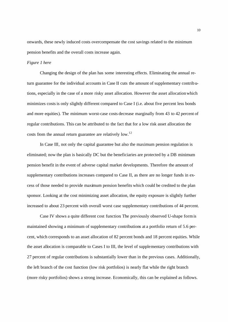
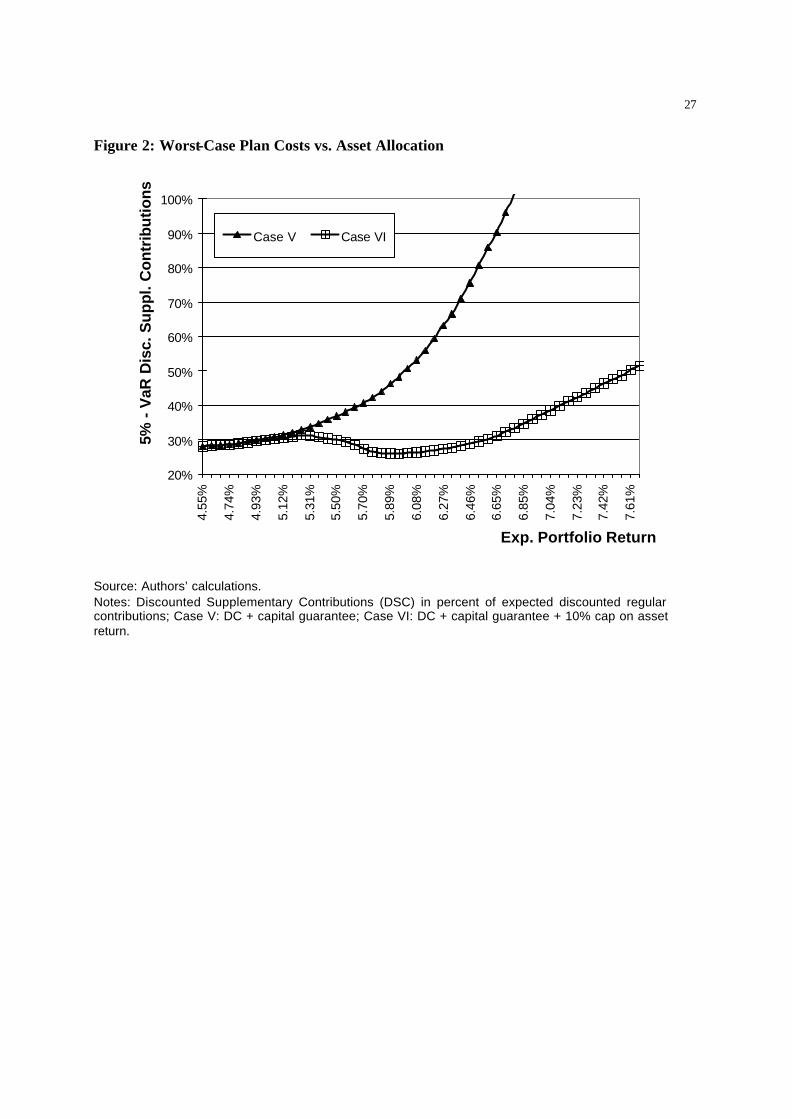
We now turn to the cases with no explicit defined minimum or maximum benefit, de-

picted in Figure 2. Case V shows a plan with unlimited upside potential but with a shortfall pro-

tection resulting from the annual return guarantee. It is obvious that this plan design implies in-

creasing supplementary contributions, the higher the equity exposure. Hence, minimizing the

costs in terms of supplementary contributions leads to the minimum volatility portfolio, consist-

ing of 82 percent short-term and 17 percent long-term bonds, and only 1 percent equities. The

resulting costs amount to 27 percent of regular contributions.

Figure 2 here

Similar to Case V, Case VI offers an annual capital guarantee and therefore protection

against return shortfalls. However, the upside potential is limited due to the 10 percent return

cap. This return cap has a significant impact on the shape of the cost curve. While the amount of

supplementary contributions in Cases V and VI is approximately equal for low risk asset alloca-

12

tions, the costs in Case VI initially decrease for increasing portfolio return and volatility. For

these allocations the increasing costs resulting from the capital guarantee are overcompensated

by the profits the plan sponsor can generate through cashing in any returns that exceed the 10

percent cap. From a certain point onwards, however, the costs of the capital guarantee rise dis-

proportionately with further increasing volatility, leading to overall growing supplementary con-

tributions. At minimum worst case costs of 26 percent, resulting from investing in about 69 per-

cent bonds and 31 percent equities, this case proves to be the cheapest of all hybrid plan designs

discussed. This holds for the minimum cost asset allocation and especially for all portfolios with

high expected returns and volatilities.

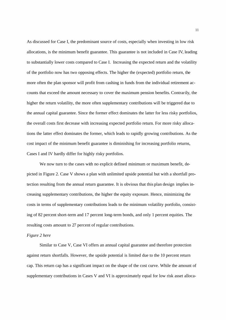
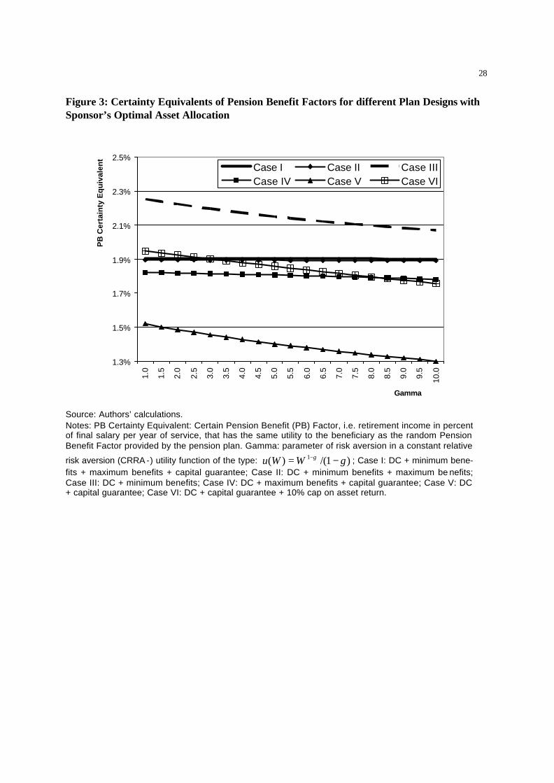
Implications for Plan Beneficiaries. The implications of investing in the cost-minimizing port-

folios for expected pension benefits can now be derived (see Figure 3). Panel 3 of Table 3 sum-

marizes expected pension benefit factors and their standard deviation, expressing the pension

benefits as a percentage of final salary per year of service. In order to relate the probability dis-

tribution of the pension benefit factors to the risk aversion of a representative beneficiary, the

pension factor certainty equivalents are calculated for a range of risk aversion parameters using

the standard CRRA utility function. This allows a direct evaluation of the cost-optimal asset al-

location for the various plan designs, Case I to VI, from the perspective of plan members with

different levels of risk aversion. Figure 3 depicts the certainty equivalents for all parameters of

risk aversion from one to 10 in half steps. Additionally, numerical results for selected levels of

risk aversion (gamma = 1, 5, and 10) are presented in Panel 3 of Table 3.

Figure 3 here

The Figure shows that Case III results in the highest pension benefit factors for all levels

of risk aversion under scrutiny, with the mean benefit factor being 2.26 percent (see also Table 3,

Panel 3). At the same time, Case V always produces the lowest factors, on average 1.52 percent.

13

This is an interesting result, as both cases show structural similarities. Cases III and V both offer

downside protection to the beneficiaries, Case III by means of guaranteed minimum pension

benefits, Case V with the annual capital guarantee for the individual accounts. Neither case limits

the upside potential.

An explanation for this can be found when looking at the different cost-minimal asset al-

locations. Optimizing the amount of supplementary contributions in Case V, the plan sponsor

will only invest in short- and long-term bonds, resulting in the lowest risk exposure with respect

to the capital guarantee. With highly conservative risk and return profile of the assets simultane-

ously low pension benefits are expected. Such an asset allocation, however, is not appropriate in

Case III, since its return expectations are insufficient to cover the costs resulting from the gua r-

anteed minimum benefits, i.e. 2 percent of the career-average salary per year of service. Rather,

it is necessary to implement a portfolio strategy that offers higher mean returns, coming at the

cost of higher volatility. This, in turn, leads to substantially higher supplementary contributions,

since the plan sponsor fully bears the downside volatility while only the beneficiaries profit from

the upside volatility.

Implementing a maximum benefit cap (2 percent of final salary per year of service) re-

sults in considerably reduced volatilities of the pension benefit factors, i.e. 0.05 percent for Cases

I and II, and 0.10 percent for Case IV (see Table 3, panel 3). Consequently, the certainty equiva-

lents of the pension benefit factors are nearly constant for the various risk aversion coefficients

reported in Figure 3. Among these cases, Case I offers the highest pension benefits but is also the

most costly design. Case II only offers slightly lower benefits combined with slightly lower

costs.

In general, it can be concluded that hybrid plans that offer the highest expected pension

benefits tend to cause the highest amount of supplementary contributions. Yet there are two ex-

14

ceptions: Case V offers by far the lowest pension benefits, but even given optimal asset alloca-

tion patterns, additional costs are not small. By contrast, Case VI has the lowest supplementary

contribution, and will lead to expected pensions benefits that exceed all but one other case. The

rather high volatility of the pension benefit factor, however, causes the certainty equivalents to

drop below those of most other cases for higher levels of risk aversion.

Beneficiaries’ Investment Decisions

In this section we assume that the asset allocation decisions are made by the plan partici-

pants, rather than the plan sponsor; here the plan members’ objective function is to maximize the

expected utility of pension benefits by choosing an appropriate asset allocation. This analysis is

undertaken for Cases I-VI and also for Case VII, a pure defined contribution plan. Our interest

here is to look at the resulting pension benefits for plan members with different levels of risk

aversion, as well as the composition of the optimal asset allocation. For simplicity, we assume

that the asset allocation decision made by the beneficiaries and their cost impact have no reper-

cussive effects on plan member salaries; neither will rising supplementary contributions lead to

lower salaries/salary increases nor will reductions of plan costs be passed on to the workers.

As above, we derive the benefit-optimal portfolio allocations from the set of mean-

variance efficient portfolio returns. Details of the optimal investment weights (i.e. the mean and

volatility of asset returns, mean and certainty equivalents of pension benefit factors for plan

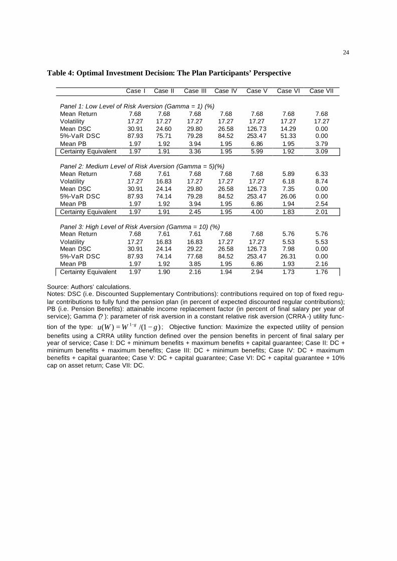
members as well the resulting costs in terms of supplementary contributions for the plan sponsor)

are shown in Table 4. The first Panel contains the results for a representative plan member with a

low coefficient of risk aversion (gamma = 1), while the other panels show findings for a medium

(gamma = 5) and a high (gamma = 10) coefficient. Table 5 provides details regarding the in-

vestment weights.

15

Table 4 and 5 here

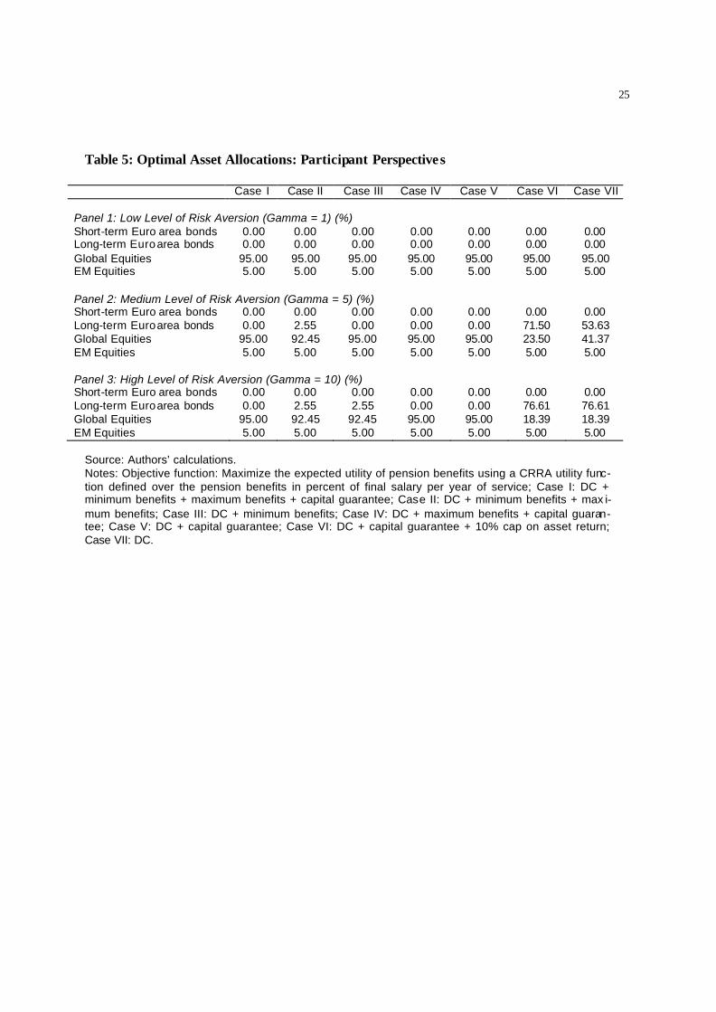
The results show that, independent of risk aversion, plan beneficiaries would opt for the

asset allocation that offers the highest or almost the highest expected return and the highest or

almost the highest volatility in Cases I-V. Table 5 indicates that the optimal asset allocation con-

sists of 100 percent stocks. This is because beneficiaries are protected against downside volatility

of the equity and bond markets by guaranteed minimum pension benefits and the annual capital

guarantee. The value of this downside protection ceteris paribus increases with return volatility.

By analogy to option pricing theory, the minimum pension bene fit and the capital guarantee can

be interpreted as a put option, for which the value is also positively related to the volatility of the

underlying.

Analyzing the level of supplementary contributions associated with these asset alloca-

tions, it appears that costs for the plan sponsor would be prohibitively high. This is particularly

true for Case V, in which the members’ individual accounts are protected against negative fluc-

tuations in the capital markets while at the same time offering full participation in positive re-

turns. Here, the certainty equivalents of the pension benefit factors vary between 5.99 percent for

a low risk aversion (gamma = 1) and 2.94 percent for a higher risk aversion (gamma = 10).

These high pension benefits are associated with worst-case (mean) supplementary contributions

of 253 percent (127 percent).

Cases I, II, and IV limit the upside potential available to the beneficiaries by incorporat-

ing the maximum pension benefit restriction. This results in lower benefits and lower costs com-

pared to Case V, yet plan members still have the incentive to choose portfolios with very high

volatility. Even though the costs are substantially reduced, they are still intolerably high. For ex-

ample in Case IV, i.e. Case V with incorporated maximum benefit limit, the worst case (ex-

16

pected) supplementary contributions amount to 85 percent (27 percent), being about three times

as high as in case the plan sponsor chooses the asset allocation.

Case VI produces a different picture: now, the annual capital guarantee and a 10 percent

cap on the maximum annual asset return limit the credits to the beneficiaries’ individual ac-

counts. Beneficiaries with a low level of risk aversion (gamma = 1) will still invest in the maxi-

mum expected return/maximum volatility portfolio, but more risk averse plan members will

choose an asset allocation with substantially reduced exposure to capital market risk. For a me-

dium (high) level of risk aversion (gamma = 5 vs. 10), the allocation to bonds will increase from

none (at gamma = 1), to 72 (77) percent (see Table 5). We compare this optimal asset allocation

from the members’ perspective (with moderate to high risk aversion) to the cost optimal asset

allocation from the sponsor’s perspective in Panel 1 of Table 3. It is noteworthy that from both

perspectives, the optimal investment strategy is nearly identical – a high exposure to bonds and

low exposure to equities. This results in quite similar cost implication in terms of supplementary

contributions. If the plan sponsor were to set the asset allocation, the five percent Value-at-Risk

of supplementary contributions would be 26 percent (panel 2 of Table 3); if the representative

member with a medium or high risk aversion selected the optimal asset allocation, this would

equally result in supplementary contributions for the plan sponsor of 26 percent. Hence, if the

benefit structure of the pension plan is designed according to Case VI, members’ and sponsor’s

interests are consistent, at least with respect to the asset allocation decision for a given plan de-

sign.

Case VI might seem to be most suitable for a hybrid pension plan, as it combines accept-

able cost consequences for the sponsor and attractive pension benefit factors for the plan mem-

bers. Nevertheless a superior plan design exists. Case VII is a pure defined contribution plan

with no capital guarantee and no return cap. By construction, this plan causes no additional costs

17

in term of supplementary contributions for the sponsor. Additionally, as shown in Table 4, a pure

DC plan provides higher mean pension benefits as well as certainty equivalents for all levels of

risk aversion. This result is due to the specification of the floor/cap structure, i.e. a minimum rate

of return of 0 percent per year and a return maximum of 10 percent per year. Alternatively, set-

ting the cap to an annual return of 12.5 percent and leaving the floor constant at 0 percent implies

the following results: For members with a low level of risk aversion (gamma = 1), the certainty

equivalent for the benefit factor of the hybrid plan is still lower than in the case of a pure DC

plan (2 percent compared to 3 percent). For members with medium to high levels of risk aversion

(gamma = 5 or 10), the hybrid plan is more attractive than the pure defined contribution plan. 13

Yet when increasing the cap to 12.5 percent, the plan members will again choose the maximum

volatility portfolio (i.e.100 percent equities), independent of their level of risk aversion. Unfortu-

nately this will cause unacceptable costs in terms of supplementary contributions for the plan

sponsor.

Conclusions

This chapter evaluates key properties of hypothetical hybrid pension plans in terms of

their implications for plan costs and pension benefits, by adapting a pure defined contribution

scheme to include minimum and maximum limits for pension benefits, as well as minimum

guarantees and return caps on individual investment accounts. In particular we explore optimal

investment strategies from the perspectives of both plan sponsor and beneficiaries. We find that

introducing DB elements substantially increases the overall costs of running the pension plan and

has a major impact on the resulting optimal portfolios.

The investment strategy chosen and the additional plan costs show strong interrelation-

ship. If only minimum rate of return guarantees are included in the plan design, additional costs

increase exponentially as a function of higher expected asset return and volatility. Consequently,

18

plan sponsors choose the minimum risk portfolio consisting of around 82 percent short-term

bonds, around 17 percent long-term bonds, and only 1 percent equities. Enhancing this plan with

a cap on returns credited to the individual accounts leads to a U-shaped cost curve for a broad

range of possible asset allocations. Here, the optimal portfolio consists of about 69 percent bonds

and 31 percent equities, i.e. about 50 percent more equities than for any other plan design opti-

mized from the sponsor’s perspective. At the same time, with this design the additional costs are

reduced to 26 percent from 27 percent in the case without the return cap.

For plan designs that guarantee minimum pension benefits, the implied additional costs

(expected and worst case values) are also U-shaped as a function of expected investment returns.

Therefore, assuming the objective to minimize the worst case value of additional costs, the spon-

sor will opt for asset allocations which deviate from the minimum risk allocation as well. These

portfolios comprise between 77 and 84 percent bonds and between 16 and 23 percent equities.

The additional costs for these plans lie in the range of 42 and 44 percent of regular contributions,

i.e. about 50 percent above the costs of a plan only guaranteeing a minimum rate of return.

Taking the beneficiaries’ perspective, we first evaluate the utility implications of alterna-

tive defined benefit elements based on the sponsor’s optimal asset allocation decisions. To this

end, certainty equivalents of pension benefits are calculated for a range of risk aversion parame-

ters. Generally higher additional costs imply higher expected pension benefits, but the introduc-

tion of caps on credited asset returns allows cost reductions with only slightly lower certainty

equivalents of random pension benefits. We also evaluate optimal investment choices from the

beneficiaries’ perspective, and we find that almost independent of risk aversion, plan members

tend to select maximum return, maximum risk asset allocations where the plan either guarantees

minimum pension benefits or minimum return guarantees. However, if the minimum rate of re-

turn guarantees are combined with a cap on the maximum return credited to individual accounts,

19

risk averse members opt for less risky asset allocations. In this case, the optimal asset allocation

includes about 72 percent in bonds and 28 percent in equities.

Our results are directly relevant to the moral hazard problem faced by agencies offering

insurance against pension plan defaults, including the Pension Benefit Guaranty Corporation

(PBGC) in the United States, and the newly established Pension Protection Fund in the United

Kingdom (see, e.g., Warshawsky et al. 2005; Coronado and Liang 2005; McCarthy and Neuber-

ger 2005). Like the plan sponsor in this paper, those organizations issue a put option on the value

of the assets invested in the insured pension plans. Therefore, they should be interested in rather

conservative pension fund asset allocations mainly concentrated in bonds. If, as for the benefici-

aries in this chapter, the price of such an option (i.e. the insurance premium) is set independently

of its value, and if the insured party can influence the value, there is a chance that the insured

party will seek to boost the probability of exercising the option – by investing in high-risk assets

or by underfunding the pension plan. A possible solution to this moral hazard problem is to im-

plement funding requirements that take into account both current level of funding as well as in-

vestment risk, as for example is done for the German Individual Investment Accounts (“Riester”

accounts; c.f. Maurer and Schlag 2004).

The analysis presented in this study can be useful when discussing possible designs of

hybrid pension plans. Some plan designs appear to be Pareto-inefficient (e.g. minimum and

maximum pension benefits in combination with minimum rate of return guarantee) as they are

dominated by others which imply lower additional costs and higher expected utility for plan

members. Furthermore, if plan sponsors and beneficiaries are jointly responsible for investment

decision, caps on investment returns may reduce conflicts of interest as asset allocations will di-

verge less between the parties.

20

References

Bacinello, Anna R. 2000. “Valuation of contingent-claims characterizing particular pension

schemes.” Insurance: Mathematics and Economics 27: 177-188.

Bernadell, Carlos, Joachim Coche and Ken Nyholm. 2005. “Yield Curve Prediction for the Stra-

tegic Investor.” Working Paper No 472, European Central Bank.

Bodie, Zvi, and E. Philip Davis. 2000. The Foundations of Pension Finance. Cheltenham, UK :

Edward Elgar: xvi.

Bodie, Zvi, Alan J. Marcus, and Robert C. Merton. 1988. “Defined Benefit versus Defined Con-

tribution Pension Plans: What are the real Tradeoffs?” In Pensions in the U.S. Economy,

eds. Zvi Bodie, John B. Shoven, and David A. Wise. Chicago, IL: University of Chicago

Press: 139-162.

Bodie, Zvi, and Robert C. Merton. 1992. “Pension Benefit Guarantees in the United States: a

Functional Analysis.” In The Future of Pensions in the United States, ed. Raymond

Schmitt. Philadelphia, PA: University of Pennsylvania Press : 194-234.

Clark, Robert, and Sylvester J. Schieber. 2004 “Adopting Cash Balance Pension Plans: Implica-

tions and Issues.” The Journal of Pension Economics and Finance 3(3): 271-295.

Coronado, Julia L., and Philip C. Copeland. 2004. “Cash Balance Pension Plan Conversions and

the New Economy.” The Journal of Pension Economics and Finance 3(3): 297-314.

Coronado, Julia L., and Nellie Liang. 2005. “The Influence of PBGC Insurance on Pension Fund

Finances.” This volume.

Johnson, Richard W., and Eugene Steuerle. 2004. “Promoting Work at Older Ages: the Role of

Hybrid Pension Plans in an Aging Population.” The Journal of Pension Economics and

Finance 3(3): 315-337.

21

Lachance, Marie-Eve, and Olivia S. Mitchell. 2004. “Understanding Individual Account Guaran-

tees.” In The Pension Challenge: Risk Transfers and Retirement Income Security. eds.

Olivia S. Mitchell and Kent Smetters. Oxford University Press: 159-186.

Maurer, Raimond, and Christian Schlag. 2004. “Money-Back Guarantees in Individual Account

Pensions: Evidence from the German Pension Reform.” In The Pension Challenge: Risk

Transfers and Retirement Income Security, eds. Olivia S. Mitchell and Kent Smetters.

Oxford University Press: 187-213.

McCarthy, David, and Anthony Neuberger. 2005. “The UK Approach to Insuring Defined Bene-

fit Pension Plans.” This volume.

Mitchell, Olivia S., and Janemarie Mulvey. 2004. “Potential Implications of Mandating Choice

in Corporate Defined Benefit Plans.” The Journal of Pension Economics and Finance

3(3):339-354.

Pennacchi, George G. 1999. “The Value of Guarantees on Pension Fund Returns.” The Journal

of Risk and Insurance 66(2): 219-237.

Pesando, James E. 1996. “The Government’s Role in Insuring Pensions.” In Securing Employer

Based Pensions: An International Perspective, eds. Zvi Bodie, Olivia S. Mitchell and

John A. Turner. Philadelphia: University of Pennsylvania Press, 1996: 286-305.

Sylvester J. Schieber. 2003. A Symposium on Cash Balance Pensions: Background and Introduc-

tion.” Pension Research Council Working Paper, Wharton School.

http://rider.wharton.upenn.edu/~prc/wpcashbalance.html

Warshawsky, Mark J., Neal McCall, and John D. Worth. 2005. “A Modern Approach to Single

Employer Defined Benefit Pension Regulation: Motivations for the Administration’s

Pension Reform Proposal.” This volume.

22

Table 1: Summary of Hybrid Pension Plan Designs

Case I Case II Case III Case IV Case V Case VI Case VII

Individual Account √ √ √ √ √ √ √ Minimum Benefits √ √ √ Maximum Benefits √ √ √ Capital Guarantee √ √ √ √ Return Cap √

Source: Authors’ compilations. Notes: Minimum benefits are defined as 2 percent of career-average salary per year of service; maxi-mum benefits are defined as 2 percent of final salary per year of service; capital guarantee refers to a guaranteed minimal return of 0 percent per year for the individual accounts; the return cap limits the annual return credited to the individual accounts to 10 percent.

Table 2: Parameter Assumptions for Asset Returns, Interest Rates, and Inflation Dynamics

Correlations

Mean (%)

Volatility (%)

Short-term Euro area

bonds

Long-term Euro area

bonds

Global Equities

EM Equities

Short-term Bonds 4.3 2.5 1 Long-term Bonds 5.1 3.7 0.43 1 Global Equities 7.6 17.9 -0.01 0.21 1 EM Equities 9.1 27.5 0.08 0.1 0.73 1 Correlations of Innovations θ κ σ 10y Interest Rate Inflation Rate 10y Interest Rate 0.05 0.08 0.01 1 Inflation Rate 0.02 0.29 0.01 0.81 1 Short-term Bonds - - - -0.07 -0.05 Long-term Bonds - - - 0.14 0.07 Global Equities - - - 0.00 0.01 EM Equities - - - 0.00 0.01

Source: Authors’ calculations. Notes: Return expectations are derived using yield curve projections as laid down in Bernadell et al. (2005) as well as the assumption of equity risk premia of 2.5% and 4% for Global Equities and Emerging Markets (EM) Equities respectively. Furthermore, the return dynamics are assumed to follow a geometric Brownian motion. The ten-year interest rate as well as the inflation rate are modeled using the process specified by

ttt dWdtXdX σθκ +−= )( , where Xt is the value of the Ornstein/Uhlenbeck process in t, kappa (κ) is the speed of mean-reversion, theta (θ) is the long-run mean, and sigma (σ) is the volatility of changes of the process. dWt is the increment of a standard Wiener process. For the above estimates we rely on data pro-vided by JP Morgan European Bond indices (Euro area bonds), MSCI World ex EMU index (Global Equities) and MSCI Emerging Markets index (EM Equities), as well as German inflation rates, and German long-term interest rates.

23

Table 3: Optimal Investment Decisions: The Plan Sponsor’s Perspective

Case I Case II Case III Case IV Case V Case VI Panel 1: Cost-Optimal Asset Allocation (%) Mean Return 5.57 5.70 5.76 5.63 4.48 5.95 Volatility 4.68 5.23 5.53 4.94 2.40 6.53 Short-term Euro area bonds 0.00 0.00 0.00 0.00 81.51 0.00 Long-term Euro area bonds 84.27 79.16 76.61 81.72 17.19 68.95 Global Equities 10.73 15.84 18.39 13.28 1.30 26.05 Emerging Markets Equities 5.00 5.00 5.00 5.00 0.00 5.00 Panel 2: Distributional Characteristics of DSC with Optimal Asset Allocation (%) Mean DSC 19.64 18.44 22.14 9.24 12.76 7.00 Std. DSC 13.03 12.89 12.60 9.62 7.76 9.17 5%-VaR DSC 42.49 41.50 43.95 27.01 27.04 25.87 25%-Q DSC 10.27 9.04 12.71 0.00 7.23 0.00 50%-Q DSC 17.56 16.12 19.87 6.70 11.47 2.77 75%-Q DSC 26.92 25.65 29.41 15.17 17.00 11.39 Panel 3: Distributional Characteristics of PB with Optimal Asset Allocation (%) Mean PB 1.86 1.87 2.26 1.79 1.52 1.94 Std. PB 0.05 0.05 0.42 0.10 0.35 0.31 Certainty Equivalent (γ = 1) 1.87 1.87 2.22 1.79 1.49 1.92 Certainty Equivalent (γ = 5) 1.87 1.87 2.12 1.78 1.37 1.83 Certainty Equivalent (γ = 10) 1.87 1.87 2.04 1.75 1.27 1.73

Source: Authors’ calculations. Notes: Asset weights in percent; DSC (i.e. Discounted Supplementary Contributions): contributions required on top of fixed regular contributions to fully fund the pension plan (in percent of expected dis-counted regular contributions); PB (i. e. Pension Benefits): attainable income replacement factor (in percent of final salary per year of service); Gamma (γ): parameter of risk aversion in a constant rela-

tive risk aversion (CRRA -) utility function of the type: )1/()( 1 γγ −= −WWu ; Objective function: Minimize the 5 percent VaR of DSC; Q: quantile; Case I: DC + minimum benefits + maximum benefits + capital guarantee; Case II: DC + minimum benefits + maximum benefits; Case III: DC + minimum benefits; Case IV: DC + maximum benefits + capital guarantee; Case V: DC + capital guarantee; Case VI: DC + capital guarantee + 10% cap on asset return.

24

Table 4: Optimal Investment Decision: The Plan Participants’ Perspective

Case I Case II Case III Case IV Case V Case VI Case VII Panel 1: Low Level of Risk Aversion (Gamma = 1) (%) Mean Return 7.68 7.68 7.68 7.68 7.68 7.68 7.68 Volatility 17.27 17.27 17.27 17.27 17.27 17.27 17.27 Mean DSC 30.91 24.60 29.80 26.58 126.73 14.29 0.00 5%-VaR DSC 87.93 75.71 79.28 84.52 253.47 51.33 0.00 Mean PB 1.97 1.92 3.94 1.95 6.86 1.95 3.79 Certainty Equivalent 1.97 1.91 3.36 1.95 5.99 1.92 3.09 Panel 2: Medium Level of Risk Aversion (Gamma = 5)(%) Mean Return 7.68 7.61 7.68 7.68 7.68 5.89 6.33 Volatility 17.27 16.83 17.27 17.27 17.27 6.18 8.74 Mean DSC 30.91 24.14 29.80 26.58 126.73 7.35 0.00 5%-VaR DSC 87.93 74.14 79.28 84.52 253.47 26.06 0.00 Mean PB 1.97 1.92 3.94 1.95 6.86 1.94 2.54 Certainty Equivalent 1.97 1.91 2.45 1.95 4.00 1.83 2.01 Panel 3: High Level of Risk Aversion (Gamma = 10) (%) Mean Return 7.68 7.61 7.61 7.68 7.68 5.76 5.76 Volatility 17.27 16.83 16.83 17.27 17.27 5.53 5.53 Mean DSC 30.91 24.14 29.22 26.58 126.73 7.98 0.00 5%-VaR DSC 87.93 74.14 77.68 84.52 253.47 26.31 0.00 Mean PB 1.97 1.92 3.85 1.95 6.86 1.93 2.16 Certainty Equivalent 1.97 1.90 2.16 1.94 2.94 1.73 1.76

Source: Authors’ calculations. Notes: DSC (i.e. Discounted Supplementary Contributions): contributions required on top of fixed regu-lar contributions to fully fund the pension plan (in percent of expected discounted regular contributions); PB (i.e. Pension Benefits): attainable income replacement factor (in percent of final salary per year of service); Gamma (? ): parameter of risk aversion in a constant relative risk aversion (CRRA -) utility func-

tion of the type: )1/()( 1 γγ −= −WWu ; Objective function: Maximize the expected utility of pension benefits using a CRRA utility function defined over the pension benefits in percent of final salary per year of service; Case I: DC + minimum benefits + maximum benefits + capital guarantee; Case II: DC + minimum benefits + maximum benefits; Case III: DC + minimum benefits; Case IV: DC + maximum benefits + capital guarantee; Case V: DC + capital guarantee; Case VI: DC + capital guarantee + 10% cap on asset return; Case VII: DC.

25

Table 5: Optimal Asset Allocations: Participant Perspectives

Case I Case II Case III Case IV Case V Case VI Case VII Panel 1: Low Level of Risk Aversion (Gamma = 1) (%) Short-term Euro area bonds 0.00 0.00 0.00 0.00 0.00 0.00 0.00 Long-term Euro area bonds 0.00 0.00 0.00 0.00 0.00 0.00 0.00 Global Equities 95.00 95.00 95.00 95.00 95.00 95.00 95.00 EM Equities 5.00 5.00 5.00 5.00 5.00 5.00 5.00 Panel 2: Medium Level of Risk Aversion (Gamma = 5) (%) Short-term Euro area bonds 0.00 0.00 0.00 0.00 0.00 0.00 0.00 Long-term Euro area bonds 0.00 2.55 0.00 0.00 0.00 71.50 53.63 Global Equities 95.00 92.45 95.00 95.00 95.00 23.50 41.37 EM Equities 5.00 5.00 5.00 5.00 5.00 5.00 5.00 Panel 3: High Level of Risk Aversion (Gamma = 10) (%) Short-term Euro area bonds 0.00 0.00 0.00 0.00 0.00 0.00 0.00 Long-term Euro area bonds 0.00 2.55 2.55 0.00 0.00 76.61 76.61 Global Equities 95.00 92.45 92.45 95.00 95.00 18.39 18.39 EM Equities 5.00 5.00 5.00 5.00 5.00 5.00 5.00

Source: Authors’ calculations. Notes: Objective function: Maximize the expected utility of pension benefits using a CRRA utility func-tion defined over the pension benefits in percent of final salary per year of service; Case I: DC + minimum benefits + maximum benefits + capital guarantee; Case II: DC + minimum benefits + max i-mum benefits; Case III: DC + minimum benefits; Case IV: DC + maximum benefits + capital guaran-tee; Case V: DC + capital guarantee; Case VI: DC + capital guarantee + 10% cap on asset return; Case VII: DC.

26

Figure 1: Worst-Case Plan Costs vs. Asset Allocation

20%

30%

40%

50%

60%

70%

80%

90%

100%4.

55%

4.74

%

4.93

%

5.12

%

5.31

%

5.50

%

5.70

%

5.89

%

6.08

%

6.27

%

6.46

%

6.65

%

6.85

%

7.04

%

7.23

%

7.42

%

7.61

%

Exp. Portfolio Return

5% -

VaR

Dis

c. S

up

pl.

Co

ntr

ibu

tion

s

Case I Case II

Case III Case IV

Source: Authors’ calculations. Notes: Discounted Supplementary Contributions (DSC) in percent of expected discounted regular contributions; Case I: DC + minimum benefits + maximum benefits + capital guarantee; Case II: DC + minimum benefits + maximum benefits; Case III: DC + minimum benefits; Case IV: DC + maxi-mum benefits + capital guarantee

27

Figure 2: Worst-Case Plan Costs vs. Asset Allocation

20%

30%

40%

50%

60%

70%

80%

90%

100%4.

55%

4.74

%

4.93

%

5.12

%

5.31

%

5.50

%

5.70

%

5.89

%

6.08

%

6.27

%

6.46

%

6.65

%

6.85

%

7.04

%

7.23

%

7.42

%

7.61

%

Exp. Portfolio Return

5% -

VaR

Dis

c. S

up

pl.

Co

ntr

ibu

tion

s

Case V Case VI

Source: Authors’ calculations. Notes: Discounted Supplementary Contributions (DSC) in percent of expected discounted regular contributions; Case V: DC + capital guarantee; Case VI: DC + capital guarantee + 10% cap on asset return.

28

Figure 3: Certainty Equivalents of Pension Benefit Factors for different Plan Designs with Sponsor’s Optimal Asset Allocation

1.3%

1.5%

1.7%

1.9%

2.1%

2.3%

2.5%

1.0

1.5

2.0

2.5

3.0

3.5

4.0

4.5

5.0

5.5

6.0

6.5

7.0

7.5

8.0

8.5

9.0

9.5

10.0

Gamma

PB

Cer

tain

ty E

qu

ival

ent

Case I Case II Case IIICase IV Case V Case VI

Source: Authors’ calculations. Notes: PB Certainty Equivalent: Certain Pension Benefit (PB) Factor, i.e. retirement income in percent of final salary per year of service, that has the same utility to the beneficiary as the random Pension Benefit Factor provided by the pension plan. Gamma: parameter of risk aversion in a constant relative

risk aversion (CRRA -) utility function of the type: )1/()( 1 γγ −= −WWu ; Case I: DC + minimum bene-fits + maximum benefits + capital guarantee; Case II: DC + minimum benefits + maximum be nefits; Case III: DC + minimum benefits; Case IV: DC + maximum benefits + capital guarantee; Case V: DC + capital guarantee; Case VI: DC + capital guarantee + 10% cap on asset return.

29

Endnotes

1 Pension promises in the US have traditionally been either of the pure defined benefit (DB) or

pure defined contribution (DC) type (Schieber, 2003). In a DB scheme, the plan sponsor prom-

ises to the plan benefic iaries a final level of pension benefits. This level is usually defined ac-

cording to a benefit formula, as a function of salary trajectory and years of service. Benefits are

usually paid as a life annuity rather than as a lump sum. As Bodie et al. (1988) note, the foremost

advantage of a DB plan is that it offers stable income replacement rates to retired beneficiaries.

The major drawbacks of DB schemes include the lack of benefit portability when leaving the

company and the complex valuation of plan liabilities. Moreover, the plan sponsor is exposed to

substantial investment and longevity risk, which could result in significant contribution ex-

penses. In a DC scheme, by contrast, the plan sponsor commits to paying funds into the benefi-

ciaries’ individual accounts according to a specified formula, e.g. a fixed percentage of annual

salary. The most prominent feature of a DC scheme is its inherent flexibility: by construction, it

is fully funded in individual accounts. The value of the pension benefits is simply determined as

the market value of the backing assets. Therefore, the pension benefits are easily portable in case

of job change. Additionally, the beneficiaries have control over their funds’ investment strategy

and at retirement can usually take the money as a life annuity, a phased withdrawal plan, a lump

sum payment, or some combination of these. While the employer is only obliged to make regular

contributions, the employee bears the risk of uncertain replacement rates, especially caused by

fluctuations in the capital markets (Bodie and Merton, 1992).

2 An in-depth discussion of the implications of introducing hybrid pension plans in the United

States can – among others – be found in Clark and Schieber (2004), Coronado and Copeland

(2004), Johnson and Steuerle (2004), and Mitchell and Mulvey (2004).

30

3 The European Central Bank (ECB) operates a hybrid pension scheme; plan assets, which exist

solely for the purpose of providing benefits for members of the plan and their dependents, are

included in the other assets of the ECB. Benefits payable, resulting from the ECBs contributions,

have minimum guarantees underpinning the defined contribution benefits.

4 For example, we do not handle dependent benefits and we assume a simplified population

model.

5 A contribution rate of 17 percent can be considered as reasonable assumption given the typical

structure of European pension plans. For example, in Germany, contributions to the state-run

pay-as-you-go pension system currently amount to 19.5 percent of salaries. As provisions for

dependents’ pensions are neglected in this study, reducing the contribution rate by 2.5 percent

compared to the German state pension system seems a reasonable assumption.

6 Alternatively to a focus on absolute return, a minimum fixed rate of return guarantee could be

applied to a relative rate of return. For example, Chile’s private pension funds were long required

to earn an annual real rate of return that depended on the average annual real rate of return

earned by all of Chile’s private pension funds (Pennacchi 1999). Or the guarantee may be ap-

plied to the account balance at the time of retirement, instead of the assumed annual basis.

7 The maximum pension benefits generally exceed the guaranteed minimum pensions for two

reasons. Typically the wage path until retirement is non-decreasing and thus the career-average

salary will usually be lower than the final salary. Moreover we impose a limit on the number of

years in service that may be considered in the calculation of the minimum and maximum pension

benefits. When calculating the maximum pension benefits, we allow for five more years in se r-

vice to be included than in the calculation of the minimum pension benefits.

8 This link between assets and liabilities is in contrast to the analogy developed by Bodie and

Davis (2000) who compare a pension plan to an equipment trust such as those set up by an air-

31

line to finance the purchase of airplanes. Here the equipment serves as specific collateral for the

associated debt obligation. The borrowing firm’s liability is not affected by the value of the col-

lateral. So, for instance, if the market value of the equipment were to double, this would greatly

increase the security of the promised payments, but it would not increase their size. As opposed

to this scenario, in the scheme developed in this paper, the value of the assets may well affect the

liabilities as a high return in a given year may increase the value of the liabilities as outlined

above.

9 A drawback of the Ornstein/Uhlenbeck process is the theoretically positive probability of nega-

tive nominal interest rates, but this is eliminated in the simulation procedure by cutting off the

negative nominal interest rates.

10 The EIU forecasts are constructed with the aid of an econometric world model, maintained by

the UK based Oxford Economic Forecasting.

11 The certainty equivalent of a lottery is defined as the fixed payment that provides the same

utility as the random lottery.

12 Analyzing the costs of Individual Account guarantees, Lachance and Mitchell (2004) argue

that guarantee costs tend to be insensitive to the asset allocation in cases where the exercise of

the guarantees is either extremely likely or extremely unlikely.

13 The certainty equivalents are 2.10 percent compared to 2.01 percent for gamma = 5, and 1.91

percent compared to 1.76 percent for gamma = 10.