Embed Size (px)
Citation preview

DEPARTMENT OF TECHNOLOGY AND BUILT ENVIROMENT
Implementing RF Masurement System: SNA
Wang Lei
Gävle University, May 2010
…………………Bachelors Thesis in Telecommunication………………
………………………….Examiner: Jose Chilo…………………………...

Abstract
The thesis purpose is to be implementing a system where a sweeping signal generator
connected to a scalar network analyzer (SNA). The SNA is a less complicated that the
VNA and normally much cheaper. Between these two instruments only the cable fro
synchronization between then needed. The synchronization signal is simply low
frequency saw tooth signal not so sensitive for disturbance as RF signal. Therefore a
very simple cable can be used.
For my part of the project is that use the PC to control the SNA and acquire the data
from the SNA. The method is that connect PC with the SNA by GPIB table, then use
the Labview to identify the SNA, and build the control driver, use the command code
to control and acquire data from the SNA, store the data .

To my parents and my sisters and brother
Acknowledgements
The author of this thesis work would like to give great gratitude to the following
persons for their help and support:
Thanks to Jose Chilo, my examiner at Gavle University, for his excellent guidance
and patience. Help me find the instruments and check the results and report, then give
me some precious suggestions.
Thanks to the two teachers where they are from Peru, they check my programming
and help me solve some problems.
Thanks to all the teachers which they have taught and help me. They make me feel
happiness during the study at Gävle University.
Thanks to all classmates at University of Gävle. Knowing all of you is my biggest
acquirement in Sweden.
Last, but not the least, special thanks for all my friends in ZhengZhou, China. You are
the most important treasure in my life. Without your support and encouragement, I
would not be here.
Good luck to all
Lei

List of some of the acronyms used
AM Amplitude Modulation
FM Frequency Modulation
DUT Device Under Test
NA Network Analyzer
SNA Scalar Network Analyzer
VNA Vector Network Analyzer
GPIB General Purpose Interface Bus
VSWR Voltage Network Analyzer
LO Local Oscillator
ADC Analog-to-Digital Converter
IF Intermediated Frequency
DSP Digital Signal Processing
PC Personal Computer
RF Radio Frequency
SSM Signal Sideband Modulation

Table of contents
1. Introduction
1.1. Background…………………………………………………………………..1
1.2The objective of the measurement…………………………………………….1
2. Theory ……………………………………………………………….2
2.1. The signal……………………………………………………………………. 2
2.2 The Network analyzer (NA) …………………………………………………..2
2.2.1. Description of network analyzer (NA)…………………………………..2
2.2.2 The Scalar Network Analyzer (SNA).......................................................3
2.2.3 The Vector Network Analyzer(SNA).......................................................3
2.2.4 Compare the SNA and VNA…………………………………………….3
2.3 IEEE-488 bus Standard and IEEE-488 bus Card……………………………...4
2.3.1 Description of the IEEE-488 bus………………………………………..4
2.3.2 IEEE 488.1 and IEEE 488.2……………………………………………..6
2.3.3 The IEEE-488 bus Card………………………………………………….6
2.4 The instrument with Labview and Matlab……………………………………...7
2.4.1The instrument with the Matlab…………………………………………...7
2.4.2The instrument with the Labview………………………………………...8
2.5 The frequency domain to time domain………………………………………...9
3. Process and Results.............................................................................9
3.1 Calibrate and Test the Instruments…………………………………………….9
3.1.1 Calibrate and Test the signal generator…………………………………9
3.1.2 Calibrate and Test the SNA……………………………………………..10
3.2 GPIB card in SNA and Computer……………………………………………..12
3.2.1 GPIB card in SNA………………………………………………………12
3.2.2 GPIB card in Computer ………………………………………………...13
3.3 Connection and response between SNA and PC using GPIB cable…………..13
3.4 Programming of control and measure with the Labview……………………...14
3.5 Presentation of the results of measurements…………………………………..16
3.5.1 Connect SNA with Signal Generator by the cable……………………..16
3.5.2 Connect SNA and Signal Generator with Antenna…………………….17
3.6 Process measurements with Matlab…………………………………………...18
4. Discussion……………………………………………………………19
5. Conclusions and Future work………………………………………...20
References………………………………………………………………20
Appendices Tables……………………………………………………..21

1. Introduction
1.1 The background.
When measurements at radio frequencies (RF) are supposed to be done often
vector network analyzers (VNA) are used. These instruments are giving information
about the amplitude and phase response of a system. A disadvantage with these
instruments is that it can be problem when it is a long distance between the input and
the output, for example when measuring between two antennas. First of all is that the
cables are expensive, where the price increases with the cable length. Also losses and
interferences from the environment are a problem that also will be depending on the
cable length.
1.2 The objective of the measurement
The thesis purpose is to be implementing a system where a sweeping signal
generator connected to a scalar network analyzer (SNA). Use the SNA to measure the
AM signal, and connect SNA with PC by GPIB cable. Control SNA and get the data
using PC. The results will be analyzed, processed using Matlab.
The measurement system will use the old existent instruments in the laboratory
of Gavle University, and use new tools as PC and softwares as labview, Matlab and so
on.
The method is that connect PC with the SNA by GPIB table, then use the
Labview to identify the SNA, and build the control driver, use the command code to
control and acquire data from the SNA, store the data .
The measurement system will be showed in Figure1.
Figure 1 Measurement System
The next section is the theory of Instrument and Measurement.
1

2. Theory
2.1 Signal
Amplitude modulation (AM) is used to transmit information via a radio carrier
wave. AM works by varying the strength of the transmitted signal in relation to the
information being sent.
Use the Figure 2 to tell you how about the operation of AM
Figure 2 the Operation of AM
The Math model of the AM:
The equation [1] for the AM waveform (envelope) is
e= ( Ec + Eisinwit )sinwct
Where Ec = the peak amplitude of the carrier signal
Ei = the peak amplitude of the intelligence signal
Wit = the radian frequency of the intelligence signal
Wct = the radian frequency of the carrier signal
W = 2Pi f
Demodulation is that extract the original information-bearing signal from a
modulated carrier wave.
The simplest form of AM demodulator consists of a diode which is configured to
act as envelope detector. Another type of demodulator, the product detector, can
provide better quality demodulation, at the cost of added circuit complexity.
2.2 The Network analyzer(NA)
2.2.1 Description of network analyzer(NA)
A network analyzer is an instrument, measures the electronic network of
network parameters. Today, the network analyzer used in the S - parameters, because
the reflection and transmission of electronic networks can easily be measured at high
frequencies, but there are other network parameters, such as y - parameters set
outside,
2

Z - parameters, and H - parameters. Network analyzer is often used to describe
such as amplifiers and filters of two-port network, but they can be used with a
network any number of ports.
The two main types of network analyzers are:
Scalar Network Analyzer(SNA)- measures amplitude propertiesonly.
Vector Network Analyzer(VNA)-measuree both amplitude and pgase properties.
2.2.2 The Scalar Network Analyzer (SNA)
Scalar network analyzer is an RF network analyzer, a device that only measures
the amplitude of properties in test form, and in this it is a different type of analyzer
simple view. In fact, a scalar network analyzer works only as a spectrum analyzer
tracking generator combination. When the tracking generator and spectrum analyzer
with the use of power is closely related to its operation. Tracking generator on
thesame frequency generator, spectrum analyzer sweep signal reception。
From this tracking generator output is connected directly to a spectrum analyzer's
input, and keep track line will set out across the generator output amplitude analyzer
see on the screen. If the device is placed in the two projects, then the magnitude
spectrum analyzer will notice any change. In this example, the response of a filter can
be drawn. In the continuous tracking generator output will be passed to the filter,
where the filter response will change it according to frequency and that the frequency
response of the filter, and in this way the spectrum analyzer should be able to display
the anti-filter. It can be seen, the scalar network analyzer is a very useful measurement
of the various components of the amplitude of the response [2].
2.2.3 The Vector Network Analyzer(VNA)
Vector network analyzer, network analyzer is a radio frequency than the SNA
network analyzer is more useful form, because it is able to measure multiple
parameters of the DUT. It is not only measured amplitude response, but in the first
stage, it seems good. Therefore, vector network analyzer, network analyzer can also
be known as the gain phase table or automatic network analyzer. It can measure the
amplitude response, including various different parameters, and network scattering
parameters, or S - parameter, which is the device transmission and reflection
coefficients of the test. The S - parameters that contain both amplitude and phase
information, the vector network analyzer, network analyzer can provide a very
comprehensive view of the equipment[3].
2.2.4 Compare the SNA and VNA
Scalar Network Analyzer(SNA)- measures amplitude propertiesonly.Vector
Network Analyzer(VNA)-measuree both amplitude and pgase properties. The VNA
3

can measure more sensitive signal compare with SNA. The other different is that the
price of VNA more expensive than SNA.
2.3 IEEE-488 bus Standard and IEEE-488 bus Card
2.3.1 Description of the IEEE-488 bus
IEEE-488 is a short-range digital communications bus specification. It was
created for use with automated test equipment in the late 1960s, and is still in use for
that purpose. IEEE-488 was created as HP-IB (Hewlett-Packard Interface Bus), and is
commonly called GPIB (General Purpose Interface Bus). It has been the subject of
several standards. The bus uses 16 signal lines to effect transfer of data and
commands do as many as 15 instruments [4].
The instruments on the bus are connected in parallel, as shown in Figure.
Eight of the signal lines (DIO 1 thru DIO 8) are used for the transfer of data and other
messages in a byte-serial, bit-parallel form. The others lines are used to communicate
timing (handshake), control, and status information.
5 control lines
3 handshake lines
8 bit-directional data lines
The entire bus consists of 24 lines, with the remaining lines occupied by ground wires.
Additional features include: TTL logic levels (negative true logic), the ability to
communicate in a number of different language formats, and no minimum operational
transfer limit. The maximum data transfer rate is determined by a number of factors,
but is assumed to be 1Mb/s [5].
Devices exist on the bus in any one of 3 general forms:
1. Controller
2. Talker
3. Listener
A single device may incorporate all three options, although only one option may
be active at a time.
In addition to the 3 basic functions of the controller, talker, and listener the
system also incorporates a number of operational features, such as; serial poll, parallel
poll, secondary talk and listen addresses, remote/local capability, and a device clear
(trigger).
The functional information regarding the individual control lines is provided
below.
1. ATN(attention), 2. EOI(end or identify), 3.IFC(interface clear), 4.REN(remote
enable), 5.SQR(service request).
Device dependent messages are moved over the GPIB in conjunction with the
4

data byte transfer control lines. These three lines (DAV, NRFD, and NDAC) are
used to form a three wire „interlocking‟ handshake (Figure 6) [6] which controls the
passage of data.
Figure 6 Typical Handshake Operations
DAV(data valid), Goes TRUE (arrow 1) when the talker have (1) sensed that
NRFD is FALSE, (2) placed a byte of data on the bus, and (3) waited an appropriate
length of time for the data to settle.[6]
NRFD(not ready for data). Goes TRUE (arrow 2) when a listener indicates that
valid data has not yet been accepted. The time between the events shown by arrows 1
and 2 is variable and depends upon the speed with which a listener can accept the
information [7].
NDAC (not data accepted). Goes FALSE to indicate that a listener has accepted
the current data byte for internal processing. When the data byte has been accepted,
the listener releases its hold on NDAC and allows the line to go FALSE. However
since the GPIB is constructed in a wired-OR configuration, NDAC will not go
FALSE until all listeners participating in the interchange have also released the line.
As show by arrow 3, when DNAC goes FALSE, DAV follows suit a short time later.
The FALSE state of DAV indicates that valid data has been removed; consequently,
DNAC goes LOW in preparation for the next data interchange (arrow 4).[6]
All lines in the GPIB are tri-state except for „SQR‟, „NRFD‟, and „NDAC‟ which
are open-collector. The standard bus termination is a 3K resistor connected to 5 volts
in series with a 6.2K resistor to ground - all values having a 5% tolerance.
The standard also allows for identification of the devices on the bus. Each
device should have a string of 1 or 2 letters placed somewhere on the body of the
device (near or on the GPIB connector). These letters signify the capabilities of the
device on the GPIB bus.
C: Controller
5

T: Talker
L: Listener
AH: Acceptor Handshake
SH: Source Handshake
DC: Device Clear
DT: Device Trigger
RL: Remote Local
PP: Parallel Poll
TE: Talker Extended
LE: Listener Extended
Devices are connected together on the bus in a daisy chained fashion. Normally
the GPIB connector (after being connected to the device with the male side) has an
female interface so that another connector may be attached to it. This allows the
devices to be daisy chained. Devices are connected together in either a Linear or Star
fashion.
2.3.2 IEEE 488.1 and IEEE 488.2
In 1975, the IEEE standardized the bus as Standard Digital Interface for
Programmable Instrumentation, IEEE-488 (now IEEE-488.1). It formalized the
mechanical, electrical, and basic protocol parameters of GPIB, but said nothing about
the format of commands or data.
In 1987, IEEE introduced Standard Codes, Formats, Protocols, and Common
Commands, IEEE-488.2, re-designating the previous specification as IEEE-488.1.
IEEE-488.2 provided for basic syntax and format conventions, as well as
device-independent commands, data structures, error protocols, and the like.
IEEE-488.2 built on -488.1 without superseding it; equipment can conform to IEEE
-488.1 without following IEEE -488.2 [4].
While IEEE-488.1 defined the hardware, and IEEE-488.2 defined the protocol, there
was still no standard for instrument-specific commands. Commands to control the
same class of instrument (e.g., multimeters) would vary between manufacturers and
even models. The Standard Commands for Programmable Instrumentation (SCPI)
specification builds on the commands given by the IEEE 488.2 specification to define
a standard instrument command set that can be used by GPIB or other interfaces.
2.3.3 The IEEE-488 bus Card
The IEEE-488 bus card required for GPIB operation is between the instrument
and controller. The card can offer the GPIB interface and storage information.
For the GPIB card in the instrument, it makes remote control possible, and
storage some command code.
6

For the GPIB card in the PC, it makes PC connect with instrument, and make
programming control the instrument. Get the data from the instrument. It fits into any
free expansion slot in your computer. It has a standard IEEE-488 connector on the
rear panel. When possible, the card uses Direct Memory Access, DMA, to transfer
data from the IEEE-488 bus straight into the computer's memory at very high speed.
The DMA channel and interrupt lines are disconnected by the software when not in
use
2.4 The instrument with Labview and Matlab
2.4.1The instrument with the Matlab
MATLAB representatives "matrix laboratory", is a numerical computing
environment and the fourth-generation programming language. Developed by The
Math Works, MATLAB allows matrix manipulations, plotting of functions and data,
implementation of algorithms, creation of user interfaces, and interfacing with
programs written in other languages, including C, C++, and FORTRAN [8].
Although MATLAB is mainly used for numerical calculation, an optional
toolbox uses MuPAD symbolic engine, allowing access to symbolic computing power.
Another package, simulation, adds the graphical multi-domain dynamic simulation
and embedded systems and model-based design.
The Instrument Control Toolbox is one of the Matlab optional toolboxes. It
provides a variety of ways to communicate with instruments. The ways include:
Instrument drivers, Communication protocols, Graphical user interface, and
Simulation blocks.
For this project, The Instrument driver is very important. Most of the instruments
have GPIB interface. Using the GPIB cable connects with the PC. We can build some
driver to control the instrument through programming in the Instrument Control
Toolbox.
The method (Figure 7) of controlling GIPB instrument using Matlab is:
First step: Using GPIB vendor tools to identify and test the GPIB resources.
Second step: Creating a GPIB object.
Third step: configuring the GPIB address.
Forth step: building a M-file and programming.
Fifth step: controlling the instrument and get the data.
7

Figure 7 the block diagram of the Method controlling
2.4.2 The instrument with the Labview
LabVIEW is a graphical programming environment for the millions of
engineers and scientists to develop sophisticated measurement, testing, control system
uses an intuitive graphical icons and wires, similar to a flowchart.
For the engineers, using the labview is easy to program and build the driver of
the insturment.If the programming has problem, the engineers can visually see the
wrong place, and immediately changes. For those who do not drive their own
equipment, ,they can be programmed to build a driver without identification[7].
The method (Figure 8) of controlling GIPB instrument using Labview is:
Figure 8 the block diagram of the Method controlling
8

For this project, the instrument has GPIB interface. Using the GPIB cable
connects with the PC. We can build the driver with Labview.
2.5 The frequency domain to time domain
Time domain
Time Domain - independent variable is time, that the horizontal axis is time,
vertical axis is the signal changes. The dynamic signal x (t) is to describe the signal
values at different time functions.
Frequency domain
Frequency domain - the independent variable is frequency, which is the
horizontal frequency, vertical axis is the magnitude of the frequency signal, which is
often said that the frequency spectrum. Spectrum describes the frequency of the signal
frequency and the frequency of the structure and the relationship between the
amplitude of the signal.
The next section is Preocessing and Results of the measurement.
3. Process and results
3.1 Calibrate the SNA
3.1 Calibrate and Test the instruments
3.1.1 Calibrate and Test the signal generator
Connected output interface of the Agilent 33120ª with the input interface with the
Marconi Instruments 2031, and Connected RF output of Marconi Instruments 2031
with the channel A of the Agilant 54621A oscilloscope[9].
The test for AM:
Set the Intelligence signal Square wave
Frequency: 20 kHz
Amplitude: 5V
Set the Carrier Signal Sine wave
Frequency: 1MHz or 20MHz
RF level: -10dBm
Signal modulation mode AM depth 50%
9

We get the graph from Agilant 54621A oscilloscope:
When the Carrier is 1 MHz, we get the graph is Figure 9
When the Carrier is 20MHz, we get the graph is Figure 10
Figure 9 the Intelligence signal and AM signal Figure 10
The test for FM:
Set the Intelligence signal Square wave
Frequency: 500 Hz
Amplitude: 5V
Set the Carrier Signal Sine wave
Frequency:10kHz
RF level: -10dBm
FM Devn: 1.5 kHz
We get the graph (Figure 11) from Agilant 54621A oscilloscope
Figure 11 the Intelligence signal and FM signal
The graph is perfect, and accord with the theory, so the Signal generator is good.
3.2.2 Calibrate and Test the SNA
Calibrate the RF analyzer, Wiltron Model 6409 [10], the Figure 12 will show
that how to connection:
10

Figure 12 the Calibration Connection
There are four steps for calibration:
Step1. Settings: Start Frequency, Stop Frequency, Frequency Data Points
Step2. Calibrate: Press the Calibration button, then press the select to begin calibrate.
Then, connect Chanel A detector to test port, Press the select when ready. Wait,
calibration data being taken. Connect test device, Press the select when ready. Finish
the Calibration.
Step3. Measure: Connect the Channel a detector to the antenna port, and get some
signals.
Test the SNA directly without the test device, it is difficult. We can‟t find the test
device, so we should find other way to test the SNA. In Laboratory, have the perfect
VAN. We know the VNA is calibrated and exact, Use the SNA and VAN to measure
the same signal, then compare the results, if the two results is same, that means the
SNA is exact, if not , that means the SNA is not exact.
Setting:
Set the Intelligence signal Square wave
Frequency: 20 kHz
Amplitude: 5V
Set the Carrier Signal Sine wave
Frequency: 20MHz
RF level: -10dBm
Signal modulation mode AM depth 50%
Set the SNA and VNA Power level: 10dBm
The center frequency: 20MHz
The width frequency: 100 kHz
We couldn‟t get the graph from the SNA and VNA, so we take photo for the
results. Figure 13 is the Measurement graph using VNA and Figure 14 is the
Measurement graph using SNA.
11

Figure 13 Measurement graph using VNA Figure 14 Measurement graph using SNA
From the pictures, we can see, the shape of graph is not similar. So the SNA is not
good.
3.2 GPIB card in SNA and Computer.
3.2.1 GPIB card in SNA
From the Figure 15, the GPIB card in SNA has two part, one is the GPIB
interface, and the other part is used to set the address. When use the GPIB to connect
the SNA, first you should set a address for the SNA.
Figure 15 the picture of GPIB interface of the SNA
The only interconnection required for GPIB operation is between the
analyzer and the controller. This interconnection is via a special GPIB cable. The
Wilton part number for such a cable is 2100-5, -1,-2, or -4.
The analyzer leaves the factory preset to address 5. If a different address is
desired, the address switches on the GPIB connector panel provide for selecting any
address number between 0 and 31.
The data is delimiting on the GPIB by either the carriage return ASCII
character or both the carriage return and line feed ASCII characters. The 6400
software accommodates either character automatically.
12

3.2.2 GPIB card in Computer
Figure 16 show the IN PIC GPIB card
Figure 16 the picture of NI PCI-GPIB
The NI PCI-GPIB performs all the basic IEEE-488.1 functions such as talker,
listener and system controller. The IEEE-488.2 compatible functions make it fully
compliant with the IEEE-488.2 specification. In controller applications, you can
control typically up to 15 devices (instruments). If operated as a talker/listener (device)
interface it does exchange data and state information with the current
controller-in-charge of the GPIB bus.
The NI PCI-GPIB fits into any free expansion slot in your computer. It has a
standard IEEE-488 connector on the rear panel. When possible, the card uses Direct
Memory Access, DMA, to transfer data from the IEEE-488 bus straight into the
computer's memory at very high speed. The DMA channel and interrupt lines are
disconnected by the software when not in use.
3.3 Connection and response between SNA and PC using GPIB cable
Figure 17 show the GPIB cable that connected SNA with PC.
Figure 17 the picture of the GPIB cable
There are four steps for connection and get the response.
Step1: use the GPIB cable to connect with GPIB interfaces of SNA and PC.
Step2: set the GPIB address 3, then open the PC and install the
software-Measurement& Automation if you don‟t install it.
13
Step3: use this software to scan the instruments, and find a instrument that
the address is 3.
Step4: the SAN will test itself and the PC will try to identify the SNA, and
get more information about the SNA.
The result is that the PC gets the address of SNA and couldn‟t identify the
SNA. This is why I use the Labview.
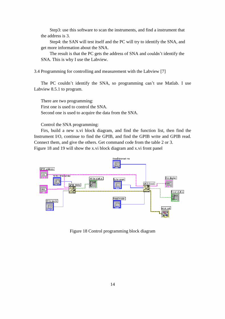
3.4 Programming for controlling and measurement with the Labview [7]
The PC couldn‟t identify the SNA, so programming can‟t use Matlab. I use
Labview 8.5.1 to program.
There are two programming:
First one is used to control the SNA.
Second one is used to acquire the data from the SNA.
Control the SNA programming:
Firs, build a new x.vi block diagram, and find the function list, then find the
Instrument I/O, continue to find the GPIB, and find the GPIB write and GPIB read.
Connect them, and give the others. Get command code from the table 2 or 3.
Figure 18 and 19 will show the x.vi block diagram and x.vi front panel
Figure 18 Control programming block diagram
14

Figure 19 Control programming front panel
The acquiring the data from the SNA programming:
For this programming, the total idea is that : first , make a marker command
code, like M1 100, the marker command code means that the M1line move to place of
100 MHz. then give the read command code to the SNA and get the value of dB, and
storage it.Use the For Loop to circulate and change number of the marker command
code. Get the value at different points.
The command codes are from table1-2[11]
Figure 20 and 21 will show the x.vi block diagram and x.vi front panel
Figure 20 Acquire data programming block diagram
15

Figure 21 Acquire data programming front panel
3.5 Presentation of the results of measurements
3.5.1 Connect SNA with Signal Generator by the cable
Figure 22 show how to connect SNA with signal Generator by cable
Figure 22 Connection with cable
16

Setting:
Set the Intelligence signal Square wave
Frequency: 20 kHz
Amplitude: 5V
Set the Carrier Signal Sine wave
Frequency: 20MHz
RF level: -10dBm
Signal modulation mode AM depth 50%
Set the SNA Power level: 10dBm
The center frequency: 20MHz
The width frequency: 100 kHz
The maker line move at least 10kH for one time. So we get 10 points.
Use the PC get the data is:
Frequency(MHz) 19.95 19.96 19.97 19.98 19.99 20 20.01 20.02 20.03 20.04
The of dB -9.12 -9.44 -9.16 -9.83 -9.02 -9.06 -8.39 -8.31 -8.63 -8.72
3.5.2 Connect SNA and Signal Generator with Antenna
Figure 23 show that how to Connect SNA and Signal Generator with Antenna
Figure 23 Connection with antenna
Set the Intelligence signal Square wave
Frequency: 20 kHz
Amplitude: 5V
Set the Carrier Signal Sine wave
Frequency: 20MHz
RF level: -10dBm
Signal modulation mode AM depth 50%
Set the SNA Power level: 10dBm
The center frequency: 20MHz
The width frequency: 100 kHz
The maker line move at least 10kH for one time. So we get 10 points.
17

Use the PC get the data is:
Frequency(MHz) 19.95 19.96 19.97 19.98 19.99 20 20.01 20.02 20.03 20.04
The of dB -28.65 -28.67 -28.64 -28.59 -28.65 -28.64 -28.63 -28.62 -28.61 -28.65
The results are not exactly, the main reason is that SNA couldn‟t work.
3.6 Process measurements with Matlab
Use the Matlab to get the graph, and also use the inverse fast Fourier transform to
get the signal in time domain from the frequency domain.
We get the graphs:
Figure 24 is the graph of the data that connected with cable
Figure 24 The graph of Data of connected with cable
Figure 25 is the graph of the data that connected with antenna
18
19.95 19.96 19.97 19.98 19.99 20 20.01 20.02 20.03 20.04-10
-9.8
-9.6
-9.4
-9.2
-9
-8.8
-8.6
-8.4
-8.2
-8
Frequency (MHz)
dB
valu
e
The measurement signal in frequency domain

Figure25 Graph of data that connected with antenna
4. Discussion
For this project, getting the results is not good. I think the first causation is that
some elements of the SNA are aging, and lose the precision. The other causation is
that the detector didn‟t work, and the SNA could not receive the correct signal.
The SNA can be remote controlled, and we can acquire data from the SNA in the
real time using PC. When read the data, the SNA couldn‟t talk after reading 50 points,
I think the first causation is that the Cache of the SNA is too small, it is full after the
reading 50 points and the SNA couldn‟t continue to read. And the other causation is
that the speed of the operation of the SNA is too slow.
Maybe somebody wants to know why I use the so old SNA.
The reasons are:
First one: the measurement must be used SNA.
Second one: In our laboratory, I couldn‟t find the other style SNA.
19
19.95 19.96 19.97 19.98 19.99 20 20.01 20.02 20.03 20.04-28.67
-28.66
-28.65
-28.64
-28.63
-28.62
-28.61
-28.6
-28.59
-28.58
Frequency (MHz)
dB
valu
e
The measurement signal in frequency domain

5. Conclusions and Future Work
For the total of the thesis work, it is good. Use the PC to control the SNA and
acquire data.
The connection with the SNA, use the GPIB cable and connect the SNA with the
PC. Using the PC could find the SNA. For the control with the programming, use the
Labview to program and build a driver. We can give some command code to the SNA,
and control it, and acquire data, then save in a file. Use the Matlab to open it and
analyze the data.
The results of the measurement, it is not good. The SAN is too old and it couldn‟t
natural work.
Future work, use the Matlab to control the SNA and acquire the data.
References
[1] Jeffrey S.Beasley & Gary M, “Acceoption of AM,” in Modern Electronic
Communication ,9th Edtion, Pearson Education, New Jersey,USA,2008,pp. 116-163.
[2] Hoberecht, V., “SNA Function Management,” IEEE Trans. Communications,
vol. 28, pp 584-603, Apr. 1980.
[3] Ruttan, T.G.; Grossman, B.; Ferrero, A.; Teppati, V. and Martens, J., “Multiport
VNA measurement,” IEEE Trans. Microwave magazine, vol. 9, no. 3, pp. 56-69, Jun.
2008.
4] Cash, Ronald and Aronhime, Peter, “an IEEE 488 Interface Bus Controller,”
IEEE Trans. Industrial Electronics, vol. IE-29, pp 308-311, Nov. 1987.
[5] “GPIB instrument Control Tutorial”, National instruments, 24 Aguest 2009.
[6] Operation and maintenance manual models 6407 and 6409 RF analyzer,
1editon, WILTRON, USA, 1985, pp: 4.1-4.5.
[7] Shea, J.J., “ LabVIEW applications and solutions,” IEEE electrical insulation
magazine, vol. 15, pp 47 Dec. 1999.
[8] A. Krishnamurthy, J. Nehrbass, J. Chaves, and S. Samsi, “Survey of parallel
MATLAB techniques and applications to signal and image processing,” in Proc.
IEEE Int. Conf. Acoustics, Speech and Signal Processing, vol. 4, 2007,pp.
1181–1184.
20

[9] Aglient Technologies 54600-Series Oscilloscopes data sheet, Agilent
Technologies, 2009, pp.1-4.
[10] Operation and maintenance manual models 6407 and 6409 RF analyzer,
1editon, WILTRON, USA, 1985, pp: 1.4-1.6..
Appendices
Table 1 -1
Name of Instrument Description of
Instrument
Feature of Instrument
Wiltron 6409 RF
Analyzers
The 6409 RF
Analyzers are complete
measurement systems for
testing RF components and
systems. Each includes a
radio frequency analyzer,
has its own built-in scalar
network analyzer and a
scanning frequency source,
an external radio
frequency detector, and the
SWR Autotester. The RF
detector is used to measure
the transmission loss, and
absolute power, while the
SWR Autotester is used to
measure the return loss.
FrequencyRange: 10MHz
to 2000MHz
Frequency Resolution:
10kHz
Display: 178mm
Scale Resolution: 0.1 dB
to 10dB per division in 0.1
dB step.
Offset Range: +99.9dB to
-99.9 dB
Makers: Up to eight
individually controllled
markers, with 10 kHz
resolution , can be placed
on the display.
Transmission Loss
Accuracy: Transmission
Loss Accuray = Channel
Accuracy + Mismatch
Uncertainty.
Detector: The 6400 series
detectors are used to make
precision transmission loss
or gain and absolute power
measurements.
21

Agilant 54621 A
oscilloscope
Agilent 54621A
2-channel oscilloscope
brings MegaZoom deep
memory, high-definition
display and flexible all the
benefits, triggering the
downstream river with the
requirements of the
designers of these values.
54621A 60 MHz to
provide you an affordable
way to see a long period of
time, while maintaining
the high sampling rate, so
you can see the details of
your design [15].
1. 60 MHz
2. Lowest cost deep
memory scope
3. Patentedhigh-definition
display with superior
horizontal resolution.
4. 4 MB deep memory
mapped to 32 levels fo
intensity, 25million
vectors/sec.
5. Powerful, flexible
triggering including
SPI, LIN, CAN and
USB.
6. Standard built-in
floppy, RS-232 and
parallel ports, FFT‟s.
Marconi instrument
10kHz-2.7GHz signal
generator 2031
The Marconi
Instruments 2031 is a used
Signal Generator that has a
frequency range of 10kHz
to 2.7 GHz.
1. Frequency Range:
10kHz-2.7GHz.
2. Frequency Resolution:
0.1Hz.
3. Output Accuracy:
1.0dB.
4. Output Range:
-144dBm - +13dBm.
5. Output Resolution:
0.1dB.
6. Programmable
Interface: IEEE 488.2.
7. SSB phase Noise
Range: dBc/Hz.
8. Time Base
Stability:0.2/yr
22

Hewlett packard 33120 A Agilent 33120A
function/arbitrary
generator offers the
rock-solid stability of
digital synthesis at a price
you can feel good
about. Not only do you
get better performance,
you get arbitrary
waveforms available for
the first time in this price
range. Just imagine the
ways you could use
complex custom
waveforms (with 12-bit
resolution) from
simulating heartbeats and
vibrations to testing
circuits.
1. 15MHz sine and
square wave outputs
2. 12-bit, 40Msa/s,
16000-point deep
arbitrary waveforms
3. Sine,triangle, square,
ramp, noise and more
4. Direct Digital
Synthedid for excellent
stability
5. Option 001:
hig-Stability Time
Base and PLL
available
Hewlett Packard 8753D
30kHz-3GHz network
analyzer
HP 8753D network
analyzer provides
affordable excellence in
RF network measurement
for the lab and production
testing. It has an integrated
S-parameter test set for
longer-lasting calibrations,
exceptional reliability, and
improved resistance to
ESD. The HP 8753D gives
you a complete solution
for characterizing active or
passive networks, devices,
or components from 30
kHz to 3 GHz--with a cost
savings over the previous
model with a test set .
1. 30 kHz to 3GHz (or to 6
GHz w/Option 6 frequency
Extension) frequency
range.
2.Integrated S-parameter
test set
3.Integrated 1-Hz
resolution synthesized
source Optional
time-domain and
swept-harmonic
measurements
4.Up to 110dB of dynamic
range
5.Group delay and
deviation from linear
phase Save/recall to
built-in disk drive built-in
accuracy enhancement
23

Table 1-2
RF Anayzer Command codes
AA : Chanel A to Autoscale ACL: Trace A to Cablibration
ADD: Trace A Resonlution dB/Div ADR Trace A Reference
AH: Trace A high Limit Line AL: Trace A Low Limit Line
AOF: Trace A Offset AP: Channel A to Power
AR: Chanel A to Return Loss AS: Trace A Select
AT: Channel A to Transmission CAL: Cablbrate Trace
CON: Continue DMR: Display Marker Readout
DS: Display Area Control FM: Frequency Markers
GR: Graticule On/Off HLD: Hold
HP: Halt Printing M1-M8: Markers M1 thru M8
PG: Pint Graph PSS: Panel Setup Recall
RAM: Read Trace A Marker RES:Reset
RP: Read Parameter RS: Read Status
SAC: sweep Alternate Center Frequency SAP: sweep Alternate Stop Frequency
SAT: sweep Alternate Start Frequency SC: Sweep Center Frequency
SW: Sweep Width TST: Self Test
24