Embed Size (px)
Citation preview
ARL-TR-7605 ● FEB 2016
US Army Research Laboratory
Implementing network Common Data Form (netCDF) for the 3DWF Model
by Giap Huynh and Yansen Wang Approved for public release; distribution is unlimited.
NOTICES
Disclaimers
The findings in this report are not to be construed as an official Department of the Army position unless so designated by other authorized documents. Citation of manufacturer’s or trade names does not constitute an official endorsement or approval of the use thereof. Destroy this report when it is no longer needed. Do not return it to the originator.
ARL-TR-7605 ● FEB 2016
US Army Research Laboratory
Implementing network Common Data Form (netCDF) for the 3DWF Model
by Giap Huynh and Yansen Wang Computational and Information Sciences Directorate, ARL Approved for public release; distribution is unlimited.
ii
REPORT DOCUMENTATION PAGE Form Approved OMB No. 0704-0188
Public reporting burden for this collection of information is estimated to average 1 hour per response, including the time for reviewing instructions, searching existing data sources, gathering and maintaining the data needed, and completing and reviewing the collection information. Send comments regarding this burden estimate or any other aspect of this collection of information, including suggestions for reducing the burden, to Department of Defense, Washington Headquarters Services, Directorate for Information Operations and Reports (0704-0188), 1215 Jefferson Davis Highway, Suite 1204, Arlington, VA 22202-4302. Respondents should be aware that notwithstanding any other provision of law, no person shall be subject to any penalty for failing to comply with a collection of information if it does not display a currently valid OMB control number. PLEASE DO NOT RETURN YOUR FORM TO THE ABOVE ADDRESS.
1. REPORT DATE (DD-MM-YYYY)
February 2016 2. REPORT TYPE
Final 3. DATES COVERED (From - To)
08/31/2015 4. TITLE AND SUBTITLE
Implementing network Common Data Form (netCDF) for the 3DWF Model 5a. CONTRACT NUMBER
5b. GRANT NUMBER
5c. PROGRAM ELEMENT NUMBER
6. AUTHOR(S)
Giap Huynh and Yansen Wang 5d. PROJECT NUMBER
5e. TASK NUMBER
5f. WORK UNIT NUMBER
7. PERFORMING ORGANIZATION NAME(S) AND ADDRESS(ES)
US Army Research Laboratory ATTN: RDRL-CIE-M 2800 Powder Mill Road Adelphi, MD 20783-1138
8. PERFORMING ORGANIZATION REPORT NUMBER
ARL-TR-7605
9. SPONSORING/MONITORING AGENCY NAME(S) AND ADDRESS(ES)
10. SPONSOR/MONITOR'S ACRONYM(S)
11. SPONSOR/MONITOR'S REPORT NUMBER(S)
12. DISTRIBUTION/AVAILABILITY STATEMENT
Approved for public release; distribution is unlimited.
13. SUPPLEMENTARY NOTES
14. ABSTRACT
Until recently, the Three-dimensional Wind Field (3DWF) model developed by the US Army Research Laboratory (ARL) had produced geographic coordinated wind data results only in standard Grib format on the Windows platform and was not easily read by other platforms. Having recognized this limitation, recent efforts have been made to improve the model, including the capability to format the results data file in network Common Data Form (netCDF) so that the distributed results can be easily accessible to other machines and operating platforms. This improvement will also allow for easier creation of code and sharing of scientific data. This technical report describes processes, software, and written programs needed in order to produce the 3DWF model’s results in netCDF data format. In addition, data extraction from netCDF-formatted Weather Research and Forecasting (WRF) model results necessary for the 3DWF model’s wind initialization will also be documented.
15. SUBJECT TERMS
3DWF, netCDF, GUI, WFR
16. SECURITY CLASSIFICATION OF: 17. LIMITATION OF ABSTRACT
UU
18. NUMBER OF PAGES
36
19a. NAME OF RESPONSIBLE PERSON
Giap Huynh a. REPORT
Unclassified b. ABSTRACT
Unclassified c. THIS PAGE
Unclassified 19b. TELEPHONE NUMBER (Include area code)
301-394-1156 Standard Form 298 (Rev. 8/98) Prescribed by ANSI Std. Z39.18
Approved for public release; distribution is unlimited. iii
Contents
List of Figures iv
Acknowledgments v
1. Introduction 1
2. netCDF Requirement for the 3DWF Model 1
3. Implementing netCDF to the 3DWF Model 2
3.1 Weather Research and Forecasting (WRF) domain and results 3
3.2 Extracting Variables from netCDF Formatted WRF Data File 5
3.3 Converting the 3DWF’s Results into netCDF 11
4. Conclusion 14
5. References 15
Appendix. Procedures to Prepare C/C++ Programs in Visual Studio 2013 and to Produce MATLAB Executable Code 17
List of Symbols, Abbreviations, and Acronyms 27
Distribution List 28
Approved for public release; distribution is unlimited. iv
List of Figures
Fig. 1 netCDF processing flow chart in the 3DWF model and its GUI ...........3
Fig. 2 WRF model terrain contours drawn every 100 m for the 1 km grid spacing nest 4 .........................................................................................4
Fig. 3 Drop box for “WRF result” from the top portion of the 3DWF GUI menu page ..............................................................................................9
Fig. 4 WRF file list prompt (Left) and the MATLAB code to create it (Right)10
Fig. 5 Drop box to convert output results into netCDF from the 3DWF GUI menu page ............................................................................................12
Fig. 6 Illustration of grid’s AGL heights in a small portion of a cross section along the x-z axis (shown only around x = 3 and at y = 5) ..................13
Fig. A-1 MATLAB Compiler window ...............................................................22
Approved for public release; distribution is unlimited. v
Acknowledgments
Dr Brian Reen (BED/ARL) for technical reviewing and great inputs.
Approved for public release; distribution is unlimited. vi
INTENTIONALLY LEFT BLANK.
Approved for public release; distribution is unlimited. 1
1. Introduction
As a common practice, a computer model should be able to produce its results in a format that allows for easy sharing, accessing, and creation of scientific data regardless of the computing platform. For this purpose, recent improvements have been made to the US Army Research Laboratory’s (ARL) Three-dimensional Wind Field (3DWF) model and its Graphical User Interface (GUI) to allow the model to use and to generate the results in a widely accessible format. In order to successfully produce the aforementioned universal format, we used the network Common Data Form (netCDF) software package for Windows distributed by the Unidata Program Center at the University Corporation for Atmospheric Research (UCAR) in Boulder, Colorado. Since the netCDF for the Windows software package is still undergoing development and is currently available only with a C libraries version, a C/C++ compiler also had to be installed. Additionally, required netCDF-C libraries’ accessible paths needed to be specified correctly in order for the code to be compiled successfully. This technical report documents the detailed process to implement netCDF capability for the 3DWF model and also includes step-by-step instructions on how to operate its updated GUI.
2. netCDF Requirement for the 3DWF Model
The 3DWF model was developed at ARL and has been constantly improved over the past several years. The model is based on the mass conservation principle, wherein the divergence in a flow field is eliminated. A detailed description of the model has been provided in several papers by Wang et al. (2005, 2007, and 2010). One of the capabilities of the 3DWF model is using the mesoscale Weather Research and Forecasting (WRF) (Skamarock et al., 2008) model results for its initial conditions. However, until recently, the 3DWF model was designed to ingest standard ASCII or Grib format and only generated results in standard ASCII format, while the provided WRF model results are often in netCDF format. Therefore, the 3DWF model and its GUI needed to be modified so that they can process netCDF data input and generate results in netCDF format, as well. The netCDF format has become popular and adopted by many scientific research and government sites dues to its many advantages. Some of these advantages include that it is self-describing, which decreases the likelihood of misinterpretations of the data; it automatically generates the code needed to interact with netCDF files in most languages, such as Fortran and C/C++; and it can be directly read by data analysis/plotting packages such as MATLAB. Due to the recognition of these
Approved for public release; distribution is unlimited. 2
advantages, netCDF capabilities have been added to 3DWF, one of several useful improvements recently made to the 3DWF model and its user-friendly GUI.
The netCDF software package we adopted is offered by the Unidata Program Center at UCAR. On its website, there are several different versions for different platforms, such as for Linux and Windows, and they are downloadable for free. Since the 3DWF GUI was developed on the Windows 64-bit platform, we selectively downloaded and installed the latest release version, netCDF4.3.3.1-NC4-64.exe, from the netCDF-C Libraries for Windows’s Visual Studio link: http://www.unidata.ucar.edu/software/netcdf/docs/winbin.html
As mentioned previously, since UCAR’s netCDF for Windows package is currently available only for C/C++ programs, a C compiler must be available on a Windows computer so that a compiled C program can interface with the netCDF-C libraries during the compiling process. We used Microsoft’s Visual Studio 2013 software because it offers both C and C++ compilers that can help to generate executable code for the 3DWF GUI. For our application, the generated executable code from C/C++ will be used for writing 3DWF results in netCDF format. Alternatively, a MATLAB version, such as MATLAB 2014a, can also be used since it already includes a built-in netCDF library. For convenience, we used this MATLAB software only for producing executable code to extract and to prepare selected input variables from a WRF model result data file.
In order to successfully compile a C or C++ program created by Visual Studio 2013, required paths need to be specified correctly (explained in step 3 of Appendix A-1) so that the program can access netCDF-C libraries files. A detailed procedure to create such a C or C++ program is documented in Appendix A-1. Once the program is successfully complied, its executable code is ready to be used by the 3DWF GUI.
3. Implementing netCDF to the 3DWF Model
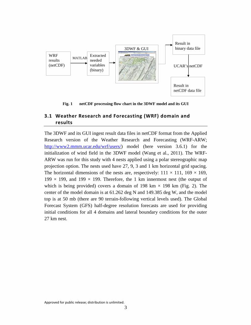
In order to improve the 3DWF model with netCDF capability, its updated GUI version not only must be able to produce results in a netCDF format, but also must be able to extract variables necessary for the initialization of the wind field from the WRF model results in netCDF format. For practicality, we used MATLAB’s netCDF library and functions to create executable code for extracting needed variables from a WRF data file, and used UCAR’s netCDF package for Windows to produce executable code for translating 3DWF’s output results from binary into netCDF format. The implementation of the netCDF data capability in 3DWF model is described using the flow chart in Fig. 1.
Approved for public release; distribution is unlimited. 3
MATLAB
UCAR’s netCDF
WRF results (netCDF)
Extracted needed variables (binary)
3DWF & GUI
Result in binary data file
Result in netCDF data file
Fig. 1 netCDF processing flow chart in the 3DWF model and its GUI
3.1 Weather Research and Forecasting (WRF) domain and results
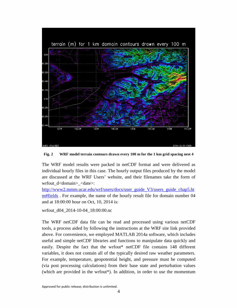
The 3DWF and its GUI ingest result data files in netCDF format from the Applied Research version of the Weather Research and Forecasting (WRF-ARW; http://www2.mmm.ucar.edu/wrf/users/) model (here version 3.6.1) for the initialization of wind field in the 3DWF model (Wang et al., 2011). The WRF-ARW was run for this study with 4 nests applied using a polar stereographic map projection option. The nests used have 27, 9, 3 and 1 km horizontal grid spacing. The horizontal dimensions of the nests are, respectively: 111 × 111, 169 × 169, 199 × 199, and 199 × 199. Therefore, the 1 km innermost nest (the output of which is being provided) covers a domain of 198 km × 198 km (Fig. 2). The center of the model domain is at 61.262 deg N and 149.385 deg W, and the model top is at 50 mb (there are 90 terrain-following vertical levels used). The Global Forecast System (GFS) half-degree resolution forecasts are used for providing initial conditions for all 4 domains and lateral boundary conditions for the outer 27 km nest.
Approved for public release; distribution is unlimited. 4
Fig. 2 WRF model terrain contours drawn every 100 m for the 1 km grid spacing nest 4
The WRF model results were packed in netCDF format and were delivered as individual hourly files in this case. The hourly output files produced by the model are discussed at the WRF Users’ website, and their filenames take the form of wrfout_d<domain>_<date>: http://www2.mmm.ucar.edu/wrf/users/docs/user_guide_V3/users_guide_chap5.htm#fields . For example, the name of the hourly result file for domain number 04 and at 18:00:00 hour on Oct, 10, 2014 is:
wrfout_d04_2014-10-04_18:00:00.nc
The WRF netCDF data file can be read and processed using various netCDF tools, a process aided by following the instructions at the WRF site link provided above. For convenience, we employed MATLAB 2014a software, which includes useful and simple netCDF libraries and functions to manipulate data quickly and easily. Despite the fact that the wrfout* netCDF file contains 148 different variables, it does not contain all of the typically desired raw weather parameters. For example, temperature, geopotential height, and pressure must be computed (via post processing calculations) from their base state and perturbation values (which are provided in the wrfout*). In addition, in order to use the momentum
Approved for public release; distribution is unlimited. 5
parameters (u and v) in 3DWF, they must be de-staggered from the Arakawa-C grid, which they are provided on in the wrfout*, and also converted from grid-relative to earth-relative values.
Near the bottom of the webpage referenced in the URL above, there is information to assist with some of these steps. There are “surface” or screen-level diagnostic parameters computed and stored in the wrfout* file valid at 2 m above ground level (AGL) (temperature and humidity) and 10-m AGL (u and v winds) height levels, and these parameters do not have to be post-processed or de-staggered (although the 10-m AGL u and v wind components still need to be transformed to earth relative from grid relative). In addition, the temperatures WRF outputs into wrfout* (other than 2-m temperature (T2M)) are base state and perturbation potential temperatures; therefore, the user must be sure to convert from potential temperature to temperature.
For the improved 3DWF model’s wind field initialization, the following required variables are extracted from the WRF netCDF data file, saved in a standard binary data file, and named as “Lat_Long_uvw_T_P_Pb_Hgt.dat” before it can be read by the 3DWF GUI:
Latitude and longitude
Wind components: u, v, and w (in m/s)
Perturbation potential temperature T (in K)
Perturbation pressure P (in Pa)
Base state pressure PB (in Pa)
WRF Terrain heights (in m)
3.2 Extracting Variables from netCDF Formatted WRF Data File
A typical netCDF file contains a header section followed by a data section. For example, the WRF output netCDF file “wrfout_d04_2014-11-23_18_00_00” contains data collected for domain number 04 at 18:00:00 on 23 November 2014. Since the file is very large and stores 148 different variables, as mentioned earlier, we only list here the first 2 variables—latitude and longitude—as an example. After being converted to text (via the program ncdump), the beginning of the header section looks like this:
netcdf wrfout_d04_2014-11-23_18_00_00 {
dimensions:
Approved for public release; distribution is unlimited. 6
Time = UNLIMITED ; // (1 currently)
DateStrLen = 19 ;
west_east = 198 ;
south_north = 198 ;
bottom_top = 89 ;
bottom_top_stag = 90 ;
soil_layers_stag = 4 ;
west_east_stag = 199 ;
south_north_stag = 199 ;
variables:
char Times(Time, DateStrLen) ;
float XLAT(Time, south_north, west_east) ;
XLAT:FieldType = 104 ;
XLAT:MemoryOrder = "XY " ;
XLAT:description = "LATITUDE, SOUTH IS NEGATIVE" ;
XLAT:units = "degree_north" ;
XLAT:stagger = "" ;
float XLONG(Time, south_north, west_east) ;
XLONG:FieldType = 104 ;
XLONG:MemoryOrder = "XY " ;
XLONG:description = "LONGITUDE, WEST IS NEGATIVE" ;
XLONG:units = "degree_east" ;
XLONG:stagger = "" ;
…………………
The text presentation of the netCDF file begins with the name of the netCDF file, and is followed by the domain’s dimensions and a list of variables, along with their data type and units. From the example file above, latitude and longitude will have the same dimension of (south_north, west_east), which is 198 × 198 here. In
Approved for public release; distribution is unlimited. 7
WRF case, the header also declares all global attributes of the data file. For the example file above, the beginning of this section looks like this:
// global attributes:
:TITLE = " OUTPUT FROM WRF V3.6.1 MODEL" ;
:START_DATE = "2014-11-23_12:00:00" ;
:SIMULATION_START_DATE = "2014-11-23_12:00:00" ;
:WEST-EAST_GRID_DIMENSION = 199 ;
:SOUTH-NORTH_GRID_DIMENSION = 199 ;
:BOTTOM-TOP_GRID_DIMENSION = 90 ;
:DX = 1000.f ;
:DY = 1000.f ;
:STOCH_FORCE_OPT = 0 ;
:GRIDTYPE = "C" ;
:DIFF_OPT = 2 ;
:KM_OPT = 4 ;
:DAMP_OPT = 3 ;
:DAMPCOEF = 0.2f ;
:KHDIF = 0.f ;
:KVDIF = 0.f ;
:MP_PHYSICS = 8 ;
:RA_LW_PHYSICS = 1 ;
:RA_SW_PHYSICS = 1 ;
:SF_SFCLAY_PHYSICS = 2 ;
.
…………………………………
After the header, all collected data are stored in the data section and in the order as indicated in the header. The data section begins with a time stamp as defined in the header and followed by the data. For the sake of brevity, the following
Approved for public release; distribution is unlimited. 8
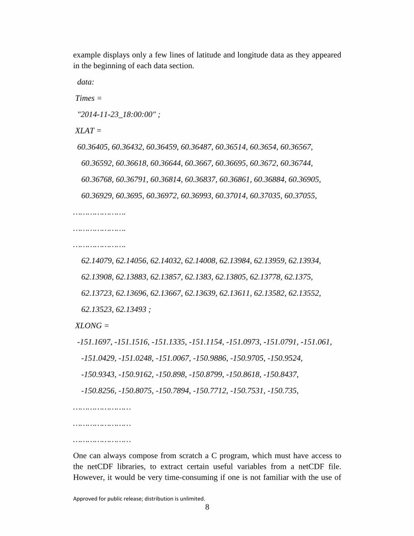
example displays only a few lines of latitude and longitude data as they appeared in the beginning of each data section.
data:
Times =
"2014-11-23_18:00:00" ;
XLAT =
60.36405, 60.36432, 60.36459, 60.36487, 60.36514, 60.3654, 60.36567,
60.36592, 60.36618, 60.36644, 60.3667, 60.36695, 60.3672, 60.36744,
60.36768, 60.36791, 60.36814, 60.36837, 60.36861, 60.36884, 60.36905,
60.36929, 60.3695, 60.36972, 60.36993, 60.37014, 60.37035, 60.37055,
………………….
………………….
………………….
62.14079, 62.14056, 62.14032, 62.14008, 62.13984, 62.13959, 62.13934,
62.13908, 62.13883, 62.13857, 62.1383, 62.13805, 62.13778, 62.1375,
62.13723, 62.13696, 62.13667, 62.13639, 62.13611, 62.13582, 62.13552,
62.13523, 62.13493 ;
XLONG =
-151.1697, -151.1516, -151.1335, -151.1154, -151.0973, -151.0791, -151.061,
-151.0429, -151.0248, -151.0067, -150.9886, -150.9705, -150.9524,
-150.9343, -150.9162, -150.898, -150.8799, -150.8618, -150.8437,
-150.8256, -150.8075, -150.7894, -150.7712, -150.7531, -150.735,
……………………
……………………
……………………
One can always compose from scratch a C program, which must have access to the netCDF libraries, to extract certain useful variables from a netCDF file. However, it would be very time-consuming if one is not familiar with the use of
Approved for public release; distribution is unlimited. 9
netCDF’s functions and syntax. Of course, one can also try to extract variables from the dumped text format version of the file shown above (created using the netCDF program ncdump). The problem is if the text file is too large and contains many different types of data, such as the one from WRF, it is also very time-consuming to track down the record number for skipping due to the unpredictable number of data values on each record after being converted into text, and this is likely to be error-prone. As mentioned previously, there are various commercial netCDF tools available to extract data quickly, and we found that the MATLAB 2014a version provides conveniently quick and easy-to-operate tools in dealing with netCDF. Not only does MATLAB 2014a contain already built-in netCDF libraries and functions, but it also includes “deploytool”, a feature that enables the GUI designer to generate executable code for use in any application. In order to produce the executable code file, a free MATLAB Runtime package for Windows must be downloaded and installed from the MATLAB website’s link, http://www.mathworks.com/products/compiler/mcr/. This package contains a standalone set of libraries that is needed to enable the execution of the compiled code. Once the executable code is generated, it can run on any desktop without the need for a MATLAB license or a netCDF software package. The procedure to produce an executable code file in MATLAB is listed in Appendix A-2.
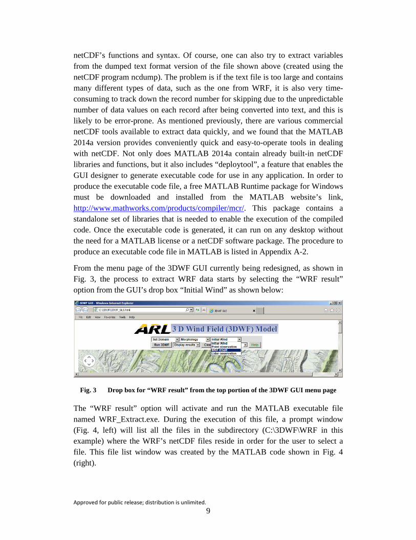
From the menu page of the 3DWF GUI currently being redesigned, as shown in Fig. 3, the process to extract WRF data starts by selecting the “WRF result” option from the GUI’s drop box “Initial Wind” as shown below:
Fig. 3 Drop box for “WRF result” from the top portion of the 3DWF GUI menu page
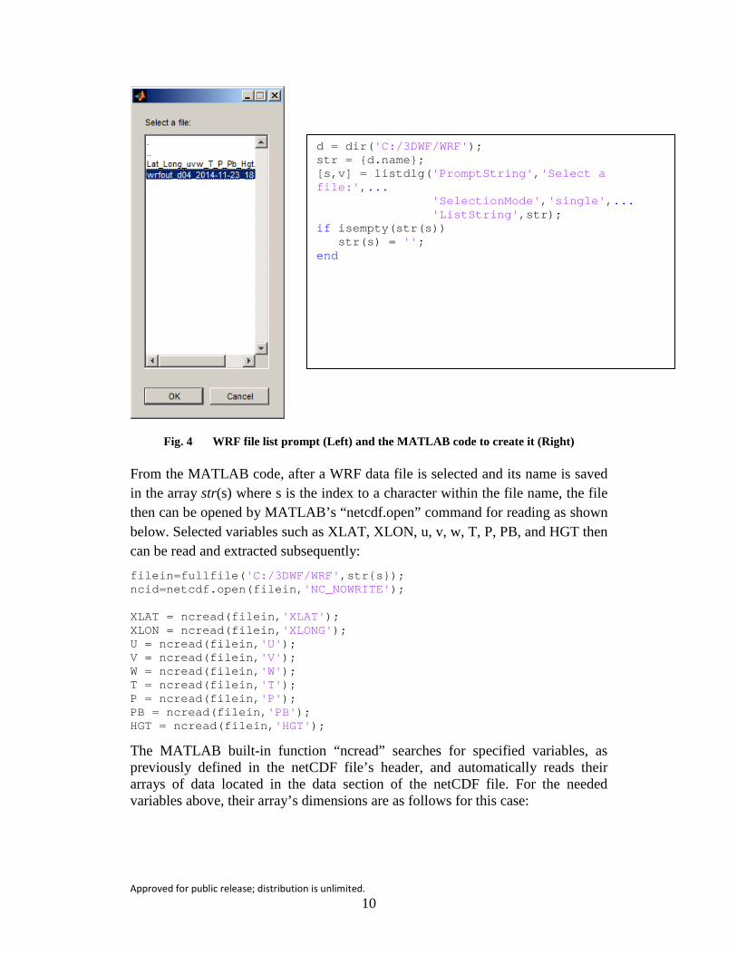
The “WRF result” option will activate and run the MATLAB executable file named WRF_Extract.exe. During the execution of this file, a prompt window (Fig. 4, left) will list all the files in the subdirectory (C:\3DWF\WRF in this example) where the WRF’s netCDF files reside in order for the user to select a file. This file list window was created by the MATLAB code shown in Fig. 4 (right).
Approved for public release; distribution is unlimited. 10
Fig. 4 WRF file list prompt (Left) and the MATLAB code to create it (Right)
From the MATLAB code, after a WRF data file is selected and its name is saved in the array str(s) where s is the index to a character within the file name, the file then can be opened by MATLAB’s “netcdf.open” command for reading as shown below. Selected variables such as XLAT, XLON, u, v, w, T, P, PB, and HGT then can be read and extracted subsequently: filein=fullfile('C:/3DWF/WRF',str{s}); ncid=netcdf.open(filein,'NC_NOWRITE'); XLAT = ncread(filein,'XLAT'); XLON = ncread(filein,'XLONG'); U = ncread(filein,'U'); V = ncread(filein,'V'); W = ncread(filein,'W'); T = ncread(filein,'T'); P = ncread(filein,'P'); PB = ncread(filein,'PB'); HGT = ncread(filein,'HGT');
The MATLAB built-in function “ncread” searches for specified variables, as previously defined in the netCDF file’s header, and automatically reads their arrays of data located in the data section of the netCDF file. For the needed variables above, their array’s dimensions are as follows for this case:
d = dir('C:/3DWF/WRF'); str = {d.name}; [s,v] = listdlg('PromptString','Select a file:',... 'SelectionMode','single',... 'ListString',str); if isempty(str(s)) str(s) = ''; end
Approved for public release; distribution is unlimited. 11
Variables Dimension (x,y,z) ________________ _______________ XLAT, XLON, HGT 198x198 u 199x198x89 v 198x199x89 w 198x198x90 T 198x198x89 P 198x198x89 PB 198x198x89
From the GUI designer point of view, another advantage of using MATLAB software is that the data record and array can be verified immediately and easily in its “Workspace” area. After being read, these variables then can be written into a standard binary data file ready for the 3DWF model’s wind initialization process. For example, the extracted data file is named as “Lat_Long_uvw_T_P_Pb_Hgt.dat” and was created by the following MATLAB commands: fileout=fullfile('C:/3DWF/WRF/Lat_Long_uvw_T_P_Pb_Hgt.dat'); fid=fopen(fileout,'w','ieee-le'); fwrite(fid, XLAT, 'float'); fwrite(fid, XLON, 'float'); fwrite(fid, HGT, 'float'); fwrite(fid, U, 'float'); fwrite(fid, V, 'float'); fwrite(fid, W, 'float'); fwrite(fid, T, 'float'); fwrite(fid, P, 'float'); fwrite(fid, PB, 'float'); fclose(fid);
3.3 Converting the 3DWF’s Results into netCDF
For converting the 3DWF model’s results into netCDF format, UCAR’s netCDF for Windows package and Microsoft’s Visual Studio’s C compiler were used to generate executable code. Currently, UCAR only offers a C version of the package for the Windows platform. Therefore, a C compiler for Windows, such as the one included in Visual Studio 2013, must be installed. From Visual Studio 2013, the user can compose and compile a C or C++ program that will translate the 3DWF model’s results into netCDF format. An example program is listed in Appendix A-3. Besides the usual ‘#include’ statements required for a C program, the user must also add the following ‘#include’ statement in order for the program to link with the netCDF-C libraries. For example, if netCDF is installed at “C:\Program Files (x86)\netCDF 4.3.2”, then the following include line would be needed:
#include "C:\Program Files (x86)\netCDF 4.3.2\include\netcdf.h"
Approved for public release; distribution is unlimited. 12
The program begins with ‘#define’ section to define each variable’s dimension and unit. For example, the 3 dimensional u wind component will be defined as:
#define RANK_u 3
After the usual declaration of all data types in the main section, the program essentially consists of 2 parts: reading the 3DWF model’s results and preparing a netCDF data file. First, it reads all necessary parameters about the domain stored in the file “3DWF_parameters.txt”. It then creates 1, 2, and 3 dimensional arrays necessary for storing of the data from the 3DWF model’s results (in file ‘result_3dwf_uvwelevlatlon.gdat’). For the second part, after using netCDF’s nc_create function to create a new empty netCDF file, ‘NetCDF_3DWF_uvwelevlatlon.nc’, the program uses nc_def_dim and nc_def_var functions to define all data dimensions and units. Next, it uses nc_put_att_text and nc_put_var_float functions to write data to the new empty netCDF file. Although the order of variables in the netCDF file is not important to code written to interact with the file, for the 3DWF’s results, we arranged data in the following order: latitude, longitude, terrain elevation, u wind, v wind, and w wind component.
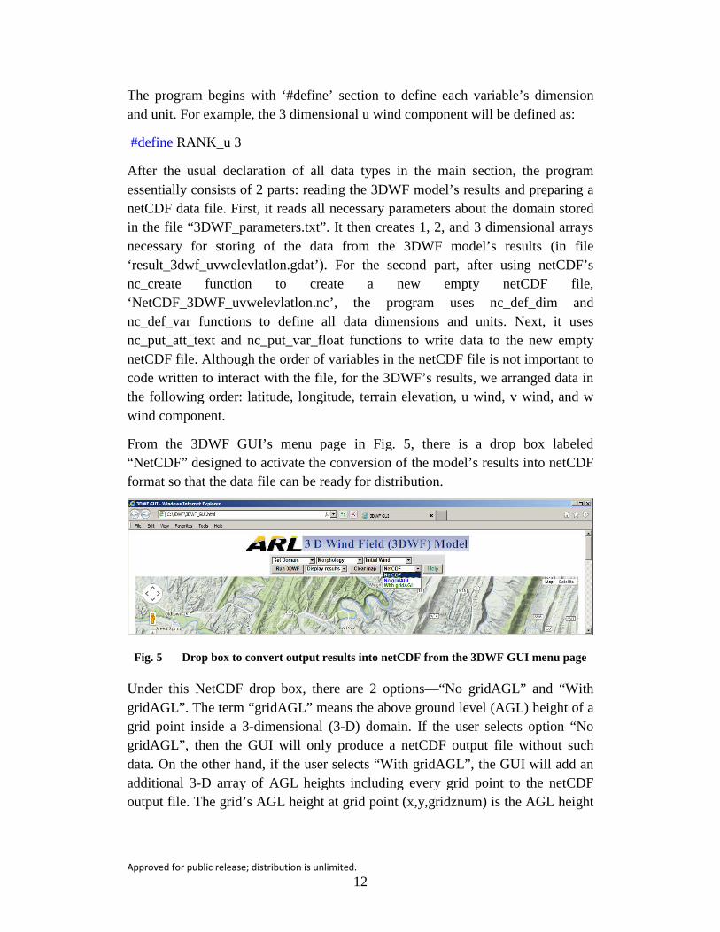
From the 3DWF GUI’s menu page in Fig. 5, there is a drop box labeled “NetCDF” designed to activate the conversion of the model’s results into netCDF format so that the data file can be ready for distribution.
Fig. 5 Drop box to convert output results into netCDF from the 3DWF GUI menu page
Under this NetCDF drop box, there are 2 options—“No gridAGL” and “With gridAGL”. The term “gridAGL” means the above ground level (AGL) height of a grid point inside a 3-dimensional (3-D) domain. If the user selects option “No gridAGL”, then the GUI will only produce a netCDF output file without such data. On the other hand, if the user selects “With gridAGL”, the GUI will add an additional 3-D array of AGL heights including every grid point to the netCDF output file. The grid’s AGL height at grid point (x,y,gridznum) is the AGL height
Approved for public release; distribution is unlimited. 13
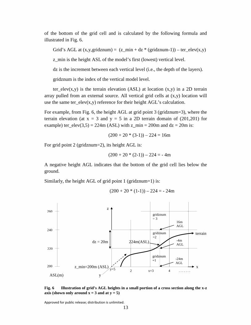
of the bottom of the grid cell and is calculated by the following formula and illustrated in Fig. 6.
Grid’s AGL at (x,y,gridznum) = (z_min + dz * (gridznum-1)) – ter_elev(x,y)
z_min is the height ASL of the model’s first (lowest) vertical level.
dz is the increment between each vertical level (i.e., the depth of the layers).
gridznum is the index of the vertical model level.
ter_elev(x,y) is the terrain elevation (ASL) at location (x,y) in a 2D terrain array pulled from an external source. All vertical grid cells at (x,y) location will use the same ter_elev(x,y) reference for their height AGL’s calculation.
For example, from Fig. 6, the height AGL at grid point 3 (gridznum=3), where the terrain elevation (at x = 3 and y = 5 in a 2D terrain domain of (201,201) for example) ter_elev(3,5) = 224m (ASL) with z_min = 200m and dz = 20m is:
(200 + 20 * (3-1)) – 224 = 16m
For grid point 2 (gridznum=2), its height AGL is:
(200 + 20 * (2-1)) – 224 = - 4m
A negative height AGL indicates that the bottom of the grid cell lies below the ground.
Similarly, the height AGL of grid point 1 (gridznum=1) is:
(200 + 20 * (1-1)) – 224 = - 24m
gridznum = 3
260
200
220
240
-24m AGL
16m AGL
x=1 2 x=3 4 . . . . . . . y=5
z
terrain
dz = 20m 224m(ASL)
z_min=200m (ASL) x
ASL(m) y
gridznum =2
gridznum=1
-4m AGL
Fig. 6 Illustration of grid’s AGL heights in a small portion of a cross section along the x-z axis (shown only around x = 3 and at y = 5)
Approved for public release; distribution is unlimited. 14
In addition to converting into netCDF format, the 3DWF GUI’s NetCDF drop box is also designed to generate a text version of the netCDF file so that the user can examine its content.
4. Conclusion
Since netCDF has become a standard format for archiving and accessing data at many educational, research, and government agencies due to its many advantages—such as being self-describing and being accessible by other computer platforms and computer languages for direct manipulation, plotting, and analysis of data—it is advantageous to implement netCDF capability in the 3DWF model. The popular and freely available netCDF for Windows software package offered by UCAR, along with netCDF libraries and tools offered by MATLAB, proved to be an excellent choice for implementing netCDF capability into the 3DWF model. In further support of this effort, a user-friendly GUI for the 3DWF model is currently being redesigned that adopts a state-of-the-art Google Maps display and incorporates netCDF capabilities. The newly improved 3DWF GUI will not only be able to extract variables from WRF’s netCDF data file that are necessary for the wind initialization, but also will be able to produce results in netCDF format that are, thus, ready for quick distribution.
Approved for public release; distribution is unlimited. 15
5. References
Skamarock WC, Klemp JB, Dudhia J, Gill DO, Barker DM, Duda MG, Huang X-Y, Wang W, Powers JG. A description of the advanced research WRF version 3. NCAR/TN-475+STR. 113pp, 2008.
Wang Y, Williamson C, Huynh G. Three Dimensional Wind Field (3DWF) Model for AFWA’s Applications: A Customer project Report. Pages 6–8, 2011.
WRF Descriptions, user’s guide, and data processing tools: see the web site http://www2.mmm.ucar.edu/wrf/users/
Wang Y, Williamson C, Garvey D, Chang S, Cogan J. Application of a multigrid method to a mass consistent diagnostic wind model. J. Appl. Meteorology. 2005;44:1078–1089.
Wang Y, Williamson C, Huynh G, Emmitt D, Greco S. Diagnostic wind model initialization over a complex terrain using the airborne doppler wind lidar data. The Open Remote Sensing Journal. 2010;3:17–27.
Wang Y, Huynh G, Williamson C. Integration of google maps/earth with microscale meteorology models and data visualization. Computer and Geosciences. 2013;61:23–31.
Approved for public release; distribution is unlimited. 16
INTENTIONALLY LEFT BLANK.
Approved for public release; distribution is unlimited. 17
Appendix. Procedures to Prepare C/C++ Programs in Visual Studio 2013 and to Produce MATLAB Executable Code
Approved for public release; distribution is unlimited. 18
A-1 Procedure to Prepare a C/C++ Program in Visual Studio 2013 for Compilation
1) For a C program:
Activate Microsoft’s Visual Studio 2013 and click in sequence File –> New –> Project
A “New Project” window will pop up:
- Select “Win32 Console Application”
- Type in a name for the project in the “Name” slot at the bottom and click OK.
A “Win32 Application Wizard” window will pop up:
- Click “Next”
- Select “Console application” under “Application type” if not selected by default.
- Check mark to select “Empty project” under “Additional options”.
- Click “Finish” button when done.
Empty program area will appear in dark blue from the main page of Visual Studio 2013
and is ready for creating the project.
- Click on “PROJECT” option and then select “Add new item” from the list.
An “Add New Item” window will pop up.
- Select “C++ File (.cpp)” and then enter a program name in the “Name:” slot with file
type “.c” instead of the default type “.cpp”.
- Click “Add” when done.
Start writing C code in the reserved area (which has now turned white).
When done, click “BUILD” option and select “Compile” at the bottom of the list.
Approved for public release; distribution is unlimited. 19
After successfully compiled, click “BUILD” again and select “Build Solution” at the top of the list. This step will create the executable file (“.exe”) for the program.
If the program was created under x64 bit, then the executable file will be located under:
\Visual Studio 2013\Projects\Projectname\x64\Debug\
If the program was created under Win32, then the executable file will be located under:
\Visual Studio 2013\Projects\Projectname\Debug\
2) For a C++ program:
C++ is the default language in Visual Studio 2013.
Activate Microsoft’s Visual Studio 2013 and click in sequence File –> New –> Project
A “New Project” window will pop up:
- Select “Win32 Console Application”
- Type in a name for the project in the “Name” slot at the bottom and click OK.
A “Win32 Application Wizard” window will pop up:
- Click “Finish” (instead of “Next” in the case of C).
- Click on “PROJECT” option and then select “Add new item” from the list.
An “Add New Item” window will pop up.
- Select “C++ File (.cpp)” and then enter a program name in the “Name:” slot with the
default type “.cpp”.
- Click “Add” when done.
Start writing C code in the reserved area (which has now turned white).
When done, click “BUILD” option and select “Compile” at the bottom of the list.
Approved for public release; distribution is unlimited. 20
After successfully compiled, click “BUILD” again and select “Build Solution” at the top of the list. This step will create the executable file “.exe” for the program.
If the program was created under x64 bit, then the executable file will be located under:
.. \Visual Studio 2013\Projects\Projectname\x64\Debug\
If the program was created under Win32, then the executable file will be located under:
.. \Visual Studio 2013\Projects\Projectname\Debug\
3) Configuration for a netCDF program:
1) Since the downloaded netCDF version was the 64-bit version, the composed C or C++ program must be compiled in Visual Studio 2013 x64 platform.
Click on “Debug” drop box on the 2nd row (not the “DEBUG” button) and select “Configuration manager”.
“Configuration manager” window will pop up.
Click the down arrow under drop box “Active solution platform” and select “New”.
A small “New Solution Platform” window will appear.
Click the down arrow under drop box “Type or select the new platform (default is Win32) and select “x64”.
Click OK when done and click “Close” to exit “Configuration Manager”.
2) Either set paths so that the program can access the following 4 netCDF files or manually copy them from the installed netCDF 4.3.2 package to the C program’s debug sub-directory:
‘C:\Users\...\Visual Studio 2013\Projects\Program_name\x64\Debug’:
These following 3 files reside in C:\Program Files (x86)\netCDF 4.3.2\deps\x64\bin:
hdf5.dll
hdf5_hl.dll
Approved for public release; distribution is unlimited. 21
zlib.dll
The following file resides in C:\Program Files (x86)\netCDF 4.3.2\bin:
netcdf.dll
3) Click Project->Properties->C/C++->Preprocessor and add the error message _CRT_SECURE_NO_WARNINGS after WIN32 in “Preprocessor Definition”
4) Click Project->Properties->Linker->Input and add this path/file to the “Additional Dependencies”
C:\Program Files (x86)\netCDF 4.3.2\lib\netcdf.lib 5) Once successfully compiled, the C/C++ executable code can be
executed through a batch file.
A-2 Procedure to Produce a Standalone Executable Code in MATLAB
To activate MATLAB’s “deploytool” command, a MATLAB runtime package must be downloaded free from MATLAB’s link:
http://www.mathworks.com/products/compiler/mcr/ Select the appropriate package based on the machine on which it will be installed.
For helpful hints in MATLAB, click Help and search for tutorial on “Create and install a standalone application”. After the MATLAB program is successfully written, compiled, and run inside MATLAB, issue the following command to start the process of generating standalone executable code:
>>deploytool
A MATLAB Compiler window will appear as shown in Fig. A-1:
Approved for public release; distribution is unlimited. 22
Fig. A-1 MATLAB Compiler window
Click + button next to “Add main file”. A prompted directory window will appear showing the created .m file. Select this .m file.
Make sure the check mark is checked at “Runtime downloaded from web”.
Click the big check mark above “Package” button at the top right and a small “Package” prompt will appear like this:
Check mark at “Open output folder when process completes” and click “Close”.
A local directory window will appear showing a list of 3 generated subdirectories and files as followed (assuming the program is ExtractNetCDF.m):
Subdir: for_redistribution - MyAppInstaller_web.exe
Subdir: for_testing - ExtractNetCDF.exe
Approved for public release; distribution is unlimited. 23
- mccExcludedFiles.log - readme.txt - splash.png
Subdir: for_redistribution_files_only - ExtractNetCDF.exe - readme.txt - splash.png
The executable code file, ExtractNetCDF.exe, was produced and resided in 2 different subdirectories as shown above. Manually copy this file to whichever location is to be used as a standalone executable file.
A-3 A Sample C Program to Translate 3DWF’s Results into netCDF
The following program is a shorter version in which it only reads one variable, the u wind component result, and prepares a netCDF format file for this variable:
#include <stdio.h> #include <stdlib.h> #include <string.h> #include <stdarg.h> #include <math.h> #include "C:\Program Files (x86)\netCDF 4.3.2\include\netcdf.h" #define RANK_u 3 #define UNITS "units" void check_err(const int stat, const int line, const char *file) { if (stat != NC_NOERR) { (void)fprintf(stderr, "line %d of %s: %s\n", line, file, nc_strerror(stat)); fflush(stderr); exit(1); } } main(void) {
int x, y, z, xy_len, z_len, icount, n, code; struct rec { float val; }; double paraarray[7]; double value, centerlat, centerlon, dx, dy, dz; icount = 0; char line[25]; int stat; int ncid;
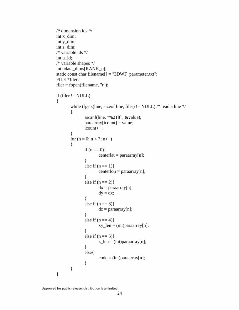
Approved for public release; distribution is unlimited. 24
/* dimension ids */ int x_dim; int y_dim; int z_dim; /* variable ids */ int u_id; /* variable shapes */ int udata_dims[RANK_u]; static const char filename[] = "3DWF_parameter.txt"; FILE *filer; filer = fopen(filename, "r"); if (filer != NULL) { while (fgets(line, sizeof line, filer) != NULL) /* read a line */ { sscanf(line, "%21lf", &value); paraarray[icount] = value; icount++; } for (n = 0; n < 7; n++) { if (n == 0){ centerlat = paraarray[n]; } else if (n == 1){ centerlon = paraarray[n]; } else if (n == 2){ dx = paraarray[n]; dy = dx; } else if (n == 3){ dz = paraarray[n]; } else if (n == 4){ xy_len = (int)paraarray[n]; } else if (n == 5){ z_len = (int)paraarray[n]; } else{ code = (int)paraarray[n]; } } }
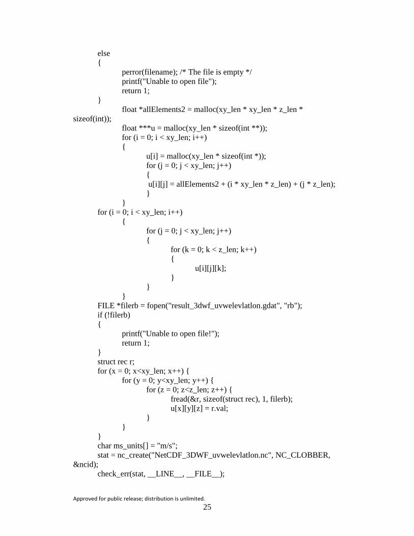
Approved for public release; distribution is unlimited. 25
else { perror(filename); /* The file is empty */ printf("Unable to open file"); return 1; } float *allElements2 = malloc(xy_len * xy_len * z_len * sizeof(int)); float ***u = malloc(xy_len * sizeof(int **)); for (i = 0; i < xy_len; i++) { u[i] = malloc(xy_len * sizeof(int *)); for (j = 0; j < xy_len; j++) { u[i][j] = allElements2 + (i * xy_len * z_len) + (j * z_len); } } for (i = 0; i < xy_len; i++) { for (j = 0; j < xy_len; j++) { for (k = 0; k < z_len; k++) { u[i][j][k]; } } } FILE *filerb = fopen("result_3dwf_uvwelevlatlon.gdat", "rb"); if (!filerb) { printf("Unable to open file!"); return 1; } struct rec r; for (x = 0; x<xy_len; x++) { for (y = 0; y<xy_len; y++) { for (z = 0; z<z_len; z++) { fread(&r, sizeof(struct rec), 1, filerb); u[x][y][z] = r.val; } } } char ms_units[] = "m/s"; stat = nc_create("NetCDF_3DWF_uvwelevlatlon.nc", NC_CLOBBER, &ncid); check_err(stat, __LINE__, __FILE__);
Approved for public release; distribution is unlimited. 26
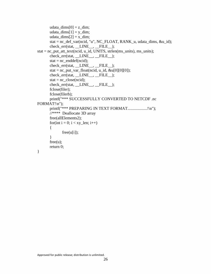
udata_dims[0] = z_dim; udata_dims[1] = y_dim; udata_dims[2] = x_dim; stat = nc_def_var(ncid, "u", NC_FLOAT, RANK_u, udata_dims, &u_id); check_err(stat, __LINE__, __FILE__); stat = nc_put_att_text(ncid, u_id, UNITS, strlen(ms_units), ms_units); check_err(stat, __LINE__, __FILE__); stat = nc_enddef(ncid); check_err(stat, __LINE__, __FILE__); stat = nc_put_var_float(ncid, u_id, &u[0][0][0]); check_err(stat, __LINE__, __FILE__); stat = nc_close(ncid); check_err(stat, __LINE__, __FILE__); fclose(filer); fclose(filerb); printf("*** SUCCESSFULLY CONVERTED TO NETCDF .nc FORMAT!\n"); printf("*** PREPARING IN TEXT FORMAT...................!\n"); //**** Deallocate 3D array free(allElements2); for(int i = 0; i < xy_len; i++) { free(u[i]); } free(u); return 0; }
Approved for public release; distribution is unlimited. 27
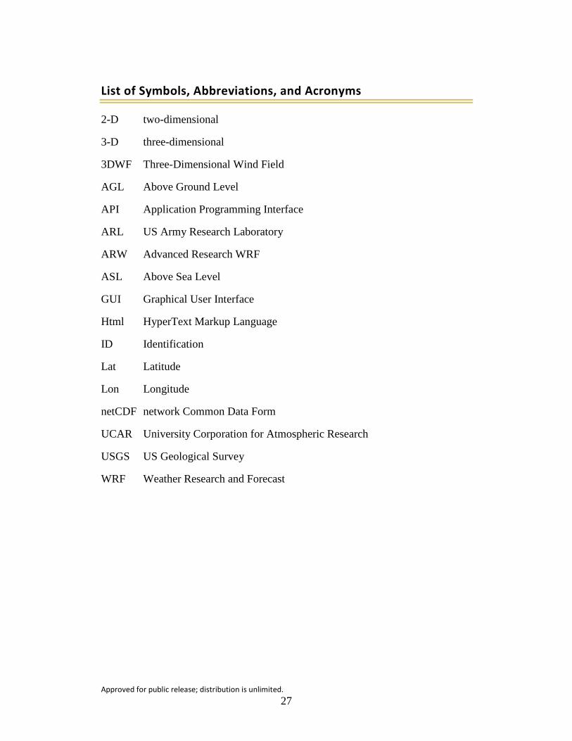
List of Symbols, Abbreviations, and Acronyms
2-D two-dimensional
3-D three-dimensional
3DWF Three-Dimensional Wind Field
AGL Above Ground Level
API Application Programming Interface
ARL US Army Research Laboratory
ARW Advanced Research WRF
ASL Above Sea Level
GUI Graphical User Interface
Html HyperText Markup Language
ID Identification
Lat Latitude
Lon Longitude
netCDF network Common Data Form
UCAR University Corporation for Atmospheric Research
USGS US Geological Survey
WRF Weather Research and Forecast
Approved for public release; distribution is unlimited. 28
1 DEFENSE TECHNICAL (PDF) INFORMATION CTR DTIC OCA 2 DIRECTOR (PDF) US ARMY RESEARCH LAB RDRL CIO LL IMAL HRA MAIL & RECORDS MGMT 1 GOVT PRINTG OFC (PDF) A MALHOTRA 1 US ARMY RSRCH LAB (PDF) RDRL WML B J CIEZAK-JENKINS 3 US ARMY RESEARCH LAB (PDF) RDRL CIE D G HUYNH Y WANG RDRL CIE P CLARK 2 US ARMY RESEARCH LAB (PDF) RDRL CIE D D KNAPP G VAUCHER


![NetCDF-4 Performance Report - The HDF Group · NetCDF-4 Performance Report Choonghwan Lee ... Introduction NetCDF-4 [1] ... netcdf4 large netcdf3 large netcdf4 small](https://img.pdfslide.us/doc/110x75/5b509b227f8b9a5a6f8ed256/netcdf-4-performance-report-the-hdf-group-netcdf-4-performance-report-choonghwan.jpg)