Embed Size (px)
Citation preview
IMPLEMENTING MACROPRUDENTIAL POLICY IN NIGEM
NIESR Discussion Paper No. 490
Date: 26 March 2018
Oriol Carreras*
E. Philip Davis**
Ian Hurst
Iana Liadze
Rebecca Piggott
James Warren*
*Formally of NIESR
**NIESR and Brunel University
About the National Institute of Economic and Social Research
The National Institute of Economic and Social Research is Britain's longest established independent
research institute, founded in 1938. The vision of our founders was to carry out research to improve
understanding of the economic and social forces that affect people’s lives, and the ways in which
policy can bring about change. Seventy-five years later, this remains central to NIESR’s ethos. We
continue to apply our expertise in both quantitative and qualitative methods and our understanding
of economic and social issues to current debates and to influence policy. The Institute is
independent of all party political interests.
National Institute of Economic and Social Research
2 Dean Trench St
London SW1P 3HE
T: +44 (0)20 7222 7665
niesr.ac.uk
Registered charity no. 306083
This paper was first published in March 2018
© National Institute of Economic and Social Research 2018
Implementing Macroprudential Policy in NiGEM
Oriol Carreras, E. Philip Davis, Ian Hurst, Iana Liadze, Rebecca Piggott, James
Warren
Abstract
In this paper we incorporate a macroprudential policy model within a semi-structural global
macroeconomic model, NiGEM. The existing NiGEM model is expanded for the UK, Germany and Italy¹ to
include two macroprudential tools: loan-to-value ratios on mortgage lending and variable bank capital
adequacy targets. The former has an effect on the economy via its impact on the housing market while the
latter acts on the lending spreads of corporate and households. A systemic risk index that tracks the
likelihood of the occurrence of a banking crisis is modelled to establish thresholds at which
macroprudential policies should be activated by the authorities. We then show counterfactual scenarios,
including a historic dynamic simulation of the subprime crisis and the endogenous response of policy
thereto, based on the macroprudential block as well as performing a cost-benefit analysis of
macroprudential policies. Conclusions are drawn relating to use of this tool for prediction and policy
analysis, as well as some of the limitations and potential further research.
Keywords: Macroprudential policy, house prices, credit, systemic risk, macroeconomic modelling
JEL Classification: E58, G28
Acknowledgements
We thank Ray Barrell and Jagjit Chadha for helpful comments.
Contact details
E. Philip Davis: [email protected] and [email protected]; Iana Liadze: [email protected];
Rebecca Piggott: [email protected]; Ian Hurst: [email protected] ;National Institute of Economic and
Social Research, 2 Dean Trench Street, London SW1P 3HE
¹ The three EU countries where NiGEM has banking sector models incorporated

1 Contents
2 Introduction ................................................................................................................................... 1
3 Taxonomies .................................................................................................................................... 1
4 Macroprudential policy in theoretical macroeconomic models......................................................... 3
5 The NiGEM model ........................................................................................................................... 4
6 Earlier work introducing macroprudential policy in NiGEM .............................................................. 5
7 Macroprudential policy in NiGEM .................................................................................................... 6
7.1 Systemic risk index ............................................................................................................................ 6
7.2 Modelling macroprudential policy in NiGEM .................................................................................. 10
7.2.1 Macroprudential tools ............................................................................................................. 11
7.2.2 Modelling spreads ................................................................................................................... 12
7.2.3 Modelling house prices and credit .......................................................................................... 12
7.2.4 Impacts on consumption and investment ............................................................................... 13
7.3 Modelling the banking sector in selected countries in NiGEM ....................................................... 13
8 Key variables ................................................................................................................................ 15
9 Simulations .................................................................................................................................. 19
9.1 Tightening of loan-to-value policy ................................................................................................... 20
9.2 Increase in risk-adjusted capital adequacy target ........................................................................... 21
9.3 Combined macroprudential tightening ........................................................................................... 21
9.4 Historic dynamic simulation for the crisis period ............................................................................ 22
10 Cost-benefit analysis ................................................................................................................. 32
11 Conclusions ............................................................................................................................... 34
12 References ................................................................................................................................ 34
Appendix 1 – Simulations with endogenous interest rates ..................................................................... 37
Appendix 2– Modelling macroprudential regulation for countries without a banking sector sub-model.. 48
Appendix 3 – Data list .......................................................................................................................... 49
1 | Implementing Macroprudential Policy in NiGEM – Discussion Paper no.490 National Institute of Economic and Social Research
2 Introduction Since the global financial crisis, there has been increasing interest among authorities in both advanced and
developing countries in introducing macroprudential policy. Macroprudential policy can be defined as being
focused on the financial system as a whole, with a view to limiting macroeconomic costs from financial
distress (Crockett 2000), and with risk taken as endogenous to the behaviour of the financial system.
However, as noted by Galati and Moessner (2014), “analysis is still needed about the appropriate
macroprudential tools, their transmission mechanism and their effect”. Theoretical models are in their
infancy and empirical evidence on the effects of macroprudential tools is still scarce, although our recent
work (Carreras et al. 2016) and its references do show promising results for the effectiveness of
macroprudential policies. A primary instrument for macroprudential policy has not yet emerged.
Meanwhile, for authorities, targets of macroprudential policy are typically house prices, credit and the
credit-GDP gap or judgemental assessments based on a range of macroprudential indicators. This leaves
aside potential for use of systemic risk indicators based on early warning models for banking crises as a
complementary target for macroprudential policy, on which there is a rich literature (see for example Davis
and Karim (2008) and Barrell et al. (2010a)).
We contend that extant model-based work often either omits feedback from the macroeconomy to the
financial sector, in particular a macroprudential reaction function, and/or would find disequilibrium hard to
manage, and that both of these difficulties can be improved in our semi-structural global macroeconomic
model NiGEM. Accordingly, in this paper we seek to introduce macroprudential considerations to an
established global macromodel (NiGEM), initially by instruments of variable bank capital adequacy and
mortgage loan-to-value ratios. The former will impact the economy by acting on the spread between
borrowing and lending of corporate and households while the latter will transmit through its impact on the
housing market.
A systemic risk indicator will keep track of the likelihood that a financial crisis takes place. Based on the
work by Karim et al. (2013), the systemic risk index will be a function of banking sector capital adequacy
and liquidity ratios, house price growth and the current account to GDP ratio. We shall enable users to
trigger macroprudential policy directly or enable policy to be triggered endogenously as the systemic risk
indicator reaches critical levels, which can itself vary between countries or be set by the user.
The paper is structured as follows: in Section 3 we present a brief taxonomy of macroprudential tools. In
Section 4 we review some of the extant theoretical work on macroprudential in the macroeconomy.
Section 5 introduces NiGEM and Section 6 looks at some earlier work on macroprudential policy in NiGEM.
Section 7 outlines the specific extensions to NiGEM that we are introducing and Section 8 concludes.
3 Taxonomies Authorities around the world are implementing a macroprudential pillar to economic policy, to
complement microprudential, monetary and fiscal policy. Such a pillar is aimed to prevent financial crises
by limiting systemic risk – the danger that there arises widespread disruption to provision of financial
services that impact in turn on the real economy. In order to appropriately calibrate such measures, there is
a clear need for a forecasting and simulation tool to assess appropriate triggers for macroprudential
intervention, the effect of such interventions and their relationship to monetary and fiscal tools. Such a tool
should also allow for global interactions and trends in financial and economic quantities and prices and
cross border spillovers. NiGEM, extended to allow for user driven as well as endogenous macroprudential
interventions, is ideally suited to such a role.
2 | Implementing Macroprudential Policy in NiGEM – Discussion Paper no.490 National Institute of Economic and Social Research
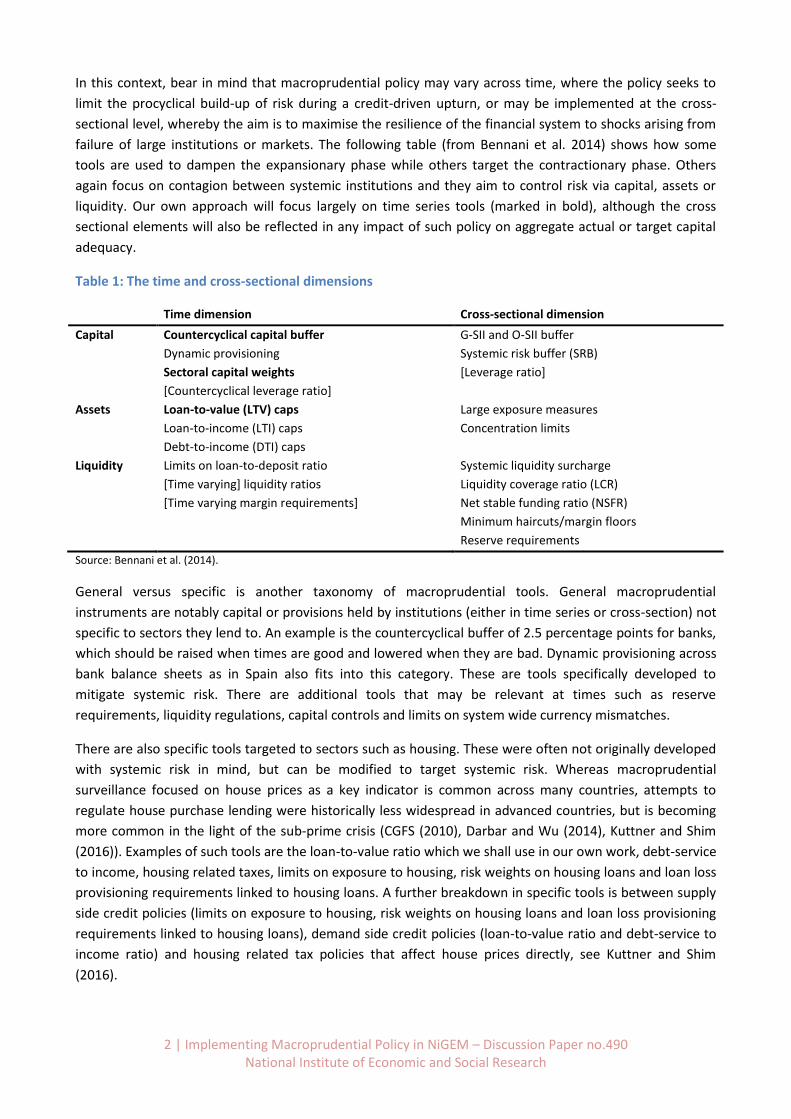
In this context, bear in mind that macroprudential policy may vary across time, where the policy seeks to
limit the procyclical build-up of risk during a credit-driven upturn, or may be implemented at the cross-
sectional level, whereby the aim is to maximise the resilience of the financial system to shocks arising from
failure of large institutions or markets. The following table (from Bennani et al. 2014) shows how some
tools are used to dampen the expansionary phase while others target the contractionary phase. Others
again focus on contagion between systemic institutions and they aim to control risk via capital, assets or
liquidity. Our own approach will focus largely on time series tools (marked in bold), although the cross
sectional elements will also be reflected in any impact of such policy on aggregate actual or target capital
adequacy.
Table 1: The time and cross-sectional dimensions
Time dimension Cross-sectional dimension
Capital Countercyclical capital buffer
Dynamic provisioning
Sectoral capital weights
[Countercyclical leverage ratio]
G-SII and O-SII buffer
Systemic risk buffer (SRB)
[Leverage ratio]
Assets Loan-to-value (LTV) caps
Loan-to-income (LTI) caps
Debt-to-income (DTI) caps
Large exposure measures
Concentration limits
Liquidity Limits on loan-to-deposit ratio
[Time varying] liquidity ratios
[Time varying margin requirements]
Systemic liquidity surcharge
Liquidity coverage ratio (LCR)
Net stable funding ratio (NSFR)
Minimum haircuts/margin floors
Reserve requirements
Source: Bennani et al. (2014).
General versus specific is another taxonomy of macroprudential tools. General macroprudential
instruments are notably capital or provisions held by institutions (either in time series or cross-section) not
specific to sectors they lend to. An example is the countercyclical buffer of 2.5 percentage points for banks,
which should be raised when times are good and lowered when they are bad. Dynamic provisioning across
bank balance sheets as in Spain also fits into this category. These are tools specifically developed to
mitigate systemic risk. There are additional tools that may be relevant at times such as reserve
requirements, liquidity regulations, capital controls and limits on system wide currency mismatches.
There are also specific tools targeted to sectors such as housing. These were often not originally developed
with systemic risk in mind, but can be modified to target systemic risk. Whereas macroprudential
surveillance focused on house prices as a key indicator is common across many countries, attempts to
regulate house purchase lending were historically less widespread in advanced countries, but is becoming
more common in the light of the sub-prime crisis (CGFS (2010), Darbar and Wu (2014), Kuttner and Shim
(2016)). Examples of such tools are the loan-to-value ratio which we shall use in our own work, debt-service
to income, housing related taxes, limits on exposure to housing, risk weights on housing loans and loan loss
provisioning requirements linked to housing loans. A further breakdown in specific tools is between supply
side credit policies (limits on exposure to housing, risk weights on housing loans and loan loss provisioning
requirements linked to housing loans), demand side credit policies (loan-to-value ratio and debt-service to
income ratio) and housing related tax policies that affect house prices directly, see Kuttner and Shim
(2016).
3 | Implementing Macroprudential Policy in NiGEM – Discussion Paper no.490 National Institute of Economic and Social Research
In this context, according to empirical work (as summarised and extended in Carreras et al. (2016)),
effective tools of macroprudential policy include loan-to-value ratios, debt-to-income limits and bank
capital requirements (which may be sectoral or general). We have scope, as discussed below, for
implementing loan-to-value and capital requirements in NiGEM. We note that these tools are effective in
the time series dimension and at most indirectly in the cross-sectional one.
4 Macroprudential policy in theoretical macroeconomic models Before discussing NiGEM per se, we highlight some recent work in the field of macroprudential policy and
macroeconomics as background. Galati and Moessner (2014) give a helpful breakdown of progress in
macroprudential modelling, into three areas: banking/finance models, three-period banking or DSGE
models, and infinite horizon general equilibrium models, which we follow in this paper.
Banking/finance models, in the tradition of Diamond and Dybvig (1983) highlight how financial contracts
are affected by various incentive problems related to information asymmetry and commitment that can
entail default. Then, there can be self-fulfilling equilibria generated by shocks, leading to systemic financial
instability. They accordingly seek to explain the interaction of borrowers and lenders. For example, Perotti
and Suarez (2011) look at price based and quantity based regulation of systemic externalities arising from
banks’ short term funding. Accordingly, current liquidity regulation could be justified, together with a
Pigovian tax on short term funding. However, such models tend to be cross section and omit the time series
dimension and thus cannot be used to address procyclicality. Furthermore, they tend to be partial
equilibrium and thus omit key general equilibrium effects.
Such effects are included in three period general equilibrium models of the interaction of asset prices and
non-financial and financial sector systemic risk. Such models assess risk taking by heterogeneous agents in
an economy vulnerable to such systemic risks. For example there may be financial amplification during
booms and busts that have external effects as in Goodhart et al. (2012) and Gersbach and Rochet (2012a
and b). Individual agents take decisions without allowing for the general equilibrium effects of their actions,
in particular the effects of asset sales caused by excessive borrowing on asset prices. Accordingly, they
generate patterns of feedback loops entailing falling asset prices, financial constraints and fire sales. Then,
macroprudential tools can be shown as helpful in preventing fire sales and credit crunches, including loan-
to-value ratios, capital requirements, liquidity coverage rations, dynamic loss provisioning and margin limits
on repos by shadow banks (Goodhart et al. 2013).
Further results of interest are provided by models that focus on the functions of banks in the economy such
as improving liquidity insurance, risk sharing and raising funding, which as shown by Kashyap et al. (2014)
can then be used to analyse weaknesses underlying the global financial crisis, notably excessive risk taking
by underfunded banks relying on short term funding and exploiting the safety net. Horvath and Wagner
(2013), meanwhile, show that macroprudential regulations can lead savers and banks to alter other
portfolio choices. Countercyclical regulation can worsen cross sectional risk for example, although tools to
reduce cross sectional risk may reduce procyclicality.
Infinite horizon DSGE models with financial frictions build on the insights of papers such as Bernanke et al.
(1999) on the financial accelerator. Such models (e.g. Goodfriend and McCallum 2007) were traditionally
linear, so found it hard to deal with non-linearities implicit in systemic risk and changes in regulation. They
tended to assume complete markets and that defaults either do not occur or are exogenous. And
furthermore they tended to ignore endogenous leverage. So a crisis is modelled as a big negative shock that
gets amplified rather than a credit boom that gets out of control (Boissay et al. 2013).
4 | Implementing Macroprudential Policy in NiGEM – Discussion Paper no.490 National Institute of Economic and Social Research
More recent models have sought to overcome these problems, with multiple equilibria, non-linearity,
externalities and amplification mechanisms being more sophisticated. Hence macroprudential policies can
be better assessed, although the models have to remain small due to the difficulty of the solution methods
(Galati and Moessner 2014). Borrowers may, for example, face occasional binding endogenous borrowing
constraints in times of crisis as in Fisher’s (1933) debt deflation paradigm, linked to falling asset prices and
declining net worth, see for example Benigno et al. (2013). Meanwhile models such as Brunnermeier and
Sannikov (2014) look at global dynamics in continuous time models with financial frictions. The financial
sector does not internalise the costs associated with excessive risks, so there is high leverage and maturity
mismatch. Securitisation allows risk to be offloaded by the financial sector but raises overall risk taking. The
economy has low volatility and adequate growth in steady state but the steady state is unstable due to
large shocks provoking endogenous leverage and risk taking with feedback loops from the financial to the
real economy. The model features a pattern of rising leverage and amplification when aggregate risk
declines, as in the great moderation.
Antipa and Matheron (2014) review potential tensions between monetary and macroprudential policies
given overlapping impacts. They use a DSGE model calibrated to Euro Area data with a financial friction
manifested in a collateral constraint. Macroprudential policy affects this constraint cyclically and the work
entails investigation of the zero lower bound (ZLB). Results include the following: macroprudential policies
act as a useful complement to monetary policy during crises, by attenuating the decrease in investment
and, hence, output; forward guidance is very effective at the ZLB, by providing a substantial boost to
demand and reducing the costs of private deleveraging at the same time; overall, countercyclical
macroprudential policies do not undo the benefits of forward guidance, but rather sustain them.
In general, such models highlight the transmission mechanism of real and financial factors, with the
combination of macroeconomic boom, credit boom and low interest rates being dangerous, with
consumption smoothing and precautionary saving being key underlying factors in financial imbalances’
build-up. Model calibrations can help with understanding how macroprudential regulation can reduce the
risk of crisis. State contingent taxes can also play a role, as can Pigovian taxes and an optimal mix of
macroprudential policy and bailouts.
5 The NiGEM model This section provides a succinct non-technical exposition of the National Institute’s Global Econometric
model, NiGEM which we use in our research. Where relevant to the analysis, details of the model will be
presented in the text to follow, but an in-depth discussion falls beyond the scope of this paper.1
NiGEM is a global econometric model, and most countries in the EU and the OECD as well as major
emerging markets are modelled individually. The rest of the world is modelled through a set of regional
blocks so that the model is global in scope. All country models contain the determinants of domestic
demand, export and import volumes, prices, current accounts and gross foreign assets and liabilities.
Output is tied down in the long run by factor inputs and technical progress interacting through production
functions. Economies are linked through trade, competitiveness and financial markets and are fully
simultaneous.
Agents are presumed to be forward-looking, at least in some markets, but nominal rigidities slow the
process of adjustment to external shocks. The model has complete demand and supply sides and there is
1 For further details, the reader is referred to the NiGEM website: https://nimodel.niesr.ac.uk/ .
5 | Implementing Macroprudential Policy in NiGEM – Discussion Paper no.490 National Institute of Economic and Social Research
an extensive monetary and financial sector, together with household and government sectors. As far as
possible, the same theoretical structure has been adopted for each country. As a result, variations in the
properties of each country model reflect genuine differences emerging from estimation, rather than
different theoretical approaches.
Policy reactions are important in the determination of speeds of adjustment. Nominal short-term interest
rates are set in relation to a forward looking feedback rule. Long-term interest rates are the forward
convolution of future short-term interest rates with an exogenous term premium. An endogenous tax rule
ensures that governments remain solvent in the long run; the deficit and debt stock return to sustainable
levels after any shock, as is discussed in Blanchard and Fisher (1989). Exchange rates are forward looking
and so can ‘jump’ in response to a shock.
Within NiGEM, labour markets in each country are described by a wage equation (see Barrell and Dury,
2003 for a detailed description) and a labour demand equation (see, for example, Barrell and Pain, 1997).
The wage equations depend on productivity and unemployment, and have a degree of rational
expectations embedded in them – that is to say the wage bargain is assumed to depend partly on expected
future inflation and partly on current inflation. The speed of the wage adjustment is estimated for each
country. Wages adjust to bring labour demand in line with labour supply. Employment depends on real
producer wages, output and trend productivity, again with speeds of adjustment of employment estimated
and varying for each country.
NiGEM allows the macroeconomy to be affected directly by financial regulation and financial instability.
When banks increase the spread between borrowing and lending rates for individuals it changes their
incomes, and can also change their decision making on the timing of consumption, with the possibility of
inducing sharp short term reductions. The volumes of deposits and lending that result are demand
determined. Changing the spread between borrowing and lending rates for firms may change the user cost
of capital and hence investment, and the equilibrium level of output and capital in the economy in a
sustained way.
6 Earlier work introducing macroprudential policy in NiGEM To incorporate macroprudential policy in NiGEM for a project commissioned by Sveriges Riksbank, Davis et
al. (2011) undertook a number of modifications of the existing Swedish model. First, housing wealth was
included in the consumption function; second, household liabilities were allowed to be driven by housing
wealth (previously it had been driven by income); and third, the house price equation incorporated an
income, wealth and mortgage effect as well as an effect of long real rates and the household sector lending
spread (the previous equation had included only the interest rate terms). Hence, the effect of banks on the
economy via lending spreads is broadened from fixed investment, the stock of capital and consumption to
also include house prices, which affects consumption via housing wealth.
Besides standard simulations, Davis et al. (2011) imposed three macroprudential ones. One is for a 3
percentage point rise in the bank spread for mortgages only, to show the effect of higher countercyclical
capital requirements on mortgages for 2 years. Subsequently, they apply the same shock to all bank lending
so it also affects the spread for the corporate sector, showing the effect of rising general capital
requirements for banks. Finally a fall in regulated loan-to-value ratios was proxied by shocking the implicit
user cost of housing by 3 percentage points for 2 years. The main difference between the bank spread for
household lending and the user cost of capital is the effect of the household lending spread on personal
income which is absent for the user cost of capital shock.
6 | Implementing Macroprudential Policy in NiGEM – Discussion Paper no.490 National Institute of Economic and Social Research
Evidence from these NiGEM simulations suggests that macroprudential policies, focused on the housing
market, can have a distinctive impact on the economy which could helpfully complement monetary policy
at most points in the cycle. These results are in turn broadly consistent with work assessing theoretically
how macroprudential policies may affect the economy, as cited above.
Accordingly, a generalised rise in capital adequacy affecting all lending is shown to have a quite marked
impact in GDP, mainly via investment rather than consumption, while a more focused capital adequacy rise
for mortgage lending only or a loan-to-value ratio policy appear to have scope to reduce credit and house
prices and hence consumption with less effect on the rest of the economy than other options, although the
housing based policy may of course be more subject than capital adequacy based policies to
disintermediation. Capital adequacy for mortgage lending affects GDP more than the loan-to-value ratio
policy since it has more of an impact on personal income and hence consumption. Monetary policy does of
course also affect housing market variables but also has a greater effect on the wider economy.
Catte et al. (2010) use the National Institute Global Econometric Model (NiGEM) for the US over the period
2002 to 2007. They perform a number of counterfactual simulations to investigate two central elements of
the story, namely: (a) an over-expansionary US monetary policy and the absence of effective macro-
prudential supervision, which permitted a prolonged expansion of debt-financed consumer spending; (b)
the decision of China and other emerging countries to pursue an export-led growth strategy supported by
pegging their currencies to the US dollar, resulting in a huge build-up of their official reserves, in
conjunction with sluggish domestic demand in surplus advanced economies characterized by low potential
output growth.
They assume in turn a policy was feasible that would influence spreads on mortgages and show that along
with monetary policy tightening, this would have mitigated the housing cycle (reducing real house price
rises by 1/3 over 2002-2007). However, growth would have been lower and the improvement in the current
account deficit, though not trivial, would have presumably been too small to eliminate the risk of a
disorderly correction. For that, a rebalancing of global demand via expansionary policies elsewhere would
have been required.
7 Macroprudential policy in NiGEM
7.1 Systemic risk index We extend NiGEM to include a systemic risk index which will identify when the financial system and
economy show signs of needing macroprudential intervention owing to heightened risk of a financial crisis.
This index drives the macroprudential policy levers (capital buffers and loan-to-value ratios) and is based on
the work by Karim et al. (2013), where unweighted banking sector capital adequacy, the banking sector
liquidity ratio, the change in real house prices and the current balance to GDP ratio drive systemic risk.
Given the prominent role that the systemic risk function plays in our modelling of macroprudential policy in
NiGEM, we briefly summarize in this section the work by Karim et al. (2013).
Karim et al. (2013) utilise a multinomial logit to model the probability that a financial crisis occurs at any
point in time. The dependent variable is a binary banking crisis indicator that takes the value of one at the
onset of the crisis and zero otherwise.2 The dataset includes data on systemic and non-systemic banking
2 An alternative approach would be to consider a binary variable that takes a value of one whenever a country is in a
banking crisis. However, this might bias the results as policy actions implemented during a crisis may have a direct
7 | Implementing Macroprudential Policy in NiGEM – Discussion Paper no.490 National Institute of Economic and Social Research
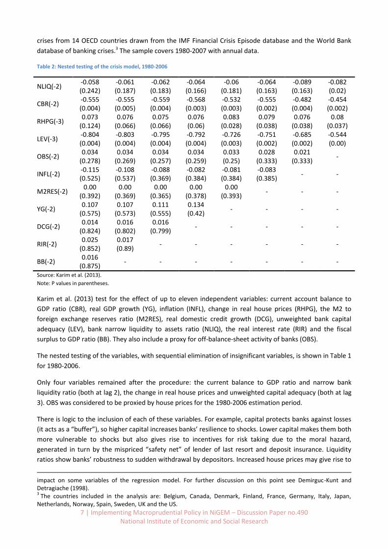
crises from 14 OECD countries drawn from the IMF Financial Crisis Episode database and the World Bank
database of banking crises.3 The sample covers 1980-2007 with annual data.
Table 2: Nested testing of the crisis model, 1980-2006
NLIQ(-2) -0.058 (0.242)
-0.061 (0.187)
-0.062 (0.183)
-0.064 (0.166)
-0.06 (0.181)
-0.064 (0.163)
-0.089 (0.163)
-0.082 (0.02)
CBR(-2) -0.555 (0.004)
-0.555 (0.005)
-0.559 (0.004)
-0.568 (0.003)
-0.532 (0.003)
-0.555 (0.002)
-0.482 (0.004)
-0.454 (0.002)
RHPG(-3) 0.073
(0.124) 0.076
(0.066) 0.075
(0.066) 0.076 (0.06)
0.083 (0.028)
0.079 (0.038)
0.076 (0.038)
0.08 (0.037)
LEV(-3) -0.804 (0.004)
-0.803 (0.004)
-0.795 (0.004)
-0.792 (0.004)
-0.726 (0.003)
-0.751 (0.002)
-0.685 (0.002)
-0.544 (0.00)
OBS(-2) 0.034
(0.278) 0.034
(0.269) 0.034
(0.257) 0.034
(0.259) 0.033 (0.25)
0.028 (0.333)
0.021 (0.333)
-
INFL(-2) -0.115 (0.525)
-0.108 (0.537)
-0.088 (0.369)
-0.082 (0.384)
-0.081 (0.384)
-0.083 (0.385)
- -
M2RES(-2) 0.00
(0.392) 0.00
(0.369) 0.00
(0.365) 0.00
(0.378) 0.00
(0.393) - - -
YG(-2) 0.107
(0.575) 0.107
(0.573) 0.111
(0.555) 0.134 (0.42)
- - - -
DCG(-2) 0.014
(0.824) 0.016
(0.802) 0.016
(0.799) - - - - -
RIR(-2) 0.025
(0.852) 0.017 (0.89)
- - - - - -
BB(-2) 0.016
(0.875) - - - - - - -
Source: Karim et al. (2013).
Note: P values in parentheses.
Karim et al. (2013) test for the effect of up to eleven independent variables: current account balance to
GDP ratio (CBR), real GDP growth (YG), inflation (INFL), change in real house prices (RHPG), the M2 to
foreign exchange reserves ratio (M2RES), real domestic credit growth (DCG), unweighted bank capital
adequacy (LEV), bank narrow liquidity to assets ratio (NLIQ), the real interest rate (RIR) and the fiscal
surplus to GDP ratio (BB). They also include a proxy for off-balance-sheet activity of banks (OBS).
The nested testing of the variables, with sequential elimination of insignificant variables, is shown in Table 1
for 1980-2006.
Only four variables remained after the procedure: the current balance to GDP ratio and narrow bank
liquidity ratio (both at lag 2), the change in real house prices and unweighted capital adequacy (both at lag
3). OBS was considered to be proxied by house prices for the 1980-2006 estimation period.
There is logic to the inclusion of each of these variables. For example, capital protects banks against losses
(it acts as a “buffer”), so higher capital increases banks’ resilience to shocks. Lower capital makes them both
more vulnerable to shocks but also gives rise to incentives for risk taking due to the moral hazard,
generated in turn by the mispriced “safety net” of lender of last resort and deposit insurance. Liquidity
ratios show banks’ robustness to sudden withdrawal by depositors. Increased house prices may give rise to
impact on some variables of the regression model. For further discussion on this point see Demirguc-Kunt and Detragiache (1998). 3 The countries included in the analysis are: Belgium, Canada, Denmark, Finland, France, Germany, Italy, Japan,
Netherlands, Norway, Spain, Sweden, UK and the US.
8 | Implementing Macroprudential Policy in NiGEM – Discussion Paper no.490 National Institute of Economic and Social Research
higher borrowing without major increases in leverage, but levels may be unsustainable. House prices are
also correlated with commercial property prices, trends in which link closely to fragility in the banking
sector (Davis and Zhu 2009); together they are key indicators of a credit-driven cycle.
A number of potential links can also be traced from current account deficits to risk of banking crises.
Deficits may be accompanied by monetary inflows that enable banks to expand credit excessively and may
link to economic overheating. Inflows may also both generate and reflect a high demand for credit, and
boosting asset prices in a potentially unsustainable manner. Such patterns may be worsened by lower real
interest rates driven by inflows. Inflows to finance deficits may be sensitive to the risk of monetisation via
inflation, and such a cessation can disrupt asset markets and banks’ funding.
OECD countries are usually seen as relatively less subject than emerging markets to such “sudden stops”.
However, as argued by McKinnon and Pill (1994), capital inflows in a weakly regulated banking system with
a safety net may lead to booms in lending, consumption and asset prices as well as further increases in
current account deficits. This pattern may lead on to exchange rate appreciation, loss of competitiveness
and a slowdown in growth, as in the US in the middle of the last decade. It may also lead to a banking crisis,
again much as we saw in the US in the late 2000s, although unlike for traditional “sudden stops” the
currency did not collapse.
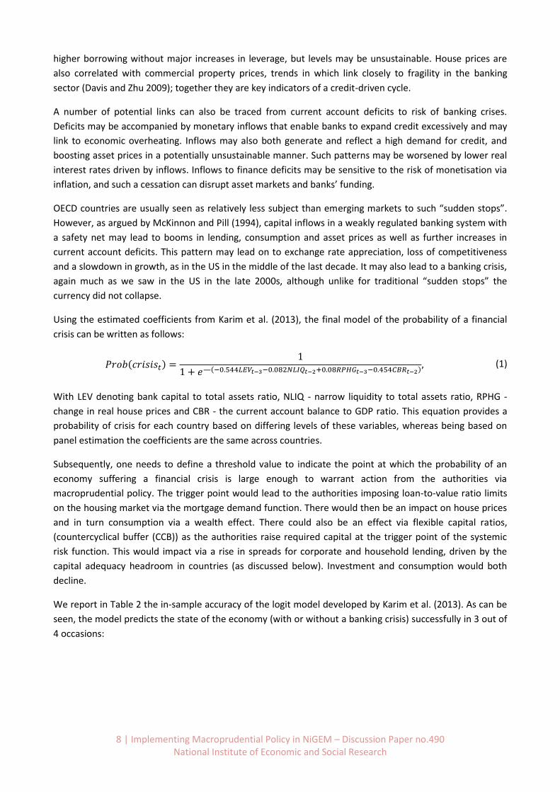
Using the estimated coefficients from Karim et al. (2013), the final model of the probability of a financial
crisis can be written as follows:
𝑃𝑟𝑜𝑏(𝑐𝑟𝑖𝑠𝑖𝑠𝑡) =1
1 + 𝑒—(−0.544𝐿𝐸𝑉𝑡−3−0.082𝑁𝐿𝐼𝑄𝑡−2+0.08𝑅𝑃𝐻𝐺𝑡−3−0.454𝐶𝐵𝑅𝑡−2), (1)
With LEV denoting bank capital to total assets ratio, NLIQ - narrow liquidity to total assets ratio, RPHG -
change in real house prices and CBR - the current account balance to GDP ratio. This equation provides a
probability of crisis for each country based on differing levels of these variables, whereas being based on
panel estimation the coefficients are the same across countries.
Subsequently, one needs to define a threshold value to indicate the point at which the probability of an
economy suffering a financial crisis is large enough to warrant action from the authorities via
macroprudential policy. The trigger point would lead to the authorities imposing loan-to-value ratio limits
on the housing market via the mortgage demand function. There would then be an impact on house prices
and in turn consumption via a wealth effect. There could also be an effect via flexible capital ratios,
(countercyclical buffer (CCB)) as the authorities raise required capital at the trigger point of the systemic
risk function. This would impact via a rise in spreads for corporate and household lending, driven by the
capital adequacy headroom in countries (as discussed below). Investment and consumption would both
decline.
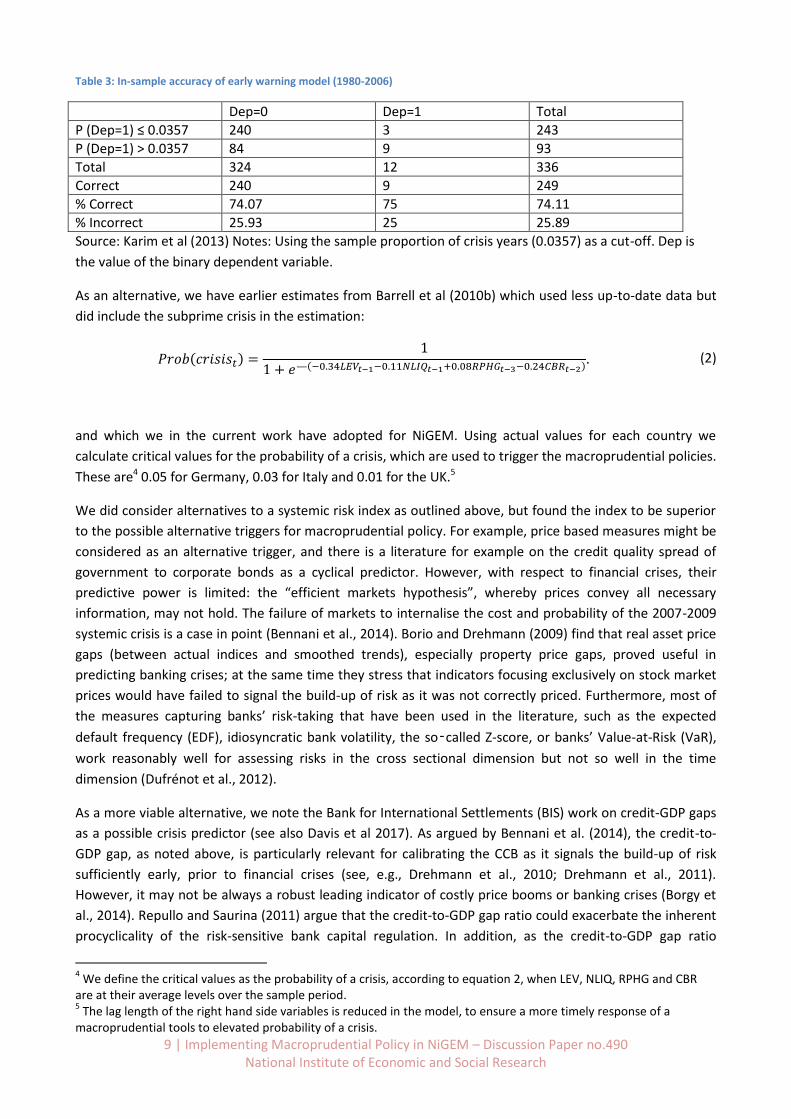
We report in Table 2 the in-sample accuracy of the logit model developed by Karim et al. (2013). As can be
seen, the model predicts the state of the economy (with or without a banking crisis) successfully in 3 out of
4 occasions:
9 | Implementing Macroprudential Policy in NiGEM – Discussion Paper no.490 National Institute of Economic and Social Research
Table 3: In-sample accuracy of early warning model (1980-2006)
Dep=0 Dep=1 Total
P (Dep=1) ≤ 0.0357 240 3 243
P (Dep=1) > 0.0357 84 9 93
Total 324 12 336
Correct 240 9 249
% Correct 74.07 75 74.11
% Incorrect 25.93 25 25.89
Source: Karim et al (2013) Notes: Using the sample proportion of crisis years (0.0357) as a cut-off. Dep is
the value of the binary dependent variable.
As an alternative, we have earlier estimates from Barrell et al (2010b) which used less up-to-date data but
did include the subprime crisis in the estimation:
𝑃𝑟𝑜𝑏(𝑐𝑟𝑖𝑠𝑖𝑠𝑡) =1
1 + 𝑒—(−0.34𝐿𝐸𝑉𝑡−1−0.11𝑁𝐿𝐼𝑄𝑡−1+0.08𝑅𝑃𝐻𝐺𝑡−3−0.24𝐶𝐵𝑅𝑡−2). (2)
and which we in the current work have adopted for NiGEM. Using actual values for each country we
calculate critical values for the probability of a crisis, which are used to trigger the macroprudential policies.
These are4 0.05 for Germany, 0.03 for Italy and 0.01 for the UK.5
We did consider alternatives to a systemic risk index as outlined above, but found the index to be superior
to the possible alternative triggers for macroprudential policy. For example, price based measures might be
considered as an alternative trigger, and there is a literature for example on the credit quality spread of
government to corporate bonds as a cyclical predictor. However, with respect to financial crises, their
predictive power is limited: the “efficient markets hypothesis”, whereby prices convey all necessary
information, may not hold. The failure of markets to internalise the cost and probability of the 2007-2009
systemic crisis is a case in point (Bennani et al., 2014). Borio and Drehmann (2009) find that real asset price
gaps (between actual indices and smoothed trends), especially property price gaps, proved useful in
predicting banking crises; at the same time they stress that indicators focusing exclusively on stock market
prices would have failed to signal the build-up of risk as it was not correctly priced. Furthermore, most of
the measures capturing banks’ risk-taking that have been used in the literature, such as the expected
default frequency (EDF), idiosyncratic bank volatility, the so‑called Z-score, or banks’ Value-at-Risk (VaR),
work reasonably well for assessing risks in the cross sectional dimension but not so well in the time
dimension (Dufrénot et al., 2012).
As a more viable alternative, we note the Bank for International Settlements (BIS) work on credit-GDP gaps
as a possible crisis predictor (see also Davis et al 2017). As argued by Bennani et al. (2014), the credit-to-
GDP gap, as noted above, is particularly relevant for calibrating the CCB as it signals the build-up of risk
sufficiently early, prior to financial crises (see, e.g., Drehmann et al., 2010; Drehmann et al., 2011).
However, it may not be always a robust leading indicator of costly price booms or banking crises (Borgy et
al., 2014). Repullo and Saurina (2011) argue that the credit-to-GDP gap ratio could exacerbate the inherent
procyclicality of the risk-sensitive bank capital regulation. In addition, as the credit-to-GDP gap ratio
4 We define the critical values as the probability of a crisis, according to equation 2, when LEV, NLIQ, RPHG and CBR
are at their average levels over the sample period. 5 The lag length of the right hand side variables is reduced in the model, to ensure a more timely response of a
macroprudential tools to elevated probability of a crisis.
10 | Implementing Macroprudential Policy in NiGEM – Discussion Paper no.490 National Institute of Economic and Social Research
corresponds to the deviation from a filtered trend, its real-time use depends mostly on the reliability of the
end-of-sample estimates of credit and GDP. Some authors argue that subsequent revisions of
macroeconomic statistics could be as large as the gap itself (Edge and Meisenzahl, 2011), which can raise
concerns about the robustness of the credit-to-GDP gap if used as the sole indicator for CCB
implementation.
We note that the “horse race” of indicators in Basel Committee (2010) which found the credit gap superior,
did not include the output of any systemic risk function as an alternative. For our own practical purposes,
using the credit-to-GDP gap would require, in addition to household debt, inclusion of corporate and non-
bank financial institution debt, which is not present in most country models in NiGEM. We do however
retain it as an alternative option. Other possible triggers can include borrower leverage, lending standards,
debt-to-income ratios for households and corporations and exposure of households and corporates to
interest rate and currency risks. However, the systemic risk index is our preferred method of triggering
macroprudential policy.
7.2 Modelling macroprudential policy in NiGEM This section lays out the general form of the macroprudential block in NiGEM, following from Carreras et a
(2017). We describe the macroprudential levers, how they interact with our systemic risk index and the
effects that macroprudential tools have on the economy. Our approach will also consider the costs and
benefits of macroprudential action.
A growing literature (extensively surveyed in Carreras et al., 2016) has pointed out that macroprudential
tools are effective at curbing asset price and credit growth as well as ensuring minimum levels of bank
capital or liquid assets to total assets. The work of Karim et al. (2013), among others, on modelling the
probability of a financial crisis and the costs of financial instability (see also Barrell et al (2009), (2010c))
indicates that the aforementioned effects of macroprudential policy may indeed limit the likelihood of a
costly crisis and subsequent recession taking place. However, the implementation of such policies is likely
to increase the cost of financial intermediation. Thus, we will explicitly take into account the beneficial
effects of macroprudential policy on limiting the risk of a crisis taking place, while incorporating the costs as
captured by the impact of macroprudential tools on the borrowing and lending spread and on house prices
and subsequently on real activity.
Before delving into the details, we introduce in an informal manner the main ingredients and channels of
the model underlying the macroprudential block. We will consider two macroprudential variables: loan-to-
value ratios on mortgage lending, and bank capital adequacy. The choice is based on work from FIRSTRUN
Deliverable 4.7 (Carreras et al., 2016) that found loan-to-value ratios and variable bank capital adequacy to
have a statistically significant impact on house price and household credit growth in advanced OECD
countries. Loan-to-value ratios are specific to the housing sector and will impact the economy primarily via
private consumption. By limiting the quantity of available credit for housing, this lever will have an impact
on house prices, which in turn will impact the aggregate consumption equation via a wealth effect.
Meanwhile, an important element of Basel III is discretion of the authorities in setting capital adequacy for
macroprudential purposes, as discussed further below (Basel Committee 2010, 2015). Bank capital
adequacy will act on the spread between borrowing and lending rates of households and corporates,
subsequently having an impact on private sector investment via its effect on the user cost of capital and on
private consumption via an impact on house prices and real personal disposable income (rpdi).

11 | Implementing Macroprudential Policy in NiGEM – Discussion Paper no.490 National Institute of Economic and Social Research
7.2.1 Macroprudential tools
The loan-to-value ratio (ltv) is the first macroprudential lever that we include in the model. It takes the
form of a discrete function whose value depends on our systemic risk index (sri). While nothing constrains
the number of values that ltv might take, in our benchmark specification ltv will be a binary variable that
takes the value of zero or one, with unity representing a tightening of policy, which is triggered when sri
exceeds a certain threshold value, 𝑠𝑟𝑖̅̅ ̅̅ (0.05 for Germany, 0.03 for Italy and 0.01 for the UK). Easing can
accordingly take place after the sri is below crisis levels. We have defined the ltv function in NiGEM to
return to 0 after sri has dropped below the critical value and remained below for 3 years. The 3 year lag is
to prevent the policy being switched on and off if sri is fluctuating around its critical value and to ensure
that easing does not occur prematurely.
We note there could be a more gradual adjustment whereby there are intermediate as well as maximum
applications of the ltv policy (so, it might first rise to 0.5 at an intermediate level before attaining 1 at crisis
levels of sri). In addition, ltv can be set manually rather than being triggered by changes in sri, and in this
case it may be set to values other than 0 or 1.
Target capital adequacy that banks will have to follow with their actual risk adjusted leverage will also be
triggered by the systemic risk indicator and constitutes the second macroprudential lever of the model. The
way in which sri triggers the reaction function would be different from the ltv, and occurs through the
target risk adjusted bank leverage variable levrrt. We follow the approach of the countercyclical buffer in
Basel III, whereby the increase in capital adequacy in response to concerns about systemic risk can be up to
a maximum of 2.5 per cent, although as noted in Basel Committee (2015), authorities can exceed this if
they see fit. Generally authorities allow up to 1 year for banks to adjust to a rise in the CCB, but falls can be
taken immediately.
We have modelled target capital adequacy such that in simulation, once sri rises above its critical value,
levrrt immediately jumps to a level 2.5 percentage points above its baseline. Similarly to ltv, once levrrt is
triggered it remains 2.5 percentage points above baseline until sri has dropped below its critical value and
remained there for 3 years, after which levrrt reverts to its baseline level. The risk-weighted capital-to-asset
ratio, levrr, adjusts gradually in response to the change in levrrt. We consider our sri function to be a
superior trigger to the credit/GDP gap that is recommended by the Basel Committee (2015), as discussed
above.
Note that use of the risk adjusted capital to asset ratio (levrr) and its target (levrrt) are in line with the
existing work on NiGEM such as Davis and Liadze (2012) as discussed further below, as well as with the
current regulatory regime which focuses on risk weighted assets. This is accordingly distinct from the actual
estimates of the sri set out above that used unweighted capital/assets. However, as shown in Barrell et al
(2009), who adopted a similar approach to us, the correlation coefficient for weighted and unweighted
capital ratios is 0.92.6
Finally, note that the inclusion of the capital adequacy ratio in the sri function means that the policy of
increasing capital adequacy requirements has a direct effect of reducing systemic risk, while the effect of ltv
on systemic risk is indirect, via house prices.
6 They also noted “If we regress the weighted capital ratio on a constant and an unweighted capital ratio for
the UK the coefficient on unweighted capital is 1.0007 with a standard error of 19.6 and hence there is no problem in linking our results in this section [banking sector modelling] with those in the section above on the causes of crises” (Barrell et al 2009, p26).
12 | Implementing Macroprudential Policy in NiGEM – Discussion Paper no.490 National Institute of Economic and Social Research
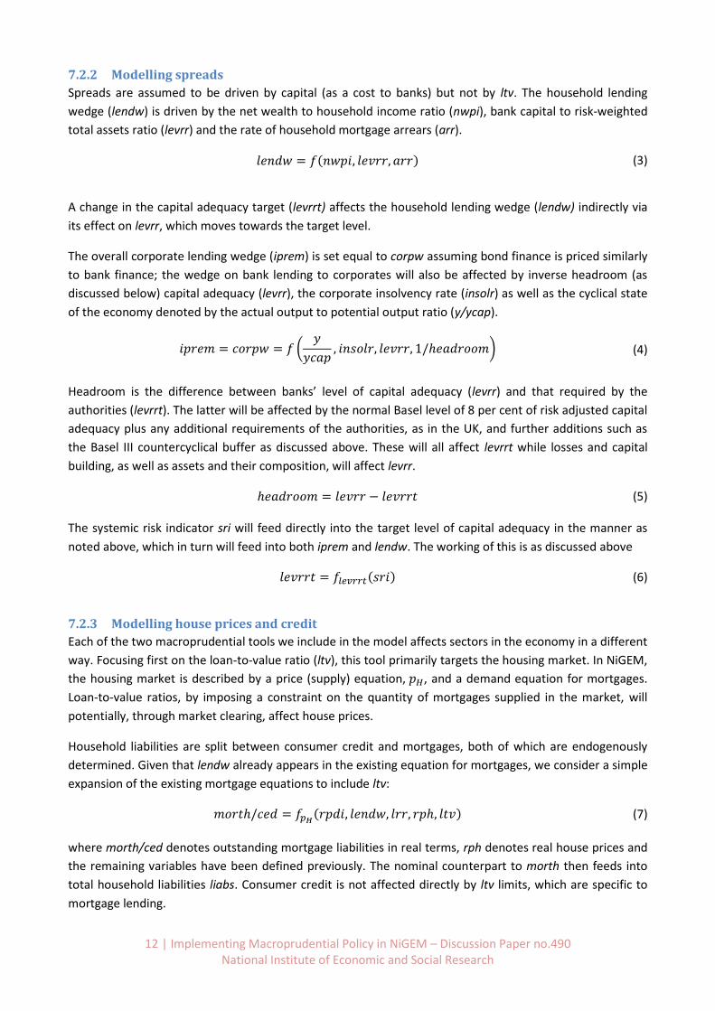
7.2.2 Modelling spreads
Spreads are assumed to be driven by capital (as a cost to banks) but not by ltv. The household lending
wedge (lendw) is driven by the net wealth to household income ratio (nwpi), bank capital to risk-weighted
total assets ratio (levrr) and the rate of household mortgage arrears (arr).
𝑙𝑒𝑛𝑑𝑤 = 𝑓(𝑛𝑤𝑝𝑖, 𝑙𝑒𝑣𝑟𝑟, 𝑎𝑟𝑟) (3)
A change in the capital adequacy target (levrrt) affects the household lending wedge (lendw) indirectly via
its effect on levrr, which moves towards the target level.
The overall corporate lending wedge (iprem) is set equal to corpw assuming bond finance is priced similarly
to bank finance; the wedge on bank lending to corporates will also be affected by inverse headroom (as
discussed below) capital adequacy (levrr), the corporate insolvency rate (insolr) as well as the cyclical state
of the economy denoted by the actual output to potential output ratio (y/ycap).
𝑖𝑝𝑟𝑒𝑚 = 𝑐𝑜𝑟𝑝𝑤 = 𝑓 (𝑦
𝑦𝑐𝑎𝑝, 𝑖𝑛𝑠𝑜𝑙𝑟, 𝑙𝑒𝑣𝑟𝑟, 1/ℎ𝑒𝑎𝑑𝑟𝑜𝑜𝑚) (4)
Headroom is the difference between banks’ level of capital adequacy (levrr) and that required by the
authorities (levrrt). The latter will be affected by the normal Basel level of 8 per cent of risk adjusted capital
adequacy plus any additional requirements of the authorities, as in the UK, and further additions such as
the Basel III countercyclical buffer as discussed above. These will all affect levrrt while losses and capital
building, as well as assets and their composition, will affect levrr.
ℎ𝑒𝑎𝑑𝑟𝑜𝑜𝑚 = 𝑙𝑒𝑣𝑟𝑟 − 𝑙𝑒𝑣𝑟𝑟𝑡
(5)
The systemic risk indicator sri will feed directly into the target level of capital adequacy in the manner as
noted above, which in turn will feed into both iprem and lendw. The working of this is as discussed above
𝑙𝑒𝑣𝑟𝑟𝑡 = 𝑓𝑙𝑒𝑣𝑟𝑟𝑡(𝑠𝑟𝑖) (6)
7.2.3 Modelling house prices and credit
Each of the two macroprudential tools we include in the model affects sectors in the economy in a different
way. Focusing first on the loan-to-value ratio (ltv), this tool primarily targets the housing market. In NiGEM,
the housing market is described by a price (supply) equation, 𝑝𝐻, and a demand equation for mortgages.
Loan-to-value ratios, by imposing a constraint on the quantity of mortgages supplied in the market, will
potentially, through market clearing, affect house prices.
Household liabilities are split between consumer credit and mortgages, both of which are endogenously
determined. Given that lendw already appears in the existing equation for mortgages, we consider a simple
expansion of the existing mortgage equations to include ltv:
𝑚𝑜𝑟𝑡ℎ/𝑐𝑒𝑑 = 𝑓𝑝𝐻(𝑟𝑝𝑑𝑖, 𝑙𝑒𝑛𝑑𝑤, 𝑙𝑟𝑟, 𝑟𝑝ℎ, 𝑙𝑡𝑣) (7)
where morth/ced denotes outstanding mortgage liabilities in real terms, rph denotes real house prices and
the remaining variables have been defined previously. The nominal counterpart to morth then feeds into
total household liabilities liabs. Consumer credit is not affected directly by ltv limits, which are specific to
mortgage lending.
13 | Implementing Macroprudential Policy in NiGEM – Discussion Paper no.490 National Institute of Economic and Social Research
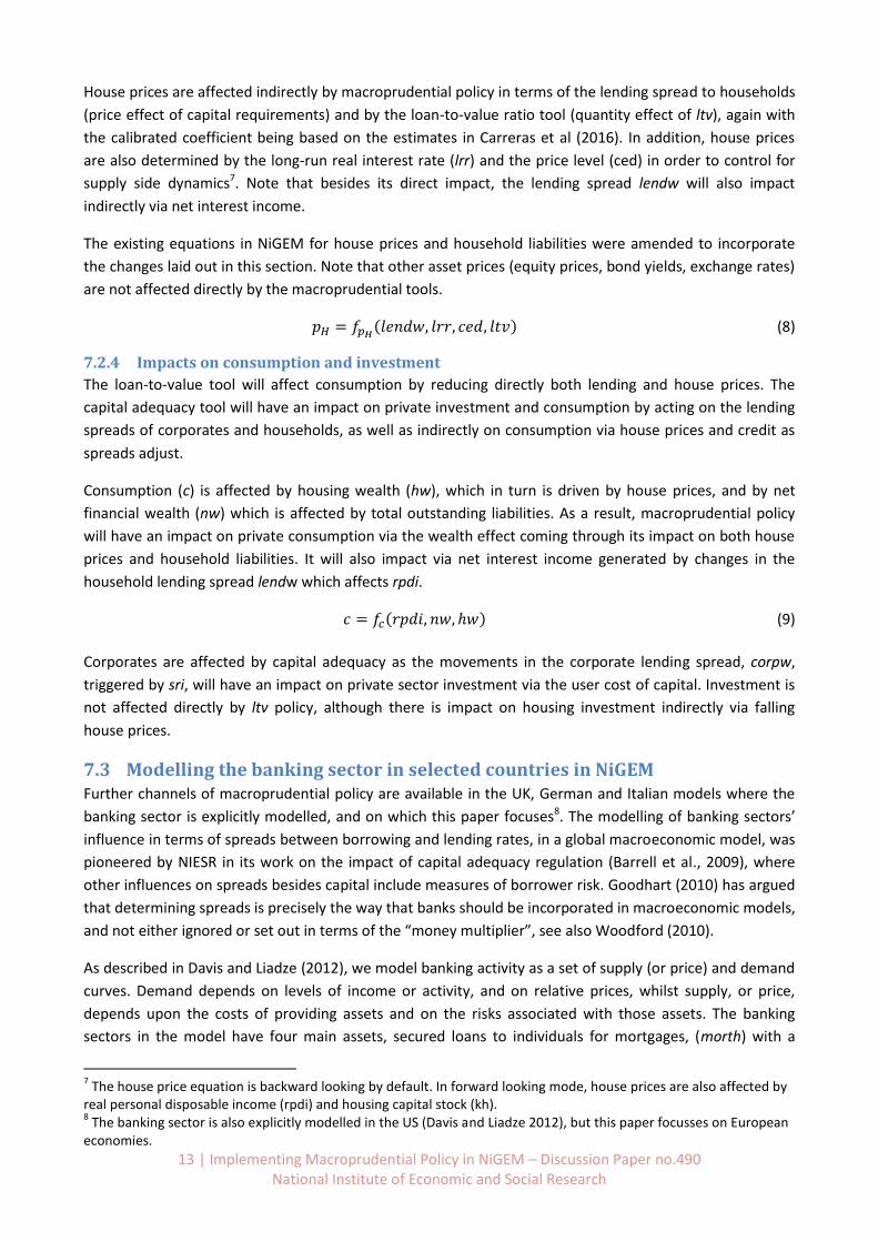
House prices are affected indirectly by macroprudential policy in terms of the lending spread to households
(price effect of capital requirements) and by the loan-to-value ratio tool (quantity effect of ltv), again with
the calibrated coefficient being based on the estimates in Carreras et al (2016). In addition, house prices
are also determined by the long-run real interest rate (lrr) and the price level (ced) in order to control for
supply side dynamics7. Note that besides its direct impact, the lending spread lendw will also impact
indirectly via net interest income.
The existing equations in NiGEM for house prices and household liabilities were amended to incorporate
the changes laid out in this section. Note that other asset prices (equity prices, bond yields, exchange rates)
are not affected directly by the macroprudential tools.
𝑝𝐻 = 𝑓𝑝𝐻(𝑙𝑒𝑛𝑑𝑤, 𝑙𝑟𝑟, 𝑐𝑒𝑑, 𝑙𝑡𝑣) (8)
7.2.4 Impacts on consumption and investment
The loan-to-value tool will affect consumption by reducing directly both lending and house prices. The
capital adequacy tool will have an impact on private investment and consumption by acting on the lending
spreads of corporates and households, as well as indirectly on consumption via house prices and credit as
spreads adjust.
Consumption (c) is affected by housing wealth (hw), which in turn is driven by house prices, and by net
financial wealth (nw) which is affected by total outstanding liabilities. As a result, macroprudential policy
will have an impact on private consumption via the wealth effect coming through its impact on both house
prices and household liabilities. It will also impact via net interest income generated by changes in the
household lending spread lendw which affects rpdi.
𝑐 = 𝑓𝑐(𝑟𝑝𝑑𝑖, 𝑛𝑤, ℎ𝑤) (9)
Corporates are affected by capital adequacy as the movements in the corporate lending spread, corpw,
triggered by sri, will have an impact on private sector investment via the user cost of capital. Investment is
not affected directly by ltv policy, although there is impact on housing investment indirectly via falling
house prices.
7.3 Modelling the banking sector in selected countries in NiGEM Further channels of macroprudential policy are available in the UK, German and Italian models where the
banking sector is explicitly modelled, and on which this paper focuses8. The modelling of banking sectors’
influence in terms of spreads between borrowing and lending rates, in a global macroeconomic model, was
pioneered by NIESR in its work on the impact of capital adequacy regulation (Barrell et al., 2009), where
other influences on spreads besides capital include measures of borrower risk. Goodhart (2010) has argued
that determining spreads is precisely the way that banks should be incorporated in macroeconomic models,
and not either ignored or set out in terms of the “money multiplier”, see also Woodford (2010).
As described in Davis and Liadze (2012), we model banking activity as a set of supply (or price) and demand
curves. Demand depends on levels of income or activity, and on relative prices, whilst supply, or price,
depends upon the costs of providing assets and on the risks associated with those assets. The banking
sectors in the model have four main assets, secured loans to individuals for mortgages, (morth) with a
7 The house price equation is backward looking by default. In forward looking mode, house prices are also affected by
real personal disposable income (rpdi) and housing capital stock (kh). 8 The banking sector is also explicitly modelled in the US (Davis and Liadze 2012), but this paper focusses on European
economies.
14 | Implementing Macroprudential Policy in NiGEM – Discussion Paper no.490 National Institute of Economic and Social Research
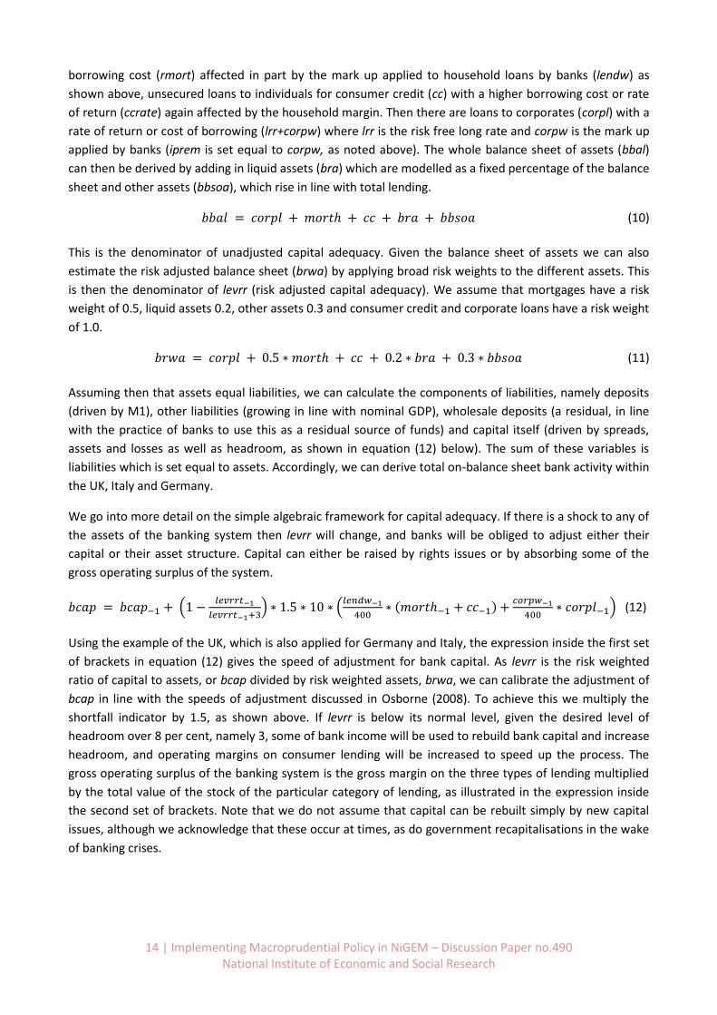
borrowing cost (rmort) affected in part by the mark up applied to household loans by banks (lendw) as
shown above, unsecured loans to individuals for consumer credit (cc) with a higher borrowing cost or rate
of return (ccrate) again affected by the household margin. Then there are loans to corporates (corpl) with a
rate of return or cost of borrowing (lrr+corpw) where lrr is the risk free long rate and corpw is the mark up
applied by banks (iprem is set equal to corpw, as noted above). The whole balance sheet of assets (bbal)
can then be derived by adding in liquid assets (bra) which are modelled as a fixed percentage of the balance
sheet and other assets (bbsoa), which rise in line with total lending.
𝑏𝑏𝑎𝑙 = 𝑐𝑜𝑟𝑝𝑙 + 𝑚𝑜𝑟𝑡ℎ + 𝑐𝑐 + 𝑏𝑟𝑎 + 𝑏𝑏𝑠𝑜𝑎 (10)
This is the denominator of unadjusted capital adequacy. Given the balance sheet of assets we can also
estimate the risk adjusted balance sheet (brwa) by applying broad risk weights to the different assets. This
is then the denominator of levrr (risk adjusted capital adequacy). We assume that mortgages have a risk
weight of 0.5, liquid assets 0.2, other assets 0.3 and consumer credit and corporate loans have a risk weight
of 1.0.
𝑏𝑟𝑤𝑎 = 𝑐𝑜𝑟𝑝𝑙 + 0.5 ∗ 𝑚𝑜𝑟𝑡ℎ + 𝑐𝑐 + 0.2 ∗ 𝑏𝑟𝑎 + 0.3 ∗ 𝑏𝑏𝑠𝑜𝑎 (11)
Assuming then that assets equal liabilities, we can calculate the components of liabilities, namely deposits
(driven by M1), other liabilities (growing in line with nominal GDP), wholesale deposits (a residual, in line
with the practice of banks to use this as a residual source of funds) and capital itself (driven by spreads,
assets and losses as well as headroom, as shown in equation (12) below). The sum of these variables is
liabilities which is set equal to assets. Accordingly, we can derive total on-balance sheet bank activity within
the UK, Italy and Germany.
We go into more detail on the simple algebraic framework for capital adequacy. If there is a shock to any of
the assets of the banking system then levrr will change, and banks will be obliged to adjust either their
capital or their asset structure. Capital can either be raised by rights issues or by absorbing some of the
gross operating surplus of the system.
𝑏𝑐𝑎𝑝 = 𝑏𝑐𝑎𝑝−1 + (1 −𝑙𝑒𝑣𝑟𝑟𝑡−1
𝑙𝑒𝑣𝑟𝑟𝑡−1+3) ∗ 1.5 ∗ 10 ∗ (
𝑙𝑒𝑛𝑑𝑤−1
400∗ (𝑚𝑜𝑟𝑡ℎ−1 + 𝑐𝑐−1) +
𝑐𝑜𝑟𝑝𝑤−1
400∗ 𝑐𝑜𝑟𝑝𝑙−1) (12)
Using the example of the UK, which is also applied for Germany and Italy, the expression inside the first set
of brackets in equation (12) gives the speed of adjustment for bank capital. As levrr is the risk weighted
ratio of capital to assets, or bcap divided by risk weighted assets, brwa, we can calibrate the adjustment of
bcap in line with the speeds of adjustment discussed in Osborne (2008). To achieve this we multiply the
shortfall indicator by 1.5, as shown above. If levrr is below its normal level, given the desired level of
headroom over 8 per cent, namely 3, some of bank income will be used to rebuild bank capital and increase
headroom, and operating margins on consumer lending will be increased to speed up the process. The
gross operating surplus of the banking system is the gross margin on the three types of lending multiplied
by the total value of the stock of the particular category of lending, as illustrated in the expression inside
the second set of brackets. Note that we do not assume that capital can be rebuilt simply by new capital
issues, although we acknowledge that these occur at times, as do government recapitalisations in the wake
of banking crises.
15 | Implementing Macroprudential Policy in NiGEM – Discussion Paper no.490 National Institute of Economic and Social Research
Changes in the speed of adjustment in this equation change the short run, but not the long run effects of
changes in capital adequacy targets. Equation (12) is extended when there are endogenous arrears and
insolvencies to reflect the losses imposed on bank capital by corresponding defaults. We have not
incorporated this in the current exercise.
Then if regulation is tightened, for example via higher capital adequacy requirements as in Basel III, then
increasing margins and reducing lending will both move banks back toward their desired capital ratio. If the
capital adequacy target ratio (levrrt) rises then risk weighted capital adequacy (levrr) will increase and so
will the cost of corporate and personal sector borrowing, raising the gross operating surplus that can be
devoted to rebuilding capital, and reducing assets which raises levrr via a smaller denominator. In models
where arrears and bankruptcies are endogenous, there can also be a deduction from capital for losses.
In the UK, for example, there has been a normal excess above the required minimum level of capital
adequacy, which has averaged 3 percentage points in this sample, with a corresponding difference applied
in Italy and Germany. As the difference between actual and target levels of risk weighted capital to asset
ratios shrinks, we might expect banks to push up their borrowing charges. As headroom goes to zero we
would expect there to be significant non-linear increases in borrowing costs. In order to capture this we
included inverse headroom in the corporate wedge equations, as shown above.
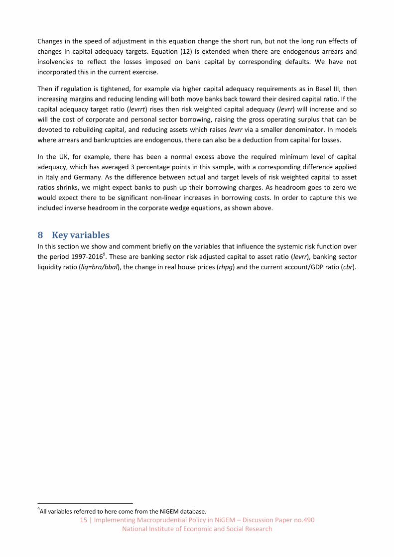
8 Key variables In this section we show and comment briefly on the variables that influence the systemic risk function over
the period 1997-20169. These are banking sector risk adjusted capital to asset ratio (levrr), banking sector
liquidity ratio (liq=bra/bbal), the change in real house prices (rhpg) and the current account/GDP ratio (cbr).
9All variables referred to here come from the NiGEM database.
16 | Implementing Macroprudential Policy in NiGEM – Discussion Paper no.490 National Institute of Economic and Social Research
Chart 3.1: Bank risk adjusted capital adequacy (levrr)
As shown in Chart 3.1, the risk-weighted capital to asset ratio was relatively flat from 1997-2007 despite
the increasing risk of financial instability. A slight upward trend is apparent in Germany from around 8 per
cent to just over 10 per cent while in the UK the ratio fluctuated around 15 per cent (reflecting partly the
higher trigger ratios applied in that country bank by bank). Italian banks had ratios that were at an
intermediate level of around 12.5 per cent.
Since 2007 the ratio has increased over time, in line with Basel III, but according to our data this is much
more apparent for Italy and the UK than for Germany. The UK and Italian ratios are around 20-25 per cent
in the period since 2015, whereas the German ratio rose only to around 14 per cent at the end of the
period. It needs to be borne in mind in assessing these data that the risk adjusted ratio itself is an imperfect
measure of bank risk, especially under Basel II, in the run-up to 2007, as subprime assets were given
inappropriately low risk weights following generous credit ratings being obtained for them.
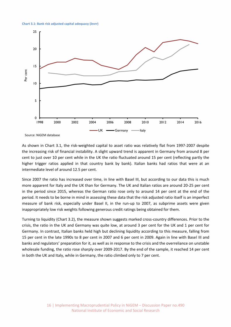
Turning to liquidity (Chart 3.2), the measure shown suggests marked cross-country differences. Prior to the
crisis, the ratio in the UK and Germany was quite low, at around 3 per cent for the UK and 1 per cent for
Germany. In contrast, Italian banks held high but declining liquidity according to this measure, falling from
15 per cent in the late 1990s to 8 per cent in 2007 and 6 per cent in 2009. Again in line with Basel III and
banks and regulators’ preparation for it, as well as in response to the crisis and the overreliance on unstable
wholesale funding, the ratio rose sharply over 2009-2017. By the end of the sample, it reached 14 per cent
in both the UK and Italy, while in Germany, the ratio climbed only to 7 per cent.
0
5
10
15
20
25
1998 2000 2002 2004 2006 2008 2010 2012 2014 2016
Per
cent
UK Germany Italy
Source: NiGEM database
17 | Implementing Macroprudential Policy in NiGEM – Discussion Paper no.490 National Institute of Economic and Social Research
Chart 3.2: Bank liquidity ratio (liq=bra/bbal)
Chart 3.3: Real house price growth (rhpg)
House prices (Chart 3.3) show greater volatility in the UK compared to Italy and especially Germany where
annual change fluctuated around zero prior to 2010, after which a steady rise was seen. There were
noteworthy falls in the UK over 2008-9 and in Italy over 2009-16.
0
2
4
6
8
10
12
14
16
1998 2000 2002 2004 2006 2008 2010 2012 2014 2016
Per
cent
UK Germany Italy
Source: NiGEM database and authors' calculations
-15
-10
-5
0
5
10
15
20
1998 2000 2002 2004 2006 2008 2010 2012 2014 2016
Perc
enta
ge c
han
ge, ye
ar-o
n-y
ear
UK Germany Italy
Source: NiGEM database
18 | Implementing Macroprudential Policy in NiGEM – Discussion Paper no.490 National Institute of Economic and Social Research
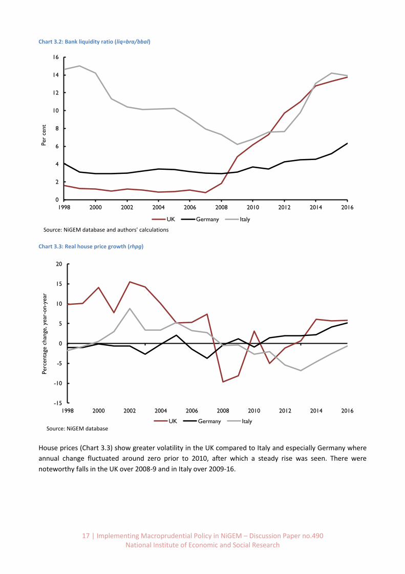
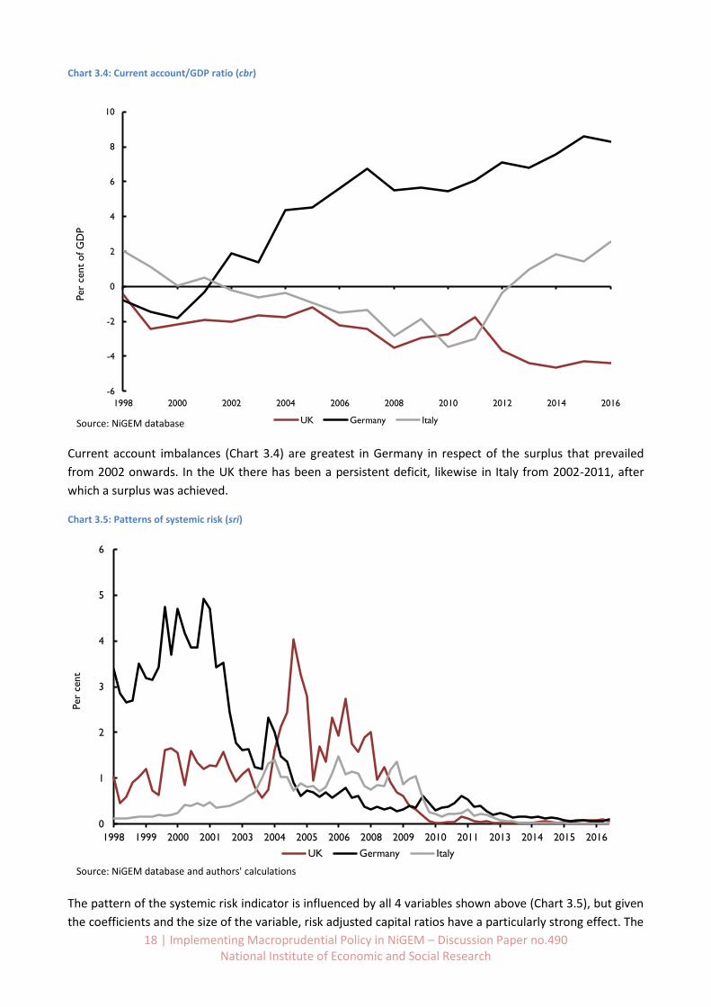
Chart 3.4: Current account/GDP ratio (cbr)
Current account imbalances (Chart 3.4) are greatest in Germany in respect of the surplus that prevailed
from 2002 onwards. In the UK there has been a persistent deficit, likewise in Italy from 2002-2011, after
which a surplus was achieved.
Chart 3.5: Patterns of systemic risk (sri)
The pattern of the systemic risk indicator is influenced by all 4 variables shown above (Chart 3.5), but given
the coefficients and the size of the variable, risk adjusted capital ratios have a particularly strong effect. The
-6
-4
-2
0
2
4
6
8
10
1998 2000 2002 2004 2006 2008 2010 2012 2014 2016
Per
cent
of G
DP
UK Germany ItalySource: NiGEM database
0
1
2
3
4
5
6
1998 1999 2000 2001 2003 2004 2005 2006 2008 2009 2010 2011 2013 2014 2015 2016
Per
cent
UK Germany Italy
Source: NiGEM database and authors' calculations
19 | Implementing Macroprudential Policy in NiGEM – Discussion Paper no.490 National Institute of Economic and Social Research
period prior to the 2007 crisis showed a strong rise in the ratio in the UK, and to a lesser extent in Italy, thus
giving some advance warning. In the case of the UK this was driven particularly by house prices and the
current account, since capital and liquidity did not change much, while in Italy the decline in liquidity had a
marked effect, as did the current account and house prices. The very high levels in Germany in the late
1990s reflect the weak data for bank risk measures shown above, offset later by the improving current
account and relatively stable house prices.
In the years since the crisis it is notable that for all the countries, this measure has been declining, and since
2015 has typically been close to zero per cent. This pattern largely reflects the improvement in banking risk
measures following the regulatory tightening of the crisis and Basel III, as well as the lower rates of change
in house prices.
9 Simulations We undertook four sets of simulations for Germany, Italy and the UK - the EU countries with banking
sectors in the NiGEM model.
1. Tightening of ltv policy - we assess the impact of imposing tighter loan-to-value limits on the housing
market on a permanent basis.
2. Tightening capital adequacy policy – we permanently raise the target risk adjusted capital adequacy by
2.5 percentage points, which represents the effect of imposing Basel III countercyclical buffer fully.10
3. General macroprudential tightening – we combine the two policies, imposing higher ltv limits and
raising the countercyclical buffer simultaneously.
4. Crisis mitigation – this is a historic dynamic simulation over the subprime crisis period. We allow the
macroprudential policies to be triggered by the level of the systemic risk indicator over 2004-2032. As
noted, critical values for sri are 0.01 in UK, 0.03 in Italy and 0.05 in Germany (derived from sample
averages).
We show the responses of the economies of Germany, Italy and the UK in the charts below. Comments on
the patterns follow. Note that we exogenise the monetary response, which means that interest rates do
not react to the deviations from inflation and nominal targets (simulation results with endogenous
monetary policy are presented in Appendix 1, showing the effects of endogenous monetary policy are
relatively minor). Fiscal policy follows a default feedback rule which ensures that the deficit achieves an
equilibrium trajectory by using the direct tax rate as an instrument. Simulations were done one country at a
time, apart from the historic dynamic simulation, where we simulated the effects on all three countries
simultaneously.
10
Due to the forward looking nature of financial markets in the model, long term interest rates decline from the very first period of the simulation, which stimulates investment. To offset this, we increase the user cost of capital in the first period of the simulation.
20 | Implementing Macroprudential Policy in NiGEM – Discussion Paper no.490 National Institute of Economic and Social Research
By default, financial markets in NiGEM are forward looking, as are factor markets. All of these may be
affected by changes in financial regulation. Changing the spread between borrowing and lending rates for
individuals changes their incomes, and can also change their decision making on the timing of consumption.
Changing the spread between borrowing and lending rates for firms may change the user cost of capital
and hence the equilibrium level of output and capital in the economy in a sustained way. A further
important effect is of lower expected inflation on long rates, which means that there is a partial offset to
any increase in the user cost of capital on investment arising from the corporate wedge. Charts are at the
end of Section 4.
9.1 Tightening of loan-to-value policy The first simulation is the tightening of ltv policy. We see from Chart 4.1.1 that household liabilities decline
in every country in the sample by around 2.0 per cent after 5 years. We note, however, that mortgage
lending is not sizeable in Italy (or Germany) relative to GDP (around 60 per cent debt/income ratio for
households) as compared to the UK (110 per cent). Equally, house prices fall in each country by around 3-
3.5 per cent over the same period (Chart 4.1.2). These results are to be expected since we have applied a
direct exogenous shock to ltv in each of the relevant equations, in line with estimates in Carreras et al
(2016). On the other hand, the patterns of bank capital adequacy and GDP growth are more varied. We see
from Chart 4.1.3 that the risk adjusted capital to asset ratio rises in each case, but only marginally in
Germany, by about 0.04 percentage point and by 0.07 percentage point in the UK and Italy, respectively.
This reflects the changing size and pattern of bank assets over the period following the shock.
The policy has a contractionary impact on GDP, albeit a fairly marginal one, with output falling by around
0.05-0.15 per cent at the trough. The components of this are shown in the subsequent charts. We see from
Chart 4.1.5 that, after five years, consumption falls quite markedly by 0.2-0.5 per cent in all three countries,
reflecting the wealth effect of falling house prices following the increase in ltv ratio and households’ need
to save for deposits. However, dynamic patterns differ, reflecting different speeds of adjustments to the
shocks in the economies. The fall in output depresses investment and in the short term private investment
drops by about 0.2 per cent (Chart 4.1.6). However, in the medium term there is a partial recovery in
investment. The fall in consumption generates a marked rise in the saving ratio of up to around 0.3
percentage point (Chart 4.1.7), which is to be expected since the ltv policy requires households buying
property to save more for a deposit. The current balance improves, largely due to fall in domestic demand,
but also following improvement in competitiveness lead by a reduction in domestic prices (Chart 4.1.8).
Given that monetary policy is deactivated in the simulations, exchange rates (vis a vis the dollar) do not
change.
Looking at the banking and financial market effects of the policy, the lending wedges for corporates and
households are relatively unaffected by the ltv policy so changes are quite small (Charts 4.1.9 and 4.1.10).
This policy affects the volume of credit and not its price, and bank assets fall both on an unweighted as well
as weighted basis by 1.5 and 1.4 per cent, respectively (Charts 4.1.12 and 4.1.13). The decline in risk
adjusted assets is smaller than that of the unweighted measure, as mortgages have a relatively low risk
weight.
Finally, the policy has a negative effect on the systemic risk indicator for the UK and Germany but not to a
significant degree in Italy (Chart 4.1.14). The differences in sri are driven largely by the different effects on
risk adjusted capital adequacy, which has a considerably greater effect than house prices or the current
account (both of which also move favourably for financial stability) in the equation. However, it should be
taken into account that the baseline sri in Italy is very low owing to the levels of capital and liquidity being
high while house prices are stable. These means that the amount by which the Italian sri can improve is
21 | Implementing Macroprudential Policy in NiGEM – Discussion Paper no.490 National Institute of Economic and Social Research
highly limited (zero is the lower bound to the sri index), and implies in turn that macroprudential policy is
less needed for financial stability in that country as long as that configuration persists.
9.2 Increase in risk-adjusted capital adequacy target Moving to the second simulation on the countercyclical capital buffer, Chart 4.2.1 shows that there is a
decline in household liabilities, driven by the overall downturn in the economy (Chart 4.2.4) and the rise in
the household lending wedge (Chart 4.2.10). House prices also decline, after rising initially, being affected
by the increase in lending wedge, but by much less than in the ltv scenario (Chart 4.2.2). We see from Chart
4.2.3 that risk adjusted capital adequacy rises in line with the target set by the authorities, by 2.5
percentage points, with a lag, as is permitted by the Basel rules.
GDP falls in this scenario to a much greater degree than in the ltv case, with the declines after 5 years being
greater in Germany and Italy than the UK where the decline is quite small (Chart 4.2.4). Looking at the
components, we see that both consumption and investment decline. However, compared to the previous
scenario, the impact on consumption is smaller, while on private investment the impact is markedly larger.
Private investment falls less in the UK than Germany and Italy (Chart 4.2.6), in the light of rises in the
corporate lending wedge (Chart 4.2.9) and declines in other components of GDP. The saving ratio falls as
real personal disposable income declines more than consumption, again markedly so in Italy (Chart 4.2.7).
Similar to the previous case, it is not surprising to see an improvement in the current account balance as
domestic demand decreases following the introduction of higher capital requirements (Chart 4.2.8).
As regards the financial patterns, the corporate wedge rises in each country, stabilizing at around 0.5-0.7
percentage points above base after five years (Chart 4.2.9). The household wedge rises rather less, by
around 0.15-0.2 percentage points (Chart 4.2.10). These patterns are driven by the higher levels of capital
required for banks, which affect banks’ costs and are present in the equations for the wedges. Corporate
lending falls to a much greater extent than lending to households (Chart 4.2.11, compare Chart 4.2.12), by 6
per cent, in line with the greater rise in the wedge for companies. Bank assets fall to a greater extent than
in case of implementation of tighter ltv policy, for all three countries but the falls is greater in Germany and
Italy than the UK (Charts 4.2.12-4.2.13); the fall is comparable for both risk weighted and unweighted
capital adequacy since the brunt of the shock is taken by corporate lending with a risk weight of 1. Finally
the systemic risk indicator falls by more than in the ltv case for the UK and Germany, reflecting the key
influence of bank capital adequacy on systemic risks (Chart 4.2.14), although again the ratio in Italy is little
affected. Note that the scales on the sri charts 4.1.14, 4.2.14/4.3.14, and 4.4.14 differ.
9.3 Combined macroprudential tightening Combining the two above mentioned policies as a third scenario gives a greater impact on financial stability
and also on the macroeconomy and financial sector. We in effect see both patterns described above
superimposed. We note highlights rather than going chart by chart. Both consumption and investment
(Charts 4.3.5 and 4.3.6) fall markedly, although GDP is partly buoyed by the improvement in the current
account (Chart 4.3.8). The saving ratio rises in the UK and Germany, showing a greater relative impact of
the ltv shock, while it falls in Italy (as personal income is reduced more than private consumption) (Chart
4.3.7). Declines in bank assets and in the sri are correspondingly greater in the combined application of
macroprudential policies (Charts 4.3.12-4.3.14). The sri pattern is however dominated by the impact of the
capital adequacy tightening.
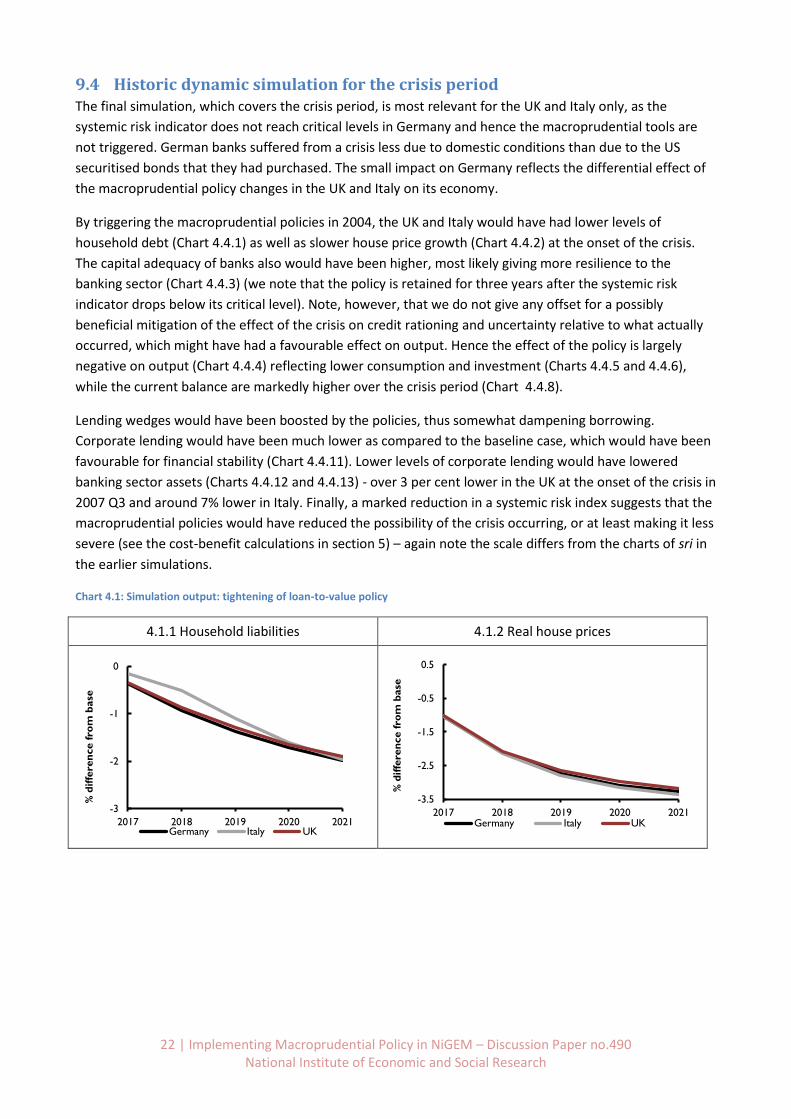
22 | Implementing Macroprudential Policy in NiGEM – Discussion Paper no.490 National Institute of Economic and Social Research
9.4 Historic dynamic simulation for the crisis period The final simulation, which covers the crisis period, is most relevant for the UK and Italy only, as the
systemic risk indicator does not reach critical levels in Germany and hence the macroprudential tools are
not triggered. German banks suffered from a crisis less due to domestic conditions than due to the US
securitised bonds that they had purchased. The small impact on Germany reflects the differential effect of
the macroprudential policy changes in the UK and Italy on its economy.
By triggering the macroprudential policies in 2004, the UK and Italy would have had lower levels of
household debt (Chart 4.4.1) as well as slower house price growth (Chart 4.4.2) at the onset of the crisis.
The capital adequacy of banks also would have been higher, most likely giving more resilience to the
banking sector (Chart 4.4.3) (we note that the policy is retained for three years after the systemic risk
indicator drops below its critical level). Note, however, that we do not give any offset for a possibly
beneficial mitigation of the effect of the crisis on credit rationing and uncertainty relative to what actually
occurred, which might have had a favourable effect on output. Hence the effect of the policy is largely
negative on output (Chart 4.4.4) reflecting lower consumption and investment (Charts 4.4.5 and 4.4.6),
while the current balance are markedly higher over the crisis period (Chart 4.4.8).
Lending wedges would have been boosted by the policies, thus somewhat dampening borrowing.
Corporate lending would have been much lower as compared to the baseline case, which would have been
favourable for financial stability (Chart 4.4.11). Lower levels of corporate lending would have lowered
banking sector assets (Charts 4.4.12 and 4.4.13) - over 3 per cent lower in the UK at the onset of the crisis in
2007 Q3 and around 7% lower in Italy. Finally, a marked reduction in a systemic risk index suggests that the
macroprudential policies would have reduced the possibility of the crisis occurring, or at least making it less
severe (see the cost-benefit calculations in section 5) – again note the scale differs from the charts of sri in
the earlier simulations.
Chart 4.1: Simulation output: tightening of loan-to-value policy
4.1.1 Household liabilities 4.1.2 Real house prices
-3
-2
-1
0
2017 2018 2019 2020 2021
% d
iffe
ren
ce f
rom
base
Germany Italy UK
-3.5
-2.5
-1.5
-0.5
0.5
2017 2018 2019 2020 2021
% d
iffe
ren
ce f
rom
base
Germany Italy UK
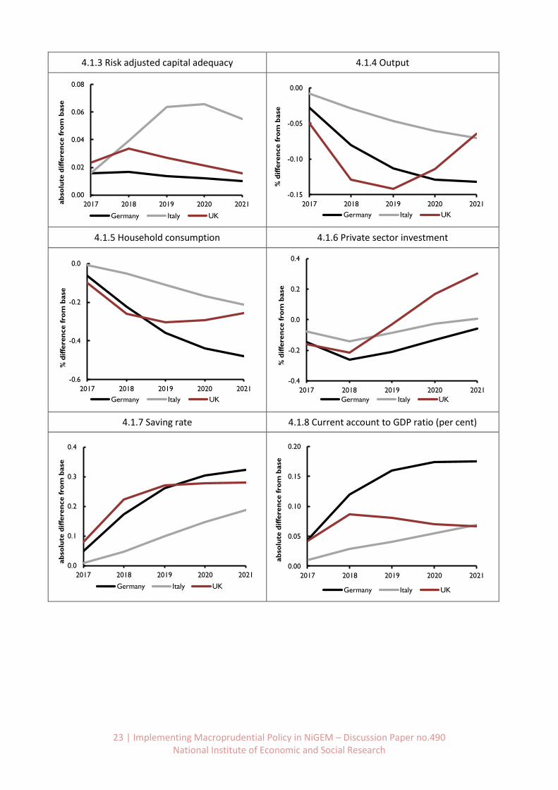
23 | Implementing Macroprudential Policy in NiGEM – Discussion Paper no.490 National Institute of Economic and Social Research
4.1.3 Risk adjusted capital adequacy 4.1.4 Output
4.1.5 Household consumption 4.1.6 Private sector investment
4.1.7 Saving rate 4.1.8 Current account to GDP ratio (per cent)
0.00
0.02
0.04
0.06
0.08
2017 2018 2019 2020 2021ab
solu
te d
iffe
ren
ce fro
m b
ase
Germany Italy UK
-0.15
-0.10
-0.05
0.00
2017 2018 2019 2020 2021
% d
iffe
ren
ce f
rom
base
Germany Italy UK
-0.6
-0.4
-0.2
0.0
2017 2018 2019 2020 2021
% d
iffe
ren
ce f
rom
base
Germany Italy UK
-0.4
-0.2
0.0
0.2
0.4
2017 2018 2019 2020 2021
% d
iffe
ren
ce f
rom
base
Germany Italy UK
0.0
0.1
0.2
0.3
0.4
2017 2018 2019 2020 2021
ab
solu
te d
iffe
ren
ce fro
m b
ase
Germany Italy UK
0.00
0.05
0.10
0.15
0.20
2017 2018 2019 2020 2021
ab
solu
te d
iffe
ren
ce fro
m b
ase
Germany Italy UK
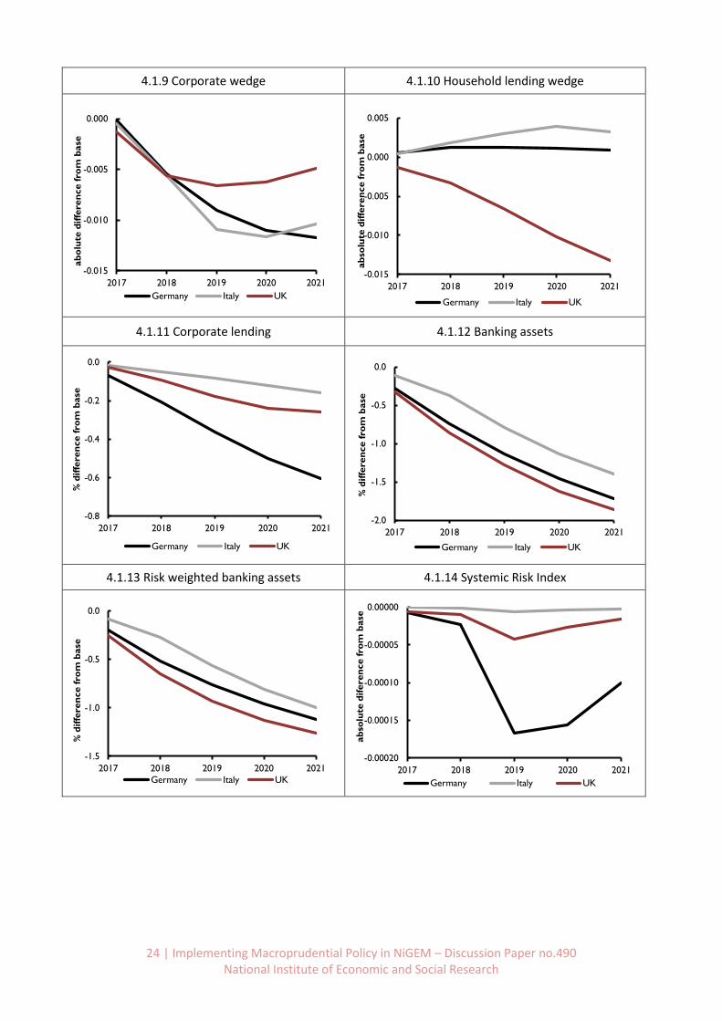
24 | Implementing Macroprudential Policy in NiGEM – Discussion Paper no.490 National Institute of Economic and Social Research
4.1.9 Corporate wedge 4.1.10 Household lending wedge
4.1.11 Corporate lending 4.1.12 Banking assets
4.1.13 Risk weighted banking assets 4.1.14 Systemic Risk Index
-0.015
-0.010
-0.005
0.000
2017 2018 2019 2020 2021
ab
olu
te d
iffe
ren
ce fro
m b
ase
Germany Italy UK
-0.015
-0.010
-0.005
0.000
0.005
2017 2018 2019 2020 2021
ab
solu
te d
iffe
ren
ce fro
m b
ase
Germany Italy UK
-0.8
-0.6
-0.4
-0.2
0.0
2017 2018 2019 2020 2021
% d
iffe
ren
ce f
rom
base
Germany Italy UK
-2.0
-1.5
-1.0
-0.5
0.0
2017 2018 2019 2020 2021
% d
iffe
ren
ce f
rom
base
Germany Italy UK
-1.5
-1.0
-0.5
0.0
2017 2018 2019 2020 2021
% d
iffe
ren
ce f
rom
base
Germany Italy UK
-0.00020
-0.00015
-0.00010
-0.00005
0.00000
2017 2018 2019 2020 2021
ab
solu
te d
ifere
nce fro
m b
ase
Germany Italy UK
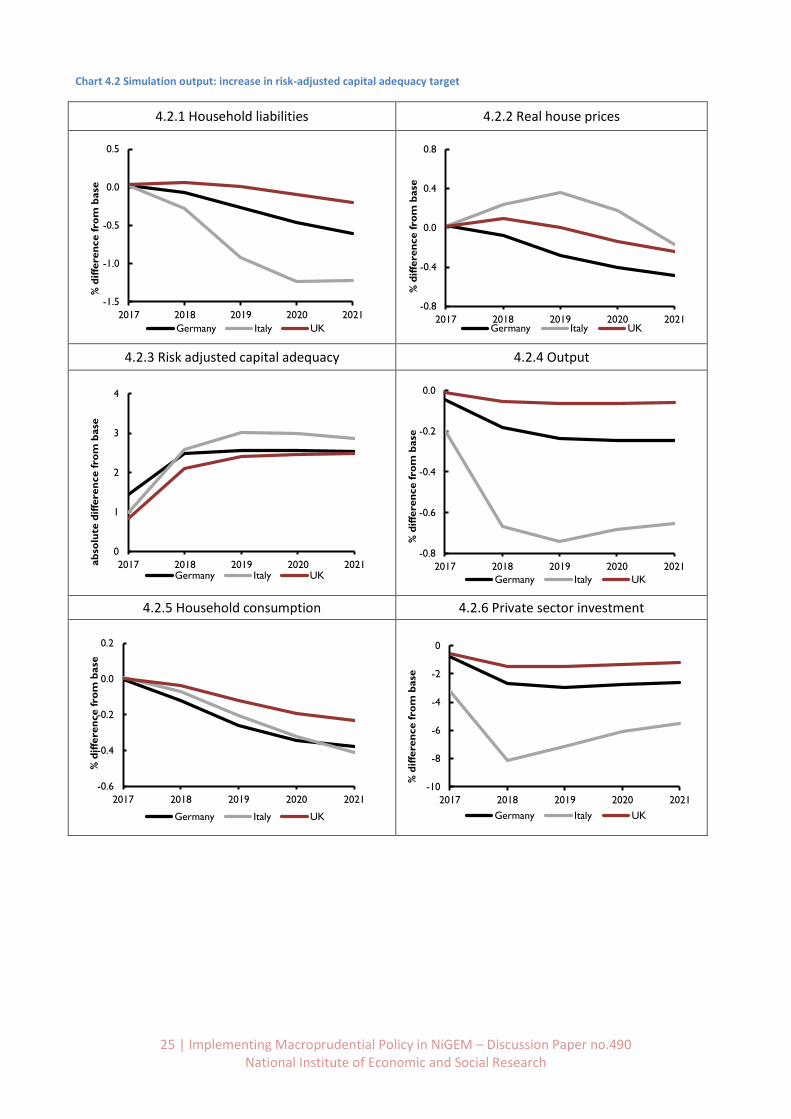
25 | Implementing Macroprudential Policy in NiGEM – Discussion Paper no.490 National Institute of Economic and Social Research
Chart 4.2 Simulation output: increase in risk-adjusted capital adequacy target
4.2.1 Household liabilities 4.2.2 Real house prices
4.2.3 Risk adjusted capital adequacy 4.2.4 Output
4.2.5 Household consumption 4.2.6 Private sector investment
-1.5
-1.0
-0.5
0.0
0.5
2017 2018 2019 2020 2021
% d
iffe
ren
ce f
rom
base
Germany Italy UK
-0.8
-0.4
0.0
0.4
0.8
2017 2018 2019 2020 2021
% d
iffe
ren
ce f
rom
base
Germany Italy UK
0
1
2
3
4
2017 2018 2019 2020 2021ab
solu
te d
iffe
ren
ce fro
m b
ase
Germany Italy UK
-0.8
-0.6
-0.4
-0.2
0.0
2017 2018 2019 2020 2021
% d
iffe
ren
ce f
rom
base
Germany Italy UK
-0.6
-0.4
-0.2
0.0
0.2
2017 2018 2019 2020 2021
% d
iffe
ren
ce f
rom
base
Germany Italy UK
-10
-8
-6
-4
-2
0
2017 2018 2019 2020 2021
% d
iffe
ren
ce f
rom
base
Germany Italy UK
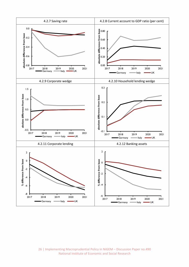
26 | Implementing Macroprudential Policy in NiGEM – Discussion Paper no.490 National Institute of Economic and Social Research
4.2.7 Saving rate 4.2.8 Current account to GDP ratio (per cent)
4.2.9 Corporate wedge 4.2.10 Household lending wedge
4.2.11 Corporate lending 4.2.12 Banking assets
-0.8
-0.6
-0.4
-0.2
0.0
2017 2018 2019 2020 2021ab
solu
te d
iffe
ren
ce fro
m b
ase
Germany Italy UK
0.00
0.20
0.40
0.60
0.80
2017 2018 2019 2020 2021
ab
solu
te d
iffe
ren
ce fro
m b
ase
Germany Italy UK
-0.5
0.0
0.5
1.0
1.5
2017 2018 2019 2020 2021
ab
olu
te d
iffe
ren
ce fro
m b
ase
Germany Italy UK
-0.1
0.1
0.2
0.3
2017 2018 2019 2020 2021
ab
solu
te d
iffe
ren
ce fro
m b
ase
Germany Italy UK
-8
-6
-4
-2
0
2
2017 2018 2019 2020 2021
% d
iffe
ren
ce f
rom
base
Germany Italy UK
-6
-4
-2
0
2
2017 2018 2019 2020 2021
% d
iffe
ren
ce f
rom
base
Germany Italy UK
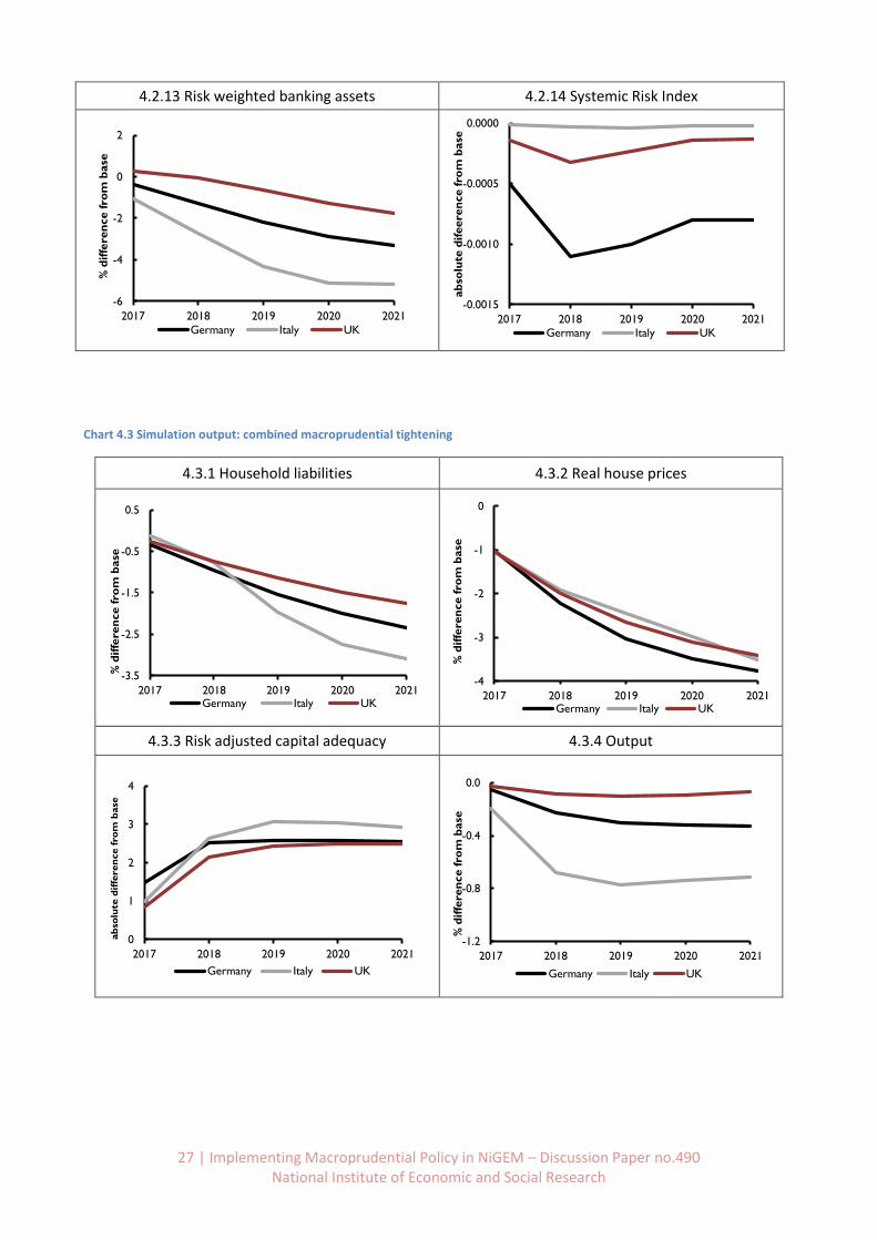
27 | Implementing Macroprudential Policy in NiGEM – Discussion Paper no.490 National Institute of Economic and Social Research
4.2.13 Risk weighted banking assets 4.2.14 Systemic Risk Index
Chart 4.3 Simulation output: combined macroprudential tightening
4.3.1 Household liabilities 4.3.2 Real house prices
4.3.3 Risk adjusted capital adequacy 4.3.4 Output
-6
-4
-2
0
2
2017 2018 2019 2020 2021
% d
iffe
ren
ce f
rom
base
Germany Italy UK
-0.0015
-0.0010
-0.0005
0.0000
2017 2018 2019 2020 2021
ab
solu
te d
ifeere
nce fro
m b
ase
Germany Italy UK
-3.5
-2.5
-1.5
-0.5
0.5
2017 2018 2019 2020 2021
% d
iffe
ren
ce f
rom
base
Germany Italy UK
-4
-3
-2
-1
0
2017 2018 2019 2020 2021
% d
iffe
ren
ce f
rom
base
Germany Italy UK
0
1
2
3
4
2017 2018 2019 2020 2021
ab
solu
te d
iffe
ren
ce f
rom
base
Germany Italy UK
-1.2
-0.8
-0.4
0.0
2017 2018 2019 2020 2021
% d
iffe
ren
ce f
rom
base
Germany Italy UK
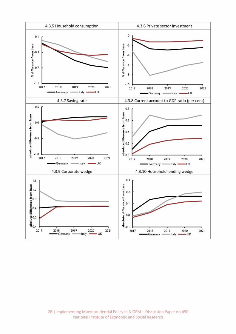
28 | Implementing Macroprudential Policy in NiGEM – Discussion Paper no.490 National Institute of Economic and Social Research
4.3.5 Household consumption 4.3.6 Private sector investment
4.3.7 Saving rate 4.3.8 Current account to GDP ratio (per cent)
4.3.9 Corporate wedge 4.3.10 Household lending wedge
-1.1
-0.7
-0.3
0.1
2017 2018 2019 2020 2021
% d
iffe
ren
ce f
rom
base
Germany Italy UK
-10
-8
-6
-4
-2
0
2017 2018 2019 2020 2021
% d
iffe
ren
ce f
rom
base
Germany Italy UK
-1.0
-0.5
0.0
0.5
2017 2018 2019 2020 2021ab
solu
te d
iffe
ren
ce fro
m b
ase
Germany Italy UK
0.0
0.2
0.4
0.6
0.8
2017 2018 2019 2020 2021
ab
solu
te d
iffe
ren
ce fro
m b
ase
Germany Italy UK
-0.4
0.0
0.4
0.8
1.2
1.6
2017 2018 2019 2020 2021
ab
olu
te d
iffe
ren
ce fro
m b
ase
Germany Italy UK
-0.1
0.0
0.1
0.2
0.3
2017 2018 2019 2020 2021
ab
solu
te d
iffe
ren
ce fro
m b
ase
Germany Italy UK
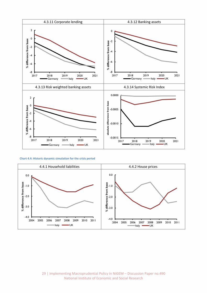
29 | Implementing Macroprudential Policy in NiGEM – Discussion Paper no.490 National Institute of Economic and Social Research
4.3.11 Corporate lending 4.3.12 Banking assets
4.3.13 Risk weighted banking assets 4.3.14 Systemic Risk Index
Chart 4.4: Historic dynamic simulation for the crisis period
4.4.1 Household liabilities 4.4.2 House prices
-8
-6
-4
-2
0
2
2017 2018 2019 2020 2021
% d
iffe
ren
ce f
rom
base
Germany Italy UK
-8
-6
-4
-2
0
2017 2018 2019 2020 2021
% d
iffe
ren
ce f
rom
base
Germany Italy UK
-8
-6
-4
-2
0
2
2017 2018 2019 2020 2021
% d
iffe
ren
ce f
rom
base
Germany Italy UK
-0.0015
-0.0010
-0.0005
0.0000
2017 2018 2019 2020 2021
ab
solu
te d
ifeere
nce f
rom
base
Germany Italy UK
-4.0
-3.0
-2.0
-1.0
0.0
2004 2005 2006 2007 2008 2009 2010 2011
% d
iffe
ren
ce f
rom
base
Italy UK
-4.0
-3.0
-2.0
-1.0
0.0
2004 2005 2006 2007 2008 2009 2010 2011
% d
iffe
ren
ce f
rom
base
Italy UK
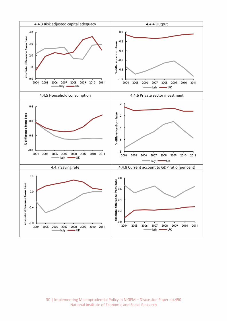
30 | Implementing Macroprudential Policy in NiGEM – Discussion Paper no.490 National Institute of Economic and Social Research
4.4.3 Risk adjusted capital adequacy 4.4.4 Output
4.4.5 Household consumption 4.4.6 Private sector investment
4.4.7 Saving rate 4.4.8 Current account to GDP ratio (per cent)
0.0
1.0
2.0
3.0
4.0
2004 2005 2006 2007 2008 2009 2010 2011
ab
solu
te d
iffe
ren
ce fro
m b
ase
Italy UK
-1.0
-0.8
-0.6
-0.4
-0.2
0.0
2004 2005 2006 2007 2008 2009 2010 2011
% d
iffe
ren
ce f
rom
base
Italy UK
-0.8
-0.4
0.0
0.4
2004 2005 2006 2007 2008 2009 2010 2011
% d
iffe
ren
ce f
rom
base
Italy UK
-8
-6
-4
-2
0
2004 2005 2006 2007 2008 2009 2010 2011
% d
iffe
ren
ce f
rom
base
Italy UK
-0.8
-0.4
0.0
0.4
2004 2005 2006 2007 2008 2009 2010 2011
ab
solu
te d
iffe
ren
ce fro
m b
ase
Italy UK
0.0
0.2
0.4
0.6
0.8
2004 2005 2006 2007 2008 2009 2010 2011
ab
solu
te d
iffe
ren
ce fro
m b
ase
Italy UK
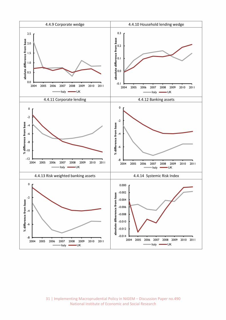
31 | Implementing Macroprudential Policy in NiGEM – Discussion Paper no.490 National Institute of Economic and Social Research
4.4.9 Corporate wedge 4.4.10 Household lending wedge
4.4.11 Corporate lending 4.4.12 Banking assets
4.4.13 Risk weighted banking assets 4.4.14 Systemic Risk Index
0.0
0.5
1.0
1.5
2.0
2.5
2004 2005 2006 2007 2008 2009 2010 2011
ab
olu
te d
iffe
ren
ce fro
m b
ase
Italy UK
-0.1
0.0
0.1
0.2
0.3
2004 2005 2006 2007 2008 2009 2010 2011
ab
solu
te d
iffe
ren
ce fro
m b
ase
Italy UK
-12
-10
-8
-6
-4
-2
0
2004 2005 2006 2007 2008 2009 2010 2011
% d
iffe
ren
ce f
rom
base
Italy UK
-8
-6
-4
-2
0
2004 2005 2006 2007 2008 2009 2010 2011
% d
iffe
ren
ce f
rom
base
Italy UK
-8
-6
-4
-2
0
2004 2005 2006 2007 2008 2009 2010 2011
% d
iffe
ren
ce f
rom
base
Italy UK
-0.014
-0.012
-0.010
-0.008
-0.006
-0.004
-0.002
0.000
2004 2005 2006 2007 2008 2009 2010 2011
ab
solu
te d
ifeere
nce fro
m b
ase
Italy UK
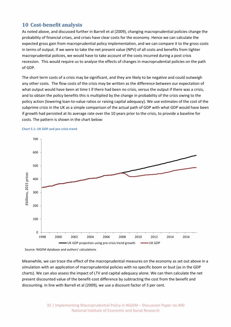
32 | Implementing Macroprudential Policy in NiGEM – Discussion Paper no.490 National Institute of Economic and Social Research
10 Cost-benefit analysis As noted above, and discussed further in Barrell et al (2009), changing macroprudential policies change the
probability of financial crises, and crises have clear costs for the economy. Hence we can calculate the
expected gross gain from macroprudential policy implementation, and we can compare it to the gross costs
in terms of output. If we were to take the net present value (NPV) of all costs and benefits from tighter
macroprudential policies, we would have to take account of the costs incurred during a post crisis
recession. This would require us to analyse the effects of changes in macroprudential policies on the path
of GDP.
The short term costs of a crisis may be significant, and they are likely to be negative and could outweigh
any other costs. The flow costs of the crisis may be written as the difference between our expectation of
what output would have been at time t if there had been no crisis, versus the output if there was a crisis,
and to obtain the policy benefits this is multiplied by the change in probability of the crisis owing to the
policy action (lowering loan-to-value ratios or raising capital adequacy). We use estimates of the cost of the
subprime crisis in the UK as a simple comparison of the actual path of GDP with what GDP would have been
if growth had persisted at its average rate over the 10 years prior to the crisis, to provide a baseline for
costs. The pattern is shown in the chart below:
Chart 5.1: UK GDP and pre-crisis trend
Meanwhile, we can trace the effect of the macroprudential measures on the economy as set out above in a
simulation with an application of macroprudential policies with no specific boom or bust (as in the GDP
charts). We can also assess the impact of LTV and capital adequacy alone. We can then calculate the net
present discounted value of the benefit-cost difference by subtracting the cost from the benefit and
discounting. In line with Barrell et al (2009), we use a discount factor of 3 per cent.
0
100
200
300
400
500
600
700
1998 2000 2002 2004 2006 2008 2010 2012 2014 2016
£b
illio
ns,
20
15
pri
ces
UK GDP projection using pre-crisis trend growth UK GDP
Source: NiGEM database and authors' calculations
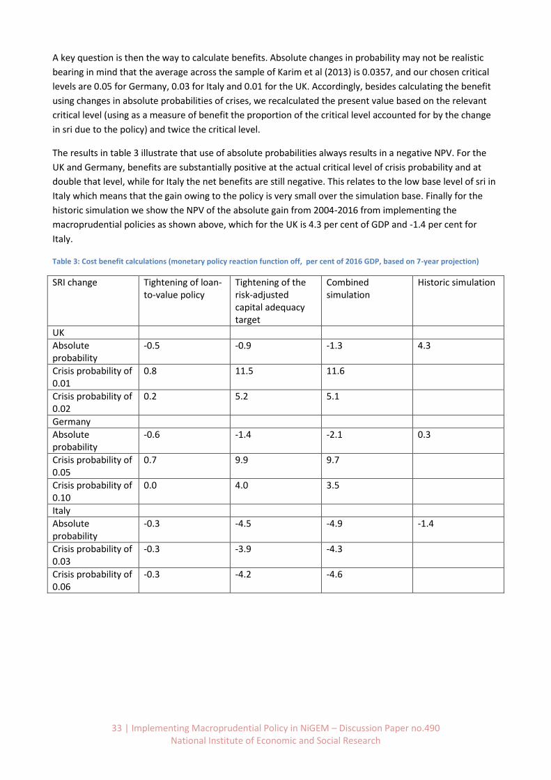
33 | Implementing Macroprudential Policy in NiGEM – Discussion Paper no.490 National Institute of Economic and Social Research
A key question is then the way to calculate benefits. Absolute changes in probability may not be realistic
bearing in mind that the average across the sample of Karim et al (2013) is 0.0357, and our chosen critical
levels are 0.05 for Germany, 0.03 for Italy and 0.01 for the UK. Accordingly, besides calculating the benefit
using changes in absolute probabilities of crises, we recalculated the present value based on the relevant
critical level (using as a measure of benefit the proportion of the critical level accounted for by the change
in sri due to the policy) and twice the critical level.
The results in table 3 illustrate that use of absolute probabilities always results in a negative NPV. For the
UK and Germany, benefits are substantially positive at the actual critical level of crisis probability and at
double that level, while for Italy the net benefits are still negative. This relates to the low base level of sri in
Italy which means that the gain owing to the policy is very small over the simulation base. Finally for the
historic simulation we show the NPV of the absolute gain from 2004-2016 from implementing the
macroprudential policies as shown above, which for the UK is 4.3 per cent of GDP and -1.4 per cent for
Italy.
Table 3: Cost benefit calculations (monetary policy reaction function off, per cent of 2016 GDP, based on 7-year projection)
SRI change Tightening of loan-to-value policy
Tightening of the risk-adjusted capital adequacy target
Combined simulation
Historic simulation
UK
Absolute probability
-0.5 -0.9 -1.3 4.3
Crisis probability of 0.01
0.8 11.5 11.6
Crisis probability of 0.02
0.2 5.2 5.1
Germany
Absolute probability
-0.6 -1.4 -2.1 0.3
Crisis probability of 0.05
0.7 9.9 9.7
Crisis probability of 0.10
0.0 4.0
3.5
Italy
Absolute probability
-0.3 -4.5 -4.9 -1.4
Crisis probability of 0.03
-0.3 -3.9 -4.3
Crisis probability of 0.06
-0.3 -4.2 -4.6
34 | Implementing Macroprudential Policy in NiGEM – Discussion Paper no.490 National Institute of Economic and Social Research
11 Conclusions In this paper, we first illustrate our specific extensions to NiGEM for a macroprudential block, before going
on to the results of counterfactual scenarios based on the macroprudential block. We also perform a cost-
benefit analysis of macroprudential policies, whereby the benefit is captured by the diminished probability
of a crisis and the cost by the impact of macroprudential policies on output. The policies are tested in the
NiGEM models for the UK, Germany and Italy, all of which have a banking sector submodel in NiGEM. An
explanation of the data sources is carried out in Appendix 3.
Concerning limitations, we note that macroprudential policy is more likely to be implemented in a
discretionary manner, rather than be triggered by systemic risk in the model given current low levels of the
latter, which in turn reflect Basel III improvements to capital adequacy. The systemic risk function is of
course largely focused on banking sector risk and resilience, and accordingly the model will not forecast as
it stands the types of crisis that have originated in the non-bank sector such as the 1998 Russian financial
crisis or the recent European sovereign debt crisis. Consequently, an assessment of non-bank imbalances
may be a further area for research.
Further research might focus on additional macroprudential tools such as the Debt-To-Income ratio for
mortgages as well as taxes on financial institutions, both of which were shown to be effective in Carreras et
al (2016). A further important issue is to implement feedback from the real economy to bank capital
adequacy and lending in the form of mortgage arrears for households and insolvencies for companies.
Relevant equations were estimated in Davis and Liadze (2012) for these quantities. We can also assess the
impact of macroprudential policy when monetary and fiscal policy do not partly offset their impact, i.e.
varying the policy mix, as is illustrated in Appendix 1, although effects of this are quite small (compare for
example Chart 4.1.4 and Chart A.1.4 showing a small offset of ltv policy by monetary policy easing).
12 References Antipa, P. and Matheron, S. (2014), “Interactions between monetary and macroprudential policies”,
Banque de France Financial Stability Review, 18, pp. 225-239.
Barrell, R., Davis, E. P., Fic, T., Holland, D., Kirby, S. and Liadze, I. (2009), “Optimal regulation of bank capital
and liquidity: how to calibrate new international standards” FSA Occasional Paper no. 38, October.
Barrell, R., Davis, E. P., Karim, D., Liadze, I., (2010a), “Bank regulation, property prices and early warning
systems for banking crises in OECD countries”, Journal of Banking and Finance, 34, pp. 2255–2264.
Barrell, R., Davis, E. P., Karim, D. and Liadze, I. (2010b), " The impact of global imbalances: Does the current
account balance help to predict banking crises in OECD countries?", NIESR Discussion Paper No. 351.
Barrell, R., Davis, E., Liadze, I., Karim, D, (2010c), “The Effects Of Banking Crises On Potential Output In
OECD Countries” NIESR Discussion Paper no. 358,
Barrell R., and Dury, K. (2003) 'Asymmetric labour markets in a converging Europe: Do differences matter?'
National Institute Economic Review No. 183, January 2003
Barrell, R., and N. Pain (1997), 'Foreign Direct Investment, Technological Change, and Economic Growth
Within Europe', Economic Journal, 107, pp. 1770-1776.
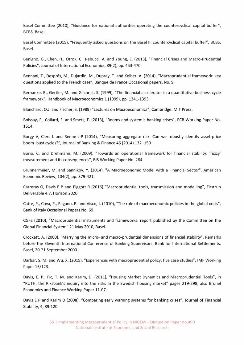
35 | Implementing Macroprudential Policy in NiGEM – Discussion Paper no.490 National Institute of Economic and Social Research
Basel Committee (2010), “Guidance for national authorities operating the countercyclical capital buffer”,
BCBS, Basel.
Basel Committee (2015), “Frequently asked questions on the Basel III countercyclical capital buffer”, BCBS,
Basel.
Benigno, G., Chen, H., Otrok, C., Rebucci, A. and Young, E. (2013), "Financial Crises and Macro-Prudential
Policies", Journal of International Economics, 89(2), pp. 453-470.
Bennani, T., Després, M., Dujardin, M., Duprey, T. and Kelber, A. (2014), “Macroprudential framework: key
questions applied to the French case”, Banque de France Occasional papers, No. 9
Bernanke, B., Gertler, M. and Gilchrist, S. (1999), "The financial accelerator in a quantitative business cycle
framework", Handbook of Macroeconomics 1 (1999), pp. 1341-1393.
Blanchard, O.J. and Fischer, S. (1989) “Lectures on Macroeconomics”, Cambridge: MIT Press.
Boissay, F., Collard, F. and Smets, F. (2013), "Booms and systemic banking crises", ECB Working Paper No.
1514.
Borgy V, Clerc L and Renne J-P (2014), “Measuring aggregate risk: Can we robustly identify asset-price
boom–bust cycles?”, Journal of Banking & Finance 46 (2014) 132–150
Borio, C. and Drehmann, M. (2009), "Towards an operational framework for financial stability: ‘fuzzy’
measurement and its consequences", BIS Working Paper No. 284.
Brunnermeier, M. and Sannikov, Y. (2014), "A Macroeconomic Model with a Financial Sector", American
Economic Review, 104(2), pp. 379-421.
Carreras O, Davis E P and Piggott R (2016) “Macroprudential tools, transmission and modelling”, Firstrun
Deliverable 4.7, Horizon 2020
Catte, P., Cova, P., Pagano, P. and Visco, I. (2010), "The role of macroeconomic policies in the global crisis",
Bank of Italy Occasional Papers No. 69.
CGFS (2010), “Macroprudential instruments and frameworks: report published by the Committee on the
Global Financial System” 21 May 2010, Basel.
Crockett, A. (2000), "Marrying the micro- and macro-prudential dimensions of financial stability", Remarks
before the Eleventh International Conference of Banking Supervisors. Bank for International Settlements.
Basel, 20-21 September 2000.
Darbar, S. M. and Wu, X. (2015), “Experiences with macroprudential policy, five case studies”, IMF Working
Paper 15/123.
Davis, E. P., Fic, T. M. and Karim, D. (2011), “Housing Market Dynamics and Macroprudential Tools”, in
“RUTH, the Riksbank’s inquiry into the risks in the Swedish housing market” pages 219-298, also Brunel
Economics and Finance Working Paper 11-07.
Davis E P and Karim D (2008), “Comparing early warning systems for banking crises”, Journal of Financial
Stability, 4, 89-120
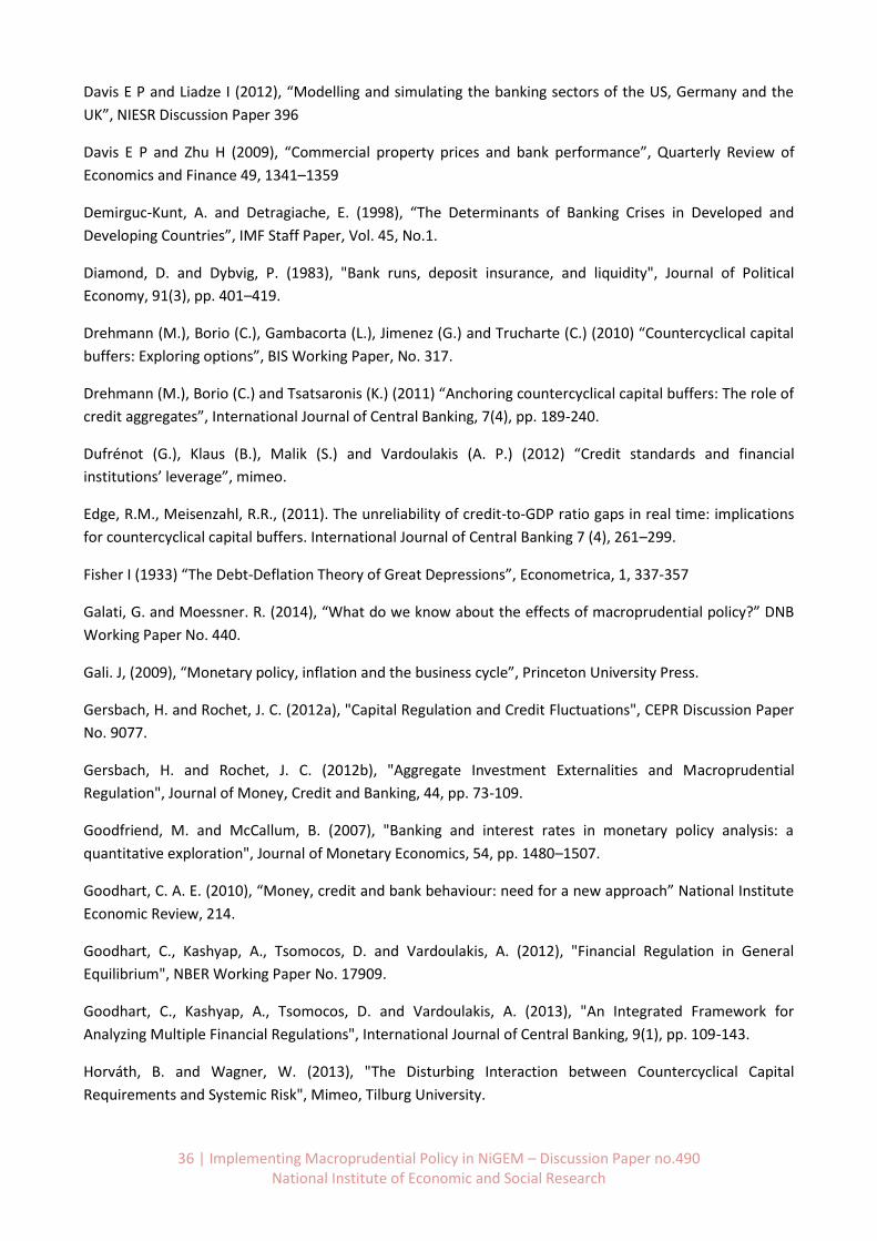
36 | Implementing Macroprudential Policy in NiGEM – Discussion Paper no.490 National Institute of Economic and Social Research
Davis E P and Liadze I (2012), “Modelling and simulating the banking sectors of the US, Germany and the
UK”, NIESR Discussion Paper 396
Davis E P and Zhu H (2009), “Commercial property prices and bank performance”, Quarterly Review of
Economics and Finance 49, 1341–1359
Demirguc-Kunt, A. and Detragiache, E. (1998), “The Determinants of Banking Crises in Developed and
Developing Countries”, IMF Staff Paper, Vol. 45, No.1.
Diamond, D. and Dybvig, P. (1983), "Bank runs, deposit insurance, and liquidity", Journal of Political
Economy, 91(3), pp. 401–419.
Drehmann (M.), Borio (C.), Gambacorta (L.), Jimenez (G.) and Trucharte (C.) (2010) “Countercyclical capital
buffers: Exploring options”, BIS Working Paper, No. 317.
Drehmann (M.), Borio (C.) and Tsatsaronis (K.) (2011) “Anchoring countercyclical capital buffers: The role of
credit aggregates”, International Journal of Central Banking, 7(4), pp. 189-240.
Dufrénot (G.), Klaus (B.), Malik (S.) and Vardoulakis (A. P.) (2012) “Credit standards and financial
institutions’ leverage”, mimeo.
Edge, R.M., Meisenzahl, R.R., (2011). The unreliability of credit-to-GDP ratio gaps in real time: implications
for countercyclical capital buffers. International Journal of Central Banking 7 (4), 261–299.
Fisher I (1933) “The Debt-Deflation Theory of Great Depressions”, Econometrica, 1, 337-357
Galati, G. and Moessner. R. (2014), “What do we know about the effects of macroprudential policy?” DNB
Working Paper No. 440.
Gali. J, (2009), “Monetary policy, inflation and the business cycle”, Princeton University Press.
Gersbach, H. and Rochet, J. C. (2012a), "Capital Regulation and Credit Fluctuations", CEPR Discussion Paper
No. 9077.
Gersbach, H. and Rochet, J. C. (2012b), "Aggregate Investment Externalities and Macroprudential
Regulation", Journal of Money, Credit and Banking, 44, pp. 73-109.
Goodfriend, M. and McCallum, B. (2007), "Banking and interest rates in monetary policy analysis: a
quantitative exploration", Journal of Monetary Economics, 54, pp. 1480–1507.
Goodhart, C. A. E. (2010), “Money, credit and bank behaviour: need for a new approach” National Institute
Economic Review, 214.
Goodhart, C., Kashyap, A., Tsomocos, D. and Vardoulakis, A. (2012), "Financial Regulation in General
Equilibrium", NBER Working Paper No. 17909.
Goodhart, C., Kashyap, A., Tsomocos, D. and Vardoulakis, A. (2013), "An Integrated Framework for
Analyzing Multiple Financial Regulations", International Journal of Central Banking, 9(1), pp. 109-143.
Horváth, B. and Wagner, W. (2013), "The Disturbing Interaction between Countercyclical Capital
Requirements and Systemic Risk", Mimeo, Tilburg University.
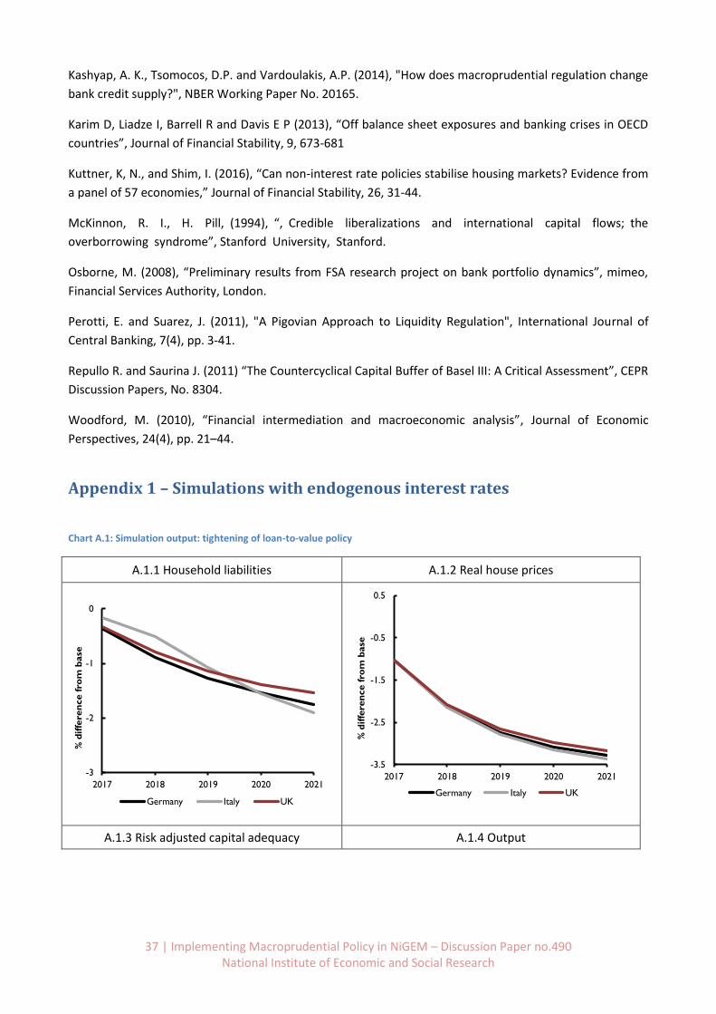
37 | Implementing Macroprudential Policy in NiGEM – Discussion Paper no.490 National Institute of Economic and Social Research
Kashyap, A. K., Tsomocos, D.P. and Vardoulakis, A.P. (2014), "How does macroprudential regulation change
bank credit supply?", NBER Working Paper No. 20165.
Karim D, Liadze I, Barrell R and Davis E P (2013), “Off balance sheet exposures and banking crises in OECD
countries”, Journal of Financial Stability, 9, 673-681
Kuttner, K, N., and Shim, I. (2016), “Can non-interest rate policies stabilise housing markets? Evidence from
a panel of 57 economies,” Journal of Financial Stability, 26, 31-44.
McKinnon, R. I., H. Pill, (1994), “, Credible liberalizations and international capital flows; the
overborrowing syndrome”, Stanford University, Stanford.
Osborne, M. (2008), “Preliminary results from FSA research project on bank portfolio dynamics”, mimeo,
Financial Services Authority, London.
Perotti, E. and Suarez, J. (2011), "A Pigovian Approach to Liquidity Regulation", International Journal of
Central Banking, 7(4), pp. 3-41.
Repullo R. and Saurina J. (2011) “The Countercyclical Capital Buffer of Basel III: A Critical Assessment”, CEPR
Discussion Papers, No. 8304.
Woodford, M. (2010), “Financial intermediation and macroeconomic analysis”, Journal of Economic
Perspectives, 24(4), pp. 21–44.
Appendix 1 – Simulations with endogenous interest rates
Chart A.1: Simulation output: tightening of loan-to-value policy
A.1.1 Household liabilities A.1.2 Real house prices
A.1.3 Risk adjusted capital adequacy A.1.4 Output
-3
-2
-1
0
2017 2018 2019 2020 2021
% d
iffe
ren
ce f
rom
base
Germany Italy UK
-3.5
-2.5
-1.5
-0.5
0.5
2017 2018 2019 2020 2021
% d
iffe
ren
ce f
rom
base
Germany Italy UK
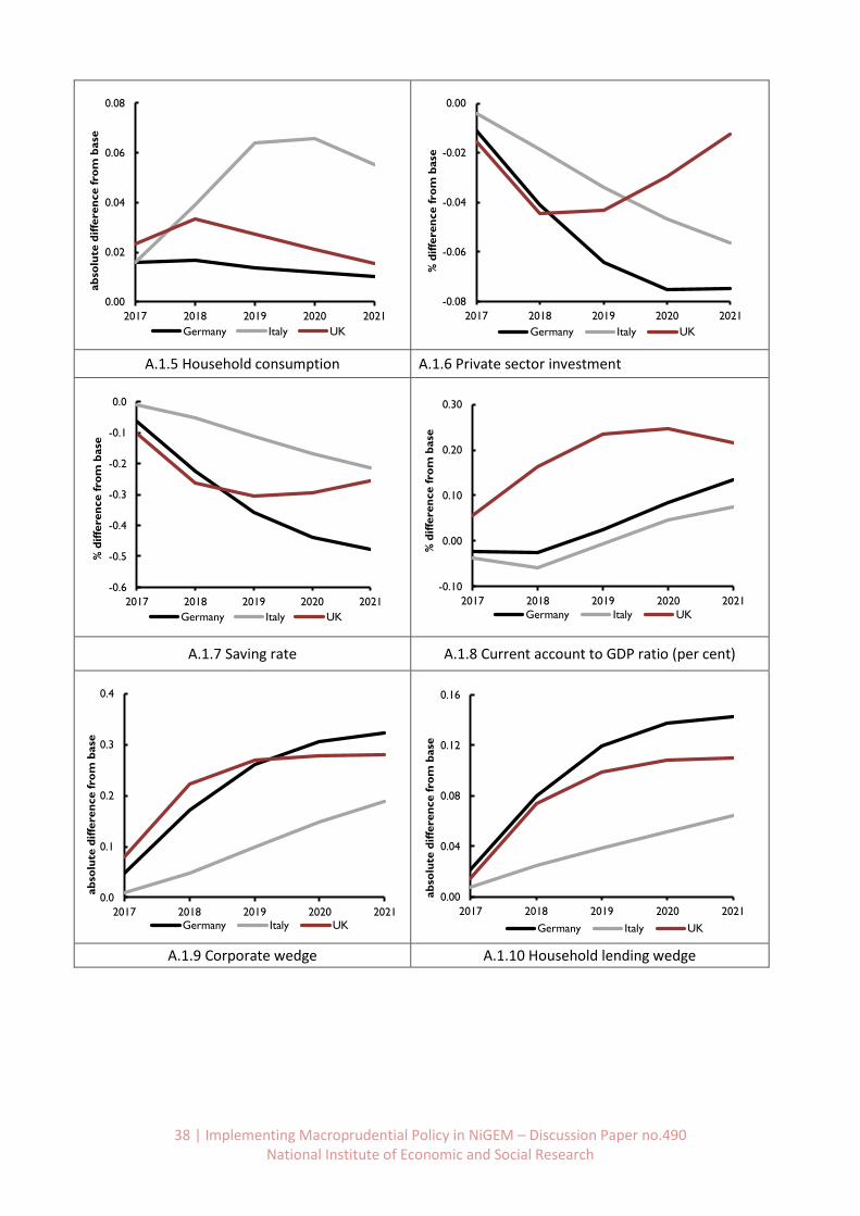
38 | Implementing Macroprudential Policy in NiGEM – Discussion Paper no.490 National Institute of Economic and Social Research
A.1.5 Household consumption A.1.6 Private sector investment
A.1.7 Saving rate A.1.8 Current account to GDP ratio (per cent)
A.1.9 Corporate wedge A.1.10 Household lending wedge
0.00
0.02
0.04
0.06
0.08
2017 2018 2019 2020 2021
ab
solu
te d
iffe
ren
ce fro
m b
ase
Germany Italy UK
-0.08
-0.06
-0.04
-0.02
0.00
2017 2018 2019 2020 2021
% d
iffe
ren
ce f
rom
base
Germany Italy UK
-0.6
-0.5
-0.4
-0.3
-0.2
-0.1
0.0
2017 2018 2019 2020 2021
% d
iffe
ren
ce f
rom
base
Germany Italy UK
-0.10
0.00
0.10
0.20
0.30
2017 2018 2019 2020 2021
% d
iffe
ren
ce f
rom
base
Germany Italy UK
0.0
0.1
0.2
0.3
0.4
2017 2018 2019 2020 2021
ab
solu
te d
iffe
ren
ce fro
m b
ase
Germany Italy UK
0.00
0.04
0.08
0.12
0.16
2017 2018 2019 2020 2021
ab
solu
te d
iffe
ren
ce fro
m b
ase
Germany Italy UK
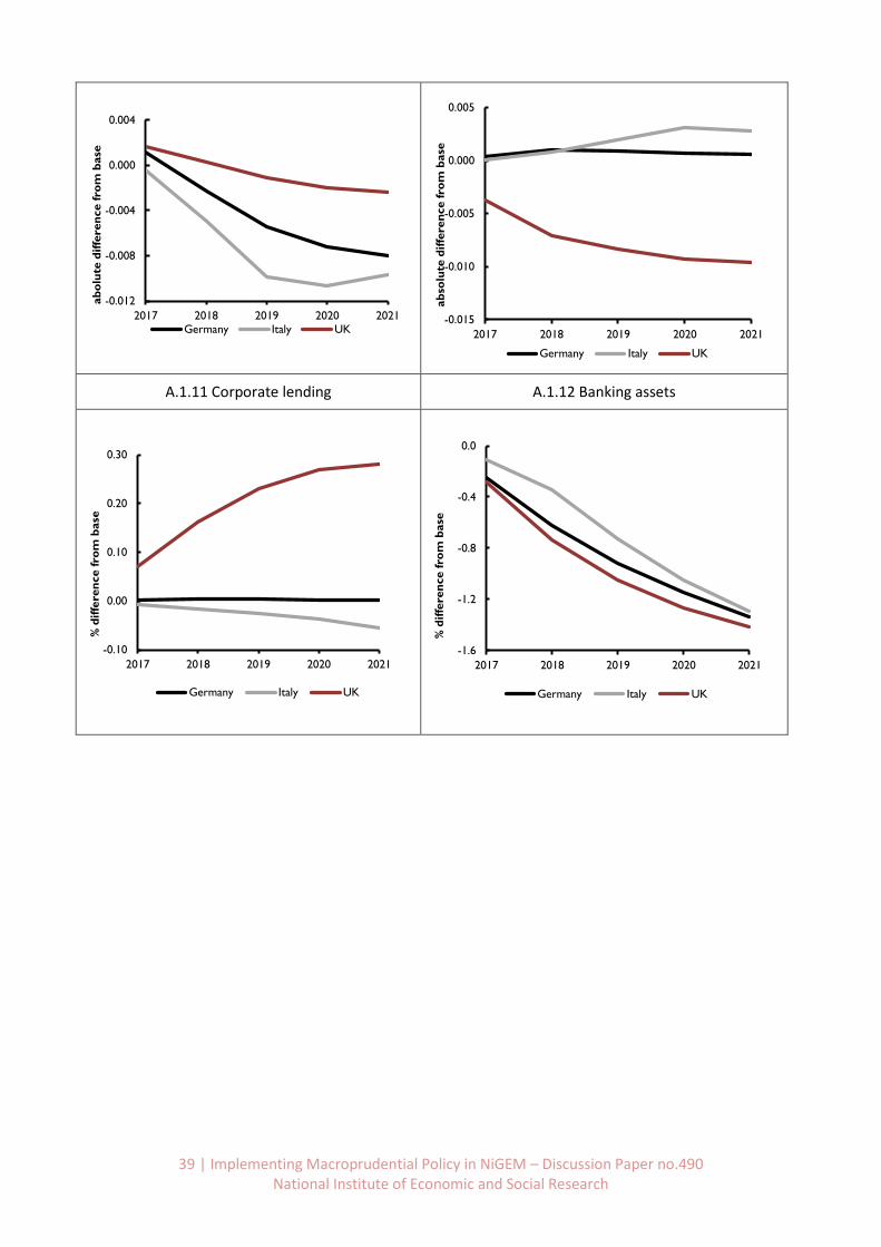
39 | Implementing Macroprudential Policy in NiGEM – Discussion Paper no.490 National Institute of Economic and Social Research
A.1.11 Corporate lending A.1.12 Banking assets
-0.012
-0.008
-0.004
0.000
0.004
2017 2018 2019 2020 2021
ab
olu
te d
iffe
ren
ce fro
m b
ase
Germany Italy UK-0.015
-0.010
-0.005
0.000
0.005
2017 2018 2019 2020 2021
ab
solu
te d
iffe
ren
ce fro
m b
ase
Germany Italy UK
-0.10
0.00
0.10
0.20
0.30
2017 2018 2019 2020 2021
% d
iffe
ren
ce f
rom
base
Germany Italy UK
-1.6
-1.2
-0.8
-0.4
0.0
2017 2018 2019 2020 2021
% d
iffe
ren
ce f
rom
base
Germany Italy UK
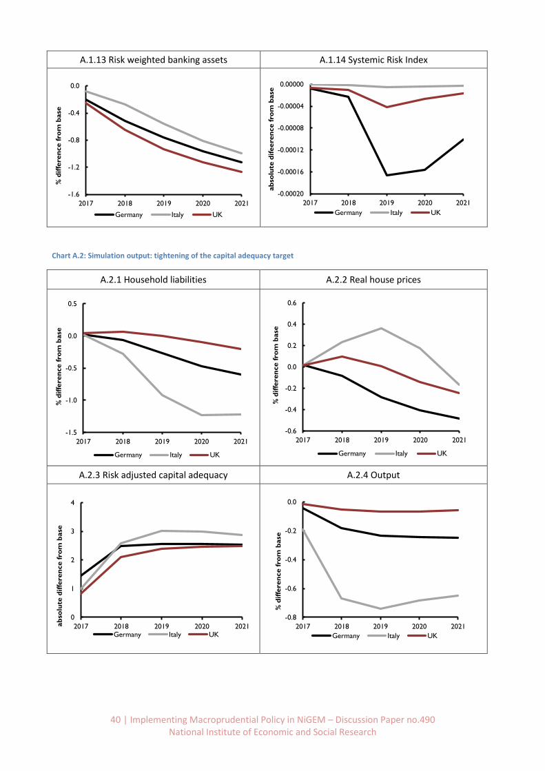
40 | Implementing Macroprudential Policy in NiGEM – Discussion Paper no.490 National Institute of Economic and Social Research
A.1.13 Risk weighted banking assets A.1.14 Systemic Risk Index
Chart A.2: Simulation output: tightening of the capital adequacy target
A.2.1 Household liabilities A.2.2 Real house prices
A.2.3 Risk adjusted capital adequacy A.2.4 Output
-1.6
-1.2
-0.8
-0.4
0.0
2017 2018 2019 2020 2021
% d
iffe
ren
ce f
rom
base
Germany Italy UK
-0.00020
-0.00016
-0.00012
-0.00008
-0.00004
0.00000
2017 2018 2019 2020 2021
ab
solu
te d
ifeere
nce fro
m b
ase
Germany Italy UK
-1.5
-1.0
-0.5
0.0
0.5
2017 2018 2019 2020 2021
% d
iffe
ren
ce f
rom
base
Germany Italy UK
-0.6
-0.4
-0.2
0.0
0.2
0.4
0.6
2017 2018 2019 2020 2021
% d
iffe
ren
ce f
rom
base
Germany Italy UK
0
1
2
3
4
2017 2018 2019 2020 2021ab
solu
te d
iffe
ren
ce fro
m b
ase
Germany Italy UK
-0.8
-0.6
-0.4
-0.2
0.0
2017 2018 2019 2020 2021
% d
iffe
ren
ce f
rom
base
Germany Italy UK
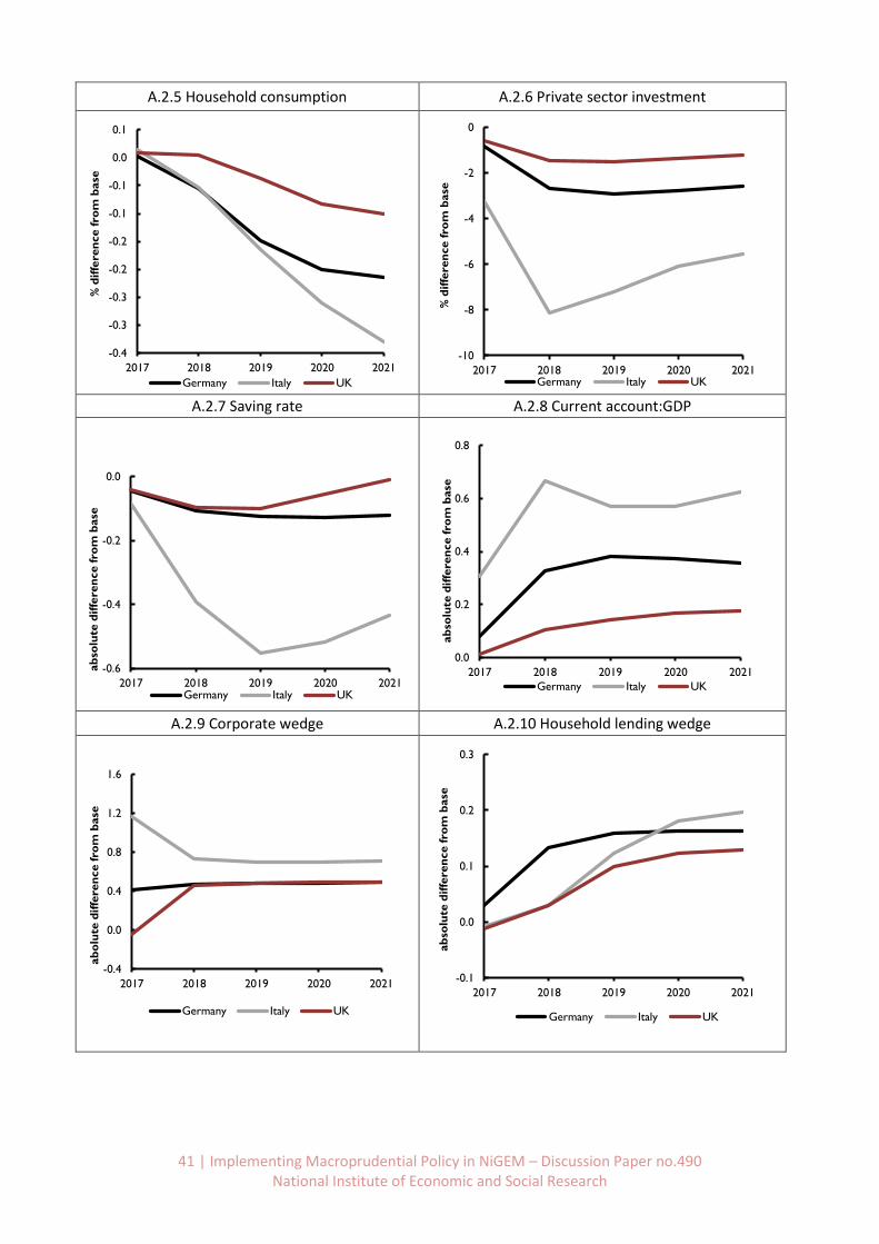
41 | Implementing Macroprudential Policy in NiGEM – Discussion Paper no.490 National Institute of Economic and Social Research
A.2.5 Household consumption A.2.6 Private sector investment
A.2.7 Saving rate A.2.8 Current account:GDP
A.2.9 Corporate wedge A.2.10 Household lending wedge
-0.4
-0.3
-0.3
-0.2
-0.2
-0.1
-0.1
0.0
0.1
2017 2018 2019 2020 2021
% d
iffe
ren
ce f
rom
base
Germany Italy UK
-10
-8
-6
-4
-2
0
2017 2018 2019 2020 2021
% d
iffe
ren
ce f
rom
base
Germany Italy UK
-0.6
-0.4
-0.2
0.0
2017 2018 2019 2020 2021
ab
solu
te d
iffe
ren
ce fro
m b
ase
Germany Italy UK
0.0
0.2
0.4
0.6
0.8
2017 2018 2019 2020 2021
ab
solu
te d
iffe
ren
ce fro
m b
ase
Germany Italy UK
-0.4
0.0
0.4
0.8
1.2
1.6
2017 2018 2019 2020 2021
ab
olu
te d
iffe
ren
ce fro
m b
ase
Germany Italy UK
-0.1
0.0
0.1
0.2
0.3
2017 2018 2019 2020 2021
ab
solu
te d
iffe
ren
ce fro
m b
ase
Germany Italy UK
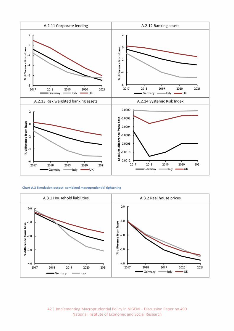
42 | Implementing Macroprudential Policy in NiGEM – Discussion Paper no.490 National Institute of Economic and Social Research
A.2.11 Corporate lending A.2.12 Banking assets
A.2.13 Risk weighted banking assets A.2.14 Systemic Risk Index
Chart A.3 Simulation output: combined macroprudential tightening
A.3.1 Household liabilities A.3.2 Real house prices
-8
-6
-4
-2
0
2
2017 2018 2019 2020 2021
% d
iffe
ren
ce f
rom
base
Germany Italy UK
-6
-4
-2
0
2
2017 2018 2019 2020 2021
% d
iffe
ren
ce f
rom
base
Germany Italy UK
-6
-4
-2
0
2
2017 2018 2019 2020 2021
% d
iffe
ren
ce f
rom
base
Germany Italy UK
-0.0012
-0.0010
-0.0008
-0.0006
-0.0004
-0.0002
0.0000
2017 2018 2019 2020 2021
ab
solu
te d
ifeere
nce fro
m b
ase
Germany Italy UK
-4.0
-3.0
-2.0
-1.0
0.0
2017 2018 2019 2020 2021
% d
iffe
ren
ce f
rom
base
Germany Italy
-4.0
-3.0
-2.0
-1.0
0.0
2017 2018 2019 2020 2021
% d
iffe
ren
ce f
rom
base
Germany Italy UK
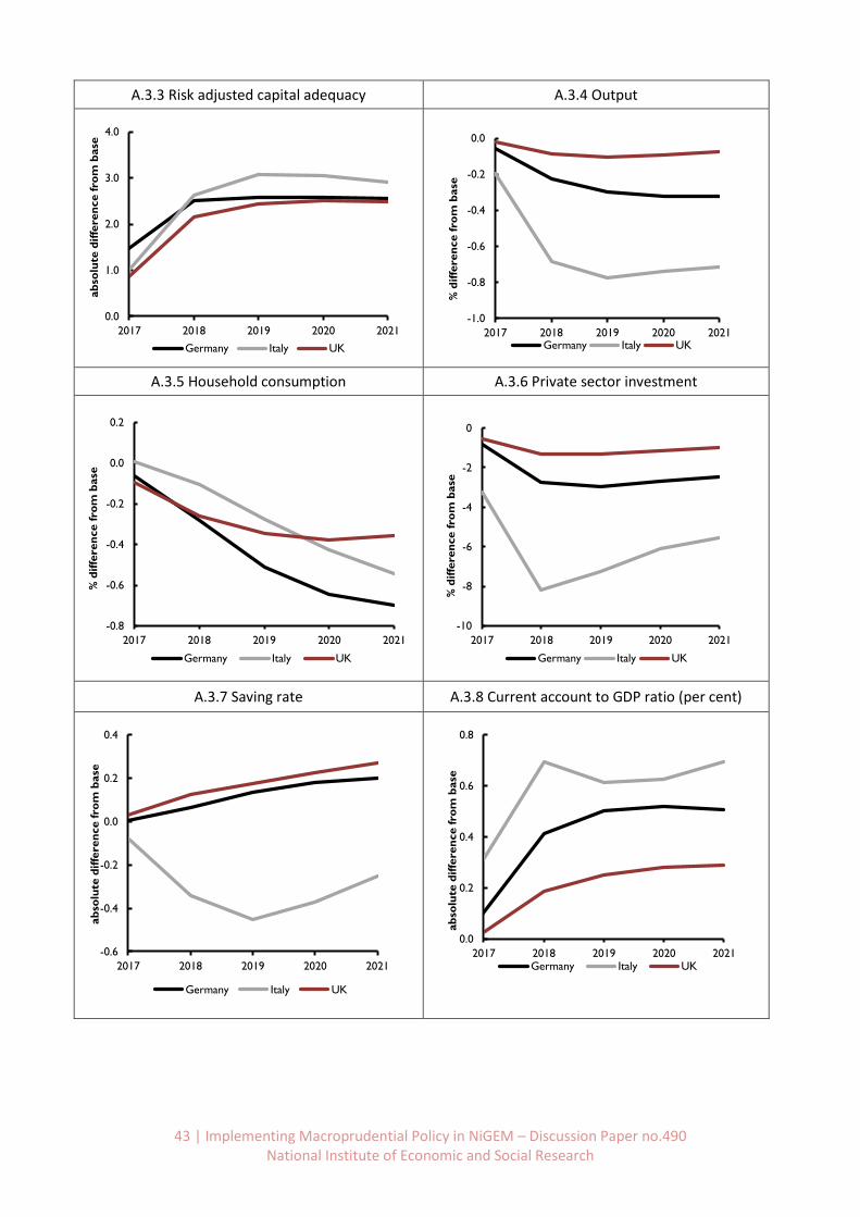
43 | Implementing Macroprudential Policy in NiGEM – Discussion Paper no.490 National Institute of Economic and Social Research
A.3.3 Risk adjusted capital adequacy A.3.4 Output
A.3.5 Household consumption A.3.6 Private sector investment
A.3.7 Saving rate A.3.8 Current account to GDP ratio (per cent)
0.0
1.0
2.0
3.0
4.0
2017 2018 2019 2020 2021
ab
solu
te d
iffe
ren
ce fro
m b
ase
Germany Italy UK
-1.0
-0.8
-0.6
-0.4
-0.2
0.0
2017 2018 2019 2020 2021
% d
iffe
ren
ce f
rom
base
Germany Italy UK
-0.8
-0.6
-0.4
-0.2
0.0
0.2
2017 2018 2019 2020 2021
% d
iffe
ren
ce f
rom
base
Germany Italy UK
-10
-8
-6
-4
-2
0
2017 2018 2019 2020 2021
% d
iffe
ren
ce f
rom
base
Germany Italy UK
-0.6
-0.4
-0.2
0.0
0.2
0.4
2017 2018 2019 2020 2021
ab
solu
te d
iffe
ren
ce fro
m b
ase
Germany Italy UK
0.0
0.2
0.4
0.6
0.8
2017 2018 2019 2020 2021
ab
solu
te d
iffe
ren
ce fro
m b
ase
Germany Italy UK
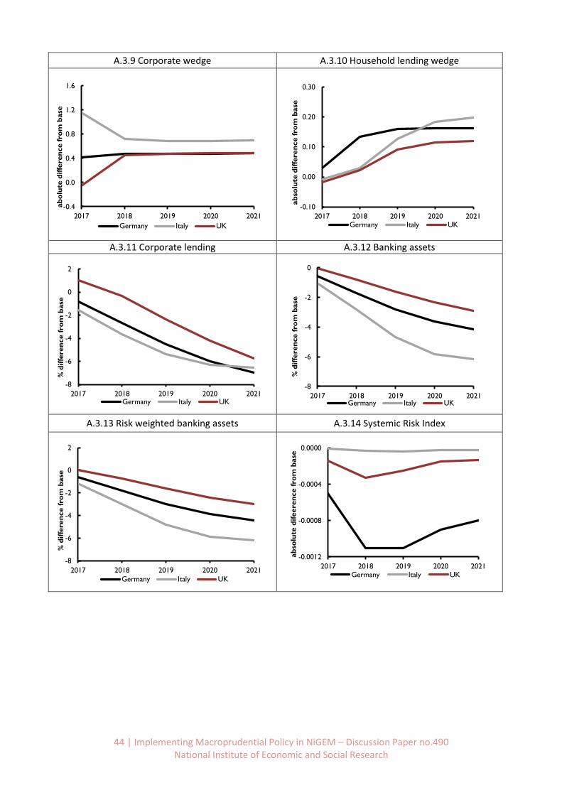
44 | Implementing Macroprudential Policy in NiGEM – Discussion Paper no.490 National Institute of Economic and Social Research
A.3.9 Corporate wedge A.3.10 Household lending wedge
A.3.11 Corporate lending A.3.12 Banking assets
A.3.13 Risk weighted banking assets A.3.14 Systemic Risk Index
-0.4
0.0
0.4
0.8
1.2
1.6
2017 2018 2019 2020 2021
ab
olu
te d
iffe
ren
ce fro
m b
ase
Germany Italy UK
-0.10
0.00
0.10
0.20
0.30
2017 2018 2019 2020 2021
ab
solu
te d
iffe
ren
ce fro
m b
ase
Germany Italy UK
-8
-6
-4
-2
0
2
2017 2018 2019 2020 2021
% d
iffe
ren
ce f
rom
base
Germany Italy UK
-8
-6
-4
-2
0
2017 2018 2019 2020 2021
% d
iffe
ren
ce f
rom
base
Germany Italy UK
-8
-6
-4
-2
0
2
2017 2018 2019 2020 2021
% d
iffe
ren
ce f
rom
base
Germany Italy UK
-0.0012
-0.0008
-0.0004
0.0000
2017 2018 2019 2020 2021
ab
solu
te d
ifeere
nce fro
m b
ase
Germany Italy UK
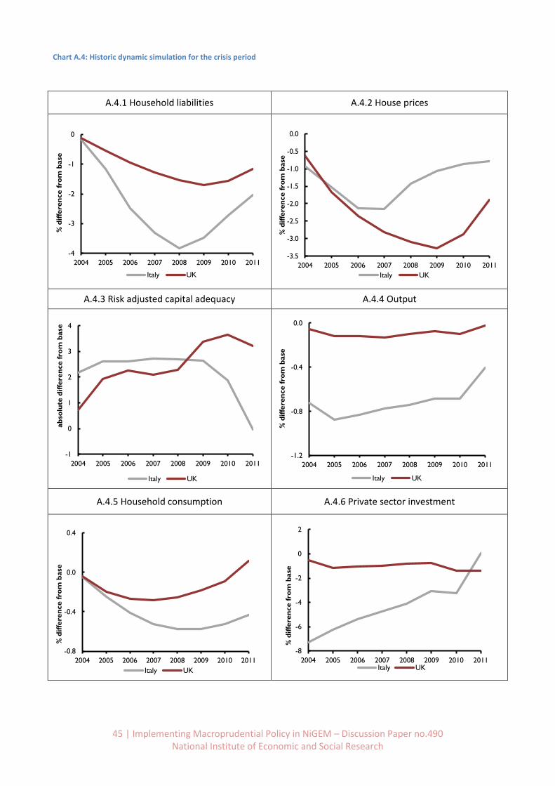
45 | Implementing Macroprudential Policy in NiGEM – Discussion Paper no.490 National Institute of Economic and Social Research
Chart A.4: Historic dynamic simulation for the crisis period
A.4.1 Household liabilities A.4.2 House prices
A.4.3 Risk adjusted capital adequacy A.4.4 Output
A.4.5 Household consumption A.4.6 Private sector investment
-4
-3
-2
-1
0
2004 2005 2006 2007 2008 2009 2010 2011
% d
iffe
ren
ce f
rom
base
Italy UK
-3.5
-3.0
-2.5
-2.0
-1.5
-1.0
-0.5
0.0
2004 2005 2006 2007 2008 2009 2010 2011
% d
iffe
ren
ce f
rom
base
Italy UK
-1
0
1
2
3
4
2004 2005 2006 2007 2008 2009 2010 2011
ab
solu
te d
iffe
ren
ce fro
m b
ase
Italy UK
-1.2
-0.8
-0.4
0.0
2004 2005 2006 2007 2008 2009 2010 2011
% d
iffe
ren
ce f
rom
base
Italy UK
-0.8
-0.4
0.0
0.4
2004 2005 2006 2007 2008 2009 2010 2011
% d
iffe
ren
ce f
rom
base
Italy UK
-8
-6
-4
-2
0
2
2004 2005 2006 2007 2008 2009 2010 2011
% d
iffe
ren
ce f
rom
base
Italy UK
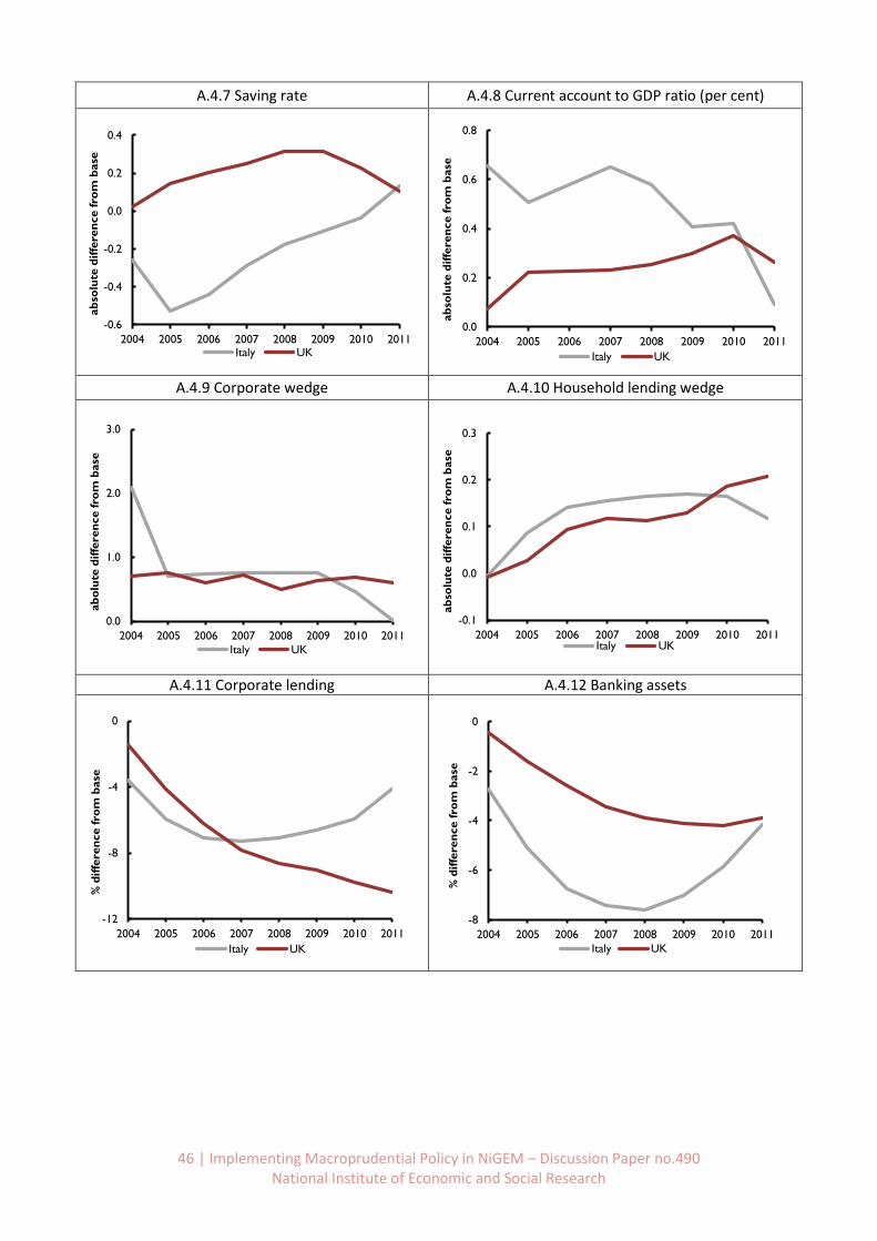
46 | Implementing Macroprudential Policy in NiGEM – Discussion Paper no.490 National Institute of Economic and Social Research
A.4.7 Saving rate A.4.8 Current account to GDP ratio (per cent)
A.4.9 Corporate wedge A.4.10 Household lending wedge
A.4.11 Corporate lending A.4.12 Banking assets
-0.6
-0.4
-0.2
0.0
0.2
0.4
2004 2005 2006 2007 2008 2009 2010 2011
ab
solu
te d
iffe
ren
ce fro
m b
ase
Italy UK
0.0
0.2
0.4
0.6
0.8
2004 2005 2006 2007 2008 2009 2010 2011
ab
solu
te d
iffe
ren
ce fro
m b
ase
Italy UK
0.0
1.0
2.0
3.0
2004 2005 2006 2007 2008 2009 2010 2011
ab
olu
te d
iffe
ren
ce fro
m b
ase
Italy UK
-0.1
0.0
0.1
0.2
0.3
2004 2005 2006 2007 2008 2009 2010 2011
ab
solu
te d
iffe
ren
ce fro
m b
ase
Italy UK
-12
-8
-4
0
2004 2005 2006 2007 2008 2009 2010 2011
% d
iffe
ren
ce f
rom
base
Italy UK
-8
-6
-4
-2
0
2004 2005 2006 2007 2008 2009 2010 2011
% d
iffe
ren
ce f
rom
base
Italy UK
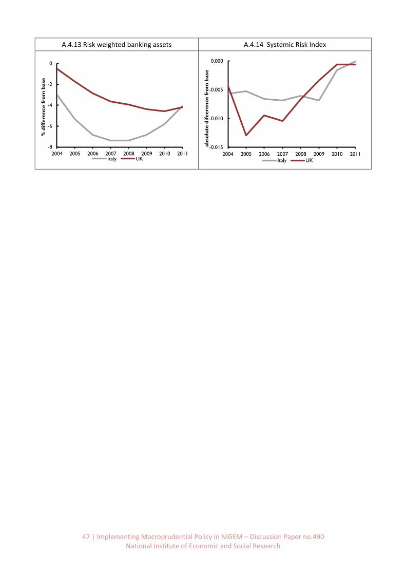
47 | Implementing Macroprudential Policy in NiGEM – Discussion Paper no.490 National Institute of Economic and Social Research
A.4.13 Risk weighted banking assets A.4.14 Systemic Risk Index
-8
-6
-4
-2
0
2004 2005 2006 2007 2008 2009 2010 2011
% d
iffe
ren
ce f
rom
base
Italy UK
-0.015
-0.010
-0.005
0.000
2004 2005 2006 2007 2008 2009 2010 2011
ab
solu
te d
ifeere
nce fro
m b
ase
Italy UK
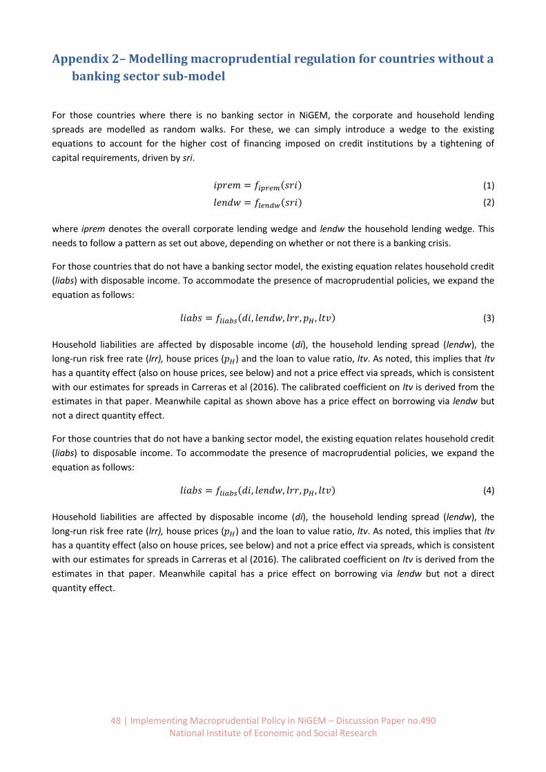
48 | Implementing Macroprudential Policy in NiGEM – Discussion Paper no.490 National Institute of Economic and Social Research
Appendix 2– Modelling macroprudential regulation for countries without a
banking sector sub-model
For those countries where there is no banking sector in NiGEM, the corporate and household lending
spreads are modelled as random walks. For these, we can simply introduce a wedge to the existing
equations to account for the higher cost of financing imposed on credit institutions by a tightening of
capital requirements, driven by sri.
𝑖𝑝𝑟𝑒𝑚 = 𝑓𝑖𝑝𝑟𝑒𝑚(𝑠𝑟𝑖) (1)
𝑙𝑒𝑛𝑑𝑤 = 𝑓𝑙𝑒𝑛𝑑𝑤(𝑠𝑟𝑖) (2)
where iprem denotes the overall corporate lending wedge and lendw the household lending wedge. This
needs to follow a pattern as set out above, depending on whether or not there is a banking crisis.
For those countries that do not have a banking sector model, the existing equation relates household credit
(liabs) with disposable income. To accommodate the presence of macroprudential policies, we expand the
equation as follows:
𝑙𝑖𝑎𝑏𝑠 = 𝑓𝑙𝑖𝑎𝑏𝑠(𝑑𝑖, 𝑙𝑒𝑛𝑑𝑤, 𝑙𝑟𝑟, 𝑝𝐻 , 𝑙𝑡𝑣) (3)
Household liabilities are affected by disposable income (di), the household lending spread (lendw), the
long-run risk free rate (lrr), house prices (𝑝𝐻) and the loan to value ratio, ltv. As noted, this implies that ltv
has a quantity effect (also on house prices, see below) and not a price effect via spreads, which is consistent
with our estimates for spreads in Carreras et al (2016). The calibrated coefficient on ltv is derived from the
estimates in that paper. Meanwhile capital as shown above has a price effect on borrowing via lendw but
not a direct quantity effect.
For those countries that do not have a banking sector model, the existing equation relates household credit
(liabs) to disposable income. To accommodate the presence of macroprudential policies, we expand the
equation as follows:
𝑙𝑖𝑎𝑏𝑠 = 𝑓𝑙𝑖𝑎𝑏𝑠(𝑑𝑖, 𝑙𝑒𝑛𝑑𝑤, 𝑙𝑟𝑟, 𝑝𝐻 , 𝑙𝑡𝑣) (4)
Household liabilities are affected by disposable income (di), the household lending spread (lendw), the
long-run risk free rate (lrr), house prices (𝑝𝐻) and the loan to value ratio, ltv. As noted, this implies that ltv
has a quantity effect (also on house prices, see below) and not a price effect via spreads, which is consistent
with our estimates for spreads in Carreras et al (2016). The calibrated coefficient on ltv is derived from the
estimates in that paper. Meanwhile capital has a price effect on borrowing via lendw but not a direct
quantity effect.

49 | Implementing Macroprudential Policy in NiGEM – Discussion Paper no.490 National Institute of Economic and Social Research
Appendix 3 – Data list
Variable names Definitions
ARR Rate of household mortgage arrears
BBAL Banking sector assets (total)
BBSOA Banking sector other assets
BCAP Banking sector capital
BRA Banking sector liquid assets
BRWA Risk-weighted banking assets
C Consumption
CBR Current account to GDP ratio
CC Consumer credit held by households
CCRATE Household unsecured borrowing rate
CED Consumer expenditure deflator
CORPL Non-financial corporate debt
CORPW Non-financial corporate sector lending wedge
HW Value of personal sector housing stock (FOF)
INSOLR Rate of company liquidations
IPREM Investment premium
KH Capital stock (housing)
LENDW Rate Spread - household (borrowing - lending)
LEVRR Risk-weighted capital to asset ratio
LEVRRT Risk-weighted capital to asset ratio target
LIABS Household liabilities (total)
LRR Long real rates
LTV Loan-to-value ratio
MORTH Mortgage debt of households
NW Net wealth, personal sector

50 | Implementing Macroprudential Policy in NiGEM – Discussion Paper no.490 National Institute of Economic and Social Research
NWPI Net wealth to personal income ratio
PI Personal income
R3M 3 month interest rates
RHPG Change in real house prices
RMORT Average offered mortgage rate
RPDI Real personal disposable income
SRI Sytemic risk index
Y Real gross domestic product
YCAP Trend output for capacity utilisation