Embed Size (px)
Citation preview

Code Generation and Optimisation
Haskell for Compiler Writers
Implementing compilers
There are two basic requirements of any compiler implementation:
1. To represent the source / target program in a data structure, usually referred to as an abstract syntax tree.
2. To traverse the abstract syntax tree, extracting information and transforming it from one form to another.
Why Haskell?
Haskell has two main features which make it good for writing compilers.
1. Algebraic data types allow an abstract syntax tree to be easily constructed.
2. Pattern matching makes it easy to define functions that traverse an abstract syntax tree.
This lecture
How to:
define abstract syntax
transform abstract syntax trees
using Haskell.
Aim: to appreciate features of Haskell that make it good for implementing compilers.

FUNCTIONS AND APPLICATIONS
Principles of Haskell
Functions
The factorial function in Haskell:
fact :: Int -> Int
Type signature
“is of type”
Function names begin with a lower-case letter.
fact(n) = if n == 1 then 1 else n * fact(n-1)
Equation
Application and reduction
A function applied to an input is called an application, e.g.
An application reduces to the right-hand-side of the first matching equation.
fact(3)
if 3 == 1 then 1 else 3 * fact(3-1)
fact(3) ⇒
“reduces to”
Evaluation
fact(3) ⇒ if 3 == 1 then 1 else 3 * fact(3-1) ⇒ if False then 1 else 3 * fact(3-1) ⇒ 3 * fact(3-1) ⇒ 3 * fact(2) ⇒ ... ⇒ 6
Expressions are evaluated by repeatedly reducing applications.
6 fact(3) ⇒*
“evaluates to”

LISTS AND TUPLES
Commonly used data types
Lists
The empty list is written []
The list with head h and tail t is written h:t
[5,6,7] ≡ 5:6:7:[]
[1] ≡ 1:[]
['x', 'y'] ≡ 'x' : ('y':[])
“cons” “the list containing 1”
The type of a list
The type of a list of elements of type a is written [a].
If x:xs is of type [a]
then x must have type a
and xs must have type [a].
For example, the list ['a', 'b'] is a value of type [Char].
Sum
A function to sum the elements of a list:
sum :: [Int] -> Int
sum([]) = 0 sum(x:xs) = x + sum(xs)
Two equations
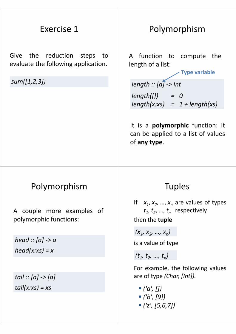
Exercise 1
Give the reduction steps to evaluate the following application.
sum([1,2,3])
Polymorphism
A function to compute the length of a list:
length :: [a] -> Int
length([]) = 0 length(x:xs) = 1 + length(xs)
It is a polymorphic function: it can be applied to a list of values of any type.
Type variable
Polymorphism
A couple more examples of polymorphic functions:
head :: [a] -> a
head(x:xs) = x
tail :: [a] -> [a]
tail(x:xs) = xs
Tuples
If x1, x2, …, xn are values of types t1, t2, …, tn respectively
then the tuple
is a value of type
For example, the following values are of type (Char, [Int]).
(x1, x2, …, xn)
(t1, t2, …, tn)
('a', []) ('b', [9]) ('z', [5,6,7])

Multiple inputs
min :: (Int, Int) -> Int
min(x, y) = if x < y then x else y
Tuples can be used to pass multiple inputs to a function.
min(5, 10) 5 ⇒*
For example:
Exercise 2
Define a function
append :: ([a], [a]) -> [a]
append([1,4,2], [3,4])
that joins two lists into a single list, e.g.
[1,4,2,3,4]
⇒*
Homework Exercise
Define a function
first :: (Int, [a]) -> [a]
such that first(n, xs) returns the first n elements of the list xs, e.g.
first(2, [9,8,3,5]) ⇒* [9,8]
first(4, [3,5]) ⇒* [3,5]
Infix operators
Infix operators can be defined for functions of two arguments. For example, the definition
allows ++ to be used as follows.
xs ++ ys = append(xs, ys)
[1,2] ++ [3] ++ [4,5,6]
[1,2,3,4,5,6]
⇒*

Precedence and associativity
Any Haskell operator can be given a precedence (from 0 to 9) and left, right, or non-associativity.
For example, we can write:
infixl 6 – infixr 7 *
So x–y–z is interpreted as (x–y)–z.
And x–y*z is interpreted as x–(y*z).
Exercise 3
Why make ++ right-associative?
infixr 5 ++
In Haskell, we have:
USER-DEFINED TYPES
Type synonyms and algebraic data types
Type synonyms
Type synonyms allow a new (more meaningful) name to be given to an existing type, e.g.
The new type String is entirely
equivalent to [Char]. In Haskell:
type String = [Char]
New name Existing type
['h', 'i', '!'] ≡ "hi!"

Algebraic data types
A data definition introduces a new type, and a set of constructors that can be used to create values of that type.
Type and constructor names begin with an upper-case letter.
data Bool = True | False
data Colour = Red | Green | Blue
Data type Data constructors
Pattern matching
Examples of functions involving Bool and Colour:
not :: Bool -> Bool
not(False) = True not(True) = False
isRed :: Colour -> Bool
isRed(Red) = True isRed(x) = False
Shapes
A data constructor may have associated components, e.g.
data Shape = Circ(Float) | Rect(Float, Float)
Circ(10.5)
Rect(10.2, 20.9)
Example values of type Shape:
Component values (width & height)
Component value (radius)
Area
A function to compute the area of any given shape.
area :: Shape -> Float
area(Rect(w, h)) = w * h area(Circ(r)) = pi * r * r
(Compare with C code for same task in LSA Chapter 2.)

CASE STUDY
A simplifier for arithmetic expressions.
Concrete syntax
Here is a concrete syntax for arithmetic expressions.
v = [a-z]+
n = [0-9]+
e → v | n | e + e | e * e | ( e )
Example expression:
x * y + (z* 10)
Simplification
Consider the algebraic law:
∀e. e * 1 = e
Example simplification:
x * (y * 1) → x * y
This law can be used to simplify expressions by using it as a rewrite rule from left to right.
Problem
1. Define an abstract syntax, in Haskell, for arithmetic.
2. Implement the simplification rule as a Haskell function over abstract syntax trees.

Abstract syntax
data Op = Add | Mul data Expr = Num(Int) | Var(String) | Apply(Expr, Op, Expr)
An op is an addition or a multiplication
An expression is a number, or a variable, or an application of an op to two sub-expressions
Abstract syntax trees
Apply( Var("x") , Add , Apply( Var("y") , Mul , Num(2)))
An abstract syntax tree that represents the expression
x + (y * 2)
is represented by the following Haskell expression
Abstract syntax trees
We can view constructors as nodes of a tree and the constructor components as sub-trees. For example:
App
Var
Var
2
'x'
App
Num Mul
Add
'y'
Simplification
simplify :: Expr -> Expr
simplify(Apply(e, Mul, Num(1))) = simplify(e)
simplify(Apply(e1, op, e2)) = Apply(simplify(e1), op, simplify(e2))
simplify(e) = e
e * 1 → e
is implemented by

Homework exercise
What is result if the simplifier is given the following input?
1*(1*1)
Is it correct? If not, can you fix it?
(Source code for the simplifier available on the CGO web page.)
Homework exercise
Extend the simplifier to exploit the following algebraic law.
∀e. e * 0 = 0
“SYNTACTIC SUGAR”
Convenient features of Haskell.
Guards
Equations may contain boolean conditions called guards.
The chosen equation is the first
one whose guard succeeds. The keyword otherwise is equivalent to True.
fib :: Int -> Int fib(n) | n == 0 = 0 | n == 1 = 1 | otherwise = fib(n-1) + fib(n-2)
Guards

Case expressions
Using a case expression, pattern matching can be expressed on the RHS of an equation, e.g.
isEmpty :: [a] -> Bool isEmpty([]) = True isEmpty(x:xs) = False
isEmpty :: [a] -> Bool isEmpty(xs) = case xs of [] -> True x:xs -> False
≡
List enumerations
A list of values can be created using an enumeration, e.g.
The start and end of the range need not be literals, e.g.
A step can be specified by giving the first two values, e.g.
[1..5] ⇒* [1, 2, 3, 4, 5]
[length([1,2])..fact(3)] ⇒* [2,3,4,5,6]
[0,2..10] ⇒* [0, 2, 4, 6, 8, 10]
List comprehensions
Recall from MCS, we can write
{ n | n ∊ {1..10} ∧ odd(n) }
to denote the set of odd numbers between 1 and 10. Similarly, in Haskell we can write
[n | n <- [1..10], odd(n) ]
“drawn from” Filter
Example
The function
increments each element of a given list. For example
evaluates to [2,3,4].
inc :: [Int] -> [Int] inc(xs) = [x+1 | x <- xs]
inc([1, 2, 3])

Exercise 4
Define a function omit
such that omit(x, ys) returns ys omitting all occurrences of x. For example,
omit :: (Int, [Int]) -> [Int]
omit(1, [1, 2, 1, 3])
should evaluate to [2,3].
Homework Exercise
Define a function unique
such that unique(xs) returns xs omitting duplicates.
For example,
unique :: [Int] -> [Int]
unique([1, 2, 1, 3, 1, 3])
should evaluate to [1,2,3]. (Order doesn’t matter.)
TYPE CLASSES
Making types more general
Type classes
We have seen that == can compare values of type Int.
But what if we want to compare values of type Char, Colour, or [Bool] using the == operator?
'x' == 'y'
Red == Green
[True, False] == [True]
Type classes let us do this.

Type classes
A type class is a set of types providing a common set of functions.
Example: Eq is a type class providing functions == and /=.
Members of the Eq class include Int and Char, e.g.
1 == 2 ⇒ False
'x' == 'x' ⇒ True
Deriving classes
One way to make an algebraic data type, such as Colour, a member of Eq class is to write:
This gives == the “obvious”
meaning on values of type Colour. For example:
data Colour = Red | Green | Blue deriving Eq
Red == Red ⇒ True
Red == Green ⇒ False
Class constraints
Class constraints may appear in type signatures of polymorphic functions. For example:
The constraint states that type t
must be in the Eq class. This is because values of type t are compared using == in the body of the function.
member :: Eq t => (t, [t]) -> Bool member(x, []) = False member(x, y:ys) = x == y || member(x, ys)
Other standard classes
Besides the Eq class, there are the Num, Ord and Show classes.
To illustrate:
Class Functions
Eq ==, /=
Num +, -, *
Ord <=, <, >, >=
Show show
'a' <= 'b' ⇒ True
show(Red) ⇒ "Red"
show([1,2,3]) ⇒ "[1, 2, 3]"

Local definitions
Definitions local to a particular equation can be defined using a where clause. To illustrate, here is QuickSort in Haskell.
sort :: Ord a => [a] -> [a] sort([]) = [] sort(pivot:xs) = sort(smaller) ++ [pivot] ++ sort(greater) where smaller = [x | x <- xs, x <= pivot] greater = [x | x <- xs, x > pivot]
HIGHER-ORDER FUNCTIONS AND CURRYING
Two Haskell features NOT used in CGO
Higher-order functions
Functions can take functions as inputs and return functions as results. These are called higher-order functions.
To illustrate, each(f, xs) applies f to each element in the list xs.
each :: (a -> b, [a]) -> [b] each(f, []) = [] each(f, x:xs) = f(x) : each(f, xs)
each(not, [False, True]) ⇒* [True, False]
Currying
A function of 2 arguments can be implemented as a function that returns a function e.g.
or more simply:
The same idea works for functions of n > 2 arguments.
add :: Int -> (Int -> Int) add(x) = f where f(y) = x+y
add :: Int -> Int -> Int add x y = x + y
add(1)(2) ⇒ 3
add 1 2 ⇒ 3

CGO notes, questions, and practicals will assume no knowledge of higher order functions and currying.
But if you are comfortable with these features, feel free to use them in your answers.
FINITE MAPS
A simple but very useful data structure
Finite Map
A finite map of type
is a data structure that maps values of type a (domain) to values of type b (range).
It can be represented as a list of (a, b) pairs.
type Map a b = [(a, b)]
Map a b
Keys and Values
goals :: Map String Int goals = [ ("Charlton", 49) , ("Owen", 40) , ("Lineker", 48) ]
“Key” “Value”
key :: (a, b) -> a key(k, v) = k
value :: (a, b) -> b value(k, v) = v

Fetch
A common operation is to fetch the value associated with a given key.
fetch :: Eq a => (Map a b, a) -> b fetch(p:ps, k) | key(p) == k = value(p) | otherwise = fetch(ps, k)
fetch(goals, "Owen") ⇒* 40
For example:
Fetch operator
We will use the symbol ! as an infix operator for fetch:
For example:
m ! k = fetch(m, k)
goals ! "Owen" ⇒* 40
Exercise 5
Define a function to insert a given key/value pair into a map. For example,
insert(goals, “Owen", 41)
[ ("Charlton", 49), ("Owen", 41), ("Lineker", 48) ]
should return the following map.
Modified to 41
Summary
Algebraic data types and functions defined by pattern matching are the core features.
Other features such as
– infix operators
– list comprehensions
– type classes
are nice but not as important.
Powerful data structures such as finite maps are easily defined.
These ingredients will let us write concise compilers!
![INDEX [] · 3 Compiler construction tools 4 Cousins of the compiler 5 Compilers in programming languages Review Questions Q1 What is Compiler? CO308.1 Q2](https://img.pdfslide.us/doc/110x75/5af634e57f8b9a74448f36ac/index-compiler-construction-tools-4-cousins-of-the-compiler-5-compilers-in-programming.jpg)