Embed Size (px)
Citation preview

Implementing a Process Scheduler UsingNeural Network Technology
Master’s thesis
Author : Peter Bex ([email protected])Student nr. : 0115460
AI Supervisor : Louis Vuurpijl ([email protected])External supervisors : Erik Poll ([email protected])
Theo Schouten ([email protected])

Abstract
This Master’s thesis describes the design, implementation and evaluation of aneural network in an operating system kernel to classify processes based ontheir behaviour and assign scheduling priorities accordingly. The design of thesystem allows easy addition of features, making it an excellent platform for rapidprototyping of new scheduler features without requiring a rewrite or substantialmodification of an existing scheduler.


Contents
1 Introduction 3
1.1 Motivation . . . . . . . . . . . . . . . . . . . . . . . . . . . . . . 41.1.1 Increasing performance . . . . . . . . . . . . . . . . . . . 41.1.2 Increasing user-friendliness . . . . . . . . . . . . . . . . . 41.1.3 Maximizing customizability . . . . . . . . . . . . . . . . . 5
1.2 Outline of thesis . . . . . . . . . . . . . . . . . . . . . . . . . . . 5
2 Process scheduling 6
2.1 Introduction . . . . . . . . . . . . . . . . . . . . . . . . . . . . . . 62.2 Job-shop scheduling . . . . . . . . . . . . . . . . . . . . . . . . . 62.3 Preemptive scheduling . . . . . . . . . . . . . . . . . . . . . . . . 72.4 Multithreading . . . . . . . . . . . . . . . . . . . . . . . . . . . . 82.5 Multiple CPUs . . . . . . . . . . . . . . . . . . . . . . . . . . . . 92.6 Existing research . . . . . . . . . . . . . . . . . . . . . . . . . . . 9
3 AI techniques 11
3.1 Genetic algorithms . . . . . . . . . . . . . . . . . . . . . . . . . . 113.2 Decision tree learning . . . . . . . . . . . . . . . . . . . . . . . . 123.3 Rule-based knowledge system . . . . . . . . . . . . . . . . . . . . 123.4 Bayesian networks . . . . . . . . . . . . . . . . . . . . . . . . . . 133.5 Neural Networks . . . . . . . . . . . . . . . . . . . . . . . . . . . 133.6 Existing research . . . . . . . . . . . . . . . . . . . . . . . . . . . 14
4 System overview 15
4.1 Requirements of the network . . . . . . . . . . . . . . . . . . . . 154.1.1 The problem of representing time . . . . . . . . . . . . . . 164.1.2 The solution . . . . . . . . . . . . . . . . . . . . . . . . . 16
4.2 Infrastructural changes . . . . . . . . . . . . . . . . . . . . . . . . 184.3 Pre-existing priorities . . . . . . . . . . . . . . . . . . . . . . . . 19
5 Implementation details 20
5.1 The system . . . . . . . . . . . . . . . . . . . . . . . . . . . . . . 205.2 Typical usage . . . . . . . . . . . . . . . . . . . . . . . . . . . . . 205.3 Shared code . . . . . . . . . . . . . . . . . . . . . . . . . . . . . . 215.4 Kernel level implementation . . . . . . . . . . . . . . . . . . . . . 22
5.4.1 Pseudo-devices . . . . . . . . . . . . . . . . . . . . . . . . 235.4.2 Scheduler and feature collection . . . . . . . . . . . . . . . 23
5.5 User level implementation . . . . . . . . . . . . . . . . . . . . . . 24
1

2 CONTENTS
5.5.1 Tools for interacting with the kernel . . . . . . . . . . . . 245.5.2 Training tools . . . . . . . . . . . . . . . . . . . . . . . . . 245.5.3 Miscellaneous tools . . . . . . . . . . . . . . . . . . . . . . 24
5.6 Implementation issues . . . . . . . . . . . . . . . . . . . . . . . . 255.6.1 Floating point . . . . . . . . . . . . . . . . . . . . . . . . 255.6.2 Range and precision problems . . . . . . . . . . . . . . . . 265.6.3 No audio mixing . . . . . . . . . . . . . . . . . . . . . . . 265.6.4 The X Window System . . . . . . . . . . . . . . . . . . . 27
6 Results 28
6.1 Features . . . . . . . . . . . . . . . . . . . . . . . . . . . . . . . . 286.2 Network accuracy . . . . . . . . . . . . . . . . . . . . . . . . . . . 296.3 Influence of the memory layer . . . . . . . . . . . . . . . . . . . . 326.4 Overhead . . . . . . . . . . . . . . . . . . . . . . . . . . . . . . . 32
6.4.1 Feature gathering overhead . . . . . . . . . . . . . . . . . 336.5 Perceived speed . . . . . . . . . . . . . . . . . . . . . . . . . . . . 346.6 Assessment of features . . . . . . . . . . . . . . . . . . . . . . . . 37
6.6.1 Sockets . . . . . . . . . . . . . . . . . . . . . . . . . . . . 376.6.2 Audio . . . . . . . . . . . . . . . . . . . . . . . . . . . . . 396.6.3 Terminal . . . . . . . . . . . . . . . . . . . . . . . . . . . 396.6.4 Filesystem . . . . . . . . . . . . . . . . . . . . . . . . . . . 416.6.5 Application classification . . . . . . . . . . . . . . . . . . 45
7 Conclusion and future work 47
7.1 Personal notes . . . . . . . . . . . . . . . . . . . . . . . . . . . . 49
A Correction of the Turing-completeness proof for NNs 51
A.1 Background . . . . . . . . . . . . . . . . . . . . . . . . . . . . . . 51A.2 Proof . . . . . . . . . . . . . . . . . . . . . . . . . . . . . . . . . . 53

Chapter 1
Introduction
Contemporary OSes (operating systems) use exceedingly complex process schedul-ing strategies (see chapter 2 for more information about OS scheduling) to han-dle scheduling on multiple CPUs, but when it comes to uniprocessor schedulingthere has not been much new development. Current scheduling algorithms arenot very suitable for modern multimedia applications ([33]) because these algo-rithms do not take into account the multimedia aspects of these applications.Traditional schedulers were designed for large multi-user systems and aimed atimproving total throughput of the system, being fair to all users. Multimediaapplications represent the opposite of this model; they need all the system’sresources to generate smooth video or audio playback. Only when the system isfast enough to deliver all the resources the application needs can other applica-tions be scheduled without resulting in a stutter in the multimedia application.
Application scheduling priorities are calculated based on simple heuristicsthat can improve throughput. For example, a priority could be boosted whena process is newly entered into the ready queue or lowered when a process isforcedly removed from the CPU because it exceeded its allotted time quantum.However, the base priority of a program must still be defined by the user ifit should be something else than the default. It is tedious to do this for ev-ery program, and casual users often do not even know this functionality exists.Ideally, the computer should determine the priority automatically. This is avery hard problem to solve in a generic way, because different users have dif-ferent needs. On a web server one would assign the highest priority to batchprocessing-like functionality (disk/database access and network usage), whileon a personal multimedia computer, batch processing would have the lowestpriority and interactive processes would have a higher priority (audio and videooutput mostly, but also CPU usage for decoding of audio, for example). Thisproblem could be solved by creating operating systems (or schedulers) tuned fora specific usage scenario, but that would sacrifice generality. Most, if not all,of today’s operating systems are designed to be general-purpose, thus a genericsolution would be preferred.
This master thesis proposes to use the Artificial Intelligence technique ofneural networks to create a solution to the problem described above. Thus,this thesis strives to find an answer to the following question: How could neuralnetworks be used to schedule processes in an operating system? To answer thisquestion, a proof-of-concept implementation was created by patching an existing
3

4 1.1. MOTIVATION
operating system kernel’s scheduler such that it delegated its scheduling deci-sions to a neural network. One of the advantages of using neural networks isthat they can be trained for specific use cases by experts and advanced users andthen re-used by less technically inclined users without requiring any knowledgeabout neural networks or schedulers. The particular neural network used hereis a backpropagation network with an added memory layer, but in future re-search different network topologies may be explored. Features that are used forinput to the neural network ideally include everything that a human would useto determine whether a process is “multimedia”, but the features used in thisimplementation are based on audio, disk, terminal and socket I/O. Other typi-cal “multimedia features” would be harder to obtain under Unix-like operatingsystems, as discussed in section 5.6.
1.1 Motivation
1.1.1 Increasing performance
Operating systems still perform rather poorly when running multimedia ap-plications. This is partly canceled by the ever increasing speed of computersystems, but applications also continue to demand more from computer sys-tems. In fact, OS performance does not increase at the same speed as hardwaredoes, as indicated by [35] and [41], for example.
The fact that there are specialized workshops for improving multimedia sup-port in OSes, like NOSSDAV1 and ESTIMedia2, indicates that there is certainlya demand for better handling of multimedia in operating systems.
1.1.2 Increasing user-friendliness
A large percentage of computer users are nontechnical and simply want to gettheir work done. These users do not have the time or inclination to find out howto tweak their computer for optimal performance. For this reason, operatingsystems should be designed in such a way that at least their default settingswill provide optimal performance to this kind of user.
On many operating systems, all processes have the same default base priority.This priority does not normally change unless the user explicitly indicates itshould be different from the default. Because typically only so-called “power-users” know about the existence of this functionality, the average user’s systemwill not have the perceived performance it could have if the process prioritieswere optimally assigned.
A neural network scheduler can take care of assigning priority to processesfor the user in the background, without requiring any interaction. This willcreate the opportunity for average computer users to enjoy the same perceivedperformance from their system as power users do. The only thing that is requiredis that a technical user at one time creates and tunes a neural network for theusage pattern of the particular type of user, be it desktop user, server user oranything in between. After that, the user can simply select the network labeled,
1International Workshop on Network and Operating System Support for Digital Audio andVideo, see http://www.nossdav.org.
2Workshop on Embedded Systems for Real-Time Multimedia, seehttp://www.codes-isss.org/.

CHAPTER 1. INTRODUCTION 5
for example, “multimedia desktop” and run the system in the configuration thatis optimal for them.
1.1.3 Maximizing customizability
Each user has their own individual needs. Some users might only use an oper-ating system to run a spreadsheet program, some users might use it for playingcomputer games and even others might run a personal web server. The processprofiles of these uses are very different. In order to cater to all these users’ needs,an operating system needs to be versatile and customizable. Focusing purely onthe requirements of multimedia applications would decrease the generality of thesystem, since this would necessarily mean that the system would be less thanoptimal in non-multimedia environments where throughput is more importantthan interactive responsiveness, for example web servers or batch computationsystems. In order to maintain generality, the system needs to be customizablefor all use scenarios. Neural networks are a useful tool to obtain this generality,because one network can be trained for different situations. This means an op-erating system could contain a generic “neural network driver” which can loadany network that was specially designed and trained for the expected situationsthe machine will be used in. A proof-of-concept implementation of such a driveris presented in this thesis. However, this thesis will mostly focus on the specificaspect of scheduling multimedia applications.
1.2 Outline of thesis
This thesis has been broken up in such a way that the background material isdiscussed first, so the reader has a foundation to help interpret the implemen-tation and testing results.
In chapter 2 the problem of application scheduling in an operating system isexplored. Next, in chapter 3, several possible techniques from the field of Artifi-cial Intelligence are discussed that could help us solve the application schedulingproblem. These two chapters end in a short section where we investigate whatexisting research we can use to base our neural network scheduler design upon.
After the background material, the proof of concept implementation thatwas created to explore this problem is introduced. A description of the generalnetwork architecture can be found in chapter 4. How the network can be trainedand tested offline and how features are gathered from running processes by thekernel, as well as some issues that had an influence on the implementation aredescribed in detail in chapter 5. The preliminary features used to test theeffect of using this type of scheduler are described in chapter 6, along withan assessment of their usefulness and the results of benchmarking the originalscheduler and the new scheduler. Finally, we come to a conclusion in chapter 7.The appendix describes a minor correction in the proof of [18], such that a studythat is useful but known to be presented slightly incorrectly would not have tobe removed from the bibliography.
Chapter 2
Process scheduling
2.1 Introduction
Today’s Operating Systems can handle large numbers of programs, all appearingto be running concurrently from a user’s point of view. In actuality, whathappens on a single CPU is that processes are run one after another for a smallperiod of time in quick succession. This produces the illusion that they all runat the same time. This is called multitasking.
Of these processes, several may simply be waiting for some kind of hardwareevent to occur, so they will not all have to or be able to run at the same time.The problem of process scheduling arises when there are more processes readyto run (on the ready queue) than there are available processors in the system.That is, which process will be next to run on the CPU, given several to choosefrom? A short introduction to this problem will be given in this chapter. Formore detailed information, the reader is referred to one of the many high-qualitytextbooks on operating systems that are available (e.g. [46], [15]).
2.2 Job-shop scheduling
Job-shop scheduling, also called linear workshop process scheduling ([13], [27])stems from industrial environments. There, the ‘processes’ are actually jobs tobe processed and the machines are the different stages the jobs will go through.The scheduling problem here is how to arrange the job processing order ofmachines so the jobs have to wait in line for a machine the shortest possibleamount of time.
For example, if the job is a car to be produced, the different machines thatwould process it are welding and bolting machines specialized to fit particularcomponents the car is made out of. Tires can only be bolted onto an axle, whichhas to be welded to the chassis by another machine. The machine which boltsthe tires cannot perform its job unless the car has already been processed bythe machine which welds the axle to the chassis. Dependencies like this imposea partial order in which the jobs must be processed by the different machines.The goal here is to maximize throughput (thus, minimizing total processingtime) by reducing the time each machine has to wait for other machines tofinish. This can be achieved by having as many machines busy at the same
6
CHAPTER 2. PROCESS SCHEDULING 7
time as possible by putting them to work on mutually independent parts of theproduction process and only later putting these bigger parts together.
This does have some resemblance to the process scheduling problem in oper-ating systems research, and some ideas have been taken from it. For the problemat hand it is unsuitable for the simple reason that the algorithm requires knowl-edge of the total job completion time in advance. One cannot know the totaljob completion time for any application for which the lifetime depends on theinput. One would have to have solved the famous Halting Problem ([10]) inorder to be able to do so because one would have to calculate the time it takesfor an application to complete given a specific input. Jobs in a job-shop process-ing system are always completely executed before taking on another job (batchprocessing). This makes these algorithms impractical for OS process schedulingpurposes because this means it is impossible to dynamically add a new processat runtime. In short, the job-shop scheduling is too static for process schedulingin an operating system.
2.3 Preemptive scheduling
In preemptive scheduling, a process is given a time quantum during which itis allowed to run. If the process exceeds that quantum, the kernel reclaimsthe CPU and the next process on the ready queue is allowed to run. This isgenerally implemented by a clock interrupt which is raised after a set period oftime, giving control back to the kernel so it can save and modify the CPU statein such a way that another process is set up to resume processing.
A process can also voluntarily yield (give up, free) the CPU by performing anI/O operation. The process will then be removed from the CPU until that I/O iscompleted. There are a number of other operations that will also put a processto sleep until some event occurs. In nonpreemptive or cooperative schedulinga process is expected to always voluntarily relinquish the CPU because thekernel is not equipped to forcedly reclaim it from a process. In this paper, onlypreemptive scheduling is considered. This is not particularly restrictive becausemodern operating systems rarely use cooperative scheduling.
When there is more than one process on the ready queue, the question “whichprocess will the system select to run on the CPU?” arises. Most strategies arevery simple. For example, in round-robin the head of the ready queue is alwaysselected to run next. Processes which go into the ready state will be inserted atthe tail of the ready queue. This is by far the most popular scheduling strategy.For an overview of strategies, see [9].
This is not necessarily the best strategy. It may be important to schedule aprocess which is doing a lot of I/O soon after it becomes ready. This will maxi-mize throughput if the process is expected to go to sleep again after requestingmore I/O. There are also classes of processes where a short response time isimportant. Examples include multimedia processes where even a short delay inaudio or video output is very noticeable to the user. On a desktop computerused for multimedia these processes should preferably be scheduled more oftenthan processes where a delay is less noticeable.
For these reasons, most operating systems introduce the concept of schedul-ing priority. From all processes in the ready queue, the one with the highestpriority will be scheduled to run on the CPU. Care must be taken to avoid

8 2.4. MULTITHREADING
starvation, which is said to occur when a process is never selected to run. Moreadvanced scheduling techniques involve varying the quantum as well.
Usually the goal of process scheduling is maximizing throughput, minimizingresource usage and response times. The emphasis may vary from system tosystem, depending on the situations it is typically used in.
2.4 Multithreading
In the preceding discussion, concurrent threads of control within one processwere not considered. Different systems implement threads differently. In thissection the differences will be discussed.
The simplest model for multithreading from the kernel’s point of view isto employ an N:1 mapping for user-level threads to kernel-level threads. Inthese systems, threads exist only on the user-level and are implemented as alibrary. There, the discussion of the previous section applies directly, as thekernel does not know about threads at all. There are very few, if any, modernoperating systems which still use this model. Portable threading libraries thatcan be employed by applications to get threading support under such operatingsystems are “MIT threads” ([36]) and the GNU “pth” library ([21]).
In Linux ([30], [5]), OpenBSD ([48]) and newer versions of Solaris ([47]),threads are mapped 1:1 to so-called light-weight processes (LWP). In these sys-tems, the scheduler does not need to differentiate between threads and processes.A thread is merely a LWP which shares memory resources with another LWP.This model is easy to understand: just substitute “thread” for “process” in theprevious section.
The FreeBSD, NetBSD and Mach schedulers employ an M:N model called“scheduler activations” ([3], [7], [49], [24]). This model tries to profit from theadvantages that 1:1 and N:1 threads offer and suffer from none of the disad-vantages. In this model, a user-level threading library implements a schedulerwhich can communicate with the kernel’s scheduler to enable maximum controlover scheduling of threads within a process. The kernel scheduler views threadsas “units of execution of a process”. The threads themselves are mostly sched-uled like in a 1:1 model. Simply put, the difference lies in what happens whena thread yields the CPU. When it yields, the thread is notified and the user-level thread scheduler is invoked. This can choose to have a different user-levelthread take over or have the kernel-level thread yield entirely. The kernel seesonly LWPs, just as in the above discussion of the 1:1 model. The user levelthread library does the extra work of dividing the threads across these LWPs,but the kernel does not need to know about this.
As can be inferred from this section, threads do not necessarily introduce asmuch complexity to the kernel scheduler as one might think. From this pointon, threads will be largely ignored for reasons of simplicity. A neural networkscheduler can be designed to assign per-thread priorities or per-process prioritiesin much the same way. The current implementation assigns priorities on a per-process basis because of its usage of the nice value (see also section 4.3).

CHAPTER 2. PROCESS SCHEDULING 9
2.5 Multiple CPUs
Most current operating systems support multiple CPUs in one system, but inthis thesis only single-CPU scheduling is considered for simplicity. The systemunder discussion only assigns priority to processes. It does not actually scheduleprocesses. Because of this, the algorithms for CPU assignment in the operatingsystem proper can remain in place without hindrance from the system underdiscussion, making multiple CPU support a non-issue. If one were to build ascheduler based on a neural network from scratch, processor affinity can mostlikely be implemented as a post-processing step to be applied after running thenetwork.
2.6 Existing research
During my literature research, I mostly found articles on either scheduling forSMP (Symmetric MultiProcessing, where multiple processing units work in par-allel) or simple job-shop scheduling. See section 2.2 for a description of why thisis not very useful for process scheduling. There has not been much serious re-search on uniprocessor scheduling since the early eighties, with some exceptionsthat will be discussed below.
The emphasis in SMP scheduling is mostly on the difficulty of communicatingbetween the different processors. Some advanced research focuses also on thecase where not all processors are equal, but all this is not very relevant to thecase of simple uniprocessor scheduling.
Some newer research painstakingly tries to make use of the job shop schedul-ing algorithms. Deadline notification is introduced in (soft) real-time schedulerssuch as those mentioned in [34], [16] and [26]. With deadline notification an ap-plication notifies the OS about its deadline for a certain (sub)computation. TheOS can then calculate when the application must be scheduled and for how longin order to reach the deadline. In hard real-time systems the deadline mustbe reached, or the computation is worthless. For example, in a medical envi-ronment a system could be used to regulate a patient’s heartbeat. The exactmoment and duration of electric shocks emitted to the heart are literally vital.In short, hard real-time system essentially must ensure the deadlines can bemet, without exception.
In soft real-time systems the deadline is important, but exceeding it is not aproblem. Generally, the deadline will be met on average, sometimes exceedingit, sometimes being early. Multimedia applications are a typical example ofsoft real-time applications. Using deadline notification is a good solution forthis type of applications, because for example a video player can drop frameswhen it does not meet its deadlines and an audio player might switch to a lowersampling frequency.
Introducing deadline notification entails a change in the API (ApplicationProgramming Interface) of the OS which in turn requires a change in the applica-tions. This is not an option for simple non-realtime scheduling, for two reasons:a) Every application must be altered to use the new API, which is impossible formany applications. For example sometimes common applications are no longermaintained and the source code may not be available. b) Not every applicationknows its deadline (either total running deadline or short-term deadline for a

10 2.6. EXISTING RESEARCH
job). Some applications have semi-infinite data to process in unlimited time.For example, consider a video encoding application that encodes data from anincoming video feed and writes it to a file. This can start at any time and canuse all the system resources assigned to it until it is finished (someone pressesa “stop recording” button). There is no time limit for the entire process andthere are no intermediate deadlines either.

Chapter 3
AI techniques
There are a number of available AI techniques that could be used for scheduling.The most appropriate ones will be listed here, along with a short discussion ontheir applicability to this particular problem. For an in-depth discussion ofavailable AI techniques, the reader is referred to any good textbook on artificialintelligence techniques, for example [43].
3.1 Genetic algorithms
Genetic algorithms are a technique where a population of possible solutions toa problem is (often randomly) generated. These solutions are then ordered onthe basis of their fitness and the top (best) n are randomly grouped in pairswhich are combined by genetic operators like crossover and mutation. The restis discarded1. The crossover function selects a random point at which to splitthe representation of each of the “parent” individuals of a pair. It attachesthe first part of one individual to the second part of the other individual andvice-versa, generating two “children” which both have part of their parent’sgenetic material. The children are optionally mutated at a random point intheir representation. The new generation contains either only the children, orthe children and the parents. This process is repeated until there is a solutionin the set that exceeds a minimum fitness.
This method requires a simple string-like representation of the target schedul-ing algorithm which must still be valid after random mutation. Also, a fitnessfunction must be formulated for that representation. In our case, the fitnessfunction could very simply be the sum of the per-process deviation from thedesired priority. The goal of the evolving individuals would thus be to assigna priority to each process that matches the priority as assigned by the user ona training run2. Algorithms represented as strings to be used as genes are bynature reasonably static in what they can represent. The genetic informationwould have to represent a general algorithm which can schedule any kind ofprocess. It would be interesting to see research that solves this in a generic way
1Usually some of the unfit individuals survive, with lower probability. This keeps thepopulation more versatile and can prove beneficial in a later stage.
2This method is very similar to the way the neural network under discussion is trained;see chapter 4.
11

12 3.2. DECISION TREE LEARNING
for the problem domain at hand.
There has been at least one known research project on implementing geneticalgorithm-based schedulers [20]. In this scheduler the evolving entity was notthe scheduler algorithm, but the applications. The scheduler used the fitnessof the applications as priority, and applications could attempt to change theirresource usage profile in order to get scheduled more often. The evolution inthis case is in the applications, which also means that applications have to bemodified in order to work correctly with this scheduler. The advantage of thisspecific system is that it is backwards-compatible in a way, so old applicationsdo not necessarily have to be adapted for this new scheduler. This would meanthat one would have to calculate a static fitness for every existing applicationor use a default fitness and assign that to every existing application that doesnot have a fitness value.
3.2 Decision tree learning
Decision tree learning is a way to build a decision tree (or “classification tree”,in our case) from a full set of examples that are expressed in discrete values. Itrecursively looks for a predicate that would divide the set as equally as possibleat the branch under consideration. These predicates do not have to be binary.This process creates a shallow, balanced tree with the predicates at every nodeand a final decision (or class) at every leaf. This decision tree can be used toquickly classify new problems. One can simply feed an example into the treeand at every node let the result of applying the predicate to the example decidedown which branch to descend.
The algorithm is very simple and easily implemented. The biggest disad-vantage for using it as a priority assignment function is that it requires discretevalues to work with. This can only be done by looking at the input and, for ex-ample, introducing “bigger than x?”-like statements into the decision set. Thisis possible, but it is less precise than continuous values. Also, the data aboutprocesses is continuous in nature since most are either counters or ratios of somesort. Furthermore, this method is very sensitive to noise, since every value con-trols which branch is taken at a particular node, which means the classificationprocess can be easily thrown off by an odd value [38]. Yet another possibledisadvantage is the fact that the granularity of the now-discrete values is tobe determined in advance. If, in the target use scenario, a variable fluctuatesaround a small range of values, the other possible values the variable can attainare less important than the small differences in that range. This has to be re-flected in the way the values are turned into discrete ranges. The problem canbe eliminated by asking the user who builds the tree to supply the ranges, butthis also makes the system harder to use.
3.3 Rule-based knowledge system
This technique is basically a simple set of “if-then” rules. This has most of thedisadvantages as decision tree learning and it also means the rules have to behand crafted. This would make the entire system quite static and it would betiresome to produce new rule sets.

CHAPTER 3. AI TECHNIQUES 13
This solution drastically reduces the number of people who can produceschedulers that perform well. Only programmers can do this, generally speaking.The goal is to design a scheduling system that is easily modified by slightlyadvanced users.
3.4 Bayesian networks
Bayesian belief networks are very similar to neural networks. They representprobability values by connecting two nodes a and b and assigning a weight tothat connection which has the value of P (b|a). The certainty of a particularproposition can be calculated by traversing a path from the input to the nodethat represents the proposition. Every node’s probability can be calculatedby doing a summation over the incoming connection weights multiplied by thecertainty of the nodes they are connected to.
The disadvantage of this approach is that all the network’s nodes must havea meaningful interpretation to be able to assign a probability value to its con-nections. There is no real structure that can easily be imposed on the data thesystem produces in our case. This structure is not required for a neural net-work. The backpropagation training algorithms for neural networks determinethe underlying structure required for the network to function correctly, but thisstructure is usually not “meaningful” to human observers.
3.5 Neural Networks
Neural networks, or more precisely, Artificial Neural Networks (ANNs), are asimplified model of biological neural networks like those found in the brainsof humans and animals. ANNs consist of nodes (also called units) which areinterconnected with certain weights. Usually the nodes are arranged in layers,and nodes are only connected to the nodes in the next layer.
There is an input layer, optionally a number of “hidden layers” and anoutput layer. The network is run by clamping input values on the nodes in theinput layer as activation. A node’s net input is calculated by multiplying everyincoming connection’s weight by the associated node’s activation and summingthese values. The node’s actual activation is calculated by applying a functionto its net input, which usually is a sigmoid or “step” function.
A commonly used learning rule is backpropagation learning, which takes thedifference between the desired activation value of the output node and the actualoutput provided by the network. This is the network error. This error is prop-agated backwards through the network, adjusting each weight in the directionthat would lessen the error for its node.
This type of learning is called supervised learning, because the target valueof the output is known and the network is adjusted to respond as desired. Thereare also networks which are trained by using unsupervised learning techniques,for example Kohonen’s Self Organizing Map (see for example [29]). These havea different topology. They have not been used in this research because time didnot allow it.
Neural networks are the ideal AI technique to use here because they can bedeployed in different situations by training them for these. The input and output

14 3.6. EXISTING RESEARCH
are continuous numbers, which the available process data usually is as well. Italso allows for a kind of “brute force” search by experimentation. One can simplyadd features, even if it is still largely unclear how these features can be used tocalculate process priorities. The network can “figure out” how to do this, if it ispossible. Also, in case of noise in the input, neural networks degrade gracefully.When features are introduced by subsystems that are “equally important” forclassification, the problem starts to resemble so-called P-type problems [38]. Ifthis is the case, neural networks will perform better than algorithms that lookat their input values one at a time in a hierarchical fashion, e.g. decision treealgorithms.
A disadvantage of neural networks is that it is very hard to get any mean-ing out of their structure, because their knowledge is encoded sub-symbolically.When a network is trained for a new feature, it will not give much insight tohow the feature relates logically to other features. None of the other tech-niques discussed above have this disadvantage. On the other hand, there hasbeen some research with the intent to extract rules from neural networks ([50],[44]). This could be useful to create more optimized rule-based schedulers afterexperimentation with the neural network scheduler.
3.6 Existing research
All neural network scheduling research I have been able to find focuses solelyon the job shop scheduling problem (see section 2.2). This is not relevant forthis project because job shop scheduling makes assumptions about availableknowledge about processes that is not available (see the previous section). Thiscan not be generalized to the problem at hand, because job-shop schedulingdeals with static data, where change across time is not involved.
Therefore, using neural networks for process scheduling is a relatively un-explored field. The project under discussion is an ideal catalyst for startingmore research in this area. Hopefully it will be picked up by operating systemresearchers as well as neural network researchers.

Chapter 4
System overview
4.1 Requirements of the network
To repeat our problem statement: We want to control a running process’scheduling priority automatically and dynamically1 without requiring manualintervention from the user. The basic assumption we work with is that a pro-cess’ desired priority can be determined by analyzing its behaviour. We definebehaviour to be (any kind of) direct interaction of the process with the kernel,as this is most easily measured by the OS. 2. This behaviour classifies a processas “interactive”, “multimedia”, “cpu-bound” or any other classes one wishes todistinguish from. The user defines the classes and the priorities to be assignedto processes that fall into these classes.
The activities of a process will fluctuate quite a bit depending on availabilityof resources, user instructions3 and other factors. To mitigate these factors, wewill furthermore assume that the basic nature of a process will be “rather stable”.In concrete terms, this means we assume its behaviour will either stay the same,or evolve gradually over time. Any abrupt fluctuations are purely the result ofthe changes described above and will not fundamentally change the processclass. This is a simplifying, but realistic assumption since in most standardschedulers processes already have a constant (albeit user-changeable) priorityas well, and most applications have a well-defined task. That the most commontasks do not feature such erratic behaviour is a “common sense” observation wewill leave for later research to (dis)prove.
If the neural network classifies a process based only on its most recent ac-tivity profile, processes will most likely be assigned different priorities on eachclassification cycle because of these fluctuations, despite our assumption that on
1As opposed to complete a priori analysis of the processes, like in job-shop scheduling (seechapter 2).
2We do not exclude the possibility that a program can be inspected or even instrumentedto provide more information, especially if emulation (eg, QEMU [8] or Xen [6]) is employedor the OS is run as a regular process (eg, User-mode Linux [17] or NetBSD/usermode [31]),but this is beyond the scope of this project
3Examples of user instructions that influence a program’s behaviour: A desktop environ-ment will perform different tasks (“clean up the trash”, “run program”, “find this file”, “bringprogram to foreground” etc) depending on the commands entered by the user. A computergame’s behaviour is almost completely dependent on the user’s input and in many cases onhis reaction time.
15

16 4.1. REQUIREMENTS OF THE NETWORK
average a process has a rather stable behaviour. To lessen this fluctuation, theneural network has to be enhanced with some form of memory. This memorycan only be effective if the above assumptions hold, otherwise a process whichfrequently changes its behaviour will be regarded as a constant process whichfluctuates because of instabilities in resource availability or user response time.
The neural network used in this project is a simple back-propagation net-work. To represent time, an approach similar to what Elman ([19]) suggestedis taken, but generalized so the memory is input pattern-specific. The followingsubsection will explain how time is represented.
4.1.1 The problem of representing time
Usually in networks that have a memory, this memory is used to store the featurevalues on the inputs at previous time steps. In our case the inputs at any giventime step have nothing to do with the previous (see also section 4.3). Everynetwork cycle a new process is selected, and its features clamped onto the inputnodes. Generally speaking, processes are unrelated. Thus, at one point in timewe have the features of one process clamped onto the input, but the memorywill contain a value related to the inputs of the previous, unrelated processes.This will hamper learning rather than facilitate it.
The input at network cycle t is completely unrelated to the input at cyclet − 1. If there are k processes, the input at cycle t is related to that at cyclet−k, but only if no processes were created or destroyed in that time span. Thisbecomes too complicated too quickly. What we really want is a memory of inputhistory per process. The global history which represents the relationship betweenprocesses is important in scheduling as well, but these issues are offloaded ontothe existing scheduler (see also section 4.3). This means the neural networkscheduler can focus on the main issues of calculating a priority for each processbased on their isolated behaviour.
4.1.2 The solution
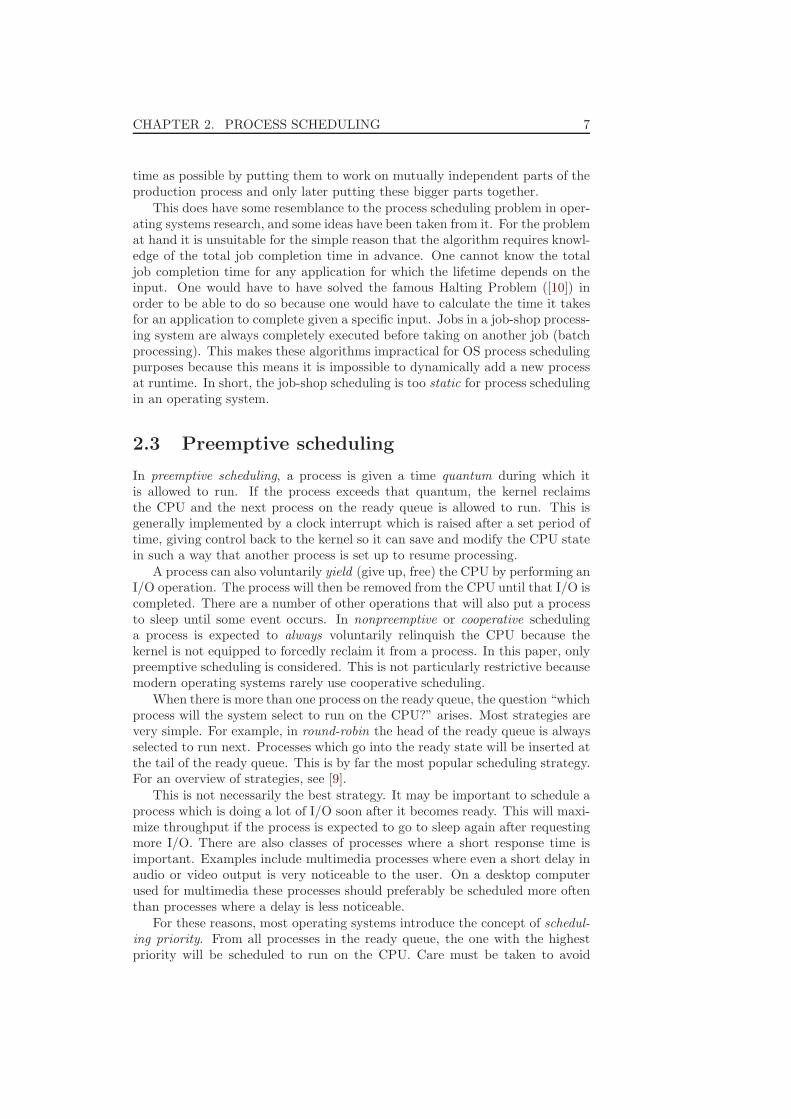
Input history per process is realized by viewing memory nodes as “secondaryinput”. This means that when the features of a process are presented to thenetwork by clamping them onto the input units, the memory of the process willalso be clamped onto the memory units. This logic is captured in pseudo-codein Algorithm 4.1.
CHAPTER 4. SYSTEM OVERVIEW 17
Algorithm 4.1 Calculate priorities
for all proc in proclist do
gather features(proc) {Reset counters, perform preprocessing}for i = 0 to nfeatures do {Clamp input and memory}
network.input[i] ⇐ proc.features[i]network.memory[i] ⇐ proc.memory[i]
end for
run network(network, proc)proc.nice ⇐ output to nice(network.output[0])for i = 0 to nfeatures do {Remember new memory values}
proc.memory[i] ⇐ network.memory[i]end for
end for
After running the network and updating activations, the new activations ofthe memory nodes are extracted from the network and stored in the processcontrol block (PCB)4 for the next cycle. This is repeated for the next process.This network is shown in Figure 4.1.
Features
Input & memory
2H H1
32
O
"layer"
network dataCommon
Memorize previous input
M1 M MIII1 32
Hidden layer(s)
Output layer
PCB
Figure 4.1: Design of the network
When we consider a particular process, the memory will be a function of thefeatures at the previous time steps of only that process. The network’s weightswill still be updated on the basis of the network error value of every process,but the memory will be process-specific for every network cycle. The strengthof the memory can be modified by changing the weight values of the recurrentconnections.
4The PCB is the structure where all the data relevant to a process is stored.

18 4.2. INFRASTRUCTURAL CHANGES
subsys
PCB
Application
System call API Kernel mode
User mode
Featurecollector
PriorityNetworkNeuralFeatures
SchedulerOther process data
subsysDiskTerminal
subsysNetwork
Figure 4.2: The data-flow of the system
4.2 Infrastructural changes
To augment a process scheduler with a neural network, the operating system’sscheduling infrastructure will necessarily become more complex because a neuralnetwork requires features to operate, which means the kernel needs to be set upto collect these.
The kernel can be logically divided into subsystems that service requests toprograms. These requests can be translated to features, for example the numberof disk reads or writes a process performs. These features need to be gatheredfor every process. Thus, every subsystem that can report features must add itsfeature data to the process control block of the relevant process so the schedulercan make use of these features. This implies an extra record in the PCB forevery feature that gets added in this fashion, which will quickly lead to a hugenumber of new records in the PCB. Usually a PCB already contains many fieldsto begin with, so adding feature fields to the existing ones will make the PCBtoo large to handle.
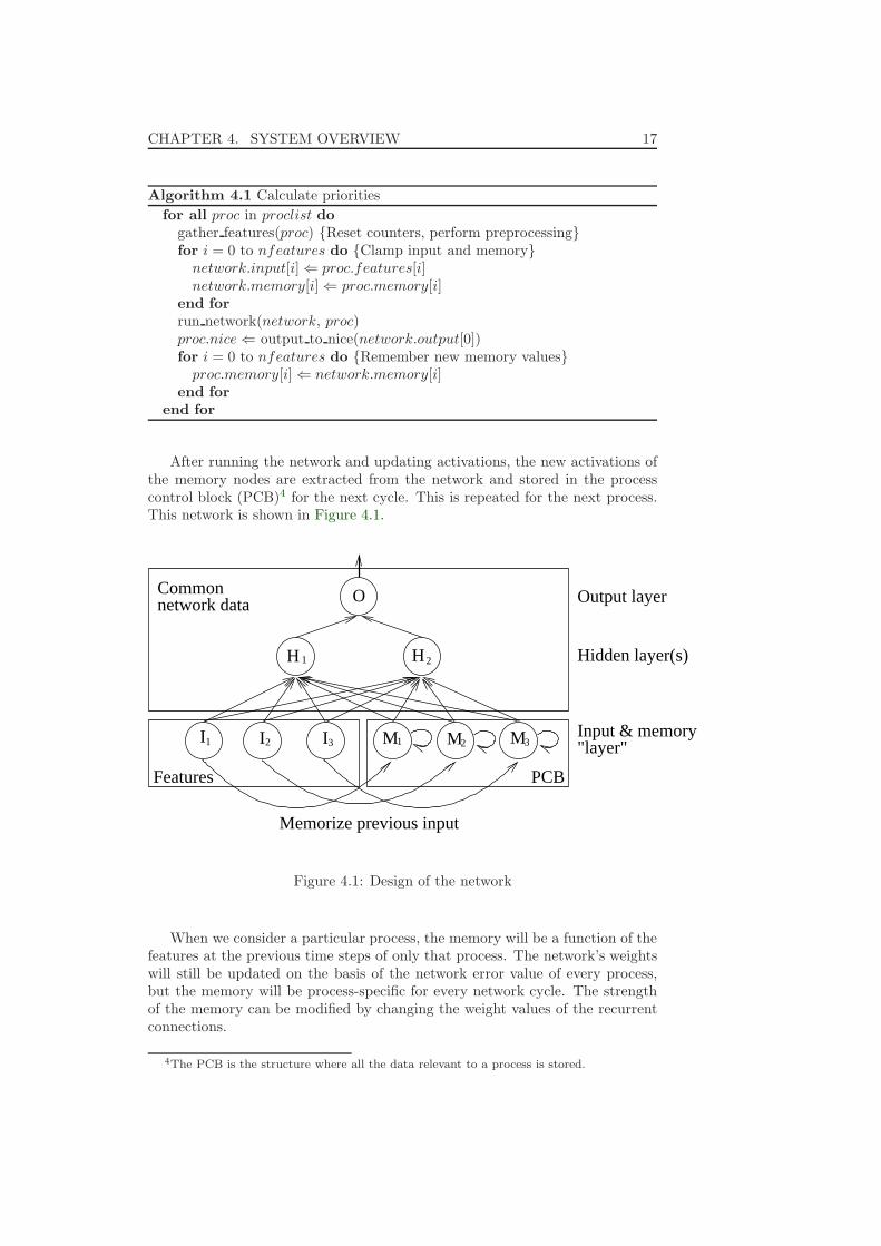
To control this complexity, a central feature collection API was implementedto which the various subsystems report their feature data. The layout of thissystem is shown in Figure 4.2. As can be seen, there is only one new API thatwas added, and subsystems have no knowledge of features of other subsystems.The feature collector dynamically allocates and deallocates memory in PCBsto hold this feature data whenever new features are registered or new processesare created. Only one extra field needs to be added to the PCB in this case,namely one which holds the list of feature data. An added advantage of this isthat features can be introduced dynamically while the system is running, whichcan happen when a new loadable kernel module (LKM) is loaded, for example.
CHAPTER 4. SYSTEM OVERVIEW 19
Whenever the scheduler updates process priorities (once per second), thefeature collection subsystem asks every subsystem that registered features for acalculation of these features. The feature data is not extracted directly from thePCB because some features may require preprocessing or special initialization.For example, calculating the ratio of reads versus writes on a (pseudo-)terminalis done by storing reads and writes in a substructure of the PCB. Only theterminal subsystem knows how to interpret this substructure. When the fea-tures are to be calculated, the feature collection subsystem asks the terminalsubsystem to extract the read/write ratio feature. The terminal subsystem thenextracts the reads and writes from the substructure, returns the ratio and resetsthe number of reads and writes again for the next cycle.
4.3 Pre-existing priorities
All throughout the preceding discussion, it has been implicated that the neuralnetwork scheduler calculates the priority completely on its own. This is notexactly true. The intention is to leave the existing scheduler in place, so we canfocus on the pure problem of assigning the priorities.
Selection of processes based on priority, in such a way that no starvation5 canoccur, is a separate problem that has already been solved by the designers of theoperating system in which our scheduler will be integrated. There is no reasonto implement it ourselves. It will suffice to simply use the existing scheduler,while only manipulating the base priority for a process. This is consistent withthe notion of the neural network scheduler as a helpful tool for the user thattakes away the work of deciding on a base priority by hand.
5Starvation occurs when a process never gets its turn on the CPU.
Chapter 5
Implementation details
This chapter describes implementation details that are useful mostly to thosewho wish to work with the code or use the programs. First we will describethe system used for testing, then an overview of a typical usage scenario ispresented. The chapter is concluded by a list of the various subsystems in thekernel and the various utilities that were implemented.
The source code to the implementation described in this chapter will bemade available for download from http://nnsched.sourceforge.net.
5.1 The system
The implementation of the project was done under NetBSD 2.0 and later on 4.0Release Candidate 11. Tests and measurements were performed with NetBSD4 on an iBook G4 (PowerPC processor) with 512 Mb of RAM. The kernel wastweaked by adding an options HZ=1000 line to the configuration file in order tohave its clock interrupt at 1000 Hz instead of the normal 100 Hz for improvedprecision2, as described in [22]. NetBSD was chosen for its clean, modulardesign, the availability of its source code and the author’s familiarity with itscode base.
5.2 Typical usage
A description of how to use the collection of tools created for this project willbe described below. The words printed in typewriter font are names of pro-grams. More information on these programs can be found in section 5.5.
Training a network is done completely offline. This means it is not requiredto have a modified kernel to train the networks. In fact, the networks can betrained (as well as tested) on any other OS if this is required. The feature datais extracted from a running modified kernel and written to a file which can
1See http://www.netbsd.org.2With this modification, the clock interrupts more often. Processes that go to sleep soon
after they are allowed to run on the CPU will cause the system to idle for a shorter time,because a new process can be selected sooner. Increased clock resolution also means moreoverhead since the scheduler is invoked more frequently.
20

CHAPTER 5. IMPLEMENTATION DETAILS 21
be used for training and testing. The training application writes the trainednetwork to a file which can be uploaded to a modified kernel at any time.
To create a working network, the first thing one must do is set up the machinein such a way that it will run all programs that are typically used. These mustall be assigned a priority at which they are supposed to operate. In essence, anormal working situation is created, with the difference that a lot more programsare run at the same time. This can be automated by running progstarter witha suitable configuration file.
The activity patterns of the processes are captured by running nnfmon. Theresulting feature file is then given as input to nntrain, which will train a net-work. This network can be tested on another dataset with nntest to see howwell it generalizes. This can be repeated while tweaking parameters like thelearning rate, number of hidden layers and units in those layers and so on untilthe user is satisfied with the results. nngather is intended to automate thisprocess somewhat. It just requires a training and a testing dataset and trains anumber of networks with different settings, compares the settings and generatesstatistical output on which performed best.
The trained network can be installed with the nnconf utility. This will“upload” the network to the kernel’s neural network scheduler. From thenon, it will be activated and the processes should be assigned a fitting priorityautomatically, in a way transparent to the user. For the user, it simply should“just work”, without having to think about it. The system can be set up to loadthis network every time at startup, to make use of the neural network scheduleras unobtrusive as possible.
Training a network and fine-tuning it is too technical for the typical desktopuser. For this type of users, a set of pre-trained networks for certain commonusage situations could be shipped with the OS. The installation process couldimprove user-friendliness by asking what the computer will be typically used for,install the appropriate network and ensure it will always be loaded at startup.
5.3 Shared code
Since the neural network is the engine of most of the programs and subsystemsdescribed below, it is only natural to share as much code as possible.
Everything that is used in both the kernel and the utilities is located inthe file sys/kern/kern nnnetwork.c. This is the code used to build a networkfrom scratch and to calculate net inputs and activations per layer. The utilities’code pulls this in and makes use of it.
There is some utility-specific code under usr.sbin/nntrain/nnnetwork.c,which is used in nntrain as well as in nntest. It contains the functionsrequired to generate random weights, calculate network error and functionsto select and clamp inputs. The reading code for network and feature filesis also shared between the testing, training and configuration programs inusr.sbin/nntest/nnread.c and usr.bin/nntrain/nnfeat.c.
22 5.4. KERNEL LEVEL IMPLEMENTATION
Interrupt
NeuralNetwork
ExtendedPCB
StandardNetBSDscheduler
Call
Features
nnsched
Nice value
Nice value Priority
Figure 5.1: Overview of interaction between scheduler parts
5.4 Kernel level implementation
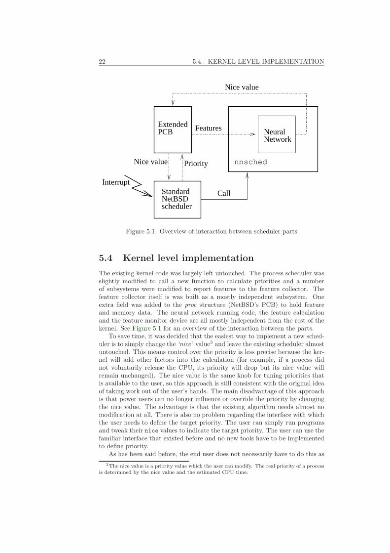
The existing kernel code was largely left untouched. The process scheduler wasslightly modified to call a new function to calculate priorities and a numberof subsystems were modified to report features to the feature collector. Thefeature collector itself is was built as a mostly independent subsystem. Oneextra field was added to the proc structure (NetBSD’s PCB) to hold featureand memory data. The neural network running code, the feature calculationand the feature monitor device are all mostly independent from the rest of thekernel. See Figure 5.1 for an overview of the interaction between the parts.
To save time, it was decided that the easiest way to implement a new sched-uler is to simply change the ‘nice’ value3 and leave the existing scheduler almostuntouched. This means control over the priority is less precise because the ker-nel will add other factors into the calculation (for example, if a process didnot voluntarily release the CPU, its priority will drop but its nice value willremain unchanged). The nice value is the same knob for tuning priorities thatis available to the user, so this approach is still consistent with the original ideaof taking work out of the user’s hands. The main disadvantage of this approachis that power users can no longer influence or override the priority by changingthe nice value. The advantage is that the existing algorithm needs almost nomodification at all. There is also no problem regarding the interface with whichthe user needs to define the target priority. The user can simply run programsand tweak their nice values to indicate the target priority. The user can use thefamiliar interface that existed before and no new tools have to be implementedto define priority.
As has been said before, the end user does not necessarily have to do this as
3The nice value is a priority value which the user can modify. The real priority of a processis determined by the nice value and the estimated CPU time.

CHAPTER 5. IMPLEMENTATION DETAILS 23
developers and distributors can ship the system with pre-trained networks fora variety of common usage scenarios and have the installer offer to select one ofthem for loading when the system boots.
5.4.1 Pseudo-devices
The following pseudo-devices are available to applications for retrieving featuredata from the kernel and uploading configuration data to the kernel.
nnfmon
The neural network’s feature monitor pseudo-device, nnfmon, exports featuredata from the kernel to applications. Every second, just before the features areupdated, nnfcoll sends the old feature values to nnfmon, which stores these ina freshly allocated buffer. These buffers can be accessed by a process by openingand reading from the pseudo-device.
nnconf
The configuration pseudo-device for the neural network. This allows applica-tions to configure the neural network scheduler and upload a neural network’slayout and connection weights to the kernel.
5.4.2 Scheduler and feature collection
nnsched
The existing scheduler in kern synch.c is modified to call the nice calculatorevery hz clock ticks (every second), if the neural network has been initialized.The nice calculator (which is located in kern nnsched.c) simply runs the net-work from kern nnnetwork.c in feedforward mode, resulting in an activationvalue on the output node. It is assumed that there is only one output node,which represents the processes’ priority. This priority is expressed as a valuebetween 0 and 1, which is inverted and scaled back to an integer in the range of0 to 40, from which 20 is subtracted to get a value between -20 and +20 (whichis the range of Unix nice values). See also section 6.1.
nnfcoll
On startup, all subsystems which collect data for a feature will register thisfeature with the neural network’s feature collection subsystem, nnfcoll. Thisallocates a unique feature identifier (ufid, for short) and associates this with thecallback function pointers for this feature in the list of known features. Thereare three callback functions: One for allocation of process-specific feature data(which is treated as opaque data by anything but the subsystem for which it isintended), one for deallocation of this data, and one for calculating features.
The feature calculation function is called every time process priorities areupdated, for every process. This happens just before the features are fed intothe neural network for a new epoch. The allocation and deallocation functionsare called on process creation and exit.

24 5.5. USER LEVEL IMPLEMENTATION
5.5 User level implementation
5.5.1 Tools for interacting with the kernel
nnfmon
The neural network’s feature monitor nnfmon is both the pseudo-device dis-cussed in subsection 5.4.1 and the name of a program which reads data fromthis device. This application simply empties all nnfmon feature buffers, stor-ing the information in them in a file. This file is later read in by other neuralnetwork applications.
nnconf
This simple program reads a saved neural network and ‘uploads’ its layout andweight data to the kernel by means of ioctls on the nnconf pseudo-device.
5.5.2 Training tools
nntrain
The training application for the neural network. This application reads out afile as stored by nnfmon and allows the user to create a network and train itwith these data as input. It accepts network configuration on the command linein the form of size and number of hidden layers, maximum net error, maximumnumber of epochs to train, learning rate, momentum and initial weights formemory connections. It initializes the other weights and biases randomly.
nntest
An application intended for comparing existing pre-trained networks. It displaysa net’s error with regard to an nnfmon feature file.
nngather
This is a simple program used to gather data on the effectiveness of combinationsof features and settings in the nntrain program, by training a number of netsand testing them on a training and testing set.
5.5.3 Miscellaneous tools
typesim
This is a very small program that will attach to a terminal and send simulatedkeystrokes to it. These keystrokes will trigger writes to the terminal as thoughthey were real ones, thus creating a “fake interaction” with an interactive pro-cess.
progstarter
This is a program that sets up a system to run a number of programs withspecified priority settings and calls nnfmon to record their feature values. It can
CHAPTER 5. IMPLEMENTATION DETAILS 25
optionally also start an instance of typesim to create a fake interaction withsome of these processes.
featmerge
This little tool can merge two output files from nnfmon. It is necessary whenone wishes to combine application runs which claim the audio device, if thereis no in-kernel mixing available. It can also be very useful to try out differentcombinations of programs. One can simply run each program on its own, captureits features and combine these output files to create usage scenarios.
gentest
A simple program used to generate test sets. One can define a number of“features” and a number of “processes”. It will divide the range of nice valuesequally among the simulated processes. The feature values that are writtenare random, but they all add up to their converted nice value (meaning -20 ismapped to 0 and 20 is mapped to 1). This program is useful if people wouldwant to test different kinds of network implementations or modifications to theexisting one.
5.6 Implementation issues
This section will deal with some practical problems that arose during imple-mentation of the network.
5.6.1 Floating point
In NetBSD, it is not allowed to use floating point instructions inside the kernel.At first, when all subsystems are initialized, the floating point unit (FPU) is notinitialized yet. About halfway through the main initialization process, when thehardware is probed, the FPU is initialized.
The features are registered during hardware probe, as well, since their datais generated by device drivers. We cannot control the order of device driverinitialization and probing, so there is no guarantee that the FPU has been ini-tialized at feature initialization time. When a feature is registered, any processwhich is forked afterwards will have its NN data structures initialized. This willcause the system to crash if the FPU is not yet initialized at that time, becausethese data are in floating point format.
A solution would be to wait until the FPU is initialized and only then initial-izing the NN data structures for every existing process. This was implementedand worked for a while, until a process used the FPU. This would cause a crashas well because the kernel changes the FPU status while calculating features.Saving and restoring of FPU register status is very slow on many machines, sothe kernel does not do this on every switch to kernel level, only when doinga process switch. As a consequence, the kernel can not use any floating pointinstructions at all.
Therefore, the current implementation uses fixed point arithmetic. Thisconsiderably slowed down the implementation of the project, because the authorhad no previous experience in writing fixed point arithmetic and there are many

26 5.6. IMPLEMENTATION ISSUES
subtle things that can go wrong while using fixed point. A decent tutorial tofixed point can be found in [28]. On the upside, because this required closeattention to the representation of the numbers, it provided some insights thatwould otherwise probably have gone unnoticed.
5.6.2 Range and precision problems
Theoretically, neural networks can be used to calculate any mathematical func-tion one can think of. In other words, they are Turing-Complete (See [18] fora proof4). In practice, however, the computational power of neural networks isdirectly proportional to the numerical range and precision of the implementa-tion.
Consider a simple network with one input node and one output node. Forsimplicity, let us assume we try to learn only two patterns, namely (0.001)where the output shall be (1) and (0) where the output shall be (0). In orderto represent a network that can compute this, we must allow numbers as largeas 1000 in the weights. Also, in certain situations only very small changes inweights can make a big difference. If the chosen representation does not allowsuch precision, it may be impossible to learn such a pattern.
Fortunately this was not a real problem in practice, but it might matterin the future for certain new patterns or features. Extra preprocessing couldprobably be used to change ranges or clustering of activity in such cases. Itmust be noted that the same problems can occur with other algorithms as well.Even floating point has a maximum precision. The major difference is thatfixed point is much less flexible, because one has to decide a priori what theposition of the point will be. On the upside, fixed point is many times fasterthan floating point on most systems, making it more suitable for use in kernels.
5.6.3 No audio mixing
NetBSD does not provide a possibility to multiplex the audio device. Onceone process has claimed the audio device, others can not access this device.The kernel does not mix sound channels. This is not a real problem becausethere are various ways to multiplex audio using userland applications, but thismeans feature information about the application that outputs the audio is lost.The kernel only sees audio output from the mixing application. To remedythis, a program was created to combine feature outputs from several monitoringruns. One can start a number of applications which includes up to one processwith direct kernel audio output. These can then be monitored for features,after which a different combination of applications can be started for featuremonitoring. Finally these two feature files can be combined. This leads toa feature file which interleaves the feature values from the first two featurefiles. This circumvents the audio mixing problem by mixing the feature valuesafterwards.
This has no negative effects, because this output would look exactly thesame if the processes were actually started together, if in-kernel audio mixingwas available.
4This proof is slightly incomplete, see the appendix for a discussion.

CHAPTER 5. IMPLEMENTATION DETAILS 27
5.6.4 The X Window System
In Unix, a graphical shell is optional. The most common Graphical User Inter-face (GUI) for Unix is X11, which is generally not integrated in the kernel. Thesystem consists of a server and a number of clients. The server program controlsthe display resources of the workstation while the clients send commands to itover a socket. This means the clients look to the kernel like simple network pro-grams. Generally, the server does not know (indeed it does not need to know)which process is requesting graphical output. This makes it very difficult togather process information from X.
Probably the most interesting features for multimedia are the frequency andnature of graphical requests by a process. To get this information availableto our scheduler, it must be extended with a way for X to communicate thisinformation to it. X would need to be modified as well. Because of a lack of timethis project did not include the task of making these modifications to X andthe kernel, but theoretically these should certainly improve the recognition ofmultimedia processes. Etsion et al. [23] describe a system that does somethingvery similar, and it would be interesting to see this system re-implemented interms of features for our neural network scheduler.

Chapter 6
Results
Here we will present the results of running the neural network on certain exampleprogram sets and a benchmark of the overhead of running a neural network inthe kernel.
The kernel that was used in the tests below is the GENERIC kernel for theMacintosh PowerPC (“macppc”) port. There is a GENERIC kernel for everyport in the NetBSD source tree. These kernels include almost all drivers andsubsystems supported by the OS on that particular platform. This is the kernelthat one will find in a default installation of the operating system because it ismost likely to work on a wide range of hardware configurations.
Using such a “default” configuration means these results will be easier toreproduce in other experiments if needed, since the configuration is not specialor tuned to specific hardware in any way. As stated before in section 5.1, therewas one change in this configuration: an options HZ=1000 line was added toincrease feature gathering granularity. The neural network kernel used is simplya GENERIC configuration with the added neural network scheduler subsystem.
6.1 Features
The features that were used were the same for all subsystems: The numberof reads and writes were recorded, as well as the number of reads divided bythe number of writes. The number of reads divided by the number of writeswas deemed a good feature because it can not be calculated by the wiring ofa simple network with few layers. It does provide useful information, sincea process may do a lot of reads and writes or just a small number of readsand writes, but the ratio might be the same. This will hopefully remove thedifferences in hardware and/or bandwidth, making pre-trained networks moregenerally deployable. The following subsystems were monitored for these threefeatures:
• Sockets (which can be both network and interprocess communication).The expectation is that applications like HTTP daemons will need to begiven an elevated priority on server machines and filesharing programs willneed to be given a lowered priority on desktop machines. Another reasonto use this feature is that X window clients use sockets to communicate
28

CHAPTER 6. RESULTS 29
with the X server, which handles graphics, so it can help us in furtherdistinguishing background processes from interactive processes.
• Terminal interface (including pseudo-terminals like xterm). In most situ-ations, terminal emulators should have a reasonably fast response becausethey provide the main interaction with the system.
• Audio. Multimedia applications generally produce audio output, whichwould make this a very suitable feature for detecting this kind of applica-tion on a desktop system.
• Filesystem. Indexing of the filesystem, archiving, making backups andmany other typical background tasks interact solely with the filesystem,which makes this a useful feature to detect these kinds of applications.
Target values were nice values, specified by a progstarter configuration file.Nice values are in the range [−20, +20]. The network works with a linear acti-vation function which has the range [0, +1], so target nice values were originallynormalized by the following function:
convert nice(n) =n + 20
40
After some experimentation, it was observed that the network would notlearn very well. After some consideration it was determined that the reason forthis was that the calculation of the network would be biased in favor of highpriorities, because low nice values close to zero actually give high priority tothe processes. When a process does not have particularly interesting features,it will result in zero values being clamped upon the input nodes of the network.
Uninteresting processes should run at a default nice value and only be el-evated if they are interesting. There is no way by which a zero value can bemultiplied so that it will result in a more useful value. Biases introduced inthe network will help a little bit, but the training process tended to drop thebias connection weights down, so this would often result in the network favoringelevated priority. By inverting the output node value, this problem is solved.This results in the following function to convert a nice value to a target value:
convert nice′(n) =−1 · n + 20
40=
20 − n
40
6.2 Network accuracy
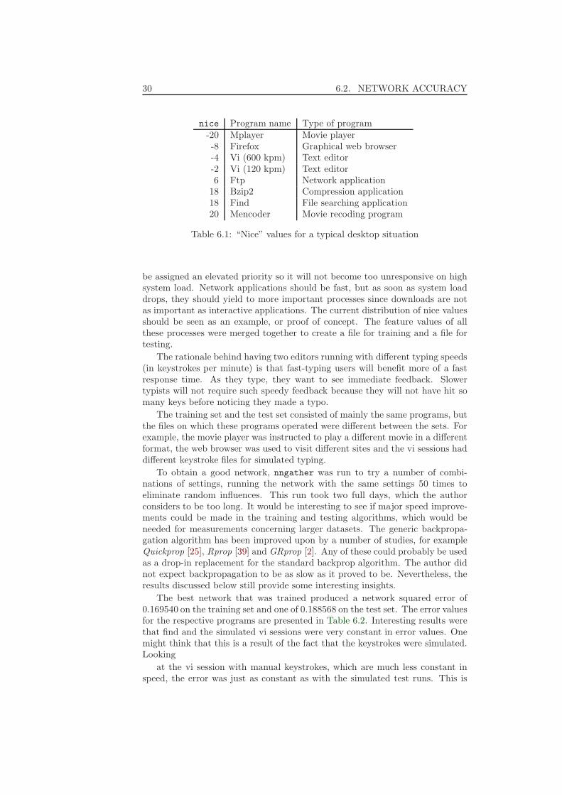
To measure how well the network was able to learn feature sets for runningprocesses, data was gathered by running one program at a time with a targetnice value and monitoring its features using nnfmon. The target nice valuesselected for each of the observed programs can be observed in Table 6.1. Thesenice values are just an example of what a typical desktop user would most likelyprefer.
It is assumed most desktop users want their multimedia applications to runat the highest priority (lowest nice) and processes that only perform a lot ofdisk access (like find) to run at the lowest priority. Usually an editor does notneed the highest priority to achieve acceptable response times, but it should
30 6.2. NETWORK ACCURACY
nice Program name Type of program-20 Mplayer Movie player-8 Firefox Graphical web browser-4 Vi (600 kpm) Text editor-2 Vi (120 kpm) Text editor6 Ftp Network application
18 Bzip2 Compression application18 Find File searching application20 Mencoder Movie recoding program
Table 6.1: “Nice” values for a typical desktop situation
be assigned an elevated priority so it will not become too unresponsive on highsystem load. Network applications should be fast, but as soon as system loaddrops, they should yield to more important processes since downloads are notas important as interactive applications. The current distribution of nice valuesshould be seen as an example, or proof of concept. The feature values of allthese processes were merged together to create a file for training and a file fortesting.
The rationale behind having two editors running with different typing speeds(in keystrokes per minute) is that fast-typing users will benefit more of a fastresponse time. As they type, they want to see immediate feedback. Slowertypists will not require such speedy feedback because they will not have hit somany keys before noticing they made a typo.
The training set and the test set consisted of mainly the same programs, butthe files on which these programs operated were different between the sets. Forexample, the movie player was instructed to play a different movie in a differentformat, the web browser was used to visit different sites and the vi sessions haddifferent keystroke files for simulated typing.
To obtain a good network, nngather was run to try a number of combi-nations of settings, running the network with the same settings 50 times toeliminate random influences. This run took two full days, which the authorconsiders to be too long. It would be interesting to see if major speed improve-ments could be made in the training and testing algorithms, which would beneeded for measurements concerning larger datasets. The generic backpropa-gation algorithm has been improved upon by a number of studies, for exampleQuickprop [25], Rprop [39] and GRprop [2]. Any of these could probably be usedas a drop-in replacement for the standard backprop algorithm. The author didnot expect backpropagation to be as slow as it proved to be. Nevertheless, theresults discussed below still provide some interesting insights.
The best network that was trained produced a network squared error of0.169540 on the training set and one of 0.188568 on the test set. The error valuesfor the respective programs are presented in Table 6.2. Interesting results werethat find and the simulated vi sessions were very constant in error values. Onemight think that this is a result of the fact that the keystrokes were simulated.Looking
at the vi session with manual keystrokes, which are much less constant inspeed, the error was just as constant as with the simulated test runs. This is

CHAPTER 6. RESULTS 31
Average squared error Program name0.480523 Mplayer0.305481 Firefox0.059364 Vi (600 kpm)0.058685 Vi (360 kpm)0.058640 Vi (manual typing)0.036316 Vi (120 kpm)0.121804 Ftp0.127144 Bzip20.169342 Find0.136162 Mencoder
Table 6.2: Error values of the tested programs
an indication that the memory layer does exactly what it was designed to do;make the input smoother.
We can also observe that the features are apparently not quite suitableenough for classifying multimedia processes. The errors of the movie playerand the web browser are notably higher than the other processes. The fact thatthe web browser was classified badly was expected since it does not have anyvery distinguishing features. It mostly does some disk reads and some networkaccess, like a combination of the compression and download programs. On theother hand, the movie player can be accurately identified by its sound output, soit was expected that it should be recognized by the network. The other featuresapparently drown out the importance of the audio features. Introducing moremultimedia-specific features would hopefully balance this out.
In [23], a number of “Human-Centered” metrics are explored which can beused for priority heuristics. The results shown in this studies are promising. Itwould be trivial to implement these metrics as features for our neural network.The biggest problem with these metrics is that the data required to measurethem are not available to the kernel directly. To make the kernel aware of, forexample, GUI features like horizontal and vertical size of a window, one needsto implement a feature reporting system. Userlevel applications need a way tonotify the kernel about the service requests they receive from other applications.In Unix much information is not available to the kernel, because for example thegraphics device is multiplexed to other userland applications by X. This is alsotrue for audio and pseudo terminals on certain systems. Where such systemsare in use, these would have to be modified as well as the kernel to realize thegathering of these additional features.
On microkernel systems (examples are QNX [37], Windows NT [32], EROS[45] and Mach [1] and its descendants Hurd [11] and Darwin/Mac OS X [4]) thiswould probably be less of a problem. Microkernel systems are systems whichhave a tiny kernel that performs only the minimal number of tasks required forthe OS to function. Functionality that is provided by the kernel in traditionalsystems is provided by several processes or threads. This also allows easy re-placement of kernel subsystems by simply starting a different implementation ofthat particular subsystem. This architecture is more open to userland processes,so on these systems it may be easier for these resource-multiplexing applications

32 6.3. INFLUENCE OF THE MEMORY LAYER
to access process information and report this to the neural network scheduler.On systems with a monolithic design, where each and every resource is handledby the kernel, these problems are nonexistent because all needed information isdirectly available to the kernel.
6.3 Influence of the memory layer
One interesting, but possibly problematic result of introducing the memorylayer is that training a network toward a low error does not mean a testset willproduce the same error. If one trains a network, the memory layer is trainedas well, producing a memory “fingerprint” unique to this particular trainingrun. The weights are updated to reflect more or less importance of the relevantfeature’s history with regards to the current value of the feature (ie, the degreeof “decay” of the memory). The history that has been built up to this pointis still subject to the previous memory weight values. This is mathematicallyexpressed in Equation 6.1. Here am and ai are the activations of one memoryunit and its input unit, respectively. wim and wmm are the weights from theinput unit to its memory unit and the recurrent weight from the memory unitto itself, respectively.
netinputm(t) = ai(t − 1) ∗ wim(t) + am(t − 1) ∗ wmm(t) (6.1)
This is not incorrect, but when one runs a test, the memory history will alwaysbe different even on the same dataset, since the equation does not rely onchanging weights but assumes they are constants as can be seen in Equation 6.2.
netinputm(t) = ai(t − 1) ∗ wim + am(t − 1) ∗ wmm (6.2)
Introducing the LOCK MEMORY WEIGHTS option (which is a C preprocessordefine) into nntrain allowed experimentation with this phenomenon. Whenone trains a network using nntrain, the network error is printed during training.When testing this network with nntest, we only get exactly the same errornntrain printed after the last epoch when memory weights are locked and thenumber of runs of the training set is equal to the number of training epochs.When the number of “epochs” of the test program is different, the memory layerdoes not store the exact same history for all processes as the training programrecorded during its run.
6.4 Overhead
To measure the overhead of the neural network scheduler, a number of testruns were performed with the benchmarking program hackbench [42], whichwas specifically developed for benchmarking scheduling algorithms. This bench-marking program creates a number of process groups which communicate througha socket. It creates an equal number of senders and receivers in each group. Allof the senders in a group send one hundred bytes to all of the receivers in itsgroup, repeated a hundred times. The size of a group is 40 processes (meaning,20 receivers and 20 senders).
The overhead calculation is performed by measuring the total execution timeor “wall clock time” of a hackbench session. By subtracting the end time of a

CHAPTER 6. RESULTS 33
0
20
40
60
80
100
120
140
160
180
200
0 10 20 30 40 50 60 70 80 90 100
tim
ein
seco
nds
client/server groups
no networkGENERIC
12x8x112x12x8x1
Figure 6.1: Runs of hackbench with different kernels and networks
session from the start time, a result is obtained. These results can be comparedbetween different kernels to see how much scheduling overhead is involved bysubtracting one kernel’s total time of the same number of hackbench groupsfrom the other kernel’s total running time of these groups. The difference is theextra time spent inside the scheduler, considering everything else is equal.
These tests were conducted in the so-called single-user mode, which is anoperating mode in which no services are started except for the ones that arevital to keep the system running. This was done to minimize interference fromother processes that otherwise might be running (for instance, cron which mightrun a daily script that performs quite heavy disk seeks). Each test was run 5times and the results averaged to reduce further anomalies. After every batchof 5, the system was rebooted to ensure earlier tests would not influence latertests. The results are displayed in Figure 6.1.
6.4.1 Feature gathering overhead
The original NetBSD scheduler (marked GENERIC in the Figure 6.1) has a veryslight curve, indicating quadratic complexity of the scheduler. This curve be-comes more pronounced as more time is being taken by the neural networkscheduler. The complexity of running the network and feature gathering for oneprocess is constant with respect to the number of processes. The features for oneprocess are gathered and the network for that process is run completely inde-pendent from all other processes. Because the feature gathering is run for every

34 6.5. PERCEIVED SPEED
process, the total overhead of the feature gathering is linear. The network is runinside the scheduler so, having constant complexity of itself, the scheduler as awhole will be of quadratic complexity since O(1) · O(n2) = O(n2). The featuregathering is not run inside the scheduler. Considering the total overhead of thenew system, this will still be of quadratic complexity as O(n2)+O(n) = O(n2).
In the graph we can see the overhead of the feature gathering (marked nonetwork in the figure) compared to a normal GENERIC kernel without featuregathering. At around 15 groups of processes of hackbench (making 600 processesin total) one starts to see a clear difference between a regular GENERIC kernelversus the feature gathering kernel. The difference in feature gathering overheadas compared to the kernel without feature gathering is about 8 milliseconds perprocess group or 0.2 milliseconds per process.
This overhead consists of three things: First, when a process is created, thekernel allocates of a buffer to hold bookkeeping information which is needed totrack the data required for calculating the feature’s input value for the network.It initializes this buffer for each feature by copying from the parent process thatinvoked the new process. Second, at every call in the subsystem which registeredthe feature, there will be a call to a procedure that will increment a tally for thisfeature or do something else, depending on the feature. Third, when a processis destroyed, the kernel needs to deallocate the feature buffers.
To determine the overhead of the neural network itself, the above processwas repeated after loading a network into the kernel, causing it to go through thesteps of calculating the features as well as running the network in feedforwardfashion to calculate nice values for all the processes. The nice values wouldall be exactly equal, so as not to cause skews in the measurements. This wasensured by simply setting all the network’s weights to zero, thereby making allprocesses get an equal nice value of 20 (lowest priority).
We can see that the overhead of a network is quite noticeable. The over-head of the 12x8x1 network over the feature gathering is about as much as theoverhead of the feature gathering over a GENERIC kernel; it is roughly 12.5 mil-liseconds per process group or 0.31 millisecond per process. The total overheadof this network as compared to a GENERIC kernel is thus about 20.5 millisecondsper process group or 0.51 milliseconds per process. The overhead of adding anextra hidden layer of 12 nodes to the network is roughly 8.5 milliseconds perprocess group or 0.21 milliseconds per process.
Seeing these numbers compared to each other is a strong motivation tochoose features very carefully in a production system, so that the total numberof nodes can be kept to a minimum. In actual usage of the system, it is moreinteresting to see what the perceived speed is, as experienced by the user. Thiswill be dealt with in the next section.
6.5 Perceived speed
Most computer users are not interested in minor speed differences between pro-cesses and schedulers. The reason for using a neural network scheduler on adesktop system in a multimedia context is to see if it is possible to improve thesubjective speed or the speed the user perceives the system to have. When aninteractive or multimedia process slows down on a desktop system, this is muchmore noticeable and annoying than when any long-running background process
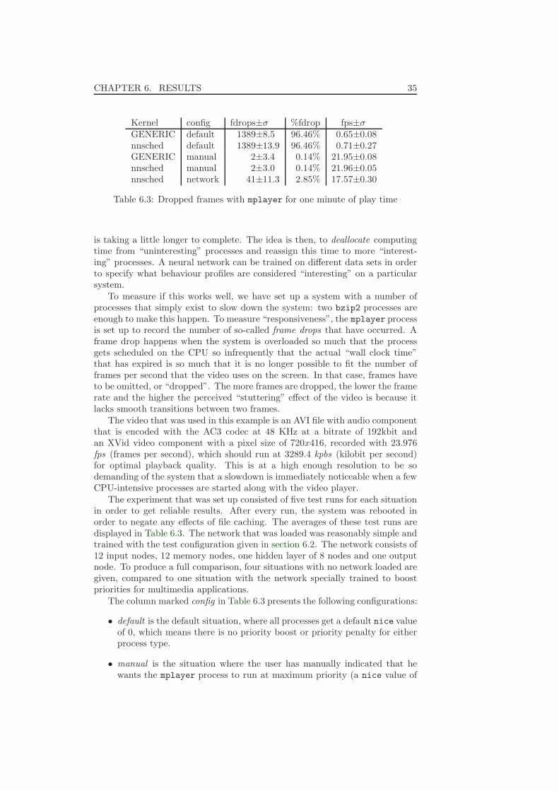
CHAPTER 6. RESULTS 35
Kernel config fdrops±σ %fdrop fps±σ
GENERIC default 1389±8.5 96.46% 0.65±0.08nnsched default 1389±13.9 96.46% 0.71±0.27GENERIC manual 2±3.4 0.14% 21.95±0.08nnsched manual 2±3.0 0.14% 21.96±0.05nnsched network 41±11.3 2.85% 17.57±0.30
Table 6.3: Dropped frames with mplayer for one minute of play time
is taking a little longer to complete. The idea is then, to deallocate computingtime from “uninteresting” processes and reassign this time to more “interest-ing” processes. A neural network can be trained on different data sets in orderto specify what behaviour profiles are considered “interesting” on a particularsystem.
To measure if this works well, we have set up a system with a number ofprocesses that simply exist to slow down the system: two bzip2 processes areenough to make this happen. To measure “responsiveness”, the mplayer processis set up to record the number of so-called frame drops that have occurred. Aframe drop happens when the system is overloaded so much that the processgets scheduled on the CPU so infrequently that the actual “wall clock time”that has expired is so much that it is no longer possible to fit the number offrames per second that the video uses on the screen. In that case, frames haveto be omitted, or “dropped”. The more frames are dropped, the lower the framerate and the higher the perceived “stuttering” effect of the video is because itlacks smooth transitions between two frames.
The video that was used in this example is an AVI file with audio componentthat is encoded with the AC3 codec at 48 KHz at a bitrate of 192kbit andan XVid video component with a pixel size of 720x416, recorded with 23.976fps (frames per second), which should run at 3289.4 kpbs (kilobit per second)for optimal playback quality. This is at a high enough resolution to be sodemanding of the system that a slowdown is immediately noticeable when a fewCPU-intensive processes are started along with the video player.
The experiment that was set up consisted of five test runs for each situationin order to get reliable results. After every run, the system was rebooted inorder to negate any effects of file caching. The averages of these test runs aredisplayed in Table 6.3. The network that was loaded was reasonably simple andtrained with the test configuration given in section 6.2. The network consists of12 input nodes, 12 memory nodes, one hidden layer of 8 nodes and one outputnode. To produce a full comparison, four situations with no network loaded aregiven, compared to one situation with the network specially trained to boostpriorities for multimedia applications.
The column marked config in Table 6.3 presents the following configurations:
• default is the default situation, where all processes get a default nice valueof 0, which means there is no priority boost or priority penalty for eitherprocess type.
• manual is the situation where the user has manually indicated that hewants the mplayer process to run at maximum priority (a nice value of

36 6.5. PERCEIVED SPEED
-19 — note that the user needs to have root privileges in order to be ableto do this) and the bzip2 process to run at the minimum priority (a nice
value of 20). This is the best situation imaginable when simply runningonly bzip2 and mplayer and we are only interested in making mplayer runas fast as possible. Any background process (like the X server, the windowmanager, the user’s shell etc) still run at nice 0, or default priority.
• network is the situation where the neural network scheduler is loadedand actively monitoring and scheduling processes. Any nice value setby the user is ignored and reassigned by the neural network scheduler.All processes are automatically assigned priorities by the scheduler, notonly the mplayer and bzip2 processes under discussion. This includes theuser’s shell, X and the window manager. The network was trained withexample sets such that mplayer should receive a nice value of -19 andbzip2 should receive a nice value of 20.
The column marked fdrops presents the average number of frames droppedby mplayer in the given configuration and its standard deviation on the oneminute of play time in four trial runs.
The column marked %fdrop presents the average percentage of droppedframes. The total number of frames in one minute of the video used for thetests was 1440.
Finally, the column marked fps presents the average frames per second andstandard deviation that was achieved on the four runs in the given configuration.This is what concretely determines how smooth the video plays for a human eye.This number can differ from the fdrops average because even though a minuteof video was requested, the actual play time can be slightly higher dependingon the amount of stutter. When audio and video get out of sync because ofstuttering and video frame drops, the player needs to compensate by waitingfor the audio track to catch up. This means that with higher frame drop counts,the total time taken for the video varies more. It is always higher than the totaltime of the video clip. The better fps rate of the nnsched kernel in the defaultconfig is the result of such fluctuation, as can be determined from standarddeviation.
These results indicate that the neural network scheduler performs quite wellin this task and does exactly what it was designed to do: take the nice valueassignment out of the hands of the user and automate it. The GENERICscheduler in the default situation does not take into account the fact that themplayer process is more important to the desktop user than the bzip2 processesand simply divides the CPU time equally to the processes. This is not goodenough because it results in an extreme amount of dropped frames. The neuralnetwork scheduler without a network loaded behaves identically.
When a network is loaded, the neural network scheduler adjusts the prioritiesautomatically by determining that the mplayer process is using audio outputand uses that to boost its priority, resulting in a negligible amount of droppedframes. This certainly makes the video more pleasant to watch.

CHAPTER 6. RESULTS 37
0
100
200
300
400
500
600
700
800
900
0 100 200 300 400 500 600 700 800 900 1000
sock
etre
ads,
wri
tes
time (seconds)
firefox readsfirefox writes
mplayer writesftp reads
Figure 6.2: Socket reads and writes for firefox, mplayer and ftp processes
6.6 Assessment of features
Even though this is only a proof of concept implementation, the usefulness ofthe features used in the initial study will be described here.
6.6.1 Sockets
The socket features were expected to be indicative of X programs and net-work programs. It turned out that multimedia programs are not necessarily de-tectable this way because programs like mplayer and firefox use the X videoextension [12] in conjunction with the MIT shared memory extension [14]. Thiscombination of extensions to the X protocol allows client programs residing onthe same machine as the X server to store graphics in memory and grant accessto the X server to read this memory directly, instead of having to pass everypixel over the socket connection. The only information going over the socketconnection is the client’s request to have the server read a new frame frommemory.
This is shown in Figure 6.2, where it is clearly visible that the mplayer
process has a constant amount of socket writes per second: around 22 persecond, corresponding to the frame rate. It performed no reads at all so thisis not shown. The lower spikes in the firefox plot are when the user hasscrolled or performed some other action that requires a redraw of the page.The bigger spikes correspond to HTTP requests for new pages or images on

38 6.6. ASSESSMENT OF FEATURES
0
5000
10000
15000
20000
25000
30000
35000
40000
45000
0 100 200 300 400 500 600 700 800 900 1000
sock
etre
ad/w
rite
ratio
time (seconds)
firefoxfirefox, smoothed
ftpftp, smoothed
Figure 6.3: Socket read/write ratio for firefox and ftp processes
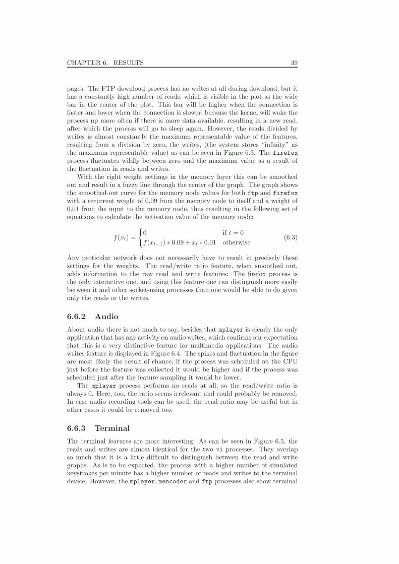
CHAPTER 6. RESULTS 39
pages. The FTP download process has no writes at all during download, but ithas a constantly high number of reads, which is visible in the plot as the widebar in the center of the plot. This bar will be higher when the connection isfaster and lower when the connection is slower, because the kernel will wake theprocess up more often if there is more data available, resulting in a new read,after which the process will go to sleep again. However, the reads divided bywrites is almost constantly the maximum representable value of the features,resulting from a division by zero, the writes, (the system stores “infinity” asthe maximum representable value) as can be seen in Figure 6.3. The firefox
process fluctuates wildly between zero and the maximum value as a result ofthe fluctuation in reads and writes.
With the right weight settings in the memory layer this can be smoothedout and result in a fuzzy line through the center of the graph. The graph showsthe smoothed-out curve for the memory node values for both ftp and firefox
with a recurrent weight of 0.09 from the memory node to itself and a weight of0.01 from the input to the memory node, thus resulting in the following set ofequations to calculate the activation value of the memory node:
f(xt) =
{
0 if t = 0
f(xt−1) ∗ 0.09 + xt ∗ 0.01 otherwise(6.3)
Any particular network does not necessarily have to result in precisely thesesettings for the weights. The read/write ratio feature, when smoothed out,adds information to the raw read and write features: The firefox process isthe only interactive one, and using this feature one can distinguish more easilybetween it and other socket-using processes than one would be able to do givenonly the reads or the writes.
6.6.2 Audio
About audio there is not much to say, besides that mplayer is clearly the onlyapplication that has any activity on audio writes, which confirms our expectationthat this is a very distinctive feature for multimedia applications. The audiowrites feature is displayed in Figure 6.4. The spikes and fluctuation in the figureare most likely the result of chance; if the process was scheduled on the CPUjust before the feature was collected it would be higher and if the process wasscheduled just after the feature sampling it would be lower.
The mplayer process performs no reads at all, so the read/write ratio isalways 0. Here, too, the ratio seems irrelevant and could probably be removed.In case audio recording tools can be used, the read ratio may be useful but inother cases it could be removed too.
6.6.3 Terminal
The terminal features are more interesting. As can be seen in Figure 6.5, thereads and writes are almost identical for the two vi processes. They overlapso much that it is a little difficult to distinguish between the read and writegraphs. As is to be expected, the process with a higher number of simulatedkeystrokes per minute has a higher number of reads and writes to the terminaldevice. However, the mplayer, mencoder and ftp processes also show terminal
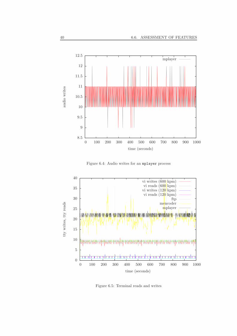
40 6.6. ASSESSMENT OF FEATURES
8.5
9
9.5
10
10.5
11
11.5
12
12.5
0 100 200 300 400 500 600 700 800 900 1000
audio
wri
tes
time (seconds)
mplayer
Figure 6.4: Audio writes for an mplayer process
0
5
10
15
20
25
30
35
40
0 100 200 300 400 500 600 700 800 900 1000
tty
wri
tes,
tty
reads
time (seconds)
vi writes (600 kpm)vi reads (600 kpm)
vi writes (120 kpm)vi reads (120 kpm)
ftpmencoder
mplayer
Figure 6.5: Terminal reads and writes
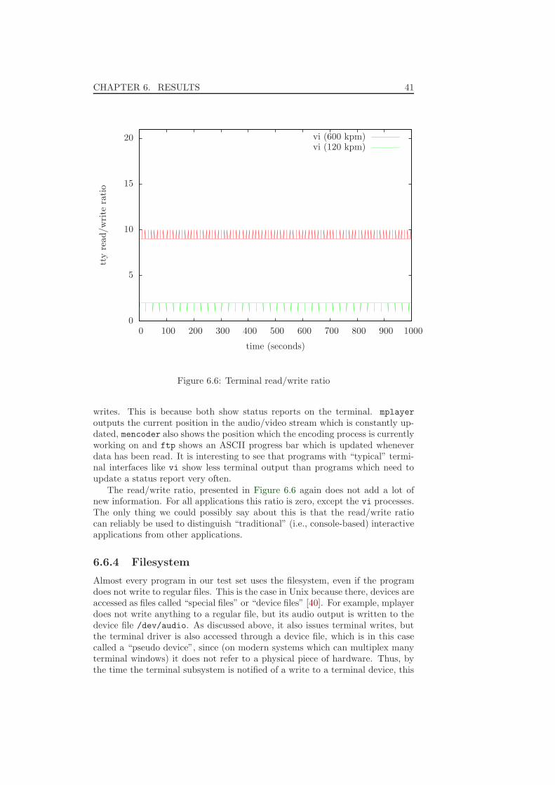
CHAPTER 6. RESULTS 41
0
5
10
15
20
0 100 200 300 400 500 600 700 800 900 1000
tty
read/w
rite
ratio
time (seconds)
vi (600 kpm)vi (120 kpm)
Figure 6.6: Terminal read/write ratio
writes. This is because both show status reports on the terminal. mplayer
outputs the current position in the audio/video stream which is constantly up-dated, mencoder also shows the position which the encoding process is currentlyworking on and ftp shows an ASCII progress bar which is updated wheneverdata has been read. It is interesting to see that programs with “typical” termi-nal interfaces like vi show less terminal output than programs which need toupdate a status report very often.
The read/write ratio, presented in Figure 6.6 again does not add a lot ofnew information. For all applications this ratio is zero, except the vi processes.The only thing we could possibly say about this is that the read/write ratiocan reliably be used to distinguish “traditional” (i.e., console-based) interactiveapplications from other applications.
6.6.4 Filesystem
Almost every program in our test set uses the filesystem, even if the programdoes not write to regular files. This is the case in Unix because there, devices areaccessed as files called “special files” or “device files” [40]. For example, mplayerdoes not write anything to a regular file, but its audio output is written to thedevice file /dev/audio. As discussed above, it also issues terminal writes, butthe terminal driver is also accessed through a device file, which is in this casecalled a “pseudo device”, since (on modern systems which can multiplex manyterminal windows) it does not refer to a physical piece of hardware. Thus, bythe time the terminal subsystem is notified of a write to a terminal device, this

42 6.6. ASSESSMENT OF FEATURES
0
200
400
600
800
1000
0 100 200 300 400 500 600 700 800 900 1000
FS
reads,
FS
wri
tes
time (seconds)
ftp writesmencoder reads
mencoder writesbzip2 reads
bzip2 writesmplayer reads
Figure 6.7: Filesystem activity on the high end
0
10
20
30
40
50
60
70
80
90
100
0 100 200 300 400 500 600 700 800 900 1000
FS
reads,
FS
wri
tes
time (seconds)
firefox readsfirefox writes
vi reads (120kpm)vi writes (120kpm)vi reads (600kpm)vi writes (600kpm)
mplayer writes
Figure 6.8: Filesystem activity on the low end

CHAPTER 6. RESULTS 43
0
5
10
15
20
0 100 200 300 400 500 600 700 800 900 1000
tty
read/w
rite
ratio
time (seconds)
mplayervi (600 kpm)vi (120 kpm)
mencoderfirefox
Figure 6.9: Filesystem read/write ratio
has already passed through the subsystem that deals with the filesystem.
The only application that does not interact with the file system is, oddlyenough, the find application. Even though find searches through the filesys-tem, it does not actually read from or write to any files. Because accessing thecontents of directories is not done through the same system calls as reading orwriting files, the filesystem feature handler does not register any activity forfind processes. This could be fixed by adding hooks for the features in thecorresponding kernel system call implementations.
In Figure 6.7, we see filesystem activity of applications which issue a largenumber of filesystem requests per second. ftp shows prominently in this graph,as it simply writes back to disk whatever it reads from the network. Comparethis band of the graph with Figure 6.2 and we see this relation clearly. Thebzip2 application has about an equal number of reads and writes, which overlapalmost entirely. The mencoder process writes out a quite consistent streamof information, however the reads include peaks of activity. It may be thatthese peaks correspond to small transitions in frames which means the decodingprocess can fetch the next frames quickly without having to do a lot of decodingwork, but this is only speculation. mplayer itself also shows peaks which couldbe of the same kind.
For the write behaviour of mplayer, we turn our attention to Figure 6.8,which shows the low end of the filesystem activity. From this graph, the bzip2
activity was excluded because it would obscure the other graphs, since it hassuch a wide graph. The mplayer graph ends up in this figure because there isa lot less data that mplayer needs to write (only audio, not video), resulting in

44 6.6. ASSESSMENT OF FEATURES
0 100 200 300 400 500 600 700 8000
250
500
750
1000
0
10
20
30
40
tty writes
firefoxftp
bzip2vi (120kpm)vi (600kpm)
mplayermencoder
find
socket reads
fs writes
tty writes
Figure 6.10: Filesystem, socket and tty features
smaller numbers than for the read activity. It is also much less erratic becausethe audio output must be very constant; the movie’s audio layer is encoded at aconstant frequency which needs to be maintained to produce the correct sounds.
We also see that firefox has very few filesystem requests. The few peaksare when web requests were made, and it read or wrote the received informationfrom or to its page and image cache. During reading and scrolling of the page, itdoes not exhibit any disk activity. Lastly, we have a look at the vi processes. Ifwe compare these graphs to Figure 6.5, we see that these do indeed, as noted atthe beginning of this section, correspond to the writes to the terminal (pseudo-)device file. Here, too, the reads and writes overlap so much they become almostindistinguishable.
The filesystem read/write ratio graph, presented in Figure 6.9 contains abit more information than the other read/write ratio graphs. On the left andright sides of the graph, we can see the “spikes” up to the maximum possiblevalue (which were cut off to keep the rest of the graph readable) for the firefoxprocess. These occur during time frames when the process reads but does notwrite. In the lower part of the figure, we also see the vi graphs from Figure 6.6repeated here, as expected. The mplayer and mencoder follow the graph ofthe reads for these processes. Again, we can conclude that the read/write ratiofeature does not add any information and could probably be discarded from thefeature set.

CHAPTER 6. RESULTS 45
010000
2000030000
400000
10000
20000
30000
40000
0
0.5
1
1.5
2
tty
firefoxftp
bzip2vi (120kpm)vi (600kpm)
mplayermencoder
find
socket
fs
tty
Figure 6.11: read/write ratios
6.6.5 Application classification
In this final subsection we will try to visualize the classification process forapplications. In Figure 6.10 we see the data points for our processes plottedacross three dimensions. The axes that can be seen are those of the numberof socket reads, filesystem writes and writes to the terminal device. From thisvisualization it again becomes clear that mencoder, bzip2 and ftp can bestbe identified by their filesystem writing activity. The correspondence betweensocket reads and filesystem writes for ftp which we noted earlier becomes veryprominent in this graph. There is another correspondence between two featuresthat becomes clear here, which we had not noticed before; namely that whenmencoder writes more to the disk, it also outputs more information to theterminal. This is logical, as it has to update the percentage that it has completedmore often if it has been able to write more to disk. What is interesting is thatfirefox can be better identified by its socket reads than became clear fromFigure 6.2, the 2d graph that displayed socket read and write activity acrosstime.
Further, the vi process belonging to the fast “typist” can be identified quitewell. However, the other vi process ends jumbled up with the find processand some parts of the firefox and bzip2 processes. Interestingly, the mplayer
process is reasonably easy to pick out, even without the audio feature.
To test the conclusion that the read/write ratios are mostly useless for clas-sifications, we tried to visualize the feature space with the read/write ratios forthe filesystem, sockets and terminal features. This is displayed in Figure 6.11.

46 6.6. ASSESSMENT OF FEATURES
As we can see, there is hardly any information in this plot. All the data pointscollapse on just a few values, and clusters from one process split far apart, whilevalues from different processes are clustered together. The only reasonably infor-mational feature is the terminal read/write ratio. This confirms the conclusionmade in the preceding sections, that the ratio is mostly a useless feature andshould be left out, except for the terminal and possibly the smoothed-out socketfeature (see Figure 6.3 and the accompanying description).

Chapter 7
Conclusion and future work
This thesis described how a neural network was integrated in an operating sys-tem. The implementation was described in detail; how process features can beobtained and used as input for a neural network, and how the output of thisnetwork can be used as a classification of the application. This output couldeven be used directly as a scheduler priority value. The goal of this was to rec-ognize multimedia applications automatically and schedule on a desktop systemwith a higher priority than less important “background” applications. Testingresults showed that this was reasonably successful, but that the features couldbe better.
Investigating the features resulted in the insight that the read and write fea-tures are quite useful for the processes that were studied, except for audio reads,but this feature could prove useful in situations with different types of processes.The read/write ratio was useless in all cases except the socket case, as no infor-mation was added by it that was not also in the reads or the writes themselves.It turned out that the socket read/write ratio feature, when smoothed out a lit-tle, was the distinguishing feature for the web browser process. The multimediaprocess could very easily be picked out by writes to the audio device and puredownloading could be picked out by the large number of reads from the networkand writes to disk. The application that walked the filesystem hierarchy (findin this study) was the only application that showed no activity on any of thefeatures. This could be remedied by modifying the filesystem feature such thatit would also note when an application simply traversed the file hierarchy, or byadding a new feature that does this.
The implementation is a proof-of-concept, but it was designed in a very mod-ular fashion. This makes it an ideal platform for testing new ways of classifyingprocesses without spending a disproportionate amount of time modifying orrewriting the existing scheduler. It allows researchers to freely experiment andto evaluate the influence of different metrics on process scheduling performance.Adding a new feature to the network is trivial and the effects can be observedinstantly with existing tools. Most new tools or modifications to measure orimprove performance are automatically independent of particular features, ben-efiting everyone. Hopefully, this helps giving research on uniprocessor schedulingthe impulse it needed.
Using a neural network to assign priorities instead of requiring the user tomanually assign them is a design that works pretty well on the desktop. The
47

48
results show that it visibly improves multimedia performance. In retrospect,on a server it should be less useful, because the variety of applications runningon any particular server is much smaller, and it could be more effective to letan administrator assign these priorities manually. Having the neural networkscheduler from this paper in a scheduler would not preclude this possibility, be-cause the server’s administrator could simply not load a network at all, therebykeeping manual control of all priority assignment.
Unfortunately, one of the most important aspects of scheduling multimediaapplications under Unix was not touched upon by this research simply because itwould be too big an undertaking. This would be gathering process feature datafrom the X windowing system. This is important because multimedia applica-tions are often graphics-intensive, and under Unix X is the system that drawswindows and all graphics output goes through X. For example, the “Human-Centered” metrics explored in the study of Etsion et al. (described in [23]) couldbe implemented as features for a neural network. Hopefully, this will providesome features that can strongly improve the scheduling on multimedia desk-top computers. This would require substantial modification of the X Windowsystem as well as the kernel in order to get the data from X to the kernel.
Another approach for making multimedia information available to the sched-uler would be to move the scheduler to an external process. This process coulddecide the “nice values” of other processes. This would be advantageous fordesktop environments, for example. Projects like the KDE or the GNOME desk-top environments could build a userspace-only scheduler. The advantage hereis that if every application’s operations are performed through the abstractionlayers provided by these desktop environments, more multimedia informationis available to the scheduler. Because the neural network part of the scheduleris in userspace, there is less overhead in the kernel. For example, desktop en-vironments often have an audio multiplexer application.1 These multiplexingprocesses should be able to register their feature with a scheduler in such a waythat the feature can be attributed to the process that requests its service. Asspeculated in section 6.1, OSes with a microkernel architecture should not needto implement such a complex system because they are designed around smallprocesses that perform system tasks and communicate with each other. This isa very promising architecture for implementing a neural network scheduler.
Another interesting subject for future research would be to use unsupervisedlearning techniques (for example Kohonen’s Self Organizing Map, as described in[29]). This could be done by having this network identify classes of applicationsand then presenting the user with these classes along with the names of theprocesses in that class. Then the user could assign the desired priority for eachclass. The memory system presented in this paper could be maintained bycreating a hybrid backpropagation network/Kohonen map. This can consist ofa memory and an input layer which are connected to an output layer of thesame size as the input layer. The resulting output can then be used as input tothe Kohonen map.
It is unfortunate that AI developments do not seem to have influenced re-searchers in the scheduling field and the Operating System field in general. Itwould be interesting to see what results would come from a higher degree of
1For example, KDE uses aRts (http://www.arts-project.org/) and Gnome uses Esound(http://developer.gnome.org/doc/whitepapers/esd/) to multiplex their audio.
CHAPTER 7. CONCLUSION AND FUTURE WORK 49
collaboration between the research areas in the future.
7.1 Personal notes
In this section I will describe what I have personally learned from this project.Implementing a neural network appears to be quite easy, but it becomes
very difficult when things go wrong. Debugging a neural network that does notcrash but does contain a bug is extremely difficult, in my opinion. If there isno particular point where anything goes wrong, one has to step through thenetwork code with a debugger. Even this is not necessarily very helpful if thenetwork appears to learn correctly in the first number of epochs. The little stepsdo not give a “big picture” of what is happening, and one can easily get lost indetails.
All of this means that the implementation of the neural network took avery long time. It took so much longer than expected that there was not a lotof time left for large-scale experimentation and measurements of effectivenessof features. Also because of this, it was very disappointing to see that theevaluation of the work focused only on the thesis and not on what constitutedthe bulk of the work and in which most time was invested, namely the code.
Before this project, I was under the impression that neural networks areformalized in a mathematical model. I learned that this may be true in theory,but that in practice there are many common issues that can only be solvedempirically. For example, determining the best number of hidden units, andthe best values for the learning rate and momentum are a matter of trying outwhat works best for the particular test set under consideration.
Another issue was that a network’s activation function can make a world ofdifference. When the test set has continuous (instead of binary) target outputs,the best activation function is a simple linear function. In retrospect, this is veryobvious, but at the time of implementation it was something I had not thoughtabout. I also did not expect that backprop would be such a slow algorithm. Itis the standard algorithm taught in neural network courses and tutorials, but itis unacceptably slow for real-world applications. If this was known beforehand,perhaps a different training algorithm could have been chosen.
The fact that floating point instructions can not be used in an OS kernelwas quite surprising to me. After a short discussion on the NetBSD kernelmailing list, it became clear that there is no decent solution for this problem ina portable OS. Certain systems might have no FPU (Floating Point Unit) atall and on most architectures, saving and restoring the FPU registers are suchslow operations that the overhead is unacceptable. Implementing fixed point isnot very difficult, but it is very prone to errors. This was the source of quite anumber of bugs.
The helper progstarter program was written in a bit of a hurry, as well asthe nnread and nnwrite modules (which read and write a network from a file).I did not spend much time thinking about them and wrote the code quickly,expecting that I would not have to work with the code much after creating them.Unfortunately, this assumption was not true. After some attempts to extendnnread and nnwrite, I decided to completely rewrite these functions and alsochange the file format. The code is a lot cleaner now, but the file format is stillvery much a hack. The total time I spent writing and rewriting these modules

50 7.1. PERSONAL NOTES
could probably have been spent better by designing a good, extensible formatand writing a real parser for it using, for example, lex and yacc instead offscanf. Progstarter was extended without having to rewrite it, but thesechanges cost more time than they should.

Appendix A
Correction of the
Turing-completeness proof
for NNs
The proof given in the diploma thesis [18] is not entirely correct. There is asmall error that will be discussed here. The author apparently forgot that anaspect of his model required more bookkeeping than he uses in his proof.
The paper consists of a long path of proofs by simulation, starting from Tur-ing machines, simulating these in stack machines, going from there to countermachines, adder machines, alarm clock machines, restless counters and finallysigmoidal neural networks, thus proving that these neural networks can simu-late Turing machines. In other words, sigmoidal neural networks are Turing-complete. I will assume the reader has read the paper in question.
The flaw is in the proof of Proposition 3.3.1. To repeat the proposition:
Proposition 3.3.1 An acyclic k-adder machine can be simulated by a (k2 +k + 4)-restless counter machine.
This proposition should be modified to read:
Proposition 3.3.1’ An acyclic k-adder machine can be simulated by a (k2 +k + 8)-restless counter machine.
We already know from Proposition 3.2.1 that an acyclic k-adder machine
D that computes in time T can be simulated by a (k2+k2 +2)-alarm clock machine
in time O(T 3).
A.1 Background
Like in the original paper, we are simulating an alarm clock machine in a restlesscounter machine. An alarm clock machine (which is in turn used to simulate anadder machine) consists of a number of timers which all hold a number. Thisnumber represents the number of time steps it takes for them to wind down
51

52 A.1. BACKGROUND
0
1
2
3
4
5
0 2 4 6 8 10 12 14 16 18 20 22 24 26 28
counte
rva
lue
time (t)
morningevening
Figure A.1: One simulated alarm clock

APPENDIX A. CORRECTION OF THE TURING-COMPLETENESSPROOF FOR NNS 53
and “sound an alarm”. In a normal situation, every time step every clock’snumber decreases by one. The machine is described by a transition functionδ : {0, 1}5k → 2{delay(i),lengthen(i):1≤i≤k}∪{halt}. The domain of δ is {0, 1}5k
because we need to remember the last 5 time steps for our simulation of anadder machine. A 1 at position 5k + i in the vector means alarm clock Ai
alarmed at timestep k. The information about an alarm clock’s period andtime to alarm is the input for the machine. The alarm clocks can be delay-ed or lengthen-ed by finite control, which means either the time to alarm isincreased by one (delay) or both the time to alarm and the period are increasedby one (lengthen).
To simulate an acyclic adder machine D with adders D1, ..., Dk, we use analarm clock machine with clocks A0, A1, ..., Ak, A00, Aij : 1 ≤ i < j ≤ k. Theclocks A1, ..., Ak are used to simulate D1, ..., Dk, the clocks A00 and A0 are usedto synchronize the machine. If any clock alarms simultaneously with A00, it getsdelayed. If A00 and A0 alarm simultaneously, the delay and lengthen operationsare completed and a new cycle can begin. For more details, please refer to [18].
A.2 Proof
In the restless counter machine, every alarm clock Ai is simulated by two restlesscounters, a morning (Mi) and an evening (Ei)
1 counter. The period of the clockis represented by the duration of the cycle of the two counters. The time toalarm is represented by the time it takes the morning counter to hit zero. SeeFigure A.1 for a depiction of this process.
Two counters for every alarm clock in the alarm clock machine gives us thefollowing number of counters if we use the alarm clock to simulate an acyclick-adder machine:
(k2 + k
2+ 2) ∗ 2 = (k2 + k + 4) (A.1)
An alarm clock that goes off corresponds to its morning counter hitting 0. Analarm clock’s counters are said to be in the morning from the point the morningcounter starts counting upwards from 0, and we are in the evening from thepoint the evening counter is counting upwards from 0 (intuitively speaking,alarm clocks generally go off in the morning).
Mi and Ei will be in a cycle with a phase shift of 2p time steps as describedin the original paper. It will count up to 2p − 1 and then it will count backto 0 and stay there for two additional time steps, before it will start to countup again, as we can observe in Figure A.1. To be able to distinguish the threestates at which the counter is 0 (the zero states) when we refer to them, twonew zero values are introduced, 0′ and 0′′. When a counter reaches 0, finitecontrol will wake up and set the associated counter’s direction to Down. So ifEi hits 0 at time t, Mi starts to drop at t + 1, and vice-versa. This causes thepair of counters to cycle with period 4p, simulating one alarm clock of periodp. The mistake in the original paper is in the implementation of the delay andlengthen operations. These work as follows:
• Delay. To delay we switch the direction of the corresponding morningand evening counters for a duration of two time steps. Since finite control
1This includes the Aij counters.

54 A.2. PROOF
0
1
2
3
4
5
6
7
8
0 2 4 6 8 10 12 14 16 18 20 22 24 26 28
counte
rva
lue
time (t)
morningevening
Figure A.2: Lengthening a clock in the morning
only wakes up when a counter hits 0, there must be a timer that hits 0 atthe end of the two time steps in order to be able to revert the directionback to normal again. The original paper does not provide a counter likethis. We will first look at the other operation, lengthen, before we try tofix this.
• Lengthen while in the morning. To lengthen Ai when in the morning,its evening counter, Ei, will be incremented for one timestep and thenchanged back to normal. This causes an (intended) delay which results inthe evening counter dropping to 0 four timesteps later than would normallybe the case. See Figure A.2 for clarification. Before the delay operation,we see that the period is 10 since after hitting 0 it takes an additional 10time steps for the morning counter to hit 0 again. We will need anotherextra counter that hits zero to be able to turn it back around.
• Lengthen while in the evening. Lengthen-ing Ai when it is in theevening is more problematic. Simply changing the evening counter likewe do when in the morning does not work, because the morning counterhits zero before the evening counter. The delay that is implicit in thelengthen operation does not take effect then. The morning counter willsimply continue decreasing until it hits 0, as if nothing happened. Thismeans the period will be longer from then on. Changing the morningcounter directly like we changed the evening counter is effective, but thedelay caused by this is only half a delay. Consider Figure A.3(a). We

APPENDIX A. CORRECTION OF THE TURING-COMPLETENESSPROOF FOR NNS 55
0
1
2
3
4
5
6
7
8
0 2 4 6 8 10 12 14 16 18 20 22 24 26 28
counte
rva
lue
time (t)
morningevening
(a) Wrong attempt
0
1
2
3
4
5
6
7
8
0 2 4 6 8 10 12 14 16 18 20 22 24 26 28
counte
rva
lue
time (t)
morningevening
(b) Correct attempt
Figure A.3: Two attempts at lengthening a clock in the evening

56 A.2. PROOF
t c0 c1 c2 c3 Partial output (c0, c1, c2, c3)0 (0, Down) (1, Down) (0′′, Up) (0′, Up) (U, N, D, N)1 (0′, Up) (0, Down) (1, Down) (0′′, Up) (N, I, N, D)2 (0′′, Up) (0′, Up) (0, Down) (1, Down) (D, N, I, N)3 (1, Down) (0′′, Up) (0′, Up) (0, Down) (N, D, N, I)4 (0, Down) (1, Down) (0′′, Up) (0′, Up) (U, N, D, N)
Table A.1: State changes of the extra control counters
can see that the original period is 10. When we do a lengthen operationon the morning counter (similar to the evening situation), it will hit 0two timesteps later, making the effective period of the previous cycle 12.On the other hand, the period has become 14, as we can see from themorning counter’s graph to the right of t = 12. This means the initialdelay is half from what it is supposed to be. Recall that one timestepof the alarm clock machine is simulated by four timesteps of the restlesscounter machine. Thus, the delay is half a timestep of the alarm clockmachine.
The correct way to get the implicit delay when in the evening is to delaythe morning counter twice. Doubling the delay of Figure A.3(a) causesit to be a delay of one timestep in the alarm clock machine. This causesa new problem. The lengthening was correct in our previous attempt,only the delay needed to be fixed. By doing the operation twice, thelengthening is doubled too. This means that a lengthen operation wouldcause a lengthening of two timesteps. To remedy this, we also have tocause a delay in the evening counter, as shown in Figure A.3(b).
Only when A00 hits 0 in the alarm clock machine there will be an action ofthe finite control, and this translates to M00 hitting 0 in our restless countermachine. Only then will there be a delay or lengthen operation taking place.The lengthen operation in the evening requires a counter to hit zero everytimestep, because it requires four changes in direction. So, we will need at leastthree extra counters, one for each timestep after M00 hits 0 (one or two will notbe enough, because we can only take action on a counter hitting 0. 0′ and 0′′
do not wake up finite control). Naturally, the other operations can “borrow”these counters.
Because every timestep of the alarm clock machine is simulated by fourtimesteps of the restless counter machine, we want our newly added “controlcounters” to oscillate with period 4. The state changes can be observed in detailfrom Table A.1.2 Because M00 does not necessarily hit zero every simulated
2Here the Up direction is used in all zero states except the first. The original paper doesnot clearly specify if 0’ is greater than 0 (in the ordering laid down by Up and Down) or ifthe Up/Down directions even have any effect on counters in the zero states. Since they must
remain in the zero position for two timesteps, the actual direction encoded is irrelevant. Itis unambiguous which state the counter will be in after any of the zero positions. The onlyimportant aspect is that when it leaves the last zero state, 0′, it should go to the state (1, Up).Using Up throughout the zero states except the first is perhaps the best choice conceptually,because directions may only be changed at zero events. This way, counters can switch theirown direction unaided from Down to Up when hitting 0, thus going through these phases:

APPENDIX A. CORRECTION OF THE TURING-COMPLETENESSPROOF FOR NNS 57
time step (it can be lengthened too), we require an extra counter to keep ourcounters under control. This is the fourth counter in Table A.1. Essentially itkeeps c1 from spinning off when M00 does not hit 0. The last column displaysa partial output of the mapping that is the restless counter machine, namelythe values for the four counters under consideration. N means No change, I
means Increase from next timestep onwards and D means Decrease from nexttimestep onwards. All that is left to do when these changes are applied is toadd mappings to the function that defines the machine to ensure the delayed orlengthened operations are completed by reversing the affected counters again.
In conclusion, we add these four counters to Equation A.1 and we end upwith:
(k2 + k + 4) + 4 = (k2 + k + 8) (A.2)
which is what our modified version of the original proposition (Proposition
3.3.1’) reads.
(0, Down) → (0′, Up) → (0′′, Up). from 0, then going Up because it changed. From thisfollows that 0 > 0′ and 0′ < 0′′.

Bibliography
[1] Mike Accetta, Robert Baron, William Bolosky, David Golub, RichardRashid, Avadis Tevenian Jr., and Michael Young. Mach: A new kernelfoundation for UNIX development. In Proceedings of the USENIX Summerconference, pages 93–112. USENIX Association, June 1986. 6.2
[2] Aristoklis D. Anastasiadis, George D. Magoulas, and Michael N. Vrahatis.A new learning rates adaptation strategy for the resilient propagation algo-rithm. In Proceedings of the 12th European Symposium on Neural Networks(ESANN-04), April 2004. 6.2
[3] Thomas E. Anderson, Brian N. Berschad, Edward D. Lazowska, andHenry M. Levy. Scheduler activations: Effective kernel support for theuser-level management of parallelism. In ACM Transactions on ComputerSystems, volume 10, pages 53–79. University of Washington, ACM, Febru-ary 1992. 2.4
[4] Apple Computer, Inc., 1 Infinite Loop, Cupertino, CA. Kernel Program-ming, 2005. Available from http://developer.apple.com. 6.2
[5] Moshe Bar. The linux process model. Linux Journal, 71, March 2000. 2.4
[6] Paul Barham, Boris Dragovic, Keir Fraser, Steven Hand, Tim Harris, AlexHo, Rolf Neugebauer, Ian Pratt, and Andrew Warfield. Xen and the artof virtualization. In ACM SIGOPS Operating Systems Review, volume 37,pages 164–177. ACM, December 2003. 2
[7] Paul Barton-Davis, Dylan McNamee, Raj Vaswani, and Edward D. La-zowska. Adding scheduler activations to mach. Technical Report 92-08-03,Department of Computer Science and Engineering University of Washing-ton, Seattle, Washington 98195, March 1993. 2.4
[8] Fabrice Bellard. QEMU, a fast and portable dynamic translator. In Pro-ceedings of the FREENIX Track: 2005 USENIX Annual Technical Confer-ence, pages 41–46. USENIX Association, April 2005. 2
[9] William G. Bulgren and Lee-Ho Hwang. A simulation study of time-slicingin non-exponential service environments. In ANSS ’80: Proceedings of the13th annual symposium on Simulation, pages 161–180, Piscataway, NJ,USA, 1980. IEEE Press. 2.3
[10] Leslie Burkholder. The halting problem. SIGACT News, 18(3):48–60, 1987.2.2
58
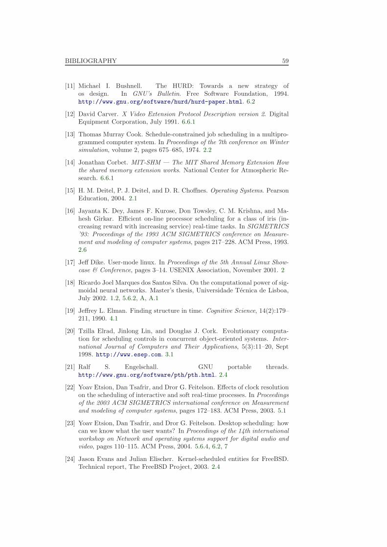
BIBLIOGRAPHY 59
[11] Michael I. Bushnell. The HURD: Towards a new strategy ofos design. In GNU’s Bulletin. Free Software Foundation, 1994.http://www.gnu.org/software/hurd/hurd-paper.html. 6.2
[12] David Carver. X Video Extension Protocol Description version 2. DigitalEquipment Corporation, July 1991. 6.6.1
[13] Thomas Murray Cook. Schedule-constrained job scheduling in a multipro-grammed computer system. In Proceedings of the 7th conference on Wintersimulation, volume 2, pages 675–685, 1974. 2.2
[14] Jonathan Corbet. MIT-SHM — The MIT Shared Memory Extension Howthe shared memory extension works. National Center for Atmospheric Re-search. 6.6.1
[15] H. M. Deitel, P. J. Deitel, and D. R. Choffnes. Operating Systems. PearsonEducation, 2004. 2.1
[16] Jayanta K. Dey, James F. Kurose, Don Towsley, C. M. Krishna, and Ma-hesh Girkar. Efficient on-line processor scheduling for a class of iris (in-creasing reward with increasing service) real-time tasks. In SIGMETRICS’93: Proceedings of the 1993 ACM SIGMETRICS conference on Measure-ment and modeling of computer systems, pages 217–228. ACM Press, 1993.2.6
[17] Jeff Dike. User-mode linux. In Proceedings of the 5th Annual Linux Show-case & Conference, pages 3–14. USENIX Association, November 2001. 2
[18] Ricardo Joel Marques dos Santos Silva. On the computational power of sig-moidal neural networks. Master’s thesis, Universidade Tecnica de Lisboa,July 2002. 1.2, 5.6.2, A, A.1
[19] Jeffrey L. Elman. Finding structure in time. Cognitive Science, 14(2):179–211, 1990. 4.1
[20] Tzilla Elrad, Jinlong Lin, and Douglas J. Cork. Evolutionary computa-tion for scheduling controls in concurrent object-oriented systems. Inter-national Journal of Computers and Their Applications, 5(3):11–20, Sept1998. http://www.esep.com. 3.1
[21] Ralf S. Engelschall. GNU portable threads.http://www.gnu.org/software/pth/pth.html. 2.4
[22] Yoav Etsion, Dan Tsafrir, and Dror G. Feitelson. Effects of clock resolutionon the scheduling of interactive and soft real-time processes. In Proceedingsof the 2003 ACM SIGMETRICS international conference on Measurementand modeling of computer systems, pages 172–183. ACM Press, 2003. 5.1
[23] Yoav Etsion, Dan Tsafrir, and Dror G. Feitelson. Desktop scheduling: howcan we know what the user wants? In Proceedings of the 14th internationalworkshop on Network and operating systems support for digital audio andvideo, pages 110–115. ACM Press, 2004. 5.6.4, 6.2, 7
[24] Jason Evans and Julian Elischer. Kernel-scheduled entities for FreeBSD.Technical report, The FreeBSD Project, 2003. 2.4

60 BIBLIOGRAPHY
[25] Scott E. Fahlman. An empirical study of learning speed in back-propagationnetworks. Technical Report CMU-CS-88-162, Carnegie-Mellon University,September 1988. 6.2
[26] Wu-chun Feng and Jane W.-S. Liu. Algorithms for scheduling real-timetasks with input error and end-to-end deadlines. IEEE Trans. Softw. Eng.,23(2):93–106, 1997. 2.6
[27] Mario J. Gonzalez, Jr. Deterministic processor scheduling. In ACM Com-puting Surveys, volume 9, pages 173–204, September 1977. 2.2
[28] Brian Hook. An introduction to fixed point math. Book of Hook, September2004. Available from http://www.bookofhook.com. 5.6.1
[29] Teuvo Kohonen. The ‘neural’ phonetic typewriter. Computer, 21(3):11–22,1988. 3.5, 7
[30] Robert Love. Linux Kernel Development. Novell Press, 2nd edition, 2005.2.4
[31] Jared D McNeill. NetBSD/usermode. E-mail tothe NetBSD tech-kern mailinglist, December 2007.http://mail-index.netbsd.org/tech-kern/2007/12/28/0001.html. 2
[32] Microsoft Corporation. MS Windows NT kernel-mode user and GDI whitepaper. Available from http://technet.microsoft.com. 6.2
[33] Jason Nieh, James G. Hanko, J. Duane Northcutt, and Gerard A. Wall.SVR4 UNIX scheduler unacceptable for multimedia applications. InD. Shepherd, G. Blair, G. Coulson, N. Davies, and F. Garcia, editors,Proceedings of the 4th International Workshop on Network and Operat-ing System Support for Digital Audio and Video, volume 846 of LectureNotes in Computer Science, pages 41–53, Lancaster, U.K., November 1993.Springer-Verlag. 1
[34] Jason Nieh and Monica S. Lam. A smart scheduler for multimedia appli-cations. ACM Trans. Comput. Syst., 21(2):117–163, 2003. 2.6
[35] John K. Ousterhout. Why aren’t operating systems getting faster as fastas hardware? In Proceedings of the USENIX Summer conference, pages247–256. USENIX Association, 1990. 1.1.1
[36] Christopher Provenzano. Portable threads library.ftp://sipb.mit.edu/pub/pthreads/. 2.4
[37] QNX Software Systems Ltd., 175 Terence Matthews Crescent, Kanata, On-tario, Canada. System Architecture (QNX Neutrino 6.2.1), 2003. Availablefrom http://www.qnx.com. 6.2
[38] J. R. Quinlan. Comparing connectionist and symbolic learning methods.In Computational Learning Theory and Natural Learning Systems, volumeI: Constraints and Prospects, pages 445–456. MIT Press, 1994. 3.2, 3.5
[39] Martin Riedmiller. Rprop - description and implementation details. Tech-nical report, University of Karlsruhe, January 1994. 6.2
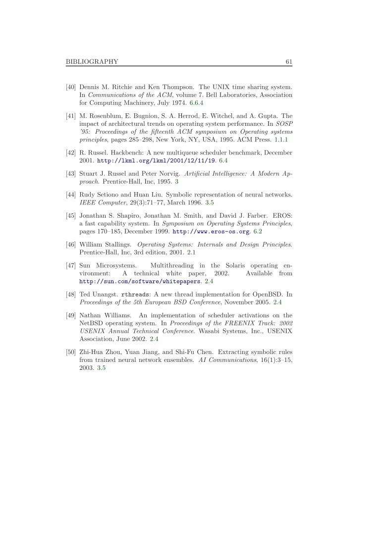
BIBLIOGRAPHY 61
[40] Dennis M. Ritchie and Ken Thompson. The UNIX time sharing system.In Communications of the ACM, volume 7. Bell Laboratories, Associationfor Computing Machinery, July 1974. 6.6.4
[41] M. Rosenblum, E. Bugnion, S. A. Herrod, E. Witchel, and A. Gupta. Theimpact of architectural trends on operating system performance. In SOSP’95: Proceedings of the fifteenth ACM symposium on Operating systemsprinciples, pages 285–298, New York, NY, USA, 1995. ACM Press. 1.1.1
[42] R. Russel. Hackbench: A new multiqueue scheduler benchmark, December2001. http://lkml.org/lkml/2001/12/11/19. 6.4
[43] Stuart J. Russel and Peter Norvig. Artificial Intelligence: A Modern Ap-proach. Prentice-Hall, Inc, 1995. 3
[44] Rudy Setiono and Huan Liu. Symbolic representation of neural networks.IEEE Computer, 29(3):71–77, March 1996. 3.5
[45] Jonathan S. Shapiro, Jonathan M. Smith, and David J. Farber. EROS:a fast capability system. In Symposium on Operating Systems Principles,pages 170–185, December 1999. http://www.eros-os.org. 6.2
[46] William Stallings. Operating Systems: Internals and Design Principles.Prentice-Hall, Inc, 3rd edition, 2001. 2.1
[47] Sun Microsystems. Multithreading in the Solaris operating en-vironment: A technical white paper, 2002. Available fromhttp://sun.com/software/whitepapers. 2.4
[48] Ted Unangst. rthreads: A new thread implementation for OpenBSD. InProceedings of the 5th European BSD Conference, November 2005. 2.4
[49] Nathan Williams. An implementation of scheduler activations on theNetBSD operating system. In Proceedings of the FREENIX Track: 2002USENIX Annual Technical Conference. Wasabi Systems, Inc., USENIXAssociation, June 2002. 2.4
[50] Zhi-Hua Zhou, Yuan Jiang, and Shi-Fu Chen. Extracting symbolic rulesfrom trained neural network ensembles. AI Communications, 16(1):3–15,2003. 3.5