Embed Size (px)
Citation preview
University of South Carolina University of South Carolina
Scholar Commons Scholar Commons
Theses and Dissertations
Summer 2019
Implementation of View Factor Model and Radiative Heat Transfer Implementation of View Factor Model and Radiative Heat Transfer
Model in MOOSE Model in MOOSE
Abdurrahman Ozturk
Follow this and additional works at: https://scholarcommons.sc.edu/etd
Part of the Nuclear Engineering Commons
Recommended Citation Recommended Citation Ozturk, A.(2019). Implementation of View Factor Model and Radiative Heat Transfer Model in MOOSE. (Master's thesis). Retrieved from https://scholarcommons.sc.edu/etd/5348
This Open Access Thesis is brought to you by Scholar Commons. It has been accepted for inclusion in Theses and Dissertations by an authorized administrator of Scholar Commons. For more information, please contact [email protected].
IMPLEMENTATION OF VIEW FACTOR MODEL
AND RADIATIVE HEAT TRANSFER MODEL IN MOOSE
by
Abdurrahman Ozturk
Bachelor of Science
Hacettepe University, 2012
Submitted in Partial Fulfillment of the Requirements
For the Degree of Master of Science in
Nuclear Engineering
College of Engineering and Computing
University of South Carolina
2019
Accepted by:
Travis W. Knight, Director of Thesis
Benjamin Spencer, Reader
Cheryl L. Addy, Vice Provost and Dean of the Graduate School

ii
© Copyright by Abdurrahman Ozturk, 2019
All Rights Reserved.

iii
DEDICATION
This work is dedicated to my family who has never given up supporting me. I also
want to dedicate this work to any person who has contribution on me during my life.

iv
ACKNOWLEDGEMENTS
This material is based upon work partially supported by the U.S. Department of
Energy NEUP IRP program under award agency number DE-NE-0008531. I also would
like to acknowledge Dr. Travis W. Knight and Dr. Benjamin Spencer for his guidance
and encouragement throughout the course of this research.
v
ABSTRACT
View factors are functions that represent the geometric relationship between
surfaces. They are important parameters for radiative heat transfer calculations. View
factor catalogues are available for simple geometries in the current literature. However, in
the case of complicated geometry, analytical or numerical methods are needed to evaluate
view factors. The Monte Carlo (MC) method is the most flexible one among numerical
methods, which are used to calculate view factors, since it can be applied to any
geometry.
When experimental studies are not affordable to conduct, modeling of
engineering problems gains more importance. Idaho National Laboratory (INL)’s finite
element framework Multiphysics Object Oriented Simulation Environment (MOOSE) is
a robust engineering tool to model physical problems including heat transfer. However,
MOOSE doesn’t have a method to calculate view factors. Hence, a method is needed to
calculate radiative heat transfer using view factors. Implementing a new model in
MOOSE and using it in heat transfer calculations for an arbitrary geometry will enable
the detailed evaluation of radiative heat transfer in complex geometries.
In this study, a nuclear fuel pellet heating and cracking experimental case is
modeled as a sample case by using the new MOOSE methods that are implemented in
this study. The effect of radiative heat transfer on radial and axial temperature profile is
evaluated.
vi
TABLE OF CONTENTS
DEDICATION ................................................................................................................... iii
ACKNOWLEDGEMENTS ............................................................................................... iv
ABSTRACT .........................................................................................................................v
LIST OF TABLES ........................................................................................................... viii
LIST OF FIGURES ........................................................................................................... ix
LIST OF SYMBOLS ........................................................................................................ xii
LIST OF ABBREVIATIONS .......................................................................................... xiii
CHAPTER 1: INTRODUCTION AND MOTIVATION ....................................................1
CHAPTER 2: LITERATURE REVIEW .............................................................................3
2.1. THEORY ................................................................................................................3
2.2. LITERATURE REVIEWS ...................................................................................10
2.3. FINITE ELEMENT MODELING (MOOSE) ......................................................11
CHAPTER 3: METHODOLOGY .....................................................................................14
3.1. MONTE CARLO METHOD ................................................................................14
3.2. MOOSE MESH STRUCTURE ............................................................................14
3.3. MOOSE USER OBJECTS ...................................................................................16
3.4. VIEW FACTOR MODEL ....................................................................................17
3.5. RADIATIVE HEAT TRANSFER MODEL ........................................................48

vii
CHAPTER 4: RESULTS AND DISCUSSION .................................................................50
4.1. PARALLEL RECTANGLES ...............................................................................51
4.2. PERPENDICULAR RECTRANGLES ................................................................55
4.3. COAXIAL DISKS ................................................................................................59
4.4. COAXIAL CYLINDERS .....................................................................................61
4.5. CONCENTRIC SPHERES ...................................................................................62
4.6. CASE STUDY: MODELING OF PELLET HEATING EXPERIMENT ............63
CHAPTER 5: CONCLUSION ..........................................................................................69
BIBLIOGRAPHY ..............................................................................................................70
viii
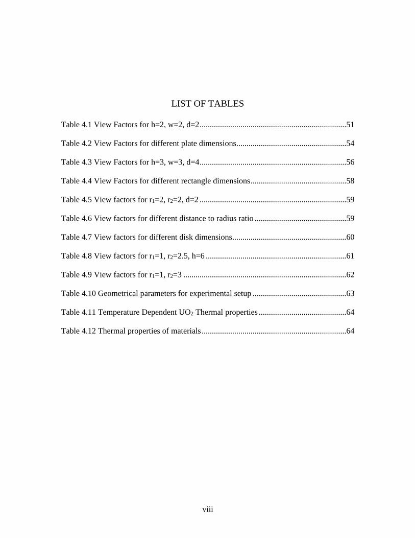
LIST OF TABLES
Table 4.1 View Factors for h=2, w=2, d=2 ........................................................................51
Table 4.2 View Factors for different plate dimensions......................................................54
Table 4.3 View Factors for h=3, w=3, d=4 ........................................................................56
Table 4.4 View Factors for different rectangle dimensions ...............................................58
Table 4.5 View factors for r1=2, r2=2, d=2 ........................................................................59
Table 4.6 View factors for different distance to radius ratio .............................................59
Table 4.7 View factors for different disk dimensions........................................................60
Table 4.8 View factors for r1=1, r2=2.5, h=6 .....................................................................61
Table 4.9 View factors for r1=1, r2=3 ................................................................................62
Table 4.10 Geometrical parameters for experimental setup ..............................................63
Table 4.11 Temperature Dependent UO2 Thermal properties ...........................................64
Table 4.12 Thermal properties of materials .......................................................................64
ix
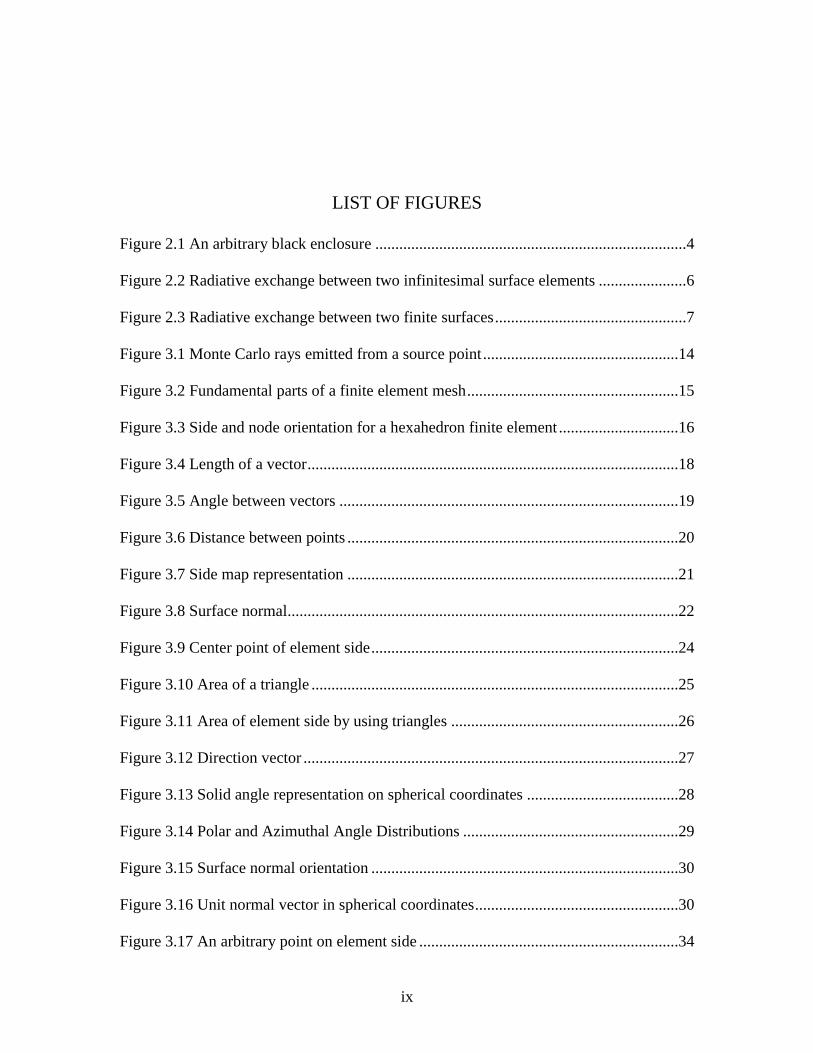
LIST OF FIGURES
Figure 2.1 An arbitrary black enclosure ..............................................................................4
Figure 2.2 Radiative exchange between two infinitesimal surface elements ......................6
Figure 2.3 Radiative exchange between two finite surfaces ................................................7
Figure 3.1 Monte Carlo rays emitted from a source point .................................................14
Figure 3.2 Fundamental parts of a finite element mesh .....................................................15
Figure 3.3 Side and node orientation for a hexahedron finite element ..............................16
Figure 3.4 Length of a vector .............................................................................................18
Figure 3.5 Angle between vectors .....................................................................................19
Figure 3.6 Distance between points ...................................................................................20
Figure 3.7 Side map representation ...................................................................................21
Figure 3.8 Surface normal..................................................................................................22
Figure 3.9 Center point of element side .............................................................................24
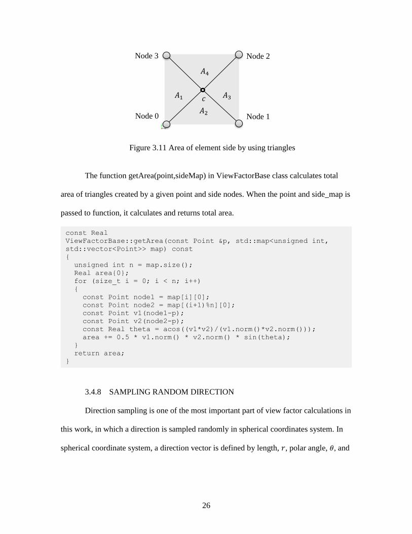
Figure 3.10 Area of a triangle ............................................................................................25
Figure 3.11 Area of element side by using triangles .........................................................26
Figure 3.12 Direction vector ..............................................................................................27
Figure 3.13 Solid angle representation on spherical coordinates ......................................28
Figure 3.14 Polar and Azimuthal Angle Distributions ......................................................29
Figure 3.15 Surface normal orientation .............................................................................30
Figure 3.16 Unit normal vector in spherical coordinates ...................................................30
Figure 3.17 An arbitrary point on element side .................................................................34
x
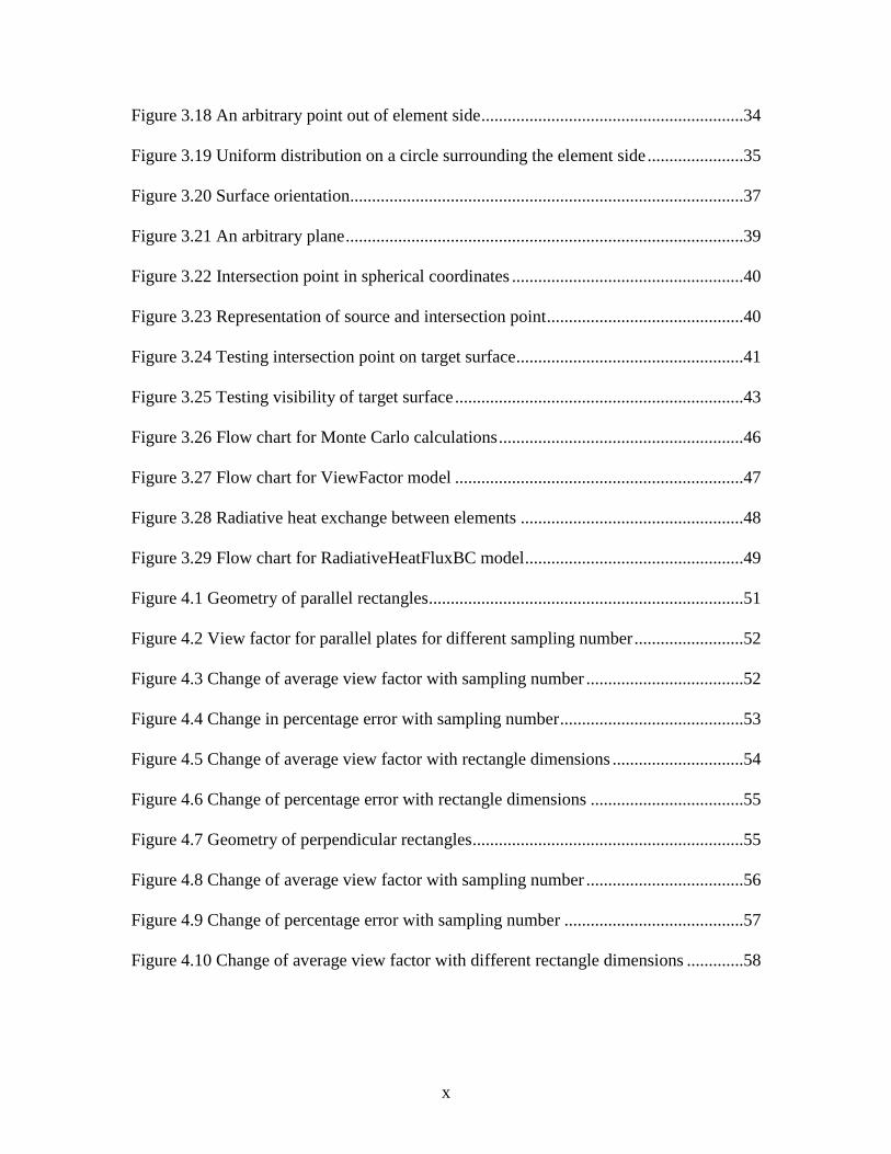
Figure 3.18 An arbitrary point out of element side ............................................................34
Figure 3.19 Uniform distribution on a circle surrounding the element side ......................35
Figure 3.20 Surface orientation..........................................................................................37
Figure 3.21 An arbitrary plane ...........................................................................................39
Figure 3.22 Intersection point in spherical coordinates .....................................................40
Figure 3.23 Representation of source and intersection point .............................................40
Figure 3.24 Testing intersection point on target surface ....................................................41
Figure 3.25 Testing visibility of target surface ..................................................................43
Figure 3.26 Flow chart for Monte Carlo calculations ........................................................46
Figure 3.27 Flow chart for ViewFactor model ..................................................................47
Figure 3.28 Radiative heat exchange between elements ...................................................48
Figure 3.29 Flow chart for RadiativeHeatFluxBC model ..................................................49
Figure 4.1 Geometry of parallel rectangles ........................................................................51
Figure 4.2 View factor for parallel plates for different sampling number .........................52
Figure 4.3 Change of average view factor with sampling number ....................................52
Figure 4.4 Change in percentage error with sampling number ..........................................53
Figure 4.5 Change of average view factor with rectangle dimensions ..............................54
Figure 4.6 Change of percentage error with rectangle dimensions ...................................55
Figure 4.7 Geometry of perpendicular rectangles ..............................................................55
Figure 4.8 Change of average view factor with sampling number ....................................56
Figure 4.9 Change of percentage error with sampling number .........................................57
Figure 4.10 Change of average view factor with different rectangle dimensions .............58

xi
Figure 4.11 Geometry of coaxial disks ..............................................................................59
Figure 4.12 Change of average view factor with distance to radius ratio ..........................60
Figure 4.13 Change of average view factor with disk radius ............................................60
Figure 4.14 Geometry of coaxial cylinders ........................................................................61
Figure 4.15 Geometry of concentric spheres .....................................................................62
Figure 4.16 Geometry representation of experimental setup .............................................63
Figure 4.17 Computation model of experimental setup .....................................................64
Figure 4.18 Pellet centerline temperature for only concentric cylinders ...........................66
Figure 4.19 Pellet centerline temperature for computational geometry ............................67
Figure 4.20 Axial temperature profile in pellet .................................................................67
Figure 4.21 Radial temperature profile in pellet ................................................................68

xii
LIST OF SYMBOLS
F View factor
Fij View factor between surfaces i and j
q Heat flux
Unit direction vector
n Surface normal
N Total number of sampled rays
m Number of rays hitting target surface
E Emissive Power

xiii
LIST OF ABBREVIATIONS
CDF ................................................................................. Cumulative Distribution Function
FEM ................................................................................................. Finite Element Method
INL .............................................................................................. Idaho National Laboratory
JFNK ...................................................................................... Jacobian-free Newton Krylov
LWR ...................................................................................................... Light Water Reactor
MBM ....................................................................................... MOOSE-BISON-MARMOT
MC .................................................................................................................... Monte Carlo
MOOSE..........................................Multiphysics Object Oriented Simulation Environment
PDF .................................................................................. Probability Distribution Function
RIA .......................................................................................... Reactivity Initiated Accident
TREAT ................................................................................. Transient Reactor Test Facility
USC ......................................................................................... University of South Carolina

1
CHAPTER 1
INTRODUCTION AND MOTIVATION
Heat or energy is one of the main driving forces for transition from non-
equilibrium state to steady state for a system. The system might be as complicated as a
nuclear power plant or as simple as an ice cream. In almost all areas of science, it is
essential to account for heat transfer to analyze the system correctly.
Heat is transferred by three mechanisms which are conduction in solids,
convection of fluids and radiation between surfaces that are at high enough temperatures.
In processes which require high temperatures such as power generation, combustion
applications, heat treatment experiments and solar energy applications radiative heat
transfer becomes significant and should be taken into consideration besides conduction
and convection.[1]
In nuclear science, modeling is important because of the difficulty and safety
concerns in experimental studies. Heat transfer, neutron transport, thermal hydraulic,
fluid dynamics, material science are popular topics that researchers are developing
computer codes to analyze systems. The finite element framework Multiphysics-Object-
Oriented-Simulation-Environment (MOOSE), which is developed by Idaho National
Laboratory (INL), is a powerful tool to model variety of engineering problems including
nuclear science related problems such as fuel behavior under operating conditions. Since
the temperature levels are very high for a nuclear reactor, the radiative heat transfer
becomes dominant and should be modeled. Physically, radiative heat transfer occurs

2
between surfaces, so the geometric relationship between surfaces affects the heat
exchange. However, the current radiative heat transfer model in MOOSE calculates heat
transfer by assuming surfaces are infinitely parallel to each other and doesn’t consider
view factors in calculations.
In this research, it is aimed to implement new MOOSE models which are able to
calculate the view factors and radiative heat transfer between surfaces. After literature
review and doing some research to guide in choosing the right method, because of its
applicability and feasibility for complex geometries, being one of the most efficient and
commonly used numerical solution technique, Monte Carlo (MC) method is chosen in
order to use in view factor calculations.
3
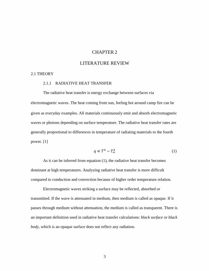
CHAPTER 2
LITERATURE REVIEW
2.1 THEORY
2.1.1 RADIATIVE HEAT TRANSFER
The radiative heat transfer is energy exchange between surfaces via
electromagnetic waves. The heat coming from sun, feeling hot around camp fire can be
given as everyday examples. All materials continuously emit and absorb electromagnetic
waves or photons depending on surface temperature. The radiative heat transfer rates are
generally proportional to differences in temperature of radiating materials to the fourth
power. [1]
𝑞 ∝ 𝑇4 − 𝑇∞4 (1)
As it can be inferred from equation (1), the radiative heat transfer becomes
dominant at high temperatures. Analyzing radiative heat transfer is more difficult
compared to conduction and convection because of higher order temperature relation.
Electromagnetic waves striking a surface may be reflected, absorbed or
transmitted. If the wave is attenuated in medium, then medium is called as opaque. If it
passes through medium without attenuation, the medium is called as transparent. There is
an important definition used in radiative heat transfer calculations: black surface or black
body, which is an opaque surface does not reflect any radiation.
4
Another important term, emissive power, (E), is defined as the radiative heat flux
emitted from a surface in all directions and calculated as,
𝐸(𝑇) = ∫ 𝐸𝑣(𝑇, 𝑣)𝑑𝑣∞
0
(2)
and blackbody emissive power is calculated by Stefan-Boltzman Law,
𝐸𝑏(𝑇) = ∫ 𝐸𝑏𝑣(𝑇, 𝑣)𝑑𝑣∞
0
= 𝑛2𝜎𝑇4 (3)
where 𝜎 = 5.67𝑒 − 8𝑊
𝑚2𝐾4 is known as Stefan-Boltzmann constant
𝑛 is refractive index (𝑛 ≅ 1 for vacuum and gases)
To describe radiative heat flux leaving a surface, it is inadequate to use only
emissive power. The direction dependent quantity, radiative intensity, (I), can be used
instead.
𝐼(𝑟, �̂�) = ∫ 𝐼𝜆(𝑟, �̂�, 𝜆)𝑑𝜆∞
0
(4)
Integrating radiative intensity over all possible directions will give total energy emission
from surface,
𝐸(𝑟) = ∫ 𝐼(𝑟, �̂�) �̂� ∙ �̂� 𝑑𝛺2𝜋
(5)
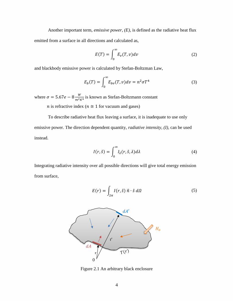
Figure 2.1 An arbitrary black enclosure
𝐻𝑜
𝑑𝐴
𝑑𝐴′
r
r'
0
5
Figure 2.1 shows a black-walled enclosure of arbitrary geometry. The temperature
distribution is indicated by 𝑇(𝑟). Energy balance for a small area of 𝑑𝐴 gives,
𝑞(𝑟) = 𝐸𝑏(𝑟) − 𝐻(𝑟) (6)
𝐻(𝑟) is the irradiation onto 𝑑𝐴 including both from entire enclosure and from outside.
𝐻(𝑟) = ∫ 𝐸𝑏(𝑟′)𝑑𝐹𝑑𝐴−𝑑𝐴′
𝐴
+ 𝐻𝑜(𝑟) (7)
𝑞(𝑟) = 𝐸𝑏(𝑟) − ∫ 𝐸𝑏(𝑟′)𝑑𝐹𝑑𝐴−𝑑𝐴′
𝐴
− 𝐻𝑜(𝑟) (8)
where 𝑑𝐹𝑑𝐴−𝑑𝐴′ is the view factor between surface 𝑑𝐴 and 𝑑𝐴′.
If the enclosure is divided into N isothermal sub-surfaces, the average heat flux becomes
𝑞𝑖 = 𝐸𝑏𝑖 − ∑ 𝐸𝑏𝑗𝐹𝑖−𝑗
𝑁
𝑗=1
− 𝐻𝑜(𝑟) (9)
where 𝐹𝑖−𝑗 is the view factor between surface 𝐴𝑖 and 𝐴𝑗.
2.1.2 VIEW FACTORS
The radiative energy transfer between surfaces is nearly not affected by the
medium that separates them. The participating media could be vacuum, monoatomic or
diatomic gases at low temperatures. Such examples include solar collectors, radiative
space heaters, illumination problems etc. Radiative heat exchange between surfaces can
be analyzed by making assumptions of an idealized enclosure and surface properties. [1]
The most useful one is assuming that all surfaces are black, which means that
there is no radiation reflection on surfaces and no direction dependency for radiation
emission from surface. Reflection, absorption and transmission can be account for more
realistic radiative heat transfer analyzes.
6
There is no range limit for thermal radiation, and if there is no participating
media, photon will travel unimpeded from one surface to another. Therefore, no matter
how far it is, surfaces can exchange radiative energy with one another. How much energy
would be exchanged depends on surface areas, the distance separates them and their
orientation. All these are represented by a geometric function called view factor. It is
sometimes called as configuration factor, angle factor and shape factor. [1]
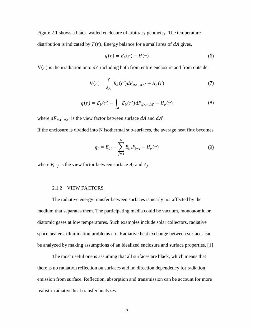
Figure 2.2 Radiative exchange between two infinitesimal surface elements
Figure 2.2 illustrates the radiative exchange between two infinitesimal surface elements
𝑑𝐴𝑖 and 𝑑𝐴𝑗 . The view factor for these surfaces determines how much energy leaves an
arbitrary surface element toward the other one. For surface 𝑑𝐴𝑖 and 𝑑𝐴𝑗 in figure, view
factor is defined as,
𝑑𝐹𝑑𝐴𝑖−𝑑𝐴𝑗=
𝑑𝑖𝑓𝑓𝑢𝑠𝑒 𝑒𝑛𝑒𝑟𝑔𝑦 𝑙𝑒𝑎𝑣𝑖𝑛𝑔 𝑑𝐴𝑖 𝑑𝑖𝑟𝑒𝑐𝑡𝑙𝑦 𝑡𝑜𝑤𝑎𝑟𝑑 𝑎𝑛𝑑 𝑖𝑛𝑡𝑒𝑟𝑐𝑒𝑝𝑡𝑒𝑑 𝑑𝐴𝑗
𝑡𝑜𝑡𝑎𝑙 𝑑𝑖𝑓𝑓𝑢𝑠𝑒 𝑒𝑛𝑒𝑟𝑔𝑦 𝑙𝑒𝑎𝑣𝑖𝑛𝑔 𝑑𝐴𝑖
(10)
𝑆
𝑛ሬԦ𝑖
𝑛ሬԦ𝑗
𝑑𝐴𝑖
𝑑𝐴𝑗 𝜃𝑗
𝜃𝑖
𝑟𝑖
𝑟𝑗
7
the heat transfer rate from 𝑑𝐴𝑖 to 𝑑𝐴𝑗 is determined by the radiative intensity as,
𝐼(𝑟𝑖)(𝑑𝐴𝑖 cos 𝜃𝑖)𝑑𝛺𝑗 =𝐼(𝑟𝑖) cos 𝜃𝑖 cos 𝜃𝑗 𝑑𝐴𝑖𝑑𝐴𝑗
𝑆2 (11)
total radiative energy leaving 𝑑𝐴𝑖 is called as radiosity and related to intensity as
𝐽(𝑟𝑖)𝑑𝐴𝑖 = [𝐸(𝑟𝑖) + 𝜌(𝑟𝑖)𝐻(𝑟𝑖)]𝑑𝐴𝑖 = 𝜋𝐼(𝑟𝑖)𝑑𝐴𝑖 (12)
Then view factor between two infinitesimal diffuse surfaces is
𝑑𝐹𝑑𝐴𝑖−𝑑𝐴𝑗=
cos 𝜃𝑖 cos 𝜃𝑗
𝜋𝑆2𝑑𝐴𝑗 (13)
The view factors have an important rule called law of reciprocity which is derived from
the equation (13), and it says
𝑑𝐴𝑖𝑑𝐹𝑑𝐴𝑖−𝑑𝐴𝑗= 𝑑𝐴𝑗𝑑𝐹𝑑𝐴𝑖−𝑑𝐴𝑗
(14)
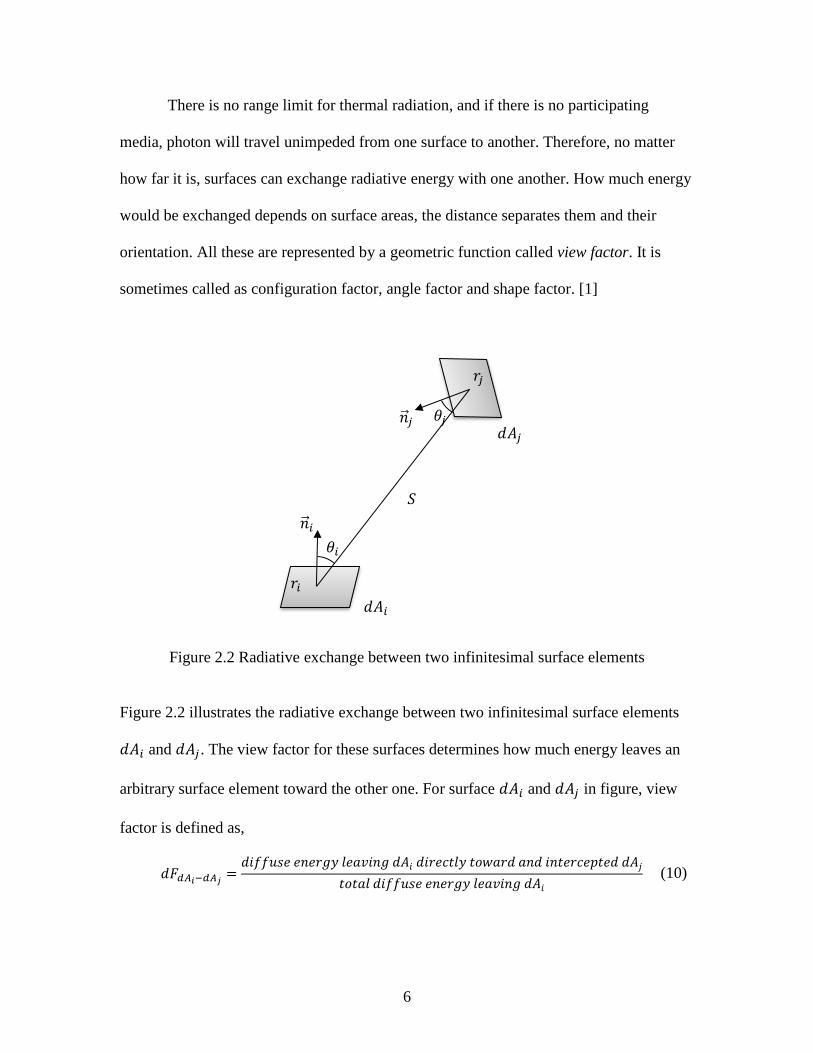
The definition of view factor can be expanded to include radiative change between two
finite surfaces shown in Figure 2.3.
Figure 2.3 Radiative exchange between two finite surfaces
𝑆
𝑛ሬԦ𝑖
𝑛ሬԦ𝑗
𝑑𝐴𝑖
𝑑𝐴𝑗 𝜃𝑗
𝜃𝑖
𝑟𝑖
𝑟𝑗
8
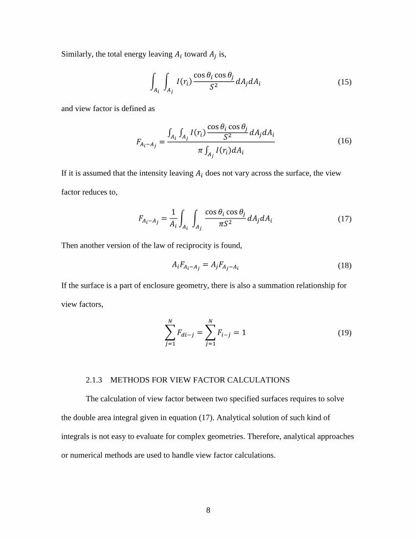
Similarly, the total energy leaving 𝐴𝑖 toward 𝐴𝑗 is,
∫ ∫ 𝐼(𝑟𝑖)cos 𝜃𝑖 cos 𝜃𝑗
𝑆2𝑑𝐴𝑗𝑑𝐴𝑖
𝐴𝑗𝐴𝑖
(15)
and view factor is defined as
𝐹𝐴𝑖−𝐴𝑗=
∫ ∫ 𝐼(𝑟𝑖)cos 𝜃𝑖 cos 𝜃𝑗
𝑆2 𝑑𝐴𝑗𝑑𝐴𝑖𝐴𝑗𝐴𝑖
𝜋 ∫ 𝐼(𝑟𝑖)𝑑𝐴𝑖𝐴𝑗
(16)
If it is assumed that the intensity leaving 𝐴𝑖 does not vary across the surface, the view
factor reduces to,
𝐹𝐴𝑖−𝐴𝑗=
1
𝐴𝑖∫ ∫
cos 𝜃𝑖 cos 𝜃𝑗
𝜋𝑆2𝑑𝐴𝑗𝑑𝐴𝑖
𝐴𝑗𝐴𝑖
(17)
Then another version of the law of reciprocity is found,
𝐴𝑖𝐹𝐴𝑖−𝐴𝑗= 𝐴𝑗𝐹𝐴𝑗−𝐴𝑖
(18)
If the surface is a part of enclosure geometry, there is also a summation relationship for
view factors,
∑ 𝐹𝑑𝑖−𝑗
𝑁
𝑗=1
= ∑ 𝐹𝑖−𝑗
𝑁
𝑗=1
= 1 (19)
2.1.3 METHODS FOR VIEW FACTOR CALCULATIONS
The calculation of view factor between two specified surfaces requires to solve
the double area integral given in equation (17). Analytical solution of such kind of
integrals is not easy to evaluate for complex geometries. Therefore, analytical approaches
or numerical methods are used to handle view factor calculations.
9
Evaluation methods for view factors can be categorized into three groups,
1- Direct integration
2- Special methods
3- Statistical determination
The view factor formula (Eq. (17)) can be solved directly by numerical or
analytical integration methods if the geometry is not too complicated. Area integration
and contour integration are known methods for direct integration. Furthermore, there are
special methods using view factor algebra, including reciprocity and summation rules,
instead of calculating integration.
Experimental methods can also be used to calculate view factors. Unit sphere
method introduced as the first experimental method by Nusselt in 1928. It is a powerful
method to calculate view factors between one infinitesimal and one finite area. Later on,
ray casting method was developed based on unit sphere method, which is using computer
graphics technique to construct the projected area. [1]
Another way to calculate view factors is statistical sampling with Monte Carlo
(MC) method. MC method is a class of numerical techniques based on the statistical
characteristics of physical models. The method was developed by early workers trying to
analyze the potential behavior of nuclear weapons. Experiments were difficult and
analysis methods were not able to provide accurate prediction. Thus, simulating neutrons
and tracking their behavior was the solution to understand average weapon behavior. An
early description of the philosophy behind the MC approach was given by Metropolis and
Ulam (1949) [2].
10
In view factor calculations, a total number of rays (N) are emitted from a surface
with identical properties but random directions. Some of the rays will hit target surface
while others will not. If the number of rays hit is m, then view factor is calculated as,
𝐹𝑖𝑗 =𝑚
𝑁 (20)
2.2 LITERATURE REVIEWS
In literature there are many works done by researchers for view factor
calculations. Different methods were tested for complex geometries for which
theoretical formulas cannot be used.
Bopche and Sridharan (2009) presented an application of contour integral
technique to calculation of diffuse view factors for elements of nuclear fuel bundle.
They derived analytical expressions for different cases including two identical
cylindrical rods, two cylindrical rods with interference by another rod, and between
one cylindrical rod and a non-concentric cylindrical enclosure. They compared results
obtain from their expressions with literature and concluded that using infinite length
approximations in finite length calculations can cause high computational errors. [7]
Narayanaswamy (2015) has used Nusselt’s unit sphere method to calculate
view factor between two arbitrarily oriented planar triangles and planar polygons. The
main reason of focusing only these two arbitrary shapes was that most mesh
generation software for finite element analysis and computer graphics discretize
geometry into them. He ended up with deriving an expression for view factor between
two arbitrarily oriented planar polygons, which obeying reciprocity rule of view
factors. Another conclusion of this study was that the numerical quadrature is not

11
needed for evaluation of the special function in the analytical view factor
expression.[8]
Lei Yang and Wenzhen Chen (2014) thought that existing theoretical formulas
for view factor between nuclear fuel bundles are not suitable for non-standard
assembly geometries such as hexagonal or circular. For view factor calculations, they
used discrete transfer model (DTRM) and discrete ordinates model (DO), which both
are proposed on CFD method. They concluded that DTRM method can be used to
calculate view factors accurately. [9].
Barry and Ying (2016) calculated numerically view factors between hot and
cold side ceramic plates within a thermoelectric device with ray tracing method by
utilizing hybrid CPU-GPU high performance computing. They tried different set of
dimensions for plates and obtain very accurate results. [10]
Mirhosseini and Saboonchi (2011) applied the MC method to calculate view
factors for a plate including strip elements to circular. They investigated the
performance of MC technique by changing number of strip elements and number of
rays. They observed that the error decreased as the number of rays increased, which
was expected for a statistical method.[11]
2.3 FINITE ELEMENT MODELING (MOOSE)
Modeling physical problems is a powerful way for engineers and scientists to
understand the nature of the problem. Computational models can bring light for special
cases that are difficult measure experimentally. Especially in nuclear industry, because of
safety and cost related concerns, computational studies take an important place.

12
Every phenomenon in nature can be described by the laws of physics with terms
of algebraic, differential, and/or integral equations, which is called analytical description
of physical phenomenon or mathematical models. The solution of mathematical models
is sometimes not easy to solve and requires making reasonable assumptions or using
numerical methods. Rapid development in computer science makes it possible to solve
many engineering problems numerically. [4]
The finite element method and its generalizations are the most powerful
computer-oriented methods ever devised to analyze practical engineering problems.
Today, finite element analysis has a significant place in many fields of engineering
design and manufacturing. [4]
In finite element, first, the geometry of problem is divided into subdomains or
finite elements. Then, for each element, governing equations that represent the physics of
the problem are approximated by polynomials. Finally, the equations are solved, and an
approximate solution is found on finite elements.
Multiphysics Object Oriented Simulation Environment (MOOSE) is a parallel
computational framework has been under development since 2008 to provide solutions to
systems of coupled, nonlinear partial differential equations (PDEs) which are important
for nuclear processes. Differ from traditional data-flow oriented computational
frameworks, MOOSE uses Jacobian-free Newton-Krylov (JFNK) scheme in order to
reduce memory and time consumption. This scheme employs Krylov method for solving
the linear system that result from the application of Newton’s method. Since the Krylov
iterative methods require only matrix-vector product rather than full matrix product, the
full Jacobian matrix is not needed. [5]
13
Starting with a discrete problem of length N,
𝐹(𝑥) = 0 (21)
the Jacobian of the system is defined by the 𝑁 𝑥 𝑁 matrix
𝒥(𝑥) =𝜕𝐹(𝑥)
𝜕𝑥 (22)
The Newton iteration can be expressed as
𝒥(𝑥𝑘)𝛿𝑥𝑘 = −𝐹(𝑥𝑘) (23)
which leads to
𝑥𝑘+1 = 𝑥𝑘 + 𝜕𝑥𝑘 (24)
By using Krylov solvers, the Jacobian matrix is reduced to a matrix-vector
𝒥(𝑥𝑘)𝛿𝑥𝑘 ≈𝐹(𝑥𝑘 + 𝜖𝛿𝑥𝑘) − 𝐹(𝑥𝑘)
𝜖 (25)
14
CHAPTER 3
METHODOLOGY
3.1 MONTE CARLO METHOD
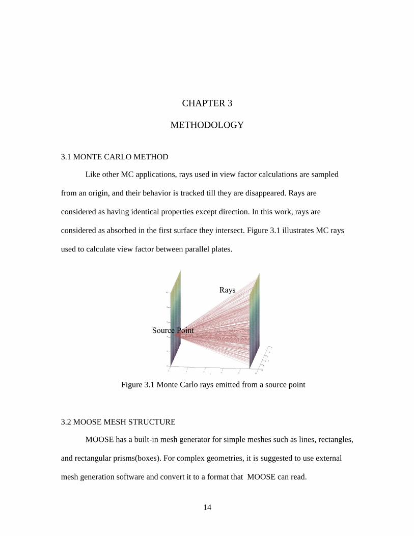
Like other MC applications, rays used in view factor calculations are sampled
from an origin, and their behavior is tracked till they are disappeared. Rays are
considered as having identical properties except direction. In this work, rays are
considered as absorbed in the first surface they intersect. Figure 3.1 illustrates MC rays
used to calculate view factor between parallel plates.
Figure 3.1 Monte Carlo rays emitted from a source point
3.2 MOOSE MESH STRUCTURE
MOOSE has a built-in mesh generator for simple meshes such as lines, rectangles,
and rectangular prisms(boxes). For complex geometries, it is suggested to use external
mesh generation software and convert it to a format that MOOSE can read.
Source Point
Rays
15
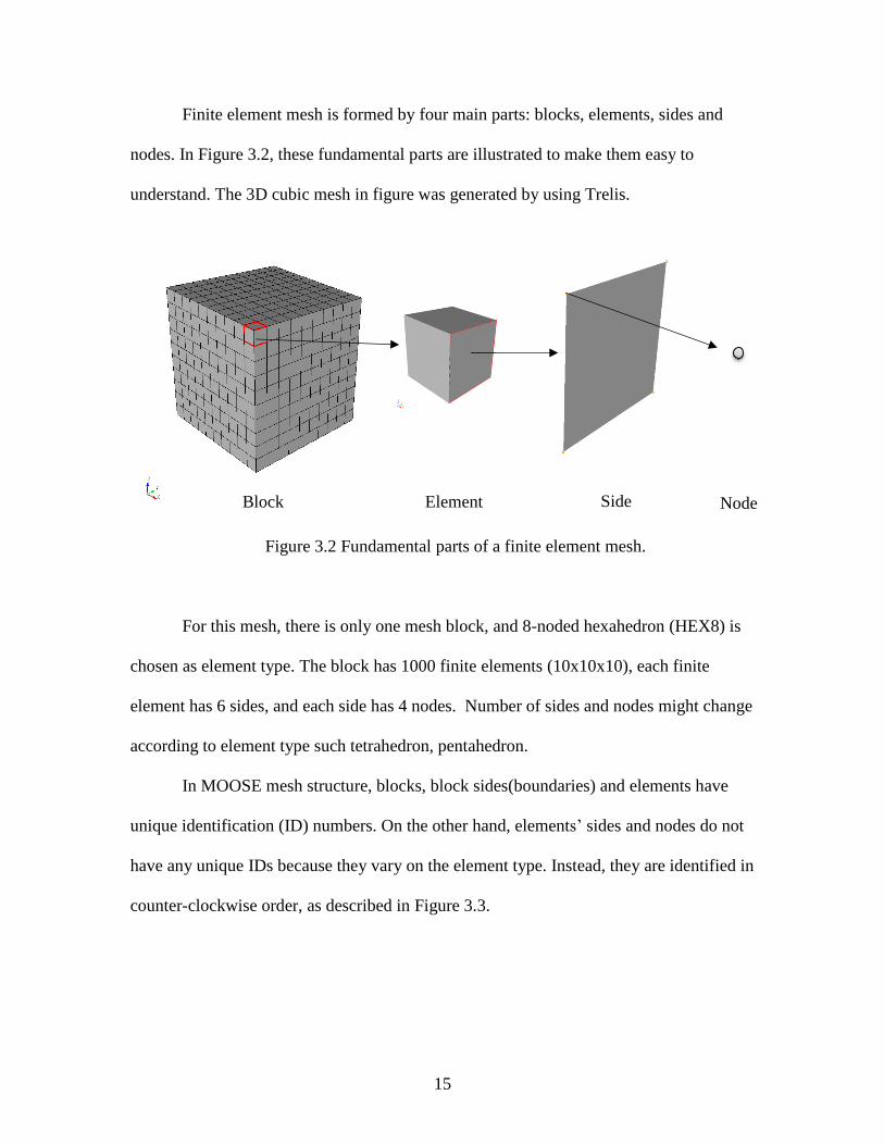
Finite element mesh is formed by four main parts: blocks, elements, sides and
nodes. In Figure 3.2, these fundamental parts are illustrated to make them easy to
understand. The 3D cubic mesh in figure was generated by using Trelis.
Figure 3.2 Fundamental parts of a finite element mesh.
For this mesh, there is only one mesh block, and 8-noded hexahedron (HEX8) is
chosen as element type. The block has 1000 finite elements (10x10x10), each finite
element has 6 sides, and each side has 4 nodes. Number of sides and nodes might change
according to element type such tetrahedron, pentahedron.
In MOOSE mesh structure, blocks, block sides(boundaries) and elements have
unique identification (ID) numbers. On the other hand, elements’ sides and nodes do not
have any unique IDs because they vary on the element type. Instead, they are identified in
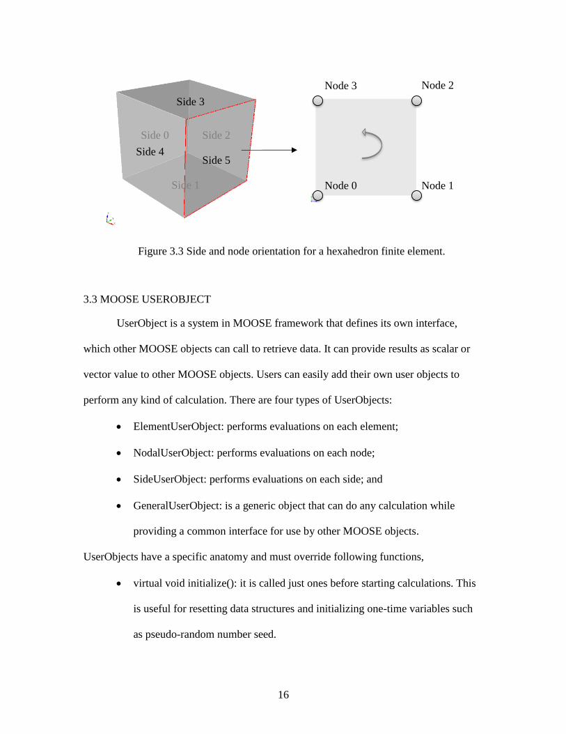
counter-clockwise order, as described in Figure 3.3.
Element Node Side Block
16
Figure 3.3 Side and node orientation for a hexahedron finite element.
3.3 MOOSE USEROBJECT
UserObject is a system in MOOSE framework that defines its own interface,
which other MOOSE objects can call to retrieve data. It can provide results as scalar or
vector value to other MOOSE objects. Users can easily add their own user objects to
perform any kind of calculation. There are four types of UserObjects:
• ElementUserObject: performs evaluations on each element;
• NodalUserObject: performs evaluations on each node;
• SideUserObject: performs evaluations on each side; and
• GeneralUserObject: is a generic object that can do any calculation while
providing a common interface for use by other MOOSE objects.
UserObjects have a specific anatomy and must override following functions,
• virtual void initialize(): it is called just ones before starting calculations. This
is useful for resetting data structures and initializing one-time variables such
as pseudo-random number seed.
Side 5
Side 0
Side 4
Side 1
Side 2
Side 3
Node 0 Node 1
Node 2 Node 3
17
• virtual void execute(): it is called once on each geometric object(element,node
or side) or just one time per calculation for a GeneralUserObject. All
calculations are done inside this function.
• virtual void threadJoin(const UserObject &y): it is used during threaded
execution to join together calculations generated on different threads. the “y”
needs to be casted to a constant reference of type of UserObject itself, then the
data from “y” needs to be extracted and added to the data in current(this)
object.
• virtual void finalize(): it is the very last function called after all calculations
have been completed. The user must take all of the calculations performed in
execute() and do some last operation to get final values.
• In addition to these functions, to provide data or result to other MOOSE
objects, an accessor function is defined, allowing for other MOOSE object can
call this function and get the result of the calculations done by user object.
The accessor function can be named as getValue(), averageValue(), etc…
3.4 VIEW FACTOR MODEL
Since it is extremely powerful and flexible, user object system is chosen to
calculate view factors. The implemented user object model is named as “ViewFactor”. It
is a derived class inheriting from a base class “ViewFactorBase”, which keeps all user
defined variables and user defined functions. All geometrical calculations, linear algebra
operations and MC sampling are done via user defined functions. It is safer and easier to
understand the code when functions are used instead of writing the whole code in just one
18
complex script. All user defined functions used in this work, and the physics behind them
are explained in details in this section.
ViewFactorBase class contains the following functions,
• getSideMap(elemPTR,sideID)
• getNormal(sideMap)
• getCenterPoint(sideMap)
• getArea(point, sideMap)
• getRandomDirection(normal, dimension)
• isOnSurface(point, sideMap)
• getRandomPoint(sideMap)
• isIntersected(point, direction, sideMap)
• isSidetoSide(sideMap, sideMap)
• isVisible(sideMap, sideMap)
• doMonteCarlo(sideMap, sideMap, sourceNumber, samplingNumber)
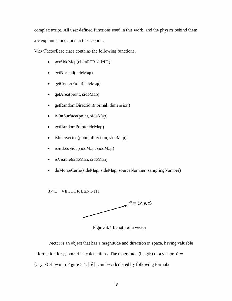
3.4.1 VECTOR LENGTH
Figure 3.4 Length of a vector
Vector is an object that has a magnitude and direction in space, having valuable
information for geometrical calculations. The magnitude (length) of a vector 𝑣Ԧ =
⟨𝑥, 𝑦, 𝑧⟩ shown in Figure 3.4, ‖𝑣Ԧ‖, can be calculated by following formula.
𝑣Ԧ = ⟨𝑥, 𝑦, 𝑧⟩
19
‖𝑣Ԧ‖ = √𝑥2 + 𝑦2 + 𝑧2 (26)
The function norm() in Point class is using this equation to calculate vector magnitude.
3.4.2 ANGLE BETWEEN VECTORS
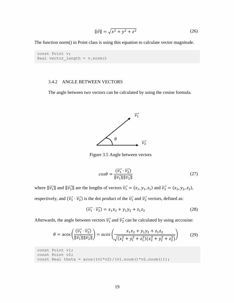
The angle between two vectors can be calculated by using the cosine formula.
Figure 3.5 Angle between vectors
𝑐𝑜𝑠𝜃 =(𝑣1ሬሬሬሬԦ ⋅ 𝑣2ሬሬሬሬԦ)
‖𝑣1ሬሬሬሬԦ‖‖𝑣2ሬሬሬሬԦ‖ (27)
where ‖𝑣1ሬሬሬሬԦ‖ and ‖𝑣2ሬሬሬሬԦ‖ are the lengths of vectors 𝑣1ሬሬሬሬԦ = ⟨𝑥1, 𝑦1, 𝑧1⟩ and 𝑣2ሬሬሬሬԦ = ⟨𝑥2, 𝑦2, 𝑧2⟩,
respectively, and (𝑣1ሬሬሬሬԦ ⋅ 𝑣2ሬሬሬሬԦ) is the dot product of the 𝑣1ሬሬሬሬԦ and 𝑣2ሬሬሬሬԦ vectors, defined as:
(𝑣1ሬሬሬሬԦ ⋅ 𝑣2ሬሬሬሬԦ) = 𝑥1𝑥2 + 𝑦1𝑦2 + 𝑧1𝑧2 (28)
Afterwards, the angle between vectors 𝑣1ሬሬሬሬԦ and 𝑣2ሬሬሬሬԦ can be calculated by using arccosine:
𝜃 = acos ((𝑣1ሬሬሬሬԦ ⋅ 𝑣2ሬሬሬሬԦ)
‖𝑣1ሬሬሬሬԦ‖‖𝑣2ሬሬሬሬԦ‖) = 𝑎𝑐𝑜𝑠 (
𝑥1𝑥2 + 𝑦1𝑦2 + 𝑧1𝑧2
√(𝑥12 + 𝑦1
2 + 𝑧12)(𝑥2
2 + 𝑦22 + 𝑧2
2)) (29)
const Point v;
Real vector_length = v.norm()
𝑣1ሬሬሬሬԦ
𝑣2ሬሬሬሬԦ 𝜃
const Point v1;
const Point v2;
const Real theta = acos((v1*v2)/(v1.norm()*v2.norm()));
20
3.4.3 DISTANCE BETWEEN POINTS
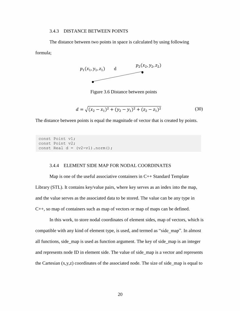
The distance between two points in space is calculated by using following
formula;
Figure 3.6 Distance between points
𝑑 = √(𝑥2 − 𝑥1)2 + (𝑦2 − 𝑦1)2 + (𝑧2 − 𝑧1)2 (30)
The distance between points is equal the magnitude of vector that is created by points.
3.4.4 ELEMENT SIDE MAP FOR NODAL COORDINATES
Map is one of the useful associative containers in C++ Standard Template
Library (STL). It contains key/value pairs, where key serves as an index into the map,
and the value serves as the associated data to be stored. The value can be any type in
C++, so map of containers such as map of vectors or map of maps can be defined.
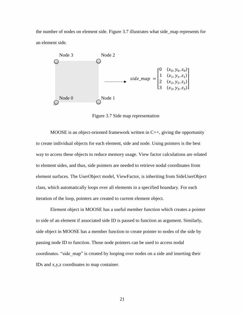
In this work, to store nodal coordinates of element sides, map of vectors, which is
compatible with any kind of element type, is used, and termed as “side_map”. In almost
all functions, side_map is used as function argument. The key of side_map is an integer
and represents node ID in element side. The value of side_map is a vector and represents
the Cartesian (x,y,z) coordinates of the associated node. The size of side_map is equal to
d 𝑝1(𝑥1, 𝑦1, 𝑧1) 𝑝2(𝑥2, 𝑦2, 𝑧2)
const Point v1;
const Point v2;
const Real d = (v2-v1).norm();
21
the number of nodes on element side. Figure 3.7 illustrates what side_map represents for
an element side.
Figure 3.7 Side map representation
MOOSE is an object-oriented framework written in C++, giving the opportunity
to create individual objects for each element, side and node. Using pointers is the best
way to access these objects to reduce memory usage. View factor calculations are related
to element sides, and thus, side pointers are needed to retrieve nodal coordinates from
element surfaces. The UserObject model, ViewFactor, is inheriting from SideUserObject
class, which automatically loops over all elements in a specified boundary. For each
iteration of the loop, pointers are created to current element object.
Element object in MOOSE has a useful member function which creates a pointer
to side of an element if associated side ID is passed to function as argument. Similarly,
side object in MOOSE has a member function to create pointer to nodes of the side by
passing node ID to function. Those node pointers can be used to access nodal
coordinates. “side_map” is created by looping over nodes on a side and inserting their
IDs and x,y,z coordinates to map container.
𝑠𝑖𝑑𝑒_𝑚𝑎𝑝 =
ۏێێۍ0 ⟨𝑥0, 𝑦0, 𝑧0⟩
1 ⟨𝑥1, 𝑦1, 𝑧1⟩
2 ⟨𝑥2, 𝑦2, 𝑧2⟩
3 ⟨𝑥3, 𝑦3, 𝑧3⟩ےۑۑې
Node 0 Node 1
Node 2 Node 3
22
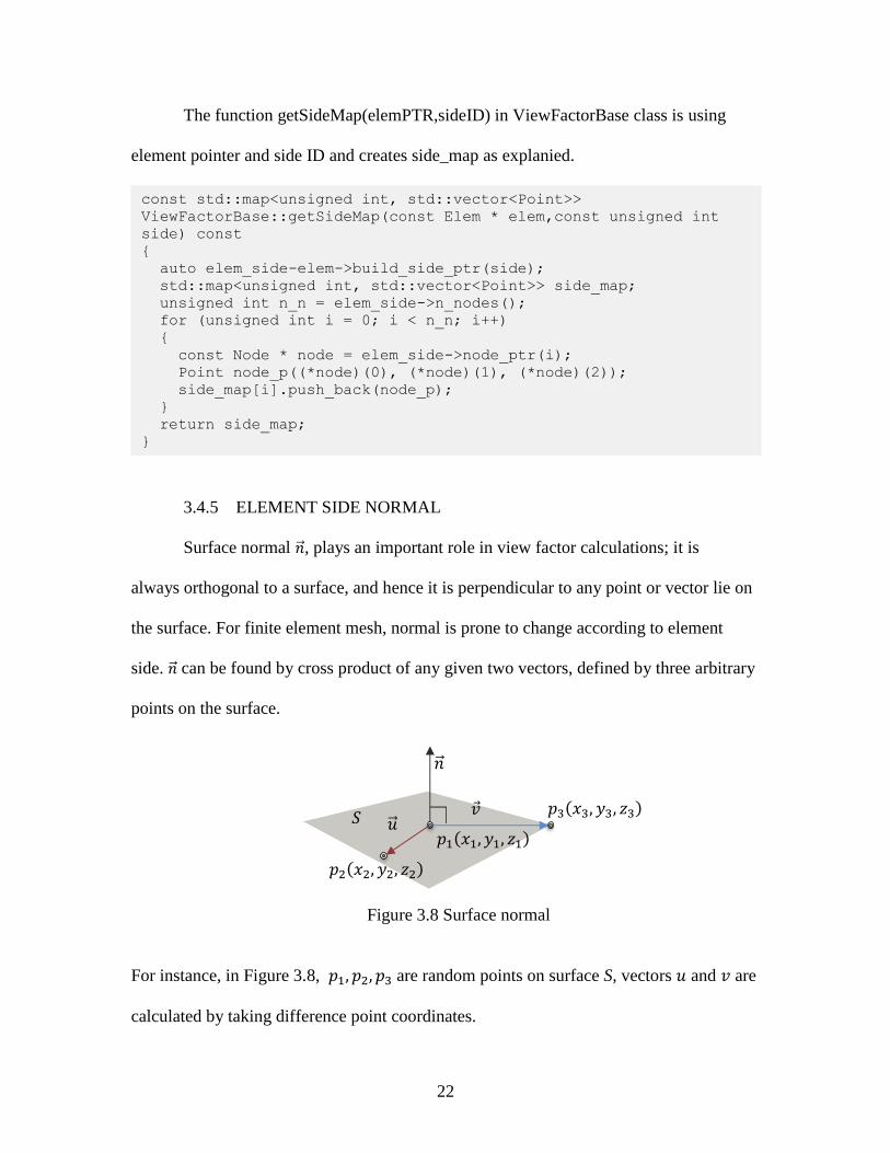
The function getSideMap(elemPTR,sideID) in ViewFactorBase class is using
element pointer and side ID and creates side_map as explanied.
3.4.5 ELEMENT SIDE NORMAL
Surface normal 𝑛ሬԦ, plays an important role in view factor calculations; it is
always orthogonal to a surface, and hence it is perpendicular to any point or vector lie on
the surface. For finite element mesh, normal is prone to change according to element
side. 𝑛ሬԦ can be found by cross product of any given two vectors, defined by three arbitrary
points on the surface.
Figure 3.8 Surface normal
For instance, in Figure 3.8, 𝑝1, 𝑝2, 𝑝3 are random points on surface S, vectors 𝑢 and 𝑣 are
calculated by taking difference point coordinates.
𝑛ሬԦ
𝑣Ԧ
𝑢ሬԦ
𝑝1(𝑥1, 𝑦1, 𝑧1)
𝑝2(𝑥2, 𝑦2, 𝑧2)
𝑝3(𝑥3, 𝑦3, 𝑧3) 𝑆
const std::map<unsigned int, std::vector<Point>>
ViewFactorBase::getSideMap(const Elem * elem,const unsigned int
side) const
{
auto elem_side-elem->build_side_ptr(side);
std::map<unsigned int, std::vector<Point>> side_map;
unsigned int n_n = elem_side->n_nodes();
for (unsigned int i = 0; i < n_n; i++)
{
const Node * node = elem_side->node_ptr(i);
Point node_p((*node)(0), (*node)(1), (*node)(2));
side_map[i].push_back(node_p);
}
return side_map;
}
23
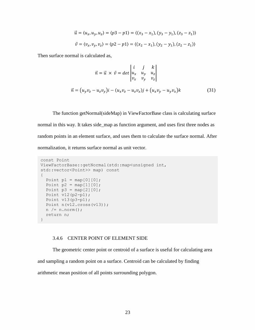
𝑢ሬԦ = ⟨𝑢𝑥 , 𝑢𝑦, 𝑢𝑧⟩ = ⟨𝑝3 − 𝑝1⟩ = ⟨(𝑥3 − 𝑥1), (𝑦3 − 𝑦1), (𝑧3 − 𝑧1)⟩
𝑣Ԧ = ⟨𝑣𝑥 , 𝑣𝑦, 𝑣𝑧⟩ = ⟨𝑝2 − 𝑝1⟩ = ⟨(𝑥2 − 𝑥1), (𝑦2 − 𝑦1), (𝑧2 − 𝑧1)⟩
Then surface normal is calculated as,
𝑛ሬԦ = 𝑢ሬԦ × 𝑣Ԧ = 𝑑𝑒𝑡 |
𝑖 𝑗 𝑘𝑢𝑥 𝑢𝑦 𝑢𝑧
𝑣𝑥 𝑣𝑦 𝑣𝑧
|
𝑛ሬԦ = (𝑢𝑦𝑣𝑧 − 𝑢𝑧𝑣𝑦)𝑖 − (𝑢𝑥𝑣𝑧 − 𝑢𝑧𝑣𝑥)𝑗 + (𝑢𝑥𝑣𝑦 − 𝑢𝑦𝑣𝑥)𝑘 (31)
The function getNormal(sideMap) in ViewFactorBase class is calculating surface
normal in this way. It takes side_map as function argument, and uses first three nodes as
random points in an element surface, and uses them to calculate the surface normal. After
normalization, it returns surface normal as unit vector.
3.4.6 CENTER POINT OF ELEMENT SIDE
The geometric center point or centroid of a surface is useful for calculating area
and sampling a random point on a surface. Centroid can be calculated by finding
arithmetic mean position of all points surrounding polygon.
const Point
ViewFactorBase::getNormal(std::map<unsigned int,
std::vector<Point>> map) const
{
Point p1 = map[0][0];
Point p2 = map[1][0];
Point p3 = map[2][0];
Point v12(p2-p1);
Point v13(p3-p1);
Point n(v12.cross(v13));
n /= n.norm();
return n;
}
24
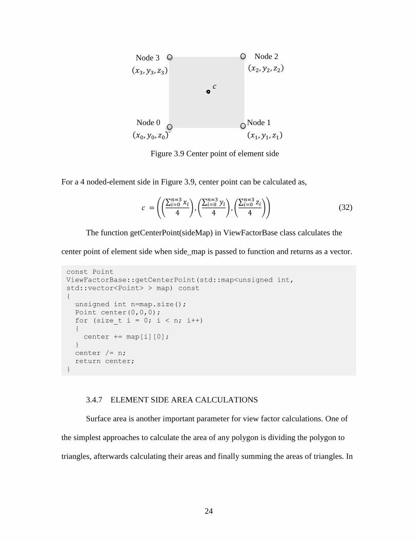
Figure 3.9 Center point of element side
For a 4 noded-element side in Figure 3.9, center point can be calculated as,
𝑐 = ((∑ 𝑥𝑖
𝑛=3𝑖=0
4) , (
∑ 𝑦𝑖𝑛=3𝑖=0
4) , (
∑ 𝑧𝑖𝑛=3𝑖=0
4)) (32)
The function getCenterPoint(sideMap) in ViewFactorBase class calculates the
center point of element side when side_map is passed to function and returns as a vector.
3.4.7 ELEMENT SIDE AREA CALCULATIONS
Surface area is another important parameter for view factor calculations. One of
the simplest approaches to calculate the area of any polygon is dividing the polygon to
triangles, afterwards calculating their areas and finally summing the areas of triangles. In
Node 0 Node 1
Node 2 Node 3
(𝑥0, 𝑦0, 𝑧0) (𝑥1, 𝑦1, 𝑧1)
(𝑥2, 𝑦2, 𝑧2) (𝑥3, 𝑦3, 𝑧3)
𝑐
const Point
ViewFactorBase::getCenterPoint(std::map<unsigned int,
std::vector<Point> > map) const
{
unsigned int n=map.size();
Point center(0,0,0);
for (size_t i = 0; i < n; i++)
{
center += map[i][0];
}
center /= n;
return center;
}
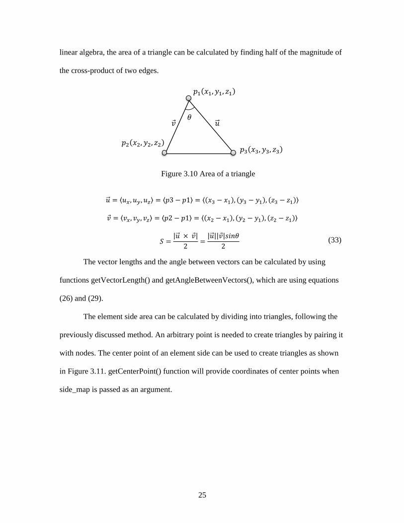
25
linear algebra, the area of a triangle can be calculated by finding half of the magnitude of
the cross-product of two edges.
Figure 3.10 Area of a triangle
𝑢ሬԦ = ⟨𝑢𝑥 , 𝑢𝑦, 𝑢𝑧⟩ = ⟨𝑝3 − 𝑝1⟩ = ⟨(𝑥3 − 𝑥1), (𝑦3 − 𝑦1), (𝑧3 − 𝑧1)⟩
𝑣Ԧ = ⟨𝑣𝑥 , 𝑣𝑦, 𝑣𝑧⟩ = ⟨𝑝2 − 𝑝1⟩ = ⟨(𝑥2 − 𝑥1), (𝑦2 − 𝑦1), (𝑧2 − 𝑧1)⟩
𝑆 =|𝑢ሬԦ × 𝑣Ԧ|
2=
|𝑢ሬԦ||𝑣Ԧ|𝑠𝑖𝑛𝜃
2 (33)
The vector lengths and the angle between vectors can be calculated by using
functions getVectorLength() and getAngleBetweenVectors(), which are using equations
(26) and (29).
The element side area can be calculated by dividing into triangles, following the
previously discussed method. An arbitrary point is needed to create triangles by pairing it
with nodes. The center point of an element side can be used to create triangles as shown
in Figure 3.11. getCenterPoint() function will provide coordinates of center points when
side_map is passed as an argument.
𝑝1(𝑥1, 𝑦1, 𝑧1)
𝑝2(𝑥2, 𝑦2, 𝑧2) 𝑝3(𝑥3, 𝑦3, 𝑧3)
𝑢ሬԦ
𝑣Ԧ
𝜃
26
Figure 3.11 Area of element side by using triangles
The function getArea(point,sideMap) in ViewFactorBase class calculates total
area of triangles created by a given point and side nodes. When the point and side_map is
passed to function, it calculates and returns total area.
3.4.8 SAMPLING RANDOM DIRECTION
Direction sampling is one of the most important part of view factor calculations in
this work, in which a direction is sampled randomly in spherical coordinates system. In
spherical coordinate system, a direction vector is defined by length, 𝑟, polar angle, 𝜃, and
Node 0 Node 1
Node 2 Node 3
𝑐 𝐴1
𝐴2
𝐴3
𝐴4
const Real
ViewFactorBase::getArea(const Point &p, std::map<unsigned int,
std::vector<Point>> map) const
{
unsigned int n = map.size();
Real area{0};
for (size_t i = 0; i < n; i++)
{
const Point node1 = map[i][0];
const Point node2 = map[(i+1)%n][0];
const Point v1(node1-p);
const Point v2(node2-p);
const Real theta = acos((v1*v2)/(v1.norm()*v2.norm()));
area += 0.5 * v1.norm() * v2.norm() * sin(theta);
}
return area;
}
27
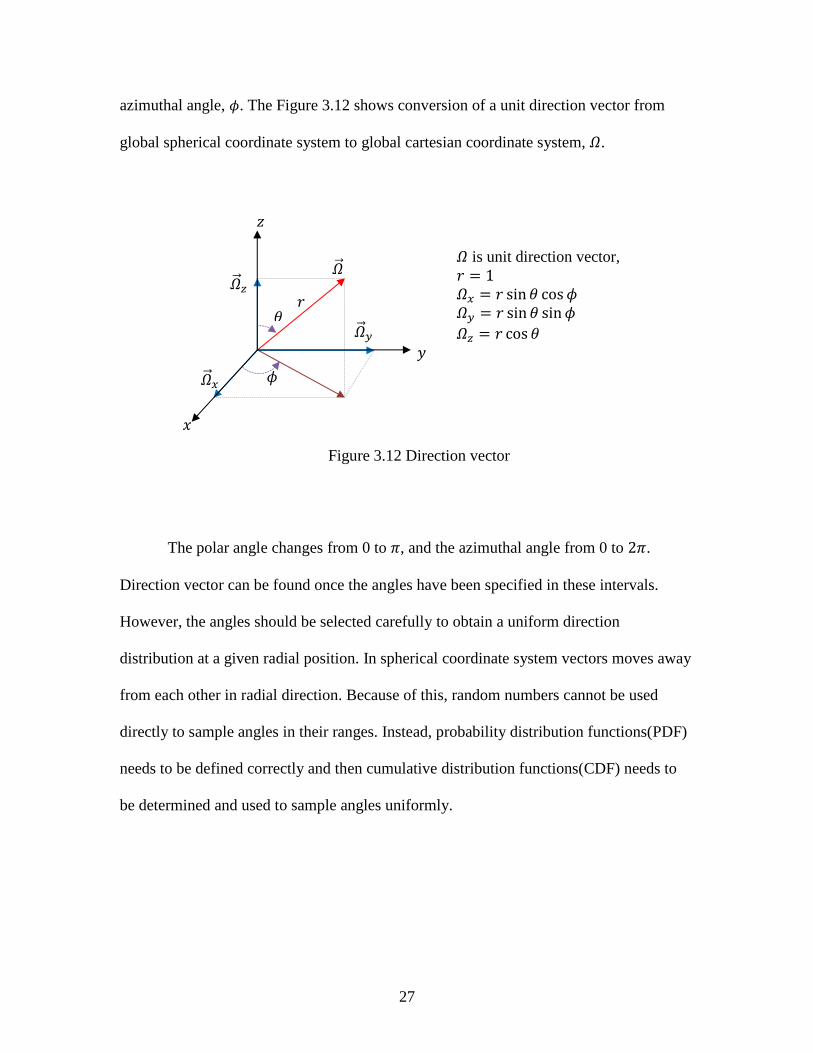
azimuthal angle, 𝜙. The Figure 3.12 shows conversion of a unit direction vector from
global spherical coordinate system to global cartesian coordinate system, 𝛺.
Figure 3.12 Direction vector
The polar angle changes from 0 to 𝜋, and the azimuthal angle from 0 to 2𝜋.
Direction vector can be found once the angles have been specified in these intervals.
However, the angles should be selected carefully to obtain a uniform direction
distribution at a given radial position. In spherical coordinate system vectors moves away
from each other in radial direction. Because of this, random numbers cannot be used
directly to sample angles in their ranges. Instead, probability distribution functions(PDF)
needs to be defined correctly and then cumulative distribution functions(CDF) needs to
be determined and used to sample angles uniformly.
𝑟
𝑧
𝑥
𝑦
𝛺ሬԦ
𝛺ሬԦ𝑥
𝛺ሬԦ𝑦
𝛺ሬԦ𝑧
𝜃
𝜙
𝛺 is unit direction vector,
𝑟 = 1
𝛺𝑥 = 𝑟 sin 𝜃 cos 𝜙
𝛺𝑦 = 𝑟 sin 𝜃 sin 𝜙
𝛺𝑧 = 𝑟 cos 𝜃
28
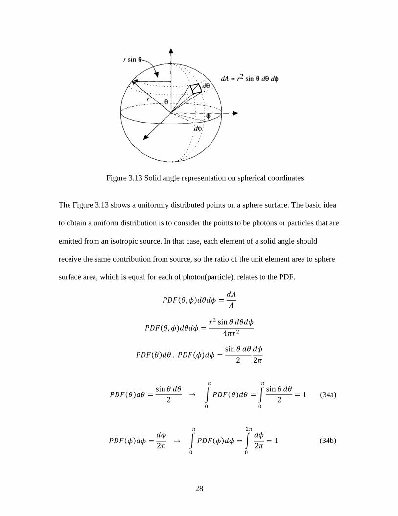
Figure 3.13 Solid angle representation on spherical coordinates
The Figure 3.13 shows a uniformly distributed points on a sphere surface. The basic idea
to obtain a uniform distribution is to consider the points to be photons or particles that are
emitted from an isotropic source. In that case, each element of a solid angle should
receive the same contribution from source, so the ratio of the unit element area to sphere
surface area, which is equal for each of photon(particle), relates to the PDF.
𝑃𝐷𝐹(𝜃, 𝜙)𝑑𝜃𝑑𝜙 =𝑑𝐴
𝐴
𝑃𝐷𝐹(𝜃, 𝜙)𝑑𝜃𝑑𝜙 =𝑟2 sin 𝜃 𝑑𝜃𝑑𝜙
4𝜋𝑟2
𝑃𝐷𝐹(𝜃)𝑑𝜃 . 𝑃𝐷𝐹(𝜙)𝑑𝜙 =sin 𝜃 𝑑𝜃
2
𝑑𝜙
2𝜋
𝑃𝐷𝐹(𝜃)𝑑𝜃 =sin 𝜃 𝑑𝜃
2 → ∫ 𝑃𝐷𝐹(𝜃)𝑑𝜃
𝜋
0
= ∫sin 𝜃 𝑑𝜃
2= 1
𝜋
0
(34a)
𝑃𝐷𝐹(𝜙)𝑑𝜙 =𝑑𝜙
2𝜋 → ∫ 𝑃𝐷𝐹(𝜙)𝑑𝜙
𝜋
0
= ∫𝑑𝜙
2𝜋= 1
2𝜋
0
(34b)
29
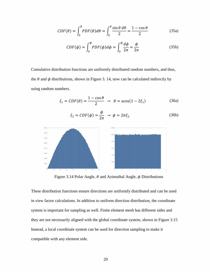
𝐶𝐷𝐹(𝜃) = ∫ 𝑃𝐷𝐹(𝜃)𝑑𝜃𝜃
0
= ∫sin 𝜃 𝑑𝜃
2
𝜃
0
=1 − cos 𝜃
2 (35a)
𝐶𝐷𝐹(𝜙) = ∫ 𝑃𝐷𝐹(𝜙)𝑑𝜙𝜙
0
= ∫𝑑𝜙
2𝜋
𝜙
0
=𝜙
2𝜋 (35b)
Cumulative distribution functions are uniformly distributed random numbers, and thus,
the 𝜃 and 𝜙 distributions, shown in Figure 3. 14, now can be calculated indirectly by
using random numbers.
𝜉1 = 𝐶𝐷𝐹(𝜃) =1 − cos 𝜃
2 → 𝜃 = acos(1 − 2𝜉1) (36a)
𝜉2 = 𝐶𝐷𝐹(𝜙) =𝜙
2𝜋 → 𝜙 = 2𝜋𝜉2 (36b)
Figure 3.14 Polar Angle, 𝜃 and Azimuthal Angle, 𝜙 Distributions
These distribution functions ensure directions are uniformly distributed and can be used
in view factor calculations. In addition to uniform direction distribution, the coordinate
system is important for sampling as well. Finite element mesh has different sides and
they are not necessarily aligned with the global coordinate system, shown in Figure 3.15
Instead, a local coordinate system can be used for direction sampling to make it
compatible with any element side.
30
Figure 3.15 Surface normal orientation
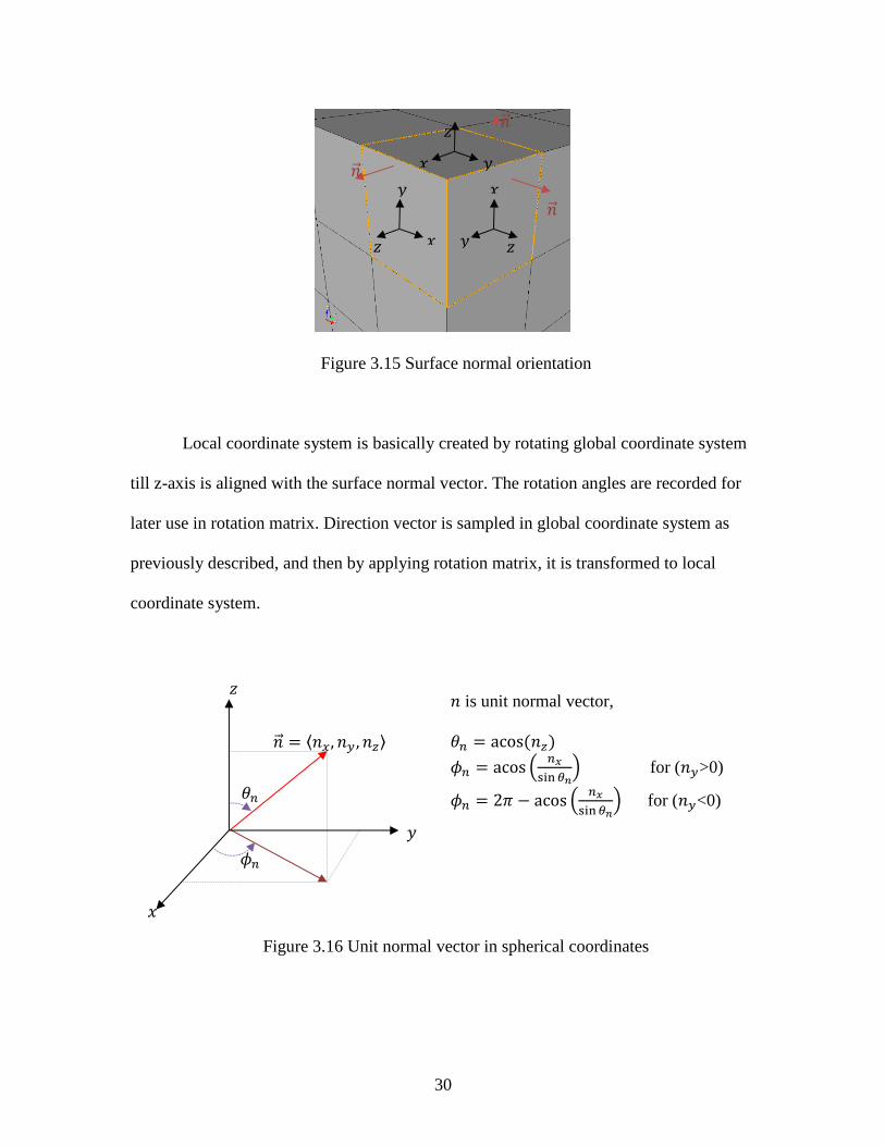
Local coordinate system is basically created by rotating global coordinate system
till z-axis is aligned with the surface normal vector. The rotation angles are recorded for
later use in rotation matrix. Direction vector is sampled in global coordinate system as
previously described, and then by applying rotation matrix, it is transformed to local
coordinate system.
Figure 3.16 Unit normal vector in spherical coordinates
𝑧
𝑥 𝑦
𝑧 𝑥
𝑦
𝑧
𝑥
𝑦
𝑛ሬԦ
𝑛ሬԦ
𝑛ሬԦ
𝑛 is unit normal vector,
𝜃𝑛 = acos(𝑛𝑧)
𝜙𝑛 = acos ቀ𝑛𝑥
sin 𝜃𝑛ቁ for (𝑛𝑦>0)
𝜙𝑛 = 2𝜋 − acos ቀ𝑛𝑥
sin 𝜃𝑛ቁ for (𝑛𝑦<0)
𝑛ሬԦ = ⟨𝑛𝑥, 𝑛𝑦 , 𝑛𝑧⟩
𝑧
𝑥
𝑦
𝜃𝑛
𝜙𝑛
31
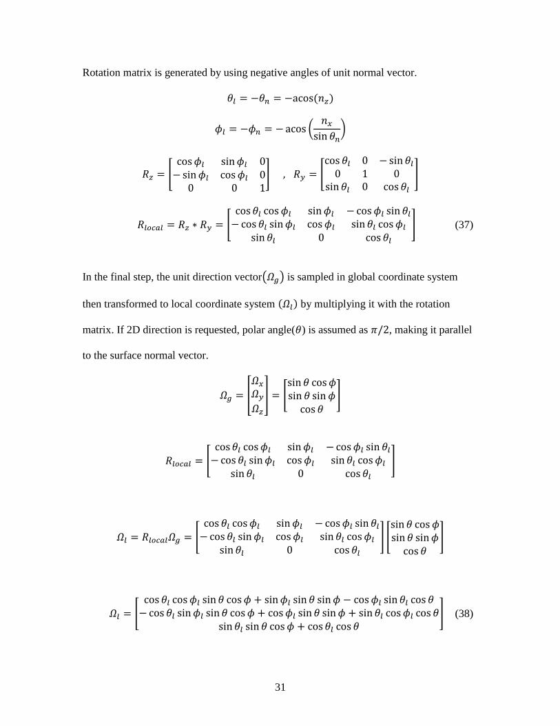
Rotation matrix is generated by using negative angles of unit normal vector.
𝜃𝑙 = −𝜃𝑛 = −acos (𝑛𝑧)
𝜙𝑙 = −𝜙𝑛 = − acos (𝑛𝑥
sin 𝜃𝑛)
𝑅𝑧 = [cos 𝜙𝑙 sin 𝜙𝑙 0
− sin 𝜙𝑙 cos 𝜙𝑙 00 0 1
] , 𝑅𝑦 = [cos 𝜃𝑙 0 − sin 𝜃𝑙
0 1 0sin 𝜃𝑙 0 cos 𝜃𝑙
]
𝑅𝑙𝑜𝑐𝑎𝑙 = 𝑅𝑧 ∗ 𝑅𝑦 = [
cos 𝜃𝑙 cos 𝜙𝑙 sin 𝜙𝑙 − cos 𝜙𝑙 sin 𝜃𝑙
− cos 𝜃𝑙 sin 𝜙𝑙 cos 𝜙𝑙 sin 𝜃𝑙 cos 𝜙𝑙
sin 𝜃𝑙 0 cos 𝜃𝑙
] (37)
In the final step, the unit direction vector(𝛺𝑔) is sampled in global coordinate system
then transformed to local coordinate system (𝛺𝑙) by multiplying it with the rotation
matrix. If 2D direction is requested, polar angle(𝜃) is assumed as 𝜋/2, making it parallel
to the surface normal vector.
𝛺𝑔 = [
𝛺𝑥
𝛺𝑦
𝛺𝑧
] = [sin 𝜃 cos 𝜙sin 𝜃 sin 𝜙
cos 𝜃
]
𝑅𝑙𝑜𝑐𝑎𝑙 = [
cos 𝜃𝑙 cos 𝜙𝑙 sin 𝜙𝑙 − cos 𝜙𝑙 sin 𝜃𝑙
− cos 𝜃𝑙 sin 𝜙𝑙 cos 𝜙𝑙 sin 𝜃𝑙 cos 𝜙𝑙
sin 𝜃𝑙 0 cos 𝜃𝑙
]
𝛺𝑙 = 𝑅𝑙𝑜𝑐𝑎𝑙𝛺𝑔 = [
cos 𝜃𝑙 cos 𝜙𝑙 sin 𝜙𝑙 − cos 𝜙𝑙 sin 𝜃𝑙
− cos 𝜃𝑙 sin 𝜙𝑙 cos 𝜙𝑙 sin 𝜃𝑙 cos 𝜙𝑙
sin 𝜃𝑙 0 cos 𝜃𝑙
] [sin 𝜃 cos 𝜙sin 𝜃 sin 𝜙
cos 𝜃
]
𝛺𝑙 = [
cos 𝜃𝑙 cos 𝜙𝑙 sin 𝜃 cos 𝜙 + sin 𝜙𝑙 sin 𝜃 sin 𝜙 − cos 𝜙𝑙 sin 𝜃𝑙 cos 𝜃− cos 𝜃𝑙 sin 𝜙𝑙 sin 𝜃 cos 𝜙 + cos 𝜙𝑙 sin 𝜃 sin 𝜙 + sin 𝜃𝑙 cos 𝜙𝑙 cos 𝜃
sin 𝜃𝑙 sin 𝜃 cos 𝜙 + cos 𝜃𝑙 cos 𝜃] (38)
32
The function getRandomDirection(normal,dim) takes the unit normal vector and
dimension as function arguments, and does all of the calculations explained above. It
considers the dimension requested and returns unit direction vector.
const Point
ViewFactorBase::getRandomDirection(const Point & n,const int dim)
const
{
Real theta_normal = acos(n(2));
Real phi_normal{0};
if (theta_normal!=0)
if (n(1)<0)
phi_normal = 2 * _PI-acos(n(0)/sin(theta_normal));
else
phi_normal = acos(n(0)/sin(theta_normal));
const Real theta_local = -theta_normal;
const Real phi_local = -phi_normal;
Real
Rlocal[3][3]={{(cos(theta_local)*cos(phi_local)),sin(phi_local),(-
cos(phi_local)*sin(theta_local))},{(-
cos(theta_local)*sin(phi_local)),cos(phi_local),(sin(theta_local)*
sin(phi_local))},{sin(theta_local),0,cos(theta_local)}};
Real theta{0},phi{0};
const Real rand_phi = std::rand() / (1. * RAND_MAX);
const Real rand_theta = std::rand() / (1. * RAND_MAX);
switch (dim)
case 2:
theta = _PI/2;
phi = 2 * _PI * rand_phi;
break;
case 3:
theta = 0.5 * acos(1 - 2 * rand_theta);
phi = 2 * _PI * rand_phi;
break;
const Point
dir_global(sin(theta)*cos(phi),sin(theta)*sin(phi),cos(theta));
const Point
dir_local((Rlocal[0][0]*dir_global(0)+Rlocal[0][1]*dir_global(1)+R
local[0][2]*dir_global(2)),
(Rlocal[1][0]*dir_global(0)+Rlocal[1][1]*dir_global(1)+Rlocal[1][2
]*dir_global(2)),
(Rlocal[2][0]*dir_global(0)+Rlocal[2][1]*dir_global(1)+Rlocal[2][2
]*dir_global(2)));
return dir_local;
}
33
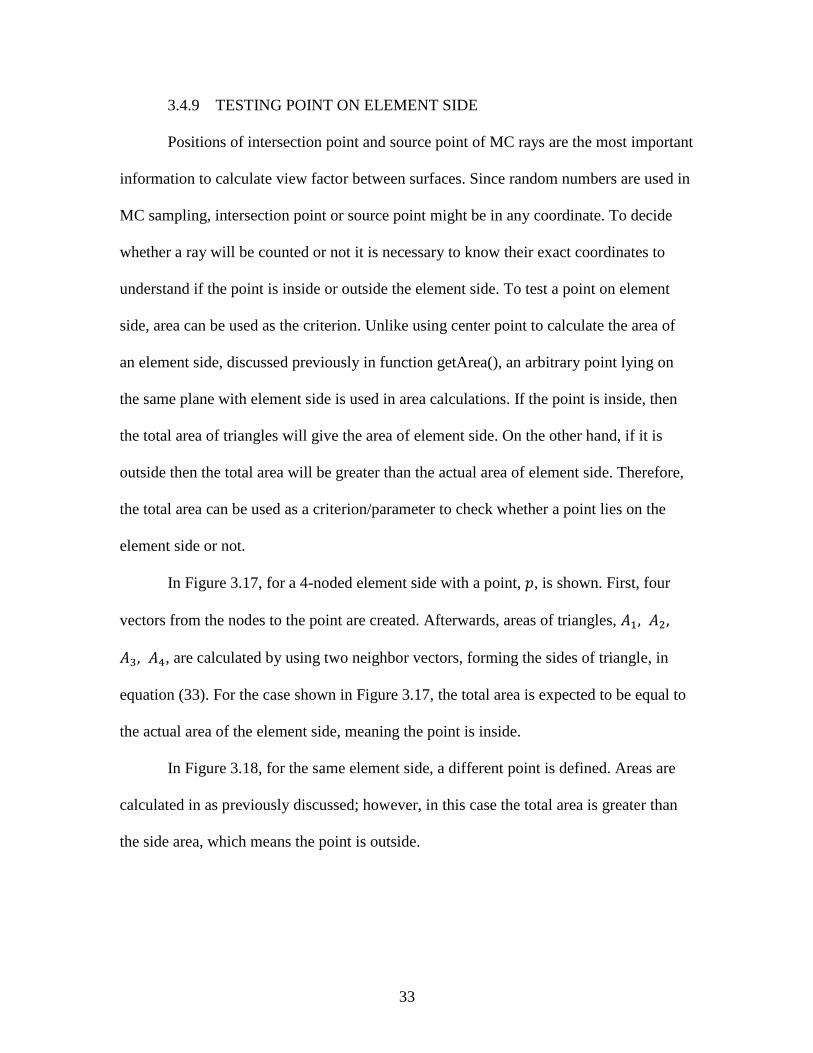
3.4.9 TESTING POINT ON ELEMENT SIDE
Positions of intersection point and source point of MC rays are the most important
information to calculate view factor between surfaces. Since random numbers are used in
MC sampling, intersection point or source point might be in any coordinate. To decide
whether a ray will be counted or not it is necessary to know their exact coordinates to
understand if the point is inside or outside the element side. To test a point on element
side, area can be used as the criterion. Unlike using center point to calculate the area of
an element side, discussed previously in function getArea(), an arbitrary point lying on
the same plane with element side is used in area calculations. If the point is inside, then
the total area of triangles will give the area of element side. On the other hand, if it is
outside then the total area will be greater than the actual area of element side. Therefore,
the total area can be used as a criterion/parameter to check whether a point lies on the
element side or not.
In Figure 3.17, for a 4-noded element side with a point, 𝑝, is shown. First, four
vectors from the nodes to the point are created. Afterwards, areas of triangles, 𝐴1, 𝐴2,
𝐴3, 𝐴4, are calculated by using two neighbor vectors, forming the sides of triangle, in
equation (33). For the case shown in Figure 3.17, the total area is expected to be equal to
the actual area of the element side, meaning the point is inside.
In Figure 3.18, for the same element side, a different point is defined. Areas are
calculated in as previously discussed; however, in this case the total area is greater than
the side area, which means the point is outside.
34
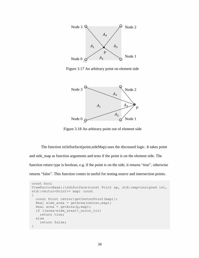
Figure 3.17 An arbitrary point on element side
Figure 3.18 An arbitrary point out of element side
The function isOnSurface(point,sideMap) uses the discussed logic. It takes point
and side_map as function arguments and tests if the point is on the element side. The
function return type is boolean, e.g. if the point is on the side, it returns “true”, otherwise
returns “false”. This function comes in useful for testing source and intersection points.
Node 0 Node 1
Node 2 Node 3
𝑝
𝐴1
𝐴2
𝐴3
𝐴4
Node 0 Node 1
Node 2 Node 3
𝑝 𝐴1
𝐴2
𝐴3
𝐴4
const bool
ViewFactorBase::isOnSurface(const Point &p, std::map<unsigned int,
std::vector<Point>> map) const
{
const Point center{getCenterPoint(map)};
Real elem_area = getArea(center,map);
Real area = getArea(p,map);
if ((area-elem_area)<_error_tol)
return true;
else
return false;
}
35
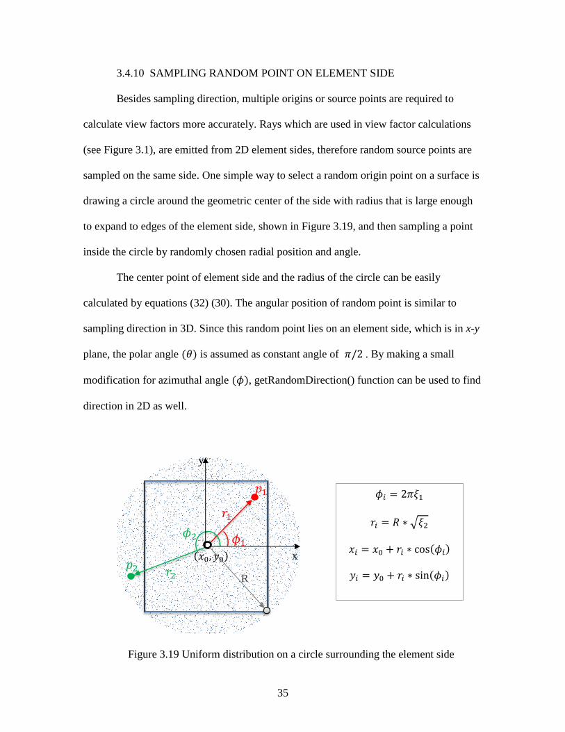
3.4.10 SAMPLING RANDOM POINT ON ELEMENT SIDE
Besides sampling direction, multiple origins or source points are required to
calculate view factors more accurately. Rays which are used in view factor calculations
(see Figure 3.1), are emitted from 2D element sides, therefore random source points are
sampled on the same side. One simple way to select a random origin point on a surface is
drawing a circle around the geometric center of the side with radius that is large enough
to expand to edges of the element side, shown in Figure 3.19, and then sampling a point
inside the circle by randomly chosen radial position and angle.
The center point of element side and the radius of the circle can be easily
calculated by equations (32) (30). The angular position of random point is similar to
sampling direction in 3D. Since this random point lies on an element side, which is in x-y
plane, the polar angle (𝜃) is assumed as constant angle of 𝜋/2 . By making a small
modification for azimuthal angle (𝜙), getRandomDirection() function can be used to find
direction in 2D as well.
Figure 3.19 Uniform distribution on a circle surrounding the element side
𝜙𝑖 = 2𝜋𝜉1
𝑟𝑖 = 𝑅 ∗ √𝜉2
𝑥𝑖 = 𝑥0 + 𝑟𝑖 ∗ cos(𝜙𝑖)
𝑦𝑖 = 𝑦0 + 𝑟𝑖 ∗ sin(𝜙𝑖)
𝜙1 𝜙2
𝑝1
𝑝2 R
x
y
𝑟2
𝑟1
(𝑥0, 𝑦0)
36
The 𝜙 has uniform distribution, and it can be sampled over 2𝜋 by using pseudo-
random numbers. The radial position of random point needs to be sampled over circle
radius, R. To make radial position distribution uniform, sampling needs to be done
according to inverse square law which states that a physical quantity or intensity is
inversely proportional to the square of the distance from its source in space. This is
similar to using cosine distribution for 𝜃 in 3D direction sampling to get a uniform
distribution. Once the radial and angular position of point is found, they are converted to
global cartesian coordinate system to be used in calculations.
As mentioned before, the random points are chosen to be in a circle that surrounds
the element side. However, since the element side is not circular, it is possible that some
points will be outside the element side. For example, in Figure 3.19, point 𝑝2 is not on the
element side and thus it is rejected as an origin point. This method is termed rejection
method, in which first of all, points are chosen randomly, and then tested whether they
are inside the domain of interest.
const Point
ViewFactorBase::getRandomPoint(std::map<unsigned int,
std::vector<Point>> map) const
{
const Point n = getNormal(map);
const Point center{getCenterPoint(map)};
Real rad{0},d{0}; //radius, distance
for (size_t i = 0; i < map.size(); i++)
Point p = map[i][0];
d = (p-center).norm();
if (d>rad)
rad=d;
while (true)
const Real rand_r = std::rand() / (1. * RAND_MAX);
const Real r =rad * std::sqrt(rand_r);
const Point dir(getRandomDirection(n,2));
const Point p(center + r*dir);
if (isOnSurface(p,map))
return p;
}
37
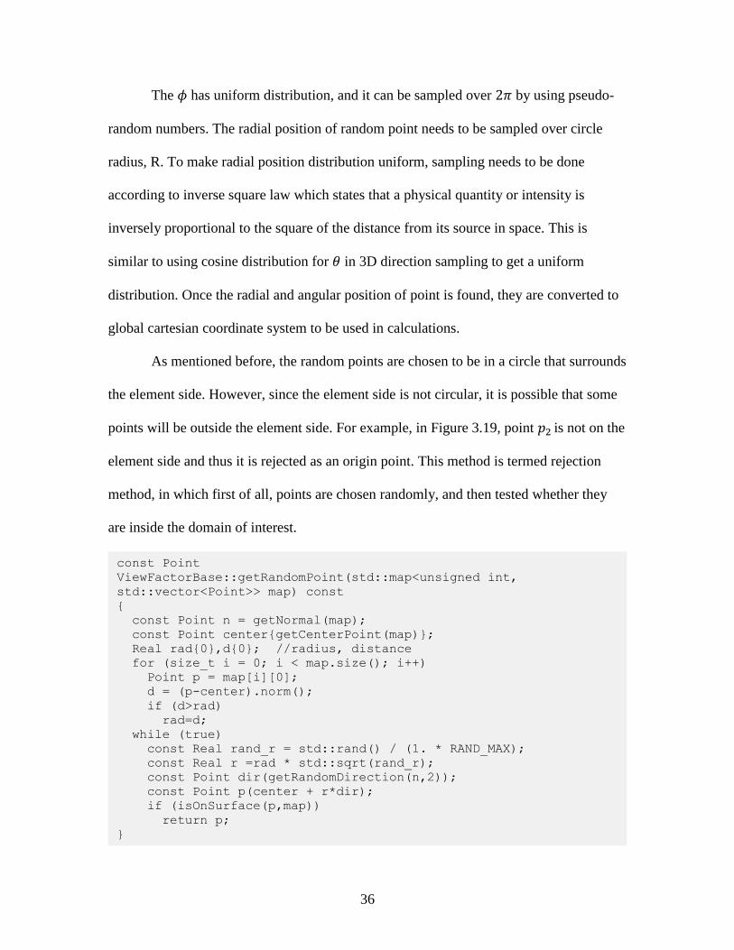
The function getRandomPoint(sideMap) takes side_map as argument, creates a
circle and samples a random point on it. After testing the point is on the element side by
utilizing isOnSurface() function, it accepts the point as origin if it is on element side, and
rejects one that is not.
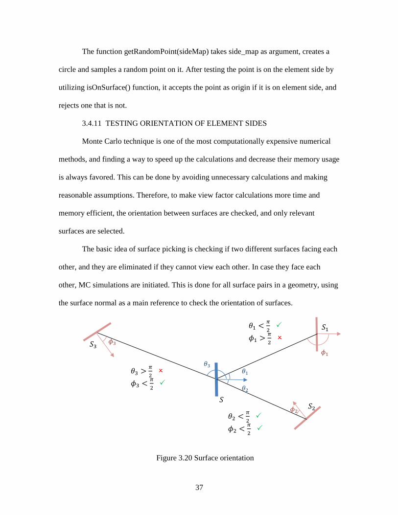
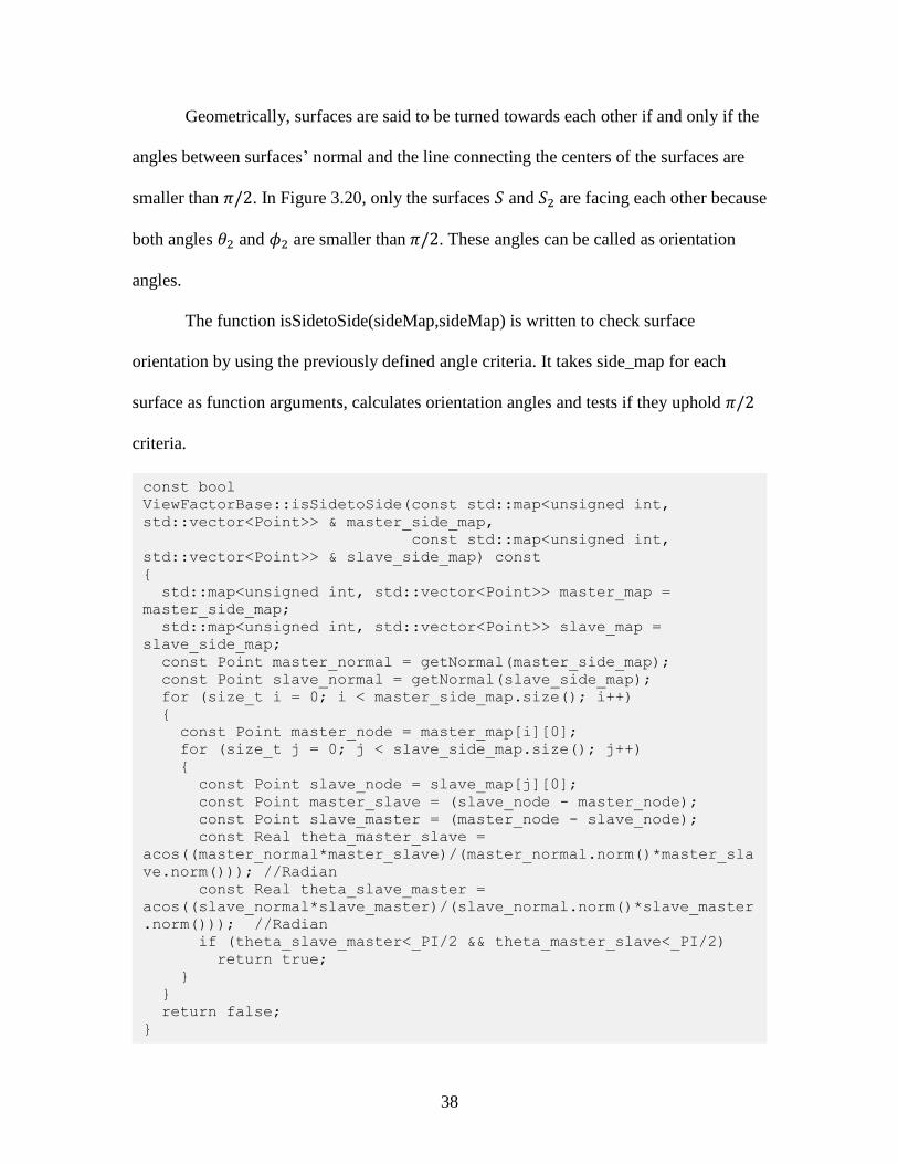
3.4.11 TESTING ORIENTATION OF ELEMENT SIDES
Monte Carlo technique is one of the most computationally expensive numerical
methods, and finding a way to speed up the calculations and decrease their memory usage
is always favored. This can be done by avoiding unnecessary calculations and making
reasonable assumptions. Therefore, to make view factor calculations more time and
memory efficient, the orientation between surfaces are checked, and only relevant
surfaces are selected.
The basic idea of surface picking is checking if two different surfaces facing each
other, and they are eliminated if they cannot view each other. In case they face each
other, MC simulations are initiated. This is done for all surface pairs in a geometry, using
the surface normal as a main reference to check the orientation of surfaces.
Figure 3.20 Surface orientation
𝜃1
𝜃2
𝜙1
𝜙2
𝜙3
𝜃3
𝑆1
𝑆3
𝑆2 𝑆
𝜃3 >𝜋
2
𝜙3 <𝜋
2
𝜃1 <𝜋
2
𝜙1 >𝜋
2
𝜃2 <𝜋
2
𝜙2 <𝜋
2
38
Geometrically, surfaces are said to be turned towards each other if and only if the
angles between surfaces’ normal and the line connecting the centers of the surfaces are
smaller than 𝜋/2. In Figure 3.20, only the surfaces 𝑆 and 𝑆2 are facing each other because
both angles 𝜃2 and 𝜙2 are smaller than 𝜋/2. These angles can be called as orientation
angles.
The function isSidetoSide(sideMap,sideMap) is written to check surface
orientation by using the previously defined angle criteria. It takes side_map for each
surface as function arguments, calculates orientation angles and tests if they uphold 𝜋/2
criteria.
const bool
ViewFactorBase::isSidetoSide(const std::map<unsigned int,
std::vector<Point>> & master_side_map,
const std::map<unsigned int,
std::vector<Point>> & slave_side_map) const
{
std::map<unsigned int, std::vector<Point>> master_map =
master_side_map;
std::map<unsigned int, std::vector<Point>> slave_map =
slave_side_map;
const Point master_normal = getNormal(master_side_map);
const Point slave_normal = getNormal(slave_side_map);
for (size_t i = 0; i < master_side_map.size(); i++)
{
const Point master_node = master_map[i][0];
for (size_t j = 0; j < slave_side_map.size(); j++)
{
const Point slave_node = slave_map[j][0];
const Point master_slave = (slave_node - master_node);
const Point slave_master = (master_node - slave_node);
const Real theta_master_slave =
acos((master_normal*master_slave)/(master_normal.norm()*master_sla
ve.norm())); //Radian
const Real theta_slave_master =
acos((slave_normal*slave_master)/(slave_normal.norm()*slave_master
.norm())); //Radian
if (theta_slave_master<_PI/2 && theta_master_slave<_PI/2)
return true;
}
}
return false;
}
39
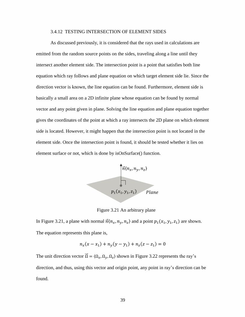
3.4.12 TESTING INTERSECTION OF ELEMENT SIDES
As discussed previously, it is considered that the rays used in calculations are
emitted from the random source points on the sides, traveling along a line until they
intersect another element side. The intersection point is a point that satisfies both line
equation which ray follows and plane equation on which target element side lie. Since the
direction vector is known, the line equation can be found. Furthermore, element side is
basically a small area on a 2D infinite plane whose equation can be found by normal
vector and any point given in plane. Solving the line equation and plane equation together
gives the coordinates of the point at which a ray intersects the 2D plane on which element
side is located. However, it might happen that the intersection point is not located in the
element side. Once the intersection point is found, it should be tested whether it lies on
element surface or not, which is done by isOnSurface() function.
Figure 3.21 An arbitrary plane
In Figure 3.21, a plane with normal 𝑛ሬԦ⟨𝑛𝑥 , 𝑛𝑦, 𝑛𝑧⟩ and a point 𝑝1(𝑥1, 𝑦1, 𝑧1) are shown.
The equation represents this plane is,
𝑛𝑥(𝑥 − 𝑥1) + 𝑛𝑦(𝑦 − 𝑦1) + 𝑛𝑧(𝑧 − 𝑧1) = 0
The unit direction vector ΩሬሬԦ = ⟨Ω𝑥 , Ω𝑦, Ω𝑧⟩ shown in Figure 3.22 represents the ray’s
direction, and thus, using this vector and origin point, any point in ray’s direction can be
found.
𝑛ሬԦ⟨𝑛𝑥, 𝑛𝑦 , 𝑛𝑧⟩
𝑝1(𝑥1, 𝑦1, 𝑧1) 𝑃𝑙𝑎𝑛𝑒
40
Figure 3.22 Intersection point in spherical coordinates
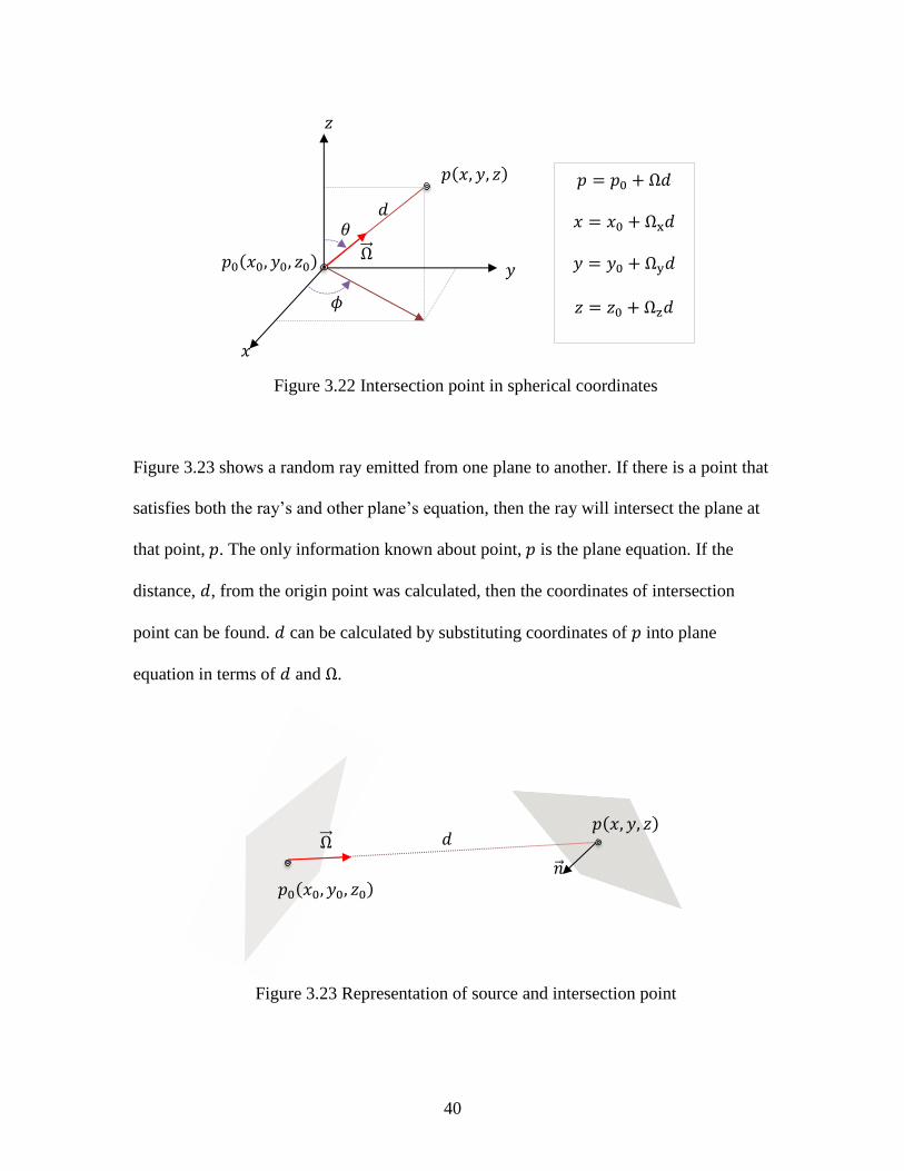
Figure 3.23 shows a random ray emitted from one plane to another. If there is a point that
satisfies both the ray’s and other plane’s equation, then the ray will intersect the plane at
that point, 𝑝. The only information known about point, 𝑝 is the plane equation. If the
distance, 𝑑, from the origin point was calculated, then the coordinates of intersection
point can be found. 𝑑 can be calculated by substituting coordinates of 𝑝 into plane
equation in terms of 𝑑 and Ω.
Figure 3.23 Representation of source and intersection point
𝑑
𝑝(𝑥, 𝑦, 𝑧)
𝑝0(𝑥0, 𝑦0, 𝑧0) ΩሬሬԦ
𝑧
𝑥
𝑦
𝜃
𝜙
𝑝 = 𝑝0 + Ω𝑑
𝑥 = 𝑥0 + Ωx𝑑
𝑦 = 𝑦0 + Ωy𝑑
𝑧 = 𝑧0 + Ωz𝑑
𝑛ሬԦ
𝑝(𝑥, 𝑦, 𝑧) 𝑑
𝑝0(𝑥0, 𝑦0, 𝑧0)
ΩሬሬԦ
41
Plane equation,
𝑛𝑥(𝑥 − 𝑥1) + 𝑛𝑦(𝑦 − 𝑦1) + 𝑛𝑧(𝑧 − 𝑧1) = 0
Line equations,
𝑥 = 𝑥0 + Ωx𝑑 𝑦 = 𝑦0 + Ωy𝑑 𝑧 = 𝑧0 + Ωz𝑑
Substitute line equations into plane equations,
𝑛𝑥(𝑥0 + Ωx𝑑 − 𝑥1) + 𝑛𝑦(𝑦0 + Ωy𝑑 − 𝑦1) + 𝑛𝑧(𝑧0 + Ωz𝑑 − 𝑧1) = 0
Solve for 𝑑,
𝑑 =𝑛𝑥(𝑥1 − 𝑥0) + 𝑛𝑦(𝑦1 − 𝑦0) + 𝑛𝑧(𝑧1 − 𝑧0)
𝑛𝑥Ω𝑥 + 𝑛𝑦Ω𝑦 + 𝑛𝑧Ω𝑧 (39)
Then, the coordinates of intersection point are calculated, 𝑝(𝑥, 𝑦, 𝑧)
𝑥 = 𝑥0 + Ωx𝑑
𝑦 = 𝑦0 + Ωy𝑑
𝑧 = 𝑧0 + Ωz𝑑
(40)
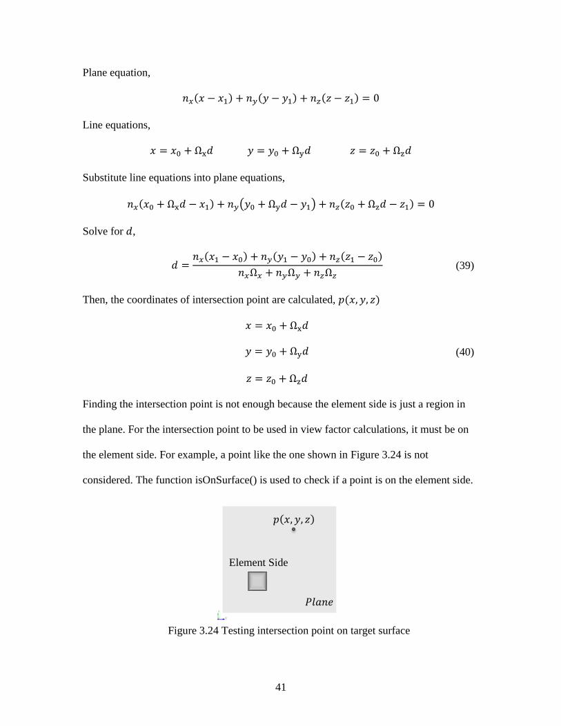
Finding the intersection point is not enough because the element side is just a region in
the plane. For the intersection point to be used in view factor calculations, it must be on
the element side. For example, a point like the one shown in Figure 3.24 is not
considered. The function isOnSurface() is used to check if a point is on the element side.
Figure 3.24 Testing intersection point on target surface
𝑝(𝑥, 𝑦, 𝑧)
𝑃𝑙𝑎𝑛𝑒
Element Side
42
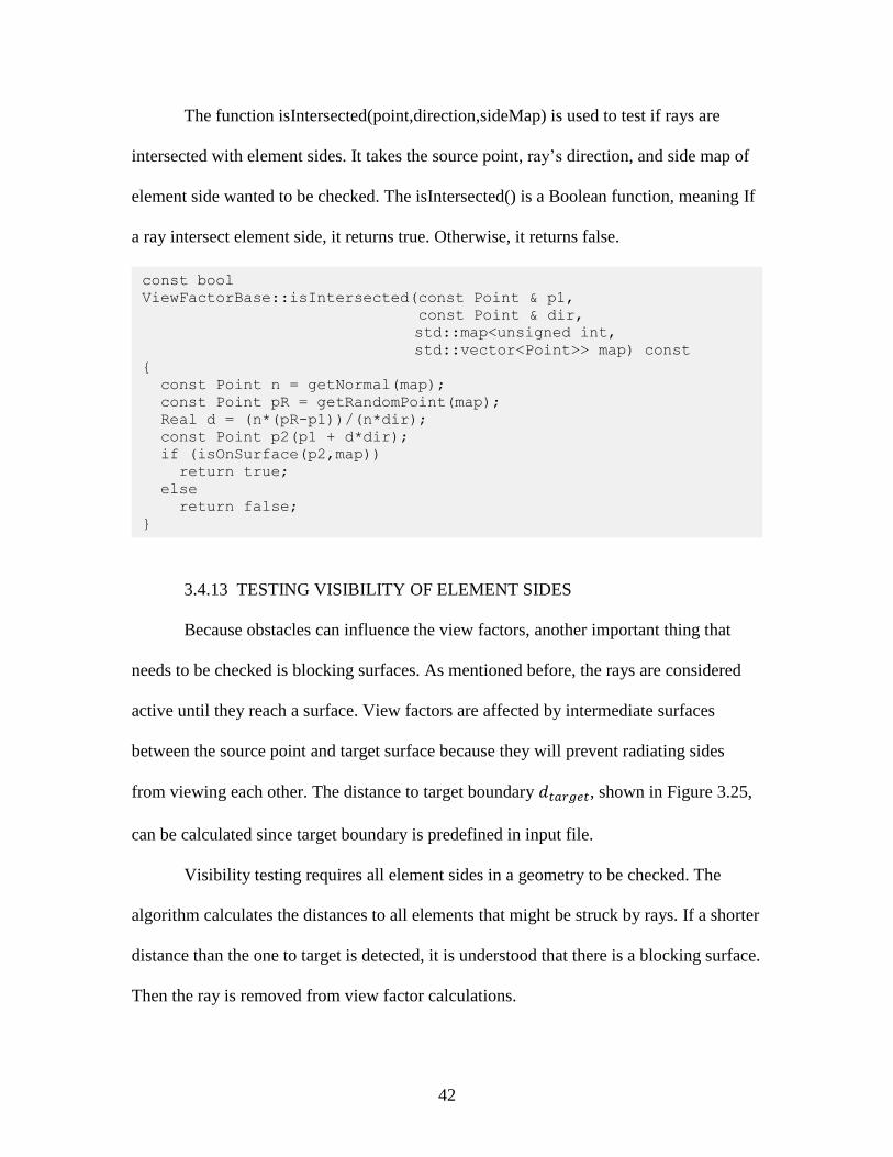
The function isIntersected(point,direction,sideMap) is used to test if rays are
intersected with element sides. It takes the source point, ray’s direction, and side map of
element side wanted to be checked. The isIntersected() is a Boolean function, meaning If
a ray intersect element side, it returns true. Otherwise, it returns false.
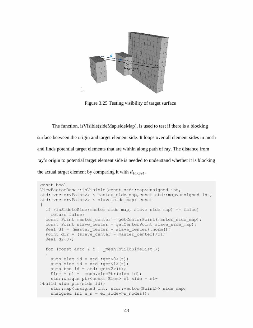
3.4.13 TESTING VISIBILITY OF ELEMENT SIDES
Because obstacles can influence the view factors, another important thing that
needs to be checked is blocking surfaces. As mentioned before, the rays are considered
active until they reach a surface. View factors are affected by intermediate surfaces
between the source point and target surface because they will prevent radiating sides
from viewing each other. The distance to target boundary 𝑑𝑡𝑎𝑟𝑔𝑒𝑡, shown in Figure 3.25,
can be calculated since target boundary is predefined in input file.
Visibility testing requires all element sides in a geometry to be checked. The
algorithm calculates the distances to all elements that might be struck by rays. If a shorter
distance than the one to target is detected, it is understood that there is a blocking surface.
Then the ray is removed from view factor calculations.
const bool
ViewFactorBase::isIntersected(const Point & p1,
const Point & dir,
std::map<unsigned int,
std::vector<Point>> map) const
{
const Point n = getNormal(map);
const Point pR = getRandomPoint(map);
Real d = (n*(pR-p1))/(n*dir);
const Point p2(p1 + d*dir);
if (isOnSurface(p2,map))
return true;
else
return false;
}
43
Figure 3.25 Testing visibility of target surface
The function, isVisible(sideMap,sideMap), is used to test if there is a blocking
surface between the origin and target element side. It loops over all element sides in mesh
and finds potential target elements that are within along path of ray. The distance from
ray’s origin to potential target element side is needed to understand whether it is blocking
the actual target element by comparing it with 𝑑𝑡𝑎𝑟𝑔𝑒𝑡.
𝑑
𝑑𝑡𝑎𝑟𝑔𝑒𝑡
const bool
ViewFactorBase::isVisible(const std::map<unsigned int,
std::vector<Point>> & master_side_map,const std::map<unsigned int,
std::vector<Point>> & slave_side_map) const
{
if (isSidetoSide(master_side_map, slave_side_map) == false)
return false;
const Point master_center = getCenterPoint(master_side_map);
const Point slave_center = getCenterPoint(slave_side_map);
Real d1 = (master_center - slave_center).norm();
Point dir = (slave_center - master_center)/d1;
Real d2{0};
for (const auto & t : _mesh.buildSideList())
{
auto elem_id = std::get<0>(t);
auto side_id = std::get<1>(t);
auto bnd_id = std::get<2>(t);
Elem * el = _mesh.elemPtr(elem_id);
std::unique_ptr<const Elem> el_side = el-
>build_side_ptr(side_id);
std::map<unsigned int, std::vector<Point>> side_map;
unsigned int n_n = el_side->n_nodes();

44
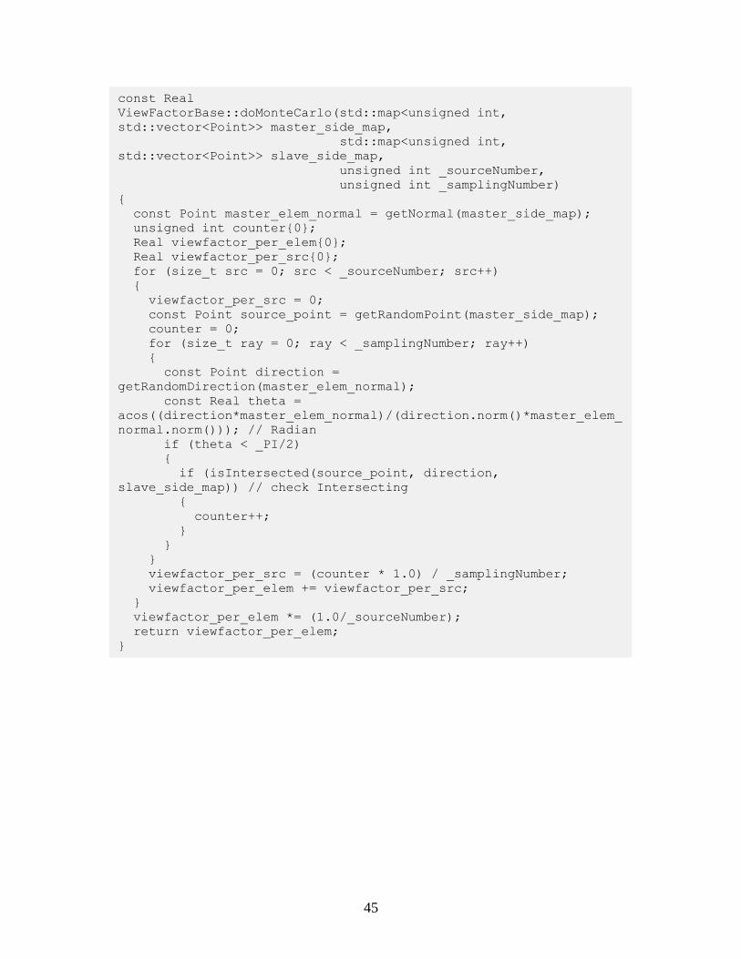
3.4.14 MONTE CARLO CALCULATIONS
The functions described so far perform calculations related to geometry, while
providing the basis for MC simulation. View factor calculations done using Monte Carlo
simulation relies on tracking rays and counting how many of them strike the desired
element sides.
The number of rays and number of source points are input parameters for Monte
Carlo simulations. UserObject model gives the user a chance to define both in the input
file. In model, a separate member function, which is doMonteCarlo(), is defined in
ViewFactorBase class for Monte Carlo calculations. The function takes number of rays,
number of source points and side maps of source and target element sides as function
argument. It calculates surface normal for both sides by getNormal(), samples random
source point location by getRandomPoint(), samples random direction by
getRandomDirection(). At the end, it calculates view factor as a ratio of total intersected
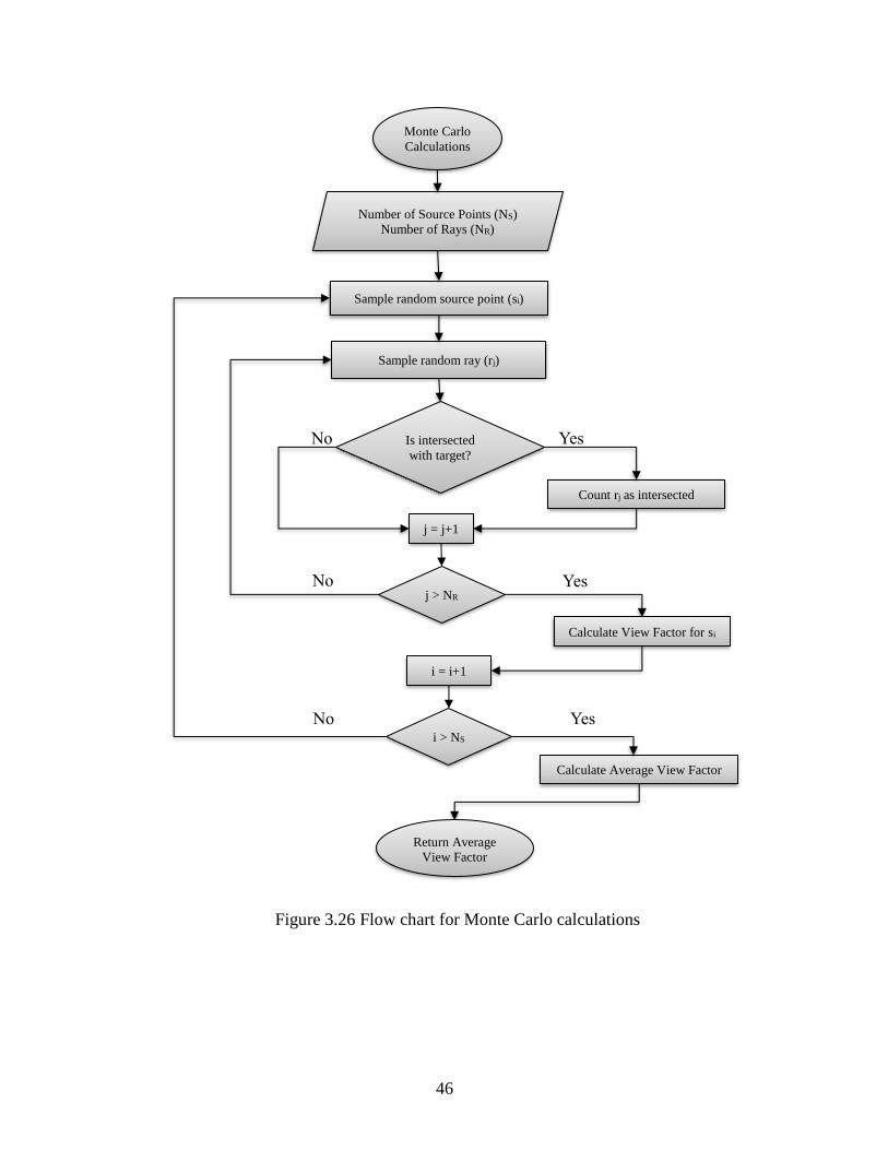
rays to total number of rays and returns it. Figure 3.26 is flow chart for doMonteCarlo()
function, and the one in Figure 3.27 is the flow chart for ViewFactor model.
for (unsigned int i = 0; i < n_n; i++)
{
const Node * node = el_side->node_ptr(i);
Point node_p((*node)(0), (*node)(1), (*node)(2));
side_map[i].push_back(node_p);
}
const Point side_center = getCenterPoint(side_map);
d2 = (master_center - side_center).norm();
if (isSidetoSide(master_side_map, side_map) &&
isIntersected(master_center, dir, side_map) &&
d2 < d1)
{
return false;
}
}
return true;
}
45
const Real
ViewFactorBase::doMonteCarlo(std::map<unsigned int,
std::vector<Point>> master_side_map,
std::map<unsigned int,
std::vector<Point>> slave_side_map,
unsigned int _sourceNumber,
unsigned int _samplingNumber)
{
const Point master_elem_normal = getNormal(master_side_map);
unsigned int counter{0};
Real viewfactor_per_elem{0};
Real viewfactor_per_src{0};
for (size_t src = 0; src < _sourceNumber; src++)
{
viewfactor_per_src = 0;
const Point source_point = getRandomPoint(master_side_map);
counter = 0;
for (size_t ray = 0; ray < _samplingNumber; ray++)
{
const Point direction =
getRandomDirection(master_elem_normal);
const Real theta =
acos((direction*master_elem_normal)/(direction.norm()*master_elem_
normal.norm())); // Radian
if (theta < _PI/2)
{
if (isIntersected(source_point, direction,
slave_side_map)) // check Intersecting
{
counter++;
}
}
}
viewfactor_per_src = (counter * 1.0) / _samplingNumber;
viewfactor_per_elem += viewfactor_per_src;
}
viewfactor_per_elem *= (1.0/_sourceNumber);
return viewfactor_per_elem;
}
46
Figure 3.26 Flow chart for Monte Carlo calculations
Calculate Average View Factor
Yes
Yes No
No
No
Return Average
View Factor
i > NS
j > NR
Is intersected
with target?
Count rj as intersected
Sample random ray (rj)
Monte Carlo
Calculations
Number of Source Points (NS)
Number of Rays (NR)
Sample random source point (si)
Calculate View Factor for si
Yes
j = j+1
i = i+1
47
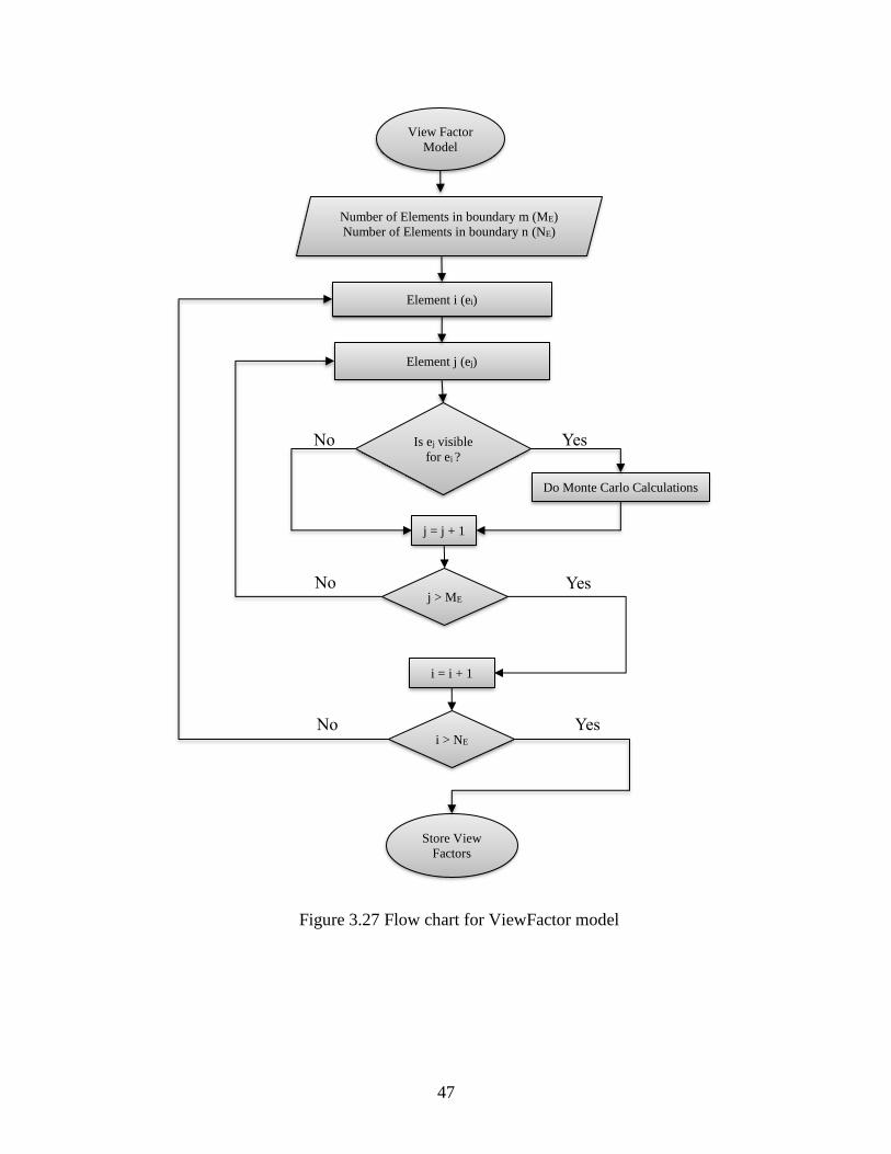
Figure 3.27 Flow chart for ViewFactor model
Yes
Yes No
No
No
Store View
Factors
i > NE
j > ME
Is ej visible
for ei ?
Do Monte Carlo Calculations
Element j (ej)
View Factor
Model
Number of Elements in boundary m (ME)
Number of Elements in boundary n (NE)
Element i (ei)
Yes
j = j + 1
i = i + 1
48
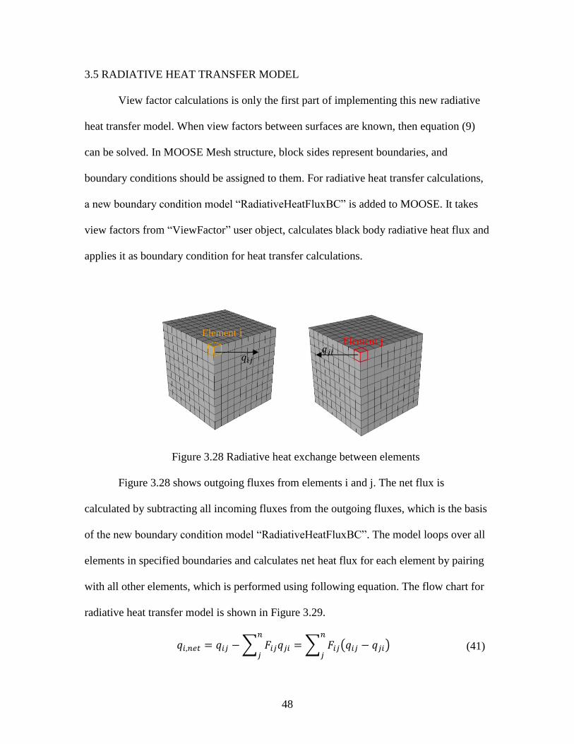
3.5 RADIATIVE HEAT TRANSFER MODEL
View factor calculations is only the first part of implementing this new radiative
heat transfer model. When view factors between surfaces are known, then equation (9)
can be solved. In MOOSE Mesh structure, block sides represent boundaries, and
boundary conditions should be assigned to them. For radiative heat transfer calculations,
a new boundary condition model “RadiativeHeatFluxBC” is added to MOOSE. It takes
view factors from “ViewFactor” user object, calculates black body radiative heat flux and
applies it as boundary condition for heat transfer calculations.
Figure 3.28 Radiative heat exchange between elements
Figure 3.28 shows outgoing fluxes from elements i and j. The net flux is
calculated by subtracting all incoming fluxes from the outgoing fluxes, which is the basis
of the new boundary condition model “RadiativeHeatFluxBC”. The model loops over all
elements in specified boundaries and calculates net heat flux for each element by pairing
with all other elements, which is performed using following equation. The flow chart for
radiative heat transfer model is shown in Figure 3.29.
𝑞𝑖,𝑛𝑒𝑡 = 𝑞𝑖𝑗 − ∑ 𝐹𝑖𝑗𝑞𝑗𝑖
𝑛
𝑗= ∑ 𝐹𝑖𝑗(𝑞𝑖𝑗 − 𝑞𝑗𝑖)
𝑛
𝑗 (41)
𝑞𝑖𝑗 𝑞𝑗𝑖
Element i Element j
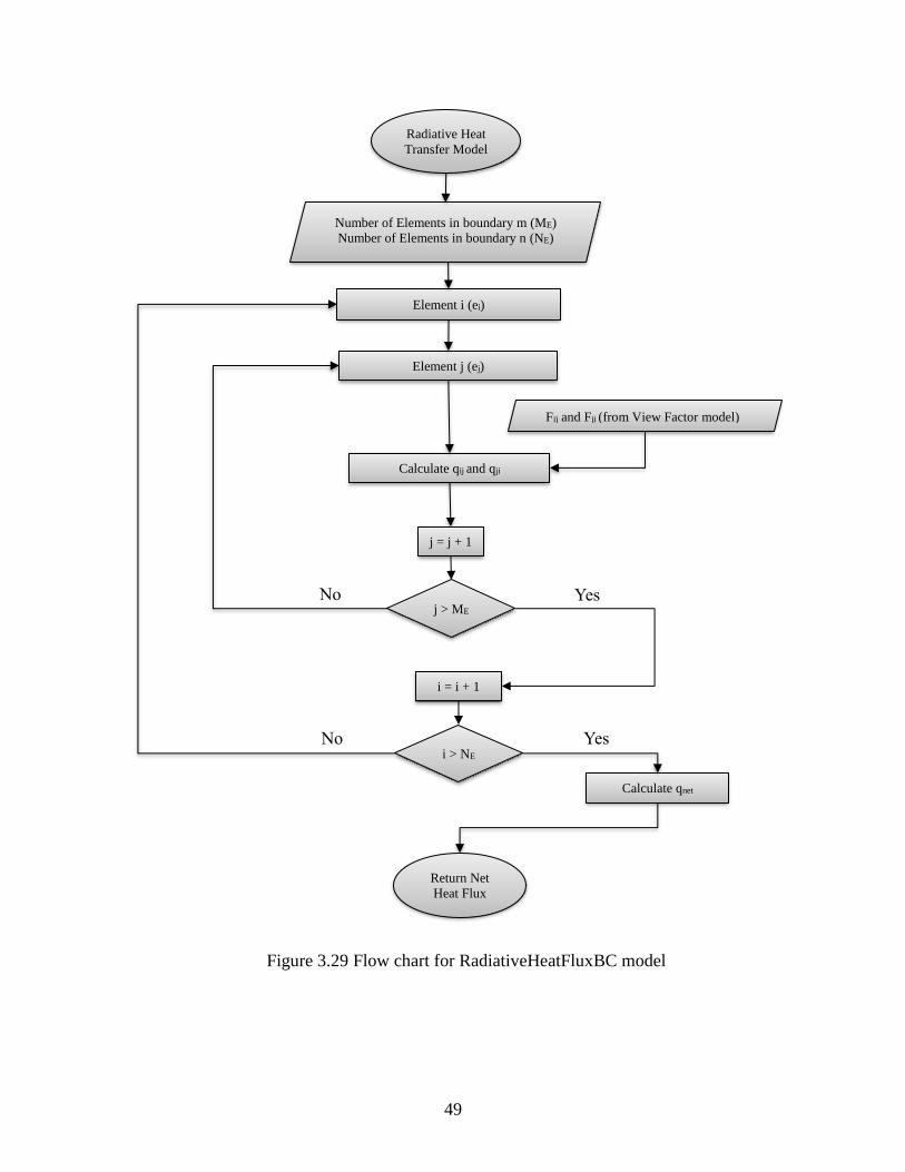
49
Figure 3.29 Flow chart for RadiativeHeatFluxBC model
Calculate qnet
Yes No
No
Return Net
Heat Flux
i > NE
j > ME
Fij and Fji (from View Factor model)
Calculate qij and qji
Element j (ej)
Radiative Heat
Transfer Model
Number of Elements in boundary m (ME)
Number of Elements in boundary n (NE)
Element i (ei)
Yes
j = j + 1
i = i + 1
50
CHAPTER 4
RESULTS AND DISCUSSION
The implemented view factor model is tested by using simple geometries. The
finite element meshes are generated by using Trelis software. Different geometric
parameters such as height, width, radius and the distance between surfaces, are used to
generate geometries. Analytical view factor values (Fanalytical) are calculated by using the
formulas presented in Appendix D in textbook written by Modest [1]. The percentage
error is calculated by following equation,
%𝐸𝑟𝑟𝑜𝑟 = 100 ∗|𝐹𝑎𝑛𝑎𝑙𝑦𝑡𝑖𝑐𝑎𝑙 − 𝐹𝑐𝑎𝑙𝑐𝑢𝑙𝑎𝑡𝑒𝑑|
𝐹𝑎𝑛𝑎𝑙𝑎𝑦𝑡𝑖𝑐𝑎𝑙 (42)
Since the view factors are calculated between the finite element surfaces, which are
flat, not curved, the results obtained for flat geometries such as rectangles, disks, provide
more insight about accuracy of ViewFactor model.
The radiative heat transfer model is tested by a case study which is pellet heating
experiment. The current GapHeatTransfer model in MOOSE is used for comparison of
results.
51
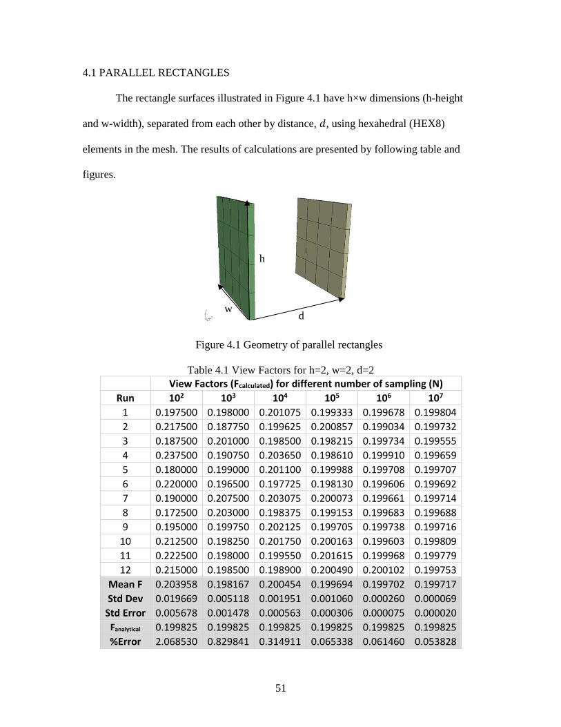
4.1 PARALLEL RECTANGLES
The rectangle surfaces illustrated in Figure 4.1 have h×w dimensions (h-height
and w-width), separated from each other by distance, 𝑑, using hexahedral (HEX8)
elements in the mesh. The results of calculations are presented by following table and
figures.
Figure 4.1 Geometry of parallel rectangles
Table 4.1 View Factors for h=2, w=2, d=2 View Factors (Fcalculated) for different number of sampling (N)
Run 102 103 104 105 106 107
1 0.197500 0.198000 0.201075 0.199333 0.199678 0.199804
2 0.217500 0.187750 0.199625 0.200857 0.199034 0.199732
3 0.187500 0.201000 0.198500 0.198215 0.199734 0.199555
4 0.237500 0.190750 0.203650 0.198610 0.199910 0.199659
5 0.180000 0.199000 0.201100 0.199988 0.199708 0.199707
6 0.220000 0.196500 0.197725 0.198130 0.199606 0.199692
7 0.190000 0.207500 0.203075 0.200073 0.199661 0.199714
8 0.172500 0.203000 0.198375 0.199153 0.199683 0.199688
9 0.195000 0.199750 0.202125 0.199705 0.199738 0.199716
10 0.212500 0.198250 0.201750 0.200163 0.199603 0.199809
11 0.222500 0.198000 0.199550 0.201615 0.199968 0.199779
12 0.215000 0.198500 0.198900 0.200490 0.200102 0.199753
Mean F 0.203958 0.198167 0.200454 0.199694 0.199702 0.199717
Std Dev 0.019669 0.005118 0.001951 0.001060 0.000260 0.000069
Std Error 0.005678 0.001478 0.000563 0.000306 0.000075 0.000020
Fanalytical 0.199825 0.199825 0.199825 0.199825 0.199825 0.199825
%Error 2.068530 0.829841 0.314911 0.065338 0.061460 0.053828
d w
h
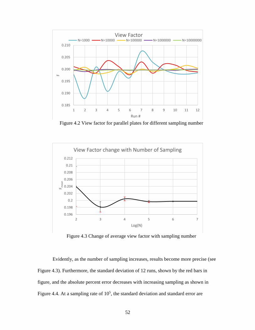
52
Figure 4.2 View factor for parallel plates for different sampling number
Figure 4.3 Change of average view factor with sampling number
Evidently, as the number of sampling increases, results become more precise (see
Figure 4.3). Furthermore, the standard deviation of 12 runs, shown by the red bars in
figure, and the absolute percent error decreases with increasing sampling as shown in
Figure 4.4. At a sampling rate of 105, the standard deviation and standard error are
0.185
0.190
0.195
0.200
0.205
0.210
1 2 3 4 5 6 7 8 9 10 11 12
F
Run #
View FactorN=1000 N=10000 N=100000 N=1000000 N=10000000
0.196
0.198
0.2
0.202
0.204
0.206
0.208
0.21
0.212
2 3 4 5 6 7
F mea
n
Log(N)
View Factor change with Number of Sampling
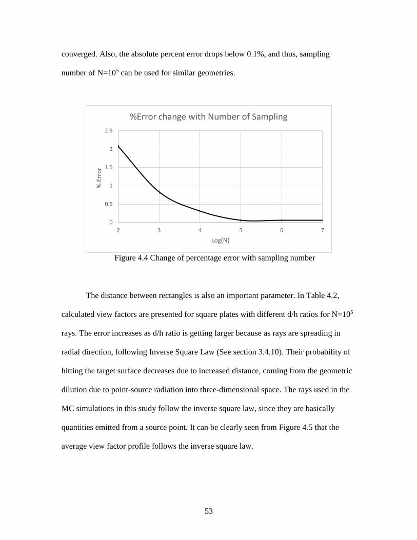
53
converged. Also, the absolute percent error drops below 0.1%, and thus, sampling
number of N=105 can be used for similar geometries.
Figure 4.4 Change of percentage error with sampling number
The distance between rectangles is also an important parameter. In Table 4.2,
calculated view factors are presented for square plates with different d/h ratios for N=105
rays. The error increases as d/h ratio is getting larger because as rays are spreading in
radial direction, following Inverse Square Law (See section 3.4.10). Their probability of
hitting the target surface decreases due to increased distance, coming from the geometric
dilution due to point-source radiation into three-dimensional space. The rays used in the
MC simulations in this study follow the inverse square law, since they are basically
quantities emitted from a source point. It can be clearly seen from Figure 4.5 that the
average view factor profile follows the inverse square law.
0
0.5
1
1.5
2
2.5
2 3 4 5 6 7
% E
rro
r
Log(N)
%Error change with Number of Sampling
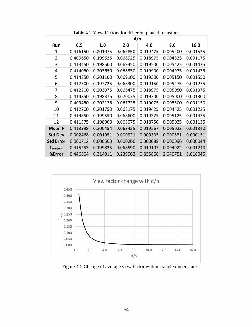
54
Table 4.2 View Factors for different plate dimensions d/h
Run 0.5 1.0 2.0 4.0 8.0 16.0
1 0.416150 0.201075 0.067850 0.019475 0.005200 0.001525
2 0.409650 0.199625 0.068925 0.018975 0.004325 0.001175
3 0.413450 0.198500 0.069450 0.019500 0.005425 0.001425
4 0.414050 0.203650 0.068350 0.019900 0.004975 0.001475
5 0.414850 0.201100 0.069100 0.019300 0.005150 0.001550
6 0.417500 0.197725 0.068300 0.019150 0.005275 0.001275
7 0.412200 0.203075 0.066475 0.018975 0.005050 0.001375
8 0.414850 0.198375 0.070075 0.019300 0.005000 0.001300
9 0.409450 0.202125 0.067725 0.019075 0.005300 0.001150
10 0.412200 0.201750 0.068175 0.019425 0.004425 0.001225
11 0.414850 0.199550 0.068600 0.019375 0.005125 0.001475
12 0.411575 0.198900 0.068075 0.018750 0.005025 0.001125
Mean F 0.413398 0.200454 0.068425 0.019267 0.005023 0.001340
Std Dev 0.002468 0.001951 0.000921 0.000305 0.000331 0.000151
Std Error 0.000712 0.000563 0.000266 0.000088 0.000096 0.000044
Fanalytical 0.415253 0.199825 0.068590 0.019107 0.004922 0.001240
%Error 0.446804 0.314911 0.239962 0.835866 2.040751 8.016045
Figure 4.5 Change of average view factor with rectangle dimensions
0.000
0.050
0.100
0.150
0.200
0.250
0.300
0.350
0.400
0.450
0.0 2.0 4.0 6.0 8.0 10.0 12.0 14.0 16.0
F mea
n
d/h
View factor change with d/h
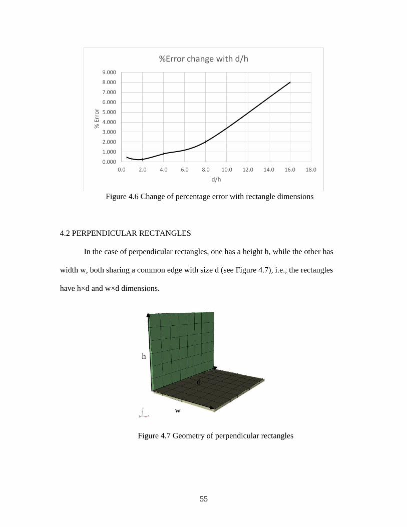
55
Figure 4.6 Change of percentage error with rectangle dimensions
4.2 PERPENDICULAR RECTANGLES
In the case of perpendicular rectangles, one has a height h, while the other has
width w, both sharing a common edge with size d (see Figure 4.7), i.e., the rectangles
have h×d and w×d dimensions.
Figure 4.7 Geometry of perpendicular rectangles
0.000
1.000
2.000
3.000
4.000
5.000
6.000
7.000
8.000
9.000
0.0 2.0 4.0 6.0 8.0 10.0 12.0 14.0 16.0 18.0
% E
rro
r
d/h
%Error change with d/h
w
h
d
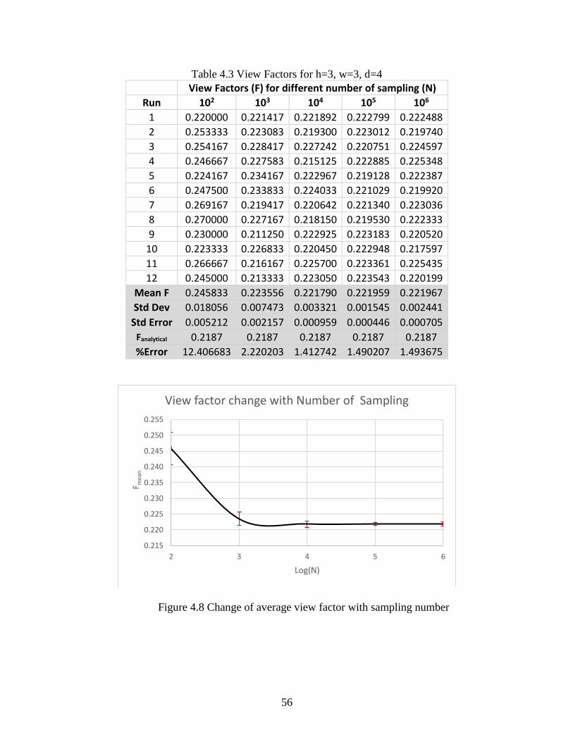
56
Table 4.3 View Factors for h=3, w=3, d=4 View Factors (F) for different number of sampling (N)
Run 102 103 104 105 106
1 0.220000 0.221417 0.221892 0.222799 0.222488
2 0.253333 0.223083 0.219300 0.223012 0.219740
3 0.254167 0.228417 0.227242 0.220751 0.224597
4 0.246667 0.227583 0.215125 0.222885 0.225348
5 0.224167 0.234167 0.222967 0.219128 0.222387
6 0.247500 0.233833 0.224033 0.221029 0.219920
7 0.269167 0.219417 0.220642 0.221340 0.223036
8 0.270000 0.227167 0.218150 0.219530 0.222333
9 0.230000 0.211250 0.222925 0.223183 0.220520
10 0.223333 0.226833 0.220450 0.222948 0.217597
11 0.266667 0.216167 0.225700 0.223361 0.225435
12 0.245000 0.213333 0.223050 0.223543 0.220199
Mean F 0.245833 0.223556 0.221790 0.221959 0.221967
Std Dev 0.018056 0.007473 0.003321 0.001545 0.002441
Std Error 0.005212 0.002157 0.000959 0.000446 0.000705
Fanalytical 0.2187 0.2187 0.2187 0.2187 0.2187
%Error 12.406683 2.220203 1.412742 1.490207 1.493675
Figure 4.8 Change of average view factor with sampling number
0.215
0.220
0.225
0.230
0.235
0.240
0.245
0.250
0.255
2 3 4 5 6
F mea
n
Log(N)
View factor change with Number of Sampling
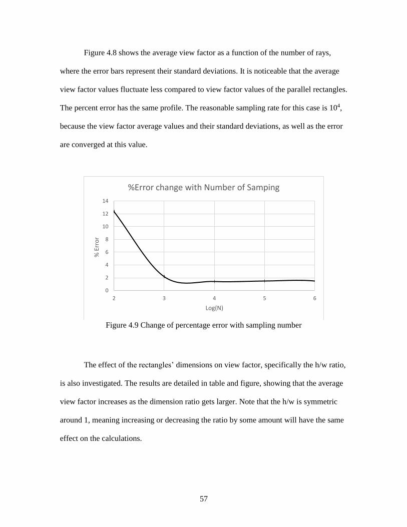
57
Figure 4.8 shows the average view factor as a function of the number of rays,
where the error bars represent their standard deviations. It is noticeable that the average
view factor values fluctuate less compared to view factor values of the parallel rectangles.
The percent error has the same profile. The reasonable sampling rate for this case is 104,
because the view factor average values and their standard deviations, as well as the error
are converged at this value.
Figure 4.9 Change of percentage error with sampling number
The effect of the rectangles’ dimensions on view factor, specifically the h/w ratio,
is also investigated. The results are detailed in table and figure, showing that the average
view factor increases as the dimension ratio gets larger. Note that the h/w is symmetric
around 1, meaning increasing or decreasing the ratio by some amount will have the same
effect on the calculations.
0
2
4
6
8
10
12
14
2 3 4 5 6
% E
rro
r
Log(N)
%Error change with Number of Samping
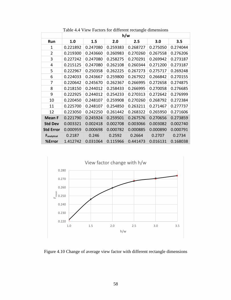
58
Table 4.4 View Factors for different rectangle dimensions h/w
Run 1.0 1.5 2.0 2.5 3.0 3.5
1 0.221892 0.247080 0.259383 0.268727 0.275050 0.274044
2 0.219300 0.243660 0.260983 0.270260 0.267558 0.276206
3 0.227242 0.247080 0.258275 0.270291 0.269942 0.273187
4 0.215125 0.247080 0.262108 0.260344 0.271200 0.273187
5 0.222967 0.250358 0.262225 0.267273 0.275717 0.269248
6 0.224033 0.243667 0.259800 0.267922 0.266842 0.270155
7 0.220642 0.245670 0.262367 0.266995 0.272658 0.274875
8 0.218150 0.244012 0.258433 0.266995 0.270058 0.276685
9 0.222925 0.244012 0.254233 0.270313 0.272642 0.276999
10 0.220450 0.248107 0.259908 0.270260 0.268792 0.272384
11 0.225700 0.248107 0.254850 0.263211 0.271467 0.277737
12 0.223050 0.242250 0.261442 0.268322 0.265950 0.271606
Mean F 0.221790 0.245924 0.259501 0.267576 0.270656 0.273859
Std Dev 0.003321 0.002418 0.002708 0.003066 0.003082 0.002740
Std Error 0.000959 0.000698 0.000782 0.000885 0.000890 0.000791
Fanalytical 0.2187 0.246 0.2592 0.2664 0.2707 0.2734
%Error 1.412742 0.031064 0.115966 0.441473 0.016131 0.168038
Figure 4.10 Change of average view factor with different rectangle dimensions
0.220
0.230
0.240
0.250
0.260
0.270
0.280
1.0 1.5 2.0 2.5 3.0 3.5
F mea
n
h/w
View factor change with h/w
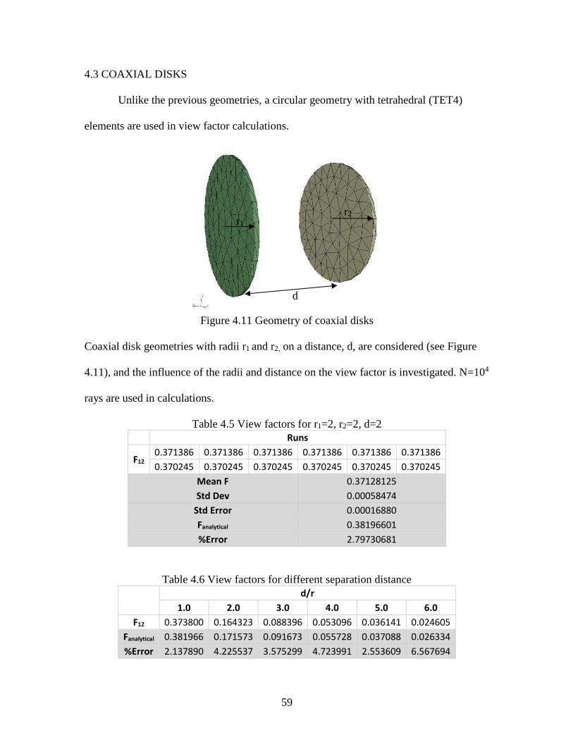
59
4.3 COAXIAL DISKS
Unlike the previous geometries, a circular geometry with tetrahedral (TET4)
elements are used in view factor calculations.
Figure 4.11 Geometry of coaxial disks
Coaxial disk geometries with radii r1 and r2, on a distance, d, are considered (see Figure
4.11), and the influence of the radii and distance on the view factor is investigated. N=104
rays are used in calculations.
Table 4.5 View factors for r1=2, r2=2, d=2 Runs
F12 0.371386 0.371386 0.371386 0.371386 0.371386 0.371386
0.370245 0.370245 0.370245 0.370245 0.370245 0.370245
Mean F 0.37128125
Std Dev 0.00058474
Std Error 0.00016880
Fanalytical 0.38196601
%Error 2.79730681
Table 4.6 View factors for different separation distance
d/r
1.0 2.0 3.0 4.0 5.0 6.0
F12 0.373800 0.164323 0.088396 0.053096 0.036141 0.024605
Fanalytical 0.381966 0.171573 0.091673 0.055728 0.037088 0.026334
%Error 2.137890 4.225537 3.575299 4.723991 2.553609 6.567694
d
r1
r2
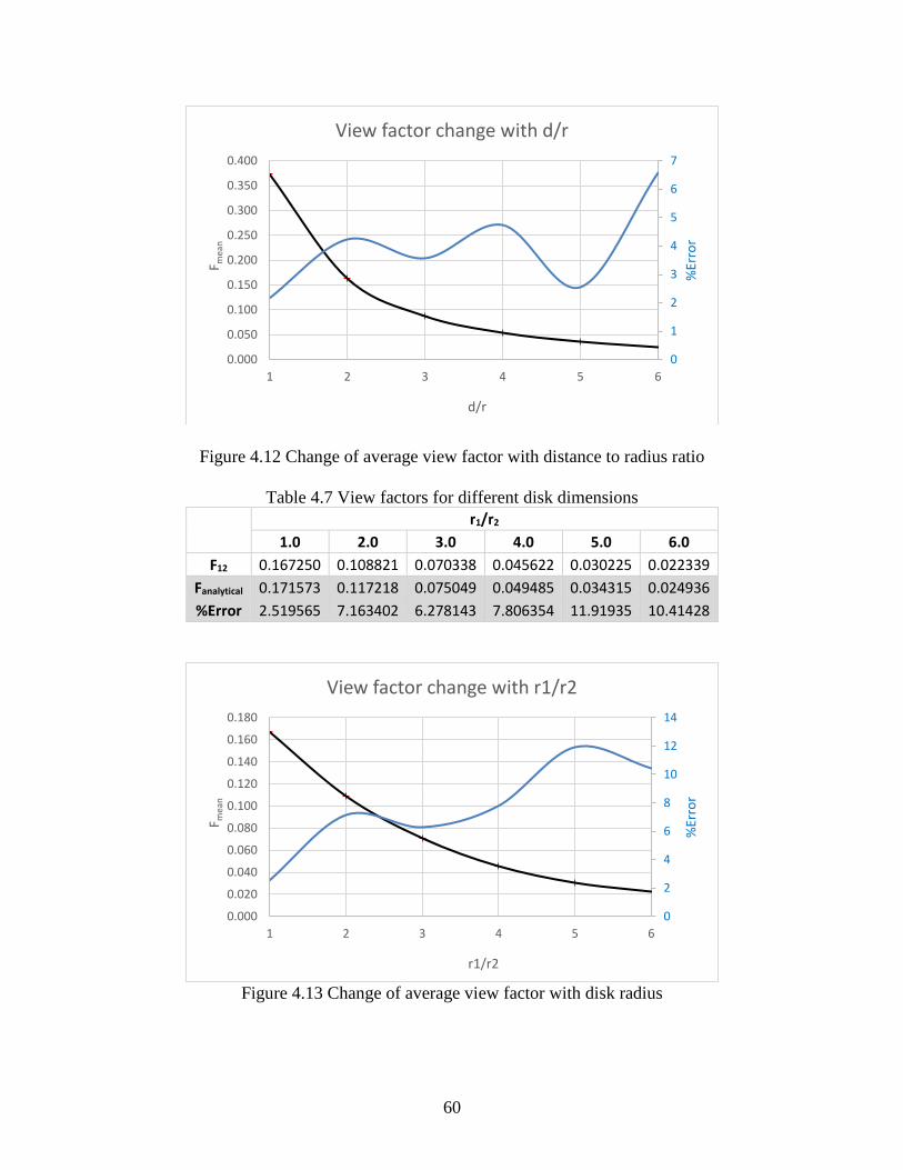
60
Figure 4.12 Change of average view factor with distance to radius ratio
Table 4.7 View factors for different disk dimensions
r1/r2
1.0 2.0 3.0 4.0 5.0 6.0
F12 0.167250 0.108821 0.070338 0.045622 0.030225 0.022339
Fanalytical 0.171573 0.117218 0.075049 0.049485 0.034315 0.024936
%Error 2.519565 7.163402 6.278143 7.806354 11.91935 10.41428
Figure 4.13 Change of average view factor with disk radius
0
1
2
3
4
5
6
7
0.000
0.050
0.100
0.150
0.200
0.250
0.300
0.350
0.400
1 2 3 4 5 6
%Er
ror
F mea
n
d/r
View factor change with d/r
0
2
4
6
8
10
12
14
0.000
0.020
0.040
0.060
0.080
0.100
0.120
0.140
0.160
0.180
1 2 3 4 5 6
%Er
ror
F mea
n
r1/r2
View factor change with r1/r2
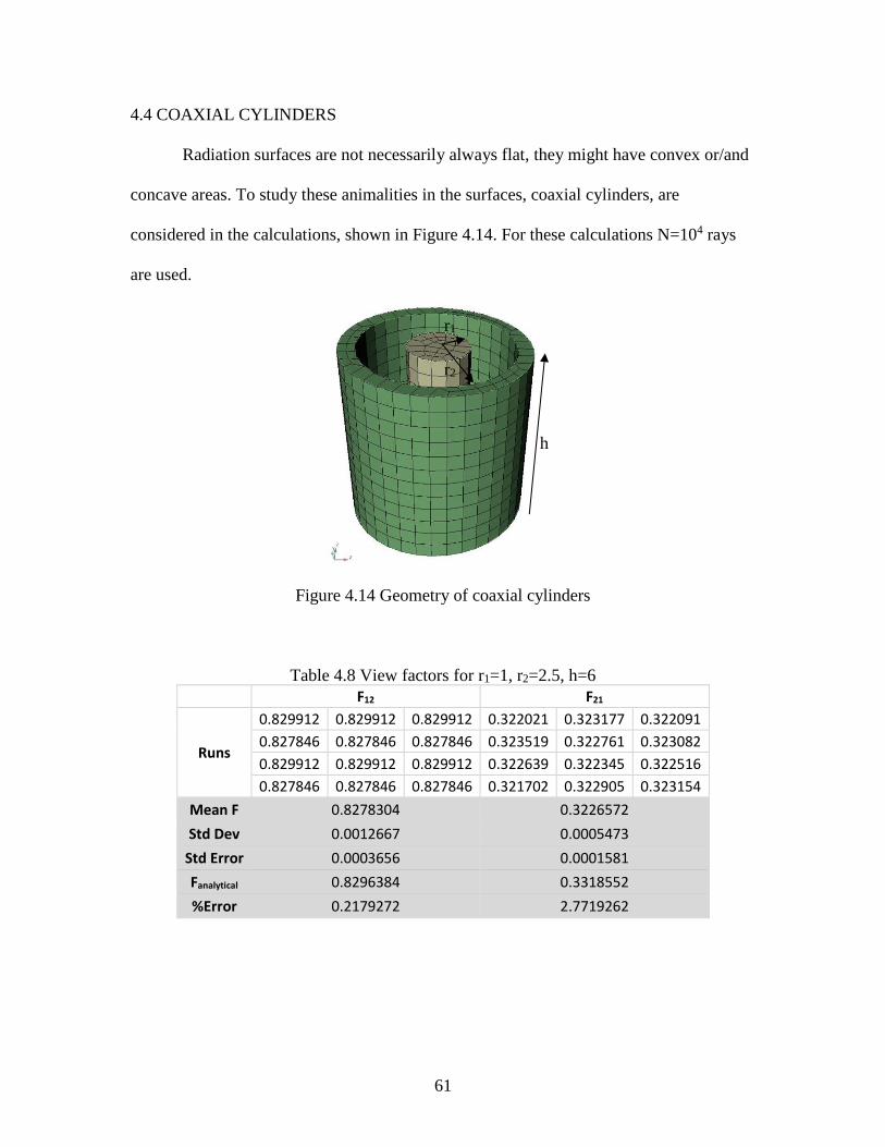
61
4.4 COAXIAL CYLINDERS
Radiation surfaces are not necessarily always flat, they might have convex or/and
concave areas. To study these animalities in the surfaces, coaxial cylinders, are
considered in the calculations, shown in Figure 4.14. For these calculations N=104 rays
are used.
Figure 4.14 Geometry of coaxial cylinders
Table 4.8 View factors for r1=1, r2=2.5, h=6
F12 F21
Runs
0.829912 0.829912 0.829912 0.322021 0.323177 0.322091
0.827846 0.827846 0.827846 0.323519 0.322761 0.323082
0.829912 0.829912 0.829912 0.322639 0.322345 0.322516
0.827846 0.827846 0.827846 0.321702 0.322905 0.323154
Mean F 0.8278304 0.3226572
Std Dev 0.0012667 0.0005473
Std Error 0.0003656 0.0001581
Fanalytical 0.8296384 0.3318552
%Error 0.2179272 2.7719262
r1
r2
h
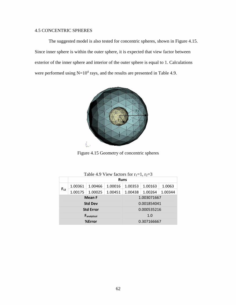
62
4.5 CONCENTRIC SPHERES
The suggested model is also tested for concentric spheres, shown in Figure 4.15.
Since inner sphere is within the outer sphere, it is expected that view factor between
exterior of the inner sphere and interior of the outer sphere is equal to 1. Calculations
were performed using N=104 rays, and the results are presented in Table 4.9.
Figure 4.15 Geometry of concentric spheres
Table 4.9 View factors for r1=1, r2=3 Runs
F12 1.00361 1.00466 1.00016 1.00353 1.00163 1.0063
1.00175 1.00025 1.00451 1.00438 1.00264 1.00344
Mean F 1.003071667
Std Dev 0.001854041
Std Error 0.000535216
Fanalytical 1.0
%Error 0.307166667
r1
r2
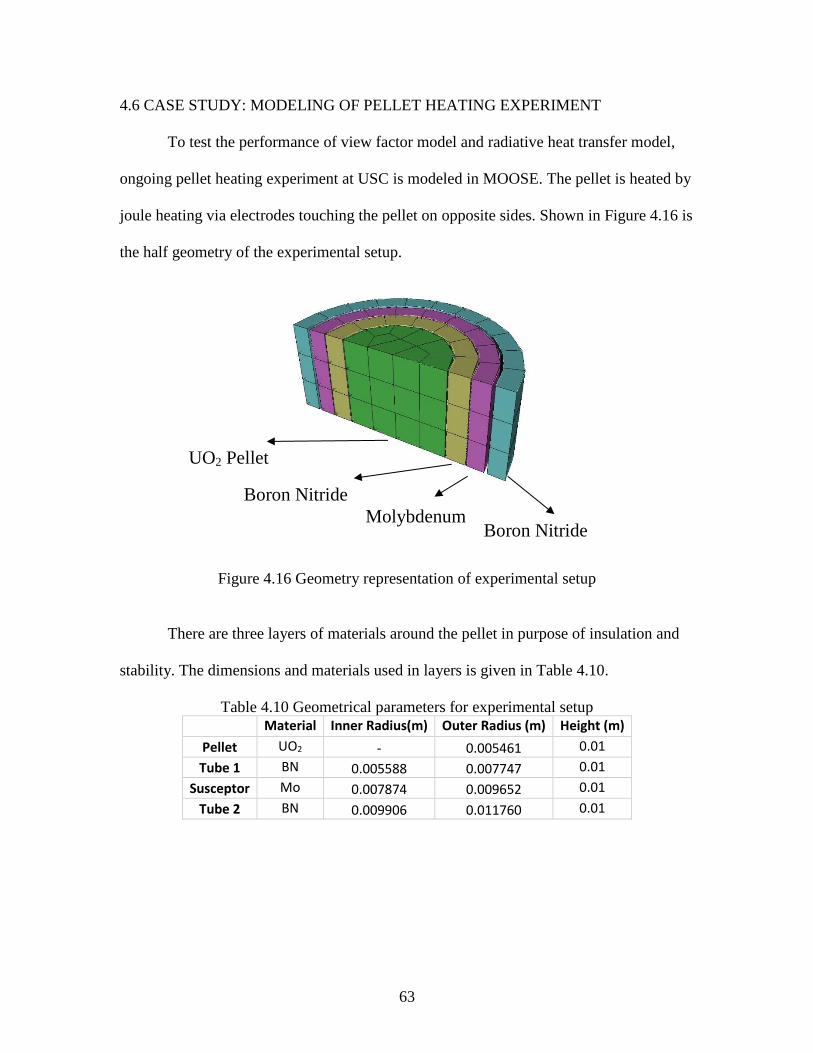
63
4.6 CASE STUDY: MODELING OF PELLET HEATING EXPERIMENT
To test the performance of view factor model and radiative heat transfer model,
ongoing pellet heating experiment at USC is modeled in MOOSE. The pellet is heated by
joule heating via electrodes touching the pellet on opposite sides. Shown in Figure 4.16 is
the half geometry of the experimental setup.
Figure 4.16 Geometry representation of experimental setup
There are three layers of materials around the pellet in purpose of insulation and
stability. The dimensions and materials used in layers is given in Table 4.10.
Table 4.10 Geometrical parameters for experimental setup Material Inner Radius(m) Outer Radius (m) Height (m)
Pellet UO2 - 0.005461 0.01
Tube 1 BN 0.005588 0.007747 0.01
Susceptor Mo 0.007874 0.009652 0.01
Tube 2 BN 0.009906 0.011760 0.01
UO2 Pellet
Boron Nitride
Molybdenum Boron Nitride
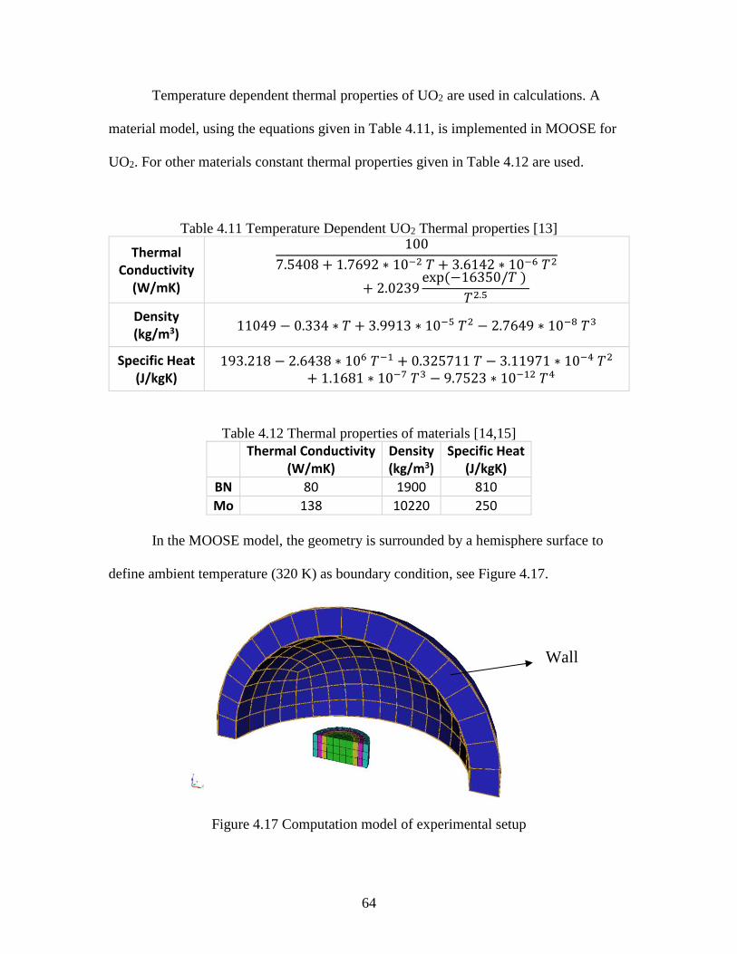
64
Temperature dependent thermal properties of UO2 are used in calculations. A
material model, using the equations given in Table 4.11, is implemented in MOOSE for
UO2. For other materials constant thermal properties given in Table 4.12 are used.
Table 4.11 Temperature Dependent UO2 Thermal properties [13]
Thermal Conductivity
(W/mK)
100
7.5408 + 1.7692 ∗ 10−2 𝑇 + 3.6142 ∗ 10−6 𝑇2
+ 2.0239exp (−16350/𝑇 )
𝑇2.5
Density (kg/m3)
11049 − 0.334 ∗ 𝑇 + 3.9913 ∗ 10−5 𝑇2 − 2.7649 ∗ 10−8 𝑇3
Specific Heat (J/kgK)
193.218 − 2.6438 ∗ 106 𝑇−1 + 0.325711 𝑇 − 3.11971 ∗ 10−4 𝑇2
+ 1.1681 ∗ 10−7 𝑇3 − 9.7523 ∗ 10−12 𝑇4
Table 4.12 Thermal properties of materials [14,15] Thermal Conductivity
(W/mK) Density (kg/m3)
Specific Heat (J/kgK)
BN 80 1900 810
Mo 138 10220 250
In the MOOSE model, the geometry is surrounded by a hemisphere surface to
define ambient temperature (320 K) as boundary condition, see Figure 4.17.
Figure 4.17 Computation model of experimental setup
Wall
65
Heat is generated in the pellet region by joule heating as a result of the voltage
difference between electrodes.
Electrical Fourier Equation,
𝐽𝑥 = 𝜎𝑥
𝛥𝑉
𝛥𝑥 (43)
where 𝐽𝑥 : current flux [𝐴𝑚𝑝/𝑚2]
𝜎𝑥 : electrical conductivity, 1/𝜌𝑥 , [1/𝛺𝑚]
𝜌𝑥 : electrical resistivity, 1/𝜎𝑥 , [𝛺𝑚]
𝛥𝑥 : spatial coordinate in the direction of current flow [𝑚]
𝛥𝑉 : voltage difference [𝑣𝑜𝑙𝑡]
Joule Heating,
𝑄 = 𝐽2𝜌 (44)
where 𝑄 : joule heating power [𝑊/𝑚3]
Then heat conduction equation with joule heating source term becomes,
𝜌𝐶𝑝
𝜕𝑇
𝜕𝑡− 𝛥 ∙ 𝑘𝛥𝑇 − 𝑄 = 0 (45)
Electrical conductivity of UO2 is found from literature and assumed as constant. [16]
𝜎𝑥 = 1 𝛺𝑚−1
The applied voltage on electrodes is equal to 10V and constant during experiment.
The volumetric heat generation is calculated as 82 MW/m3 by equations (43) and (44)
according to constant.
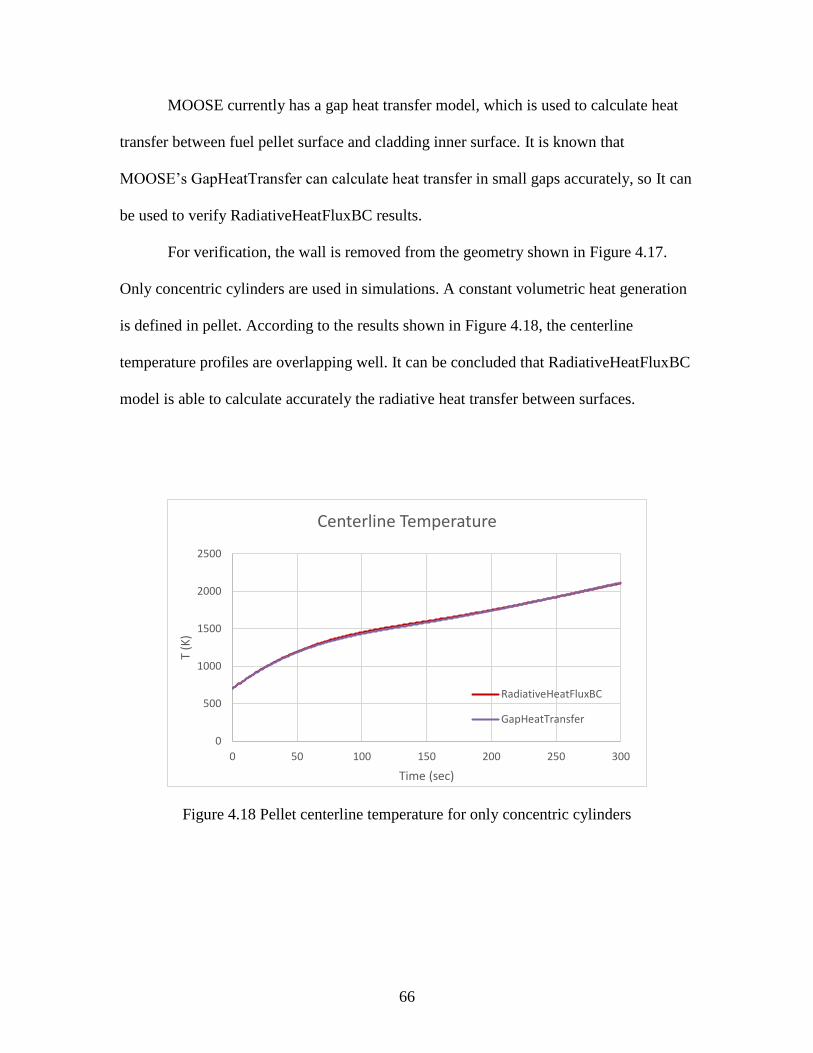
66
MOOSE currently has a gap heat transfer model, which is used to calculate heat
transfer between fuel pellet surface and cladding inner surface. It is known that
MOOSE’s GapHeatTransfer can calculate heat transfer in small gaps accurately, so It can
be used to verify RadiativeHeatFluxBC results.
For verification, the wall is removed from the geometry shown in Figure 4.17.
Only concentric cylinders are used in simulations. A constant volumetric heat generation
is defined in pellet. According to the results shown in Figure 4.18, the centerline
temperature profiles are overlapping well. It can be concluded that RadiativeHeatFluxBC
model is able to calculate accurately the radiative heat transfer between surfaces.
Figure 4.18 Pellet centerline temperature for only concentric cylinders
0
500
1000
1500
2000
2500
0 50 100 150 200 250 300
T (K
)
Time (sec)
Centerline Temperature
RadiativeHeatFluxBC
GapHeatTransfer
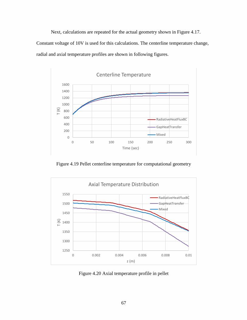
67
Next, calculations are repeated for the actual geometry shown in Figure 4.17.
Constant voltage of 10V is used for this calculations. The centerline temperature change,
radial and axial temperature profiles are shown in following figures.
Figure 4.19 Pellet centerline temperature for computational geometry
Figure 4.20 Axial temperature profile in pellet
0
200
400
600
800
1000
1200
1400
1600
0 50 100 150 200 250 300
T (K
)
Time (sec)
Centerline Temperature
RadiativeHeatFluxBC
GapHeatTransfer
Mixed
1250
1300
1350
1400
1450
1500
1550
0 0.002 0.004 0.006 0.008 0.01
T (K
)
z (m)
Axial Temperature Distribution
RadiativeHeatFluxBC
GapHeatTransfer
Mixed
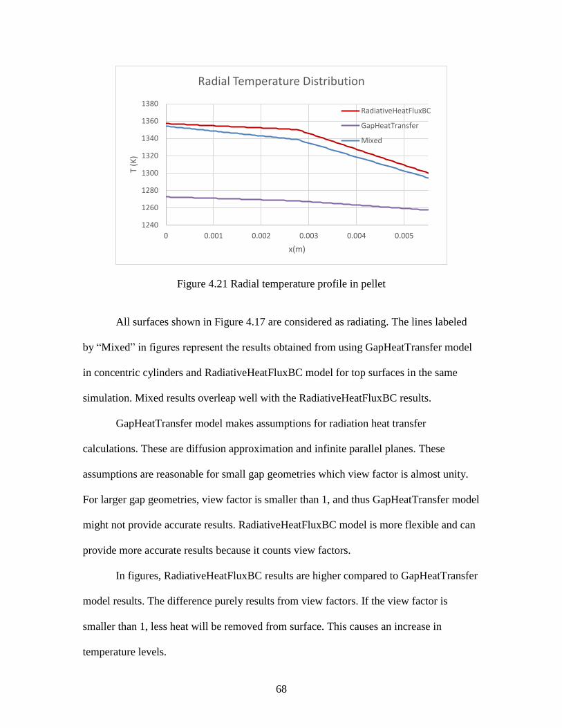
68
Figure 4.21 Radial temperature profile in pellet
All surfaces shown in Figure 4.17 are considered as radiating. The lines labeled
by “Mixed” in figures represent the results obtained from using GapHeatTransfer model
in concentric cylinders and RadiativeHeatFluxBC model for top surfaces in the same
simulation. Mixed results overleap well with the RadiativeHeatFluxBC results.
GapHeatTransfer model makes assumptions for radiation heat transfer
calculations. These are diffusion approximation and infinite parallel planes. These
assumptions are reasonable for small gap geometries which view factor is almost unity.
For larger gap geometries, view factor is smaller than 1, and thus GapHeatTransfer model
might not provide accurate results. RadiativeHeatFluxBC model is more flexible and can
provide more accurate results because it counts view factors.
In figures, RadiativeHeatFluxBC results are higher compared to GapHeatTransfer
model results. The difference purely results from view factors. If the view factor is
smaller than 1, less heat will be removed from surface. This causes an increase in
temperature levels.
1240
1260
1280
1300
1320
1340
1360
1380
0 0.001 0.002 0.003 0.004 0.005
T (K
)
x(m)
Radial Temperature Distribution
RadiativeHeatFluxBC
GapHeatTransfer
Mixed
69
CHAPTER 5
CONCLUSION
Two new model have been implemented to MOOSE for view factor and radiative
heat transfer calculations. In view factor model, the MC method is used and the user
object “ViewFactor” is created. In radiative heat transfer model, calculations are done by
assuming surfaces are black, and a boundary condition model “RadiativeHeatFluxBC” is
added to MOOSE.
The MC method provides flexibility to calculate view factors for any kind of
geometry. Although there are some drawbacks of MC method such as statistical error and
computing time, by using high performance computers they could be minimized.
There is still work that can be done to improve implemented models. The view
factor model is currently based on MC method. Other methods can be added as future
work to give user option. The radiative heat flux model is calculating heat transfer by
assuming surfaces are black. As a future work, it can be modified in order to use for
radiative heat exchange between gray or diffuse surfaces, considering absorption,
transmission and reflection.

70
BIBLIOGRAPHY
[1] Modest, M.F. 1993. Radiative Heat Transfer. McGraw-Hill. New York.
[2] Howell, J.R. 1998. The Monte Carlo method in radiative heat transfer. Journal of
Heat Transfer 120 547-560.
[3] Metropolis, Nicholas, and Ulam, S. 1949. The Monte Carlo Method. Journal of
American Statistical Association. 44-247 335-341.
[4] Junuthula Narasimha Reddy. An introduction to the finite element method, volume 2.
McGraw-Hill New York, 1993.
[5] Derek Gaston, Chris Newman, Glen Hansen, and Damien Lebrun-Grandie. Moose:
A parallel computational framework for coupled systems of nonlinear equations.
Nuclear Engineering and Design, 239(10):1768–1778, 2009.
[6] JohnW. Peterson, Alexander D. Lindsay, Fande Kong, Overview of the
incompressible Navier-Stokes simulation capabilities in the MOOSE framework,
Advances in Engineering Software, 119:68-92, 2008.
[7] Santosh B. Bopche, Arunkumar Sridharan, Determination of view factors by contour
integral technique, Annals of Nuclear Energy, 36: 1681-1688, 2009.
[8] Arvind Narayanaswamy, An analytic expression for radiation view factor between
two arbitrarily oriented planar polygons, International Journal of Heat and Mass
Transfer, 90: 841-847, 2015.
[9] Lei Yang, Wenzhen Chen, Lei Luo, Xinwen Zhao, Calculation of radiation heat
transfer view factors among fuel rod bundles based on CFD method, Annals of
Nuclear Energy, 71: 462-466, 2014.
[10] Matthew Barry, Justin Ying, Michael J. Durka, Corey E. Clifford, B.V.K. Reddy,
Minking K. Chyu, Numerical solution of radiation view factors within a
thermoelectric device, Energy, 102:427-435, 2016.
[11] M. Mirhosseini, A. Saboonchi, View Factor calculation using Monte Carlo method
for a 3D strip element to circular cylinder, Energy Procedia 142 513-518, 2017.

71
[12] P.Mahanta, Subhash C. Mishra, Collapsed dimension method applied to radiative
transfer problems in complex enclosures with participating medium, Numerical Heat
Transfer, 42:4, 367-388, 2010.
[13] Uffelen P.V., Konings R.J.M., Vitanza C., Tulenko J. (2010) Analysis of Reactor
Fuel Rod Behavior. In: Cacuci D.G. (eds) Handbook of Nuclear Engineering, 1519-
1627.
[14] Technical Products Inc. Boron Nitride Grade AX05 Material Specifications,
www.technicalproductsinc.com.
[15] International Molybdenum Association. Molybdenum Properties,
https://www.imoa.info/molybdenum/molybdenum-properties.php
[16] Shoji Lida, Electrical Properties of Non-Stoichiometric Uranium Dioxide, Japanese
Journal of Applied Physics, 4-11, 1