Implementation of Univariate Paradigm for Streamflow

Received May 2, 2019, accepted May 28, 2019, date of publication June 5, 2019, date of current version June 20, 2019.

Digital Object Identifier 10.1109/ACCESS.2019.2920916

Implementation of Univariate Paradigm forStreamflow Simulation Using HybridData-Driven Model: Case Study inTropical Region

ZAHER MUNDHER YASEEN 1, WAN HANNA MELINI WAN MOHTAR2,AMEEN MOHAMMED SALIH AMEEN3, ISA EBTEHAJ4,SITI FATIN MOHD RAZALI2, HOSSEIN BONAKDARI 4,SINAN Q SALIH5,6, NADHIR AL-ANSARI7, ANDSHAMSUDDIN SHAHID11School of Civil Engineering, Faculty of Engineering, Universiti Teknologi Malaysia, Skudai, Johor Bahru 81310, Malaysia2Sustainable and Smart Township Research Centre (SUTRA), Faculty of Engineering and Built Environment, Universiti Kebangsaan Malaysia, Bangi, Selangor

43600, Malaysia3Department of Water Resources, University of Baghdad, Baghdad, Iraq4Department of Civil Engineering, Razi University, Kermanshah 97146, Iran5Institute of Research and Development, Duy Tan University, Da Nang 550000, Vietnam6Computer Science Department, College of Computer Science and Information Technology, University of Anbar, Ramadi, Iraq7Civil, Environmental and Natural Resources Engineering, Lulea University of Technology, 97187 Lulea, Sweden

Corresponding author: Zaher Mundher Yaseen ([email protected])

This work was supported by the Professional Development Research University (PDRU) under Grant Q.J130000.21A2.04E47.

ABSTRACT The performance of the bio-inspired adaptive neuro-fuzzy inference system (ANFIS) models

are proposed for forecasting highly non-linear streamflow of Pahang River, located in a tropical climatic

region of Peninsular Malaysia. Three different bio-inspired optimization algorithms namely particle swarm

optimization (PSO), genetic algorithm (GA), and differential evolution (DE) were individually used to tune

the membership function of ANFIS model in order to improve the capability of streamflow forecasting. Dif-

ferent combination of antecedent streamflow was used to develop the forecasting models. The performance

of the models was evaluated using a number of metrics including mean absolute error (MAE), root mean

square error (RMSE), coefficient of determination (R2), and Willmott’s Index (WI) statistics. The results

revealed that increasing number of inputs has a positive impact on the forecasting ability of both ANFIS and

hybrid ANFIS models. The comparison of the performance of three optimization methods indicated PSO

improved the capability of ANFIS model (RMSE = 7.96; MAE = 2.34; R2 = 0.998 and WI = 0.994)

more compared to GA and DE in forecasting streamflow. The uncertainty band of ANFIS-PSO forecast was

also found the lowest (±0.217), which indicates that ANFIS-PSO model can be used for reliable forecasting

of highly stochastic river flow in tropical environment.

INDEX TERMS Streamflow forecasting, fuzzy logic, evolutionary algorithm, uncertainty analysis, tropical

environment.

I. INTRODUCTION

Streamflow forecasting is one of the essential concerns for

hydrologists and engineers for the planning and management

of water resources and for designing water resources projects.

Short-term and long-term streamflow forecasting can provide

a valuable information on the possibility of designing and

The associate editor coordinating the review of this manuscript andapproving it for publication was Mauro Tucci.

managing water infrastructures and the availability of water

resources [1]–[3]. Therefore, a wide variety of methods has

been developed and successfully implemented for forecasting

river flow. Streamflow forecasting can be categorized into

four categories: conceptual, metric, physical-based, and data-

driven models [4]. Conceptual models evaluate hydrological

processes i.e. precipitation, water storage, evaporation, rain-

fall runoff, evapotranspiration using simple equations. How-

ever, the major drawback of these models is the difficulties

VOLUME 7, 20192169-3536 2019 IEEE. Translations and content mining are permitted for academic research only.

Personal use is also permitted, but republication/redistribution requires IEEE permission.See http://www.ieee.org/publications_standards/publications/rights/index.html for more information.

74471

https://orcid.org/0000-0003-3647-7137

https://orcid.org/0000-0001-6169-3654

Z. M. Yaseen et al.: Implementation of Univariate Paradigm for Streamflow Simulation Using Hybrid Data-Driven Model

in calibration of the results due to involvement of many

variables in the equation [5]. Metric models use the gathered

hydrological data such as rainfall as its basic input. While

the physical-based models employ water-balance equations

based on the law of energy conservation for modelling

streamflow. Lastly, the data-driven models establish rela-

tionship between input and output variables for forecasting

streamflow. The data-driven models do not need catchment

physical information and able to forecast streamflow with

limited amount and incomplete data [5]. Therefore, such

models have been widely used for forecasting streamflow in

recent years.

Linear regression is traditionally used for the development

of data-driven models. The capability of linear regression-

based models is very limited to forecast non-linear pattern of

streamflow. To overcome this difficulty, data-driven models

based on soft computing (SC) techniques have been vastly

developed in last three decades [5]–[9]. In recent years, there

has been massive attention of exploring and developing new

innovative SC methods that can mimic and capture highly

complicated streamflow pattern [10]. This is owing to their

feasibility on capturing the complexity of stochastic prob-

lems such as nonlinearity, nonstationary and redundancy [11].

A large number of data-driven models using SC techniques

such as artificial neural network (ANN), fuzzy logic, adaptive

network-based fussy interface system, genetic programming,

and swarm intelligence methods have been proposed for

forecasting streamflow [12]. However, the forecasting abil-

ity of the models in terms of accuracies are often debat-

able [13], [14]. This is because of the non-linear pattern of

streamflow which limits the ability of the aforementioned

models.

The ANN is the most popular SC-based method employed

for streamflow forecasting due its capability to solve diverse

complex problems [15]–[17]. The assignment of weights to

the neurons for optimum performance of ANN is the major

challenge in ANN-based forecasting model. The weights are

controlled by both the internal tuning parameters of network

learning algorithm and its architecture. In addition, the use of

multiple layers with many nodes as hidden layer results an

extremely complex system. The learning rates and the num-

ber of memory taps also significantly impact the performance

of ANN model.

Besides ANN, the fuzzy logic (FL) which uses the con-

cept of uncertainty is another SC-based technique that has

been received much attention for modeling hydrological phe-

nomena in last three decades [18], [19]. Similar to ANN,

the FL has several shortcomings such as decision on suit-

able variables. To overcome the drawbacks of ANN and FL,

adaptive neuro-fuzzy inference system (ANFIS) which is a

combination of ANN and FL is introduced. ANFIS is a class

of adaptive multi-layer feedforward networks that use fuzzy

logic in performing different functions or criteria for better

outcomes and intelligence [20]. It utilizes parallel computa-

tion where the learning ability is obtained from ANN and the

problem-solving ability based on if-then rules is gained from

fuzzy logic. Therefore, the advantages of ANN and FL can

be utilized in ANFIS while the shortcomings of the individual

methods can be overcome at the same time. ANFIS can fulfill

approximation function and follow rules efficiently almost

similar to human intuition [21] and thus, leads to higher accu-

racy in prediction [22]. The implementation of neuro-fuzzy

concept can positively solve the non-linear characteristics and

the associated uncertainties [23].

The major algorithms used for training ANFIS are back-

propagation (BP), hybrid of BP and least square (BP-LS).

A number of studies have been conducted to evaluate the

performance of the training algorithms to determine the best

ANFIS model for streamflow forecasting [24], [25]. The

most remarkable shortcomings of these algorithms are trap-

ping in the local optima during the learning process and

very slow convergence [26], [27]. Newly developed intel-

ligence algorithms such as nature inspired algorithms like

particle swarm optimization, genetic algorithm, differential

evolution etc. have been used in the recent years for the

optimization of ANFIS parameters to improve its forecast-

ing ability [28], [29]. The integration of evolutionary opti-

mization algorithms with artificial intelligence (AI) models

has showed outstanding performance in regression prob-

lems [30]–[33]. Thus, research focusing on identification of

best optimization algorithm to be used with AI in order to

achieve the most accurate and effective streamflow forecast-

ing has gained much attention in recent years. PSO, GA and

DE algorithms have been found to optimize ANFIS model

effectively where the local minima and dimension problems

are positively solved [34].

The main objective of the present study is to explore the

feasibility of newly developed robust hybridized intelligence

models, ANFIS integrated with three optimization algo-

rithms, i.e. particle swarm optimization (ANFIS-PSO),

genetic algorithm (ANFIS-GA) and differential evolution

algorithm (ANFIS-DE) for forecasting monthly streamflow

based on univariate modeling paradigm where only the

antecedent streamflow data is used to build the predictive

model. The performance of such hybrid models in forecasting

streamflow in tropical environment has not been investi-

gated yet. The models developed in the present study were

used for forecasting highly stochastic streamflow of Pahang

River located in the central region of Peninsular Malaysia.

The streamflow of Pahang River is influenced by highly vari-

able rainfall dominated by two monsoons. Besides, the heavy

convective rainfall during inter-monsoonal periods has made

the streamflowof the river highly complex. The PahangRiver,

the longest river in Peninsular Malaysia often experiences

floods due to extreme rainfall during northwest monsoon

(November-March). Reliable forecasting of streamflow of

Pahang River is therefore very important for Malaysia.

II. CASE STUDY

The Pahang River lies between the latitude 2◦48′45′′ -

3◦40′24′′N and longitude 101◦16′31′′ - 103◦29′34′′E

(Figure 1). The total length of the river is 460 km which

74472 VOLUME 7, 2019


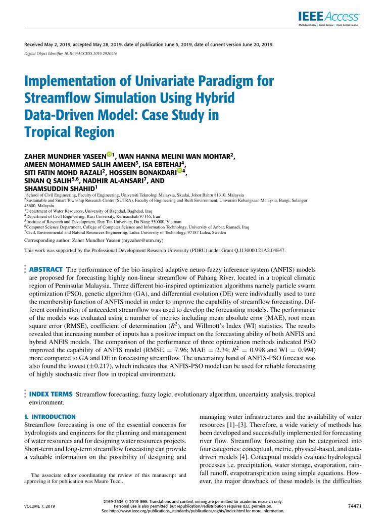
FIGURE 1. Location of Pahang River in the map of Peninsular Malaysia.

FIGURE 2. Streamflow time series of Pahang River at a station 3527410.

covers a catchment area of approximately 27,000 km2.

The streamflow of Pahang River is highly variable and

stochastic [35]. This is owing to the fact that the climate

of the catchment is characterized by high monsoon rainfall

which causes a high fluctuation in the flow. The motivation of

the development of an intelligent forecasting system for this

specific river lies on the necessity of flood forecasting and

estimation of water availability. The streamflow of Pahang

river measured at a station (ID 3527410), located in the

most downstream (Lubok Paku) of the river was used in

the present study. Monthly streamflow data for the period

2000-2014 was collected from the Department of Irrigation

and Drainage (DID), Malaysia. Flood is a common phe-

nomenon in Pahang River basin. It experienced 18 major

floods during 2006-2014 which caused extensive damage

to properties and inconvenience to the local community.

In December 2007, a large flood in Pahang River basin

caused an inundation depth of about 2.0 m in Pekan and

some other major towns of Termerloh and Maran districts

[36]. About US$ 86 Million was estimated as the total flood

damage. Forecasting river flow at monthly scale can indicate

the possibility of occurrence of floods which in turn can help

in flood management and mitigation of its impacts on society

and economy. The streamflow time series of Pahang River is

presented in Figure 2.

III. METHODOLOGY

A. ANFIS MODELLING THEORY

Themain concept of neuro-fuzzy system is amodeling frame-

work to overcome the impediments in both neural network

and fuzzy logic [37]. Therefore, ANFIS has been found well

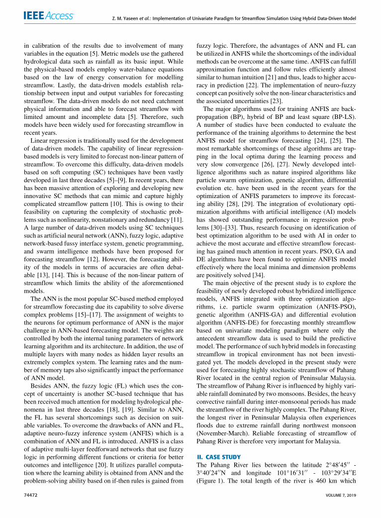
FIGURE 3. Auto-correlation function (ACF) of the raw streamflow timeseries.

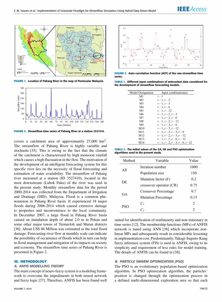
TABLE 1. Different input combinations of antecedent data considered forthe development of streamflow forecasting models.

TABLE 2. The initial values of the GA, DE and PSO optimizationalgorithms used in the present study.

suited for identification of nonlinearity and non-stationary in

time series [12]. The membership functions (MFs) of ANFIS

network is tuned using ANN [38] which incorporate non-

linear MFs and subsequently result in considerable lessening

in implementation cost. Predominantly, Takagi-Sugeno-Kang

fuzzy inference system (FIS) is used in ANFIS, owing to its

simplicity and requirement of less rules for model training.

The details of ANFIS can be found in [38].

B. PARTICLE SWARM OPTIMIZATION (PSO)

The PSO is an evolutionary population-based optimization

algorithm. In PSO optimization algorithm, the particles’

position is changed through the optimization process in

a defined multi-dimensional exploration area so that each

VOLUME 7, 2019 74473


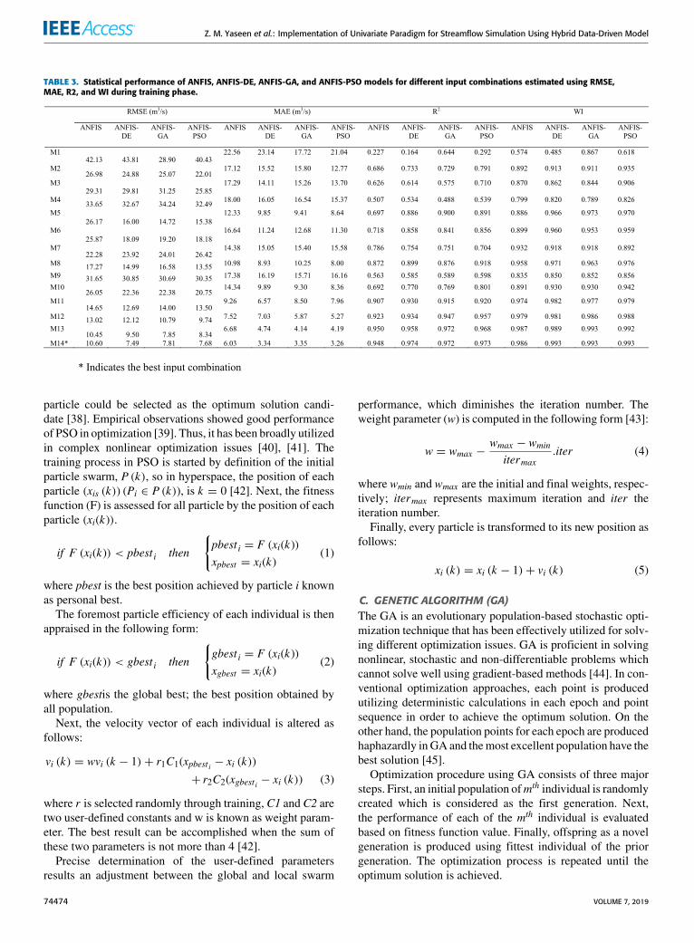
TABLE 3. Statistical performance of ANFIS, ANFIS-DE, ANFIS-GA, and ANFIS-PSO models for different input combinations estimated using RMSE,MAE, R2, and WI during training phase.

particle could be selected as the optimum solution candi-

date [38]. Empirical observations showed good performance

of PSO in optimization [39]. Thus, it has been broadly utilized

in complex nonlinear optimization issues [40], [41]. The

training process in PSO is started by definition of the initial

particle swarm, P (k), so in hyperspace, the position of each

particle (xis (k)) (Pi ∈ P (k)), is k = 0 [42]. Next, the fitness

function (F) is assessed for all particle by the position of each

particle (xi(k)).

if F (xi(k)) < pbest i then

{

pbest i = F (xi(k))

xpbest = xi(k)(1)

where pbest is the best position achieved by particle i known

as personal best.

The foremost particle efficiency of each individual is then

appraised in the following form:

if F (xi(k)) < gbest i then

{

gbest i = F (xi(k))

xgbest = xi(k)(2)

where gbestis the global best; the best position obtained by

all population.

Next, the velocity vector of each individual is altered as

follows:

vi (k) = wvi (k − 1) + r1C1(xpbest i − xi (k))

+ r2C2(xgbest i − xi (k)) (3)

where r is selected randomly through training, C1 and C2 are

two user-defined constants and w is known as weight param-

eter. The best result can be accomplished when the sum of

these two parameters is not more than 4 [42].

Precise determination of the user-defined parameters

results an adjustment between the global and local swarm

performance, which diminishes the iteration number. The

weight parameter (w) is computed in the following form [43]:

w = wmax −wmax − wmin

itermax.iter (4)

where wmin and wmax are the initial and final weights, respec-

tively; itermax represents maximum iteration and iter the

iteration number.

Finally, every particle is transformed to its new position as

follows:

xi (k) = xi (k − 1) + vi (k) (5)

C. GENETIC ALGORITHM (GA)

The GA is an evolutionary population-based stochastic opti-

mization technique that has been effectively utilized for solv-

ing different optimization issues. GA is proficient in solving

nonlinear, stochastic and non-differentiable problems which

cannot solve well using gradient-based methods [44]. In con-

ventional optimization approaches, each point is produced

utilizing deterministic calculations in each epoch and point

sequence in order to achieve the optimum solution. On the

other hand, the population points for each epoch are produced

haphazardly inGA and themost excellent population have the

best solution [45].

Optimization procedure using GA consists of three major

steps. First, an initial population ofmth individual is randomly

created which is considered as the first generation. Next,

the performance of each of the mth individual is evaluated

based on fitness function value. Finally, offspring as a novel

generation is produced using fittest individual of the prior

generation. The optimization process is repeated until the

optimum solution is achieved.

74474 VOLUME 7, 2019


TABLE 4. Statistical performance of ANFIS, ANFIS-DE, ANFIS-GA and ANFIS-PSO models for different input combinations estimated using RMSE, MAE,R2 and WI during testing phase.

TABLE 5. Relative error in forecasting of ANFIS, ANFIS-DE, ANFIS-GA andANFIS-PSO models for different input combination during model testing.

Offspring generation process comprises three essen-

tial steps: crossover, mutation and reproduction. In GA,

an individual is represented as gene sequence known as

chromosomes. The crossover and mutation are employed for

reproduction. In crossover, the genes related to parent chro-

mosome are altered, while in mutation genes in parent chro-

mosome are randomly modified. Both of these operators

have significant impact on optimization result. Defined oper-

ators in GA hop into obscure ranges within the look space

(mutation) and offer assistance in finding new solution space

(crossover) [46].

The evolutionary process in GA proceeds for different

generations until an end condition is satisfied. The best gene

is chosen based on the fitness function values and is reported

as the optimum solution of the problem.

D. DIFFERENTIAL OPTIMIZATION

Differential Evolution (DE) is an evolutionary population-

based optimization algorithm [47]. Use of differential muta-

tion makes the DE different from other evolutionary-based

algorithms. InDE, fixed vector numbers are created randomly

within n-dimensional space. To discover the different search

spaces in order to minimize fitness function, an evolutionary

process over time is required. To generatemutation factor (µ),

a mutation function (F : Iµ → Iµ) is defined in the following

form:

−→vi =−→ar1 + F

(−→ar2 −−→ar3

)

i = 1, 2, . . . , µ (6)

where r1, r2, r3 ∈ [1, 2, . . . , µ] are selected randomly, ai is

trial vector, F is the mutation factor and µ is the population

size. The mutation factor (F) is a constant positive value in

the range of [0 2]. Considering the larger values of population

size (µ), mutation factor (F) tends to enhance the global

search capacity of DE algorithm by discovering new search

space.

The vectors (−→vi = [−→v1i,−→v2i, . . . . . . ,

−→vdi] are mutated using

crossover operator (CR : Iµ → Iµ) in DE to generate trial

vectors as follows:

a′ji =

{

vji if (randb (j) ≤ CR) or j = rnbr (i)

aji if (randb (j) ≤ CR) or j 6= rnbr (i)

j = 1, 2, . . . , 2 i = 1, 2, . . . , d (7)

where rnbr (i) ∈ 1, 2, . . . , d) is an index for random selec-

tion, CR is the crossover operator, randb (j) denotes random-

ized producer assessment in the range of [0, 1]. The CR is

employed to enhance the individuals’ variety in populations.

Similar to mutated vectors, large values of CR results in

enhancement in offspring vectors. Consequently, the conver-

gence speed of the DE algorithm is augmented.

VOLUME 7, 2019 74475


If cases CR = 0, children and parents’ vectors differ by

only one variable (Eq. 7). The costliest fitness function is

selected using selection operator to generate trial vector for

next generation.

if 8(−→a′i (g) < 8

(−→ai (g))

, then −→ai (g+ 1) =−→a′i (g)

else −→ai (g+ 1) =−→ai (g+ 1) =

−→ai (g) (8)

where g is the current generation.

E. MODELS DEVELOPMENT

Fourteen different combinations of antecedent streamflow

values were considered for the selection of best input com-

bination for the development of forecasting models. Usu-

ally, most recent antecedent values are more correlated with

the target streamflow [11], [12]. Therefore, consecutive two

antecedent values, t−1 and t−2 were considered as possible

input. Besides, 3-, 6- and 12-month antecedent values were

tested as possible input considering the seasonal variability

due to two monsoons and annual variability of streamflow.

Indeed, this was determined based on the statistical procedure

commonly used for time series forecasting such as autocorre-

lation function (ACF) as presented in Figure 3. The fourteen

input combinations of these five antecedent values are given

in Table 1. All the 14 input combinations (M1 to M14)

were used for the development of ANFIS and hybrid ANFIS

(ANFIS-DE, ANFIS-GA, and ANFIS-PSO)model. The opti-

mum values of the DE, GA, and PSO algorithms are given

in Table 2. The values of fixed parameters of ANFIS model

were considered as follows: the initial step size is 0.001, step

size decrease is 0.009, step size increase is 1.001 and the

number of the MF for each input is 6.

F. PERFORMANCE SKILL INDICATORS

To examine the prediction capability of the developed mod-

els, several statistical indicators were used which includes

mean absolute error (MAE), root mean square error (RMSE),

coefficient of determination (R2) and Willmott’s Index

(WI) [48]–[50]. Besides, the predictive capability of the mod-

els was examined using relative error (RE) [51], [52]. The

uncertainty in prediction of streamflow by different models

was also assessed for fair comparison of model performance.

For this purpose, the difference between predicted and tar-

get values were first calculated to estimate the prediction

error (PE):

ej = Pj − Tj (9)

The standard deviation (STD) and mean (MPE) of PE were

calculated as:

Se =

√

∑n

j=1

(

ej − e)2

n− 1and e =

∑n

j=1ej (10)

A positive (or negative) value of MPE illustrates the over-

estimation (or underestimation) by the prediction models.

Using Wilson score without continuity correction, a con-

fidence band was defined around the predict error values

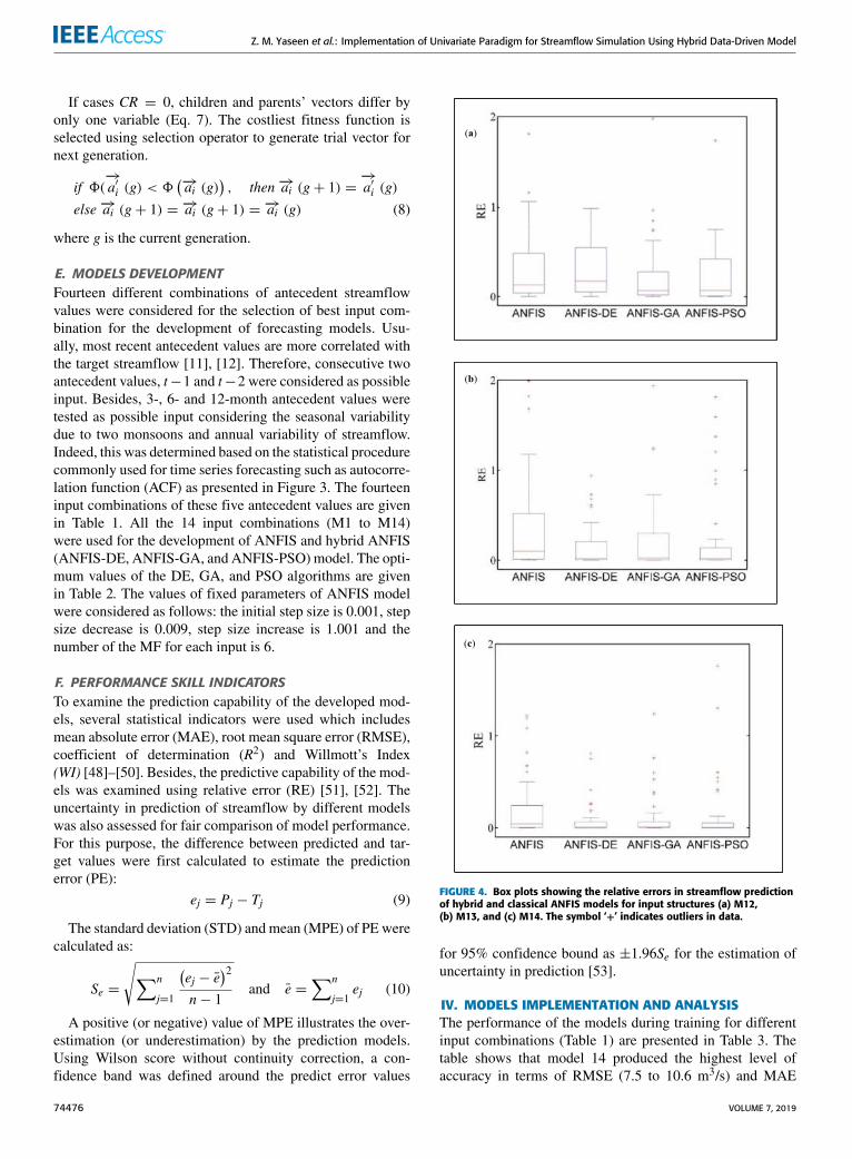
FIGURE 4. Box plots showing the relative errors in streamflow predictionof hybrid and classical ANFIS models for input structures (a) M12,(b) M13, and (c) M14. The symbol ‘+’ indicates outliers in data.

for 95% confidence bound as ±1.96Se for the estimation of

uncertainty in prediction [53].

IV. MODELS IMPLEMENTATION AND ANALYSIS

The performance of the models during training for different

input combinations (Table 1) are presented in Table 3. The

table shows that model 14 produced the highest level of

accuracy in terms of RMSE (7.5 to 10.6 m3/s) and MAE

74476 VOLUME 7, 2019


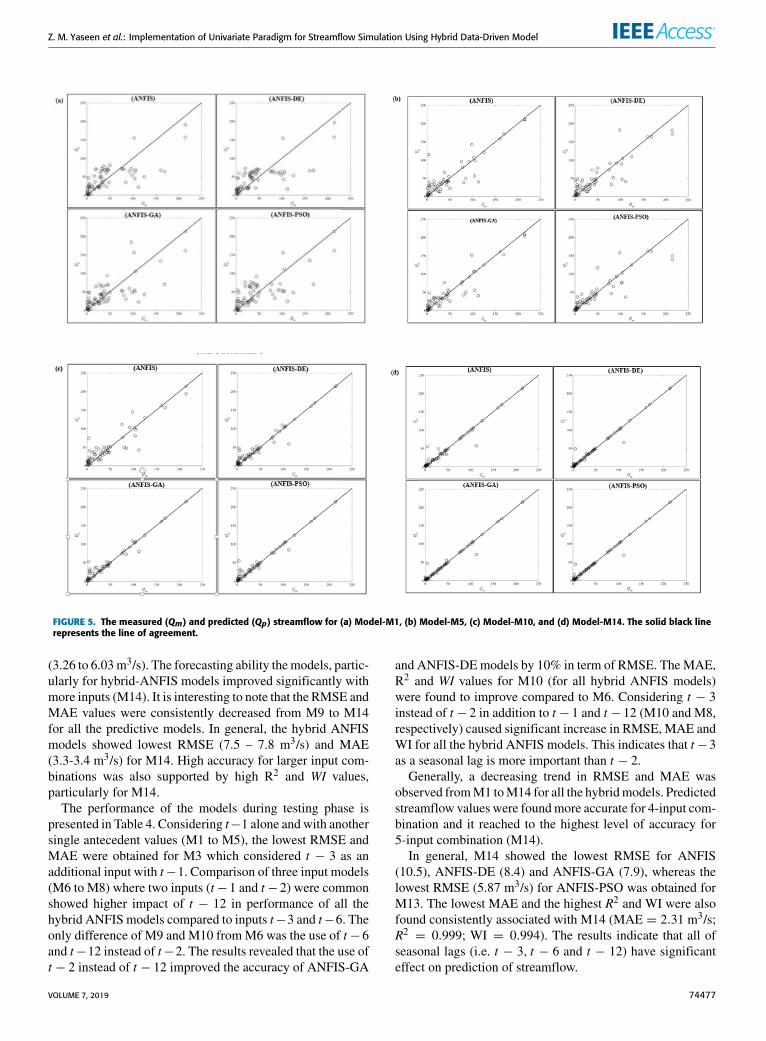
FIGURE 5. The measured (Qm) and predicted (Qp) streamflow for (a) Model-M1, (b) Model-M5, (c) Model-M10, and (d) Model-M14. The solid black linerepresents the line of agreement.

(3.26 to 6.03m3/s). The forecasting ability themodels, partic-

ularly for hybrid-ANFIS models improved significantly with

more inputs (M14). It is interesting to note that the RMSE and

MAE values were consistently decreased from M9 to M14

for all the predictive models. In general, the hybrid ANFIS

models showed lowest RMSE (7.5 – 7.8 m3/s) and MAE

(3.3-3.4 m3/s) for M14. High accuracy for larger input com-

binations was also supported by high R2 and WI values,

particularly for M14.

The performance of the models during testing phase is

presented in Table 4. Considering t−1 alone and with another

single antecedent values (M1 to M5), the lowest RMSE and

MAE were obtained for M3 which considered t − 3 as an

additional input with t−1. Comparison of three input models

(M6 to M8) where two inputs (t−1 and t−2) were common

showed higher impact of t − 12 in performance of all the

hybrid ANFIS models compared to inputs t−3 and t−6. The

only difference of M9 and M10 fromM6 was the use of t−6

and t−12 instead of t−2. The results revealed that the use of

t − 2 instead of t − 12 improved the accuracy of ANFIS-GA

and ANFIS-DEmodels by 10% in term of RMSE. TheMAE,

R2 and WI values for M10 (for all hybrid ANFIS models)

were found to improve compared to M6. Considering t − 3

instead of t − 2 in addition to t − 1 and t − 12 (M10 and M8,

respectively) caused significant increase in RMSE, MAE and

WI for all the hybrid ANFIS models. This indicates that t−3

as a seasonal lag is more important than t − 2.

Generally, a decreasing trend in RMSE and MAE was

observed fromM1 toM14 for all the hybridmodels. Predicted

streamflow values were foundmore accurate for 4-input com-

bination and it reached to the highest level of accuracy for

5-input combination (M14).

In general, M14 showed the lowest RMSE for ANFIS

(10.5), ANFIS-DE (8.4) and ANFIS-GA (7.9), whereas the

lowest RMSE (5.87 m3/s) for ANFIS-PSO was obtained for

M13. The lowest MAE and the highest R2 and WI were also

found consistently associated with M14 (MAE = 2.31 m3/s;

R2 = 0.999; WI = 0.994). The results indicate that all of

seasonal lags (i.e. t − 3, t − 6 and t − 12) have significant

effect on prediction of streamflow.

VOLUME 7, 2019 74477


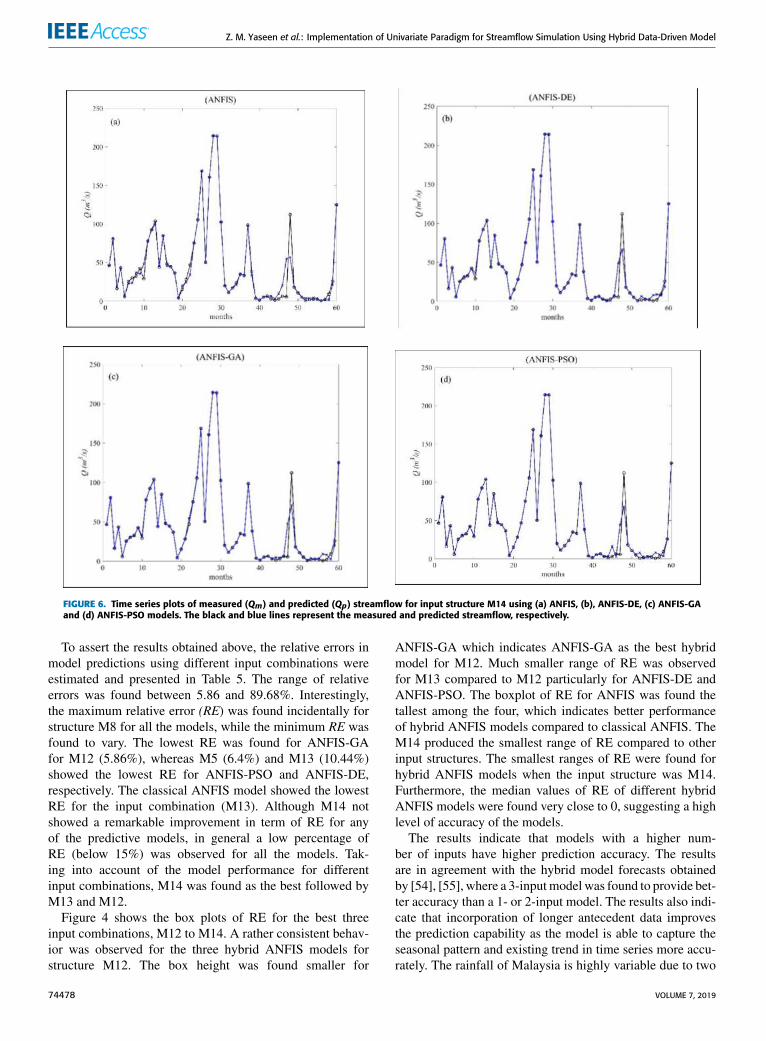
FIGURE 6. Time series plots of measured (Qm) and predicted (Qp) streamflow for input structure M14 using (a) ANFIS, (b), ANFIS-DE, (c) ANFIS-GAand (d) ANFIS-PSO models. The black and blue lines represent the measured and predicted streamflow, respectively.

To assert the results obtained above, the relative errors in

model predictions using different input combinations were

estimated and presented in Table 5. The range of relative

errors was found between 5.86 and 89.68%. Interestingly,

the maximum relative error (RE) was found incidentally for

structure M8 for all the models, while the minimum RE was

found to vary. The lowest RE was found for ANFIS-GA

for M12 (5.86%), whereas M5 (6.4%) and M13 (10.44%)

showed the lowest RE for ANFIS-PSO and ANFIS-DE,

respectively. The classical ANFIS model showed the lowest

RE for the input combination (M13). Although M14 not

showed a remarkable improvement in term of RE for any

of the predictive models, in general a low percentage of

RE (below 15%) was observed for all the models. Tak-

ing into account of the model performance for different

input combinations, M14 was found as the best followed by

M13 and M12.

Figure 4 shows the box plots of RE for the best three

input combinations, M12 to M14. A rather consistent behav-

ior was observed for the three hybrid ANFIS models for

structure M12. The box height was found smaller for

ANFIS-GA which indicates ANFIS-GA as the best hybrid

model for M12. Much smaller range of RE was observed

for M13 compared to M12 particularly for ANFIS-DE and

ANFIS-PSO. The boxplot of RE for ANFIS was found the

tallest among the four, which indicates better performance

of hybrid ANFIS models compared to classical ANFIS. The

M14 produced the smallest range of RE compared to other

input structures. The smallest ranges of RE were found for

hybrid ANFIS models when the input structure was M14.

Furthermore, the median values of RE of different hybrid

ANFIS models were found very close to 0, suggesting a high

level of accuracy of the models.

The results indicate that models with a higher num-

ber of inputs have higher prediction accuracy. The results

are in agreement with the hybrid model forecasts obtained

by [54], [55], where a 3-inputmodel was found to provide bet-

ter accuracy than a 1- or 2-input model. The results also indi-

cate that incorporation of longer antecedent data improves

the prediction capability as the model is able to capture the

seasonal pattern and existing trend in time series more accu-

rately. The rainfall of Malaysia is highly variable due to two

74478 VOLUME 7, 2019


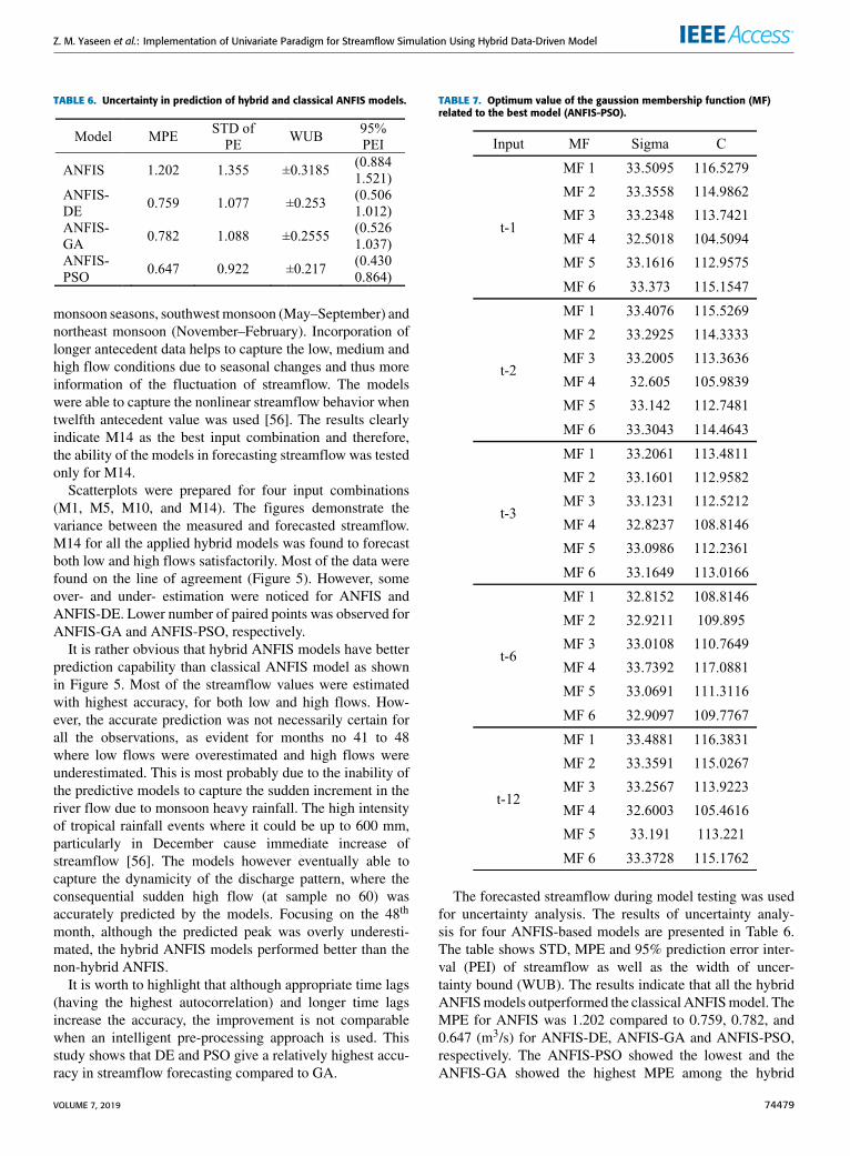
TABLE 6. Uncertainty in prediction of hybrid and classical ANFIS models.

monsoon seasons, southwestmonsoon (May–September) and

northeast monsoon (November–February). Incorporation of

longer antecedent data helps to capture the low, medium and

high flow conditions due to seasonal changes and thus more

information of the fluctuation of streamflow. The models

were able to capture the nonlinear streamflow behavior when

twelfth antecedent value was used [56]. The results clearly

indicate M14 as the best input combination and therefore,

the ability of the models in forecasting streamflow was tested

only for M14.

Scatterplots were prepared for four input combinations

(M1, M5, M10, and M14). The figures demonstrate the

variance between the measured and forecasted streamflow.

M14 for all the applied hybrid models was found to forecast

both low and high flows satisfactorily. Most of the data were

found on the line of agreement (Figure 5). However, some

over- and underestimation were noticed for ANFIS and

ANFIS-DE. Lower number of paired points was observed for

ANFIS-GA and ANFIS-PSO, respectively.

It is rather obvious that hybrid ANFIS models have better

prediction capability than classical ANFIS model as shown

in Figure 5. Most of the streamflow values were estimated

with highest accuracy, for both low and high flows. How-

ever, the accurate prediction was not necessarily certain for

all the observations, as evident for months no 41 to 48

where low flows were overestimated and high flows were

underestimated. This is most probably due to the inability of

the predictive models to capture the sudden increment in the

river flow due to monsoon heavy rainfall. The high intensity

of tropical rainfall events where it could be up to 600 mm,

particularly in December cause immediate increase of

streamflow [56]. The models however eventually able to

capture the dynamicity of the discharge pattern, where the

consequential sudden high flow (at sample no 60) was

accurately predicted by the models. Focusing on the 48th

month, although the predicted peak was overly underesti-

mated, the hybrid ANFIS models performed better than the

non-hybrid ANFIS.

It is worth to highlight that although appropriate time lags

(having the highest autocorrelation) and longer time lags

increase the accuracy, the improvement is not comparable

when an intelligent pre-processing approach is used. This

study shows that DE and PSO give a relatively highest accu-

racy in streamflow forecasting compared to GA.

TABLE 7. Optimum value of the gaussion membership function (MF)related to the best model (ANFIS-PSO).

The forecasted streamflow during model testing was used

for uncertainty analysis. The results of uncertainty analy-

sis for four ANFIS-based models are presented in Table 6.

The table shows STD, MPE and 95% prediction error inter-

val (PEI) of streamflow as well as the width of uncer-

tainty bound (WUB). The results indicate that all the hybrid

ANFISmodels outperformed the classical ANFISmodel. The

MPE for ANFIS was 1.202 compared to 0.759, 0.782, and

0.647 (m3/s) for ANFIS-DE, ANFIS-GA and ANFIS-PSO,

respectively. The ANFIS-PSO showed the lowest and the

ANFIS-GA showed the highest MPE among the hybrid

VOLUME 7, 2019 74479


models. The uncertainty bound for hybrid models were in the

range of ±0.22 to ±0.26, while it was found ±0.3185 for

the classical ANFIS. The highest 95%PEI was observed for

classical ANFIS, while the lowest MPE and WUB were

observed for ANFIS-PSO. The optimum value related to the

best model is presented in Table 7.

The most crucial characteristics of time series forecasting

model is its capability to capture the pattern exist in the series

and generalize the captured pattern outside the domain of

calibration data. The performance of a data driven models to

generalize the captured pattern depends on the complexity of

the time series to be forecasted. It is not possible to decide

which model is best for forecasting a time series without

comparing the performance of different models. Even when

a data driven method is found suitable for forecasting a time

series, its performance largely depends on the tuning of its

hyper parameters. Proper tuning of parameters allows better

mapping of input-output relationship. Besides, when the time

series forecasting is only based on historical data of the

same series, selection of optimum combination of antecedent

time lag data as input is important as inappropriate input can

propagate error to output and deteriorate prediction accuracy.

Therefore, performance of different tuning algorithms was

assessed in this study for different combinations of inputs

in order to find the most appropriate model in term of both

tuning algorithm and input combination. The present study

revealed that ANFISmodel is capable to capture the pattern of

streamflow time series and generalize the pattern for forecast-

ing streamflow with unknown data when its parameters were

tuned with PSO and five antecedent data including three most

recent data and the seasonal and annual lag data were used

as input. Though ANFIS-PSO with five inputs was found as

the best model for forecasting monthly streamflow in tropical

environment, it cannot be guaranteed that same model will

perform best in other environment, even for other river in

tropical region. The framework proposed in this study can be

used for the selection of the state-of-art optimization method

for the tuning of model parameter and selection of best input

combination for the selection of most accurate forecasting

model for any other study area.

V. CONCLUSION

Three different evolutionary algorithms namely, GA, DE,

and PSO were integrated with ANFIS for forecasting highly

stochastic monthly streamflow of a tropic river. Fourteen

different combinations of antecedent streamflow values were

considered for the selection of best input combination for the

development of the forecasting models. The results indicated

that incorporation of longer antecedent data improves the

prediction capability as the model is able to capture the

seasonal pattern and the existing trend in time series more

accurately. The best performance was obtained for the model

with 5 input variables (t − 1, t − 2, t − 3, t − 6, t − 12),

with a 68% prediction improvement than the model with

1 input variable (t−1). Comparison of the performance of the

evolutionary hybrid ANFIS models with the classical ANFIS

model revealed the ability of evolutionary algorithms in the

optimization of ANFIS membership function in order to min-

imize the prediction error. Comparison of evolutionary opti-

mization techniques indicated the higher capability of PSO

in optimization of ANFIS membership functions compared

to GA and DE. ANFIS-PSOmodel provided better prediction

than non-hybrid ANFIS by 25%, slightly higher than ANFIS-

GA and ANFIS-DE (24% and 20%, respectively). The uncer-

tainty analysis revealed the lowest width of uncertainty band

for ANFIS-PSO than the other hybrid methods and classical

ANFIS. Therefore, the ANFIS-PSO model can be used for

reliable forecasting of highly stochastic river flow in tropical

environment.

DATA AVAILABILITY

Hydrological data obtained from the Department of Irrigation

and Drainage (DID), Malaysia.

ACKNOWLEDGMENT

Authors would like to acknowledge their gratitude to the

Department of Irrigation and Drainage (DID), Malaysia, for

providing streamflow data of Pahang River. Also, authors

appreciate the three reviewers and the Editors whose com-

ments have improved the overall quality of this research

paper.

CONFLICTS OF INTEREST

The authors declare no conflict of interest.

REFERENCES

[1] C.-F. Yeh, J. Wang, H.-F. Yeh, and C.-H. Lee, ‘‘Spatial and temporal

streamflow trends in northern taiwan,’’ Water, vol. 7, no. 2, pp. 634–651,

2015.[2] L. Sun, I. Nistor, and O. Seidou, ‘‘Streamflow data assimilation in SWAT

model using extended Kalman filter,’’ J. Hydrol., vol. 531, pp. 671–684,

Dec. 2015.[3] Y. Liu, J. Guo, H. Sun, W. Zhang, Y. Wang, and J. Zhou, ‘‘Multiobjective

optimal algorithm for automatic calibration of daily streamflow forecasting

model,’’ Math. Problems Eng., vol. 2016, Jul. 2016, Art. no. 8215308.[4] L. E. Besaw, D. M. Rizzo, P. R. Bierman, and W. R. Hackett, ‘‘Advances

in ungauged streamflow prediction using artificial neural networks,’’

J. Hydrol., vol. 386, pp. 27–37, May 2010.[5] C. L. Wu, K. W. Chau, and Y. S. Li, ‘‘Predicting monthly streamflow using

data-driven models coupled with data-preprocessing techniques,’’ Water

Resour. Res., vol. 45, no. 8, pp. 1–23, 2009.[6] R. Maity, P. P. Bhagwat, and A. Bhatnagar, ‘‘Potential of support vector

regression for prediction of monthly streamflow using endogenous prop-

erty,’’ Hydrol. Process., vol. 24, no. 7, pp. 917–923, 2010.[7] Z. A. Al-Sudani, S. Q. Salih, A. Sharafati, and Z. M. Yaseen, ‘‘Develop-

ment of multivariate adaptive regression spline integrated with differential

evolution model for streamflow simulation,’’ J. Hydrol., vol. 573, pp. 1–12,

Jun. 2019.[8] L. Diop, A. Bodian, K. Djaman, Z. M. Yaseen, R. C. Deo, A. El-Shafie,

and L. C. Brown, ‘‘The influence of climatic inputs on stream-flow pattern

forecasting: Case study of upper senegal river,’’Environ. Earth Sci., vol. 77,

no. 5, p. 182, 2018.[9] J. E. Shortridge, S. D. Guikema, and B. F. Zaitchik, ‘‘Machine learning

methods for empirical streamflow simulation: A comparison of model

accuracy, interpretability, and uncertainty in seasonal watersheds,’’Hydrol.

Earth Syst. Sci., vol. 20, no. 7, pp. 2611–2628, 2016.[10] F. Fahimi, Z. M. Yaseen, and A. El-Shafie, ‘‘Application of soft computing

based hybrid models in hydrological variables modeling: A comprehensive

review,’’ Theor. Appl. Climatol., vol. 128, pp. 875–903, May 2016.[11] M. A. Ghorbani, R. Khatibi, V. Karimi, Z. M. Yaseen, and M. Zounemat-

Kermani, ‘‘Learning from multiple models using artificial intelligence to

improve model prediction accuracies: Application to river flows,’’ Water

Resour. Manage., vol. 32, no. 13, pp. 4201–4215, 2018.

74480 VOLUME 7, 2019


[12] Z. M. Yaseen, A. El-shafie, O. Jaafar, H. A. Afan, and K. N. Sayl, ‘‘Arti-

ficial intelligence based models for stream-flow forecasting: 2000–2015,’’

J. Hydrol., vol. 530, pp. 829–844, Nov. 2015.[13] Z. M. Yaseen, S. O. Sulaiman, R. C. Deo, and K.-W. Chau, ‘‘An enhanced

extreme learning machine model for river flow forecasting: State-of-the-

art, practical applications in water resource engineering area and future

research direction,’’ J. Hydrol., vol. 569, pp. 387–408, Feb. 2019.[14] R. J. Abrahart, F. Anctil, P. Coulibaly, C. W. Dawson, N. J. Mount,

L. M. See, A. Y. Shamseldin, D. P. Solomatine, E. Toth, and R. L. Wilby,

‘‘Two decades of anarchy? Emerging themes and outstanding challenges

for neural network river forecasting,’’ Prog. Phys. Geogr., Earth Environ.,

vol. 36, no. 4, pp. 480–513, 2012.[15] W. Wang, P. H. A. J. M. Van Gelder, J. K. Vrijling, and J. Ma, ‘‘Fore-

casting daily streamflow using hybrid ANN models,’’ J. Hydrol., vol. 324,

nos. 1–4, pp. 383–399, 2006.[16] S. Isik, L. Kalin, J. E. Schoonover, P. Srivastava, and B. G. Lockaby,

‘‘Modeling effects of changing land use/cover on daily streamflow:

An artificial neural network and curve number based hybrid approach,’’

J. Hydrol., vol. 485, pp. 103–112, Apr. 2013.[17] M. Kothari and K. D. Gharde, ‘‘Application of ANN and fuzzy logic

algorithms for streamflow modelling of Savitri catchment,’’ J. Earth Syst.

Sci., vol. 124, no. 5, pp. 933–943, 2015.[18] M. Demirci and A. Baltaci, ‘‘Prediction of suspended sediment in river

using fuzzy logic and multilinear regression approaches,’’ Neural Comput.

Appl., vol. 23, pp. 145–151, Dec. 2013.[19] G. Tayfur and L. Brocca, ‘‘Fuzzy logic for rainfall-runoff modelling

considering soil moisture,’’ Water Resour. Manage., vol. 29, no. 10,

pp. 3519–3533, 2015.[20] Z. M. Yaseen, M. I. Ghareb, I. Ebtehaj, H. Bonakdari, R. Siddique,

S. Heddam, A. A. Yusif, and R. Deo, ‘‘Rainfall pattern forecasting using

novel hybrid intelligent model based ANFIS-FFA,’’ Water Resour. Man-

age., vol. 32, no. 1, pp. 105–122, 2018.[21] O. Kisi and Z. M. Yaseen, ‘‘The potential of hybrid evolutionary fuzzy

intelligence model for suspended sediment concentration prediction,’’

Catena, vol. 174, pp. 11–23, May 2019.[22] V. S. Ghomsheh,M. A. Shoorehdeli, andM. Teshnehlab, ‘‘Training ANFIS

structure with modified PSO algorithm,’’ in Proc. Medit. Conf. Control

Automat., 2007, pp. 1–6.[23] Z. M. Yaseen, I. Ebtehaj, H. Bonakdari, R. C. Deo, A. D. Mehr,

W. H. M. W. Mohtar, L. Diop, A. El-Shafie, and V. P. Singh, ‘‘Novel

approach for streamflow forecasting using a hybrid ANFIS-FFA model,’’

J. Hydrol., vol. 554, pp. 263–276, Nov. 2017.[24] H. R. Maier et al., ‘‘Evolutionary algorithms and other metaheuristics in

water resources: Current status, research challenges and future directions,’’

Environ. Model. Softw., vol. 62, pp. 271–299, Dec. 2014.[25] A. P. Piotrowski and J. J. Napiorkowski, ‘‘Optimizing neural networks

for river flow forecasting—Evolutionary computation methods versus

the Levenberg–Marquardt approach,’’ J. Hydrol., vol. 407, nos. 1–4,

pp. 12–27, 2011.[26] M. A. Shoorehdeli, M. Teshnehlab, and A. K. Sedigh, ‘‘A novel training

algorithm in ANFIS structure,’’ in Proc. Amer. Control Conf., 2006, p. 6.[27] J. T. Lalis, B. D. Gerardo, and Y. Byun, ‘‘An adaptive stopping criterion

for backpropagation learning in feedforward neural network,’’ Int. J. Mul-

timedia Ubiquitous Eng., vol. 9, no. 8, pp. 149–156, 2014.[28] Y. W. Chen, L. C. Chang, C. W. Huang, and H. J. Chu, ‘‘Applying

genetic algorithm and neural network to the conjunctive use of surface and

subsurface water,’’Water Resour. Manage., vol. 27, no. 14, pp. 4731–4757,

2013.[29] E. Tapoglou, I. C. Trichakis, Z. Dokou, I. K. Nikolos, and G. P. Karatzas,

‘‘Groundwater-level forecasting under climate change scenarios using

an artificial neural network trained with particle swarm optimization,’’

Hydrolog. Sci. J., vol. 59, no. 6, pp. 1225–1239, 2014.[30] I. Ebtehaj and H. Bonakdari, ‘‘Comparison of genetic algorithm and

imperialist competitive algorithms in predicting bed load transport in clean

pipe,’’ Water Sci. Technol., vol. 70, no. 10, pp. 1695–1701, 2014.[31] S. R. Naganna, P. C. Deka, M. A. Ghorbani, S. M. Biazar, N. Al-Ansari,

and Z. M. Yaseen, ‘‘Dew point temperature estimation: Application of

artificial intelligence model integrated with nature-inspired optimization

algorithms,’’ Water, vol. 11, no. 4, p. 742, 2019.[32] A. Zimmer, A. Schmidt, A. Ostfeld, and B. Minsker, ‘‘Evolutionary algo-

rithm enhancement for model predictive control and real-time decision

support,’’ Environ. Model. Softw., vol. 69, pp. 330–341, Jul. 2015.[33] S. Maroufpoor, E. Maroufpoor, O. Bozorg-Haddad, J. Shiri, and

Z. M. Yaseen, ‘‘Soil moisture simulation using hybrid artificial intelligent

model: Hybridization of adaptive neuro fuzzy inference system with grey

wolf optimizer algorithm,’’ J. Hydrol., vol. 575, pp. 544–556, Aug. 2019.

[34] W. Chen, M. Panahi, and H. R. Pourghasemi, ‘‘Performance evaluation of

GIS-based new ensemble data mining techniques of adaptive neuro-fuzzy

inference system (ANFIS) with genetic algorithm (GA), differential evo-

lution (DE), and particle swarm optimization (PSO) for landslide spatial

modelling,’’ Catena, vol. 157, pp. 310–324, Oct. 2017.

[35] M. B. Gasim, M. E. Toriman, I. Mushrifah, P. Lun, M. K. A. Kamarudin,

A. A. A. Nor, M. Mazlin, and M. S. A. Sharifah, ‘‘River flow conditions

and dynamic state analysis of Pahang river,’’ Amer. J. Appl. Sci., vol. 10,

no. 1, pp. 42–57, 2013.

[36] A. Ab Ghani, C. K. Chang, C. S. Leow, and N. A. Zakaria, ‘‘Sungai Pahang

digital flood mapping: 2007 flood,’’ Int. J. River Basin Manage., vol. 10,

no. 2, pp. 139–148, 2012.

[37] J.-S. R. Jang, ‘‘ANFIS: Adaptive-network-based fuzzy inference sys-

tem,’’ IEEE Trans. Syst., Man, Cybern., vol. 23, no. 3, pp. 665–685,

May/Jun. 1993.

[38] I. Ebtehaj and H. Bonakdari, ‘‘Performance evaluation of adaptive neural

fuzzy inference system for sediment transport in sewers,’’ Water Resour.

Manage., vol. 28, no. 13, pp. 4765–4779, 2014.

[39] J. Kennedy and R. Eberhart, ‘‘A new optimizer using particle swarm

theory,’’ in Proc. 6th Int. Symp. Micro Mach. Hum. Sci., 1995, pp. 39–43.

[40] W.-J. Yu, J.-Z. Li, W.-N. Chen, and J. Zhang, ‘‘A parallel double-level

multiobjective evolutionary algorithm for robust optimization,’’ Appl. Soft

Comput., vol. 59, pp. 258–275, Oct. 2017.

[41] W. Srisukkham, L. Zhang, S. C. Neoh, S. Todryk, and C. P. Lim, ‘‘Intel-

ligent leukaemia diagnosis with bare-bones PSO based feature optimiza-

tion,’’ Appl. Soft Comput., vol. 56, pp. 405–419, Jul. 2017.

[42] I. Ebtehaj and H. Bonakdari, ‘‘Assessment of evolutionary algorithms in

predicting non-deposition sediment transport,’’ Urban Water J., vol. 13,

no. 5, pp. 499–510, 2016.

[43] H. Moeeni, H. Bonakdari, and I. Ebtehaj, ‘‘Integrated SARIMA with

neuro-fuzzy systems and neural networks for monthly inflow prediction,’’

Water Resour. Manage., vol. 31, no. 7, pp. 2141–2156, 2017.

[44] M. Jakubcová, P. Máca, and P. Pech, ‘‘Parameter estimation in rainfall-

runoff modelling using distributed versions of particle swarm optimization

algorithm,’’ Math. Problems Eng., vol. 2015, Aug. 2015, Art. no. 968067.

[45] Y.-H. Chen and F.-J. Chang, ‘‘Evolutionary artificial neural networks

for hydrological systems forecasting,’’ J. Hydrol., vol. 367, nos. 1–2,

pp. 125–137, 2009.

[46] J. H. Holland, ‘‘Genetic algorithms,’’ Sci. Amer., vol. 267, no. 1,

pp. 66–72, Jul. 1992.

[47] R. Storn and K. Price, ‘‘Differential evolution—A simple and efficient

heuristic for global optimization over continuous spaces,’’ J. Global

Optim., vol. 11, no. 4, pp. 341–359, 1997.

[48] H. Tao, L. Diop, A. Bodian, K. Djaman, P. M. Ndiaye, and Z. M. Yaseen,

‘‘Reference evapotranspiration prediction using hybridized fuzzy model

with firefly algorithm: Regional case study in Burkina Faso,’’ Agricult.

Water Manage., vol. 208, pp. 140–151, Sep. 2018.

[49] T. Chai and R. R. Draxler, ‘‘Root mean square error (RMSE) or mean abso-

lute error (MAE)?—Arguments against avoiding RMSE in the literature,’’

Geosci. Model Develop., vol. 7, no. 3, pp. 1247–1250, 2014.

[50] C. J.Willmott, S.M. Robeson, and K.Matsuura, ‘‘A refined index of model

performance,’’ Int. J. Climatol., vol. 32, no. 13, pp. 2088–2094, 2011.

[51] H. Sanikhani, R. C. Deo, Z. M. Yaseen, O. Eray, and O. Kisi, ‘‘Non-tuned

data intelligent model for soil temperature estimation: A new approach,’’

Geoderma, vol. 330, pp. 52–64, Nov. 2018.

[52] Z. M. Yaseen, M. T. Tran, S. Kim, T. Bakhshpoori, and R. C. Deo, ‘‘Shear

strength prediction of steel fiber reinforced concrete beam using hybrid

intelligence models: A new approach,’’ Eng. Struct., vol. 177, no. April,

pp. 244–255, 2018.

[53] I. Ebtehaj, H. Bonakdari, and S. Shamshirband, ‘‘Extreme learning

machine assessment for estimating sediment transport in open channels,’’

Eng. Comput., vol. 32, no. 4, pp. 691–704, 2016.

[54] H. Badrzadeh, R. Sarukkalige, and A. W. Jayawardena, ‘‘Impact of multi-

resolution analysis of artificial intelligence models inputs on multi-step

ahead river flow forecasting,’’ J. Hydrol., vol. 507, pp. 75–85, 2013.

[55] C. Sudheer, R. Maheswaran, B. K. Panigrahi, and S. Mathur, ‘‘A hybrid

SVM-PSO model for forecasting monthly streamflow,’’ Neural Comput.

Appl., vol. 24, no. 6, pp. 1381–1389, 2013.

[56] N. H. Sulaiman, M. K. A. Kamarudin, M. E. Toriman, H. Juahir, F. M. Ata,

A. Azid, N. J. A. Wahab, R. Umar, S. I. Khalit, M. Makhtar, A. Arfan, and

U. Sideng, ‘‘Relationship of rainfall distribution and water level on major

flood 2014 in Pahang River Basin, Malaysia,’’ EnvironmentAsia, vol. 10,

no. 1, pp. 1–8, 2017.

VOLUME 7, 2019 74481

Documents

Implementation of Univariate Paradigm for Streamflow