Embed Size (px)
Citation preview
Implementation of SchedulingAlgorithms in an OpenMP Runtime
LibraryMaster Thesis
Natural Science Faculty of the University of Basel
Department of Mathematics and Computer Science
High Performance Computing
https://hpc.dmi.unibas.ch
Examiner: Prof. Dr. Florina M. Ciorba
Supervisor: Jonas Henrique Muller Korndorfer, MSc.
Akan Yilmaz
10-927-473
30.06.2019

Acknowledgments
I want to thank Prof. Dr. Florina M. Ciorba for her kind availability, motivational speeches
and this very interesting topic. I also want to thank Jonas H. M. Korndorfer for supervising
me in a very nice and enjoyable way and his help during the period of my master’s thesis.
Special thanks go to Dr.-Ing. Michael Klemm et al @ Intel for their help on code level hints
of libomp.
Further thanks for their helpful hints and consultation go to: Ali Omar Abdulazim Mo-
hammed, MSc, Ahmed Hamdy Mohamed Eleliemy, MSc, Dr. Aurelien Cavelan and Dr.
Danilo Guerrera.
Abstract
Loops are the biggest source of parallelism in parallel programs. The scheduling task, in
which the iterations of a loop are assigned to available processors, plays an important role in
how efficiently the underlying system is used. OpenMP, the de-facto standard for parallelism,
lists three loop scheduling techniques, static, dynamic and guided. Implementations of that
standard must support at least these three to meet the OpenMP specification. Existing
OpenMP runtime libraries, such as GCC’s libgomp or LLVM’s libomp, provide ready-to-
use scheduling techniques for programmers, however, intensive research from the past has
shown multiple and more advanced loop scheduling techniques that are not implemented in
these libraries. As recent works have tested the advanced techniques in existing runtimes,
it has been proven that depending on the system, application and loop characteristics, one
strategy is superior to the others. Libraries must, therefore, implement more techniques in
order to provide the best performance for a broad range of distinctive loops. The LLVM
OpenMP runtime library, which has a big impact on the industry, still misses many of the
techniques to be implemented and tested. This thesis implements numerous dynamic loop
scheduling algorithms into the LLVM OpenMP runtime library. Different benchmarks from
suites including NAS 3.4, CORAL, Rodinia and SPEC OMP 2012 are chosen to evaluate and
compare the new techniques to the available solutions. The results justify that each newly
implemented technique can outperform every other in particular software and hardware
configurations. Performance improvements of up to 6 % are measured in comparison to the
fastest available OpenMP strategy and up to 7 % in unequal threads-per-core bindings. The
experiments indicate that increasing numbers of cores per node and heterogeneous systems
benefit even more from the implementation and require advanced software for the most
efficient usage. In future OpenMP versions, an extension to the techniques of the standard
would be a desirable update allowing the user to better exploit parallelism.

Table of Contents
Acknowledgments ii
Abstract iii
Abbreviations vii
1 Introduction 1
2 Background 4
2.1 Parallelism . . . . . . . . . . . . . . . . . . . . . . . . . . . . . . . . . . . . . 4
2.1.1 Shared Memory . . . . . . . . . . . . . . . . . . . . . . . . . . . . . . . 4
2.1.2 Multithreading . . . . . . . . . . . . . . . . . . . . . . . . . . . . . . . 5
2.2 Loop Scheduling . . . . . . . . . . . . . . . . . . . . . . . . . . . . . . . . . . 5
2.2.1 Static Techniques . . . . . . . . . . . . . . . . . . . . . . . . . . . . . . 6
2.2.1.1 Static Chunking . . . . . . . . . . . . . . . . . . . . . . . . . 6
2.2.2 Dynamic Techniques . . . . . . . . . . . . . . . . . . . . . . . . . . . . 6
2.2.2.1 Self-Scheduling . . . . . . . . . . . . . . . . . . . . . . . . . . 7
2.2.2.2 Fixed Size Chunking . . . . . . . . . . . . . . . . . . . . . . . 8
2.2.2.3 Guided Self-Scheduling . . . . . . . . . . . . . . . . . . . . . 8
2.2.2.4 Trapezoid Self-Scheduling . . . . . . . . . . . . . . . . . . . . 8
2.2.2.5 Factoring . . . . . . . . . . . . . . . . . . . . . . . . . . . . . 9
2.2.2.6 Weighted Factoring . . . . . . . . . . . . . . . . . . . . . . . 9
2.2.2.7 Taper . . . . . . . . . . . . . . . . . . . . . . . . . . . . . . . 10
2.2.2.8 Fractiling . . . . . . . . . . . . . . . . . . . . . . . . . . . . . 11
2.2.2.9 The Bold Strategy . . . . . . . . . . . . . . . . . . . . . . . . 11
2.2.2.10 Adaptive Weighted Factoring . . . . . . . . . . . . . . . . . . 13
2.2.2.11 Adaptive Weighted Factoring Variants . . . . . . . . . . . . . 15
2.2.2.12 Adaptive Factoring . . . . . . . . . . . . . . . . . . . . . . . 16
2.3 OpenMP . . . . . . . . . . . . . . . . . . . . . . . . . . . . . . . . . . . . . . . 17
2.3.1 Scheduling in OpenMP . . . . . . . . . . . . . . . . . . . . . . . . . . 18
2.3.2 LLVM OpenMP Runtime Library . . . . . . . . . . . . . . . . . . . . 18
3 Related Work 20
4 Loop Scheduling in LLVM 23

Table of Contents v
4.1 Scheduling Overview in libomp . . . . . . . . . . . . . . . . . . . . . . . . . . 23
4.2 Methodology on Extending libomp . . . . . . . . . . . . . . . . . . . . . . . . 24
5 Implementation 26
5.1 Environment Variables . . . . . . . . . . . . . . . . . . . . . . . . . . . . . . . 27
5.2 Fixed Size Chunking . . . . . . . . . . . . . . . . . . . . . . . . . . . . . . . . 28
5.3 Factoring . . . . . . . . . . . . . . . . . . . . . . . . . . . . . . . . . . . . . . 29
5.4 Weighted Factoring . . . . . . . . . . . . . . . . . . . . . . . . . . . . . . . . . 29
5.5 Taper . . . . . . . . . . . . . . . . . . . . . . . . . . . . . . . . . . . . . . . . 30
5.6 The Bold Strategy . . . . . . . . . . . . . . . . . . . . . . . . . . . . . . . . . 30
5.7 Adaptive Weighted Factoring Variants . . . . . . . . . . . . . . . . . . . . . . 30
5.8 Adaptive Factoring . . . . . . . . . . . . . . . . . . . . . . . . . . . . . . . . . 31
6 Optimizations 32
7 Validation 34
7.1 Nonadaptive Techniques . . . . . . . . . . . . . . . . . . . . . . . . . . . . . . 34
7.2 Adaptive Techniques . . . . . . . . . . . . . . . . . . . . . . . . . . . . . . . . 35
8 Experiments 36
8.1 The System . . . . . . . . . . . . . . . . . . . . . . . . . . . . . . . . . . . . . 36
8.2 Scheduling Overhead and Compiler vs Runtime . . . . . . . . . . . . . . . . . 37
8.3 The Benchmarks . . . . . . . . . . . . . . . . . . . . . . . . . . . . . . . . . . 37
8.4 Design of Experiments . . . . . . . . . . . . . . . . . . . . . . . . . . . . . . . 39
8.4.1 Pinning Strategy . . . . . . . . . . . . . . . . . . . . . . . . . . . . . . 39
8.5 Profiling . . . . . . . . . . . . . . . . . . . . . . . . . . . . . . . . . . . . . . . 42
8.6 NAS Parallel Benchmarks . . . . . . . . . . . . . . . . . . . . . . . . . . . . . 43
8.7 CORAL Benchmarks . . . . . . . . . . . . . . . . . . . . . . . . . . . . . . . . 49
8.8 Sphynx and SPH-EXA . . . . . . . . . . . . . . . . . . . . . . . . . . . . . . . 52
8.9 SPEC OMP 2012 . . . . . . . . . . . . . . . . . . . . . . . . . . . . . . . . . . 54
8.10 Rodinia Benchmark Suite . . . . . . . . . . . . . . . . . . . . . . . . . . . . . 57
8.11 OmpSCR . . . . . . . . . . . . . . . . . . . . . . . . . . . . . . . . . . . . . . 58
8.12 Mandelbrot and Adjoint Convolution . . . . . . . . . . . . . . . . . . . . . . . 60
8.13 Random Sleep . . . . . . . . . . . . . . . . . . . . . . . . . . . . . . . . . . . . 61
9 Conclusion and Future Work 62
Bibliography 64
Appendix A Pin2 Results 69
Appendix B Random Sleep 73

Table of Contents vi
Declaration on Scientific Integrity 75

Abbreviations
ADLS Adaptive DLS
AF Adaptive Factoring
AWF Adaptive Weighted Factoring
BOLD The Bold Strategy
c.o.v. coefficient of variation
DLS Dynamic Loop Scheduling
FAC Factoring
FRAC Fractiling
FSC Fixed Size Chunking
GCC GNU Compiler Collection
GSS Guided Self-Scheduling
KNL Knights Landing
libgomp GNU Offloading and Multi Processing Runtime Library
libomp LLVM OpenMP runtime library
NADLS Nonadaptive DLS
OpenMP Open Multi-Processing
OpenMP API OpenMP Application Programming Interface
PUs Processing Units
SC Static Chunking
SRR Smart Round-Robin
SS Self-Scheduling
TAP Taper
TSS Trapezoid Self-Scheduling
WF Weighted Factoring

1Introduction
Parallelization is more and more coming into the limelight with computer systems that have
an increasing number of Processing Units (PUs) . The software, however, must evolve as
well to efficiently use current computer systems and push them to their limits. Scientific
applications, for instance, which typically have a big demand for execution power, would
benefit greatly of such an efficient system utilization. These applications are often composed
by large loops which usually are a good source of parallelism. Therewith, many research
efforts have been done to enhance and exploit the possible parallelizations for such appli-
cations. How the workload of a loop, i.e., the iterations, are scheduled, has a big impact
on the resulting performance of parallelizing scientific applications. For exactly this task,
there exist multiple so called loop scheduling techniques. The reason for their existence lies
in the characteristics of applications and their loops. Loop iteration execution times can
vary and thus have a negative impact on the system’s load balance. Assigning equal amount
of iterations to each PU could end up in one PU taking much more time for executing its
portion because of these variations, while the rest is waiting. Such loops are also called
irregular loops. The techniques counteract this issue. They differ in assigning iterations
either statically or dynamically. Static in a way, where a loop is split into fixed-size portions
for each PU prior to the execution. Static techniques are well suited for regular loops, where
the iterations’ execution times are similar. In contrast, Dynamic Loop Scheduling (DLS)
techniques balance the load during execution and are the prominent choice when it comes
to irregular loops with varying iteration execution times. Depending on which DLS method
is used, the amount of iterations assigned to a PU at a time varies. Among all the different
techniques, one can characterize them in two dimensions. One being the degree of load
balancing provided and the other how much overhead the scheduling algorithm itself pro-
duces. The ideal case would be maximum load balance with minimum scheduling overhead.
Sadly, this is not possible since scheduling requires chunk size calculations of iterations,
bookkeeping, communication and more. The extremes are formed by the two techniques
static scheduling and Self-Scheduling (SS) as depicted in figure 1.1. Unlike static, SS dy-
namically schedules a single iteration at a time during the execution of a loop, promising
best load balance. Details can be found in Chapter 2, Section 2.2. Nevertheless, depending
on the loop, one technique should be chosen that fits best. Fortunately, there is a standard-

Introduction 2
scheduling overhead
load balance +++---
+++---stat
ic SS
Figure 1.1: The interaction between load balancing and scheduling overhead. Maximizingload balance typically induces scheduling overhead. Static scheduling and SS mark theextremes of all existing techniques.
ized way in how to parallelize code. The Open Multi-Processing (OpenMP) specification [1]
defines the OpenMP Application Programming Interface (OpenMP API) for parallelism in
C, C++ and Fortran programs. Many popular compilers already support this specification
and provide parallelization for developers [2]. OpenMP does not only require a compiler
that supports the specification, but also a runtime library which provides an interface to the
compiler. The scheduling task, for instance, is handled by that library. There exist multiple
runtime implementations, such as the LLVM OpenMP runtime library (libomp) for LLVM’s
Clang compiler [3] or GNU Offloading and Multi Processing Runtime Library (libgomp) [4]
for the GNU Compiler Collection (GCC) [5]. Runtime library routines are used to examine
and modify execution parameters during runtime, e.g., getting the available number of PUs
or the number of threads. The user can benefit from these routine functions in source code
which then later are handled by the runtime library. As an example, the LLVM Clang
compiler has its libomp [3], which handles calls from the running application, as well as the
user-level runtime routines. To better understand how OpenMP works, figure 1.2 shows its
solution stack [6]. The runtime library is hereby linked to the application whenever it is
executed.
Use
r Lay
er End User
Application
Prog
.La
yer
Directives,Compiler OpenMP Library Environment
Variables
Syst
em L
ayer
OpenMP Runtime Library
OS/system support for shared memory and threading
Har
dwar
e ...Shared Address Space
PU 1 PU 2 PU 3 PU 4 PU N
Figure 1.2: The solution stack of OpenMP. Our focus lies on the shaded boxes, namely, theruntime library and environment variables.
The problem with OpenMP arises, when taking a closer look at its scheduling specification.
Introduction 3
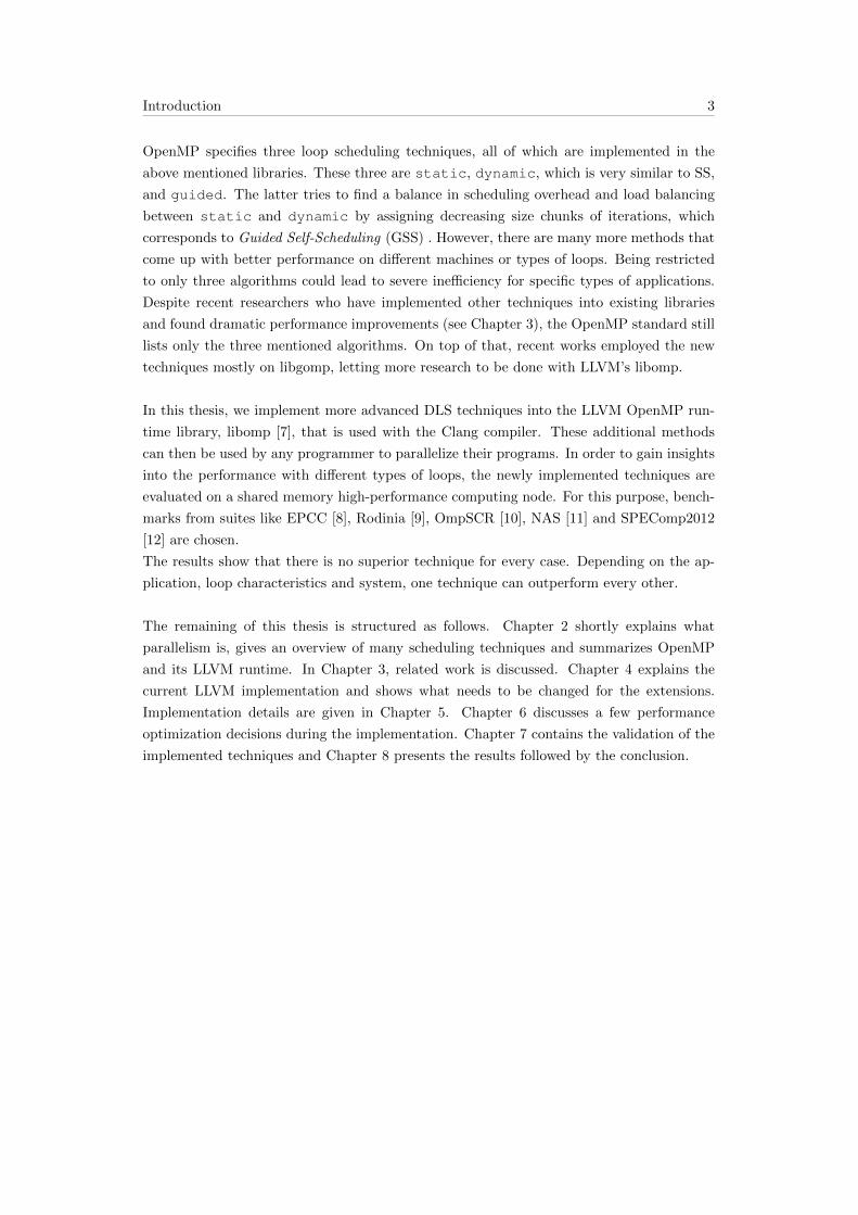
OpenMP specifies three loop scheduling techniques, all of which are implemented in the
above mentioned libraries. These three are static, dynamic, which is very similar to SS,
and guided. The latter tries to find a balance in scheduling overhead and load balancing
between static and dynamic by assigning decreasing size chunks of iterations, which
corresponds to Guided Self-Scheduling (GSS) . However, there are many more methods that
come up with better performance on different machines or types of loops. Being restricted
to only three algorithms could lead to severe inefficiency for specific types of applications.
Despite recent researchers who have implemented other techniques into existing libraries
and found dramatic performance improvements (see Chapter 3), the OpenMP standard still
lists only the three mentioned algorithms. On top of that, recent works employed the new
techniques mostly on libgomp, letting more research to be done with LLVM’s libomp.
In this thesis, we implement more advanced DLS techniques into the LLVM OpenMP run-
time library, libomp [7], that is used with the Clang compiler. These additional methods
can then be used by any programmer to parallelize their programs. In order to gain insights
into the performance with different types of loops, the newly implemented techniques are
evaluated on a shared memory high-performance computing node. For this purpose, bench-
marks from suites like EPCC [8], Rodinia [9], OmpSCR [10], NAS [11] and SPEComp2012
[12] are chosen.
The results show that there is no superior technique for every case. Depending on the ap-
plication, loop characteristics and system, one technique can outperform every other.
The remaining of this thesis is structured as follows. Chapter 2 shortly explains what
parallelism is, gives an overview of many scheduling techniques and summarizes OpenMP
and its LLVM runtime. In Chapter 3, related work is discussed. Chapter 4 explains the
current LLVM implementation and shows what needs to be changed for the extensions.
Implementation details are given in Chapter 5. Chapter 6 discusses a few performance
optimization decisions during the implementation. Chapter 7 contains the validation of the
implemented techniques and Chapter 8 presents the results followed by the conclusion.
2Background
This chapter gives an overview of many scheduling techniques. Starting by a brief explana-
tion about parallelism in Section 2.1, the techniques itself in Section 2.2 and an introduction
to OpenMP in Section 2.3.
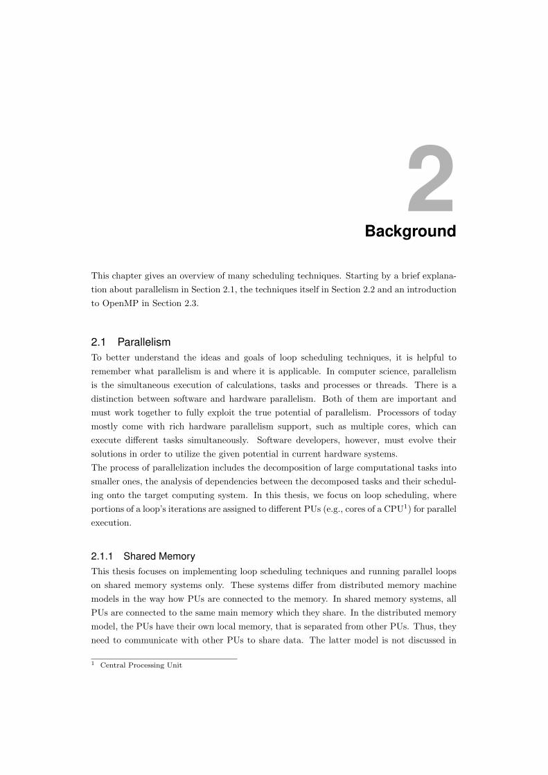
2.1 ParallelismTo better understand the ideas and goals of loop scheduling techniques, it is helpful to
remember what parallelism is and where it is applicable. In computer science, parallelism
is the simultaneous execution of calculations, tasks and processes or threads. There is a
distinction between software and hardware parallelism. Both of them are important and
must work together to fully exploit the true potential of parallelism. Processors of today
mostly come with rich hardware parallelism support, such as multiple cores, which can
execute different tasks simultaneously. Software developers, however, must evolve their
solutions in order to utilize the given potential in current hardware systems.
The process of parallelization includes the decomposition of large computational tasks into
smaller ones, the analysis of dependencies between the decomposed tasks and their schedul-
ing onto the target computing system. In this thesis, we focus on loop scheduling, where
portions of a loop’s iterations are assigned to different PUs (e.g., cores of a CPU1) for parallel
execution.
2.1.1 Shared MemoryThis thesis focuses on implementing loop scheduling techniques and running parallel loops
on shared memory systems only. These systems differ from distributed memory machine
models in the way how PUs are connected to the memory. In shared memory systems, all
PUs are connected to the same main memory which they share. In the distributed memory
model, the PUs have their own local memory, that is separated from other PUs. Thus, they
need to communicate with other PUs to share data. The latter model is not discussed in
1 Central Processing Unit

Background 5
this thesis.
2.1.2 MultithreadingMultithreading is a way of how an application can use multiple threads, supported by the
operating system, to execute operations on one PU (e.g., core of a CPU) or simultaneously on
multiple PUs. The difference between multiprocessing and multithreading is that threads
of an application use the same address space and can access on the same data, wherein
processes have their own address space, thus, they are considered to be heavier than threads.
OpenMP, discussed in Section 2.3, uses threads, which makes multithreading the prominent
process model of this thesis.
2.2 Loop SchedulingLoops are the dominant source of parallelism. Large programs, especially those of scientific
areas which compute simulations of, for example, physical interactions of bodies [13], contain
one or more large loops that consume most of the computation time. Parallelizing those
heavy loops can dramatically speedup the program execution time. By parallelizing loops,
we mean the decomposition of a loop in blocks of iterations, i.e., smaller tasks, and the
scheduling of these blocks to available PUs. The process of parallelization, however, has
one constraint that must be analyzed. The dependency analysis. To be able to parallelize a
loop, the iterations must be independent of each other so that the order of execution does
not change the final result. The programmer must take care of the dependencies himself.
In this thesis, we only focus on loop scheduling and assume that the dependency analysis is
made correctly by the programmer.
Scheduling in computer science is defined as the ordering of computation and data in space
and time. In this case, the distribution of loop iterations over PUs and time. The parallel
execution of iterations among the available PUs increase the performance of the program.
However, loop iteration execution times can vary because of conditional statements inside
the loop or input values. These variations can lead to uneven execution finishing times
of PUs, also called load imbalance. If one PU takes much more time to finish its portion
of iterations than the other PUs, the idling PUs and their potential computation power
are wasted. Scheduling techniques try to balance the load among the PUs in order to
produce even finishing times and reduce wasted potential. However, scheduling involves
overhead which can lead to bad performance. In general, there is a fundamental trade-
off in loop scheduling between load balance and scheduling overhead. Depending on the
loop characteristics, one scheduling technique fits better than the others to reduce overall
execution time. There are many different approaches of realizing loop scheduling. The
following sections give an overview of static and dynamic loop scheduling techniques. Table
2.1 declares many of the common variables that are used in the following sections.

Background 6
Table 2.1: Declaration of common variables, which are used in the loop schedulingtechniques’ descriptions.
Variable Description
P The number of PUs.N The number of iterations.Cs The chunk size.R The number of remaining iterations.µ The mean value of iteration execution times.σ The standard deviation of iteration execution times.h The scheduling overhead time.
2.2.1 Static TechniquesStatic loop scheduling techniques take scheduling decisions before the execution of an ap-
plication. Fixed size chunks are given to PUs before the execution of the loop. Static
techniques produce the least amount of scheduling overhead time. They favor regular loops
with constant-length iterations. Irregular loops can produce serious load imbalance when
parallelized with static techniques because of uneven finishing times.
2.2.1.1 Static Chunking
One example of static loop scheduling techniques would be Static Chunking (SC) , in which,
a loop is decomposed into P equal sized chunks of iterations. The chunk size
Cs =N
P(2.1)
is computed prior the execution of the loop. An example of SC is depicted in figure 2.1.
It illustrates the bad case of static techniques, where iteration execution times vary and,
therefore, the PUs finish unevenly.
PU 1
Time
250 Iterations
PU 2 250 Iterations
PU 3 250 Iterations
PU 4 250 Iterations
Figure 2.1: Example illustration of SC with P = 4 and N = 1000. White areas show thecomputation time. Shaded areas depict idle times (i.e., inefficiency). The dashed red linemarks the overall finishing time of loop execution.
2.2.2 Dynamic TechniquesDynamic scheduling techniques have a major difference when compared to static methods.
The scheduling decisions are made during application execution. In other words, idling PUs
dynamically grab iterations during runtime until the loop is computed. This can be realized

Background 7
either in a centralized fashion, e.g., a master PU that assigns new tasks to the worker PUs,
or in a decentralized way, in which all of the PUs reassign tasks by themselves using a
common pool of iterations. DLS methods are also differed to the categories Nonadaptive
DLS (NADLS) techniques and Adaptive DLS (ADLS) techniques.
Nonadaptive DLS techniques are dynamic loop scheduling techniques, which use pre-
computed information or data obtained prior execution time to make scheduling decisions
during runtime. Information obtained prior loop execution does not change during runtime.
Adaptive DLS techniques are dynamic loop scheduling methods, which adapt their
scheduling decisions to information obtained during runtime.
2.2.2.1 Self-Scheduling
SS [14] is one of the oldest DLS techniques. It assigns a single new iteration to an idling PU
until all of the iterations are computed. The chunk size is
Cs = 1. (2.2)
SC and SS mark the extremes regarding the fundamental trade-off in loop scheduling tech-
niques. Where SC provides the least amount of scheduling overhead time with the cost of the
worst load balance, SS come with the best load balance possible while producing the biggest
amount of scheduling overhead due to the many scheduling states. Figure 2.2 illustrates an
example of SS. This example does not stem from a simulation or real scenario but it shows
PU 1
Time
PU 2
PU 3
PU 4
Figure 2.2: Example illustration of SS with P = 4 and N = 67. White segments show thecomputation time of individual iterations. Black segments illustrate scheduling overheadtime (fixed h for this illustration). Shaded segments mark load prior to the loop execution.The dashed red line marks the overall finishing time of loop execution. Note: This is not areal simulation.
a representative case where iteration execution times can vary and PU 1 is slower. The
idea of SS is to even out PUs’ finishing times even with highly irregular loops or systemic
load imbalances. While PU 1 computes only 7 iterations, PUs 2-4 are executing more than
twice of this amount each. The PUs’ finishing times are almost the same but SS comes with
the cost of high scheduling overhead. In [14], they claim that scheduling overhead can be
reduced if SS is implemented in a decentralized model with a common variable to get loop
iterations.
Background 8
2.2.2.2 Fixed Size Chunking
In Fixed Size Chunking (FSC) [15], the idea is to reduce the immense scheduling overhead
of SS by scheduling chunks of iterations instead of a single one. The chunk size is
Cs =
( √2Nh
σP√
logP
) 23
. (2.3)
The formula stems from mathematical analysis and tests to find an optimal size for reducing
scheduling overhead while still providing a good load balance. The chunks are added to a
common pool or queue from which idling PUs can take their chunks of iterations. This is
the first method discussed in this thesis, that involves the standard deviation of iteration
execution times obtained from previous runs of the same loop. In [15], assumptions are
made, that the scheduling overhead h is independent of the amount of iterations scheduled
at once.
2.2.2.3 Guided Self-Scheduling
GSS [16] tries a different approach by scheduling decreasing chunk sizes across the PUs
instead of a fixed size. The goal is to reduce the scheduling overhead time of SS with less
chunks and still provide a good load balance. One assumption made in [16], is that PUs
have unequal starting times caused by, for instance, other work prior to the loop calculation.
To counteract this problem, they have designed decreasing chunk sizes calculated by
Csi =
⌈RiP
⌉, (2.4)
where Ri denotes the remaining number of iterations for the ith chunk and R1 = N . This
method does not involve the values µ and σ, thus, profiling of previous runs is not necessary
in contrast to FSC. However, a big first chunk size could lead to bad load balance if the first
PU takes too much time for calculating the first and biggest chunk.
2.2.2.4 Trapezoid Self-Scheduling
Trapezoid Self-Scheduling (TSS) [17] wants to extract the advantage of GSS and at the same
time provide a simple linear function for decreasing chunk sizes. Furthermore, it takes two
inputs from the user which specify the size of the first chunk, f , and last chunk l. The chunk
size is then calculated according to equations 2.5.
A =
⌈2N
f + l
⌉,
δ =f − lA− 1
,
Cs(1) = f,
Cs(t) = Cs(t− 1)− δ.
(2.5)
In the above equations, t denotes the number of the current scheduling operation (also
called chore) and A is the number of chores (i.e., chunks). The authors in [17] give a general
suggestion for the first chunk size with f = N2P . Furthermore, they claim that the linearity
makes TSS more simple and efficient to implement, which reduces scheduling overhead.

Background 9
2.2.2.5 Factoring
Factoring (FAC) , a generalized version of GSS and FSC, was presented in [18]. The idea of
FAC is to be more robust and resistant to iteration execution time variance than GSS. FAC
also makes use of decreasing chunk sizes for better load balancing. In contrast to earlier
methods, this technique schedules iterations in batches of P equal size chunks. For each
batch, one chunk size is calculated according to equations 2.6 and then P chunks of the
calculated size are placed at the head of the scheduling queue.
Csj =
⌈RjxjP
⌉,
R0 = N,Rj+1 = Rj − PCsj ,
bj =P
2√Rj
σ
µ,
x0 = 1 + b20 + b0
√b20 + 2,
xj = 2 + b2j + bj
√b2j + 4, j > 0.
(2.6)
j denotes the batch index. One batch is calculated and placed after the previous batch is
scheduled. FAC uses a probabilistic analysis to calculate the chunk size. More precisely,
the number of iterations per batch is determined by estimating the maximum portion of the
remaining iterations R, that have a high probability of being calculated before the optimal
time, µNP , of all the remaining iterations, when the iterations in each batch are equally
divided into P chunks. This is also why the method is called Factoring because each
batch gets a fixed ratio of R. The relation to GSS and FSC can be described as follows.
FAC is like GSS, when each batch contains only one chunk, and like FSC, when there is
only one batch.
A simplified version of FAC for practical use, called FAC2, is presented in [18]. FAC2 sets
x = 2, which leads to the chunk size
Csj =
⌈Rj2P
⌉=
⌈(1− 1
2
)jN
2P
⌉
=
⌈(1
2
)j+1N
P
⌉.
(2.7)
Determining x for each batch is difficult in practice, because precise knowledge of the mean
and standard deviation is required. FAC2 solves this problem. An illustrative example can
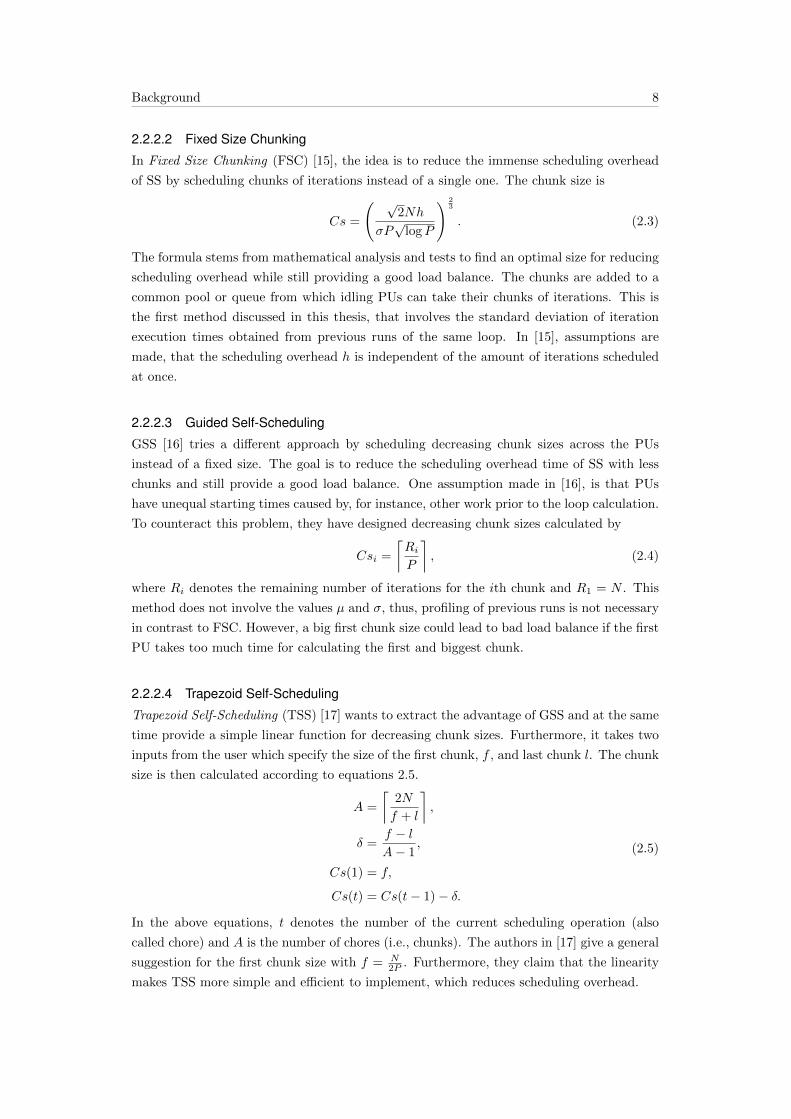
be seen in figure 2.3.
FAC is extremely general and robust to different variances of iterations. It behaves, depend-
ing on whether σ is high or low, like SS or static.
2.2.2.6 Weighted Factoring
Weighted Factoring (WF) [19] is very similar to FAC. However, this strategy takes PU
speeds into consideration for calculating the chunk sizes. The idea is to dynamically assign
Background 10
Loop Iterations
......
32 32 32 32
125 125 125 125 63 63 63 63Queue
PU 1
PU 2
PU 3
PU 4
1st Batch 2nd Batch
3rd Batch
Figure 2.3: Example illustration of FAC2 with P = 4 and N = 1000. In this example, acommon variable or queue is used for scheduling.
decreasing size chunks of iterations, like in FAC, to PUs in proportion to their processing
speeds. In conclusion, each PU is associated with a weight w that represents its relative
speed. These weights are normalized and add up to the number of available PUs. After the
batch and chunk size are calculated like in FAC, the chunks of a batch are multiplied by
the weights and assigned to the corresponding PUs. The following equation 2.8 shows the
chunk size of batch j for PU i.
Csij = wi × Cs factoringj and
P∑i=1
wi = P. (2.8)
The weights are estimated by benchmarking the system a priori. During runtime, the
weights stay constant. This strategy is meant for heterogeneous work-stations with different
PU speeds and system-induced impact to the performance.
2.2.2.7 Taper
Based on GSS, Taper (TAP) [20] tries to achieve optimal load balance, while scheduling the
largest possible chunk size to decrease the number of chunks scheduled and, with that, the
scheduling overhead. It differs from GSS by taking the mean µ and standard deviation σ
of iteration times into account to get a better load balance. The chunk size formula, given
in equations 2.9, is derived from probabilistic analysis to achieve an optimum for the above
idea.
Csi = max
{Csmin,
⌈Ti +
v2α2− vα
√2Ti +
v2α4
⌉},
Ti =RiP,
vα =ασ
µ.
(2.9)
In the above equations, i is the chunk index, Csmin denotes the minimum chunk size and
α is a scaling factor of the coefficient of variation (c.o.v.) , that is found empirically [20].
It is influenced by the overhead time and the ratio of N to P . Furthermore, TAP is GSS,
when σ = 0.
Background 11
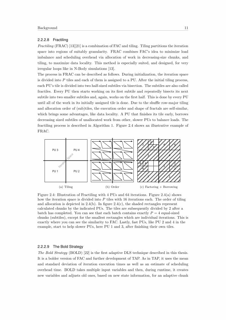
2.2.2.8 Fractiling
Fractiling (FRAC) [13][21] is a combination of FAC and tiling. Tiling partitions the iteration
space into regions of suitably granularity. FRAC combines FAC’s idea to minimize load
imbalance and scheduling overhead via allocation of work in decreasing-size chunks, and
tiling, to maximize data locality. This method is especially suited, and designed, for very
irregular loops like in N-Body simulations [13].
The process in FRAC can be described as follows. During initialization, the iteration space
is divided into P tiles and each of them is assigned to a PU. After the initial tiling process,
each PU’s tile is divided into two half-sized subtiles via bisection. The subtiles are also called
fractiles. Every PU then starts working on its first subtile and repeatedly bisects its next
subtile into two smaller subtiles and, again, works on the first half. This is done by every PU
until all of the work in its initially assigned tile is done. Due to the shuffle row-major tiling
and allocation order of (sub)tiles, the execution order and shape of fractals are self-similar,
which brings some advantages, like data locality. A PU that finishes its tile early, borrows
decreasing sized subtiles of unallocated work from other, slower PUs to balance loads. The
fractiling process is described in Algorithm 1. Figure 2.4 shows an illustrative example of
FRAC.
Iteratio
n SpacePU 3 PU 4
PU 2PU 1
(a) Tiling (b) Order
3
3
1
4
2
4 43
2
22
2
4
4 4
(c) Factoring + Borrowing
Figure 2.4: Illustration of Fractiling with 4 PUs and 64 iterations. Figure 2.4(a) showshow the iteration space is divided into P tiles with 16 iterations each. The order of tilingand allocation is depicted in 2.4(b). In figure 2.4(c), the shaded rectangles representcalculated chunks by the indicated PUs. The tiles are subsequently divided by 2 after abatch has completed. You can see that each batch contains exactly P = 4 equal-sizedchunks (subtiles), except for the smallest rectangles which are individual iterations. This isexactly where you can see the similarity to FAC. Lastly, fast PUs, like PU 2 and 4 in theexample, start to help slower PUs, here PU 1 and 3, after finishing their own tiles.
2.2.2.9 The Bold Strategy
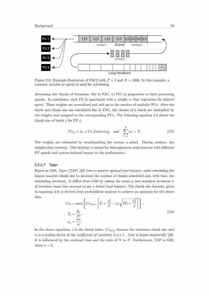
The Bold Strategy (BOLD) [22] is the first adaptive DLS technique described in this thesis.
It is a bolder version of FAC and further development of TAP. As in TAP, it uses the mean
and standard deviation of iteration execution times as well as an estimate of scheduling
overhead time. BOLD takes multiple input variables and then, during runtime, it creates
new variables and adjusts old ones, based on new state information, for an adaptive chunk

Background 12
Algorithm 1 Fractiling [21]
1: divide iteration space into P tiles of size NP
2: assign one for each PU in shuffled row-major numbering3: for all PU do . in parallel4: allocate the fractile corresponding to half of the initial PU assignment5: while there are fractiles not done on the level do6: do the allocated fractile7: enter a mutex lock8: while there is a fractile in the initial assignment to do do9: successively allocate the next fractile in decreasing chunk size and in shuffle
order10: end while11: while there are remaining fractiles to do in other PU assignments do12: successively allocate a fractile in decreasing chunk size and in shuffle order13: end while14: exit the mutex lock15: end while16: end for
size calculation. The driving idea behind the final strategy was to increase early chunk sizes
in order to reduce scheduling overhead, while considering the risk of a potential big chunk
that could last until the end and, thus, lengthen the overall executing time. The strategy
derives from probabilistic analysis of that idea. It is designed for loops with algorithmic
(e.g., conditional statements in loop body) and system-induced (cache misses and other
system interferences) variance. BOLD is intended to be implemented in a centralized model
with a master who assigns chunks of iterations to requesting PUs. Assumptions are made
that the scheduling overhead time h is a fixed delay, independent of the number of iterations
scheduled at once or the amount of PUs requesting new work at once. Furthermore, the
authors note that the calculation might produce more overhead because of its complexity.
The algorithms 2 and 3, which show the strategy, need some explanation for the used
variables and how they are adapted during runtime [22]:
boldM The number of iterations that either are unassigned or belong to chunks currently
under execution [22]. It is initialized to N. This variable has to be adjusted during
runtime in the following way. Whenever a PU completes a chunk of size Cs, boldM is
decremented by Cs [22].
totalspeed “Indicates the expected number of iterations completed per time unit, taking
the allocation delay into account, and tends to lie slightly below Pµ .” [22]. This variable
is initialized to 0. It is adjusted whenever a PU starts or finishes working on a chunk.
At the start of a chunk of size Cs, the PU increments totalspeed by CsCsµ+h , and after
the execution of the chunk, it decrements totalspeed by the same value. This variable
is used to maintain boldN .
boldN This variable is an estimate of the number of iterations that have not yet been
executed [22]. It is initialized to N. Furthermore, it assumes that while a PU is
executing a chunk, it makes steady progress at exactly one iteration every µ time
units. Maintaining boldN during runtime requires totalspeed and three points in time,
Background 13
t1, t, t2. Figure 2.5 [22] describes the mentioned points in time. To maintain boldN ,
time
Figure 2.5: Description of the time points t1, t, t2 used to update boldN . Computationtime is shown shaded. At t1, the processing of a new chunk of size Cs begins (includingoverhead time for scheduling). The processing ends at time t2. t is defined as the lastpoint in time before t2 at which a chunk is completed or a new one is allocated.
the variable is adjusted at time t2, before totalspeed is updated, by
boldNnew = boldNold −
(t2 − t) totalspeed︸ ︷︷ ︸collective progress since t
+Cs− (t2 − t1)Cs
Csµ+ h︸ ︷︷ ︸correction term
. (2.10)
Q The number of remaining unassigned iterations per PU.
Algorithm 2 Bold initialization [22]
1: a = 2(σµ
)22: b = 8a ln (8a)3: if b > 0 then4: ln b = ln (b)5: end if6: p inv = 1.0
P
7: c1 = hµ ln(2)
8: c2 =√
2πc19: c3 = ln (c2)
10: boldM = N11: boldN = N12: totalspeed = 0
2.2.2.10 Adaptive Weighted Factoring
Adaptive Weighted Factoring (AWF) [23] is similar to WF but addresses the limitation of
the weights not being adapted during computation. Furthermore, it does not need prior
knowledge of system load. Therefore, profiling is not necessary. AWF is designed for time-
stepping applications, like N-Body simulations, where each time step involves one heavy
loop. Weights are adjusted only after each time step, thus, not during loop execution. AWF
is still described here since there are variations based on it which allow non-time-stepping
applications. The variations are discussed in the following Section 2.2.2.11. In AWF, the
cumulative performance of each PU from all the previous steps is used for determining the
weights. This technique incorporates both loop characteristics and PU speeds in calculating
the chunk sizes.

Background 14
Algorithm 3 Bold routine for subsequently determining chunk sizes [22]
1: function CalculateChunkSize(P,N,R, a, b, p inv, ln b, c1, c2, c3, boldM, boldN)2: Q = R
P3: if Q ≤ 1 then4: return 15: end if6: r = max {R, boldN}7: t = p inv × r8: ln Q = ln (Q)9: v = Q
b+Q
10: d = R1+ 1
ln Q−v11: if d ≤ c2 then12: return t13: end if14: s = a (ln (d)− c3)
(1 + boldM
rP
)15: if b > 0 then16: w = ln (v × ln Q) + ln b17: else18: w = ln (ln Q)19: end if
20: return min{t+ max {0, c1w}+ s
2 −√s(t+ s
4
), t}
21: end function
In a master-worker model, after each time step, the PUs send their total execution time to
the master PU, not including the scheduling time. The master then computes the weights
for all PUs. For this, it first determines the weighted average ratio
πi =
(∑sj=1 j × tij
)(∑s
j=1 j × nij) , (2.11)
which gives the average ratio of execution time per iterations,tijnij
, of a step j, of all the
executed steps s on PU i. More recent steps are weighted higher to produce a better
adaptation of very recent workloads. The next step is to compute the average weighted
average ratio
π =
∑Pi=1 πiP
, (2.12)
of all PUs. Now, the raw weight of PU i is defined as
ρi =π
πi. (2.13)
In order to fulfill the requirement of WF, where weights must add up to the number of P ,
the master needs to normalize the raw weights ρi. Equation (2.14) shows the normalized
weight wi for PU i using the above variables.
wi =ρi × Pρ
, where ρ =
P∑i=1
ρi. (2.14)
The weights are initially set to 1 and then adjusted after each step. Finally, like in WF, the
master can use the determined weights, which do not change during a time step, to weight

Background 15
the chunk sizes obtained from FAC and calculate the final chunk size
Csij = wi × Cs factoringj and
P∑i=1
wi = P (2.15)
for a PU i and batch j. The following variants of AWF provide the possibility to adapt
during a loop.
2.2.2.11 Adaptive Weighted Factoring Variants
There exist variants [24] of the above described technique AWF from Section 2.2.2.10. In
this part, four variations of AWF, AWF-B, AWF-C, AWF-D and AWF-E, are shown. All
of them have a common goal. They address the limitation of AWF to rely on time-stepping
applications, where the adaptation happens only after each step. The variants allow adapta-
tion during loop execution. Depending on the chosen variant, the PU weights are adjusted
less or more frequently. The calculation of chunk sizes is very similar to AWF but the
variants use a modified formula for the weighted average ratio
πi =
(∑sij=1 j × tij
)(∑si
j=1 j × nij) . (2.16)
Unlike in AWF, the modified version above determines the weighted average ratio of the
executed chunks j, 1 ≤ j ≤ si, by PU i instead of previous time steps. This is exactly the
modification which allows updates during a loop. Initially, the weights are set to 1 for all
PUs like in AWF and an arbitrarily chosen first batch size of β0×N , 0 < β0 < 1, is selected
like in AF to determine the initial chunk size
Csi1 = ni1 = β0 ×N
P(2.17)
for a PU i. From here on, the succeeding chunks are determined differently by one of the
following variants:
AWF-B schedules the remaining iterations by batches. The weights are adjusted after each
batch based on timings from previous chunks.
AWF-C schedules the remaining iterations by chunks, similar to AF, instead of batches. The
idea of this variation is to address a possible issue of AWF-B (as well as FAC, WF
and AWF), where faster PUs which already have computed their portion of the batch
could be assigned remaining chunks of less-than-optimal size from the current batch.
The reason is that in these methods, the chunk sizes are fractions of the current FAC
batch size which, once scheduled, do not change. AWF-C tries to solve this issue by
recomputing a new batch size each time a PU requests for work and before applying
AWF for weight calculation. This modification results in faster PUs being assigned
larger chunks from all the remaining iterations and not just from the ones left in
current batch.
AWF-D is like AWF-B but the execution time of iterations of a chunk j, tij , is redefined as
the total chunk time. This not only includes the execution time but also the time spent
by the PU in doing tasks associated with the execution of a chunk (e.g., bookkeeping).
Background 16
AWF-E is like AWF-C but uses to total chunk time as in AWF-D.
2.2.2.12 Adaptive Factoring
The last adaptive DLS technique discussed in this thesis is Adaptive Factoring (AF) [25][26].
As the name indicates, it is based on FAC. The difference is that AF relaxes the require-
ment in FAC, where mean µ and standard deviation σ are known a priori and additionally
that they are the same on all PUs. The statistical values of µ and σ are calculated and
adjusted during runtime. AF is thus a more generalized technique than FAC or WF and it
is advantageous if the mean and variance are unknown and vary during runtime. Besides
the adaptivity and generality, AF uses, like in FAC, a probabilistic model to calculate chunk
sizes and dynamically allocate chunks of iterations to PUs such that the average finishing
time for completion of the chunks occurs before the optimal time, µNP , of the whole re-
maining task [25]. In other words, the expected finishing time of the current batch has a
high probability to occur before the optimal finishing time of the whole remaining task. In
direct comparison with WF, where weights are statically assigned to each PU, AF does not
use fixed weights but dynamically computes the size of a new chunk for a PU based on
its performance information gathered from recently executed chunks. In other words, AF
dynamically weights chunk sizes for individual PUs based on their recent performance.
AF can be implemented with a master-worker model in which the request messages of
workers contain updated performance data (µ and σ) of recently executed chunks [26]. The
master uses this information to compute the chunk sizes with
Cs(n)i =
Dn + 2TnRn−1 −√D2n + 4DnTnRn−1
2µi, n > 1
and Cs(1) ≥ 100, n = 1
(2.18)
for a PU i and step (or batch) n. The variables D and T incorporate the latest estimator
for the means and standard deviations of every PU. They are calculated as shown in (2.19).
Dn =
P∑i=1
σ2i
µi, Tn =
(P∑i=1
1
µi
)−1
, n > 1. (2.19)
The remaining iterations Rn after step n are calculated as
R0 = N,
R1 = R0 − PCs(1),
Rn = Rn−1 −P∑i=1
Cs(n)i , n > 1.
(2.20)
Since AF does not need a priori profiling, it first estimates the mean and standard deviation
for each PU i in an arbitrarily sized initial batch (step 1) with P chunks of size Cs(1). For
this, the PUs have to record their finishing times Xij of each iteration j, 1 ≤ j ≤ Cs(1). The
initial estimators for the mean µi and standard deviation σi of a PU i are then calculated
with
µi =
∑n1 Xij
Cs(1)and σi =
(∑n1 X
2ij − Cs(1)µ2
i
Cs(1) − 1
) 12
. (2.21)

Background 17
Algorithm 4 shows the steps in AF for how chunk sizes are calculated and iterations are
allocated. Step 1 allocates the iterations in batch. Afterwards, there is no need for allocating
Algorithm 4 AF algorithm for chunk size calculation and allocation [25].
1: procedure AdaptiveFactoring2: n← 1 . step number3: AFInitialize . step 1, there are R1 iterations left4: while R > 0 do5: n← n+ 16: AFAllocate(n) . step n, there are Rn iterations left7: end while8: end procedure9:
10: procedure AFInitialize11: assign to each PU Cs(1) iterations, with Cs(1) ≥ 10012: record finishing times Xij of each iteration j for each PU i13: end procedure14:
15: procedure AFAllocate(n) . can be executed for any individual PU i requesting16: estimate µ and σ for each PU i using information of previous steps and (2.21)
17: assign Cs(n)i iterations to PU i using (2.18)
18: record finishing times Xij for each iteration j in every PU i19: end procedure
in batches. Whenever a PU finishes its chunk, a new one of size (2.18) is immediately
allocated by the master.
When comparing AF to AWF and its variants, it is important to mention that AF introduces
more overhead because of the intensive time measurements on an iteration level rather than
batch or chunk levels.
2.3 OpenMPOpenMP is a standard for shared memory parallel programming. It consists of directives
and pragmas, which collectively define the specification of the OpenMP Application Pro-
gramming Interface (OpenMP API). In order to use OpenMP, a compiler is required that
supports the OpenMP specification and implements the API. Many popular compilers, like
GCC [5][4], Intel C++ Compiler [27] and LLVM Clang [28], already support the specifica-
tion [2] and can be used for parallelizing programs. Compilers with OpenMP support can
compile one or many of the languages C, C++ and Fortran [1].
OpenMP uses the shared memory programming model, i.e., execution happens on one node
with same address space. Directives or pragmas can be elegantly used in the source code to
implicitly parallelize parts of a program. The directives tell the compiler how statements are
to be executed and which parts are parallel. The compiler then generates multithreaded code
by reading the directives. There are many constructs in OpenMP, such as parallel regions,
work-sharing, variable scoping, critical regions and synchronization, to parallelize a program
but we focus on the work-sharing part, where a loop and its iterations are split among
threads. Parallelizing loops is one of the most popular features of OpenMP. Doing this only
Background 18
requires one single line in C/C++ before a for-loop, namely, #pragma omp parallel
for. The user can also set clauses within a pragma to, for example, select whether or not
threads have their own copy of a variable, or how a loop should be scheduled. The exact
syntax of the work-sharing-loop construct for C/C++, as described in the specification [1],
is
#pragma omp for [clause[[,]clause]...]new-line
for-loops
where the schedule clause corresponds to schedule([modifier[, modifier]:]kind[, chunk size]).
The modifiers can be used to specify whether chunks are executed in increasing logical
iteration order or not. Our focus lies on the kind, which specifies the scheduling algorithm.
Which values currently are available for kind and what they stand for is described in the
following subsection.
2.3.1 Scheduling in OpenMPOpenMP lists three loop scheduling techniques in the specification [1], however, there are
many more which are not listed. Therefore, available OpenMP implementations, like the
ones mentioned in Subsection 2.3.2, are only required to implement the listed techniques
in the specification. These are static, dynamic and guided. On top of that, the user
must specify a chunk size within the pragma. Based on that size, the chosen technique, for
instance static, statically schedules blocks of iterations of given size to each PU prior to
loop execution. The option dynamic dynamically schedules chunks of iterations of specified
size to idling PUs during runtime. Lastly, guided uses a dynamic scheduling approach
with decreasing chunk sizes down to the specified size. These three techniques are similar to
the explained techniques in Section 2.2, Static, SS and GSS, but the exact implementation
depends on the used OpenMP library. Furthermore, the schedule selection can be postponed
to be chosen during runtime by using the kind runtime. An example of it looks like
#pragma omp for schedule(runtime).
Every loop with the above schedule clause will then be scheduled by the strategy which is
set in the environment variable OMP SCHEDULE. The value of this variable takes the form
[modifier:]kind[, chunk].
2.3.2 LLVM OpenMP Runtime LibraryLLVM’s Clang supports OpenMP 3.1 by default since version 3.8.0 [7]. The LLVM runtime,
libomp, stems from Intel’s open source OpenMP runtime [29] and contains almost the exact
same code as Intel has merged its open-source library to the LLVM project where further
development takes place [30]. While this library is compatible with Intel, GCC and LLVM’s
compilers, GCC’s libgomp is not compatible with Clang. The fact that libomp is Intel and
LLVM’s production library for OpenMP while supporting GCC, makes it very significant.
Since this thesis is focusing on the LLVM compiler infrastructure, an overview of the devel-
opment process with LLVM is given in figure 2.6 [29]. The compile-time involves compiling

Background 19
C/C++ source code including OpenMP directives using Clang which is a C language fam-
ily compiler front-end for LLVM. Clang uses the LLVM compiler infrastructure, a compiler
tool chain, as its back-end to finally compile the source code into a binary file. During
runtime, the application uses libomp for routine calls. To link the library, the compile flag
-fopenmp must be used. It is also possible to link a runtime explicitly by its name with
-fopenmp=<library-name>.
Compile-time Run-time
.cppC/C++ Front-End
(Clang)Back-End
(LLVM)
LLVM OpenMPRTL
a.out
Figure 2.6: The process of compiling C/C++ source code with OpenMP and LLVM. Theruntime library handles calls from the binary during runtime.
Once a binary is produced, the environment variables indicate, for example, which runtime
library to use or what kind of scheduling technique should be picked if the programmer has
set schedule(runtime) inside the pragma. The path to the library can be specified in
the environment variable LD LIBRARY PATH. A recompilation is not needed if this path
changes, which makes it easy to switch between different implementations of the runtime
library. The number and type of available scheduling techniques depend on the actual
implementation. For instance, the current checked out code of libomp only implements
static, guided, dynamic and trapezoidal loop scheduling techniques. As for now,
the latter technique is not yet listed in the library’s latest manual [3], since the manual has
not been built for three years from now. The absence of many other DLS techniques in
libomp is the gap that we want to fill in this thesis by implementing additional techniques.

3Related Work
In this chapter, related works from the past are discussed. Since this thesis focuses on the
implementation of additional loop scheduling techniques into an OpenMP runtime library, it
is important to see what others have done in that area for existing OpenMP implementations.
All the above methods from Section 2.2 have already been implemented and tested but none
of them, except for similar versions of SC, SS, GSS and TSS, have been implemented into
the LLVM OpenMP runtime library. Most of them have not even been implemented in
any existing OpenMP runtime library since the OpenMP specification does not list more
than three methods. However, past research projects have implemented new techniques into
existing OpenMP runtime libraries, such as GCC’s libgomp [4] and evaluated the results.
Officially, libgomp provides only static, dynamic and guided scheduling techniques.
The work by Buder P. [31], which is the closest to this thesis, implemented and tested
six additional DLS techniques in libgomp. Additionally, a related paper to Buder’s work
was published by Ciorba et al. [32]. The newly implemented methods which were used by
Buder are FSC, TSS, FAC, WF, TAP and BOLD. All these methods were implemented into
libgomp by extending the existing code and using the environment variable OMP SCHEDULE
for selecting a technique whenever the OpenMP schedule clause schedule(runtime) is
used. To assess the implemented techniques, four benchmark suites, Rodinia [9], OmpSCR
[10], NAS [11] and SPEComp [12] were used and, when necessary, modified to obtain profiling
information of loop iteration times for the mean µ and standard deviation σ input values
which are required in some of the techniques. The results show that no single method fits best
for every application but rather, depending on the chosen benchmark, one is superior to the
others. This is the evidence that OpenMP must include more loop scheduling techniques to
cover much more types of applications with respect to performance. In this thesis, not only
the methods used by Buder but also other, especially adaptive, techniques are implemented
into the LLVM OpenMP runtime library.
Another close work to this thesis is recently done at TU Dresden [33] which presents a generic
methodology for implementing additional scheduling techniques to an OpenMP runtime.
They demonstrated the proposed methodology by implementing FAC to LLVM’s libomp
and presented first results with four scientific applications.
In the context of load balancing strategies, Penna et al. introduced a new design methodol-

Related Work 21
ogy, including a simulator for assessing loop scheduling strategies, which helps to guide the
study of new workload-aware loop scheduling techniques [34]. In contrast to other strate-
gies, workload-aware scheduling methods try to achieve better load balance by taking the
input workload into account and evenly distribute it among the threads. To validate their
methodology, they proposed a new strategy as a proof of concept called Smart Round-Robin
(SRR) [35] and implemented it in libgomp. This new method considers the input workload
(i.e., the length of each iteration) in order to achieve near-optimal load balance. Since this
technique depends on the iteration lengths, it requires some sort of profiling and preprocess-
ing prior to the actual scheduling. A second novel workload-aware strategy was implemented
in libgomp, called BinLPT [36]. One difference between SRR and this new strategy is that
BinLPT schedules chunks of iterations instead of single ones. The results of both techniques
have shown that they outperform OpenMP’s static and dynamic scheduling strategies
in irregular applications. Their approach of evenly distributing workload differs from all the
techniques described in this thesis especially in how profiling is done. SRR and BinLPT both
depend on precise workload information obtained beforehand to be able to evenly assign the
workload across the threads. Techniques used in this thesis either use only mean and stan-
dard deviation inputs or obtain load information during runtime. Another difference is that
SRR and BinLPT preprocess an optimal map for the iteration/thread assignment based on
workload data which is a static scheduling description.
Similar work is done by Mottet L. who ported the same SRR technique from Penna et
al. into Intel’s OpenMP runtime [37]. He found similar results where SRR is 15% better
than OpenMP’s dynamic scheduling in some conditions. Furthermore, this work is of high
relevance to this thesis since Intel’s runtime is the same as LLVM’s.
When dealing with NUMA2 multicore machines, it is crucial to distribute work and its
associated data in a way which exploits data locality to maximize performance. OpenMP’s
dynamic strategy is the first choice when scheduling irregular loops, however, it does not
respect memory locality in NUMA machines. Durand et al. proposed a new scheduling
technique called adaptive with the goal to provide a better dynamic scheduling technique
for NUMA machines and irregular loops, while respecting data locality [38]. This new
technique starts a static initial distribution of the iteration space, scheduling NP iterations
for each thread. Load balancing is then done via work-stealing where idling threads steal half
of the remaining iterations of another thread. On top of that, they extended adaptive
with new OpenMP APIs to deal with the mentioned data locality. Their new strategy
outperformed OpenMP’s techniques on memory-bound and irregular loops, while providing
similar performance to static on regular loads. In contrast to the work of Durand et al.,
this thesis does not focus on NUMA machines.
A different approach can be found in [39], [40] and [41], which proposed an automatic
technique without having the user to choose a specific strategy. Their methods either auto-
matically select an appropriate known loop scheduling technique for a given loop or derive a
strategy based on online-profiling, loop analysis and system state. For instance, Zhang et al.
[39] presented a hierarchical adaptive OpenMP loop scheduling technique for hyper-threaded
2 Non-Uniform Memory Access

Related Work 22
SMP3 systems. This strategy samples different known techniques on a loop in its first several
runs and then adapts by selecting a more appropriate technique on the remaining runs of the
same loop. This is only applicable on loops which have multiple complete executions. Addi-
tionally, it decides based on the first few runs whether to use hyper-threading or not. Their
approaches payed off especially in loaded systems, where unpredictable behavior is the case.
This thesis does not implement any hierarchical or automatic, selection-based techniques,
instead, it focuses on implementing and testing every particular strategy separately.
The last related work, that is discussed in this chapter is done by Kale V., who recently
proposed a new addition to the OpenMP standard for adding user-defined scheduling tech-
niques to OpenMP [42]. With this, the user can choose his custom strategy in code in a
standardized way with the use of an extended schedule() clause. The user is hereby
required to provide and link a custom library that implements the needed functions for the
scheduling task.
3 symmetric multiprocessing

4Loop Scheduling in LLVM
This chapter explains how loop scheduling works in LLVM’s libomp and mentions the re-
quirements to implement new techniques. It also describes the methodology of how we
have extended libomp. Exploiting parallelism on hardware with an increasing number of
processing units requires complex techniques to schedule the tasks across the cores in an
optimal way. Algorithms that contain parallel loops, which are responsible for most of their
execution time, can use the full potential of the underlying system to improve the overall
performance. Among different possibilities of realizing parallelism for loops on shared mem-
ory systems, OpenMP has proved itself as the de facto standard for parallelism. LLVM,
with its Clang compiler and OpenMP runtime library, also called libomp, implements this
standard to be used for parallelism. A general overview of LLVM is given in 2.3.2 in Chap-
ter 2. The current state of libomp, from LLVM 8.0, provides four different loop scheduling
techniques, static, dynamic, guided and trapezoidal. Many more techniques exist
but they are not implemented in LLVM. However, the structure and design of libomp makes
it possible to add new techniques by editing and extending a few files. To understand the
requirements of such an extension, section 4.1 describes the design and workflow of loop
scheduling in libomp.
4.1 Scheduling Overview in libompLibomp uses three functions to schedule iterations of a parallelized loop to processing units.
Figure 4.1 shows the main parts of the scheduling process. Once an application is compiled
with the use of a compiler like Clang, ICC or GCC, and thereafter linked to libomp by us-
ing the compiler flag -fopenmp, every loop that is parallelized with the compiler directive
omp parallel for including the use of the scheduling clause schedule(runtime) is
then scheduled by libomp. The library consists of many source files but since this thesis is
focusing on the loop scheduling implementation only, six files suffice to be further discussed.
These are kmp.h, kmp settings.cpp, kmp runtime.cpp, kmp global.cpp, kmp dispatch.h and
kmp dispatch.cpp. The three main functions responsible for the actual scheduling are in-
side of kmp dispatch.cpp as depicted in Figure 4.1. Before the call of any of those men-
tioned functions, libomp first prepares a few things. The file kmp.h is the runtime header
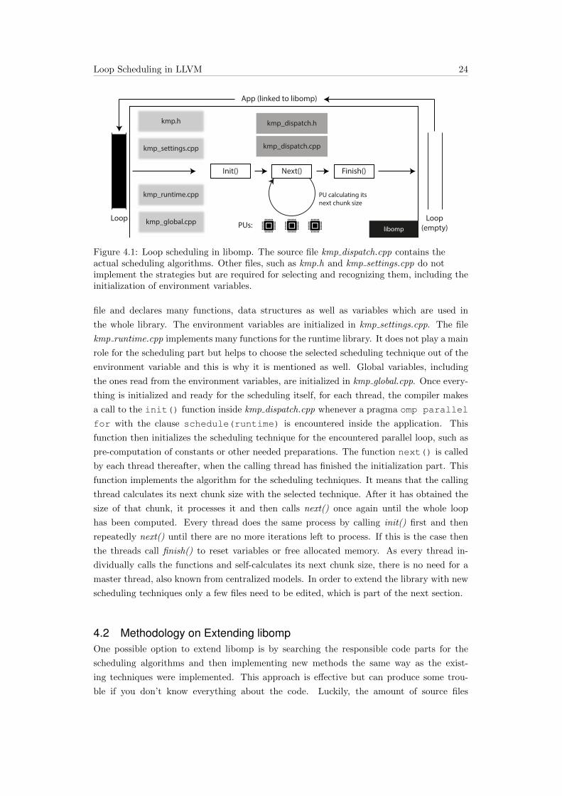
Loop Scheduling in LLVM 24
PUs:
App (linked to libomp)
Loop
Init()
Loop(empty)
Next() Finish()
kmp.h
kmp_settings.cpp
kmp_runtime.cpp
kmp_global.cpp
kmp_dispatch.cpp
PU calculating itsnext chunk size
libomp
kmp_dispatch.h
Figure 4.1: Loop scheduling in libomp. The source file kmp dispatch.cpp contains theactual scheduling algorithms. Other files, such as kmp.h and kmp settings.cpp do notimplement the strategies but are required for selecting and recognizing them, including theinitialization of environment variables.
file and declares many functions, data structures as well as variables which are used in
the whole library. The environment variables are initialized in kmp settings.cpp. The file
kmp runtime.cpp implements many functions for the runtime library. It does not play a main
role for the scheduling part but helps to choose the selected scheduling technique out of the
environment variable and this is why it is mentioned as well. Global variables, including
the ones read from the environment variables, are initialized in kmp global.cpp. Once every-
thing is initialized and ready for the scheduling itself, for each thread, the compiler makes
a call to the init() function inside kmp dispatch.cpp whenever a pragma omp parallel
for with the clause schedule(runtime) is encountered inside the application. This
function then initializes the scheduling technique for the encountered parallel loop, such as
pre-computation of constants or other needed preparations. The function next() is called
by each thread thereafter, when the calling thread has finished the initialization part. This
function implements the algorithm for the scheduling techniques. It means that the calling
thread calculates its next chunk size with the selected technique. After it has obtained the
size of that chunk, it processes it and then calls next() once again until the whole loop
has been computed. Every thread does the same process by calling init() first and then
repeatedly next() until there are no more iterations left to process. If this is the case then
the threads call finish() to reset variables or free allocated memory. As every thread in-
dividually calls the functions and self-calculates its next chunk size, there is no need for a
master thread, also known from centralized models. In order to extend the library with new
scheduling techniques only a few files need to be edited, which is part of the next section.
4.2 Methodology on Extending libompOne possible option to extend libomp is by searching the responsible code parts for the
scheduling algorithms and then implementing new methods the same way as the exist-
ing techniques were implemented. This approach is effective but can produce some trou-
ble if you don’t know everything about the code. Luckily, the amount of source files

Loop Scheduling in LLVM 25
that need modifications is not high. Section 4.1 already described the relevant files for
scheduling and these are exactly the files that require edits. A very recent case study
[33] presented a generic methodology for extending an OpenMP runtime with new schedul-
ing strategies. An example was given by implementing FAC into libomp. In this thesis,
the methodology of implementing new strategies into libomp is based on the same ap-
proach as in the case study. The following description summarizes the methodology. First,
the library must be able to select new strategies. For this, the enumeration kmp sched
listing all available scheduling techniques in header file kmp.h must be extended with a
new item for each new strategy. In kmp runtime.cpp, new case handling must be added
for each new technique inside the function kmp get schedule. Finally, the source file
kmp settings.cpp needs a modification to allow the user selecting new scheduling techniques
by their names. The relevant functions here are kmp parse single omp schedule and
kmp stg print omp schedule which must recognize the new strategies by their names.
The second part of extending libomp takes place in source file kmp dispatch.cpp. This
is the file to which the actual scheduling logic and algorithm belongs. Starting with the
initialization of a scheduling technique, a new case for each new strategy must be added to
function kmp dispatch init algorithm. This function is called once for each thread
before the loop calculation begins. It focuses on initializing and preparing data structures,
constants or even pre-computations of scheduling related information which are then needed
later. Libomp already provides thread-private and shared data structures which can be
extended in header file kmp dispatch.h. Needed information can be stored in these data
structures and read during the whole process of a single loop. The structures are called
dispatch private info template and dispatch shared info template.
The third part also takes place in source file kmp dispatch.cpp but this time inside the func-
tion kmp dispatch next algorithm. Once again, for each new scheduling technique,
you must add a new case handler, that contains the actual scheduling algorithm to calculate
the next chunk size. This function is also called by each thread, as soon as they have finished
the initialization or computed a previous chunk and want to calculate their next chunk size
for computation.
Finally, when there is no iteration left, the threads call kmp dispatch finish or
kmp dispatch finish chunk to cleanup. Scheduling related variables might need to
be reset for the next loop.
Note: If there is need for additional environment variables that must be read and used in
some scheduling strategies, additional modifications must take place. This can be done by
declaring new variables in header file kmp.h and initializing them to a default value in file
kmp global.cpp. Lastly, the file kmp settings.cpp must be modified to give libomp the ability
to recognize, read and initialize the new environment variables. More precisely, the table
kmp stg table[] must be extended with a new entry for each new environment variable
and an appropriate parser function. Chapter 5 gives more details about how each technique
is implemented.

5Implementation
This chapter describes how we have implemented the new DLS strategies which are pre-
sented in detail in Chapter 2. During implementation, the outlined methodology from
Section 4.2 is followed. The newly implemented strategies have a common logic part that
is described first in this chapter. Further deviations for a chosen technique are mentioned
in the corresponding sections below. The main code for the strategies lies in source file
kmp dispatch.cpp, containing the two functions init() and next(), which are called by
each thread separately, when a parallel loop has been encountered in the application. Gen-
erally, the structure of each technique’s initialization and chunk size calculation is based on
a common way. To initialize a scheduling technique, before the loop calculations starts, the
function init() pre-computes variables or constants and stores them into thread-private
or shared data structures to be used later. Algorithm 5 shows the common part of the
Algorithm 5 Initialization
1: procedure kmp dispatch init2: switch schedule do3: case factoring4: preparations5: private← variables6: shared← variables7: case bold8: ...9: end procedure
initialization. Depending on the technique’s requirements, different preparations are made.
The same thing applies to the function next(), which calculates the next chunk size for a
calling thread. A general picture of how that code block looks like can be seen in Algorithm
6. A chosen scheduling case is executed to compute the chunk size and, in the end, set the
loop boundaries for that new chunk to be processed. Mostly, a while loop is used in which
the chunk size is calculated and, if the current starting point is not already taken by another
thread, the while loop ends successfully and, if needed, updated variables are stored back to
thread-private or shared data structures. After a thread has obtained its next chunk size,
it processes that chunk with the calculated loop boundaries and calls the function next()

Implementation 27
again until the loop is done.
Algorithm 6 Next chunk
1: procedure kmp dispatch next algorithm2: switch schedule do3: case factoring4: while 1 do5: init← shared . read current start iteration6: cs← calculate chunk size7: limit← init+ cs . next starting point8: if obtain chunk == successful then9: shared← limit . update shared start iteration
10: break11: end if12: private← variables13: shared← variables14: end while15: set loop boundaries for current chunk to process
16: case bold17: ...18: end procedure
Some of the implemented techniques require additional environment variables to give the
user the ability to set input values, which can be used in the appropriate strategy. Section
5.1 lists all implemented environment variables.
5.1 Environment VariablesWhile most of the newly implemented techniques don’t require user-provided input values,
some of them do. The ones which require them are FSC, TAP, FAC, WF and BOLD. Other
strategies may have optional input values, such as static, dynamic or guided. Section 2.2
from Chapter 2 has detailed descriptions of the input values and their meaning. Table 5.1
summarizes all implemented environment variables and to which technique they belong.
The environment variables were implemented in source file kmp settings.cpp, following the
methodology described in Section 4.2.
Implementation 28
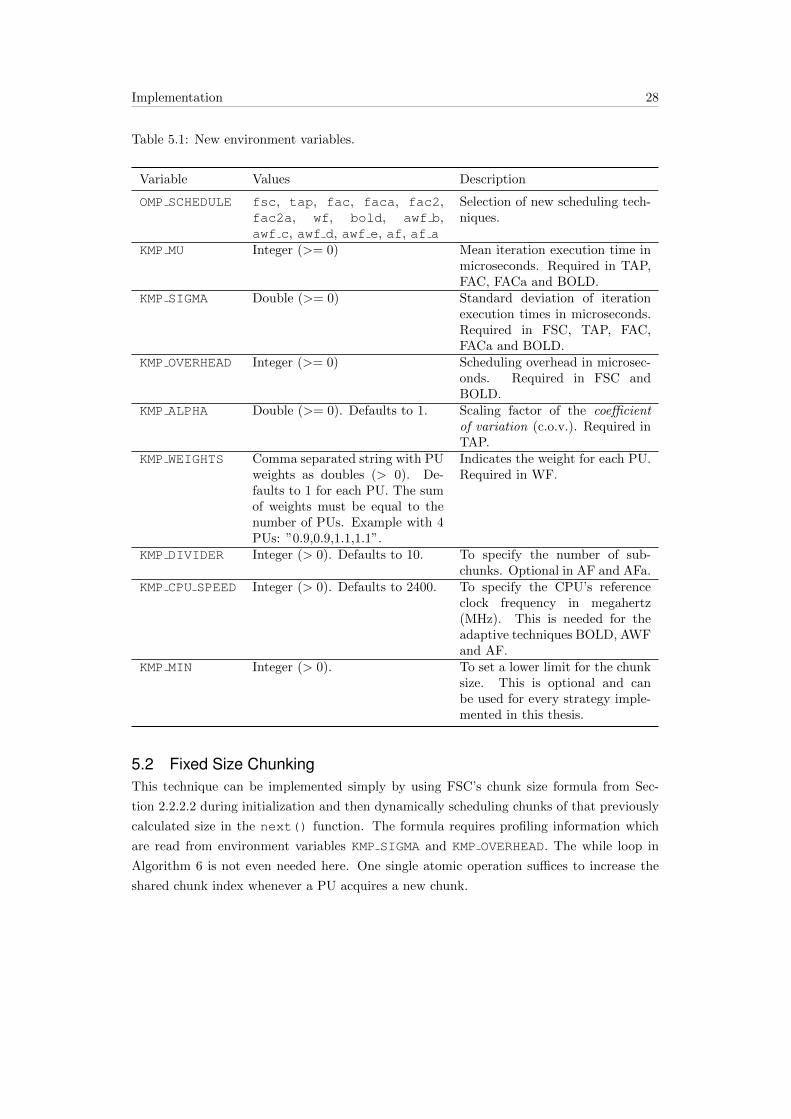
Table 5.1: New environment variables.
Variable Values Description
OMP SCHEDULE fsc, tap, fac, faca, fac2,fac2a, wf, bold, awf b,awf c, awf d, awf e, af, af a
Selection of new scheduling tech-niques.
KMP MU Integer (>= 0) Mean iteration execution time inmicroseconds. Required in TAP,FAC, FACa and BOLD.
KMP SIGMA Double (>= 0) Standard deviation of iterationexecution times in microseconds.Required in FSC, TAP, FAC,FACa and BOLD.
KMP OVERHEAD Integer (>= 0) Scheduling overhead in microsec-onds. Required in FSC andBOLD.
KMP ALPHA Double (>= 0). Defaults to 1. Scaling factor of the coefficientof variation (c.o.v.). Required inTAP.
KMP WEIGHTS Comma separated string with PUweights as doubles (> 0). De-faults to 1 for each PU. The sumof weights must be equal to thenumber of PUs. Example with 4PUs: ”0.9,0.9,1.1,1.1”.
Indicates the weight for each PU.Required in WF.
KMP DIVIDER Integer (> 0). Defaults to 10. To specify the number of sub-chunks. Optional in AF and AFa.
KMP CPU SPEED Integer (> 0). Defaults to 2400. To specify the CPU’s referenceclock frequency in megahertz(MHz). This is needed for theadaptive techniques BOLD, AWFand AF.
KMP MIN Integer (> 0). To set a lower limit for the chunksize. This is optional and canbe used for every strategy imple-mented in this thesis.
5.2 Fixed Size ChunkingThis technique can be implemented simply by using FSC’s chunk size formula from Sec-
tion 2.2.2.2 during initialization and then dynamically scheduling chunks of that previously
calculated size in the next() function. The formula requires profiling information which
are read from environment variables KMP SIGMA and KMP OVERHEAD. The while loop in
Algorithm 6 is not even needed here. One single atomic operation suffices to increase the
shared chunk index whenever a PU acquires a new chunk.
Implementation 29
5.3 FactoringFactoring can be implemented in different ways. This thesis implements it in four versions,
namely, FAC, FACa, FAC2 and FAC2a. The original version of Factoring, as described in
Chapter 2, Section 2.2.2.5, is represented by FAC. FAC relies on strong synchronization
between the threads. FACa does the exact same thing as FAC and produces the same
chunks but avoids synchronization by involving more computation. In other words, FAC
lets the first thread compute the chunk size for a given batch number, and every following
thread, that wants its next chunk size from the same batch number, can simply read and
re-use the already computed chunk size without computing it again. This means that for
each batch, the chunk size is calculated only once and then shared among all threads. To
implement this, the whole scheduling and chunk size calculation in function next() must
be synchronized with the use of a mutex. No more than one single thread is allowed to
calculate the next chunk size at the same time. Consequently, a while loop is not needed in
FAC. A shared queue counter is used which holds the number of remaining chunks of the
current batch. Whenever a thread wants to acquire a new chunk but the queue is empty, it
calculates the chunk size for the new batch and stores it into the shared data structure.
FACa on the other hand uses a shared counter so that the threads can identify what the
current batch number j = counterP is. There is no need to synchronize the scheduling part,
instead, the threads atomically increment the shared counter at the beginning of function
next() and calculate their next chunk size themselves by using the batch number and the
factoring formula. This involves more computation since every thread calculates its next
chunk size for a given batch number redundantly. Which one is the better choice depends on
the system. If synchronization costs are higher than the costs caused by more computation,
the user should choose FACa.
The other two implementations, FAC2 and FAC2a, don’t use any profiling information. As
with FACa, a shared counter is used to identify the current batch number. However, the
chunk size formula is much simpler and less computationally intensive since the variable x is
set to 2. FAC2 and FAC2a produce the exact same chunks but they defer in the way how they
calculate the chunk size for a given batch number j. FAC2 uses the formula Cs = d 12j+1∗NP e.
FAC2a uses a loop as in FACa to calculate the chunk size for the current batch number.
The reasoning to provide this is to reduce redundancy and only apply the factoring formula
to the last known batch’s chunk size. By storing the last known, thread-private chunk size
you can reduce the amount of calculations.
5.4 Weighted FactoringThe strategy WF uses the exact same algorithm as FAC2a from Section 5.3 but with the
addition of weights. These are read from the environment variable KMP WEIGHTS and the
resulting FAC2a chunk sizes are multiplied with the PU’s weight.

Implementation 30
5.5 TaperTaper is the only technique that requires a scaling factor α, read from the environment
variable KMP ALPHA. This factor is needed, in addition to µ and σ, to pre-compute the
variable vα during initialization. In the function next() the TAP formula 2.9, shown in
Chapter 2, is used to calculate the chunk size. The number of remaining iterations is hereby
calculated by the number of total iterations minus the current start iteration init obtained
from the shared data structure.
5.6 The Bold StrategyThis technique is the first adaptive strategy implemented in this thesis. It makes use of many
variables that are initialized first in function init() and then continuously updated in
next() to adapt to current system and loop iteration states. BOLD also requires profiling
information, i.e., KMP MU, KMP SIGMA and KMP OVERHEAD. These three user inputs are
needed during initialization as shown in Algorithm 2. After initializing all these variables,
they must be stored in either thread-private or shared data structures. The variables boldM,
boldN, totalspeed and bold time are shared, all other remain private.
In function next(), Algorithm 3 is used to calculate the next chunk size of a PU. However,
an updated variable boldN must be used in the mentioned algorithm. To maintain the
shared variable boldN, you need timing information. For this, the implementation stores
three time points t1, t and t2, also depicted in Figure 2.5. The time t2 is initialized to the
current time at the beginning of function next(). Immediately, also at the beginning, the
time point t is read from a shared variable bold time which then itself is updated to the
current time like t2. bold time can then be used by every other thread, to initialize t. The
remaining time point t1 is nothing else than the old t2 of that same PU. This is done by
storing t2 in thread-private data to be used in the next chunk. With all these information,
the next chunk size can be calculated according to BOLD’s algorithm from Chapter 2.
5.7 Adaptive Weighted Factoring VariantsAll AWF variants are based on WF’s implementation. The difference is that AWF adapts
the weights before being applied to factoring. AWF-B uses batches as in FAC. The first
batch size is calculated during initialization in init() by taking 12 ×N as the initial batch
size and 12 ×
NP as its chunk size. The weights are initially set to 1 for the first chunk.
AWF-B uses a shared vector of size P to hold each PU’s current π, also called the weighted
average ratio. This vector is initialized to all zeros, meaning, no PU has yet finished any
chunk and updated its π.
In function next(), after the very first chunk has been computed with an initial weight
of 1, AWF-B first calculates the weight of a PU and then continues like WF. The weight
calculation happens before the while loop. The procedure and formulae to update the
weight are described in Section 2.2.2.10 of Chapter 2. The implementation includes shared
locks (from C++14) to protect individual elements of the shared vector from corruptness.
To measure the time of individual chunk execution times, a time point is stored at the
Implementation 31
beginning of function next() and at the end of it. The time difference between the end
of a previous scheduling task and the beginning of a succeeding one is taken as the chunk
execution time.
AWF-C is very similar to AWF-B but it is not batched. Instead, each chunk size is calculated
by applying the factoring rule to the remaining iterations. The remaining variants AWF-D
and AWF-E have the exact same implementations as AWF-C and AWF-B but the only
difference here lies in the time measurement, that not only measures the chunk execution
time but also includes the scheduling time itself. For this, a single time point is stored at
the beginning of each scheduling task and the time difference between the last stored point
and the new one is taken for the formula to adapt the weight.
5.8 Adaptive FactoringThis technique is the last adaptive one implemented in this thesis. Algorithm 4 shows the
steps of how the chunk sizes are calculated. However, the implementation defers slightly
from the description in Section 2.2.2.12 because of performance reasons. Instead of mea-
suring every individual iteration’s execution time and adapting to every each of them, the
implementation schedules portions of a calculated chunk size (i.e. sub-chunks) of iterations
and records their average finishing times. In other words, one sub-chunk gives one average
iteration finishing time. This information is then used to calculate the mean and standard
deviation of the whole chunk, once all of its sub-chunks are finished. After a whole chunk
has been computed, a new chunk is calculated using AF’s formulae and the new estimations
from previous chunks. The new chunk is again divided into sub-chunks and the process is
repeated. The size of a sub-chunk relies on the number of sub-chunks you want. Per de-
fault, a chunk is divided by 4 and, thus, resulting in four sub-chunks. To give the user more
flexibility, the divider can be set in environment variable KMP DIVIDER. Furthermore, two
shared vectors of size P are used to store the current mean and standard deviation values
of each PU. As in AWF, the access to the shared vectors are protected by shared locks.
AF a uses the exact same implementation as AF but with the difference that it not only
takes the chunk execution times into account but the total time including scheduling.

6Optimizations
This chapter holds explanations and performance tests of a few optimizations made to the
implementation. More precisely, the choice of time measurement functions, atomic versus
mutex implementations and different factoring variants are discussed.
The first choice was to find the most efficient way to measure execution times or global time
points. There is the chrono library from C++ standard [43] and the hardware instruction
RDTSCP [44], that returns the Time Stamp Counter (TSC) from the CPU. Figure 6.1(a)
compares these two methods to obtain the current time point. The number of CPU cycles
(or ticks) needed is way higher when using the chrono library than calling the function
rdtscp(). Both calls require less than a millisecond but if a scheduling technique makes use
of many time function calls, this can come costly. This was the reason why we used rdtscp()
in every scheduling technique for time measurements. Figure 6.1(b) shows the two time
function in action while using BOLD strategy with the EPCC schedbench benchmark [8].
This test is an average of 20 repetitions and there is a measurable difference between chrono
and rdtscp(). The difference is even higher when comparing an implementation of BOLD
using atomic accesses (i.e. hardware instructions) or doing the same with mutexes. This
is the reason, why the implementation of every scheduling strategy makes use of atomic
instructions instead of mutexes. However, in some techniques, such as FAC, the use of
mutual exclusion is inescapable.
The reasoning of four different factoring implementations (FAC, FACa, FAC2, FAC2a), as
presented in Section 5.3, is to find the fastest and most efficient one. FAC and FAC2 are
the original implementations based on the description of factoring in Chapter 2. FACa tries
to improve performance of FAC by avoiding mutual exclusion and, instead, using atomic
operations. FAC2 uses the factoring formula to compute the chunk sizes while FAC2a uses an
improved loop for the same formula. Figure 6.2 compares all four factoring implementations,
using the EPCC schedbench benchmark. While FAC is the slowest, FAC2 and FAC2a are
around 1.453 % faster than FAC. The mutex-free variant FACa is also faster than FAC.
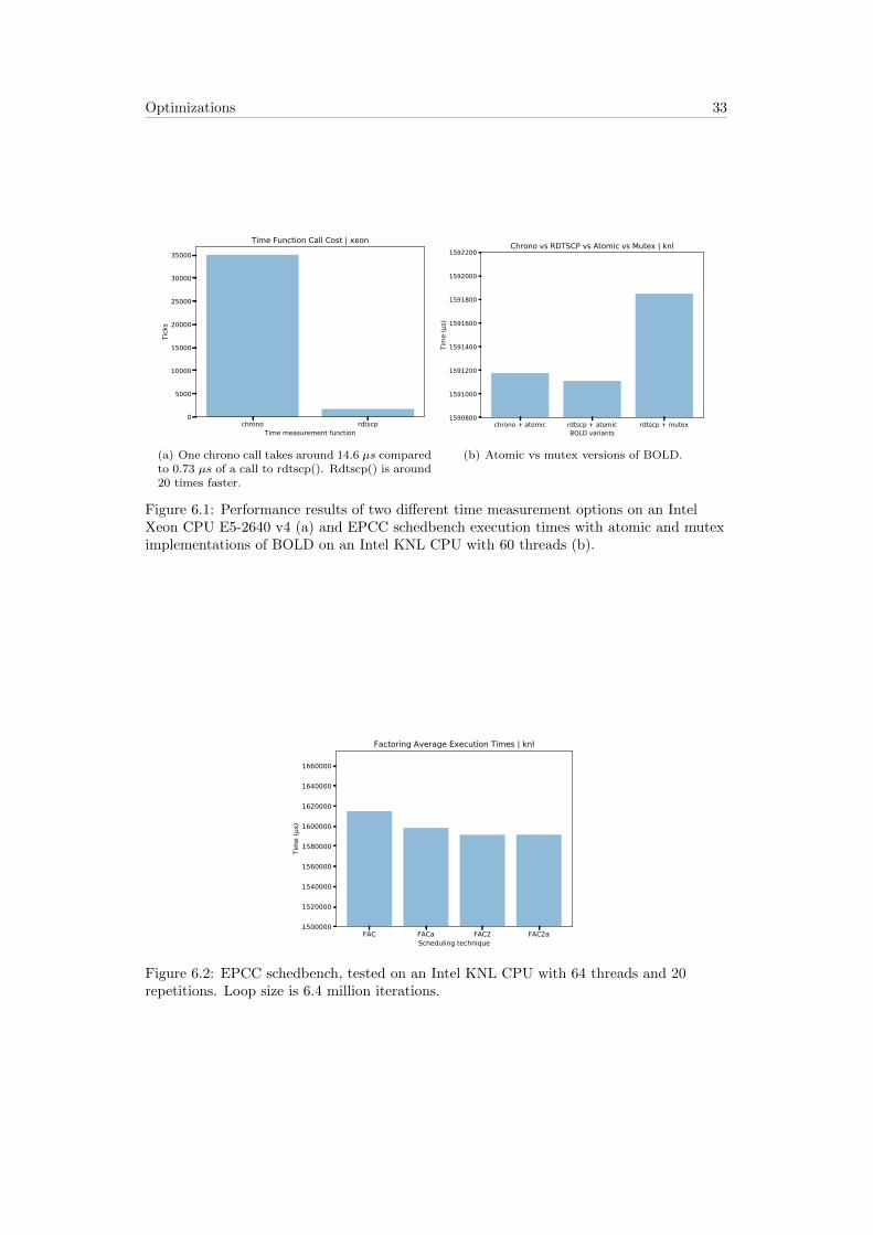
Optimizations 33
chrono rdtscpTime measurement function
0
5000
10000
15000
20000
25000
30000
35000
Tick
s
Time Function Call Cost | xeon
(a) One chrono call takes around 14.6 µs comparedto 0.73 µs of a call to rdtscp(). Rdtscp() is around20 times faster.
chrono + atomic rdtscp + atomic rdtscp + mutexBOLD variants
1590800
1591000
1591200
1591400
1591600
1591800
1592000
1592200
Tim
e (
s)
Chrono vs RDTSCP vs Atomic vs Mutex | knl
(b) Atomic vs mutex versions of BOLD.
Figure 6.1: Performance results of two different time measurement options on an IntelXeon CPU E5-2640 v4 (a) and EPCC schedbench execution times with atomic and muteximplementations of BOLD on an Intel KNL CPU with 60 threads (b).
FAC FACa FAC2 FAC2aScheduling technique
1500000
1520000
1540000
1560000
1580000
1600000
1620000
1640000
1660000
Tim
e (
s)
Factoring Average Execution Times | knl
Figure 6.2: EPCC schedbench, tested on an Intel KNL CPU with 64 threads and 20repetitions. Loop size is 6.4 million iterations.

7Validation
The implemented strategies from Chapter 5 must undergo a validation process to verify the
correctness of chunk size calculation. This can be done in different ways, such as comparing
the chunks with another, already verified implementation or a standalone tool that only
calculates the chunk sizes based on the proposed formulae. However, since the most reliable
source of a strategy is the original paper itself, we compare the produced chunks with
the expected ones that we calculate based on instructions from the according paper. The
following sections give more details on how the validation process works for nonadaptive
and adaptive strategies.
7.1 Nonadaptive TechniquesNonadaptive techniques are simpler to validate because the chunk sizes are calculated based
on formulae with fixed information and no adaptation to system state or other side effects
which could change the calculation. By printing out the scheduled chunk sizes and com-
paring these with the expected chunks based on the paper, you can verify that the strategy
itself is correct. An example can be given for FAC2 below. It shows the expected and
experimented chunks when using a loop with 128 iterations and 4 threads. The expected
chunks are calculated with the FAC2 formula from 2.2.2.5. The experimented results can
have different orders of chunks due to PUs being slower or faster and the chunks being
scheduled dynamically. However, the chunks should appear with the same size and amount
as in the expected case and the total number of iterations must be the same.
# Iterations in this loop: 128
# Threads: 4
Expected chunk sizes (formula 2.7):
Each batch has P = 4 chunks of the same size calculated by R/(2*P)
↪→ .
The rule is, that there are P chunks of the same size,
and each batch’ size is divided by 2.

Validation 35
-------------- Expected --------------
Something similar to the following should happen:
[B 1] [B 2] .........[B 6]
Thread 0: My chunks were: [16] [8] [4] [2] [1] [1] . Sum = 32.
Thread 1: My chunks were: [16] [8] [4] [2] [1] [1] . Sum = 32.
Thread 2: My chunks were: [16] [8] [4] [2] [1] [1] . Sum = 32.
Thread 3: My chunks were: [16] [8] [4] [2] [1] [1] . Sum = 32.
------------ Experimented ------------
Thread 3: My chunks were: [16] [8] [4] [2] [1] [1] . Sum = 32.
Thread 2: My chunks were: [16] [8] [4] [2] [2] [1] . Sum = 33.
Thread 0: My chunks were: [16] [8] [4] [1] [1] [1] . Sum = 31.
Thread 1: My chunks were: [16] [8] [4] [2] [1] [1] . Sum = 32.
7.2 Adaptive TechniquesAs with nonadaptive techniques, the adaptive ones are validated similarly but the process is
more complex. The chunk sizes are not only calculated with fixed formulae and constants but
a few variables can change during runtime. To overcome this issue, we decided to print out
every state information during runtime, i.e. the adapted variables and time measurements,
and use this data to manually calculate the expected result, again, with the help of the paper
itself. When the experimented chunks coincide with the expected result, the validation
succeeds.

8Experiments
Here, the results of this thesis are presented. Starting with the used system, a short discus-
sion about scheduling overhead and compiler versus runtime performance tests, continuing
with an overview of all the used benchmark applications, the design of experiments and, fi-
nally, concluding with benchmark suites and their results thereafter. The goal of this chapter
is to show how the newly implemented techniques perform compared to the available schedul-
ing strategies. Many different benchmarks are picked to give a broad view of application
and loop characteristics. It is expected that with irregular loops and/or system variances,
strategies with better load balancing outperform techniques like static or FSC. One more
interesting thing is to see if there are strategies that can perform well in every application,
or polarizing ones, that either perform the best in some benchmarks and the worst in others.
8.1 The SystemFor every test and benchmark run, the miniHPC cluster of the University of Basel was used.
It consists of 22 dual socket Intel Xeon CPUs and 4 Intel Xeon Phi Knights Landing (KNL)
CPUs. The detailed specifications can be seen in Table 8.1.
Table 8.1: System specifications of miniHPC cluster.
Intel R© Xeon R© Processor E5-2640 v4 [45]
Intel R© Xeon PhiTM Processor7210 [46]
Node count 22 (44 CPUs) 4CPU speed (GHz) 2.4 1.3Cores / CPU 10 64Threads / CPU 20 256RAM (GB) 64 128Cache (MB) L3: 25 L2: 32
All C/C++/Fortran applications and libomp are compiled with Intel Compiler 19.0.

Experiments 37
8.2 Scheduling Overhead and Compiler vs RuntimeEach strategy has its own scheduling overhead depending on the complexity of the used
algorithm. To gain more insight in scheduling overhead of the implemented strategies, one
can use the EPCC schedbench application [8] which measures the overhead of a parallel
run compared to a reference run without parallel execution, thus, no loop scheduling at all.
Figure 8.1(a) depicts the measured execution times of all scheduling techniques where the
orange bar illustrates the overhead compared to a reference serial execution. As expected,
dynamic (or SS) with chunk size 1 produces the most scheduling overhead. AF does produce
the seconds most overhead while all other remain similar.
stat
icdy
nam
icdy
nam
ic,64
guid
edtra
pezo
idal fsc tap fac
faca
fac2
fac2
a wfbo
ldaw
f_baw
f_caw
f_daw
f_e afaf
_a
Scheduling technique
0
2000
4000
6000
8000
10000
12000
14000
16000
Tim
e (
s)
EPCC Schedbench Overhead Measurement | xeon | pin1AVGOverhead
(a) EPCC Scheduling overhead
stat
ic
dyna
mic
dyna
mic,
64
guid
ed
Scheduling technique
0
2000
4000
6000
8000
10000
12000
Tim
e (
s)
EPCC Schedbench Compiler vs Runtime | xeon | pin1CompilerRuntime
(b) EPCC compiler vs runtime
Figure 8.1: EPCC schedbench results tested on Xeon node with 20 threads, 50 repetitions,2000 microseconds test time and 1 microsecond delay time.
Figure 8.1(b) shows the difference of using the OpenMP parallel directive with
schedule(static|dynamic|guided) and schedule(runtime). The call to the run-
time requires the environment variable to be read and could produce more overhead. How-
ever, the results show that no big changes are expected. In all the following experiments,
the scheduling technique is always selected with the environment variable.
8.3 The BenchmarksTo assess all the implemented techniques, 5 different benchmark suites and a total of 24
applications were selected, analyzed, prepared and tested on the miniHPC cluster. The
applications stem from various scientific domains, such as molecular dynamics, physics, n-
body simulations, math and weather prediction. To have a better overview, all applications
and relevant information can be seen in Table 8.3.

Exp
erimen
ts38
Table 8.3: The tested benchmark suites and applications.
Suite App Language Domain Used Parallelism # of parallel loops withschedule(runtime)
# of runs
NAS 3.4
BTFortran Math
OpenMP
3
30
CG 1FT 4IS C Bucket Sort 2LU
Fortran Math
5MG 1SP 3EP 1
CORAL Lulesh C Hydrodynamics 3CORAL2 Quicksilver C++ Monte Carlo transport
simulationsOpenMP, MPI +OpenMP (4 nodes)
1
N/ASphynx Fortran Smoothed Particle
Hydrodynamics (SPH)MPI + OpenMP (4nodes)
1- SPH-EXA C++ 2
SPEC OMP 2012
350mdFortran
Molecular Dynamics
OpenMP
9351bwaves Computational Fluid
Dynamics3
352nab C Molecular Modeling 5360ilbdc
FortranLattic Boltzmann 5
362fma3d Mechanical ResponseSimulation
1
363swim Weather Prediction 3
Rodinialud
C
Linear Algebra 1lavaMD Molecular Dynamics 1
OmpSCRcmandel Math 1md Molecular Dynamics 1
N/AMANDELBROT Math 1AC Adjoint Convolution 1

Experiments 39
8.4 Design of ExperimentsAll applications were tested on the miniHPC cluster with 30 repetitions. Multithreading
was always deactivated. For every Xeon test, 20 threads were used and 64 threads for KNL
respectively. To prepare the applications to be tested, they were first traced with a tool
called Score-P [47]. With these traces and the help of a visualization tool, Vampir, you
can find the most time consuming parallel loops inside the application. It is crucial to use
the DLS techniques only for the heaviest loops, otherwise, you will produce more overhead
than accelerating the application. After having found the biggest loops, they were modified
in the source files by using the clause schedule(runtime) to make sure our new imple-
mentations are called. Some of the strategies require profiling information which must be
obtained prior to the tests. For this, we have implemented a special technique itself called
profiling that schedules single iterations and measures their mean and standard deviation of
execution times. This must be done for both CPU types (Xeon and KNL) separately. After
all these preparations, the application can be tested. To guarantee that each repetition
is performed on a clean and fresh node, a Slurm [48] job script was used that submitted
each benchmark job separately to an available node. With 26 total apps (including hybrid
versions and different input sizes for certain apps), 3 pinning strategies for Xeon and 1 for
KNL, 19 scheduling techniques and 30 repetitions, a total of 44460 individual jobs were
executed on Xeon nodes and 14820 on KNL.
8.4.1 Pinning StrategyMost of the applications were tested with 3 different pinning strategies. OpenMP provides
the environment variables OMP PROC BIND and OMP PLACES which can be used to enable
custom pinning strategies. Our first pinning strategy makes sure that the threads are not
allowed to change cores and produces an equal thread-to-core alignment with 1 thread per
core. Pinning 2 uses unequal and non-fixed binding. It binds the first half of threads
(incremental thread id) to a set of the first 1/4 cores (double-loaded). The remaining half of
threads is assigned to a set of the second half of cores (single-loaded). The binding within
a set is not further defined and may change. Pinning 3 uses fixed thread-to-core binding
like pinning 1 but with unequal balance like pinning 2. More precisely, a core can have 1
to 4 threads pinned to it. In this chapter, only results with pinning 1 and 3 are shown, the
second pinning strategy can be seen in Appendix A. The idea of overloaded CPU cores is
to analyze the weighted and adaptive techniques whether they can improve performance or
not. Appropriate weights must be set in the environment variable KMP WEIGHTS to be used
in WF. If a core has two threads on it, the weight is set to 0.5, if there are four threads, the
weight is 0.25, etc. Table 8.5 shows the details of each pinning strategy for Xeon tests and
which weights are used. Table 8.7 does the same for KNL tests. As for Xeon, Figure 8.2
contains an illustration of all three pinning strategies.
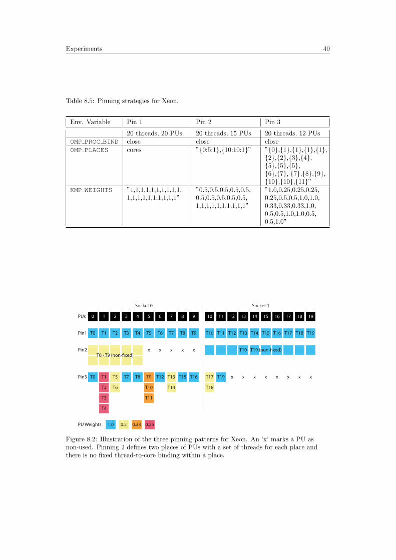
Experiments 40
Table 8.5: Pinning strategies for Xeon.
Env. Variable Pin 1 Pin 2 Pin 3
20 threads, 20 PUs 20 threads, 15 PUs 20 threads, 12 PUsOMP PROC BIND close close closeOMP PLACES cores ”{0:5:1},{10:10:1}” ”{0},{1},{1},{1},{1},
{2},{2},{3},{4},{5},{5},{5},{6},{7}, {7},{8},{9},{10},{10},{11}”
KMP WEIGHTS ”1,1,1,1,1,1,1,1,1,1,1,1,1,1,1,1,1,1,1,1”
”0.5,0.5,0.5,0.5,0.5,0.5,0.5,0.5,0.5,0.5,1,1,1,1,1,1,1,1,1,1”
”1.0,0.25,0.25,0.25,0.25,0.5,0.5,1.0,1.0,0.33,0.33,0.33,1.0,0.5,0.5,1.0,1.0,0.5,0.5,1.0”
Socket 0 Socket 1
Pin1
Pin2
Pin3
PUs 0 1 2 3 4 5 6 7 8 9 10 11 12 13 14 15 16 17 18 19
T0 T1 T2 T3 T4 T5 T6 T7 T8 T9 T10 T11 T12 T13 T14 T15 T16 T17 T18 T19
PU Weights: 1.0 0.5 0.33 0.25
x x x x xT0 - T9 (non-�xed)
T10 - T19 (non-�xed)
T0 T1
T2
T3
T4
T5
T6
T7 T8 T9
T10
T11
T12 T13
T14
T15 T16 T17
T18
T19 x x x x x x x x
Figure 8.2: Illustration of the three pinning patterns for Xeon. An ’x’ marks a PU asnon-used. Pinning 2 defines two places of PUs with a set of threads for each place andthere is no fixed thread-to-core binding within a place.
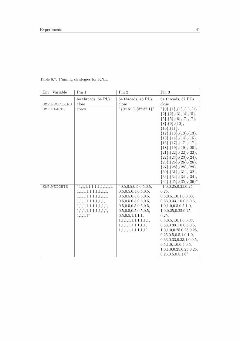
Experiments 41
Table 8.7: Pinning strategies for KNL.
Env. Variable Pin 1 Pin 2 Pin 3
64 threads, 64 PUs 64 threads, 48 PUs 64 threads, 37 PUsOMP PROC BIND close close closeOMP PLACES cores ”{0:16:1},{32:32:1}” ”{0},{1},{1},{1},{1},
{2},{2},{3},{4},{5},{5},{5},{6},{7},{7},{8},{9},{10},{10},{11},{12},{13},{13},{13},{13},{14},{14},{15},{16},{17},{17},{17},{18},{19},{19},{20},{21},{22},{22},{22},{22},{23},{23},{24},{25},{26},{26},{26},{27},{28},{28},{29},{30},{31},{31},{32},{33},{34},{34},{34},{34},{35},{35},{36}”
KMP WEIGHTS ”1,1,1,1,1,1,1,1,1,1,1,1,1,1,1,1,1,1,1,1,1,1,1,1,1,1,1,1,1,1,1,1,1,1,1,1,1,1,1,1,1,1,1,1,1,1,1,1,1,1,1,1,1,1,1,1,1,1,1,1,1,1,1,1”
”0.5,0.5,0.5,0.5,0.5,0.5,0.5,0.5,0.5,0.5,0.5,0.5,0.5,0.5,0.5,0.5,0.5,0.5,0.5,0.5,0.5,0.5,0.5,0.5,0.5,0.5,0.5,0.5,0.5,0.5,0.5,0.5,1,1,1,1,1,1,1,1,1,1,1,1,1,1,1,1,1,1,1,1,1,1,1,1,1,1,1,1,1,1,1,1”
”1.0,0.25,0.25,0.25,0.25,0.5,0.5,1.0,1.0,0.33,0.33,0.33,1.0,0.5,0.5,1.0,1.0,0.5,0.5,1.0,1.0,0.25,0.25,0.25,0.25,0.5,0.5,1.0,1.0,0.33,0.33,0.33,1.0,0.5,0.5,1.0,1.0,0.25,0.25,0.25,0.25,0.5,0.5,1.0,1.0,0.33,0.33,0.33,1.0,0.5,0.5,1.0,1.0,0.5,0.5,1.0,1.0,0.25,0.25,0.25,0.25,0.5,0.5,1.0”
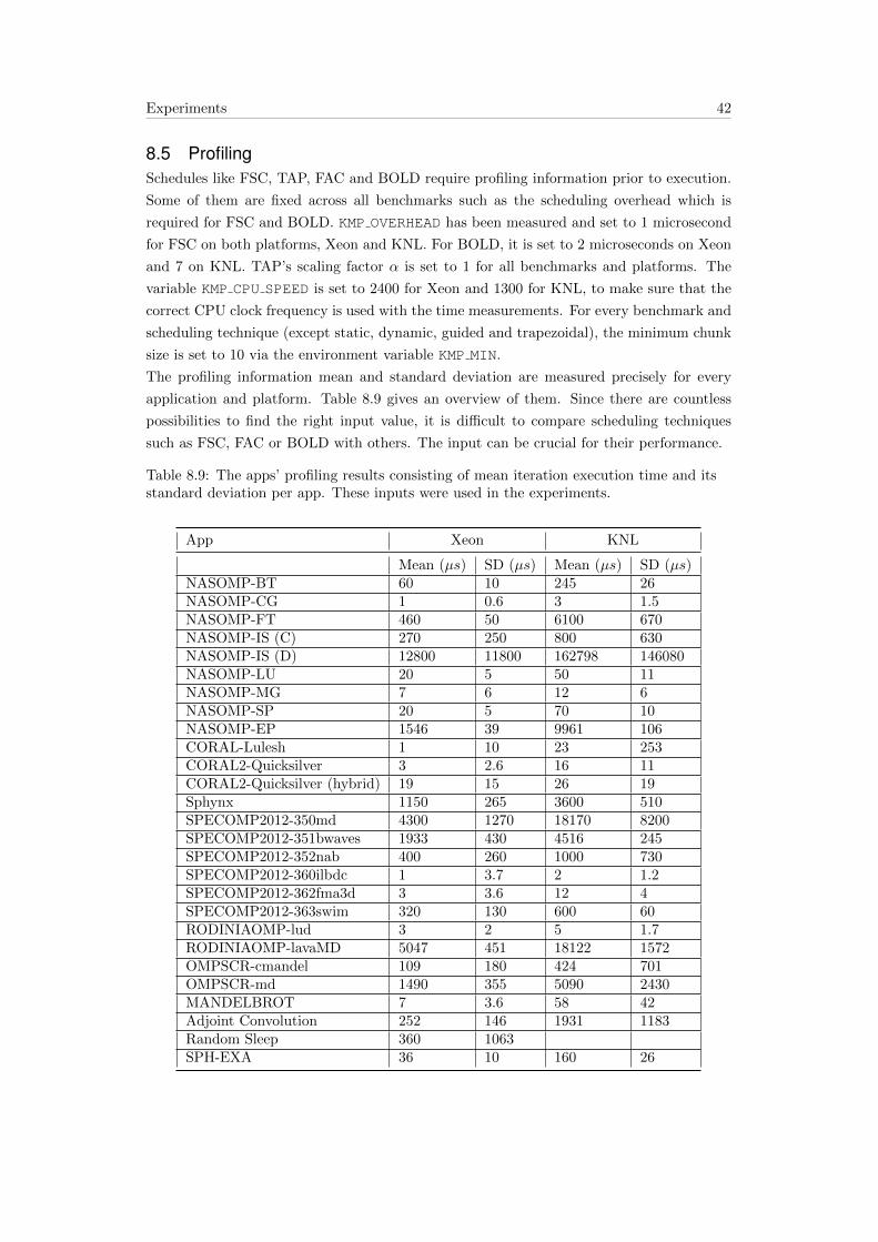
Experiments 42
8.5 ProfilingSchedules like FSC, TAP, FAC and BOLD require profiling information prior to execution.
Some of them are fixed across all benchmarks such as the scheduling overhead which is
required for FSC and BOLD. KMP OVERHEAD has been measured and set to 1 microsecond
for FSC on both platforms, Xeon and KNL. For BOLD, it is set to 2 microseconds on Xeon
and 7 on KNL. TAP’s scaling factor α is set to 1 for all benchmarks and platforms. The
variable KMP CPU SPEED is set to 2400 for Xeon and 1300 for KNL, to make sure that the
correct CPU clock frequency is used with the time measurements. For every benchmark and
scheduling technique (except static, dynamic, guided and trapezoidal), the minimum chunk
size is set to 10 via the environment variable KMP MIN.
The profiling information mean and standard deviation are measured precisely for every
application and platform. Table 8.9 gives an overview of them. Since there are countless
possibilities to find the right input value, it is difficult to compare scheduling techniques
such as FSC, FAC or BOLD with others. The input can be crucial for their performance.
Table 8.9: The apps’ profiling results consisting of mean iteration execution time and itsstandard deviation per app. These inputs were used in the experiments.
App Xeon KNL
Mean (µs) SD (µs) Mean (µs) SD (µs)NASOMP-BT 60 10 245 26NASOMP-CG 1 0.6 3 1.5NASOMP-FT 460 50 6100 670NASOMP-IS (C) 270 250 800 630NASOMP-IS (D) 12800 11800 162798 146080NASOMP-LU 20 5 50 11NASOMP-MG 7 6 12 6NASOMP-SP 20 5 70 10NASOMP-EP 1546 39 9961 106CORAL-Lulesh 1 10 23 253CORAL2-Quicksilver 3 2.6 16 11CORAL2-Quicksilver (hybrid) 19 15 26 19Sphynx 1150 265 3600 510SPECOMP2012-350md 4300 1270 18170 8200SPECOMP2012-351bwaves 1933 430 4516 245SPECOMP2012-352nab 400 260 1000 730SPECOMP2012-360ilbdc 1 3.7 2 1.2SPECOMP2012-362fma3d 3 3.6 12 4SPECOMP2012-363swim 320 130 600 60RODINIAOMP-lud 3 2 5 1.7RODINIAOMP-lavaMD 5047 451 18122 1572OMPSCR-cmandel 109 180 424 701OMPSCR-md 1490 355 5090 2430MANDELBROT 7 3.6 58 42Adjoint Convolution 252 146 1931 1183Random Sleep 360 1063SPH-EXA 36 10 160 26

Experiments 43
8.6 NAS Parallel BenchmarksThe first set of applications that are tested in this thesis come from the NAS Parallel
Benchmarks 3.4 [11]. We have tested 8 applications out of this suite. The modifications and
details are listed in Table 8.11.
Table 8.11: NAS Parallel Benchmarks details.
App Size Modified loop file/line Description
BT C x solve.f/49, y solve/49, z solve/49 Solve a synthetic system of nonlin-ear PDEs using block tridiagonalkernel.
CG C cg.f/517 Estimate the smallest eigenvalue ofa large sparse symmetric positive-definite matrix using the inverse it-eration with the conjugate gradientmethod as a subroutine for solvingsystems of linear equations.
FT C ft.f/170, ft.f/205, ft.f/524, ft.f/570 Solve a three-dimensional partialdifferential equation (PDE) usingthe fast Fourier transform (FFT).
IS C, D is.c/544, is.c/707 Sort small integers using the bucketsort.
LU C ssor.f/103, ssor.f/135, rhs.f/63,rhs.f/189, rhs.f/345
Solve a synthetic system of nonlin-ear PDEs using symmetric succes-sive over-relaxation (SSOR) solverkernel.
MG C mg.f/606 Approximate the solution to athree-dimensional discrete Poissonequation using the V-cycle multi-grid method.
SP C x solve.f/30, y solve.f/30,z solve.f/35
Solve a synthetic system of nonlin-ear PDEs using scalar pentadiago-nal kernel.
EP C ep.f/166 Generate independent Gaus-sian random variates using theMarsaglia polar method.
When looking at the results with pin1 strategy, the first clear thing is that depending on the
application and loop characteristics, one technique can be good or bad. There is no superior
strategy for every case. As an example, dynamic can perform worse than all others such as
in Figure 8.3(a) but may also be the best in NAS IS as depicted in Figure 8.4(c). However,
one can say that very load-balanced techniques such as dynamic or FAC2 and AWF variants
perform better with irregular loops. The opposite is with regular loops which have almost
no variance in iteration times, where static outperforms every other strategy. This behavior
can be seen in NAS CG, depicted in 8.3(c), or MG in Figure 8.6(a). The variance of a
loop, however, does not decide alone whether dynamic or static should be chosen. It also
depends on the system, number of iterations, their mean execution time and data locality
demands. Just by running the same applications CG and MG on the KNL platform with 64

Experiments 44
74
75
NAS-BT-C | xeon | pin1MeanSD
stat
icdy
nam
icdy
nam
ic,64
guid
edtra
pezo
idal fsc tap fac
faca
fac2
fac2
a wfbo
ldaw
f_baw
f_caw
f_daw
f_e afaf
_a
Scheduling technique
54
56
58
Tim
e (s
)
(a) Xeon Pin 1
194
196
198
200NAS-BT-C | xeon | pin3
MeanSD
stat
icdy
nam
icdy
nam
ic,64
guid
edtra
pezo
idal fsc tap fac
faca
fac2
fac2
a wfbo
ldaw
f_baw
f_caw
f_daw
f_e afaf
_a
Scheduling technique
120
140
160
180Tim
e (s
)
(b) Xeon Pin 3
stat
icdy
nam
icdy
nam
ic,64
guid
edtra
pezo
idal fsc tap fac
faca
fac2
fac2
a wfbo
ldaw
f_baw
f_caw
f_daw
f_e afaf
_a
Scheduling technique
18
20
22
24
26
28
NAS-CG-C | xeon | pin1MeanSD
Tim
e (s
)
(c) Xeon Pin 1
stat
icdy
nam
icdy
nam
ic,64
guid
edtra
pezo
idal fsc tap fac
faca
fac2
fac2
a wfbo
ldaw
f_baw
f_caw
f_daw
f_e afaf
_a
Scheduling technique
80
90
100
110
120
130
140NAS-CG-C | xeon | pin3
MeanSD
Tim
e (s
)
(d) Xeon Pin 3
stat
icdy
nam
icdy
nam
ic,64
guid
edtra
pezo
idal fsc tap fac
faca
fac2
fac2
a wfbo
ldaw
f_baw
f_caw
f_daw
f_e afaf
_a
Scheduling technique
72
74
76
78
80
82
84
86
NAS-BT-C | knl | pin1MeanSD
Tim
e (s
)
(e) KNL Pin 1
200
400
600
NAS-CG-C | knl | pin1MeanSD
stat
icdy
nam
icdy
nam
ic,64
guid
edtra
pezo
idal fsc tap fac
faca
fac2
fac2
a wfbo
ldaw
f_baw
f_caw
f_daw
f_e afaf
_a
Scheduling technique
12.5
15.0
17.5
20.0
22.5Tim
e (s
)
(f) KNL Pin 1
Figure 8.3: NAS BT and CG Class-C results.
PUs instead of 20 (see Figures 8.3(f) and 8.6(e)), the performance of static falls behind and
is no longer the best. In the case of MG on KNL, the techniques FSC and FAC2 improve
the performance by 6.1 % compared to the fastest OpenMP strategy guided. This gives an
idea of how different systems require advanced or better-fitting strategies.

Experiments 45
stat
icdy
nam
icdy
nam
ic,64
guid
edtra
pezo
idal fsc tap fac
faca
fac2
fac2
a wfbo
ldaw
f_baw
f_caw
f_daw
f_e afaf
_a
Scheduling technique
0.950
0.975
1.000
1.025
1.050
1.075
1.100
1.125
1.150NAS-IS-C | xeon | pin1
MeanSD
Tim
e (s
)
(a) Xeon Pin 1
stat
icdy
nam
icdy
nam
ic,64
guid
edtra
pezo
idal fsc tap fac
faca
fac2
fac2
a wfbo
ldaw
f_baw
f_caw
f_daw
f_e afaf
_a
Scheduling technique
3.3
3.4
3.5
3.6
3.7
3.8
3.9
NAS-IS-C | xeon | pin3MeanSD
Tim
e (s
)
(b) Xeon Pin 3
44
45
46
NAS-IS-D | xeon | pin1MeanSD
stat
icdy
nam
icdy
nam
ic,64
guid
edtra
pezo
idal fsc tap fac
faca
fac2
fac2
a wfbo
ldaw
f_baw
f_caw
f_daw
f_e afaf
_a
Scheduling technique
30
32
34
36
38Tim
e (s
)
(c) Xeon Pin 1
stat
icdy
nam
icdy
nam
ic,64
guid
edtra
pezo
idal fsc tap fac
faca
fac2
fac2
a wfbo
ldaw
f_baw
f_caw
f_daw
f_e afaf
_a
Scheduling technique
100
110
120
130
140NAS-IS-D | xeon | pin3
MeanSD
Tim
e (s
)
(d) Xeon Pin 3
1.54
1.56
1.58
NAS-IS-C | knl | pin1MeanSD
stat
icdy
nam
icdy
nam
ic,64
guid
edtra
pezo
idal fsc tap fac
faca
fac2
fac2
a wfbo
ldaw
f_baw
f_caw
f_daw
f_e afaf
_a
Scheduling technique
0.60
0.65
0.70
0.75Tim
e (s
)
(e) KNL Pin 1
75
80
85
90
NAS-IS-D | knl | pin1MeanSD
stat
icdy
nam
icdy
nam
ic,64
guid
edtra
pezo
idal fsc tap fac
faca
fac2
fac2
a wfbo
ldaw
f_baw
f_caw
f_daw
f_e afaf
_a
Scheduling technique
25
30
35
40Tim
e (s
)
(f) KNL Pin 1
Figure 8.4: NAS IS Class-C and D results.
The picture is different when comparing pin3 strategy with pin1. Due to the cause of
overloaded PUs with more than one thread, a PU can perform worse if it is assigned chunks
from multiple threads simultaneously. The strategy static can lead to massive performance
loss in this case since it distributes equal-sized chunks to all PUs. Figures 8.7(a) and 8.7(b)

Experiments 46
stat
icdy
nam
icdy
nam
ic,64
guid
edtra
pezo
idal fsc tap fac
faca
fac2
fac2
a wfbo
ldaw
f_baw
f_caw
f_daw
f_e afaf
_a
Scheduling technique
12.5
13.0
13.5
14.0
14.5
15.0
15.5NAS-FT-C | xeon | pin1
MeanSD
Tim
e (s
)
(a) Xeon Pin 1
43
44
45
NAS-FT-C | xeon | pin3MeanSD
stat
icdy
nam
icdy
nam
ic,64
guid
edtra
pezo
idal fsc tap fac
faca
fac2
fac2
a wfbo
ldaw
f_baw
f_caw
f_daw
f_e afaf
_a
Scheduling technique
36
38
40
42
Tim
e (s
)
(b) Xeon Pin 3
50
51
52
53NAS-LU-C | xeon | pin1
MeanSD
stat
icdy
nam
icdy
nam
ic,64
guid
edtra
pezo
idal fsc tap fac
faca
fac2
fac2
a wfbo
ldaw
f_baw
f_caw
f_daw
f_e afaf
_a
Scheduling technique
38
40
42
44
Tim
e (s
)
(c) Xeon Pin 1
stat
icdy
nam
icdy
nam
ic,64
guid
edtra
pezo
idal fsc tap fac
faca
fac2
fac2
a wfbo
ldaw
f_baw
f_caw
f_daw
f_e afaf
_a
Scheduling technique
156
158
160
162
164
166
168
170NAS-LU-C | xeon | pin3
MeanSD
Tim
e (s
)
(d) Xeon Pin 3
stat
icdy
nam
icdy
nam
ic,64
guid
edtra
pezo
idal fsc tap fac
faca
fac2
fac2
a wfbo
ldaw
f_baw
f_caw
f_daw
f_e afaf
_a
Scheduling technique
40
45
50
55
60
NAS-FT-C | knl | pin1MeanSD
Tim
e (s
)
(e) KNL Pin 1
100
200
300
NAS-LU-C | knl | pin1MeanSD
stat
icdy
nam
icdy
nam
ic,64
guid
edtra
pezo
idal fsc tap fac
faca
fac2
fac2
a wfbo
ldaw
f_baw
f_caw
f_daw
f_e afaf
_a
Scheduling technique
65
66
Tim
e (s
)
(f) KNL Pin 1
Figure 8.5: NAS FT and LU Class-C results.
illustrate this phenomena very well, where static performs bad in combination with pin3
strategy. At the same time, WF can show an improvement of almost 20% compared to
FAC2 and FAC2a, which are the same strategy but without the weights. Nearly in every

Experiments 47
stat
icdy
nam
icdy
nam
ic,64
guid
edtra
pezo
idal fsc tap fac
faca
fac2
fac2
a wfbo
ldaw
f_baw
f_caw
f_daw
f_e afaf
_a
Scheduling technique
5.0
5.5
6.0
6.5
7.0
7.5
8.0
8.5
9.0
NAS-MG-C | xeon | pin1MeanSD
Tim
e (s
)
(a) Xeon Pin 1
stat
icdy
nam
icdy
nam
ic,64
guid
edtra
pezo
idal fsc tap fac
faca
fac2
fac2
a wfbo
ldaw
f_baw
f_caw
f_daw
f_e afaf
_a
Scheduling technique
15
16
17
18
19
20
NAS-MG-C | xeon | pin3MeanSD
Tim
e (s
)
(b) Xeon Pin 3
72
74
76
NAS-SP-C | xeon | pin1MeanSD
stat
icdy
nam
icdy
nam
ic,64
guid
edtra
pezo
idal fsc tap fac
faca
fac2
fac2
a wfbo
ldaw
f_baw
f_caw
f_daw
f_e afaf
_a
Scheduling technique
42.5
45.0
47.5
50.0Tim
e (s
)
(c) Xeon Pin 1
stat
icdy
nam
icdy
nam
ic,64
guid
edtra
pezo
idal fsc tap fac
faca
fac2
fac2
a wfbo
ldaw
f_baw
f_caw
f_daw
f_e afaf
_a
Scheduling technique
130
140
150
160
170
180
NAS-SP-C | xeon | pin3MeanSD
Tim
e (s
)
(d) Xeon Pin 3
20
30
40
50NAS-MG-C | knl | pin1
MeanSD
stat
icdy
nam
icdy
nam
ic,64
guid
edtra
pezo
idal fsc tap fac
faca
fac2
fac2
a wfbo
ldaw
f_baw
f_caw
f_daw
f_e afaf
_a
Scheduling technique
6.0
6.5
7.0
7.5Tim
e (s
)
(e) KNL Pin 1
200
400
600NAS-SP-C | knl | pin1
MeanSD
stat
icdy
nam
icdy
nam
ic,64
guid
edtra
pezo
idal fsc tap fac
faca
fac2
fac2
a wfbo
ldaw
f_baw
f_caw
f_daw
f_e afaf
_a
Scheduling technique
56
58
60
Tim
e (s
)
(f) KNL Pin 1
Figure 8.6: NAS MG and SP Class-C results.
pin3 case, WF is faster than its FAC2 counterpart. This shows us, that weighted strategies
can improve systemic load imbalance or heterogeneous PUs. Same accounts for the adaptive
techniques AWF and AF which perform often better than static or dynamic, as depicted in
8.3(b) or 8.5(b). Pin3 strategy does not perfectly simulate this case but it gives an idea of
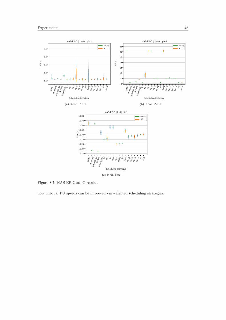
Experiments 48
stat
icdy
nam
icdy
nam
ic,64
guid
edtra
pezo
idal fsc tap fac
faca
fac2
fac2
a wfbo
ldaw
f_baw
f_caw
f_daw
f_e afaf
_a
Scheduling technique
5.0
5.5
6.0
6.5
7.0
NAS-EP-C | xeon | pin1MeanSD
Tim
e (s
)
(a) Xeon Pin 1
stat
icdy
nam
icdy
nam
ic,64
guid
edtra
pezo
idal fsc tap fac
faca
fac2
fac2
a wfbo
ldaw
f_baw
f_caw
f_daw
f_e afaf
_a
Scheduling technique
8
10
12
14
16
18
20
22
NAS-EP-C | xeon | pin3MeanSD
Tim
e (s
)
(b) Xeon Pin 3
stat
icdy
nam
icdy
nam
ic,64
guid
edtra
pezo
idal fsc tap fac
faca
fac2
fac2
a wfbo
ldaw
f_baw
f_caw
f_daw
f_e afaf
_a
Scheduling technique
10.22
10.24
10.26
10.28
10.30
10.32
10.34
10.36
10.38NAS-EP-C | knl | pin1
MeanSD
Tim
e (s
)
(c) KNL Pin 1
Figure 8.7: NAS EP Class-C results.
how unequal PU speeds can be improved via weighted scheduling strategies.

Experiments 49
8.7 CORAL BenchmarksThe second set of tests stem from the CORAL and CORAL2 suites [49]. Two applications,
Lulesh and Quicksilver, were chosen and, this time, a combination of MPI + OpenMP tests
are done. Table 8.13 contains the selected applications and how they have been modified.
Table 8.13: CORAL Benchmarks details.
App Size Modified loop file/line Description
Lulesh 60 lulesh.cc/810,lulesh.cc/1037,lulesh.cc/1538
Shock hydrodynam-ics for unstructuredmeshes. Fine-grainedloop level threading.
Quicksilver 100000000 particles(OpenMP only),10000000 particles(MPI + OpenMP)
mc omp parallel forschedule static.hh/4
Monte Carlo transportbenchmark with multi-group cross sectionlookups. Stressesmemory latency, sig-nificant branching,and one large kernelthat is 1000’s of linesbig.
Static does a great job in Lulesh, performing the best on both platforms. Dynamic is about
4 times slower than static in Figure 8.8(a). When looking at Lulesh’s profiling info in Table
8.9, the loop iterations definitely show execution time variance but the mean execution time
is only 1 microsecond which could cause rather high overhead when scheduling individual
and very small iterations, thus the bad performance with dynamic. But the other dynamic
techniques, such as TAP, FAC, FAC2 or AWF are similarly fast as static which is a good
mix of balance between load balance and scheduling overhead even when dealing with very
short iterations. Quicksilver, on the other hand, does not really show a favorite scheduling
technique, except for the non-hybrid version, see Figure 8.9(a), where dynamic is again the
worst performer. One interesting thing here is again WF being the fastest with pin3 strategy
that can be seen in Figure 8.9(d).

Experiments 50
stat
icdy
nam
icdy
nam
ic,64
guid
edtra
pezo
idal fsc tap fac
faca
fac2
fac2
a wfbo
ldaw
f_baw
f_caw
f_daw
f_e afaf
_a
Scheduling technique
60
80
100
120
140
160
180
200
CORAL-LULESH-60 | xeon | pin1MeanSD
Tim
e (s
)
(a) Xeon Pin 1
stat
icdy
nam
icdy
nam
ic,64
guid
edtra
pezo
idal fsc tap fac
faca
fac2
fac2
a wfbo
ldaw
f_baw
f_caw
f_daw
f_e afaf
_a
Scheduling technique
200
250
300
350
400
CORAL-LULESH-60 | xeon | pin3MeanSD
Tim
e (s
)
(b) Xeon Pin 3
1000
1500
2000
2500CORAL-LULESH-60 | knl | pin1
MeanSD
stat
icdy
nam
icdy
nam
ic,64
guid
edtra
pezo
idal fsc tap fac
faca
fac2
fac2
a wfbo
ldaw
f_baw
f_caw
f_daw
f_e afaf
_a
Scheduling technique
200
300
400
Tim
e (s
)
(c) KNL Pin 1
Figure 8.8: CORAL Lulesh results.

Experiments 51
stat
icdy
nam
icdy
nam
ic,64
guid
edtra
pezo
idal fsc tap fac
faca
fac2
fac2
a wfbo
ldaw
f_baw
f_caw
f_daw
f_e afaf
_aScheduling technique
540
560
580
600
620
640
660
680
CORAL2-QS-100M | xeon | pin1MeanSD
Tim
e (s
)
(a) Xeon Pin 1
stat
icdy
nam
icdy
nam
ic,64
guid
edtra
pezo
idal fsc tap fac
faca
fac2
fac2
a wfbo
ldaw
f_baw
f_caw
f_daw
f_e afaf
_a
Scheduling technique
400
600
800
1000
1200
1400
CORAL2-QS-100M | xeon | pin3MeanSD
Tim
e (s
)(b) Xeon Pin 3
stat
icdy
nam
icdy
nam
ic,64
guid
edtra
pezo
idal fsc tap fac
faca
fac2
fac2
a wfbo
ldaw
f_baw
f_caw
f_daw
f_e afaf
_a
Scheduling technique
88
90
92
94
96
98
100
102
104CORAL2-QS-4N-10M-HYBRID | xeon | pin1
MeanSD
Tim
e (s
)
(c) Xeon Pin 1
stat
icdy
nam
icdy
nam
ic,64
guid
edtra
pezo
idal fsc tap fac
faca
fac2
fac2
a wfbo
ldaw
f_baw
f_caw
f_daw
f_e afaf
_aScheduling technique
90
95
100
105
110
115
120
CORAL2-QS-4N-10M-HYBRID | xeon | pin3MeanSD
Tim
e (s
)
(d) Xeon Pin 3
stat
icdy
nam
icdy
nam
ic,64
guid
edtra
pezo
idal fsc tap fac
faca
fac2
fac2
a wfbo
ldaw
f_baw
f_caw
f_daw
f_e afaf
_a
Scheduling technique
700
750
800
850
900
950
1000
CORAL2-QS-100M | knl | pin1MeanSD
Tim
e (s
)
(e) KNL Pin 1
140
160
180
200CORAL2-QS-4N-10M-HYBRID | knl | pin1
MeanSD
stat
icdy
nam
icdy
nam
ic,64
guid
edtra
pezo
idal fsc tap fac
faca
fac2
fac2
a wfbo
ldaw
f_baw
f_caw
f_daw
f_e afaf
_a
Scheduling technique
115
120
125Tim
e (s
)
(f) KNL Pin 1
Figure 8.9: CORAL2 Quicksilver results. The hybrid version was tested on 4 nodes forboth CPU types.

Experiments 52
8.8 Sphynx and SPH-EXASphynx [50] and SPH-EXA [51] are two applications which are developed and maintained
at the University of Basel. The modifications and short descriptions can be seen in Table
8.15.
Table 8.15: SPH benchmarks details.
App Size Modified loop file/line Description
Sphynx 1000000 particles treewalkmodgrav mefec.f90/104
An accurate density-basedsmoothed particle hydro-dynamics (SPH) methodfor astrophysical applica-tions.
SPH-EXA -n 150 -s 5 -w -1 domain.hpp/40,MomentumEnergy-SqPatch.hpp/29
In this work an extensivestudy of three SPH im-plementations SPHYNX,ChaNGa, and XXX is per-formed, to gain insightsand to expose any limi-tations and characteristicsof the codes. These codesare the starting point of aninterdisciplinary co-designproject, SPH-EXA, forthe development of anExascale-ready SPH mini-app.
In both cases, Sphynx and SPH-EXA, the technique dynamic always is the worst with pin1
strategy. Especially in Sphynx on KNL, as depicted in Figure 8.10(e), it is very interesting
to see that defining the chunk size of dynamic can improve the performance from, by far, the
worst, to the best. This is once again a trial and error game to find the best fitting chunk
size, as much as finding the best input values for strategies like FSC or BOLD. Other than
that, all methods are similarly fast except for FAC being often slightly behind FAC2 and
FAC2a which might be caused by the mutual exclusion overhead or not the best profiling
information. Same accounts for BOLD that can suffer from bad profiling information.

Experiments 53
680
685
690
SPHYNX-4N-1M | xeon | pin1MeanSD
stat
icdy
nam
icdy
nam
ic,64
guid
edtra
pezo
idal fsc tap fac
faca
fac2
fac2
a wfbo
ldaw
f_baw
f_caw
f_daw
f_e afaf
_aScheduling technique
340
360
380Tim
e (s
)
(a) Xeon Pin 1
996
998
1000
1002
1004SPHYNX-4N-1M | xeon | pin3
MeanSD
stat
icdy
nam
icdy
nam
ic,64
guid
edtra
pezo
idal fsc tap fac
faca
fac2
fac2
a wfbo
ldaw
f_baw
f_caw
f_daw
f_e afaf
_a
Scheduling technique
600
700
800
Tim
e (s
)(b) Xeon Pin 3
100.0
100.5
101.0
101.5
102.0SPH-EXA-150-5S | xeon | pin1
MeanSD
stat
icdy
nam
icdy
nam
ic,64
guid
edtra
pezo
idal fsc tap fac
faca
fac2
fac2
a wfbo
ldaw
f_baw
f_caw
f_daw
f_e afaf
_a
Scheduling technique
84
86
88
90
Tim
e (s
)
(c) Xeon Pin 1
324
326
328
SPH-EXA-150-5S | xeon | pin3MeanSD
stat
icdy
nam
icdy
nam
ic,64
guid
edtra
pezo
idal fsc tap fac
faca
fac2
fac2
a wfbo
ldaw
f_baw
f_caw
f_daw
f_e afaf
_aScheduling technique
190
200
210
220
230Tim
e (s
)
(d) Xeon Pin 3
700750800850900
SPHYNX-4N-1M | knl | pin1MeanSD
stat
icdy
nam
icdy
nam
ic,64
guid
edtra
pezo
idal fsc tap fac
faca
fac2
fac2
a wfbo
ldaw
f_baw
f_caw
f_daw
f_e afaf
_a
Scheduling technique
570
580
590Tim
e (s
)
(e) KNL Pin 1
stat
icdy
nam
icdy
nam
ic,64
guid
edtra
pezo
idal fsc tap fac
faca
fac2
fac2
a wfbo
ldaw
f_baw
f_caw
f_daw
f_e afaf
_a
Scheduling technique
510
520
530
540
550
560
570
580
SPH-EXA-150-5S | knl | pin1MeanSD
Tim
e (s
)
(f) KNL Pin 1
Figure 8.10: Sphynx and SPH-EXA results. Sphynx was tested in hybrid mode (MPI +OpenMP) on 4 nodes for both CPU types.

Experiments 54
8.9 SPEC OMP 2012SPEC OMP 2012 [12] is a very popular benchmark suite used by many companies such as
Intel to benchmark their products. We have tested six applications from this suite with our
DLS implementation. Table 8.17 lists all use applications and their modified loops.
Table 8.17: SPEC OMP 2012 details.
App Size Modified loop file/line Description
350md ref int ion mix direct.f/84/41/132,int ion pure direct.f/85/42/142,int nn direct.f/117/55/186
Physics: Molecular Dynamics
351bwaves ref block solver.F/277,shell lam.F/260, jaco-bian lam.F/32
Physics: Computational FluidDynamics (CFD)
352nab ref eff.c/1992/2234/2948/2729/1732 Molecular Modeling360ilbdc ref mod relax.f90/52, ilbdc-
kernel.f90/149/ 169/178,mod benchgeo.f90/33
Lattic Boltzmann
362fma3d ref platq.f90/269 Mechanical Response Simulation363swim ref swim.f/421/334/276 Weather Prediction
In application md, performed on KNL nodes, FAC and FACa are the fastest, even faster than
their counterpart FAC2, that can be seen in Figure 8.11(b). Thinking of all the other results,
this is a rather surprising outcome since FAC and FACa often lie slightly behind FAC2. One
possible explanation could be the big number of 64 PUs a KNL processor comes with and
FAC’s batch size sharing nature among the threads which leads to less computation. When
looking at the exact same application on Xeon in Figure 8.11(a), it is no longer the case that
FAC is faster than FAC2. Xeon’s less crowded 20 PUs and higher core processing speeds
might not benefit that much from FAC’s batch size sharing. Nevertheless, the problem with
finding the best profiling information, which is required in FAC and FACa, could also be
just luckily chosen. This issue of schedules requiring input values makes comparisons a lot
harder. One of the highlights in SPEC can be found in nab in Figures 8.11(e) and 8.11(f)
where static and dynamic are overwhelmingly outperformed by schedules like guided, FSC,
FAC2, AWF variants and AF. Where static took almost 1000 seconds, FAC2 could finish in
under 750 seconds. With KNL, the difference is even higher.
Another interesting result is depicted in 8.12(f), in which dynamic is faster than any other
technique, which is rather a rare thing to observe. The same application on Xeon shows
a completely different picture where static is by far the fastest technique. This example
shows that not only the application itself but also the system can change the decision on
which technique should be considered. Finally, in swim, see Figure 8.12(e), it is very well
explainable that static is the fastest because when looking at this application’s iteration
times in Table 8.9, there is not much of variance compared to the mean execution time. In
the case of KNL the difference is even higher, thus static being the leader.

Experiments 55
2000
3000
SPECOMP2012-MD-REF | xeon | pin1MeanSD
stat
icdy
nam
icdy
nam
ic,64
guid
edtra
pezo
idal fsc tap fac
faca
fac2
fac2
a wfbo
ldaw
f_baw
f_caw
f_daw
f_e afaf
_aScheduling technique
680
700
720
740
760Tim
e (s
)
(a) Xeon Pin 1
2000
3000
4000
5000SPECOMP2012-MD-REF | knl | pin1
MeanSD
stat
icdy
nam
icdy
nam
ic,64
guid
edtra
pezo
idal fsc tap fac
faca
fac2
fac2
a wfbo
ldaw
f_baw
f_caw
f_daw
f_e afaf
_a
Scheduling technique
1260
1280
1300
Tim
e (s
)(b) KNL Pin 1
stat
icdy
nam
icdy
nam
ic,64
guid
edtra
pezo
idal fsc tap fac
faca
fac2
fac2
a wfbo
ldaw
f_baw
f_caw
f_daw
f_e afaf
_a
Scheduling technique
500
600
700
800
900
1000
1100SPECOMP2012-BWAVES-REF | xeon | pin1
MeanSD
Tim
e (s
)
(c) Xeon Pin 1
stat
icdy
nam
icdy
nam
ic,64
guid
edtra
pezo
idal fsc tap fac
faca
fac2
fac2
a wfbo
ldaw
f_baw
f_caw
f_daw
f_e afaf
_aScheduling technique
700
750
800
850
SPECOMP2012-BWAVES-REF | knl | pin1MeanSD
Tim
e (s
)
(d) KNL Pin 1
1000
1500
2000
SPECOMP2012-NAB-REF | xeon | pin1MeanSD
stat
icdy
nam
icdy
nam
ic,64
guid
edtra
pezo
idal fsc tap fac
faca
fac2
fac2
a wfbo
ldaw
f_baw
f_caw
f_daw
f_e afaf
_a
Scheduling technique
750
800
850Tim
e (s
)
(e) Xeon Pin 1
2000
2200
2400SPECOMP2012-NAB-REF | knl | pin1
MeanSD
stat
icdy
nam
icdy
nam
ic,64
guid
edtra
pezo
idal fsc tap fac
faca
fac2
fac2
a wfbo
ldaw
f_baw
f_caw
f_daw
f_e afaf
_a
Scheduling technique
1400
1500
1600
1700Tim
e (s
)
(f) KNL Pin 1
Figure 8.11: SPEC OMP 2012 350md, 351bwaves and 352nab results. These benchmarkswere performed with pinning strategy 1 only.

Experiments 56
9900
9950
10000
10050SPECOMP2012-ILBDC-REF | xeon | pin1
MeanSD
stat
icdy
nam
icdy
nam
ic,64
guid
edtra
pezo
idal fsc tap fac
faca
fac2
fac2
a wfbo
ldaw
f_baw
f_caw
f_daw
f_e afaf
_aScheduling technique
1000
1200
1400Tim
e (s
)
(a) Xeon Pin 1
10000
15000
20000
25000
SPECOMP2012-ILBDC-REF | knl | pin1MeanSD
stat
icdy
nam
icdy
nam
ic,64
guid
edtra
pezo
idal fsc tap fac
faca
fac2
fac2
a wfbo
ldaw
f_baw
f_caw
f_daw
f_e afaf
_a
Scheduling technique
600
625
650
675
700Tim
e (s
)(b) KNL Pin 1
900950
100010501100
SPECOMP2012-FMA3D-REF | xeon | pin1MeanSD
stat
icdy
nam
icdy
nam
ic,64
guid
edtra
pezo
idal fsc tap fac
faca
fac2
fac2
a wfbo
ldaw
f_baw
f_caw
f_daw
f_e afaf
_a
Scheduling technique
750
800
850
Tim
e (s
)
(c) Xeon Pin 1
1300
1400
1500
1600SPECOMP2012-FMA3D-REF | knl | pin1
MeanSD
stat
icdy
nam
icdy
nam
ic,64
guid
edtra
pezo
idal fsc tap fac
faca
fac2
fac2
a wfbo
ldaw
f_baw
f_caw
f_daw
f_e afaf
_aScheduling technique
1120
1140
1160
1180
Tim
e (s
)
(d) KNL Pin 1
stat
icdy
nam
icdy
nam
ic,64
guid
edtra
pezo
idal fsc tap fac
faca
fac2
fac2
a wfbo
ldaw
f_baw
f_caw
f_daw
f_e afaf
_a
Scheduling technique
600
700
800
900
1000
1100
1200
1300
SPECOMP2012-SWIM-REF | xeon | pin1MeanSD
Tim
e (s
)
(e) Xeon Pin 1
stat
icdy
nam
icdy
nam
ic,64
guid
edtra
pezo
idal fsc tap fac
faca
fac2
fac2
a wfbo
ldaw
f_baw
f_caw
f_daw
f_e afaf
_a
Scheduling technique
760
780
800
820
840
860
880SPECOMP2012-SWIM-REF | knl | pin1
MeanSD
Tim
e (s
)
(f) KNL Pin 1
Figure 8.12: SPEC OMP 2012 360ilbdc, 362fma3d and 363swim results. Thesebenchmarks were performed with pinning strategy 1 only.
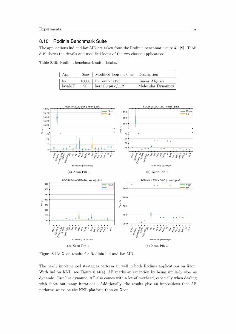
Experiments 57
8.10 Rodinia Benchmark SuiteThe applications lud and lavaMD are taken from the Rodinia benchmark suite 3.1 [9]. Table
8.19 shows the details and modified loops of the two chosen applications.
Table 8.19: Rodinia benchmark suite details.
App Size Modified loop file/line Description
lud 16000 lud omp.c/123 Linear AlgebralavaMD 90 kernel cpu.c/112 Molecular Dynamics
61.0061.2561.5061.7562.00
RODINIA-LUD-16K | xeon | pin1MeanSD
stat
icdy
nam
icdy
nam
ic,64
guid
edtra
pezo
idal fsc tap fac
faca
fac2
fac2
a wfbo
ldaw
f_baw
f_caw
f_daw
f_e afaf
_a
Scheduling technique
15
20
25
30Tim
e (s
)
(a) Xeon Pin 1
88.0
88.5
89.0
RODINIA-LUD-16K | xeon | pin3MeanSD
stat
icdy
nam
icdy
nam
ic,64
guid
edtra
pezo
idal fsc tap fac
faca
fac2
fac2
a wfbo
ldaw
f_baw
f_caw
f_daw
f_e afaf
_a
Scheduling technique
45
50
55
60Tim
e (s
)
(b) Xeon Pin 3
stat
icdy
nam
icdy
nam
ic,64
guid
edtra
pezo
idal fsc tap fac
faca
fac2
fac2
a wfbo
ldaw
f_baw
f_caw
f_daw
f_e afaf
_a
Scheduling technique
180
200
220
240
260
280
300
320RODINIA-LAVAMD-90 | xeon | pin1
MeanSD
Tim
e (s
)
(c) Xeon Pin 1
stat
icdy
nam
icdy
nam
ic,64
guid
edtra
pezo
idal fsc tap fac
faca
fac2
fac2
a wfbo
ldaw
f_baw
f_caw
f_daw
f_e afaf
_a
Scheduling technique
300
400
500
600
700
RODINIA-LAVAMD-90 | xeon | pin3MeanSD
Tim
e (s
)
(d) Xeon Pin 3
Figure 8.13: Xeon results for Rodinia lud and lavaMD.
The newly implemented strategies perform all well in both Rodinia applications on Xeon.
With lud on KNL, see Figure 8.14(a), AF marks an exception by being similarly slow as
dynamic. Just like dynamic, AF also comes with a lot of overhead, especially when dealing
with short but many iterations. Additionally, the results give an impressions that AF
performs worse on the KNL platform than on Xeon.
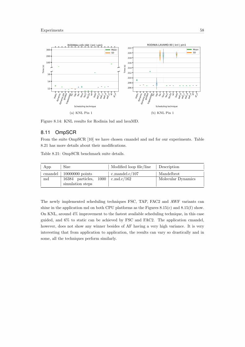
Experiments 58
100
200
300
RODINIA-LUD-16K | knl | pin1MeanSD
stat
icdy
nam
icdy
nam
ic,64
guid
edtra
pezo
idal fsc tap fac
faca
fac2
fac2
a wfbo
ldaw
f_baw
f_caw
f_daw
f_e afaf
_a
Scheduling technique
12
14
16
Tim
e (s
)
(a) KNL Pin 1
stat
icdy
nam
icdy
nam
ic,64
guid
edtra
pezo
idal fsc tap fac
faca
fac2
fac2
a wfbo
ldaw
f_baw
f_caw
f_daw
f_e afaf
_a
Scheduling technique
206
208
210
212
214
216
218
220
222RODINIA-LAVAMD-90 | knl | pin1
MeanSD
Tim
e (s
)
(b) KNL Pin 1
Figure 8.14: KNL results for Rodinia lud and lavaMD.
8.11 OmpSCRFrom the suite OmpSCR [10] we have chosen cmandel and md for our experiments. Table
8.21 has more details about their modifications.
Table 8.21: OmpSCR benchmark suite details.
App Size Modified loop file/line Description
cmandel 10000000 points c mandel.c/107 Mandelbrotmd 16384 particles, 1000
simulation stepsc md.c/162 Molecular Dynamics
The newly implemented scheduling techniques FSC, TAP, FAC2 and AWF variants can
shine in the application md on both CPU platforms as the Figures 8.15(c) and 8.15(f) show.
On KNL, around 4% improvement to the fastest available scheduling technique, in this case
guided, and 6% to static can be achieved by FSC and FAC2. The application cmandel,
however, does not show any winner besides of AF having a very high variance. It is very
interesting that from application to application, the results can vary so drastically and in
some, all the techniques perform similarly.
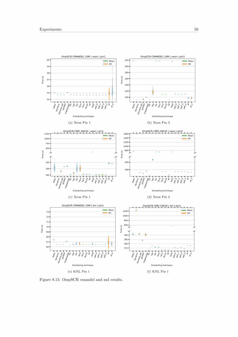
Experiments 59
stat
icdy
nam
icdy
nam
ic,64
guid
edtra
pezo
idal fsc tap fac
faca
fac2
fac2
a wfbo
ldaw
f_baw
f_caw
f_daw
f_e afaf
_a
Scheduling technique
54
55
56
57
58
59
60OmpSCR-CMANDEL-10M | xeon | pin1
MeanSD
Tim
e (s
)
(a) Xeon Pin 1
stat
icdy
nam
icdy
nam
ic,64
guid
edtra
pezo
idal fsc tap fac
faca
fac2
fac2
a wfbo
ldaw
f_baw
f_caw
f_daw
f_e afaf
_a
Scheduling technique
100
120
140
160
180
200
220OmpSCR-CMANDEL-10M | xeon | pin3
MeanSD
Tim
e (s
)(b) Xeon Pin 3
500
750
1000
1250OmpSCR-CMD-16K1K | xeon | pin1
MeanSD
stat
icdy
nam
icdy
nam
ic,64
guid
edtra
pezo
idal fsc tap fac
faca
fac2
fac2
a wfbo
ldaw
f_baw
f_caw
f_daw
f_e afaf
_a
Scheduling technique
185
190
195
Tim
e (s
)
(c) Xeon Pin 1
800
1000
1200
1400
1600OmpSCR-CMD-16K1K | xeon | pin3
MeanSD
stat
icdy
nam
icdy
nam
ic,64
guid
edtra
pezo
idal fsc tap fac
faca
fac2
fac2
a wfbo
ldaw
f_baw
f_caw
f_daw
f_e afaf
_aScheduling technique
400
500
Tim
e (s
)
(d) Xeon Pin 3
stat
icdy
nam
icdy
nam
ic,64
guid
edtra
pezo
idal fsc tap fac
faca
fac2
fac2
a wfbo
ldaw
f_baw
f_caw
f_daw
f_e afaf
_a
Scheduling technique
66
67
68
69
70
71
72
73
OmpSCR-CMANDEL-10M | knl | pin1MeanSD
Tim
e (s
)
(e) KNL Pin 1
600
800
1000
1200
OmpSCR-CMD-16K1K | knl | pin1MeanSD
stat
icdy
nam
icdy
nam
ic,64
guid
edtra
pezo
idal fsc tap fac
faca
fac2
fac2
a wfbo
ldaw
f_baw
f_caw
f_daw
f_e afaf
_a
Scheduling technique
375
380
385
390
Tim
e (s
)
(f) KNL Pin 1
Figure 8.15: OmpSCR cmandel and md results.

Experiments 60
8.12 Mandelbrot and Adjoint ConvolutionThe last two applications stem from a freely available source and are called MANDELBROT
[52] and AC [53]. Table 8.23 has more details about the two applications.
Table 8.23: MANDELBROT and AC details.
App Size Modified loop file/-line
Description
MANDELBROT -x pix 8000 -y pix8000
mb 1D collapsed.c/136
Mandelbrot
AC matrix size = 1000 ac.c/49 Adjoint Convolution
25
26
27
MANDELBROT-8K | xeon | pin1MeanSD
stat
icdy
nam
icdy
nam
ic,64
guid
edtra
pezo
idal fsc tap fac
faca
fac2
fac2
a wfbo
ldaw
f_baw
f_caw
f_daw
f_e afaf
_a
Scheduling technique
24.04
24.06
24.08
24.10Tim
e (s
)
(a) Xeon Pin 1
stat
icdy
nam
icdy
nam
ic,64
guid
edtra
pezo
idal fsc tap fac
faca
fac2
fac2
a wfbo
ldaw
f_baw
f_caw
f_daw
f_e afaf
_a
Scheduling technique
40
50
60
70
80
90
100
110MANDELBROT-8K | xeon | pin3
MeanSD
Tim
e (s
)
(b) Xeon Pin 3
24.0
24.5
25.0
25.5
26.0AC-8K | xeon | pin1
MeanSD
stat
icdy
nam
icdy
nam
ic,64
guid
edtra
pezo
idal fsc tap fac
faca
fac2
fac2
a wfbo
ldaw
f_baw
f_caw
f_daw
f_e afaf
_a
Scheduling technique
12.6
12.7
12.8
12.9
13.0Tim
e (s
)
(c) Xeon Pin 1
84.5084.7585.0085.2585.50
AC-8K | xeon | pin3MeanSD
stat
icdy
nam
icdy
nam
ic,64
guid
edtra
pezo
idal fsc tap fac
faca
fac2
fac2
a wfbo
ldaw
f_baw
f_caw
f_daw
f_e afaf
_a
Scheduling technique
20
25
30
35
40Tim
e (s
)
(d) Xeon Pin 3
Figure 8.16: Xeon results for MANDELBROT and AC.
The first thing to say about MANDELBROT and AC is that static is always a bad choice
in every case. These two applications really show that DLS techniques can’t be avoided
if performance demands are critical. In every pin1 case, the techniques FAC2 and AWF

Experiments 61
stat
icdy
nam
icdy
nam
ic,64
guid
edtra
pezo
idal fsc tap fac
faca
fac2
fac2
a wfbo
ldaw
f_baw
f_caw
f_daw
f_e afaf
_a
Scheduling technique
58
60
62
64
66
MANDELBROT-8K | knl | pin1MeanSD
Tim
e (s
)
(a) KNL Pin 1
stat
icdy
nam
icdy
nam
ic,64
guid
edtra
pezo
idal fsc tap fac
faca
fac2
fac2
a wfbo
ldaw
f_baw
f_caw
f_daw
f_e afaf
_a
Scheduling technique
30
40
50
60
70
AC-8K | knl | pin1MeanSD
Tim
e (s
)
(b) KNL Pin 1
Figure 8.17: KNL results for MANDELBROT and AC.
variants belong to the best performers. The same is true for guided. With pin3 strategy,
the technique WF is again faster than its non-weighted version FAC2.
8.13 Random SleepFor experiment reasons, a very small and synthetic application was written in this thesis
(see source in Appendix B) to give dynamic a better chance, showing its strength. This
application consists of a single parallel loop that contains 10000 iterations and is repeated
10 times. The loop simply lets a thread wait for a uniformly distributed random time
variable between 1 to 6000 microseconds for the first 10% of iterations. The remaining 90%
of iterations let the thread wait for 1 to 6 microseconds, thus, having a much higher variance
in the beginning of the loop. It is very interesting to see that, besides dynamic and AF, even
FSC can achieve a very good performance with the right input values. Guided, trapezoidal
and factoring techniques perform still twice as fast as static.
stat
icdy
nam
icdy
nam
ic,64
guid
edtra
pezo
idal fsc tap fac
faca
fac2
fac2
a wfbo
ldaw
f_baw
f_caw
f_daw
f_e afaf
_a
Scheduling technique
2
4
6
8
10
12
14
16RANDOM-SLEEP | xeon | pin1
MeanSD
Tim
e (s
)
Figure 8.18: Xeon results for Random Sleep with pin1 strategy.

9Conclusion and Future Work
We have implemented 11 new DLS techniques into libomp and tested them with 24 different
benchmark applications. We have shown that not one specific scheduling technique fits for
all cases. Depending on the chosen application and its loop characteristics, either static
methods or certain dynamic ones achieve the best performance. The available OpenMP
scheduling techniques, static, dynamic and guided do not reach the best performance in
every application and system. New systems with many, more complex and heterogeneous
processing units, could benefit from adaptive or weighted strategies. This thesis gives an
example with its implementation and wants to motivate future OpenMP versions to allow
and include new scheduling techniques.
The results have shown that every strategy has its strengths and weaknesses. In the case of
dynamic (or SS), it is almost never a good choice since it produces too much overhead. It
was one of the worst performers when looking at this thesis’ results. However, in irregular
applications with long iteration execution times, such as SPEC OMP 2012’s swim applica-
tion, and especially when ran on KNL with 64 PUs, dynamic could outperform every other
scheduling strategy. Irregular loop iteration times do not mean that dynamic is the best
choice since it also depends on the system, number of iterations, their mean execution times
and data locality demands. Very small iterations, but large in their amount, can produce
extreme overhead with dynamic as seen with Lulesh. Additionally, since threads pick single
iterations randomly, the effect of data locality is lost. By specifying the chunk size to 64 or
another desired size, you can reduce dynamic’s overhead and improve data locality within
a chunk.
When looking at the factoring methods, almost in all cases, FAC2 performed better than
FAC. This can be justified by the fact that FAC uses mutual exclusion in its scheduling
algorithm and it relies on good profiling info where FAC2 uses a less complex algorithm with
faster atomic function calls instead of mutual exclusion and there is no need for profiling
information. In general, FAC2 produced very good results across all applications and plat-
forms. One could say, if you don’t know what to choose, take FAC2. The adaptive weighted
factoring techniques have shown similar speeds as FAC2.
Two different pinning strategies were presented in this thesis, to test the weighted and
adaptive DLS techniques and how they interact with overloaded PUs. The results have

Conclusion and Future Work 63
shown that WF is almost always faster than its identical counterpart FAC2a but without
the weights. This shows that the weights can help to improve load balance when the system
has certain unequal PU speeds or other constant systemic load imbalance. AF could also
lead to better performance with overloaded PUs in pin3 strategy. With heterogeneous PUs
it could show even more of its adaptive strength. We could not measure a benefit of AWF
with pin3 strategy compared to FAC2 but if different PU speeds were available, this could
have given another picture.
Strategies like FSC, TAP, FAC and BOLD require profiling information which is a critical
part to make them work as intended. The results show that BOLD is often a bad performer
because of its bad input data. At the same time, FSC could outperform every technique,
even static, when using good input data. The process of finding them, however, is extremely
difficult and time consuming since the application must be profiled prior to runtime.
For the future, it would be interesting to see if scheduling techniques could be implemented
by the user itself and used by the compiler. There is ongoing work in this area, also called
User Defined Scheduling or UDS. By allowing the user providing these techniques, one could
take this thesis’ implementation and use it without the need of a compiler or runtime that
must implement it. Talking about compilers, one possible work could be to implement all
the DLS methods, provided by this thesis, into the compiler itself so that the technique can
be chosen as static or guided. Other work could be to make this implementation production
ready and push back into the official libomp repository to make it available for everyone.
For this, however, a few changes might be needed since this thesis did use a few components,
such as std::vector or std::mutex, from the C++ standard library. By resolving these depen-
dencies and using optimized functions provided by libomp itself, the compatibility would be
maintained. A very interesting topic would be to test this implementation on heterogeneous
systems with truly different processing unit speeds, not just an unbalanced pinning strat-
egy, and see what the weighted and adaptive techniques perform. The technique fractiling
was not implemented in this thesis due the expected high overhead in its work-stealing (or
borrowing) feature. Nevertheless, it would be interesting to see if fractiling can improve
performance with its data locality usage on shared memory systems. Finally, to tackle an
issue with multiple and different loops inside an application and the techniques that require
profiling information, it would be interesting to find a way of giving multiple input values,
one for each loop, that then can be used by the runtime for the particular loops. The libomp
version in this thesis does only allow profiling information for one single loop. Strategies
like FSC, FAC, TAP and BOLD could benefit from multiple input values.
Bibliography
[1] OpenMP Application Programming Interface, 5.0 edition (2018). The OpenMP 5.0
Specification.
[2] OpenMP Compilers and Tools (2018). URL https://www.openmp.org/resources/
openmp-compilers-tools/. Accessed: November 14, 2018.
[3] LLVM. LLVM OpenMP* Runtime Library . LLVM Project (2015). Describes the
interface provided by the LLVM OpenMP runtime library to the compiler.
[4] Libgomp, G. GNU Offloading and Multi Processing Runtime Library: The GNU
OpenMP and OpenACC Implementation. GNU (2015). The libgomp manual.
[5] Stallman, R. M. et al. Using the GNU compiler collection. Free Software Foundation,
4(02) (2003).
[6] Mattson, T. and Meadows, L. A ”Hands-on” Introduction to OpenMP (2008).
[7] LLVM. OpenMP R©: Support for the OpenMP language. https://openmp.llvm.org/
(2018). Accessed: November 04, 2018.
[8] Bull, J. M. Measuring Synchronisation and Scheduling Overheads in OpenMP. In
Proceedings of First European Workshop on OpenMP , pages 99–105 (1999).
[9] Che, S., Boyer, M., Meng, J., Tarjan, D., Sheaffer, J. W., Lee, S., and Skadron, K.
Rodinia: A benchmark suite for heterogeneous computing. In 2009 IEEE International
Symposium on Workload Characterization (IISWC), pages 44–54 (2009).
[10] Dorta, A. J., Rodriguez, C., and de Sande, F. The OpenMP source code repository.
In 13th Euromicro Conference on Parallel, Distributed and Network-Based Processing ,
pages 244–250 (2005).
[11] Bailey, D. H. NAS Parallel Benchmarks. In Padua, D., editor, Encyclopedia of Parallel
Computing , pages 1254–1259. Springer US, Boston, MA (2011).
[12] Aslot, V., Domeika, M., Eigenmann, R., Gaertner, G., Jones, W. B., and Parady, B.
SPEComp: A New Benchmark Suite for Measuring Parallel Computer Performance. In
Eigenmann, R. and Voss, M. J., editors, OpenMP Shared Memory Parallel Program-
ming , pages 1–10. Springer Berlin Heidelberg, Berlin, Heidelberg (2001).
[13] Banicescu, I. and Flynn Hummel, S. Balancing Processor Loads and Exploiting Data
Locality in N-body Simulations. In Proceedings of the 1995 ACM/IEEE Conference on
Supercomputing , Supercomputing ’95. ACM, New York, NY, USA (1995).
Bibliography 65
[14] Tang, P. and Yew, P. Processor self-scheduling for multiple-nested parallel loops. In
Hwang, K., Jacobs, S., and Swartzlander, E., editors, Proceedings of the International
Conference on Parallel Processing , pages 528–535. IEEE, Urbana, Illinois, USA (1986).
[15] Kruskal, C. P. and Weiss, A. Allocating Independent Subtasks on Parallel Processors.
IEEE Transactions on Software Engineering , SE-11(10):1001–1016 (1985).
[16] Polychronopoulos, C. D. and Kuck, D. J. Guided Self-Scheduling: A Practical
Scheduling Scheme for Parallel Supercomputers. IEEE Transactions on Computers,
C-36(12):1425–1439 (1987).
[17] Tzen, T. H. and Ni, L. M. Trapezoid self-scheduling: a practical scheduling scheme for
parallel compilers. IEEE Transactions on Parallel and Distributed Systems, 4(1):87–98
(1993).
[18] Hummel, S. F., Schonberg, E., and Flynn, L. E. Factoring: A Method for Scheduling
Parallel Loops. Commun. ACM , 35(8):90–101 (1992).
[19] Hummel, S. F., Schmidt, J., Uma, R. N., and Wein, J. Load-sharing in Heterogeneous
Systems via Weighted Factoring. In Proceedings of the Eighth Annual ACM Symposium
on Parallel Algorithms and Architectures, SPAA ’96, pages 318–328. ACM, New York,
NY, USA (1996).
[20] Lucco, S. A Dynamic Scheduling Method for Irregular Parallel Programs. In Proceed-
ings of the ACM SIGPLAN 1992 Conference on Programming Language Design and
Implementation, PLDI ’92, pages 200–211. ACM, New York, NY, USA (1992).
[21] Banicescu, I. Load Balancing and Data Locality in the Parallelization of the Fast Mul-
tiple Algorithm. Dissertation, Polytechnic University, Brooklyn, New York (1996).
[22] Hagerup, T. Allocating Independent Tasks to Parallel Processors. Journal of Parallel
and Distributed Computing , 47(2):185–197 (1997).
[23] Banicescu, I., Velusamy, V., and Devaprasad, J. On the Scalability of Dynamic Schedul-
ing Scientific Applications with Adaptive Weighted Factoring. Cluster Computing ,
6(3):215–226 (2003).
[24] Carino, R. L. and Banicescu, I. Dynamic load balancing with adaptive factoring meth-
ods in scientific applications. The Journal of Supercomputing , 44(1):41–63 (2008).
[25] I Banicescu, Z. L. Adaptive factoring: A dynamic scheduling method tuned to the rate
of weight changes. In Proc. of the High Performance Computing Symposium, pages
122–129 (2000).
[26] Banicescu, I. and Velusamy, V. Load Balancing Highly Irregular Computations with the
Adaptive Factoring. In Proceedings of the 16th International Parallel and Distributed
Processing Symposium, IPDPS ’02, pages 195–. IEEE Computer Society, Washington,
DC, USA (2002).

Bibliography 66
[27] Intel. Intel R© C++ Compiler 19.0 Developer Guide and Reference. https:
//software.intel.com/en-us/cpp-compiler-developer-guide-and-reference (2018). Ac-
cessed: November 24, 2018.
[28] Lattner, C. LLVM and Clang: Next generation compiler technology. Presentation,
LLVM, Ottawa, Canada (2008). The BSD Conference.
[29] Bataev, A., Bokhanko, A., and Cownie, J. Towards OpenMP Support in LLVM. In
2013 European LLVM Conference (2013).
[30] Intel. Intel R© OpenMP* Runtime Library. https://www.openmprtl.org/. Accessed:
December 13, 2018.
[31] Buder, P. Evaluation and Analysis of Dynamic Loop Scheduling in OpenMP . Master’s
thesis, University of Basel (2017).
[32] Ciorba, F. M., Iwainsky, C., and Buder, P. OpenMP Loop Scheduling Revisited: Mak-
ing a Case for More Schedules. In de Supinski, B. R., Valero-Lara, P., Martorell, X.,
Mateo Bellido, S., and Labarta, J., editors, Evolving OpenMP for Evolving Architec-
tures, pages 21–36. Springer International Publishing, Cham (2018).
[33] Kasielke, F., Tscuter, R., Velten, M., Ciorba, F. M., Iwainsky, C., and Banicescu,
I. Exploring Loop Scheduling Enhancements in OpenMP: An LLVM Case Study. In
Proceedings of the 18th International Symposium on Parallel and Distributed Computing
(ISPDC 2019). Amsterdam (2019).
[34] Penna, P. H., Castro, M., Freitas, H. C., Broquedis, F., and Mehaut, J.-F. De-
sign methodology for workload-aware loop scheduling strategies based on genetic al-
gorithm and simulation. Concurrency and Computation: Practice and Experience,
29(22) (2017).
[35] Penna, P. H., Inacio, E. C., Castro, M., Plentz, P., Freitas, H. C., Broquedis, F., and
Mehaut, J.-F. Assessing the Performance of the SRR Loop Scheduler with Irregular
Workloads. Procedia Computer Science, 108:255 – 264 (2017). International Conference
on Computational Science, ICCS 2017, 12-14 June 2017, Zurich, Switzerland.
[36] Penna, P., Castro, M., Plentz, P., Freitas, H., Broquedis, F., and Mehaut, J.-F.
BinLPT: A Novel Workload-Aware Loop Scheduler for Irregular Parallel Loops. In
XVIII Simposio em Sistemas Computacionais de Alto Desempenho. Campinas, Brazil
(2017).
[37] Mottet, L. Smart Round-Robin loop scheduling strategy in Intel Runtime OpenMP
(2017). Implementing SRR into Intel OpenMP Runtime.
[38] Durand, M., Broquedis, F., Gautier, T., and Raffin, B. An Efficient OpenMP Loop
Scheduler for Irregular Applications on Large-Scale NUMA Machines. In Rendell, A. P.,
Chapman, B. M., and Muller, M. S., editors, OpenMP in the Era of Low Power Devices
and Accelerators, pages 141–155. Springer Berlin Heidelberg, Berlin, Heidelberg (2013).

Bibliography 67
[39] Zhang, Y., Burcea, M., Cheng, V., Ho, R., and Voss, M. An Adaptive OpenMP Loop
Scheduler for Hyperthreaded SMPs. In ISCA PDCS , pages 256–263 (2004).
[40] Thoman, P., Jordan, H., Pellegrini, S., and Fahringer, T. Automatic OpenMP Loop
Scheduling: A Combined Compiler and Runtime Approach. In Chapman, B. M., Mas-
saioli, F., Muller, M. S., and Rorro, M., editors, OpenMP in a Heterogeneous World ,
pages 88–101. Springer Berlin Heidelberg, Berlin, Heidelberg (2012).
[41] Ayguade, E., Blainey, B., Duran, A., Labarta, J., Martınez, F., Martorell, X., and
Silvera, R. Is the Schedule Clause Really Necessary in OpenMP? In Proceedings of the
OpenMP Applications and Tools 2003 International Conference on OpenMP Shared
Memory Parallel Programming , WOMPAT’03, pages 147–159. Springer-Verlag, Berlin,
Heidelberg (2003).
[42] Kale, V. and Gropp, W. D. A user-defined schedule for OpenMP. In Proceedings of the
2017 Conference on OpenMP, Stonybrook, New York, USA, volume 11 (2017).
[43] Josuttis, N. M. The C++ standard library: a tutorial and reference. Addison-Wesley
(2012).
[44] Paoloni, G. How to Benchmark Code Execution Times on Intel R© IA-32 and IA-64
Instruction Set Architectures. https://www.intel.com/content/dam/www/public/us/
en/documents/white-papers/ia-32-ia-64-benchmark-code-execution-paper.pdf (2010).
Accessed: June 29, 2019.
[45] Intel. Intel R© Xeon R© Processor E5-2640 v4. http://ark.intel.com/products/92984/
Intel-Xeon-Processor-%20E5-2640-v4-25M-Cache-2 40-GHz (2016). Accessed: June
29, 2019.
[46] Intel. Intel R© Xeon PhiTM Processor 7210. https://ark.intel.com/content/www/
us/en/ark/products/94033/intel-xeon-phi-processor-7210-16gb-1-30-ghz-64-core.html
(2016). Accessed: June 29, 2019.
[47] Knupfer, A., Rossel, C., Mey, D. a., Biersdorff, S., Diethelm, K., Eschweiler, D., Geimer,
M., Gerndt, M., Lorenz, D., Malony, A., Nagel, W. E., Oleynik, Y., Philippen, P.,
Saviankou, P., Schmidl, D., Shende, S., Tschuter, R., Wagner, M., Wesarg, B., and
Wolf, F. Score-P: A Joint Performance Measurement Run-Time Infrastructure for
Periscope,Scalasca, TAU, and Vampir. In Brunst, H., Muller, M. S., Nagel, W. E.,
and Resch, M. M., editors, Tools for High Performance Computing 2011 , pages 79–91.
Springer Berlin Heidelberg, Berlin, Heidelberg (2012).
[48] Yoo, A. B., Jette, M. A., and Grondona, M. SLURM: Simple Linux Utility for Resource
Management. In Feitelson, D., Rudolph, L., and Schwiegelshohn, U., editors, Job
Scheduling Strategies for Parallel Processing , pages 44–60. Springer Berlin Heidelberg,
Berlin, Heidelberg (2003).
[49] Collaboration, C. CORAL-2 Benchmarks. https://asc.llnl.gov/coral-2-benchmarks/
(2017). Accessed: June 29, 2019.

Bibliography 68
[50] Cabezon, R., Garcıa-Senz, D., and Figueira, J. SPHYNX: An accurate density-based
SPH method for astrophysical applications. Astronomy and Astrophysics, 606 (2017).
[51] Guerrera, D., Cavelan, A., Cabezon, R., Imbert, D., Piccinali, j., Mohammed, A.,
Mayer, L., Reed, D., and Ciorba, F. SPH-EXA: Enhancing the Scalability of SPH
codes Via an Exascale-Ready SPH Mini-App (2019).
[52] Burkardt, J. Mandelbrot. https://github.com/rtschueter/mandelbrot (2012). Accessed:
June 29, 2019.
[53] Unknown. Adjoint Convolution. https://github.com/rtschueter/adjoint convolution
(2018). Accessed: June 29, 2019.

APin2 Results
Here are the results of pin2 strategy. This thesis does not comment on these because of
pin2’s non-fixed thread-to-core binding. For completeness reasons, it is included here.
stat
icdy
nam
icdy
nam
ic,64
guid
edtra
pezo
idal fsc tap fac
faca
fac2
fac2
a wfbo
ldaw
f_baw
f_caw
f_daw
f_e afaf
_a
Scheduling technique
75
80
85
90
95
100
105
110
NAS-BT-C | xeon | pin2MeanSD
Tim
e (s
)
(a) Xeon Pin 2
70
75
80NAS-CG-C | xeon | pin2
MeanSD
stat
icdy
nam
icdy
nam
ic,64
guid
edtra
pezo
idal fsc tap fac
faca
fac2
fac2
a wfbo
ldaw
f_baw
f_caw
f_daw
f_e afaf
_a
Scheduling technique
40
50
60
Tim
e (s
)
(b) Xeon Pin 2
stat
icdy
nam
icdy
nam
ic,64
guid
edtra
pezo
idal fsc tap fac
faca
fac2
fac2
a wfbo
ldaw
f_baw
f_caw
f_daw
f_e afaf
_a
Scheduling technique
21
22
23
24
25
26
NAS-FT-C | xeon | pin2MeanSD
Tim
e (s
)
(c) Xeon Pin 2
stat
icdy
nam
icdy
nam
ic,64
guid
edtra
pezo
idal fsc tap fac
faca
fac2
fac2
a wfbo
ldaw
f_baw
f_caw
f_daw
f_e afaf
_a
Scheduling technique
2.0
2.2
2.4
2.6
2.8
3.0
NAS-IS-C | xeon | pin2MeanSD
Tim
e (s
)
(d) Xeon Pin 2
Figure A.1: NAS BT, CG, FT and IS-C results with pin2 strategy.

Pin2 Results 70
stat
icdy
nam
icdy
nam
ic,64
guid
edtra
pezo
idal fsc tap fac
faca
fac2
fac2
a wfbo
ldaw
f_baw
f_caw
f_daw
f_e afaf
_a
Scheduling technique
52.5
55.0
57.5
60.0
62.5
65.0
67.5
70.0
NAS-IS-D | xeon | pin2MeanSD
Tim
e (s
)
(a) Xeon Pin 2
stat
icdy
nam
icdy
nam
ic,64
guid
edtra
pezo
idal fsc tap fac
faca
fac2
fac2
a wfbo
ldaw
f_baw
f_caw
f_daw
f_e afaf
_a
Scheduling technique
80
85
90
95
100
105
110
115
NAS-LU-C | xeon | pin2MeanSD
Tim
e (s
)(b) Xeon Pin 2
stat
icdy
nam
icdy
nam
ic,64
guid
edtra
pezo
idal fsc tap fac
faca
fac2
fac2
a wfbo
ldaw
f_baw
f_caw
f_daw
f_e afaf
_a
Scheduling technique
9.0
9.5
10.0
10.5
11.0
11.5
12.0
12.5NAS-MG-C | xeon | pin2
MeanSD
Tim
e (s
)
(c) Xeon Pin 2
92.5
95.0
97.5
100.0
NAS-SP-C | xeon | pin2MeanSD
stat
icdy
nam
icdy
nam
ic,64
guid
edtra
pezo
idal fsc tap fac
faca
fac2
fac2
a wfbo
ldaw
f_baw
f_caw
f_daw
f_e afaf
_aScheduling technique
65
70
75
80Tim
e (s
)
(d) Xeon Pin 2
10.5
11.0
11.5
12.0
NAS-EP-C | xeon | pin2MeanSD
stat
icdy
nam
icdy
nam
ic,64
guid
edtra
pezo
idal fsc tap fac
faca
fac2
fac2
a wfbo
ldaw
f_baw
f_caw
f_daw
f_e afaf
_a
Scheduling technique
7
8
9
10Tim
e (s
)
(e) Xeon Pin 2
Figure A.2: NAS IS-D, LU, MG, SP and EP results with pin2 strategy.

Pin2 Results 71
280
290
300
310
320CORAL-LULESH-60 | xeon | pin2
MeanSD
stat
icdy
nam
icdy
nam
ic,64
guid
edtra
pezo
idal fsc tap fac
faca
fac2
fac2
a wfbo
ldaw
f_baw
f_caw
f_daw
f_e afaf
_a
Scheduling technique
120
140
160
180
200Tim
e (s
)
(a) Xeon Pin 2
1900
2000
2100
CORAL2-QS-100M | xeon | pin2MeanSD
stat
icdy
nam
icdy
nam
ic,64
guid
edtra
pezo
idal fsc tap fac
faca
fac2
fac2
a wfbo
ldaw
f_baw
f_caw
f_daw
f_e afaf
_a
Scheduling technique
500
550
600
Tim
e (s
)(b) Xeon Pin 2
stat
icdy
nam
icdy
nam
ic,64
guid
edtra
pezo
idal fsc tap fac
faca
fac2
fac2
a wfbo
ldaw
f_baw
f_caw
f_daw
f_e afaf
_a
Scheduling technique
90
95
100
105
110CORAL2-QS-4N-10M-HYBRID | xeon | pin2
MeanSD
Tim
e (s
)
(c) Xeon Pin 2
600
700
800
SPHYNX-4N-1M | xeon | pin2MeanSD
stat
icdy
nam
icdy
nam
ic,64
guid
edtra
pezo
idal fsc tap fac
faca
fac2
fac2
a wfbo
ldaw
f_baw
f_caw
f_daw
f_e afaf
_aScheduling technique
460
480
500Tim
e (s
)
(d) Xeon Pin 2
170
175
180SPH-EXA-150-5S | xeon | pin2
MeanSD
stat
icdy
nam
icdy
nam
ic,64
guid
edtra
pezo
idal fsc tap fac
faca
fac2
fac2
a wfbo
ldaw
f_baw
f_caw
f_daw
f_e afaf
_a
Scheduling technique
130
135
140
145
150Tim
e (s
)
(e) Xeon Pin 2
Figure A.3: CORAL, Sphynx and SPH-EXA pin2 results.

Pin2 Results 72
stat
icdy
nam
icdy
nam
ic,64
guid
edtra
pezo
idal fsc tap fac
faca
fac2
fac2
a wfbo
ldaw
f_baw
f_caw
f_daw
f_e afaf
_a
Scheduling technique
250
300
350
400
450
500RODINIA-LAVAMD-90 | xeon | pin2
MeanSD
Tim
e (s
)
(a) Xeon Pin 2
74.5
75.0
75.5
76.0
RODINIA-LUD-16K | xeon | pin2MeanSD
stat
icdy
nam
icdy
nam
ic,64
guid
edtra
pezo
idal fsc tap fac
faca
fac2
fac2
a wfbo
ldaw
f_baw
f_caw
f_daw
f_e afaf
_a
Scheduling technique
2530354045Ti
me
(s)
(b) Xeon Pin 2
80
90
100
110
OmpSCR-CMANDEL-10M | xeon | pin2MeanSD
stat
icdy
nam
icdy
nam
ic,64
guid
edtra
pezo
idal fsc tap fac
faca
fac2
fac2
a wfbo
ldaw
f_baw
f_caw
f_daw
f_e afaf
_a
Scheduling technique
73.0
73.2
73.4
73.6Tim
e (s
)
(c) Xeon Pin 2
500
1000
1500OmpSCR-CMD-16K1K | xeon | pin2
MeanSD
stat
icdy
nam
icdy
nam
ic,64
guid
edtra
pezo
idal fsc tap fac
faca
fac2
fac2
a wfbo
ldaw
f_baw
f_caw
f_daw
f_e afaf
_aScheduling technique
260
270
280
290Tim
e (s
)
(d) Xeon Pin 2
35
40
45
50
55MANDELBROT-8K | xeon | pin2
MeanSD
stat
icdy
nam
icdy
nam
ic,64
guid
edtra
pezo
idal fsc tap fac
faca
fac2
fac2
a wfbo
ldaw
f_baw
f_caw
f_daw
f_e afaf
_a
Scheduling technique
32.0
32.5
33.0
33.5
34.0Tim
e (s
)
(e) Xeon Pin 2
stat
icdy
nam
icdy
nam
ic,64
guid
edtra
pezo
idal fsc tap fac
faca
fac2
fac2
a wfbo
ldaw
f_baw
f_caw
f_daw
f_e afaf
_a
Scheduling technique
20
25
30
35
40
AC-8K | xeon | pin2MeanSD
Tim
e (s
)
(f) Xeon Pin 2
Figure A.4: Results for Rodinia, OmpSCR, MANDELBROT and AC with pin2 strategy.

BRandom Sleep
#include <thread>
#include <random>
#include <chrono>
#include <iostream>
#include <omp.h>
int main()
{
const long size = 10000;
const int reps = 10;
double start, end, time;
std::mt19937_64 eng{std::random_device{}()};
std::uniform_int_distribution<> dist1{1, 6000};
std::uniform_int_distribution<> dist2{1, 6};
start = omp_get_wtime();
#pragma omp parallel shared(eng, dist1, dist2)
{
for (int i = 0; i < reps; i++)
{
#pragma omp for schedule(runtime)
for (long n = 0; n < size; ++n) {
if (n < size * 0.1)
std::this_thread::sleep_for(std::chrono::
↪→ microseconds{dist1(eng)});
else
std::this_thread::sleep_for(std::chrono::
↪→ microseconds{dist2(eng)});
}

Random Sleep 74
}
}
end = omp_get_wtime();
time = end - start;
std::cout << "Time: " << time << " seconds.\n";
}
Declaration on Scientific Integrity
Erklarung zur wissenschaftlichen Redlichkeit
includes Declaration on Plagiarism and Fraud
beinhaltet Erklarung zu Plagiat und Betrug
Author — Autor
Akan Yilmaz
Matriculation number — Matrikelnummer
10-927-473
Title of work — Titel der Arbeit
Implementation of Scheduling Algorithms in an OpenMP Runtime Library
Type of work — Typ der Arbeit
Master Thesis
Declaration — Erklarung
I hereby declare that this submission is my own work and that I have fully acknowledged
the assistance received in completing this work and that it contains no material that has
not been formally acknowledged. I have mentioned all source materials used and have cited
these in accordance with recognised scientific rules.
Hiermit erklare ich, dass mir bei der Abfassung dieser Arbeit nur die darin angegebene
Hilfe zuteil wurde und dass ich sie nur mit den in der Arbeit angegebenen Hilfsmitteln
verfasst habe. Ich habe samtliche verwendeten Quellen erwahnt und gemass anerkannten
wissenschaftlichen Regeln zitiert.
Basel, 30.06.2019
Signature — Unterschrift