Implementation of Online Brain Computer Interface …projekter.aau.dk/projekter/files/9923301/07gr1085a.pdf · Department of Health Science and Technology, Aalborg University TITLE:

Implementation of Online BrainComputer Interface Using Motor

Imagery In LabVIEW.

Anurag GargAsbjørn Binderup

Semester 9-10

Date: 7th June 2007

Aalborg UniversityDepartment of Health Science And Technology

Department of Health Science and Technology, Aalborg University

TITLE:Implementation of Online Brain Computer Interface Using MotorImagery In LabVIEW

PROJECT PERIOD:1st September, 2006 - 7th June,2007

SEMESTER:

9th-10th

GROUP:

Group 1085a

GROUP MEMBERS:

Anurag GargAsbjørn Binderup

SUPERVISORS:

Alvaro Fuentes CabreraKim Dremstrup Nielsen

NUMBER OF COPIES: 5

NUMBER OF PAGES: 72

APPENDIX: 33

ABSTRACT

The purpose of this study was to demonstrate the effectof training on a subject’s performance using an onlineBrain Computer Interface system with feedback.In order to do so, we developed an Online systemBCILab which performs data acquisition, signalprocessing, feature extraction, classification and savingof all parameters. The data acquisition was done using aTCP connection with the ACQUIRE program. Spatialfilter (common average reference) and detrending wereused during signal processing to achieve high signalto noise ratio and stationarity of signal respectively.The power spectrum calculated for the autoregressivecoefficients for channel C3 and C4 at 8, 10 and 12 Hzwere used as the features for classification by a bayesianclassifier.The data for training of the classifier was collectedduring a single screening session and multiple feedbacksessions when the subject was asked to perform the leftor right motor imagery task depending on target state.The performance of the subject was analysed over eachsession and over days.As the study had only two subjects, it was consideredas a case study. However, in case of both subjectsthe performance of over days has shown improvement,in case of subject 1 it improved from (48%±15%)to (67%±10%) and for subject 2 (50%±0%) to(56%±11%) over 3 and 4 days respectively.

Keywords:Electroencephalogram,Mu Rhythms,Motor Imagery,Autoregressive Modelling,Bayesian Classifier.

Acknowledgement

We would like to thank our supervisors, Alvaro Fuentes Cabrera and Kim Dremstrup Nielsen,for their guidance, ideas and patience. We would also like to thank Omar Feix Do Nascimentofor his guidance in making connectors and setup files for the system. Clemens Eder gets ourthanks for providing the program managing the TCP connection with ACQUIRE. Finally,we would like to thank Department of Health Science and Technology, Aalborg University forproviding us all the necessary needs for the project.

Aalborg University, June 2007

BME GROUP 1085a

———————————–Anurag Garg

———————————–Asbjørn Binderup

Abbreviations

AAR Adaptived AutoregressionAR AutoregressionAIC Akaike Information CriterionBCI Brain Computer InterfaceCAR Common Average ReferenceEEG ElectroencephalogramEKG ElectrocardiogramEMG ElectromyogramERD Event Related DesynchronisationERP Event Related PotentialsERS Event Related SynchronisationFFT Fast Fourier TransformFLD Fisher’s Linear DiscrimminantFPE Function Prediction ErrorfMRI Functional Magnetic Resonance ImagingIIR Infinite Impulse ResponseMEM Max Entropy MethodMI Motor ImiginaryNMI Non-Motor ImiginaryWSS Wide Sense StationarySL FDM Surface Laplacian using Finite Difference MethodsSL SS Surface Laplacian using Spherical SplineSMA Supplementary Motor AreaSNR Signal to Noise RatioTCP Transmission Control Protocol

iv

CONTENTS

1 Introduction 1

1.1 BCI History . . . . . . . . . . . . . . . . . . . . . . . . . . . . . . . . . . . . . 1

1.2 A BCI System . . . . . . . . . . . . . . . . . . . . . . . . . . . . . . . . . . . 3

1.3 Problem Statement . . . . . . . . . . . . . . . . . . . . . . . . . . . . . . . . . 5

2 Neurophysiological Theory for BCI 6

2.1 The Human Brain . . . . . . . . . . . . . . . . . . . . . . . . . . . . . . . . . 6

2.2 Physiology of Movement . . . . . . . . . . . . . . . . . . . . . . . . . . . . . . 7

2.3 Information related to Movement in EEG . . . . . . . . . . . . . . . . . . . . 8

2.3.1 Event Related Synchronization and De synchronization . . . . . . . . 9

2.3.2 Motor Imagery . . . . . . . . . . . . . . . . . . . . . . . . . . . . . . . 10

3 Signal Processing Tools 12

3.1 Preprocessing . . . . . . . . . . . . . . . . . . . . . . . . . . . . . . . . . . . . 12

3.1.1 Spatial Filtering . . . . . . . . . . . . . . . . . . . . . . . . . . . . . . 12

3.1.2 Detrending . . . . . . . . . . . . . . . . . . . . . . . . . . . . . . . . . 13

3.2 Feature Extraction . . . . . . . . . . . . . . . . . . . . . . . . . . . . . . . . . 14

3.2.1 Selection of Method . . . . . . . . . . . . . . . . . . . . . . . . . . . . 14

3.2.2 AutoRegression Modeling . . . . . . . . . . . . . . . . . . . . . . . . . 15

3.2.3 Selection of Order . . . . . . . . . . . . . . . . . . . . . . . . . . . . . 16

3.2.4 Maximum Entropy Method for Power Spectral Density estimation . . 16

3.3 Feature Selection . . . . . . . . . . . . . . . . . . . . . . . . . . . . . . . . . . 17

3.3.1 Fisher’s Linear Discriminant (FLD) . . . . . . . . . . . . . . . . . . . 17

3.4 Classification . . . . . . . . . . . . . . . . . . . . . . . . . . . . . . . . . . . . 18

v

CONTENTS

3.5 Offline Tools . . . . . . . . . . . . . . . . . . . . . . . . . . . . . . . . . . . . 20

3.5.1 R Square . . . . . . . . . . . . . . . . . . . . . . . . . . . . . . . . . . 20

3.5.2 Cross Validation . . . . . . . . . . . . . . . . . . . . . . . . . . . . . . 21

4 Experiment Protocol 22

4.1 Subjects . . . . . . . . . . . . . . . . . . . . . . . . . . . . . . . . . . . . . . . 22

4.2 System Set-Up . . . . . . . . . . . . . . . . . . . . . . . . . . . . . . . . . . . 22

4.2.1 Screening Session . . . . . . . . . . . . . . . . . . . . . . . . . . . . . . 24

4.2.2 Feedback Session . . . . . . . . . . . . . . . . . . . . . . . . . . . . . . 24

5 The BCILab Online Program 28

5.1 The Control Tap . . . . . . . . . . . . . . . . . . . . . . . . . . . . . . . . . . 29

5.1.1 Main Controls . . . . . . . . . . . . . . . . . . . . . . . . . . . . . . . 29

5.1.2 Parameters . . . . . . . . . . . . . . . . . . . . . . . . . . . . . . . . . 31

5.1.3 Session Control . . . . . . . . . . . . . . . . . . . . . . . . . . . . . . . 33

5.2 The Display Tap . . . . . . . . . . . . . . . . . . . . . . . . . . . . . . . . . . 35

5.2.1 Channels Overview . . . . . . . . . . . . . . . . . . . . . . . . . . . . . 35

5.2.2 Screening Display . . . . . . . . . . . . . . . . . . . . . . . . . . . . . . 35

5.2.3 Feedback Display . . . . . . . . . . . . . . . . . . . . . . . . . . . . . . 35

5.3 Data storage . . . . . . . . . . . . . . . . . . . . . . . . . . . . . . . . . . . . 39

5.3.1 State definitions . . . . . . . . . . . . . . . . . . . . . . . . . . . . . . 39

5.3.2 Parameters . . . . . . . . . . . . . . . . . . . . . . . . . . . . . . . . . 40

5.3.3 Feature Space File . . . . . . . . . . . . . . . . . . . . . . . . . . . . . 40

5.3.4 Training Data File . . . . . . . . . . . . . . . . . . . . . . . . . . . . . 41

5.4 Timing . . . . . . . . . . . . . . . . . . . . . . . . . . . . . . . . . . . . . . . . 41

6 Offline Analysis Tools 43

6.1 General Options . . . . . . . . . . . . . . . . . . . . . . . . . . . . . . . . . . 43

6.2 One by One Examination . . . . . . . . . . . . . . . . . . . . . . . . . . . . . 45

6.3 Multiple Feature Examination . . . . . . . . . . . . . . . . . . . . . . . . . . . 47

6.4 Compute Error and Make Training File . . . . . . . . . . . . . . . . . . . . . 47

6.5 Classify Other Data . . . . . . . . . . . . . . . . . . . . . . . . . . . . . . . . 48

vi

CONTENTS

7 Results 50

7.1 Overall Success Rate and Success Rate Per Second . . . . . . . . . . . . . . . 50

7.1.1 Subject 1 . . . . . . . . . . . . . . . . . . . . . . . . . . . . . . . . . . 50

7.1.2 Subject 2 . . . . . . . . . . . . . . . . . . . . . . . . . . . . . . . . . . 52

7.2 Error Success Rate . . . . . . . . . . . . . . . . . . . . . . . . . . . . . . . . . 54

7.3 Spectrum Plots using 6 Features Classification . . . . . . . . . . . . . . . . . 56

7.4 Comparison of Single Feature with 6 Feature Classification . . . . . . . . . . 56

8 Discussion 61

8.1 The Biased Classifier . . . . . . . . . . . . . . . . . . . . . . . . . . . . . . . . 61

8.2 Training And Improvement . . . . . . . . . . . . . . . . . . . . . . . . . . . . 62

8.2.1 Performance of Subject 1 . . . . . . . . . . . . . . . . . . . . . . . . . 62

8.2.2 Performance of Subject 2 . . . . . . . . . . . . . . . . . . . . . . . . . 63

8.3 Error Success Rate . . . . . . . . . . . . . . . . . . . . . . . . . . . . . . . . . 63

8.4 Performance With a Single Feature . . . . . . . . . . . . . . . . . . . . . . . . 64

8.5 Information Transfer Rate . . . . . . . . . . . . . . . . . . . . . . . . . . . . . 65

9 Conclusion 66

BIBLIOGRAPHY 72

APPENDIX 73

A Study on the NetReader C++ Program 74

A.1 Introduction . . . . . . . . . . . . . . . . . . . . . . . . . . . . . . . . . . . . . 74

A.2 Program Functionality . . . . . . . . . . . . . . . . . . . . . . . . . . . . . . . 74

A.2.1 Data Transmission . . . . . . . . . . . . . . . . . . . . . . . . . . . . . 74

A.2.2 Primary Control Window . . . . . . . . . . . . . . . . . . . . . . . . . 75

A.2.3 Channel Selection Window . . . . . . . . . . . . . . . . . . . . . . . . 76

A.3 Dynamic Library Links . . . . . . . . . . . . . . . . . . . . . . . . . . . . . . 77

A.4 Modularization of the NetReader Program . . . . . . . . . . . . . . . . . . . . 77

A.4.1 Program Flowchart . . . . . . . . . . . . . . . . . . . . . . . . . . . . . 78

A.5 Supplementary . . . . . . . . . . . . . . . . . . . . . . . . . . . . . . . . . . . 78

vii

CONTENTS

A.5.1 Acquire TCP Packages . . . . . . . . . . . . . . . . . . . . . . . . . . . 78

A.5.2 UML Diagram . . . . . . . . . . . . . . . . . . . . . . . . . . . . . . . 81

B EEG Rhythms 83

C Signal Processing Tools Theory 85

C.1 AutoRegressive Models . . . . . . . . . . . . . . . . . . . . . . . . . . . . . . . 85

C.2 Levinson-Durbin Algorithm . . . . . . . . . . . . . . . . . . . . . . . . . . . . 87

D Testing of Modules and System 88

D.1 Selection of AR Model . . . . . . . . . . . . . . . . . . . . . . . . . . . . . . . 88

D.1.1 Testing with sample data . . . . . . . . . . . . . . . . . . . . . . . . . 88

D.1.2 Testing with actual data . . . . . . . . . . . . . . . . . . . . . . . . . . 88

D.2 Testing of System . . . . . . . . . . . . . . . . . . . . . . . . . . . . . . . . . . 90

E I/P and O/P of Modules 91

E.1 Online Modules . . . . . . . . . . . . . . . . . . . . . . . . . . . . . . . . . . . 91

E.1.1 BCILab Main . . . . . . . . . . . . . . . . . . . . . . . . . . . . . . . . 91

E.1.2 Conversion to MicroVolt . . . . . . . . . . . . . . . . . . . . . . . . . . 91

E.1.3 Spatial Filtering . . . . . . . . . . . . . . . . . . . . . . . . . . . . . . 92

E.1.4 Detrending . . . . . . . . . . . . . . . . . . . . . . . . . . . . . . . . . 92

E.1.5 AR Modelling . . . . . . . . . . . . . . . . . . . . . . . . . . . . . . . . 93

E.1.6 Selecting Features . . . . . . . . . . . . . . . . . . . . . . . . . . . . . 93

E.1.7 Bayesian Classifier . . . . . . . . . . . . . . . . . . . . . . . . . . . . . 94

E.1.8 Training File Reader . . . . . . . . . . . . . . . . . . . . . . . . . . . . 94

E.2 Offline Modules . . . . . . . . . . . . . . . . . . . . . . . . . . . . . . . . . . . 95

E.2.1 Feature Search . . . . . . . . . . . . . . . . . . . . . . . . . . . . . . . 95

E.2.2 Feature Reader . . . . . . . . . . . . . . . . . . . . . . . . . . . . . . . 95

E.2.3 Cut Feature Space . . . . . . . . . . . . . . . . . . . . . . . . . . . . . 95

E.2.4 Train & Test . . . . . . . . . . . . . . . . . . . . . . . . . . . . . . . . 96

viii

CONTENTS

F Setup of the 64 Channel Electro Cap 97

F.1 Introduction . . . . . . . . . . . . . . . . . . . . . . . . . . . . . . . . . . . . . 97

F.2 Rewirering Connectors . . . . . . . . . . . . . . . . . . . . . . . . . . . . . . . 97

F.3 Acquire Setup File . . . . . . . . . . . . . . . . . . . . . . . . . . . . . . . . . 100

F.4 Identifying Problems . . . . . . . . . . . . . . . . . . . . . . . . . . . . . . . . 101

F.5 The 40 Channel Setup . . . . . . . . . . . . . . . . . . . . . . . . . . . . . . . 101

F.6 Tune In Stage . . . . . . . . . . . . . . . . . . . . . . . . . . . . . . . . . . . . 103

F.7 Adding EMG Electrodes . . . . . . . . . . . . . . . . . . . . . . . . . . . . . . 103

G Data Storage File 105

ix

CONTENTS

x

List of Figures

1.1 Modularized online BCI system. . . . . . . . . . . . . . . . . . . . . . . . . . . . 4

2.1 The human brain. The four lobes of the cerebrum and the motor and sensory

strips.[1] . . . . . . . . . . . . . . . . . . . . . . . . . . . . . . . . . . . . . . . 7

2.2 The Homunculus, representing the involvement of a body part to a corresponding

region in the brain.[1] . . . . . . . . . . . . . . . . . . . . . . . . . . . . . . . . 7

2.3 Examples of band pass filtered EEG trials from voluntary finger movement dis-

playing desynchronization of mu rhythms and an embedded burst of gamma band

oscillations. [2] . . . . . . . . . . . . . . . . . . . . . . . . . . . . . . . . . . . 9

2.4 Figure showing the synchronization and desynchronization activities during a brisk

finger movement. [2] . . . . . . . . . . . . . . . . . . . . . . . . . . . . . . . . 10

2.5 Figure showing an example of ERD maps for a single subject calculated for the

cortical surface of a realistic head model for motor imagery. [2] . . . . . . . . . . 11

4.1 A simple arrangement of BCI System. Figure partially adopted from [3]. . . . . . 23

4.2 Subject sitting in the Setup. . . . . . . . . . . . . . . . . . . . . . . . . . . . . 23

4.3 Screening Display . . . . . . . . . . . . . . . . . . . . . . . . . . . . . . . . . . 25

4.4 Feedback Display . . . . . . . . . . . . . . . . . . . . . . . . . . . . . . . . . . 26

5.1 The ”Main Controls” page. . . . . . . . . . . . . . . . . . . . . . . . . . . . . . 30

5.2 The ”Parameters” page. . . . . . . . . . . . . . . . . . . . . . . . . . . . . . . . 32

5.3 The ”Session Control” page. . . . . . . . . . . . . . . . . . . . . . . . . . . . . 34

5.4 The ”Channels Overview” page. . . . . . . . . . . . . . . . . . . . . . . . . . . 36

5.5 The ”Screening Display” page. . . . . . . . . . . . . . . . . . . . . . . . . . . . 37

5.6 The ”Feedback Display” page. . . . . . . . . . . . . . . . . . . . . . . . . . . . 38

xi

LIST OF FIGURES

6.1 The general options. . . . . . . . . . . . . . . . . . . . . . . . . . . . . . . . . . 44

6.2 The ”One by one examination” page. . . . . . . . . . . . . . . . . . . . . . . . 46

6.3 The ”Multiple feature examination” page. . . . . . . . . . . . . . . . . . . . . . 47

6.4 The ”Compute error and make training file” page. . . . . . . . . . . . . . . . . . 48

6.5 The ”Classify Other Data” page. . . . . . . . . . . . . . . . . . . . . . . . . . . 48

7.1 Subject 1 Performance on day 1. . . . . . . . . . . . . . . . . . . . . . . . . . . 51

7.2 Subject 1 Performance on day 2. . . . . . . . . . . . . . . . . . . . . . . . . . 51






7.8 Comparison of overall Success Rate with Error Success Rate, Subject 2 Day 3. . 55

7.9 Comparison of overall Success Rate with Error Success Rate, Subject 1 Day 2. . 55

7.10 The power spectrum (microvolt) for the mu band (8-12 Hz), Subject 2 Screening

session, Target1 = Target Left, Target2 = Target Right. . . . . . . . . . . . . . 56

7.11 The power spectrum (microvolt) for the mu band (8-12 Hz), Subject 2 Day 1,

Target1 = Target Left, Target2 = Target Right. . . . . . . . . . . . . . . . . . . 57

7.12 The power spectrum (microvolt) for the mu band (8-12 Hz), Subject 2 Day 2,

Target1 = Target Left, Target2 = Target Right. . . . . . . . . . . . . . . . . . . 57

7.13 Comparison of 6 features classification with single feature classification, Subject 2

Day 1. . . . . . . . . . . . . . . . . . . . . . . . . . . . . . . . . . . . . . . . . 58


Day 2. . . . . . . . . . . . . . . . . . . . . . . . . . . . . . . . . . . . . . . . . 59


Day 3. . . . . . . . . . . . . . . . . . . . . . . . . . . . . . . . . . . . . . . . . 59

7.16 Comparison of 6 feature classification with single feature classification, Subject 2

Day 4. . . . . . . . . . . . . . . . . . . . . . . . . . . . . . . . . . . . . . . . . 60

A.1 System setup . . . . . . . . . . . . . . . . . . . . . . . . . . . . . . . . . . . . 75

A.2 Primary Control Window . . . . . . . . . . . . . . . . . . . . . . . . . . . . . . 75

A.3 Channel Selection Window . . . . . . . . . . . . . . . . . . . . . . . . . . . . . 76

xii

LIST OF FIGURES

A.4 Program flowchart . . . . . . . . . . . . . . . . . . . . . . . . . . . . . . . . . . 78

A.5 Package Combinations . . . . . . . . . . . . . . . . . . . . . . . . . . . . . . . 80

A.6 Supported Languages . . . . . . . . . . . . . . . . . . . . . . . . . . . . . . . . 81

A.7 UML Diagram . . . . . . . . . . . . . . . . . . . . . . . . . . . . . . . . . . . . 82

B.1 Different types of normal EEG rhythms[4]. . . . . . . . . . . . . . . . . . . . . . 83

C.1 AR Process generator. . . . . . . . . . . . . . . . . . . . . . . . . . . . . . . . . 86

D.1 Functional Prediction Error vs AR Model Order, error seems to be consistent after

order 12. . . . . . . . . . . . . . . . . . . . . . . . . . . . . . . . . . . . . . . . 89

D.2 FPE vs Model Order for 38 channels averaged over ten 1s of data. . . . . . . . . 89

D.3 FPE vs Model Order, mean FPE obtained by averaging over 38 channels. . . . . 90

F.1 The Cap Connector 1. . . . . . . . . . . . . . . . . . . . . . . . . . . . . . . . 98

F.2 The Cap Connector 2. . . . . . . . . . . . . . . . . . . . . . . . . . . . . . . . 98

F.3 The Connection Setup. . . . . . . . . . . . . . . . . . . . . . . . . . . . . . . . 99

F.4 59 channel setup. . . . . . . . . . . . . . . . . . . . . . . . . . . . . . . . . . . 100

F.5 Trace of a blink pulse. . . . . . . . . . . . . . . . . . . . . . . . . . . . . . . . . 101

F.6 Signal transient. . . . . . . . . . . . . . . . . . . . . . . . . . . . . . . . . . . . 102

F.7 40 channel setup. . . . . . . . . . . . . . . . . . . . . . . . . . . . . . . . . . . 102

F.8 Tune in stage. . . . . . . . . . . . . . . . . . . . . . . . . . . . . . . . . . . . . 103

F.9 Setup with EMG channels. . . . . . . . . . . . . . . . . . . . . . . . . . . . . . 104

xiii

List of Tables

8.1 Multiple feature examination results for Subject 1. . . . . . . . . . . . . . . . . . 61

8.2 Multiple feature examination results for Subject 2. . . . . . . . . . . . . . . . . . 61

8.3 Success Rate per Session based on overall Success Rate. . . . . . . . . . . . . . 62

8.4 Success Rate per Session based on Success Rate per Second. . . . . . . . . . . . 62

8.5 Success Rate per Session based on Error Rate. . . . . . . . . . . . . . . . . . . . 64

8.6 Success Rate per Session based on a single feature (C4, 10 Hz) for Subject 2. . . 64

A.1 Endian Explanation . . . . . . . . . . . . . . . . . . . . . . . . . . . . . . . . . 79

xiv

Chapter 1

Introduction

When we talk about interfacing with a computer, we usually talk about usage of a keyboardor a mouse which in other words means controlled through physical activity. The idea of ourproject is to make an interface with a computer, but using changes in brain activity ratherthan a real physical movement as controller. In order to get insight into brain activity weanalyze Electroencephalogram (EEG). EEG is electrical recordings from the scalp that areproduced by the neurons present in the outer layer of the brain. These raw EEG signals canbe converted into control signals using signal processing techniques and statistical methodsmentioned in later sections. This way of contact between the brain to the external environ-ment as to control a device using a computer interface is commonly known as Brain ComputerInterface (BCI). Also, it can be described as a direct technological interface between a brainand a computer not requiring any physical movement from the user.

1.1 BCI History

In other words, BCI provide their users a communication channel that does not depend on theoutput of the brain to the peripheral nerves and muscles. The main interest of BCI lies in therehabilitation of patients with severe motor disabilities - disabilities making them incapableof movements involving voluntary control. The early research in the field goes back to 1967when Dewan used biofeedback training (where the subject has the feedback how well he or sheis controlling the device) to modulate the occipital alpha rhythm in order to transmit Morsecode messages. In 1988 Farwell and Donchin at University of Illinois used a technique fordetecting P300 component of a subject’s Event Related Brain Potential (ERP) and used it toselect from an array of 36 screen positions. They placed an electrode over the parietal cortexand the signals were processed using a peak picking algorithm which identifies P300. Thesystem could communicate an average of 2.3 characters per minute [5]. In 1994 McFarlandand Wolpaw at the New York State Department of Health trained subjects to control their murhythm (alpha rhythms over motor cortex). The amplitude of mu rhythm was used to controlcursor movement on computer screen. Two electrodes were placed over the motor cortex areain the sensorimotor cortex area. Fast Fourier Transform (FFT) was used to calculate the9Hz EEG component (alpha band)in real time. The FFT was used to control graded verticalmovement of the cursor. A target at a randomly chosen height and fixed width then made its

1

CHAPTER 1. INTRODUCTION

way from left to right edge of the screen in a 8 seconds period. The subject was told to movethe cursor on the right edge of the screen so as to intercept the target. The best subject aftera training period of a few weeks was able to hit 75 percents of the targets.

Over the past 10 years, research in this field has grown tremendously. In 1995, there werenot more than 6 groups working in it but now there are more than 20 [6]. One of the majorinterest areas for researchers is look at the physiological signals for communication and op-eration of devices for severely motor disabled as well as healthy people. In particular a fewgroups like Wolpaw and McFarland [6], Kalcher [7] and Millan [8] are working on recognitionof EEG signals during thought on different tasks. The type of task can be divided into twocategories, Motor Imagery (MI) and Non Motor Imagery (NMI) where MI consists of imag-ining a real movement, for example when asking a subject to think of moving his hand or leg.NMI consists of imagination like asking a subject to think that he is listening to a music orhe is standing in a room. Hence, the choice of imaginary task type is very important for thetype of signal processing the BCI has to use to extract features for classification. Researcherssuch as Birbaumer [9] and his team mates measured shifts of slow cortical potential oververtex whereas Wolpaw [10] and co-workers [11] focus on sensorimotor cortex, they measurecontinuous changes in the amplitudes of mu and beta rhythms. Pfurtscheller in contrary hasfocused on the issue that the event related phenomena represents frequency specific changesof the ongoing EEG activity and may consist,in general terms,either increase or decrease ofpower in given frequency bands. He has attributed this could be due to increase or decreaseof synchrony of the underlying neuronal populations respectively. The decrease is called asEvent Related Desynchronisation (ERD) whereas increase as Event Related Synchronization(ERS) [12].

In 1992, PfurtScheller designed the online graz BCI I system. One subject was trained touse the system for over four and a half hour session. The subject was set to the task ofmoving a cursor on a screen either left or right depending on the target. The protocol wasthe following: A beep prepared the user for the start of the task, after a few seconds a cursorappeared in the middle of the screen indicating that the user should press the appropriateswitch. About 80 such trials were performed during the session. Using the electrodes C3 andC4 and a neural network classification of autoregressive features the classifier predicted 70%of movement correctly. After four such sessions this increased to 85%. This points provedthat more training data improves the classification result [13].

Later in 1996, PfurtScheller showed how left and right index finger movement and toe andtongue movement could be differentiated by their ERD/ERS’s. They used the concept thatfinger or hand movement is accompanied by a blocking of mu rhythm and by a short Gammarhythm. He used 8 electrodes in a rectangular array over the sensorimotor cortex area andcalculated power spectral estimates for the following: 10-12Hz (finger and tongue), 30-33Hz(toe), 38-40Hz (finger and tongue). They were calculated for periods of 250ms. With thehelp of this study, he developed online graz BCI II and it could control this movements,right and left index finger and a right foot movement. Four subjects were trained to use theinterface over four sessions of one and half hour each in a period of 2 weeks. Each sessionhad four blocks of 60 trials with 5 minute break in between. In each trial the subject wasseated looking at a cross on a computer screen. One second after a beep, an arrow appeared

2

1.2. A BCI SYSTEM

pointing left, right or down. When the arrow disappeared after 1.25s, the subject pressed aswitch with his right or left index finger or moved the toes upwards. The EEG signals in thesecond before movement were classified by a learning vector quantifier. Data from the firstsession were used to train the classifiers. The system was able to correctly classify the datawith 80% of success [14].

However, the main problem with the BCI systems developed by 2000 was that they were de-signed for a specific BCI method and therefore not suited for the systematic studies that areessential for continued progress [15]. Addressing this problem, a group of researchers GerwinSchalk, Dennis J. McFarland, Thilo Hinterberger, Niels Birbaumer, and Jonathan R.Wolpawdeveloped a general purpose research and development platform BCI2000 at the WadsworthCenter of the New York State Department of Health in Albany, New York, USA. BCI2000has been successful in meeting the requirements for the real time BCI Systems and has sub-stantially reduced the labour and cost. BCI2000 can be described a system of four modules :Operator, Source, Signal Processing and Application. The source module digitizes and storesbrain signals and passes them on without any further preprocessing to signal processing. Itconsists of a data acquisition and a data storage component. The signal processing moduleconverts signals from the brain into signals that control an output device. This conversionhas two stages: feature extraction and feature translation. And the user application modulereceives control signals from signal processing and uses them to drive an application. It isprogrammed in C++ language and uses Borland C++ as the builder. It was designed forWindows 2000/XP as a operating system [15]. For more information please visit [16].

To support BCI 2000, Alvaro Fuentes Cabrera at SMI, the Department of Health Science andTechnology, Aalborg University is working (since 2004) on developing an offline analysis BCItool Smario. This system is programmed in Matlab. For further enquires about the Smarioplease contact Alvaro Fuentes Cabrera [17] ,Aalborg University, Denmark.

1.2 A BCI System

As described above, BCI acts a means of communication for the subjects suffering from neu-rological disorders that hinders the normal communication due to the loss of motor functions.We will be using a EEG based BCI system, which will use mental activity to control theexternal devices. The basic concept is, mental activities or imaginations of any movementsproduce some electrophysiological changes which can be detected by a BCI system and canbe converted into a control signals to use external device. Hence a BCI system can be seen asdoing three basic functions : acquiring an input signals, translating this input signals into acontrol signals using a translation algorithm, controlling a external device using this controlsignals.

Though there already exists different kinds of BCI system we have gained interest in develop-ing our own. Both as a programming learning experience and to get a better understandingof the different elements involved in a BCI. Based on the results and documentation fromprevious research in the field, we have decided to put out focus on motor imagery tasks for

3

CHAPTER 1. INTRODUCTION

our BCI, due to that field being well documented and tested. As we do not plan to test thesystem on people with neural disabilities at this first stage of development we will aim it a”normal” people with no disabilities.

First we tried to continue developing on the NetReader program that had previously beenused by Alvaro Fuentes Cabrera [17] in a study of steady-state visual evoked potentials anduse this as the program for our BCI. The results of these effort can be found in appendix A.As the complexity for making this program in C++ reached beyond our skills we had to findan alternative tool.

Instead we decided to make our program in LabVIEW. LabVIEW is a visual orientated pro-gramming tool that has been in use for more than 20 years. It focus on the developmentof virtual instruments used for data acquisition, processing and display. The environment isaimed at real-time execution which we need for an online BCI. To record the EEG signals wewill use a 64 channel EEG cap and the ACQUIRE program developed by Neuroscan for usewith their amplifiers. ACQUIRE will then send the recorded signals to our program (BCILab)through TCP.

One of the task of the project is to make the BCI a modularized system, which means makingit in a form so that parts or modules can be replaced with some other without changing therest of the structure. The flow diagram for such a system is as shown in figure: 1.1

Figure 1.1: Modularized online BCI system.

An online acquisition system will acquire EEG signals from the subject. Before performingany further processing, the signals are preprocessed to make them less noisy and more signif-icant. For this, Spatial Filtering and Detrending is performed, once the signal is processed itis then passed through an AutoRegressive (AR) filter, and using FFT a power spectrum isgenerated for an AR coefficients. The features extracted from the power spectrum are thenclassified using a Bayesian Classifier. They are classified for left or right motor imagery. Basedon the classification, a visual display will indicate the the result of the subject’s thought inform of left or right.

The online system also needs to save the data that is being the recorded and all paramtersfor the signal processing modules for any later offline analysis. We decided to try and storein the same file format as specified by BCI2000, so offline tools made for one program couldwork on both.

4

1.3. PROBLEM STATEMENT

1.3 Problem Statement

In basic, a BCI system contains two adaptive components. One being the recording andclassification program the other being the subject. As previously mentioned a lot of researchhas been done in tuning the adaptive program part through examination of filtering, featureselection and classification methods. This is often done offline with previous recorded EEGdata. Instead we will focus on the training of the subject in an online system and with feed-back he receives from the program.

We plan to base our selection of signal processing modules on common and proven methodswithin the field. After selection we do not plan to change the parameters for these modulesduring sessions. We will do a screening session on the untrained subject for left and righthand imaginary movement during which no classification is done to provide feedback abouthis performance. The screening session is used to select the best given features to classifyfrom this session. We will use these as training data for the classifier during feedback sessionwhere the subject gets the feedback about his performance based on the classification.

We want to prove that - Using data from a single screening session to train a clas-sifier, a subject can improve his classification success rate over multiple sessionswhen using an online program that provides feedback of his performance duringthe sessions. In other words, it means that a subject performance can be improved overdays of training. The classification success rate will be evaluated on the subjects ability toget the correct classification of a target imaginary movement.

5

Chapter 2

Neurophysiological Theory for BCI

This chapter aims at providing neurophysiological background related to BCI.

2.1 The Human Brain

The human brain can be divided into four different regions depending on their location andtheir function. The brief information about the different lobes is as follows, refer figure: 2.1:

Frontal Lobe

• Located in most anterior, right under the forehead.

Functions:

• The frontal lobes have been found to play a part in impulse control, judgment, languageproduction, working memory,motor function, problem solving,sexual behavior, social-ization, and spontaneity. The frontal lobes assist in planning, coordinating, controlling,and executing behavior.

Parietal Lobe

• Located near the back and top of the head.

Functions:

• The parietal lobe plays important roles in integrating sensory information from variousparts of the body, and in the manipulation of objects. Portions of the parietal lobe areinvolved with visuo-spatial processing.

Occipital Lobe

• Located most posterior, at the back of the head.

Functions:

• The function of the occipital lobe is to control vision and colour recognition.

6

2.2. PHYSIOLOGY OF MOVEMENT

Temporal Lobe

• Located at the side of head above the ears.

Functions:

• The temporal lobe is involved in auditory processing and also in the recognition ofboth speech and vision. The temporal lobe contains the hippocampus and is thereforeinvolved in memory formation as well.

Figure 2.1: The human brain. The four lobes of the cerebrum and the motor and sensory strips.[1]

Figure 2.2: The Homunculus, representing the involvement of a body part to a corresponding regionin the brain.[1]

2.2 Physiology of Movement

A simple movement from walking to moving your lips for talking involves motor function.There are many anatomical regions involved in motor functionality, the primary one being

7

CHAPTER 2. NEUROPHYSIOLOGICAL THEORY FOR BCI

the motor cortex. This is located in the frontal lobe and its function is to generate the im-pulses to control movement. Signals from primary motor cortex cross the body’s midline toactivate skeletal muscles on the opposite side of the body, meaning that the left hemisphereof the brain controls the right side of the body, and the right hemisphere controls the leftside of the body. Every part of the body is represented in the primary motor cortex, andthese representations are arranged in a particular order - the foot is next to the leg which isnext to the trunk which is next to the arm and the hand. The amount of brain area devotedto any particular body part represents the amount of control that the primary motor cortexhas over that body part. For example, a lot of brain space is required to control the complexmovements of the hand and fingers, and these body parts have larger representations in pri-mary motor cortex than the trunk or legs. The figure 2.2 shows this arrangement of differentbody parts in the motor cortex as well as the sensory cortex.

Other regions of the cortex involved in motor function are called the secondary motor cor-tices. These regions include the posterior parietal cortex, the premotor cortex, and thesupplementary motor area (SMA). The posterior parietal cortex is involved in transformingvisual information into motor commands. For example, the posterior parietal cortex would beinvolved in determining how to steer the arm to a glass of water based on where the glass islocated in space. The posterior parietal areas send this information on to the premotor cortexand the supplementary motor area. The premotor cortex lies just in front of (anterior to)the primary motor cortex. It is involved in the sensory guidance of movement, and controlsthe more proximal muscles and trunk muscles of the body. The supplementary motor arealies above, or medial to, the premotor area, also in front of the primary motor cortex. It isinvolved in the planning of complex movements and in coordinating two-handed movements.The supplementary motor area and the premotor regions both send information to the pri-mary motor cortex as well as to brainstem motor regions.

Information from the primary motor cortex, SMA and premotor cortex goes to the fibers ofthe corticospinal tract. The corticospinal tract is the only direct pathway from the cortex tothe spine and is composed of over a million fibers. The corticospinal tract is the main path-way for control of voluntary movement in humans. There are other motor pathways whichoriginate from subcortical groups of motor neurons (nuclei). These pathways control postureand balance, coarse movements of the proximal muscles, and coordinate head, neck and eyemovements in response to visual targets. Subcortical pathways can modify voluntary move-ment through interneuronal circuits in the spine and through projections to cortical motorregions [18].

2.3 Information related to Movement in EEG

Earlier researches have shown that, during the planning or execution of any movement, certainchanges occurs in EEG [19]. These changes are known as Event Related De-Synchronizationand Event Related Synchronization. These information can be extracted from the recordedEEG signals. Considering these as important concepts for the project understanding alongwith the Motor Imagery which is the area of investigation we would like to provide brief

8

2.3. INFORMATION RELATED TO MOVEMENT IN EEG

information on these concepts.

2.3.1 Event Related Synchronization and De synchronization

Event Related Synchronization (ERS) and Event Related De-synchronization (ERD) falls un-der the category of event related EEG response. They are also associated as non phase lockedevent unlike Event Related Potentials (ERPs)which are known as phase locked events.

ERD and ERS are measurable time limited changes in the ongoing EEG rhythm arising fromspecific neurons. These changes occurs in specific bands and location of cortex. Coherentactivity in large neuronal pools can result in high amplitude and low frequency oscillations (eg: alpha band rhythms), whereas synchrony in localized neuronal pools can be the source ofgamma oscillations [2]. The dynamic of such a network can result in phasic changes in thesynchrony of cell populations due to externally or internally paced events and lead to char-acteristics EEG patterns. Two of such patterns are, event related desynchronization whereamplitude attenuation occurs and the event related synchronization where the enhancementof specific frequency components occurs as shown in figure: 2.3 [2].

Figure 2.3: Examples of band pass filtered EEG trials from voluntary finger movement displayingdesynchronization of mu rhythms and an embedded burst of gamma band oscillations. [2]

According to Pfurtscheller the study of voluntary movements can be considered as a goodmodel to investigate the dynamics of brain oscillations. It is supposed that the cortical ac-tivity is involved in preparation,producing and controlling motor behavior, which means thatmotor behavior requires the activation of a large number of cortical and subcortical systems[2].

9

CHAPTER 2. NEUROPHYSIOLOGICAL THEORY FOR BCI

Pfurtscheller has stated that approximately 1.5-2 seconds prior to movement the mu ERDoccurs, initially restricted to the contralateral hemisphere and later on, shortly before themovement-onset, also on the ipsilateral side. During the execution of the movement, ERDseems to be almost symmetric on both hemisphere and it starts recovering once the movementis offset. The gamma ERS starts approximately at the same time as that of the mu ERD butit ends before the onset of the movement. After the termination of movement, ERD recoversslowly within a few seconds in the alpha(mu) band and relatively quicker in the beta band.However, beta ERD not only shows a fast recovery but also a rebound in the form of a burstof oscillations. An illustration of ERD/ERS and movement related potentials in a simplefinger movement is shown in figure: 2.4.

Figure 2.4: Figure showing the synchronization and desynchronization activities during a brisk fingermovement. [2]

2.3.2 Motor Imagery

Motor imagery and execution of actual movement. However, Decety [20] stated that themain difference between performance and imagery is that in the latter case execution wouldbe blocked at the cortico-spinal level. So, this fact explains that the mental rehearsal mayhelp in motor skill learning and also in motor performance.

Hallet [21] has shown in his studies of Functional Magnetic Resonance Imaging (fMRI) thereare some activation region in the primary motor cortex during motor imagery, though to alesser extent than during the actual motor performance.

Study conducted by Pfurtscheller and Neuper [12],[2] has strongly shown that there is a activ-ity of motor cortex in the mental simulation of movement. In the study conducted, subjectswere required to perform a brisk dorsiflexion movement of the left or right hand, as directedby the arrow on the computer screen. During the imagination condition, subjects were askedto imagine the same movement but without actually making any physical real movement andbeing in a relaxed position.

It was observed that independent of the condition that is imagined or the real movement,the prominent changes in the EEG were localized in the hand area sensorimotor cortex. A

10

2.3. INFORMATION RELATED TO MOVEMENT IN EEG

similar ERD has been found on the contralateral side during the motor imagery as is usuallyfound during the planning or preparation of real movement. An example of ERD distribu-tion during motor imagery, mapped on the reconstructed cortical surface of one subject is asshown in figure: 2.5. It can be observed from the figure that, a circumscribed ERD with afocus on the primary hand movement is clearly distinct incase of imaged movement of rightor left hand movement. During an execution of a real movement, the initially contralateralERD develops a bilateral distribution whereas in case of imagined movement it seems to bemore concentrated on the contralateral side only.

Figure 2.5: Figure showing an example of ERD maps for a single subject calculated for the corticalsurface of a realistic head model for motor imagery. [2]

Imagery can be defined as the imagined execution of a real movement, means imaging a motoract without any sensory input or any output in form of muscular movements. It is believedthat imaging a real movement involves similar brain regions/functions which are involved inplanning.

11

Chapter 3

Signal Processing Tools

This chapter aims at providing the theory for the signal processing techniques used in thestudy. Before the signal or the data appears at the signal processing modules, it is in itsraw form which means it contains a lot of noise and signals from unwanted movement. Asour study is based on EEG signals from motor imagery, any signals generated from physicalmovement of body or eye movement are considered as artifacts. Before using the signals foractual study all this unwanted information has to be removed using proper selection of signalprocessing methods.

A block diagram which illustrates the signal processing tools in the project is shown in fig-ure: 1.1.

3.1 Preprocessing

3.1.1 Spatial Filtering

The Spatial filtering of EEG data is very important when analyzing the brain activity. Spatialfiltering helps in increasing signal to noise ratio (SNR) and thus provides a better classifica-tion of analyzed mental states [22] [11] [23].

As mentioned earlier, this noises could be due to Electromyogram (EMG), Electrocardiogram(EKG) and eye movement or eye blink potentials, and non-mu EEG components such asvisual alpha rhythms.

However, it is very important to choose the correct spatial filtering technique. The most com-mon techniques are Common Average Reference (CAR), Small Laplacian and Large Lapla-cian, Surface Laplacian using Finite Difference Methods (SL FDM) and Surface Laplacianusing Spherical Spline approach (SL SS). The proper selection of technique is determined bythe wanted control signals, like mu rhythms, and the location and strength of EEG sourcesand non-EEG noise. The main criteria for selection is to find a filter which provides the high-est SNR. The researchers McFarland, Mourino and their co-researchers analyzed which of theabove mentioned technique is best suited for EEG filtering. The research have concluded that

12

3.1. PREPROCESSING

CAR is a better technique than the others mentioned.

McFarland supported the argument that CAR and Large Laplacian appear to be well-suitedfor a communication system using the mu rhythm or closely related beta activity, they wouldnot necessarily be appropriate for systems using more broadly distributed activity, such asthe P300 system described by Farwell and Donchin. For each system, the spatial filter chosenshould maximally accentuate the control signal and maximally attenuate other EEG activityand non-EEG artifacts [11].

Mourino has shown in his research that SL FDM is not efficient when dealing with fewerelectrodes due to the lack of information as the filter is always under boundary restrictions.However, CAR and SL SS has shown better results with fewer electrodes [22].

Based on the information gathered from the above mentioned researches, we decided to useCAR as a spatial filter for our study as we would be interested in analyzing the electrodesonly sensor motor cortex area and motor cortex area.

CAR subtracts the common activity in the brain to the position of interest [24]. The mainidea here is to remove the averaged brain activity which can be seen as EEG noise. Theformula to calculate CAR is:

V CARi = V ER

i − 1n

n∑

j=1

V ERj . (3.1)

where V ERi is the potential between the ith electrode and the reference and n is the number

of electrodes recorded.

3.1.2 Detrending

Detrending is a mathematical or statistical tool for removing trends from the data. Detrend-ing is very efficiently used in preprocessing to prepare a data for analysis by methods thatassumes stationarity. Trends can be defined as slow and gradual change in the statisticalproperty of the process under the whole interval under investigation. It is also sometimesdefined as long term change in the mean of the process but it could refer to other statisticalproperties also. Detrending has same effect on the frequency spectrum as that of a high passfilter, which means the variance at the low frequencies is diminished in comparison to thevariance at high frequencies [25].

In our study we would be using Autoregression (AR) modeling for feature extraction whichassumes a data to be stationary, which means a data to AR model has to strictly follow theproperties of Wide Sense Stationary (WSS) signals.

A WSS signal has the following properties :

13

CHAPTER 3. SIGNAL PROCESSING TOOLS

• The mean value of the process X(t) is a constant i.e,

E[X(t)] = m = constant (3.2)

• Its autocorrelation RXX function depends only on τ and not on t i.e,

E[X(t)X(t + τ)] = RXX(τ) (3.3)

We have use linear detrending for our system. Linear detrending calculates the best linear fit(trend) for the signal and then subtracts it from the signal to obtain a detrended signal.

DetrendedSignal = Signal − trend (3.4)

3.2 Feature Extraction

This phase involves extracting those features of the signal that display certain characteristicproperties of EEG signal that are unique to the signal and are thus suitable for the clas-sification purpose. Extracting these features also reduces the amount of data that is fedto classifier and thus reduce the processing time of the BCI system. The features that aregenerally used for classification include FFTs, the PSDs, The Auto Regressive Coefficients,The Multivariate Autoregressive Coefficients and The Time- Frequency transforms (like theWigner Ville transform).

The feature extraction should be performed in such a way that the task of classifying theEEG signal becomes as easy as possible. In order to achieve this, a prior knowledge about thechanges that occur in the EEG signal during planning and execution of movements is used toselect the type of features that best describes these changes.

This section explained the feature selection method used for the study and also the estimationof various parameters required for it.

3.2.1 Selection of Method

The classical approach to feature extraction in BCI is to estimate the power at the carefullychosen frequency bands in Fast Fourier Transform (FFT) generated spectra [26] [5] [10]. Butrecently AR spectral analysis has been widely used in BCI applications [27] [28] [26] [29]. ARspectral analysis is preferred over FFT by many researchers [26] [30] [31]. AR has followingadvantage in comparison to FFT technique in the field of BCI: firstly, AR modeling providesa better frequency resolution, this is due to the fact that AR estimation is a function ofcontinuously varying frequency so there is no special significance to specific equally spacedfrequency as there in FFT [26]. Secondly, with AR good spectral can be obtained even withshort EEG segments. This is very important feature in regard to BCI as shortening the time

14

3.2. FEATURE EXTRACTION

segment will enhance the speed of the system which in return provides a quicker classificationrate in case of real time BCI [26] [30].

All these findings have motivated us to choose AR modeling for our study as feature extractionmethod. Now, the decision is to select the specefic AR technique. Two of the most commonapproaches for AR modeling is a simple fixed AR Model and an Adaptive AR model (AAR).The AR model is only capable of modeling stationary signals, but usually the signals forwhich AR models are used are non-stationary. In order to be able to do so, there are possiblemethods: first, to segment the signal into stationary segments of fixed length and performAR modeling on these individual segments. Secondly, to use the modified version of ARthat is AAR, AAR is capable of handling a non-stationary signal and for each instant of timeestimates the AAR model based on the present information and past information of the signal.

However, many researches have preferred AAR over AR when it comes to real time due totheir adaptive nature [27] [28], but it has been shown that if the data segment to AR modelcan be made stationary for sure, then AR model can perform better than AAR [32]. In orderto achieve the stationarity for AR model, we decide to include a detrending module priorto AR modeling which made sure that the data received by AR module is stationary, refersubsection: 3.1.2.

Hence, we decided to choose AR modeling as feature extraction tool for our study.

3.2.2 AutoRegression Modeling

Autoregression is also known as Infinite Impulse Filter (IIR),as there exists memory or feed-back in this system. It is also known as an all pole system.

The equation describing an basic AR filter is :

Xt =P∑

i=1

AiXt−i + εt (3.5)

where Ai are the autoregression coefficients, Xt is the series under investigation and P is theorder of the filter and ε is the noise term.

There are various methods to calculate AR coefficients, the two most common methods areBurg’s method and Yule-Walker method. Earlier research have shown that Burg’s methodgives a better classification result in comparison to least square method for BCI [32] [33].It is due to this reason that Yule-Walker method does not work efficiently with short timesequences as it requires more data points relative to model order of the system. On theother hand, Burg’s method has shown good results with short time sequences with the onlyrestriction that model order should be carefully selected [33].

Based on the information gathered from the above mentioned studies we decided to chooseBurg’s method for our study. The TSA AR Spectrum VI of LabVIEW uses Levinson-Durbin

15


Algorithm for calculating AR coefficients for Burg Lattice method, for Levinson-Durbin Al-gorithm and more details on AR please refer Appendix: C

3.2.3 Selection of Order

While working with AR modeling, it is very important to have correct values of Ai for agiven Xt, and this can be assured by using a proper order for the system. If the selectedmodel order is too low it will cause low resolution and loss of information where as too highmodel order will give spurious spectral results with lot of noise and unwanted information [33].

One way to test the order of system is to plot Function Prediction Error (FPE) or AkaikeInformation Criterion (AIC) versus order of the system. The curve will initially show an ex-ponential decrease and becomes flat after a particular order. The order after which responsebecomes flat or consistent is chosen as appropriate order, in other words the model order ischosen which minimizes the following functions given by eq: 3.6, eq: 3.8 .

A Functional Prediction Error is defined by :

FPE = S2P

N + P + 1N − P − 1

(3.6)

where N is number of data points, P is the order of filter and S2P is the total squared error

divided by N.

S2P =

1N

N−1∑

P

ε2t (3.7)

And Akaike Information Criterion is given by :

AIC = NlnS2P + 2P (3.8)

Both FPE and AIC gives very much similar result while plotting against order of the filter[34]. We have used FPE in order to select the order for our system.

The various tests and results for the model order selection can be found in Appendix: C

3.2.4 Maximum Entropy Method for Power Spectral Density estimation

The AR coefficients obtained from the AR model were used to generate the Power SpectralDensity (PSD). The Maximum Entropy Method (MEM) uses an all pole AR model to calculatethe PSD for the data sequence X(t) [33]:

S(f) =σ2

df |∑N−1k=0 A

′kexp− j2Πkf

fs|2 (3.9)

16

3.3. FEATURE SELECTION

It can be calculated by using eq: 3.7, where S(f) is the PSD of the time series. df is thefrequency interval or the frequency resolution, which is computed as fs/N. N is the numberof frequency bins, fs is the sampling rate, and σ2 is the noise variance of the estimated ARmodel of the time series. A is an array that contains the coefficients of the AR model. A=[1,A1, A2,...,An], where n is AR model order. This array A is then zero-padded by (N-n) timeszeros for form A

′.

For our study, we have used N = 125 in order to achieve the frequency resolution df of (fs/N)= (250/125) = 2 Hz. The obtained Spectral information from the MEM filter is used as thefeature space for the proceedings modules. It is represented as the PSD value for each fre-quency bin and its corresponding channel. The number of frequency bins used to represent thePSD is (N/2 + 1 ), i.e 63 as the other half will carry the same information as that of first half.

3.3 Feature Selection

The number of features compared to the number of samples must be adequate, as too manyfeatures in relation to the number of samples can produce over-fitting problems when classifi-cation is performed [35]. Hence, it is important to perform feature selection before conductingclassification.

The feature selection is divided into two steps, first step is it to select good representativefeatures to distinctive between classes. This is done to decrease the computational time andignore features with irrelevant information. This selection can either be based on the infor-mation in the literature or statistical analysis tools such as R Square. The theory behind RSquare is explained later in section: 3.5.1.

Second step is to project the data on to a one dimensional plane so that it can be classifiedusing a linear classifier such as Bayesian.

3.3.1 Fisher’s Linear Discriminant (FLD)

FLD is a classification method that projects high-dimensional data onto a line and performsclassification in this one-dimensional space. The projection maximizes the distance betweenthe means of the classes while minimizing the variance within each class [35].

The aim is to classify two different tasks, and FLD helps in finding a line that best dividesthe two tasks and minimize the error to least.

Considering an example where we have set of n d-dimensional samples x1,....xn, n1 in thesubset ω1 and n2 in the subset ω2. A linear combination of the components of x can bewritten as :

17


y = wtx (3.10)

A corresponding set of n samples y1,....yn divided into subsets Y1 and Y2. If ||w||=1, theneach yi will represent a projection of corresponding xi on to a line in the direction of w. Themagnitude of w is not of any real significance but it is important to have correct direction for w.

And a best direction for w is one for which the ratio of between class separability to withinclass variability is maximum.

w = S−1W (m1−m2) (3.11)

where m1 and m2 are means of class1 and class2 and SW is the covariance matrix for thewithin class.

Hence, FLD reduces the multi-dimensional feature space into one dimension. However, if thefeature space can be reduced in more than one dimension that is 1 or 2, classification accuracycan be increased. However care shall be taken in increasing the number of dimensions, as theoptimal number of dimensions is a trade off between increasing the classification accuracyand over-fitting the classifier. Many dimensions induce many features, including irrelevantand redundant features, which can result in a confuse training of the classifier and therebydisguise the function of the relevant features [35].

For more information please refer [35].

3.4 Classification

In BCI, it is very common to use the linear classifier and this is due to their simplicity ofapplication. Linear classifiers are generally more robust than their nonlinear counterparts,since they have only limited flexibility (less free parameters to tune) and are, thus, less proneto over-fitting [3] [36].

We have used a Bayesian classifier on the reduced feature space. The Bayesian classifier aprobabilistic approach to the pattern classification where the classification is independent ofthe specific training samples but instead depends on the class conditional probability.

The Bayes formula can be represented as:

posterior =likelihoodXprior

evidence(3.12)

or

P (ωj |x) =p(x|ωj)p(x)

(3.13)

18

3.4. CLASSIFICATION

There are many different ways to represent pattern classifiers. One of the most useful is interms of discriminant functions gi(x), i= 1,......c. The classifier is said to assign a featurevector x to class ωi if

gi(x) > gj(x) for all i 6= j (3.14)

When features overlap in a Bayesian classifier, it selects the class having the highest posteriorprobability, and there by minimizing the error. The discriminant functions gi(x) defining theclassifier are therefore the posterior probability, which can be represented as:

gi(x) = P (ωj |x) =p(x|ωj)P (ωi)

p(x)(3.15)

Since p(x) is the same for all classes and the a priori probabilities P (ωi) are the same forboth classes in our study, the problem was reduced to finding p(x|ωi). The conditionalprobabilities can be found by assuming a Gaussian distribution of features, in which case thestandard expression for the multivariate normal distribution can be used:

gi(x) =1

(2Π)d2 |Σ 1

2 |exp[−1

2(x− µ)tΣ−1(x− µ)] (3.16)

where x is the feature vector of d dimensions µi and Σi are the mean vector and covariancematrix for the ith class.

Using the above discriminant function we can obtain the equation for minimum rate classifi-cation, which can be expressed as :

gi(x) = ln p(x|ωi) + ln P (ωi) (3.17)

This expression can be readily evaluated if the densities p(x|ωi) are multivariate normal thatis, if p(x|ωi) ∼ N(µi,Σi). In this case, 3.16 can be solved as :

gi(x) = −12(x− µi)tΣ−1

i (x− µi) − d

2ln2Π − 1

2ln|Σi| + lnP (ωi) (3.18)

or 3.18 can be re-written as:

gi(x) = xtWix + wtix + wi0 (3.19)

whereWi = −1

2Σ−1i , wi = Σ−1

i µi (3.20)

wi0 = −12µ

t

iΣ−1i µi − 1

2ln|Σi| + lnP (ωi) (3.21)

In this manner, we have reduced our calculation to mean and covariance vectors and usingthem we can train our classifier. And using this mean and covariance calculated g1 and g2 in

19


order to have a classification result.

Based on their values if g1 > g2, then the result is classified as class 1 (left) in other case itis classified as class 2 (right). However, we have also used the values of g1 and g2 in order tocalculate gerror , which is saved as a one of the States.

gerror = g1 − g2 (3.22)

The normalised value of gerror is used in the feedback display. The feedback display has aaxis of +1 to -1 representing left and right respectively. Using the maximum and minimumvalue of gerror from the Screening data, the positive half and negative half of feedback displayis normalised respectively. The gerror computed during each second classification is then nor-malised using gerror max or gerror min depending on whether it is positive or negative and isdisplayed on feedback display. To have look at the feedback display, please refer section: 4.2.2.

For more details about the Bayesian Classifier, please refer [35].

3.5 Offline Tools

3.5.1 R Square

As mentioned, the first step of feature selection is to reduce the feature space as to removeirrelevant information, in order to achieve the same we have implemented R Square operationon whole feature space.

R Square also known as coefficient of determination is defined as variability in the data setthat is due to the statistic model. R Square can be described in two forms depending on thenumber of independent variables.

R Square or coefficient of simple determination is defined as the percentage of variance in thedependent variable that can be explained by the independent variable.

r2 =SSRegression

SSTotal(3.23)

And R Square, the coefficient of multiple determination is defined as the percentage of variancein the dependent variable that can be explained by taking all the independent variablestogether, which is the case in our project,

R2 = 1− SSError

SSTotal=

SSRegression

SSTotal(3.24)

where SS Error is the sum squared of errors, SS Regression is the sum squared of regressionand the SS Total is the sum squared of total variation in variable,where.

20

3.5. OFFLINE TOOLS

SSError =∑

(yi − y)2, SSRegression =∑

(yi − y)2, SSRegression =∑

(yi − y)2 +∑

(yi − y)2

(3.25)

Hence, in our case R Square helps in determining the features that best describes the twodifferent classes, depending on the desired number of features the topmost values from RSquare module is used in the future module.

The R Square module in our program is implemented on the basis of matlab code providedby Marco [37] and Alvaro [17].

3.5.2 Cross Validation

Previous section provides a explanation about the classification technique used, but the clas-sifier cannot be trusted unless it is being tested for its performance. Therefore, in order totest the performance of the classifier, we implemented cross validation in the offline analysisto validate our classifier.

Cross-Validation is a technique where the data is divided into several subsets, where onesubset is used as the testing subset and the rest all are used as training subsets.

For our project, we have K-Fold Cross-Validation technique, where initially the data is dividedin to K number of subsets each of equal size. Of this K subsets, one is selected for validation orthe testing and the rest (K-1) are used as the training subsets. The same process is repeatedK times, with each of K subsets used as the testing data only once. The K results obtainedfrom the Cross Validation are then added in order to get a single estimation of all the data.

In our case, we have used 10-Fold Cross Validation.

21

Chapter 4

Experiment Protocol

This chapter provides the detailed description of the experimental procedure followed as wellas the parameters which are vital in consideration to the experimental design.

4.1 Subjects

2 subjects both males participated in the experiment as volunteers. They reported no historyof neurological disorders.

4.2 System Set-Up

The subject was made to sit in a reclining chair looking at the center of computer screen keptat 90 degree to table and 100cm from them with a straight head as shown in figure: 4.1. Thewhole experiment was conducted with no power in the room and with The BCILab programto record the sessions running on a laptop powered by battery. Only the external screen forthe subject to look at was powered and that with a cable from the adjacent room connectionin order to avoid any electrical interferences. Also, it was made sure that subject was notdistracted by any other sources of external noise.

An elastic Electro-Cap cap was placed on the scalp and used to record EEG signals through 38channels. The arrangement of the cap was according to an extended 10-20 system of electrodeplacement as shown in the appendix: F figure: F.7. The channels on the cap were referencedto the electrically linked earlobes, A1 and A2. These were cleaned to remove dead skin cellsbefore connecting the electrodes. The impedances of all the electrodes was maintained at lessthan 5kΩ using an electro gel. 6 EMGs channels were added in order to detect any physicalmovement due to the hand movement or the eye. Two pairs of electrodes were placed onleft and right forearm, acting one as reference. Another two were placed near the left eye,one placed on the chick bone and the other right adjacent to the eye to record the verticalas well as the horizontal movements of the eyes. All the EMG electrodes were grounded toan electrode connected on leg where as the EEG electrodes were grounded to one of the cap

22

4.2. SYSTEM SET-UP

Figure 4.1: A simple arrangement of BCI System. Figure partially adopted from [3].

Figure 4.2: Subject sitting in the Setup.

electrodes (Electrode GND). The complete arrangement of the system can be seen in thefigure: 4.2. Further details can be found in appendix: F.

The data was acquired using the ACQUIRE program in conjunction with the BCILab pro-gram. ACQUIRE is a part of Scan 4.3 package provided by the Neuroscan. The NuAmpamplifier by Neuroscan was set to a high pass filter value of 0.5 Hz and a notch filter at 50 Hztogether with a sampling rate of 250 Hz and a gain of 19. The data acquired by ACQUIRE wastransferred continuously to BCILab using a TCP connection. BCILab stored all the data ac-quired by ACQUIRE together with BCILab parameters, States and Subject information. Forthe information regarding the BCILab setup parameters please refer chapter: 5 and chapter: 6.

The experiment was divided into sessions, one screening session followed by feedback sessionsover the following days. The subject was asked to imagine a movement with his finger asif he was tapping a mouse button both during the screening as well as during the feedbacksessions. After starting of the sessions the subject was left alone in the room. The following

23

CHAPTER 4. EXPERIMENT PROTOCOL

sections will take each session in detail.

4.2.1 Screening Session

Screening Session was aimed at collecting the data in order to train the classifier. Hence, ascreening session was done once for each subject at the start of the study. The model gener-ated from the screening data was used as a training data in further feedback sessions.

The screen display for the subject during the screening session can be seen in figure: ??. Thesubject was given an oral warning for the start of experiment. The tank filling display, calledTime Before Screening was a visual information for the appearance of target. As soon as thetank was filled to half of its capacity, either the indicator for target left or target right wouldlight up. The total time for the tank to get filled was 10s and as soon as the tank got filled,subject started performing his task. Each trial ran for 10s during in which subject performedthe task while the EEG signals got processed and the feature spaces saved every second. Thensubject got a break of 7s before the start of the next trial. For a single session, a total numberof 10 trials are made, where each trail was 10s long run. Hence, a single recording sessionhad 100s of feature spaces.

After the completion of the screening session, the model from the recorded data was generatedusing the Feature Selector program found in the BCILab.llb and was saved as a .txt which waslater used in the feedback session. We have used 6 features for our classifier, from C3 andC4 at 8, 10, and 12 Hz. The selection of these particular features was based on the literaturewhich had proved that left and right imaginary finger movement can be classified using C3and C4 at the mu rhythms [38] [13] [39] [40].

4.2.2 Feedback Session

The feedback session had a similar setup as that of the screening, the difference was duringfeedback session subject received the visual feedback about his performance. The screendisplay for the feedback session can be seen in figure: ??.

The Error Meter provided the feedback information about the performance of every second.The Success Rating indicator accumulated the number of classified lefts against number ofclassified rights during a single 10s trial. When the trial was over the value of Success Ratinggave the result state and the target indicator for the class found in majority would blinkduring the reward time (5s). In the case of equal amount of classified lefts and rights noneof the indicators would blink. The Error Meter, Success Rating and result code were reset tozero after every trial.

During the feedback session data was recorded for offline analysis too, so, if desired, the fea-ture spaces could be examinated. Feedback sessions also had 10 trials of 10s each.

24

4.2. SYSTEM SET-UP

Figure 4.3: Screening Display

25

CHAPTER 4. EXPERIMENT PROTOCOL

Figure 4.4: Feedback Display

26

4.2. SYSTEM SET-UP

Note: The BCILab program and data recorded during the study can be found in attached CDand at the BCI server respectively.

27

Chapter 5

The BCILab Online Program

The Online program is called BCILab.vi and can be found in the BCILab.llb library file. Itis made on a basis of another program made by Clemens Eder [41] which interacts with theACQUIRE program through TCP. Clemens program was meant for monitoring a single EEGchannel and contained no options for selecting multiple channels, storage of data or control ofsessions. This we had to implement. What we did get from Clemens program was the TCPsetup and data receiving tools. For our program to run it has to be on the same computer asACQUIRE.

The program has 3 modes decided by which page is visible on the Display Tap when start-ing the data acquisition. The mode can not be changed during runtime. The pages on theControl Tap can always be flipped through, also during run time. All parameters has to beset though before acquisition start. This start happens when the Start Acquisition buttonis pressed. Naturally, parameters can also be set before the program is even run. The onlyoption that has to be set before program run to work is the selection of .asc-file. This isnot required for the program to run though. Starting of the ACQUIRE server should bedone before program run, remember to set the same port in both programs. After start ofacquisition the program should be stopped again by pressing the STOP button, this will closedown the TCP connection properly. If the program gets terminated with Abort Execution oranything similar the ACQUIRE server has to be restarted.

In short is the program operated by first setting and selecting all parameters. Then the pro-gram is executed by pressing Run. Any forgotten parameters can still be set until the StartAcquisition button is pressed, and by selecting a page in the Display Tap the program modeis chosen. To start a screening or feedback session the operator has now to push the StartTest button. The test will automatically run its course and ends with the Start Test buttongoing back to its default position (’false’). The program can at any time be ended by pressingthe STOP button.

28

5.1. THE CONTROL TAP

5.1 The Control Tap

These pages contains mostly the controls for the parameters of the program. They also con-tains the buttons to control the program flow. Lastly they contain some indicators that areuseful for the operator of the program, but that the subject should not be bothered withduring sessions. Most parameters are important during screening and feedback sessions, butnot when using the Channels Overview.

5.1.1 Main Controls

Figure 5.1 shows the page for the Main Controls.

• A: The TCP port number. Has to match the one in ACQUIRE. Our selection is 4001but can be any available.

• B: The size of the data buffer where the received samples are stored. During screeningand feedback sessions this buffer should be at least as long as the sampling frequency,but it is no problem if it is longer. When using the Channels Overview mode this arraywill be plotted in the Channels Display. The number of seconds plotted will then beequal to the size of this data buffer divided by the sampling frequency. Our selection is1000.

• C: Total number of recorded channels. This value is provided to the program throughan inquiry to ACQUIRE after program run.

• D: Sampling frequency. Also this value is provided by ACQUIRE.

• E: This operator is the only left unknown operator from [41] program. Apparently thevalue has to be one.

• F: Gives the current count of samples in each channel stored in the data buffer. Thisnumber is the same for all channels. During screening and feedback sessions it willreturn to zero after it has reached the value of the sampling frequency indicating thatthe data has been processed and saved and a second has passed.

• G: The name of the subject.

• H: The current session number for the subject.

• I: Name of the .dat file where program parameters and the raw data should be saved. Ifthe file already exist the program will prompt the operator when starting the acquisition.

• J: Path to the training data parameters generated by the Offline Tools.

• K: Path to the .asc channel name information file. This file can be generated in AC-QUIRE by exporting the Channel Layout. The path should be set before program runto work.

29

CHAPTER 5. THE BCILAB ONLINE PROGRAM

Figure 5.1: The ”Main Controls” page.

30


• L: Sends a command to ACQUIRE to start sending data while at the same time endsthe program setup phase. If the program mode is either screening or feedback allinformation about parameters and setup will be saved in the .dat file. If the programmode is Channel Overview no data will be saved.

• M: This button stops the program and ends it. It will only work after Start Acquisitionhas been pressed.

• N: If a .asc has been selected before program run these boxes will show the name of thechannels. If a file has not been selected or there are more channels on the page thannames, the boxes will just show the channel number followed by ’Unknown’. This hasno effect on if a channel can be recorded and processed or not.

• O: The tick boxes in this column indicates if a channels should be run through thesignal processing or not. For screening and feedback sessions all EEG channels shouldbe selected. In Channels Overview mode will the selected channels be the only onesshown on the Channel Display.

• P: The tick box in this column indicates if the channel should pass through the trans-mission filter or not. If a channel does not go through the transmission filter it willnot be used in the detrend calculations. All non-EEG channels should be ticked whendoing screening and feedback sessions. The option has no influence on the ChannelsOverview.

5.1.2 Parameters

These controls are only of effect during screening and feedback sessions. They control thesignal processing modules we have implemented. Figure 5.1 shows the page for the Parame-ters.

• Q: The voltage offset for all channels. Our selection is zero.

• R: The voltage gain for all channels. This value is dependent on the amplifier and, inthe case of the NuAmb, always be 19, which is also our selection.

• S: The bit to micro Volt conversion ratio. After the program has received the datasamples it has to convert it into micro Volt before saving it as raw data in the .datfile. This is following the BCI2000 standard. The conversion value can be found in theACQUIRE program on the Amplifier page in the ”Overall Parameters...” option. Ourselection is the fixed value for the NuAmp; 0.063 uV/LSB.

• T: Sets how many seconds the two tank indicators Time before Screening or Time beforeTest should fill up before the subject has to focus on the chosen target. The target statewill be randomly chosen after half of this time. Our selection is 10 seconds.

• U: Sets the total number of trials for the session. That means the total number of timesthe subject will be presented with a new target to hit. Our selection is 10 trials.

31


Figure 5.2: The ”Parameters” page.

32


• V: During a feedback session this option decides for how long the resulting target indi-cator should blink. Our selection is 5 seconds.

• W: The time for the resting period between trials. Our selection is 7 seconds.

• X: Selects the method for our detrend module, see 3.1.2 for more info. Our selection isLinear.

• Y: The order of our AR module, see 3.2.3 for more info. Our selection is 16.

• Z: The method for our AR module, see 3.2.2 for more info. Our selection is Burg-Lattice.

• AA: The number of desired frequency bins in the AR module, see 3.2.4 for more info.Our selection is 125 bins.

• AB: During feedback sessions the feature bins used for classification is displayed here.The bins are loaded from the training data file. The layout is similar to the ChannelTable described in the Offline Tools, see 6.1. It is not advised to change values in thetable manually.

5.1.3 Session Control

This page shows indicators of progress during screening and feedback sessions. As not tohave the subject distracted by the indicators it is advised to scroll the front panel to theright so only the Display Tap and the Start Session button is visible. All state parameters getsaved as states in the .dat file every second. Figure 5.1 shows the page for the Session Control.

• AC: State parameter. Every time the data buffer has received the sampling frequencynumber of samples it is assumed that one second has passed and this indicator updates.It start at zero when Start Acquisition is pressed.

• AD: Gives the number of the current trial.

• AE: The number of trials left until the total number of trials for the session is reached.

• AF: During a feedback session this indicator shows how many of the targets that wereclassified correct by the end of the trial.

• AG: State parameter. Indicates if the program is running or not. Will always be ’true’during runtime.

• AH: State parameter. Indicates if data is being processed and stored in the featurespace save file.

• AI: State parameter. Indicates the target code during the trial, 0: none, 1: left, 2:right.

• AJ: State parameter. Indicates the result code after the trial is over, 0: none, 1: left,2: right.

33


Figure 5.3: The ”Session Control” page.

34

5.2. THE DISPLAY TAP

• AK: Starts the session. When the session is over the button will return to default(’false’).

5.2 The Display Tap

The visible page on the Display Tap determines the mode of the program. During screeningand feedback sessions is it important to center the Display Tap in front of the target. The pro-gram is made to always give the same amount of left and right targets but the order is random.

5.2.1 Channels Overview

This mode is useful to check if raw data is being received or not. It is also possible to displayonly a few selected channels for display unlike in ACQUIRE. Unlike the two other displaypages does this one contain controllers which can both be changed during runtime. Figure5.4 shows the page for the Channels Overview.

• AL: Displays the channels by plotting the samples in the data buffer. The channels willbe plotted one after another with channel 1 in the bottom. Channels that have notbeen selected for plotting will be shown as a line.

• AM: Controls the distance between the plotted channels. By increasing it the channelsbe come more separate.

• AN: Multiplier for the plotted data. This multiplies the amplitude of the samples andworks like a zoom in/zoom out controller.

5.2.2 Screening Display

The only information the subject gets during screening sessions is what target movement toimagine and when. Figure 5.5 shows the page for the Screening Display.

• AO: Indicators for the target movement to imagine. One of them will turn on when theTime before Screening is half filled up and will turn off when the trial enter the restingperiod.

• AP: Starts filling up at the beginning of the trial one element pr. second.

5.2.3 Feedback Display

The indicators on this page are similar to those on the Screening Display but with two moreadded: Error Meter and Success Rating. Both of these gives visual feedback to the subjectduring sessions about his performance. After a trial is over the accumulated result in Success

35


Figure 5.4: The ”Channels Overview” page.

36

5.2. THE DISPLAY TAP

Figure 5.5: The ”Screening Display” page.

37


Figure 5.6: The ”Feedback Display” page.

Rating will be evaluated. If it is positive to either of the targets that indicator will blinkduring the reward time phase and that target will be set as Result State. If the SuccessRating is zero no indicator will blink and the Result State will be zero. All indicators resetwhen a new trial is about to begin. Figure 5.6 shows the page for the Feedback Display.

• AQ: Indicators for the target movement to imagine. One of them will turn on when theTime before Screening is half filled up and will turn off when the trial enter the restingperiod.

• AR: Accumulates the results of the classifier every second. It will fill up toward thetarget that gets classified. If the classification result shifts to the opposite target the fillwill decrease to zero and then start fill up toward that target.

• AS: State parameter. Displays the gerror value of the last classification, see 3.4 for more

38

5.3. DATA STORAGE

info. The indicator is updated every second.

• AT: Starts filling up at the beginning of the trial one element pr. second.

5.3 Data storage

We are trying to store the recorded data in a format according to the specifications of BCI2000in .dat files. This is done to allow us use of the advanced off line analysis tools for BCI2000 forour data recordings. The storage files contains three elements: state definitions, parametersand binary data. The state definitions and parameters are saved during initialization of theLabVIEW program while the binary data is saved continuously during runtime. The binarydata contains the sample values of all channels followed by the state values.

Sadly we encountered some unknown problems getting our .dat files read by the newest filereader module for BCI2000 called load bcidat.m, instead our files can be read by anotherreader module called bci2k readdat.m.

5.3.1 State definitions

The state definitions describes the name and bit size of the states that you want to save forevery sample recording. The states are defined like this:

’name’ ’length ’value’ ’byte number’ ’bit number’ CRLF

The ’name’ is of course the name of the state. ’length’ defines the bit size. ’value’ is thedefault value of the state. The ’byte number’ and ’bit number’ describes how it is located inthe state bytes. This is done not to waste multiple bytes of saving space for different booleanor few bit states. Instead they are combined. As example 4 states: state1 is 4 bit, state2 is 1bit, state3 is 8 bit (1 byte) and state4 is 13 bit. Their definition will look like this:

state1 4 0 0 0state2 1 0 0 4state3 8 0 0 5state4 13 0 1 5

This will give a total of 3 bytes and 2 bits for storing states. This has to be rounded up tonearest byte, so 4 bytes in all. When saving the states in the binary data it is important tokeep their order correct.

Our saved states are:

• SourceTime, 16 bit. Time in seconds since acquisition start.

39


• Running, 1 bit. If program is running.

• Recording, 1 bit. If signal processing is being done and feature space saved.

• TargetState, 2 bit. What the target state for the subject is during trial, 0: none, 1: left,2: right.

• ResultState, 2 bit. What the result state for the subject is after trial, 0: none, 1: left,2: right.

• ErrorRatingSign, 1 bit. Sign of the gerror value, 0: plus, 1: minus.

• ErrorRating, 8 bit. Value of gerror.

As states are unsigned integers we had to save the sign for gerror in its own state. Also, as thefloating point value for gerror often was below one we decided to multiply it with 100 beforesaving. The value saved has not been normalised for left or right but the normalisation factorcan always be found in the training data file used during the feedback session.

5.3.2 Parameters

This is how you store the setup values for your recording. The format is:

’section’ ’data type’ ’name’ ’value’ ’default value’ ’low range’ ’high range’ // ’comment’ CRLF

The ’section’ refers to which type of parameter this is. ’value’ refers to the actual value of theparameter while ’default value’ is not really of importance. ’low range’ refers to the possiblelowest value of the parameter and ’high value’ to the highest. The comment describing eachparameter can be read in the .dat file by opening it with a text editor. An example of the.dat file header containing state and parameter information can be found in appendix G.

5.3.3 Feature Space File

During sessions we save the feature spaces in a separate file. This is done so our Offline Toolscan work on this file. The file is in simple text format and can be viewed in a text editor. Itcontains the values for all frequency bins on all selected channels for every second during asession computed by our AR module. Channels that have not been ticked for processing onthe General Controls page will not be saved. Information about Target Code and the indexnumber of the channel are also saved. Index zero is channel one.

40

5.4. TIMING

5.3.4 Training Data File

The Offline Tools can generate these files which contains training data for the classifier in theonline system system. If FLD is in use the values for this will be saved too. The file alsocontains scores for the best left and right gerror values. The file is in text format too.

5.4 Timing

As timing during sessions is the most important that will be the one described here. Thetiming of the system is controlled by the data acquisition from ACQUIRE. As there is noway to control the package flow through the TCP channel for our program it has to relyon ACQUIRE sending the number of samples per second in accordance with the samplingfrequency. It has been tested and verified that ACQUIRE has a new data packages available40ms. The number of samples in these packages increases with the sampling frequency rang-ing from 5 samples per channel when sampling frequency is 125 Hz to 40 samples pr channelwhen sampling frequency is 1000 Hz.

Three threads control the flow in BCI Lab. First thread handles the data receiving fromACQUIRE and stores it in the data buffer within the program. The thread has an idle timebetween executions of 30ms, a bit faster than ACQUIRE generates packages. This is noproblem as the first thing the thread will do is execute a command to go to the TCP port andwait for package. The package should arrive 10ms later and gets removed from the channel.There is no chance of re-reading the same package twice as that is being prohibited by TCP.It should be noted that if the amplifier simulator mode is being used in ACQUIRE it will notgenerate a package every 40ms but every time a package is removed from the channel. Themethod of going to the port and wait gives BCILab an possibility to ”catch up” if it is fallingbehind timing vise.

Second thread has an idle time of 10ms between executions. It will always check if the numberof data in the data buffer equals the sampling frequency or not. If true, it will execute thesignal processing and saving of the data and clear the data buffer. At the same time it willincrease the Time counter for BCILab by one. As the threads idles less than the first threadit will have multiple opportunities to check the data buffer and empty the data buffer beforethe first thread adds more. A semaphore prevents access to the data buffer by both threadsat the same time.

Last thread handles session execution and checks every 100ms if the Start Session button isactive. If so it will execute the session protocol for either screening or feedback.

As explained here it does not seem possible in theory for BCILab to receive more samplesthan the sampling frequency before the data buffer is processed. Still, visual inspection ofthe stored data files indicates that some times one package gets too much received beforeprocessing. The frequency of this happening is little though, like less than one time out of

41


ten. Therefore you can easily have trials of recordings with out it happening at all. Also, asour AR module takes the sampling frequency into consideration it does not have much effecton our processing even if it should happen. (i.e. 250 or 260 samples sampled at 250 Hz doesnot do much of a difference.

42

Chapter 6

Offline Analysis Tools

The offline analysis tools we have developed can be executed by running the Feature Search.viprogram in the bci.llb library file. The tools are used to examine and process the saved featurespace files from the online program. It is also used to generate the training file needed to runthe feedback sessions in the online program.

The front panel consist of some controllers for general options and a tap control that decidesthe program mode. An execution of the program will make it run one time and stop auto-matically. Only the page for the selected program mode will be updated during a run. Allcontrollers need to be set before executing the program.

6.1 General Options

Figure 6.1 shows the controls for the general options.

• A: Path and file name of the feature space file that is wanted for processing.

• B: Selects if the feature space file should be loaded or not. As this can take some timethe feature spaces will be stored in memory in the Feature Cluster Array object atmarker G. If the same set of feature spaces have to be processed multiple times thisoption should be ticked after the first run.

• C: Selects if classification should be done with FLD or not. This parameter will getstored in the training file. Our selection is ’true’.

• D: The number of groups used in the Cross-Validation tests. The total number of fea-ture spaces has to be a multiple of this number. Our selection is 10.

43

CHAPTER 6. OFFLINE ANALYSIS TOOLS

Figure 6.1: The general options.

44

6.2. ONE BY ONE EXAMINATION

• E: A feature selection table. Here you can manually type in the features that are desiredfor examination. It has multiple purposes which will be described later under each ofthe program modes. In the first column are the numbers for the channels typed in. Thisnumber refer to their index number in the feature space file (starting at index 0). In thefollowing columns are the frequency bins for the channels typed in, again by their indexnumber. It is not necessary to have the same number of frequency bins selected foreach channel except when trying to run R square under the ”One by one examination”page. Our selection is channel 15 (C3) and 19 (C4) and the frequency bins 4, 5 and 6(frequency 8, 10 and 12).

• F: Info about the feature spaces loaded from the feature space file.

• G: Storage object for the feature spaces after they have been loaded.

6.2 One by One Examination

This program mode is used when the distinctiveness of the features are to be examined in-dependently one by one. The whole feature space can be processed or only those specifiedby the Channel Table. One feature bin will be taken from all of the feature spaces and berandom divided in to the number of groups specified by No. of Testing Groups. There willbe the same number of feature bins in all groups. The feature bins are then tested throughthe method of Cross-Validation, see 3.5.2. The scores for successful classified lefts and rightare being stored for every feature. At the same time is the R square values, see 3.5.1, be-ing computed. If the feature spaces have been limited by selection in the Channel Table arethe resulting indexes in reference to the index in the Channel Table and not the previous index.

Figure 6.2 shows the controls and displays on the page.

• H: Path to the folder containing the R square anu.m file and the files with the subfunctions that file uses. The program uses a MATLAB script node to handle these files.Therefore MATLAB 6.5 or later needs to be installed on the computer for it to work.As the node works through ActiveX it will only work on Windows computers. Only thepath to the folder should be specified, not the file it self.

• I: The result of the R square computations. First column specifies the channel indexand the second the frequency bin. Third column is the R square value. The array issorted after highest R square value.

• J: Progress indicators telling how many features have been processed already and whenis the end.

45


Figure 6.2: The ”One by one examination” page.

46

6.3. MULTIPLE FEATURE EXAMINATION

Figure 6.3: The ”Multiple feature examination” page.

• K: Select if all of the feature space should be processed or only those specified by Chan-nel Table.

• L: Scores for the features. First are the scores sorted by their Joint Success value. Thesevalues are then mean of success for left added the success for right. If a value has ahigh Joint Success it could indicate a high success for both left and right and wouldtherefore be a good feature to separate the classes. Following the Joint Success is thescores again listed, but now sorted after best left and then best right. This is to seewhich single features are the best to classify either left or right.

6.3 Multiple Feature Examination

In this program mode is all of the feature bins selected by the Channel Table and used in asingle test with Cross-Validation. The aim is to see how well the classification of the datais with multiple features. The scores are displayed on the page, figure 6.3. This is usefulto compare the performance of a group of features that might have had good individual scores.

6.4 Compute Error and Make Training File

The program will in this mode generate the training file that the online system will use totrain the classifier. Unlike the previous modes this one does not use Cross-Validation. Insteadit computes one model for the selected feature bins over all the feature spaces. Like in theprevious mode the feature bins are selected by the Channel Table. The program will alsocompute Best Left Error and Best Right Error and save them. See 3.4 for information aboutthese values. The FLD values will be saved in the training file if FLD has been selected,otherwise only the Channel Table and the ’w’-values will be saved.

Figure 6.4 shows the page.

• M: Path and file name of the generated training data file. If the name of feature spacefile in process is of the pattern ”name” featsp.txt the name of the training file will au-tomatically be generated to ”name” trainingdata.txt. The program will automatically

47


Figure 6.4: The ”Compute error and make training file” page.

Figure 6.5: The ”Classify Other Data” page.

overwrite any file of the same name without questioning the user.

• N: The computed values of Best Left and Best Right Error.

6.5 Classify Other Data

This mode is used when it is desired to train the classifier on one set of feature space and clas-sify another set. The feature bins used to train and classify are selected by the Channel Table.The results will be saved in a file. The mode is useful when you want to examine offline if a dif-ferent selection of features might have improved the classification. Figure 6.5 shows the page.

• O: Path and name of the feature space file wanted for examination.

48

6.5. CLASSIFY OTHER DATA

• P: Path and name of the file where the result of the classification will be saved. The namewill be automatically generated if both feature space files end on ”name” featsp.txt. Thefile will contain two columns: The target state of the feature space and the classifiedresult.

49

Chapter 7

Results

Addressing to our hypothesis, this section will provide the results for the later discussion onwhether the subject is been able to train over multiple days of sessions.

7.1 Overall Success Rate and Success Rate Per Second

In order to investigate the same, we plot the results for the subject’s performance over sessionsevery day. The bar plot shows information regarding subject’s Success Rating (ClassificationPercentage) for each session on a particular day (1 Session = 10 trails) and also representshow many of lefts and rights targets have been classified correctly during a trail. The numberof correct classified lefts are marked with a red colour while the number of correct classifiedrights are marked with a green. The two results are stacked on top of each other to providethe overall Success Rate.

We have also looked into the subject’s performance based on classification per second (calledSuccess Rate per Second), meaning instead of having 1 result for a 10s trail and comparing itwith target code, we look at the classification result for every second and compare this to thetarget code. The Success Rate per Second could give a better resolution of the performance.Hence, in order to see if there exists any relation between the overall Success Rate and SuccessRate per Second we plot them together.

We will be presenting each subject individually for each day.

7.1.1 Subject 1

For Subject 1 we had made 3 days of recording with 6, 8 and 7 sessions recorded on each dayrespectively.

50

7.1. OVERALL SUCCESS RATE AND SUCCESS RATE PER SECOND

Looking at the figure: 7.1, it can be seen that subject has a better classification for left targetsthan right. For 5 out of 6 sessions, the overall Success Rate is ranging from 50% to 60%.However, going by the Success Rate per Second, it shows that the subject classification foreach session is actually better than overall classification result. Also, the Success Rate perSecond more or less follows same pattern as that of overall Success Rate.

0 1 2 3 4 5 6 70

0.1

0.2

0.3

0.4

0.5

0.6

0.7

0.8

0.9

1

Session Number

Suc

cess

Rat

ing

Subject 1 Day 1

Success LeftSuccess RightSuccess Rate Per Second

Figure 7.1: Subject 1 Performance on day 1.

Looking at the subjects performance on day 2 refer figure: 7.2, it can be observed that theoverall Success Rate for day 2 is ranging from 40% to 80%. Success Rate per Second rangesonly between 45% to 69%. But for most of sessions except 5,6,7, Success Rate per Secondscores better than the overall Success Rate.

0 1 2 3 4 5 6 7 8 90

0.1

0.2

0.3

0.4

0.5

0.6

0.7

0.8

0.9

1

Session Number

Suc

cess

Rat

ing

Subject 1 Day 2



For the 3rd day refer figure: 7.3, the overall Success Rate ranges from 50% to 80% and the

51

CHAPTER 7. RESULTS

Success Rate per Second is from 55% t0 63%.

0 1 2 3 4 5 6 70

0.1

0.2

0.3

0.4

0.5

0.6

0.7

0.8

0.9

1

Session Number

Suc

cess

Rat

ing

Subject 1 Day 3



7.1.2 Subject 2

For the subject 2 we made 4 days of recordings having 4, 6, 7, 7 sessions on the respective days.

From the figure: 7.4, it can be seen that subject has a flat performance of 50% for all thesessions during the day. The subject was not able to classify any right target during the day.The Success Rate per Second ranging from 45% to 53%, has given a classification of morethan 50% for the session 2 while for the other sessions it was less than 50%.

0.5 1 1.5 2 2.5 3 3.5 4 4.50

0.1

0.2

0.3

0.4

0.5

0.6

0.7

0.8

0.9

1

Session Number

Suc

cess

Rat

ing

Subject 2 Day 1



52

7.1. OVERALL SUCCESS RATE AND SUCCESS RATE PER SECOND

On day 2 refer figure: 7.5, the overall Success Rate ranges from 50% to 60% whereas theSuccess Rate per Second ranges from 48% to 57%. During the last two sessions, subject wasable to make rights and hence contributed to classification improvement.

0 1 2 3 4 5 6 70

0.1

0.2

0.3

0.4

0.5

0.6

0.7

0.8

0.9

1

Session Number

Suc

cess

Rat

ing

Subject 2 Day 2



Figure: 7.6 shows that during day 3 subject has a better overall Success Rate in comparison toprevious days ranging from 50% to 70%. The Success Rate per Second has higher value thanoverall Success Rate for every session during the whole day. The Success Rate per Secondrange from 53% to 64%.

0 1 2 3 4 5 6 7 80

0.1

0.2

0.3

0.4

0.5

0.6

0.7

0.8

0.9

1

Session Number

Suc

cess

Rat

ing

Subject 2 Day 3



For the 4th day, subject’s overall classification rate rose to 80% for session 5 refer figure: 7.7.The overall Success Rate was ranging between 50% to 80% where as the Success Rate per

53

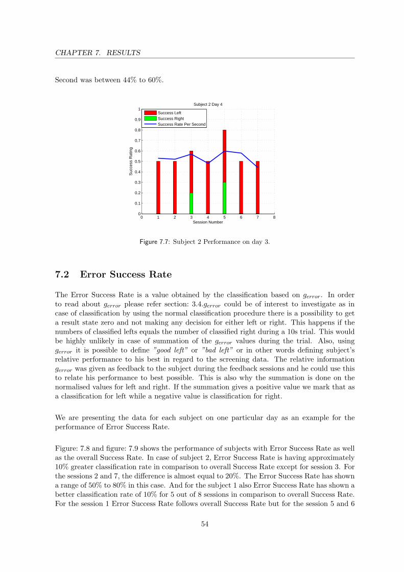
CHAPTER 7. RESULTS

Second was between 44% to 60%.

0 1 2 3 4 5 6 7 80

0.1

0.2

0.3

0.4

0.5

0.6

0.7

0.8

0.9

1

Session Number

Suc

cess

Rat

ing

Subject 2 Day 4



7.2 Error Success Rate

The Error Success Rate is a value obtained by the classification based on gerror. In orderto read about gerror please refer section: 3.4.gerror could be of interest to investigate as incase of classification by using the normal classification procedure there is a possibility to geta result state zero and not making any decision for either left or right. This happens if thenumbers of classified lefts equals the number of classified right during a 10s trial. This wouldbe highly unlikely in case of summation of the gerror values during the trial. Also, usinggerror it is possible to define ”good left” or ”bad left” or in other words defining subject’srelative performance to his best in regard to the screening data. The relative informationgerror was given as feedback to the subject during the feedback sessions and he could use thisto relate his performance to best possible. This is also why the summation is done on thenormalised values for left and right. If the summation gives a positive value we mark that asa classification for left while a negative value is classification for right.

We are presenting the data for each subject on one particular day as an example for theperformance of Error Success Rate.

Figure: 7.8 and figure: 7.9 shows the performance of subjects with Error Success Rate as wellas the overall Success Rate. In case of subject 2, Error Success Rate is having approximately10% greater classification rate in comparison to overall Success Rate except for session 3. Forthe sessions 2 and 7, the difference is almost equal to 20%. The Error Success Rate has showna range of 50% to 80% in this case. And for the subject 1 also Error Success Rate has shown abetter classification rate of 10% for 5 out of 8 sessions in comparison to overall Success Rate.For the session 1 Error Success Rate follows overall Success Rate but for the session 5 and 6

54

7.2. ERROR SUCCESS RATE

0 1 2 3 4 5 6 7 80

0.1

0.2

0.3

0.4

0.5

0.6

0.7

0.8

0.9

1

Session Number

Suc

cess

Rat

ing

Subject 2 Day 3

Success LeftSuccess RightError Success Rate

Figure 7.8: Comparison of overall Success Rate with Error Success Rate, Subject 2 Day 3.

0 1 2 3 4 5 6 7 8 90

0.1

0.2

0.3

0.4

0.5

0.6

0.7

0.8

0.9

1

Session Number

Suc

cess

Rat

ing

Subject 1 Day 2

Success LeftSuccess RightError Success Rate

Figure 7.9: Comparison of overall Success Rate with Error Success Rate, Subject 1 Day 2.

55

CHAPTER 7. RESULTS

it reduces by 10%.

7.3 Spectrum Plots using 6 Features Classification

In this section, we are presenting spectrum plots obtained by the autoregressive spectralmethod for the screening as well as the feedback sessions for the first 2 days averaged over allthe sessions for each day. As the selected features for the classifier were at 8, 10 and 12 Hzfrom channel C3 and C4, we have plot the same features together with 6 and 14 Hz for boththe channels in this plots. It is to be note that the frequency resolution for these plots is 2 Hz.

Figure 7.10: The power spectrum (microvolt) for the mu band (8-12 Hz), Subject 2 Screening session,Target1 = Target Left, Target2 = Target Right.

Figure: 7.10 shows the spectrum for C3 and C4 for the screening session. It can be observedthat C3 channel shows a greater activity at 10 Hz for the target2 (target right). On the otherhand for target 1 (target left) activity in both the channels at all the features seems to be same.

Observing the subjects performance for the 1st day, it can be seen that, there is no distin-guished activity in any of channel for either target. And following subject’s performance on2nd day (figure: 7.12),it can be seen that 10 HZ feature at C4 for target 2 is more prominent,where as rest of all other features seems be behave in similar manner.

7.4 Comparison of Single Feature with 6 Feature Classification

In the previous section’s plots, it was observed that there is a prominent activity in channelC4 at 10 Hz. So, we are interested in looking what is the classification rate if we would haveused this single feature instead of 6. This process is done using the Offline Tools, please

56

7.4. COMPARISON OF SINGLE FEATURE WITH 6 FEATURE CLASSIFICATION

Figure 7.11: The power spectrum (microvolt) for the mu band (8-12 Hz), Subject 2 Day 1, Target1 =Target Left, Target2 = Target Right.

Figure 7.12: The power spectrum (microvolt) for the mu band (8-12 Hz), Subject 2 Day 2, Target1 =Target Left, Target2 = Target Right.

57

CHAPTER 7. RESULTS

refer: 6.5.

We are presenting the performance of Subject 2 over the days during training. The bar plotsplotted adjacent to each other are based on 6 features and single feature classification. Theyalso present, how many of lefts and rights targets have been classified correctly during eachsession.

Figure 7.13: Comparison of 6 features classification with single feature classification, Subject 2 Day 1.

Figure: 7.13 shows the performance of subject for day 1. It can be seen that for both using6 features and single feature, classification rate is 50% and there is not a single target rightcorrectly classified. Where as on day 2 also (figure: 7.14), classification rate is similar in bothcase except for session 3 and 4 where there has been an addition of correctly classified right.

Following on to the performance of day 3 (figure: 7.15), the classification rate is identical formost of sessions except for session 5 and 6 where there is increment and decrement of 10%classification rate respectively. In both of these sessions, number of classified lefts is same forsingle and 6 features case but number of rights has shown variance.

Similar characteristics can be seen for day 4 (figure: 7.16), where both the classificationmethods yields same results except for session 3 and 7. In session 3 there is increment of 10%classification rate due to an additional classified right for single feature and in session 7 theclassification rate falls by 10% due to an reduced classified left using single feature.

58

7.4. COMPARISON OF SINGLE FEATURE WITH 6 FEATURE CLASSIFICATION



59

CHAPTER 7. RESULTS

Figure 7.16: Comparison of 6 feature classification with single feature classification, Subject 2 Day 4.

60

Chapter 8

Discussion

As we only have two subjects and a limited amount of recorded data we look on our resultsas a case study.

8.1 The Biased Classifier

Before going deeper into our result we have to explain the concept called ”the biased clas-sifier”. This is a classifier that have been fed with training data and have a preference toclassify one state over another. A non-biased classifier would ideally classify an equal amountsof lefts and right when given random values as input. We evaluated the amount of bias in theOffline Tools using the Multiple feature examination before generating the training data. Ifthe percentages between the numbers of successful classification of the screening data is toohigh ,i.e. the Success Rating Left could be 90% while Success Rating Right is 10%, trainingdata generated on this screening session with the selected features would produce a heavilyleft biased classifier. The results of the Multiple feature examination for the screening dataused to generate the training data with our selected features are given in decision tables 8.1and 8.2. ”Classified” is the decided state while ”Target” is the true state.

Subject 1 Target Left Target RightClassified Left 47% 35%

Classified Right 53% 65%

Table 8.1: Multiple feature examination results for Subject 1.

Subject 2 Target Left Target RightClassified Left 83% 58%

Classified Right 17% 42%

Table 8.2: Multiple feature examination results for Subject 2.

The probability for correct classification for Subject 1 gets calculated to PC = 56% and for

61

CHAPTER 8. DISCUSSION

Subject 2 to PC = 63%. This shows that Subjects 2’s classifier is performing slightly betterthan Subject 1’s at least on the screening data. Still, Subject 2’s classifier is also the one withthe highest ratio between correct scored lefts and rights (nearly 2:1 ratio) so we call it a leftbiased classifier as it apparently classifies left much better than right. Subject 1’s classifieronly shows a slight bias toward right ( 1:1.4 ratio).

8.2 Training And Improvement

The average Success Rate per Session has been computed for both subjects over all days alongwith the standard deviation. The results can be seen in table 8.3.

Subject Day 1 Day 2 Day 3 Day 41 48±15% 55±14% 67±10% -2 50±0% 52±4% 57±8% 56±11%

Table 8.3: Success Rate per Session based on overall Success Rate.

For both subjects there seem to be a steady increase in performance over the days. Comparedto the success rate per session when using Success Rate per Second as the variable gives table8.4.


Table 8.4: Success Rate per Session based on Success Rate per Second.

Also here does it seem to be an increase, though not as much in the previous table. Thisindicates that it is possible to improve the overall Success Rate without improving much onthe Success Rate per Second. This is possible if the subject equally distributes his correctclassifications between trials which will make him score a much better overall result. Anexample would be a subject with a fixed Success per Second Rate of 60%. If he equally dis-tributes this out between trials he will always score 6 out of 10 correct and thereby getting anoverall Success Rate of 100%. As our feedback to the subject informs him how many correctclassifications he is having during the trial it is possible he uses this to his advantage.

8.2.1 Performance of Subject 1

Even as Subject 1 had a right biased classifier it seemed through the sessions to be a biggertask for the subject to get a correct right classification than left. Already one day 1 was themajority of classifications for the left and not right. But it was also clear that it was possiblefor the subject to somehow influence classification to one side or the other as it did not seem

62

8.3. ERROR SUCCESS RATE

like some biased side was dominating. If the classification had randomly shifted between leftand right we would have gotten more zero results for the trials and poorer overall SuccessRate. On day 2 the subject steadily increased performance in both the overall Success Rateand in Success Rate per Second and this continued on day 3. While the value of the overallSuccess Rate and Success Rate per Second increased the standard deviation decreased, mean-ing that not only did performance increase it also become more consistent. It is not clear ifthe subject has reached his max performance level yet.

8.2.2 Performance of Subject 2

As mentioned earlier Subject 2 had a left biased classifier. This could explain why all trialsduring day 1 got classified as left even when the target was right. Though, the Success Rateper Second was fluctuating indicating that not all classifications was left. During day 2 thesubject got a better hold of making rights as can be seen in the increase of Success Rate perSecond. Also he managed to get two trials classified correctly as right by the end of the day.By day 3 the subject continued to improve the right classification and both the overall SuccessRate and Success Rate per Second continued to improve. Day 4 did not show much improve-ment except for a single session with the top score for Subject 2 of 80% correct classification.Sadly, after this the subject lost focus and performed poorer in the last two sessions. Forthis subject the standard deviation increased over the days, following the increase of correctclassifications of right. As it seems like the subject has no problems getting left classificationit is expected that continued training will help to improve the right.

8.3 Error Success Rate

As mentioned about the point of interest in investigating Error Success Rate in section: 7.2.

In the case of no classification by overall Success Rate, it is still possible to decide on a classi-fication for left or right using Error Rate. However, it could be argued that in order to avoidthe no classification problem, the number of seconds in trail could be made 11 or 9 instead of10 and this would have resulted in classification in all cases. But in that setup the classifier’sbiasing effect would influence the system, as for example if the 11th target code is same asthat of biased side of classifier then it would potentially classify it based on the bias and noton the subjects performance. Hence, it will not be a good idea to use odd number of secondsin a trial to avoid the no classification problem. While in case of using Error Rate for thesame trial we could be sure that we would be having a result even in the above mentioned cases.

From the table: 8.3 and table: 8.5 it can be seen that overall Success Rate and Error SuccessRate does not follow same pattern in Success Rate per Session for Subject 1, which meansthat it will not be justified to use Error Rate to circumvent the problems of no classificationas the classification result is generally widely different between the methods.

63

CHAPTER 8. DISCUSSION


Table 8.5: Success Rate per Session based on Error Rate.

The pattern in the Success Rate per Session is the same for Subject 2 though with even betterperformance, so the method can not be completely dismissed. It could be possible that if theError Meter display was used instead of the Success Rating display as the primary feedbackto the subject the Error Success Rate could improve.

8.4 Performance With a Single Feature

Because of the heavy left bias for Subject 2 we looked at the spectrum plot of the 6 featuresduring the screening session and the feedback sessions. As seen in the results chapter thepower is rather low for all 6 features and does not change much between the screening sessionfor left and right. Except channel C4 at the feature bin 10 Hz during the recordings for targetright. Looking at the average spectrum plots during the feedback sessions we noticed some-thing odd. During day 1, where the subject go nothing but left classification in his trials,there were very little difference in the features. Only one day two and the following dayswould a feature show a difference. But not in C3 as during the screening but instead in C4still at 10 Hz in the recordings for right. As we classify with a linear combination in the FLDa change in feature (C4, 10 Hz) would be similar to a change in (C3, 10 Hz) when there isvery little variance between the rest of the features.

To see if the discriminant feature (C4, 10 Hz) potentially would have been a better classifieron its own we used the Offline Tools to compute the classification rate for all feedback sessionswith the original screening data but now only using this single feature. Table 8.6 shows thesuccess per session in the two cases.

Number of features Day 1 Day 2 Day 3 Day 46 50±0% 52±4% 57±8% 56±11%1 50±0% 55±5% 59±7% 56±14%

Table 8.6: Success Rate per Session based on a single feature (C4, 10 Hz) for Subject 2.

So by using this single feature we see slightly increased performance than by using the six.It can not be said that this feature would have been a good to have trained the classifieron after the screening session though. Most obviously was it not C4 but C3 that had thediscriminating feature in the screening session.

64

8.5. INFORMATION TRANSFER RATE

8.5 Information Transfer Rate

Having some values for the performance of our system and knowing its speed it is possiblefor us to compute its information transfer rate. This is a widely used parameter indicatingspeed and accuracy of a BCI system. For further detail we refer to [6]. If we base our systemsaccuracy on the mean of the performance of our subjects on their last day we end up with 61%.

If we base the speed of our system on the decision of a trial (10 sec) we get a transfer rate of:0.2 bit/min.If the base the speed of our system on the decision rate of the per second classification we geta transfer rate of: 2.1 bit/min.

Compared to other BCI system with a transfer rate of 5-25 bit/min our system is very slow.Both due to the limited amount of targets and the low success rate. As we had no plansinitially about making a speedy system we do not consider it a problem a the current pointof development.

65

Chapter 9

Conclusion

To test our hypothesis, Using data from a single screening session to train a classifier, asubject can improve his classification success rate over multiple sessions when using an onlineprogram that provides feedback of his performance during the sessions, we designed an onlineBCI system. The system included data acquisition, signal processing, performance feedbackand storage of all data and setup parameters. To support the online system we also madesome offline tools for feature selection and generating training data for the online classification.

We used two subjects for our research, and recorded data for multiple feedback sessions over3-4 days. The success scores for correct classified lefts and rights for the subject was exami-nated. Different criteria for correct classification was used. One being the classified state inregards to the target state on a one second basis. Another, and our primary criterion, was anaccumulated result based on the per second classification over a trial (10 seconds). Lastelywe inspected a parameter indicating a quantisation of the classification. As we only had fewsubjects and limited number of sessions we do not have enough data for any statisticallyconclusive results. Instead we looked at our two subjects as case studies.

As our results and discussion shows it was not only possible for the subjects to influence theoutcome of the classifier but there were also a noticable increase in performance over the days.This was true when using our primary criterion as well as the per second based criterion forcalculating the success rate. These results support our hypothesis.

To avoid the problems of no classification during trials with an even amount of seconds ofclassification and the influence by a biased classifier we examinated our last criterion. It didnot show the same trends as the other two but as it was not intended as the primary feedbackto the subject that does not conclude anything. What it does conclude, is that you can notchange to this criterion in a case of no classification with the primary criterion as the resultsare quite different between the two.

66

Future Work

More subjects and sessions needs to be recorded to support or dismiss our hypothesis. Also itcould be attempted to use different features for the classifier than the ones we had selected.Instead R square could be used to find the features with largest seperability between states.

67

Bibliography

[1] . [online, cited May, 2007]. Available from: http://www.massgeneral.org/childhoodepilepsy/images/glossary/gt cerebrum-l.jpg .

[2] Marjan Jahanshahi, Mark Hallet. The Bereitschaftpotetial-Movement Related CorticalPotentials. Kluwen Academic and Plenum Publishers, 2003.

[3] Klaus-Robert Muller, Charles W. Anderson, and Gary E. Birch. Linear and NonlinearMethods for Brain Computer Interfaces. IEEE Transactions On Neural Systems AndRehabilitation Engineering, 11-2:165, 2003.

[4] Webster. Medical Instrumentation-Application and Design. John Wiley and Sons, 1998.

[5] Theresa M. Vaughan, Jonathan R. Wolpaw, and Emanuel Donchin. EEG Based Commu-nication: Prospects and Problems. IEEE Transactions On Rehabilitation Engineering,4, 1996.

[6] Jonathan R.Wolpaw (Guest Editor), Niels Birbaumer,William J. Heetderks, Dennis J.McFarland, P. Hunter Peckham, Gerwin Schalk, Emanuel Donchin, Louis A. Quatrano,Charles J. Robinson, and Theresa M. Vaughan (Guest Editor). Brain Computer Inter-face: A Review of First International Meeting. IEEE Transactions On RehabilitationEngineering,, 8, June,2000. number 2.

[7] Kalcher J, Flotzinger D, Neuper C, Golly S, Pfurtscheller G. Graz Brain ComputerInterface II: towards communication between humans and computers based on onlineclassification of three different EEG patterns. Med Biol Eng Comput, 34:382–388, 2005.

[8] Millan J del R, Mourino J, Babiloni F, Cincotti F, Varsta M, Heikkonen J. Local neuralclassifier for EEG based recognition of mental tasks. Procedings of International JointConference on Neural Networks, pages 632–636, July,2000.

[9] Birbaumer N, Ghanayim N, Hinterberger T, Iversen I, Kotchoubey B, Kubler A, Perel-mouter J, Taub E, Flor H . A spelling device for paralysed nature. Journal of AppliedPhysiology, 398:297–298, 1999.

[10] Wolpaw JR, McFarland DJ. Multichannel EEG-based brain-computer communication.Electroencephalography Clinical Neurophysiology, 90:444–449, 1994.

[11] McFarland DJ, McCane LM, David SV, Wolpaw JR. Spatial filter selection for EEGbased communication. Electroencephalography Clinical Neurophysiology, 103:386–394,1997.

69

BIBLIOGRAPHY

[12] G. Pfurtscheller, FH Lopes da Silva. Event Related EEG/MEG synchronisation anddesynchronisation: basic principles. Clinical Neurophysilogy, 110:1842–1857, 1999.

[13] Pfurtscheller G, Flotzinger D, Mohl W, Peltoranta M. Prediction of the side of handmovements from single-trial multi-channel EEG data using neural networks. Electroen-cephalogr Clin Neurophysiol., 82(4):313–315, 1992.

[14] Pfurtscheller G, J. Kalcher, C. Neuper, D. Flotzinger, M. Pregenzer. Online EEG clas-sification during externally based hand movements using neural networks. Electroen-cephalogr Clin Neurophysiol., 99:416–425, 1996.

[15] Gerwin Schalk, Member, IEEE, Dennis J. McFarland, Thilo Hinterberger, Niels Bir-baumer, and Jonathan R.Wolpaw. BCI2000: A General-Purpose Brain-Computer Inter-face (BCI) System. IEEE Transactions On Biomedical Engineering, 51:1034, 2004.

[16] BCI2000 Home Page [online]. Available from: http://www.bci2000.org/BCI2000/Home.html .

[17] Alvaro Fuentes Cabrera. A Phd Student Member at BCI Group At SMI. De-partment of Health Science and Technology, Aalborg University, contact information:[email protected].

[18] Eric Kandel, J H Schwartz, T M Jessell. Principles of Neural Science. McGraw Hill, 4thedition, 2000.

[19] G. Pfurtscheller and A. Aranibar. Event-Related Cortical Desynchronization DetectedBy Power Measurements Of Scalp EEG. Electroencephalography and Clinical Neurophys-iology, 42:817–826, 1977.

[20] Decety J. The neurophysiological basis of motor imagery. Behav. Brain Res., 77, 1996.

[21] Hallet M, Fieldman J, Cohen L.G, Sadato N, Pacula-Leone A. Involvement of primarmotor cortex in motor imagery and mental practice. Behav. Brain Science, 17, 1994.

[22] Joseph Mourino, R Milan, F Cincotti. Spatial Filtering in the training process of theBrain Computer Interface. 23rd Annual EMBS International Conference, 2001.

[23] C. Guger, H. Ramoser, and G. Pfurtscheller. Real Time EEG Analysis with SubjectSpecific Spatial Patterns for a Brain Computer Interface (BCI). IEEE Transactions onRehabilitation Engineering, 8, Dec 2000.

[24] O Bertrand, F Perrin, J Pernier. A theoritical justification of the average reference intopographic evoked potential studies. Electroencephalography and clinical Neurophysiol-ogy, 62:462–464, 1985.

[25] Dave Meko. [online, cited March, 2007]. Available from: http://www.ltrr.arizona.edu/ ∼dmeko/notes 7.pdf#search=%22detrending%22 .

[26] Mark Polak, Alexsander Kostov. Feature Extraction In Development Of Brain-ComputerInterface: A Case Study. IEEE Engineering in Medicine and Biology Society, 20, 1998.

70

BIBLIOGRAPHY

[27] Gert Pfurtscheller, Christa Neuper, Alois Schogl, and Klaus Lugger. Separability of EEGSignals Recorded During Right and Left Motor ImageryUsing Adaptive AutoregressiveParameters. IEEE Transactions On Rehabilitation Engineering, 6:316, 1998.

[28] G. Pfurtscheller, C. Neuper, C. Guger, W. Harkam, H. Ramoser, A. Schlogl, B. Ober-maier, and M. Pregenzer. Current Trends in Graz Brain Computer Interface (BCI)Research. IEEE Transactions On Rehabilitation Engineering, 8:216–219, 2000.

[29] Nai Jen Huan and Ramaswamy Palaniappan. Neural network classification of autore-gressive features from electroencephalogram signals for brain computer interface design.Journal Of Neural Engineering, 2004.

[30] J.M Spyers-Ashby, P.G Bain, S.G Roberts. A comparison of fast fourier transform (FFT)and autoregressive (AR)spectral estimation techniques for the analysis of tremor data.Journal of Neuroscience Methods, 83:35–43, 1998.

[31] P. J. Franaszczuk, K. J. Blinowska, and M. Kowalczyk. The Application of ParametricMultichannel Spectral Estimates in the Study of Electrical Brain Activity. Biol. Cybern,51:239–247, 1985.

[32] Nai-Jen, Huan, Ramaswamy Palaniappan. Classification Of Mental Tasks Using FixedAnd Adaptive Autoregressive Models Of EEg Signals. IEEE, 2004.

[33] Dan Mulally, Hyung W. Paik. Power Spectral Density Estimation Simulation using theMaximum Entropy Method.

[34] R Palaniappan, P.Raveendran, Shogo Nishida and Naoki Saiwaki. Autoregressive Spec-tral Analysis and Model Order Selection Criteria for EEG Signals.

[35] R. O. Duda, P. E. Hart, and D. G. Stork. Pattern Classification. Wiley Interscience, 2ndedition, 2004.

[36] Deon Garrett, David A. Peterson, Charles W. Anderson, and Michael H. Thaut. Compar-ison of Linear, Nonlinear, and Feature Selection Methods for EEG Signal Classification.IEEE Transactions On Neural Systems And Rehabilitation Engineering, 11-2:141, 2003.

[37] Marco Mattiocco. Contact information: m.mattioccohsantalucia.it.

[38] Wenyan Jia, Xianghua Zhao, Hesheng Liu, Xiaorong Gao, Shangkai Gao, Fusheng Yang.Classification of Single Trial EEG during Motor Imagery based on ERD. Proceedings ofthe 26th Annual International Conference of the IEEE EMBS, 2004.

[39] Ming Cheng, Wenyan Jia, Xiaorong Gao, Shangkai Gao, Fusheng Yang. Mu rhythm-based cursor control: an offline analysis. Clinical Neurophysiology, 115:745–751, 2004.

[40] S. J. Roberts, W.D. Penny. Real-time brain-computer interfacing: a preliminary studyusing Bayesian learning. Med. Biol. Eng. Comput, 38:56–61, 2000.

[41] Clemens Eder. A Phd Student Member at BCI Group At SMI. Department of HealthScience and Technology, Aalborg University.

[42] Pfurtscheller G, Lopes da Silva. Handbook of Electromyography and ClinicalNeurophysiology-Event Related Desynchronization. Elsivier, 1999a.

71

BIBLIOGRAPHY

[43] Simon Haykin. Adaptive Filter Theory. Prentice Hall, 3rd edition, 1996.

72

Appendix

73

Appendix A

Study on the NetReader C++Program

A.1 Introduction

This document describes our research on the NetReader program and its code. The NetReaderprogram is used to view EEG either recorded or stored signals through a network connection.It was originally released together with the Scan4.3 program package from Neuroscan. Itwas later modified by Antanas Veiverys for usage in the SS-VEP online BCI study by AlvaroCabrera. This modification involved some separation of functionality into a dynamic librarylink (dll) module and addition of some simple signal processing. As little information isavailable on the program dynamics this document is meant as general description of the Ne-tReader program and the modifications our group provided to it. This should make it easierfor people with further interest in modifying the program. The program is written in C++ us-ing Microsoft Foundation Classes (MFC) as framework to be able to use a Windows interface.

A.2 Program Functionality

A.2.1 Data Transmission

The NetReader program is a client program which runs in conjunction with the Acquiredata acquisition program. This program is also a part of the Scan4.3 program package.Acquire acts as server feeding NetReader with samples through a TCP protocol. The datais sent in specific packages. Further information about these packages can be found in thedocumentation for the Acquire program, which is copied in this document in section A.5.1.This gives the possibility of running NetReader on a different computer than Acquire thoughboth programs also can also run on the same. The setup is seen in figure A.1.

The Acquire program can run either in reording or simulation mode. To initialize the simu-lation mode you need to setup the default parameters for the amplifier. Press the ”Edit”-tapand select the ”Overall Parameters” option. From the new window select the ”Amplifiers”-tap

74

A.2. PROGRAM FUNCTIONALITY

Figure A.1: System setup

and press ”Ok” to the two message boxes that will appear. Then close the ”Setup”-windowby pressing ”Ok”. You can now start simulation by pressing the ”Start Data Pisplay”-button.

A.2.2 Primary Control Window

Figure A.2: Primary Control Window

Before the data exchange between Acquire and NetReader can happen they need to be setupto be able to find each other. This is firstly done by specifying the machine name or hostwhere Acquire will be running. If both programs are running on the same machine this wouldbe ’localhost’ which has to by be typed in the ’Server Name’ field (A). If Acquire is runningon a different computer the IP-address of that computer has to go to that field. Then the portnumber has to be specified which of course should be the same for Acquire and NetReader.This value goes to the ’Port’ field (B). The functions of fields C and D were not really testedbut at least they got nothing to do with the server/client setup. When the server is runningin Acquire press ’Connect’ (E) to start the client. After starting the recordings in the Acquireprogram the signals will also be displayed in this window.

The ’File Input..’ option (F) was made by Antanas Veiverys and allows you to load an .asc

75

APPENDIX A. STUDY ON THE NETREADER C++ PROGRAM

file into the program. This file is a stored recording. You have to setup channels throughthe ’Channels’ option (G) to have any process on these stored recordings going on. Also,the ’Connect’ button has to be pressed once no matter if you want to connect to a server ornot before you can load .asc files. The ’Channels’ option opens the Channel Selection window.

A.2.3 Channel Selection Window

Figure A.3: Channel Selection Window

This window controls the setup for the channels you are receiving. The window list 40 chan-nels listed from 0 to 39 which put some limitations on the channel setup you can use in theAcquire program. For each channel you can select a data process operation (A). This meansthat the data process on an individual channel is independent of the process on other channelsand that you can not join channels together for comparison. The option ’Save’ (B) allowsyou to save a channel setup, and option ’Load’ allows you to load one. The data processesavailable are Discard data, File output and Build-in FFT.

The discard data operation is a bit redundant as all channels which are not marked for any-thing else do this by default.

76

A.3. DYNAMIC LIBRARY LINKS

A.3 Dynamic Library Links

Dynamic Library Links (dll) are used to provide code functionality to programs without re-vealing the code of this functionality. To use a dll you need to know the name and syntax ofthe functions it contains before you can use them. After having build your program the dllis required to be accessible to the executable file (normally the .exe-file) for the functions tobe available. More than one program can use functions from a dll at a time.

Antanas Veiverys changed the structure of the NetReader and placed the TCP client interfacefunctionality in a dll on its own using MFC support. This means that the dll does not exportthe syntax of its functions so you can not load them in a traditional C-manner. Instead youhave to include the acquire.h file in your code and link with the acquire.lib (library file) tobuild the program. You still need to have the acquire.dll available to the executable file duringrun-time.

A.4 Modularization of the NetReader Program

Our primary modification to the NetReader program was to take the signal processing pos-sibilities used in the Channel Selection Window and also place them in .dll-files. These alsoended using MFC support. This lead to 3 dll’s:

• DiscardPluginDll.dll, which discards the data.

• FilePluginDll.dll, which saves data.

• FFTPluginDll.dll, which does the fft operation and frequency recognition.

By moving these functionalities into their own dll’s it gives the possibility of using them lateron in other applications. The interface for these 3 dll’s are similar.

• CString Name();This function returns the name of the primary function in the dll.

• CString Description();This function returns a short description of the primary function.

• int Execute(float *data, const int fs, const CChannelSettings *chan);This function executes the primary function of the dll. The input is a pointer to thedata, the sampling frequency and the channel setup. The return value is 0 for successgot the FilePluginDll.dll

• int Destroy();This function clears the memory usage of the dll.

77


It should be noted that the FFTPluginDll.dll does FFT by using the code provided by Lau-rent de Soras in the files FFTReal.h and FFTReal.cpp so if the dll is to be recompiled andbuild it needs access to these.

A.4.1 Program Flowchart

Figure A.4: Program flowchart

A UML diagram of the NetReader program can be found in the supplementary section A.5.2.

A.5 Supplementary

A.5.1 Acquire TCP Packages

This text is copied from the Acquire documentation regarding the TCP.

Packet structures and command set

Who should read this section? This section is intended for users who want to writetheir own client program to pull data online from the ACQUIRE server during acquisition.The ACQUIRE program uses stream sockets (neither datagram nor raw sockets) to guaranteedata delivery in the proper order. Refer to Windows Socket Specification or books on TCPfor more information on this socket type and socket programming.

Packet structure. All information sent between the client and server is organized as pack-ets. Each packet consists of a 12-byte header and an optional body. The header structure isthe following:

typedef structchar m chId[4]; // ID string, no trailingWORD m wCode; // CodeWORD m wRequest; // RequestDWORD m dwSize; // Body size (in bytes)PacketHeader;

78

A.5. SUPPLEMENTARY

If body size field is 0, then no body is sent. Otherwise, the receiving socket should read thespecified number of bytes and process them according to meaning of the header’s ID string,Code and Request fields.

Byte ordering. Different machine architectures store data using different byte orders. Forexample, Intel-based machines store data in the reverse order of Macintosh (Motorola) ma-chines. Intel’s byte order, called ”little-Endian,” is also the reverse of the network standard”big-Endian” order. The following table A.1 explains these terms:

Byte ordering MeaningBig-Endian The most significant byte is on the left end of a word.

Little-Endian The most significant byte is on the right end of a word.

Table A.1: Endian Explanation

ACQUIRE always sends the packet header translated to ”big-Endian”(network) notation.But the content of the data and file packets (as proprietary information) is always sent innative Intel ”little-Endian” format. This means that ACQUIRE performs the following op-erations on packet’s header:

void PacketHeader::Convert(BOOL bSending)if (bSending) // Convert from host byte order to network byte order// (Little-Endian to Big-Endian) while sendingm wCode = htons (m wCode);m wRequest = htons (m wRequest);m dwSize = htonl (m dwSize); else // Convert from network byte order to host byte order// (Big-Endian to Little-Endian) while receivingm wCode = ntohs (m wCode);m wRequest = ntohs (m wRequest);m dwSize = ntohl (m dwSize);

Command set. The Header ID string consists of 4 upper case letters, without the trailing.It can be one of the following:

”CTRL” - control code”FILE” - file packet

”DATA” - data packet

This ID specifies what kind of information is sent in other fields and in the optional body.The following table summarizes the possible combinations: figure A.5

79


Figure A.5: Package Combinations

The Server computer sends general and server control codes, file and data packets. The Clientside should send only general and client control codes, and be able to process (or simply drop)incoming file and data packets.

The formats for ”Version Information”, ”EDF Header” and ”Neuroscan 16-bit Raw Data”packets are presented in ”acq client.c” source code, included in the ”NetReader” directory.

Important note. As ACQUIRE uses some other codes and requests internally, avoid theusage of numbers not presented in the table.

Program examples

Standard client operations. Normally, the client program first connects to the ACQUIREserver; second, it requests for configuration information and processes it; third, it asks forEEG data and then receives them for further processing/display/ storage; and, finally, itdisconnects from the ACQUIRE server. The following are basic client actions:

1. Connect to ACQUIRE server through TCP socket.

2. Send ”Request for EDF Header”.

3. Read ”DATA” packet with EDF Header and process it to extract electrode information.

4. Send ”Request to Start Sending Data”.

5. Read incoming ”DATA” packets with 16/32-bit EEG data with further processing,displaying and storage.

6. Send ”Request to Stop Sending Data”.

7. Send ”Closing Up Connection”.

8. Disconnect from ACQUIRE server by closing up the client TCP socket.

80

A.5. SUPPLEMENTARY

See example code ”acq client.c” for such client implementation.

”Minimum” client operations. The basic sequence can be reduced. If you manuallyset the number of channels on the client side, then you may skip steps 2 and 3. Exiting theclient program will also close all sockets, so you may also trim out steps 6-8. Finally, theminimum sequence of operations is:

1. Connect to ACQUIRE server through TCP socket.

2. Send ”Request to Start Sending Data”.

3. Read incoming ”DATA” packets with 16/32 EEG data, process and display them.

4. Exit from client program (to automatically disconnect from ACQUIRE server).

See the sample code ”acq client min.c” for implementation of the ”minimum” client.

The ”NetReader” directory contains the following program examples:

Figure A.6: Supported Languages

Example ”Reader” program and source code. Included with the 4.3 installation is asample ”reader” program that can be used to display the data on a second computer (withoutthe need for a second SCAN license). To run the program, go to the \Scan4.3 folder and runthe NetReader.exe program. You can run the program on the same computer where you haveSCAN, if you wish. Follow the directions on the displayed screen. You should see the EEGsignals on the ”reader” at the same time as you see them in ACQUIRE. Event informationwill also be displayed. The source code for the program in found in the \Scan4.3\NetAcquirefolder.

A.5.2 UML Diagram

This diagram was made by Antanas Veiverys before our changes to the NetReader program.

81


Figure A.7: UML Diagram

82

Appendix B

EEG Rhythms

The rhythms of the EEG are classified into various subtypes on the basis of the frequency andthe associated cortical and the mental areas. The various rhythms shown in the figure: B.1are :

Figure B.1: Different types of normal EEG rhythms[4].

Delta

Delta rhythms falls in the category of waves having a frequency less than 3.5Hz. They occurfor around 2-3secs. They are usually present during a deep sleep and also in new born babies.

83

APPENDIX B. EEG RHYTHMS

Theta

Theta rhythms lies in the range of 4-7Hz. It is found typically in parietal and temporal re-gion of children. However, it can also be seen in the adults experiencing emotional stress ordisappointment.

Alpha

Alpha rhythms lies in the range of 8-13Hz and amplitude varying between 20-200µV. It haslarger amplitude in comparison to other rhythms and more like sinusoidal in shape. Alphaactivity can be recorded from occipital,parietal and posterior temporal regions of the cortex.It is associated with the wakefulness, physical relaxation and relatively mental inactivity.

Beta

Beta rhythms lies in the frequency range of 14Hz to 80Hz. The activity is usually asynchro-nous and its amplitude is always below 30µV. It can be divided into categories as lower betaactivity and higher beta activity. The lower beta activity lies in the range 14-30Hz and ispresent in the frontal and central regions of the cerebral cortex. It signifies the limited mentalactivity and they disappears when the mental activity is enhanced. The higher beta activityis known as Gamma activity and is described below.

Gamma

Gamma rhythms lies in the range of 30-80Hz where 30-60Hz lies in lower band and 60-80Hzin higher band , they however similar in shape and location to lower beta rhythms but theiramplitude is much lower to beta rhythms and is usually in µV. Gamma activity is associatedwith the high mental activity and is considered due to the processing of sensory,cognitive orsensorimotor information, for example planning a motor action.

The above section is based on the information provided in [4] and [42].

84

Appendix C

Signal Processing Tools Theory

C.1 AutoRegressive Models

A time series u(n),u(n-1),......,u(n-M) represents the realisation of an autoregressive process(AR) of order M if it satisfies the difference equation:

u(n) + a∗1u(n− 1) + ...... + a∗Mu(n−M) = v(n) (C.1)

where a1, a2, ......., aM are constants called AR parameters and v(n) is a white noise process.The term a∗ku(n−k) is the scalar version of inner product of ak and u(n-k), where k= 1,2,...,M.

The eq: C.1 can be rewritten as:

u(n) = w∗1u(n− 1) + ...... + w∗Mu(n−M) + v(n) (C.2)

where wk = −ak. It can be seen that the present value of the process u(n) is a linearcombination of the past values of the process, u(n-1),.......,u(n-M), and a noise term. Thisequation can be represent as linear model:

y =M∑

k=1

w∗kx(k) + v (C.3)

where y is said to be regressed on the x1, x2, ....., xM and since in eq: C.2 u(n) is regressedon past values of itself, it is called as autoregressive process.

The eq: C.1 can be represented as convolution of u(n) and a∗n :

M∑

k=0

a∗ku(n− k) = v(n) (C.4)

where a0=1. By taking z-transform, it can be represented as:

85

APPENDIX C. SIGNAL PROCESSING TOOLS THEORY

HA(z)U(z) = V (z) (C.5)

where,

HA(z) =∑M

n=0 a∗nz−n , U(z) =∑∞

n=0 u(n)z−n (C.6)

With the white noise as input, we can produce the AR process u(n) as output as shown infigure: C.1, and the transfer function for the this process generator is equal to:

HG(z) =U(z)V (z)

(C.7)

From eq: C.5, it can be seen as:

HG(z) =1

HA(z)=

1∑Mn−0 a∗nz−n

(C.8)

Figure C.1: AR Process generator.

The process generator shown in figure: C.1 is an all-pole filter. It is so called because HG(z)is completely defined by specifying the location of its poles:

HG(z) =1

(1− p1z−1)(1− p2z−1).....(1− pMz−1)(C.9)

86

C.2. LEVINSON-DURBIN ALGORITHM

The parameters p1, p2, ...., pM are poles of HG(z); they are defined by the roots of the equation:

1 + a∗1z−1 + a∗2z

−2 + .... + a∗nz−n = 0 (C.10)

For the all-pole AR process generator to be stable, the roots of the eq: C.10 must lie insidethe unit circle in the z-plane. This is also a necessary and sufficient condition for wide sensestationary of the AR process produced by figure: C.1.

C.2 Levinson-Durbin Algorithm

This section briefly describes the stages of Levinson-Durbin Algorithm. For more detailsplease refer [43].

Initialize the algorithm by setting:

a0,0 = 1; P0 = r(0); (C.11)

For m = 1, 2, ....., M, where M is the selected model order, compute:

Reflection Coefficients:

km = − 1Pm−1

M−1∑

i=0

r(i−m)am−1,i (C.12)

AR Coefficients:

am,i =

1 for i = 0am−1,i +kma∗m−1,m−i for i = 1,2,....m-1km for i = m

Updating Error :

Pm = Pm−1(1− |km|2) (C.13)

87

Appendix D

Testing of Modules and System

D.1 Selection of AR Model

D.1.1 Testing with sample data

An EEG data which were acquired during a study at Graz University of Technology, Austriaby Gert Pfurtscheller and Alois Schlogl were used to test the order of system. Data werecollected during a feedback session where the task was to control a feedback bar by means ofimagery left or right hand movements. The Data was collected for 140 training and 140 testtrials, at 3 channels, 128Hz sampling rate, 0.5-30Hz filter, each trial of 9s long.

As mentioned in chapter: 3, we chose Burg’s method to calculate AR coefficients and observedthe drop in FPE with order.

The mean FPE was calculated over all the 140 trails and for each order. Figure: D.1 showsFPE vs Model Order for all the 3 channels recorded and it can be seen that FPE falls till theorder the 12 and then becomes almost consistent for channel 1 and 3, where as for channel2 also the error seems to be more or less consistent after order 12 hence model order of 12could be chosen as appropriate order for this system.

D.1.2 Testing with actual data

In previous section, we have used the data acquired by other researchers, however once wehad starting recording for our system we performed the same test for model order on ourrecorded data.

The analysis was done on the data recorded during several sessions for motor imaginary task.The data was acquired in the ideal experimental condition, which includes subject in thesetup with a cap on and all the electrodes at the impedance lower than 5kOhms and amplifierparameters were set to the same values as mentioned in the chapter: 4.

88

D.1. SELECTION OF AR MODEL

0 2 4 6 8 10 12 14 16 18 200.5

1

1.5

2

2.5

3x 10

−3

Model Order

FP

E

Selection of Model Order

Channel1Channel2Channel3

Figure D.1: Functional Prediction Error vs AR Model Order, error seems to be consistent after order12.

The FPE was calculated for each 1s of data out of 10s for all the 38 EEG electrodes and thenaveraged over 10s, figure: D.2 shows an example for the same. Then, a mean FPE curve wasobtained as averaged over 38 channels and is shown in figure: D.3. A model order is observedfor the same. In this particular case, it can be seen that a model order of 9 is appropriate forthe system.

This has been repetitively calculated for several 10s trials over different sessions. Using anTSA AR Modeling Order VI from LabVIEW, we obtained the appropriate model order forthe calculated FPE. The model order observed from the TSA VI was ranging between 8 to 10over several trials, hence we decided to have average value 9 as our model order for the system.

Figure D.2: FPE vs Model Order for 38 channels averaged over ten 1s of data.

89

APPENDIX D. TESTING OF MODULES AND SYSTEM

Figure D.3: FPE vs Model Order, mean FPE obtained by averaging over 38 channels.

D.2 Testing of System

Before we could start using BCILab for our sessions we needed to test if we had implementedthe system correctly. For this purpose we needed a source that would generate a known andclearly distinctive features. A function generator to help us with that. We set up a normalscreening session with a subject, but instead of having the subject trying to imagine a move-ment for the target given we probed in a 10Hz sinusoid wave of 2mV PtP on either the C3electrode for a right target or the C4 electrode for a left target. We processed this data in theOffline Tools and could see hugely distinctive features at the expected feature bins with 100%correct classification for left and right. We generated a training file for our 6 selected featureswith this data and made a feedback session. Again we used the probe to generate signals andhad perfect classification for both left and right. We then concluded that our programs andmodules were working as desired. The data file for the screening session with the amplifier iscalled Ampli 1.dat.

90

Appendix E

I/P and O/P of Modules

This appendix aims at providing the information regarding the various inputs and outputsof the Online and Offline modules used in BCILab. However, for more details about BCILabfunctionalities please refer: 5 and 6 . All the below mentioned modules can be found inBCILab.llb in BCI group directory, SMI, Aalobrg University.

E.1 Online Modules

E.1.1 BCILab Main

It is the main Online module, which performs the data acquisition, signal processing,feature selection and as well as classification. Below discussed are the sub VIs of BCILab main.

E.1.2 Conversion to MicroVolt

Converts the given input into microvolts using the following information:

Inputs

SourceChGain: The gain value of the amplifier.SourceChOffset : The offset value for the amplifier.Event Channels: Number of event channels.Input Signal: Input Signal to the module, Channels X Samples.

91

APPENDIX E. I/P AND O/P OF MODULES

Output

Output Signal: Signal in microvolt, Channels X Samples.

E.1.3 Spatial Filtering

Performs the spatial filtering on all the working channels as well as act as a transmis-sion filter to remove the channels don’t need to be processed further.

Inputs

Input Signal: Signal in microvolt, Channels X Samples.Working Channels: Channels need to be sent to signal processing modules .Not Transmitted Channels: Channels which don’t need to be processed.

Output

Output Signal: Spatial Filtered Signal, Samples X Working Channels.

E.1.4 Detrending

Performs linear detrending on the given input signal. If desired the method of de-trending can be changed.

Inputs

Input Signal: Spatially filtered signal, Samples X Working Channels.Detrending Method: Method used for detrending.

Output

Output Signal: Detrended Signal, Working Channels X Samples.

92

E.1. ONLINE MODULES

E.1.5 AR Modelling

Generates the feature array for the input signal, by calculating the PSD values of ARcoefficients generated from the given method and model order.

Inputs

Input Signal: Detrended signal,Working Channels X Samples.AR Method: Method to be used for AR modelling.AR Order: Model Order for the system.AR Frequency Bins: No. of Frequency to be calculated, (Sampling rate/AR FequencyBins) gives the resolution for the spectrum.

Output

Feature Array: PSD values of the working channels, Working Channels X Frequency Bins.

E.1.6 Selecting Features

Selects the features provided in the Channel Table (refer figure: 5.2) in the Parameterstab and pass those features to the classifier.

Inputs

Feature Array: PSD values of all the working channels, Working Channels X FrequencyBins.Feature Table: Features that need to be selected from the respective channels, column onerepresents the channel number, Selected Channels X Selected Frequency Bins. It reads thistable from the Training Data File loaded at the front panel.

Outputs

Selected Features: Selected features arranged in a 1D array with the channels appendedone below the other.No of Features: Gives the number of features selected.

93


E.1.7 Bayesian Classifier

Performs the classification on the input signal using the selected features from theprevious modules.

Inputs

Classification Data: The data from the selected channels and the frequency bins, SelectedChannels X Selected Frequency Bins.FLD: Whether FLD needs to be perform or not, True or False.Training: Whether its Training or Classification, in this case (Online) it should be False.W FLD in: The W FLD values calculated using FLD operation. It reads this value fromthe Training Data File loaded at the front panel.Input Cluster: Contains all the w values calculated during the formation of Training DataFile. It reads this values from the Training Data File loaded at the front panel.

Outputs

Error: Gives the error value for the error meter display.Left ?: Gives True or False depending on result code, True is Left.

E.1.8 Training File Reader

It reads the Training File, which is formed during the Offline Training stage.

Inputs

Input File: Path to the Training File.

Outputs

FLD: Whether FLD was performed while computing Training File.Output Cluster: Contains all the w values calculated during the formation of Training DataFile.FLD Values: The W FLD values calculated using FLD operation.Channel Table: Features used to compute the Training File Selected Channels X SelectedFrequency Bins.Best Left Error: The highest g value for the left target.

94

E.2. OFFLINE MODULES

Best Right Error: The highest g value for the right target.

E.2 Offline Modules

E.2.1 Feature Search

It is an main Offline module, which performs feature selection and generates trainingfile to be used in online module. Below discussed modules are sub VIs of Feature Search.

E.2.2 Feature Reader

Reads the feature file and put the information in a cluster.

Input

Feature File Path: Path to the feature file.

Output

Feature Cluster Array: Cluster containing all the information in the feature file.

E.2.3 Cut Feature Space

Cuts the feature space according the parameters in Feature Table.

Input

Feature Cluster Array In: Feature array containing all information regarding featurespace, target code, selected channels.Limited Feature Space ?: True if the offline analysis needs to be done on selected channelsand feature bins else False.Selector: Feature table with the channel number and frequency bins information on whichanalysis needs to be done.

95


Output

Feature Cluster Array Out: Contains all the information as that of Input array but onlyfor the selected channels and feature bins.

E.2.4 Train & Test

Gets (k-1) subgroups for both state 1 and 2 and train the classifier with that data.The it classifies a single subgroup of either state.

Input

Training Array Class 1: Data to train the classifier for state 1.Training Array Class 2: Data to train the classifier for state 2.Classification Array Class 1: State 1 data to be classified.Classification Array Class 2: State 2 data to be classified.FLD: If FLD is in use or not.

Output

Success Rating Class 1: The percentage of the state 1 data that got classified correct.Success Rating Class 2: The percentage of the state 2 data that got classified correct.

96

Appendix F

Setup of the 64 Channel ElectroCap

F.1 Introduction

This document describes how to connect and setup the 64 channel EEG Electro Cap. Thecap in reality does not contain 64 EEG electrodes but has 59. These 59 electrodes are thenconnected to wires that are bundled into two cables. One cable (referred to as Cap Connector1) contains 31 wires while the other (referred to as Cap Connector 2) contains 28 wires. Bothend in a 37 pin connector plug. The electrode/pin connection can be seen in the followingpicture F.1 and F.2 for both connectors.

F.2 Rewirering Connectors

Two NuAmps amplifiers made by Neuroscan are used to record from the cap. Each amplifierhas 40 available channels for recording and are also equipped with a 37 pin connector plug.Sadly, even though the connectors from the cap can go directly into the plug on the amplifiersthis will not work. The channel layout of the connector plug and the amplifier plug does notmatch. Therefor it is required to rewire the channels from the cap plug directly into the 40inputs on top of the amplifiers. We have created two connector cables for this purpose. Dueto some restrictions in the Acquire software about how to label channels in multiple amplifiersit is required to wire 7 channels from Cap Connector to Amplifier 1 and the rest to Amplifier2. The setup can be seen in the following, see figure: F.3.

This also shows that the two reference channels (A1 and A2) has to be connected to bothamplifiers. Ground also needs to be connected. The electrode labeled ”GND” can be used forthis purpose. Normally this electrode would be connected to Amplifier 1 in channel port 37but to use it as ground is has to be put in one of the ”GND” channel ports on either amplifier.

The channels has to be connected to the amplifiers in the following order, see figure: F.4.

97

APPENDIX F. SETUP OF THE 64 CHANNEL ELECTRO CAP

Figure F.1: The Cap Connector 1. Figure F.2: The Cap Connector 2.

98

F.2. REWIRERING CONNECTORS

Figure F.3: The Connection Setup.

99


Figure F.4: 59 channel setup.

Due to unavailability of the correct letters some of the connector plugs had a small renaming.Their alternative name is found in the lower left part of the picture. To get the physicalchannel numbers for the second amplifier just subtract 40 from the numbers on the picture.

Both amplifiers should be connected to a USB hub and the hub then connected to a com-puter. It can take a little while before the computer recognizes both amplifiers and installtheir drivers.

F.3 Acquire Setup File

We have produced at channel setup file that is to be used in the Acquire software programto give the correct labeling of the channels. The name of the setup file isNuAmps 59 64chan Electrocap.ast. There seem to be a mix up of channel A1 and A2 onthe second amplifier. Even tough they are connected to the physical channels 67(27) and73(33) on the second amplifier and the Channel Assignment Table verifies that, their valuesare actually recorded at channel 62(22) and 63(23). This means that it is not possible toverify low impedance on the reference channels for the second amplifier. It is not advised toput the connector plugs for A1 and A2 anywhere else than 67 and 73 as those are still beingused as reference.

100

F.4. IDENTIFYING PROBLEMS

Figure F.5: Trace of a blink pulse.

F.4 Identifying Problems

We tested our setup and encountered some serious problems. All our testing was done on alaptop running on battery and all electrical devices in the room turned off. The samplingfrequency is 250 Hz. Firstly, it we observed in figure: F.5 some phase problems. As seen inthe following picture of a blink movement, it seems like there is a change of phase in the twoamplifiers.

When signals from one amplifier increases they decrease on the other. Secondly we observedin figure: F.6, transients in the channels on the second amplifier. These transient camerandomly with a very characteristic shape. We tried to change the order of the amplifiers butthe ”second” amplifier would still give the same problems. We contacted Neuroscan aboutthese problems but have not gotten any reply till the time of writing this.

F.5 The 40 Channel Setup

Due to the problems described previously and to lessen complexity of our system we decidedto reduce the number of channels to record on to 38 and with the A1 and A2 channels having40 channels all in all. Thereby we would only need one amplifier in the setup.

The channel layout for the 40 channels are seen in figure: F.7.

It should be noted that it is still required to connect channels from both cap connectors tothe amplifier. The ACQUIRE setup file for this setup is NuAmps 59 40chan Electrocap.ast.

101


Figure F.6: Signal transient.

Figure F.7: 40 channel setup.

102

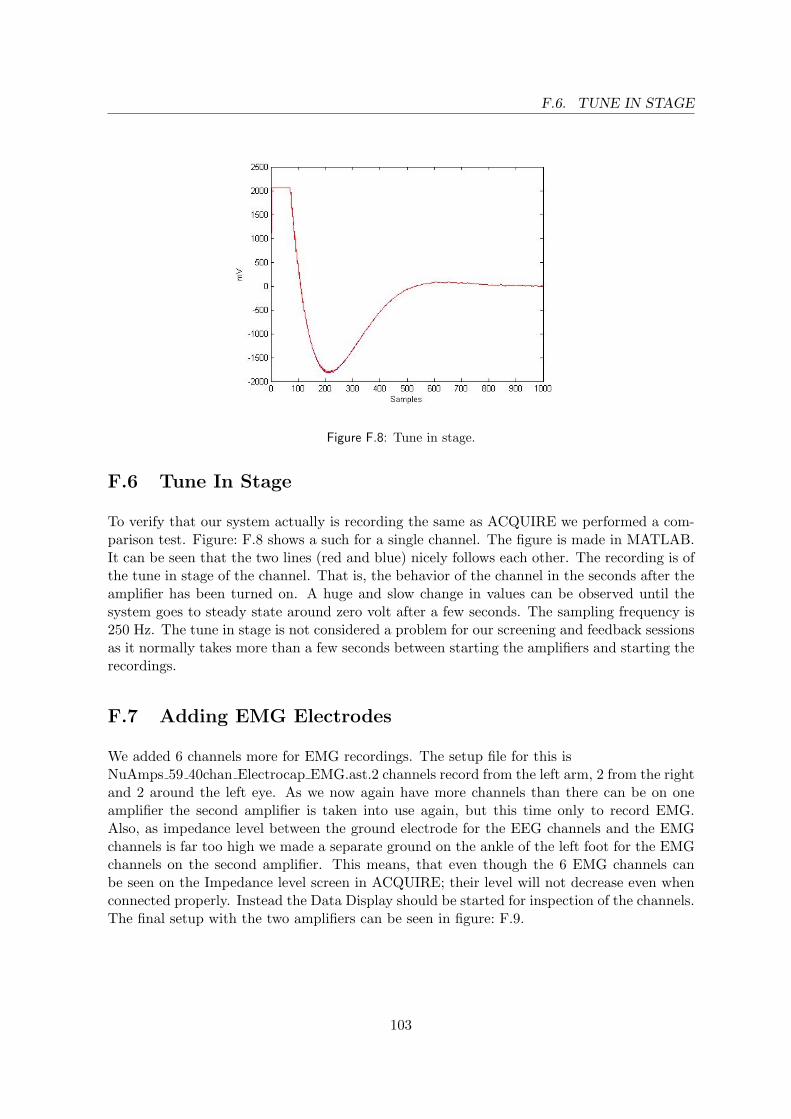
F.6. TUNE IN STAGE

Figure F.8: Tune in stage.

F.6 Tune In Stage

To verify that our system actually is recording the same as ACQUIRE we performed a com-parison test. Figure: F.8 shows a such for a single channel. The figure is made in MATLAB.It can be seen that the two lines (red and blue) nicely follows each other. The recording is ofthe tune in stage of the channel. That is, the behavior of the channel in the seconds after theamplifier has been turned on. A huge and slow change in values can be observed until thesystem goes to steady state around zero volt after a few seconds. The sampling frequency is250 Hz. The tune in stage is not considered a problem for our screening and feedback sessionsas it normally takes more than a few seconds between starting the amplifiers and starting therecordings.

F.7 Adding EMG Electrodes

We added 6 channels more for EMG recordings. The setup file for this isNuAmps 59 40chan Electrocap EMG.ast.2 channels record from the left arm, 2 from the rightand 2 around the left eye. As we now again have more channels than there can be on oneamplifier the second amplifier is taken into use again, but this time only to record EMG.Also, as impedance level between the ground electrode for the EEG channels and the EMGchannels is far too high we made a separate ground on the ankle of the left foot for the EMGchannels on the second amplifier. This means, that even though the 6 EMG channels canbe seen on the Impedance level screen in ACQUIRE; their level will not decrease even whenconnected properly. Instead the Data Display should be started for inspection of the channels.The final setup with the two amplifiers can be seen in figure: F.9.

103


Figure F.9: Setup with EMG channels.

104

Appendix G

Data Storage File

This is an example of a the header of a storage file for state definitions and parameters fol-lowing the BCI2000 standart. Parameter format is:

’section’ ’data type’ ’name’ ’value’ ’default value’ ’low range’ ’high range’ // ’comment’ CRLF

All parameters are being described by their comment. For more information about the formatconsult the BCI2000 documentation [16].

HeaderLen= 3486 SourceCh= 46 StatevectorLen= 4[StateV ectorDefinition]SourceTime 16 0 0 0Running 1 0 2 0Recording 1 0 2 1TargetCode 2 0 2 2ResultCode 2 0 2 4ErrorRatingSign 1 0 2 6ErrorRating 8 0 2 7[ParameterDefinition]System int SessionType= 2 1 1 2 // The type of recording session (1: Screening, 2: Testing)UsrTask int NumberOfTrials= 10 1 1 100 // The number of trials Source int SoftwareCh=46 38 1 64 //the number of received and stored channelsSource int SampleBlockSize= 250 250 125 1000 //the number of samples transmitted at atime (sample frequency)Source int TransmitCh= 38 38 1 64 // the number of transmitted channelsSource intlist TransmitChList= 38 1 2 3 4 5 6 7 8 9 10 11 12 13 14 15 16 17 18 19 20 21 2223 24 25 26 27 28 29 30 31 32 33 34 35 36 37 38 38 1 64 //list of transmitted channelsFilter int SpatialFilteredCh= 38 38 1 64 // the number of channels spatially filteredFilter intlist SpatialFilteredList= 38 1 2 3 4 5 6 7 8 9 10 11 12 13 14 15 16 17 18 19 20 21 2223 24 25 26 27 28 29 30 31 32 33 34 35 36 37 38 38 1 64 //list of spatially filtered channelsSource int SamplingRate= 250 250 125 1000 //the sample rate (sample frequency)Storage string SubjectName= Asbjoern Name a z //subject alias Storage string SubjectSes-sion= 1 001 0 999 //session number (max. 3 characters)

105

APPENDIX G. DATA STORAGE FILE

Storage string FileInitials= C:\Documents%20and%20Settings\Alvaro%20F.%20Cabrera\Desktop\06GR985\Recordings\Asbjoern\28-05-07 a z 0 //Initials of file nameStorage string FeatureSpaceFile= C:\Documents%20and%20Settings\Alvaro%20F.%20Cabrera\Desktop\06GR985\Recordings\Asbjoern\28-05-07\AB 1 F featsp.txt a z 0 //Name and path of the features space storage fileStorage string TrainingDataFile= C:\Documents%20and%20Settings\Alvaro%20F.%20Cabrera\Desktop\06GR985\Recordings\Asbjoern\25-05-07\AB 1 Sr trainingdata.txt a z 0 //Name and path of the training data fileFiltering floatlist SourceChOffset= 46 0 0 0 0 0 0 0 0 0 0 0 0 0 0 0 0 0 0 0 0 0 0 0 0 0 0 0 0 00 0 0 0 0 0 0 0 0 0 0 0 0 0 0 0 0 0 -500 500 //offset for channels in A/D unitsFiltering floatlist SourceChGain= 46 19 19 19 19 19 19 19 19 19 19 19 19 19 19 19 19 19 1919 19 19 19 19 19 19 19 19 19 19 19 19 19 19 19 19 19 19 19 19 19 19 19 19 19 19 19 19 -500500 //gain for each channel (A/D units -¿ muV)UsrTask int TargetSizeLeft= 3600 1 1 10000 // Size of the left target indicator (in pixels)UsrTask int TargetSizeRight= 3600 1 1 10000 // Size of the right target indicator (in pixels)UsrTask int ErrorDisplaySize= 17856 1 1 10000 // Size of the Error Meter display (in pixels)UsrTask int SuccessDisplaySize= 4408 1 1 10000 // Size of the Success Rating display (inpixels)UsrTask int RewardDuration= 5 3 1 100 // The time for reward (in seconds)UsrTask int PreTrailPause= 5 5 1 100 // The time for between the target light up and record-ing starts (in seconds)UsrTask int RestingPeriod= 7 7 1 100 // The time for rest between trials (in seconds)UsrTask int TrialTimeLength= 10 10 1 100 // The recording time (in seconds)Filtering string DetrendMethod= Linear Linear a z // The detrend methodFiltering int AROrder= 16 16 1 20 // The order of the AR filterFiltering int ARFrequencyBins= 125 125 1 1000 // The number of frequency bins for the ARfilterFiltering string ARMethod= Burg-Lattice Linear a z // The detrend method System intStateVectorLength= 3 3 1 30 //length of the state vector in bytes ...followed by the binarydata...

106