IMPLEMENTATION OF FRICTION STIR WELDING IN … of friction stir welding in 3003 aluminum plates inspected by ultrasonic testing . tesis . maestro en ciencias con especialidad en sistemas

Implementation of Friction Stir Welding in 3003 AluminumPlates Inspected by Ultrasonic Testing-Edición Única

Title Implementation of Friction Stir Welding in 3003 Aluminum PlatesInspected by Ultrasonic Testing-Edición Única

Issue Date 2010-12-01

Publisher Instituto Tecnológico y de Estudios Superiores de Monterrey

Item Type Tesis de maestría

Downloaded 22/05/2018 12:13:52

Link to Item http://hdl.handle.net/11285/569962

http://hdl.handle.net/11285/569962

IMPLEMENTATION OF FRICTION STIR WELDING IN 3003 ALUMINUM PLATES INSPECTED BY ULTRASONIC TESTING

TESIS

MAESTRO EN CIENCIAS CON ESPECIALIDAD EN SISTEMAS DE MANUFACTURA

Instituto Tecnológico y de Estudios Superiores de Monterrey

Por

Ing. Tomás Lamuño Encorrada

Diciembre de 2010


TESIS


Instituto Tecnológico y de Estudios Superiores de Monterrey

Por

Ing. Tomás Lamuño Encorrada

Diciembre de 2010

INSTITUTO TECNOLÓGICO Y DE ESTUDIOS SUPERIORES DE MONTERREY

CAMPUS MONTERREY

DIVISIÓN DE INGENIERÍA PROGRAMA DE GRADUADOS EN INGENIERÍA

Los miembros del comité de tesis recomendamos que el presente proyecto de tesis presentado por el Tomás Lamuño Encorrada sea aceptado como requisito

parcial para obtener el grado académico de:


Comité de Tesis:

Aprobado:

Dr. Ciro Angel Rodríguez González

Director - Maestría en Ciencias con Especialidad en Sistemas de Manufactura

Diciembre 2010

IMPLEMENTATION OF FRICTION STIR WELDING IN 3003 ALUMINUM PLATES EXAMINATED BY ULTRASONIC TESTING

POR:

Tomás Lamuño Encorrada

TESIS

PRESENTADA AL PROGRAMA DE GRADUADOS EN INGENIERÍA

ESTE TRABAJO ES REQUISITO PARCIAL PARA OBTENER EL GRADO ACADEMICO DE MAESTRO EN CIENCIAS CON ESPECIALIDAD EN

SISTEMASDE DE MANUFACTURA

INSTITUTO TECNOLÓGICO Y DE ESTUDIOS SUPERIORES DE MONTERREY

Diciembre de 2010

To my family for the unconditional support they have always given me,

thank you mom and dad for trusting me. To my sisters whose are my

pillars to follow.

vi

Acknowledgement

Externalize a sincere desire to thank the people who in some helped shape in the

development of this thesis.

I would like to thank Dr. Juan Oscar Molina Solis and MsC Lorena Cruz Matus for many

helpful discussions and their interest in this work.

Thanks to Ing. Regina Vargas and Julio Cesar for the help and the time dedicated.

The research was supported by a grant from the Materials Laboratories at the ITESM.

To my family, my colleagues and friends who have shared this process and that always

gave me encouragement in difficult times.

And thanks to my parents because they've got here.

Thank you

Tomás Lamuño Encorrada Instituto Tecnológico y de Estudios Superiores de Monterrey

Diciembre de 2010

vii

Resume


Tomás Lamuño Encorrada

Instituto Tecnológico y de Estudios Superiores de Monterrey, 2010

Asesor de la tesis: Dr. Juan Oscar Molina Solís

In this thesis, the Friction Stir Welding parameters and how they affect the

functionality of the weld are analyzed. The parameters, the type of tool used to

weld, welding speeds of rotation and transverse, are interrelated to obtain a

functional welding,

To find out the quality of the weld an ultrasonic testing was made, with which it can

be seen from the construction of a block pattern for measurement to the

assessment and analysis of the ultrasonic test. This test was held in concordance

with the ASTM standards, which gave as a result a couple of specimens with

different discontinuities.

viii

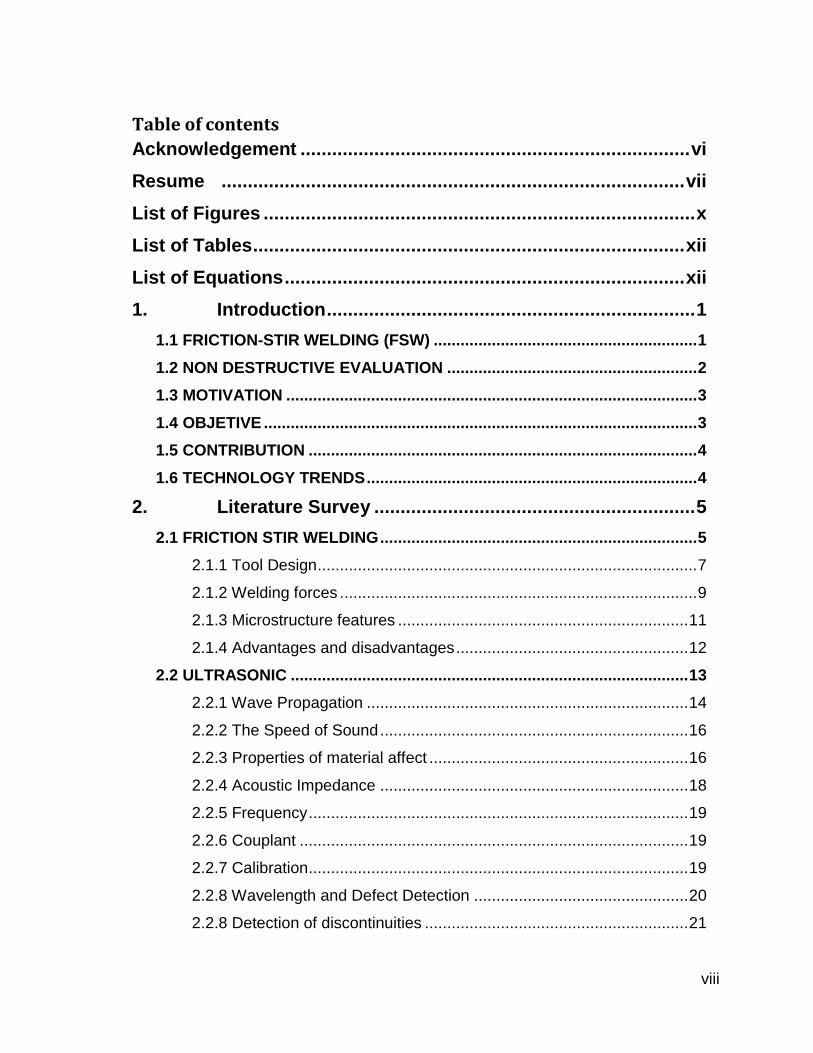
Table of contents

Acknowledgement .......................................................................... vi

Resume ........................................................................................ vii

List of Figures .................................................................................. x

List of Tables .................................................................................. xii

List of Equations ............................................................................ xii

1. Introduction ...................................................................... 1

1.1 FRICTION-STIR WELDING (FSW) ........................................................... 1

1.2 NON DESTRUCTIVE EVALUATION ........................................................ 2

1.3 MOTIVATION ............................................................................................ 3

1.4 OBJETIVE ................................................................................................. 3

1.5 CONTRIBUTION ....................................................................................... 4

1.6 TECHNOLOGY TRENDS .......................................................................... 4

2. Literature Survey ............................................................. 5

2.1 FRICTION STIR WELDING ....................................................................... 5

2.1.1 Tool Design ..................................................................................... 7

2.1.2 Welding forces ................................................................................ 9

2.1.3 Microstructure features ................................................................. 11

2.1.4 Advantages and disadvantages .................................................... 12

2.2 ULTRASONIC ......................................................................................... 13

2.2.1 Wave Propagation ........................................................................ 14

2.2.2 The Speed of Sound ..................................................................... 16

2.2.3 Properties of material affect .......................................................... 16

2.2.4 Acoustic Impedance ..................................................................... 18

2.2.5 Frequency ..................................................................................... 19

2.2.6 Couplant ....................................................................................... 19

2.2.7 Calibration ..................................................................................... 19

2.2.8 Wavelength and Defect Detection ................................................ 20

2.2.8 Detection of discontinuities ........................................................... 21

ix

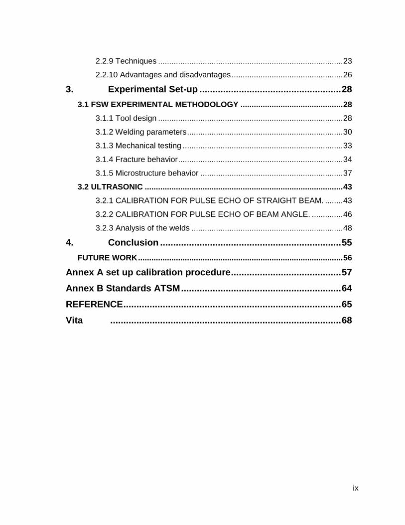
2.2.9 Techniques ................................................................................... 23

2.2.10 Advantages and disadvantages .................................................. 26

3. Experimental Set-up ...................................................... 28

3.1 FSW EXPERIMENTAL METHODOLOGY .............................................. 28

3.1.1 Tool design ................................................................................... 28

3.1.2 Welding parameters ...................................................................... 30

3.1.3 Mechanical testing ........................................................................ 33

3.1.4 Fracture behavior .......................................................................... 34

3.1.5 Microstructure behavior ................................................................ 37

3.2 ULTRASONIC ......................................................................................... 43

3.2.1 CALIBRATION FOR PULSE ECHO OF STRAIGHT BEAM. ........ 43

3.2.2 CALIBRATION FOR PULSE ECHO OF BEAM ANGLE. .............. 46

3.2.3 Analysis of the welds .................................................................... 48

4. Conclusion ..................................................................... 55

FUTURE WORK ............................................................................................ 56

Annex A set up calibration procedure .......................................... 57

Annex B Standards ATSM ............................................................. 64

REFERENCE ................................................................................... 65

Vita ........................................................................................ 68

x

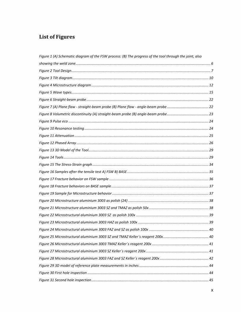
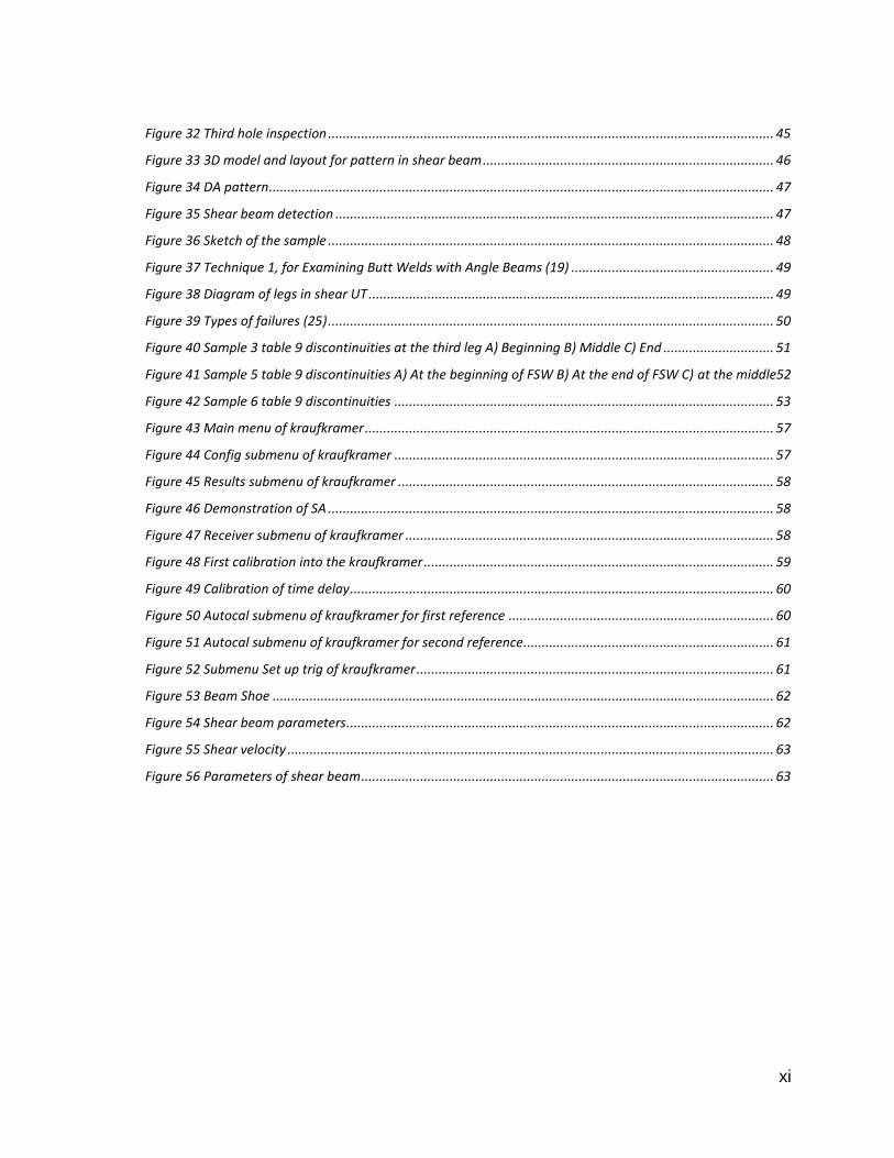
List of Figures

Figure 1 (A) Schematic diagram of the FSW process: (B) The progress of the tool through the joint, also

showing the weld zone........................................................................................................................................ 6

Figure 2 Tool Design ............................................................................................................................................ 7

Figure 3 Tilt diagram ......................................................................................................................................... 10

Figure 4 Microstructure diagram ...................................................................................................................... 12

Figure 5 Wave types.......................................................................................................................................... 15

Figure 6 Straight-beam probe ........................................................................................................................... 22

Figure 7 (A) Plane flaw - straight-beam probe (B) Plane flaw - angle-beam probe .......................................... 22

Figure 8 Volumetric discontinuity (A) straight-beam probe (B) angle-beam probe .......................................... 23

Figure 9 Pulse eco ............................................................................................................................................. 24

Figure 10 Resonance testing ............................................................................................................................. 24

Figure 11 Attenuation ....................................................................................................................................... 25

Figure 12 Phased Array ..................................................................................................................................... 26

Figure 13 3D Model of the Tool......................................................................................................................... 29

Figure 14 Tools .................................................................................................................................................. 29

Figure 15 The Stress-Strain graph ..................................................................................................................... 34

Figure 16 Samples after the tensile test A) FSW B) BASE .................................................................................. 35

Figure 17 Fracture behavior on FSW sample .................................................................................................... 36

Figure 18 Fracture behaviors on BASE sample .................................................................................................. 37

Figure 19 Sample for Microstructure behavior ................................................................................................. 37

Figure 20 Microstructure aluminium 3003 as polish (24) ................................................................................. 38

Figure 21 Microstructure aluminium 3003 SZ and TMAZ as polish 50x ............................................................ 38

Figure 22 Microstructural aluminium 3003 SZ as polish 100x ......................................................................... 39

Figure 23 Microstructural aluminium 3003 HAZ as polish 100x ....................................................................... 39

Figure 24 Microstructural aluminium 3003 FAZ and SZ as polish 100x ............................................................ 40

Figure 25 Microstructural aluminium 3003 SZ and TMAZ Keller´s reagent 200x .............................................. 40

Figure 26 Microstructural aluminium 3003 TMAZ Keller´s reagent 200x ......................................................... 41

Figure 27 Microstructural aluminium 3003 SZ Keller´s reagent 200x ............................................................... 41

Figure 28 Microstructural aluminium 3003 FAZ and SZ Keller´s reagent 200x ................................................. 42

Figure 29 3D model of reference plate measurements in inches ...................................................................... 44

Figure 30 First hole inspection .......................................................................................................................... 44

Figure 31 Second hole inspection ...................................................................................................................... 45

xi

Figure 32 Third hole inspection ......................................................................................................................... 45

Figure 33 3D model and layout for pattern in shear beam ............................................................................... 46

Figure 34 DA pattern ......................................................................................................................................... 47

Figure 35 Shear beam detection ....................................................................................................................... 47

Figure 36 Sketch of the sample ......................................................................................................................... 48

Figure 37 Technique 1, for Examining Butt Welds with Angle Beams (19) ....................................................... 49

Figure 38 Diagram of legs in shear UT .............................................................................................................. 49

Figure 39 Types of failures (25) ......................................................................................................................... 50

Figure 40 Sample 3 table 9 discontinuities at the third leg A) Beginning B) Middle C) End .............................. 51

Figure 41 Sample 5 table 9 discontinuities A) At the beginning of FSW B) At the end of FSW C) at the middle52

Figure 42 Sample 6 table 9 discontinuities ....................................................................................................... 53

Figure 43 Main menu of kraufkramer ............................................................................................................... 57

Figure 44 Config submenu of kraufkramer ....................................................................................................... 57

Figure 45 Results submenu of kraufkramer ...................................................................................................... 58

Figure 46 Demonstration of SA ......................................................................................................................... 58

Figure 47 Receiver submenu of kraufkramer .................................................................................................... 58

Figure 48 First calibration into the kraufkramer ............................................................................................... 59

Figure 49 Calibration of time delay ................................................................................................................... 60

Figure 50 Autocal submenu of kraufkramer for first reference ........................................................................ 60

Figure 51 Autocal submenu of kraufkramer for second reference.................................................................... 61

Figure 52 Submenu Set up trig of kraufkramer ................................................................................................. 61

Figure 53 Beam Shoe ........................................................................................................................................ 62

Figure 54 Shear beam parameters .................................................................................................................... 62

Figure 55 Shear velocity .................................................................................................................................... 63

Figure 56 Parameters of shear beam ................................................................................................................ 63

xii

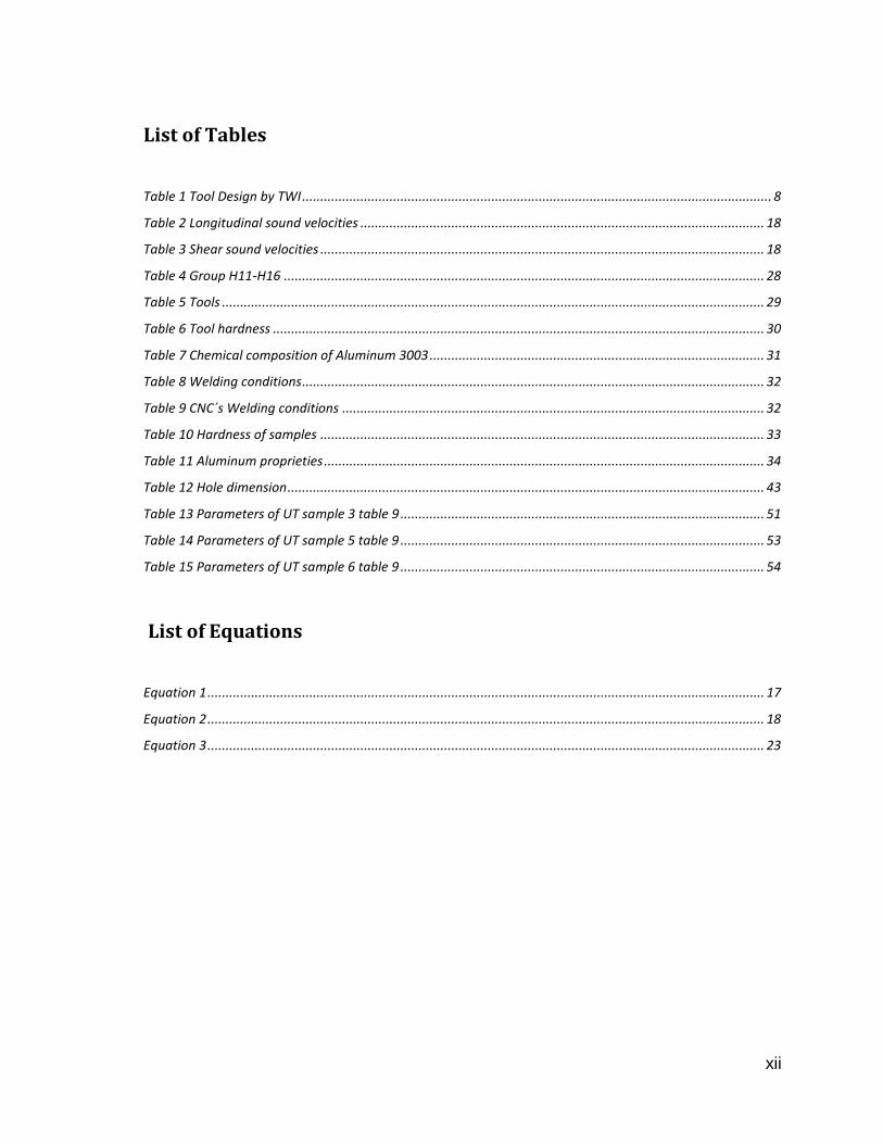
List of Tables

Table 1 Tool Design by TWI ................................................................................................................................. 8

Table 2 Longitudinal sound velocities ............................................................................................................... 18

Table 3 Shear sound velocities .......................................................................................................................... 18

Table 4 Group H11-H16 .................................................................................................................................... 28

Table 5 Tools ..................................................................................................................................................... 29

Table 6 Tool hardness ....................................................................................................................................... 30

Table 7 Chemical composition of Aluminum 3003 ............................................................................................ 31

Table 8 Welding conditions ............................................................................................................................... 32

Table 9 CNC´s Welding conditions .................................................................................................................... 32

Table 10 Hardness of samples .......................................................................................................................... 33

Table 11 Aluminum proprieties ......................................................................................................................... 34

Table 12 Hole dimension ................................................................................................................................... 43

Table 13 Parameters of UT sample 3 table 9 .................................................................................................... 51



List of Equations

Equation 1 ......................................................................................................................................................... 17

Equation 2 ......................................................................................................................................................... 18

Equation 3 ......................................................................................................................................................... 23

1

1. Introduction

1.1 Friction-stir welding (FSW)

Friction-stir welding (FSW) is a solid-state joining process (meaning the metal

is not melted during the process) and is used for applications where the original

metal characteristics must remain unchanged as far as possible. This process is

primarily used on aluminum, and most often on large pieces which cannot be

easily heat treated post weld to recover temper characteristics. It was invented

and experimentally proven by Wayne Thomas and a team of his colleagues at The

Welding Institute (TWI) UK in December 1991. TWI holds a number of patents on

the process, the first being the most descriptive (1).

The method is based on the forged aluminum components without the

temperature exceeds the melting point of the material. This is achieved by using of

a rotating tool moving along the board uniting components by setting. After curing,

the junctions are free from tensions greatly and offer an area perfect union

because the welding was carried out from a side. Thus the need for additional work

is reduced to least. Using this method, the full board is only formed by the original

material, no filler material and impurities.

Application areas suitable for FSW • Shipbuilding. • Offshore oil platforms. • Aerospace. • Rail wagons, trams, underground trains. • Automotive industry. • Brewing Industry. • Construction of bridges. • Production of electric motors. • Defense industry. • Elements of cooling.

2

1.2 Non Destructive Evaluation

The NDE are trials or non-destructive testing, which are made to materials, be

they metals, plastics (polymers), ceramics or composites. (2) Such trials generally

used to determine certain physical or chemical property of the material in question.

The main applications are found in the NDE:

• Detection of discontinuities (internal and surface). • Determination of chemical composition. • Leak detection. • Measurement of thickness and corrosion monitoring. • Adhesion between materials. • Inspection of welded joints.

The NDE are very important in the continued industrial development. Thanks to

them is possible, for example, determine the presence of defects in materials or

welds equipment such as pressure vessels, where catastrophic failure can

represent huge losses in money, human life and damage to the environment. The

ultrasonic test is based on the generation, propagation and detection of elastic

waves through the materials (3).

The sound or vibration, in the form of elastic waves, propagates through the

material until it completely loses its intensity or until encounters an interface,

namely some other material such as air or water and, consequently, waves can

undergo reflection, refraction, distortions. This can result in a change in intensity,

direction and angle of wave propagation original.

Thus, it is possible to apply the method of ultrasound to determine certain

characteristics of materials such as:

• Speed of wave propagation. • Grain size in metals. • Presence of discontinuities (cracks, pores, laminations, etc.). • Adhesion between materials. • Weld Inspection. • Measurement of wall thickness.

As can be seen with the ultrasound method is possible to obtain an assessment

of the internal condition of the material in question. However, the ultrasound

3

method is more complex in practice than theory, which requires trained personnel

for implementation and interpretation of signs or test results (4).

1.3 MOTIVATION

In regard to the FSW is a very recent technology no more than 20 years, so

there is a wide range of work to develop new methods and processes, which

means you have an opportunity to contribute to the analysis of this system welding

to be increasingly employed in the industry but has many uses.

In today's world we have different ways to get the data to determine the flaws in

the material, but the preventive study materials before they fail is a world explored

but is not highly developed, usually when some part fails is when for the error and

corrected, in contrast with non-destructive tests can be done a study preventive

and detect faults before they occur.

1.4 OBJETIVE

The objective of this work is to determine the value of the parameters in

operation on the Friction Stir Welding, such as transverse speed, rotational speed,

load applied and tool design, affect the friction stir welding. For this purpose

different samples with different welding parameters were used to achieve a

functional weldment, which were inspected by ultrasonic testing.

Welded materials present changes in the microstructures respect to original

plates. Through these features is possible to observe internal defects but it is

necessary to destroy the joined sample and it only shows features of a plane.

It is intended that the Ultrasonic Testing can provide the flaws that occur on the

weld and its location without having to destroy the sample, because the UT lets us

to examinate completely the welded and affected zone along longitudinal axe of a

non-destructive way.

4

1.5 CONTRIBUTION

If successful in research and build the prototype for the test, the laboratory will

be expanded. Be recognized that the error is occurring in the micro-structure.

Knowledge of the rules may help reduce the time requested. Since that show

how the material is affected from a different point of view that is currently done in

laboratories.

1.6 TECHNOLOGY TRENDS

Currently within the technology for nondestructive testing has been increasing

throughout the aerospace industry, since most of the time these faults are

undetectable, which makes preventive maintenance in the aerospace industry to

address failures to identify micro structure (5).

Considering these points and facing the trend of not being able to wait until

problems arise from failures to stop macro metric for the exchange of parts needed

to obtain a common and easiest method to have a broader preventive

maintenance.

Friction stir welding technology has been a major boon to industry advanced

since its inception. In spite of its short history, it has found widespread applications

in diverse industries. Hard materials such as steel and other important engineering

alloys can now be welded efficiently using this process.

Significant progress has also been made in the fundamental understanding of

both the welding process and the structure and properties of the welded joints. The

understanding has been useful in reducing defects and improving uniformity of

weld properties and, at the same time, expanding the applicability of FSW to new

engineering alloys. With better quantitative understanding of the underlying

principles of heat transfer, material flow, tool-work–piece contact conditions and

effects of various process parameters, efficient tools have been devised. At the

current pace of development, FSW is likely to be more widely applied in the future.

5

2. Literature Survey

2.1 Friction Stir Welding

There are around 2000 patents on FSW of which is searched to find those that

affect the issue proposed for greater scope and understanding of welding by this

method (6).

There are several magazines published on materials, there is specializing in

what is solder, which were obtained some items of this section of research to find

the data and understanding of the FSW.

According to the patents found there are several devices to the FSW, at which

sought to make a design according to the literature found to obtain samples for

characterization.

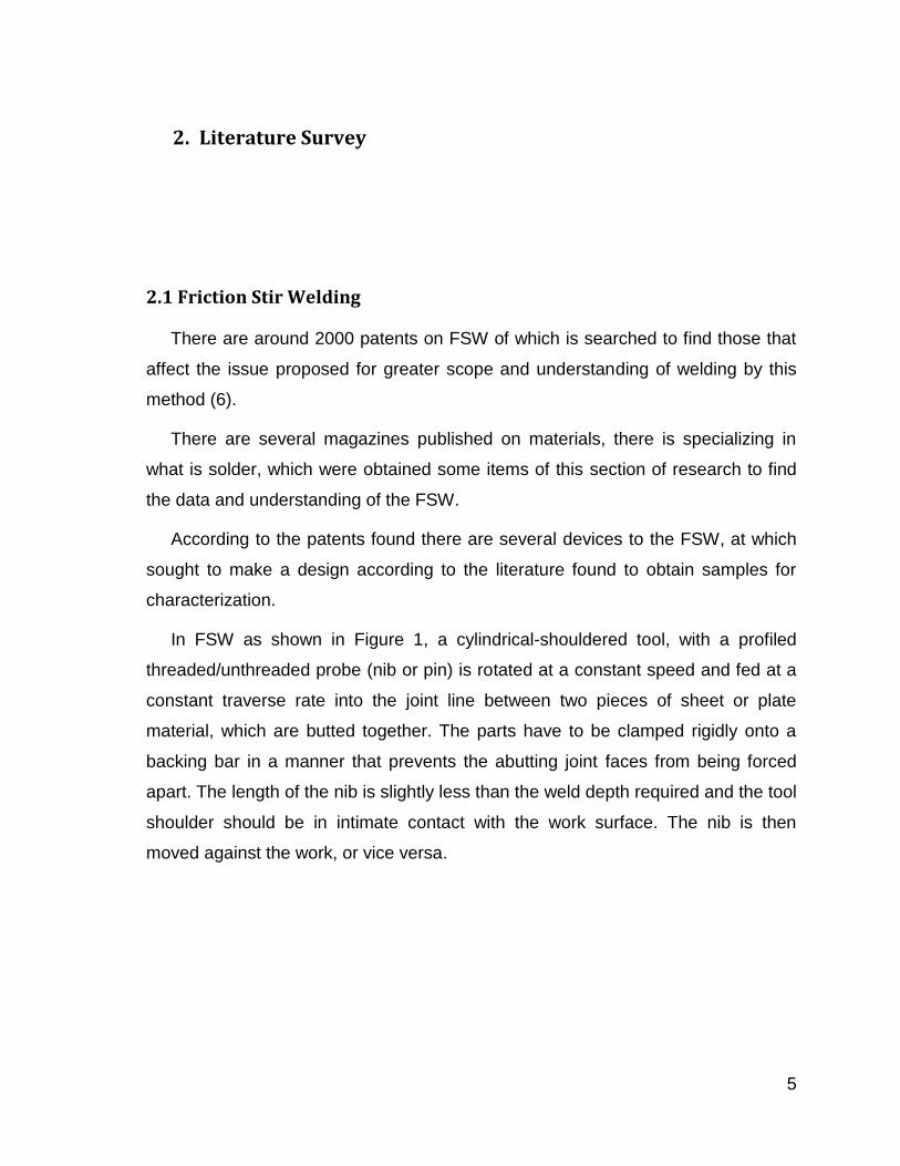
In FSW as shown in Figure 1, a cylindrical-shouldered tool, with a profiled

threaded/unthreaded probe (nib or pin) is rotated at a constant speed and fed at a

constant traverse rate into the joint line between two pieces of sheet or plate

material, which are butted together. The parts have to be clamped rigidly onto a

backing bar in a manner that prevents the abutting joint faces from being forced

apart. The length of the nib is slightly less than the weld depth required and the tool

shoulder should be in intimate contact with the work surface. The nib is then

moved against the work, or vice versa.

6

Figure 1 (A) Schematic diagram of the FSW process: (B) The progress of the tool through the joint, also showing the weld zone

Frictional heat is generated between the wear-resistant welding tool shoulder

and nib, and the material of the work pieces. This heat, along with the heat

generated by the mechanical mixing process and the adiabatic heat within the

material, cause the stirred materials to soften without reaching the melting point

allowing the traversing of the tool along the weld line in a plasticized tubular shaft

of metal.

This heat causes the latter to soften without reaching the melting point and

allows traversing of the tool along the weld line. The plasticized material is

transferred from the leading edge of the tool to the trailing edge of the tool probe

and is forged by the intimate contact of the tool shoulder and the pin profile. It

leaves a solid phase bond between the two pieces. The process can be regarded

as a solid phase keyhole welding technique since a hole to accommodate the

probe is generated, then filled during the welding sequence (6).

As the pin is moved in the direction of welding, the leading face of the pin,

assisted by a special pin profile, forces plasticized material to the back of the pin

while applying a substantial forging force to consolidate the weld metal. The

welding of the material is facilitated by severe plastic deformation in the solid state,

involving dynamic recrystallization of the base material (7).

7

2.1.1 Tool Design

The design of the tool is a critical factor as a good tool can improve both the

quality of the weld and the maximum possible welding speed.

It is desirable that the tool material is sufficiently strong, tough and hard

wearing, at the welding temperature. Further it should have a good oxidation

resistance and a low thermal conductivity to minimize heat loss and thermal

damage to the machinery further up the drive train. Hot-worked tool steel such as

AISI H12 has proven perfectly acceptable for welding aluminum alloys within

thickness ranges of 0.5 – 50 mm (8) but more advanced tool materials are

necessary for more demanding applications such as highly abrasive metal matrix

composites or higher melting point materials such as steel or titanium.

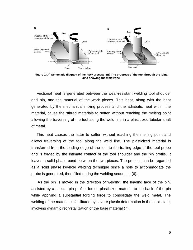
The majority of tools have a concave shoulder profile which acts as an escape

volume for the material displaced by the pin, prevents material from extruding out

of the sides of the shoulder and maintains downwards pressure and hence good

forging of the material behind the tool as shown in Figure 2.

Figure 2 Tool Design

Tool design influences heat generation, plastic flow, the power required, and the

uniformity of the welded joint. The shoulder generates most of the heat and

prevents the plasticized material from escaping from the work–piece, while both

the shoulder and the tool–pin affect the material flow.

Improvements in tool design have been shown to cause substantial

improvements in productivity and quality. TWI has developed tools specifically

designed to increase the depth of penetration and so increase the plate thickness

8

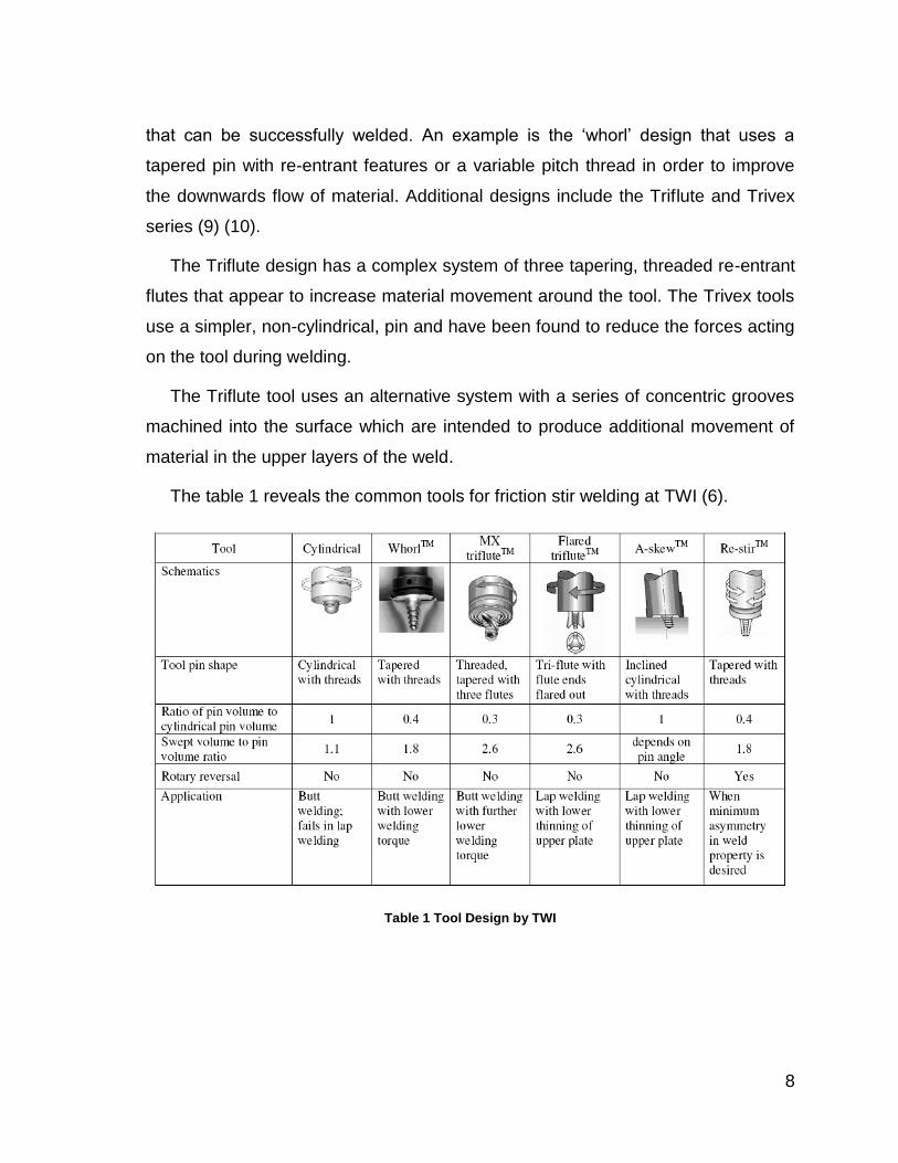
that can be successfully welded. An example is the ‘whorl’ design that uses a

tapered pin with re-entrant features or a variable pitch thread in order to improve

the downwards flow of material. Additional designs include the Triflute and Trivex

series (9) (10).

The Triflute design has a complex system of three tapering, threaded re-entrant

flutes that appear to increase material movement around the tool. The Trivex tools

use a simpler, non-cylindrical, pin and have been found to reduce the forces acting

on the tool during welding.

The Triflute tool uses an alternative system with a series of concentric grooves

machined into the surface which are intended to produce additional movement of

material in the upper layers of the weld.

The table 1 reveals the common tools for friction stir welding at TWI (6).

Table 1 Tool Design by TWI

9

2.1.2 Welding forces

During welding a number of forces will act on the tool:

A downwards force is necessary to maintain the position of the tool at or

below the material surface. Some friction-stir welding machines operate

under load control but in many cases the vertical position of the tool are

preset and so the load will vary during welding.

The traverse force acts parallel to the tool motion and is positive in the

traverse direction. Since this force arises as a result of the resistance of the

material to the motion of the tool it might be expected that this force will

decrease as the temperature of the material around the tool is increased.

The lateral force may act perpendicular to the tool traverse direction and is

defined here as positive towards the advancing side of the weld.

Torque is required to rotate the tool, the amount of which will depend on the

down force and friction coefficient (sliding friction) and/or the flow strength of

the material in the surrounding region (sticking friction).

In order to prevent tool fracture and to minimize excessive wear and tear on the

tool and associated machinery, the welding cycle should be modified so that the

forces acting on the tool are as low as possible.

There are two tool speeds to be considered in friction-stir welding; how fast the

tool rotates and how quickly it traverses the interface. These two parameters have

considerable importance and must be chosen with care to ensure a successful and

efficient welding cycle. The relationship between the welding speeds and the heat

input during welding is complex but, in general, it can be said that increasing the

rotation speed or decreasing the traverse speed will result in a hotter weld. In order

to produce a successful weld it is necessary that the material surrounding the tool

is hot enough to enable the extensive plastic flow required and minimize the forces

acting on the tool. If the material is too cool then voids or other flaws may be

present in the stir zone and in extreme cases the tool may break.

10

At the other end of the scale excessively high heat input may be detrimental to

the final properties of the weld. Theoretically, this could even result in defects due

to the liquation of low-melting-point phases.

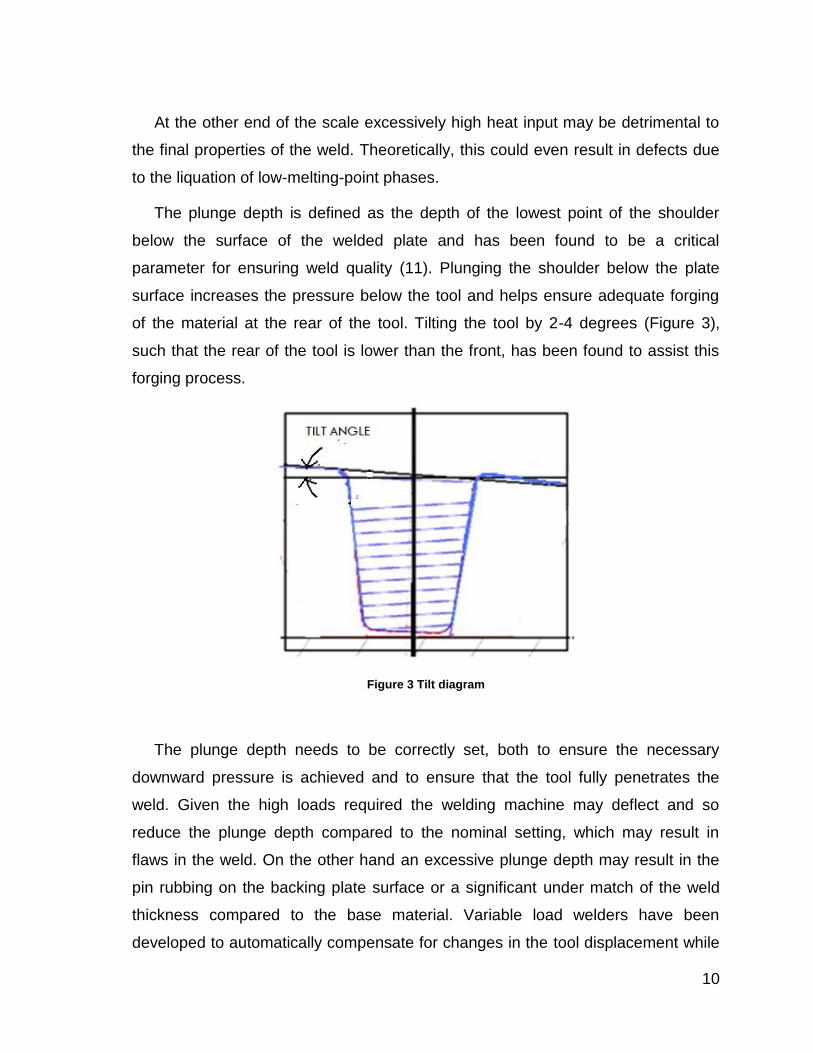
The plunge depth is defined as the depth of the lowest point of the shoulder

below the surface of the welded plate and has been found to be a critical

parameter for ensuring weld quality (11). Plunging the shoulder below the plate

surface increases the pressure below the tool and helps ensure adequate forging

of the material at the rear of the tool. Tilting the tool by 2-4 degrees (Figure 3),

such that the rear of the tool is lower than the front, has been found to assist this

forging process.

Figure 3 Tilt diagram

The plunge depth needs to be correctly set, both to ensure the necessary

downward pressure is achieved and to ensure that the tool fully penetrates the

weld. Given the high loads required the welding machine may deflect and so

reduce the plunge depth compared to the nominal setting, which may result in

flaws in the weld. On the other hand an excessive plunge depth may result in the

pin rubbing on the backing plate surface or a significant under match of the weld

thickness compared to the base material. Variable load welders have been

developed to automatically compensate for changes in the tool displacement while

11

TWI has demonstrated a roller system that maintains the tool position above the

weld plate.

2.1.3 Microstructure features

The solid-state nature of the FSW process, combined with its unusual tool and

asymmetric nature, results in a highly characteristic microstructure. The

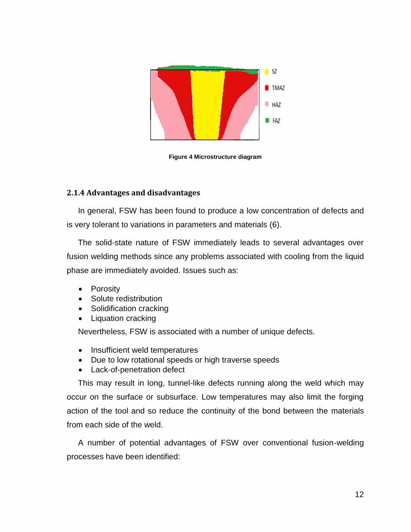
microstructure can be broken up into the following zones (Figure 4):

The stir zone (SZ) is a region of heavily deformed material that roughly

corresponds to the location of the pin during welding. The grains within the

stir zone are roughly equiaxed and often an order of magnitude smaller than

the grains in the parent material. The precise origin of these rings has not

been firmly established.

The flow arm zone (FAZ) is on the upper surface of the weld and consists of

material that is dragged by the shoulder from the retreating side of the weld,

around the rear of the tool, and deposited on the advancing side.

The thermo-mechanically affected zone (TMAZ) occurs on either side of the

stir zone. In this region the strain and temperature are lower and the effect

of welding on the microstructure is correspondingly smaller. Unlike the stir

zone the microstructure is recognizably that of the parent material, albeit

significantly deformed and rotated. Although the term TMAZ technically

refers to the entire deformed region it is often used to describe any region

not already covered by the terms stir zone and flow arm.

The heat-affected zone (HAZ) is common to all welding processes. As

indicated by the name, this region is subjected to a thermal cycle but is not

deformed during welding. The temperatures are lower than those in the

TMAZ but may still have a significant effect if the microstructure is thermally

unstable. In fact, in age-hardened aluminum alloys this region commonly

exhibits the poorest mechanical properties (12).

12

Figure 4 Microstructure diagram

2.1.4 Advantages and disadvantages

In general, FSW has been found to produce a low concentration of defects and

is very tolerant to variations in parameters and materials (6).

The solid-state nature of FSW immediately leads to several advantages over

fusion welding methods since any problems associated with cooling from the liquid

phase are immediately avoided. Issues such as:

Porosity

Solute redistribution

Solidification cracking

Liquation cracking

Nevertheless, FSW is associated with a number of unique defects.

Insufficient weld temperatures

Due to low rotational speeds or high traverse speeds

Lack-of-penetration defect

This may result in long, tunnel-like defects running along the weld which may

occur on the surface or subsurface. Low temperatures may also limit the forging

action of the tool and so reduce the continuity of the bond between the materials

from each side of the weld.

A number of potential advantages of FSW over conventional fusion-welding

processes have been identified:

13

1. Good mechanical properties in the as welded condition 2. Improved safety due to the absence of toxic fumes or the spatter of molten

material. 3. No consumables - A pin made of conventional steel can weld over 1000m of

aluminum and no filler or gas shield is required for aluminum. (13) 4. Easily automated on simple milling machines - lower setup costs and less

training. 5. Can operate in all positions (horizontal, vertical, etc.), as there is no weld

pool. 6. Generally good weld appearance and minimal thickness under/over-

matching, thus reducing the need for expensive machining after welding. 7. Low environmental impact.

However, some disadvantages of the process have been identified:

Exit hole left when tool is withdrawn.

Large down forces required with heavy-duty clamping necessary to hold the plates together.

Less flexible than manual and arc processes (difficulties with thickness variations and non-linear welds).

Often slower traverse rate than some fusion welding techniques although this may be offset if fewer welding passes are required.

2.2 Ultrasonic

NDT has been practiced for many decades, with initial rapid developments in

instrumentation spurred by the technological advances that occurred during World

War II and the subsequent defense effort. During the earlier days, the primary

purpose was the detection of defects. As a part of "safe life" design, it was

intended that a structure should not develop macroscopic defects during its life,

with the detection of such defects being a cause for removal of the component

from service. In response to this need, increasingly sophisticated techniques using

ultrasonic, eddy currents, x-rays, dye penetrate, magnetic particles, and other

forms of interrogating energy emerged.

In the early 1970's, two events occurred which caused a major change in the

NDT field. First, improvements in the technology led to the ability to detect small

flaws, which caused more parts to be rejected even though the probability of

component failure had not changed. However, the discipline of fracture mechanics

14

emerged, which enabled one to predict whether a crack of a given size will fail

under a particular load when a material has fracture toughness properties are

known. Other laws were developed to predict the growth rate of cracks under cyclic

loading (fatigue). With the advent of these tools, it became possible to accept

structures containing defects if the sizes of those defects were known. This formed

the basis for the new philosophy of "damage tolerant" design. Components having

known defects could continue in service as long as it could be established that

those defects would not grow to a critical, failure producing size (14).

Many ultrasonic flaw detectors have a trigonometric function that allows for fast

and accurate location determination of flaws when performing shear wave

inspections. Cathode ray tubes, for the most part, have been replaced with LED or

LCD screens. These screens, in most cases, are extremely easy to view in a wide

range of ambient lighting. Bright or low light working conditions encountered by

technicians have little effect on the technician's ability to view the screen. Screens

can be adjusted for brightness, contrast, and on some instruments even the color

of the screen and signal can be selected. Transducers can be programmed with

predetermined instrument settings. The operator only has to connect the

transducer and the instrument will set variables such as frequency and probe drive.

Along with computers, motion control and robotics have contributed to the

advancement of ultrasonic inspections. Early on, the advantage of a stationary

platform was recognized and used in industry. Computers can be programmed to

inspect large, complex shaped components, with one or multiple transducers

collecting information. Automated systems typically consisted of an immersion

tank, scanning system, and recording system for a printout of the scan.

2.2.1 Wave Propagation

UT is based on time-varying deformations or vibrations in materials, which is

generally referred to as acoustics. All material substances are comprised of atoms,

which may be forced into vibration motion about their equilibrium positions. Many

15

different patterns of vibration motion exist at the atomic level; however, most are

irrelevant to acoustics and ultrasonic testing.

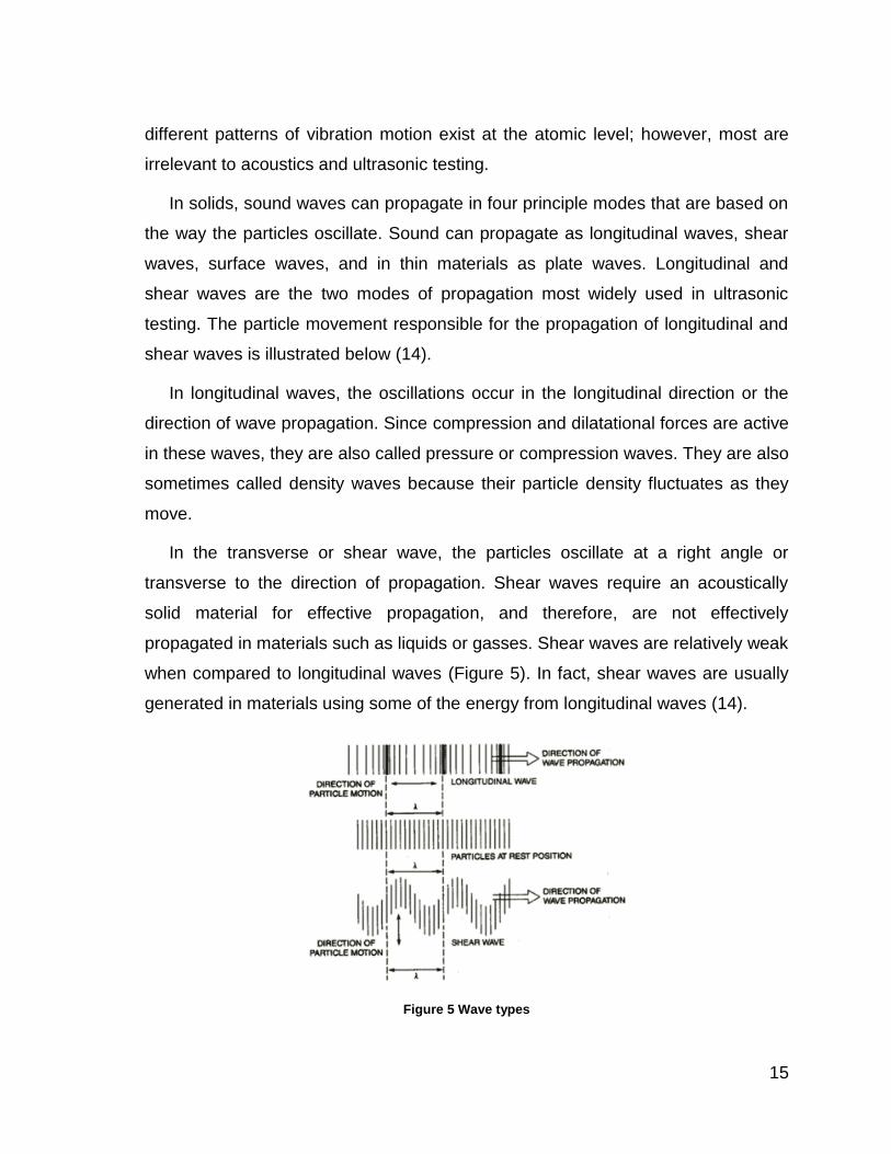
In solids, sound waves can propagate in four principle modes that are based on

the way the particles oscillate. Sound can propagate as longitudinal waves, shear

waves, surface waves, and in thin materials as plate waves. Longitudinal and

shear waves are the two modes of propagation most widely used in ultrasonic

testing. The particle movement responsible for the propagation of longitudinal and

shear waves is illustrated below (14).

In longitudinal waves, the oscillations occur in the longitudinal direction or the

direction of wave propagation. Since compression and dilatational forces are active

in these waves, they are also called pressure or compression waves. They are also

sometimes called density waves because their particle density fluctuates as they

move.

In the transverse or shear wave, the particles oscillate at a right angle or

transverse to the direction of propagation. Shear waves require an acoustically

solid material for effective propagation, and therefore, are not effectively

propagated in materials such as liquids or gasses. Shear waves are relatively weak

when compared to longitudinal waves (Figure 5). In fact, shear waves are usually

generated in materials using some of the energy from longitudinal waves (14).

Figure 5 Wave types

2.2.2 The Speed of Sound

Hooke's Law, when used along with Newton's Second Law, can explain a few

things about the speed of sound. The speed of sound within a material is a function

of the properties of the material and is independent of the amplitude of the sound

wave. Newton's Second Law says that the force applied to a particle will be

balanced by the particle's mass and the acceleration of the particle.

Mathematically, Newton's Second Law is written as F = m * a Hooke's Law then

says that this force will be balanced by a force in the opposite direction that is

dependent on the amount of displacement and the spring constant F = -k * x

therefore, since the applied force and the restoring force are equal, m * a = -k * x

can be written. The negative sign indicates that the force is in the opposite

direction (15).

Since the mass m and the spring constant k are constants for any given

material, it can be seen that the acceleration a and the displacement x are the only

variables. It can also be seen that they are directly proportional. For instance, if the

displacement of the particle increases, so does its acceleration. It turns out that the

time that it takes a particle to move and return to its equilibrium position is

independent of the force applied. So, within a given material, sound always travels

at the same speed no matter how much force is applied when other variables, such

as temperature, are held constant.

2.2.3 Properties of material affect

Of course, sound does travel at different speeds in different materials. This is

because the mass of the atomic particles and the spring constants are different for

different materials. The mass of the particles is related to the density of the

material, and the spring constant is related to the elastic constants of a material.

The general relationship between the speed of sound in a solid and its density and

elastic constants is given by the following equation:

16

Where V is the speed of sound, C is the elastic constant, and p is the material

density. This equation may take a number of different forms depending on the type

of wave (longitudinal or shear) and which of the elastic constants that are used

(15).

The typical elastic constants of materials include:

• Young's Modulus, E: a proportionality constant between uniaxial stress and strain.

• Poisson's Ratio, n: the ratio of radial strain to axial strain • Bulk modulus, K: a measure of the incompressibility of a body subjected to

hydrostatic pressure. • Shear Modulus, G: also called rigidity, a measure of a substance's

resistance to shear. • Lame's Constants, l and m: material constants that are derived from

Young's Modulus and Poisson's Ratio.

When calculating the velocity of a longitudinal wave, Young's Modulus and

Poisson's Ratio are commonly used. When calculating the velocity of a shear

wave, the shear modulus is used. It is often most convenient to make the

calculations using Lame's Constants, which are derived from Young's Modulus and

Poisson's Ratio.

It must also be mentioned that the subscript ij attached to C in the above

equation is used to indicate the directionality of the elastic constants with respect to

the wave type and direction of wave travel. In isotropic materials, the elastic

constants are the same for all directions within the material. However, most

materials are anisotropic and the elastic constants differ with each direction. For

example, in a piece of rolled aluminum plate, the grains are elongated in one

direction and compressed in the others and the elastic constants for the

longitudinal direction are different than those for the transverse or short transverse

directions.

17

Equation 1

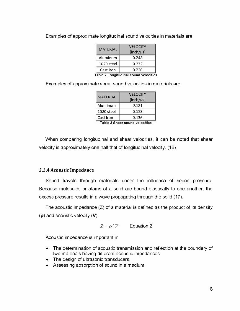
Examples of approximate longitudinal sound velocities in materials are:

VELOCITY MATERIAL

VELOCITY MATERIAL

(inch/u.s) (inch/u.s)

Aluminum 0.248

1020 steel 0.232

Cast iron 0.220 Table 2 Longitudinal sound velocities

Examples of approximate shear sound velocities in materials are:

VELOCITY MATERIAL

VELOCITY MATERIAL

(inch/u.s) (inch/u.s)

Aluminum 0.121

1020 steel 0.128

Cast iron 0.136 Table 3 Shear sound velocities

When comparing longitudinal and shear velocities, it can be noted that shear

velocity is approximately one half that of longitudinal velocity. (16)

2.2.4 Acoustic Impedance

Sound travels through materials under the influence of sound pressure.

Because molecules or atoms of a solid are bound elastically to one another, the

excess pressure results in a wave propagating through the solid (17).

The acoustic impedance (Z) of a material is defined as the product of its density

(p) and acoustic velocity (V).

Z = p*V Equation 2

Acoustic impedance is important in

• The determination of acoustic transmission and reflection at the boundary of two materials having different acoustic impedances.

• The design of ultrasonic transducers. • Assessing absorption of sound in a medium.

18

19

2.2.5 Frequency

Each ultrasonic operational frequency has its own unique characteristics. These

characteristics can be used to determine which frequencies might be best suited to

a given application (18).

Ultrasonic testing involves frequencies of 500 KHz to 20 MHz, although higher

and lower frequencies (> 20 KHz) are also used.

2.2.6 Couplant

Couplant, usually a liquid or semi liquid, is required between the face of the

search unit and the examination surface to permit the transmission of ultrasonic

waves from the search unit into the material under examination. Typical couplants

include glycerin, water, cellulose gel, oil, water-soluble oils, and grease (19).

2.2.7 Calibration

Calibration refers to the act of evaluating and adjusting the precision and

accuracy of measurement equipment. In ultrasonic testing, several forms of

calibration must occur. First, the electronics of the equipment must be calibrated to

ensure that they are performing as designed. This operation is usually performed

by the equipment manufacturer and will not be discussed further in this material. It

is also usually necessary for the operator to perform a "user calibration" of the

equipment. This user calibration is necessary because most ultrasonic equipment

can be reconfigured for use in a large variety of applications. The user must

"calibrate" the system, which includes the equipment settings, the transducer, and

the test setup, to validate that the desired level of precision and accuracy are

achieved. The term calibration standard is usually only used when an absolute

value is measured and in many cases, the standards are traceable back to

standards at the National Institute for Standards and Technology (14).

20

In ultrasonic testing, there is also a need for reference standards. Reference

standards are used to establish a general level of consistency in measurements

and to help interpret and quantify the information contained in the received signal.

Reference standards are used to validate that the equipment and the setup provide

similar results from one day to the next and that similar results are produced by

different systems. Reference standards also help the inspector to estimate the size

of flaws. In a pulse-echo type setup, signal strength depends on both the size of

the flaw and the distance between the flaw and the transducer. The inspector can

use a reference standard with an artificially induced flaw of known size and at

approximately the same distance away for the transducer to produce a signal. By

comparing the signal from the reference standard to that received from the actual

flaw, the inspector can estimate the flaw size.

2.2.8 Wavelength and Defect Detection

In ultrasonic testing, the inspector must make a decision about the frequency of

the transducer that will be used. As we learned on the previous page, changing the

frequency when the sound velocity is fixed will result in a change in the wavelength

of the sound. The wavelength of the ultrasound used has a significant effect on the

probability of detecting a discontinuity. A general rule of thumb is that a

discontinuity must be larger than one-half the wavelength to stand a reasonable

chance of being detected.

Sensitivity and resolution are two terms that are often used in ultrasonic

inspection to describe a technique's ability to locate flaws. Sensitivity is the ability

to locate small discontinuities. Sensitivity generally increases with higher frequency

(shorter wavelengths). Resolution is the ability of the system to locate

discontinuities that are close together within the material or located near the part

surface. Resolution also generally increases as the frequency increases (20).

The wave frequency can also affect the capability of an inspection in adverse

ways. Therefore, selecting the optimal inspection frequency often involves

21

maintaining a balance between the favorable and unfavorable results of the

selection. Before selecting an inspection frequency, the material's grain structure

and thickness, and the discontinuity's type, size, and probable location should be

considered. As frequency increases, sound tends to scatter from large or course

grain structure and from small imperfections within a material. Cast materials often

have coarse grains and other sound scatters that require lower frequencies to be

used for evaluations of these products. Wrought and forged products with

directional and refined grain structure can usually be inspected with higher

frequency transducers.

Since more things in a material are likely to scatter a portion of the sound

energy at higher frequencies, the penetrating power (or the maximum depth in a

material that flaws can be located) is also reduced. Frequency also has an effect

on the shape of the ultrasonic beam. Beam spread, or the divergence of the beam

from the center axis of the transducer, and how it is affected by frequency will be

discussed later.

It should be mentioned, so as not to be misleading, that a number of other

variables will also affect the ability of ultrasound to locate defects. These include

the pulse length, type and voltage applied to the crystal, properties of the crystal,

backing material, transducer diameter, and the receiver circuitry of the instrument.

2.2.8 Detection of discontinuities

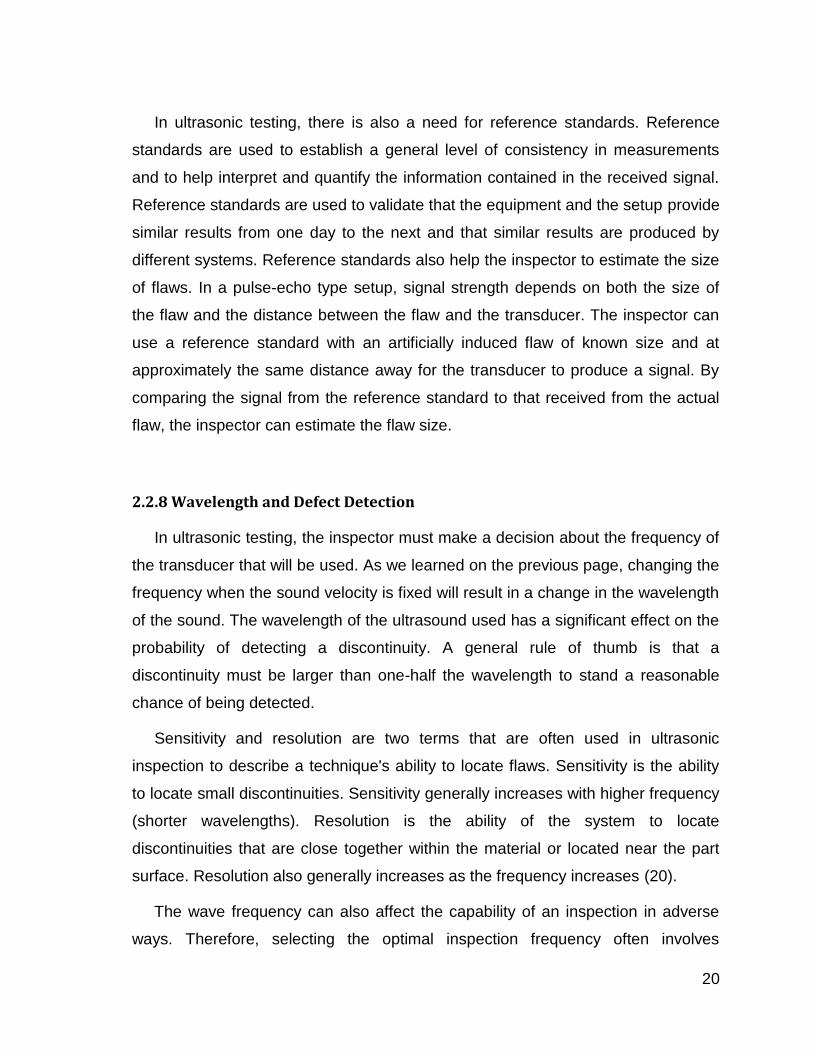
The essential "tool" for the ultrasonic operator is the probe, the piezoelectric

element, excited by an extremely short electrical discharge, transmits an ultrasonic

pulse (Figure 6). The same element on the other hand generates an electrical

signal when it receives an ultrasonic signal thus causing it to oscillate. The probe is

coupled to the surface of the test object with a liquid or coupling paste so that the

sound waves from the probe are able to be transmitted into the test object (16).

22

Figure 6 Straight-beam probe

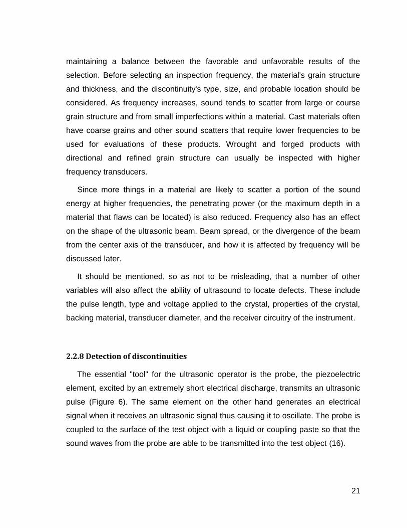
The operator then scans the test object into different types of probes such as

longitudinal waves in straight beam probe and shear waves in the angle beam

probe (Figure 7).

Figure 7 (A) Plane flaw - straight-beam probe (B) Plane flaw - angle-beam probe

The operator moves the probe evenly to and fro across the surface. In doing

this, he observes an instrument display for any signals caused by reflections from

internal discontinuities.

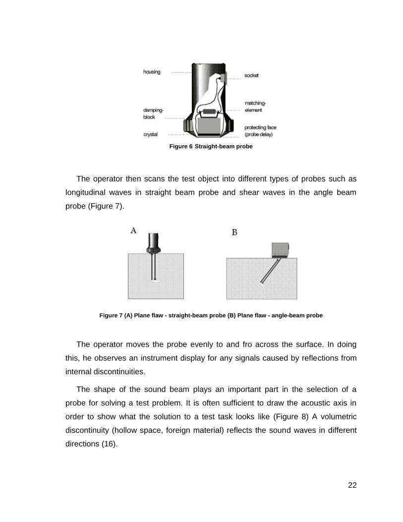
The shape of the sound beam plays an important part in the selection of a

probe for solving a test problem. It is often sufficient to draw the acoustic axis in

order to show what the solution to a test task looks like (Figure 8) A volumetric

discontinuity (hollow space, foreign material) reflects the sound waves in different

directions (16).

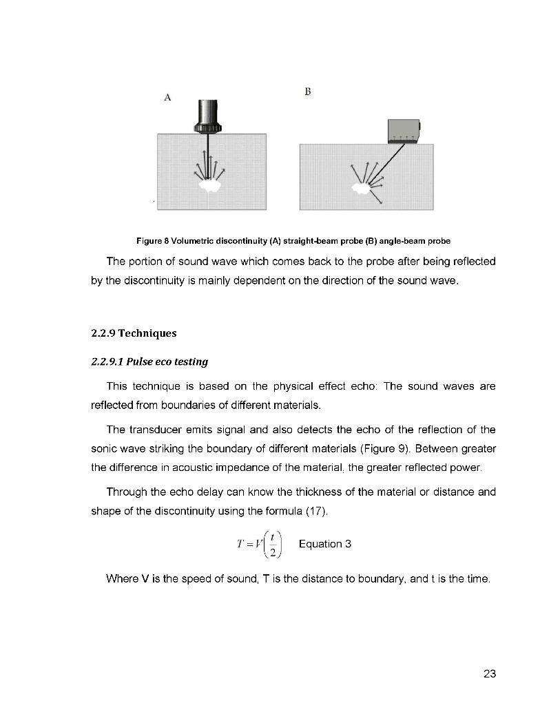
Figure 8 Volumetric discontinuity (A) straight-beam probe (B) angle-beam probe

The portion of sound wave which comes back to the probe after being reflected

by the discontinuity is mainly dependent on the direction of the sound wave.

2.2.9 Techniques

2.2.9.1 Pulse eco testing

This technique is based on the physical effect echo: The sound waves are

reflected from boundaries of different materials.

The transducer emits signal and also detects the echo of the reflection of the

sonic wave striking the boundary of different materials (Figure 9). Between greater

the difference in acoustic impedance of the material, the greater reflected power.

Through the echo delay can know the thickness of the material or distance and

shape of the discontinuity using the formula (17).

23

Equation 3

Where V is the speed of sound, T is the distance to boundary, and t is the time.

24

Figure 9 Pulse eco

2.2.9.2 Resonance testing

Acoustic measurement technology is very sensitive; even minor changes in the

oscillatory behavior of mechanical structures can be detected. Resonance analysis

is a qualitative process that compares the actual oscillatory situation with the target

one derived from a learning base. This learning base is established by using

defined standard parts.

It uses the physical effect known in which a body, having been excited in some

ways characteristic vibrations and frequencies as shown in Figure 10. These

vibrations when passing through the test object leaves a "fingerprint" which can be

captured by a sensor and then graphically exposed (18).

Figure 10 Resonance testing

25

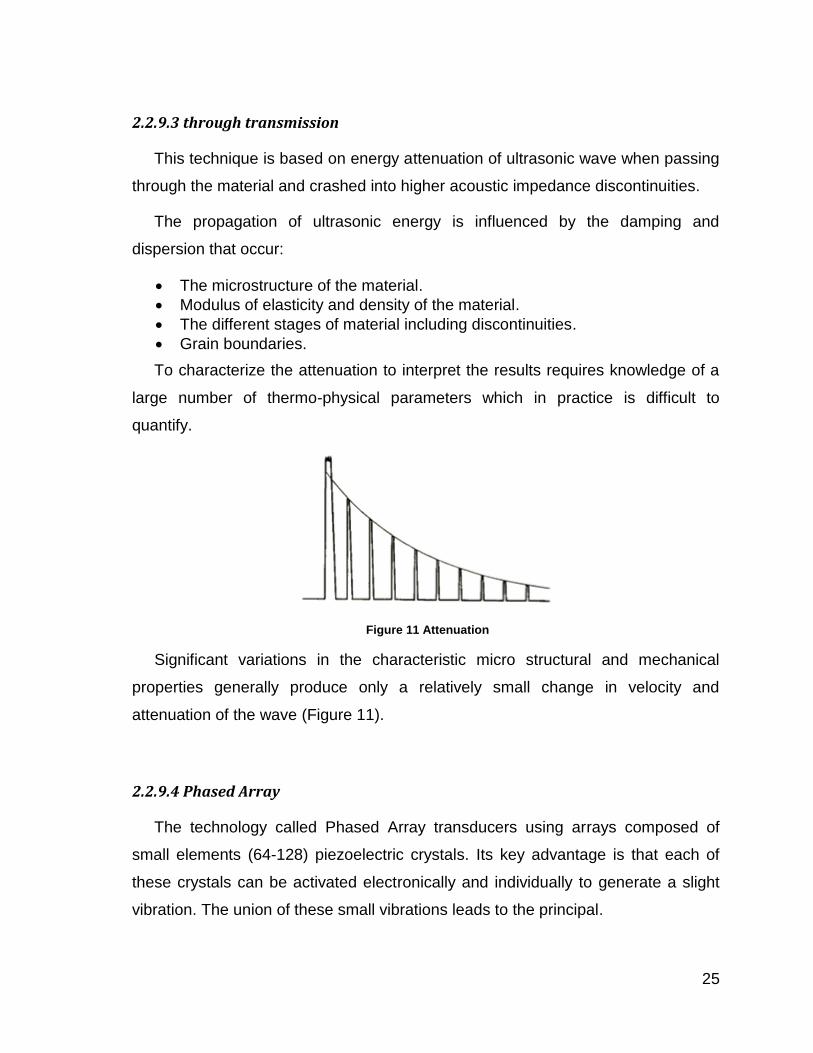
2.2.9.3 through transmission

This technique is based on energy attenuation of ultrasonic wave when passing

through the material and crashed into higher acoustic impedance discontinuities.

The propagation of ultrasonic energy is influenced by the damping and

dispersion that occur:

The microstructure of the material.

Modulus of elasticity and density of the material.

The different stages of material including discontinuities.

Grain boundaries.

To characterize the attenuation to interpret the results requires knowledge of a

large number of thermo-physical parameters which in practice is difficult to

quantify.

Figure 11 Attenuation

Significant variations in the characteristic micro structural and mechanical

properties generally produce only a relatively small change in velocity and

attenuation of the wave (Figure 11).

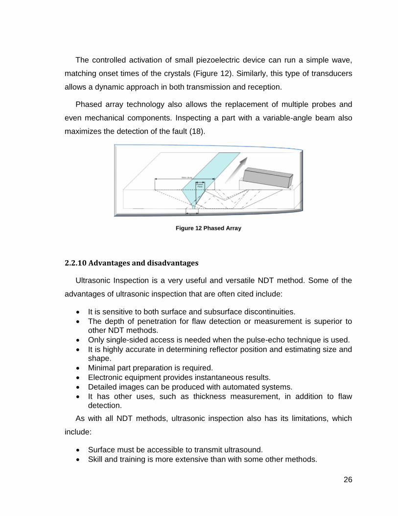
2.2.9.4 Phased Array

The technology called Phased Array transducers using arrays composed of

small elements (64-128) piezoelectric crystals. Its key advantage is that each of

these crystals can be activated electronically and individually to generate a slight

vibration. The union of these small vibrations leads to the principal.

26

The controlled activation of small piezoelectric device can run a simple wave,

matching onset times of the crystals (Figure 12). Similarly, this type of transducers

allows a dynamic approach in both transmission and reception.

Phased array technology also allows the replacement of multiple probes and

even mechanical components. Inspecting a part with a variable-angle beam also

maximizes the detection of the fault (18).

Figure 12 Phased Array

2.2.10 Advantages and disadvantages

Ultrasonic Inspection is a very useful and versatile NDT method. Some of the

advantages of ultrasonic inspection that are often cited include:

It is sensitive to both surface and subsurface discontinuities.

The depth of penetration for flaw detection or measurement is superior to other NDT methods.

Only single-sided access is needed when the pulse-echo technique is used.

It is highly accurate in determining reflector position and estimating size and shape.

Minimal part preparation is required.

Electronic equipment provides instantaneous results.

Detailed images can be produced with automated systems.

It has other uses, such as thickness measurement, in addition to flaw detection.

As with all NDT methods, ultrasonic inspection also has its limitations, which

include:

Surface must be accessible to transmit ultrasound.

Skill and training is more extensive than with some other methods.

27

It normally requires a coupling medium to promote the transfer of sound energy into the test specimen.

Materials that are rough, irregular in shape, very small, exceptionally thin or not homogeneous are difficult to inspect.

Cast iron and other coarse grained materials are difficult to inspect due to low sound transmission and high signal noise.

Linear defects oriented parallel to the sound beam may go undetected.

Reference standards are required for both equipment calibration and the characterization of flaws.

The above provides a simplified introduction to the NDT method of ultrasonic

testing. However, to effectively perform an inspection using ultrasonic, much more

about the method needs to be known.

28

3. Experimental Set-up

3.1 FSW Experimental methodology

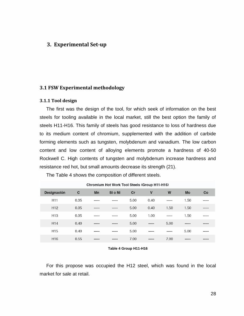
3.1.1 Tool design

The first was the design of the tool, for which seek of information on the best

steels for tooling available in the local market, still the best option the family of

steels H11-H16. This family of steels has good resistance to loss of hardness due

to its medium content of chromium, supplemented with the addition of carbide

forming elements such as tungsten, molybdenum and vanadium. The low carbon

content and low content of alloying elements promote a hardness of 40-50

Rockwell C. High contents of tungsten and molybdenum increase hardness and

resistance red hot, but small amounts decrease its strength (21).

The Table 4 shows the composition of different steels.

Table 4 Group H11-H16

For this propose was occupied the H12 steel, which was found in the local

market for sale at retail.

29

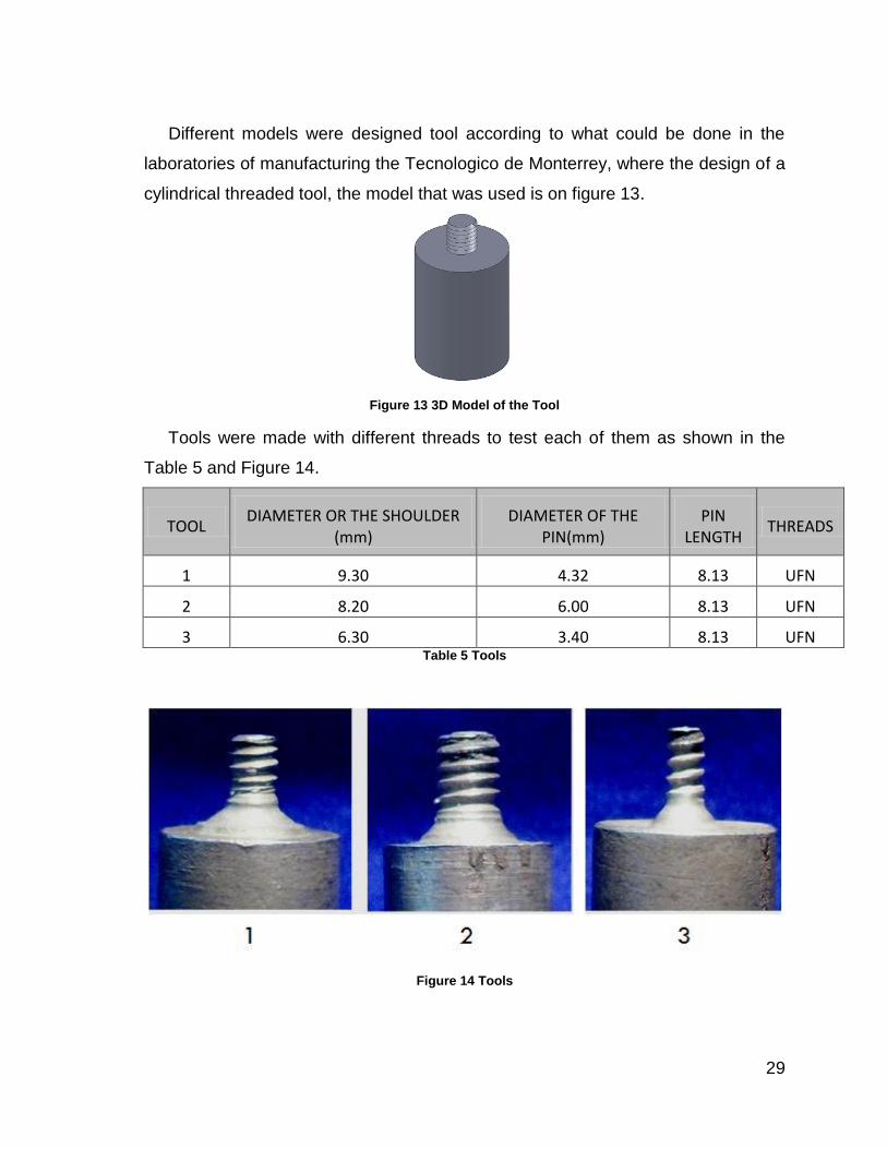
Different models were designed tool according to what could be done in the

laboratories of manufacturing the Tecnologico de Monterrey, where the design of a

cylindrical threaded tool, the model that was used is on figure 13.

Figure 13 3D Model of the Tool

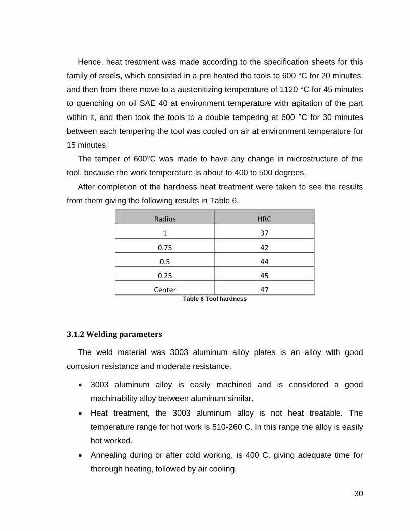
Tools were made with different threads to test each of them as shown in the

Table 5 and Figure 14.

TOOL DIAMETER OR THE SHOULDER

(mm) DIAMETER OF THE

PIN(mm) PIN

LENGTH THREADS

1 9.30 4.32 8.13 UFN

2 8.20 6.00 8.13 UFN

3 6.30 3.40 8.13 UFN Table 5 Tools

Figure 14 Tools

30

Hence, heat treatment was made according to the specification sheets for this

family of steels, which consisted in a pre heated the tools to 600 °C for 20 minutes,

and then from there move to a austenitizing temperature of 1120 °C for 45 minutes

to quenching on oil SAE 40 at environment temperature with agitation of the part

within it, and then took the tools to a double tempering at 600 °C for 30 minutes

between each tempering the tool was cooled on air at environment temperature for

15 minutes.

The temper of 600°C was made to have any change in microstructure of the

tool, because the work temperature is about to 400 to 500 degrees.

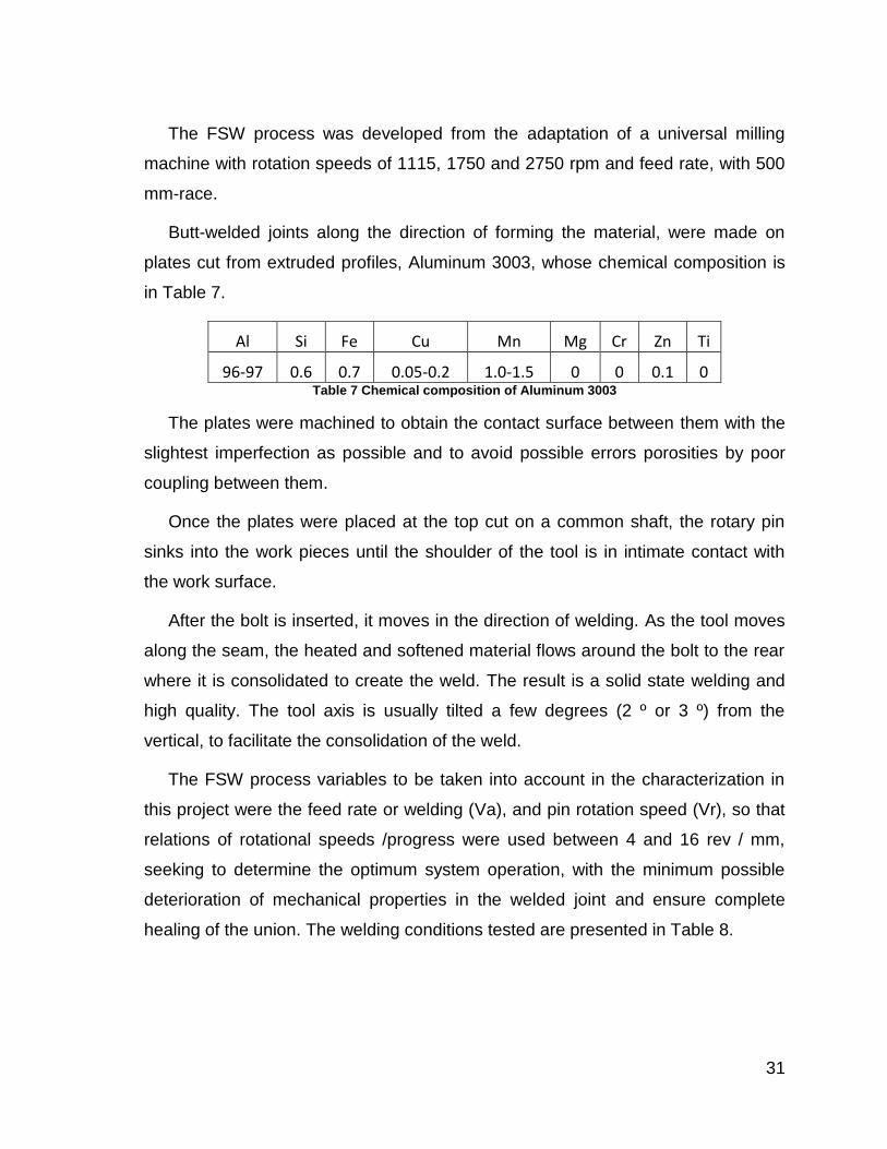
After completion of the hardness heat treatment were taken to see the results

from them giving the following results in Table 6.

Radius HRC

1 37

0.75 42

0.5 44

0.25 45

Center 47 Table 6 Tool hardness

3.1.2 Welding parameters

The weld material was 3003 aluminum alloy plates is an alloy with good

corrosion resistance and moderate resistance.

3003 aluminum alloy is easily machined and is considered a good

machinability alloy between aluminum similar.

Heat treatment, the 3003 aluminum alloy is not heat treatable. The

temperature range for hot work is 510-260 C. In this range the alloy is easily

hot worked.

Annealing during or after cold working, is 400 C, giving adequate time for

thorough heating, followed by air cooling.

31

The FSW process was developed from the adaptation of a universal milling

machine with rotation speeds of 1115, 1750 and 2750 rpm and feed rate, with 500

mm-race.

Butt-welded joints along the direction of forming the material, were made on

plates cut from extruded profiles, Aluminum 3003, whose chemical composition is

in Table 7.

Al Si Fe Cu Mn Mg Cr Zn Ti

96-97 0.6 0.7 0.05-0.2 1.0-1.5 0 0 0.1 0 Table 7 Chemical composition of Aluminum 3003

The plates were machined to obtain the contact surface between them with the

slightest imperfection as possible and to avoid possible errors porosities by poor

coupling between them.

Once the plates were placed at the top cut on a common shaft, the rotary pin

sinks into the work pieces until the shoulder of the tool is in intimate contact with

the work surface.

After the bolt is inserted, it moves in the direction of welding. As the tool moves

along the seam, the heated and softened material flows around the bolt to the rear

where it is consolidated to create the weld. The result is a solid state welding and

high quality. The tool axis is usually tilted a few degrees (2 º or 3 º) from the

vertical, to facilitate the consolidation of the weld.

The FSW process variables to be taken into account in the characterization in

this project were the feed rate or welding (Va), and pin rotation speed (Vr), so that

relations of rotational speeds /progress were used between 4 and 16 rev / mm,

seeking to determine the optimum system operation, with the minimum possible

deterioration of mechanical properties in the welded joint and ensure complete

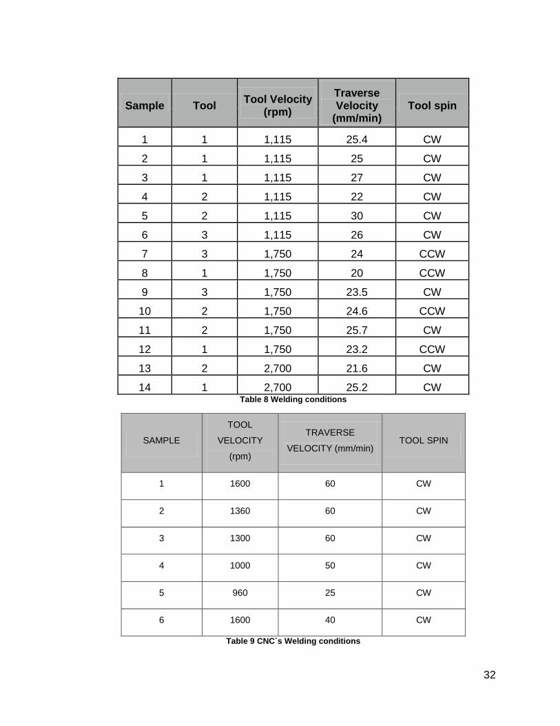
healing of the union. The welding conditions tested are presented in Table 8.

32

Sample Tool Tool Velocity

(rpm)

Traverse Velocity

(mm/min) Tool spin

1 1 1,115 25.4 CW

2 1 1,115 25 CW

3 1 1,115 27 CW

4 2 1,115 22 CW

5 2 1,115 30 CW

6 3 1,115 26 CW

7 3 1,750 24 CCW

8 1 1,750 20 CCW

9 3 1,750 23.5 CW

10 2 1,750 24.6 CCW

11 2 1,750 25.7 CW

12 1 1,750 23.2 CCW

13 2 2,700 21.6 CW

14 1 2,700 25.2 CW Table 8 Welding conditions

SAMPLE

TOOL

VELOCITY

(rpm)

TRAVERSE

VELOCITY (mm/min) TOOL SPIN

1 1600 60 CW

2 1360 60 CW

3 1300 60 CW

4 1000 50 CW

5 960 25 CW

6 1600 40 CW

Table 9 CNC´s Welding conditions

33

The results of the Table 9 represent those achieved in the CNC for these

samples had the same tool and the spin tool was CW.

3.1.3 Mechanical testing

Welded plates representative samples were taken for mechanical testing by

tension tests, hardness of welded joints.

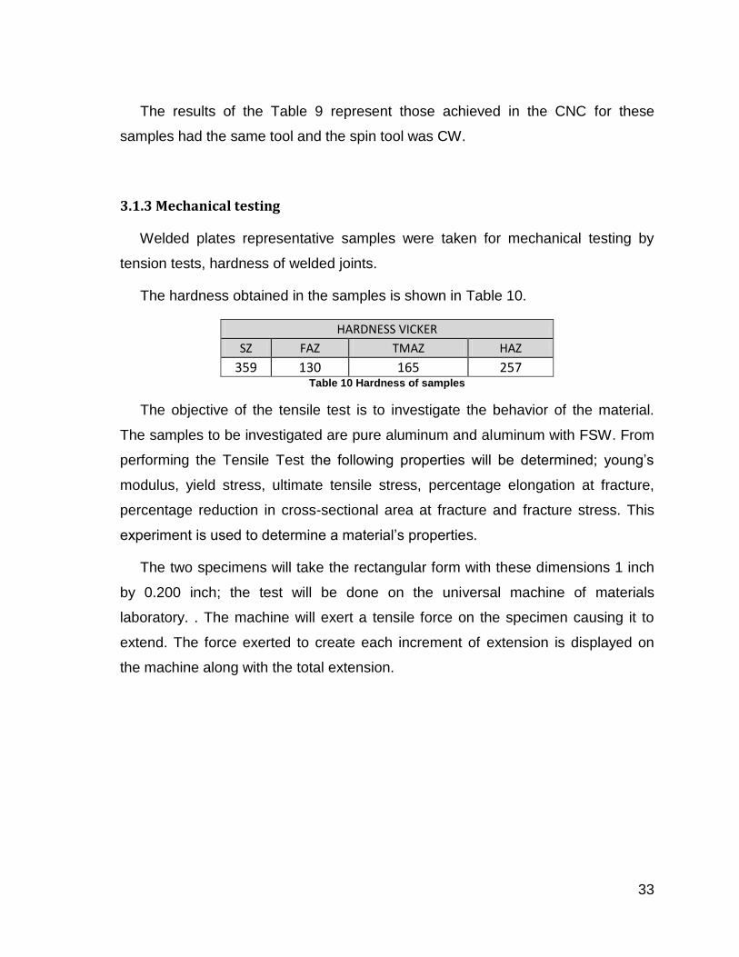
The hardness obtained in the samples is shown in Table 10.

HARDNESS VICKER

SZ FAZ TMAZ HAZ

359 130 165 257 Table 10 Hardness of samples

The objective of the tensile test is to investigate the behavior of the material.

The samples to be investigated are pure aluminum and aluminum with FSW. From

performing the Tensile Test the following properties will be determined; young’s

modulus, yield stress, ultimate tensile stress, percentage elongation at fracture,

percentage reduction in cross-sectional area at fracture and fracture stress. This

experiment is used to determine a material’s properties.

The two specimens will take the rectangular form with these dimensions 1 inch

by 0.200 inch; the test will be done on the universal machine of materials

laboratory. . The machine will exert a tensile force on the specimen causing it to

extend. The force exerted to create each increment of extension is displayed on

the machine along with the total extension.

34

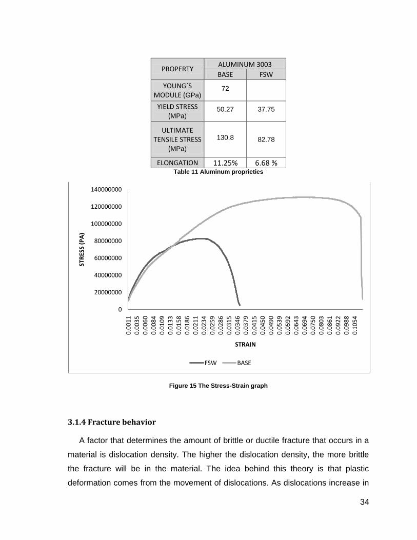
PROPERTY ALUMINUM 3003 BASE FSW

YOUNG´S MODULE (GPa)

72

YIELD STRESS (MPa)

50.27 37.75

ULTIMATE TENSILE STRESS

(MPa)

130.8 82.78

ELONGATION 11.25% 6.68 % Table 11 Aluminum proprieties

Figure 15 The Stress-Strain graph

3.1.4 Fracture behavior

A factor that determines the amount of brittle or ductile fracture that occurs in a

material is dislocation density. The higher the dislocation density, the more brittle

the fracture will be in the material. The idea behind this theory is that plastic

deformation comes from the movement of dislocations. As dislocations increase in

0

20000000

40000000

60000000

80000000

100000000

120000000

140000000

0.0

01

10

.00

35

0.0

06

00

.00

84

0.0

10

90

.01

33

0.0

15

80

.01

86

0.0

21

10

.02

34

0.0

25

90

.02

86

0.0

31

50

.03

46

0.0

37

90

.04

15

0.0

45

00

.04

90

0.0

53

90

.05

92

0.0

64

30

.06

94

0.0

75

00

.08

03

0.0

86

10

.09

22

0.0

98

80

.10

54

STR

ESS

(PA

)

STRAIN

FSW BASE

35

a material due to stresses above the materials yield point, it becomes increasingly

difficult for the dislocations to move because they pile into each other. So a

material that already has a high dislocation density can only deform but so much

before it fractures in a brittle manner. The last factor is grain size. As grains get

smaller in a material, the fracture becomes more brittle.

So the samples have a brittle fracture, and have two types of fractures seen:

transgranular and intergranular.

In transgranular fracture, the fracture travels through the grain of the material.

The fracture changes direction from grain to grain due to the different lattice

orientation of atoms in each grain.

Intergranular fracture is the crack traveling along the grain boundaries, and not

through the actual grains. Intergranular fracture usually occurs when the phase in

the grain boundary is weak and brittle.

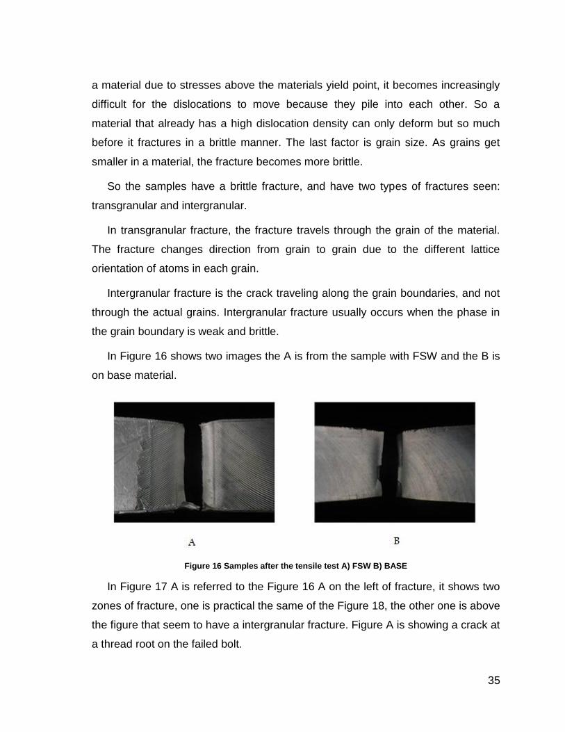
In Figure 16 shows two images the A is from the sample with FSW and the B is

on base material.

Figure 16 Samples after the tensile test A) FSW B) BASE

In Figure 17 A is referred to the Figure 16 A on the left of fracture, it shows two

zones of fracture, one is practical the same of the Figure 18, the other one is above

the figure that seem to have a intergranular fracture. Figure A is showing a crack at

a thread root on the failed bolt.

36

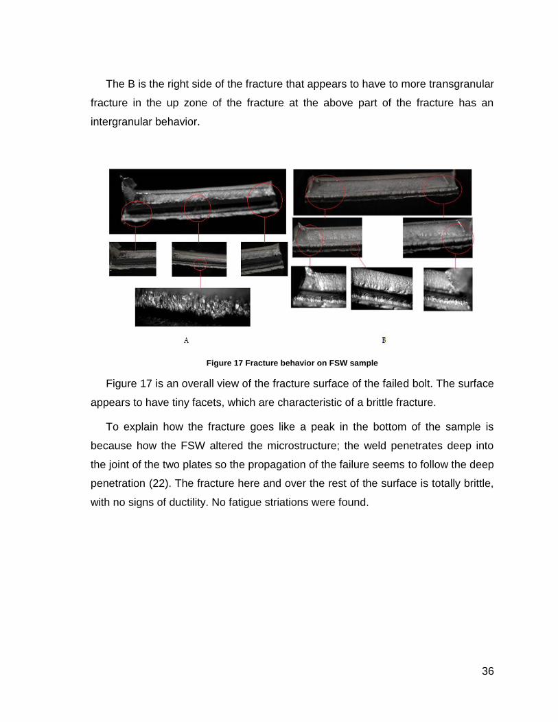
The B is the right side of the fracture that appears to have to more transgranular

fracture in the up zone of the fracture at the above part of the fracture has an

intergranular behavior.

Figure 17 Fracture behavior on FSW sample

Figure 17 is an overall view of the fracture surface of the failed bolt. The surface

appears to have tiny facets, which are characteristic of a brittle fracture.

To explain how the fracture goes like a peak in the bottom of the sample is

because how the FSW altered the microstructure; the weld penetrates deep into

the joint of the two plates so the propagation of the failure seems to follow the deep

penetration (22). The fracture here and over the rest of the surface is totally brittle,

with no signs of ductility. No fatigue striations were found.

37

Figure 18 Fracture behaviors on BASE sample

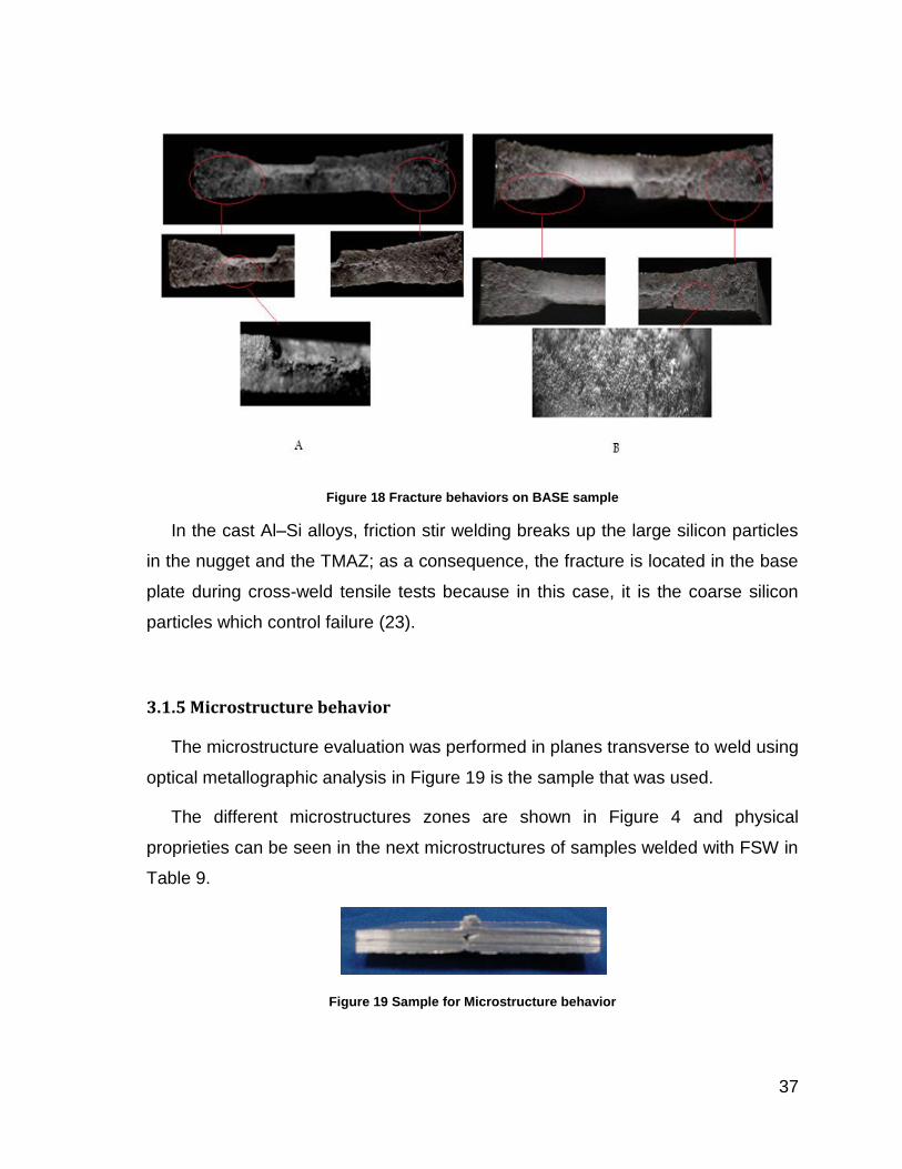
In the cast Al–Si alloys, friction stir welding breaks up the large silicon particles

in the nugget and the TMAZ; as a consequence, the fracture is located in the base

plate during cross-weld tensile tests because in this case, it is the coarse silicon

particles which control failure (23).

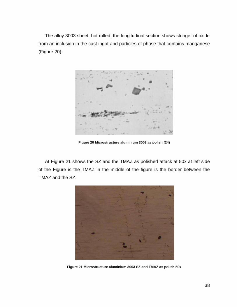
3.1.5 Microstructure behavior

The microstructure evaluation was performed in planes transverse to weld using

optical metallographic analysis in Figure 19 is the sample that was used.

The different microstructures zones are shown in Figure 4 and physical

proprieties can be seen in the next microstructures of samples welded with FSW in

Table 9.

Figure 19 Sample for Microstructure behavior

38

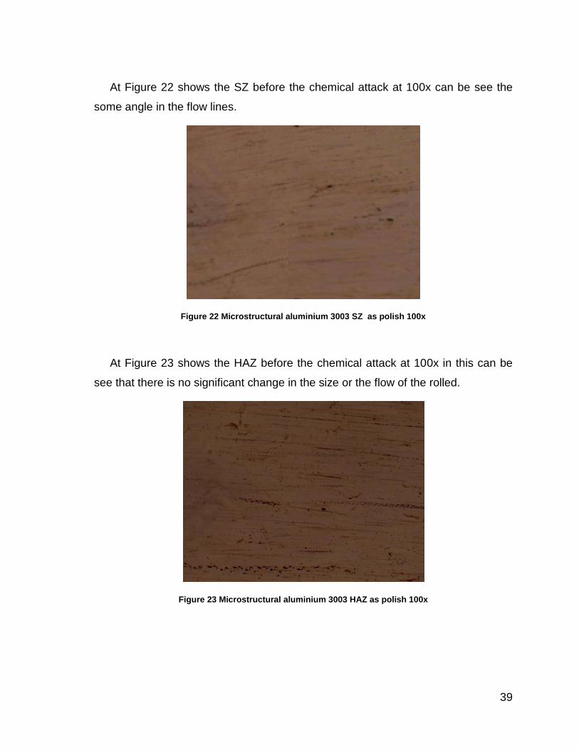
The alloy 3003 sheet, hot rolled, the longitudinal section shows stringer of oxide

from an inclusion in the cast ingot and particles of phase that contains manganese

(Figure 20).

Figure 20 Microstructure aluminium 3003 as polish (24)

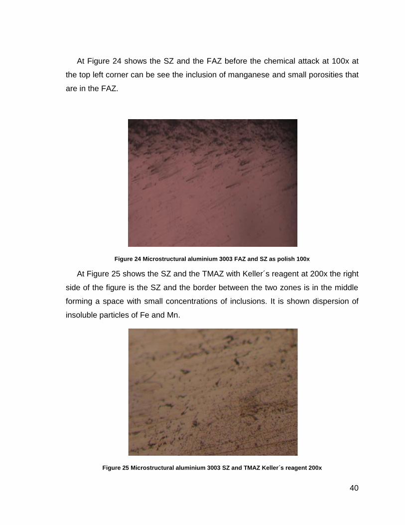
At Figure 21 shows the SZ and the TMAZ as polished attack at 50x at left side

of the Figure is the TMAZ in the middle of the figure is the border between the

TMAZ and the SZ.

Figure 21 Microstructure aluminium 3003 SZ and TMAZ as polish 50x

39

At Figure 22 shows the SZ before the chemical attack at 100x can be see the

some angle in the flow lines.

Figure 22 Microstructural aluminium 3003 SZ as polish 100x

At Figure 23 shows the HAZ before the chemical attack at 100x in this can be

see that there is no significant change in the size or the flow of the rolled.

Figure 23 Microstructural aluminium 3003 HAZ as polish 100x

40

At Figure 24 shows the SZ and the FAZ before the chemical attack at 100x at

the top left corner can be see the inclusion of manganese and small porosities that

are in the FAZ.

Figure 24 Microstructural aluminium 3003 FAZ and SZ as polish 100x

At Figure 25 shows the SZ and the TMAZ with Keller´s reagent at 200x the right

side of the figure is the SZ and the border between the two zones is in the middle

forming a space with small concentrations of inclusions. It is shown dispersion of

insoluble particles of Fe and Mn.

Figure 25 Microstructural aluminium 3003 SZ and TMAZ Keller´s reagent 200x

41

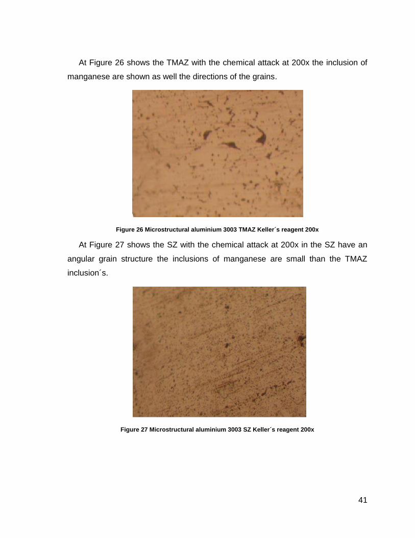
At Figure 26 shows the TMAZ with the chemical attack at 200x the inclusion of

manganese are shown as well the directions of the grains.

Figure 26 Microstructural aluminium 3003 TMAZ Keller´s reagent 200x

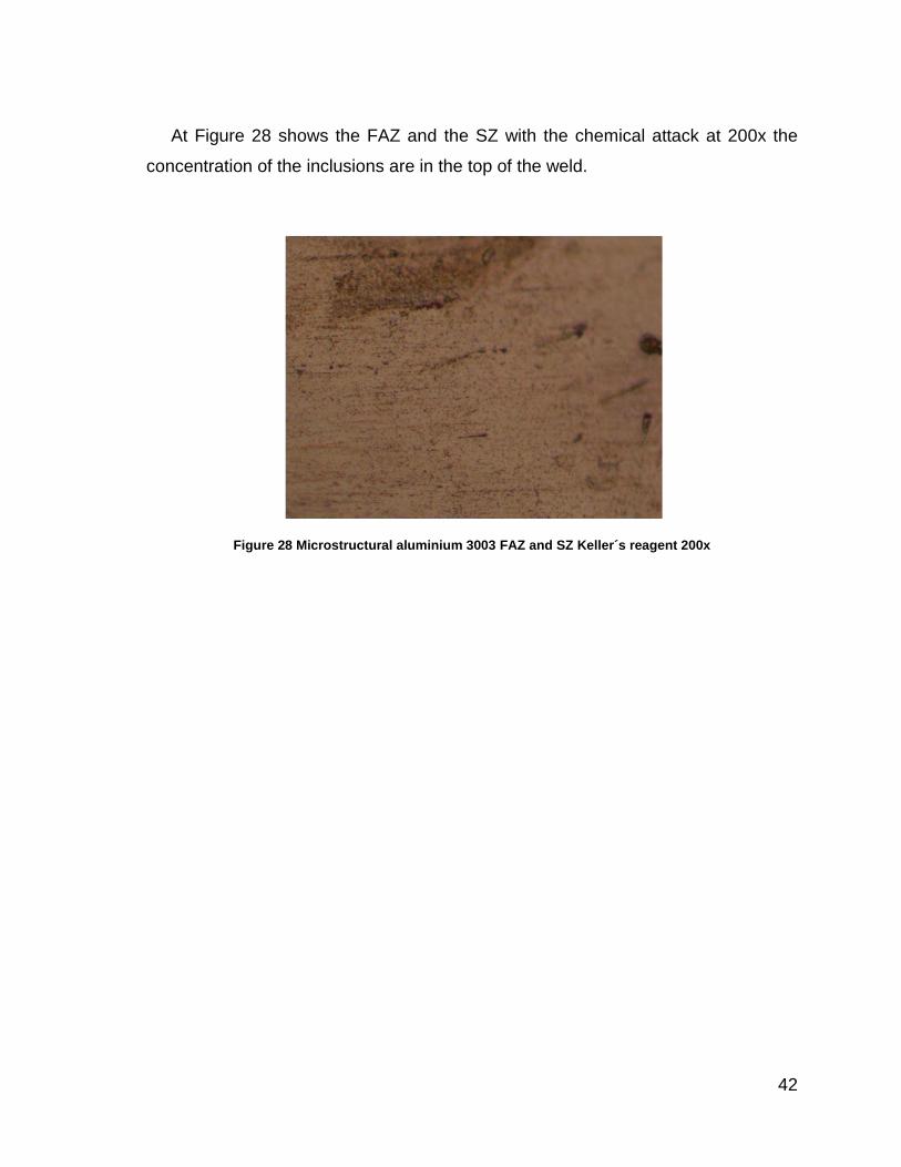
At Figure 27 shows the SZ with the chemical attack at 200x in the SZ have an

angular grain structure the inclusions of manganese are small than the TMAZ

inclusion´s.

Figure 27 Microstructural aluminium 3003 SZ Keller´s reagent 200x

42

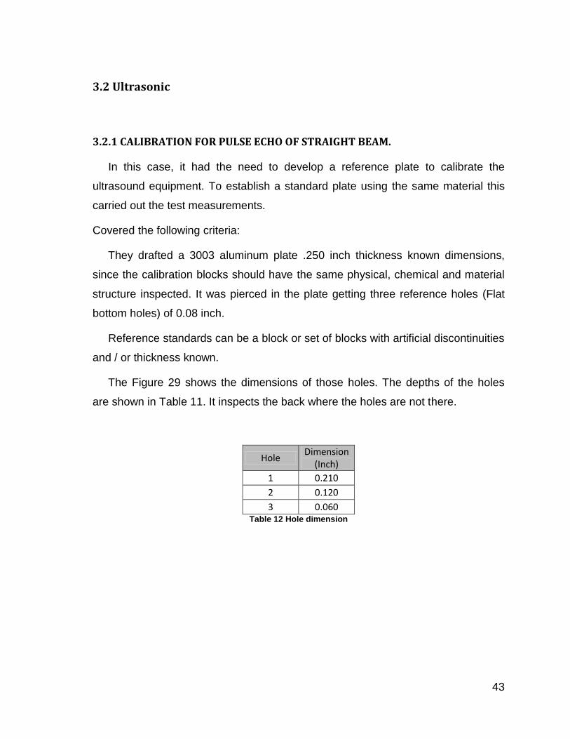
At Figure 28 shows the FAZ and the SZ with the chemical attack at 200x the

concentration of the inclusions are in the top of the weld.

Figure 28 Microstructural aluminium 3003 FAZ and SZ Keller´s reagent 200x

43

3.2 Ultrasonic

3.2.1 CALIBRATION FOR PULSE ECHO OF STRAIGHT BEAM.

In this case, it had the need to develop a reference plate to calibrate the

ultrasound equipment. To establish a standard plate using the same material this

carried out the test measurements.

Covered the following criteria:

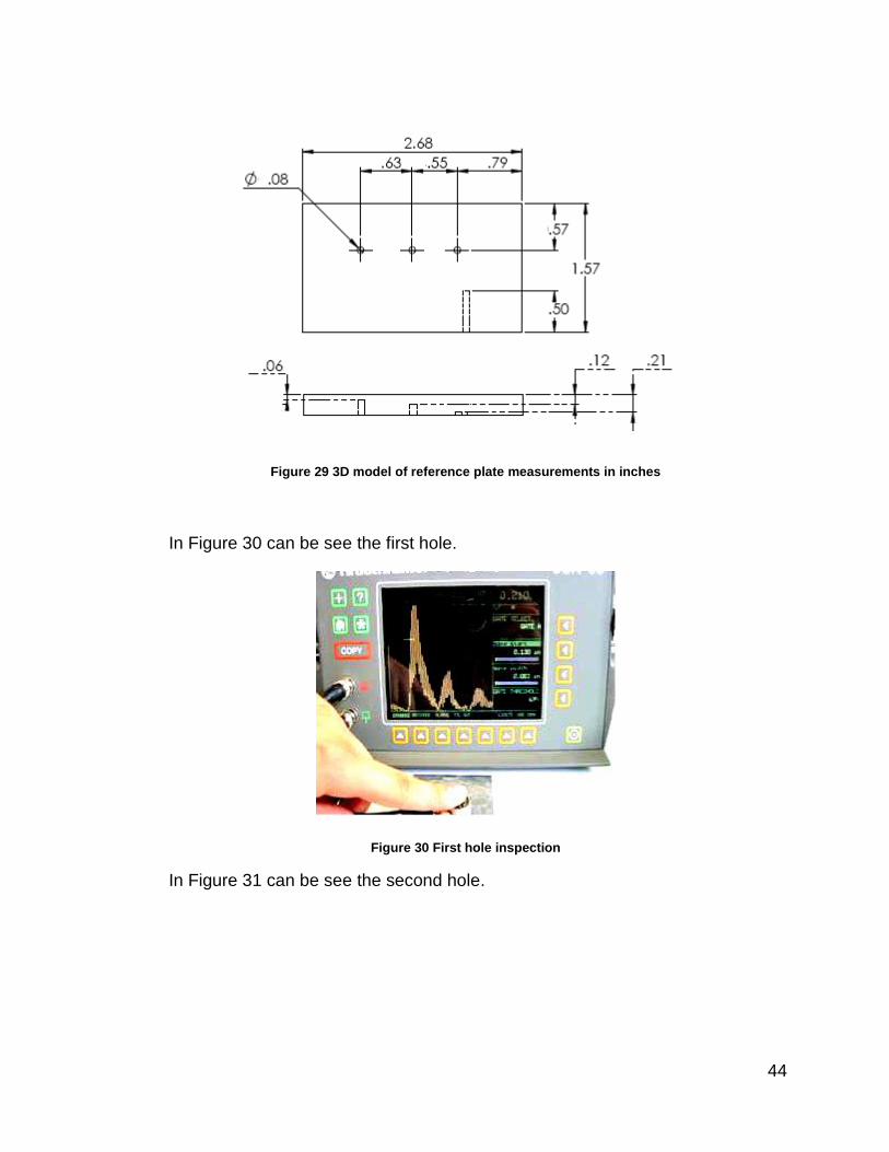
They drafted a 3003 aluminum plate .250 inch thickness known dimensions,

since the calibration blocks should have the same physical, chemical and material

structure inspected. It was pierced in the plate getting three reference holes (Flat

bottom holes) of 0.08 inch.

Reference standards can be a block or set of blocks with artificial discontinuities

and / or thickness known.

The Figure 29 shows the dimensions of those holes. The depths of the holes

are shown in Table 11. It inspects the back where the holes are not there.

Hole Dimension

(Inch) 1 0.210

2 0.120

3 0.060 Table 12 Hole dimension

44

Figure 29 3D model of reference plate measurements in inches

In Figure 30 can be see the first hole.

Figure 30 First hole inspection

In Figure 31 can be see the second hole.

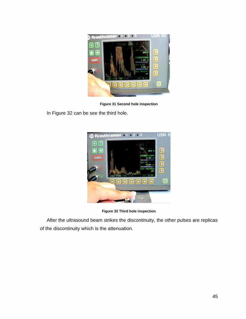
45

Figure 31 Second hole inspection

In Figure 32 can be see the third hole.

Figure 32 Third hole inspection

After the ultrasound beam strikes the discontinuity, the other pulses are replicas

of the discontinuity which is the attenuation.

3.2.2 CALIBRATION FOR PULSE ECHO OF BEAM ANGLE.

We do not have a pattern that has two holes perpendicular to the cross section

of the board; therefore we will use a pattern with a single hole with known location.

Figure 33 shows the layout of the location and its 3D model.

Figure 33 3D model and layout for pattern in shear beam

Calculate the distances SA and PA by trigonometry to shoe for the 45° and 60°

for the first leg.

The depth to which is the hole is removed according to the machining process

that was taken and results in a DA = 0.120 inches.

Since DA is calculated the following measures to two different types of shoes to

each other at 45° and 60°.

We set the distance DA, SA and PA in the pattern and place the probe at a

distance PA = 0.120 inches of discontinuity as shown below in Figure 34.

46

45°

SA = DA / Senβ SA= 0.12/Sen(45)

SA 4 5 ° = 0.1697" PA = 0.12 "

45°

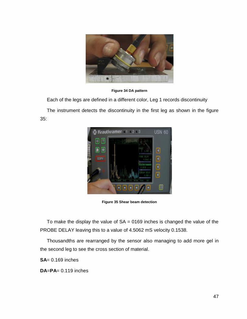
47

Figure 34 DA pattern

Each of the legs are defined in a different color, Leg 1 records discontinuity

The instrument detects the discontinuity in the first leg as shown in the figure

35:

Figure 35 Shear beam detection

To make the display the value of SA = 0169 inches is changed the value of the

PROBE DELAY leaving this to a value of 4.5062 mS velocity 0.1538.

Thousandths are rearranged by the sensor also managing to add more gel in

the second leg to see the cross section of material.

SA= 0.169 inches

DA=PA= 0.119 inches

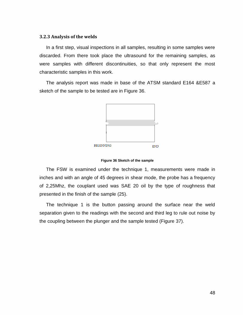
48

3.2.3 Analysis of the welds

In a first step, visual inspections in all samples, resulting in some samples were

discarded. From there took place the ultrasound for the remaining samples, as

were samples with different discontinuities, so that only represent the most

characteristic samples in this work.

The analysis report was made in base of the ATSM standard E164 &E587 a

sketch of the sample to be tested are in Figure 36.

Figure 36 Sketch of the sample

The FSW is examined under the technique 1, measurements were made in

inches and with an angle of 45 degrees in shear mode, the probe has a frequency

of 2,25Mhz, the couplant used was SAE 20 oil by the type of roughness that

presented in the finish of the sample (25).

The technique 1 is the button passing around the surface near the weld

separation given to the readings with the second and third leg to rule out noise by

the coupling between the plunger and the sample tested (Figure 37).

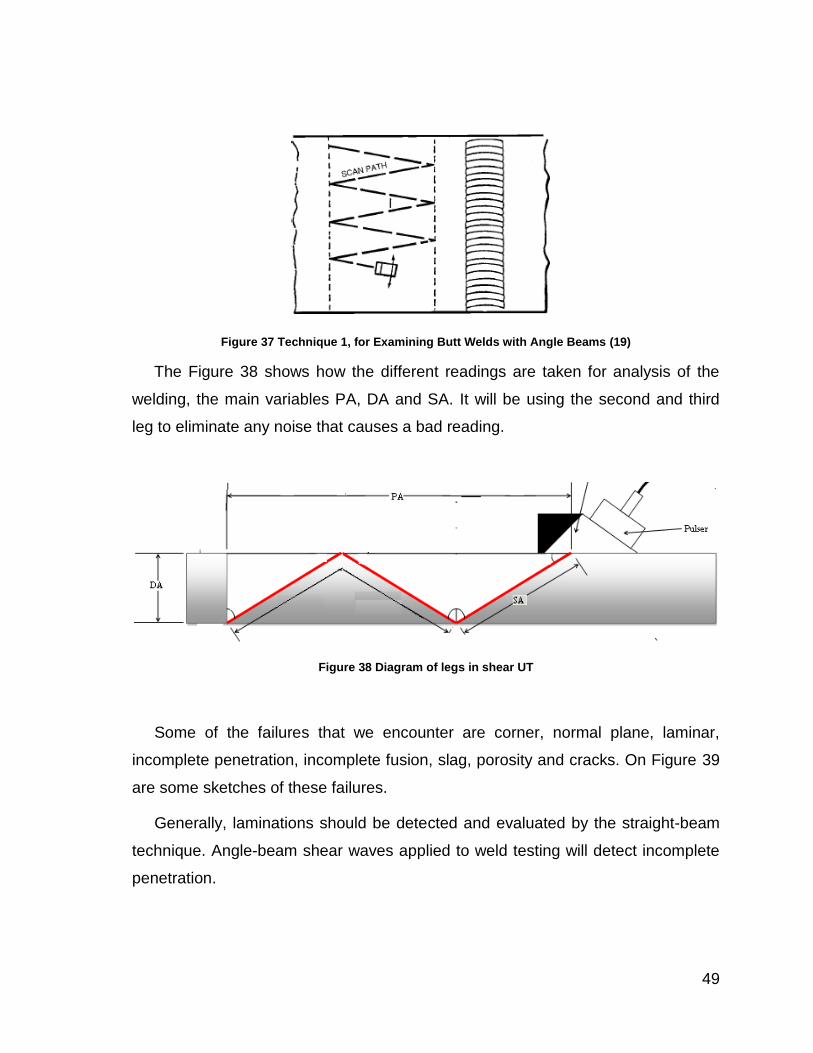
49

Figure 37 Technique 1, for Examining Butt Welds with Angle Beams (19)

The Figure 38 shows how the different readings are taken for analysis of the

welding, the main variables PA, DA and SA. It will be using the second and third

leg to eliminate any noise that causes a bad reading.

Figure 38 Diagram of legs in shear UT

Some of the failures that we encounter are corner, normal plane, laminar,

incomplete penetration, incomplete fusion, slag, porosity and cracks. On Figure 39

are some sketches of these failures.

Generally, laminations should be detected and evaluated by the straight-beam

technique. Angle-beam shear waves applied to weld testing will detect incomplete

penetration.

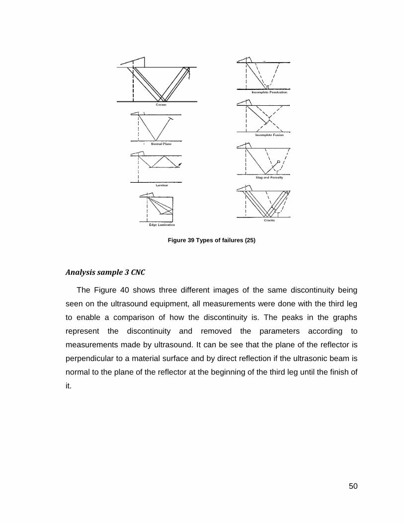
50

Figure 39 Types of failures (25)

Analysis sample 3 CNC

The Figure 40 shows three different images of the same discontinuity being

seen on the ultrasound equipment, all measurements were done with the third leg

to enable a comparison of how the discontinuity is. The peaks in the graphs

represent the discontinuity and removed the parameters according to

measurements made by ultrasound. It can be see that the plane of the reflector is

perpendicular to a material surface and by direct reflection if the ultrasonic beam is

normal to the plane of the reflector at the beginning of the third leg until the finish of

it.

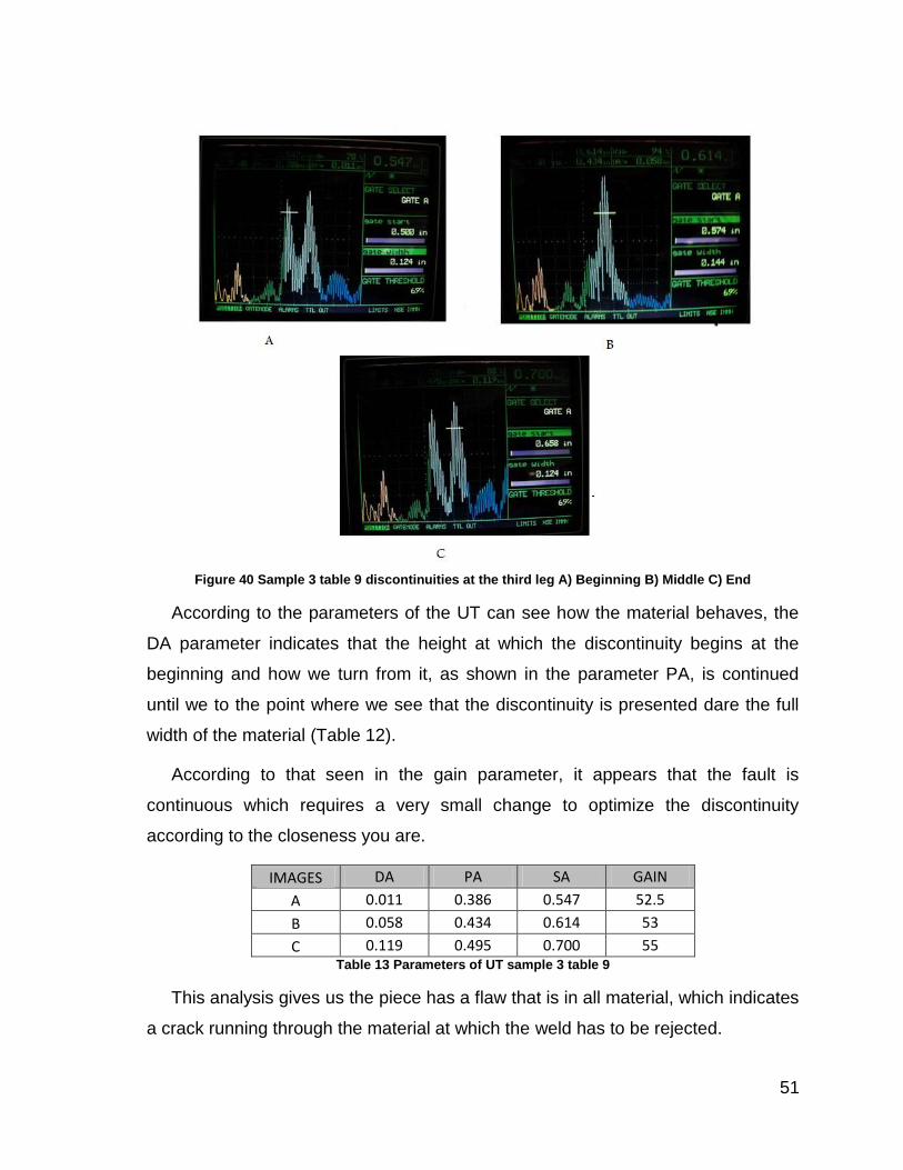
51

Figure 40 Sample 3 table 9 discontinuities at the third leg A) Beginning B) Middle C) End

According to the parameters of the UT can see how the material behaves, the

DA parameter indicates that the height at which the discontinuity begins at the

beginning and how we turn from it, as shown in the parameter PA, is continued

until we to the point where we see that the discontinuity is presented dare the full

width of the material (Table 12).

According to that seen in the gain parameter, it appears that the fault is

continuous which requires a very small change to optimize the discontinuity

according to the closeness you are.

IMAGES DA PA SA GAIN

A 0.011 0.386 0.547 52.5

B 0.058 0.434 0.614 53

C 0.119 0.495 0.700 55 Table 13 Parameters of UT sample 3 table 9

This analysis gives us the piece has a flaw that is in all material, which indicates

a crack running through the material at which the weld has to be rejected.

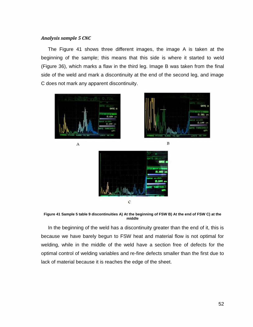
52


The Figure 41 shows three different images, the image A is taken at the

beginning of the sample; this means that this side is where it started to weld

(Figure 36), which marks a flaw in the third leg. Image B was taken from the final

side of the weld and mark a discontinuity at the end of the second leg, and image

C does not mark any apparent discontinuity.

Figure 41 Sample 5 table 9 discontinuities A) At the beginning of FSW B) At the end of FSW C) at the middle

In the beginning of the weld has a discontinuity greater than the end of it, this is

because we have barely begun to FSW heat and material flow is not optimal for

welding, while in the middle of the weld have a section free of defects for the

optimal control of welding variables and re-fine defects smaller than the first due to

lack of material because it is reaches the edge of the sheet.

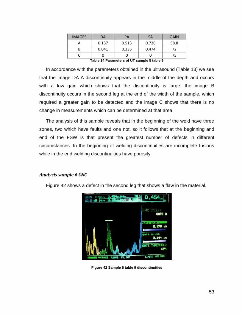
53

IMAGES DA PA SA GAIN

A 0.137 0.513 0.726 58.8

B 0.041 0.335 0.474 72

C 0 0 0 75 Table 14 Parameters of UT sample 5 table 9

In accordance with the parameters obtained in the ultrasound (Table 13) we see

that the image DA A discontinuity appears in the middle of the depth and occurs

with a low gain which shows that the discontinuity is large, the image B

discontinuity occurs in the second leg at the end of the width of the sample, which

required a greater gain to be detected and the image C shows that there is no

change in measurements which can be determined at that area.

The analysis of this sample reveals that in the beginning of the weld have three

zones, two which have faults and one not, so it follows that at the beginning and

end of the FSW is that present the greatest number of defects in different

circumstances. In the beginning of welding discontinuities are incomplete fusions

while in the end welding discontinuities have porosity.


Figure 42 shows a defect in the second leg that shows a flaw in the material.

Figure 42 Sample 6 table 9 discontinuities

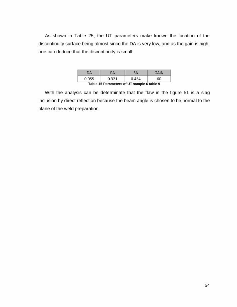
54

As shown in Table 25, the UT parameters make known the location of the

discontinuity surface being almost since the DA is very low, and as the gain is high,

one can deduce that the discontinuity is small.

DA PA SA GAIN

0.055 0.321 0.454 60 Table 15 Parameters of UT sample 6 table 9

With the analysis can be determinate that the flaw in the figure 51 is a slag

inclusion by direct reflection because the beam angle is chosen to be normal to the

plane of the weld preparation.

55

4. Conclusion

Friction stir welding technology has been a major boon to industry advanced

since its inception. In spite of its short history, it has found widespread applications

in diverse industries.

The fundamental understanding of both the welding process and the

structure/properties of the aluminum 3003 into the welded joints has been useful in

reducing defects and improving uniformity of weld properties.

FSW does not seem to have an advantage with respect to the strength of the

fusion zone. The TMAZ is somewhat softer than the fusion zone because the latter

dynamic recrystallization into a fine grain structure.

Different tools and were designed according to the given experiment, it was

found that the tool 1 showed the best results, and this is made of H12 steel heat

treated under a preheated, a quenching and double tempered at 600 Celsius.

It is able to obtain several alternative sets of welding parameters involving

combinations of the welding speed, rotational speed and tool. For this work the

best parameters were 25 mm/min, 960 rpm and tool 1.

Over the years, ultrasound examination has taken the lead X-ray examination in

a variety of applications, thanks to a number of advantages that account.

Optimum ultrasonic reflections at defects in aluminum 3003 alloy FSW can be

obtained by using angle ultrasonic method. The echo signals resulting from welds

show a good detectability to small weld defect.

Considerations for UT:

For each transducer will have to adjust the frequency at which it works

For each material has a different speed of ultrasonic propagation

The opening or closing speed makes the echoes shown

We must learn to visualize and maximize up signals before the gain

To get a good measurement is to meet 80 percent of the signal to eliminate

noise signals

56

It is important to see the wide gate to get a better measurement

The outputs are concerned according to the sampling requirements

In reading angle beam need to know how this leg to get a good read

In beam angle for each pad (30 °, 45 °, 60 °, 70 °) must be calculated under

the parameters trigonometry

Excessive use can cause false readings

The viscosity helps minimize noise coupling in reading

Future work

Weld different materials, such as aluminum with another material and see how it

behaves in each case welded joint

A different design tools in order to determine the best tool according to the

properties of the material to be welded, as well as getting a better weld.

A modeling of heat generated according to the tool used and the material to be

welded, this implies that is a factor affecting the development of welding defects

(Douglas C. Hofmann and Kenneth S. Vecchio).

A modeling of the residual stress prediction, the presence of residual stress in a

weld plate affects its distortion behavior and ability to sustain applied loads while

maintaining structural integrity (A. P. Reynolds, Wei Tang, T. Gnaupel-Herold).

A modeling material flow according to the tool, this would serve to determine the

arrangement of material and to check with the microstructure that is what happens

in reality (P. A. Colegrove and H. R. Shercliff).

Make a non-destructive inspection using X-rays to find the similarities between

the discontinuities seen on ultrasound and radiography.

Evaluate the behavior of the welded material according to the direction of grain

that shows the plates, these results in different properties in the material.

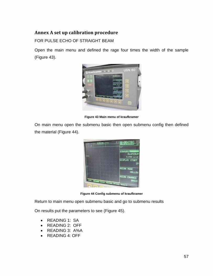
57

Annex A set up calibration procedure

FOR PULSE ECHO OF STRAIGHT BEAM

Open the main menu and defined the rage four times the width of the sample

(Figure 43).

Figure 43 Main menu of kraufkramer

On main menu open the submenu basic then open submenu config then defined

the material (Figure 44).

Figure 44 Config submenu of kraufkramer

Return to main menu open submenu basic and go to submenu results

On results put the parameters to see (Figure 45).

READING 1: SA

READING 2: OFF

READING 3: A%A

READING 4: OFF

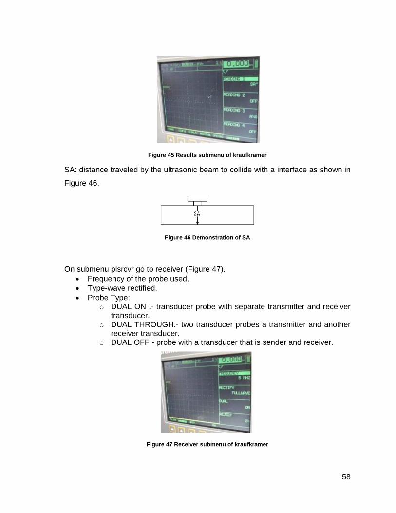
58

Figure 45 Results submenu of kraufkramer

SA: distance traveled by the ultrasonic beam to collide with a interface as shown in

Figure 46.

Figure 46 Demonstration of SA

On submenu plsrcvr go to receiver (Figure 47).

Frequency of the probe used.

Type-wave rectified.

Probe Type: o DUAL ON .- transducer probe with separate transmitter and receiver

transducer. o DUAL THROUGH.- two transducer probes a transmitter and another

receiver transducer. o DUAL OFF - probe with a transducer that is sender and receiver.

Figure 47 Receiver submenu of kraufkramer

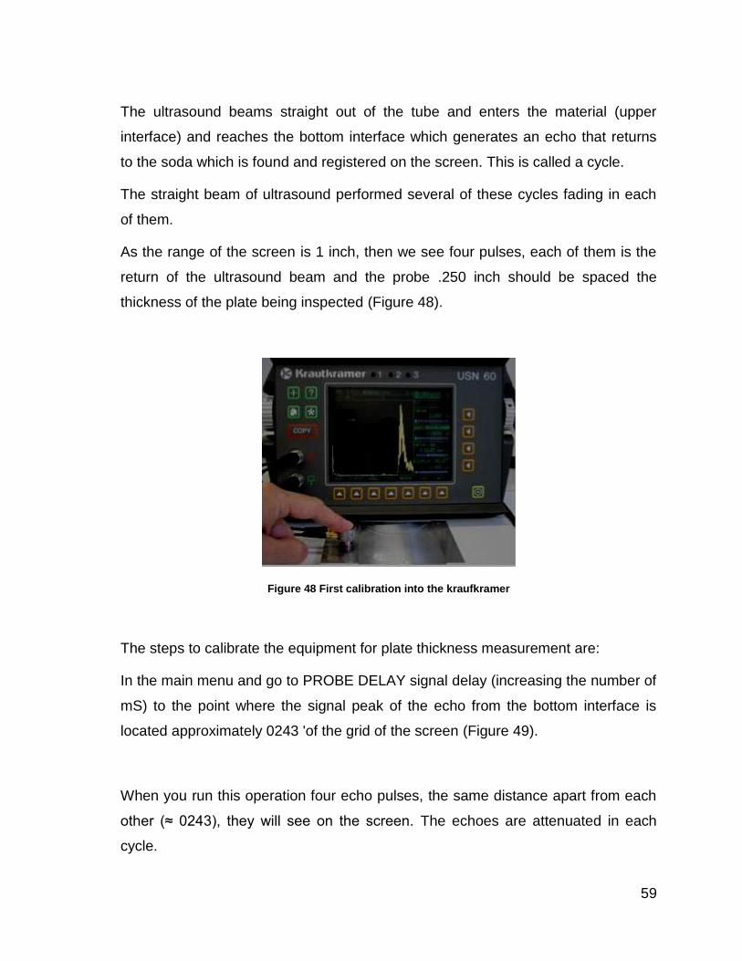
59

The ultrasound beams straight out of the tube and enters the material (upper

interface) and reaches the bottom interface which generates an echo that returns

to the soda which is found and registered on the screen. This is called a cycle.

The straight beam of ultrasound performed several of these cycles fading in each

of them.

As the range of the screen is 1 inch, then we see four pulses, each of them is the

return of the ultrasound beam and the probe .250 inch should be spaced the

thickness of the plate being inspected (Figure 48).

Figure 48 First calibration into the kraufkramer

The steps to calibrate the equipment for plate thickness measurement are:

In the main menu and go to PROBE DELAY signal delay (increasing the number of

mS) to the point where the signal peak of the echo from the bottom interface is

located approximately 0243 'of the grid of the screen (Figure 49).

When you run this operation four echo pulses, the same distance apart from each

other (≈ 0243), they will see on the screen. The echoes are attenuated in each

cycle.

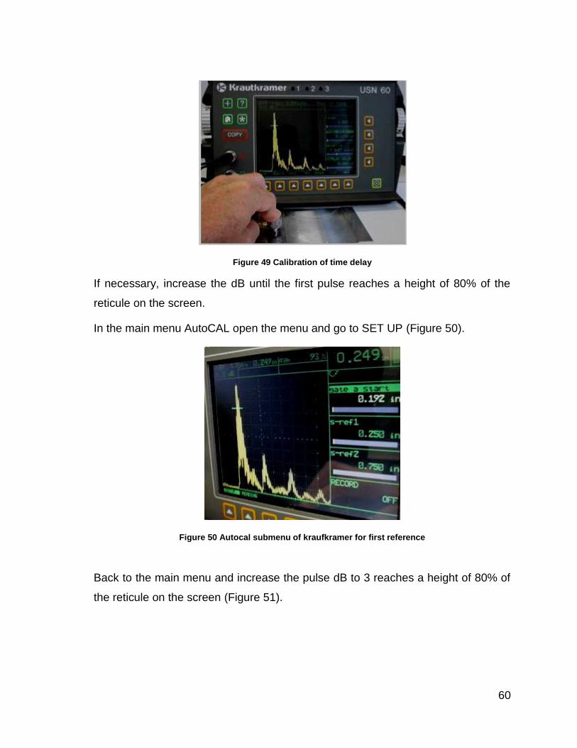
60

Figure 49 Calibration of time delay

If necessary, increase the dB until the first pulse reaches a height of 80% of the

reticule on the screen.

In the main menu AutoCAL open the menu and go to SET UP (Figure 50).

Figure 50 Autocal submenu of kraufkramer for first reference

Back to the main menu and increase the pulse dB to 3 reaches a height of 80% of

the reticule on the screen (Figure 51).

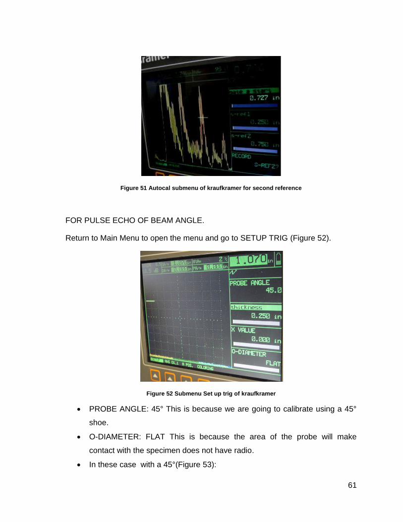
61

Figure 51 Autocal submenu of kraufkramer for second reference

FOR PULSE ECHO OF BEAM ANGLE.

Return to Main Menu to open the menu and go to SETUP TRIG (Figure 52).

Figure 52 Submenu Set up trig of kraufkramer

PROBE ANGLE: 45° This is because we are going to calibrate using a 45°

shoe.

O-DIAMETER: FLAT This is because the area of the probe will make

contact with the specimen does not have radio.

In these case with a 45°(Figure 53):

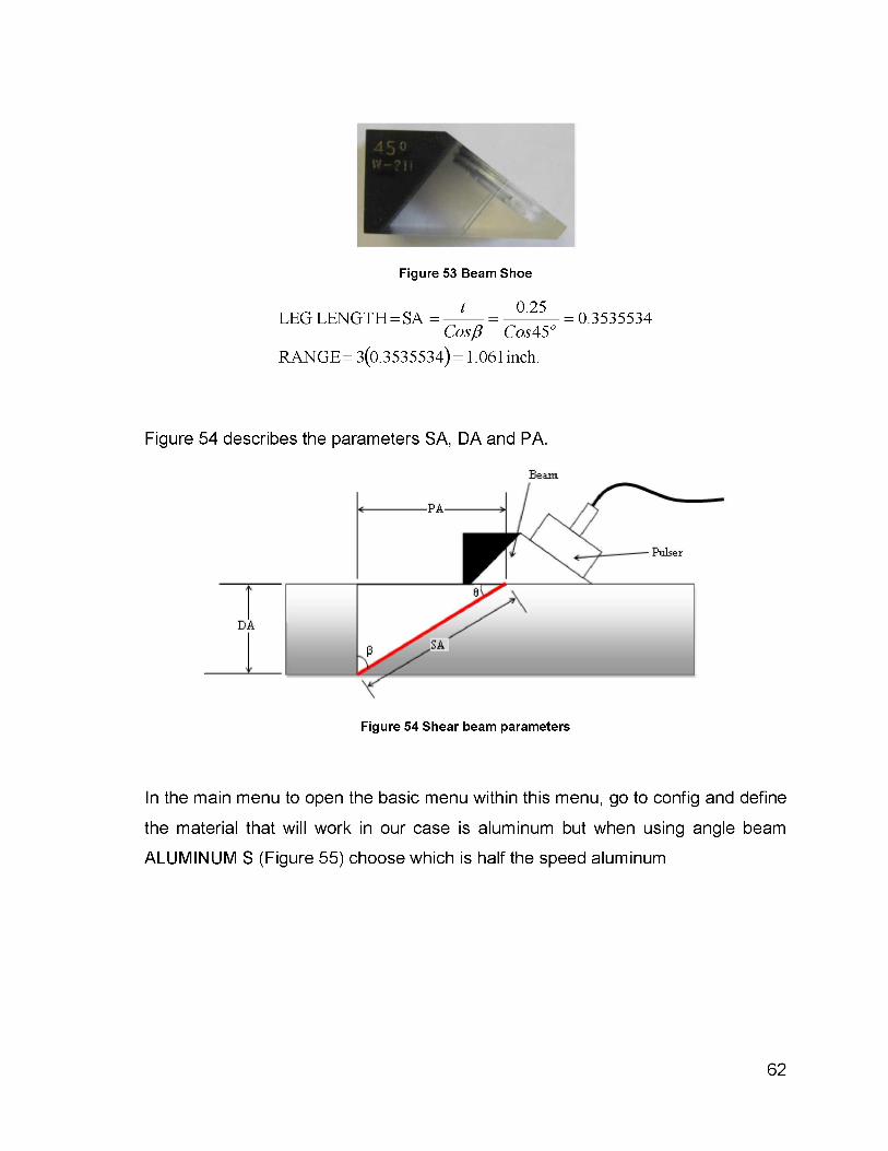
Figure 54 describes the parameters SA, DA and PA.

Figure 54 Shear beam parameters

In the main menu to open the basic menu within this menu, go to config and define

the material that will work in our case is aluminum but when using angle beam

ALUMINUM S (Figure 55) choose which is half the speed aluminum

62

Figure 53 Beam Shoe

LEG LENGTH = SA = t

Cosβ 0.25

Cos45o = 0.3535534

RANGE = 3(0.3535534) = 1.061 inch.

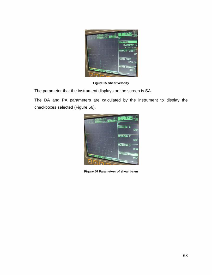
63

Figure 55 Shear velocity

The parameter that the instrument displays on the screen is SA.

The DA and PA parameters are calculated by the instrument to display the

checkboxes selected (Figure 56).

Figure 56 Parameters of shear beam

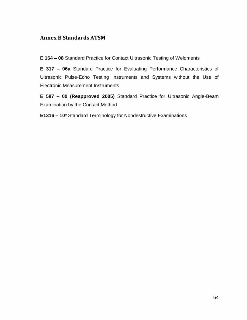
64

Annex B Standards ATSM

E 164 – 08 Standard Practice for Contact Ultrasonic Testing of Weldments

E 317 – 06a Standard Practice for Evaluating Performance Characteristics of

Ultrasonic Pulse-Echo Testing Instruments and Systems without the Use of

Electronic Measurement Instruments

E 587 – 00 (Reapproved 2005) Standard Practice for Ultrasonic Angle-Beam

Examination by the Contact Method

E1316 – 10ª Standard Terminology for Nondestructive Examinations

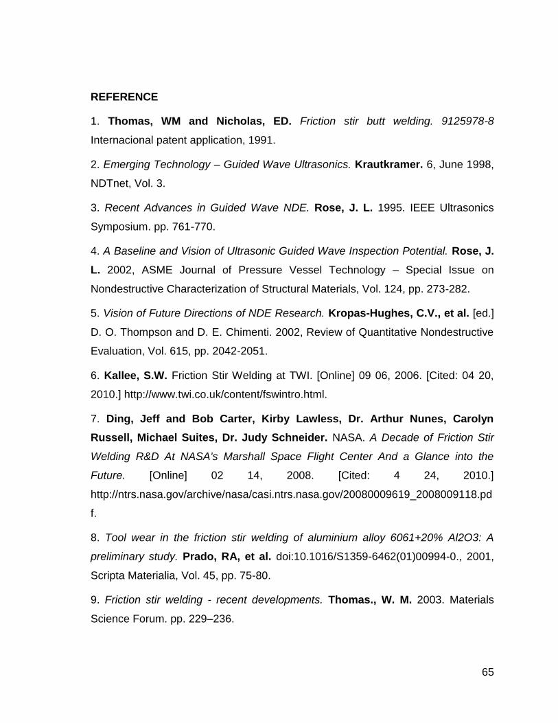
65

REFERENCE

1. Thomas, WM and Nicholas, ED. Friction stir butt welding. 9125978-8

Internacional patent application, 1991.

2. Emerging Technology – Guided Wave Ultrasonics. Krautkramer. 6, June 1998,

NDTnet, Vol. 3.

3. Recent Advances in Guided Wave NDE. Rose, J. L. 1995. IEEE Ultrasonics

Symposium. pp. 761-770.

4. A Baseline and Vision of Ultrasonic Guided Wave Inspection Potential. Rose, J.

L. 2002, ASME Journal of Pressure Vessel Technology – Special Issue on

Nondestructive Characterization of Structural Materials, Vol. 124, pp. 273-282.

5. Vision of Future Directions of NDE Research. Kropas-Hughes, C.V., et al. [ed.]

D. O. Thompson and D. E. Chimenti. 2002, Review of Quantitative Nondestructive

Evaluation, Vol. 615, pp. 2042-2051.

6. Kallee, S.W. Friction Stir Welding at TWI. [Online] 09 06, 2006. [Cited: 04 20,

2010.] http://www.twi.co.uk/content/fswintro.html.

7. Ding, Jeff and Bob Carter, Kirby Lawless, Dr. Arthur Nunes, Carolyn

Russell, Michael Suites, Dr. Judy Schneider. NASA. A Decade of Friction Stir

Welding R&D At NASA's Marshall Space Flight Center And a Glance into the

Future. [Online] 02 14, 2008. [Cited: 4 24, 2010.]

http://ntrs.nasa.gov/archive/nasa/casi.ntrs.nasa.gov/20080009619_2008009118.pd

f.

8. Tool wear in the friction stir welding of aluminium alloy 6061+20% Al2O3: A

preliminary study. Prado, RA, et al. doi:10.1016/S1359-6462(01)00994-0., 2001,

Scripta Materialia, Vol. 45, pp. 75-80.

9. Friction stir welding - recent developments. Thomas., W. M. 2003. Materials

Science Forum. pp. 229–236.

66

10. Friction stir welding-recent developments. W. M. Thomas, K. I. Johnson, and

C. S. Wiesner. 2003, Advanced Engineering Materials, pp. 485–490.

11. Microstructure and aging behaviour of FSW in Al alloys 2014A-T651 and 7075-

T651. Leonard, AJ. Gothenburg, Sweden. : 2nd International Symposium on

FSW, 2009.

12. Dynamic recrystallisation in the friction-stir welding of aluminium alloy 1100.

Murr, LE, Liu, G and McClure, JC. 1997, Journal of Materials Science Letters 16

(22), pp. 1801-1803. doi:10.1023/A:1018556332357..

13. Recent Advances in Friction Stir Welding Process, Weldment. R. Nandan, T.

DebRoy and H. K. D. H. Bhadeshia. 2008, Progress in Materials Science, pp.

980-1023.

14. Iowa State University. NDT Education Resource Center. [Online] The

Collaboration for NDT Education, 2001-2010. [Cited: 5 19, 2010.] www.ndt-ed.org.

15. MEASUREMENTS AT THE SPEED OF ULTRASOUND: FRIENDLY

REGARDS FROM FERMAT. LYNNWORTH, LAWRENCE C. s.l. : Panametrics,

06 20, 2002, THE BENT OF. UR-242TBP-WV.

16. Nondestructive Material Testing with Ultrasonics. Berke, Michael. 09, 09 2000,

The e-Journal of Nondestructive Testing & Ultrasonics -, Vol. 5. ISSN: 1435-4934.

17. Nondestructive evaluation. Shull, P.J. United States : CRC Press, 2002.

18. Inc., Olympus NDT. Olympus: cámaras de video de alta velocidad, equipos

para inspecciones visuales remotas, equipos END (ultrasonidos, ultrasonidos

phased array, corrientes de Foucault, medidores de espesor, detectores de

defectos). [Online] 2010. [Cited: 06 12, 2010.] www.olympus-ims.com.

19. ATSM. Standard Practice for Contact Ultrasonic Testing of Weldments1.

United States : s.n., 2008. E 164 – 08.

20. Application of Ultrasonic C-Scan Techniques for Tracing Defects in Laminated

Composite Materials. Hasiotis T., Badogiannis E. and Tsouvalis N.G. Greece :

4th international conference on NDT, 2007.

67

21. Asm International Handbook Committee. Metals Handbook. United States :

CRC Press, 1998. Vol. 2. 0871706547.

22. Al to Mg Friction Stir Welding: Effect of Positions of Al and Mg with Respect to

the Welding Tool. S., Firouzdor V. and Kou. Wisconsin : The Welding Journal,

2009, Vol. 88.

23. H. Liu, H. Fulii, M. Maeda, and K. Nogi. Tensile properties and fracture

locations of friction stir welded joints of 6061–T6 aluminium alloy. Journal of

Materials Science Letters. 2003. Vol. 22, 1061-1063.

24. ASM Metals Comittee. Metal handbook. United States : CRC Press, 1998.

Vol. 9. 0871706547.

25. Committee, ASTM. Standard Practice for Ultrasonic Angle-Beam Examination

by the Contact Method. ASTM. United States : s.n., 2005. E587.

Documents

IMPLEMENTATION OF FRICTION STIR WELDING IN … of friction stir welding in 3003 aluminum plates inspected by ultrasonic testing . tesis . maestro en ciencias con especialidad en sistemas