Embed Size (px)
Citation preview

Implementation of Dubin curves-based RRT* using an
aerial image for the determination of obstacles and path
planning to avoid them during displacement of the mobile
robot.
Daniel Tenezaca B.1, Christian Canchignia 1, Wilbert Aguilar1, Dario Mendoza 1
1 Universidad de las Fuerzas Armadas - ESPE, Sangolquí, Ecuador
{hdtenezaca, cscanchignia, wgaguilar,djmendoza}@espe.edu.ec
Abstract. The application of mobile robots in autonomous navigation has con-
tributed to the development of exploration tasks for the recognition of unknown
environments. There are different methodologies for obstacles avoidance imple-
mented in mobile robots, however, this research introduces a novel approach for
a path planning of an Unmanned Ground Vehicle (UGV) using the camera of a
drone to get an aerial view that allows to recognize ground features through im-
age processing algorithms for detecting obstacles and target them in a determined
environment. After aerial recognition a global planner with Rapidly-exploring
Random Tree Star (RRT*) algorithm is executed, Dubins curves are the method
used in this case for nonholonomic robots. The study also focuses on determining
the compute time which is affected by a growing number of iterations in the
RRT*, the value of step size between the tree’s nodes and finally the impact of
number of obstacles placed in the environment. This project is the initial part of
a larger research about a Collaborative Aerial-Ground Robotic System.
Keywords: RRT*, Path planning, image processing.
1 Introduction
Unmanned Aerial Vehicles (UAVs) and mobile robots are used in different opera-
tions according to their performances. UAVs have many limitations, for example, the
carrying capacity, flight time, etc. However, UAVs has a more ample range of vision
of a workspace and higher velocities [1]. On the contrary, mobile robots present many
advantages compared to UAVs. Mobile robots can carry heavier loads, have more
power units, and higher capacity for processing [2] [3]. The purpose is to combine them
to create a hybrid system taking into consideration the advantages of those two robotic
systems. In this proposal, the UAV is able to analyze a broad portion of ground in spe-
cific workspace to provide safe displacement directions to the grounded vehicle [4] [5].
The research presents a study to establish a global planner that represents the data
obtained from a top view generated by UAV [6]. First, the system develops an image
through processing algorithms based on artificial vison in order to determinate the most
relevant features inside the picture. In this case, the algorithm estimates the position of
the obstacles as well as the mobile vehicle’s destination.
2
LaValle [7] proposed RRT algorithm considered as an optimal technique to construct
trajectories in nonconvex high-dimensional spaces and used to solve path planning
problems. Commonly, an RRT is deficient to solve a problem related with the planning,
therefore, it is necessary to implement a path planning algorithm based on that RRT*
to expand the tree in free spaces [8]. The kinematic constraints of the ground vehicle
based on Ackerman steering makes RRT* algorithm grows drawing curves easy to
adapt the vehicle turning movements. This kind of curves is named Dubins path. Fi-
nally, it is important to consider adjusting many parameters to expand the tree, it will
allow to know how the algorithm is affected when existing variations of the obstacles,
number of iterations and the length of the connection between the tree’s nodes.
In section 2, the article presents an image processing algorithm for constructing a
global planner. In section 3, it details an analysis to stablish a RRT* algorithm using a
geometrically method based on constructing tangent lines that connect two points with
a shortest curve in a Euclidean plane. Finally in section 4 results will be presented ac-
cording the data obtained in different scenarios and various obstacle configurations.
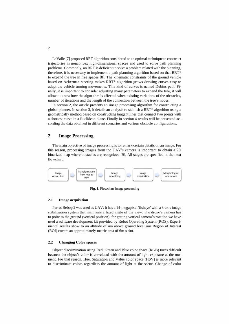
2 Image Processing
The main objective of image processing is to remark certain details on an image. For
this reason, processing images from the UAV’s camera is important to obtain a 2D
binarized map where obstacles are recognized [9]. All stages are specified in the next
flowchart:
Fig. 1. Flowchart image processing
2.1 Image acquisition
Parrot Bebop 2 was used as UAV. It has a 14-megapixel 'fisheye' with a 3-axis image
stabilization system that maintains a fixed angle of the view. The drone’s camera has
to point to the ground (vertical position), for getting vertical camera’s rotation we have
used a software development kit provided by Robot Operating System (ROS). Experi-
mental results show to an altitude of 4m above ground level our Region of Interest
(ROI) covers an approximately metric area of 6m x 4m.
2.2 Changing Color spaces
Object discrimination using Red, Green and Blue color space (RGB) turns difficult
because the object’s color is correlated with the amount of light exposure at the mo-
ment. For that reason, Hue, Saturation and Value color space (HSV) is more relevant
to discriminate colors regardless the amount of light at the scene. Change of color
Image Acquisition
Transformation from RGB to
HSV
Image smoothing
Image binarization
Morphological operations
3
spaces from RGB to HSV in this application allows better adapting of the obstacles’
algorithm to light changes, in cases which shadows contribute to false positives [10].
2.3 Image smoothing
Noise reduction is a very important factor for good image processing. In this case, it
is applied a Gaussian Blur filter [11]. This means that each pixel was affected for a
kernel (neighbor pixels). A kernel of size 5 was used and a Gaussian kernel standard
deviation in an X direction of 0, where the target is not to get a blurred image if else to
eliminate the small percent of noise.
2.4 Binarization
In our application, it was important to separate foreground elements (obstacles) from
the background of the image, binarization or thresholding methods are commonly used
for that purpose [12]. The obstacles were considered the most outstanding element on
the ground, therefore, establishing a binarized map where the obstacles have a pixel
value of 0 and a pixel value of 1 is a free space. The Hue value which represents red
color goes from 0º – 30º and 330º – 0º approximately. Another stage is using the bina-
rization to detect the target blue [13].
2.5 Edge dilatation and erosion
The dilation convolution adds pixels to the boundaries of the obstacles’ structure
reducing noise, while erosion remove pixels on the outside boundaries of the obstacles’
structure. The dilatation and erosion combined result in better filter. It fills holes (open-
ing) and removes small objects (closing). The opening operation works with a structur-
ing element a size kernel of 5. The operation affects the pixel and a 5x5 matrix size,
meanwhile closing operation uses a size kernel of 21 [14].
3 RRT* Algorithm
Dubins curves-based RRT* is used as a global planner. It establishes the path by two
type of configurations divided in Curve – straight – curve (CSC) and Curve- curve-
curve (CCC), which are the pattern of expansion in the RRT* algorithm. Random sam-
ple paths are generated from combination of straight lines and curves.
3.1 Initial requirements
Data input to get the path with the RRT* algorithm serve as initial state and orienta-
tion, numbers of iterations, goal state, step size. To set Dubin curves parameters it is
necessary to know the minimum turning radius of the robot. Finally, another important
input data is having the binarized map (workspace).
4
3.2 RRT* Algorithm
Acording to Noreen et al [15] RRT* is based in a group of features which allow tree
expansion very similar to RRT algorithm. The difference between the systems is that
RRT* incorporates two special properties called near neighbor search and rewiring tree
operations.
The algorithm is represented by a tree denoted as 𝑇 = (𝑉, 𝐸), where V is a set of
vertices and E is a set of edges. The initial configuration (𝑞𝑖𝑛𝑖𝑡) includes a set of vertices
that represents where the tree starts. In each iterations configured (Lines 3-11), the al-
gorithm stablishes a random position (𝑞𝑟𝑎𝑛𝑑) in free region, (𝑞𝑛𝑒𝑎𝑟𝑒𝑠𝑡) is searched in
the tree according to predefined step size from (𝑞𝑟𝑎𝑛𝑑) and immediately the algorithm
stablishes a new configuration (𝑞𝑛𝑒𝑤) with 𝑆𝑡𝑒𝑒𝑟 function which guides the system
from (𝑞𝑟𝑎𝑛𝑑) to (𝑞𝑛𝑒𝑎𝑟𝑒𝑠𝑡). The function 𝐶ℎ𝑜𝑜𝑠𝑒𝑝𝑎𝑟𝑒𝑛𝑡 allows to select the best parent
node for the new configuration (𝑞𝑛𝑒𝑤) before its insertion in tree considering the closest
nodes that lie inside of a circular area, finding(𝑞𝑚𝑖𝑛). Finally near neighbor operations
allows to generate the optimal path repeating the previous process [16].
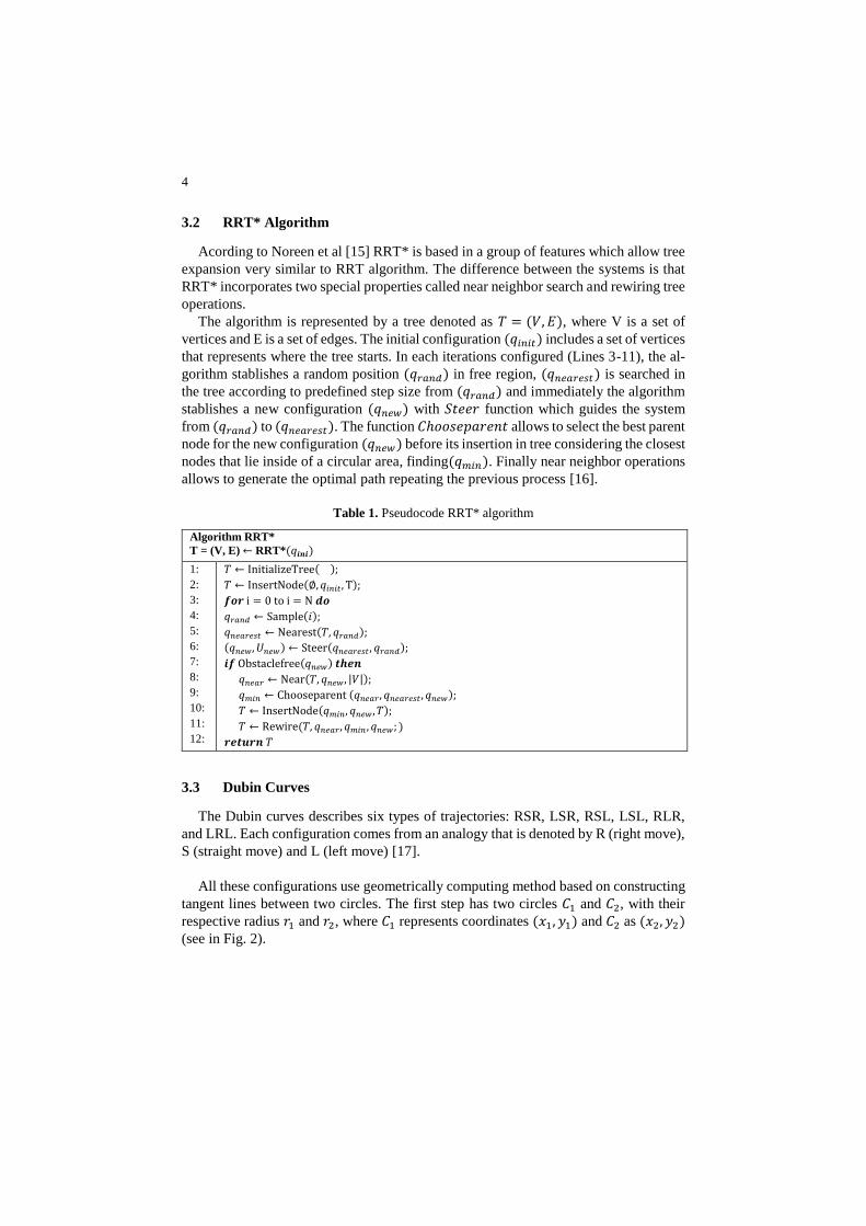
Table 1. Pseudocode RRT* algorithm
Algorithm RRT*
T = (V, E) ← RRT*(𝑞𝒊𝒏𝒊)
1:
2:
3:
4:
5:
6:
7:
8:
9:
10:
11:
12:
𝑇 ← InitializeTree( );
𝑇 ← InsertNode(∅, 𝑞𝑖𝑛𝑖𝑡, T);
𝒇𝒐𝒓 i = 0 to i = N 𝒅𝒐
𝑞𝑟𝑎𝑛𝑑 ← Sample(𝑖);
𝑞𝑛𝑒𝑎𝑟𝑒𝑠𝑡 ← Nearest(𝑇, 𝑞𝑟𝑎𝑛𝑑);
(𝑞𝑛𝑒𝑤, 𝑈𝑛𝑒𝑤) ← Steer(𝑞𝑛𝑒𝑎𝑟𝑒𝑠𝑡, 𝑞𝑟𝑎𝑛𝑑);
𝒊𝒇 Obstaclefree(𝑞𝑛𝑒𝑤) 𝒕𝒉𝒆𝒏
𝑞𝑛𝑒𝑎𝑟 ← Near(𝑇, 𝑞𝑛𝑒𝑤 , |𝑉|);
𝑞𝑚𝑖𝑛 ← Chooseparent (𝑞𝑛𝑒𝑎𝑟, 𝑞𝑛𝑒𝑎𝑟𝑒𝑠𝑡, 𝑞𝑛𝑒𝑤);
𝑇 ← InsertNode(𝑞𝑚𝑖𝑛, 𝑞𝑛𝑒𝑤 , 𝑇);
𝑇 ← Rewire(𝑇, 𝑞𝑛𝑒𝑎𝑟, 𝑞𝑚𝑖𝑛 , 𝑞𝑛𝑒𝑤; )
𝒓𝒆𝒕𝒖𝒓𝒏 𝑇
3.3 Dubin Curves
The Dubin curves describes six types of trajectories: RSR, LSR, RSL, LSL, RLR,
and LRL. Each configuration comes from an analogy that is denoted by R (right move),
S (straight move) and L (left move) [17].
All these configurations use geometrically computing method based on constructing
tangent lines between two circles. The first step has two circles 𝐶1 and 𝐶2, with their
respective radius 𝑟1 and 𝑟2, where 𝐶1 represents coordinates (𝑥1, 𝑦1) and 𝐶2 as (𝑥2, 𝑦2)
(see in Fig. 2).
5
Fig. 2. Circles initial configuration
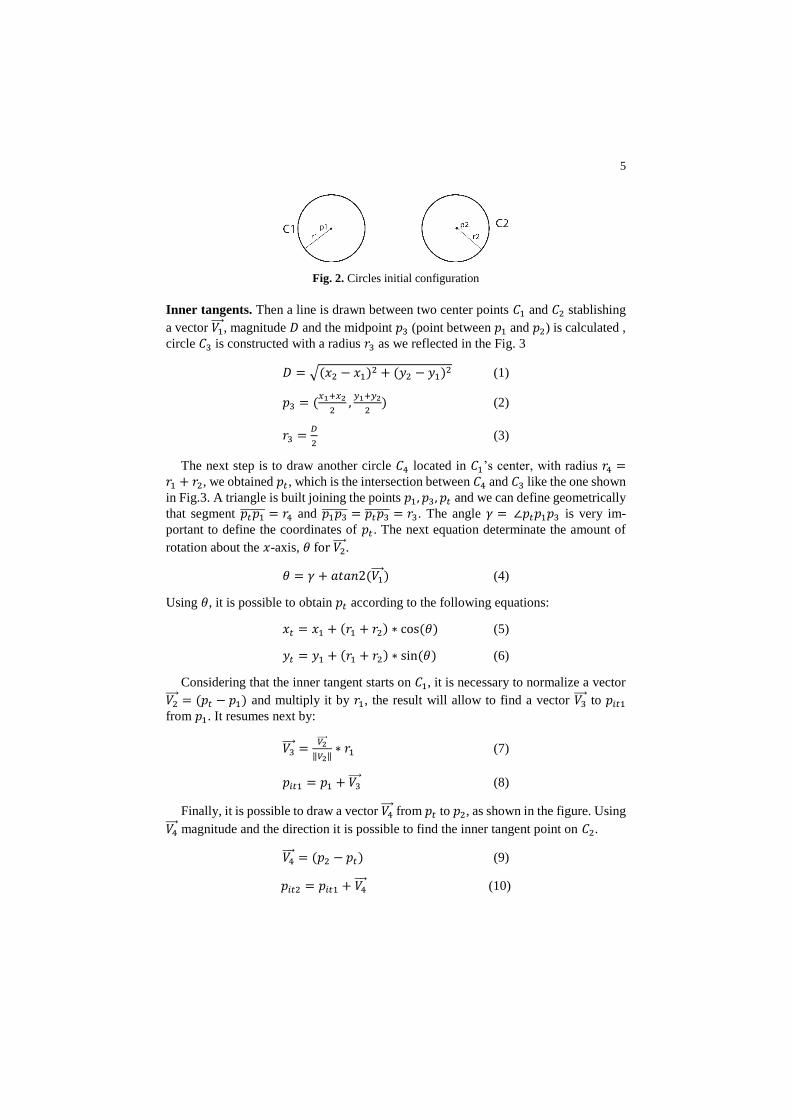
Inner tangents. Then a line is drawn between two center points 𝐶1 and 𝐶2 stablishing
a vector 𝑉1 , magnitude 𝐷 and the midpoint 𝑝3 (point between 𝑝1 and 𝑝2) is calculated ,
circle 𝐶3 is constructed with a radius 𝑟3 as we reflected in the Fig. 3
𝐷 = √(𝑥2 − 𝑥1)2 + (𝑦2 − 𝑦1)
2 (1)
𝑝3 = (𝑥1+𝑥2
2,𝑦1+𝑦2
2) (2)
𝑟3 =𝐷
2 (3)
The next step is to draw another circle 𝐶4 located in 𝐶1’s center, with radius 𝑟4 =𝑟1 + 𝑟2, we obtained 𝑝𝑡 , which is the intersection between 𝐶4 and 𝐶3 like the one shown
in Fig.3. A triangle is built joining the points 𝑝1, 𝑝3, 𝑝𝑡 and we can define geometrically
that segment 𝑝𝑡𝑝1 = 𝑟4 and 𝑝1𝑝3 = 𝑝𝑡𝑝3 = 𝑟3. The angle 𝛾 = ∠𝑝𝑡𝑝1𝑝3 is very im-
portant to define the coordinates of 𝑝𝑡 . The next equation determinate the amount of
rotation about the 𝑥-axis, 𝜃 for 𝑉2 .
𝜃 = 𝛾 + 𝑎𝑡𝑎𝑛2(𝑉1 ) (4)
Using 𝜃, it is possible to obtain 𝑝𝑡 according to the following equations:
𝑥𝑡 = 𝑥1 + (𝑟1 + 𝑟2) ∗ cos (𝜃) (5)
𝑦𝑡 = 𝑦1 + (𝑟1 + 𝑟2) ∗ sin (𝜃) (6)
Considering that the inner tangent starts on 𝐶1, it is necessary to normalize a vector
𝑉2 = (𝑝𝑡 − 𝑝1) and multiply it by 𝑟1, the result will allow to find a vector 𝑉3
to 𝑝𝑖𝑡1
from 𝑝1. It resumes next by:
𝑉3 =
𝑉2
‖𝑉2‖∗ 𝑟1 (7)
𝑝𝑖𝑡1 = 𝑝1 + 𝑉3 (8)
Finally, it is possible to draw a vector 𝑉4 from 𝑝𝑡 to 𝑝2, as shown in the figure. Using
𝑉4 magnitude and the direction it is possible to find the inner tangent point on 𝐶2.
𝑉4 = (𝑝2 − 𝑝𝑡) (9)
𝑝𝑖𝑡2 = 𝑝𝑖𝑡1 + 𝑉4 (10)
6
Fig. 3. Inner tangents
Outer tangents. The process is very similar to the one of inner tangents, having two
circles 𝐶1 and 𝐶2, and considering 𝑟1 ≥ 𝑟2, the procedure is the same as before, 𝐶4 is
centered at 𝑝1, with a difference the radius 𝑟4 = 𝑟1 − 𝑟2, after getting 𝑝𝑡 and following
all steps performed for the interior tangents, 𝑉2 is obtained and the first outer tangent
point 𝑝𝑜𝑡1. This condition produces that 𝑟4 < 𝑟1. To get the second outer tangent 𝑝𝑜𝑡2
an addition is performed by:
𝑝𝑜𝑡2 = 𝑝𝑜𝑡1 + 𝑉4 (11)
The main difference between calculating outer tangents compared to inner tangents is
the construction of circle 𝐶4; all steps keeps the same.
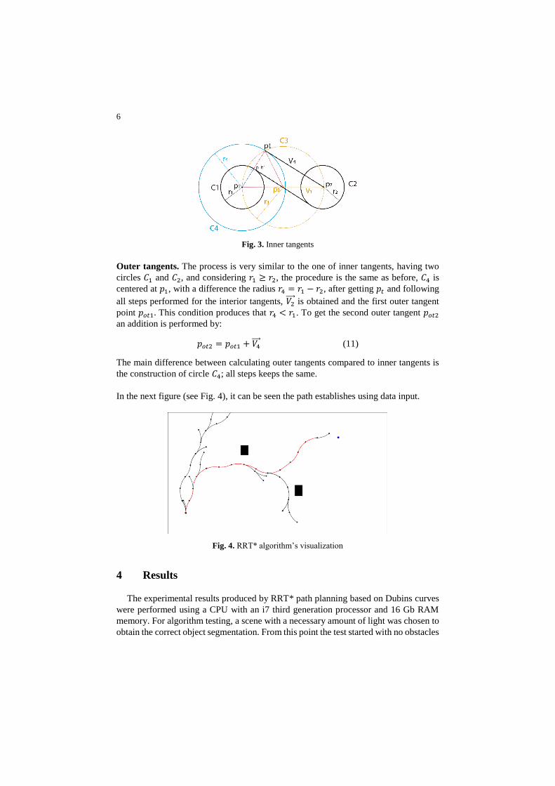
In the next figure (see Fig. 4), it can be seen the path establishes using data input.
Fig. 4. RRT* algorithm’s visualization
4 Results
The experimental results produced by RRT* path planning based on Dubins curves
were performed using a CPU with an i7 third generation processor and 16 Gb RAM
memory. For algorithm testing, a scene with a necessary amount of light was chosen to
obtain the correct object segmentation. From this point the test started with no obstacles
7
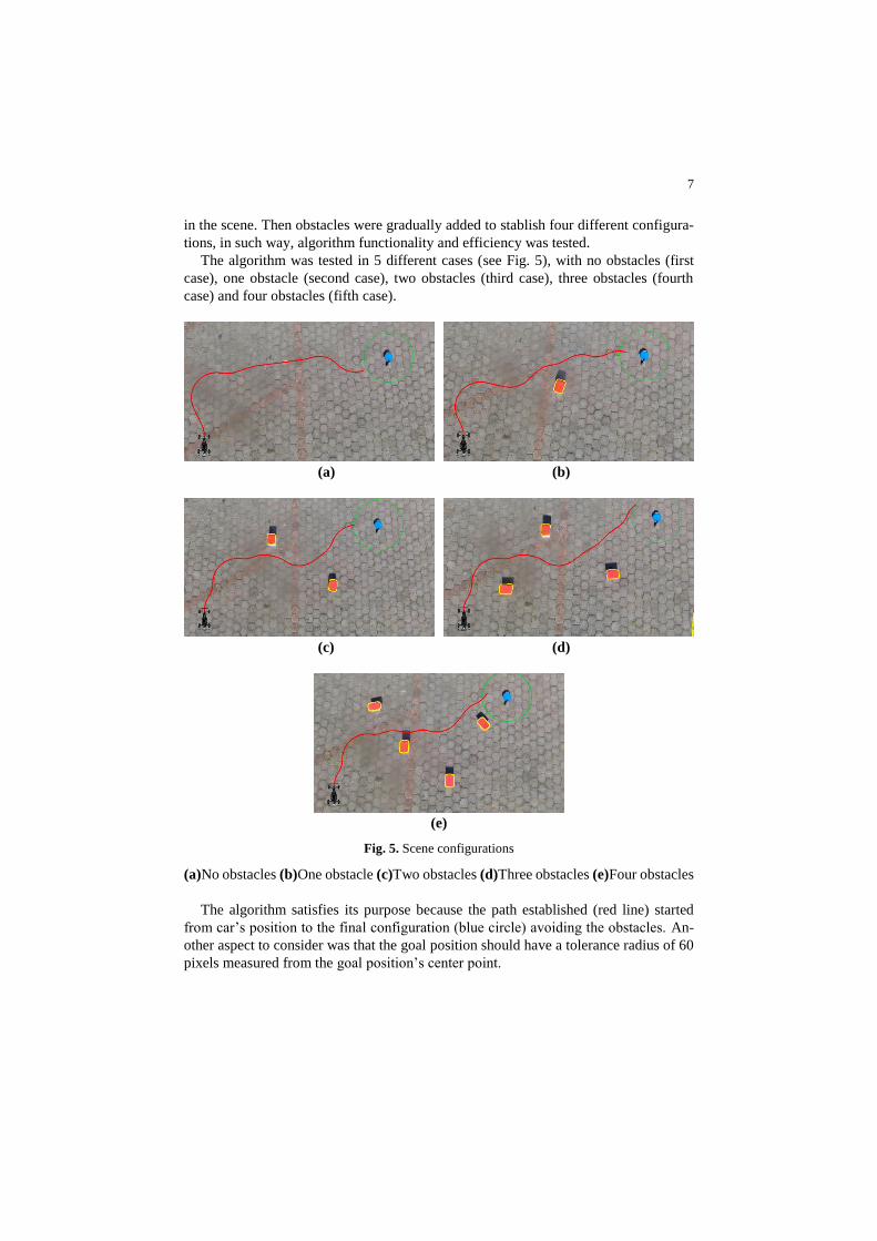
in the scene. Then obstacles were gradually added to stablish four different configura-
tions, in such way, algorithm functionality and efficiency was tested.
The algorithm was tested in 5 different cases (see Fig. 5), with no obstacles (first
case), one obstacle (second case), two obstacles (third case), three obstacles (fourth
case) and four obstacles (fifth case).
(a) (b)
(c) (d)
(e)
Fig. 5. Scene configurations
(a)No obstacles (b)One obstacle (c)Two obstacles (d)Three obstacles (e)Four obstacles
The algorithm satisfies its purpose because the path established (red line) started
from car’s position to the final configuration (blue circle) avoiding the obstacles. An-
other aspect to consider was that the goal position should have a tolerance radius of 60
pixels measured from the goal position’s center point.
8
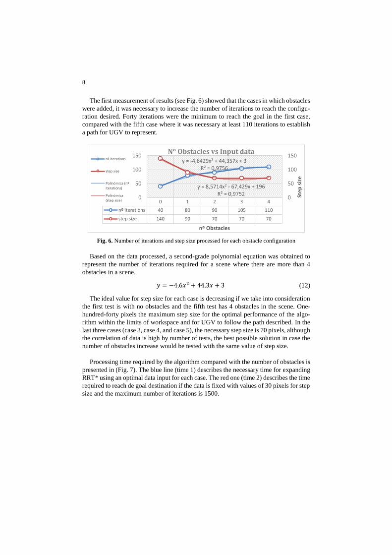
The first measurement of results (see Fig. 6) showed that the cases in which obstacles
were added, it was necessary to increase the number of iterations to reach the configu-
ration desired. Forty iterations were the minimum to reach the goal in the first case,
compared with the fifth case where it was necessary at least 110 iterations to establish
a path for UGV to represent.
Fig. 6. Number of iterations and step size processed for each obstacle configuration
Based on the data processed, a second-grade polynomial equation was obtained to
represent the number of iterations required for a scene where there are more than 4
obstacles in a scene.
𝑦 = −4,6𝑥2 + 44,3𝑥 + 3 (12)
The ideal value for step size for each case is decreasing if we take into consideration
the first test is with no obstacles and the fifth test has 4 obstacles in the scene. One-
hundred-forty pixels the maximum step size for the optimal performance of the algo-
rithm within the limits of workspace and for UGV to follow the path described. In the
last three cases (case 3, case 4, and case 5), the necessary step size is 70 pixels, although
the correlation of data is high by number of tests, the best possible solution in case the
number of obstacles increase would be tested with the same value of step size.
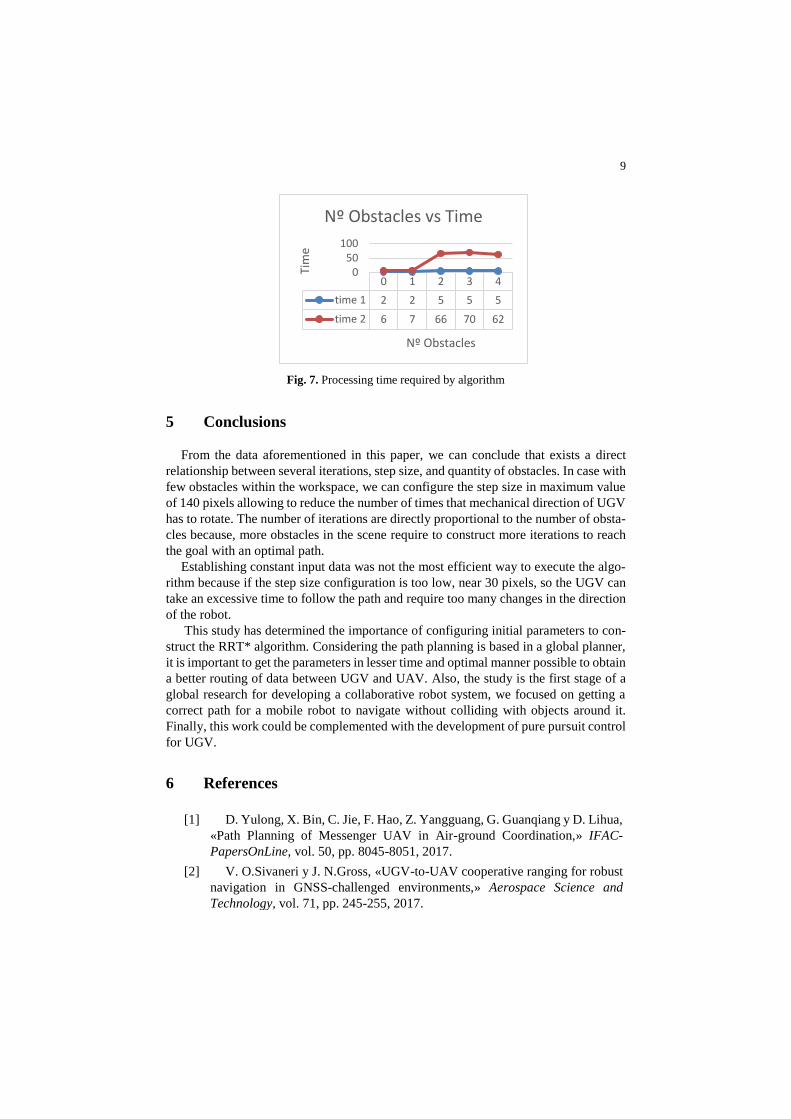
Processing time required by the algorithm compared with the number of obstacles is
presented in (Fig. 7). The blue line (time 1) describes the necessary time for expanding
RRT* using an optimal data input for each case. The red one (time 2) describes the time
required to reach de goal destination if the data is fixed with values of 30 pixels for step
size and the maximum number of iterations is 1500.
0 1 2 3 4
nº iterations 40 80 90 105 110
step size 140 90 70 70 70
y = -4,6429x2 + 44,357x + 3R² = 0,9756
y = 8,5714x2 - 67,429x + 196R² = 0,9752
0
50
100
150
0
50
100
150
Ste
p s
ize
nº Obstacles
Nº Obstacles vs Input data nº iterations
step size
Polinómica (nºiterations)
Polinómica(step size)
9
Fig. 7. Processing time required by algorithm
5 Conclusions
From the data aforementioned in this paper, we can conclude that exists a direct
relationship between several iterations, step size, and quantity of obstacles. In case with
few obstacles within the workspace, we can configure the step size in maximum value
of 140 pixels allowing to reduce the number of times that mechanical direction of UGV
has to rotate. The number of iterations are directly proportional to the number of obsta-
cles because, more obstacles in the scene require to construct more iterations to reach
the goal with an optimal path.
Establishing constant input data was not the most efficient way to execute the algo-
rithm because if the step size configuration is too low, near 30 pixels, so the UGV can
take an excessive time to follow the path and require too many changes in the direction
of the robot.
This study has determined the importance of configuring initial parameters to con-
struct the RRT* algorithm. Considering the path planning is based in a global planner,
it is important to get the parameters in lesser time and optimal manner possible to obtain
a better routing of data between UGV and UAV. Also, the study is the first stage of a
global research for developing a collaborative robot system, we focused on getting a
correct path for a mobile robot to navigate without colliding with objects around it.
Finally, this work could be complemented with the development of pure pursuit control
for UGV.
6 References
[1] D. Yulong, X. Bin, C. Jie, F. Hao, Z. Yangguang, G. Guanqiang y D. Lihua,
«Path Planning of Messenger UAV in Air-ground Coordination,» IFAC-
PapersOnLine, vol. 50, pp. 8045-8051, 2017.
[2] V. O.Sivaneri y J. N.Gross, «UGV-to-UAV cooperative ranging for robust
navigation in GNSS-challenged environments,» Aerospace Science and
Technology, vol. 71, pp. 245-255, 2017.
0 1 2 3 4
time 1 2 2 5 5 5
time 2 6 7 66 70 62
050
100
Tim
e
Nº Obstacles
Nº Obstacles vs Time
10
[3] R. Rahimi, F. Abdollahi y K. Naqshi, «Time-varying formation control of
a collaborative heterogeneous multi agent system,» Robotics and Autonomous
Systems, vol. 62, pp. 1799-1805, 2014.
[4] J. Melin, M. Lauri, A. Kolu, J. Koijonen y R. Ritala, «Cooperative Sensing
and Path Planning in a Multi-vehicle Environment,» IFAC-PapersOnLine, pp.
198-203, 2015.
[5] L. Rosa, M. Cognetti, A. Nicastro, P. Alvarez y G. Oriolo, «Multi-task
Cooperative Control in a Heterogeneous Ground-Air Robot Team,» IFAC-
PapersOnLine, vol. 48, pp. 53-58, 2015.
[6] F. Ropero, P. Muñoz y M. D. R-Moreno, «TERRA: A path planning
algorithm for cooperative UGV-UAV exploration,» Engineering Applications
of Artificial Intelligence, 2019.
[7] S. LaValle, «The RRT Page,» 1999. [En línea]. Available:
http://msl.cs.uiuc.edu/rrt/index.html.
[8] A. Abbadi y V. Prenosil, «Collided Path Replanning in Dynamic
Environments Using RRT and Cell Decomposition Algorithms,» Modelling
and Simulation for Autonomous Systems: Second International Workshop, pp.
131-143, 2015.
[9] T. Sieberth, R. Wackrow y J. H. Chandler, «Automatic detection of blurred
images in UAV image sets,» ISPRS Journal of Photogrammetry and Remote
Sensing, vol. 122, pp. 1-16, 2016.
[10] V. Chernov, J. Alander y V. Bochko, «Integer-based accurate conversion
between RGB and HSV color spaces,» Computer & Electrical Engineering ,
vol. 46, pp. 328-337, 2015.
[11] J. Huang, H. Feng, Z. Xu, Q. Li y Y. Chen, «A robust deblurring algorithm
for noisy images with just noticeable blur,» Optik, vol. 168, pp. 577-589, 2018.
[12] S. Chen y D. Li, «Image binarization focusing on objects,»
Neurocomputing, vol. 69, pp. 2411-2415, 2006.
[13] E. Dougherty, Mathematical Morphology in image processing, Nueva
York: Marcel Dekker, 1993.
[14] OpenCV, «OpenCV 2.4.13.7 documentation,» [En línea]. Available:
https://docs.opencv.org/2.4/modules/imgproc/doc/filtering.html.
[15] I. Noreen, A. Khan y Z. Habib, «Comparison of RRT, RTT* and RRT*-
Smart Path Planning Algorithms,» IJCSNS International Journal of Computer
Science and Network Security, 2016.
[16] S. Karaman y E. Frazzoli, «Sampling-based algorithms for optimal,» The
International Journal of Robotic Research, 2011.
[17] W. Yao, N. Qi, J. Zhao y N. Wan, «Bounded curvature path planning with
expected length for Dubins vehicle entering target manifold,» Robotics and
Autonomous Systems, vol. 97, pp. 217-229, 2017.