Embed Size (px)
Citation preview
IMPLEMENTATION OF A PHASED ARRAY ANTENNA USING DIGITAL BEAMFORMING
by
Juan A. Torres-Rosario
A thesis submitted in partial fulfillment of the requirements for the degree of
MASTER OF SCIENCES. in
ELECTRICAL ENGINEERING
UNIVERSITY OF PUERTO RICO MAYAGÜEZ CAMPUS
2005 Approved by: ________________________________ Jose G. Colom-Ustáriz, Ph. D. Member, Graduate Committee
__________________ Date
________________________________ Rafael A. Rodríguez-Solís, Ph. D. Member, Graduate Committee
__________________ Date
________________________________ Shawn Hunt, Ph. D. President, Graduate Committee
__________________ Date
________________________________ Pedro Vazquez, Ph. D. Representative of Graduate Studies
__________________ Date
________________________________ Isidoro Couvertier, Ph. D. Chairperson of the Department
__________________ Date

ii
ABSTRACT
This work presents the design of a transmitter/receiver Digital Beamformer (DBF)
based on the mathematical model of a far-field plane wave incident on a sensor array.
Simulations of a DBF transmitter and receiver are performed to control the power pattern
of a 4-element linear array, a 16-element linear array and a 16-element rectangular array.
For each sensor array, two spatial filters were constructed with different pattern
requirements to demonstrate the operation of the DBF. An implementation of a DBF
transmitter was performed using a digital processing board containing a Virtex-II
XC2V6000 FPGA to control the radiation pattern of a Phased Array Antenna transmitter.
A 16-element patch antenna array and the RF front end were fabricated and its radiation
pattern was measured in an anechoic chamber to test the performance of the DBF
transmitter giving an error of less than 5 degrees in each angular direction of the main
beam’s angle-of-transmission.
iii
RESUMEN
Este trabajo presenta el diseño de un “digital beamformer" (DBF) transmisor y
receptor basados en el modelo matemático de una onda plana que incide en un arreglo de
sensores. Simulaciones del DBF transmisor y receptor fueron realizadas para controlar el
patrón de radiación de tres arreglos con geometrías diferentes. Para cada arreglo de
sensores, dos filtros espaciales fueron construidos con requisitos específicos con el
propósito de demostrar el funcionamiento del DBF y comparar sus resultados con los
resultados obtenidos al calcular el patrón teóricamente. Una implementación del DBF
tipo transmisor fue realizada utilizando una tarjeta de procesamiento de datos con un
Virtex-II XC2V6000 FPGA para controlar el patrón de radiación de un arreglo de antenas
transmisor. Para implementar los componentes RF del arreglo de antenas se diseñaron y
construyeron un arreglo de parches con 16 elementos, una etapa de distribución para la
señal del oscilador local, y una etapa de mezclado y amplificación de potencia.
Finalmente, el patrón de radiación del arreglo de antenas fue medido utilizando una
cámara anecoica con el fin de mostrar el funcionamiento del DBF transmisor donde se
obtuvo patrones con menos de 5 grados de error en el ángulo de transmisión de su lóbulo
principal.

iv
ACKNOWLEDGEMENTS
This section is written to recognize those who have helped me during my life to work
hard, and finish my work. To my God, my utmost thanks for giving me the courage and
strength to follow my dreams and achieve my goals. To my Family and Friends, thanks
for your unconditional love and support through all these years. Thanks to my advisor
Prof. Shawn Hunt and my research professor Prof. Rafael Rodriguez for giving me the
opportunity to research under your supervision and give me guidance through these years
as a graduate student. Also, a special thanks to other Prof. Jose Colom, Prof. Manuel
Jimenez and Prof. Domingo Rodriguez for your help during the course of my
investigation.
NSF CASA ERC, 0313747 and NSF ECS-0093650 provided the funding and the
resources for the development of this research.
“El principio de la sabiduría es el temor de Jehová…”, Proverbios 1:7
v
Table of Contents
ABSTRACT .................................................................................................................................................II
RESUMEN ................................................................................................................................................. III
ACKNOWLEDGEMENTS ..................................................................................................................... IV
TABLE OF CONTENTS.............................................................................................................................V
TABLE LIST .............................................................................................................................................VII
FIGURE LIST ............................................................................................................................................ IX
1 INTRODUCTION ...........................................................................................................................14
2 THEORETICAL BACKGROUND ................................................................................................20
2.1 ARRAY PROCESSING THEORY.....................................................................................................20 2.1.1 Frequency-wavenumber Response and Beam Patterns.........................................................20 2.1.2 Delay-and-Sum Beamformer .................................................................................................25 2.1.3 Narrowband Beamformer......................................................................................................26 2.1.4 Spatial Filter Design .............................................................................................................28
2.2 PHASED ARRAY ANTENNA IMPLEMENTATIONS ..........................................................................33 2.3 DBF RECEIVER...........................................................................................................................35
2.3.1 Mathematical Model of DBF Receiver ..................................................................................35 2.3.2 DBF Receiver Design ............................................................................................................43
2.4 DBF TRANSMITTER ....................................................................................................................53 2.4.1 Mathematical Model of DBF Transmitter .............................................................................53 2.4.2 DBF Transmitter Design .......................................................................................................58
3 SIMULATION AND IMPLEMENTATION RESULTS ............................................................64
3.1 4-ELEMENT LINEAR PAA RECEIVER PROTOTYPE .....................................................................65 3.1.1 First Spatial Filter Example: Beam pattern with Uniform Amplitude Weight Function pointing to θMRA = 45º..........................................................................................................................70 3.1.2 Second Spatial Filter Example: Synthesized Beam pattern using Schlkunoff polynomial null-placement method ................................................................................................................................77 3.1.3 Beam pattern Granularity for 4-element linear PAA ............................................................84
3.2 16-ELEMENT LINEAR PAA TRANSMITTER PROTOTYPE ............................................................87 3.2.1 First Spatial Filter Example: Beam pattern with Taylor Amplitude Weight Function pointing to θMRA = 60º........................................................................................................................................92 3.2.2 Second Spatial Filter Example: Beam pattern with Blackman-Harris Amplitude Weight Function pointing to θMRA = 82º ........................................................................................................100 3.2.3 Beam pattern Granularity for 16-element linear PAA ........................................................107
3.3 16-ELEMENT RECTANGULAR PAA TRANSMITTER PROTOTYPE..............................................110
vi
3.3.1 First Spatial Filter Example: Beam pattern with Uniform Amplitude Weight Function pointing to φMRA = 0º and θMRA = 30º ................................................................................................111 3.3.2 Second Spatial Filter Example: Beam pattern with Dolph-Chebyshev Amplitude Weight Function pointing to φMRA = 122º and θMRA = 16º .............................................................................120 3.3.3 Beam pattern Granularity for 16-element rectangular PAA ...............................................130
3.4 16-ELEMENT RECTANGULAR PAA TRANSMITTER ..................................................................132 3.4.1 DBF Transmitter .................................................................................................................134 3.4.2 RF Up-Conversion Stage.....................................................................................................140 3.4.3 Rectangular Patch Antenna Array.......................................................................................155 3.4.4 PAA Measurement Results...................................................................................................161
4 CONCLUSIONS AND FUTURE WORK ..................................................................................169
4.1 CONCLUSIONS .........................................................................................................................169 4.2 FUTURE WORK.........................................................................................................................171
APPENDIX A. MATLAB CODE FILES........................................................................................178
vii
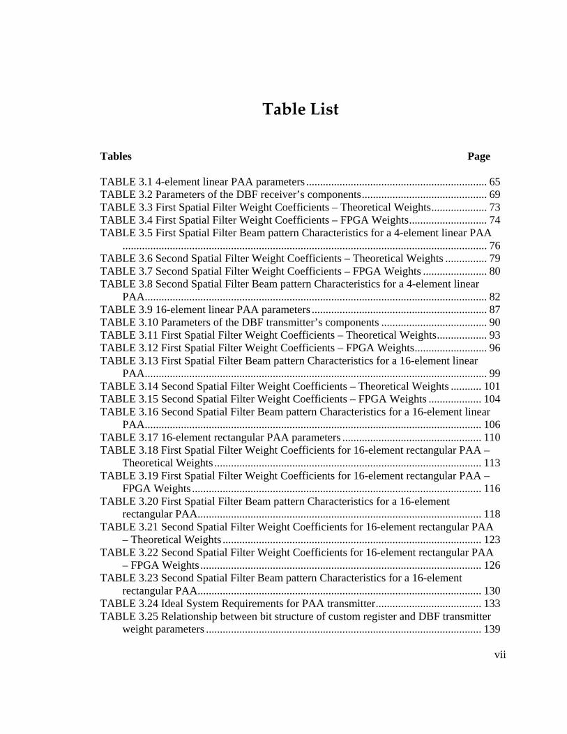
Table List
Tables Page TABLE 3.1 4-element linear PAA parameters ................................................................. 65 TABLE 3.2 Parameters of the DBF receiver’s components............................................. 69 TABLE 3.3 First Spatial Filter Weight Coefficients – Theoretical Weights.................... 73 TABLE 3.4 First Spatial Filter Weight Coefficients – FPGA Weights............................ 74 TABLE 3.5 First Spatial Filter Beam pattern Characteristics for a 4-element linear PAA
................................................................................................................................... 76 TABLE 3.6 Second Spatial Filter Weight Coefficients – Theoretical Weights ............... 79 TABLE 3.7 Second Spatial Filter Weight Coefficients – FPGA Weights ....................... 80 TABLE 3.8 Second Spatial Filter Beam pattern Characteristics for a 4-element linear
PAA........................................................................................................................... 82 TABLE 3.9 16-element linear PAA parameters ............................................................... 87 TABLE 3.10 Parameters of the DBF transmitter’s components ...................................... 90 TABLE 3.11 First Spatial Filter Weight Coefficients – Theoretical Weights.................. 93 TABLE 3.12 First Spatial Filter Weight Coefficients – FPGA Weights.......................... 96 TABLE 3.13 First Spatial Filter Beam pattern Characteristics for a 16-element linear
PAA........................................................................................................................... 99 TABLE 3.14 Second Spatial Filter Weight Coefficients – Theoretical Weights ........... 101 TABLE 3.15 Second Spatial Filter Weight Coefficients – FPGA Weights ................... 104 TABLE 3.16 Second Spatial Filter Beam pattern Characteristics for a 16-element linear
PAA......................................................................................................................... 106 TABLE 3.17 16-element rectangular PAA parameters .................................................. 110 TABLE 3.18 First Spatial Filter Weight Coefficients for 16-element rectangular PAA –
Theoretical Weights ................................................................................................ 113 TABLE 3.19 First Spatial Filter Weight Coefficients for 16-element rectangular PAA –
FPGA Weights ........................................................................................................ 116 TABLE 3.20 First Spatial Filter Beam pattern Characteristics for a 16-element
rectangular PAA...................................................................................................... 118 TABLE 3.21 Second Spatial Filter Weight Coefficients for 16-element rectangular PAA
– Theoretical Weights ............................................................................................. 123 TABLE 3.22 Second Spatial Filter Weight Coefficients for 16-element rectangular PAA
– FPGA Weights..................................................................................................... 126 TABLE 3.23 Second Spatial Filter Beam pattern Characteristics for a 16-element
rectangular PAA...................................................................................................... 130 TABLE 3.24 Ideal System Requirements for PAA transmitter...................................... 133 TABLE 3.25 Relationship between bit structure of custom register and DBF transmitter
weight parameters ................................................................................................... 139

viii
TABLE 3.26 Parameters of the Power Divider circuit ................................................... 148 TABLE 3.27 S-Parameters for Constructed Power Divider Network Circuits at 5.85 GHz
................................................................................................................................. 152 TABLE 3.28 Power Gain of each PAA channel in the second circuit ........................... 155 TABLE 3.29 Parameters of the Rectangular Patch Array .............................................. 155

ix
Figure List
Figures Page
Figure 2.1 Diagram of an N-element sensor array receiving a plane wave signal f(t,p) coming from the far-field.......................................................................................... 21
Figure 2.2 Diagram of a Delay-and-Sum Beamformer .................................................... 25 Figure 2.3 Diagram of Narrowband Beamformer............................................................. 28 Figure 2.4 Diagram of PAA using an RF Beamformer .................................................... 34 Figure 2.5 Diagram of a PAA using a Digital Beamformer ............................................. 35 Figure 2.6 Block diagram (including equations) of RF Modulator and DDC.................. 40 Figure 2.7 Block diagram of CWM phase........................................................................ 42 Figure 2.8 Architecture of CIC Decimation Filter............................................................ 48 Figure 2.9 Power Response of a CIC Filter with the following parameters: N = 8, M = 1,
R = 10........................................................................................................................ 49 Figure 2.10 Design of a DDC for a DBF Receiver........................................................... 51 Figure 2.11 Design of CWM for a DBF Receiver ............................................................ 52 Figure 2.12 Block Diagram (with equations) of CWM and DUC for a DBF Transmitter56 Figure 2.13 Design of CWM for a DBF Transmitter........................................................ 59 Figure 2.14 Architecture of CIC Interpolation Filter........................................................ 61 Figure 2.15 Design of DUC for a DBF Transmitter ......................................................... 62 Figure 3.1 Diagram of a simulated 4-element DBF receiver............................................ 67 Figure 3.2 Diagram of simulated DDC (3.2a) and CWM (3.2b) stage in DBF receiver.. 68 Figure 3.3 Polar Plot of Beam pattern Magnitude of a 4-element linear DBF pointing at
θMRA = 45º.................................................................................................................. 71 Figure 3.4 Rectangular plot of Beam pattern Magnitude of a 4-element linear DBF
pointing at θMRA = 45º ............................................................................................... 72 Figure 3.5 Time plots for plane wave signals with the angle of arrival changing from 90º
to 0º for first spatial filter on 4-element linear DBF................................................. 74 Figure 3.6 Time plots for plane wave signals with the angle of arrival changing from 90º
to 180º for first spatial filter on 4-element linear DBF............................................. 75 Figure 3.7 Polar Plot of Beam pattern Magnitude of a 4-element linear DBF Simulation
pointing at θMRA = 45º ............................................................................................... 76 Figure 3.8 Rectangular plot of Beam pattern Magnitude of a 4-element linear DBF
pointing at θMRA = 45º ............................................................................................... 77 Figure 3.9 Polar Plot of Beam pattern Magnitude of a 4-element linear DBF with beam
pattern nulls placed at 30º, 60º, and 100º.................................................................. 79 Figure 3.10 Rectangular Plot of Beam pattern Magnitude of a 4-element linear DBF with
beam pattern nulls placed at 30º, 60º, and 100º ........................................................ 79

x
Figure 3.11 Time plots for plane wave signals with the angle of arrival changing from 90º to 0º for second spatial filter on 4-element linear DBF ............................................ 80
Figure 3.12 Time plots for plane wave signals with the angle of arrival changing from 90º to 180º for second spatial filter on 4-element linear DBF ........................................ 81
Figure 3.13 Polar Plot of Beam pattern Magnitude of a simulated 4-element linear DBF with beam pattern nulls placed at 30º, 60º, and 100º ................................................ 82
Figure 3.14 Rectangular Plot of Beam pattern Magnitude of a simulated 4-element linear DBF with beam pattern nulls placed at 30º, 60º, and 100º ....................................... 83
Figure 3.15 Beam pattern Granularity Plot for a 4-element linear DBF with 8 bits of resolution on the weight coefficient’s phase............................................................. 85
Figure 3.16 Beam pattern Granularity Plot for a 4-element linear DBF with 4 bits of resolution on the weight coefficient’s phase............................................................. 86
Figure 3.17 Beam pattern Granularity Plot for a 4-element linear DBF with 16 bits of resolution on the weight coefficient’s phase............................................................. 86
Figure 3.18 Diagram of the simulated 16-element linear DBF transmitter ...................... 88 Figure 3.19 Diagram of the DUC (3.19a) and CWM (3.19b) of the simulated DBF
transmitter ................................................................................................................. 90 Figure 3.20 Polar Plot of Beam pattern Magnitude of a 4-element linear DBF with Taylor
Amplitude Distribution pointing at θMRA = 60º. ........................................................ 94 Figure 3.21 Rectangular Plot of Beam pattern Magnitude of a 4-element linear DBF with
Taylor Amplitude Distribution pointing at θMRA = 60º .............................................95 Figure 3.22 Signal Plots of 4 of the 16-elements in the linear DBF transmitter for first
spatial filter simulation ............................................................................................. 97 Figure 3.23 Polar Plot of Beam pattern Magnitude of a simulated 4-element linear DBF
with Taylor Amplitude Distribution pointing at θMRA = 60º ..................................... 98 Figure 3.24 Rectangular Plot of Beam pattern Magnitude of a simulated 4-element linear
DBF with Taylor Amplitude Distribution pointing at θMRA = 60º ............................ 99 Figure 3.25 Polar Plot of Beam pattern Magnitude of a 4-element linear DBF with
Blackmann-Harris Amplitude Distribution pointing at θMRA = 82º ........................ 102 Figure 3.26 Rectangular Plot of Beam pattern Magnitude of a 4-element linear DBF with
Blackmann-Harris Amplitude Distribution pointing at θMRA = 82º ........................ 103 Figure 3.27 Signal Plots of 4 of the 16-elements in the linear DBF transmitter for second
spatial filter simulation ........................................................................................... 104 Figure 3.28 Polar Plot of Beam pattern Magnitude of simulated 4-element linear DBF
with Blackmann-Harris Amplitude Distribution pointing at θMRA = 82º ................ 106 Figure 3.29 Rectangular Plot of Beam pattern Magnitude of simulated 4-element linear
DBF with Blackmann-Harris Amplitude Distribution pointing at θMRA = 82º ....... 107 Figure 3.30 Beam pattern Granularity Plot for a 16-element linear DBF with 8 bits of
resolution on the weight coefficient’s phase........................................................... 108 Figure 3.31 Beam pattern Granularity Plot for a 16-element linear DBF with 4 bits of
resolution on the weight coefficient’s phase........................................................... 109

xi
Figure 3.32 Beam pattern Granularity Plot for a 16-element linear DBF with 16 bits of resolution on the weight coefficient’s phase........................................................... 109
Figure 3.33 Top View Polar Plot of Beam pattern Magnitude of 16-element rectangular DBF with Uniform Amplitude Distribution pointing at φMRA = 0º and θMRA = 30º 114
Figure 3.34 Rectangular Plots of Beam pattern Magnitude of 16-element rectangular DBF with Uniform Amplitude Distribution pointing at φMRA = 82º and θMRA = 0º for Plane cut on φ = 0º and φ = 45º ........................................................................................ 114
Figure 3.35 Surf Plot of Beam pattern Magnitude of 16-element rectangular DBF with Uniform Amplitude Distribution pointing at φMRA = 0º and θMRA = 30º ................. 115
Figure 3.36 Signal Plots of 4 of the 16-elements in the rectangular DBF transmitter for first spatial filter simulation.................................................................................... 117
Figure 3.37 Top View Polar Plot of Beam pattern Magnitude of simulated 16-element rectangular DBF with Uniform Amplitude Distribution pointing at φMRA = 0º and θMRA = 30º................................................................................................................ 119
Figure 3.38 Rectangular Plots of Beam pattern Magnitude of simulated 16-element rectangular DBF with Uniform Amplitude Distribution pointing at φMRA = 0º and θMRA = 30º for Plane cut on φ = 0º and φ = 45º....................................................... 119
Figure 3.39 Surf Plot of Beam pattern Magnitude of simulated 16-element rectangular DBF with Uniform Amplitude Distribution pointing at φMRA = 0º and θMRA = 30º 120
Figure 3.40 Top View Polar Plot of Beam pattern Magnitude of 16-element rectangular DBF with Dolph-Chebyshev Amplitude Distribution pointing at φMRA = 122º and θMRA = 16º................................................................................................................ 124
Figure 3.41 Rectangular Plots of Beam pattern Magnitude of 16-element rectangular DBF with Dolph-Chebyshev Amplitude Distribution pointing at φMRA = 122º and θMRA = 16º for Plane cut on φ = 122º and φ = 302º ............................................................ 125
Figure 3.42 Surf Plot of Beam pattern Magnitude of 16-element rectangular DBF with Dolph-Chebyshev Amplitude Distribution pointing at φMRA = 122º and θMRA = 16º................................................................................................................................. 125
Figure 3.43 Signal Plots of 4 of the 16-elements in the rectangular DBF transmitter for second spatial filter simulation ............................................................................... 127
Figure 3.44 Top View Polar Plot of Beam pattern Magnitude of simulated 16-element rectangular DBF with Dolph-Chebyshev Amplitude Distribution pointing at φMRA = 122º and θMRA = 16º................................................................................................. 128
Figure 3.45 Rectangular Plots of Beam pattern Magnitude of simulated 16-element rectangular DBF with Dolph-Chebyshev Amplitude Distribution pointing at φMRA = 122º and θMRA = 16º for Plane cut on φ = 122º and φ = 302º.................................. 129
Figure 3.46 Surf Plot of Beam pattern Magnitude of simulated 16-element rectangular DBF with Dolph-Chebyshev Amplitude Distribution pointing at φMRA = 122º and θMRA = 16º................................................................................................................ 129
Figure 3.47 Beam pattern Granularity Surf Plot for a 16-element rectangular DBF with 8 bits of resolution on the weight coefficient’s phase................................................ 131
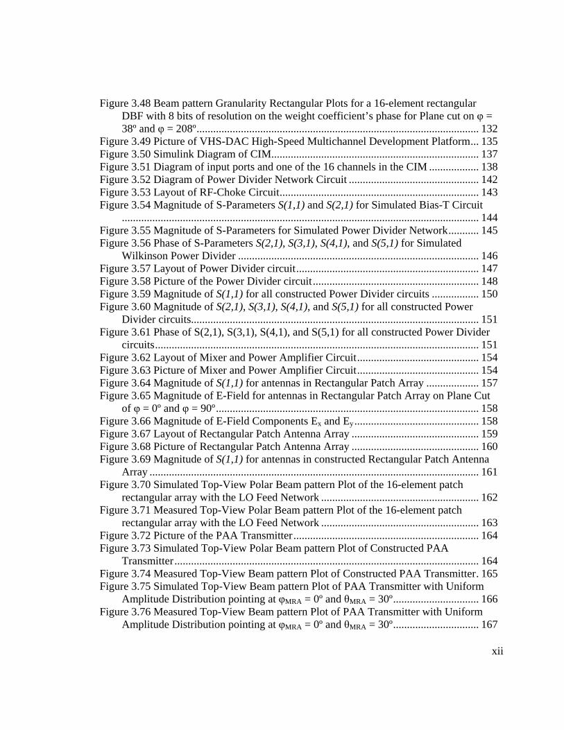
xii
Figure 3.48 Beam pattern Granularity Rectangular Plots for a 16-element rectangular DBF with 8 bits of resolution on the weight coefficient’s phase for Plane cut on φ = 38º and φ = 208º...................................................................................................... 132
Figure 3.49 Picture of VHS-DAC High-Speed Multichannel Development Platform... 135 Figure 3.50 Simulink Diagram of CIM........................................................................... 137 Figure 3.51 Diagram of input ports and one of the 16 channels in the CIM .................. 138 Figure 3.52 Diagram of Power Divider Network Circuit ............................................... 142 Figure 3.53 Layout of RF-Choke Circuit........................................................................ 143 Figure 3.54 Magnitude of S-Parameters S(1,1) and S(2,1) for Simulated Bias-T Circuit
................................................................................................................................. 144 Figure 3.55 Magnitude of S-Parameters for Simulated Power Divider Network........... 145 Figure 3.56 Phase of S-Parameters S(2,1), S(3,1), S(4,1), and S(5,1) for Simulated
Wilkinson Power Divider ....................................................................................... 146 Figure 3.57 Layout of Power Divider circuit.................................................................. 147 Figure 3.58 Picture of the Power Divider circuit............................................................ 148 Figure 3.59 Magnitude of S(1,1) for all constructed Power Divider circuits ................. 150 Figure 3.60 Magnitude of S(2,1), S(3,1), S(4,1), and S(5,1) for all constructed Power
Divider circuits........................................................................................................ 151 Figure 3.61 Phase of S(2,1), S(3,1), S(4,1), and S(5,1) for all constructed Power Divider
circuits..................................................................................................................... 151 Figure 3.62 Layout of Mixer and Power Amplifier Circuit............................................ 154 Figure 3.63 Picture of Mixer and Power Amplifier Circuit............................................ 154 Figure 3.64 Magnitude of S(1,1) for antennas in Rectangular Patch Array ................... 157 Figure 3.65 Magnitude of E-Field for antennas in Rectangular Patch Array on Plane Cut
of φ = 0º and φ = 90º............................................................................................... 158 Figure 3.66 Magnitude of E-Field Components Ex and Ey............................................. 158 Figure 3.67 Layout of Rectangular Patch Antenna Array .............................................. 159 Figure 3.68 Picture of Rectangular Patch Antenna Array .............................................. 160 Figure 3.69 Magnitude of S(1,1) for antennas in constructed Rectangular Patch Antenna
Array ....................................................................................................................... 161 Figure 3.70 Simulated Top-View Polar Beam pattern Plot of the 16-element patch
rectangular array with the LO Feed Network ......................................................... 162 Figure 3.71 Measured Top-View Polar Beam pattern Plot of the 16-element patch
rectangular array with the LO Feed Network ......................................................... 163 Figure 3.72 Picture of the PAA Transmitter................................................................... 164 Figure 3.73 Simulated Top-View Polar Beam pattern Plot of Constructed PAA
Transmitter.............................................................................................................. 164 Figure 3.74 Measured Top-View Beam pattern Plot of Constructed PAA Transmitter. 165 Figure 3.75 Simulated Top-View Beam pattern Plot of PAA Transmitter with Uniform
Amplitude Distribution pointing at φMRA = 0º and θMRA = 30º............................... 166 Figure 3.76 Measured Top-View Beam pattern Plot of PAA Transmitter with Uniform
Amplitude Distribution pointing at φMRA = 0º and θMRA = 30º............................... 167

xiii
Figure 3.77 Simulated Surf Plot of Beam pattern Magnitude for a PAA Transmitter with Uniform Amplitude Distribution pointing at φMRA = 0º and θMRA = 30º................ 167
Figure 3.78 Measured Surf Plot of Beam pattern Magnitude for a PAA Transmitter with Uniform Amplitude Distribution pointing at φMRA = 0º and θMRA = 30º................ 168
Figure 4.1 Diagram of PAA with single MRA beam and steering capability ................ 173
xiv
1 INTRODUCTION
Phased array antennas are known for their capability to steer the beam pattern
electronically with high effectiveness, managing to get minimal side-lobe levels and
narrow beamwidths. Implementations beginning during the 1950s depended largely on
microwave circuitry components such as phase shifters, and variable amplifiers. To
achieve performance specifications such as narrow beamwidth or considerable scanning
range with high angle resolution, a large number of antenna elements were needed to
construct the array. The use of these microwave components in large quantities pose
numerous obstacles to good performance and complicate the maintenance process of the
phased array antenna.
Phase shifters, which are used in great quantities in a phased array antenna, have
high power consumption. This might be perceived as a decrease in the gain of the phased
antenna array. Another problem with phase shifters and their intrinsic tolerance of a
phase shift value. The progressive phase shift between each phase shifter needs to be
equal for all phase shifters in order to achieve a defined beam to fulfill antenna
specifications. In order to achieve constant phase progression between phase shifters,
every phase shifter in a phased array antenna needs to be calibrated. The calibration
process is done after the array has been fabricated to ensure the correction of all the
effects of phase and amplitude errors in the excitation. This calibration process tends to
15
complicate the integration process of a communication system using a large phased array
antenna. Also, since the phase shifter has inherent variations in its operation due to
temperature, time, mechanical vibrations, etc., repetition of this calibration process may
be needed over time.
An alternative approach in the design of a phased array antenna is to use digital
beamforming. Digital beamforming consists of the spatial filtering of a signal where the
phase shifting, amplitude scaling, and adding are implemented digitally. The idea is to
use a computational and programmable environment which processes a signal in the
digital domain to control the progressive phase shift between each antenna element in the
array. Digital beamforming has many of the advantages a digital computational
environment has over its analog counterpart. In most cases, less power is needed to
perform the beam steering of the phased array antenna. Another advantage is the
reduction of variations associated with time, temperature, and other environmental
changes found in analog devices. The phased array antenna will still contain analog
components such as Low Noise Amplifiers (LNAs) and Power Amplifiers (PA) found in
the RF stages, but the number of analog components in general can be greatly reduced for
large antenna arrays. Finally, an important reason which favors the use of a digital
beamformer on a phased array antenna is its versatility. Digital beamformers can
accomplish minimization of side-lobe levels, interference canceling and multiple beam
operation without changing the physical architecture of the phased array antenna. Every
16
mode of operation of the digital beamformer is created and controlled by means of code
written on a programmable device of the digital beamformer.
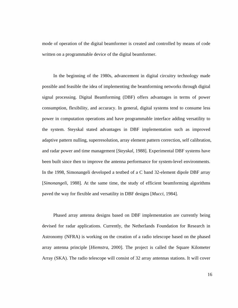
In the beginning of the 1980s, advancement in digital circuitry technology made
possible and feasible the idea of implementing the beamforming networks through digital
signal processing. Digital Beamforming (DBF) offers advantages in terms of power
consumption, flexibility, and accuracy. In general, digital systems tend to consume less
power in computation operations and have programmable interface adding versatility to
the system. Steyskal stated advantages in DBF implementation such as improved
adaptive pattern nulling, superresolution, array element pattern correction, self calibration,
and radar power and time management [Steyskal, 1988]. Experimental DBF systems have
been built since then to improve the antenna performance for system-level environments.
In the 1998, Simonangeli developed a testbed of a C band 32-element dipole DBF array
[Simonangeli, 1988]. At the same time, the study of efficient beamforming algorithms
paved the way for flexible and versatility in DBF designs [Mucci, 1984].
Phased array antenna designs based on DBF implementation are currently being
devised for radar applications. Currently, the Netherlands Foundation for Research in
Astronomy (NFRA) is working on the creation of a radio telescope based on the phased
array antenna principle [Hiemstra, 2000]. The project is called the Square Kilometer
Array (SKA). The radio telescope will consist of 32 array antennas stations. It will cover
17
an area of a square kilometer with a frequency range from 200 MHz to 2 GHz. A series
of four feasibility stages of four different array antennas are been developed for research
and development purposes. In the two final array antennas, DBF will be implemented
with a multi-processor computational environment. The DBF will consist of a processing
board containing FPGAs and a DSP. For the third array antenna called Thousand Element
Array (THEA), a group of six FPGAs will be used to process the signal. The DSP will be
used to implement an adaptive algorithm based on Minimum Variance (MV) to calculate
the beamformer’s weigth coefficients [Alliot, 2000]. The signal will have a bandwidth of
20 MHz.
Finally, phased array antennas have been used largely in communication systems.
Their capability to change radiation pattern electronically, multi-beam capacity and high
spatial resolution has made them attractive for mobile communication applications.
Miura [Miura, 1997] worked with a DBF Multibeam Antenna for mobile satellite
communication. The DBF consisted on a 4 x 4 ring patch array which received a signal
with a carrier frequency of 1542.5 MHz and a bandwidth of 11 kHz. The spatial filtering
was performed using a DSP board of ten FPGAs. An adaptive beamforming algorithm
called constant modulus algorithm (CMA) was used to perform the satellite tracking. To
achieve multibeam operation, an FFT beamformer was implemented in conjunction with
Multibeam selector, which decides the beam with the strongest receiving power to
receive the arriving signal. Dreher [Dreher, 1999, 2003] worked with a planar DBF for

18
satellite navigation. The antenna array, a 5 x 5 aperture coupled patch array, was
designed to receive a signal with a carrier frequency of 5.15 GHz and a bandwidth of 16
MHz. The RF-signal is processed through an Intermediate Frequency (IF) network,
digitized using a sub-sampling mechanism with a 40 Msps 10-bit ADC converters,
modulated to baseband with DDC, and the actual beamforming is performed by a PC.
The data transfer between the IF networks and the PC was done via the IEEE 488
standard bus. The calculation of the weights of the spatial filter was made using
Schelkunnoff’s method, where the radiation patterns’ nulls are located at detected
interfering signals.
In the next chapter of this thesis, a theoretical background of array signal processing
is presented. The chapter describes the mathematical model of the DBF receiver and
transmitter based on the behavior of a far-field plane wave traveling along a
homogeneous medium and incident on an array of sensor. Detailed designs of the DBF
receiver and transmitter are then derived, based on their mathematical model, with the
goal of reducing the mathematical operational complexity of each DBF stage. In chapter
3, different spatial filters are designed as examples to satisfy certain requirements in the
beam pattern of three different antenna arrays. A digital computational environment was
programmed to corroborate the simplified DBF transmitter design presented in this thesis.
Also, the rectangular patch antenna and two microwave circuits were simulated and
tested to verify their performance on a 16-element rectangular PAA. Finally, the last

19
chapter presents concluding remarks about the results obtained in each stage of the PAA
and recommendations are suggested to improve the performance and decrease the
complexity of a PAA.

20
2 THEORETICAL BACKGROUND
2.1 Array Processing Theory 2.1.1 Frequency-wavenumber Response and Beam Patterns
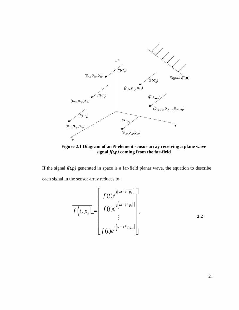
An array of sensors can be organized in any form in space, where the position of each
sensor can be described by a coordinate p = ( px, py, pz ). If a plane wave signal f(t,p) is
arriving at a particular point in space, and the position each sensor in space is different,
the signal received by each sensor will be the same original signal with a time-delay,
depending on the position of the sensor. The following vector can be used to describe the
signal received by each sensor:
( )
0
1
1
0
1
1
( ) ( )
( ) ( ), ,
( )( )N
p
p
Np
f t f t
f t f tf t
f tf t
ττ
τ− −
− − = = −
p 2.1
where N is the number of elements in the array and τi is a time-delay associated with the
position of the element. Figure 1 shows an arbitrary N-element sensor array.
21
Figure 2.1 Diagram of an N-element sensor array receiving a plane wave
signal f(t,p) coming from the far-field
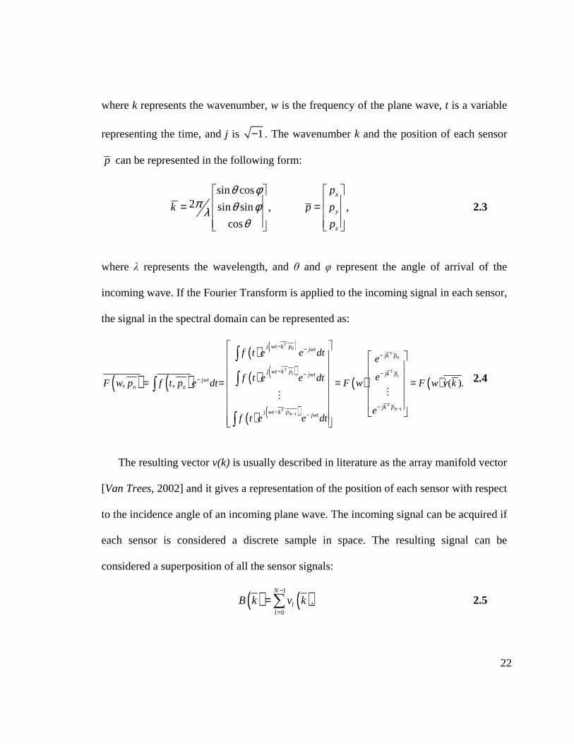
If the signal f(t,p) generated in space is a far-field planar wave, the equation to describe
each signal in the sensor array reduces to:
( )
( )
( )
( )
0
1
1
( )
( ), ,
( )
T
T
TN
j wt k p
j wt k p
n
j wt k p
f t e
f t ef t p
f t e−
−
−
−
=
2.2
22
where k represents the wavenumber, w is the frequency of the plane wave, t is a variable
representing the time, and j is 1− . The wavenumber k and the position of each sensor
p can be represented in the following form:
sin cos2 sin sin , ,
cos
x
y
z
p
k p p
p
θ φπ θ φλ
θ
= =
2.3
where λ represents the wavelength, and θ and φ represent the angle of arrival of the
incoming wave. If the Fourier Transform is applied to the incoming signal in each sensor,
the signal in the spectral domain can be represented as:
( ) ( )
( ) ( )
( ) ( )
( ) ( )
( ) ( )
0
0
1 1
11
, , ( ).
T
T
T T
TNT
N
j wt k p jwtjk p
j wt k p jk pjwtjwt
n n
jk pj wt k p jwt
f t e e dte
ef t e e dtF w p f t p e dt F w F w v k
ef t e e dt
−−
− −−
− −−−
−− −
= = = =
∫
∫∫
∫
2.4
The resulting vector v(k) is usually described in literature as the array manifold vector
[Van Trees, 2002] and it gives a representation of the position of each sensor with respect
to the incidence angle of an incoming plane wave. The incoming signal can be acquired if
each sensor is considered a discrete sample in space. The resulting signal can be
considered a superposition of all the sensor signals:
( ) ( )1
0
.N
ll
B k v k−
=
=∑ 2.5
23
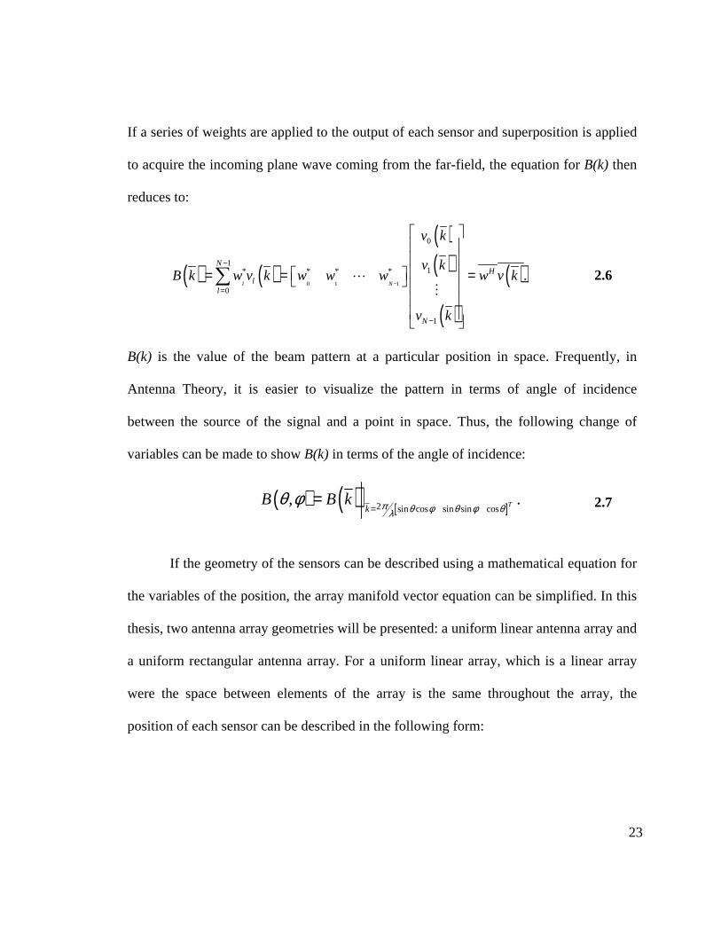
If a series of weights are applied to the output of each sensor and superposition is applied
to acquire the incoming plane wave coming from the far-field, the equation for B(k) then
reduces to:
( ) ( )
( )( )
( )
( )0 1 1
0
11* * * *
0
1
.l N
NH
ll
N
v k
v kB k w v k w w w w v k
v k
−
−
=
−
= = =
∑
2.6
B(k) is the value of the beam pattern at a particular position in space. Frequently, in
Antenna Theory, it is easier to visualize the pattern in terms of angle of incidence
between the source of the signal and a point in space. Thus, the following change of
variables can be made to show B(k) in terms of the angle of incidence:
( ) ( ) [ ]2 sin cos sin sin cos, .T
kB B k π θ φ θ φ θλ
θ φ=
= 2.7
If the geometry of the sensors can be described using a mathematical equation for
the variables of the position, the array manifold vector equation can be simplified. In this
thesis, two antenna array geometries will be presented: a uniform linear antenna array and
a uniform rectangular antenna array. For a uniform linear array, which is a linear array
were the space between elements of the array is the same throughout the array, the
position of each sensor can be described in the following form:
24
0 0
0 0 ,
1
2
n
zn
p
p Nn z
= = − − ∆
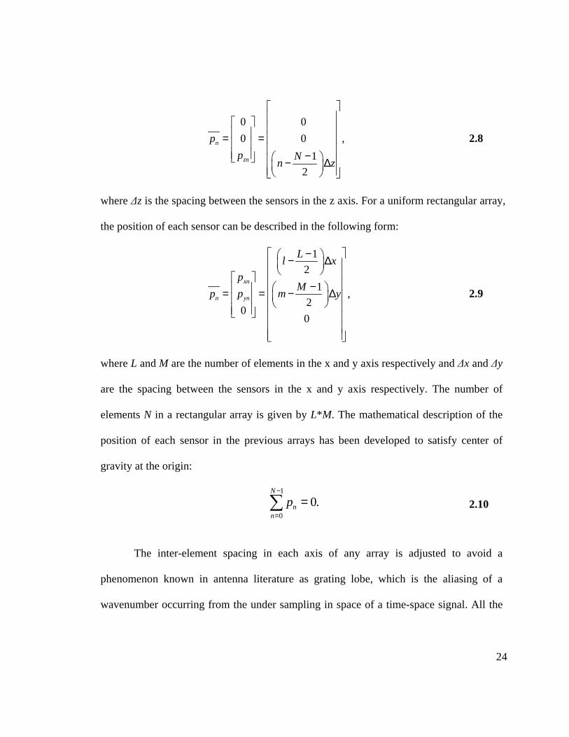
2.8
where ∆z is the spacing between the sensors in the z axis. For a uniform rectangular array,
the position of each sensor can be described in the following form:
1
2
1,
20
0
xn
n yn
Ll x
pM
p p m y
− − ∆
− = = − ∆
2.9
where L and M are the number of elements in the x and y axis respectively and ∆x and ∆y
are the spacing between the sensors in the x and y axis respectively. The number of
elements N in a rectangular array is given by L*M. The mathematical description of the
position of each sensor in the previous arrays has been developed to satisfy center of
gravity at the origin:
1
0
0.N
nn
p−
=
=∑ 2.10
The inter-element spacing in each axis of any array is adjusted to avoid a
phenomenon known in antenna literature as grating lobe, which is the aliasing of a
wavenumber occurring from the under sampling in space of a time-space signal. All the
25
arrays described in this work will have inter-element spacing of 0.5λ in each axis, where
λ is the wavelength of the carrier wave received by the array.
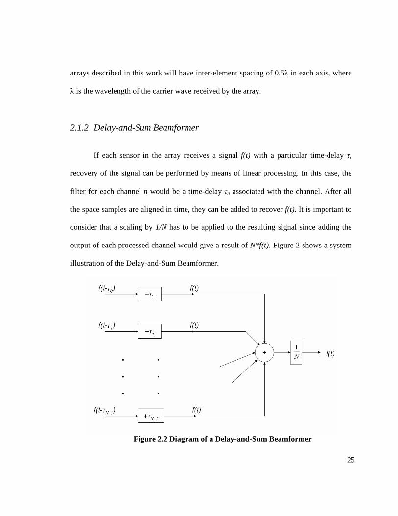
2.1.2 Delay-and-Sum Beamformer
If each sensor in the array receives a signal f(t) with a particular time-delay τ,
recovery of the signal can be performed by means of linear processing. In this case, the
filter for each channel n would be a time-delay τn associated with the channel. After all
the space samples are aligned in time, they can be added to recover f(t). It is important to
consider that a scaling by 1/N has to be applied to the resulting signal since adding the
output of each processed channel would give a result of N*f(t). Figure 2 shows a system
illustration of the Delay-and-Sum Beamformer.
Figure 2.2 Diagram of a Delay-and-Sum Beamformer
26
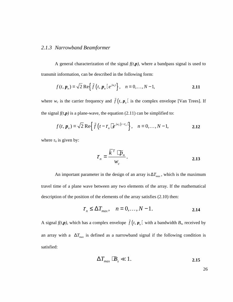
2.1.3 Narrowband Beamformer
A general characterization of the signal f(t,p), where a bandpass signal is used to
transmit information, can be described in the following form:
( ) ( , ) 2 Re , , 0, , 1,cjw tn nf t f t e n N= = − …p p 2.11
where wc is the carrier frequency and ( ), nf t p is the complex envelope [Van Trees]. If
the signal f(t,p) is a plane-wave, the equation (2.11) can be simplified to:
( ) ( ) ( , ) 2 Re , 0, , 1,c njw tn nf t f t e n Nττ −= − = − …p 2.12
where τn is given by:
.T
nn
c
k p
wτ ⋅= 2.13
An important parameter in the design of an array ismaxT∆ , which is the maximum
travel time of a plane wave between any two elements of the array. If the mathematical
description of the position of the elements of the array satisfies (2.10) then:
, 0, , 1.n maxT n Nτ ≤ ∆ = −… 2.14 A signal f(t,p), which has a complex envelope ( ), nf t p with a bandwidth Bs, received by
an array with a maxT∆ is defined as a narrowband signal if the following condition is
satisfied:
1.max sT B∆ ⋅ 2.15
27
When the signal f(t,p) is considered a narrowband signal, a suitable and convenient
approximation can be used on the complex envelope:
( ) ( ) , 0, , 1.nf t f t n Nτ− = − … 2.16
This approximation modifies the mathematical representation of f(t,p) into:
( ) ( ) ( )
( , ) 2 Re , 0, , 1
2 Re .
c n
c c n
jw tn
jw t jw
f t f t e n N
f t e e
τ
τ
−
−
= = −
=
…
p 2.17
From this simplification, it can be seen that the delay lines associated with τn can be
replaced with a phase shift c njwe τ−. An array which uses phase shifts to approximate the
delay lines to process a narrowband space-time signal is known as a phased array. For a
uniform array, a progressive phase shift can be used to steer the main response axis
(MRA), which is the direction where the beam pattern has its maximum absolute value,
to any desired value. If additional requirements are imposed on the beam pattern of an
array, such as a particular sidelobe level, minimum half-power beamwidth, and null
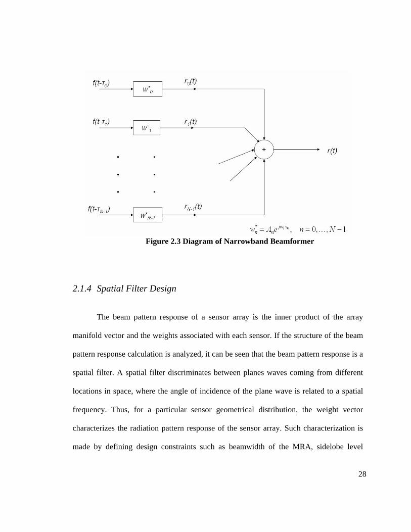
placement, the amplitude of each sensor in the array needs to be adjusted. This leads to a
beamformer configuration where the resulting signal becomes a linear combination of the
received or transmitted signals and each sensor signal has a complex weight w*n,
described in (2.6), which controls the MRA and the beam pattern characteristics of the
array. A diagram of the narrowband beamformer model is shown in Figure 2.3.
28
Figure 2.3 Diagram of Narrowband Beamformer
2.1.4 Spatial Filter Design
The beam pattern response of a sensor array is the inner product of the array
manifold vector and the weights associated with each sensor. If the structure of the beam
pattern response calculation is analyzed, it can be seen that the beam pattern response is a
spatial filter. A spatial filter discriminates between planes waves coming from different
locations in space, where the angle of incidence of the plane wave is related to a spatial
frequency. Thus, for a particular sensor geometrical distribution, the weight vector
characterizes the radiation pattern response of the sensor array. Such characterization is
made by defining design constraints such as beamwidth of the MRA, sidelobe level
29
behavior, null pattern placement, null-to-null beamwidth, etc. the same way a filter in the
time domain characterizes a frequency response. For example, the beamwidth of the
MRA defines the half-power angular difference near the maximum radiation intensity
point in the beam pattern, similar to the passband frequency difference found in time
series analysis. As for sidelobe level behavior, the sidelobe level defines the power level
of the sidelobes with respect to the main lobe, analogous to the passband to stopband
power difference found in the spectral representation of a time series. Although filter
design is important in the radation pattern response of an antenna array, array geometry
may impose limitations on some desirable beam pattern response characteristics.
Analogous to choosing an appropriate sampling frequency in the time domain, spatial
sampling selection, which is determined by the geometrical distribution and size of the
array, determines some beam pattern response characteristics.
The process of obtaining a geometrical distribution and the coefficients for the
weight vector for a beam pattern response is called beam pattern synthesis. In Antenna
Theory, the radiation pattern response is constructed based on a realization of an
analytical or desired model by an antenna model [Balanis, 1997]. The classification of
beam pattern synthesis techniques are based on three beam pattern design constraints:
null placement, beam shaping, and beamwidth-sidelobe behavior. Null placement
synthesis consists of determining the coefficients of the weight vector based on the
position of nulls in the radiation pattern response of the sensor array. A popular null
30
placement synthesis technique is the Schelkunoff polynomial method. This method
derives the weight coefficients of the array based on the root placement of a complex
polynomial, which is derived form the beam pattern response equation (Eq. 2.6). In beam
shaping synthesis, the weight vector is calculated based on a specified beam pattern
response sampled at discrete wavenumber values. Classic antenna pattern synthesis
methods included in this category are the Woodward-Lawson method, the Fourier
Transform method and the z-transform method.
The last category of beam pattern synthesis based on spatial response design
constraints is the beamwidth-sidelobe behavior. In these techniques, the weight vector
coefficients are determined based on the desired behavior of the MRA’s beamwidth and
sidelobe level. A common synthesis technique used in the spectral analysis of time series
in signal processing is the Spectral Weighting technique [Van Trees, 2002]. This
technique defines a set of weights based on a windowing function, which simplifies the
weight calculation procedure. The Uniform window, Cosine window, Hamming window,
Hann window, etc. are just a few of the windowing functions available to control the
response of a sensor array. Each window function provides a constant weight vector
which defines a fixed beam pattern response. Through performance analysis of each
windowing function, a tradeoff can be found between minimizing the MRA’s beamwidth,
reducing the sidelobe level, and increasing the directivity of the radiation pattern
response. Other beamwidth-sidelobe behavior methods include Taylor distrimution
31
method, Villanueava distribution and Dolph-Chevyshev method where the beamwidth of
the radiation pattern’s MRA is minimized for a particular sidelobe level value. Beam
pattern synthesis can also be obtained through adaptive array processing. By changing the
weights of each sensor adaptively, design goals such as minimizing the noise variance of
the signal, minimizing the square error between the beamformer output and a reference
signal, or maximize the signal-to-noise ratio of the receiver [Haynes] can be satisfied.
Antennas using adaptive beamforming are, often referred as, “Smart Antennas” in
communication literature.
Another method of synthesizing a beam pattern is beamspace processing. In this
approach, a set of beams created at an introductory step are processed instead of the
signals arriving at each sensor element [Van Trees, 2002]. The latter method of pattern
synthesis is known as “element-space processing.” Beamspace processing is typically
used in applications where the number of elements in the array is very large and the
received signals need to be reduced to simplify further processing. Three types of
beamspace processing methods are full-dimension beamspace, reduced-dimension
beamspace and multiple-beam beamspace. In full-dimension beamspace, the signals of
the N sensor in the array are processed to deliver an output of N orthogonal beams. In the
case of reduced-dimension beamspace, only a set of beams covering a particular
wavenumber region are calculated. As for multiple-beam beamspace, multiple beams are
created to span specific regions of the space. An example of a beamspace beamformer is
32
the FFT beamformer (often called the conventional beamformer). In FFT beamforming,
the Discrete Fourier Transform is used to process samples separated in distance to
produce multiple beams separated in the space domain. All the generated beams in the
FFT beamformer are orthogonal, fixed and equally spaced. The FFT beamformer
depends largely on the spatial resolution of the array antenna. This beamformer performs
a “spatial FFT” [Haynes] where input samples are separated by space and outputs
samples are separated by direction-of-arrival. One disadvantage of FFT beamformers is
its fixed beam performance. Alliot [Alliot, 2000] comments on beamforming
interpolation techniques for FFT beamformers. Beamforming interpolation consists of the
creation of a beam by adding of various beams generated by the FFT beamformer
multiplied by real weights corresponding to a particular coordinate. The combination of
multiple beam radiation pattern and versatility in direction of observation are the main
advantages of beamforming interpolation.
In spatial filter design, alternative filter structures have been presented to solve the
problem of narrow bandwidth in phased array antennas (PAA), such as the use of a filter-
and-sum beamformer [Kajala, 1999, 2001]. The filter-and-sum beamforming operates on
the amplitude and the phase of the digitized antenna element current signal. Each antenna
element has its filter and the output of each filter is added in a summing network to
acquire the desired spatial beam pattern. Various methods have been proposed to
implement filter-and-sum beamformers. For example, Kajala implements spatial filtering
33
through an optimized polynomial FIR filter. The polynomial FIR filters’s coefficients are
chosen to minimize the mean square error (MSE) between the desired and the actual
response of the beamformer.
2.2 Phased Array Antenna Implementations
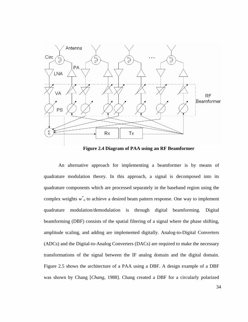
The PAA is composed of a group of similar antennas, each with its power feed
network, phase shifter, variable amplifiers and a summing network which gives a
resulting signal representing a beam on an expected location. Figure 2.4 shows a diagram
of the transmitter and receiver stages of a phased array antenna. The complex weight w*n
associated with each antenna element is implemented by means of a variable amplifier
and a phase shifter. Analog components such as Low Noise Amplifiers (LNAs) and
Power Amplifiers (PA) found in the RF stages are needed in order to condition the signal
to be transmitted or received by the antenna array.
34
Figure 2.4 Diagram of PAA using an RF Beamformer
An alternative approach for implementing a beamformer is by means of
quadrature modulation theory. In this approach, a signal is decomposed into its
quadrature components which are processed separately in the baseband region using the
complex weights w*n to achieve a desired beam pattern response. One way to implement
quadrature modulation/demodulation is through digital beamforming. Digital
beamforming (DBF) consists of the spatial filtering of a signal where the phase shifting,
amplitude scaling, and adding are implemented digitally. Analog-to-Digital Converters
(ADCs) and the Digital-to-Analog Converters (DACs) are required to make the necessary
transformations of the signal between the IF analog domain and the digital domain.
Figure 2.5 shows the architecture of a PAA using a DBF. A design example of a DBF
was shown by Chang [Chang, 1988]. Chang created a DBF for a circularly polarized
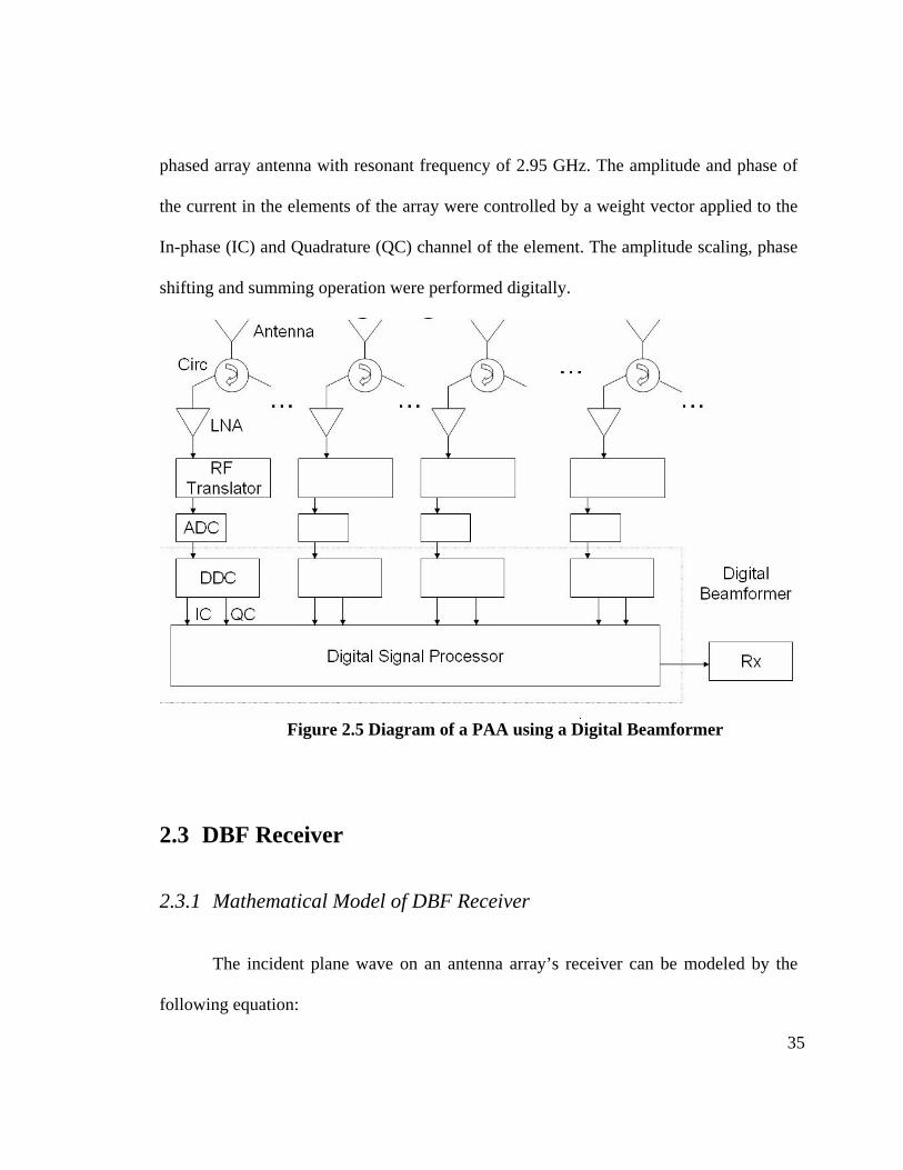
35
phased array antenna with resonant frequency of 2.95 GHz. The amplitude and phase of
the current in the elements of the array were controlled by a weight vector applied to the
In-phase (IC) and Quadrature (QC) channel of the element. The amplitude scaling, phase
shifting and summing operation were performed digitally.
Figure 2.5 Diagram of a PAA using a Digital Beamformer
2.3 DBF Receiver
2.3.1 Mathematical Model of DBF Receiver
The incident plane wave on an antenna array’s receiver can be modeled by the
following equation:
36
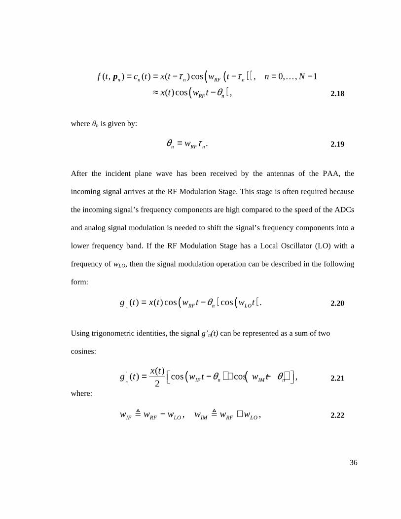
( )( )( , ) ( ) ( ) cos , 0, , 1n n n RF nf t c t x t w t n Nτ τ= = − − = −…p
( )( )cos ,RF nx t w t θ≈ − 2.18
where θn is given by:
.n RF nwθ τ= 2.19
After the incident plane wave has been received by the antennas of the PAA, the
incoming signal arrives at the RF Modulation Stage. This stage is often required because
the incoming signal’s frequency components are high compared to the speed of the ADCs
and analog signal modulation is needed to shift the signal’s frequency components into a
lower frequency band. If the RF Modulation Stage has a Local Oscillator (LO) with a
frequency of wLO, then the signal modulation operation can be described in the following
form:
( ) ( )' ( ) ( ) cos cos .n RF n LOg t x t w t w tθ= − 2.20
Using trigonometric identities, the signal g’n(t) can be represented as a sum of two
cosines:
( ) ( )' ( )( ) cos cos ,
2n IF n IM n
x tg t w t w tθ θ = − + − 2.21
where:
, ,IF RF LO IM RF LOw w w w w w− + 2.22
37
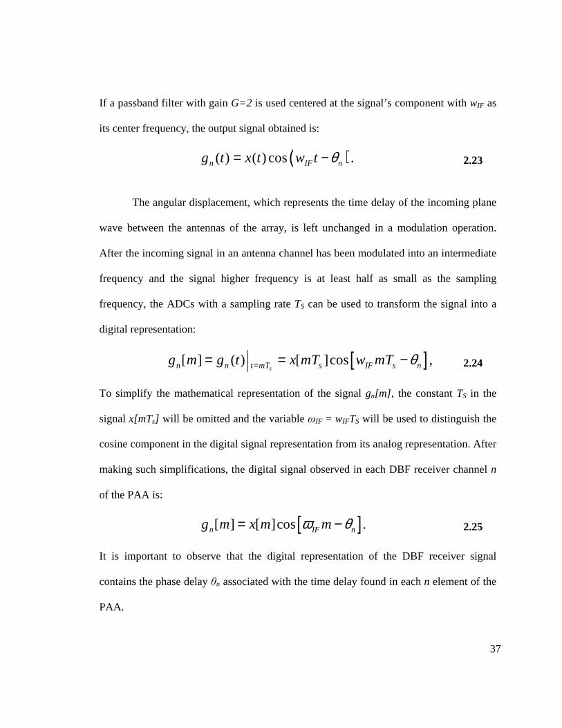
If a passband filter with gain G=2 is used centered at the signal’s component with wIF as
its center frequency, the output signal obtained is:
( )( ) ( ) cos .n IF ng t x t w t θ= − 2.23
The angular displacement, which represents the time delay of the incoming plane
wave between the antennas of the array, is left unchanged in a modulation operation.
After the incoming signal in an antenna channel has been modulated into an intermediate
frequency and the signal higher frequency is at least half as small as the sampling
frequency, the ADCs with a sampling rate TS can be used to transform the signal into a
digital representation:
[ ][ ] ( ) [ ]cos ,sn n t mT s IF s ng m g t x mT w mT θ== = − 2.24
To simplify the mathematical representation of the signal gn[m] , the constant TS in the
signal x[mTs] will be omitted and the variable ωIF = wIFTS will be used to distinguish the
cosine component in the digital signal representation from its analog representation. After
making such simplifications, the digital signal observed in each DBF receiver channel n
of the PAA is:
[ ][ ] [ ]cos .n IF ng m x m mω θ= − 2.25
It is important to observe that the digital representation of the DBF receiver signal
contains the phase delay θn associated with the time delay found in each n element of the
PAA.
38
After the antenna signal has been successfully sampled into the digital domain,
the signal needs to be processed by the first stage of the DBF receiver, which is the
Digital Down-Converter (DDC). The Digital Down-Conversion is performed by
multiplying the digital signal with a sinusoidal signal and a 90º phase-shifted version of
the sinusoidal signal, both generated by digital local oscillator. Both mathematical
operations can be represented in the following form:
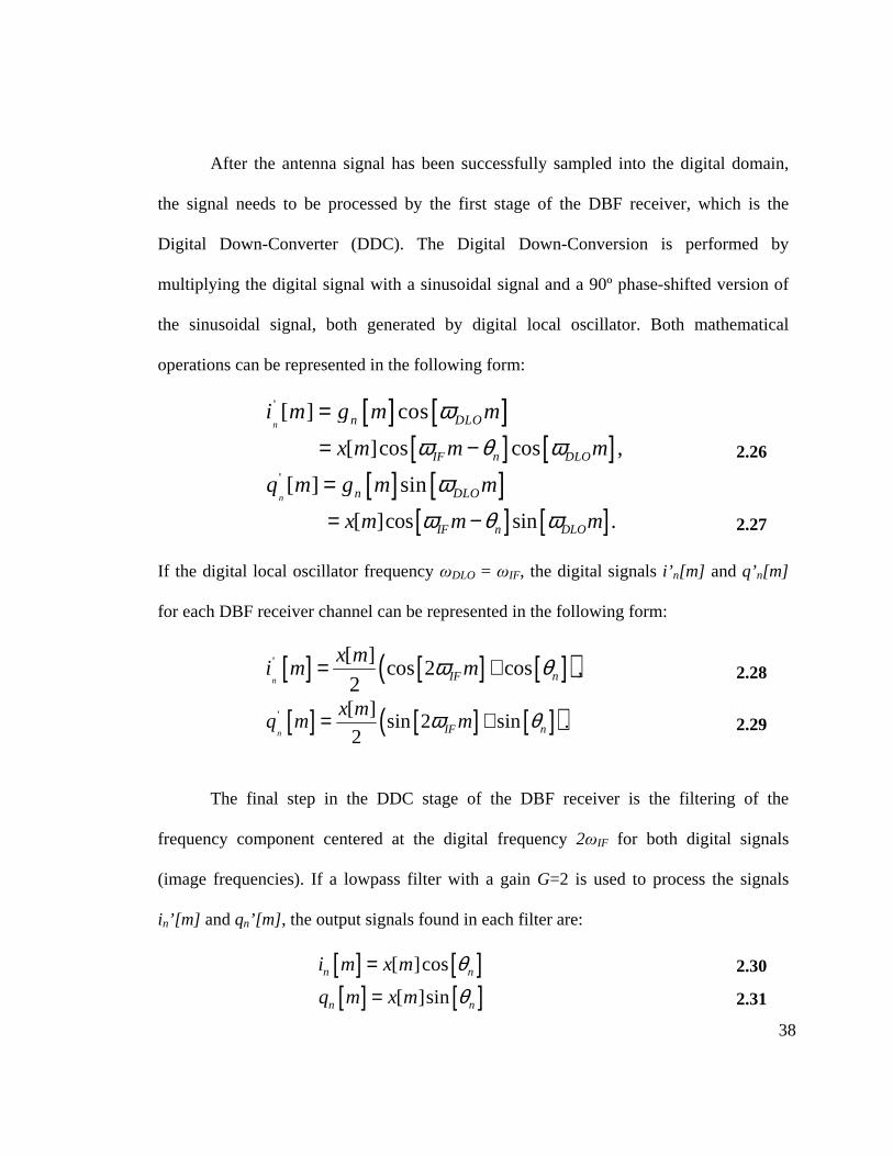
[ ] [ ]' [ ] cosn n DLOi m g m mω=
[ ] [ ][ ]cos cos ,IF n DLOx m m mω θ ω= − 2.26
[ ] [ ]' [ ] sinn n DLOq m g m mω=
[ ] [ ][ ]cos sin .IF n DLOx m m mω θ ω= − 2.27
If the digital local oscillator frequency ωDLO = ωIF, the digital signals i’ n[m] and q’n[m]
for each DBF receiver channel can be represented in the following form:
[ ] [ ] [ ]( )' [ ]cos 2 cos ,
2n IF n
x mi m mω θ= + 2.28
[ ] [ ] [ ]( )' [ ]sin 2 sin .
2n IF n
x mq m mω θ= + 2.29
The final step in the DDC stage of the DBF receiver is the filtering of the
frequency component centered at the digital frequency 2ωIF for both digital signals
(image frequencies). If a lowpass filter with a gain G=2 is used to process the signals
in’[m] and qn’[m] , the output signals found in each filter are:
[ ] [ ][ ]cosn ni m x m θ= 2.30
[ ] [ ][ ]sinn nq m x m θ= 2.31

39
It can be seen that the DDC stage of the DBF receiver transforms a digital bandpass
signal with the time-delay τn into two digital baseband signals where the phase
information of the bandpass signal is represented in the amplitude of both baseband
signals. The previous transformation of the signal into its quadrature components is
necessary in order to apply the next filtering phase as a double-input, double-output
lowpass filter operation, which is equivalent to a single-input, single-output bandpass
filter operation [Franks, 1969]. Figure 2.6 shows a block diagram of the RF modulator
and the DDC stage of each antenna channel in the PAA with the mathematical equations
derived previously.

40
Figure 2.6 Block diagram (including equations) of RF Modulator and DDC
The second stage of the DBF receiver is the Complex Weight Multiplication
(CWM) stage. In this stage, the complex weight w*n associated with each antenna
channel in the PAA is multiplied by the digital baseband signals in[m] and qn[m] . To
represent this complex multiplication operation, a signal bn[m] will be defined which is
composed of the signals in[m] and qn[m] :
[ ] [ ][ ] [ ]( )
[ ]
[ ] cos sin
n n n
n n
b m i m jq m
x m jθ θ
= −
= −
[ ] .njx m e θ−= 2.32
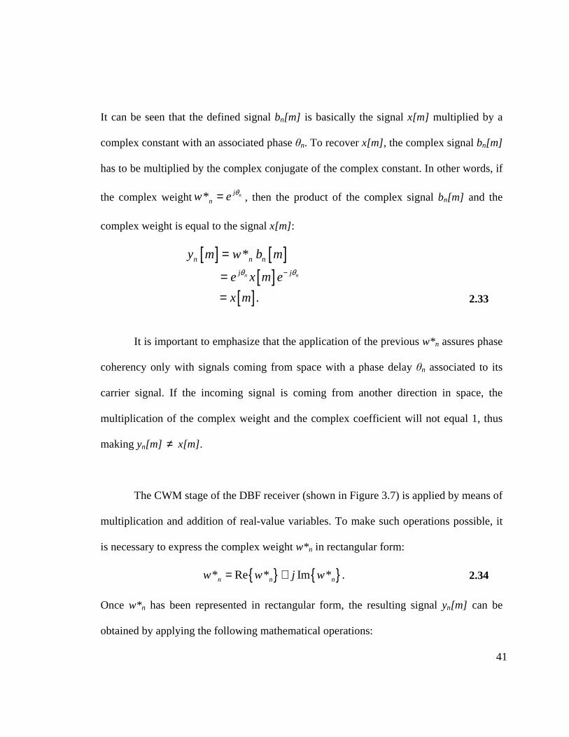
41
It can be seen that the defined signal bn[m] is basically the signal x[m] multiplied by a
complex constant with an associated phase θn. To recover x[m], the complex signal bn[m]
has to be multiplied by the complex conjugate of the complex constant. In other words, if
the complex weight * njnw e θ= , then the product of the complex signal bn[m] and the
complex weight is equal to the signal x[m]:
[ ] [ ]
[ ]*
n n
n n n
j j
y m w b m
e x m eθ θ−
=
=
[ ].x m= 2.33
It is important to emphasize that the application of the previous w*n assures phase
coherency only with signals coming from space with a phase delay θn associated to its
carrier signal. If the incoming signal is coming from another direction in space, the
multiplication of the complex weight and the complex coefficient will not equal 1, thus
making yn[m] ≠ x[m].
The CWM stage of the DBF receiver (shown in Figure 3.7) is applied by means of
multiplication and addition of real-value variables. To make such operations possible, it
is necessary to express the complex weight w*n in rectangular form:
* Re * Im * .n n nw w j w= + 2.34
Once w*n has been represented in rectangular form, the resulting signal yn[m] can be
obtained by applying the following mathematical operations:

42
[ ] [ ] ( ) [ ] [ ]( )
*
Re * Im *
n n n
n n n n
y m w b m
w j w i m jq m
=
= + −
[ ] [ ],n nr m js m= + 2.35
where:
[ ] [ ] [ ]( ) ( )Re * Im * ,n n n n nr m i m w q m w= + − − 2.36
[ ] [ ] [ ]( ) ( )Im * Re * .n n n n ns m i m w q m w= + − 2.37
Figure 2.7 Block diagram of CWM phase
The last stage of the DBF receiver involves the addition of all the resulting signals yn[m] :
[ ] [ ] [ ] [ ]1 1 1
0 0 0
1 1 1N N N
n n nn n n
y m y m r m j s mN N N
− − −
= = =
= = +∑ ∑ ∑
[ ] [ ]r m js m= + 2.38

43
An amplitude scaling by a factor of N is needed to recover x[m] without gain. If desired,
the amplitude scaling factor can be included in the complex weight coefficient and
omitted in the last phase of the DBF receiver. The signals r[m] and s[m], which are the
output of the DBF receiver, are the quadrature components of the resulting signal y[m].
Post-processing of this quadrature signals, which is done by other components of the
system where the PAA is used, is needed for proper retrieval and analysis of the
information signal x[m].
2.3.2 DBF Receiver Design
The physical design of a DBF Receiver is based on the mathematical model
described in the previous section. The design of the DBF Receiver considers how the
mathematical model can be implemented using real components and takes into account
limitations found in the physical implementation of the PAA system. The design of the
DBF Receiver can be divided into four main components: RF Modulation Stage, Digital-
Down Conversion stage, Complex Weight Multiplication stage, and the Summation
stage. It is important to remember that the RF Modulation Stage is not implemented
digitally (technically, it is not part of the Digital Beamformer), but it is essential in the
implementation of the PAA and thus, its design will be also explained in this section.
The first stage in the implementation of an antenna channel in a PAA system is
the RF Modulation Stage (also called RF Translator [Haynes]). The RF Modulator is
44
implemented using an RF Mixer. RF Mixers are available as Integrated Circuits (ICs)
component packages and can be bought in commercial microwave components stores. RF
Mixers need to receive sufficient signal power in its input ports in order to work properly.
In PAA systems, the power of the signal found at the output port of each antenna in the
array is very low. Since the first stage of a receiver has a major effect on the noise
performance of the system [Pozar, 1998], it is necessary to include Low Noise
Amplifiers at the RF Modulator Stage. The LNAs help to reduce the Noise Figure in a
microwave circuit and increase the Signal-to-Noise Ratio (SNR) of the PAA system.
Therefore, the RF Modulator Stage of each antenna channel has one LNA and one RF
mixer. Also, the lines that connect each component of this stage need to be designed to
work in a 50Ω system at the desired RF carrier frequency of the antenna array.
An intermediate stage found in the antenna receiver channel of a PAA
implemented using DBF is the ADC. The ADC transforms the analog signal found in the
output of the RF Translator into a digital representation for further processing by the
DBF. ADCs implement the operations of sampling, quantizing, and encoding of the
analog signal [Garret, 1981]. Different ADC techniques can be used to perform the
signal acquisition such as successive-approximation conversion technique, sigma-delta
conversion technique, dual-slope conversion technique, voltage-comparison tracking
conversion technique and charge balance conversion technique. Two important ADC
parameters are the bit resolution and the sampling frequency per channel. The bit
45
resolution parameter determines the quantization error found in the analog-to-digital
transformation. This quantization error can be represented as noise power, which affects
the SNR of the antenna channel’s signal. The sampling rate parameter determines the
analog frequency band which can be represented in the digital domain, which extends
from DC to the folding frequency (one half of the sampling frequency). These two
parameters are set depending on the desired frequency of operation and SNR level of the
PAA design. ADCs are available as IC component packages. In the implementation of a
PAA, it is important to use a single clock to digitize all the channels in the antenna array
to assure proper synchronization.
The first stage of the DBF Receiver (the second stage in antenna channel) is the
Digital-Down Conversion Stage. The DDC receives an incoming digital IF signal
(usually from an ADC), and modulates the signal into baseband and produces an in-phase
signal and a quadrature signal as outputs. The design of the DDC can be implemented
using FPGAs or dedicated ICs. The quadrature modulation is performed by the
multiplication of the IF signal with a digital oscillator, as mentioned in the previous
section. The implementation of the digital oscillator is accomplished using a direct digital
synthesizer (DDS). Direct digital synthesis is a technique by which a sinusoidal signal is
created by the generation of digital numbers which controls the input of a sinusoidal
look-up table [Manassewitsch, 1980]. The digital numbers are generated by a phase
accumulator, which receives a binary instruction representing a specific frequency of
46
oscillation. The frequency of this digital oscillator is proportional to the phase increment
created in the phase accumulator. Since the signal is produced by a look-up table, phase
synchronization between the digital local oscillator and its 90º phase-shifted version can
be achieved easier than an equivalent analog implementation counterpart. A single DDS
must be used for all the channels in the DBF receiver in order to assure proper
synchronization between the signals of each antenna channel. After the in-phase and
quadrature signals have been produced, a lowpass filter is used to remove image
frequency components located on both signals.
Some DDC designs may also include a multirate filter component. The multirate
filter is a filter that alters the data rates [Harris, 1987]. In PAA applications, the received
RF signals are centered at a high carrier frequency, which imposes the need for fast
ADCs and DDCs with high sample rate frequencies. On the other hand, cost limitations
and simplicity may motivate the need to use Digital Signal Processors (DSPs) working at
low sample rate frequencies in the final stages of the DBF. The multirate filter, thus,
allows the interconnection between fast DDCs and DSPs operating at different sample
rate frequencies. In the case of a DBF receiver, a decimation filter is used to down-
sample the output signal of the DDC. A typical decimation filter implementation is
composed of a lowpass filtering stage and a subsampling stage. The design of both stages
is related to the decrease ratio between the high input sample rate frequency and the low
output sample rate frequency. An interesting approach to simplifying the DBF receiver
47
design is the use of one single lowpass filter per antenna channel in the implementation
of a DDC. The lowpass filter would accomplish two important tasks: removing image
frequencies after modulation (DDC standard stage) and removing higher frequency
components before subsampling (multirate filter stage).
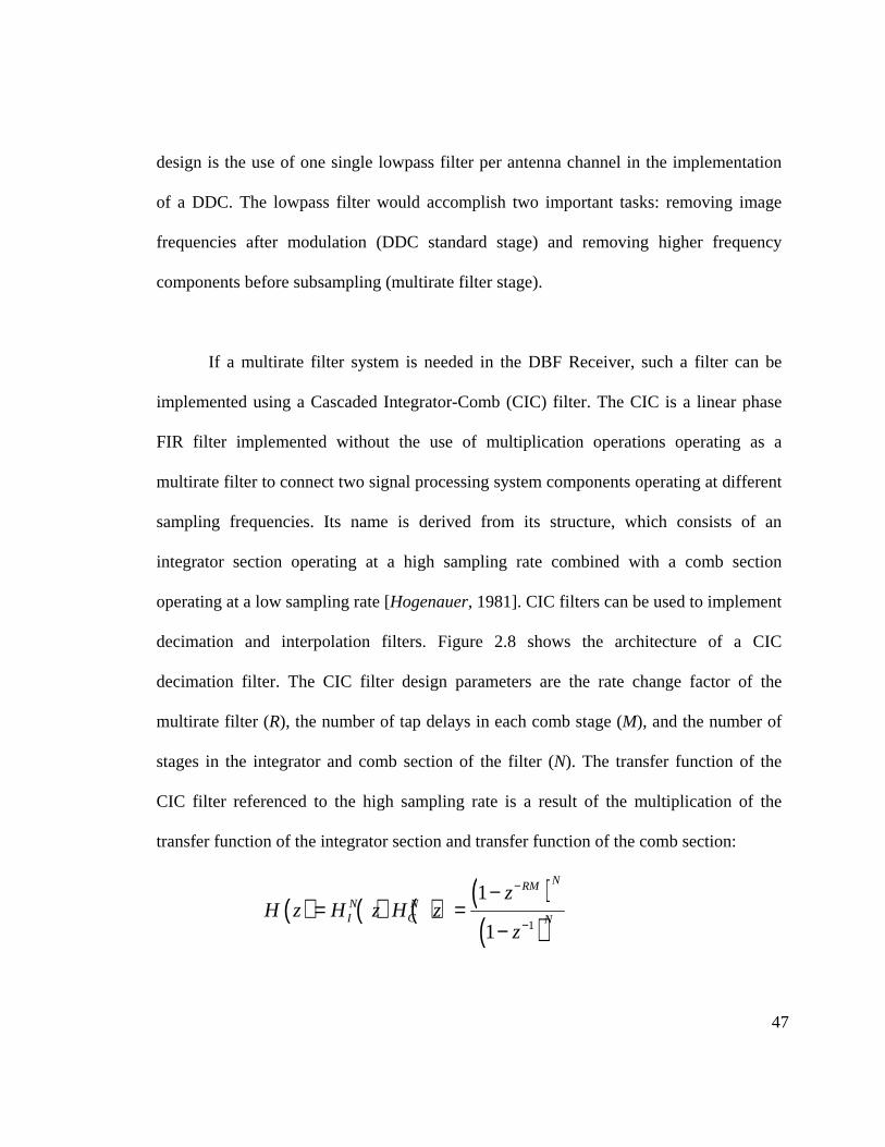
If a multirate filter system is needed in the DBF Receiver, such a filter can be
implemented using a Cascaded Integrator-Comb (CIC) filter. The CIC is a linear phase
FIR filter implemented without the use of multiplication operations operating as a
multirate filter to connect two signal processing system components operating at different
sampling frequencies. Its name is derived from its structure, which consists of an
integrator section operating at a high sampling rate combined with a comb section
operating at a low sampling rate [Hogenauer, 1981]. CIC filters can be used to implement
decimation and interpolation filters. Figure 2.8 shows the architecture of a CIC
decimation filter. The CIC filter design parameters are the rate change factor of the
multirate filter (R), the number of tap delays in each comb stage (M), and the number of
stages in the integrator and comb section of the filter (N). The transfer function of the
CIC filter referenced to the high sampling rate is a result of the multiplication of the
transfer function of the integrator section and transfer function of the comb section:
( ) ( ) ( ) ( )( )1
1
1
NRM
N NI C N
zH z H z H z
z
−
−
−= =
−

48
1
0
,NRM
k
k
z−
−
=
= ∑ 2.39
where:
( ) ( ) 1
11 , , .
1RM
C IH z z H z zz
−−= − = ∈
− 2.40
Figure 2.8 Architecture of CIC Decimation Filter
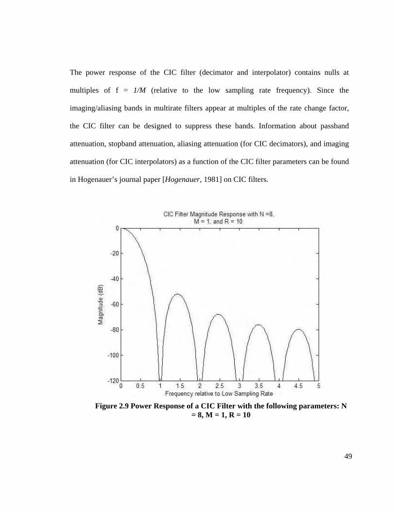
The power frequency response (shown graphically in Figure 2.9) of the CIC filter relative
to the low sampling rate is given by the following equation:
( ) ( )2
sin.
sin
N
MfP f
f
R
ππ
=
2.41
49
The power response of the CIC filter (decimator and interpolator) contains nulls at
multiples of f = 1/M (relative to the low sampling rate frequency). Since the
imaging/aliasing bands in multirate filters appear at multiples of the rate change factor,
the CIC filter can be designed to suppress these bands. Information about passband
attenuation, stopband attenuation, aliasing attenuation (for CIC decimators), and imaging
attenuation (for CIC interpolators) as a function of the CIC filter parameters can be found
in Hogenauer’s journal paper [Hogenauer, 1981] on CIC filters.
Figure 2.9 Power Response of a CIC Filter with the following parameters: N
= 8, M = 1, R = 10

50
Each comb stage of the CIC filter is a subtraction operation of the current sample
by a sample with an M delay. In the case of the integrator stage, each integrator has a
unity feedback coefficient. When CIC decimation filters are employed, register overflow
occurs in all integrator stages. To avoid consequences in the output of the filter, two
requirements must be fulfilled: 1) the implementation of filter arithmetic must be based
on a number system which allows “wrap-around” between the most positive and most
negative number (like the two’s complement arithmetic) and 2) the range of the number
system must be greater than or equal to the maximum magnitude expected at the output
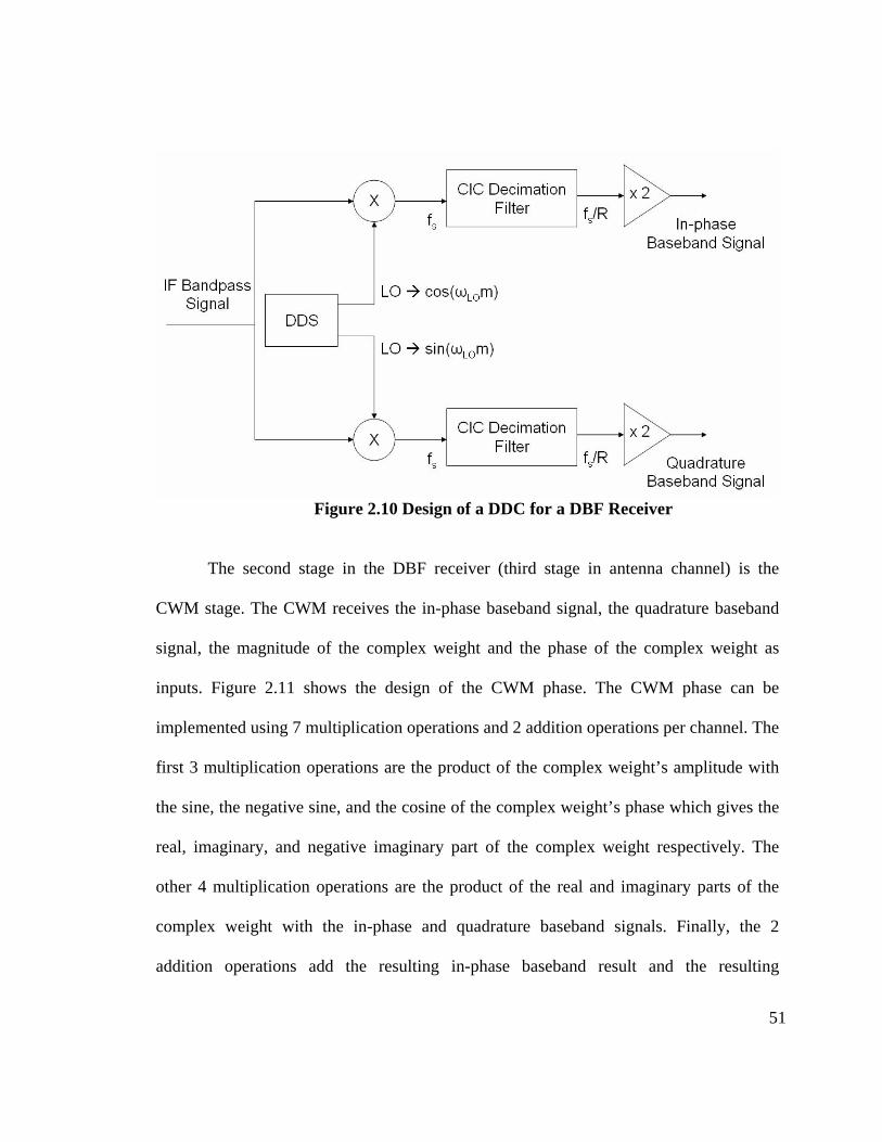
of the filter [Hogenauer, 1981]. Figure 2.10 shows the design of the DDC with the
multirate filter (CIC implementation). An additional scale block is included at the output
of the CIC filter to increase the gain of the signal by a factor of 2. Since digital circuits
are implemented using binary arithmetic, the scale block by a factor of 2 can be easily
implemented using a “shift right” operation on the sample’s binary point.
51
Figure 2.10 Design of a DDC for a DBF Receiver
The second stage in the DBF receiver (third stage in antenna channel) is the
CWM stage. The CWM receives the in-phase baseband signal, the quadrature baseband
signal, the magnitude of the complex weight and the phase of the complex weight as
inputs. Figure 2.11 shows the design of the CWM phase. The CWM phase can be
implemented using 7 multiplication operations and 2 addition operations per channel. The
first 3 multiplication operations are the product of the complex weight’s amplitude with
the sine, the negative sine, and the cosine of the complex weight’s phase which gives the
real, imaginary, and negative imaginary part of the complex weight respectively. The
other 4 multiplication operations are the product of the real and imaginary parts of the
complex weight with the in-phase and quadrature baseband signals. Finally, the 2
addition operations add the resulting in-phase baseband result and the resulting

52
quadrature baseband result in each channel. Also, 2 negation operators are needed to
calculate the negative value of the quadrature baseband signal and the negative sine
function and a sine look-up table is necessary to evaluate the sine and cosine function of
the complex weight’s phase.
Figure 2.11 Design of CWM for a DBF Receiver
The CWM stage can be implemented using an FPGA or a DSP. The advantage of
implementing the CWM in one of the previous devices mentioned strives in the tradeoff
between speed of algorithm and cost of implementation. If a DSP is used, a single
Multiply-accumulate (MAC) unit can be used to perform the addition and multiplication
operations and a single look-up table can be used to evaluate the sine, negative sine and
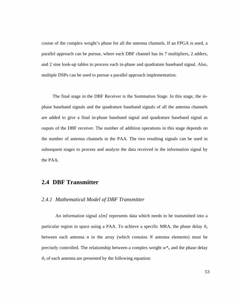
53
cosine of the complex weight’s phase for all the antenna channels. If an FPGA is used, a
parallel approach can be pursue, where each DBF channel has its 7 multipliers, 2 adders,
and 2 sine look-up tables to process each in-phase and quadrature baseband signal. Also,
multiple DSPs can be used to pursue a parallel approach implementation.
The final stage in the DBF Receiver is the Summation Stage. In this stage, the in-
phase baseband signals and the quadrature baseband signals of all the antenna channels
are added to give a final in-phase baseband signal and quadrature baseband signal as
ouputs of the DBF receiver. The number of addition operations in this stage depends on
the number of antenna channels in the PAA. The two resulting signals can be used in
subsequent stages to process and analyze the data received in the information signal by
the PAA.
2.4 DBF Transmitter
2.4.1 Mathematical Model of DBF Transmitter
An information signal x[m] represents data which needs to be transmitted into a
particular region in space using a PAA. To achieve a specific MRA, the phase delay θn
between each antenna n in the array (which contains N antenna elements) must be
precisely controlled. The relationship between a complex weight w*n and the phase delay
θn of each antenna are presented by the following equation:

54
( ) ( )* cos sin , 0,1,..., 1.njn n nw e j n Nθ θ θ= = + = − 2.42
The complex weight’s magnitude An for each antenna channel can have a particular value
(different from one) if different beam pattern characteristics (change sidelobe level
behavior, increase beamwidth, null placement, etc.) are required. The first stage of the
DBF transmitter is the CWM stage, which consists in the multiplication of the
information signal with the real part and the imaginary part of the complex weight. Two
resulting signals in[m] and qn[m] are obtained for each antenna channel:
[ ] [ ]Re * ,n ni m x m w= 2.43
[ ] [ ] Im * ,n nq m x m w= 2.44
where:
[ ] [ ]Re * cos , Im * sin .n n n n n nw A w Aθ θ= = 2.45
The second stage of the DBF transmitter is the Digital-Up Conversion stage. In
this stage, the signals in[m] and qn[m] are multiplied by a sinusoidal signal and its 90º
phase-shifted version generated by a digital local oscillator with a sinosiodal frequency
ωIF. The output of the product the signals in[m] and qn[m] and the digital local oscillator
are:
[ ] [ ] [ ] [ ][ ] cos [ ]cos cos ,n n IF n n IFfi m i m m A x m mω θ ω= = ⋅ 2.46
[ ] [ ] [ ] [ ] [ ]sin [ ]sin sin .n n IF n n IFfq m i m m A x m mω θ ω= = ⋅ 2.47
Using trigonometric identities, the signals fin[m] and fqn[m] can be represented in the
following form:
55
[ ] [ ]( )[ ][ ] cos cos ,
2n
n IF n IF n
A x mfi m m mω θ ω θ⋅= + + − 2.48
[ ] [ ] [ ]( )[ ]cos cos .
2n
n IF n IF n
A x mfq m m mω θ ω θ⋅= − − + 2.49
Then, the signals fin[m] and fqn[m] are added in order to generate a bandpass signal f[m]
with the desired phase delay θn:
[ ] [ ][ ] [ ] [ ]cos .n n n n IF nf m fi m fq m A x m mω θ= + = ⋅ − 2.50
The last stage in the DBF transmitter consists of the transformation of the digital
signal into the analog domain. If a Digital-to-Analog Converter (DAC) with a sampling
frequency of fs is used to transform the digital signal, the output of the DAC can be
represented in the following form:
( ) [ ] ( ) ( )cos .sn m tf n s IF s nf t f m A x tf f tω θ== = ⋅ − 2.51
To simplify the mathematical representation of the signal fn(t), the constant fS in the
signal x(tfs) will be omitted and the variable wIF = ωIFfS will be used to distinguish the
cosine component in the analog domain from its digital representation. After making such
simplifications, the analog signal observed at the output of each DBF transmitter n of the
PAA is:
( ) ( ) ( )cos .n n IF nf t A x t w t θ= ⋅ − 2.52
From the previous equation, it can be seen that the output of the DBF transmitter contains
the phase delay θn and the magnitude An, necessary to construct the desired beam pattern
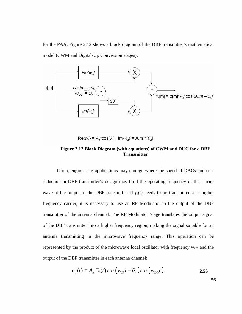
56
for the PAA. Figure 2.12 shows a block diagram of the DBF transmitter’s mathematical
model (CWM and Digital-Up Conversion stages).
Figure 2.12 Block Diagram (with equations) of CWM and DUC for a DBF
Transmitter
Often, engineering applications may emerge where the speed of DACs and cost
reduction in DBF transmitter’s design may limit the operating frequency of the carrier
wave at the output of the DBF transmitter. If fn(t) needs to be transmitted at a higher
frequency carrier, it is necessary to use an RF Modulator in the output of the DBF
transmitter of the antenna channel. The RF Modulator Stage translates the output signal
of the DBF transmitter into a higher frequency region, making the signal suitable for an
antenna transmitting in the microwave frequency range. This operation can be
represented by the product of the microwave local oscillator with frequency wLO and the
output of the DBF transmitter in each antenna channel:
( ) ( )' ( ) ( ) cos cos .n n IF n LOc t A x t w t w tθ= ⋅ − 2.53
57
Using trigonometric identities, the signal c’n(t) can be represented as a sum of two
cosines:
( ) ( )' ( )( ) cos cos ,
2n
nRF n IM n
A x tc t w t w tθ θ⋅
= − + − 2.54
where:
, .RF LO IF IM LO IFw w w w w w− + 2.55 If a passband filter with gain G=2 is centered at the signal’s component with wRF as its
center frequency, the output signal obtained is:
( )( ) ( ) cos .n n RF nc t A x t w t θ= ⋅ − 2.56
The signal cn(t) has a higher frequency carrier than the output signal of the DBF
transmitter and the phase delay θn and the magnitude An for each antenna channel has
been left unchanged during the mixing operation. If the bandwidth of the signal is small
compared to the carrier’s frequency (see Eq. 2.15), then cn(t) is considered a narrowband
signal (in array processing theory context) and the following approximation is satisfied:
( )( )( )
( ) ( ) cos
( ) cos
n n RF n
n RF n
c t A x t w t
A x t w t
θ
τ
= ⋅ −
= ⋅ −
( )( )( ) cos ( , ),n n RF n nA x t w t f tτ τ≈ ⋅ − − = p 2.57
where τn is the necessary time-delay experienced between each antenna’s irradiated plane
wave in the PAA. Finally, the signal cn(t) satisfies the necessary conditions in order to
direct the MRA of the beam pattern into a particular region in space and fulfill specific
beam pattern requirements.
58
2.4.2 DBF Transmitter Design
The physical design of a DBF transmitter is based on the mathematical model
described in the previous section. The design of the DBF transmitter can be divided into
three main stages: the CWM stage, the Digital-Up Converter (DUC) stage, and the RF
Modulation Stage. As it was explained in section 2.3.2, the RF Modulation is not part of
the Digital Beamformer, but it is important in the implementation of the PAA, and thus,
its role will be discussed in the DBF transmitter.
The first stage in the DBF transmitter is the CWM stage. Its function in the DBF
transmitter is quite similar to its equivalent in the DBF receiver; it controls the amplitude
of the in-phase and quadrature signals prior to the Digital-Up Conversion. The CWM
stage receives the information signal as input, multiplies the signal by the real part and
imaginary part of the complex weight assign to the channel, and outputs an in-phase
signal and a quadrature signal. A simple CWM architecture consists of 4 multiplication
operations per channel. The first 2 multiplication operations are used to evaluate the
product of the complex weight’s amplitude with the sine, and the cosine of the complex
weight’s phase which gives the real, and imaginary part of the complex weight
respectively. The other 2 multiplication operations are used to evaluate the product of the
real and imaginary parts of the complex weight with the information signal. In addition,
as in the CWM for the DBF receiver, a sine look-up table is necessary to evaluate the sine
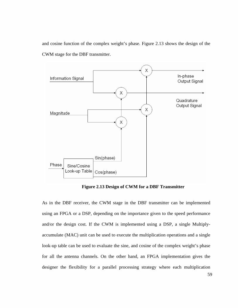
59
and cosine function of the complex weight’s phase. Figure 2.13 shows the design of the
CWM stage for the DBF transmitter.
Figure 2.13 Design of CWM for a DBF Transmitter
As in the DBF receiver, the CWM stage in the DBF transmitter can be implemented
using an FPGA or a DSP, depending on the importance given to the speed performance
and/or the design cost. If the CWM is implemented using a DSP, a single Multiply-
accumulate (MAC) unit can be used to execute the multiplication operations and a single
look-up table can be used to evaluate the sine, and cosine of the complex weight’s phase
for all the antenna channels. On the other hand, an FPGA implementation gives the
designer the flexibility for a parallel processing strategy where each multiplication
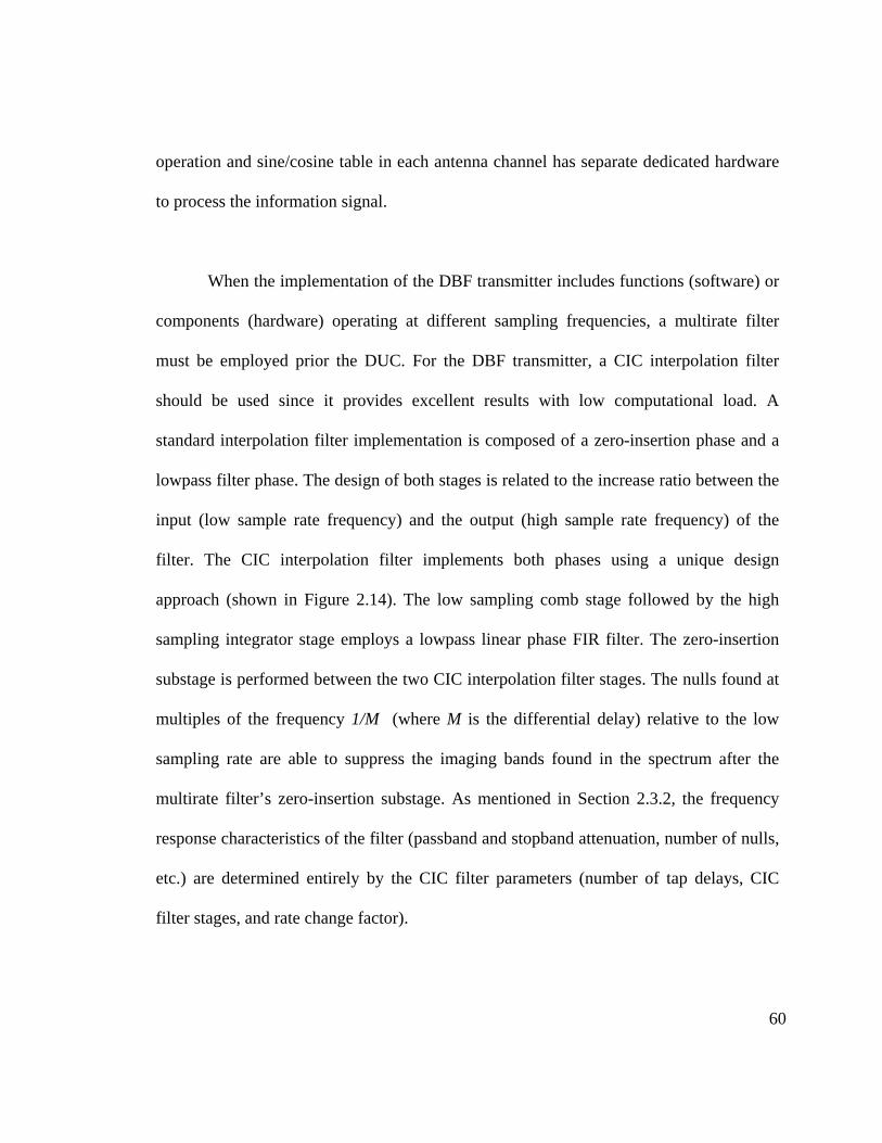
60
operation and sine/cosine table in each antenna channel has separate dedicated hardware
to process the information signal.
When the implementation of the DBF transmitter includes functions (software) or
components (hardware) operating at different sampling frequencies, a multirate filter
must be employed prior the DUC. For the DBF transmitter, a CIC interpolation filter
should be used since it provides excellent results with low computational load. A
standard interpolation filter implementation is composed of a zero-insertion phase and a
lowpass filter phase. The design of both stages is related to the increase ratio between the
input (low sample rate frequency) and the output (high sample rate frequency) of the
filter. The CIC interpolation filter implements both phases using a unique design
approach (shown in Figure 2.14). The low sampling comb stage followed by the high
sampling integrator stage employs a lowpass linear phase FIR filter. The zero-insertion
substage is performed between the two CIC interpolation filter stages. The nulls found at
multiples of the frequency 1/M (where M is the differential delay) relative to the low
sampling rate are able to suppress the imaging bands found in the spectrum after the
multirate filter’s zero-insertion substage. As mentioned in Section 2.3.2, the frequency
response characteristics of the filter (passband and stopband attenuation, number of nulls,
etc.) are determined entirely by the CIC filter parameters (number of tap delays, CIC
filter stages, and rate change factor).
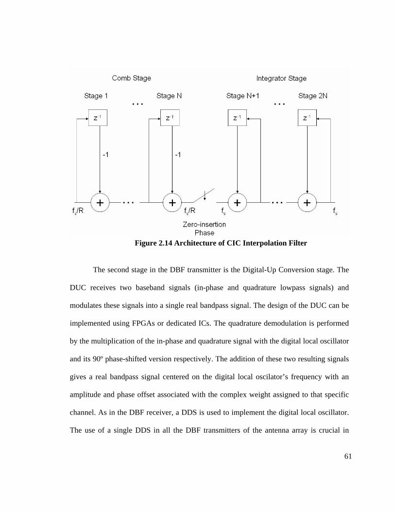
61
Figure 2.14 Architecture of CIC Interpolation Filter
The second stage in the DBF transmitter is the Digital-Up Conversion stage. The
DUC receives two baseband signals (in-phase and quadrature lowpass signals) and
modulates these signals into a single real bandpass signal. The design of the DUC can be
implemented using FPGAs or dedicated ICs. The quadrature demodulation is performed
by the multiplication of the in-phase and quadrature signal with the digital local oscillator
and its 90º phase-shifted version respectively. The addition of these two resulting signals
gives a real bandpass signal centered on the digital local oscilator’s frequency with an
amplitude and phase offset associated with the complex weight assigned to that specific
channel. As in the DBF receiver, a DDS is used to implement the digital local oscillator.
The use of a single DDS in all the DBF transmitters of the antenna array is crucial in
62
guaranteeing proper synchronization between the signals of each antenna channel. Figure
2.15 shows the design of the DUC with the multirate filter (CIC implementation).
Figure 2.15 Design of DUC for a DBF Transmitter
The gateway between the output of the DBF, which is a digital signal, and the
input of the RF Translator (which is an analog signal) is the DAC. The DAC transforms a
digital signal into an analog representation. A DAC can be considered a digitally
controlled potentiometer that provides an output current or voltage normalized to its full-
scale [Garret, 1981]. The DAC has the same parameters as the ADC, which is its
equivalent in a DBF receiver. In the implementation of a PAA, it is important to use a
single clock for all the DACs to assure proper synchronization between each channel in
the DBF transmitter.

63
The last stage in the antenna channel is the RF Translator. The RF Translator in
the antenna’s transmitter modulates an input signal, found in an intermediate frequency
band, to a higher frequency band where it can be use as input to the PAA’s antennas.
Analogous to the DBF receiver’s RF Translator, the RF Translator in the DBF transmitter
is implemented using an RF Mixer per antenna channel. Typically, the level of signal
power found at the output of the RF Mixer might not be high enough to excite the
antenna ports of the PAA. In a typical microwave communication system, a power
amplifier (PA) is used after the RF Mixer to amplify the microwave signal, which is then
radiated by each antenna of the array [Pozar, 1998]. Finally, the lines that connect each
component in this stage need to be designed to work on a 50Ω system at the desired RF
carrier frequency of the PAA.

64
3 SIMULATION AND IMPLEMENTATION
RESULTS
In this chapter, one DBF receiver and two DBF transmitter design prototypes will be
presented. The difference between each design prototype consists in the number of
elements and the geometrical distribution of the PAA where the DBF is used. The DBF
receiver model shown in this chapter is designed for a 4-element linear PAA. As for DBF
transmitters, models shown in this chapter are designed for a 16-element linear PAA and
a 16-element 4x4 rectangular PAA. Two spatial filters will be applied to each design
prototype and the resulting beam pattern on the simulations will be compared with the
ideal beam pattern calculated using array processing theory. The computation of the ideal
beam pattern is performed on MATLAB using the beam pattern equation (Eq. 2.6). All
beam pattern plots shown in this chapter have been normalize with reference to the beam
pattern’s maximum value. Each DBF prototype has been designed in order to be
implemented on an FPGA device using fixed-point two’s complement arithmetic. The
simulation of each DBF receiver and transmitter is performed on MATLAB’s Simulink
environment using the FPGA functional blocks provided by the Xilinx’s System
Generator Blockset. Finally, a 16-element 4x4 rectangular PAA will be constructed and a
DBF transmitter, implemented on a commercial digital signal processing system, will be
used to control the beam pattern of the PAA.
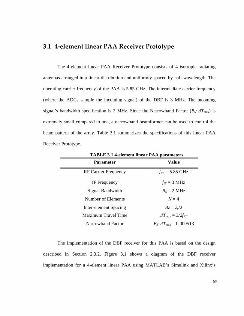
65
3.1 4-element linear PAA Receiver Prototype
The 4-element linear PAA Receiver Prototype consists of 4 isotropic radiating
antennas arranged in a linear distribution and uniformly spaced by half-wavelength. The
operating carrier frequency of the PAA is 5.85 GHz. The intermediate carrier frequency
(where the ADCs sample the incoming signal) of the DBF is 3 MHz. The incoming
signal’s bandwidth specification is 2 MHz. Since the Narrowband Factor (BS· ∆Tmax) is
extremely small compared to one, a narrowband beamformer can be used to control the
beam pattern of the array. Table 3.1 summarizes the specifications of this linear PAA
Receiver Prototype.
TABLE 3.1 4-element linear PAA parameters
Parameter Value
RF Carrier Frequency fRF = 5.85 GHz
IF Frequency fIF = 3 MHz
Signal Bandwidth BS = 2 MHz
Number of Elements N = 4
Inter-element Spacing ∆z = λc/2
Maximum Travel Time ∆Tmax = 3/2fRF
Narrowband Factor BS· ∆Tmax = 0.000513
The implementation of the DBF receiver for this PAA is based on the design
described in Section 2.3.2. Figure 3.1 shows a diagram of the DBF receiver
implementation for a 4-element linear PAA using MATLAB’s Simulink and Xilinx’s
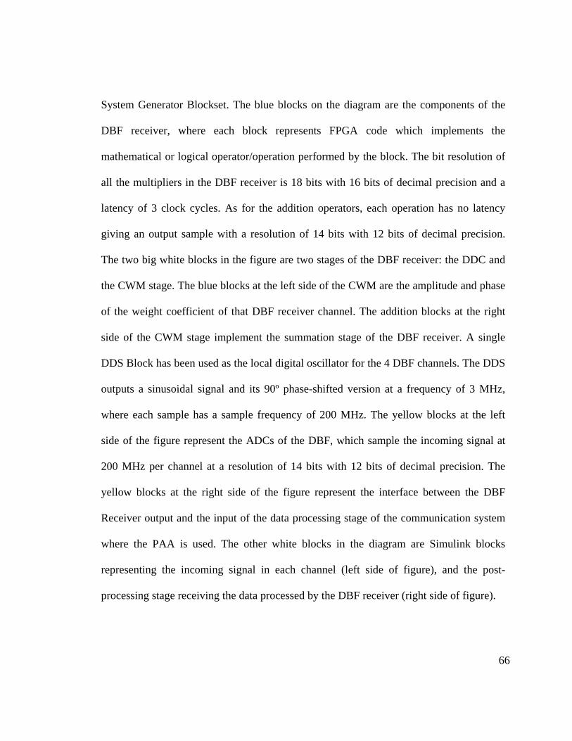
66
System Generator Blockset. The blue blocks on the diagram are the components of the
DBF receiver, where each block represents FPGA code which implements the
mathematical or logical operator/operation performed by the block. The bit resolution of
all the multipliers in the DBF receiver is 18 bits with 16 bits of decimal precision and a
latency of 3 clock cycles. As for the addition operators, each operation has no latency
giving an output sample with a resolution of 14 bits with 12 bits of decimal precision.
The two big white blocks in the figure are two stages of the DBF receiver: the DDC and
the CWM stage. The blue blocks at the left side of the CWM are the amplitude and phase
of the weight coefficient of that DBF receiver channel. The addition blocks at the right
side of the CWM stage implement the summation stage of the DBF receiver. A single
DDS Block has been used as the local digital oscillator for the 4 DBF channels. The DDS
outputs a sinusoidal signal and its 90º phase-shifted version at a frequency of 3 MHz,
where each sample has a sample frequency of 200 MHz. The yellow blocks at the left
side of the figure represent the ADCs of the DBF, which sample the incoming signal at
200 MHz per channel at a resolution of 14 bits with 12 bits of decimal precision. The
yellow blocks at the right side of the figure represent the interface between the DBF
Receiver output and the input of the data processing stage of the communication system
where the PAA is used. The other white blocks in the diagram are Simulink blocks
representing the incoming signal in each channel (left side of figure), and the post-
processing stage receiving the data processed by the DBF receiver (right side of figure).
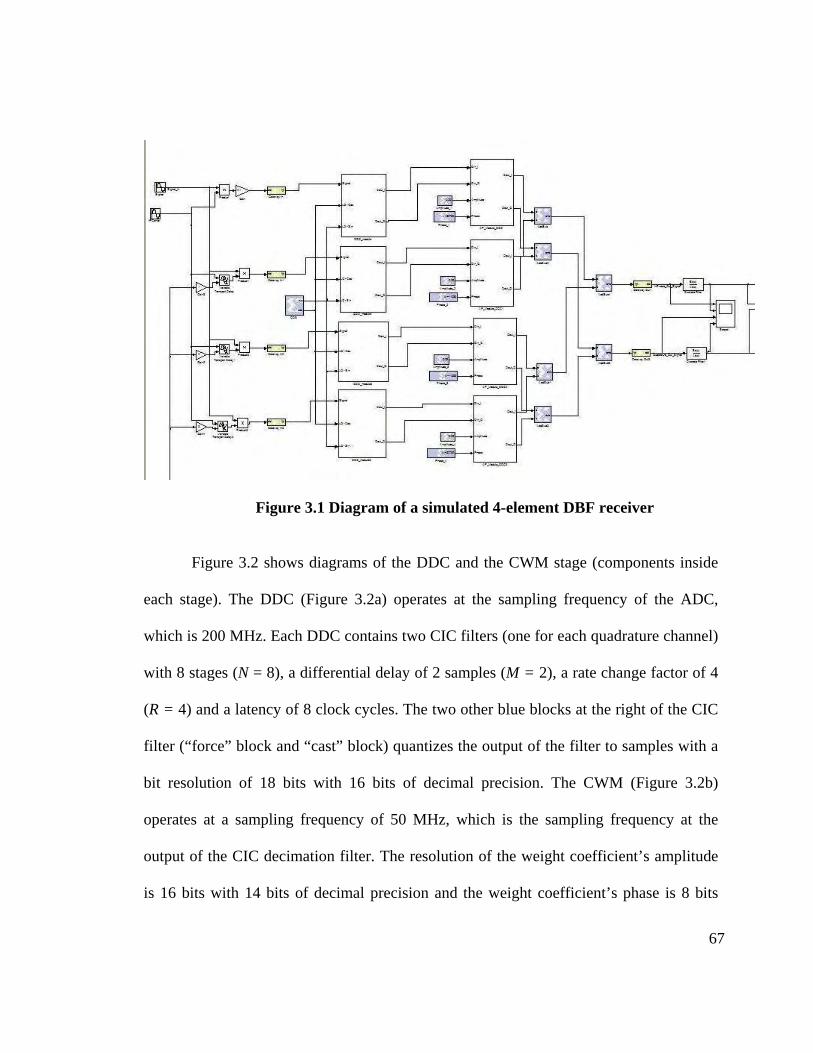
67
Figure 3.1 Diagram of a simulated 4-element DBF receiver
Figure 3.2 shows diagrams of the DDC and the CWM stage (components inside
each stage). The DDC (Figure 3.2a) operates at the sampling frequency of the ADC,
which is 200 MHz. Each DDC contains two CIC filters (one for each quadrature channel)
with 8 stages (N = 8), a differential delay of 2 samples (M = 2), a rate change factor of 4
(R = 4) and a latency of 8 clock cycles. The two other blue blocks at the right of the CIC
filter (“force” block and “cast” block) quantizes the output of the filter to samples with a
bit resolution of 18 bits with 16 bits of decimal precision. The CWM (Figure 3.2b)
operates at a sampling frequency of 50 MHz, which is the sampling frequency at the
output of the CIC decimation filter. The resolution of the weight coefficient’s amplitude
is 16 bits with 14 bits of decimal precision and the weight coefficient’s phase is 8 bits
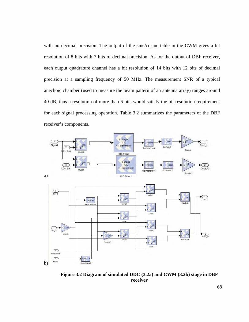
68
with no decimal precision. The output of the sine/cosine table in the CWM gives a bit
resolution of 8 bits with 7 bits of decimal precision. As for the output of DBF receiver,
each output quadrature channel has a bit resolution of 14 bits with 12 bits of decimal
precision at a sampling frequency of 50 MHz. The measurement SNR of a typical
anechoic chamber (used to measure the beam pattern of an antenna array) ranges around
40 dB, thus a resolution of more than 6 bits would satisfy the bit resolution requirement
for each signal processing operation. Table 3.2 summarizes the parameters of the DBF
receiver’s components.
a)
b)
Figure 3.2 Diagram of simulated DDC (3.2a) and CWM (3.2b) stage in DBF receiver
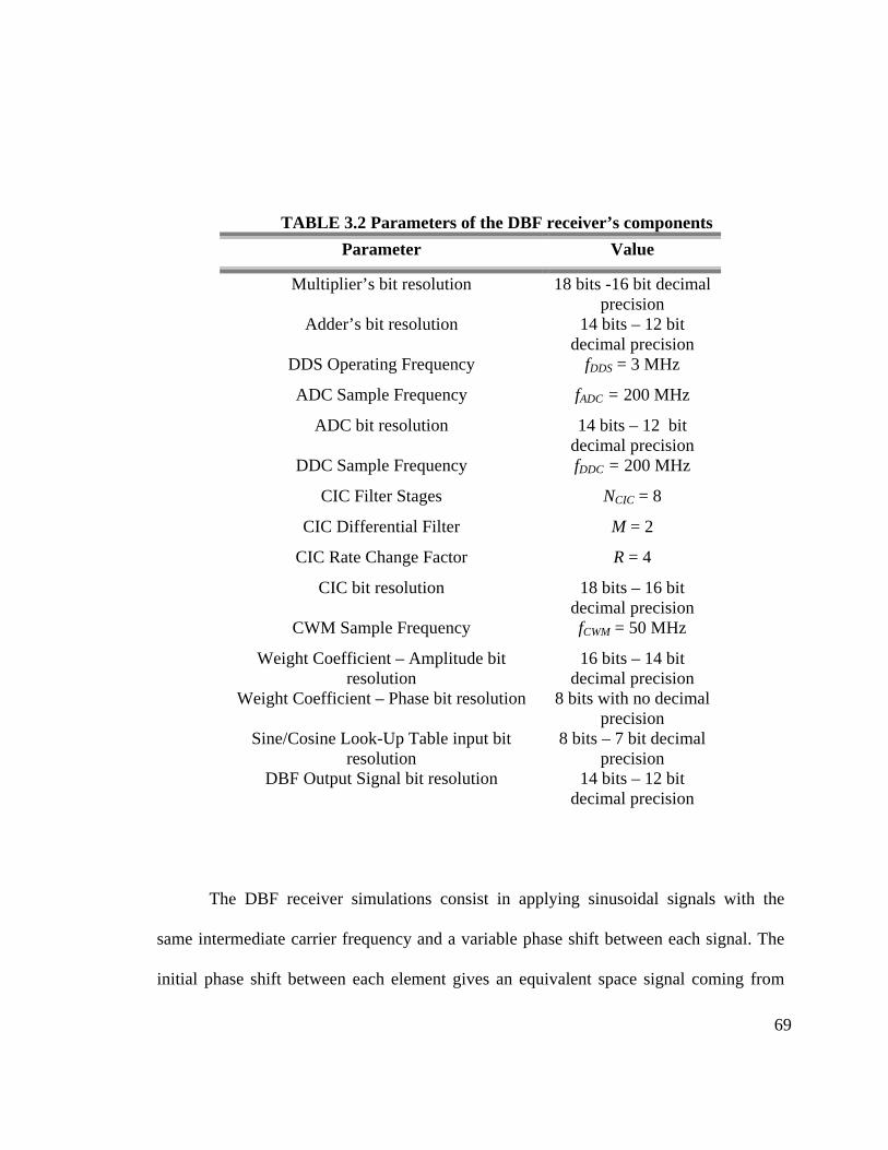
69
TABLE 3.2 Parameters of the DBF receiver’s components
Parameter Value
Multiplier’s bit resolution 18 bits -16 bit decimal precision
Adder’s bit resolution 14 bits – 12 bit decimal precision
DDS Operating Frequency fDDS = 3 MHz
ADC Sample Frequency fADC = 200 MHz
ADC bit resolution 14 bits – 12 bit decimal precision
DDC Sample Frequency fDDC = 200 MHz
CIC Filter Stages NCIC = 8
CIC Differential Filter M = 2
CIC Rate Change Factor R = 4
CIC bit resolution 18 bits – 16 bit decimal precision
CWM Sample Frequency fCWM = 50 MHz
Weight Coefficient – Amplitude bit resolution
16 bits – 14 bit decimal precision
Weight Coefficient – Phase bit resolution 8 bits with no decimal precision
Sine/Cosine Look-Up Table input bit resolution
8 bits – 7 bit decimal precision
DBF Output Signal bit resolution 14 bits – 12 bit decimal precision
The DBF receiver simulations consist in applying sinusoidal signals with the
same intermediate carrier frequency and a variable phase shift between each signal. The
initial phase shift between each element gives an equivalent space signal coming from

70
endfire (direction parallel to the array’s axis) at the left side of the array. As the
simulation iterates, the relative phase difference between each element changes until it
reaches to a phase shift equivalent to a signal coming from endfire at the right side of the
array. Since the weight coefficients of each DBF channel is held constant, the output in-
phase and quadrature channel of the DBF receiver will experience changes on each
signal’s amplitude as the simulation time progresses. In the post-processing phase of the
PAA, the two quadrature output signals are use to calculate the resulting beam pattern’s
amplitude and phase. The resulting beam pattern of each DBF receiver simulation shown
in this chapter will be compared with the theorical beam pattern calculated using Eq. 2.6.
3.1.1 First Spatial Filter Example: Beam pattern with Uniform Amplitude Weight Function pointing to θMRA = 45º
The first spatial filter example used in the DBF receiver for a 4-element linear
PAA produces a beam pattern with an MRA pointing at an angular position of 45º with
respect to endfire on the right side of the array. If the desired beam pattern of a PAA has
only one MRA, the weigh coefficients for each channel can be derived using the
Narrowband Beamformer model discussed in Section 2.1.3:
( ),1* ,
TMRA MRA nj k p
nw eN
θ φ ⋅= 3.1
where the wavenumber k and the position vector p are:
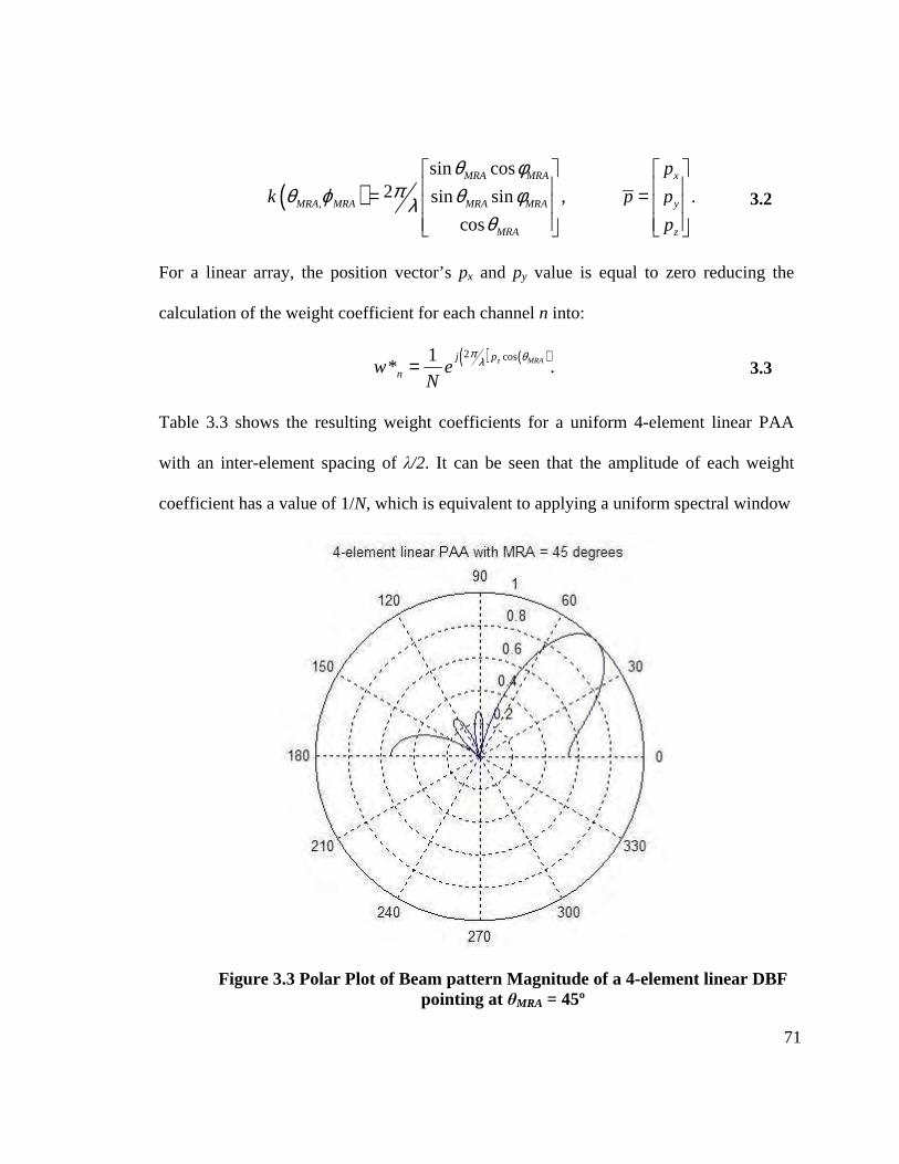
71
( ),
sin cos2 sin sin , .
cos
MRA MRA x
MRA MRA MRA MRA y
MRA z
p
k p p
p
θ φπθ ϕ θ φλ
θ
= =
3.2
For a linear array, the position vector’s px and py value is equal to zero reducing the
calculation of the weight coefficient for each channel n into:
( ) ( )2 cos1* .z MRAj p
nw eN
π θλ= 3.3
Table 3.3 shows the resulting weight coefficients for a uniform 4-element linear PAA
with an inter-element spacing of λ/2. It can be seen that the amplitude of each weight
coefficient has a value of 1/N, which is equivalent to applying a uniform spectral window
Figure 3.3 Polar Plot of Beam pattern Magnitude of a 4-element linear DBF pointing at θMRA = 45º
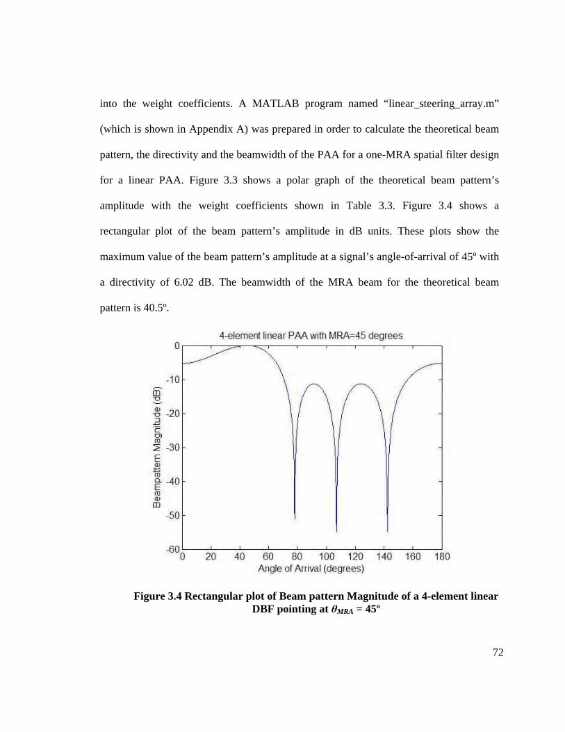
72
into the weight coefficients. A MATLAB program named “linear_steering_array.m”
(which is shown in Appendix A) was prepared in order to calculate the theoretical beam
pattern, the directivity and the beamwidth of the PAA for a one-MRA spatial filter design
for a linear PAA. Figure 3.3 shows a polar graph of the theoretical beam pattern’s
amplitude with the weight coefficients shown in Table 3.3. Figure 3.4 shows a
rectangular plot of the beam pattern’s amplitude in dB units. These plots show the
maximum value of the beam pattern’s amplitude at a signal’s angle-of-arrival of 45º with
a directivity of 6.02 dB. The beamwidth of the MRA beam for the theoretical beam
pattern is 40.5º.
Figure 3.4 Rectangular plot of Beam pattern Magnitude of a 4-element linear DBF pointing at θMRA = 45º

73
TABLE 3.3 First Spatial Filter Weight Coefficients – Theoretical Weights
Element Weight
1 w1 = 0.25 ∟169.0812º
2 w2 = 0.25 ∟-63.6396º
3 w3 = 0.25 ∟63.6396º
4 w1 = 0.25 ∟-169.0812º
After the weight coefficients have been calculated, the next step in the simulation
preparation is the transformation of these coefficients into a form suitable for the DBF
receiver to use. A MATLAB program named “linear_DBFreceiver_parameters.m”
(included in the Appendix A) was prepared to quantize and transform the weight
coefficients for each channel and set all the necessary DBF receiver parameters (shown in
Table 3.2) needed to perform the DBF receiver simulation. The total simulation time used
for this DBF receiver was 2 x 10⁻⁵ seconds, which is equivalent to 60 periods of the
intermediate carrier frequency. The weight coefficients obtained after quantization of the
weight values into the fixed-point representation used in the DBF receiver simulation are
shown in Table 3.4. The results of the DBF receiver for the first spatial filter showing the
behavior of the in-phase output signal, quadrature output signal and the amplitude and
phase signals obtained in the post-processing phase of the PAA are shown in Figure 3.5
and Figure 3.6. Figure 3.5 and Figure 3.6 shows the time plots for plane wave signals
with the angle of arrival changing from 90º to 0º and 90º to 180º, respectively, with
respect to right-side endfire. The change in amplitude experienced in the in-phase and
quadrature output signals as time progresses illustrates the spatial filter’s response

74
characteristics with respect to signals with different angle-of-arrival directions. These
characteristics can be seen clearer in the amplitude and phase plots shown at the bottom
of each figure, which where generated in the post-processing phase (not part of the DBF
receiver) using the in-phase and quadrature output signals.
TABLE 3.4 First Spatial Filter Weight Coefficients – FPGA Weights
Element Weight
1 w1 = 0.25 ∟168.75º
2 w2 = 0.25 ∟-63.2813º
3 w3 = 0.25 ∟63.2813º
4 w1 = 0.25 ∟-168.75º
Figure 3.5 Time plots for plane wave signals with the angle of arrival changing from 90º to 0º for first spatial filter on 4-element linear DBF
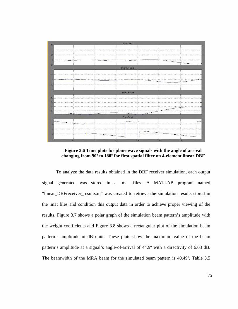
75
Figure 3.6 Time plots for plane wave signals with the angle of arrival changing from 90º to 180º for first spatial filter on 4-element linear DBF
To analyze the data results obtained in the DBF receiver simulation, each output
signal generated was stored in a .mat files. A MATLAB program named
“linear_DBFreceiver_results.m” was created to retrieve the simulation results stored in
the .mat files and condition this output data in order to achieve proper viewing of the
results. Figure 3.7 shows a polar graph of the simulation beam pattern’s amplitude with
the weight coefficients and Figure 3.8 shows a rectangular plot of the simulation beam
pattern’s amplitude in dB units. These plots show the maximum value of the beam
pattern’s amplitude at a signal’s angle-of-arrival of 44.9º with a directivity of 6.03 dB.
The beamwidth of the MRA beam for the simulated beam pattern is 40.49º. Table 3.5

76
shows the results obtained from the DBF receiver simulation with the results obtained in
the theoretical beam pattern calculation.
Figure 3.7 Polar Plot of Beam pattern Magnitude of a 4-element linear DBF Simulation pointing at θMRA = 45º
TABLE 3.5 First Spatial Filter Beam pattern Characteristics for a 4-element
linear PAA
Beam pattern Characteristic Theoretical Result Simulation Result
MRA angle-of-arrival ΘMRA = 45º ΘMRA = 45.09º
Half-power Beamwidth ΘBW = 40.47º ΘBW = 40.28º
Directivity DdB = 6.02 dB DdB = 6.03 dB
Sidelobe level SLLdB = -11.30 dB SLLdB = -11.43 dB
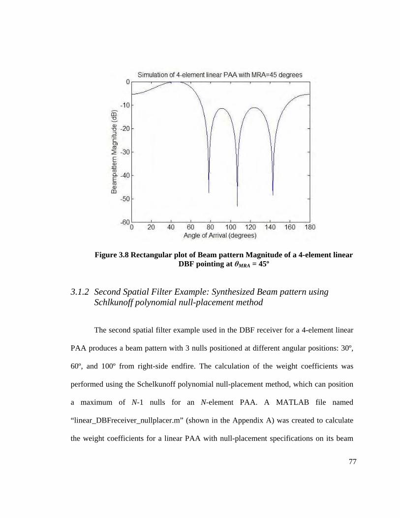
77
Figure 3.8 Rectangular plot of Beam pattern Magnitude of a 4-element linear DBF pointing at θMRA = 45º
3.1.2 Second Spatial Filter Example: Synthesized Beam pattern using Schlkunoff polynomial null-placement method
The second spatial filter example used in the DBF receiver for a 4-element linear
PAA produces a beam pattern with 3 nulls positioned at different angular positions: 30º,
60º, and 100º from right-side endfire. The calculation of the weight coefficients was
performed using the Schelkunoff polynomial null-placement method, which can position
a maximum of N-1 nulls for an N-element PAA. A MATLAB file named
“linear_DBFreceiver_nullplacer.m” (shown in the Appendix A) was created to calculate
the weight coefficients for a linear PAA with null-placement specifications on its beam
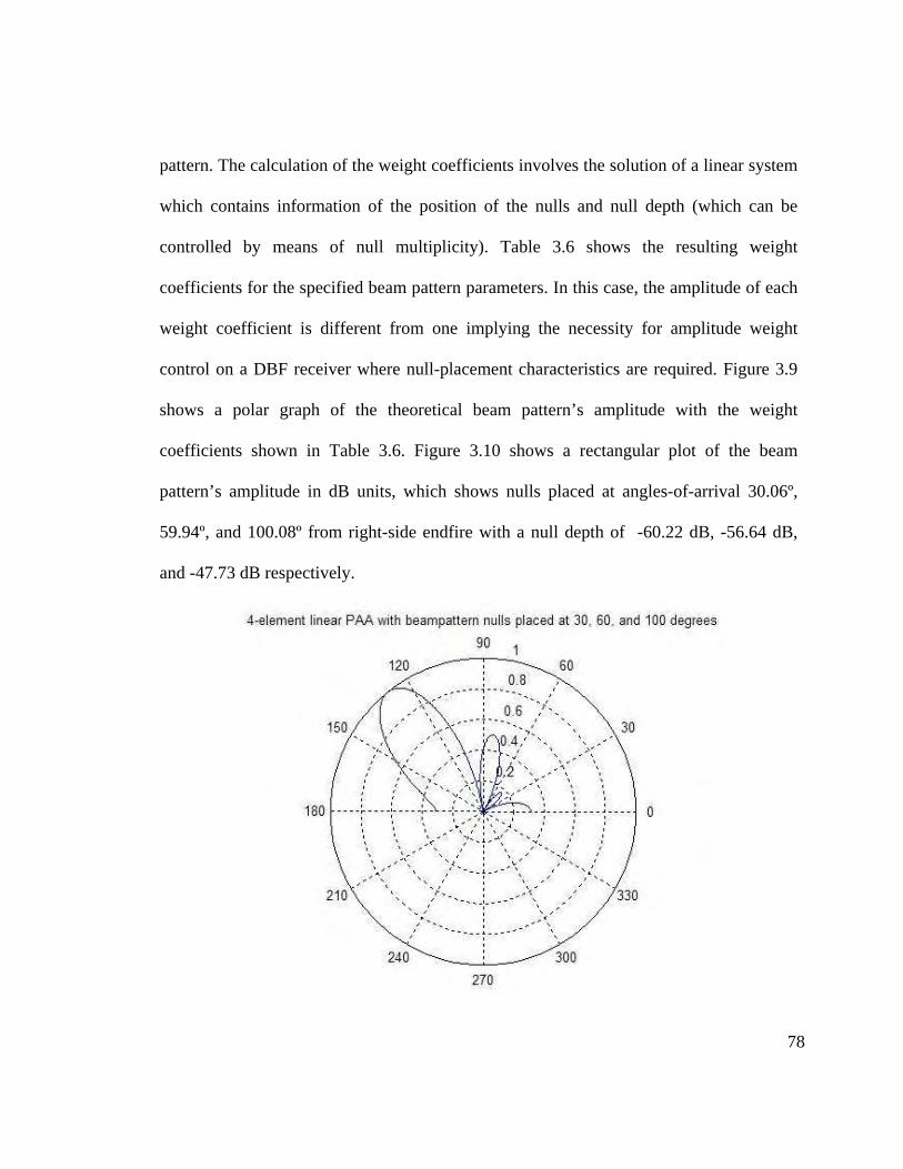
78
pattern. The calculation of the weight coefficients involves the solution of a linear system
which contains information of the position of the nulls and null depth (which can be
controlled by means of null multiplicity). Table 3.6 shows the resulting weight
coefficients for the specified beam pattern parameters. In this case, the amplitude of each
weight coefficient is different from one implying the necessity for amplitude weight
control on a DBF receiver where null-placement characteristics are required. Figure 3.9
shows a polar graph of the theoretical beam pattern’s amplitude with the weight
coefficients shown in Table 3.6. Figure 3.10 shows a rectangular plot of the beam
pattern’s amplitude in dB units, which shows nulls placed at angles-of-arrival 30.06º,
59.94º, and 100.08º from right-side endfire with a null depth of -60.22 dB, -56.64 dB,
and -47.73 dB respectively.
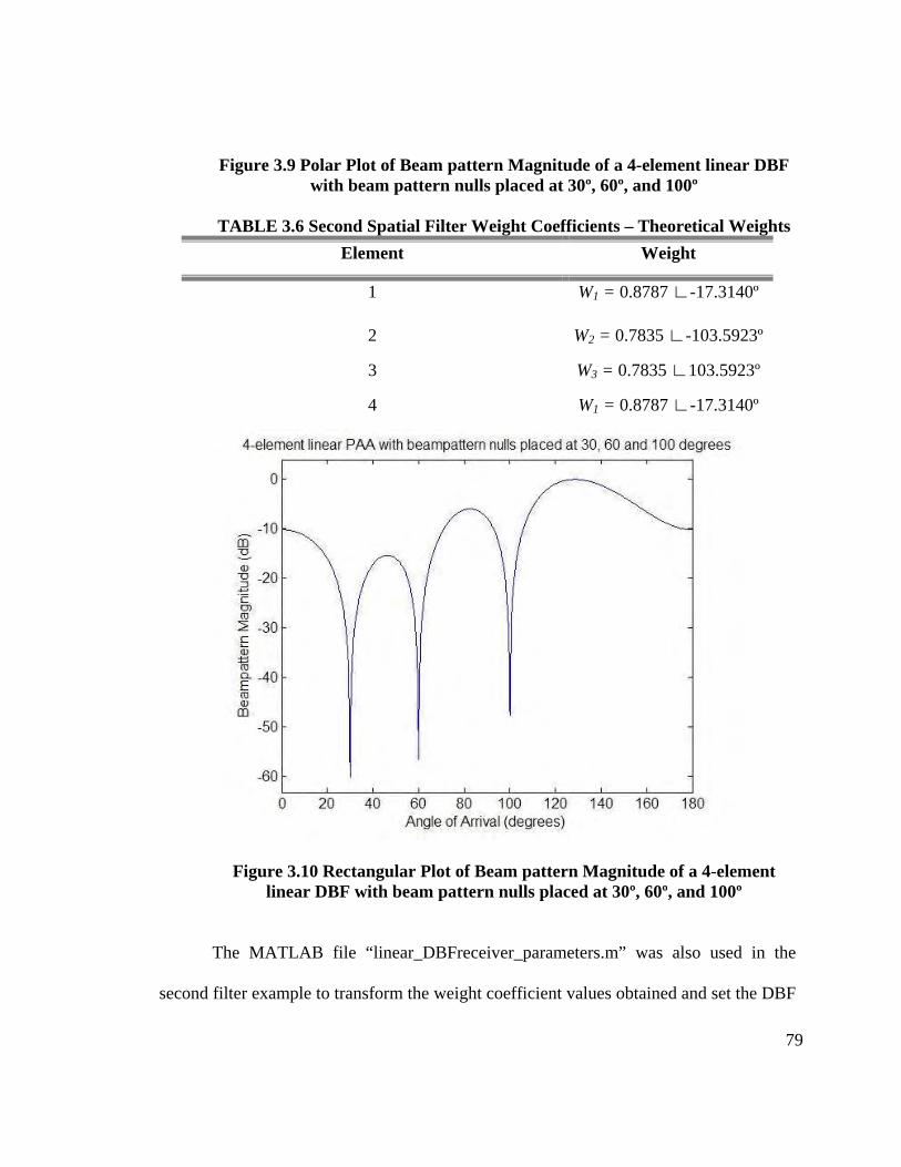
79
Figure 3.9 Polar Plot of Beam pattern Magnitude of a 4-element linear DBF with beam pattern nulls placed at 30º, 60º, and 100º
TABLE 3.6 Second Spatial Filter Weight Coefficients – Theoretical Weights
Element Weight
1 W1 = 0.8787 ∟-17.3140º
2 W2 = 0.7835 ∟-103.5923º
3 W3 = 0.7835 ∟103.5923º
4 W1 = 0.8787 ∟-17.3140º
Figure 3.10 Rectangular Plot of Beam pattern Magnitude of a 4-element linear DBF with beam pattern nulls placed at 30º, 60º, and 100º
The MATLAB file “linear_DBFreceiver_parameters.m” was also used in the
second filter example to transform the weight coefficient values obtained and set the DBF
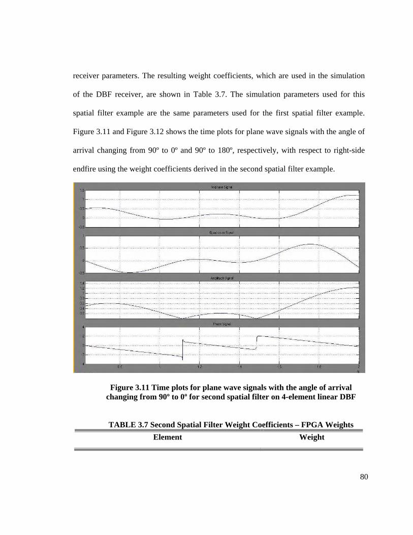
80
receiver parameters. The resulting weight coefficients, which are used in the simulation
of the DBF receiver, are shown in Table 3.7. The simulation parameters used for this
spatial filter example are the same parameters used for the first spatial filter example.
Figure 3.11 and Figure 3.12 shows the time plots for plane wave signals with the angle of
arrival changing from 90º to 0º and 90º to 180º, respectively, with respect to right-side
endfire using the weight coefficients derived in the second spatial filter example.
Figure 3.11 Time plots for plane wave signals with the angle of arrival changing from 90º to 0º for second spatial filter on 4-element linear DBF
TABLE 3.7 Second Spatial Filter Weight Coefficients – FPGA Weights
Element Weight
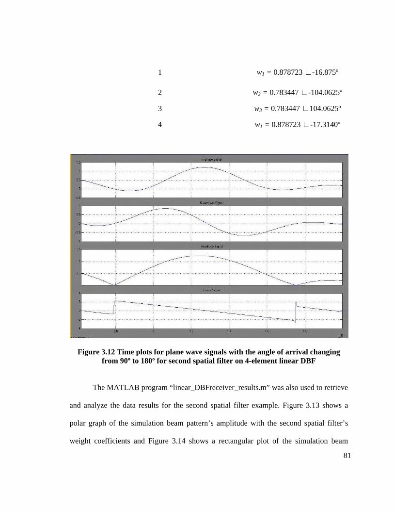
81
1 w1 = 0.878723 ∟-16.875º
2 w2 = 0.783447 ∟-104.0625º
3 w3 = 0.783447 ∟104.0625º
4 w1 = 0.878723 ∟-17.3140º
Figure 3.12 Time plots for plane wave signals with the angle of arrival changing
from 90º to 180º for second spatial filter on 4-element linear DBF
The MATLAB program “linear_DBFreceiver_results.m” was also used to retrieve
and analyze the data results for the second spatial filter example. Figure 3.13 shows a
polar graph of the simulation beam pattern’s amplitude with the second spatial filter’s
weight coefficients and Figure 3.14 shows a rectangular plot of the simulation beam

82
pattern’s amplitude in dB units. These plots show the beam pattern nulls placed at angles-
of-arrival 29.77º, 60.26º, and 99.91º from right-side endfire with a null depth of -55.56
dB, -56.43 dB, and -55.3 dB respectively. Table 3.8 shows the beam pattern
characteristics of the theoretical results and the simulation results for the second spatial
filter example.
Figure 3.13 Polar Plot of Beam pattern Magnitude of a simulated 4-element linear DBF with beam pattern nulls placed at 30º, 60º, and 100º
TABLE 3.8 Second Spatial Filter Beam pattern Characteristics for a 4-element linear PAA
Beam pattern Characteristic Theoretical Result Simulation Result
Null #1: Angle of Arrival = 30º ΘN1 = 30.06º ΘN1 = 29.77º
Null-depth of Null #1 | B(ΘN1)|dB = -60.22 dB | B(ΘN1)|dB = -55.56 dB
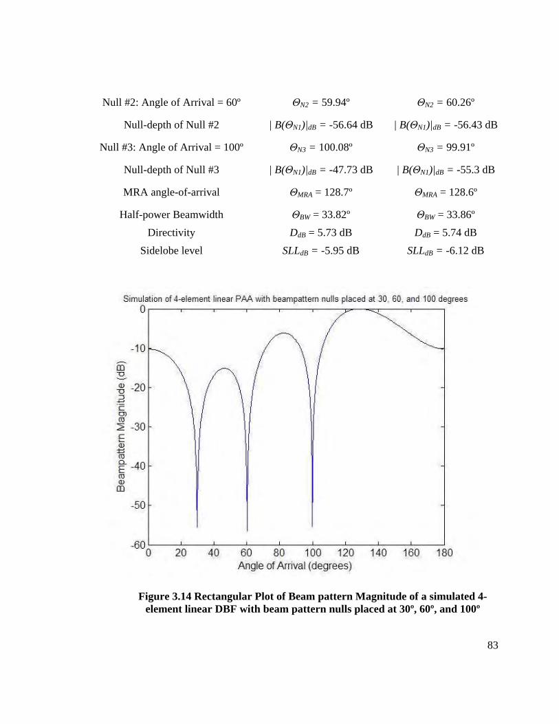
83
Null #2: Angle of Arrival = 60º ΘN2 = 59.94º ΘN2 = 60.26º
Null-depth of Null #2 | B(ΘN1)|dB = -56.64 dB | B(ΘN1)|dB = -56.43 dB
Null #3: Angle of Arrival = 100º ΘN3 = 100.08º ΘN3 = 99.91º
Null-depth of Null #3 | B(ΘN1)|dB = -47.73 dB | B(ΘN1)|dB = -55.3 dB
MRA angle-of-arrival ΘMRA = 128.7º ΘMRA = 128.6º
Half-power Beamwidth ΘBW = 33.82º ΘBW = 33.86º
Directivity DdB = 5.73 dB DdB = 5.74 dB
Sidelobe level SLLdB = -5.95 dB SLLdB = -6.12 dB
Figure 3.14 Rectangular Plot of Beam pattern Magnitude of a simulated 4-element linear DBF with beam pattern nulls placed at 30º, 60º, and 100º
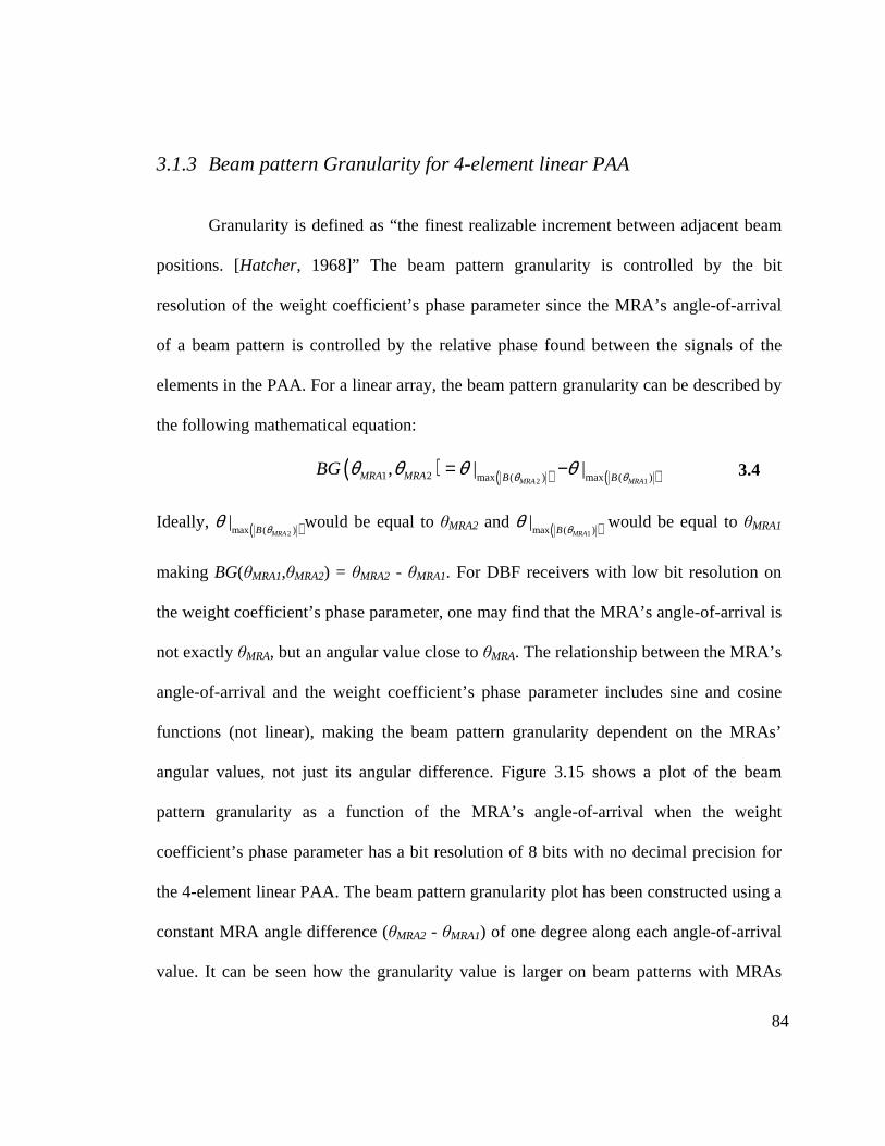
84
3.1.3 Beam pattern Granularity for 4-element linear PAA
Granularity is defined as “the finest realizable increment between adjacent beam
positions. [Hatcher, 1968]” The beam pattern granularity is controlled by the bit
resolution of the weight coefficient’s phase parameter since the MRA’s angle-of-arrival
of a beam pattern is controlled by the relative phase found between the signals of the
elements in the PAA. For a linear array, the beam pattern granularity can be described by
the following mathematical equation:
( ) ( ) ( )2 11 2 max ( ) max ( ), | |
MRA MRAMRA MRA B B
BG θ θθ θ θ θ= − 3.4
Ideally, ( )2max ( )
|MRAB θθ would be equal to θMRA2 and ( )1max ( )
|MRAB θθ would be equal to θMRA1
making BG(θMRA1,θMRA2) = θMRA2 - θMRA1. For DBF receivers with low bit resolution on
the weight coefficient’s phase parameter, one may find that the MRA’s angle-of-arrival is
not exactly θMRA, but an angular value close to θMRA. The relationship between the MRA’s
angle-of-arrival and the weight coefficient’s phase parameter includes sine and cosine
functions (not linear), making the beam pattern granularity dependent on the MRAs’
angular values, not just its angular difference. Figure 3.15 shows a plot of the beam
pattern granularity as a function of the MRA’s angle-of-arrival when the weight
coefficient’s phase parameter has a bit resolution of 8 bits with no decimal precision for
the 4-element linear PAA. The beam pattern granularity plot has been constructed using a
constant MRA angle difference (θMRA2 - θMRA1) of one degree along each angle-of-arrival
value. It can be seen how the granularity value is larger on beam patterns with MRAs
85
pointing towards endfire of the array (leftside and rightside) with a value of
approximately 5 degrees from beam patterns with MRAs pointing near broadside where
the beam pattern granularity has a value close to one degree, which is the desired MRA
angle difference. Figure 3.16 and Figure 3.17 shows beam pattern granularity for weight
coefficient’s phase parameters with bit resolutions of 4 bits with no decimal precision and
16 bits with no decimal precision, respectively. In these figures, it can be seen how low
bit resolution results into poor beam pattern granularity restricting the MRA’s
permissible angular value whereas high bit resolution results into good beam pattern
graunularity where the resulting MRA’s angle difference is very close the proposed
angular difference.
Figure 3.15 Beam pattern Granularity Plot for a 4-element linear DBF with 8 bits of resolution on the weight coefficient’s phase
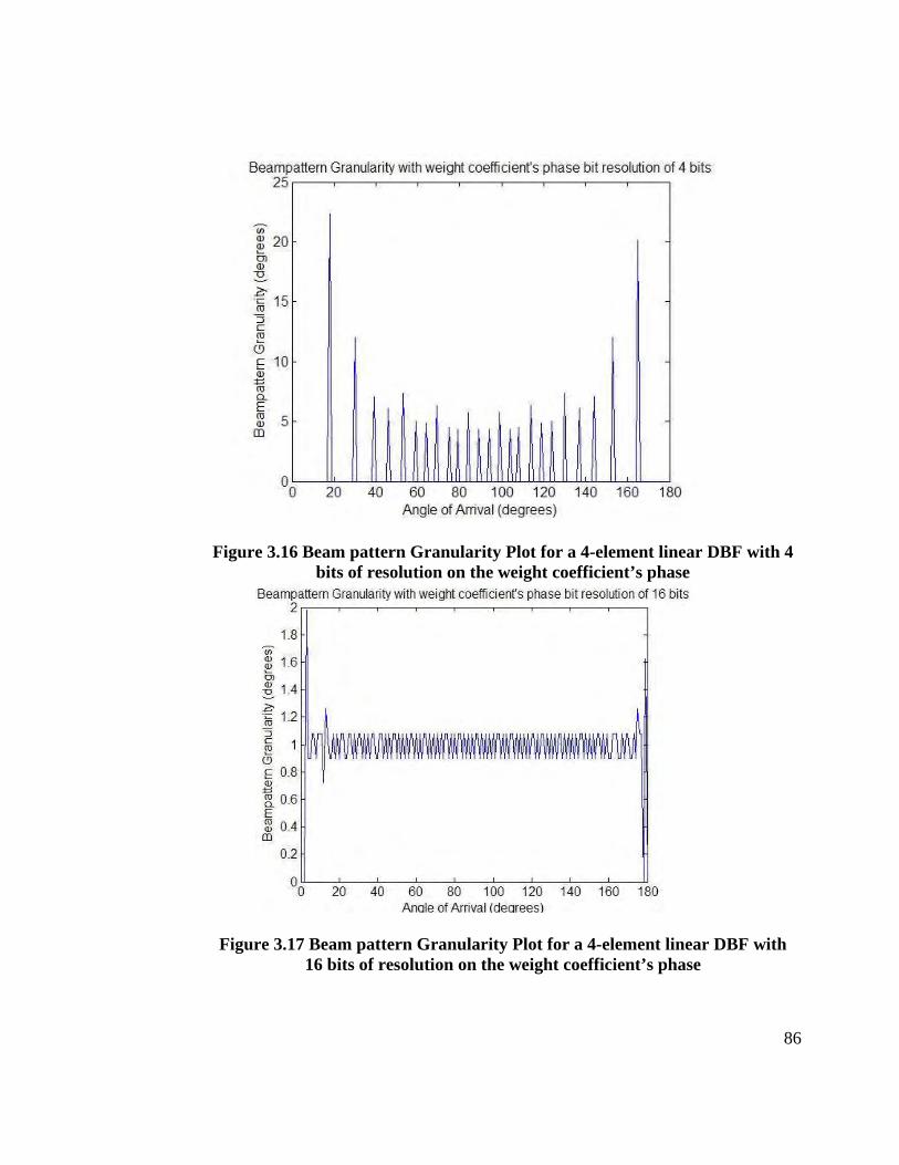
86
Figure 3.16 Beam pattern Granularity Plot for a 4-element linear DBF with 4 bits of resolution on the weight coefficient’s phase
Figure 3.17 Beam pattern Granularity Plot for a 4-element linear DBF with 16 bits of resolution on the weight coefficient’s phase

87
3.2 16-element linear PAA Transmitter Prototype The 16-element linear PAA Transmitter Prototype consists of 16 isotropic radiating
antennas arranged in a linear distribution and uniformly spaced by half-wavelength.
Some PAA parameters, such as signal bandwidth, RF carrier frequency, IF frequency and
inter-element spacing, are the same parameters used in the 4-element linear PAA receiver
prototype. Since this PAA has a different number of elements, the Narrowband Factor
needs to be recalculated to assure proper array performance based on narrowband
beamformer model implementation. Table 3.9 shows the PAA parameters for this 16-
element linear array. In this case, the Narrowband Factor (BS· ∆Tmax) is extremely small
compared to one thus, the narrowband beamformer can be used to control the beam
pattern of this 16-element PAA.
TABLE 3.9 16-element linear PAA parameters
Parameter Value
RF Carrier Frequency fRF = 5.85 GHz
IF Frequency fIF = 3 MHz
Signal Bandwidth BS = 2 MHz
Number of Elements N = 16
Inter-element Spacing ∆z = λc/2
Maximum Travel Time ∆Tmax = 15/2fRF
Narrowband Factor BS· ∆Tmax = 0.0026
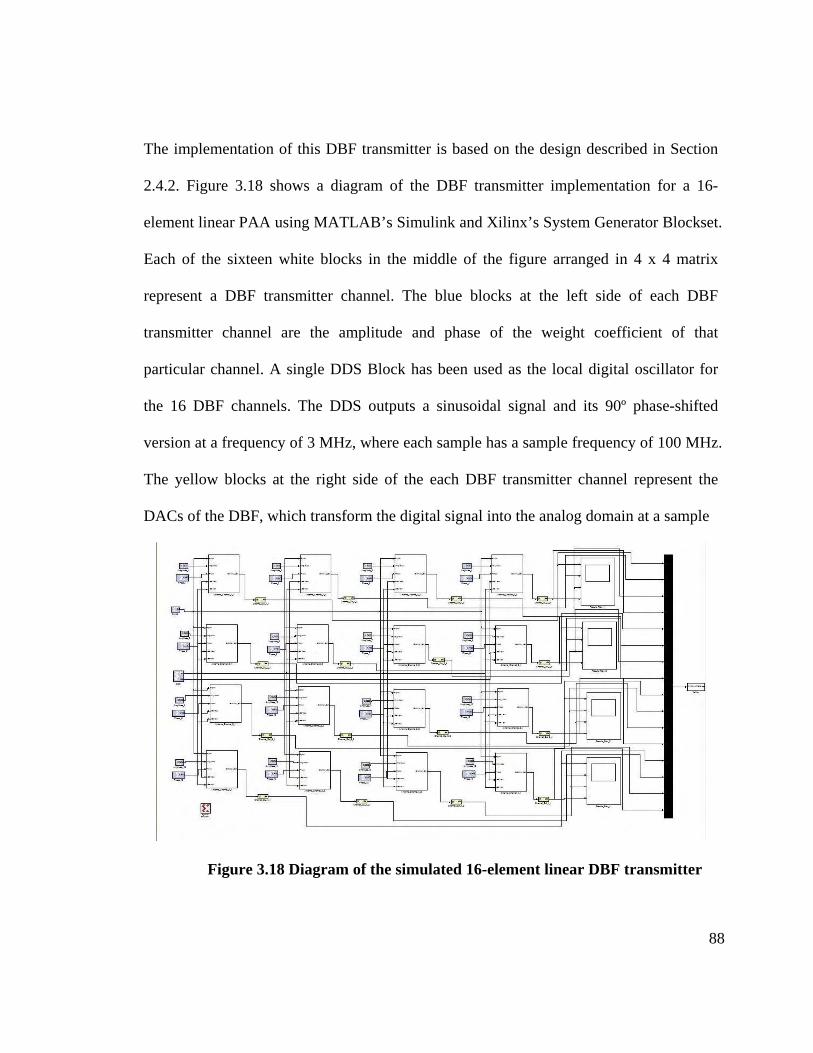
88
The implementation of this DBF transmitter is based on the design described in Section
2.4.2. Figure 3.18 shows a diagram of the DBF transmitter implementation for a 16-
element linear PAA using MATLAB’s Simulink and Xilinx’s System Generator Blockset.
Each of the sixteen white blocks in the middle of the figure arranged in 4 x 4 matrix
represent a DBF transmitter channel. The blue blocks at the left side of each DBF
transmitter channel are the amplitude and phase of the weight coefficient of that
particular channel. A single DDS Block has been used as the local digital oscillator for
the 16 DBF channels. The DDS outputs a sinusoidal signal and its 90º phase-shifted
version at a frequency of 3 MHz, where each sample has a sample frequency of 100 MHz.
The yellow blocks at the right side of the each DBF transmitter channel represent the
DACs of the DBF, which transform the digital signal into the analog domain at a sample
Figure 3.18 Diagram of the simulated 16-element linear DBF transmitter

89
rate of 100 MHz per channel at a resolution of 14 bits with 12 bits of decimal precision.
At the left side of the figure, the white figures and black figures are Simulink blocks used
to display and store as a .mat file the 16 generated IF signals.
Figure 3.19 shows diagrams of the DUC and the CWM phase components, which
are inside of each DBF transmitter channel. The CWM (Figure 3.19a) operates at a
sampling frequency of 10 MHz, which is the sampling frequency at the input of the CIC
interpolation filter. The resolution of the weight coefficient’s amplitude is 16 bits with 14
bits of decimal precision and the weight coefficient’s phase is 8 bits with no decimal
precision. The output of the sine/cosine table in the CWM gives a bit resolution of 8 bits
with 7 bits of decimal precision. The mathematical operations in the DBF transmitter
channel (addition and multiplication) have the same bit resolution used in the 4-element
linear PAA receiver. The DUC (right side of Figure 3.19b) operates at the sampling
frequency of the DAC, which is 100 MHz. Each DUC contains two CIC filters (one for
each quadrature channel) with 2 stages (N = 2), a differential delay of 1 samples (M = 1),
a rate change factor of 10 (R = 10) and a latency of 2 clock cycles. The two other blue
blocks at the right of the CIC filter (“force” block and “cast” block) quantizes the output
of the filter to samples with a bit resolution of 18 bits with 16 bits of decimal precision.
The two scale blocks located at the output of the register, which are part of the CIC filter
implementation, are used to condition the output of the CIC filter and prevent overflow in
the multiplication stages. As for the output of DBF transmitter, each output channel has a

90
bit resolution of a resolution of 14 bits at a sampling frequency of 100 MHz. Table 3.10
summarizes the parameters of the DBF receiver’s components.
a)
b)
Figure 3.19 Diagram of the DUC (3.19a) and CWM (3.19b) of the simulated DBF transmitter
TABLE 3.10 Parameters of the DBF transmitter’s components
Parameter Value
Multiplier’s bit resolution 18 bits -16 bit decimal precision
Adder’s bit resolution 14 bits – 12 bit decimal precision

91
DDS Operating Frequency fDDS = 3 MHz
DAC Sample Frequency fDAC = 100 MHz
DAC bit resolution 14 bits – 12 bit decimal precision
DUC Sample Frequency fDUC = 100 MHz
CIC Filter Stages NCIC = 2
CIC Differential Filter M = 1
CIC Rate Change Factor R = 10
CIC bit resolution 18 bits – 16 bit decimal precision
CWM Sample Frequency fCWM = 10 MHz
Weight Coefficient – Amplitude bit resolution
16 bits – 14 bit decimal precision
Weight Coefficient – Phase bit resolution 8 bits with no decimal precision
Sine/Cosine Look-Up Table input bit resolution
8 bits – 7 bit decimal precision
DBF Output Signal bit resolution 14 bits – 12 bit decimal precision
The DBF transmitter simulations consist in generating a single data signal in the
FPGA code for all the 16 DBF transmitter channels. At the output of the DBF transmitter
simulation, 16 IF signals are generated, each with a relative phase shit associated with the
channel’s weight coefficients. Four signal scopes are placed at the right side of each row
channel to display the output of each DBF channel and make a visual comparison of the
amplitude and relative phase difference between each signal. As for a post-processing
phase for the PAA transmitter, the 16 IF signals are stored on a .mat file as a matrix
variable where, later, they will be analyzed to observe the beam pattern formed based on
the spatial combination of all the output signals.
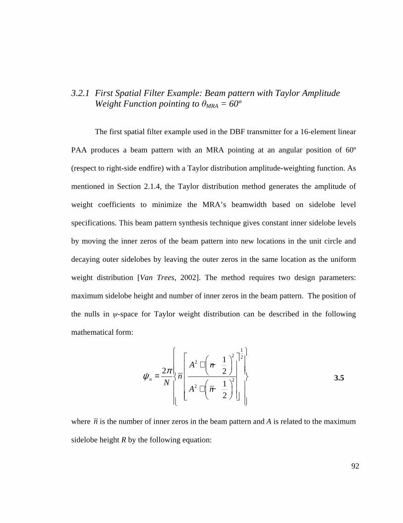
92
3.2.1 First Spatial Filter Example: Beam pattern with Taylor Amplitude Weight Function pointing to θMRA = 60º
The first spatial filter example used in the DBF transmitter for a 16-element linear
PAA produces a beam pattern with an MRA pointing at an angular position of 60º
(respect to right-side endfire) with a Taylor distribution amplitude-weighting function. As
mentioned in Section 2.1.4, the Taylor distribution method generates the amplitude of
weight coefficients to minimize the MRA’s beamwidth based on sidelobe level
specifications. This beam pattern synthesis technique gives constant inner sidelobe levels
by moving the inner zeros of the beam pattern into new locations in the unit circle and
decaying outer sidelobes by leaving the outer zeros in the same location as the uniform
weight distribution [Van Trees, 2002]. The method requires two design parameters:
maximum sidelobe height and number of inner zeros in the beam pattern. The position of
the nulls in ψ-space for Taylor weight distribution can be described in the following
mathematical form:
12 2
2
22
12 2
12
n
A nn
NA n
πψ
+ − = + −
3.5
where n is the number of inner zeros in the beam pattern and A is related to the maximum
sidelobe height R by the following equation:
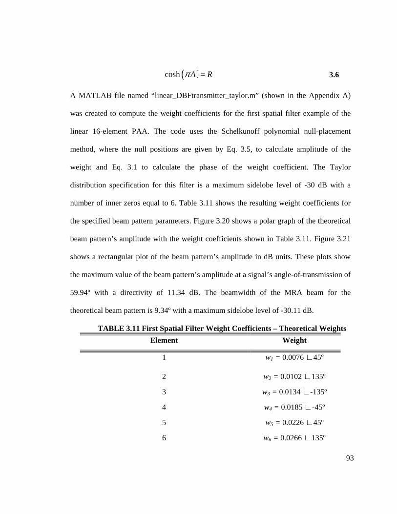
93
( )cosh A Rπ = 3.6
A MATLAB file named “linear_DBFtransmitter_taylor.m” (shown in the Appendix A)
was created to compute the weight coefficients for the first spatial filter example of the
linear 16-element PAA. The code uses the Schelkunoff polynomial null-placement
method, where the null positions are given by Eq. 3.5, to calculate amplitude of the
weight and Eq. 3.1 to calculate the phase of the weight coefficient. The Taylor
distribution specification for this filter is a maximum sidelobe level of -30 dB with a
number of inner zeros equal to 6. Table 3.11 shows the resulting weight coefficients for
the specified beam pattern parameters. Figure 3.20 shows a polar graph of the theoretical
beam pattern’s amplitude with the weight coefficients shown in Table 3.11. Figure 3.21
shows a rectangular plot of the beam pattern’s amplitude in dB units. These plots show
the maximum value of the beam pattern’s amplitude at a signal’s angle-of-transmission of
59.94º with a directivity of 11.34 dB. The beamwidth of the MRA beam for the
theoretical beam pattern is 9.34º with a maximum sidelobe level of -30.11 dB.
TABLE 3.11 First Spatial Filter Weight Coefficients – Theoretical Weights
Element Weight
1 w1 = 0.0076 ∟45º
2 w2 = 0.0102 ∟135º
3 w3 = 0.0134 ∟-135º
4 w4 = 0.0185 ∟-45º
5 w5 = 0.0226 ∟45º
6 w6 = 0.0266 ∟135º
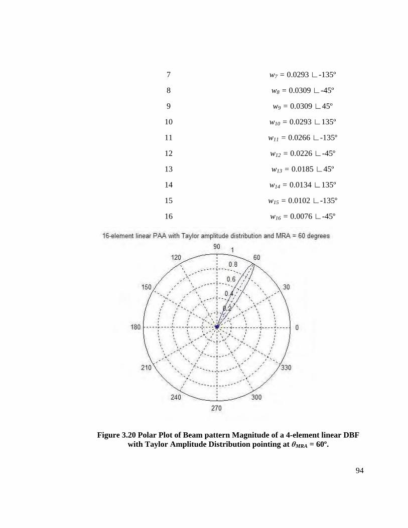
94
7 w7 = 0.0293 ∟-135º
8 w8 = 0.0309 ∟-45º
9 w9 = 0.0309 ∟45º
10 w10 = 0.0293 ∟135º
11 w11 = 0.0266 ∟-135º
12 w12 = 0.0226 ∟-45º
13 w13 = 0.0185 ∟45º
14 w14 = 0.0134 ∟135º
15 w15 = 0.0102 ∟-135º
16 w16 = 0.0076 ∟-45º
Figure 3.20 Polar Plot of Beam pattern Magnitude of a 4-element linear DBF with Taylor Amplitude Distribution pointing at θMRA = 60º.
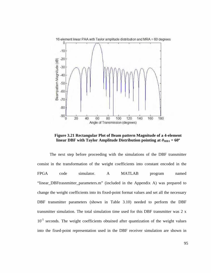
95
Figure 3.21 Rectangular Plot of Beam pattern Magnitude of a 4-element linear DBF with Taylor Amplitude Distribution point ing at θMRA = 60º
The next step before proceeding with the simulations of the DBF transmitter
consist in the transformation of the weight coefficients into constant encoded in the
FPGA code simulator. A MATLAB program named
“linear_DBFtrasnmitter_parameters.m” (included in the Appendix A) was prepared to
change the weight coefficients into its fixed-point format values and set all the necessary
DBF transmitter parameters (shown in Table 3.10) needed to perform the DBF
transmitter simulation. The total simulation time used for this DBF transmitter was 2 x
10-5 seconds. The weight coefficients obtained after quantization of the weight values
into the fixed-point representation used in the DBF receiver simulation are shown in
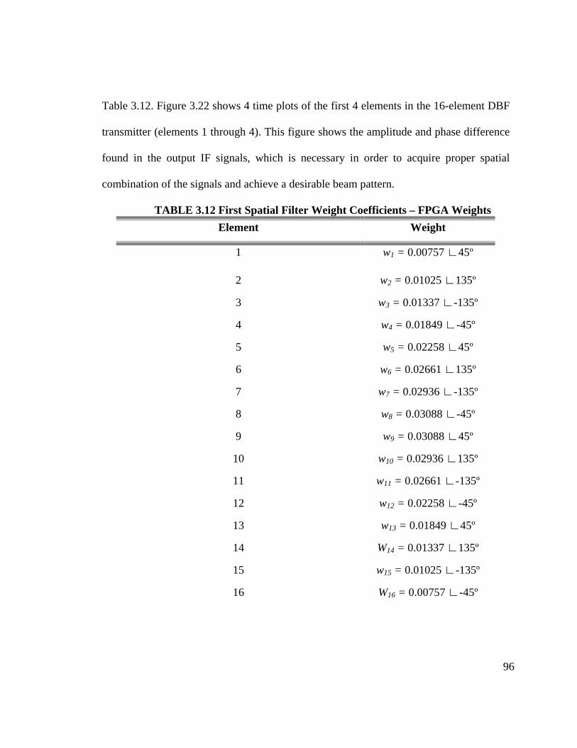
96
Table 3.12. Figure 3.22 shows 4 time plots of the first 4 elements in the 16-element DBF
transmitter (elements 1 through 4). This figure shows the amplitude and phase difference
found in the output IF signals, which is necessary in order to acquire proper spatial
combination of the signals and achieve a desirable beam pattern.
TABLE 3.12 First Spatial Filter Weight Coefficients – FPGA Weights
Element Weight
1 w1 = 0.00757 ∟45º
2 w2 = 0.01025 ∟135º
3 w3 = 0.01337 ∟-135º
4 w4 = 0.01849 ∟-45º
5 w5 = 0.02258 ∟45º
6 w6 = 0.02661 ∟135º
7 w7 = 0.02936 ∟-135º
8 w8 = 0.03088 ∟-45º
9 w9 = 0.03088 ∟45º
10 w10 = 0.02936 ∟135º
11 w11 = 0.02661 ∟-135º
12 w12 = 0.02258 ∟-45º
13 w13 = 0.01849 ∟45º
14 W14 = 0.01337 ∟135º
15 w15 = 0.01025 ∟-135º
16 W16 = 0.00757 ∟-45º
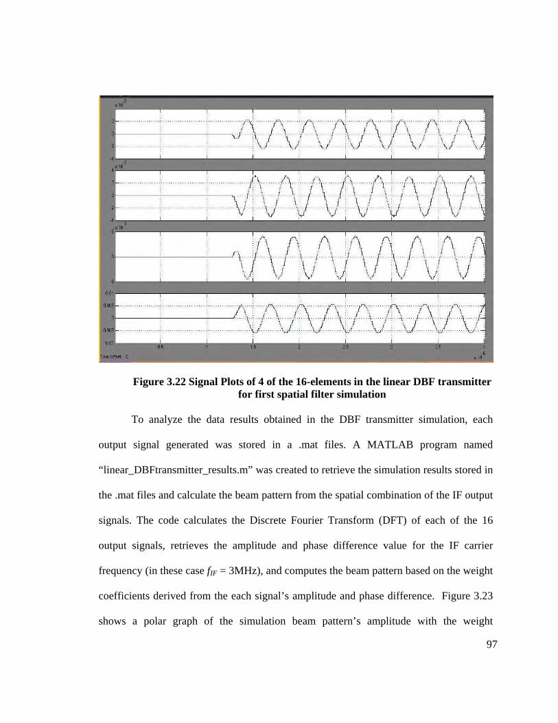
97
Figure 3.22 Signal Plots of 4 of the 16-elements in the linear DBF transmitter for first spatial filter simulation
To analyze the data results obtained in the DBF transmitter simulation, each
output signal generated was stored in a .mat files. A MATLAB program named
“linear_DBFtransmitter_results.m” was created to retrieve the simulation results stored in
the .mat files and calculate the beam pattern from the spatial combination of the IF output
signals. The code calculates the Discrete Fourier Transform (DFT) of each of the 16
output signals, retrieves the amplitude and phase difference value for the IF carrier
frequency (in these case fIF = 3MHz), and computes the beam pattern based on the weight
coefficients derived from the each signal’s amplitude and phase difference. Figure 3.23
shows a polar graph of the simulation beam pattern’s amplitude with the weight
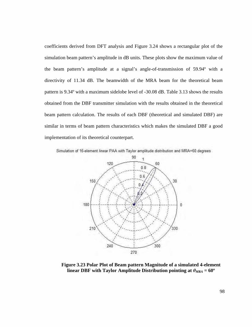
98
coefficients derived from DFT analysis and Figure 3.24 shows a rectangular plot of the
simulation beam pattern’s amplitude in dB units. These plots show the maximum value of
the beam pattern’s amplitude at a signal’s angle-of-transmission of 59.94º with a
directivity of 11.34 dB. The beamwidth of the MRA beam for the theoretical beam
pattern is 9.34º with a maximum sidelobe level of -30.08 dB. Table 3.13 shows the results
obtained from the DBF transmitter simulation with the results obtained in the theoretical
beam pattern calculation. The results of each DBF (theoretical and simulated DBF) are
similar in terms of beam pattern characteristics which makes the simulated DBF a good
implementation of its theoretical counterpart.
Figure 3.23 Polar Plot of Beam pattern Magnitude of a simulated 4-element linear DBF with Taylor Amplitude Distribution point ing at θMRA = 60º
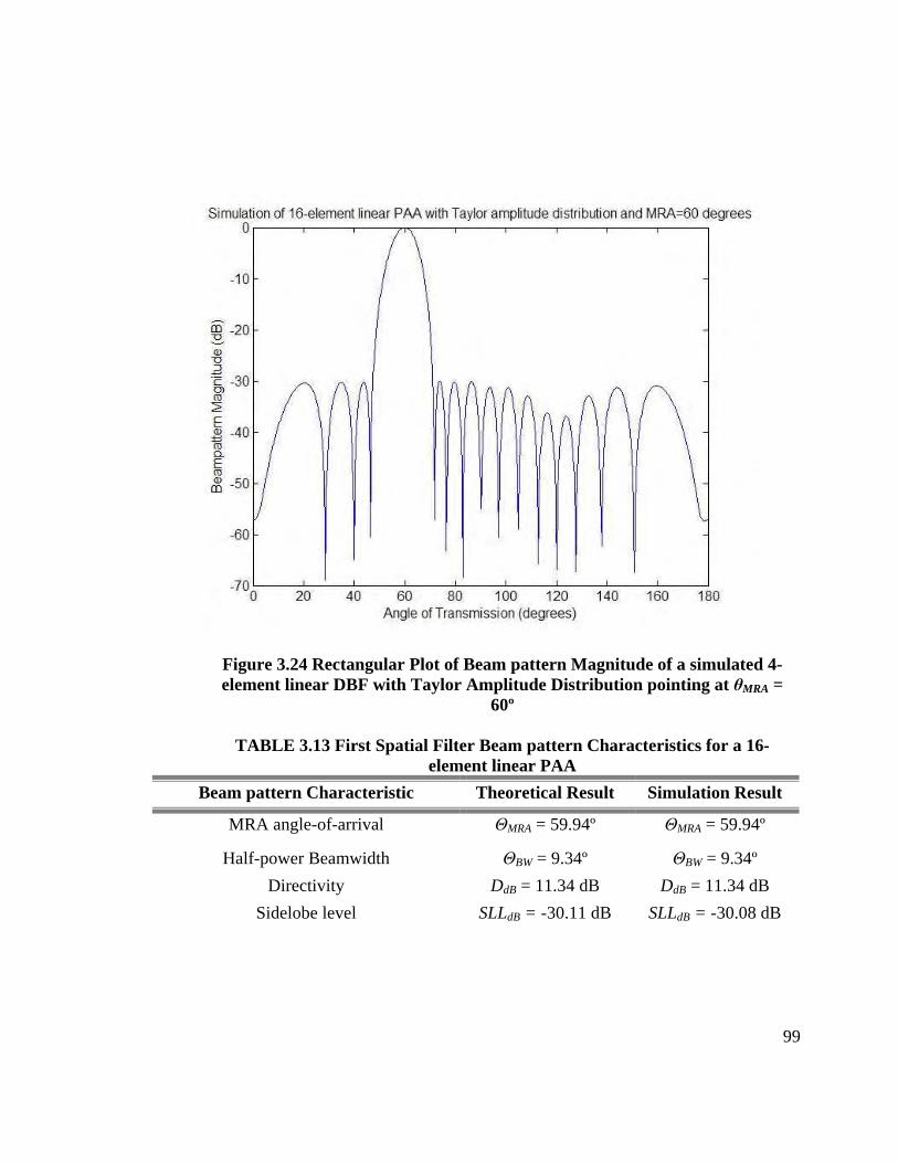
99
Figure 3.24 Rectangular Plot of Beam pattern Magnitude of a simulated 4-element linear DBF with Taylor Amplitude Distributi on pointing at θMRA =
60º
TABLE 3.13 First Spatial Filter Beam pattern Characteristics for a 16-element linear PAA
Beam pattern Characteristic Theoretical Result Simulation Result
MRA angle-of-arrival ΘMRA = 59.94º ΘMRA = 59.94º
Half-power Beamwidth ΘBW = 9.34º ΘBW = 9.34º
Directivity DdB = 11.34 dB DdB = 11.34 dB
Sidelobe level SLLdB = -30.11 dB SLLdB = -30.08 dB
100
3.2.2 Second Spatial Filter Example: Beam pattern with Blackman-Harris Amplitude Weight Function pointing to θMRA = 82º
The second spatial filter example used in the DBF transmitter for a 16-element
linear PAA produces a beam pattern with an MRA pointing at an angular position of 82º
(respect to right-side endfire) with a Blackman-Harris window amplitude-weighting
function. The Blackman-Harris window is one of the Spectral Windows used to control
the beam pattern behavior of a PAA, as mentioned in Section 2.1.4. It contains all the
characterisitics associated with a Spectral Window where the beam pattern characteristics
such as beamwidth, sidelobe behavior and directivity are fixed by the number of elements
in the PAA. The amplitude weight coefficients for each DBF element can be obtained
using the mathematical equation [Van Trees, 2001] associated with this Spectral Window:
( ) 2 4 1 10.42 0.5cos 0.08cos , .
2 2
n n N Nw n n
N N
π π − − = + + − ≤ ≤
3.7
The beam pattern characteristics of an N-element PAA with a Blackman-harris spectral
window can be calculated using the following mathematical equations:
21.65 ,BW N
Θ = 3.8
56.6 ,dBSLL dB= − 3.9
( )1010 log 0.577 .dBD N= ⋅ ⋅ 3.10
A MATLAB file named “linear_DBFtransmitter_blackmannharris.m” (shown in the
Appendix A) was created to compute the weight coefficients for the second spatial filter
example of the linear 16-element PAA. The code uses the Blackman-Harris amplitude
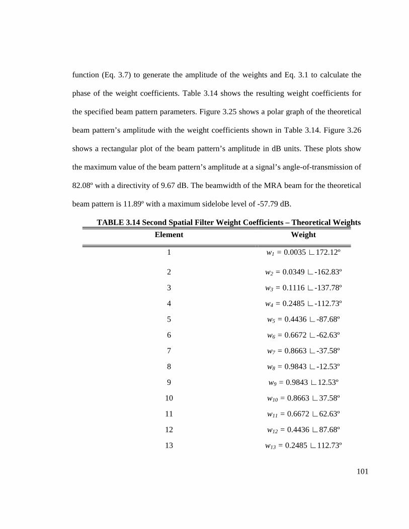
101
function (Eq. 3.7) to generate the amplitude of the weights and Eq. 3.1 to calculate the
phase of the weight coefficients. Table 3.14 shows the resulting weight coefficients for
the specified beam pattern parameters. Figure 3.25 shows a polar graph of the theoretical
beam pattern’s amplitude with the weight coefficients shown in Table 3.14. Figure 3.26
shows a rectangular plot of the beam pattern’s amplitude in dB units. These plots show
the maximum value of the beam pattern’s amplitude at a signal’s angle-of-transmission of
82.08º with a directivity of 9.67 dB. The beamwidth of the MRA beam for the theoretical
beam pattern is 11.89º with a maximum sidelobe level of -57.79 dB.
TABLE 3.14 Second Spatial Filter Weight Coefficients – Theoretical Weights
Element Weight
1 w1 = 0.0035 ∟172.12º
2 w2 = 0.0349 ∟-162.83º
3 w3 = 0.1116 ∟-137.78º
4 w4 = 0.2485 ∟-112.73º
5 w5 = 0.4436 ∟-87.68º
6 w6 = 0.6672 ∟-62.63º
7 w7 = 0.8663 ∟-37.58º
8 w8 = 0.9843 ∟-12.53º
9 w9 = 0.9843 ∟12.53º
10 w10 = 0.8663 ∟37.58º
11 w11 = 0.6672 ∟62.63º
12 w12 = 0.4436 ∟87.68º
13 w13 = 0.2485 ∟112.73º

102
14 w14 = 0.1116 ∟137.78º
15 w15 = 0.0349 ∟162.83º
16 w16 = 0.0035 ∟-172.12º
Figure 3.25 Polar Plot of Beam pattern Magnitude of a 4-element linear DBF with Blackmann-Harris Amplitude Distribution pointi ng at θMRA = 82º
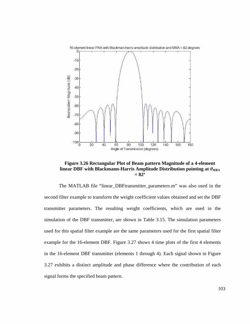
103
Figure 3.26 Rectangular Plot of Beam pattern Magnitude of a 4-element linear DBF with Blackmann-Harris Amplitude Distribu tion pointing at θMRA
= 82º The MATLAB file “linear_DBFtransmitter_parameters.m” was also used in the
second filter example to transform the weight coefficient values obtained and set the DBF
transmitter parameters. The resulting weight coefficients, which are used in the
simulation of the DBF transmitter, are shown in Table 3.15. The simulation parameters
used for this spatial filter example are the same parameters used for the first spatial filter
example for the 16-element DBF. Figure 3.27 shows 4 time plots of the first 4 elements
in the 16-element DBF transmitter (elements 1 through 4). Each signal shown in Figure
3.27 exhibits a distinct amplitude and phase difference where the contribution of each
signal forms the specified beam pattern.
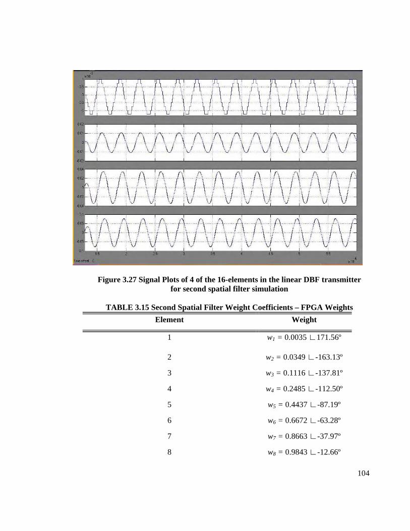
104
Figure 3.27 Signal Plots of 4 of the 16-elements in the linear DBF transmitter for second spatial filter simulation
TABLE 3.15 Second Spatial Filter Weight Coefficients – FPGA Weights
Element Weight
1 w1 = 0.0035 ∟171.56º
2 w2 = 0.0349 ∟-163.13º
3 w3 = 0.1116 ∟-137.81º
4 w4 = 0.2485 ∟-112.50º
5 w5 = 0.4437 ∟-87.19º
6 w6 = 0.6672 ∟-63.28º
7 w7 = 0.8663 ∟-37.97º
8 w8 = 0.9843 ∟-12.66º
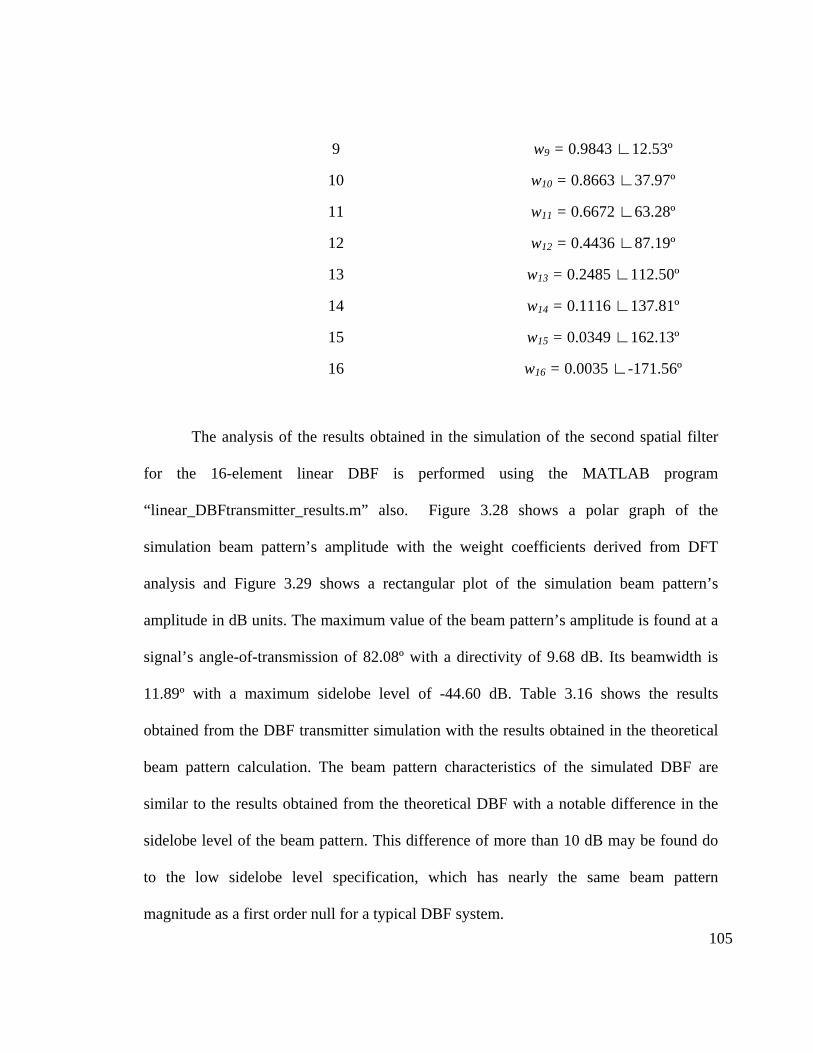
105
9 w9 = 0.9843 ∟12.53º
10 w10 = 0.8663 ∟37.97º
11 w11 = 0.6672 ∟63.28º
12 w12 = 0.4436 ∟87.19º
13 w13 = 0.2485 ∟112.50º
14 w14 = 0.1116 ∟137.81º
15 w15 = 0.0349 ∟162.13º
16 w16 = 0.0035 ∟-171.56º
The analysis of the results obtained in the simulation of the second spatial filter
for the 16-element linear DBF is performed using the MATLAB program
“linear_DBFtransmitter_results.m” also. Figure 3.28 shows a polar graph of the
simulation beam pattern’s amplitude with the weight coefficients derived from DFT
analysis and Figure 3.29 shows a rectangular plot of the simulation beam pattern’s
amplitude in dB units. The maximum value of the beam pattern’s amplitude is found at a
signal’s angle-of-transmission of 82.08º with a directivity of 9.68 dB. Its beamwidth is
11.89º with a maximum sidelobe level of -44.60 dB. Table 3.16 shows the results
obtained from the DBF transmitter simulation with the results obtained in the theoretical
beam pattern calculation. The beam pattern characteristics of the simulated DBF are
similar to the results obtained from the theoretical DBF with a notable difference in the
sidelobe level of the beam pattern. This difference of more than 10 dB may be found do
to the low sidelobe level specification, which has nearly the same beam pattern
magnitude as a first order null for a typical DBF system.

106
Figure 3.28 Polar Plot of Beam pattern Magnitude of simulated 4-element linear DBF with Blackmann-Harris Amplitude Distribu tion pointing at θMRA
= 82º
TABLE 3.16 Second Spatial Filter Beam pattern Characteristics for a 16-element linear PAA
Beam pattern Characteristic Theoretical Result Simulation Result
MRA angle-of-arrival ΘMRA = 82.08º ΘMRA = 82.08º
Half-power Beamwidth ΘBW = 11.89º ΘBW = 11.89º
Directivity DdB = 9.67 dB DdB = 9.68 dB
Sidelobe level SLLdB = -57.79 dB SLLdB = -44.60 dB

107
Figure 3.29 Rectangular Plot of Beam pattern Magnitude of simulated 4-
element linear DBF with Blackmann-Harris Amplitude Distribution pointing at θMRA = 82º
3.2.3 Beam pattern Granularity for 16-element linear PAA
The beam pattern granularity, which was introduced as an important parameter in
Section 3.1.3, is also affected by the number of elements in the PAA. Figure 3.30 shows a
plot of the beam pattern granularity as a function of the MRA’s angle-of-arrival when the
weight coefficient’s phase parameter has a bit resolution of 8 bits with no decimal
precision for the 16-element linear PAA. Eq. 3.4 was also used to calculate the beam
pattern granularity of this linear array. As in the case of the 4-element linear PAA, the

108
granularity value is larger on beam patterns with MRAs pointing towards endfire of the
array (leftside and rightside) with a value of approximately 5 degrees from beam patterns
with MRAs pointing near broadside where the beam pattern granularity has a value close
to one degree, which is the desired MRA angle difference. Figure 3.31 and Figure 3.33
shows beam pattern granularity for weight coefficient’s phase parameters with bit
resolutions of 4 bits with no decimal precision and 16 bits with no decimal precision for
the 16-element linear PAA, respectively. If these beam pattern granularity plots are
compared with the ones shown in Section 3.1.3, it can be seen that for the same bit
resolution a linear array with more elements exhibits a better beam pattern granularity in
terms of an obtained degree difference closer to the real degree difference found between
the two MRAs.
Figure 3.30 Beam pattern Granularity Plot for a 16-element linear DBF with 8 bits of resolution on the weight coefficient’s phase

109
Figure 3.31 Beam pattern Granularity Plot for a 16-element linear DBF with 4 bits of resolution on the weight coefficient’s phase
Figure 3.32 Beam pattern Granularity Plot for a 16-element linear DBF with 16 bits of resolution on the weight coefficient’s phase
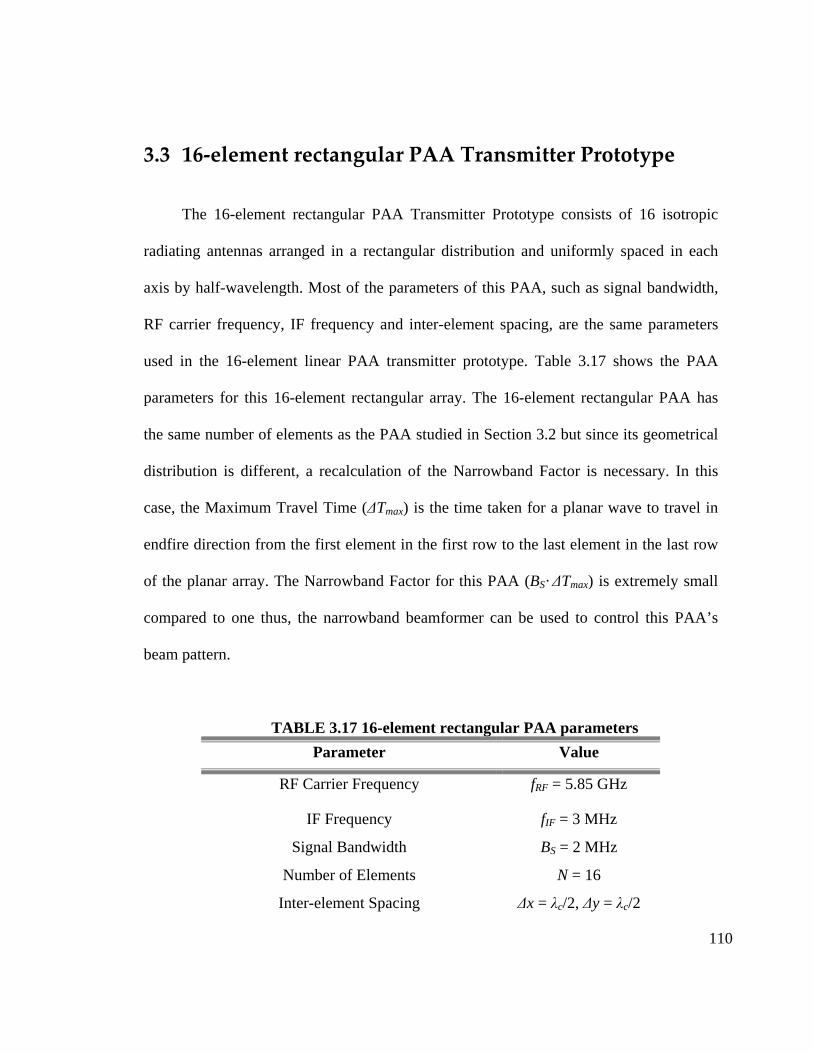
110
3.3 16-element rectangular PAA Transmitter Prototype
The 16-element rectangular PAA Transmitter Prototype consists of 16 isotropic
radiating antennas arranged in a rectangular distribution and uniformly spaced in each
axis by half-wavelength. Most of the parameters of this PAA, such as signal bandwidth,
RF carrier frequency, IF frequency and inter-element spacing, are the same parameters
used in the 16-element linear PAA transmitter prototype. Table 3.17 shows the PAA
parameters for this 16-element rectangular array. The 16-element rectangular PAA has
the same number of elements as the PAA studied in Section 3.2 but since its geometrical
distribution is different, a recalculation of the Narrowband Factor is necessary. In this
case, the Maximum Travel Time (∆Tmax) is the time taken for a planar wave to travel in
endfire direction from the first element in the first row to the last element in the last row
of the planar array. The Narrowband Factor for this PAA (BS· ∆Tmax) is extremely small
compared to one thus, the narrowband beamformer can be used to control this PAA’s
beam pattern.
TABLE 3.17 16-element rectangular PAA parameters
Parameter Value
RF Carrier Frequency fRF = 5.85 GHz
IF Frequency fIF = 3 MHz
Signal Bandwidth BS = 2 MHz
Number of Elements N = 16
Inter-element Spacing ∆x = λc/2, ∆y = λc/2
111
Maximum Travel Time ∆Tmax = 2 *3/2fRF
Narrowband Factor BS· ∆Tmax = 0.000725
The implementation of this DBF transmitter is based on the design described in Section
2.4.2. The DBF architecture provides design flexibility where a DBF with a particular
number of channels can be used with any PAA with the same amount of antennas, not
taking into account the geometrical distribution of the array. Since the 16-element
rectangular PAA has the same amount of channels as its linear counterpart studied in
Section 3.2, the architecture, design parameters, and simulation process of the DBF are
the same as the one explained in Section 3.2. The architecture design of the DBF
transmitter for this PAA can be reviewed in Figures 3.18 and 3.19 and its DBF design
parameters are shown in Table 3.10.
3.3.1 First Spatial Filter Example: Beam pattern with Uniform Amplitude Weight Function pointing to φMRA = 0º and θMRA = 30º
The first spatial filter example used in the DBF transmitter for a 16-element
rectangular PAA produces a beam pattern with an MRA pointing at angular positions of
φ = 0º (angle formed in the planar axis) and θ = 30º (angle formed in the axis
perpendicular to the planar array) with a uniform distribution amplitude-weighting
function. In Section 3.1, Eq. 1 showed the calculation of the weight coefficients for a
general PAA with one MRA beam specification. For a rectangular array, the position

112
vector’s pz value is equal to zero reducing the calculation of the weight coefficient for
each channel n into:
( ) ( ) ( ) ( )2 sin cos sin1* .MRA x MRA y MRAj p p
nw eN
π θ φ φλ + = 3.11
The phase value found in each weight coefficient can be viewed as the sum of the phase
differences between neighboring elements in the same x axis value and phase difference
between neighboring elements in the same y axis of the rectangular array. This
relationship can be seen by restructuring Eq. 3.11 into the following mathematical form:
( )1* ,x yj
nw eN
ψ ψ∆ +∆= 3.12
where:
( ) ( ) ( )2 sin cos ,x x MRA MRApπψ θ φλ∆ = 3.13
( ) ( ) ( )2 sin sin .y y MRA MRApπψ θ φλ∆ = 3.14
Table 3.18 shows the resulting weight coefficients for a uniform 16-element rectangular
PAA with an inter-element spacing of λ/2 in x and y axis, which are the axis parallel to
the planar array. A MATLAB program named “rectangular_DBFtransmitter_steering.m”
(which is shown in Appendix A) was prepared in order to calculate the theoretical beam
pattern, the directivity and the beamwidth of the PAA for a one-MRA spatial filter design
for a rectangular PAA. Figure 3.33 shows a top view polar graph of the theoretical beam
pattern’s amplitude with the weight coefficients shown in Table 3.18. The top view polar
graph was generated using MATLAB function polar3D() provided by Dr. Sébastien

113
Rondineau, Research Professor at the University of Colorado at Boulder. Figure 3.34
shows rectangular plots of the beam pattern’s amplitude in dB units for beam pattern cuts
of φ = 0º and φ = 45º. These plots show the maximum value of the beam pattern’s
amplitude at a signal’s angle-of-transmission of φ = 0º and θ = 30º with a directivity of
12.80 dB. The beamwidth of the MRA beam (shown in Figure 3.34a) for the theoretical
beam pattern is 30.68º with a sidelobe of -7.40 dB (shown in Figure 3.34b). Figure 3.35
shows a 3D surf plot of the beam pattern’s amplitude for this spatial filter design.
TABLE 3.18 First Spatial Filter Weight Coefficients for 16-element rectangular PAA – Theoretical Weights
Element Weight
1, 1 w1,1 = 0.0625 ∟-135º
1, 2 w1,2 = 0.0625 ∟-135º
1, 3 w1,3 = 0.0625 ∟-135º
1, 4 w1,4 = 0.0625 ∟-135º
2, 1 w2,1 = 0.0625 ∟-45º
2, 2 w2,2 = 0.0625 ∟-45º
2, 3 w2,3 = 0.0625 ∟-45º
2, 4 w2,4 = 0.0625 ∟-45º
3, 1 w3,1 = 0.0625 ∟45º
3, 2 w3,2 = 0.0625 ∟45º
3, 3 w3,3 = 0.0625 ∟45º
3, 4 w3,4 = 0.0625 ∟45º
4, 1 w4,1 = 0.0625 ∟135º
4, 2 w4,2 = 0.0625 ∟135º
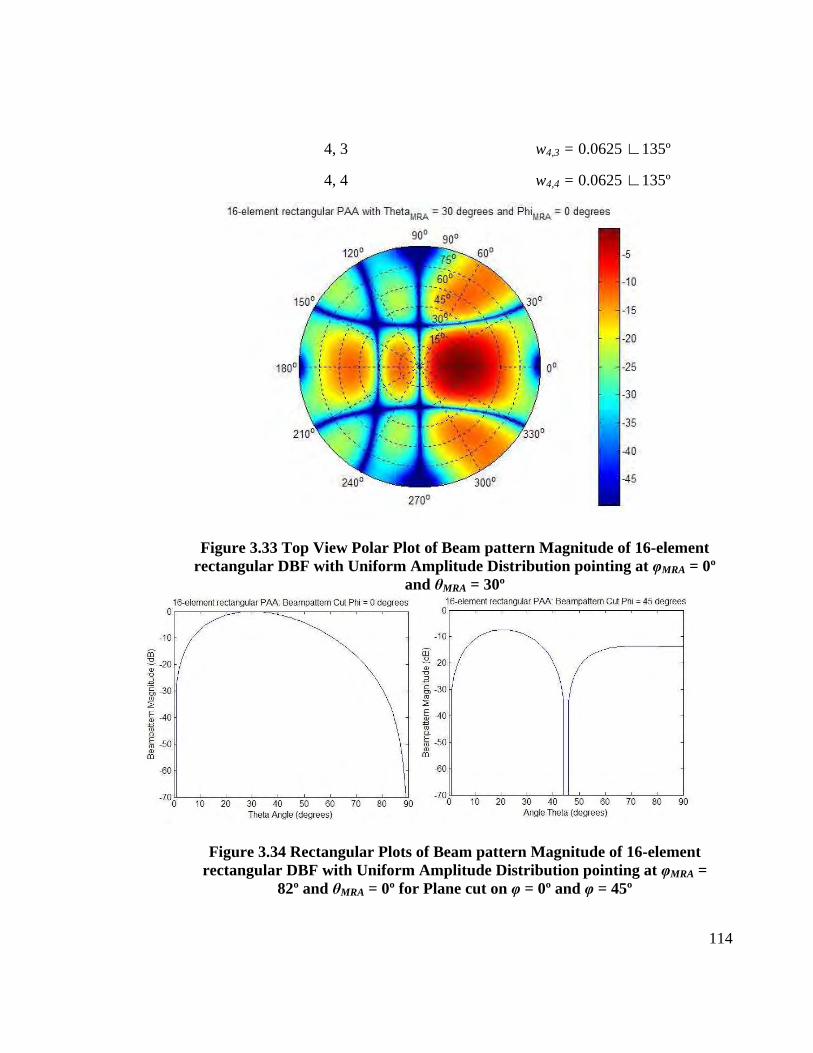
114
4, 3 w4,3 = 0.0625 ∟135º
4, 4 w4,4 = 0.0625 ∟135º
Figure 3.33 Top View Polar Plot of Beam pattern Magnitude of 16-element rectangular DBF with Uniform Amplitude Distribution pointing at φMRA = 0º
and θMRA = 30º
Figure 3.34 Rectangular Plots of Beam pattern Magnitude of 16-element rectangular DBF with Uniform Amplitude Distribution pointing at φMRA =
82º and θMRA = 0º for Plane cut on φ = 0º and φ = 45º

115
Figure 3.35 Surf Plot of Beam pattern Magnitude of 16-element rectangular DBF with Uniform Amplitude Distribution pointing at φMRA = 0º and θMRA =
30º
Before a simulation of the rectangular PAA is performed, transformation of the
weight coefficients into constant encoded in the FPGA code simulator is required. A
MATLAB program named “rectangular_DBFtransmitter_parameters.m” (included in the
Appendix A) was prepared to change the weight coefficients into its fixed-point format
values and set all the necessary DBF transmitter parameters. This MATLAB file is
similar to the file created to set DBF parameters and condition weight coefficients values
for a 16-element linear PAA. The difference strives in the way the file reads the weight
coefficient; weights in a linear array are stored in vector form whereas weights in a
rectangular array are stored in matrix form. The total simulation time used for this DBF
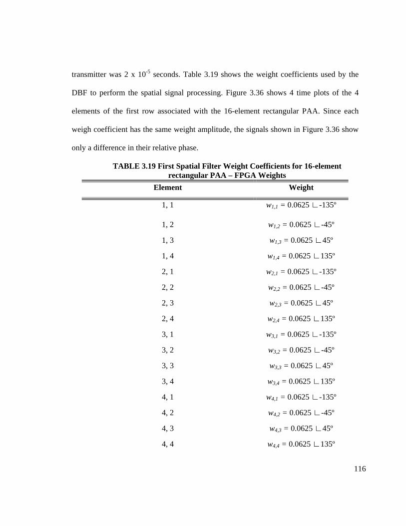
116
transmitter was 2 x 10⁻⁵ seconds. Table 3.19 shows the weight coefficients used by the
DBF to perform the spatial signal processing. Figure 3.36 shows 4 time plots of the 4
elements of the first row associated with the 16-element rectangular PAA. Since each
weigh coefficient has the same weight amplitude, the signals shown in Figure 3.36 show
only a difference in their relative phase.
TABLE 3.19 First Spatial Filter Weight Coefficients for 16-element rectangular PAA – FPGA Weights
Element Weight
1, 1 w1,1 = 0.0625 ∟-135º
1, 2 w1,2 = 0.0625 ∟-45º
1, 3 w1,3 = 0.0625 ∟45º
1, 4 w1,4 = 0.0625 ∟135º
2, 1 w2,1 = 0.0625 ∟-135º
2, 2 w2,2 = 0.0625 ∟-45º
2, 3 w2,3 = 0.0625 ∟45º
2, 4 w2,4 = 0.0625 ∟135º
3, 1 w3,1 = 0.0625 ∟-135º
3, 2 w3,2 = 0.0625 ∟-45º
3, 3 w3,3 = 0.0625 ∟45º
3, 4 w3,4 = 0.0625 ∟135º
4, 1 w4,1 = 0.0625 ∟-135º
4, 2 w4,2 = 0.0625 ∟-45º
4, 3 w4,3 = 0.0625 ∟45º
4, 4 w4,4 = 0.0625 ∟135º
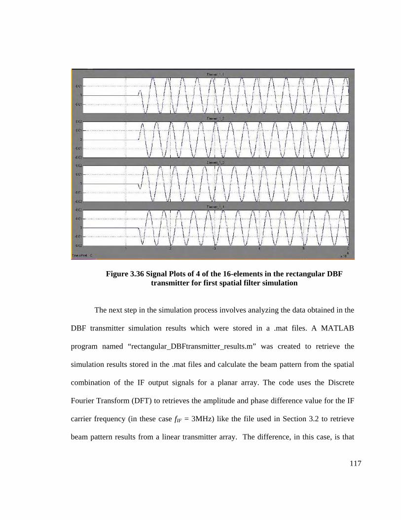
117
Figure 3.36 Signal Plots of 4 of the 16-elements in the rectangular DBF transmitter for first spatial filter simulation
The next step in the simulation process involves analyzing the data obtained in the
DBF transmitter simulation results which were stored in a .mat files. A MATLAB
program named “rectangular_DBFtransmitter_results.m” was created to retrieve the
simulation results stored in the .mat files and calculate the beam pattern from the spatial
combination of the IF output signals for a planar array. The code uses the Discrete
Fourier Transform (DFT) to retrieves the amplitude and phase difference value for the IF
carrier frequency (in these case fIF = 3MHz) like the file used in Section 3.2 to retrieve
beam pattern results from a linear transmitter array. The difference, in this case, is that

118
the weight coefficient’s phase value for each element is calculated using Eq. 3.12, where
the relative phase difference considers phase difference between neighboring elements in
x and phase difference between neighboring elements in the y axis. Figure 3.37 shows a
top view polar graph of the simulation beam pattern’s amplitude with the weight
coefficients derived from DFT analysis. Figure 3.38 shows rectangular plots of the
simulation beam pattern’s amplitude in dB units for beam pattern cuts of φ = 0º and φ =
45º. These plots show the maximum value of the beam pattern’s amplitude at a signal’s
angle-of-transmission of φ = 0º and θ = 30º with a directivity of 12.80 dB. The
beamwidth of the MRA beam (shown in Figure 3.38a) for the theoretical beam pattern is
30.81º with a sidelobe of -7.37 dB (shown in Figure 3.38b). Figure 3.39 shows a 3D surf
plot of the beam pattern’s amplitude for this spatial filter design. Table 3.20 shows the
results obtained from the DBF transmitter simulation with the results obtained in the
theoretical beam pattern calculation.
TABLE 3.20 First Spatial Filter Beam pattern Characteristics for a 16-element rectangular PAA
Beam pattern Characteristic Theoretical Result Simulation Result
MRA angle-of-arrival φMRA = 0º, ΘMRA = 30º
φMRA = 0º, ΘMRA = 30º
Half-power Beamwidth ΘBW = 30.68º @ φMRA = 0º
ΘBW = 30.80º @ φMRA = 0º
Directivity DdB = 12.80 dB DdB = 12.80 dB
Sidelobe level SLLdB = -7.40 dB @ φMRA = 45º
SLLdB = -7.37 dB @ φMRA = 45º

119
Figure 3.37 Top View Polar Plot of Beam pattern Magnitude of simulated 16-element rectangular DBF with Uniform Amplitude Distribution pointing at
φMRA = 0º and θMRA = 30º
Figure 3.38 Rectangular Plots of Beam pattern Magnitude of simulated 16-element rectangular DBF with Uniform Amplitude Distribution pointing at
φMRA = 0º and θMRA = 30º for Plane cut on φ = 0º and φ = 45º

120
Figure 3.39 Surf Plot of Beam pattern Magnitude of simulated 16-element rectangular DBF with Uniform Amplitude Distribution pointing at φMRA = 0º
and θMRA = 30º 3.3.2 Second Spatial Filter Example: Beam pattern with Dolph-Chebyshev
Amplitude Weight Function pointing to φMRA = 122º and θMRA = 16º
The second spatial filter example used in the DBF transmitter for a 16-element
rectangular PAA produces a beam pattern with an MRA pointing at angular positions of
φ = 122º (angle formed in the planar axis) and θ = 16º (angle formed in the axis
perpendicular to the planar array) with a Dolph-Chebyshev distribution amplitude-
weighting function. As mentioned in Section 2.1.4, the Dolph-Chebyshev distribution
method generates the amplitude of weight coefficients to minimize the MRA’s
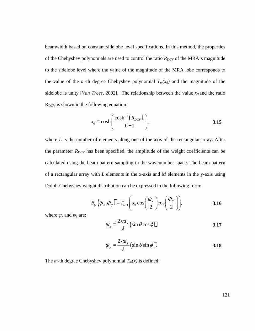
121
beamwidth based on constant sidelobe level specifications. In this method, the properties
of the Chebyshev polynomials are used to control the ratio RDCV of the MRA’s magnitude
to the sidelobe level where the value of the magnitude of the MRA lobe corresponds to
the value of the m-th degree Chebyshev polynomial Tm(x0) and the magnitude of the
sidelobe is unity [Van Trees, 2002]. The relationship between the value x0 and the ratio
RDCV is shown in the following equation:
( )1
0
coshcosh ,
1DCVR
xL
− = −
3.15
where L is the number of elements along one of the axis of the rectangular array. After
the parameter RDCV has been specified, the amplitude of the weight coefficients can be
calculated using the beam pattern sampling in the wavenumber space. The beam pattern
of a rectangular array with L elements in the x-axis and M elements in the y-axis using
Dolph-Chebyshev weight distribution can be expressed in the following form:
( ) 1 0, cos cos ,2 2
yxx y LB T xψ
ψψψ ψ −
= 3.16
where ψx and ψy are:
( )2sin cos ,x
x
dπψ θ ϕλ
= 3.17
( )2sin sin .y
y
dπψ θ ϕ
λ= 3.18
The m-th degree Chebyshev polynomial Tm(x) is defined:
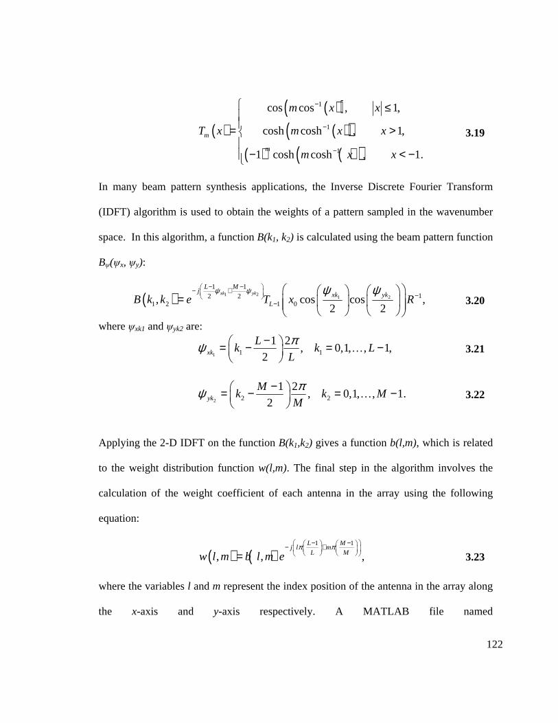
122
( )( )( )
( )( )( ) ( )( )
1
1
1
cos cos , 1,
cosh cosh , 1,
1 cosh cosh , 1.
m
m
m x x
T x m x x
m x x
−
−
−
≤= >
− < −
3.19
In many beam pattern synthesis applications, the Inverse Discrete Fourier Transform
(IDFT) algorithm is used to obtain the weights of a pattern sampled in the wavenumber
space. In this algorithm, a function B(k1, k2) is calculated using the beam pattern function
Bψ(ψx, ψy):
( ) 1 2 1 2
1 112 2
1 2 1 0, cos cos ,2 2
xk ykL M
jxk yk
LB k k e T x Rψ ψ ψ ψ− − − + −
−
=
3.20
where ψxk1 and ψyk2 are:
1 1 1
1 2, 0,1, , 1,
2xk
Lk k L
L
πψ − = − = −
… 3.21
2 2 2
1 2, 0,1, , 1.
2yk
Mk k M
M
πψ − = − = −
… 3.22
Applying the 2-D IDFT on the function B(k1,k2) gives a function b(l,m), which is related
to the weight distribution function w(l,m). The final step in the algorithm involves the
calculation of the weight coefficient of each antenna in the array using the following
equation:
( ) ( )1 1
, , ,L M
j l mL Mw l m b l m e
π π − − − + = 3.23
where the variables l and m represent the index position of the antenna in the array along
the x-axis and y-axis respectively. A MATLAB file named

123
“rectangular_DBFtransmitter_dolphchebyshev.m” (shown in the Appendix A) was
created to compute the weight coefficients for the second spatial filter example of the
rectangular 16-element PAA. The code uses the Dolph-Chebyshev polynomials to
calculate the amplitude of the weight coefficients and Eq. 3.11 to calculate the phase of
the weight coefficients. Table 3.21 shows the resulting weight coefficients for the
specified beam pattern parameters. Figure 3.40 shows a top view polar graph of the
theoretical beam pattern’s amplitude with the weight coefficients shown in Table 3.21.
Figure 3.41 shows rectangular plots of the beam pattern’s amplitude in dB units for beam
pattern cuts of φ = 122º and φ = 302º. These plots show the maximum value of the beam
pattern’s amplitude at a signal’s angle-of-transmission of φ = 122º and θ = 16º with a
directivity of 12.58 dB. The beamwidth of the MRA beam (shown in Figure 3.41a) for
the theoretical beam pattern is 33.1º with a sidelobe of -25.00 dB (shown in Figure 3.41b).
Figure 3.42 shows a 3D surf plot of the beam pattern’s amplitude for this spatial filter
design.
TABLE 3.21 Second Spatial Filter Weight Coefficients for 16-element rectangular PAA – Theoretical Weights
Element Weight
1, 1 w1,1 = 0.0204 ∟-23.68º
1, 2 w1,2 = 0.0611 ∟-49.97º
1, 3 w1,3 = 0.0611 ∟-76.26º
1, 4 w1,4 = 0.0204 ∟-102.55º
2, 1 w2,1 = 0.0611 ∟18.40º
2, 2 w2,2 = 0.1075 ∟-7.89º

124
2, 3 w2,3 = 0.1075 ∟-34.18º
2, 4 w2,4 = 0.0611 ∟-60.48º
3, 1 w3,1 = 0.0611 ∟60.48º
3, 2 w3,2 = 0.1075 ∟34.18º
3, 3 w3,3 = 0.1075 ∟7.89º
3, 4 w3,4 = 0.0611 ∟-18.49º
4, 1 w4,1 = 0.0204 ∟102.55º
4, 2 w4,2 = 0.0611 ∟76.26º
4, 3 w4,3 = 0.0611 ∟49.97º
4, 4 w4,4 = 0.0204 ∟23.68º
Figure 3.40 Top View Polar Plot of Beam pattern Magnitude of 16-element rectangular DBF with Dolph-Chebyshev Amplitude Distribution pointing at
φMRA = 122º and θMRA = 16º
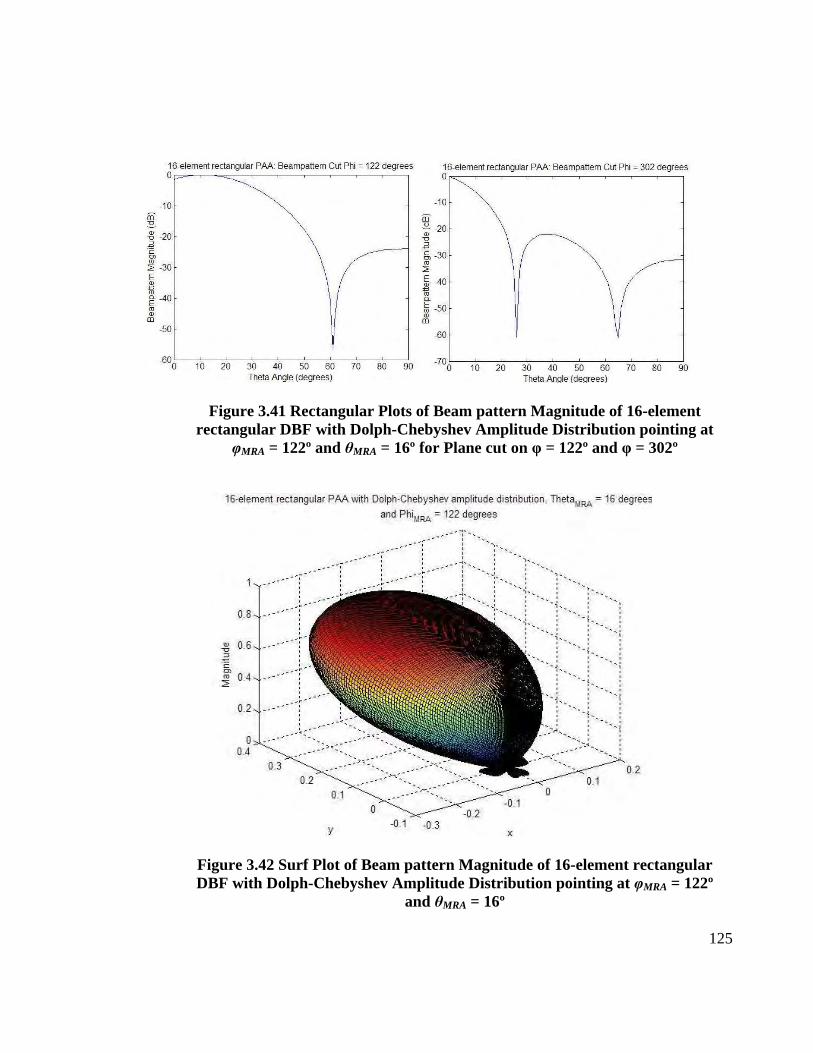
125
Figure 3.41 Rectangular Plots of Beam pattern Magnitude of 16-element rectangular DBF with Dolph-Chebyshev Amplitude Distribution pointing at
φMRA = 122º and θMRA = 16º for Plane cut on φ = 122º and φ = 302º
Figure 3.42 Surf Plot of Beam pattern Magnitude of 16-element rectangular DBF with Dolph-Chebyshev Amplitude Distribution pointing at φMRA = 122º
and θMRA = 16º
126
The MATLAB file “rectangular_DBFtransmitter_parameters.m” was also used to set
DBF parameters and condition weight coefficients values for the second spatial filter
simulation for the 16-element rectangular PAA. Table 3.22 shows the weight coefficients
used by the DBF to perform the second spatial filter on the FPGA simulation. Figure 3.40
shows 4 time plots of the 4 elements of the first row associated with the 16-element
rectangular PAA. The difference in the amplitude of each signal shown in Figure 3.43 is
related to the Dolph-Chebyshev amplitude-distribution function, which assigns the
magnitude of the weights to each antenna element in the array.
TABLE 3.22 Second Spatial Filter Weight Coefficients for 16-element rectangular PAA – FPGA Weights
Element Weight
1, 1 w1,1 = 0.0204 ∟-23.91º
1, 2 w1,2 = 0.0611 ∟-50.63º
1, 3 w1,3 = 0.0611 ∟-75.94º
1, 4 w1,4 = 0.0204 ∟-102.66º
2, 1 w2,1 = 0.0611 ∟18.28º
2, 2 w2,2 = 0.1075 ∟-8.44º
2, 3 w2,3 = 0.1075 ∟-33.75º
2, 4 w2,4 = 0.0611 ∟-60.47º
3, 1 w3,1 = 0.0611 ∟60.47º
3, 2 w3,2 = 0.1075 ∟33.75º
3, 3 w3,3 = 0.1075 ∟8.44º
3, 4 w3,4 = 0.0611 ∟-18.28º
4, 1 w4,1 = 0.0204 ∟102.66º

127
4, 2 w4,2 = 0.0611 ∟75.94º
4, 3 w4,3 = 0.0611 ∟50.63º
4, 4 w4,4 = 0.0204 ∟23.91º
Figure 3.43 Signal Plots of 4 of the 16-elements in the rectangular DBF transmitter for second spatial filter simulation
After storing the results obtained in the simulation of the second spatial filter, the
data is analyzed by means of the DFT, exactly like the first spatial filter example. The
MATLAB program “rectangular_DBFtransmitter_results.m” was used to retrieve the
results obtained in the simulation and analyze the data of each DBF channel. Figure 3.44
shows a top view polar graph of the simulation beam pattern’s amplitude with the weight
coefficients derived from DFT analysis. Figure 3.45 shows rectangular plots of the

128
simulation beam pattern’s amplitude in dB units for beam pattern cuts of φ = 122º and φ
= 302º. These plots show the maximum value of the beam pattern’s amplitude at a
signal’s angle-of-transmission of φ = 122º and θ = 16º with a directivity of 12.60 dB. The
beamwidth of the MRA beam (shown in Figure 3.45a) for the theoretical beam pattern is
33.01º with a sidelobe of -25.00 dB (shown in Figure 3.45b). Figure 3.46 shows a 3D surf
plot of the beam pattern’s amplitude for this spatial filter design. Table 3.23 shows the
results obtained from the DBF transmitter simulation with the results obtained in the
theoretical beam pattern calculation.
Figure 3.44 Top View Polar Plot of Beam pattern Magnitude of simulated 16-element rectangular DBF with Dolph-Chebyshev Amplitude Distribution
pointing at φMRA = 122º and θMRA = 16º
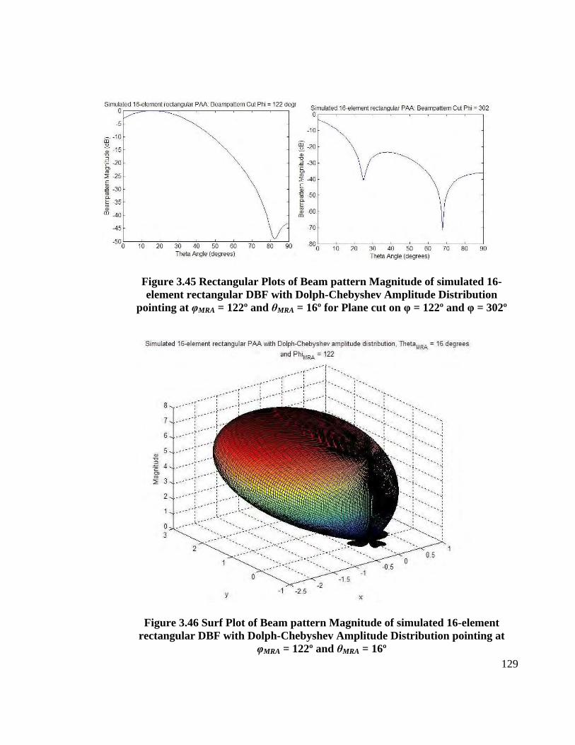
129
Figure 3.45 Rectangular Plots of Beam pattern Magnitude of simulated 16-element rectangular DBF with Dolph-Chebyshev Amplitude Distribution
pointing at φMRA = 122º and θMRA = 16º for Plane cut on φ = 122º and φ = 302º
Figure 3.46 Surf Plot of Beam pattern Magnitude of simulated 16-element rectangular DBF with Dolph-Chebyshev Amplitude Distribution pointing at
φMRA = 122º and θMRA = 16º
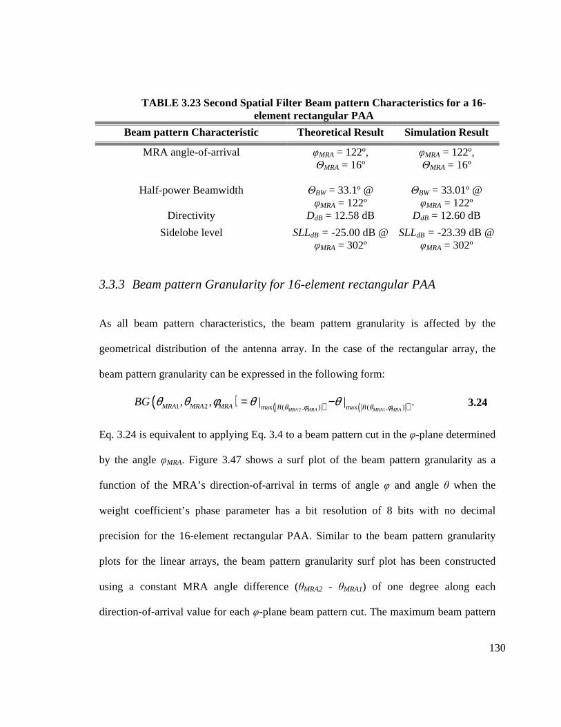
130
TABLE 3.23 Second Spatial Filter Beam pattern Characteristics for a 16-element rectangular PAA
Beam pattern Characteristic Theoretical Result Simulation Result
MRA angle-of-arrival φMRA = 122º, ΘMRA = 16º
φMRA = 122º, ΘMRA = 16º
Half-power Beamwidth ΘBW = 33.1º @ φMRA = 122º
ΘBW = 33.01º @ φMRA = 122º
Directivity DdB = 12.58 dB DdB = 12.60 dB
Sidelobe level SLLdB = -25.00 dB @ φMRA = 302º
SLLdB = -23.39 dB @ φMRA = 302º
3.3.3 Beam pattern Granularity for 16-element rectangular PAA
As all beam pattern characteristics, the beam pattern granularity is affected by the
geometrical distribution of the antenna array. In the case of the rectangular array, the
beam pattern granularity can be expressed in the following form:
( ) ( ) ( )2 11 2 max ( , ) max ( , ), , | | .
MRA MRA MRA MRAMRA MRA MRA B B
BG θ φ θ φθ θ φ θ θ= − 3.24
Eq. 3.24 is equivalent to applying Eq. 3.4 to a beam pattern cut in the φ-plane determined
by the angle φMRA. Figure 3.47 shows a surf plot of the beam pattern granularity as a
function of the MRA’s direction-of-arrival in terms of angle φ and angle θ when the
weight coefficient’s phase parameter has a bit resolution of 8 bits with no decimal
precision for the 16-element rectangular PAA. Similar to the beam pattern granularity
plots for the linear arrays, the beam pattern granularity surf plot has been constructed
using a constant MRA angle difference (θMRA2 - θMRA1) of one degree along each
direction-of-arrival value for each φ-plane beam pattern cut. The maximum beam pattern
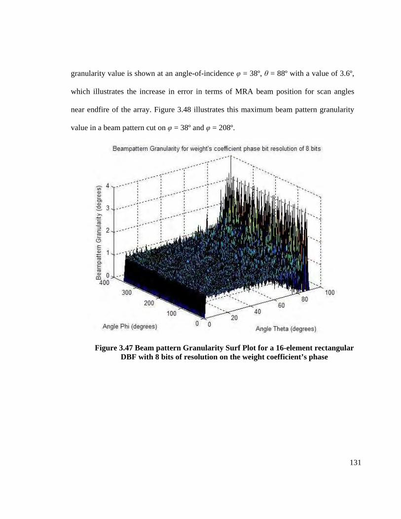
131
granularity value is shown at an angle-of-incidence φ = 38º, θ = 88º with a value of 3.6º,
which illustrates the increase in error in terms of MRA beam position for scan angles
near endfire of the array. Figure 3.48 illustrates this maximum beam pattern granularity
value in a beam pattern cut on φ = 38º and φ = 208º.
Figure 3.47 Beam pattern Granularity Surf Plot for a 16-element rectangular DBF with 8 bits of resolution on the weight coefficient’s phase
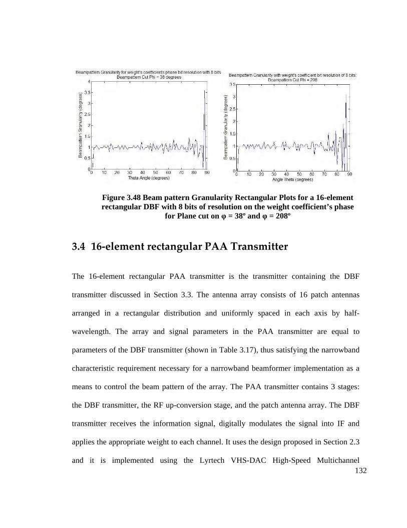
132
Figure 3.48 Beam pattern Granularity Rectangular Plots for a 16-element rectangular DBF with 8 bits of resolution on the weight coefficient’s phase
for Plane cut on φ = 38º and φ = 208º
3.4 16-element rectangular PAA Transmitter
The 16-element rectangular PAA transmitter is the transmitter containing the DBF
transmitter discussed in Section 3.3. The antenna array consists of 16 patch antennas
arranged in a rectangular distribution and uniformly spaced in each axis by half-
wavelength. The array and signal parameters in the PAA transmitter are equal to
parameters of the DBF transmitter (shown in Table 3.17), thus satisfying the narrowband
characteristic requirement necessary for a narrowband beamformer implementation as a
means to control the beam pattern of the array. The PAA transmitter contains 3 stages:
the DBF transmitter, the RF up-conversion stage, and the patch antenna array. The DBF
transmitter receives the information signal, digitally modulates the signal into IF and
applies the appropriate weight to each channel. It uses the design proposed in Section 2.3
and it is implemented using the Lyrtech VHS-DAC High-Speed Multichannel

133
Development Platform. The RF up-conversion stage distributes the Local Oscillator
signal into each antenna channel, mixes the IF information signal with the LO signal, and
amplifies the resulting signal prior transmission of the signal by means of power
amplification. The final stage of the microwave transmitter consists in the transmission of
the signal using a 16-element rectangular patch antenna array. The S-Parameter
simulations of all the RF circuits in the RF up-conversion stage and the Electromagnetic
simulations of the rectangular patch antenna array were performed using Ansoft Designer
V2. Table 3.24 shows the ideal system requirements for each stage of the PAA
transmitter.
TABLE 3.24 Ideal System Requirements for PAA transmitter
Requirement Value
Wilkinson Power Dividers (WPD)
VSWR at input port of each circuit Less than 2
Gain of each output port 5 dB
Relative amplitude difference between output port
0 dB
Relative phase difference between output port
0º
Mixer/Amplifier Stage
Relative amplitude difference between output port
0 dB
Relative phase difference between output port
0º
Rectangular Patch Array
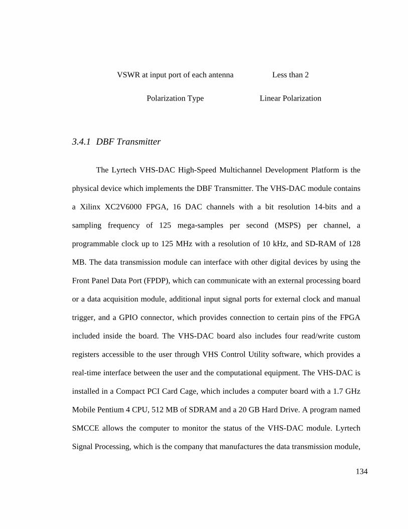
134
VSWR at input port of each antenna Less than 2
Polarization Type Linear Polarization
3.4.1 DBF Transmitter
The Lyrtech VHS-DAC High-Speed Multichannel Development Platform is the
physical device which implements the DBF Transmitter. The VHS-DAC module contains
a Xilinx XC2V6000 FPGA, 16 DAC channels with a bit resolution 14-bits and a
sampling frequency of 125 mega-samples per second (MSPS) per channel, a
programmable clock up to 125 MHz with a resolution of 10 kHz, and SD-RAM of 128
MB. The data transmission module can interface with other digital devices by using the
Front Panel Data Port (FPDP), which can communicate with an external processing board
or a data acquisition module, additional input signal ports for external clock and manual
trigger, and a GPIO connector, which provides connection to certain pins of the FPGA
included inside the board. The VHS-DAC board also includes four read/write custom
registers accessible to the user through VHS Control Utility software, which provides a
real-time interface between the user and the computational equipment. The VHS-DAC is
installed in a Compact PCI Card Cage, which includes a computer board with a 1.7 GHz
Mobile Pentium 4 CPU, 512 MB of SDRAM and a 20 GB Hard Drive. A program named
SMCCE allows the computer to monitor the status of the VHS-DAC module. Lyrtech
Signal Processing, which is the company that manufactures the data transmission module,
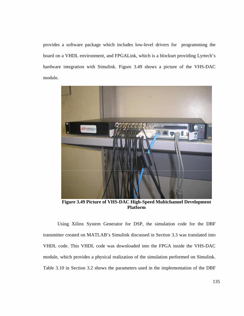
135
provides a software package which includes low-level drivers for programming the
board on a VHDL environment, and FPGALink, which is a blockset providing Lyrtech’s
hardware integration with Simulink. Figure 3.49 shows a picture of the VHS-DAC
module.
Figure 3.49 Picture of VHS-DAC High-Speed Multichannel Development
Platform
Using Xilinx System Generator for DSP, the simulation code for the DBF
transmitter created on MATLAB’s Simulink discussed in Section 3.3 was translated into
VHDL code. This VHDL code was downloaded into the FPGA inside the VHS-DAC
module, which provides a physical realization of the simulation performed on Simulink.
Table 3.10 in Section 3.2 shows the parameters used in the implementation of the DBF

136
transmitter for the PAA. An additional hardware module was designed to interface the
control unit with the DBF transmitter. This hardware module, which was programmed in
the FPGA through Simulink software, controls the assignation of amplitude and phase
weight coefficients for each of the DBF channels. Figure 3.50 shows the Simulink
diagram of the Control Interface Module (CIM). Figure 3.51 shows a diagram of the
input and one of the channels of the CIM. Initially, the CIM was constructed to interface
with the memory of the VHS-DAC, which is a typical communication topology in digital
control systems. This initial design provided the flexibility of separating the DBF
transmitter with the algorithm generating the weight coefficients, where the system
memory would be used the link to interchange data between the two system components.
Unfortunatly, a problem with the memory and its block module in the Simulink
environment prevented it from functioning properly under real-time operation. Inactivity

137
Figure 3.50 Simulink Diagram of CIM
of the memory’s “request signal” and “ready signal” in the block module was the main
problem found in the system memory’s performance. During the debugging process,
Lyrtech Signal Processing was notified of the errors in the performance in the memory,
only to find out that its lack of performance under certain conditions is a known issue,
which is currently being attended.
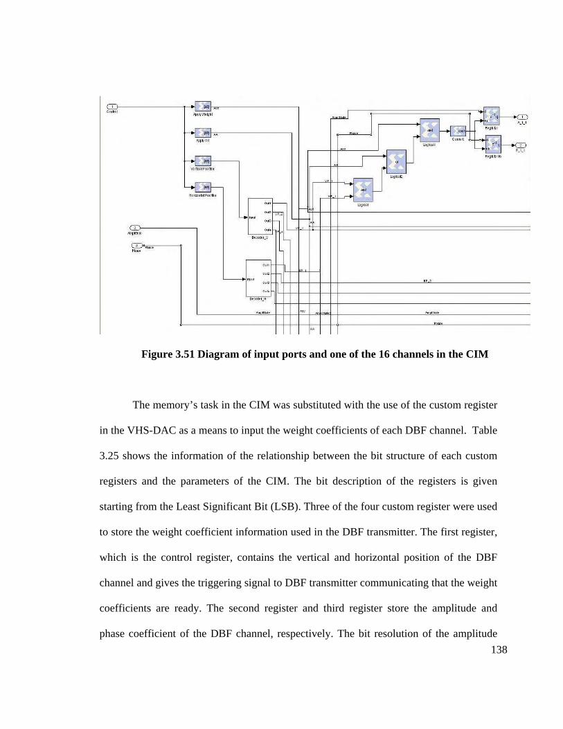
138
Figure 3.51 Diagram of input ports and one of the 16 channels in the CIM
The memory’s task in the CIM was substituted with the use of the custom register
in the VHS-DAC as a means to input the weight coefficients of each DBF channel. Table
3.25 shows the information of the relationship between the bit structure of each custom
registers and the parameters of the CIM. The bit description of the registers is given
starting from the Least Significant Bit (LSB). Three of the four custom register were used
to store the weight coefficient information used in the DBF transmitter. The first register,
which is the control register, contains the vertical and horizontal position of the DBF
channel and gives the triggering signal to DBF transmitter communicating that the weight
coefficients are ready. The second register and third register store the amplitude and
phase coefficient of the DBF channel, respectively. The bit resolution of the amplitude
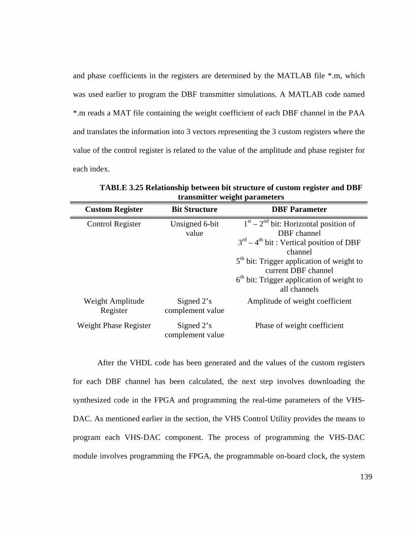
139
and phase coefficients in the registers are determined by the MATLAB file *.m, which
was used earlier to program the DBF transmitter simulations. A MATLAB code named
*.m reads a MAT file containing the weight coefficient of each DBF channel in the PAA
and translates the information into 3 vectors representing the 3 custom registers where the
value of the control register is related to the value of the amplitude and phase register for
each index.
TABLE 3.25 Relationship between bit structure of custom register and DBF transmitter weight parameters
Custom Register Bit Structure DBF Parameter
Control Register Unsigned 6-bit value
1st – 2nd bit: Horizontal position of DBF channel
3rd – 4th bit : Vertical position of DBF channel
5th bit: Trigger application of weight to current DBF channel
6th bit: Trigger application of weight to all channels
Weight Amplitude Register
Signed 2’s complement value
Amplitude of weight coefficient
Weight Phase Register Signed 2’s complement value
Phase of weight coefficient
After the VHDL code has been generated and the values of the custom registers
for each DBF channel has been calculated, the next step involves downloading the
synthesized code in the FPGA and programming the real-time parameters of the VHS-
DAC. As mentioned earlier in the section, the VHS Control Utility provides the means to
program each VHS-DAC component. The process of programming the VHS-DAC
module involves programming the FPGA, the programmable on-board clock, the system

140
memory, the channel gains, and the custom register’s content. The user is encouraged to
read the user manual of the VHS-DAC [Lyrtech, 2004] to find details on the procedure of
programming each device. The file generated by Xilinx System’s Generator and the
vectors generated in the MATLAB code *.m are used to program the FPGA and assign
the values of the custom registers, respectively.
3.4.2 RF Up-Conversion Stage
The RF up-conversion stage of the microwave system contains three important
sub-stages: the power divider network of the LO, the mixer stage, and power
amplification of the RF carrier signal. The power divider network receives the signal of
the LO and distributes the LO signal into each element of the PAA. The output signals of
this stage must have the necessary power to assure proper operation of the mixer stage,
since a minimum power requirement is expected at the input port of the LO of the mixers.
The PAA controls the beam pattern of the array by means of progressive phase shift
between each antenna element, thus the relative phase difference between each output
signal in the power divider network must be very small. The mixer stage modulates the IF
signal into the RF signal with the use of the LO received from the power divider network.
The final stage of the RF up-conversion stage is the power amplification stage, where the
RF signal received from the mixer stage is amplified in order to be transmitted by the
antenna array. Two microwave circuits were designed to implement the RF up-
conversion stage of the microwave transmitter. The first designed circuit was a 1-to-4
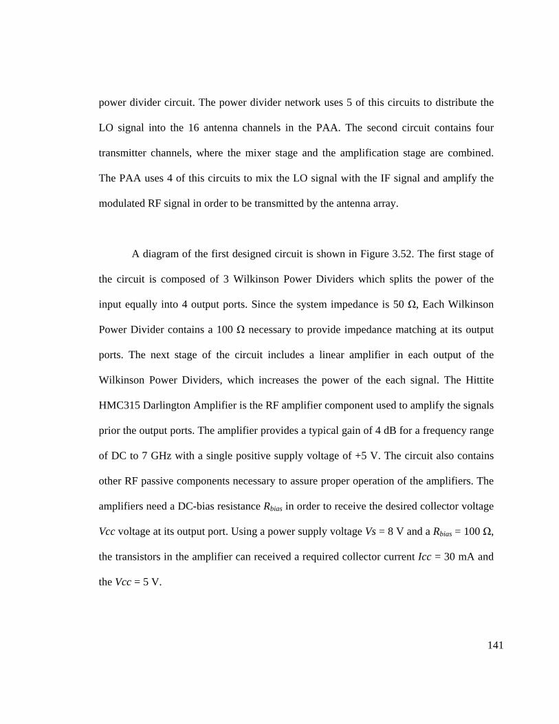
141
power divider circuit. The power divider network uses 5 of this circuits to distribute the
LO signal into the 16 antenna channels in the PAA. The second circuit contains four
transmitter channels, where the mixer stage and the amplification stage are combined.
The PAA uses 4 of this circuits to mix the LO signal with the IF signal and amplify the
modulated RF signal in order to be transmitted by the antenna array.
A diagram of the first designed circuit is shown in Figure 3.52. The first stage of
the circuit is composed of 3 Wilkinson Power Dividers which splits the power of the
input equally into 4 output ports. Since the system impedance is 50 Ω, Each Wilkinson
Power Divider contains a 100 Ω necessary to provide impedance matching at its output
ports. The next stage of the circuit includes a linear amplifier in each output of the
Wilkinson Power Dividers, which increases the power of the each signal. The Hittite
HMC315 Darlington Amplifier is the RF amplifier component used to amplify the signals
prior the output ports. The amplifier provides a typical gain of 4 dB for a frequency range
of DC to 7 GHz with a single positive supply voltage of +5 V. The circuit also contains
other RF passive components necessary to assure proper operation of the amplifiers. The
amplifiers need a DC-bias resistance Rbias in order to receive the desired collector voltage
Vcc voltage at its output port. Using a power supply voltage Vs = 8 V and a Rbias = 100 Ω,
the transistors in the amplifier can received a required collector current Icc = 30 mA and
the Vcc = 5 V.

142
Figure 3.52 Diagram of Power Divider Network Circuit An RF-choke circuit was designed at the output of the amplifier in order to protect
the DC power supply from the RF output signal. The requirements for the two-port
circuit included good impedance match at a frequency of 5.85 GHz, which is the
frequency of the LO, and low transmission losses. The layout diagram of the RF-shoke
circuit is shown in Figure 3.53. The circuit is based on the Bias-T model and contains the
100 Ω bias resistor and 2 chip capacitors with a capacitance of 220 pF. A simulation of
the RF-choke circuit was performed in order to calculate its S-Parameters. The Scattering
Parameters (S-Parameters) of a circuit relates the voltage waves incident on the ports to
those reflected from the ports [Pozar, 1998]. Figure 3.54 shows rectangular plots of the
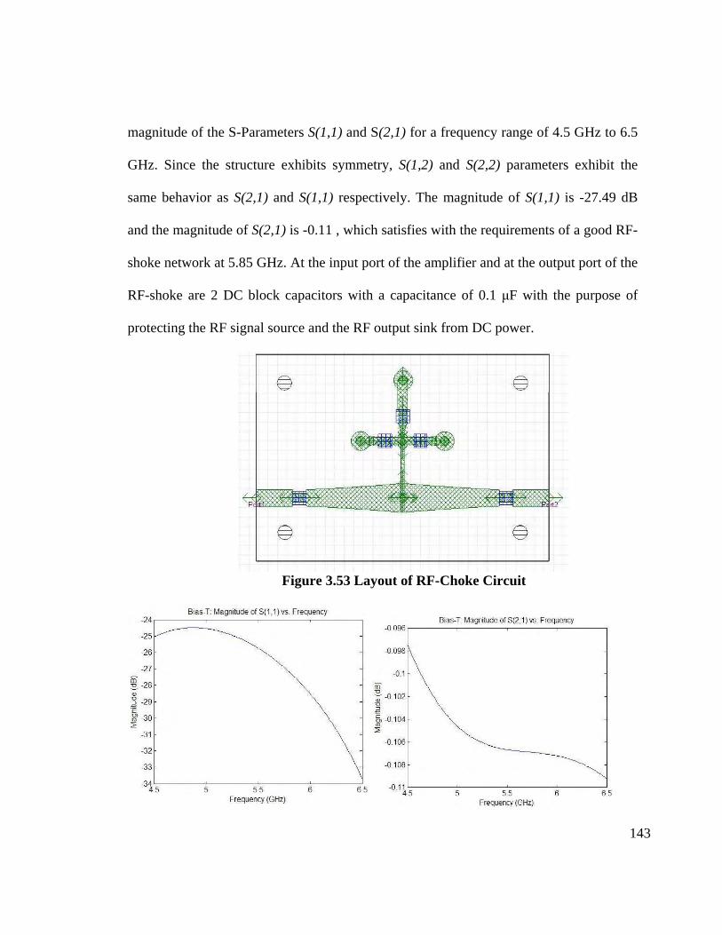
143
magnitude of the S-Parameters S(1,1) and S(2,1) for a frequency range of 4.5 GHz to 6.5
GHz. Since the structure exhibits symmetry, S(1,2) and S(2,2) parameters exhibit the
same behavior as S(2,1) and S(1,1) respectively. The magnitude of S(1,1) is -27.49 dB
and the magnitude of S(2,1) is -0.11 , which satisfies with the requirements of a good RF-
shoke network at 5.85 GHz. At the input port of the amplifier and at the output port of the
RF-shoke are 2 DC block capacitors with a capacitance of 0.1 µF with the purpose of
protecting the RF signal source and the RF output sink from DC power.
Figure 3.53 Layout of RF-Choke Circuit
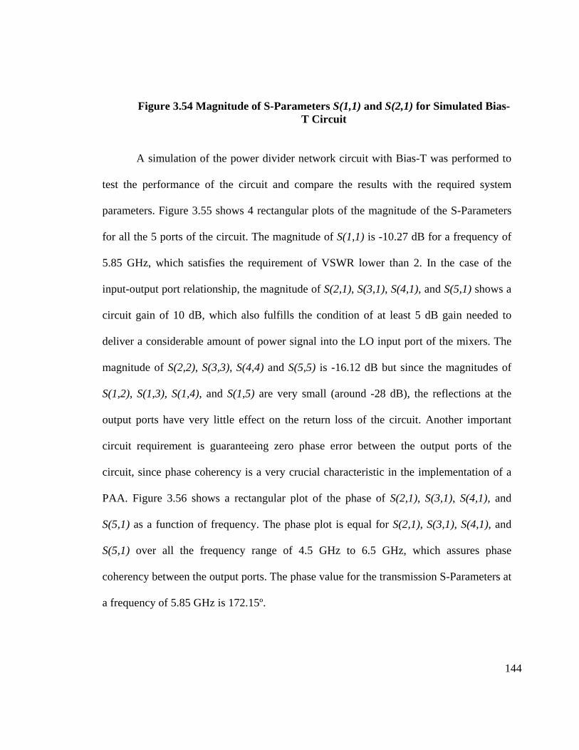
144
Figure 3.54 Magnitude of S-Parameters S(1,1) and S(2,1) for Simulated Bias-T Circuit
A simulation of the power divider network circuit with Bias-T was performed to
test the performance of the circuit and compare the results with the required system
parameters. Figure 3.55 shows 4 rectangular plots of the magnitude of the S-Parameters
for all the 5 ports of the circuit. The magnitude of S(1,1) is -10.27 dB for a frequency of
5.85 GHz, which satisfies the requirement of VSWR lower than 2. In the case of the
input-output port relationship, the magnitude of S(2,1), S(3,1), S(4,1), and S(5,1) shows a
circuit gain of 10 dB, which also fulfills the condition of at least 5 dB gain needed to
deliver a considerable amount of power signal into the LO input port of the mixers. The
magnitude of S(2,2), S(3,3), S(4,4) and S(5,5) is -16.12 dB but since the magnitudes of
S(1,2), S(1,3), S(1,4), and S(1,5) are very small (around -28 dB), the reflections at the
output ports have very little effect on the return loss of the circuit. Another important
circuit requirement is guaranteeing zero phase error between the output ports of the
circuit, since phase coherency is a very crucial characteristic in the implementation of a
PAA. Figure 3.56 shows a rectangular plot of the phase of S(2,1), S(3,1), S(4,1), and
S(5,1) as a function of frequency. The phase plot is equal for S(2,1), S(3,1), S(4,1), and
S(5,1) over all the frequency range of 4.5 GHz to 6.5 GHz, which assures phase
coherency between the output ports. The phase value for the transmission S-Parameters at
a frequency of 5.85 GHz is 172.15º.

145
Figure 3.55 Magnitude of S-Parameters for Simulated Power Divider Network
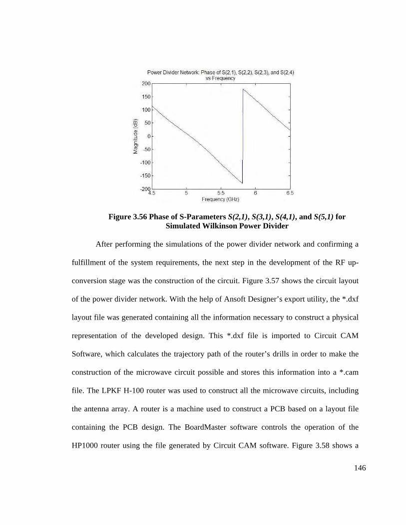
146
Figure 3.56 Phase of S-Parameters S(2,1), S(3,1), S(4,1), and S(5,1) for Simulated Wilkinson Power Divider
After performing the simulations of the power divider network and confirming a
fulfillment of the system requirements, the next step in the development of the RF up-
conversion stage was the construction of the circuit. Figure 3.57 shows the circuit layout
of the power divider network. With the help of Ansoft Designer’s export utility, the *.dxf
layout file was generated containing all the information necessary to construct a physical
representation of the developed design. This *.dxf file is imported to Circuit CAM
Software, which calculates the trajectory path of the router’s drills in order to make the
construction of the microwave circuit possible and stores this information into a *.cam
file. The LPKF H-100 router was used to construct all the microwave circuits, including
the antenna array. A router is a machine used to construct a PCB based on a layout file
containing the PCB design. The BoardMaster software controls the operation of the
HP1000 router using the file generated by Circuit CAM software. Figure 3.58 shows a
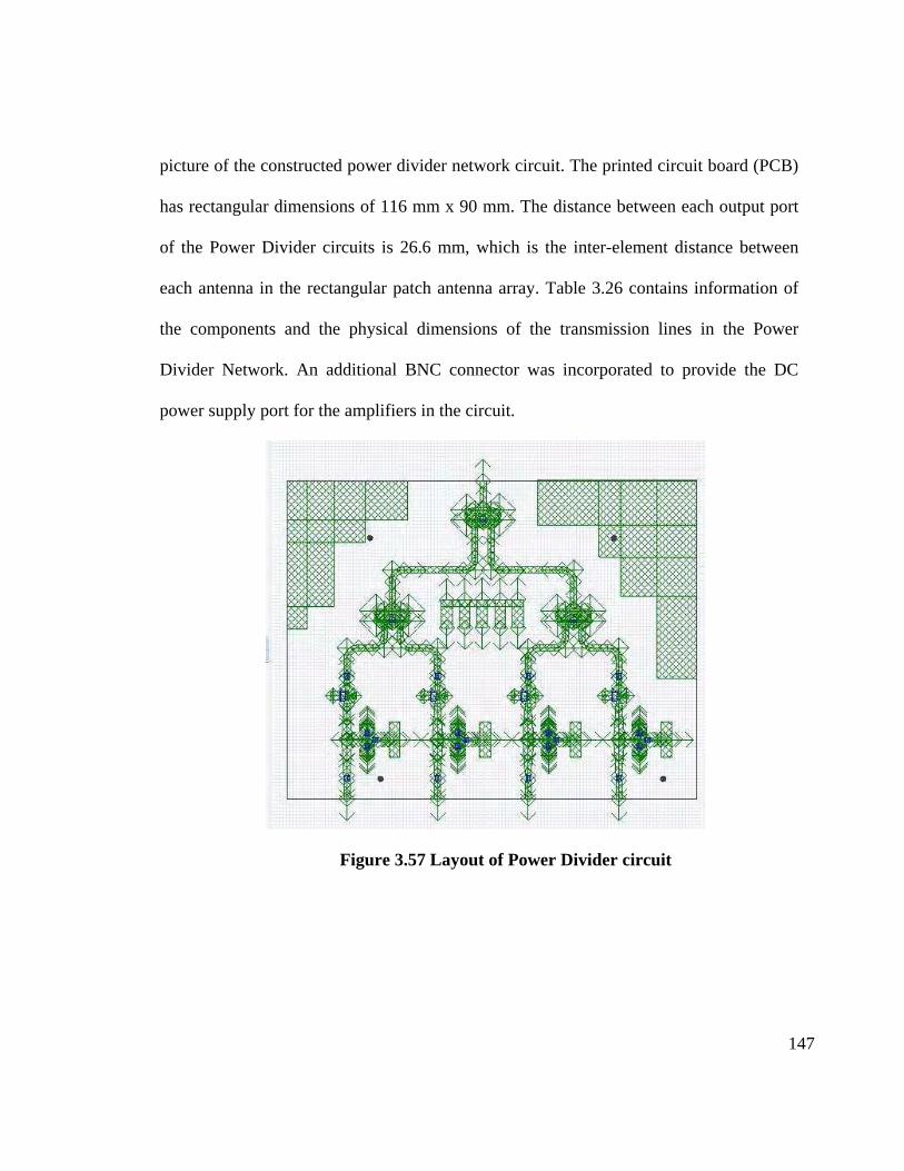
147
picture of the constructed power divider network circuit. The printed circuit board (PCB)
has rectangular dimensions of 116 mm x 90 mm. The distance between each output port
of the Power Divider circuits is 26.6 mm, which is the inter-element distance between
each antenna in the rectangular patch antenna array. Table 3.26 contains information of
the components and the physical dimensions of the transmission lines in the Power
Divider Network. An additional BNC connector was incorporated to provide the DC
power supply port for the amplifiers in the circuit.
Figure 3.57 Layout of Power Divider circuit

148
Figure 3.58 Picture of the Power Divider circuit
TABLE 3.26 Parameters of the Power Divider circuit
Parameter Value
Wilkinson Power Dividers (WPD)
Width of 50 transmission lines 1.7316 mm
Width of 50*√2 transmission lines 0.9444 mm
Length of λ/4 lines 7.8711 mm
Length of transmission lines interconnecting 1st WPD with 2nd WPD
42.5232 mm
Length of transmission lines interconnecting 2nd WPD with amplifiers
19.291 mm
Resistance of WPD resistor 100 Ω
Amplifier Stage
Capacitance of DC Block Capacitors 0.1 µF
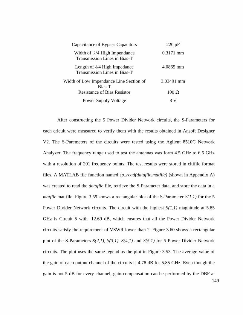
149
Capacitance of Bypass Capacitors 220 pF
Width of λ/4 High Impendance Transmission Lines in Bias-T
0.3171 mm
Length of λ/4 High Impedance Transmission Lines in Bias-T
4.0865 mm
Width of Low Impendance Line Section of Bias-T
3.03491 mm
Resistance of Bias Resistor 100 Ω
Power Supply Voltage 8 V
After constructing the 5 Power Divider Network circuits, the S-Parameters for
each cricuit were measured to verify them with the results obtained in Ansoft Designer
V2. The S-Paremeters of the circuits were tested using the Agilent 8510C Network
Analyzer. The frequency range used to test the antennas was form 4.5 GHz to 6.5 GHz
with a resolution of 201 frequency points. The test results were stored in citifile format
files. A MATLAB file function named sp_read(datafile,matfile) (shown in Appendix A)
was created to read the datafile file, retrieve the S-Parameter data, and store the data in a
matfile.mat file. Figure 3.59 shows a rectangular plot of the S-Parameter S(1,1) for the 5
Power Divider Network circuits. The circuit with the highest S(1,1) magnitude at 5.85
GHz is Circuit 5 with -12.69 dB, which ensures that all the Power Divider Network
circuits satisfy the requirement of VSWR lower than 2. Figure 3.60 shows a rectangular
plot of the S-Parameters S(2,1), S(3,1), S(4,1) and S(5,1) for 5 Power Divider Network
circuits. The plot uses the same legend as the plot in Figure 3.53. The average value of
the gain of each output channel of the circuits is 4.78 dB for 5.85 GHz. Even though the
gain is not 5 dB for every channel, gain compensation can be performed by the DBF at

150
the mixer stage. Finally, Figure 3.61 shows a rectangular plot of the phase of S-
Parameters S(2,1), S(3,1), S(4,1) and S(5,1) as a function of frequency. The average value
of the phase of each output channel of the circuits is -97.56 for 5.85 GHz. The larges
phase error between two output of any of the output channels is 80º. Still, this relative
phase error can be compensated by the DBF at the mixer stage of the RF up-converter.
Table 3.27 shows important S-Parameters values of Power Divider Circuit for 5.85 GHz.
Figure 3.59 Magnitude of S(1,1) for all constructed Power Divider circuits
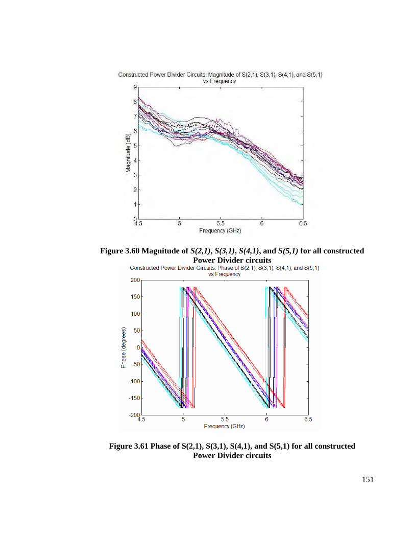
151
Figure 3.60 Magnitude of S(2,1), S(3,1), S(4,1), and S(5,1) for all constructed Power Divider circuits
Figure 3.61 Phase of S(2,1), S(3,1), S(4,1), and S(5,1) for all constructed Power Divider circuits
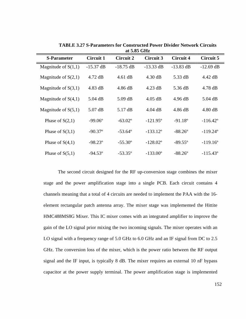
152
TABLE 3.27 S-Parameters for Constructed Power Divider Network Circuits at 5.85 GHz
S-Parameter Circuit 1 Circuit 2 Circuit 3 Circuit 4 Circuit 5
Magnitude of S(1,1) -15.37 dB -18.75 dB -13.33 dB -13.83 dB -12.69 dB
Magnitude of S(2,1) 4.72 dB 4.61 dB 4.30 dB 5.33 dB 4.42 dB
Magnitude of S(3,1) 4.83 dB 4.86 dB 4.23 dB 5.36 dB 4.78 dB
Magnitude of S(4,1) 5.04 dB 5.09 dB 4.05 dB 4.96 dB 5.04 dB
Magnitude of S(5,1) 5.07 dB 5.17 dB 4.04 dB 4.86 dB 4.80 dB
Phase of S(2,1) -99.06º -63.02º -121.95º -91.18º -116.42º
Phase of S(3,1) -90.37º -53.64º -133.12º -88.26º -119.24º
Phase of S(4,1) -98.23º -55.30º -128.02º -89.55º -119.16º
Phase of S(5,1) -94.53º -53.35º -133.00º -88.26º -115.43º
The second circuit designed for the RF up-conversion stage combines the mixer
stage and the power amplification stage into a single PCB. Each circuit contains 4
channels meaning that a total of 4 circuits are needed to implement the PAA with the 16-
element rectangular patch antenna array. The mixer stage was implemented the Hittite
HMC488MS8G Mixer. This IC mixer comes with an integrated amplifier to improve the
gain of the LO signal prior mixing the two incoming signals. The mixer operates with an
LO signal with a frequency range of 5.0 GHz to 6.0 GHz and an IF signal from DC to 2.5
GHz. The conversion loss of the mixer, which is the power ratio between the RF output
signal and the IF input, is typically 8 dB. The mixer requires an external 10 nF bypass
capacitor at the power supply terminal. The power amplification stage is implemented
153
using the Hittite HMC407MS8G Power Amplifier. This power amplifier operates at a
frequency range of 5.0 GHz to 7.0 GHz, with a gain of 15 dB, and a saturated power of
+29 dBm. The power amplifier has an integrated power down capability pin, which can
be used to power down the amplifier when transmission is not required reducing the
consumption of the 230mA of supply current. The amplifier has a thermal paddle at the
bottom, which needs to be connected to the ground of the circuit in order to improve the
heat dissipation of the component. Three 220 pF bypass capacitors and a 2.2 µF Tantalum
capacitor are needed at the voltage supply terminals to assure proper operation.
The mixer, which is the first stage in the second circuit, is a nonlinear device.
Thus, the S-Parameter simulation, which is a linear operation calculating voltage ratio
between circuit ports, cannot be performed. Still, the Ansoft Designer V2 software was
used to construct the layout diagram. Transmission lines between the mixers and the
power amplifiers were designed to satisfy the requirement of good 50Ω-impedance match
at 5.85 GHz. Figure 3.62 shows the layout diagram of the second circuit. The circuit was
constructed using the Circuit CAM software, the BoardMaster software and the H-100
router. Figure 3.63 shows the constructed circuit. Two signal generators and a spectrum
analyzer were used to test the performance of the 4 constructed circuits. An IF signal of 0
dBm at 3 MHz and a LO signal of 0 dBm at 5.85 GHz were used as input to the circuit.
Table 3.28 shows the power obtained at the output of each channel in the 4 circuits. Even
though the relative power difference between each circuit is not zero, the IF signal

154
coming from the DBF stage can be used to compensate for gain differences between the
channels of the PAA.
Figure 3.62 Layout of Mixer and Power Amplifier Circuit
Figure 3.63 Picture of Mixer and Power Amplifier Circuit
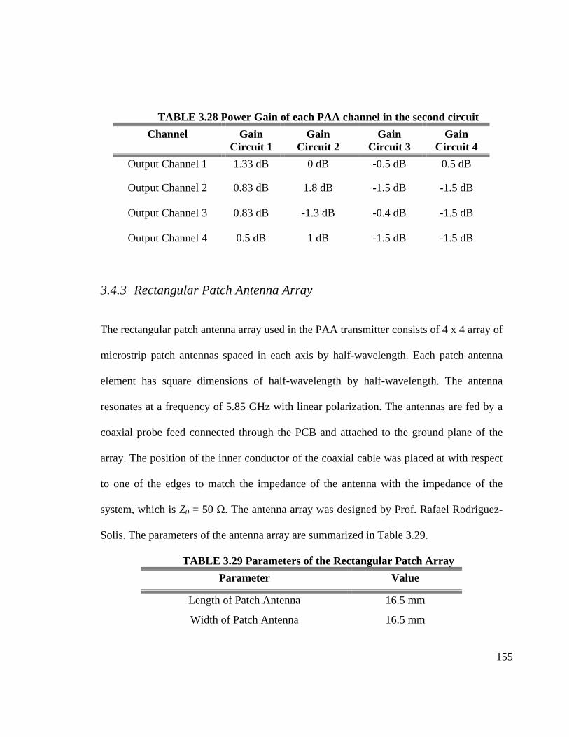
155
TABLE 3.28 Power Gain of each PAA channel in the second circuit
Channel Gain Circuit 1
Gain Circuit 2
Gain Circuit 3
Gain Circuit 4
Output Channel 1 1.33 dB 0 dB -0.5 dB 0.5 dB
Output Channel 2 0.83 dB 1.8 dB -1.5 dB -1.5 dB
Output Channel 3 0.83 dB -1.3 dB -0.4 dB -1.5 dB
Output Channel 4 0.5 dB 1 dB -1.5 dB -1.5 dB
3.4.3 Rectangular Patch Antenna Array
The rectangular patch antenna array used in the PAA transmitter consists of 4 x 4 array of
microstrip patch antennas spaced in each axis by half-wavelength. Each patch antenna
element has square dimensions of half-wavelength by half-wavelength. The antenna
resonates at a frequency of 5.85 GHz with linear polarization. The antennas are fed by a
coaxial probe feed connected through the PCB and attached to the ground plane of the
array. The position of the inner conductor of the coaxial cable was placed at with respect
to one of the edges to match the impedance of the antenna with the impedance of the
system, which is Z0 = 50 Ω. The antenna array was designed by Prof. Rafael Rodriguez-
Solis. The parameters of the antenna array are summarized in Table 3.29.
TABLE 3.29 Parameters of the Rectangular Patch Array
Parameter Value
Length of Patch Antenna 16.5 mm
Width of Patch Antenna 16.5 mm
156
Inter-element spacing in x-axis and y-axis 25.6 mm
Distance of probe feed in the x-axis 8.3 mm
Distance of probe feed in the y-axis 10.77 mm
The simulation of the antenna array was performed using Ansoft Designer V2,
which calculates the S-Parameters and the current distribution of the antennas using the
method of moments. The S-Parameters for the antenna port, which for a one-port network
is S(1,1), determines the amount of power loss as a result of impedance mismatch
between the RF Up-conversion stage and the antenna. The current distribution in the
antenna determines the type of polarization exhibited in the waves radiated or received by
the antenna. Also, the Fourier Transform relates the current distribution along the antenna
to its far-field pattern. The simulation was performed in a frequency range of 4.5 GHz to
6.5 GHz. Figure 3.64 shows the magnitude of the S-Parameter S(1,1) for all the antenna’s
in the rectangular array. The magnitude of S(1,1) -32.19 dB for a frequency of 5.85 GHz,
thus satisfying the requirement for a S(1,1) magnitude lower than -10 dB, which is a
Voltage Standing Wave Ratio (VSWR) smaller than 2. The Electric Field (E-Field)
pattern of the array, shown in Figure 3.65, has a beamwidth of 24.5º with sidelobe levels
of -13.8dB. The E-Field magnitude in the x-direction (Ex) and the E-Field magnitude in
the y-direction (Ey) plots are show in Figure 3.66 for a field φ-plane cut of 0º. Since the
magnitude of Ey is *20 dB lower than the magnitude of Ex, the antenna array exhibits
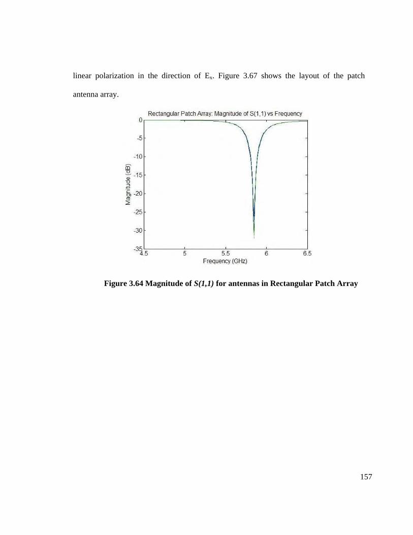
157
linear polarization in the direction of Ex. Figure 3.67 shows the layout of the patch
antenna array.
Figure 3.64 Magnitude of S(1,1) for antennas in Rectangular Patch Array
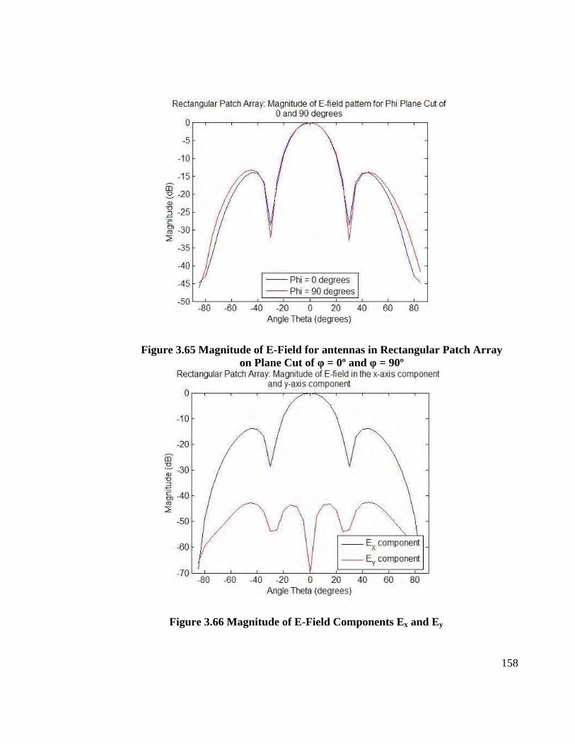
158
Figure 3.65 Magnitude of E-Field for antennas in Rectangular Patch Array on Plane Cut of φ = 0º and φ = 90º
Figure 3.66 Magnitude of E-Field Components Ex and Ey

159
Figure 3.67 Layout of Rectangular Patch Antenna Array
Since the antenna array simulations results satisfied the specified requirements in
terms of bandwidth and beam pattern characteristics, the next step in the process of
implementing the PAA was the construction of the rectangular patch antenna array.
Figure 3.68 shows a picture of the constructed rectangular patch array antenna. The S-
Parameters for each antenna port in the constructed array was measured to verify the
reflection coefficient of the antennas and compare them with the simulation results
obtained in Ansoft Designer V2. The S-Paremeters of the antennas were tested using the
Agilent 8510C Network Analyzer. The frequency range used to test the antennas was
form 4.5 GHz to 6.5 GHz with a resolution of 201 frequency points. The test results for
each antenna were stored in citifile format files. A MATLAB file function named
sp_read(datafile,matfile) (shown in Appendix A) was created to read the datafile file,
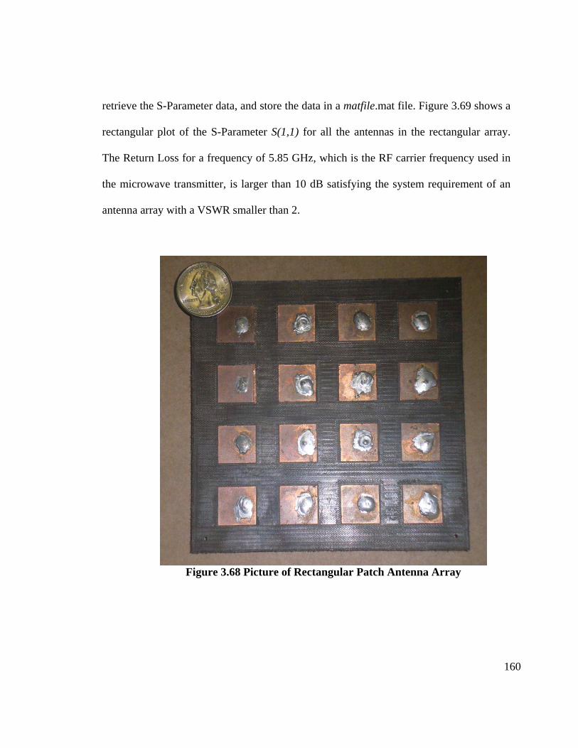
160
retrieve the S-Parameter data, and store the data in a matfile.mat file. Figure 3.69 shows a
rectangular plot of the S-Parameter S(1,1) for all the antennas in the rectangular array.
The Return Loss for a frequency of 5.85 GHz, which is the RF carrier frequency used in
the microwave transmitter, is larger than 10 dB satisfying the system requirement of an
antenna array with a VSWR smaller than 2.
Figure 3.68 Picture of Rectangular Patch Antenna Array
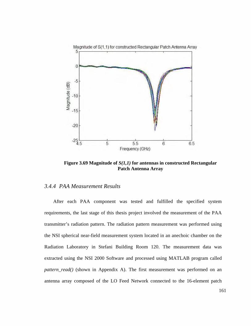
161
Figure 3.69 Magnitude of S(1,1) for antennas in constructed Rectangular Patch Antenna Array
3.4.4 PAA Measurement Results
After each PAA component was tested and fulfilled the specified system
requirements, the last stage of this thesis project involved the measurement of the PAA
transmitter’s radiation pattern. The radiation pattern measurement was performed using
the NSI spherical near-field measurement system located in an anechoic chamber on the
Radiation Laboratory in Stefani Building Room 120. The measurement data was
extracted using the NSI 2000 Software and processed using MATLAB program called
pattern_read() (shown in Appendix A). The first measurement was performed on an
antenna array composed of the LO Feed Network connected to the 16-element patch
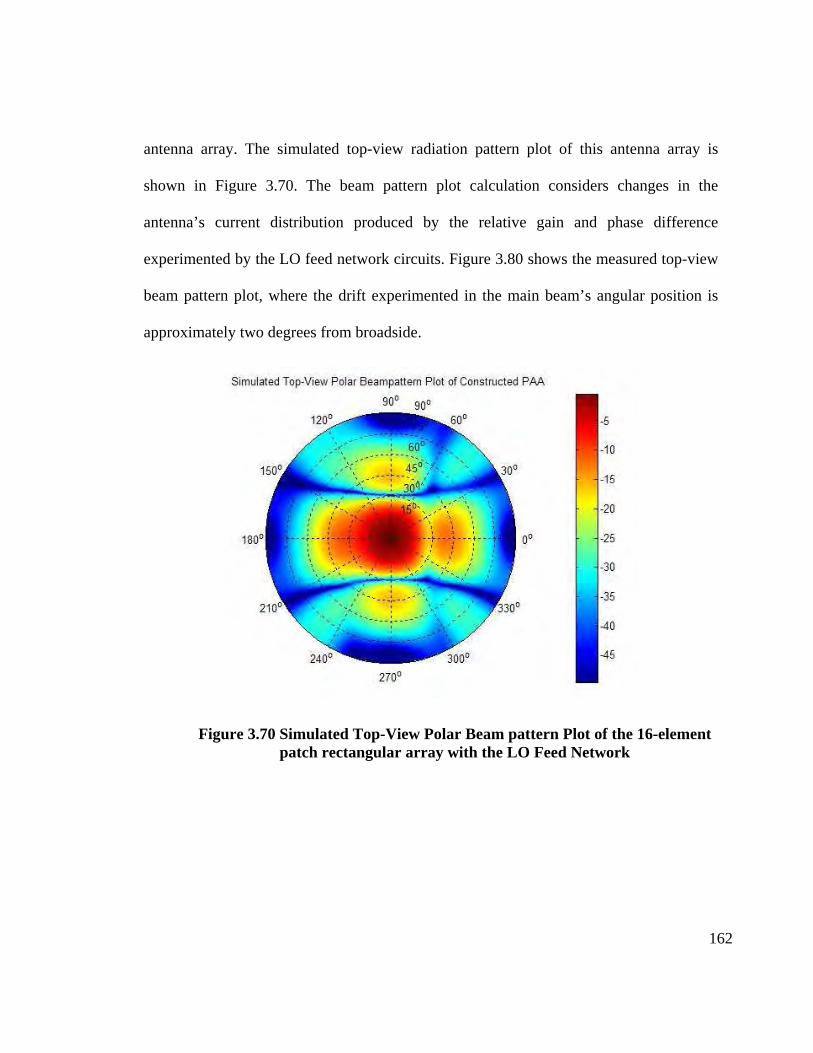
162
antenna array. The simulated top-view radiation pattern plot of this antenna array is
shown in Figure 3.70. The beam pattern plot calculation considers changes in the
antenna’s current distribution produced by the relative gain and phase difference
experimented by the LO feed network circuits. Figure 3.80 shows the measured top-view
beam pattern plot, where the drift experimented in the main beam’s angular position is
approximately two degrees from broadside.
Figure 3.70 Simulated Top-View Polar Beam pattern Plot of the 16-element patch rectangular array with the LO Feed Network
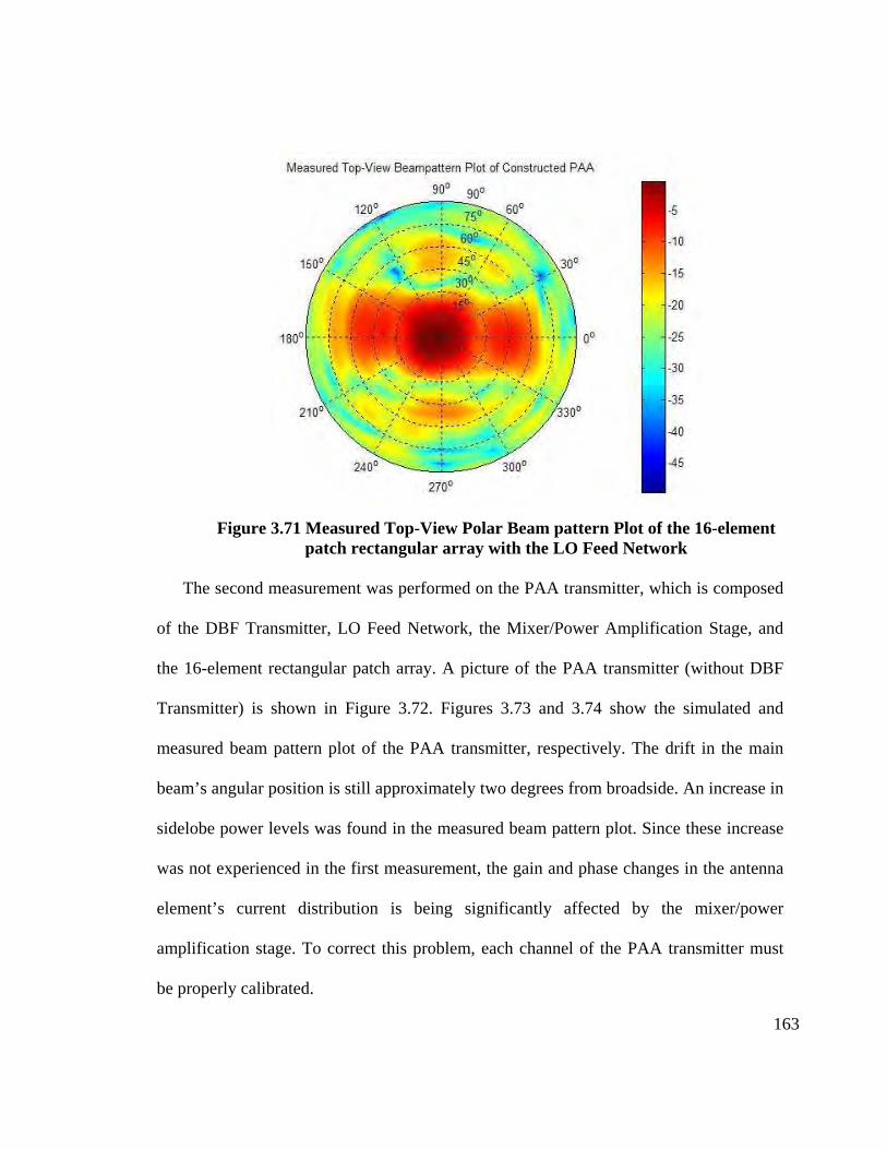
163
Figure 3.71 Measured Top-View Polar Beam pattern Plot of the 16-element patch rectangular array with the LO Feed Network
The second measurement was performed on the PAA transmitter, which is composed
of the DBF Transmitter, LO Feed Network, the Mixer/Power Amplification Stage, and
the 16-element rectangular patch array. A picture of the PAA transmitter (without DBF
Transmitter) is shown in Figure 3.72. Figures 3.73 and 3.74 show the simulated and
measured beam pattern plot of the PAA transmitter, respectively. The drift in the main
beam’s angular position is still approximately two degrees from broadside. An increase in
sidelobe power levels was found in the measured beam pattern plot. Since these increase
was not experienced in the first measurement, the gain and phase changes in the antenna
element’s current distribution is being significantly affected by the mixer/power
amplification stage. To correct this problem, each channel of the PAA transmitter must
be properly calibrated.
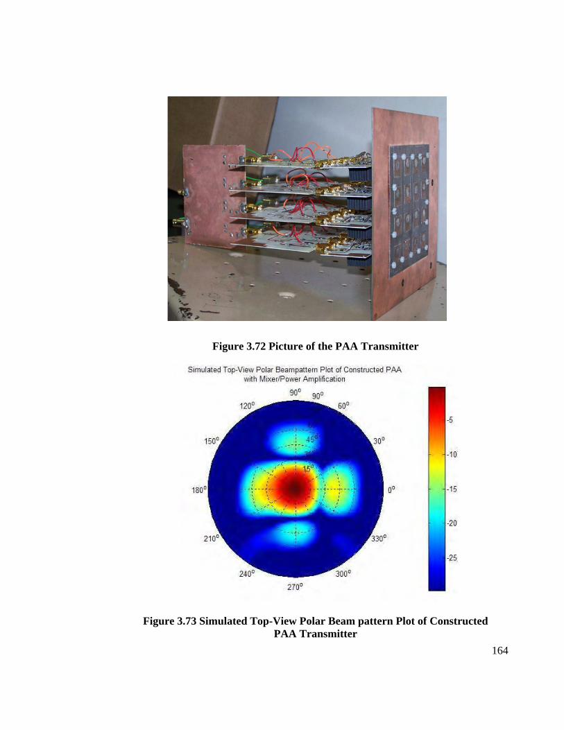
164
Figure 3.72 Picture of the PAA Transmitter
Figure 3.73 Simulated Top-View Polar Beam pattern Plot of Constructed PAA Transmitter
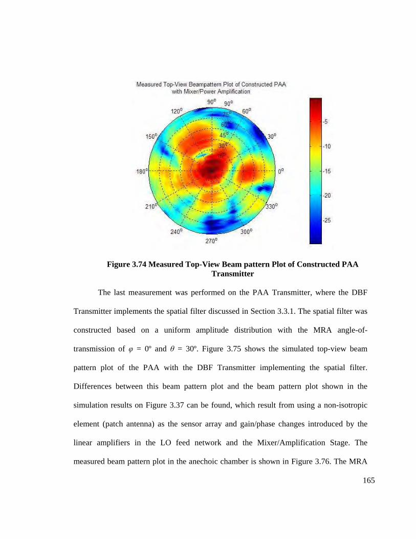
165
Figure 3.74 Measured Top-View Beam pattern Plot of Constructed PAA Transmitter
The last measurement was performed on the PAA Transmitter, where the DBF
Transmitter implements the spatial filter discussed in Section 3.3.1. The spatial filter was
constructed based on a uniform amplitude distribution with the MRA angle-of-
transmission of φ = 0º and θ = 30º. Figure 3.75 shows the simulated top-view beam
pattern plot of the PAA with the DBF Transmitter implementing the spatial filter.
Differences between this beam pattern plot and the beam pattern plot shown in the
simulation results on Figure 3.37 can be found, which result from using a non-isotropic
element (patch antenna) as the sensor array and gain/phase changes introduced by the
linear amplifiers in the LO feed network and the Mixer/Amplification Stage. The
measured beam pattern plot in the anechoic chamber is shown in Figure 3.76. The MRA
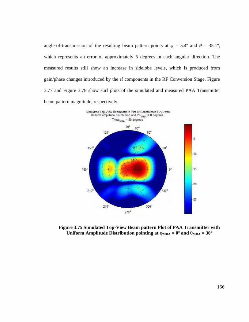
166
angle-of-transmission of the resulting beam pattern points at φ = 5.4º and θ = 35.1º,
which represents an error of approximately 5 degrees in each angular direction. The
measured results still show an increase in sidelobe levels, which is produced from
gain/phase changes introduced by the rf components in the RF Conversion Stage. Figure
3.77 and Figure 3.78 show surf plots of the simulated and measured PAA Transmitter
beam pattern magnitude, respectively.
Figure 3.75 Simulated Top-View Beam pattern Plot of PAA Transmitter with Uniform Amplitude Distribution pointing at φMRA = 0º and θMRA = 30º
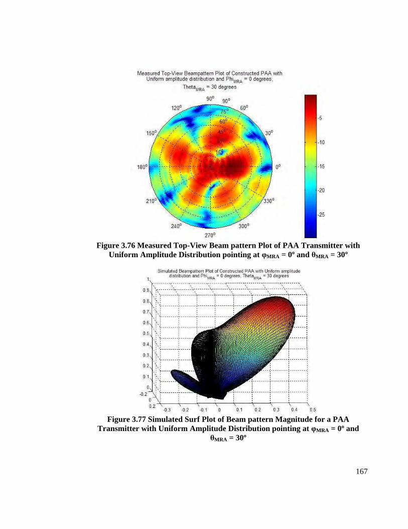
167
Figure 3.76 Measured Top-View Beam pattern Plot of PAA Transmitter with
Uniform Amplitude Distribution pointing at φMRA = 0º and θMRA = 30º
Figure 3.77 Simulated Surf Plot of Beam pattern Magnitude for a PAA
Transmitter with Uniform Amplitude Distribution poi nting at φMRA = 0º and θMRA = 30º
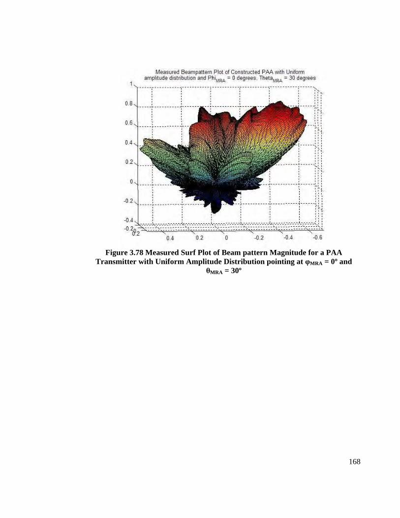
168
Figure 3.78 Measured Surf Plot of Beam pattern Magnitude for a PAA
Transmitter with Uniform Amplitude Distribution poi nting at φMRA = 0º and θMRA = 30º
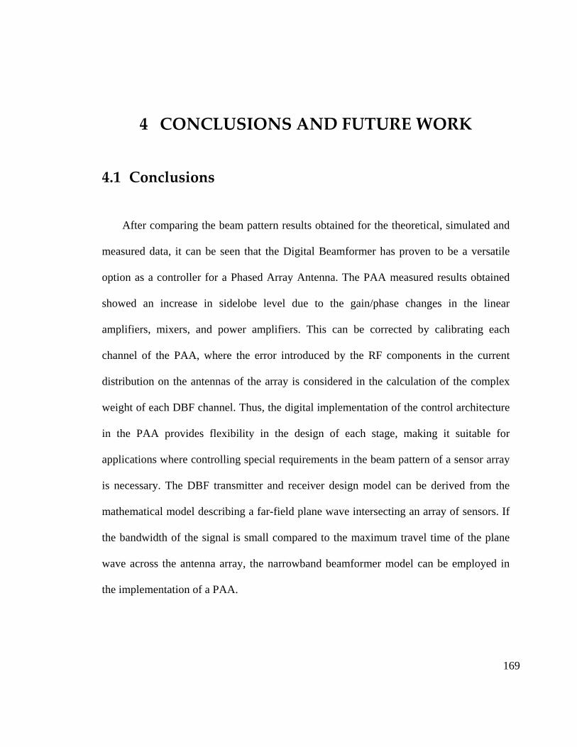
169
4 CONCLUSIONS AND FUTURE WORK
4.1 Conclusions
After comparing the beam pattern results obtained for the theoretical, simulated and
measured data, it can be seen that the Digital Beamformer has proven to be a versatile
option as a controller for a Phased Array Antenna. The PAA measured results obtained
showed an increase in sidelobe level due to the gain/phase changes in the linear
amplifiers, mixers, and power amplifiers. This can be corrected by calibrating each
channel of the PAA, where the error introduced by the RF components in the current
distribution on the antennas of the array is considered in the calculation of the complex
weight of each DBF channel. Thus, the digital implementation of the control architecture
in the PAA provides flexibility in the design of each stage, making it suitable for
applications where controlling special requirements in the beam pattern of a sensor array
is necessary. The DBF transmitter and receiver design model can be derived from the
mathematical model describing a far-field plane wave intersecting an array of sensors. If
the bandwidth of the signal is small compared to the maximum travel time of the plane
wave across the antenna array, the narrowband beamformer model can be employed in
the implementation of a PAA.

170
Compared to the Delay-and-Sum Beamformer model, which uses time delays in each
channel as a means of creating the beam pattern, the Narrowband Beamformer model can
be expressed as a Finite Impulse Response (FIR) spatial filter with complex coefficients
operating on a space-time signal. In the case of the antenna array, the weight coefficients
control the amplitude and relative phase of the current in the antennas. Since the current
distribution is related to the beam pattern of an antenna by the Fourier Transform, a
synthesized beam pattern can be implemented by carefully choosing the coefficients of
each antenna channel in the array. The resulting spatial filter, thus, can be used in the
DBF receiver or transmitter to create a beam pattern based on the geometrical distribution
of the antennas in the array. The results obtained in each simulation prove the versatility
of the DBF in implementing the control of a PAA. Different spatial filters were tested,
where each one represented particular beam pattern characteristics. The simulations,
which were performed in MATLAB’s Simulink using software code representing FPGA
hardware based on Xilinx’s System Generator for DSP Blockset, gave results closely
matching the results obtained from a theoretical DBF. After obtaining successful
simulations results, the System Generator for DSP tool was used to transform the DBF
transmitter design into VHDL code. The resulting code was used to program the FPGA in
the digital processing board.
Another advantage offered by the DBF is its independence on the geometrical
distribution of the array. A DBF with an N-channel capacity is able to operate on a PAA
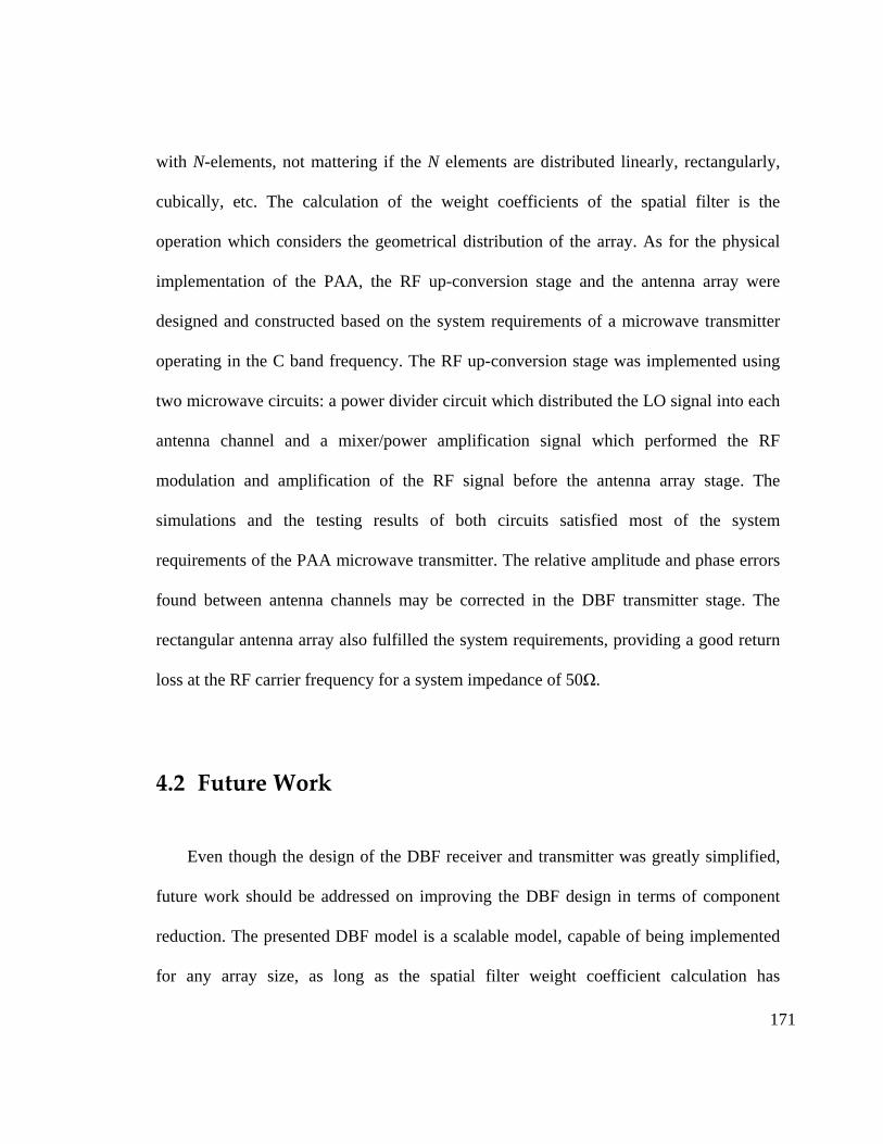
171
with N-elements, not mattering if the N elements are distributed linearly, rectangularly,
cubically, etc. The calculation of the weight coefficients of the spatial filter is the
operation which considers the geometrical distribution of the array. As for the physical
implementation of the PAA, the RF up-conversion stage and the antenna array were
designed and constructed based on the system requirements of a microwave transmitter
operating in the C band frequency. The RF up-conversion stage was implemented using
two microwave circuits: a power divider circuit which distributed the LO signal into each
antenna channel and a mixer/power amplification signal which performed the RF
modulation and amplification of the RF signal before the antenna array stage. The
simulations and the testing results of both circuits satisfied most of the system
requirements of the PAA microwave transmitter. The relative amplitude and phase errors
found between antenna channels may be corrected in the DBF transmitter stage. The
rectangular antenna array also fulfilled the system requirements, providing a good return
loss at the RF carrier frequency for a system impedance of 50Ω.
4.2 Future Work
Even though the design of the DBF receiver and transmitter was greatly simplified,
future work should be addressed on improving the DBF design in terms of component
reduction. The presented DBF model is a scalable model, capable of being implemented
for any array size, as long as the spatial filter weight coefficient calculation has

172
considered the number of elements and the geometrical distribution of the antenna array.
Still, a large PAA with very strict beam pattern requirements might prove to be costly and
complex in terms of system integration. Alternative PAA designs must be considered,
where reducing the complexity of the design should lie on how rigorous the system
requirements of the application containing the PAA are. For example, if the system
requires a beam pattern with a single MRA beam and MRA steering control, the
progressive phase shift nature found in the currents of the antenna array can be exploited
to reduce the complexity of the PAA system. Figure 4.1 shows a diagram of a simplified
PAA implementation for a single MRA-beam beam pattern known as row-column
phasing architecture [Corey, 1996]. The PAA uses a phase-shifted LO signal and a phase-
shifted IF signal to generate the progressive phase shift necessary to steer the beam into a
desired direction. If the LO signal is mixed twice, where one mixing stage adds the
relative phase shift in the x-axis and the second mixing stage adds the relative phase shift
in the y-axis (Eq. 3.12), theoretically an L*M antenna array can be controlled by
processing L+M IF signals in the DBF stage. Still, the condition of a fixed amplitude
value in the input of the mixers might limit the dynamic range of the weight coefficient’s
amplitude in the DBF transmitter.
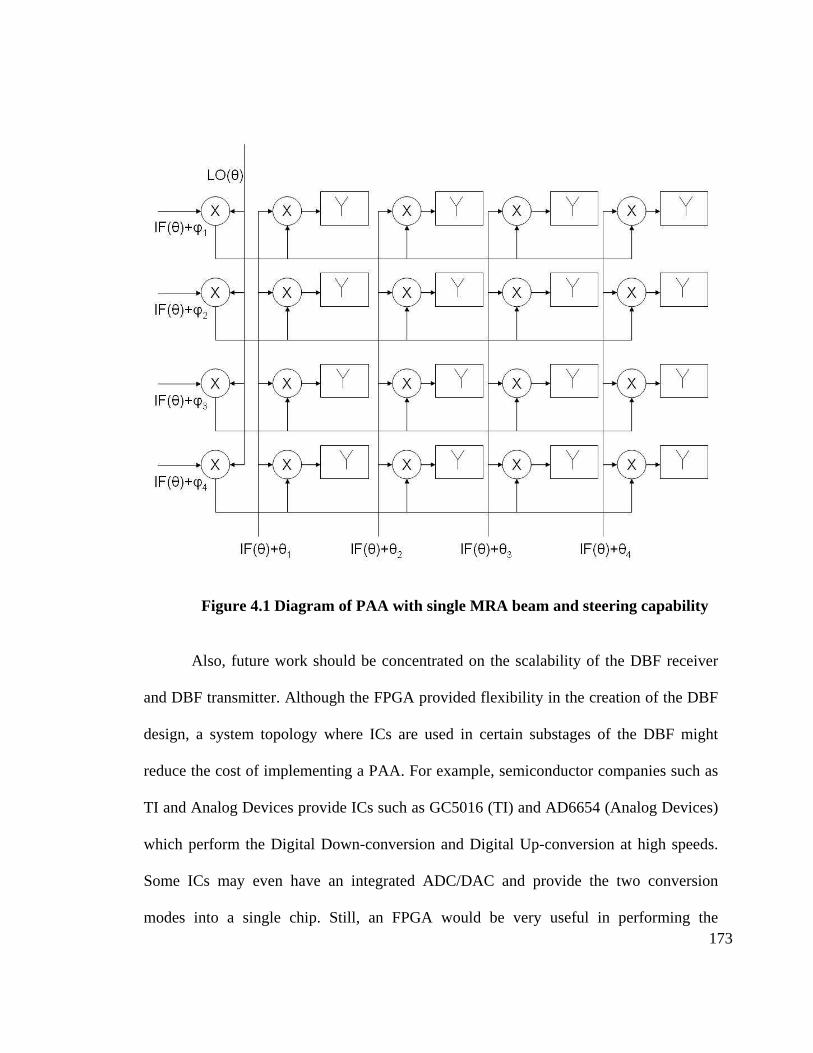
173
Figure 4.1 Diagram of PAA with single MRA beam and steering capability Also, future work should be concentrated on the scalability of the DBF receiver
and DBF transmitter. Although the FPGA provided flexibility in the creation of the DBF
design, a system topology where ICs are used in certain substages of the DBF might
reduce the cost of implementing a PAA. For example, semiconductor companies such as
TI and Analog Devices provide ICs such as GC5016 (TI) and AD6654 (Analog Devices)
which perform the Digital Down-conversion and Digital Up-conversion at high speeds.
Some ICs may even have an integrated ADC/DAC and provide the two conversion
modes into a single chip. Still, an FPGA would be very useful in performing the

174
necessary “gluelogic” in order to interconnect the different digital devices in the DBF
receiver/transmitter. The FPGA’s use as an interconnection component versus a signal
processing component might increase its capacity in terms of number of DBF channels
interconnected by a single FPGA. If low sampling frequencies can be obtained on the
signal processing stage in the DBF, a DSP can be used to perform weight coefficient
calculation.
Finally, the use of an analog pre-processor might improve the performance of a
PAA with strict system requirements. RF Discrete Lens Antenna Arrays (DLAA) might
be used to transform the signals from an element-space domain into a beamspace signal
domain, were each signal in the DBF receiver or transmitter represents beams that are
separated by space instead of being signals separated by distance. In this approach, a
spatial filter with real coefficients might satisfy the beam pattern characteristics of the
PAA. However, the use of a DLAA requires a change in the way signals are processed
inside the DBF [Torres, 2005]. Algorithms which only considers power incidence at the
antennas on the focal surface of the DLAA are suitable for this type of systems.
175
REFERENCES
Alliot S., “THEA Adaptive Weight Estimation, implemented on a DSP”; Tech. Report, ASTRON, Dwingeloo, March 2000. Alliot S., Cazamier W., “Beamforming Interpolation for THEA ”; Research Report-THEA-00024, Astron: October 2000. Balanis C.A., Antenna Theory: Analysis and Design, Second Edition, John Wiley & Sons, New York, 1997. Chang, D.C.D.; Klimczak, W.N.; Busche, G.C. “An Experimental Digital Beamforming Array” ; Antennas and Propagation Society International Symposium, 1988. AP-S. Digest, 6-10 June 1988; Pages: 1300 - 1303 vol.3. Corey, L “A Survey of Russian Low Cost Phased-Array Technology” ; Antennas and Propagation Society International Symposium, 1988. AP-S. Digest, 6-10 June 1988; Pages: 1300 - 1303 vol.3. Dreher, A.; Hekmat, T.; Niklasch, N.E.; Lieke, M.; Klefenz, F.; Schroth, A. “Planar Digital-Beamforming Antenna for Satellite Navigation”; Microwave Symposium Digest, 1999 IEEE MTT-S International , Volume: 2 , 13-19; June 1999 Pages:647 - 650 vol.2 Dreher, A.; Niklasch, N.; Klefenz, F.; Schroth, A. “Antenna and Receiver System with Digital Beamforming for Satellite Navigation and Communication”; Microwave Theory and Techniques, IEEE Transactions on , Volume: 51 , Issue: 7 , July 2003; Pages:1815 - 1821 Franks L. E., Signal Theory, Prentice-Hall, Englewood Cliffs, N.J., 1969. Garret P. H., Analog I/O Design: Acquisiton: Conversion: Recovery, Reston Publishing Company, Reston, 1981 Harris F. J. “Multirate FIR Filters for Interpolating and Desampl ing” , Handbook of Digital Signal Processing: Engineering Applications, Academic Press, San Diego, 1987 Hatcher, B. R. “Granularity of Beam Positions in Digital Phased Arrays”; Proceedings of the IEEE, Volume: 56, Issue: 11, November 1968; Pages:1795 - 1800 Haynes T., “A Primer on Digital Beamforming”; Spectrum Signal Processing.
176
Hiemstra L., “Real-Time Digital Signal Processing implemented on a Multi-Processor System”; Tech. Report., NFRA, Dwingeloo, July 2000. Hogenauer E., “An Economical Class of Digital Filters for Decimation and Interpolation ”, Acoustics, Speech, and Signal Processing, IEEE Transactions on Volume 29, Issue 2, Apr 1981, Pages:155-162. Kajala, M.; Hamalainen, M. “Filter-and-Sum Beamformer with Adjustable Filter Characteristics”; Acoustics, Speech, and Signal Processing, 2001. Proceedings. (ICASSP '01). 2001 IEEE International Conference on, Volume: 5, 7-11; May 2001 Pages:2917 - 2920 vol.5. Kajala, M.; Hamaldinen, M. “Broadband Beamforming Optimization for Speech Enhancement in Noisy Environments”; Applications of Signal Processing to Audio and Acoustics, 1999 IEEE Workshop on , 17-20; Oct. 1999 Pages:19 – 22. Lyrtech Processing Company, SM-VHS-DAC User’s Manual, November 2004 Manassewitch V., Frequency Synthesizers: Theory and Design, Second Edition. John Wiley & Sons, New York, 1980. Miura, R.; Tanaka, T.; Chiba, I.; Horie, A.; Karasawa, Y. “Beamforming Experiment with a DBF Multibeam Antenna in a Mobile Satellite Environment” ; Antennas and Propagation, IEEE Transactions on , Volume: 45 , Issue: 4 , April 1997; Pages:707 – 714 Mucci R., “A Comparison of Efficient Beamforming Algorithms” , Acoustics, Speech, and Signal Processing [see also IEEE Transactions on Signal Processing], IEEE Transactions on Volume 32, Issue 3, Jun 1984 Page(s):548 - 558 Pozar D. M., Microwave Engineering, Second Edition. John Wiley & Sons, New York, 1998. Simonangeli L. J., Agrawal A., “A C-Band Digital Beamforming Array” , Antennas and Propagation Society International Symposium, 1988. AP-S. Digest 6-10 June 1988 Page(s):1385 - 1388 vol.3 Steyskal, H., “Digital Beamforming – An Emerging Approach”; Military Communications Conference, 1988. MILCOM 88, Conference record. '21st Century Military Communications - What's Possible?’ 1988 IEEE, 23-26 Oct. 1988; Pages: 399 - 403 vol.2.

177
Torres-Rosario J. A., Rodríguez-Solís R., Hunt S., Popovic Z., “Adaptive Discrete Lens Antenna Array for Direction of Arrival Detection ”, Antennas and Propagation Society International Symposium, 2005. AP-S. Digest, 6-10 June 2005. Van Trees, Harry L. Optimum Array Processing: Detection, Estimation, and Modulation Theory, Part IV . Wiley Interscience, New York, 2002
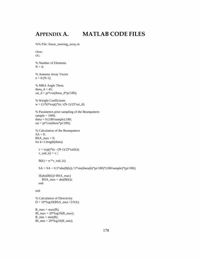
178
APPENDIX A. MATLAB CODE FILES
%% File: linear_steering_array.m clear; clc; % Number of Elements N = 4; % Antenna Array Vector n = 0:(N-1); % MRA Angle Theta theta_d = 45; sai_d = pi*cos(theta_d*pi/180); % Weight Coefficients w = (1/N)*exp(j*(n.'-(N-1)/2)*sai_d); % Parameters prior sampling of the Beampattern sample = 1000; theta = 0:(180/sample):180; sai = pi*cos(theta*pi/180); % Calculation of the Beampattern SA = 0; BSA_max = 0; for k=1:length(theta) v = exp(j*(n - (N-1)/2)*sai(k)); v_sai(:,k) = v.'; B(k) = w'*v_sai(:,k); SA = SA + 0.5*abs(B(k)).^2*sin(theta(k)*pi/180)*(180/sample)*(pi/180); if(abs(B(k))>BSA_max) BSA_max = abs(B(k)); end end % Calculation of Directivity D = 10*log10(BSA_max.^2/SA); B_max = max(B); Bl_max = 20*log10(B_max); B_min = min(B); Bl_min = 20*log10(B_min);
179
% Calculation of Beamwidth B_3dB = B_max/2; theta_beam = theta([abs(B)]>=B_3dB); Beamwidth_theta = theta(610)-theta(1); % Result Figures figure(1) polar(theta*pi/180,abs(B)); figure(2) plot(theta,20*log10(abs(B))); %% File: linear_DBFreceiver_parameters.m % Information Signal fis = 0; sig_ts = 1e-9; samp_period = 100; % Carrier Signal fif = 3e6; i_phase = pi/2-2*pi*(fif)*(3/200e6); % ADC Parameters adc_ts = 1/200e6; adc_bit_res = 14; adc_point_res = 12; % Operation Precision Parameters % Adder Block Parameters add_bit_width = 14; add_point_width = 12; % Multiply Block Parameters mult_bit_width = 18; mult_point_width = 16; mult_latency = 3; % Operator Parameters prec_bit_width = 18; prec_point_width = 16; % Antenna Weights and Digital Beamformer w_amp = abs(w); phase_res = 8; w_phase_d = angle(w)*180/pi; w_phase_r = angle(w); bit_phase = w_phase_r*2^phase_res/(2*pi); db_ts = 1/50e6; wamp_bit_res = 16; wamp_point_res = 14; wphase_bit_res = phase_res; wphase_point_res = 0;
180
% Max Time Delay plane_wave_angle = 0; ant_spacing = 0.5; fant = 8.2e9; maxt = ant_spacing/fif; sim_t = 1e-5; slope_t = maxt/sim_t; % DDS Parameters output_width = 32; flo = fif; ddc_ts = adc_ts; npi = flo*ddc_ts; % Scope Parameters scope_ts = 1e-11; scope_sig = 1e-11; % Latency Repair lat_n = 12; lat_time = lat_n*100e-9; total_time = lat_time+sim_t; % CIC Specs d_sample = db_ts/adc_ts; n_stages = 8; cic_lat = 8; diff_delay = 2; force_bit_width = 45; scale_factor = 0; % Butterworth Analog Filter for post-processing [Nb,Wnb]=buttord(3e6*db_ts,4e6*db_ts,3,25); [Bb,Ab]=butter(Nb,Wnb); % Gain of IF Signal prior Time Delay K2 = 0.99; K1 = 1; %% File: linear_DBFreceiver_results.m clear all; clear; % load MAT Files load signal_out_0; load signal_out_1; load signal_out_2; load signal_out_3; load signal_out_4; load signal_out_5;
181
% Simulation Parameters total_time = 1e-5; db_ts = 1/50e6; delta_index = total_time/db_ts; angle_low_index = 251; angle_high_index = angle_low_index+delta_index; mag_low_index = 310; mag_high_index = mag_low_index+delta_index; phase_low_index = 310; phase_high_index = phase_low_index+delta_index; % Retrieving Beampattern Results angle = [fliplr(angle_0_90(2,angle_low_index:angle_high_index)) angle_90_180(2,(angle_low_index+1):angle_high_index)]; mag = [fliplr(mag_0_90(2,mag_low_index:mag_high_index)) mag_90_180(2,(mag_low_index+1):mag_high_index)]; mag = mag/max(mag); phase = [fliplr(phase_0_90(2,phase_low_index:phase_high_index)) phase_90_180(2,(phase_low_index+1):phase_high_index)]; % Calculation of Directivity in Beampattern SA = 0; BSA_max = 0; for k=1:(length(angle)-1) SA = SA + 0.5*mag(k).^2*sin(angle(k)*pi/180)*(angle(k+1)-angle(k))*(pi/180); if(mag(k)>BSA_max) BSA_max = mag(k); end end D = 10*log10(BSA_max.^2/SA); % Result Figures figure(1) polar(angle*pi/180,mag); figure(2) plot(angle,20*log10(mag)); %% File: linear_DBFreceiver_nullplacer.m clear; clc; % Number of Antennas N = 4; % Generation of Antenna Array Vector n = 0:(N-1);

182
% Calculation of Weight Coefficients based on Null Placement parameters Bd = [1 zeros(1,N-1)]; MRA = 0; Nulls = [30 60 100]; theta_d = [MRA Nulls]; sai_d = pi*cos(theta_d*pi/180); for k=1:length(theta_d) v = exp(j*(n - (N-1)/2)*sai_d(k)); v_sai_d(:,k) = v.'; end w = (inv(v_sai_d))'*Bd'; % Parameters prior sampling of the Beampatter sample = 1000; theta = 0:(180/sample):180; sai = pi*cos(theta*pi/180); % Calculation of the Beampattern SA = 0; BSA_max = 0; for k=1:length(theta) v = exp(j*(n - (N-1)/2)*sai(k)); v_sai(:,k) = v.'; B(k) = w'*v_sai(:,k); SA = SA + 0.5*abs(B(k)).^2*sin(theta(k)*pi/180)*(180/sample)*(pi/180); if(abs(B(k))>BSA_max) BSA_max = abs(B(k)); end end % Calculation of the Directivity D = 10*log10(BSA_max.^2/SA); B = B/max(B); B_max = abs(max(B)); Bl_max = 20*log10(B_max); B_min = abs(min(B)); Bl_min = 20*log10(B_min);
183
% Result Figures figure(1); plot(theta,20*log10(abs(B))); axis([0 180 Bl_min-3 Bl_max+4]); figure(2); polar(theta*pi/180,abs(B)); %% File: linear_DBFtransmitter_taylor.m clear; clc; % Number of Antennas N = 16; % Inter-element Spacing (in lambda terms) d = 0.5; % Generation of Array Vector n = 0:(N-1); % Parameters of Taylor Amplitude Function R_l = 20; R = 10^(R_l/20); A = acosh(R)/pi; n_l = 4; % Calculation of Taylor Amplitude Function based on Null-placement Method Nulls = []; if (round(N/2)-N/2)==0.5 for k=1:(N-1)/2 Nulls(k)=2*pi/N*(n_l*sqrt((A^2+(k-0.5)^2)/(A^2+(n_l-0.5)^2))); end Nulls = [Nulls -1*Nulls]; % MRA Broadside MRA = pi*cos(90*pi/180); sai_d = [MRA Nulls]; Bd = [1 zeros(1,N-1)]; else theta_d = [89.9 90.1];

184
u_d = cos(theta_d*pi/180); Bd = sin(N*d*u_d)./(pi*N*d*u_d); for k=1:(N-1)/2 Nulls(k)=2*pi/N*(n_l*sqrt((A^2+(k-0.5)^2)/(A^2+(n_l-0.5)^2))); end Nulls = [Nulls -1*Nulls]; sai_d = [pi*u_d Nulls]; Bd = [Bd zeros(1,N-2)]; end for k=1:length(sai_d) v = exp(j*(n - (N-1)/2)*sai_d(k)); v_sai_d(:,k) = v.'; end w_t = (inv(v_sai_d))'*Bd'; % Calculation of MRA Beam Direction theta_d = 82; sai_d = pi*cos(theta_d*pi/180); w = w_t.*exp(j*(n.'-(N-1)/2)*sai_d); % Parameters prior sampling of the Beampattern sample = 1000; theta = 0:(180/sample):180; sai = pi*cos(theta*pi/180); % Calculation of Beampattern SA = 0; BSA_max = 0; for k=1:length(theta) v = exp(j*(n - (N-1)/2)*sai(k)); v_sai(:,k) = v.'; B(k) = w'*v_sai(:,k); SA = SA + 0.5*abs(B(k)).^2*sin(theta(k)*pi/180)*(180/sample)*(pi/180);
185
if(abs(B(k))>BSA_max) BSA_max = abs(B(k)); end end % Calculation of Directivity D = 10*log10(BSA_max.^2/SA); % Result Figures figure(1) polar(theta*pi/180,abs(B)); figure(2) plot(theta,20*log10(abs(B))); % File: linear_DBFtransmitter_parameters.m % Information Signal sig_ts = 1e-8; % Information Signal output_width = 16; fis = 1e6; db_ts = 1/10e6; npi = fis*db_ts; % Antenna Weights and Digital Beamformer phase_res = 8; w_amp = abs(w); w_phase_d = angle(w)*180/pi; w_phase_r = angle(w); bit_phase = w_phase_r*2^phase_res/(2*pi); wamp_bit_res = 16; wamp_point_res = 14; wphase_bit_res = 8; wphase_point_res = 0; w_phase_d_corr = round(bit_phase)*2*pi/(2^phase_res)*180/pi; % DAC dac_ts = 1/100e6; dac_bit_res = 14; dac_point_res = 12; % System Frequencies fc = 8.2e9; fif = 3e6; error_index = 0; i_phase = pi/2-(2*pi*fif)*(1e-8)*error_index;
186
% DDS Parameters output_width = 16; flo = fif; duc_ts = dac_ts; npd = flo*duc_ts; % Max Time Delay plane_wave_angle = 0; ant_spacing = 0.5; maxt = (fc/fif)*ant_spacing/fc; sim_t = 1e-5; slope_t = maxt/sim_t; % DUC Filter Specs filter_order = 30; factor = 10; u_sample = db_ts/dac_ts; hp = u_sample*fir1(filter_order,1/(factor*u_sample)); filter_lat = 15; % CIC Specs n_stages = 2; cic_lat = 2; diff_delay = 2; force_bit_width = 18; scale_factor = -2; % Scope Parameters scope_ts = 1e-8; scope_sig = 1e-8; % Latency Repair lat_duc_n = 3 + filter_lat; lat_db_n = 8; lat_time = (lat_duc_n+filter_order)*duc_ts+lat_db_n*db_ts; total_time = lat_time+sim_t; % Operation Precision add_bit_width = 14; add_point_width = 12; mult_bit_width = 18; mult_point_width = 16; prec_bit_width = 16; prec_point_width = 14; % Transforming Weight Matrix into vector form w_amp = reshape(w_amp,sqrt(N),sqrt(N)).'; bit_phase = reshape(bit_phase,sqrt(N),sqrt(N)).'; %% File: linear_DBFtransmitter_results.m clear;
187
clc; % Load MAT FILE load TRANSMITTER; % Removing Transient State of Transmission Signal total_time = 2e-5; sim_time = 1e-5; sim_period = 1e-8; extra_samples = (total_time-sim_time)/sim_period; [r_trans_signal,c_trans_signal] = size(trans_signal); trans_signal = trans_signal(:,(c_trans_signal-extra_samples):c_trans_signal); [r_trans_signal,c_trans_signal] = size(trans_signal); % Calculate FFT of each antenna signal fft_size = 2^16; spectral_signal = []; for k=1:r_trans_signal-1 spectral_signal(k,:) = fft(trans_signal(k+1,:),fft_size); end f_range = 0:1/(fft_size*sim_period):1/sim_period-1/(fft_size*sim_period); index_range = 1:length(f_range); % Frequencies and index where information signal is present center_f = 3e6; delta_f = 1/(2*fft_size*sim_period); center_f_index = [f_range>=center_f-delta_f & f_range<=center_f+delta_f]*index_range.'; % Rectangular Array Size N = 1; M = 16; w_phase_x = []; w_phase_x(:,1) = zeros(N,1); % Calculation of Weight Coefficient's Phase for k=2:M center_phase = -1*(angle(spectral_signal(k,center_f_index))-angle(spectral_signal(1,center_f_index))); if (center_phase>=180) center_phase = center_phase-360; end w_phase_x(k)=center_phase; end % Calculation of Weight Coefficient's Magnitude for k=1:M
188
w_abs(k) = abs(spectral_signal(k,center_f_index))/2; end % Number of Antennas N = 16; % Generation of Array Vector n = 0:(N-1); % Calculation of Array Weight w = (w_abs.*exp(j*w_phase_x)).'; save WEIGHT_INFO w; % Parameters prior sampling of the Beampattern sample = 1000; theta = 0:(180/sample):180; sai = pi*cos(theta*pi/180); % Calculation of the Beampattern SA = 0; BSA_max = 0; for k=1:length(theta) v = exp(j*(n - (N-1)/2)*sai(k)); v_sai(:,k) = v.'; B(k) = w'*v_sai(:,k); SA = SA + 0.5*abs(B(k)).^2*sin(theta(k)*pi/180)*(180/sample)*(pi/180); if(abs(B(k))>BSA_max) BSA_max = abs(B(k)); end end % Calculation of the Directivity D = 10*log10(BSA_max.^2/SA); % Result Figures figure(1) polar(theta*pi/180,abs(B)); figure(2) plot(theta,20*log10(abs(B))); % File: linear_DBFtransmitter_blackmannharris.m

189
clear; clc; % Number of Antennas N = 16; % Generation of Array Vector n = 0:(N-1); % Calculation of MRA Beam Direction theta_d = 82; sai_d = pi*cos(theta_d*pi/180); % Calculation of Weight's Amplitude based on Blackmann-harris Spectral % Window function w_abs = (0.42+0.5*cos(2*pi*(n-(N-1)/2)/N)+0.08*cos(4*pi*(n-(N-1)/2)/N)).'; % Calculation of Weight Coefficients w = w_abs.*exp(j*(n.'-(N-1)/2)*sai_d); % Paramaters prior sampling of the Beampatter sample = 1000; theta = 0:(180/sample):180; sai = pi*cos(theta*pi/180); % Calculation of Beampattern SA = 0; BSA_max = 0; for k=1:length(theta) v = exp(j*(n - (N-1)/2)*sai(k)); v_sai(:,k) = v.'; B(k) = w'*v_sai(:,k); SA = SA + 0.5*abs(B(k)).^2*sin(theta(k)*pi/180)*(180/sample)*(pi/180); if(abs(B(k))>BSA_max) BSA_max = abs(B(k)); end end % Calculation of Directivity D = 10*log10(BSA_max.^2/SA); % Result Figures figure(1) polar(theta*pi/180,abs(B)); figure(2)

190
plot(theta,20*log10(abs(B))); %% File: rectangular_DBFtransmitter_steering.m clear; clc; % Rectangular Array Size N = 4; M = 4; [n,m] = meshgrid(-1*(N-1)/2:(N-1)/2,-1*(M-1)/2:(M-1)/2); % Inter-element spacing in lambda terms dx = 0.5; dy = 0.5; % Weight function theta_d = 30; phi_d = 0; sai_x_d = 2*pi*dx*sin(theta_d*pi/180)*cos(phi_d*pi/180); sai_y_d = 2*pi*dy*sin(theta_d*pi/180)*sin(phi_d*pi/180); W = (1/(M*N))*exp(j*(n*sai_x_d + m*sai_y_d)); w = reshape(W,N*M,1); save TRAINING -append W; % Creating U and Sai Space sample_u_x = 100; sample_u_y = 100; u_x = -1:1/(sample_u_x*2):1; u_y = -1:1/(sample_u_y*2):1; sai_x = 2*pi*dx*u_x; sai_y = 2*pi*dy*u_y; % 2-D Beampattern Calculation for k=1:length(sai_x) for h=1:length(sai_y) V = exp(j*(n*sai_x(k) + m*sai_y(h))); v = reshape(V,N*M,1); B(k,h) = w'*v; end
191
end % 2-D Beampattern Calculation in Angle Space phi_coor_real = 0:360; theta_coor_real = 0:90; theta_coor_extra = 0:180; V = []; v = []; SA = 0; for k=1:length(phi_coor_real) for h=1:length(theta_coor_extra) sai_x_now = 2*pi*dx*sin(theta_coor_extra(h)*pi/180)*cos(phi_coor_real(k)*pi/180); sai_y_now = 2*pi*dx*sin(theta_coor_extra(h)*pi/180)*sin(phi_coor_real(k)*pi/180); V = exp(j*(n*sai_x_now + m*sai_y_now)); v = reshape(V,N*M,1); if theta_coor_extra(h) <= 90 B_sph(k,h) = w'*v; phi_coor_real_sph(k,h) = phi_coor_real(k); theta_coor_real_sph(k,h) = theta_coor_real(h); if (phi_coor_real(k)~=360) SA = SA + (abs(B_sph(k,h)))^2*sin(theta_coor_real(h)*pi/180)*(pi/180)^2; end else B_SA = w'*v; if (phi_coor_real(k)~=360 && theta_coor_extra(h)~=180 ) SA = SA + (abs(B_SA))^2*sin(theta_coor_extra(h)*pi/180)*(pi/180)^2; end end end end SA = SA/(4*pi);

192
% Calculation of Directivity D = abs(B_sph(phi_d+1,theta_d+1))^2/SA; D_dB = 10*log10(D); B_max = max(max(abs(B_sph))); B_sph = B_sph/max(max(abs(B_sph))); [x_B,y_B,z_B] = sph2cart(phi_coor_real_sph*pi/180, (-(theta_coor_real_sph-90)*pi/180), abs(B_sph)); % Phi = 0 & Phi = MRA_phi Cut Beampattern Calculation phi_1 = 0; phi_2 = phi_d; phi_3 = phi_d + 45; theta = 0:1:90; for k=1:length(theta) u_x_1 = sin(theta(k)*pi/180)*cos(phi_1*pi/180); u_y_1 = sin(theta(k)*pi/180)*sin(phi_1*pi/180); u_x_2 = sin(theta(k)*pi/180)*cos(phi_2*pi/180); u_y_2 = sin(theta(k)*pi/180)*sin(phi_2*pi/180); u_x_3 = sin(theta(k)*pi/180)*cos(phi_3*pi/180); u_y_3 = sin(theta(k)*pi/180)*sin(phi_3*pi/180); sai_x_1 = 2*pi*dx*u_x_1; sai_y_1 = 2*pi*dy*u_y_1; sai_x_2 = 2*pi*dx*u_x_2; sai_y_2 = 2*pi*dy*u_y_2; sai_x_3 = 2*pi*dx*u_x_3; sai_y_3 = 2*pi*dy*u_y_3; V_1 = exp(j*(n*sai_x_1 + m*sai_y_1)); v_1 = reshape(V_1,N*M,1); Bt_1(k) = w'*v_1; V_2 = exp(j*(n*sai_x_2 + m*sai_y_2)); v_2 = reshape(V_2,N*M,1); Bt_2(k) = w'*v_2; V_3 = exp(j*(n*sai_x_3 + m*sai_y_3)); v_3 = reshape(V_3,N*M,1); Bt_3(k) = w'*v_3;
193
end if (phi_2<180) Bt_s = [fliplr(Bt_2) Bt_3]; else Bt_s = [fliplr(Bt_3) Bt_2]; end % Calculation of Beamwidth in Phi Plane Cut Bt_s = Bt_s([1:92 94:182]); theta_m = 0:180; Bt_s_max = max(abs(Bt_s)); Bt_s_3dB = Bt_s_max/2; theta_beam = theta_m([abs(Bt_s)]>=Bt_s_3dB); Beamwidth_theta = max(theta_beam)-min(theta_beam); figure('Name','Beam Pattern of Standard Rectangular Array'); surf(x_B,y_B,z_B); title('Magnitude in dB of Rectangular Array Beam Pattern'); xlabel('x'); ylabel('y'); zlabel('Magnitude (dB)'); polar3D(theta_coor_real,phi_coor_real,(20*log10(abs(B_sph)))',50,3,'Rectangular Array Beam Pattern Polar Plot'); function hpol = polar3D(theta,phi,z,graph_dynamic,fig_nb,title_fig) %POLAR3D 3D Polar coordinate plot. % polar3D(THETA,PHI,Z,GRAPH_DYNAMIC,FIG_NB,TITLE_FIG) makes a plot using polar coordinates of % the angles THETA and PHI, in degrees, versus the 3rd dimension Z. % GRAPH_DYNAMIC allows to display the dynamic range from the maximum value of Z. % FIG_NB indicates the figure number in which the graph has to be displayed. % TITLE_FIG is a string containing the figure's title. % % Copyright Sebastien and Marcelo, The Dream-Team, Nov. 21, 2003. % get hold state figure(fig_nb) cax = newplot; next = lower(get(cax,'NextPlot')); hold_state = ishold; % get x-axis text color so grid is in same color tc = get(cax,'xcolor'); ls = get(cax,'gridlinestyle'); % Hold on to current Text defaults, reset them to the % Axes' font attributes so tick marks use them.

194
fAngle = get(cax, 'DefaultTextFontAngle'); fName = get(cax, 'DefaultTextFontName'); fSize = get(cax, 'DefaultTextFontSize'); fWeight = get(cax, 'DefaultTextFontWeight'); fUnits = get(cax, 'DefaultTextUnits'); set(cax, 'DefaultTextFontAngle', get(cax, 'FontAngle'), ... 'DefaultTextFontName', get(cax, 'FontName'), ... 'DefaultTextFontSize', get(cax, 'FontSize'), ... 'DefaultTextFontWeight', get(cax, 'FontWeight'), ... 'DefaultTextUnits','data') % transform data to Cartesian coordinates. xx=theta.'*cos(pi*phi/180); yy=theta.'*sin(pi*phi/180); pcolor(xx,yy,z), shading interp; if (graph_dynamic~=0) caxis([(max(max(z))-graph_dynamic) max(max(z))]); end axis square; colorbar; title(title_fig) % plot gird on top of data % make a radial grid hold on; max_theta = max( max(abs(theta))); hhh=plot([-max_theta -max_theta max_theta max_theta],[-max_theta max_theta max_theta -max_theta]); set(gca,'dataaspectratio',[1 1 1],'plotboxaspectratiomode','auto') v = [get(cax,'xlim') get(cax,'ylim')]; ticks = 7; delete(hhh); % check radial limits and ticks rmin = 0; rmax = 90; rticks = max(ticks-1,2); % define a circle th = 0:pi/50:2*pi; xunit = cos(th); yunit = sin(th); % now really force points on x/y axes to lie on them exactly inds = 1:(length(th)-1)/4:length(th); xunit(inds(2:2:4)) = zeros(2,1); yunit(inds(1:2:5)) = zeros(3,1); % draw radial circles c82 = cos(82*pi/180); s82 = sin(82*pi/180); rinc = (rmax-rmin)/rticks; for i=(rmin+rinc):rinc:rmax hhh = plot(xunit*i,yunit*i,ls,'color',tc,'linewidth',1,... 'handlevisibility','off');
195
text((i+rinc/20)*c82,(i+rinc/20)*s82, ... [' ' num2str(i) '^o'],'verticalalignment','bottom',... 'handlevisibility','off') end set(hhh,'linestyle','-') % Make outer circle solid % plot spokes th = (1:6)*2*pi/12; cst = cos(th); snt = sin(th); cs = [-cst; cst]; sn = [-snt; snt]; plot(rmax*cs,rmax*sn,ls,'color',tc,'linewidth',1,... 'handlevisibility','off') % annotate spokes in degrees rt = 1.1*rmax; for i = 1:length(th) text(rt*cst(i),rt*snt(i),[int2str(i*30) '^o'],... 'horizontalalignment','center',... 'handlevisibility','off'); if i == length(th) loc = int2str(0); else loc = int2str(180+i*30); end text(-rt*cst(i),-rt*snt(i),[loc '^o'],'horizontalalignment','center',... 'handlevisibility','off') end % set view to 2-D view(2); % set axis limits axis(rmax*[-1 1 -1.15 1.15]); % Reset defaults. set(cax, 'DefaultTextFontAngle', fAngle , ... 'DefaultTextFontName', fName , ... 'DefaultTextFontSize', fSize, ... 'DefaultTextFontWeight', fWeight, ... 'DefaultTextUnits',fUnits ); hold off; if nargout > 0 hpol = q; end if ~hold_state set(gca,'dataaspectratio',[1 1 1]), axis off; set(cax,'NextPlot',next); end set(get(gca,'xlabel'),'visible','on') set(get(gca,'ylabel'),'visible','on')
196
hold off; % File: rectangular_DBFtransmitter_parameters.m % Information Signal sig_ts = 1e-8; % Information Signal output_width = 16; fis = 1e6; db_ts = 1/10e6; npi = fis*db_ts; % Antenna Weights and Digital Beamformer phase_res = 8; w_amp = abs(W)/sum(sum(abs(W))); w_phase_d = angle(W)*180/pi; w_phase_r = angle(W); bit_phase = w_phase_r*2^phase_res/(2*pi); wamp_bit_res = 16; wamp_point_res = 14; wphase_bit_res = phase_res; wphase_point_res = 0; w_phase_d_corr = round(bit_phase)*2*pi/(2^phase_res)*180/pi; % DAC dac_ts = 1/100e6; dac_bit_res = 14; dac_point_res = 12; % System Frequencies fc = 8.2e9; fif = 3e6; error_index = 0; i_phase = pi/2-(2*pi*fif)*(1e-8)*error_index; % DDS Parameters output_width = 16; flo = fif; duc_ts = dac_ts; npd = flo*duc_ts; % Max Time Delay plane_wave_angle = 0; ant_spacing = 0.5; maxt = (fc/fif)*ant_spacing/fc; sim_t = 1e-5; slope_t = maxt/sim_t; % DUC Filter Specs filter_order = 30;

197
factor = 10; u_sample = db_ts/dac_ts; hp = u_sample*fir1(filter_order,1/(factor*u_sample)); filter_lat = 15; % CIC Specs n_stages = 2; cic_lat = 2; diff_delay = 2; force_bit_width = 18; scale_factor = -2; % Scope Parameters scope_ts = 1e-8; scope_sig = 1e-8; % Latency Repair lat_duc_n = 3 + filter_lat; lat_db_n = 8; lat_time = (lat_duc_n+filter_order)*duc_ts+lat_db_n*db_ts; total_time = lat_time+sim_t; % Operation Precision add_bit_width = 14; add_point_width = 12; mult_bit_width = 18; mult_point_width = 16; prec_bit_width = 16; prec_point_width = 14; load TRAINING; save WEIGHT_INFO w_amp w_phase_r w_phase_d_corr; %% File: rectangular_DBFtransmitter_results.m clear; clc; % Load MAT FILE load TRANSMITTER; % Removing Transient State of Transmission Signal total_time = 1.1e-5; sim_time = 1e-5; sim_period = 1e-8; extra_samples = (total_time-sim_time)/sim_period; [r_trans_signal,c_trans_signal] = size(trans_signal); trans_signal = trans_signal(:,(c_trans_signal-extra_samples):c_trans_signal); [r_trans_signal,c_trans_signal] = size(trans_signal);
198
% Calculate FFT of each antenna signal fft_size = 2^16; spectral_signal = []; for k=1:r_trans_signal-1 spectral_signal(k,:) = fft(trans_signal(k+1,:),fft_size); end f_range = 0:1/(fft_size*sim_period):1/sim_period-1/(fft_size*sim_period); index_range = 1:length(f_range); % Frequencies and index where information signal is present center_f = 3e6; delta_f = 1/(2*fft_size*sim_period); center_f_index = [f_range>=center_f-delta_f & f_range<=center_f+delta_f]*index_range.'; % Rectangular Array Size N = 4; M = 4; w_phase_x = []; w_phase_x(:,1) = zeros(N,1); % Calculation of Weight Coefficients' Phase for k=1:N for h=2:M center_phase = -1*(angle(spectral_signal(h+(k-1)*N,center_f_index))-angle(spectral_signal(1+(k-1)*N,center_f_index))); if (center_phase>=180) center_phase = center_phase-360; end w_phase_x(k,h)=center_phase; end end w_phase_y = []; w_phase_y(1,:) = zeros(1,M); for k=2:N for h=1:M center_phase = -1*(angle(spectral_signal(h+(k-1)*N,center_f_index))-angle(spectral_signal(h,center_f_index))); if (center_phase>=180) center_phase = center_phase-360; end w_phase_y(k,h)=center_phase; end end
199
% Calculation of Weight Coefficients' Magnitude for k=1:N for h=1:M w_abs(k,h) = abs(spectral_signal(h+(k-1)*N,center_f_index))/2; end end % Rectangular Array Size N = 4; M = 4; [n,m] = meshgrid(-1*(N-1)/2:(N-1)/2,-1*(M-1)/2:(M-1)/2); % Inter-element spacing in lambda terms dx = 0.5; dy = 0.5; % Weight function theta_d = 16; phi_d = 122; sai_x_d = 2*pi*dx*sin(theta_d*pi/180)*cos(phi_d*pi/180); sai_y_d = 2*pi*dy*sin(theta_d*pi/180)*sin(phi_d*pi/180); W = w_abs.*exp(j*(w_phase_x + w_phase_y)); w = reshape(W,N*M,1); save WEIGHT_INFO W -append; % Creating U and Sai Space sample_u_x = 100; sample_u_y = 100; u_x = -1:1/(sample_u_x*2):1; u_y = -1:1/(sample_u_y*2):1; sai_x = 2*pi*dx*u_x; sai_y = 2*pi*dy*u_y; % [u_x,u_y] = meshgrid(2*pi*dx*(-1:1/(sample_u_x*2):1),2*pi*dy*(-1:1/(sample_u_y*2):1)); % 2-D Beampattern Calculation for k=1:length(sai_x) for h=1:length(sai_y) V = exp(j*(n*sai_x(k) + m*sai_y(h))); v = reshape(V,N*M,1); B(k,h) = w'*v; end

200
end % 2-D Beampattern Calculation in Angle Space phi_coor_real = 0:360; theta_coor_real = 0:90; theta_coor_extra = 0:180; V = []; v = []; SA = 0; for k=1:length(phi_coor_real) for h=1:length(theta_coor_extra) sai_x_now = 2*pi*dx*sin(theta_coor_extra(h)*pi/180)*cos(phi_coor_real(k)*pi/180); sai_y_now = 2*pi*dx*sin(theta_coor_extra(h)*pi/180)*sin(phi_coor_real(k)*pi/180); V = exp(j*(n*sai_x_now + m*sai_y_now)); v = reshape(V,N*M,1); if theta_coor_extra(h) <= 90 B_sph(k,h) = w'*v; phi_coor_real_sph(k,h) = phi_coor_real(k); theta_coor_real_sph(k,h) = theta_coor_real(h); if (phi_coor_real(k)~=360) SA = SA + (abs(B_sph(k,h)))^2*sin(theta_coor_real(h)*pi/180)*(pi/180)^2; end else B_SA = w'*v; if (phi_coor_real(k)~=360 && theta_coor_extra(h)~=180 ) SA = SA + (abs(B_SA))^2*sin(theta_coor_extra(h)*pi/180)*(pi/180)^2; end end end end SA = SA/(4*pi);
201
D = abs(B_sph(phi_d+1,theta_d+1))^2/SA; D_dB = 10*log10(D); B_max = max(max(abs(B_sph))); [x_B,y_B,z_B] = sph2cart(phi_coor_real_sph*pi/180, (-(theta_coor_real_sph-90)*pi/180), abs(B_sph)); % Phi = 0 & Phi = MRA_phi Cut Beampattern Calculation phi_1 = 0; phi_2 = phi_d; phi_3 = phi_d + 180; theta = 0:1:90; for k=1:length(theta) u_x_1 = sin(theta(k)*pi/180)*cos(phi_1*pi/180); u_y_1 = sin(theta(k)*pi/180)*sin(phi_1*pi/180); u_x_2 = sin(theta(k)*pi/180)*cos(phi_2*pi/180); u_y_2 = sin(theta(k)*pi/180)*sin(phi_2*pi/180); u_x_3 = sin(theta(k)*pi/180)*cos(phi_3*pi/180); u_y_3 = sin(theta(k)*pi/180)*sin(phi_3*pi/180); sai_x_1 = 2*pi*dx*u_x_1; sai_y_1 = 2*pi*dy*u_y_1; sai_x_2 = 2*pi*dx*u_x_2; sai_y_2 = 2*pi*dy*u_y_2; sai_x_3 = 2*pi*dx*u_x_3; sai_y_3 = 2*pi*dy*u_y_3; V_1 = exp(j*(n*sai_x_1 + m*sai_y_1)); v_1 = reshape(V_1,N*M,1); Bt_1(k) = w'*v_1; V_2 = exp(j*(n*sai_x_2 + m*sai_y_2)); v_2 = reshape(V_2,N*M,1); Bt_2(k) = w'*v_2; V_3 = exp(j*(n*sai_x_3 + m*sai_y_3)); v_3 = reshape(V_3,N*M,1); Bt_3(k) = w'*v_3; end

202
if (phi_2<180) Bt_s = [fliplr(Bt_2) Bt_3]; else Bt_s = [fliplr(Bt_3) Bt_2]; end % Calculation of Beamwidth in Phi Cut Plane Bt_s = Bt_s([1:92 94:182]); theta_m = 0:180; Bt_s_max = max(abs(Bt_s)); Bt_s_3dB = Bt_s_max/2; theta_beam = theta_m([abs(Bt_s)]>=Bt_s_3dB); Beamwidth_theta = max(theta_beam)-min(theta_beam); % Theta = MRA_theta Cut Pattern theta_1 = theta_d; phi = 0:360; for k=1:length(phi) u_x_p = sin(theta_1*pi/180)*cos(phi(k)*pi/180); u_y_p = sin(theta_1*pi/180)*sin(phi(k)*pi/180); sai_x_p = 2*pi*dx*u_x_p; sai_y_p = 2*pi*dy*u_y_p; V_p = exp(j*(n*sai_x_p + m*sai_y_p)); v_p = reshape(V_p,N*M,1); B_p(k) = w'*v_p; end % Result Figures figure('Name','Simulated Beam Pattern of Standard Rectangular Array'); surf(x_B,y_B,z_B); title('Magnitude in dB of Rectangular Array Beam Pattern'); xlabel('x'); ylabel('y'); zlabel('Magnitude (dB)'); polar3D(theta_coor_real,phi_coor_real,(20*log10(abs(B_sph)))',50,6,'Simulated Rectangular Array Beam Pattern Polar Plot'); %% File: rectangular_DBFtransmitter_dolphchebyshev.m clear; clc; % Rectangular Array Size

203
N = 4; M = 4; [n,m] = meshgrid(-1*(N-1)/2:(N-1)/2,-1*(M-1)/2:(M-1)/2); % Inter-element spacing in lambda terms dx = 0.5; dy = 0.5; % Calculation of Weight Coefficients theta_d = 16; phi_d = 122; sai_x_d = 2*pi*dx*sin(theta_d*pi/180)*cos(phi_d*pi/180); sai_y_d = 2*pi*dy*sin(theta_d*pi/180)*sin(phi_d*pi/180); W = (1/M*N)*exp(j*(n*sai_x_d + m*sai_y_d)); w = reshape(W,N*M,1); R_l = 25; R = 10^(R_l/20); x0=cosh(acosh(R)/(N-1)); for k1=0:N-1 for k2=0:M-1 saix_k1 = (k1-(N-1)/2)*2*pi/N; saiy_k2 = (k2-(M-1)/2)*2*pi/M; ev(k1+1,k2+1) = x0*cos(saix_k1/2)*cos(saiy_k2/2); if abs(ev(k1+1,k2+1)) <= 1 B_n(k1+1,k2+1) = exp(-j*((N-1)/2*saix_k1+(M-1)/2*saiy_k2))*cos((N-1)*acos(ev(k1+1,k2+1)))/R; elseif ev(k1+1,k2+1) > 1 B_n(k1+1,k2+1) = exp(-j*((N-1)/2*saix_k1+(M-1)/2*saiy_k2))*cosh((N-1)*acosh(ev(k1+1,k2+1)))/R; else B_n(k1+1,k2+1) = exp(-j*((N-1)/2*saix_k1+(M-1)/2*saiy_k2))*(-1)^(N-1)*cosh((N-1)*acosh(ev(k1+1,k2+1)))/R; end end end b_n = ifft2(B_n,N,M); for a_i=0:N-1 for b_i=0:M-1 E_m(a_i+1,b_i+1) = exp(j*(a_i*pi*(N-1)/N+b_i*pi*(M-1)/M)); end
204
end W_dc = b_n./E_m; w_dc = reshape(W_dc,N*M,1); w = w.*w_dc; W = reshape(w,N,M); save TRAINING -append W; % Creating U and Sai Space sample_u_x = 100; sample_u_y = 100; u_x = -1:1/(sample_u_x*2):1; u_y = -1:1/(sample_u_y*2):1; sai_x = 2*pi*dx*u_x; sai_y = 2*pi*dy*u_y; % 2-D Beampattern Calculation for k=1:length(sai_x) for h=1:length(sai_y) V = exp(j*(n*sai_x(k) + m*sai_y(h))); v = reshape(V,N*M,1); B(k,h) = w'*v; end end % 2-D Beampattern Calculation in Angle Space phi_coor_real = 0:360; theta_coor_real = 0:90; theta_coor_extra = 0:180; V = []; v = []; SA = 0; for k=1:length(phi_coor_real) for h=1:length(theta_coor_extra) sai_x_now = 2*pi*dx*sin(theta_coor_extra(h)*pi/180)*cos(phi_coor_real(k)*pi/180); sai_y_now = 2*pi*dx*sin(theta_coor_extra(h)*pi/180)*sin(phi_coor_real(k)*pi/180); V = exp(j*(n*sai_x_now + m*sai_y_now)); v = reshape(V,N*M,1);
205
if theta_coor_extra(h) <= 90 B_sph(k,h) = w'*v; phi_coor_real_sph(k,h) = phi_coor_real(k); theta_coor_real_sph(k,h) = theta_coor_real(h); if (phi_coor_real(k)~=360) SA = SA + (abs(B_sph(k,h)))^2*sin(theta_coor_real(h)*pi/180)*(pi/180)^2; end else B_SA = w'*v; if (phi_coor_real(k)~=360 && theta_coor_extra(h)~=180 ) SA = SA + (abs(B_SA))^2*sin(theta_coor_extra(h)*pi/180)*(pi/180)^2; end end end end SA = SA/(4*pi); % Calculation of Directivity D = abs(B_sph(phi_d+1,theta_d+1))^2/SA; D_dB = 10*log10(D); B_max = max(max(abs(B_sph))); B_sph = B_sph/max(max(abs(B_sph))); [x_B,y_B,z_B] = sph2cart(phi_coor_real_sph*pi/180, (-(theta_coor_real_sph-90)*pi/180), abs(B_sph)); % Phi = 0 & Phi = MRA_phi Cut Beampattern Calculation phi_1 = phi_d; phi_2 = phi_d-45; phi_3 = phi_d+45; phi_4 = phi_d+180; % sample_theta = 100; theta = 0:1:90;
206
for k=1:length(theta) u_x_1 = sin(theta(k)*pi/180)*cos(phi_1*pi/180); u_y_1 = sin(theta(k)*pi/180)*sin(phi_1*pi/180); u_x_2 = sin(theta(k)*pi/180)*cos(phi_2*pi/180); u_y_2 = sin(theta(k)*pi/180)*sin(phi_2*pi/180); u_x_3 = sin(theta(k)*pi/180)*cos(phi_3*pi/180); u_y_3 = sin(theta(k)*pi/180)*sin(phi_3*pi/180); u_x_4 = sin(theta(k)*pi/180)*cos(phi_4*pi/180); u_y_4 = sin(theta(k)*pi/180)*sin(phi_4*pi/180); sai_x_1 = 2*pi*dx*u_x_1; sai_y_1 = 2*pi*dy*u_y_1; sai_x_2 = 2*pi*dx*u_x_2; sai_y_2 = 2*pi*dy*u_y_2; sai_x_3 = 2*pi*dx*u_x_3; sai_y_3 = 2*pi*dy*u_y_3; sai_x_4 = 2*pi*dx*u_x_4; sai_y_4 = 2*pi*dy*u_y_4; V_1 = exp(j*(n*sai_x_1 + m*sai_y_1)); v_1 = reshape(V_1,N*M,1); Bt_1(k) = w'*v_1; V_2 = exp(j*(n*sai_x_2 + m*sai_y_2)); v_2 = reshape(V_2,N*M,1); Bt_2(k) = w'*v_2; V_3 = exp(j*(n*sai_x_3 + m*sai_y_3)); v_3 = reshape(V_3,N*M,1); Bt_3(k) = w'*v_3; V_4 = exp(j*(n*sai_x_4 + m*sai_y_4)); v_4 = reshape(V_4,N*M,1); Bt_4(k) = w'*v_4; end if (phi_2<180) Bt_s = [fliplr(Bt_2) Bt_3]; else

207
Bt_s = [fliplr(Bt_3) Bt_2]; end % Calculation of Beamwidth in Phi Cut Plane Bt_s = Bt_s([1:92 94:182]); theta_m = 0:180; Bt_s_max = max(abs(Bt_s)); Bt_s_3dB = Bt_s_max/2; theta_beam = theta_m([abs(Bt_s)]>=Bt_s_3dB); Beamwidth_theta = max(theta_beam)-min(theta_beam); % Theta = MRA_theta Cut Pattern theta_1 = theta_d; phi = 0:360; for k=1:length(phi) u_x_p = sin(theta_1*pi/180)*cos(phi(k)*pi/180); u_y_p = sin(theta_1*pi/180)*sin(phi(k)*pi/180); sai_x_p = 2*pi*dx*u_x_p; sai_y_p = 2*pi*dy*u_y_p; V_p = exp(j*(n*sai_x_p + m*sai_y_p)); v_p = reshape(V_p,N*M,1); B_p(k) = w'*v_p; end B_p_max = max(abs(B_p)); B_p_3dB = B_p_max/2; phi_beam = phi([abs(B_p)]>=B_p_3dB); Beamwidth_phi = max(phi_beam)-min(phi_beam); % Result Figures figure('Name','Beam Pattern of Standard Rectangular Array'); surf(x_B,y_B,z_B); title('Magnitude in dB of 2-D Beam Pattern'); xlabel('x'); ylabel('y'); zlabel('Magnitude (dB)'); polar3D(theta_coor_real,phi_coor_real,(20*log10(abs(B_sph)))',50,4,'Polar Color Plot'); function status = sp_read(data_filename,mat_filename) % SP_read S-Parameter File Reader (Cititype file) % SP_read(data_filename,mat_filename) retrieves S-Parameter data stored % in cititype format named data_filename and stores the S-Parameter % values in .MAT format on a file named mat_filename.mat. SP_read()
208
% stores the frequency vector 'freq', the name of the S-Parameter % 'SP_Name' and the S-Parameter value 'SP' where each row of the matrix % represents an S-Parameter at frequencies specified by the frequency % vector. % Author: Juan A. Torres-Rosario fid = fopen(data_filename,'r'); % Read the filetype name ftype = fgetl(fid); % Read Network Analyzer Version NAversion = fgetl(fid); % Read citifile type cftype = fgetl(fid); % Read register value register_value = fgetl(fid); % Read comment comment_var = fgetl(fid); % Read Number of S-Parameters in File k = 0; l = 1; SP_Name(l,:)=fread(fid,14,'uint8=>char').'; fread(fid,2,'uint8=>char'); next = fread(fid,4,'uint8=>char').'; if next~='DATA' k = 1; end l = l+1; while k==0 SP_Name(l,:)=[next fread(fid,10,'uint8=>char').']; fread(fid,2,'uint8=>char'); next = fread(fid,4,'uint8=>char').'; if next~='DATA' k = 1; end l = l+1; end
209
% Read Segment Begin Label begin_label = [next fread(fid,10,'uint8=>char').']; fread(fid,2,'uint8=>char'); % Read Number of Frequency Points in S-Parameter File % Note: Only works when 3 digits are used to express number of % frequency points freq_label = fgetl(fid); freq_min = str2num(freq_label(5:14)); freq_max = str2num(freq_label(16:25)); freq_points = str2num(freq_label(27:29))-1; freq_delta = (freq_max-freq_min)/freq_points; freq = freq_min:freq_delta:freq_max; % Read Segment End Label end_label = fgetl(fid); % Read Comment Information (Time,Date,Year) comment_label = fgetl(fid); comment_info = fgetl(fid); %% Use space later for file information % Begin process of reading S-Parameters SP = []; for j=1:size(SP_Name,1) begin_splabel = fgetl(fid); for k=1:length(freq) SP_line = fgetl(fid); SP_value = str2num(SP_line); if SP_Name(j,13:14)=='RI' SP(j,k) = complex(SP_value(1),SP_value(2)); end end end_splabel = fgetl(fid); end
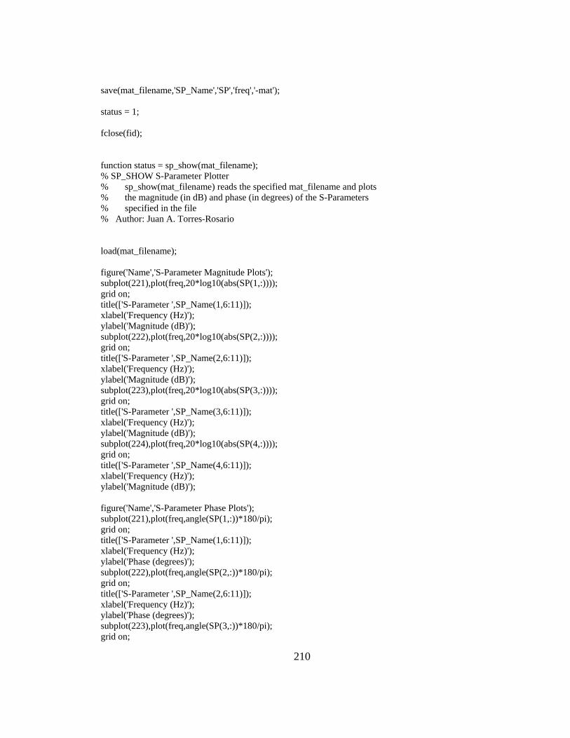
210
save(mat_filename,'SP_Name','SP','freq','-mat'); status = 1; fclose(fid); function status = sp_show(mat_filename); % SP_SHOW S-Parameter Plotter % sp_show(mat_filename) reads the specified mat_filename and plots % the magnitude (in dB) and phase (in degrees) of the S-Parameters % specified in the file % Author: Juan A. Torres-Rosario load(mat_filename); figure('Name','S-Parameter Magnitude Plots'); subplot(221),plot(freq,20*log10(abs(SP(1,:)))); grid on; title(['S-Parameter ',SP_Name(1,6:11)]); xlabel('Frequency (Hz)'); ylabel('Magnitude (dB)'); subplot(222),plot(freq,20*log10(abs(SP(2,:)))); grid on; title(['S-Parameter ',SP_Name(2,6:11)]); xlabel('Frequency (Hz)'); ylabel('Magnitude (dB)'); subplot(223),plot(freq,20*log10(abs(SP(3,:)))); grid on; title(['S-Parameter ',SP_Name(3,6:11)]); xlabel('Frequency (Hz)'); ylabel('Magnitude (dB)'); subplot(224),plot(freq,20*log10(abs(SP(4,:)))); grid on; title(['S-Parameter ',SP_Name(4,6:11)]); xlabel('Frequency (Hz)'); ylabel('Magnitude (dB)'); figure('Name','S-Parameter Phase Plots'); subplot(221),plot(freq,angle(SP(1,:))*180/pi); grid on; title(['S-Parameter ',SP_Name(1,6:11)]); xlabel('Frequency (Hz)'); ylabel('Phase (degrees)'); subplot(222),plot(freq,angle(SP(2,:))*180/pi); grid on; title(['S-Parameter ',SP_Name(2,6:11)]); xlabel('Frequency (Hz)'); ylabel('Phase (degrees)'); subplot(223),plot(freq,angle(SP(3,:))*180/pi); grid on;
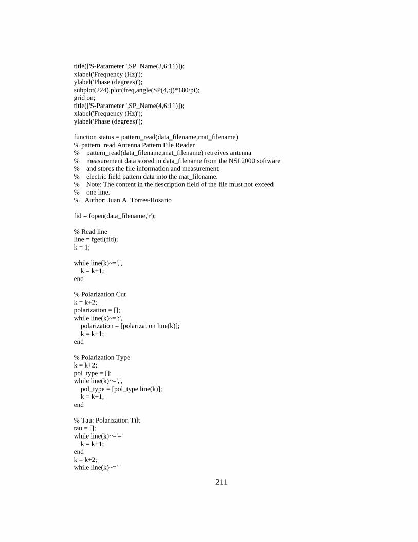
211
title(['S-Parameter ',SP_Name(3,6:11)]); xlabel('Frequency (Hz)'); ylabel('Phase (degrees)'); subplot(224),plot(freq,angle(SP(4,:))*180/pi); grid on; title(['S-Parameter ',SP_Name(4,6:11)]); xlabel('Frequency (Hz)'); ylabel('Phase (degrees)'); function status = pattern_read(data_filename,mat_filename) % pattern_read Antenna Pattern File Reader % pattern_read(data_filename,mat_filename) retreives antenna % measurement data stored in data_filename from the NSI 2000 software % and stores the file information and measurement % electric field pattern data into the mat_filename. % Note: The content in the description field of the file must not exceed % one line. % Author: Juan A. Torres-Rosario fid = fopen(data_filename,'r'); % Read line line = fgetl(fid); k = 1; while line(k)~=',', k = k+1; end % Polarization Cut k = k+2; polarization = []; while line(k)~=':', polarization = [polarization line(k)]; k = k+1; end % Polarization Type k = k+2; pol_type = []; while line(k)~=',', pol_type = [pol_type line(k)]; k = k+1; end % Tau: Polarization Tilt tau = []; while line(k)~='=' k = k+1; end k = k+2; while line(k)~=' '
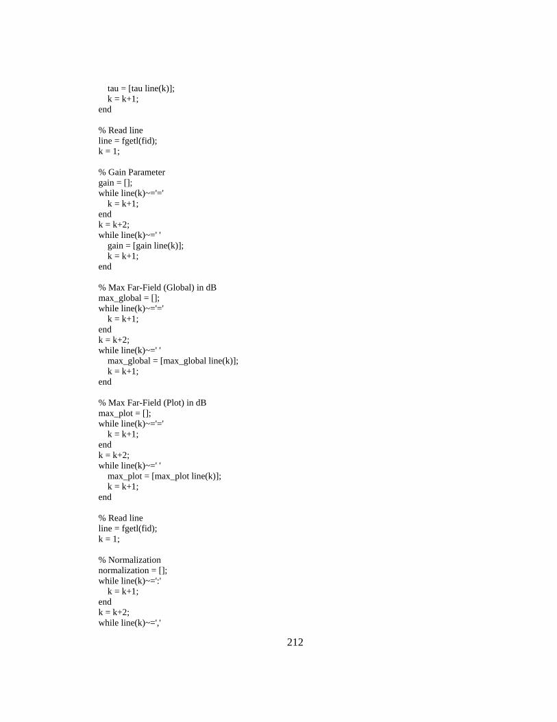
212
tau = [tau line(k)]; k = k+1; end % Read line line = fgetl(fid); k = 1; % Gain Parameter gain = []; while line(k)~='=' k = k+1; end k = k+2; while line(k)~=' ' gain = [gain line(k)]; k = k+1; end % Max Far-Field (Global) in dB max_global = []; while line(k)~='=' k = k+1; end k = k+2; while line(k)~=' ' max_global = [max_global line(k)]; k = k+1; end % Max Far-Field (Plot) in dB max_plot = []; while line(k)~='=' k = k+1; end k = k+2; while line(k)~=' ' max_plot = [max_plot line(k)]; k = k+1; end % Read line line = fgetl(fid); k = 1; % Normalization normalization = []; while line(k)~=':' k = k+1; end k = k+2; while line(k)~=','
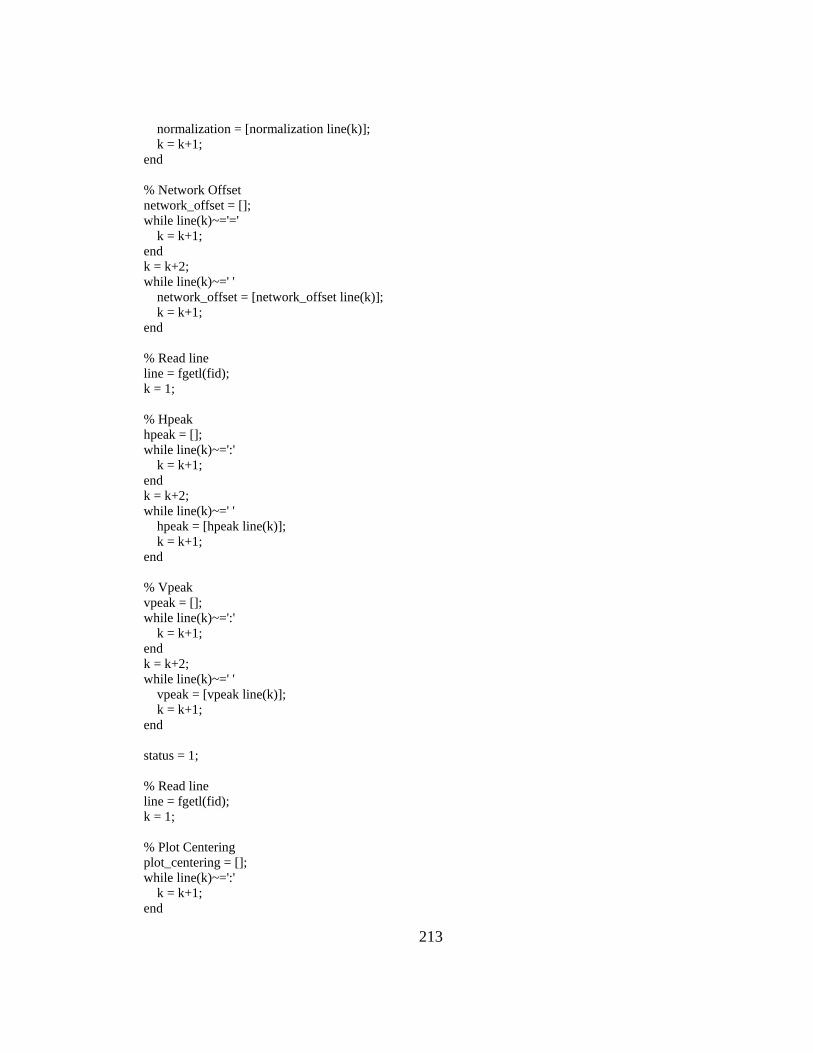
213
normalization = [normalization line(k)]; k = k+1; end % Network Offset network_offset = []; while line(k)~='=' k = k+1; end k = k+2; while line(k)~=' ' network_offset = [network_offset line(k)]; k = k+1; end % Read line line = fgetl(fid); k = 1; % Hpeak hpeak = []; while line(k)~=':' k = k+1; end k = k+2; while line(k)~=' ' hpeak = [hpeak line(k)]; k = k+1; end % Vpeak vpeak = []; while line(k)~=':' k = k+1; end k = k+2; while line(k)~=' ' vpeak = [vpeak line(k)]; k = k+1; end status = 1; % Read line line = fgetl(fid); k = 1; % Plot Centering plot_centering = []; while line(k)~=':' k = k+1; end

214
k = k+2; while k<=length(line) plot_centering = [plot_centering line(k)]; k = k+1; end % Read line line = fgetl(fid); k = 1; % Directivity directivity = []; while line(k)~='=' k = k+1; end k = k+2; while line(k)~=' ' directivity = [directivity line(k)]; k = k+1; end % FF Amplitude Info Structure FF_amplitude_info = struct('Eprincipal',pol_type,'Tau',str2num(tau),'Gain',str2num(gain),... 'Global_Max_Farfield',str2num(max_global),'Plot_Max_Farfield',str2num(max_plot),... 'Normalization',normalization,'Network_Offset',str2num(network_offset),'Hpeak',str2num(hpeak),... 'Vpeak',str2num(vpeak),'Plot_Centering',plot_centering,'Directivity',str2num(directivity)); % Read line line = fgetl(fid); k = 1; % Read line line = fgetl(fid); k = 1; % Read line line = fgetl(fid); k = 1; % Description Description = line; % Read line line = fgetl(fid); k = 1; % Read line line = fgetl(fid); k = 1; % Read line
215
line = fgetl(fid); k = 1; % Program Version prog_version = []; while line(k)~=',' prog_version = [prog_version line(k)]; k = k+1; end % Filename filename = []; while line(k)~=':' k = k+1; end k = k+1; while k<=length(line) filename = [filename line(k)]; k = k+1; end % Read line line = fgetl(fid); k = 1; % Measurement Date/Time measurement_date = []; while line(k)~=':' k = k+1; end k = k+2; while line(k)~=' ' measurement_date = [measurement_date line(k)]; k = k+1; end k = k+1; measurement_time = []; while line(k)~=',' measurement_time = [measurement_time line(k)]; k = k+1; end % Filetype filetype = []; while line(k)~=':' k = k+1; end k = k+2; while k<=length(line) filetype = [filetype line(k)]; k = k+1; end

216
% File Info Structure File_info = struct('Program_Version',prog_version,'Filename',filename,'Measurement_date',measurement_date,... 'Measurement_Time',measurement_time,'Filetype',filetype); %% Far-Field Display Setup % Read line line = fgetl(fid); k = 1; % Read line line = fgetl(fid); k = 1; % Read line line = fgetl(fid); k = 1; % Theta_Info theta_span = []; theta_center = []; theta_points = []; while line(k)~='=' k = k+1; end k = k+2; while line(k)~=' ' theta_span = [theta_span line(k)]; k = k+1; end while line(k)~='=' k = k+1; end k = k+2; while line(k)~=' ' theta_center = [theta_center line(k)]; k = k+1; end while line(k)~='=' k = k+1; end k = k+2; while line(k)~=' ' theta_points = [theta_points line(k)]; k = k+1; end % Read line line = fgetl(fid); k = 1;

217
theta_start = []; theta_stop = []; theta_delta = []; while line(k)~='=' k = k+1; end k = k+2; while line(k)~=' ' theta_start = [theta_start line(k)]; k = k+1; end while line(k)~='=' k = k+1; end k = k+2; while line(k)~=' ' theta_stop = [theta_stop line(k)]; k = k+1; end while line(k)~='=' k = k+1; end k = k+2; while line(k)~=' ' theta_delta = [theta_delta line(k)]; k = k+1; end % Read line line = fgetl(fid); k = 1; % Read line line = fgetl(fid); k = 1; % Phi_Info phi_span = []; phi_center = []; phi_points = []; while line(k)~='=' k = k+1; end k = k+2; while line(k)~=' ' phi_span = [phi_span line(k)]; k = k+1; end while line(k)~='=' k = k+1; end k = k+2;
218
while line(k)~=' ' phi_center = [phi_center line(k)]; k = k+1; end while line(k)~='=' k = k+1; end k = k+2; while line(k)~=' ' phi_points = [phi_points line(k)]; k = k+1; end % Read line line = fgetl(fid); k = 1; phi_start = []; phi_stop = []; phi_delta = []; while line(k)~='=' k = k+1; end k = k+2; while line(k)~=' ' phi_start = [phi_start line(k)]; k = k+1; end while line(k)~='=' k = k+1; end k = k+2; while line(k)~=' ' phi_stop = [phi_stop line(k)]; k = k+1; end while line(k)~='=' k = k+1; end k = k+2; while line(k)~=' ' phi_delta = [phi_delta line(k)]; k = k+1; end % Read Line line = fgetl(fid); k = 1; % Plot Rotation plot_rotation = []; while line(k)~='='
219
k = k+1; end k = k+2; while line(k)~=' ' plot_rotation = [plot_rotation line(k)]; k = k+1; end % Read Line line = fgetl(fid); k = 1; % Interpolation interpolation = []; while line(k)~=':' k = k+1; end k = k+2; while k<=length(line) interpolation = [interpolation line(k)]; k = k+1; end % Read Line line = fgetl(fid); k = 1; % Coordinate System coordinate_system = []; while line(k)~=':' k = k+1; end k = k+2; while line(k)~=';' coordinate_system = [coordinate_system line(k)]; k = k+1; end % Far-Field Display Polarization display_polarization = []; while line(k)~=':' k = k+1; end k = k+2; while k<=length(line) display_polarization = [display_polarization line(k)]; k = k+1; end % FF Display Setup Info Structure FF_display_setup_info = struct('Theta_Span',str2num(theta_span),'Theta_Center',str2num(theta_center),...
220
'Theta_Points',str2num(theta_points),'Theta_Start',str2num(theta_start),'Theta_Stop',str2num(theta_stop),... 'Theta_Delta',str2num(theta_delta),'Phi_Span',str2num(phi_span),'Phi_Center',str2num(phi_center),... 'Phi_Points',str2num(phi_points),'Phi_Start',str2num(phi_start),'Phi_Stop',str2num(phi_stop),... 'Phi_Delta',str2num(phi_delta),'Plot_Rotation',str2num(plot_rotation),'Interpolation',interpolation,... 'Coordinate_System',coordinate_system,'Display_Polarization',display_polarization); %% Far-Field Transform % Read Line line = fgetl(fid); k = 1; % Read Line line = fgetl(fid); k = 1; % FFT Size fft_size = []; while line(k)~=':' k = k+1; end k = k+3; while k<=length(line) fft_size = [fft_size line(k)]; k = k+1; end % Read Line line = fgetl(fid); k = 1; % Far-Field Display Polarization filter_mode = []; while line(k)~=':' k = k+1; end k = k+2; while line(k)~=',' filter_mode = [filter_mode line(k)]; k = k+1; end zoom = []; while line(k)~=':' k = k+1; end k = k+2; while k<=length(line) zoom = [zoom line(k)]; k = k+1; end
221
% Read Line line = fgetl(fid); k = 1; % Probe Setup probe_setup = []; while line(k)~=':' k = k+1; end k = k+2; while k<=length(line) probe_setup = [probe_setup line(k)]; k = k+1; end % Read Line line = fgetl(fid); k = 1; % Probe Model probe_model = []; while line(k)~=':' k = k+1; end k = k+2; while k<=length(line) probe_model = [probe_model line(k)]; k = k+1; end % FF Transform Setup Info Structure FF_transform_setup_info = struct('FFT_Size',fft_size,'Filter_Mode',filter_mode,... 'Zoom',zoom,'Probe_Setup',probe_setup,'Probe_Model',probe_model); %% Beam Information (Code valid only for one beam) % Read Line line = fgetl(fid); k = 1; % Read Line line = fgetl(fid); k = 1; % Read Line line = fgetl(fid); k = 1; % Read Line line = fgetl(fid); k = 1;
222
% Beam - Future work involves rearranging the information beam_info = line; %% Near-field setup % Read Line line = fgetl(fid); k = 1; % Read Line line = fgetl(fid); k = 1; % Read Line line = fgetl(fid); k = 1; % Near-field data near_field_data = []; while line(k)~='-' k = k+1; end k = k+2; while k<=length(line) near_field_data = [near_field_data line(k)]; k = k+1; end % Read Line line = fgetl(fid); k = 1; % Truncation truncation = []; while line(k)~=':' k = k+1; end k = k+2; while k<=length(line) truncation = [truncation line(k)]; k = k+1; end % Read Line line = fgetl(fid); k = 1; % Amplitude Tapering amplitude_tapering = []; while line(k)~=':' k = k+1;
223
end k = k+2; while k<=length(line) amplitude_tapering = [amplitude_tapering line(k)]; k = k+1; end % Read Line line = fgetl(fid); k = 1; % Network Correction network_correction = []; while line(k)~=':' k = k+1; end k = k+2; while k<=length(line) network_correction = [network_correction line(k)]; k = k+1; end % Read Line line = fgetl(fid); k = 1; % Phase Correction phase_correction = []; while line(k)~=':' k = k+1; end k = k+2; while k<=length(line) phase_correction = [phase_correction line(k)]; k = k+1; end % NF Setup Info Structure NF_setup_info = struct('Data',near_field_data,'Truncation',truncation,'Amplitude_Tapering',amplitude_tapering,... 'Network_Correction',network_correction,'Position_Phase_Correction',phase_correction); %% Measured Data % Read Line line = fgetl(fid); k = 1; % Read Line line = fgetl(fid); k = 1;
224
% Read Line line = fgetl(fid); k = 1; % Measured Theta_Info mtheta_span = []; mtheta_center = []; mtheta_points = []; while line(k)~='=' k = k+1; end k = k+2; while line(k)~=' ' mtheta_span = [mtheta_span line(k)]; k = k+1; end while line(k)~='=' k = k+1; end k = k+2; while line(k)~=' ' mtheta_center = [mtheta_center line(k)]; k = k+1; end while line(k)~='=' k = k+1; end k = k+2; while line(k)~=' ' mtheta_points = [mtheta_points line(k)]; k = k+1; end % Read line line = fgetl(fid); k = 1; mtheta_start = []; mtheta_stop = []; mtheta_delta = []; while line(k)~='=' k = k+1; end k = k+2; while line(k)~=' ' mtheta_start = [mtheta_start line(k)]; k = k+1; end while line(k)~='=' k = k+1; end
225
k = k+2; while line(k)~=' ' mtheta_stop = [mtheta_stop line(k)]; k = k+1; end while line(k)~='=' k = k+1; end k = k+2; while line(k)~=' ' mtheta_delta = [mtheta_delta line(k)]; k = k+1; end % Read line line = fgetl(fid); k = 1; % Read line line = fgetl(fid); k = 1; % Phi_Info mphi_span = []; mphi_center = []; mphi_points = []; while line(k)~='=' k = k+1; end k = k+2; while line(k)~=' ' mphi_span = [mphi_span line(k)]; k = k+1; end while line(k)~='=' k = k+1; end k = k+2; while line(k)~=' ' mphi_center = [mphi_center line(k)]; k = k+1; end while line(k)~='=' k = k+1; end k = k+2; while line(k)~=' ' mphi_points = [mphi_points line(k)]; k = k+1; end % Read line
226
line = fgetl(fid); k = 1; mphi_start = []; mphi_stop = []; mphi_delta = []; while line(k)~='=' k = k+1; end k = k+2; while line(k)~=' ' mphi_start = [mphi_start line(k)]; k = k+1; end while line(k)~='=' k = k+1; end k = k+2; while line(k)~=' ' mphi_stop = [mphi_stop line(k)]; k = k+1; end while line(k)~='=' k = k+1; end k = k+2; while line(k)~=' ' mphi_delta = [mphi_delta line(k)]; k = k+1; end % Read Line line = fgetl(fid); k = 1; % AUT Dimensions aut_height = []; aut_width = []; while line(k)~=':' k = k+1; end k = k+2; while line(k)~=' ' aut_width = [aut_width line(k)]; k = k+1; end while line(k)~=',' k = k+1; end k = k+2; while line(k)~=' ' aut_height = [aut_height line(k)];
227
k = k+1; end % Read Line line = fgetl(fid); k = 1; % H/V Max Far-field Angles h_max_angle = []; v_max_angle = []; while line(k)~=':' k = k+1; end k = k+2; while line(k)~=' ' h_max_angle = [h_max_angle line(k)]; k = k+1; end while line(k)~=',' k = k+1; end k = k+2; while line(k)~=' ' v_max_angle = [v_max_angle line(k)]; k = k+1; end % Read Line line = fgetl(fid); k = 1; % Measurement Radius measure_radius = []; while line(k)~=':' k = k+1; end k = k+2; while line(k)~=' ' measure_radius = [measure_radius line(k)]; k = k+1; end % Read Line line = fgetl(fid); k = 1; % MRE mre = []; while line(k)~=':' k = k+1; end k = k+2;

228
while line(k)~=' ' mre = [mre line(k)]; k = k+1; end % Read Line line = fgetl(fid); k = 1; % Read Line line = fgetl(fid); k = 1; % Measured Data Info Structure Measured_data_info = struct('Measured_Theta_Span',str2num(mtheta_span),'Measured_Theta_Center',str2num(mtheta_center),... 'Measured_Theta_Points',str2num(mtheta_points),'Measured_Theta_Start',str2num(mtheta_start),'Measured_Theta_Stop',str2num(mtheta_stop),... 'Measured_Theta_Delta',str2num(mtheta_delta),'Measured_Phi_Span',str2num(mphi_span),'Measured_Phi_Center',str2num(mphi_center),... 'Measured_Phi_Points',str2num(mphi_points),'Measured_Phi_Start',str2num(mphi_start),'Measured_Phi_Stop',str2num(mphi_stop),... 'Measured_Phi_Delta',str2num(mphi_delta),'AUT_Width',str2num(aut_width),'AUT_Height',str2num(aut_height),'H_Max_Farfield_Angle',str2num(h_max_angle),... 'V_Max_Farfield_Angle',str2num(v_max_angle),'Measurement_Radius',str2num(measure_radius),'MRE',str2num(mre)); % Measurement Type measure_type = []; while line(k)~=':' k = k+1; end k = k+2; while k<=length(line) measure_type = [measure_type line(k)]; k = k+1; end % Read Line line = fgetl(fid); k = 1; % Scan Options scan_options = []; while line(k)~=':' k = k+1; end
229
k = k+2; while k<=length(line) scan_options = [scan_options line(k)]; k = k+1; end % Read Line line = fgetl(fid); k = 1; % Beamset Smear beamset_smear = []; while line(k)~=':' k = k+1; end k = k+2; while line(k)~=' ' beamset_smear = [beamset_smear line(k)]; k = k+1; end %% Probe setup as acquired % Read Line line = fgetl(fid); k = 1; % Read Line line = fgetl(fid); k = 1; % Beamset Smear mprobe_model = []; while line(k)~=':' k = k+1; end k = k+2; while k<=length(line) mprobe_model = [mprobe_model line(k)]; k = k+1; end % Read Line line = fgetl(fid); k = 1; % Probe 1 probe_1 = []; while line(k)~=':' k = k+1; end k = k+2; while line(k)~=','
230
probe_1 = [probe_1 line(k)]; k = k+1; end % Probe 2 probe_2 = []; while line(k)~=':' k = k+1; end k = k+1; while k<=length(line) probe_2 = [probe_2 line(k)]; k = k+1; end % Measurement Info Structure Measurement_info = struct('Measure_Type',measure_type,'Scan_Options',scan_options,... 'Beamset_Smear',str2num(beamset_smear),'Probe_Setup','as Acquired','Probe_Model',mprobe_model,... 'Probe_1',probe_1,'Probe_2',probe_2); %% RF System % Read Line line = fgetl(fid); k = 1; % Read Line line = fgetl(fid); k = 1; % Read Line line = fgetl(fid); k = 1; % Integration Time integration_time = []; while line(k)~=':' k = k+1; end k = k+2; while line(k)~=' ' integration_time = [integration_time line(k)]; k = k+1; end % Read Line line = fgetl(fid); k = 1; % Scan Speed scan_speed = [];

231
while line(k)~=':' k = k+1; end k = k+2; while line(k)~=' ' scan_speed = [scan_speed line(k)]; k = k+1; end % Read Line line = fgetl(fid); k = 1; % Scan Info scan_info = line; % Read Line line = fgetl(fid); k = 1; % Amp/Phase Initial amp_initial = []; phase_initial = []; while line(k)~='=' k = k+1; end k = k+3; while line(k)~=' ' amp_initial = [amp_initial line(k)]; k = k+1; end while line(k)~=',' k = k+1; end k = k+3; while line(k)~=' ' phase_initial = [phase_initial line(k)]; k = k+1; end % Read Line line = fgetl(fid); k = 1; % Amp/Phase Drift amp_drift = []; phase_drift = []; while line(k)~='=' k = k+1; end k = k+3; while line(k)~=' '
232
amp_drift = [amp_drift line(k)]; k = k+1; end while line(k)~=',' k = k+1; end k = k+3; while line(k)~=' ' phase_drift = [phase_drift line(k)]; k = k+1; end % RF System Info Structure RF_system_info = struct('Integration_Time',str2num(integration_time),'Scan_Speed',str2num(scan_speed),... 'Amp_Initial',str2num(amp_initial),'Phase_Initial',str2num(phase_initial),'Amp_Drift',str2num(amp_drift),... 'Phase_Drift',str2num(phase_drift)); %% Measurement Data % Read Line line = fgetl(fid); k = 1; % Read Line line = fgetl(fid); k = 1; for p=1:FF_display_setup_info.Phi_Points for q=1:FF_display_setup_info.Theta_Points % Read Line line = fgetl(fid); k = 1; % Change String Format into Numerical Format nline = str2num(line); % Spherical Coordinates theta_coor(p,q) = nline(1); phi_coor(p,q) = nline(2); % E-field Pattern E_field(p,q) = 10^(nline(3)/20).*exp(j*nline(4)*pi/180); end end

233
save(mat_filename,'FF_amplitude_info','File_info','FF_display_setup_info','FF_transform_setup_info',... 'NF_setup_info','Measured_data_info','Measurement_info','RF_system_info','theta_coor','phi_coor',... 'E_field','-mat'); fclose(fid); function status = pattern_calc(Ephi_filename,Etheta_filename,Efield_filename) % pattern_calc Antenna Pattern Calculator % pattern_calc(Ephi_filename,Etheta_filename,Efield_filename) retrieves % Electric Field measurement data from Ephi_filename and % Etheta_filename MAT files, calculates the Magnitude of the Electric Field, and % stores the result in the Efield_filename mat file. % Note: Linear antenna is placed along Azimuth plane % Author: Juan A. Torres-Rosario % Load Ephi Component load(Ephi_filename); E_phi = E_field; % Load Etheta Component load(Etheta_filename); E_theta = E_field; % Calculate Electric Field Radiation Pattern E_field = sqrt(abs(E_theta).^2+abs(E_phi).^2); [E_x,E_y,E_z] = sph2cart(phi_coor*pi/180, (-(theta_coor)*pi/180), abs(E_field)); theta_coor = theta_coor+90; % Calculate Efield for Polar Plot View E_polar = E_field(:,1:101); % Calculate Theta vector theta_vector = [-1*fliplr(theta_coor(151,2:201)) theta_coor(51,1:201)]; % Calculate Elevation Cut El_cut = [fliplr(E_field(151,2:201)) E_field(51,1:201)]; % Calculate Azimuth Cut Az_cut = [fliplr(E_field(101,2:201)) E_field(1,1:201)]; save(Efield_filename,'E_field','theta_coor','phi_coor','theta_vector','E_x','E_y','E_z','Az_cut','El_cut',... 'E_phi','E_theta','E_polar');