PE 2019

Implementation of a Pavement Friction Management Program for

Virginia DOTBy

Ross McCarthy

Virginia Tech Transportation Institute

PE 2019

Outline• Introduction

• Objectives

• Methodology

• Example

• Conclusions

PE 2019

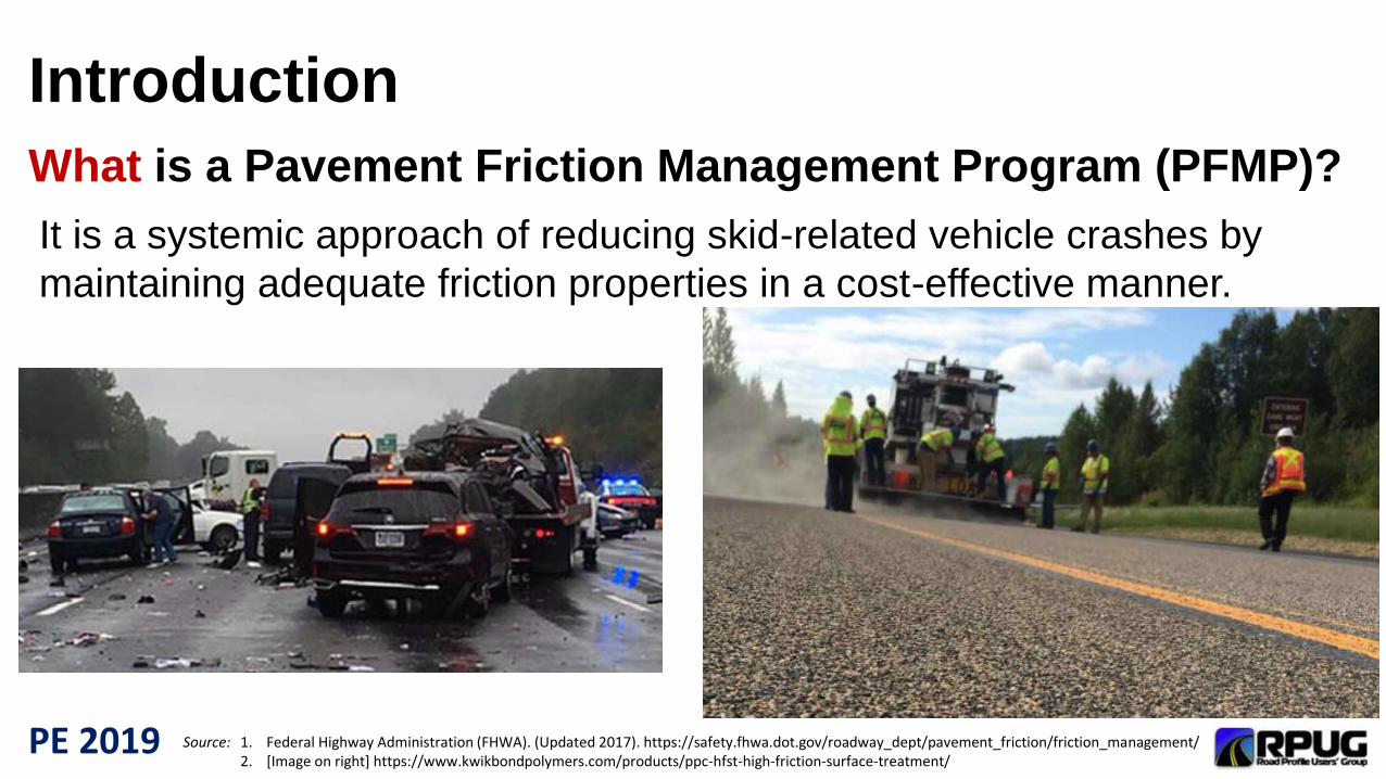
Introduction

What is a Pavement Friction Management Program (PFMP)?

Source: 1. Federal Highway Administration (FHWA). (Updated 2017). https://safety.fhwa.dot.gov/roadway_dept/pavement_friction/friction_management/2. [Image on right] https://www.kwikbondpolymers.com/products/ppc-hfst-high-friction-surface-treatment/

It is a systemic approach of reducing skid-related vehicle crashes by

maintaining adequate friction properties in a cost-effective manner.

PE 2019

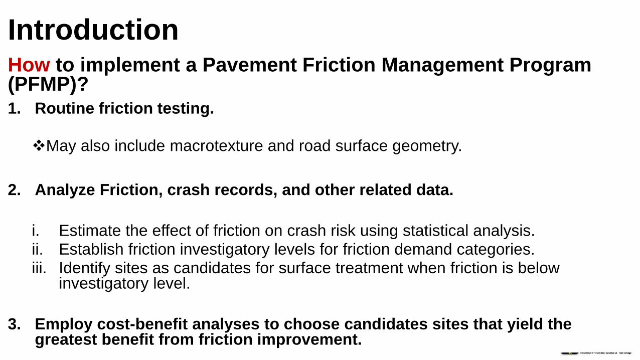
IntroductionHow to implement a Pavement Friction Management Program (PFMP)?1. Routine friction testing.

May also include macrotexture and road surface geometry.

2. Analyze Friction, crash records, and other related data.

i. Estimate the effect of friction on crash risk using statistical analysis.ii. Establish friction investigatory levels for friction demand categories.iii. Identify sites as candidates for surface treatment when friction is below

investigatory level.

3. Employ cost-benefit analyses to choose candidates sites that yield the greatest benefit from friction improvement.

PE 2019

Introduction: Terminology

What is Friction Demand?

The amount of friction needed to safely maneuver a vehicle:

1. Acceleration

2. Braking

3. Steering

PE 2019

Introduction: Terminology

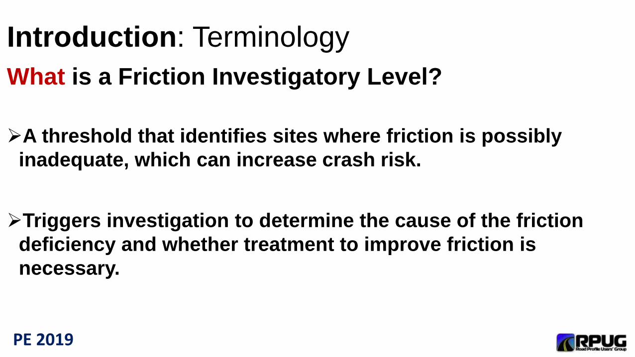
What is a Friction Investigatory Level?

A threshold that identifies sites where friction is possibly

inadequate, which can increase crash risk.

Triggers investigation to determine the cause of the friction

deficiency and whether treatment to improve friction is

necessary.

PE 2019

Objective

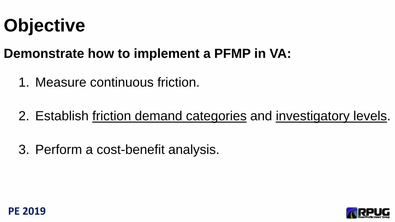
Demonstrate how to implement a PFMP in VA:

1. Measure continuous friction.

2. Establish friction demand categories and investigatory levels.

3. Perform a cost-benefit analysis.

PE 2019

Methodology

PE 2019

Methodology

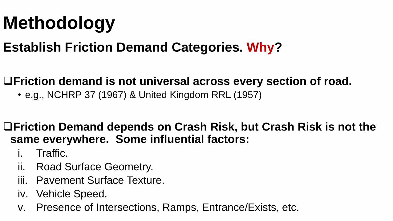
Establish Friction Demand Categories. Why?

Friction demand is not universal across every section of road. • e.g., NCHRP 37 (1967) & United Kingdom RRL (1957)

Friction Demand depends on Crash Risk, but Crash Risk is not the same everywhere. Some influential factors:

i. Traffic.

ii. Road Surface Geometry.

iii. Pavement Surface Texture.

iv. Vehicle Speed.

v. Presence of Intersections, Ramps, Entrance/Exists, etc.

PE 2019

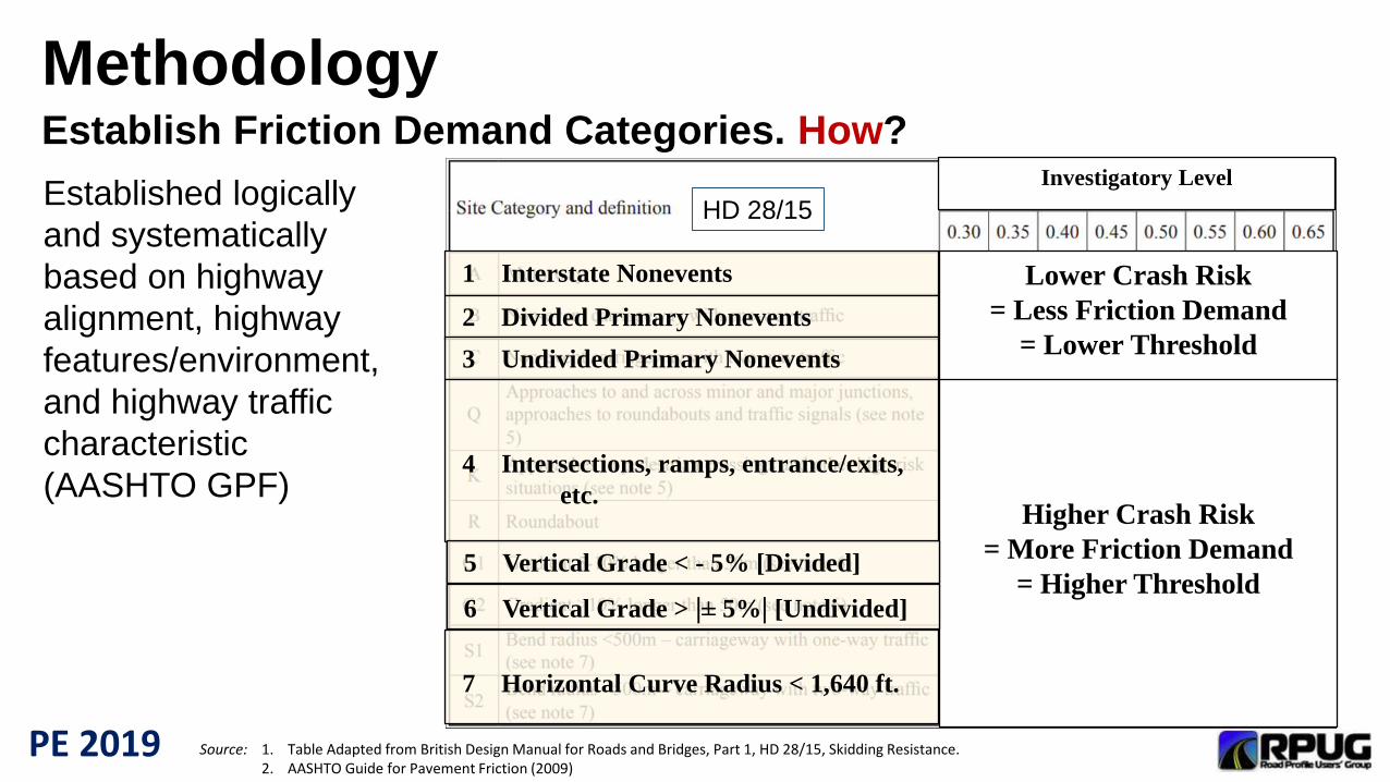
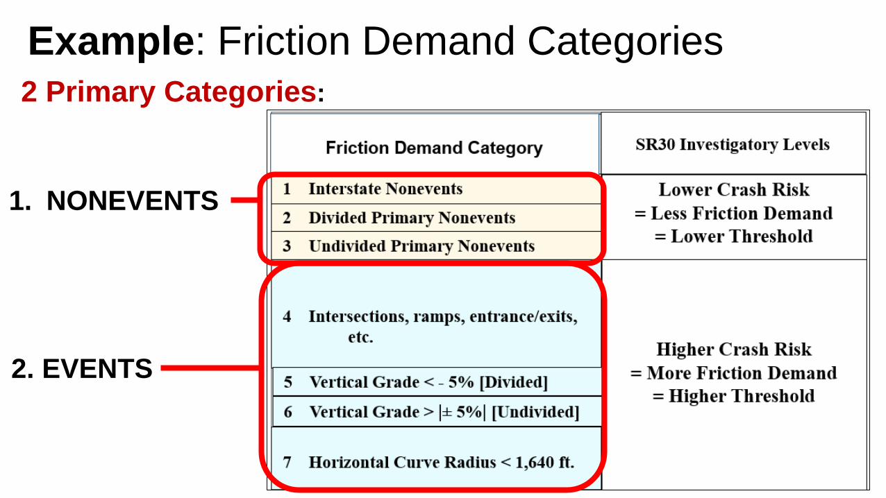
MethodologyEstablish Friction Demand Categories. How?

Source: 1. Table Adapted from British Design Manual for Roads and Bridges, Part 1, HD 28/15, Skidding Resistance.2. AASHTO Guide for Pavement Friction (2009)

1 Interstate Nonevents

Investigatory Level

2 Divided Primary Nonevents

3 Undivided Primary Nonevents

4 Intersections, ramps, entrance/exits,

etc.

7 Horizontal Curve Radius < 1,640 ft.

Lower Crash Risk

= Less Friction Demand

= Lower Threshold

Higher Crash Risk

= More Friction Demand

= Higher Threshold

Established logically

and systematically

based on highway

alignment, highway

features/environment,

and highway traffic

characteristic

(AASHTO GPF)

5 Vertical Grade < - 5% [Divided]

6 Vertical Grade > |± 5%| [Undivided]

HD 28/15

PE 2019

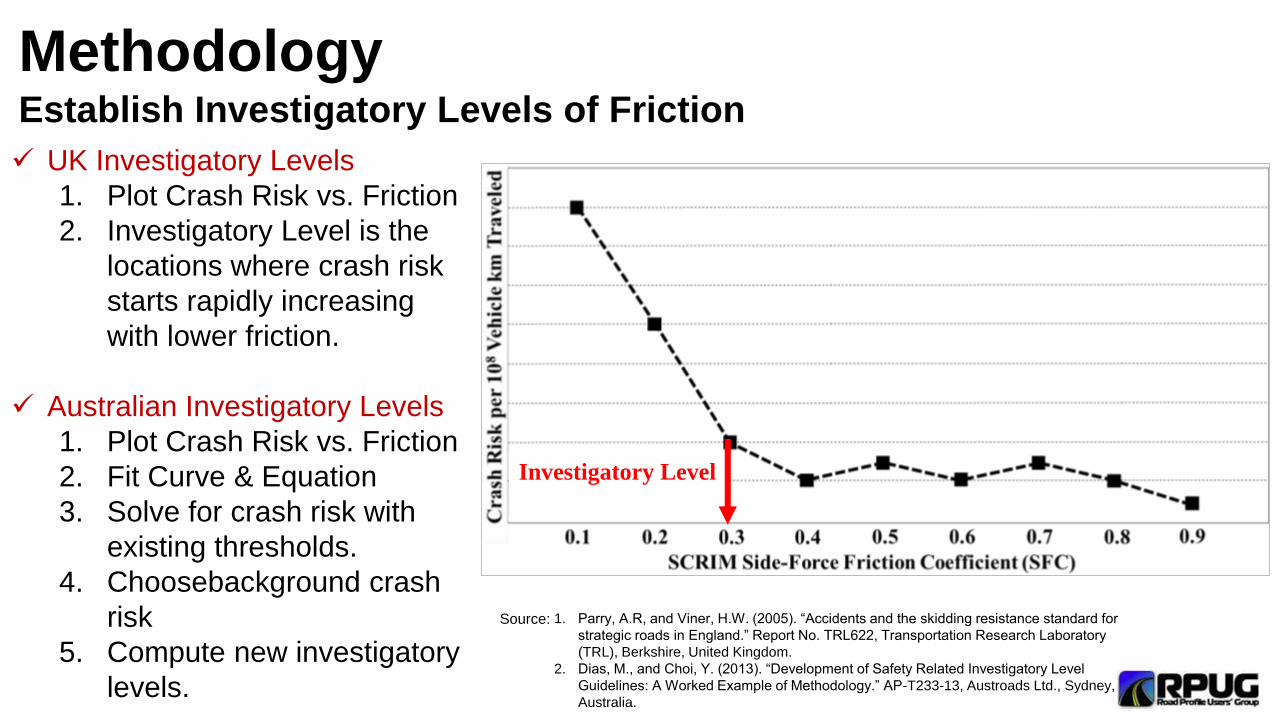
MethodologyEstablish Investigatory Levels of Friction

Source: 1. Parry, A.R, and Viner, H.W. (2005). “Accidents and the skidding resistance standard for

strategic roads in England.” Report No. TRL622, Transportation Research Laboratory

(TRL), Berkshire, United Kingdom.

2. Dias, M., and Choi, Y. (2013). “Development of Safety Related Investigatory Level

Guidelines: A Worked Example of Methodology.” AP-T233-13, Austroads Ltd., Sydney,

Australia.

UK Investigatory Levels

1. Plot Crash Risk vs. Friction

2. Investigatory Level is the

locations where crash risk

starts rapidly increasing

with lower friction.

Australian Investigatory Levels

1. Plot Crash Risk vs. Friction

2. Fit Curve & Equation

3. Solve for crash risk with

existing thresholds.

4. Choosebackground crash

risk

5. Compute new investigatory

levels.

Investigatory Level

PE 2019

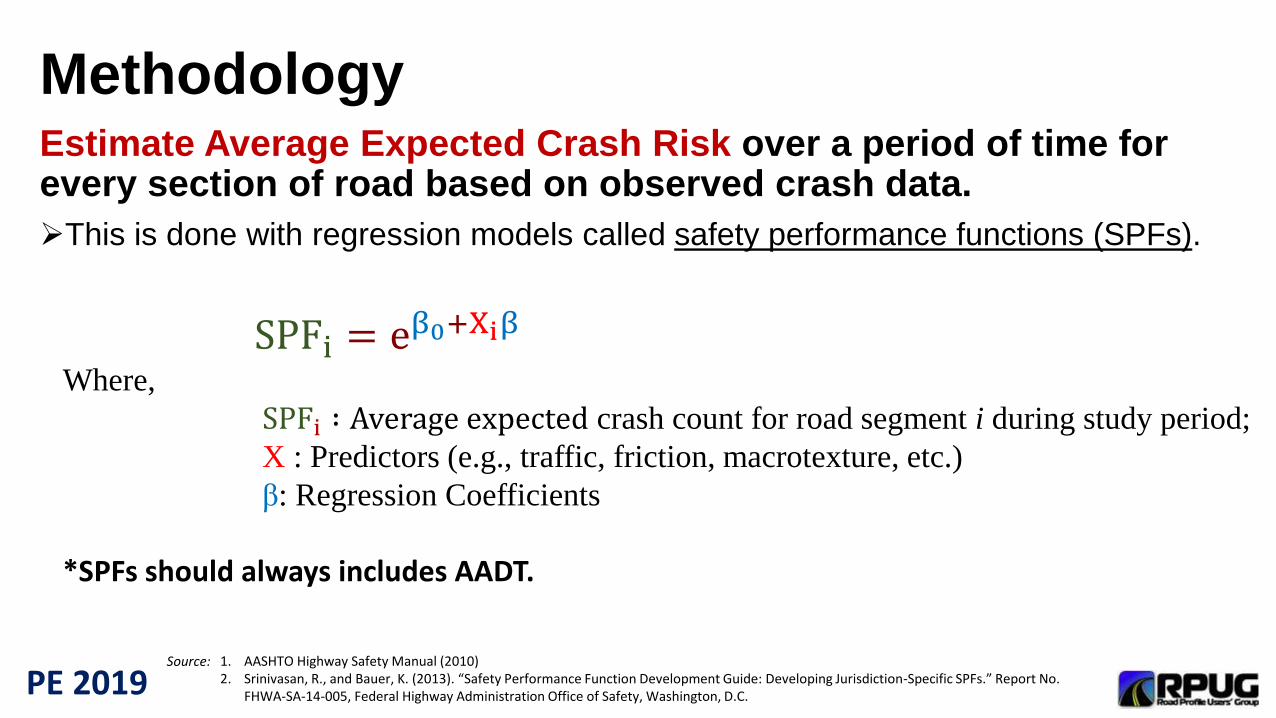
MethodologyEstimate Average Expected Crash Risk over a period of time for every section of road based on observed crash data.

This is done with regression models called safety performance functions (SPFs).

Source: 1. AASHTO Highway Safety Manual (2010)2. Srinivasan, R., and Bauer, K. (2013). “Safety Performance Function Development Guide: Developing Jurisdiction-Specific SPFs.” Report No.

FHWA-SA-14-005, Federal Highway Administration Office of Safety, Washington, D.C.

SPFi = eβ0+Xiβ

Where,

SPFi ∶ Average expected crash count for road segment i during study period;

X : Predictors (e.g., traffic, friction, macrotexture, etc.)

β: Regression Coefficients

*SPFs should always includes AADT.

PE 2019

MethodologyIn order to assess benefits of surface treatment in a PFMP, statistically reliable estimates

of average expected crash counts are required.

Research has shown that statistical reliability is improved by combining observed crash counts and SPF estimates into a weighted average.

Empirical Bayes (EB) Methodology

Source: Hauer, E., Harwood, D.W., Council, F.M., and Griffith, M.S. (2002). “Estimating Safety by the Empirical Bayes Method: A Tutorial.” Transportation Research Board, (1784), 126-131.

2 types of information:1. SPF

2. Observed Crash Count, y

Computation:

𝐄𝐁𝐢 = 𝐰𝐢 ∗ 𝐒𝐏𝐅𝐢 + 𝟏 −𝐰𝐢 ∗ 𝐲i

weight parameter: 𝐰𝐢 =𝟏

𝟏+𝐒𝐏𝐅𝐢×𝛂; where 𝛂 is the overdispersion parameter from SPF

PE 2019

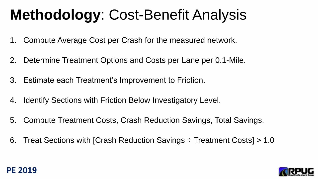
Methodology: Cost-Benefit Analysis

1. Compute Average Cost per Crash for the measured network.

2. Determine Treatment Options and Costs per Lane per 0.1-Mile.

3. Estimate each Treatment’s Improvement to Friction.

4. Identify Sections with Friction Below Investigatory Level.

5. Compute Treatment Costs, Crash Reduction Savings, Total Savings.

6. Treat Sections with [Crash Reduction Savings ÷ Treatment Costs] > 1.0

PE 2019

Example

PE 2019

1 23 4

5

87

9

6

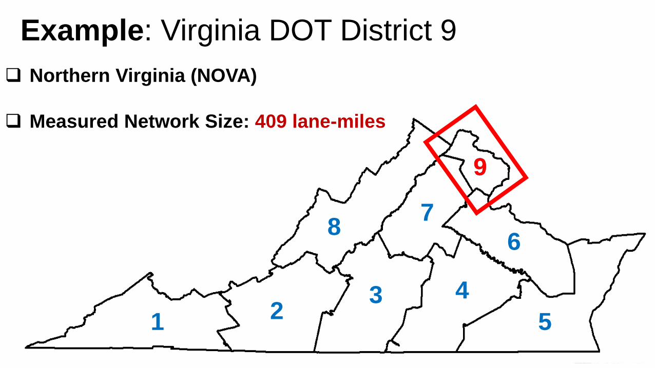
Example: Virginia DOT District 9

Northern Virginia (NOVA)

Measured Network Size: 409 lane-miles

9

PE 2019

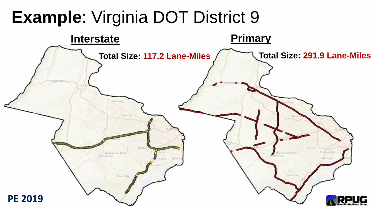
Example: Virginia DOT District 9 Interstate

Total Size: 117.2 Lane-Miles

Primary

Total Size: 291.9 Lane-Miles

PE 2019

Example: Data Collection & Processing

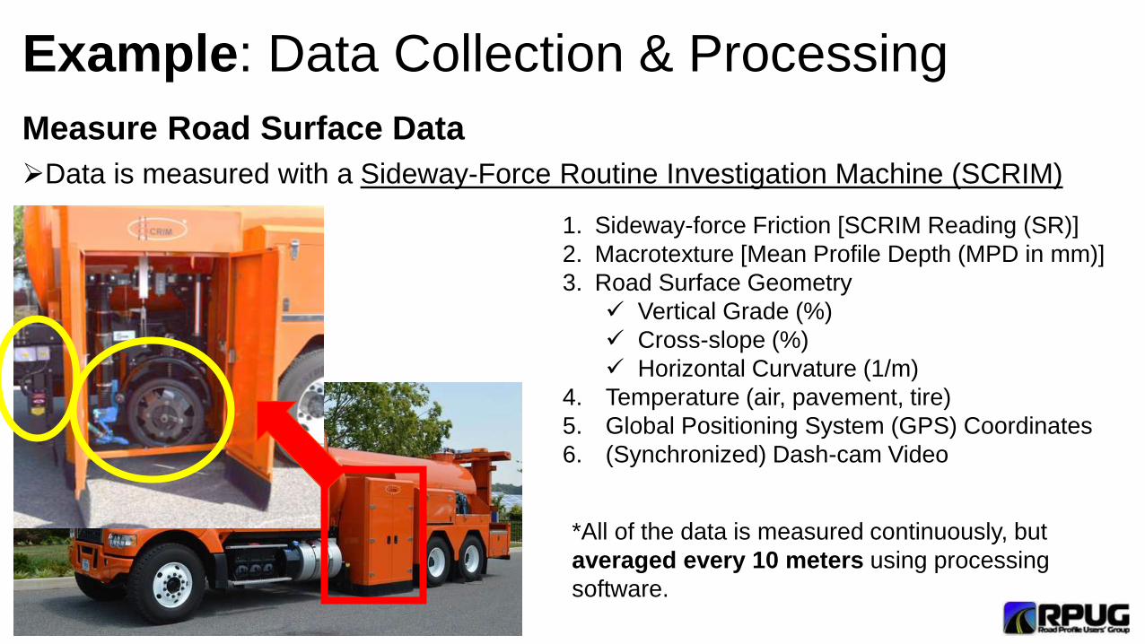
Measure Road Surface Data

Data is measured with a Sideway-Force Routine Investigation Machine (SCRIM)

1. Sideway-force Friction [SCRIM Reading (SR)]

2. Macrotexture [Mean Profile Depth (MPD in mm)]

3. Road Surface Geometry

Vertical Grade (%)

Cross-slope (%)

Horizontal Curvature (1/m)

4. Temperature (air, pavement, tire)

5. Global Positioning System (GPS) Coordinates

6. (Synchronized) Dash-cam Video

*All of the data is measured continuously, but

averaged every 10 meters using processing

software.

PE 2019

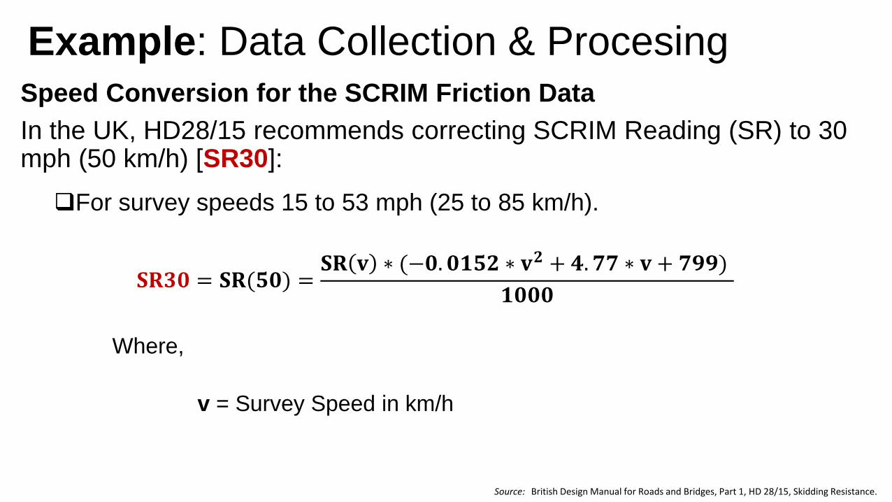
Example: Data Collection & ProcesingSpeed Conversion for the SCRIM Friction Data

In the UK, HD28/15 recommends correcting SCRIM Reading (SR) to 30 mph (50 km/h) [SR30]:

For survey speeds 15 to 53 mph (25 to 85 km/h).

𝐒𝐑𝟑𝟎 = 𝐒𝐑(𝟓𝟎) =𝐒𝐑 𝐯 ∗ (−𝟎. 𝟎𝟏𝟓𝟐 ∗ 𝐯𝟐 + 𝟒. 𝟕𝟕 ∗ 𝐯 + 𝟕𝟗𝟗)

𝟏𝟎𝟎𝟎

Where,

v = Survey Speed in km/h

Source: British Design Manual for Roads and Bridges, Part 1, HD 28/15, Skidding Resistance.

PE 2019

Example: Data Collection & Processing

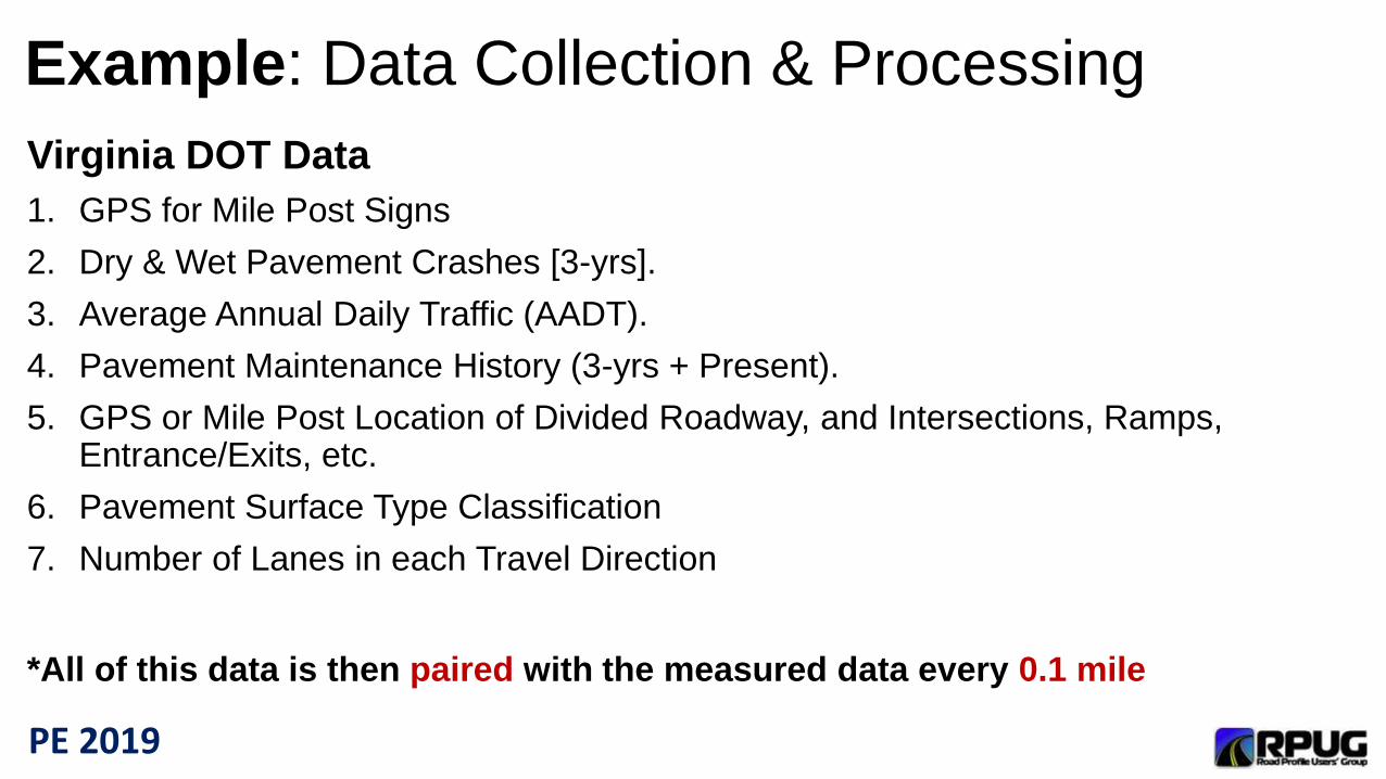
Virginia DOT Data

1. GPS for Mile Post Signs

2. Dry & Wet Pavement Crashes [3-yrs].

3. Average Annual Daily Traffic (AADT).

4. Pavement Maintenance History (3-yrs + Present).

5. GPS or Mile Post Location of Divided Roadway, and Intersections, Ramps, Entrance/Exits, etc.

6. Pavement Surface Type Classification

7. Number of Lanes in each Travel Direction

*All of this data is then paired with the measured data every 0.1 mile

PE 2019

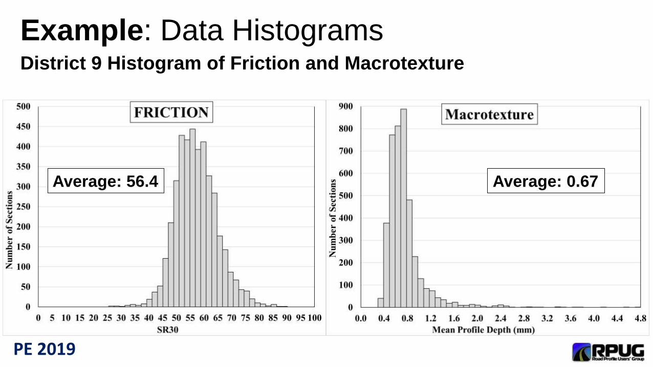
Example: Data HistogramsDistrict 9 Histogram of Friction and Macrotexture

Average: 56.4 Average: 0.67

PE 2019

Example: Friction Demand Categories 2 Primary Categories:

1. NONEVENTS

2. EVENTS

PE 2019

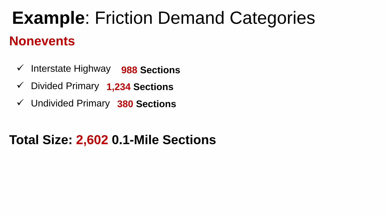
Example: Friction Demand Categories

Nonevents

Total Size: 2,602 0.1-Mile Sections

Interstate Highway

Divided Primary

Undivided Primary 380 Sections

988 Sections

1,234 Sections

PE 2019

Example: Friction Demand Categories

Events

Total Size: 1,478 0.1-Mile Sections

Intersections, ramps, entrances/exits, etc.

Horizontal Curve Radius < 1,640 feet.

Divided Vertical Gradient < -5%

Undivided Vertical Gradient > |±5%|45 Sections

1,371 Sections

62 Sections

PE 2019

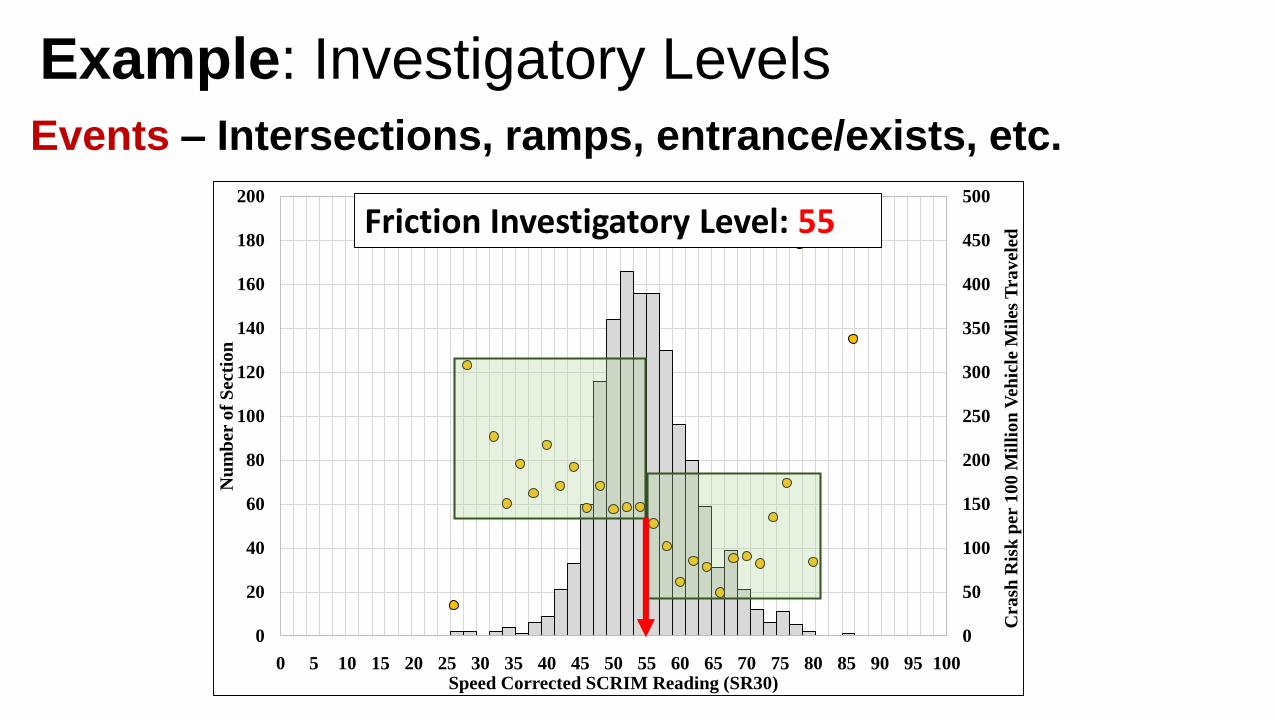
Example: Investigatory Levels

Events – Intersections, ramps, entrance/exists, etc.

0 5 10 15 20 25 30 35 40 45 50 55 60 65 70 75 80 85 90 95 100

0

50

100

150

200

250

300

350

400

450

500

0

20

40

60

80

100

120

140

160

180

200

Cra

sh R

isk

per

10

0 M

illi

on

Veh

icle

Mil

es T

rav

eled

Nu

mb

er o

f S

ecti

on

Speed Corrected SCRIM Reading (SR30)

Friction Investigatory Level: 55

PE 2019

Example: Investigatory LevelsEvents

Investigatory Level: 55

Nonevents

Investigatory Level: 50

NOTE:

Thresholds for FHWA Project

Events: 50 – 60

Nonevents: 35 – 45

PE 2019

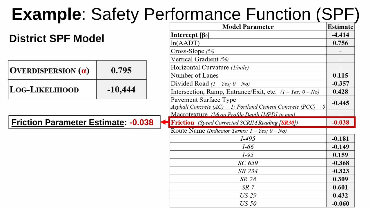
Example: Safety Performance Function (SPF)

District SPF Model

Friction Parameter Estimate: -0.038

PE 2019

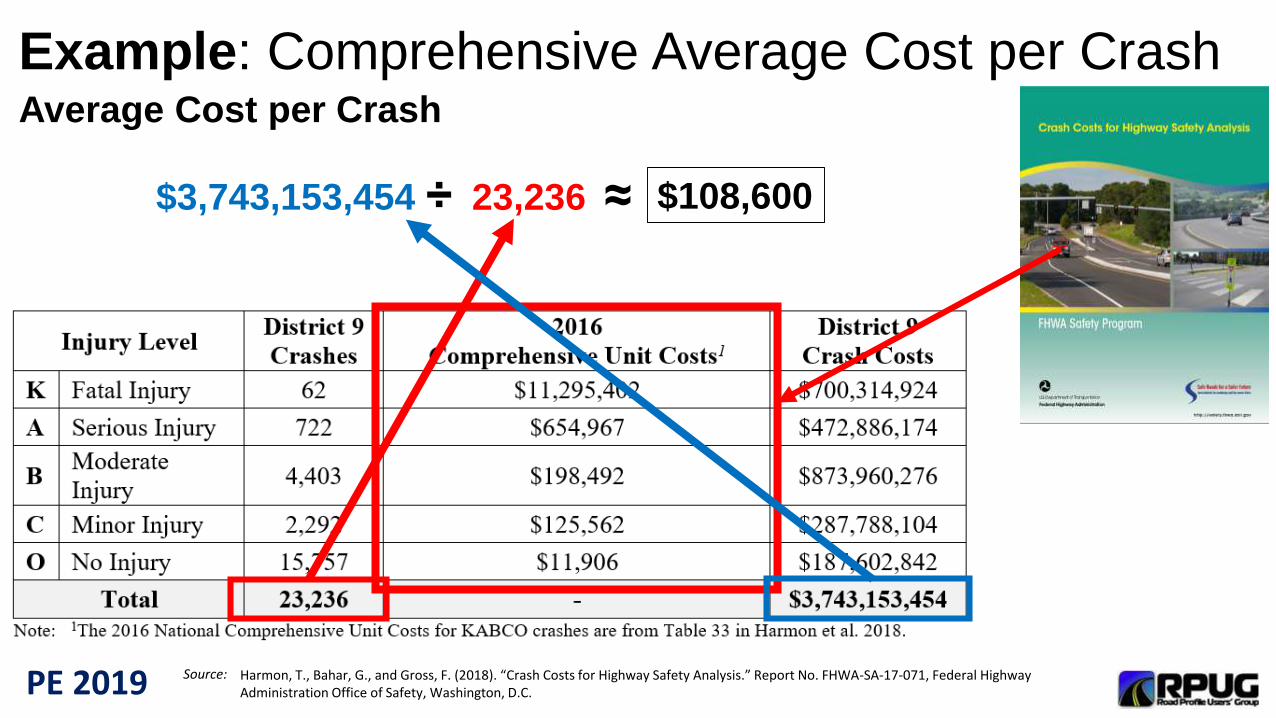
Example: Comprehensive Average Cost per CrashAverage Cost per Crash

Source: Harmon, T., Bahar, G., and Gross, F. (2018). “Crash Costs for Highway Safety Analysis.” Report No. FHWA-SA-17-071, Federal Highway Administration Office of Safety, Washington, D.C.

$3,743,153,454 23,236÷ ≈ $108,600

PE 2019

Example: Treatment Options NOTE: Example for Asphalt Concrete [AC] Surfaces only.

AC Treatment Options:

1. Hot Mix Asphalt (HMA) Overlay

Cost per Lane per 0.1-Mile: $8,230

SR30 = 65

2. High Friction Surface (HFS)

Cost per Lane per 0.1-Mile: $19,000

SR30 = 80

PE 2019

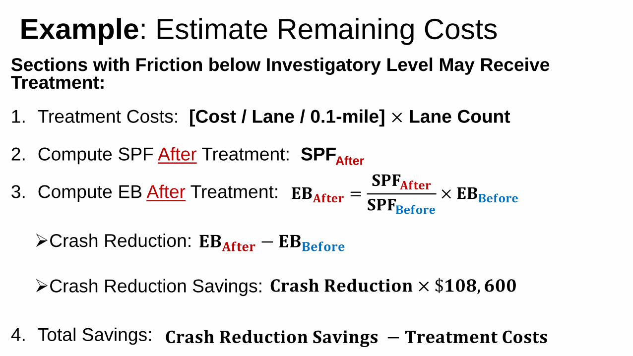
Example: Estimate Remaining Costs Sections with Friction below Investigatory Level May Receive Treatment:

1. Treatment Costs: [Cost / Lane / 0.1-mile] × Lane Count

2. Compute SPF After Treatment: SPFAfter

3. Compute EB After Treatment:

Crash Reduction:

Crash Reduction Savings:

4. Total Savings:

𝐄𝐁𝐀𝐟𝐭𝐞𝐫 =𝐒𝐏𝐅𝐀𝐟𝐭𝐞𝐫𝐒𝐏𝐅𝐁𝐞𝐟𝐨𝐫𝐞

× 𝐄𝐁𝐁𝐞𝐟𝐨𝐫𝐞

𝐄𝐁𝐀𝐟𝐭𝐞𝐫 − 𝐄𝐁𝐁𝐞𝐟𝐨𝐫𝐞

𝐂𝐫𝐚𝐬𝐡 𝐑𝐞𝐝𝐮𝐜𝐭𝐢𝐨𝐧 × $𝟏𝟎𝟖, 𝟔𝟎𝟎

𝐂𝐫𝐚𝐬𝐡 𝐑𝐞𝐝𝐮𝐜𝐭𝐢𝐨𝐧 𝐒𝐚𝐯𝐢𝐧𝐠𝐬 − 𝐓𝐫𝐞𝐚𝐭𝐦𝐞𝐧𝐭 𝐂𝐨𝐬𝐭𝐬

PE 2019

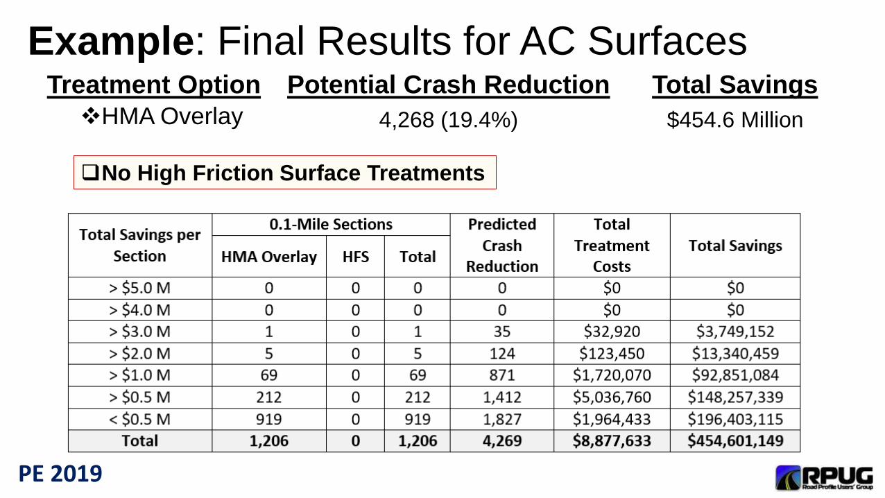
Example: Final Results for AC SurfacesTreatment Option

HMA Overlay

Potential Crash Reduction

4,268 (19.4%)

Total Savings

$454.6 Million

No High Friction Surface Treatments

PE 2019

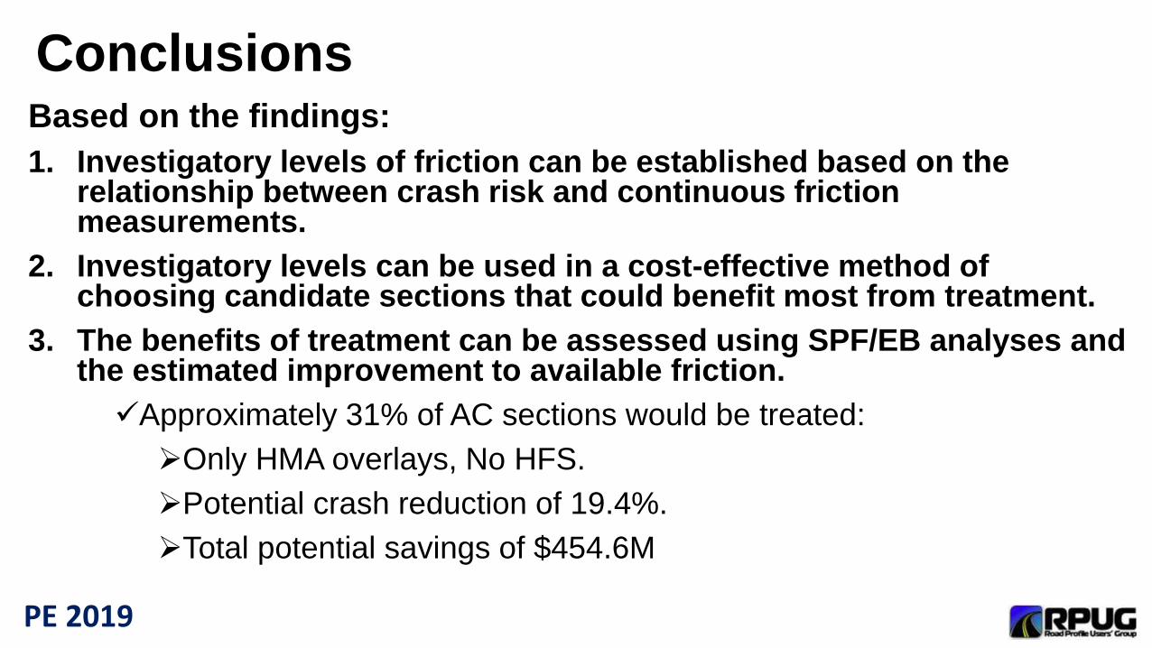
ConclusionsBased on the findings:

1. Investigatory levels of friction can be established based on the relationship between crash risk and continuous friction measurements.

2. Investigatory levels can be used in a cost-effective method of choosing candidate sections that could benefit most from treatment.

3. The benefits of treatment can be assessed using SPF/EB analyses and the estimated improvement to available friction.

Approximately 31% of AC sections would be treated:

Only HMA overlays, No HFS.

Potential crash reduction of 19.4%.

Total potential savings of $454.6M