NASA Contractor Report 195056

ICASE Report No. 95-16

SIMPLEMENTATION OF A PARALLEL UNSTRUCTURED

EULER SOLVER ON THE CM-5

E. Morano

D. J. Mavriplis(NASA-CR-19505b) IMPLEMENTATION OF

A PARALLEL UNSTRUCTUREO EULER

SOLVER ON THE CM-5 (ICASE) 22 p

N95-25106

Unclas

G3/64 0045769

Contract No. NAS 1-19480March 1995

Institute for Computer Applications in Science and Engineering

NASA Langley Research Center

Hampton, VA 23681-0001

Operated by Universities Space Research Association

https://ntrs.nasa.gov/search.jsp?R=19950018686 2018-06-29T09:21:45+00:00Z

IMPLEMENTATION OF A PARALLELUNSTRUCTURED EULER SOLVER

ON THE CM-5*

E. Morano and D. J. Mavriplis

Institute for Computer Applications in Science and Engineering

MS 132C, NASA Langley Research Center

Hampton, VA 23681-0001 USA

ABSTRACT

An efficient unstructured 3D Euler solver is parallelized on a Thinking Machine Corpo-

ration Connection Machine 5, distributed memory computer with vectorizing capability. In

this paper, the SIMD strategy is employed through the use of the CM Fortran language and

the CMSSL scientific library. The performance of the CMSSL mesh partitioner is evaluated

and the overall efficiency of the parallel flow solver is discussed .

"This research was supported by the National Aeronautics and Space Administration under NASA Con-tract No. NAS1-19480 while the authors were in residence at the Institute for Computer Applications in

Science and Engineering (ICASE), NASA Langley Research Center, Hampton, VA 23681-0001. The firstauthor was also partially supported by INRIA, "R_gion Provence-Alpes-Cdte d'Azur" (France).

1 INTRODUCTION

Computer technology has grown rapidly over the last several years especially with regard to parallel archi-

tectures. Such machines are becoming useful for solving very large computational fluid dynamics problems,such as inviscid and viscous three dimensional flows about complex configurations, using upwards of one

million grid points.Since many different architectures have been developed and are available, efficient solution techniques and

software are required which are adapted to the computational problem and also to the particular machine.

There are essentially two requirements: the software must be parallelizable and here, also vectorizable, since

each processing node of the CM-5 partition contains 4 vector units (VU's). For example, a Jacobi cycle

is suitable, but a Gauss-Seidel iteration is not inherently vectorizable. This vectorization is provided by

the compiler and does not require any explicit colored-type implementation. Moreover, the algorithm must

also be efficient enough [1, 2], that is, must require a minimum number of operations to obtain a converged

solution. In the case of unstructured meshes, only a few algorithms satisfy these requirements. In this work,

it will be shown how a multistage explicit 3D Euler solver may be implemented on the CM-5 machine.

The CM-5 architecture can be used as a Single Instruction Multiple Data (SIMD) machine or as a

Multiple Instruction Multiple Data (MIMD) machine. In the first approach each processing node performsthe same instructions but on different data elements, while in the second approach, each processing node

executes different instructions on different data sets. The SIMD approach on the CM-5 will be studied in

this paper. This is done by making use of the CM Fortran (CMF) language. This language is an extensionof the Fortran 90 language and has the particularity of treating entire arrays as variables. It provides a much

more compact way of programming. Moreover, on the CM-5 computer, the programmer may access a large

set of libraries: CM Fortran Utility Library [3] and Connection Machine Scientific Software Library (CMSSL

[4]) for CM Fortran [5]. The first library provides subroutines such as "CMF_fe_array_from/to_CM" to use,

or to produce, CM-objects instead of writing lower-level software. The second library is related to the use of

scientific functions such as the manipulation of CM-arrays: L2 vector/matrix norms and the gather/scatter

operations for sparse matrices, for example, which are required here.

While this programming model gives the illusion of an SIMD architecture, the global CMF code is in fact

transformed by the compiler into an MIMD program which is then run simultaneously on each processor.

Since the memory is distributed on this machine, each VU has its own memory where the data elements

are located and the distribution of the data elements over the vector units can strongly affect the overall

performance, because of the time required for the interprocessor communication. Therefore, a partitioner

provided in the CMSSL library, developed by Johan [4, 6], will be used with a slight modification.All codes are compiled using CMF 2.1.1.2 and CMSSL 3.2. They are run on a CM-5 computer with 128

processing nodes (512 VU's) under CMOST 7.3 Final 1 Rev 3. All the examples run on the latter systemare timeshared for the 32 and 64 processing node executions, while they are run in dedicated mode for the

128 processing node executions: this allows the use of the entire available memory (3.48 GBytes) for a single

job. Each 32 node partition represents 891 MBytes of memory, the difference between the original 1 GByteand the 891 MBytes is due to the overhead. All reported timings correspond to CM-Busy times. This work

was introduced in [7] with slight differences.

2 UNSTRUCTURED SOLVER

The basis for the implementation is a three dimensional unstructured single-grid Euler solver. Unstructured

meshes provide the most flexible means for the discretization of complex domains and for adaptation of

the mesh to flow features. Since an explicit scheme may be considered as the product of a sparse matrix

bv a vector, unstructured meshes result in (very) large sparse matrices and therefore require the use of

gather/scatter operations to enable vectorization and/or parallelization.

Venkatakrishnanet al. in [8]implementamesh-vertexfinitevolumeupwindschemefor solvingthe Eulerequationson triangular unstructuredmesheson the Intel iPSC/860,an MIMD computer. A four-stageRunge-Kuttaschemeis usedto advancethesolutionin time. Farhatet al. in [9]proposethe discretizationofthe2DNavier-Stokesequationsusingasecondorderaccuratemonotonicupwindschemefor conservationlaws(MUSCL)on fully unstructuredgrids.Thespatialapproximationcombinesanupv)indfinite volumemethodfor the discretizationof the convectivefluxeswith a Galerkinfinite elementmethodfor the discretizationof the diffusivefluxes. The time integrationis performedthroughan expficit secondorder Runge-Kuttaschemeand the codeis implementedon a CM-2 computer. Johan et al. in [10, 6] solve the 3D Euler

equations with a finite element program implemented on the CM-5 in CM Fortran. The variational form is

based on the Galerkin/least-squares formulation. They use an implicit scheme to converge the solution to

steady state. A matrix-free GMRES technique is used to solve the linear system at each time-step. More

recently, Farhat et al. in [11] proposed the evaluation of different massively parallel architectures through the

simulation of unsteady and steady viscous flows on the iPSC-860, the CM-5 and the KSR-1 computers. The

discretization relies on a mixed finite element/finite volume formulation on unstructured meshes. The spatial

approx_imation combines a Galerkin approximation for the viscous terms and an upwind Roe scheme for the

convective fluxes. Second order solutions are provided through a MUSCL (Monotonic Upwind Scheme for

Conservative Laws) approach. The time integration is achieved through a 3 stage variant of the Runge-Kutta

method. Message Passing codes are implemented on the machines and an SIMD version of the solver is also

implemented on the CM-5. The performances confirm the results presented in [7]: 107 MFlops on a 392161

edge based unstructured 2D mesh using 32 processing nodes.

This work was already partially introduced in [7] and the sequential version of this algorithm has been

already reported in [12]. A parallel version was implemented on the Intel iPSC/860 hypercube using the

PARTI primitives [13]. The equations are discretized on the unstructured mesh using a Galerkin finite-element formulation. The flow variables are stored at the vertices of the mesh, and piecewise linear flux

functions are assumed over the individual tetrahedra of the mesh. The scheme is a so-called central differ-

encing scheme [14]. Artificial dissipation, constructed as a blend of a Laplacian and biharmonic operator, is

added to maintain stability. The main data-structure of this code is an edge-based data-structure. Residuals

are constructed by executing loops over the edges of the mesh. At mesh boundaries, an additional loop

over the triangular faces which form the boundary is then performed. The resulting spatially discretized

equations must be integrated in time to obtain the steady-state solution. This is achieved using a 5-stage

Runge-Kutta scheme. More details of this scheme are available in [12].

3 PARTITIONING OF DATA

As mentioned in the introduction, the memory is distributed over all the VU's (each processing node has

4 VU's). Thus, it is necessary to understand how, in the processors, the memory is managed and how the

vectorization is performed, and both must be worked out together. These will be illustrated through the

following example.

An array containing 2800 data elements is to be distributed on a CM-5 comprising 32 processing nodes,

that is 128 vector units, each of them managing its own memory. The quotient of the division of 2800 by

128, i.e. 21, should be the number of data per VU. Actually, in order to distribute the data, two features

are available.

• There is what can be called "the rule of 8". The length of the pipeline of a vector unit is equal to 8.

thus the size of the data to be distributed on each VU has to be a multiple of 8. 21 is obviously not

a multiple of 8 and the next number multiple of 8 is 24. The quotient of the division of 2800 by 24.

i.e. 116, represent the number of VU's that will contain 24 data, the remaining data (2800-(116"24) =

16) goes in the llT-th VU. As explained in [4], the first 24 data will be allocated to the first VU, thesecond 24 data to the second VU and so forth... In this example only 117 VU's are used, instead of

128,andthe arrayis not largeenoughto fit the machinecorrectly.However,this problemdisappearsfor largermeshes.

• Anotherfeatureof the last releasedCMSSLlibrary is that this rule of 8 is no longermandatorytoensurepropervectorization.Theonly requirementis that the lengthof each-datasetin eachVU beamultipleof a positivepowerof 2. Thepreviousexampleis consideredasfollows:21 is not a multipleof anypositivepowerof 2, while22 is. Hence,the numberof VU's containing22data is 127,theremaining6 data beingassignedto the 128thVU. In this case,all the VU's arebeingusedwhichresultsin anexcessof communicationtime with respectto the computationaltime. Hereagain,thisproblemtendsto disappearwhenthe sizeof the meshincreasesfor a givenarchitecture.In ordertousethis option,thepartitionerandthesolversoftwaremustbecompiledwith the "-nopadding"option(for further detailsseein [15]).

Thepartitionerprovidedin theCMSSLlibrary isdesignedto partition FiniteElementmeshes:for claritya 2Dmesh,built with triangles,is considered.In orderto usethe partitioner, the graphto be partitionedneedsto bedescribed.In theCMSSLlibrary, sincethetrianglesarepartitioned,thegraphconsideredis thedual to the triangulationwhereeachtriangleis representedasa vertexin the graph. The graphis definedby the array "idual":

idual(m,n)= • thenumberof the trianglethat sharesthefacem with the trianglen.• 0 if thereis noneighbour(i.e. at theboundary).

In thepresentcase,theverticesof the triangulation are partitioned rather than the triangles. Therefore,

the graph to be partitioned is the triangulation itself. The graph is thus described in terms of nodes connected

by edges. First to be determined is the maximum number of neighbors a node may have (max_ngh) all overthe mesh, then the actual number of neighbors for each node (act_ngh). The graph is built using the array

"idual" defined as:

idual(m,n) = • the number of the edge that shares the node m with the edge n.

• 0 if n > act_ngh.

The partitioning is achieved through the use of a parallel recursive spectral bisection (RSB) implemented

in CMF by Johan et al. [6]. The call of the routine "Partition_Mesh" will provide a new numbering of

the nodes of the mesh through an array of permutation. It is important to note that the RSB partitioner

implelnented in the CMSSL library does not necessarily ensure a unique solution. Therefore, two runs on

the same graph usually produce two slightly different results [6].

Since most of the computation is based upon edge loops, edges are the primary representation of the

mesh and, once the permutation array is obtained, the edges are partitioned. An edge is represented by its

origin and extremity. If both nodes of an edge belong to the same processor, then the edge is allocated to

that same processor. If the two end nodes of an edge reside ill different processors, the edge is then allocated

to one of the two processors. Since either processor can be chosen, at this point, the edges are assigned in a

manner which ensures even size partitions of edges for each processor. For example, in Fig.l, is shown the

case of a 2D mesh. and how, from the original mesh and through the edges, the renumbering is achieved.

The mesh comprises 25 nodes aad 56 edges. The "Partition_Mesh" routine provides then 3 partitions with 8

nodes each and 1 partition with 1 node. The boundary between each partition is depicted by the thick dash

line.

In an unstructured mesh. the way the edges are to be distributed depends strongly on the connectivity of

each node (number of connecting neighbors). Therefore, one processor may receive a greater number of edges

than another. This results in non-equal length sets of data. In order to ensure proper data distribution and

to provide maximum computational rates, dummy data elements called "zeros". since they are actually zero

© PartitionIh

0 _[_i__

3i[] Partition II

1,

2.

:4

_0 /

_Partition IV

6' -0

Partition III

Figure 1: Partitioning Example.

valued data elements during the computation, are added to each partition. When the VU pipeline length is

8, it is important to employ partitions in which the data sets are multiples of 8, in order to maximize the VU

computational rates. In general, the partitions will not naturally be divisible by 8. Therefore, the "zeros"

are added such that the number of edges per processor be divisible by 8.

A similar partitioning is carried out for the triangular boundary faces, since these form the basis of the

boundary condition loops. Since the number of boundary faces is smaller than the number of mesh edges

(see Table 2.B for example) they do not affect the computation significantly. Yet, it is useful to note that

each face (actually a face is represented by a tetrahedron, since the interior node needs to be known for

computational purposes) is comprised of 4 nodes. Each of these nodes may be on a different processor, hencethe number of "zeros" to be added per node is proportionally greater than for the edges. This number may"

be regarded as much smaller than the number of edges but is not negligible.The number of nodes is obviously not affected by the previous methods and remains the same as before

the partitioning.The following particular ratio is to be of some importance:

cut_edges_partedge_ratio = max_edges '

where cut_edges_part is the number of cut edges, divided by the number of partitions, and max_edges the

maximum number of edges strictly included in a processor. The quantity cut_edges_part represents a good

metric of the interprocessor communication time and max_edges a good metric of the pure computational

time. This ratio will govern the overall performance of the code. A similar face_ratio may have beenstudied but was not considered for clarity purpose. The only cases where such a ratio could be considered

significant is when the faces represent more than 20 % of the computational operations. This happens when

small meshes are distributed on a large number of processors which obviously becomes rapidly inefficient

and therefore need be neither used nor studied.

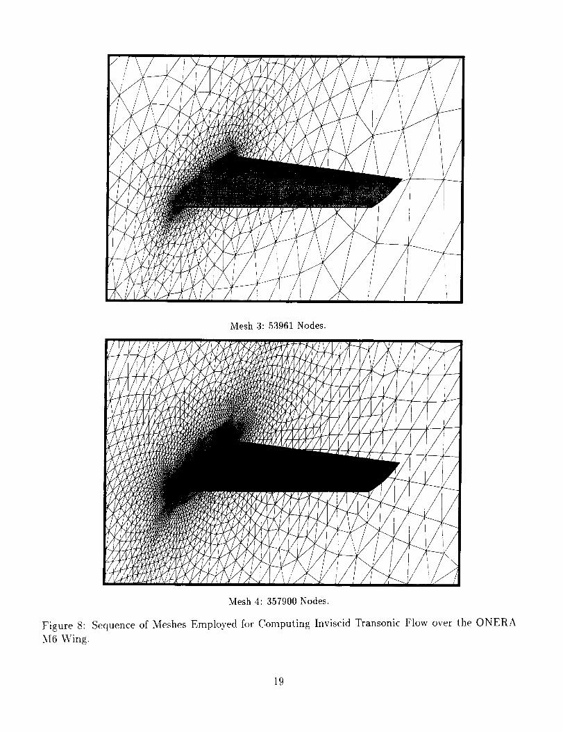
Severalresultsobtainedwith the partitionerappliedto an ONERAM6 wingmesh(Fig.8)and a meshoveran aircraft configuration (Fig.10) are discussed. The meshes being used are described in Table 1.

Tables 2 to 4, showing partitioner execution summary, are to be read as follows:

• The size of the meshes is expressed as the number of nodes, edges (the.most relevant data) and

boundary faces before being partitioned.

The memory required to run the code is obtained by including "isys = system('cmps')" as the last

command line in the code. The result of the sum of the VU heap and stack is expressed in KBytes

per VU. In order to obtain the memory allocated to run the code on the entire machine it is necessary

to multiply the value by the number of VU's (a division by 1024 gives the value in MBytes).

CPU times are measured for the execution of the "Partition_Mesh" CMSSL subroutine and for the

total partitioning process, that is for "Partition_Mesh" and for renumbering and reordering the edges

and the faces (I/O operations are not considered).

The edge_ratio: for a given geometry, it is expected that the statement "the bigger the mesh thebetter" will hold. Indeed, the density of nodes increases faster than the interprocessor boundary size;

hence, the value of edge_ratio decreases for larger meshes. Therefore more CPU time will be spent in

the computation compared to the communication, and the global performance will improve.

• The resulting number of edges and faces after the partitioning process (due to the addition of the

"zeros" ).

• The percentage of the number of faces over the number of edges.

One particular feature of the CM Fortran available on the CM-5 is that it supports a dynamic array

allocation. This feature has been used in the last release of the code used here to partition the data. The

interest of the use of the dynamic array allocation resides in a more fle_ble way to run the code. It becomes

unnecessary to re-compile it prior to each run. The main difficulty concerns the precise measurement of the

memory through the use of the "cmps" command. Indeed, this command gives the status of the system

when requested, hence the possible lack of precision due to the fact that some arrays might not be allocatedat this time.

Tables 2.A to 2.E show the partitioner execution summary for the 32 node configuration computer

respectively for:

1. Tile rule of S.

. The rule of 8 with the "low-storage" option, an option that allows a smaller memory allocation re-

quirement than the "default-storage" option, (the latter of which was used exclusively in [7]. However,

the "low-storage" option requires more CPU time (see [15]).

3. The "-nopadding" option.

4. The "-nopadding'" and "low-storage" options.

Tables 3 and 4 depict the results for the 64 and 128 node configuration respectively.

As for memory measurements, the results ill Table 2.A and the results reported in [7] appear slightly

different but nevertheless consistent. This difference may result from the present use of the dynamic array

allocation (in [7] this feature was not used), but also from the new operating system, the new CMSSL library

and maybe from the non-uniqueness of the solution of the "Partition_Mesh" subroutine (i.e. the resulting

mesh is possibly larger or smaller than those shown in [7]). The increase of the number of edges ranges from

0.7 % to 21 7c.. The larger the mesh on a given configuration the lower the increase because the density of

6

inner processoredgesis larger. Fora givenmeshthe largerthe numberof processingnodesthe larger theincreasesincethe samenumberof edgeshasto distributedon a largernumberof processors.The increaseof the numberof facesfollowsthe samerulesbut at a muchhigherdegree(from 98%to ashigh as287%!), sincea facecanbe sharedby asmanyas4 differentVU's (this casedoesnot generallyappearand 3seemsto be the maximum). The "Partition.Mesh"subroutinerequires20-50% of the total partitioningprocess.This is explainedby the fact that the codeis not entirely paralle!ized.Completeparallelizationwould requirea largeamountof communication and dramatic reductions in CPU time cannot be expected.

When the "low storage" option is used, the "Partition_Mesh" subroutine requires 50 % more time, but the

memory requirements are only 65 % as of those required as with the "default storage" option.

In Fig.2, the memory requirements with respect to the number of edges for each available option on

the 32 node machine are depicted. A simple extrapolation (curves are linear) shows what the 2403874 edge

mesh would require in terms of memory and time. The memory requirement can be attained with the 64

node machine using the "low storage" option with either the "-nopadding" or the "rule of 8" options, which

requires 1.39 or 1.44 GBytes respectively. Although the CPU time does not appear to be a limitation a

priori, it is obviously preferable, when possible, to use the "default storage" option. The time required

to partition the 2403874 edge mesh cannot be extrapolated as easily since partitioning the same mesh on a

larger architecture increases communication but provides better computational performance, and the balancebetween these two factors is not a priori known. As shown in [6], time is not a linear function of the number

of processing nodes. Therefore, the options are in favor (slightly !) of the "low storage" and the "-nopadding'"

for the memory requirement.The results for the 64 node runs are presented in Table 3. The memory requirement for the 2403874 edge

mesh, with 1.32 GBytes, proves the previous estimation to be vMid. The same type of results are shown on

Table 4 for the 128 node partition, where no limitation was found for the presented meshes.

It is clear, and expected, that the "edge_ratio", for a given geometry, decreases when the mesh gets larger.

Yet, this "edge_ratio" increases when the configuration of the machine gets larger. Indeed, a given mesh

is partitioned on a greater number of processors thus creating more interprocessor boundaries. Therefore,

it is expected that the overall computational performance will be "optimal" when this "edge_ratio" will be

minimum. As for the aircraft configuration, despite a greater number of edges (697992) versus the second

largest M6 wing (353476), a great improvement in terms of performance cannot be expected since their

respective values of the "edge_ratio" are similar.

4 PERFORMANCE RESULTS

In the Tables 5 to 8 results are presented as follows:

• Meshes are represented by their number of nodes, edges and faces.

• The memory requirement is expressed in KBytes per VU. This is obtained through the command line

"isys = system('cmps')" as for the partitioner. Since this code does not use dynamic array allocation

memory, the memory measurements should be more accurate than those of the partitioner.

• The CPU time entry contains two columns: the first one represents only the computational time

whereas the second takes into account the computational time and the communication time which

is included in the gather/scatter operations. These operations are performed through the use of the

following routines available in the CMSSL library [4]:

- "Part_Gather/Scatter" for single dimension arrays,

- "Part_Vector_Gather/Scatter" for multiple dimension arrays.

The CPU time is expressed as an average computed over 100 iterations.

• Theoverallperformanceof the code is expressed in MFlops.

As for memory requirements, here again, the results in Table 6.A are consistent with those that appear

in [7]. The previous remarks concerning the differences related to the partitioner still apply.

As seen in Table 5, computations done directly without partitioning the meshes reflect that partitioning

does improve the overall performance of the code. For example, although the non-partitioned 353476 edge

mesh is smaller than the partitioned 360448 edge mesh (addition of "zero-edges" and "zero-faces" in the

partitioned mesh) the memory allocation needed by the gather/scatter routines is larger. Indeed, since the

nodes are randomly distributed among the processors, the number of cut edges is larger and the gather

process produces more duplications. The computational times are of the same magnitude for both meshes.

On the other hand, the total time shows a 7-fold increase resulting in low overall performance.

Even in the partitioned cases, shown in Tables 6 to 8, the computational time is around 10 times smaller

than the total time. Therefore, pure computational performance of about 1 GFlops are dramatically reduced

to 104 MFlops. The communication time in all these cases is much larger than the computation time. Thus,

the overall computational rates of 20 MFlops per processor achieved by Johan [6] cannot be expected nor

achieved, h_t, an average of 0.8 Mflops per processor attained here are similar to those presented in [11].

Indeed, the codes used in [7] and [11] are somehow similar with respect to the discretization and the time

marching algorithm.

Table 9 depicts the execution summary of the code during one iteration, routine by routine where the

computational performance is pointed out: STEP represents the computation of the time step, DEFLUX (D)

the artificial diffusion, DEFLUX (C) the convection fluxes, PSMOO the residual smoothing and MONITR

the computation of the RMS average of all flow field residuals. The values are given in the first Runge-

Kutta step for DEFLUX (D), DEFLUX (C) and PSMOO. In the PSMOO subroutine, two iterations of a

Jacobi iterative process (implicit residual averaging, see [16]) are performed over the whole mesh and the

result is the average. STEP and MONITR are calculated respectively at the beginning and at the end of

the global iteration. The mesh used is the partitioned 360448 edge mesh of the M6 wing. The various

computations are performed over edges, faces and nodes. This table shows the CPU times required for the

gather operation, the computation and the total time including gather, computation and scatter. The gather

bandwidth for double precision data is calculated by dividing the number of bytes transferred (either within

a processor or between processors) by the time used to do so. For example, the number of transferred data

from an array A(5.mnode) to an array GA(2,5,medge), where 5 is the number of variables in 3D, mnode

the number of nodes and medge the number of edges, amounts to a total of 2 x 5 x medge x 8 bytes.

The gather bandwidth per processing node for the edges results in 15 Mbytes/s for each routine. When

the performances obtained with the computational time only (MFlops (C)) are compared to the total time

(MFlops (T)). it is easily seen that performance considerably deteriorates in the particular subroutines which

include large portions of communication. The pure computational performance is pointed out since more

than 1 GFlops for computation only are obtained. Therefore, these results show that the compiler provides

a good vectorization of the code and that the communication rates are similar to those achieved by Johan

in [6] which ensures that the meshes are well partitioned. The deterioration is due to the large number of

communication steps used in each routine.

Fig.3 shows the memory requirement of the solver, expressed in MBytes, with respect to the number of

edges of each mesh. for the three possible configurations of the machine (32, 64 and 128 processing nodes).

For the 32 node configuration, since the 2403874 edge mesh could not be neither partitioned nor run with

the solver, an extrapolation has been performed. The theoretical size of the partitioned mesh is extrapolated

from tile results obtained in Table 2.E and results in a 2432489 edge mesh. Then, its memory requirement is

extrapolated from results obtained in Table 6.C. It shows clearly that such a computation is possible neither

with the :/2 node machine nor with the 64 node configuration. Indeed, the double and triple dash lines show

respectively the available memory for the 32 and the 64 node configuration. It is also interesting to note that

the :3 curves are almost the same, demonstrating again the quality of the partitioning process. The previous

remarksarealsoreflectedin Fig.4,wherethememoryrequirements,expressedin MBytes,arepresentedwithrespectto thenumberof processorsfor eachinitial mesh.Again,thememoryrequirementexpressedfor the357900nodemeshon the 32and64nodemachineareonlyextrapolations,andasexpectedthecomputationof the 2433280edgemesh(seeTable.3)couldnot beachievedon the64nodemachine.

Fig.5 depictsthe overallperformancewith respectto the numberof edgesfor the threepossiblecon-figurationsof the machine(32, 64 and 128processingnodes). As for the 32 and 64nodeconfiguration,the overal!performanceshowsa rapid stallwhenthe numberof edgesincreases,confirmingthe increaseofcommunicationtime. In thesecases,the resultsobtainedwith the largestnumberof edgescorrespondtothe aircraft configurationmesh,while the resultsof the secondlargestnumberof edgescorrespondto thesecondlargestM6 wingmesh,thusthey maynot reflectthe realattainableperformance.However,and asa confirmationof the previousassumption,whenthesemeasuresareperformedwith the 128nodemachine,thestall appearsaswellwith the largestmeshwhichdiscretizesthe sameM6 wing.

The overallperformancewith respectto the valueof the edge_ratio is depicted in Fig.6. The number of

MFlops is seen to be strongly related to the value of the edge_ratio. Since the edge_ratio is more favorable, for

larger meshes and for a given geometry, the performance is better. The density of the mesh increases faster

than the number of cut edges per partition for a given geometry and the computation time predominates

the communication time thereby enhancing the performance. The importance of the value of this ratio is

well demonstrated with the 32 node machine. In this case the smallest value of the edge_ratio corresponds

to the aircraft while the immediately greater corresponds to the second largest M6 wing. The performance

with the aircraft configuration mesh is about the same as that obtained with the second largest mesh over

the M6 wing, since they exhibit similar edge_ratio. Yet, this trend seems to disappear when the size of the

machine increases: the inherent differences of both meshes are more apparent.

Fig.7 depicts the overall performance for each mesh with respect to the machine configuration. Except for

the largest mesh (computed only on the 128 node machine), the performance increases almost linearly with

the number of processing nodes. For each mesh, the curves are straight lines with a similar slope, proving

again the efficiency of the partitioner. The value of the performance obtained with the smallest mesh on the

64 and 128 node configuration may appear somehow suspicious. In fact, this result is to be expected, since

for such a mesh the communication time clearly dominates the computational time.

Finally, while the overall computational rates achieved appear to be rather low, the totM time required to

obtain a solution is competitive with other unstructured mesh implementations [10, 6]. The simple structure

of this explicit algorithm results in a low number of operations for each individual loop. This leads to a high

communication/computation ratio on parallel machines, and thus to a low overall computational rate on the

CM-5. This is confirmed by the results obtained on the Delta machine [14]: the Delta machine providescommunication times smaller than the CM-5, while the CM-5 provides computational times smaller than

the Delta through the VU's.

An example of the solution computed over the ONERA M6 wing is depicted Fig.9.

5 CONCLUSION

In this work. it has been shown that the implementation of the 3D Euler solver did not pose any major prob-

lems on the CM-5 for the CM Fortran language is very similar for the experienced Fortran-77 programmer.

The set of utility subroutines found within the CMSSL library is mostly user-friendly and easy to implement.

However. CM Fortran is restrictive in terms of effectiveness. The main drawbacks are:

• Large memory requirements with respect to the size of the problem.

• Large amount of communication, degrading the overall performances to the detriment of rather excep-

tional pure computational performances.

• Poorcommunicationbandwidthperprocessingnodeis not wellsuitedfor programsthat performalargeamountof inter-processorcommunication(gather/scatter).

The spectralmeshpartitionerimplementedin [6]resultedin largelyimprovedsolverperformance.How-ever,moreefficientimplementationsof the solverand the partitionerdemanda thoroughunderstandingofthecomputerarchitecture.Thesolveritself requiresalargeamountof communicationwhichresultsin a lowoverallperformance.It is alsoshownthat the communicationratesarestronglyrelatedto the valueof theedge_ratio. Improvements could have been achieved either through faster communication rate or through a

memory extension of the processors that would allow one to employ larger meshes on the same number of

processors.At last, in [11], the result of a message passing version of their code implemented on the CM-5 reports

an overall performance of 102 MFlops for a 786631 edge 2D mesh using 32 processing nodes. While this

rate is similar to that achieved in the present work, the former implementation was performed in Fortran-77

and does not make use of the vector units. A message-passing version written in CM Fortran, which would

enable the use of the vector units should provide better overall performance.

6 ACKNOWLEDGEMENTS

We warmly thank Zdenek Johan and Earl Renaud for their constant help with the CM Fortran version of

this code.

Our thanks extend to the team of Joel Saltz at the University of Maryland at College Park for providing

the CM-5 computer access.

Finally, this work completed the postdoctorate year of Eric Morano supported by INRIA, "R@gion

Provence Alpes C6te d'Azur" (FRANCE) and by ICASE (USA).

10

References

[1] E. Morano, M.H. Lallemand, M.P. Leclercq, H. Steve, B. Stoufflet, and A. Dervieux. Local iterative

upwind methods for steady compressible flows. In GMD-Studien Nr. 189, Multigrid Methods: Special

Topics and Applications II, 1991. Third Conference on Multigrid Methods, Bonn 1990.

[2] E. Morano and A. Dervieux. Looking for O(N) Navier-Stokes solutions on non-structured meshes. In

Sixth Copper Mountain Conference on Multigrid Methods, pages 449-463. NASA, 1993. NASA CP-3224,

Part 2.

[3] Thinking Machine Corporation. CM Fortran Utility Library Reference Manual, Version 2.0 Beta, 1993.

[4] Thinking Machine Corporation. CMSSL for CM Fortran: CM-5 Edition, Volumes I and II, I'_rsion 3.1

Beta 2, 1993.

[5] Thinking Machine Corporation. CM Fortran Reference Manual, Version 2.0 Beta, 1992.

[6] Z. Johan, K. Mathur, S. Johnsson, and T. Hughes. An efficient communication strategy for finite elementmethods on the connection machine CM-5 system. Technical report, Thinking Machine Corporation,

1993. Submitted to Computational Methods in Applied Mechanics and Engineering.

[7] E. Morano and D. Mavriplis. Implementation of a parallel unstructured Euler solver on the CM5.Technical Report 94-0755, AIAA, 1994. 32nd Aerospace Sciences Meeting & Exhibit, January 10-13,

Reno, Nevada, USA.

[8] V. Venkatakrishnan, H. Simon, and T. Barth. A MIMD implementation of a parallel Euler solver for

unstructured grids. The Journal of Supercomputing, 6:117-137, 1992.

[9] C. Farhat, L. Fezoui, and S. Lanteri. Two-dimensional viscous flow computations on the connectionmachine: unstructured meshes, upwind schemes and massively parallel computations. Computational

Methods in Applied Mechanics and Engineering, 102:61-88, 1993.

[10] Z. Johan. Data parallel finite element technique for large-scale computational fluid dynamics. PhD

thesis, Stanford University, 1992.

[11] C. Farhat and S. Lanteri. Simulation of compressible viscous flows on a variety of mpps: Computationalalgortihms for unstructured dynamic meshes and performance results. Technical Report 2154, INRIA,

1994.

[12] D. Mavriplis. Three dimensional unstructured multigrid for the Euler equations. Technical Report

91-1549CP, AIAA, 1991.

[13] R. Das, D. J. Mavriplis, J. Saltz, S. Gupta, and R. Ponnusamy. The design and implementation of a

parallel unstructured Euler solver using software primitives. Technical Report 92-12, ICASE, 1992.

[14] D. Mavriplis. Implementation of a parallel unstructured Euler solver on shared and distributed memoryarchitectures. Technical Report 92-68, ICASE, 1992.

[15] Thinking Machines Corporation. CMSSL Release Notes, Preliminary Documentation for Version 3.2Beta. 1993.

[16] A. Jameson. Numerical solution of the Euler equations for compressible inviscid fluids. In F. Angrand.

A. Dervieux. J.A. D_sid_ri, and R. Glowinski, editors, Numerical Methods for the Euler Equations of

Fluid Dynamics, pages 199-245. SIAM, Philadelphia, 1985.

11

Configurations Nodes Edges

ONERA M6 Wing 2800 17377

ONERA M6 Wing 9428 59863

ONERA M6 Wing 53961 353476

ONERA M6 Wing 357900 2403874

Aircraft [ 106064 [ 697992

Boundary Faces2004

5864

23108

91882

31886

Table 1: Test-case meshes.

Initial Meshes

(nodes/edges/b. faces)

Memory

(KBytes/VU)

2800/17377/2004 324

9428/59863/5864 604

53961/353476/23108 2552

106064/697992/31886 5020

Initial Meshes

(nodes/edges/b.faces)

2800/17377/2004

9428/59863/5864

53961/353476/23108

106064/697992/31886

InitialMeshes

(nodes/edges/b. faces)

2800/17377/2004

9428/59863/5864

53961/353476/23108

106064/697992/31886

Memory

(KBytes/VU)260

408

1644

3260

CPU (sec)

Partition._Mesh Total

4.99 17.64

13.39 51.01

78.00 274.63

214.80 577.43

A. Rule of 8.

Edge_Ratio Final Meshes

(edges/b.faces)

B. Faces/Edges

(%)0.77 20480/5120 25.0

0.43 66560/13312 20.0

0.20 360448/48128 13.35

0.16 707584/71680 10.13

CPU (sec)Partition_Mesh Total

8.42 21.23

20.34 57.96

127.06 320.83

367.73 729.78

Edge_Ratio Final Meshes

(edges/b.faces)

B. Faces/Edges

(_)0.79 20480/5120 25.0

0.43 67584/13312 19.69

0.20 360448/48128 13.35

0.16 707584/71680 10.13

B. Rule of 8 -Low Storage.

Memory

(KBytes/VU)192

468

2484

4948

CPU (sec)

Partition_Mesh I Total4.63 17.48

12.19 50.31

80.44 275.85

214.47 572.19

C. No Padding.

Edge_Ratio Final Meshes

(edges/b. faces)

B. Faces/Edges

(%)0.80 18432/3968 21.52

0.44 61696/11776 19.08

0.21 358144/49152 13.72

0.16 703104/71168 10.12

Initial Meshes

(edges/b. faces)

Memory

(KBytes/VV)

2800/17377/2004 128

9428/59863/5864 336

53961/353476/23108 1636

106064/697992/31886 3252

CPU (sec)

Partition_.Mesh Total

6.45 19.36

18.45 56.74

129.91 324.63

357.11 719.89

Edge_Ratio Final Meshes

(edges/b. faces)

B. Faces/Edges

(%)0.78 18432/4096 22.22

0.44 61696/11776 19.08

0.21 358272/49152 13.71

0.16 703744/70784 10.06

D. No Padding - Low Storage.

Table 2: Partitioner Execution Summary - 32 Processing Nodes.

12

O

2000

1782

1000891

'Rule of 8 -,.- 'R.uleo,fS.- Low Storage -,-.

o a oln ,.-. /..,_o _a_din_ - Low Storage-,,--

_°'*"..oo.°,,o*°°"

• °""s""" ..,_,_h

..°°'°°° _

/

0 0 500000 le_-06 1.5_I-06 2e-_-06 ]

Figure 2: Partitioner's Memory Requirements vs. the Number of Edges - 32 Processing Nodes.

Initial Meshes

(nodes/edges/b. faces)

2800/17377/2004

9428/59863/5864

53961/353476/23108

106064/697992/31886

Memory

(KBytes/VU)160

300

1248

2476

357900/2403874/91882 *l 5404

CPU (sec)Partition_Mesh

3.83

8.82

49.01

128.05

759.95

[ Total18.93

49.29

250.49

501.38

1994.20

Edge_Ratio

1.31

0.65

0.29

0.22

0.14

Final Meshes

(edges/b. faces)

18944/5120

62464/14080

361472/54016

707840/81664

2433280/234240

B. Faces/Edges

(%)27.03

22.54

14.94

11.54

9.6

(*: low storage)

Table 3: Partitioner Execution Summary - No Padding - 64 Processing Nodes.

InitialMeshes Memory CPU (sec) Edge_Ratio Final Meshes B. Faces/Edges

(nodes/edges/b. faces) (KBytes/VU) Partition__Mesh Total (edges/b. faces) (%)

2800/17377/2004 84 4.68 22.56 1.93 20992/6144 29.27

9428/59863/5864 184 8.28 53.98 0.91 66560/16384 24.61

53961/353476/23108 692 31.18 248.03 0.41 366592/62464 17.04

106064/697992/31886 1244 72.09 463.74 0.32 714752/123392 11.044140 265.50 1551.57 0.19 2448384/270336 17.26357900/2403874/91882

Table 4: Partitioner Execution Summary - No Padding - 128 Processing Nodes.

13

Meshes Memory CPU 11ter (see) MFlops

nodes/edges/b, faces KBytes/VU Computation Total

2800/17377/2004 160 0.022 1.104 13.15

9428/59863/5864 484 0.066 3.705 13.25

53961/353476/23108 2724 0.349 22.649 12.34

106064/697992/31886 5308 0.662 53.858 10.02

Table 5: Euler 3D Solver Execution Summary - Not Partitioned - No Padding - 32 Processing Nodes.

Meshes Memory CPU 11ter (sec) MFlopsTotal

0.027 0.349 56.90

0.078 0.782 77.19

0.379 2.937 104.31

0.714 5.173 112.38

nodes/edges/b, faces KBytes/VU Computation

2800/20480/5120 216

9428/66560/13312 524

53961/360448/48128 2384

106064/707584/71680 4416

A. Rule of 8.

Meshes Memory CPU 11ter (sec) MFlopsTotal

0.024 0.312 54.40

0.072 0.724 76.72

0.380 2.896 105.51

0.711 5.403 106.92

nodes/edges/b, faces KBytes/VU Computation

2800/18432/3968 152

9428/61696/11776 452

53961/358144/49152 2320

106064/703104/71168 4412

B. No Padding.

Table 6: Euler 3D Solver Execution Summary - 32 Processing Nodes.

Meshes Memory CPU 11ter (sec) MFlops

nodes/edges/b, faces KBytes/VU Computation Total

2800/18944/5120 76 0.016 0.227 80.94

9428/62464/14080 232 0.039 0.482 120.59

53961/361472/54016 1240 0.202 1.712 182.32

106064/707840/81664 2308 0.366 3.076 191.88

1357900/2433280/234240 NOT FEASIBLE: OUT OF MEMORY

Table 7: Euler 3D Solver Execution Summary - No Padding - 64 Processing Nodes.

Meshes Memory CPU 1 Iter (sec)TotM

0.0111 0.181

0.0235 O.309

0.106 1.021

0.205 1.773

0.622 4.859

nodes/edges/b, faces KBytes/VU Computation

2800/20992/6144 72

9428/66560/16384 152

53961/366592/62464 684

106064/714752/123392 1228

357900/2448384/270336 3868

MFlops

114.65

203.79

316.56

356.48

417.76

Table 8: Euler 3D Solver Execution Summary- No Padding - 128 Processing Nodes.

14

Subroutine LoopIndex Gather(sec) Computation(sec) MFlops(C) Total (sec) MFlops (T)STEP Edges 0.0687 0.0125 688 0.0978 96

B. Faces 0.0274 0.0061 480 78Nodes

MONITR

0.0003 355i 0.0391

DEFLUX (D) Edges 0.0798 0.0292 764 0.2234 122Nodes 0.0011 228

DEFLUX (C) Edges 0.0135 1332 0.1034 209

B. Faces 0.0087 771 0.0354 216

PSMOO Edges 0.0580 0.0065 551 0.3589 40

Nodes 0.0013 585

Nodes 0.0024 218

Table 9:1 Iteration, Routine by Routine, Solver's Execution Summary.

v

2O0O

1782

! | |

32 Processing Nodes92yrocessm.g r_oaes --,-.l z_ vrocessmg r_oaes ..o.

1000891

Number of Edges

00 500000 le+06 1.5e+06 2e+06

F'igure 3: Solver's Memory Requirements vs. the Number of Edges.

15

2000

1782

1000891

'''''='-L'='_'''='''m'm''',m.l,=,l, R , _ ,,, .A

° ,°, ,,o o°, ,,, o,, ,o, ,,° ,°° ,,, ° ...... °o°,, °,, .°, b'D°bO°°_ .°" O'°°', 'O' 'l' °°° '" ''O ,,, "OO''° O°° ,'' '0' ''b O" °'" °'_ ,°, ,° ..........

2800 Node Mesh9428 Node Mesh --,.-53961 Node Mesh ....106064 Node Mesh -_.357900 Node Mesh -,_..

0 0

• ...................... • ................................................ •

Number of Processin_ Nodesl ................... 1".......................... " .......... !

32 64 128

Figure 4: Solver's Memory Requirements vs. the Number of Processing Nodes.

_' 32 Processing N_es- _xrocessin.g l_qs --,--

_z_ rrocessmg r_oaes .._.°o,,,,°o°°O,,,°"°_400 ..............

,o°,,°oo°°O'°

°,°°°,o°o,°,,,°°'°*°°

°,._°,°,°o°.°°°°°°'

°°,,°"

_,°,.°°

300 .-

.-.

200 i

100

Number of Edges

0 0 i , , ,500000 !e+06 1.5e+06 2e+06

Figure 5: Solver's Overall Performance vs. the Number of Edges.

16

_" 32 Processing Nodes _

l" _Yoc- essifig bloaes "'"

400

%'1_, ,

00 ""'".°,,,,,,,.%.,°,°,,.,,,,.•,,_.,°.

20C . ............._*B,_, °',,l,,,,,

100 _ ..................... "

I] ) 0.2 0,4 0.6 0,8 1 1.2 1.4 1.6 1.8 2

Figure 6: Solver's Overall Performance vs. the Value of the ed9 e-rati°"

Figure 7:

2800 Node Mesh "4-

9824 Nod h ,.o.53961 No •106064 Node Mesh -'_"357900 Node Mesh400

_,,'_

i j.f ,..,"

300 "/"" ..........

j_.°,,,'"

200t ..........

Number of Processing Nodes

0[___, _ 128

Solver's Overall Performance vs. the Number of Processing Nodes,

17

Mesh1:2800Nodes.

Mesh2:9428Nodes.

18

Mesh3:53961Nodes.

Figure 8:M6 Wing.

Mesh4:357900Nodes.

Sequenceof MeshesEmployedfor Computing Inviscid TransonicFlow over the ONERA

19

\

//

/

\Figure 9: Computed Mach Contours over the 357900 Node ONERA M6 Wing.

Figure 10:106064 Node Mesh of a 3D Aircraft Configuration.

2O

Form Approved

REPORT DOCUMENTATION PAGE OMB No 0704-0188

Public reporting burden for this collection of information is estimated to average 1 hour per response, including the time for reviewing instructions, searching existing data sources,gathering and maintainin_ the data needed, and completing and reviewing the collection of information. Send comments regarding this burden estimate or any other aspect of thiscollection of information, mcluding suggestions for reducing this burden, to Washington Headquarters Services, Directorate for Information Operations and Reports, ] 215 JeffersonDavis Highway, Suite ]204, Arlington, VA 22202-4302, and to the Office of Management and Budget, Paperwork Reduction Project (0704-0188), Washington, DC 20503.

1. AGENCY USE ONLY(Leave blank) 2. REPORT DATE 3. REPORT TYPE AND DATES COVERED

March 1995 Contractor Report/

4. TITLE AND SUBTITLE S. FUNDING NUMBERS

IMPLEMENTATION OF A PARALLEL UNSTRUCTURED

EULER SOLVER ON THE CM-5

6. AUTHOR(S)

E. Morano

D. J. Mavriplis

7. PERFORMING ORGANIZATION NAME(S) AND ADDRESS(ES)

Institute for Computer Applications in Science

and Engineering

Mail Stop 132C, NASA Langley Research Center

Hampton, VA 23681-0001

9. SPONSORING/MONITORING AGENCY NAME(S) AND ADDRESS(ES)

National Aeronautics and Space Administration

Langley Research Center

Hampton, VA 23681-0001

C NAS1-19480

WU 505-90-52-01

8. PERFORMING ORGANIZATION

REPORT NUMBER

ICASE Report No. 95-16

10. SPONSORING/MONITORING

AGENCY REPORT NUMBER

NASA CR-195056

ICASE Report No. 95-16

11. SUPPLEMENTARY NOTES

Langley Technical Monitor: Dennis M. Bushnell

Final Report

To be submitted to the International Journal of Computational Fluid Dynamics

12a. DISTRIBUTION/AVAILABILITY STATEMENT 12b. DISTRIBUTION CODE

Unclassified-Unlimited

Subject Category 64

13. ABSTRACT (Maximum 200 words)

An efficient unstructured 3D Euler solver is parallelized on a Thinking Machine Corporation Connection Machine 5,

distributed memory computer with vectorizing capability. In this paper, the SIMD strategy is employed through the

use of the CM Fortran language and the CMSSL scientific library. The performance of the CMSSL mesh partitioneris evaluated and the overall efficiency of the parallel flow solver is discussed.

14. SUBJECT TERMS

CM-5; Parallel; SIMD; CMF; CMSSL; Unstructured; 3D Euler

17. SECURITY CLASSIFICATION

OF REPORT

Unclassifed

NSN 7540-01-280-5500

18. SECURITY CLASSIFICATION

OF THIS PAGE

Unclassified

15. NUMBER OF PAGES

22

16. PRICE CODE

A03

19. SECURITY CLASSIFICATION 20. LIMITATION

OF ABSTRACT OF ABSTRACT

Standard Form 298(Rev. 2-89)Prescribed by ANSI Std. Z39-18298 102