Embed Size (px)
Citation preview

Digital Image Processing
Image Restoration
DR TANIA STATHAKI READER (ASSOCIATE PROFFESOR) IN SIGNAL PROCESSING IMPERIAL COLLEGE LONDON
What is Image Restoration?
Image Restoration refers to a class of methods that aim at reducing or removing various types of distortions of the image of interest. These can be: • Distortion due to sensor noise. • Out-of-focus camera. • Motion blur. • Weather conditions. • Scratches, holes, cracks caused by aging of the image. • Others.
Classification of restoration methods
Image restoration methods can be classified according to the type and amount of information related to the images involved in the problem and also the distortion. • Deterministic or stochastic methods.
In deterministic methods, we work directly with the image values in either space or frequency domain.
In stochastic methods, we work with the statistical properties of the image of interest (autocorrelation function, covariance function, variance, mean etc.)
• Non-blind or semi-blind or blind methods. In non-blind methods the degradation process is known. This is a
typical so-called Inverse Problem. In semi-blind methods the degradation process is partly-known. In blind methods the degradation process is unknown.
Classification of implementation types of restoration methods
• Direct methods. The signals we are looking for (original undistorted” image and degradation model) are obtained through a single closed-form expression.
• Iterative methods. The signals we are looking for are obtained through a mathematical procedure that generates a sequence of improving approximate solutions to the problem.
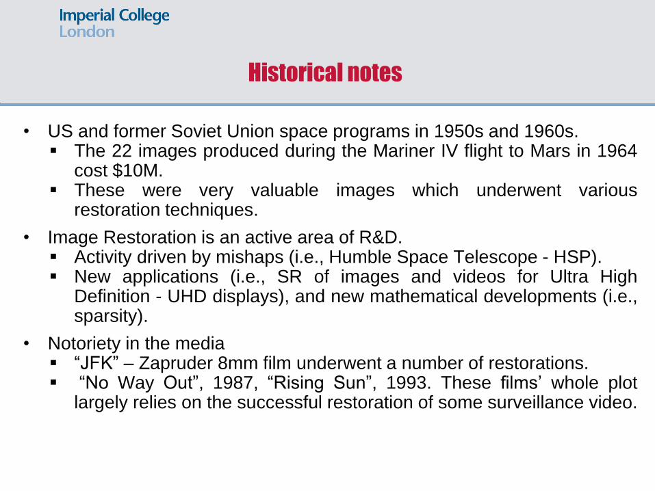
Historical notes
• US and former Soviet Union space programs in 1950s and 1960s. The 22 images produced during the Mariner IV flight to Mars in 1964
cost $10M. These were very valuable images which underwent various
restoration techniques.
• Image Restoration is an active area of R&D. Activity driven by mishaps (i.e., Humble Space Telescope - HSP). New applications (i.e., SR of images and videos for Ultra High
Definition - UHD displays), and new mathematical developments (i.e., sparsity).
• Notoriety in the media “JFK” – Zapruder 8mm film underwent a number of restorations. “No Way Out”, 1987, “Rising Sun”, 1993. These films’ whole plot
largely relies on the successful restoration of some surveillance video.
A generic model of an image restoration system
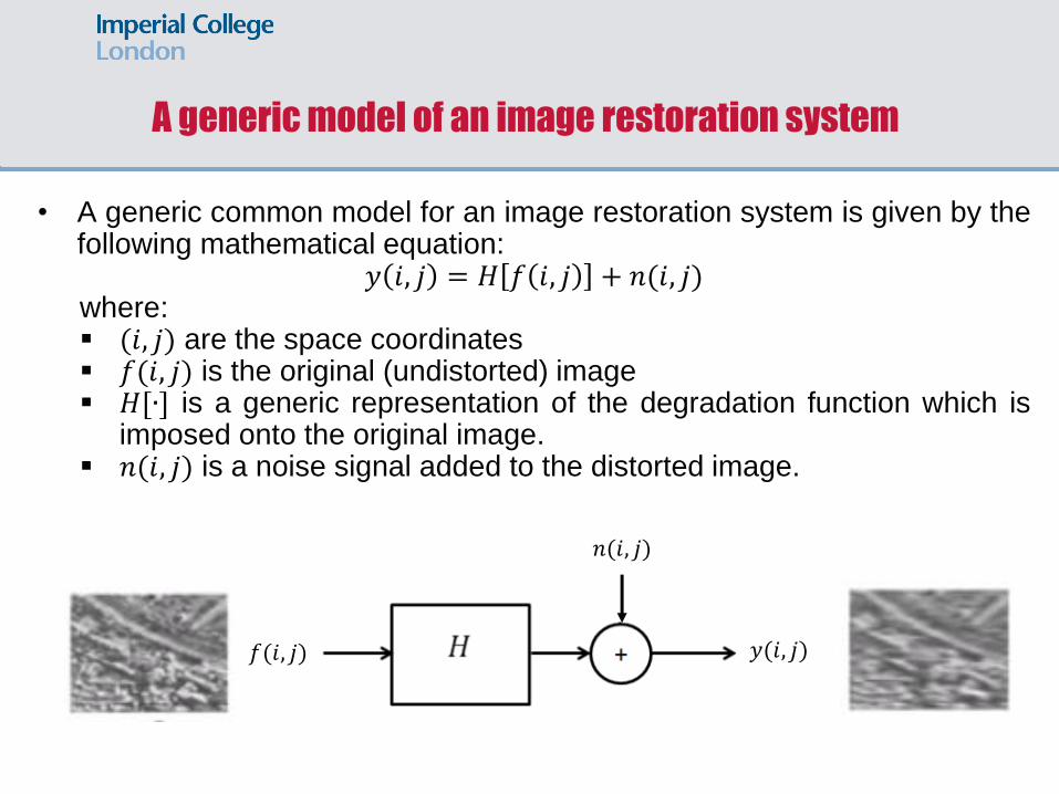
• A generic common model for an image restoration system is given by the following mathematical equation:
𝑦 𝑖, 𝑗 = 𝐻 𝑓 𝑖, 𝑗 + 𝑛(𝑖, 𝑗) where: (𝑖, 𝑗) are the space coordinates 𝑓(𝑖, 𝑗) is the original (undistorted) image 𝐻[∙] is a generic representation of the degradation function which is
imposed onto the original image. 𝑛(𝑖, 𝑗) is a noise signal added to the distorted image.
𝑓(𝑖, 𝑗)
𝑛(𝑖, 𝑗)
𝑦(𝑖, 𝑗)
𝑓 (𝑖, 𝑗)
A generic model of an image restoration system
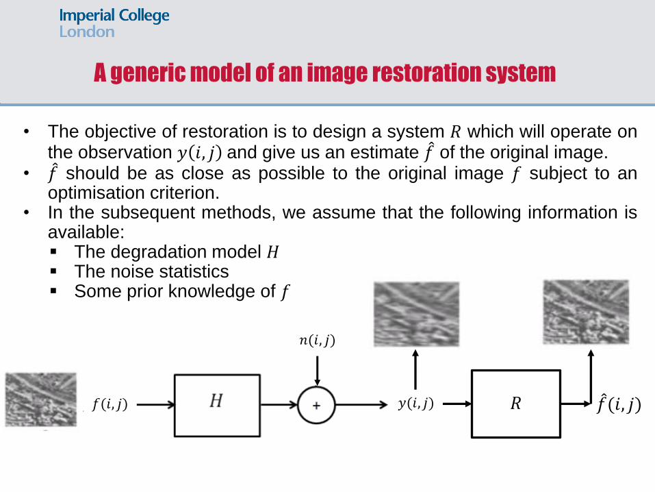
• The objective of restoration is to design a system 𝑅 which will operate on the observation 𝑦 𝑖, 𝑗 and give us an estimate 𝑓 of the original image.
• 𝑓 should be as close as possible to the original image 𝑓 subject to an optimisation criterion.
• In the subsequent methods, we assume that the following information is available: The degradation model 𝐻 The noise statistics Some prior knowledge of 𝑓
𝑅 𝑓(𝑖, 𝑗)
𝑛(𝑖, 𝑗)
𝑦(𝑖, 𝑗) 𝑓(𝑖, 𝑗)
Linear and space invariant (LSI) degradation model
In the degradation model: 𝑦 𝑖, 𝑗 = 𝐻 𝑓 𝑖, 𝑗 + 𝑛(𝑖, 𝑗)
we are interested in the definitions of linearity and space-invariance.
• The degradation model is linear if 𝐻 𝑘1𝑓1 𝑖, 𝑗 +𝑘2 𝑓2 𝑖, 𝑗 = 𝑘1𝐻 𝑓1 𝑖, 𝑗 + 𝑘2𝐻 𝑓2 𝑖, 𝑗
• The degradation model is space or position invariant if 𝐻 𝑓 𝑖 − 𝑖0, 𝑗 − 𝑗0 = 𝑦 𝑖 − 𝑖0, 𝑗 − 𝑗0
• In the above definitions we ignore the presence of external noise.
• In real life scenarios, various types of degradations can be approximated by linear, space-invariant operators.
Advantages and drawbacks of LSI assumptions
Advantages • It is much easier to deal with linear and space-invariant models because
mathematics are easier. • The distorted image is the convolution of the original image and the
distortion model. • Software tools are available.
Drawbacks For various realistic types of image degradations, assumptions for linearity and space-invariance are too strict and significantly deviate from the true degradation model.
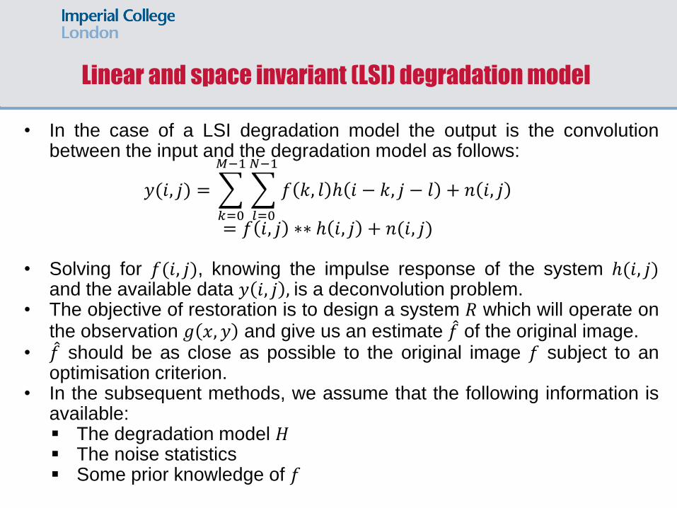
Linear and space invariant (LSI) degradation model
• In the case of a LSI degradation model the output is the convolution between the input and the degradation model as follows:
𝑦(𝑖, 𝑗) = 𝑓 𝑘, 𝑙 ℎ 𝑖 − 𝑘, 𝑗 − 𝑙
𝑁−1
𝑙=0
𝑀−1
𝑘=0
+ 𝑛 𝑖, 𝑗
= 𝑓 𝑖, 𝑗 ∗∗ ℎ 𝑖, 𝑗 + 𝑛(𝑖, 𝑗)
• Solving for 𝑓(𝑖, 𝑗), knowing the impulse response of the system ℎ(𝑖, 𝑗) and the available data 𝑦 𝑖, 𝑗 , is a deconvolution problem.
• The objective of restoration is to design a system 𝑅 which will operate on the observation 𝑔 𝑥, 𝑦 and give us an estimate 𝑓 of the original image.
• 𝑓 should be as close as possible to the original image 𝑓 subject to an optimisation criterion.
• In the subsequent methods, we assume that the following information is available: The degradation model 𝐻 The noise statistics Some prior knowledge of 𝑓
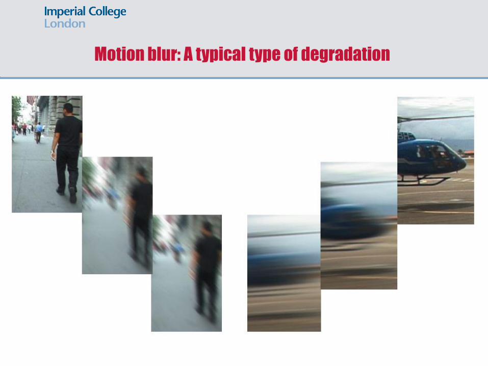
Motion blur: A typical type of degradation
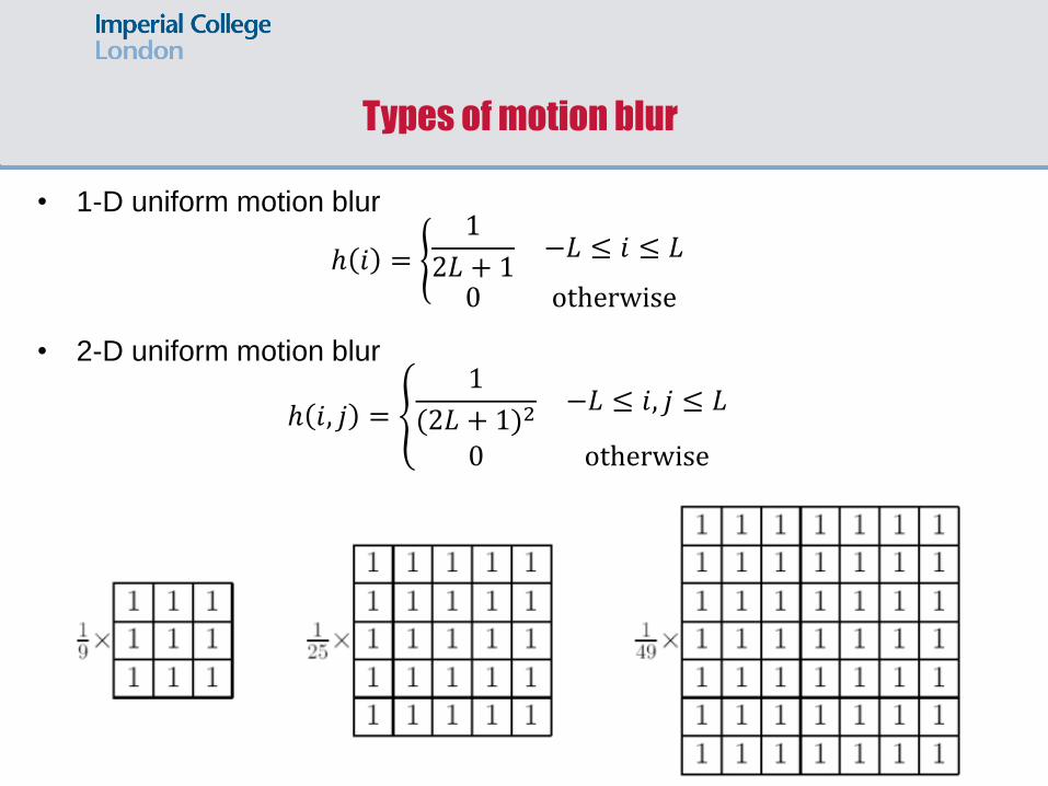
Types of motion blur
• 1-D uniform motion blur
ℎ 𝑖 = 1
2𝐿 + 1−𝐿 ≤ 𝑖 ≤ 𝐿
0 otherwise
• 2-D uniform motion blur
ℎ 𝑖, 𝑗 =
1
(2𝐿 + 1)2−𝐿 ≤ 𝑖, 𝑗 ≤ 𝐿
0 otherwise
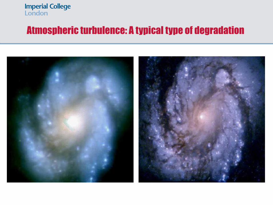
Atmospheric turbulence: A typical type of degradation
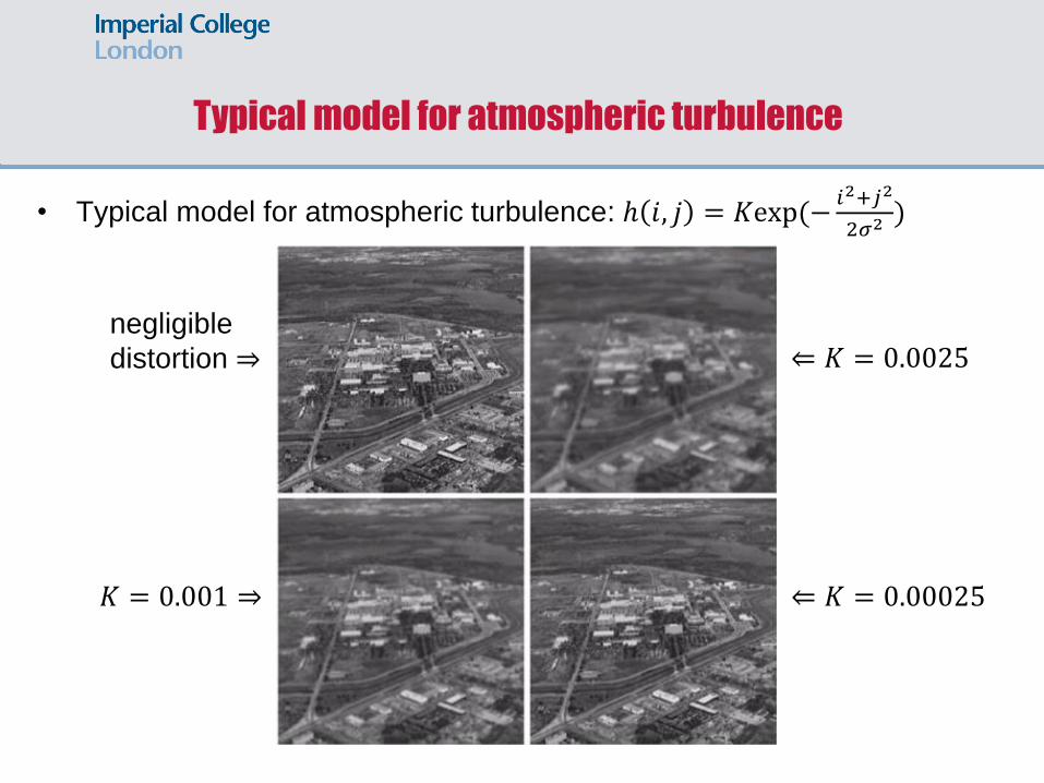
• Typical model for atmospheric turbulence: ℎ 𝑖, 𝑗 = 𝐾exp(−𝑖2+𝑗2
2𝜎2)
Typical model for atmospheric turbulence
negligible
distortion ⇒ ⇐ 𝐾 = 0.0025
⇐ 𝐾 = 0.00025 𝐾 = 0.001 ⇒
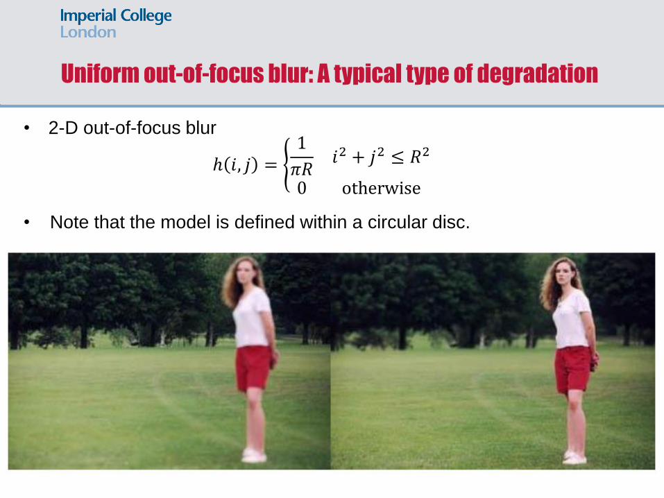
Uniform out-of-focus blur: A typical type of degradation
• 2-D out-of-focus blur
ℎ 𝑖, 𝑗 = 1
𝜋𝑅𝑖2 + 𝑗2 ≤ 𝑅2
0 otherwise
• Note that the model is defined within a circular disc.
An objective degradation metric
• Blurred Signal-to-Noise Ratio (BSNR)
This is a metric that reflects the severity of additive noise 𝑛(𝑖, 𝑗) in relation to the blurred image.
𝑧 𝑖, 𝑗 = 𝑦 𝑖, 𝑗 − 𝑛 𝑖, 𝑗 = 𝑓 𝑘, 𝑙 ℎ 𝑖 − 𝑘, 𝑗 − 𝑙𝑁−1𝑙=0
𝑀−1𝑘=0 is the
distorted image due to the formal degradation ℎ(𝑖, 𝑗) only.
𝑧 𝑖, 𝑗 = 𝐸{𝑧 𝑖, 𝑗 } is the expected value of 𝑧(𝑖, 𝑗). The BSNR is defined as follows:
BSNR = 10log10
1𝑀𝑁
𝑧 𝑖, 𝑗 − 𝑧 (𝑖, 𝑗) 2𝑗𝑖
𝜎𝑛2
The numerator is the variance of the blurred but noiseless signal
𝑧 𝑖, 𝑗 = 𝑓 𝑘, 𝑙 ℎ 𝑖 − 𝑘, 𝑗 − 𝑙
𝑁−1
𝑙=0
𝑀−1
𝑘=0
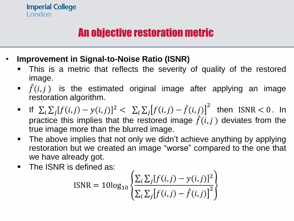
An objective restoration metric
• Improvement in Signal-to-Noise Ratio (ISNR)
This is a metric that reflects the severity of quality of the restored image.
𝑓 (𝑖, 𝑗 ) is the estimated original image after applying an image restoration algorithm.
If 𝑓 𝑖, 𝑗 − 𝑦(𝑖, 𝑗) 2𝑗𝑖 < 𝑓 𝑖, 𝑗 − 𝑓 (𝑖, 𝑗)
2𝑗𝑖 then ISNR < 0 . In
practice this implies that the restored image 𝑓 (𝑖, 𝑗 ) deviates from the true image more than the blurred image.
The above implies that not only we didn’t achieve anything by applying restoration but we created an image “worse” compared to the one that we have already got.
The ISNR is defined as:
ISNR = 10log10 𝑓 𝑖, 𝑗 − 𝑦(𝑖, 𝑗) 2
𝑗𝑖
𝑓 𝑖, 𝑗 − 𝑓 (𝑖, 𝑗)2
𝑗𝑖
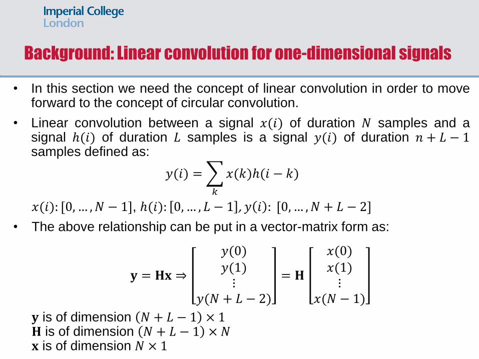
Background: Linear convolution for one-dimensional signals
• In this section we need the concept of linear convolution in order to move forward to the concept of circular convolution.
• Linear convolution between a signal 𝑥(𝑖) of duration 𝑁 samples and a signal ℎ(𝑖) of duration 𝐿 samples is a signal 𝑦(𝑖) of duration 𝑛 + 𝐿 − 1 samples defined as:
𝑦(𝑖) = 𝑥(𝑘)ℎ(𝑖 − 𝑘)
𝑘
𝑥(𝑖): [0, … , 𝑁 − 1], ℎ(𝑖): 0, … , 𝐿 − 1 , 𝑦 𝑖 : [0, … , 𝑁 + 𝐿 − 2]
• The above relationship can be put in a vector-matrix form as:
𝐲 = 𝐇𝐱 ⇒
𝑦(0)𝑦(1)⋮
𝑦(𝑁 + 𝐿 − 2)
= 𝐇
𝑥(0)𝑥(1)⋮
𝑥(𝑁 − 1)
𝐲 is of dimension 𝑁 + 𝐿 − 1 × 1 𝐇 is of dimension 𝑁 + 𝐿 − 1 × 𝑁 𝐱 is of dimension 𝑁 × 1
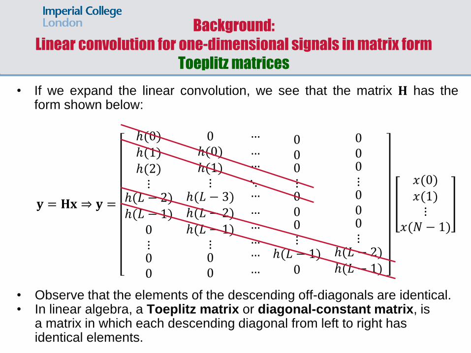
Background:
Linear convolution for one-dimensional signals in matrix form
Toeplitz matrices
• If we expand the linear convolution, we see that the matrix 𝐇 has the form shown below:
𝐲 = 𝐇𝐱 ⇒ 𝐲 =
ℎ(0)ℎ(1)ℎ(2)⋮
ℎ(𝐿 − 2)ℎ(𝐿 − 1)
0⋮00
0ℎ(0)ℎ(1)⋮
ℎ(𝐿 − 3)ℎ(𝐿 − 2)ℎ(𝐿 − 1)
⋮00
⋱
000⋮000⋮
ℎ(𝐿 − 1)0
000⋮000⋮
ℎ(𝐿 − 2)ℎ(𝐿 − 1)
𝑥(0)𝑥(1)⋮
𝑥(𝑁 − 1)
• Observe that the elements of the descending off-diagonals are identical. • In linear algebra, a Toeplitz matrix or diagonal-constant matrix, is
a matrix in which each descending diagonal from left to right has identical elements.
…
… …
…
… … … …
…
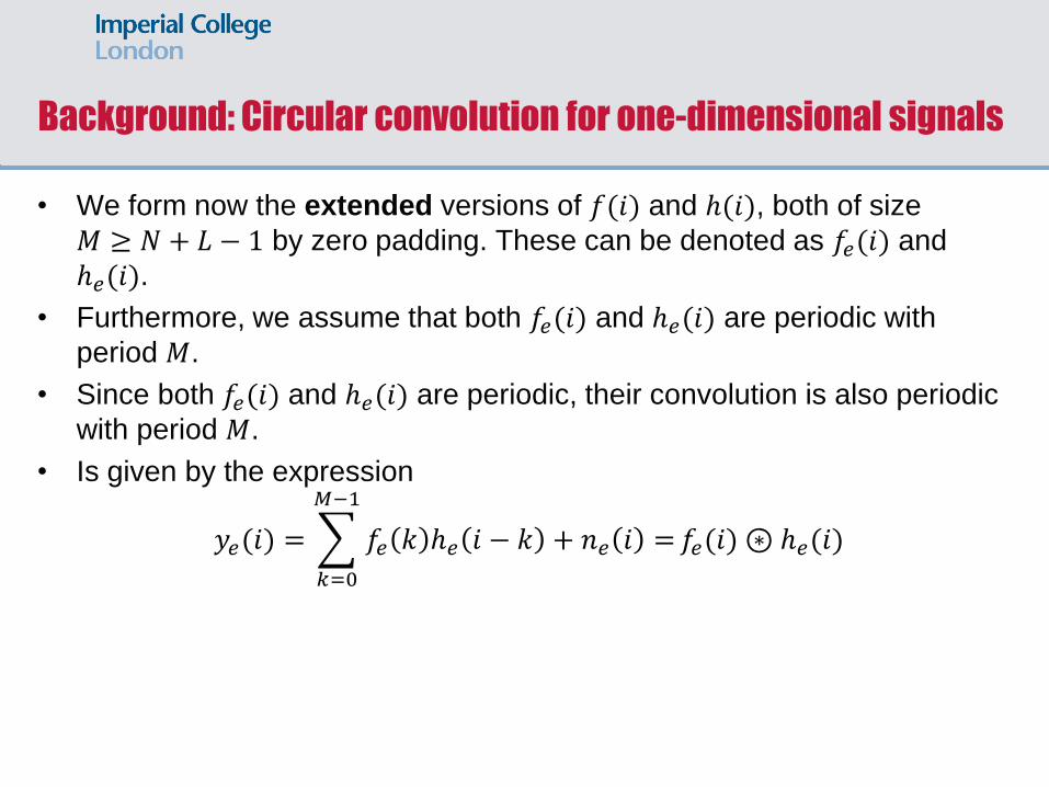
Background: Circular convolution for one-dimensional signals
• We form now the extended versions of 𝑓(𝑖) and ℎ(𝑖), both of size
𝑀 ≥ 𝑁 + 𝐿 − 1 by zero padding. These can be denoted as 𝑓𝑒(𝑖) and
ℎ𝑒(𝑖).
• Furthermore, we assume that both 𝑓𝑒(𝑖) and ℎ𝑒(𝑖) are periodic with
period 𝑀.
• Since both 𝑓𝑒(𝑖) and ℎ𝑒(𝑖) are periodic, their convolution is also periodic
with period 𝑀.
• Is given by the expression
𝑦𝑒(𝑖) = 𝑓𝑒 𝑘 ℎ𝑒 𝑖 − 𝑘 + 𝑛𝑒 𝑖 =
𝑀−1
𝑘=0
𝑓𝑒(𝑖) ⊛ ℎ𝑒(𝑖)
Background: Circular convolution for one-dimensional signals
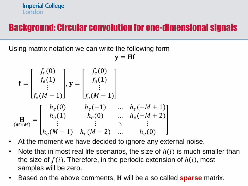
Using matrix notation we can write the following form
𝐲 = 𝐇𝐟
𝐟 =
𝑓𝑒(0)𝑓𝑒(1)⋮
𝑓𝑒(𝑀 − 1)
, 𝐲 =
𝑓𝑒(0)𝑓𝑒(1)⋮
𝑓𝑒(𝑀 − 1)
𝐇(𝑀×𝑀)
=
ℎ𝑒(0) ℎ𝑒(−1) … ℎ𝑒(−𝑀 + 1)ℎ𝑒(1) ℎ𝑒(0) … ℎ𝑒(−𝑀 + 2)⋮ ⋮ ⋱ ⋮
ℎ𝑒(𝑀 − 1) ℎ𝑒(𝑀 − 2) … ℎ𝑒(0)
• At the moment we have decided to ignore any external noise.
• Note that in most real life scenarios, the size of ℎ(𝑖) is much smaller than
the size of 𝑓(𝑖). Therefore, in the periodic extension of ℎ 𝑖 , most
samples will be zero.
• Based on the above comments, 𝐇 will be a so called sparse matrix.
Circular convolution for one-dimensional signals
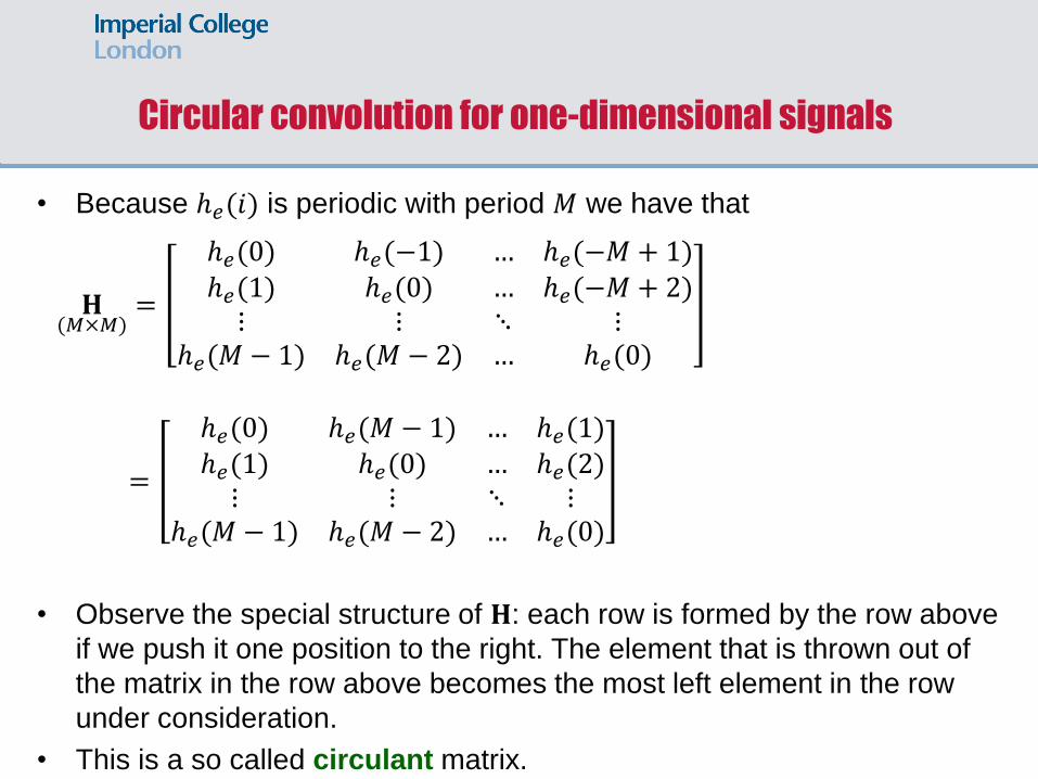
• Because ℎ𝑒(𝑖) is periodic with period 𝑀 we have that
𝐇(𝑀×𝑀)
=
ℎ𝑒(0) ℎ𝑒(−1) … ℎ𝑒(−𝑀 + 1)ℎ𝑒(1) ℎ𝑒(0) … ℎ𝑒(−𝑀 + 2)⋮ ⋮ ⋱ ⋮
ℎ𝑒(𝑀 − 1) ℎ𝑒(𝑀 − 2) … ℎ𝑒(0)
=
ℎ𝑒(0) ℎ𝑒(𝑀 − 1) … ℎ𝑒(1)ℎ𝑒(1) ℎ𝑒(0) … ℎ𝑒(2)⋮ ⋮ ⋱ ⋮
ℎ𝑒(𝑀 − 1) ℎ𝑒(𝑀 − 2) … ℎ𝑒(0)
• Observe the special structure of 𝐇: each row is formed by the row above
if we push it one position to the right. The element that is thrown out of
the matrix in the row above becomes the most left element in the row
under consideration.
• This is a so called circulant matrix.
Eigenvalues of circulant matrices
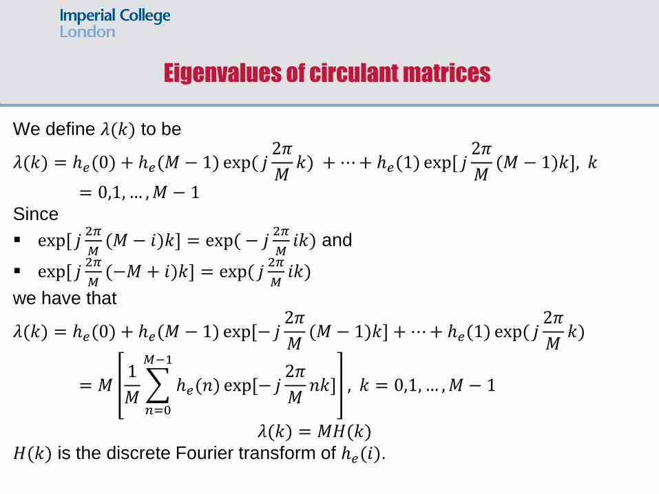
We define 𝜆(𝑘) to be
𝜆(𝑘) = ℎ𝑒(0) + ℎ𝑒(𝑀 − 1) exp( 𝑗2𝜋
𝑀𝑘) + ⋯+ ℎ𝑒(1) exp[ 𝑗
2𝜋
𝑀(𝑀 − 1)𝑘], 𝑘
= 0,1, … ,𝑀 − 1
Since
exp[ 𝑗2𝜋
𝑀(𝑀 − 𝑖)𝑘] = exp( − 𝑗
2𝜋
𝑀𝑖𝑘) and
exp[ 𝑗2𝜋
𝑀(−𝑀 + 𝑖)𝑘] = exp( 𝑗
2𝜋
𝑀𝑖𝑘)
we have that
𝜆(𝑘) = ℎ𝑒(0) + ℎ𝑒(𝑀 − 1) exp[− 𝑗2𝜋
𝑀(𝑀 − 1)𝑘] + ⋯+ ℎ𝑒(1) exp( 𝑗
2𝜋
𝑀𝑘)
= 𝑀1
𝑀 ℎ𝑒(𝑛) exp[− 𝑗
2𝜋
𝑀𝑛𝑘]
𝑀−1
𝑛=0
, 𝑘 = 0,1, … ,𝑀 − 1
𝜆(𝑘) = 𝑀𝐻(𝑘) 𝐻(𝑘) is the discrete Fourier transform of ℎ𝑒(𝑖).
Eigenvalues and eigenvectors of circulant matrices
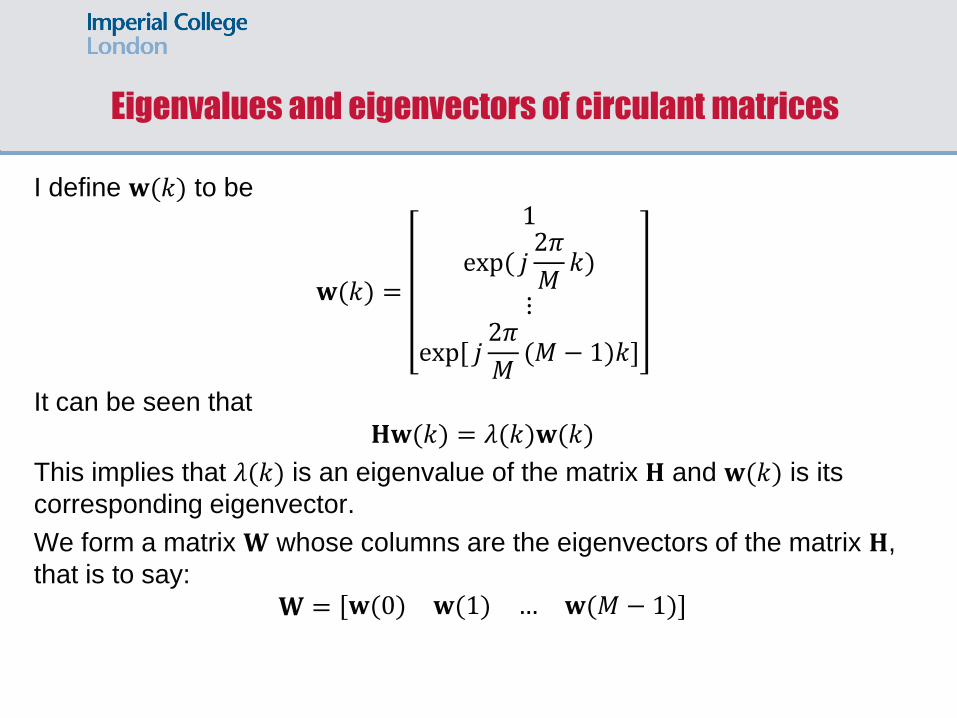
I define 𝐰(𝑘) to be
𝐰(𝑘) =
1
exp( 𝑗2𝜋
𝑀𝑘)
⋮
exp[ 𝑗2𝜋
𝑀(𝑀 − 1)𝑘]
It can be seen that
𝐇𝐰(𝑘) = 𝜆(𝑘)𝐰(𝑘)
This implies that 𝜆(𝑘) is an eigenvalue of the matrix 𝐇 and 𝐰(𝑘) is its
corresponding eigenvector.
We form a matrix 𝐖 whose columns are the eigenvectors of the matrix 𝐇,
that is to say:
𝐖 = 𝐰(0) 𝐰(1) … 𝐰(𝑀 − 1)
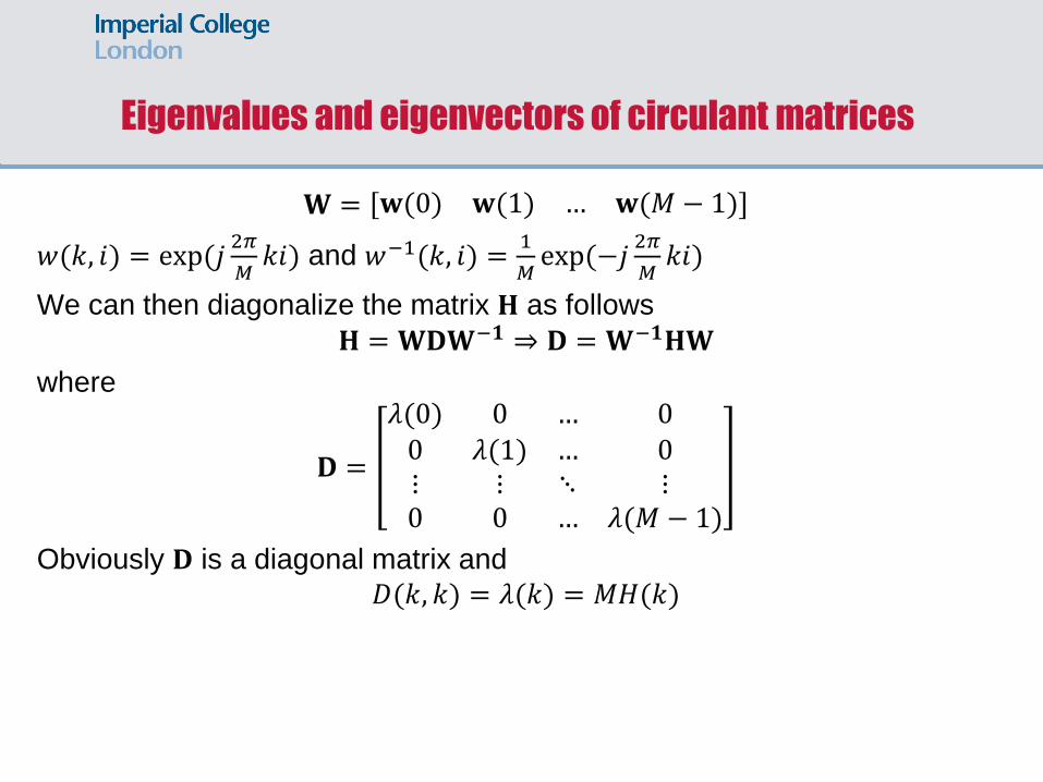
Eigenvalues and eigenvectors of circulant matrices
𝐖 = 𝐰(0) 𝐰(1) … 𝐰(𝑀 − 1)
𝑤(𝑘, 𝑖) = exp(𝑗2𝜋
𝑀𝑘𝑖) and 𝑤−1(𝑘, 𝑖) =
1
𝑀exp(−𝑗
2𝜋
𝑀𝑘𝑖)
We can then diagonalize the matrix 𝐇 as follows
𝐇 = 𝐖𝐃𝐖−𝟏 ⇒ 𝐃 = 𝐖−𝟏𝐇𝐖
where
𝐃 =
𝜆(0) 0 … 00 𝜆(1) … 0⋮ ⋮ ⋱ ⋮0 0 … 𝜆(𝑀 − 1)
Obviously 𝐃 is a diagonal matrix and
𝐷(𝑘, 𝑘) = 𝜆(𝑘) = 𝑀𝐻(𝑘)
Circular convolution and DFT
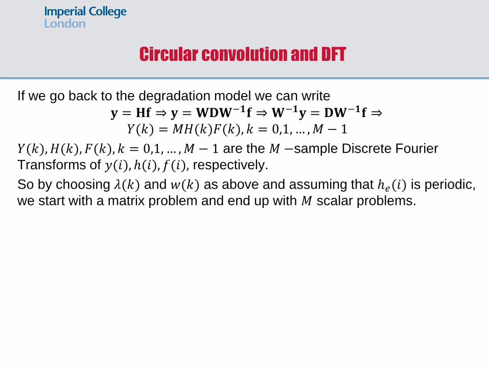
If we go back to the degradation model we can write
𝐲 = 𝐇𝐟 ⇒ 𝐲 = 𝐖𝐃𝐖−𝟏𝐟 ⇒ 𝐖−𝟏𝐲 = 𝐃𝐖−𝟏𝐟 ⇒
𝑌(𝑘) = 𝑀𝐻(𝑘)𝐹(𝑘), 𝑘 = 0,1, … ,𝑀 − 1
𝑌(𝑘), 𝐻(𝑘), 𝐹(𝑘), 𝑘 = 0,1, … ,𝑀 − 1 are the 𝑀 −sample Discrete Fourier
Transforms of 𝑦(𝑖), ℎ(𝑖), 𝑓(𝑖), respectively.
So by choosing 𝜆(𝑘) and 𝑤(𝑘) as above and assuming that ℎ𝑒(𝑖) is periodic,
we start with a matrix problem and end up with 𝑀 scalar problems.
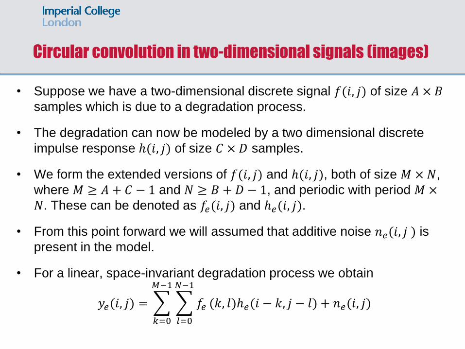
Circular convolution in two-dimensional signals (images)
• Suppose we have a two-dimensional discrete signal 𝑓(𝑖, 𝑗) of size 𝐴 × 𝐵
samples which is due to a degradation process.
• The degradation can now be modeled by a two dimensional discrete
impulse response ℎ(𝑖, 𝑗) of size 𝐶 × 𝐷 samples.
• We form the extended versions of 𝑓(𝑖, 𝑗) and ℎ(𝑖, 𝑗), both of size 𝑀 ×𝑁,
where 𝑀 ≥ 𝐴 + 𝐶 − 1 and 𝑁 ≥ 𝐵 + 𝐷 − 1, and periodic with period 𝑀 ×𝑁. These can be denoted as 𝑓𝑒(𝑖, 𝑗) and ℎ𝑒(𝑖, 𝑗).
• From this point forward we will assumed that additive noise 𝑛𝑒(𝑖, 𝑗 ) is
present in the model.
• For a linear, space-invariant degradation process we obtain
𝑦𝑒(𝑖, 𝑗) = 𝑓𝑒
𝑁−1
𝑙=0
(𝑘, 𝑙)ℎ𝑒(𝑖 − 𝑘, 𝑗 − 𝑙) + 𝑛𝑒(𝑖, 𝑗)
𝑀−1
𝑘=0
Lexicographic ordering
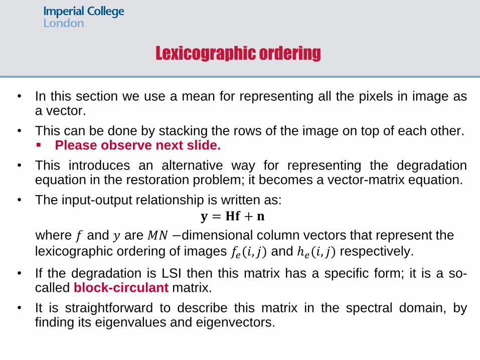
• In this section we use a mean for representing all the pixels in image as a vector.
• This can be done by stacking the rows of the image on top of each other. Please observe next slide.
• This introduces an alternative way for representing the degradation equation in the restoration problem; it becomes a vector-matrix equation.
• The input-output relationship is written as:
𝐲 = 𝐇𝐟 + 𝐧
where 𝑓 and 𝑦 are 𝑀𝑁 −dimensional column vectors that represent the
lexicographic ordering of images 𝑓𝑒(𝑖, 𝑗) and ℎ𝑒(𝑖, 𝑗) respectively.
• If the degradation is LSI then this matrix has a specific form; it is a so-called block-circulant matrix.
• It is straightforward to describe this matrix in the spectral domain, by finding its eigenvalues and eigenvectors.
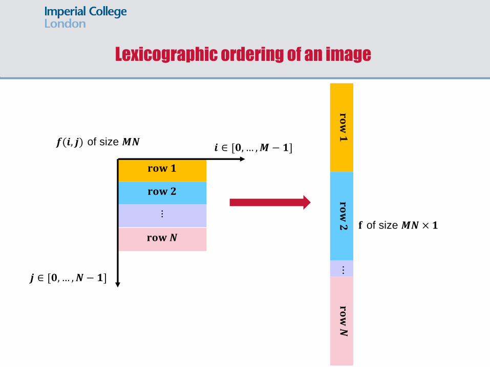
Lexicographic ordering of an image
𝐫𝐨𝐰 𝟏
𝐫𝐨𝐰 𝟐
𝐫𝐨𝐰 𝟏
𝐫𝐨𝐰 𝟐
⋮
𝐫𝐨𝐰 𝑵
𝐫𝐨𝐰 𝑵
⋯
𝒊 ∈ [𝟎,… ,𝑴 − 𝟏]
𝒋 ∈ [𝟎,… ,𝑵 − 𝟏]
𝒇(𝒊, 𝒋) of size 𝑴𝑵
𝐟 of size 𝑴𝑵× 𝟏
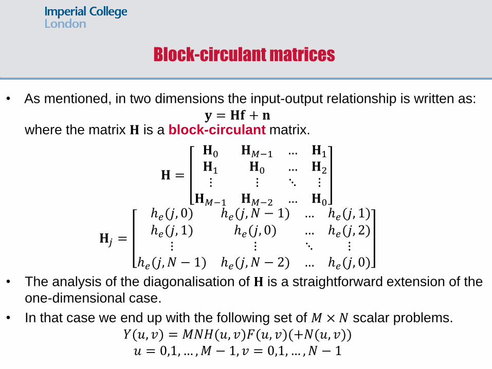
Block-circulant matrices
• As mentioned, in two dimensions the input-output relationship is written as:
𝐲 = 𝐇𝐟 + 𝐧 where the matrix 𝐇 is a block-circulant matrix.
𝐇 =
𝐇0 𝐇𝑀−1 … 𝐇1
𝐇1 𝐇0 … 𝐇2
⋮ ⋮ ⋱ ⋮𝐇𝑀−1 𝐇𝑀−2 … 𝐇0
𝐇𝑗 =
ℎ𝑒(𝑗, 0) ℎ𝑒(𝑗, 𝑁 − 1) … ℎ𝑒(𝑗, 1)ℎ𝑒(𝑗, 1) ℎ𝑒(𝑗, 0) … ℎ𝑒(𝑗, 2)
⋮ ⋮ ⋱ ⋮ℎ𝑒(𝑗, 𝑁 − 1) ℎ𝑒(𝑗, 𝑁 − 2) … ℎ𝑒(𝑗, 0)
• The analysis of the diagonalisation of 𝐇 is a straightforward extension of the
one-dimensional case.
• In that case we end up with the following set of 𝑀 ×𝑁 scalar problems.
𝑌(𝑢, 𝑣) = 𝑀𝑁𝐻(𝑢, 𝑣)𝐹(𝑢, 𝑣)(+𝑁(𝑢, 𝑣)) 𝑢 = 0,1, … ,𝑀 − 1, 𝑣 = 0,1, … , 𝑁 − 1
Periodic extension of images and degradation model
• In image restoration we often work with Discrete Fourier Transforms.
• DFT assumes periodicity of the signal in time or space.
• Therefore, periodic extension of signals is required.
• Distorted image is the convolution of the original image and the distortion model. We are able to assume this because of the linearity and space invariance assumptions.
• Convolution increases the size of signals.
• Periodic extension must take into consideration the presence of convolution: zero-padding is required.
• Every signal involved in an image restoration system must be extended by zero-padding and also treated as virtually periodic.
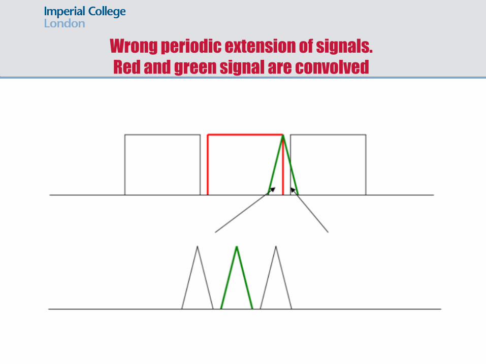
Wrong periodic extension of signals.
Red and green signal are convolved
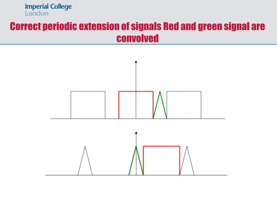
Correct periodic extension of signals Red and green signal are
convolved
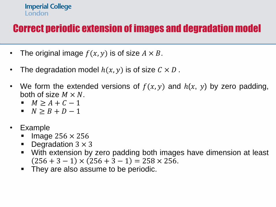
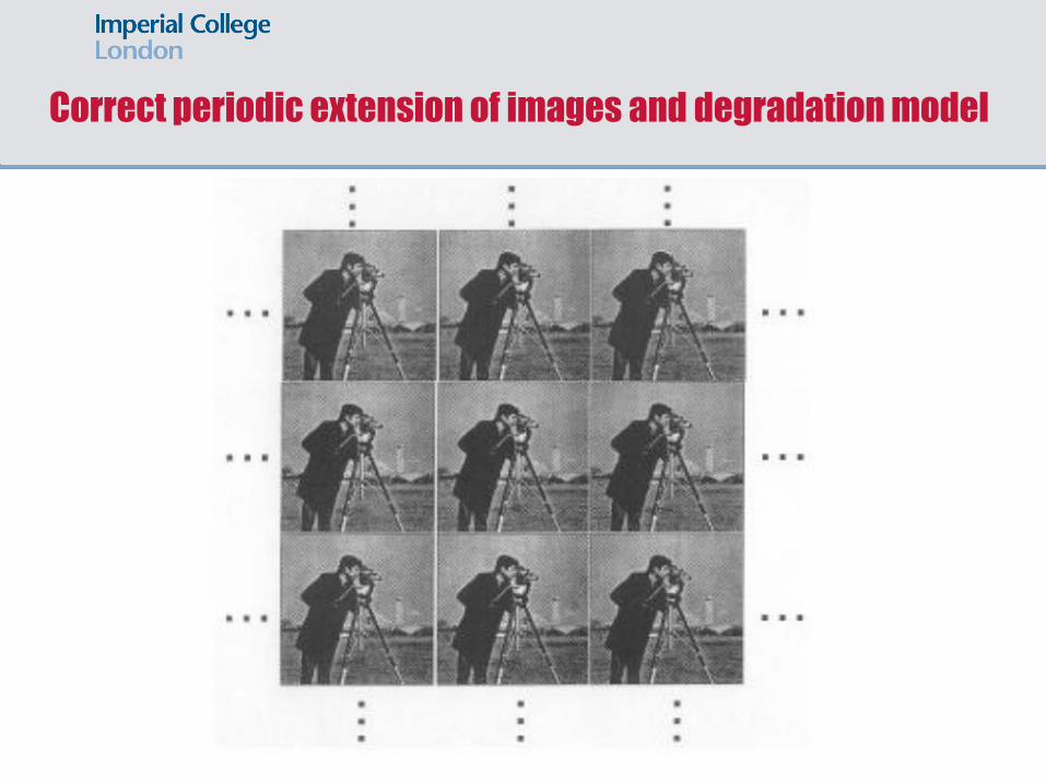
Correct periodic extension of images and degradation model
• The original image 𝑓(𝑥, 𝑦) is of size 𝐴 × 𝐵.
• The degradation model ℎ(𝑥, 𝑦) is of size 𝐶 × 𝐷 . • We form the extended versions of 𝑓(𝑥, 𝑦) and ℎ(𝑥, 𝑦) by zero padding,
both of size 𝑀 ×𝑁. 𝑀 ≥ 𝐴 + 𝐶 − 1 𝑁 ≥ 𝐵 + 𝐷 − 1
• Example
Image 256 × 256 Degradation 3 × 3 With extension by zero padding both images have dimension at least
256 + 3 − 1 × 256 + 3 − 1 = 258 × 256. They are also assume to be periodic.
Correct periodic extension of images and degradation model
Inverse filtering for image restoration
• Inverse filtering is a deterministic and direct method for image restoration.
• The images involved must be lexicographically ordered. That means that an image is converted to a column vector by stacking the rows one by one after converting them to columns.
• Therefore, an image of size 𝑀 ×𝑁 = 256 × 256 is converted to a column vector of size (256 × 256) × 1 = 65536 × 1.
• The degradation model is written in a matrix form as 𝐲 = 𝐇𝐟
where the images are vectors and the degradation process is a huge but sparse matrix of size 𝑀𝑁 ×𝑀𝑁.
• The above relationship is ideal. The true degradation model is 𝐲 = 𝐇𝐟 + 𝐧 where 𝐧 is a lexicographically ordered two dimensional noisy signal which corrupts the distorted image 𝑦(𝑖, 𝑗).
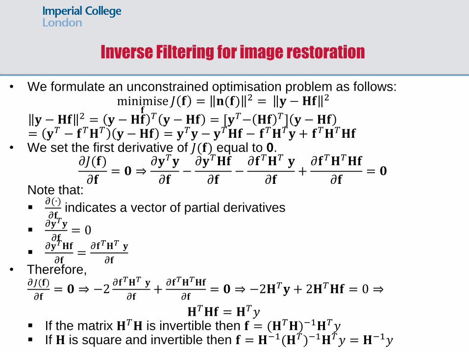
Inverse Filtering for image restoration
• We formulate an unconstrained optimisation problem as follows: minimise
𝐟𝐽 𝐟 = 𝐧(𝐟) 2 = 𝐲 − 𝐇𝐟 2
𝐲 − 𝐇𝐟 2 = 𝐲 − 𝐇𝐟 𝑇 𝐲 − 𝐇𝐟 = [𝐲𝑇− 𝐇𝐟 𝑇] 𝐲 − 𝐇𝐟 = 𝐲𝑇 − 𝐟𝑇𝐇𝑇 𝐲 − 𝐇𝐟 = 𝐲𝑇𝐲 − 𝐲𝑇𝐇𝐟 − 𝐟𝑇𝐇𝑇𝐲 + 𝐟𝑇𝐇𝑇𝐇𝐟
• We set the first derivative of 𝐽(𝐟) equal to 0. 𝜕𝐽(𝐟)
𝜕𝐟= 𝟎 ⇒
𝜕𝐲𝑇𝐲
𝜕𝐟−𝜕𝐲𝑇𝐇𝐟
𝜕𝐟−𝜕𝐟𝑇𝐇𝑇 𝐲
𝜕𝐟+𝜕𝐟𝑇𝐇𝑇𝐇𝐟
𝜕𝐟= 𝟎
Note that:
𝜕(∙)
𝜕𝐟 indicates a vector of partial derivatives
𝜕𝐲𝑇𝐲
𝜕𝐟= 0
𝜕𝐲𝑇𝐇𝐟
𝜕𝐟=
𝜕𝐟𝑇𝐇𝑇 𝐲𝜕𝐟
• Therefore, 𝜕𝐽(𝐟)
𝜕𝐟= 𝟎 ⇒ −2
𝜕𝐟𝑇𝐇𝑇 𝐲𝜕𝐟
+𝜕𝐟𝑇𝐇𝑇𝐇𝐟
𝜕𝐟= 𝟎 ⇒ −2𝐇𝑇𝐲 + 2𝐇𝑇𝐇𝐟 = 0 ⇒
𝐇𝑇𝐇𝐟 = 𝐇𝑇𝑦 If the matrix 𝐇𝑇𝐇 is invertible then 𝐟 = (𝐇𝑇𝐇)−1𝐇𝑇𝑦 If 𝐇 is square and invertible then 𝐟 = 𝐇−1(𝐇𝑇)−1𝐇𝑇𝑦 = 𝐇−1𝑦
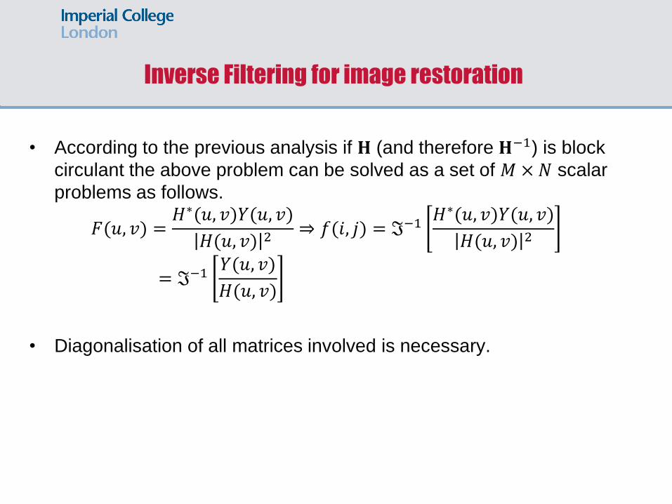
Inverse Filtering for image restoration
• According to the previous analysis if 𝐇 (and therefore 𝐇−1) is block
circulant the above problem can be solved as a set of 𝑀 ×𝑁 scalar
problems as follows.
𝐹(𝑢, 𝑣) =𝐻∗(𝑢, 𝑣)𝑌(𝑢, 𝑣)
𝐻(𝑢, 𝑣) 2⇒ 𝑓(𝑖, 𝑗) = ℑ−1
𝐻∗(𝑢, 𝑣)𝑌(𝑢, 𝑣)
𝐻(𝑢, 𝑣) 2
= ℑ−1𝑌(𝑢, 𝑣)
𝐻(𝑢, 𝑣)
• Diagonalisation of all matrices involved is necessary.
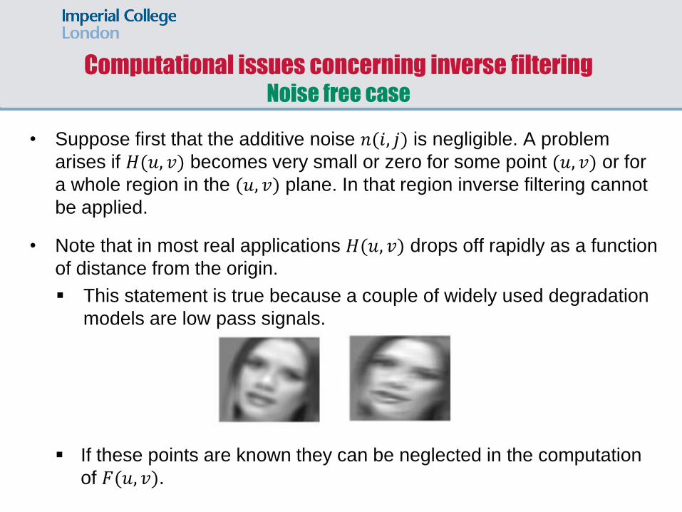
Computational issues concerning inverse filtering Noise free case
• Suppose first that the additive noise 𝑛(𝑖, 𝑗) is negligible. A problem
arises if 𝐻(𝑢, 𝑣) becomes very small or zero for some point (𝑢, 𝑣) or for
a whole region in the (𝑢, 𝑣) plane. In that region inverse filtering cannot
be applied.
• Note that in most real applications 𝐻(𝑢, 𝑣) drops off rapidly as a function
of distance from the origin.
This statement is true because a couple of widely used degradation
models are low pass signals.
If these points are known they can be neglected in the computation
of 𝐹(𝑢, 𝑣).
Computational issues concerning inverse filtering Noisy case
• In the presence of external noise we have that
𝐹 (𝑢, 𝑣) =𝐻∗(𝑢, 𝑣) 𝑌(𝑢, 𝑣) − 𝑁(𝑢, 𝑣)
𝐻(𝑢, 𝑣) 2=
𝐻∗(𝑢, 𝑣)𝑌(𝑢, 𝑣)
𝐻(𝑢, 𝑣) 2−𝐻∗ 𝑢, 𝑣 𝑁 𝑢, 𝑣
𝐻 𝑢, 𝑣 2⇒
𝐹 (𝑢, 𝑣) = 𝐹(𝑢, 𝑣) −𝑁(𝑢, 𝑣)
𝐻(𝑢, 𝑣)
• If 𝐻(𝑢, 𝑣) becomes very small, the term 𝑁(𝑢, 𝑣) dominates the result.
• In that case we have the so-called noise amplification effect.
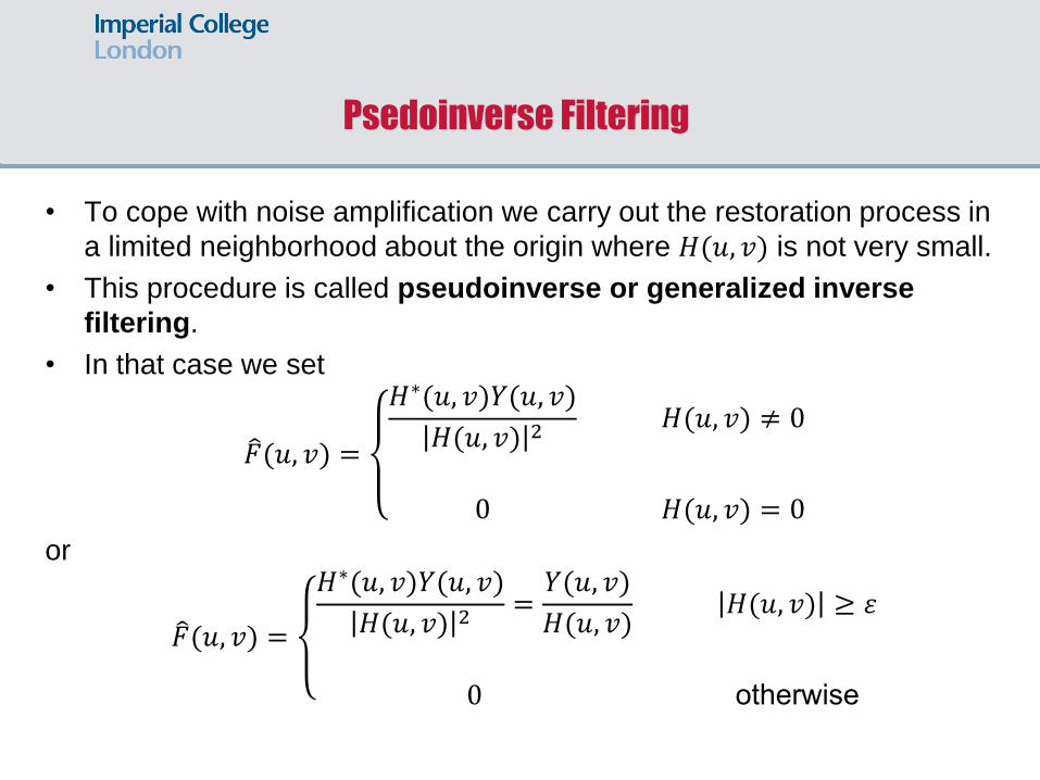
Psedoinverse Filtering
• To cope with noise amplification we carry out the restoration process in
a limited neighborhood about the origin where 𝐻(𝑢, 𝑣) is not very small.
• This procedure is called pseudoinverse or generalized inverse
filtering.
• In that case we set
𝐹 (𝑢, 𝑣) =
𝐻∗(𝑢, 𝑣)𝑌(𝑢, 𝑣)
𝐻(𝑢, 𝑣) 2𝐻(𝑢, 𝑣) ≠ 0
0 𝐻(𝑢, 𝑣) = 0
or
𝐹 (𝑢, 𝑣) =
𝐻∗(𝑢, 𝑣)𝑌(𝑢, 𝑣)
𝐻(𝑢, 𝑣) 2=𝑌(𝑢, 𝑣)
𝐻(𝑢, 𝑣)𝐻(𝑢, 𝑣) ≥ 𝜀
0 otherwise
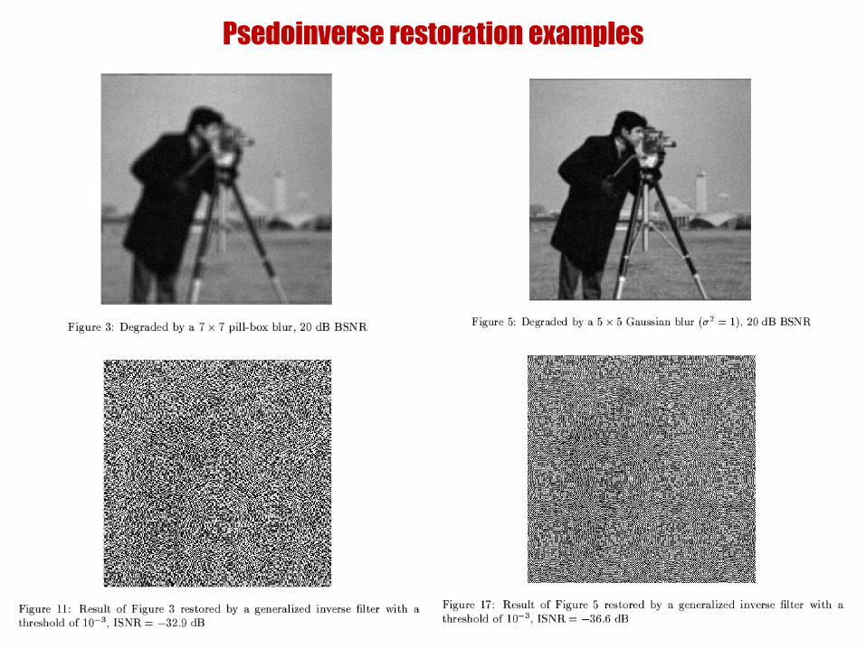
Psedoinverse restoration examples
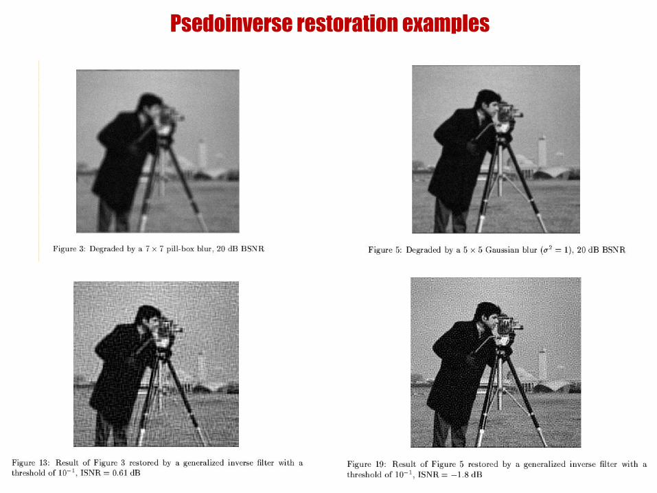
Psedoinverse restoration examples
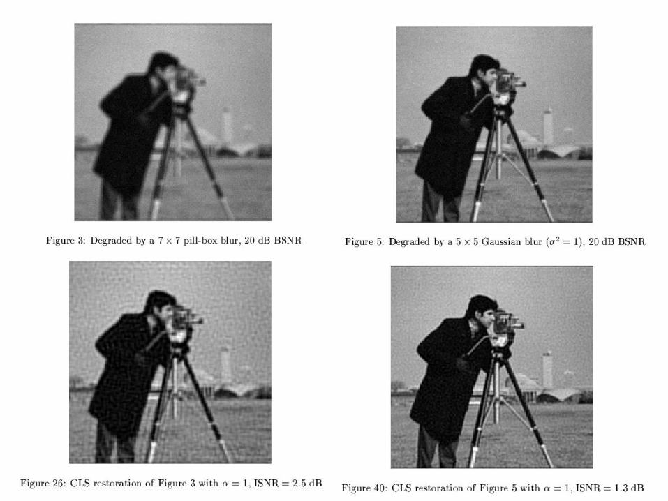
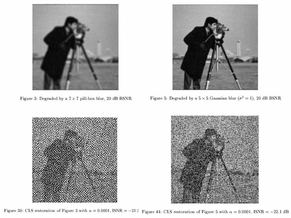
Constrained Least Squares (CLS) Restoration
• By introducing a so called Lagrange multiplier or regularisation parameter 𝛼, we transform the constrained optimisation problem to an unconstrained one as follows.
• The problem 𝐦𝐢𝐧𝐢𝐦𝐢𝐬𝐞
𝐟𝑱 𝐟 = 𝐲 − 𝐇𝐟 𝟐
subject to 𝐂𝐟 𝟐 < 𝜺 is equivalent to
𝐦𝐢𝐧𝐢𝐦𝐢𝐬𝐞𝐟
𝑱 𝐟 = 𝐲 − 𝐇𝐟 𝟐 + 𝜶 𝐂𝐟 𝟐
• The imposed constraint implies that the energy of the restored image at
high frequencies is below a threshold.
• It is basically a smoothness constraint. 𝐂 a high pass filter operator 𝐂f a high pass filtered version of the image
Constrained Least Squares (CLS) Restoration
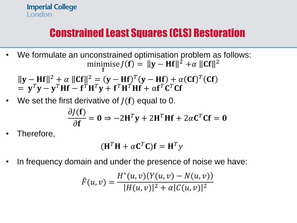
• We formulate an unconstrained optimisation problem as follows: minimise
𝐟𝐽 𝐟 = 𝐲 − 𝐇𝐟 2 +𝛼 𝐂𝐟 2
𝐲 − 𝐇𝐟 2 + 𝛼 𝐂𝐟 2 = 𝐲 − 𝐇𝐟 𝑇 𝐲 − 𝐇𝐟 + 𝛼 𝐂𝐟 𝑇 𝐂𝐟 = 𝐲𝑇𝐲 − 𝐲𝑇𝐇𝐟 − 𝐟𝑇𝐇𝑇𝐲 + 𝐟𝑇𝐇𝑇𝐇𝐟 + α𝐟𝑇𝐂𝑇𝐂𝐟
• We set the first derivative of 𝐽(𝐟) equal to 0.
𝜕𝐽(𝐟)
𝜕𝐟= 𝟎 ⇒ −2𝐇𝑇𝐲 + 2𝐇𝑇𝐇𝐟 + 2𝛼𝐂𝑇𝐂𝐟 = 𝟎
• Therefore,
(𝐇𝑇𝐇+ 𝛼𝐂𝑇𝐂)𝐟 = 𝐇𝑇𝑦
• In frequency domain and under the presence of noise we have:
𝐹 (𝑢, 𝑣) =𝐻∗(𝑢, 𝑣) 𝑌(𝑢, 𝑣) − 𝑁(𝑢, 𝑣)
𝐻(𝑢, 𝑣) 2 + 𝛼 𝐶(𝑢, 𝑣) 2
Constrained Least Squares (CLS) Restoration
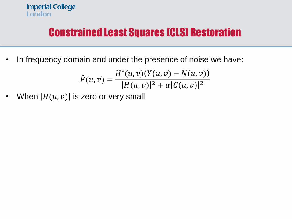
• In frequency domain and under the presence of noise we have:
𝐹 (𝑢, 𝑣) =𝐻∗(𝑢, 𝑣) 𝑌(𝑢, 𝑣) − 𝑁(𝑢, 𝑣)
𝐻(𝑢, 𝑣) 2 + 𝛼 𝐶(𝑢, 𝑣) 2
• When 𝐻(𝑢, 𝑣) is zero or very small
Constrained Least Squares (CLS) Restoration: Observations
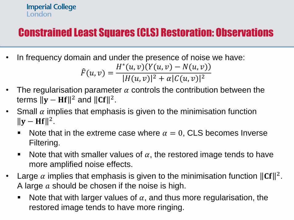
• In frequency domain and under the presence of noise we have:
𝐹 (𝑢, 𝑣) =𝐻∗(𝑢, 𝑣) 𝑌(𝑢, 𝑣) − 𝑁(𝑢, 𝑣)
𝐻(𝑢, 𝑣) 2 + 𝛼 𝐶(𝑢, 𝑣) 2
• The regularisation parameter 𝛼 controls the contribution between the
terms 𝐲 − 𝐇𝐟 2 and 𝐂𝐟 2.
• Small 𝛼 implies that emphasis is given to the minimisation function
𝐲 − 𝐇𝐟 2.
Note that in the extreme case where 𝛼 = 0, CLS becomes Inverse
Filtering.
Note that with smaller values of 𝛼, the restored image tends to have
more amplified noise effects.
• Large 𝛼 implies that emphasis is given to the minimisation function 𝐂𝐟 2.
A large 𝑎 should be chosen if the noise is high.
Note that with larger values of 𝛼, and thus more regularisation, the
restored image tends to have more ringing.
Choice of 𝜶 cont.
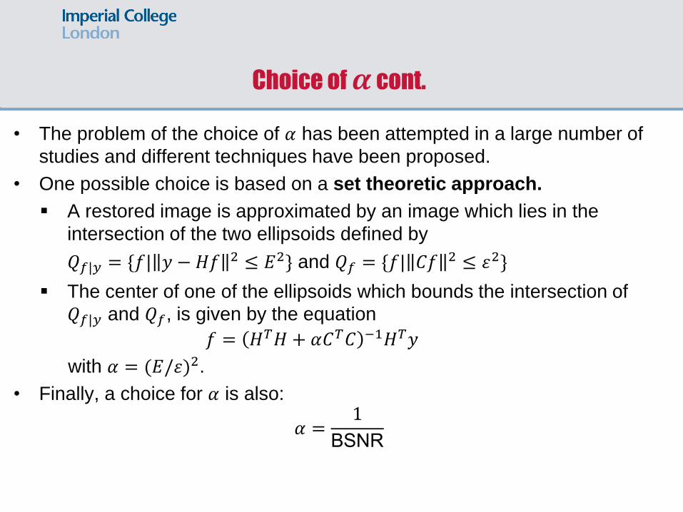
• The problem of the choice of 𝛼 has been attempted in a large number of
studies and different techniques have been proposed.
• One possible choice is based on a set theoretic approach.
A restored image is approximated by an image which lies in the
intersection of the two ellipsoids defined by
𝑄𝑓|𝑦 = {𝑓| 𝑦 − 𝐻𝑓 2 ≤ 𝐸2} and 𝑄𝑓 = {𝑓| 𝐶𝑓 2 ≤ 𝜀2}
The center of one of the ellipsoids which bounds the intersection of
𝑄𝑓|𝑦 and 𝑄𝑓, is given by the equation
𝑓 = 𝐻𝑇𝐻 + 𝛼𝐶𝑇𝐶 −1𝐻𝑇𝑦
with 𝛼 = (𝐸/𝜀)2.
• Finally, a choice for 𝛼 is also:
𝛼 =1
BSNR
Choice of 𝜶
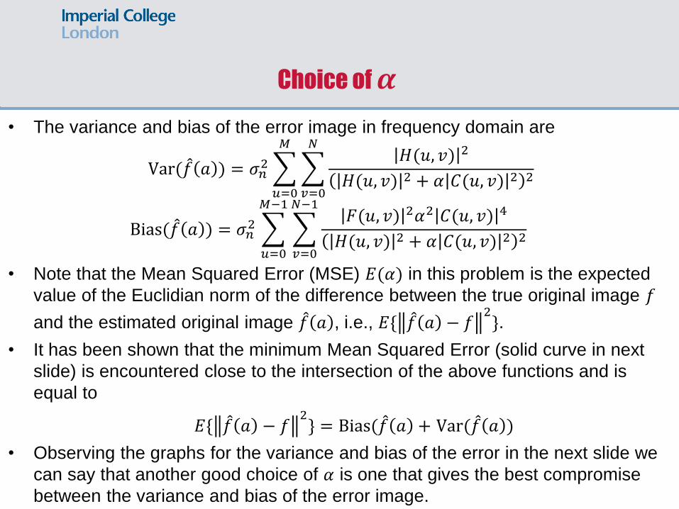
• The variance and bias of the error image in frequency domain are
Var(𝑓 𝑎 ) = 𝜎𝑛2
𝐻(𝑢, 𝑣) 2
𝐻(𝑢, 𝑣) 2 + 𝛼 𝐶(𝑢, 𝑣) 2 2
𝑁
𝑣=0
𝑀
𝑢=0
Bias(𝑓 𝑎 ) = 𝜎𝑛2
𝐹(𝑢, 𝑣) 2𝛼2 𝐶(𝑢, 𝑣) 4
𝐻(𝑢, 𝑣) 2 + 𝛼 𝐶(𝑢, 𝑣) 2 2
𝑁−1
𝑣=0
𝑀−1
𝑢=0
• Note that the Mean Squared Error (MSE) 𝐸(𝛼) in this problem is the expected
value of the Euclidian norm of the difference between the true original image 𝑓
and the estimated original image 𝑓 𝑎 , i.e., 𝐸{ 𝑓 𝑎 − 𝑓2}.
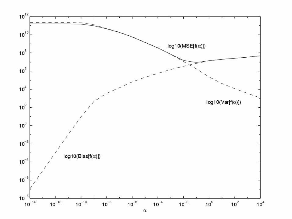
• It has been shown that the minimum Mean Squared Error (solid curve in next
slide) is encountered close to the intersection of the above functions and is
equal to
𝐸{ 𝑓 𝑎 − 𝑓2} = Bias(𝑓 𝑎 + Var(𝑓 𝑎 )
• Observing the graphs for the variance and bias of the error in the next slide we
can say that another good choice of 𝛼 is one that gives the best compromise
between the variance and bias of the error image.
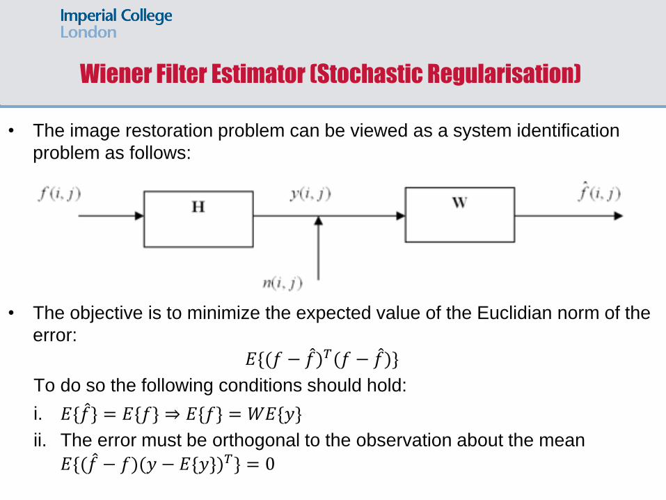
Wiener Filter Estimator (Stochastic Regularisation)
• The image restoration problem can be viewed as a system identification
problem as follows:
• The objective is to minimize the expected value of the Euclidian norm of the
error:
𝐸{(𝑓 − 𝑓 )𝑇(𝑓 − 𝑓 )}
To do so the following conditions should hold:
i. 𝐸{𝑓 } = 𝐸{𝑓} ⇒ 𝐸{𝑓} = 𝑊𝐸{𝑦}
ii. The error must be orthogonal to the observation about the mean
𝐸{(𝑓 − 𝑓)(𝑦 − 𝐸{𝑦})𝑇} = 0
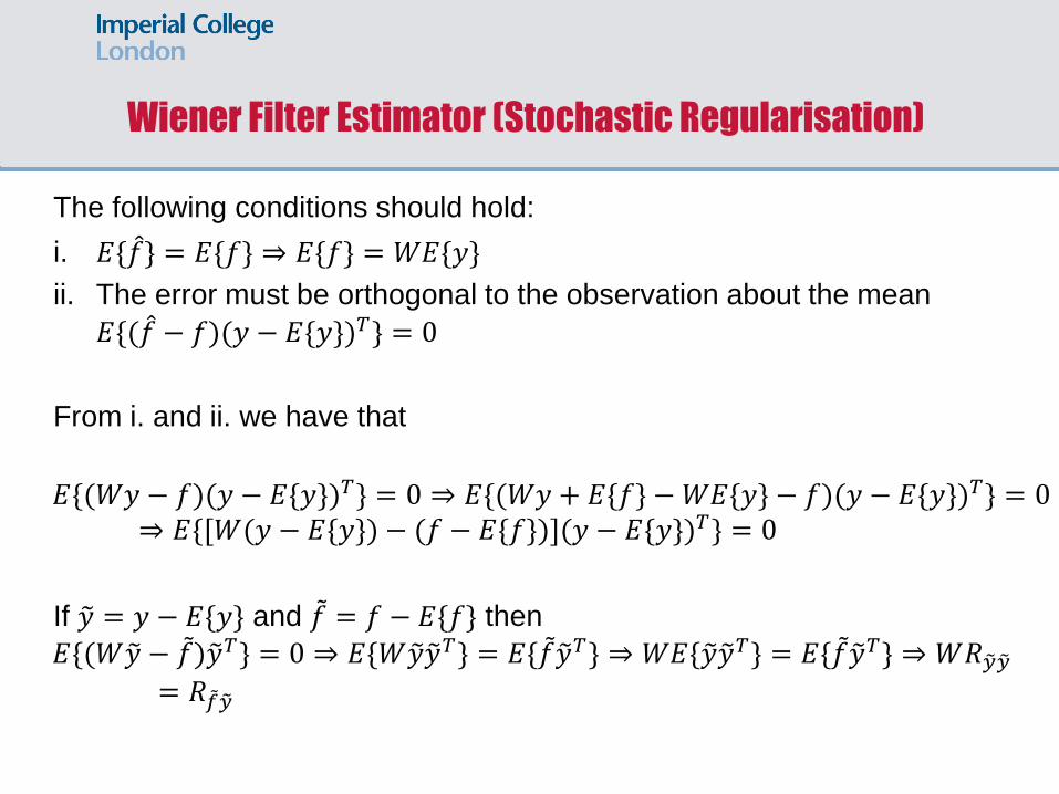
The following conditions should hold:
i. 𝐸{𝑓 } = 𝐸{𝑓} ⇒ 𝐸{𝑓} = 𝑊𝐸{𝑦}
ii. The error must be orthogonal to the observation about the mean
𝐸{(𝑓 − 𝑓)(𝑦 − 𝐸{𝑦})𝑇} = 0
From i. and ii. we have that
𝐸{(𝑊𝑦 − 𝑓)(𝑦 − 𝐸{𝑦})𝑇} = 0 ⇒ 𝐸{(𝑊𝑦 + 𝐸{𝑓} −𝑊𝐸{𝑦} − 𝑓)(𝑦 − 𝐸{𝑦})𝑇} = 0⇒ 𝐸{[𝑊(𝑦 − 𝐸{𝑦}) − (𝑓 − 𝐸{𝑓})](𝑦 − 𝐸{𝑦})𝑇} = 0
If 𝑦 = 𝑦 − 𝐸{𝑦} and 𝑓 = 𝑓 − 𝐸{𝑓} then
𝐸{(𝑊𝑦 − 𝑓 )𝑦 𝑇} = 0 ⇒ 𝐸{𝑊𝑦 𝑦 𝑇} = 𝐸{𝑓 𝑦 𝑇} ⇒ 𝑊𝐸{𝑦 𝑦 𝑇} = 𝐸{𝑓 𝑦 𝑇} ⇒ 𝑊𝑅𝑦 𝑦 = 𝑅𝑓 𝑦
Wiener Filter Estimator (Stochastic Regularisation)
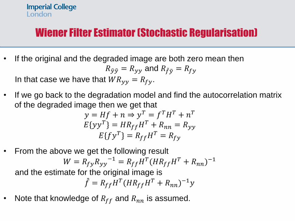
• If the original and the degraded image are both zero mean then
𝑅𝑦 𝑦 = 𝑅𝑦𝑦 and 𝑅𝑓 𝑦 = 𝑅𝑓𝑦
In that case we have that 𝑊𝑅𝑦𝑦 = 𝑅𝑓𝑦.
• If we go back to the degradation model and find the autocorrelation matrix
of the degraded image then we get that
𝑦 = 𝐻𝑓 + 𝑛 ⇒ 𝑦𝑇 = 𝑓𝑇𝐻𝑇 + 𝑛𝑇
𝐸{𝑦𝑦𝑇} = 𝐻𝑅𝑓𝑓𝐻𝑇 + 𝑅𝑛𝑛 = 𝑅𝑦𝑦
𝐸{𝑓𝑦𝑇} = 𝑅𝑓𝑓𝐻𝑇 = 𝑅𝑓𝑦
• From the above we get the following result
𝑊 = 𝑅𝑓𝑦𝑅𝑦𝑦−1 = 𝑅𝑓𝑓𝐻
𝑇(𝐻𝑅𝑓𝑓𝐻𝑇 + 𝑅𝑛𝑛)
−1
and the estimate for the original image is
𝑓 = 𝑅𝑓𝑓𝐻𝑇(𝐻𝑅𝑓𝑓𝐻
𝑇 + 𝑅𝑛𝑛)−1𝑦
• Note that knowledge of 𝑅𝑓𝑓 and 𝑅𝑛𝑛 is assumed.
Wiener Filter Estimator (Stochastic Regularisation)
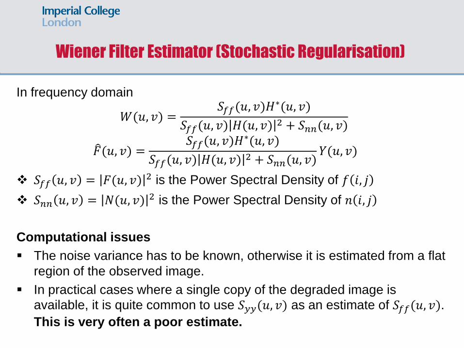
In frequency domain
𝑊(𝑢, 𝑣) =𝑆𝑓𝑓(𝑢, 𝑣)𝐻
∗(𝑢, 𝑣)
𝑆𝑓𝑓(𝑢, 𝑣) 𝐻(𝑢, 𝑣)2 + 𝑆𝑛𝑛(𝑢, 𝑣)
𝐹 (𝑢, 𝑣) =𝑆𝑓𝑓(𝑢, 𝑣)𝐻
∗(𝑢, 𝑣)
𝑆𝑓𝑓(𝑢, 𝑣) 𝐻(𝑢, 𝑣)2 + 𝑆𝑛𝑛(𝑢, 𝑣)
𝑌(𝑢, 𝑣)
𝑆𝑓𝑓 𝑢, 𝑣 = 𝐹(𝑢, 𝑣) 2 is the Power Spectral Density of 𝑓 𝑖, 𝑗
𝑆𝑛𝑛 𝑢, 𝑣 = 𝑁(𝑢, 𝑣) 2 is the Power Spectral Density of 𝑛 𝑖, 𝑗
Computational issues
The noise variance has to be known, otherwise it is estimated from a flat
region of the observed image.
In practical cases where a single copy of the degraded image is
available, it is quite common to use 𝑆𝑦𝑦(𝑢, 𝑣) as an estimate of 𝑆𝑓𝑓(𝑢, 𝑣).
This is very often a poor estimate.
Wiener Filter Estimator (Stochastic Regularisation)
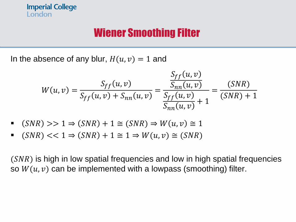
In the absence of any blur, 𝐻(𝑢, 𝑣) = 1 and
𝑊 𝑢, 𝑣 =𝑆𝑓𝑓 𝑢, 𝑣
𝑆𝑓𝑓 𝑢, 𝑣 + 𝑆𝑛𝑛 𝑢, 𝑣=
𝑆𝑓𝑓 𝑢, 𝑣
𝑆𝑛𝑛 𝑢, 𝑣
𝑆𝑓𝑓 𝑢, 𝑣
𝑆𝑛𝑛 𝑢, 𝑣+ 1
=(𝑆𝑁𝑅)
(𝑆𝑁𝑅) + 1
𝑆𝑁𝑅 >> 1 ⇒ 𝑆𝑁𝑅 + 1 ≅ (𝑆𝑁𝑅) ⇒ 𝑊 𝑢, 𝑣 ≅ 1
(𝑆𝑁𝑅) << 1 ⇒ 𝑆𝑁𝑅 + 1 ≅ 1 ⇒ 𝑊(𝑢, 𝑣) ≅ (𝑆𝑁𝑅)
(𝑆𝑁𝑅) is high in low spatial frequencies and low in high spatial frequencies
so 𝑊(𝑢, 𝑣) can be implemented with a lowpass (smoothing) filter.
Wiener Smoothing Filter
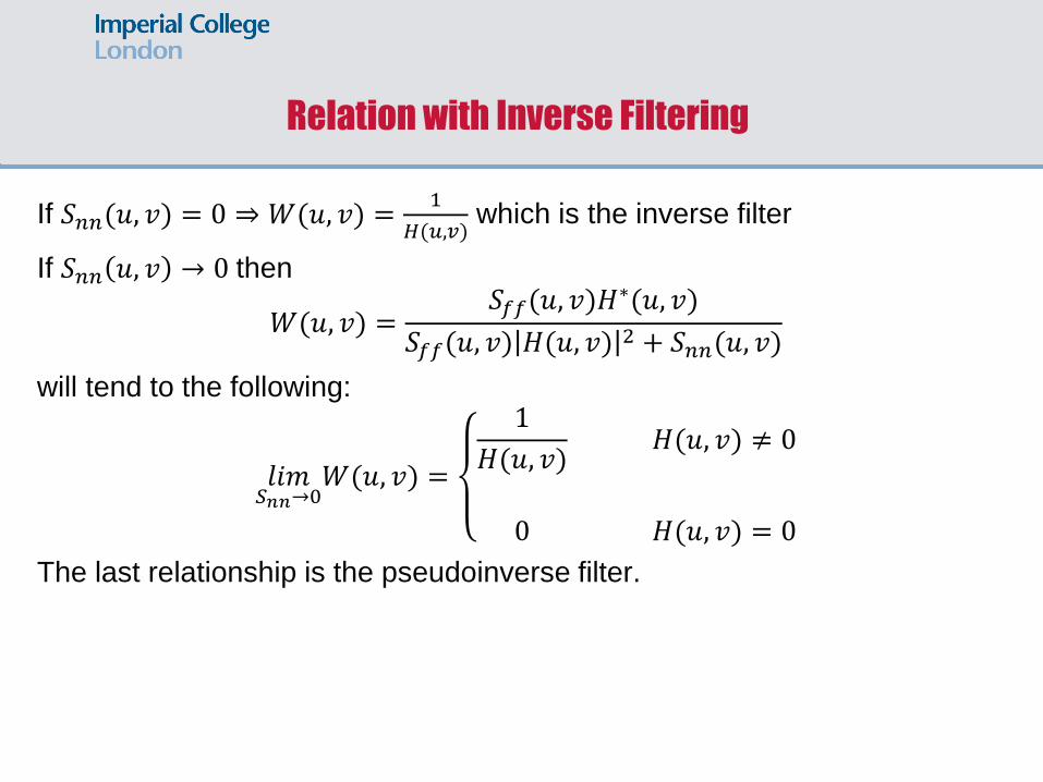
If 𝑆𝑛𝑛(𝑢, 𝑣) = 0 ⇒ 𝑊(𝑢, 𝑣) =1
𝐻(𝑢,𝑣) which is the inverse filter
If 𝑆𝑛𝑛 𝑢, 𝑣 → 0 then
𝑊(𝑢, 𝑣) =𝑆𝑓𝑓(𝑢, 𝑣)𝐻
∗(𝑢, 𝑣)
𝑆𝑓𝑓(𝑢, 𝑣) 𝐻(𝑢, 𝑣)2 + 𝑆𝑛𝑛(𝑢, 𝑣)
will tend to the following:
𝑙𝑖𝑚𝑆𝑛𝑛→0
𝑊(𝑢, 𝑣) =
1
𝐻(𝑢, 𝑣)𝐻(𝑢, 𝑣) ≠ 0
0 𝐻(𝑢, 𝑣) = 0
The last relationship is the pseudoinverse filter.
Relation with Inverse Filtering