Embed Size (px)
Citation preview

Clemson UniversityTigerPrints
All Theses Theses
8-2017
Impacts of Rail Transit Investments onDemographics and Land Use: 1990-2010Aubrey TrinidadClemson University, [email protected]
Follow this and additional works at: https://tigerprints.clemson.edu/all_theses
Part of the Transportation Engineering Commons, and the Urban, Community and RegionalPlanning Commons
This Thesis is brought to you for free and open access by the Theses at TigerPrints. It has been accepted for inclusion in All Theses by an authorizedadministrator of TigerPrints. For more information, please contact [email protected].
Recommended CitationTrinidad, Aubrey, "Impacts of Rail Transit Investments on Demographics and Land Use: 1990-2010" (2017). All Theses. 2726.https://tigerprints.clemson.edu/all_theses/2726

IMPACTS OF RAIL TRANSIT INVESTMENTS ON DEMOGRAPHICS
AND LAND USE: 1990–2010
A Thesis
Presented to
the Graduate School of
Clemson University
In Partial Fulfillment
of the Requirements for the Degree
Master of City and Regional Planning
by
Aubrey Trinidad
August 2017
Accepted by:
Dr. Eric Morris , Committee Chair
Prof. Stephen Sperry
Dr. Timothy Green

ii
ABSTRACT
This paper studies the changes in land use and population characteristics around
station areas following the building of rail transit stations in 14 major cities in the United
States from 1990 to 2010. It answers the question: how have investments in US rail
transit made since the 1990s affected land use and demographics? It also looks at the
specific effects of investments on population density, race, and ethnicity, means of
transportation, median housing value, median household income, vehicle access share,
occupations, and land use represented by the share of multifamily versus single-family
housing. Using block group level US census data at three time periods and GIS boundary
files from NHGIS.org, as well as the spatially-matched rail stations, this research looks at
the 0.5-mile buffer around rail stations as its treatment area and the 1-mile buffer around
it, excluding the treatment area, as its control zone. It uses a combination of longitudinal
and cross-sectional data. For its quantitative analyses, it uses GIS analyses and panel
regression analyses to determine the overall impact of rail transit investments as well as
the impact on stations that are near versus those that are far from the Central Business
District.
An investment in rail transit leads to an increase in the share of workers
commuting by public transportation and a decrease in median incomes around the station.
The investment also brings about the growth in non-white population around central city
stations, an increase in the share of public transit, a decrease in the proportion of
telecommuters, and a drop in the car share in areas that are far from the CBD, and a
decline in median household income in both areas. However, the investment has no
significant effect on population density, housing value, the share of multifamily housing,
vehicle access, race, ethnicity, and the employment structure near the stations. The results
show that the new rail transit stations or systems have helped disadvantaged populations,
but that rail investments have ambiguous impacts on development and growth around the
stations.

iii
ACKNOWLEDGMENTS
I would first like to thank my thesis committee chair, Dr. Eric Morris, for his
guidance, patience, and constructive feedback on my work. He pushed me to strive for
excellence, and he was always available whenever I had questions about my statistical
models or my research, in general. I would also like to acknowledge the other members
of my committee, Prof. Steve Sperry, and Dr. Tim Green, for their support and comments
on this research.
A special thank you goes to the Clemson Center for Geospatial Technologies,
especially to Palak and Patricia, for the workspace and GIS-related support including the
helpful suggestion on the use of the NHGIS website resources for my census and GIS
data requirements.
Finally, I would like to acknowledge friends and family who supported me during
my time at Clemson. I would like to thank my lola Polie, papa Edwel, my sister Mayette,
and my husband Sherwin for their love, strength, prayers and support from across the
miles. They are my inspiration. I would also like to thank my MCRP cohort and my
friends here and abroad for the encouragement. To them, I say thank you, gracias, xie xie,
merci, terima kasih, and maraming salamat.

iv
TABLE OF CONTENTS
Page
TITLE PAGE .................................................................................................................... i
ABSTRACT ..................................................................................................................... ii
ACKNOWLEDGMENTS .............................................................................................. iii
LIST OF TABLES .......................................................................................................... vi
LIST OF FIGURES ....................................................................................................... vii
CHAPTER
I. INTRODUCTION ......................................................................................... 1
Problem Statement and Significance of the Study ................................... 4
II. LITERATURE REVIEW: THEORIES AND EMPIRICAL FINDINGS 7
Theoretical Framework ............................................................................ 7
Empirical Findings ................................................................................... 9
Conclusion ............................................................................................. 26
III. METHODOLOGY ...................................................................................... 28
Conceptual Framework .......................................................................... 29
Research Hypotheses ............................................................................. 30
Data Collection and Description ............................................................ 32
Quantitative Methods ............................................................................. 38
GIS spatial analysis ................................................................................ 38
Regression models ................................................................................. 40
IV. DISCUSSION OF RESULTS ..................................................................... 47
Treatment and Control Areas ................................................................. 47
Effects of the Rail Transit Investments .................................................. 50
Effects on Areas Near the CBD vs those Far from the CBD ................. 54
V. CONCLUSION ............................................................................................ 59

v
Table of Contents (Continued)
Page
APPENDICES ............................................................................................................... 63
A: US Heavy and Light Rail Systems: 1851-2012 ........................................... 64
B: Selected Studies: 1977 to 2016 .................................................................... 69
C: Rail Transit Constructions in the United States: 1990-2000 ....................... 79
D: Data Sources for the Station Locations ........................................................ 86
E: GIS Model and Procedure ............................................................................ 87
F: GIS Process: No Double Counting .............................................................. 91
G: Regression Analyses Results ....................................................................... 92
REFERENCES ............................................................................................................ 184
vi
LIST OF TABLES
Table Page
1 Land Use Considerations ............................................................................. 16
2 Research Hypotheses ................................................................................... 31
3 Predictor and Outcome Variables ................................................................ 44
4 Model 1 Regression Analyses Results ......................................................... 48
5 Model 1 Regression Analyses Results for Jobs ........................................... 49
6 Model 2 Regression Analyses Results ......................................................... 52
7 Model 2 Regression Analyses Results for Jobs ........................................... 53
8 Model 3 Regression Analyses Results ......................................................... 57
9 Model 3 Regression Analyses Results for Jobs ........................................... 58
vii
LIST OF FIGURES
Figure Page
1 Number of Rail Transit Systems: 1980 to 2015............................................. 3
2 Total Transit Subsidies: Buses and Rail Transit ............................................ 4
3 Per Person Transit Subsidies: Buses and Rail Transit .................................. 4
4 Bid-Rent Model ............................................................................................ 8
5 Hoyt’s Sector Model ..................................................................................... 9
6 Conceptual Framework ............................................................................... 29
7 Effects on Demographics and Land Use ...................................................... 30
8 The Fifteen Rail Transit Systems ................................................................. 34
9 Treatment and Control Areas: Washington, DC Stations ............................ 39
10 Sample Stata Station Area Coding ............................................................... 41

1
CHAPTER ONE
INTRODUCTION
More than a century ago, the launch of the rail system could dramatically change
the built environment. From the 1830s onwards, a connection to the intercity rail system
brought prosperity to cities. Within cities, the development of horsecar and electric
streetcar networks dramatically shaped land use and development. Since these modes
significantly increased travel speed compared to walking, new rail transit lines to the
urban periphery spurred residential development as formerly rural land became urban. At
the same time, radial rail transit networks attracted industry and commerce into city
centers. However, all of this happened before the advent of the automobile, which would
dramatically sap rail transit’s ridership. In the present day, do rail transit systems still have
the same powerful influence on the city and the built environment?
In addition, according to a study by Glaeser, Kahn, and Rappaport (2000), the poor
live closer to city centers because of their higher need for public transit, which
disproportionately is sited near city centers. However, according to their findings, new
public transit investments are not directed toward poor areas. Thus the group’s needs may
remain unmet. Is new rail transit serving underprivileged populations?
These questions are of great import because often new rail transit is built in
underdeveloped areas which at the time of construction do not have the population density
to support transit. Builders maintain that this is not problematic because “if they build,
development will follow.” Given the large costs of investment in rail transit, it is
important to ask whether development has followed the opening of new near rail stations.

2
This study looks at heavy and light rail transit systems. Heavy rail includes
subways and elevated trains, which are powered by electricity, have the capacity to
accommodate a heavy volume of traffic and run on exclusive and grade-separated tracks
(i.e., the vehicles do not have to stop at intersections with surface streets, generally
because they run in tunnels or on elevated tracks). Light rail, on the other hand, includes
streetcars and trolleys, which run on exclusive tracks but are generally at street level; they
are electricity-powered with the current delivered by overhead wires.1 Figure 1 shows the
rail transit systems built from 1980 to 2015. While there were more commuter and heavy
rail systems built in 1980, the trend shifted, starting 1990, towards more light rail and
streetcar systems. Currently, there are 15 heavy rail transit systems and 39 light rail transit
systems in the United States2.
1 From https://www.transit.dot.gov/ntd/national-transit-database-ntd-glossary. 2 See Appendix A for the complete list of US light and heavy rail systems since 1821.

3
Figure 1 Number of Rail Transit Systems: 1980 to 20153
Transit, whether rail or bus, requires a subsidy for construction and operations. A
recent study by Taylor and Morris (2015) compared the transit subsidies for buses versus
rail transit from 1995 to 2009. While the subsidies for both modes have increased, there
has been a shift in investment priority from buses to rail transit, especially in 2009. Figure
2 shows that while the total subsidies have increased between 1995 to 2009, the bus
subsidy from 2001 to 2009 has decreased by 15% from its previous rate in 1995 to 2001,
while total rail subsidy has increased to 30%. A look at the per person subsidy on Figure 3
reveals that rail is more expensive, particularly on a per-user basis. Thus, it is worth
asking whether rail can be justified in part because it fosters hoped-for land use impacts
like development and densification.
3 From APTA, 2015

4
Figure 2 Total Transit Subsidies: Buses and Rail Transit4
Figure 3 Per Person Transit Subsidies: Buses and Rail Transit5
4 From Taylor and Morris, 2015 5 From Taylor and Morris, 2015

5
Problem Statement and Significance of the Study
This paper studies the changes in land use and population characteristics around
station areas following the introduction of rail service investments in 14 major cities in the
United States. Land use refers to residential, commercial, and industrial purposes, but for
this research, I am just looking at residential land uses. Population characteristics include
population density, income, race and ethnicity, and types of job occupation of nearby
residents. It also considers the links between transportation investment and housing prices,
vehicle ownership, and means of transportation to work. This research looks at changes
over a twenty-year period, from 1990 to 2010, focusing on investments in heavy and light
rail systems that took place during that time and their aftermath.
This research answers the main question: how have investments in US rail transit
made since the 1990s, affected land use and demographics? Specific questions include:
i) What are the effects of the rail transit stations on the population and population
density in neighborhoods around the stations?
ii) What are the effects of the rail transit investment on the incomes of residents who
live near stations?
iii) What are the effects of rail transit on the racial and ethnic composition of the
population who live close to stations?
iv) What are the effects of the rail transit investments on housing prices near stations?
v) What are the effects of the rail transit investments on the commuting mode of
workers who live near stations?
vi) What are the effects of the rail transit investments on vehicle ownership near

6
stations?
vii) What are the effects of the rail transit investments on land uses in neighborhoods
around the new stations?
This research is intended to influence investments and policy decisions on whether
to focus on public transportation versus other public infrastructure projects, whether to
prioritize rail versus other public transportation modes such as bus, and whether it is a
good strategy to build rail in underdeveloped areas with the expectation that development
will follow.
The expected audience of this research includes policymakers, planners,
researchers, and transportation professionals, as well as general readers who know little
about the topic. The research focuses on US cities, but the results of the study could also
be relevant in other parts of the world.
The section that follows reviews the existing literature on the impact of passenger
rail investment on demographics and land use to ensure a thorough understanding of the
topic and identify knowledge gaps that may require further study.

7
CHAPTER TWO
LITERATURE REVIEW: THEORIES AND EMPIRICAL FINDINGS
Theoretical Framework
The following models of the interaction between transportation and land use
guide this research.
Monocentric bid-rent model. One model that explains the link between
transportation and land use is the bid rent theory introduced by William Alonso (1964).
This model shows that different users of land (commerce, industry, residential) are
willing to pay different prices based on a location’s accessibility. The model makes the
abstraction that all economic activity is located in the central business district (CBD).
Therefore, the closer an area is to the CBD, the higher the price of land in that location
should be because the transportation costs associated with locating there will be lower.
As Figure 4 shows, when an investment in transportation increases the speed of travel to
the CBD, land in peripheral locations becomes more valuable, and the bid-rent curve
moves from X-X to Z-Z. When peripheral land becomes more valuable, it should see a
higher intensity of land use development.

8
Figure 4 Bid-Rent Model6
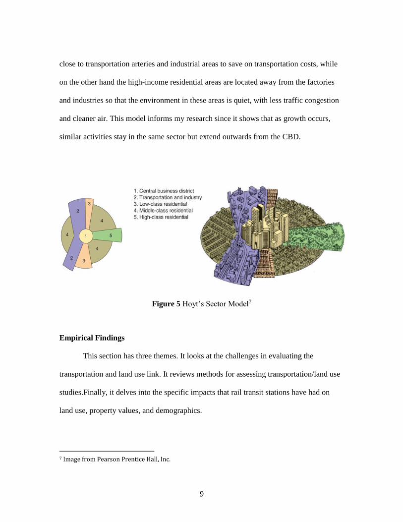
Hoyt’s sector model. In the late 1930s, Homer Hoyt developed a model
illustrating that cities grow in sectors and wedges along transportation corridors
originating from the city center (see Figure 5). To come up with his model, Hoyt
analyzed several towns and mapped housing data using various socio-economic
indicators that include housing age or value, race of tenants, owner occupancy, and
overcrowding (APA, 2009). Hoyt’s Model, or the Sector Model, shows that factories and
industry concentrate along rivers, rail lines, and roads that connect to the central business
district (CBD). It also indicates that low-income residential housing units are located
6 Image from https://image.slidesharecdn.com/settlementrevisionpack-090426020542-
phpapp02/95/settlement-revision-pack-41-728.jpg?cb=1240711619
9
close to transportation arteries and industrial areas to save on transportation costs, while
on the other hand the high-income residential areas are located away from the factories
and industries so that the environment in these areas is quiet, with less traffic congestion
and cleaner air. This model informs my research since it shows that as growth occurs,
similar activities stay in the same sector but extend outwards from the CBD.
Figure 5 Hoyt’s Sector Model7
Empirical Findings
This section has three themes. It looks at the challenges in evaluating the
transportation and land use link. It reviews methods for assessing transportation/land use
studies.Finally, it delves into the specific impacts that rail transit stations have had on
land use, property values, and demographics.
7 Image from Pearson Prentice Hall, Inc.
10
Challenges in assessing the transportation and land use link
The impact of transportation investment on land use is important to planners and
policy makers. However, there are methodological difficulties in studying the relationship
between transit proximity and land use and demographic changes. According to Giuliano
(2004), these could be because, first, in terms of the longitudinal research, the built
environment is durable and thus it takes a long time for land use and demographic
changes to happen. What is then an ideal timeframe? The following section discusses this
in reference to the San Francisco Bay Area Rapid Transit (BART)’s developments.
Second, another challenge is the absence of suitable control groups. No two areas are
exactly alike, and so it is difficult to compare the treatment area with another area with
the same characteristics. Third, the scale of the research is also a factor since most of the
existing studies only focus on a specific system(s). Fourth, there are also other factors
that affect development near rail stations. These include zoning and other government
policies, the attractiveness of the site, and the overall growth of the region as well as
within the region. Transportation changes happen in a dynamic system, and so when
similar investments are made in similar rail systems, we would still expect variations in
the outcomes.
Short-term versus long-term: a case of time periods
Does the extent of the study period affect the results? Most of the impact
assessments covered in Vessali’s report had study periods that were less than 20 years in
span (Dingemans, 1978; Dvett & Castle, 1978; Fajans et al, 1978; ULI, 1979; Dunphy,
1980; SANDAG, 1984; Dunphy, 1984; Ayer & Hocking, 1986; CATS, 1986; Harrold,

11
1985; Nothern VA Planning, 1993; Quackenbush, 1987; Cervero & Landis, 1993). Only
two of the studies had longer time spans: Cervero and Landis (1995), and Landis et al.
(1995).
As has been noted, Cervero & Landis (1995) did a landmark study that reviewed
the impact of BART twenty years after it was built. They reported that a criticism of the
original BART impact study was that its results were premature. The authors emphasized
that the expected land use changes could not be expected to happen right away.
According to them, “(w)hile transportation investments always have some degree of
short-term impacts on travel behavior, only over the long run do demonstrable changes in
urban form take place” (p.310).
Earlier assessments of BART by Dyett & Castle (1978) showed that there was a
small increase in development near stations and some spread further into fringe areas but
no evidence of higher densities was shown. The study of Dingemans (1978) revealed that
no clustering of housing development was found near rail transit stations: while 25% of
housing developments were found within two miles of the nearest station, the rest were
more than 2 miles away. Another assessment that was carried out around this time by
Fajans et al. (1978) showed that BART affected location decisions of small and multiple-
worker households. The studies by Falcke (1978) and the Metropolitan Transportation
Commission (1979) revealed that although BART induced real estate speculation in a few
areas, the finding of negligible impact on retail was still premature at that time.
Interestingly, the BART @20 study by Cervero & Landis (1995) reached findings
that were similar to results of the original studies: there were land use changes, but these

12
were in some areas only—in downtown San Francisco, Oakland, and a few suburban
stations--and that the land use changes were not large scale. Their study also showed that
the non-BART corridors even had more office/commercial additions than the BART
areas.
After the two BART studies highlighted in Vessali’s report, most of the transit
impact studies (Bollinger & Ihlanfeldt, 1997; Hurst & West, 2014; Schuetz, 2014;
Bhattacharjee & Goetz, 2016, among others) did not have extended study periods. Only
one land-use-related study by Davis (2008) had a span of more than 20 years; however,
its methodology was weak since it relied solely on qualitative comparison of
development plans. This present study addresses this problem by looking at systems in
several cities using a longer timeframe and quantitative approach.
Other factors that influence development near rail stations
According to Knight and Trygg (1997), other factors that affect land use changes
include the availability of developable land, the attractiveness of an area for development,
adjacent property investment, local land use policies (such as zoning and development
incentives), a region’s demand for new development, and other government regulations
on taxation and infrastructure provision. The fact that these vary from area to area, and
within areas, make it difficult to measure the effect of the transit station in isolation.
Higgins et al. (2014) arrived at very similar conclusions. According to the
authors, improvement in accessibility, regional growth and demand for development,
physical characteristics of the station areas, social features of station areas, availability of
developable land, and complimentary policies and planning contribute to transit’s ability

13
to promote land use change. In 2009, Cervero also emphasized these issues in his report.
According to him, prerequisites for significant land use changes include a healthy
regional economy and the presence of policies such as transit service incentives and
automobile disincentives.
These factors should be taken into consideration in rail transit impact
assessments, as these services affect the results of studies leading to the
inconsistencies in the actual results.
Methodologies for assessing the impact of passenger rail investments
In terms of accessibility to transit stations, empirical studies have used different
study areas, including from 1 km from the station to within a quarter mile of the station.
According to Guerra, Cervero, and Tischler (2011), the recommended distances are a
quarter mile catchment areas for jobs and half-mile catchment area for the population.
Also, different scholars have used varying methodologies to measure the effect of
transit investment on the built environment. According to the TCRP Report 35 (1998),
the methods should vary depending on the purpose of the study: whether these methods
are predictive or evaluative. The following is an inventory of the methods that past
studies have commonly used.
Longitudinal Analysis looks at a study area before and after the change is
introduced. Previous studies since the 1970s that have used this method include Knight
and Trygg, 1977; Dyett and Castle, 1978; Fajans et al, 1978; MTC, 1979; ULI, 1979;

14
Donnelly, 1982; SANDAG, 1984; CATS, 1986; Quakenbush, et al, 1987; Hurst and
West, 2014; and Bhattacharjee and Goetz, 2016. According to Giuliano (2004), a
downside of this approach is that this may not control for shifts in land use activities that
are not related to the presence of the station, such as a general population growth.
Cross-Sectional Analysis compares the study area with the similar area that did
not receive rail transit, the “no project cases.” Such studies have included Dingemans,
1978; Falcke, 1978b; Dunphy, 1982; Harrold, 1987; Cervero & Landis, 1993; Cervero &
Landis, 1995; Landis et al.,1995; and Bhattacharjee and Goetz, 2016. Giuliano (2004)
noted reasons for expressing caution in the selection of the control area or corridor—it
may be different, or if “investment causes a shift in activity location, the comparison will
exaggerate the extent of the impact.” (p.254)
The Matched-Pair Comparison Method. Cervero and Landis (1995), in their
BART impact study, use this method to compare differences in housing development
prices around BART stations against nearby areas near freeway interchanges along the
Fremont and Richmond lines. The main matching criteria are that the paired stations and
freeway interchanges are within two miles of each other, have similar surrounding land
use compositions, and are connected by the same arterial roadway.
Hedonic Price Models are regression models that provide estimates of how access
to transit is converted into land values (TCRP Report 35). The studies of Cervero &
Landis (1993), Landis et al. (1995), Knaap, Ding & Hopkins (2001), Hess & Almeida
(2007), and Weinberger (2014) use hedonic price modeling.

15
The difference in difference (DID) analysis is a statistical tool used in economics
to evaluate the effects of public interventions over time. It requires data before and after
the intervention happens. This data could either be cohort, panel, or cross-sectional. The
use of panel data involves repeated measures over time of treatment and control areas.
According to Abadie (2005), “(t)he conventional DID estimator requires that, in the
absence of the treatment, the average outcomes for the treated and control groups would
have followed parallel paths over time.” This analysis can either be useful for system-
specific study or research covering a regional scale (Baum-Snow, Kahn, and Voith
(2005); Schuetz, 2014; Hurst & West, 2014).
Panel Data Analysis, such as the fixed effect analysis, is a regression model that
looks at the combination of longitudinal and cross-sectional data and examines the
relationship between predictor and outcome variables that vary over time. According to
Torres-Reyna (2007), fixed effect modeling “removes the effect of time-invariant
features allowing for the assessment of the net effect of the predictors on the outcome or
dependent variables.” Baum-Snow and Kahn used it in 2000 for their research using a
multivariate regression that incorporated a fixed effect analysis to determine public
transit use. They used city fixed effects, a central city dummy, and distance to the station
to predict transit use, where the city fixed effect controls for factors such as transit fares,
transit quality such as speed, and other factors such as the city economy. Results of the
regression analyses showed that better access to transit encourages more use, and those

16
who walk and ride transit benefit from new transit investment in terms of commuting
time saved.
Case Studies/Interviews/Focus Groups/Surveys. These methods are useful in a
system- or city-specific analysis when there are local factors which are difficult to
observe and could influence the results of the study statistically. Based on the TCRP
Report 35, these method are used “for predicting the direction and order of magnitude of
economic impacts” (TCRP, p. 48). Most of the studies (Dyett and Castle, 1976; Fajans et
al. 1978; Falcke, 1978b; MTC, 1979, Ayer & Hocking, 1986; SANDAG,1984) include
these methods to supplement their analyses. One example of this is the summary report of
the Metropolitan Washington Council of Governments’ Transit Impact Studies prepared
by Donnelly (1982). The report used case comparisons, interviews and workshop
documentation to come up with the report on travel impacts, economic impacts, and land
use impacts of three rail transit systems (MARTA, WMATA, and San Diego Metro
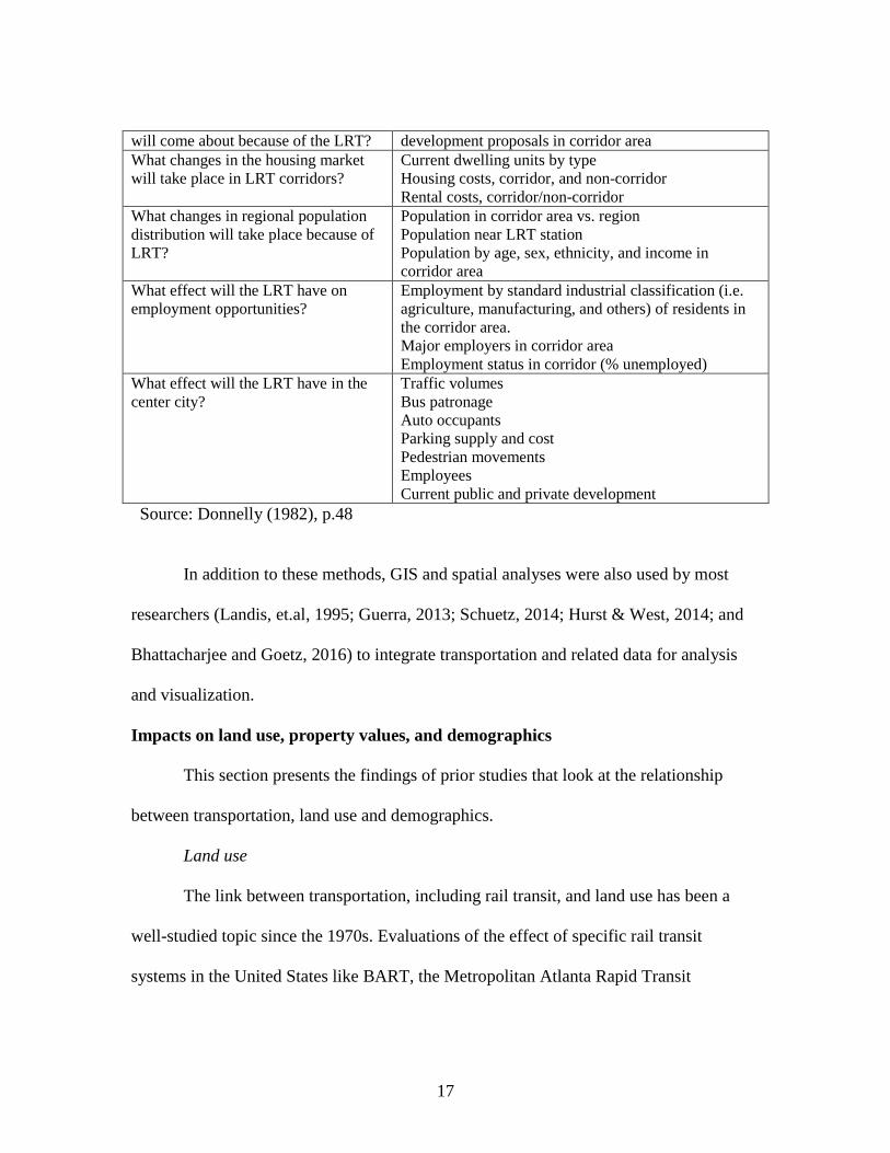
Transit System). For the land use impact section, Donnelly listed the questions and data
requirements (see Table 1). What is not clear from his list though is if the specific
information is examined before and after the investments are introduced.
Table 1 Land Use Considerations
Questions Data Needs
What changes in land use will come
about because of LRT?
Maps of composite land uses from jurisdictions in LRT
corridor area
What zoning changes will come about
because of LRT?
Composite zoning maps from jurisdictions in LRT
corridor area
What will happen to land costs in the
LRT area, particularly around stations?
Inventory of current land values
What public and private development Inventory through interviews public and private
17
will come about because of the LRT? development proposals in corridor area
What changes in the housing market
will take place in LRT corridors?
Current dwelling units by type
Housing costs, corridor, and non-corridor
Rental costs, corridor/non-corridor
What changes in regional population
distribution will take place because of
LRT?
Population in corridor area vs. region
Population near LRT station
Population by age, sex, ethnicity, and income in
corridor area
What effect will the LRT have on
employment opportunities?
Employment by standard industrial classification (i.e.
agriculture, manufacturing, and others) of residents in
the corridor area.
Major employers in corridor area
Employment status in corridor (% unemployed)
What effect will the LRT have in the
center city?
Traffic volumes
Bus patronage
Auto occupants
Parking supply and cost
Pedestrian movements
Employees
Current public and private development
Source: Donnelly (1982), p.48
In addition to these methods, GIS and spatial analyses were also used by most
researchers (Landis, et.al, 1995; Guerra, 2013; Schuetz, 2014; Hurst & West, 2014; and
Bhattacharjee and Goetz, 2016) to integrate transportation and related data for analysis
and visualization.
Impacts on land use, property values, and demographics
This section presents the findings of prior studies that look at the relationship
between transportation, land use and demographics.
Land use
The link between transportation, including rail transit, and land use has been a
well-studied topic since the 1970s. Evaluations of the effect of specific rail transit
systems in the United States like BART, the Metropolitan Atlanta Rapid Transit

18
Authority (MARTA), the Washington Metropolitan Area Transit Authority (WMATA),
as well as reviews of studies on these subjects (including Knight and Trygg, 1997;
Vessali, 1996; Huang, 1996; and Higgins et al., 2014) have been conducted stretching
back over the last 40 years, since new rail transit systems and lines began to be
constructed in the US following a long hiatus8. The report by Knight and Trygg (1977)
was the first empirical study that did a thorough evaluation of the effect of public
transportation investments on land use. It sought to understand the effects of rail
investments on the overall economic and population growth, the concentration of
residences and activities, and the importance of the central business districts, as well as
the impacts of the different rail transit systems on the built environment. The study had
its weaknesses, though, as it only focused on historical and descriptive studies, but it
paved the way for other research and reviews.
Since that time many studies have examined the links between rail transit, land
use and demographics. Three noteworthy papers summarized and analyzed their results.
In 1996, Vessali reviewed the studies on the land use impacts of rail transit investments
prepared from 1970 up to 1995. He asked questions such as: “does high-density
development cluster around transit stations?” “has BART induced real estate speculation
in station areas?” and “how were land use types and development rates affected by the
opening of new transit stations?” among others. He also examined land-value-related
studies since accessibility benefits from rails should translate to more expensive land.
Huang (1996), in his review of research on the impacts of systems in the US and Canada,
8 See Appendix B for the compilation of studies from 1977 to 2016.

19
tried to answer two questions: (1) whether rail transit systems have a significant impact
on urban development, and (2) why there are more developments in some station areas
than others. Higgins et al. (2014) looked at the factors that influence land use impacts or
rail transit investments by reviewing past studies and literature reviews. The following
are the significant findings of these studies and the research they examined.
According to Vessali (1996), the effect of new rail transit on land use has been
small for heavy rail systems, and smaller for light rail systems. These findings were based
on studies done by Dingemans, (1978), Dunphy (1982), and Landis et al. (1995).
Dingemans (1978) did an assessment of BART suburban stations to see if the
investments have led to a clustering of commercial and residential uses around them. He
found that only a small share of housing locates close to the stations. Dunphy (1982)
compared the pre- and post-Washington Metro housing, employment and retail trends
and did not find direct correlations between the locations of new development and transit
stations. The study of Landis et al (1995) on the effect of rail transit investments on land
use near stations among five California rail systems found that although there were some
land use changes when the stations were built, the location of stations did not have a large
effect on land use patterns, and for one system, the San Diego Trolley, the presence of the
stations was not a significant predictor of land use change.
More recent studies done on specific systems and stations, however, showed more
of an effect. A 2008 study by Davis demonstrated that the Shady Grove line of the
Washington Metro positively influenced the land uses around it. It attracted higher
density residential developments, and it had significant growth in population and housing
20
in its first six years of operation. The approach of this research was descriptive. It
reviewed the different land uses, analyzed demographics and economic changes, and
discussed goals and policy recommendations of sector plans, but it was specific to a small
number of stations. A more recent study by Bhattacharjee and Goetz (2016) that
evaluated land parcels from the City of Denver and its surrounding suburbs noted that
multi-family housing increased in areas close to the stations, but these gains were not
significantly greater than the increases in housing in areas far from the stations.
According to Vessali (1996), the greatest land use impacts are found not around
the city center but towards the end-of-the-line stations. The suburbs are the least
developed areas to start with, and so these regions have more room for development
when rail transit extends towards these locations. This phenomenon holds true for Dyett
& Castle’s BART study in 1978, the San Diego Trolley study (SANDAG, 1984), and
even for the rail system expansion study for Mexico City (Guerra, 2013). However, the
1995 BART study by Cervero and Landis presented the opposite results as employment
increased more in downtown San Francisco and Oakland.
According to Vessali (1996), commercial land uses tend to replace residential and
industrial uses around rail transit stations over time. However, system-specific studies
showed different results (Quakenbush et al., 1987; Cervero and Landis, 1995; Davis,
2008; Weinberger, 2001). Quakenbush et al. (1987) noted that some land was rezoned
from industrial to office use during the construction of Boston’s Red Line. Davis (2008),
in a study of the developments around the Washington Metro’s Shady Grove station,
noted that the transformation was from agriculture and forestland into to a mixture of low

21
and medium-density residential and industrial uses. Similarly, in the BART study of
Cervero and Landis (1995), downtown San Francisco and downtown Oakland
experienced expansion in office and commercial space after the opening of the stations.
BART also had lines that produced multi-family housing development (like the Fremont
corridor), but some lines did not experience any growth at all (like the Daly City transit
line).
In 2014, Hurst and West conducted a study that involved a citywide estimation to
determine the effect of light rail on land use in Minneapolis. They evaluated whether land
use change would be more likely to occur within 0.5 miles of LRT stations compared
with the rest of the city across three time periods (1997-2000, 2000-2005, 2005-2010).
The researchers used three models, all with logit specifications. Model 1 estimates the
effect of being within 0.5-mile from the station, comparing before and after the
introduction of the infrastructure investment, without any control variables. Model 2
includes the distance to the CBD and local parks and highways, plus land use categories
(single-family, multifamily, industrial, and commercial purposes). The third model,
Model 3, adds demographic and economic indicators, and controls for parcel and
neighborhood characteristics such as income and race. Results from Model 1 do not
support the hypothesis that properties within 0.5 miles from the station would have
greater land use change than properties located farther away from the station. Results of
Model 2 show that location variables such as distance to CBD and the land use variables
explain the land use change. They also found out that properties located within 0.5 miles
of the LRT stations after the LRT went into operation have a greater chance of changing

22
use than properties outside the area. Model 3 shows more significant results, with areas
within 0.5 miles of the LRT having have a greater likelihood of land use change
compared to areas outside the transit corridor. Overall, the results of the study suggest
that, relative to pre-construction, proximity to LRT during construction does not have an
effect on land use. On the other hand, proximity to LRT during operation has significant
effects on land use (i.e. the share of multifamily housing grew, but industrial land
decreased in areas closer to the stations).
Overall, the body of literature suggests that rail transit investment can influence
land use. However, there are no uniform conditions under which this happens. The effect
varies for heavy and light rail systems. It is not felt evenly within a system (Cervero and
Landis, 1995). High-income areas do not necessarily see greater effects (Bollinger &
Ihlanfelldt, 1997; Bhattacharjee & Goetz, 2016). Also, impacts tend to be limited to
rapidly growing regions where the demand for high-density developments are high
(Vessali, 1996; Knight and Trygg, 1977; Quackenbush, 1987).
Land and property value
As has been noted, based on urban economic theory, properties with better
accessibility should command a higher price, so those properties that are near transit
locations are expected to be more expensive, all else equal, than properties that are far
from the transit corridor (Weinberger, 2014).
However, in 1996, Vessali pointed out that the impacts of transit accessibility on
the value of properties that are close to stations were mixed and inconsistent (p. 97). A
partial explanation for these findings comes from Knaap (2001), who pointed out that

23
plans to invest in transportation infrastructure could increase property values even before
the system is even in place, reducing the apparent before-and-after effects. However,
other studies are consistent with Vessali’s findings.
Huang (1996), looking at studies that cover both heavy and light rail, reported that
for the heavy rail systems:
● BART had a positive but small effect on office rents in downtown San Francisco
and two other areas,
● Proximity to MARTA (the Atlanta heavy rail system) increased home values in
low-income neighborhoods but decreased home values in higher-income areas
because of the noise and traffic at the transit stations,
● For Washington DC’s Metro, the rent premiums were more evident in the older
and more deteriorated sections of downtown.
In 2007, Hess and Almeida reported that every foot closer to a light rail increases
average property values by $2.31 per square foot (using topographic distance) and by
$0.99 (using ArcGIS Network Analyst). Their study also showed that homes located
within half a mile of the rail stations earn a price premium of 2 to 5 percent compared
with the city's median home value. These rates were almost the same values generated in
other studies (such as Cervero & Landis 1993 and Landis et al. 1995). However, there
was a catch in Hess and Almeida’s results. They found out that it was not station
proximity that was driving the housing prices. Rather, the rent premium was due to
additional housing features such as the number of bathrooms in a dwelling unit, the size
of the parcel, and location of the houses (either on the East or West side of Buffalo).

24
In Weinberger’s (2014) research that examined the effect of an LRT system on
commercial rents in Santa Clara, California, her dependent variable was a measure of
price, controlling for other relevant variables such as characteristics of the space, lease
terms, other locational attributes, and the transaction year as a proxy for several economic
cycle effects. She tested the hypothesis that proximity to a rail transit station has no
effect on property values. Weinberger found that when controlling for other factors,
properties located within 0.5-mile from a rail station would have a higher lease rate than
other properties in the county. Also, when controlling for highway access, proximity to
rail would still have a positive association with property values.
Giuliano (2004), in her review of specific rail systems, pointed out that in some
locations, the investment has a positive impact on commercial lease rates (i.e. in San
Jose, California where ridership is low) and residential land values (i.e. in Toronto, which
is the second busiest system next to New York). On the other hand, some systems (such
as the light rail system in Buffalo, New York) showed minimal or no significant effect on
rents and land values.
Thus, rail transit investment may affect land and property values, but the effects
are not consistent. Some systems increased property values even before the stations were
constructed. Some increased property values in low-income neighborhoods, but some
caused a decline in property value, presumably because of the associated noise and other
negative externalities associated with the presence of the stations.
Demographic impacts. This section looks at the effect of the rail investments in
population and jobs.

25
Donnelly (1982) conducted interviews about the impact of MARTA on
population near stations and reported that displacement occurred during the construction
of MARTA; further, residents were bothered by the noise generated from the operation of
the rail system. However, people believed that the returns from MARTA offset the
inconvenience during construction and the people who were displaced tended not to
move too far away from the stations. Guerra (2013), in his Mexico City investigation of
the expansion of Line B into the suburbs of Mexico, did a before and after analysis,
looking at the areas near stations six years before construction and seven years after
construction. He discovered that Line B had a significant effect on population density.
However, his findings showed that while the proportion of suburban residents who live
near Line B grew, the percentage of the population who live near city center stations was
lower in 2005 than its share in 1990; most of the recent population growth has occurred
in housing developments on the fringes and not at the city center.
In terms of employment, Cervero and Landis (1995) reported that employment
density increased in downtown San Francisco, but other BART stations had less job
growth than the non-BART areas. Nelson and Sanchez’s (1997) research on the impact
of MARTA showed that population adjacent to rail stations declined, and although the
number of jobs increased in areas close to the stations, the share of jobs relative to rest of
the region declined. In Bollinger and Ihlanfeldt’s (1997) economic analysis, they did not
find any significant impact of MARTA on population and total employment in station
areas. Schuetz (2014) reported that centrally-located stations experience a decline in retail

26
activity and jobs, and new suburban stations are more likely to have an increase in retail
employment.
Overall, these studies show that the impact of rail transit investments on
population and job densities are inconsistent and leaning towards no effect. The addition
of new rail systems and stations have led to various outcomes. There were population
displacements in certain areas while in others, investments have led to population growth
in the suburbs. Some investments have led to job growth in certain stations while in
some, no growth or a decline in population and jobs were shown.
Literature Review Conclusion
In summary, studies of the land use, land value and demographic impacts of rail
station investments since the 1970s have yielded mixed results. Transit may in some
circumstances influence land use, but the effect is small for both heavy rail and light rail
systems. Outside of the San Francisco area, the greatest land use impacts were found not
around the city center but towards the end-of-the-line stations. Some of the impacts were
smaller in high-income areas; some were limited to rapidly growing regions where the
demand for high-density developments was high. Regarding land value, properties near
train stations were expected to be more expensive, but results were somewhat
inconclusive. Giuliano (2004) presented possible causes of the inconsistencies. The first
challenge is due to the length of time for changes in the built environment to materialize.
Second is the identification of the control area(s) since no two areas are exactly alike. A
third issue is the scale of the studies. Lastly, the presence of other factors such as other

27
land use policies also impacts land use changes. My research fills this gap by looking at a
longer timeframe, a wider scale, and better control areas that are more comparable to the
treatment areas.
Rail remains among many cities’ prime transit movers, accessibility providers,
and economic growth boosters, especially in the main cities around the world and in the
United States. Over the last two and a half decades (from 1980 to 2015), there have been
86 new rail systems and line extensions in the US stretching across include new 15 heavy
rail systems and 39 new light rail and streetcar systems. This growth reflects the
increased investment in passenger transit services in the country. However, the question
remains: are passenger rail systems still worth the public investment even if results of the
impact studies remain inconclusive? Can new lines and stations that are built in poor,
low-density areas be counted on to bring the development needed to support the transit
investment? With the recent accidents involving aging rail transit, should the government
focus the funds on the maintenance of existing systems rather than in building new ones?
Alternatively, should funds be used for BRT and other cheaper transportation systems
instead to get the most benefits?

28
CHAPTER THREE
METHODOLOGY
The overall research design of this study involved a quantitative approach. The
research used a systematic process where Geographic Information Systems (GIS) and
econometric regression analyses procedures were combined to measure the impact of
passenger rail investments on demographics and land use across a number of quantitative
metrics. The analytical method was a combination of a longitudinal and cross-sectional
transportation analyses, which according to Giuliano (2004) is the ideal research design
for establishing causality. The research covered cities that received capital funding for
subways and light rail transit from 1990 to 2010. To identify cities with new rail lines and
stations, I used the table from Baum-Snow, Kahn, and Voith (2005). I then did a web
search and identified the locations of the specific rail lines and stations. US Census data
on population and race, jobs by industry, housing prices, income, means of
transportation, car ownership, and land use for the 14 cities were collected and processed,
comparing areas immediately adjacent to the stations (within walking distance) with the
areas immediately beyond them serving as controls.

29
Conceptual Framework
This study adapted Giuliano’s (2004) transportation and land use models for the
conceptual framework. A transportation investment in the form of a new rail transit line
or an additional station may promote accessibility that can affect land uses, such as
housing structure (single family versus multifamily housing), in affected areas. It should
also eventually affect activity patterns, and the demographics in the area as well,
including population and race, incomes, job distribution, and commuting modes. (see
Figures 6 and 7).
Figure 6 Conceptual Framework (Giuliano, 2004)

30
Figure 7 Effects on Demographics and Land Use9
Research Hypotheses
As the monocentric bid-rent model indicates, the more accessible an area is,
including its distance from the Central Business District (CBD) and also its level of
transportation infrastructure, the higher the rent that the land parcel should have.
Therefore, my research hypotheses are:
● With a new capital investment in a rail station, transportation costs (in terms of
time and money) would go down and accessibility to the CBD would increase.
This should cause population density in stations close to the CBD to go up
relative to population density in stations farther away from the CBD, similarly
9 Adapted from Giuliano (2004)
Infrastructure Investment
(Change in Accessibility)
Change in Transportation System Performance
Changes in:
Population Distribution (density, income, race)
Job Distribution
Housing Value
Commuting Modes
Vehicle Ownership
Land Use (housing structures)

31
density should rise in areas that get stations compared to control areas,
● Businesses near stations will increase and so will jobs, with the most relative
growth in stations farther from the CBD,
● Housing prices near the stations will increase,
● There will be an increase in rail transit commuters,
● Car ownership near rail stations will go down since there will be some switching
to transit,
● There will be a decline in median income near rail stations since low-income
transit-dependent people would move nearer to stations, and
● The racial and ethnic composition of residents near rail stations would change,
becoming a more heavily minority, largely because of income differences.
Table 2 presents the hypothesized associations of the different variables with the
rail transit investment. These data variables are selected based on past literature,
especially the studies by Donnelly (1982), Baum-Snow, Kahn, and Voith (2005), and
Hurst and West (2014).
Table 2 Research Hypotheses
Variable Hypothesized Association
Population density +
Income -
Race and ethnicity More minorities
Occupations + (jobs associated with the CBD)
Housing value +
Commuting mode or means of transportation + (public transportation users)
Vehicle ownership -
Land use (represented by type of housing, i.e.
single family vs. multifamily households)
+ (multifamily housing around the
station)

32
Data Collection and Description
This study uses the following data and variables.
Rail transit stations. This study adapted the list of Baum-Snow, Kahn, and Voith
(2005) in choosing the heavy and light rail systems to include in the research. It looked at
the 165 heavy and light rail stations built from 1990 to 2004 in 14 cities across the United
States10. These cities include Atlanta, Baltimore, Chicago, Dallas, Denver, Los Angeles,
Miami, Portland, Sacramento, San Diego, San Francisco, Santa Clara, St. Louis, and
Washington, DC. The study included relatively new rail systems like Denver’s Regional
Transportation District, St Louis’ MetroLink, Dallas Area Rapid Transit, and Los Angeles
Metro. It covered ten light rail transit systems (San Francisco, Baltimore, Denver, San
Diego, San Jose, Portland, Sacramento, LA, St. Louis, and Dallas) and five heavy rail
systems (Chicago’s L, Washington Metro, Atlanta’s MARTA, Miami, and Los Angeles
Metro). The study excluded New York and Boston (two areas with high rail transit
ridership) since these systems did not have expansions since the 1990s. The very young
rail transit systems or stations, those that opened after 2005, are also excluded to ensure a
sufficient lag time to observe a significant change in the area. Appendix C lists the
specific rail lines, the dates when they opened, the cost of building each segment, the
location of the 165 stations, and the station IDs that were generated from the GIS
analysis. Appendix D lists the websites and sources of the station locations. Transit
stations/points were from ArcGIS Online. Finding the station locations and matching
10 The initial stations identified reached more than 200 however, only 165 of them were matched with
transit points (that were generated from ArcGIS Online)

33
them with their GIS coordinates was complex because different sources used different
notations. The locations of the rail transit systems that are part of this study are presented
in Figure 8.
Population. Population density, measured by dividing the total number of people
by the total land area, is available at the block group level for 1990, 2000, 2010. The
study uses the American Community Survey (ACS) estimates for 2010 which are
available from the US Bureau of the Census (Decennial Census). The aggregate census
data for the census years 1990, 2000, and ACS 2010 can be found on the National
Historical Geographic Information System website (www.NHGIS.org).
Jobs. Employment in the industry-specific professions, which includes wholesale
and retail trade, manufacturing, construction, professional services, finance,
transportation, information, and education, health and social sciences (EHSS) are
available for 1990, 2000 and the 2010 block group data from the US Bureau of Census.
The NHGIS website (www.NHGIS.org) has the employment by industry data but the
employment classifications differ for the years selected, and so the 1990 classifications
are used.

34
Figure 8 The Fifteen Rail Transit Systems
35
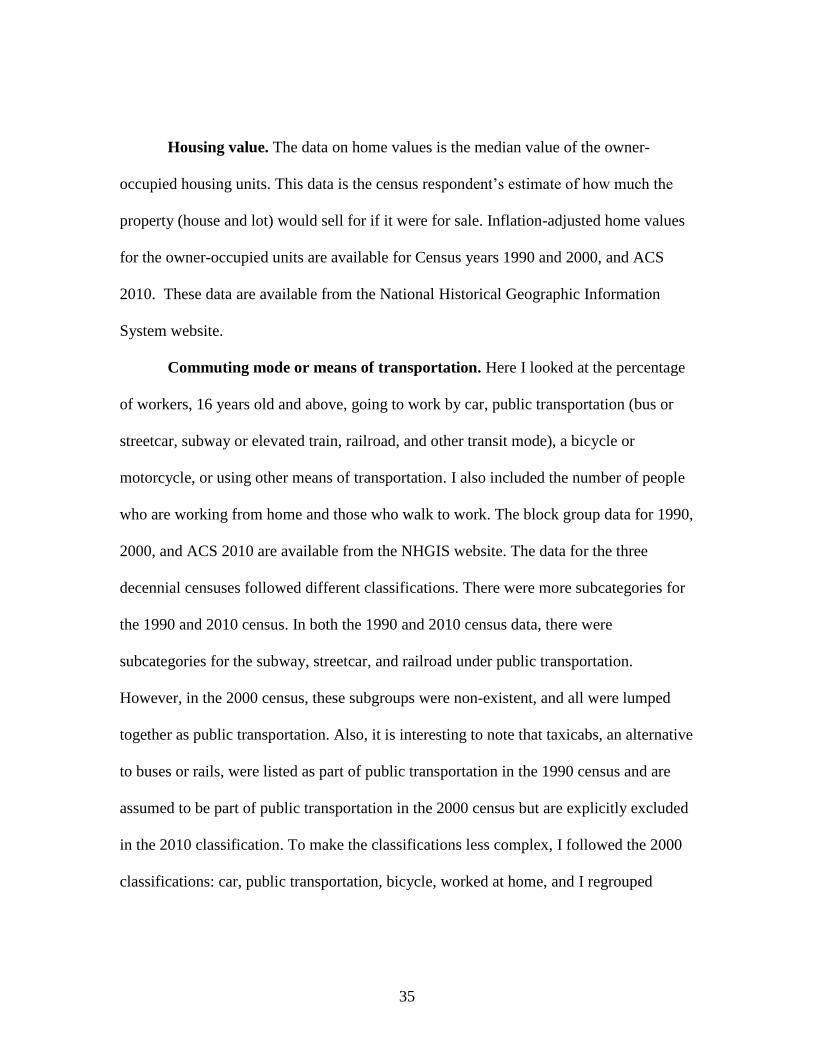
Housing value. The data on home values is the median value of the owner-
occupied housing units. This data is the census respondent’s estimate of how much the
property (house and lot) would sell for if it were for sale. Inflation-adjusted home values
for the owner-occupied units are available for Census years 1990 and 2000, and ACS
2010. These data are available from the National Historical Geographic Information
System website.
Commuting mode or means of transportation. Here I looked at the percentage
of workers, 16 years old and above, going to work by car, public transportation (bus or
streetcar, subway or elevated train, railroad, and other transit mode), a bicycle or
motorcycle, or using other means of transportation. I also included the number of people
who are working from home and those who walk to work. The block group data for 1990,
2000, and ACS 2010 are available from the NHGIS website. The data for the three
decennial censuses followed different classifications. There were more subcategories for
the 1990 and 2010 census. In both the 1990 and 2010 census data, there were
subcategories for the subway, streetcar, and railroad under public transportation.
However, in the 2000 census, these subgroups were non-existent, and all were lumped
together as public transportation. Also, it is interesting to note that taxicabs, an alternative
to buses or rails, were listed as part of public transportation in the 1990 census and are
assumed to be part of public transportation in the 2000 census but are explicitly excluded
in the 2010 classification. To make the classifications less complex, I followed the 2000
classifications: car, public transportation, bicycle, worked at home, and I regrouped

36
motorcycles with cars, and added the number of people who walk to work with those
taking other transportation modes.
Vehicle availability. I looked at the aggregate number of vehicles per housing
unit and reclassified them as homes with “no vehicle” and “with vehicle access.” Then I
calculated the shares of homes with and without vehicle access. The block group data for
1990, 2000, and 2010 (using the ACS 2006-2010 data) are available from the NHGIS
website.
Income. The median household incomes for the years immediately preceding the
Census years were used. A household may either include a single person living alone, a
family, or a group of occupants not related by blood, a common housing set-up in city
centers. The income data are from the US Bureau of Census. The data for 1990 and 2000
are available; however, for 2010, I used the American Community Survey data for 2006-
2010. The aggregate census data for 1990, 2000 and 2006-2010 are available from the
National Historical Geographic Information System website (www.NHGIS.org).
Race. This research used the data on the number of white, black, American
Indian, Asian, and other race individuals in each block group to represent the racial
composition of the population. To be consistent with the 1990 classifications, I regrouped
“Asians” to include Pacific Islanders as well. I also regrouped all the non-white numbers
to come up with “all other race” variable and compare this cluster with the racial majority
(whites). The aggregate Census data for these variables for the decennial years 1990,
2000 and the 2010 American Community Survey five-year estimates data are available
from NHGIS.

37
Hispanic Origin. The research includes the percentage of population with
Hispanic roots. The US Office of Management and Budget (OMB) has defined Hispanic
origin as an ethnicity and is different from race.11 For the year 1990, the Hispanic share
was further classified to include the Hispanics who are from Mexico, Puerto Rico, Cuba,
and other areas. However, these subcategories were not available for the succeeding
decennial years: 2000 and 2010, and so this research focused only on the aggregate share
of people with Spanish ancestries.
Land use. As a proxy variable for an intensity of land use, I used the number of
units in housing structures. The US Census Bureau has the number of housing units in
structures of specified type and size (i.e. single-detached, single-attached, a building with
2 or more apartments (the list goes up to 50 or more), mobile home or trailer, and other
types of living quarters). I then reclassified these as “single-family units” and “multi-
family” units. I also grouped mobile homes and other types of living quarters as “other
units.” The data for 1990, 2000, and ACS 2006-2010 are available from the National
Historical Geographic Information System website (www.NHGIS.org).
11 From the 1997 OMB issued Revisions to the Standards for the Classification of Federal Data on Race
and Ethnicity. See https://www.whitehouse.gov/omb/fedreg_1997standards.

38
Quantitative Methods
This research utilized both GIS spatial analysis and panel regression analyses. It
then integrated the results of these methods to arrive at answers to the research questions.
Adapting the methods used in the papers of Cervero (1995), Baum-Snow, Kahn,
and Voith (2005), and Hurtz and West (2014), my research looked at stations that opened
between 1990 to 2004 across 14 cities and three-time periods. No two areas are exactly
alike and so in order to compare the effect on areas with the intervention (a new rail
transit station) to those without them, I used the block groups closer to the stations
(within half a mile buffer) as the treatment group and the block groups that are farther
away (within 1-mile buffer around the treatment zones, excluding the treatment area) as
the control group. I used the half-mile buffer following the recommended catchment
areas of Guerra, Cervero, and Tishcler (2011). As they pointed out, ¼ of a mile is the
catchment area for jobs and ½ of a mile is the catchment area for the population. It is also
the ideal standard for transit-oriented development (TOD) planning.
GIS spatial analysis
To create the buffers around stations (see Figure 9 for an example of the stations
in Washington, DC), I used the GIS models, outlined in Appendix E, to merge the rail
stations and block group level census attributes. I also used that same model to determine
the changes in population, income, and other demographics between 1990 to 2010 both
for the treatment and control areas around rail transit stations.

39
To ensure that the process is complete and accurate, I made sure that I have the
rail transit station points as well as census data at the block group level for population,
race, income, means of transportation, vehicle access, housing value, housing units, and
jobs by industry. I also made sure that there is no overlap or that areas or block groups
are only attributed to one station, (especially for stations that are located close to one
another). See Appendix F for an illustration.
Figure 9 Treatment and Control Areas: Washington, DC Stations

40
Regression models
This research utilized panel data since it deals with the different demographic and
land use attributes of 165 rail station-adjacent areas with measurements at three points in
time. Therefore, the fixed effects (FE) and random effects (RE) panel models are used.
The fixed effect model compares the changes between each of the six observations
(inside and outside the station areas in 1990, 2000, and 2010) as the areas change over
time. Figure 10 presents an example of how each station area is coded using Stata12.
Fixed effects modeling allows us to control for factors that cannot be observed or
measured such as area or station-specific differences. With the fixed effect model, it is as
if the across group differences are controlled for by a station-specific dummy (in this
case, I have Area FE which is just equivalent to having the 164 station dummy variables)
and so only the within-station characteristics that vary within the area or over time are
accounted for in the model. However, there may be other factors (i.e. time-variant
factors) that could significantly affect the dependent variables. Thus I include variables
for the year of the observation. To enrich this study and to avoid omitted variable bias, I
also used the random effects model. FE cannot investigate the time-invariant variables
because the intercept absorbs these. Random effects models, on the other hand, account
for the time-invariant factors that vary across groups (i.e. across the treatment and control
zones, and across stations that are near or far from the CBD). I used random effects
specifically to study differing impacts on stations near and far from the CBD (I grouped
stations into one of these categories)
12 The regression analyses were processed using Stata 14.

41
Figure 10 Sample Stata Station Area Coding
To assess the relationship between the treatment and control areas, I examined the
effect of the rail transit investment on each outcome variable and determined the effect of
the transit investment on stations that are near and far from the city center. I use the
following models:
Model 1 checks for the similarities between the treatment and control areas in
terms of their attributes. The model allows for the comparison of the two zones prior to
the infrastructure investments, at year=0 or in 1990. The research makes the assumption
that most characteristics such as demographics and the built environment will be similar
inside the treatment area compared with the area immediately beyond it. The purpose of
this model is to determine whether the treatment and control areas are as similar as I
assumed.

42
For the Fixed Effects Model: Yit = β0 + β1Treatmentit + Area FE + e it
For the Random Effects Model: Yit = β0 + β1Treatmentit + Area RE +e it
Where:
t (=0 for 1990)
i (=1 to n, for stations 1 to n)
Treatment (1= treatment area; 0=control area)
Model 2, the main model, examines the effect of the rail transit investment on
demographics and land use. It has four predictor variables which are all dummy variables
(year, whether the area is in the treatment or control areas, whether the station has been
built or not, and an interaction variable for being in the treatment area when the station is
built). This model also includes the exponential or log transformation of the outcome
variables to check which results have a better fit (i.e. with higher R2).
For the Fixed Effects Model:
Yit =β0 +β1Year + β2Treatmentit + β3Stationbuiltit +β4Treatment*Stationit+Area FE
+e it
lnYit = β0+ β1Year+β2Treatmentit+β3Stationbuiltt+ β4Treatment*Stationit +Area FE
+e it
For the Random Effects Model:
Yit =β0 +β1Year + β2Treatmentit + β3Stationbuiltit +β4Treatment*Stationit +
Area RE +e it
lnYit = β0+ β1Year+β2Treatmentit+β3Stationbuiltt+ β4Treatment*Stationit +
Area RE +e it
Where:
t (=0 for 1990, 10 for 2000 or 20 for 2010)
i (=1 to n, for stations 1 to n)
Year (1990, 2000 or 2010)
Treatment (1= treatment area; 0=control area)

43
Stationbuilt (1=station is built; o=otherwise)
Treatment*Station (1=in the treatment zone when the station is built;
0=otherwise)
Model 3 looks at the effect of the investment on stations that are near or far from
the CBD.
For the Fixed Effects Model:
(3.1) Far from the CBD
Yit =β0 +β1Year + β2Treatmentit + β3Stationbuiltit +β4Treatment*Stationitd +Area
FE + e it
lnYit = β0+ β1Year+β2Treatmentit+β3Stationbuiltt+ β4Treatment*Stationitd +Area
FE +e it
Where:
t (=0 for 1990, 10 for 2000 or 20 for 2010)
i (=1 to n, for stations 1 to n)
d (1=station far from the CBD)
Year (1990, 2000 or 2010)
Treatment (1= treatment area; 0=control area)
Stationbuilt (1=station is built; o=otherwise)
Treatment*Station (1=in the treatment zone when the station is built;
0=otherwise)
(3.2) Near the CBD
Yit =β0 +β1Year + β2Treatmentit + β3Stationbuiltit +β4Treatment*Stationitd +Area
FE +e it
lnYit = β0+ β1Year+β2Treatmentit+β3Stationbuiltt+ β4Treatment*Stationitd +Area
FE + e it
Where:
t (=0 for 1990, 10 for 2000 or 20 for 2010)
i (=1 to n, for stations 1 to n)
d (0=station near the CBD)
Treatment (1= treatment area; 0=control area)
Stationbuilt (1=station is built; o=otherwise)
Treatment*Station (1=in the treatment zone when the station is built;
0=otherwise)
Distance (0=station near the CBD)

44
For the Random Effects Model:
Yit =β0 +β1Year + β2Treatmentit + β3Stationbuiltit +β4Near + β5 Near*station +
β5Treatment*nearitd + β6 Treatment*Station*nearitd + Area RE +e it
ln Yit =β0 +β1Year + β2Treatmentit + β3Stationbuiltit +β4Near +
β5 Near*station+β5Treatment*nearitd + β6 Treatment*Station*nearitd +
Area RE +e it
Where:
t (=0 for 1990, 10 for 2000 or 20 for 2010)
i (=1 to n, for stations 1 to n)
d (0=station near the CBD)
Treatment (1= treatment area; 0=control area)
Stationbuilt (1=station is built; 0=otherwise)
Near (1=station near the CBD, 0=otherwise)
Near*station (1=station near the CBD when the station is built, 0=otherwise)
Treatment*near(1=in the treatment zone when the station is near the CBD,
0=otherwise)
Treatment*Station (1=in the treatment zone when the station is built;
0=otherwise)
Treatment*station*near (1=in the treatment area when the station is built and the
station is near the CBD)
Table 3 presents the predictor and outcome variables that are part of this research.
Table 3 Predictor and Outcome Variables
Variable Description
A. Predictor Variables
Treatment or Near station Dummy variable to distinguish the block groups
close to the station from those farther away, in the
control area Year Dummy variable for the year 2000 and year 2010
Station built Dummy variable to differentiate whether a station
is built or not in 1990, 2000, and 2010.
Near Dummy variable which is =1 for areas near the
CBD, otherwise =0 for areas far from the CBD
Near*station Interaction variable which describes the areas that
are close to the CBD when the station is built

45
Treatment*near Interaction variable which describes the areas near
the station that are near the CBD
Treatment*station Interaction variable which refers to the areas near
the station when the station is built
Treatment*station*near Interaction variable which refers to areas near the
station when the station is built for stations near
the CBD
B. Outcome Variables
Pop density The population per square mile
Median housing value Median housing value adjusted to the 2010 prices
Median household income Median household income adjusted to the 2010
prices
% White Share of the white population
% Black Share of the black population
% Asian Share of the Asian population
% Other race Share of other race
% All other race Share of all non-white/minority population
% With Hispanic origin Share of the population with Hispanic roots
% With vehicle access Share of housing units with vehicle access
% Car Share of car users among the working age
population
% Public transpo Share of public transportation users among the
working age population
% Bicycle Share of bicycle riders among the working age
population
% Other means of transpo Share of workers taking other means of
transportation
% Work at home Share of workers who telecommute or work at
home
% Multifamily units Share of multi dwelling units in an area
% Manufacturing Share of workers in the manufacturing sector
% Construction Share of workers in the construction sector
% Finance Share of workers in the finance sector
% Professional Share of workers in the professional services
(including doctors, lawyers, engineers, among
others)
% Transportation Share of workers in the transportation sector
% Wholesale trade Share of workers in the wholesale trade sector
% Retail trade Share of workers in the retail trade business
% Arts and entertainment Share of workers in arts and entertainment
% Other services Share of workers in other service sector

46
All the regression analyses were processed using Stata. The data were copied into
a Stata data editor, and data calculations and operations were done using a do-file to
allow for revisions and repetitions.

47
CHAPTER FOUR
DISCUSSION OF THE RESULTS
This section presents the results of the regression analyses and examines the
implications of the rail investments for land use and demographics. I looked at both the
panel regression results of each outcome variable as well as its exponential or log
transformation (the former is the unit change and the latter is the percent change). The
results presented here are the ones with higher R squared values.
Treatment and Control Areas
Results of the random effect regression analyses (presented in Tables 4 and 5)
show that the treatment and control areas are similar in terms of ethnicity (% with
Hispanic origin) and race (% white, % black, % Asian, % other race, and % all other
race). However, they differ in population density, income, housing value, means of
transportation, vehicle access, and land use. Before the rail transit investments were
introduced, the areas closer to the stations were predicted to have had a higher population
density (by 18 percent) and higher proportion of public transit users (by 2.2 percentage
points). This could be because these areas are centrally located or are catchment areas
that are adjacent to a lot of residential and employment locations. As expected, the area
closer to the stations also had greater proportion of multifamily housing (by 6.3
percentage points), lower share of vehicle ownership (1.6 percentage points lower), and
lower median household income ($14840 lower) before the stations were built. Among
the working age population, the treatment areas also had lower proportion of users of
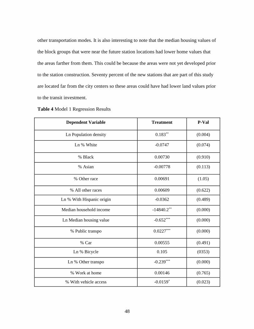
48
other transportation modes. It is also interesting to note that the median housing values of
the block groups that were near the future station locations had lower home values that
the areas farther from them. This could be because the areas were not yet developed prior
to the station construction. Seventy percent of the new stations that are part of this study
are located far from the city centers so these areas could have had lower land values prior
to the transit investment.
Table 4 Model 1 Regression Results
Dependent Variable Treatment P-Val
Ln Population density 0.183** (0.004)
Ln % White -0.0747 (0.074)
% Black 0.00730 (0.910)
% Asian -0.00778 (0.113)
% Other race 0.00691 (1.05)
% All other races 0.00609 (0.622)
Ln % With Hispanic origin -0.0362 (0.489)
Median household income -14840.2** (0.000)
Ln Median housing value -0.652*** (0.000)
% Public transpo 0.0227*** (0.000)
% Car 0.00555 (0.491)
Ln % Bicycle 0.105 (0353)
Ln % Other transpo -0.239*** (0.000)
% Work at home 0.00146 (0.765)
% With vehicle access -0.0159* (0.023)

49
% Multifamily housing 0.0632*** (0.000)
p-values in parentheses; Significance: * p < 0.05,
** p < 0.01,
*** p < 0.001
In terms of jobs, the two areas are alike except for three occupations. The station-
adjacent areas have a higher share of workers in professional services, but a lower share
of workers in the finance, education, health, and social services (EHSS) sector, as well as
in the information sector.
The fixed effect regression analyses generated similar results for these outcome
variables. (See Appendix G for the full regression analyses results).
Table 5 Model 1 Regression Results for Jobs
Dependent Variable Coefficient for being in the
treatment area
P-Val
Ln % Manufacturing -0.0224 (0.412)
Ln % Construction -0.0519 (0.241)
% Transportation 0.00207 (0.161)
Ln % Finance -0.0680* (0.038)
% Professional Services 0.00798** (0.002)
Ln % Other Services -0.0503 (0.079)
Ln % Arts and entertainment -0.0940 (0.096)
Ln % Information -0.150** (0.005)
Ln % Wholesale trade -0.0447 (0.189)
% Retail Trade 0.00364 (0.242)
Ln % Education, health, and social services -0.0599* (0.010)
p-values in parentheses; Significance: * p < 0.05,
** p < 0.01,
*** p < 0.001

50
Thus, no two areas are exactly alike. The treatment areas and control areas may
not be exact substitutes, but they are similar in in certain aspects such as in terms of
location within the city, being served by the same transit lines, and others. Moreover, my
models control for treatment versus control area, so differences between the two areas
should be reflected in the estimates for my dummy variable for this. However, as is the
case in much prior research, my treatment and control areas are not a perfect match,
which is a limitation of this study.
Effects of the Rail Transit Investment13
The effects of the station are reflected in the parameter estimates for the
interaction variable treatment*station. Transit investments bring many types of benefits
such as new development or shifts in travel behavior. Findings show that the opening of
the station has no significant effect on race, ethnicity, land use, housing value, and
vehicle access. Rail transit is expected to boost economic development, bring in jobs and
increase property values; however; the regression results do not support these expected
outcomes. Some of these results, however, are consistent with the literature.
The existence of the rail station does not have a significant effect on population
density. Although this result is consistent with the earlier impact studies, this outcome is
not consistent with my prior hypothesis. I expected more people would want to live
closer to the stations because of transportation access and the opportunities available due
13 (With the R2, F-stat and significance level).

51
to access to the rail transit system. However, there may be other factors that hinder
people from moving closer to the stations.
The rail transit investment has a positive but insignificant effect on the share of
public transit users. It has a negative and significant effect on the percentage of car users.
This is an expected result since the two modes, car, and public transit, are substitutes. The
share of car users was predicted to be 30.8 percentage points lower for treatment areas
when the stations were built.
Being both in the treatment areas when the stations were built has a negative and
significant relationship on the median household income; it is associated with incomes
that are 25.4% lower. This result is consistent with the findings of Glaeser and Kahn
(2000) that many low-income households would cluster around transit stations because of
their transportation needs (i.e., lack of private vehicle access).
It is also interesting to note that the investment has caused a decline in the share
of people working at home (by 13.6%). It implies that more people are shifting towards
other commuting modes, particularly public transit.
Another interesting result is the positive and significant effect of the investments
on other means of transportation when the stations were built. This could be influenced
by those who walk to work and by people who have the tendency to use public transit
more who choose to live in block groups that are closer to public transit location.
Tables 6 and 7 present the random effect regression results with the outcome
variable or its log transformation depending on which had the higher R-square value.14
14 Refer to Appendix G for the complete results of the Fixed Effect regressions.

52
Table 6 Model 2 Regression Results
Dependent Variable Coefficient for
Treatment*station
P-Val
Ln Population density -0.0785 (0.068)
Ln % White 0.00820 (0.726)
% Black 0.00238 (0.751)
% Asian 0.00472 (0.369)
Ln % Other race -0.00913 (0.873)
Ln % All other races 0.0150 (0.573)
Ln % With Hispanics origin 0.0410 (0.266)
Ln Median household income -0.254*** (0.000)
Median housing value 0.0960 (0.068)
Ln % Public transportation 0.0968 (0.062)
% Car -0.0308*** (0.000)
% Bicycle -0.000254 (0.733)
Ln % Other transportation 0.237*** (0.000)
Ln % Work at home -0.120* (0.039)
% With vehicle access -0.00127 (0.804)
% Multifamily housing 0.00216 (0.818)
p-values in parentheses; Significance: * p < 0.05,
** p < 0.01,
*** p < 0.001
The rail transit investment also did not appear to change the employment
distribution in areas closer to the stations.

53
Table 7 Model 2 Regression Results for Jobs
Dependent Variable Coefficient for
Treatment*station
P-Val
Ln % Manufacturing -0.00919 (0.839)
Ln % Construction -0.0511 (0.219)
% Transportation -0.00320 (0.140)
Ln % Finance 0.0300 (0.421)
Ln % Professional services -0.0225 (0.459)
Ln % Other services -0.0370 (0.442)
Ln % Arts and entertainment 0.0615 (0.224)
Ln % Information 0.0322 (0.597)
Ln % Wholesale trade -0.0301 (0.548)
% Retail trade -0.000448 (0.875)
% Education, health, and social services -0.00140 (0.741)
p-values in parentheses; Significance: * p < 0.05,
** p < 0.01,
*** p < 0.001
Fixed effect (FE) and OLS regression runs were also conducted to compare them
with the random effect results. While the RE and FE results are similar for almost all
outcome variables, RE’s result for housing value was not significant at the 0.95 level.
The OLS regression results, on the other hand, only showed significant results for
income, the share of car use, as well as the proportion of other transportation modes.

54
Effects on Areas Near the CBD versus Far from the CBD15
Results of the random effect regression analyses presented in Tables 8 and 9
indicate that there is little difference in the effects of the stations in terms of population
density, race, ethnicity (i.e. share of people with Hispanic roots), housing value, vehicle
access, and land use depending on whether the stations are near or far from the city
center.
The results indicate that the rail transit investment has a negative and significant
effect on median household income in both areas. Income declined by 19.6 percent in
stations that are far from the CBD, and by 44 percent in stations that are closer to the
CBD. The results also show that the investment is associated with a positive and
significant effect on the share of the non-white population. To be in the treatment area
when the station is built has led to a 12 % increase in the proportion of the minority
population living close to the city center. These changes in income and the racial
composition are consistent with the prior hypothesis including the findings of Glaser,
Khan, and Rappaport (2000).
In terms of the transportation modes, the results indicate that the rail transit
investment has a negative and significant effect on car use in areas far from the CBD. It
declined by 2.3 percentage points in stations that are far from downtown. . This result is
consistent with my hypothesis. It indicates that the investments have caused a shift in
travel behavior, particularly for public transit. The investment also has a positive and
significant effect on public transit use in areas far from the CBD. The public transit share
15 (With the R2, F-stat and significance level).

55
increased by 15.8 percentage points. Seventy percent of the stations are located far from
the Central Business District, so this implies that people are using transit, especially those
that are far from the city center. This result is expected and consistent with the literature.
Rail investments, however, have a negative and significant effect on the share of
public transportation commuters in stations that are close to the city center. There may be
other factors that could have caused this decline. As Giuliano (2004) pointed out,
transportation-related changes happen in a dynamic system so other influences could
have affected this result. This effect could be a topic for further investigation.
Another interesting result is the increase in users of other transportation modes in
areas that are both near and far from the CBD. The share of other transit modes could be
influenced by those who walk to work or to other destinations. It could also be a self-
selection effect. As Cervero and Duncan (2008) have pointed out, self-selection is a result
of people who have the tendency to take transit to live close to transit locations because
they either want to reduce the stress of driving to work, or they want to save money and
time, or that they want to support the environment (i.e. through “green” transportation).
In terms of jobs, there is no difference between the two areas except for the share
of workers who are in the wholesale trade business. There was an increase in its share in
areas closer to the CBD (by 21.8%) and a decrease in areas farther away (by 12.5%).
These results are consistent with the literature since wholesale trade is an industry
associated with the CBD, and presumably better transit access would be more valuable to
workers nearer to the CBD than farther away.

56
The results of the fixed effects panel regressions were consistent with the results
of the random effect regressions for all outcome variables. (Refer to Appendix G for the
specific results).

57
Table 8 Model 3 Regression Results16
Dependent Variable Coefficient and
(P-val) for
Treatment+ station
Dependent Variable Coefficient and (P-val):
for
Treatment+station+near
the CBD
Ln Pop density -0.0410 (0.365) Ln Pop density -0.140 (0.228)
% White 0.0122 (0.150) % White -0.0462* (0.035)
Ln % Black -0.0 884(0.067) Ln % Black 0.210 (0.055)
% Asian 0.000949 (0.868) Ln % Asian 0.0138 (0.265)
Ln % Other race -0.00438 (0.943) Ln % Other race -0.0101 (0.945)
Ln % All other races -0.0229 (0.433) Ln % All other races 0.144* (0.019)
LN % with Hispanic
origin
0.0338 (0.411) Ln % with Hispanics
origin
0.0292 (0.748)
Ln median household
income -0.196*** (0.000) Ln median household
income
-0.247* (0.034)
Ln median housing
value
0.0725 (0.147) Ln median housing value 0.0546 (0.714)
Ln % Public
transportation
0.158* (0.015) % Public transportation -0.222* (0.018)
% Car -0.0238*** (0.000) % Car -0.0230 (0.290)
% Bicycle 0.000385 (0.708) % Bicycle -0.00294 (0.364)
% Other transpo 0.0176*** (0.000) % Other transportation 0.0385** (0.007)
Ln % Work at home -0.165** (0.009) Ln % Work at home 0.147 (0.311)
% With vehicle access 0.00105 (0.819) % With vehicle access -0.0115 (0.496)
% Multifamily
housing 0.00776 (0.499) % Multifamily housing -0.0229 (0.254)
p-values in parentheses ; Significance:* p < 0.05,
** p < 0.01,
*** p < 0.001
16 Results reported have higher R-square values (a combination of the linear and the log-transformation of the outcome variables).

58
Table 9 Model 3 Regression Results for Jobs17
Dependent Variable Coefficient and (P-
val) for
Treatment+station:
Dependent
Variable
Coefficient and (P-val)
for
Treatment+station+near:
Ln % Manufacturing -0.0107 (0.800) Ln %
Manufacturing
0.0145 (0.910)
Ln % Construction -0.0322 (0.481) Ln % Construction -0.0683 (0.514)
% Transportation -0.00275 (0.275) % Transportation -0.00211 (0.669)
% Finance 0.00236 (0.317) % Finance -0.00654 (0.383)
Ln % Professional
services -0.00577 (0.854) Ln % Professional
services
-0.0689 (0.386)
Ln % Other services -0.0380 (0.432) Ln % Other
services
-0.00486 (0.971)
Ln % Arts and
entertainment 0.0822 (0.144) Ln % Arts and
entertainment
-0.0706 (0.564)
Ln % Information 0.0310 (0.628) Ln % Information 0.00626 (0.969)
Ln % Wholesale trade -0.125* (0.022) Ln % Wholesale
trade
0.343** (0.004)
% Retail trade -0.00424 (0.144) % Retail trade 0.0143 (0.063)
Ln % Education, health
and social services
(EHSS)
-0.00366 (0.433) % Education,
health and social
services (EHSS)
0.00947 (0.370)
p-values in parentheses; Significance: * p < 0.05,
** p < 0.01,
*** p < 0.001
17 Results reported have higher R-square values (a combination of the linear and the log-transformation of the outcome variables).

59
CHAPTER FIVE
CONCLUSION
This research adds to the growing literature on the connection between
transportation and land use. Its primary objective is to assess the impact of rail transit
investment on demographics and land use, specifically, on population density, race,
ethnicity (represented by the percent of Hispanics), modes of transportation, vehicle
access, household income, housing value, and residential land uses using a longer
timeframe and covering subways and light rail systems with new stations built between
1990 to 2010. It uses 0.5-mile buffer around stations as its impact area and a 1-mile
buffer immediately around them as controls. Findings, however, show that the treatment
and control areas are not exactly alike.
This research confirms that rail systems still have significant influence in cities
and the built environment. Findings show that an investment in rail transit leads to an
increase in the share of workers commuting by public transportation and a decline in
median incomes around the station. For the stations that are near and far from the CBD,
results show that the investments have brought about the growth in the non-white
population in central city rail transit locations, and an increase in the share of public
transportation as well as a decrease in car share in areas far from the city center. It also
brought an increase in other means of transportation and a decline in median household
income in both areas. These results imply that stations, whether in the city center or those

60
located towards the end of the line, are benefiting from the investment. However, overall,
the investment has no significant effect on population density, housing values, land use,
vehicle access, race, ethnicity (share of Hispanics) and the structure of employment near
the stations by sector. These results imply that transit alone cannot be expected to bring
many types of benefits such as new development.
This study shows that rail transit systems are helping disadvantaged populations,
by creating a more attractive environment near stations for those who must rely on
transit. If the goal of the rail transit investment is to provide access to jobs and
opportunities to the poor and the disadvantaged, then the investment program appears to
have succeeded. The research has shown that more of the minorities (the non-whites) and
the households with low income have moved closer to the stations. These results are
consistent with Hoyt’s sector model as well as with results of previous studies.
This research, however, could not fully support the hypothesis that development
and growth followed the opening of new rail stations. Rail transit investment is associated
with a high capital investment, and so it is important to ensure that the investment has a
positive impact on station areas. However, in the areas close to the stations, the
population density did not increase, the share of minorities increase, and the median
household income dipped. The rail transit investments may have caused a shift in the
population composition in the areas around the stations. More minorities came because of
the accessibility and opportunities associated with the locations. However, the investment
could have driven away another group: the wealthy and white population because of the

61
negative externalities associated with the rail investment (i.e. noise and increased vehicle
and foot traffic).
There are policy implications of the research findings. First, investing in rail
transit has attracted a group of people close to the stations. The area around stations has
accessibility advantage; it also has residential and commercial development potential. For
these development possibilities to emerge and for growth to happen, policymakers should
ensure that transit-oriented development policies (especially those policies that provide
transportation-land use integration) are there to complement the rail transit investment
and attract not just the minorities and poor but also other population groups of different
races and income streams. Second, the investment shows positive effects on public transit
use as well as shifts from other transportation modes, especially from car users. If the rail
transit investment is made right and complementary policies (i.e. those that ensure
commuter and pedestrian safety and connectivity), are instituted, more people could be
encouraged to take public transit. Third, findings show that there is an increase of
alternative transportation modes near the stations and the city centers. This result could
be attributed to walking. Linking rail transit investment with pedestrian improvements (as
well as providing seamless transfers to other transportation modes) could promote better
connectivity and encourage more people to commute.

62
Limitations and Implication for Future Research
The results of the study should be interpreted carefully because of its limitations.
These include (1) the unavailability of detailed land use and job density information, (2)
the exclusion of some of the stations either because these were misreported or were not
eventually built making the sample size smaller, and (3) the disparities between the
treatment and control areas.
Despite the limitations, this study raises some opportunities for future research.
First, the study could be extended to focus on the effect of the investment on specific rail
systems or specific cities looking at a combination of quantitative and qualitative
analyses. Second, additional variables such as the detailed land use information per city
and job densities could be included in the analysis to come up with more comprehensive
results.
In conclusion, the research findings show that rail transit investments have
significant influence in US cities. The capital expenditures may not have brought new
development into areas close to the rail transit stations. However, these investments may
have powerful social service impacts for the poor and might get cars off the road.

63
APPENDICES

64
APPENDIX A: US Heavy and Light Rail Systems: 1851-2012
Region State System Year
Established Lines Authority
Type
(FTA)
New York (Staten
Island) New York
Staten Island
Railway
1851
Staten Island Rapid
Transit Operating
Authority
Heavy rail
Boston Massachusetts MBTA Subway 1897 Green Line
Massachusetts Bay
Transportation
Authority
Light rail
New York New York
New York City
Subway
1904 New York City Transit
Authority
Heavy rail
Philadelphia Pennsylvania
SEPTA Trolley
Lines
1906
Subway-Surface
lines (routes 10, 11,
13, 34 and 36), and
suburban routes 101
and 102
SEPTA Light rail
Philadelphia Pennsylvania
Norristown High-
Speed Line
1907 SEPTA Heavy rail
New York
New York and New
Jersey
Port Authority
Trans-Hudson
1908 Port Authority of New
York and New Jersey
Heavy rail
Cleveland Ohio
RTA Rapid
Transit
1920 Blue and Green Lines
Greater Cleveland
Regional Transit
Authority
Light rail
Jersey City/Hudson
County
New York and New
Jersey
Port Authority
Trans-Hudson
1921 Port Authority of New
York and New Jersey
Heavy rail
San Diego California San Diego Trolley 1930 Blue, Green,
and Orange Lines
San Diego
Metropolitan Transit Light rail

65
System
Philadelphia and
Camden, NJ
Pennsylvania and Ne
w Jersey
PATCO
Speedline
1936 Port Authority Transit
Corporation
Heavy rail
Chicago Illinois The L 1947 Chicago Transit
Authority
Heavy rail
Cleveland Ohio
RTA Rapid
Transit
1955 Red Line
Greater Cleveland
Regional Transit
Authority
Heavy rail
Boston Massachusetts MBTA Subway 1964 Blue Line, Orange
Line, and Red Line
Massachusetts Bay
Transportation
Authority
Heavy rail
Buffalo New York Metro Rail 1967
Niagara Frontier
Transportation
Authority
Light rail
Philadelphia Pennsylvania
SEPTA Subway-
Elevated Lines
1968 SEPTA Heavy rail
Philadelphia
Pennsylvania and Ne
w Jersey
PATCO
Speedline
1969 Port Authority Transit
Corporation
Heavy rail
Washington
District of Columbia,
Maryland,
and Virginia
Metrorail 1969
Washington
Metropolitan Area
Transit Authority
Heavy rail
Baltimore Maryland Metro Subway 1970 Maryland Transit
Administration
Heavy rail
Denver Colorado Light Rail 1972 Regional
Transportation District
Light rail
San Francisco Bay
Area California
Bay Area Rapid
Transit 1972
San Francisco Bay
Area Rapid Transit
District
Heavy rail
San Jose California Light Rail 1973
Alum Rock – Santa
Teresa, Mountain
View – Winchester,
Santa Clara Valley
Transportation
Authority
Light rail

66
and Almaden Shuttle
Atlanta Georgia
MARTA Rail
System
1979
Metropolitan Atlanta
Rapid Transit
Authority
Heavy rail
Houston Texas METRORail 1979
North/Red, Southeast/
Purple, and East
End/Greenlines
Metropolitan Transit
Authority of Harris
County, Texas
Light rail
Jersey City/Hudson
County New Jersey
Hudson-Bergen
Light Rail
1979 New Jersey Transit Light rail
Miami Florida Metrorail 1984 Miami-Dade Transit Heavy rail
Pittsburgh Pennsylvania The T 1984
Red Line, Blue Line -
South Hills Village,
and Blue Line -
Library
Port Authority of
Allegheny County
Light rail
Portland Oregon MAX 1986
Blue, Green, Orange,
Red,
and Yellow Lines
TriMet Light rail
Sacramento California Light Rail 1987 Blue Line, Gold Line,
and Green Line
Sacramento Regional
Transit DistrictLight rail
Los Angeles California Metro Rail 1990
Blue Line, Expo
Line, Green Line,
and Gold Line
Los Angeles County
Metropolitan
Transportation
Authority
Light rail
Los Angeles California Metro Rail 1993 Purple Line and Red
Line
Los Angeles County
Metropolitan
Transportation
Authority
Heavy rail
St. Louis Missouri and Illinois MetroLink 1993 Red Line and Blue
Line
Bi-State Development
AgencyLight rail

67
Dallas Texas DART Light Rail 1996 Green, Blue, Red,
and Orange Lines
Dallas Area Rapid
Transit
Light rail
Salt Lake City Utah TRAX 1999
Blue Line (701), Red
Line (703), and Green
Line (704)
Utah Transit Authority Light rail
San Francisco California Muni Metro 1999
Lines J, K, L, M, N, S
(very limited service),
and T
Municipal
Transportation Agency
Light rail
Tacoma Washington Link Light Rail 1999 Tacoma Link Sound Transit Light rail
Miami Florida Tri-Rail 2003
South Florida Regional
Transportation
Authority
Commuter
rail
New York New York AirTrain JFK 2003 Port Authority of New
York and New Jersey
Automated
light rail
Minneapolis-Saint
Paul Minnesota METRO 2004 Blue and Green lines Metro Transit Light rail
Baltimore Maryland Light Rail 2006 Maryland Transit
Administration
Light rail
Newark New Jersey
Newark Light
Rail
2006 New Jersey Transit Light rail
Charlotte North Carolina
LYNX Rapid
Transit Services
2007 Blue Line
Charlotte Area Transit
System
Light rail
Oceanside California SPRINTER 2008 North County Transit
District
Light rail
Phoenix Arizona Valley Metro Rail 2008 Valley Metro Light rail

68
Seattle Washington Link light rail 2009 Central Link
Sound
Transit (operation
contracted to King
County Metro)
Light rail
Norfolk Virginia Tide Light Rail 2011 Hampton Roads
Transit
Light rail
Boston Massachusetts MBTA Subway 2012 Ashmont–Mattapan
High-Speed Line
Massachusetts Bay
Transportation
Authority
Heritage
light rail
Source: Wikipedia’s list of rail transit systems in the United States with a cross-reference to specific rail system’s websites. The researcher
added the year rail systems were established. This list excludes the rest of the transit systems (i.e. streetcars, monorails, Puerto Rico Rail,
commuter rail, automated guideway transit, and tram-trains).

69
APPENDIX B: Selected Studies: 1977 to 2016
Authors/ Study
Area/ Study Period
Transit Mode Property
Type/ Sample
Size
Research Question Accessibility
Measures
Study Design/
Methodology
Results
Knight & Trygg
(1977) 9 cities
across N. America
(1960-1975)
Heavy rail,
light rail,
commuter rail
All types Densities, rates and timing
of land use change, local
land use policy change
NA Before and
after, cross-
sectional, case
studies
“Some densification, but only
where other favorable forces
(strong real estate market,
supportive land use policies).
No evidence of regional
growth impacts.”
Dingemans (1978)
BART
(1960-1976)
Heavy Rail,
Commuter
Rail, Hybrid
Multi-family
residential (80
townhouse
developments
(14,299 units)
Does high-density
development cluster around
transit stations?
Street distance
to nearest
station
Cross-sectional,
non-parametric
statistics
Investment led to 25% increase
in townhouses within two mi.
of nearest
Station, 55% increase in
houses between 2 to 5 mi of
stations), 20% increase in
houses over five mi. away
from stations. An average of
4.5 mi., no clustering of houses
were found near stations.
Dyett and Castle
(1978) BART
Impact Study
(1962-1976)
Heavy Rail,
Commuter
Rail, Hybrid
Has BART induced
residential development?
At higher densities? Further
into fringe?
Within 1500
feet, density,
within
communities
"affected by
BART" (rate
and spread of
development)
Longitudinal,
non-parametric
statistics, key
informant
interviews
“Small increase in
development near stations and
some spread further into fringe
areas, no evidence of higher
densities.”

70
Fajans et al., (1978)
BART Impact
Study
(1965-1977)
Heavy rail,
commuter rail,
hybrid
NA Does accessibility to BART
affect population and
employment growth rates
in nearby areas
Straight line
distance
between the
station and the
"zone."
Longitudinal
regression
analyses, non-
parametric
statistics, key
informant
interviews
“Rates of employment growth
and housing development
affected, suggesting BART
impacts location decisions of
small, multiple-worker
households.”
Falcke (1978b)
BART Impact
Study
Heavy rail,
Commuter,
Rail Hybrid
Has BART induced real
estate speculation in station
areas?
Study-defined
"station areas."
Cross-sectional,
key informant
interviews,
regression
analyses
“BART has induced some
speculation, but not
extensively, in certain station
areas, Author suggests
unrelated market demand may
explain differences.”
MTC (1979) BART
IMPACT Study
(1960-1977)
Heavy rail,
Commuter,
Rail Hybrid
All types (276
workers, 34
stations, 26
developers, ten
station areas,
nine residential
zones)
Employment growth, new
office construction,
property values, resident’s
attitudes
Communities
with stations vs.
those without,
station areas vs.
rest of the city
Before and
after, Delphi
interviews,
surveys, shift-
share analysis,
non-parametric
statistics
“BART caused land use policy
shifts, mostly pro-, some anti-
development, some office
clustering, no residential
clustering or residential
location impacts, no evidence
of regional growth effects,
little impact on retail.”
Urban Land
Institute (1979),
Philadelphia, DC,
Montreal, Boston,
Toronto
(1977-1979)
Heavy Rail Commercial (7
joint
development
projects)
What are good
management, zoning and
incentive approaches to
joint dev?
Agency-defined
"stations areas."
Before and
after, case
studies (key
informant
interviews,
descriptive
statistics)
“Need lead agency with
decision-making power, land
assembly and site preparation
in advance by the public
sector, good design, zoning
and density bonuses.”
Donnelly (1982)
Atlanta/MARTA;
DC Metrorail, San
Diego’s San Diego
Metro
Heavy Rail All types (18
station areas,
100
households, 70
merchants)
Land use changes, resident
and merchant attitudes
Agency-defined
"station areas" -
1/4 mi. walking
distance
Before and
after, case
studies (mostly
interviews)
“In DC, land use plans
changed to incorporate higher
density, mixed-use nodal
development in downtown and
around stations like Friendship

71
(1970-1982) Heights, freeways that
appeared on earlier maps are
no longer planned (e.g.
freeway connecting Arlington)
In Atlanta, land prices have
risen faster in areas closer to
the stations.”
Dunphy (1982), DC
Metrorail
(1970-1980)
Heavy Rail Residential
(except single-
family
detached)
What proportion of new
residential building permits
were issued within "station
areas?"
Station areas are
within 15
minutes walking
time or 0.7
miles’ straight
line distance of
a station
Cross-sectional,
non-parametric
statistics
“No direct correlations found
between locations of new
development and transit
stations. Around 7% of new
permits were authorized for
areas around operating
stations, another 12% were for
future station areas, leaving
over 80% outside of Metro
access.”
SANDAG (1984)
San Diego Trolley
(1980-1984)
Light Rail Residential,
commercial,
industrial (10
leasing agents
and
developers)
Suburban vs. center city
development decisions
Within 1/3mi. of
stations ("land
use impact
area")
Before and after
analysis,
surveys
“Trolley important factor in
suburban station development
decisions but not in CBD
stations.”
Ayer & Hocking
(1986) Chicago
O'Hare extension;
Miami Metrorail
(1970-1985)
Heavy Rail Commercial (6
private
developments,
four joint
development
projects, three
public
developments)
Suburban vs. center city
development decisions
Within 1/3 mi.
of stations
("land use
impact area")
Non-
comparative
case study
(mostly non-
parametric
statistics and
key informant
interviews)
“Rapid transit tends to induce
speculation (in Miami total
assessment within 1000 ft. of
stations increased by 30%
during three-year construction
period) and speed up
development process, thereby
inducing "new" growth within
any given period.”

72
CATS (Chicago
Area Transit Study)
(1986)- Chicago O-
Hare Extension
(1970-1985)
Heavy Rail Residential,
Commercial,
How were land use types
and development rates
affected by the opening of
new transit stations?
Within 1 mile of
transit station
Before and
after, non-
parametric
statistics
“Vacant land around stations
was developed at the same rate
before 1980 as it was
afterward. However, before
1980, 64% of development
was residential, but after 1980,
only 7% was.”
Harold (1987)
Baltimore Metro
(1983-1985)
Heavy Rail Residential,
Commercial
How is the rate of building
permits affected by the
presence of a transit line?
Presence in
transit corridor
vs. other parts of
the city
Cross-sectional,
non-parametric
statistics
“Transit corridor showed a
higher rate of new residential
permits than rest of city, but
results were mixed for
commercial permits.”
Nelson and Sanchez
(1997) MARTA
Heavy Rail Influence of the
Metropolitan Atlanta Rapid
Transit Authority
(MARTA) on population
and employment location
Descriptive
study: analysis
of the
Transportation
Analysis Zone
(TAZ) data for
1980 and 1990
“Population adjacent to rail
stations decreased;
employment increased, but
employment share decreased
relative to the rest of the
region.”
Bollinger and
Ihlanfeldt (1997),
MARTA
(1980- 1990)
Heavy Rail,
Light Rail,
Commuter
Rail
Residential,
Commercial
Effects that Atlanta’s
MARTA rail line has had
on population and
employment in station
areas
Within quarter-
mile around the
stations
General
equilibrium
model of
population and
employment at
the
neighborhood
(census tracts)
level
Results indicate that 1)
MARTA has had neither a
positive nor a negative impact
on the total population and
total employment in station
areas, and 2) MARTA has
attracted more government
offices rather than private
offices to station areas.

73
Davis (2008)
Washington Metro
(1980-2000)
Heavy Rail Impact of Metro stations on
land use and development
Within a one-
mile radius of
the stations
Review of
development
plans
“The land use has transformed
from predominate agriculture
and forest to a mixture of low
and medium-density
residential, institutional, and
industrial, with small pockets
of commercial and open
space.”
Guerra (2013)
Mexico City's Line
B
(2004 and 2007)
Heavy Rail Residential,
Commercial
Mexico City’s Suburban
Land Use and Transit
Connections: The effect of
the Line B-Metro
Expansion
Used six
treatment areas:
1 km (close to 1
mi) from Line
B, in the
surrounding
municipality of
Ecatepec, 1 km
from any metro
station, in
similar distances
from downtown,
in Mexico State,
in the entire
metro region
Difference in
difference
analysis,
descriptive
statistics, use of
GIS maps to
visualize
density of trips
by household
location and by
destination
location for
non-home trips
“Transit increased the
proportion of residents of the
State of Mexico living near the
Metro by about five times, but
growth much more rapid away
from the Metro than around it.
Line B appears to have
significant local effects but
quite modest about overall
trends in housing patterns.“
Schuetz, J. (2014), 4
California’s MTA,
MUNI, BART
(1992-2009)
Heavy Rail,
Light Rail,
Retail,
Commercial
Do rail transit stations
encourage neighborhood
retail activity?
Within one-
quarter mile
around the
station
Regression
analysis
(comparing new
station
neighborhoods
to areas around
older stations as
well as
designated
census tracts
“New rail stations located in
areas with initially high
employment density, outside
the city centers. The impact of
new stations on nearby retail
activity varies within and
across metropolitan areas. In
the LA and Sacramento MSAs,
new stations are negatively
associated with retail. Newly

74
that are within
one-half mile of
any rail
stations),
GIS/spatial
analysis
opened stations are positively
related to retail employment
around rural stations, but have
a negative relationship near
downtown stations.”
Hurst, N. B., &
West, S. E. (2014),
Minnesota’s Metro
Blue Line
(1997-2010)
Light Rail Residential,
Commercial
The effect of METRO Blue
lines on land use in
Minneapolis, Minnesota
Treatment areas:
neighborhoods
that are within
0.5 miles of the
station; control
areas:
neighborhoods
that are outside
these areas
Before and
after, difference
in difference
analysis of
areas within 0.5
miles of a
station versus
areas further
away from the
station; property
level data; GIS
“Within the corridor,
proximity appears to affect
only industrial and single-
family parcels. Industrial
properties closer to LRT were
converted during construction
after LRT was operational,
developers converted buildings
farther away. Proximity to
station areas is driving these
estimates rather than some
other corridor-specific change.
No relationship between LRT
proximity and development (or
redevelopment) of vacant
parcels found. Improved
access due to public transit
may not be a sufficient short-
run catalyst for the accelerated
development of vacant land in
targeted urban areas.”

75
Bhattacharjee, and
Goetz (2016)
Denver Metro
Region
(2000 to 2010)
Light Rail Commercial,
mixed,
industrial,
multi-family,
single family
near and far the
rail system
Are areas near the rail
transit system accounting
for more land use
development than the
average for the entire
Denver metro region?
Study areas
include rail
transit-served,
non-rail transit-
served, and
proposed rail
transit-served
areas
Before and
after, cross-
sectional
analysis, non-
parametric
statistical
significance test
(Wilcoxon/Krus
kal-Wallis test)
to compare near
and far from the
rail system,
spatial analysis,
GIS
“Commercial areas grew in
downtown (in both rail-served,
and non-rail- served areas);
changes in multifamily groups
not significantly different;
change in number of single
family housing greatest in non-
rail areas; commercial and
multi-family residential land
uses growing at faster rate than
other uses; growth supported
by government transit policies
such as creation of TOD areas
and rezoning.”
Land Value Studies
Baum-Snow &
Kahn (2000)
(1980-1990)
Atlanta, Boston,
Chicago, Portland,
Washington
Heavy and
light rail
Effect of new
transportation project on
rail transit use, housing
values, demographic group
characteristics
Census tracts in
five cities
distance to
nearest transit
station (w/in
25km radius of
the CBD)
Before and
after, panel data
using fixed
effect
estimation
Rail transit improvement led to
a small but positive increase in
transit users; greatest
beneficiaries are non-blacks
and people over age 35;
increase in use attributable
to new migrants who reside
on tracts.
Knaap, Ding &
Hopkins (2001)
Oregon,
Light Rail The effects of light rail plan
on land values in station
areas
Hedonic model “Plans to invest in
transportation infrastructure
can affect property values even
before the infrastructure is in
place. Plans for light rail
investments had positive
effects on land values.”

76
Hess & Almeida
(2007); Buffalo,
New York
Light Rail
Residential
Impact of proximity to light
rail rapid transit on station-
area property values in
Buffalo, New York
Study areas are
those within 0.5
miles of each of
the 14 light rail
stations
Hedonic model
“For houses located in the
study area, every foot closer to
a light rail station increases
average property values
by $2.31 rent premium (using
geographical straight-line
distance) and $0.99 (using
network distance). A home
located within the study area
earns a premium of $1300-
3000, or 2-5 percent of the
city's median home value.
However, the study showed
that the number of bathrooms,
the size of the parcel, and
location on the East side or
West side of Buffalo are more
influential than rail proximity
in predicting property values. “
Weinberger (2014)
Sta. Clara County,
CA
Light Rail Commercial Does light rail proximity
provide benefit or
detriment in the case of
Santa Clara County,
California?
Hedonic model “Properties that lie within 0.5
mi of a rail station have higher
lease rate than other properties
in the county. Controlling for
highway access, the rail
proximity benefit was
maintained, and highway
coverage in the county is so
dense that there are no
locational advantages
associated with highway
coverage.”

77
Hybrid Studies: Land Use and Land Value
Quakenbush et al.
(1987) Boston/
MBTA Red Line
Extension
(1978-1986)
Heavy Rail Heavy Rail, Light
Rail, Commuter
Rail
How were land use types
and housing prices affected
by the opening of new
transit stations?
Study-defined
"station areas."
Before and after,
non-parametric
statistics
“Industrial land uses declined
for office spaces, parking,
and open space. House price
trends were mixed and not
well explained.”
Cervero & Landis
(1993), DC
Metrorail; Atlanta/
MARTA
(1978-1989)
Heavy Rail Commercial
(suburban office
developments)
Rates of absorption &
vacancy, % of regional
growth, rent, size of
development
"Station" vs.
"non-station"
sites as defined
by transit
agencies
Cross-sectional
(transit
developments vs.
highway-
developments)/
Matched-pair
comparisons
using difference
of means tests
$2 to 3.50 (13-18%) rent
premium for transit areas in 3
of the 4 locations in DC and
Atlanta (stat. sig. at 95% in
only 1); mixed, insignificant
result everywhere else.
Cervero & Landis
(1995), BART
(1970-1990)
Heavy Rail,
Commuter,
Rail Hybrid
All Types (34
"super districts"
152 zip codes, 25
station areas,
33,291 parcels)
Population & employment
growth, employment
density, land use change,
development rates
BART corridors
vs. freeway
corridors;
station areas vs.
freeway
interchanges
Cross-sectional
(transit station vs.
highway
interchange areas,
control corridors
vs. impact
corridors)/ Non-
parametric
statistics,
matched-pair
comparisons,
logit, and linear
regression models
“Except in CBD, population
and employment grew faster
in non-BART areas, some
employment densification
seen around stations. More
land use change around
BART stations than freeway
interchange matched pairs.”

78
Landis et al (1995)
BART, San Diego
LRT, San Jose LRT,
CalTrain,
Sacramento LRT
(1965-1990)
Light Rail,
Heavy Rail,
Commuter,
Rail Hybrid
Single family
residential,
commercial (2600
SF, >4500
commercial lots,
13 stations)
Property values, land use
change
"station areas"
vs "non-station
areas"
Cross-
sectional/Hedonic
Price Models,
Logit Models,
Analysis of
Variance
$2/meter premium for homes
close to stations (BART and
San Diego), none elsewhere,
mixed for commercial
property, some positive
impact on rate and type of
land use change.
Debrezion, G., Pels,
E., & Rietveld, P.
(2007)
City not indicated
Heavy Rail,
Light Rail,
Commuter
Rail
Residential,
Commercial
Land prices and land use in
a polycentric city under
various regulatory regimes
of land markets
Properties
within 0.25 mile
from the station
Metaanalysis,
Hedonic Price
Model
“Effect of railway stations on
commercial property value
takes place only at short
distances. Commercial
properties within the 0.25-
mile range of station 12.2%
more expensive than
residential properties.
For every 250 m a residence
is located closer to a station
its price is 2.3% higher than
commercial properties.
Commuter railway stations
have a higher positive impact
on the property value
compared to light and heavy
railway/Metro stations.”
Source: 1970 to 1995 studies from Vessali, K. 1996, pp. 78-85

79
APPENDIX C: Rail Transit Constructions in the United States, 1990-2000 ***
City Line Length
(miles)
Open
by
Estimated cost
per mile (in a
million USD,
2005 prices)
Type of
construction a
Location/ Stations and Station IDs b Station
ID c
Atlanta c Gold Line
Green Line
Blue Line
Red Line
Red Line
1
2
3
7
2
Dec 1992
Dec 1992
Jun 1993
Jun 1996
Dec 2000
33
33
33
52
33
E
R
R
H
E
Doraville Station
Bankhead
Kensington
Dunwoody
Sandy Springs
2235
2268
2267
2228
2219
Baltimore Metro Subway
Light Rail
Light Rail
2
23
8
1994
1993e
1997
--
18
14
T
S/H/R
R
Section C: Johns Hopkins Extension
1992:
Timonium
Patapsco
1993:
Linthicum
Cromwell/Glen Burne
Hunt Valley
Penn Station
BWI Airport
1667
1635
1450
1458
1466
1629
1661
1463
Chicago Orange Line 9 1993 56 R 35th/Archer
Ashland
Halsted
Kedzie
Midway
Pulaski
Western
754
747
727
661
788
774
769
Dallas DART 20 May 1997 43 S/R/T Mockingbird Station
Illinois Station
Ledbetter Station
VA Medical Center Station
2321
2378
2401
2398

80
DART
13
Dec 2002 43 R/H Arapaho Center Station
Bush Turnpike Station
Downtown Plano Station
Galatyn Park Station
Forest/Jupiter Station
Forest Lane Station
LBJ/Skillman Station
Park Lane Station
Walnut Hill Station
LBJ/Central Station
Spring Valley Station
Parker Road Station
2308
2305
2304
2307
2313
2312
2315
2317
2316
2310
2309
2303
Denver D
C/D
C
6
9
2
Oct 1994
July 2000
April 2002
21
22
24
S
S
R
10th and Osage
Alameda
16th and California
16th and Stout
18th and California
18th and Stout,
30th and Downing Station
I-25 and Broadway Station
Evans
Englewood
Oxford/Sheridan
Littleton/Downtown
Littleton-Mineral Stations
Auraria West
Mile High
Union Station
1614
1615
1603
1602
1601
1592
1616
1618
1620
1621
1623
1624
1608
1607
1774
Los Angeles Red Line
4
Jan 1993
330
T
Civic Center/Grand Park
Pershing Square
Union Station,
Westlake/MacArthur Park
2198
2199
2196

81
Red Line
Red Line
Blue Line
Green Line
7
12
22
20
July 1996
2000
1990
1995
245
227
40
36
T
T
R
H/E
Wilshire/Vermont
Hollywood/Highland
North Hollywood
Universal City/Studio City
Long Beach: 1st Street,
5th Street,
Anaheim
Pacific Ave.
Pacific Coast Highway
Downtown Long Beach
Wardlow
Compton: Artesia
Compton
Racho Dominguez: Del Amo
Florence-Graham: Firestone
Florence
Slauson
LA: Grand/LATTC
San Pedro
Vernon
Washington
Willowbrook: Willowbrook/Rosa Parks
LA: Avalon,
Aviation/LAX,
Harbor Freeway;
Hawthorne: Crenshaw,
Hawthrone/Lennox,
Vermont/Athens
El Segundo: Douglas
El Segundo;
Downey: Lakewood Boulevard
Lynwood: Long Beach Boulevard
Norwalk
2188
2169
2154
2160
2271
2266
2260
2263
2257
2226
2253
2242
2237
2249
2215
2213
2210
2203
2204
2208
2205
2254
2224
2220
2221
2218
2222
2234
2230
2232
2226
2229

82
Gold Line
14
July 2003
63
R
Redondo Beach
Pasadena: Allen
Del Mar
Filmore,
Lake
Memorial Park
Sierra Madre Villa;
LA: Chinatown
Southwest Museum
2238
2155
2159
2161
2156
2158
2157
2186
2170
Miami Metrorail 2 May 2003 -- E Palmetto 2459
Portland c MAX Blue and Red
Lines
MAX Red Line
MAX Yellow Line
18
6
6
Sep 1998
July 2001
May 2004
54
23
63
S/T/H
E/H
S
Westside: (Hatfield Government
Center,
Library/Galleria/SW 9th/10th)
Airport: (Portland Int’l. Airport
Gateway TC)
Interstate Avenue: (Expo Center
Rose Quarter TC)
Interstate/Rose Quarter
Albina/Mississippi
Overlook Park
North Prescott Street
North Killingsworth Street
North Rosa Parks Way
North Lombard Transit Center
Kenton/ North Denver Avenue
Delta Park/Vanport
90
109
42
61
40
64
63
52
51
50
48
49
44
43
41
Sacramento East Line
South Line
2
6
Jan 1998
Dec 2003
15
35
S/R
R
Mather Field/Mills
City College
1788
1902
San Diego Orange Line
2 1990
32
R
Convention Center
Gaslamp Quarter
2390
2393

83
Blue Line
Blue Line
1
6
1992
1997
--
37
R
E
County Center/Little Italy
Mission San Diego
2377
2350
San Francisco BART
BART
BART
MUNI
2
7
6
2
Feb 1996
Dec 1996
May 1997
1998
106
--
--
37
T
--
H
S
Colma Station
Pittsburg/Bay Point Station
Dublin/Pleasanton Line
San Francisco Airport
Brannan
Folsom
2020
1911
2014
1831
1820
Santa Clara d Valley Transportation
Authority (VTA)
VTA
8
2
Dec 1999
May 2001
25
42
H
S
Baypointe
Bayshore/NASA
Borregas
Crossman,
Mountain View,
Evelyn,
Fair Oaks,
Lockheed Martin,
Middlefield,
Moffett Park,
Reamwood,
Vienna,
Whisman
Cisco Way,
I-880/Milpitas
2057
2047
2052
2066
2069
2049
2065
2064
2058
2068
2045

84
St. Louis MetroLink
MetroLink
16
1
July 1993
June 1995g
27
27
R
E
8th & Pine,
Central West End,
Civic Center,
Convention Center,
Delmar Loop,
Forest Park-DeBaliviere
Grand
Laclede’s Landing,
North Hanley,
Rock Road,
Stadium,
UMSL North,
UMSL South,
Union Station,
Wellston
Lambert Airport Terminal 1
1773
1766
1776
1761
1762
1769
1754
1758
1756
1757
1774
1759
1751
Washington,
DC
Red Line
Green Line
Green Line
3
2
3
Sep 1990
May 1991
Dec 1991
--
--
--
T
T
T
Forest Glen (in MD),
Wheaton (Montgomery County,
Maryland)
U Street Cardozo
Shaw-Howard Univ,
Mt Vernon Square-UDC
Waterfront,
Navy Yard,
Anacostia
West Hyattsville (MD)
1487
1483
1681
1682
1688
1723
1722
1728
1503

85
Green Line
Red Line
Green Line
Green Line
7
1
3
7
Dec 1993
July 1998
Sept 1999
Jan 2001
--
162
222
138
R
T
T
T/H/E
Prince George’s Plaza
College Park-U of Md
Greenbelt station
Glenmont
Columbia Heights
GeorgiaAve.-Petworth
Branch Avenue (in Suitland, Maryland)
1500
1497
1488
1480
1515
1510
1737
Source: Adapted from Baum-Snow, Kahn & Voith (2005)
Notes:
*** Excludes the small segments in Cleveland, New York, and Salt Lake City a Construction types: E= elevated, H= highway median, R= railway right of way, S= street, T= tunnel b Transit stations from various sources. Refer to list below c GIS-assigned station IDs (calculated by the researcher). dFor Atlanta, Baum-Snow, Kahn, and Voith (2005) used East/West for the Green/Blue line and North/South for the Gold/Red line. For Portland, the
authors did not identify specific line segments.e San Jose is listed under Santa Clara VTA in Baum-Snow, Kahn, and Voith (2005)’s list. e For Baltimore LTR, the list of stations for 1993 include those that opened in 1992. f Chicago’s Green line opened in 1993 then closed in 1994 for a transit rehabilitation (see https://en.wikipedia.org/wiki/Green_Line_(CTA) and
http://www.chicago-l.org/operations/lines/lake.html g For St. Louis, the Lambert Airport station’s opening date is listed as June 1994 in Baum-Snow, Kahn and Voith (2005).
-- Information not available.

86
APPENDIX D: Data Sources for the Station Locations
Atlanta:
MARTA: https://en.wikipedia.org/wiki/List_of_MARTA_rail_stations
Baltimore:
Metro Subway: http://www.roadstothefuture.com/Baltimore_Metro.html#Section_C
Light Rail Transit: http://lrt.daxack.ca/Cities/Baltimore/index.html
Chicago:
Orange Line: http://www.chicago-l.org/operations/lines/orange.html
https://en.wikipedia.org/wiki/List_of_Chicago_%22L%22_stations
Green Line: https://en.wikipedia.org/wiki/Green_Line_(CTA)
http://www.chicago-l.org/operations/lines/lake.html
Dallas:
https://www.dart.org/about/history.asp
Denver: https://en.wikipedia.org/wiki/List_of_Denver_RTD_rail_stations#Stations
Los Angeles:
https://en.wikipedia.org/wiki/List_of_Los_Angeles_Metro_Rail_stations
Miami-Dade:
http://www.miamidade.gov/transit/history.asp
https://en.wikipedia.org/wiki/Palmetto_station
Portland:
MAX: https://en.wikipedia.org/wiki/MAX_Light_Rail;
West Blue Line: https://trimet.org/history/westblueline.htm;
Yellow Line: https://trimet.org/history/yellowline.htm
TRIMET map: http://trimet.org/maps/img/trimetsystem.png
MAX Yellow Line: https://en.wikipedia.org/wiki/List_of_MAX_Light_Rail_stations
Sacramento:
https://en.wikipedia.org/wiki/List_of_Sacramento_Regional_Transit_light_rail_stations
San Francisco:
BART: http://www.bart.gov/sites/default/files/docs/PosterTimeline_v2.pdf
Santa Clara:
VTA: https://en.wikipedia.org/wiki/List_of_Santa_Clara_VTA_Light_Rail_stations
St. Louis:
Metrolink:https://en.wikipedia.org/wiki/List_of_MetroLink_(St._Louis)_stations#cite_note-1993opening-5
Washington DC:
http://www.wmata.com/about_metro/docs/history.pdf
Green Line: https://en.wikipedia.org/wiki/Green_Line_(Washington_Metro)
http://greatergreaterwashington.org/post/23637/watch-metro-grow-from-one-short-line-in-1976-to-the-
silver-line-today/

87
APPENDIX E: GIS Model and Procedure
Complete GIS Model

88
GIS Model: Treatment and Control Areas
Creating a buffer around a point feature and using it to extract attributes from an overlapping polygon feature class
(Adapted from ESRI’s steps in creating a buffer around a point feature)
These steps describe how to create a buffer around a point feature (rail station) and use it to extract attributes from an
overlapping polygon feature class (the census data variables). In most cases, the buffer does not cover whole polygons. This
procedure allows for calculating the percentage of a polygon the buffer encompasses, and then dividing the data by that
percentage.
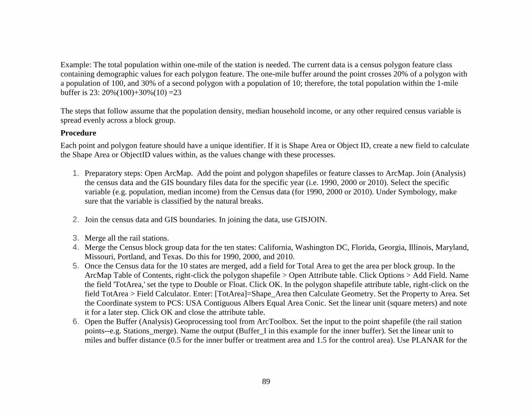
89
Example: The total population within one-mile of the station is needed. The current data is a census polygon feature class
containing demographic values for each polygon feature. The one-mile buffer around the point crosses 20% of a polygon with
a population of 100, and 30% of a second polygon with a population of 10; therefore, the total population within the 1-mile
buffer is 23: 20%(100)+30%(10) =23
The steps that follow assume that the population density, median household income, or any other required census variable is
spread evenly across a block group.
Procedure
Each point and polygon feature should have a unique identifier. If it is Shape Area or Object ID, create a new field to calculate
the Shape Area or ObjectID values within, as the values change with these processes.
1. Preparatory steps: Open ArcMap. Add the point and polygon shapefiles or feature classes to ArcMap. Join (Analysis)
the census data and the GIS boundary files data for the specific year (i.e. 1990, 2000 or 2010). Select the specific
variable (e.g. population, median income) from the Census data (for 1990, 2000 or 2010). Under Symbology, make
sure that the variable is classified by the natural breaks.
2. Join the census data and GIS boundaries. In joining the data, use GISJOIN.
3. Merge all the rail stations.
4. Merge the Census block group data for the ten states: California, Washington DC, Florida, Georgia, Illinois, Maryland,
Missouri, Portland, and Texas. Do this for 1990, 2000, and 2010.
5. Once the Census data for the 10 states are merged, add a field for Total Area to get the area per block group. In the
ArcMap Table of Contents, right-click the polygon shapefile > Open Attribute table. Click Options > Add Field. Name
the field 'TotArea,' set the type to Double or Float. Click OK. In the polygon shapefile attribute table, right-click on the
field TotArea > Field Calculator. Enter: [TotArea]=Shape_Area then Calculate Geometry. Set the Property to Area. Set
the Coordinate system to PCS: USA Contiguous Albers Equal Area Conic. Set the linear unit (square meters) and note
it for a later step. Click OK and close the attribute table.
6. Open the Buffer (Analysis) Geoprocessing tool from ArcToolbox. Set the input to the point shapefile (the rail station
points--e.g. Stations_merge). Name the output (Buffer_I in this example for the inner buffer). Set the linear unit to
miles and buffer distance (0.5 for the inner buffer or treatment area and 1.5 for the control area). Use PLANAR for the

90
method to create a Euclidean buffer. Choose Dissolve All. Click OK.
7. For the Control Area Buffer or Buffer _C, an extra step is needed to exclude the inner buffer or the treatment area.
Open the Erase (Analysis) tool. Add Buffer_C as the input feature and Buffer_I as the erase feature.
8. Open the Intersect (Analysis) Geoprocessing tool from ArcToolbox. Set the input to the joint census data (e.g.
Census1990_merge) and the Buffer1 result (e.g. Buffer_I which is the output of the buffer analysis). Set the output
location and name ('Intersect_I' for this example). Set the join attributes to ALL. Click OK. Click Run
9. Merge back the buffer and the stations to attribute the values to the stations. To do this, use Spatial Join. The target
features would be the result of the buffer intersect (e.g. “Intersect_I”). The join feature is ‘Stations_merge.' Set the join
operation as JOIN_ONE_TO_MANY. The match option is CLOSEST, and the radius would either be 0.5 or 1.5 miles.
10. From the ArcMap Table of Contents, right-click the result of the spatial join (i.e. “SpatialjoinI”).Open Attribute table.
Click Options > Add Field. Name it ‘StationID,' set the type to Double or Float. Click OK. Add another field:
'Area_intersect,' set the type to Double or Float. Click OK.
11. In the SpatialjoinI shapefile attribute table, right-click on the field Area_intersect > Field Calculator. Enter:
Area_intersect =Shape_Area then Calculate Geometry. Set the Property to Area. Set the Coordinate system to a USA
Contiguous Albers Equal Area Conic. Set the linear units to be the same as was used in Step 6 to calculate TotArea.
Click OK.
12. In the IntersectA attribute table, click Options > Add Field. Name it 'Percent,' set the type to Float or Double. Click
OK.
13. Right-click on the field Percent > Field Calculator. Enter: [Area_intersect]/[TotArea] and click OK. All of the values
should be between 0 and 1.
14. Add a new field for every field in the polygon shapefile or feature class that needs to be divided proportionately. Do it
for population density, race, median housing value, median household income, means of transportation, occupations,
vehicle access, and housing units.
15. Right-click on one of the fields that was just created > Field Calculator. Enter the field name of the source field (i.e.,
the population field), and multiply it by the Percent field. For example [Pop density]*[Percent]
16. Repeat this step for each of the fields created in the previous step. Close the attribute table.
17. Open the Dissolve (Data Management) Geoprocessing tool from ArcToolbox. Set the input as IntersectA. Set the
output name and location ('Dissolve1' in this example). Set the Dissolve field to the original point shapefile's unique
identifying field (ObjectID). Set the Statistics fields to each of the fields created in the previous steps that contain the
proportions the data, and set the type to AVE. Get the count for StationID. Click OK.

91
APPENDIX F: GIS Process: No Double Counting of Areas/Block Groups

92
APPENDIX G: Regression Results
Model 1: Treatment and Control Areas
Model 1: Fixed Effect Regression Results
Dependent Variable Coefficient for Being in
Treatment Area
P-Val
Population density 308.4 (0.488)
% White -0.00589 (0.634)
% Black 0.00602 (0.593)
% Asian -0.00780 (0.114)
% Other race 0.00696 (0.293)
% All other races 0.00589 (0.634)
Median household income -14999.4*** (0.000)
Median housing value -59298.9*** (0.000)
% Public transportation 0.0226*** (0.000)
% Car -0.00518 (0.512)
% Bicycle -0.000255 (0.734)
% Other transportation -0.0182** (0.006)
%Work at home 0.00105 (0.832)
% With vehicle access -0.0158* (0.024)
% Multifamily housing 0.0632*** (0.000)
p-values in parentheses; Significance: * p < 0.05,
** p < 0.01,
*** p < 0.001

93
Dependent Variable Coefficient for
Treatment Area
P-Val
% Manufacturing -0.00136 (0.764 )
% Construction 0.000231 (0.890)
% Transportation 0.00212 (0.153)
% Finance -0.0000899 (0.968)
% Professional services 0.00750** (0.004)
% Other services -0.00217 (0.397)
% Arts and entertainment -0.0000512 (0.954)
% Information -0.00194* (0.041)
% Wholesale trade 0.000939 (0.507)
% Retail trade 0.00407 (0.187)
% Education, health, and social services (EHSS) -0.00657* (0.045)
p-values in parentheses ; Significance: * p < 0.05,
** p < 0.01,
*** p < 0.001
(1)
Popdensitysqmi
treatment 308.4 (0.488)
_cons 7409.6*** (0.000)
N 326
r2 0.00303
F 0.484
df_m 0
df_r 164 p-values in parentheses * p < 0.05, ** p < 0.01, *** p < 0.001
(1)
% white
treatment -0.00589 (0.634)
_cons 0.562*** (0.000)
N 327
r2 0.00142
F 0.227
df_m 0
df_r 164
p-values in parentheses * p < 0.05, ** p < 0.01, *** p < 0.001

94
(1)
% black
treatment 0.00602 (0.593)
_cons 0.250*** (0.000)
N 327
r2 0.00178
F 0.287
df_m 0
df_r 164
p-values in parentheses * p < 0.05, ** p < 0.01, *** p < 0.001
(1)
% asian
treatment -0.00780 (0.114)
_cons 0.0660*** (0.000)
N 327
r2 0.0155
F 2.521
df_m 0
df_r 164
p-values in parentheses * p < 0.05, ** p < 0.01, *** p < 0.001
% other race
treatment 0.00696 (0.293)
_cons 0.116*** (0.000)
N 327
r2 0.00690
F 1.115
df_m 0
df_r 164
p-values in parentheses * p < 0.05, ** p < 0.01, *** p < 0.001
(1)
% all other race
treatment 0.00589 (0.634)
_cons 0.438*** (0.000)
N 327
r2 0.00142
F 0.227
df_m 0
df_r 164
p-values in parentheses * p < 0.05, ** p < 0.01, *** p < 0.001

95
(1)
Median household income
treatment -14999.4*** (0.000)
_cons 33745.5*** (0.000)
N 329
r2 0.569
F 211.6
df_m 0
df_r 166
p-values in parentheses * p < 0.05, ** p < 0.01, *** p < 0.001
(1)
Median housing value
treatment -59298.9*** (0.000)
_cons 146931.7*** (0.000)
N 329
r2 0.406
F 109.9
df_m 0
df_r 166
p-values in parentheses * p < 0.05, ** p < 0.01, *** p < 0.001
(1)
% public transpo
treatment 0.0226*** (0.000)
_cons 0.122*** (0.000)
N 326
r2 0.131
F 24.05
df_m 0
df_r 164
p-values in parentheses * p < 0.05, ** p < 0.01, *** p < 0.001
(1)
% car
treatment -0.00518 (0.521)
_cons 0.722*** (0.000)
N 326
r2 0.00258
F 0.413
df_m 0
df_r 164
p-values in parentheses * p < 0.05, ** p < 0.01, *** p < 0.001

96
(1)
% bicycle
treatment -0.000255 (0.734)
_cons 0.00733*** (0.000)
N 326
r2 0.000724
F 0.116
df_m 0
df_r 164
p-values in parentheses * p < 0.05, ** p < 0.01, *** p < 0.001
(1)
% other transpo
treatment -0.0182** (0.006)
_cons 0.121*** (0.000)
N 326
r2 0.0455
F 7.601
df_m 0
df_r 164
p-values in parentheses * p < 0.05, ** p < 0.01, *** p < 0.001
(1)
% workathome
treatment 0.00105 (0.832)
_cons 0.0287*** (0.000)
N 326
r2 0.000284
F 0.0453
df_m 0
df_r 164
p-values in parentheses * p < 0.05, ** p < 0.01, *** p < 0.001
(1)
% with vehicle access
treatment -0.0158* (0.024)
_cons 0.845*** (0.000)
N 328
r2 0.0314
F 5.165
df_m 0
df_r 166
p-values in parentheses * p < 0.05, ** p < 0.01, *** p < 0.001

97
(1)
% multi family housing
treatment 0.0632*** (0.000)
_cons 0.568*** (0.000)
N 327
r2 0.147
F 27.62
df_m 0
df_r 164
p-values in parentheses * p < 0.05, ** p < 0.01, *** p < 0.001
(1)
% manufacturing
treatment -0.00136 (0.764)
_cons 0.176*** (0.000)
N 327
r2 0.000564
F 0.0905
df_m 0
df_r 164
p-values in parentheses * p < 0.05, ** p < 0.01, *** p < 0.001
(1)
% finance
treatment -0.0000899 (0.968)
_cons 0.0729*** (0.000)
N 327
r2 0.0000101
F 0.00163
df_m 0
df_r 164
p-values in parentheses * p < 0.05, ** p < 0.01, *** p < 0.001
(1)
% retail trade
treatment 0.00407 (0.187)
_cons 0.156*** (0.000)
N 327
r2 0.0108
F 1.752
df_m 0
df_r 164
p-values in parentheses * p < 0.05, ** p < 0.01, *** p < 0.001

98
(1)
% wholesale trade
treatment 0.000939 (0.507)
_cons 0.0453*** (0.000)
N 327
r2 0.00275
F 0.442
df_m 0
df_r 164
p-values in parentheses * p < 0.05, ** p < 0.01, *** p < 0.001
(1)
% professional services
treatment 0.00750** (0.004)
_cons 0.106*** (0.000)
N 327
r2 0.0495
F 8.365
df_m 0
df_r 164
p-values in parentheses * p < 0.05, ** p < 0.01, *** p < 0.001
(1)
% construction
treatment 0.000231 (0.890)
_cons 0.0514*** (0.000)
N 327
r2 0.000119
F 0.0192
df_m 0
df_r 164
p-values in parentheses * p < 0.05, ** p < 0.01, *** p < 0.001
(1)
% ehss
treatment -0.00657* (0.045)
_cons 0.145*** (0.000)
N 327
r2 0.0248
F 4.085
df_m 0
df_r 164
p-values in parentheses * p < 0.05, ** p < 0.01, *** p < 0.001

99
(1)
% other services
treatment -0.00217 (0.397)
_cons 0.0836*** (0.000)
N 327
r2 0.00448
F 0.722
df_m 0
df_r 164
p-values in parentheses * p < 0.05, ** p < 0.01, *** p < 0.001
(1)
% arts
treatment -0.0000512 (0.954)
_cons 0.0178*** (0.000)
N 327
r2 0.0000204
F 0.00327
df_m 0
df_r 164
p-values in parentheses * p < 0.05, ** p < 0.01, *** p < 0.001
(1)
% transpo
treatment 0.00212 (0.153)
_cons 0.0495*** (0.000)
N 327
r2 0.0127
F 2.063
df_m 0
df_r 164
p-values in parentheses * p < 0.05, ** p < 0.01, *** p < 0.001
(1)
% info
treatment -0.00194* (0.041)
_cons 0.0259*** (0.000)
N 327
r2 0.0258
F 4.255
df_m 0
df_r 164
p-values in parentheses * p < 0.05, ** p < 0.01, *** p < 0.001

100
Model 2: Effects of the Rail Transit Investment
Model 2: Fixed effect regression reults
Dependent Variable Coefficient for
Treatment*station
P-Val
Ln Population density -0.0771 (0.075)
% White 0.00105 (0.902)
% Black 0.00226 (0.763)
% Asian 0.00465 (0.378)
Ln % Other race -0.0101 (0.859)
Ln % All other races 0.0133 (0.617)
% With Hispanic origin 0.0405 (0.272)
Ln Median household income -0.253*** (0.000)
Median Housing Value -9588.7 (0.070)
Ln % Public transportation 0.0978 (0.061)
% Car -0.0308*** (0.000)
% Bicycle -0.000622 (0.586)
% Other transportation 0.0289*** (0.000)
Ln % Work at home -0.117* (0.044)
% With vehicle access -0.000587 (0.905)
% Multifamily housing 0.00137 (0.880)
p-values in parentheses; Significance: * p < 0.05,
** p < 0.01,
*** p < 0.001

101
Model 2: Fixed effect regression reults for jpbs
Dependent Variable Coefficient for
Treatment*station
P-Val
Ln % Manufacturing -0.00746 (0.870)
Ln % Construction -0.0433 (0.292)
% Transportation -0.00320 (0.142)
% Finance 0.00119 (0.643)
Ln % Professional services -0.0193 (0.526)
Ln % Other services -0.0218 (0.641)
Ln % Arts and entertainment 0.0579 (0.239)
% Information -0.00000715 (0.996)
Ln % Wholesale trade -0.0290 (0.569)
% Retail trade -0.00144 (0.597)
% Education, health, and social services -0.00250 (0.532)
p-values in parentheses ; Significance: * p < 0.05,
** p < 0.01,
*** p < 0.001
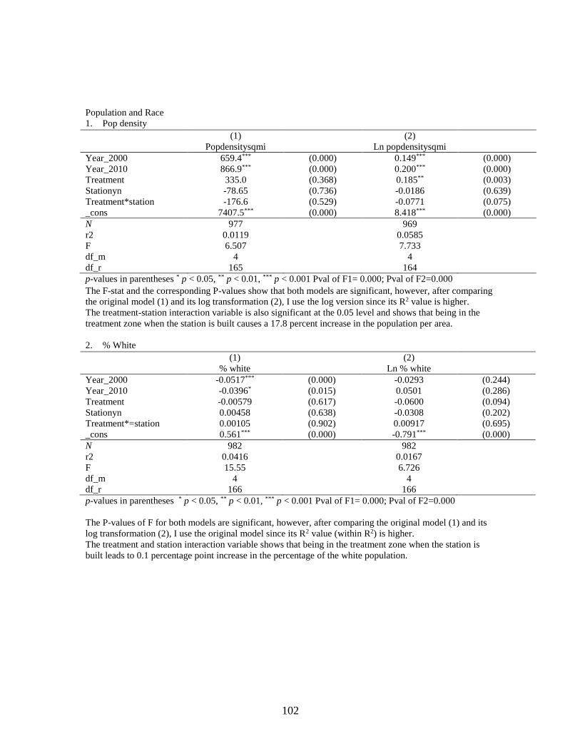
102
Population and Race
1. Pop density
(1) (2)
Popdensitysqmi Ln popdensitysqmi
Year_2000 659.4*** (0.000) 0.149*** (0.000)
Year_2010 866.9*** (0.000) 0.200*** (0.000)
Treatment 335.0 (0.368) 0.185** (0.003)
Stationyn -78.65 (0.736) -0.0186 (0.639)
Treatment*station -176.6 (0.529) -0.0771 (0.075)
_cons 7407.5*** (0.000) 8.418*** (0.000)
N 977 969
r2 0.0119 0.0585
F 6.507 7.733
df_m 4 4
df_r 165 164
p-values in parentheses * p < 0.05, ** p < 0.01, *** p < 0.001 Pval of F1= 0.000; Pval of F2=0.000
The F-stat and the corresponding P-values show that both models are significant, however, after comparing
the original model (1) and its log transformation (2), I use the log version since its R2 value is higher.
The treatment-station interaction variable is also significant at the 0.05 level and shows that being in the
treatment zone when the station is built causes a 17.8 percent increase in the population per area.
2. % White
(1) (2)
% white Ln % white
Year_2000 -0.0517*** (0.000) -0.0293 (0.244)
Year_2010 -0.0396* (0.015) 0.0501 (0.286)
Treatment -0.00579 (0.617) -0.0600 (0.094)
Stationyn 0.00458 (0.638) -0.0308 (0.202)
Treatment*=station 0.00105 (0.902) 0.00917 (0.695)
_cons 0.561*** (0.000) -0.791*** (0.000)
N 982 982
r2 0.0416 0.0167
F 15.55 6.726
df_m 4 4
df_r 166 166
p-values in parentheses * p < 0.05, ** p < 0.01, *** p < 0.001 Pval of F1= 0.000; Pval of F2=0.000
The P-values of F for both models are significant, however, after comparing the original model (1) and its
log transformation (2), I use the original model since its R2 value (within R2) is higher.
The treatment and station interaction variable shows that being in the treatment zone when the station is
built leads to 0.1 percentage point increase in the percentage of the white population.

103
3. % Black
(1) (2)
% black Ln % black
Year_2000 -0.0138* (0.027) 0.0597 (0.301)
Year_2010 -0.0457*** (0.000) -0.0801 (0.288)
Treatment 0.00167 (0.871) -0.00129 (0.982)
Stationyn 0.0114 (0.106) 0.0303 (0.595)
Treatment*station 0.00226 (0.763) -0.0290 (0.521)
_cons 0.251*** (0.000) -2.159*** (0.000)
N 982 980
r2 0.0362 0.0131
F 7.451 5.845
df_m 4 4
df_r 166 166
p-values in parentheses * p < 0.05, ** p < 0.01, *** p < 0.001 Pval of F1=0.000; Pval of F2=0.000
The P-values of F for both models are significant however, after comparing the original model (1) and its
log transformation (2), I use the original model since its R2 value (within R2) is higher.
The treatment-station variable shows that being in the treatment zone when the station is built leads to 0.2
percentage point increase in the share of the black population.
4. % Asian
(1) (2)
% Asian Ln % Asian
Year_2000 0.0278*** (0.000) 0.314*** (0.000)
Year_2010 0.0410*** (0.000) 0.494*** (0.000)
Treatment -0.00187 (0.720) -0.0662 (0.327)
Stationyn -0.00993* (0.038) -0.134 (0.084)
Treatment*station 0.00465 (0.378) 0.00313 (0.966)
_cons 0.0629*** (0.000) -3.454*** (0.000)
N 982 967
r2 0.0913 0.0572
F 9.729 9.488
df_m 4 4
df_r 166 166
p-values in parentheses * p < 0.05, ** p < 0.01, *** p < 0.001 Pval of F1= 0.000 ; Pval of F2=0.000
The P-values of F for both models are significant however, after comparing the original model (1) and its
log transformation (2), I use the original model since its R2 value (within R2) is higher.
The treatment-station interaction variable shows that being in the treatment zone when the station is built
leads to an increase in the proportion of Asian population.

104
5. % Other Race
(1) (2)
% other race % ln other race
Year_2000 0.0351*** (0.000) 0.571*** (0.000)
Year_2010 0.0429*** (0.000) 1.003*** (0.000)
Treatment 0.00584 (0.376) -0.0931 (0.114)
Stationyn -0.00443 (0.572) -0.147 (0.073)
Treatment*station -0.00773 (0.182) -0.0101 (0.859)
_cons 0.118*** (0.000) -3.102*** (0.000)
N 982 969
r2 0.0664 0.256
F 12.60 27.85
df_m 4 4
df_r 166 165
p-values in parentheses * p < 0.05, ** p < 0.01, *** p < 0.001 Pval of F1=0.000; Pval of F2=0.000
The P-values of F for both models are significant however, after comparing the original model (1) and its
log transformation (2), I use the log trasnformation model since its R2 value (within R2) is higher.
The treatment*station variable shows that being in the treatment zone when the station is built leads to a
decline in the share of this outcome variable.
6. All other race
(1) (2)
% All other race % ln All other race
Year_2000 0.0517*** (0.000) 0.263*** (0.000)
Year_2010 0.0396* (0.015) 0.294*** (0.000)
Treatment 0.00579 (0.617) -0.00777 (0.816)
Stationyn -0.00458 (0.638) -0.0764* (0.032)
Treatment*station -0.00105 (0.902) 0.0133 (0.617)
_cons 0.439*** (0.000) -1.110*** (0.000)
N 982 982
r2 0.0416 0.103
F 15.55 14.94
df_m 4 4
df_r 166 166
p-values in parentheses * p < 0.05, ** p < 0.01, *** p < 0.001 Pval of F1= 0.000 Pval of F2=0.000
The P-values of F for both models are significant however, after comparing the original model (1) and its
log transformation (2), I use the log version since its R2 value (within R2) is higher.
The treatment and station interaction variable shows that being in the treatment zone when the station is
built leads to an increase in the share of this outcome variable.

105
7. Share of Hispanics
(1) (2)
% Hispanic Ln % Hispanic
Year_2000 0.0656*** (0.000) 0.451*** (0.000)
Year_2010 0.0985*** (0.000) 0.700*** (0.000)
Treatment -0.00338 (0.755) -0.0597 (0.220)
Stationyn -0.0101 (0.226) -0.1000* (0.020)
Treatment*station -0.00327 (0.701) 0.0405 (0.272)
_cons 0.211*** (0.000) -2.302*** (0.000)
N 985 981
r2 0.160 0.302
F 18.08 34.91
df_m 4 4
df_r 166 166
p-values in parentheses * p < 0.05, ** p < 0.01, *** p < 0.001
The F-stat and p-value (p<0.05) of models 1 and 2 confirm that they are both significant. Model 2, which
has the log transformation, has a slightly higher R2 and so this version is used for a better interpretability.
The treatment and station interaction variable is not significant at the 0.05 level.
8. Real Household Income
(1) (2)
Real hh income Ln real hh income
Year_2000 1282.4 (0.076) 0.0672 (0.074)
Year_2010 -2818.8** (0.006) -0.182*** (0.001)
Treatment -15260.2*** (0.000) -0.605*** (0.000)
Stationyn 1656.7 (0.071) 0.0885* (0.046)
Treatment*station -3821.0*** (0.000) -0.253*** (0.000)
_cons 33923.9*** (0.000) 10.33*** (0.000)
N 987 980
r2 0.525 0.537
F 88.85 105.1
df_m 4 4
df_r 166 166
p-values in parentheses * p < 0.05, ** p < 0.01, *** p < 0.001
Pval of F1= 0.000; Pval of F2=0.000
The F-stat and p-value (p<0.05) of models 1 and 2 confirm that they are both significant. Model 2, which
has the log transformation, has a slightly higher R2 and so this version is used for a better interpretability.
The treatment and station interaction variable is significant at the 0.05 level and shows that being in the
treatment zone when the station is built causes a 25.3 percent decline in the average household income.

106
9. Real Housing Value
(1) (2)
Real housing value Ln real housing value
Year_2000 3034.9 (0.664) 0.126* (0.024)
Year_2010 91710.8*** (0.000) 0.741*** (0.000)
Treatment -59419.7*** (0.000) -0.640*** (0.000)
Stationyn -4423.3 (0.624) -0.201** (0.001)
Treatment*station -9588.7 (0.070) 0.0988 (0.061)
_cons 147404.0*** (0.000) 11.68*** (0.000)
N 987 976
r2 0.420 0.412
F 76.66 90.05
df_m 4 4
df_r 166 166
p-values in parentheses * p < 0.05, ** p < 0.01, *** p < 0.001 Pval of F1= 0.000; Pval of F2= 0.000
The P-values of F for both models are significant, however, after comparing the original model (1) and its
log transformation (2), I use the original model since its R2 value (within R2) is slightly higher.
The treatment-station interaction variable is not significant at the 0.05 level but it indicates a negative effect
in the outcome variable.
10. With Vehicle Access
(1) (2)
% with vehicle % ln with vehicle
Year_2000 0.128*** (0.000) 0.174*** (0.000)
Year_2010 -0.0527* (0.015) -0.0428 (0.371)
Treatment -0.0124* (0.021) -0.00938 (0.622)
Stationyn 0.0391* (0.046) 0.0473 (0.152)
Treatment*station -0.000587 (0.905) -0.00822 (0.625)
_cons 0.843*** (0.000) -0.208*** (0.000)
N 983 983
r2 0.429 0.241
F 57.80 43.48
df_m 4 4
df_r 166 166
p-values in parentheses * p < 0.05, ** p < 0.01, *** p < 0.001 Pval of F1=0.000; Pval of F2=0.000
The overall goodness of fit tests (looking at F-stas and p-values) indicate that both models are significant.
However, model 1has a higher R2 and so this version is utilized.
The treatment-station variable shows that being in the treatment zone when the station is built leads to a
0.05 percentage point decrease in the share of the outcome variable.

107
Means of Transportation
11. Public Transportation
(1) (2)
% pubtranspo Ln % publictranspo
Year_2000 -0.00620 (0.344) -0.0689 (0.345)
Year_2010 -0.00997 (0.268) -0.0845 (0.340)
Treatment 0.0152*** (0.000) 0.0477 (0.275)
Stationyn 0.0117 (0.103) 0.214** (0.004)
Treatment*station 0.00502 (0.268) 0.0978 (0.061)
_cons 0.125*** (0.000) -2.494*** (0.000)
N 981 974
r2 0.0495 0.0651
F 7.772 10.01
df_m 4 4
df_r 166 166
p-values in parentheses * p < 0.05, ** p < 0.01, *** p < 0.001 Pval of F1=0.000 Pval of F2=0.000
The F-stat and p-value (p<0.05) of models 1 and 2 confirm that both models are significant. Model 2,
which has the log transformation, has a slightly higher R2 and so this version is used for a better
interpretability.
The interaction variable between treatment is not significant at the 0.05 level. It shows that being in the
treatment zone when the station is built leads to an 9.8 percentage points increase in the share of the
outcome variable.
12. Car Use
(1) (2)
% car Ln % car
Year_2000 0.0437*** (0.000) 0.0747*** (0.000)
Year_2010 0.0331* (0.028) 0.0662** (0.008)
Treatment -0.00782 (0.304) -0.00362 (0.852)
Stationyn -0.00639 (0.545) 0.00300 (0.879)
Treatment*station -0.0308*** (0.000) -0.0571** (0.001)
_cons 0.723*** (0.000) -0.384*** (0.000)
N 981 981
r2 0.0821 0.0604
F 15.06 13.22
df_m 4 4
df_r 166 166
p-values in parentheses * p < 0.05, ** p < 0.01, *** p < 0.001 Pval of F1=0.000; Pval of F2=0.000
The F-stat and p-value (p<0.05) of models 1 and 2 confirm that both models are significant, however, after
comparing the two models, I use Model 1 because it has a higher R2 value.
The treatment*station interaction variable demonstrates that being in the treatment zone when the station
gets built leads to a 3 percent decrease in the share of the outcome variable.

108
13. Bicycle Use
(1) (2)
% bicycle Ln % bicycle
Year_2000 0.000269 (0.867) 0.0943 (0.529)
Year_2010 0.00607** (0.002) 0.456* (0.017)
Treatment 0.000267 (0.684) 0.0465 (0.662)
Stationyn 0.00305 (0.101) 0.197 (0.243)
Treatment*station -0.000622 (0.586) -0.164 (0.181)
_cons 0.00702*** (0.000) -5.319*** (0.000)
N 981 816
r2 0.0990 0.0784
F 6.911 10.21
df_m 4 4
df_r 166 160
p-values in parentheses * p < 0.05, ** p < 0.01, *** p < 0.001 Pval of F1= 0.000; Pval of F2=0.000
The overall goodness of fit tests indicate that both models are significant. However, model 1has a higher R2
and so this version is used. The 2010 dummy variable is significant at the 0.05 level and indicates that
relative to the base year, the share of bicycle riders is associated with a 0.06 percentage point increase in
2010. The treatment dummy variable, station dummy variable and the treatment*station variable are not
significant at the 0.05 level.
Other Transportation
(1) (2)
% other transpluspo Ln % othertranspo
Year_2000 -0.0363*** (0.000) -0.465*** (0.000)
Year_2010 -0.0391*** (0.000) -0.509*** (0.000)
treatment -0.00805 (0.173) -0.146** (0.003)
stationyn -0.0127* (0.014) -0.000994 (0.989)
Treatment*station 0.0289*** (0.000) 0.237*** (0.000)
_cons 0.116*** (0.000) -2.568*** (0.000)
N 981 977
r2 0.154 0.141
F 20.32 35.36
df_m 4 4
df_r 166 166
p-values in parentheses * p < 0.05, ** p < 0.01, *** p < 0.001 Pval of F1= 0.000; Pval of F2=0.000
The F-stat and p-value (p<0.05) of models 1 and 2 confirm that both models are significant, however, after
comparing the two models, I use Model 1 because it has a higher R2 value. Most of the predictor variables
are significant at the 0.05 level. The interaction variable treatment-station variable, however, demonstrates
that being in the treatment zone when the station gets built leads to a 2.89 percentage points increase in the
share of the outcome variable.

109
14. Work at home
(1) (2)
% work at home Ln % work at home
Year_2000 -0.00141 (0.772) 0.196** (0.004)
Year_2010 0.00995 (0.102) 0.512*** (0.000)
Treatment 0.000371 (0.921) -0.0416 (0.443)
Stationyn 0.00435 (0.448) 0.0741 (0.349)
Treatment*station -0.00245 (0.532) -0.117* (0.044)
_cons 0.0289*** (0.000) -3.873*** (0.000)
N 981 965
r2 0.0460 0.182
F 16.12 46.88
df_m 4 4
df_r 166 166
p-values in parentheses * p < 0.05, ** p < 0.01, *** p < 0.001 Pval of F1=0.000; Pval of F2=0.000
The F-stat and p-value (p<0.05) of models 1 and 2 confirm that both models significant. Model 2, which
has the log transformation, has a slightly higher R2 and so this version is used for a better interpretability.
The interaction variable of treatment-station shows that being in the treatment zone when the station gets
built leads to an 11.7 percent decrease in the share of people working from home.
Occupations
15. Manufacturing
(1) (2)
% manuf ln % manuf
Year_2000 -0.0334*** (0.000) -0.283*** (0.000)
Year_2010 -0.0974*** (0.000) -1.036*** (0.000)
Treatment -0.000421 (0.911) -0.0248 (0.321)
Stationyn -0.0161* (0.015) -0.0998* (0.044)
Treatment*station 0.00422 (0.259) -0.00746 (0.870)
_cons 0.176*** (0.000) -1.904*** (0.000)
N 982 980
r2 0.572 0.606
F 103.8 224.7
df_m 4 4
df_r 166 166
p-values in parentheses * p < 0.05, ** p < 0.01, *** p < 0.001 Pval of F1=0.000; Pval of F2=0.000
The F-stat and p-value (p<0.05) of models 1 & 2 confirm that both are significant. Model 2, which has the
log transformation, is used because it has a slightly higher R2.
The treatment dummy variable and the interaction variable treatment-station which is between treatment
and the presence of a station are not significant at the 0.05 level but for both, the share of manufacturing
jobs are expected to decline.

110
16. Construction
(1) (2)
% construct ln % construct
Year_2000 0.0125* (0.012) 0.143 (0.069)
Year_2010 -0.00523 (0.399) -0.259* (0.014)
Treatment 0.000815 (0.659) -0.0504 (0.173)
Stationyn -0.00618 (0.234) -0.0831 (0.293)
Treatment*station 0.00102 (0.676) -0.0433 (0.292)
_cons 0.0515*** (0.000) -3.045*** (0.000)
N 982 976
r2 0.0968 0.155
F 16.86 23.30
df_m 4 4
df_r 166 166
p-values in parentheses * p < 0.05, ** p < 0.01, *** p < 0.001 Pval of F1=0.000; Pval of F2=0.000
The overall goodness of fit results indicate that both models are significant. However, model 2 has a higher
R2 and so this version is used.
The treatment dummy variable, station dummy variable and the treatment*station variable are not
significant at the 0.05 level.
17. Transportation
(1) (2)
% transpo % ln transpo
Year_2000 0.00187 (0.480) 0.00123 (0.984)
Year_2010 0.0301*** (0.000) 0.449*** (0.000)
Treatment 0.00138 (0.336) -0.0321 (0.240)
Stationyn -0.0174*** (0.000) -0.318*** (0.000)
Treatment*station -0.00320 (0.142) -0.0991* (0.029)
_cons 0.0498*** (0.000) -3.083*** (0.000)
N 982 973
r2 0.203 0.141
F 23.94 31.69
df_m 4 4
df_r 166 166
p-values in parentheses * p < 0.05, ** p < 0.01, *** p < 0.001 Pval of F1= 0.000; Pval of F2=0.000
The F-stat and p-value (p<0.05) of models 1 & 2 confirm that both are significant. Model 1 is used because
it has a slightly higher R2.
The treatment dummy variable and the treatment*station variable are not significant at the 0.05 level.

111
18. Finance
(1) (2)
% finance % ln finance
Year_2000 -0.0119*** (0.000) -0.139*** (0.001)
Year_2010 0.00474 (0.283) 0.0866 (0.141)
Treatment -0.000578 (0.791) -0.0654* (0.024)
Stationyn 0.00905* (0.018) 0.0698 (0.167)
Treatmentplusstation 0.00119 (0.643) 0.0313 (0.402)
_cons 0.0731*** (0.000) -2.704*** (0.000)
N 982 981
r2 0.118 0.107
F 16.12 16.55
df_m 4 4
df_r 166 166
p-values in parentheses * p < 0.05, ** p < 0.01, *** p < 0.001 Pval of F1= 0.000; Pval of F2= 0.000
The overall goodness of fit test results indicate that both models are significant. However, model 1 has a
slightly higher R2 and so this version is used.
The treatment dummy variable and the treatment*station variable are not significant at the 0.05 level.
19. Information
(1) (2)
% info % ln info
Year_2000 0.0518*** (0.000) 1.158*** (0.000)
Year_2010 0.00441 (0.140) -0.242* (0.012)
Treatment -0.000983 (0.300) -0.102* (0.019)
Stationyn -0.00770** (0.002) -0.0255 (0.738)
Treatment*station -0.00000715 (0.996) 0.0309 (0.603)
_cons 0.0254*** (0.000) -3.776*** (0.000)
N 982 968
r2 0.748 0.595
F 343.0 294.2
df_m 4 4
df_r 166 166
p-values in parentheses * p < 0.05, ** p < 0.01, *** p < 0.001 Pval of F1= 0.0000; Pval of F2= 0.000
The F-stat and p-value (p<0.05) of models 1 & 2 confirm that both are significant but Model 1, is chosen
because it has a slightly higher R2.
The treatment dummy variable and treatment-station variable are not significant at the 0.05 level, but for
both, the share of workers in the information industry is expected to decline.

112
20. Professional Services
(1) (2)
% professional % ln professional
Year_2000 0.0245*** (0.000) 0.180*** (0.000)
Year_2010 0.0812*** (0.000) 0.538*** (0.000)
Treatment 0.00741** (0.002) 0.0356 (0.068)
Stationyn 0.000547 (0.921) 0.0140 (0.756)
Treatment*station -0.00187 (0.656) -0.0193 (0.526)
_cons 0.106*** (0.000) -2.279*** (0.000)
N 982 980
r2 0.426 0.455
F 68.12 130.2
df_m 4 4
df_r 166 166
p-values in parentheses * p < 0.05, ** p < 0.01, *** p < 0.001 Pval of F1= 0.000; Pval fo F2= 0.000
The F-stat and p-value (p<0.05) of models 1 & 2 confirm that both are significant but Model 2, which has
the logarithmic transformation, is chosen because it has a slightly higher R2.
The treatment*station variable is not significant at the 0.05 level. The interaction variable is expected to
cause a decline in the outcome variable.
21. Other Services
(1) (2)
% other services %ln other services
Year_2000 -0.0274*** (0.000) -0.319*** (0.000)
Year_2010 -0.0489*** (0.000) -0.883*** (0.000)
Treatment -0.00222 (0.276) -0.0541* (0.026)
Stationyn 0.00456 (0.305) 0.0928 (0.130)
Treatment*station 0.00185 (0.480) -0.0218 (0.641)
_cons 0.0835*** (0.000) -2.595*** (0.000)
N 982 978
r2 0.275 0.392
F 34.57 74.29
df_m 4 4
df_r 166 166
p-values in parentheses * p < 0.05, ** p < 0.01, *** p < 0.001 Pval of F1= 0.000; Pval of F2= 0.0000
The overall goodness of fit test results indicate that both models are significant. However, model 2 has a
slightly higher R2 and so this version is used.
The treatment-station interaction variable is not significant at the 0.05 level.

113
22. Wholesale Trade
(1) (2)
% wholesale trade % ln whoelsale trade
Year_2000 -0.00435 (0.103) -0.157* (0.015)
Year_2010 -0.0350*** (0.000) -1.247*** (0.000)
Treatment 0.00153 (0.225) -0.0253 (0.404)
Stationyn 0.00986** (0.002) 0.310*** (0.000)
Treatment*station -0.00160 (0.305) -0.0290 (0.569)
_cons 0.0451*** (0.000) -3.173*** (0.000)
N 982 972
r2 0.464 0.526
F 138.1 110.3
df_m 4 4
df_r 166 166
p-values in parentheses * p < 0.05, ** p < 0.01, *** p < 0.001 Pval of F1= 0.000; Pval of F2= 0.000
The F-stat and p-value (p<0.05) of models 1 & 2 confirm that both are significant but model 2 is used
because it has a higher R2.
The interaction variable for treatment and station indicates that a decline in the share of workers in the
wholesale trade sector is expected. However the interaction variable is not significant at 0.05 level, and so
are the treatment variable and station dummy variable separately.
23. Retail Trade
(1) (2)
% retail trade % ln retail trade
Year_2000 -0.0822*** (0.000) -0.736*** (0.000)
Year_2010 -0.0914*** (0.000) -0.890*** (0.000)
Treatment 0.00220 (0.353) 0.00224 (0.900)
Stationyn -0.00250 (0.611) -0.0568 (0.327)
Treatment*station -0.00144 (0.597) -0.0393 (0.164)
_cons 0.156*** (0.000) -1.877*** (0.000)
N 982 977
r2 0.742 0.671
F 245.5 377.4
df_m 4 4
df_r 166 165
p-values in parentheses * p < 0.05, ** p < 0.01, *** p < 0.001
Pval of F1= 0.000; Pval of F2= 0.000
The F-stat and p-value (p<0.05) of models 1 & 2 confirm that both are significant but model 1 is used
because it has a higher R2.
The interaction variable for treatment and station indicates that a decline in the share of workers in the
retail trade sector is expected. However the interaction variable is not significant at 0.05 level, and so are
the treatment variable and station dummy variable separately.

114
24. Arts and Entertainment
(1) (2)
% arts % ln arts
Year_2000 0.128*** (0.000) 2.165*** (0.000)
Year_2010 0.0839*** (0.000) 1.807*** (0.000)
Treatment -0.00355** (0.009) -0.0925* (0.034)
Stationyn 0.0356** (0.002) 0.345*** (0.000)
Treatment*station 0.00268 (0.444) 0.0579 (0.239)
_cons 0.0194*** (0.000) -4.204*** (0.000)
N 982 972
r2 0.702 0.861
F 492.3 654.8
df_m 4 4
df_r 166 166
p-values in parentheses * p < 0.05, ** p < 0.01, *** p < 0.001
Pval of F1=0.000; Pval of F2=0.000
The F-stat and p-value (p<0.05) of models 1 and 2 confirm that both models are significant, however, after
comparing the two models, I use Model 2 because it has a slightly higher R2 value.
All of the predictor variables, except for the treatment and station interaction variable, are significant at the
0.05 level.
25. Education, Health, and Social Sciences (EHSS)
(1) (2)
% ehss % ln ehss
_Iyear_2000 -0.0349*** (0.000) -0.336*** (0.000)
_Iyear_2010 0.112*** (0.000) 0.639*** (0.000)
treatment -0.00368 (0.182) -0.0500* (0.025)
stationyn -0.0154 (0.161) -0.103 (0.191)
Treatment*station -0.00250 (0.532) 0.00689 (0.814)
_cons 0.144*** (0.000) -1.994*** (0.000)
N 982 976
r2 0.630 0.617
F 136.4 191.9
df_m 4 4
df_r 166 165
p-values in parentheses * p < 0.05, ** p < 0.01, *** p < 0.001
Pval of F1=0.000; Pval of F2=0.000
The F-stat and the corresponding P-values show that both models are significant, however, after comparing
the original model (1) and its log transformation (2), Model 1 is used since its R2 value is higher.
The treatment-station interaction variable has a coefficient that is not significant at the 0.05 level, but it
causes a decline in the outcome variable.

115
Land Use
% Multi-family Units
(1) (2)
% Multi family % ln Multi-family
Year_2000 0.255*** (0.000) 0.523*** (0.000)
Year_2010 0.0492* (0.045) 0.138 (0.060)
Treatment 0.0460*** (0.000) 0.0344 (0.338)
Stationyn -0.0348 (0.136) -0.0823 (0.227)
Treatment*station 0.00137 (0.880) 0.00826 (0.813)
_cons 0.576*** (0.000) -0.700*** (0.000)
N 981 979
r2 0.519 0.296
F 101.8 49.82
df_m 4 4
df_r 166 166
p-values in parentheses * p < 0.05, ** p < 0.01, *** p < 0.001
Pval of F1= 0.000; Pval of F2= 0.000
The treatment-station interaction variable is not significant at the 0.05 level.
Model 3: Effects of the Investment on Near versus Far from CBD Stations
Model 3: Fixed Effect Regression Results
Dependent Variable
(Far from CBD)
Coefficient and (P-
val) for
Treatment+station
Dependent Variable
(Near the CBD)
Coefficient and (P-
val) for
Treatment+station:
Ln pop density 0.0991 (0.112) Ln pop density 0.359 (0.089)
% white 0.0126 (0.140) % white -0.0335 (0.107)
% black -0.00507 (0.493) % black 0.0230 (0.228)
% Asian 0.000901 (0.875) Ln % Asian 0.101 (0.490)
Ln % other race -0.00583 (0.925) Ln % other race -0.0140 (0.918)
Ln % all other races -0.0243 (0.406) Ln % all other races 0.118* (0.035)
Ln % Hispanic 0.0330 (0.425) Ln % Hispanic 0.0625 (0.446)
Ln real household
income -0.195
***(0.000) Ln real household income --0.439
***(0.000)
Ln Real housing value 0.0778 (0.121) Real housing value 416.7 (0.968)
Ln % public
transportation 0.158
* (0.016) Ln % public transportation -0.0626 (0.365)
% car -0.0240***
(0.000) L% car -0.0459* (0.036)

116
% bicycle 0.000403 (0.696) Ln % bicycle 0.155 (0.427)
Ln % other transpo 1.207***
(0.000) Ln % other transportation 1.875***
(0.000)
Ln % Work at home -0.172**
(0.007) Ln % Work at home -0.0571 (0.670)
% With vehicle access 0.000668 (0.879) % With vehicle access -0.00270 (0.853)
% Multifamily housing 0.00638 (0.569) % Multifamily housing -0.0162 (0.329)
p-values in parentheses; Significance: * p < 0.05,
** p < 0.01,
*** p < 0.001
Model 3 Regression Results for Jobs
Dependent Variable Coefficient and
(P-val) for
Treatment+station:
Far from CBD
Dependent Variable Coefficient and (P-
val) for
Treatment+station:
Near CBD
Ln % Manufacturing -0.0116 (0.782) Ln % Manufacturing 0.0166 (0.894)
Ln % Construction -0.0330 (0.470) % Construction 0.00133 (0.761)
% Transportation -0.00261 (0.303) % Transportation -0.00519 (0.235)
% Finance 0.00244 (0.302) % Finance -0.00385 (0.595)
% Professional services -0.000285 (0.946) Ln % Professional
services
-0.0642 (0.389)
Ln % Other services -0.0357 (0. 456) Ln % Other services 0.0121 (0.918)
Ln % Arts and
entertainment
0.0808 (0.154) Ln % Arts and
entertainment
0.00212 (0.983)
% Information -0.000856 (0.568) % Information 0.00201 (0.572)
Ln % Wholesale trade -0.133* (0.016) Ln % Wholesale trade 0.240
* (0.038)
% Retail trade -0.00415 (0.158) % Retail trade 0.00599 (0.355)
Ln % Education, health
and social services (EHSS)
-0.00850 (0.797) % Education, health
and social services
(EHSS)
0.00136 (0.874)
p-values in parentheses; Significance: * p < 0.05,
** p < 0.01,
*** p < 0.001

117
Population and Race
(1) Far (2) Far (3) Near (4) Near
Popdensitysqmi lnpopdensitysqmi Popdensitysqmi lnpopdensitysqmi
Year_2000 671.7*** 0.154*** 534.7 0.128
(0.000) (0.000) (0.068) (0.110)
Year_2010 767.5*** 0.195*** 1002.4 0.201
(0.000) (0.000) (0.060) (0.053)
Treatment -7.551 0.167** 1361.5 0.238
(0.981) (0.005) (0.234) (0.169)
Station -206.0 -0.0360 445.8 0.0416
(0.450) (0.399) (0.311) (0.703)
Treatment*station 181.8 -0.0414 -1247.9* -0.176
(0.556) (0.363) (0.042) (0.115)
_cons 7083.1*** 8.329*** 8230.4*** 8.657***
(0.000) (0.000) (0.000) (0.000)
N 712 707 265 262
r2 0.0156 0.0711 0.0178 0.0441
F 7.580 6.568 1.830 1.757
df_m 4 4 4 4
df_r 119 119 45 44
p-values in parentheses * p < 0.05, ** p < 0.01, *** p < 0.001
(1) Far (2) Far (3) Near (4) Near
% White Ln % white % Whit Ln % white
Year_2000 -0.0657*** -0.0536 -0.0184 0.0273
(0.000) (0.087) (0.209) (0.418)
Year_2010 -0.0691*** -0.00654 0.0345 0.190*
(0.001) (0.908) (0.155) (0.018)
Treatment -0.0186 -0.0767* 0.0321 -0.0105
(0.089) (0.021) (0.314) (0.919)
Stationyn -0.00408 -0.0390 0.0327 0.00222
(0.711) (0.153) (0.089) (0.962)
Treatment*station 0.0126 0.0219 -0.0335 -0.0301
(0.140) (0.379) (0.107) (0.568)
_cons 0.588*** -0.754*** 0.490*** -0.889***
(0.000) (0.000) (0.000) (0.000)
N 712 712 270 270
r2 0.107 0.0246 0.0632 0.0448
F 17.52 6.429 6.465 4.943
df_m 4 4 4 4
df_r 120 120 45 45
p-values in parentheses * p < 0.05, ** p < 0.01, *** p < 0.001 P-val: F1: 0.000; F2: 0.000; F3: 0.001; F4: 0.0011

118
(1) Far (2) Far (3) Near (4) Near
% Black Ln % black % Black Ln % black
Year_2000 -0.00891 0.0999 -0.0231** -0.0510
(0.252) (0.169) (0.005) (0.377)
Year_2010 -0.0305* 0.0119 -0.0811*** -0.325***
(0.017) (0.901) (0.000) (0.000)
Treatment 0.00714 0.00159 -0.0146 -0.0105
(0.466) (0.978) (0.614) (0.944)
Stationyn 0.0144 0.0459 -0.00199 -0.00525
(0.060) (0.506) (0.897) (0.950)
Treatment*station -0.00507 -0.0897 0.0230 0.123
(0.493) (0.066) (0.228) (0.221)
_cons 0.225*** -2.308*** 0.321*** -1.766***
(0.000) (0.000) (0.000) (0.000)
N 712 711 270 269
r2 0.0188 0.0141 0.0954 0.0567
F 3.109 3.394 7.463 7.996
df_m 4 4 4 4
df_r 120 120 45 45 p-values in parentheses * p < 0.05, ** p < 0.01, *** p < 0.001 P-val: F1: 0.0113; F2: 0.0067; F3: 0.000; F4: 0.000
(1) Far (2) Far (3) Near (4) Near
% Asian Ln % Asian % Asian Ln % Asian
Year_2000 0.0279*** 0.276*** 0.0269*** 0.401**
(0.000) (0.000) (0.000) (0.009)
Year_2010 0.0382*** 0.398*** 0.0468*** 0.727***
(0.000) (0.000) (0.000) (0.000)
Treatment -0.000144 -0.109 -0.00701 0.0594
(0.981) (0.133) (0.472) (0.711)
Stationyn -0.00580 -0.0985 -0.0191* -0.192
(0.311) (0.235) (0.019) (0.312)
Treatment*station 0.000901 -0.0429 0.0147 0.101
(0.875) (0.621) (0.196) (0.490)
_cons 0.0671*** -3.372*** 0.0523*** -3.677***
(0.000) (0.000) (0.000) (0.000)
N 712 704 270 263
r2 0.0900 0.0469 0.103 0.131
F 6.168 5.057 5.433 10.21
df_m 4 4 4 4
df_r 120 120 45 45 p-values in parentheses * p < 0.05, ** p < 0.01, *** p < 0.001 P-val: F1: 0.0000; F2: 0.003; F3: 0.0005; F4: 0.000

119
(1) Far (2) Far (3) Near (4) Near
% other race Ln % other race % other race Ln % otherrace
Year_2000 0.0444*** 0.618*** 0.0105 0.459*
(0.000) (0.000) (0.390) (0.013)
Year_2010 0.0601*** 1.089*** -0.00257 0.783**
(0.000) (0.000) (0.880) (0.003)
Treatment 0.0113 -0.0785 -0.0104 -0.137
(0.059) (0.173) (0.590) (0.395)
Stationyn -0.00344 -0.122 -0.00792 -0.219
(0.687) (0.176) (0.673) (0.266)
Treatment*station -0.00813 -0.00583 -0.00418 -0.0140
(0.154) (0.925) (0.783) (0.918)
_cons 0.115*** -3.097*** 0.127*** -3.115***
(0.000) (0.000) (0.000) (0.000)
N 712 703 270 266
r2 0.158 0.334 0.0200 0.112
F 17.60 27.49 0.711 3.399
df_m 4 4 4 4
df_r 120 119 45 45 p-values in parentheses * p < 0.05, ** p < 0.01, *** p < 0.001 P-val: F1: 0.000; F2: 0.003; F3: 0.6180; F4: 0.0109
(1) Far (2) Far (3) Near (4) Near
% all other race Ln % all other
race
% all other race Ln %all other
race
Year_2000 0.0657*** 0.324*** 0.0184 0.107*
(0.000) (0.000) (0.209) (0.030)
Year_2010 0.0691*** 0.410*** -0.0345 -0.0118
(0.001) (0.000) (0.155) (0.874)
Treatment 0.0186 0.0195 -0.0321 -0.0890
(0.089) (0.593) (0.314) (0.234)
Stationyn 0.00408 -0.0472 -0.0327 -0.156**
(0.711) (0.255) (0.089) (0.008)
Treatmen*station -0.0126 -0.0243 0.0335 0.118*
(0.140) (0.406) (0.107) (0.035)
_cons 0.412*** -1.221*** 0.510*** -0.814***
(0.000) (0.000) (0.000) (0.000)
N 712 712 270 270
r2 0.107 0.196 0.0632 0.0681
F 17.52 18.45 6.465 5.644
df_m 4 4 4 4
df_r 120 120 45 45 p-values in parentheses * p < 0.05, ** p < 0.01, *** p < 0.001 P-val: F1: 0.000; F2: 0.003; F3: 0.6180; F4: 0.0109
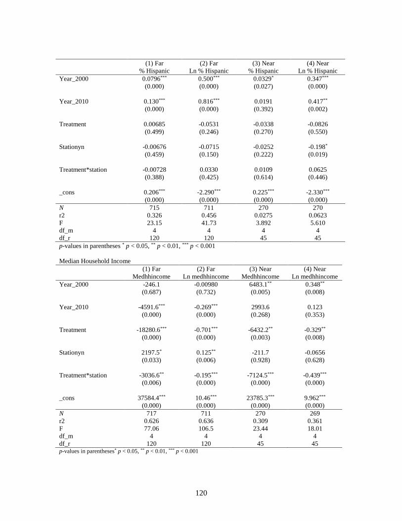
120
(1) Far (2) Far (3) Near (4) Near
% Hispanic Ln % Hispanic % Hispanic Ln % Hispanic
Year_2000 0.0796*** 0.500*** 0.0329* 0.347***
(0.000) (0.000) (0.027) (0.000)
Year_2010 0.130*** 0.816*** 0.0191 0.417**
(0.000) (0.000) (0.392) (0.002)
Treatment 0.00685 -0.0531 -0.0338 -0.0826
(0.499) (0.246) (0.270) (0.550)
Stationyn -0.00676 -0.0715 -0.0252 -0.198*
(0.459) (0.150) (0.222) (0.019)
Treatment*station -0.00728 0.0330 0.0109 0.0625
(0.388) (0.425) (0.614) (0.446)
_cons 0.206*** -2.290*** 0.225*** -2.330***
(0.000) (0.000) (0.000) (0.000)
N 715 711 270 270
r2 0.326 0.456 0.0275 0.0623
F 23.15 41.73 3.892 5.610
df_m 4 4 4 4
df_r 120 120 45 45
p-values in parentheses * p < 0.05, ** p < 0.01, *** p < 0.001
Median Household Income
(1) Far (2) Far (3) Near (4) Near
Medhhincome Ln medhhincome Medhhincome Ln medhhincome
Year_2000 -246.1 -0.00980 6483.1** 0.348**
(0.687) (0.732) (0.005) (0.008)
Year_2010 -4591.6*** -0.269*** 2993.6 0.123
(0.000) (0.000) (0.268) (0.353)
Treatment -18280.6*** -0.701*** -6432.2** -0.329**
(0.000) (0.000) (0.003) (0.008)
Stationyn 2197.5* 0.125** -211.7 -0.0656
(0.033) (0.006) (0.928) (0.628)
Treatment*station -3036.6** -0.195*** -7124.5*** -0.439***
(0.006) (0.000) (0.000) (0.000)
_cons 37584.4*** 10.46*** 23785.3*** 9.962***
(0.000) (0.000) (0.000) (0.000)
N 717 711 270 269
r2 0.626 0.636 0.309 0.361
F 77.06 106.5 23.44 18.01
df_m 4 4 4 4
df_r 120 120 45 45 p-values in parentheses* p < 0.05, ** p < 0.01, *** p < 0.001

121
Median Housing Value
(1) Far (2) Far (3) Near (4) Near
Med houseval Ln medhouseval Med houseval Ln med houseval
Year_2000 -9941.7 -0.00262 40851.8* 0.521***
(0.183) (0.962) (0.013) (0.000)
Year_2010 66626.1*** 0.541*** 160094.1*** 1.329***
(0.000) (0.000) (0.000) (0.000)
Treatment -69187.5*** -0.688*** -30951.9* -0.488**
(0.000) (0.000) (0.018) (0.007)
Stationyn 4384.1 -0.163* -26773.7 -0.345*
(0.650) (0.013) (0.208) (0.029)
Treatment*station -15210.9* 0.0778 416.7 0.122
(0.011) (0.121) (0.968) (0.397)
_cons 162406.2*** 11.81*** 106280.1*** 11.30***
(0.000) (0.000) (0.000) (0.000)
N 717 709 270 267
r2 0.496 0.534 0.416 0.362
F 64.20 111.1 28.49 30.27
df_m 4 4 4 4
df_r 120 120 45 45 p-values in parentheses* p < 0.05, ** p < 0.01, *** p < 0.001
Means of Transportation
(1) Far (2) Far (3) Near (4) Near
% pubtranspo ln % pubtranspo % pubtranspo ln % pubtranspo
Year_2000 -0.00521 -0.0694 -0.00284 0.0107
(0.482) (0.434) (0.838) (0.884)
Year_2010 0.00260 -0.0430 -0.0347 -0.128
(0.789) (0.694) (0.066) (0.212)
Treatment 0.0108*** 0.0104 0.0279* 0.151*
(0.001) (0.843) (0.044) (0.043)
Stationyn 0.00691 0.275** 0.0164 -0.00845
(0.311) (0.002) (0.356) (0.919)
Treatment*station 0.0125** 0.158* -0.0153 -0.0626
(0.002) (0.016) (0.236) (0.365)
_cons 0.0952*** -2.781*** 0.203*** -1.741***
(0.000) (0.000) (0.000) (0.000)
N 711 706 270 268
r2 0.113 0.124 0.0768 0.0844
F 11.07 12.51 3.305 2.337
df_m 4 4 4 4
df_r 120 120 45 45
p-values in parentheses * p < 0.05, ** p < 0.01, *** p < 0.001

122
(1) Far (2) Far (3) Near (4) Near
% car Ln % car % car Ln % car
Year_2000 0.0349* 0.0529* 0.0639*** 0.129***
(0.013) (0.015) (0.000) (0.000)
Year_2010 0.0163 0.0301 0.0765** 0.164**
(0.361) (0.276) (0.001) (0.001)
Treatment -0.00362 -0.00811 -0.0193 0.0110
(0.506) (0.325) (0.449) (0.880)
Stationyn -0.0160 -0.0223 0.0178 0.0655
(0.185) (0.234) (0.339) (0.234)
Treatment*station -0.0240*** -0.0318*** -0.0459* -0.122
(0.000) (0.000) (0.036) (0.056)
_cons 0.802*** -0.237*** 0.516*** -0.775***
(0.000) (0.000) (0.000) (0.000)
N 711 711 270 270
r2 0.0943 0.0804 0.187 0.142
F 13.74 12.47 9.645 10.64
df_m 4 4 4 4
df_r 120 120 45 45
p-values in parentheses * p < 0.05, ** p < 0.01, *** p < 0.001
(1) Far (2) Far (3) Near (4) Near
% bicycle Ln % bicycle % bicycle Ln %bicycle
Year_2000 -0.00114 -0.0922 0.00277 0.645**
(0.400) (0.612) (0.646) (0.003)
Year_2010 0.00219 0.153 0.0151* 1.277***
(0.154) (0.514) (0.026) (0.000)
Treatment 0.000563 0.181 -0.000462 -0.323
(0.418) (0.148) (0.773) (0.094)
Stationyn 0.00164 0.316 0.00771 -0.183
(0.309) (0.138) (0.230) (0.442)
Treatment*station 0.000403 -0.290 -0.00305 0.155
(0.696) (0.058) (0.333) (0.427)
_cons 0.00605*** -5.514*** 0.00960*** -4.829***
(0.000) (0.000) (0.000) (0.000)
N 711 581 270 235
r2 0.0583 0.0383 0.230 0.336
F 3.363 3.697 5.068 21.09
df_m 4 4 4 4
df_r 120 116 45 43
p-values in parentheses * p < 0.05, ** p < 0.01, *** p < 0.001

123
(1) Far (2) Far (3) Near (4) Near
%othertranspo Ln %
othertranspo
% othertransp Ln %
othertranspo
Year_2000 -0.0301*** -0.495*** -0.0509*** -0.345*
(0.000) (0.000) (0.000) (0.016)
Year_2010 -0.0312*** -0.551*** -0.0614*** -0.368*
(0.000) (0.000) (0.000) (0.024)
Treatment -0.00963* -0.179*** -0.00419 -0.0532
(0.011) (0.001) (0.838) (0.671)
Stationyn 0.00131 0.0709 -0.0465*** -0.207
(0.796) (0.423) (0.000) (0.100)
Treatment*station 0.0177*** 0.196* 0.0558*** 0.322**
(0.000) (0.011) (0.000) (0.004)
_cons 0.0734*** -2.877*** 0.227*** -1.760***
(0.000) (0.000) (0.000) (0.000)
N 711 708 270 269
r2 0.153 0.132 0.264 0.215
F 14.25 21.78 15.38 16.99
df_m 4 4 4 4
df_r 120 120 45 45 p-values in parentheses * p < 0.05, ** p < 0.01, *** p < 0.001
(1) Far (2) Far (3) Near (4) Near
% workathome Ln % workathome % workathome Ln % workathome
Year_2000 0.00151 0.224** -0.0129 0.0832
(0.777) (0.005) (0.281) (0.524)
Year_2010 0.0101 0.503*** 0.00446 0.476*
(0.136) (0.000) (0.748) (0.011)
Treatment 0.00184 -0.0570 -0.00392 0.00428
(0.467) (0.358) (0.764) (0.970)
Stationyn 0.00617 0.107 0.00462 0.0546
(0.227) (0.237) (0.782) (0.742)
Treatment*station -0.00665* -0.165** 0.00849 -0.0111
(0.019) (0.010) (0.517) (0.932)
_cons 0.0232*** -3.977*** 0.0441*** -3.604***
(0.000) (0.000) (0.000) (0.000)
N 711 699 270 266
r2 0.0802 0.190 0.0409 0.189
F 33.27 49.59 6.600 11.27
df_m 4 4 4 4
df_r 120 120 45 45
p-values in parentheses* p < 0.05, ** p < 0.01, *** p < 0.001

124
Vehicle Access
(1) Far (2) Far (3) Near (4) Near
% Withaccess Ln % withaccess % Withaccess Ln %withaccess
Year_2000 0.104*** 0.118*** 0.223*** 0.387*
(0.000) (0.000) (0.000) (0.022)
Year_2010 -0.0180 -0.0225 -0.0866 0.00444
(0.309) (0.316) (0.157) (0.981)
Treatment -0.0118** -0.0186** -0.0135 0.0181
(0.009) (0.008) (0.420) (0.801)
Stationyn 0.00761 0.0124 0.0639 0.0396
(0.596) (0.493) (0.248) (0.744)
Treatment*station 0.000668 0.00328 -0.00270 -0.0398
(0.879) (0.606) (0.853) (0.539)
_cons 0.886*** -0.129*** 0.731*** -0.417***
(0.000) (0.000) (0.000) (0.000)
N 713 713 270 270
r2 0.428 0.362 0.570 0.306
F 57.01 48.51 54.96 38.51
df_m 4 4 4 4
df_r 120 120 45 45 p-values in parentheses * p < 0.05, ** p < 0.01, *** p < 0.001
% Multi family housing
(1) Far (2) Far (3) Near (4) Near
% Multifam Ln % multifam % Multifam Ln % multifam
Year_2000 0.271*** 0.553*** 0.194*** 0.406***
(0.000) (0.000) (0.000) (0.000)
Year_2010 0.0116 0.0392 0.105* 0.299**
(0.673) (0.656) (0.016) (0.007)
Treatment 0.0356** 0.0131 0.0758** 0.0942
(0.008) (0.762) (0.004) (0.143)
Stationyn 0.00622 0.0227 -0.0964* -0.254*
(0.808) (0.780) (0.020) (0.014)
Treatment*station 0.00638 0.0157 -0.0162 -0.0214
(0.569) (0.730) (0.329) (0.650)
_cons 0.505*** -0.833*** 0.762*** -0.354***
(0.000) (0.000) (0.000) (0.000)
N 711 709 270 270
r2 0.599 0.343 0.390 0.275
F 114.4 51.01 15.26 10.75
df_m 4 4 4 4
df_r 120 120 45 45 p-values in parentheses * p < 0.05, ** p < 0.01, *** p < 0.001
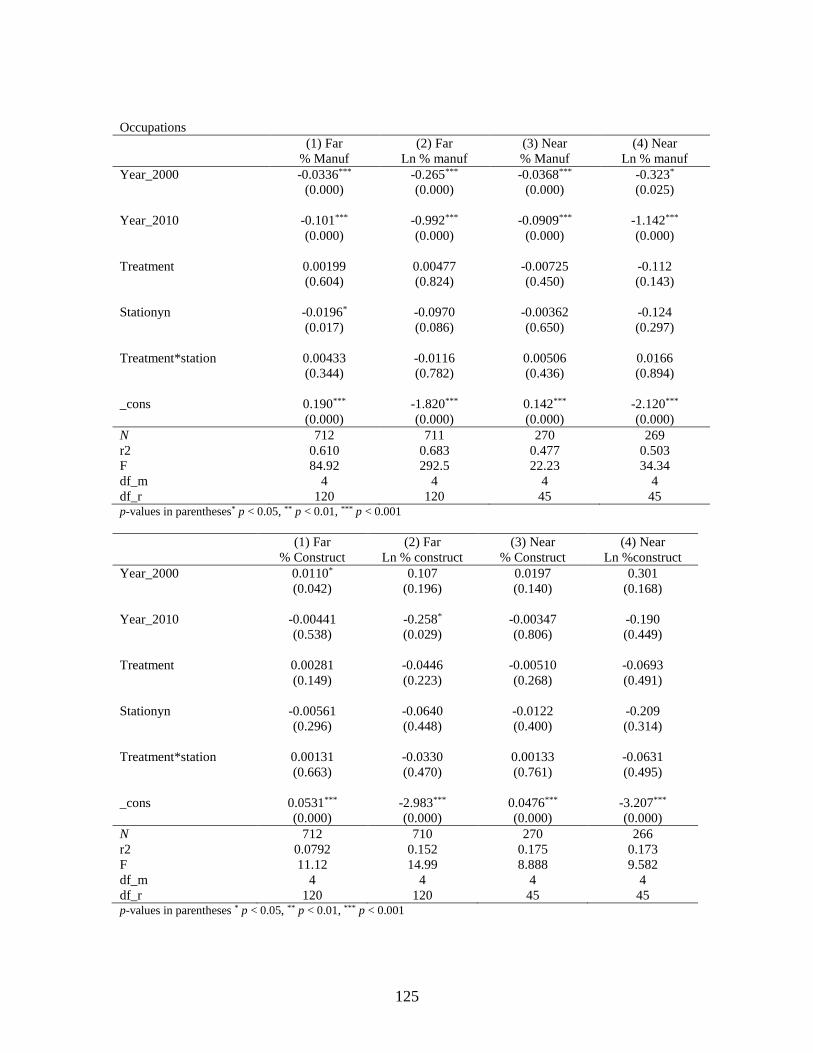
125
Occupations
(1) Far (2) Far (3) Near (4) Near
% Manuf Ln % manuf % Manuf Ln % manuf
Year_2000 -0.0336*** -0.265*** -0.0368*** -0.323*
(0.000) (0.000) (0.000) (0.025)
Year_2010 -0.101*** -0.992*** -0.0909*** -1.142***
(0.000) (0.000) (0.000) (0.000)
Treatment 0.00199 0.00477 -0.00725 -0.112
(0.604) (0.824) (0.450) (0.143)
Stationyn -0.0196* -0.0970 -0.00362 -0.124
(0.017) (0.086) (0.650) (0.297)
Treatment*station 0.00433 -0.0116 0.00506 0.0166
(0.344) (0.782) (0.436) (0.894)
_cons 0.190*** -1.820*** 0.142*** -2.120***
(0.000) (0.000) (0.000) (0.000)
N 712 711 270 269
r2 0.610 0.683 0.477 0.503
F 84.92 292.5 22.23 34.34
df_m 4 4 4 4
df_r 120 120 45 45 p-values in parentheses* p < 0.05, ** p < 0.01, *** p < 0.001
(1) Far (2) Far (3) Near (4) Near
% Construct Ln % construct % Construct Ln %construct
Year_2000 0.0110* 0.107 0.0197 0.301
(0.042) (0.196) (0.140) (0.168)
Year_2010 -0.00441 -0.258* -0.00347 -0.190
(0.538) (0.029) (0.806) (0.449)
Treatment 0.00281 -0.0446 -0.00510 -0.0693
(0.149) (0.223) (0.268) (0.491)
Stationyn -0.00561 -0.0640 -0.0122 -0.209
(0.296) (0.448) (0.400) (0.314)
Treatment*station 0.00131 -0.0330 0.00133 -0.0631
(0.663) (0.470) (0.761) (0.495)
_cons 0.0531*** -2.983*** 0.0476*** -3.207***
(0.000) (0.000) (0.000) (0.000)
N 712 710 270 266
r2 0.0792 0.152 0.175 0.173
F 11.12 14.99 8.888 9.582
df_m 4 4 4 4
df_r 120 120 45 45 p-values in parentheses * p < 0.05, ** p < 0.01, *** p < 0.001

126
(1) Far (2) Far (3) Near (4) Near
% Transpo Ln % transpo % Transpo Ln % transpo
Year_2000 0.00540 0.0564 -0.00885 -0.154
(0.080) (0.382) (0.080) (0.394)
Year_2010 0.0396*** 0.576*** 0.00518 0.115
(0.000) (0.000) (0.450) (0.528)
Treatment 0.000331 -0.0569 0.00456 0.0424
(0.845) (0.067) (0.095) (0.463)
Stationyn -0.0223*** -0.365*** -0.00423 -0.190
(0.000) (0.000) (0.459) (0.324)
Treatment*station -0.00261 -0.0575 -0.00519 -0.210*
(0.303) (0.232) (0.235) (0.044)
_cons 0.0512*** -3.068*** 0.0458*** -3.126***
(0.000) (0.000) (0.000) (0.000)
N 712 706 270 267
r2 0.258 0.187 0.132 0.122
F 18.64 24.59 9.494 8.684
df_m 4 4 4 4
df_r 120 120 45 45 p-values in parentheses * p < 0.05, ** p < 0.01, *** p < 0.001
(1) Far (2) Far (3) Near (4) Near
% Fin Ln %fin % Fin Ln % fin
Year_2000 -0.0133*** -0.148*** -0.00622 -0.0968
(0.000) (0.001) (0.541) (0.415)
Year_2010 0.00432 0.0950 0.00786 0.0857
(0.345) (0.122) (0.509) (0.573)
Treatment -0.00475** -0.107*** 0.0116 0.0552
(0.004) (0.000) (0.098) (0.490)
Stationyn 0.00961** 0.0726 0.00644 0.0505
(0.009) (0.166) (0.590) (0.727)
Treatment*station 0.00244 0.0460 -0.00385 -0.0249
(0.302) (0.166) (0.595) (0.813)
_cons 0.0731*** -2.712*** 0.0725*** -2.686***
(0.000) (0.000) (0.000) (0.000)
N 712 711 270 270
r2 0.178 0.173 0.0702 0.0391
F 26.79 30.34 2.323 1.485
df_m 4 4 4 4
df_r 120 120 45 45 p-values in parentheses * p < 0.05, ** p < 0.01, *** p < 0.001

127
(1) Far (2) Far (3) Near (4) Near
% Profes Ln % profess % Profess Ln % profess
Year_2000 0.0250*** 0.180** 0.0190* 0.169**
(0.000) (0.002) (0.026) (0.005)
Year_2010 0.0777*** 0.523*** 0.0853*** 0.561***
(0.000) (0.000) (0.000) (0.000)
Treatment 0.00280 0.0130 0.0211** 0.102*
(0.152) (0.490) (0.003) (0.049)
Stationyn -0.00186 0.00737 0.0129 0.0508
(0.772) (0.895) (0.138) (0.388)
Treatment*station -0.000285 -0.00557 -0.00809 -0.0642
(0.946) (0.860) (0.447) (0.389)
_cons 0.103*** -2.309*** 0.115*** -2.201***
(0.000) (0.000) (0.000) (0.000)
N 712 711 270 269
r2 0.454 0.445 0.409 0.489
F 62.00 98.41 24.78 36.05
df_m 4 4 4 4
df_r 120 120 45 45 p-values in parentheses* p < 0.05, ** p < 0.01, *** p < 0.001
(1) Far (2) Far (3) Near (4) Near
% Arts Ln % arts % Arts Ln % arts
Year_2000 0.120*** 2.132*** 0.152*** 2.272***
(0.000) (0.000) (0.000) (0.000)
Year_2010 0.0618*** 1.645*** 0.142*** 2.206***
(0.000) (0.000) (0.000) (0.000)
Treatment -0.00236 -0.0999* -0.00738* -0.0762
(0.113) (0.049) (0.022) (0.382)
Stationyn 0.0478*** 0.468*** 0.00320 0.0463
(0.000) (0.000) (0.853) (0.740)
Treatment*station 0.00426 0.0808 -0.000564 0.00212
(0.215) (0.154) (0.950) (0.983)
_cons 0.0190*** -4.240*** 0.0210*** -4.109***
(0.000) (0.000) (0.000) (0.000)
N 712 707 270 265
r2 0.718 0.861 0.703 0.875
F 379.3 548.5 155.2 167.0
df_m 4 4 4 4
df_r 120 120 45 45 p-values in parentheses p < 0.05, ** p < 0.01, *** p < 0.001
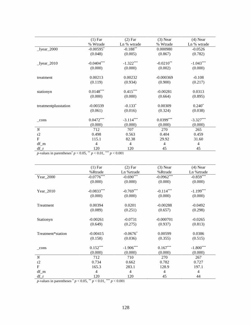
128
(1) Far (2) Far (3) Near (4) Near
% Wtrade Ln % wtrade % Wtrade Ln % wtrade
_Iyear_2000 -0.00595* -0.188** 0.000980 -0.0526
(0.048) (0.005) (0.867) (0.782)
_Iyear_2010 -0.0404*** -1.322*** -0.0210** -1.043***
(0.000) (0.000) (0.002) (0.000)
treatment 0.00213 0.00232 -0.000369 -0.108
(0.119) (0.934) (0.900) (0.217)
stationyn 0.0148*** 0.415*** -0.00281 0.0313
(0.000) (0.000) (0.664) (0.895)
treatmentplusstation -0.00339 -0.133* 0.00309 0.240*
(0.061) (0.016) (0.324) (0.038)
_cons 0.0472*** -3.114*** 0.0399*** -3.327***
(0.000) (0.000) (0.000) (0.000)
N 712 707 270 265
r2 0.498 0.563 0.404 0.459
F 115.1 82.38 29.92 31.60
df_m 4 4 4 4
df_r 120 120 45 45 p-values in parentheses* p < 0.05, ** p < 0.01, *** p < 0.001
(1) Far (2) Far (3) Near (4) Near
%Rtrade Ln %rtrade %Rtrade Ln %rtrade
Year_2000 -0.0776*** -0.690*** -0.0962*** -0.859***
(0.000) (0.000) (0.000) (0.000)
Year_2010 -0.0833*** -0.769*** -0.114*** -1.199***
(0.000) (0.000) (0.000) (0.000)
Treatment 0.00394 0.0201 -0.00288 -0.0492
(0.089) (0.251) (0.657) (0.298)
Stationyn -0.00261 -0.0731 -0.000701 -0.0265
(0.649) (0.275) (0.937) (0.813)
Treatment*station -0.00415 -0.0676* 0.00599 0.0386
(0.158) (0.036) (0.355) (0.515)
_cons 0.152*** -1.906*** 0.167*** -1.800***
(0.000) (0.000) (0.000) (0.000)
N 712 710 270 267
r2 0.734 0.662 0.782 0.727
F 165.3 283.1 128.9 197.1
df_m 4 4 4 4
df_r 120 120 45 44 p-values in parentheses * p < 0.05, ** p < 0.01, *** p < 0.001

129
(1) Far (2) Far (3) Near (4) Near
% Ehss Ln % ehss % Ehss Ln % ehss
Year_2000 -0.0384*** -0.376*** -0.0182 -0.167
(0.000) (0.000) (0.342) (0.278)
Year_2010 0.127*** 0.753*** 0.0895** 0.463*
(0.000) (0.000) (0.001) (0.011)
Treatment -0.00101 -0.0255 -0.0114 -0.122*
(0.715) (0.255) (0.121) (0.038)
Stationyn -0.0256* -0.200* -0.00357 0.0215
(0.030) (0.017) (0.883) (0.902)
Treatment*station -0.00344 -0.00850 0.00136 0.0594
(0.452) (0.797) (0.874) (0.353)
_cons 0.143*** -1.995*** 0.146*** -1.986***
(0.000) (0.000) (0.000) (0.000)
N 712 709 270 267
r2 0.703 0.709 0.467 0.429
F 128.4 173.8 34.08 50.12
df_m 4 4 4 4
df_r 120 120 45 44 p-values in parentheses * p < 0.05, ** p < 0.01, *** p < 0.001

130
Random Effects Regression Results
(1) (2) (3)
Popdensitysqmi Popdensitysqmi Popdensitysqmi
Near station 297.2
(0.501)
335.7
(0.364)
-4.768
(0.988)
Years 0
(.)
28.25**
(0.008)
28.43**
(0.008)
Station built
230.6
(0.332)
9.875
(0.972)
Treatment*station
-179.3
(0.523)
181.1
(0.556)
Near
1023.1
(0.426)
Near*station
845.3
(0.138)
Treatment*near
1360.2
(0.238)
Treatment*station*near
-1423.4*
(0.033)
_cons 7397.6***
(0.000)
7424.3***
(0.000)
7125.4***
(0.000)
N 326 977 977
R2
within
between
overall
0.0030
0.0010
0.0004
0.0107
0.0183
0.0031
0.0151
0.0162
0.0159
p-values in parentheses * p < 0.05, ** p < 0.01, *** p < 0.001
Model 1:
There is no difference in the share of population per square mile whether at the area nearer to the stations or
farther from them.
Model 2:
Being in the treatment areas when the stations were built does not have an effect on population density.
Model 3:
Being both in the treatment areas when the stations were built brought about a 1,242 units decline in
population per square mile in areas closer to the CBD.

131
(1) (2) (3)
Ln popdensitysqmi Ln popdensitysqmi Ln popdensitysqmi
Near station 0.183**
(0.004)
0.184**
(0.002)
0.165**
(0.005)
Years 0
(.)
0.00782***
(0.000)
0.00788***
(0.000)
Station built
0.0275
(0.494)
0.00183
(0.969)
Treatment*station
-0.0785
(0.068)
-0.0410
(0.365)
Near
0.326
(0.082)
Near*station
0.0913
(0.329)
Treatment*near
0.0767
(0.664)
Treatment*station*near
-0.140
(0.228)
_cons 8.399***
(0.000)
8.406***
(0.000)
8.316***
(0.000)
N 324 969 969
R2
within
between
overall
0.0563
0.0374
0.0050
0.0554
0.0006
0.0062
0.0568
0.0265
0.0292
p-values in parentheses* p < 0.05, ** p < 0.01, *** p < 0.001
Model 1:
The areas nearer to the stations have 18.3 percent higher population density than those areas farther from
them..
Model 2:
Being in the treatment areas when the stations were built does not have an effect on population density.
Model 3:
Being both in the treatment areas that are near the city center when the stations were built does not have an
effect on the number of people per area.

132
(1) (2) (3)
% white % white % white
Near station -0.00609
(0.622)
-0.00594
(0.608)
-0.0186
(0.087)
Years 0
(.)
-0.000518
(0.529)
-0.000543
(0.511)
Station built -0.0246*
(0.012)
-0.0536***
(0.000)
Treatment*station 0.000631
(0.941)
0.0122
(0.150)
Near -0.0833
(0.052)
Near*station 0.109***
(0.000)
Treatment*near 0.0505
(0.125)
Treatment*station*near -0.0462*
(0.035)
_cons 0.564***
(0.000)
0.555***
(0.000)
0.577***
(0.000)
N 327 982 982
R2
within
between
overall
0.0014
0.0013
0.0002
0.0214
0.1066
0.0171
0.0594
0.0256
0.0199
p-values in parentheses * p < 0.05, ** p < 0.01, *** p < 0.001
Model 1:
There is no difference in the share of white population whether at the area nearer to the stations or farther
from them.
Model 2:
Being in the treatment areas when the stations were built does not have an effect on the share of white
population.
Model 3:
Being both in the treatment areas that are near the city center when the stations were built brought about a
4.6 percentage points decline in the share of white population (compared to being in areas that are far from
the CBD).

133
(1) (2) (3)
Ln % white Ln % white Ln % white
Near station -0.0747
(0.074)
-0.0604
(0.091)
-0.0767*
(0.019)
Years 0
(.)
0.00554*
(0.026)
0.00551*
(0.027)
Station built
-0.0912***
(0.000)
-0.139***
(0.000)
Treatment*station
0.00820
(0.726)
0.0212
(0.392)
Near
-0.111
(0.357)
Near*station
0.178**
(0.001)
Treatment*near
0.0659
(0.536)
Treatment*station*near
-0.0528
(0.357)
_cons -0.778***
(0.000)
-0.799***
(0.000)
-0.770***
(0.000)
N 327 982 982
R2
within
between
overall
0.0192
0.0010
0.0020
0.0106
0.0958
0.0202
0.0219
0.0587
0.0181
p-values in parentheses * p < 0.05, ** p < 0.01, *** p < 0.001
Model 1:
There is no difference in the share of white population whether at the area nearer to the stations or farther
from them.
Model 2:
Being in the treatment areas when the stations were built does not have an effect on the share of white
population.
Model 3:
Being both in the treatment areas when the stations were built does not have a difference on the share of
white population whether in the areas close to the CBD or far from them..

134
(1) (2) (3)
% black % black % black
Near station 0.00623
(0.579)
0.00174
(0.866)
0.00713
(0.465)
Years 0
(.)
-0.00280***
(0.000)
-0.00279***
(0.000)
Station built
0.0215**
(0.004)
0.0351***
(0.000)
Treatment*station
0.00238
(0.751)
-0.00497
(0.500)
Near
0.0923
(0.057)
Near*station
-0.0507**
(0.005)
Treatment*near
-0.0217
(0.469)
Treatment*station*near
0.0281
(0.159)
_cons 0.248***
(0.000)
0.250***
(0.000)
0.225***
(0.000)
N 327 982 982
R2
within
between
overall
0.0018
0.0020
0.0002
0.0334
0.1007
0.0153
0.0450
0.0220
0.0241
p-values in parentheses * p < 0.05, ** p < 0.01, *** p < 0.001
Model 1:
There is no difference in the share of black population either in the area closer to the stations or farther
from them.
Model 2:
Being in the treatment areas when the stations were built does not have an effect on the share of black
population.
Model 3:
Being both in the treatment areas near the city center when the stations were built does not account for a
difference in the share of black population (compared to being in areas far from the CBD).

135
(1) (2) (3)
Ln % black Ln % black Ln % black
Near station 0.00730
(0.910)
-0.000513
(0.993)
0.00170
(0.977)
Years 0
(.)
-0.00845*
(0.012)
-0.00845*
(0.013)
Station built 0.118*
(0.022)
0.198***
(0.000)
Treatment*station -0.0285
(0.527)
-0.0884
(0.067)
Near 0.524*
(0.025)
Near*station -0.287**
(0.004)
Treatment*near -0.0114
(0.942)
Treatment*station*near 0.210
(0.055)
_cons -2.167***
(0.000)
-2.155***
(0.000)
-2.297***
(0.000)
N 327 980 980
R2
within
between
overall
0.0000
0.0101
0.0001
0.0049
0.0443
0.0113
0.0156
0.0271
0.0252
p-values in parentheses * p < 0.05, ** p < 0.01, *** p < 0.001
Model 1:
There is no difference in the share of black population either in the area nearer to the stations or farther
from them.
Model 2:
Being in the treatment areas when the stations were built does not have an effect on the share of black
population.
Model 3:
Being both in the treatment areas near the city center when the stations were built does not account for a
difference in the share of black population (compared to being in areas far from the CBD).

136
(1) (2) (3)
% Asian % Asian % Asian
Near station -0.00778
(0.113)
-0.00188
(0.719)
-0.000167
(0.979)
Years 0
(.)
0.00179***
(0.000)
0.00178***
(0.000)
Station built -0.00471
(0.303)
-0.00261
(0.606)
Treatment*station 0.00472
(0.369)
0.000949
(0.868)
Near -0.0166
(0.286)
Near*station -0.00724
(0.302)
Treatment*near -0.00674
(0.552)
Treatment*station*near 0.0138
(0.265)
_cons 0.0658***
(0.000)
0.0646***
(0.000)
0.0692***
(0.000)
N 327 982 982
R2
within
between
overall
0.0155
0.0000
0.0021
0.0865
0.0010
0.0167
0.0876
0.0089
0.0241
p-values in parentheses* p < 0.05, ** p < 0.01, *** p < 0.001
Model 1:
There is no difference in the share of Asian population either in areas nearer to the stations or farther from
them.
Model 2:
Being in the treatment areas when the stations were built does not influence the share of Asian population.
Model 3:
Being both in treatment areas that are near the CBD when the stations were built does not have an effect in
the share of Asian population (compared to being in areas far from the CBD).

137
(1) (2) (3)
Ln % Asian Ln % Asian Ln % Asian
Near station -0.119
(0.071)
-0.0668
(0.320)
-0.110
(0.127)
Years 0
(.)
0.0230***
(0.000)
0.0228***
(0.000)
Station built -0.0965
(0.208)
-0.132
(0.087)
Treatment*station 0.00733
(0.921)
-0.0373
(0.665)
Near -0.300
(0.165)
Near*station 0.151
(0.172)
Treatment*near 0.171
(0.320)
Treatment*station*near 0.139
(0.408)
_cons -3.460***
(0.000)
-3.459***
(0.000)
-3.379***
(0.000)
N 326 967 967
R2
within
between
overall
0.0200
0.0001
0.0018
0.0551
0.0329
0.0143
0.0679
0.0097
0.0165
p-values in parentheses * p < 0.05, ** p < 0.01, *** p < 0.001
Model 1:
There is no difference in the share of Asian population either in areas nearer to the stations or farther from
them.
Model 2:
Being in the treatment areas when the stations were built does not have an effect on the share of Asian
population.
Model 3:
Being both in treatment areas that are near the CBD when the stations were built does not have an effect in
the share of Asian population (compared to being in areas far from the CBD).

138
(1) (2) (3)
% otherrace % otherrace % otherrace
Near station 0.00691
(1.05)
0.00585
(0.89)
0.0113
(1.89)
Years 0
(.)
0.00170***
(3.52)
0.00170***
(3.51)
Station built 0.00455
(0.60)
0.0180*
(2.19)
Treatment*station -0.00758
(-1.31)
-0.00798
(-1.41)
Near 0.00223
(0.08)
Near*station -0.0498***
(-3.43)
Treatment*near -0.0218
(-1.11)
Treatment*station*near 0.00395
(0.25)
_cons 0.116***
(10.08)
0.124***
(10.25)
0.124***
(8.82)
N 327 982 982
R2
within
between
overall
0.0069
0.0002
0.0004
0.0563
0.0551
0.0098
0.0898
0.0142
0.0209 t statistics in parentheses * p < 0.05, ** p < 0.01, *** p < 0.001
Model 1:
There is no difference in the share of other race either in areas nearer to the stations or farther from them.
Model 2:
Being in the treatment areas when the stations were built does not have an effect on the share of other race.
Model 3:
Being both in treatment areas that are near the CBD when the stations were built does not have an effect in
the share of other race (compared to being in stations far from the CBD).

139
(1) (2) (3)
Ln % otherrace Ln % otherrace Ln % otherrace
Near station -0.0810
(0.201)
-0.0923
(0.116)
-0.0777
(0.176)
Years 0
(.)
0.0484***
(0.000)
0.0484***
(0.000)
Station built -0.111
(0.159)
-0.0241
(0.780)
Treatment*station -0.00913
(0.873)
-0.00438
(0.943)
Near -0.0702
(0.802)
Near*station -0.315*
(0.020)
Treatment*near -0.0609
(0.716)
Treatment*station*near -0.0101
(0.945)
_cons -3.135***
(0.000)
-3.087***
(0.000)
-3.065***
(0.000)
N 324 969 969
R2
within
between
overall
0.0105
0.0012
0.0004
0.2540
0.0138
0.0573
0.2639
0.0135
0.0640
p-values in parentheses * p < 0.05, ** p < 0.01, *** p < 0.001
Model 1:
There is no difference in the share of other race either in areas closer to the stations or farther from them.
Model 2:
Being in the treatment areas when the stations were built does not have an effect on the share of other race.
Model 3:
Being both in treatment areas that are near the CBD when the stations were built does not have an effect in
the share of other race (compared to being in stations far from the CBD).

140
(1) (2) (3)
% Allotherrace % Allotherrace % Allotherrace
Near station 0.00609
(0.622)
0.00594
(0.608)
0.0186
(0.087)
Years 0
(.)
0.000518
(0.529)
0.000543
(0.511)
Station built 0.0246*
(0.012)
0.0536***
(0.000)
Treatment*station -0.000631
(0.941)
-0.0122
(0.150)
Near 0.0833
(0.052)
Near*station -0.109***
(0.000)
Treatment*near -0.0505
(0.125)
Treatment*station*near 0.0462*
(0.035)
_cons 0.436***
(0.000)
0.445***
(0.000)
0.423***
(0.000)
N 327 982 982
R2
within
between
overall
0.0014
0.0013
0.0002
0.0214
0.1066
0.0171
0.0594
0.0256
0.0199
p-values in parentheses * p < 0.05, ** p < 0.01, *** p < 0.001
Model 1:
There is no difference in the share of all non-white population (or all other race) either in areas nearer to the
stations or farther from them.
Model 2:
Being in the treatment areas when the stations were built does not have an effect on the share of all non-
white population.
Model 3:
Being both in treatment areas when the stations were built accounts to a 3.4 percentage points increase in
the share of all non-white population in areas that are near the CBD.
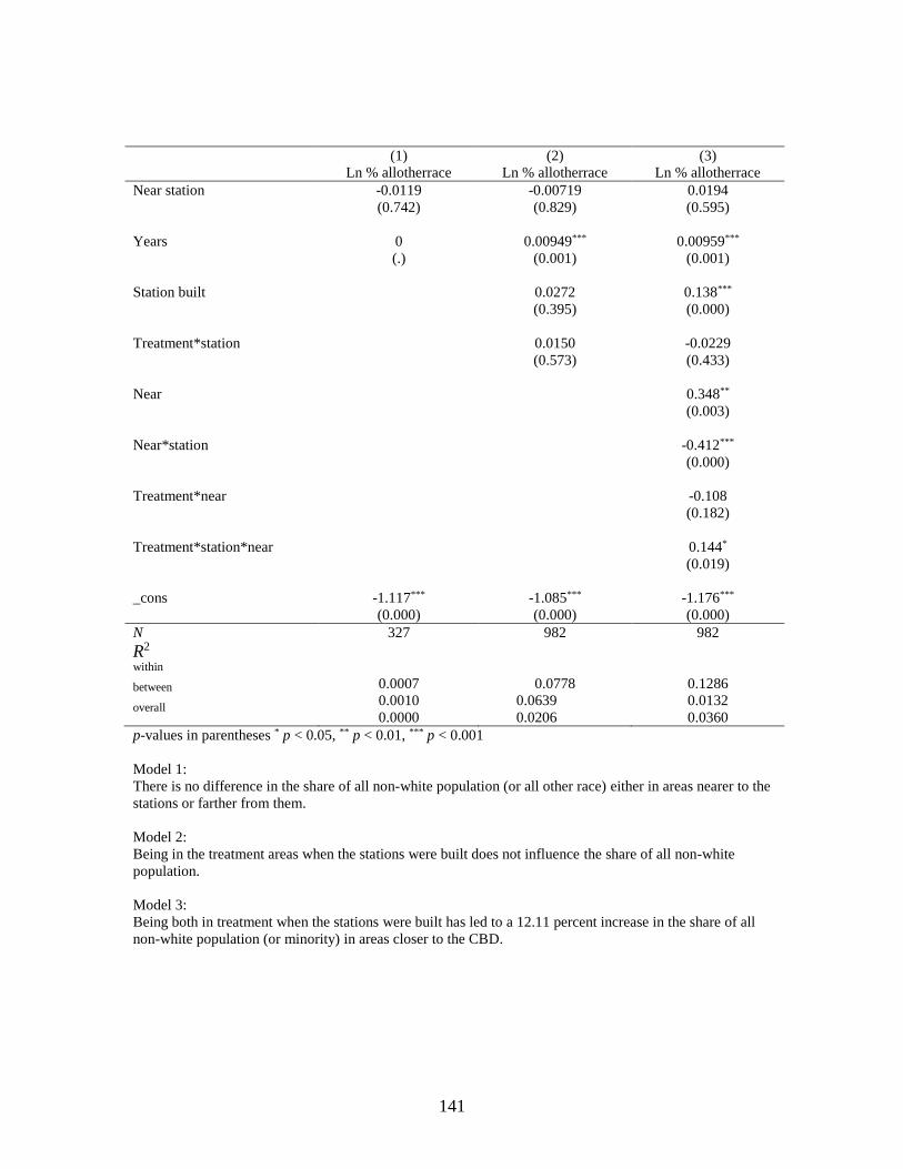
141
(1) (2) (3)
Ln % allotherrace Ln % allotherrace Ln % allotherrace
Near station -0.0119
(0.742)
-0.00719
(0.829)
0.0194
(0.595)
Years 0
(.)
0.00949***
(0.001)
0.00959***
(0.001)
Station built 0.0272
(0.395)
0.138***
(0.000)
Treatment*station 0.0150
(0.573)
-0.0229
(0.433)
Near 0.348**
(0.003)
Near*station -0.412***
(0.000)
Treatment*near -0.108
(0.182)
Treatment*station*near 0.144*
(0.019)
_cons -1.117***
(0.000)
-1.085***
(0.000)
-1.176***
(0.000)
N 327 982 982
R2
within
between
overall
0.0007
0.0010
0.0000
0.0778
0.0639
0.0206
0.1286
0.0132
0.0360
p-values in parentheses * p < 0.05, ** p < 0.01, *** p < 0.001
Model 1:
There is no difference in the share of all non-white population (or all other race) either in areas nearer to the
stations or farther from them.
Model 2:
Being in the treatment areas when the stations were built does not influence the share of all non-white
population.
Model 3:
Being both in treatment when the stations were built has led to a 12.11 percent increase in the share of all
non-white population (or minority) in areas closer to the CBD.

142
(1) (2) (3)
% with Hispanic
origin
% with Hispanic
origin
% with Hispanic
origin
Near station -0.000951
(0.924)
-0.00342
(0.752)
0.00677
(0.503)
Years 0
(.)
0.00443***
(0.000)
0.00442***
(0.000)
Station built -0.000206
(0.981)
0.0261**
(0.010)
Treatment*station -0.00313
(0.713)
-0.00716
(0.394)
Near 0.00559
(0.897)
Near*station -0.0968***
(0.000)
Treatment*near -0.0410
(0.192)
Treatment*station*near 0.0183
(0.421)
_cons 0.207***
(0.000)
0.218***
(0.000)
0.217***
(0.000)
N 327 985 985
R2
within
between
overall
0.0000
0.0003
0.0000
0.1530
0.0379
0.0220
0.2009
0.0159
0.0353
p-values in parentheses * p < 0.05, ** p < 0.01, *** p < 0.001
Model 1:
There is no difference in the share of all people with Hispanic roots either in areas closer to the station or
farther from them.
Model 2:
Being in the treatment areas when the stations were built does not influence the share of all non-white
population.
Model 3:
Being both in treatment areas when the stations were built does not have an effect on the share of the
population with Hispanic roots whether in areas that are near or far from the CBD.

143
(1) (2) (3)
Ln % with
Hispanic origin
Ln % with
Hispanic origin
Ln % with
Hispanic origin
Near station -0.0362
(0.489)
-0.0595
(0.221)
-0.0528
(0.247)
Years 0
(.)
0.0321***
(0.000)
0.0320***
(0.000)
Station built -0.0427
(0.300)
0.0695
(0.154)
Treatment*station 0.0410
(0.266)
0.0338
(0.411)
near -0.0680
(0.780)
Near*station -0.400***
(0.000)
Treatment*near -0.0319
(0.824)
Treatment*station*near 0.0292
(0.748)
_cons -2.327***
(0.000)
-2.269***
(0.000)
-2.247***
(0.000)
N 326 981 981
R2
within
between
overall
0.0031
0.0009
0.0001
0.2929
0.0256
0.0390
0.3233
0.0146
0.0508
p-values in parentheses * p < 0.05, ** p < 0.01, *** p < 0.001
Model 1:
There is no difference in the share of all people with Hispanic roots either in areas closer to the station or
farther from them.
Model 2:
Being in the treatment areas when the stations were built does not have an effect on the share of all non-
white population.
Model 3:
Being both in treatment areas when the stations were built does not have an effect in the share of people
with Hispanic roots whether in areas near or far from the CBD.

144
(1) (2) (3)
Median hh
income
Median hh
income
Median hh
income
Near station -14840.2***
(0.000)
-15179.4***
(0.000)
-18232.9***
(0.000)
Years 0
(.)
-223.9***
(0.000)
-233.0***
(0.000)
Station built 3330.1**
(0.004)
2531.2*
(0.047)
Treatment*station -3817.2***
(0.000)
-3011.7**
(0.006)
Near -12992.6***
(0.000)
Near*station 4295.4***
(0.001)
Treatment*near 12017.0***
(0.000)
Treatment*station*near -4235.5*
(0.035)
_cons 33621.2***
(0.000)
34490.1***
(0.000)
37913.3***
(0.000)
N 329 987 987
R2
within
between
overall
0.5686
0.0011
0.2628
0.5157
0.0075
0.3174
0.5482
0.0465
0.3668
p-values in parentheses* p < 0.05, ** p < 0.01, *** p < 0.001
Model 1:
To be in areas nearer to the stations result to a $14,840 decline in median household income.
Model 2:
Being in the treatment areas when the stations were built cause a $3,817.2 decline in the median household
income.
Model 3:
Being both in treatment areas when the stations were built lead to a $7247 decline in the share of median
household income for the block groups that are closer to the CBD. On the other hand, the block groups that
are far from the CBD experience a $3,011 decline in median household income.

145
(1) (2) (3)
Ln median hh income Ln median hh income Ln median hh income
Near station -0.599***
(0.000)
-0.601***
(0.000)
-0.698***
(0.000)
Years 0
(.)
-0.0143***
(0.000)
-0.0147***
(0.000)
Station built 0.191***
(0.000)
0.159**
(0.001)
Treatment*station -0.254***
(0.000)
-0.196***
(0.000)
Near -0.459***
(0.000)
Near*station 0.165**
(0.003)
Treatment*near 0.380**
(0.002)
Treatment*station*near -0.247*
(0.034)
_cons 10.33***
(0.000)
10.36***
(0.000)
10.48***
(0.000)
N 326 980 980
R2
within
between
overall
0.5472
0.0495
0.2467
0.5194
0.0017
0.3329
0.5315
0.0656
0.3697
p-values in parentheses * p < 0.05, ** p < 0.01, *** p < 0.001
R2 of the log-transformed variable is higher.
Model 1:
To be in areas nearer to the stations results to a 59.9 percent decline in median household income.
Model 2:
Being in the treatment areas when the stations were built causes a 25.4 percent decline the median
household income.
Model 3:
Being both in treatment areas that are near the CBD when the stations were built lead to a 44.3 percent
decline in the share of median household income. On the other hand, the areas that are far from the CBD
experience a 19.6 percent decline in median household income.
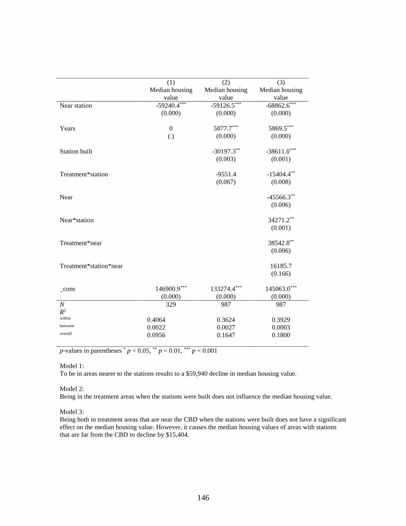
146
(1) (2) (3)
Median housing
value
Median housing
value
Median housing
value
Near station -59240.4***
(0.000)
-59126.5***
(0.000)
-68862.6***
(0.000)
Years 0
(.)
5877.7***
(0.000)
5869.5***
(0.000)
Station built -30197.3**
(0.003)
-38611.0***
(0.001)
Treatment*station -9551.4
(0.067)
-15404.4**
(0.008)
Near -45566.3**
(0.006)
Near*station 34271.2**
(0.001)
Treatment*near 38542.8**
(0.006)
Treatment*station*near 16185.7
(0.166)
_cons 146900.9***
(0.000)
133274.4***
(0.000)
145063.0***
(0.000)
N 329 987 987
R2
within
between
overall
0.4064
0.0022
0.0956
0.3624
0.0027
0.1647
0.3929
0.0003
0.1800
p-values in parentheses * p < 0.05, ** p < 0.01, *** p < 0.001
Model 1:
To be in areas nearer to the stations results to a $59,940 decline in median housing value.
Model 2:
Being in the treatment areas when the stations were built does not influence the median housing value.
Model 3:
Being both in treatment areas that are near the CBD when the stations were built does not have a significant
effect on the median housing value. However, it causes the median housing values of areas with stations
that are far from the CBD to decline by $15,404.

147
(1) (2) (3)
Ln median
housing value
Ln median
housing value
Ln median
housing value
Near station -0.652***
(0.000)
-0.636***
(0.000)
-0.684***
(0.000)
Years 0
(.)
0.0439***
(0.000)
0.0438***
(0.000)
Station built -0.338***
(0.000)
-0.441***
(0.000)
Treatment*station 0.0960
(0.068)
0.0725
(0.147)
Near -0.406***
(0.001)
Near*station 0.399***
(0.000)
Treatment*near 0.202
(0.261)
Treatment*station*near 0.0546
(0.714)
_cons 11.68***
(0.000)
11.59***
(0.000)
11.69***
(0.000)
N 324 976 976
R2
within
between
overall
0.4154
0.0002
0.1268
0.3816
0.0026
0.1751
0.4090
0.0001
0.1880
p-values in parentheses * p < 0.05, ** p < 0.01, *** p < 0.001
Model 1:
To be in areas nearer to the stations results to a 65% decline in median housing value.
Model 2:
Being in the treatment areas when the stations were built does not influence the median housing value.
Model 3:
Being both in treatment areas when the stations were built does not have a significant effect on the median
housing value whether in areas near or far from the CBD.

148
(1) (2) (3)
% pubtranspo % pubtranspo % pubtranspo
Near station 0.0227***
(0.000)
0.0153***
(0.000)
0.0109***
(0.001)
Years 0
(.)
-0.000552
(0.193)
-0.000543
(0.195)
Station built 0.0127
(0.058)
0.0164**
(0.005)
Treatment*station 0.00502
(0.265)
0.0125**
(0.001)
Near 0.109***
(0.000)
Near*station -0.0136
(0.166)
Treatment*near 0.0170
(0.216)
Treatment*station*near -0.0275*
(0.036)
_cons 0.121***
(0.000)
0.123***
(0.000)
0.0932***
(0.000)
N 326 981 981
R2
within
between
overall
0.1310
0.0023
0.0111
0.0493
0.0365
0.0185
0.0719
0.2202
0.1955
p-values in parentheses * p < 0.05, ** p < 0.01, *** p < 0.001
Model 1:
To be in areas closer to the stations results to a 2.27 percentage points increase in the share of workers
taking public transportation.
Model 2:
Being in the treatment areas when the stations were built does not influence the share of public
transportation.
Model 3:
Being both in treatment areas when the stations were built leads to a 1.5 percentage points decline in the
share of public transportation in areas closer to the CBD. Areas that are far from the CBD, on the other
hand, experience a 1.25 increase in the share of public transportation.

149
(1) (2) (3)
Ln % publictranspo Ln % publictranspo Ln % publictranspo
Near station 0.0690
(0.160)
0.0498
(0.255)
0.0139
(0.792)
Years 0
(.)
-0.00415
(0.277)
-0.00399
(0.290)
Station built 0.213***
(0.000)
0.297***
(0.000)
Treatment*station 0.0968
(0.062)
0.158*
(0.015)
Near 1.097***
(0.000)
Near*station -0.315***
(0.000)
Treatment*near 0.138
(0.121)
Treatment*station*near -0.222*
(0.018)
_cons -2.524***
(0.000)
-2.521***
(0.000)
-2.820***
(0.000)
N 324 974 974
R2
within
between
overall
0.0099
0.0794
0.0024
0.0642
0.0315
0.0277
0.1125
0.2234
0.1965
p-values in parentheses * p < 0.05, ** p < 0.01, *** p < 0.001
Model 1:
There is no difference in the share of workers taking public station either in areas closer to the station or
farther from them.
Model 2:
Being in the treatment areas when the stations were built does not influence the share of public
transportation.
Model 3:
Being both in treatment areas when the stations were built leads to a 6.4 percent decline in the share of
public transportation in areas closer to the CBD. Areas that are far from the CBD, on the other hand,
experience a 15.8 increase in the share of public transportation.

150
(1) (2) (3)
% car % car % car
Near station -0.00555
(0.491)
-0.00789
(0.299)
-0.00377
(0.488)
Years 0
(.)
0.000833
(0.214)
0.000814
(0.216)
Station built 0.0100
(0.298)
-0.0123
(0.167)
Treatment*station -0.0308***
(0.000)
-0.0238***
(0.000)
Near -0.284***
(0.000)
Near*station 0.0808***
(0.000)
Treatment*near -0.0150
(0.557)
Treatment*station*near -0.0230
(0.290)
_cons 0.721***
(0.000)
0.733***
(0.000)
0.811***
(0.000)
N 326 981 981
R2
within
between
overall
0.0026
0.0091
0.0004
0.0506
0.0045
0.0089
0.1092
0.4560
0.4033
p-values in parentheses * p < 0.05, ** p < 0.01, *** p < 0.001
Model 1:
There is no difference in the share of workers who drive to work either in areas closer to the station or
farther from them.
Model 2:
Being in the treatment areas when the stations were built leads to a 30.8 percentage points decline in the
share of workers driving to work.
Model 3:
Being both in treatment areas when the stations were built does not affect the share of workers driving to
work in areas close to the CBD. In areas with stations that are far from the CBD, there is a 23.8 percentage
points decline in the share of workers driving to work.

151
(1) (2) (3)
Ln %car Ln % car Ln % car
Near station -0.00290
(0.884)
-0.00379
(0.844)
-0.00832
(0.311)
Years 0
(.)
0.00212
(0.063)
0.00206
(0.066)
Station built 0.0268
(0.147)
-0.0253
(0.097)
Treatment*station -0.0569***
(0.001)
-0.0316***
(0.000)
Near -0.528***
(0.000)
Near*station 0.192***
(0.000)
Treatment*near 0.0200
(0.781)
Treatment*station*near -0.0914
(0.138)
_cons -0.386***
(0.000)
-0.370***
(0.000)
-0.226***
(0.000)
N 326 981 981
R2
within
between
overall
0.0000
0.0089
0.0001
0.0420
0.0018
0.0080
0.1039
0.4316
0.3715
p-values in parentheses * p < 0.05, ** p < 0.01, *** p < 0.001
Model 1:
There is no difference in the share of workers who drive to work either in areas closer to the station or
farther from them.
Model 2:
Being in the treatment areas when the stations were built leads to a 5.69 percent decline in the share of
workers driving to work.
Model 3:
Being both in treatment areas when the stations were built does not affect the share of workers driving to
work in areas close to the CBD. In areas far from the CBD, there is a 3.16 percent decline in the share of
workers driving to work.
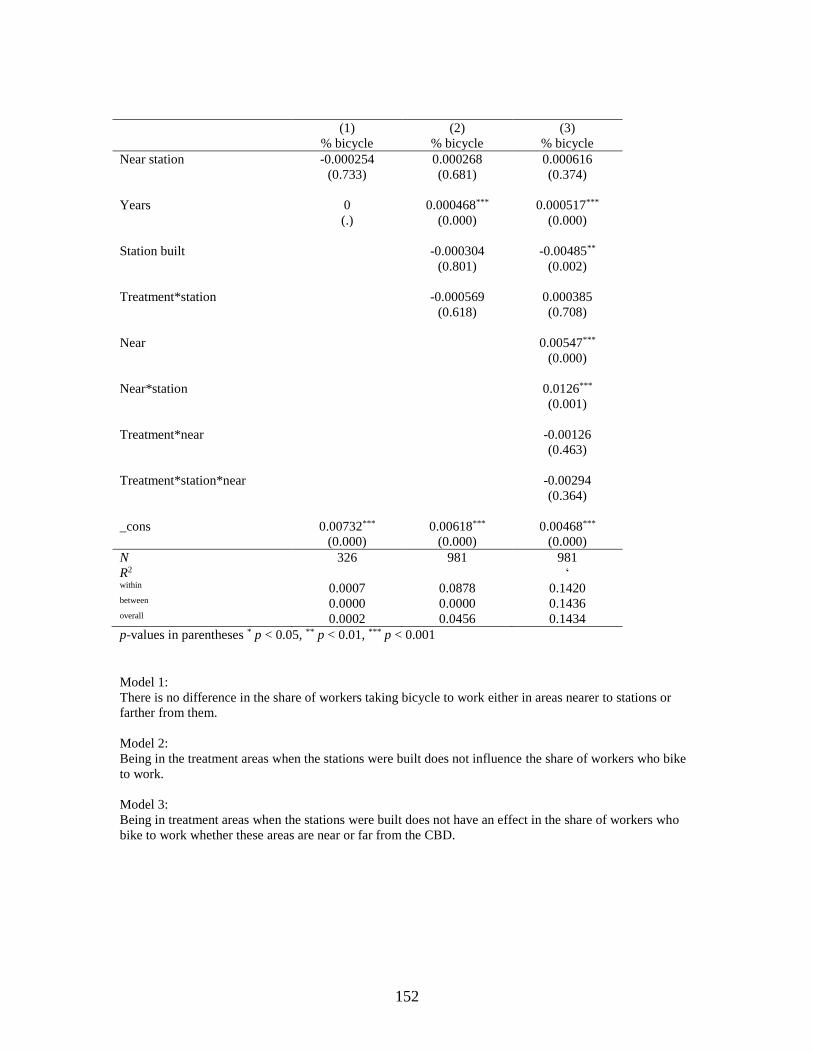
152
(1) (2) (3)
% bicycle % bicycle % bicycle
Near station -0.000254
(0.733)
0.000268
(0.681)
0.000616
(0.374)
Years 0
(.)
0.000468***
(0.000)
0.000517***
(0.000)
Station built -0.000304
(0.801)
-0.00485**
(0.002)
Treatment*station -0.000569
(0.618)
0.000385
(0.708)
Near 0.00547***
(0.000)
Near*station 0.0126***
(0.001)
Treatment*near -0.00126
(0.463)
Treatment*station*near -0.00294
(0.364)
_cons 0.00732***
(0.000)
0.00618***
(0.000)
0.00468***
(0.000)
N 326 981 981
R2
within
between
overall
0.0007
0.0000
0.0002
0.0878
0.0000
0.0456
‘
0.1420
0.1436
0.1434
p-values in parentheses * p < 0.05, ** p < 0.01, *** p < 0.001
Model 1:
There is no difference in the share of workers taking bicycle to work either in areas nearer to stations or
farther from them.
Model 2:
Being in the treatment areas when the stations were built does not influence the share of workers who bike
to work.
Model 3:
Being in treatment areas when the stations were built does not have an effect in the share of workers who
bike to work whether these areas are near or far from the CBD.

153
(1) (2) (3)
Ln % bicycle Ln % bicycle Ln % bicycle
Near station 0.105
(0.353)
0.0856
(0.422)
0.229
(0.070)
Years 0
(.)
0.0302***
(0.000)
0.0321***
(0.000)
Station built 0.0617
(0.680)
-0.0636
(0.702)
Treatment*station -0.153
(0.209)
-0.270
(0.073)
Near 0.923***
(0.000)
Near*station 0.278
(0.050)
Treatment*near -0.517*
(0.020)
Treatment*station*near 0.431
(0.073)
_cons -5.419***
(0.000)
-5.491***
(0.000)
-5.740***
(0.000)
N 274 816 816
R2
within
between
overall
0.0001
0.1325
0.0085
0.0727
0.0742
0.0380
0.0970
0.1750
0.1383
p-values in parentheses * p < 0.05, ** p < 0.01, *** p < 0.001
Model 1:
There is no difference in the share of workers taking bicycle to work either in areas nearer to the station or
farther from it.
Model 2:
Being in the treatment areas when the stations were built does not influence the share of workers who bike
to work.
Model 3:
Being in treatment areas when the stations were built does not have an effect in the share of workers who
bike to work whether these areas are near or far from the CBD.

154
(1) (2) (3)
% othertranspo % othertranspo % othertranspo
Near station -0.0178**
(0.007)
-0.00805
(0.173)
-0.00958*
(0.010)
Years 0
(.)
-0.00147***
(0.000)
-0.00145***
(0.000)
Station built
-0.0224***
(0.000)
-0.00272
(0.549)
Treatment*station
0.0288***
(0.000)
0.0176***
(0.000)
Near
0.151***
(0.000)
Near*station
-0.0715***
(0.000)
Treatment*near
0.00499
(0.807)
Treatment*station*near
0.0385**
(0.007)
_cons 0.122***
(0.000)
0.111***
(0.000)
0.0698***
(0.000)
N 326 981 981
R2
within
between
overall
0.0455
0.0080
0.0049
0.1302
0.0040
0.0298
0.2106
0.4096
0.3564
p-values in parentheses * p < 0.05, ** p < 0.01, *** p < 0.001
Model 1:
Being in near the stations leads to a decline of 1.78 percentage points in the share of other modes of
transportation.
Model 2:
Being in the treatment areas when the stations were built leads to a 2.88 percentage points increase the
share of workers taking other transportation option.
Model 3:
Compared to areas far from the CBD, being in treatment areas that are near the CBD when the stations
were built causes a 5.61 percentage points increase in the share of workers taking other transportation
modes. Being far from the CBD, on the other hand, causes a 1.76 percentage points increase in the share of
workers taking other transportation option.

155
(1) (2) (3)
Ln %othertranspo Ln % othertranspo Ln % othertranspo
Near station -0.239***
(0.000)
-0.147**
(0.003)
-0.181***
(0.000)
Years 0
(.)
-0.0189***
(0.000)
-0.0182***
(0.000)
Station built -0.132
(0.060)
-0.106
(0.131)
Treatment*station 0.237***
(0.000)
0.197*
(0.010)
Near 1.144***
(0.000)
Near*station -0.132
(0.097)
Treatment*near 0.123
(0.347)
Treatment*station*near 0.131
(0.308)
_cons -2.513***
(0.000)
-2.620***
(0.000)
-2.936***
(0.000)
N 326 977 977
R2
within
between
overall
0.1286
0.0000
0.0159
0.1079
0.0046
0.0309
0.1172
0.3985
0.3203
p-values in parentheses * p < 0.05, ** p < 0.01, *** p < 0.001
Model 1:
Being in near the stations leads to a 23.9 percent decline in the share of other modes of transportation.
Model 2:
Being in the treatment areas when the stations were built leads to a 23.7percent increase the share of
workers taking other transportation option.
Model 3:
Being in treatment areas that are near the CBD when the stations were built does not affect the share of
workers taking other transportation options. Being in areas far from the CBD, on the other hand, cause a
19.7 percent increase in the share of workers taking other transportation option.
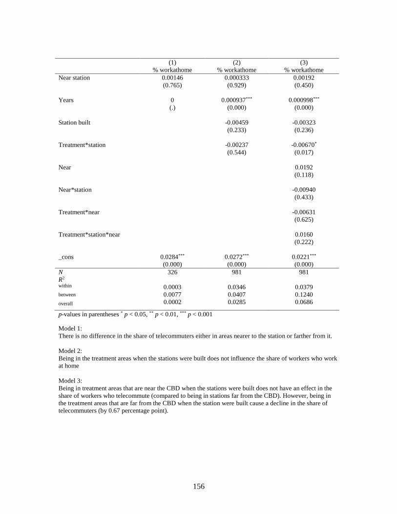
156
(1) (2) (3)
% workathome % workathome % workathome
Near station 0.00146
(0.765)
0.000333
(0.929)
0.00192
(0.450)
Years 0
(.)
0.000937***
(0.000)
0.000998***
(0.000)
Station built -0.00459
(0.233)
-0.00323
(0.236)
Treatment*station -0.00237
(0.544)
-0.00670*
(0.017)
Near 0.0192
(0.118)
Near*station -0.00940
(0.433)
Treatment*near -0.00631
(0.625)
Treatment*station*near 0.0160
(0.222)
_cons 0.0284***
(0.000)
0.0272***
(0.000)
0.0221***
(0.000)
N 326 981 981
R2
within
between
overall
0.0003
0.0077
0.0002
0.0346
0.0407
0.0285
0.0379
0.1240
0.0686
p-values in parentheses * p < 0.05, ** p < 0.01, *** p < 0.001
Model 1:
There is no difference in the share of telecommuters either in areas nearer to the station or farther from it.
Model 2:
Being in the treatment areas when the stations were built does not influence the share of workers who work
at home
Model 3:
Being in treatment areas that are near the CBD when the stations were built does not have an effect in the
share of workers who telecommute (compared to being in stations far from the CBD). However, being in
the treatment areas that are far from the CBD when the station were built cause a decline in the share of
telecommuters (by 0.67 percentage point).

157
(1) (2) (3)
Ln % workathome Ln % workathome Ln % workathome
Near station -0.00625
(0.925)
-0.0399
(0.460)
-0.0587
(0.339)
Years 0
(.)
0.0308***
(0.000)
0.0316***
(0.000)
Station built
-0.0295
(0.682)
-0.0126
(0.860)
Treatment*station
-0.120*
(0.039)
-0.165**
(0.009)
Near
0.353**
(0.003)
Near*station
-0.106
(0.325)
Treatment*near
0.0705
(0.586)
Treatment*station*near
0.147
(0.311)
_cons -3.892***
(0.000)
-3.886***
(0.000)
-3.983***
(0.000)
N 319 965 965
R2
within
between
overall
0.0003
0.0086
0.0000
0.1787
0.0104
0.0943
0.1834
0.1084
0.1445
p-values in parentheses* p < 0.05, ** p < 0.01, *** p < 0.001
Model 1:
There is no difference in the share of telecommuters either in areas closer to stations or farther from them.
Model 2:
Being in the treatment areas when the stations causes a 12 percent decline share of those who work from
home
Model 3:
Being in treatment areas that are near the CBD when the stations were built does not have an effect in the
share of workers who telecommute (compared to being in stations far from the CBD). However, being in
the treatment area that are far from the CBD when the station was built causes a decline in the share of
telecommuters (by 16.5 percent).

158
(1) (2) (3)
% with vehicle % with vehicle % with vehicle
Near station -0.0159*
(0.023)
-0.0123*
(0.023)
-0.0121**
(0.007)
Years 0
(.)
-0.00633***
(0.000)
-0.00612***
(0.000)
Station built
0.114***
(0.000)
0.0945***
(0.000)
Treatment*station
-0.00127
(0.804)
0.00105
(0.819)
Near
-0.140***
(0.000)
Near*station
0.0557
(0.066)
Treatment*near
0.000967
(0.957)
Treatment*station*near
-0.0115
(0.496)
_cons 0.846***
(0.000)
0.891***
(0.000)
0.928***
(0.000)
N 328 983 983
R2
within
between
overall
0.0314
0.0003
0.0023
0.0861
0.0148
0.02430
0.0958
0.2376
0.1423
p-values in parentheses * p < 0.05, ** p < 0.01, *** p < 0.001
Model 1:
Being in the treatment area causes a 1.59 percentage points decline in the share of housing units with
vehicle access.
Model 2:
Being in the treatment areas when the stations were built does not influence the share housing units with
vehicle access
Model 3:
Being in treatment areas when the stations were built does not have an effect in the share of housing units
with vehicle access whether these areas are located close or far from the CBD.

159
(1) (2) (3)
Ln % with vehicle Ln % withvehicle Ln% with vehicle
Near station -0.0117
(0.643)
-0.00935
(0.621)
-0.0189**
(0.006)
Years 0
(.)
-0.00689***
(0.000)
-0.00690***
(0.000)
Station built
0.143***
(0.000)
0.108***
(0.000)
Treatment*station
-0.00909
(0.590)
0.00371
(0.571)
Near
-0.251**
(0.001)
Near*station
0.130*
(0.044)
Treatment*near
0.0399
(0.578)
Treatment*station*near
-0.0533
(0.411)
_cons -0.205***
(0.000)
-0.147***
(0.000)
-0.0801***
(0.000)
N 328 983 983
R2
within
between
overall
0.0012
0.0003
0.0003
0.0448
0.0062
0.0129
0.0582
0.2331
0.1202
p-values in parentheses * p < 0.05, ** p < 0.01, *** p < 0.001
Model 1:
There is no difference in the share of housing units with vehicle access either in areas nearer to the station
or farther from it.
Model 2:
Being in the treatment areas when the stations were built does not influence the share of housing units with
vehicle access.
Model 3:
Being in treatment areas when the stations were built does not have an effect in the share of housing units
with vehicle access whether these areas are located close or far from the CBD.

160
(1) (2) (3)
% multifam % multifam % multifam
Near station 0.0632***
(0.000)
0.0452***
(0.000)
0.0345*
(0.010)
Years 0
(.)
-0.00526**
(0.007)
-0.00513**
(0.009)
Station built
0.119**
(0.002)
0.124**
(0.003)
Treatment*station
0.00216
(0.818)
0.00776
(0.499)
Near
0.217***
(0.000)
Near*station
-0.0242
(0.204)
Treatment*near
0.0409
(0.155)
Treatment*station*near
-0.0229
(0.254)
_cons 0.570***
(0.000)
0.643***
(0.000)
0.583***
(0.000)
N 327 981 981
R2
within
between
overall
0.1468
0.0002
0.0123
0.0588
0.0118
0.0300
0.0645
0.1993
0.1535
p-values in parentheses * p < 0.05, ** p < 0.01, *** p < 0.001
Model 1:
Being in the treatment areas lead to a 6.32 percentage points increase in the share of multi dwelling units.
Model 2:
Being in the treatment areas when the stations were built does not influence the share of multifamily
housing units.
Model 3:
Being in treatment areas when the stations were built does not have an effect in the share of multifamily
housing units whether these areas are located close or far from the CBD.

161
(1) (2) (3)
Ln % multifam Ln % multifam Ln % multifam
Near station 0.0530
(0.222)
0.0348
(0.341)
0.0143
(0.744)
Years 0
(.)
-0.00836
(0.052)
-0.00802
(0.060)
Station built
0.221**
(0.007)
0.234**
(0.007)
Treatment*station
0.00899
(0.799)
0.0172
(0.705)
Near
0.398***
(0.000)
Near*station
-0.0678
(0.123)
Treatment*near
0.0787
(0.309)
Treatment*station*near
-0.0351
(0.591)
_cons -0.710***
(0.000)
-0.571***
(0.000)
-0.680***
(0.000)
N 326 979 979
R2
within
between
overall
0.0083
0.0100
0.0018
0.0242
0.0104
0.0166
0.0288
0.1407
0.0924
p-values in parentheses* p < 0.05, ** p < 0.01, *** p < 0.001
Model 1:
There is no difference in the share of multifamily in areas closer to the stations or farther from them.
Model 2:
Being in the treatment areas when the stations were built does not influence the share of multifamily
housing units.
Model 3:
Being in treatment areas when the stations were built does not have an effect in the share of multifamily
housing units whether these areas are located close or far from the CBD.

162
(1) (2) (3)
% manuf % manuf % manuf
Near station -0.00158
(0.727)
-0.000429
(0.909)
0.00187
(0.627)
Years 0
(.)
-0.00539***
(0.000)
-0.00541***
(0.000)
Station built
-0.00552
(0.379)
-0.0119
(0.087)
Treatment*station
0.00424
(0.257)
0.00438
(0.339)
Near
-0.0522***
(0.000)
Near*station
0.0236**
(0.004)
Treatment*near
-0.00875
(0.388)
Treatment*station*near
0.000494
(0.950)
_cons 0.177***
(0.000)
0.181***
(0.000)
0.196***
(0.000)
N 327 982 982
R2
within
between
overall
0.0006
0.0105
0.0002
0.5593
0.0053
0.2268
0.5673
0.0597
0.2670
p-values in parentheses * p < 0.05, ** p < 0.01, *** p < 0.001
Model 1:
There is no difference in the share of workers in the manufacturing sector whether in areas closer to the
stations or farther from them.
Model 2:
Being in the treatment areas when the stations were built does not influence the share of workers in the
manufacturing sector.
Model 3:
Being in treatment areas when the stations were built does not have an effect in the share of workers in the
manufacturing sector whether in areas located close or far from the CBD.
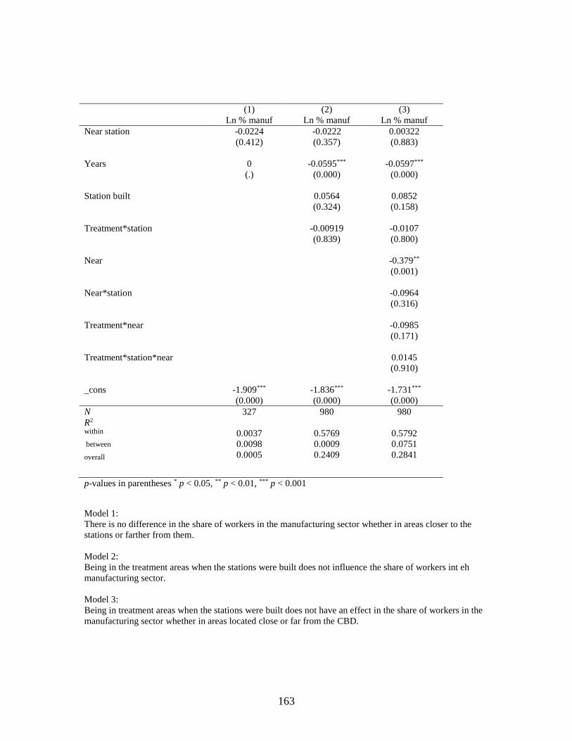
163
(1) (2) (3)
Ln % manuf Ln % manuf Ln % manuf
Near station -0.0224
(0.412)
-0.0222
(0.357)
0.00322
(0.883)
Years 0
(.)
-0.0595***
(0.000)
-0.0597***
(0.000)
Station built
0.0564
(0.324)
0.0852
(0.158)
Treatment*station
-0.00919
(0.839)
-0.0107
(0.800)
Near
-0.379**
(0.001)
Near*station
-0.0964
(0.316)
Treatment*near
-0.0985
(0.171)
Treatment*station*near
0.0145
(0.910)
_cons -1.909***
(0.000)
-1.836***
(0.000)
-1.731***
(0.000)
N 327 980 980
R2
within
between
overall
0.0037
0.0098
0.0005
0.5769
0.0009
0.2409
0.5792
0.0751
0.2841
p-values in parentheses * p < 0.05, ** p < 0.01, *** p < 0.001
Model 1:
There is no difference in the share of workers in the manufacturing sector whether in areas closer to the
stations or farther from them.
Model 2:
Being in the treatment areas when the stations were built does not influence the share of workers int eh
manufacturing sector.
Model 3:
Being in treatment areas when the stations were built does not have an effect in the share of workers in the
manufacturing sector whether in areas located close or far from the CBD.
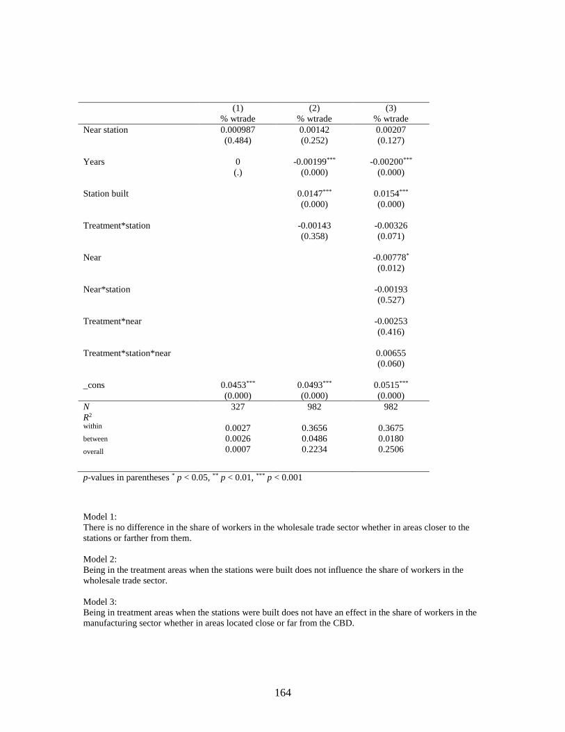
164
(1) (2) (3)
% wtrade % wtrade % wtrade
Near station 0.000987
(0.484)
0.00142
(0.252)
0.00207
(0.127)
Years 0
(.)
-0.00199***
(0.000)
-0.00200***
(0.000)
Station built
0.0147***
(0.000)
0.0154***
(0.000)
Treatment*station
-0.00143
(0.358)
-0.00326
(0.071)
Near
-0.00778*
(0.012)
Near*station
-0.00193
(0.527)
Treatment*near
-0.00253
(0.416)
Treatment*station*near
0.00655
(0.060)
_cons 0.0453***
(0.000)
0.0493***
(0.000)
0.0515***
(0.000)
N 327 982 982
R2
within
between
overall
0.0027
0.0026
0.0007
0.3656
0.0486
0.2234
0.3675
0.0180
0.2506
p-values in parentheses * p < 0.05, ** p < 0.01, *** p < 0.001
Model 1:
There is no difference in the share of workers in the wholesale trade sector whether in areas closer to the
stations or farther from them.
Model 2:
Being in the treatment areas when the stations were built does not influence the share of workers in the
wholesale trade sector.
Model 3:
Being in treatment areas when the stations were built does not have an effect in the share of workers in the
manufacturing sector whether in areas located close or far from the CBD.

165
(1) (2) (3)
Ln % wtrade Ln % wtrade Ln % wtrade
Near station -0.0447
(0.189)
-0.0250
(0.406)
0.000724
(0.979)
Years 0
(.)
-0.0711***
(0.000)
-0.0714***
(0.000)
Station built
0.490***
(0.000)
0.524***
(0.000)
Treatment*station
-0.0301
(0.548)
-0.125*
(0.022)
Near
-0.242*
(0.011)
Near*station
-0.103
(0.303)
Treatment*near
-0.0992
(0.260)
Treatment*station*near
0.343**
(0.004)
_cons -3.165***
(0.000)
-3.028***
(0.000)
-2.961***
(0.000)
N 327 972 972
R2
within
between
overall
0.0112
0.0022
0.0018
0.4179
0.0152
0.2566
0.4236
0.0107
0.2810
p-values in parentheses * p < 0.05, ** p < 0.01, *** p < 0.001
Model 1:
There is no difference in the share of workers in the wholesale trade either in areas nearer to the station or
farther from it.
Model 2:
Being in the treatment areas when the stations were built does not influence the share of workers in the
wholesale trade.
Model 3:
Being in treatment areas when the stations were built lead to a 22 percent increase in the share of workers
in wholesale trade in areas close to the CBD. In areas far from the CBD, on the other hand, the share of
workers in wholesale trade declined by 12.5 percent.
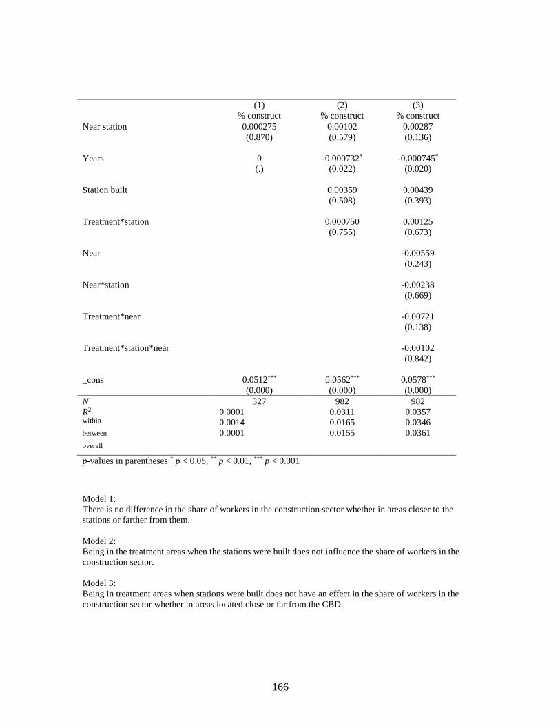
166
(1) (2) (3)
% construct % construct % construct
Near station 0.000275
(0.870)
0.00102
(0.579)
0.00287
(0.136)
Years 0
(.)
-0.000732*
(0.022)
-0.000745*
(0.020)
Station built
0.00359
(0.508)
0.00439
(0.393)
Treatment*station
0.000750
(0.755)
0.00125
(0.673)
Near
-0.00559
(0.243)
Near*station
-0.00238
(0.669)
Treatment*near
-0.00721
(0.138)
Treatment*station*near
-0.00102
(0.842)
_cons 0.0512***
(0.000)
0.0562***
(0.000)
0.0578***
(0.000)
N 327 982 982
R2
within
between
overall
0.0001
0.0014
0.0001
0.0311
0.0165
0.0155
0.0357
0.0346
0.0361
p-values in parentheses * p < 0.05, ** p < 0.01, *** p < 0.001
Model 1:
There is no difference in the share of workers in the construction sector whether in areas closer to the
stations or farther from them.
Model 2:
Being in the treatment areas when the stations were built does not influence the share of workers in the
construction sector.
Model 3:
Being in treatment areas when stations were built does not have an effect in the share of workers in the
construction sector whether in areas located close or far from the CBD.

167
(1) (2) (3)
Ln % construct Ln % construct Ln % construct
Near station -0.0519
(0.241)
-0.0427
(0.260)
-0.0418
(0.253)
Years 0
(.)
-0.0219***
(0.000)
-0.0223***
(0.000)
Station built
0.105
(0.179)
0.114
(0.137)
Treatment*station
-0.0511
(0.219)
-0.0322
(0.481)
Near
-0.227*
(0.039)
Near*station
-0.00828
(0.942)
Treatment*near
-0.00222
(0.984)
Treatment*station*near
-0.0683
(0.514)
_cons -3.062***
(0.000)
-2.966***
(0.000)
-2.904***
(0.000)
N 325 976 976
R2
within
between
overall
0.0146
0.1667
0.0009
0.0957
0.0066
0.0483
0.0964
0.0421
0.0755
p-values in parentheses * p < 0.05, ** p < 0.01, *** p < 0.001
Model 1:
There is no difference in the share of workers in the construction sector whether in areas closer to the
stations or farther from them.
Model 2:
Being in the treatment areas when the stations were built does not influence the share of workers in the
construction sector.
Model 3:
Being in treatment areas when stations were built does not have an effect in the share of workers in the
construction sector whether in areas located close or far from the CBD.

168
(1) (2) (3)
% transportation % transportation % transportation
Near station 0.00207
(0.161)
0.00137
(0.335)
0.000292
(0.862)
Years 0
(.)
0.00178***
(0.000)
0.00176***
(0.000)
Station built
-0.0229***
(0.000)
-0.0199***
(0.000)
Treatment*station
-0.00320
(0.140)
-0.00275
(0.275)
Near
-0.00627*
(0.031)
Near*station
-0.00925**
(0.002)
Treatment*near
0.00415
(0.189)
Treatment*station*near
-0.00211
(0.669)
_cons 0.0496***
(0.000)
0.0457***
(0.000)
0.0474***
(0.000)
N 327 982 982
R2
within
between
overall
0.0127
0.0023
0.0017
0.1321
0.0173
0.0344
0.1417
0.0087
0.0602
p-values in parentheses * p < 0.05, ** p < 0.01, *** p < 0.001
Model 1:
There is no difference in the share of workers in the transportation sector whether in areas closer to the
stations or farther from them.
Model 2:
Being in the treatment areas when the stations were built does not influence the share of workers in the
transportation sector.
Model 3:
Being in treatment areas when stations were built does not have an effect in the share of workers in the
transportation sector whether in areas located close or far from the CBD.
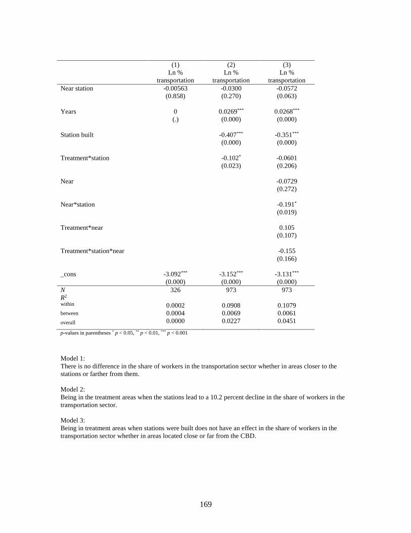
169
(1) (2) (3)
Ln %
transportation
Ln %
transportation
Ln %
transportation
Near station -0.00563
(0.858)
-0.0300
(0.270)
-0.0572
(0.063)
Years 0
(.)
0.0269***
(0.000)
0.0268***
(0.000)
Station built
-0.407***
(0.000)
-0.351***
(0.000)
Treatment*station
-0.102*
(0.023)
-0.0601
(0.206)
Near
-0.0729
(0.272)
Near*station
-0.191*
(0.019)
Treatment*near
0.105
(0.107)
Treatment*station*near
-0.155
(0.166)
_cons -3.092***
(0.000)
-3.152***
(0.000)
-3.131***
(0.000)
N 326 973 973
R2
within
between
overall
0.0002
0.0004
0.0000
0.0908
0.0069
0.0227
0.1079
0.0061
0.0451
p-values in parentheses * p < 0.05, ** p < 0.01, *** p < 0.001
Model 1:
There is no difference in the share of workers in the transportation sector whether in areas closer to the
stations or farther from them.
Model 2:
Being in the treatment areas when the stations lead to a 10.2 percent decline in the share of workers in the
transportation sector.
Model 3:
Being in treatment areas when stations were built does not have an effect in the share of workers in the
transportation sector whether in areas located close or far from the CBD.
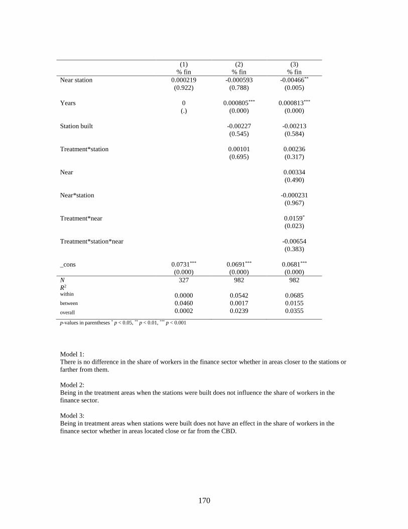
170
(1) (2) (3)
% fin % fin % fin
Near station 0.000219
(0.922)
-0.000593
(0.788)
-0.00466**
(0.005)
Years 0
(.)
0.000805***
(0.000)
0.000813***
(0.000)
Station built
-0.00227
(0.545)
-0.00213
(0.584)
Treatment*station
0.00101
(0.695)
0.00236
(0.317)
Near
0.00334
(0.490)
Near*station
-0.000231
(0.967)
Treatment*near
0.0159*
(0.023)
Treatment*station*near
-0.00654
(0.383)
_cons 0.0731***
(0.000)
0.0691***
(0.000)
0.0681***
(0.000)
N 327 982 982
R2
within
between
overall
0.0000
0.0460
0.0002
0.0542
0.0017
0.0239
0.0685
0.0155
0.0355
p-values in parentheses * p < 0.05, ** p < 0.01, *** p < 0.001
Model 1:
There is no difference in the share of workers in the finance sector whether in areas closer to the stations or
farther from them.
Model 2:
Being in the treatment areas when the stations were built does not influence the share of workers in the
finance sector.
Model 3:
Being in treatment areas when stations were built does not have an effect in the share of workers in the
finance sector whether in areas located close or far from the CBD.

171
(1) (2) (3)
Ln % fin Ln % fin Ln % fin
Near station -0.0680*
(0.038)
-0.0656*
(0.023)
-0.106***
(0.000)
Years 0
(.)
0.0113***
(0.000)
0.0114***
(0.000)
Station built
-0.0703
(0.197)
-0.0613
(0.302)
Treatment*station
0.0300
(0.421)
0.0457
(0.170)
Near
0.0674
(0.328)
Near*station
-0.0301
(0.679)
Treatment*near
0.157
(0.058)
Treatment*station*near
-0.0729
(0.502)
_cons -2.698***
(0.000)
-2.756***
(0.000)
-2.776***
(0.000)
N 327 981 981
R2
within
between
overall
0.0280
0.0113
0.0040
0.0494
0.0115
0.0240
0.0583
0.0164
0.0323
p-values in parentheses * p < 0.05, ** p < 0.01, *** p < 0.001
Model 1:
Being in the treatment area causes a decline in the share of workers in the finance sector (by 7%).
Model 2:
Being in the treatment areas when the stations were built does not influence the share of workers in the
finance sector.
Model 3:
Being in treatment areas when stations were built does not have an effect in the share of workers in the
finance sector whether in areas located close or far from the CBD.

172
(1) (2) (3)
% profess % profess % profess
Near station 0.00798**
(0.002)
0.00754**
(0.001)
0.00292
(0.137)
Years 0
(.)
0.00450***
(0.000)
0.00453***
(0.000)
Station built
-0.00817
(0.176)
-0.0129
(0.056)
Treatment*station
-0.00215
(0.608)
-0.000383
(0.927)
near
0.0130*
(0.017)
Near*station
0.0163
(0.133)
Treatment*near
0.0182**
(0.009)
Treatment*station*near
-0.00804
(0.473)
_cons 0.106***
(0.000)
0.101***
(0.000)
0.0972***
(0.000)
N 327 982 982
R2
within
between
overall
0.0495
0.0745
0.0135
0.4075
0.0006
0.2564
0.4137
0.1011
0.2975
p-values in parentheses * p < 0.05, ** p < 0.01, *** p < 0.001
Model 1:
Being near the station causes a 0.8 percentage point increase in the share of workers in the professional
services sector.
Model 2:
Being in the treatment areas when the stations were built does not influence the share of professionals.
Model 3:
Being in treatment areas when stations were built does not have an effect in the share of workers in the
professional services whether in areas located close or far from the CBD.

173
(1) (2) (3)
Ln % profess Ln % profess Ln % profess
Near station 0.0402
(0.073)
0.0379
(0.051)
0.0138
(0.465)
Years 0
(.)
0.0292***
(0.000)
0.0294***
(0.000)
Station built
-0.0329
(0.453)
-0.0515
(0.268)
Treatment*station
-0.0225
(0.459)
-0.00577
(0.854)
Near
0.120**
(0.008)
Near*station
0.0577
(0.353)
Treatment*near
0.0948
(0.075)
Treatment*station*near
-0.0689
(0.386)
_cons -2.279***
(0.000)
-2.305***
(0.000)
-2.339***
(0.000)
N 327 980 980
R2
within
between
overall
0.0165
0.0507
0.0051
0.4415
0.0134
0.2811
0.4435
0.0858
0.3164
p-values in parentheses * p < 0.05, ** p < 0.01, *** p < 0.001
Model 1:
There is no difference in the share of professional whether in areas closer to the stations or farther from
them.
Model 2:
Being in the treatment areas when the stations were built does not influence the share of professional.
Model 3:
Being in treatment areas when stations were built does not have an effect in the share of workers in the
professional services whether in areas located close or far from the CBD.

174
(1) (2) (3)
% oservices % oservices % oservices
Near station -0.00203
(0.428)
-0.00171
(0.382)
-0.00253
(0.083)
Years 0
(.)
-0.00233***
(0.000)
-0.00226***
(0.000)
Station built
0.00278
(0.366)
0.00536
(0.158)
Treatment*station
0.000435
(0.882)
0.00151
(0.511)
Near
0.0195**
(0.002)
Near*station
-0.0130
(0.115)
Treatment*near
0.00386
(0.553)
Treatment*station*near
-0.00604
(0.554)
_cons 0.0839***
(0.000)
0.0827***
(0.000)
0.0773***
(0.000)
N 327 982 982
R2
within
between
overall
0.0045
0.0075
0.0004
0.2738
0.0311
0.2026
0.2860
0.0807
0.2273
p-values in parentheses * p < 0.05, ** p < 0.01, *** p < 0.001
Model 1:
There is no difference in the share of workers in other services whether in areas closer to the stations or
farther from them.
Model 2:
Being in the treatment areas when the stations were built does not influence the share of workers in other
services.
Model 3:
Being in treatment areas when stations were built does not have an effect in the share of workers in other
services whether in areas located close or far from the CBD.
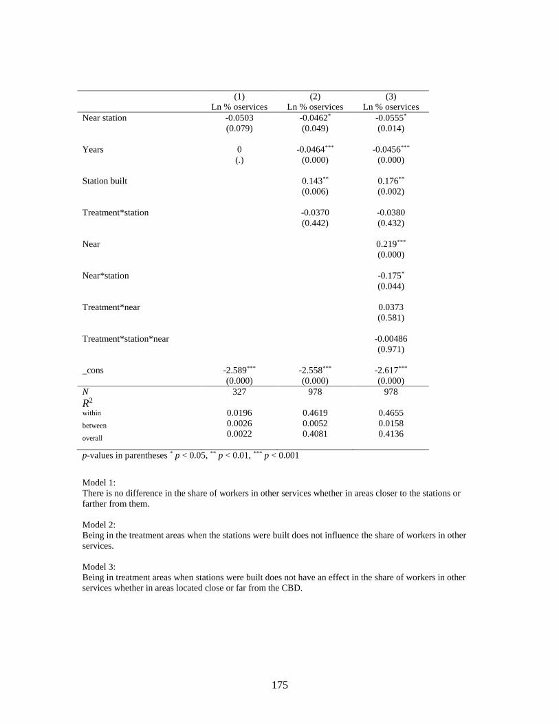
175
(1) (2) (3)
Ln % oservices Ln % oservices Ln % oservices
Near station -0.0503
(0.079)
-0.0462*
(0.049)
-0.0555*
(0.014)
Years 0
(.)
-0.0464***
(0.000)
-0.0456***
(0.000)
Station built
0.143**
(0.006)
0.176**
(0.002)
Treatment*station
-0.0370
(0.442)
-0.0380
(0.432)
Near
0.219***
(0.000)
Near*station
-0.175*
(0.044)
Treatment*near
0.0373
(0.581)
Treatment*station*near
-0.00486
(0.971)
_cons -2.589***
(0.000)
-2.558***
(0.000)
-2.617***
(0.000)
N 327 978 978
R2
within
between
overall
0.0196
0.0026
0.0022
0.4619
0.0052
0.4081
0.4655
0.0158
0.4136
p-values in parentheses * p < 0.05, ** p < 0.01, *** p < 0.001
Model 1:
There is no difference in the share of workers in other services whether in areas closer to the stations or
farther from them.
Model 2:
Being in the treatment areas when the stations were built does not influence the share of workers in other
services.
Model 3:
Being in treatment areas when stations were built does not have an effect in the share of workers in other
services whether in areas located close or far from the CBD.

176
(1) (2) (3)
% arts % arts % arts
Near station -0.000113
(0.899)
-0.00380**
(0.006)
-0.00249
(0.080)
Years 0
(.)
0.00270***
(0.000)
0.00273***
(0.000)
Station built
0.0652***
(0.000)
0.0581***
(0.000)
Treatment*station
0.00343
(0.318)
0.00519
(0.113)
near
-0.000580
(0.937)
Near*station
0.0227*
(0.031)
Treatment*near
-0.00504
(0.171)
Treatment*station*near
-0.00519
(0.582)
_cons 0.0179***
(0.000)
0.0466***
(0.000)
0.0466***
(0.000)
N 327 982 982
R2
within
between
overall
0.0000
0.0188
0.0001
0.4619
0.0052
0.4081
0.4655
0.0158
0.4136
p-values in parentheses * p < 0.05, ** p < 0.01, *** p < 0.001
Model 1:
There is no difference in the share of workers in arts and entertainment whether in areas closer to the
stations or farther from them.
Model 2:
Being in the treatment areas when the stations were built does not influence the share of workers in arts and
entertainment.
Model 3:
Being in treatment areas when stations were built does not have an effect in the share of workers in arts and
entertainment whether in areas located close or far from the CBD.

177
(1) (2) (3)
Ln % arts Ln % arts Ln % arts
Near station -0.0940
(0.096)
-0.0997*
(0.024)
-0.102*
(0.044)
Years 0
(.)
0.0708***
(0.000)
0.0713***
(0.000)
Station built
0.727***
(0.000)
0.683***
(0.000)
Treatment*station
0.0615
(0.224)
0.0822
(0.144)
Near
0.0441
(0.689)
Near*station
0.125
(0.363)
Treatment*near
0.00907
(0.930)
Treatment*station*near
-0.0706
(0.564)
_cons -4.201***
(0.000)
-3.795***
(0.000)
-3.807***
(0.000)
N 319 972 972
R2
within
between
overall
0.0156
0.0086
0.0053
0.6212
0.0538
0.5747
0.6211
0.0790
0.5764
p-values in parentheses * p < 0.05, ** p < 0.01, *** p < 0.001
Model 1:
There is no difference in the share of workers in arts and entertainment whether in areas closer to the
stations or farther from them.
Model 2:
Being in the treatment areas when the stations were built does not influence the share of workers in arts and
entertainment.
Model 3:
Being in treatment areas when stations were built does not have an effect in the share of workers in arts and
entertainment whether in areas located close or far from the CBD.

178
(1) (2) (3)
% info % info % info
Near station -0.00181
(0.054)
-0.00116
(0.241)
-0.00124
(0.179)
Years 0
(.)
-0.000790*
(0.017)
-0.000811*
(0.014)
Station built
0.0123*
(0.045)
0.0108
(0.086)
Treatment*station
0.000198
(0.900)
-0.000615
(0.688)
Near
-0.00810*
(0.019)
Near*station
0.00730
(0.124)
Treatment*near
0.000360
(0.905)
Treatment*station*near
0.00272
(0.536)
_cons 0.0259***
(0.000)
0.0410***
(0.000)
0.0431***
(0.000)
N 327 982 982
R2
within
between
overall
0.0258
0.0280
0.0046
0.0512
0.0608
0.0180
0.0526
0.0153
0.0250
p-values in parentheses * p < 0.05, ** p < 0.01, *** p < 0.001
Model 1:
There is no difference in the share of workers in the information sector whether in areas closer to the
stations or farther from them.
Model 2:
Being in the treatment areas when the stations were built does not influence the share of workers in the
information sector.
Model 3:
Being in treatment areas when stations were built does not have an effect in the share of workers in the
information sector whether in areas located close or far from the CBD.

179
(1) (2) (3)
Ln % info Ln % info Ln % info
Near station -0.150**
(0.005)
-0.105*
(0.019)
-0.109*
(0.010)
Years 0
(.)
-0.0358***
(0.000)
-0.0358***
(0.000)
Station built
0.448**
(0.003)
0.357*
(0.019)
Treatment*station
0.0322
(0.597)
0.0310
(0.628)
Near
-0.243*
(0.036)
Near*station
0.328*
(0.020)
Treatment*near
0.0137
(0.917)
Treatment*station*near
0.00626
(0.969)
_cons -3.756***
(0.000)
-3.370***
(0.000)
-3.305***
(0.000)
N 322 968 968
R2
within
between
overall
0.0561
0.0182
0.0116
0.0736
0.0052
0.0378
0.0819
0.0076
0.0453
p-values in parentheses * p < 0.05, ** p < 0.01, *** p < 0.001
Model 1:
Being in close to the station causes a decline in the share of workers in the information sector (by 15
percent).
Model 2:
Being in the treatment areas when the stations were built does not influence the share of workers in the
information sector.
Model 3:
Being in treatment areas when stations were built does not have an effect in the share of workers in the
information sector whether in areas located close or far from the CBD.

180
(1) (2) (3)
% rtrade % rtrade % rtrade
Near station 0.00364
(0.242)
0.00159
(0.519)
0.00413
(0.073)
Years 0
(.)
-0.00328***
(0.000)
-0.00327***
(0.000)
Station built
-0.0288***
(0.000)
-0.0215***
(0.000)
Treatment*station
-0.000448
(0.875)
-0.00424
(0.144)
Near
0.0165**
(0.004)
Near*station
-0.0275***
(0.000)
Treatment*near
-0.0101
(0.161)
Treatment*station*near
0.0143
(0.063)
_cons 0.156***
(0.000)
0.146***
(0.000)
0.142***
(0.000)
N 327 982 982 R2
within
between
overall
0.0108
0.0364
0.0013
0.6330
0.1264
0.5648
0.6419
0.1392
0.5727
p-values in parentheses * p < 0.05, ** p < 0.01, *** p < 0.001
Model 1:
There is no difference in the share of workers in the retail trade sector whether in areas closer to the stations
or farther from them.
Model 2:
Being in the treatment areas when the stations were built does not influence the share of workers in the
retail trade sector.
Model 3:
Being in treatment areas when stations were built does not have an effect in the share of workers in the
retail trade sector whether in areas located close or far from the CBD.
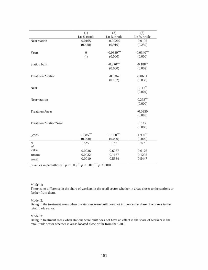
181
(1) (2) (3)
Ln % rtrade Ln % rtrade Ln % rtrade
Near station 0.0165
(0.428)
-0.00202
(0.910)
0.0195
(0.259)
Years 0
(.)
-0.0339***
(0.000)
-0.0340***
(0.000)
Station built
-0.270***
(0.000)
-0.188**
(0.002)
Treatment*station
-0.0367
(0.192)
-0.0661*
(0.038)
Near
0.117**
(0.004)
Near*station
-0.293***
(0.000)
Treatment*near
-0.0850
(0.088)
Treatment*station*near
0.112
(0.088)
_cons -1.885***
(0.000)
-1.960***
(0.000)
-1.990***
(0.000)
N 325 977 977
R2
within
between
overall
0.0036
0.0022
0.0010
0.6067
0.1177
0.5334
0.6176
0.1295
0.5447
p-values in parentheses * p < 0.05, ** p < 0.01, *** p < 0.001
Model 1:
There is no difference in the share of workers in the retail sector whether in areas closer to the stations or
farther from them.
Model 2:
Being in the treatment areas when the stations were built does not influence the share of workers in the
retail trade sector.
Model 3:
Being in treatment areas when stations were built does not have an effect in the share of workers in the
retail trade sector whether in areas located close or far from the CBD.

182
(1) (2) (3)
% ehss % ehss % ehss
Near station -0.00666*
(0.041)
-0.00373
(0.178)
-0.000720
(0.797)
Years 0
(.)
0.00776***
(0.000)
0.00775***
(0.000)
Station built
-0.0590***
(0.000)
-0.0558***
(0.000)
Treatment*station
-0.00140
(0.741)
-0.00366
(0.433)
Near
0.0173
(0.058)
Near*station
-0.0117
(0.231)
Treatment*near
-0.0119
(0.119)
Treatment*station*near
0.00947
(0.370)
_cons 0.145***
(0.000)
0.116***
(0.000)
0.111***
(0.000)
N 327 982 982
R2
within
between
overall
0.0248
0.0027
0.0043
0.3330
0.0067
0.2468
0.3337
0.0038
0.2495
p-values in parentheses * p < 0.05, ** p < 0.01, *** p < 0.001
Model 1:
Being near the station causes a decrease in the share of workers in the education, health and social sciences
sector by 0.6 percentage point.
Model 2:
Being in the treatment areas when the stations were built does not influence the share of workers in the
education, health and social science sector.
Model 3:
Being in treatment areas when stations were built does not have an effect in the share of workers in the
education, health, and social services retail trade sector whether in areas located close or far from the CBD.

183
(1) (2) (3)
Ln % ehss Ln % ehss Ln % ehss
Near station -0.0599*
(0.010)
-0.0480*
(0.029)
-0.0239
(0.288)
Years 0
(.)
0.0458***
(0.000)
0.0461***
(0.000)
Station built
-0.383***
(0.000)
-0.388***
(0.000)
Treatment*station
0.00440
(0.882)
-0.0121
(0.720)
Near
0.124
(0.056)
Near*station
-0.00975
(0.882)
Treatment*near
-0.0944
(0.114)
Treatment*station*near
0.0678
(0.336)
_cons -1.988***
(0.000)
-2.196***
(0.000)
-2.229***
(0.000)
N 326 976 976
R2
within
between
overall
0.0411
0.0087
0.0056
0.2626
0.0074
0.2000
0.2642
0.0003
0.2062
p-values in parentheses * p < 0.05, ** p < 0.01, *** p < 0.001
Model 1:
Being near the station causes a decrease in the share of workers in the education, health and social sciences
sector by 6 percent.
Model 2:
Being in the treatment areas when the stations were built does not influence the share of workers in the
education, health and social secience sector.
Model 3:
Being in treatment areas when stations were built does not have an effect in the share of workers in the
education, health, and social services retail trade sector whether in areas located close or far from the CBD.
REFERENCES
Abadie, A. (2005). Semiparametric difference-in-differences estimators. The Review of
Economic Studies, 72(1), 1-19. doi:10.1111/0034-6527.00321
American Planning Association Economic Development Group (2009, November 16) Dr.
Homer Hoyt: Planning’s Unsung Hero. Retrieved from
http://apaeconomicdevelopment.blogspot.com/2009/11/dr-homer-hoyt-plannings-
unsung-hero.html
American Public Transportation Association. Ridership Report 1890-2014
American Public Transportation Association (2015) Public Transportation Background
Data
Ayer, L, Hocking, R (1986). Land Development Impact of Transit Construction. Journal
of Transportation Engineering 112, 19 January): 77-87.
Baum-Snow N., Kahn, M.E. (2000). The Effects of New Project to Expand Urban Rail
Transit. Journal of Public Economics 77, 241-263.
Baum-Snow, N., Kahn, M. E., & Voith, R. (2005). Effects of urban rail transit
expansions: Evidence from Sixteen Cities, 1970-2000.Brookings-Wharton Papers on
Urban Affairs, 147-206.
Bhattacharjee, S., & Goetz, A. R. (2016). The Rail Transit System and Land Use Change
in the Denver Metro Region. Journal of Transport Geography, 54, 440-450.
doi:http://dx.doi.org/10.1016/j.jtrangeo.2016.02.004
Bollinger, C. R., & Ihlanfeldt, K. R. (1997). The Impact of Rapid Rail Transit on
Economic Development: The Case of Atlanta's MARTA. Journal of Urban
Economics, 42(2), 179-204.
Cervero, R, and Landis, J (1993) Assessing the Impacts of Urban Rail Transit on Local
Real Estate Markets Using Quasi-Experimental Comparisons. Transportation
Research A 27A, 1:13-22.
Cervero, R., and Landis, J. (1995) "BART at 20: Land use impacts." Paper presented at
the 74th annual meeting of the Transportation Research Board, Washington,
DC, January.
Cervero, R. and Duncan, M. (2008) Residential Self Selection and Rail Commuting: A
Nested Logit Analysis. University of California Transportation Center Working

185
Paper.
Cervero, R. (2009) Urban Development on Railway-served Land: Lessons and
Opportunities for the Developing World. UC Berkeley Center for Future Urban
Transport Working Paper UCB-ITS-VWP-2009-13
Davis, V. O. (2008). mpact of Metrorail Stations in Washington, DC on Land Use and
Development: Shady Grove Metro Station Case Study. In Transportation Land Use,
Planning, and Air Quality (pp. 118-123). ASCE.
Debrezion, G., Pels, E., & Rietveld, P. (2007). The effects of railway investments in a
polycentric city: A comparison of competitive and segmented land markets.
Environment and Planning A, 39(9), 2048-2067. doi:10.1068/a39180
Dingemans, D. (1978) Rapid Transit, and Suburban Residential Land Use. Traffic
Quarterly April: 289-306
Donnelly, P. 1982. Rail Transit Impact Studies: Atlanta, Washington, and San Diego.
Washington: Urban Mass Transportation Administration.
Dyet, M. and Castle, G. (1978) Study of the Housing Industry. Working paper, BART
Impact Program. Berkeley, CA. Metropolitan Transportation Commission
September.
Fajans, M., Dyett, M., and Dornbush, D. (1978) Study of Development Patterns. Working
paper, BART Impact Program. Berkeley, CA Metropolitan Transportation
Commission September.
Falcke, C. (1978b) Study of Property Acquisition and Occupancy: BART’s Effects on
Speculation. Working paper, BART Impact Program, Berkeley, CA. Metropolitan
Transportation Commission. October.
Federal Transit Authority: National Transit Database
Flater, D. ( ) Understanding Geodesic Buffering. Esri Geoprocessing Development Team.
www.esri.com
Glaeser, E., Kahn, M., & Rappaport, J. (2000). Why do the Poor Live in Cities?. NBER
Working Paper N 7636.
Giuliano, G. (2004) Land use impacts of transportation investments: Highway and transit.
In S. Hanson and G. Giuliano (Eds.), The Geography of Urban Transportation, 3rd
Edition. New York: Guilford Press.

186
Guerra, E. Cervero, R, Tishler, D (2011) The Half-Mile Circle: Does it Best Represent
Transit Station Catchments? UC Berkeley Institute of Transportation Studies,
Working Paper UCB-ITS-VWP-2011-5
Guerra, Erick Strom. (2013). The New Suburbs: Evolving travel behavior, the built
environment, and subway investment in Mexico City. UC Berkeley: University of
California Transportation Center.
Handy, S. (2005). Smart Growth and the Transportation-Land Use Connection: What
Does the Research Tell Us? International Regional Science Review, 28(2), 146-167.
Harold, C. (1987) Staff Paper 54- Section A Baltimore Metro Impact Study: A Before
and After Comparison. Baltimore: Regional Planning Council
Hess, D. B., & Almeida, T. M. (2007). Impact of Proximity to Light Rail Rapid Transit
on Station-Area Property Values in Buffalo, New York. Urban Studies, 44(5-6),
1041-1068.
Higgins, C., Ferguson, M., & Kanaroglou, P. (2014). Light rail and land use change: Rail
transit’s role in reshaping and revitalizing cities. Journal of Public Transportation,
17(2), 5.
Huang, H. (1996). The land-use impacts of urban rail transit systems. Journal of
Planning Literature, 11(1), 17-30. doi:10.1177/088541229601100103
Hurst, N. B., & West, S. E. (2014). Public transit and urban redevelopment: The effect of
light rail transit on land use in Minneapolis, Minnesota. Regional Science and Urban
Economics, 46, 57-72.
Knaap, G. J., Ding, C., & Hopkins, L. D. (2001). Do plans matter?: The effects of light
rail plans on land values in station areas. Journal of Planning Education and
Research, 21(1), 32-39. doi:10.1177/0739456X0102100103
Knight, R. L., & Trygg, L. L. (1977). Evidence of land use impacts of rapid transit
systems. Transportation, 6(3), 231-247.
Knight, R., & Trygg, J. (1978). Urban mass transit and land use impacts.
Transportation, 5(1), 12-24.
Landis, J, Guhathakurta, S, Huang, W, and Zhang, M (1995) Rail Transit Investments,
Real Estate Values, and Land Use Change: A Comparative Analysis of Five
California Rail Transit Systems. Monograph #48 Institute of Urban and Regional
Development. Berkeley. July.

187
MTC (Metropolitan Transportation Commission) (1979) BART in the San Francisco Bay
Area: The Final Report of the BART Impact Program. June
Minnesota Population Center. National Historical Geographic Information System
(NHGIS.org): Version 11.0 [Database]. Minneapolis: University of Minnesota.
2016. http://doi.org/10.18128/D050.V11.0.
Nelson, A.C. Sanchez, T.L., 1997. The Influence of MARTA on Population and
Employment Location. Presented at the 76th Annual Meeting of the Transportation
Research Board, Washington, DC
Nyerges, T. (2004) GIS in Urban-Regional Transportation Planning. In S. Hanson and G.
Giuliano (Eds.), The Geography of Urban Transportation, 3rd Edition. New York:
Guilford Press.
Quackenbush, K, Holtst-Roness, E, Humphrey, T (1987) Red Line Extension to Alewife:
Before/after Study – Appendices. Boston: Central Transportation Planning Staff for
the Massachusetts Bay Transportation Authority.
Rail Passenger Service Act of 1970
Schuetz, J. (2014). Do Rail Transit Stations Encourage Neighbourhood Retail
Activity?. Urban Studies, 0042098014549128.
Taylor, B.D. & Morris, E.A. Public Transportation Objectives and Rider Demographics:
Are Transit’s Priorities Poor Public Policy? (2015) 42: 347.doi:10.1007/s11116-014-
9547-0
Torres-Reyna, O., Panel Data Analysis: Fixed and Random Effects using Stata (2007)
Princeton University
Transit Cooperative Research Program (TCRP Report 35). 1998. Economic Impact
Analysis of Transit Investments. Transportation Research Board. National Academy
Press.
Urban Land Institute (ULI) Research Division (1979) Joint Development: Making the
Real Estate- Transit Connection. Urban Land Institute, Washington DC
US Census Bureau Population, Income, Housing Values, Means of Transportation, and
other related data, Available from www.census.gov
US Government Accountability Office. June 2010 Transit Rail: Potential Rail Car Cost-
Saving Strategies Exist. From http://www.gao.gov/new.items/d10730.pdf

188
Vessali, K. V. (1996). Land use impacts of rapid transit: A review of the empirical
literature. Berkeley Planning Journal, 11(1)
Wegener, M., & Fuerst, F. (2009). Land-Use Transport Interaction: State of the
Art. Social Science Research Network Working Paper Series. Deliverable 2a of the
project TRANSLAND (Integration of Transport and Land Use Planning) of the 4th
RTD Framework Programme of the European Commission
Weinberger, R. (2014). Light Rail Proximity: Benefit or Detriment in the Case of Santa
Clara County, California