Impacts of non-farm income on inequality and

poverty: the case of rural China

Nong Zhu (INRS-UCS, University of Quebec)*

Xubei Luo (DECVP, The World Bank)**

Abstract: Based on data from the Living Standards Measurement Surveys, we examine the

effects of non-farm income on inequality and poverty in rural China using two approaches.

Firstly, we consider non-farm income as an “exogenous transfer”, which adds to the total

household income, and study the contribution of different types of income on inequality

using the decomposition of the Gini index. Secondly, we consider non-farm income as a

“potential substitute” for other household earnings, and compare the distribution of the

simulated income in the absence of non-farm activities with that of the observed income to

examine the impact of participation in non-farm activities on inequality and on poverty. We

find that, the prosperity of the non-farm sector after the economic reform alleviates rural

inequality and poverty. It increases the income levels of the poorest households and reduces

the income gaps between poor households.

JEL Classification: D63, O15, Q12

Key words: Non-farm income, Inequality, Poverty, China

1 INTRODUCTION

In developing countries, non-farm activities play a more and more important

role in sustainable development and poverty reduction in rural areas. Non-farm

activities can influence the rural economy through various channels. First, non-

farm employment reduces the pressure on the demand for land in poor areas.

Consequently, non-farm activities can contribute to breaking the vicious cycle of

“poverty – extensive cultivation – ecological deterioration – poverty”. Second, the

income obtained from non-farm activities can significantly increase total household

income and hence enhance the investment capacity in farm activities. It can also

mitigate income fluctuations and enable the adoption of some more profitable but

“risky” agricultural technologies, which favor the transformation of traditional

agriculture to modern agriculture. Third, non-farm income is often a source of

savings, which plays an important role in food security. The households that

diversify their income by participating in non-farm activities are more capable of

overcoming negative shocks.

Many researchers show that non-farm activities have an important impact on

income distribution. The impact depends on the ranking of the household in the

social scale as well as on the specific types of non-farm activities involved. Results

* E-Mail: nong_zhu@inrs-ucs.uquebec.ca. ** E-Mail: xluo@worldbank.org.

vary across regions and differ according to the methods of analyses used. Most

research shows that non-farm income distribution is more unequal than that of farm

income. 1 By improving the rural income as a whole, the participation in non-farm

activities can increase income disparities, in particular, in poor areas. However,

some other researchers show that as the proportion of non-farm income in total

income increases, the distribution of the latter will become more uniform, which

reduces income inequality, as well as the social and political tension. 2

China is an agricultural country with a typical dualist socio-economic structure,

as predicted by Lewis (1954). Given the high demographic pressure on the

countryside and the relatively limited quantity of cultivable land,3 the agricultural

income per capita has always been low. In such a situation, non-farm sectors play a

particularly important role in absorbing the surplus agricultural labor, in enhancing

the income of farmers, and in reducing rural poverty. The economic reforms, which

began in the late 1970s, in particular, the implementation of the Household

Responsibility System (HRS), led to a massive rural/urban migration and a rapid

development of rural non-farm sectors. It strongly reinforced economic growth and

enhanced household income in rural areas. The proportion of non-farm income in

total rural household income has been increasing as time passes.

Some studies show that rural inequality significantly increases with economic

reforms, and that the increase in this inequality is essentially explained by the

enhancement of the proportion of non-farm income in total income. Knight and

Song (1993) argue that the distribution of non-farm income is less egalitarian

compared to that of farm income in China, based on a country-level survey.

Hussain et al. (1994) draw a similar conclusion about the unequal distribution of

non-farm income and point out that non-farm income contributes to the rise in rural

inequality. These results suggest that rural inequality aggravates as rural labor

becomes more engaged in non-farm activities. Many researchers suggest that the

growing importance of non-farm activities in rural areas, which may result in an

increase in inequality, will increase the cost of economic restructuring during the

transition process in China. 4

However, in our opinion, most of the studies above are based on a

macroeconomic analysis, using data at the provincial or county levels. The role of

non-farm activities is rarely examined from the angle of microeconomic behavior

of rural households. In addition, these studies consider non-farm income only as an

exogenous/extra income, which adds to the resources of household. They do not

take into account the interactions between the participation in various productive

activities. A further review of the literature shows that the results depend largely on

the method of analysis. For example, some other studies, such as Adams and He

1 Barham and Boucher (1998); Elbers and Lanjouw (2001); Escobal (2001); Khan and Riskin (2001);

Leones and Feldman (1998); Reardon and Taylor (1996); Shand (1987). 2 Chinn (1979); Lachaud (1999); Richard and Adams (1994); Sadoulet and De Janvry (2001); Stark et

al. (1986). 3 In 2000, the quantity of per capita cultivable land in rural area was only 0.138 hectare (National

Statistics Bureau of China, 2001: p. 374). 4 Bhalla (1990) ; Yao (1999) ; Zhu (1991).

3

(1995) and Adams (1999), argue that non-farm income reduces the overall

inequality in Pakistan and in Egypt, respectively. They argue that households poor

in farm income (because of the unequal accessibility to land, etc) are more engaged

in non-farm activities, and the pro-poor distribution of non-farm income across the

income scale of the population mitigates the inequality.

The present study tries to examine the role of non-farm activities in overall

income distribution, taking into account the specialties of rural household

production in China. Based on data from the Living Stands Measurement Surveys

(LSMS), we study the impacts of the participation in non-farm activities on the

inequality and poverty in rural China, and analyze the determinants of farmers’

income at the micro level. We use two different approaches, on the one hand

considering non-farm income as an “exogenous transfer”, and on the other hand, as

a “potential substitute” for other household earnings. In the following section, we

briefly describe the development of the non-farm activities in rural areas of China

and articulate its growing important role. Section 3 discusses the methods of

analysis. Section 4 focuses on the data. Section 5 comments on the results. We

conclude in section 6.

2 ECONOMIC REFORMS AND FARMERS' NON-FARM INCOME IN

CHINA

The Chinese countryside has been characterized by economic autarchy and

traditional agriculture for a long time. Following the model of the former-USSR,

China gave priority to the development of heavy industries at an early stage of

industrialization. Farmers were heavily taxed – enormous agricultural surplus was

transferred to industrial investments. Before the reforms, in order to stabilize

agricultural production, farmers were fixed on land in two ways: (i) through rural

collectivization, and (ii) by the famous civil status system “hukou”. 5 Rural

collectivization tightened the links between farmers’ income and their daily work-

participation in collective land – a farmer gained “working-points” if he or she

worked on the collective land, the points he or she got depended on how much time

he or she spent on the collective land (gongfenzhi).6 The civil status system

consisted in closely combining the civil status with the supply of consumption

goods and access to jobs. Without urban civil status, rural/urban migrants could not

settle down on a permanent basis outside their original place. These two ways

divided the Chinese society into two completely different parts – urban area and

rural area, that is to say, the dualist economy predicted by Lewis (1954). We argue

that this division, which led to the inefficient allocation of resources and the low

incentive in productive activities, was the essential source of rural poverty. The

objective of agricultural reform was to remove/abolish the above constraints and to

establish a new agricultural mechanism.

5 Davin (1999); Zhu (2002). 6 See McMillan et al. (1989: pp.783-785).

The economic reforms that began in the late 1970s brought big changes in rural

China. First, the collapse of the system of “People's Commune”, as well as the

implementation and generalization of the Household Responsibility System in rural

areas,7 restored greater liberty to farmers – farmers could freely allocate their time,

and freely choose their careers and their mode of production. Second, agricultural

reforms strongly increased agricultural production and the supply of grains in the

markets, which enabled people living in urban areas without urban civil status

(hukou) to purchase food in free markets. It finally led to abandoning the rationing

system. Since 1984, gradually, the market of alimentary goods became open, and

housing in cities became marketable. These two factors enabled farmers to enter

cities and stay there in a permanent way without changing their civil status (hukou).

Third, with the development of various non-state economies, the urban labor

market was gradually established, which made it possible for rural/urban migrants

to seek jobs and earn their living in cities. In addition, the development of urban

infrastructure required extra labor, and the diversification of consumption resulting

from the improvement of living standards created the niches for the survival of

small businesses. All these factors led to an increase in the demand for labor in

urban areas, which accommodated the vast movement of agricultural labor from

rural areas to cities in China since the 1980s. The spontaneous movement of rural

population progressively broke the constraints on migration. Finally, the relaxing

of the control on migration by the Government in 1984 further led to the vast rural /

urban exodus. .

Given the heavy demographic pressure on land, agricultural labor productivity

continues to stay at a very low level. The stagnant and low rural income strongly

encourages farmers to quit working on land. However, although the shortage of

food is no longer a threat, the government continues to control rural/urban

migration with some direct or indirect measures for three principal reasons. First,

urban residents are not willing to share their relatively higher living standards with

rural residents (Zhao, 1999a). Second, urban infrastructure is not capable of

supporting a great exodus to cities, due to, for example, the capacity of some public

facilities. Finally, urban areas also suffer from serious unemployment problems due

to the reform of State-Own-Enterprises (SOEs), and have difficulties in absorbing

more labor force. The pushing forces from the countryside are strong, but the

attracting forces in cities are insufficient. In this context, farmers develop non-farm

activities, which do not suffer from the shortage of land, to reap the gains. Thus,

the non-agricultural sector has developed rapidly in rural China, and absorbs a

large quantity of the surplus agricultural labor that seeks better job opportunities

and higher income.8 The rural non-farm sector consists mainly of Township and

Village Enterprises (TVEs) and the rural private economy.

The rural/urban migration and the development of the rural non-farm sector

strongly modified rural household income. Non-farm activities gradually become

7 See De Beer and Rocca (1997 : p.56) ; Zhu and Jiang (1993). 8 Aubert (1995); Banister and Taylor (1990); Byrd and Lin (1994); Goldstein and Goldstein (1991);

Zhou (1994).

5

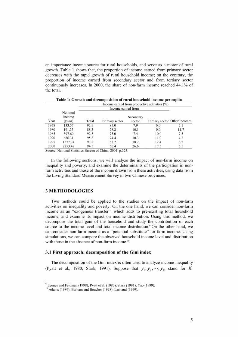
an importance income source for rural households, and serve as a motor of rural

growth. Table 1 shows that, the proportion of income earned from primary sector

decreases with the rapid growth of rural household income; on the contrary, the

proportion of income earned from secondary sector and from tertiary sector

continuously increases. In 2000, the share of non-farm income reached 44.1% of

the total.

Table 1: Growth and decomposition of rural household income per capita Income earned from productive activities (%)

Income earned from

Year

Net total

income

(yuan)

Total Primary sector

Secondary

sector

Tertiary sector

Other incomes

1978 133.57 92.9 85.0 7.9 0.0 7.1

1980 191.33 88.3 78.2 10.1 0.0 11.7

1985 397.60 92.5 75.0 7.4 10.0 7.5

1990 686.31 95.8 74.4 10.3 11.0 4.2

1995 1577.74 93.8 63.2 18.2 12.4 6.2

2000 2253.42 94.5 50.4 26.6 17.5 5.5

Source: National Statistics Bureau of China, 2001: p.323.

In the following sections, we will analyze the impact of non-farm income on

inequality and poverty, and examine the determinants of the participation in non-

farm activities and those of the income drawn from these activities, using data from

the Living Standard Measurement Survey in two Chinese provinces.

3 METHODOLOGIES

Two methods could be applied to the studies on the impact of non-farm

activities on inequality and poverty. On the one hand, we can consider non-farm

income as an “exogenous transfer”, which adds to pre-existing total household

income, and examine its impact on income distribution. Using this method, we

decompose the total gain of the household and study the contribution of each

source to the income level and total income distribution.9 On the other hand, we

can consider non-farm income as a “potential substitute” for farm income. Using

simulations, we can compare the observed household income level and distribution

with those in the absence of non-farm income.10

3.1 First approach: decomposition of the Gini index

The decomposition of the Gini index is often used to analyze income inequality

(Pyatt et al., 1980; Stark, 1991). Suppose that Kyyy ,,, 21 L stand for K

9 Leones and Feldman (1998); Pyatt et al. (1980); Stark (1991); Yao (1999). 10 Adams (1989); Barham and Boucher (1998); Lachaud (1999).

components of household income and 0y is the total income so that: ∑=

=K

k

kyy1

0 .

The Gini index of total income, 0G , can be decomposed as follows:

∑=

=K

k

kkk SGRG1

0 (1)

where kS stands for the proportion of the component k in total income, kG is the

Gini index corresponding to the component k ; and kR is the correlation of the

Gini of the component k with the total income. The formula (1) allows decomposing the role of the different components in

three interpretable terms: (i) the relative importance of the component k in total

income, kS , (ii) the inequality in distribution of the component in question, kG ,

and (iii) the correlation of the component in question with total income, kR .

To understand the impact of non-farm income on inequality, we compare the

Gini index of total income (which includes the contribution of non-farm activities),

0G , and that of farm activities only, aG . If 0G is inferior to aG , then non-farm

income reduces income inequality; and vice-versa.

Furthermore, using this decomposition, we can calculate the impact of a

marginal variation of a particular component on the Gini index of total income as

well as on the social welfare level.11

Although this approach provides a direct and simple measure of how non-farm

income contributes to income distribution, it does not address the economic issue

of what the non-farm workers would be contributing to their families if they had

not participated in non-farm activities. In other words, this approach implies some

hypothesis on the independence of the participation of various activities, which is

not always justified, since inside a household there exists a certain substitution

between the participation of non-farm activities and farm-activities. Due to some

unobservable characteristics, it is possible that the participations of various

productive activities correlate (Escobal, 2001; Kimhi, 1994). Hence, it is necessary

to employ a mixed estimation to exploit all available information and obtain as

efficient estimators as possible. Herein follows our second approach: household

income simulation.

3.2 Second approach: household income simulation

We should take the interactions between the participation in non-farm activities

and that in farm activities into account when studying the impact of non-farm

income on inequality and poverty. To do that, we compare the observed household

income distribution with an economically interesting counterfactual income

distribution-one without non-farm activities. Adams (1989) estimates a household

11 Stark (1991: pp.258-261, 269-271).

7

income function for non-migrant households. Then, he applies the coefficient

estimates and the endowment bundles of migrant households (without migration

and remittances) to impute their earnings under a no-migration scenario, and

studies the impact of remittance on inequality. In a similar research, Barham and

Boucher (1998) correct the selection bias and improve the model. Using a bivariate

probit model of double selection, Lachaud (1999) moves a step forward to simulate

the household income obtained in the absence of remittances and migration, and

examines the impact of private transfer on poverty. Following these researchers,

we will first estimate the household income equations from the observed values;

then simulate the household income in the case that the household participates only

in farm activities using the income equation; finally we will compare the statistics

of the simulated income with those of the observed income (the total gain in the

presence of non-farm income), and examine the impact of non-farm income on

inequality and poverty.

3.2.1 Estimation of income equations

In rural China, the implementation of the HRS led to the change of the mode of

production. The households became productive units after that. As a rational agent,

farmers naturally try to maximize their utilities by optimizing their decisions on

participation in productive activities and by allocating their labor between farm

activities, local rural non-farm activities, migration, etc. The income of a household

obtained from a given activity depends on two factors: first, whether the household

participates in the activity in question and, second, the net income that the

household obtained if it participates in this specific activity. The anticipated

income of a particular activity is hence the product of the probability of

participation in this activity and the net anticipated income received by the

household subject to participation in this activity (Taylor and Yunez-Naude, 1999:

pp.55-58).

Since households that participate in non-farm activities do not spread randomly

and uniformly among the sample, the estimation of the income equations might be

biased. The method of Heckman (1979) is often used to correct the selection bias.

Using the Probit model, we first estimate participation equation in which a dummy

variable equals 1 if the household participates in the activity and 0 if not, and

regress over all the independent variables:

00

01

*

*

*

≤⇔=

>⇔=

+=

ii

ii

iii

PP

PP

ZP εα

(2)

where *

iP is a non-observed continuous latent variable and iP is an observed

binary variable, which equals 1 if the household participates in the non-farm

activity and 0 if not; iZ is a vector of independent variables of the participation

equation. Then, we estimate two income equations respectively, one for the

households that participate in non-farm activities, and the other for the households

that participate only in farm activities by introducing the inversed Mills ratio

obtained from equation (2) to correct the selection bias:

iiii Xy ,1,111log µλγβ ++= for 1=iP (3)

iiii Xy ,0,000log µλγβ ++= for 0=iP (4)

where iy is the total household income; iX is a vector of independent variables;

i,1λ and i,0λ respectively the inversed Mills ratios of the two groups of

households.12 We consider equation (4) as the income equation in the case that

household participates only in farm-activities.

3.2.2 Simulation of income

Having estimated the income equations, we can simulate the living standards in

the absence of non-farm income for the households that actually participate in non-

farm activities.

We predict the income obtained only from farm activities for all households,

iy ,0ˆ , using equation (4) estimated above:

iii Xy ,000,0ˆˆˆlog λγβ += for all households (5)

For the households that participate only in farm activities ( 0=iP ), their total

income can be expressed by:

iii yy ,0,0ˆloglog µ+= for 0=iP (6)

where iy and iy ,0ˆ stand for observed income and simulated income respectively;

i,0µ being the residual. For the households that have participated in non-farm

activities, we do not know the unobservable part, i.e. the residual. Hence, it is

necessary to simulate the residual for each household that has participated in non-

farm activities.

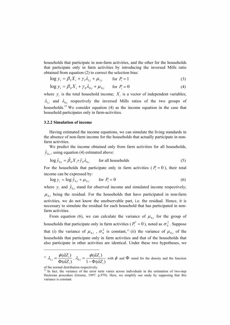
From equation (6), we can calculate the variance of i,0µ for the group of

households that participate only in farm activities ( 0* =iP ), noted as 2

0σ . Suppose

that (i) the variance of i,0µ , 2

0σ is constant,13 (ii) the variance of i,0µ of the

households that participate only in farm activities and that of the households that

also participate in other activities are identical. Under these two hypotheses, we

12 )ˆ(

)ˆ(,1

i

ii

Z

Z

ααφ

λΦ

= , )ˆ(1

)ˆ(,0

i

ii

Z

Z

ααφ

λΦ−

= with φ and Φ stand for the density and the function

of the normal distribution respectively. 13 In fact, the variance of the error term varies across individuals in the estimation of two-step

Heckman procedure (Greene, 1997: p.979). Here, we simplify our study by supposing that this

variance is constant.

9

simulate the residual of each household that participates in non-farm activities

( 1* =iP ) using the Monte Carlo method:

)(ˆ 1

0,0 ri

−Φ=σµ (7)

where r stands for a random number between )1,0[ . 1−Φ the inverse of the

cumulative probability function of the normal distribution. So i,0µ̂ follows a

normal distribution with the parameters ),0( 2

0σ . We define the income obtained in

the case that the household participates only in farm activities by:

+=

ii

i

iy

yy

,0,0

,0'

,0ˆˆlog

loglog

µ

1

0

*

*

=

=

i

i

P

P (8)

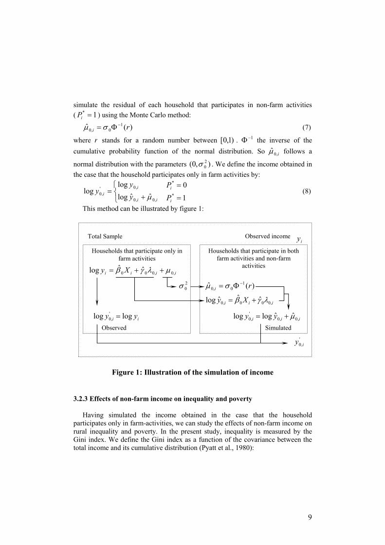
This method can be illustrated by figure 1:

Figure 1: Illustration of the simulation of income

3.2.3 Effects of non-farm income on inequality and poverty

Having simulated the income obtained in the case that the household

participates only in farm-activities, we can study the effects of non-farm income on

rural inequality and poverty. In the present study, inequality is measured by the

Gini index. We define the Gini index as a function of the covariance between the

total income and its cumulative distribution (Pyatt et al., 1980):

Households that participate in both

farm activities and non-farm

activities

Households that participate only in

farm activities

2

0σ )(ˆ 1

0,0 ri

−Φ=σµ

'

,0 iy

Simulated

value Observed

value

iiii Xy ,0,000ˆˆlog µλγβ ++=

iii Xy ,000,0ˆˆˆlog λγβ +=

iii yy ,0,0

'

,0ˆˆloglog µ+=

iy Total Sample

ii yy loglog '

,0 =

Observed income

( )y

yFyyG

)(,cov2)( = (9)

where y stands for the household income; y and )(yF the average and the

cumulative distribution of y respectively.

We calculate, respectively, the Gini index of the observed income, )( iyG , and

that of the simulated income, in case that the household participates only in farm

activities, )( '

,0 iyG . If )( iyG is inferior to )('

iyG , the non-farm income reduces

income inequality, and vice-versa.

Following the same idea, we study the impact of non-farm income on poverty.

Poverty is captured by the class of Foster-Greer-Thorbecke (FGT) indices14.

Considering a vector of household income in ascending order,

),,,( 21 nyyyy L= where nyyy ≤≤≤ L21 . 0>z is the poverty line, which is

predetermined, and ),( zyqq = the number of households whose income is less

than or equal to z . The general form of the measure of poverty can be expressed as follows:

∑=

−=

q

i

i

z

yz

nP

1

1α

α =α 0, 1, 2 (10)

0P , 1P and 2P , respectively, measure the headcount ratio (the proportion of

poor), the average normalized poverty gap, and the average squared normalized

poverty gap. Having estimated the indices of poverty, we can calculate their

corresponding standard error using the method proposed by Kakwani (1990) and

test the significance of the variation of poverty.

4 DATA

In this paper, we use data from LSMS, which took place in January 1996 and

February 1997 in two Chinese provinces: Hebei and Liaoning. The survey recorded

the information of 787 rural households that constitute our sample of interest.

These 787 households were spread over 31 villages of 15 towns or townships in 6

counties.

Household income can be divided into three categories according to the sources:

(i) income earned from farm activities, including monetary income or income in

kind earned from agricultural activities, livestock farming, forestry, fishing, etc.;

(ii) income earned from non-farm activities, including the income earned from self-

employment activities and the formal or informal wage income; and (iii) income

earned from non-productive activities, for example, pensions, transfers,

grants/subsidies, financial income, etc. We consider (ii) as the non-farm household

14 Foster et al. (1984); Sen (1976).

11

income. Among the 787 households in the sample, 205 received only farm income,

38 only non-farm income, 537 both farm income and non-farm income, and 7

neither farm income nor non-farm income.

Two principal factors determine the decision of households on non-farm

activity participation: first, the motivation related to some factors such as the

relative return and the risk of agricultural production; second, the capacity of non-

farm activity participation, which is determined by education, the welfare level of

the household, and the access to credit, etc. (FAO, 1998: p.285). Suppose that these

two factors are both determined by the intrinsic endowment of the household,

which is essentially captured by the accumulation of physical capital and human

capital, and by the external environment. We introduce the following independent

variables in the estimation of the participation equation and income equation:

The number of workers in the household. We define here the members who are

at least 15 years old and who are employed as workers. We suppose that this

variable plays a positive role in non-farm activity participation.

The average number of years in school of the household members who are at

least 15 years old, and its quadratic term. Many researchers show that the

improvement of human capital has an important effect on non-farm income and

that households with higher education level engage more in non-farm activities15.

The proportion of members that have received some technical or professional

training. This is another variable that captures the human capital accumulation of

the household. Such training can facilitate the access to non-farm employment and

increase the mobility of potential migrants.

The land surface of the household. For a rural household, land is the principle

physical capital. The shortage of land encourages farmers to participate in non-

farm activities. We introduce here the land surface and its quadratic term in order

to detect whether the relationship between land and the dependant variables is non-

linear.

The actual value of the house. The house is the most important property of rural

households. We consider this variable as a proxy for the welfare level of the

household.

The number of dependent persons (equal or over 6 years old). According to

some researchers, for example Zhao (1999b), the dependent persons play the role

of safeguarding the household’s right to land by supplying a minimum amount of

farm labor, and hence facilitating the exit of labor. We introduce here the number

of dependent persons, including the household members who are not currently

employed; while children below 5 years are excluded, for they do not offer labor

services.

The distance between the center of the village and the nearest railway station

and that between the center of the village and the nearest bus station. In general,

the railway station situates in the hubs of transport/communication, or in urban

centers. Hence, this distance can be used as the proxy for the transport easiness, the

15 Berdegué et al. (2001); Deininger and Olinto (2001); Estudillo and Otsuka (1999); Kimhi (1994);

Sadoulet and De Janvry (2001); Yunez-Naude and Taylor (2001).

cost of participation in non-farm activities, and the accessibility to information and

to markets (Wang, 1995). The distance between the center of the village and the

nearest bus station can also be used as proxy for the transport condition. If the first

distance reflects the cost of a long-distance migration, the second captures rather

that of the short-distance trip of the household members.

The per capita cultivable land of the village. As we have mentioned earlier, the

shortage of land is an important factor that motivates farmers to quit agricultural

production. We expect that this variable has a negative effect on the participation in

non-agricultural activities.

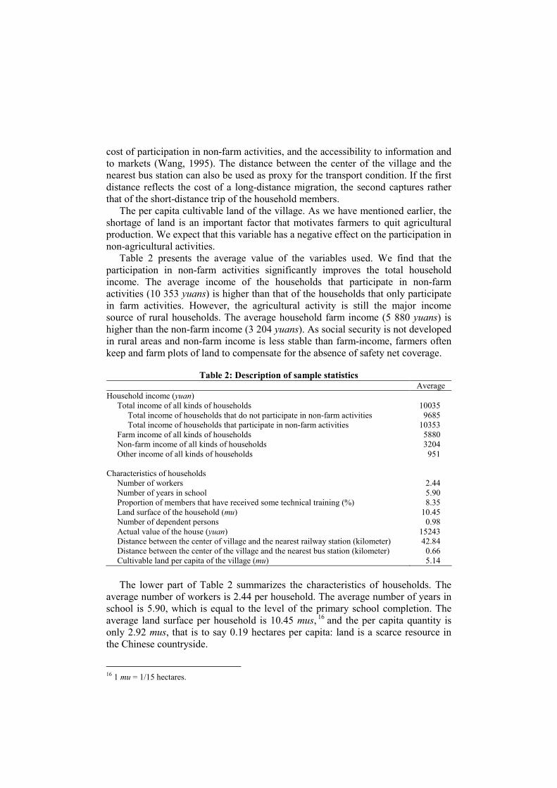
Table 2 presents the average value of the variables used. We find that the

participation in non-farm activities significantly improves the total household

income. The average income of the households that participate in non-farm

activities (10 353 yuans) is higher than that of the households that only participate

in farm activities. However, the agricultural activity is still the major income

source of rural households. The average household farm income (5 880 yuans) is

higher than the non-farm income (3 204 yuans). As social security is not developed

in rural areas and non-farm income is less stable than farm-income, farmers often

keep and farm plots of land to compensate for the absence of safety net coverage.

Table 2: Description of sample statistics Average

Household income (yuan)

Total income of all kinds of households 10035

Total income of households that do not participate in non-farm activities 9685

Total income of households that participate in non-farm activities 10353

Farm income of all kinds of households 5880

Non-farm income of all kinds of households 3204

Other income of all kinds of households 951

Characteristics of households

Number of workers 2.44

Number of years in school 5.90

Proportion of members that have received some technical training (%) 8.35

Land surface of the household (mu) 10.45

Number of dependent persons 0.98

Actual value of the house (yuan) 15243

Distance between the center of village and the nearest railway station (kilometer) 42.84

Distance between the center of the village and the nearest bus station (kilometer) 0.66

Cultivable land per capita of the village (mu) 5.14

The lower part of Table 2 summarizes the characteristics of households. The

average number of workers is 2.44 per household. The average number of years in

school is 5.90, which is equal to the level of the primary school completion. The

average land surface per household is 10.45 mus, 16 and the per capita quantity is

only 2.92 mus, that is to say 0.19 hectares per capita: land is a scarce resource in

the Chinese countryside.

16 1 mu = 1/15 hectares.

13

5 RESULTS AND COMMENTS

The results of our analysis are presented in two parts: first, the results of the

decomposition of the Gini index; second, the results of the simulations of income.

5.1 Non-farm income and inequality: exogenous transfer

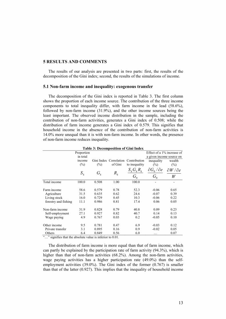
The decomposition of the Gini index is reported in Table 3. The first column

shows the proportion of each income source. The contribution of the three income

components to total inequality differ, with farm income in the lead (58.6%),

followed by non-farm income (31.9%), and the other income sources being the

least important. The observed income distribution in the sample, including the

contribution of non-farm activities, generates a Gini index of 0.508; while the

distribution of farm income generates a Gini index of 0.579. This signifies that

household income in the absence of the contribution of non-farm activities is

14.0% more unequal than it is with non-farm income. In other words, the presence

of non-farm income reduces inequality.

Table 3: Decomposition of Gini Index Effect of a 1% increase of

a given income source on

Proportion

in total

income

(%)

Gini Index

(%)

Correlation

of Gini

Contribution

to inequality inequality

(%)

wealth

(%)

kS kG kR

0G

RGS kkk

0

0 /

G

eG ∂∂

W

eW ∂∂ /

Total income 100.0 0.508 1.00 100.0 - -

Farm income 58.6 0.579 0.78 52.3 -0.06 0.65

Agriculture 31.5 0.635 0.62 24.6 -0.07 0.39

Living stock 16.0 0.729 0.45 10.3 -0.06 0.22

forestry and fishing 11.1 0.986 0.81 17.4 0.06 0.05

Non-farm income 31.9 0.828 0.79 40.8 0.09 0.23

Self-employment 27.1 0.927 0.82 40.7 0.14 0.13

Wage paying 4.9 0.767 0.03 0.2 -0.05 0.10

Other income 9.5 0.781 0.47 6.9 -0.03 0.12

Private transfer 3.1 0.895 0.16 0.9 -0.02 0.05

Others 6.4 0.849 0.56 6.0 … 0.07

“…” signifies that the absolute value is inferior to 0.01.

The distribution of farm income is more equal than that of farm income, which

can partly be explained by the participation rate of farm activity (94.3%), which is

higher than that of non-farm activities (68.2%). Among the non-farm activities,

wage paying activities has a higher participation rate (49.0%) than the self-

employment activities (39.0%). The Gini index of the former (0.767) is smaller

than that of the latter (0.927). This implies that the inequality of household income

earned from self-employment activities is higher than that earned from wage

remuneration.

Given the high value of the Gini index for non-farm income and the low value

of the Gini index for total income, we can imagine qualitatively that farm income

and non-farm income are substitutes to some extent.

The effects of a 1% increase in an income source on the Gini index of total

income distribution depend on three factors: (i) the positions of the recipients of

this income source in the income scale of the sample, (ii) the importance of this

source in total income and (iii) the distribution of this source (Stark, 1991: p.268).

Hence, though farm income represents a large proportion in total income (58.6%)

and the correlation between these two is high, the contribution of farm income to

total inequality is only 52.3%, because the value of its Gini index is relatively low.

A 1% increase in farm income would reduce the Gini index by 0.06%. On the

contrary, non-farm income plays a more important role in determining total

inequality (40.8%) than total income (31.9%), which implies a positive elasticity.

The contribution of the non-productive income in total income is only 9.5%, and its

Gini correlation is rather weak (0.47), so its contribution to Gini index is quite

small (6.9%).

We turn to examine the welfare changes resulting from a 1% increase in a given

source. The variation of farm income results in the greatest welfare change – a 1%

increase in the farm income will lead to a 0.65% welfare increase. However, the

impact of non-farm income is also important, since a 1% increase in non-farm

income will lead to a 0.23% increase of wealth. On the contrary, the role of the

other incomes is less important. In short, our results show that the increase of non-

farm income has the second largest impact on welfare improvement, following that

of farm income.

5.2 Non-farm income, inequality and poverty: potential substitute

We estimate first the participation equation and income equation. These two

equations allow us, on the one hand, to specify the determinants of the participation

in different activities and those of the total income; and on the other hand, to

simulate the income in the case that the household does not participate in non-farm

activities. Then we will compare the Gini indices and FGT indices.

5.2.1 Estimation of participation equation and income equation

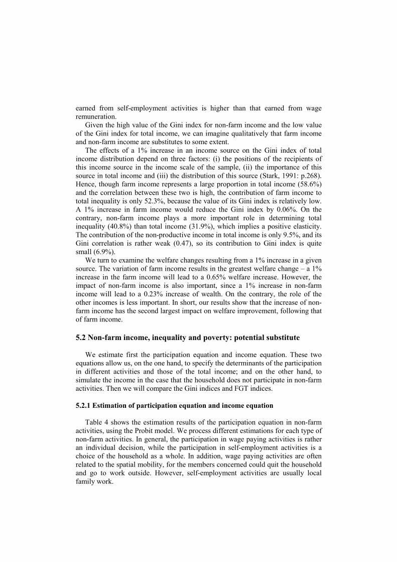
Table 4 shows the estimation results of the participation equation in non-farm

activities, using the Probit model. We process different estimations for each type of

non-farm activities. In general, the participation in wage paying activities is rather

an individual decision, while the participation in self-employment activities is a

choice of the household as a whole. In addition, wage paying activities are often

related to the spatial mobility, for the members concerned could quit the household

and go to work outside. However, self-employment activities are usually local

family work.

15

Table 4: Estimation of participation equations

Regression 1:

Non-farm

activities

Regression 2:

Self-

employment

activities

Regression 3:

Wage paying

activities

Number of workers 0.436*** 0.061 0.463***

(6.54) (1.16) (8.10)

Average number of years in school 0.143* 0.296*** -0.060

(1.68) (3.72) (-0.75)

Average number of years in school in square -0.002 -0.021*** 0.013*

(-0.32) (-3.15) (1.93)

Proportion of household members that have

received some technical and professional

trainings 0.859** 0.481* 0.181

(2.32) (1.76) (0.63)

Land surface of the household -0.031*** -0.004 -0.017**

(-4.01) (-0.30) (-2.19)

Land surface of the household in square

(/100) 0.012* -0.024 0.008

(1.82) (-0.81) (1.22)

Number of dependent persons 0.046 0.126** -0.107**

(0.77) (2.49) (-2.06)

Actual value of the house (/100000) 0.793* 0.689** 0.003

(1.92) (2.28) (0.01)

Distance between the village center and the

nearest railway station -0.002* 0.001 -0.004***

(-1.93) (1.25) (-3.98)

Distance between the village center and the

nearest bus station -0.087 -0.140*** 0.015

(-1.55) (-2.60) (0.28)

Cultivable land per capita of the village -0.056*** -0.002 -0.054***

(-2.62) (-0.10) (-2.64)

Constant -0.562* -1.470*** -0.662**

(-1.82) (-4.88) (-2.23)

Maximum likelihood in log -381.900 -498.386 -469.798

Pseudo R2 0.167 0.053 0.139

Number of observation 787 787 787

The t-student are in brackets. *** significant in 1%; ** significant in 5%; * significant in 10% .

First, we find that households rich in labor are more likely to participate in non-

farm activities, generally speaking. The problem of surplus farm labor (or

disguised unemployment) became explicit in rural area after the implementation of

HRS. As the quantity of the cultivable land is very limited, the large number of

surplus farm labor keeps the per capita rural income at a low level, which pushes

labor leaving the farms. However, the number of workers does not influence the

participation in self-employment activities, that is to say, the non-farm work of the

household. It can be explained by the fact that self-employment activities require

entrepreneurship. In addition, the dependent persons themselves can also partially

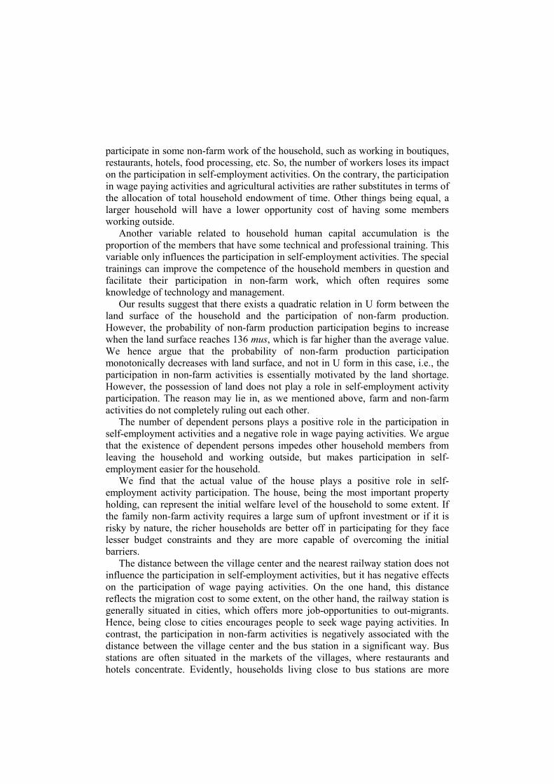
participate in some non-farm work of the household, such as working in boutiques,

restaurants, hotels, food processing, etc. So, the number of workers loses its impact

on the participation in self-employment activities. On the contrary, the participation

in wage paying activities and agricultural activities are rather substitutes in terms of

the allocation of total household endowment of time. Other things being equal, a

larger household will have a lower opportunity cost of having some members

working outside.

Another variable related to household human capital accumulation is the

proportion of the members that have some technical and professional training. This

variable only influences the participation in self-employment activities. The special

trainings can improve the competence of the household members in question and

facilitate their participation in non-farm work, which often requires some

knowledge of technology and management.

Our results suggest that there exists a quadratic relation in U form between the

land surface of the household and the participation of non-farm production.

However, the probability of non-farm production participation begins to increase

when the land surface reaches 136 mus, which is far higher than the average value.

We hence argue that the probability of non-farm production participation

monotonically decreases with land surface, and not in U form in this case, i.e., the

participation in non-farm activities is essentially motivated by the land shortage.

However, the possession of land does not play a role in self-employment activity

participation. The reason may lie in, as we mentioned above, farm and non-farm

activities do not completely ruling out each other.

The number of dependent persons plays a positive role in the participation in

self-employment activities and a negative role in wage paying activities. We argue

that the existence of dependent persons impedes other household members from

leaving the household and working outside, but makes participation in self-

employment easier for the household.

We find that the actual value of the house plays a positive role in self-

employment activity participation. The house, being the most important property

holding, can represent the initial welfare level of the household to some extent. If

the family non-farm activity requires a large sum of upfront investment or if it is

risky by nature, the richer households are better off in participating for they face

lesser budget constraints and they are more capable of overcoming the initial

barriers.

The distance between the village center and the nearest railway station does not

influence the participation in self-employment activities, but it has negative effects

on the participation of wage paying activities. On the one hand, this distance

reflects the migration cost to some extent, on the other hand, the railway station is

generally situated in cities, which offers more job-opportunities to out-migrants.

Hence, being close to cities encourages people to seek wage paying activities. In

contrast, the participation in non-farm activities is negatively associated with the

distance between the village center and the bus station in a significant way. Bus

stations are often situated in the markets of the villages, where restaurants and

hotels concentrate. Evidently, households living close to bus stations are more

17

likely to participate in family non-farm activities. In addition, being close to the

bus station would encourage the commute between village and fairs or cities,

which makes household non-farm exploitation easier.

Finally, as we expect, the shortage of land in the village acts as a repulsion force

that drives rural labor to quit the land and participate in non-farm activities.

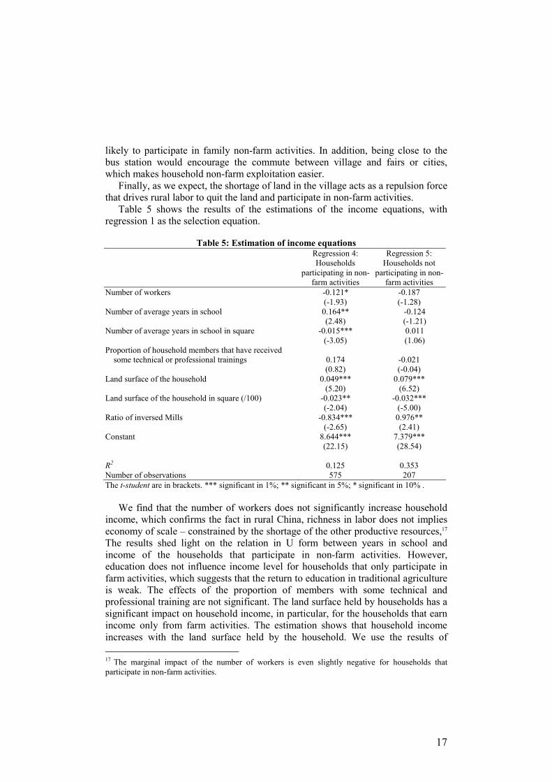
Table 5 shows the results of the estimations of the income equations, with

regression 1 as the selection equation.

Table 5: Estimation of income equations

Regression 4:

Households

participating in non-

farm activities

Regression 5:

Households not

participating in non-

farm activities

Number of workers -0.121* -0.187

(-1.93) (-1.28)

Number of average years in school 0.164** -0.124

(2.48) (-1.21)

Number of average years in school in square -0.015*** 0.011

(-3.05) (1.06)

Proportion of household members that have received

some technical or professional trainings 0.174 -0.021

(0.82) (-0.04)

Land surface of the household 0.049*** 0.079***

(5.20) (6.52)

Land surface of the household in square (/100) -0.023** -0.032***

(-2.04) (-5.00)

Ratio of inversed Mills -0.834*** 0.976**

(-2.65) (2.41)

Constant 8.644*** 7.379***

(22.15) (28.54)

R2 0.125 0.353

Number of observations 575 207

The t-student are in brackets. *** significant in 1%; ** significant in 5%; * significant in 10% .

We find that the number of workers does not significantly increase household

income, which confirms the fact in rural China, richness in labor does not implies

economy of scale – constrained by the shortage of the other productive resources,17

The results shed light on the relation in U form between years in school and

income of the households that participate in non-farm activities. However,

education does not influence income level for households that only participate in

farm activities, which suggests that the return to education in traditional agriculture

is weak. The effects of the proportion of members with some technical and

professional training are not significant. The land surface held by households has a

significant impact on household income, in particular, for the households that earn

income only from farm activities. The estimation shows that household income

increases with the land surface held by the household. We use the results of

17 The marginal impact of the number of workers is even slightly negative for households that

participate in non-farm activities.

regression 5 to simulate the income of the households that participate in non-farm

activities in the case that they participate only in farm activities.

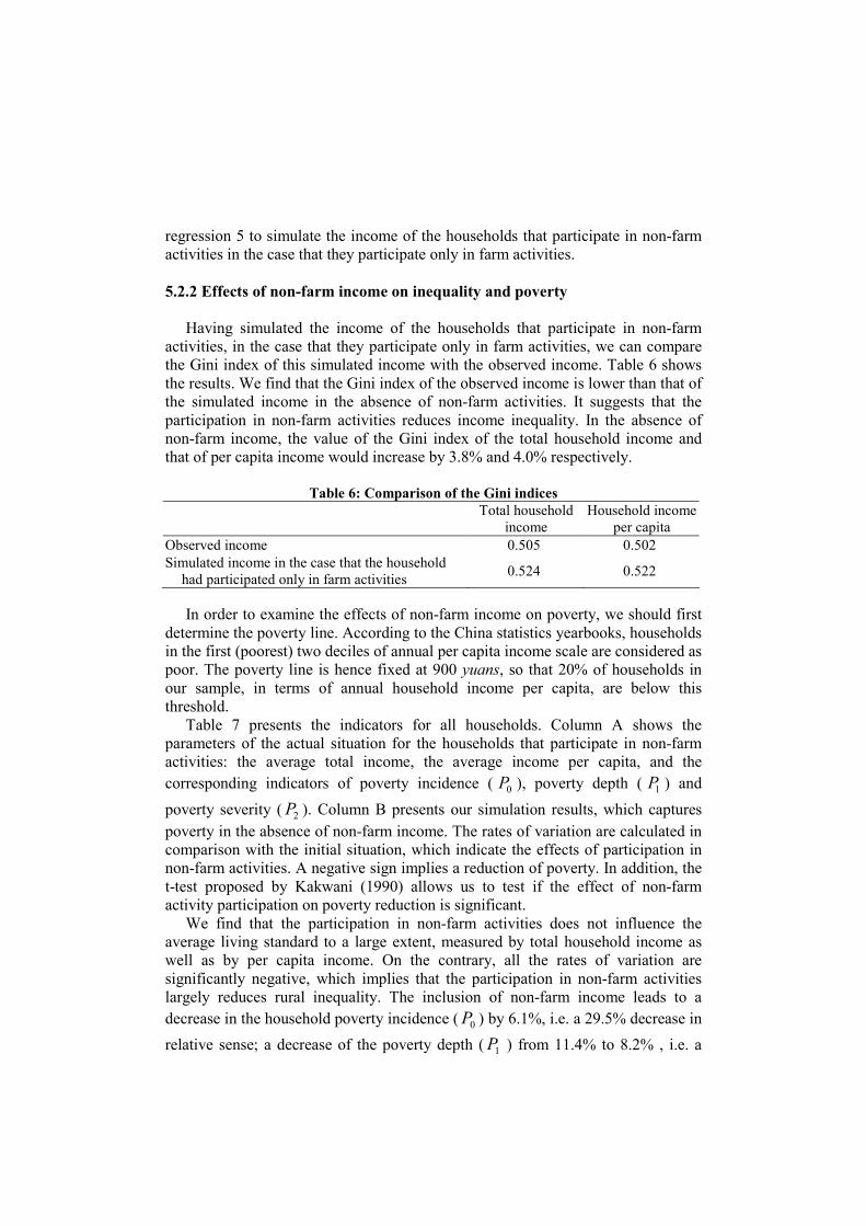
5.2.2 Effects of non-farm income on inequality and poverty

Having simulated the income of the households that participate in non-farm

activities, in the case that they participate only in farm activities, we can compare

the Gini index of this simulated income with the observed income. Table 6 shows

the results. We find that the Gini index of the observed income is lower than that of

the simulated income in the absence of non-farm activities. It suggests that the

participation in non-farm activities reduces income inequality. In the absence of

non-farm income, the value of the Gini index of the total household income and

that of per capita income would increase by 3.8% and 4.0% respectively.

Table 6: Comparison of the Gini indices

Total household

income

Household income

per capita

Observed income 0.505 0.502

Simulated income in the case that the household

had participated only in farm activities 0.524 0.522

In order to examine the effects of non-farm income on poverty, we should first

determine the poverty line. According to the China statistics yearbooks, households

in the first (poorest) two deciles of annual per capita income scale are considered as

poor. The poverty line is hence fixed at 900 yuans, so that 20% of households in

our sample, in terms of annual household income per capita, are below this

threshold.

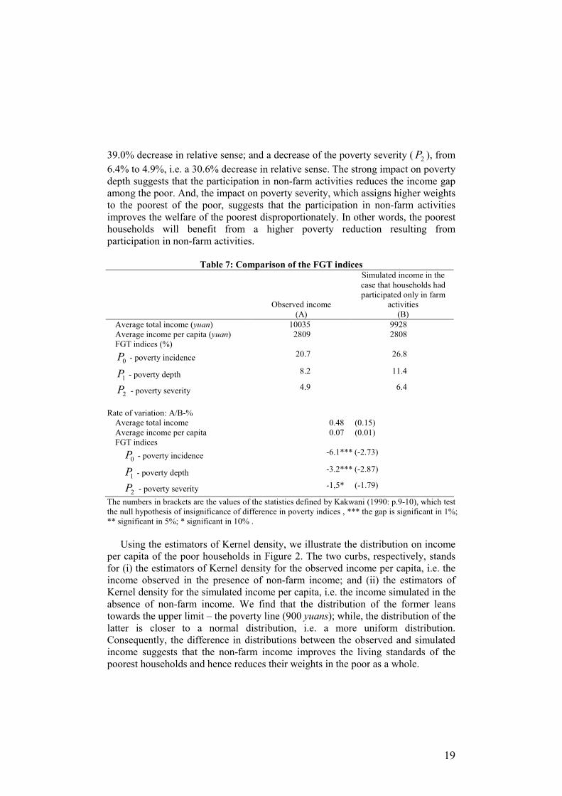
Table 7 presents the indicators for all households. Column A shows the

parameters of the actual situation for the households that participate in non-farm

activities: the average total income, the average income per capita, and the

corresponding indicators of poverty incidence ( 0P ), poverty depth ( 1P ) and

poverty severity ( 2P ). Column B presents our simulation results, which captures

poverty in the absence of non-farm income. The rates of variation are calculated in

comparison with the initial situation, which indicate the effects of participation in

non-farm activities. A negative sign implies a reduction of poverty. In addition, the

t-test proposed by Kakwani (1990) allows us to test if the effect of non-farm

activity participation on poverty reduction is significant.

We find that the participation in non-farm activities does not influence the

average living standard to a large extent, measured by total household income as

well as by per capita income. On the contrary, all the rates of variation are

significantly negative, which implies that the participation in non-farm activities

largely reduces rural inequality. The inclusion of non-farm income leads to a

decrease in the household poverty incidence ( 0P ) by 6.1%, i.e. a 29.5% decrease in

relative sense; a decrease of the poverty depth ( 1P ) from 11.4% to 8.2% , i.e. a

19

39.0% decrease in relative sense; and a decrease of the poverty severity ( 2P ), from

6.4% to 4.9%, i.e. a 30.6% decrease in relative sense. The strong impact on poverty

depth suggests that the participation in non-farm activities reduces the income gap

among the poor. And, the impact on poverty severity, which assigns higher weights

to the poorest of the poor, suggests that the participation in non-farm activities

improves the welfare of the poorest disproportionately. In other words, the poorest

households will benefit from a higher poverty reduction resulting from

participation in non-farm activities.

Table 7: Comparison of the FGT indices

Observed income

(A)

Simulated income in the

case that households had

participated only in farm

activities

(B)

Average total income (yuan) 10035 9928

Average income per capita (yuan) 2809 2808

FGT indices (%)

0P - poverty incidence 20.7 26.8

1P - poverty depth 8.2 11.4

2P - poverty severity 4.9 6.4

Rate of variation: A/B-%

Average total income 0.48 (0.15)

Average income per capita 0.07 (0.01)

FGT indices

0P - poverty incidence -6.1*** (-2.73)

1P - poverty depth -3.2*** (-2.87)

2P - poverty severity -1,5* (-1.79)

The numbers in brackets are the values of the statistics defined by Kakwani (1990: p.9-10), which test

the null hypothesis of insignificance of difference in poverty indices , *** the gap is significant in 1%;

** significant in 5%; * significant in 10% .

Using the estimators of Kernel density, we illustrate the distribution on income

per capita of the poor households in Figure 2. The two curbs, respectively, stands

for (i) the estimators of Kernel density for the observed income per capita, i.e. the

income observed in the presence of non-farm income; and (ii) the estimators of

Kernel density for the simulated income per capita, i.e. the income simulated in the

absence of non-farm income. We find that the distribution of the former leans

towards the upper limit – the poverty line (900 yuans); while, the distribution of the

latter is closer to a normal distribution, i.e. a more uniform distribution.

Consequently, the difference in distributions between the observed and simulated

income suggests that the non-farm income improves the living standards of the

poorest households and hence reduces their weights in the poor as a whole.

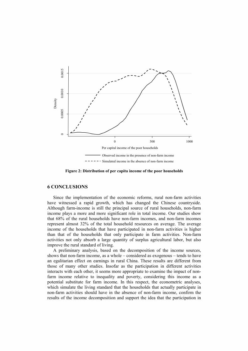
Figure 2: Distribution of per capita income of the poor households

6 CONCLUSIONS

Since the implementation of the economic reforms, rural non-farm activities

have witnessed a rapid growth, which has changed the Chinese countryside.

Although farm-income is still the principal source of rural households, non-farm

income plays a more and more significant role in total income. Our studies show

that 68% of the rural households have non-farm incomes, and non-farm incomes

represent almost 32% of the total household resources on average. The average

income of the households that have participated in non-farm activities is higher

than that of the households that only participate in farm activities. Non-farm

activities not only absorb a large quantity of surplus agricultural labor, but also

improve the rural standard of living.

A preliminary analysis, based on the decomposition of the income sources,

shows that non-farm income, as a whole – considered as exogenous – tends to have

an egalitarian effect on earnings in rural China. These results are different from

those of many other studies. Insofar as the participation in different activities

interacts with each other, it seems more appropriate to examine the impact of non-

farm income relative to inequality and poverty, considering this income as a

potential substitute for farm income. In this respect, the econometric analyses,

which simulate the living standard that the households that actually participate in

non-farm activities should have in the absence of non-farm income, confirm the

results of the income decomposition and support the idea that the participation in

Simulated income in the absence of non-farm income

Observed income in the presence of non-farm income

Density

Per capital income of the poor households

0

0.0005

0.0010

0.0015

0 500 1000

21

non-farm activities mitigates, noticeably, rural poverty. Our results indicate that the

participation in non-farm activities reduces rural poverty by 6.1%. It also reduces,

considerably, poverty depth and poverty severity, which suggests that participation

in non-farm activities, not only reduces income gap between rural poor households,

but also disproportionately improves the household income of the poorest.

In fact, in rural China, following the implementation of HRS, the basic budget

unit became the household. Land was allocated as a function of the household size.

As rural households do not have the property right but only utilization right over

the land they cultivate, the land market does not exist. Hence, farm income is

relatively stable because it is impossible to increase the size of farm work. Because

of this, non-farm activities may serve as a solution for rural surplus labor. The

participation in non-farm activities provides an addition income source to rural

households, which improves their living standards and reduces their income gaps.

As Gillis et al. (1983: p.560) suggest: “To the extent that small enterprises can

generate more employment per unit and can locate in smaller cities and towns, they

will promote greater income equality among families, among regions, and between

rural and urban areas.”

The HRS significantly increases farm productivities. However, the weakness of

this system began to appear recently in the 1990s. For example, the division of land

into small plots strongly impedes the development of agricultural modernization.

Given China’s geography and existing technology, in the short run, agriculture

development cannot mainly rely on land surface increase or on technical

improvement, but on regrouping the plots and allocating them to experimental

farmers to seek greater economies of scale. Therefore, a great part of the surplus

agricultural labor must leave the agricultural sector, and non-farm activities will

thus continue to play a critically important role in rural development and poverty

reduction.

REFERENCES

Adams R.H.J. (1989) “Worker Remittances and Inequality in Rural Egypt”, Economic

Development and Cultural Change 38(1): pp.45-71.

(1999), “Non-farm Income, Inequality and Land in Rural Egypt”, Policy Research Working Paper 2178, The World Bank.

, He J.J. (1995), “Sources of Income Inequality and Poverty in Rural Pakistan”, IFPRI Research Report 102.

Aubert C. (1995), “Exode rural, exode agricole en Chine, la grande mutation ?”, Espace

Populations Société (1995-2): pp. 231-245.

Banister J., Taylor J.R. (1990) “China: Surplus Labour and Migration”, Asia-Pacific

Population Journal 4(4): pp.3-20.

Berdegué J.A., Ramirez E., Reardon T., Escobar G. (2001), “Rural Nonfarm Employment

and Income in Chile”, World Development 29(3): pp.411-425.

Bhalla A.S. (1990) “Rural-Urban Disparities in India and China”, World Development

18(8): pp.1097-1110.

Barham B., Boucher S. (1998) “Migration, remittances, and inequality: estimating the

effects of migration on income distribution”, Journal of Development Economics 55:

pp.307-331.

Byrd W., Lin Q. (1994), China’s Rural Industry: Structure, Development, and Reform,

Oxford, Oxford University Press, 622 p.

Chinn D.L. (1979) “Rural Poverty and the Structure of Farm Household Income in

Developing Countries: Evidence from Taiwan”, Economic Development and Cultural

Change 27(2): pp.283-301.

Davin D. (1999), Internal Migration in Contemporary China, New York: St.Martin’s Press,

Inc., 177 p.

De Beer P., Rocca J-L (1997), La Chine à la fin de l’ère DENG Xiaoping, Paris, Le Monde-

Editions, 216 p.

Deininger K., Olinto P., (2001), “Rural Nonfarm Employment and Income Diversification

in Colombia”, World Development 29(3): pp.455-465.

Elbers C., Lanjouw P. (2001), “Intersectoral Transfert, Growth, and Inequality in Rural

Ecuador”, World Development 29(3), pp.481-496.

Escobal J. (2001), “The Determinants of Nonfarm Income Diversification in Rural Peru”,

World Development 29(3): pp.497-508.

Estudillo J.P., Otsuka K. (1999), “Green Revelution, Human Capital, and Off-Farm

Employment: Changing Sources of Income among Farm Household in Central Luzon,

1966-1994”, Economic Development and Cultural Change 47(3): pp.497-523.

FAO (1998) The state of food and agriculture 1998, Rome, FAO.

Foster J., Greer J., Thorbecke E. (1984), “A class of decomposable poverty measures”,

Econometrica 52(3): pp.761-766.

Gillis M., Perkins D.H., Roemer M., Snodgrass D.R. (1983), Economics of developpement,

New York/London: W.W.Norton & Company, 599 p.

Goldstein S., Goldstein A. (1991), “Rural industrialization and migration in the People’s

Republic of China”, Social Science History 15(3): pp.289-314.

Greene W.H. (1997), Econometric Analysis, New Jersey, Prentice-Hall International,

1075p.

Heckman J. (1979), “Sample selection bias as a specification error”, Econometrica 47(1):

pp.153-161.

Hussain A., Lanjouw P., Stern N. (1994), “Incom Inequalities in China: Evidence from

Household Survey Data”, World Development 22(12): pp.1947-1957.

Kakwani N. (1990), Testing for Significance of Poverty Differences: With Application to

Côte d’Ivoire (Living Standards Measurement Study Working Paper No.62),

Washington, The World Bank, 40 p.

Khan A.R., Risin C. (2001), Inequality and Poverty in China in the Age of Globalization,

New York, Oxford University Press, 184 p.

Kimhi A. (1994), “Quasi Maximum Likelihood Estimation of Multivariate Probit Models:

Farm Couples’ Labor Participation”, American Journal of Agricultural Economics

76(4): pp.828-835.

Knight J., Song L. (1993), “The spatial contribution to income inequality in rural China”,

Cambridge Jounal of Economics 17: pp. 195-213.

Lachaud J-P. (1999), “Envois de fonds, inégalité et pauvreté au Burkina Faso”, Revue Tiers

Monde 40(160): pp.793-827.

Leones J.P., Feldman S. (1998), “Nonfarm Activity and Rural Household Income:

Evidence from Philippine Microdata”, Economic Development and Cultural Change

46(4): pp.789-806.

23

Lewis W.A. (1954), “Economic Developement with Unlimited Supply of Labour”, The

Manchester School of Economic and Social Studies 47(3): pp. 139-191.

McMillan J., Whalley J., Zhu L. (1989), “The Impact of China’s Economic Reforms on

Agricultural Productivity Growth”, Journal of Political Economiy 97(4): pp. 781-807.

National Bureau of Statistics of China (2001), China Statistical Yearbook 2001, Beijing:

Chinese Statistics Press, 899 p.

Pyatt G., Chen C., Fei J. (1980), “The Distribution of Income by Factor Component”,

Quartely Journal of Economics 95(3): pp.451-473.

Reardon T., Taylor J.E. (1996), “Agroclimatic Shock, Income Inequality, and Poverty:

Evidence from Burkina Faco”, World Development 24(5): pp.901-914.

Richard H., Adams R.H.J. (1994), “Non-Farm Income and Inequality in Rural Pakistan: A

Decomposition Analysis”, The Journal of Development Studies 31(1): pp.110-133.

Sadoulet E., De Janvry A., (2001), “Income Strategies Among Rural Households in

Mexico: The Role of Off-farm Activities”, World Development 29(3): pp.467-480.

Sen A.K. (1976), “Poverty: an ordinal approch to measurement”, Econometrica 44(2):

pp.219-231.

Shand R.T. (1987), “Income Distribution in a Dynamic Rural Sector: Some Evidence from

Malasia”, Economic Development and Cultural Change 36(1987): pp.35-50.

Stark O. (1991), The Migration of Labor, Oxford, Basil Blackwell, 406 p.

, Taylor J.E., Yitzhaki S. (1986), “Remittances and Inegality”, Economic Journal 96(383): pp.722-740.

StataCorp. (1997) Stata Reference Manual Release 5.0, Volume II, Texas, Stata Press.

Taylor J.E., Yunez-Naude A. (1999), Education, migration et productivité : une analyse

des zones rurales au Mexique, Paris : Centre de Développement de l’OCDE, 108 p.

Wang Y. (1995), “Permanent Income and Wealth Accumulation: A Cross-Sectional Study

of Chinese Urban and Rural Households”, Economic Development and Cultural Change

43(3): pp.523-550.

Yao S. (1999), “Economic Growth, Income Inequality and Poverty in China under

Economic Reforms”, Journal of Development Studies 35(6): pp.103-130.

Yunez-Naude A., Taylor J.E. (2001), “The Determinants of Nonfarm Activities and

Incomes of Rural Households in Mexico, with Emphasis on Education”, World

Development 29(3), pp. 561-572.

Zhao Y. (1999a), “Labor Migration and Earnings Differences: The Case of Rural China”,

Economic Development and Cultural Change 47(4): pp.767-782.

(1999b), “Leaving the Countryside: Rural-to-Urban Migration Decision in China”, The American Economic Review 89(2): pp. 281-286.

Zhou Q. (1994), Rural reforms and Development in China, Hong Kong: Oxford University

Press, 360 p.

Zhu L. (1991), Rural Reform and Peasant Income in China, London: Macmillan, 218 p.

, Jiang Z. (1993), “From brigade to village community: the land tenure system and rural development in China”, Cambridge Journal of Economics 17: pp.441-461.

Zhu N. (2002), Analyse des migrations en Chine: mobilité spatiale et mobilité

professionnelle, Thèse de doctorat, CERDI, Clermont-Ferrand, novembre 2002, 337 p.