The Pennsylvania State University

The Graduate School

IMPACTS OF IMPURITIES AND THERMAL HISTORY ON

THE ELECTRICAL CONDUCTION AND CHARGE TRAPPING

CHARACTERISTICS IN CROSSLINKED POLYETHYLENE

THIN FILMS

A Dissertation in

Materials Science and Engineering

by

Roger Craig Walker II

© 2020 Roger Craig Walker II

Submitted in Partial Fulfillment

of the Requirements

for the Degree of

Doctor of Philosophy

August 2020

ii

The dissertation of Roger C. Walker II was reviewed and approved by the following:

Michael T. Lanagan

Professor of Engineering Science & Mechanics

Dissertation Adviser

Chair of Committee

Ramakrishnan Rajagopalan

Assistant Professor of Engineering, Applied Materials at Penn State DuBois

Ralph Colby

Professor of Materials Science and Engineering

Professor of Chemical Engineering

T.C. Mike Chung

Professor of Materials Science and Engineering

John Mauro

Professor of Materials Science and Engineering

Chair of the Materials Science and Engineering Program

iii

Abstract

The work presented in this dissertation is primarily aimed at improving the understanding of the

electrical properties of the insulating polymer crosslinked polyethylene (XLPE) in order to support

its use as power cable insulation. XLPE has been used for decades as the material of choice in this

application due to its low cost, the ease of maintaining it, its improved environmental friendliness

over what it was replacing, and – most importantly – its low DC conductivity and AC losses.

However, it has several unaddressed issues associated with its use in the long term due to extrinsic

impurities (such as water and acetophenone) and intrinsic variability (due to its semicrystalline

nature). A better understanding of how these factors influence the electrical properties of XLPE is

needed both to enhance the fundamental knowledge regarding this prominent polymer and to

improve its utility as power cable insulation.

As such, an analysis of the electrical properties of XLPE was carried out by using four separate

types of analyses. Broadband dielectric spectroscopy (BDS) was used to analyze the AC response.

Conduction current measurement (CCM) and current-voltage measurement (IVM) were used to

analyze the DC response. Thermally stimulated depolarization current (TSDC) technique was used

to analyze the charge trapping characteristics of polyethylene. XLPE thin film samples were

generated by melt pressing pellets of low-density polyethylene (LDPE) that were infused with the

crosslinking agent dicumyl peroxide (DCP). Some LDPE pellets were not infused with DCP and

used to make LDPE thin films for comparative purposes. After fabrication, a selection of films

was degassed in order to remove impurities. Some of those films were then soaked in specific

impurities to intentionally re-introduce that one in particular. Aluminum electrodes were then

applied to the samples in the same high-vacuum evaporation chamber to a thickness of 50 nm at a

deposition rate of 2.5 A/s. Electrode diameters were fixed at either 1 cm or 3 cm, and the thickness

was measured after electrode deposition.

Chapter 3 goes into the details of the AC analysis of polyethylene. Samples were characterized

electrically by their dielectric loss, a measure of inefficiency during the AC cycle that can also be

related to the AC conductivity. It was found that the presence of impurities such as DCP

byproducts had a strong impact on the AC response in two different ways. One is that the presence

of impurities above a certain threshold led to significant increases in the dielectric loss at room

temperature. The other is that excess impurities modified the structure as was seen by alterations

in the temperature coefficient of capacitance (TCC). The impurities are polar in nature and created

an internal pressure that enhanced thermal expansion when compared to degassed XLPE and to

as-received LDPE.

Chapter 4 goes into the details of the phenomenon of electrical compensation in polyethylene.

Compensation is an observed trend where the activation energy and pre-exponential factor for

conductivity are correlated. It had been previously observed in the DC conduction of LDPE and it

was found that it can also be observed in the DC conduction of XLPE via CCM. Additionally, it

was also found in AC conduction as observed in the BDS results. Electrical compensation was not

observed in as-received XLPE samples that were water soaked instead of degassed for AC

conduction, and those samples generally had low activation energy of 0.2 eV or less. All other

samples exhibited variation in the range of 0.2 eV to 1.4 eV in AC. All samples showed

compensation in DC in the range of 0.2 eV to 1.0 eV for activation energies. The observed

compensation was determined to arise from sample to sample variation in polar impurities such as

water and was sensitive to the thermal history of each sample.

iv

Chapter 5 goes into the details of charge trapping in polyethylene as examined using the TSDC

technique. TSDC analysis results in a spectrum of current measured as the temperature rises,

indicating what temperatures were needed to release trapped charges as well as the amount of

stored charge and the energy associated with that release. As-received XLPE samples tended to

exhibit one peak in the TSDC spectra associated with impurities. Their removal via degassing

meant that three peaks could be observed – that same impurity peak, but also peaks associated with

molecular motions near the glass transition temperature and with charge injection in the melting

range of polyethylene. Harsher degassing was shown to reduce the impacts of these impurities and

of charge injection. Acetophenone was found to be the key DCP byproduct in determining the

overall trapping characteristics of XLPE.

Chapter 6 goes into the details of a brief examination of the response of XLPE to applied DC

bias using IVM. Both the time response of the current and the current-voltage spectra were

examined. It was found that that overall response of XLPE could be altered depending on one of

two things: the thermal history via changing the degassing temperature and the presence of

impurities via the addition of acetophenone. Both the standard 65°C degassed and the test 90°C

degassed samples exhibited true conduction current with the 90°C samples having reduced

conductivity and higher activation energy in comparison. The addition of ACP into the standard

degassed samples reduced the activation energy and the conductivity but the current response was

now due to polarization rather than true conduction. Additionally, standard samples were found to

exhibit space charge limited current while the others had ohmic or sub-ohmic response.

Chapter 7 contains a summary and directions for future work. In general, it is suggested that

future investigations should combine experiment and simulation to best determine how thermal

history and impurities determine the electrical properties of XLPE samples. What is needed to

know is how precisely these two factors alter the resulting structure of the XLPE and contribute to

changes in these various responses to applied electrical fields. It was also suggested to look into

the impacts of other impurities not related to DCP such as antioxidants and nanoparticles.

v

Table of Contents

List of Figures ............................................................................................................................................. vii

List of Tables .............................................................................................................................................. xii

Acknowledgements .....................................................................................................................................xiii

Chapter 1 – Introduction and Literature Review........................................................................................... 1

1.1 Cross-linked Polyethylene as used in Power Cable Insulation ........................................................... 1

1.2 Polyethylene Morphology, Degassing, and Crosslinking ................................................................... 4

1.3 Oxidation of Polyethylene .................................................................................................................. 9

1.4 Breakdown Phenomena in LDPE and XLPE .................................................................................... 12

1.5 Dielectric Properties of LDPE and XLPE ......................................................................................... 14

1.6 Electrical Conduction in LDPE and XLPE ....................................................................................... 16

1.7 Space Charge Phenomena in LDPE and XLPE ................................................................................ 18

1.8 Trap States in LDPE and XLPE ........................................................................................................ 19

Chapter 2 – Experimental Procedure .......................................................................................................... 22

2.1 Preparation of LDPE and XLPE electrical test samples ................................................................... 22

2.2 Broadband dielectric spectroscopy (BDS) ........................................................................................ 27

2.3 Conduction current measurement (CCM) and current-voltage measurement (IVM) ....................... 30

2.4 Thermally stimulated depolarization current (TSDC) ...................................................................... 32

2.5 Structural and chemical characterization techniques ........................................................................ 36

Chapter 3 – Effects of crosslinks and residual molecules on the dielectric response and structure of

polyethylene ................................................................................................................................................ 38

3.1 Temperature coefficient of capacitance of XLPE and LDPE ........................................................... 38

3.2 Impacts of degassing on room temperature dielectric loss of XLPE and LDPE .............................. 41

3.3 Impacts of degassing on the AC conductivity at 90°C of XLPE and LDPE .................................... 44

3.4 Effect of crosslinking temperature on the dielectric response and TCC ........................................... 47

3.5 Effect of DCP concentration on the dielectric response and TCC .................................................... 49

3.6 Acetophenone impacts on the dielectric loss, AC conductivity, and TCC ....................................... 53

3.7 Impacts of radiation exposure on the conductivity and TCC of LDPE ............................................ 58

Chapter 4 – Continuously variable activation energy in polyethylene ....................................................... 63

4.1 Background on electrical compensation, the isokinetic temperature, and the Meyer-Neldel Rule .. 63

4.2 Compensation law in the DC conductivity of degassed XLPE and LDPE ....................................... 69

4.3 Compensation law comparison between AC and DC conductivity .................................................. 73

vi

4.4 Impacts of small molecules such as water ........................................................................................ 77

4.5 Impacts of repeated measurements ................................................................................................... 80

4.6 Impacts of radiation exposure ........................................................................................................... 86

4.7 The origins of electrical compensation in polyethylene ................................................................... 88

Chapter 5 – Electronic and ionic traps in polyethylene active in different temperature ranges .................. 91

5.1 Basic TSDC spectra of XLPE and LDPE ......................................................................................... 91

5.2 Comparison of the TSDC spectra as-received and degassed XLPE ................................................. 98

5.3 Impacts of DCP byproducts on the XLPE and LDPE..................................................................... 101

5.4 Impacts of antioxidants on the TSDC spectra of XLPE and LDPE ................................................ 104

5.5 Summary of trap states detectable in polyethylene by TSDC ......................................................... 107

5.6 Impacts of the poling parameters on the TSDC spectra of XLPE samples ..................................... 112

Chapter 6 – High-field current-voltage measurements of polyethylene ................................................... 118

6.1 Time response and current decay in XLPE ..................................................................................... 118

6.2 Current-voltage response of degassed XLPE and impact of degassing temperature ...................... 121

6.3 Current-voltage response of degassed LDPE and comparison to XLPE ........................................ 126

6.3 Changes in degassed XLPE due to acetophenone soaking ............................................................. 127

6.4 Overall summary of the obtained current-voltage relationship in polyethylene ............................. 130

Chapter 7 – Summary and Suggestions for Future Work ......................................................................... 132

References ................................................................................................................................................. 137

vii

List of Figures

Figure 1.1 HVDC cable with XLPE insulation. Source:

https://wiki.openelectrical.org/index.php?title=Cable_Construction ............................................. 3 Figure 1.2 Trend in XLPE cable insulation thickness over time during the 1990s [4] .................. 4

Figure 1.3 Small molecules associated with the crosslinking reaction in polyethylene ................ 6 Figure 1.4 a) Byproduct removal in 5.5 mm thick XLPE medium voltage cable insulation [22];

b) Measured trend of increased LDPE crystallinity with longer annealing [45]. ........................... 8 Figure 1.5 Thermogravimetric analysis plot of low-density polyethylene. The dashed line

indicates the crosslinking temperature. ......................................................................................... 11

Figure 1.6 Infrared spectroscopy comparison of oxidation content in different polyethylene

samples processed under the same conditions. Calculated result is based on sample absorbance in

the spectral range of 1719 – 1730 cm-1, corresponding to the stretching of a carbon oxygen

double bond. .................................................................................................................................. 12 Figure 1.7 Current-voltage plot of LDPE and XLPE from the literature [47,75–81]. ................. 17 Figure 2.1 Weight change of the LDPE pellets depends on the square root of time at short times

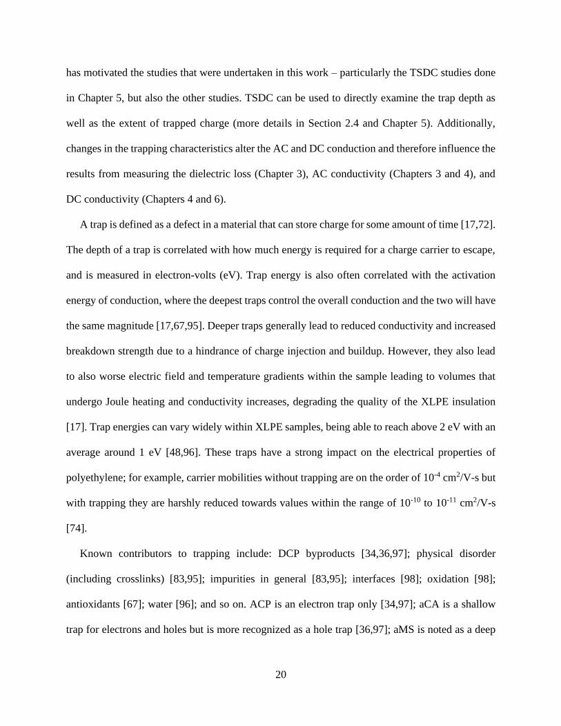
and exponential dependency close to fully soaked state. .............................................................. 23 Figure 2.2 FTIR mapping of the pellet cross-section shows complete soaking of the pellet with

DCP ............................................................................................................................................... 24 Figure 2.3 Comparison of the FTIR mapping profile (yellow circles) and modeling result (solid

lines) .............................................................................................................................................. 24

Figure 2.4 Schematic of the overall experimental procedure ...................................................... 27 Figure 2.5 Measurement equipment used for BDS ...................................................................... 28

Figure 2.6 Measurement equipment used for CCM and IVM ..................................................... 31 Figure 2.7 Schematic of applied field and temperature over time for samples with a storage

temperature of a) 25°C and b) -150°C. The black solid line represents the temperature and the

purple dashed line represents the electric field. ............................................................................ 33 Figure 2.8 Measurement equipment used for TSDC ................................................................... 34

Figure 2.9 Representative TSDC spectra with a storage temperature of -150°C for degassed

LDPE with differing applied electric fields as listed in the supplied legend. ............................... 36

Figure 2.10 DSC traces of low-density polyethylene. The negative peak (endothermic) is

associated with melting and the positive peak (exothermic) is associated with solidification. .... 37 Figure 3.1 a) TCC measurement of 2 samples of low-density polyethylene (LDPE) and

comparison to literature data for the LTEC of the same polymer. Xc represents the crystallinity of

polyethylene. LTEC data reproduced from White, G. K.; Choy, C. L. J. Polym. Sci. Polym. Phys.

Ed. 1984. b) Average TCC comparison between as-received XLPE, as-received LDPE, degassed

XLPE, and degassed LDPE samples. ........................................................................................... 38

Figure 3.2 Mass change in as-received XLPE (2% DCP) and LDPE as measured via TGA. ..... 40 Figure 3.3 Average TCC comparison between as-received XLPE, degassed XLPE, and 90°C

degassed XLPE samples ............................................................................................................... 41 Figure 3.4 Comparison of the room temperature dielectric loss values measured at 10 Hz and

below for XLPE and LDPE samples crosslinked at various temperatures. .................................. 42

Figure 3.5 Comparison of raw broadband dielectric spectra for XLPE and LDPE samples

crosslinked at various temperatures. ............................................................................................. 43 Figure 3.6 Comparison of the room temperature dielectric loss values measured at 10 Hz and

below for various XLPE samples. ................................................................................................ 43

viii

Figure 3.7 a) Dielectric loss of as-received XLPE and LDPE samples measured at 90°C; b)

Conductivity of as-received XLPE and LDPE samples measured at 90°C; c) Average low

frequency conductivity of the same samples from frequencies of 10 Hz and below. ................... 44 Figure 3.8 Average low frequency conductivity (f ≤ 10 Hz) at 90°C conductivity comparison

between as-received and degassed a) XLPE samples; b) LDPE samples. ................................... 46 Figure 3.9 Average low frequency conductivity (f ≤ 10 Hz) at 90°C conductivity comparison

between various XLPE samples.................................................................................................... 47

Figure 3.10 Average low frequency 90°C conductivity comparison between as-received XLPE

samples crosslinked at different temperatures. ............................................................................. 48 Figure 3.11 TCC comparison between as-received XLPE samples crosslinked at different

temperatures. ................................................................................................................................. 48 Figure 3.12 TCC comparison between degassed XLPE samples crosslinked with different

concentrations of DCP added. A comparison to as-received samples has been included. ............ 49

Figure 3.13 a) Mass change in as-received XLPE with different amounts of DCP as measured

via TGA. An LDPE and a degassed XLPE sample were also prepared for comparative purposes;

b) Concentration of ACP in XLPE (13% DCP) samples with and without degassing. ................ 50

Figure 3.14 Average low frequency room temperature dielectric loss in degassed XLPE samples

crosslinked with different DCP concentrations............................................................................. 52 Figure 3.15 Average low frequency 90°C conductivity comparison between degassed XLPE

samples crosslinked with different concentrations of DCP added. ............................................... 53 Figure 3.16 Negative TCC comparison between different XLPE types: a) all sample types; b)

zoom in on XLPE, degassed XLPE, and XLPE after a soak in water for two hours. .................. 54 Figure 3.17 Average dielectric loss at 0.1 Hz as a function of temperature for XLPE samples

treated under different conditions. ................................................................................................ 55

Figure 3.18 a) Log scale plot of the average dielectric loss at 0.1 Hz as a function of temperature

for XLPE samples treated under different conditions; b) comparison at 90°C. ........................... 55 Figure 3.19 Capacitance at 1 kHz of the XLPE samples analyzed in Figure 3.16. ..................... 57 Figure 3.20 Temperature and frequency dependence of the capacitance of a) a representative

degassed XLPE sample soaked with ACP; b) a representative as-received XLPE sample

containing antioxidant. .................................................................................................................. 58

Figure 3.21 Comparison of the room temperature dielectric loss values measured at 10 Hz and

below for various LDPE sample types. ......................................................................................... 59 Figure 3.22 Average low frequency conductivity (f ≤ 10 Hz) at 90°C conductivity comparison

between various LDPE samples.................................................................................................... 60 Figure 3.23 Negative TCC comparison between different LDPE types. ..................................... 61 Figure 3.24 Temperature and frequency dependence of the capacitance of a) a representative as-

received LDPE sample exposed to radiation in ambient; b) a representative as-received LDPE

sample exposed to radiation while sealed; c) a representative as-received LDPE sample. .......... 62

Figure 4.1 a) Raw current data for a degassed XLPE measured at various temperatures with 2

kV applied; b) Raw current data for a degassed LDPE measured at various temperatures with 2

kV applied; c) Current data converted into conductivity and plotted against temperature to obtain

the activation energy. .................................................................................................................... 63 Figure 4.2 Compensation plots for a) low-density polyethylene [130] and b) various organic

semiconducting compounds [131]. ............................................................................................... 64 Figure 4.3 Charge carrier mobility in organic field effect transistors based on C60. The gate

voltage was varied with two different drain voltages applied as shown in the two plots [135]. .. 66

ix

Figure 4.4 Reference examples where compensation and isokinetic temperature are not observed

together. a,b) Compensation behavior without a corresponding isokinetic temperature. c,d)

Isokinetic temperature without corresponding compensation behavior [132]. ............................. 67 Figure 4.5 Compensation plot comparing degassed XLPE and degassed LDPE. Comparison

LDPE data from the work of Sawa et al [130] is indicated separately. ........................................ 70 Figure 4.6 Plot of activation energy against pre-exponential factor for two degassed LDPE

samples as a function of the measurement time. The number presented in the legend is the

earliest time at which the current is counted for extraction of the Arrhenius parameters. ........... 71 Figure 4.7 a) Conductivity vs temperature plot and b) compensation law plot for degassed XLPE

samples .......................................................................................................................................... 72 Figure 4.8 a) Conductivity vs temperature plot and b) compensation law plot for degassed LDPE

samples .......................................................................................................................................... 72

Figure 4.9 Compensation law plots for a) degassed XLPE and b) degassed LDPE comparing the

DC and AC results. The corresponding conductivity vs temperature data for the AC

measurements are shown in c) and d) ........................................................................................... 74

Figure 4.10 a) AC conductivity vs temperature plot and b) compensation law plot for water-

soaked XLPE samples. A comparison to the degassed XLPE samples discussed previously is

included in the plot on the right .................................................................................................... 77 Figure 4.11 Compensation law plot for XLPE samples that have been both water-soaked and

degassed. A comparison to the XLPE samples that have been either degassed or water-soaked is

included in the plot........................................................................................................................ 79

Figure 4.12 Repeated temperature-dependent conductivity measurements for degassed a) XLPE

and b) LDPE. In part c), the loops for XLPE and LDPE were preceded by either heating from

25°C to 90°C or cooling down from 90°C to 25°C the sample in the oven with no electrical field

applied. .......................................................................................................................................... 81

Figure 4.13 a) Compensation plot comparing all the XLPE and LDPE samples to the runs shown

in Figure 4.5 after initial runs or treatments; b) Extrapolated conductivity at the nominal

‘isokinetic point’ of 120.9°C for the same samples plotted in red. Legend is shown separately

below the conductivity plot. .......................................................................................................... 83 Figure 4.14 a) Compensation plot of degassed XLPE samples repeatedly measured under AC

conditions and comparison to the samples presented in Figure 4.8; b) Combination of AC and

DC data showing the changes in the compensation plot due to the annealing that occurs with

repeat measurement or pre-treatment. ........................................................................................... 86

Figure 4.15 Compensation plot of irradiated LDPE samples and comparison to as-received and

degassed LDPE under a) AC and b) DC measurement conditions. .............................................. 87 Figure 4.16 All compensation plots of DC conduction for samples discussed in this chapter. ... 89

Figure 4.17 All compensation plots of AC conduction for samples discussed in this chapter. ... 89

Figure 5.1 Representative TSDC spectra with a storage temperature of -150°C for degassed a)

LDPE and b) XLPE with differing applied electric fields as listed in the supplied legend. The

XLPE samples were crosslinked with 2.1% and 2.2% DCP respectively. ................................... 91 Figure 5.2 Cyclical TSDC discharges of a cable sample conventionally polarized at Tp = 90 °C,

T0 = 50 °C, Vp = 8 kV, tp = 60 min. Samples were brought up to 140°C before poling and at the

end of the heating run during each cycle. [23].............................................................................. 93

Figure 5.3 TSDC spectra of a degassed XLPE repeatedly poled at 10 kV/mm with a) 65°C or b)

90°C degas prior to measurement. The storage temperature is a constant at 25°C. ..................... 94

x

Figure 5.4 TSDC spectra with a storage temperature of -150°C for XLPE samples degassed at

two different temperatures: a) 65°C; b) 90°C. Applied fields are listed in the legend. ................ 94

Figure 5.5 Activation energy and maximum temperature of major peaks in the TSDC spectra of

degassed LDPE and XLPE samples. All samples are included in this figure, showcasing the full

variation. ....................................................................................................................................... 96 Figure 5.6 a) TSDC spectra with a storage temperature of -150°C for as-received XLPE

samples; b) Activation energy and maximum temperature of the medium temperature peak for

as-received and degassed samples. ............................................................................................... 99 Figure 5.7 Concentration of ACP in various XLPE samples as determined by IR spectroscopy.

..................................................................................................................................................... 100 Figure 5.8 TSDC spectra with a storage temperature of -150°C for degassed XLPE samples

soaked in acetophenone (ACP). .................................................................................................. 101

Figure 5.9 TSDC spectra with a storage temperature of -150°C for degassed XLPE samples

soaked in methylstyrene (aMS). ................................................................................................. 103 Figure 5.10 Peak maximum current and cumulative stored charge on average for the medium

temperature peak in different sample types. ............................................................................... 104

Figure 5.11 a) Schematic structure and names of the two antioxidants used in this study; b)

TSDC spectra for as-received XLPE samples containing the two different types of antioxidant.

..................................................................................................................................................... 105

Figure 5.12 TSDC spectra of as-received LDPE samples with antioxidant added. ................... 107 Figure 5.13 Activation energy and maximum temperature of major peaks in TSDC spectra of

degassed XLPE samples, sorted by type, with a comparison to as-received samples. ............... 108 Figure 5.14 Activation energy and maximum temperature of major peaks in TSDC spectra of

various types of as-received XLPE samples, sorted by type. ..................................................... 109

Figure 5.15 TSDC spectra of degassed XLPE samples measured under varying a) poling

temperatures and b) applied fields. The parameters used for each sample are shown in the legend.

..................................................................................................................................................... 113 Figure 5.16 Maximum temperature and current of the high temperature TSDC peak as a function

of the poling temperature for a fixed poling field. ...................................................................... 114 Figure 5.17 Maximum a) temperature and b) current of the high temperature TSDC peak as a

function of the poling field for a fixed poling temperature. ....................................................... 116 Figure 6.1 Time response of the current in degassed XLPE at 90°C depending on the applied

voltage in linear (left) and log (right) scales. The legend is the same for both plots. ................. 119

Figure 6.2 Time response of the current in a) degassed XLPE with ACP at 90°C and b) degassed

LDPE at 90°C depending on the applied voltage. ...................................................................... 120 Figure 6.3 Plot of measured current density against the applied electric field for standard

degassed XLPE samples. ............................................................................................................ 122

Figure 6.4 Plot of measured current density against the applied electric field for XLPE samples

degassed at 90°C. ........................................................................................................................ 124 Figure 6.5 Comparison plot of measured current density against the applied electric field for

standard degassed XLPE samples and for XLPE samples degassed at 90°C. ............................ 125 Figure 6.6 Plot of measured current density against the applied electric field for standard

degassed LDPE samples ............................................................................................................. 127

Figure 6.7 a) Plot of measured current density against the applied electric field for standard

degassed XLPE samples soaked in ACP; b) Comparison plot of measured current density against

xi

the applied electric field for standard degassed XLPE samples without and with soaking in ACP

..................................................................................................................................................... 128

Figure 6.8 Current-voltage measurements of LDPE and XLPE, including comparisons to

literature from the following sources: [47,75–81]. ..................................................................... 131

xii

List of Tables

Table 1.1 Properties of the three major DCP byproducts .............................................................. 7 Table 1.2 Dielectric strength of LDPE and XLPE ....................................................................... 13 Table 1.3 Literature values of dielectric loss for polyethylene samples measured at 50 Hz. ...... 15

Table 3.1 Room temperature dielectric loss for samples discussed in the main text. .................. 52 Table 4.1 A list of materials exhibiting the compensation law [133,134] ................................... 65 Table 4.1 Compensation parameters of the degassed XLPE and LDPE samples discussed up to

this point, as well as several literature references of LDPE ......................................................... 76 Table 4.2 Compensation parameters of all XLPE and LDPE samples discussed in this chapter. 90

Table 5.1 Activation energy and maximum temperature of major peaks in TSDC spectra of

various types of XLPE and LDPE samples discussed up to this point. ...................................... 109 Table 6.1 Exponent of the power law time response of the current in degassed XLPE depending

on the applied voltage. ................................................................................................................ 119 Table 6.2 Exponent of the power law time response of the current in degassed XLPE with ACP

at 90°C and degassed LDPE at 90°C depending on the applied voltage. ................................... 120

Table 6.3 Activation energy and power law exponents for standard degassed XLPE samples . 123 Table 6.4 Activation energy and power law exponents for XLPE samples degassed at 90°C .. 124

Table 6.5 Comparison of activation energy and power law exponents standard degassed XLPE

samples and for XLPE samples degassed at 90°C ...................................................................... 125 Table 6.6 Comparison of conductivity values for standard degassed XLPE samples and for

XLPE samples degassed at 90°C ................................................................................................ 126 Table 6.7 Activation energy and power law exponents standard degassed LDPE samples ...... 127

Table 6.8 Comparison of activation energy and power law exponents standard degassed XLPE

samples soaked in acetophenone ................................................................................................ 128

Table 6.9 Comparison of activation energy and power law exponents standard degassed XLPE

samples and for XLPE samples degassed at 90°C ...................................................................... 129 Table 6.10 Comparison of conductivity values for standard degassed XLPE samples and for

XLPE samples degassed at 90°C ................................................................................................ 129 Table 6.11 Exponent of the power law time response of the current in degassed XLPE with and

without ACP depending on the applied voltage and temperature............................................... 130

xiii

Acknowledgements

I would like to thank my research adviser (Dr. Michael Lanagan) and my collaborators (Hossein

Hamedi, Cesar Nieves, Jiasheng Ru, Dr. Maryam Sarkarat, Dr. Ramakrishnan Rajagopalan, Dr.

Eugene Furman, and Dr. William Hunter Woodward) for their assistance and many great

discussions. I also want to give a great thanks to many groups of people for their support over the

years, including: my family and friends; my fellow graduate students in the Materials Science

department and across the university; the PSU social dance community (including Centre Social

Dance, PSU Social Dance Club, and the Late Night Lindyhop and Blues crew); the Penn State

Taiko Club and all of their supporters; all the people involved in the State College Board Gaming

meetup; the staff at Zeno’s; the State College Pokémon GO community; and many others!

This project was funded by the Dow Chemical Company (UPI225559AM) and was completed

with the assistance of the Penn State Materials Characterization Laboratory, the Penn State

Nanofabrication Facility, the Penn State Radiation Science and Engineering Center, and the Penn

State Electrical Characterization Laboratory. Funding for additional experiments was provided by

the Alfred P. Sloan Foundation’s Minority Ph.D. scholarship (G‐2016‐20166039).

1

Chapter 1 – Introduction and Literature Review

This section introduces several important concepts with regard to the use of crosslinked

polyethylene (XLPE) as a material in power cable insulation. First, the context in which this

material is used will be discussed. Second, its means of fabrication and the resulting morphology

will be established. Third, the electrical properties of XLPE will be analyzed using various lenses:

breakdown phenomena, dielectric phenomena, electrical conduction, space charge, and trap states.

1.1 Cross-linked Polyethylene as used in Power Cable Insulation High voltage power cable insulation was first created in the late 1800s when the process of

electrifying societies began in earnest, and started existence as oil-impregnated paper [1,2]. This

material is still in use today in old cables. However, with the advent of synthetic plastics in the

mid-20th century, there has been an accelerating push to develop new insulation from them, and

the one currently used most often is crosslinked polyethylene (XLPE), which started replacing oil-

impregnated paper insulation during the 1960s [1–6]. The transition to XLPE for high voltage

alternating current (HVAC) and high-voltage direct current (HVDC) cables has occurred due to

favorable properties such as low dielectric losses, simple maintenance, and environmental

friendliness when compared to the old fluid-filled insulation [1,4,5]. The evolution of HV cable

insulation has been driven by requirements for reliable, high volume, and environmentally-friendly

power distribution across large geographic areas by the public and by the need for low-cost

production of large quantities of cable that require only minor maintenance by the manufacturers

and utility owners [4,5,7]. The voltages that define HV tend to increase over time, but other design

needs stay the same such as stability over decades, stability under variable loads, and stability in

ambient conditions [2]. As such, XLPE cable insulation must be able to demonstrate good

performance and reliability by meeting these requirements while also being low cost [4,8].

2

XLPE is made up of a three-dimensional network of interconnected branched polymer chains.

It is a major material used for power cable insulation [4,5,9–12], particularly in Japan and northern

Europe [4,10]. XLPE has mostly replaced oil-impregnated paper as cable insulation. It is made by

taking its base form, low-density polyethylene (LDPE), and generating crosslinks through the use

of an external agent, in this case dicumyl peroxide (DCP). More details regarding this process will

be given in the next section; here, the focus will be on the use of polyethylene in power cables as

insulation. Both LDPE and XLPE are in use as power cable insulation. These materials are

preferred due to several favorable properties they have. Among them are being low cost,

electrically insulating, showing chemical resistance, having simple processing and installation, and

being more environmentally friendly than oil-impregnated paper [13,14]. XLPE is preferred over

LDPE due its superior mechanical stability over a wide temperature range due to its crosslinks

[6,14,15]. The gel-like thermoset XLPE will not flow with prolonged exposure to elevated

temperatures [3,16]. As such, it is able to be operated continuously at 90°C and in emergency

scenarios can be run up to 140°C [3].

The main applications of HVDC cables are long-range power transmission and regional

interconnects [17]. The main advantages of using HVDC over HVAC are not having capacitive

charging currents as part of the transmission and not needing to synchronize between different AC

networks [1,16]. This promotes its use for very long cables, especially ones meant to run

underwater. It is also more suitable for renewable generation such as with wind and solar [1]. The

main disadvantage is the higher overall costs for the system, which means it is used for long-

distance transmission primarily [16].

XLPE specifically as insulation for HVDC has been studied since the 1980s, has in use since

1999 at 80 kV rating, and can go to 525 kV as of 2016 [17]. It has been similarly successfully used

3

in HVAC applications and is desired to be used in HVDC mainly because of the success in HVAC.

Cables are constructed as follows: 1. A conductive copper wire is coated with tape; 2. Layers of

semicon, insulation, and semicon are co-extruded onto the wire; 3. This structure is heat-treated in

a degassing procedure; 4. An outer coating is applied of a metal sheath and a polyethylene jacket

[3,16]. The semicon layer refers to a polymer layer made conductive by the use of carbon black.

It promotes adhesion of the insulation to the wire and creates a smooth interface between the two.

A picture of a completed cable is presented in Figure 1.1.

Figure 1.1 HVDC cable with XLPE insulation. Source:

https://wiki.openelectrical.org/index.php?title=Cable_Construction

However, failure is common for reasons that will be explored in more detail in Sections 1.6 and

1.7. Excess charges [18,19], both free and trapped, and defects [20,21] are two of the key limiting

4

factors to XLPE performance, and are often related [11]. The main factor limiting the further

development of XLPE is the buildup of space charge [1]. Residual stresses induced by these

charges and defects leads to voiding, reduced breakdown strength, and eventual failure [2,6]. As

such, cables that are designed for 20 to 30 years have failed in half that time due to factors such as

oxidation, moisture, electrical stresses, and defects [2,3]. This degradation over time tends to take

the form of electrical and water trees, which can be mitigated by better cable design and improving

the quality of the XLPE insulation [3]. It is known that producing large volumes with minimal

defects is a limiting factor in XLPE cable manufacture [22], and it has been claimed that trapped

some extrinsic defects is inevitable due to viscosity [13]. However, improvements have been made

that allowed the insulation to be made thinner over time [4], as shown in Figure 1.2.

Figure 1.2 Trend in XLPE cable insulation thickness over time during the 1990s [4]

1.2 Polyethylene Morphology, Degassing, and Crosslinking The polyethylene family consists of non-polar semi-crystalline polymers based on repeating CH2

units [23,24]. As this is the only requirement for a molecule to be considered polyethylene, several

5

variants exist beyond low-density polyethylene (LDPE), a version with large concentrations of

branches splitting from the main chains and crosslinked polyethylene (XLPE), a version where

branches are connected to each other in order to generate a three-dimensional network. However,

only these two variants will be discussed within this text.

Crosslinks are most commonly made using the small molecule dicumyl peroxide (DCP) [21],and

are primarily added to provide additional thermo-mechanical stability to the polymer [12,14,25]

while maintaining [26–28] or enhancing [5,24] its insulating behavior. XLPE-based power cables

have a maximum continuous operating temperature of 90°C, which is 20°C higher than allowed

for LDPE-based power cables [28,29]. XLPE can be used at such a temperature due to the

crosslinks keeping it physically stable even though its melting range is from 50°C to 110°C

[23,30]. The DCP compound is mixed with LDPE pellets to allow for the crosslinking reaction to

occur at high temperatures during the extrusion or pressing process. The generally accepted

temperature range for this is between 160°C and 220°C [31] as the polymer needs to be fully

molten for the reaction to proceed most efficiently [14].

Crosslinking occurs in the following stages: first, the peroxide bond in DCP is broken, creating

two radicals; second, each radical scavenges a hydrogen off of a polyethylene molecule; third, two

radical elements on different polyethylene molecules react and form a bond, creating a crosslink

[13,14,26]. If the DCP radical directly scavenges a hydrogen, then it becomes cumyl alcohol

(aCA), which can then break down into water and methylstyrene (aMS). If the DCP breaks apart

and gives off a methyl radical before interacting with a polyethylene molecule, then acetophenone

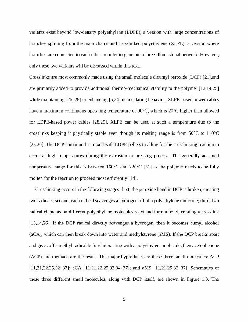
(ACP) and methane are the result. The major byproducts are these three small molecules: ACP

[11,21,22,25,32–37]; aCA [11,21,22,25,32,34–37]; and aMS [11,21,25,33–37]. Schematics of

these three different small molecules, along with DCP itself, are shown in Figure 1.3. The

6

byproducts are distributed throughout the volume [21] based on curing time and temperature [22],

with greater concentrations in less dense regions [25]. ACP and aCA are found in greater

concentration than aMS, and aMS will also diffuse out the fastest as ACP and aCA will compete

with each other [21]. Less common are other defects such as methane and water [22,34], residual

DCP and 2,4-diphenyl-4-methyl-1-pentene [21], dimethylbenzyl alcohol [33], and phenol

compounds [11], so the main three will be the focus here. A table listing several of their relevant

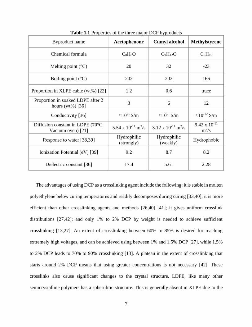
properties is provided in Table 1.1.

Figure 1.3 Small molecules associated with the crosslinking reaction in polyethylene

7

Table 1.1 Properties of the three major DCP byproducts

Byproduct name Acetophenone Cumyl alcohol Methylstyrene

Chemical formula C8H8O C9H12O C9H10

Melting point (°C) 20 32 -23

Boiling point (°C) 202 202 166

Proportion in XLPE cable (wt%) [22] 1.2 0.6 trace

Proportion in soaked LDPE after 2

hours (wt%) [36] 3 6 12

Conductivity [36] ≈10-6 S/m ≈10-8 S/m ≈10-12 S/m

Diffusion constant in LDPE (70°C,

Vacuum oven) [21] 5.54 x 10-11 m2/s 3.12 x 10-11 m2/s

9.42 x 10-11

m2/s

Response to water [38,39] Hydrophilic

(strongly)

Hydrophilic

(weakly) Hydrophobic

Ionization Potential (eV) [39] 9.2 8.7 8.2

Dielectric constant [36] 17.4 5.61 2.28

The advantages of using DCP as a crosslinking agent include the following: it is stable in molten

polyethylene below curing temperatures and readily decomposes during curing [33,40]; it is more

efficient than other crosslinking agents and methods [26,40] [41]; it gives uniform crosslink

distributions [27,42]; and only 1% to 2% DCP by weight is needed to achieve sufficient

crosslinking [13,27]. An extent of crosslinking between 60% to 85% is desired for reaching

extremely high voltages, and can be achieved using between 1% and 1.5% DCP [27], while 1.5%

to 2% DCP leads to 70% to 90% crosslinking [13]. A plateau in the extent of crosslinking that

starts around 2% DCP means that using greater concentrations is not necessary [42]. These

crosslinks also cause significant changes to the crystal structure. LDPE, like many other

semicrystalline polymers has a spherulitic structure. This is generally absent in XLPE due to the

8

crosslinks interfering with macroscopic organization, so spherulites are either distorted or absent

[6,15]. The density and crystallinity of the polyethylene film also drops after crosslinking

[14,15,21,27,43,44] but this drop is sometimes small [15,21].

However, the use of DCP as a crosslinking agent also means that its byproducts will be left

behind in the resulting film. As such, degassing is used to remove the byproducts [11,21,22]. In

this procedure, XLPE is heated in a vacuum environment to hasten the out-diffusion of byproducts,

which proceeds slowly in ambient [21,22]. This is done before any outer layers are added. For

cables, the generally temperature accepted range is 50°C to 80°C, with 60°C to 70°C being most

used for practical reasons [22]. Thick cables require very long degassing times on the order of

hundreds of hours to remove the byproducts, as shown in Figure 1.4a [22]. Degassing is a form of

annealing in vacuum or reduced environments, and leads to increases in the crystallinity [16]. Even

short anneals (for example, 2 hours at 50°C) have been shown to increase the crystallinity [45]. A

trend showing the increase in crystallinity with annealing at 50°C is shown in Figure 1.4b. This is

a trend that continues with long-term aging; however, too much aging leads to samples that can

become brittle and fail mechanically [13].

Figure 1.4 a) Byproduct removal in 5.5 mm thick XLPE medium voltage cable insulation [22];

b) Measured trend of increased LDPE crystallinity with longer annealing [45].

9

Morphological differences between polyethylene variants, as well as changes within a sample,

can be measured electrically using techniques such as broadband dielectric spectroscopy and

conduction current measurements [46]. This has motivated several of the experiments to be

discussed in later chapters. With the defects removed, the morphology becomes more important in

governing electrical properties, and is controlled by processing parameters such as temperature

and additives [47]. Included in the morphology of LDPE are major polar groups such as hydroxyl,

carbonyl, and methyl, each of which are sources of loss [24]. Simulations created by combining

density functional theory and molecular dynamics have supported this idea, revealing that these

groups add trap states in the LDPE band gap [48]. They are expected to be retained in XLPE, along

with voids between spherulites that contribute to reductions in dielectric strength [5]. Additionally

in LDPE, low density regions were suggested to trap electrons [48,49] while branches and

crosslinks were suggested to trap holes [48]. Trap states that could be attributed to these were

found experimentally in LDPE [19,50]. Most studies on morphology focused on LDPE and few

have looked at XLPE. One study looking mostly at LDPE observed reduced conductivity in

degassed XLPE when compared to LDPE and correlated this to changes in morphology [47].

Another study claims that crosslinking independent of DCP byproducts has minimal impact on

space charge buildup [37], while another has shown that recrystallization at high temperatures will

impact charging [51]. However, not much work has been done to conclusively show how

crosslinking and other morphological changes alone matter.

1.3 Oxidation of Polyethylene Oxidation has been shown to have a significant impact on the electrical properties of polyethylene,

and occurs preferentially in the amorphous regions. The oxidation process starts when a radical

site can be attacked by molecular oxygen, forming an oxidized radical that scavenges a hydrogen,

10

resulting in a hydroperoxide group [52]. That group then scavenges another hydrogen, leading to

the creation of water and two reactive sites – one with and one without an oxygen – leading to

further reactions. Antioxidants can be used to delay the onset of oxidation, which is important

commercially for power cable insulation. Careful control over the electrical properties is needed.

For example, oxidation in the form of carbonyl groups creates traps with an average energy of

around 1 eV and adds to the overall conduction current by introducing a dipolar component [53].

Other authors have shown that some oxidation can reduce conductivity in LDPE but that further

oxidation will then lead to increased conductivity [54]. Similarly, oxidation was also found

enhance conductivity in LDPE by an order of magnitude by other authors [55]. The activation

energy of conduction was not found to be altered by oxidation, remaining around 1.1 eV, implying

that the concentration of traps is altered by oxidation but not their energy. Oxidation also has the

effect of increasing both the permittivity and the dielectric loss [56].

As shown in a thermogravimetric analysis (TGA) plot of an LDPE thin film sample (Figure

1.5), oxidation can occur over a wide temperature range and leads to mass gain. This process

occurs due to the formation of oxygen-bearing side groups such as hydroxyls and carbonyls. The

TGA data shows that oxidation can occur across a wide temperature range, becoming more

prominent once the polyethylene melts (Tm = 105°C). Since there is no longer a crystalline region

in the molten polymer, all bonds are available to be attacked [57]. As such, oxidation is expected

in the melt pressed films which are processed at 180°C. There is also a difference in the extent of

oxidation when DCP is introduced, due to extra oxidation that can occur from the introduction of

a peroxide. This difference is reflected in infrared spectroscopy data (Figure 1.6), where there is

more oxidation in crosslinked samples (compare LDPE and XLPE) as determined by measurement

of vibrations due to carbon oxygen bonds. The added antioxidant (P and M) is able to prevent this

11

extra oxidation, so those samples are comparable to base LDPE in terms of oxidation. However,

the introduction of the antioxidant has its own impacts on the electrical properties [54], motivating

some investigations detailed later in the dissertation.

Oxidation also has an important secondary effect. Oxygen groups are polar and hydrophilic,

and their presence promotes water uptake. It has been determined that an increase of oxygen groups

by 30 ppm corresponds to a 1 pm increase in water solubility [58]. Further diffusion is then

dependent not on time nor water content, but on oxidation level. There was also a noted

dependence with the oxygen-bearing side group, as hydroxyl, hydroperoxide, and carboxylic

groups, groups that naturally form during oxidation, bind water very strongly when compared to

other possibilities such as ketones and ester groups. This implies that water treeing will be a natural

consequence of the oxidation that occurs during aging in ambient environments, and thus be the

ultimate cause of failure. As such, minimizing both oxidation and water uptake are critical for the

long lifetime of XLPE power cable insulation. This is done in practice by a combination of harsh

vacuum degassing, antioxidant incorporation, and protection with an outer protective jacket.

Figure 1.5 Thermogravimetric analysis plot of low-density polyethylene. The dashed line

indicates the crosslinking temperature.

12

Figure 1.6 Infrared spectroscopy comparison of oxidation content in different polyethylene

samples processed under the same conditions. Calculated result is based on sample absorbance in

the spectral range of 1719 – 1730 cm-1, corresponding to the stretching of a carbon oxygen

double bond.

1.4 Breakdown Phenomena in LDPE and XLPE Ultimately, XLPE cables fail due to electrical breakdown. At sufficiently high electrical fields,

charge carriers such as electrons are able to knock out other charge carriers out of bonds and traps

via Auger recombination, leading to runaway growth in the electrical current [59]. This can occur

either locally or throughout the material. It is accompanied by physical deformation, electrical

arcing, melting, and other detriments. The lowest field at which this takes place is known as the

dielectric strength, and the corresponding voltage measured across the sample is the breakdown

voltage. The design dielectric strength of XLPE is approximately two orders of magnitude lower

than literature values due to trapped charges and defects, leading to thick cables that are difficult

13

to fully degas [5,22]. Thickness-dependence in the dielectric strength of XLPE will be expected if

there are significant concentrations of defects [60], along with a drop in the strength when

compared to degassed films [31,61]. Typical dielectric strengths for LDPE and XLPE are provided

in Table 1.2. While some variation exists, there are no clear differences between LDPE and

degassed XLPE. XLPE without degassing shows a decrease in the dielectric strength due to

interference from the defects.

Table 1.2 Dielectric strength of LDPE and XLPE

LDPE or XLPE Dielectric Strength

(MV/cm) Ref. Notes

XLPE 8 [5] Intrinsic resin strength

LDPE 6.25 [62] LDPE, 30°C

LDPE 6 [63] Room temperature strength; strength drops to

1 MV/cm as film melts

LDPE 5.5 [61]

XLPE 4.89 [31] Reference degassed XLPE (6 days, 70°C)

XLPE 4.88 [31] Degassed XLPE (6 days, 70°C)

XLPE 4.47 [31] Degassed XLPE (6 days, 70°C)

XLPE 4.45 [31] Not-degassed XLPE

XLPE 4.42 [31] Not-degassed XLPE

XLPE 4.27 [31] Reference not-degassed XLPE

XLPE 4 [61] Degassed one hour in vacuum chamber

LDPE 4 [62] LDPE, 50°C

LDPE 3.42 [62] LDPE, 70°C

LDPE 3.19 [62] LDPE, 90°C

XLPE 2 [61] No degassing; maximum electrical field was

3.5 MV/cm

XLPE 0.08 [5] Power cable design strength due to defects

For XLPE, breakdown in both AC and DC conditions is associated with space charge buildup

of homocharge and heterocharge (discussed in more detail in Section 1.6). In short, homocharge

injected at the electrodes at high fields becomes trapped rather than moving through the sample,

leading to failure as it accumulates and the local field becomes arbitrarily large [64]. Injection

occurs at both electrodes [59] with holes being associated with the anode [64] and electrons being

associated with the cathode. Heterocharge, however, is associated with impurities such as DCP

14

byproducts but has the same impact [65]. There are some differences between AC and DC. For

example, AC breakdown is reportedly not significantly influenced by DCP byproducts [66], but

the same could not be said for DC breakdown [61]. An increase in temperature leads to a reduced

dielectric strength for DC breakdown, which is associated with electromechanical failure [67]. The

same temperature sensitivity was not seen for AC conditions [62].

1.5 Dielectric Properties of LDPE and XLPE Polymeric insulators are characterized in this application by their dielectric loss and by their AC

conductivity. Dielectric loss is defined as the energy lost during AC operation relative to the total

energy stored by a dielectric during the polarization cycle. It is also referred to as the loss tangent

and presented as tan δ. Loss and the AC conductivity are related by the following equation:

(1) 𝜎 = 휀′ ∗ tan 𝛿 ∗ 2𝜋𝑓

where σ is the AC conductivity, ε′ is the real component of the complex permittivity, tan δ is the

dielectric loss, and f is the frequency. This value is often measured at power frequency (50 Hz),

and a table of literature values for the dielectric loss in LDPE is provided in Table 1.3. Low

frequency dielectric loss is proportional to the leakage current [8,68], and large currents are

detrimental to the XLPE insulation. Low loss thus leads to negligible conductivity in AC

conditions, and also in the case of direct current (DC) as the frequency approaches zero. Such a

state can be achieved by removing sources of trapped charges such as DCP byproducts [22]. The

low loss then allows the material to survive at high electric fields before breaking down [4] and

thus achieve a high dielectric strength. High loss, on the other hand, leads to unwanted heating,

excess conductivity, and eventual failure. Whether or not XLPE reaches the ideal low loss state is

governed by a mix of intrinsic and extrinsic factors, of which the extrinsic defects added due to

crosslinking are the most critical for XLPE.

15

Table 1.3 Literature values of dielectric loss for polyethylene samples measured at 50 Hz.

Sample Dielectric Loss Electric Field

(kV/mm)

Temperature Ref.

LDPE ~0.01 1 <50°C [69]

LDPE ~0.01 0.5 n/a [34]

LDPE coated with acetophenone ~0.3 0.5 n/a [34]

LDPE ~0.01 5 25°C [70]

LDPE ~0.01 40 25°C [70]

LDPE mixed with acetophenone

(0.3 wt%)

~0.01 5 25°C [70]

LDPE mixed with acetophenone

(0.3 wt%)

~0.2 40 25°C [70]

Dielectric loss is known to depend on both the frequency and temperature in polyethylene [68].

In summary: at low frequency, the loss increases as the frequency is reduced; at high frequency,

the loss increases as the frequency is increased; at intermediate frequencies, the loss is low and

constant. The low frequency conductive losses are known to be temperature-dependent. Degassing

is generally confirmed to reduce dielectric losses in XLPE [16,68]. As was discussed in Section

1.3, degassing removes impurities and increases crystallinity. However, there is only a limited

amount of work relating structural changes to modification of the electrical properties [24,47,71].

It was shown by Sato and Yashiro that the secondary structure (crosslinks, branches, etc.) can be

as important in determining the dielectric loss as polar impurities, though this effect tends to be

seen only at very high frequencies (e.g. MHz). Preventing oxidation and reducing branching

concentration was recommended for reducing losses [24]. This was also be seen in current density

measurements [47]. Meanwhile, aging will lead to increases in the loss [68].

Testing of cables is essential for monitoring their condition during use, as well as for quality

testing beforehand, to ensure that the appropriate dielectric and electrical performance can still be

maintained. Many technical specifications exist for such testing. As far as the insulation is

concerned, the main features to be monitored are the dimensions, strength, elongation, resistivity,

16

and water absorption. Visual inspections need to be done, as well as tests for partial discharges

and high voltage performance. Dielectric losses are important to the overall wasted energy in the

system and need to be minimized, hence the need to check for defects and excess conductivity.

The overall wasted energy in XLPE is determined by the applied voltage, the dielectric loss, and

the geometry. For a cable, this means the ratio of the insulation outer and inner radii. As such, a

technique such as BDS that measures the complex capacitance, and can thus give information on

both the geometry and the loss, is quite useful for testing purposes. As such, it has been proposed

as a technique to detect aging over time [68]. For the experimental work discussed in Chapter 3,

the single temperature measurements developed in that reference were extended into temperature-

dependent measurements in order to obtain parameters such as activation energy and temperature

coefficient of capacitance. Given that both are related to fundamental phenomena and can be

obtained in the same BDS measurement, it will be useful to also obtain these during testing of

XLPE cable insulation if it can be done swiftly and without too much additional expense.

1.6 Electrical Conduction in LDPE and XLPE The general electrical conduction behavior of XLPE and LDPE can be described as follows

[47,72]: low field conduction is Ohmic, with expected conductivity values on the order of 10-15

S/m; medium field conduction is due to space charge limited current (SCLC), which will be

controlled by the available trap states; and high field conduction is from tunneling and precedes

intrinsic breakdown. SCLC leads to complex non-linear currents in these polymers governed by

the available trap states (discussed in more detail in Section 1.7) [46,73–75]. A plot showing all

the different literature results for conductivity of LDPE and XLPE is presented in Figure 1.7. It is

clear that experimental values from LDPE and XLPE films vary by several orders of magnitude.

From studies comparing LDPE to XLPE, it seems clear that XLPE will be more insulating when

17

degassed due to differences in morphology and trap states [47,76,77]. The positive impact of

degassing on XLPE is more apparent when as-received and degassed samples are directly

compared [78].

Figure 1.7 Current-voltage plot of LDPE and XLPE from the literature [47,75–81].

Polyethylene inherently has low conductivity, and minimizing it depends on the intrinsic

structure and extrinsic impurities. The measured conduction can come from the motion of charge

carriers such as injected electrons and holes and ionizable impurities [50,64]. Electrons and holes

move differently, as electrons do not move easily within chains and holes do [64]. Both species

are capable of hopping between chains; however, the electrons tend to remain near the injected

electrode due to this limitation. As holes more easily move in the material, they are the primary

species contributing to conduction when ionizable impurities have minimal presence. They are

injected and move through polyethylene samples as charge packets [64,82]. Their motion is

governed by thermally activated hopping over barriers and between trap states in the amorphous

phase and between chains [50,64,67,83] as band conduction applies within the chains [50]. The

states used for hopping are the shallowest available local traps and carriers need to have similar

energy to overcome those barriers as influenced by any present space charge [83]. The crystalline

18

regions exhibit high mobility with a low carrier concentration due to motion along chains, while

the opposite is true for amorphous regions due to motion between trap states [73,74]. The interfaces

between the two regions also act as a barrier to conduction [64,73].

It should be noted that prior stresses will affect future measurements [84]. Additionally, a

combined application of electrical and thermal stress leads to increased crystallinity [85], much as

would annealing without an applied field. Modification of the physical structure leads to changes

in the electrical properties; for example; longer degassing at the same fixed temperature leads to

reduced conductivity in LDPE [45]. Greater crystallinity generally leads to enhanced mobility, but

how that affects the overall conduction is expected to vary by the particulars of each sample [64].

1.7 Space Charge Phenomena in LDPE and XLPE Space charge accumulation in polyethylene is a major determinant in its aging, degradation, and

failure [11,13,30]. Extrinsic impurities such as DCP byproducts increase the vulnerability of XLPE

towards charging [11,25,35–37,47]. It has been shown by adding these byproducts to LDPE that

ACP leads to dominance of negative heterocharge, especially in the presence of moisture or sulfur-

bearing antioxidants, aCA increases the total stored charge when compared to clean films and

promotes charge injection, and aMS has minimal impact on heterocharge but has a small influence

on homocharge buildup and dissipation [25,35,37,86,87]. The negative heterocharge was

determined to arise from the ionization of ACP in the presence of polar molecules containing

oxygen or sulfur such as water and antioxidants [87,88]. Additionally, it has been shown using

XLPE thin films that degassing at 80°C can lead to a removal of all space charge, clearly showing

the relation between DCP byproducts and space charge buildup [11,87]. The same procedure had

minimal impact on LDPE, which lacked these species [11]. The same process also occurs in AC

conduction at very low frequencies (mHz and below). It was found that heterocharge from

19

impurities and defects needs time to build up but can start building up at low fields while injected

homocharge can build up rapidly but only at high fields [89]. Degassing was also found to be

useful in significantly reducing the trapped space charge for that case. Degassing and other anneals

are not a permanent solutions and space charge can re-appear. That said, the susceptibility is

reduced with degassing and more thorough degassing leads to greater improvements [74].

One study demonstrated that annealing LDPE at temperatures of 45°C or greater under applied

electric field led a structural transformation occurs that reduces space charge susceptibility [71].

This shows that even without byproducts present, the knowledge of how space charge buildups in

polyethylene is still needed. Space charge buildup is a natural consequence of having gradients in

the electrical current density due to inhomogeneities, which will still exist as the material is a semi-

crystalline polymer. Internal interfaces, temperature gradients, and variations in the structure

remain relevant for space charge buildup [90]. More DCP byproducts means more heterocharge,

and degassed samples have primarily homocharge due to charge injection [74,91]. Space charge

accumulation tends to begin above the thresholds of non-linear conduction and aging, and

continued aging lowers these thresholds over time [90]. That said, it can be modified by altering

the structure [46,90,92] or by intentionally adding specific impurities [46,90,93]. Importantly, the

crosslinks in XLPE have been noted to reduce space charge susceptibility when compared to

LDPE, as well as conductivity due to lost carriers and gained traps [46].

1.8 Trap States in LDPE and XLPE Ultimately, XLPE is of interest for power cable insulation primarily due to its highly insulating

nature [4,5,9,11,12,32,50,94]. Its mechanical stability, low cost, ease of manufacturing, and simple

maintenance are secondary benefits [4,7]. As stated in Sections 1.5 and 1.6, trap states are key

determinants of the overall electrical properties of polyethylene. Adding to this knowledge base

20

has motivated the studies that were undertaken in this work – particularly the TSDC studies done

in Chapter 5, but also the other studies. TSDC can be used to directly examine the trap depth as

well as the extent of trapped charge (more details in Section 2.4 and Chapter 5). Additionally,

changes in the trapping characteristics alter the AC and DC conduction and therefore influence the

results from measuring the dielectric loss (Chapter 3), AC conductivity (Chapters 3 and 4), and

DC conductivity (Chapters 4 and 6).

A trap is defined as a defect in a material that can store charge for some amount of time [17,72].

The depth of a trap is correlated with how much energy is required for a charge carrier to escape,

and is measured in electron-volts (eV). Trap energy is also often correlated with the activation

energy of conduction, where the deepest traps control the overall conduction and the two will have

the same magnitude [17,67,95]. Deeper traps generally lead to reduced conductivity and increased

breakdown strength due to a hindrance of charge injection and buildup. However, they also lead

to also worse electric field and temperature gradients within the sample leading to volumes that

undergo Joule heating and conductivity increases, degrading the quality of the XLPE insulation

[17]. Trap energies can vary widely within XLPE samples, being able to reach above 2 eV with an

average around 1 eV [48,96]. These traps have a strong impact on the electrical properties of

polyethylene; for example, carrier mobilities without trapping are on the order of 10-4 cm2/V-s but

with trapping they are harshly reduced towards values within the range of 10-10 to 10-11 cm2/V-s

[74].

Known contributors to trapping include: DCP byproducts [34,36,97]; physical disorder

(including crosslinks) [83,95]; impurities in general [83,95]; interfaces [98]; oxidation [98];

antioxidants [67]; water [96]; and so on. ACP is an electron trap only [34,97]; aCA is a shallow

trap for electrons and holes but is more recognized as a hole trap [36,97]; aMS is noted as a deep

21

trap for both electrons and holes [97]. Interfaces and oxidation are also deep traps [98], along with

antioxidants [67]. Trapping at the interfaces is due to charge pileups [98]. In simulations and

experiments, distorted bonds and conformational disorder can lead to shallow states with energy

of 0.3 eV and below while chemical modifications on the chains such as hydroxyl groups, carbonyl

groups, double bonds, and so on led to deeper traps up to 2 eV [48,95]. Removal of impurities,

especially water, has been shown to lead to an increase in the measured activation energy up to the

2 eV threshold [96]. As impurities are removed, the inherent structure of the polymer becomes

more important and dominates more of the electrical properties. Exploring the relationship

between these three facets was the main goal of this dissertation.

22

Chapter 2 – Experimental Procedure

2.1 Preparation of LDPE and XLPE electrical test samples LPDE pellets were provided by the DOW Chemical Company. According to DOW, the LDPE is

made via reacting ethylene molecules with peroxides under high-pressure, creating high-pressure

LDPE (HP-LDPE). The molecules are end-capped using molecular hydrogen. The long chains

attaching to each other during this process is what creates the branched structure typical of LDPE

resins. The HP-LDPE resin architecture has been designed to have long chain branching to

facilitate cable extrusion processing. It is a nominal 2 melt flow index, 0.92 g/cm3 density resin.

Typical branching data for similar HP-LDPE resins is available in the literature, and is not directly

measured by DOW as the company’s primary concern is processability. DCP was also provided

by them, originating from Sigma-Aldrich, and was added to the pellets prior to XLPE thin film

fabrication.

The LDPE was provided in pellet form, with each having a diameter on the order of 2 to 3 mm.

They were soaked in DCP at 70°C within an oven, and were agitated constantly to aid the inclusion

of the molecule into the polymer. A brief study was done to characterize the diffusion of DCP into

LDPE. The weight of the beads was measured periodically until the soak was complete. The

soaked pellets were cross-sectioned using a cryostat into 100-micron-thick sections. Using FTIR

microscopy, the DCP concentration was mapped in the cross-section with the spatial resolution of

one IR spectra per 200 microns. The spectral resolution was 4 cm-1 with 100 scans ranging from

400 cm-1 (25 μm) to 4000 cm-1 (2.5 μm).

On short timescales, the weight change of a spherical particles due to diffusion can be

characterized by the following equation, which was used to extract the diffusion coefficient D [99]:

𝑀𝑡

𝑀∞=2

𝑟(𝐷 ∗ 𝑡

𝜋)

12

23

As shown in Figure 2.1, the equation applies on timescales where Mt/M∞ < 0.5 (less than two

days). Above that timescale, the diffusion characteristics change and further incorporation slows

down significantly. The diffusion of DCP in LDPE pellets was calculated to be 5 μm2/s from fitting

the data at short times. This result is in agreement with values reported in literature [21,100–102].

After 5 days of soaking, the soaked pellets were characterized using FTIR mapping. The data,

presented in Figure 2.2, shows that while some variation of DCP concentration in LDPE still exists,

the variation is seemingly random and not dependent on direction as it would be if the soaking was

not complete. The result from this mapping across the entire slice is shown in Figure 2.3, along

with simulated curves showing the diffusion into the LDPE beads over time. Using the calculated

diffusion coefficient, the transport of DCP into a spherical geometry was solved numerically using

a finite difference method and the results show that a few days are required to obtain complete

soaking with a roughly uniform profile.

Figure 2.1 Weight change of the LDPE pellets depends on the square root of time at short times

and exponential dependency close to fully soaked state.

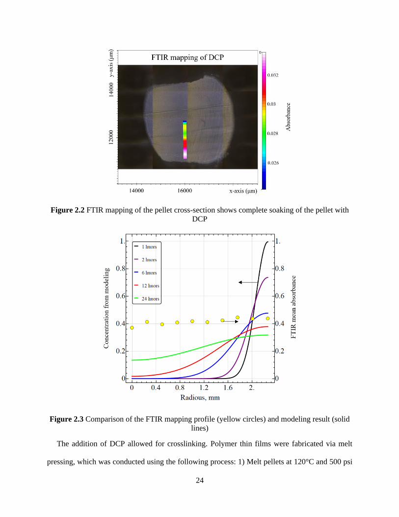
24

Figure 2.2 FTIR mapping of the pellet cross-section shows complete soaking of the pellet with

DCP

Figure 2.3 Comparison of the FTIR mapping profile (yellow circles) and modeling result (solid

lines)

The addition of DCP allowed for crosslinking. Polymer thin films were fabricated via melt

pressing, which was conducted using the following process: 1) Melt pellets at 120°C and 500 psi

25

for 3 minutes; 2) Further press at 2500 psi for 3 minutes; 3) Let film cool, cut into smaller pieces,

and reload; 4) Melt film at 120°C and 500 psi for 3 minutes; 5) Increase temperature to the curing

temperature (Tc), which is typically – but not necessarily – 180°C and pressure to 2500 psi for the

curing time (tc), which is typically – but not always – 12 minutes. Crosslinking occurs during the

final step if DCP was added to the LDPE pellets. An antioxidant was also added to certain samples.

The samples remain under pressure during final cooling.

XLPE films were degassed in a vacuum oven at an elevated temperature to determine how

degassing impacts the electrical properties via removal of DCP byproducts. This was used to

ensure that XLPE intrinsic properties can be observed [22], so that morphology impacts can be

independently examined. The standard procedure for degassing in vacuum was 65°C for 3 days,

and effect of varying degassing temperature was also examined. Degassed LDPE films were

prepared for comparative purposes. To analyze the impact of each of the major small molecules

removed from degassing, the three main DCP byproducts were added to a subset of XLPE films

after degassing by soaking the films in the individual liquids [32]. The DCP byproducts ACP,

aCA, and aMS were purchased from Sigma-Aldrich, with purities of 99%, 97% and 99%,

respectively. The soaking was always done at 50°C for a time of 2 hours to ensure maximal

diffusion of DCP byproducts into the polymer [36]. The same was also done for water both with

and without degassing.

A wide variety of electrodes have been used to study the electrical properties of polyethylene,

including gold, aluminum, tin, copper, silver, and others. Aluminum electrodes were selected for

this work due to their common use in studying the electrical properties of polyethylene

[76,84,96,103–108]. One study comparing aluminum and semicon electrodes found the aluminum

electrodes to lead to reduced conductivity with comparable activation energy [107]. For example,

26

a study comparing the impact of electrodes on the space charge buildup within polyethylene found

that aluminum electrodes led to minimal space charge buildup, which was mostly negative in sign.

For comparison, indium and silver led to a buildup of positive charge throughout the bulk of the

sample [103]. In that paper, space charge was ultimately determined to arise due to interface states,

and each type of electrode interface would have its own impact on the electrical properties. These

interface states have significant impacts on the electrical properties, as shown by studies on the

impact of the electrodes on other insulating polymers [109]. Electrodes such as aluminum and

chromium that react with polymers and form insulating layers were found to have higher

breakdown voltage due to reduced charge injection when compared to electrodes that use

unreactive metals like gold and silver.

Efforts to conclusively determine these impacts in polyethylene have had mixed results,

however. Comparing the work of many authors has not found a significant electrode impact for

polyethylene despite wide disparities in work function and contact potentials overall [84,96].

Similarly, the choice of electrodes does not seem to have an impact on other factors such as the

presence of electrical compensation [105] though it does seem to matter for charge storage

characteristics [108]. These results imply that other factors such as sample preparation and thermal

history may be more important for analyzing the electrical properties of polyethylene. This would

be good to verify in future work, but for the sake of simplicity only one choice of electrodes was

analyzed in this work, which was aluminum for the reasons mentioned previously as well as its

use as electrodes in power cables alongside copper. Several examples of XLPE insulation taken

from cables with aluminum cores have been studied in the literature [23,30,51,110]. In those

studies, the aluminum wire was retained as an electrode. Within cables, the aluminum or copper

metal is typically stranded into multi-wire cores, and is separated from the XLPE by an extruded

27

layer of semicon. In this setting, highly conductive aluminum of high purity is typical. The main

advantages of aluminum over copper are its relative lightness and cheapness, as copper has the

advantage in raw conductivity. For those reasons, aluminum is attractive for power transmission

and is commonly used on its own or with copper plating.

As such, prior to electrical testing, 50 nm thick aluminum electrodes were deposited via electron

beam evaporation in a high vacuum chamber. Electrodes were 3 cm across unless stated otherwise.

In general, electrical measurements are quite useful in determining physical, chemical, and

morphological properties of dielectrics such as polyethylene [46]. A few key electrical

characterization techniques were used here, each with a unique vantage point into the electrical

properties. An overall schematic of the experimental methods is presented in Figure 2.4 below,

and each characterization technique is described in detail afterwards. For all temperature-

dependent electrical measurements, a Delta Design 9023 Environmental Test Chamber was used

for heating and cooling.

Figure 2.4 Schematic of the overall experimental procedure

2.2 Broadband dielectric spectroscopy (BDS) LDPE and XLPE samples were electrically characterized under AC conditions using broadband

dielectric spectroscopy (BDS), allowing for the extraction of loss, conductivity, and capacitance

28

values over a frequency range from 0.1 to 1000 Hz. A 1 V rms AC signal was applied during

measurement. The impedance was measured and converted to capacitance and dielectric loss

values, allowing for extraction of conductivity. Loss and conductivity values from room

temperature and 90°C were examined. Analysis of the capacitance in 10°C steps allowed for

estimation of the temperature coefficient of capacitance for LDPE and XLPE, and the 90°C data

were obtained during this sweep. A Solartron Modulab dielectric spectrometer was used to do

these measurements and is shown in Figure 2.5.

Figure 2.5 Measurement equipment used for BDS

BDS was also used to obtain the temperature coefficient of capacitance (TCC). TCC values for

polymers are typically negative, and can be used as approximations of the linear thermal expansion

coefficient (LTEC) [111]. Significant changes from this can be attributed to either extrinsic factors

such as impurities or intrinsic factors such as changes in the polymer structure. Thus, variations in

the TCC can be used to understand the structural differences between samples. TCC is defined as

29

the fractional change in the capacitance (C) of a dielectric during a unit change of temperature (T)

at constant pressure. In equation form:

(2.1) 𝑇𝐶𝐶 =1

𝐶′∗ (

𝜕𝐶′

𝜕𝑇)𝑃=

1

𝜀′∗ (

𝜕𝜀′

𝜕𝑇)𝑃+ 𝛼𝑇

It can be seen in Equation 2.1 that TCC is related to the LTEC (αT), which in a semicrystalline

material will be influenced by the crystallinity as both the amorphous and crystalline phases

contribute to the total TCC. By using the Clausius-Mossotti relation, the term involving the

permittivity can be expanded further [111]. This is shown in Equations 2.2 and 2.3:

(2.2) 𝜀−1

𝜀+2=

𝛼𝑚

3�̅�𝜀0

(2.3) 𝜕𝜀

𝜕𝑇= (휀 + 2)(휀 − 1) (

1

3𝛼𝑚

𝜕𝛼𝑚

𝜕𝑇− 𝛼𝑇)

Equation 2.3 was obtained by differentiating Equation 2.2 with respect to temperature. In these

equations, αm is the molecular polarizability, V is the molar volume, and ε0 is the vacuum

permittivity. The thermal expansion coefficient that appears in Equation 2.3 comes from changes

in the molar volume of the sample. Substituting Equation 2.3 into Equation 2.1 would yield the

full TCC equation as seen in Equation 2.4. TCC values for a given material will therefore be

determined by thermal expansion and changes in polarizability. The expression above assumed

that the two were independent; if not, another term must be added [111].

(2.4) 𝑇𝐶𝐶 =(𝜀+2)(𝜀−1)

𝜀(

1

3𝛼𝑚

𝜕𝛼𝑚

𝜕𝑇− 𝛼𝑇) + 𝛼𝑇

By making certain assumptions, the TCC expression can be simplified [111]. The relative

permittivity of the non-magnetic material polyethylene is governed by its refractive index of

roughly 1.5, the square of which is equivalent to the relative permittivity of roughly 2.25. The

dielectric response in this material is solely from polarized electrons, as it lacks any dipolar or

ionic species. Space charge polarization is only relevant in conditions with high electrical field and

30

low frequency and will not be considered here. As such, only the polarizability of the electrons in

polyethylene will determine the polarizability of the whole molecule. The factors determining this

number include the electron density on the atom and the average distance of the electron cloud

from the nucleus. These factors are not expected to depend much on the temperature or the molar

volume of the material. As such, terms involving changes in polarizability can be set to zero.

Following this, the relative permittivity could then be considered constant, having a value around

2 based on the refractive index of polyethylene. This allows the TCC to be simplified as follows:

(2.5) 𝑇𝐶𝐶 =(2+2)(2−1)

2(−𝛼𝑇) + 𝛼𝑇

(2.6) 𝑇𝐶𝐶 = −𝛼𝑇

These assumptions that led to Equation 2.6 can then be checked via measurement of TCC using

BDS and comparing to literature values of the LTEC for polyethylene.

2.3 Conduction current measurement (CCM) and current-voltage measurement

(IVM) DC electrical characterization was carried out using conduction current measurements (CCM) and

current-voltage measurements (IVM). In these two techniques, the DC current is measured by

holding the sample at specific temperatures and voltages. The main difference between them is in

how those two parameters are varied. CCM was done by applying a 2000 V bias across the film

and measuring the current at evenly spaced temperatures in a range from 25°C to 90°C. IVM was

done by applying an electric field in 500 V steps from 500 V to 3500 V at the temperatures of

50°C, 70°C, and 90°C. Essentially, CCM explores only the temperature-dependence of the current,

while IVM explores the impact of both temperature and electric field. This makes CCM useful for

fast studies on the activation energy while IVM is useful for longer studies investigating both that

and fundamental conduction mechanisms. The current was measured for 1000 seconds and the

31

average value of the current obtained from 500 to 1000 seconds was taken as representative for

each temperature and voltage and used to compute values for the conductivity. The same HP

4140B pA meter / voltage source and Trek Model 610D amplifier were used for both

measurements and are shown in Figure 2.6.

Figure 2.6 Measurement equipment used for CCM and IVM

By obtaining the conductivity at various temperatures, the activation energy can be obtained by

fitting the data to the Arrhenius equation as polyethylene typically exhibits thermally activated

conduction [47,75]. The conversation from current to conductivity and then obtain the activation

energy is shown in Equations 2.7 and 2.8. The pre-exponential factor was also obtained during the

fitting process.

(2.7) 𝜎 =𝑖𝑡

𝑉𝐴= (

𝜕𝑖

𝜕𝑉) (

𝑡

𝐴)

(2.8) ln(𝜎) = −𝐸𝐴1

𝑘𝐵𝑇= ln(𝜎0)

In these equations, i is the measured average current, t is the measured sample thickness, V is the

fixed voltage, A is the fixed sample area, σ is the extracted conductivity, EA is the activation energy

32

of conduction, kB is the Boltzmann constant, and σ0 is the pre-exponential factor. For CCM, the

measured current and fixed voltage are used. For IVM, the slope between the current and the

voltage is used instead.

There are a few more additions specific to IVM. 500 seconds are allowed to elapse at

temperature without the application of electric field between measurements at different voltages.

A power law fit was carried out to help determine conduction mechanisms. Ohmic conduction

would return a value of 1 while space charge limited current would return a value of 2, for example.

A power law fit was also applied on the current to analyze its decay over time. It was been reported

that two distinct types of responses can be expected in polyethylene [84]. An exponent with

magnitude greater than 0.6 is typical of slow polarization of dipoles while one with magnitude less

than 0.4 is typical of conduction currents. Further discussion will be provided in Chapter 6x

detailing the measurement results.

2.4 Thermally stimulated depolarization current (TSDC) The thermally stimulated depolarization current (TSDC) technique was originally developed as a

thermoelectric means of analyzing the polarization process in alkali halides and other ionic solids,

and is based on the principles of ionic thermoconductivity [112]. Only later were names such as

thermally stimulated current (TSC), thermally stimulated discharge current, and thermally

stimulated depolarization current applied. In all cases, the fundamental principles are essentially

the same. First, a sample is brought up to the poling temperature (Tp) and held there for some time

(tp) with an electric field applied (Ep). During this step, charges and ions within the sample will

move corresponding to the electric field, and dipoles will orient themselves with the field.

Additionally, charge can be injected from the electrodes if the applied field is sufficiently intense.

The sample is then cooled down to the storage temperature (T0) with the field left on. This is done

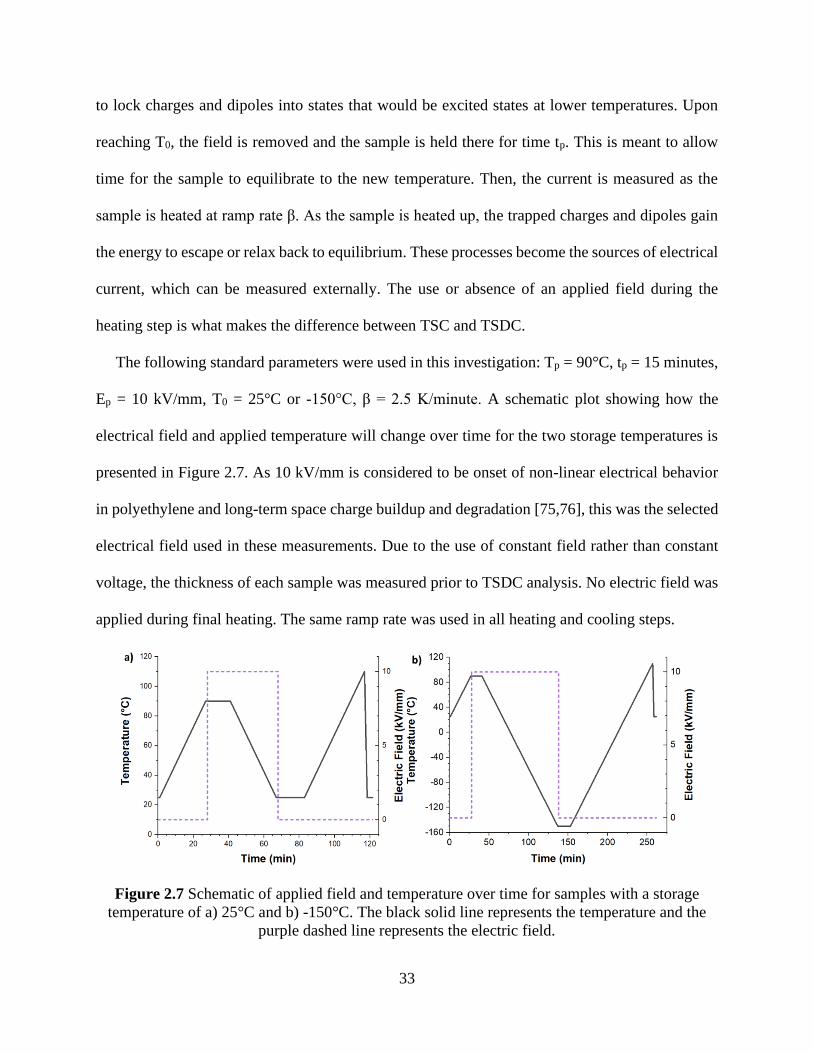
33

to lock charges and dipoles into states that would be excited states at lower temperatures. Upon

reaching T0, the field is removed and the sample is held there for time tp. This is meant to allow

time for the sample to equilibrate to the new temperature. Then, the current is measured as the

sample is heated at ramp rate β. As the sample is heated up, the trapped charges and dipoles gain

the energy to escape or relax back to equilibrium. These processes become the sources of electrical

current, which can be measured externally. The use or absence of an applied field during the

heating step is what makes the difference between TSC and TSDC.

The following standard parameters were used in this investigation: Tp = 90°C, tp = 15 minutes,

Ep = 10 kV/mm, T0 = 25°C or -150°C, β = 2.5 K/minute. A schematic plot showing how the

electrical field and applied temperature will change over time for the two storage temperatures is

presented in Figure 2.7. As 10 kV/mm is considered to be onset of non-linear electrical behavior

in polyethylene and long-term space charge buildup and degradation [75,76], this was the selected

electrical field used in these measurements. Due to the use of constant field rather than constant

voltage, the thickness of each sample was measured prior to TSDC analysis. No electric field was

applied during final heating. The same ramp rate was used in all heating and cooling steps.

Figure 2.7 Schematic of applied field and temperature over time for samples with a storage

temperature of a) 25°C and b) -150°C. The black solid line represents the temperature and the

purple dashed line represents the electric field.

34

Tp, β, and T0 determine the thermal history of the sample during charging, which helps

determine which peaks are present and the resulting stored charge [51]. Tp and T0 are upper and

lower bounds for the temperatures at which charges can be trapped [23,113]. β is inversely related

to the amount of time available for stored charges and polarization to relax – reducing β allows for

traps with lower and low effective frequencies to be observed [114]. This allows for the analysis

of low-frequency phenomena out of the reach of other techniques such as BDS [18]. The

temperature was given one minute to stabilize before poling and before storage. The heating run

was terminated at a nominal temperature above Tp, typically set as 100°C or 110°C. The sample

was then cooled back down to room temperature. On repeat analyses, all parameters used for that

sample were kept the same. As the peaks are sensitive to polarization conditions [115], the impact

of varying these parameters was also examined. The true temperature in the test chamber was

recorded during the heating ramp to allow for proper analysis of temperature dependent discharge

currents. A picture of the equipment used for these experiments is shown in Figure 2.8. An HP

4140B pA meter / voltage source and Trek Model 1010B amplifier was used for applying the

voltage and measuring the current. An HP Agilent 34401A multimeter was used for recording

temperatures.

Figure 2.8 Measurement equipment used for TSDC

35

After the completion of the TSDC analysis, data was obtained in the form of a temperature-

dependent current, which signifies the average change in stored charge across the entire sample

[115]. An example of this is shown in Figure 2.9 for representative degassed LDPE samples with

applied electric fields of 0, 10, and -10 kV/mm. A positive field was applied to most samples, and

the use of negative field here was to verify that the field polarity would not have significant

influence. For each source of charge, when the relaxation timescale is on the same timescale as the

experiment (i.e. seconds as opposed to hours) and there is a sufficient quantity of stored charge, a

measurable current above the noise threshold is expected. The discharge or depolarization is a

thermally activated process, meaning that there is a maximum temperature (Tmax) associated with

each discharge or depolarization [114]. Below that temperature, the process would proceed more

slowly and less current would be observed. Above that temperature, so much stored charge has

already been released that the current also drops. As such, there should be a series of peaks

observed in the current vs temperature data, with each peak coming from a unique source of charge

or dipoles. As the process is thermally activated, it is also possible to extract an activation energy

(EA) from each peak. Curve fits can be done, but a simpler approach is to use the initial rise of the

peak to estimate EA [114,115]. This approach will be used here due to good reported agreements

with curve fits. Additionally, each peak has an effective relaxation frequency, which can be

correlated to the activation energy and the peak maximum temperature [114]. These peaks tend to

have effective frequencies in the mHz range [18,23,94], meaning they would be difficult to detect

in true AC techniques such as dielectric spectroscopy. The peaks measured in this investigation

will be characterized by their Tmax and EA in order to pinpoint common origins of stored charge

between different samples.

36

Figure 2.9 Representative TSDC spectra with a storage temperature of -150°C for degassed

LDPE with differing applied electric fields as listed in the supplied legend.

2.5 Structural and chemical characterization techniques Further characterization was done using thermogravimetric analysis (TGA), wide-angle X-ray

scattering (WAXS), Fourier transform infrared spectroscopy (FTIR), and differential scanning

calorimetry (DSC). TGA was used to analyze potential changes in sample mass with heating. It

was done using a TA Instruments Discovery Series TGA Q5500 on samples with an initial mass

around 2 mg. Samples were heated in an alumina pan at a rate of 10°C/minute from 25°C to 300°C

in ambient air with a nitrogen purge flow of 100 mL/min. WAXS was used to calculate the

crystalline fraction. A Xenocs Xeuss 2.0 beamline in transmission mode was used for the

measurements. Samples with 100 μm thickness were used for the measurement, and areas of 1 cm2

were mapped with resolution of 1 mm2. FTIR was used to obtain the concentration of byproducts

in the samples. It was performed via the Bruker HYPERION 3000 FT-IR microscope in

37

transmission mode on samples with approximately 100 μm thickness. To detect acetophenone in

the XLPE, the C=O stretching peak at 1695 cm-1 was measured in mapping areas of around 1 cm2

with a resolution of 100 μm2. To compare samples, the measured peak was normalized with the

corresponding polyethylene backbone peak. DSC was used to qualitatively study the crystallinity

of polyethylene samples, and was done using a TA Instruments DSC Q2000 unit. A nitrogen purge

flow of 50 mL/min and a ramp rate of 10°C/min were used. The obtained DSC results (shown in

Figure 2.10) show that LDPE melts at a nominal temperature of 109°C, close to the commonly

reported value of 105°C. Upon cooling, it crystallizes around 98°C. There is evolution in the

crystallinity upon repeat measurements, where the second time through there is less apparent

crystallization. Additionally, the melting temperature is reduced (109.2°C → 108.8°C) and the

crystallization temperature is increased (97.7°C → 98.5°C). This result showcases the sensitivity

of a sample to its thermal history, and helps to motivate several of the studies undertaken to better

understand the impact of thermal history on electrical properties.

Figure 2.10 DSC traces of low-density polyethylene. The negative peak (endothermic) is

associated with melting and the positive peak (exothermic) is associated with solidification.

38

Chapter 3 – Effects of crosslinks and residual molecules on the dielectric

response and structure of polyethylene

3.1 Temperature coefficient of capacitance of XLPE and LDPE The assumptions that led to the simplified TCC equations discussed in Section 2.2 can be

confirmed via measurement of TCC using BDS and comparing to literature values of the LTEC

for polyethylene. The results from such a measurement and comparison are shown in Figure 3.1a.

Only capacitance data taken at 1 kHz were used for the TCC data in this comparison and the

majority of the figures here to avoid space charge or conduction contributions that can impact the

capacitance at elevated temperatures and/or low frequencies. An example of what that can look

like is shown in Sections 3.6 and 3.7 where the impacts of added impurities and radiation exposure,

respectively, are discussed.

Figure 3.1 a) TCC measurement of 2 samples of low-density polyethylene (LDPE) and

comparison to literature data for the LTEC of the same polymer. Xc represents the crystallinity of

polyethylene. LTEC data reproduced from White, G. K.; Choy, C. L. J. Polym. Sci. Polym. Phys.

Ed. 1984. b) Average TCC comparison between as-received XLPE, as-received LDPE, degassed

XLPE, and degassed LDPE samples.

The experimental data cited from literature examined the impact of the crystalline fraction on

thermal expansion of LDPE [116]. Two samples of low-density polyethylene were prepared with

39

crystallinity around 42%, matching that of one of the literature samples. The values of negative

TCC extracted from the LDPE samples were good matches for LTEC data from LDPE with similar

crystallinity. Thus, there can be good confidence not only that TCC data can be used to

approximate the LTEC but also that the TCC could reveal information regarding the structure of

polyethylene samples [116–118]. While capacitance data exists up to 100°C, the data above 60°C

was not critically examined in this work due to a lack of LTEC data for molten polyethylene.

A comparison of TCC values was made between PE samples with different impurity levels: as-

received XLPE, as-received LDPE, degassed XLPE, and degassed LDPE. The result of this is

shown in Figure 3.1b. Around room temperature and below, the as-received XLPE and LDPE are

similar. The magnitude of the TCC increases significantly for XLPE at elevated temperatures when

compared to LDPE starting at 40°C. By analyzing these samples via TGA as shown in Figure 3.2,

it became clear that this difference was due to the DCP byproducts left behind in the XLPE. The

as-received XLPE lost mass upon heating at a rate that accelerated near 40°C. That process ceased

near 90°C with a total mass loss of approximately 1.5%, a value congruent with the loss of residual

DCP byproducts [22]. The LDPE, meanwhile, had no significant change in mass below 90°C. We

therefore concluded that the increase in the magnitude of the TCC above 40°C was caused by an

increase in thermal expansion due to contributions from the trace concentrations of the DCP

byproducts trapped within voids and amorphous regions. As the temperature increases, their

increased vibration contributes to the overall increase in volume. They create an internal pressure

that forces the compliant polymer to expand around them and accommodate their motions.

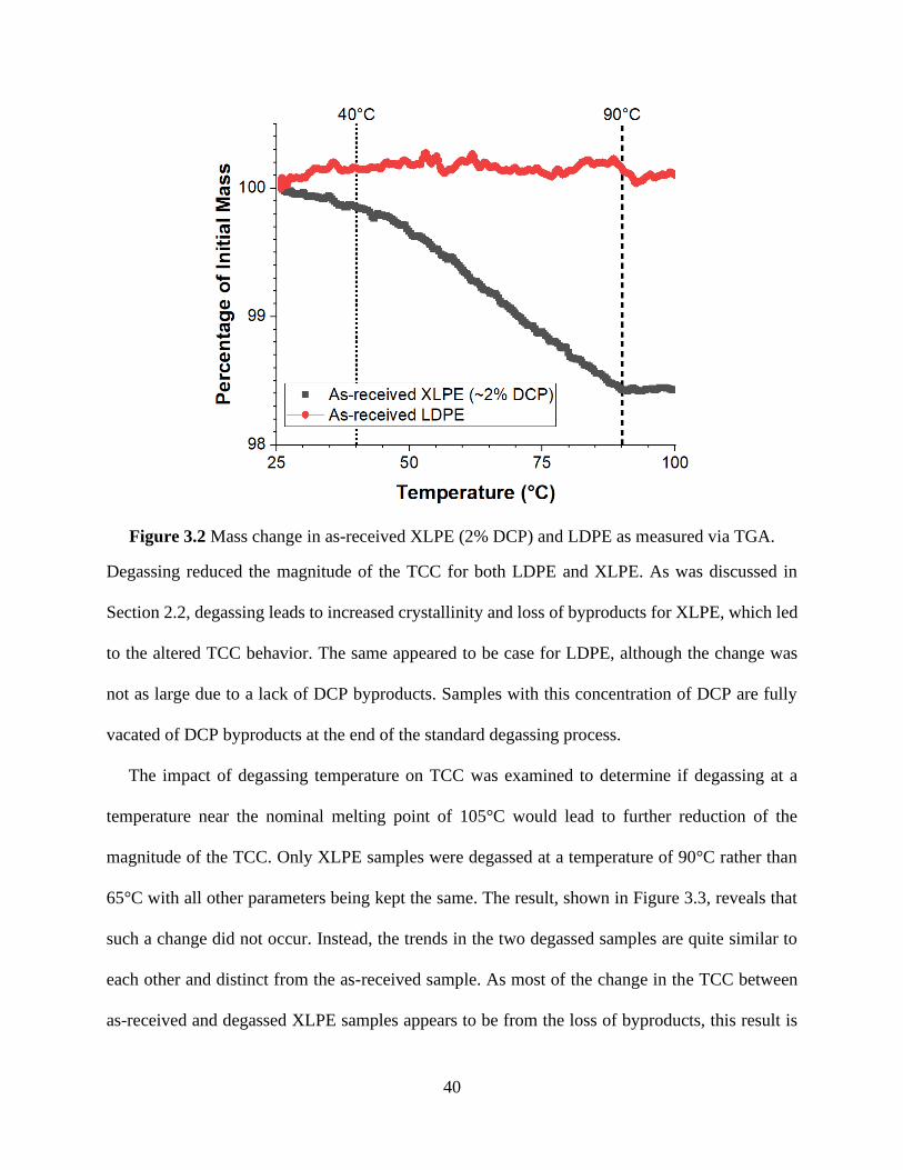
40

Figure 3.2 Mass change in as-received XLPE (2% DCP) and LDPE as measured via TGA.

Degassing reduced the magnitude of the TCC for both LDPE and XLPE. As was discussed in

Section 2.2, degassing leads to increased crystallinity and loss of byproducts for XLPE, which led

to the altered TCC behavior. The same appeared to be case for LDPE, although the change was

not as large due to a lack of DCP byproducts. Samples with this concentration of DCP are fully

vacated of DCP byproducts at the end of the standard degassing process.

The impact of degassing temperature on TCC was examined to determine if degassing at a

temperature near the nominal melting point of 105°C would lead to further reduction of the

magnitude of the TCC. Only XLPE samples were degassed at a temperature of 90°C rather than

65°C with all other parameters being kept the same. The result, shown in Figure 3.3, reveals that

such a change did not occur. Instead, the trends in the two degassed samples are quite similar to

each other and distinct from the as-received sample. As most of the change in the TCC between

as-received and degassed XLPE samples appears to be from the loss of byproducts, this result is

41

sensible. According to known data, the diffusion rates of byproducts out of polyethylene increases

by roughly an order of magnitude for a 30°C increase in temperature given a constant annealing

atmosphere [21]. Given that the standard conditions are enough to remove all byproducts from

these samples [119], they were also vacated from the more harshly degassed sample. The higher

degassing temperature can be correlated with a greater increase in the crystallinity [45]. A greater

understanding of how crystallinity is related to TCC will need to be uncovered in future work.

Figure 3.3 Average TCC comparison between as-received XLPE, degassed XLPE, and 90°C

degassed XLPE samples

3.2 Impacts of degassing on room temperature dielectric loss of XLPE and LDPE To determine if changes in morphology and the concentration of byproducts due to degassing

also impacted the dielectric loss, a comparison was made between XLPE (which contains DCP

byproducts in the as-received state) and LDPE (which would not). The result of a comparison

made at room-temperature is presented in Figure 3.4. The raw broadband dielectric spectra for

42

these samples are shown in Figure 3.5. The loss values were similar between the as-received

samples of these two materials, which agrees with prior investigations [120]. Degassing reduced

the dielectric loss for both XLPE and LDPE. The choice of crosslinking temperature also did not

lead to systematic variations in the dielectric loss for samples in either condition. Such differences

could not be explained by variations in the content of DCP byproducts, as the LDPE films lacked

them and their concentration should have systematically varied with the choice of crosslinking

temperature following their consumption to create crosslinks [27]. It was observed that increasing

the degassing temperature from 65°C to 90°C led to further reduction of the dielectric loss, as

shown in Figure 3.6. The crystallinity also increased with increased degassing temperature (≈31%

with 65°C vs. ≈35% with 90°C). As such, these differences were attributed to morphological

changes induced by degassing, in particular the changes to the crystallinity and crystal structure.

Figure 3.4 Comparison of the room temperature dielectric loss values measured at 10 Hz and

below for XLPE and LDPE samples crosslinked at various temperatures.

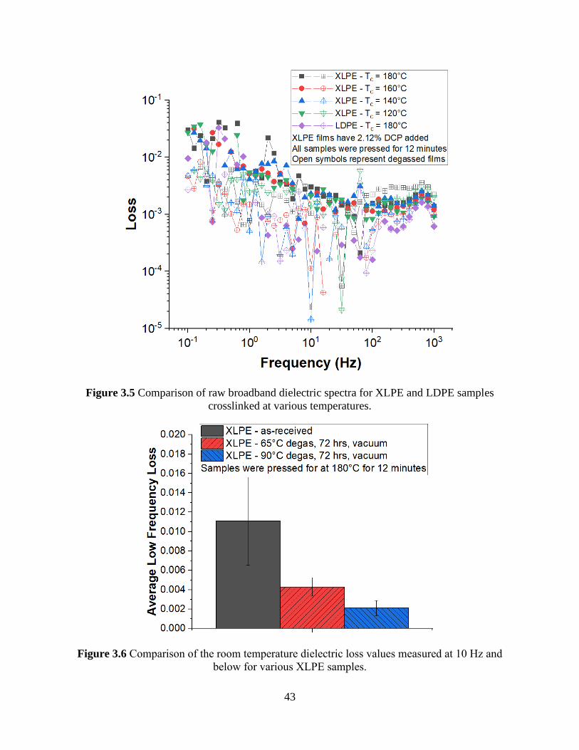
43

Figure 3.5 Comparison of raw broadband dielectric spectra for XLPE and LDPE samples

crosslinked at various temperatures.

Figure 3.6 Comparison of the room temperature dielectric loss values measured at 10 Hz and

below for various XLPE samples.

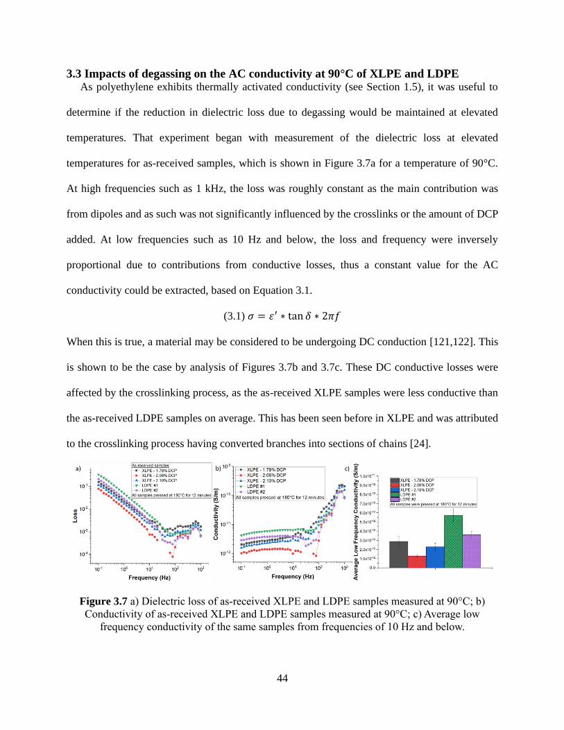
44

3.3 Impacts of degassing on the AC conductivity at 90°C of XLPE and LDPE As polyethylene exhibits thermally activated conductivity (see Section 1.5), it was useful to

determine if the reduction in dielectric loss due to degassing would be maintained at elevated

temperatures. That experiment began with measurement of the dielectric loss at elevated

temperatures for as-received samples, which is shown in Figure 3.7a for a temperature of 90°C.

At high frequencies such as 1 kHz, the loss was roughly constant as the main contribution was

from dipoles and as such was not significantly influenced by the crosslinks or the amount of DCP

added. At low frequencies such as 10 Hz and below, the loss and frequency were inversely

proportional due to contributions from conductive losses, thus a constant value for the AC

conductivity could be extracted, based on Equation 3.1.

(3.1) 𝜎 = 휀′ ∗ tan 𝛿 ∗ 2𝜋𝑓

When this is true, a material may be considered to be undergoing DC conduction [121,122]. This

is shown to be the case by analysis of Figures 3.7b and 3.7c. These DC conductive losses were

affected by the crosslinking process, as the as-received XLPE samples were less conductive than

the as-received LDPE samples on average. This has been seen before in XLPE and was attributed

to the crosslinking process having converted branches into sections of chains [24].

Figure 3.7 a) Dielectric loss of as-received XLPE and LDPE samples measured at 90°C; b)

Conductivity of as-received XLPE and LDPE samples measured at 90°C; c) Average low

frequency conductivity of the same samples from frequencies of 10 Hz and below.

45

Similarly, by comparing degassed and as-received samples in Figure 3.8, it became possible to

see distinct differences between XLPE and LDPE samples. In Figure 3.8a, it can be seen that the

degassed XLPE samples were less conductive than their as-received counterparts by roughly an

order of magnitude. On the other hand, the degassed and as-received LDPE samples were

comparable as seen in Figure 3.8b. The differences in electrical behavior between these samples

can be attributed to the differences in structure between these samples and how that structure

responds to elevated temperatures. There was a slightly greater reduction of conductivity than loss

upon degassing XLPE, which may be a sign that changes occurred during measurement at elevated

temperatures. Meanwhile, the LDPE conductivity was roughly unchanged. As the measurement

temperature of 90°C is a significant fraction of the nominal melting temperature of LDPE

(≈105°C), the benefits of degassing appear to have been lost. When varying the degassing

temperature, it was found that the samples degassed at 65°C were less conductive at 90°C than the

samples degassed at 90°C (see Figure 3.9). Both, however, were much less conductive than the as-

received samples. This suggests that the elevated degassing temperature may lead to a change in

the XLPE structure that leads to reduced room temperature loss and increased high temperature

conductivity. The exact nature of this change would need to be examined in future work.

46

Figure 3.8 Average low frequency conductivity (f ≤ 10 Hz) at 90°C conductivity comparison

between as-received and degassed a) XLPE samples; b) LDPE samples.

47

Figure 3.9 Average low frequency conductivity (f ≤ 10 Hz) at 90°C conductivity comparison

between various XLPE samples

3.4 Effect of crosslinking temperature on the dielectric response and TCC As far as the impact of crosslinking temperature goes, a 90°C conductivity analysis shown in

Figure 3.10 revealed no clear dependence between crosslinking temperature and conductivity with

one major exception. The sample with the lowest crosslinking temperature used in this study had

a significantly higher conductivity when compared to the other samples. An analysis of the

crystallinity of these samples helps to show why this occurred. The sample crosslinked at 120°C

had the highest crystallinity, with decreased extent of crystallinity corresponding to increased

temperature for 140°C and 160°C, and above this point the crystallinity appeared to be invariant

with respect to temperature [119]. This corresponded with literature data showing that the

crosslinking reaction is highly temperature dependent [27]. As such, the XLPE sample crosslinked

at 120°C would have had the smallest extent of crosslinking reaction occur and thus had both

crystallinity and conductivity most similar to LDPE. The variation in TCC for these samples was

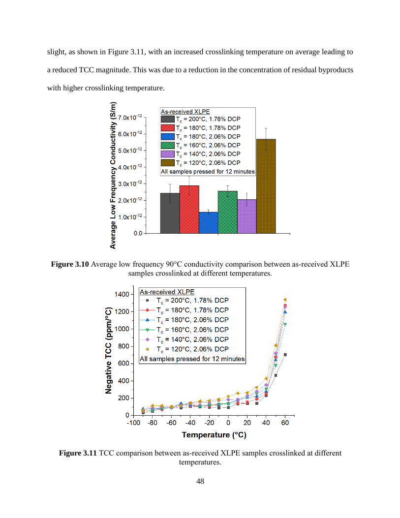
48

slight, as shown in Figure 3.11, with an increased crosslinking temperature on average leading to

a reduced TCC magnitude. This was due to a reduction in the concentration of residual byproducts

with higher crosslinking temperature.

Figure 3.10 Average low frequency 90°C conductivity comparison between as-received XLPE

samples crosslinked at different temperatures.

Figure 3.11 TCC comparison between as-received XLPE samples crosslinked at different

temperatures.

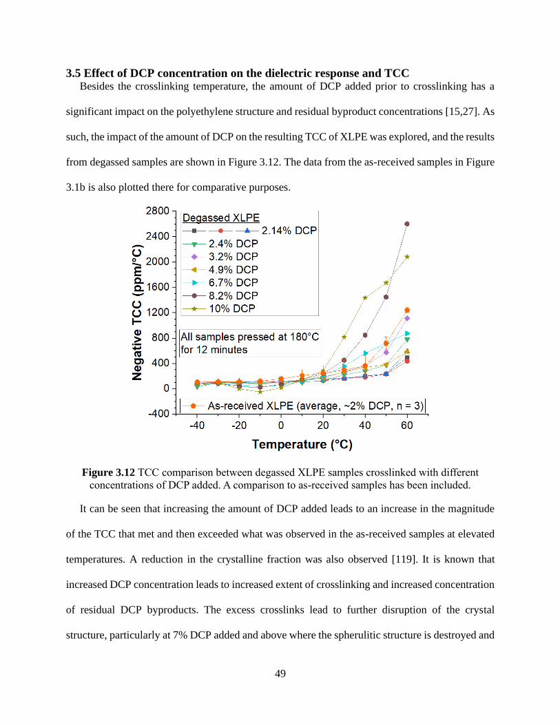
49

3.5 Effect of DCP concentration on the dielectric response and TCC Besides the crosslinking temperature, the amount of DCP added prior to crosslinking has a

significant impact on the polyethylene structure and residual byproduct concentrations [15,27]. As

such, the impact of the amount of DCP on the resulting TCC of XLPE was explored, and the results

from degassed samples are shown in Figure 3.12. The data from the as-received samples in Figure

3.1b is also plotted there for comparative purposes.

Figure 3.12 TCC comparison between degassed XLPE samples crosslinked with different

concentrations of DCP added. A comparison to as-received samples has been included.

It can be seen that increasing the amount of DCP added leads to an increase in the magnitude

of the TCC that met and then exceeded what was observed in the as-received samples at elevated

temperatures. A reduction in the crystalline fraction was also observed [119]. It is known that

increased DCP concentration leads to increased extent of crosslinking and increased concentration

of residual DCP byproducts. The excess crosslinks lead to further disruption of the crystal

structure, particularly at 7% DCP added and above where the spherulitic structure is destroyed and

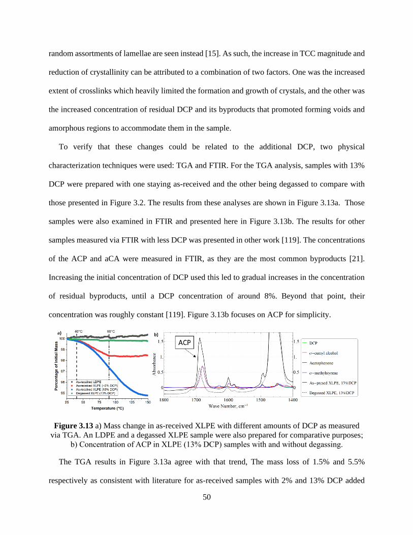
50

random assortments of lamellae are seen instead [15]. As such, the increase in TCC magnitude and

reduction of crystallinity can be attributed to a combination of two factors. One was the increased

extent of crosslinks which heavily limited the formation and growth of crystals, and the other was

the increased concentration of residual DCP and its byproducts that promoted forming voids and

amorphous regions to accommodate them in the sample.

To verify that these changes could be related to the additional DCP, two physical

characterization techniques were used: TGA and FTIR. For the TGA analysis, samples with 13%

DCP were prepared with one staying as-received and the other being degassed to compare with

those presented in Figure 3.2. The results from these analyses are shown in Figure 3.13a. Those

samples were also examined in FTIR and presented here in Figure 3.13b. The results for other

samples measured via FTIR with less DCP was presented in other work [119]. The concentrations

of the ACP and aCA were measured in FTIR, as they are the most common byproducts [21].

Increasing the initial concentration of DCP used this led to gradual increases in the concentration

of residual byproducts, until a DCP concentration of around 8%. Beyond that point, their

concentration was roughly constant [119]. Figure 3.13b focuses on ACP for simplicity.

Figure 3.13 a) Mass change in as-received XLPE with different amounts of DCP as measured

via TGA. An LDPE and a degassed XLPE sample were also prepared for comparative purposes;

b) Concentration of ACP in XLPE (13% DCP) samples with and without degassing.

The TGA results in Figure 3.13a agree with that trend, The mass loss of 1.5% and 5.5%

respectively as consistent with literature for as-received samples with 2% and 13% DCP added

51

[119]. Adding more DCP than is typically used led clearly to more byproducts, though it was noted

that the concentration of byproducts introduced did not scale with the amount of DCP added.

Additionally, the degassed sample that had 13% DCP used for crosslinking exhibited negligible

mass loss in TGA despite still having byproducts according to FTIR. This suggests that the use of

large amounts of DCP not only introduces more byproducts into the sample, but also changes how

they are incorporated into the sample. These dipolar species may now be grafted onto the chains

in addition to being trapped within voids and amorphous regions. This leads to altered TCC

behavior for degassed samples with high DCP content because the dipolar additions to the chains

further increase the internal pressure introduced by the byproducts.

Additionally, at low temperatures, the TCC switched from negative to positive with a positive

peak around -10°C. A small and positive TCC is typical of glasses and ionic inorganic materials,

and is due to an increase in ionic polarizability with increasing temperature and/or volume

[111,123]. This feature was not observed in the as-received samples, and only appeared in

degassed ones with at least 6.7% DCP, supporting the idea that there was some categorical charge

in the crosslinking reaction beyond that point. This effect was more pronounced in the radiation

exposed samples discussed in Section 3.7 due to the heavy damage to the polyethylene structure.

The increase in the byproduct concentration with greater initial DCP addition would also be

expected to increase the low frequency dielectric loss, and the data shown in Figure 3.14 clearly

indicates that this occurred for DCP concentrations above 7-8%. As such, we determined that

surpassing a certain threshold in DCP concentration is necessary for increases in dielectric loss to

be observed. This also explains why XLPE made with low amounts of DCP appeared to be

indistinguishable from LDPE, as the loss was governed by factors intrinsic to the polymer that

were not different between the two. Data values for these and all samples discussed in this chapter

52

are presented in Table 3.1. More discussion will be given to the three samples at the end of the

table in the next section.

Figure 3.14 Average low frequency room temperature dielectric loss in degassed XLPE samples

crosslinked with different DCP concentrations.

Table 3.1 Room temperature dielectric loss for samples discussed in the main text.

Sample Dielectric Loss

As-received LDPE and XLPE 0.0103 ± 0.0028

Degassed LDPE and XLPE w/ ~2% DCP 0.0023 ± 0.0006

Degassed XLPE w/ up to 6.7% DCP 0.0029 ± 0.0002

Degassed XLPE w/ 8.2% DCP 0.0064

Degassed XLPE w/ 10% DCP 0.0083

As-received XLPE soaked in water 0.0104 ± 0.0034

As-received XLPE w/ anti-oxidant 0.2813 ± 0.1092

Degassed XLPE soaked in acetophenone 0.4236 ± 0.0957

53

With that comparison made, an analysis of these samples at higher temperatures was done to

extract the conductivity. The result is shown in Figure 3.15. Low frequency conductivity values

could not be extracted from the sample crosslinked with 8.2% DCP. Here, the addition of more

DCP, which was confirmed to lead to a greater concentration of byproducts, did not lead to

enhanced conductivity. It may be tentatively surmised that the slightly reduced conductivity with

greater initial DCP concentration was due to the slightly reduced crystalline fraction from the extra

crosslinks. Excess concentrations of DCP byproducts may not contribute much to quasi-DC

conduction when compared to the changes in the AC dielectric loss discussed previously.

Figure 3.15 Average low frequency 90°C conductivity comparison between degassed XLPE

samples crosslinked with different concentrations of DCP added.

3.6 Acetophenone impacts on the dielectric loss, AC conductivity, and TCC A comparison was also made between the as-received and degassed XLPE samples discussed

previously with three other sample types: degassed XLPE exposed to excess concentrations of

acetophenone (ACP), as-received XLPE containing antioxidant (AO), and as-received XLPE

soaked in water. Antioxidant was added to films during the addition of DCP. The as-received films

54

were laminated with Teflon™ sheets prior to electrode deposition to prevent mass diffusion of

byproducts out of the film. A summary of the TCC results of analyzing these samples and a

comparison with the previously discussed XLPE samples is shown in Figure 3.16, while the effect

on the dielectric loss at various temperatures is shown in Figure 3.17. The same plot in log scale

and a comparison at 90°C is presented in Figure 3.18.

Figure 3.16 Negative TCC comparison between different XLPE types: a) all sample types; b)

zoom in on XLPE, degassed XLPE, and XLPE after a soak in water for two hours.

55

Figure 3.17 Average dielectric loss at 0.1 Hz as a function of temperature for XLPE samples

treated under different conditions.

Figure 3.18 a) Log scale plot of the average dielectric loss at 0.1 Hz as a function of temperature

for XLPE samples treated under different conditions; b) comparison at 90°C.

56

It is well known that ACP is involved in a solvation reaction with water or antioxidants with

oxygen or sulfur groups, producing ions and space charge [35,87,88]. It was thus expected that

intentionally retaining these ions and molecules should lead to significant changes not only in the

dielectric loss and conductivity, but also in the capacitance. There were significant changes in the

TCC due to these byproducts. For the sample with excess ACP, there was a positive peak around

-10°C and a negative peak around 30°C. For the sample with antioxidant, the positive peak was

around 10°C instead. The values associated with these peaks were too large to be explained by

thermal expansion of the polymer. In fact, they were outside of the range expected for typical solid

insulators [111], which indicated that a different explanation should be pursued.

Acetophenone is a small molecule with a melting point of 20°C. It has a permanent dipole due

to its ketone group and is also quite large due to its phenyl group. This gives it a dielectric constant

in the range of 17-18, much larger than the 2.2 of polyethylene. The ketone group also gives it the

ability to have hydrogen bond and electron pair interactions with solvents. Meanwhile, water is a

polar solvent that melts at 0°C with a dielectric constant around 80 in this temperature range and

a larger TCC magnitude than polyethylene [124]. The two molecules are mutually soluble.

As such, the following explanation is proposed for the observed results. First, at very low

temperatures, the capacitance for these samples came solely from the XLPE, which was much

smaller than expected from the exposure to these chemicals (see Figure 3.19). Second, as the

samples were heated up and approached the melting points of water and ACP, the two acquired

sufficient energy to move through the polymer matrix. When sufficient quantities met, they then

underwent the solvation reaction. ACP will form hydrogen bonds with water, and the water

molecules will congregate into a shell surrounding the ACP molecule. The formation of complexes

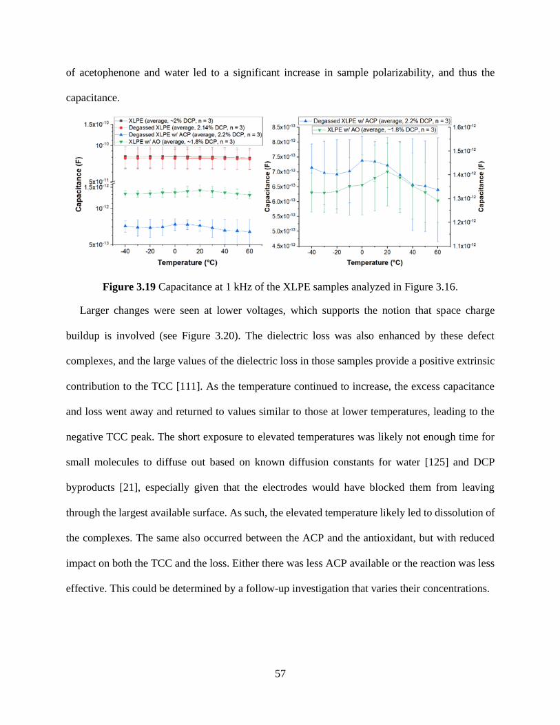
57

of acetophenone and water led to a significant increase in sample polarizability, and thus the

capacitance.

Figure 3.19 Capacitance at 1 kHz of the XLPE samples analyzed in Figure 3.16.

Larger changes were seen at lower voltages, which supports the notion that space charge

buildup is involved (see Figure 3.20). The dielectric loss was also enhanced by these defect

complexes, and the large values of the dielectric loss in those samples provide a positive extrinsic

contribution to the TCC [111]. As the temperature continued to increase, the excess capacitance

and loss went away and returned to values similar to those at lower temperatures, leading to the

negative TCC peak. The short exposure to elevated temperatures was likely not enough time for

small molecules to diffuse out based on known diffusion constants for water [125] and DCP

byproducts [21], especially given that the electrodes would have blocked them from leaving

through the largest available surface. As such, the elevated temperature likely led to dissolution of

the complexes. The same also occurred between the ACP and the antioxidant, but with reduced

impact on both the TCC and the loss. Either there was less ACP available or the reaction was less

effective. This could be determined by a follow-up investigation that varies their concentrations.

58

Figure 3.20 Temperature and frequency dependence of the capacitance of a) a representative

degassed XLPE sample soaked with ACP; b) a representative as-received XLPE sample

containing antioxidant.

It was noted that the as-received sample soaked in water did not exhibit this altered TCC

behavior, but was instead similar to as-received XLPE without water exposure. Meanwhile, these

samples also had loss values intermediate between the original as-received samples and the

degassed samples. Water exposure over such a short time frame may not have allowed for

sufficient diffusion of water into the XLPE sample. Further experiments with longer water

exposure times would be useful in refining the understanding of the interactions between DCP

byproducts and moisture in XLPE samples.

3.7 Impacts of radiation exposure on the conductivity and TCC of LDPE The use of DCP as a crosslinking agent is common due to its many practical benefits that are

discussed in Section 1.2. However, ionizing radiation such as gamma rays can also be used to

induce crosslinks [126,127]. The main mechanism can be briefly summarized as scission of main

and side chains be the high energy particles leading to hydrogen evolution and radicals that are

able to form crosslinks. Methyl groups and double bonds are also produced as side products. The

main reasons for using this approach are that it can be done at room temperature and the resulting

material is free of additives, which means this method is typically used for bio-compatible wear-

59

resistant polyethylene [128]. However, the expense involved means that the much cheaper

chemical crosslinking method is preferred for power cables [26]. This leaves the electrical

properties of radiation crosslinked polyethylene understudied in comparison to the peroxide

crosslinked version.

Here, a Co-60 gamma ray source was used for the radiation-induced crosslinking with a dose

rate of around 2.5 × 105 rad/hr and a total dose of 5 Mrad. Radiation-exposed samples were split

into two groups: one left as-is to be exposed under ambient conditions and the other vacuum-sealed

to be exposed without significant oxygen presence. This was done to determine the impact of the

differing oxygen levels on the resulting films. Oxygen is reported to contribute to crosslinking by

forming peroxide bridges [26]. A separate group of as-received LDPE samples were used as a

control group. The impacts on the dielectric loss, 90°C AC conductivity, and TCC were examined,

and the results are shown in Figures 3.21, 3.22, and 3.23 respectively.

Figure 3.21 Comparison of the room temperature dielectric loss values measured at 10 Hz and

below for various LDPE sample types.

60

By examining the changes in the electrical properties, two things became apparent. One is that the

radiation exposure in air significantly (p-value = 0.016) increased both the dielectric loss and the

90°C AC conductivity with respect to an unexposed film. The other is that while the radiation

exposed and vacuum-sealed samples were not significantly different at room temperature from the

as-received samples (p-value = 0.3), they were an order of magnitude more conductive than the

as-received samples at 90°C. This is in stark contrast to the peroxide crosslinked XLPE samples

which were similar to LDPE at room temperature but were less conductive at elevated

temperatures. Due to the lack of chemical impurities, the sheer extent of the structural damage due

to the radiation appears must be suspected as the cause of the increase in conductivity. With the

addition of oxygen present, oxidation and peroxide bridge formation were promoted and led to

further increases in both the dielectric loss and the 90°C AC conductivity. It was also suspected

that these changes would be tunable by altering the extent of radiation and the choice of ambient.

Figure 3.22 Average low frequency conductivity (f ≤ 10 Hz) at 90°C conductivity comparison

between various LDPE samples.

61

Additionally, the TCC of the LDPE sample exposed to radiation while in ambient was significantly

different from both the unexposed and the exposed in vacuum samples. In particular, the TCC of

the radiation-exposed in ambient was actually positive below room temperature, with a peak

centered at -10°C, as was seen with samples crosslinked with high DCP content. The origin was

the same in these samples as for those discussed in Section 3.5 but was more pronounced under

these conditions. Combined with the results regarding the electrical properties, it can thus be

suggested that radiation exposure turns polyethylene into an ionic conducting material whereas it

normally would exhibit either electronic conduction or a mix of ionic and electronic conduction.

Further discussion along these lines is present in Chapter 4 with a comparison between AC and

DC conduction in radiation crosslinked samples.

Figure 3.23 Negative TCC comparison between different LDPE types.

These ions contribute to space charge polarization that is apparent in the enhanced conductivity

at elevated temperatures and in enhanced capacitance at low frequency and high temperature (see

62

Figure 3.24). Above room temperature, these samples followed the same trend in the TCC as the

other LDPE samples, but with a reduced magnitude. This was suggestive of the crosslinks

restricting thermal expansion, unlike for the peroxide crosslinked samples were the loss of

crystallinity and presence of byproducts meant that thermal expansion was enhanced instead.

Further examinations regarding the nature of these ionic species and what environments promote

their formation would be useful in better understanding these results.

Figure 3.24 Temperature and frequency dependence of the capacitance of a) a representative as-

received LDPE sample exposed to radiation in ambient; b) a representative as-received LDPE

sample exposed to radiation while sealed; c) a representative as-received LDPE sample.

63

Chapter 4 – Continuously variable activation energy in polyethylene

4.1 Background on electrical compensation, the isokinetic temperature, and the

Meyer-Neldel Rule Electrical conduction in many polymeric insulators, such as polyethylene, is typically a

thermally activated process. The conductivity, 𝜎, under moderate electrical fields where Ohm’s

law applies is governed by the Arrhenius equation,

(1) 𝜎 = 𝜎0 exp (−𝐸𝐴

𝑘𝐵𝑇)

where kB is the Boltzmann constant, T is the absolute temperature, EA is the activation energy, and

𝜎0 is the pre-exponential term. A typical example of thermally activated conduction in LDPE and

XLPE samples is shown in Figure 4.1. Figure 4.1a and Figure 4.1b show the raw data for

polyethylene samples in terms of current measured as a function of time for different measurement

temperatures. Figure 4.1c shows that data converted into the form of conductivity versus

temperature, from which EA and 𝜎0were obtained.

Figure 4.1 a) Raw current data for a degassed XLPE measured at various temperatures with 2

kV applied; b) Raw current data for a degassed LDPE measured at various temperatures with 2

kV applied; c) Current data converted into conductivity and plotted against temperature to obtain

the activation energy.

Usually, the activation energy EA and the pre-exponential term 𝜎0 are considered constant for

a specific material. However, for many materials including ionic conductors, electronic

semiconductors, and polymers, it has been observed that within a family of related materials or for

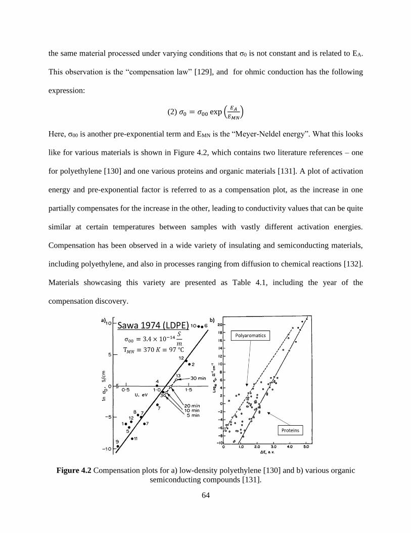
64

the same material processed under varying conditions that σ0 is not constant and is related to EA.

This observation is the “compensation law” [129], and for ohmic conduction has the following

expression:

(2) 𝜎0 = 𝜎00 exp (𝐸𝐴

𝐸𝑀𝑁)

Here, σ00 is another pre-exponential term and EMN is the “Meyer-Neldel energy”. What this looks

like for various materials is shown in Figure 4.2, which contains two literature references – one

for polyethylene [130] and one various proteins and organic materials [131]. A plot of activation

energy and pre-exponential factor is referred to as a compensation plot, as the increase in one

partially compensates for the increase in the other, leading to conductivity values that can be quite

similar at certain temperatures between samples with vastly different activation energies.

Compensation has been observed in a wide variety of insulating and semiconducting materials,

including polyethylene, and also in processes ranging from diffusion to chemical reactions [132].

Materials showcasing this variety are presented as Table 4.1, including the year of the

compensation discovery.

Figure 4.2 Compensation plots for a) low-density polyethylene [130] and b) various organic

semiconducting compounds [131].

65

Table 4.1 A list of materials exhibiting the compensation law [133,134]

Material Year

Semiconducting organic substances 1968

Low-density polyethylene 1972

Hydrogenated amorphous silicon (a-Si:H) prepared by glow-discharge deposition 1980

GaAs and GaInAs solar cells 1984

Chalcogenide glasses 1991

Electrodeposited CulnSe2 thin films 1992

Liquid semiconductors 1995

Nasicon 1992

a-Si:H prepared by homogeneous chemical vapor deposition (HOMOCVD) 1995

Polycrystalline semiconducting FeSi2 films 1998

Fullerenes 1998

Non-metallic YBa2Cu3Oy films 1998

Thin-film transistors with intrinsic heterogeneous silicon 1999

Amorphous strontium titanate thin films 2000

Amorphous and polycrystalline silicon thin-film transistors 2003

Porous silicon and hydrogenated amorphous silicon 2001

Ionic conductors 2002

Hydrogenated amorphous silicon carbide (a-SiCx:H) 2006

Se and S-doped hydrogenated amorphous silicon 2007

Sol–gel derived polycrystalline ZnO:Al thin films 2008

Highly crystallized undoped microcrystalline silicon films 2008

Crystalline Si and non-hydrogenated a-Si 2008

By combining Equation (1) and Equation (2) into Equation (3), it can be shown that there should

exist a temperature where conductivity is invariant of EA. This is the “isokinetic temperature”. The

relationship between isokinetic temperature and Meyer-Neldel energy is shown in Equation (4).

(3) 𝜎 = 𝜎00 exp (𝐸𝐴

𝐸𝑀𝑁) exp (−

𝐸𝐴

𝑘𝐵𝑇) = 𝜎00 exp(𝐸𝐴 (

1

𝐸𝑀𝑁−

1

𝑘𝐵𝑇))

(4) 𝐸𝑀𝑁 = 𝑘𝐵𝑇𝑀𝑁

An example of an isokinetic relationship in electrical conductivity is shown in Figure 4.3 for a

field effect transistor base on the semiconducting material C60 [135]. The figure shows that the

isokinetic temperature is sensitive to measurement conditions. In the paper, it was also reported

that changing the structure by increasing the crystallinity and grain size altered this temperature

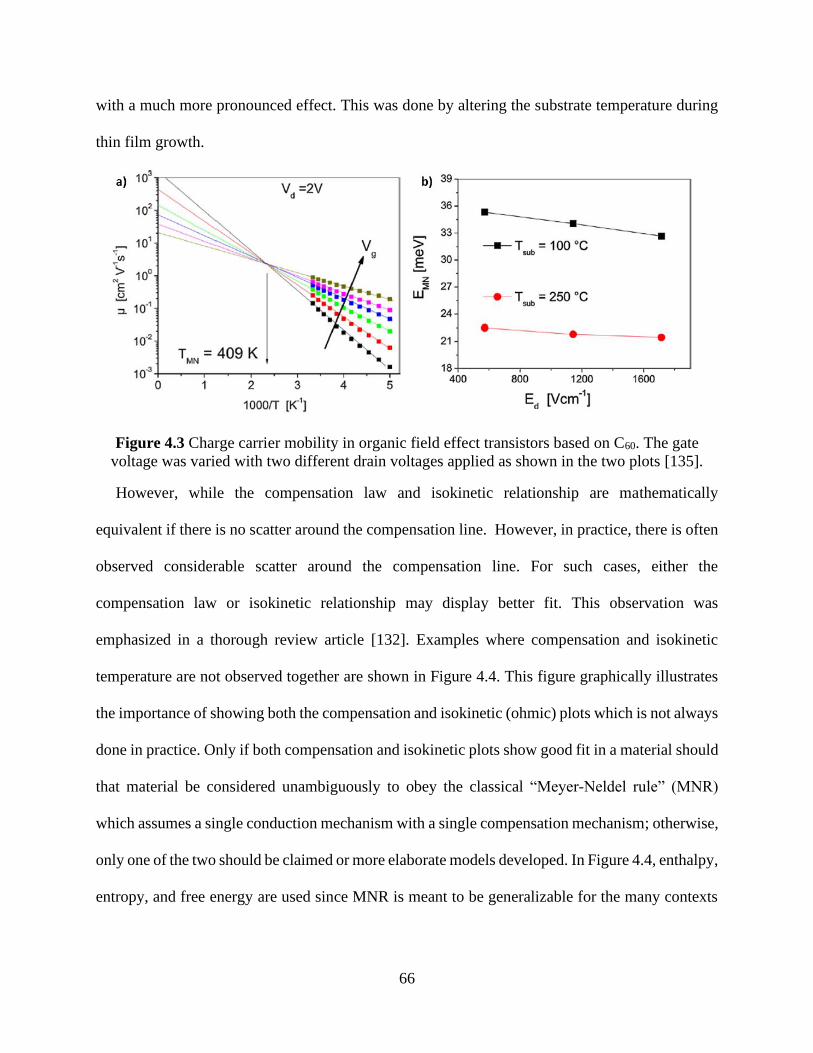
66

with a much more pronounced effect. This was done by altering the substrate temperature during

thin film growth.

Figure 4.3 Charge carrier mobility in organic field effect transistors based on C60. The gate

voltage was varied with two different drain voltages applied as shown in the two plots [135].

However, while the compensation law and isokinetic relationship are mathematically

equivalent if there is no scatter around the compensation line. However, in practice, there is often

observed considerable scatter around the compensation line. For such cases, either the

compensation law or isokinetic relationship may display better fit. This observation was

emphasized in a thorough review article [132]. Examples where compensation and isokinetic

temperature are not observed together are shown in Figure 4.4. This figure graphically illustrates

the importance of showing both the compensation and isokinetic (ohmic) plots which is not always

done in practice. Only if both compensation and isokinetic plots show good fit in a material should

that material be considered unambiguously to obey the classical “Meyer-Neldel rule” (MNR)

which assumes a single conduction mechanism with a single compensation mechanism; otherwise,

only one of the two should be claimed or more elaborate models developed. In Figure 4.4, enthalpy,

entropy, and free energy are used since MNR is meant to be generalizable for the many contexts

67

in which the MNR can appear. As such, the free energy can be considered analogous to the

conductivity, the enthalpy to the activation energy and the entropy to the pre-exponential factor.

Figure 4.4 Reference examples where compensation and isokinetic temperature are not observed

together. a,b) Compensation behavior without a corresponding isokinetic temperature. c,d)

Isokinetic temperature without corresponding compensation behavior [132].

Unlike the activation energy, the Meyer-Neldel energy does not appear to have one fixed

meaning. Several models have been developed over the past few decades that provide an origin

for this concept. For example, a phenomenological model has been developed where the isokinetic

temperature is a temperature below which disorder is frozen into a sample [136]. Along similar

lines, it has been shown that if multiple transport mechanisms are available where one is intrinsic

and another is extrinsic, then the Meyer-Neldel rule should be observed [137]. Water is notable as

an impurity that can lead to the observation of MNR [96,138–140]. Several models have been

68

proposed that use the temperature [141] or the energy [142–145] as a means of describing states

within the band gap. Roberts [141] describes TMN as indicating the distribution of states within the

band gap of an insulating material, where an infinite temperature corresponds to a uniform

distribution and a finite temperature corresponds to an exponential distribution. Yelon et al.

[142,143] developed the multi-excitation entropy (MEE) model to root compensation in

fundamental thermodynamics. To carry out any process with a large energy requirement, such as

having an electron cross a large band gap, it is more likely to obtain multiple excitations with small

energy rather than a large excitation. Thus, processes with larger energy requirements need more

excitations, meaning there are more ways to combine them. In this way, increases in enthalpy (or

activation energy) are compensated by increases in entropy (or pre-exponential factor). The

obtained Meyer-Neldel energy is considered to correspond to the energy of each of these

excitations. The statistical shift model [144,145] is rooted in Fermi-Dirac statistics. The change in

the Fermi level with respect to temperature is shown to influence both the activation energy and

the pre-exponential factor. The Meyer-Neldel energy is characteristic of density of states in the

band gap. The dispersive transport model which explicitly takes into account micro-structural and

chemical disorder also leads to the Meyer-Neldel rule [146]. Of these models, impurities and MEE

have been the most commonly invoked for insulators such as polyethylene. MNR has also been

observed for ionic transport in chalcogenide and oxide ionic conductors [147–152]. The models

for electronic and ionic compensation tend to be similar.

Compensation has been observed for low-density polyethylene (LDPE) as early as the 1970s

[130,134,153]. Thermally activated conduction for LDPE generally occurs below its melting point

of 115°C (e.g. 50°C to 90°C) with a compensation law in irradiated, annealed LDPE with TMN = -

13°C and σ00 = 5 × 10−21 S/m [134]. The authors found that irradiation changed these parameters

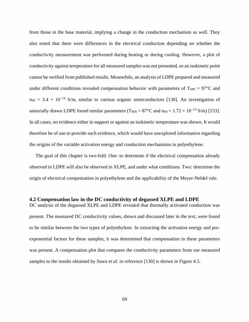
69

from those in the base material, implying a change in the conduction mechanism as well. They

also noted that there were differences in the electrical conduction depending on whether the

conductivity measurement was performed during heating or during cooling. However, a plot of

conductivity against temperature for all measured samples was not presented, so an isokinetic point

cannot be verified from published results. Meanwhile, an analysis of LDPE prepared and measured

under different conditions revealed compensation behavior with parameters of TMN = 97°C and

σ00 = 3.4 × 10−14 S/m, similar to various organic semiconductors [130]. An investigation of

uniaxially drawn LDPE found similar parameters (TMN = 87°C and σ00 = 1.72 × 10−14 S/m) [153].

In all cases, no evidence either in support or against an isokinetic temperature was shown. It would

therefore be of use to provide such evidence, which would have unexplored information regarding

the origins of the variable activation energy and conduction mechanisms in polyethylene.

The goal of this chapter is two-fold. One: to determine if the electrical compensation already

observed in LDPE will also be observed in XLPE, and under what conditions. Two: determine the

origin of electrical compensation in polyethylene and the applicability of the Meyer-Neldel rule.

4.2 Compensation law in the DC conductivity of degassed XLPE and LDPE DC analysis of the degassed XLPE and LDPE revealed that thermally activated conduction was

present. The measured DC conductivity values, shown and discussed later in the text, were found

to be similar between the two types of polyethylene. In extracting the activation energy and pre-

exponential factors for these samples, it was determined that compensation in these parameters

was present. A compensation plot that compares the conductivity parameters from our measured

samples to the results obtained by Sawa et al. in reference [130] is shown in Figure 4.5.

70

Figure 4.5 Compensation plot comparing degassed XLPE and degassed LDPE. Comparison

LDPE data from the work of Sawa et al [130] is indicated separately.

For both XLPE and LDPE, good linear fits were obtained from the plot of EA vs. log σ0 with

R2 values of 0.967 and 0.939, respectively. There was a clear difference in the obtained Meyer-

Neldel temperature between our samples (58°C for XLPE and 53°C for LDPE), the Sawa literature

reference (97°C for LDPE), and the previously mentioned examples. The data shown in Sawa et

al. was combined from several reports of thermally activated conduction in LDPE. Sawa reported

an absence of any apparent correlation between the processing parameters used to make samples

and where their Arrhenius parameters lied on the compensation law plot. The same is true in our

case. On the other hand, Sawa found that holding the applied dc voltage for a longer time in

isothermal current measurements led to monotonic increases in both EA and σ0, and thus

compensation could be observed in a single sample by varying experimental conditions for the

conductivity measurements. However, we found examples where there were monotonic decreases

in both parameters, in addition to examples of the monotonic increases (see Figure 4.6 for an

71

example). This implies that the changes in activation energy and conductivity over time may

depend on more than one physical mechanism controlling overall compensation behavior. The

dispersive transport model is well-suited for explaining increasing activation energy with time as

observed for sample #2 [146]. For the dispersive transport, progressively deeper traps become

prevalent in charge trapping leading to increasing activation energy with time [154]. For sample

#1, a reduction in activation energy with time can be accounted by the dielectrophoretic transport

of water molecules into the regions of high electric field. As water is more polarizable than the

matrix, it is driven into the regions of high electric field, resulting in lowering of activation energy

because of time dependent increase in the polarizability of hydrated regions. In polyethylene,

temperatures below the isokinetic temperature, the most insulating regions are the ones with the

highest activation energy for conduction. Consequently, water penetration into such regions can

have strong influence on the effective activation energy. It can be concluded that the key difference

between the two samples was whether or not water had access to the most insulating regions.

Figure 4.6 Plot of activation energy against pre-exponential factor for two degassed LDPE

samples as a function of the measurement time. The number presented in the legend is the

earliest time at which the current is counted for extraction of the Arrhenius parameters.

72

In attempt to determine the origin of the variability in activation energy, plots of DC

conductivity vs temperature were prepared for the degassed XLPE and LDPE samples. If an

isokinetic point was present, then the Meyer-Neldel rule would apply and conventional

explanations such as multi-excitation entropy [142,143] could be applied to polyethylene. If not,

then another explanation must be sought. The conductivity versus temperature plots are presented

for XLPE in Figure 4.7 and for LDPE in Figure 4.8.

Figure 4.7 a) Conductivity vs temperature plot and b) compensation law plot for degassed XLPE

samples

Figure 4.8 a) Conductivity vs temperature plot and b) compensation law plot for degassed LDPE

samples

73

For both, the compensation plots are provided for a side-by-side comparison. The obtained

Meyer-Neldel temperatures are indicated on the conductivity versus temperature plots. Raw DC

conductivity values were comparable between XLPE and LDPE and tended to range from 10-15 to

10-13 S/m as shown in Figures 2 and 3. These values are comparable to what has been seen in the

literature [47]. This means that correlations cannot be made between physical parameters like

crystallinity and electrical parameters like the conductivity. The average crystallinity for XLPE

(≈30%) and for LDPE (≈40%) differ due to the crosslinks disrupting the crystallization process.

These differences in crystallinity and crosslinking density had no apparent impact on the measured

conductivity. This is in line with the results found in polyethylene [130] as well as other polymers

[138]. An isokinetic point was absent in the DC conduction of both XLPE and LDPE. The presence

of compensation without an isokinetic point precluded the existence of the Meyer-Neldel rule in

polyethylene and motivated the search for a different explanation. First, measurement and/or

experimental error should be ruled out [132,155,156]. Such errors are reported to lead to an

apparent isokinetic effect [155,156] and a much narrower range of activation parameters than

observed here [157]. There is sufficient variation in the conductivity of these samples and their

temperature-dependence that an apparent isokinetic effect can be ruled out as easily as a true

isokinetic effect. As such, a cause of the large variations in activation energy and pre-exponential

term was sought out.

4.3 Compensation law comparison between AC and DC conductivity With knowledge of the time-dependence of the compensation parameters under DC conditions in

mind, it was decided to investigate AC conduction and determine if the same phenomena could be

observed there as well. The results of this investigation are shown in Figure 4.9. The compensation

law plots are presented in 4.9a for XLPE and 4.9b for LDPE, along with comparisons to the DC

74

data. In 4.9c and 4.9d are the corresponding plots of AC conductivity versus temperature for all

the samples used to make the compensation plots, with the frequency used during measurement

labelled in the legend.

Figure 4.9 Compensation law plots for a) degassed XLPE and b) degassed LDPE comparing the

DC and AC results. The corresponding conductivity vs temperature data for the AC

measurements are shown in c) and d)

The compensation parameters for both AC and DC are shown in the compensation plots, and

the energy is translated into its corresponding isokinetic temperature in the plots of conductivity

versus temperature. Again, there was compensation between the activation energy and pre-

exponential factor without a true isokinetic point. Instead, there was clustering to similar but not

equivalent values near TMNR. While small differences between EMN were observed, the main

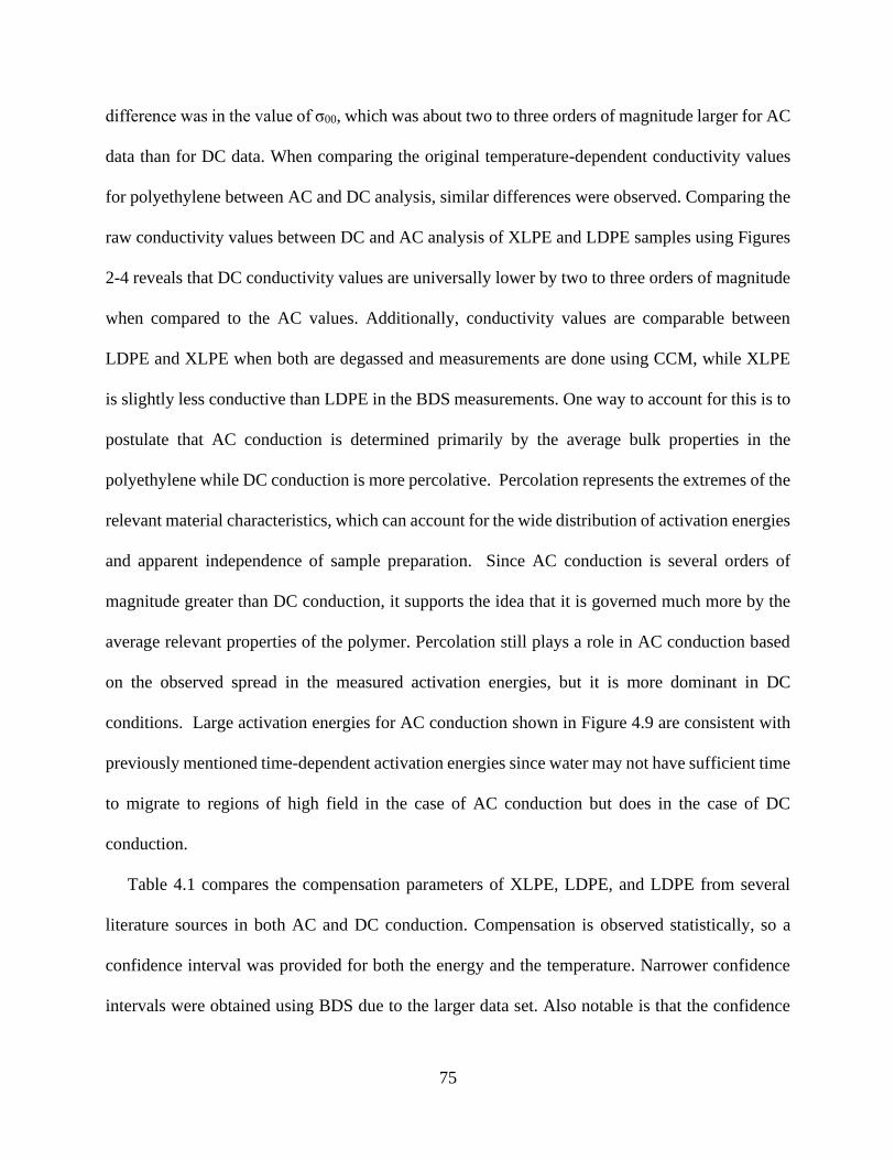
75

difference was in the value of σ00, which was about two to three orders of magnitude larger for AC

data than for DC data. When comparing the original temperature-dependent conductivity values

for polyethylene between AC and DC analysis, similar differences were observed. Comparing the

raw conductivity values between DC and AC analysis of XLPE and LDPE samples using Figures

2-4 reveals that DC conductivity values are universally lower by two to three orders of magnitude

when compared to the AC values. Additionally, conductivity values are comparable between

LDPE and XLPE when both are degassed and measurements are done using CCM, while XLPE

is slightly less conductive than LDPE in the BDS measurements. One way to account for this is to

postulate that AC conduction is determined primarily by the average bulk properties in the

polyethylene while DC conduction is more percolative. Percolation represents the extremes of the

relevant material characteristics, which can account for the wide distribution of activation energies

and apparent independence of sample preparation. Since AC conduction is several orders of

magnitude greater than DC conduction, it supports the idea that it is governed much more by the

average relevant properties of the polymer. Percolation still plays a role in AC conduction based

on the observed spread in the measured activation energies, but it is more dominant in DC

conditions. Large activation energies for AC conduction shown in Figure 4.9 are consistent with

previously mentioned time-dependent activation energies since water may not have sufficient time

to migrate to regions of high field in the case of AC conduction but does in the case of DC

conduction.

Table 4.1 compares the compensation parameters of XLPE, LDPE, and LDPE from several

literature sources in both AC and DC conduction. Compensation is observed statistically, so a

confidence interval was provided for both the energy and the temperature. Narrower confidence

intervals were obtained using BDS due to the larger data set. Also notable is that the confidence

76

intervals of LDPE and XLPE have significant overlap in DC analysis (p-value = 0.923) but barely

any in AC analysis (p-value = 0.008). The similarity between XLPE and LDPE in CCM suggests

that adding crosslinks does not change the conduction mechanisms for polyethylene in DC

conditions. The same cannot be said for AC conditions based on the existing data, but it could not

be determined if this statistically significant difference had any practical implications.

Table 4.1 Compensation parameters of the degassed XLPE and LDPE samples discussed up to

this point, as well as several literature references of LDPE

Samples EMN

(meV)

EMN

95% CI

(meV)

TMN

(°C)

TMN

95% CI

(°C)

σ00

(S/m)

d-XLPE – CCM 28.1 (25.4, 31.5) 53.3 (21.9, 92.3) 3.5 × 10-15

d-XLPE – BDS 31.3 (30.6, 32) 89.9 (82.2, 97.9) 3.0 × 10-12

d-LDPE – CCM 28.6 (20.2, 48.4) 58.3 (-47.6, 352) 9.9 × 10-15

d-LDPE – BDS 29.7 (28.7, 30.7) 71.0 (59.8, 82.9) 1.9 × 10-12

Irradiated LDPE [134] 22.4 - -13 - 5 × 10-21

LDPE [130] 31.9 - 97 - 3.4 × 10-14

Drawn LDPE [153] 31 - 87 - 1.72 × 10-14

In any case, the physical cause of the variable activation energy had yet to be determined. It

needed to be something that would be active in both AC and DC conduction, and that would be

present in both XLPE and LDPE. For these polyethylene variants, two main possibilities exist

based on its composite structure. These two materials consist of multiple phases (amorphous,

crystalline, and interface) and contain trace levels of various impurities (DCP byproducts, water,

oxygen, etc.). All the XLPE samples are fully degassed thin films, so the DCP byproducts would

play a reduced role. This leaves other impurities such as water and oxygen as the possible culprits.

These impurities have varying trap depths in polyethylene [48], so variance in the most common

trap states between samples may explain the variance in EA. This would be independent of the

choice of XLPE or LDPE. Alternatively, variation in the connectivity of the conductive interface

regions could also work as an explanation [158,159]. Most of the difference would have to occur

between samples, rather than between the two different types of PE, even though they have

77

significant differences in morphology [15]. With percolative transport in play, however, the

average differences may not be so significant. The differences in the extremes of energy barriers

may matter more. The data presented here suggested that variation in these extremes is intrinsic to

polyethylene and does not appear to be influenced by crosslinking or crystallinity.

4.4 Impacts of small molecules such as water To help examine these two possible cases – variation in impurities against variation in interfaces

– samples of XLPE were soaked in water and then measured in both AC and DC conduction

modes. Rather than being degassed, the XLPE thin films were left to sit in a water bath kept at

50°C for two hours. Electrodes were then applied as previously described. The results of the AC

and DC measurements are presented in Figure 4.10. In Figure 4.10a are the AC and DC

conductivity results obtained from the water-soaked samples. In Figure 4.10b is the resulting

compensation plot that includes both sets of results, and also provides a comparison to the degassed

XLPE samples.

Figure 4.10 a) AC conductivity vs temperature plot and b) compensation law plot for water-

soaked XLPE samples. A comparison to the degassed XLPE samples discussed previously is

included in the plot on the right

78

Not only was the isokinetic point not observed in the water-soaked samples, but compensation

was also absent in AC conduction. Instead, there was a clear clustering of the activation energy

values around 0.15 eV and pre-exponential factor around 10-10 S/m. A few of the samples were

then measured in DC conduction and lined up with the previously measured degassed XLPE

samples. It should be kept in mind that the DC measurements were always done after the AC

measurements. This allows for the possibility of different degree of hydration for the AC and DC

measurements of conductivity. In general, water near the electrodes regions is more important in

AC conduction while water throughout the bulk of the sample is important for DC conduction.

It can be concluded from these results that concentrations of impurities such as water have a

strong impact on the electrical properties of polyethylene. It has been reported that water addition

will enhance the conductivity and decrease the activation energy of polymers, including

polyethylene [96,138–140]. Upon dehydration, the activation energy can be increased up to values

of around 2 eV, far in excess of the values measured here [96]. As such, the degassed samples can

be said to be only partially dehydrated, likely from picking up moisture between degassing and

measurement as well as having some residual trapped water. Polar molecules like water have also

been shown to influence the pre-exponential factor [139,140]. When water is absorbed by

polyethylene, it is captured by a trap in the amorphous region and heavily modifies its activation

energy, which will be determined by the final arrangement of molecules [96]. As such, the extent

of hydration is sufficient to explain the observed compensation phenomena.

To clarify whether or not the water in the water-soaked samples was from the crosslinking

reaction or from the water-soaking, XLPE samples were degassed and then soaked in water to

determine how comparable they were to the samples used to generate the previous figure. The

79

samples were determined to have compensation characteristic similar to the degassed films without

water soaking under both AC and DC conditions as shown in Figure 4.11.

Figure 4.11 Compensation law plot for XLPE samples that have been both water-soaked and

degassed. A comparison to the XLPE samples that have been either degassed or water-soaked is

included in the plot

Parameters obtained in AC for the degassed and water-soaked samples were 97.4°C (31.9 meV)

and 1.66 × 10-12 S/m, very similar to those obtained for the degassed samples and distinct from

those obtained from the water-soaked samples. It was concluded from this that the short exposure

to water was likely not enough time to have significant concentrations of water soak into the

polyethylene. As such, the water concentrations that led to the different behavior were already

inside the sample, likely generated during the dehydration of crosslinking byproducts, and were

removed when degassing was used. These molecules should be expected to reside in pores and

within the amorphous region. It is possible that extended water soaking to ensure the incorporation

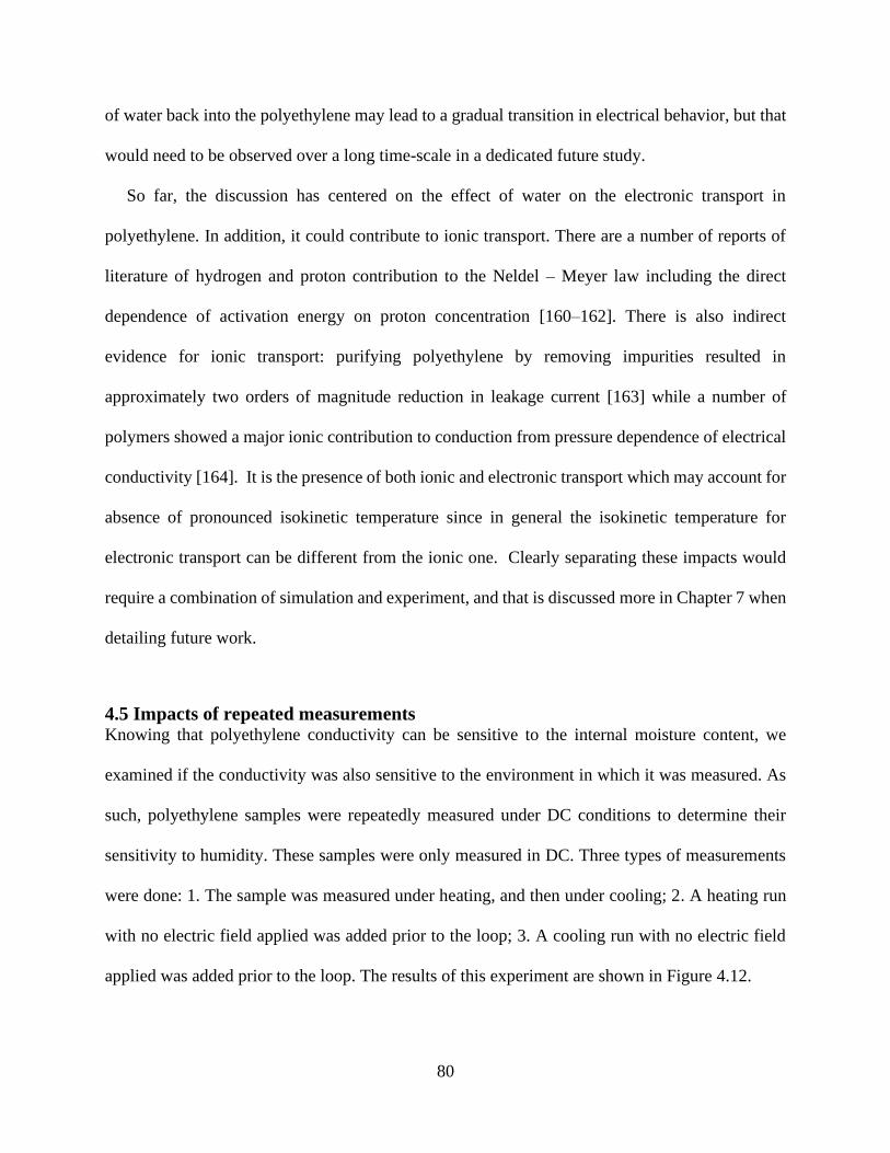
80

of water back into the polyethylene may lead to a gradual transition in electrical behavior, but that

would need to be observed over a long time-scale in a dedicated future study.

So far, the discussion has centered on the effect of water on the electronic transport in

polyethylene. In addition, it could contribute to ionic transport. There are a number of reports of

literature of hydrogen and proton contribution to the Neldel – Meyer law including the direct

dependence of activation energy on proton concentration [160–162]. There is also indirect

evidence for ionic transport: purifying polyethylene by removing impurities resulted in

approximately two orders of magnitude reduction in leakage current [163] while a number of

polymers showed a major ionic contribution to conduction from pressure dependence of electrical

conductivity [164]. It is the presence of both ionic and electronic transport which may account for

absence of pronounced isokinetic temperature since in general the isokinetic temperature for

electronic transport can be different from the ionic one. Clearly separating these impacts would

require a combination of simulation and experiment, and that is discussed more in Chapter 7 when

detailing future work.

4.5 Impacts of repeated measurements Knowing that polyethylene conductivity can be sensitive to the internal moisture content, we

examined if the conductivity was also sensitive to the environment in which it was measured. As

such, polyethylene samples were repeatedly measured under DC conditions to determine their

sensitivity to humidity. These samples were only measured in DC. Three types of measurements

were done: 1. The sample was measured under heating, and then under cooling; 2. A heating run

with no electric field applied was added prior to the loop; 3. A cooling run with no electric field

applied was added prior to the loop. The results of this experiment are shown in Figure 4.12.

81

Figure 4.12 Repeated temperature-dependent conductivity measurements for degassed a) XLPE

and b) LDPE. In part c), the loops for XLPE and LDPE were preceded by either heating from

25°C to 90°C or cooling down from 90°C to 25°C the sample in the oven with no electrical field

applied.

82

The results from the initial measurements of XLPE (Figure 4.12a) and LDPE (Figure 4.12b)

are similar to those observed in Figures 4.7 and 4.8. Unlike in many of those measurements,

however, there was a region with a steep slope and a region with a shallow slope rather than having

one consistent slope over the entire measurement range. This was translated as having a region of

thermally activated conduction (steep slope) and a region approaching saturation (shallow slope).

Such a result has been previously observed in the literature and was attributed to an annealing

effect that occurs at temperatures of 318 K (45°C) and above [71]. For the additional

heating/cooling cycles, there were still two regions but the temperature ranges in which they were

observed were flipped. The conductivity values were also decreased with the repeated

measurements. The general trend was of further reduction in conductivity as the measurements

went on but with the biggest change happening between the initial heating and the initial cooling

run. When samples were either heated from 25°C to 90°C or brought to 90°C and then cooled

down to 25°C in a simulation of these runs with no applied field, the next measurement run

exhibited a roughly invariant conductivity at lower temperatures and then thermally-activated

conduction at higher temperatures as shown in Figure 4.12c. This resembled the behavior of the

samples in Figure 4.12a and 4.12b after the initial measurement. As such, this change can be

attributed solely to the applied heat, which is consistent with other examinations of polyethylene

[71,96,134]. The samples had similar conductivity and activation energy values after either the

initial run or the heat treatment. This suggests that the electrical properties of samples may

equilibrate over time. In fact, measurement of one of these samples one week after sitting in

ambient did not lead to any significant changes in the observed behavior. Whatever changes

occurred in the sample due to annealing appear to be permanent. Further examinations would be

useful to confirm this. It also showed that changes in crystallinity do not correlate to changes in

83

conductivity, confirming the importance of the amorphous phase to electrical conduction in

polyethylene. Using the activation energies and pre-exponential factors from these samples, it was

decided to determine if the compensation law and/or isokinetic point were present. The results are

shown in Figure 4.13.

Figure 4.13 a) Compensation plot comparing all the XLPE and LDPE samples to the runs shown

in Figure 4.5 after initial runs or treatments; b) Extrapolated conductivity at the nominal

‘isokinetic point’ of 120.9°C for the same samples plotted in red. Legend is shown separately

below the conductivity plot.

84

Figure 4.13a shows the compensation behavior of two groups of XLPE and LDPE samples.

The black squares are the combined XLPE and LDPE samples examined in Figure 4.5. The red

circles are the combined XLPE and LDPE samples examined in Figure 4.12 except for the Heat

#1 shown in Figures 4.12a and 4.12b. These two groups lay upon two clearly distinct lines. As

expected, there was much less variation in the samples that had been subject to the heat treatment

prior to measurement, with activation energy values ranging from 0.4 eV to 0.8 eV. However, this

was much smaller than the approximate maximum of 2 eV value expected if water had been

completely evacuated from the samples. Furthermore, the compensation law was still applicable.

Thus, these irreversible changes should not be linked to large changes in moisture content. Instead,

there are two other possibilities: 1. There is some other volatile species that comes off during

prolonged annealing; 2. There is an irreversible change in the structure during prolonged

annealing. Given that the films are already degassed and it is known that annealing will increase

the crystallinity of polyethylene, there is more support for explanation 2 than for explanation 1.

Based on the analysis of the water-soaked samples, it would make sense that if the applied heat to

the sample can alter the arrangement of water and polyethylene molecules, then changes in the

pre-exponential factor and activation energy would be observed as they were in this work. Such

changes would then lead to altered compensation behavior. This would be useful to examine via

simulation, and would be of use towards determining the impact of other molecules like DCP

byproducts if a generalizable model can be developed.

The compensation parameters for the combined data in Figure 4.13a are the following: 58.3°C

(28.6 meV) and 5.65 × 10-15 S/m for the black squares; 120.9°C (34 meV) and 6.19 × 10-15 S/m

for the red circles. This difference in Meyer-Neldel energy was confirmed to be statistically

significant (p-value = 0.0072). Changes of this sort have been observed in other disordered

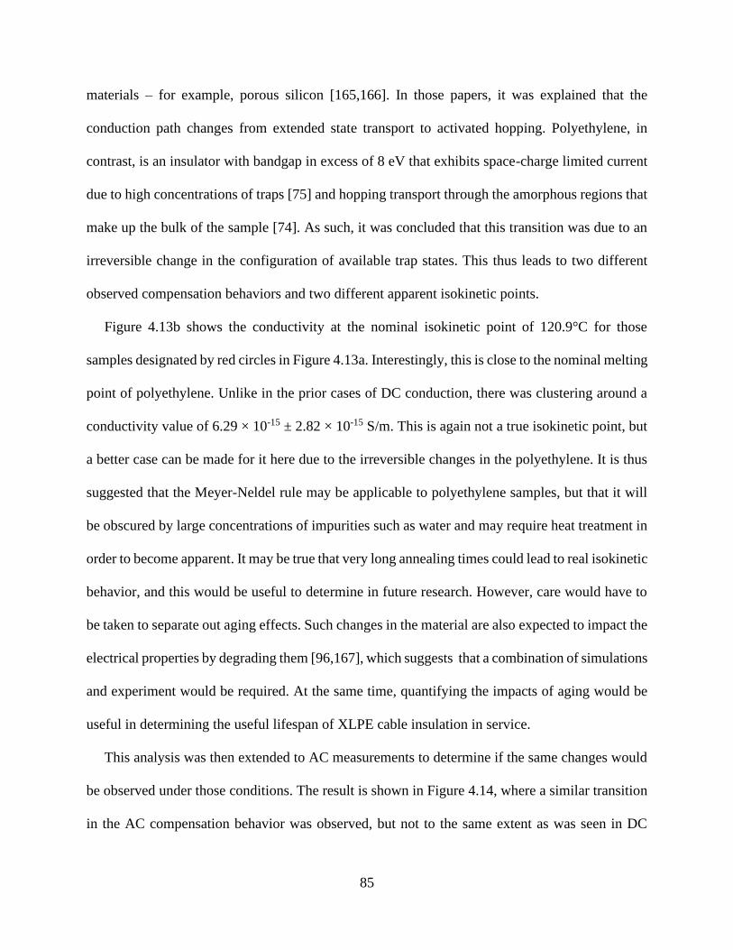
85

materials – for example, porous silicon [165,166]. In those papers, it was explained that the

conduction path changes from extended state transport to activated hopping. Polyethylene, in

contrast, is an insulator with bandgap in excess of 8 eV that exhibits space-charge limited current

due to high concentrations of traps [75] and hopping transport through the amorphous regions that

make up the bulk of the sample [74]. As such, it was concluded that this transition was due to an

irreversible change in the configuration of available trap states. This thus leads to two different

observed compensation behaviors and two different apparent isokinetic points.

Figure 4.13b shows the conductivity at the nominal isokinetic point of 120.9°C for those

samples designated by red circles in Figure 4.13a. Interestingly, this is close to the nominal melting

point of polyethylene. Unlike in the prior cases of DC conduction, there was clustering around a

conductivity value of 6.29 × 10-15 ± 2.82 × 10-15 S/m. This is again not a true isokinetic point, but

a better case can be made for it here due to the irreversible changes in the polyethylene. It is thus

suggested that the Meyer-Neldel rule may be applicable to polyethylene samples, but that it will

be obscured by large concentrations of impurities such as water and may require heat treatment in

order to become apparent. It may be true that very long annealing times could lead to real isokinetic

behavior, and this would be useful to determine in future research. However, care would have to

be taken to separate out aging effects. Such changes in the material are also expected to impact the

electrical properties by degrading them [96,167], which suggests that a combination of simulations

and experiment would be required. At the same time, quantifying the impacts of aging would be

useful in determining the useful lifespan of XLPE cable insulation in service.

This analysis was then extended to AC measurements to determine if the same changes would

be observed under those conditions. The result is shown in Figure 4.14, where a similar transition

in the AC compensation behavior was observed, but not to the same extent as was seen in DC

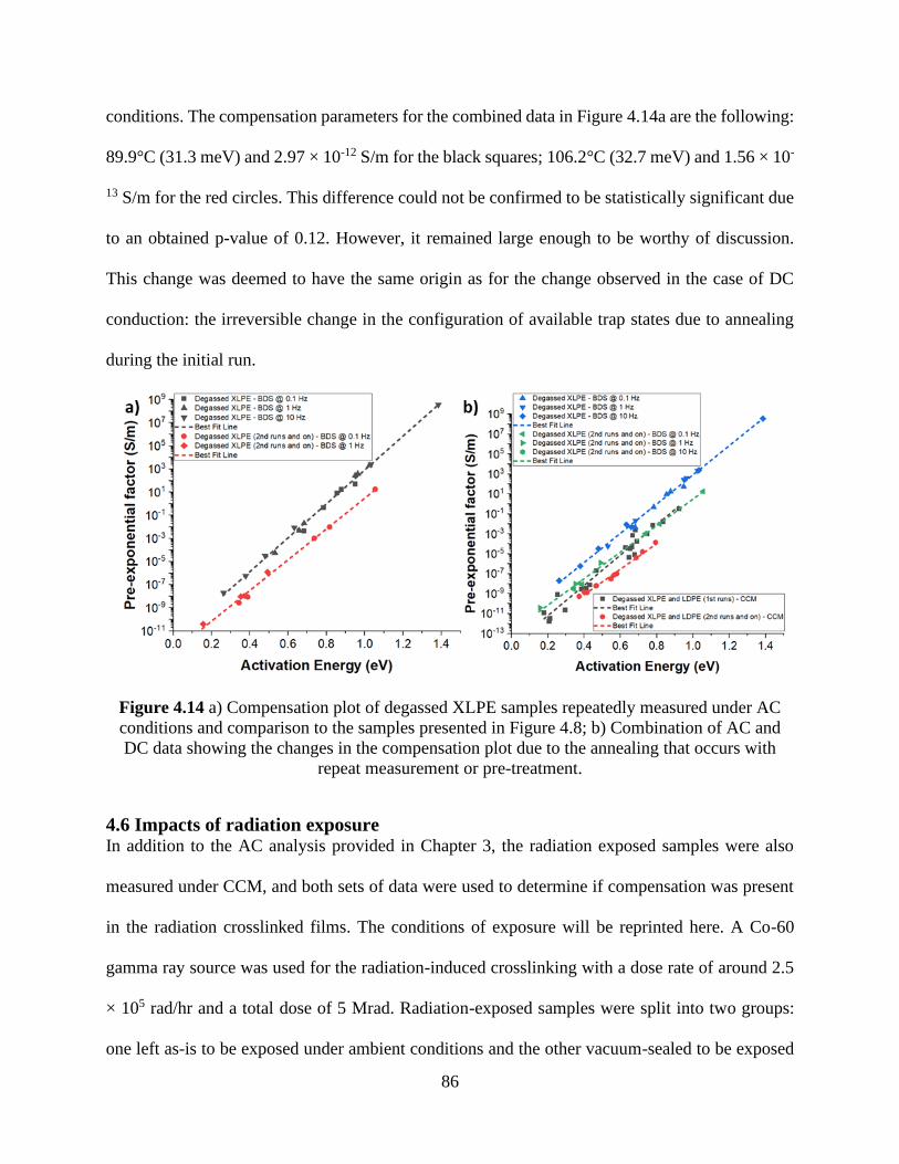
86

conditions. The compensation parameters for the combined data in Figure 4.14a are the following:

89.9°C (31.3 meV) and 2.97 × 10-12 S/m for the black squares; 106.2°C (32.7 meV) and 1.56 × 10-

13 S/m for the red circles. This difference could not be confirmed to be statistically significant due

to an obtained p-value of 0.12. However, it remained large enough to be worthy of discussion.

This change was deemed to have the same origin as for the change observed in the case of DC

conduction: the irreversible change in the configuration of available trap states due to annealing

during the initial run.

Figure 4.14 a) Compensation plot of degassed XLPE samples repeatedly measured under AC

conditions and comparison to the samples presented in Figure 4.8; b) Combination of AC and

DC data showing the changes in the compensation plot due to the annealing that occurs with

repeat measurement or pre-treatment.

4.6 Impacts of radiation exposure In addition to the AC analysis provided in Chapter 3, the radiation exposed samples were also

measured under CCM, and both sets of data were used to determine if compensation was present

in the radiation crosslinked films. The conditions of exposure will be reprinted here. A Co-60

gamma ray source was used for the radiation-induced crosslinking with a dose rate of around 2.5

× 105 rad/hr and a total dose of 5 Mrad. Radiation-exposed samples were split into two groups:

one left as-is to be exposed under ambient conditions and the other vacuum-sealed to be exposed

87

without significant oxygen presence. A separate group of as-received LDPE samples were used as

a control group.

The resulting compensation plots are shown in Figure 4.15 for AC measurements in Figure

4.15a and DC measurements in Figure 4.15b. Included in those plots are results from the as-

received and degassed LDPE samples for comparative purposes. There were distinct differences

between the observed AC and DC compensation in radiation exposed samples. Under DC

conditions, there was ultimately not much difference between the samples with and without

radiation exposure. Under AC conditions, however, the activation energies were limited to a range

of about 1 to 1.2 eV for samples exposed in air and about 0.8 to 1.4 eV for samples exposed in

vacuum. This suggests that the coupling between ionic and electronic conduction should also be

present in these radiation-crosslinked samples, and the variations here are due to the subtle

variations in the structure caused by the damage introduced by the radiation. It was suggested in

Chapter 3 that LDPE with radiation crosslinking becomes more of an ionic conductor, and this

finding helps support that result. A general trend relating the activation energy to the conduction

mechanism was devised based on these results and is shown in the next section.

Figure 4.15 Compensation plot of irradiated LDPE samples and comparison to as-received and

degassed LDPE under a) AC and b) DC measurement conditions.

88

4.7 The origins of electrical compensation in polyethylene The many significant changes in the XLPE compensation parameters as shown in Figure 4.11,

4.14b, and Figure 4.15 have two distinct causes: chemical from impurities; and physical from

annealing. The impurities from the crosslinking process clustered in voids and amorphous regions

had the effect of not allowing compensation to occur, leading to the clustering of activation

energies as mentioned previously. Degassing removes these extrinsic DCP byproducts from the

films, but there is always some intrinsic trapped water as well as water that can be added with air

exposure or with intentional soaking. As such, there will be coupled ionic and electronic transport

that reduces the activation energy far below the expected value of around 2 eV for fully dehydrated

samples. It is proposed that variation in the extent of hydration between samples of the same type

lead to the observed compensation. When samples are annealed, the coupling is retained but altered

due to the physical re-arrangement of water and polyethylene molecules and dehydration that

reduced the ionic contribution. This led to the altered compensation and isokinetic behavior.

Radiation exposure also altered the compensation behavior due to its promotion of ionic

conduction within the overall paradigm of coupled conduction. As such, the following overall

trend is supposed. Small molecules such as DCP byproducts lead to very low activation energies

of 0.2 eV and below and no compensation due to purely ionic transport. With their removal,

conduction becomes a mix of ionic and electronic allowing for a wide range of activation energies

between 0.2 eV and 1.4 eV. Changes in the configurations of these traps due to annealing or due

to radiation exposure can then alter the exact energies available, which also depends on the

measurement technique. Summary figures showing all the different changes in the compensation

parameters are presented in Figure 4.16 and Figure 4.17 and the table of the associated

compensation parameters is in Table 4.2.

89

Figure 4.16 All compensation plots of DC conduction for samples discussed in this chapter.

Figure 4.17 All compensation plots of AC conduction for samples discussed in this chapter.

90

Table 4.2 Compensation parameters of all XLPE and LDPE samples discussed in this chapter.

Samples EMN

(meV)

EMN

95% CI

(meV)

TMN

(°C)

TMN

95% CI

(°C)

σ00

(S/m)

d-XLPE – CCM 28.1 (25.4, 31.5) 53.3 (21.9, 92.3) 3.5 × 10-15

d-XLPE – BDS 31.3 (30.6, 32) 89.9 (82.2, 97.9) 3.0 × 10-12

d-LDPE – CCM 28.6 (20.2, 48.4) 58.3 (-47.6, 352) 9.9 × 10-15

d-LDPE – BDS 29.7 (28.7, 30.7) 71.0 (59.8, 82.9) 1.9 × 10-12

XLPE w/ H2O – BDS not applicable

d-XLPE w/ H2O – BDS 31.9 (29.6, 34.6) 97.4 (70.7, 128.6) 1.7 × 10-12

d-XLPE – CCM 2nd+ runs 34.0 (31.4, 37) 120.9 (91.1, 156) 6.2 × 10-15

d-XLPE – BDS 2nd+ runs 32.7 (30.8, 34.8) 106.2 (84.3, 130.9) 1.6 × 10-13

r-LDPE – CCM 31.8 (23.5, 48.9) 95.8 (0, 294.8) 1.2 × 10-14

r-LDPE – BDS 30.9 (28.9, 33.2) 85.2 (62, 111.8) 1.9 × 10-12

r-LDPE w/ 5 Mrad – CCM 28.0 (23.1, 35.6) 52.2 (-4.7, 139.6) 1.1 × 10-14

r-LDPE w/ 5 Mrad – BDS 34.3 (31.9, 37.2) 125.2 (96.6, 158.5) 5.9 × 10-8

r-LDPE (vacuum-sealed)

w/ 5 Mrad – CCM

25.6 (18, 44.4) 24.0 (-64.5, 243) 1.9 × 10-16

r-LDPE (vacuum-sealed)

w/ 5 Mrad – BDS

28.6 (27.1, 30.2) 58.7 (41.6, 77.7) 2.1 × 10-11

91

Chapter 5 – Electronic and ionic traps in polyethylene active in different

temperature ranges

5.1 Basic TSDC spectra of XLPE and LDPE TSDC investigations of charge trapped below room temperature are limited for LDPE

[18,94,168] and appear to not exist for XLPE. As such, an investigation was carried out to see

what peaks could be observed below room temperature in XLPE in addition to the features known

to exist at elevated temperatures [23,30,51]. Results are shown in Figure 5.1, with the applied

electric field presented in the legend and a T0 of -150°C for all samples. Figure 5.1a presents the

same data as was shown in Figure 2.6. Samples subjected to the TSDC characterization without

an applied field did not exhibit peaks (0 kV/mm traces in Figure 5.1). There were three distinct

peaks observed in samples with Ep = 10 kV/mm, and the temperatures at which they were observed

were consistent between the two types of polyethylene. The same three peaks were observed with

Ep = -10 kV/mm. A positive field was applied to most samples going forward, and the use of

negative field on one LDPE sample was to verify that the field polarity would not have significant

influence.

Figure 5.1 Representative TSDC spectra with a storage temperature of -150°C for degassed a)

LDPE and b) XLPE with differing applied electric fields as listed in the supplied legend. The

XLPE samples were crosslinked with 2.1% and 2.2% DCP respectively.

92

The high temperature peak around 90°C had a greater absolute maximum current on average in

LDPE than in XLPE by roughly an order of magnitude. Such a reduction of intensity for a peak in

this temperature range has been seen before in HDPE and was attributed to a reduction in crystallite

size due to adding functionalized branches [169]. Similarly, the crosslinks in XLPE interfere with

crystallization and limit their thickness [6,15] and would thus have similar impact. The other two

main peaks had a maximum temperature around 0°C and a maximum temperature between -75°C

and -50°C. The medium temperature peak was more prominent in XLPE than in LDPE both in

absolute terms (absolute maximum current is greater by a factor of 3) and in relative terms

(medium temperature peak has a much greater intensity relative to the high temperature peak in

XLPE than in LDPE). This suggests that it was related to some factor such as impurities or

crosslinks, which would be more prominent in the XLPE. The low temperature peak was not

significantly different between the two forms of polyethylene, suggesting it should have an origin

that is independent of the crosslinks or impurities.

In the TSDC literature, a distinction is made between homocharge and heterocharge, where

homocharge will have the same sign as the charge at the electrodes while heterocharge will have

the opposite sign. For a positively applied voltage, this would correspond to a positive current for

heterocharge and negative current for homocharge. A literature example of this is shown in Figure

5.2 from an XLPE cable section with inner and outer diameters of 7 and 13 mm [23]. That sample

was poled at 8 kV and exhibited primarily heterocharge with injection of homocharge over time

with more annealing. The heterocharge was attributed to crosslinking byproducts and charge

buildup at interfaces in that paper [23]. Homocharge in polyethylene seen at elevated temperatures

is commonly attributed to charge injection regardless of the extent of crosslinking [23,113]. As

such, the observed negative current was attributed to homocharge for the peaks presented in Figure

93

5.1. These differences between Figures 5.1 and 5.2 at high temperature should be attributed to

reduced impurity concentration and increased electric field.

Figure 5.2 Cyclical TSDC discharges of a cable sample conventionally polarized at Tp = 90 °C,

T0 = 50 °C, Vp = 8 kV, tp = 60 min. Samples were brought up to 140°C before poling and at the

end of the heating run during each cycle. [23].

The literature has shown that there are structural changes that occur during heat treatment of

polyethylene that can impact the electrical properties [51,71]. Similarly, we have found differences

between samples of XLPE degassed in different manners. A comparison between samples

degassed at 65°C and 90°C is shown in Figures 5.3 and 5.4. Figure 5.3 shows the spectra with T0

of 25°C, while Figure 5.4 shows the spectra with T0 of -150°C. The data in Figure 5.4a includes

the data in 5.1b. In Figure 5.4a, the data in green is from a repeat run on the same sample used to

obtain the data in blue. In Figure 5.4b, the data in blue is from a repeat run on the same sample

used to obtain the data in red. The high temperature peak around 90°C diminished on intensity on

repeat runs in XLPE samples regardless of the storage temperature used, and the same was also

observed for LDPE.

94

Figure 5.3 TSDC spectra of a degassed XLPE repeatedly poled at 10 kV/mm with a) 65°C or b)

90°C degas prior to measurement. The storage temperature is a constant at 25°C.

Figure 5.4 TSDC spectra with a storage temperature of -150°C for XLPE samples degassed at

two different temperatures: a) 65°C; b) 90°C. Applied fields are listed in the legend.

95

The three peaks were retained upon changing the degassing temperature. Significant changes

were observed in each peak with the change in degassing temperature. First, on average, the high

temperature peak flipped sign from negative to positive with the higher degassing temperature,

and was reduced by about half. This is apparent in both Figure 5.3 and 5.4. However, rather than

being true heterocharge, it was deemed more likely to be deeply injected homocharge that

completed the circuit and emerged at the opposite electrode, given that these samples were

processed in the same way other than the choice of degassing temperature. Highly mobile charges

can create an appearance of heterocharge [170]. The movement of injected charge packets in XLPE

has been a subject of active research, and is known to be influenced by impurities and temperature

[171] and the choice of electrodes [82]. This result was a sign that degassing the samples caused a

physical change that also influenced charge packet movement, having allowed for greater

migration but reduced trapping of these injected charges. Second, there was a significant reduction

in the amount of charge trapped in the peak observed just below room temperature, again by a

factor of around four. Such a reduction was correlated to further removal of byproducts given two

factors. Namely, the crystallinity was around 30% in the degassed XLPE samples regardless of

degassing temperature and the peak intensity became similar to the degassed LDPE samples with

higher degassing temperature. Further discussion on this peak is provided in later sections of this

chapter. Third, the lowest temperature peak had a slight increase in peak intensity of around 13%

with the higher degassing temperature. However, the change was not large enough given

experimental variation to warrant further discussion.

A summary plot showing activation energy and peak maximum temperature of each of the three

major peaks for all measured samples was prepared and is shown in Figure 5.5. The activation

energy was calculated using the initial rise method, where the initial rise of a peak can be

96

approximated as following Arrhenius behavior [114]. The temperature associated with the

maximum of each peak was also recorded. The averages for both these values are displayed in the

legend, along with the sample standard deviation. The high temperature peak had the greatest

spread in the activation energy and narrowest spread in maximum temperature. The opposite was

true for the low temperature peak. The middle temperature peak was intermediate in both. Some

variation was expected simply due to the fact that polyethylene is a semicrystalline material that

is more amorphous than crystalline.

Figure 5.5 Activation energy and maximum temperature of major peaks in the TSDC spectra of

degassed LDPE and XLPE samples. All samples are included in this figure, showcasing the full

variation.

Each of these peaks had a different speculated origin. The high temperature peak was due to

charge injection from the electrodes [23,30,51,168]. Typical observed energies for charge injection

are around 1 eV, matching the average observed here [172]. The variation observed matches what

was seen in the literature [48,96]. The intrinsic barriers to charge injection are quite high (3 eV for

holes and 5.5 eV for electrons) but are reduced by impurities and interface states [48,172–174].

97

The LDPE was more susceptible to charge injection than the XLPE samples despite never having

had DCP byproducts, indicating they were not relevant for that peak and may actually interfere

with it. Instead, interface states and impurities from the electrodes mattered. There was no

meaningful difference in the obtained activation energies between the two types of samples,

however. Degassing temperature appeared to influence how far charges were able to migrate

through the sample during poling for XLPE by altering these interface states, which influenced the

resulting discharge current. It also increased the activation energy on average (1.81 ± 0.38 eV for

samples degassed at 90°C compared to 0.68 ± 0.47 eV for the standard degassed samples),

indicating that only deep traps were made available at high temperature with the harsher degassing.

The activation energies observed for the low temperature and medium temperature peaks were

appropriate for physical (branches and distorted bonds) and chemical (impurities) traps,

respectively [48,95,173]. Low energy traps such as the ones seen at low temperature are often

attributed to disturbances in bonds. The low temperature peak was not far from the glass transition

temperature (Tg) of polyethylene (approximately -80°C [175]) and was found to be associated

with that [169,176–178] and polymer main chain motions [169,176,179]. The energy associated

with crankshaft rotations, for example, has been reported as being 10 kcal/mol, or approximately

0.43 eV/molecule [180], which suggests that those motions in this material are sub-molecular and

that what was measured was the aggregate of many motions. Similarly, peaks with 0.1 to 0.2 eV

have been observed in LLDPE and HDPE due to the glass transition and local cooperative small

scale motions [169,176]. Typically, a semicrystalline polymer exhibits a loss peak just above Tg

in both mechanical and dielectric spectra obtained at 1 Hz [178]. TSDC peaks are comparable to

very low frequency dielectric responses in the mHz regime [18,23,94]. Normally, this means

conductivity should be suspected as a cause; however, polyethylene conductivity is thermally

98

activated as was discussed in Chapter 1 and is thus negligible at very low temperatures such as Tg.

Combined, these facts mean that this peak can be correlated to the relaxations that occur as the

polymer is heated above Tg. Such a dipolar relaxation is typically homopolar, which is what was

observed here.

The medium temperature peak between 0 and 25°C was deemed to be associated with either

crosslinks or impurities as those are more prominent in XLPE than in LDPE as shown in Figure

5.1. It was reduced with a higher degassing temperature, which indicates that impurities should be

more important. Additionally, an activation energy of 0.4 eV was measured for the diffusion of

DCP byproducts such as acetophenone within polyethylene according to measurements done by a

collaborator. It became a focal point for further work regarding the TSDC response of polyethylene

around room temperature. Work discussed in the next two sections regarding as-received samples

and degassed samples soaked in byproducts was needed to confirm that this peak was related to

the presence of impurities.

5.2 Comparison of the TSDC spectra as-received and degassed XLPE Two investigations on the impact of small molecules were carried out: one with byproducts (see

Section 5.3); one with antioxidants (see Section 5.4). In order to support these investigations, as-

received XLPE samples without antioxidant were also prepared. Byproducts were intentionally

kept from escaping the sample before electrode application by the use of Teflon™ sheets. The

results of analyzing as-received XLPE samples without are presented in Figure 5.6. In Figure 5.6a

is the TSDC spectra of as-received XLPE; in Figure 5.6b is a comparison of activation energy of

as-received and degassed samples. The same storage temperature of -150°C was used for all

samples discussed in this section as well as in Section 5.3 and 5.4. Other TSDC parameters were

also kept constant.

99

Figure 5.6 a) TSDC spectra with a storage temperature of -150°C for as-received XLPE

samples; b) Activation energy and maximum temperature of the medium temperature peak for

as-received and degassed samples.

Unlike degassed XLPE, the as-received XLPE exhibited only one peak, and it was centered

around a temperature of 26°C. That result confirmed that this observed peak was due to the

byproducts. These traps introduced by excess concentrations of byproducts appeared to dominate

the spectra and thus the trapping from other sources was not observed. It was speculated that the

activity of at least one of the byproducts was able to interfere with the high temperature charge

injection and low temperature relaxation. A mechanism for this could not be determined solely

from this data, however, and would need to be investigated in future work.

The activation energy of the trap states corresponding to this peak in the as-received samples

was consistently around 0.675 eV. There was little variation in either the peak temperature or the

activation energy when compared to degassed samples (±0.88% and ±3% versus ±1.54% and

±35%, respectively). Traps with similar energy observed at similar temperatures in other

polyethylene variants were associated with charge released from interfaces [169,176], suggesting

that these small molecules congregate there during polarization and are released during

measurement. Similarly, it is close to the activation energy of the initial diffusion of byproducts

out of XLPE [21]. TGA data discussed in Chapter 3 and IR data shown in Figure 5.7 confirms that

100

degassed samples still retain byproducts, though their concentration is reduced by about one order

of magnitude. However, even with a reduced concentration of byproducts, traps were still

contributed that determined the overall properties.

Figure 5.7 Concentration of ACP in various XLPE samples as determined by IR spectroscopy.

To repeat what was stated in Section 1.7 regarding how these byproducts trap charge: ACP is

an electron trap only; aCA and aMS generally support trapping of holes; all are considered to be

shallow traps and fill in small voids, which eases charge transport [34,36,86,97]. All are present

in as-received samples, so trapping of both electrons and holes was expected. Interestingly, this

peak was also homocharge given the sign conventions used in this work. Typically, heterocharge

is expected from impurities [23,110], but those same studies were also focused on trapping that

occurs at much higher temperatures in the melting and recrystallization regimes. However, work

has been done to show that impurities can also lead to homocharge. In a cable sample, diffusion

of impurities from the semicon layer into the XLPE led to high-temperature homopolar charge

injection [30]. What this result implies for these samples is that charge injection can also occur

around room temperature and is aided by these DCP byproducts. The presence of this peak in

101

degassed LDPE and the 90°C degassed XLPE was then attributed to water, which has trace

concentrations in polyethylene both with [22] and without [58] crosslinking due to adsorption [37].

It was clear that having roughly an order of magnitude concentration increase for these small

molecules was enough to drastically alter the trapping characteristics of XLPE. The next step was

then to investigate each byproduct individually and for their separate impacts.

5.3 Impacts of DCP byproducts on the XLPE and LDPE The impact of adding excess byproducts into degassed XLPE on the TSDC spectra was examined

in order to determine the following: 1) if any changes in the spectra could be observed by solely

by the addition of a single byproduct; 2) if these results were in line with the observed results from

space charge studies. The results are split into two figures: Figure 5.8 for acetophenone and Figure

5.9 for methylstyrene. Each byproduct had a different impact on the observed spectra. An

examination of cumyl alcohol was also attempted, but due to issues incorporating it into the

degassed XLPE samples it was not possible to analyze those results in any meaningful way.

Figure 5.8 TSDC spectra with a storage temperature of -150°C for degassed XLPE samples

soaked in acetophenone (ACP).

102

Adding acetophenone (ACP) into the degassed XLPE films led to changes to the TSDC spectra

that resulted in it being qualitatively similar to the as-received samples. The two peaks associated

with high temperature charge injection and low temperature molecular motions were not observed,

leaving only the medium temperature peak. The temperatures where this peak is observed are

consistent with the same peak in the degassed and as-received samples, and the activation energy

of these states is comparable to those observed in the as-received sample (0.632 ± 0.187 eV versus

0.675 ± 0.023 eV, respectively). In certain samples, the peak has a positive sign instead of the

usual negative one. Co-existence of a homopolar and heteropolar feature in XLPE cable insulation

has been studied before and was attributed to variations in the concentration of crosslinking

byproducts [110]. Variation in hydration should also play a role, as was discussed in Chapter 4,

and these two factors led to a complex set of spectra.

However, given the sign convention in Section 5.1, this positive peak should be assigned to

heterocharge only if a causal phenomenon can be found. In the literature, there have been multiple

reports of negative heterocharge generation in ACP-containing samples of polyethylene,

especially in the presence of water or antioxidant [35,37,87,88]. That reaction was discussed

briefly in Chapter 3 for its impact on the AC response and played a role in these results as well.

This process involves the ionization and migration of the ACP when in the presence of moisture,

producing negative ions and protons [35,37,87,88]. Very low frequencies in the mHz or less are

needed to promote heterocharge formation and storage in XLPE [89], corresponding to TSDC

parameters. Both charge injection and ionized impurity migration and dynamic processes,

explaining why there is variation in the extent of homocharge and heterocharge [89]. Similarly,

moisture is explicitly needed to heterocharge to be observed, with more heterocharge being

103

observed as moisture is added. Without moisture, homocharge is still expected in samples with

ACP added [35,88].

Figure 5.9 TSDC spectra with a storage temperature of -150°C for degassed XLPE samples

soaked in methylstyrene (aMS).

Adding methylstyrene (aMS) into the degassed XLPE samples led to samples that were

qualitatively very similar to those without aMS added. The main difference was a relative increase

in the charge trapped in the medium temperature peak. A comparison of the peak intensity and

total stored charge in this peak between different samples is shown in Figure 5.10 for reference.

The presented trend shows a link between concentrations of these small molecules and increased

trapped charge in this specific peak. This is in line with results where methylstyrene contributes to

already existing trapping processes by enhancing them [37]. This was attributed to the

methylstyrene introducing additional trap states in that temperature range. This was accompanied

by slight reduction of peak intensity in both the high temperature and low temperature peaks. It

can be suggested that aMS qualitatively has similar impact to ACP in that it promotes charge

trapping around room temperature and interferes with charge trapping at other temperatures.

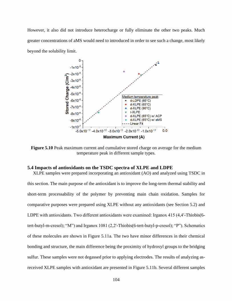
104

However, it also did not introduce heterocharge or fully eliminate the other two peaks. Much

greater concentrations of aMS would need to introduced in order to see such a change, most likely

beyond the solubility limit.

Figure 5.10 Peak maximum current and cumulative stored charge on average for the medium

temperature peak in different sample types.

5.4 Impacts of antioxidants on the TSDC spectra of XLPE and LDPE XLPE samples were prepared incorporating an antioxidant (AO) and analyzed using TSDC in

this section. The main purpose of the antioxidant is to improve the long-term thermal stability and

short-term processability of the polymer by preventing main chain oxidation. Samples for

comparative purposes were prepared using XLPE without any antioxidants (see Section 5.2) and

LDPE with antioxidants. Two different antioxidants were examined: Irganox 415 (4,4′-Thiobis(6-

tert-butyl-m-cresol); “M”) and Irganox 1081 (2,2'-Thiobis(6-tert-butyl-p-cresol); “P”). Schematics

of these molecules are shown in Figure 5.11a. The two have minor differences in their chemical

bonding and structure, the main difference being the proximity of hydroxyl groups to the bridging

sulfur. These samples were not degassed prior to applying electrodes. The results of analyzing as-

received XLPE samples with antioxidant are presented in Figure 5.11b. Several different samples

105

were analyzed. The original test sample with “M” antioxidant was made using 1.73% DCP and

0.41% AO (black in Figure 5.11b). The second set of samples with “M” antioxidant were made

using 3.5% DCP and 1.5% AO (red, green, and purple in Figure 5.11b). The only set of samples

made with “P” antioxidant were made using 3.2% DCP and 3.4% AO (blue, yellow, and cyan in

Figure 5.11b).

Figure 5.11 a) Schematic structure and names of the two antioxidants used in this study; b)

TSDC spectra for as-received XLPE samples containing the two different types of antioxidant.

106

In the XLPE samples with antioxidant, the primary observed features were peaks in the range

of -25°C to 50°C. There were categorical differences in the spectra depending on the antioxidant

used. In Figure 5.11b, the data in purple is a repeat run on the same sample used to obtain the data

in green and the data in cyan is a repeat run on the same sample used to obtain the data in yellow.

With the “M” antioxidant, there was a tendency to observed a peak around 10°C or around 30°C.

In one sample, both were seen. In general, the spectra were considered qualitatively similar to

those of the as-received samples. With the “P” antioxidant, two or three peaks are observed. One

around -24°C was always observed, and peaks around 10°C, 30°C, and 50°C were seen in certain

cases. These spectra are considered to be qualitatively distinct to those of the as-received spectra.

The magnitude of these peaks was also often larger than for the other XLPE samples. The other

two main peaks were seen a few times, but not in most samples. These results suggest that the

presence of byproducts induced significant changes in the electrical properties of XLPE, and

adding in antioxidants on top of that led to further changes. This can arise from the excess charges

introduced by the reaction of acetophenone specifically with antioxidants and/or moisture, going

by prior literature [35,87,88], which is likely the case for antioxidant “M”. However, the “P”

antioxidant appeared to interact in a different manner with the byproducts despite its physical and

chemical similarity with the “M” antioxidant. These two antioxidants are chemically similar,

commercially available, and commonly used, yet had distinct impacts on charge trapping in XLPE.

Such differences should be rooted in the few differences between the two, which include the

location and orientation of -OH groups on these molecules. Further work would be warranted to

more deeply investigate how and why such differences in chemistry influence the available trap

states in XLPE.

107

The results for the LDPE samples with antioxidant added can be found as Figure 5.12. Weight

percent of antioxidant is 7% for samples with antioxidant “M” (Irganox 415) and 6.1% for samples

with antioxidant “P” (Irganox 1081). In the LDPE samples with “M”, the peaks tended to be the

same as those observed in LDPE samples with no antioxidant. In the LDPE samples with “P”, the

peaks tended to be distinct from those observed in LDPE samples with no antioxidant. This

supports the argument that the antioxidants, despite their chemical similarity, can have vastly

differing impacts on electrical properties.

Figure 5.12 TSDC spectra of as-received LDPE samples with antioxidant added.

5.5 Summary of trap states detectable in polyethylene by TSDC A plot comparing the activation energy and maximum temperature of the three major peaks

found in degassed XLPE (d-XLPE) and LDPE (d-LDPE) samples to those found in XLPE samples

with excess byproducts and the as-received samples (r-XLPE) is shown in Figure 5.13. A plot

accomplishing the same for comparing r-XLPE to the samples with antioxidant is shown in Figure

5.14. The r-LDPE samples with antioxidant are also included in that plot. A table listing out all

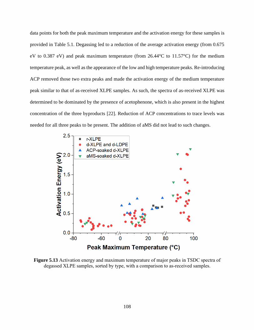
108

data points for both the peak maximum temperature and the activation energy for these samples is

provided in Table 5.1. Degassing led to a reduction of the average activation energy (from 0.675

eV to 0.387 eV) and peak maximum temperature (from 26.44°C to 11.57°C) for the medium

temperature peak, as well as the appearance of the low and high temperature peaks. Re-introducing

ACP removed those two extra peaks and made the activation energy of the medium temperature

peak similar to that of as-received XLPE samples. As such, the spectra of as-received XLPE was

determined to be dominated by the presence of acetophenone, which is also present in the highest

concentration of the three byproducts [22]. Reduction of ACP concentrations to trace levels was

needed for all three peaks to be present. The addition of aMS did not lead to such changes.

Figure 5.13 Activation energy and maximum temperature of major peaks in TSDC spectra of

degassed XLPE samples, sorted by type, with a comparison to as-received samples.

109

Figure 5.14 Activation energy and maximum temperature of major peaks in TSDC spectra of

various types of as-received XLPE samples, sorted by type.

Table 5.1 Activation energy and maximum temperature of major peaks in TSDC spectra of

various types of XLPE and LDPE samples discussed up to this point.

Speculated Peak

Origin Sample Type

Peak Maximum

Temperature (°C) Activation Energy

Charge Injection

d-XLPE

90.74 1.651248204

90.71 0.519404359

87.85 0.137082963

94.55 1.034882063

96.58 0.421617846

96.73 0.321542885

95.81 0.362397846

90.52 0.917781679

95.55 0.755159902

d-LDPE 92.91 0.528134444

96.78 1.084691917

d-XLPE w/ 90°C degas

93.74 1.366195436

95.69 2.016686325

94.99 2.033683915

d-XLPE w/ aMS 85.53 1.306228427

110

88.49 2.033733253

97.61 2.163106369

95.99 1.01177179

85.22 0.964468391

r-XLPE w/ “M” AO 93.8 1.113970008

r-XLPE w/ “P” AO 95.2 0.939251854

r-LDPE w/ “M” AO 70.78 0.465911465

80.47 0.963245209

Small molecules

including: DCP

byproducts; water;

antioxidants

d-XLPE

13.52 0.196762908

15.61 0.594452094

17.48 0.478953672

8.55 0.37940269

15.67 0.605017007

10.79 0.571033487

2.96 0.468501313

10.05 0.440006053

15.47 0.334091566

d-LDPE 10.87 0.177525318

14.29 0.187230747

d-XLPE w/ 90°C degas

10.16 0.515673714

17.17 0.355493167

15.61 0.416445464

11.32 0.215856492

d-XLPE w/ ACP

0.92 0.707923625

4.91 0.517059895

22.72 0.617440894

16.14 0.48958739

7.23 0.51899526

6.63 0.749046651

12.08 0.885812591

26.23 0.639084515

30.13 0.902409614

d-XLPE w/ aMS

14.38 0.417000897

13.1 0.269258971

16.75 0.376620274

8.59 0.241801762

17.73 0.450842404

r-XLPE

23.53 0.706515673

26.89 0.652672965

29.8 0.677066706

25.55 0.66259364

r-XLPE w/ “M” AO

9.65 0.675799366

28.49 0.607118008

13.34 0.383479847

29.03 0.634142996

111

29.97 0.491815181

r-XLPE w/ “P” AO

-24.25 0.201593026

50.82 0.130633256

-23.28 0.228778683

13.91 0.2479801

49.71 0.370544799

-23.45 0.256577869

29.56 0.162950384

r-LDPE w/ “M” AO -3.71 0.20942554

70.78 0.465911465

r-LDPE w/ “P” AO

-36.79 0.255254777

18.76 0.294405333

44.01 0.621318429

-79.52 0.74101975

-34.91 0.262324596

18.79 0.250152207

Glass transition /

molecular motions

d-XLPE

-67.6 0.273157559

-65.75 0.119429749

-65.65 0.191347061

-58.48 0.19190906

-62.46 0.180306313

-52.94 0.191411359

-66.97 0.086656832

-65.77 0.156032989

d-LDPE

-66.28 0.231864242

-74.86 0.325848387

-55.09 0.168659483

d-XLPE w/ 90°C degas

-69.31 0.313647186

-68.58 0.380396643

-61.49 0.229250743

-73.37 0.173701278

d-XLPE w/ aMS

-71.72 0.236283406

-70.41 0.268560297

-77.39 0.94595421

r-XLPE w/ “M” AO -74.89 1.050184314

r-XLPE w/ “P” AO -73.37 0.266929813

r-LDPE w/ “M” AO -75.64 0.94692177

r-LDPE w/ “P” AO -73.22 0.347496485

-79.52 0.74101975

XLPE without degassing exhibited trapped charge in one peak observed near room temperature,

which was associated with DCP byproducts including acetophenone and methylstyrene. Degassing

112

did not remove this peak entirely under the conditions used in this work, but it was clear that

harsher degassing such as with higher temperatures helped to eliminate this source of trapped

charge. With degassing, two other sources of trapped charge became prominent – one near the

melting point of polyethylene due to charge injection from the electrodes and one close to the glass

transition temperature of polyethylene speculated to be from either that or molecular motions.

Their prominence was shown to depend on the degassing procedure, with charge injection

significantly less prominent and molecular motions slightly more prominent with harsher

degassing procedures. All three of these peaks were also observed in LDPE, which lacks the main

DCP byproducts but does contain water, implying that moisture content can also have an impact

on polyethylene electrical properties. However, in LDPE it will lack acetophenone to react with

and thus had a reduced impact on that material when compared to XLPE. Conversely, LDPE

suffered much more from charge injection, which makes XLPE a superior choice overall for power

cable applications given the wide temperatures the insulation will be expected to withstand.

Meanwhile, the addition of antioxidants radically altered charge trapping characteristics in the

temperature range around room temperature in a way that also depended on the choice of

antioxidant. Further studies would be useful in better understanding why this occurs and which

antioxidants can be used that might not lead to such a result.

5.6 Impacts of the poling parameters on the TSDC spectra of XLPE samples All the previous TSDC studies have revealed the importance of structure and impurities in

determining the available trap states in polyethylene. However, it has shown that the choice of

measurement parameters such as poling field, poling temperature, poling time, and ramp rate can

also influence the stored polarization [168,181,182]. Importantly, the variation in a certain peak

due to variation in its parameters may be helpful in determining the origins of said peaks when

113

they can otherwise not be given a clear cause. All the main peaks observed in degassed XLPE so

far have known or suspected causes. However, the information that can be obtained from such a

study will still have other uses. For example, one can speculate and suggest that changes in a peak

with an increase in the poling time might indicate degradation, and would be expected when in

service. Alternatively, polyethylene has differing conduction mechanisms at different electrical

fields, as discussed in Chapter 2, so a change in the peaks by increasing the field may reflect a

change in mechanisms. Additionally, a change in the temperature of the peak with increases in the

electrical field are indicative to specific origins for that peak [183]. To examine some of these

factors, a short experiment was conducted where the poling temperature and field were varied

independently of each other. The end result is presented in Figure 5.15, split into Figure 5.15a for

the temperature and Figure 5.15b for the field. Temperatures lower than 90°C were selected in

order to avoid going over the nominal melting point of polyethylene (105°C).

Figure 5.15 TSDC spectra of degassed XLPE samples measured under varying a) poling

temperatures and b) applied fields. The parameters used for each sample are shown in the legend.

It can be seen here that these two parameters differ considerably in their impact on degassed

XLPE. While there were also slight increases in the measured current for the other two peaks, the

choice of poling temperature at the fixed applied field of 10 kV/mm mainly affected the high

temperature peak related to charge injection. For poling temperatures of 50°C and 70°C, the peak

114

is pronounced as it would be if 90°C were used but has a Tmax near the new Tpol and not 90°C. For

a poling temperature of 30°C, however, the peak is both significantly reduced in intensity and has

a Tmax near 50°C instead of near the new Tpol. A plot tracking these changes is presented in Figure

5.16, including the degassed XLPE samples mentioned in earlier sections that were poled at 90°C.

This shows that the charge injection must be highly temperature dependent, and can be sharply

attenuated by keeping the XLPE cooled down below a certain threshold. Conclusively determining

this threshold would be a useful avenue for future work. Interestingly, there was also more stored

charge observed at 70°C and 50°C than at 90°C. Temperatures that are too high may not allow for

as much stored charge. An optimum poling temperature for maximum TSDC signal has been

observed previously in polyethylene [51]. There, it was explained that most of the charge is stored

during the recrystallization that occurs upon cooling, and that the most recrystallization occurs at

an optimum temperature below the nominal melting point. Their result suggested that it should be

around 90°C, but such was not the case in this work.

Figure 5.16 Maximum temperature and current of the high temperature TSDC peak as a function

of the poling temperature for a fixed poling field.

115

Increasing the applied field while at fixed poling temperatures of 50°C and 30°C had slightly

different effects depending on the temperature used. Plots tracking these changes are shown in

Figure 5.17 with the impact on the peak temperature in Figure 5.17a and the peak current in Figure

5.17b.

In Figure 5.17a, focus was put upon the low temperature peak and the medium temperature

peak as the high temperature peak showed a strong temperature dependence as well for its

maximum temperature. The medium temperature peak had its maximum temperature continuously

decrease as the electrical field was increased. Meanwhile, the maximum temperature of the low

temperature peak was relatively unaffected. This indicates that the two peaks come from trapped

charge and defect dipoles, respectively [183]. In the first case, the trapped charge can be associated

the motion of charged impurities through the sample. As was mentioned in Section 5.2, the charges

originate from charge injection promoted by the impurities. In the second case, the defects likely

come from side groups such as methyl groups, vinyl groups, hydroxyl groups, and so on [24].

These groups are present in polyethylene and can thus be expected in both crosslinked and non-

crosslinked films.

For 50°C, continually increasing the field reduced the intensity of the high temperature peak

and increased the intensity of the medium temperature peak, as shown in Figure 5.17b. The low

temperature peak was relatively unaffected up until 20 kV/mm. At the highest field of 20 kV/mm

and a poling temperature of 50°C, the sample suffered local breakdown corresponding to the

medium temperature peak, which was the only one observed. However, such local breakdown was

not observed with a poling temperature of 30°C. Instead, there was a significant increase in the

intensity of the low temperature peak, which was accompanied by a small increase in the medium

temperature peak and a small decrease in the high temperature peak.

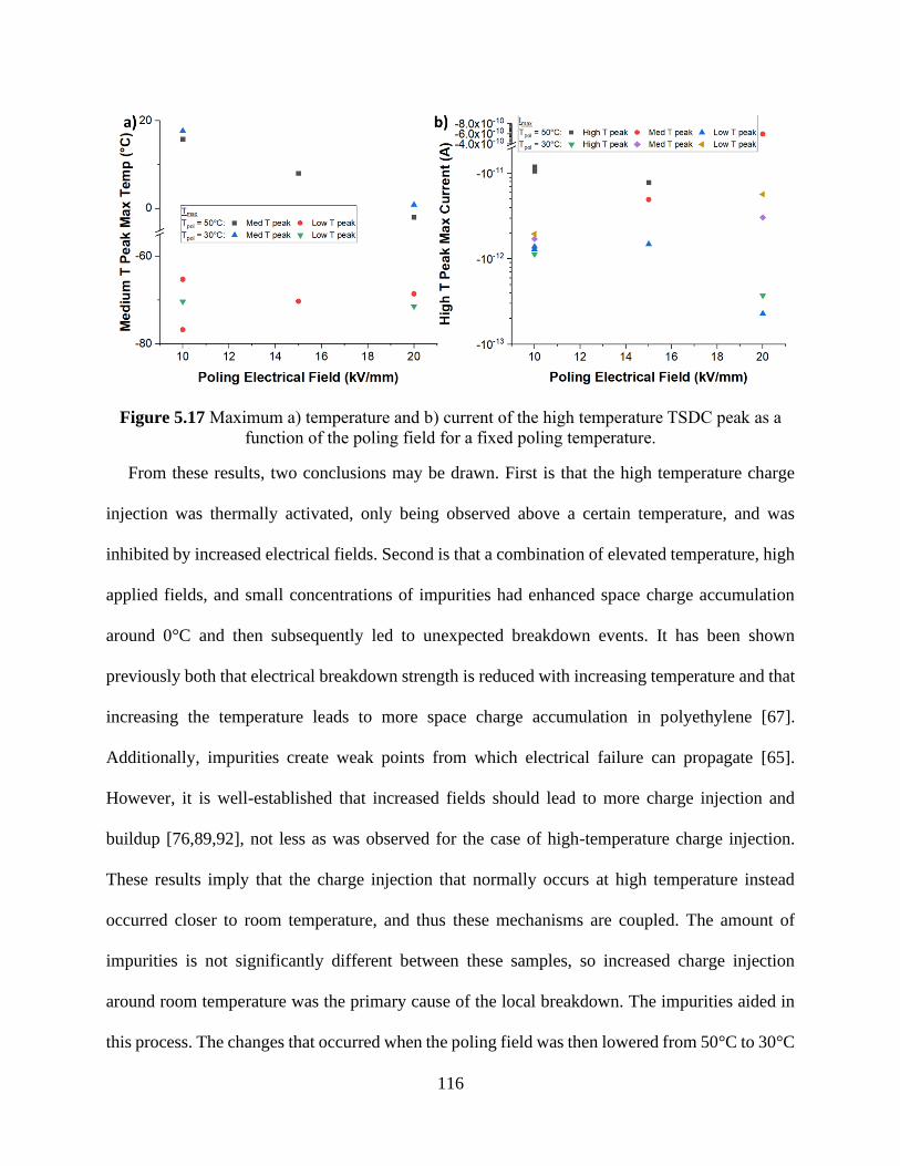
116

Figure 5.17 Maximum a) temperature and b) current of the high temperature TSDC peak as a

function of the poling field for a fixed poling temperature.

From these results, two conclusions may be drawn. First is that the high temperature charge

injection was thermally activated, only being observed above a certain temperature, and was

inhibited by increased electrical fields. Second is that a combination of elevated temperature, high

applied fields, and small concentrations of impurities had enhanced space charge accumulation

around 0°C and then subsequently led to unexpected breakdown events. It has been shown

previously both that electrical breakdown strength is reduced with increasing temperature and that

increasing the temperature leads to more space charge accumulation in polyethylene [67].

Additionally, impurities create weak points from which electrical failure can propagate [65].

However, it is well-established that increased fields should lead to more charge injection and

buildup [76,89,92], not less as was observed for the case of high-temperature charge injection.

These results imply that the charge injection that normally occurs at high temperature instead

occurred closer to room temperature, and thus these mechanisms are coupled. The amount of

impurities is not significantly different between these samples, so increased charge injection

around room temperature was the primary cause of the local breakdown. The impurities aided in

this process. The changes that occurred when the poling field was then lowered from 50°C to 30°C

117

when the field was kept at 20 kV/mm, seem to imply that there might also be coupling between

the charge injection and the defect dipoles associated with the low temperature relaxation. After

repeating this at various temperatures to confirm that the trend holds, further investigations are

suggested for better understanding this phenomenon.

118

Chapter 6 – High-field current-voltage measurements of polyethylene

6.1 Time response and current decay in XLPE Along with Broadband Dielectric Spectroscopy (BDS), Current-Voltage Measurement (IVM) is

one of the most basic ways of characterizing polyethylene – the two being the AC and DC

analogues for each other. BDS at low frequency provides information on electronic and ionic

conduction in the linear ohmic range. IVM is important for understanding nonlinear conduction

at high electric field. As such, there have been a large number of studies using this technique to

analyze polyethylene [47,75–81]. The work in this chapter was done in order to extend this

established knowledge base in the following ways. First, by directly studying the impact of cross-

linking byproducts and degassing procedures on XLPE conduction. Second, by attempting to

understand the impact of XLPE morphology when there are no byproducts. Third, by analyzing

the time response of the current under applied fields. In order to accomplish these things, a wide

variety of samples were examined. They include: XLPE degassed as usual, XLPE that was

degassed at 90°C instead, degassed XLPE that was then soaked in ACP, and degassed LDPE. The

time response of the current is discussed primarily in this section, and the current-voltage data is

discussed primarily in the following sections. At the end, an overall summary and comparison to

the literature data is provided.

The time response of the DC electrical conductivity is indicative of its origin. The conductivity

over time is expected to obey the following power law relationship, which is called the Curie –

von Schweidler law [84]:

(6.1) 𝜎 = 𝜎1𝑡−𝑛

Here, σ1 is the conductivity extracted at one second of electrical field application and n is the power

law exponent of conductivity decay. As the voltage is fixed in these measurements, the current

119

may be used as a substitute with no loss of information. The data for this in this chapter will be

presented as current against time. An exponent of n > 0.6 is indicative of field-independent

polarization and n < 0.4 is indicative of field-dependent conduction current [84]. This exponent

has been reported to be dependent on both the temperature and the applied field. As such, we have

sought to determine if other factors such as morphology and impurities matter. First, the behavior

of the standard degassed XLPE was established at a temperature of 90°C by analyzing two

samples, with the resulting plot in Figure 6.1 and table of the exponent n in Table 6.1. Conductivity

for both these samples was in the range of 10-14 to 10-13 S/m. At lower temperatures, the samples

had conductivity values in line with the value of 10-15 S/m cited in Section 1.5 and within the

literature variation shown in Figure 1.5.

Figure 6.1 Time response of the current in degassed XLPE at 90°C depending on the applied

voltage in linear (left) and log (right) scales. The legend is the same for both plots.

Table 6.1 Exponent of the power law time response of the current in degassed XLPE depending

on the applied voltage.

Voltage (V) Degassed XLPE sample #1 Degassed XLPE sample #2

500 0.91 0.71

1000 0.40 0.30

1500 0.26 0.17

2000 0.18 n/a

2500 0.14 n/a

3000 0.12 0.04

3500 n/a n/a

120

Data from all points in time except for t = 0 were used in determining this exponent. A ‘n/a’

was reported instead of a number if there was an incomplete dataset (that is, there is at least one

time with an erroneous or outlier current). Enough data points were available so that conclusions

may be drawn from this analysis. Here, it was seen that there was a clear change in the time

response between 500 V and all other voltages used in this study. At the lowest voltage, the current

was from polarization, while currents at all other voltages were from conduction. It was determined

by measurement that this type of response was not altered by the addition of ACP and was also

observed in the non-crosslinked LDPE samples, as shown in Figure 6.2. A table for the extracted

exponents for those samples are provided in Table 6.2.

Figure 6.2 Time response of the current in a) degassed XLPE with ACP at 90°C and b) degassed

LDPE at 90°C depending on the applied voltage.

Table 6.2 Exponent of the power law time response of the current in degassed XLPE with ACP

at 90°C and degassed LDPE at 90°C depending on the applied voltage.

Voltage (V) Degassed XLPE sample w/ ACP Degassed LDPE sample

500 0.71 0.89

1000 0.29 0.28

1500 0.27 0.24

2000 0.25 0.21

2500 0.17 0.22

3000 0.22 0.19

3500 0.27 n/a

121

However, there was one key difference between the standard degassed XLPE and the other two

types of samples shown so far. The other two types of samples, despite having had time responses

that match up with conduction currents, had currents that did not have a strong dependence of the

applied field. Such behavior is more typical of polarization currents [84]. While such a result for

the XLPE sample containing the small molecule ACP could be explained by that molecule, as will

be further examined later on in this chapter, this result having been obtained for LDPE had no

explanation as of the time of writing this document. As will be seen in the following sections, these

differences were also present within the current-voltage plots and influenced the attempts to extract

activation energies and power law exponents of conduction.

6.2 Current-voltage response of degassed XLPE and impact of degassing temperature The current-voltage plot for several standard degassed XLPE samples is shown in Figure 6.3. The

same set of voltages was applied to all samples, leading to different applied fields due to the

varying thicknesses between samples. There was also some variation between samples, even at

similar fields. As was discussed in Chapter 4, some inherent variability is expected in polyethylene

samples. As the samples were not so different from each other for one to be thrown out as an

outlier, all were examined further to glean more information on the conductivity in XLPE.

122

Figure 6.3 Plot of measured current density against the applied electric field for standard

degassed XLPE samples.

Thermally activated conduction was clearly present in all samples, and as such an activation

energy was obtained for each sample. It was noted that some samples had a change in slope with

increasing field, and in those samples only the linear part of the curve was used to obtain the

activation energy. Additionally, a power law fit was carried out to help determine conduction

mechanisms via extraction of the value of the exponent x as shown in Equation 6.2. In that equation

also are J (the current density), B (a constant), and E (the electric field). Portions of the curve that

were not found to fit the power law relation were not included in that analysis. Determining which

data points were applicable to both fits was done manually on a sample-to sample basis.

(6.2) 𝐽 = 𝐵𝐸𝑥

The tabulated data for these is shown in Table 6.3. The activation energies of these samples were

quite similar to each other, forming a cluster in the range of 0.4 to 0.5 eV. These values are

consistent with the degassed XLPE samples discussed in Chapter 4 and measured via CCM. In

123

that chapter, it was determined that the overall action energy is determined by the relative

contributions between ionic and electronic conduction as well as the coupling between them. The

same conditions should apply here, so these values are indicative of the coupled conduction

mechanism. Additionally, the extracted exponents indicated that space charge limited current was

present and its appearance was controlled by the temperature. Unlike in the literature, many

samples did not exhibit a transition between the ohmic and SCLC regions [75,76]. They were

instead consistently one or the other. The current data suggests that there was a transition from

ohmic to non-ohmic conduction with continued exposure to electric field and temperature. To

verify this, it would be useful to do the same measurements, but either going from 90°C to 50°C

or adding more measurements at intermediate temperatures (60°C and 80°C) as all the

measurements were done from 50°C to 90°C for these samples.

Table 6.3 Activation energy and power law exponents for standard degassed XLPE samples

Sample Activation Energy (eV) x – 50°C x – 70°C x – 90°C

d-XLPE #3 0.424 0.917 1.515 2.240

d-XLPE #4 0.492 1.690 2.207 2.402

d-XLPE #5 0.495 1.290 1.756 2.106

It was observed in Chapters 3 and 5 that the choice of degassing temperature had an impact on the

AC response and charge trapping characteristics of XLPE. As such, it was decided to determine if

the same was true for the DC response. The results of measuring samples that were degassed at

90°C is shown in Figure 6.4 and a comparison between one sample that underwent standard

degassing and one that was degassed at 90°C is shown in Figure 6.5. A table displaying the

obtained activation energies and power law exponents for the 90°C degassed samples when

available is also presented as Table 6.4.

124

Figure 6.4 Plot of measured current density against the applied electric field for XLPE samples

degassed at 90°C.

Table 6.4 Activation energy and power law exponents for XLPE samples degassed at 90°C

Sample Activation Energy (eV) x – 50°C x – 70°C x – 90°C

#1 n/a 0.043 -0.304 0.974

#2 0.715 0.255 0.660 1.214

#3 n/a 0.057 -0.144 -0.305

#4 n/a -0.205 -0.277 0.446

Unlike the samples degassed under standard conditions, most of these samples lacked the usual

trend of the current density consistently increasing with the applied field. Instead, a positive

relationship would be observed at some temperatures and a negative one would be observed at

other temperatures. Only one sample consistently displayed the usual trend, and an activation

energy was extracted for it that was higher than for the standard degassed samples. Additionally,

it exhibited remarkably different power law behavior having transitioned from sub-ohmic to ohmic

behavior. The comparison plot (Figure 6.5) helps to showcase how different this sample is from

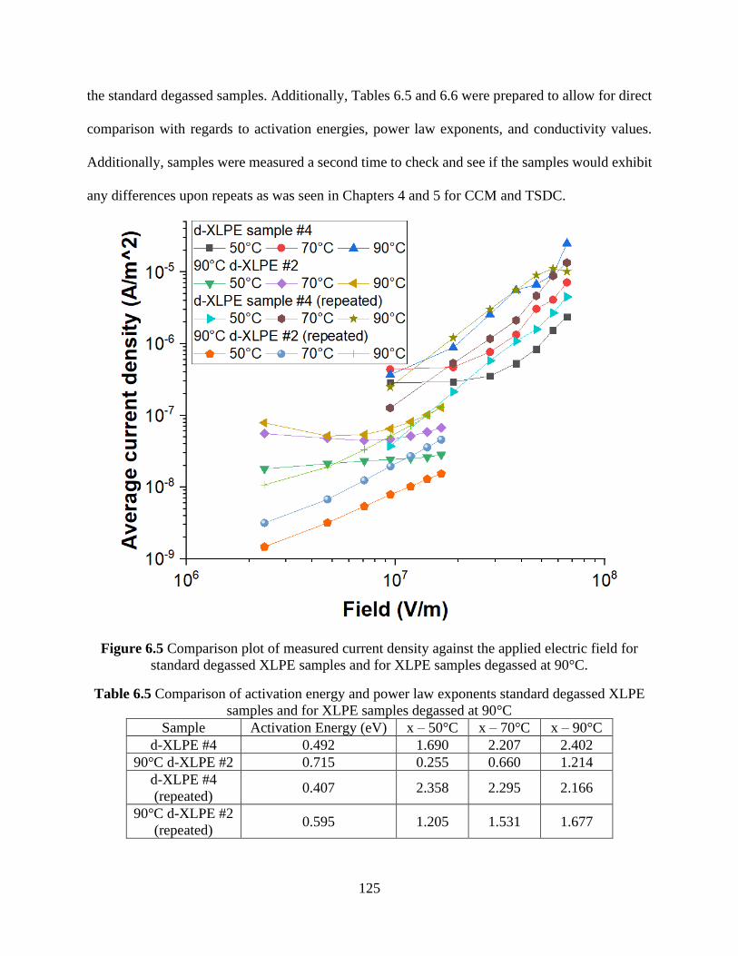
125

the standard degassed samples. Additionally, Tables 6.5 and 6.6 were prepared to allow for direct

comparison with regards to activation energies, power law exponents, and conductivity values.

Additionally, samples were measured a second time to check and see if the samples would exhibit

any differences upon repeats as was seen in Chapters 4 and 5 for CCM and TSDC.

Figure 6.5 Comparison plot of measured current density against the applied electric field for

standard degassed XLPE samples and for XLPE samples degassed at 90°C.

Table 6.5 Comparison of activation energy and power law exponents standard degassed XLPE

samples and for XLPE samples degassed at 90°C

Sample Activation Energy (eV) x – 50°C x – 70°C x – 90°C

d-XLPE #4 0.492 1.690 2.207 2.402

90°C d-XLPE #2 0.715 0.255 0.660 1.214

d-XLPE #4

(repeated) 0.407 2.358 2.295 2.166

90°C d-XLPE #2

(repeated) 0.595 1.205 1.531 1.677

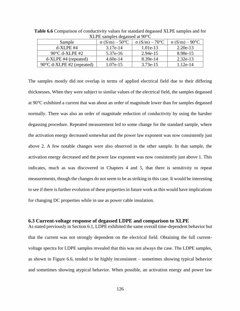
126

Table 6.6 Comparison of conductivity values for standard degassed XLPE samples and for

XLPE samples degassed at 90°C

Sample σ (S/m) – 50°C σ (S/m) – 70°C σ (S/m) – 90°C

d-XLPE #4 3.17e-14 1.01e-13 2.20e-13

90°C d-XLPE #2 5.37e-16 2.94e-15 8.98e-15

d-XLPE #4 (repeated) 4.60e-14 8.39e-14 2.32e-13

90°C d-XLPE #2 (repeated) 1.07e-15 3.73e-15 1.12e-14

The samples mostly did not overlap in terms of applied electrical field due to their differing

thicknesses. When they were subject to similar values of the electrical field, the samples degassed

at 90°C exhibited a current that was about an order of magnitude lower than for samples degassed

normally. There was also an order of magnitude reduction of conductivity by using the harsher

degassing procedure. Repeated measurement led to some change for the standard sample, where

the activation energy decreased somewhat and the power law exponent was now consistently just

above 2. A few notable changes were also observed in the other sample. In that sample, the

activation energy decreased and the power law exponent was now consistently just above 1. This

indicates, much as was discovered in Chapters 4 and 5, that there is sensitivity to repeat

measurements, though the changes do not seem to be as striking in this case. It would be interesting

to see if there is further evolution of these properties in future work as this would have implications

for changing DC properties while in use as power cable insulation.

6.3 Current-voltage response of degassed LDPE and comparison to XLPE As stated previously in Section 6.1, LDPE exhibited the same overall time-dependent behavior but

that the current was not strongly dependent on the electrical field. Obtaining the full current-

voltage spectra for LDPE samples revealed that this was not always the case. The LDPE samples,

as shown in Figure 6.6, tended to be highly inconsistent – sometimes showing typical behavior

and sometimes showing atypical behavior. When possible, an activation energy and power law

127

exponent was obtained to be shown in Table 6.7, but few conclusions could be drawn from this

data at this moment in time due to the inconsistencies.

Figure 6.6 Plot of measured current density against the applied electric field for standard

degassed LDPE samples

Table 6.7 Activation energy and power law exponents standard degassed LDPE samples

Sample Activation Energy (eV) x – 50°C x – 70°C x – 90°C

#1 0.580 1.796 2.926 1.529

#2 n/a 0.987 -0.060 0.579

6.3 Changes in degassed XLPE due to acetophenone soaking As was discussed in Chapters 3 and 5, the presence of the small molecule acetophenone (ACP) led

to significant changes in the electrical properties of crosslinked polyethylene samples. The same

was found to be the case in IVM, as is shown in Figure 6.7. Figure 6.7a shows the current-voltage

plot for only the degassed samples soaked in ACP and Figure 6.7b shows a comparison between

128

one of those samples with the same standard sample used to analyze the impact of degassing

temperature. Similarly, tables were prepared to show activation energy and power law exponents

for samples soaked in ACP (Table 6.8), make a comparison of those to the standard degassed

XLPE sample (Table 6.9), and compare the conductivity values between those two samples (Table

6.10). Repeated measurements were also done for the ACP soaked sample used for comparisons.

Figure 6.7 a) Plot of measured current density against the applied electric field for standard

degassed XLPE samples soaked in ACP; b) Comparison plot of measured current density against

the applied electric field for standard degassed XLPE samples without and with soaking in ACP

Table 6.8 Comparison of activation energy and power law exponents standard degassed XLPE

samples soaked in acetophenone

Sample Activation Energy (eV) x – 50°C x – 70°C x – 90°C

#1 ≈0 0.429 0.357 0.453

#2 ≈0 0.555 0.218 0.407

#3 ≈0 0.778 0.961 0.465

#4 ≈0 0.398 0.759 0.725

#5 0.216 0.909 1.045 0.999

#5 (repeated) 0.130 1.194 1.312 0.803

The ACP soaked samples maintained the general trend of the current density increasing with the

applied field. However, they otherwise exhibited quite distinct behavior from the samples without

ACP. These ACP-soaked samples had no apparent thermally activated conduction on average,

have EA close to zero for all samples but one. That samples also had EA of only 0.216 eV, which

129

was reduced further to 0.130 eV upon the repeat measurement. That sample was also the only one

to exhibit a power law exponent close to 1 for all temperatures selected, and maintained a similar

behavior in the repeat measurement. All the others had sub-ohmic conduction in almost all cases.

Table 6.9 Comparison of activation energy and power law exponents standard degassed XLPE

samples and for XLPE samples degassed at 90°C

Sample Activation Energy (eV) x – 50°C x – 70°C x – 90°C

d-XLPE #4 0.492 1.690 2.207 2.402

d-XLPE w/ ACP

#5 0.216 0.909 1.045 0.999

d-XLPE #4

(repeated) 0.407 2.358 2.295 2.166

d-XLPE w/ ACP

#5 (repeated) 0.130 1.194 1.312 0.803

Table 6.10 Comparison of conductivity values for standard degassed XLPE samples and for

XLPE samples degassed at 90°C

Sample σ (S/m) – 50°C σ (S/m) – 70°C σ (S/m) – 90°C

d-XLPE #4 3.17e-14 1.01e-13 2.20e-13

d-XLPE w/ ACP #5 9.68e-16 1.26e-15 2.29e-15

d-XLPE #4 (repeated) 4.60e-14 8.39e-14 2.32e-13

d-XLPE w/ ACP #5

(repeated) 1.14e-15 1.42e-15 1.91e-15

A direct comparison to the standard degassed samples made the changes introduced by adding

ACP more obvious. Current densities were reduced in the ACP soaked samples when compared

to the degassed samples by about one to two orders of magnitude. Similarly, the conductivity was

reduced by about two orders of magnitude as well. The activation energy was altered and became

similar to those of the as-received and water-soaked samples examined in Chapter 4. This was

considered then a clear sign that these very low activation energies observed in polyethylene can

be attributed to polar species such as water and acetophenone whenever there is evidence that such

molecules should be present. Along with that change, a corresponding change in the time-

dependence of the current decay was also observed. Unlike with the measurement only at 90°C,

130

the measurement at all three temperatures revealed that the ACP-soaked samples were now

dominated by polarization or mixed conduction instead of pure conduction current. The obtained

exponents are shown in Table 6.11. It should be noted that this particular ACP-soaked sample was

measured from high temperature to low, but other samples that were measured in the usual way

also showed this behavior for the current decay. Given the changes introduced by large amounts

of ACP, it would be useful in the future to determine how much ACP is necessary to induce this

transition by careful control of the soaking parameters.

Table 6.11 Exponent of the power law time response of the current in degassed XLPE with and

without ACP depending on the applied voltage and temperature.

Voltage

(V)

d-XLPE

50°C

d-XLPE

70°C

d-XLPE

90°C

d-XLPE

(ACP)

50°C

d-XLPE

(ACP)

70°C

d-XLPE

(ACP)

90°C

500 -0.15 0.11 0.26 n/a 0.97 0.56

1000 0.28 0.23 0.14 0.92 0.87 0.48

1500 0.20 0.16 0.05 0.82 0.85 0.56

2000 0.17 0.14 0.12 0.76 0.80 0.57

2500 0.15 n/a 0.26 0.74 0.81 0.53

3000 0.09 n/a n/a 0.72 0.75 0.56

3500 n/a n/a 0.03 0.75 0.69 0.56

6.4 Overall summary of the obtained current-voltage relationship in polyethylene A summary figure comparing the current-voltage values obtained here to literature values is

presented in Figure 6.8. The conductivity values obtained in this work were in line with the

established literature. Harsher degassing reduced the current values and conductivity, but so did

acetophenone exposure. Even in those cases, however, variation in the DC electrical properties

was still observed, implying that such variation is to be expected in this semicrystalline polymer.

When large quantities of an extrinsic impurity such as ACP are present, the current will largely be

due to polarization or mixed polarization-conduction current – such molecules need to be removed

in order to observe the true conduction current alone. The true conduction current can be attributed

131

to either ohmic conduction or space charge limited current of charges originating from charge

injection processes. The behavior that was observed appeared to depend on the temperature used

for the degassing procedure. However, care must be taken in drawing such a conclusion since the

applied electric fields were not exactly the same between the two types of samples. Conclusively

determining if the choice of degassing temperature controls the type of conduction observed will

require a second study with samples perfectly calibrated to have the same thickness after the two

different degassing procedures.

Figure 6.8 Current-voltage measurements of LDPE and XLPE, including comparisons to

literature from the following sources: [47,75–81].

132

Chapter 7 – Summary and Suggestions for Future Work

The main purpose of this dissertation was to generate a fundamental understanding of the roles of

impurities and structure on the electrical properties of XLPE. As such, a variety of electrical tests

were developed to explore transport and polarization phenomena as a function of temperature,

frequency and applied electric field.

Regarding the AC response of XLPE (Chapter 3), it was determined that the overall most

important factor was the presence of small molecular species, whether they be introduced by the

use of DCP as a crosslinking agent or by radiation exposure in the presence of oxygen. In addition,

a direct correlation between the temperature coefficient of capacitance and thermal expansion was

discovered. The presence of DCP byproducts led to a significant increase in the thermal expansion

above 40°C which was explained by internal pressure from these volatile crosslinking byproducts.

Additionally, when these molecules were present in high concentrations, they led to significant

increases in the dielectric loss due to the added polarization. Similar results were also seen in the

radiation crosslinked films. However, the DCP byproducts in as-received films did not contribute

as much to excess conductivity at elevated temperatures as the ionic species generated in the

radiation crosslinked films. Furthermore, the byproducts only had a significantly negative impact

via enhancement of the dielectric loss at room temperature at concentrations far in excess of what

would be expected in power cable insulation. Their impact in both cases could be reduced by the

use of degassing in the case of peroxide crosslinking or by crosslinking in vacuum in the case of

radiation crosslinking.

Regarding the electrical compensation response of XLPE (Chapter 4), it could be observed in

both AC and DC conduction and was present in both XLPE and LDPE samples. Overall, the

mechanism for compensation was determined to be as follows. Two types of conduction are

133

generally available in polyethylene: ionic (usually extrinsic) and electronic (usually intrinsic). The

two are coupled and usually coexist in real samples. The samples with the most impurities tended

to have very low EA (0.2 eV or less) and not show compensation. Once those were removed, water

became the dominant impurity, and it allowed for a wide variation in EA from 0.2 eV to 1.4 eV

due to the coupled conduction. Variation was observed within that range due to differences in

structure and relative contributions of ionic and electronic conduction.

Regarding the stored charge and polarization within XLPE (Chapter 5), three main causes of

stored charge were observed: thermally activated charge injection at high temperatures in the

melting range, motion of charged impurities and ionization of acetophenone at intermediate

temperatures generally close to or just below room temperature, and molecular motions of defect

dipoles at low temperatures near the glass transition temperature. The relative presence or absence

of impurities, as well as which types of impurities were present, determined the exact mechanisms

available within a sample as they needed to be removed for charge injection and molecular motions

to be able to play a role. Of the typical DCP byproducts, ACP was deemed to have the most control

over the trapping mechanisms available in XLPE samples.

Regarding the DC response of XLPE (Chapter 6), the current-voltage data also confirmed the

importance of small molecules by revealing that their presence heavily altered the activation

energy and current generation mechanism. Films with high concentrations of ACP exhibited small

activation energy of 0.2 eV or less, ohmic response, and polarization current. Films without ACP

exhibited moderate activation energies of 0.4 eV to 0.8 eV, space charge response, and conduction

current. This corresponded to a promotion of shallow trapping by the added impurity. Varying the

degassing temperature led to variation in the activation energy as a higher degassing temperature

134

led to a higher activation energy due to variation in trace levels in the impurity concentrations, as

was seen in the compensation response.

Overall, the importance of extrinsic impurities and thermal history on the electrical properties

of XLPE cannot be overstated. Acetophenone, in particular, appeared to be a key shaper of the

overall observed response. It allowed for the buildup of charge observable in both BDS and TSDC

that had clear implications for DC conduction as well. Its impact as a trap was felt in two distinct

ways. In one case, it provided shallow traps for DC conduction with energy around 0.2 eV (Chapter

6). In the other case, it provided sites for charge to be trapped with deeper energy of up to 0.7 eV

due to its diffusion through the sample when charged and its reaction with residual moisture that

produces ions (Chapter 5). The removal of acetophenone was shown to be needed for observing

the true properties of XLPE. With that in mind, the importance of the thermal history becomes

clear. By using harsher degassing, both charge injection and conductivity could be reduced while

the activation energy of charge injection and conductivity were both increased. Additionally,

annealing was able to alter the compensation behavior of polyethylene, which was obscured by

byproducts like acetophenone. Along those same lines, since the conductivity in polyethylene is

governed by charge injection as discussed in Section 1.5, the variation in the activation energies

observed in Chapter 4 for AC and DC conduction and in Chapter 5 for the peak related to charge

injection should be related and both arise from variations in impurity content and structural

features between different samples.

Much future work has been suggested that would be directly relevant to these obtained results.

In general, it was suggested to better understand the mechanics of how degassing altered the XLPE

structure and the precise extent to which small molecules and structural changes controlled the

electrical properties with all the utilized techniques. This would require a combination of

135

simulations and experiments to obtain the finest understanding. Additionally, there are other topics

that would be useful to address regarding better control over the properties. For example, it has

been shown in various results that the crosslinks seem not to have much of an impact on the

electrical properties themselves – what matters most are impurity concentrations and thermal

history. It should be possible to verify this using a combination of careful experiments and

molecular simulations. Additionally, the impact of antioxidants was only briefly examined and

would be worthy of further examination considering their use in the currently existing AC and DC

cable insulation. Similarly, the impact of the semicon electrode (a semiconducting mix of carbon

black and polyethylene) used in power cables would be worth examining.

In general, the desired characteristics for HVDC cable insulation are as follows: having a

generally low conductivity that is not highly dependent on the applied field or the ambient

temperature; having a large thermal conductivity to easily dissipate heat; having little to no space

charge accumulation; having a dielectric strength that is as large as possible [1]. This work was

mostly aimed at addressing the first point with the AC and DC analyses and the third point with

the TSDC analyses. The conductivity was found to be highly variable and depend on multiple

factors. Obtaining a conductivity with the lowest possible activation energy and field-dependence

was obtained by adding ACP under DC conditions, but that behavior was not matched in AC

conditions where it was instead obtained by water-soaking of the as-received samples. The charge

build-up was minimized for a completely different type of sample – the ones that were degassed

at temperatures above those typically used for cable manufacture. Overall, it may be suggested

that a combination of harsh annealing and using some other type of intentionally-added impurity

such as inorganic nanoparticles [1,184] or polycyclic aromatics [185] may be the best path forward

for improving XLPE electrical properties. There are already some results showing that these

136

inclusions are useful in reducing space charge buildup [184,185], but how to incorporate them on

an industrial scale is still an open question. It is also not year clear how they will interact with the

antioxidants and other small molecules typically incorporated into commercial cables. While not

having to degas the samples would be preferred for energy and environmental reasons, it remains

necessary at this point in time due to the multiple hazards presented by the DCP byproducts. Future

development regarding the addition of other particles and molecules and/or modification of the

crosslinking process will be needed to make that process obsolete.

137

References

1. Chen, G., Hao, M., Xu, Z., Vaughan, A., Cao, J., and Wang, H. (2015) Review of high

voltage direct current cables. CSEE J. Power Energy Syst., 1 (2), 9–21.

2. Ware, P.H. (1967) Polyethylene as a high voltage cable insulation. 7th Electr. Insul. Conf.

EIC 1967, 255.

3. Hampton, N., Hartlein, R., Lennartsson, H., Orton, H., and Ramachandran, R. (2007)

Long-Life Xlpe Insulated Power Cable. 7th Int. Conf. Insul. Power Cable, Jicable, Fr.

4. HAMMONS, T.J. (2003) Power Cables in the Twenty-First Century. Electr. Power

Components Syst., 31 (10), 967–994.

5. Vahedy, V. (2006) Polymer insulated high voltage cables. IEEE Electr. Insul. Mag., 22

(3), 13–18.

6. Olasz, L. (2006) Residual Stresses and Strains in Cross-linked Polyethylene Power Cable

Insulation.

7. Hasegawa, Y., Takihana, J., and Ohki, Y. (2014) Estimation of thermal expansion

coefficients of polymeric insulating films from temperature dependence of dielectric

permittivity. Jpn. J. Appl. Phys., 53 (7), 071501.

8. Liu, T., Fothergill, J., Dodd, S., and Nilsson, U. (2009) Dielectric spectroscopy

measurements on very low loss cross-linked polyethylene power cables. J. Phys. Conf.

Ser., 183, 012002.

9. Kageyama, S., Ono, M., and Chabata, S. (1975) Microvoids in crosslinked polyethylene

insulated cables. IEEE Trans. Power Appar. Syst., 94 (4), 1258–1263.

10. Fukuda, T. (1988) Technological progress in high-voltage XLPE power cables in Japan. I.

IEEE Electr. Insul. Mag., 4 (5), 9–16.

138

11. Wang, X., Yoshimura, N., Murata, K., Tanaka, Y., and Takada, T. (1998) Space-charge

characteristics in polyethylene. J. Appl. Phys., 84 (3), 1546–1550.

12. Scarpa, P.C.N., Svatik, a, and DasGupta, D.K. (1996) Dielectric spectroscopy of

polyethylene in the frequency range of 10(-5) Hz to 10(6) Hz. Polym. Eng. Sci., 36 (8),

1072–1080.

13. Gulmine, J.V., and Akcelrud, L. (2006) Correlations between structure and accelerated

artificial ageing of XLPE. Eur. Polym. J., 42 (3), 553–562.

14. Lazár, M., Rado, R., and Rychlý, J. (2012) Crosslinking of polyolefins, in Polymer

Physics, pp. 149–197.

15. Nilsson, S., Hjertberg, T., and Smedberg, A. (2010) Structural effects on thermal

properties and morphology in XLPE. Eur. Polym. J., 46 (8), 1759–1769.

16. Ghorbani, H. (2016) Characterization of conduction and polarization properties of HVDC

cable XLPE insulation materials.

17. Li, Z., and Du, B. (2018) Polymeric insulation for high-voltage dc extruded cables:

Challenges and development directions. IEEE Electr. Insul. Mag., 34 (6), 30–43.

18. Suh, K.-S., Tanaka, J., and Damon, D. (1992) What is TSC? IEEE Electr. Insul. Mag., 8

(6), 13–20.

19. Sawa, G., Kawade, M., Lee, D.C., and Ieda, M. (1974) Thermally stimulated current from

polyethylene in high-temperature region. Jpn. J. Appl. Phys., 13 (10), 1547–1553.

20. Huan, T.D., Boggs, S., Teyssedre, G., Laurent, C., Cakmak, M., Kumar, S., and

Ramprasad, R. (2016) Advanced polymeric dielectrics for high energy density

applications. Prog. Mater. Sci., 83, 236–269.

21. Sahyoun, J., Crepet, A., Gouanve, F., Keromnes, L., and Espuche, E. (2017) Diffusion

139

mechanism of byproducts resulting from the peroxide crosslinking of polyethylene. J.

Appl. Polym. Sci., 134 (9), 44525.

22. Andrews, T., Hampton, R.N., Smedberg, A., Wald, D., Waschk, V., and Weissenberg, W.

(2006) The role of degassing in XLPE power cable manufacture. IEEE Electr. Insul.

Mag., 22 (6), 5–16.

23. Tamayo, I., Belana, J., Mudarra, M., Diego, J.A., and Sellarés, J. (2003) Thermally

stimulated depolarization currents of crosslinked polyethylene relaxations in the fusion

range of temperatures. J. Polym. Sci. Part B Polym. Phys., 41 (12), 1412–1421.

24. Sato, Y., and Yashiro, T. (1978) The effect of polar groups on the dielectric loss of

polyethylene. J. Appl. Polym. Sci., 22 (8), 2141–2153.

25. Hussin, N., and Chen, G. (2009) The trapping characteristic of low density polyethylene in

the presence of crosslinking by-products. J. Phys. Conf. Ser., 183 (1), 012007.

26. Tamboli, S.M., Mhaske, S.T., and Kale, D.D. (2004) Crosslinked polyethylene. Indian J.

Chem. Technol., 11 (6), 853–864.

27. Gulmine, J. V., and Akcelrud, L. (2004) Correlations between the processing variables

and morphology of crosslinked polyethylene. J. Appl. Polym. Sci., 94 (1), 222–230.

28. Steennis, E.F., and Kreuger, F.H. (1990) Water treeing in polyethylene cables. IEEE

Trans. Electr. Insul., 25 (5), 989–1028.

29. Gregory, B., Jeffs, M.D., and Vail, J. (1993) The choice of cable type for application at

EHV system voltage. Third Int. Conf. Power Cables Accessories, 10kV-500kV, 276.

30. Tamayo, I., Belana, J., Diego, J.A., Cañadas, J.C., Mudarra, M., and Sellarès, J. (2004)

Space charge studies of crosslinked polyethylene midvoltage cable insulation by thermally

stimulated depolarization current, infrared/fourier transform infrared, and scanning

140

electron microscopy. J. Polym. Sci. Part B Polym. Phys., 42 (22), 4164–4174.

31. Fazal, A., Hao, M., Vaughan, A.S., Chen, G., Cao, J., and Wang, H. (2016) The effect of

composition and processing on electric characteristics of XLPE in HVDC cable

applications. 2016 IEEE Electr. Insul. Conf., 440–443.

32. Jang, Y.T., and Phillips, P.J. (1983) Dielectric loss behavior of cross-linked polyethylene

and analog materials. J. Appl. Polym. Sci., 28 (3), 1137–1146.

33. Hulse, G.E., Kersting, R.J., and Warfel, D.R. (1981) Chemistry of dicumyl peroxide-

induced crosslinking of linear polyethylene. J. Polym. Sci. Polym. Chem. Ed., 19 (3), 655–

667.

34. Aida, F., Tanimoto, G., Aihara, M., and Hosokawa, E. (1990) Influence of curing by-

products on dielectric loss in XLPE insulation. Annu. Conf. Electr. Insul. Dielectr.

Phenom., 465–473.

35. Sekii, Y., Ohbayashi, T., Uchimura, T., Mochizuki, U., and Maeno, T. (2002) The effects

of material properties and inclusions on the space charge profiles of LDPE and XLPE.

Annu. Rep. Conf. Electr. Insul. Dielectr. Phenom., 635–639.

36. Hirai, N., Minarni, R., Tanaka, T., Ohki, Y., Okashita, M., and Maeno, T. (2003)

Chemical group in crosslinking byproducts responsible for charge trapping in

polyethylene. IEEE Trans. Dielectr. Electr. Insul., 10 (2), 320–330.

37. Maeno, Y., Hirai, N., Ohki, Y., Tanaka, T., Okashita, M., and Maeno, T. (2005) Effects of

crosslinking byproducts on space charge formation in crosslinked polyethylene. IEEE

Trans. Dielectr. Electr. Insul., 12 (1), 90–97.

38. Iwata, S., Uehara, H., Sekii, Y., and Takada, T. (2019) Behavior of water molecules

between molecular layers of by-products of dicumyl peroxide or surfactants in an external

141

electric field: Computational insight. Comput. Mater. Sci., 163, 134–140.

39. Iwata, S. (2017) Interaction between 1-phenylethanone, 2-phenyl-2-propanol, and

isopropenylbenzene with water molecules: A computational study. Comput. Theor. Chem.,

1117, 188–195.

40. Gregorian, R.S., and Bafford, R.A. (1964) Evaluation of Peroxides as Cross-linking

Agents for High Density Polyethylene. Ind. Eng. Chem. Prod. Res. Dev., 3 (4), 267–269.

41. Anbarasan, R., Babot, O., and Maillard, B. (2004) Crosslinking of high-density

polyethylene in the presence of organic peroxides. J. Appl. Polym. Sci., 93 (1), 75–81.

42. Celina, M., and George, G.A. (1995) Characterisation and degradation studies of peroxide

and silane crosslinked polyethylene. Polym. Degrad. Stab.

43. Liu, S.-Q., Gong, W.-G., and Zheng, B.-C. (2014) The Effect of Peroxide Cross-Linking

on the Properties of Low-Density Polyethylene. J. Macromol. Sci. Part B, 53 (1), 67–77.

44. Khonakdar, H.A., Morshedian, J., Wagenknecht, U., and Jafari, S.H. (2003) An

investigation of chemical crosslinking effect on properties of high-density polyethylene.

Polymer (Guildf)., 44 (15), 4301–4309.

45. Ghorbani, H., Hoq, T., and Edin, H. (2017) Effect of heat treatment on morphology and

dielectric properties of PE cable insulation material. Proc. Nord. Insul. Symp., 53–58.

46. Montanari, G.C. (2004) Dielectric Material Properties Investigated Through Space Charge

Measurements. IEEE Trans. Dielectr. Electr. Insul., 11 (1), 56–64.

47. Boudou, L., and Guastavino, J. (2002) Influence of temperature on low-density

polyethylene films through conduction measurement. J. Phys. D. Appl. Phys., 35 (13),

317.

48. Chen, L., Huan, T.D., and Ramprasad, R. (2017) Electronic Structure of Polyethylene:

142

Role of Chemical, Morphological and Interfacial Complexity. Sci. Rep., 7 (6128), 1–10.

49. Jones, J.P., Llewellyn, J.P., and Lewis, T.J. (2005) The contribution of field-induced

morphological change to the electrical aging and breakdown of polyethylene. IEEE Trans.

Dielectr. Electr. Insul., 12 (5), 951–966.

50. Ieda, M. (1984) Electrical Conduction and Carrier Traps in Polymeric Materials. IEEE

Trans. Electr. Insul., EI-19 (3), 162–178.

51. Diego, J.A., Belana, J., Òrrit, J., Sellarès, J., Mudarra, M., and Cañadas, J.C. (2006) TSDC

study of XLPE recrystallization effects in the melting range of temperatures. J. Phys. D.

Appl. Phys., 39 (9), 1932–1938.

52. Oluwoye, I., Altarawneh, M., Gore, J., and Dlugogorski, B.Z. (2015) Oxidation of

crystalline polyethylene. Combust. Flame, 162 (10), 3681–3690.

53. Fischer, P. (1978) Electrical conduction in polyolefins. J. Electrostat., 4 (2), 149–173.

54. Karlsson, M.E., Xu, X., Hillborg, H., Ström, V., Hedenqvist, M.S., Nilsson, F., and

Olsson, R.T. (2020) Lamellae-controlled electrical properties of polyethylene-

morphology, oxidation and effects of antioxidant on the DC conductivity. RSC Adv., 10

(8), 4698–4709.

55. Fischer, P., and Röhl, P. (2007) Transient currents in oxidized low-density polyethylene,

in Mehrphasige Polymersysteme, pp. 149–153.

56. Hvidsten, S., Vandbakk, M., and Mauseth, F. (2012) Dielectric properties of organic

contaminations in XLPE cable insulation. Annu. Rep. - Conf. Electr. Insul. Dielectr.

Phenomena, CEIDP, 684–687.

57. Veitmann, M., Jumeau, R., Bourson, P., Ferriol, M., and Lahure, F. (2014) Understanding

and Control of High Temperature Oxidation Flaws of Low-Density Poly(ethylene) with

143

Raman Spectroscopy. Int. J. Spectrosc., 2014, 1–9.

58. McCall, D.W., Douglass, D.C., Blyler, L.L., Johnson, G.E., Jelinski, L.W., and Bair, H.E.

(1984) Solubility and Diffusion of Water in Low-Density Polyethylene. Macromolecules,

17 (9), 1644–1649.

59. Kao, K.C. (1984) New theory of electrical discharge and breakdown in low-mobility

condensed insulators. J. Appl. Phys., 55 (3), 752.

60. Fischer, P. (1982) Dielectric Breakdown Phenomena in Polymers, in Electrical Properties

of Polymers, pp. 319–367.

61. Tanaka, Y., Kato, T., Suzuki, H., Miyake, H., and Maeno, T. (2014) Breakdown processes

in low density polyethylene and cross-linked polyethylene under DC high stress. Proc.

2014 Int. Symp. Electr. Insul. Mater., 108–111.

62. Zhang, J., Li, J., Wang, Y., Bao, L., and Zhang, X. (2014) Electrical breakdown properties

of low density polyethylene under DC voltage. ICHVE 2014 - 2014 Int. Conf. High Volt.

Eng. Appl., 1–4.

63. Hikita, M., Tajima, S., Kanno, I., Ishino, I., Sawa, G., and Ieda, M. (1985) High-field

conduction and electrical breakdown of polyethylene at high temperatures. Jpn. J. Appl.

Phys., 24 (8 R), 988–996.

64. Lewis, T.J., and Llewellyn, J.P. (2013) Electrical conduction in polyethylene: The role of

positive charge and the formation of positive packets. J. Appl. Phys., 113 (22), 223705.

65. Zhang, Y., Lewiner, J., Alquié, C., and Hampton, N. (1996) Evidence of strong correlation

between space-charge buildup and breakdown in cable insulation. IEEE Trans. Dielectr.

Electr. Insul., 3 (6), 778–783.

66. Amyot, N., Lee, S.Y., David, E., and Lee, I.H. (2005) The effect of residual crosslinking

144

by-products on the local dielectric strength of HV extruded cables. 2000 Annu. Rep. Conf.

Electr. Insul. Dielectr. Phenom. (Cat. No.00CH37132), 743–746.

67. Wang, S., Chen, P., Li, H., Li, J., and Chen, Z. (2017) Improved DC performance of

crosslinked polyethylene insulation depending on a higher purity. IEEE Trans. Dielectr.

Electr. Insul., 24 (3), 1809–1817.

68. Fothergill, J.C., Dodd, S.J., Dissado, L.A., Liu, T., and Nilsson, U.H. (2011) The

measurement of very low conductivity and dielectric loss in XLPE cables: A possible

method to detect degradation due to thermal aging. IEEE Trans. Dielectr. Electr. Insul.,

18 (5), 1544–1553.

69. Tanimoto, G., Okashita, M., Aida, F., and Fujiwara, Y. (2002) Temperature dependence

of tan delta in polyethylene. Proc. 3rd Int. Conf. Prop. Appl. Dielectr. Mater., 1068–1071.

70. Nakatsuka, T., Takahashi, T., Miyata, H., Yokoyama, A., Ishikawa, I., and Niwa, T.

(1994) Effect on dielectric loss of polyethylene caused by acetophenone and

cumylalcohol. Proc. 1994 IEEE Int. Symp. Electr. Insul., 574–577.

71. Boudou, L., and Guastavino, J. (2000) Influence of temperature treatment on the electrical

properties of low-density polyethylene. J. Phys. D. Appl. Phys., 33 (21), L129–L131.

72. Moiz, S.A., Khan, I.A., Younis, W.A., and Karimov, K.S. (2016) Space Charge–Limited

Current Model for Polymers, in Conducting Polymers, pp. 91–117.

73. Upadhyay, A.K., and Reddy, C.C. (2017) On the mechanism of charge transport in low

density polyethylene. J. Appl. Phys., 122 (6), 064105.

74. Fleming, R.J. (1999) Space charge in polymers, particularly polyethylene. Brazilian J.

Phys., 29 (2), 280–294.

75. Lan, L., Wu, J., Yin, Y., Li, X., and Li, Z. (2014) Effect of temperature on space charge

145

trapping and conduction in cross-linked polyethylene. IEEE Trans. Dielectr. Electr. Insul.,

21 (4), 1784–1791.

76. Montanari, G.C., Mazzanti, G., Palmieri, F., Motori, A., Perego, G., and Serra, S. (2001)

Space-charge trapping and conduction in LDPE, HDPE and XLPE. J. Phys. D. Appl.

Phys., 34 (18), 2902–2911.

77. Montanari, G.C., Laurent, C., Teyssedre, G., Campus, A., and Nilsson, U.H. (2005) From

LDPE to XLPE: investigating the change of electrical properties. Part I. space charge,

conduction and lifetime. IEEE Trans. Dielectr. Electr. Insul., 12 (3), 438–446.

78. Suh, K.S., Lee, C.R., Noh, J.S., Tanaka, J., and Damon, D.H. (1994) Electrical conduction

in polyethylene with semiconductive electrodes. IEEE Trans. Dielectr. Electr. Insul., 1

(2), 224–230.

79. Boggs, S. (2004) A rational consideration of space charge. IEEE Electr. Insul. Mag., 20

(4), 22–27.

80. Montanari, G.C., Fabiani, D., Bencivenni, L., Garros, B., and Audry, C. (1999) Space-

charge and conduction-current measurements for the evaluation of aging of insulating

materials for DC applications. 1999 Annu. Rep. Conf. Electr. Insul. Dielectr. Phenom.

(Cat. No.99CH36319), 38–42.

81. Teyssedre, G., Laurent, C., Montanari, G.C., Palmieri, F., See, A., Dissado, L.A., and

Fothergill, J.C. (2001) Charge distribution and electroluminescence in cross-linked

polyethylene under dc field. J. Phys. D. Appl. Phys., 34 (18), 2830–2844.

82. Chen, G., Tay, T.Y.G., Davies, A.E., Tanaka, Y., and Takada, T. (2001) Electrodes and

charge injection in low-density polyethylene using the pulsed electroacoustic technique.

IEEE Trans. Dielectr. Electr. Insul., 8 (6), 867–873.

146

83. Laurent, C., Baudoin, F., Griseri, V., Le Roy, S., and Teyssedre, G. (2011) A discussion

on the electronic properties of polyethylene interfaces. Proc. 2011 Int. Symp. Electr. Insul.

Mater., 139–143.

84. Adamec, V., and Calderwood, J.H. (1981) On the determination of electrical conductivity

in polyethylene. J. Phys. D. Appl. Phys., 14 (8), 1487–1494.

85. Khalil, M.S., Henriksen, M., and Henk, P.O. (1991) Electrical conduction in plain

polyethylene and polyethylene doped with an inorganic additive. 1991 Annu. Report.

Conf. Electr. Insul. Dielectr. Phenomena, 169–175.

86. Hussin, N., and Chen, G. (2008) The effect of acetophenone and alpha-methylstyrene on

the space charge properties of low density polyethylene. 2008 Annu. Rep. Conf. Electr.

Insul. Dielectr. Phenom., 702–705.

87. Sekii, Y., Ohbayashi, T., Uchimura, T., Hukuyama, T., and Maeno, T. (2002) A study on

the space charge formation in XLPE. 2001 Annu. Rep. Conf. Electr. Insul. Dielectr.

Phenom. (Cat. No.01CH37225), 469–472.

88. Sekii, Y., Taya, A., and Maeno, T. (2006) Effect of antioxidants on space charge

generation in cross-linked polyethylene and EPR. Annu. Rep. - Conf. Electr. Insul.

Dielectr. Phenomena, CEIDP.

89. Wang, X., Yoshimura, N., Tanaka, Y., Murata, K., and Takada, T. (1998) Space charge

characteristics in cross-linking polyethylene under electrical stress from dc to power

frequency. J. Phys. D. Appl. Phys., 31 (16), 2057–2064.

90. Alijagic-Jonuz, B. (2007) Dielectric properties and space charge dynamics of polymeric

high voltage DC insulating materials.

91. Ying Li, Yasuda, M., and Takada, T. (1991) Influence on spatial charge distribution of

147

cross-linking agent residues in XLPE. [1991] Proc. 3rd Int. Conf. Prop. Appl. Dielectr.

Mater., 1210–1213.

92. Tanaka, Y., Li, Y., Takada, T., and Ikeda, M. (1995) Space charge distribution in low-

density polyethylene with charge-injection suppression layers. J. Phys. D. Appl. Phys., 28

(6), 1232–1238.

93. Du, B.X., Han, C., Li, J., and Li, Z. (2019) Effect of voltage stabilizers on the space

charge behavior of XLPE for HVDC cable application. IEEE Trans. Dielectr. Electr.

Insul., 26 (1), 34–42.

94. Logakis, E., Petersson, L., and Viertel, J. (2013) Dielectric spectroscopy and thermally

stimulated depolarization current investigations in low density polyethylene. Proc. IEEE

Int. Conf. Solid Dielectr. ICSD, 948–951.

95. Huzayyin, A., Boggs, S., and Ramprasad, R. (2013) Depths of chemical impurity states in

Polyethylene; The big picture from first principles. 2013 IEEE Int. Conf. Solid Dielectr.,

15–18.

96. Garton, C.G., and Parkman, N. (1976) Experimental and theoretical investigation of

conduction in polyethylene from 4 MV/m up to “intrinsic” breakdown. Proc. Inst. Electr.

Eng., 123 (3), 271–276.

97. Teyssedre, G., Laurent, C., Aslanides, A., Quirke, N., Dissado, L.A., Montanari, G.C.,

Campus, A., and Martinotto, L. (2001) Deep Trapping Centers in Crosslinked

Polyethylene Investigated by Molecular Modeling and Luminescence Techniques. IEEE

Trans. Dielectr. Electr. Insul., 8 (5), 744–752.

98. Bartnikas, R. (1997) Performance characteristics of dielectrics in the presence of space

charge. IEEE Trans. Dielectr. Electr. Insul., 4 (5), 544–557.

148

99. Gupta, J.P., and Sefton, M. V (1984) Absorption of dicumyl peroxide by extruded

polyethylene: Difference between surface and bulk morphology. J. Appl. Polym. Sci., 29

(7), 2383–2393.

100. Saleem, M., Asfour, A.A., De Kee, D., and Harrison, B. (1989) Diffusion of organic

penetrants through low density polyethylene (LDPE) films: Effect of size and shape of the

penetrant molecules. J. Appl. Polym. Sci., 37 (3), 617–625.

101. Wutzler, A., Radusch, H., and Gehrmann, K. (1999) Diffusion of Acetophenone in

Peroxide Cross-Linked Cable Compounds. J. Macromol. Sci. Part B, 38 (5–6), 1095–

1099.

102. Jackson, R.A., Oldland, S.R.D., and Pajaczkowski, A. (1968) Diffusion of Additives in

Polyolefins. J. Appl. Polym. Sci., 12 (6), 1297–1309.

103. Taleb, M., Teyssèdre, G., Roy, S., and Laurent, C. (2013) Modeling of charge injection

and extraction in a metal/polymer interface through an exponential distribution of surface

states. IEEE Trans. Dielectr. Electr. Insul., 20 (1), 311–320.

104. Bambery, K.R., and Fleming, R.J. (2003) Activation energies and electron transport in

LDPE. Conf. Electr. Insul. Dielectr. Phenom. (CEIDP), Annu. Rep., 28–31.

105. Crine, J. ‐P (1982) Influence of Electric Field and Low Pressure on the Activation Energy

for Conduction in Polyethylene. Phys. status solidi, 72 (2), 789–797.

106. Yan, P., Zhou, Y., and Yoshimura, N. (2000) DC conduction in polyethylene films under

high electric field after annealing. Jpn. J. Appl. Phys., 39 (Part 1, Number 6A), 3492.

107. Suh, K.S., Lee, C.R., Noh, J.S., Tanaka, J., and Damon, D.H. (1994) Electrical conduction

in polyethylene with semiconductive electrodes. IEEE Trans. Dielectr. Electr. Insul., 1

(2), 224–230.

149

108. Suh, K.-S., Tanaka, J., and Damon, D. (1988) Effect of the metal on metal/polymer

contacts. Conf. Rec. 1988 IEEE Int. Symp. Electr. Insul., 64–67.

109. Chen, Q., Chu, B., Zhou, X., and Zhang, Q.M. (2007) Effect of metal-polymer interface

on the breakdown electric field of poly(vinylidene fluoride-trifluoroethylene-

chlorofluoroethylene) terpolymer. Appl. Phys. Lett., 91 (6), 062907.

110. Belana, J., Diego, J.A., Orrit, J., Tamayo, I., and Mudarra, M. (2011) Study of an initial

transient relaxation in XLPE cable insulation by TSDC and PEA. IEEE Trans. Dielectr.

Electr. Insul., 18 (6), 2074–2082.

111. Cockbain, A.G., and Harrop, P.J. (1968) The Temperature Coefficient of Capacitance. J.

Appl. Phys., 1 (2), 1109–1115.

112. Bucci, C., and Fieschi, R. (1964) Ionic thermoconductivity. Method for the investigation

of polarization in insulators. Phys. Rev. Lett., 12 (1), 16–19.

113. Hashimoto, T., Shiraki, M., and Sakai, T. (1975) Current reversal in the thermally

stimulated current spectra of polyethylene. J. Polym. Sci. Polym. Phys. Ed., 13 (12), 2401–

2410.

114. Carr, S.H. (1982) Thermally Stimulated Discharge Current Analysis of Polymers, in

Electrical Properties of Polymers (eds.D.A. Seanor), Academic Press, New York, pp.

215–239.

115. Neagu, R.M., Neagu, E.R., Kalogeras, I.M., and Vassilikou-Dova, A. (2001) Evaluation

of the dielectric parameters from TSDC spectra: Application to polymeric systems. Mater.

Res. Innov., 4 (2–3), 115–125.

116. White, G.K., and Choy, C.L. (1984) Thermal expansion and Grüneisen parameters of

isotropic and oriented polyethylene. J. Polym. Sci. Polym. Phys. Ed., 22 (5), 835–846.

150

117. Buckley, C.P., and McCrum, N.G. (1973) The thermal expansion of single-crystal texture

linear polyethylene between 0 and -190° C. J. Mater. Sci., 8 (8), 1123–1135.

118. Kardos, J.L., Raisoni, J., Piccarolo, S., and Halpin, J.C. (1979) Prediction and

measurement of the thermal expansion coefficient of crystalline polymers. Polym. Eng.

Sci., 19 (14), 1000–1009.

119. Akbarian, D., Hamedi, H., Damirchi, B., Yilmaz, D.E., Penrod, K., Woodward, W.H.H.,

Moore, J., Lanagan, M.T., van Duin, A.C.T., Damirichi, B., Yilmaz, D.E., Penrod, K.,

Woodward, H., Moore, J., Lanagan, M.T., and van Duin, A.C.T. (2019) Atomistic-scale

insights into the crosslinking of polyethylene induced by peroxides. Polymer (Guildf).,

183, 121901.

120. Aida, F., Wang, S., Fujita, M., and Tanimoto, G. (1997) Space Charge Behavior in

Polyethylene: Influence of Moisture and Temperature. IEEJ Trans. Fundam. Mater., 117

(9), 922–929.

121. Jonscher, A.K. (1981) A new understanding of the dielectric relaxation of solids. J. Mater.

Sci., 16 (8), 2037–2060.

122. Greenhoe, B.M., Hassan, M.K., Wiggins, J.S., and Mauritz, K.A. (2016) Universal power

law behavior of the AC conductivity versus frequency of agglomerate morphologies in

conductive carbon nanotube-reinforced epoxy networks. J. Polym. Sci. Part B Polym.

Phys., 54 (19), 1918–1923.

123. Harrop, P.J. (1969) Temperature coefficients of capacitance of solids. J. Mater. Sci., 4 (4),

370–374.

124. Malmberg, C.G., and Maryott, A.A. (1956) Dielectric constant of water from 0 to 100 C.

J. Res. Natl. Bur. Stand. (1934)., 1 (56), 1.

151

125. Wang, M., Wu, P., Sengupta, S.S., Chadhary, B.I., Cogen, J.M., and Li, B. (2011)

Investigation of water diffusion in low-density polyethylene by attenuated total reflectance

fourier transform infrared spectroscopy and two-dimensional correlation analysis. Ind.

Eng. Chem. Res., 50 (10), 6447–6454.

126. Mitsui, H., Hosoi, F., and Kagiya, T. (1973) γ-radiation-induced cross-linking of

polyethylene. Polym. J., 4 (1), 79–86.

127. Pearson, R.W. (1957) Mechanism of the radiation crosslinking of polyethylene. J. Polym.

Sci., 25 (109), 189–200.

128. Oral, E., and Muratoglu, O.K. (2007) Radiation cross-linking in ultra-high molecular

weight polyethylene for orthopaedic applications. Nucl. Instrum. Methods Phys. Res. B.,

265 (1), 18–22.

129. Meyer, W., and Neldel, H. (1937) Relation between the energy constant and the quantity

constant in the conductivity–temperature formula of oxide semiconductors. Z. Tech. Phys.,

18 (12), 588–593.

130. Sawa, G., Ieda, M., and Kitagawa, K. (1974) Relation between pre-exponential factor and

activation energy in dark conductivity of polyethylene. Electron. Lett., 10 (5), 50.

131. Eley, D.D. (1967) Energy gap and pre-exponential factor in dark conduction by organic

semiconductors. J. Polym. Sci. Part C Polym. Symp., 17 (1), 73–91.

132. Liu, L., and Guo, Q.-X. (2001) Isokinetic Relationship, Isoequilibrium Relationship, and

Enthalpy−Entropy Compensation. Chem. Rev., 101 (3), 673–696.

133. Mehta, N. (2010) Meyer-Neldel rule in chalcogenide glasses: Recent observations and

their consequences. Curr. Opin. Solid State Mater. Sci., 14 (5), 95–106.

134. Sawa, G., Kitagawa, K., and Ieda, M. (1972) Pre-Exponential Factor in Electrical

152

Conductivity of Irradiated Polyethylene. Jpn. J. Appl. Phys., 11 (3), 416B – 417.

135. Ullah, M., Pivrikas, A., Fishchuk, I.I., Kadashchuk, A., Stadler, P., Simbrunner, C.,

Sariciftci, N.S., and Sitter, H. (2011) Electric field and grain size dependence of Meyer–

Neldel energy in C60 films. Synth. Met., 161 (17–18), 1987–1990.

136. Dyre, J.C. (1986) A phenomenological model for the Meyer-Neldel rule. J. Phys. C Solid

State Phys., 19 (28), 5655–5664.

137. Widenhorn, R., Rest, A., and Bodegom, E. (2002) The Meyer–Neldel rule for a property

determined by two transport mechanisms. J. Appl. Phys., 91 (10), 6524.

138. Palacios, J.C., Olayo, M.G., Cruz, G.J., and Chávez-Carvayar, J.A. (2014) Meyer-Neldel

Rule in Plasma Polythiophene Thin Films. Open J. Polym. Chem., 04 (03), 31–37.

139. Rosenberg, B., Bhowmik, B.B., Harder, H.C., and Postow, E. (1968) Pre‐exponential

Factor in Semiconducting Organic Substances. J. Chem. Phys., 49 (9), 4108–4114.

140. Eley, D.D., Fawcett, A.S., and Willis, M.R. (1968) Semiconductivity of organic

substances. Part 12. - Electrode injection of charge carriers into crystals of small aromatic

molecules. Trans. Faraday Soc., 1513.

141. Roberts, G.G. (1971) Thermally assisted tunnelling and pseudointrinsic conduction: Two

mechanisms to explain the Meyer-Neldel rule. J. Phys. C Solid State Phys., 4 (18), 3167–

3176.

142. Yelon, A., and Movaghar, B. (1990) Microscopic explanation of the compensation

(Meyer-Neldel) rule. Phys. Rev. Lett., 65 (5), 618–620.

143. Boisvert, G., Lewis, L.J., and Yelon, A. (1995) Many-Body Nature of the Meyer-Neldel

Compensation Law for Diffusion. Phys. Rev. Lett., 75 (3), 469–472.

144. Drüsedau, T., and Bindemann, R. (1986) The Meyer‐ Neldel Rule and the Fundamental

153

Pre‐Exponential Factor in the Conductivity of a‐Si:H. Phys. status solidi, 136 (1), K61–

K64.

145. Kikuchi, M. (1988) The Meyer-Neldel rule and the statistical shift of the Fermi level in

amorphous semiconductors. J. Appl. Phys., 64 (10), 4997.

146. Jackson, W.B. (1988) Connection between the Meyer-Neldel relation and multiple-

trapping transport. Phys. Rev. B, 38 (5), 3595–3598.

147. DOSDALE, T., and BROOK, R.J. (1983) Comparison of Diffusion Data and of

Activation Energies. J. Am. Ceram. Soc., 66 (6), 392–395.

148. Dosdale, T., and Brook, R.J. (1978) Cationic conduction and diffusion and the

compensation law. J. Mater. Sci., 13 (1), 167–172.

149. Almond, D.P., and West, A.R. (1986) Entropy effects in ionic conductivity. Solid State

Ionics, 18–19 (2), 1105–1109.

150. Almond, D.P., and West, A.R. (1983) Anomalous conductivity prefactors in fast ion

conductors. Nature, 306 (5942), 456–457.

151. Almond, D.P., and West, A.R. (1987) The activation entropy for transport in ionic

conductors. Solid State Ionics, 23 (1–2), 27–35.

152. Ngai, K.L. (1998) Meyer-Neldel rule and anti Meyer-Neldel rule of ionic conductivity:

Conclusions from the coupling model. Solid State Ionics, 105 (1–4), 231–235.

153. Masui, M., Nagasaka, H., and Yahagi, K. (1977) Pre-Exponential Factor in Electrical

Conductivity of Uniaxially Drawn Low Density Polyethylene. Jpn. J. Appl. Phys., 16 (1),

177–178.

154. Tiedje, T., and Rose, A. (1981) A physical interpretation of dispersive transport in

disordered semiconductors. Solid State Commun., 37 (1), 49–52.

154

155. Barrie, P.J. (2012) The mathematical origins of the kinetic compensation effect: 1. the

effect of random experimental errors. Phys. Chem. Chem. Phys., 14 (1), 318–326.

156. Barrie, P.J. (2012) The mathematical origins of the kinetic compensation effect: 2. the

effect of systematic errors. Phys. Chem. Chem. Phys., 14 (1), 327–336.

157. Yelon, A., Sacher, E., and Linert, W. (2012) Comment on “The mathematical origins of

the kinetic compensation effect” Parts 1 and 2 by P. J. Barrie, Phys. Chem. Chem. Phys.,

2012, 14, 318 and 327. Phys. Chem. Chem. Phys., 14 (22), 8232.

158. Wieczorek, W., and Siekierski, M. (1994) A description of the temperature dependence of

the conductivity for composite polymeric electrolytes by effective medium theory. J. Appl.

Phys., 76 (4), 2220–2226.

159. Unge, M., Christen, T., and Tornkvist, C. (2012) Electronic structure of polyethylene —

Crystalline and amorphous phases of pure polyethylene and their interfaces. 2012 Annu.

Rep. Conf. Electr. Insul. Dielectr. Phenom., 525–530.

160. Jones, A.G. (2014) Compensation of the Meyer-Neldel Compensation Law for H diffusion

in minerals. Geochemistry, Geophys. Geosystems, 15 (6), 2616–2631.

161. Yelon, A. (2017) High and low activation energy kinetics are different: Implications for

hydrogen and protons in condensed matter. MRS Adv., 2 (7), 425–429.

162. Shinar, J., Shinar, R., Wu, X.L., Mitra, S., and Girvan, F.R. (1991) Hydrogen dynamics in

a-Si:H: Multiple trapping, structural relaxation, and the Meyer-Neldel relation. Phys. Rev.

B, 43 (2), 1631–1636.

163. Partridge, R.H. (1967) The extrinsic nature of electrical conductivity in polyethylene. J.

Polym. Sci. Part B Polym. Lett., 5 (2), 205–208.

164. Saito, S., Sasabe, H., Nakajima, T., and Yada, K. (1968) Dielectric relaxation and

155

electrical conduction of polymers as a function of pressure and temperature. J. Polym. Sci.

Part A-2 Polym. Phys., 6 (7), 1297–1315.

165. Lubianiker, Y., and Balberg, I. (1997) Two meyer-neldel rules in porous silicon. Phys.

Rev. Lett., 78 (12), 2433.

166. Lubianiker, Y., and Balberg, I. (1998) A comparative study of the Meyer-Neldel rule in

porous silicon and hydrogenated amorphous silicon. J. Non. Cryst. Solids, 227–230 (1),

180–184.

167. Palacios, J.C., Olayo, M.G., Cruz, G.J., and Chávez-Carvayar, J.A. (2014) Meyer-Neldel

Rule in Plasma Polythiophene Thin Films. Open J. Polym. Chem., 04 (03), 31–37.

168. Tebani, M., Boudou, L., and Guastavino, J. (2008) Thermally stimulated depolarization

current and space charge measurements on low-density polyethylene: Influence of the

presence of antioxidant. J. Appl. Polym. Sci., 109 (5), 2768–2773.

169. Laredo, E., Suarez, N., Bello, A., Rojas de Gáscue, B., Gomez, M.A., and Fatou, J.M.G.

(1999) α, β and γ relaxations of functionalized HD polyethylene: a TSDC and a

mechanical study. Polymer (Guildf)., 40 (23), 6405–6416.

170. Bambery, K.R., and Fleming, R.J. (1998) Space charge accumulation in two power cable

grades of XLPE. IEEE Trans. Dielectr. Electr. Insul., 5 (1), 103–109.

171. Suzuki, H., Nozomu, A., Miyake, H., Tanaka, Y., and Maeno, T. (2013) Space charge

accumulation and electric breakdown in XLPE under DC high electric field. Annu. Rep. -

Conf. Electr. Insul. Dielectr. Phenomena, CEIDP, 250–253.

172. Chen, L., Huan, T.D., Quintero, Y.C., and Ramprasad, R. (2015) Charge injection barriers

at metal/polyethylene interfaces. J. Mater. Sci., 51 (1), 506–512.

173. Teyssedre, G., and Laurent, C. (2005) Charge transport modeling in insulating polymers:

156

From molecular to macroscopic scale. IEEE Trans. Dielectr. Electr. Insul., 12 (5), 857–

875.

174. El-Shahat, M., Huzayyin, A., and Anis, H. (2019) Effect of chemical impurities on charge

injection barriers at the interface of copper and polyethylene. IEEE Trans. Dielectr.

Electr. Insul., 26 (2), 642–647.

175. Boyer, R.F. (1973) Glass Temperatures of Polyethylene. Macromolecules, 6 (2), 288–299.

176. Laredo, E., Suarez, N., Bello, A., and Marquez, L. (1996) The glass transition in linear

low density polyethylene determined by thermally stimulated depolarization currents. J.

Polym. Sci. Part B Polym. Phys., 34 (4), 641–648.

177. Berticat, P., Ai, B., Giam, H.T., Chatain, D., and Lacabanne, C. (1976) Depolarization

thermocurrent and dielectric study in polyethylene. Die Makromol. Chemie, 177 (5),

1583–1596.

178. Bur, A.J. (1985) Dielectric properties of polymers at microwave frequencies: a review.

Polymer (Guildf)., 26 (7), 963–977.

179. Suljovrujić, E., Kačarević-Popović, Z., Kostoski, D., and Dojčilović, J. (2001) Effect of

ageing on the dielectric relaxation of oriented and gamma irradiated LDPE. Polym.

Degrad. Stab., 71 (3), 367–373.

180. Boyd, R.H., and Breitling, S.M. (1974) The Conformational Analysis of Crankshaft

Motions in Polyethylene. Macromolecules, 7 (6), 855–862.

181. Liu, W.-E. (2009) Impedance/Thermally Stimulated Depolarization Current and

Microstructural Relations At Interfaces in Degraded Perovskite Dielectrics.

182. Akkopru-akgun, B., Marincel, D., Randall, C.A., and Lanagan, M.T. (2019) Thermally

Stimulated Depolarization Current Measurements on Degraded Lead Zirconate Titanate

157

Films. 1–17.

183. P. Braunlich (1977) Thermally stimulated relaxation in solids.

184. Salah Khalil, M., Cherifi, A., Toureille, A., and Reboul, J.P. (1996) Influence of BaTiO 3

additive and electrode material on space-charge formation in polyethylene: Evidence from

thermal step space-charge measurements. IEEE Trans. Dielectr. Electr. Insul., 3 (6), 743–

746.

185. Zha, J.-W., Yao, S.-C., Qiu, Y., Zheng, M.-S., and Dang, Z.-M. (2019) Enhanced

dielectric properties and energy storage of the sandwich-structured poly(vinylidene

fluoride-co-hexafluoropropylene) composite films with functional BaTiO3@Al2O3

nanofibres. IET Nanodielectrics, 2 (3), 103–108.

Vita

Education:

The Pennsylvania State University (2017 – present)

University Park, PA

Materials Science and Engineering – Ph.D.

The Pennsylvania State University (2014 – 2017)

University Park, PA

Materials Science and Engineering – M.S.

University of Pittsburgh (2010 –2014)

Pittsburgh, PA

Materials Science and Engineering – B.S.

Presentations:

1. R. C. Walker II, H. Hamedi, W. H. Hunter Woodward, R. Rajagopalan, M. Lanagan.

Thermally Stimulated Depolarization Current Analysis of Stored Charge in LDPE and

XLPE. Poster presented at the Conference on Electrical Insulation and Dielectric

Phenomena 2019 in Richland, WA, October 22nd, 2019.

2. R. C. Walker II, H. Hamedi, W. H. Hunter Woodward, R. Rajagopalan, M. Lanagan. An

examination of conductivity in crosslinked polyethylene thin films. Poster presented at the

Graduate Exhibition, University Park, PA, March 24th 2018.

3. R. C. Walker II, H. Hamedi, W. H. Hunter Woodward, R. Rajagopalan, M. Lanagan.

Impacts of crosslinking and degassing on the conductivity and morphology of

polyethylene. Talk presented at the International Conference on Broadband Dielectric

Spectroscopy 2018 in Brussels, Belgium, August 27th, 2018.

4. R. C. Walker II, H. Hamedi, W. H. Hunter Woodward, R. Rajagopalan, M. Lanagan.

Impact of Crosslinking on the Dielectric Loss and Temperature Coefficient of Capacitance

of Polyethylene. Poster presented at the Graduate Exhibition, University Park, PA, March

25th 2018 and the International Conference on Dielectrics 2018, Budapest, Hungary, July

5th 2018.

Activities:

Materials Research Institute Safety Olympics Committee

(Spring 2018 – Fall 2019)

Penn State Science Policy Society

(Fall 2017 – present)

College of Earth and Mineral Sciences Diversity Council

(Fall 2016 – present)

Penn State Taiko

(Summer 2014 – present)

Honors:

• Sloan Scholar, Alfred P. Sloan Foundation’s Minority Ph.D. (MPHD) Program, awarded

in 2016‐17