IMPACTS OF DISTRIBUTIONS AND TRAJECTORIES ON NAVIGATION

UNCERTAINTY USING LINE-OF-SIGHT MEASUREMENTS TO KNOWN

LANDMARKS IN GPS-DENIED ENVIRONMENTS

by

Ryan D. Lamoreaux

A thesis submitted in partial fulfillmentof the requirements for the degree

of

MASTER OF SCIENCE

in

Electrical Engineering

Approved:

Rajnikant Sharma, Ph.D. Jacob Gunther, Ph.D.Major Professor Committee Member

Todd Moon, Ph.D. Morgan Davidson, M.S.Committee Member Committee Member

Mark R. McLellan, Ph.DVice President for Research and

Dean of the School of Graduate Studies

UTAH STATE UNIVERSITYLogan, Utah

2017

ii

Copyright c© Ryan D. Lamoreaux 2017

All Rights Reserved

iii

ABSTRACT

Impacts of Distributions and Trajectories on Navigation Uncertainty Using Line-of-Sight

Measurements to Known Landmarks in GPS-Denied Environments

by

Ryan D. Lamoreaux, Master of Science

Utah State University, 2017

Major Professor: Rajnikant Sharma, Ph.D.Department: Electrical and Computer Engineering

To date, global positioning systems (GPS) occupy a crucial place in most navigation

systems. Because reliable GPS is not universally available, navigation within GPS-denied

environments is an area of deep interest in both military and civilian applications. Image-

aided inertial navigation is one alternative navigational solution in GPS-denied environ-

ments. One form of image-aided navigation measures the bearing from the vehicle to a

feature or landmark of known location using a monocular imager to deduce information

about the vehicle’s position and attitude. This work uncovers and explores several impacts

of trajectories and landmark distributions on the navigation information gained from this

type of aiding measurement. To do so, a modular system model and extended Kalman

filter (EKF) are described and implemented. A quadrotor system model is first presented.

This model is implemented and then used to produce sensor data for several trajectories

of varying shape, altitude, and landmark density. Next, navigation data is produced by

running the sensor data through an EKF. The data is plotted and examined to determine

effects of each variable. These effects are then explained. Finally, an equation describing

the quantity of information in each measurement is derived and related to the patterns

seen in the data. The resulting equation is then used to explain selected patterns in the

iv

data. Other uses of this equation are presented, including applications to path planning

and landmark placement.

(84 pages)

v

PUBLIC ABSTRACT

Impacts of Distributions and Trajectories on Navigation Uncertainty Using Line-of-Sight

Measurements to Known Landmarks in GPS-Denied Environments

Ryan D. Lamoreaux

Unmanned vehicles are increasingly common in our world today. Self-driving ground

vehicles and unmanned aerial vehicles (UAVs) such as quadcopters have become the fastest

growing area of automated vehicles research. These systems use three main processes to au-

tonomously travel from one location to another: guidance, navigation, and controls (GNC).

Guidance refers to the process of determining a desired path of travel or trajectory, affect-

ing velocities and orientations. Examples of guidance activities include path planning and

obstacle avoidance. Effective guidance decisions require knowledge of one’s current loca-

tion. Navigation systems typically answer questions such as: “Where am I? What is my

orientation? How fast am I going?” Finally, the process is tied together when controls are

implemented. Controls use navigation estimates (e.g., “Where I am now?”) and the desired

trajectory from guidance processes (e.g., “Where do I want to be?”) to control the moving

parts of the system to accomplish relevant goals.

Navigation in autonomous vehicles involves intelligently combining information from

several sensors to produce accurate state estimations. To date, global positioning systems

(GPS) occupy a crucial place in most navigation systems. However, GPS is not universally

reliable. Even when available, GPS can be easily spoofed or jammed, rendering it useless.

Thus, navigation within GPS-denied environments is an area of deep interest in both mili-

tary and civilian applications. Image-aided inertial navigation is an alternative navigational

solution in GPS-denied environments. One form of image-aided navigation measures the

bearing from the vehicle to a feature or landmark of known location using a single lens

imager, such as a camera, to deduce information about the vehicle’s position and attitude.

vi

This work uncovers and explores several of the impacts of trajectories and landmark

distributions on the navigation information gained from this type of aiding measurement.

To do so, a modular system model and extended Kalman filter (EKF) are described and

implemented. A quadrotor system model is first presented. This model is implemented and

then used to produce sensor data for several trajectories of varying shape, altitude, and

landmark density. Next, navigation data is produced by running the sensor data through

an EKF. The data is plotted and examined to determine effects of each variable. These

effects are then explained. Finally, an equation describing the quantity of information in

each measurement is derived and related to the patterns seen in the data. The resulting

equation is then used to explain selected patterns in the data. Other uses of this equation

are presented, including applications to path planning and landmark placement.

vii

ACKNOWLEDGMENTS

I am grateful to Dr. Rajnikant Sharma for patiently guiding me through this work,

even when his career moved him across the country before we even really began. I am also

grateful to the rest of my committee members for their invaluable help in every step of

this process. Several friends and coworkers at the Space Dynamics Laboratory in Logan,

Utah, including Morgan Davidson, Randy Christensen, Keith Blonquist, Jonathan Haws,

and Kori Moore were also encouraging, enabling and helpful. Most of all, I am grateful to

my wife, Ashli, and our kids. They have been patient with me while I have worked diligently

to finish everything up.

Ryan D. Lamoreaux

viii

CONTENTS

Page

ABSTRACT . . . . . . . . . . . . . . . . . . . . . . . . . . . . . . . . . . . . . . . . . . . . . . . . . . . . . . iii

PUBLIC ABSTRACT . . . . . . . . . . . . . . . . . . . . . . . . . . . . . . . . . . . . . . . . . . . . . . . v

ACKNOWLEDGMENTS . . . . . . . . . . . . . . . . . . . . . . . . . . . . . . . . . . . . . . . . . . . . vii

LIST OF TABLES . . . . . . . . . . . . . . . . . . . . . . . . . . . . . . . . . . . . . . . . . . . . . . . . . x

LIST OF FIGURES . . . . . . . . . . . . . . . . . . . . . . . . . . . . . . . . . . . . . . . . . . . . . . . . xi

MATH NOTATION . . . . . . . . . . . . . . . . . . . . . . . . . . . . . . . . . . . . . . . . . . . . . . . . xii

CHAPTER

1 INTRODUCTION . . . . . . . . . . . . . . . . . . . . . . . . . . . . . . . . . . . . . . . . . . . . . . . 11.1 GPS-Denied and Image-Aided Navigation . . . . . . . . . . . . . . . . . . . 11.2 Contributions . . . . . . . . . . . . . . . . . . . . . . . . . . . . . . . . . . . 31.3 Overview . . . . . . . . . . . . . . . . . . . . . . . . . . . . . . . . . . . . . 5

2 Background . . . . . . . . . . . . . . . . . . . . . . . . . . . . . . . . . . . . . . . . . . . . . . . . . . . . 7

3 Methods . . . . . . . . . . . . . . . . . . . . . . . . . . . . . . . . . . . . . . . . . . . . . . . . . . . . . . 103.1 Experiment Overview . . . . . . . . . . . . . . . . . . . . . . . . . . . . . . 10

3.1.1 Trajectory Shape . . . . . . . . . . . . . . . . . . . . . . . . . . . . . 103.1.2 Altitude . . . . . . . . . . . . . . . . . . . . . . . . . . . . . . . . . . 113.1.3 Apparent Landmark Densities . . . . . . . . . . . . . . . . . . . . . . 123.1.4 Experiment Outline . . . . . . . . . . . . . . . . . . . . . . . . . . . 13

3.2 Coordinate Frames . . . . . . . . . . . . . . . . . . . . . . . . . . . . . . . . 143.2.1 Inertial I -Frame . . . . . . . . . . . . . . . . . . . . . . . . . . . . . 143.2.2 Vehicle V -Frame . . . . . . . . . . . . . . . . . . . . . . . . . . . . . 153.2.3 Vehicle-1 V 1-Frame . . . . . . . . . . . . . . . . . . . . . . . . . . . 153.2.4 Vehicle-2 V 2-Frame . . . . . . . . . . . . . . . . . . . . . . . . . . . 163.2.5 Body B-Frame . . . . . . . . . . . . . . . . . . . . . . . . . . . . . . 173.2.6 Camera F -Frame . . . . . . . . . . . . . . . . . . . . . . . . . . . . 193.2.7 Image X -Frame . . . . . . . . . . . . . . . . . . . . . . . . . . . . . 20

3.3 System Truth Model . . . . . . . . . . . . . . . . . . . . . . . . . . . . . . . 213.3.1 System States . . . . . . . . . . . . . . . . . . . . . . . . . . . . . . . 223.3.2 System Kinematics and Dynamics Model . . . . . . . . . . . . . . . 243.3.3 Controls and Desired Trajectories . . . . . . . . . . . . . . . . . . . . 253.3.4 Desired Trajectories . . . . . . . . . . . . . . . . . . . . . . . . . . . 26

3.4 Sensor Models . . . . . . . . . . . . . . . . . . . . . . . . . . . . . . . . . . . 263.4.1 Accelerometers . . . . . . . . . . . . . . . . . . . . . . . . . . . . . . 27

ix

3.4.2 Gyroscopes . . . . . . . . . . . . . . . . . . . . . . . . . . . . . . . . 283.4.3 GPS . . . . . . . . . . . . . . . . . . . . . . . . . . . . . . . . . . . . 283.4.4 Camera . . . . . . . . . . . . . . . . . . . . . . . . . . . . . . . . . . 30

3.5 State Estimation . . . . . . . . . . . . . . . . . . . . . . . . . . . . . . . . . 323.5.1 Filter States . . . . . . . . . . . . . . . . . . . . . . . . . . . . . . . . 333.5.2 Filter Propagation . . . . . . . . . . . . . . . . . . . . . . . . . . . . 343.5.3 General EKF Updates . . . . . . . . . . . . . . . . . . . . . . . . . . 393.5.4 GPS Measurement Update Equations . . . . . . . . . . . . . . . . . 403.5.5 LOS Measurement Updates Equations . . . . . . . . . . . . . . . . . 42

4 Results And Analysis . . . . . . . . . . . . . . . . . . . . . . . . . . . . . . . . . . . . . . . . . . . . . 484.1 The Data . . . . . . . . . . . . . . . . . . . . . . . . . . . . . . . . . . . . . 48

4.1.1 3σ Uncertainty Comparison . . . . . . . . . . . . . . . . . . . . . . . 484.1.2 Data Organization . . . . . . . . . . . . . . . . . . . . . . . . . . . . 49

4.2 Summary of Observations . . . . . . . . . . . . . . . . . . . . . . . . . . . . 504.3 Initial Analysis of Observations . . . . . . . . . . . . . . . . . . . . . . . . . 52

4.3.1 Trajectory Shapes . . . . . . . . . . . . . . . . . . . . . . . . . . . . 524.3.2 Attitude Confidence . . . . . . . . . . . . . . . . . . . . . . . . . . . 524.3.3 Position Confidence and Apparent Landmark Density . . . . . . . . 534.3.4 Position Confidence and Line-of-Sight Angles . . . . . . . . . . . . . 564.3.5 Position Confidence and Altitude . . . . . . . . . . . . . . . . . . . . 56

4.4 Position Information from LOS Measurements . . . . . . . . . . . . . . . . . 594.5 Summary of Findings . . . . . . . . . . . . . . . . . . . . . . . . . . . . . . 66

5 Conclusion and Future Work . . . . . . . . . . . . . . . . . . . . . . . . . . . . . . . . . . . . . . . 675.1 Conclusion . . . . . . . . . . . . . . . . . . . . . . . . . . . . . . . . . . . . 675.2 Future Work and Relevant Applications . . . . . . . . . . . . . . . . . . . . 68

REFERENCES . . . . . . . . . . . . . . . . . . . . . . . . . . . . . . . . . . . . . . . . . . . . . . . . . . . 70

x

LIST OF TABLES

Table Page

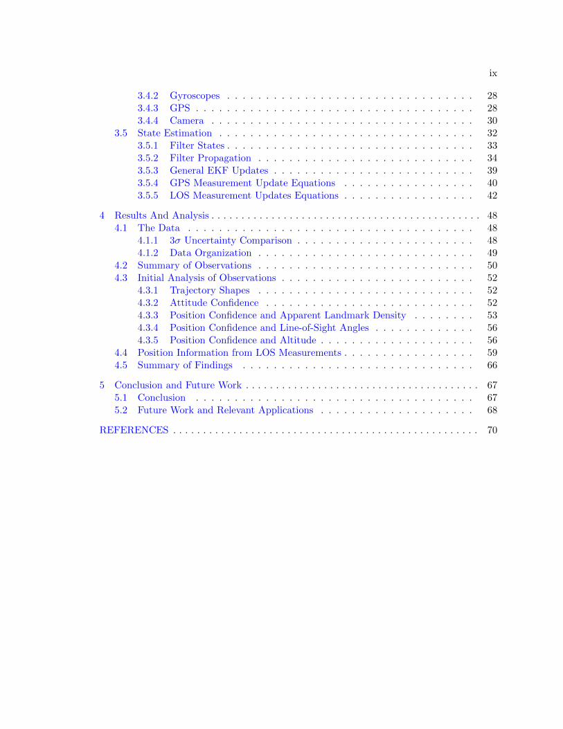
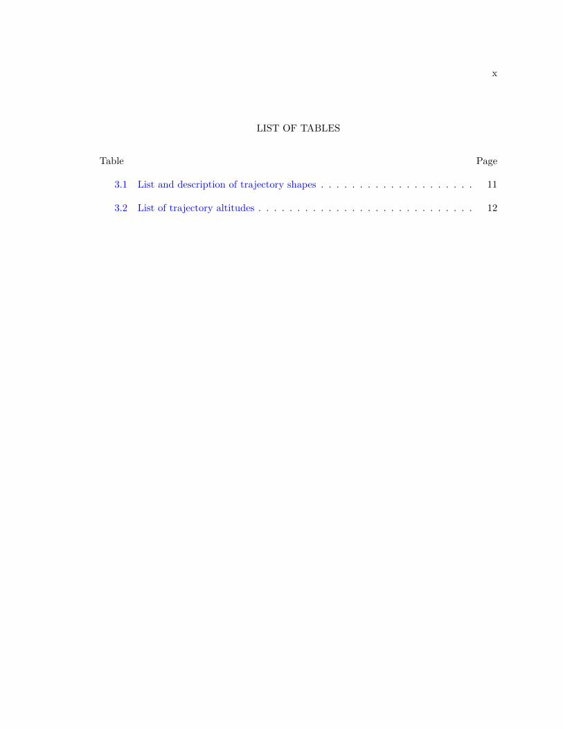
3.1 List and description of trajectory shapes . . . . . . . . . . . . . . . . . . . . 11

3.2 List of trajectory altitudes . . . . . . . . . . . . . . . . . . . . . . . . . . . . 12

xi

LIST OF FIGURES

Figure Page

1.1 A visual representation of navigation using line-of-sight measurements . . . 3

1.2 Overview of experimentation process in block diagram form . . . . . . . . . 6

3.1 Example of maintaining an ALD across altitudes . . . . . . . . . . . . . . . 13

3.2 Relationship between the inertial and vehicle frames . . . . . . . . . . . . . 15

3.3 Relationship between the vehicle and vehicle-1 frames . . . . . . . . . . . . 16

3.4 Relationship between the vehicle-1 and vehicle-2 frames . . . . . . . . . . . 17

3.5 Relationship between the vehicle-2 and body frames . . . . . . . . . . . . . 18

3.6 Relationship between the body and camera frames . . . . . . . . . . . . . . 20

3.7 Relationship between the body and camera frames . . . . . . . . . . . . . . 21

3.8 Overview of truth model process in block diagram form . . . . . . . . . . . 22

3.9 Representation of pinhole camera perspective projection . . . . . . . . . . . 30

4.1 Trajectory shape comparison example of north position . . . . . . . . . . . 50

4.2 Altitude comparison example of north position . . . . . . . . . . . . . . . . 51

4.3 ALD comparison example of north position . . . . . . . . . . . . . . . . . . 51

4.4 Attitude confidence for the different altitudes . . . . . . . . . . . . . . . . . 53

4.5 ALD comparison showing increased information for more landmark observa-tions . . . . . . . . . . . . . . . . . . . . . . . . . . . . . . . . . . . . . . . . 54

4.6 ALD comparison of north position at 15 meters . . . . . . . . . . . . . . . . 55

4.7 40 ALDs comparison of north position . . . . . . . . . . . . . . . . . . . . . 55

4.8 40 ALDs time-slice comparison of all position states with number of land-marks matched . . . . . . . . . . . . . . . . . . . . . . . . . . . . . . . . . . 57

4.9 ALD 5 and 6 comparison for north position with number of landmarks matched 58

4.10 Altitude comparison for a line trajectory using ALD 5 . . . . . . . . . . . . 58

xii

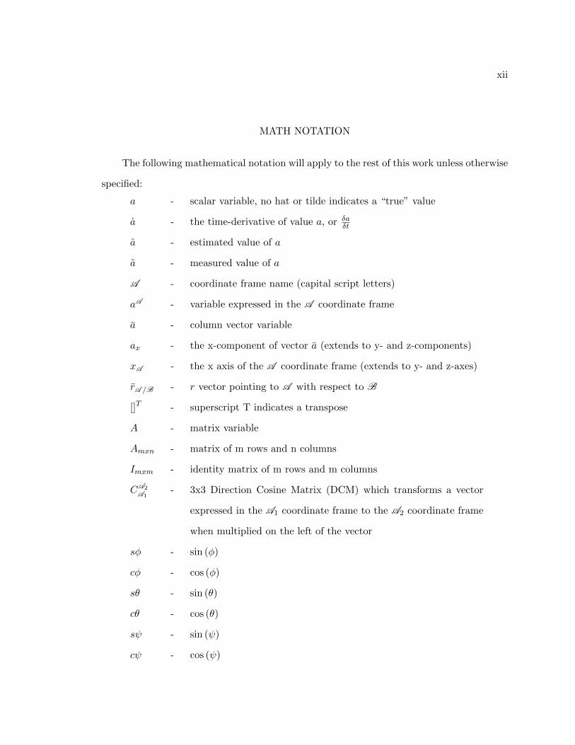
MATH NOTATION

The following mathematical notation will apply to the rest of this work unless otherwise

specified:

a - scalar variable, no hat or tilde indicates a “true” value

a - the time-derivative of value a, or δaδt

a - estimated value of a

a - measured value of a

A - coordinate frame name (capital script letters)

aA - variable expressed in the A coordinate frame

a - column vector variable

ax - the x-component of vector a (extends to y- and z-components)

xA - the x axis of the A coordinate frame (extends to y- and z-axes)

rA /B - r vector pointing to A with respect to B

[]T - superscript T indicates a transpose

A - matrix variable

Amxn - matrix of m rows and n columns

Imxm - identity matrix of m rows and m columns

CA2A1

- 3x3 Direction Cosine Matrix (DCM) which transforms a vector

expressed in the A1 coordinate frame to the A2 coordinate frame

when multiplied on the left of the vector

sφ - sin (φ)

cφ - cos (φ)

sθ - sin (θ)

cθ - cos (θ)

sψ - sin (ψ)

cψ - cos (ψ)

CHAPTER 1

INTRODUCTION

1.1 GPS-Denied and Image-Aided Navigation

Navigation, the process of accurately estimating states such as position and planning a

course of travel, is an essential part of vehicle automation. Once these states are estimated,

the vehicle can plan its course of travel and then apply control commands to get to where

it needs to go. Without an accurate estimation of where the vehicle is, it could never

accomplish its intended purpose.

The common backbone of most modern navigation systems consists of an inertial mea-

surement unit (IMU) [1–3]. An IMU is composed of several accelerometers and gyroscopes.

Much like the human ear, these sensors provide three-dimensional translation and rota-

tion information to the vehicle in the form of accelerations and rotational rates. Given a

starting location and orientation, these sensor readings enable the vehicle to estimate its

orientation, or attitude, and position over time by integrating the sensor measurements.

This integration process is called dead reckoning [4].

If the accelerometers and gyroscopes in an IMU were perfect, the vehicle could simply

navigate by dead reckoning with no problems. However, there are always errors with these

sensors such as misalignments, biases, and scaling factors because it is impossible to build

a perfect sensor. These imperfections make navigation by dead reckoning over extended

periods of time inaccurate and therefore unacceptable. The results would be similar to a

human trying to walk from one end of their house to the other while closing their eyes and

not feeling for obstacles.

To remedy this problem, more sensors may be added to the system to provide more

information about the navigation states, such as position, velocity, and attitude. Unlike

the IMU, these sensors, commonly referred to as aiding devices, provide useful information

2

through their measurements of the surrounding environment. These different measurements,

if combined intelligently, can help the system by increasing state knowledge and minimizing

uncertainty. It has become common practice to combine this information in what is called a

Kalman filter. Kalman filters come in many varieties, but in the context of navigation, they

are generally used to combine sensor information to provide state estimates and calculate

a measure of certainty regarding the resulting estimates.

One of the most common and important aiding systems in modern vehicle automation

and navigation is the global positioning system, or GPS [1–3]. However, GPS can be easily

jammed and is often unreliable in environments such as natural and urban canyons [5, 6].

Situations or environments in which GPS is unreliable or denied are referred to as GPS-

denied environments. Both military and civilian applications have fueled a growing interest

in recent years to find effective GPS-denied navigation systems.

Image-aided navigation is one alternative to GPS-aided systems that has been explored

extensively. Relevant works are discussed in the next section of this chapter. This method

of navigation used to be impractical in real-time applications due to limitations of onboard

sensors and processors in small vehicles. However, modern hardware has started to make

image-aided navigation a real possibility and it has been proven to be a plausible mode of

navigation when GPS is unavailable [1, 7]. Several ideas and algorithms related to making

image-aided navigation work well have been developed in recent years [8–14].

Among the many versions of image-aided navigation, Wu et al. present a simple, yet

promising algorithm that uses the line-of-sight (LOS) vectors from a monocular camera

towards known landmarks to provide position and attitude information to the navigation

system [7]. In this work, this type of measurement is referred to as a LOS measurement.

The algorithm processes the image from the sensor, searching for landmarks with known

positions in the environment. It then extracts useful information related to position and

attitude for navigation from the observed angles of the LOS vector to the landmark by

comparing its measurement to the estimated relative position of the landmark. Fig. 1.1

shows a representation of three LOS measurements being made to a lamp post, a mailbox,

3

and a traffic light in an urban environment. Similar measurements can be made to any

landmark that is recognizable by image processing software.

Fig. 1.1: A visual representation of navigation using line-of-sight measurements

Even though Wu et. al. proved the promise of these measurements in hardware during

short simulated GPS outages, the impacts of many variables related to trajectory and

landmark placement are not well understood [7]. There are several works which explore

various landmark placement algorithms which will be discussed in the next chapter of this

document. None, however, explore the relationships between vehicle trajectory, position

uncertainty, relative position, and the distribution landmarks. This work explores these

relationships by identifying and explaining various patterns observed by varying trajectory

shape, altitude, and apparent landmark density. An equation describing the amount of

information contained in a given measurement to a single landmark is presented along with

some path-planning implications and applications.

1.2 Contributions

Image-aided navigation has recently become a hot topic and is no longer considered

4

new. As has been shown in the previous section, much work has been done exploring the

uses of image-aided navigation. Contributions that the research in this work adds include

the following:

1. A modular experimental framework was developed and implemented in MATLAB

and SIMULINK which allows for easy manipulation of variables of interest. These

variables include but are not limited to

• a quadrotor model as developed by Beard that has been modified to use states

expressed in the inertial frame and

• a continuous-discrete Kalman filter that can incorporate GPS and/or LOS mea-

surements for easy comparison.

2. A new derivation for the attitude portion of the measurement geometry matrix for

LOS measurements for Euler angle attitude states rather than the quaternion version

presented by Wu et. al. [7].

3. Image-aided navigation solutions were computed for over 540 unique combinations of

trajectory shape, altitude, and landmark distribution. This data was then analyzed

to identify patterns in the data which will be useful to areas such as path planning

and landmark placement.

4. These resulting patterns were tied together in the derivation of the trace of the infor-

mation matrix for LOS measurements. The resulting equation produces an estimate of

how much information comes from a single measurement based on its relative position

to the camera.

5. The analysis of the data uncovered several patterns which need to be explored fur-

ther to better characterize LOS measurements, especially at lower altitudes. Any

research areas uncovered by this analysis could be especially useful in path planning

and landmark placement for small UAV applications in the future.

5

1.3 Overview

In order to explore the relationships mentioned above that will build upon previous

work, several key elements are needed to provide realistic data for analysis. These elements

are shown as the blocks in Fig. 1.2 as a step-by-step process along with any resulting data

from each step. Steps 1-3 and the format of their resulting data is described in greater detail

in chapter 2 of this work. To summarize these steps, a vehicle model with true-state feedback

is first implemented and run to generate sensor data for several trajectories. The sensor

data then has noise added to it and is combined in an extended Kalman filter (EKF) with

dynamically created camera measurements (steps 2 and 3). This filter produces estimated

states and a measure of estimate confidence called covariance. Results are organized and

analyzed in steps 4 and 5, as detailed in chapters 3-4. Finally, conclusions are drawn and

ideas for future work are discussed in chapter 6.

6

Step 1:Run Truth Model

True StatesLandmark Distributions

Noiseless GPS DataNoiseless IMU Data

Step 2:Add Noise to GPS and IMU Measurements

Create Camera Measurements

Step 3:Estimate States

Estimated StatesState Estimate Confidences

Step 4:Plot Estimated States

Analyze Results

Step 5:Develop Design Tools from Patterns

Fig. 1.2: Overview of experimentation process in block diagram form

CHAPTER 2

Background

As previously described, GPS-aided navigation systems have become commonplace in

autonomous vehicles. Due to the publicly known frequency of GPS signals, both military

and civilian users encounter problems with GPS signals [5, 6]. These problems continue to

prompt an increased interest in alternative navigation aiding measurements. Various aiding

sensors have been implemented, including imagers. Image-aided navigation is an attractive

solution because most systems come equipped with a simple, small, and cost-effective system

already installed. As was shown in several studies discussed below, image-aided navigation

can be a promising solution for GPS-denied navigation problems.

One interesting form of image-aided navigation involved the placement of static sensors

in the environment. Jourdan and Roy studied the placement of static sensors on the walls

of buildings to minimize average position error [15]. Vitus and Tomlin later approached the

problem with the intent of minimizing estimation error [16]. The problems with a static

sensor method of aiding-measurements are twofold. First, it still relies on a continuous

communication link between static sensors and the vehicle, making it less autonomous.

Second, it is much more expensive to place multiple static sensors in the environment as

the vehicle’s travel area grows. Given these shortcomings, this work focuses on building

upon knowledge of systems with on-board sensors.

In the world of unmanned aerial vehicles (UAVs), keeping the cost of the image sensor

low is not difficult. This is partly because so many systems come already equipped with

a simple imaging system consisting of a single-lens, or monocular, camera. The potential

of these readily available systems has been noted by several navigation and guidance ex-

perts. A simple measurement model is set forth by Wu et. al., which shows how a pixel

measurement can be compared to the estimated relative position of the landmark [7]. From

this comparison, which is referred to as a line-of-sight, or LOS, measurement, they can find

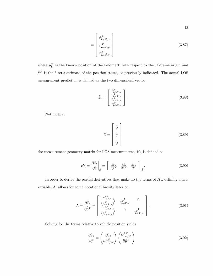
8

position and attitude information. Though not a new form of measurement, they were able

to show positive results in both simulation and in real-time hardware demonstrations.

This basic measurement has been built upon and extended in several ways, mostly in

an effort to obtain depth information. Mohamed, Patra, and Lanzon added a few lasers

to their system which were oriented to known angles [13]. Detecting the location of the

laser dots in the image allows them to infer depth information. Sharma and Pack used the

same basic measurement as Wu et. al. and then added a priori knowledge of the physical

target size to get depth information [12]. Wang and Zhang et. al. independently decided to

augment their LOS measurements with a preloaded depth map, allowing them to tap into

a third dimensional measurement [9, 17]. Zhang et. al. later improved on their simulated

data by applying their approach in hardware [18]. Bachrach et. al. took this approach

one step further and attempted to also map the environment using a depth sensor with the

camera.

This type of measurement is also useful in estimating target states. Sharma et. al. use

bearing-only measurements in a cooperative setting to geo-localize a target [19]. The term

bearing-only refers to the same type of measurement being discussed previously. Chowdary

et. al. attempt to navigate without any a priori knowledge by using a version of simultane-

ous localization and mapping, or SLAM, that employs the same measurement model [11].

All of these references qualify the statement of interest in and use of the measurement

presented by Wu as mentioned earlier.

Interest in this type of measurement has brought a wealth of questions forward that the

authors address. Work by Sala et. al. briefly discusses what constitutes a good landmark

and only chose landmarks that are always visible [10]. Several papers consider where to

optimally place man-made landmarks, though most refer to a two-dimensional navigation

problem [8,20–22]. Most sources try to minimize the number of needed landmarks. Ahn et.

al. try to do this by using a vanishing point method, but their method is limited to indoor

flight [8]. One big question that is addressed extensively is that of path planning [14,23,24].

Bopardikar et. al. present an especially interesting approach to path planning in which

9

they realize both path distance and error covariance can be treated as costs. Path length

is minimized first, while error covariance is treated second.

In all of this previous work, there has been no attempt to understand the relationship

between vehicle trajectory, the number of visible landmarks, and the system’s ability to

maintain a high level of navigation confidence when using an LOS-type aiding measure-

ment. There are several attempts in the works cited above to augment the system with

extra sensors. However, it appears that our collective knowledge of system design is lacking

when it comes to image-aided navigation because we do not fully understand the impli-

cations of this type of measurement. How much information does one LOS measurement

give? What effect does trajectory altitude have on this kind of measurement? How much

navigation confidence does the system gain for different apparent landmark densities at

different altitudes? This work attempts to address these questions in an effort to provide a

more informed approach to designing path-planning and guidance systems in the future.

CHAPTER 3

Methods

The previous chapter calls to attention a collective lack of knowledge regarding the

relationship between trajectories, the number of measured ground landmarks, and the re-

sulting navigation confidence. Fig. 1.2 then shows a method to generate data with the

purpose of identifying patterns and eventually providing observations and tools that will

aid in future guidance and path-planning algorithms. This chapter expands steps 1-3 of

this method in detail.

Section 3.1 presents a description of the variables that were tested and why they were

chosen. The experiment is then outlined in more detail including a description of each of

the steps shown in Fig. 1.2. To facilitate the discussion of mathematics behind the system

and data to be used, section 3.2 first identifies the coordinate frames used in this work.

Next, the system’s truth and sensor models from step 1 in Fig. 1.2 are described in detail

in sections 3.3 and 3.4. The results are discussed later in section 4.

3.1 Experiment Overview

The purpose of this work is to provide valuable insight into the relationship between

trajectories, the number of LOS-measurements to landmarks, and the resulting navigation

confidence of LOS-type image-aided navigation. The overall approach of this experiment is

to compare the EKF solution confidence of several scenarios that vary in trajectory shape,

trajectory altitude, and landmark distributions. As will be described later in section 3.2.6,

the camera is assumed to point in a nominally nadir direction.

3.1.1 Trajectory Shape

In this work, trajectory shape means the actual path and orientation that the vehicle

travels. Nine different trajectory shapes were used to create sensor data for this experiment.

11

Three of these trajectories are loitering patterns that cause the vehicle to remain in a

bounded area. The rest travel in different patterns along a line that is 100 meters long.

Each trajectory is named and described in Table 3.1 below.

Table 3.1: List and description of trajectory shapes

Traj. Type Traj. Name Description

Horizontal Circle 45 meter radius horizontal circle

Loitering Horizontal Figure 8 60x60 meter horizontal figure 8

Tilted Figure 8 60x60x20 meter tilted figure 8

Traveling Line 100 meter straight line

Traveling Twist Line 100 meter line,[−π

2 ,π2

]varying heading

Traveling Sine Line 100 meter horizontal sinusoid

Traveling Alt. Sine Line 100 meter vertical sinusoid

Traveling Tilted Sine Line 100 meter horizontal and vertical sinusoid

Traveling Corkscrew 100 meter corkscrew

3.1.2 Altitude

Altitude is defined in this work as the relative distance from the ground to the vehicle’s

center of mass as measured along the negative z-axis of the inertial frame (see section 3.2.1

for a description of the inertial frame). Altitudes within all trajectory shapes included in this

work are kept relatively constant to facilitate the comparison of landmark measurements at

each altitude. At the beginning of this work, it was unknown what range in altitude would

be the most informative and interesting to examine. The six linearly separated altitudes

in Table 3.2 are considered in this survey. This sampling of altitudes was chosen to create

data points that spread across a wide range of applications, therefore making the results

more generally valuable.

12

Table 3.2: List of trajectory altitudes

Altitude [meters]

15

412

809

1206

1603

2000

3.1.3 Apparent Landmark Densities

There are two challenges with this experiment when dealing with landmark distri-

butions because this work seeks to compare changes in two variables that are correlated:

altitude and the number of observed landmarks in a given image. First, when comparing

altitude results it is important to measure the same number of landmarks at each altitude.

At the same time, it is equally important to maintain a similar perceived landmark spacing

at each altitude. This is done by creating one landmark distribution for each altitude where

the angular distance to the camera is maintained for each altitude. One set of landmark dis-

tributions that meets these criteria across all the altitudes is called an apparent landmark

density, or ALD, for the remainder of this work. Using different landmark distributions

with the same apparent density tricks the vehicle into making similar LOS measurements

at different altitudes. An example of this is given in Fig. 3.1. Both plots show the same

corkscrew trajectory shape in red, but at two different altitudes (15 and 412 meters). The

blue circles represent the landmarks on the ground. On the left, the landmarks are phys-

ically much closer together than those on the right. However, because of the difference in

vehicle altitude, they appear to the camera to have the same density. For this example, the

vehicle expects to see at most four landmarks at a time, even though the landmarks are

physically spaced differently in the two scenes.

The second challenge is in being able to compare the number of observed landmarks.

This is made possible by creating several distribution sets with different apparent landmark

densities. This work examines the effect of 10 ALDs at each altitude. For future clarity,

13

010

Alti

tude

[m]

Corkscrew Line at 15 m Altitudewith ALD 4

50

50

East [m]

0

North [m]

0

-50 -50

0

200

Alti

tude

[m] 400

500

Corkscrew Line at 412 m Altitudewith ALD 4

500

East [m]

0

North [m]

0-500

-500

Fig. 3.1: Example of maintaining an ALD across altitudes

ALDs are named in this work with a number 1 to 10. These ALD numbers refer to the

maximum number of landmarks the camera should be able to observe within its 30 × 20

degree field of view on the ground when flying flat and level.

Landmarks in each scene are distributed into uniform grids to avoid making measure-

ments with too much redundant navigation information. Though not usually realistic, doing

this maximizes the amount of measurement geometry information available in each image

from the camera.

3.1.4 Experiment Outline

To observe and explain the patterns and relationships between these variables, each

of the steps from Fig. 1.2 are completed. Step 1 independently runs each combination of

trajectory shape and altitude. Each landmark distribution is created also as part of step 1.

The resulting data included noiseless vehicle position, velocity, and attitude states; noiseless

GPS measurements at 1 Hz; noiseless accelerometer and gyroscope data at 200 Hz; and 10

ALDs made up of 10 landmark distributions for each of the six altitudes.

Steps 2 and 3 must be taken together for each combination of trajectory shape, altitude,

and ALD. For a given combination, the previously generated sensor data first has random

white noise injected into it. The camera measurements are also created and have random

noise injected into them as well. When all of these measurements are prepared, they are

14

run through an extended Kalman filter (EKF) in step 3. The EKF produces a set of

estimated states for that trajectory, altitude, and ALD combination along with a measure

of its confidence called covariance. This data is stored to be compared and analyzed later.

Steps 2 and 3 are run again for each combination, applying new random noise to each sensor

measurement at each iteration.

Next, the EKF results are plotted in step 4 and examined to identify interesting pat-

terns. Step 5 is finally applied when these patterns are used to develop relationships that

can be used in design tools in future work. These last two steps are treated in chapter 4.

3.2 Coordinate Frames

It is often useful to express different subsystems and variables relative to each other

from different perspectives. Doing so can modularize the way the system is viewed and

can serve to simplify the math that describes and relates these subsystems. Coordinate

frames simply define the views from which states can be observed. This section describes

the relationships between each of the coordinate frames used in this work. The relationships

between the I -frame, V -frame, V1-frame, V2-frame, and B-frame are all patterned after

work by Beard and McLain [3]. All rotations described below and throughout the remainder

of this work follow the conventions of the right-hand rule. Also, for clarity in the figures

contained in this section, the red portions of the quadrotor drawings indicate the “front”

of the vehicle.

3.2.1 Inertial I -Frame

The inertial, or I -frame, is a static coordinate frame whose x, y, and z-axes point

north, east, and down (towards earth center), respectively. This type of static orientation

is referred to as north-east-down, or NED, for the remainder of this work. The origin of

the I -frame is defined to be the reference origin. In this work, all vehicle and landmark

position values are measured with reference to this origin location. Fig. 3.2 in the following

subsection gives a visual representation of the I -frame. It is important at this point to

acknowledge that the I -frame is fixed to the earth and therefore the rotation of the earth

15

is ignored for simplicity.

3.2.2 Vehicle V -Frame

The V -frame is constantly aligned with the I -frame, meaning that it is an NED frame

as described in section 3.2.1. Its origin, however, is always collocated with the center of

mass of the vehicle as shown in Fig. 3.2.

𝑥ℐ (North)𝑦ℐ (East)

𝑧ℐ (Down)

ℐ-Frame

𝑥𝒱 (North)𝑦𝒱 (East)

𝑧𝒱 (Down)

𝒱-Frame

Fig. 3.2: Relationship between the inertial and vehicle frames

The transformation of a vector from the I -frame to the V -frame is given by

aV = CVI a

I (3.1)

where

CVI = I3x3. (3.2)

3.2.3 Vehicle-1 V 1-Frame

The origin of the V1-frame is collocated with the origin of the V -frame. Its orientation

is obtained by rotating the V -frame about its z-axis by the vehicle’s yaw angle, ψ. This

results in the V1-frame’s z-axis pointing down towards earth center. If the vehicle had no

16

pitch or roll, the x-axis would point directly out the front of the vehicle and the y-axis would

point directly out the starboard side of the vehicle. This relationship is shown in Fig. 3.3.

𝑥𝒱

𝒱-Frame

𝒱1-Frame

𝑥𝒱1

𝑦𝒱

𝑦𝒱1

𝜓

𝑧𝒱,𝒱1

Fig. 3.3: Relationship between the vehicle and vehicle-1 frames

The transformation of a vector from the V -frame to the V1-frame is given by

aV1 = CV1V aV (3.3)

where

CV1V =

cosψ sinψ 0

− sinψ cosψ 0

0 0 1

. (3.4)

3.2.4 Vehicle-2 V 2-Frame

The origin of the V2-frame is collocated with the origin of the V - and V1-frames.

However, its orientation is obtained by rotating the V1-frame about its y-axis by the vehicle’s

pitch angle, θ. This results in the V2-frame’s z-axis pointing straight down out of the vehicle

and the x-axis pointing directly out the front of the vehicle. If the vehicle had no roll, the

y-axis would point directly out the starboard side of the vehicle as shown in Fig. 3.4.

17

𝒱1-Frame

𝒱2-Frame

𝜃

𝑥𝒱1

𝑧𝒱1

𝑦𝒱1,𝒱2𝑥𝒱2

𝑧𝒱2

Fig. 3.4: Relationship between the vehicle-1 and vehicle-2 frames

This transformation of a vector from the V1-frame to the V2-frame is given by

aV2 = CV2V1aV1 (3.5)

where

CV2V1

=

cos θ 0 − sin θ

0 1 0

sin θ 0 cos θ

. (3.6)

3.2.5 Body B-Frame

The body, or B-frame, is collocated with the center of mass of the vehicle, just as

the V , V1, and V2 frames are. The orientation of the B-frame is obtained by rotating the

V2-frame about its x-axis by the vehicle roll angle, φ. This results in the B-frame’s x-axis

always pointing out the front of the vehicle, the y-axis always pointing out the right of the

vehicle, and the z-axis always pointing out the bottom of the vehicle as shown in Fig. 3.5.

The transformation of a vector from the V2-frame to the B-frame is given by

aB = CBV2aV2 (3.7)

where

18

ℬ -Frame

𝒱2-Frame

𝜙

𝑦𝒱2

𝑧ℬ

𝑦ℬ 𝑥𝒱2,ℬ

𝑧𝒱2

Fig. 3.5: Relationship between the vehicle-2 and body frames

CBV2

=

1 0 0

0 cosφ sinφ

0 − sinφ cosφ

. (3.8)

At this point, it is appropriate to show that a complete transformation of a vector from

the V -frame to the B-frame may be mathematically obtained by

aB = CBV2CV2

V1CV1

V aV (3.9)

= CBV a

V (3.10)

where φ, θ, and ψ are roll, pitch, and yaw Euler angles, respectively,

CBV =

cθcψ cθsψ −sθ

sφsθcψ − cφsψ sφsθsψ + cφcψ sφcθ

cφsθcψ + sφsψ cφsθsψ − sφcψ cφcθ

, (3.11)

and

cφ = cosφ (3.12)

cθ = cos θ (3.13)

cψ = cosψ (3.14)

19

sφ = sinφ (3.15)

sθ = sin θ (3.16)

sψ = sinψ. (3.17)

For later derivations in this work, the following values of CBV are defined for convenience

and space

c11 c12 c13

c21 c22 c23

c31 c32 c33

=

cθcψ cθsψ −sθ

sφsθcψ − cφsψ sφsθsψ + cφcψ sφcθ

cφsθcψ + sφsψ cφsθsψ − sφcψ cφcθ

. (3.18)

3.2.6 Camera F -Frame

In dealing with a camera, a new frame needs to be introduced to account for the

orientation of the camera with respect to the vehicle. This makes it possible to relate

camera measurements to the vehicle orientation and position. This new camera frame, or

F -frame, is collocated at the center of mass to simplify the math in later derivations. Since

the camera model is not gimbaled, its orientation is obtained by rotating the B-frame by

-90 degrees or π2 radians about its y-axis. This results in the F -frame’s x-axis pointing

down out the bottom of the vehicle’s body along the B-frame’s z-axis. The assumption

here is that the focal point of the camera is also located at the center of mass of the vehicle.

See Fig. 3.6 for a visual representation of the F -frame with respect to the B-frame.

The transformation of a vector from the B-frame to the F -frame is given by

aF = CFB a

B (3.19)

where

CFB =

cos(−π

2

)0 − sin

(−π

2

)0 1 0

sin(−π

2

)0 cos

(−π

2

) (3.20)

20

ℬ-Frame

𝑥ℬ

𝑦ℬ,ℱ

𝑧ℱ

ℱ -Frame

Fig. 3.6: Relationship between the body and camera frames

=

0 0 1

0 1 0

−1 0 0

. (3.21)

3.2.7 Image X -Frame

Since camera measurements are obtained as pixel locations, it is necessary for a frame

to be defined describing the orientation of the image focal plane. Image pixels are typically

referred to as having the positive x-direction increasing to the right along a row of pixels,

while the positive y-direction increases down the image along the column of pixels [25]. For

this work, the camera is oriented such that the top of the image is nearest the front of the

vehicle with the x-axis of the X -frame pointing out the right of the vehicle. The origin of

the X -frame is located at a distance of the camera’s focal length along the F -frame’s x-axis

and shifted over from the center of the image to the top-left of the image plane (distances

given by the camera’s principle point in pixels). The X -frame’s y-axis points out the back

21

of the vehicle and its z-axis points down out the bottom of the vehicle. This is visually

represented in Fig. 3.7.

𝒳-Frame𝑦𝒳

𝑧𝒳

𝑥𝒳𝑝𝑥 , 𝑝𝑦

𝑧ℱ

𝑥ℱ

𝑦ℱ

ℱ-Frame

Fig. 3.7: Relationship between the body and camera frames

The transformation of a vector from the F -frame to the X -frame is given by

aX = CXF aF (3.22)

where

CXF =

0 1 0

0 0 1

1 0 0

. (3.23)

3.3 System Truth Model

With a firm understanding of its coordinate frames, this section now describes the

system truth model to be used in step 1 shown in Fig. 1.2. The vehicle system used in

this work is a small quadrotor unmanned aerial vehicle. As mentioned in section 3.1, this

model was run several times to produce noiseless sensor data for each trajectory shape and

altitude.

Conceptually, this system is organized much like a classical control system where the

22

feedback is a pure feedback. This means that the control system operates off of true states.

Though this is not realistic in a hardware system, this is appropriate for this simulation

as it still provides simulation data that is representative of quadrotor kinematics and dy-

namics. To better understand the components of this system, Fig. 3.8 shows step 1 of Fig.

1.2 expanded to its own functional block diagram. Each block can be treated as a math-

ematical function with inputs and outputs. Each block’s inputs, outputs, and underlying

mathematics are described in the following subsections.

Desired Trajectory

ClockDifferential

FlatnessController

Quadrotor Kinematics

and Dynamics

Sensor Models

Noiseless Sensor Data

True Quadrotor

States

Fig. 3.8: Overview of truth model process in block diagram form

Note that the sensor models and their resulting measurements are treated in section

3.4.

3.3.1 System States

Quantities described in this work are expressed in terms of the vehicle state vector

components. The quadrotor state vector, x consists of the following 12 states:

23

pIn - the inertial north position of the quadrotor along the x-axis of the

I -frame

pIe - the inertial east position of the quadrotor along the y-axis of the

I -frame

pId - the inertial down position of the quadrotor along the z-axis of the

I -frame

vIn - the inertial north velocity of the quadrotor along the x-axis of the

I -frame

vIe - the inertial east velocity of the quadrotor along the y-axis of the

I -frame

vId - the inertial down velocity of the quadrotor along the z-axis of the

I -frame

φ - the roll angle defined as the positive right-hand rotation about the

x-axis of the V2-frame

θ - the pitch angle defined as the positive right-hand rotation about

the y-axis of the V1-frame

ψ - the yaw angle defined as the positive right-hand rotation about

the z-axis of the V -frame

p - the roll rate measured about the x-axis of the B-frame

q - the pitch rate measured about the y-axis of the B-frame

r - the yaw rate measured about the z-axis of the B-frame

These states are modeled after work done by Beard, though position and velocity

states are given in the inertial frame as opposed to having the velocity states in the body

frame [26]. Three-dimensional position, velocity, and attitude are referred as p, v, and α

column vectors for the remainder of this work.

24

3.3.2 System Kinematics and Dynamics Model

The derivation of the system kinematics and dynamics is also based on Beard’s same

work [26]. He solves for the following constant inertia matrix J which assumes that the

vehicle is inertially symmetric about each of its axes:

J =

Jx 0 0

0 Jy 0

0 0 Jz

. (3.24)

The inverse of this inertia matrix can be expressed for later use as

J−1 =

1Jx

0 0

0 1Jy

0

0 0 1Jz

. (3.25)

The four propellers on the quadrotor work together to produce both torque and lift.

The three-dimensional torques produced by the motors expressed in the B-frame are defined

as

τB =

τφ

τθ

τψ

. (3.26)

Expressions for aIg as the acceleration due to gravity expressed in the I -frame, g as

the value of gravitational acceleration, and aBthrust as the acceleration due to the thrust

expressed in the B-frame are defined as

aIg =

0

0

g

(3.27)

g ≈ 9.81m

s(3.28)

25

aBthrust =

0

0

−FTm

(3.29)

where FT is the force of the thrust along the z-axis of the B-frame, and m is the mass of

the vehicle.

Using these definitions, the six degree of freedom model for the quadrotor’s kinematics

and dynamics can be summarized as

˙x =

˙pI

˙vI

˙α

˙ω

=

˙vI

aIg + CI

B aBthrust

Jy−JzJx

qr

Jz−JxJy

pr

Jx−JyJz

pq

+ J−1τB

J−1τB

. (3.30)

3.3.3 Controls and Desired Trajectories

Rather than inventing or re-deriving a novel method of controls, this work follows the

work done by Ferrin et. al. on controls using differential flatness [27]. They make the

matter of controlling the vehicle a relatively simple and straight forward process. The

reader is directed to their paper for a full explanation of differential flatness and their

ensuing algorithm, as only a brief summary is presented here.

The differential flatness algorithm accepts the desired trajectory’s differentially flat

position and heading with their first and second time derivatives. It uses these values to

calculate the state and reference inputs. The current vehicle states are subtracted from the

desired states, passed through a linear quadratic regulator (LQR) controller and finally re-

combined with the reference inputs. These quantities are run through a simple proportional,

integral, derivative (PID) controller to control the attitude and thrust.

26

3.3.4 Desired Trajectories

The desired trajectories have already been named at the beginning of section 3.1.

However, it is important to mention what general elements make up each of the trajectories.

Each trajectory was simply a function of time and had the following outputs:

pIdesired - desired position

˙pIdesired - desired velocity, or time derivative of pI

desired

¨pIdesired - desired acceleration, or double time derivative of pI

desired

ψdesired - desired heading

ψdesired - desired heading rate, or time derivative of θdesired

ψdesired - desired heading angular acceleration, or double time derivative of

θdesired

3.4 Sensor Models

As discussed in the introduction, a navigation system is typically built with several

sensors to aid in state estimation. Generally, the basic building blocks in navigation systems

include accelerometers, gyroscopes, and GPS. Measurements from these sensors are then

often combined in some form of Kalman filter to estimate system states such as position,

velocity, and attitude. These sensors were modeled and implemented in Simulink to output

perfect, noiseless measurements. However, as shown in Fig. 3.8, these sensor values were

not included in the model’s feedback control.

The following subsections describe each sensor model along with any assumptions. A

model for GPS measurements is included because GPS-aided solutions are created for each

trajectory shape and altitude. These results are used later as a performance baseline to

which image-aided solutions are compared. A camera model is also included and discussed

in detail to provide LOS measurements.

27

3.4.1 Accelerometers

Accelerometers measure the rate of change of the velocity in the B-frame. True ac-

celeration due to system forces (no external forces such as wind) can be expressed for this

system as

aB =

0

0

−fTm

(3.31)

where fT is the force due to the trust generated by the actuators and m is the mass of

the vehicle. Gravity is an environmentally induced acceleration and cannot be detected

directly by the accelerometers. It is introduced into the measurements via the system

dynamics equations detailed earlier. To simplify the model, wind conditions are assumed

to be zero since they should not have any affect on navigation solution confidence.

Real accelerometers are often modeled to include various error sources. These error

sources may include biases, scale factors, internal misalignments, and mounting misalign-

ments. It is common practice in many applications to use the navigation system’s Kalman

filter to settle on a more accurate estimation of these error sources. Since this work does

not explore the efficacy of LOS measurements in estimating those error sources, this work

assumes a good estimation of them has already been obtained and applied. Though it is

impossible to perfectly determine the exact values of these error sources in real life, it is

sufficient for this application to model the error sources as Gaussian, random white noise.

Thus, the sensor model becomes

˜aB =

0

0

−fTm

+ ηaccel (3.32)

where ηaccel is zero mean white noise of strength σaccel. New random white noise errors are

only added each time the measurements are fed into the state estimation filter.

28

3.4.2 Gyroscopes

Gyroscopes measure angular rate. Angular rates induced by the system are modeled

as

ω =

p

q

r

(3.33)

where p, q, and r are defined as the the roll, pitch, and yaw rates measured about the axes

of the B-frame as defined in section 3.3.1.

Real gyroscopes suffer from the same types of error sources as accelerometers. Following

the same logic as in section 3.4.1, these error sources can be simplified for this application

to simple Gaussian, random white noise. Therefore, the sensor model becomes

˜ω =

p

q

r

+ ηgryo (3.34)

where ηgryo is zero mean white noise of strength σgryo. New random white noise errors are

only added each time the measurements are fed into the state estimation filter.

3.4.3 GPS

Global positioning system, or GPS, uses pseudo-range measurements to calculate a

measure of three-dimensional position. Carrier phase Doppler measurements from GPS can

also be used to calculate three-dimensional velocity [3]. It is assumed that the GPS used in

this system provides north, east, and up measurements of both position and velocity with

respect to the inertial reference I -frame rather than in latitude, longitude, and altitude:

˜pI =

pIn

pIe

pIh

(3.35)

29

˜vI =

vIn

vIe

vIh

.

(3.36)

Note that pIh is the height or altitude position with respect to the I -frame, measured

positively along the negative z-axis of the I -frame. It follows that vIh is the velocity of the

vehicle along the negative z-axis of the I -frame.

These were combined to a single measurement vector, ˜γGPS :

˜γGPS =

pIn

pIe

pIh

vIn

vIe

vIh

.

(3.37)

GPS measurement noise should be modeled as a Gauss-Markov process. However, since

this work does not include bias estimations, the GPS measurement noise is modeled as

Gaussian white noise like in the cases of IMU sensors discussed earlier. GPS measurements

with noise added thus become

˜γγ =

pIn

pIe

pIh

vIn

vIe

vIh

+ ηγ (3.38)

where ηγ is zero mean white noise. The terms corresponding to position measurements are

of strength σγp and terms corresponding to velocity measurements are of strength σγv . New

random white noise errors are only added each time the measurements are fed into the state

30

estimation filter.

3.4.4 Camera

Much like the work described by Wu et. al., the camera sensor model is divided into

two parts. First, they defined a perspective projection model of a basic, ideal pinhole

camera [7]. This model projects the three-dimensional landmark location onto the two-

dimensional image plane. This projection is shown in Fig. 3.9. It is worth noting here that

the camera model used in this work has a 30× 20 degree field of view.

Focal length (𝑓)

Image Plane

(𝑥𝑜, 𝑦𝑜) Principle Point

3D Landmark Location, L

(𝑥, 𝑦) Pixel Location

ℱ-Frame

𝒳-Frame

𝑥ℱ

𝑧𝒳

𝑦ℱ

𝑧ℱ

𝑥𝒳

𝑦𝒳

Fig. 3.9: Representation of pinhole camera perspective projection

The undistorted, two-dimensional pixel position in the image plane, (xu, yu), is given

by the following equations:

xu = xo − fxrXL/F ,x

rXL/F ,z

(3.39)

yu = yo − fyrXL/F ,y

rXL/F ,z

(3.40)

where fx and fy are the camera’s horizontal and vertical focal lengths, respectively, (xo, yo)

31

is the camera’s principle point, and rXL/F is the position vector of the landmark with respect

to the focal point of the camera expressed in the X -frame. In simulation, the camera is

assumed to have identical horizontal and vertical focal lengths. Thus, f = fx = fy.

Realistically, a simple pinhole camera model is not an adequate representation of the

problem. With a real camera, the image would be distorted by the lens and therefore would

need to be undistorted. Because the effects of the camera are so central to this work, this

distortion is also implemented and then the equations to remove the distortion are applied.

The process of distorting the image in simulation to mimic the effects of a real-world camera

is a more complicated, iterative process. Due to the space required to discuss this process,

the reader is referred to Brown’s work [25]. The distorted pixel locations are referred to

here as (xd,noiseless, yd,noiseless).

LOS measurement noise must be added to the distorted pixel measurement, since that

is where the noise occurs in a real camera. Noise in this sensor, ηδλ, is a Gaussian white

noise of strength σδλ. However, it is defined as an angular measurement noise and therefore

must be added in angle space rather than in pixel space by using the equations:

xd = xd,noiseless + fxηδλ,x (3.41)

yd = yd,noiseless + fyηδλ,y. (3.42)

After noise has been added to the distorted pixel location, the measurement is ready

to be undistorted. Brown does define a common, simple set of equations for removing the

distortion and revealing the undistorted location of the landmark on the image plane. These

equations are altered slightly for this application to give:

xu = xd(1 + k1r

2 + k2r4)

2p1xdyd + p2

(r2 + 2x2

d

)(3.43)

yu = yd(1 + k1r

2 + k2r4)

2p2xdyd + p1

(r2 + 2y2

d

)(3.44)

where xd and yd are the distorted pixel locations as they would be given in the X -frame

by the physical camera and r is the distance from the camera’s principle point. The rest of

32

the variables are the following camera parameters:

(p1, p2) = principle point (3.45)

(k1, k2) = radial distortion coefficient with units

[1

pix2,

1

pix4

]. (3.46)

At this point, the camera measurement is simply given as an undistorted x and y pixel

location. The measurement should be expressed next as a line-of-sight vector, or the vector

from the focal point of the camera to the pixel location. This is given in the F -frame as

˜lF =

lFx

lFy

lFz

(3.47)

˜lF = CFX

xu

yu

−f

. (3.48)

Finally, this LOS vector can be used to create the same measurement as that used by

Wu et. al. [7]:

˜z =

lFylFx

lFzlFx

. (3.49)

3.5 State Estimation

Given these sensor models and their resulting data, equations can be derived which

more directly translate into vehicle state estimation. However, real-world sensors are im-

perfect. Sensors by themselves must be believed, but what happens when sensors start

to disagree with each other? For example, what if integrating accelerometer and gyro-

scope information to get position information gives increasingly different results than GPS

measurements? Fortunately, sensor manufacturers give a measure of how accurate each

sensor can be trusted to be. Given models of the system dynamics and sensors, having

33

the measurement noise parameters of each sensor allows the sensor data to be intelligently

combined in an extended Kalman filter (EKF). The filter then produces estimates of the

specified states as well as a measure of how confident it is in its estimations.

This work employs a continuous-discrete EKF to combine sensor data intelligently

to form its estimates. The filter is a continuous-discrete filter because it takes continuous

dynamics models and produces discrete state estimates. Kalman filters have two basic steps:

propagation via inertial sensors and updates via aiding sensors. Both steps are discussed in

more detail in their respective subsections.

This section defines which states the filter estimates, describes the filter propagation

and update steps, and defines the equations specific to this application that are used by

each step. It is appropriate at this point to clarify the difference in notation between true

(noiseless) variables, measurements produced by sensors, and quantities that are estimated

by the EKF. An arbitrary variable, a, is considered a sensor-measured value if it is written

as a. That same variable is interpreted as an estimated value if it is written as a. It is

considered a true, noiseless value if it is written simply as a. Please refer to the Math

Notation page at the beginning of this work for more details.

3.5.1 Filter States

The first question to answer when setting up an EKF is, “Which states will the filter

estimate?” This question depends on which states have equations that are functions of

input sensor data. The filter for this work estimates position, velocity, and attitude states,

but not attitude rate. The filter state vector is defined as

34

ˆx =

pIn

pIe

pId

vIn

vIe

vId

φ

θ

ψ

. (3.50)

Other variables of interest include the covariance for each state. Covariance values are what

give the measure of estimation confidence mentioned earlier. This concept is explained in

greater detail later in this work, but it is important to note that it was recorded from the

equations in the following subsection when the filter was run.

3.5.2 Filter Propagation

The beginning states are usually reasonably well known. However, as time progresses,

the estimated vehicle states must be propagated forward. Accelerometer and gyroscope

measurements from the IMU allow the Kalman filter to do so. In a continuous-discrete

Kalman filter, the propagation step computes the following general-form terms for each

IMU sample in the order they appear here.

1. Propagate the states using the dynamics model, ˙x (x, u) which is a function of the

most current filter states and the IMU sensor measurements:

ˆx+ = ˆx− +

(ToutN

)(˙x(ˆx−, u

))(3.51)

35

2. Compute the gradient matrix, A, evaluated with ˆx and u:

A =∂ ˙x

∂ ˆx

∣∣∣∣∣ˆx+,u

(3.52)

3. Propagate the covariance matrix, P:

P = P +

(ToutN

)(AP + PAT +GQGT

)(3.53)

Some definitions are required to apply this work’s application to these three steps. The

state models as a function of IMU data (accelerations and angular rates) and other states

are

˙x(ˆx, u)

=

ˆvI

aIg + CI

B˜aB

Rzyxgyro ˜ωBgyro

(3.54)

where ˜aB is the measured acceleration from the accelerometers expressed in the B-frame,

˜ωBgyro is the vector of measured angular rates from the gyroscopes expressed in the B-frame,

and the matrix, Rzyxgyro, that relates angular rates to roll, pitch, and yaw is defined as

Rzyxgyro =

1 sin

(φ)

tan (θ) cos(φ)

tan (θ)

0 cos(φ)

− sin(φ)

0 sin(φ)

sec (θ) cos(φ)

sec (θ)

. (3.55)

36

Noting that this vehicle’s system causes no accelerations in the B-frame’s x or y direc-

tions, ˙x can be re-written as

˙x(ˆx, u)

=

vIn

vIe

vId

0

0

g

+

cθcψ sφsθcψ − cφsψ cφsθcψ + sφsψ

cθsψ sφsθsψ + cφcψ cφsθsψ − sφcψ

−sθ sφcθ cφcθ

0

0

aBz

1 sin(φ)

tan(θ)

cos(φ)

tan(θ)

0 cos(φ)

− sin(φ)

0 sin(φ)

sec(θ)

cos(φ)

sec(θ)ωBp

ωBq

ωBr

(3.56)

=

vIn

vIe

vId

(cφsθcψ + sφsψ

)aBz(

cφsθsψ − sφcψ)aBz

g +(cφcθ

)aBz

ωBp + ωB

q

(sin(φ)

tan(θ))

+ ωBr

(cos(φ)

tan(θ))

ωBq

(cos(φ))

+ ωBr

(− sin

(φ))

ωBq

(sin(φ)

sec(θ))

+ ωBr

(cos(φ)

sec(θ))

(3.57)

37

=

vIx

vIy

vIz(

cos φ sin θ cos ψ + sin φ sin ψ)az(

cos φ sin θ sin ψ − sin φ cos ψ)az

g +(

cos φ cos θ)az

ωp + ωq sin φ tan θ + ωr cos φ tan θ

ωq cos φ− ωr sin φ

ωq sin φ sec θ + ωr cos φ sec θ

. (3.58)

It then follows that the A matrix is

A =

0 0 0 1 0 0 0 0 0

0 0 0 0 1 0 0 0 0

0 0 0 0 0 1 0 0 0

0 0 0 0 0 0 ∂ ˙x4∂φ

∂ ˙x4∂θ

∂ ˙x4∂ψ

0 0 0 0 0 0 ∂ ˙x5∂φ

∂ ˙x5∂θ

∂ ˙x5∂ψ

0 0 0 0 0 0 ∂ ˙x6∂φ

∂ ˙x6∂θ

0

0 0 0 0 0 0 ∂ ˙x7∂φ

∂ ˙x7∂θ

0

0 0 0 0 0 0 ∂ ˙x8∂φ

0 0

0 0 0 0 0 0 ∂ ˙x9∂φ

∂ ˙x9∂θ

0

(3.59)

where

∂ ˙x4

∂φ=(− sin φ sin θ cos ψ + cos φ sin ψ

)az (3.60)

∂ ˙x4

∂θ=(

cos φ cos θ cos ψ)az (3.61)

∂ ˙x4

∂ψ=(− cos φ sin θ sin ψ + sin φ cos ψ

)az (3.62)

∂ ˙x5

∂φ=(− sin φ sin θ sin ψ − cos φ cos ψ

)az (3.63)

38

∂ ˙x5

∂θ=(

cos φ cos θ sin ψ)az (3.64)

∂ ˙x5

∂ψ=(

cos φ sin θ cos ψ + sin φ sin ψ)az (3.65)

∂ ˙x6

∂φ=(− sin φ cos θ

)az (3.66)

∂ ˙x6

∂θ=(− cos φ sin θ

)az (3.67)

∂ ˙x7

∂φ= ωq

(cos φ tan θ

)+ ωr

(− sin φ tan θ

)(3.68)

∂ ˙x7

∂θ=(ωq sin φ+ ωr cos φ

)sec2 θ (3.69)

∂ ˙x8

∂φ= ωq

(− sin φ

)+ ωr

(− cos φ

)(3.70)

∂ ˙x9

∂φ=(ωq cos φ+ ωr

(− sin φ

))sec θ (3.71)

∂ ˙x9

∂θ=(ωq

(− sin φ

)+ ωr (− cosφ)

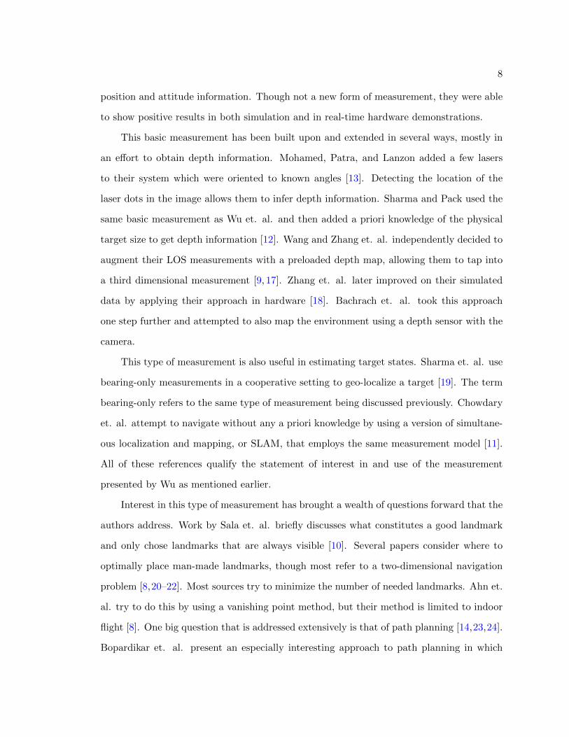
)tan θ sec θ. (3.72)

The matrix, Q, contains information about the process noise. The strength of the

process noise is defined by the IMU sensors’ accuracy:

Q =

σ2ax 0 0 0 0 0

0 σ2ay 0 0 0 0

0 0 σ2az 0 0 0

0 0 0 σ2ωx 0 0

0 0 0 0 σ2ωy 0

0 0 0 0 0 σ2ωz

(3.73)

where σax , σay , and σaz are the standard deviations of the accelerometer noise in the x,

y, and z directions respectively, and σωx , σωy , and σωz are the standard deviations of the

gyroscope noise about the x, y, and z-axes.

Finally, the G matrix, which projects the IMU sensor noise into the states, is defined

as

39

G =

0 0 0 0 0 0

0 0 0 0 0 0

0 0 0 0 0 0

0 0 cos (φ) sin (θ) 0 0 0

0 0 − sin (φ) 0 0 0

0 0 cos (φ) cos (θ) 0 0 0

0 0 0 1 sin (φ) tan (θ) cos (φ) tan (θ)

0 0 0 0 cos (φ) − sin (φ)

0 0 0 0 sin (φ) sec (θ) cos (φ) sec (θ)

. (3.74)

These propagation equations are run at the frequency of the IMU samples. For this

work, the IMU frequency is 150 Hz.

3.5.3 General EKF Updates

The general equations for a continuous-discrete Kalman filter are set forth here. Recall

that accelerometers and gyroscopes, as part of the IMU, are being used in a dynamic model

replacement mode. Their measurements, as described above, are essentially integrated into

the propagation step. The update step in a Kalman filter only operates on aiding sensors. A

given system can have several aiding sensors including, but not limited to GPS and cameras.

If a system has n aiding sensors, let sensor i be any one of those aiding sensors. Each time

the filter receives a measurement from sensor i, zi, the filter applies the measurement update

after a normal propagation by computing the following equations in order:

1. Predict the expected measurement:

zi = hi(ˆx)

(3.75)

2. Compute the measurement geometry matrix, Hi, which projects the sensor measure-

ment into the filter states:

40

Hi

(ˆx)

=∂hi

(ˆx)

∂ ˆx

∣∣∣∣∣ˆx

(3.76)

3. Compute the residual covariance matrix, R:

R = HiP−HT

i +Ri (3.77)

where Ri is the measurement noise matrix which is made from the standard deviation

of the sensor.

4. Compute the Kalman gain matrix, Ki:

Ki = P−HTi R

−1 (3.78)

5. Update the states using a Kalman-weighted measurement residual:

ˆx+ = ˆx− +Ki (zi − zi) (3.79)

6. Update the state covariance using Joseph’s form of the update:

P+ = (I −KiHi)P− (I −KiHi)

T +KiRiKTi (3.80)

These equations are applied to both GPS and LOS measurements in the next two

sections of this work. To clarify, each trajectory was run once with GPS measurements

enabled and LOS measurements disabled. Then, GPS measurements were disabled and

LOS measurements were enabled for every combination of trajectory and apparent landmark

density. The variables in the equations above are defined for GPS and LOS measurements

in the following subsections.

3.5.4 GPS Measurement Update Equations

A baseline Kalman filter performance is needed for the purpose of this work. GPS

41

measurements are implemented to fill this capacity because GPS-aided navigation is very

well characterized relative to image-aided navigation.

There are only three variables from the general equations in the preceding subsection

that need to be defined for each measurement. The first is, ˆzγ , which is comprised of a set

of equations which give the expected GPS measurements:

ˆzγ =

pIn

pIe

−pId

vIn

vIe

−vId

. (3.81)

Note that the third position and velocity states in the filter are defined as a downward

direction with respect to the I -frame origin expressed in the I -frame, while the GPS

measurements define them as height or upward direction with respect to and expressed in

the same frame.

Next, the measurement geometry matrix for GPS updates is derived to be

HGPS =

1 0 0 0 0 0 0 0 0

0 1 0 0 0 0 0 0 0

0 0 1 0 0 0 0 0 0

0 0 0 1 0 0 0 0 0

0 0 0 0 1 0 0 0 0

0 0 0 0 0 1 0 0 0

. (3.82)

42

Finally, the measurement noise matrix for GPS updates, RGPS , is defined as

RGPS =

σ2γpn

0 0 0 0 0

0 σ2γpe

0 0 0 0

0 0 σ2γph

0 0 0

0 0 0 σ2γvn

0 0

0 0 0 0 σ2γve

0

0 0 0 0 0 σ2γvh

(3.83)

where σγpn , σγpe , σγph , σγvn , σγve , and σγvh are the standard deviations of the GPS position

and velocity noise in the north, east, and up directions.

3.5.5 LOS Measurement Updates Equations

The same variables need to be estimated for image-aided navigation using LOS mea-

surements. Each time the image sensor produces an image frame, the filter must complete

an update step for each landmark detected in the frame. Therefore, the following definitions

and equations apply to each detected landmark in turn for a given image.

First, the relative position of the landmark with respect to the F -frame, ˆrFL/F , must

be predicted. The relative position vector can be predicted in place of predicting the LOS

vector measured by the camera (defined as the pixel position relative to the focal point of

the camera) because the final version of the predicted measurement yields the same ratio

as that of the final version of the actual measurement if they point in the same direction.

Magnitudes do not matter because both vectors form similar right triangles. The prediction

of ˆrFL/F is given as

ˆrFL/F = pF

L − ˆpF (3.84)

= CFB C

BV C

VI p

IL − CF

B CBV C

VI

ˆpI (3.85)

= CFB C

BV C

VI

(pIL − ˆpI

)(3.86)

43

=

rFL/F ,x

rFL/F ,y

rFL/F ,z

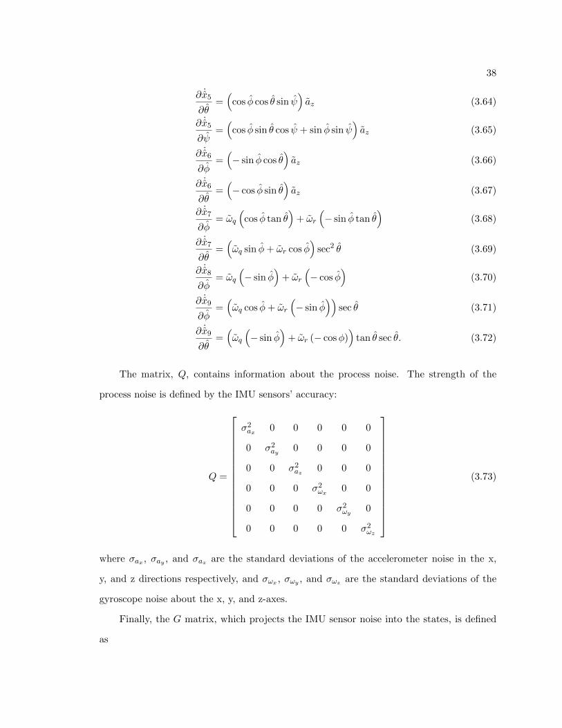
(3.87)

where pFL is the known position of the landmark with respect to the I -frame origin and

ˆpI is the filter’s estimate of the position states, as previously indicated. The actual LOS

measurement prediction is defined as the two-dimensional vector

ˆzλ =

rFL/F,y

rFL/F,x

rFL/F,z

rFL/F,x

. (3.88)

Noting that

ˆα =

φ

θ

ψ

(3.89)

the measurement geometry matrix for LOS measurements, Hλ is defined as

Hλ =∂ ˆzλ∂ ˆx

∣∣∣∣ˆx

=

[∂ ˆzλ∂ ˆpI

∂ ˆzλ∂ ˆvI

∂ ˆzλ∂ ˆα

]∣∣∣∣ˆx

. (3.90)

In order to derive the partial derivatives that make up the terms of Hλ, defining a new

variable, Λ, allows for some notational brevity later on:

Λ =∂ ˆzλ

∂ˆlF=

−rF

L/F,y(rFL/F,x

)21

rFL/F,x

0

−rFL/F,z(

rFL/F,x

)2 0 1rFL/F,x

. (3.91)

Solving for the terms relative to vehicle position yields

∂ ˆzλ∂ ˆp

=

(∂ ˆzλ

∂ ˆrFL/F

)(∂ ˆrF

L/F

∂ ˆpI

)(3.92)

44

= Λ

(CF

B CBV C

VI ∂ ˆrI

L/F

∂ ˆpI

)(3.93)

= ΛCFB C

BV C

VI

(∂ ˆrI

L/F

∂ ˆpI

)(3.94)

= ΛCFI

(∂(pIL − ˆpI

)∂ ˆpI

)(3.95)

= ΛCFI (−I3x3) (3.96)

= −ΛCFI . (3.97)

For use later in this work, this term is defined as

Hpos = −ΛCFI . (3.98)

Solving for the terms relative to vehicle velocity yields

∂ ˆzλ∂ ˆv

=

(∂ ˆzλ

∂ˆlF

)(∂ ˆrFL/F

∂ ˆvI

)(3.99)

= Λ03x3 (3.100)

= 02x3. (3.101)

Both the position and velocity partial derivatives match the results obtained by Wu

et. al., but their filter state vector defines the attitude states as a quaternion vector [7].

However, the attitude states in this work are stored as Euler angles. Therefore, the final

partial derivative is re-derived for this work here:

∂ ˆzλ∂ ˆα

=

(∂ ˆzλ

∂ ˆrFL/F

)(∂ ˆrF

L/F

∂ ˆα

)(3.102)

= ΛCFB

∂(CB

V CVI

ˆrIL/F

)∂ ˆα

(3.103)

= ΛCFB

∂(CB

V CVI

(pIf − ˆpI

))∂ ˆα

. (3.104)

45

To solve for∂(CB

V CVI

ˆrIL/F

)∂ ˆα

, the CBV C

VI

ˆrIL/F term is written out as

CBV C

VI

ˆrIL/F =

cθcψ cθsψ −sθ

sφsθcψ − cφsψ sφsθsψ + cφcψ sφcθ

cφsθcψ + sφsψ cφsθsψ − sφcψ cφcθ

1 0 0

0 1 0

0 0 1

ˆrIL/F ,x

ˆrIL/F ,y

ˆrIL/F ,z

(3.105)

ˆrBL/F ,x

ˆrBL/F ,y

ˆrBL/F ,z

=

ˆrIL/F ,x

(cθcψ

)+ ˆrI

L/F ,y

(cθsψ

)+ ˆrI

L/F ,z

(−sθ

)ˆrIL/F ,x

(sφsθcψ − cφsψ

)+ ˆrI

L/F ,y

(sφsθsψ + cφcψ

)+ ˆrI

L/F ,z

(sφcθ

)ˆrIL/F ,x

(cφsθcψ + sφsψ

)+ ˆrI

L/F ,y

(cφsθsψ − sφcψ

)+ ˆrI

L/F ,z

(cφcθ

)

(3.106)

where

cφ = cos φ (3.107)

cθ = cos θ (3.108)

cψ = cos ψ (3.109)

sφ = sin φ (3.110)

sθ = sin θ (3.111)

sψ = sin ψ. (3.112)

From here, the partial derivative term becomes the following 3× 3 matrix

∂(CB

V CVI

ˆrIL/F

)∂ ˆα

=

L11 L12 L13

L21 L22 L23

L31 L32 L33

(3.113)

where

L11 =∂ ˆrB

L/F ,x

∂φ(3.114)

46

= 0 (3.115)

L12 =∂ ˆrB

L/F ,x

∂θ(3.116)

= ˆrBL/F ,x (−sθcψ) + ˆrB

L/F ,y (−sθsψ) + ˆrBL/F ,z (−cθ) (3.117)

L13 =∂ ˆrB

L/F ,x

∂ψ(3.118)

= ˆrBL/F ,x (−cθsψ) + ˆrB

L/F ,y (cθcψ) (3.119)

L21 =∂ ˆrB

L/F ,y

∂φ(3.120)

= ˆrBL/F ,x (cφsθcψ + sφsψ) + ˆrB

L/F ,y (cφsθsψ − sφcψ) + ˆrBL/F ,z (cφcθ) (3.121)

L22 =∂ ˆrB

L/F ,y

∂θ(3.122)

= ˆrBL/F ,x (sφcθcψ) + ˆrB

L/F ,y (sφcθsψ) + ˆrBL/F ,z (−sφsθ) (3.123)

L23 =∂ ˆrB

L/F ,y

∂ψ(3.124)

= ˆrBL/F ,x (−sφsθsψ − cφcψ) + ˆrB

L/F ,y (sφsθcψ − cφsψ) (3.125)

L31 =∂ ˆrB

L/F ,z

∂φ(3.126)

= ˆrBL/F ,x (−sφsθcψ + cφsψ) + ˆrB

L/F ,y (−sφsθsψ − cφcψ) + ˆrBL/F ,z (−sφcθ) (3.127)

L32 =∂ ˆrB

L/F ,z

∂θ(3.128)

= ˆrBL/F ,x (cφcθcψ) + ˆrB

L/F ,y (cφcθsψ) + ˆrBL/F ,z (−cφsθ) (3.129)

L33 =∂ ˆrB

L/F ,z

∂ψ(3.130)

= ˆrBL/F ,x (−cφsθsψ + sφcψ) + ˆrB

L/F ,y (cφsθcψ + sφsψ) . (3.131)

The measurement noise matrix for LOS updates, Rλ is defined as

Rλ =

σ2δλx

0

0 σ2δλy

(3.132)

47

where σδλx and σδλx are the standard deviations of the camera x and y pixel measurement

noise respectively.

CHAPTER 4

Results And Analysis

As stated in previous chapters, the questions addressed by this work deal with the

relationships between trajectory shape, altitude, and the number of landmarks observed

when using LOS measurements in image-aided navigation. Fig. 1.2 shows the overall setup

by which these questions are addressed in this work. Section 3.1 details how this process

was run to estimate vehicle states and produce filter covariance for all of the combinations of

trajectory shapes, altitudes, and ALDs for GPS-aided and image-aided navigation solutions.

This chapter discusses the presentation of that data, identifies several patterns, and then

discusses the implications of these findings.

4.1 The Data

There are two main points to clarify about how the data presented below is to be

interpreted. First, what exactly is plotted? And second, how is it organized? The following

two subsections address these questions.

4.1.1 3σ Uncertainty Comparison

Since this work addresses questions concerning the effect of variables on how confident

the filter is, only the covariance data is examined here. The square root of the diagonal

terms of the EKF’s resulting covariance matrix gives the standard deviation of the states:

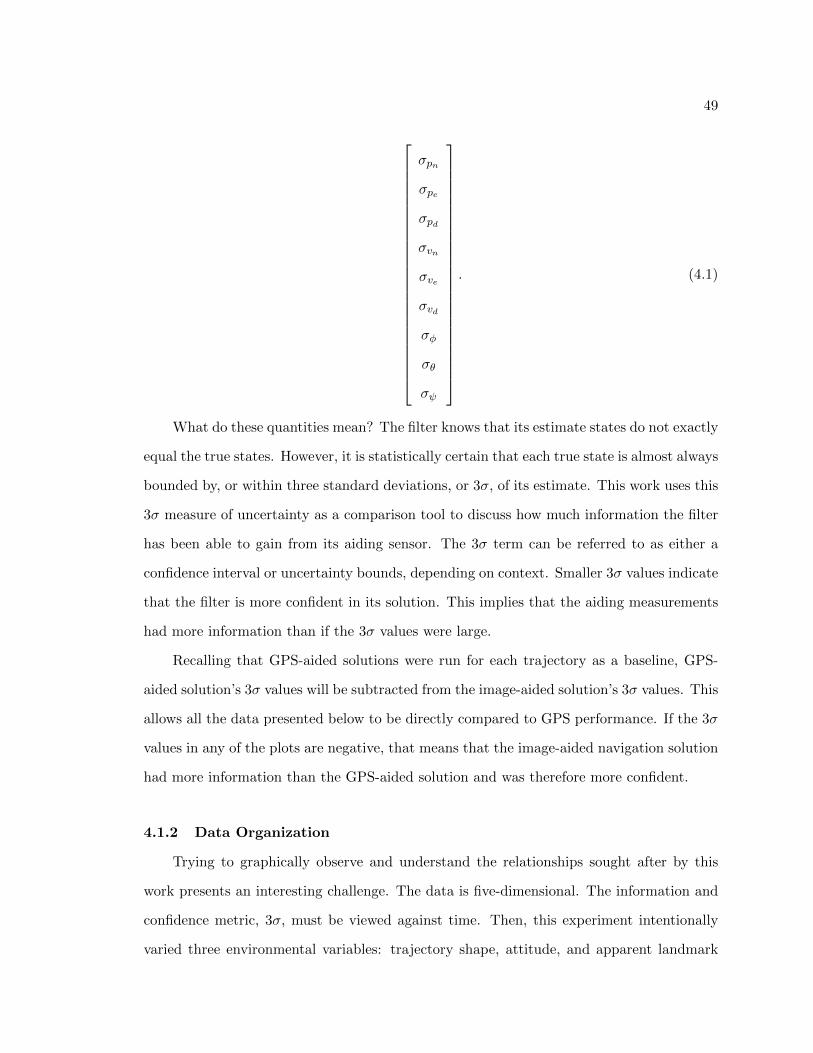
49

σpn

σpe

σpd

σvn

σve

σvd

σφ

σθ

σψ

. (4.1)

What do these quantities mean? The filter knows that its estimate states do not exactly

equal the true states. However, it is statistically certain that each true state is almost always

bounded by, or within three standard deviations, or 3σ, of its estimate. This work uses this

3σ measure of uncertainty as a comparison tool to discuss how much information the filter

has been able to gain from its aiding sensor. The 3σ term can be referred to as either a

confidence interval or uncertainty bounds, depending on context. Smaller 3σ values indicate

that the filter is more confident in its solution. This implies that the aiding measurements

had more information than if the 3σ values were large.

Recalling that GPS-aided solutions were run for each trajectory as a baseline, GPS-

aided solution’s 3σ values will be subtracted from the image-aided solution’s 3σ values. This

allows all the data presented below to be directly compared to GPS performance. If the 3σ

values in any of the plots are negative, that means that the image-aided navigation solution

had more information than the GPS-aided solution and was therefore more confident.

4.1.2 Data Organization

Trying to graphically observe and understand the relationships sought after by this

work presents an interesting challenge. The data is five-dimensional. The information and

confidence metric, 3σ, must be viewed against time. Then, this experiment intentionally

varied three environmental variables: trajectory shape, attitude, and apparent landmark

50

density.

To address this issue and pursue the search for patterns that indicate a relationship of

interest, three categories of plots were made for all nine filter states. Each category holds

two of the three environmental and varies the third in a given plot. The first category

of plots varied the trajectory shape. Fig. 4.1 shows an example comparing the different

trajectory shapes for an altitude of 412 meters using ALD 5 for the north position. Next,

the second category of plots varied the altitude. Fig. 4.2 shows an example comparing the

different altitudes for a straight-line trajectory using ALD 5 for the north position. Finally,

that leaves the last category to vary the ALD. Fig. 4.3 shows an example comparing the

different ALDs for a straight-line trajectory at an altitude of 412 meters. Viewing these

types of plots revealed several interesting patterns.

Fig. 4.1: Trajectory shape comparison example of north position

4.2 Summary of Observations

Several patterns were observed in the plots resulting from running all of the trajectory,

altitude, and apparent landmark density combinations. The following observations will be

discussed in the next section of this chapter.

1. None of the different trajectory shapes tested in this work have any distinguishable

effects on filter confidence for any of the estimated states.

51

0 10 20 30 40 50 60 70 80 90 100

Time [s]

-5

0

5

10

15

pn 3

-sig

ma

[m]

pn LOS-GPS 3 Difference vs Time for Each Altitude

for line with ALD 5

15m412m809m1206m1603m2000m

Fig. 4.2: Altitude comparison example of north position

Fig. 4.3: ALD comparison example of north position

52

2. Attitude confidence is practically the same and is consistently as good as GPS per-

formance.

3. Position confidence generally increases with more measurements towards some maxi-

mum knowledge.

4. Position confidence is better when landmarks are observed closer to the edge of the

image.

5. Position confidence is increasingly worse at high altitudes.

Following the initial discussion of these observations, a mathematical representation is

derived tying together some of the observations about position confidence.

4.3 Initial Analysis of Observations

4.3.1 Trajectory Shapes

The various trajectory shapes included in tests for this work do not have any discernible

patterns to suggest a superior trajectory. There are plenty of differences between the results,

but all the changes in confidence for each of the trajectories are directly correlated to the

number of landmarks observed during the change. There was no evidence of one trajectory

shape seeing more or less landmarks than another. This, however, is not a completely

conclusive finding. One failing of this experiment is that all of the trajectory shapes were

relatively flat and level. None of them had significant variation in pitch or roll. Given the

derivation and analysis in section 4.4, it would be interesting to examine results from a

trajectory shape with higher pitch and roll angles as part of a future work.

4.3.2 Attitude Confidence

All of the data gathered and examined as part of this work indicated that attitude

confidence remained largely unaffected by the changing variables. The only differences can

53

be partially attributed to relative distance and measurement noise in the form of camera

pixel size, though this remains unproved in this work. One interesting finding is related to

the vehicle’s altitude and how much attitude information is available. Fig. 4.4 shows the

roll confidence for all altitudes when flying a straight line using ALD. The most confident

scenario is when the vehicle is flying at 15 meters. However, the next highest altitude is the

least confident altitude. The confidence appears to get better as the vehicle gets higher for

the rest of the altitudes tested. The same pattern appears in all three attitude states.

0 10 20 30 40 50 60 70 80 90 100

Time [s]

-1

-0.5

0

0.5

1

3-s

igm

a [r

ad]

10-3

LOS-GPS 3 Difference vs Time for Each Altitudefor line with ALD 5

15 m412 m809 m1206 m1603 m2000 m

Fig. 4.4: Attitude confidence for the different altitudes

It appears that there is a trade-off between distance from the landmark and the mea-

surement noise. When the landmark is close, the imager is able to capture its position more

exactly and the filter understands this. However, at smaller distances, small rotations can

appear similar to small translations to the camera. The filter would have a difficult time

telling those apart. As distance increases, this effect becomes less apparent.

Although this is an interesting exercise, the effects described here are small (see scale

of the plot in Fig. 4.4). Due to its relatively small impact, the concepts observed here are

secondary to those in the following section. The proof is therefore left for future work.

4.3.3 Position Confidence and Apparent Landmark Density

Examining ALD-varying plots such as Fig. 4.5 consistently reveals a correlation be-

tween the number of landmarks observed and the level of position confidence. The top

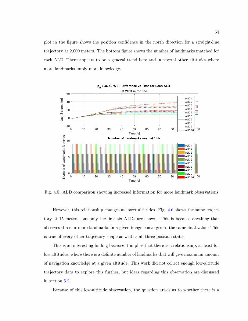
54

plot in the figure shows the position confidence in the north direction for a straight-line

trajectory at 2,000 meters. The bottom figure shows the number of landmarks matched for

each ALD. There appears to be a general trend here and in several other altitudes where

more landmarks imply more knowledge.

Fig. 4.5: ALD comparison showing increased information for more landmark observations

However, this relationship changes at lower altitudes. Fig. 4.6 shows the same trajec-

tory at 15 meters, but only the first six ALDs are shown. This is because anything that

observes three or more landmarks in a given image converges to the same final value. This

is true of every other trajectory shape as well as all three position states.

This is an interesting finding because it implies that there is a relationship, at least for

low altitudes, where there is a definite number of landmarks that will give maximum amount

of navigation knowledge at a given altitude. This work did not collect enough low-altitude

trajectory data to explore this further, but ideas regarding this observation are discussed

in section 5.2.

Because of this low-altitude observation, the question arises as to whether there is a

55

0 10 20 30 40 50 60 70 80 90 100

Time [s]

-6

-4

-2

0

2

4

pn 3

-sig

ma

[m]

pn LOS-GPS 3 Difference vs Time for Each ALD

at 15m for line

ALD 1ALD 2ALD 3ALD 4ALD 5ALD 6

0 10 20 30 40 50 60 70 80 90 100

Time [s]

0

2

4

6

Num

ber

of F

eatu

res

Mat

ched Number of features seen at 1Hz

altSineLineazTwistLinecorkscrewLineflat8flatCircflatSineLine

Fig. 4.6: ALD comparison of north position at 15 meters

similar behavior at high altitudes. To explore this further, 30 additional ALDs were created,

bringing the total to 40. Two trajectories were run at each altitude above 15 meters (since

the 15 meter case had proven to converge) and both showed similar trends. Fig. 4.7 show

this trend by plotting the north position results of running the altitude-varying sinusoidal

line at 2,000 meters against all 40 ALDs. The legend was omitted from this plot due to

its size. The general trend holds true: more landmarks mean more certainty, though each

additional landmark adds less information than the ones before it.

Fig. 4.7: 40 ALDs comparison of north position

This trend is also present at the other altitudes. To better understand how much

information is added by each successive measurement, a time slice was taken at 60 seconds

of Fig. 4.7 along with the other altitudes down to and including 412 meters. This results

in a 3σ difference value for each ALD at the 60 second mark of the run. This was done for

56

all three position states at each altitude and the results are shown in Fig. 4.8. The number

of observed landmarks is included in the bottom plot to show that a nearly linear increase

in landmarks observed yields a curve for each altitude that appears to be converging to a

final value.

One detail to recall here is that each landmark distribution is laid out in a uniform

grid to maximize the measurement information from each camera image. Because of this

detail, this empirical data may be a close representation of an ideal curve describing the

relationship between altitude and information gained by each successive landmark. Each

curve is also approaching zero. The way that this data is shown, this means that the LOS

solution is approaching the confidence of a GPS-aided solution.

4.3.4 Position Confidence and Line-of-Sight Angles

Another consistent pattern appears in the position uncertainty plots. On the surface,

it appears that a higher apparent landmark density can give less information than a lower

apparent landmark density. This first appeared in plots like the one in Fig. 4.9, which has

had all other ALD lines removed for clarity. Both ALDs ended up giving the exact same

number of landmark observation throughout each simulation.

Because of the way the landmarks are distributed, landmarks observed in these sim-

ulations likely would have had similar positions. The difference between the two ALDs is

that the ALD 6 makes the landmarks appear slightly further away from the edges because

they are denser (i.e. physically closer together) than the landmarks in ALD 5. In other

words, the difference is in the measurement geometry of the problem. What is the best

measurement geometry? It appears that observations made closer to the edge of the image

are better. This makes sense since the measurements are more perpendicular to each other.

This is further explained and proved in section 4.4.

4.3.5 Position Confidence and Altitude

The final observation to be discussed in this work is the apparent effect of altitude on

position confidence. Every plot that compared results for varying altitudes showed a strong

57

0 5 10 15 20 25 30 35 40

Apparant Landmark Density

-5

0

5

10

LOS

-GP

S 3

-Sig

ma

[m]

azTwistLine LOS-GPS 3-Sigma Diffs for p

n vs AFD at 60 seconds

412m809m1206m1603m2000m

0 5 10 15 20 25 30 35 40

Apparant Landmark Density

0

5

10

LOS

-GP

S 3

-Sig

ma

[m]

azTwistLine LOS-GPS 3-Sigma Diffs for p

e vs AFD at 60 seconds

412m809m1206m1603m2000m

0 5 10 15 20 25 30 35 40

Apparant Landmark Density

-5

0

5

10

15

LOS

-GP

S 3

-Sig

ma

[m]

azTwistLine LOS-GPS 3-Sigma Diffs for p

d vs AFD at 60 seconds

412m809m1206m1603m2000m

0 5 10 15 20 25 30 35 40

Apparant Landmark Density

0

10

20

30

40

Num

ber

of L

andm

arks

Mat

ched Number of Landmarks Seen at 60 seconds

412m809m1206m1603m2000m

Fig. 4.8: 40 ALDs time-slice comparison of all position states with number of landmarksmatched

58

0 10 20 30 40 50 60 70 80 90 100

Time [s]

-5

0

5

10

15

pn 3

-sig

ma

[m]

pn LOS-GPS 3 Difference vs Time for Each ALD

at 1603m for altSineLine

ALD 5ALD 6

0 10 20 30 40 50 60 70 80 90 100

Time [s]

0

2

4

6

Num

ber

of L

andm

arks

Mat

ched Number of Landmarks seen at 1 Hz

ALD 5ALD 6

Fig. 4.9: ALD 5 and 6 comparison for north position with number of landmarks matched

similarity to Fig. 4.10. The plot shows results from each of the six altitudes for the line

trajectory using ALD 5, but any other altitude comparison plot could have been shown here

to similar effect. There is a very clear correlation between altitude and position confidence.

Position confidence gets worse as altitude increases.

0 10 20 30 40 50 60 70 80 90 100

Time [s]

-5

0

5

10

15

pn 3

-sig

ma

[rad

]

pn LOS-GPS 3 Difference vs Time for Each Altitude

for line with ALD 5

15 m412 m809 m1206 m1603 m2000 m

Fig. 4.10: Altitude comparison for a line trajectory using ALD 5

59

The mathematical proof for this pattern is found in section 4.4 because of its implica-

tions in connection to more fully answering sections 4.3.3 and 4.3.4.

4.4 Position Information from LOS Measurements

There is one derivation that supports the observations from above and answers several

questions posed by this work regarding the amount of position information obtained from a

single LOS measurement: take the trace of the position information matrix, HTposR

−1Hpos.

This matrix projects the measurement noise into the measurement geometry matrix, re-

sulting in something that tells how much information is in the measurement. This can be

better explained by some of the special properties of this matrix.

First, if a matrix is viewed as an organized group of values that stores information, the

eigenvectors of a matrix conceptually point in the direction of that information. Eigenvalues,

being the magnitude of their corresponding eigenvectors, tell how much information is in

those directions. It can therefore be said that the sum of the eigenvalues is a measure of

how much information is in a matrix. One special property of matrices is that the sum

of the main diagonal terms of a matrix, or trace, is equal to the sum of its eigenvectors.

Therefore, the trace of a matrix is conceptually a measure of how much information is in

the matrix.

Earlier, the measurement geometry matrix for position, Hpos, was defined in 3.98. It

is written here for clarity in this derivation:

Hpos = −ΛCFI (4.2)

Substituting this into HTR−1H gives

HTR−1H = CIF ΛTR−1ΛCF

I . (4.3)

This appears to be overly complicated. However, it can be simplified using the principle

of eigenvalue decomposition given that the trace of a matrix is equal to the sum of its

eigenvalues. Let

60

A = BRBT (4.4)

where A is an n × n matrix and B is some matrix, D, multiplied by a direction cosine

matrix, C, on the left:

B = CD. (4.5)

Combining these two definitions yields

A = CDRDTCT . (4.6)

Applying eigenvalue decomposition to A would yield

A = V EV T (4.7)

where E is the diagonal eigenvalue matrix and V is a rotation matrix comprised of the

unit-length eigenvectors of A.

Now, let matrix G be equal to A without its outer rotation matrices:

G = DRDT . (4.8)

This implies that

A = CGCT . (4.9)

Eigenvalue decomposition of G gives

G = WFW T . (4.10)

where W is a rotation matrix comprised of the eigenvectors of G, and F is a diagonal matrix

containing the eigenvalues of G. This can then be substituted back into A to yield

61

A = CWFW TCT . (4.11)

Since C, V , and W are rotation matrices, the following definitions must be true:

V = CW , and (4.12)

E = F. (4.13)

In other words, the eigenvalues of A are the same as the eigenvalues of G. C therefore

changes the eigenvectors, not the eigenvalues. This then implies that the sum of the eigen-

values of A are equal to the sum of the eigenvalues of G. Given that the trace of a matrix

is equal to the sum of its eigenvalues, the trace of A must then be equal to the trace of G.

Substituting the original LOS-related matrices into this thinking, it follows that

Trace(HTR−1H

)= Trace

(CI

F ΛTR−1ΛCFI

)(4.14)

= Trace(ΛTR−1Λ

). (4.15)

From here, ΛTR−1Λ is expanded using 3.91 to give

ΛTR−1Λ =

−rFT/F,y(

rFT/F,x

)2

−rFT/F,z(

rFT/F,x

)2

1rFT/F,x

0

0 1rFT/F,x

1

σ2δλx

0

0 1σ2δλy

−rFT/F,y(

rFT/F,x

)21

rFT/F,x

0

−rFT/F,z(

rFT/F,x

)2 0 1rFT/F,x

(4.16)

=

1

σ2δλx

−rFT/F,y(

rFT/F,x

)21

σ2δλy

−rFT/F,z(

rFT/F,x

)2

1σ2δλx

1rFT/F,x

0

0 1σ2δλy

1rFT/F,x

−rFT/F,y(

rFT/F,x

)21

rFT/F,x

0

−rFT/F,z(

rFT/F,x

)2 0 1rFT/F,x

. (4.17)

Since this derivation is aimed at solving for the trace of ΛTR−1Λ and the trace is the

62

sum of the main diagonal elements, only the main diagonal elements are solved for here. If

ΛTR−1Λ is defined as

ΛTR−1Λ =

(ΛTR−1Λ

)11

(ΛTR−1Λ

)12

(ΛTR−1Λ

)13(

ΛTR−1Λ)

21

(ΛTR−1Λ

)22

(ΛTR−1Λ

)23(

ΛTR−1Λ)

31

(ΛTR−1Λ

)32

(ΛTR−1Λ

)33

, (4.18)

then diagonals are

(ΛTR−1Λ

)11

=1

σ2δλx

−rFT/F ,y(

rFT/F ,x

)2

2

+1

σ2δλy

−rFT/F ,z(

rFT/F ,x

)2

2

(4.19)

(ΛTR−1Λ

)22

=1

σ2δλx

(1

rFT/F ,x

)2

(4.20)

(ΛTR−1Λ

)33

=1

σ2δλx

(1

rFT/F ,x

)2

. (4.21)

Finally, the trace of ΛTR−1Λ is the sum of these elements.

Trace(ΛTR−1Λ

)=

1

σ2δλx

−rFT/F ,y(

rFT/F ,x

)2

2

(4.22)

+1

σ2δλy

−rFT/F ,z(

rFT/F ,x

)2

2

(4.23)

+1

σ2δλx

(1

rFT/F ,x

)2

(4.24)

+1

σ2δλx

(1

rFT/F ,x

)2

. (4.25)

At this point, it is appropriate to assume that in a given camera, the measurement noise

will likely be very similar or the same in both directions. This means that 1σ2δλx

= 1σ2δλy

= 1σ2δλ

.

63

This allows the equation to be simplified to

Trace(ΛTR−1Λ

)=

1

σ2δλ

2(rFT/F ,x

)2 +

(−rF

T/F ,y

)2

(rFT/F ,x

)4 +

(−rF

T/F ,z

)2

(rFT/F ,x

)4

. (4.26)

Note that ˆrFT/F is the relative position vector of the observed landmark with respect to

the vehicle expressed in the F -frame. This equation can be expressed in terms of relative

distance as

Trace(ΛTR−1Λ

)=

1

σ2δλ

2(rFT/F ,x

)2 +

(−rF

T/F ,y

)2

(rFT/F ,x

)4 +

(−rF

T/F ,z

)2

(rFT/F ,x

)4

(4.27)

=1

σ2δλ

2(rFT/F ,x

)2+(−rF

T/F ,y

)2+(−rF

T/F ,z

)2

(rFT/F ,x

)4

(4.28)

=1

σ2δλ

rFT/F ,x + d2(rFT/F ,x

)4

(4.29)

where d is the relative distance to the landmark.

The values of this vector when expressed in the F -frame are harder to understand

from an outside, inertial perspective because it is not expressed in inertially defined terms.

Questions mentioned earlier seek to understand the relationship between LOS measure-

ments and position state confidence. To more directly answer this question, the expression

for Trace(HTR−1H

)should be expressed in terms of ˆrI

T/F (the relative position of the

landmark with respect to the camera expressed in the I -frame). This would express the

result in relative north, east, and downward components. Expressing it this way gives more

complete insight into questions brought up in sections 4.3.3 and 4.3.4.

Recalling that

c11 c12 c13

c21 c22 c23

c31 c32 c33

=

cθcψ cθsψ −sθ

sφsθcψ − cφsψ sφsθsψ + cφcψ sφcθ

cφsθcψ + sφsψ cφsθsψ − sφcψ cφcθ

(4.30)

64

from 3.18, ˆrFT/F can be written out as

ˆrFT/F = CF

B CBV C

VI

ˆrIT/F (4.31)

=

0 0 1

0 1 0

−1 0 0

c11 c12 c13

c21 c22 c23

c31 c32 c33

1 0 0

0 1 0

0 0 1

ˆrIT/F (4.32)

rFT/F ,x

rFT/F ,y

rFT/F ,z

=

c31 c32 c33

c21 c22 c23

−c11 −c12 −c13

rIT/F ,n

rIT/F ,e

rIT/F ,d

(4.33)

=

(c31r

IT/F ,n + c32r

IT/F ,e + c33r

IT/F ,d

)(c21r

IT/F ,n + c22r

IT/F ,e + c23r

IT/F ,d

)(−c11r

IT/F ,n − c12r

IT/F ,e − c13r

IT/F ,d

) . (4.34)

Substituting these definitions gives

Trace(ΛTR−1Λ

)=

1

σ2δλ

c31rIT/F ,n + c32r

IT/F ,e + c33r

IT/F ,d + d2(

c31rIT/F ,n + c32rI

T/F ,e + c33rIT/F ,d

)4

. (4.35)

If the attitude of the vehicle is zero, meaning that the vehicle is flying flat, level, and

pointing north, then 4.26 is equal to 4.35:

Trace(ΛTR−1Λ

)=

1

σ2δλ

rIT/F ,d + d2(rIT/F ,d

)4

. (4.36)

For most flight trajectories, the pitch and roll of the vehicle will be nearly zero. This

assumption is consistent with what inadvertently happened creating the observations dis-

cussed in section 4.3.1. It explains why similar amounts of information were gained by all

of the different trajectories. The attitude of any one trajectory was not different enough

from the others to give it either an advantage or disadvantage over the other trajectories.

This derivation appears to contain information that is key to fully explaining the other

65

observations. 4.36 is likely the central equation to understanding how much information

each successive measurement gives. Once this relationship is more completely understood,

it is likely that this derivation could also be central to calculating how many landmarks are

needed to maximize navigation knowledge at any altitude.

Beyond alluding to information about how many landmarks are needed, it very clearly

provides information about where each landmark should be in relation to the vehicle to

provide the most position information. This can be interpreted in two ways: where land-

marks should be placed along a desired trajectory, or where the vehicle’s trajectory should

be planned to maximize information available by landmarks that already exist.

Contained in this derivation are proofs for two of the other observations as well. First, it

is apparent that, as the vehicle travels closer to a landmark, the navigation system will gain

more position information. For a vehicle flying nearly flat and level as is assumed by the final

equation, a valid measurement must occur within the sensor’s field of view. This limiting

factor along with the assumption says that distance from the landmark being measured is

dominated by altitude. With these physical boundaries in place, 4.35 is dominated by the

altitude in the denominator.

The second observation that can easily be proved is that measurements closer to the

edges of the image give more position information. If altitude is kept constant, 4.35 becomes

Trace(ΛTR−1Λ

)=

1

σ2δλ

(a+ d2

a4

). (4.37)

What this shows is that, if altitude relative to the landmark is kept constant, the

distance from the landmark must be increased in the relative north, east, south, or west

direction to get more information. This information then is bounded by the sensor’s field of

view. Maximum position information is therefore observed at the boundaries of the image.

Given the observations and relationships shown in this derivation, these equations

clearly have potential to aid in several applications. Some of these ideas are discussed in

the final chapter of this work.

66

4.5 Summary of Findings

The examination of the covariance data from the EKF provided several insights into

what design decisions can be used to positively affect image-aided navigation that uses

LOS measurements. Several observations are identified above. The quantities varied in this

experiment had minimal effect on the filter’s attitude confidence. Changing the trajectory

shape had no discernible effect. Several patterns were identified in the position uncertainty

relating to the number and relative position of observed landmarks.

Most of these patterns connect to one central equation produced by deriving the trace

of the position information matrix. The resulting equation and the patterns observed in

the data are mutually supportive. Understanding that the trace of the position information

matrix gives a measure of the information related to position is a valuable key to better

understanding how image-aided navigation using LOS-measurements can be optimized.

CHAPTER 5

Conclusion and Future Work

5.1 Conclusion

In this thesis, sensor data was created using a basic quadrotor model. A continuous-

discrete extended Kalman filter then combined it with camera line-of-sight measurements

to compute image-aided navigation solutions for various scenarios. Trajectory shapes, alti-

tudes, and apparent landmark densities were each varied and the results were searched for

patterns and connecting relationships.

Before this work began, the desired outcome was to produce results that would address

three things: to provide some insight into the relationships between trajectory shape, alti-

tude, apparent landmark density, and a vehicle’s navigation confidence; to provide a tool

for system designs; and to uncover more potential areas of research dealing with the effects

of LOS measurements. Accomplishing this would be of worth to the field because it would

help to steer research in the direction of better understanding how to maximize information

from, and use of, LOS measurements.

The data and analysis presented in this thesis comprise a good start. Several patterns

were identified that will be useful to the field of image-aided navigation that have not been

formally presented or documented in this context. An equation relating relative landmark

location to the amount of information available from the measurement was derived. Both the

simplified and general forms of this equation are believed to be potentially useful in several

areas of future work to be discussed in the next subsection. And, finally, specific regions

of interest in the discussed patterns open the door for new research to better understand

different regions of operation.

Image-aided navigation is a quickly expanding solution to the challenges of GPS-denied

environments. Though image-aided navigation will not likely replace GPS-aided navigation

68

as the standard, there is much to learn and improve upon. There were some holes in this

research because there was little to no direction as to where to start. Those holes will be

filled in as a result of future work.

5.2 Future Work and Relevant Applications

The first suggested future work would be to fill in some of the gaps of this work. There

were several questions uncovered as to the relationship between altitude and the number

of observations needed to maximize position information. Examining a higher resolution of

lower altitude levels would provide valuable insight into this relationship. This is especially

important information to have because it is so applicable for the rapidly growing field of

small UAVs.

Some interesting applications of this work reside in guidance problems. There is great

potential to develop a path planning algorithm similar to work done by Bopardikar et. al.,

but to use 4.36 as a means to minimize both the covariance and the number of landmarks

needed [24].

Another area to apply this equation would be to use it to expand on the landmark

placement algorithms developed by Beinhofer et. al. as well as Rathinam and Sharma

[20–22]. The idea would be to place the landmarks where they would guarantee maximum

position information.

Landmark placement algorithms that utilize the findings of this work would be par-

ticularly valuable in urban canyons. There has been general interest in recent years of

developing drone delivery services, but GPS signals can be patchy in urban canyons. Us-

ing this work’s findings to help build up a method of image-aided navigation by placing

self-describing landmarks could be a door to the future.

Being able to measure relative position between vehicles in cooperative localization

situations is important. Relationships and patterns identified by this work could be applied

to these scenarios in order to maximize swarm position knowledge.

On a different line of thinking, one possible expansion to this work could be to explore

how more dynamics could be introduced into the system to explore the effects of viewing

69

landmarks from very different angles. Several systems include a gimbaled camera, which

could be used to more easily explore the effects that relative sensor attitude has on position

knowledge in measurements.

What is written here is only a small sampling of where the results of this research

could be applied and extended. This work hopefully has provided an entry point into better

understanding the fundamental relationships between line-of-sight measurements and the

variables that affect them the most.

70

Bibliography

[1] H. B. Christophersen, R. W. Pickell, J. C. Neidhoefer, A. A. Koller, S. K.Kannan, and E. N. Johnson, “A compact guidance, navigation, and controlsystem for unmanned aerial vehicles,” Journal of aerospace computing, information,and communication, vol. 3, no. 5, pp. 187–213, 2006. [Online]. Available:http://arc.aiaa.org/doi/abs/10.2514/1.18998

[2] J. Wendel, A. Maier, J. Metzger, and G. Trommer, “Comparison of Extendedand Sigma-Point Kalman Filters for Tightly Coupled GPS/INS Integration,” inAIAA Guidance, Navigation, and Control Conference and Exhibit. AmericanInstitute of Aeronautics and Astronautics, 2005. [Online]. Available: http://arc.aiaa.org/doi/abs/10.2514/6.2005-6055

[3] R. W. Beard and T. W. McLain, Small Unmanned Aircraft Theory and Practice, 1st ed.Princeton University Press, 2012.

[4] W.-W. Kao, “Integration of GPS and dead-reckoning navigation systems,” in VehicleNavigation and Information Systems Conference, 1991, vol. 2, Oct. 1991, pp. 635–643.

[5] D. Hoey and P. Benshoof, “Civil GPS Systems and Potential Vulnerabilities,”TEST GROUP ( 46TH) HOLLOMAN AFB NM, TEST GROUP ( 46TH)HOLLOMAN AFB NM, Tech. Rep., Oct. 2005. [Online]. Available: http://www.dtic.mil/docs/citations/ADA440372

[6] J. R. Rufa and E. M. Atkins, “Unmanned Aircraft System Navigation in the UrbanEnvironment: A Systems Analysis,” Journal of Aerospace Information Systems, vol. 13,no. 4, pp. 143–160, 2016. [Online]. Available: https://doi.org/10.2514/1.I010280

[7] A. D. Wu, E. N. Johnson, M. Kaess, F. Dellaert, and G. Chowdhary, “AutonomousFlight in GPS-Denied Environments Using Monocular Vision and Inertial Sensors,”Journal of Aerospace Information Systems, vol. 10, no. 4, pp. 172–186, 2013. [Online].Available: http://dx.doi.org/10.2514/1.I010023

[8] Y.-M. Ahn, D. J. Block, and R. S. Sreenivas, “Autonomous Navigation andLocalization of a Quadrotor in an Indoor Environment,” Journal of AerospaceInformation Systems, vol. 12, no. 12, pp. 699–709, 2015. [Online]. Available:http://dx.doi.org/10.2514/1.I010249

[9] J. Zhang, W. Liu, and Y. Wu, “Novel Technique for Vision-Based UAV Navigation,”IEEE Transactions on Aerospace and Electronic Systems, vol. 47, no. 4, pp. 2731–2741,Oct. 2011.

[10] P. Sala, R. Sim, A. Shokoufandeh, and S. Dickinson, “Landmark Selection forVision-Based Navigation,” IEEE Transactions on Robotics, vol. 22, no. 2, pp. 334–349,Apr. 2006. [Online]. Available: http://ieeexplore.ieee.org/document/1618744/

71

[11] G. Chowdhary, E. N. Johnson, D. Magree, A. Wu, and A. Shein, “GPS-deniedIndoor and Outdoor Monocular Vision Aided Navigation and Control of UnmannedAircraft,” Journal of Field Robotics, vol. 30, no. 3, pp. 415–438, 2013. [Online].Available: http://onlinelibrary.wiley.com/doi/10.1002/rob.21454/full

[12] R. Sharma and D. Pack, “Cooperative Sensor Resource Management to Aid MultiTarget Geolocalization Using a Team of Small Fixed-wing Unmanned Aerial Vehicles,”in AIAA Guidance, Navigation, and Control (GNC) Conference. American Instituteof Aeronautics and Astronautics, 2013, dOI: 10.2514/6.2013-4706. [Online]. Available:https://arc.aiaa.org/doi/abs/10.2514/6.2013-4706

[13] M. K. Mohamed, S. Patra, and A. Lanzon, “Designing simple indoor navigation systemfor UAVs,” in 2011 19th Mediterranean Conference on Control Automation (MED),Jun. 2011, pp. 1223–1228.

[14] A. Bachrach, S. Prentice, R. He, P. Henry, A. S. Huang, M. Krainin, D. Maturana,D. Fox, and N. Roy, “Estimation, planning, and mapping for autonomous flightusing an RGB-D camera in GPS-denied environments,” The International Journalof Robotics Research, vol. 31, no. 11, pp. 1320–1343, Sep. 2012. [Online]. Available:http://ijr.sagepub.com.dist.lib.usu.edu/content/31/11/1320

[15] D. B. Jourdan and N. Roy, “Optimal Sensor Placement for Agent Localization,” in 2006IEEE/ION Position, Location, And Navigation Symposium, Apr. 2006, pp. 128–139.

[16] M. P. Vitus and C. J. Tomlin, “Sensor placement for improved roboticnavigation,” Robotics: Science and Systems VI, p. 217, 2011. [Online]. Available:http://www.roboticsproceedings.org/rss06/p28.pdf

[17] T. Wang, “Augmented UAS navigation in GPS denied terrain environmentsusing synthetic vision,” Ph.D., Iowa State University, United States – Iowa,2016. [Online]. Available: https://search-proquest-com.dist.lib.usu.edu/docview/1845054014/abstract/2904121C770949ECPQ/1

[18] J. Zhang, Y. Wu, W. Liu, and X. Chen, “Novel Approach to Position and OrientationEstimation in Vision-Based UAV Navigation,” IEEE Transactions on Aerospace andElectronic Systems, vol. 46, no. 2, pp. 687–700, Apr. 2010.

[19] R. Sharma, R. W. Beard, C. N. Taylor, and D. Pack, “Bearing-onlycooperative geo-localization using unmanned aerial vehicles,” in American ControlConference (ACC), 2012. IEEE, Jun. 2012, pp. 3883–3888. [Online]. Available:http://ieeexplore.ieee.org/document/6315255/

[20] S. Rathinam and R. Sharma, “A multiple vehicle path covering problem with localiza-tion constraints: Formulation and algorithms,” in 2015 American Control Conference(ACC), Jul. 2015, pp. 3746–3751.

[21] M. Beinhofer, J. Mller, and W. Burgard, “Effective landmark placementfor accurate and reliable mobile robot navigation,” Robotics and AutonomousSystems, vol. 61, no. 10, pp. 1060–1069, Oct. 2013. [Online]. Available:http://linkinghub.elsevier.com/retrieve/pii/S0921889012001418

72

[22] ——, “Landmark Placement for Accurate Mobile Robot Navigation.” in ECMR, 2011,pp. 55–60. [Online]. Available: http://aass.oru.se/Agora/ECMR2011/proceedings/papers/ECMR2011 0016.pdf

[23] J. v. d. Berg, P. Abbeel, and K. Goldberg, “LQG-MP: Optimized path planning forrobots with motion uncertainty and imperfect state information,” The InternationalJournal of Robotics Research, vol. 30, no. 7, pp. 895–913, Jun. 2011. [Online].Available: http://ijr.sagepub.com.dist.lib.usu.edu/content/30/7/895

[24] S. D. Bopardikar, B. Englot, and A. Speranzon, “Multiobjective Path Planning: Local-ization Constraints and Collision Probability,” IEEE Transactions on Robotics, vol. 31,no. 3, pp. 562–577, Jun. 2015.

[25] D. C. Brown, “Close-range camera calibration,” Photogrammetric Engineering, vol. 37,no. 8, pp. 855–866, 1971.

[26] R. Beard, “Quadrotor Dynamics and Control Rev 0.1,” All Faculty Publications, May2008. [Online]. Available: http://scholarsarchive.byu.edu/facpub/1325

[27] J. Ferrin, R. Leishman, R. Beard, and T. McLain, “Differential flatness based controlof a rotorcraft for aggressive maneuvers,” in Intelligent Robots and Systems (IROS),2011 IEEE/RSJ International Conference on. IEEE, Sep. 2011, pp. 2688–2693.[Online]. Available: http://ieeexplore.ieee.org/document/6095098/