Embed Size (px)
Citation preview

IMPACTS OF CLIMATE CHANGE ON FLOW COMPOSITION
USING A MODEL TAILORED TO RUNOFF COMPONENTS
W.J. Schreur March 2019


Title Impacts of climate change on flow composition using a model tailored to runoff components
Author Wouter Jan Schreur
Institute University of Twente Institute of Geophysics, Polish Academy of Sciences
Supervisors Dr. ir. M.J. Booij University of Twente, Department of Water Engineering and Management Dr. M.S. Krol University of Twente, Department of Water Engineering and Management
Advisor Prof. dr. hab. eng. R.J. Romanowicz Institute of Geophysics, Polish Academy of Sciences; Department of Hydrology and Hydrodynamics
Date 12 March 2019

Summary
Over the past decades various studies have indicated that climate change and its accompanying hydrological impacts
are a prevalent issue. Without proper measures the impact of floods and droughts can extend to various water
dependent sectors including agriculture, forestry, fishing, hydropower and tourism. Generally, climate change
impact on river discharge is assessed based on projected changes to the total runoff. It is however argued that
looking exclusively at the total river discharge is not a sufficient indicator and additional insights in the runoff would
be a step towards improvements on runoff modelling and gaining insight in climate change impacts. The goal of this
research is to gain insight in the runoff components that together make up the total runoff and how to calibrate a
hydrological model such that the skill at which the individual runoff components are simulated improves. These new
insights will then be applied to calibrate a hydrological model tailored towards simulating runoff components and
assess the impacts of climate change not only on the total runoff but also the impact it has on the runoff components
and the composition of the total runoff.
For this research, hydrological modelling will be done using the Hydrologiska Byråns Vattenbalansavdelning (HBV)
model. Three Polish catchments: Biala Tarnowska, Dunajec and Narewka catchments are used as test cases in this
research.
To find if there is a relationship between the criteria that are used in model calibration and the skill at which the HBV
model simulates the runoff components two objective functions have been used for model calibration. The two
criteria or objective functions that are used for model calibration are the Nash-Sutcliffe efficiency criterion (NS) that
emphasised high flows and the logarithmically transformed Nash-Sutcliffe (NSL) which emphasises baseflow. The
two objective functions are used in a weighted manner by assigning a weight to each function to be able to later
identify a trade-off between the objective functions. The weights assigned to both objective functions are varied
between 0% to 100% at increments of 10% while keeping the sum of the weights equal to 100%. Calibration was
done using the SCEM-UA calibration algorithm which resulted in 11 unique parameter sets for each catchment, each
corresponding to a combination of NS and NSL function weights.
The contributions of the runoff components are derived from the total runoff using the Wittenberg baseflow filter
(Wittenberg, 1999). The skill at which the runoff components are simulated is assessed by using the NS as
performance indicator and comparing the individual runoff components derived from simulations to those derived
from the observations. Correlation between the skill at which runoff components are simulated and the NSL weight
used in model calibration indicates that, for all three catchments, there is a significant correlation between the NSL
weight and the HBV model its ability to skilfully simulate the baseflow component. A significant correlation between
the NSL weight used in calibration and the skill at which the HBV model simulates the fast runoff component was
only found for the Narewka catchment. Because the goal is to improve on the skill at which runoff components are
simulated, the final calibration has been done using exclusively the NSL as performance indicator for model
calibration.
Using the HBV model that is calibrated for the three catchments using the NSL as performance indicator, climate
change impacts on the total runoff have been assessed and additionally the impact that climate change has on the
runoff components and the composition of the runoff are assessed. For climate change (re)assessment synthetic
climate data is used from the EURO-CORDEX initiative. The datasets consist of precipitation and temperature
simulations generated by seven combinations of General Circulation Models (GCM) and Regional Climate Models
(RCM)

Assessment of climate change impacts on projected flow resulted in findings that correspond to earlier modelling
studies that have used the considered catchments as case studies (Osuch et al., 2016; Piniewski, 2017). The annual
total runoff is projected to increase with the largest projected increase observed in the winter (December, January
and February) and spring (March, April and May) periods.
Separation of the runoff in the fast runoff component and the baseflow component indicated that there are
differences in the composition of the total runoff between the three catchments for the observational period. When
projected flows are assessed differences between the catchment are still present but differences between the
simulations that are done using the GCM/RCM combinations are also present. These differences between the seven
GCM/RCM combinations appeared to be consistent between the catchments and are assumed to be related to the
individual GCM and/or RCM models that are used in simulating the climate data. Looking at the impact that projected
climate change will have on the composition of the runoff indicated that the composition of the total runoff is not
projected to change in the future for either of the climate models.
Previously, climate change projections have shown that the intensity of precipitation evens is projected to increase
which results in the expectations that more fast runoff will occur. Findings from this research however do not
support this expectation. This might be caused by not taking into account changes that the catchments themselves
may undergo over the upcoming decades. Wang & Cai (2010) have shown that the main driving force in changes in
the flow composition is human interference (e.g. urbanisation or canalisation), an aspect that is not taken into
account in this study. Another explanation for the absence of these changes can be found in the climate data that
has been used in this research. Simulations from the GCM or downscaling to a RCM could have resulted in climate
data that does not contain this increase in intensity but rather display a gradual uptrend in the precipitation. These
possible causes however were outside of the scope of this research and have not been further pursued.
In conclusion, there appears to be a significant relationship between objective functions that are used in model
calibration and the skill at which runoff components can be simulated. This again shows the importance of selecting
the most suited objective functions according to the research objective. But even while new insights have been
gained in this area it displays that the impacts of climate change on river runoff might be restricted to changes in the
total runoff after all. And that the composition of the runoff is not projected to change when compared to runoff
simulations of the present situation. To conclude this research, several recommendations have been made that
might be a worthwhile endeavour to pursue in order to be able to make these results more applicable wider variety
of cases and to further improve on modelling runoff components.

1
Table of Contents
1 Introduction .......................................................................................................................................................... 5
1.1 Background and Relevance .......................................................................................................................... 5
1.2 Problem Description .................................................................................................................................... 6
1.3 Research objective ....................................................................................................................................... 6
1.4 Research Strategy and Reading Guide ......................................................................................................... 7
2 Study area and data sets ....................................................................................................................................... 9
2.1 Catchments .................................................................................................................................................. 9
2.1.1 Biała Tarnowska ..................................................................................................................................... 10
2.1.2 Dunajec .................................................................................................................................................. 10
2.1.3 Narewka ................................................................................................................................................. 10
2.2 Observational data sets.............................................................................................................................. 11
2.2.1 Discharge ............................................................................................................................................... 11
2.2.2 Precipitation........................................................................................................................................... 12
2.2.3 Temperature .......................................................................................................................................... 13
2.3 Climate change data sets ........................................................................................................................... 14
3 Methodology....................................................................................................................................................... 17
3.1 Hydrological model .................................................................................................................................... 17
3.1.1 Model choice ......................................................................................................................................... 17
3.1.2 Model description and model equations ............................................................................................... 18
3.2 Sensitivity analysis ...................................................................................................................................... 21
3.2.1 Objective functions ................................................................................................................................ 21
3.2.2 Sobol’s method ...................................................................................................................................... 22
3.3 Model calibration ....................................................................................................................................... 24
3.3.1 Calibration algorithm choice .................................................................................................................. 24
3.3.2 Calibration algorithm ............................................................................................................................. 24
3.3.3 Calibration and validation period .......................................................................................................... 25
3.4 Simulation of runoff components .............................................................................................................. 25
3.4.1 Hydrograph separation .......................................................................................................................... 25
3.4.2 Simulation of runoff components .......................................................................................................... 26
3.5 Climate change impact ............................................................................................................................... 27
4 Results ................................................................................................................................................................. 29
4.1 Sensitivity Analysis ..................................................................................................................................... 29

2
4.2 Model calibration ....................................................................................................................................... 31
4.2.1 Parameter ranges .................................................................................................................................. 31
4.2.2 Calibration Results ................................................................................................................................. 33
4.3 Simulation of runoff components .............................................................................................................. 36
4.4 Trade-off between objective functions ...................................................................................................... 37
4.5 Climate change impact ............................................................................................................................... 38
4.5.1 Model performance on reference period .............................................................................................. 38
4.5.2 Climate change impact on the total runoff ............................................................................................ 40
4.5.3 Climate change impact on the runoff components ............................................................................... 41
4.5.4 Projected changes in low flows ............................................................................................................. 44
5 Discussion ........................................................................................................................................................... 47
5.1 Datasets ..................................................................................................................................................... 47
5.2 Model calibration ....................................................................................................................................... 47
5.3 Results ........................................................................................................................................................ 48
6 Conclusion ........................................................................................................................................................... 51
7 Recommendations .............................................................................................................................................. 52
8 References .......................................................................................................................................................... 53
9 Appendices.......................................................................................................................................................... 59
A. Appendix A ..................................................................................................................................................... 59
B. Appendix B ...................................................................................................................................................... 62
C. Appendix C ...................................................................................................................................................... 63
D. Appendix D ..................................................................................................................................................... 66

3
List of Figures
Figure 2-1: Geographical locations of the considered catchments. (Romanowicz et al., 2016).................................... 9
Figure 2-2: Daily mean discharges for the Biała Tarnowska, Dunajec and Narewka catchments for the 1971-2010
period .......................................................................................................................................................................... 11
Figure 2-3: Mean monthly precipitation values for the observation period 1971-2010 ............................................. 12
Figure 2-4: Observed mean daily temperature for the 1971-2010 period .................................................................. 13
Figure 2-5: Annual sum precipitation for the Biała Tarnowska, Dunajec and Narewka catchments for the 1971-2100
period from the seven GCM/RCM combinations ........................................................................................................ 14
Figure 2-6: Annual mean temperature for the Biała Tarnowska, Dunajec and Narewka catchments for the 1971-2100
period from the seven GCM/RCM combinations ........................................................................................................ 15
Figure 3-1: HBV model structure, adopted from Knoben (2013) ................................................................................ 18
Figure 3-2: Visual representation of the temperature interval and temperature threshold (Knoben, 2013) ............. 19
Figure 3-3: Wittenberg's baseflow separation applied to the Biala TArnowska catchment for the year 1976........... 26
Figure 4-1: Results of variance decomposition for the Biała Tarnowska catchment .................................................. 30
Figure 4-2: Results of variance decomposition for the Dunajec catchment ................................................................ 30
Figure 4-3: Results of variance decomposition for the Narewka catchment .............................................................. 30
Figure 4-4: Calibration results for the Biała Tarnowska catchment ............................................................................ 33
Figure 4-5: Calibration results for the Dunajec catchment.......................................................................................... 34
Figure 4-6: : Calibration results for the Narewka catchment ...................................................................................... 35
Figure 4-7: NS Scores for the fast runoff and baseflow components for the Biała Tarnowska catchment ................. 36
Figure 4-8: NS scores for the fast runoff and baseflow components for the Dunajec catchment .............................. 36
Figure 4-9: NS scores for the fast runoff and baseflow components for the Narewka catchment ............................. 37
Figure 4-10: Modelled Annual mean flow from the Biała Tarnowska, Dunajec and Narewka catchments for the 1971-
2100 period ................................................................................................................................................................. 41

4
List of Tables
Table 2-1: Observed mean flow and standard deviation for the years 1971-2010 ..................................................... 12
Table 2-2: Minimum, mean and maximum observed yearly precipitation for the Biała Tarnowska, Dunajec and
Narewka catchments ................................................................................................................................................... 13
Table 2-3: List of GCM/RCM combinations used in this study .................................................................................... 14
Table 3-1: SCEM-UA algorithm parameters (Vrugt et al., 2003b) ............................................................................... 25
Table 4-1: HBV model parameters that will be taken into account for model calibration per catchment ................. 31
Table 4-2: Definitive parameter ranges used in calibration of the HBV model for the Biała Tarnowska catchment .. 31
Table 4-3: Definitive parameter ranges used in calibration of the HBV model for the Dunajec catchment ............... 32
Table 4-4: Definitive parameter ranges used in calibration of the HBV model for the Narewka catchment .............. 32
Table 4-5: Default parameter values for the HBV model (SMHI, 2006) ...................................................................... 32
Table 4-6: Correlations between the NS scores of the components and the weight assigned to the NSL ................. 37
Table 4-7: Mean runoff from the Biała Tarnowska catchment per GCM/RCM combination and deviation from the
observated mean runoff .............................................................................................................................................. 39
Table 4-8: Mean runoff from the Dunajec catchment per GCM/RCM combinations and deviation from the observed
mean runoff ................................................................................................................................................................. 39
Table 4-9: Mean runoff from the Narewka catchment per GCM/RCM combinations and deviation from the observed
mean runoff ................................................................................................................................................................. 39
Table 4-10: changes in percentage per year in modelled annual runoff over the 1971-2100 period for the Biała
Tarnowska, Dunajec and Narewka catchments........................................................................................................... 41
Table 4-11: Derived BFI for the Biała Tarnowska catchment from runoff simulations for each of the seven GCM/RCM
combinations for the reference, near-future and far-future period ........................................................................... 42
Table 4-12: Derived BFI for the Dunajec catchment from runoff simulations for each of the seven GCM/RCM
combinations for the reference, near-future and far-future period ........................................................................... 42
Table 4-13: Derived BFI for the Narewka catchment from runoff simulations for each of the seven GCM/RCM
combinations for the reference, near-future and far-future period ........................................................................... 42
Table 4-14: Seasonal BFI contributions to the total fow for the Biała TArnowska catchment for the reference, near-
future and far-future periods ...................................................................................................................................... 43
Table 4-15: Seasonal BFI contributions to the total fow for the Dunajec catchment for the reference, near-future and
far-future periods ........................................................................................................................................................ 43
Table 4-16: Seasonal BFI contributions to the total fow for the Narewka catchment for the reference, near-future
and far-future periods ................................................................................................................................................. 43
Table 4-17: Q90 for the Biała Tarnowska, Dunajec and Narewka catchments derived from the observed runoff for
the reference period .................................................................................................................................................... 44
Table 4-18: Mean Q90 for the Biała Tarnowska, Dunajec and Narewka catchments derived from the simulated runoff
for the reference, near-future and far-future period .................................................................................................. 44

5
1 INTRODUCTION This chapter of the report will be used to introduce the topic of this research and will set the scope of what this
research will consist of. In section 1.1 background information on the topic will be discussed and the relevance of
this research will be pointed out. The problem description is presented in section 1.2 along with the research
questions that have been defined in section 1.3. An overview of how the report will be structured is presented in
section 1.4.
1.1 BACKGROUND AND RELEVANCE
From studies and observations it has become more and more apparent that climate change and its hydrological
impacts are a prevalent issue. Without proper measures the impact of floods and droughts extend to various water
dependent sectors, including agriculture, forestry, fishing, hydropower and tourism. (Demirel et al., 2013)
Additionally extreme events can have direct societal impacts by disrupting e.g. domestic water supply and
infrastructure. Therefore, it is important to gain more insight in the occurrence of hydrologically extreme events and
projected changes in their magnitude and probability of occurrence (CHIHE, 2016). In the Intergovernmental Panel
on Climate Change’s Assessment Report 5 it is described that, over mid-latitude regions, it is very likely that extreme
precipitation events will become more frequent and also become more intense (Pachauri & Meyer, 2014) which
leads to an increased risk of urban- and flash flooding caused by rainfall. In addition to this, projections also show a
shorter snow season in mountainous areas which means that less snow will accumulate which leads to a decreased
risk of spring floods (WHO, JRC, & EEA, 2008).
Translation of climatic variables and catchment characteristics to river discharge is done using hydrological models.
Many studies have been done into the functioning of these models as well as the application of the models on case
studies. In the majority of the case studies where hydrological models are applied to model runoff from catchments
the focus has been on the total runoff (e.g. Lindström et al., 1997; Beven, 2012). Also, for assessment of the impacts
of climate change the effects are generally assessed based on changes to the projected total runoff (e.g. Bisterbosch,
2010; Osuch et al., 2016). For various Polish catchments for example, studies on climate change impact have shown
that projected changes will lead to a shift in the timing of runoff and change in the magnitude of runoff peaks. The
flood season is expected to shift from March-April to January-February due to the earlier snowmelt (Romanowicz et
al., 2016).
The total runoff can also be seen as the combined sum of the runoff components, a faster, direct runoff component
and, a slower, baseflow component. These individual components often go unobserved as generally only the total
runoff is measured and the origins of the runoff remain unknown. Retracing the origin of the baseflow can be done
by tracer analysis if the data is present in addition to the observations of the runoff. Alternatively, the baseflow can
be derived from the total runoff by making use of filtering techniques. These filtering techniques can be based on
different measurable aspects of the hydrograph but are most commonly based on the recession parameter that is
derived from the receding part of the hydrograph. Studies into the impact of climate change on the total runoff are
common and widespread but studies into runoff components and the composition of the total runoff are far more
uncommon.
For proper functioning of a hydrological model it is paramount that the correct parameter values are found for the
hydrological model by calibrating them. In model calibration one or more objective functions can be used to assess
the model performance by comparing the model output to observations. Different objective functions emphasise
different parts of the hydrograph during the model calibration and the correct objective function should be
determined a-priori according to the goal of the research (Chang, 2014). Often a single objective function is used in

6
model calibration (e.g. Knoben, 2013; Osuch et al., 2016; Romanowicz et al., 2016) but there are also various
reported cases where a combination of objective functions was used in model calibration (e.g. Dawdy et al., 1971;
Li et al., 2014; Lv et al., 2018). Model calibration using multiple objective functions in e.g. the aforementioned studies
was done by assigning static weights to the objective functions which were arbitrarily assigned. Because of the static
weights that were assigned to the different objective functions it is uncertain if the weighting of the functions has
resulted in the best parameterisation of the model of the research purpose.
1.2 PROBLEM DESCRIPTION
Assessing impacts of climate change by looking at the total river discharge does not give full insight in the alterations
the river discharge might undergo. Even looking at more specific parts of the hydrograph, e.g. the maximum, mean
or seasonal flows does not show the full picture of the hydrological impact of climate change on river runoff. A more
thorough way to assess the changes a river system undergoes is to decompose the runoff into its components that
together make up the total runoff and look at the impact that climate change has on the individual components and
the composition of the total runoff.
Because the individual components of the runoff are usually not observed (Romanowicz, 2017), calibration and
validation of hydrological models is therefore done based on the hydrograph representing the total runoff. This
might lead to a model calibration that and performs best for simulating the total runoff but might not correctly
describe the individual runoff components. The underlying problem herein is that little research has been done into
a calibration method that can be applied such that the model output not only corresponds to the observed total
runoff but that also the derived runoff components are simulated correctly. It is known that different objective
functions emphasize different parts of the hydrograph and objective functions can be chosen according to the goal
of the research. However, the impact that different objective functions have on the model its ability to simulate the
individual runoff components is a topic in which little research has been done. This limitation leads to the
uncertainty on the reliability of more detailed analysis on the effect of changing climatological conditions not only
on the projected total runoff but also on the runoff components and the composition of the runoff.
1.3 RESEARCH OBJECTIVE
The goal of this research is to find whether there is a relationship between the objective functions that are used
during model calibration and the ability of a hydrological model to correctly simulate runoff components in addition
to correctly simulating the total runoff. This potential relationship will then be used to calibrate a hydrological model
that is tailored towards simulation of runoff components. With this calibrated model, the impact of climate change
will be assessed for a test case considering three Polish catchments. The impact of climate change will be evaluated
by assessing the impact that projected climate change has on the composition of the runoff in addition to the impact
it has on the total runoff.
To reach these objectives and guide the research the following research questions have been formulated:
1. What is the trade-off between objective functions for model calibration for the accuracy at which runoff
components are simulated?
2. Which parameter set allows the HBV model to correctly simulate both the total runoff and the runoff
components for the Biała Tarnowska, Dunajec and Narewka catchments?
3. What are the contributions of the runoff components to the observed runoff for the Biała Tarnowska,
Dunajec and Narewka catchments?
4. What are the impacts of projected climate change on the runoff components and the composition of the
runoff?

7
1.4 RESEARCH STRATEGY AND READING GUIDE
To answer the aforementioned research questions and achieve the objective of this research the research and report
are structured as follows. Firstly, the HBV model will be set up with a reduced number of parameters. The parameters
which will be involved in the model calibration are determined per catchment by executing a sensitivity analysis. The
model will be calibrated for various combinations of weights assigned to the Nash-Sutcliffe and the logarithmic Nash-
Sutcliffe objective functions. Multiple calibrations for various objective function weights allow for a comparison
between the scores achieved on the objective functions and the weights assigned to the objective functions. From
this comparison insight will be gained in the trade-off between the objective functions and the model its ability to
correctly simulate the runoff components. Based on the trade-off between the objective functions the most
appropriate weights that will be assigned to the individual objective functions will be determined in order to allow
for the most accurate simulation of the individual runoff components.
With the model being correctly set up and calibrated the impact of climate change can be assessed. The impacts of
climate change will firstly be evaluated on the total runoff before going into a more detailed analysis of the impact
that climate change is projected to have on the runoff components. Assessing the impact of climate change will be
done by comparing the projected changes for the near-future (2021-2050) and far-future (2071-2100) to the
reference period (1976-2005).
Climate change impact on the runoff components will be evaluated by looking more closely at the composition of
the total runoff. The total runoff will be separated into the baseflow components and the quick runoff component.
The contribution of the two individual components to the runoff will be used to indicate whether climate change
will impact the composition of projected flows for the near-future and far-future relative to the composition of the
flow in the reference period.
The Biała Tarnowska, Dunajec and Narewka catchments that are considered in this research as well as the datasets
what will be used will be presented in chapter 2. In chapter 3, the aforementioned approach to the research will be
discussed in more detail. The results that are obtained will be presented in chapter 4 and discussed in chapter 5 with
the final conclusions and recommendations being presented in chapters 6 and 7.

8

9
2 STUDY AREA AND DATA SETS In this chapter of the report the data sets that will be used in this study will be presented. In chapter 2.1 the
catchments that will be used in the case study are presented along with a description of the characteristics of the
catchments. Chapter 2.2 will be used to describe the datasets containing the observational data and in chapter 2.3
the datasets containing the climate projections will be presented.
2.1 CATCHMENTS
In the case study that will be executed in this research three Polish catchments will be considered. The three
catchments that are chosen for this purpose are the Biała Tarnowska, the Dunajec and the Narewka catchments. In
the following sections these catchments will be individually described and characterized.
The choice for these specific catchments has been made based on previous research. The Polish-Norwegian project
Climate Change Impact on Hydrological Extremes (CHIHE) has identified catchments that were suited for rainfall
runoff and climate change modelling. Romanowicz et al. (2016) describes the selection procedure that was used to
identify these catchments. In this study, ten nearly-natural Polish catchments were identified and flood regimes have
been attributed to each catchment.
In earlier modelling studies from the CHIHE project for these catchments, rainfall runoff modelling has been done
by using the HBV model. The accuracy at which their calibrated models were able to reproduce the observed river
runoff has been used as criteria for catchment selection in this study. Both the calibration and validation periods are
taken into account in this consideration. This choice should ensure that catchments with the best data quality will
be used. In Figure 2-1 a map is displayed where the geographical location of the catchments can be found along with
the flood regime attributed to each catchment.
FIGURE 2-1: GEOGRAPHICAL LOCATIONS OF THE CONSIDERED CATCHMENTS. (ROMANOWICZ ET AL., 2016)

10
2.1.1 BIAŁA TARNOWSKA The Biała Tarnowska catchment is located in the southern regions of Poland in the Carpathian Mountains and
extends north from the Polish-Slovakian border. The source of the river has an elevation of 730 m above mean sea
level and the total length of the Biała Tarnowska is 101.8 km along which the river banks are unregulated and in a
natural state. The catchment area of the Biała Tarnowska that is drained by the river is 956.9 km2 and is in a nearly-
natural state (Napiorkowski et al., 2014).
The southern, mountainous, region of the catchment representing about 25% of the catchment area is covered with
woodland and has relatively steep river slopes which are in the range of 10‰. The northern regions of the catchment
can be described as deep river valleys where fields, meadows and pastures predominate. In this area of the
catchment the river slope is much gentler in the range of 0.9 – 5 ‰. Biała Tarnowska is a perennial river that is
characterized by its mixed runoff regime that contains elements of both snowmelt and rainfall as driving mechanisms
for runoff generation (Romanowicz et al.,2016). T
2.1.2 DUNAJEC
The Dunajec catchment is situated in southern Poland in the Tarta Mountains and is formed at the confluence of the
Czarny Dunajec (Black Dunajec) and the Biały Dunajec (White Dunajec). The Dunajec River has a length of 274 km
of which 27 km forms a natural border between Slovakia and Poland.
The drainage area of the Dunajec basin that discharges to the Dunajec River is 681.1 km2 of which nearly 60% is used
for agricultural purposes. The Dunajec is a nearly natural the river with unregulated banks that are in a natural state
and an average slope of the Dunajec is 8‰ (Rowinsky, 2013; Kundewicz et al., 2016). Romanowicz et al. (2016)
classified the runoff regime of the Dunajec River as a predominantly rainfall fed river.
2.1.3 NAREWKA The Narewka Catchment is located in the north-eastern regions of Poland on the Polish Plain and extends over the
border with Belarus. The area of the catchment is 635.3 km2 of which the largest part is on Polish territory. The
Narewka river that is fed from this catchment has a length of 61.1 km of which approximately 22 km in Belarus with
the slope of the river ranging between 0.35‰ and 0.64‰ (Jedrzejewska & Jedrzejewski, 1998).
In Romanowicz et al. (2016) the Narewka catchment was classified as a nearly-natural catchment with a flood regime
that is predominantly fed by snowmelt. Nearly the entire catchment (88%) is covered with forests. Of the remaining
area 11% is used for agriculture.

11
2.2 OBSERVATIONAL DATA SETS
The observational datasets that are used for this study contain observations on the river discharge and climatological
variables for the selected catchments. The datasets contain observations covering the period from 1971 until the
2010 measured at daily intervals. The datasets have been checked on data quality i.e. the datasets contain no
obvious outliers and/or missing values. In the following sections the available datasets will individually be described
briefly and presented in figures.
2.2.1 DISCHARGE
Discharge data as provided by the Institute of Geophysics Poland (IGF PAN) is the observed river discharge at the
gauging station at the outlet of the catchment. The river discharge is determined based on water level measurements
which have been converted using rating curves. In Figure 2-2 the mean daily observed discharge for each of the three
catchments are presented. Peaks in the discharge can be observed mainly in the spring and summer periods. These
spring floods are largely the result of snowmelt whereas discharge peaks in the summer are caused by precipitation
events. Mean flow and standard deviation for the catchments are presented in Table 2-1Error! Reference source
not found..
FIGURE 2-2: DAILY MEAN DISCHARGES FOR THE BIAŁA TARNOWSKA, DUNAJEC AND NAREWKA CATCHMENTS FOR THE 1971-2010 PERIOD

12
TABLE 2-1: OBSERVED MEAN FLOW AND STANDARD DEVIATION FOR THE YEARS 1971-2010
Catchment Mean flow [m3 s-1] Standard deviation [m3 s-1]
Biała Tarnowska 9.5 20.3
Dunajec 14.6 17.1
Narewka 3.1 3.5
2.2.2 PRECIPITATION
Precipitation data for the catchments is taken from one or a combination of multiple meteorological observation
stations located in or close to the catchment. The Narewka catchment is the only catchment that makes use of
observations from only one measurement station. The data sets of the Biała Tarnowska and Dunajec make use of
data derived from 5 and 3 measurement stations respectively. The areal average precipitations that is used in this
study is derived from the observations from the individual meteorological stations and averaged to one
representative value for the entire catchment by using Thiessen polygons (Benninga et al., 2017). Precipitation
values are provided in mm at daily measurement intervals.
In Figure 2-3 the average monthly precipitation over the observation period is presented to show how the
precipitation is distributed over the year. It can be seen that the Biała Tarnowska and Dunajec catchments where
the flood regime is dominated by rainfall or is a mixed regime the summer precipitation is relatively much higher
than in the snowmelt dominated Narewka catchment. Annual minimum, mean and maximum observed values for
the precipitation over the 1971-2010 period are presented in Table 2-2.
FIGURE 2-3: MEAN MONTHLY PRECIPITATION VALUES FOR THE OBSERVATION PERIOD 1971-2010

13
TABLE 2-2: MINIMUM, MEAN AND MAXIMUM OBSERVED YEARLY PRECIPITATION FOR THE BIAŁA TARNOWSKA, DUNAJEC AND NAREWKA
CATCHMENTS
Catchment Minimum observed precipitation [mm]
Average observed precipitation [mm]
Maximum observed precipitation [mm]
Biała Tarnowska 552 752 1 073
Dunajec 816 1 120 1 460
Narewka 448 651.1 933
2.2.3 TEMPERATURE
From the same measurement stations that are used for the precipitation observations the temperature observations
are obtained for the three catchments. In Figure 2-4 the mean daily observed temperature for the 1971-2010 period
is displayed in degrees Celsius. The temperature observations are used in calculating the potential
evapotranspiration according to the method of Hamon (Hamon, 1961) and as model inputs for the snow
accumulation and snowmelt routines of the hydrological model.
FIGURE 2-4: OBSERVED MEAN DAILY TEMPERATURE FOR THE 1971-2010 PERIOD

14
2.3 CLIMATE CHANGE DATA SETS
The datasets containing the future climate projections contain the results from several climate model simulations.
The climate projection data used in this research consists of the daily temperature and precipitation and were
obtained from the EURO-CORDEX initiative (http://www.euro-cordex.net/). The climate change scenario that these
projections represent is the RCP 4.5 scenario which is described in the Fifth Assessment Report (AR5) by the
Intergovernmental Panel on Climate Change (IPCC, 2013).
All climate simulations are done using a General Circulation Model (GCM) and a Regional Climate Model (RCM). In
total seven GCM/RCM combinations are used to generate the dataset resulting in an ensemble of seven different
projections. The seven GCM/RCM combinations that are used to generate the climate change projections are
presented in Table 2-3 along with the affiliated institute (Meresa & Romanowicz, 2017).
TABLE 2-3: LIST OF GCM/RCM COMBINATIONS USED IN THIS STUDY
GCM RCM Institute
1 EC-EARTH RCA-4 Swedish Meteorological and Hydrological Institute
2 EC-EARTH HIRHAM5 Danish Meteorological Institute
3 EC-EARTH CCLM-4-8-17 NCAR UCAR
4 EC-EARTH RACMO22E Danish Meteorological Institute
5 MPI-ESM-LR CCLM-4-8-17 Max Planck Institute for Meteorology
6 MPI-ESM-LR RCA4 Max Planck Institute for Meteorology
7 CNRM-CM5 CCLM4-8-17 CARFACS, France
In Figure 2-5 the projected annual precipitation from the seven GCM/RCM models is presented for the 1971-2100
period for the three catchments considered in this study. Each coloured dot represents a GCM/RCM combination
and the black line represents the ensemble mean annual precipitation of the seven GCM/RCM combinations. All
three catchments show an upward trend in the mean annual precipitation with the strongest upward trend for the
Narewka catchment.
FIGURE 2-5: ANNUAL SUM PRECIPITATION FOR THE BIAŁA TARNOWSKA, DUNAJEC AND NAREWKA CATCHMENTS FOR THE 1971-2100 PERIOD
FROM THE SEVEN GCM/RCM COMBINATIONS

15
In Figure 2-6 the projected annual mean air temperatures are presented for the Biała Tarnowska, Dunajec and
Narewka catchments for the 1971-2100 period obtained from the seven GCM/RCM combinations. Each coloured
dot represents a GCM/RCM combination and the black line represents the ensemble mean annual air temperature
between the seven GCM/RCM combinations. Also, for the temperature projections, for all three catchments an
upward trend is observed. The largest projected increase in annual mean temperature is observed for the Dunajec
catchment.
FIGURE 2-6: ANNUAL MEAN TEMPERATURE FOR THE BIAŁA TARNOWSKA, DUNAJEC AND NAREWKA CATCHMENTS FOR THE 1971-2100 PERIOD
FROM THE SEVEN GCM/RCM COMBINATIONS

16

17
3 METHODOLOGY In this chapter the approach that will be taken to the research and answering the research questions will be
presented. Section 3.1 will elaborate on the choice of which hydrological model will be used and describe how the
hydrological model functions. The sensitivity analysis that will be applied is presented in section 3.2. The approach
to model calibration will be presented in section 3.3 including considerations made on what calibration algorithm
will be applied and which objective functions will be used. Section 3.4 will go into how the runoff components will
be derived from the model outputs and the methods that will be used to assess how well the individual runoff
components are simulated. Lastly in section 3.5 the approach to assessing climate change impacts on both the total
runoff and the individual runoff components will be presented.
3.1 HYDROLOGICAL MODEL
This chapter will elaborate on the choice for using the Hydrologiska Byråns Vattenbalansavdelning (HBV) model in
section 3.1.1. The model structure, model equations and model parameters will be presented in section 3.1.2.
3.1.1 MODEL CHOICE
Models are a simplified representation of real-world systems (Stevenson, 2002). For hydrological models this means
that the dominant processes that govern the conversion from precipitation to runoff are simplified to a set of
equations. Using precipitation, temperature and potential evapotranspiration as model inputs, hydrological models
enable the modeler to obtain an estimate of the runoff that is generated from the catchment. This has made
hydrological models an essential component in many fields, including spatial planning, water quality modelling and
flood and drought forecasting. Besides these applications, hydrological models are also an important tool for
assessing the impacts of climate change on river discharge.
A large number of hydrological models exist, all using different model structures and/or representations of the
physical processes that lead to the generation of runoff (Singh, 1995). Hydrological models can be classified into
various archetypes, e.g. conceptual models, physics-based models or empirical models (Pechlivanidis et al., 2011).
In this research the conceptual Hydrologiska Byråns Vattenbalansavdelning (HBV) model will be applied. Conceptual
models represent the hydrological processes that are considered to be dominant in the translation from
climatological input variables to runoff following a predetermined model structure. Not all model parameters have
a direct physical interpretation and therefore have to be estimated by calibrating them against observed data
(Pechlivanidis et al., 2011; Jajarmizadeh et al., 2012).
The HBV model was originally developed by the Swedish Meteorological and Hydrological Institute and has a long
history with its first application as early as 1973 (Bergström and Forsman, 1973). Ever since its development and
firsts applications the model has been improved and modified which has also led to a steady increase of the scope
of the model and its applications (Lindström et al., 1997). Since its initial development the HBV model has been
successfully applied in over 90 countries for various applications including forecasting (e.g. Bergström & Lindström,
2015; Benninga et al., 2017) and climate change impact studies (e.g. Booij, 2004; Romanowicz et al. 2016;
Kundzewicz et al., 2017). These aforementioned studies have shown that the HBV model is able to skilfully model
rainfall runoff in terms of total flow.
Besides the widespread successful application of the HBV model another argument for the HBV model is that the
model outputs are dependent on the climatological inputs: temperature, potential evapotranspiration and
precipitation of which historical data as well as future projections are available. This makes the HBV model a suitable

18
model for assessing climate change impacts as seen from many previous studies (e.g. Tian et al., 2013; Al-Safi &
Sarukkalige, 2017; Worqlul, 2018). (Al-Safi & Sarukkalige, 2017) (Worqlul, et al., 2018) (Tian, Xu, & Zhang, Assessment
of Climate Change Impacts on River High Flows through Comparative Use of GR4J, HBV and Xinanjiang Models, 2013).
3.1.2 MODEL DESCRIPTION AND MODEL EQUATIONS
In Figure 3-1 the model structure of the HBV-96 model is displayed. The model consists of five storages that are
linked together by the fluxes between them. Inputs for the model are the temperature (T) in [oC], potential
evapotranspiration (PET) in [mm d-1] and the precipitation (P) in [mm d-1]. The precipitation is also the flux going into
the model. Outgoing fluxes are the evapotranspiration (ET) in [mm d-1] and the runoff (Q) in [mm d-1]. The total
runoff that is calculated by the model consists of a fast component and a slow component. The fast component is
generated from a nonlinear reservoir whereas the slow component is generated from a linear storage box
(Bergström, 1992).
In the HBV-96 model four routines can be identified: (1) precipitation, (2) soil moisture, (3) fast response and (4)
slow response. Each routine is governed by its own model parameters with a total of 14 parameters in the HBV-96
model that can be calibrated.
.
FIGURE 3-1: HBV MODEL STRUCTURE, ADOPTED FROM KNOBEN (2013)

19
Precipitation routine
In the precipitation routine the total precipitation is split up into rainfall and snowfall or a combination of the two.
At every time step (t) the total precipitation P is divided into rainfall Pr and snowfall Ps based on the air temperature
T. Parameters TT in [oC] and TTI [oC] are used to define an interval of size TTI centred around TT along which it is
assumed that precipitation will be a mix between rain and snow, linearly decreasing from 100% snow at the lower
threshold to 0% snow at the upper threshold. Figure 3-2, adopted from Knoben (2013), gives a visual representation
of the TT and TTI parameters and the interval and threshold that they define.
FIGURE 3-2: VISUAL REPRESENTATION OF THE TEMPERATURE INTERVAL AND TEMPERATURE THRESHOLD (KNOBEN, 2013)
This distinction between snow and rain allows to direct them to different storage boxes; the snowpack (Ssp) in [mm]
and the melt water storage (Smw) in [mm]. The HBV model uses a degree-day approach that, based on air
temperature and the water retention capacity of the snow, describes snowmelt (qm) in [mm] (eq. 3.1) and potential
refreezing of melt water (qr) in [mm] (eq. 3.2).
𝑞𝑚(𝑡) = 𝐶𝐹𝑀𝐴𝑋 ∗ (𝑇(𝑡) − 𝑇𝑇) (3.1) 𝑞𝑟(𝑡) = 𝐶𝐹𝑅 ∗ 𝐶𝐹𝑀𝐴𝑋 ∗ (𝑇𝑇 − 𝑇(𝑡)) (3.2)
TT Temperature limit for snow/rain[oC] CFMAX Degree-day factor of snowmelt [mm OC-1 d-1] CFR Degree-day factor of refreezing [mm OC-1 d-1]
Soil moisture routine
The soil moisture routine accounts for the overall wetness of the catchment. Fluxes into the soil moisture routine
are capillary transport (qc) in [mm] (eq 3.3) from the fast response routine and infiltration from the precipitation
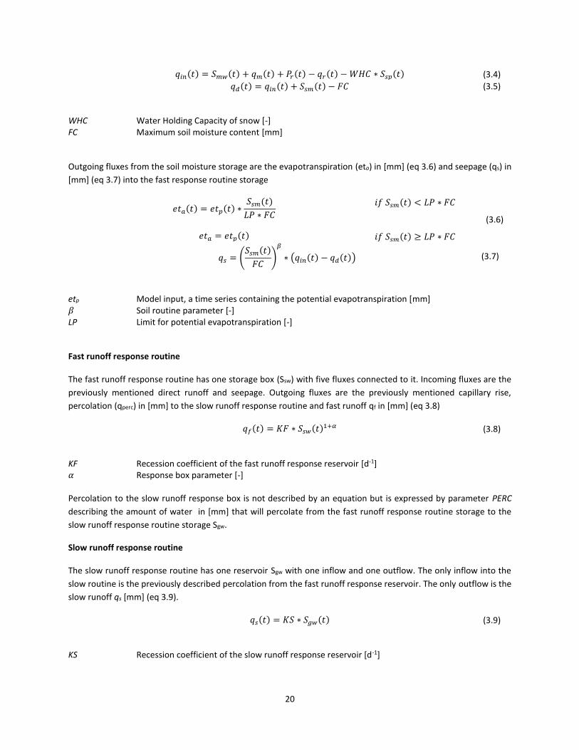
routine. The infiltration is further divided into infiltration (qin) in [mm] (eq 3.4) into the soil moisture storage box
(Ssm) and infiltration (qd) in [mm] (eq 3.5) that directly feeds into the fast response storage box (Ssw).
𝑞𝑐(𝑡) = 𝐶𝐹𝐿𝑈𝑋 ∗𝐹𝐶 − 𝑆𝑠𝑚(𝑡)
𝐹𝐶 (3.3)
CFLUX Maximum rate of capillary flow [mm d-1]
20
𝑞𝑖𝑛(𝑡) = 𝑆𝑚𝑤(𝑡) + 𝑞𝑚(𝑡) + 𝑃𝑟(𝑡) − 𝑞𝑟(𝑡) − 𝑊𝐻𝐶 ∗ 𝑆𝑠𝑝(𝑡) (3.4)
𝑞𝑑(𝑡) = 𝑞𝑖𝑛(𝑡) + 𝑆𝑠𝑚(𝑡) − 𝐹𝐶 (3.5)
WHC Water Holding Capacity of snow [-] FC Maximum soil moisture content [mm]
Outgoing fluxes from the soil moisture storage are the evapotranspiration (eta) in [mm] (eq 3.6) and seepage (qs) in
[mm] (eq 3.7) into the fast response routine storage
𝑒𝑡𝑎(𝑡) = 𝑒𝑡𝑝(𝑡) ∗
𝑆𝑠𝑚(𝑡)
𝐿𝑃 ∗ 𝐹𝐶
𝑒𝑡𝑎 = 𝑒𝑡𝑝(𝑡)
𝑖𝑓 𝑆𝑠𝑚(𝑡) < 𝐿𝑃 ∗ 𝐹𝐶
𝑖𝑓 𝑆𝑠𝑚(𝑡) ≥ 𝐿𝑃 ∗ 𝐹𝐶
(3.6)
𝑞𝑠 = (𝑆𝑠𝑚(𝑡)
𝐹𝐶)
𝛽
∗ (𝑞𝑖𝑛(𝑡) − 𝑞𝑑(𝑡)) (3.7)
etp Model input, a time series containing the potential evapotranspiration [mm] 𝛽 Soil routine parameter [-] LP Limit for potential evapotranspiration [-]
Fast runoff response routine
The fast runoff response routine has one storage box (Ssw) with five fluxes connected to it. Incoming fluxes are the
previously mentioned direct runoff and seepage. Outgoing fluxes are the previously mentioned capillary rise,
percolation (qperc) in [mm] to the slow runoff response routine and fast runoff qf in [mm] (eq 3.8)
𝑞𝑓(𝑡) = 𝐾𝐹 ∗ 𝑆𝑠𝑤(𝑡)1+𝛼 (3.8)
KF Recession coefficient of the fast runoff response reservoir [d-1] 𝛼 Response box parameter [-] Percolation to the slow runoff response box is not described by an equation but is expressed by parameter PERC
describing the amount of water in [mm] that will percolate from the fast runoff response routine storage to the
slow runoff response routine storage Sgw.
Slow runoff response routine
The slow runoff response routine has one reservoir Sgw with one inflow and one outflow. The only inflow into the
slow routine is the previously described percolation from the fast runoff response reservoir. The only outflow is the
slow runoff qs [mm] (eq 3.9).
𝑞𝑠(𝑡) = 𝐾𝑆 ∗ 𝑆𝑔𝑤(𝑡) (3.9)
KS Recession coefficient of the slow runoff response reservoir [d-1]

21
3.2 SENSITIVITY ANALYSIS
The HBV model uses 14 parameters in the model routines to translate the model inputs to a runoff value. A risk of a
high number of model parameters is that it might result in different parameter sets resulting in a similar model
performance, an issue also often referred to as overparameterization (Booij, 2005). To reduce the number of model
parameters to be calibrated in the calibration procedure a sensitivity analysis will be applied. The sensitivity analysis
will indicate which parameters are most influential for the model performance and should be considered in the
model calibration (Song et al., 2015).
Measures to assess the performance of a model are found in objective functions. These objective functions give a
quantification of how well the model output corresponds to observations. Different objective functions emphasize
different parts of the hydrograph. The objective functions that will be used in this research will be described in
section 3.2.1. Section 3.2.2 will be used to elaborate on the sensitivity analysis method.
3.2.1 OBJECTIVE FUNCTIONS Objective functions are used to quantify the quality at which model output resembles the observations. Multiple
objective functions are available for this assessment of the goodness of fit. These different objective functions all
use different mathematical functions to quantify the quality of the simulations when compared to observations.
These differences allow for the different objective functions to focus on different parts of the hydrograph (e.g. peak
flows, periods of low flow). Cheng (2014) presents an overview of classical objective functions that are regularly used
in hydrological modelling studies.
The objective of this research is to find whether there is a trade-off between using different objective functions in
model calibration when the aim is to not only simulate the total runoff correctly but also the runoff components. To
find this trade-off between objective functions, a weighted combination of two objective functions will be used.
From the two objective functions that will be selected, one objective function will put more emphasis on high flow
and the other objective function will emphasize low flows. The objective functions that have been selected for this
purpose are the Nash-Sutcliffe efficiency criterion (NS) (Nash & Sutcliffe, 1970) and the logarithmically transformed
Nash-Sutcliffe efficiency criterion (NSL) (Krause et al., 2005). The NS has been selected because fast runoff has a
large contribution to the total runoff during periods of high runoff and runoff peaks, the part of the hydrograph on
which the NS puts more emphasis. The NSL on the other hand emphasises periods of low flow more, during these
periods baseflow is the dominant runoff component.
NS is an objective function that is often used in hydrological modelling studies (e.g. Swamy & Brivio, 1997; Wu & Xu,
2006; Lemonds & McCray, 2007; Benninga et al., 2017; Romanowicz et al., 2016; Osuch et al., 2017). The so-called
efficiency that quantifies the quality of the simulation is calculated according to equation 3.10:
𝑁𝑆 = 1 −∑ (𝑄𝑜𝑏𝑠,𝑖 − 𝑄𝑠𝑖𝑚,𝑖)
2𝑖=𝑛𝑖=1
∑ (𝑄𝑜𝑏𝑠,𝑖 − 𝑄𝑜𝑏𝑠̅̅ ̅̅ ̅̅ )
2𝑖=𝑛𝑖=1
(3.10)
Where 𝑄𝑜𝑏𝑠,𝑖 denotes the observed discharge at time step 𝑖, 𝑄𝑠𝑖𝑚,𝑖 denotes the simulated discharge at time step 𝑖
and 𝑄𝑜𝑏𝑠̅̅ ̅̅ ̅̅ is the mean observed discharge. The NS is defined as one minus the sum of the differences between the
model output and observations squared and normalized by dividing by the variance of the observations from the
considered time period. The value that NS can assume ranges from −∞ to 1 where a NS value of 1 indicates that the
simulated discharge exactly agrees with the observed discharge at every time step. Values less than 1 indicate that

22
differences between the observed and simulated discharges exist with lower values indicating larger discrepancies
between the model output and the observations.
Because the NS uses the sum of the differences squared this objective function is more sensitive to high flows. This
is a valuable property for assessing the correctness at which peak flows are simulated but can be a limitation when
assessing the goodness of the simulation of low flows or baseflow.
An objective function that puts more emphasis on low flows is the logarithmically transformed NS (NSL) (Cheng,
2014). Prior to assessing the goodness of the simulation, the observed and modelled hydrographs are logarithmically
transformed (eq. 3.11). Following the same methodology as the NS for assessing the correctness of the simulation,
this method places more emphasis on low flows compared to the NS (Tesemma et al., 2014). Krause et al. (2015)
also presents the NSL as an efficiency criterion that is especially suited for assessing periods of low flow because the
influence of high flow values is greatly reduced.
𝑁𝑆𝐿 = 1 −∑ (log(𝑄𝑜𝑏𝑠,𝑖) − log(𝑄𝑠𝑖𝑚,𝑖))
2𝑖=𝑛𝑖=1
∑ (log(𝑄𝑜𝑏𝑠,𝑖) − log(𝑄𝑜𝑏𝑠̅̅ ̅̅ ̅̅ ))
2𝑖=𝑛𝑖=1
(3.11)
3.2.2 SOBOL’S METHOD A broad palette of methods is available for sensitivity analyses all of different complexities and based on different
underlying assumptions on how to correctly assess parameter sensitivity (Song et al., 2005). This can lead to different
methods resulting in different results when ranking the parameters based on their relative importance (Frey & Patil,
2002).
Sobol’s method for global sensitivity analysis is considered as one of the more robust methods available (Tang et al.,
2007). Also, the Sobol method does not rely on model structure or assumptions about the model functioning, e.g.
linearity or additivity of the model (Saltelli et al., 2000). The method is classified as a variance decomposition method
and results in the overall parameter sensitivity as well as the variance explained by interactions between parameters
(Homma & Saltelli, 1996). The goal of this sensitivity analysis is to quantify the contribution of each parameter to
the total variance in the model output. This allows the modeler to exclude insensitive parameters from the model
calibration by fixing them at a set (default) value (Saltelli et al., 2000).
The contribution of variance to the model output by a parameter Xi consists of the main effect, Vi, and the total
effect, VTi (Saltelli et al., 2004). These effects are defined by Saltelli et al. (2004) as follows (eq. 3.12 and eq. 3.13):
𝑉𝑖 = 𝑉[𝐸(𝑌|𝑋𝑖)] (3.12)
𝑉𝑇𝑖 = 𝑉[𝐸(𝑌|𝑋−𝑖)] (3.13)
Vi indicates the amount of variance that is contributed to the model result if the true value of only parameter X i was
known and the other parameters were allowed to vary. The total effect, VTi, indicates how much of the variance is
left unexplained if the exact values of all the parameters except Xi were known.

23
The sensitivity of the parameters can be found by dividing the two variance components by the total output variance
V(Y) (eq. 3.14 and eq. 3.15). Where Si is the sensitivity to first order term and STi denotes the total sensitivity index
which is a summation of the main effect and interactions with other parameters. The influence of the interactions
between parameters on the output sensitivity is determined according to equation 3.16.
𝑆𝑖 =𝑉[𝐸(𝑌|𝑋𝑖)]
𝑉(𝑌) (3.14)
𝑆𝑇𝑖 =𝐸[𝑉(𝑌|𝑋−𝑖)]
𝑉(𝑌) (3.15)
𝑆𝑖𝑛𝑡𝑒𝑟𝑎𝑐𝑡𝑖𝑜𝑛 = 𝑆𝑇𝑖 − 𝑆𝑖 (3.16)
A sensitivity analysis package was provided by the Polish Academy of Sciences, Institute of Geophysics which, among
others, included the Sobol method. The Sobol sensitivity analysis was run for all three catchments for both the NS
and the NSL objective functions (section 3.3.2). Every simulation was run using 30 000 samples and used the 30 years
of the observational data covering the years 1976 until 2005 that will also be used for model calibration. This resulted
in sensitivity indices for all 14 parameters in every catchment for both the objective functions.
Determining appropriate thresholds above which parameters are considered for model calibration and below which
parameters will be set to a default value is generally an arbitrary decision (e.g. Bastidas et al., 1999; Tang et al., 2007;
Knoben, 2013). Here, similarly, the decision on which parameters to include in the model calibration and which ones
to fix at a default value will be a subjective one.
Using the outcomes of the sensitivity analysis we can classify the model parameters in three main groups based on
the amount of variance they explain and therefore also their necessity to be calibrated:
- Parameters that have a high main effect: these parameters influence the overall model performance
independently of interaction with other model parameters;
- Parameters that have a small main effect but a high total effect: these model parameters mainly influence
the model performance through interactions with other parameters;
- Parameters that display a small main effect and a small total effect: these parameters have a negligible
effect on the overall model performance and freezing these parameters to their default value is justified
(Saltelli et al., 2004).
It is aimed to reduce the number of model parameters that will be calibrated to 8 by taking the parameters that
displayed the highest sensitivity from the sensitivity analysis. The choice on which parameters to include will be
made based on the total sensitivity index.

24
3.3 MODEL CALIBRATION
In this chapter the approach that is taken to calibrate the HBV model is presented. Firstly, the choice on which
calibration algorithm will be applied is presented in section 3.1.1. The calibration algorithm that is decided on and
will be applied in this research is presented in section 3.3.2 and the periods that will be used for model calibration
and validation presented in section 3.3.3.
3.3.1 CALIBRATION ALGORITHM CHOICE
During the calibration procedure the aim is to find the parameter set that allows the model to generate a model
output that resembles the observations as closely as possible. To find this parameter set, the Shuffled Complex
Evolution Metropolis (SCEM-UA) calibration algorithm will be used (Vrugt et al., 2003a). The SCEM-UA algorithm is
a further development of the work of Duan et al. (1992) who presented the SCE-UA algorithm for calibration (of
conceptual rainfall-runoff models). The SCE-UA algorithm combines elements from several optimization strategies
into one algorithm. Numerous case studies have demonstrated the robustness and efficiency of the SCE-UA
algorithm in finding the global optimum. The difficulty for the SCE-UA algorithm is identifying a unique best
parameter set that performs significantly better than other feasible parameter sets in its proximity (Vrugt et al.,
2003b). Calibration of the HBV model will be done by using the precipitation, the potential evapotranspiration and
the temperature observations as model inputs. The model outputs will be evaluated against the discharge
observations by using the objective functions described earlier in section 3.2.1.
To be able to identify a trade-off between the two objective functions (section 3.2.1), weights will be assigned to
both the objective functions during the model calibration. The weights assigned to both objective functions are
varied from 0% to 100% with increments of 10% while keeping the sum of the weights equal to 100%. For each of
the combination of weights assigned to the objective functions an optimum parameter set will be found resulting in
a total of 11 best performing parameter sets per catchment.
Before calibration of the HBV model will be done an exploratory Monte Carlo (MC) analysis will be done to determine
the appropriate parameter ranges. The parameters that will not be considered in the calibration have been set to
their default values according to the HBV manual version 5.10 (SMHI, 2006). For the parameters that will be
calibrated preliminary parameter ranges are adopted from Benninga (2017) and Osuch et al. (2016). In the MC
analysis the performance of 250 000 parameter sets will be evaluated where each parameter that will be calibrated
is individually sampled from a uniform distribution. For each sample the NS and NSL values are then calculated from
the output of the HBV model. By evaluating how individual parameter values from the MC samples relate to NS and
NSL achieved by the according parameter set, parameter ranges can be adjusted to more appropriate ranges whilst
still taking into account their physical meaning and interpretation
3.3.2 CALIBRATION ALGORITHM
The SCEM-UA algorithm applies Markov Chain Monte Carlo (MCMC) sampling following the Metropolis Hastings
(Metropolis et al., 1953) strategy instead of the Downhill Simplex procedure, used in the SCE-UA algorithm, for
evolution of the population. This change allows the algorithm to find the most likely parameter set as well as its
posterior probability distribution. Vrugt et al. (2003a) describe the steps that are involved in the process of finding
the ‘best’ parameter set. From the feasible parameter space bounded by the parameter minimum and maximum
values, the SCEM-UA algorithm randomly draws the initial population and ranks the sample points in descending
posterior density. These initial sample points also serve as the initial points from where the parallel chains will start
to evolve. Proposal points for evolving the chain into the next generation are drawn from the proposal distribution
that corresponds to the individual chain. The posterior distributions of the new generations are then evaluated and
can be either accepted or rejected. If the proposed evolution is accepted the chain then progresses to the new

25
position. If the proposed evolution is not accepted the chain remains at the current position. After every evolution
it is checked for convergence according to the Gelman Rubin convergence statistic (Gelman & Rubin, 1992).The
calibration process is terminated if either the Gelman Rubin convergence criteria is satisfied or if the predefined
maximum number of iterations has been executed. The default settings for the SCEM-UA algorithm are adopted
from Vrugt et al. (2003b) and are presented in Table 3-1.
TABLE 3-1: SCEM-UA ALGORITHM PARAMETERS (VRUGT ET AL., 2003B)
Setting Description Value
nSamples Population size 200
nCompl The number of complexes 5
nModelEvalsMax The maximum number of model iterations 10 000
drawInterval Shuffling rate of complexes 5
3.3.3 CALIBRATION AND VALIDATION PERIOD The provided datasets by the IGF PAN consist of 40 years of continuous observations spanning from 1 January 1971
until 31 October 2010. The dataset is used for two purposes, namely: (1) calibration of the HBV model and (2)
validation of the HBV model. To prevent biased results periods have been defined that do not overlap.
Model calibration using the SCEM-UA algorithm will be done using the observations between 1 November 1976 and
31 October 2005. The validation of the model calibration will be done by applying a split-sample test (Klemeš, 1986).
The split-sample test will be done using the observational data from 1 November 2005 until 31 October 2010.
3.4 SIMULATION OF RUNOFF COMPONENTS
There is widespread agreement that for assessing model performance the correspondence between the total
measured and modelled stream flow is not a sufficient indicator. Additional insights in the processes that take place
within the catchment would be a step towards improvement of runoff modelling (Beven, 1989). Yet, in most cases
the assessment of model performance is still done based on the total runoff because individual components that
contribute to the total runoff usually go unobserved. The information that observed hydrographs provide however,
is not limited to the absolute values of the measured runoff. Eckhardt et al. (2002) presents an example of what the
potential benefits of having insight in the runoff components can provide for model performance.
3.4.1 HYDROGRAPH SEPARATION Over the years, many methods have been developed that allow for the identification of the baseflow component
from the total runoff e.g. low-pass filtering, recursive filtering and unit hydrograph methods. Often linear reservoirs
have been used for modelling the groundwater contribution, i.e. baseflow, to the total flow (e.g. Chapman. 1999;
Fenicia et al., 2006; Eckhardt, 2005). More recent studies however by Wittenberg (1994, 1999, 2003), Gan & Luo
(2013) and Aksoy et al., (2008) have used nonlinear reservoirs for the analysis of groundwater recession and
baseflow contribution as these methods appeared to give a more realistic representation of catchment processes.
Baseflow separation in this research is done according to the non-linear reservoir approach from Wittenberg (1999).
Wittenberg’s baseflow separation method assumes a power-law relationship between the baseflow and the
groundwater storage of the catchment (eq. 3.17). With S denoting the groundwater storage and Q representing the
recession of the baseflow and 𝑎 and 𝑏 are model parameters. Parameters 𝑎 and 𝑏 for flow recessions are found by
an iterative process by calibrating them against flow recession data by utilizing a least-squares method (Wittenberg,
1999).
𝑆 = 𝑎 ∗ 𝑄𝑏 (3.17)

26
The analytical solution for the baseflow is presented by Wittenberg (1999) and is given in equation 3.18. Here QB
indicates the baseflow resulting from the nonlinear reservoir at time step t starting from initial discharge Q0.
𝑄𝐵 = 𝑄0 [1 +(1 − 𝑏) ∗ 𝑄0
1−𝑏
𝑎𝑏∗ 𝑡]
1𝑏−1
(3.18)
With the contribution of the baseflow to the total flow determined by applying Wittenberg’s baseflow separation
method the fast runoff (QF) component can easily be found by subtracting the baseflow component from the total
flow (QT) (eq. 3.19).
𝑄𝐹 = 𝑄𝑇 − 𝑄𝐵 (3.19) To illustrate the results of the hydrograph separation the hydrograph separation done for the Biała Tarnowska
catchment for the year 1976 is graphed and presented in Figure 3-3. It shows that during periods of low flow the
runoff almost entirely consists of baseflow and that fast runoff barely contributes to the total runoff. During high
runoff events it is observed that the baseflow also increases but the main contribution to the total flow becomes the
fast runoff component.
FIGURE 3-3: WITTENBERG'S BASEFLOW SEPARATION APPLIED TO THE BIALA TARNOWSKA CATCHMENT FOR THE YEAR 1976
3.4.2 SIMULATION OF RUNOFF COMPONENTS
Determining model performance in simulating the runoff components will be done by comparing the runoff
components derived from the observed runoff for the calibration period with the runoff components derived from
the simulated runoff for the calibration period. This is done for each simulation using the different parameter sets
that resulted from model calibration (section 3.3). Assessing the correctness of the simulated runoff components for
the previously determined parameter sets will be done by using the previously described NS objective function
(section 3.2.1).
Identifying a trade-off between using different objective functions and the model its ability to correctly simulate the
runoff components will be done by checking if there is a correlation between the weights assigned to the objective

27
functions and the correctness at which the individual runoff components are simulated. The determined correlation
will be checked for statistical significance using a two-sided test at a significance level of 𝛼 = 0.10.
3.5 CLIMATE CHANGE IMPACT
For assessing the impact that projected climate change will have the HBV model will be forced with the climate data
from the seven GCM/RCM combinations. From the seven resulting time it will be assessed what the impact of climate
change will be for the total runoff from the catchments. For each catchment the mean annual runoff will be
presented along for the projected changes to the mean annual runoff from the catchments.
Secondly impacts of projected changes on the flow components will be researched. This will be done by comparing
the future contributions of the flow components with the contributions of the flow components to the total flow in
the predefined reference period. For this comparison the following periods are defined: the reference period 1976-
2005, the near-future 2021-2050 and the far-future 2071-2100. Unique parameter sets will be found for the
Wittenberg filter for each period in order to obtain most realistic separation in runoff components for the individual
periods. By using 30-year periods this problem is dealt with because over the shorter 30-year periods it is assumed
that the parameters are roughly stationary and unique parameter sets will be found for each period. The goal of this
comparison is to indicate if one runoff component is projected to become more dominant in the future and flow
composition is projected to change.
In addition to assessing the contribution of the flow components on an annual time scale the contributions of the
runoff components to the total flow will be assessed at a seasonal scale. Federer (1973) and Weisman (1977) both
describe seasonal variability in the stream flow formation and attribute this to evapotranspirational losses from the
catchment. From the climate change projections, it is already known that the temperatures are projected to increase
in the three considered catchments, thus also increasing the potential evapotranspiration. By assessing the runoff
components on a shorter time scale seasonal variability in the contributions of the components can be identified.
Doing so allows to identify possible trends between the reference period, the near-future and far-future in the
seasonal contributions of the runoff components.
Lastly the impacts of projected climate change on the low flows will be assessed. As described in section 3.4.1, during
periods of low flow the runoff almost entirely consists of baseflow so this approach to looking at climate change
impacts aims to identify what changes the baseflow might undergo during periods of extended drought. To assess
the impact of projected climate change on this part of the hydrograph the changes in the 90th percentile (Q90) of
the flow will be assessed. The Q90 is a commonly used indicator to assess low flows in hydrographs and indicates
the flow threshold that is exceeded 90% of the time (e.g. Ward, 2007; Gorgen et al., 2010; Hatterman et al., 2017).
For this purpose, the Q90 that is derived from the reference period will be compared to the Q90 that is derived from
the near-future and far-future periods to indicate if the Q90 is projected to change.

28

29
4 RESULTS In this chapter the results that are obtained from this research are presented and discussed. Section 4.1 will be used
to present the results from the sensitivity analysis, followed by the results obtained for model calibration and
validation in section 4.2. How well the runoff components are simulated is evaluated in section 4.3 and trade-offs
that are identified between the objective functions are presented in section 4.4. This chapter is concluded with the
impacts of projected climate change in section 4.5.
4.1 SENSITIVITY ANALYSIS
In figures 4-1, 4-2 and 4-3 the results from the variance decomposition are presented as bar plots. For each
catchment the sensitivity to every parameter is displayed. The total sensitivity index is presented as well as the main
effect and the influence of interactions with other parameters which together make up the total sensitivity.
Following from this sensitivity analysis is a quantification of the influence of the model parameters on the model
output variance according to the NS objective function. Parameters that appear to largely contribute to the model
output variance are parameters that are part of the soil moisture routine and the fast runoff routine (FC, BETA, LP,
ALFA, KF and PERC). This is not surprising because the NS emphasizes peak flows to which the fast runoff contributes
significantly (Blume et al., 2007).
As for the sensitivity when using the NSL as objective function the KS TT, CFMAX and WHC parameters appear
prominently in the results for all three catchments. From these parameters KS is related to the lower response box
from HBV that represents the slow runoff. Parameters TT, CFMAX and WHC are part of the snow module that can
be responsible for delaying runoff depending on the temperature. Precipitation that falls in the form of snow is
therefore often not discharged as a runoff peak but rather at a more constant rate. Because of this sensitivity
towards the NS is low but it displays higher sensitivity towards the NSL.
The sensitivity analysis indicates that some parameters show a small negative sensitivity which should not be
possible. Saltelli et al. (2004) describes that these negative values are explained by numerical errors in the Sobol
method and are not uncommon when sensitivity indices have a value of approximately zero. The probability of
encountering negative values as outcome from the analysis can be reduced by increasing the sample size. Because
the negative values that are found are very small it is accepted that these values are rounded to zero.

30
FIGURE 4-1: RESULTS OF VARIANCE DECOMPOSITION FOR THE BIAŁA TARNOWSKA CATCHMENT
FIGURE 4-2: RESULTS OF VARIANCE DECOMPOSITION FOR THE DUNAJEC CATCHMENT
FIGURE 4-3: RESULTS OF VARIANCE DECOMPOSITION FOR THE NAREWKA CATCHMENT

31
It was aimed to reduce the number of parameters to 8 whilst taking an equal number of parameters from the
sensitivity analysis towards the NS as the sensitivity analysis towards the NSL. The choice on which parameters to
include was made based on the total sensitivity index. Parameters that will be considered in the model calibration
are presented inTable 4-1.
TABLE 4-1: HBV MODEL PARAMETERS THAT WILL BE TAKEN INTO ACCOUNT FOR MODEL CALIBRATION PER CATCHMENT
Biała Tarnowska Dunajec Narewka
FC BETA LP ALFA KF KS TT CFMAX
FC BETA ALFA KF KS TT CFMAX WHC
BETA LP ALFA KF KS TT CFMAX WHC
4.2 MODEL CALIBRATION
In this section the results from model calibration and intermittent steps will be presented. Firstly, the results from
the exploratory Monte Carlo simulation are presented in section 4.2.1 followed by the results of the model
calibration in section 4.2.2.
4.2.1 PARAMETER RANGES
For every parameter the sampled value for each simulation is plotted against the NS and NSL score. These plots are
presented in appendix A (figures A-1, A-2 and A-3). These plots show how the NS and NSL scores are distributed over
the preliminary parameter range for each sampled parameter. These plots are then used as an indicator according
to which the parameter ranges can be adjusted such that it encapsulates the range in which the best simulation
results are found according to both the NS and the NSL scores and excludes the parameter range where low scores
are obtained for both the NS and the NSL. Similarly, the parameter ranges can be extended further if the simulations
indicate a clustering of best simulations near the edge of a parameter range and if the physical interpretation of the
parameter is not violated. In tables 4-2, 4-3 and 4-4 the definitive parameter ranges are presented for the Biała
Tarnowska, Dunajec and Narewka catchments. Additionally, in Table 4-5 the default parameter values are presented
for the HBV model that are used for parameters that will not be considered in model calibration. These default values
are adopted from the HBV manual (SMHI, 2006).
TABLE 4-2: DEFINITIVE PARAMETER RANGES USED IN CALIBRATION OF THE HBV MODEL FOR THE BIAŁA TARNOWSKA CATCHMENT
Parameter Unit Minimum value Maximum value
FC mm 0.1 500.0
BETA - 0.01 5.00
LP - 0.10 1.00
ALFA - 0.10 1.50
KF d-1 0.0005 0.20
KS d-1 0.0005 0.20
TT oC -1.00 3.00
CFMAX mm d-1 0.00 20.00

32
TABLE 4-3: DEFINITIVE PARAMETER RANGES USED IN CALIBRATION OF THE HBV MODEL FOR THE DUNAJEC CATCHMENT
Parameter Unit Minimum value Maximum value
FC mm 0.1 1000.0
BETA - 0.01 7.00
ALFA - 0.10 1.50
KF d-1 0.0005 0.10
KS d-1 0.0005 0.30
TT oC -3.00 1.00
CFMAX mm d-1 0.00 10.00
WHC mm mm-1 0.00 1.00
TABLE 4-4: DEFINITIVE PARAMETER RANGES USED IN CALIBRATION OF THE HBV MODEL FOR THE NAREWKA CATCHMENT
Parameter Unit Minimum value Maximum value
BETA - 0.01 4.50
LP - 0.10 1.00
ALFA - 0.10 1.50
KF d-1 0.0005 0.20
KS d-1 0.0005 0.20
TT oC -3.00 2.00
CFMAX mm d-1 0.00 20.00
WHC mm mm-1 0.00 1.00
TABLE 4-5: DEFAULT PARAMETER VALUES FOR THE HBV MODEL (SMHI, 2006)
Parameter Unit Default parameter value
FC mm 200.0
LP - 0.90
CFLUX mm d-1 1.00
TTI oC 0.00
FOCFMAX - 1.00
CFR - 0.05
WHC mm mm-1 0.10

33
4.2.2 CALIBRATION RESULTS Calibration of the HBV model for the Biała Tarnowska, Dunajec and the Narewka catchments resulted in 11 best
parameter sets for each catchment, each corresponding to a combination of NS and NSL weights. The NS and NSL
scores obtained with each parameter set are presented below for separately for each catchment. The decision on
which parameter set will be used for assessment of climate change impact will be discussed separately in section
4.4.
Biała Tarnowska
For the 11 different combinations of NS and NSL weights that have been used in the calibration procedure, the
calibration results are presented in Figure 4-4. The results show that the NSL performance criteria shows a
substantially lower model performance than the NS does for all combinations of weights.
FIGURE 4-4: CALIBRATION RESULTS FOR THE BIAŁA TARNOWSKA CATCHMENT
Model performance with the parameter sets that were found during the calibration procedure appears to be low
when compared to previous hydrological modelling research on the Biała Tarnowska catchment (e.g. Benninga et
al., 2017; Osuch et al., 2016). Using the DEGL calibration algorithm and NS objective function to calibrate the HBV
model, Benninga (2017) found a parameter set that achieved NS scores of 0.78 and 0.74 for the calibration and
validation respectively for the Biała Tarnowska catchment. The parameter set found by Osuch et al. (2016) for the
HBV model achieved NS scores of 0.77 and 0.80 for the calibration and validation periods respectively. The NS scores
that are found when exclusively the NS is used for model calibration are 0.57 and 0.55 for model calibration and
validation respectively.
It must be noted that these researches both used a different calibration period than was used in this research which
might have negatively impacted the obtained calibration and validation results despite the periods having a large
overlap with the calibration period used in this research. Both Benninga (2017) and Osuch et al. (2016) used the
period spanning from 1971 until 2000 for model calibration whereas this research used the observations from the
1976-2005 period for model calibration. Also, Benninga (2017) applied a different calibration algorithm to optimize
the model parameters which might influence the results from model calibration.

34
Dunajec
The performance of the parameter sets that have been obtained from the model calibration is presented inFigure
4-5. The NS and NSL scores show very similar performance for every increment of NS and NSL weights with the NSL
scoring slightly higher than the NS score when the NSL is dominant in the model calibration. As expected, the NS
score increases when a higher weight in assigned to the NS objective function and the NSL scores decrease.
FIGURE 4-5: CALIBRATION RESULTS FOR THE DUNAJEC CATCHMENT
Comparing the model performance with the parameter set that was found by the SCEM-UA algorithm with
previously published work on hydrological modelling of the Dunajec catchment shows similar results. The NS scores
that are found in this study when exclusively the NS is used for model calibration are 0.75 and 0.77 for model
calibration and validation respectively. Osuch et al. (2016) found NS scores of 0.77 and 0.80 for model calibration
and validation respectively. Where Osuch et al. again used the years 1971-2000 for model calibration contrary to
the 1976-2005 period used in this research.
Narewka
The calibration results of the HBV model for the Narewka catchments are displayed in Figure 4-6 where the NS and
NSL scores are presented for every parameter set. The NS and NSL scores show a behaviour similar to the behaviour
found in the Dunajec catchment with the NSL scoring being higher than the NS at low NS weights during model
calibration but decreasing as the NS weight increases. Additionally, the NS shows the opposite behaviour as expected
with the performance increasing as the NS becomes the dominant performance indicator during model calibration.

35
FIGURE 4-6: CALIBRATION RESULTS FOR THE NAREWKA CATCHMENT
This parameter set found when exclusively using the NS as objective function seems to outperform the parameter
set found by Osuch et al. (2016) slightly based of the NS as performance indicator. Values found for the NS in the
work done by Osuch et al. (2016) are 0.71 for the calibration period and 0.54 for the validation period. Values found
for the NS in this study are 0.75 and 0.57 for model calibration and validation respectively.

36
4.3 SIMULATION OF RUNOFF COMPONENTS
Similar to how the model performance in simulating the total flow was presented in section 4.2.2, the model
performance in simulating the individual runoff components is presented. In figures 4-7, 4-8 and 4-9 the NS scores
of the fast and slow components are graphed for each catchment. The runoff components are derived from the total
runoff using the Wittenberg filter resulting in a fast runoff component and a baseflow component for each
simulation.
FIGURE 4-7: NS SCORES FOR THE FAST RUNOFF AND BASEFLOW COMPONENTS FOR THE BIAŁA TARNOWSKA CATCHMENT
FIGURE 4-8: NS SCORES FOR THE FAST RUNOFF AND BASEFLOW COMPONENTS FOR THE DUNAJEC CATCHMENT

37
FIGURE 4-9: NS SCORES FOR THE FAST RUNOFF AND BASEFLOW COMPONENTS FOR THE NAREWKA CATCHMENT
For all catchments it can be observed that the correctness at which the components are simulated is, although
slightly lower than the correctness of the simulation of the total flow, comparable to how well the total flow is
simulated. Because the baseflow and the fast runoff are derived from the total flow by using the Wittenberg method
it is expected that a better simulation of the total flow results in a better simulation of the individual runoff
components. The obvious outlier however seems the fast component from the Biała Tarnowska catchment,
displaying a NS score above 0.9 for all parameter sets indicating a near perfect simulation.
As described in section 3.2.1 the NS objective function is especially sensitive to high flows. It appears that the timing
of the runoff peaks of the fast component for the Biała Tarnowska is simulated nearly perfect. Over the period 1976
– 2005 the timing of runoff peaks is on average off by 0.01 to 0.02 time step for the Biała Tarnowska compared to
the 0.12 to 0.19 time step for the Dunajec and 0.12 to 0.21 time step for the Narewka catchments. The correct
simulation of the timing of the runoff peaks appears to be highly influential for achieving a good simulation of the
fast runoff component.
4.4 TRADE-OFF BETWEEN OBJECTIVE FUNCTIONS
For all three catchments the goodness at which the runoff components are simulated have been determined for
each of the 11 parameter sets. For each catchment the correlation between the NS of the components (NSFAST and
NSBASE) and the NSL weight has been determined. The results are presented below for every catchment in Table 4-6.
TABLE 4-6: CORRELATIONS BETWEEN THE NS SCORES OF THE COMPONENTS AND THE WEIGHT ASSIGNED TO THE NSL
Correlation coefficient NSFAST and NSL weight
Significant Correlation coefficient NSBASE and NSL weight
Significant
Biała Tarnowska 0.32 No 0.74 Yes
Dunajec -0.34 No 0.50 Yes
Narewka 0.94 Yes 0.61 Yes

38
For the Biała Tarnowska catchment a correlation of 0.32 has been found between the NSFAST and the NSL weight.
The correlation that was found between the NSBASE and the NSL weight is 0.74. At the predetermined confidence
level (section 3.4.2) these correlations have been checked for statistical significance. The correlation determined
between the NSFAST and the NSL weight appeared to be not significant. The correlation between the NSBASE and the
NSL weight however is significant. For the Dunajec catchment an insignificant correlation of -0.34 has been found
between the NSFAST and the NSL weight. Again, a significant correlation was identified between the NSBASE and the
NSL weight with a correlation coefficient of 0.74. The Narewka catchment is the only catchment displaying a
significant positive correlation between both the NSFAST and NSL weight and the NSBASE and NSL weight at calculated
correlations of 0.94 and 0.61 respectively.
These results display a moderate to strong correlation between the NSBASE and NSL weight for all three catchments,
therefore indicating that the best results for modelling baseflow with the HBV model for these catchments will be
obtained by using exclusively the NSL as objective function in model calibration. For the fast runoff component
however, the results from this study are not unanimous with results from two catchments indicating that there is no
correlation between the NSFAST and the NSL weight and only one catchment displaying significant correlation
between the NSFAST and the NSL weight.
These significant positive correlations between the NSL weight and the NS scores of the baseflow component show
that using a high NSL weight in model calibration allows for the best simulation of the baseflow component. There
does not appear to be an unambiguous conclusion that can be drawn from these results on how to improve on the
skill at which fast runoff is simulated by using the NS or NSL as objective function in model calibration. For assessing
the impact of climate change on the runoff components (section 4.5) the parameter sets that are found with using
exclusively the NSL objective function will be utilized. These parameter sets that are found from this calibration are
presented in Appendix B.
4.5 CLIMATE CHANGE IMPACT
In this section the climate change impact on the runoff components will be presented. Firstly, it will be validated
how well the model performs for the 1976-2005 period by forcing the model with the observed climatological
variables as well as with the synthetic climate data from the seven. Next, the impact of climate change on the total
flow will be presented in section 4.5.2.
In addition to assessing changes to the total runoff, climate change impact will be assessed by comparing the
contributions of the runoff components to the total flow for 30-year periods as described in section 3.5. Runoff
contributions for the reference period will be presented as well as projections for the near-future period and the
far-future period. Additionally, seasonal variability of the runoff components will be presented along with projected
changes herein. This chapter will be concluded with an assessment of climate change impacts on low flows.
4.5.1 MODEL PERFORMANCE ON REFERENCE PERIOD For the reference period model performance will be assessed by forcing the calibrated model with the observed
precipitation and temperature. Model performance will be assessed by looking model its ability to correctly simulate
the mean flow over the 1976-2005 period. Additionally, the performance of the model, forced with the synthetic
climate data from the seven GCM/RCM combinations, will be assessed for this performance indicator. In tables 4-7,
4-8 and 4-9 the mean flow that is obtained from observations and simulations is presented. The numbering of
GCM/RCM combinations in these tables corresponds to the numbering as used in section 2.3 where the GCM/RCM
combinations are presented.

39
TABLE 4-7: MEAN RUNOFF FROM THE BIAŁA TARNOWSKA CATCHMENT PER GCM/RCM COMBINATION AND DEVIATION FROM THE
OBSERVATED MEAN RUNOFF
Qmean [m3 s-1] Δ Qmean
Observed mean flow 9.2 -
Simulation forced with observed climate data 8.5 -7.7%
GCM/RCM 1 8.4 -8.6%
GCM/RCM 2 8.2 -11.2%
GCM/RCM 3 8.9 -3.2%
GCM/RCM 4 8.6 -6.2%
GCM/RCM 5 8.3 -9.6%
GCM/RCM 6 8.8 -4.7%
GCM/RCM 7 7.8 -15.2%
GCM/RCM mean 8.4 -8.4%
TABLE 4-8: MEAN RUNOFF FROM THE DUNAJEC CATCHMENT PER GCM/RCM COMBINATIONS AND DEVIATION FROM THE OBSERVED MEAN
RUNOFF
Qmean [m3 s-1] Δ Qmean
Observed mean flow 14.2 -
Simulation forced with observed climate data 11.2 -21.1%
GCM/RCM 1 12.0 -15.3%
GCM/RCM 2 11.0 -22.4%
GCM/RCM 3 11.9 -15.8%
GCM/RCM 4 11.9 -15.7%
GCM/RCM 5 11.4 -19.1%
GCM/RCM 6 11.9 -16.0%
GCM/RCM 7 11.0 -22.5%
GCM/RCM mean 11.6 -18.1%
TABLE 4-9: MEAN RUNOFF FROM THE NAREWKA CATCHMENT PER GCM/RCM COMBINATIONS AND DEVIATION FROM THE OBSERVED MEAN
RUNOFF
Qmean [m3 s-1] Δ Qmean
Observed mean flow 3.3 -
Simulation forced with observed climate data 3.1 -6.1%
GCM/RCM 1 3.2 -3.5%
GCM/RCM 2 3.2 -2.9%
GCM/RCM 3 3.4 2.1%
GCM/RCM 4 3.3 -1.0%
GCM/RCM 5 3.3 -0.6%
GCM/RCM 6 3.4 3.5%
GCM/RCM 7 3.2 -2.0%
GCM/RCM mean 3.3 -0.6%

40
It is observed that for every catchment the calibrated model that is forced with observed climate data
underestimates the runoff from the catchments. Similarly, the HBV model tends to underestimate the flow when
forced with synthetic climate data compared to the observed runoff in the 1965-2005 period. For the Biała
Tarnowska catchment these underestimations range from -15.2% to -3.2% with an average underestimation of -
8.4% for the 7 GCM/RCM combinations. For the Dunajec catchment these underestimations are even larger with
underestimations of the flow ranging from -22.5% to -15.3% with an average underestimation of the flow of -18.1%.
Only for the Narewka catchment all simulations with the synthetic climate data result in mean flows over the 1976-
2005 period that are comparable to the observed mean flow. Deviations between the observed and simulated flows
range from -3.5% to +3.5% with an average deviation between the observations and the simulations of -0.6%.
4.5.2 CLIMATE CHANGE IMPACT ON THE TOTAL RUNOFF
Below, in Figure 4-10, the modelled mean annual flows are presented for the Biała Tarnowska, Dunajec and Narewka
catchments for the entire sample period of 1971-2100. Each coloured dot represents a GCM/RCM combination and
the black line is the median of the seven GCM/RCM combinations. The median value from the ensemble is used to
identify changes in the annual total runoff for the catchments. In all three catchments an upward trend is detected
indicating an increase in the mean annual flows. These trends are consistent with Osuch et al. (2016) who also
identified an upward trend in the annual runoff from various Polish catchments, including the catchments
considered in this research. The severity of the changes for each GCM/RCM combination are presented in Table 4-10
as the percentage increase per year over the 1971-2100 period. The calculated upward trend is presented as the
average percentage increase per year in the mean annual flow over the 1971-2100 period. The biggest upward trend
is observed in the Narewka catchment where an average increase of 0.23% per year is observed in the annual runoff.
The upward trend is explained by the projected changes in the climatic variables that are discussed in section 2.3.
For all three catchments both the precipitation and the temperature are projected to increase. Using the future
temperature projections, the potential evapotranspiration is calculated. Combining the projected potential
evapotranspiration and the precipitation it is shown that the surplus of precipitation increases. This means that the
overall wetness of the catchments is projected to increase and therefore also the total runoff from the three
catchments. This finding on an increase of wetness of the catchments is supported by (Meresa et al., 2016).
The largest increases in runoff are observed in the winter and spring periods which is explained by the projected
changes in the temperature and the precipitation. In Appendix C the projected changes in temperature and
precipitation for the near future and far future periods are displayed in plots for all three catchments relative to the
observed temperature and precipitation in the reference period. The largest projected increase in temperature are
observed in the winter period for all three catchments. This leads to less accumulation of snow in the catchment and
more direct runoff in the winter periods. The largest increases projected increase in precipitation is observed in
March, April and May which causes the projected increase in runoff in the spring period. These results correspond
to the research of Piniewski et al. (2017) who have shown that the largest rate of change in climate change can be
observed in the winter and spring periods.

41
TABLE 4-10: CHANGES IN PERCENTAGE PER YEAR IN MODELLED ANNUAL RUNOFF OVER THE 1971-2100 PERIOD FOR THE BIAŁA TARNOWSKA,
DUNAJEC AND NAREWKA CATCHMENTS
Biała Tarnowska Dunajec Narewka
GCM/RCM 1 0,11% 0,05% 0,31%
GCM/RCM 2 0,21% 0,19% 0,37%
GCM/RCM 3 0,20% 0,15% 0,32%
GCM/RCM 4 0,03% 0,05% 0,18%
GCM/RCM 5 0,05% 0,06% 0,15%
GCM/RCM 6 0,20% 0,01% 0,17%
GCM/RCM 7 0,09% 0,06% 0,21%
GCM/RCM mean 0,11% 0,08% 0,23%
FIGURE 4-10: MODELLED ANNUAL MEAN FLOW FROM THE BIAŁA TARNOWSKA, DUNAJEC AND NAREWKA CATCHMENTS FOR THE 1971-2100
PERIOD
4.5.3 CLIMATE CHANGE IMPACT ON THE RUNOFF COMPONENTS
From the runoff simulations the flow components are derived for the predefined periods. Making use of the
Wittenberg filter again, this separation into flow components has been done individually for each of the seven
projections generated using the GCM/RCM combinations. The parameters used for the Wittenberg filter are
determined individually for each separation. The resulting baseflow indices (BFI) are presented in tables 4-11, 4-12
and 4-13 for the three time periods for each catchment.

42
TABLE 4-11: DERIVED BFI FOR THE BIAŁA TARNOWSKA CATCHMENT FROM RUNOFF SIMULATIONS FOR EACH OF THE SEVEN GCM/RCM
COMBINATIONS FOR THE REFERENCE, NEAR-FUTURE AND FAR-FUTURE PERIOD
Reference Near-future Far-future
GCM/RCM 1 0.63 0.63 0.62
GCM/RCM 2 0.64 0.63 0.63
GCM/RCM 3 0.60 0.60 0.59
GCM/RCM 4 0.61 0.59 0.60
GCM/RCM 5 0.60 0.61 0.59
GCM/RCM 6 0.61 0.61 0.60
GCM/RCM 7 0.61 0.58 0.59
GCM/RCM mean 0.61 0.61 0.60
TABLE 4-12: DERIVED BFI FOR THE DUNAJEC CATCHMENT FROM RUNOFF SIMULATIONS FOR EACH OF THE SEVEN GCM/RCM COMBINATIONS
FOR THE REFERENCE, NEAR-FUTURE AND FAR-FUTURE PERIOD
Reference Near-future Far-future
GCM/RCM 1 0.66 0.67 0.66
GCM/RCM 2 0.67 0.66 0.66
GCM/RCM 3 0.65 0.65 0.65
GCM/RCM 4 0.65 0.65 0.65
GCM/RCM 5 0.64 0.64 0.64
GCM/RCM 6 0.66 0.66 0.66
GCM/RCM 7 0.64 0.64 0.65
GCM/RCM mean 0.65 0.65 0.65
TABLE 4-13: DERIVED BFI FOR THE NAREWKA CATCHMENT FROM RUNOFF SIMULATIONS FOR EACH OF THE SEVEN GCM/RCM COMBINATIONS
FOR THE REFERENCE, NEAR-FUTURE AND FAR-FUTURE PERIOD
Reference Near-future Far-future
GCM/RCM 1 0.67 0.68 0.67
GCM/RCM 2 0.68 0.67 0.67
GCM/RCM 3 0.66 0.66 0.64
GCM/RCM 4 0.68 0.67 0.66
GCM/RCM 5 0.67 0.66 0.66
GCM/RCM 6 0.67 0.66 0.66
GCM/RCM 7 0.66 0.66 0.67
GCM/RCM mean 0.67 0.67 0.66
It is observed that the GCM/RCM combinations 1 and 2 result in a higher BFI than the other GCM/RCM combinations.
Flow projections generated using the GCM/RCM combinations 1 and 2 also display a lower variance in the projected
flows compared to the flow projections generated using the other GCM/RCM combinations. This lower variance
indicates a more constant flow where less extremes occur and/or runoff extremes are of lower magnitude. As
described in section 3.4.1 during runoff events fast runoff gains in contribution whereas the baseflow becomes the

43
dominant contributor during periods of more constant runoff. Therefore, more runoff events and/or more extreme
runoff events would result in a lower BFI which explains why the BFI derived from flow projections using GCM/RCM
combinations 1 and 2 is higher than from other GCM/RCM combinations.
It is also observed that, despite the observed differences between the seven simulations, for all three catchments
BFI appears to remain stationary between the reference period, the near-future period and the far-future period.
Considering this aspect of the runoff from the catchments, projected climate change does not seem to impact the
composition of the total runoff from the catchments when assessed on an annual basis.
In tables 4-14, 4-15 and 4-16 the derived BFI’s from the seven GCM/RCM combinations are summarized into the
mean for each season for each catchment. The seasons are defined as winter (DJF): December, January and February,
spring (MAM): March, April and May, summer (JJA): June, July and August and autumn (SON): September, October
and November. Full tables in which the results from each of the GCM/RCM combinations are presented in Appendix
D.
TABLE 4-14: SEASONAL BFI CONTRIBUTIONS TO THE TOTAL FOW FOR THE BIAŁA TARNOWSKA CATCHMENT FOR THE REFERENCE, NEAR-
FUTURE AND FAR-FUTURE PERIODS
Reference period Near-future period Far-future period
DJF 0.68 0.68 0.68
MAM 0.63 0.59 0.59
JJA 0.57 0.57 0.56
SON 0.62 0.63 0.61
TABLE 4-15: SEASONAL BFI CONTRIBUTIONS TO THE TOTAL FOW FOR THE DUNAJEC CATCHMENT FOR THE REFERENCE, NEAR-FUTURE AND
FAR-FUTURE PERIODS
Reference period Near-future period Far-future period
DJF 0.74 0.73 0.73
MAM 0.65 0.65 0.65
JJA 0.60 0.61 0.60
SON 0.69 0.69 0.69
TABLE 4-16: SEASONAL BFI CONTRIBUTIONS TO THE TOTAL FOW FOR THE NAREWKA CATCHMENT FOR THE REFERENCE, NEAR-FUTURE AND
FAR-FUTURE PERIODS
Reference period Near-future period Far-future period
DJF 0.70 0.69 0.70
MAM 0.66 0.65 0.65
JJA 0.64 0.65 0.63
SON 0.70 0.67 0.68
It is observed that for all catchments the BFI shows interseasonal variability with the BFI being higher during the
winter months and lower during the summer period. This seasonal variability in the baseflow is generally attributed
to the influence of evapotranspiration leading to a slower flow recession in the winter compared to the summer
periods (Gribovski et al., 2014). This means that the runoff peaks are less sharp and thus giving the baseflow
component more time to adjust to the total flow (Wittenberg, 2003; Wang & Cai, 2009).

44
Contribution of the flow components to the total flow is not projected to show large changes in the near-future or
far-future compared to the reference period. Wang & Cai (2010) have shown that, by comparing long term changes
in baseflow contribution to the total runoff between urban and agricultural catchments, changes in the BFI are
primarily induced by human interference. In this research nearly natural catchments are considered (Romanowicz
et al., 2016) human interference is not considered in the modelling of future projections. Therefore, it is easily
explained that the BFI is not projected to change at both annual and seasonal scales.
4.5.4 PROJECTED CHANGES IN LOW FLOWS
To assess projected changes in low flows the Q90 value is used as performance indicator as described in section 3.5.
The Q90 values derived from the reference period of the observations for the considered catchments are presented
below in Table 4-17.
TABLE 4-17: Q90 FOR THE BIAŁA TARNOWSKA, DUNAJEC AND NAREWKA CATCHMENTS DERIVED FROM THE OBSERVED RUNOFF FOR THE
REFERENCE PERIOD
Catchment Q90
Biała Tarnowska 1.90 m3 s-1
Dunajec 4.27 m3 s-1
Narewka 0.91 m3 s-1
For analysing changes in Q90 the mean values of Q90 between the seven GCM/RCM combinations will be used to
compare to the Q90 value derived from observations. This choice is made because the Q90 values derived from the
simulations displayed a large spread with no clear pattern. The Q90 values that are derived from the simulations for
the reference period are presented inTable 4-18.
Comparing the Q90 values for the reference period shows that the average Q90 from the simulated flow is similar
to the Q90 from observations for the Biała Tarnowska catchment. The Dunajec and Narewka catchments however
display a simulated Q90 that is 9% and 12% lower respectively than the Q90 from observations.
In section 4.5.1 is was already shown that for the reference period the HBV model, forced with synthetic climate
data, appeared to underestimate the total runoff generated from the catchments. Therefore, it is not unexpected
that the models also underestimate the Q90 for the reference period. In addition to this, multiple researches have
shown that because of the model structure of the HBV model, the HBV model is prone to underestimating the low
flows (Berglov et al., 2009; Demirel et al., 2013; Tian et al., 2014).
TABLE 4-18: MEAN Q90 FOR THE BIAŁA TARNOWSKA, DUNAJEC AND NAREWKA CATCHMENTS DERIVED FROM THE SIMULATED RUNOFF FOR
THE REFERENCE, NEAR-FUTURE AND FAR-FUTURE PERIOD
Reference Near-future Far-future
Biała Tarnowska 1.90 m3 s-1 2.04 m3 s-1 2.05 m3 s-1
Dunajec 3.90 m3 s-1 4.05 m3 s-1 4.04 m3 s-1
Narewka 0.80 m3 s-1 0.96 m3 s-1 0.93 m3 s-1
To indicate what the impact of climate change might be on the Q90 from the catchments the simulated Q90 derived
from the reference period will be compared to the Q90 that is derived from the projected near-future and far-future
runoffs. Derived values for the Q90 for the near-future and far-future are also found in tableTable 4-18.

45
The Q90 values for all catchments indicate that between the reference period and the near-future the Q90 values
show a similar absolute increase with the Biała Tarnowska Q90 increasing by 0.14 m3 s-1 the Dunajec Q90 increasing
by 0.15 m3 s-1 and the Narewka Q90 increasing by 0.16 m3 s-1. Relatively these changes are the largest for the
Narewka catchment where an increase of 20% is observed. For the Biala Tarnowska and Dunajec catchments the
projected changes to Q90 are an increase of 7.3% and 3.8% respectively. Between the near-future period and the
far-future period the Q90 values appear to remain stable and not display large changes despite the climatological
variables changing between the periods as was displayed in Appendix C.

46

47
5 DISCUSSION In this chapter it will be reflected on the methodologies applied in this research and the results synthesised by
applying the aforementioned methodologies.
5.1 DATASETS
The observed climatological datasets used in this research are obtained from different stations for each catchment,
but more notable also a different number of measurement stations per catchment. The datasets containing the
climatological variables of the Biała Tarnowska catchment are created from five different measurement stations and
combined into one dataset using Thiessen polygons (Knoben, 2013). The datasets of the Dunajec are derived from
three measurement stations and the datasets of the Narewka catchment are obtained from one measurement
station. This low number of measurement stations used for creating the datasets results in a coarse estimate of the
climatological characteristics that are used for the entire catchment. The Narewka catchment is relatively flat and
small, so the differences in temperature and precipitation are probably minimal. Using only a single measurement
station for the Narewka catchment could be justified. The Biała Tarnowska and Dunajec catchments however are
situated in the Carpathian Mountains so orographic effects might influence the variability of precipitation over the
catchments and cause a temperature gradient because of altitude differences. Therefore, using a low number of
measurement locations might not give the required resolution to generate datasets that accurately resemble the
climatological variables of the catchment.
To compensate for this, during model calibration model parameters from the HBV model might have to compensate
for these structural errors in PET estimates and errors in precipitation and temperature observations resulting in a
suboptimal model parameterisation. This further protrudes in the rest of the study because the obtained model
parameterisation is also used for climate change assessment.
5.2 MODEL CALIBRATION
From the sensitivity analysis it was concluded that despite the differences between the catchments several
parameters consistently represented most of the variance in the model output. For the NS and the NSL different
parameters appear to be the most sensitive parameters. For the sensitivity towards the NS objective function
especially parameters related to the fast runoff routine represented most of the model output variance whereas for
the NSL the dominant parameters were related to the slow runoff routine which was expected. These results
appeared to be mostly consistent among all three catchments giving confidence that the correct parameters are
found to which the model output is most sensitive for both objective functions.
For model calibration the SCEM-UA calibration algorithm was used. During the calibration step of the HBV model for
all three catchments the SCEM-UA converges to the set of parameter values that supposedly gives the best model
outputs according to the NS and NLS objective functions. For the Dunajec and Narewka catchments these parameter
sets that are found by the SCEM-UA algorithm display a comparable performance to earlier modelling studies in
these catchments (Osuch et al., 2016 and Romanowicz et al., 2016). Comparing the parameter values that are found
from the calibration with parameter values from the aforementioned studies it appears that equifinality (Beven &
Freer, 2011) poses a problem when using SCEM-UA for model calibration. Despite the parameter sets from the
aforementioned studies and the parameter set generated in this study having a comparable performance at
simulating the runoff from the catchments the parameter values are different between the parameter sets.
For the Biała Tarnowska catchment SCEM-UA results in a parameter set that performs significantly worse than
parameter sets found in the aforementioned studies. Parameter convergence plots show that for all parameters the

48
model converges to the supposedly optimum solution with parameter ranges similar to those used in earlier studies
(e.g. Benninga et al., 2017). Rerunning SCEM-UA with different parameter ranges and different starting points
resulted in nearly identical results with a lower NS score than earlier researches have achieved for the calibration
period. This artefact has not been dealt with and it was assumed that it would not pose a problem for identifying a
relationship between the NS and NSL function weights and the ability to simulate runoff components because the
lower scores were consistent for all combinations of function weights.
The HBV model that is used in this research has proven to be able to skilfully simulate runoff from catchments (e.g.
Booij, 2005; Benninga et al., 2017; Romanowicz et al. 2016; Kundzewicz et al., 2017). However, the performance of
the HBV model is known to be imperfect during periods of low flow (e.g. Berglöv et al., 2009; Tian et al., 2014;
Benninga et al., 2017). Demirel et al. (2013) have shown that this increase in uncertainty can be primarily attributed
to uncertainty in model parameters and to a lesser extent also to the model inputs. This uncertainty in simulation of
low flows however is not exclusive to the HBV model. Tian et al. (2014) have shown that also for the GR4J and
Xinanjiang model the uncertainty for low flows is higher than the uncertainty in simulation in high flows. During
periods of low flow, the runoff consists (almost) entirely of baseflow so this uncertainty protrudes further into the
research when decomposing the total runoff into baseflow and fast runoff where a consistent over- or
underestimation of the baseflow could have impacted the BFI that has been determined for each catchment. Using
a different (conceptual) hydrological model (e.g. GR4J or Xinanjiang) for modelling the runoff is expected to generate
similar results to this research. Correct calibration of the model and finding the most suitable parameter set for the
purpose of this research is deemed much more important than the choice of the hydrological model.
Making use of a weighted combination of objective functions for calibration of a hydrological model is a method that
has been used before by e.g. Dawdy et al. (1972) who used a combination of the sum of squared log deviations for
runoff peaks and the sum of squared log deviations for the estimated surface runoff. More recently Li et al. (2014)
employed the Nash-Sutcliffe, R2 and the Relative Mean error, Lv et al. (2018) used a combination of the pattern
correlation coefficient, the root mean squared error, the relative bias and the ratio of the standard deviation and Lv
et al. (2018) applied the correlation coefficient and also the root mean squared error. Using a weighted combination
of multiple objective functions at variable weight intervals to afterwards determine the optimal combination of
function weights appears to be a novel approach in calibration of hydrological models.
In this research the NS and the NSL are used as objective functions which both assess the goodness of the calibration
in a similar way with the difference being that the NSL is applied on the log transformed values of the runoff. It can
be argued that the similar structure of these two objective functions does not sufficiently display a trade-off between
the two functions at simulating the runoff components and that choosing an alternative combination of objective
functions would have led to different results from this research. From the results it is concluded that there is a trade-
off between the two objective functions regarding a correct simulation of the baseflow component of the runoff but
that this trade-off is not so prominent for the correct simulation the fast runoff component. This improvement at
simulating at least one of the runoff components at a higher skill indicates that, even though the objective functions
display large similarities, they are appropriately chosen. However, this does not exclude other objective functions
from being used in a similar approach. For different researches or modelling purposes different predetermined
objective functions might improve further on the ability of this calibration concept and generate even better results.
5.3 RESULTS
Identifying a trade-off between using the NS and NSL in model calibration for improving the skill at simulating the
individual runoff components was done by executing the calibration at different function weights. In total 11
intervals were used in model calibration, thus resulting in 11 optimal parameter sets. The choice of using only 11

49
intervals was made based on the time needed to run the SCEM-UA algorithm for all function weight intervals for all
three catchments. From these 11 weight intervals a trade-off between the NS and the NSL objective functions could
already be identified regarding the correctness at which runoff components are simulated. Increasing the number
of intervals at which model calibration will be done is therefore expected not to change the findings from this study,
only to increase the certainty in the correlation between the function weight and model skill at simulating the
baseflow component.
Projected changes in the total flow seemed to correspond with the findings from previous modelling studies done
on Polish catchments including the Biała Tarnowska, Dunajec and Narewka catchments (Meresa et al., 2016;
Piniewski et al., 2017). As already stated in paragraph 4.5.2 the overall wetness of the catchments is projected to
increase in addition to a projected increase in total annual runoff with the largest increases projected to be in the
winter and spring periods. Having similar findings as the two aforementioned studies is not surprising as in this study
the same synthetic climate data sets are used as in those previous studies. Reflecting on the results from those
studies and the results generated from this study gives confidence in the correctness of model set-up for modelling
the runoff from the catchments and the results obtained.
The baseflow contribution to the total flow was calculated by using Wittenberg’s baseflow filtering technique. Multi
catchment comparison studies have shown that generally, baseflow separation techniques generate comparable
results with similar baseflow contributions to the total flow (Eckhardt, 2008; Gonzalez et al. 2009). Therefore, it can
assumed that applying a different baseflow separation technique would not impact the results and conclusions
synthesised in this study.
Wittenberg’s filter as presented in section 3.4.1 uses two parameters that have to be determined from the receding
limbs from the hydrograph. These parameters can be interpreted as characteristics of the catchment describing the
runoff response. In this research the two filter parameters have been individually determined for each simulation
instead of taking using the parameters that define the runoff recession from observations. Changes in catchment
characteristics are not taken into account for modelling future runoff from the catchments so it can be argued that
the filter parameters derived from the observed runoff should be applied for assessing all time frames. However, it
is uncertain if the runoff response from the catchments will remain the same when the catchments are exposed to
different climatological conditions. The influence that the decision to define different filter parameters for each
simulation has had is uncertain, however defining unique parameters for each separation should allow for the most
accurate separation of total runoff into the runoff components.
According to Nathan and McMahon (1990) baseflow amounts to approximately 50% of the total runoff but higher
contributions are also possible depending on catchments characteristics (Romanowicz, 2010; Beck et al., 2013). For
all three catchments for all seven GCM/RCM combinations the annual contribution of the baseflow varied between
0.60 and 0.69. Romanowicz and Osuch (2011) found a BFI of 0.64 for the Narewka catchment for the 1960-2006
period whereas in this study a BFI of 0.67 was found for the Narewka catchment for the 1976-2005 period. This
relatively high baseflow contribution to the total runoff according to Nathan and McMahon (1990) is likely to be
influenced by the presence of snow in all three of the catchments. Rumsey et al. (2015) have shown that there is a
positive correlation between snowmelt and an increased contribution of baseflow to the composition of the total
runoff. The method applied for baseflow separation in this research however does not explicitly consider snowmelt
contribution to the streamflow but solely relies on the shape of the hydrograph. Quantifying the influence of
snowmelt on the runoff composition has not been considered in this research.

50

51
6 CONCLUSION The goal of this research was to establish a relationship between using different objective functions and the HBV
model its ability to correctly simulate the individual runoff components. By calibrating the HBV model for varying
objective function weights for three Polish catchments it was aimed to indicate whether such relationship exists.
Two objective functions were used for this purpose: the Nash-Sutcliffe efficiency criterion (NS) and the logarithmic
Nash-Sutcliffe efficiency criterion (NSL). After establishment of the relationship between the objective functions and
the HBV model’s ability to simulate the runoff components the most suited configuration of objective functions was
used to calibrate the HBV model and assess the impact of climate change not only on the total runoff but also on
the composition of the total runoff.
By calculating the linear correlation between the objective function weights and the skill at which the runoff
components are simulated it has been shown that there is a significant trade-off between using the NS and NSL
objective functions in calibration of the HBV model when the objective is to simulate the runoff components at the
highest skill. There is a positive linear correlation between the function weight assigned to the NSL and the HBV
model its ability to correctly simulate the baseflow component. A significant relationship between the objective
function weights and the model its ability to correctly simulate the fast runoff component was only found for the
Narewka catchment, but appeared to be absent for the Biała Tarnowska and Dunajec catchments.
Establishment of a relationship between the NSL weight and the ability to correctly simulate the baseflow
component has led to a calibration where exclusively the NSL was used as objective function for model calibration.
Using the parameter set obtained by calibrating the HBV model with the NSL objective function, climate change
simulations were run using projected climate data from 7 different combinations of General Circulation Models
(GCM) and Regional Climate Models (RCM) under the RCP4.5 emission scenario. Climate change impacts have been
assessed for the near-future (2021-2050) and far-future (2071-2100) periods relative to the reference period (1976-
2005). Analysis of the results indicates a projected increase in the overall wetness of the catchments accompanied
with an increase, of 0.3% increase per year over the 1971-2100 period, in annual runoff for all three catchments in
accordance with the findings of Osuch et al. (2016). The largest projected increases in runoff for the considered
catchments are observed in the winter and spring periods which corresponds with the results from earlier research
from Piniewski et al. (2017).
For flow decomposition Wittenberg’s filter for baseflow separation was used to decompose the total runoff in the
baseflow component and fast runoff. In the reference period the baseflow contribution to the total runoff or the
Baseflow Index (BFI) varied between 61% (0.61) and 68% (0.68) varying between the catchments and GCM/RCM
combinations with the BFI in the Biała Tarnowska being on the lower end of that range and the Dunajec and Narewka
on the higher end of that range. Separation of the projected runoff into baseflow and quick runoff for the near-
future and far-future periods resulted in similar contributions of the baseflow and quick runoff indicating that the
composition of the runoff is not projected to change compared to the reference period.
Changes to low flows specifically are indicated by assessing changes in the total runoff during periods of low flow
when the total runoff consists (almost) exclusively of baseflow. By looking at changes in the 90th percentile (Q90) of
the total runoff it is shown that similarly to how the total runoff from the catchments increases also the magnitude
of the baseflow increases. This change only appears to be apparent when comparing the near-future period to the
reference period. Between the near-future and the far-future periods the magnitude of the baseflow the baseflow
appears to have stabilized and no further projected changes are observed.

52
7 RECOMMENDATIONS In chapter 5 the applied methods and results synthesised from this research have been discussed and conclusions
have been presented in chapter 6. For further research on this topic that extends from where this research ended
several recommendations will be done.
Decomposition of the total runoff in this research has been done by applying Wittenberg’s filter for baseflow
separation to the total runoff. Gonzalez et al. (2009) have shown that different filtering techniques have little impact
on the runoff separation but that the results are inferior to flow decomposition based on tracer data. To
accommodate to this limitation that digital filters for flow separation have tracer data can be used to calibrate the
filter parameters. For the catchments considered in this research such tracer data was not available. Verifying the
results and conclusions drawn from this research can be done in further research by picking catchments that, in
addition to runoff and climatological observations, also have records of tracer data.
For runoff separation using Wittenberg’s filter, unique filter parameters were determined for each simulation. This
was done because it is uncertain if the catchment characteristics that are represented by these filter parameters
remain stationary. Investigating how the filter parameters behave under varying conditions can provide the required
insights to make a more substantiated choice on how to handle runoff separation for future periods. This should
then allow for a more accurate decomposition of the projected runoff and assessment of the impact of climate
change of runoff components when catchments are exposed to the projected climatological conditions.
For comparing model performance at simulating the flow components and identifying trade-offs between objective
functions for this purpose the Nash-Sutcliffe (NS) and logarithmic Nash-Sutcliffe (NSL) objective functions are used.
The results from this research indicated that there was a correlation between the NSL and the skill at which the HBV
model simulates the baseflow component. A relationship between an objective function and the skill at which the
HBV model simulates the fast runoff component was not found. In further research, to make a more comprehensive
comparison, it is advised to incorporate more or different objective functions in the comparison while also dedicating
time to find a relationship between an objective function and the ability to simulate the fast runoff component
therefore is a worthwhile endeavour.
The research methodologies are applied to three Polish catchments and therefore also the results are limited to a
relatively small geographic region. Similarities between the results from the three catchments have been observed
where for all three catchments using the NSL allows for the best simulation of the baseflow component. While the
results provide valuable insights in how models can be tailored towards simulating runoff components it is uncertain
whether the results also hold for catchments with different characteristics. Because of this uncertainty, extrapolating
the results conjured from this research to other catchments with different runoff regimes and driving hydrological
processes is discouraged. Further research could indicate whether the results from this research can be generalized
and extended to a wider variety of catchments with different runoff regimes or within different climatological
regions.

53
8 REFERENCES Aksoy, H., Unal, N. E., & Pektas, A. O. (2008). Smoothed minimal baseflow separation tool for perennial and
intermittent streams. Hydrological Processes, 22, 4467-4476.
Alkaeed, O., Flores, C., Jino, K., & Tsutsumi, A. (2006). Comparison of Several Reference Evapotranspiration Methods
for Itoshima Peninsula Area, Fukuoka, Japan. Memoirs of the Faculty of Engineering, Kyushu University, 66.
Al-Safi, H. I., & Sarukkalige, P. R. (2017). Assessment of future climate change impacts on hydrological behavior of
Richmond River Catchment. Water Science and Engineering, 10, 197-208.
Arnold, J. G., & Allen, P. M. (2007). Automated methods for estimating baseflow and groundwater recharge from
streamflow records. Journal of the American Water Resources Association, 35, 411-424.
Arnold, J. G., Allen, P. M., Muttiah, R., & Bernhardt, G. (1995). Automated base flow separation and recession analysis
techniques. Groundwater 33, 1010-1018.
Bastidas, L. A., Gupta, H. V., Sorooshian, S., Shuttleworth, W. J., & Yang, Z. L. (1999). Sensitivity analysis of a land
surface scheme using multicriteria methods. Journal of Heophysical Research 104, 19481-19490.
Beck, H. E., van Dijk, A. I., Miralles, D. G., de Jeu, R. A., Bruijnzeel, L. A., McVicar, T. R., & Schellekens, J. (2013). Global
patterns in base flow index and recession based on streamflow observations from 3394 catchments. Water
Resources Research, 49, 7843-7863.
Benninga, H. F., Booij, M. J., Romanowicz, R. J., & Rientjes, T. H. (2017). Performance and limitations of ensemble
river flow forecasts. Hydrology and Earth System Sciences, 21, 5273-5291.
Berglöv, G., German, J., Gustavsson, H., Harbman, U., & Johansson, B. (2009). Improvement HBV model Rhine in
FEWS: Final Report.
Bergström, S. (1992). The HBV model - Its structure and applications. SMHI.
Bergström, S., & Forsman, A. (1973). Development of a conceptual deterministic rainfall-runoff model. Hydrology
Research, 4, 144-170.
Bergström, S., & Lindström, G. (2015). Interpretation of runoff processes in hydrological modelling-experience from
the HBV-approach. Hydrological Processes 29, 3535-3545.
Beven, K. (1989). Changing ideas in hydrology: the case of physically-based models. Journal of Hydrology, 105, 157-
172.
Beven, K. (2012). Rainfall-Runoff Modelling: The Primer. Chichester: Wiley & Sons, Ltd.
Beven, K., & Freer, J. (2011). Equifinality, data assimilation, and uncertainty estimation in mechanistic modelling of
complex environmental systems using the GLUE methodology. Journal of Hydrology, 249, 11-29.
Bisterbosch, J. (2010). Impacts of climate change on low flows in the Rhine basin. Enschede: University of Twente.
Blume, T., Zehe, E., & Bronstert, A. (2007). Rainfall–runoff response, event-based runoff coefficients and hydrograph
separation. Hydrological Sciences 52, 843-862.

54
Booij, M. J. (2005). Impact of climate change on river flooding assessed with different spatial model resolutions.
Journal of Hydrology 303, 176-198.
Chapman, T. (1999). A comparison of algorithms for stream flow recession and baseflow separation. Hydrological
Processes, 13, 701-714.
Cheng, Q. (2014). Evaluating the Effect of Objective Functions on Model Calibration. Berlin: Freie Universität Berlin.
CHIHE. (2016). Research outline. Retrieved December 14, 2017, from CHIHE: Climate Change Impact on Hydrological
Extremes: http://chihe.igf.edu.pl/index.php/research-outline
Collischonn, W., & Fan, F. M. (2013). Defining Parameters for Eckhardt's Digital Baseflow Filter. Hydrological
Processes 27, 2614-2622.
Core Writing Team, Pachauri, R. K., & Meyer, L. A. (2014). Climate Change 2014: Synthesis Report. Geneva: IPCC.
Dawdy, D. R., Lichty, R. W., & Bergmann, J. M. (1972). A Rainfall-Runoff Simulation Model for Estimation of Flood
Peaks for Small Drainage Basins. Washington D.C.: United States Government Printing Office.
Demirel, M. C., Booij, M. J., & Hoekstra, A. Y. (2013). Effect of different uncertainty sources on the skill of 10 day
ensemble low flow forecasts for two hydrological models. Water resources research, 49, 4035-4053.
Duan, Q., Gupta, V. K., & Sorooshian, S. (1992). Effective and efficient global optimization for conceptual rainfall-
runoff models. Water Resources Research 28, 1015-1031.
Eckhardt, K. (2005). How to Construct Recursive Digital Filters for Base Flow Separation. Hydrological Processes 19,
507-515.
Eckhardt, K. (2008). A comparison of baseflow indices, which were calculated with seven different baseflow
separation methods. Journal of Hydrology, 352, 168-173.
Eckhardt, K., Haverkamp, S., Fohrer, N., & Frede, H. G. (2002). SWAT-G, a version of SWAT92.2 Modified for
Application to Low Mountain Range Catchments. Physics and Chemistry of the Earth 27, 641-644.
Federer, C. A. (1973). Forest transpiration greatly speeds up streamflow recession. Water Resources Research, 9,
1599-1604.
Fenicia, F., Savenije, H. H., Matgen, P., & Pfister, L. (2006). Is the groundwater reservoir linear? Learning from data
in hydrological modelling. Hydrology and Earth System Sciences, 10, 139-150.
Frey, H. C., & Patil, S. R. (2002). Identification and Review of Sensitivity Analysis Methods. Risk Analysis, 22, 553-578.
Gan, R., & Luo, Y. (2013). Using the nonlinear aquifer storage–discharge relationshipto simulate the base flow of
glacier- and snowmelt-dominated basinsin northwest China. Hydrology and Earth System Sciences, 17,
3577-3586.
Gelman, A., & Rubin, D. B. (1992). Inference from iterative simulation using multiple sequences. Stat. Sci., 7, 457-
472.
Gonzales, A. L., Nonner, J., Heijkers, J., & Uhlenbrook, S. (2009). Comparison of Different Base Flow Separation
Methods in a Lowland Catchment. Hydrology and Earth Systems Sciences, 13, 2055-2068.

55
Gorgen, K., Beersma, J., Brahmer, G., Buitenveld, H., Carambia, M., de Keizer, O., . . . Volken, D. (2010). Assessment
of climate change ompacts on discharge in the Rhine river basin: Results of the RheinBlick2050 project. CHR.
Gribovski, Z., Kalicz, P., Kucsara, M., Szilágyi, J., & Vig, P. (2014). Evapotranspiration calculation on the basis of
riparian zone water balance. Acta Silv. Lign. Hung., 4, 95-106.
Hamon, W. R. (1961). Estimating potential evapotranspiration. Journal of Hydraulics Division, 87, 107-120.
Hatterman, F. F., Vetter, T., Breur, L., Su, B., Daggupati, P., Donelly, C., . . . Krysanova, V. (2017). Sources of uncertainty
in hydrological climate inpact assessment: a cross-scale study. Environmental Reseach Letters, 13.
Homma, T., & Saltelli, A. (1996). Importance measures in global sensitivity analysis of nonlinear models. Reliability
Engineering and System Safety 52, 1-17.
IPCC. (2013). Climate Change 2013: The Physical Science Basis. Contribution of Working Group I to the Fifth
Assessment Report of the Intergovernmental Panel on Climate Change. Cambridge, United Kingdom:
Cambridge University Press.
Jajarmizadeh, M., Harun, S., & Salarpour, M. (2012). A Review on Theoretical Consideration and Types of Models in
Hydrology. Journal of Environmental Science and Technology, 5, 249-261.
Jedrzejewska, B., & Jedrzejewski, W. (1998). Predation in Vertebrate Communities. Warsaw: Mammal Research
Institute, Polish Academy of Sciences.
Klemeš, V. (1986). Operational testing of hydrological simulation models. Hydrological Sciences Journal 31, 13-24.
Knoben, W. J. (2013). Estimation of non-stationary hydrological model parameters for the Polish Welna catchment.
Enschede: University of Twente.
Kollat, J. B., Reed, P. M., & Wagener, T. (2012). When are multiobjective calibration trade-offs in hydrologic models
meaningful? Water Resources Research, 48, 3520-3538.
Krause, P., Boyle, D. P., & Bäse, F. (2005). Comparison of different efficiency criteria for hydrological model
assessment. Advances in Geosciences, 5, 89-97.
Kundzewicz, Z. W., Stoffel, M., Niedzwiedz, T., & Wyzga, B. (2016). Flood Risk in the Upper Vistula Basin. Kraków:
Springer International Publishing.
Kundzewicz, Z. W., Stoffel, M., Wyzga, B., Ruiz-Villanueva, V., Niedzwiedz, T., Kaczka, R., . . . Janecka, K. (2017).
Changes of flood risk on the northern foothills of the Tatra Mountains. Acta Geophysica 65, 799-807.
Lemonds, P. J., & McCray, J. E. (2007). Modeling hydrology in a small Rocky Mountain watershed serving large urban
populations. Journal of the American Water Resources Association, 43, 875-887.
Li, H., Beldring, S., Xu, C., & Jain, S. K. (2014). Modelling runoff and its components in Himalayan basins. Hydrology
in a Changing World: Environmental and Human Dimensions, 363, 158-264.
Lindström, G., Johansson, B., Persson, M., Gardelin, M., & Bergström, S. (1997). Development and rest of the
distributed HBV-96 Hydrological Model. Norrköping: Swedish Meteorological Institute.

56
Lindström, G., Johansson, B., Persson, M., Gardeling, M., & Bergström, S. (1997). Development and test of the
destributed HBV-96 hydrological model. Journal of Hydrology, 201, 272-288.
Linsley, R. K., Kohler, M. A., & Paulhus, J. L. (1975). Hydrology for Engineers. McGraw-Hill.
Lv, M., Lu, H., Yang, K., Xu, Z., Lv., M., & Huang , X. (2018). Assessment of Runoff Components Simulated by GLDAS
against UNH–GRDC Dataset at Global and Hemispheric Scales. Water, 10, 969-985.
Marshall, L., Nott, D., & Sharma, A. (2004). A comparative study of Markov chain Monte Carlo methods for
conceptual rainfall-runoff modeling. Water Resources Research, vol. 40, 2501-2512.
Meresa, H. K., & Romanowicz, R. J. (2017). The Critical Role of Uncertainty in Projections of Hydrological Extremes.
Warsaw: Institute of Geophysics Polish Academy of Sciences.
Meresa, H. K., Osuch, M., & Romanowicz, R. (2016). Hydro-Meteorological Drought Projections into the 21-st Century
for Selected Polish Catchments. Water, 8, Article Number: 206.
Merz, R., Parajka, J., & Blöschl, G. (2003). Parameter estimation in distributed hydrological catchment modelling
using automatic calibration with multiple objectives. Advances in Water Resources, 26, 205-216.
Metropolis, N., Rosenbluth, A. W., Rosenbluth, M., Teller, A. H., & Teller, E. (1953). Equations of state calculations
by fast computing machines. J. Chem. Phys., 21, 1087-1091.
Napiorkowski, M. J., Piotrowski, A. P., & Napiorkowski, J. J. (2014). Stream temperature forecasting by means of
ensemble of neural networks: Importance of input variables and ensemble size. River Flow 2014, 2017-
2025.
Nash, J. E., & Sutcliffe, J. V. (1970). River flow forecasting through conceptual models part I - A discussion of
principles. Journal of Hydrology, 10, 282-290.
Nathan, R. J., & McMahon, T. A. (1990). Evaluation of Automated Techniques for Base Flow and Recession Analyses.
Water Resources Research 26, 1465-1473.
Osuch, M., Lawrence, D., Meresa, H. K., Napiorkowski, J. J., & Romanowicz, R. J. (2017). Projected changes in flood
indices in selected catchments in Poland in the 21st century. Stochastic Environmental Research and Risk
Assessment, 31, 2435-2457.
Pechlivanidis, I. G., Jackson, B. M., McIntyre, N. R., & Wheater, H. S. (2011). Catchment scale hydrological modelling
:a review of model types, calibration approaches and uncertainty analysis methods in the context of recent
developments in technology and applications. Global Nest Journal 13, 193-214.
Perrin, C., Michel, C., & Andréassian, V. (2003). Improvement of a parsimonious model for streamflow simulation.
Journal of Hydrology 279, 275-289.
Piniewski, M., Mezghani, A., Szczesniak, M., & Kundzewicz, Z. W. (2017). Regional projections of temperature and
precipitation changes: Robustness and uncertainty aspects. Meteorologische Zeitschrift, 26, 223-234.
Romanowicz, R. (2010). An application of a log-transformed low-flow (LTLF) model to baseflow separation.
Hydrological Sciences Journal, 55, 952-964.

57
Romanowicz, R. J., & Osuch, M. (2011). Assessment of land use and water management induced changes in flow
regime of the Upper Narew. Physics and Chemistry of the Earth, 36, 662-672.
Romanowicz, R. J., Bogdanowicz, E., Debele, S. E., Doroszkiewicz, J., Hisdal, H., Lawrence, D., . . . Wong, W. (2016).
Climate Change Impact on Hydrological Extremes: Preliminary Results from the Polish-Norwegian Project.
Warsaw: Acta Geophysica.
Rowinski, P. (2013). Experimental and Computational Solutions of Hydraulic Problems. Warsaw: Institure of
Geophysics, Polaish Academy of Sciences.
Rumsey, C. A., Miller, M. P., Susong, D. D., Tillman, F. D., & Anning, D. W. (2015). Regional scale estimates of baseflow
and factors influencing baseflow in the Upper Colorado River Basin. Journal of Hydrology: Regional studies,
4, 91-207.
Saltelli, A., Tarantola, S., & Campolongo, F. (2000). Sensitivity Analysis as an Ingredient of Modeling. Statistical
Science 15, 377-395.
Saltelli, A., Tarantola, S., Campolongo, F., & Ratto, M. (2004). Sensitivity Analysis in Practice, A Guide to Assessing
Scientific Models. Chichester: John Wiley & Sons Ltd.
Singh, V. P. (1995). Computer Models of Watershed Hydrology. Colorado: Water Resources Publications, 2012.
SMHI. (2006). Integrated Hydrological Modelling System (IHMS) Manual Version 5.10. Norrköping: SMHI.
Sobol, I. M. (1990). Sensitivity Estimates for Nonlinear Mathematical Models. Matematicheskoe Modelirovanie, 2,
407-414.
Song, X., Zhang, J., Zhan, C., Xuan, Y., Ye, M., & Xu, C. (2015). Global sensitivity analysis in hydrological modeling:
Review of concepts, methods, theoretical framework, and applications. Journal of Hydrology 523, 739-757.
Stevenson, A. (2002). Oxford Dictionary of English (2nd ed.). Oxford: Oxford University Press.
Su, N. (1995). The Unit Hydrograph Model for Hydrograph Separation. Environment International 21, 509-515.
Swamy, A. N., & Brivio, P. A. (1997). Modelling runoff using optical sattelite remote sensing data in a high
mountainous Alpine catchment of Italy. Hydrological Processes, 11, 1475-1491.
Tallasken, L. M. (1995). A review of baseflow recession analysis. Journal of Hydrology 165, 349-370.
Tang, Y., Reed, P., Wagener, T., & Van Werkhoven, K. (2007). Comparing sensitivity analysis methods to advance
lumped watershed model identification and evaluation. Hydrology and Earth System Sciences 11, 793-817.
te Linde, A. H., Aerts, J. C., Hurkmans, R. T., & Eberle, M. (2008). Comparing model performance of two rainfall-runoff
models in the Rhine basin using different atmospheric forcing data sets. Hydrology and Earth Systems
Sciences, 943-957.
Tesemma, Z. K., Wei, Y., Peel, M. C., & Western, A. W. (2014). Effect of year-to-year variability of leaf area index on
variable infiltration capacity model performance and simulation of streamflow during drought. Hydrology
and Earth Systems Sciences 11, 10515-10522.

58
Tian, Y., Booij, M. J., & Xu, Y. P. (2014). Uncertainty in high and low flows due to model structure and parameter
errors. Stochastic Environmental Research and Risk Assessment, 28, 319-322.
Tian, Y., Xu, Y., & Zhang, X. (2013). Assessment of Climate Change Impacts on River High Flows through Comparative
Use of GR4J, HBV and Xinanjiang Models. Water Resources Management, 27, 2871-2888.
Vrught, J. A., Gupta, H. V., Bouten, W., & Sorooshian, S. (2003a). A Shuffled Complex Evolution Metropolis algorithm
for optimization and uncertainty assessment of hydrologic model parameters. Water Resources Researach,
39, 1-16.
Vrught, J. A., Gupta, H. V., Bouten, W., & Sorooshian, S. (2003b). Shuffeled Complex Evolution Metropolis (SCEM-UA)
algorithm manual. Tucson: University of Arizona.
Wang, D., & Cai, X. (2009). Detecting human interferences to low flows through base flow recession analysis. Water
Resources Research, 45, W07426. doi:https://doi.org/10.1029/2009GL041879
Wang, D., & Cai, X. (2010). Comparative study of climate and human impacts on seasonal baseflow in urban and
agricultural watersheds. Geophysical Research Letters, 37. doi:https://doi.org/10.1029/2009WR007819
Ward, P. J. (2007). A coupled climate-hydrological model for Meuse palaeodischarge modelling: set-up and
calibration. Amsterdam: Vrije Universiteit Amsterdam.
Weisman, R. N. (1977). The effect of evapotranspiration on streamflow recession. Hydrological Sciences Journal, 22,
371-377.
WHO, JRC, & EEA. (2008). Impacts of Europe's changing climate. Copenhagen: EEA.
Wittenberg, H. (1994). Nonlinear analysis of flow recession curves. IAHS publication, 221, 61-67.
Wittenberg, H. (1999). Baseflow Recession and Recharge as Nonlinear Storage Processes. Hydrological Processes 13,
715-726.
Wittenberg, H. (2003). Effects of season and man-made changes on baseflow and flow recession: case studies.
Hydrological Processes, 17, 2113-2123.
Wittenberg, H., & Sivapalan, M. (1999). Watershed Groundwater Balance Estimation Using Streamflow Recession
Analysis and Baseflow Separation. Journal of Hydrology 219, 20-33.
Worqlul, A. W., Dile, Y. T., Ayana, E. K., Jeong, J., Adem, A. A., & Gerik, T. (2018). Impact of Climate Change on
Streamflow Hydrology in Headwater Catchments of the Upper Blue Nile Basin, Ethiopia. Water, 10, 120-
137.
Wu, K., & Xu, Y. J. (2006). Evaluation of the applicability of the SWAT model for coastal watersheds in Southeastern
Louisiana. Journal of the American Water Resources Association, 42, 1247-1260.
Xuan, W., Fu, Q., Qin, G., Zhu, C., Pan, S., & Xu, Y. (2018). Hydrological Simulation and Runoff Component Analysis
over a Cold Mountainous River Basin in Southwest China. Water, 10, 1705-1720.

59
9 APPENDICES
A. APPENDIX A
FIGURE A-1: ALL POSITIVE NS AND NSL SCORES PLOTTED AGAINST THE CORRESPONDING PARAMETER VALUE FROM THE MONTE CARLO
SIMULATION FOR BIAŁA TARNOWSKA CATCHMENT

60
FIGURE A-2: ALL POSITIVE NS AND NSL SCORES PLOTTED AGAINST THE CORRESPONDING PARAMETER VALUE FROM THE MONTE CARLO
SIMULATION FOR DUNAJEC CATCHMENT

61
FIGURE A-3: ALL POSITIVE NS AND NSL SCORES PLOTTED AGAINST THE CORRESPONDING PARAMETER VALUE FROM THE MONTE CARLO
SIMULATION FOR NAREWKA CATCHMENT

62
B. APPENDIX B
TABLE B-1: CALIBRATED PARAMETER VALUES FOR THE BIAŁA TARNOWSKA, DUNAJEC AND NAREWKA CATCHMENTS
Parameter Unit Biała Tarnowska Dunajec Narewka
FC mm 103 275 200
𝛽 - 2.63 1.53 2.14
LP - 1 0.23 0.61
𝛼 - 0.40 1.15 0.42
Kf d-1 -0.12 0.002 0.03
Ks d-1 0.04 0.003 0.04
PERC mm d-1 1.6 1.6 1.6
CFLUX mm d-1 1 1 1
TT oC -0.20 0.10 -0.80
TTI oC 0 0 0
CFMAX mm oC-1 d-1 0.88 1.66 1.01
FOCFMAX - 0 0 0
CFR mm oC-1 d-1 0.05 0.05 0.05
WHC - 0.1 0 0

63
C. APPENDIX C
FIGURE C-1: PROJECTED CHANGES IN CLIMATOLOGIC VARIABLES FOR THE NEAR-FUTURE AND FAR-FUTURE FOR THE BIAŁA TARNOWSKA
CATCHMENT

64
FIGURE C-2: PROJECTED CHANGES IN CLIMATOLOGIC VARIABLES FOR THE NEAR-FUTURE AND FAR-FUTURE FOR THE DUNAJEC CATCHMENT

65
FIGURE C-3: PROJECTED CHANGES IN CLIMATOLOGIC VARIABLES FOR THE NEAR-FUTURE AND FAR-FUTURE FOR THE NAREWKA CATCHMENT

66
D. APPENDIX D
TABLE D-1: BFI FOR THE WINTER PERIOD FOR THE BIALA TARNOWSKA CATCHMENT
Reference Near-future Far-future
GCM/RCM 1 0.67 0.65 0.65
GCM/RCM 2 0.68 0.67 0.69
GCM/RCM 3 0.69 0.70 0.69
GCM/RCM 4 0.67 0.67 0.66
GCM/RCM 5 0.67 0.66 0.70
GCM/RCM 6 0.69 0.71 0.70
GCM/RCM 7 0.67 0.68 0.67
GCM/RCM mean 0.68 0.68 0.68
TABLE D-2: BFI FOR THE SPRING PERIOD FOR THE BIALA TARNOWSKA CATCHMENT
Reference Near-future Far-future
GCM/RCM 1 0.62 0.60 0.61
GCM/RCM 2 0.65 0.61 0.61
GCM/RCM 3 0.63 0.60 0.64
GCM/RCM 4 0.63 0.60 0.57
GCM/RCM 5 0.63 0.60 0.59
GCM/RCM 6 0.61 0.58 0.55
GCM/RCM 7 0.62 0.56 0.56
GCM/RCM mean 0.63 0.59 0.59
TABLE D-3: BFI FOR THE SUMMER PERIOD FOR THE BIALA TARNOWSKA CATCHMENT
Reference Near-future Far-future
GCM/RCM 1 0.62 0.66 0.62
GCM/RCM 2 0.62 0.61 0.61
GCM/RCM 3 0.54 0.55 0.50
GCM/RCM 4 0.58 0.50 0.58
GCM/RCM 5 0.55 0.57 0.52
GCM/RCM 6 0.54 0.57 0.56
GCM/RCM 7 0.55 0.52 0.53
GCM/RCM mean 0.57 0.57 0.56
TABLE D-4: BFI FOR THE AUTMN PERIOD FOR THE BIALA TARNOWSKA CATCHMENT
Reference Near-future Far-future
GCM/RCM 1 0.64 0.63 0.60
GCM/RCM 2 0.64 0.63 0.65
GCM/RCM 3 0.60 0.59 0.56
GCM/RCM 4 0.57 0.67 0.60
GCM/RCM 5 0.57 0.64 0.59
GCM/RCM 6 0.65 0.68 0.67
GCM/RCM 7 0.65 0.58 0.61
GCM/RCM mean 0.62 0.63 0.61

67
TABLE D-5: BFI FOR THE WINTER PERIOD FOR THE DUNAJEC CATCHMENT
DJF Reference Near-future Far-future
GCM/RCM 1 0.75 0.74 0.73
GCM/RCM 2 0.73 0.72 0.73
GCM/RCM 3 0.75 0.73 0.73
GCM/RCM 4 0.73 0.73 0.73
GCM/RCM 5 0.74 0.72 0.75
GCM/RCM 6 0.74 0.74 0.71
GCM/RCM 7 0.73 0.73 0.71
GCM/RCM mean 0.74 0.73 0.73
TABLE D-6: BFI FOR THE SPRING PERIOD FOR THE DUNAJEC CATCHMENT
MAM Reference Near-future Far-future
GCM/RCM 1 0.64 0.65 0.64
GCM/RCM 2 0.66 0.65 0.66
GCM/RCM 3 0.64 0.66 0.67
GCM/RCM 4 0.66 0.68 0.65
GCM/RCM 5 0.66 0.63 0.65
GCM/RCM 6 0.66 0.63 0.65
GCM/RCM 7 0.66 0.62 0.63
GCM/RCM mean 0.65 0.65 0.65
TABLE D-7: BFI FOR THE SUMMER PERIOD FOR THE DUNAJEC CATCHMENT
JJA Reference Near-future Far-future
GCM/RCM 1 0.64 0.64 0.63
GCM/RCM 2 0.63 0.64 0.62
GCM/RCM 3 0.60 0.59 0.59
GCM/RCM 4 0.58 0.57 0.60
GCM/RCM 5 0.57 0.59 0.56
GCM/RCM 6 0.60 0.63 0.63
GCM/RCM 7 0.56 0.60 0.60
GCM/RCM mean 0.60 0.61 0.60
TABLE D-8: BFI FOR THE AUTUMN PERIOD FOR THE DUNAJEC CATCHMENT
SON Reference Near-future Far-future
GCM/RCM 1 0.67 0.70 0.69
GCM/RCM 2 0.69 0.68 0.71
GCM/RCM 3 0.67 0.70 0.67
GCM/RCM 4 0.70 0.69 0.65
GCM/RCM 5 0.67 0.70 0.68
GCM/RCM 6 0.71 0.70 0.71
GCM/RCM 7 0.70 0.66 0.70
GCM/RCM mean 0.69 0.69 0.69

68
TABLE D-9: BFI FOR THE WINTER PERIOD FOR THE NAREWKA CATCHMENT
DJF Reference Near-future Far-future
GCM/RCM 1 0.70 0.70 0.71
GCM/RCM 2 0.72 0.71 0.70
GCM/RCM 3 0.69 0.70 0.70
GCM/RCM 4 0.70 0.69 0.70
GCM/RCM 5 0.69 0.68 0.68
GCM/RCM 6 0.72 0.71 0.71
GCM/RCM 7 0.69 0.67 0.71
GCM/RCM mean 0.70 0.69 0.70
TABLE D-10: BFI FOR THE SPRING PERIOD FOR THE NAREWKA CATCHMENT
MAM Reference Near-future Far-future
GCM/RCM 1 0.64 0.66 0.65
GCM/RCM 2 0.67 0.63 0.64
GCM/RCM 3 0.66 0.67 0.66
GCM/RCM 4 0.66 0.66 0.68
GCM/RCM 5 0.67 0.64 0.64
GCM/RCM 6 0.68 0.64 0.65
GCM/RCM 7 0.65 0.65 0.65
GCM/RCM mean 0.66 0.65 0.65
TABLE D-11: BFI FOR THE SUMMER PERIOD FOR THE NAREWKA CATCHMENT
JJA Reference Near-future Far-future
GCM/RCM 1 0.67 0.68 0.66
GCM/RCM 2 0.64 0.67 0.67
GCM/RCM 3 0.61 0.62 0.57
GCM/RCM 4 0.66 0.66 0.61
GCM/RCM 5 0.65 0.65 0.63
GCM/RCM 6 0.59 0.65 0.62
GCM/RCM 7 0.64 0.63 0.65
GCM/RCM mean 0.64 0.65 0.63
TABLE D-12: BFI FOR THE AUTUMN PERIOD FOR THE NAREWKA CATCHMENT
SON Reference Near-future Far-future
GCM/RCM 1 0.71 0.67 0.66
GCM/RCM 2 0.71 0.70 0.69
GCM/RCM 3 0.69 0.65 0.64
GCM/RCM 4 0.69 0.66 0.67
GCM/RCM 5 0.70 0.70 0.70
GCM/RCM 6 0.71 0.68 0.69
GCM/RCM 7 0.71 0.67 0.68
GCM/RCM mean 0.70 0.67 0.68

69

70