Impacts of an ethanol-blended fuel release on groundwater ... · Impacts of an ethanol-blended fuel release on groundwater and fate of produced methane: Simulation of field observations

Impacts of an ethanol-blended fuel release on groundwaterand fate of produced methane: Simulation of field observations

Ehsan Rasa,1,2 Barbara A. Bekins,3 Douglas M. Mackay,4 Nicholas R. de Sieyes,4

John T. Wilson,5 Kevin P. Feris,6 Isaac A. Wood,7 and Kate M. Scow4

Received 13 January 2013; revised 16 June 2013; accepted 19 June 2013; published 7 August 2013.

[1] In a field experiment at Vandenberg Air Force Base (VAFB) designed to mimic theimpact of a small-volume release of E10 (10% ethanol and 90% conventional gasoline), twoplumes were created by injecting extracted groundwater spiked with benzene, toluene, ando-xylene, abbreviated BToX (no-ethanol lane) and BToX plus ethanol (with-ethanol lane)for 283 days. We developed a reactive transport model to understand processes controllingthe fate of ethanol and BToX. The model was calibrated to the extensive field data set andaccounted for concentrations of sulfate, iron, acetate, and methane along with iron-reducingbacteria, sulfate-reducing bacteria, fermentative bacteria, and methanogenic archaea. Thebenzene plume was about 4.5 times longer in the with-ethanol lane than in the no-ethanollane. Matching this different behavior in the two lanes required inhibiting benzenedegradation in the presence of ethanol. Inclusion of iron reduction with negligible growth ofiron reducers was required to reproduce the observed constant degradation rate of benzene.Modeling suggested that vertical dispersion and diffusion of sulfate from an adjacentaquitard were important sources of sulfate in the aquifer. Matching of methane datarequired incorporating initial fermentation of ethanol to acetate, methane loss byoutgassing, and methane oxidation coupled to sulfate and iron reduction. Simulationof microbial growth using dual Monod kinetics, and including inhibition by more favorableelectron acceptors, generally resulted in reasonable yields for microbial growth of0.01–0.05.

Citation: Rasa, E., B. A. Bekins, D. M. Mackay, N. R. de Sieyes, J. T. Wilson, K. P. Feris, I. A. Wood, and K. M. Scow (2013),Impacts of an ethanol-blended fuel release on groundwater and fate of produced methane: Simulation of field observations, WaterResour. Res., 49, 4907–4926, doi:10.1002/wrcr.20382.

1. Introduction

[2] Ethanol has been increasingly used as a gasolineadditive to lower greenhouse emissions and expand the useof biofuels [Interstate Technology & Regulatory Council,2011]. A great deal of research has recently been focusedon assessing and predicting the impacts of ethanol on thebiodegradation of benzene, toluene, ethylbenzene, andxylenes (BTEX) at gasohol spill sites [e.g., Powers et al.,2001; Mackay et al., 2006; Spalding et al., 2011]. Because

ethanol is a labile electron donor readily consumed bymicroorganisms, laboratory, field, and numerical studieshave identified a number of key geochemical and microbio-logical features of such spills. Powers et al. [2001]summarized the important processes including depletion ofelectron acceptors, changes in microbial populations, andproduction of methane. Although our understanding of etha-nol fate and impacts in the subsurface has improved recently,no study to date has conducted detailed, transient numericalsimulations incorporating all of the key processes.

[3] The ability of spilled ethanol to quickly drivegroundwater systems anaerobic and potentially impact gas-oline product degradation has been illustrated in a numberof studies [Chen et al., 2008; Corseuil et al., 1998, 2011;Deeb et al., 2002; Mackay et al., 2006]. In laboratory mi-crocosm experiments conducted by Corseuil et al. [1998],anaerobic conditions quickly developed in aquifer sedi-ments when ethanol was present and significantly retardedBTEX biodegradation rates compared to aerobic micro-cosms. Deeb et al. [2002] performed laboratory studiesusing a pure culture indigenous to a gasoline-contaminatedaquifer and concluded that the biodegradation of 25 mg/Lbenzene in groundwater was highly inhibited in the pres-ence of 25 mg/L ethanol. They suggested that benzeneplume lengths can increase 16–34% in the presence of etha-nol. In a field experiment, Mackay et al. [2006] studied the

Additional supporting information may be found in the online version ofthis article.

1Department of Civil and Environmental Engineering, University ofCalifornia, Davis, California, USA.

2Now at Geosyntec Consultants, Oakland, California, USA.3U.S. Geological Survey, Menlo Park, California, USA.4Department of Land, Air, and Water Resources, University of Califor-

nia, Davis, California, USA.5U.S. Environmental Protection Agency, Ada, Oklahoma, USA.6Department of Biology, Boise State University, Boise, Idaho, USA.7CH2M-Hill Consultants, San Francisco, California, USA.

Corresponding author: E. Rasa, Geosyntec Consultants, 1111 Broad-way, Oakland, CA 94607, USA. ([email protected])

©2013. American Geophysical Union. All Rights Reserved.0043-1397/13/10.1002/wrcr.20382

4907

WATER RESOURCES RESEARCH, VOL. 49, 4907–4926, doi:10.1002/wrcr.20382, 2013

impact of ethanol on natural attenuation of benzene, tolu-ene, and o-xylene (BToX) under sulfate-reducing condi-tions in side-by-side injection experiments. They found thatsulfate was substantially depleted downgradient from aninjection of ethanol and BToX, creating a methanogenic/acetogenic zone in the area of sulfate depletion. Biodegra-dation rates for BToX in the ethanol-impacted lane weresignificantly slower than in the ethanol-free control. Chenet al. [2008] conducted a microcosm study under anaerobicconditions and reported that presence of intermediate deg-radation products of ethanol such as acetate, propionate,and butyrate can create more reducing conditions and slowdown benzene degradation. An ethanol-blended gasolinerelease experiment by Corseuil et al. [2011] showed etha-nol degradation under methanogenic conditions, while ace-tate accumulated and inhibited benzene degradation.Together these studies indicate the need for models of etha-nol spills that include the effects of sequential use anddepletion of terminal electron acceptors.

[4] Ethanol has the potential to spur microbial growth inshallow groundwater [C�apiro et al., 2008; Feris et al.,2008; Lovanh et al., 2002; Nelson et al., 2010]. Low etha-nol concentrations (1 mg/L) supported biomass growth andincreased biomass concentration by a factor of three duringan experiment by Lovanh et al. [2002]. In a study byC�apiro et al. [2008] the response of microbial communitiesto a release of neat ethanol was measured using quantitativepolymerase chain reaction (qPCR) analyses. They reportedbacteria and archaeal growth and methane production inshallow groundwater and soil samples. In a controlled etha-nol release experiment, Feris et al. [2008] reported signifi-cant ethanol impacts on the ecology of bacteria, archaea,and sulfate-reducing bacteria (SRB). Results of Feris et al.[2008] showed that the apparent reduction in naturalattenuation rates of BToX in the presence of dissolvedethanol is due a combination of altered geochemistry andmicrobial community structure and function, includingshifts in the bacterial and archaeal communities, and signif-icant increases in putative methanogenic archaeal popula-tions. These studies indicate that models of ethanolbiodegradation should account for microbial growth andpopulation shifts.

[5] When the supply of ethanol exceeds what can bedegraded using available electron acceptors, ethanol degra-dation can occur under methanogenesis and produce sub-stantial amounts of methane and organic acids [Freitaset al., 2010; Ma et al., 2012; Nelson et al., 2010; Spaldinget al., 2011; Suflita and Mormile, 1993]. In a microcosmstudy by Suflita and Mormile [1993] 50 mg/L ethanol wascompletely degraded by methanogenesis after an acclima-tion period of 25–30 days. Freitas et al. [2010] used stablecarbon isotopes to distinguish the methane origin betweengasoline and ethanol biodegradation and showed that or-ganic acids from ethanol biodegradation can persist ingroundwater even 2 years after an ethanol spill. In a recentstudy, Spalding et al. [2011] studied the effect of a spill ofmore than 75,000 L (20,000 gallons) of E95 (95% vol/volethanol) and showed that although no plume of ethanol wasdetected in groundwater underlying the spill, a plume ofBTEX and methane (more than 10 mg/L) was generated.Their data suggested that the dissolved methane wasdegraded in groundwater during transport, promoting

anaerobic conditions and benzene persistence. In contami-nant plumes, production of methane above solubility hasled to degassing of methane from the saturated zone [e.g.,Amos et al., 2005; Ma et al., 2012]. These results show thatmodels of ethanol plumes must include production and fateof methane and organic acids.

[6] Several researchers have conducted reactive trans-port modeling of ethanol in groundwater [Freitas et al.,2011; Gomez et al., 2008; Molson et al., 2002]. Thesemodels have explored one or more of the key processeslinked to ethanol degradation listed earlier. Gomez et al.[2008] used MODFLOW and RT3D to simulate the impactof ethanol on benzene plume length in a saturated hydro-geologic setting with oxygen as the only dissolved electronacceptor. Freitas et al. [2011] used BIONAPL to simulatethe mass discharge of BTEX compounds in groundwaterduring a field experiment where a residual source ofethanol-blended gasoline was emplaced below the water ta-ble. Molson et al. [2002] simulated non-aqueous phase liq-uid (NAPL) dissolution and studied the effect of ethanol onthe persistence of benzene in gasoline-contaminated aqui-fers under aerobic conditions. None of these studiesincluded sequential electron acceptors or methane produc-tion and fate. The modeling study of Gomez et al. [2008]included microbial growth but did not compare the modelresults to field data.

[7] The purpose of this study was to construct a concep-tual and numerical model that includes each of the mostimportant processes known to impact ethanol fate in thesubsurface and reproduces key features of field data froman experimental ethanol release. For the purpose of thiscomparison, we used the data set collected during the com-prehensive controlled release field experiments at Vanden-berg Air Force Base (VAFB) in 2004–2005 by Mackayet al. [2006]. The experimental design and major findingsof that study are described later. An iterative process of cal-ibration to field data followed by model refinement wasused to improve the model beyond the base case, whichallowed for identification of those physicochemical proc-esses most important for accurate representation of ethanoldegradation and impact in the field.

2. Field Experiment Design and Major Findings

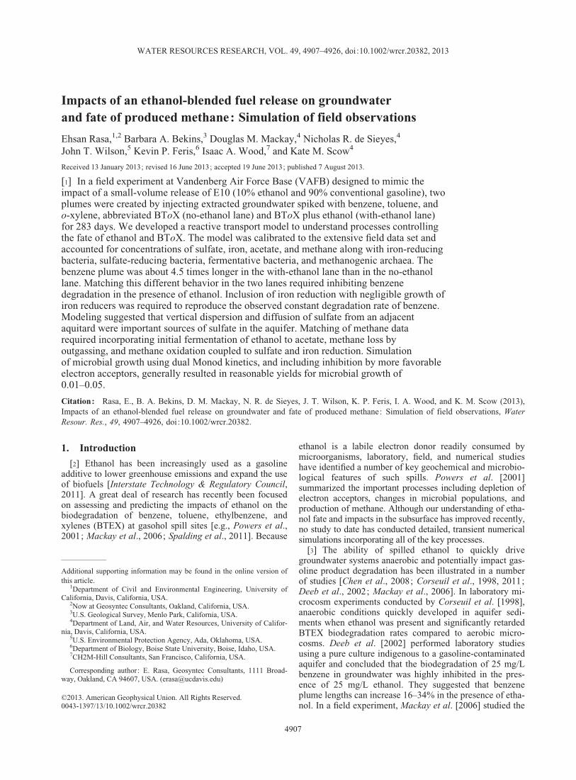
[8] Site 60, Vandenberg Air Force Base, California (Fig-ure 1), has been described in detail previously [Mackayet al., 2012, and references therein]. Within the 60 m longstudy area, several thin, horizontal, sandy layers existwithin 4 m of the ground surface, and the sand layerdenoted S3 (Figure 2) is the primary groundwater aquifer.Details of the ethanol injection experiment in 2004–2005 atVAFB are described in Mackay et al. [2006]. In brief, side-by-side experiments were conducted involving the injectionof site groundwater spiked with selected BTEX species,with and without ethanol for 283 days. On the west side(no-ethanol lane), 200 mL/min of water was injected thathad been spiked continuously with benzene (B), toluene(T), o-xylene (o-X), and periodically with tracers; hereafterthe selected BTEX species are abbreviated BToX. On theeast side (with-ethanol lane), the same flow rate of waterwas spiked continuously with ethanol plus the same con-centrations of BToX and periodically with tracers. Flow

RASA ET AL.: IMPACTS OF ETHANOL ON GROUNDWATER AND FATE OF METHANE

4908

was split equally into three injection wells for each lane.The average injection concentrations were 2.3 mg/L forbenzene, 2.2 mg/L for toluene, and 0.87 mg/L for o-xylene.In the with-ethanol lane the average ethanol injection con-centration was 470 mg/L. The progress of the experimentswas monitored with 192 monitoring wells with 0.91 m (3feet) screens spanning the S3 aquifer (Figure 1). Samplingevents consisted of five major snapshots of the BToX andethanol (at 27, 64, 115, 206, and 274 days), one majorsnapshot of other analytes (acetate, propionate, butyrate,methane, nitrate, sulfate, dissolved oxygen, pH, and ferrousiron; at 170 days), and two snapshots of microbial popula-tions in groundwater (at 152 and 244 days).

[9] The average groundwater hydraulic gradient aroundthe time of the experiment was 0.0132, and the meangroundwater flow velocity was estimated to be 0.42 m/d.Distributed groundwater recharge is considered negligible inthis location and was not included in the model. Concentra-tions of background sulfate (the predominant dissolved elec-tron acceptor in the groundwater at the site) averaged 120mg/L. Analyses by Wood [2004] found that close to wherethe experimental plumes were created, the bioavailable ferriciron concentration in the aquifer sediments was 750–1250mg/kg. Other dissolved electron acceptors, including dis-solved oxygen, were negligible or not detectable.

[10] The plumes developing at the injection point weremonitored over time as they progressed downgradient. Inboth lanes there was an initial advance of the plumes. Bothplumes then retracted but the with-ethanol lane plumeretracted more slowly. Rates of benzene degradationincreased with time. In the with-ethanol lane, sulfate wasdepleted and methane was produced, and BToX degrada-tion occurred both in the core of the plume and also alongthe plume fringes by sulfate reduction. Finally, themethane-rich and sulfate-depleted zones along the with-ethanol lane were restricted in space.

[11] Feris et al. [2008] described the observed effect ofethanol on the microbial community structure and naturalattenuation during the same experiments. In both lanesthere was an increase in SRB and total bacteria. The totalbacteria increase extended farther in the with-ethanol lane(9.4 m; EC transect) than in the no-ethanol lane (5.5 m;EB transect). Only the with-ethanol lane had an increase inarchaea. In the no-ethanol lane the injected concentrationof reduced carbon was too low to significantly affect redoxconditions except very near the injection wells. In contrast,in the with-ethanol lane the reduced carbon stimulated SRBgrowth resulting in complete consumption of sulfate. Arch-aea in the with-ethanol lane reached a maximum density5.5 m downgradient (EB transect) after 152 days and at theinjection wells (ER transect) after 244 days. In this laneratios of SRB to total bacteria decreased dramatically overthe course of the experiment [Feris et al., 2008].

3. Model Description

3.1. Conceptual Model

[12] The biodegradation kinetics adopted in this modellink ethanol degradation, microbial growth, and BToX bio-degradation under different redox conditions. Previousmonitoring data from the site show that neither oxygen nornitrate is a significant electron acceptor in the study aquifer[Rasa, 2012]. Therefore, the model includes only iron-reducing and sulfate-reducing degradation of BToX, etha-nol, and methane and fermentative-methanogenic degrada-tion of ethanol. The model describes the distribution overtime and space of 14 species, with seven aqueous or mobilechemical compounds (benzene, toluene, o-xylene, ethanol,acetate, sulfate, and methane), the immobile solid-phase ironoxy-hydroxide, and six immobile microbial populations. Thesix microbial populations are BToX-degrading iron-reducingbacteria (IRB), BToX-degrading SRB, ethanol-degradingIRB, ethanol-degrading SRB, ethanol-degrading fermenta-tive bacteria, and acetate-degrading methanogenic archaea.The only mass transfer mechanism between the immobile

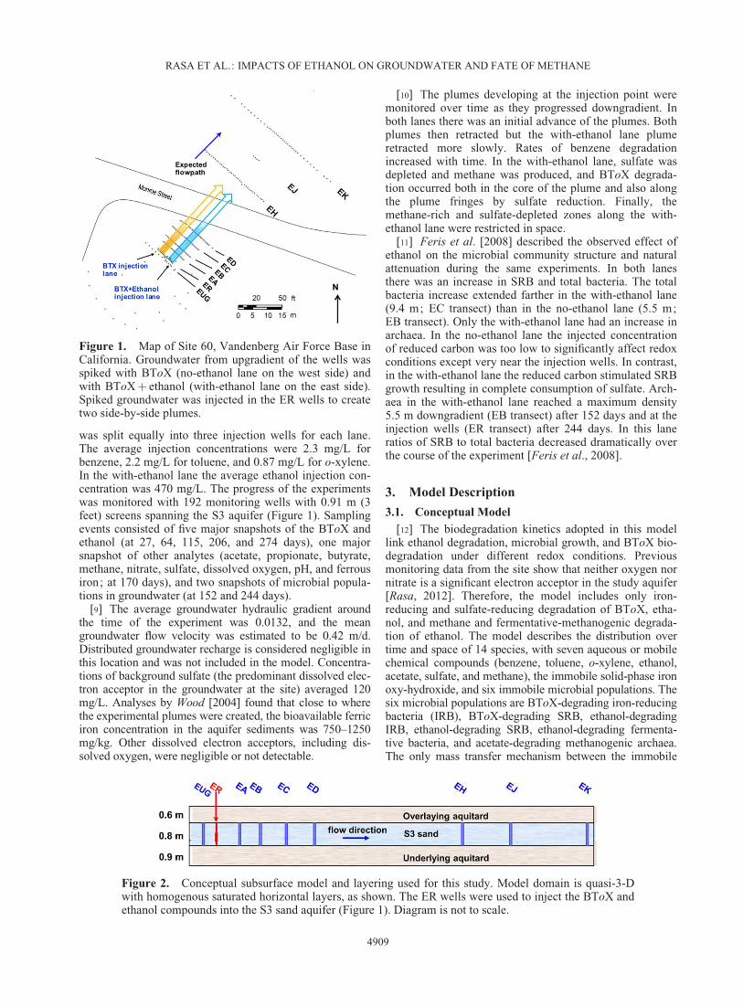
Figure 2. Conceptual subsurface model and layering used for this study. Model domain is quasi-3-Dwith homogenous saturated horizontal layers, as shown. The ER wells were used to inject the BToX andethanol compounds into the S3 sand aquifer (Figure 1). Diagram is not to scale.

Figure 1. Map of Site 60, Vandenberg Air Force Base inCalifornia. Groundwater from upgradient of the wells wasspiked with BToX (no-ethanol lane on the west side) andwith BToXþ ethanol (with-ethanol lane on the east side).Spiked groundwater was injected in the ER wells to createtwo side-by-side plumes.


4909

and aqueous phases in the model is sorption. The bacteriagrow in place and affect reaction rates. The immobile ironoxy-hydroxides are depleted by iron reduction.

[13] The conceptual model for the flow system has beendiscussed elsewhere [Mackay et al., 2012, 2006] and usedin other simulations [Rasa et al., 2011]. The model domainin this work is quasi-3-D with three horizontal layers: anupper silty aquitard (0.6 m thick), a thin sandy aquifer(0.8 m thick), and a lower silty aquitard (0.9 m thick), asshown in cross section in Figure 2. The model domain is110 m along the direction of groundwater flow (x), 55 m inthe direction perpendicular to the groundwater flow (y), and2.3 m in the vertical direction (z). The simulation time was283 days. Groundwater flow was assumed to be steady statewith no sinks and a constant hydraulic gradient of 0.0132.Transport parameters and concentrations used in the modelare given in Table 1. Hydrogeological properties includingporosity and hydraulic conductivity of the aquifer and aqui-tard layers are based on site-specific analyses or literature.

[14] Injection wells (labeled ER; Figure 2) were simu-lated by adding spiked background groundwater at 3.3 �10�3 L/s. The initial and upstream boundary concentrationsof sulfate were set to the background concentration of 120mg/L. The initial concentration of poorly crystalline ironoxy-hydroxide was assumed uniform in the experimental

area and set to 1000 mg/kg as Fe [Wood, 2004]. The injec-tion concentrations of BToX and ethanol compounds andinitial concentrations of other compounds are also listed inTable 1. Water samples taken from between the two experi-mental plumes and also upgradient of the injection sourcewere used to provide an estimate of the preexperimentalbackground microbial populations. Feris et al. [2008]reported average values of 2.8 � 104 of bacterial 16S genecopies/mL, 1.7 � 102 copies of SRB, and 1.4 � 103 arch-aeal 16S copies/mL for the regions of the aquifer unaf-fected by the controlled releases.

3.2. Governing Equations

[15] In this study the groundwater flow system is assumedat steady state with constant head boundary conditions, auniform groundwater flow gradient, and groundwater injec-tion wells. The 3-D advection-dispersion equation of a reac-tive compound is described in equation (1). Equation (2)describes the reaction of an immobile compound:

Rfi�k @Ci

@t¼ �kDx

@2Ci

@x2þ �kDy

@2Ci

@y2þ �kDz

@2Ci

@z2� �kvx

@Ci

@x

� �kvy@Ci

@y� �kvz

@Ci

@zþ qsCs

i þ Ri i ¼ 1; 7

ð1Þ

Table 1. Parameters for the Flow and Transport Modela

Parameter Value Source

Hydraulic ParametersAquifer horizontal hydraulic conductivity 10.89 m/d Rasa et al. [2013]b

Silt layers horizontal hydraulic conductivity 2 � 10�2 m/d Rasa et al. [2013]b

Horizontal to vertical hydraulic conductivity ratio 10 AssumedHydraulic gradient (i) 0.0132 Mackay et al. [2012]Aquifer effective porosity 0.34 Mackay et al. [2012]Silt layers effective porosity 0.4 Rasa et al. [2011]Injection rates 200 mL/min Mackay et al. [2006]

Transport ParametersRetardation factor of benzene (RfB) 1.2 Mackay et al. [2006]Retardation factor of toluene (RfT) 1.6 Mackay et al. [2006]Retardation factor of o-xylene (RfX) 2.3 Mackay et al. [2006]Longitudinal dispersivity (�L) 0.55 m Rasa et al. [2013]b

Transverse horizontal dispersivity (�T) 0.013 m Rasa et al. [2013]b

Transverse vertical dispersivity (�V) 1.3 � 10�3 m Rasa et al. [2013]b

Benzene aqueous diffusion coefficient (Daq)c 6.71 � 10�5 m2/d United States Environmental ProtectionAgency [2011]

Tortuosity (�) 0.40 Rasa et al. [2011]Background sulfate concentration 120 mg/L Mackay et al. [2006]Background iron concentration 1000 mg/kg Wood [2004]Initial density of BToX-degrading iron-reducing bacteria (S1)d 10�4 mg/L Assumed same as S2

Initial density of BToX-degrading sulfate-reducing bacteria (S2)e 10�4 mg/L Calculated based on Feris et al. [2008]Initial density of ethanol-degrading iron-reducing bacteria (S3)d 10�4 mg/L Assumed same as S4

Initial density of ethanol-degrading sulfate-reducing bacteria (S4)e 10�4 mg/L Calculated based on Feris et al. [2008]Initial density of fermentative bacteria (S5)f 0.0317 mg/L Calculated based on Feris et al. [2008]Initial density of acetate-degrading archaea (S6)g 0.0046 mg/L Calculated based on Feris et al. [2008]Benzene injection concentration 2.3 mg/L Mackay et al. [2006]Toluene injection concentration 2.2 mg/L Mackay et al. [2006]o-Xylene injection concentration 0.87 mg/L Mackay et al. [2006]Ethanol injection concentration 470 mg/L Mackay et al. [2006]

aSee text for discussion and assumed locations.bHydraulic conductivity and longitudinal and horizontal dispersivities were estimated by inverse modeling of long-term tracer study at the site.cRT3D model ver. 2.5 used here allows only one diffusion coefficient for the multispecies reactive transport as discussed in Rasa et al. [2011].dTotal iron-reducing bacteria is S1þ S3.eTotal sulfate-reducing bacteria is S2þ S4.fTotal bacteria is S1þ S2þ S3þ S4þ S5.gTotal archaea is S6.


4910

@Cim

@t¼ Rim im ¼ 1; 7 ð2Þ

where Rfi is the retardation factor of compound i, �k is theporosity of the media k, v is the groundwater velocity[LT�1], Ci is the aqueous-phase (mobile) concentration ofcompound i [ML�3], Cim is the solid-phase (immobile) con-centration of compound im, qs is the volumetric flow rateper unit volume of aquifer representing fluid sources andsinks [T�1], Cs

i is the concentration of the source or sinkflux for component i [ML�3], and Ri and Rim are the netreaction rates of ith compounds i and im, respectively[ML�3T�1]. The seven mobile and immobile compoundsare specific to this study, and they are defined in section3.1. Dx, Dy, and Dz are the longitudinal, horizontal, and ver-tical hydrodynamic dispersion coefficients [L2T�1], respec-tively, where Dx ¼ �Lvþ �Dm, Dy ¼ �T vþ �Dm, andDz ¼ �V vþ �Dm: �L, �T, and �V are the longitudinal, hori-zontal, and vertical dispersivities [L], respectively, Dm isthe aqueous molecular diffusion coefficient [L2T�1], and �is tortuosity [Scheidegger, 1961].

3.3. Reaction Kinetics

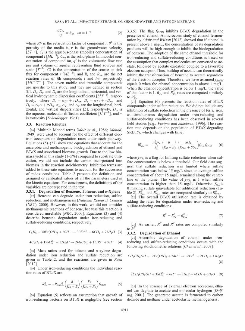
[16] Multiple Monod terms [Molz et al., 1986; Monod,1949] were used to account for the effect of different elec-tron acceptors on degradation rates under each pathway.Equations (5)–(27) show rate equations that account for theanaerobic and methanogenic biodegradation of ethanol andBToX and associated biomass growth. Due to the low bio-mass yield in this study (1–5%) compared to substrate utili-zation, we did not include the carbon incorporated intobiomass in the reaction stoichiometry. Inhibition terms areadded to these rate equations to account for the successionof redox conditions. Table 2 presents the definition andassigned or calibrated values of all the parameters used inthe kinetic equations. For conciseness, the definitions of thevariables are not repeated in the text.3.3.1. Degradation of Benzene, Toluene, and o-Xylene

[17] Benzene can degrade under iron reduction, sulfatereduction, and methanogenesis [National Research Council(NRC), 2000]. However, in this work, we did not considermethanogenic reactions of benzene, because this reaction isconsidered unreliable [NRC, 2000]. Equations (3) and (4)describe benzene degradation under iron-reducing andsulfate-reducing conditions, respectively.

C6H6 þ 30Fe OHð Þ3 þ 60Hþ ! 30Fe2þ þ 6CO2 þ 78H2O ð3Þ

4C6H6 þ 15SO2�4 þ 12H2O! 24HCO�3 þ 15HS� þ 9Hþ ð4Þ

[18] Mass ratios used for toluene and o-xylene degra-dation under iron reduction and sulfate reduction aregiven in Table 2, and the reactions are given in Rasa[2012].

[19] Under iron-reducing conditions the individual reac-tion rates of BToX are

RBFe ¼ �Rmax

BFe

B

KB þ B

� �Fe

KFe þ Fe

� �fEtOH ð5Þ

[20] Equation (5) reflects an assumption that growth ofiron-reducing bacteria on BToX is negligible (see section

3.3.5). The flag fEtOH inhibits BToX degradation in thepresence of ethanol. A microcosm study of ethanol fermen-tation by Adair and Wilson [2012] showed that if ethanol ispresent above 1 mg/L, the concentration of its degradationproducts will be high enough to inhibit the biodegradationof benzene. The adoption of the same ethanol threshold foriron-reducing and sulfate-reducing conditions is based onthe assumption that complex molecules are converted to ac-etate, followed by acetate oxidation coupled to a favorableelectron acceptor. Thus, buildup of acetate can theoreticallyinhibit the transformation of benzene to acetate regardlessof the electron acceptor. Therefore, we have assumed fEtOH

equals 0 when the ethanol concentration is above 1 mg/L.When the ethanol concentration is below 1 mg/L, the valueof this factor is 1. RT

Fe and RXFe rates are computed similarly

to RBFe.

[21] Equation (6) presents the reaction rates of BToXcompounds under sulfate reduction. We did not include anyinhibition of sulfate reduction in the presence of ferric iron,as simultaneous degradation under iron-reducing andsulfate-reducing conditions has been observed in severalfield studies [e.g., Postma and Jakobsen, 1996]. The reac-tion rate depends on the population of BToX-degradingSRB, S2, which changes with time:

RBSO4¼ �

�BS2

S2

Y BS2

B

KB þ B

� �SO4

KSO4 þ SO4

� �fSO4 fEtOH ð6Þ

where fSO4 is a flag for limiting sulfate reduction when sul-fate concentration is below a threshold. Our field data sug-gest that sulfate reduction was limited where sulfateconcentration was below 15 mg/L since an average sulfateconcentration of about 15 mg/L remained along the center-line of the plume. The value of fSO4 is 1 when sulfateconcentration is higher than 15 mg/L. Otherwise fSO4 is0 making sulfate unavailable for additional reduction (Ta-ble 2). RT

SO4and RX

SO4rates are computed similarly to RB

SO4.

[22] The overall BToX utilization rate is obtained byadding the rates for degradation under iron-reducing andsulfate-reducing conditions:

RB ¼ RBFe þ RB

SO4ð7Þ

[23] As earlier, RX and RT rates are computed similarlyto RB.3.3.2. Degradation of Ethanol

[24] Anaerobic degradation of ethanol under iron-reducing and sulfate-reducing conditions occurs with thefollowing stoichiometric relations [Chen et al., 2008]:

CH3CH2OH þ 12Fe OHð Þ3 þ 24Hþ ! 12Fe2þ þ 2CO2 þ 33H2O

ð8Þ

2CH3CH2OH þ 3SO2�4 þ 6Hþ ! 3H2S þ 4CO2 þ 6H2O ð9Þ

[25] In the absence of external electron acceptors, etha-nol can degrade to acetate and molecular hydrogen [Dolf-ing, 2001]. The generated acetate is fermented to carbondioxide and methane under acetoclastic methanogenesis :


4911

CH3CH2OH þ H2O! CH3COO� þ Hþ þ 2H2 ð10Þ

CH3COO� þ Hþ ! CH4 þ CO2 ð11Þ

[26] The ethanol degradation rates under iron reduction(equation (12)), sulfate reduction (equation (13)), and fer-mentation to acetate (equation (14)) are presented later :

REtOHFe ¼ �

�S3S3

Y EtOHS3

EtOH

KEtOH þ EtOH

� �Fe

KFe þ Fe

� �ð12Þ

REtOHSO4

¼ ��S4

S4

Y EtOHS4

EtOH

KEtOH þ EtOH

� �SO4

KSO4 þ SO4

� �fSO4 ð13Þ

Table 2. Kinetic Parameter Values

Symbol Definition Value Source

RCH4SO4

Rate of anaerobic methane oxidation coupled to sulfate (mg/L/d) 0.04 Calibrated

RCH4Fe Rate of anaerobic methane oxidation coupled to iron (mg/L/d) 0.28 Calibrated

RmaxBFe Maximum degradation rate of benzene coupled to iron (mg/L/d) 0.05 Calibrated

RmaxTFe Maximum degradation rate of toluene coupled to iron (mg/L/d) 0.05 Calibrated

RmaxXFe Maximum degradation rate of o-xylene coupled to iron (mg/L/d) 0.03 Calibrated

�BS2

Maximum specific growth rate of SRBa benzene degraders (1/d) 0.045 Calibrated

�TS2

Maximum specific growth rate of SRB toluene degraders (1/d) 0.095 Calibrated

�XS2

Maximum specific growth rate of SRB o-xylene degraders (1/d) 0.022 Calibrated�S3

Maximum specific growth rate of IRBb ethanol degraders (1/d) 0.07 Calibrated�S4

Maximum specific growth rate of SRB ethanol degraders (1/d) 0.55 Calibrated�S5

Maximum specific growth rate of fermentative bacteria (1/d) 50 Calibrated�S6

Maximum specific growth rate of methanogenic archaea (1/d) 0.06 Calibrated

Y BFe Mass ratio of iron to benzene 21.45 Stoichiometry

Y TFe Mass ratio of iron to toluene 21.83 Stoichiometry

Y XFe Mass ratio of iron to o-xylene 22.09 Stoichiometry

Y EtOHFe Mass ratio of iron to ethanol 14.54 Stoichiometry

Y CH4Fe Mass ratio of iron to methane 27.85 Stoichiometry

Y BSO4

Mass ratio of sulfate to benzene 4.61 Stoichiometry

Y TSO4

Mass ratio of sulfate to toluene 4.69 Stoichiometry

Y XSO4

Mass ratio of sulfate to o-xylene 4.75 Stoichiometry

Y EtOHSO4

Mass ratio of sulfate to ethanol 3.13 Stoichiometry

Y CH4SO4

Mass ratio of sulfate to methane 5.99 Stoichiometry

Y EtOHAcet Mass ratio of acetate to ethanol 1.3 Stoichiometry

Y AcetCH4

Mass ratio of methane to acetate 0.27 Stoichiometry

KB Benzene half-saturation concentration (mg/L) 0.5 CalibratedKT Toluene half-saturation concentration (mg/L) 0.01 CalibratedKX o-Xylene half-saturation concentration (mg/L) 0.15 CalibratedKEtOH Ethanol half-saturation concentration (mg/L) 1 CalibratedKAcet Acetate half-saturation concentration (mg/L) 0.1 CalibratedKFe Iron half-saturation concentration (mg/L) 10 CalibratedKSO4 Sulfate half-saturation concentration (mg/L) 100 Calibrated

KiSO4

Sulfate inhibition concentration (mg/L) 5 Calibrated

KiFe Iron inhibition concentration (mg/L) 2000 Calibrated

Y BS2

SRB yield per benzene mass utilized 0.015 Rittmann and McCarty [2001]

Y TS2

SRB yield per toluene mass utilized 0.014 Rittmann and McCarty [2001]

Y XS2

SRB yield per o-xylene mass utilized 0.014 Rittmann and McCarty [2001]

Y EtOHS3

IRB yield per ethanol mass utilized 0.053 Rittmann and McCarty [2001]

Y EtOHS4

SRB yield per ethanol mass utilized 0.015 Calibrated

Y EtOHS5

Fermentative bacteria yield per ethanol mass utilized 0.015 Calibrated

Y AcetS6

Archaeal yield per acetate mass utilized 0.001 Calibrated

b1 Decay rate of bacteria populations (1/d) 0.015 Calibratedb2 Decay rate of archaea (1/d) 0.01 CalibratedfEtOH Ethanol threshold flag, set to 0 if ethanol is above the value listed

at right, or 1 otherwise (mg/L)1 Adair and Wilson [2012]

fSO4 Sulfate threshold flag, set to 0 if sulfate is below the value listedat right, or 1 otherwise (mg/L)

15

aSRB is short for sulfate-reducing bacteria.bIRB is short for iron-reducing bacteria.


4912

REtOHCO2

¼ ��S5

S5

Y EtOHS5

EtOH

KEtOH þ EtOH

� �Ki

SO4

KiSO4þ SO4

!2Ki

Fe

KiFe þ Fe

� �2

ð14Þ

[27] In equation (14), we utilize a modified form of theinhibition function (the last factor). We performed numeri-cal tests (not shown here) which suggested a better matchof simulations to observed data was obtained when

KiSO4

.Ki

SO4þ SO4

� �� 2was used as an inhibition func-

tion instead of the more commonly utilized

KiSO4

.Ki

SO4þ SO4

� �[Rasa, 2012]. The proposed second-

order function strongly inhibited methanogenesis in thepresence of 40 mg/L (or more) of sulfate and below40 mg/L it quickly approached 1, allowing maximum meth-anogenic rates to be applied.

[28] The overall ethanol utilization rate is obtained by add-ing the rates from the three degradation pathways assumedhere (iron reduction, sulfate reduction, and methanogenesis):

REtOH ¼ REtOHFe þ REtOH

SO4þ REtOH

CO2ð15Þ

[29] One of the intermediate products of ethanol degra-dation under methanogenic conditions is acetate (equation(10)). Acetate is then fermented to methane (equation(11)). The overall reaction rate of acetate is

RAcet ¼ �Y EtOHAcet REtOH

CO2þ RAcet

CH4ð16Þ

where RAcetCH4¼ � �S6

S6

Y AcetS6

Acet�

KAcet þ Acetð Þ� �

is the transfor-

mation rate of acetate to methane.3.3.3. Methane Generation and Anaerobic Oxidation

[30] Biodegradation of methane coupled to both sulfate[Martens and Berner, 1977] and iron [Beal et al., 2009]was included in this modeling study. Methane oxidationcoupled with sulfate reduction is described by [Martensand Berner, 1977]

CH4 þ SO2�4 þ 2Hþ ! CO2 þ H2S þ 2H2O ð17Þ

[31] The equation for methane oxidation coupled withiron reduction [Beal et al., 2009] is

CH4 þ 8Fe OHð Þ3 þ 15Hþ ! HCO�3 þ 8Fe2þ þ 21H2O ð18Þ

[32] The rate of change in dissolved methane concentra-tion is then

RCH4 ¼ �Y AcetCH4

RAcetCH4þ fSO4 RCH4

SO4þ RCH4

Fe ð19Þ

where RCH4SO4

and RCH4Fe are the zero-order rates of anaerobic

methane oxidation under sulfate-reducing and iron-reducingconditions, respectively. We assume zero-order rates for rea-sons discussed later.3.3.4. Depletion Rate of Electron Acceptors

[33] Iron reduction (equation (20)) and sulfate reductionrates (equation (21)) are calculated using the substrate utili-zation rates and the reaction mass ratios in Table 2:

RFe ¼ Y BFeRB

Fe þ Y TFeRT

Fe þ Y XFeRX

Fe þ Y EtOHFe REtOH

Fe þ Y CH4Fe RCH4

Fe

ð20Þ

RSO4 ¼ Y BSO4

RBSO4þ Y T

SO4RT

SO4þ Y X

SO4RX

SO4þ Y EtOH

SO4REtOH

SO4

þ Y CH4SO4

RCH4SO4

ð21Þ

3.3.5. Biomass Growth[34] The growth rates of different populations are calcu-

lated based on the substrate utilization rates and the bio-mass yield. Because of the low Gibbs free energy valuesreported for anaerobic oxidation of methane [Regnier et al.,2011], we assumed no biomass growth due to methane deg-radation. Other studies such as Bekins et al. [1993] havereported biodegradation with no apparent growth undermethanogenic conditions. We also assumed no growth ofiron-reducing bacteria due to BToX degradation in thepresence of ethanol (equation (22)). This assumption isconsistent with the linear profile of benzene loss in thewith-ethanol lane observed in the experiment, which indi-cates a constant microbial population [e.g., Bekins et al.,1993]. Equations (22)–(27) relate the growth of the six mi-crobial populations to the biodegradation of BToX underiron-reducing (equation (22)) and sulfate-reducing condi-tions (equation (23)), ethanol under iron-reducing (equation(24)), sulfate-reducing (equation (25)), and methanogenicconditions (equation (26)), and acetate under methanogenicconditions (equation (27)):

RS1 ¼ 0 ð22Þ

RS2 ¼ � Y BS2

RBSO4þ Y T

S2RT

SO4þ Y X

S2RX

SO4

� �� b1S2 ð23Þ

RS3 ¼ �Y EtOHS3

REtOHFe � b1S3 ð24Þ

RS4 ¼ �Y EtOHS4

REtOHSO4� b1S4 ð25Þ

RS5 ¼ �Y EtOHS5

REtOHCO2� b1S5 ð26Þ

RS6 ¼ �Y AcetS6

RAcetCH4� b2S6 ð27Þ

where b1 and b2 are the decay rates of bacteria and archaea,respectively (Table 2). Total IRB and total SRB are givenby S1þ S3 and S2þ S4, respectively. The concentration oftotal bacteria (which includes IRB, SRB, and fermentativebacteria) is calculated as the sum of all bacteria populations(S1þ S2þ S3þ S4þ S5). The concentration of total archaeais S6.

3.4. Conversion Between Gene Copy Numbers andBiomass Concentration

[35] A common unit used for reactive transport models ismass per aqueous-phase volume. Here the modeled bio-mass (S1–S6) was in units of milligram of dry weight ofcells per liter of aqueous-phase volume. Experimental dataare in units of gene copy numbers per milliliter of waterdetermined by qPCR [Feris et al., 2008]. Rittmann andMcCarty [2001] suggest there are about 1012 bacteria in agram of biomass (dry solid weight). We assumed the samedry solid density for archaea.


4913

[36] The number of rRNA genes can vary from 1 to 15copies/prokaryote cell [Klappenbach et al., 2001].Although the range observed in gene copy number is quitelarge, there is some relationship to phylogenetic grouping.According to the database developed by Klappenbach et al.[2001], the ratio of gene copies per cell averages 5 for bac-teria and 1.7 for archaea.

[37] In this modeling study, biomass is consideredattached (i.e., immobile). However, field data were fromwater samples and therefore represent planktonic (sus-pended) cells. Bekins et al. [1999] compared suspended ver-sus attached populations of 76 sample pairs from an aquifercontaminated by crude oil and suggested that an average of15% of the total population is suspended. The relative popu-lation density of planktonic bacteria to total bacteria alsowas measured by Harvey and Barber [1992], who reported aplanktonic to total bacteria ratio of 7–31% in a sewage-contaminated groundwater. Here we assume 15% of totalpopulation is planktonic. Thus, to compare microbial qPCRdata (copies/mL) with the simulated biomass, we multipliedsimulated biomass concentrations (mg/L) by (1012 cells/g)� (10�3 g/mg) � (10�3 L/mL) � 15/85 � (gene copies/cell). Our conceptual model is that growth takes place in theattached phase and that this is reflected as a proportionateincrease in the adjacent planktonic numbers. Therefore,planktonic bacteria were assumed to follow the same distri-bution as the attached population at the sampling locationsand transport of cells was not included in the model.

3.5. Numerical Solution

[38] We used the U.S. Geological Survey (USGS) MOD-FLOW model [Harbaugh et al., 2000] to solve for ground-water flow. Grid discretizations of 0.2 and 0.2 m were usedin the x and y directions, respectively. The simulation timewas 283 days, with average transport time steps of0.02 days. A head change value of 0.01 cm was used as the

convergence criterion. The reactive transport system (equa-tions (1)–(2)) was implemented and numerically solvedusing RT3D v2.5 [Clement et al., 1998]. The standard finitedifference solver (upstream weighting) was used to solvethe advection term, while the standard explicit method wasused to solve the dispersion term. To solve the reactionterms, the Gear solver with explicit Jacobian was applied.Peclet and Courant criteria were checked (not discussedhere) to ensure convergence and stability of the transportmodel. Absolute and relative tolerance parameter values of10�13 and 10�12 were used, respectively, to control theconvergence of the reactive transport of all components inthe model.

4. Results and Discussion

[39] The simulated steady-state flow field used for thetransport model is shown in Figure S1. The flow systemdiverged slightly outward in the vicinity of the injectionwells but had parallel flow paths downgradient of the injec-tion wells.

4.1. Ethanol and BToX

[40] Figures 3–11 compare the simulated versus meas-ured concentrations of different compounds along theplume centerlines. For the measured data, the centerline isdefined to include the monitoring well in each transect withhighest substrate concentration at any given time in thewith-ethanol and no-ethanol lanes. For the simulatedresults, the centerline is the center row in the model grid.

[41] During the experiment simulated here, ethanol wasdetected in groundwater only rarely and only at one loca-tion at 0.5 m downgradient of the injection wells in with-ethanol lane [Feris et al., 2008; Mackay et al., 2006].Because there are so few ethanol data from the field experi-ment, we do not present plots comparing measured and

Figure 3. Comparison of (left) measured versus (right) simulated benzene concentrations in the center-line of the (a and b) with-ethanol and (c and d) no-ethanol experimental lanes. Benzene injection concen-tration was used as measured concentration in groundwater at distance 0 (Figures 3a and 3c).


4914

simulated ethanol over time. Although the ethanol datawere limited, the ethanol degradation rate parameters wereconstrained by the loss of electron acceptors and the pro-duction of methane.

[42] Figures 3a and 3c present the measured benzeneconcentrations in the with-ethanol and no-ethanol lanes,respectively. Several important features of the data neededto be captured by the model. First, benzene degraded inportions of both lanes under sulfate-reducing conditions.Therefore, we coupled benzene degradation to sulfatereduction in the model (equation (6)). The second featureof the benzene data was that the benzene degradation rateincreased with time in the no-ethanol lane and after 274days the benzene plume was limited to the first 3 m down-gradient of the source (Figure 3c). This suggests thatgrowth of benzene-degrading, SRBs (S2) is important(equation (23)). The third aspect was the 4.5 times greaterlength of the benzene plume in the with-ethanol lane. In themodel the inhibition of benzene degradation in the presenceof 1 mg/L of ethanol (fEtOH) was required to simulate initialadvance of the benzene plume. The benzene degradationbegins after the ethanol-degrading population has grownsufficiently large to degrade ethanol upgradient of the firstsample transect. A fourth feature of the data is that in thewith-ethanol lane, benzene degraded even after ethanoldegradation depleted most of the available sulfate, suggest-ing benzene degradation coupled to iron reduction was alsorequired in the model (equation (5)). However, benzenedegradation rates did not change significantly over time inthe with-ethanol lane (Figure 3a), suggesting that benzene-degrading, iron-reducing bacteria (S1) were not growingover time (equation (22)). Comparing the model results inFigures 3b and 3d with the data in Figures 3a and 3c showsthat including SRB growth, ethanol inhibition, and degra-

dation by iron reduction captured the differing benzenebehavior in the no-ethanol and with-ethanol lanes.

[43] The fate of toluene differed somewhat from that ofbenzene (Figures 4a and 4c). There was a similar initialadvance of the plume and retraction in the with-ethanollane due to inhibition of degradation by ethanol. Also, deg-radation of toluene in the with-ethanol lane was slowercompared to the no-ethanol lane because of the depletionof sulfate after 64 days. So toluene degradation is coupledto iron reduction downgradient of 3 m. Unlike benzene, tol-uene concentrations dropped below the detection limitthroughout the experimental area (with just a few excep-tions, all near the detection limit) by the end of the experi-ment in the with-ethanol lane. This feature was captured bythe model through a higher growth rate of toluene-degrading SRB relative to benzene-degrading SRB (�T

S2;

Table 2). As a result, once ethanol is below 1 mg/L upgra-dient of 3 m, degradation of toluene proceeds faster thanbenzene degradation consuming available sulfate near theinjection well. As presented in Figures 4b and 4d, simula-tion results showed very good agreement with the toluenedata from both lanes.

[44] Data from the field experiment showed o-xylenebehaved similarly to benzene, persisting within 13 m down-gradient of the ethanol injection source after 274 days (Fig-ures 5a and 5c). Therefore, the same approach used forbenzene degradation was used for o-xylene. Comparison ofsimulated versus measured data (Figure 5) shows that themodel could explain the important features of o-xylenedata over time and space.

4.2. Sulfate, Iron, and Methane

[45] Figures 6a and 6c present measured sulfate data at170 days. One important feature of the sulfate data was that

Figure 4. Comparison of (left) measured versus (right) simulated toluene concentrations in the center-line of the (a and b) with-ethanol and (c and d) no-ethanol experimental lanes. Toluene injection concen-tration was used as measured concentration in groundwater at distance 0 (Figures 4a and 4c).


4915

sulfate was reduced to 10–15 mg/L within the methano-genic zone in the with-ethanol lane and then remained con-stant (Figure 6a). This does not appear to be due tosubstrate limitation because within 13 m of the injectionsource in the with-ethanol lane, there are still relativelyhigh concentrations of methane (10–29 mg/L), benzene(0.5–2 mg/L), and o-xylene (0.1–0.6 mg/L) within the aqui-

fer. To capture this feature, we used a flag (fSO4 ) to limit theavailability of dissolved sulfate for all sulfate reductionpathways below the threshold of 15 mg/L that wasobserved in the field data (equations (6), (13), and (19)).

[46] A second important feature of the sulfate data wasthe increase in sulfate concentration beyond 35 m downgra-dient from the source (Figure 6a). Simulations suggested

Figure 5. Comparison of (left) measured versus (right) simulated o-xylene concentrations in the cen-terline of the (a and b) with-ethanol and (c and d) without-ethanol experimental lanes. o-Xylene injectionconcentration was used as measured concentration in groundwater at distance 0 (Figures 5a and 5c).

Figure 6. Comparison of (left) measured versus (right) simulated sulfate concentrations in the center-line of the (a and b) with-ethanol and (c and d) no-ethanol experimental lanes. Background sulfate con-centration was used as measured concentration in groundwater at distance 0 (Figures 6a and 6c).


4916

that this is due to vertical mixing of sulfate-depletedgroundwater in the aquifer with sulfate-rich groundwaterentering from the upper and lower silty aquitard layersthrough vertical dispersion and diffusion. Earlier versionsof the model used in this study only included the aquiferlayer and not the adjacent aquitards. Comparing the resultsof the same reactive transport model with and without theaquitard layers (results not presented here) suggested thatthe aquitard layers provided the additional sulfate to the aq-uifer downgradient of the source.

[47] Simulated sulfate concentrations in Figures 6b and6d indicate that the model with aquitard layers and the sul-fate threshold could reproduce the behavior of the sulfateplume in the presence and absence of ethanol. Thresholdlimitations in sulfate reduction have been reported by otherstudies [Knab et al., 2008; Roychoudhury and McCormick,2006; Roychoudhury et al., 2003]. Possible explanationsfor the limitation of sulfate reducers may be the presence oftoxic concentrations of sulfide or competition from othermicrobial populations with respect to mineralizable organiccarbon, as reported by Roychoudhury and McCormick[2006]. Leloup et al. [2007] suggested there may be athreshold concentration below which sulfate is not bioavail-able to SRB. Finally, Knab et al. [2008] reported at concen-trations below 0.2 mM (19.2 mg/L) sulfate was not readilyavailable for anaerobic oxidation of methane in marinesediments. This study may be the most relevant to theVAFB plume because the main reduced carbon sourcebeyond 13 m downgradient was methane.

[48] Upgradient of 13 m BToX is still present and couldbe coupled to sulfate reduction. Other studies of BTEXdegradation coupled to sulfate reduction have presenteddata indicating that sulfate concentrations may remainabove 10 mg/L when benzene is present at greater than1 mg/L. Anderson and Lovley [2000] studied the transienteffect of sulfate addition to a benzene-contaminated aquiferand found that sulfate initially decreased and then remainedlevel at 100–200 mmol/L (10–19 mg/L) with benzene at20–30 mmol/L (1.5–2.5 mg/L). A study of a BTEX plumeby Davis et al. [1999] indicated that the mean sulfate con-centration was 10.8 mg/L in areas of the plume where ben-zene was greater than 1 mg/L. These results are consistentwith the observation that sulfate remained at 15 mg/L atVAFB even when BToX and methane were present.

[49] Measurements of ferric iron concentration wereavailable only prior to the field experiment; therefore, nocomparison could be made to iron values simulated duringthe experiment (Figure 7). Simulations suggested that agreater amount of ferric iron was reduced in the with-ethanol lane. This is due to the inclusion in the model ofanaerobic degradation of methane coupled to iron reduc-tion. The importance of this process in the simulations isdiscussed further later.

[50] Figure 8a shows the measured concentration of dis-solved methane along the plume centerline in the with-ethanol lane. Three important features of the data needed tobe captured by the model. First, methane concentrationsmeasured at 64 days were within the levels observed at thesite prior to this experiment, indicating an increase in rateand spatial extent of methanogenesis occurred after thistime. To reproduce this feature of the data, methanogenesiswas inhibited in the presence of sulfate according to equa-tion (14), and ethanol was first fermented to acetate beforebeing transformed to methane. These two changes to themodel delayed methanogenesis until after 64 days, but thesimulated methane concentrations at 115 days are higherthan the observed values suggesting that an additionalunknown process delayed the start of methane productionin the field experiment. Possible candidates not included inthe model are toxicity of ethanol, fluctuations in injectedsulfate concentration, or greater accumulation of acetate.

[51] The second important feature is that after 115 daysthere is a linear decrease in methane concentration with dis-tance from the injection source, indicating a loss mecha-nism for methane. To capture this loss the model includesanaerobic oxidation of methane coupled to both sulfate andiron reduction. Recent studies have indicated that methaneoxidation may be coupled to iron reduction [Beal et al.,2009; NRC, 2000]. The inclusion of iron was required bythe continued loss of methane in a zone where sulfate wasbelow the posited thermodynamic threshold of 15 mg/L.Results suggested a degradation rate of 0.28 mg/L/d for an-aerobic oxidation of methane coupled to iron (Table 2).The maximum degradation rate for anaerobic oxidation ofmethane coupled to sulfate (RCH4

SO4) was 0.04 mg/L/d. Mod-

eling results indicated that by the end of 283 days, sulfatereduction could account for 12% (1.6 kg) of the methanedegradation, while 88% (13 kg) of methane degradationwas through iron reduction. The third important feature ofthe methane data is that after 200 days the highest concen-tration of dissolved methane in water samples remained

Figure 7. Simulated ferric iron concentrations in thecenterline of the (a) with-ethanol and (b) no-ethanol lanes.Note that there were no measurements made during thefield experiment.


4917

constant at 29 mg/L which is within the range of methanesolubility in groundwater [Lee et al., 2009]. These dataindicate that methane produced near the source after 200days was degassing. Thus, in the simulations we assumedthat any methane concentration above the 29 mg/L thresh-old could degas from the system. This was implementedusing a maximum concentration for the dissolved methane(29 mg/L), replacing the methane values above this thresh-old assuming the excess methane left the dissolved phase.Figure 8b compares the corresponding simulated values ofmethane concentration. The correspondence of simulatedand observed methane values when both degassing and an-aerobic methane oxidation by sulfate and iron reductionwere included indicates the importance of these processesat ethanol- and hydrocarbon-contaminated sites.

[52] Degassing of methane from groundwater aquifershas been previously reported and investigated in severalstudies. Amos et al. [2005] studied the production andtransport of methane at Bemidji crude oil spill site andusing inert gasses provided evidence that a considerableamount of methane was lost due to degassing. Results of amore recent study by Ma et al. [2012] showed that methaneconcentrations in an aquifer exposed to a continuousrelease of a 10% ethanol solution (by volume) reached thesaturation level in groundwater, and methane was detectedin a surface flux chamber indicating that degassing was animportant process. Spalding et al. [2011] also suggestedthat methane can migrate from the subsurface at ethanolspill sites and present vapor risks for nearby confinedspaces with ignitable conditions. Generation of explosivelevels of methane were reported by Nelson et al. [2010]where a continuous feed of dilute E85 was used for a col-umn study.

[53] Caldwell et al. [2008] showed that anaerobic oxida-tion of methane coupled to iron is energetically favorable.The study by Beal et al. [2009] showed that anaerobic oxi-dation of methane may be coupled to reduction of manga-nese and iron. In a methanogenic crude-oil-contaminatedaquifer near Bemidji, Minnesota, methane isotope analysesby Amos et al. [2012] indicated microbial oxidation ofmethane in an anaerobic portion of the plume. They arguedthat iron-mediated anaerobic oxidation of methane wasoccurring based on the dominance of the Fe(III)-reducinggenus Geobacter and mass balance calculations of reducedcarbon flux and depletion of labile sediment iron. Crowe

Figure 8. Comparison of (a) measured versus (b) simulated methane concentrations in the centerlineof the with-ethanol lane.

Figure 9. Total amount of methane oxidation through (a)iron reduction and (b) sulfate reduction over the 283 daysof simulation.


4918

et al. [2011] presented evidence of methane oxidation atLake Matano and argued that the oxidation was coupled toiron reduction based on the abundance of ferric iron and ab-sence of oxygen, sulfate, and nitrate. Numerical modelingpresented in this study, along with field observations, sug-gests that methane degradation occurred in an area of theplume where iron was the only available electron acceptor.Although the species involved and the reaction pathway foranaerobic oxidation of methane coupled to iron reductionare still unknown, the mass balance in the modeling andobserved constant degradation rate in the field are consist-ent with this process. Figures 9a and 9b present the simu-lated cumulative amounts of methane oxidation throughiron reduction and sulfate reduction pathways, respectively,indicating a zone within the plume where methane degrada-tion coupled to sulfate reduction was limited and iron reduc-tion was the only available process for methane oxidation.The total amount of methane oxidation coupled to ironreduction was about eight times more than by sulfate reduc-tion (13 and 1.6 kg, respectively). This finding is consistentwith our field observations suggesting that methane oxida-tion was occurring along the plume centerline (Figure 8a).

[54] The aquitard layers were added to the model toinvestigate whether the observed loss of methane could becaused by either diffusion into the aquitards or by reactionwith sulfate diffusing from the aquitards. The numericaldispersion associated with the low vertical resolution in thequasi-3-D model represents a maximum amount ofexchange with the aquitard, yet this is still inadequate toexplain the methane loss. The results support the sugges-tion that the observed methane loss may be coupled to iron

reduction. Numerical dispersion of BToX into the aquitardlayers did not change the calibrated reaction rates. Ourmodeling results before and after addition of the aquitardlayers indicated that no changes were required to the ki-netic parameters.

4.3. Bacteria and Archaea

[55] Field data suggest that densities of total bacteria,SRB, and archaeal populations were up to four orders ofmagnitude higher within the experimental lanes relative tothe background levels [Feris et al., 2008]. Simulation oftransient growth of biomass at a field site is challenging.First, because the data are sparse in time and space andcomparison of model results to data requires assumptionsabout the relationship between attached and planktonic bio-mass and conversion between qPCR data and cell density.Second, accumulation of biomass has a positive feedbackbecause it leads to faster degradation rates which in turnlead to faster growth, so it is difficult to achieve orders ofmagnitude increases in biomass in a simulation withoutexceeding the observations. Recognizing these challenges,we iterated during our simulation efforts to generate themost reasonable estimates of growth and rates given thefield observations and results of prior studies.

[56] Growth rates of bacteria and archaea in the modelare controlled by the parameters listed in Table 2 togetherwith the substrate and electron acceptor concentrations(e.g., equation (6)). Growth yields were calibrated for etha-nol degradation by SRB and fermenters and acetate degra-dation by methanogens. The remaining yields were basedon energetic calculations as described in Rittmann and

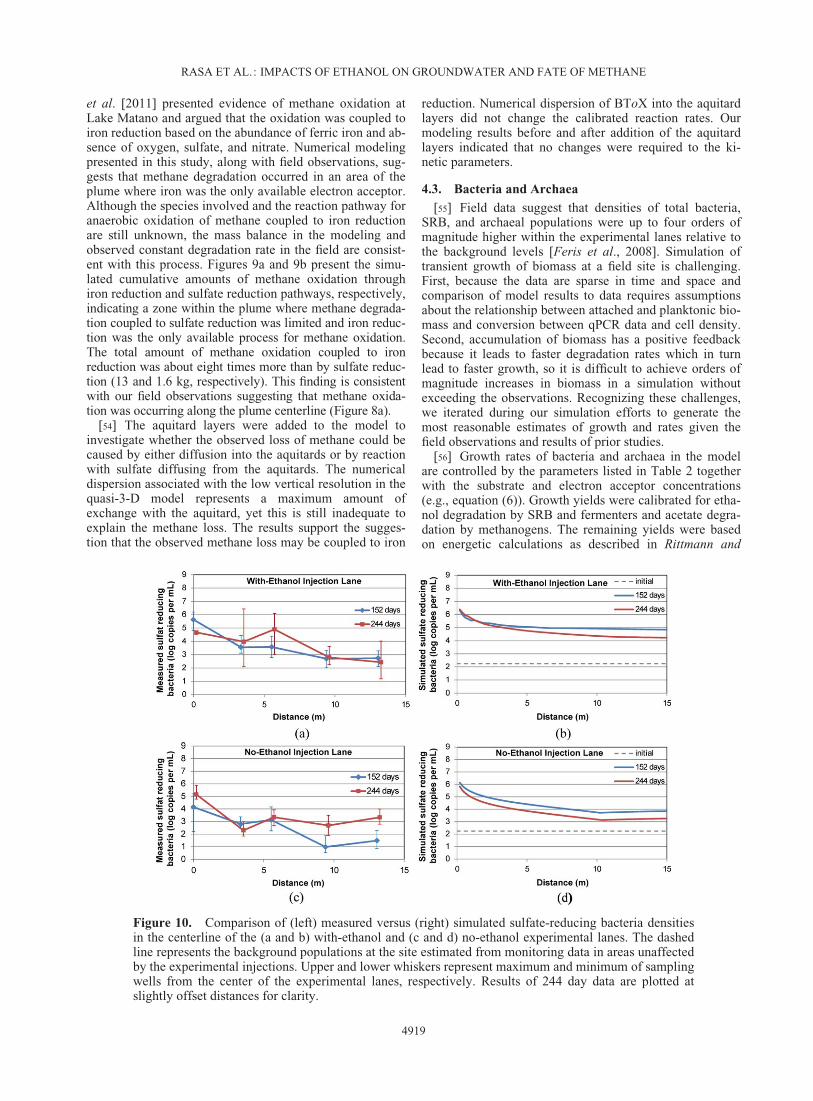
Figure 10. Comparison of (left) measured versus (right) simulated sulfate-reducing bacteria densitiesin the centerline of the (a and b) with-ethanol and (c and d) no-ethanol experimental lanes. The dashedline represents the background populations at the site estimated from monitoring data in areas unaffectedby the experimental injections. Upper and lower whiskers represent maximum and minimum of samplingwells from the center of the experimental lanes, respectively. Results of 244 day data are plotted atslightly offset distances for clarity.


4919

McCarty [2001]. Figures 10–12 present the comparisonbetween biomass data and numerical simulations. Fielddata are presented as the average of three values from sam-pling wells in the center of the experimental lanes with barsrepresenting maximum and minimum values. Simulatedvalues are converted to copy numbers per milliliter ofgroundwater for comparison with the data.

[57] At 244 days the model reproduces the observedincrease of SRB of 2–4 orders of magnitude in both lanesrelative to the background level (Figure 10). The greatestincrease occurs adjacent to the injection wells because theinjected groundwater in both lanes contained backgroundconcentrations of sulfate. The model SRB values were 106/mL near the injection well in both lanes at 244 days,whereas field results were 105/mL indicating that the modeloverpredicted growth near the injection wells. Downgradientof the injection wells, the model results were 104�105/mLSRB in the with-ethanol lane at 244 days compared to aver-ages of 103�105/mL in the field. In the no-ethanol lane themodel results were 103�104/mL SRB compared to field val-ues of 102�104/mL in the field. Thus, at the most downgra-dient locations the simulated SRB values were about10 times too high in the with-ethanol lane but matched wellin the no-ethanol lane. In the with-ethanol lane, the abun-dance of SRB decreased slightly between 152 and 244 daysat the injection well [Feris et al., 2008]. The simulationsalso show a decrease in SRB between 152 and 244 days butlocated downgradient of the injection wells (Figure 10b).The simulated SRB decrease occurs in the with-ethanol lanebecause the sulfate concentration was below the posited ther-modynamic threshold of 15 mg/L (Figure 6a). The high con-

centration of injected ethanol and growth of SRB resulted inconsumption of available sulfate below the threshold of 15mg/L, which was followed by a decline of the SRB at latertimes. In the no-ethanol lane populations initially expandedas the BToX plume advanced downgradient. The higherpopulations lead to faster BToX degradation rates andshrinking of the BToX plume. Even though sulfate washigh, the SRB population declined due to the lower BToXconcentrations.

[58] The simulations reproduced the trend of the totalbacterial density data (which include iron-reducing, sul-fate-reducing, and fermentative bacteria) in that the highestconcentration for both with-ethanol and no-ethanol lanesoccurred adjacent to the injection wells (Figure 11), similarto what was reported by Feris et al. [2008]. Simulationsproduced 1.5–2 orders of magnitude more growth in thewith-ethanol than the no-ethanol lane due to the greatersupply of reduced carbon with the ethanol injection. Simu-lations suggest that growth of total bacteria populations inthe no-ethanol lane was due to the growth of SRB. In thewith-ethanol lane, however, the model suggested thatgrowth of fermentative bacteria contributed the most to theincrease in the densities of total bacteria. Feris et al. [2008]indicated that elevated values in the with-ethanol laneextended beyond 7 m downgradient, whereas the elevatedvalues in the no-ethanol lane were limited to the first 3 m(Figures 11a and 11c). The model reproduces the elevatedvalues at 7 m in the with-ethanol lane but also predictssome growth downgradient (Figure 11b).

[59] In the no-ethanol lane the model predicts growthnear the injection wells and values similar to background

Figure 11. Comparison of (left) measured versus (right) simulated total bacteria densities in the center-line of the (a and b) with-ethanol and (c and d) no-ethanol experimental lanes. The dashed line representsthe background level at the site estimated based on data from area unaffected by the plume. Upper andlower whiskers represent maximum and minimum of sampling wells from the center of the experimentallanes, respectively. Results of 244 day data are plotted at slightly offset distances for clarity.


4920

levels downgradient of 3 m (Figure 11d), which is consist-ent with the trend of the field data. However, the modelcannot explain the very high value of 108/mL total bacteriaobserved at 244 days near the injection well in the no-ethanol lane and the comparatively lower bacterial den-sities in the with-ethanol lane. Possibly this reversal wasdue to lower energetic yield of fermentation of ethanol toacetate followed by methanogenesis from acetate, proc-esses which dominate at late time in the with-ethanol lane.Consistent with this explanation, the data earlier in theexperiment (152 days Figures 10 and 11) show SRB andtotal bacterial densities were higher in the with-ethanollane than in the no-ethanol lane. In this earlier period thebiomass level in the with-ethanol lane may still havereflected some contribution of the sulfate-reducing metabo-lism and higher yield, for example, if sulfate was suppliedto the permeable media by diffusion from lower permeabil-ity layers before their reservoirs of sulfate were exhausted.Nevertheless, when the model yields were calibrated to thefull data set, the same values were obtained for SRB andfermenting bacteria (Table 2), suggesting further investiga-tion into the yields in such dynamic settings could proveilluminating.

[60] A notable discrepancy between the model and dataoccurs at the most downgradient point, where the no-ethanol lane data show almost 106/mL bacteria versusfewer than 105/mL in the model. These differences mayoccur because the model simulates attached populationswhile the observations represent suspended cells. If 15% ofthe population growing near the injection wells had beentransported downgradient, then the observed numbers inthe no-ethanol lane could have resulted from transport of

these cells. We based our conversion of attached to plank-tonic numbers on the data of Bekins et al. [1999] for theBemidji site. Their data showed similar ratios throughoutthe plume with no indication that transport of the plank-tonic phase increased numbers in the downgradient regionof the plume. Whether the planktonic cells were transporteddowngradient at the VAFB site is unknown, but some evi-dence of transport is suggested by the observed increasesdowngradient in the no-ethanol lane in an area where littlegrowth substrate is present.

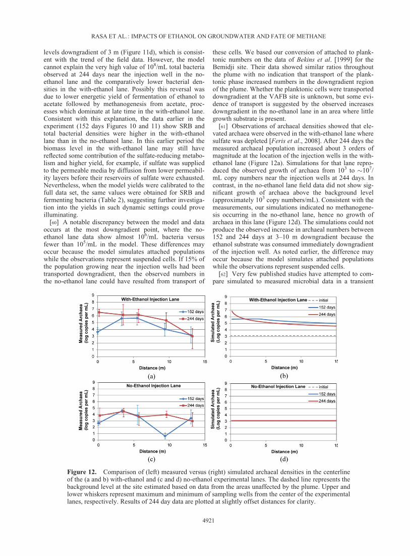
[61] Observations of archaeal densities showed that ele-vated archaea were observed in the with-ethanol lane wheresulfate was depleted [Feris et al., 2008]. After 244 days themeasured archaeal population increased about 3 orders ofmagnitude at the location of the injection wells in the with-ethanol lane (Figure 12a). Simulations for that lane repro-duced the observed growth of archaea from 103 to �107/mL copy numbers near the injection wells at 244 days. Incontrast, in the no-ethanol lane field data did not show sig-nificant growth of archaea above the background level(approximately 103 copy numbers/mL). Consistent with themeasurements, our simulations indicated no methanogene-sis occurring in the no-ethanol lane, hence no growth ofarchaea in this lane (Figure 12d). The simulations could notproduce the observed increase in archaeal numbers between152 and 244 days at 3–10 m downgradient because theethanol substrate was consumed immediately downgradientof the injection well. As noted earlier, the difference mayoccur because the model simulates attached populationswhile the observations represent suspended cells.

[62] Very few published studies have attempted to com-pare simulated to measured microbial data in a transient

Figure 12. Comparison of (left) measured versus (right) simulated archaeal densities in the centerlineof the (a and b) with-ethanol and (c and d) no-ethanol experimental lanes. The dashed line represents thebackground level at the site estimated based on data from the areas unaffected by the plume. Upper andlower whiskers represent maximum and minimum of sampling wells from the center of the experimentallanes, respectively. Results of 244 day data are plotted at slightly offset distances for clarity.


4921

plume. Essaid et al. [1995] simulated aerobic and anaero-bic biodegradation processes at the Bemidji, Minnesota,crude oil spill site and compared modeled and measuredbiomass only at the end of the simulation time (13 years).Wilson et al. [2012] developed a model based on results ofactive remediation of a BTEX plume but assumed a con-stant biomass. Ma et al. [2012] modeled microbial reac-tions and population dynamics at the fringe of a steady-state plume using dual Monod kinetics to describe the mi-crobial population dynamics. In a previous study, Eckertand Appelo [2002] simulated an in situ enhanced bioreme-diation of nitrate-contaminated aquifer with a well-pairrecirculation system using multi-Monod kinetics and bio-mass growth. However, they did not compare the modeledand field-measured biomass results. In this study, the simu-lations were somewhat successful in reproducing the orderof magnitude of observed microbial population changes.Growth of SRB, total bacteria, and archaea were required

to explain the transient behavior of the plume. The growthyields used for different populations were based either ontheoretical values or were calibrated (Table 2). A compari-son of the three calibrated values to theoretical valuesshows that the calibrated values used for growth yields ofSRB and fermenters were reasonable, but the value foracetate-utilizing archaea was 10 times lower than the theo-retical value (Table S2).

[63] Models of reactive transport with biodegradation ofmultiple solutes coupled to biomass growth typically havea great many parameters, calling into question the validityof the calibrated values. In this study, the focus has been onprocess insights gained from incrementally revising theconceptual model, rather than on emphasizing the valuesobtained for the calibrated parameters. A general discus-sion of the calibrated values seems premature for severalreasons. These include a paucity of other microbial datasets from transient field experiments, lack of consensus on

Figure 13. Simulated plumes of different compounds in the no-ethanol lane (west side) and the with-ethanol lane (east side) after 274 days of the experiment for (a) benzene, (b) o-xylene, (c) sulfate, and (d)dissolved methane. For the location of injection wells within each experimental lane refer to Figure 1.There was no detectable toluene and ethanol in the simulations after 274 days; therefore, we do notshow their contour plots here.


4922

the relationship between qPCR data and active populations,and questions on the relationship between attached andplanktonic numbers. Instead we have concentrated onachieving simulated microbial growth at comparable ordersof magnitude to the observations using reasonable growthyields. To assess which parameters were most important, theUSGS universal inverse modeling code, UCODE_2005[Poeter et al., 2005], was used to perform a sensitivity analy-sis for the calibrated parameters. The values of compositescaled sensitivity (CSS) are presented in Figure S2. Interest-ingly, the archaeal yield had the highest CSS, and the cali-brated value was low compared to the theoretical value (TableS2), suggesting that the archaeal growth at this site is poorlyunderstood. Other parameters with high sensitivities were themaximum specific growth rate of SRB ethanol degraders, sul-fate half-saturation concentration, and maximum specificgrowth rate of SRB toluene degraders, indicating the impor-tance of methane production and sulfate reduction processes.A thorough examination of parameter sensitivities and corre-

lation of parameters would be possible if more microbial datasets for these types of models become available.

[64] Figure 13 illustrates contour plots of the simulatedplume for different compounds at 274 days, correspondingto the last observed data in the experiment. The benzeneplume (defined here as concentrations greater than 20 mg/L) was about 4.5 times longer in the with-ethanol lane thanin the no-ethanol lane by the end of the 274 day simulationtime (Figure 13a). Toluene and ethanol concentrations,which were nondetectable by this time, are therefore notshown in Figure 13. Simulated o-xylene persisted in thewith-ethanol lane as was observed in the field [Mackayet al., 2006]. The methane concentrations (Figure 13d)showed good agreement with the field observations,although the simulated plume was somewhat shorter thanthe observed plume. The simulations of areal distributionsof the microbial populations (Figure 14) help identify zoneswithin which active biodegradation under different redoxconditions are to be expected. For example, Figure 14b

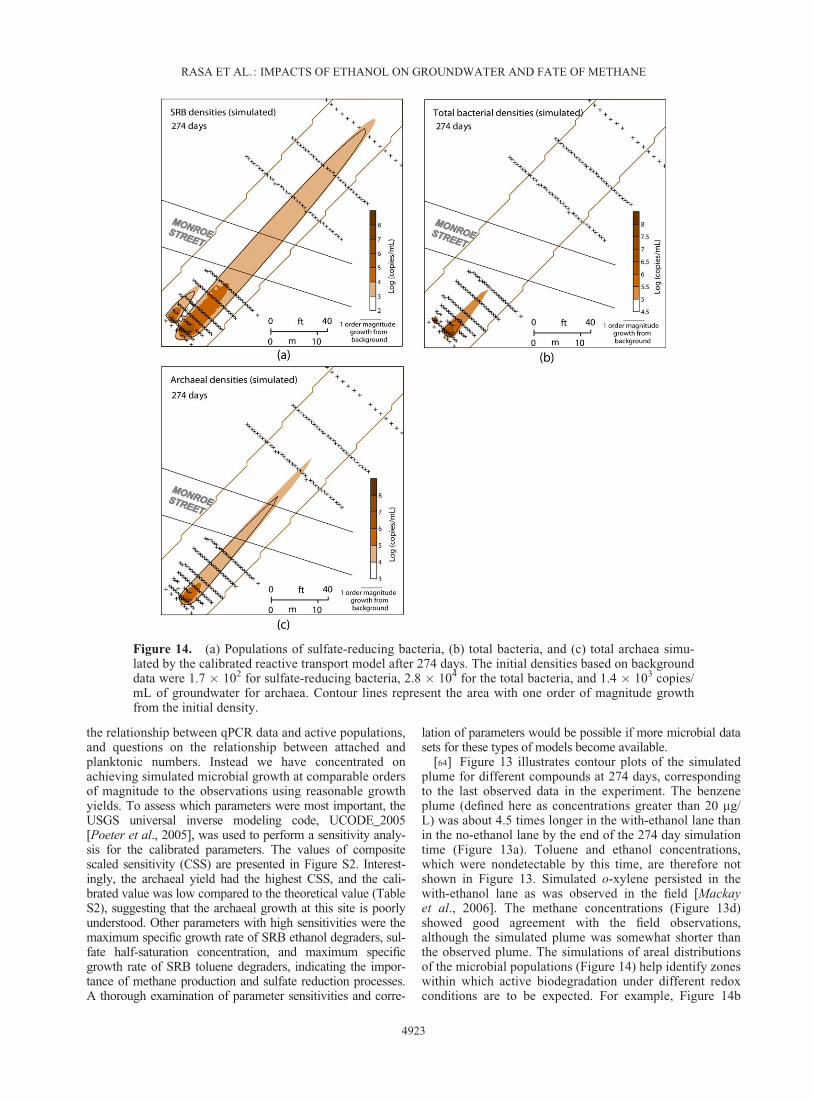
Figure 14. (a) Populations of sulfate-reducing bacteria, (b) total bacteria, and (c) total archaea simu-lated by the calibrated reactive transport model after 274 days. The initial densities based on backgrounddata were 1.7 � 102 for sulfate-reducing bacteria, 2.8 � 104 for the total bacteria, and 1.4 � 103 copies/mL of groundwater for archaea. Contour lines represent the area with one order of magnitude growthfrom the initial density.


4923

shows the area with high growth of total bacteria is also thearea with active ethanol fermentation within the first 10 mdowngradient of the with-ethanol lane injection wells.

[65] On the basis of simulated growth of archaeal popu-lations after 274 days, the methanogenic zone was found tohave extended beyond 13 m downgradient of the ethanolinjection source with the most active zone within 4 mdowngradient from the ethanol injection source. The areaswith high growth of microbial populations were consistentwith observed redox processes from chemical data and canserve as an indicator of active biodegradation zones. Due totransport of dissolved methane with groundwater flow,identifying the methanogenic zone solely based on methaneconcentration is inaccurate.

5. Summary and Conclusions

[66] A kinetics-based reactive transport model coupledto microbial growth was developed, providing quantitativeunderstanding of the impact of ethanol and its degradationproducts on petroleum hydrocarbon compounds of interest :benzene, toluene, and o-xylene. High resolution data froma field study, intended to represent a small-volume releaseof E10 gasohol (10% ethanol and 90% conventional gaso-line), were used to construct the model and identify impor-tant processes controlling the natural attenuation ofdifferent compounds.

[67] Using insights from the field experiment, weincluded in our numerical model the degradation of BToXunder sulfate reduction and iron reduction, degradation ofethanol under sulfate reduction, iron reduction, and metha-nogenesis, and anaerobic oxidation of dissolved methanecoupled to sulfate and iron. Results reproduced the field ob-servation that the natural attenuation of BToX compoundswas slowed significantly in the presence of dissolved-phaseethanol. The model results were also consistent with the ob-servation that ethanol did not persist in the aquifer morethan 0.5 m downgradient of the injection wells. Discrepan-cies between simulations and the measured BToX and etha-nol data suggested that addition of iron reduction as adegradation pathway was a necessary refinement of themodel. Also, since measurements indicated that sulfate wasdepleted to no lower than about 10–15 mg/L within themethanogenic zone, the model was further refined toaccount for this, an assumption supported by results ofprior research by others. Modeling results indicated thatvertical dispersion and diffusion of sulfate-rich ground-water from aquitard layers into the aquifer replenished thesulfate-depleted groundwater. Therefore, some BToX com-pounds for which degradation under methanogenic condi-tions was limited were biodegraded by either iron or sulfatereduction further downgradient.

[68] Based on field results, dissolved methane seemed todegrade with a constant rate over time, so the rate wasassumed constant in the model. The model predicted meth-ane concentrations in excess of the water solubility limitsuggesting that a fraction of the generated methane escapedthe groundwater. Simulations also suggested anaerobic oxi-dation of methane is required to explain methane data overtime along the plume centerline. Another highlight of thisstudy was that theoretical computed and calibrated bacteriayields resulted in microbial growth over time that matched

reasonably well with observations. The model yield forarchaea was too low by a factor of 10 indicating that morework is needed to understand growth of the archaeal popu-lations under such conditions. In creating a model thatreproduced the data for this field setting and experimentalconditions it was necessary to use some phenomenologicalcomponents based on observations. These include thresh-olds for ethanol and sulfate, negligible growth for ironreducers and methanogens on BToX, and methane oxida-tion coupled to iron reduction. We have tried to documentand discuss these assumptions so that future modelingefforts for other sites and conditions can examine whetherthe same effects occur and possibly advance methods formodeling the underlying mechanisms.

Notation

Fundamental QuantitiesB benzene concentration (mg/L).T toluene concentration (mg/L).X o-xylene concentration (mg/L).

EtOH ethanol concentration (mg/L).SO4 sulfate concentration (mg/L).

Fe3þ sediment iron concentration (mg/kg).Acet acetate concentration (mg/L).CH4 dissolved methane concentration (mg/L).

S1 BToX-degrading iron-reducing bacteria (mg/L).S2 BToX-degrading sulfate-reducing bacteria (mg/L).S3 ethanol-degrading iron-reducing bacteria (mg/L).S4 ethanol-degrading sulfate-reducing bacteria (mg/

L).S5 fermentative bacteria (mg/L).S6 acetate-degrading archaea (mg/L).

Kinetic ParametersR reaction rate (mg/L/d).

Rmax maximum degradation rate (mg/L/d).�S maximum specific growth rate (1/d).YS biomass yield coefficient.Y mass ratio of different solutes.K half-saturation concentration (mg/L).Ki inhibition concentration (mg/L).bS biomass decay rate (1/d).

fEtOH flag for BToX degradation inhibition in the pres-ence of ethanol.

fSO4 flag for limiting sulfate reduction when sulfate isless than a threshold.

[69] The specific parameters and their values are listed inTable 2.

[70] Acknowledgments. The project described was supported bygrant 2010–104864 from the American Petroleum Institute (API) andAward P42ES004699 from the National Institute of Environmental HealthSciences. The content is solely the responsibility of the authors and doesnot necessarily represent the official views of the National Institute ofEnvironmental Health Sciences or the National Institutes of Health. Addi-tional support was provided by the University Consortium for FieldFocused Groundwater Contamination Research.

ReferencesAdair, C., and J. T. Wilson (2012), Site characterization of ethanol-blended

fuel releases, in National Tanks Conference, St Louis, Mo., 20 Mar.


4924

[Available at http://www.neiwpcc.org/tanksconference/presentations/Tuesday%20Presentations/Wilson_Adair_Site%20Characterization_Tuesday.pdf.]

Amos, R. T., K. U. Mayer, B. A. Bekins, G. N. Delin, and R. L. Williams(2005), Use of dissolved and vapor-phase gases to investigate methano-genic degradation of petroleum hydrocarbon contamination in the sub-surface, Water Resour. Res., 41, W02001, doi:10.1029/2004WR003433.

Amos, R. T., B. A. Bekins, I. M. Cozzarelli, M. A. Voytek, J. D. Kirshtein,E. J. P. Jones, and D. W. Blowes (2012), Evidence for iron-mediated an-aerobic methane oxidation in a crude oil-contaminated aquifer, Geobiol-ogy, 10(6), 506–517, doi:10.1111/j.1472–4669.2012.00341.x.

Anderson, R. T., and D. R. Lovley (2000), Anaerobic bioremediation ofbenzene under sulfate-reducing conditions in a petroleum-contaminatedaquifer, Environ. Sci. Technol., 34(11), 2261–2266.

Beal, E. J., C. H. House, and V. J. Orphan (2009), Manganese- and iron-dependent marine methane oxidation, Science, 325(5937), 184–187.

Bekins, B. A., E. M. Godsy, and D. F. Goerlitz (1993), Modeling steady-state methanogenic degradation of phenols in groundwater, J. Contam.Hydrol., 14(3–4), 279–294.

Bekins, B. A., E. M. Godsy, and E. Warren (1999), Distribution of micro-bial physiologic types in an aquifer contaminated by crude oil, Microb.Ecol., 37(4), 263–275.

Caldwell, S. L., J. R. Laidler, E. A. Brewer, J. O. Eberly, S. C. Sandborgh,and F. S. Colwell (2008), Anaerobic oxidation of methane: Mechanisms,bioenergetics, and the ecology of associated microorganisms, Environ.Sci. Technol., 42(18), 6791–6799.

C�apiro, N. L., M. L. B. Da Silva, B. P. Stafford, W. G. Rixey, and P. J. J.Alvarez (2008), Microbial community response to a release of neat etha-nol onto residual hydrocarbons in a pilot-scale aquifer tank, Environ.Microbiol., 10(9), 2236–2244.

Chen, Y. D., J. F. Barker, and L. Gui (2008), A strategy for aromatic hydro-carbon bioremediation under anaerobic conditions and the impacts ofethanol: A microcosm study, J. Contam. Hydrol., 96(1–4), 17–31.

Clement, T., Y. Sun, B. Hooker, and J. Petersen (1998), Modeling multispe-cies reactive transport in ground water, Ground Water Monit. Remedia-tion, 18(2), 79–92.

Corseuil, H. X., C. S. Hunt, R. C. F. Dos Santos, and P. J. J. Alvarez (1998),The influence of the gasoline oxygenate ethanol on aerobic and anaerobicBTX biodegradation, Water Res., 32(7), 2065–2072.

Corseuil, H. X., A. L. Monier, M. Fernandes, M. R. Schneider, C. C. Nunes,M. do Rosario, and P. J. J. Alvarez (2011), BTEX plume dynamics follow-ing an ethanol blend release: Geochemical footprint and thermodynamicconstraints on natural attenuation, Environ. Sci. Technol., 45(8), 3422–3429.

Crowe, S. A., et al. (2011), The methane cycle in ferruginous Lake Matano,Geobiology, 9(1), 61–78.

Davis, G. B., C. Barber, T. R. Power, J. Thierrin, B. M. Patterson, J. L. Ray-ner, and Q. Wu (1999), The variability and intrinsic remediation of aBTEX plume in anaerobic sulphate-rich groundwater, J. Contam.Hydrol., 36(3–4), 265–290.

Deeb, R. A., J. O. Sharp, A. Stocking, S. McDonald, K. A. West, M. Lau-gier, P. J. J. Alvarez, M. C. Kavanaugh, and L. Alvarez-Cohen (2002),Impact of ethanol on benzene plume lengths: Microbial and modelingstudies, J. Environ. Eng.—ASCE, 128(9), 868–875.

Dolfing, J. (2001), The microbial logic behind the prevalence of incompleteoxidation of organic compounds by acetogenic bacteria in methanogenicenvironments, Microb. Ecol., 41(2), 83–89.

Eckert, P., and C. A. J. Appelo (2002), Hydrogeochemical modeling ofenhanced benzene, toluene, ethylbenzene, xylene (BTEX) remediation withnitrate, Water Resour. Res., 38(8), 1130, doi:10.1029/2001WR000692.

Essaid, H. I., B. A. Bekins, E. M. Godsy, E. Warren, M. J. Baedecker, and I.M. Cozzarelli (1995), Simulation of aerobic and anaerobic biodegradationprocesses at a crude oil spill site, Water Resour. Res., 31(12), 3309–3327.

Feris, K., D. Mackay, N. de Sieyes, I. Chakraborty, M. Einarson, K. Hristova,and K. Scow (2008), Effect of ethanol on microbial community structureand function during natural attenuation of benzene, toluene, and o-xylenein a sulfate-reducing aquifer, Environ. Sci. Technol., 42(7), 2289–2294.

Freitas, J. G., B. Fletcher, R. Aravena, and J. F. Barker (2010), Methaneproduction and isotopic fingerprinting in ethanol fuel contaminated sites,Ground Water, 48(6), 844–857.

Freitas, J. G., M. T. Mocanu, J. L. G. Zoby, J. W. Molson, and J. F. Barker(2011), Migration and fate of ethanol-enhanced gasoline in groundwater:A modelling analysis of a field experiment, J. Contam. Hydrol., 119(1–4),25–43.

Gomez, D. E., P. C. de Blanc, W. G. Rixey, P. B. Bedient, and P. J. J.Alvarez (2008), Modeling benzene plume elongation mechanisms

exerted by ethanol using RT3D with a general substrate interaction mod-ule, Water Resour. Res., 44, W05405, doi:10.1029/2007WR006184.

Harbaugh, A. W., E. R. Banta, M. C. Hill, and M. G. McDonald (2000),MODFLOW-2000, the U.S. Geological Survey modular ground-watermodel—User guide to modularization concepts and the ground-waterflow process, U.S. Geol. Surv. Open File Rep., 00–92, 121.

Harvey, R. W., and L. B. Barber (1992), Associations of free-living bacteriaand dissolved organic-compounds in a plume of contaminated ground-water, J. Contam. Hydrol., 9(1–2), 91–103.

Interstate Technology & Regulatory Council (2011), Biofuels: ReleasePrevention, Environmental Behavior, and Remediation, Biofuel Team,Washington, D. C. [Available at http://www.itrcweb.org/documents/bio-fuels/biofuels-1.pdf.]

Klappenbach, J. A., P. R. Saxman, J. R. Cole, and T. M. Schmidt (2001),rrndb: The ribosomal RNA operon copy number database, Nucleic AcidsRes., 29(1), 181–184.

Knab, N. J., A. W. Dale, K. Lettmann, H. Fossing, and B. B. J�rgensen(2008), Thermodynamic and kinetic control on anaerobic oxidation ofmethane in marine sediments, Geochim. Cosmochim. Acta, 72(15),3746–3757.

Lee, E. J., M. Kim, Y. Kim, and K.-K. Lee (2009), Numerical and fieldinvestigation of enhanced in situ denitrification in a shallow-zone well-to-well recirculation system, Ecol. Modell., 220(19), 2441–2449.

Leloup, J., A. Loy, N. J. Knab, C. Borowski, M. Wagner, and B. B.J�rgensen (2007), Diversity and abundance of sulfate-reducing microor-ganisms in the sulfate and methane zones of a marine sediment, BlackSea, Environ. Microbiol., 9(1), 131–142.

Lovanh, N., C. S. Hunt, and P. J. J. Alvarez (2002), Effect of ethanol onBTEX biodegradation kinetics: Aerobic continuous culture experiments,Water Res., 36(15), 3739–3746.

Ma, J., W. G. Rixey, G. E. DeVaull, B. P. Stafford, and P. J. J. Alvarez(2012), Methane bioattenuation and implications for explosion riskreduction along the groundwater to soil surface pathway above a plumeof dissolved ethanol, Environ. Sci. Technol., 46(11), 6013–6019.

Mackay, D. M., et al. (2006), Impact of ethanol on the natural attenuationof benzene, toluene, and o-xylene in a normally sulfate-reducing aquifer,Environ. Sci. Technol., 40(19), 6123–6130.

Mackay, D. M., M. D. Einarson, P. M. Kaiser, M. Nozawa-Inoue, S. Goyal,I. Chakraborty, E. Rasa, and K. M. Scow (2012), Mass discharge in atracer plume: Evaluation of the Theissen polygon method, GroundWater, 50(6), 895–907.

Martens, C. S., and R. A. Berner (1977), Interstitial water chemistry ofanoxic Long Island sound sediments: 1. Dissolved gases, Limnol. Ocean-ogr., 22(1), 10–25.

Molson, J. W., J. F. Barker, E. O. Frind, and M. Schirmer (2002), Modelingthe impact of ethanol on the persistence of benzene in gasoline-contaminated groundwater, Water Resour. Res., 38(1), 1003, doi:10.1029/2001WR000589.

Molz, F. J., M. A. Widdowson, and L. D. Benefield (1986), Simulation ofmicrobial-growth dynamics coupled to nutrient and oxygen-transport inporous-media, Water Resour. Res., 22(8), 1207–1216, doi:10.1029/WR022i008p01207.

Monod, J. (1949), The growth of bacterial cultures, Annu. Rev. Microbiol.,3, 371–394.

Nelson, D. K., T. M. LaPara, and P. J. Novak (2010), Effects of ethanol-based fuel contamination: Microbial community changes, production ofregulated compounds, and methane generation, Environ. Sci. Technol.,44(12), 4525–4530.

National Research Council (NRC) (2000), Natural Attenuation for Ground-water Remediation, National Research Council (U.S.), Committee onIntrinsic Remediation, xiv, 274 pp., Natl. Acad. Press, Washington, D. C.

Poeter, E. P., M. C. Hill, E. R. Banta, S. Mehl, and S. Christensen (2005),UCODE_2005 and six other computer codes for universal sensitivityanalysis, calibration, and uncertainty evaluation, U.S. Geol. Surv. Tech.Methods, 6-A11, 283.

Postma, D., and R. Jakobsen (1996), Redox zonation: Equilibrium con-straints on the Fe(III)/SO4-reduction interface, Geochim. Cosmochim.Acta, 60(17), 3169–3175.

Powers, S. E., C. S. Hunt, S. E. Heermann, H. X. Corseuil, D. Rice, and P.J. J. Alvarez (2001), The transport and fate of ethanol and BTEX ingroundwater contaminated by gasohol, Crit. Rev. Environ. Sci. Technol.,31(1), 79–123.

Rasa, E. (2012), Impacts of back diffusion and biodegradation on MTBE/TBA plumes and impacts of spills of ethanol-blended biofuels ongroundwater: Development of models for evaluating field experiments


4925

http://www.neiwpcc.org/tanksconference/presentations/Tuesday%20Presentations/Wilson_Adair_Site%20Characterization_Tuesday.pdf





http://www.itrcweb.org/documents/biofuels/biofuels-1.pdf

http://www.itrcweb.org/documents/biofuels/biofuels-1.pdf

and their implications, PhD dissertation, Dep. of Civ. and Environ. Eng.,Univ. of Calif., Davis, Calif.

Rasa, E., S. W. Chapman, B. A. Bekins, G. E. Fogg, K. M. Scow, and D. M.Mackay (2011), Role of back diffusion and biodegradation reactions insustaining an MTBE/TBA plume in alluvial media, J. Contam. Hydrol.,126(3–4), 235–247.

Rasa, E., L. Foglia, D. M. Mackay, and K. M. Scow (2013), Effect of differ-ent transport observations on inverse modeling results: Case study of along term groundwater tracer test monitored at high resolution, Hydro-geol. J., doi:10.1007/s10040-013-1026-8.

Regnier, P., A. W. Dale, S. Arndt, D. E. LaRowe, J. Mogollon, and P. VanCappellen (2011), Quantitative analysis of anaerobic oxidation of meth-ane (AOM) in marine sediments: A modeling perspective, Earth Sci.Rev., 106(1–2), 105–130.

Rittmann, B. E., and P. L. McCarty (2001), Environmental Biotechnol-ogy: Principles and Applications, xiv, 754 pp., McGraw-Hill, Boston,Mass.

Roychoudhury, A., and D. McCormick (2006), Kinetics of sulfate reductionin a coastal aquifer contaminated with petroleum hydrocarbons, Biogeo-chemistry, 81(1), 17–31.

Roychoudhury, A. N., P. Van Cappellen, J. E. Kostka, and E. Viollier(2003), Kinetics of microbially mediated reactions: Dissimilatory sulfate

reduction in saltmarsh sediments (Sapelo Island, Georgia, USA), Estua-rine Coastal Shelf Sci., 56(5–6), 1001–1010.

Scheidegger, A. (1961), General theory of dispersion in porous media, J.Geophys. Res., 66(10), 3273–3278, doi:10.1029/JZ066i010p03273.

Spalding, R. F., M. A. Toso, M. E. Exner, G. Hattan, T. M. Higgins, A. C.Sekely, and S. D. Jensen (2011), Long-term groundwater monitoringresults at large, sudden denatured ethanol releases, Ground Water Monit.Remediation, 31(3), 69–81.

Suflita, J. M., and M. R. Mormile (1993), Anaerobic biodegradation ofknown and potential gasoline oxygenates in the terrestrial subsurface,Environ. Sci. Technol., 27(5), 976–978.

United States Environmental Protection Agency (2011), EPA On-LineTools for Site Assessment Calculation, Jan. [Available at http://www.e-pa.gov/athens/learn2model/part-two/onsite/estdiffusion.html.]

Wilson, J. T., M. A. Toso, D. M. Mackay, N. de Sieyes, and G. E. DeVaull(2012), What’s the deal with methane at LUST spill sites?, L.U.S.T.Line:A report on federal & state programs to control leaking undergroundstorage tanks, Bull. 71, pp. 6–8, The New England Interstate Water Pol-lut. Control Comm., Lowell, Mass., Sep.

Wood, I. (2004), Assessment of potential impacts of the fuel oxygenateethanol on the natural attenuation of BTEX and MTBE at VandenbergAir Force Base, California, Master’s thesis, Univ. of Calif., Davis, Calif.


4926

http://www.epa.gov/athens/learn2model/part-two/onsite/estdiffusion.html

http://www.epa.gov/athens/learn2model/part-two/onsite/estdiffusion.html

Documents

Impacts of an ethanol-blended fuel release on groundwater ... · Impacts of an ethanol-blended fuel release on groundwater and fate of produced methane: Simulation of field observations