Impact Stresses in Wooden Baseball Bats - Worcester ... Stresses in Wooden Baseball Bats A Major Qualifying Project Report Submitted to the Faculty Of the WORCESTER POLYTECHNIC INSTITUTE

Impact Stresses in Wooden Baseball Bats

A Major Qualifying Project Report

Submitted to the Faculty

Of the

WORCESTER POLYTECHNIC INSTITUTE

In partial fulfillment of the requirements for the

Degree of Bachelor of Science

In Mechanical Engineering

By

Kyle Boucher

_____________________

Jeffrey Greenwood

_____________________

Nicholas Hunnewell

_____________________

Date:

Approved:

_____________________

Professor Mark W. Richaman, Advisor

Abstract

The purpose of this project is to predict the stresses induced throughout a wooden baseball bat

at the time of impact, and to determine where the stresses are maximum and under what circumstances

the bat will break. First, we improve an existing dynamic model for bat-ball collision to calculate the

impulsive force and the dynamical state of the bat just after impact. Then we combine the results of the

improved model with a complete stress analysis to determine the impact stresses developed during the

bat-ball collision. The properties of the bat that are varied include the shape of the bat, the coefficient

of restitution between the ball and the bat, and the location of the impact point along the length of the

bat. We find that for points of contact relatively close to the end of the barrel of the bat, the maximum

stresses occur at the contact point but are not large enough to break the bat. Interestingly, as the

contact point moves inside the “sweet spot,” the maximum stresses occur closer to the handle rather

than at the contact point itself. At some critical contact point, the stresses nearer the handle become

large enough to break the bat at locations that are consistent with observations made informally.

3

Table of Contents

Abstract ......................................................................................................................................................... 2

Table of Figures ............................................................................................................................................. 4

List of Nomenclature ..................................................................................................................................... 5

Executive Summary ....................................................................................................................................... 7

Chapter 1: Introduction ................................................................................................................................ 9

1.1 Review of Previous Work .................................................................................................................... 9

1.2 Further Work to Perform .................................................................................................................. 10

Chapter 2: Geometry of the Bat Profile ...................................................................................................... 12

2.1 Previous Profile ................................................................................................................................. 12

2.2 New Profile ........................................................................................................................................ 13

Chapter 3: Rigid Body Dynamics ................................................................................................................. 16

Chapter 4: Impulsive Shear Force and Bending Moment ........................................................................... 23

4.1 To the Left of the Impact Point ......................................................................................................... 23

4.2 To the Right of the Impact Point ....................................................................................................... 25

4.3 Results ............................................................................................................................................... 26

Chapter 5: Shear and Bending Stresses ...................................................................................................... 40

Chapter 6: Conclusion ................................................................................................................................. 54

References .................................................................................................................................................. 56

Appendix ..................................................................................................................................................... 58

Optimized Bat Profile Matlab File ........................................................................................................... 58

Uniform Bat Profile Matlab File .............................................................................................................. 65

Multi Radius Matlab File ......................................................................................................................... 73

4

Table of Figures

Figure 1 - Cubic Bat Profile from Previous MQP ......................................................................................... 13

Figure 2 – Optimized Bat Radius Profile Equation and Plot ........................................................................ 14

Figure 3: Comparison of Four different Bat Shapes .................................................................................... 15

Figure 4: Final Angular Velocity of the bat with respect to the Impact Point ............................................ 20

Figure 5: Outgoing Ball Velocity with Respect to the Impact Point ............................................................ 21

Figure 6: Free Body Diagram to the Left of the Impact Point ..................................................................... 23

Figure 7: Free Body Diagram to the Left of the Impact Point ..................................................................... 25

Figure 8 - Impulsive Shear Force for Multiple Bat Shapes at Impact Point of a=27 ................................... 27

Figure 9: impulsive moment ....................................................................................................................... 28

Figure 10 - Impulsive Shear Force for Optimized Bat Shape Varying the Impact Point a ........................... 30

Figure 11 - Impulsive Bending Moment for Optimized Bat Shape Varying the Impact Point a .................. 31

Figure 12 - Impulsive Shear Force for Uniform Bat Shape Varying the Impact Point a .............................. 32

Figure 13 - Impulsive Bending Moment for Uniform Bat Shape Varying the Impact Point a ..................... 33

Figure 14 - Impulsive Shear Force for Optimized Bat Shape Varying the Coefficient of Restitution e ....... 35

Figure 15 - Impulsive Bending Moment for Optimized Bat Shape Varying Coefficient of Restitution e .... 36

Figure 16 - Impulsive Shear Force for Optimized Bat Shape Varying Angular Velocity of the Bat ............. 38

Figure 17 - Impulsive Bending Moment for Optimized Bat Shape Varying Angular Velocity of the Bat .... 39

Figure 18 - Shear Stress for Multiple Bat Shapes at and Impact Point of a=27 .......................................... 41

Figure 19 - Bending Stress for Multiple Bat Shapes at and Impact Point of a=27 ...................................... 43

Figure 20 - Shear Stress for Uniform Bat Varying Impact Point a ............................................................... 45

Figure 21 - Bending Stress for Uniform Bat Varying Impact Point a ........................................................... 46

Figure 22 - Shear Stress for Bat Profile 1 Varying Impact Point a ............................................................... 47

Figure 23 - Bending Stress for Bat Profile 1 Varying Impact Point a ........................................................... 48

Figure 24 - Shear Stress for Bat Profile 2 Varying Impact Point a ............................................................... 49

Figure 25 - Bending Stress for Bat Profile 2 Varying Impact Point a ........................................................... 50

Figure 26 - Shear Stress for Optimal Bat Profile Varying Impact Point a .................................................... 52

Figure 27 - Bending Stress for Optimal Bat Profile Varying Impact Point a ................................................ 53

5

List of Nomenclature : Point of Impact

: Acceleration of the center of mass of the bat

: Blending function for end point 0 (function of u)

: Blending function for control point 1 (function of u)

: Blending function for control point 2 (function of u)

: Blending function for end point 3 (function of u)

: Distance to the center of rotation from x=0 on the bat before impact

: Distance to the center of rotation from x=0 on the bat after impact

: Coefficient of restitution

: Force the ball imparts on the bat

: Moment of inertia about the center of mass for the entire bat

( ): Moment of inertia about the center of mass as a function of x

( ): Moment of inertia of the cross section about the y-axis

: Length of the bat

: Ratio of the mass of the ball to the mass of the bat

: Mass of the ball

: Mass of the bat

( ): Mass of the bat as a function of x

: Impulsive bending moment

( ): Bending moment as a function of x

( ): First moment of area about the neutral axis of the cross section

( ): Radius of the bat as a function of x

: Time

: Impact time

: Non-dimensional, independent parametric variable used for the Bezier curves

6

: Incoming velocity of the ball

: Outgoing velocity of the ball

: Velocity of the contact point of the bat before impact

: Velocity of the contact point of the bat after impact

: Velocity of the center of mass of the bat before impact

: Velocity of the center of mass of the bat after impact

: Impulsive shear force

( ): Shear force as a function of x

: Distance along the length of the bat

: Center of mass of the bat

( ): Center of mass of the bat as a function of x

: Distance from the impact point to the center of mass

: Thickness of the cross section

: Maximum thickness of the cross section

: Angular acceleration of the center of mass of the bat

: Sum of the forces in the y-direction

: Sum of all the Moments about the center of mass of the bat

: Maximum bending stress

: Maximum shear stress

: Angular velocity of the bat before impact

: Angular velocity of the bat after impact

7

Executive Summary

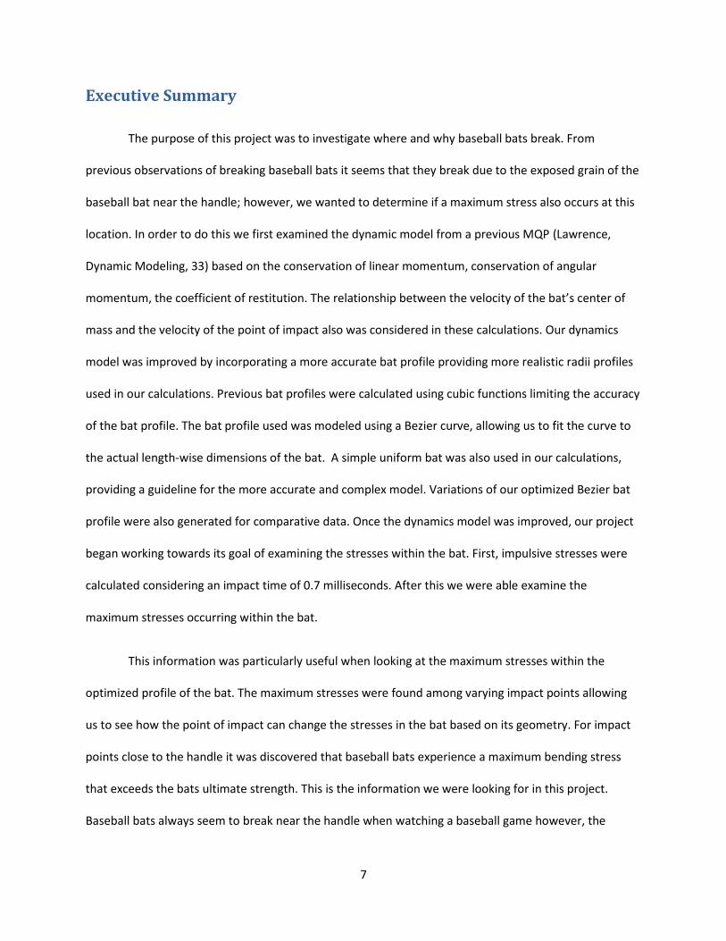
The purpose of this project was to investigate where and why baseball bats break. From

previous observations of breaking baseball bats it seems that they break due to the exposed grain of the

baseball bat near the handle; however, we wanted to determine if a maximum stress also occurs at this

location. In order to do this we first examined the dynamic model from a previous MQP (Lawrence,

Dynamic Modeling, 33) based on the conservation of linear momentum, conservation of angular

momentum, the coefficient of restitution. The relationship between the velocity of the bat’s center of

mass and the velocity of the point of impact also was considered in these calculations. Our dynamics

model was improved by incorporating a more accurate bat profile providing more realistic radii profiles

used in our calculations. Previous bat profiles were calculated using cubic functions limiting the accuracy

of the bat profile. The bat profile used was modeled using a Bezier curve, allowing us to fit the curve to

the actual length-wise dimensions of the bat. A simple uniform bat was also used in our calculations,

providing a guideline for the more accurate and complex model. Variations of our optimized Bezier bat

profile were also generated for comparative data. Once the dynamics model was improved, our project

began working towards its goal of examining the stresses within the bat. First, impulsive stresses were

calculated considering an impact time of 0.7 milliseconds. After this we were able examine the

maximum stresses occurring within the bat.

This information was particularly useful when looking at the maximum stresses within the

optimized profile of the bat. The maximum stresses were found among varying impact points allowing

us to see how the point of impact can change the stresses in the bat based on its geometry. For impact

points close to the handle it was discovered that baseball bats experience a maximum bending stress

that exceeds the bats ultimate strength. This is the information we were looking for in this project.

Baseball bats always seem to break near the handle when watching a baseball game however, the

8

reason for this could not be attributed to the weak point of the bat caused by the exposed grain of the

wood or if that bat actually experienced a maximum stress at this point. This analytical research shows

that a maximum stress does occur at 10.1 inches regardless of the exposed grain. Therefore we were

able to appropriately hypothesize that the maximum stresses and exposed grain both play a part in why

baseball bats break.

9

Chapter 1: Introduction

When a baseball player swings a bat “just right” the contact between the bat and the ball sends

the ball off at a maximum velocity for maximum distance. This contact point is known as the “sweet

spot” or in technical terms where the least amount of force from the bat is lost due to vibrations and

other variables during impact. When a baseball player contacts the bat to the ball inside the “sweet

spot” nearer the handle losses are sent throughout the bat in the form of stresses to the point where

the wooden bat is likely to break.

Wooden baseball bats have been known to break throughout the history of the sport however;

changes in the material and design of the bat have changed the frequency of these occurrences over the

years. Since 2001 the Major League Baseball has been using maple bats instead of the previously

preferred ash bats because of a record breaking homerun made by Barry Bonds in that year (Crane,

Science World 16). Also since then a rise in the number of bats breaking and injuries caused by the

debris has forced researcher’s to investigate why bats break. From this research many have found the

reason for the problem is caused by the slope of the grain in the wood (Crane, Science World 16). This

study delves further into understanding the stresses in the baseball bats that allow the bats to break.

Using a dynamic model of the impact between baseballs and bats we can begin to understand where

and why baseball bats break.

1.1 Review of Previous Work

Previous work done on collisions between baseballs and bats have defined the approach used

here for investigating where the highest impact stresses on a baseball bat occur. This section describes

the methods used in previous work that apply to this project. Based on previous work we began

calculations using a simplified case meaning a one–dimensional rigid body application. The calculation

10

for the simplified case only takes masses, initial velocities, and conservation of momentum into

consideration. However, these results are only approximate and not applicable to any real-world

application.

To create a more accurate model for real-world application many more factors need to be

considered. A coefficient of restitution is used for describing energy lost in vibrations and an effective

mass is considered because the bat and ball do not collide at the bats center of mass (Cross 2008b,

Russell 2008b). Using calculations in previous work we also considered the moment of inertia of the bat

and the maximum forced caused by the collision of the baseball and bat (Russell 2008a). After a rigid

body model is completed a dynamic model of the collision is also conducted to further the accuracy of

the results. The equations for both a rigid and dynamic model were taken from the project Dynamic

Modeling of Wooden Baseball Bats. This previous study focused on creating greater exit velocities of

baseballs due to the geometry of the bat. This means the geometry was altered for that purpose. The

purpose of this project is to determine where baseballs break due to the collision so optimal conditions

for geometry, mass, moment of inertia, and stresses were used. Using the equations in these previous

works we can find where the stresses are maximum in an effort to determine where and why baseball

bats break.

1.2 Further Work to Perform

Baseball is considered by many to be one of America’s greatest pastimes and because of this

anyone with interest in the sport ranging from the typical fan to the professional player has analyzed

how the game works. It is generally accepted that the interaction between the baseball bat and ball play

a major part in the game. Thus, the design and material used to make a baseball bat have been altered

over the years. Previous work has analyzed how the shape and other properties of the bat can be

11

altered to improve the exit velocity of the baseball from its collision with the bat. Here we use a

dynamic analysis of a designed bat profile to analyze why baseball bats break.

The goal of this project is to develop a mathematical model of where baseball bats break based

on their geometry and varying impact points. The first step involved reanalyzing the geometry of the

bat from previous work. In previous projects, bats were designed based off a cubic shape. However, for

the sake of a more accurate shape our geometry was designed using a Bezier curve which will later be

explained in full detail. However, we developed multiple geometries including the optimal bat shape to

help gain an understanding of how the bats size and shape affect the stresses acting within the baseball

bat.

Using the optimal geometry impact points were varied and evaluated using our dynamics model

to find out how the different impact points affect where and why a baseball bat breaks. The majority of

our findings are listed in shear force and bending diagrams showing when the stresses surpass the point

where the bat can withstand the force without breaking. Using this information will allow us to

understand why baseball bats break due to the stresses occurring within them.

12

Chapter 2: Geometry of the Bat Profile

One of the more important properties of wooden baseball bats is the radial profile of the bat.

As researched in previous works, it affects the important variables of the bat such as the mass, location

of the center of mass, the moment of inertia about the end of the bat, and the moment of inertia about

the center of mass. These variables in turn affect the efficiencies of the bat as well as how the bat and

ball will react after the bat-ball collision. As we found out during our research these variables have a lot

of influence over our values for the impact stresses on the bat. Any improvement on the radial profile

from previous research would be a great improvement on the resulting impact stresses. Descriptions of

the previous work as well as our improvements on it are discussed in this section.

2.1 Previous Profile

One of the key aspects to analyzing the stresses induced within the bat during impact was

creating an accurate function for the radius of the bat itself. This function (a function of the length of

the bat) can be used to accurately measure the radius at any point along the length of the bat to

determine a precise cross-sectional area that the forces act upon. Previous MQP’s have struggled with

mapping an accurate radius profile function and ended up using “optimized” models with barrels that

are too thick and handles that are too thin. This occurred mostly due to the fact that the previous MQP

teams used cubic equations to map their bat profiles. To find the coefficients of the cubic polynomial,

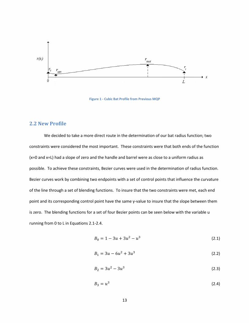
the solution was simply iterated until the profile of the bat looked reasonable. An example of the cubic

bat profile used in the previous MQP can be seen below in Figure 1.

13

Figure 1 - Cubic Bat Profile from Previous MQP

2.2 New Profile

We decided to take a more direct route in the determination of our bat radius function; two

constraints were considered the most important. These constraints were that both ends of the function

(x=0 and x=L) had a slope of zero and the handle and barrel were as close to a uniform radius as

possible. To achieve these constraints, Bezier curves were used in the determination of radius function.

Bezier curves work by combining two endpoints with a set of control points that influence the curvature

of the line through a set of blending functions. To insure that the two constraints were met, each end

point and its corresponding control point have the same y-value to insure that the slope between them

is zero. The blending functions for a set of four Bezier points can be seen below with the variable u

running from 0 to L in Equations 2.1-2.4.

(2.1)

(2.2)

(2.3)

(2.4)

14

The blending functions shown above each have a corresponding control point. The value

calculated in each blending function would be multiplied by the x and y values of its corresponding

control point with being for control point , for , and so on. The products of this multiplication

are the x and y coordinates of the controlled line. An example for the calculation of the x and y

coordinates for an arbitrary value of u can be seen below in Equation (2.5) and Equation (2.6).

( ( )) ( ( )) ( ( )) ( ( )) (2.5)

( ( )) ( ( )) ( ( )) ( ( )) (2.6)

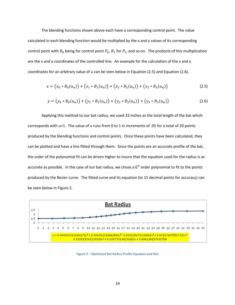
Applying this method to our bat radius, we used 33 inches as the total length of the bat which

corresponds with u=1. The value of u runs from 0 to 1 in increments of .05 for a total of 20 points

produced by the blending functions and control points. Once these points have been calculated, they

can be plotted and have a line fitted through them. Since the points are an accurate profile of the bat,

the order of the polynomial fit can be driven higher to insure that the equation used for the radius is as

accurate as possible. In the case of our bat radius, we chose a 6th order polynomial to fit to the points

produced by the Bezier curve. The fitted curve and its equation (to 15 decimal points for accuracy) can

be seen below in Figure 2.

Figure 2 – Optimized Bat Radius Profile Equation and Plot

15

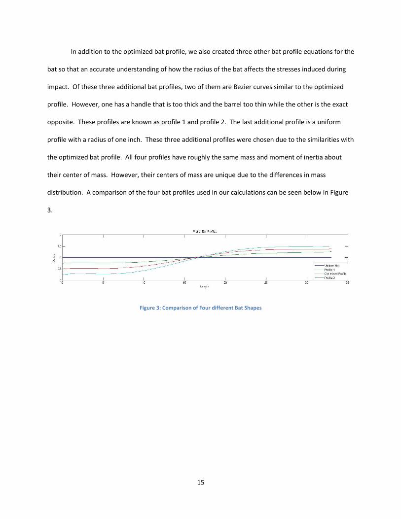
In addition to the optimized bat profile, we also created three other bat profile equations for the

bat so that an accurate understanding of how the radius of the bat affects the stresses induced during

impact. Of these three additional bat profiles, two of them are Bezier curves similar to the optimized

profile. However, one has a handle that is too thick and the barrel too thin while the other is the exact

opposite. These profiles are known as profile 1 and profile 2. The last additional profile is a uniform

profile with a radius of one inch. These three additional profiles were chosen due to the similarities with

the optimized bat profile. All four profiles have roughly the same mass and moment of inertia about

their center of mass. However, their centers of mass are unique due to the differences in mass

distribution. A comparison of the four bat profiles used in our calculations can be seen below in Figure

3.

Figure 3: Comparison of Four different Bat Shapes

16

Chapter 3: Rigid Body Dynamics

This chapter’s focus is on the instantaneous collision between a wooden baseball bat and a

baseball. During the impact the bat and ball move in the same plane, and the velocity of the ball just

prior to impact is perpendicular to the longitudinal axis of the bat. Some of the important variables

when doing the dynamic modeling are: the mass of the ball, , the velocity of the ball prior to impact,

, the length of the bat, , the mass of the bat, , the moment of inertia about the center of mass of

the bat, , the angular velocity of the bat prior to impact, . The center of rotation of the bat is actually

off the bat along the longitudinal axis at a distance of . The x-coordinate measures distance along the

bat from the knob from zero to the length of the bat, so that the x-coordinate of the center of mass of

the bat is , and the y-coordinate measures the distance along the bat from the center of mass (so that

). This means that the x- and y- coordinates are related by:

. (3.1)

The velocity, , of the center of mass of the bat prior to impact is:

( ) . (3.2)

An important aspect of this analysis is knowing that the location of the center of rotation changes from

the initial center of rotation after the bat-ball impact.

Dynamic modeling requires focusing on collision in which the point of impact between the ball

and the bat is at a location from the center of mass. The velocity of the contact point on the bat

prior to impact is:

, (3.3)

where depends on as well according Equation (3.2).

17

Typically, the mass of the ball, the mass of the bat, the location of the center of

mass as well as the moment of inertia about the center of mass of the bat are all known variables.

Also known variables are the incoming velocity of the ball, the location (or when it is a variable

later in the analysis) of the contact point, the location of the center of rotation of the bat prior to

impact as well as the angular velocity of the bat prior to impact. Analysis of the rigid body dynamics

can be used to predict the outgoing velocity of the ball, the velocity of the contact point after

impact, the velocity of the center of mass of the bat after impact, the angular velocity of the bat

after impact and the distance (positively measured off the knob of the bat) from the end of the bat to

the center of rotation of the bat after impact.

Since the impulsive force between the bat and the ball, as seen in the following chapters, is so

much larger than the forces exerted by a batter on the bat during the impact, the forces of the batter

can be neglected during the analysis of the dynamics of the bat-ball collision. This means that the bat is

essentially free of external forces when it hits the ball. The conservation of linear momentum dictates

that:

, (3.4)

meanwhile the conservation of angular momentum about the center of mass of the bat requires that:

. (3.5)

The coefficient of restitution is the energy lost in the collision, and is simply the ratio of outgoing

relative velocity to the incoming relative velocity as seen in Equation (3.6),

( )

. (3.6)

18

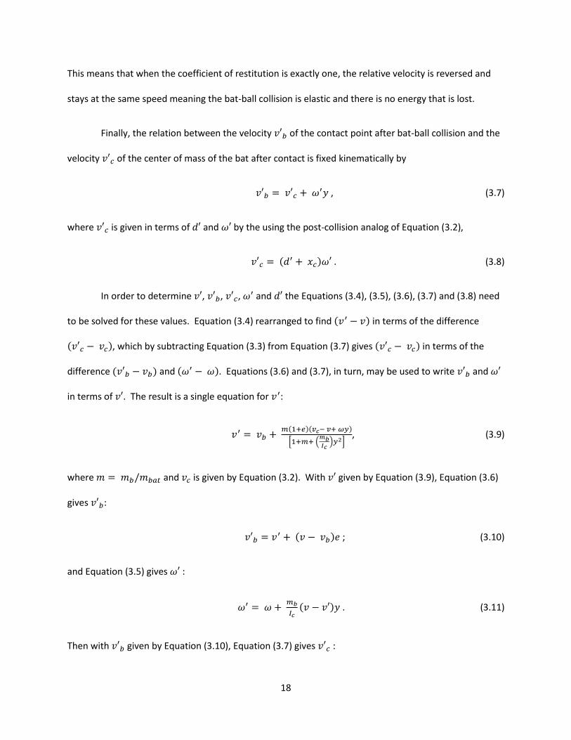
This means that when the coefficient of restitution is exactly one, the relative velocity is reversed and

stays at the same speed meaning the bat-ball collision is elastic and there is no energy that is lost.

Finally, the relation between the velocity of the contact point after bat-ball collision and the

velocity of the center of mass of the bat after contact is fixed kinematically by

, (3.7)

where is given in terms of and by the using the post-collision analog of Equation (3.2),

( ) . (3.8)

In order to determine , , , and the Equations (3.4), (3.5), (3.6), (3.7) and (3.8) need

to be solved for these values. Equation (3.4) rearranged to find ( ) in terms of the difference

( ), which by subtracting Equation (3.3) from Equation (3.7) gives ( ) in terms of the

difference ( ) and ( ). Equations (3.6) and (3.7), in turn, may be used to write and

in terms of . The result is a single equation for :

( )( )

0 .

/ 1, (3.9)

where and is given by Equation (3.2). With given by Equation (3.9), Equation (3.6)

gives :

( ) ; (3.10)

and Equation (3.5) gives :

( ) . (3.11)

Then with given by Equation (3.10), Equation (3.7) gives :

19

(3.12)

And with given by Equation (3.12) and given by Equation (3.11), Equation (3.8) gives :

. (3.13)

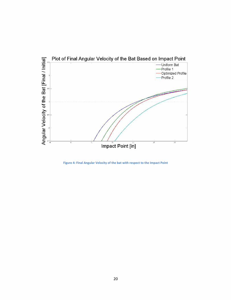
Figure 4 shows the ratio of the final angular velocity of the bat to the initial angular velocity for

all four bat profiles with an impact point of 27 inches. Figure 5 shows the ratio of the outgoing ball

velocity to the incoming ball velocity for all four bat profiles with an impact point of 27 inches.

20

Figure 4: Final Angular Velocity of the bat with respect to the Impact Point

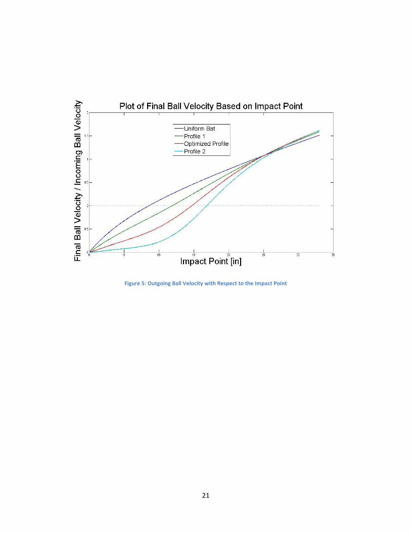
21

Figure 5: Outgoing Ball Velocity with Respect to the Impact Point

22

The focus of this project is not to analyze the dynamics of a bat-ball collision, rather it is to

understand the stresses that the bat-ball collision impart on the bat internally in order to understand

why wooden baseball bats break. The rigid body dynamics are pivotal in the calculation of the stresses

and therefore must be understood. The following chapters dive deeper into the stresses and more

analysis than the dynamics.

23

Chapter 4: Impulsive Shear Force and Bending Moment

In order to calculate the internal stresses on wooden baseball bats during the bat-ball collision

one must first discuss the shear stress and the bending moment. In a collision the force that the ball

exerts on the bat is extremely high, as well as being an impulsive force. This means that the force is not

constant but rather imparts a force that increases and reaches a maximum half way through the

impulsive collision and the last half decreases back to zero. In order to eliminate these complicating

factors involved with calculating the shear force and bending moment we calculated the impulsive shear

force and the impulsive bending moment. This means that we divide the shear force and bending

moment by the time of impact. The reason for doing this is that when researching impact times for the

bat-ball collision the times varied from four milliseconds to seven tenths of a millisecond (Russell, Elert).

This also allows us to use an average impact force rather than using a more complicated formula for the

impact force. In order to find the impulsive shear force and bending moment you must look at a section

of the bat to the left of the impact point as well as a section cut off to the right of the impact point.

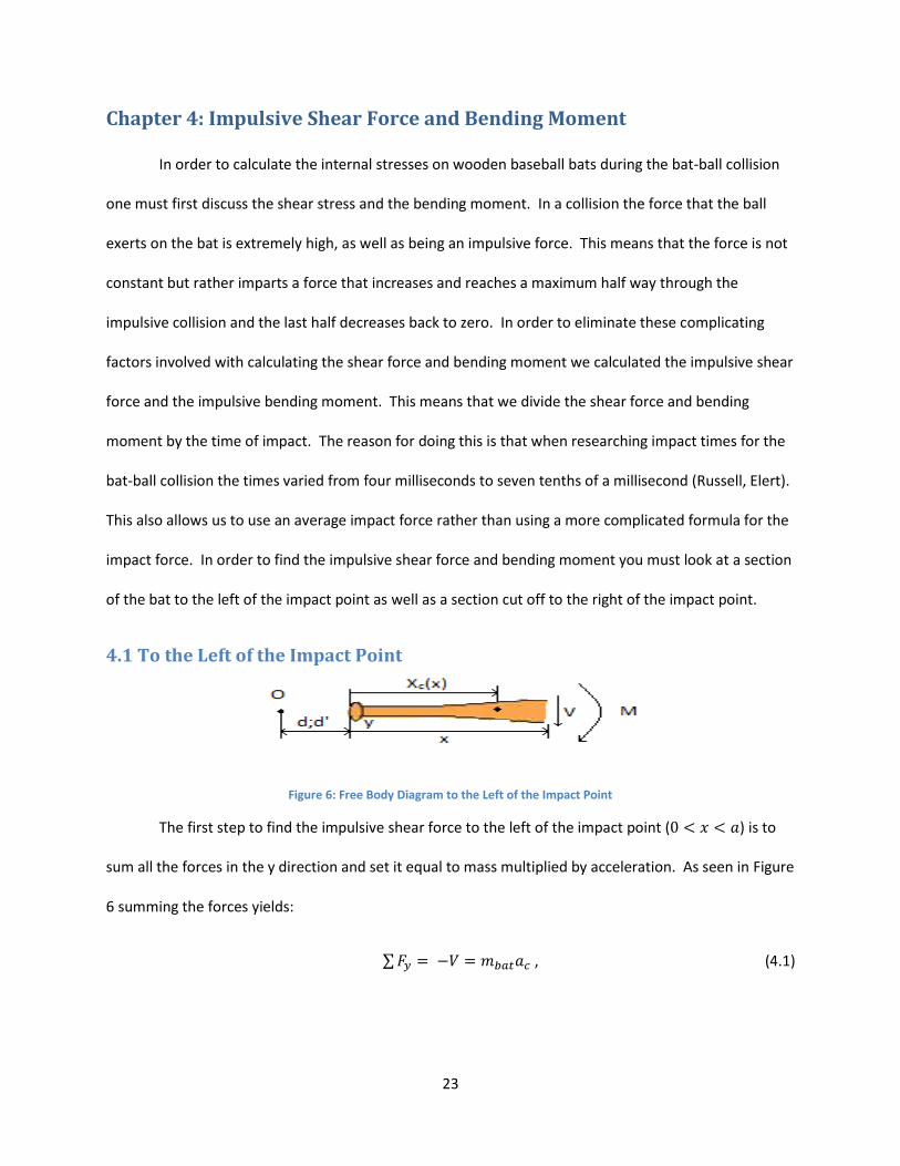
4.1 To the Left of the Impact Point

Figure 6: Free Body Diagram to the Left of the Impact Point

The first step to find the impulsive shear force to the left of the impact point ( ) is to

sum all the forces in the y direction and set it equal to mass multiplied by acceleration. As seen in Figure

6 summing the forces yields:

, (4.1)

24

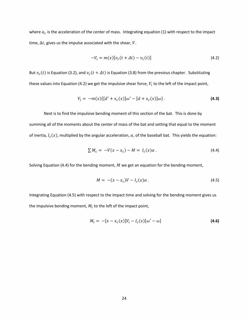
where is the acceleration of the center of mass. Integrating equation (1) with respect to the impact

time, , gives us the impulse associated with the shear, .

( ), ( ) ( )- (4.2)

But ( ) is Equation (3.2), and ( ) is Equation (3.8) from the previous chapter. Substituting

these values into Equation (4.2) we get the impulsive shear force, to the left of the impact point,

( )*, ( )- , ( )- + . (4.3)

Next is to find the impulsive bending moment of this section of the bat. This is done by

summing all of the moments about the center of mass of the bat and setting that equal to the moment

of inertia, ( ), multiplied by the angular acceleration, , of the baseball bat. This yields the equation:

( ) ( ) . (4.4)

Solving Equation (4.4) for the bending moment, we get an equation for the bending moment,

( ) ( ) . (4.5)

Integrating Equation (4.5) with respect to the impact time and solving for the bending moment gives us

the impulsive bending moment, to the left of the impact point,

, ( )- ( ), - (4.6)

25

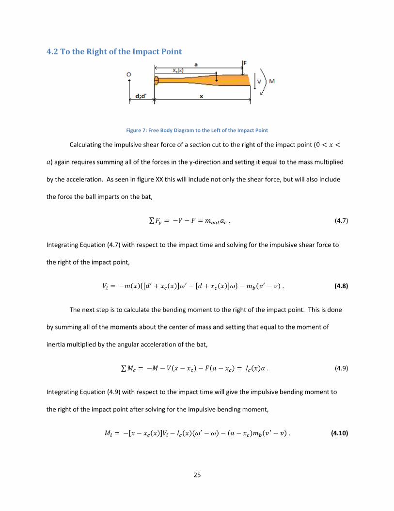
4.2 To the Right of the Impact Point

Figure 7: Free Body Diagram to the Left of the Impact Point

Calculating the impulsive shear force of a section cut to the right of the impact point (

) again requires summing all of the forces in the y-direction and setting it equal to the mass multiplied

by the acceleration. As seen in figure XX this will include not only the shear force, but will also include

the force the ball imparts on the bat,

. (4.7)

Integrating Equation (4.7) with respect to the impact time and solving for the impulsive shear force to

the right of the impact point,

( )*, ( )- , ( )- + ( ) . (4.8)

The next step is to calculate the bending moment to the right of the impact point. This is done

by summing all of the moments about the center of mass and setting that equal to the moment of

inertia multiplied by the angular acceleration of the bat,

( ) ( ) ( ) . (4.9)

Integrating Equation (4.9) with respect to the impact time will give the impulsive bending moment to

the right of the impact point after solving for the impulsive bending moment,

, ( )- ( )( ) ( ) ( ) . (4.10)

26

Equations (4.3), (4.6), (4.8) and (4.10) are the most important equations moving forward to find

the internal impact stresses of wooden baseball bats during the bat-ball collision.

4.3 Results

These impulsive shear force and bending moments provide insight into where wooden baseball

bats have the highest stresses. In this chapter we will look at how different radial profiles, different

impact points as well as different angular speeds of the bat will affect the magnitude of the impulsive

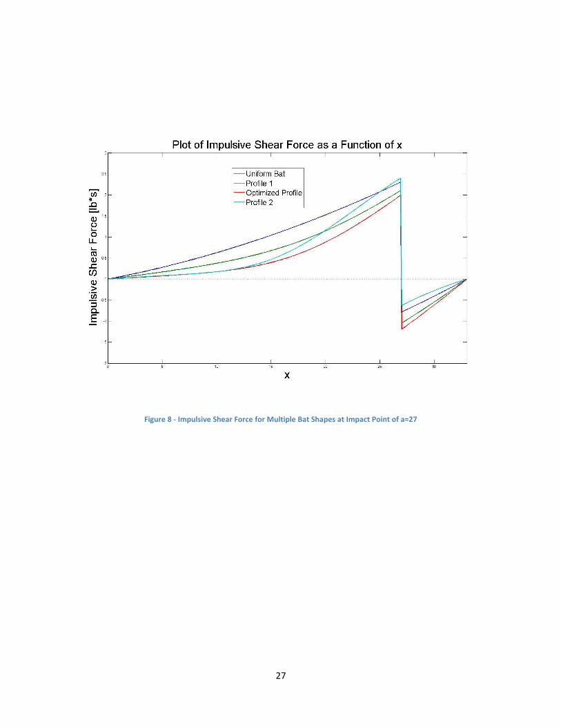
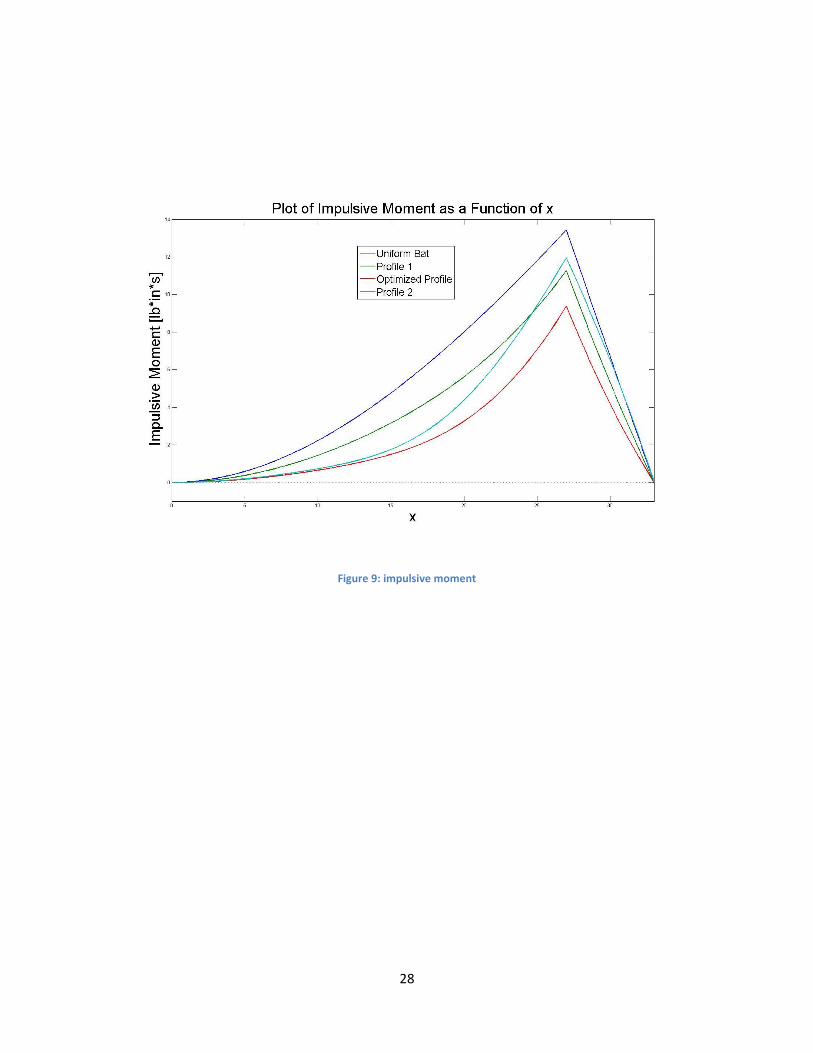
shear force and bending moment along the length of the bat. Figure 8 shows the impulsive shear force

along the length of the bat for the four different bat shapes discussed in chapter 2. Figure 9 shows the

impulsive bending moment of the four different radial profiles along the length of the bat. As you can

see the optimal radial profile has the lowest impulsive shear force and impulsive bending moment of all

the bats. This result was expected.

27

Figure 8 - Impulsive Shear Force for Multiple Bat Shapes at Impact Point of a=27

28

Figure 9: impulsive moment

29

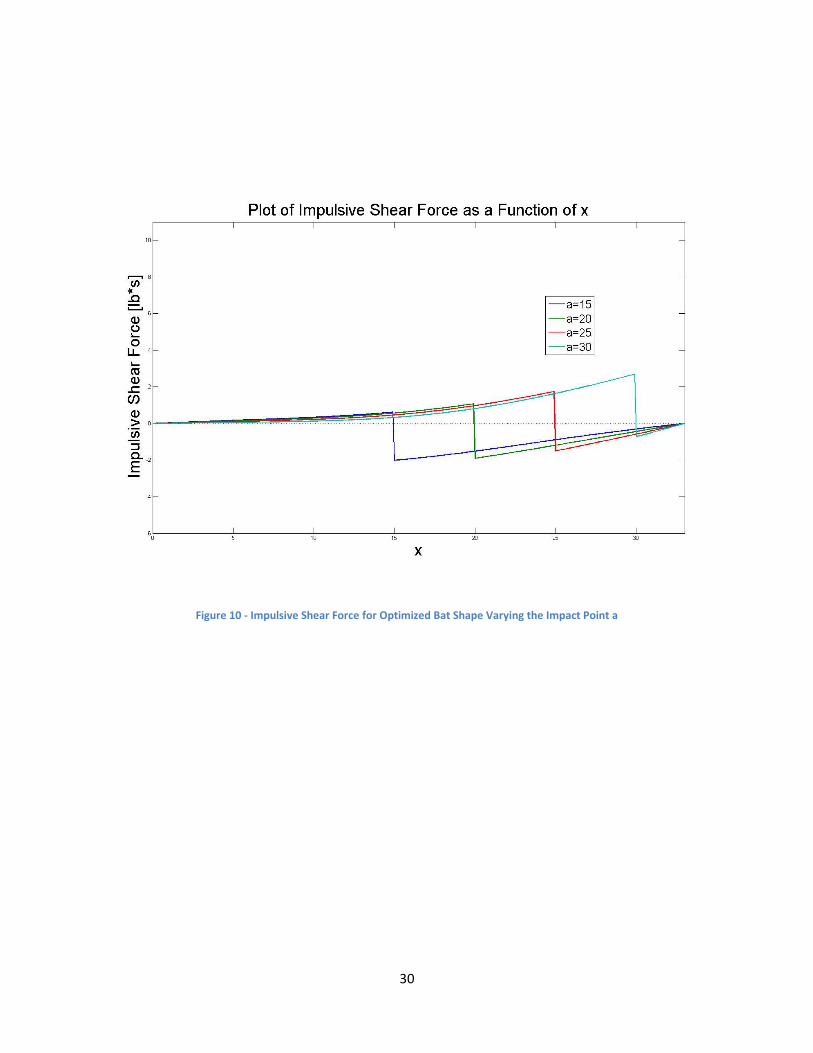
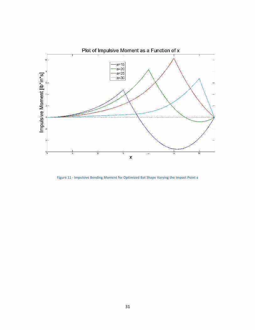
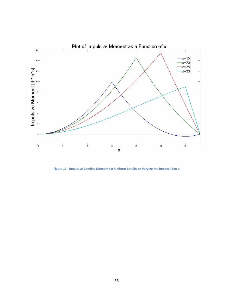
Figures 10 and 11 show that as the impact point moves closer to the handle of the bat the

impulsive shear stresses and bending moments actually become smaller, this seems a little

counterintuitive but these calculations do not take into consideration the radial profile of the bat.

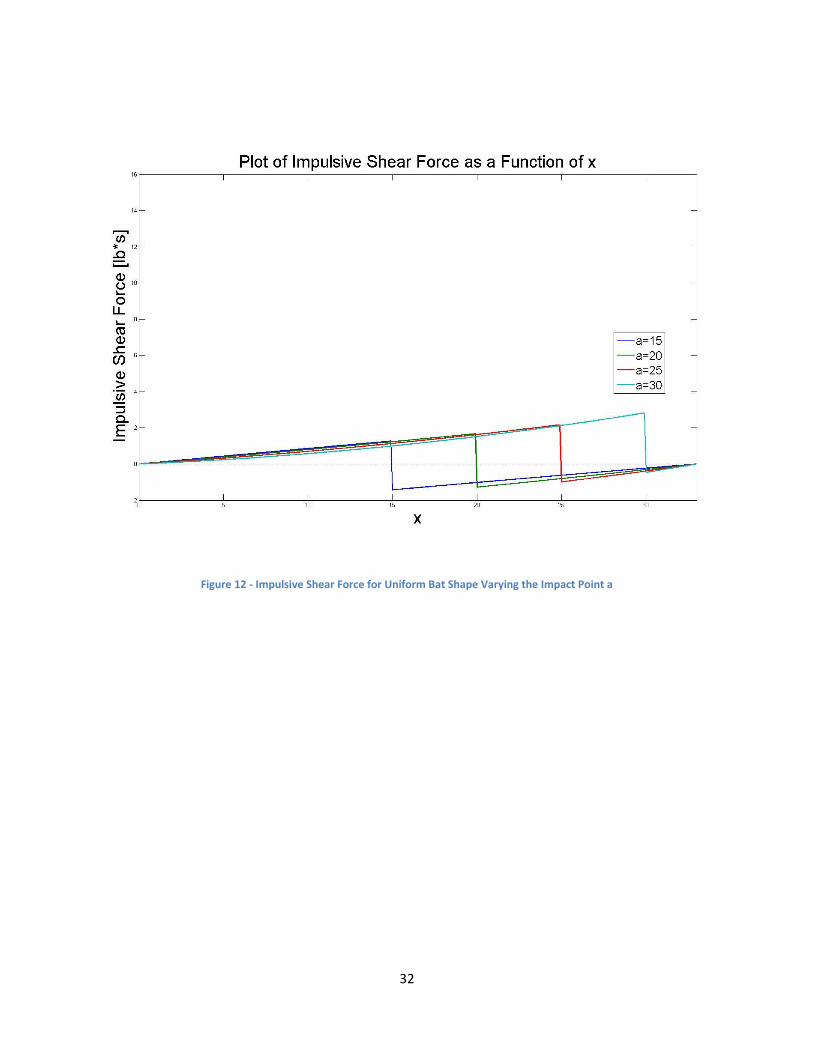
Figures 12 and 13 show that the same thing happens for a uniform radial profile of a bat, these

calculations still do not consider the changing radial profile of the bat at the handle and the barrel.

30

Figure 10 - Impulsive Shear Force for Optimized Bat Shape Varying the Impact Point a

31

Figure 11 - Impulsive Bending Moment for Optimized Bat Shape Varying the Impact Point a

32

Figure 12 - Impulsive Shear Force for Uniform Bat Shape Varying the Impact Point a

33

Figure 13 - Impulsive Bending Moment for Uniform Bat Shape Varying the Impact Point a

34

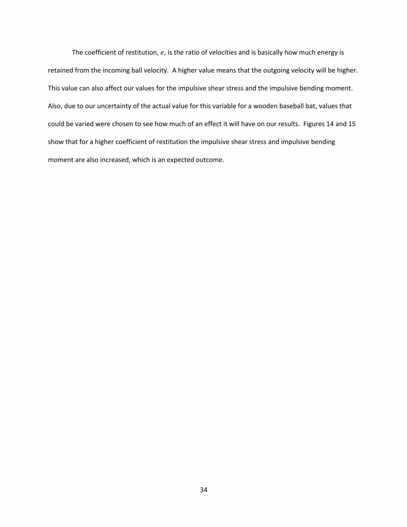
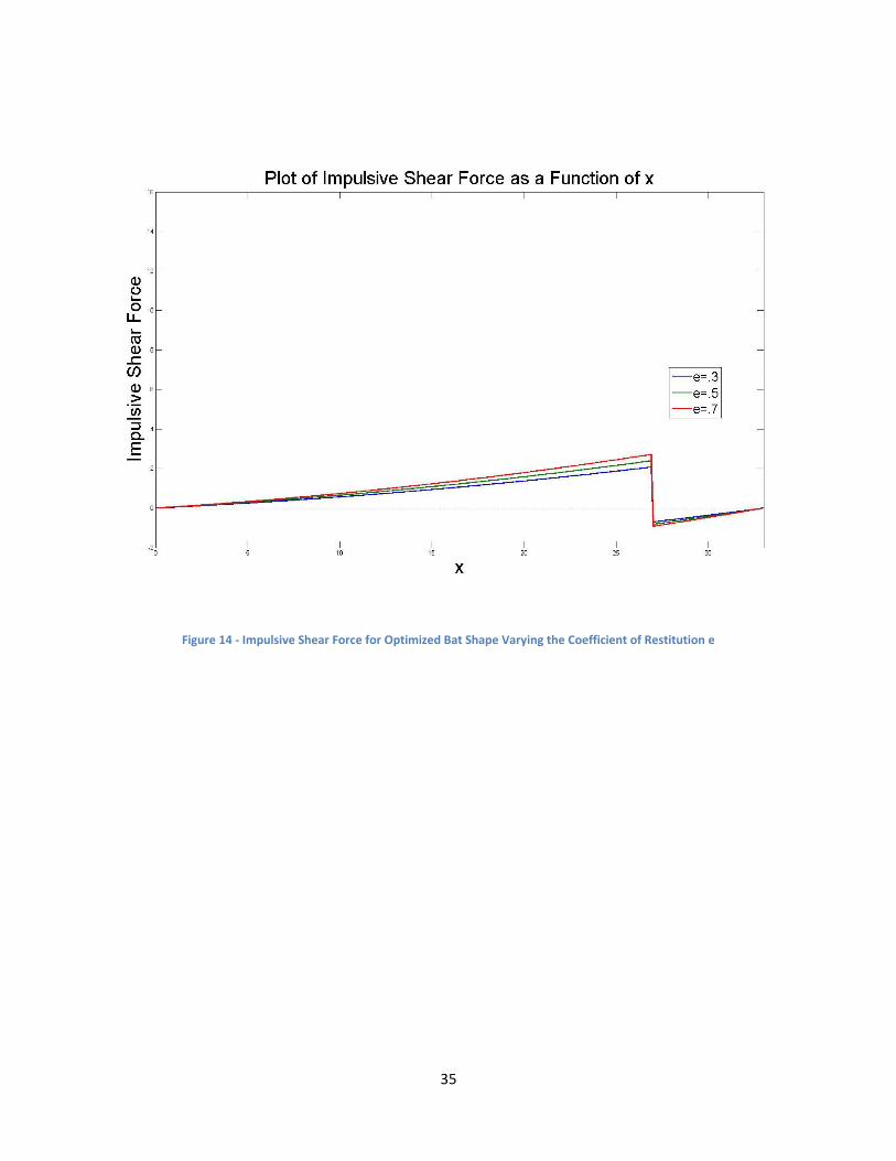
The coefficient of restitution, , is the ratio of velocities and is basically how much energy is

retained from the incoming ball velocity. A higher value means that the outgoing velocity will be higher.

This value can also affect our values for the impulsive shear stress and the impulsive bending moment.

Also, due to our uncertainty of the actual value for this variable for a wooden baseball bat, values that

could be varied were chosen to see how much of an effect it will have on our results. Figures 14 and 15

show that for a higher coefficient of restitution the impulsive shear stress and impulsive bending

moment are also increased, which is an expected outcome.

35

Figure 14 - Impulsive Shear Force for Optimized Bat Shape Varying the Coefficient of Restitution e

36

Figure 15 - Impulsive Bending Moment for Optimized Bat Shape Varying Coefficient of Restitution e

37

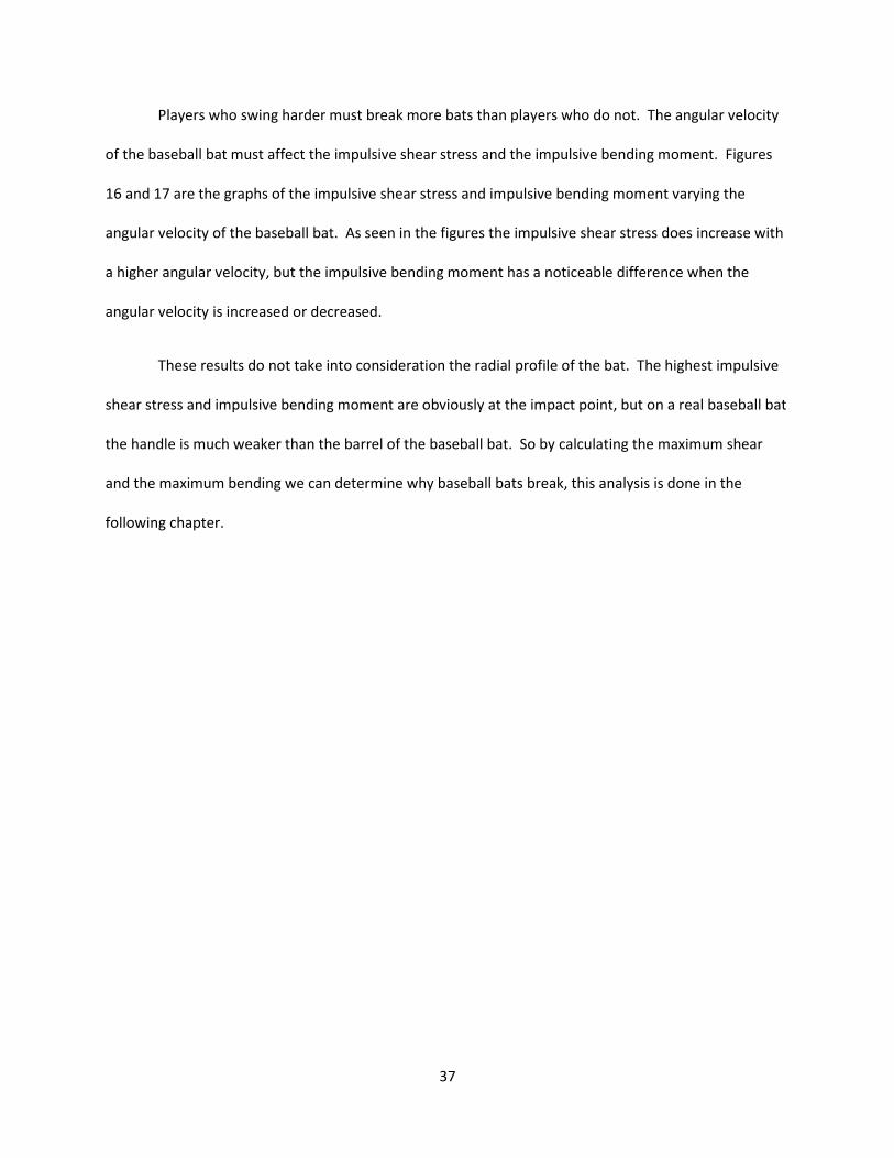
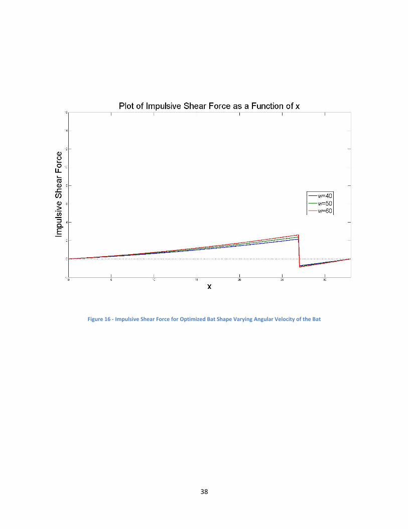
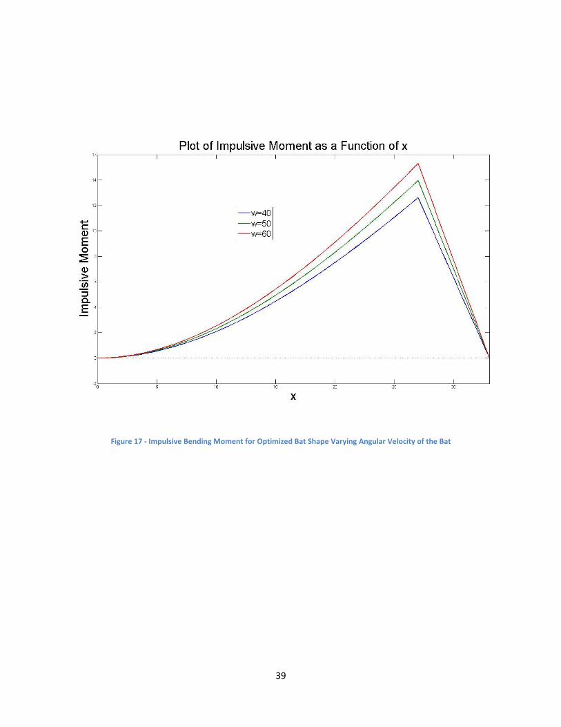
Players who swing harder must break more bats than players who do not. The angular velocity

of the baseball bat must affect the impulsive shear stress and the impulsive bending moment. Figures

16 and 17 are the graphs of the impulsive shear stress and impulsive bending moment varying the

angular velocity of the baseball bat. As seen in the figures the impulsive shear stress does increase with

a higher angular velocity, but the impulsive bending moment has a noticeable difference when the

angular velocity is increased or decreased.

These results do not take into consideration the radial profile of the bat. The highest impulsive

shear stress and impulsive bending moment are obviously at the impact point, but on a real baseball bat

the handle is much weaker than the barrel of the baseball bat. So by calculating the maximum shear

and the maximum bending we can determine why baseball bats break, this analysis is done in the

following chapter.

38

Figure 16 - Impulsive Shear Force for Optimized Bat Shape Varying Angular Velocity of the Bat

39

Figure 17 - Impulsive Bending Moment for Optimized Bat Shape Varying Angular Velocity of the Bat

40

Chapter 5: Shear and Bending Stresses

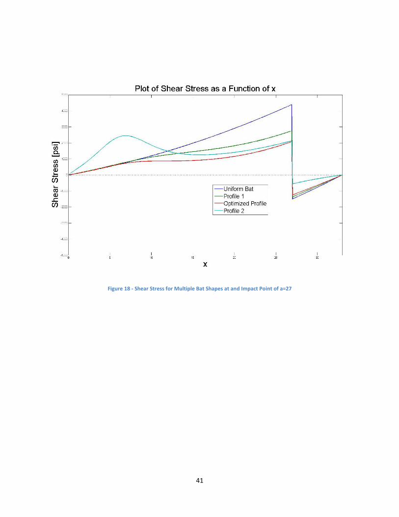
Finally, the maximum shear and bending stresses were calculated. The maximum shear stresses

were calculated first for all four of the bats we designed. These calculations showed that our optimized

bat experienced the smallest maximum shear stresses while our uniform bat experienced the greatest

maximum shear stresses. However, none of the maximum stresses shown occurring at this impact point

can break the bat based on its material properties. The maximum shear stresses are calculated using

the following equations:

( ) ( )

( ) ( ) (5.1)

Substitute:

( )

( )

( )

( )

( ) (5.2)

( )

( ) (5.3)

Into shear stress equation:

( )

( )

( ) ( )

(5.4)

Simplify:

( )

( ) (5.5)

In these equations ( ) represents shear force while ( ) represents the moment of inertia

about y. Figure 18 below shows the maximum shear stresses occurring along each of the four bats

examined at the impact point of 27 inches. This impact point is often called the “sweet spot” or the

impact point that produce the highest ball exit velocities.

41

Figure 18 - Shear Stress for Multiple Bat Shapes at and Impact Point of a=27

42

After we calculated the maximum shear stresses for each of the four bats with the impact point

occurring at the “sweet spot” we calculated the same for the maximum bending stresses. The equations

below show how the maximum bending stresses were calculated. In these equations bending moment

is represented by ( ).

( ) ( )

( ) (5.6)

Substitute:

( ) ( ) (5.7)

( )

( ) (5.8)

Into bending stress equation:

( ) ( )

( ) (5.9)

Simplify:

( )

( ) (5.10)

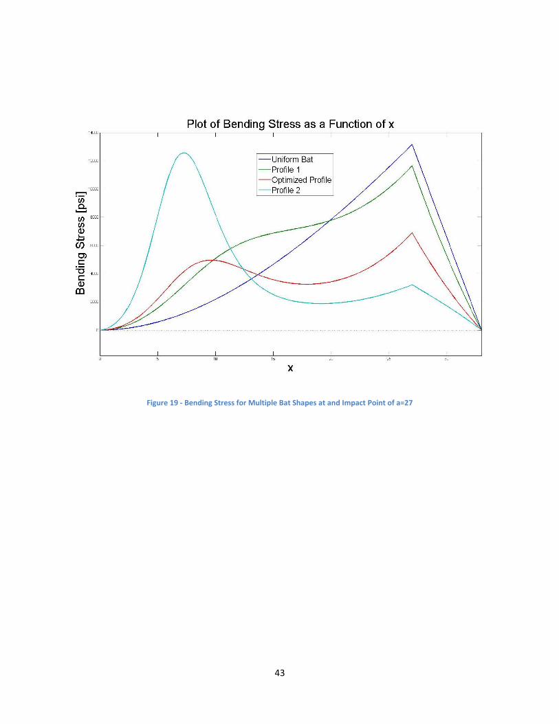
The bending stress for all of the different bat shapes can be seen below in Figure 19. It is

interesting to note the unique relationship between the bat handle radius and the stress. From this

graph you can see that our optimized bat experienced the lowest maximum stresses while the uniform

bat and the other two altered profiles experienced much greater maximum bending stresses.

43

Figure 19 - Bending Stress for Multiple Bat Shapes at and Impact Point of a=27

44

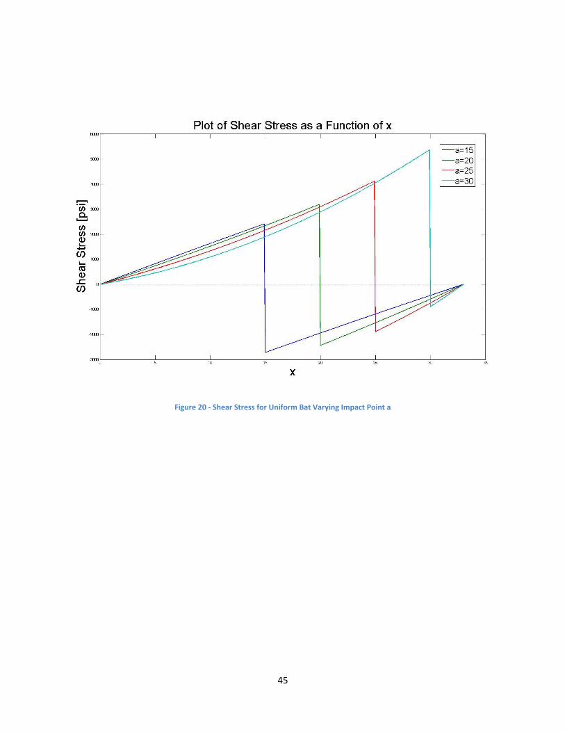
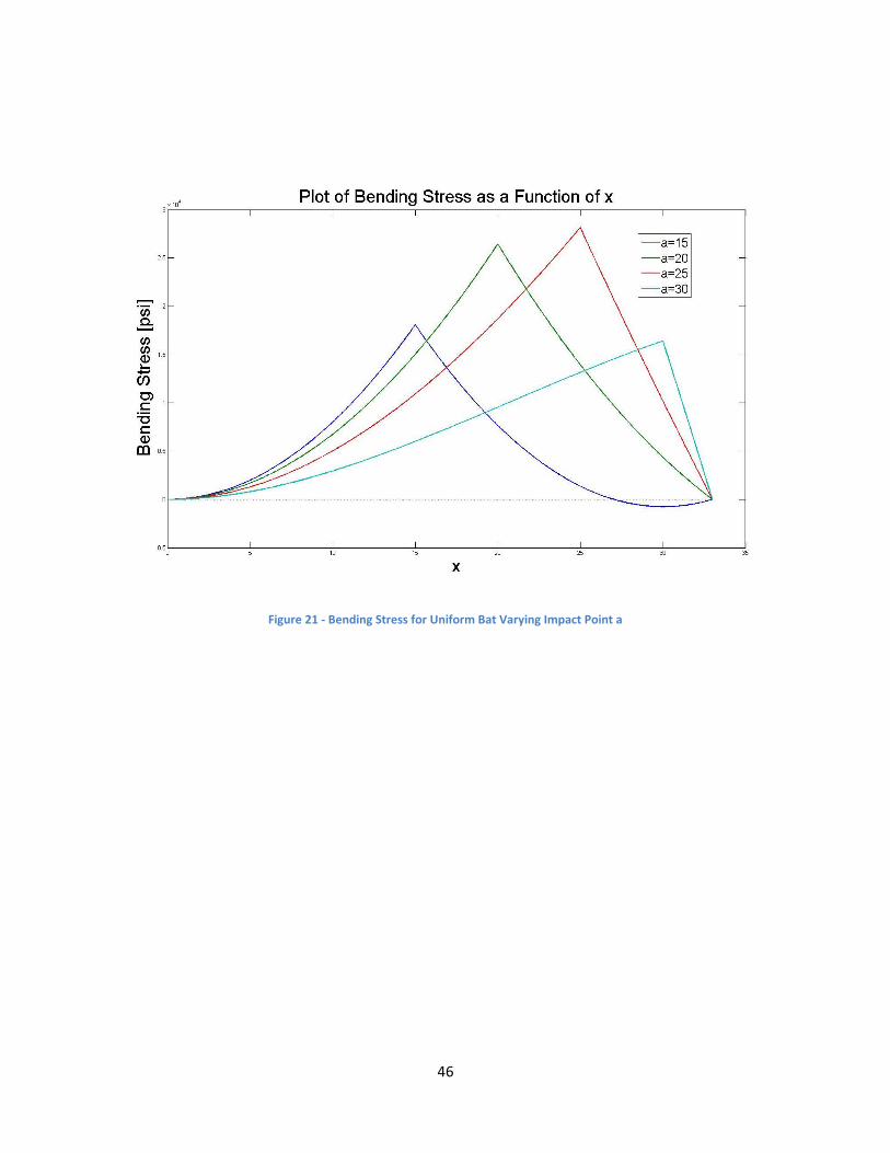
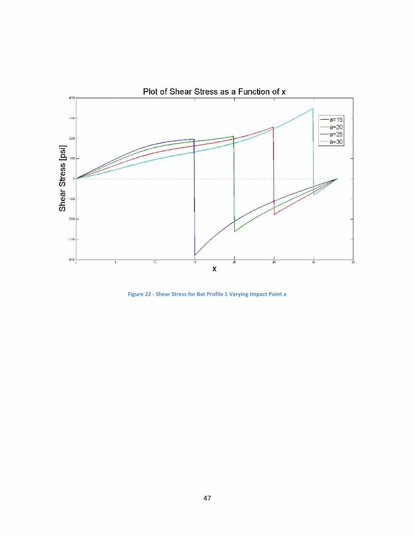
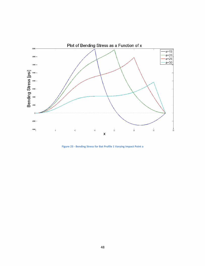
Now that there is a comparison between how the maximum stresses differ between each bat

we can plot and observe the behavior of the stresses and how the maximum stress will differ using

various impact points. Using the equations for maximum shear and bending stresses, each of the bat

profiles were plotted against different impact points. Most of these graphs have similar shapes however

what provides interesting data are the maximum stresses occurring on the optimized bat profile. The

graphs of the other bat profiles show how slight changes in shape can increase the stresses the bat

experiences greatly. The stresses for the other bat profiles could easily break the bat, often regardless of

the impact point. The two altered profiles have graphs that look very similar to the optimized profile

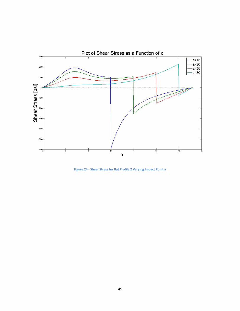
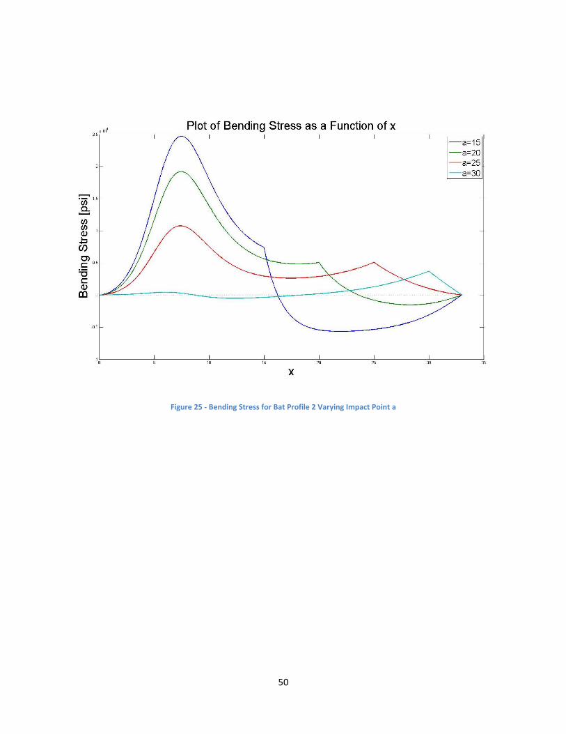
because they consist of the same general shape with different sized handles and barrels. In Figures 20-

25, the shear and bending stresses are plotted for the uniform bat, bat profile 1, and bat profile 2.

45

Figure 20 - Shear Stress for Uniform Bat Varying Impact Point a

46

Figure 21 - Bending Stress for Uniform Bat Varying Impact Point a

47

Figure 22 - Shear Stress for Bat Profile 1 Varying Impact Point a

48

Figure 23 - Bending Stress for Bat Profile 1 Varying Impact Point a

49

Figure 24 - Shear Stress for Bat Profile 2 Varying Impact Point a

50

Figure 25 - Bending Stress for Bat Profile 2 Varying Impact Point a

51

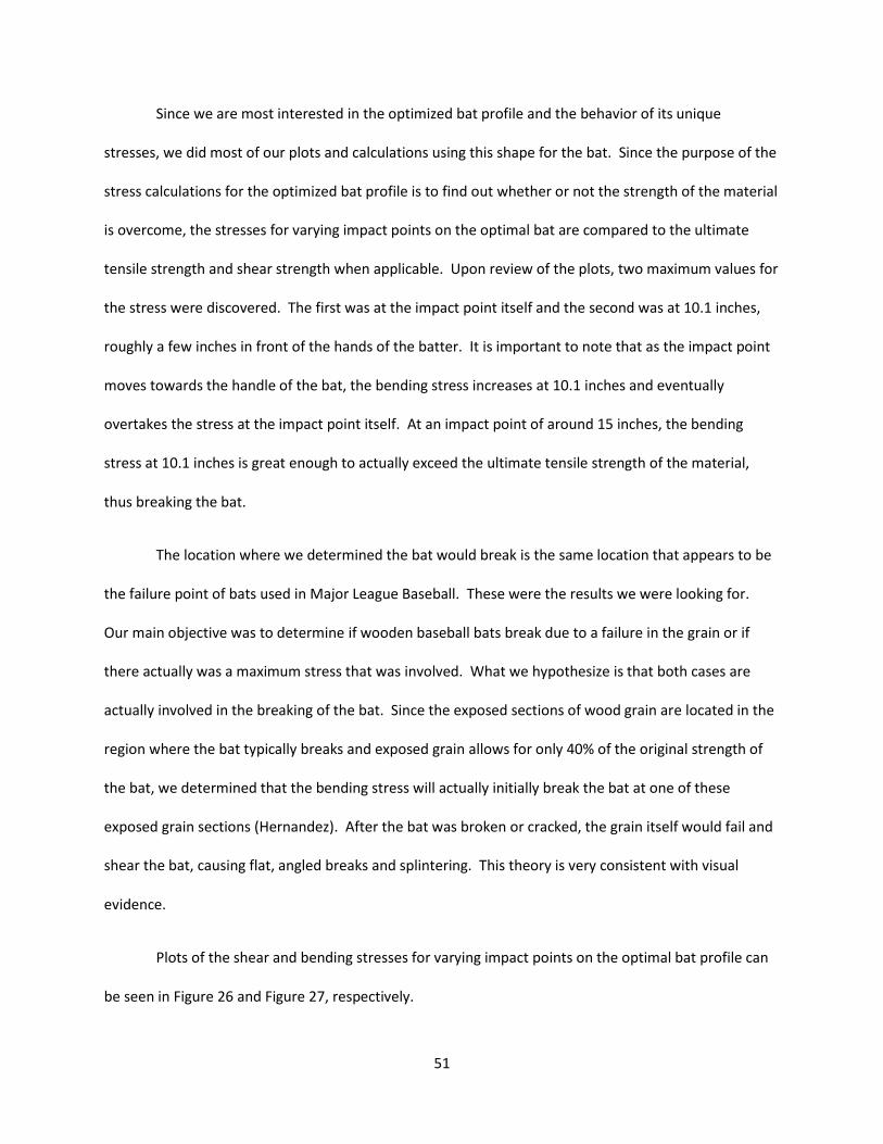
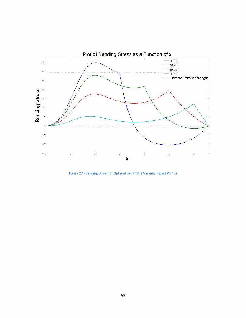
Since we are most interested in the optimized bat profile and the behavior of its unique

stresses, we did most of our plots and calculations using this shape for the bat. Since the purpose of the

stress calculations for the optimized bat profile is to find out whether or not the strength of the material

is overcome, the stresses for varying impact points on the optimal bat are compared to the ultimate

tensile strength and shear strength when applicable. Upon review of the plots, two maximum values for

the stress were discovered. The first was at the impact point itself and the second was at 10.1 inches,

roughly a few inches in front of the hands of the batter. It is important to note that as the impact point

moves towards the handle of the bat, the bending stress increases at 10.1 inches and eventually

overtakes the stress at the impact point itself. At an impact point of around 15 inches, the bending

stress at 10.1 inches is great enough to actually exceed the ultimate tensile strength of the material,

thus breaking the bat.

The location where we determined the bat would break is the same location that appears to be

the failure point of bats used in Major League Baseball. These were the results we were looking for.

Our main objective was to determine if wooden baseball bats break due to a failure in the grain or if

there actually was a maximum stress that was involved. What we hypothesize is that both cases are

actually involved in the breaking of the bat. Since the exposed sections of wood grain are located in the

region where the bat typically breaks and exposed grain allows for only 40% of the original strength of

the bat, we determined that the bending stress will actually initially break the bat at one of these

exposed grain sections (Hernandez). After the bat was broken or cracked, the grain itself would fail and

shear the bat, causing flat, angled breaks and splintering. This theory is very consistent with visual

evidence.

Plots of the shear and bending stresses for varying impact points on the optimal bat profile can

be seen in Figure 26 and Figure 27, respectively.

52

Figure 26 - Shear Stress for Optimal Bat Profile Varying Impact Point a

53

Figure 27 - Bending Stress for Optimal Bat Profile Varying Impact Point a

54

Chapter 6: Conclusion

Through a dynamic analysis of a baseball bat’s interaction with a ball we have calculated

the stresses within the bat and evaluated which are large enough to cause a break. This required a

mathematical model of the baseball bat using a Bezier curve and a dynamic analysis between the force

of impact from the ball and the Bezier bat. This dynamic analysis had to take many factors into

consideration in order to achieve an accurate stress analysis. We considered the bat’s coefficient of

restitution, bat density, time of impact, angular swing velocity, and swing geometry. The angular velocity

of the bat was determined through a function of the torque applied to the bat and the moment of

inertia about the center of rotation. In order to understand how stresses vary under different conditions

we varied the point of impact. We also varied the bat profile to find an optimal baseball bat model.

Through this dynamic analysis we were able to predict that a typical impact between the ball

and the bat near the “sweet spot” does not produce stresses large enough to break the bat. However,

interestingly when analyzing the bats maximum bending stresses two peaks are noticeable. A sharp

peak occurs at the point of impact while the other rounded peak occurs just beyond the handle at

roughly 10.1 inches. As the impact point between the ball and the bat moves closer to handle and away

from the “sweet spot” the second peak at 10.1 inches increases. When the impact point occurs at

approximately 15 inches the second peak exceeds the ultimate strength of the bat which will cause the

bat to break.

At first glance it seems strange that bending stress causes the bat to break considering in game

bats often seems to shear along the grain of the bat. However, there are many reasons that could cause

this to happen. Our first hypothesis, considers that the bending stress could be the cause of the initial

break which would spike the stresses along the bats grain. This seems likely considering our research

shows that the exposed grain of the bat could cause a decrease in strength of about 40 percent

55

(Hernandez). Another possibility is an eventual break through continuous use otherwise known as

fatigue causing a fracture. These hypotheses could be researched through a fatigue analysis and

through actual testing. Using strain gauges and accelerometers and a way to simulate the collision our

analytical research could either be reinforced or revised.

56

References

Adair, Robert K., (1998). Comment on “The sweet spot of a baseball bat,” by Rod Cross.” American

Journal of Physics, Volume 69, Number 2, pp. 229-230.

Bahill, A. Terry, (2004). The ideal moment of inertia for a baseball or softball bat. IEEE Transactions on

Systems, Man and Cybernetics – Part A: Systems and Humans, Volume 34, Number 2.

Cross, Rod. (1998a). The sweet spot of a baseball bat. American Journal of Physics, Volume 68, Number

9, pp 772-779.

Cross, Rod, (1998b). Response to “Comment on ‘The sweet spot of a baseball bat,’ by Rod Cross.”

American Journal of Physics, Volume 69, Number 2, pp 231-232.

Cross, Rod, (1999). Impact of a ball with a bat or racket. American Journal of Physics, Volume 67,

Number 8, pp 692-702.

Cross, Rod., (2008a). Physics of baseball. University of Sydney Physics Department.

http://physics.usyd.edu.au/~cross/baseball.html

Cross, Rod., (2008b). “Simple” Collisions. University of Sydney Physics Department.

http://physics.usyd.edu.au/~cross/Collisions.html Fleisig, G. S., Zheng, N., Stodden, D. F., Andrews, J. R.,

(2002). Relationship between bat mass properties and bat velocity. Sports Engineering, Volume 5, pp 1-

8.

Elert, Glenn R. "Force of a Bat on a Baseball." Hypertextbook.com. The Physics Factbook, 2000. Web. 27

Apr. 2011. http://hypertextbook.com/facts/2000/AlbertKlyachko.shtml

Hernandez, Roland P. "Wood Bat." Wood Science and How It Relates to Wooden Baseball Bats. Hard

Maple Baseball Bat Company, 2009. Web. 27 Apr. 2011. http://www.woodbat.org

Lawrence, Ryan M., Dennis W. Proulx, and Erica S. Stults. Dynamic Modeling of Wooden Baseball Bats.

Tech. Worcester: WPI, 2009.

Nathan, Alan M., (2000). Dynamics of the baseball-bat collision. American Journal of Physics, Volume 68,

Number 11, pp 979-990.

Nathan, Alan M., (2002). Characterizing the performance of baseball bats. American Journal of Physics,

Volume 71, Number 2, pp 134-143.

Russell, Daniel A., (2003). Forces between bat and ball. Science and Mathematics Department, Kettering

University. http://kettering.edu/~drussell/bats-new/impulse.html

Russell, Daniel A., (2004a). The sweet spot of a hollow baseball or softball bat. Science and Mathematics

Department, Kettering University. http://kettering.edu/~drussell/bats-new/sweetspot.html

http://hypertextbook.com/facts/2000/AlbertKlyachko.shtml

http://www.woodbat.org/

57

Russell, Daniel A., (2004b). What about corked bats? Science and Mathematics Department, Kettering

University. http://kettering.edu/~drussell/bats-new/corkedbat.html

Russell, Daniel A., (2005a). How are baseball and softball bats different? Science and Mathematics

Department, Kettering University. http://kettering.edu/~drussell/bats-new/baseball-ssoftball.html92

Russell, Daniel A., (2005b). Does it matter how tightly you grip the bat? Science and Mathematics

Department, Kettering University. http://kettering.edu/~drussell/bats-new/grip.html

Russell, Daniel A., (2005c). What is the COP (Center of Percussion) and does it matter? Science and

Mathematics Department, Kettering University. http://kettering.edu/~drussell/bats-new/cop.html

Russell, Daniel A., (2008a). Swing weight of a bat (Why moment of inertia matters more than weight).

Science and Mathematics Department, Kettering University. http://kettering.edu/~drussell/bats-

new/bat-moi.html

Russell, Daniel A., (2008b). Bat weight, swing speed and ball velocity. Science and Mathematics

Department, Kettering University. http://kettering.edu/~drussell/bats-new/batw8.html

Sawicki, Gregory S., Hubbard, Mont, Stronge, William J., (2003). How to hit home runs: Optimum

baseball bat swing parameters for maximum range trajectories. American Journal of Physics, Volume 71,

Number 11, pp 1152-1162.

Shenoy, Mahesh M., Smith, Lloyd V., Axtell, John T., (2001). Performance assessment of wood, metal,

and composite baseball bats. Elsevier Science Ltd. Composite Structures 52, pp 397-404.

http://kettering.edu/~drussell/bats-new/batw8.html

58

Appendix

Optimized Bat Profile Matlab File clear; clc; close all; %% FOR MAPLE Mass, Center of Mass, and Moment of Inertia as a Function of x;

L=33; UTS=14000; SS=7000; t=.0007; dx=.1; x=0: dx :L; p=.0257/(32.2*12); s=0: dx: L;

R=-(0.000000018643270.*(s.^6))... + (0.000002319441497.*(s.^5)) - (0.000105679130514.*(s.^4))... + (0.002074655511460.*(s.^3)) - (0.015015868091148.*(s.^2))... + (0.039733136102260.*s) + 0.494134257928135;

% Mass of Bat;

eM=(p*pi).*(R.^2); mbat=cumtrapz(s, eM);

mbatx=max(mbat);

% Center of Mass;

eXc=(R.^2).*s; Xci=cumtrapz(s, eXc); Xcl=Xci.*((pi*p)./(mbat)); Xcx=max(Xcl);

% Moment of Inertia;

eIc=4.*(pi*p).*(R.^2).*((s-Xc).^2); Ic=cumtrapz(s, eIc); Icx=max(Ic);

%% Step 2 - v', w', and d'

%Average value for e (Previous Project); e=.5; %Mass of Ball [lbs]; mball=.3125/(32.2*12); d0=2.5; %Assuming 90 MPH fastball [in/s]; v0=-1584; a=27; y=a-(Xcx); w0=50;

59

m=mbatx/mball;

%Outgoing ball velocity (vc = Velocity of center of mass, vb0 = Velocity of %bat at point of impact) [in/s]; display('Velocity of Center of Mass before Impact [in/s]') vc0=((d0+(Xcx))*w0) display('Velocity of Point of Impact before Impact [in/s]') vb0=(vc0+(w0*(y)))

%Exit Velocity; display('Ball Exit Velocity [in/s]') v= v0+((m*(1+e))*(vc0-v0+((w0*(y)))))/(1+m+((mbatx/(Icx))*((y)^2)))

%Final Bat Speed; display('Final Bat Speed [Rad/s]') w= w0+((mball/(Icx))*((v0-v)*(y)))

%New Center of Rotation display('Velocity of Point of Impact after Impact[in/s]') vb=v+((v0-vb0)*e)

display('Velocity of Center of Mass after Impact [in/s]') vc=vb-(w*(y))

display('New Center of Rotation [in/s]') d=((-Xcx)+((vc)/w))

%% Step 3 - Impulsive Shear Force and Impulsive Moment to Left of a

%Impulsive Shear Force Left of a; ViA=(((((d)+Xc)).*w)-((((d0)+Xc)).*w0)).*(-mbat);

%Impulsive Moment to the Left of a; MiA=-(((x-Xc)).*ViA)-((w-w0).*(Ic));

%% Step 4 - Impulsive Shear Force and Impulsive Moment to RIght of a

%Impulsive Shear Force Right of a; ViB=((((d+Xc).*w)-((d0+Xc).*w0)).*(-mbat))-(mball*(v-v0));

%Impulsive Moment to the Right of a; MiB=-((x-Xc).*ViB)-((w-w0).*Ic)-((a-Xc).*(mball*(v-v0)));

%% Step 5 - Plotting the Data

Vi=[0:1:330]; Mi=[0:1:330];

for j=1:(a*10)+1 Vi(j) = ViA(j)/t; end

60

for k=(a*10)+1:(L*10) +1 Vi(k) = ViB(k)/t; end

for j=1:(a*10)+1 Mi(j) = MiA(j)/t; end

for k=(a*10)+1:(L*10) +1 Mi(k) = MiB(k)/t; end

figure(1)

subplot(2,1,1) plot(s,Vi,s,0); xlabel('Length'); ylabel('Impulsive Shear Force'); title('Plot of Impulsive Shear Force as a Function of x for MAPLE Bats');

subplot(2,1,2) plot(s,Mi,s,0); xlabel('Length'); ylabel('Impulsive Moment'); title('Plot of Impulsive Moment as a Function of x fo MAPLE Bats');

%% Step 6 - Maximum Shear and Bending Stresses as Functions of X

TAU=(4/3).*((Vi)./(R.^2));

SIGMA=((Mi).*(R))./((pi/4).*(R.^4));

figure(2)

subplot(2,1,1) plot(s,TAU,s,0); xlabel('Length'); ylabel('Shear Stress'); title('Plot of Shear Stress as a Function of x for MAPLE Bats');

subplot(2,1,2) plot(s,SIGMA,s,0); xlabel('Length'); ylabel('Bending Stress'); title('Plot of Bending Stress as a Function of x for MAPLE Bats');

%% Step 7 - Principal Stress as a Function of x

61

% As discovered in another file, the maximum principal stress occurs at % z=R (the very top of the cross-section). This means that the principal % stress can be graphed as a function of x for any set contact point.

% Principal Stresses; SIGMA1=(SIGMA./2)+(sqrt(((SIGMA./2).^2)+(0))); SIGMA2=0; SIGMA3=(SIGMA./2)-(sqrt(((SIGMA./2).^2)+(0)));

TAUmax=(abs(SIGMA1-SIGMA3))./2;

figure(3)

plot(s,SIGMA1,s,SIGMA3,s,TAUmax,s,0); xlabel('Length'); ylabel('Principal Stress'); title('Plot of Principal Stresses for MAPLE Bats'); legend('SIGMA1','SIGMA3','TAUmax');

%%Mass, Center of Mass, and Moment of Inertia as a Function of x;

L=33; t=.0007; dx=.1; x=0: dx :L; p=.01987/(32.2*12); s=0: dx: L; R=-(0.000000018643270.*(s.^6))... + (0.000002319441497.*(s.^5)) - (0.000105679130514.*(s.^4))... + (0.002074655511460.*(s.^3)) - (0.015015868091148.*(s.^2))... + (0.039733136102260.*s) + 0.494134257928135;

% Mass of Bat;

eM=(p*pi).*(R.^2); mbat=cumtrapz(s, eM);

mbatx=max(mbat);

% Center of Mass;

eXc=(R.^2).*s; Xci=cumtrapz(s, eXc); Xcl=Xci.*((pi*p)./(mbat));

Xcx=max(Xcl);



62

%% Step 2 - v', w', and d'

%Average value for e (Previous Project); e=.5; %Mass of Ball [lbs]; mball=.3125/(32.2*12); d0=2.5; %Assuming 90 MPH fastball [in/s]; v0=-1584; a=27; y=a-(Xcx); w0=50; m=mbatx/mball;







%% Step 3 - Impulsive Shear Force and Impulsive Moment to Left of a

%Impulsive Shear Force Left of a; ViA=(((((d)+Xc)).*w)-((((d0)+Xc)).*w0)).*(-mbat);

%Impulsive Moment to the Left of a; MiA=-(((x-Xc)).*ViA)-((w-w0).*(Ic));

%% Step 4 - Impulsive Shear Force and Impulsive Moment to RIght of a

%Impulsive Shear Force Right of a; ViB=((((d+Xc).*w)-((d0+Xc).*w0)).*(-mbat))-(mball*(v-v0));

63

%Impulsive Moment to the Right of a; MiB=-((x-Xc).*ViB)-((w-w0).*Ic)-((a-Xc).*(mball*(v-v0)));


Vi=[0:1:330]; Mi=[0:1:330];

for j=1:(a*10)+1 Vi(j) = ViA(j)/t; end for k=(a*10)+1:(L*10) +1 Vi(k) = ViB(k)/t; end for j=1:(a*10)+1 Mi(j) = MiA(j)/t; end for k=(a*10)+1:(L*10) +1 Mi(k) = MiB(k)/t; end

figure(4)

subplot(2,1,1) plot(s,Vi,s,0); xlabel('Length'); ylabel('Shear Force'); title('Plot of Shear Force as a Function of x fo ASH Bats');

subplot(2,1,2) plot(s,Mi,s,0); xlabel('Length'); ylabel('Bending Moment'); title('Plot of Bending Moment as a Function of x fo ASH Bats');

%% Step 6 - Maximum Shear and Bending Stresses as Functions of X

TAU=(4/3).*((Vi)./(R.^2));

SIGMA=((Mi).*(R))./((pi/4).*(R.^4));

figure(5)

subplot(2,1,1) plot(s,TAU,s,0); xlabel('Length'); ylabel('Shear Stress'); title('Plot of Shear Stress as a Function of x for ASH Bats');

subplot(2,1,2)

64

plot(s,SIGMA,s,0); xlabel('Length'); ylabel('Bending Moment'); title('Plot of Moment as a Function of x for ASH Bats');

%% Step 7 - Principal Stress as a Function of x

% As discovered in another file, the maximum principal stress occurs at % z=R (the very top of the cross-section). This means that the principal % stress can be graphed as a function of x for any set contact point.

% Principal Stresses; SIGMA1=(SIGMA./2)+(sqrt(((SIGMA./2).^2)+(0))); SIGMA2=0; SIGMA3=(SIGMA./2)-(sqrt(((SIGMA./2).^2)+(0)));

TAUmax=(abs(SIGMA1-SIGMA3))./2;

figure(6)

plot(s,SIGMA1,s,SIGMA3,s,TAUmax,s,0); xlabel('Length'); ylabel('Principal Stress'); title('Plot of Principal Stresses'); legend('SIGMA1','SIGMA3','TAUmax');

65

Uniform Bat Profile Matlab File clear; clc; close all; %% Mass, Center of Mass, and Moment of Inertia as a Function of x;

L=33; t=.0007; dx=.1; x=0: dx :L; p=.01987/(32.2*12); s=0: dx: L; R=1.0*ones(size(x));

% Mass of Bat;

eM=(p*pi).*(R.^2); mbat=cumtrapz(s, eM); mbatx=max(mbat);

% Center of Mass;

eXc=(R.^2).*s; Xci=cumtrapz(s, eXc); Xcl=Xci.*((pi*p)./(mbat)); Xcx=max(Xcl);



%% Step 2 - Calculations for a1 %Impact Point; a1=15;

%Average value for e (Previous Project); e=.5; %Mass of Ball [lbs]; mball=.3284/(32.2*12); d0=2.5; %Assuming 90 MPH fastball [in/s]; v0=-1584; y=a1-(Xcx); w0=50; m=mbatx/mball;


66






%Impulsive Shear Force Left of a; ViA1=(((((d)+Xc)).*w)-((((d0)+Xc)).*w0)).*(-mbat);

%Impulsive Moment to the Left of a; MiA1=-(((x-Xc)).*ViA1)-((w-w0).*(Ic));

%Impulsive Shear Force Right of a; ViB1=((((d+Xc).*w)-((d0+Xc).*w0)).*(-mbat))-(mball*(v-v0));

%Impulsive Moment to the Right of a; MiB1=-((x-Xc).*ViB1)-((w-w0).*Ic)-((a1-Xc).*(mball*(v-v0)));

Vi1=[0:1:330]; Mi1=[0:1:330];

for j=1:(a1*10)+1 Vi1(j) = ViA1(j)/t; end for k=(a1*10)+1:(L*10) +1 Vi1(k) = ViB1(k)/t; end for j=1:(a1*10)+1 Mi1(j) = MiA1(j)/t; end for k=(a1*10)+1:(L*10) +1 Mi1(k) = MiB1(k)/t; end

TAU1=(4/3).*((Vi1)./(R.^2)); SIGMA1=((Mi1).*(R))./((pi/4).*(R.^4));

SIGMAone1=((SIGMA1./2)+(sqrt(((SIGMA1./2).^2)+(0)))); SIGMAtwo1=0; SIGMAthree1=((SIGMA1./2)-(sqrt(((SIGMA1./2).^2)+(0))));

67

TAUmax1=(abs(SIGMAone1-SIGMAthree1))/2;












%Impulsive Moment to the Right of a;

68

MiB2=-((x-Xc).*ViB2)-((w-w0).*Ic)-((a2-Xc).*(mball*(v-v0)));

Vi2=[0:1:330]; Mi2=[0:1:330];

for j=1:(a2*10)+1 Vi2(j) = ViA2(j)/t; end

for k=(a2*10)+1:(L*10) +1 Vi2(k) = ViB2(k)/t; end

for j=1:(a2*10)+1 Mi2(j) = MiA2(j)/t; end

for k=(a2*10)+1:(L*10) +1 Mi2(k) = MiB2(k)/t; end

TAU2=(4/3).*((Vi2)./(R.^2));

SIGMA2=((Mi2).*(R))./((pi/4).*(R.^4));






69










Vi3=[0:1:330]; Mi3=[0:1:330];





TAU3=(4/3).*((Vi3)./(R.^2));

70

SIGMA3=((Mi3).*(R))./((pi/4).*(R.^4));













71



Vi4=[0:1:330]; Mi4=[0:1:330];





TAU4=(4/3).*((Vi4)./(R.^2));

SIGMA4=((Mi4).*(R))./((pi/4).*(R.^4));



figure(1)

plot(s,Vi1,s,Vi2,s,Vi3,s,Vi4,s,0,'linewidth',2); xlabel('x','fontsize',30); ylabel('Impulsive Shear Force [lb*s]','fontsize',30); axis([0 33 -6 11]); title('Plot of Impulsive Shear Force as a Function of x','fontsize',30); h_legend=legend('a=15','a=20','a=25','a=30'); set(h_legend,'FontSize',20);

figure(2)

plot(s,-Mi1,s,-Mi2,s,-Mi3,s,-Mi4,s,0,'linewidth',2); xlabel('x','fontsize',30); ylabel('Impulsive Moment [lb*in*s]','fontsize',30); axis([0 33 -6 11]); title('Plot of Impulsive Moment as a Function of x','fontsize',30);

72

h_legend=legend('a=15','a=20','a=25','a=30'); set(h_legend,'FontSize',20);


figure(2)

plot(s,TAU1,s,TAU2,s,TAU3,s,TAU4,s,0,'linewidth',2); xlabel('x','fontsize',30); ylabel('Shear Stress [psi]','fontsize',30); title('Plot of Shear Stress as a Function of x','fontsize',30); h_legend=legend('a=15','a=20','a=25','a=30'); set(h_legend,'FontSize',20);

figure(3)

plot(s,-SIGMA1,s,-SIGMA2,s,-SIGMA3,s,-SIGMA4,s,0,'linewidth',2); xlabel('x','fontsize',30); ylabel('Bending Stress [psi]','fontsize',30); title('Plot of Bending Stress as a Function of x','fontsize',30); h_legend=legend('a=15','a=20','a=25','a=30'); set(h_legend,'FontSize',20);

figure(4)

subplot(3,1,1) plot(s,SIGMAone1,s,SIGMAone2,s,SIGMAone3,s,SIGMAone4,s,0); xlabel('Length'); ylabel('SIGMA1'); title('Plot of SIGMA1 as a Function of x'); legend('a=15','a=20','a=25','a=30');

subplot(3,1,2) plot(s,SIGMAthree1,s,SIGMAthree2,s,SIGMAthree3,s,SIGMAthree4,s,0); xlabel('Length'); ylabel('SIGMA3'); title('Plot of SIGMA3 as a Function of x'); legend('a=15','a=20','a=25','a=30');

subplot(3,1,3) plot(s,TAUmax1,s,TAUmax2,s,TAUmax3,s,TAUmax4,s,0); xlabel('Length'); ylabel('TAUmax'); title('Plot of TAUmax as a Function of x'); legend('a=15','a=20','a=25','a=30');

73

Multi Radius Matlab File clear; clc; close all; %% Bat Radii;

L=33; t=.0007; dx=.1; x=0: dx :L; p=.01987/(32.2*12); s=0: dx: L;

% Uniform Bat; R1=1.0*ones(size(x));

% Bat Profile 1; R2= -0.000000006140426*(s.^6) + 0.000000839928030*(s.^5)... - 0.000041249730941*(s.^4)+ 0.000861244322699*(s.^3)... - 0.006473709105308*(s.^2) + 0.0176313232063888*(s)... + 0.747225117504286;

% Optimized Bat Profile; R3=-(0.000000018643270.*(s.^6))... + (0.000002319441497.*(s.^5)) - (0.000105679130514.*(s.^4))... + (0.002074655511460.*(s.^3)) - (0.015015868091148.*(s.^2))... + (0.039733136102260.*s) + 0.494134257928135;

% Bat Profile 2; R4= -0.000000026633242*(s.^6) + 0.000003313487858*(s.^5)... - 0.000150970186605*(s.^4)+ 0.002963793590510*(s.^3)... - 0.021451240148963*(s.^2) + 0.056761623044167*(s)... + 0.241620368530675;

figure(1)

plot(s,R1,s,R2,s,R3,s,R4,s,0,'linewidth',2); xlabel('Length [in]','fontsize',20); ylabel('Radius [in]','fontsize',20); axis([0 33 0 1.7]); title('Plot of Bat Profiles','fontsize',20); h_legend=legend('Uniform Bat','Profile 1','Optimized Profile','Profile 2'); set(h_legend,'FontSize',14);

%% Mass, Center of Mass, and Moment of Inertia;

%Uniform Bat; eM1=(p*pi).*(R1.^2); mbat1=cumtrapz(s, eM1); mbatx1=max(mbat1); eXc1=(R1.^2).*s; Xci1=cumtrapz(s, eXc1); Xcl1=Xci1.*((pi*p)./(mbat1)); Xcx1=max(Xcl1); eIc1=4.*(pi*p).*(R1.^2).*((s-Xc1).^2); Ic1=cumtrapz(s, eIc1);

74

Icx1=max(Ic1);

%Profile 1; eM2=(p*pi).*(R2.^2); mbat2=cumtrapz(s, eM2); mbatx2=max(mbat2); eXc2=(R2.^2).*s; Xci2=cumtrapz(s, eXc2); Xcl2=Xci2.*((pi*p)./(mbat2)); Xcx2=max(Xcl2); eIc2=4.*(pi*p).*(R2.^2).*((s-Xc2).^2); Ic2=cumtrapz(s, eIc2); Icx2=max(Ic2);

%Optimized Bat Profile; eM3=(p*pi).*(R3.^2); mbat3=cumtrapz(s, eM3); mbatx3=max(mbat3); eXc3=(R3.^2).*s; Xci3=cumtrapz(s, eXc3); Xcl3=Xci3.*((pi*p)./(mbat3)); Xcx3=max(Xcl3); eIc3=4.*(pi*p).*(R3.^2).*((s-Xc3).^2); Ic3=cumtrapz(s, eIc3); Icx3=max(Ic3);

%Profile 2; eM4=(p*pi).*(R4.^2); mbat4=cumtrapz(s, eM4); mbatx4=max(mbat4); eXc4=(R4.^2).*s; Xci4=cumtrapz(s, eXc4); Xcl4=Xci4.*((pi*p)./(mbat4)); Xcx4=max(Xcl4); eIc4=4.*(pi*p).*(R4.^2).*((s-Xc4).^2); Ic4=cumtrapz(s, eIc4); Icx4=max(Ic4);

%% Outgoing Ball Velocity, Final Bat Speed, Center of Rotation;

a=0:dx:33; e=.5; mball=.3125/(32.2*12); v0=-1584; w0=50; d0=2.5;

%Uniform Bat; y1=a-(Xc1); m1=mbat1/mball; vc01=((d0+(Xc1))*w0); vb01=(vc01+(w0*(y1))); v1= v0+((m1.*(1+e)).*(vc01-

v0+((w0.*(y1)))))./(1+m1+((mbat1./(Ic1)).*((y1).^2))); w1= w0+((mball./(Ic1)).*((v0-v1).*(y1))); vb1=v1+((v0-vb01)*e);

75

vc1=vb1-(w1.*(y1)); d1=((-Xc1)+((vc1)./w1));

%Profile 1; y2=a-(Xc2); m2=mbat2/mball; vc02=((d0+(Xc2))*w0); vb02=(vc02+(w0*(y2))); v2= v0+((m2.*(1+e)).*(vc02-

v0+((w0.*(y2)))))./(1+m2+((mbat2./(Ic2)).*((y2).^2))); w2= w0+((mball./(Ic2)).*((v0-v2).*(y2))); vb2=v2+((v0-vb02)*e); vc2=vb2-(w2.*(y2)); d2=((-Xc2)+((vc2)./w2));

%Optimized Bat Profile; y3=a-(Xc3); m3=mbat3/mball; vc03=((d0+(Xc3))*w0); vb03=(vc03+(w0*(y3))); v3= v0+((m3.*(1+e)).*(vc03-


%Profile 2; y4=a-(Xc4); m4=mbat4/mball; vc04=((d0+(Xc4))*w0); vb04=(vc04+(w0*(y4))); v4= v0+((m4.*(1+e)).*(vc04-


figure (2)

plot(s,-v1/v0,s,-v2/v0,s,-v3/v0,s,-v4/v0,s,0,'linewidth',2); xlabel('Impact Point [in]','fontsize',30); ylabel('Final Ball Velocity / Incoming Ball Velocity','fontsize',30); title('Plot of Final Ball Velocity Based on Impact Point','fontsize',30); h_legend=legend('Uniform Bat','Profile 1','Optimized Profile','Profile 2'); set(h_legend,'FontSize',20);

figure (3)

plot(s,w1/w0,s,w2/w0,s,w3/w0,s,w4/w0,s,0,'linewidth',2); xlabel('Impact Point [in]','fontsize',30); ylabel('Angular Velocity of the Bat [Final / Initial]','fontsize',30); title('Plot of Final Angular Velocity of the Bat Based on Impact

Point','fontsize',30);

76

h_legend=legend('Uniform Bat','Profile 1','Optimized Profile','Profile 2'); set(h_legend,'FontSize',20);

figure (4)

plot(s,d1,s,d2,s,d3,s,d4,s,0,'linewidth',2); xlabel('Impact Point [in]','fontsize',30); ylabel('New Center of Rotation [in]','fontsize',30); title('Plot of New Center of Rotation Based on Impact Point','fontsize',30); h_legend=legend('Uniform Bat','Profile 1','Optimized Profile','Profile 2'); set(h_legend,'FontSize',20);

%% Impulsive Shear Force and Bending Moment aa=27;

%Uniform Bat; y1=aa-(Xcx1); m1=mbatx1/mball; vc01=((d0+(Xcx1))*w0); vb01=(vc01+(w0*(y1))); v1= v0+((m1.*(1+e)).*(vc01-

v0+((w0.*(y1)))))./(1+m1+((mbatx1./(Icx1)).*((y1).^2))); w1= w0+((mball./(Icx1)).*((v0-v1).*(y1))); vb1=v1+((v0-vb01)*e); vc1=vb1-(w1.*(y1)); d1=((-Xcx1)+((vc1)./w1));

ViA1=(((((d1)+Xc1)).*w1)-((((d0)+Xc1)).*w0)).*(-mbat1); MiA1=-(((x-Xc1)).*ViA1)-((w1-w0).*(Ic1));

ViB1=((((d1+Xc1).*w1)-((d0+Xc1).*w0)).*(-mbat1))-(mball*(v1-v0)); MiB1=-((x-Xc1).*ViB1)-((w1-w0).*Ic1)-((aa-Xc1).*(mball*(v1-v0)));

Vi1=[0:1:330]; Mi1=[0:1:330];

for j=1:(aa*10)+1 Vi1(j) = ViA1(j); end

for k=(aa*10)+1:(L*10) +1 Vi1(k) = ViB1(k); end

for j=1:(aa*10)+1 Mi1(j) = MiA1(j); end

for k=(aa*10)+1:(L*10) +1 Mi1(k) = MiB1(k); end

%Profile 1; y2=aa-(Xcx2);

77

m2=mbatx2/mball; vc02=((d0+(Xcx2))*w0); vb02=(vc02+(w0*(y2))); v2= v0+((m2.*(1+e)).*(vc02-




Vi2=[0:1:330]; Mi2=[0:1:330];





%Optimized Bat Profile; y3=aa-(Xcx3); m3=mbatx3/mball; vc03=((d0+(Xcx3))*w0); vb03=(vc03+(w0*(y3))); v3= v0+((m3.*(1+e)).*(vc03-




Vi3=[0:1:330]; Mi3=[0:1:330];

78





%Profile 2; y4=aa-(Xcx4); m4=mbatx4/mball; vc04=((d0+(Xc4))*w0); vb04=(vc04+(w0*(y4))); v4= v0+((m4.*(1+e)).*(vc04-




Vi4=[0:1:330]; Mi4=[0:1:330];





79

figure(5)

plot(s,Vi1,s,Vi2,s,Vi3,s,Vi4,s,0,'linewidth',2); xlabel('x','fontsize',30); ylabel('Impulsive Shear Force [lb*s]','fontsize',30); axis([0 33 -2 3]); title('Plot of Impulsive Shear Force as a Function of x','fontsize',30); h_legend=legend('Uniform Bat','Profile 1','Optimized Profile','Profile 2'); set(h_legend,'FontSize',20);

figure(6)

plot(s,-Mi1,s,-Mi2,s,-Mi3,s,-Mi4,s,0,'linewidth',2); xlabel('x','fontsize',30); ylabel('Impulsive Moment [lb*in*s]','fontsize',30); axis([0 33 -1 14]); title('Plot of Impulsive Moment as a Function of x','fontsize',30); h_legend=legend('Uniform Bat','Profile 1','Optimized Profile','Profile 2'); set(h_legend,'FontSize',20);

%% Stresses

% Uniform Bat TAU1=((4/3).*((Vi1)./(R1.^2)))/t; SIGMA1=(((Mi1).*(R1))./((pi/4).*(R1.^4)))/.0013;

% Profile 1 TAU2=((4/3).*((Vi2)./(R2.^2)))/t; SIGMA2=(((Mi2).*(R2))./((pi/4).*(R2.^4)))/t;

% Optimal Bat TAU3=((4/3).*((Vi3)./(R3.^2)))/t; SIGMA3=(((Mi3).*(R3))./((pi/4).*(R3.^4)))/t;

% Profile 2 TAU4=((4/3).*((Vi4)./(R4.^2)))/t; SIGMA4=(((Mi4).*(R4))./((pi/4).*(R4.^4)))/.0015;

figure(7)

plot(s,TAU1,s,TAU2,s,TAU3,s,TAU4,s,0,'linewidth',2); xlabel('x','fontsize',30); ylabel('Shear Stress [psi]','fontsize',30); axis([0 33 -5000 5000]); title('Plot of Shear Stress as a Function of x','fontsize',30); h_legend=legend('Uniform Bat','Profile 1','Optimized Profile','Profile 2'); set(h_legend,'FontSize',20);

figure(8)

plot(s,-SIGMA1,s,-SIGMA2,s,-SIGMA3,s,-SIGMA4,s,0,'linewidth',2); xlabel('x','fontsize',30); ylabel('Bending Stress [psi]','fontsize',30);

80

axis([0 33 -1800 14000]); title('Plot of Bending Stress as a Function of x','fontsize',30); h_legend=legend('Uniform Bat','Profile 1','Optimized Profile','Profile 2'); set(h_legend,'FontSize',20);

Documents

Impact Stresses in Wooden Baseball Bats - Worcester ... Stresses in Wooden Baseball Bats A Major Qualifying Project Report Submitted to the Faculty Of the WORCESTER POLYTECHNIC INSTITUTE