Embed Size (px)
Citation preview
at SciVerse ScienceDirect
Atmospheric Environment 48 (2012) 205e218
Contents lists available
Atmospheric Environment
journal homepage: www.elsevier .com/locate/atmosenv
Impact of volcanic ash plume aerosol on cloud microphysics
G. Martucci*, J. Ovadnevaite, D. Ceburnis, H. Berresheim, S. Varghese, D. Martin, R. Flanagan, C.D. O’DowdSchool of Physics & Centre for Climate and Air Pollution Studies, Ryan Institute, National University of Ireland Galway, Galway, Ireland
a r t i c l e i n f o
Article history:Received 7 February 2011Received in revised form2 November 2011Accepted 14 December 2011
Keywords:MicrophysicsVolcanicSYRSOCCDNCEffective radiusLiquid water content
* Corresponding author. Tel.: þ353 0 91 495468.E-mail address: [email protected] (
1352-2310/$ e see front matter � 2011 Elsevier Ltd.doi:10.1016/j.atmosenv.2011.12.033
a b s t r a c t
This study focuses on the dispersion of the Eyjafjallajökull volcanic ash plume over the west of Ireland, atthe Mace Head Supersite, and its influence on cloud formation and microphysics during one significantevent spanning May 16th and May 17th, 2010. Ground-based remote sensing of cloud microphysics wasperformed using a Ka-band Doppler cloud RADAR, a LIDAR-ceilometer and a multi-channel microwave-radiometer combined with the synergistic analysis scheme SYRSOC (Synergistic Remote Sensing OfCloud). For this case study of volcanic aerosol interaction with clouds, cloud droplet number concen-tration (CDNC), liquid water content (LWC), and droplet effective radius (reff) and the relative dispersionwere retrieved. A unique cloud type formed over Mace Head characterized by layer-averaged maximum,mean and standard deviation values of the CDNC, reff and LWC: Nmax ¼ 948 cm�3, N ¼ 297 cm�3,sN ¼ 250 cm�3, reff max ¼ 35.5 mm, reff ¼ 4:8 mm, sreff ¼ 4:4 mm, LWCmax ¼ 0:23 g m�3,LWC ¼ 0:055 g m�3, sLWC ¼ 0:054 g m�3, respectively. The high CDNC, for marine clean air, wereassociated with large accumulation mode diameter (395 nm) and a hygroscopic growth factor consistentwith sulphuric acid aerosol, despite being almost exclusively internally mixed in submicron sizes.Additionally, the Condensation Nuclei (CN, d > 10 nm) to Cloud Condensation Nuclei (CCN) ratio, CCN:CNw1 at the moderately low supersaturation of 0.25%. This case study illustrates the influence of volcanicaerosols on cloud formation and microphysics and shows that volcanic aerosol can be an efficient CCN.
� 2011 Elsevier Ltd. All rights reserved.
1. Introduction
On March the 20th, 2010, the Icelandic Eyjafjallajökull volcano(63�380000 N, 19�360000 W, summit elevation 1666 m) erupted afteralmost 190 years since its last most significant eruption occurredbetween 1821 and 1823. Although the eruption of 20March has beenclassified only as 1 on the Volcanic Explosivity Index (Newhall andSelf, 1982; Zehner, 2010), in the following weeks the seismicactivity, already started at the end of 2009, became more intensewith large amount of eruptive material emitted into the lowerTroposphere. The eruption of 14 April 2010 created an ash cloudconsisting mainly of tephra produced by thermal contraction fromcontactwith themelted ice cap; the explosively ejectedmaterial thatformed the ash cloud had diverse size distribution ranging from thefine <100 mm to the coarse ash <2 mm. Larger particles like lapilliand pyroclastic material fell out of the cloud in the first minutes tohours after being ejected from the vent. In the first days after theeruption the fine-ash cloud has been transported by Westerlies outto northern Europe first and to central and southern Europe there-after. The across-Europe and North Atlantic-transported ash cloud
G. Martucci).
All rights reserved.
led, under the directions of the London Volcanic Ash AdvisoryCentre, to the closure of most of the European airspaces. The scien-tific community was committed to assess the actual potentialities ofin-situ and ground/space-based remote sensor measurements todetect the ash plume and to retrieve its density and size distribution.Most of the remote sensing measurements focused on the physicaland optical properties of the ash plume leaving little focus to theactual interaction of the ash particles with clouds. This study pres-ents a case of cloud formation directly from the volcanic ash layeradvected over the GAW atmospheric station of Mace Head, Ireland,on the night between 16 and 17 May 2010.
The mechanisms regulating the formation of clouds have beenstudied for almost one hundred years now, but it is only with theonset of the recent technologies that it has been possible to investi-gate the microphysics of the aerosolsecloud interaction. Althoughnumerous studies have improved the knowledge of the aerosolindirect effects (Twomey, 1977; Ackerman et al., 2000; Rosenfeldet al., 2006), much more needs to be learned on the mechanismsleading to cloud formation from a given cloud condensation nuclei(CCN) distribution. The naturally produced CCN in the atmospheredepend strongly on the spatial distribution of several gases andparticles, namely phytoplankton emitted dimethyl-sulphide (DMS),oxidised SO2, MSA, H2SO4, SO4, organics and dust particles. Thesensitivity of the activated cloud droplets to the different populations
G. Martucci et al. / Atmospheric Environment 48 (2012) 205e218206
of CCN is a complex process (Woodhouse et al., 2010) which dependsmainly on aerosol size, hygroscopicity and on the local values oftemperature and supersaturationwith respect towater or ice or bothdepending on the cloud phase. Clouds stemming from dust or ashCCN are not uncommon although they are rarely observed due tonarrow conditions of temperature and humidity in which they formin combinationwith such CCN (Flamant et al., 2009; Bou Karamet al.,2009). In polluted areas, a large number of aerosols serving as CCNwould lead to increased cloud droplet number concentrations(CDNC). However, embryonic and fully-developed CDNCwould formin conditions of low per-droplet available water than in cleanconditions. Themore numerous cloud droplets will have smaller sizeby 20e30% increasing the albedo by almost the 25% (Kaufman et al.,2002). Smaller cloud droplets are less efficient in generatingprecipitation and this may affect the local hydrologic cycle. Never-theless, the way a population of many large aerosol particles caninfluence themechanismof cloud formation andultimately affect theprecipitation process is not well understood yet. The radiative aero-sols first and second indirect effects are still suffering from a largeruncertainty compared to the already large uncertainty related to thedirect effect by the greenhouse gases. This study is intended toprovide a quantitative microphysical analysis of the aerosol indirecteffect for a case of volcanic ash CCN.
2. Site and instruments
2.1. The site
Located on the west coast of Ireland, the Atmospheric ResearchStation at Mace Head, Carna, County Galway is unique in Europe inthat its location offers westerly exposure to the North AtlanticOcean through the clean sector (190�e300�N) and the opportunityto study atmospheric composition under Northern Hemisphericbackground conditions as well as European continental emissionswhen the winds favour transport from that region (O’Connor et al.,2008). The site location, at 53� 20 min N, 9� 54 minW, is in the pathof the mid-latitude cyclones which frequently traverse the NorthAtlantic. The instruments are located 300 m from the shore line ona gently-sloping hill (4� incline).
2.2. Instruments
2.2.1. Remote sensorsThe GAW Atmospheric Station of Mace Head is part of the
CLOUDNET programme (Illingworth et al., 2007) since 2008 usingsynergistic input data from three remote sensors to supply theCLOUDNET modules. In parallel to CLOUDNET the authors havedeveloped the SYRSOC (SYnergistic Remote Sensing Of Cloud) tech-nique (see Appendix A for a complete description and work byMartucci and O’Dowd, 2011) to retrieve the full cloud microphysicsfrom the three remote sensors, namely the Jenoptik CHM15K LIDARceilometer with 1064-nm wavelength and 15-km vertical range(Flentje et al., 2010; Martucci et al., 2010a), the RPG-HATPRO watervapour and oxygenmulti-channel microwave profiler (Lönhert et al.,2009) and the MIRA36, 35 GHz Ka-band Doppler cloud RADAR(Melchionna et al., 2008).
2.2.2. Chemical, physical and optical instrumentsThe size resolved non-refractory chemical composition of
submicron aerosol particles was measured with an Aerodyne HighResolution Time of Flight Aerosol Mass Spectrometer (HR-ToF AMS,Aerodyne, Billerica, MA). Detailed instrument description could befound in the work from DeCarlo et al. (2006). HR-ToF AMS wasroutinely calibrated according to themethods described by Jimenezet al. (2003) and Allan et al. (2003). Measurements were performed
with a time resolution of 5 min, with a vaporizer temperature ofabout 600 �C. Considering particle chemical composition andrelative humidity (Matthew et al., 2008; Middlebrook and Bahreini,2008) a collection efficiency of C ¼ 1 was applied for themeasurements discussed in this study.
The size distribution of ambient particles sampled few metersabove the ground level was performed in parallel by two instru-ments, the scanning mobility particle sizers (SMPS) over a particlediameter range from 3 nm to about 0.5 mm, and the AerodynamicParticle Sizer (APS) model 3021 (TSI Inc) with 51 channel of equallogarithmic width of 0.03 within the size range of 0.3e20.0 mm.
Aerosol scattering measurements by means of a three-wavelength integrating Nephelometer (TSI Model 3551) are con-ducted routinely at Mace Head. Aerosol absorption was measuredusing a Multi-Angle Absorption Photometer (MAAP).
3. Case description
The ash plume emitted by the Eyjafjallajökull volcano on14 May2010 reached the Troposphere aboveMace Head (z ¼ 3:7 km a:g:l:)on the night between the 16th and 17th of May. The plume wastransported from the main volcano’s crater to Mace Head in about2 days in a synoptic northwest-southeast flow. In Fig. 1a the 60-hforward-trajectory calculated by NOAA HYSPLIT model with start-ing time at 0800 UTC and 4000-m level, shows the Icelandic originof the advected air mass reaching Mace Head on 16 May. Comparedto the first volcanic plume observed at Mace Head on 19e20 April2010 (i.e. 5 days after the first Eyjafjalla explosion on 14 April 2010)some major difference have been observed (O’Dowd et al, “TheEyjafjallajökull Ash Plume e Part I: Physical, Chemical and OpticalCharacteristics” This Issue) with respect to the discussed case of16e17 May. Mainly two differences characterized the two events:(i) less sulphate (w2 mg m�3) compared to the May-event(w7 mg m�3) most likely due to cloudless conditions on the19e20 April and (ii) more diverse size distribution of ash andoverall larger sizes in April than in May (Scanning ElectronMicroscope analysis). Fig. 1b shows the temporal evolution of thespatial distribution of the volcanic plume simulated by the REMOTE(REgional MOdel with Tracer Extension) regional climate model(Langmann, 2000; Varghese et al., 2011; O’Dowd et al., 2012b) for16 May at 1500 GMT to 17 May at 0600 GMT using ECMWF analysisboundary data. The REMOTEmodel is coupled with state-of-the-artatmospheric chemistry and aerosol dynamics modules and iscapable of precise estimation of volcanic ash distribution.
Fig. 2 shows the time-height cross section of the logarithmicrange-corrected LIDAR signal normalized by the LIDAR ratio and theinstrumental LIDAR constant. The timeseries starts at 1900UTC on 16Mayand shows the volcanic plume in four highlighted areas between3 and 6 km a.g.l.; the volcanic plume is separated into three layers,between 5.5 and 6 km, between 3.7 and 4.6 km and at w3 km a.g.l.Only the middle layer which subsides from w4.6 (1930 UTC) to3.7 km a.g.l. (2230 UTC) contributes to the cloud formation.Boundary-layer stratus clouds atw1.5 km a.g.l. prevent the LIDAR todetect further above the cloud layer during 1945e2210 UTC. By thetime the boundary-layer stratus clouds dissolved, the plume at3.7 kma.g.l. becamevisible for other 20min (the lowerplume layer atw3 km a.g.l. remained visible till midnight). At 2230 UTC a cloudformed from the plume at 3.7 kma.g.l. and lasted 3.5 h (till 26 UTC onthe x-axis of Fig. 2) before evaporating and leaving the volcanic plumestill at 4 km a.g.l. A new cloud event formed from the volcanic plumeat around 0350 UTC (2650 UTC on the x-axis of Fig. 2) at almost thesame height.
The cloud observed from 2230 UTC to 0210 UTC on the followingday stemmed from two populations of sulphate-coated CCN withaccumulation mode at 390 nm and Aitken mode at 90 nm which
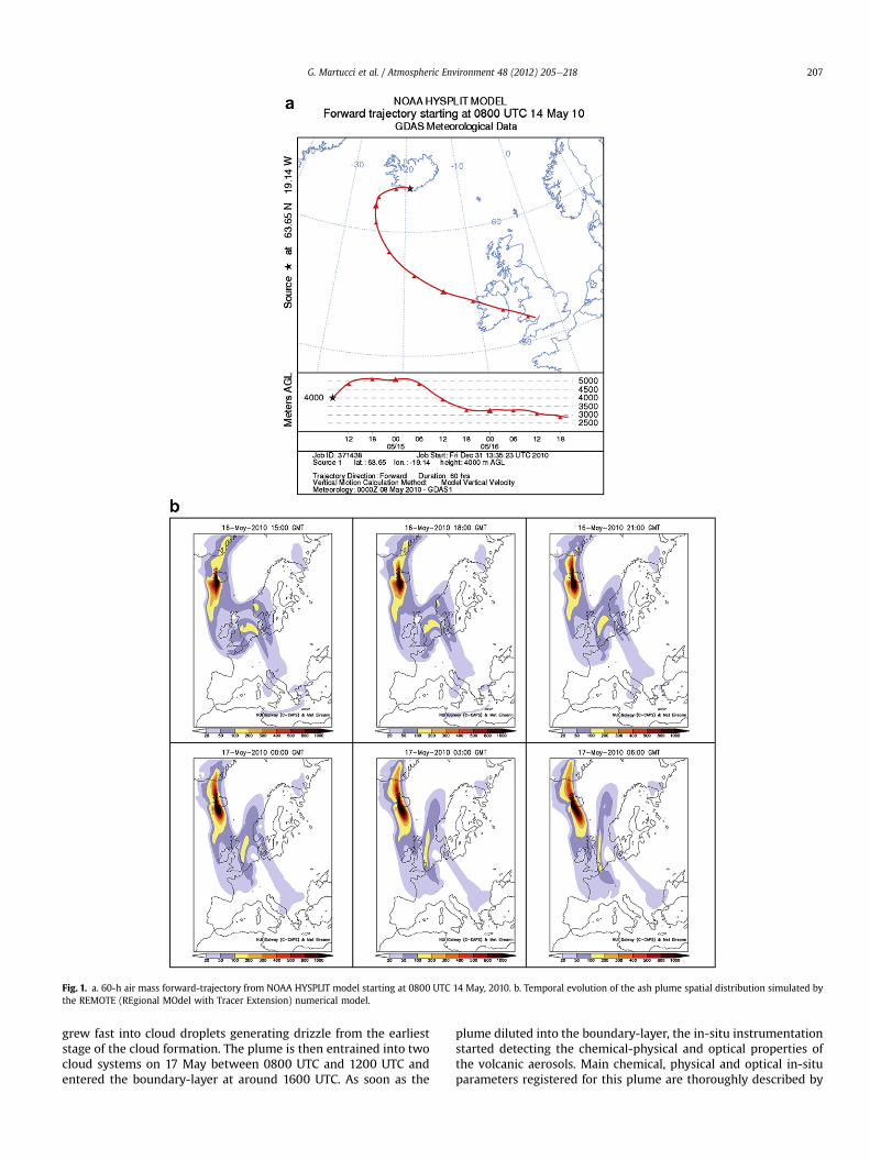
Fig. 1. a. 60-h air mass forward-trajectory from NOAA HYSPLIT model starting at 0800 UTC 14 May, 2010. b. Temporal evolution of the ash plume spatial distribution simulated bythe REMOTE (REgional MOdel with Tracer Extension) numerical model.
G. Martucci et al. / Atmospheric Environment 48 (2012) 205e218 207
grew fast into cloud droplets generating drizzle from the earlieststage of the cloud formation. The plume is then entrained into twocloud systems on 17 May between 0800 UTC and 1200 UTC andentered the boundary-layer at around 1600 UTC. As soon as the
plume diluted into the boundary-layer, the in-situ instrumentationstarted detecting the chemical-physical and optical properties ofthe volcanic aerosols. Main chemical, physical and optical in-situparameters registered for this plume are thoroughly described by
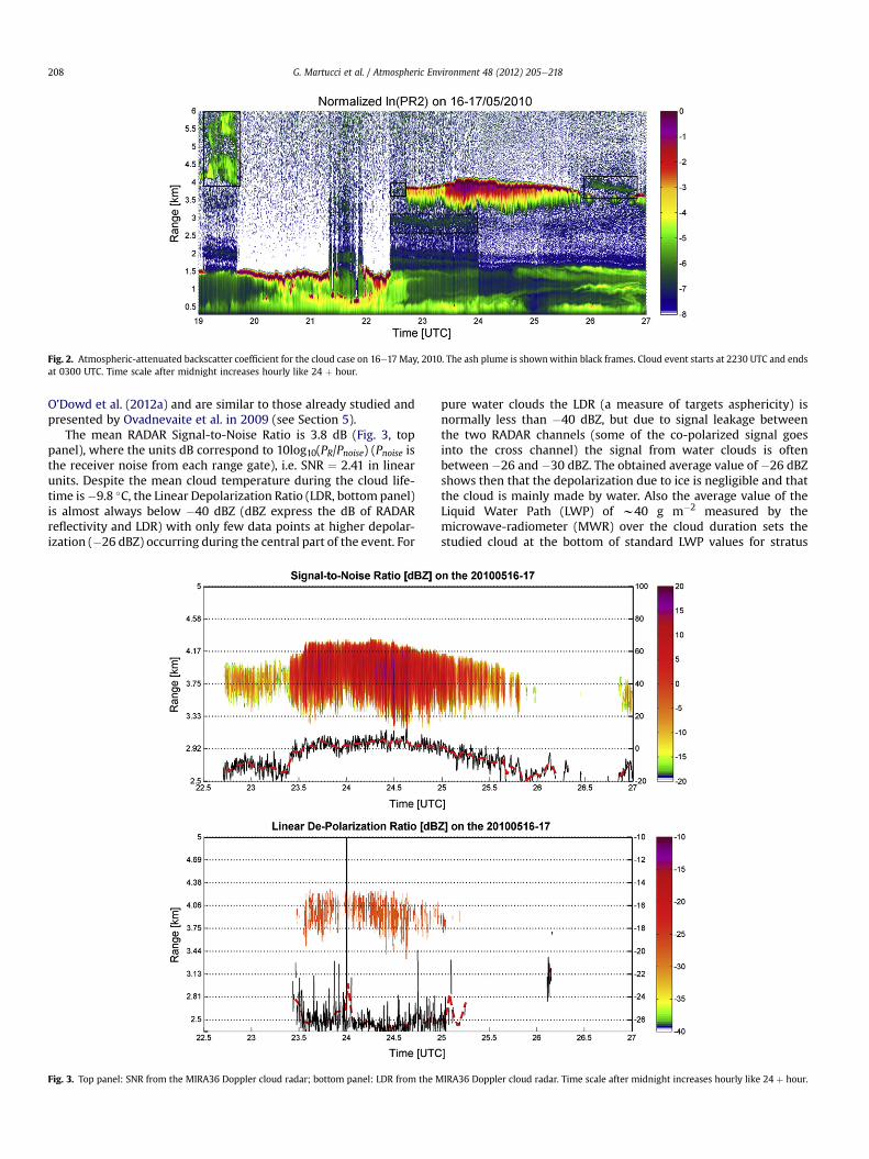
Fig. 2. Atmospheric-attenuated backscatter coefficient for the cloud case on 16e17 May, 2010. The ash plume is shownwithin black frames. Cloud event starts at 2230 UTC and endsat 0300 UTC. Time scale after midnight increases hourly like 24 þ hour.
G. Martucci et al. / Atmospheric Environment 48 (2012) 205e218208
O’Dowd et al. (2012a) and are similar to those already studied andpresented by Ovadnevaite et al. in 2009 (see Section 5).
The mean RADAR Signal-to-Noise Ratio is 3.8 dB (Fig. 3, toppanel), where the units dB correspond to 10log10(PR/Pnoise) (Pnoise isthe receiver noise from each range gate), i.e. SNR ¼ 2.41 in linearunits. Despite the mean cloud temperature during the cloud life-time is�9.8 �C, the Linear Depolarization Ratio (LDR, bottom panel)is almost always below �40 dBZ (dBZ express the dB of RADARreflectivity and LDR) with only few data points at higher depolar-ization (�26 dBZ) occurring during the central part of the event. For
Fig. 3. Top panel: SNR from the MIRA36 Doppler cloud radar; bottom panel: LDR from the M
pure water clouds the LDR (a measure of targets asphericity) isnormally less than �40 dBZ, but due to signal leakage betweenthe two RADAR channels (some of the co-polarized signal goesinto the cross channel) the signal from water clouds is oftenbetween �26 and �30 dBZ. The obtained average value of �26 dBZshows then that the depolarization due to ice is negligible and thatthe cloud is mainly made by water. Also the average value of theLiquid Water Path (LWP) of w40 g m�2 measured by themicrowave-radiometer (MWR) over the cloud duration sets thestudied cloud at the bottom of standard LWP values for stratus
IRA36 Doppler cloud radar. Time scale after midnight increases hourly like 24 þ hour.
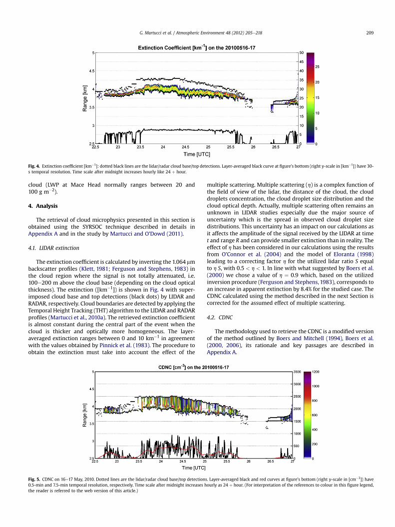
Fig. 4. Extinction coefficient [km�1]: dotted black lines are the lidar/radar cloud base/top detections. Layer-averaged black curve at figure’s bottom (right y-scale in [km�1]) have 30-s temporal resolution. Time scale after midnight increases hourly like 24 þ hour.
G. Martucci et al. / Atmospheric Environment 48 (2012) 205e218 209
cloud (LWP at Mace Head normally ranges between 20 and100 g m�2).
4. Analysis
The retrieval of cloud microphysics presented in this section isobtained using the SYRSOC technique described in details inAppendix A and in the study by Martucci and O’Dowd (2011).
4.1. LIDAR extinction
The extinction coefficient is calculated by inverting the 1.064 mmbackscatter profiles (Klett, 1981; Ferguson and Stephens, 1983) inthe cloud region where the signal is not totally attenuated, i.e.100e200 m above the cloud base (depending on the cloud opticalthickness). The extinction ([km�1]) is shown in Fig. 4 with super-imposed cloud base and top detections (black dots) by LIDAR andRADAR, respectively. Cloud boundaries are detected by applying theTemporal Height Tracking (THT) algorithm to the LIDAR and RADARprofiles (Martucci et al., 2010a). The retrieved extinction coefficientis almost constant during the central part of the event when thecloud is thicker and optically more homogeneous. The layer-averaged extinction ranges between 0 and 10 km�1 in agreementwith the values obtained by Pinnick et al. (1983). The procedure toobtain the extinction must take into account the effect of the
Fig. 5. CDNC on 16e17 May, 2010. Dotted lines are the lidar/radar cloud base/top detections0.5-min and 7.5-min temporal resolution, respectively. Time scale after midnight increases hthe reader is referred to the web version of this article.)
multiple scattering. Multiple scattering (h) is a complex function ofthe field of view of the lidar, the distance of the cloud, the clouddroplets concentration, the cloud droplet size distribution and thecloud optical depth. Actually, multiple scattering often remains anunknown in LIDAR studies especially due the major source ofuncertainty which is the spread in observed cloud droplet sizedistributions. This uncertainty has an impact on our calculations asit affects the amplitude of the signal received by the LIDAR at timet and range R and can provide smaller extinction than in reality. Theeffect of h has been considered in our calculations using the resultsfrom O’Connor et al. (2004) and the model of Eloranta (1998)leading to a correcting factor h for the utilized lidar ratio S equalto h S, with 0.5 < h < 1. In line with what suggested by Boers et al.(2000) we chose a value of h ¼ 0.9 which, based on the utilizedinversion procedure (Ferguson and Stephens, 1983), corresponds toan increase in apparent extinction by 8.4% for the studied case. TheCDNC calculated using the method described in the next Section iscorrected for the assumed effect of multiple scattering.
4.2. CDNC
Themethodology used to retrieve the CDNC is a modified versionof the method outlined by Boers and Mitchell (1994), Boers et al.(2000, 2006), its rationale and key passages are described inAppendix A.
. Layer-averaged black and red curves at figure’s bottom (right y-scale in [cm�3]) haveourly as 24 þ hour. (For interpretation of the references to colour in this figure legend,
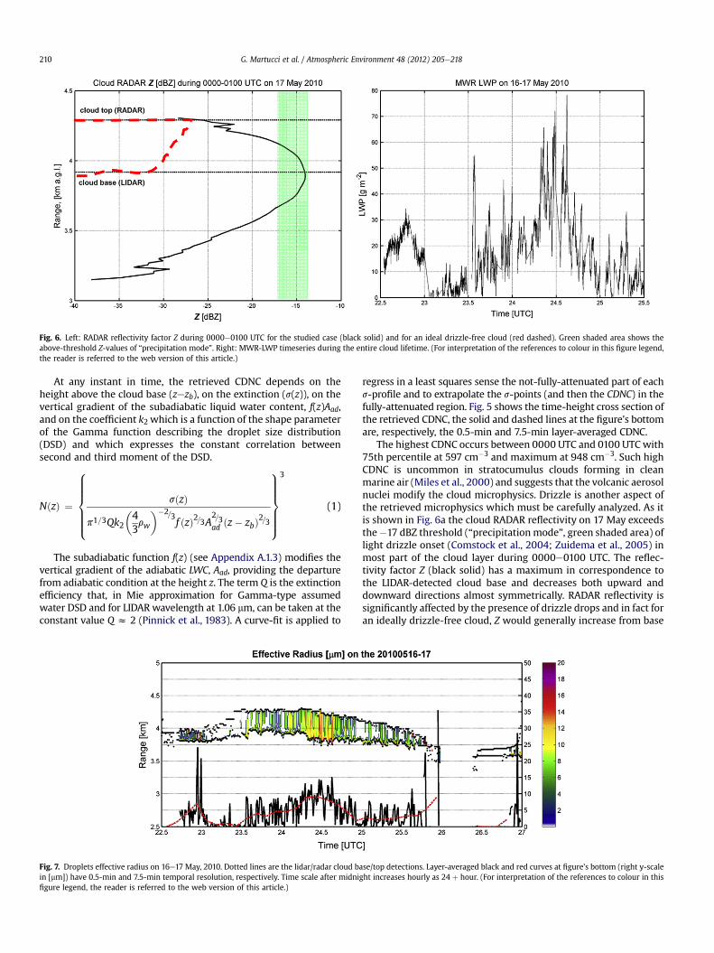
Fig. 6. Left: RADAR reflectivity factor Z during 0000e0100 UTC for the studied case (black solid) and for an ideal drizzle-free cloud (red dashed). Green shaded area shows theabove-threshold Z-values of “precipitation mode”. Right: MWR-LWP timeseries during the entire cloud lifetime. (For interpretation of the references to colour in this figure legend,the reader is referred to the web version of this article.)
G. Martucci et al. / Atmospheric Environment 48 (2012) 205e218210
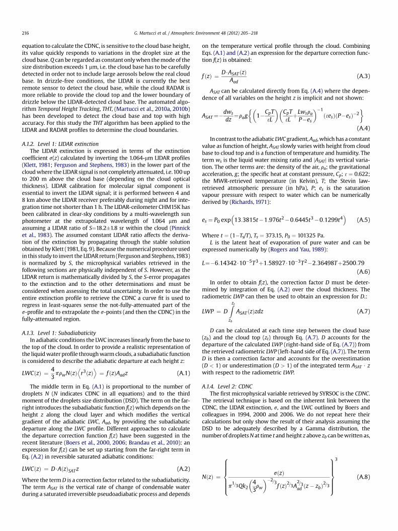
At any instant in time, the retrieved CDNC depends on theheight above the cloud base (zezb), on the extinction (s(z)), on thevertical gradient of the subadiabatic liquid water content, f(z)Aad,and on the coefficient k2 which is a function of the shape parameterof the Gamma function describing the droplet size distribution(DSD) and which expresses the constant correlation betweensecond and third moment of the DSD.
NðzÞ ¼
8>>>>><>>>>>:
sðzÞ
p1=3Qk2
�43rw
��2=3f ðzÞ2=3A2=3
ad ðz� zbÞ2=3
9>>>>>=>>>>>;
3
(1)
The subadiabatic function f(z) (see Appendix A.1.3) modifies thevertical gradient of the adiabatic LWC, Aad, providing the departurefrom adiabatic condition at the height z. The term Q is the extinctionefficiency that, in Mie approximation for Gamma-type assumedwater DSD and for LIDAR wavelength at 1.06 mm, can be taken at theconstant value Q z 2 (Pinnick et al., 1983). A curve-fit is applied to
Fig. 7. Droplets effective radius on 16e17 May, 2010. Dotted lines are the lidar/radar cloud bin [mm]) have 0.5-min and 7.5-min temporal resolution, respectively. Time scale after midnifigure legend, the reader is referred to the web version of this article.)
regress in a least squares sense the not-fully-attenuated part of eachs-profile and to extrapolate the s-points (and then the CDNC) in thefully-attenuated region. Fig. 5 shows the time-height cross section ofthe retrieved CDNC, the solid and dashed lines at the figure’s bottomare, respectively, the 0.5-min and 7.5-min layer-averaged CDNC.
The highest CDNC occurs between 0000 UTC and 0100 UTC with75th percentile at 597 cm�3 and maximum at 948 cm�3. Such highCDNC is uncommon in stratocumulus clouds forming in cleanmarine air (Miles et al., 2000) and suggests that the volcanic aerosolnuclei modify the cloud microphysics. Drizzle is another aspect ofthe retrieved microphysics which must be carefully analyzed. As itis shown in Fig. 6a the cloud RADAR reflectivity on 17 May exceedsthe�17 dBZ threshold (“precipitation mode”, green shaded area) oflight drizzle onset (Comstock et al., 2004; Zuidema et al., 2005) inmost part of the cloud layer during 0000e0100 UTC. The reflec-tivity factor Z (black solid) has a maximum in correspondence tothe LIDAR-detected cloud base and decreases both upward anddownward directions almost symmetrically. RADAR reflectivity issignificantly affected by the presence of drizzle drops and in fact foran ideally drizzle-free cloud, Z would generally increase from base
ase/top detections. Layer-averaged black and red curves at figure’s bottom (right y-scaleght increases hourly as 24 þ hour. (For interpretation of the references to colour in this
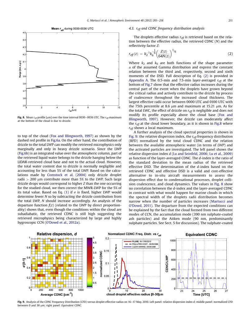
Fig. 8. Mean reff profile [mm] over the time interval 0030e0036 UTC. The reff maximumat the bottom of the cloud is due to drizzle.
G. Martucci et al. / Atmospheric Environment 48 (2012) 205e218 211
to top of the cloud (Fox and Illingworth, 1997) as shown by thedashed red profile in Fig.6a. On the other hand, the contribution ofdrizzle to the total LWP can modify the retrieved microphysics onlymarginally and only in heavy drizzle scenario. Since the LWP(Fig.6b) is an integrated value over the atmospheric column, part ofthe retrieved liquid water belongs to the drizzle hanging below theLIDAR-retrieved cloud base and not to the actual cloud. However,the total water content due to drizzle is normally negligible andaccounting for less than 5% of the total LWP. Based on the calcu-lations made by Comstock et al. (2004) only drizzle dropletradii > 200 mm contribute more than 5% to the LWP. Such largedrizzle drops would correspond to higher Z than the one occurringfor the studied cloud, we then correct the MWR-LWP for the 5% ofits total value. Based on Eq. (1) if s is fixed, higher LWP woulddetermine fewer N so by subtracting the drizzle contribution fromthe total LWP, N should increase accordingly. An analysis of thedeparture function f(z) (related to the LWP by direct proportion-ality) shows that, even though the conditions within the cloud aresubadiabatic, the retrieved CDNC is still high suggesting theretrieved microphysics being characterized by large and highlyhygroscopic CCN (O’Dowd et al., 2012a).
Fig. 9. Analysis of the CDNC Frequency Distribution (CFD) versus droplet effective radius onbetween 0 and 30 mm; right panel: Equivalent CDNC.
4.3. reff and CDNC frequency distribution analysis
The droplets effective radius reff is retrieved based on the rela-tion between the effective radius, the retrieved CDNC (N) and thereflectivity factor Z:
reff ðzÞ ¼ k�12 k
�16
6
�ZðzÞ
64NðzÞ�1=6
(2)
Where k2 and k6 are both functions of the shape parametera of the assumed Gamma distribution and express the constantrelation between the third and, respectively, second and sixthmoments of the DSD. Full description of Eq. (2) is provided inAppendix A. The 0.5-min and 7.5-min layer-averaged reff at thebottom of Fig.7 show that the effective radius increases during thecentral part of the event when the droplets have grown beyondthe critical radius and actively contribute to the drizzle by processof coalescence throughout the increased cloud thickness. Thelargest effective radii occur between 0000 UTC and 0100 UTC withthe 75th percentile at 8.6 mm and maximum at 15.21 mm. As forthe total LWC, the effect of drizzle on reff is negligible and does notmodify its profile especially above the cloud base (Fox andIllingworth, 1997). However, the drizzle can moderately affectthe reff at the cloud lower boundary, as it is shown in Fig.8 wherereff shows a local maximum.
A further analysis of the cloud spectral properties is shown inFig. 9: the relative dispersion index, the reff frequency distribution(RFD) normalized by the total cloud CDNC and the relationbetween the available atmospheric water (in terms of LWP) andthe activated particles are investigated. The left panel shows therelative dispersion index d (Lu and Seinfeld, 2006; Lu et al., 2009)as function of the layer-averaged CDNC. The d-index is the ratio ofthe standard deviation to the mean radius of the retrievedeffective DSD. The determination of the d-index based on theretrieved CDNC and effective DSD is a valid and cost-effectivealternative to in-situ aircraft measurements to assess thedispersion effect due to condensational processes, droplet colli-sion coalescence, and cloud dynamics. The values in Fig. 8 showno correlation between the d-index and the layer-averaged CDNCin contrast with what would happen for marine clouds in whichthe spectral width of the droplets radii distribution becomesnarrow when the number of particles increases (Martucci andO’Dowd, 2011). The departure from the expected conditions canbe explained by the fact that the cloud formed from two differentmodes of CCN, the accumulation mode (390 nm sulphate-coatedash particles) and the Aitken mode (90 nm, predominantlysulphate particles. See Sect. 5 for discussion). The sulphate-coated
16e17 May, 2010. Left panel: relative dispersion index d; middle panel: normalized CFD
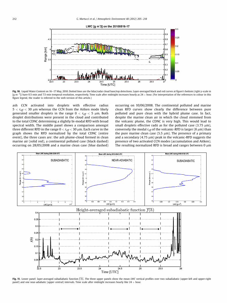
Fig. 10. Liquid Water Content on 16e17 May, 2010. Dotted lines are the lidar/radar cloud base/top detections. Layer-averaged black and red curves at figure’s bottom (right y-scale in[g m�3]) have 0.5-min and 7.5-min temporal resolution, respectively. Time scale after midnight increases hourly as 24 þ hour. (For interpretation of the references to colour in thisfigure legend, the reader is referred to the web version of this article.)
G. Martucci et al. / Atmospheric Environment 48 (2012) 205e218212
ash CCN activated into droplets with effective radius5 < reff < 30 mm whereas the CCN from the Aitken mode likelygenerated smaller droplets in the range 0 < reff < 5 mm. Bothdroplet distributions were present in the cloud and contributedto the total CDNC determining a slightly bi-modal RFD with broadspectral width. The middle panel shows a comparison amongstthree different RFD in the range 0 < reff < 30 mm. Each curve in thegraph shows the RFD normalized by the total CDNC (entireevent), the three cases are: the ash plume-cloud formed in cleanmarine air (solid red), a continental polluted case (black dashed)occurring on 28/05/2008 and a marine clean case (blue dashed)
Fig. 11. Lower panel: layer-averaged subadiabatic function f ðhÞ. The three upper panels shpanel) and one near-adiabatic (upper central) intervals. Time scale after midnight increase
occurring on 10/06/2008. The continental polluted and marineclean RFD curves show clearly the difference between purepolluted and pure clean with the hybrid plume case. In fact,despite the marine clean air in which the cloud stemmed fromthe volcanic plume, the CDNC is very high. This would lead tosmall droplets effective radii as for the polluted case (3.75 mm),conversely the modal reff of the volcanic-RFD is larger (8 mm) thanthe pure marine clean case (5.5 mm). The presence of a primaryand a secondary (4.75 mm) peak in the volcanic-RFD suggests thepresence of two activated CCN modes (accumulation and Aitken).The resulting normalized RFD is broad and ranges between 0 mm
ow the mean LWC vertical profiles over two subadiabatic (upper-left and upper-rights hourly like 24 þ hour.
G. Martucci et al. / Atmospheric Environment 48 (2012) 205e218 213
and 30 mm with only few occurrences for reff > 20 mm. The rightpanel shows the Equivalent CDNC, i.e. the ratio between theactivated droplets and the available condensed water inside thecloud (CDNC/LWP). The ratio provides information on the effi-ciency in generating CDNC.
For marine clean cases a mean value of Equivalent CDNCbetween 1 and 2 is likely to occur (Martucci and O’Dowd, 2011), forthe current case the mean value is around 220 corresponding tovery high efficiency in generating CDNC.
4.4. Liquid water content
One problemwhen retrieving the LWC is the solely dependenceon the reflectivity factor Z and the error induced by the highsensitivity of Z to the few drizzle drops. Eq. (3) expresses the LWC interms of both the LIDAR extinction s and the RADAR reflectivityfactor Z, so that the LWC depends on the optical cloud properties atdifferent wavelengths. The dependence on both Mie and Rayleighscattering ensures a correct representation of the contribution fromboth small and large droplets to the LWC. In fact, when Z is high dueto drizzle the extinction becomes almost zero balancing thecontribution of drizzle to the LWC (Appendix A.1.6):
LWCðzÞ ¼ 13rwNðzÞ�
16k�1
2 k�16
6 ZðzÞ16sðzÞ (3)
Where rw is the density of the water.The high-frequency and low-frequency averages of the LWC at
the bottom of Fig. 10 show that the layer-averaged content of waterwithin the cloud increases during the central part of the cloud
Fig. 12. Uncertainty [%] for the CDNC (upper panel
correspondingly to the larger droplets and the increased cloudthickness. The maximum of the layer-averaged LWC occursbetween 0000 UTC and 0100 UTC with 75th percentile at0.13 g m�3 and maximum at 0.232 g m�3.
Conditionswithin the cloud aremainly subadiabatic as it is shownfrom the timeseries of the layer-averaged departure function f ðzÞ atthe bottom panel of Fig. 11. Function f(z) is a function of the sub-adiabaticityASAT/Aad and the correction factorD (Appendix A.1.3). ThetermD is a correction factor accounting for the overestimation (D< 1)or underestimation (D> 1) of the theoretical LWPwith respect to the(instrumental) radiometric LWP. Departure from theoretical andpurely adiabatic conditions reaches maximum values (minimumf ðzÞ) between 2300e2330 UTC and 0100e0130 UTC when the cloudis thin and the dry air entrained from the top affects the entire cloudlayer. The LWC vertical profiles during these two periods showsignificant departure from the standard adiabatic growth, withmaxima located at mid-height (upper-right) or just above the cloudbase (upper-left). During the central part (0000e0100 UTC), thesubadiabaticity decreases (higher f ðzÞ) and the LWC shows moreadiabatic growth from cloud base to top (upper middle panel).
4.5. Method sensitivity and uncertainty
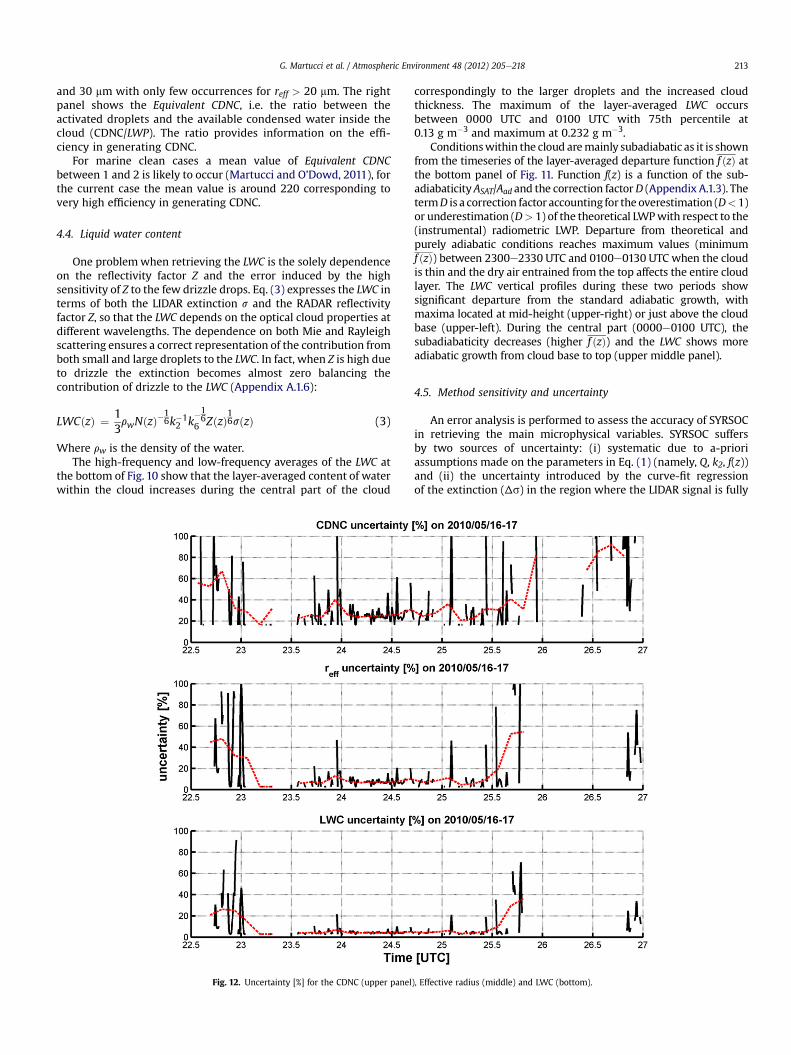
An error analysis is performed to assess the accuracy of SYRSOCin retrieving the main microphysical variables. SYRSOC suffersby two sources of uncertainty: (i) systematic due to a-prioriassumptions made on the parameters in Eq. (1) (namely, Q, k2, f(z))and (ii) the uncertainty introduced by the curve-fit regressionof the extinction (Δs) in the region where the LIDAR signal is fully
), Effective radius (middle) and LWC (bottom).
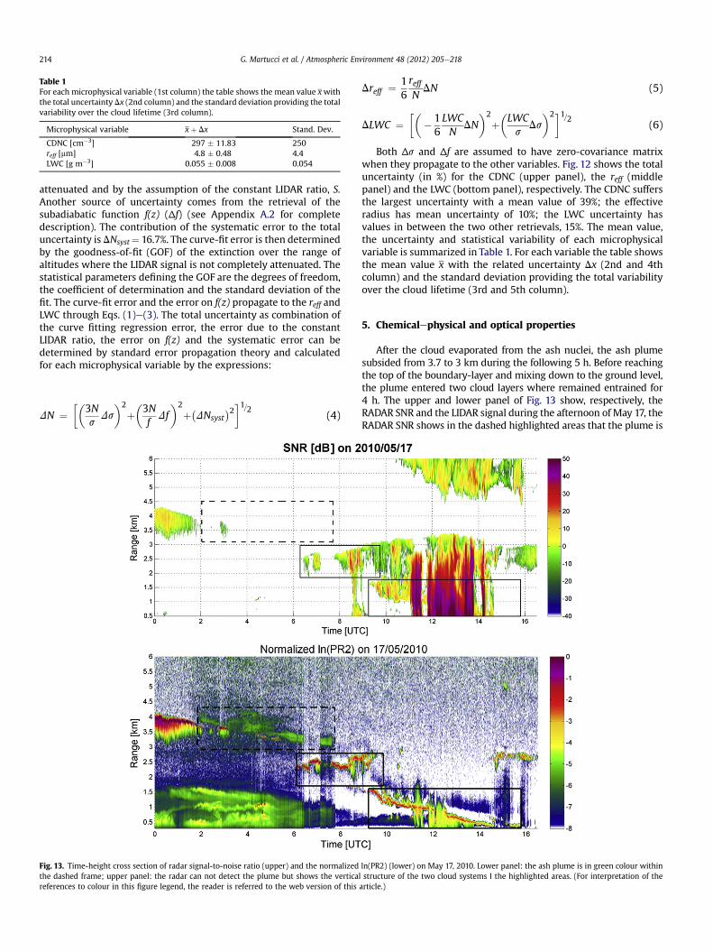
Table 1For each microphysical variable (1st column) the table shows the mean value xwiththe total uncertainty Dx (2nd column) and the standard deviation providing the totalvariability over the cloud lifetime (3rd column).
Microphysical variable xþ Dx Stand. Dev.
CDNC [cm�3] 297 � 11.83 250reff [mm] 4.8 � 0.48 4.4LWC [g m�3] 0.055 � 0.008 0.054
G. Martucci et al. / Atmospheric Environment 48 (2012) 205e218214
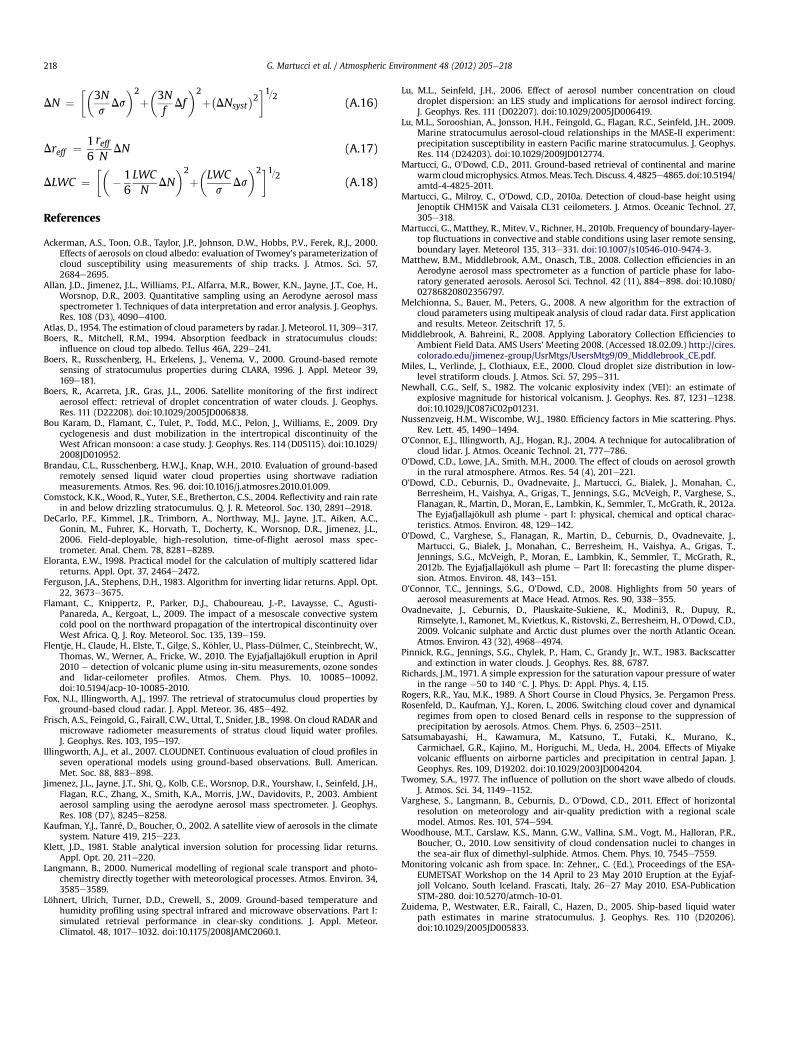
attenuated and by the assumption of the constant LIDAR ratio, S.Another source of uncertainty comes from the retrieval of thesubadiabatic function f(z) (Δf) (see Appendix A.2 for completedescription). The contribution of the systematic error to the totaluncertainty is DNsyst¼ 16.7%. The curve-fit error is then determinedby the goodness-of-fit (GOF) of the extinction over the range ofaltitudes where the LIDAR signal is not completely attenuated. Thestatistical parameters defining the GOF are the degrees of freedom,the coefficient of determination and the standard deviation of thefit. The curve-fit error and the error on f(z) propagate to the reff andLWC through Eqs. (1)e(3). The total uncertainty as combination ofthe curve fitting regression error, the error due to the constantLIDAR ratio, the error on f(z) and the systematic error can bedetermined by standard error propagation theory and calculatedfor each microphysical variable by the expressions:
DN ¼��
3Ns
Ds
�2þ�3Nf
Df�2
þ�DNsyst
�2�1=2 (4)
Fig. 13. Time-height cross section of radar signal-to-noise ratio (upper) and the normalizedthe dashed frame; upper panel: the radar can not detect the plume but shows the verticareferences to colour in this figure legend, the reader is referred to the web version of this
Dreff ¼ 16reffN
DN (5)
DLWC ¼��
� 16LWCN
DN�2
þ�LWCs
Ds�2�1=2
(6)
Both Δs and Δf are assumed to have zero-covariance matrixwhen they propagate to the other variables. Fig. 12 shows the totaluncertainty (in %) for the CDNC (upper panel), the reff (middlepanel) and the LWC (bottom panel), respectively. The CDNC suffersthe largest uncertainty with a mean value of 39%; the effectiveradius has mean uncertainty of 10%; the LWC uncertainty hasvalues in between the two other retrievals, 15%. The mean value,the uncertainty and statistical variability of each microphysicalvariable is summarized in Table 1. For each variable the table showsthe mean value x with the related uncertainty Dx (2nd and 4thcolumn) and the standard deviation providing the total variabilityover the cloud lifetime (3rd and 5th column).
5. Chemicalephysical and optical properties
After the cloud evaporated from the ash nuclei, the ash plumesubsided from 3.7 to 3 km during the following 5 h. Before reachingthe top of the boundary-layer and mixing down to the ground level,the plume entered two cloud layers where remained entrained for4 h. The upper and lower panel of Fig. 13 show, respectively, theRADAR SNR and the LIDAR signal during the afternoon of May 17, theRADAR SNR shows in the dashed highlighted areas that the plume is
ln(PR2) (lower) on May 17, 2010. Lower panel: the ash plume is in green colour withinl structure of the two cloud systems I the highlighted areas. (For interpretation of thearticle.)
G. Martucci et al. / Atmospheric Environment 48 (2012) 205e218 215
not detected by theRADARwhich, on the otherhand, candetect (solidhighlighted areas) the cloud vertical structure of the two subsequentcloud systems more efficiently than the LIDAR. The ash from theplumewas sampled atMaceHead fromthe afternoonofMay17 to theearly morning of May 18 and analyzed using Scanning ElectronMicroscope with EDX (Energy Dispersive X-ray) analysis capability.Ash deposition to the surface occurred only after the plume hadentered the boundary-layer and got mixed down to the ground, i.e.from1600UTConMay17. Thedryashparticleswere typically 1e6mmin size and the main compounds were silicon dioxide, aluminiumoxide, iron oxide and sulphur (O’Dowd et al., 2012a). Sulphurcompounds were mainly sulphate in the form of sulphuric acid andneutralized gypsum. As soon as the plume entered the boundary-layer (around 1600 UTC) it was simultaneously detected by AMS,TEOM, MAAP, Nephelometer, APS and SMPS (O’Dowd et al., 2012a“This Issue”). Measured submicron particles were dominated bysulphate (w60%of totalmass andw90%of total non-refractorymass),while supermicron particles were mostly composed of volcanic ash,presumably covered by sulphate. Sulphate concentration measuredby AMS increased from below 1 mg m�3 up to 8 mg m�3, while othercompounds such as organics, nitrate and ammonium remained atvery low concentrations. Absence of cations in submicron particles,particularly ammonium resulted in a very low degree of sulphateneutralization (DON w 0.16) indicating almost pure sulphuric acidparticles. The presence of pure sulphuric acid in the volcanic aerosolparticles is consistentwith theprevious studyof Satsumabayashi et al.(2004). High aerosol acidity and multiple volcanic plume passagethrough cloud systems indicated that predominant fraction ofsulphate aerosol measured by AMS have been formed by aqueousphase oxidation of SO2. Moreover, well defined Aitken and accumu-lationmodes showed the cloud activation of Aitkenmode particles toform an accumulation mode (O’Dowd et al., 2000). During thevolcanic plume event the diameters of both modes were unusuallylarge (90 nm for the Aitken and 395 nm for the accumulation mode)indicating the growth of particles by an excess amount of sulphate.Both chemical composition and an increase in size of the particlesresulted in very efficient particle activation to CCN. Almost, inde-pendently of the supersaturation, all condensation nuclei (CN) wereactivated into CCN during the plume, thus CCN concentration jumpedfrom the 300 particles cm�3 up to 1000 leading to CN:CCNz1,whereas the total particle concentration had not increased, but evensubsided during the event. Moreover, the very large accumulationmode alongwith a growth factor of 1.7 characteristic of sulphuric acidallow the extrapolation of a dry diameter of 236 nmwhich, based onKöhler equation, leads to efficient and rapid growth to activateddroplets at extremely low value of supersaturation (ss< 0.02%). BothCCN modes present in the cloud, the Aitken and the accumulation,were activated into droplets determining a slightly bi-modal DSD.
6. Conclusions
The Eyjafjallajökull volcanic ash plume was observed at MaceHead Atmospheric Station during 16e18 May 2010 and gave theunique opportunity to (i) study the impact of volcanic aerosol CCNon the cloud microphysics; (ii) to assess the ability and accuracy ofthe SYRSOC cloud microphysics retrieval scheme; (iii) to relate theremote sensing measurements to the physical, chemical and opticalin-situ detections of the volcanic plume.
The insoluble ash core particles coated by mainly sulphuric acidpresent in the plume acted as source of CCN for cloud formationstarting from 2230 UTC onMay 16. H2SO4-coated ash CCN activatedinto large droplets at low supersaturation (ss < 0.02%) generatingcloud droplets with effective radius 0 < reff < 30 mm and broadspectral width. The largest effective radii were reached during thecentral part of the cloud event and related to the peak in the
coalescence process. Themicrophysics retrieved by SYRSOC showedhigh CDNC during the entire cloud event with peak values of948 cm�3 and mean concentration of 297 cm�3. The retrieved highCDNC better characterize stratocumulus clouds forming in conti-nental polluted conditions rather than in clean marine air. BothAitken and the accumulation mode were present in the CCN andactivated into droplets with effective radii in the range0< reff< 5 mmand5< reff< 30 mm, respectively. The presence of twoconcomitant modes determined a slightly bi-modal reff frequencydistribution (RFD) with broad spectral width and zero-correlationbetween the relative dispersion index and the layer-averagedCDNC. The analysis of the subadiabaticity in the cloud showedthat the cloud was predominantly subadiabatic especially duringthe early and last stages of cloud lifetime when the cloud was thinand the dry entrainment more efficient. The error analysis wasperformed by assessing the different sources of systematic erroraffecting the CDNC retrieval and the error introduced by theextinction and that on the retrieval of f(z). The total CDNC uncer-tainty was obtained by summation of the squared errors and thenpropagation to the other microphysical variables. The total SYRSOCuncertainty was 39% for CDNC, 10% for effective radius and 15% forLWC retrieval. The values of the retrieved set of microphysicalvariables along with the analysis of the effective radius size distri-bution and of the dispersion performed by SYRSOC showed that thevolcanic CCN had determined the microphysics of the cloud.
In-situ measurements showed that submicron particles weredominated by sulphate (w60% of total mass), while supermicronparticles were mostly composed of the volcanic ash, presumablycoated by sulphate. Finally, the high aerosol acidity and multiplevolcanic plume passage through cloud systems indicated thatpredominant fraction of sulphate aerosol measured by AMS havebeen formed by aqueous phase oxidation of SO2.
Acknowledgements
This studywas supported by the 4th Higher Education AuthorityProgramme for Research in Third Level Institutions (HEA PRTLI4)and by EPA Ireland through the CCRP Fellowship “Research Supportfor Mace Head”. This work was also conducted as part of COSTAction ES0702 (EG-CLIMET).
Appendix A
A.1. Theory of the method
SYRSOC retrieves the microphysics of liquid clouds providingCDNC, reff, relative dispersion and LWC. SYRSOC is a three-levelalgorithm acquiring off-line input data from the set of instrumentdescribed in Section 2.2. At each level SYRSOC generates microphys-ical outputswhich are used for the next computational level: the firstlevel’s outputs consist of the cloud boundaries, the LIDAR extinctionand the cloud subadiabaticity. The three outputs are calculated usingthe reflectivity from the cloud RADAR, the atmospheric-attenuatedbackscatter from the LIDAR and the temperature and the integratedcloud liquid water from the MWR. The second level’s output is theCDNC from the LIDAR extinction, the cloud depth and the cloudsubadiabaticity. The third level’s outputs are the reff and the cloudLWCe both of which are retrieved using the CDNC, the level of cloudsubadiabaticity and the droplet size distribution.
A.1.1. Level 1: Cloud boundaries determinationDetection of the cloud boundaries plays an important role in the
retrieval of cloud microphysics. Errors of few tens of meters in thedetection of the cloud base can lead to large errors in the calculationof the CDNC. The extinction efficiency Q, which will appear in the
G. Martucci et al. / Atmospheric Environment 48 (2012) 205e218216
equation to calculate the CDNC, is sensitive to the cloud base height,its value quickly responds to variations in the droplet size at thecloudbase.Q can be regardedas constant onlywhen themode of thesize distribution exceeds 1 mm, i.e. the cloud base has to be carefullydetected in order not to include large aerosols below the real cloudbase. In drizzle-free conditions, the LIDAR is currently the bestremote sensor to detect the cloud base, while the cloud RADAR ismore reliable to provide the cloud top and the lower boundary ofdrizzle below the LIDAR-detected cloud base. The automated algo-rithm Temporal Height Tracking, THT, (Martucci et al., 2010a, 2010b)has been developed to detect the cloud base and top with highaccuracy. For this study the THT algorithm has been applied to theLIDAR and RADAR profiles to determine the cloud boundaries.
A.1.2. Level 1: LIDAR extinctionThe LIDAR extinction is expressed in terms of the extinction
coefficient s(z) calculated by inverting the 1.064-mm LIDAR profiles(Klett, 1981; Ferguson and Stephens, 1983) in the lower part of thecloudwhere the LIDAR signal is not completely attenuated, i.e.100 upto 200 m above the cloud base (depending on the cloud opticalthickness). LIDAR calibration for molecular signal component isessential to invert the LIDAR signal; it is performed between 4 and8 km above the LIDAR receiver preferably during night and for inte-gration time not shorter than 1 h. The LIDAR-ceilometer CHM15Khasbeen calibrated in clear-sky conditions by a multi-wavelength sunphotometer at the extrapolated wavelength of 1.064 mm andassuming a LIDAR ratio of S¼18.2�1.8 sr within the cloud (Pinnicket al., 1983). The assumed constant LIDAR ratio affects the deriva-tion of the extinction by propagating through the stable solutionobtainedbyKlett (1981, Eq. 9). Because the numerical procedureusedin this study to invert the LIDAR return (Ferguson and Stephens,1983)is normalized by S, the microphysical variables retrieved in thefollowing sections are physically independent of S. However, as theLIDAR return is mathematically divided by S, the S-error propagatesto the extinction and to the other determinations and must beconsidered when assessing the total uncertainty. In order to use theentire extinction profile to retrieve the CDNC a curve fit is used toregress in least-squares sense the not-fully-attenuated part of thes-profile and to extrapolate the s-points (and then the CDNC) in thefully-attenuated region.
A.1.3. Level 1: SubadiabaticityIn adiabatic conditions the LWC increases linearly from the base to
the top of the cloud. In order to provide a realistic representation ofthe liquidwater profile throughwarmclouds, a subadiabatic functionis considered to describe the adiabatic departure at each height z:
LWCðzÞ ¼ 43prwNðzÞ
Dr3ðzÞ
E¼ f ðzÞAadz (A.1)
The middle term in Eq. (A.1) is proportional to the number ofdroplets N (N indicates CDNC in all equations) and to the thirdmoment of the droplets size distribution (DSD). The term on the far-right introduces the subadiabatic function f(z) which depends on theheight z along the cloud layer and which modifies the verticalgradient of the adiabatic LWC, Aad, by providing the subadiabaticdeparture along the LWC profile. Different approaches to calculatethe departure correction function f(z) have been suggested in therecent literature (Boers et al., 2000, 2006; Brandau et al., 2010): anexpression for f(z) can be set up starting from the far-right term inEq. (A.2) in reversible saturated adiabatic conditions:
LWCðzÞ ¼ D$AðzÞSATz (A.2)
Where the termD is a correction factor related to the subadiabaticity.The term ASAT is the vertical rate of change of condensable waterduring a saturated irreversible pseudoadiabatic process and depends
on the temperature vertical profile through the cloud. CombiningEqs. (A.1) and (A.2) an expression for the departure correction func-tion f(z) is obtained:
f ðzÞ ¼ D$ASATðzÞAad
(A.3)
ASAT can be calculated directly from Eq. (A.4) where the depen-dence of all variables on the height z is implicit and not shown:
ASAT¼�dws
dz¼rag
��1�CpT
3L
��CpT
3LþLwsraP�es
��1
ð 3esÞðP�esÞ�2(A.4)
In contrast to the adiabatic LWCgradient,Aad,whichhas a constantvalue as function of height, ASAT slowly varies with height from cloudbase to cloud top and is a function of temperature and humidity. Theterm ws is the liquid water mixing ratio and jASATj its vertical varia-tion. The other terms are: the density of the air, ra; the gravitationalacceleration, g; the specific heat at constant pressure, Cp; 3¼ 0.622;the MWR-retrieved temperature (in Kelvin), T; the Stevin law-retrieved atmospheric pressure (in hPa), P; es is the saturationvapour pressure with respect to water which can be numericallyderived by (Richards, 1971):
es ¼ P0 exp13:3815t�1:976t2�0:6445t3�0:1299t4
�(A.5)
Where t ¼ (1�Ts/T), Ts ¼ 373.15, P0 ¼ 101325 Pa.L is the latent heat of evaporation of pure water and can be
expressed numerically by (Rogers and Yau, 1989):
L¼�6:14342$10�5T3þ1:58927$10�3T2�2:36498Tþ2500:79(A.6)
In order to obtain f(z), the correction factor D must be deter-mined by integration of Eq. (A.2) over the cloud thickness. Theradiometric LWP can then be used to obtain an expression for D.:
LWP ¼ DZztzb
ASAT ðzÞzdz (A.7)
D can be calculated at each time step between the cloud base(zb) and the cloud top (zt) through Eq. (A.7). D accounts for thedeparture of the calculated LWP (right-hand side of Eq. (A.7)) fromthe retrieved radiometric LWP (left-hand side of Eq. (A.7)). The termD is then a correction factor and accounts for the overestimation(D < 1) or underestimation (D > 1) of the integrated term ASAT $ zwith respect to the radiometric LWP.
A.1.4. Level 2: CDNCThe first microphysical variable retrieved by SYRSOC is the CDNC.
The retrieval technique is based on the inherent link between theCDNC, the LIDAR extinction, s, and the LWC outlined by Boers andcolleagues in 1994, 2000 and 2006. We do not repeat here theircalculations but only show the result of their analysis assuming theDSD to be adequately described by a Gamma distribution, thenumber of dropletsN at time t andheight z above zb can bewritten as,
NðzÞ ¼
8>>>>><>>>>>:
sðzÞ
p1=3Qk2
�43rw
��2=3f ðzÞ2=3A2=3
ad ðz� zbÞ2=3
9>>>>>=>>>>>;
3
(A.8)
G. Martucci et al. / Atmospheric Environment 48 (2012) 205e218 217
Where rw is the density of liquid water; s is the extinction coeffi-cient; Q is the extinction efficiency, which, in Mie approximation forGamma-type water DSD and for a LIDAR wavelength of 1.06 mm, canbe assumed constant,Qz 2 (Pinnick et al.,1983). The coefficient k2 isfunction of the size parameter a of the Gamma distribution whichdescribes the droplet spectrum. The values of a depend on the airmass in which the cloud forms and can be parameterized (Mileset al., 2000) by a ¼ 3 and a ¼ 7 in marine and continental air,respectively. Depending on the vertical resolution of the extinctionprofile a limited number of s-points (normally 10e15 points with15-m resolution) can be used to regress in least square Eq. (A.8) toeach extinction profile with N as a free parameter. The error relatedto the curve-fit to retrieve N is a major source of uncertainty, i.e. theextrapolated s-points can deviate from the true extinction profilethrough the cloud. Differences of both signs can lead to eitherunderestimated or overestimated values of N producing an uncer-tainty which propagates to the other microphysical variables.
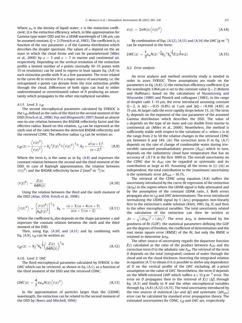
A.1.5. Level 3: reffThe second microphysical parameter calculated by SYRSOC is
the reff, defined as the ratio of the third to the secondmoment of theDSD (Frisch et al., 1998). Fox and Illingworth (1997) found an almostone-to-one relation between the RADAR reflectivity factor and theeffective radius. Based on this relation, reff can be expressed as thesixth root of the ratio between the detected RADAR reflectivity andthe retrieved CDNC. The effective radius reff can be written as:
reff ðzÞ ¼DrðzÞ3
EDrðzÞ2
E¼ k�12 f ðzÞ1=3
DrðzÞ3
E1=3; k2 ¼a
13ðaþ1Þ13ðaþ2Þ23
; (A.9)
Where the term k2 is the same as in Eq. (A.8) and expresses theconstant relation between the second and the third moment of theDSD. In case of Rayleigh approximation, the relation betweenhrðzÞ6i and the RADAR reflectivity factor Z [mm6 m�3] is:
�rðzÞ6 ¼ ZðzÞ
64NðzÞ: (A.10)
Using the relation between the third and the sixth moment ofthe DSD (Atlas, 1954; Frisch et al., 1998):
DrðzÞ3
E¼
"�rðzÞ6
k6f ðzÞ2#1=2
; k6 ¼ ðaþ 3Þðaþ 4Þðaþ 5Þaðaþ 1Þðaþ 2Þ ; (A.11)
Where the coefficient k6 also depends on the shape parameter a andexpresses the constant relation between the sixth and the thirdmoment of the DSD.
Then, using Eqs. (A.10) and (A.11) and by combining withEq. (A.9), reff can be written as:
reff ðzÞ ¼ k�12 k
�16
6
�ZðzÞ
64NðzÞ�1=6
(A.12)
A.1.6. Level 3: LWCThe third microphysical parameter calculated by SYRSOC is the
LWC which can be retrieved, as shown in Eq. (A.1), as a function ofthe third moment of the DSD and the retrieved CDNC.
LWCðzÞ ¼ 43prwNðzÞ
DrðzÞ3
E(A.13)
In the approximation of particles larger than the (LIDAR)wavelength, the extinction can be related to the second moment ofthe DSD by (Boers and Mitchell, 1994):
sðzÞ ¼ 2pNðzÞDrðzÞ2
E(A.14)
By combination of Eqs. (A.12), (A.13) and (A.14) the LWC [g m�3]can be expressed in the form:
LWCðzÞ ¼ 13rwNðzÞ�
16k�1
2 k�16
6 ZðzÞ16sðzÞ (A.15)
A.2. Error analysis
An error analysis and method sensitivity study is needed inorder to asses SYRSOC. Three assumptions are made on theparameters in Eq. (A.8): (i) the extinction efficiency coefficient Q atthe wavelength 1.064 mm is set to the constant value Q¼ 2 (Bohrenand Huffman); based on the calculations of Nussenzveig andWiscombe (1980) and Pinnick and colleagues (1983), in the rangeof droplet radii 1e15 mm, the error introduced assuming constantQ¼ 2, is DQ¼e0.15 (6.8%) at 1 mm and DQ¼þ0.106 (4.8%) at15 mm. At larger radii the error rapidly drops below 1%. (ii) The termk2 depends on the exponent of the size parameter of the assumedGamma distribution which describes the DSD. The value ofa depends on the type of air mass and can double from marine tocontinental air (Miles et al., 2000). Nonetheless, the method issufficiently stable with respect to the variations of a: when a is inthe range from 2 to 50 the relative changes in the retrieved CDNCare between 0 and 14%. (iii) The correction term D in Eq. (A.7)depends on the rate of change of condensable water during irre-versible saturated pseudoadiabatic process (ASAT) which in turn,depends on the radiometric cloud base temperature that has anaccuracy of �0.7 K in the first 1000 m. The overall uncertainty onthe CDNC due to ASAT can be regarded as systematic and itscontribution as large as 6%. Assuming all the terms in (i)e(iii) asindependent, the total contribution to the (maximum) uncertaintyis the systematic error DNsyst¼ 16.7%.
The retrieval of the CDNC using equation (A.8) suffers theuncertainty introduced by the curve-fit regression of the extinction(Dsfit) in the region where the LIDAR signal is fully attenuated andby the assumption of the constant LIDAR ratio, S. Both errorspropagate also to reff and LWC determinations. The error introducednormalizing the LIDAR signal by S (DsS) propagates non-linearlyfirst to the extinction’s stable solution (Klett, 1981, Eq. 9) and thento the other microphysical variables. The total uncertainty relatedthe calculation of the extinction can then be written as
Ds ¼ffiffiffiffiffiffiffiffiffiffiffiffiffiffiffiffiffiffiffiffiffiffiffiffiffiffiffiffiffiffiffiffiffiffiffiffiðDsfitÞ2 þ ðDsSÞ2
q. The error Dsfit is determined by the
goodness-of-fit (GOF); the statistical parameters defining the GOFare the degrees of freedom, the coefficient of determination and theroot mean square error (RMSE) of the fit, but only the RMSE isretained to determine Dsfit.
The other source of uncertainty regards the departure functionf(z) calculated as the ratio of the product between ASAT and thecorrection term D to the adiabatic rate Aad. The retrieval of the termD depends on the total (integrated) content of water through thecloud and on the cloud thickness. Inverting the integrated relationin equation (A.7) to obtain D it is possible to shelve any dependenceof D on the vertical profile of the LWC excluding all a-prioriassumption on the value of LWC. Nevertheless, the term D dependson the MWR-retrieved LWP which suffers a� 15 gm�2 error. Theerror on D propagates then to the retrieval of f(z) (Df) throughEq. (A.3) and finally to N and the other microphysical variablesthrough Eq. (A.8)-(A.12)-(A.15). The total uncertainty introduced bythe two sources of statistical (Ds and Df) and systematic (DNsyst)error can be calculated by standard error propagation theory. Theestimated uncertainties for CDNC, reff and LWC are, respectively:
G. Martucci et al. / Atmospheric Environment 48 (2012) 205e218218
DN ¼��
3NDs
�2þ�3N
Df�2
þ�DNsyst
�2�1=2 (A.16)
s fDreff ¼ 16reffN
DN (A.17)
DLWC ¼��
� 16LWCN
DN�2
þ�LWCs
Ds�2�1=2
(A.18)
References
Ackerman, A.S., Toon, O.B., Taylor, J.P., Johnson, D.W., Hobbs, P.V., Ferek, R.J., 2000.Effects of aerosols on cloud albedo: evaluation of Twomey’s parameterization ofcloud susceptibility using measurements of ship tracks. J. Atmos. Sci. 57,2684e2695.
Allan, J.D., Jimenez, J.L., Williams, P.I., Alfarra, M.R., Bower, K.N., Jayne, J.T., Coe, H.,Worsnop, D.R., 2003. Quantitative sampling using an Aerodyne aerosol massspectrometer 1. Techniques of data interpretation and error analysis. J. Geophys.Res. 108 (D3), 4090e4100.
Atlas, D., 1954. The estimation of cloud parameters by radar. J. Meteorol. 11, 309e317.Boers, R., Mitchell, R.M., 1994. Absorption feedback in stratocumulus clouds:
influence on cloud top albedo. Tellus 46A, 229e241.Boers, R., Russchenberg, H., Erkelens, J., Venema, V., 2000. Ground-based remote
sensing of stratocumulus properties during CLARA, 1996. J. Appl. Meteor 39,169e181.
Boers, R., Acarreta, J.R., Gras, J.L., 2006. Satellite monitoring of the first indirectaerosol effect: retrieval of droplet concentration of water clouds. J. Geophys.Res. 111 (D22208). doi:10.1029/2005JD006838.
Bou Karam, D., Flamant, C., Tulet, P., Todd, M.C., Pelon, J., Williams, E., 2009. Drycyclogenesis and dust mobilization in the intertropical discontinuity of theWest African monsoon: a case study. J. Geophys. Res. 114 (D05115). doi:10.1029/2008JD010952.
Brandau, C.L., Russchenberg, H.W.J., Knap, W.H., 2010. Evaluation of ground-basedremotely sensed liquid water cloud properties using shortwave radiationmeasurements. Atmos. Res. 96. doi:10.1016/j.atmosres.2010.01.009.
Comstock, K.K., Wood, R., Yuter, S.E., Bretherton, C.S., 2004. Reflectivity and rain ratein and below drizzling stratocumulus. Q. J. R. Meteorol. Soc. 130, 2891e2918.
DeCarlo, P.F., Kimmel, J.R., Trimborn, A., Northway, M.J., Jayne, J.T., Aiken, A.C.,Gonin, M., Fuhrer, K., Horvath, T., Docherty, K., Worsnop, D.R., Jimenez, J.L.,2006. Field-deployable, high-resolution, time-of-flight aerosol mass spec-trometer. Anal. Chem. 78, 8281e8289.
Eloranta, E.W., 1998. Practical model for the calculation of multiply scattered lidarreturns. Appl. Opt. 37, 2464e2472.
Ferguson, J.A., Stephens, D.H., 1983. Algorithm for inverting lidar returns. Appl. Opt.22, 3673e3675.
Flamant, C., Knippertz, P., Parker, D.J., Chaboureau, J.-P., Lavaysse, C., Agusti-Panareda, A., Kergoat, L., 2009. The impact of a mesoscale convective systemcold pool on the northward propagation of the intertropical discontinuity overWest Africa. Q. J. Roy. Meteorol. Soc. 135, 139e159.
Flentje, H., Claude, H., Elste, T., Gilge, S., Köhler, U., Plass-Dülmer, C., Steinbrecht, W.,Thomas, W., Werner, A., Fricke, W., 2010. The Eyjafjallajökull eruption in April2010 e detection of volcanic plume using in-situ measurements, ozone sondesand lidar-ceilometer profiles. Atmos. Chem. Phys. 10, 10085e10092.doi:10.5194/acp-10-10085-2010.
Fox, N.I., Illingworth, A.J., 1997. The retrieval of stratocumulus cloud properties byground-based cloud radar. J. Appl. Meteor. 36, 485e492.
Frisch, A.S., Feingold, G., Fairall, C.W., Uttal, T., Snider, J.B., 1998. On cloud RADAR andmicrowave radiometer measurements of stratus cloud liquid water profiles.J. Geophys. Res. 103, 195e197.
Illingworth, A.J., et al., 2007. CLOUDNET. Continuous evaluation of cloud profiles inseven operational models using ground-based observations. Bull. American.Met. Soc. 88, 883e898.
Jimenez, J.L., Jayne, J.T., Shi, Q., Kolb, C.E., Worsnop, D.R., Yourshaw, I., Seinfeld, J.H.,Flagan, R.C., Zhang, X., Smith, K.A., Morris, J.W., Davidovits, P., 2003. Ambientaerosol sampling using the aerodyne aerosol mass spectrometer. J. Geophys.Res. 108 (D7), 8245e8258.
Kaufman, Y.J., Tanré, D., Boucher, O., 2002. A satellite view of aerosols in the climatesystem. Nature 419, 215e223.
Klett, J.D., 1981. Stable analytical inversion solution for processing lidar returns.Appl. Opt. 20, 211e220.
Langmann, B., 2000. Numerical modelling of regional scale transport and photo-chemistry directly together with meteorological processes. Atmos. Environ. 34,3585e3589.
Löhnert, Ulrich, Turner, D.D., Crewell, S., 2009. Ground-based temperature andhumidity profiling using spectral infrared and microwave observations. Part I:simulated retrieval performance in clear-sky conditions. J. Appl. Meteor.Climatol. 48, 1017e1032. doi:10.1175/2008JAMC2060.1.
Lu, M.L., Seinfeld, J.H., 2006. Effect of aerosol number concentration on clouddroplet dispersion: an LES study and implications for aerosol indirect forcing.J. Geophys. Res. 111 (D02207). doi:10.1029/2005JD006419.
Lu, M.L., Sorooshian, A., Jonsson, H.H., Feingold, G., Flagan, R.C., Seinfeld, J.H., 2009.Marine stratocumulus aerosol-cloud relationships in the MASE-II experiment:precipitation susceptibility in eastern Pacific marine stratocumulus. J. Geophys.Res. 114 (D24203). doi:10.1029/2009JD012774.
Martucci, G., O’Dowd, C.D., 2011. Ground-based retrieval of continental and marinewarmcloudmicrophysics. Atmos.Meas. Tech. Discuss. 4, 4825e4865. doi:10.5194/amtd-4-4825-2011.
Martucci, G., Milroy, C., O’Dowd, C.D., 2010a. Detection of cloud-base height usingJenoptik CHM15K and Vaisala CL31 ceilometers. J. Atmos. Oceanic Technol. 27,305e318.
Martucci, G., Matthey, R., Mitev, V., Richner, H., 2010b. Frequency of boundary-layer-top fluctuations in convective and stable conditions using laser remote sensing,boundary layer. Meteorol 135, 313e331. doi:10.1007/s10546-010-9474-3.
Matthew, B.M., Middlebrook, A.M., Onasch, T.B., 2008. Collection efficiencies in anAerodyne aerosol mass spectrometer as a function of particle phase for labo-ratory generated aerosols. Aerosol Sci. Technol. 42 (11), 884e898. doi:10.1080/02786820802356797.
Melchionna, S., Bauer, M., Peters, G., 2008. A new algorithm for the extraction ofcloud parameters using multipeak analysis of cloud radar data. First applicationand results. Meteor. Zeitschrift 17, 5.
Middlebrook, A. Bahreini, R., 2008. Applying Laboratory Collection Efficiencies toAmbient Field Data. AMS Users’ Meeting 2008. (Accessed 18.02.09.) http://cires.colorado.edu/jimenez-group/UsrMtgs/UsersMtg9/09_Middlebrook_CE.pdf.
Miles, L., Verlinde, J., Clothiaux, E.E., 2000. Cloud droplet size distribution in low-level stratiform clouds. J. Atmos. Sci. 57, 295e311.
Newhall, C.G., Self, S., 1982. The volcanic explosivity index (VEI): an estimate ofexplosive magnitude for historical volcanism. J. Geophys. Res. 87, 1231e1238.doi:10.1029/JC087iC02p01231.
Nussenzveig, H.M., Wiscombe, W.J., 1980. Efficiency factors in Mie scattering. Phys.Rev. Lett. 45, 1490e1494.
O’Connor, E.J., Illingworth, A.J., Hogan, R.J., 2004. A technique for autocalibration ofcloud lidar. J. Atmos. Oceanic Technol. 21, 777e786.
O’Dowd, C.D., Lowe, J.A., Smith, M.H., 2000. The effect of clouds on aerosol growthin the rural atmosphere. Atmos. Res. 54 (4), 201e221.
O’Dowd, C.D., Ceburnis, D., Ovadnevaite, J., Martucci, G., Bialek, J., Monahan, C.,Berresheim, H., Vaishya, A., Grigas, T., Jennings, S.G., McVeigh, P., Varghese, S.,Flanagan, R., Martin, D., Moran, E., Lambkin, K., Semmler, T., McGrath, R., 2012a.The Eyjafjallajökull ash plume - part I: physical, chemical and optical charac-teristics. Atmos. Environ. 48, 129e142.
O’Dowd, C., Varghese, S., Flanagan, R., Martin, D., Ceburnis, D., Ovadnevaite, J.,Martucci, G., Bialek, J., Monahan, C., Berresheim, H., Vaishya, A., Grigas, T.,Jennings, S.G., McVeigh, P., Moran, E., Lambkin, K., Semmler, T., McGrath, R.,2012b. The Eyjafjallajökull ash plume e Part II: forecasting the plume disper-sion. Atmos. Environ. 48, 143e151.
O’Connor, T.C., Jennings, S.G., O’Dowd, C.D., 2008. Highlights from 50 years ofaerosol measurements at Mace Head. Atmos. Res. 90, 338e355.
Ovadnevaite, J., Ceburnis, D., Plauskaite-Sukiene, K., Modini3, R., Dupuy, R.,Rimselyte, I., Ramonet, M., Kvietkus, K., Ristovski, Z., Berresheim, H., O’Dowd, C.D.,2009. Volcanic sulphate and Arctic dust plumes over the north Atlantic Ocean.Atmos. Environ. 43 (32), 4968e4974.
Pinnick, R.G., Jennings, S.G., Chylek, P., Ham, C., Grandy Jr., W.T., 1983. Backscatterand extinction in water clouds. J. Geophys. Res. 88, 6787.
Richards, J.M., 1971. A simple expression for the saturation vapour pressure of waterin the range �50 to 140 �C. J. Phys. D: Appl. Phys. 4, L15.
Rogers, R.R., Yau, M.K., 1989. A Short Course in Cloud Physics, 3e. Pergamon Press.Rosenfeld, D., Kaufman, Y.J., Koren, I., 2006. Switching cloud cover and dynamical
regimes from open to closed Benard cells in response to the suppression ofprecipitation by aerosols. Atmos. Chem. Phys. 6, 2503e2511.
Satsumabayashi, H., Kawamura, M., Katsuno, T., Futaki, K., Murano, K.,Carmichael, G.R., Kajino, M., Horiguchi, M., Ueda, H., 2004. Effects of Miyakevolcanic effluents on airborne particles and precipitation in central Japan. J.Geophys. Res. 109, D19202. doi:10.1029/2003JD004204.
Twomey, S.A., 1977. The influence of pollution on the short wave albedo of clouds.J. Atmos. Sci. 34, 1149e1152.
Varghese, S., Langmann, B., Ceburnis, D., O’Dowd, C.D., 2011. Effect of horizontalresolution on meteorology and air-quality prediction with a regional scalemodel. Atmos. Res. 101, 574e594.
Woodhouse, M.T., Carslaw, K.S., Mann, G.W., Vallina, S.M., Vogt, M., Halloran, P.R.,Boucher, O., 2010. Low sensitivity of cloud condensation nuclei to changes inthe sea-air flux of dimethyl-sulphide. Atmos. Chem. Phys. 10, 7545e7559.
Monitoring volcanic ash from space. In: Zehner,, C. (Ed.), Proceedings of the ESA-EUMETSAT Workshop on the 14 April to 23 May 2010 Eruption at the Eyjaf-joll Volcano, South Iceland. Frascati, Italy, 26e27 May 2010. ESA-PublicationSTM-280. doi:10.5270/atmch-10-01.
Zuidema, P., Westwater, E.R., Fairall, C., Hazen, D., 2005. Ship-based liquid waterpath estimates in marine stratocumulus. J. Geophys. Res. 110 (D20206).doi:10.1029/2005JD005833.