Embed Size (px)
Citation preview
RESEARCH Open Access
Impact of trade liberalization and worldprice changes in Bangladesh: a computablegeneral equilibrium analysisMohammad Jahangir Alam1,2,3*, Jeroen Buysse3, Ismat Ara Begum4, Stephan Nolte5, Eric J. Wailes6
and Guido Van Huylenbroeck3
* Correspondence: [email protected] School of AppliedEconomics and Management,Cornell University, Ithaca 14853NY,USA2Department of Agribusiness andMarketing, Bangladesh AgriculturalUniversity, Mymensingh-2202,BangladeshFull list of author information isavailable at the end of the article
Abstract
The paper analyzes the impact of partial liberalization of trade and changes in worldprices of agricultural commodities in Bangladesh using single country ComputableGeneral Equilibrium (CGE) model. Since the agricultural sector is sensitive to overallemployment, household welfare and food security, the analysis focuses on thechanges in agricultural production, consumption, household income and welfare.The results show that trade liberalization increases the welfare of all householdgroups while world market price increases decrease welfare. It means that althoughtrade liberalization generates a welfare increase for households but this is dependenton the relative level of world commodity prices. Our results are based on theanalysis of aggregate household groups, so it may be of future research interestto extend the model with more detailed household groups using a CGE-microsimulation approach.
Keywords: Static, CGE, Trade policy, World prices, Agricultural commodities,Bangladesh
BackgroundThere are many policy debates in Bangladesh whether the country needs to further
liberalize its trade, especially after the food commodity price surges during 2007–2008
and the one going on currently, or to go back to a policy of protecting the domestic
sectors from foreign competition. Although the country has made much progress in
the liberalization of its’ trade there is still room to further reduce the protection level.
But, the 2007–2008 and the ongoing price surges have initiated the debate especially
because the world market supply was found to be unstable making prices more vola-
tile. This may make the country more vulnerable, lead to severe food insecurity both at
national and household level, and hence decreases household welfare and could deep-
ened the poverty . It is not unlikely that such price increases happen again in future as
a result of the inherent risk in agricultural production, which may be potentially exac-
erbated by increasing volatility due to climate changes and other relevant factors asso-
ciated with the commodity price volatility. As the entire population depends on rice
for a large share of their calorie intake, food security becomes for the most part analo-
gous to ‘rice security’. Therefore, food security and poverty reduction are the top
© 2016 Alam et al. Open Access This article is distributed under the terms of the Creative Commons Attribution 4.0 InternationalLicense (http://creativecommons.org/licenses/by/4.0/), which permits unrestricted use, distribution, and reproduction in any medium,provided you give appropriate credit to the original author(s) and the source, provide a link to the Creative Commons license, andindicate if changes were made.
Alam et al. Agricultural and Food Economics (2016) 4:1 DOI 10.1186/s40100-016-0045-x
priorities of development policy since colonial time in Bangladesh. Several studies
(Dorosh 2001; Ivanic and Martin 2007) show that domestic (Bangladesh) market
liberalization for inputs and outputs, along with agricultural trade liberalization (import
and export) at the border has led to higher productivity, stabilized Bangladesh’s overall
food security, and reduced real prices of agricultural commodities. But this does not
take away the existing concern that an unstable international supply or a distortion in
the export policies of major exporting countries can have detrimental effect for a net
food importing country such as Bangladesh. Computable General Equilibrium (CGE)
model has been used for a very diverse set of policy questions in Bangladesh with
results at the macro, sectoral and household level poverty, income and welfare. Marzia
(2004) models the effects of trade on women groups differentiated based on the socio-
economic characteristics and has used a gendered social accounting matrix and CGE
model for calibrating different trade policy scenarios. The author highlights the role of
trade on women and compares the results with Zambia. The main result of this study
is that trade liberalization rose female wages and employment in a labour abundant
country like Bangladesh but it is not beneficial for women in a natural-resource abun-
dant country like Zambia.
There are very few studies that have evaluated the impact of trade liberalization in
the Bangladesh economy such as Annabi et al. (2006), Hoque (2006), Khondker and
Raihan (2004), Noman (2002), Ahmed (2001) etc. Most of these studies focused on the
macroeconomic perspective rather than distributional aspects such as income, welfare.
Khondker and Raihan (2004) presented that full trade liberalization would generate
negative consequences for the macro-economy as well as for the welfare and poverty
status of the households in Bangladesh. On the contrary, Mujeri and Khondker (2002)
found that globalization efforts in Bangladesh are generally pro-poor, although the
gains accrue more to the well-off households while the extremely poor households
benefit less. Marzia and Adrian (2000) have analyzed the effect of trade on women’s
wages and jobs, household work and leisure. This paper developed a model with not
only the sectors of the market economy but also with social reproduction and leisure
activities for men and women separately. The model simulated the effects of changes in
trade policies and capital flows on a gender basis. However, the results are very diverse
and yield contradiction. Therefore, these diverse results call for a re-examination of the
issue. The plausible reasons for the variations of results from different scenarios are the
level of sectoral disaggregation, chosen elasticity values, the assumptions made in the
factor markets and in the macro constraints. Furthermore, the impact of policies may
be different depending on the adjustment path of the economy over time. The contri-
bution of the paper to the large literature are two folds. First, the present study focuses
rather disaggregated level household income and welfare in where the experiment of
partial liberalization been considered. Our work is different than the existing literature
in the sense that the authors in existing literature considered full liberalization and fo-
cused mainly at the macro level in where our study considered partial liberalization
and focused macro and household level consequences. Second, our study simulated the
world price changes to quantity the impacts also at the income and welfare of different
households in Bangladesh and compared both the scenarios. To our knowledge, there
is no study quantified the commodity price shock using computable general equilib-
rium model in the case of Bangladesh, although there are few studies that examined
Alam et al. Agricultural and Food Economics (2016) 4:1 Page 2 of 22
the impact of world prices changes in Mozambique, Uganda etc. (Arndt et. al. 2008;
Benson et al. 2008). So, the present study is also an attempt to fill this gap.
Given this backdrop our aim is to estimate the impact of freer trade and of world
food commodity price increases using a single country CGE model. So, our research
questions are –what are the consequences of further trade liberalization (50 % tariff-cut
for all imported commodities) and world agricultural commodity prices changes (25 %
increases of world market prices of import food commodities) on the macro (GDP,
imports, exports, investment, government consumption, private consumption), sectoral
(focus on rice sectors, activity output, output price, aggregate value-added, factor
prices) and household levels (income, consumption and the welfare) in Bangladesh?
The remainder of the paper is organized as follows. Section 2 presents the method-
ology which is then followed by a brief explanation of the Bangladesh social accounting
matrix of 2005, the main features of the database and the elasticity values used for
model calibration in section 3. The scenarios, results and the discussions of the study
are presented in section 4. The last section concludes and spots the limitations of the
calibrated model and potential improvements for future research. Some complementary
Tables are included in the Appendix for the interested readers.
MethodComputable General Equilibrium (CGE) model
In this study, the CGE model adopts the core features of the standard IFPRI CGE as
described in Lofgren et al. (2002) and the classical trade focused model of Dervis et al.
(1982) to calibrate the Bangladesh SAM 2005. A CGE model consists of a set of simul-
taneous linear and non-linear equations which describe the functioning of an economy.
The equations define the behavior of different actors. The equilibrium takes place
within a single period and is based on the assumption of competitive Walrassian mar-
kets both for commodities and factors of production (Decaluwe and Martens 1988).
Key assumptions are (i) producers maximize profits under convex technology; (ii) con-
sumers maximize their utility; (iii) factor payments are at the point where the marginal
value product is equal to factor prices; (iv) the model is homogenous of degree zero in
prices since only relative prices matter; and (v) output and factor market equilibrium is
achieved through adjustment of demand and supply of commodities and factors.
The basic feature of the model is ‘neo-classical’, but there is unemployment in some
factor markets (see the disaggregation of the factor markets presented in Table 1). The
model represents a two level nested production technology. At the first level, different
intermediate inputs are combined into an aggregate intermediate composite using a
Leontief function, and production factors are combined into a value-added composite
represented by a CES function. At the second level, the aggregate intermediate and the
value-added composites are used as inputs into the production of activity output using
a Leontief. The model uses a CES aggregation function to aggregate the output from
different activities into a single commodity as the model allows producing one com-
modity by more than one activity. The produced commodity output has two destina-
tions - domestic sales and/or exports. So, the model adopts imperfect transformation
of output into domestic sales and exports based on exporters’ revenue maximization
behaviour. The Powell-Gruen’s (Powell and Gruen 1968) CET function has been used
Alam et al. Agricultural and Food Economics (2016) 4:1 Page 3 of 22
here. For non-exported commodities, the total production is absorbed in the domestic
market. The commodities available in the domestic market are modeled as a composite
supply under the assumption that the import commodities are imperfect substitutes for
domestic output following Armington (1969) which is based on the cost minimization
behavior of the domestic consumers. All prices are expressed in terms of CPI which is
the model numeraire.
In the commodity markets, the composite supply is composed of both domestic pro-
duction and imported commodities. Demand for each commodity comprises of final
private and public demand, investment demand, intermediate input demand and export
demand. Final private demand is modeled using a LES derived from the maximization
of a Stone-Geary utility function (Blonigen et al. 1997 and Dervis et al. 1982). All other
demands (public demand, investment demand and intermediate input demand) are
modeled using Leontief equations. The endogenously determined price is the market
clearing variable. The equilibrium in the factor market is dependent on how the rela-
tionship between factor supply and factor prices (i. e., wage, rent) is determined. Factor
markets (except ‘labor-high skilled’ category) does deviates from neo-classical assump-
tions. The labor categories: ‘low-skilled’ and ‘semi-skilled’ are assumed to be mobile but
unemployment exists. The ‘labor-illiterate’ is assumed to be in full employment but
activity specific; two capital (physical and livestock) and three land factors are assumed
Table 1 Model closures or system constraints
System constraints Codes Closures in factor markets Types ofassumptions
1. Micro closures
1.1 Commodity markets: C Endogenous prices clear markets Neo-classical
1.2 Factor markets: FACLOS
labor 1 (illiterateagricultural workers):
flab-i Factor is fully employed & activity specific in sim Non neo-classical
labor 2 (low-skilledlabor):
flab-l Factor is unemployed & mobile in sim Non neo-classical
labor 3 (semi-skilledlabor):
flab-s Factor is unemployed & mobile in sim Non neo-classical
labor 4 (high-skilledlabor):
flab-h Factor is fully employed & mobile in sim Neo-classical
capital 1 (physicalcapital):
fcap Factor is fully employed & activity specific in sim Non neo-classical
capital 2 (livestockcapital):
fcat Factor is fully employed & activity specific in sim Non neo-classical
land (marginal land): flnd-m Factor is fully employed & activity specific in sim Non neo-classical
land (small-scale): flnd-s Factor is fully employed & activity specific in sim Non neo-classical
land (large land): flnd-l Factor is fully employed & activity specific in sim Non neo-classical
2. Macro closures
Saving-investment SICLOS Investment fixed & saving is flexed (so the MPS of alldomestic non-government institutions are flexed atthe base value) (Investment driven)
Neo-classical
Government balance GOVCLOS Government saving flexed- tax rates fixed(in ad-valorem)-therefore no scaling in the tax ratesplus government consumption fixed but CPI indexed
Neo-classical
Current account balance(ROW)
ROWCLOS Foreign saving fixed (in foreign currency) &exchange rate flexed
Neo-classical
Alam et al. Agricultural and Food Economics (2016) 4:1 Page 4 of 22
to be fully employed but activity specific. Details of how the nine factor markets are
handled in the model are presented in Table 1.
Three macro constraints are formulated as follows. The government account balance
(GOVCLOS) - the direct and the indirect taxes of domestic non-government institu-
tions (i. e., different household groups) and the real government consumption are
exogenous. So, the government saving is endogenously adjusted. In the current account
balance (ROWCLOS) - the foreign saving (which is equivalent to trade deficit) is
exogenous in foreign currency and an endogenously determined exchange rate clears
the foreign exchange market. The closure is appropriate in the context of the current
floating exchange rate policy in Bangladesh. The saving-investment closure (SICLOS)
implies that total investment is exogenous and total savings adjust to maintain the
saving-investment balance. Although it is heavily debated and controversial in mac-
roeconomics whether CGE models have to be saving or investment adjusted or
both (Nell 2003), our Bangladesh model is investment driven model. The details of
the micro and macro closures are presented in Table 1.
Equivalent Variation (EV)
Since trade liberalization and the external price changes directly influence the welfare
of households, one of the main interests in this paper is to examine the welfare impacts
at household level. The welfare is measured by using some monetary representations
‘Money Metric Utility’ (Deaton 1980) of the utility function. Anderson and Martin
(1996) reviewed the measures of welfare change and conclude that EV dominates other.
So, the EV is used as to measure the welfare impacts. The EV measures how much
income needs to be given to the households at the pre-policy-change level of prices in
order to enjoy the utility level arises after the policy.
For instance, at the base period, the initial commodity price vector is p0. Each sce-
nario correspond a new price vector p1. A household group with income Y enjoys an
initial utility u0 at price p0 and a new utility u1 at new price p1. So, the expenditure
function e (p, u) is an amount of money that a household group spends in order to
achieve u given the price vector p. Therefore, EV is defined as follows:
EV ¼ e p0;u1� �
‐e p0;u0� �
Where, EV represents the net change in welfare that causes the household groups to
get the new utility level at base price p0. A households group would be better-off if EV
is positive and would be worse-off if it is negative.
Experimental scenarios for comparisons
First is import tariff reduction. The standard trade theory argues in favor of liberalizing
trade because it allows countries to specialize in the production of goods for which they
have a comparative advantage, allows access to foreign markets, gives access to foreign
direct investment, and facilitates technology transfer and marketing networks. It is also
argued that trade liberalization reduces poverty. In Bangladesh, during the 1980s and
1990s, the government liberalized and simplified trade, although the country is not
obliged to reduce any barriers to trade under the WTO regulations. Bangladesh ranked
8th out of 119 countries across the world for its trade barriers and globalization indices
(Raihan 2004). The maximum bound duty is 200 % and the most-favored nations
Alam et al. Agricultural and Food Economics (2016) 4:1 Page 5 of 22
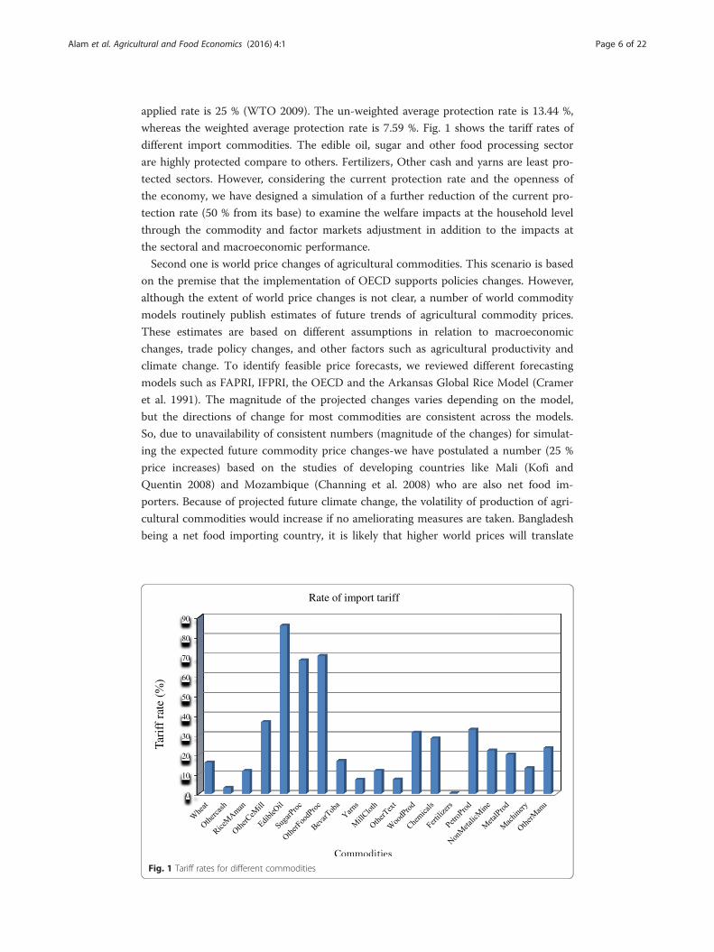
applied rate is 25 % (WTO 2009). The un-weighted average protection rate is 13.44 %,
whereas the weighted average protection rate is 7.59 %. Fig. 1 shows the tariff rates of
different import commodities. The edible oil, sugar and other food processing sector
are highly protected compare to others. Fertilizers, Other cash and yarns are least pro-
tected sectors. However, considering the current protection rate and the openness of
the economy, we have designed a simulation of a further reduction of the current pro-
tection rate (50 % from its base) to examine the welfare impacts at the household level
through the commodity and factor markets adjustment in addition to the impacts at
the sectoral and macroeconomic performance.
Second one is world price changes of agricultural commodities. This scenario is based
on the premise that the implementation of OECD supports policies changes. However,
although the extent of world price changes is not clear, a number of world commodity
models routinely publish estimates of future trends of agricultural commodity prices.
These estimates are based on different assumptions in relation to macroeconomic
changes, trade policy changes, and other factors such as agricultural productivity and
climate change. To identify feasible price forecasts, we reviewed different forecasting
models such as FAPRI, IFPRI, the OECD and the Arkansas Global Rice Model (Cramer
et al. 1991). The magnitude of the projected changes varies depending on the model,
but the directions of change for most commodities are consistent across the models.
So, due to unavailability of consistent numbers (magnitude of the changes) for simulat-
ing the expected future commodity price changes-we have postulated a number (25 %
price increases) based on the studies of developing countries like Mali (Kofi and
Quentin 2008) and Mozambique (Channing et al. 2008) who are also net food im-
porters. Because of projected future climate change, the volatility of production of agri-
cultural commodities would increase if no ameliorating measures are taken. Bangladesh
being a net food importing country, it is likely that higher world prices will translate
0
10
20
30
40
50
60
70
80
90
Tari
ffra
te(
)
Rate of import tariff
Fig. 1 Tariff rates for different commodities
Alam et al. Agricultural and Food Economics (2016) 4:1 Page 6 of 22
into higher domestic prices, which would have strong implication at the macro, sectoral
and household levels.
Farm households in Bangladesh are frequently producers as well as consumers of
these imported food commodities. Therefore it is of utmost important to measure the
impact of world price changes at the household level, so that policy makers can formu-
late policies to tackle the situation. It is well known and discussed in literature that the
increase of agricultural commodity prices is very likely to have substantial impacts on
the farm-households depending on the households’ net position whether they are net
buyer or net seller (Ivanic and Martin 2007; Wodon et al. 2008; Wodon and Zaman
2008 and World Bank 2008). The CGE analysis performed in this paper goes beyond
the analysis in these studies since we are able to investigate economy wide results.
Type of materials used
The elasticities and parameters
The model chosen elasticities and parameters found in literature (Marzia 2004). The
functions are chosen to reflect the reality of the Bangladesh economy and correspond
also to the available elasticity values in literature. The chosen elasticities are (i) Substi-
tution elasticities between factors of production are 0.5 for agricultural and 0.8 for
non-agricultural (industry and services) activities. (ii) Trade elasticities of Armington
(1969) import and Powell and Gruen (1968) export transformation are 2.0, 1.5 and 0.8
for agricultural, industrial and service commodities respectively for both import and
export. (iii) No substitutions between value-added and aggregate intermediate across all
production activities. Hence, the substitution elasticities are zero. (iv) The aggregation
elasticity which allow for a single commodity to be produced by various activities
according to the CES aggregation function, and are 0.5 for agricultural and 0.8 for non-
agricultural (industry and services) and (v) The Frisch parameters for different house-
hold groups are set based on Dervis et al. (1982) and the authors’ own judgment and
are presented in Table 2.
Social accounting matrix of Bangladesh economy
The present study uses the SAM 2005 constructed by IFPRI (Dorosh and Thurlow
2009) for Bangladesh and this is the latest SAM constructed for Bangladesh economy.
The accounts are activity accounts, commodity accounts (one commodity is produced
by more than one activity), factors of production, representative households, taxes, core
government, saving-investment and the rest of world. A total of 62 activities are speci-
fied, of which 23 are agricultural activities (six rice activities), 29 industrial activities
Table 2 Representative households and the Frisch parameters
Household groups Definitions Frisch parameters
ha-mf Marginal agricultural farm households −3.0
ha-sf Small-scale agricultural farm households −3.0
ha-lf Large-scale agricultural farm households −5.0
ha-ll Landless household engaged in agricultural production −3.0
hn-ls Non-agricultural households with low-skilled household head −3.0
hn-ss Non-agricultural households with semi-skilled household head −5.0
hn-hs Non-agricultural households with high-skilled household head −5.0
Alam et al. Agricultural and Food Economics (2016) 4:1 Page 7 of 22
and 10 are services activities. The SAM has 59 commodities, disaggregated into 20 agri-
cultural commodities (three rice commodities), 29 industrial commodities and 10
services commodities. The SAM includes nine factors of production, namely, four
labor, two capital, and three land. Households are disaggregated into seven different
groups based on broadly whether the households receive income from agricultural and
non-agricultural activities. Disaggregated households are presented in Table 2. The
mapping of micro-SAM is presented in Appendix Table 10.
Labor markets are defined as follows. Labor is separated across four education-based
categories such as (i) illiterate agricultural workers whose households still derive
incomes from agriculture (farm-laborer families); (ii) low-skilled laborer (primary
schooling or less) and illiterate workers whose households derive incomes from wage
employment and/or non-farm activities; (iii) semi-skilled labors (some level of second-
ary schooling); and (iv) high-skilled laborer (have completed secondary schooling and/
or tertiary qualifications).
Agricultural land is disaggregated across three categories: (i) marginal lands (farm-
households with less than 0.5 acre of cultivated land); (ii) small-scale lands (households
with between 0.5 and 2.5 acres land); and (iii) medium- and large-scale lands (house-
hold with more than 2.5 acres land – equivalent to one hectare of land). The two
capital accounts are- physical capital and livestock capital.
The model categorizes seven different household groups. First it distinguishes ‘agri-
cultural’ and ‘non-agricultural’ households depending on whether the household
receives any income from agricultural sector. However, even agricultural households
derive at least some of their incomes from non-farm activities and off-farm wage
employment; agricultural households are categorized into three land endowment
categories such as marginal, small and large. The SAM also identifies households who
are landless but derive some of their incomes from working in the agricultural sector.
This category is defined as ‘landless household engaged in agricultural production’.
Finally, non-agricultural households are categorized according to the education level of
the household head such as low-skilled, semi-skilled and high-skilled.
Main features of the Business-as-Usual (BaU) scenario
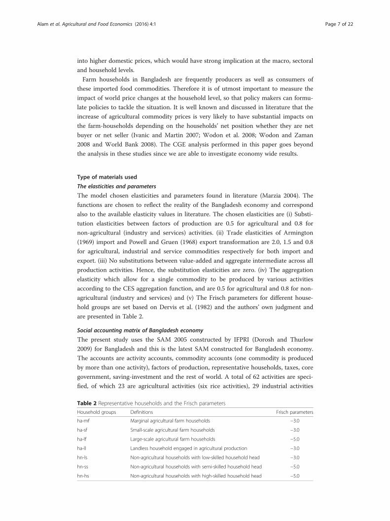
The salient features of the BaU case of the Bangladesh economy are presented in
Table 3. It shows the value-added share, production share, employment share and
import–export share. The contribution of agriculture in total value-added is 20.17
% in which various types of rice account for 6.61 %. Out of agricultural value-added,
the contribution of rice is very high with about one-third of total agricultural value-
added. The contribution of the industries and service sectors are presented in
Appendix Table 11.
The production and employment share of the rice industry in the total agricul-
tural sector is also very substantial (29.02 and 31.39 % respectively) while the share
of agricultural export and import is relatively small. The agricultural import share
is two times higher than the export share. However, it is likely that world price
surges at the world market can be channeled to the household level welfare
changes through reallocation of the sectoral production and value-added and
through the adjustment in the product and factor markets.
Alam et al. Agricultural and Food Economics (2016) 4:1 Page 8 of 22
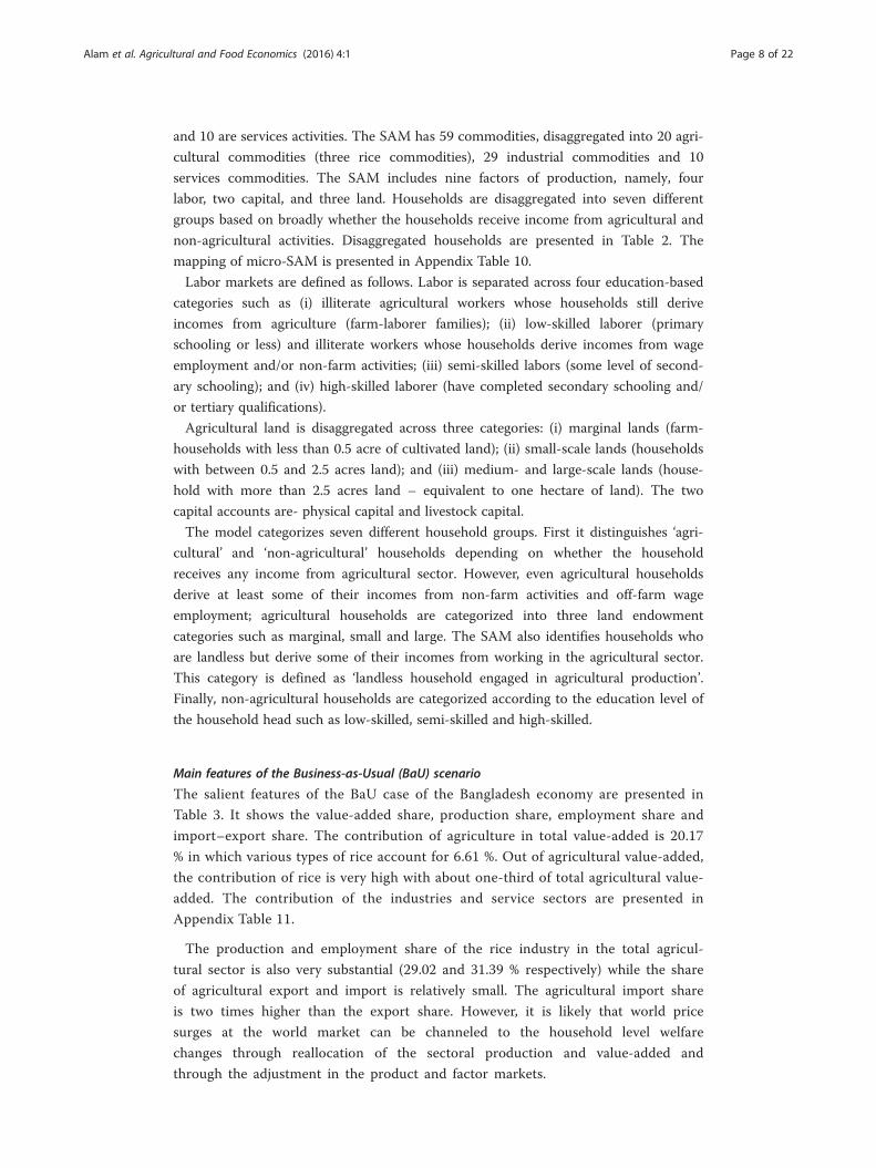
Because any policy or exogenous shocks will be transmitted to the household
level through the factor markets, it is necessary to examine the initial distribution
of the household incomes from different sources. Table 4 shows the distribution of
household income from different factor markets. Irrespective of the households’
categories-the factor income represents the largest source of household income for
Table 3 Salient features of the business-as-usual (BaU) scenario
Commodities VAshr (%) PrdShr (%) EmpShr (%) ExpShr (%) ImpShr (%)
Rice 6.61 (32.77) 5.49 (29.02) 2.13 (31.19) - -
Aus 0.38 0.35 0.11 - -
Aman 2.63 2.05 0.93 - -
Boro 3.60 3.09 1.09 - -
Wheat 0.22 0.22 0.12 - 1.81
Othercer 0.11 0.1 0.05 0.00 0.19
Jute 0.48 0.50 0.33 - -
Sugar 0.35 0.33 0.09 - -
Othercash 0.29 0.32 0.11 0.59 6.53
Pulse 0.15 0.13 0.03 - -
Rapeseed 0.11 0.09 0.02 - -
Otheroil 0.11 0.1 0.02 0.0 0.83
Spices 0.59 0.56 0.13 0.02 0.11
Potato 1.16 1.01 0.21 - -
Veget 0.32 0.28 0.06 0.35 4.27
Fruits 0.9 0.79 0.16 0.15 0.33
Livestock 2.43 2.24 1.46 0.02 0.05
Poultry 0.21 0.22 0.09 - 0.04
Shrimp 1.3 1.37 0.39 4.09 -
Otherfish 3.03 3.14 1.17 0.5 0.03
Forestry 1.81 2.06 0.26 0.31 0.001
Total agri (a) 20.17 18.92 6.83 6.05 14.2
Total non-agric (b) 79.83 81.08 93.17 93.95 85.8
Total (a + b) 100 100 100 100 100
Source: Own calculation from Bangladesh SAM, 2005Notes: VAshr value added share, PRDshr production share, EMPshr share in total employment, EXPshr sector share in totalexport, and IMPshr sector share in total imports
Table 4 Household income sources from factor markets, government & ROW (% of total)
HHs flab-i flab-l flab-s flab-h fcap fcat flnd-m flnd-s flnd-l Total Gov Row Total
ha-mf 20.67 9.72 12.19 3.51 26.16 3.44 9.92 - - 85.61 5.87 8.52 100
ha-sf 7.92 5.91 10.26 6.71 36.58 2.9 - 17.87 - 88.15 1.72 10.14 100
ha-lf 0.87 1.62 9.46 11.69 43.52 1.93 - - 23.62 92.17 0.84 6.46 100
ha-ll 50.68 11.31 8.37 0.91 16.90 - - - - 88.17 6.95 4.88 100
hn-ls 37.45 22.12 2.27 0.31 28.31 - - - - 90.46 6.94 2.59 100
hn-ss 1.25 4.01 56.06 0.71 32.81 - - - - 94.84 1.47 3.69 100
hn-hs - - 3.67 45.91 47.05 - - - - 96.63 - 3.37 100
Total 14.82 7.53 13.70 9.39 34.33 1.4 0.91 4.67 4.02 90.77 3.01 6.22 100
Source: Own calculation from Bangladesh SAM, 2005
Alam et al. Agricultural and Food Economics (2016) 4:1 Page 9 of 22
all household categories, with a range from 85.61–96.63 %. Landless households
engaged in agriculture and marginal agricultural households earn the lion share of
their income from the factor market for ‘illiterate-agricultural workers’ whereas the
non-agricultural households with high-skilled labor earn more than 90 % of their
income from the ‘high-skill labors’ and ‘capital markets’ as their principle sources
of income. Therefore, any policy that can affect factor markets will have direct
income, consumption and welfare impacts at the household level. In other words,
given the substantial differences in sources of income, it could be expected that
trade liberalization and the world price surges will have different income and wel-
fare impacts depending on how factor prices are affected.
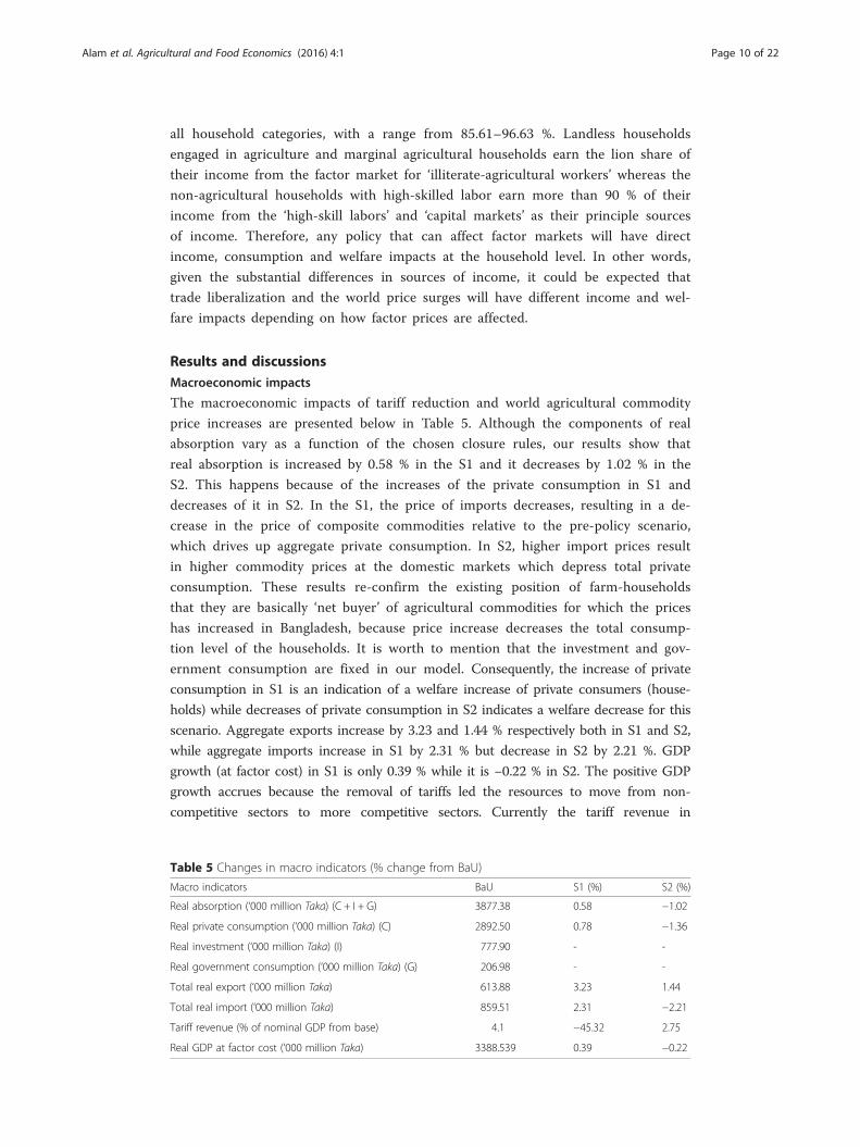
Results and discussionsMacroeconomic impacts
The macroeconomic impacts of tariff reduction and world agricultural commodity
price increases are presented below in Table 5. Although the components of real
absorption vary as a function of the chosen closure rules, our results show that
real absorption is increased by 0.58 % in the S1 and it decreases by 1.02 % in the
S2. This happens because of the increases of the private consumption in S1 and
decreases of it in S2. In the S1, the price of imports decreases, resulting in a de-
crease in the price of composite commodities relative to the pre-policy scenario,
which drives up aggregate private consumption. In S2, higher import prices result
in higher commodity prices at the domestic markets which depress total private
consumption. These results re-confirm the existing position of farm-households
that they are basically ‘net buyer’ of agricultural commodities for which the prices
has increased in Bangladesh, because price increase decreases the total consump-
tion level of the households. It is worth to mention that the investment and gov-
ernment consumption are fixed in our model. Consequently, the increase of private
consumption in S1 is an indication of a welfare increase of private consumers (house-
holds) while decreases of private consumption in S2 indicates a welfare decrease for this
scenario. Aggregate exports increase by 3.23 and 1.44 % respectively both in S1 and S2,
while aggregate imports increase in S1 by 2.31 % but decrease in S2 by 2.21 %. GDP
growth (at factor cost) in S1 is only 0.39 % while it is −0.22 % in S2. The positive GDP
growth accrues because the removal of tariffs led the resources to move from non-
competitive sectors to more competitive sectors. Currently the tariff revenue in
Table 5 Changes in macro indicators (% change from BaU)
Macro indicators BaU S1 (%) S2 (%)
Real absorption (‘000 million Taka) (C + I + G) 3877.38 0.58 −1.02
Real private consumption (‘000 million Taka) (C) 2892.50 0.78 −1.36
Real investment (‘000 million Taka) (I) 777.90 - -
Real government consumption (‘000 million Taka) (G) 206.98 - -
Total real export (‘000 million Taka) 613.88 3.23 1.44
Total real import (‘000 million Taka) 859.51 2.31 −2.21
Tariff revenue (% of nominal GDP from base) 4.1 −45.32 2.75
Real GDP at factor cost (‘000 million Taka) 3388.539 0.39 −0.22
Alam et al. Agricultural and Food Economics (2016) 4:1 Page 10 of 22
Bangladesh is 52 % of the total government revenue. Total tariff revenue is decreased by
45.32 % in the S1. However, one has to keep in mind the results are based on the static
CGE model which has limitation to capture the impact in the longer term. Nevertheless,
CGE model is widely used to analyze the trade policy impact at the macro level because
of its ability to consistently track the impact of polices and/or external shocks across
entire economy, hence CGE analysis has become a mainstay in the trade policy literature
(see Lloyd and MaLaren 2004; Hertel and Reimer 2005; Gilbert 2007; Gilbert and Wahl
2002; Polaski et al. 2008).
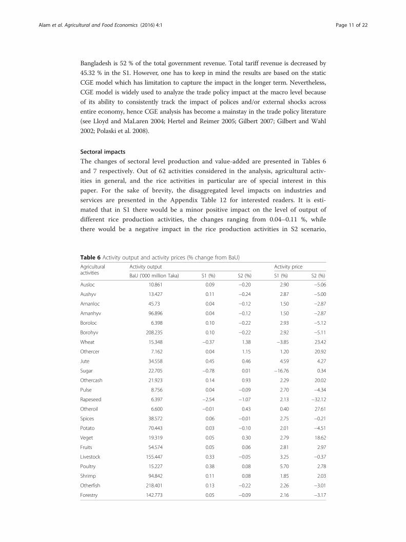
Sectoral impacts
The changes of sectoral level production and value-added are presented in Tables 6
and 7 respectively. Out of 62 activities considered in the analysis, agricultural activ-
ities in general, and the rice activities in particular are of special interest in this
paper. For the sake of brevity, the disaggregated level impacts on industries and
services are presented in the Appendix Table 12 for interested readers. It is esti-
mated that in S1 there would be a minor positive impact on the level of output of
different rice production activities, the changes ranging from 0.04–0.11 %, while
there would be a negative impact in the rice production activities in S2 scenario,
Table 6 Activity output and activity prices (% change from BaU)
Agriculturalactivities
Activity output Activity price
BaU (‘000 million Taka) S1 (%) S2 (%) S1 (%) S2 (%)
Ausloc 10.861 0.09 −0.20 2.90 −5.06
Aushyv 13.427 0.11 −0.24 2.87 −5.00
Amanloc 45.73 0.04 −0.12 1.50 −2.87
Amanhyv 96.896 0.04 −0.12 1.50 −2.87
Boroloc 6.398 0.10 −0.22 2.93 −5.12
Borohyv 208.235 0.10 −0.22 2.92 −5.11
Wheat 15.348 −0.37 1.38 −3.85 23.42
Othercer 7.162 0.04 1.15 1.20 20.92
Jute 34.558 0.45 0.46 4.59 4.27
Sugar 22.705 −0.78 0.01 −16.76 0.34
Othercash 21.923 0.14 0.93 2.29 20.02
Pulse 8.756 0.04 −0.09 2.70 −4.34
Rapeseed 6.397 −2.54 −1.07 2.13 −32.12
Otheroil 6.600 −0.01 0.43 0.40 27.61
Spices 38.572 0.06 −0.01 2.75 −0.21
Potato 70.443 0.03 −0.10 2.01 −4.51
Veget 19.319 0.05 0.30 2.79 18.62
Fruits 54.574 0.05 0.06 2.81 2.97
Livestock 155.447 0.33 −0.05 3.25 −0.37
Poultry 15.227 0.38 0.08 5.70 2.78
Shrimp 94.842 0.11 0.08 1.85 2.03
Otherfish 218.401 0.13 −0.22 2.26 −3.01
Forestry 142.773 0.05 −0.09 2.16 −3.17
Alam et al. Agricultural and Food Economics (2016) 4:1 Page 11 of 22
ranging from 0.12–0.24 %. Rice output is not affected directly by any of the sce-
narios since the tariffs for rice are already fully abolished (so no further abolition
in S1) and the world market price for rice is not increased in the S2. In S2, an
increase of world agricultural commodity prices is designed only for the commod-
ities to be imported in Bangladesh. The positive activity price impacts ranged from
1.50–2.92 % in the case of S1 whereas in S2 the negative activity price impacts
ranged from 2.87–5.11 %.
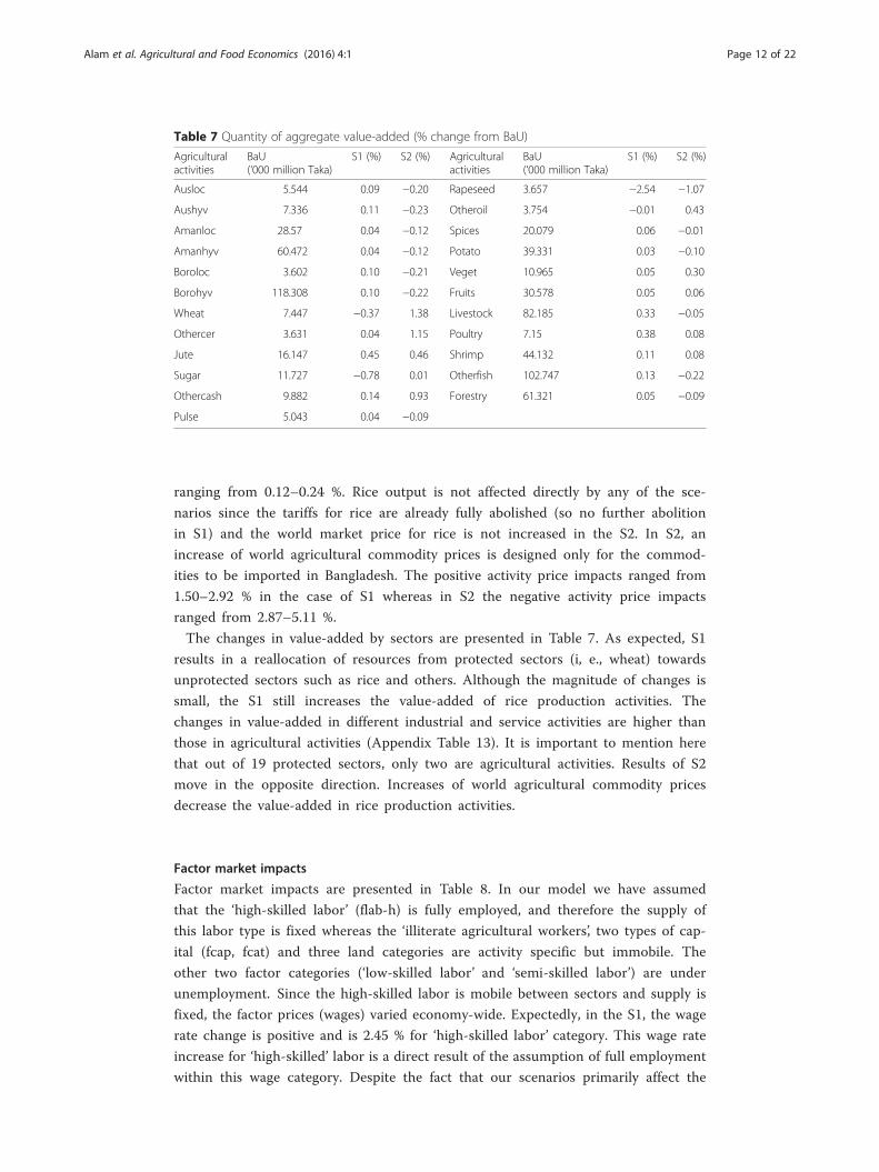
The changes in value-added by sectors are presented in Table 7. As expected, S1
results in a reallocation of resources from protected sectors (i, e., wheat) towards
unprotected sectors such as rice and others. Although the magnitude of changes is
small, the S1 still increases the value-added of rice production activities. The
changes in value-added in different industrial and service activities are higher than
those in agricultural activities (Appendix Table 13). It is important to mention here
that out of 19 protected sectors, only two are agricultural activities. Results of S2
move in the opposite direction. Increases of world agricultural commodity prices
decrease the value-added in rice production activities.
Factor market impacts
Factor market impacts are presented in Table 8. In our model we have assumed
that the ‘high-skilled labor’ (flab-h) is fully employed, and therefore the supply of
this labor type is fixed whereas the ‘illiterate agricultural workers’, two types of cap-
ital (fcap, fcat) and three land categories are activity specific but immobile. The
other two factor categories (‘low-skilled labor’ and ‘semi-skilled labor’) are under
unemployment. Since the high-skilled labor is mobile between sectors and supply is
fixed, the factor prices (wages) varied economy-wide. Expectedly, in the S1, the wage
rate change is positive and is 2.45 % for ‘high-skilled labor’ category. This wage rate
increase for ‘high-skilled’ labor is a direct result of the assumption of full employment
within this wage category. Despite the fact that our scenarios primarily affect the
Table 7 Quantity of aggregate value-added (% change from BaU)
Agriculturalactivities
BaU(‘000 million Taka)
S1 (%) S2 (%) Agriculturalactivities
BaU(‘000 million Taka)
S1 (%) S2 (%)
Ausloc 5.544 0.09 −0.20 Rapeseed 3.657 −2.54 −1.07
Aushyv 7.336 0.11 −0.23 Otheroil 3.754 −0.01 0.43
Amanloc 28.57 0.04 −0.12 Spices 20.079 0.06 −0.01
Amanhyv 60.472 0.04 −0.12 Potato 39.331 0.03 −0.10
Boroloc 3.602 0.10 −0.21 Veget 10.965 0.05 0.30
Borohyv 118.308 0.10 −0.22 Fruits 30.578 0.05 0.06
Wheat 7.447 −0.37 1.38 Livestock 82.185 0.33 −0.05
Othercer 3.631 0.04 1.15 Poultry 7.15 0.38 0.08
Jute 16.147 0.45 0.46 Shrimp 44.132 0.11 0.08
Sugar 11.727 −0.78 0.01 Otherfish 102.747 0.13 −0.22
Othercash 9.882 0.14 0.93 Forestry 61.321 0.05 −0.09
Pulse 5.043 0.04 −0.09
Alam et al. Agricultural and Food Economics (2016) 4:1 Page 12 of 22
Table 8 Factor wage changes (% change from BaU)
Activities Scenarios flab-i flab-h fcap fcat flnd-m flnd-s flnd-l
Ausloc S1 5.68 2.45 5.68 - 5.68 5.68 5.68
S2 −10.25 −0.88 −10.25 - −10.25 −10.25 −10.25
Aushyv S1 5.31 2.45 5.31 - 5.31 5.31 5.31
S2 −9.55 −0.88 −9.55 - −9.55 −9.55 −9.55
Amanloc S1 2.00 2.45 2.00 - 2.00 2.00 2.00
S2 −4.74 −0.88 −4.74 - −4.74 −4.74 −4.74
Amanhyv S1 2.01 2.45 2.01 - 2.01 2.01 2.01
S2 −4.74 −0.88 −4.74 - −4.74 −4.74 −4.74
Boroloc S1 5.24 2.45 5.24 - 5.24 5.24 5.24
S2 −9.46 −0.88 −9.46 - −9.46 −9.46 −9.46
Borohyv S1 5.20 2.45 5.20 - 5.20 5.20 5.20
S2 −9.26 −0.88 −9.26 - −9.26 −9.26 −9.26
Wheat S1 −8.35 2.45 −8.35 - −8.35 −8.35 −8.35
S2 46.37 −0.88 46.37 - 46.37 46.37 46.37
Othercer S1 1.68 2.45 1.68 - 1.68 1.68 1.68
S2 39.97 −0.88 39.97 - 39.97 39.97 39.97
Jute S1 10.02 2.45 10.02 - 10.02 10.02 10.02
S2 9.47 −0.88 9.47 - 9.47 9.47 9.47
Sugar S1 −30.41 2.45 −30.41 - −30.41 −30.41 −30.41
S2 0.39 −0.88 0.39 - 0.39 0.39 0.39
Othercash S1 6.04 2.45 6.04 - 6.04 6.04 6.04
S2 44.74 −0.88 44.74 - 44.74 44.74 44.74
Pulse S1 3.92 2.45 3.92 - 3.92 3.92 3.92
S2 −6.92 −0.88 −6.92 - −6.92 −6.92 −6.92
Rapeseed S1 −75.40 2.45 −75.40 - −75.40 −75.40 −75.40
S2 −50.74 −0.88 −50.74 - −50.74 −50.74 −50.74
Otheroil S1 0.01 2.45 0.01 - 0.01 0.01 0.01
S2 43.66 −0.88 43.66 - 43.66 43.66 43.66
Spices S1 4.28 2.45 4.28 - 4.28 4.28 4.28
S2 −0.64 −0.88 −0.64 - −0.64 −0.64 −0.64
Potato S1 2.88 2.45 2.88 - 2.88 2.88 2.88
S2 −7.38 −0.88 −7.38 - −7.38 −7.38 −7.38
Veget S1 4.08 2.45 4.08 - 4.08 4.08 4.08
S2 27.89 −0.88 27.89 - 27.89 27.89 27.89
Fruits S1 4.16 2.45 4.16 - 4.16 4.16 4.16
S2 4.44 −0.88 4.44 - 4.44 4.44 4.44
Livestock S1 8.32 2.45 8.32 8.32 - - -
S2 −1.30 −0.88 −1.30 −1.30 - - -
Poultry S1 13.09 2.45 13.09 13.09 - - -
S2 2.23 −0.88 2.23 2.23 - - -
Shrimp S1 5.40 2.45 5.40 - 5.40 5.40 5.40
Alam et al. Agricultural and Food Economics (2016) 4:1 Page 13 of 22
agricultural sector, which depend mostly on low-skilled labour, the model shows that
there still might be spill-over benefits for people less directly involved in agriculture.
It is worth to mention that the high-skilled labors are primarily employed in the
non-agricultural sectors which have the higher protection. But for all other factor
categories, the factor prices are activity specific except the two unemployed factors.
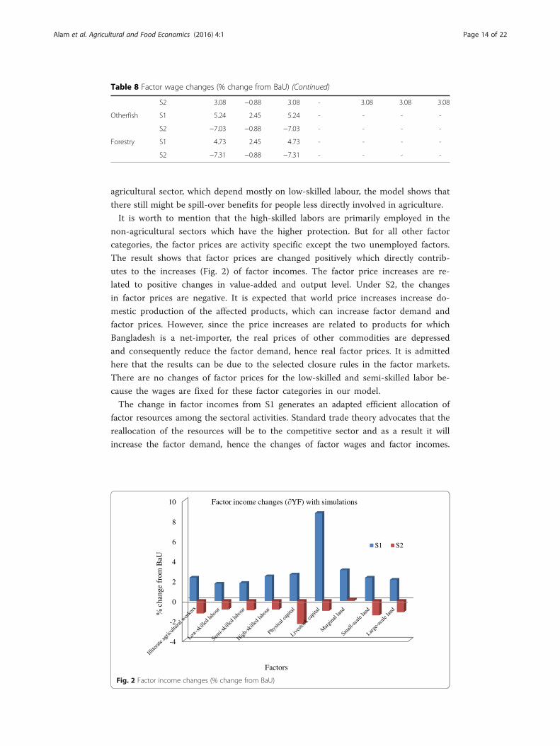
The result shows that factor prices are changed positively which directly contrib-
utes to the increases (Fig. 2) of factor incomes. The factor price increases are re-
lated to positive changes in value-added and output level. Under S2, the changes
in factor prices are negative. It is expected that world price increases increase do-
mestic production of the affected products, which can increase factor demand and
factor prices. However, since the price increases are related to products for which
Bangladesh is a net-importer, the real prices of other commodities are depressed
and consequently reduce the factor demand, hence real factor prices. It is admitted
here that the results can be due to the selected closure rules in the factor markets.
There are no changes of factor prices for the low-skilled and semi-skilled labor be-
cause the wages are fixed for these factor categories in our model.
The change in factor incomes from S1 generates an adapted efficient allocation of
factor resources among the sectoral activities. Standard trade theory advocates that the
reallocation of the resources will be to the competitive sector and as a result it will
increase the factor demand, hence the changes of factor wages and factor incomes.
Table 8 Factor wage changes (% change from BaU) (Continued)
S2 3.08 −0.88 3.08 - 3.08 3.08 3.08
Otherfish S1 5.24 2.45 5.24 - - - -
S2 −7.03 −0.88 −7.03 - - - -
Forestry S1 4.73 2.45 4.73 - - - -
S2 −7.31 −0.88 −7.31 - - - -
-4
-2
0
2
4
6
8
10
chan
ge f
rom
BaU
Factors
Factor income changes ( YF) with simulations
S1 S2
Fig. 2 Factor income changes (% change from BaU)
Alam et al. Agricultural and Food Economics (2016) 4:1 Page 14 of 22
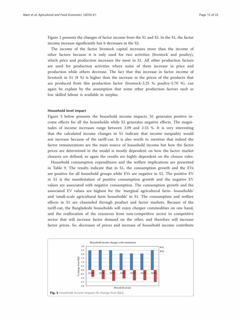
Figure 2 presents the changes of factor income from the S1 and S2. In the S1, the factor
income increase significantly but it decreases in the S2.
The income of the factor livestock capital increases more than the income of
other factors because it is only used for two activities (livestock and poultry),
which price and production increases the most in S1. All other production factors
are used for production activities where some of them increase in price and
production while others decrease. The fact that this increase in factor income of
livestock in S1 (8 %) is higher than the increase in the prices of the products that
are produced from this production factor (livestock-3.25 %; poultry-5.70 %), can
again be explain by the assumption that some other production factors such as
low skilled labour is available in surplus.
Household level impact
Figure 3 below presents the household income impacts. S1 generates positive in-
come effects for all the households while S2 generates negative effects. The magni-
tudes of income increases range between 2.09 and 2.55 %. It is very interesting
that the calculated income changes in S1 indicate that income inequality would
not increase because of the tariff-cut. It is also worth to mention that indeed the
factor remunerations are the main source of household income but how the factor
prices are determined in the model is mostly dependent on how the factor market
closures are defined, so again the results are highly dependent on the closure rules.
Household consumption expenditures and the welfare implications are presented
in Table 9. The results indicate that in S1, the consumption growth and the EVs
are positive for all household groups while EVs are negative in S2. The positive EV
in S1 is the manifestation of positive consumption growth and the negative EV
values are associated with negative consumption. The consumption growth and the
associated EV values are highest for the ‘marginal agricultural farm- households’
and ‘small-scale agricultural farm households’ in S1. The consumption and welfare
effects in S1 are channeled through product and factor markets. Because of the
tariff-cut, the Bangladeshi households will enjoy cheaper commodities on one hand,
and the reallocation of the resources from non-competitive sector to competitive
sector that will increase factor demand on the other, and therefore will increase
factor prices. So, decreases of prices and increase of household income contribute
-2.0
-1.5
-1.0
-0.5
0.0
0.5
1.0
1.5
2.0
2.5
3.0
ha-mf ha-sf ha-lf ha-ll hn-ls hn-ss hn-hs cha
nge
from
BaU
Household groups
Household income changes with simulations
S1
S2
Fig. 3 Household income impacts (% change from BaU)
Alam et al. Agricultural and Food Economics (2016) 4:1 Page 15 of 22
directly to increases of household consumption. In S2, both the consumption
growth and the EVs are negative. Increases of world market price increases the
prices of imported commodities, therefore the consumption basket becomes more
expensive, which contributes directly to decreases of the consumption and
welfare.
ConclusionsThe objective of this paper was to analyze the impact of partial liberalization of
trade and the increases of world agricultural commodity prices in Bangladesh using
a single-country static CGE model. The results suggest that partial unilateral trade
liberalization will have a marginally positive impact on output, value-added, factor
wages and hence household income and welfare. Since lots of liberalization efforts
have already been undertaken in the past by Bangladesh, it is probable that the
bulk of potential benefits from the reduction of protection level are already
exhausted. In order to increase welfare of low-income rice producing households,
policy maker might want to focus on other complementary policy options at the
sectoral level aimed at, for instance, increase productivity or improve market trans-
parency in Bangladesh. The results from our second simulation, world price in-
creases show the opposite.
However, one has to keep in mind the results are based on the static CGE model
which has limitation to capture the impact in the longer term. Nevertheless, CGE
model is widely used to analyze the trade policy impact at the macro level because of
its ability to consistently track the impact of polices and/or external shocks across en-
tire economy, hence CGE analysis has become a mainstay in the trade policy and world
price changes literature.
Future research should extend the model in a more sophisticated dynamic framework
for evaluating the impacts from medium to longer time period so that capital accumula-
tion, population growth and technological growth can be taken into account in the model
specification as well as different elasticity values and different closure rules for investigat-
ing the results’ sensitivity. Furthermore, the model uses representative household groups
which do not take into account heterogeneity among the households within each group.
Therefore, it is also a future research interest to overcome the said limitation by extending
the model to CGE-micro-simulation.
Table 9 Household consumption expenditure and welfare (% change from BaU)
Householdcategories
BaU (‘000million Taka)
S1 S2
Consumption growth (%) EV (%) Consumption growth (%-) EV (%)
ha-mf 291.92 1.05 1.1 −1.06 −1.0
ha-sf 772.992 0.95 1.0 −1.37 −1.4
ha-lf 437.884 0.66 0.7 −1.63 −1.6
ha-ll 329.567 0.69 0.7 −1.28 −1.3
hn-ls 440.567 0.65 0.6 −1.52 −1.6
hn-ss 351.741 0.48 0.2 −1.51 −1.0
hn-hs 267.844 0.57 0.5 −1.78 −1.8
Total 2892.50 - 0.7 - −1.4
Alam et al. Agricultural and Food Economics (2016) 4:1 Page 16 of 22
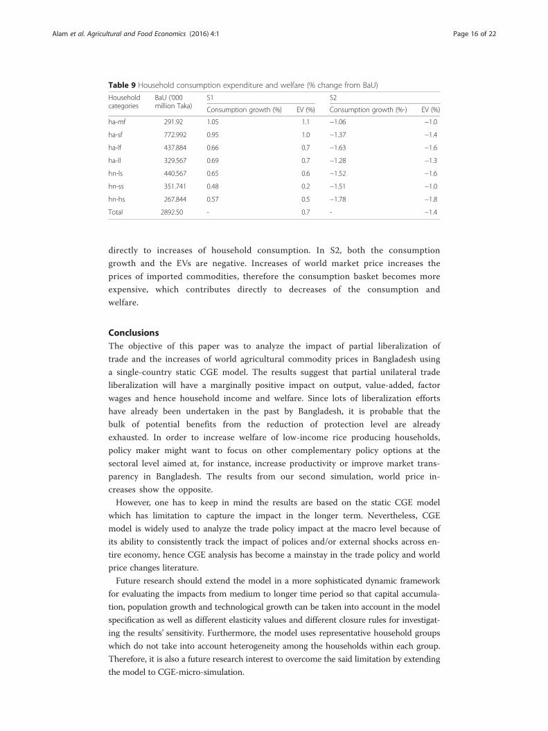
Appendix
Table 10 Mapping of Social Accounting Matrix for Bangladesh Economy, 2005
Sectors Activity code Commodity code Description
1 arausl cauric Rice Aus (Local)
2 araush Rice Aus (Hybrid)
3 aramnl camric Rice Aman (Local & Transplant)
4 aramnh Rice Aman (HYV & Hybrid)
5 arborl cboric Rice Boro (Local)
6 arborh Rice Boro (HYV & Hybrid)
7 awheat cwheat Wheat
8 aocere cocere Other Cereals
9 ajutef cjutef Jute
10 asugar csugar Sugarcane
11 aocash cocash Other Cash Crops
12 apulse cpulse Pulses
13 arapes crapes Rapeseed
14 aooilc cooilc Other Oil Crops
15 aspice cspice Spices
16 apotat cpotat Potatoes
17 aveges cveges Vegetables
18 afruit cfruit Fruits
19 alives clives Livestock
20 apoult cpoult Poultry
21 ashrmp cshrmp Shrimp Farming
22 aofish cofish Other Fishing
23 afores cfores Forestry
24 amines cmines Mining and Quarrying
25 aaumll caumll Rice Milling (Aus)
26 aammll cammll Rice Milling (Aman)
27 abrmll cbrmll Rice Milling (Boro)
28 aocmll cocmll Other Cereal Milling
29 aedoil cedoil Edible Oils
30 asugrp csugrp Sugar Processing
31 aofood cofood Other Food Processing
32 abevtb cbevtb Beverages and Tobacco
33 aleath cleath Leather and Footwear
34 ajtext cjtext Jute Textiles
35 ayarns cyarns Yarn
36 amclth cmclth Mill Cloth
37 aoclth coclth Other Cloth
38 agarms cgarms Ready-Made Garments
39 aknitw cknitw Knitwear
40 aotext cotext Other Textiles
41 awoodp cwoodp Wood and Paper
42 achems cchems Chemicals
43 aferts cferts Fertilizers
Alam et al. Agricultural and Food Economics (2016) 4:1 Page 17 of 22
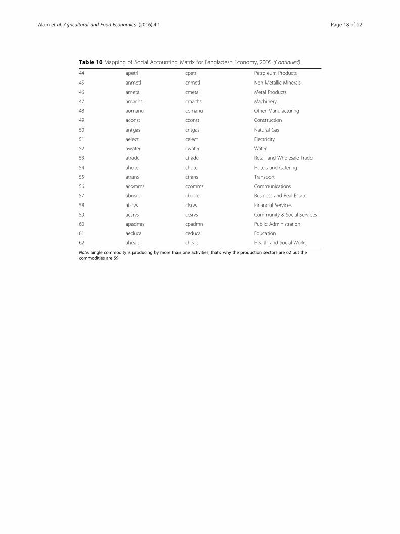
Table 10 Mapping of Social Accounting Matrix for Bangladesh Economy, 2005 (Continued)
44 apetrl cpetrl Petroleum Products
45 anmetl cnmetl Non-Metallic Minerals
46 ametal cmetal Metal Products
47 amachs cmachs Machinery
48 aomanu comanu Other Manufacturing
49 aconst cconst Construction
50 antgas cntgas Natural Gas
51 aelect celect Electricity
52 awater cwater Water
53 atrade ctrade Retail and Wholesale Trade
54 ahotel chotel Hotels and Catering
55 atrans ctrans Transport
56 acomms ccomms Communications
57 abusre cbusre Business and Real Estate
58 afsrvs cfsrvs Financial Services
59 acsrvs ccsrvs Community & Social Services
60 apadmn cpadmn Public Administration
61 aeduca ceduca Education
62 aheals cheals Health and Social Works
Note: Single commodity is producing by more than one activities, that’s why the production sectors are 62 but thecommodities are 59
Alam et al. Agricultural and Food Economics (2016) 4:1 Page 18 of 22
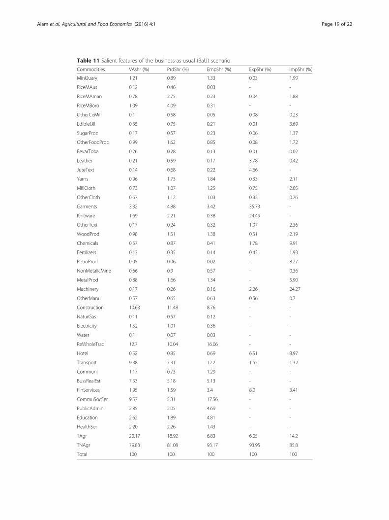
Table 11 Salient features of the business-as-usual (BaU) scenario
Commodities VAshr (%) PrdShr (%) EmpShr (%) ExpShr (%) ImpShr (%)
MinQuary 1.21 0.89 1.33 0.03 1.99
RiceMAus 0.12 0.46 0.03 - -
RiceMAman 0.78 2.75 0.23 0.04 1.88
RiceMBoro 1.09 4.09 0.31 - -
OtherCeMill 0.1 0.58 0.05 0.08 0.23
EdibleOil 0.35 0.75 0.21 0.01 3.69
SugarProc 0.17 0.57 0.23 0.06 1.37
OtherFoodProc 0.99 1.62 0.85 0.08 1.72
BevarToba 0.26 0.28 0.13 0.01 0.02
Leather 0.21 0.59 0.17 3.78 0.42
JuteText 0.14 0.68 0.22 4.66 -
Yarns 0.96 1.73 1.84 0.33 2.11
MillCloth 0.73 1.07 1.25 0.75 2.05
OtherCloth 0.67 1.12 1.03 0.32 0.76
Garments 3.32 4.88 3.42 35.73 -
Knitware 1.69 2.21 0.38 24.49 -
OtherText 0.17 0.24 0.32 1.97 2.36
WoodProd 0.98 1.51 1.38 0.51 2.19
Chemicals 0.57 0.87 0.41 1.78 9.91
Fertilizers 0.13 0.35 0.14 0.43 1.93
PetroProd 0.05 0.06 0.02 - 8.27
NonMetalicMine 0.66 0.9 0.57 - 0.36
MetalProd 0.88 1.66 1.34 - 5.90
Machinery 0.17 0.26 0.16 2.26 24.27
OtherManu 0.57 0.65 0.63 0.56 0.7
Construction 10.63 11.48 8.76 - -
NaturGas 0.11 0.57 0.12 - -
Electricity 1.52 1.01 0.36 - -
Water 0.1 0.07 0.03 - -
ReWholeTrad 12.7 10.04 16.06 - -
Hotel 0.52 0.85 0.69 6.51 8.97
Transport 9.38 7.31 12.2 1.55 1.32
Communi 1.17 0.73 1.29 - -
BussRealEst 7.53 5.18 5.13 - -
FinServices 1.95 1.59 3.4 8.0 3.41
CommuSocSer 9.57 5.31 17.56 - -
PublicAdmin 2.85 2.05 4.69 - -
Education 2.62 1.89 4.81 - -
HealthSer 2.20 2.26 1.43 - -
TAgr 20.17 18.92 6.83 6.05 14.2
TNAgr 79.83 81.08 93.17 93.95 85.8
Total 100 100 100 100 100
Alam et al. Agricultural and Food Economics (2016) 4:1 Page 19 of 22
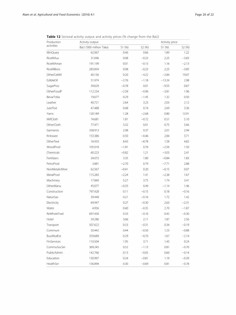
Table 12 Sectoral activity output and activity prices (% change from the BaU)
Productionactivities
Activity output Activity price
BaU (‘000 million Taka) S1 (%) S2 (%) S1 (%) S2 (%)
MinQuary 62.067 0.46 0.66 1.89 1.22
RiceMAus 31.696 0.08 −0.23 2.25 −3.83
RiceMAman 191.199 0.01 −0.13 1.16 −2.13
RiceMBoro 283.834 0.08 −0.23 2.25 −3.85
OtherCeMill 40.156 0.20 −4.22 −2.84 19.07
EdibleOil 51.974 −2.76 −1.18 −13.24 2.98
SugarProc 39.629 −0.78 0.01 −9.55 0.67
OtherFoodP 112.234 −2.39 −0.96 −3.81 1.96
BevarToba 19.677 0.29 −1.45 1.32 0.50
Leather 40.721 2.64 3.23 2.03 2.12
JuteText 47.488 0.48 0.74 2.69 3.36
Yarns 120.189 1.28 −2.68 0.80 13.91
MillCloth 74.681 1.81 −0.72 0.51 5.10
OtherCloth 77.471 3.32 0.01 0.75 5.66
Garments 338.913 2.98 0.37 2.01 2.94
Knitware 153.386 0.50 −0.46 2.84 3.71
OtherText 16.933 8.43 −8.78 1.58 4.82
WoodProd 105.018 −1.81 0.76 −2.56 1.50
Chemicals 60.223 −0.82 1.21 −3.03 2.41
Fertilizers 24.072 3.35 1.80 −0.84 1.83
PetroProd 3.881 −2.70 0.79 −7.71 2.88
NonMetalicMine 62.567 −0.41 0.20 −0.15 0.07
MetalProd 115.283 −2.24 1.41 −2.38 1.67
Machinery 17.840 5.27 3.75 1.74 3.41
OtherManu 45.077 −0.35 0.49 −1.14 1.46
Construction 797.428 0.11 −0.15 0.18 −0.16
NaturGas 39.448 0.21 −0.16 1.72 1.42
Electricity 69.947 0.27 −0.30 2.63 −2.31
Water 4.956 0.40 −0.35 2.70 −1.87
ReWholeTrad 697.430 0.33 −0.16 0.42 −0.30
Hotel 59.286 3.66 2.11 1.87 2.56
Transport 507.622 0.53 −0.31 0.34 −0.19
Communi 50.442 0.44 −0.50 1.23 −0.88
BussRealEst 359.689 0.29 −0.70 1.67 −2.14
FinServices 110.504 1.95 3.71 1.43 0.24
CommuSocSer 369.245 0.52 −1.13 0.81 −0.70
PublicAdmin 142.766 0.13 −0.05 0.60 −0.14
Education 130.997 0.24 −0.81 1.19 −0.39
HealthSer 156.894 0.30 −0.69 0.81 −0.78
Alam et al. Agricultural and Food Economics (2016) 4:1 Page 20 of 22
Competing interestsThe authors declare that they have no competing interests.
Authors’ contributionsMJA developed the concept, prepared data for analysis, conducted simulations in GAMS, contributed to the writing ofthe manuscript, worked on the estimation procedure, provided critical review. IAB worked in the conceptdevelopment, contributed to the writing of the manuscript, worked on the estimation procedure. JB and SNconducted simulations in GAMS, generated tables and figures. EJW and GVH providedinterpretation and critical review.All authors read and approved the final manuscript.
Author details1Dyson School of Applied Economics and Management, Cornell University, Ithaca 14853NY, USA. 2Department ofAgribusiness and Marketing, Bangladesh Agricultural University, Mymensingh-2202, Bangladesh. 3Department ofAgricultural Economics, Ghent University, 653 Coupure Links, 9000 Ghent, Belgium. 4Department of AgriculturalEconomics, Bangladesh Agricultural University, Mymensingh 2202, Bangladesh. 5Department of Agricultural Economics,Ghent University, 653 Coupure Links, 9000 Ghent, Belgium. 6Department of Agricultural Economics and Agribusiness,the University of Arkansas, Fayetteville, AR 72701, USA.
Received: 19 March 2015 Accepted: 12 January 2016
Table 13 Quantity of aggregate value-added (QVA) (% change from BaU)
Productionactivities
BaU (‘000million Taka)
S1(%∂QVAi)
S2(%∂QVAi)
Productionactivities
BaU (‘000million Taka)
S1(%∂QVAi)
S2(%∂QVAi)
MinQuary 41.167 0.46 0.66 ReWholeTrad 430.298 0.33 −0.16
RiceMAus 3.987 0.08 −0.23 Hotel 17.49 3.66 2.11
RiceMAman 26.366 0.01 −0.13 Transport 317.934 0.53 −0.31
RiceMBoro 36.993 0.08 −0.23 Communi 39.604 0.44 −0.50
OtherCeMill 3.549 0.20 −4.22 BussRealEst 255.168 0.29 −0.7
EdibleOil 11.856 −2.76 −1.18 FinServices 65.966 1.95 3.71
SugarProc 5.93 −0.78 0.01 CommuSocSer 324.447 0.52 −1.13
OtherFoodP 33.47 −2.39 −0.96 PublicAdmin 96.44 0.13 −0.05
BevarToba 8.931 0.29 −1.45 Education 88.70 0.24 −0.81
Leather 7.156 2.64 3.23 HealthSer 74.568 0.30 −0.69
JuteText 4.894 0.48 0.74
Yarns 32.518 1.28 −2.68
MillCloth 24.662 1.81 −0.72
OtherCloth 22.552 3.32 0.01
Garments 112.616 2.98 0.37
Knitware 57.352 0.5 −0.46
OtherText 5.753 8.43 −8.78
WoodProd 33.223 −1.81 0.76
Chemicals 19.302 −0.82 1.21
Fertilizers 4.241 3.35 1.8
PetroProd 1.655 −2.7 0.79
NonMetalicMin 22.412 −0.41 0.2
MetalProd 29.859 −2.24 1.41
Machinery 5.755 5.27 3.75
OtherManu 19.226 −0.35 0.49
Construction 360.107 0.11 −0.15
NaturGas 3.803 0.21 −0.16
Electricity 51.591 0.27 −0.3
Water 3.388 0.4 −0.35
Alam et al. Agricultural and Food Economics (2016) 4:1 Page 21 of 22
ReferencesAhmed N (2001) Trade liberalization in Bangladesh: An Investigation into Trends. The University Press Limited, DhakaAnderson JE, Martin W (1996) The Welfare Analysis of Fiscal Policy: A Simple Unified Account, Boston College Working
Papers in Economics 316. Department of Economics, Boston College, USAAnnabi N, Khondker B, Raihan S, Cockburn J, Decaluwe B (2006) Implications of WTO Agreements and Domestic Trade
Policy Reforms for Poverty in Bangladesh: Short run vs long run impacts’. In: Hertel T, Winters LA (eds) PovertyImpacts of a WTO agreemen. World Bank, Washington D.C
Armington PA (1969) A Theory of Demand for Product Distinguished by Place of production. IMF Staff Paper 16(1):159–178Arndt C, Benfica R, Maximiano N, Nucifora A, Thurlow J (2008) Higher Fuel and Food Prices: Impacts and Responses for
Mozambique. Agric Econ 39(supplement):497–511Benson T, Mugarura S and Wanda K (2008) Impacts in Uganda of Rising Global Food Prices: the Role of Diversified
Staples and Limited Price Transmission. Agricultural Economics 39(supplement): 513–24Blonigen BA, Joseph EF, Kenneth AR (1997) Sector-focused General Equilibrium Modeling. In: Francois JF, Reinert KA
(eds) Applied Methods for Trade Policy Analysis: A Handbook. Cambridge University Press, New YorkChanning A, Rui B, Nelson M, Antonio MDN, and James TT (2008) Higher Fuel and Food Prices: Economic Impacts and
Responses for Mozambique. IFPRI,Washington DC. Discussion Paper 00836Cramer GL, Wailes EJ, Goroski J, Phillips S (1991) Impact of Liberalizing Trade on the World Rice Market: A Spatial Model
including Rice Quality, Arkansas Experiment Station Special Report 153. University of Arkansas, FayettevilleDeaton A (1980) The Measurement of Welfare. Theory and Practical Applications. Living Standards Measurement Study.
Working Paper No. 7. World Bank, Washington D.CDecaluwe B, Martens A (1988) CGE modeling and Developing Economies: A Concise Empirical Survey of 73
Applications to 26 Countries. J Policy Model 10(4):529–568Dervis K, Melo JD, Robinson S (1982) General Equilibrium Models for Development Policy. Cambridge University Press,
New YorkDorosh PA (2001) Trade Liberalization and National Food Security: Rice Trade Liberalization between Bangladesh and
India. World Dev 29(4):673–689Dorosh P, Thurlow J (2009) A Social Accounting Matrix for Bangladesh. IFPRI, Washington D.CGilbert J (2007) Agricultural Trade Reform Under Doha and Poverty in India. UNESCAP, BangkokGilbert J, Wahl T (2002) Applied General Equilibrium Assessment of Trade Liberalization in China. World Economy
25(5):697–731Hertel T, Reimer J (2005) Predicting the Poverty Impacts of Trade Reform. J Int Trade Econ Develop 14(4):377–405Hoque SM (2006) A Computable General Equilibrium Model for Bangladesh for Analysis of Policy Reforms. Centre of
Policy Studies, Faculty of Business and Economics, Monash University, MelbourneIvanic M, Martin W (2007) Food and Fuel Prices: Recent Developments, Macroeconomic Impact, and Policy Responses,
IMF., Washington D.CKhondker BH, Raihan S (2004) Paper presented at the Seventh Annual Global Economic Conference, 17–19 June,
2004. World Bank, Washington DC, Welfare and Poverty Impacts of Policy Reforms in Bangladesh: A GeneralEquilibrium Approach
Kofi N, Quentin W (2008) Impact of Rising Rice Prices and Policy Responses in Mali, Policy Research Working Paper4739. The World Bank, Washington D.C
Llyod PJ, MacLaren D (2004) Gains and Losses from Regional Trading Agreements: A Survey. Econ Record 80(251):445–97Lofgren H, Harris RL and Robinson S with the assistance of Moataz El-said and Marcelle T (2002) A Standard
Computable General Equilibrium (CGE) Models in GAMS. Microcomputers in Policy Research, Vol. 5. IFPRI,Washington D.C.
Marzia F (2004) Modeling the Effects of Trade on Women at Work and at Home: Comparative Perspectives. EconomieInternationale 99:49–80
Marzia F, Adrian W (2000) Modeling the Effect of Trade on Women at Work and at Home. World Dev 28(7):1173–1190Mujeri M, and B Khondker (2002) Poverty Implications of Trade Liberalization in Bangladesh: A General Equilibrium
Approach. Mimeo, Department for International Development (DFID): Dhaka.Nell K (2003) Long-run Exogeneity between Savings and Investment: Evidence from South Africa. Working Paper 2.
Trade and Industrial Policy Strategies, JohannesburgNoman ANK (2002) The Impact of Foreign Trade Policies and External Shocks on the Agricultural Sector of Bangladesh.
Edited by D. Werner and B. Siegfried. Vol. 45, Farming and Rural Systems Economics: Margraf Verlag, GermanyPolaski S, Panda M, Ganesh-Kumar A, McDonald S, Robinson S (2008) The Impact of Changes in Agricultural Prices on
Rural and Urban Poverty. Paper presented at the 11th Annual Conference on Global Economic Analysis. Organizedby Purdue University and UN-WIDER. Helsinki, Finland
Powell AA, Gruen FHG (1968) The Constant Elasticity of Transformation Production Frontier and Linear Supply Systems.Int Econ Rev 9:315–328
Raihan S, (2004) Trade Barriers in a Global Perspective. University of Manchester, Center on Regulation andCompetition. Working Paper, 76. Manchester, UK
Wodon Q, Zaman H (2008) Poverty Impact of Higher Food Prices in Sub-Saharan Africa and Policy Responses. Mimeo,World Bank, Washington D.C
Wodon Q, Tsimpo C, Backiny-Yetna P, Joseph G, Coulombe H (2008) Impact of Higher Food Prices on Poverty in Westand Central Africa. Mimeo, World Bank, Washington D.C
World Bank (2008) Addressing the Food Crisis: the Need for Rapid and Coordinated Action. Background Paper for theFinance Ministers Meetings of the Group of Eight. Poverty Reduction and Economic Management Network,Washington D.C
WTO (2009). World Tariff Profile, 2009. World Trade Organization and International Trade Centre, UNCTAD/WTO,Geneva, Switzerland
Alam et al. Agricultural and Food Economics (2016) 4:1 Page 22 of 22


![Vendor Price Validation.pptx [Read-Only] · Price Validation When should you allow price changes? Determine price volatility How do you know the price changes your vendor is asking](https://img.pdfslide.us/doc/110x75/5ac65e007f8b9aa0518e85e2/vendor-price-read-only-validation-when-should-you-allow-price-changes-determine.jpg)