Impact of the Correlation between Flow Rates and Durations on

appor t de r ech er ch e

ISS

N02

49-6

399

ISR

NIN

RIA

/RR

--71

00--

FR+E

NG

Domaine 3

INSTITUT NATIONAL DE RECHERCHE EN INFORMATIQUE ET EN AUTOMATIQUE

Impact of the Correlation between Flow Rates andDurations on the Large-Scale Properties of

Aggregate Network Traffic

Patrick Loiseau — Paulo Gonçalves — Pascale Vicat-Blanc Primet

N° 7100

November 2009

Centre de recherche INRIA Grenoble – Rhône-Alpes655, avenue de l’Europe, 38334 Montbonnot Saint Ismier

Téléphone : +33 4 76 61 52 00 — Télécopie +33 4 76 61 52 52

Impact of the Correlation between Flow Ratesand Durations on the Large-Scale Properties of

Aggregate Network Traffic

Patrick Loiseau∗, Paulo Gonçalves∗ , Pascale Vicat-Blanc Primet∗

Domaine : Réseaux, systèmes et services, calcul distribuéÉquipe-Projet RESO

Rapport de recherche n° 7100 — November 2009 — 16 pages

Abstract: Since the discovery of long-range dependence in network traffic in1993, many models have appeared to reproduce this property, based on heavy-tailed distributions of some flow-scale properties of the traffic. However, noneof these models consider the correlation existing between flow rates and flowdurations. In this work, we extend previously proposed models to include thiscorrelation. Based on a planar Poisson process setting, which describes theflow-scale traffic structure, we analytically compute the auto-covariance func-tion of the aggregate traffic’s bandwidth and show that it exhibits long-rangedependence with a different Hurst parameter. In uncorrelated case, the modelthat we propose is consistent with existing models, and predict the same Hurstparameter. We also prove that pseudo long-range dependence with a differentindex can arise from highly variable flow rates. The pertinence of our modelchoices is validated on real web traffic traces.

Key-words: Network traffic, Long-range dependence, Heavy-tailed distribu-tions, Correlation

∗ INRIA/ENS Lyon, Université de Lyon

Impact de la corrélation entre les durées et lesdébits des flux sur les propriétés statistiques du

traffic agrégé dans les réseauxRésumé : Depuis la découverte, en 1993, de la longue mémoire dans les tracesde trafic réseaux, de nombreux modèles, basés sur les distributions à queuelourde de certaines propriétés du trafic à l’échelle flux, ont été proposés pourreproduire et interpréter cette propriété. Cependant, aucun de ces modèles netient compte de la corrélation existant entre les débits et les durées des flux.Dans ce travail, nous étendons les modèles existants pour inclure cette corréla-tion. Le modèle que nous proposons est basé sur un processus de Poisson dans leplan décrivant la structure du trafic à l’échelle flux. Il nous permet de calculeranalytiquement la fonction d’auto-covariance du trafic agrégé, et de montrerque celui-ci possède la propriété de longue mémoire, avec un paramètre de Hurstdifférent. Dans le cas décorrélé, notre modèle est cohérent avec les modèles exis-tants, et prédit le même paramètre de Hurst. Nous montrons également qu’unepseudo longue dépendance peut apparaître avec un autre paramètre de Hurstdans le cas de débits de flux très variables. Nos hypothèses de modélisation sontenfin favorablement confrontées à des traces de trafic web réel.

Mots-clés : Trafic réseau, Dépendence à longue portée, Distributions à queuelourde, Corrélation

An extension of classical LRD models in network traffic 3

Contents1 Motivation 3

2 Related work 4

3 A model accounting for the correlation between flow rates anddurations 63.1 Definitions and notations . . . . . . . . . . . . . . . . . . . . . . 63.2 Computation of the instantaneous bandwidth correlation . . . . . 8

4 Results and discussion 134.1 Trace description . . . . . . . . . . . . . . . . . . . . . . . . . . . 134.2 Confrontation of the model with the trace . . . . . . . . . . . . . 14

5 Conclusion 15

1 MotivationDeep understanding of network-traffic properties is essential for Internet Ser-vice Providers to optimally control the traffic in order to offer users the bestQuality of Service. In this context, a lot of research has been recently focusingon mathematical modeling of network traffic, especially from a statistical view-point. However, comprehensive modeling of all the characteristics of the trafficis a very arduous problem for it encompasses several difficulties of different na-tures, such as transport protocols, control mechanisms, and complexity due tothe users behavior. The design of simple models, yet rich enough to account forthe most important characteristics observed in the traffic, is thus a major issuefor many industrial applications such as network dimensioning, optimization,control, and prediction.

A major breakthrough in this direction has been the discovery in 1993 ofthe self-similar nature of aggregate time series at large time scales [?, ?]. Fol-lowing up, several models was proposed that posit the heavy-tailed nature ofthe activity periods, or ON periods, as a plausible explanation for the origin ofthe self-similar property; and clarify the relation between the tail exponent αON

and the Hurst parameter H:

H =3− αH

2, (1a)

where αH = min(αON, 2), or min(αON, αOFF, 2), (1b)

depending on wether the model include some heavy-tailed OFF periods of tailindex αOFF or not. Since then, the self-similarity property has been shown tohave a major impact on QoS, and such models, based on a flow-level charac-terization of the sources, are now commonly used to generate realistic traffictraces.

However, all of the models proposed up to now that lead to relation (1)entail a common simplified feature: the tail indices of the flow-size distributionαSI, and of the flow-duration distribution αON are identical, so that both caninterchangeably be used in relation (1). Even in models randomly drawing

RR n° 7100

4 Patrick Loiseau, Paulo Gonçalves & Pascale Vicat-Blanc Primet

the flow rates, this equality holds due to the assumption that flow rates areindependent of flow sizes (or flow durations). Such an assumption might nothold in real internet traffic, and the equality between αON and αSI would thenfall down. This have been observed since 1997 [?]. Moreover, the correlationbetween flow rates and durations is likely to become more prominent in thefuture Internet, due to the emergence of new mechanisms such as the FTTHincreasing the rates spectrum, and flow-aware control procedures which mightstrongly correlate the achieved flow rates to flow properties such as its durationor size. In this case, relation (1) is not ensured to be reliably usable to predictthe Hurst parameter of the aggregate traffic. In this context, the developmentof a model including the correlation between flow rates and durations is a majorchallenge to accurately predict the Hurst parameter of the aggregate traffic. Tothe best of our knowledge, no such model have been proposed yet.

In this paper, we propose an extension of existing models, which takes intoaccount the correlation between flow rates and durations (responsible for thedifferent tail indices αON and αSI). Based on a representation of the flows as aplanar Poisson process, we analytically calculate the auto-covariance function ofthe aggregate traffic’s instantaneous bandwidth and deduce the resulting Hurstparameter. We first briefly review existing models that reproduce the long-range dependence property in Section 2. Then we extend in Section 3 thesemodels to include the correlation between flow rates and durations and showhow to predict the resulting long-range dependence of the aggregate traffic. InSection 4, we experimentally demonstrate the ability of our model to accuratelypredict the Hurst parameter, based on a real traffic trace.

2 Related workThere exists a large number of models able at reproducing the long-range depen-dence property [?, ?]. We describe here only those which are explicitly relyingon the notion of flows, particularly meaningful in network-traffic applications.Following up Mandelbrot’s idea, these models rely on the introduction of aheavy-tailed distribution of infinite variance. We distinguish two categories ofsuch models, which mainly differ in the flow arrival process: the infinite sourcePoisson models and the renewal models.

Infinite source Poisson models. In the simplest version of the infinitesource Poisson models, flows arrive at the link as a Poisson process of rateλ, and transmit data at a fixed rate of 1 during a heavy-tailed random time oftail index αON. It is also known as the M/G/∞ model originally considered in[?]. Then, two different limiting regimes have to be considered when studyingthe cumulative bandwidth at large time scales T : if λ goes to infinity first, thenT , and a proper rescaling is applied, the resulting process is a fractional Brow-nian motion of Hurst parameter as in equation (1) (see e.g.surveys in [?, ?]).In the opposite limiting regime where the time scale T goes first to infinity,the resulting process is a Lévy motion. In the case where both λ and T goesto infinity in the same time, [?] provides conditions on the ratio between thegrowth rate of both quantities that ensure one, or the other limiting regime (seealso [?] where an intermediate case between these two conditions is studied).There exist many variants of this simple M/G/∞ model, which all rely on the

INRIA


same mechanism of a Poissonian arrival of some heavy-tailed flows and mainlydiffer on the way data is transmitted within a flow (see also a survey of infinitePoisson models in [?], and the references in [?]). In [?], the authors consider aninfinite source Poisson model with a general form of the “workload function” in-side a flow and establish (for the first time) the Gaussian limit result. A similarmodel is considered in [?] (where the “workload function” is called “transmissionschedule”) and the other limiting result is shown (the Lévy motion). In [?], thePoisson shot-noise model is developed. This model is basically very similar tothe two models previously mentioned. The “workload function” or “transmis-sion schedule” is now called “shot”, but “shots” still arrive according to a Poissonprocess. An application of this model is proposed in [?] where the shot shape isrepresentative of the AIMD mechanism with Poisson losses. In [?], the authorsconsider a model where the rate within a flow is constant, but the rate of aflow is a random variable. The flow sizes are drawn at random according to aheavy-tailed distribution of tail index αSI; and the rates are drawn at randomindependently of the sizes, according to any finite-mean distribution. Flow du-ration (flow size divided by flow rate) is then heavy-tailed with αON = αSI andthey find a long-range correlation structure of Hurst parameter H as in relation(1). A similar model where the durations and rates are drawn independentlyis proposed in [?]. The last model we mention in this infinite Poisson modelcategory is the Cluster Point Processes (CPP) model proposed in [?]. In thismodel, the discrete approach of point processes is used. Flows are “clusters”of points and the flow arrival time is the time of the first packet of the clus-ter. The flow-arrival process is Poisson. The number of points in the cluster(the flow size) is heavy-tailed of tail index αSI, and points (packets) within acluster (flows) follow a renewal process with some inter-renewal distribution de-termining the mean flow rate. Based on results on point processes (see [?, ?]),the authors calculate the aggregate traffic’s spectrum and again find long-rangedependence of Hurst parameter H as in relation (1a) where αH = αSI. As inthe model of [?], the flow duration in this model is heavy-tailed of tail indexαON = αSI. As already observed in [?], this might not hold true in real Internettraffic. For example, slow-start effects might imply higher rates for larger flows.In this case, flow rate is correlated to flow size and the tail indices of the flow-duration and the flow-size distributions are different. In [?], the authors suggestas future work to introduce multi-class CPP, for example with a class for smallflows (mice) having small rates, and another class for large flows (elephants)having high rates. Such a work, however, has not been done and the followingquestion, that we address in this work, remained open: What happens if flow-duration and flow-size distributions have different tail indices? Which of thesetail indices, if any, governs the long-range dependence of the aggregate traffic?

Renewal models. Another, closely related, class of models generating long-range dependence is the class of renewal models. They are based on the samegeneral setting firstly introduces by Mandelbrot in 1969 [?] in an economicalcontext. Each source, emitting only one flow at a time, is modeled as a re-newal reward process, where the inter-renewal time (i.e.the interval betweentwo consecutive flows) is heavy-tailed; and the reward is the rate of the flow.Many variants of such models have been considered, mainly differing in thedistribution of the reward [?, ?, ?] (see also [?]). We present here only briefly

RR n° 7100


the particular variant where the reward strictly alternate between 0 and 1: theON/OFF model [?]. This model allows including the notion of idle time be-tween the transmission of two flows through the OFF periods. Moreover, ON-and OFF-periods distributions can have different tail indices αON and αOFF.Then, it is shown in [?] that the same two limiting regimes as for the infi-nite source Poisson models yield the same limit processes. In particular, in theGaussian limit, a fractional Brownian motion is found, whose Hurst parame-ter satisfies equation (1). The difference of this model, as compared to infinitesource Poisson models is that it can account for long-range dependence inducedby heavy-tailed idle times. The flow arrival process is also no longer, in generala Poisson process. However, when αON > αOFF, which is a common case innetwork traffic (see e.g.[?]), the results in terms of predicted Hurst parameterare the same for both models.

Planar point process setting. In our model, we choose to use the infinitesource Poisson model, and we represent the flows as a planar Poisson process.Such a setting has been introduced in the context of multifractal analysis in [?] toextend binomial multiplicative cascades. It is also used in [?] also in the contextof multiplicative processes. To the best of our knowledge, this setting has beenused in the context of additive processes to study long-range dependence onlyin the previously mentioned papers [?, ?].

3 A model accounting for the correlation betweenflow rates and durations

3.1 Definitions and notationsFigure 1 depicts our setting. The point process (Ti, Di) (representing the arrivaltime and the duration of the flows) is assumed to be a planar Poisson processof measure Λ [?, ?]. This means in particular that the sequence (Di)i≥0 isindependent. The measure Λ determines the mean number of points in a partof the plane. For example, Λ(C(t1)) is the mean number of points in the coneC(t1) (see Figure 1). In the case where the measure has a constant density(or intensity), the point process is called homogeneous. Here, the measurecontains the information of the flow duration distribution. To account for aheavy-tailed flow-size distribution, we use the following form for the measure Λof an elementary square of size (dt,dd) centered on (t, d):

Λ(dt,dd) =CdtdddαON+1

, where C > 0, and αON > 1. (2)

Due to the dependence of Λ in the variable d, the point process is non-homogeous(the density of points is higher for smaller values of d). However, due to theindependence of Λ in the variable t, the arrival time of a flow Ti is independentof its duration Di. In our case where the x-axis represents the time, this specificform of the measure Λ ensures the stationarity of the resulting traffic. To avoidintegrability problems for d around zero, we also set a minimal flow durationε, under which the distribution is 0. This threshold will not play any role inour study because we concentrate on long-range dependence. A similar settingis used for example in [?], where the behavior of the measure around d = 0

INRIA


λW = E{Wt1,t2}

Di

Tit1 t2

Ri

time t

dura

tion

d

Wt1,t1

µW = E{Wt1,t1}

Wt2,t2

µW = E{Wt2,t2}

C(t1) C(t2)

Wt1,t2

Figure 1: Setting of the model. Each point represent a flow. The x-coordinaterepresents the start time Ti and the y-coordinate the duration Di. Ri is therate of the flow. At time t1, the active flows are those lying in cone C(t1) (theleft border of the cones have a slope of −1).

has a great role because the authors focus on small-scale multifractality (notehowever, that in this paper the authors study a multiplicative process whichdiffers from our additive process considered here).

Each flow emits data at a constant rate Ri during time Di. The rates arerandom variables such that sequence (Ri)i≥0 is independent. However, contrar-ily to previously proposed models (see in particular [?, ?]), we do not assumethat Ri is independent from Di. Instead, we permit some correlation betweenthe flow rates and durations that we will precise later in this section, when itbecomes necessary to pursue the calculations. The flow size, that we denote Siis then determined by Si = DiRi.

RR n° 7100


We consider two time instants t1 < t2 and introduce the following notations(see Figure 1):

Wt1,t1 =∑

(Ti,Di)∈C(t1)\C(t2)

Ri, (3)

Wt1,t2 =∑

(Ti,Di)∈C(t1)∩C(t2)

Ri, (4)

Wt1 = Wt1,t1 +Wt1,t2 =∑

(Ti,Di)∈C(t1)

Ri. (5)

The variables Wt2,t2 and Wt2 are defined similarly. The random variable Wt1

is directly the instantaneous throughput at time t1 (the sum of the rates of theflows active at time t1). The random variablesWt1,t1 andWt1,t2 are intermediaterandom variables, useful for the calculations developed in the following. We caninterpret these random variables as follows: Wt1,t1 corresponds to the traffic ofthe flows that are active at time t1 but not any more at time t2, whereas Wt1,t2

corresponds to the traffic of the flows active at time t1 and still active at timet2. For clarity purposes, we introduce the following notations for the mean:

λW = E{Wt1,t2} = Λ(C(t1) ∩ C(t2)), (6)

µW = E{Wt1,t1} = E{Wt2,t2} = Λ(C(t1)\C(t2)) = Λ(C(t2)\C(t1)), (7)

where simple calculations show that the last equality Λ(C(t1)\C(t2)) = Λ(C(t2)\C(t1))holds due to the uniform distribution of the measure Λ in time. Finally, notethat with these notations, we have:

E{Wt1} = E{Wt2} = λ+ µ. (8)

The setting described here allows us to compute the autocovariance of theinstantaneous bandwidth Wt, in order to evaluate the Hurst parameter, as weshall see now (recall that a stationary process is called long-range dependent ofHurst parameter H if its auto-covariance function decrease like τ2−2H when τgoes to infinity, where 1/2 < H < 1).

3.2 Computation of the instantaneous bandwidth correla-tion

We are interested in the computation of the autocovariance function of theinstantaneous bandwidth, that is E{Wt1Wt2} − E{Wt1}E{Wt2}.

Proposition 3.1. If the planar point process {(Ti, Di)} is Poisson, then

E{Wt1Wt2} − E{Wt1}E{Wt2} = E{W 2t1,t2} − E{Wt1,t2}2 = Var{Wt1,t2} (9)

Proof. Using the notations introduced above, we have:

E{Wt1Wt2} = E{Wt1,t1Wt2,t2}+E{Wt1,t1Wt1,t2}+E{Wt1,t2Wt2,t2}+E{W 2t1,t2}.

Due to the Poisson assumption, the random variables Wt1,t1 ,Wt2,t2 ,Wt1,t2 aremutually independent, so that

E{Wt1Wt2} = E{Wt1,t1}E{Wt2,t2}+ E{Wt1,t1}E{Wt1,t2}+ E{Wt1,t2}E{Wt2,t2}+ E{W 2t1,t2}

= µ2W + 2λWµW + E{W 2

t1,t2}= (λW + µW )2 − λ2

W + E{W 2t1,t2}

INRIA


directly giving equation (9) in view of the definition of λW (equation (6)) andof equation (8).

Proposition 3.1 shows that the autocovariance depends only on the vari-ance of the traffic due to the flows in the intersection of the cones C(t1) andC(t2). This had been noticed already in [?, ?], though the authors were focusingon small-scale properties. To complete the computation of the autocovariancefunction, we then need to compute Var{Wt1,t2}.

If the flow rates were constant and equal to 1, then Wt1,t2 would simply bethe number of points in C(t1) ∩ C(t2). Since the point process is Poisson, thevariance Var{Wt1,t2} would then simply be λW and the autocovariance wouldbe determined by the value of λW (recall that the variance of the count processassociated with a Poisson process is equal to its mean). Before proceeding withthe calculations in a more general case, we introduce additional useful notations.We denote by N the random variable corresponding to the number of points inC(t1) ∩ C(t2). We denote its mean by

λN = E{N}. (10)

Note that in the case where the rate is always 1, we simply have λW = λN . Thenext proposition gives the general form of the autocovariance function, withoutspecifying the correlation between Ri and Di yet.

Proposition 3.2.

E{Wt1Wt2} − E{Wt1}E{Wt2} = λNE{R2i }, (11)

where it is implicitly understood that the expectation is computed in C(t1)∩C(t2).

Proof. To evaluate the value of Var{Wt1,t2}, we successively compute the valuesof E{Wt1,t2} and E{W 2

t1,t2}.

E{Wt1,t2} = E{E{Wt1,t2 |N}}

=∞∑k=1

E{k∑i=1

Ri|N = k}P(N = k)

=∞∑k=1

k∑i=1

E{Ri|N = k}P(N = k)

=∞∑k=1

kE{Ri}P(N = k)

= λNE{Ri}.

E{W 2t1,t2} = E{E{W 2

t1,t2 |N}}

=∞∑k=1

E{(k∑i=1

Ri)2|N = k}P(N = k)

By independence of the sequence (Ri)i

E{(k∑i=1

Ri)2|N = k} = E{(k∑i=1

Ri)2} = kE{R2i }+ (k2 − k)E{Ri}2,

RR n° 7100


so that

E{W 2t1,t2} =

∞∑k=1

(kE{R2i }+ (k2 − k)E{Ri}2)P(N = k)

=∞∑k=1

kE{R2i }P(N = k) +

∞∑k=1

k2E{Ri}2P(N = k)−∞∑k=1

kE{Ri}2P(N = k)

= λNE{R2i }+ (λN + λ2

N )E{Ri}2 − λNE{Ri}2

= λNE{R2i }+ λ2

NE{Ri}2

Until that point, we still have not used the precise form of the measureΛ (equation (2)), and the precise form of the correlation between Ri and Di.The result of Proposition 3.2 depends only on the Poisson and independenceof the sequence (Ri)i assumptions. It shows that the autocovariance functionis the product of two terms: λN , the mean number of points in C(t1) ∩ C(t2),and E{R2

i }. The first term (λN ) depends only on the measure Λ and is easilyobtained via a simple integration (Proposition 3.3). To compute the secondterm (E{R2

i }), we need in addition to precise the correlation between Ri andDi (Proposition 3.4).

Proposition 3.3. If the measure Λ has the form of equation (2), then

λN = C1

αON(αON − 1)(t2 − t1)−αON+1 (12)

Proof.

λN =∫ ∞d=t2−t1

∫ t1

t=t1−(d−(t2−t1))Λ(du,dv)

= C

∫ ∞d=t2−t1

(d− (t2 − t1))1

dαON+1dd

= C

∫ ∞d=t2−t1

1dαON

dd− C(t2 − t1)∫ ∞d=t2−t1

1dαON+1

dd

= C1

αON − 1(t2 − t1)−αON+1 − C 1

αON(t2 − t1)−αON+1

= C1

αON(αON − 1)(t2 − t1)−αON+1

Finally, we now specify the correlation between Ri and Di to calculate theterm E{R2

i }. Our goal here is to specify a correlation which indeed leads tothe different tail indices of the flow-size and flow-duration distributions. Wehave already mentioned that taking Ri as a random variable independent ofDi would lead to the same tail indices, independently of the distribution of Ri,provided that its mean is finite (see for instance[?, ?]). The different tail indicesαSI and αON can then only come from correlation between Ri and Di. Thesimplest choice would be to deterministically take for each flow: Ri = Dβ−1

i ,

INRIA


where β = αONαSI

. In this case, we would have Si = Dβi or equivalently Di = S

1/βi .

This would effectively lead to the different tail indices αON and αSI for the flowduration and size distributions. However, this assumption of a deterministicrate for a flow of a given duration is not realistic. Instead we choose a modelwhere the conditional expectation and variance of the rate given the durationare specified. This model is given in the next proposition.

Proposition 3.4. Assume that E{Ri|Di} = KDβ−1i , where K is a constant

and Var{Ri|Di} = V , where V is a constant. We denote

α′ = αON − 2(β − 1). (13)

If α′ > 1, then

E{R2i } =

1λN

CK2 1α′(α′ − 1)

(t2 − t1)−α′+1 + V. (14)

Proof.

E{R2i } = E{E{R2

i |Di}} = K2E{D2(β−1)i }+ E{Var{Ri|Di}}

The same kind of integration as for the proof of Proposition 12 give

E{D2(β−1)i } =

1λN

C1

α′(α′ − 1)(t2 − t1)−α

′+1,

while we clearly have E{Var{Ri|Di}} = V , completing the proof.

We are now able to state the final proposition establishing the decrease ofthe autocovariance function with t2 − t1, and then the long-range dependenceof the process (Wt)t.

Proposition 3.5 (Autocorrelation function and long-range dependence of theprocess (Wt)t). If E{Ri|Di} = KDβ−1

i and Var{Ri|Di} = V , where K,V areconstants and α′ = αON − 2(β − 1) > 1, then

E{Wt1Wt2} − E{Wt1}E{Wt2} = CK2 1α′(α′−1) (t2 − t1)−α

′+1

+CV 1αON(αON−1) (t2 − t1)−αON+1. (15)

The process (Wt)t is then (asymptotically) long-range dependent with Hurst pa-rameter H following equation (1a) (H = 3−αH

2 ), where

αH = min(α′, αON). (16)

Proof. The first part is immediate from Propositions 3.2, 3.3 and 3.4. Forthe Hurst parameter, recall that a process is long-range dependent of Hurstparameter H if its autocovariance function algebraically decreases like (t2 −t1)2H−2.

Proposition 3.5 is our main result for this section. It establishes the long-range dependence of the instantaneous bandwidth and gives the Hurst param-eter. Before going back to the in2p3 trace and verifying the consistence of ourmodel choice with the data, we make a few general remarks on the result ofProposition 3.5, and the choice of the model.

Let us first comment on specific values of β = αONαSI

.

RR n° 7100


If β = 1 (αSI = αON): This case corresponds to the classical case of Taqqu’smodel and other infinite source Poisson models, where the rate is not corre-lated to the duration and we have the same tail indices for the flow-size andflow-duration distributions. In this case, the result of Proposition 3.5 reducesto Taqqu’s relation (1a), where the tail index controlling the long-range depen-dence αH is the unique tail index αSI = αON (bear in mind that there are noheavy-tailed OFF times here because we used a Poisson flow arrival).

If β > 1 (αSI < αON): This is the case of the in2p3 trace, where the rate increasesin average with the duration of the flows. In this case the tail index controllingthe long-range dependence is αH = α′ < αON. The long-term correlations arethen stronger than in the case of constant rates. Note that, depending on thevalue of β, we can have either αH < αSI, αH > αSI or αH = αSI. It meansthat the tail index controlling the long-range dependence does not necessarilylie between αSI and αON, but can be smaller than both these tail indices.

If β < 1 (αON < αSI): This case corresponds to a situation where the rate de-creases in average with the duration of the flows. This could happen for instancewith some scheduling policy giving priority to small flows. In this case the tailindex controlling the long-range dependence is αH = αON < α′.

In the case where V = 0 (this corresponds to the deterministic case Ri = Dβ−1i ),

the tail index controlling the long-range dependence is always αH = α′, evenif β < 1. Note that depending on the values of β, we can have in this casesurprising situations similar to the situations discussed for β > 1 where thetail index controlling the long-range dependence αH is greater than the two tailindices αSI and αON. Note that the calculation of the autocovariance function ofequation (15) could easily be performed with some other (non-constant) forms ofthe conditional variance Var{Ri|Di}. For example, an algebraically increasingvariance (Var{Ri|Di} = Dγ

i ) would lead to another index α′′ = αON − γ,possibly controlling the long-range dependence for some set of parameters.

The long-range dependence that we have discussed until now is asymptoticlong-range dependence. However, depending on the values of the constantsK and V , we can observe situations where within some intermediate range ofscale, the term of the autocovariance function (15) with the larger exponentdominates. For example, in the case β > 1, the first term of the autocovarianceasymptotically dominates, but if the value of V is very large and the value ofK is not too large, the second term can dominate within some scale range, thusleading to pseudo long-range dependence controlled by the tail index αON. Notethat the two constants K and V do not have the same units and cannot becompared directly to one another. Instead, the whole terms of equation (15)have to be compared.

Let us finally mention that to “specify enough” the correlation betweenthe flow rates and durations, in order to compute the autocovariance func-tion of equation (15), we had to specify only the first two conditional momentsE{Ri|Di} and Var{Ri|Di}. This is not surprising since the autocovariancefunction is a second-order moment quantity, and we found only second-orderself-similarity (i.e., long-range dependence). To investigate finer statistical prop-erties of the instantaneous bandwidth, we might need to specify the entire con-ditional probability P(Ri = r|Di = d).

INRIA


4 Results and discussion

4.1 Trace descriptionIn this section, we use a real traffic trace to validate the ability of our modelto predict the aggregate-traffic Hurst parameter. The trace is acquired at theoutput link of the in2p3 research center (Lyon, France), with the capture toolMetroFlux [?]. The traffic is captured from the VLAN corresponding to RE-NATER1 web traffic. This VLAN is encapsulated in the 10 Gbps output linkof in2p3. Although we captured more than one day of traffic, we restrict ourtrace to a 30 minutes stationary trace, corresponding to the incoming trafficbetween 3pm and 3:30pm on January 18, 2009. The mean throughput in thisperiod is 127.3 Mbps. This traffic mainly corresponds to web traffic, but has theparticularity of including a larger number of elephants than usual traffic. Sincethe in2p3 is a nuclear-physics research center, these large transfers are likely tocorrespond to the transfer of experiment results from experiment centers likeCERN.

Figure 2 shows the flow-size and flow-duration distributions. While bothdistributions clearly appear to be heavy-tailed, they exhibit sharply differenttail indices: αSI = 0.8544 and αON = 1.1994 respectively (the tail indices areestimated with the recent wavelet method proposed in [?]). Several explana-tions could be posited to interpret why longer flows achieve higher rates, thusexplaining these different tail indices. A plausible explanation might lie in tran-sient effects at the beginning of each flow. Another explanation could lie in thevariable locations of the downloaded files, if for example users tend to downloadlarge flows from closer locations (thus achieving higher rates more quickly be-cause of smaller RTTs). The largest files might also be intentionally stored onservers with the highest capacities. These are only hypotheses and we do notelaborate further here on the origin of the different tail indices for the flow-sizeand flow-duration distributions, which is out of our scope.

To investigate the long-range dependence of the aggregate traffic, we usethe wavelet method described in [?]. This method provides a robust estimationof the Hurst parameter, with an estimation of the confidence interval in theGaussian case. Here, we observed a fairly Gaussian traffic, with a kurtosisof 3.15 at scale 10 ms. Figure 3 displays the log diagram of the aggregatetraffic bandwidth in time windows of size ∆ = 10 ms. We clearly observe alinear behavior in the coarse scales, characteristic of a scaling behavior, with anestimated Hurst parameter of H = 0.901± 0.045. The estimation is performedin the scale range [0.64−40.96] s (lying far beyond the mean ON time of 0.12 s)but the same scaling behavior appears to extend to the scale 100 s. This Hurstparameter shows a good agreement with relation (1) of Taqqu’s ON/OFF model,where αH = αON would be the tail index governing the long-range dependence.However, as already mentioned, the trace studied here is not well modeled by theON/OFF model with constant rates, and we now show that the model developedin previous section match well the real trace and allows us to correctly predictthis Hurst parameter. Note finally that we observed on the trace a coarse-scale parameter of 0.65 for the flow arrival process. Such a value is unlikelyto explain the long-range dependence of the aggregate traffic. Although notstrictly satisfied, the Poisson flow arrival assumption made in our model should

1National research and education network

RR n° 7100


(a) (b)

logP

SI(s)

100

102

104

106

108

1010

10−10

10−5

100

105

1010

logP

ON

(d)

0.01ms 0.1ms 1ms 10ms 0.1s 1s 10s 100s 1000s10

−4

10−2

100

102

104

106

108

1010

log s (Size in Bytes) log d (Duration in sec)

Figure 2: (a) Flow-size distribution – (b) Flow-duration distribution. The tailindices estimated with the wavelet method are respectively: αSI = 0.8544 andαON = 1.1994. Straight lines materialize these slopes and have been verticallyadjusted to the data. The mean ON time is 0.12 s.

10ms 100ms 1s 10s 100s

Time scale 2j∆

Figure 3: Log diagram of the aggregate traffic bandwidth in time windows of size∆ = 10 ms. The estimated value of the Hurst parameter is H = 0.901 ± 0.045(scale range of estimation: [0.64− 40.96] s)

not hamper its use to predict the Hurst parameter, most likely related to theheavy-tailed flow size/durations.

4.2 Confrontation of the model with the traceOur goal here is to confront the model we proposed in previous section to the realdata, especially regarding the assumptions we made on the correlation betweenflow rates and durations in Proposition 3.5. From the in2p3 trace, we have

INRIA


E{Ri|D

i}

0.1s 1s 10s 100s 1000s10

3

104

105

106

107

Var{Ri|D

i}

0.1s 1s 10s 100s 1000s10

8

109

1010

1011

1012

1013

1014

Di Di

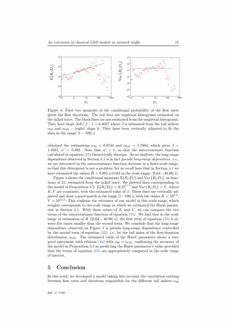
Figure 4: First two moments of the conditional probability of the flow ratesgiven the flow durations. The red dots are empirical histograms estimated onthe in2p3 trace. The black lines are not estimated from the empirical histograms.They have slope (left) β− 1 = 0.4037 where β is estimated from the tail indicesαSI and αON – (right) slope 0. They have been vertically adjusted to fit thedata in the range [1− 100] s

obtained the estimations αSI = 0.8544 and αON = 1.1994, which gives β =1.4037, α′ = 0.392. Note that α′ < 1, so that the autocovariance functioncalculated in equation (15) theoretically diverges. As we shall see, the long-rangedependence observed in Section 4.1 is in fact pseudo long-range dependence, i.e.,we are interested in the autocovariance function decrease in a finite-scale range,so that this divergence is not a problem (let us recall here that in Section 4.1 wehave estimated the values H = 0.901±0.045 in the scale range: [0.64−40.96] s).

Figure 4 shows the conditional moments E{Ri|Di} and Var{Ri|Di}, as func-tions of Di, estimated from the in2p3 trace. We plotted lines corresponding tothe model of Proposition 3.5: E{Ri|Di} = KDβ−1

i and Var{Ri|Di} = V , whereK,V are constants, with the estimated value of β. These lines are vertically ad-justed and show a good match in the range [1−100] s, with the valuesK = 105.2,V = 1012.4. This confirms the relevance of our model in this scale range, whichroughly corresponds to the scale range in which we estimated the Hurst param-eter in Section 4.1. With these values of K and V , we can compare the twoterms of the autocovariance function of equation (15). We find that in the scalerange of estimation of H ([0.64− 40.96] s), the first term of equation (15) is al-ways five times smaller than the second term. We conclude that the long-rangedependence observed on Figure 3 is pseudo long-range dependence controlledby the second term of equation (15), i.e., by the tail index of the flow-durationdistribution αON. The estimated value of the Hurst parameter shows a verygood agreement with relation (1a) with αH = αON, confirming the accuracy ofthe model in Proposition 3.5 in predicting the Hurst parameter’s value providedthat the terms of equation (15) are appropriately compared in the scale rangeof interest.

5 ConclusionIn this work, we developed a model taking into account the correlation existingbetween flow rates and durations responsible for the different tail indices αSI

RR n° 7100


and αON. Based only on specifications of the first two order moments of theconditional probability of the rates given the duration, we showed that the in-stantaneous bandwidth exhibits long-range dependence with a Hurst parameteras in relation (1a), where the controlling tail index αH can be either αON or acombination of αON and αSI, whichever is the smaller. We also showed that,in certain circumstances, pseudo long-range dependence with a different Hurstparameter can be observed in a finite scale range. In the case where the corre-lation between flow rates and durations vanishes, our results coincide with theusual results of classical models.

Finally, we validated the ability of our model to predict the correct Hurstparameter on a real web traffic trace. However, the non-stationarity inherentto real Internet data at large time scales (around one hour) constrained us torestrain our study to 30 minutes of traces. Consequently, we observed pseudolong-range dependence, and longer stationary traces would be required to il-lustrate the ability of our model to predict asymptotic long-range dependence,which, as we saw, can exhibit a different Hurst parameter.

The model proposed in this work is the first model, to the best of our knowl-edge, that includes the correlation between flow rates and durations. This cor-relation is very important. It has been observed for over a decade [?], and islikely to become even more important with the appearance of FTTH and flow-aware approaches. Further theoretical developments would be needed to givea more rigorous mathematical statement of our results, in particular concern-ing the Gaussian limit, and a potential other limit that could arise similarly toclassical models. Also, we assumed a Poisson flow arrival, which is a useful sim-plification to conduct the calculations, but might not always hold. Consideringless restrictive flow-arrival processes would also be an interesting improvementof our results, be it only to clarify in which situations a correlated flow-arrivalprocess can affect the aggregate traffic self-similarity.

INRIA

Centre de recherche INRIA Grenoble – Rhône-Alpes655, avenue de l’Europe - 38334 Montbonnot Saint-Ismier (France)

Centre de recherche INRIA Bordeaux – Sud Ouest : Domaine Universitaire - 351, cours de la Libération - 33405 Talence CedexCentre de recherche INRIA Lille – Nord Europe : Parc Scientifique de la Haute Borne - 40, avenue Halley - 59650 Villeneuve d’Ascq

Centre de recherche INRIA Nancy – Grand Est : LORIA, Technopôle de Nancy-Brabois - Campus scientifique615, rue du Jardin Botanique - BP 101 - 54602 Villers-lès-Nancy Cedex

Centre de recherche INRIA Paris – Rocquencourt : Domaine de Voluceau - Rocquencourt - BP 105 - 78153 Le Chesnay CedexCentre de recherche INRIA Rennes – Bretagne Atlantique : IRISA, Campus universitaire de Beaulieu - 35042 Rennes Cedex

Centre de recherche INRIA Saclay – Île-de-France : Parc Orsay Université - ZAC des Vignes : 4, rue Jacques Monod - 91893 Orsay CedexCentre de recherche INRIA Sophia Antipolis – Méditerranée : 2004, route des Lucioles - BP 93 - 06902 Sophia Antipolis Cedex

ÉditeurINRIA - Domaine de Voluceau - Rocquencourt, BP 105 - 78153 Le Chesnay Cedex (France)

http://www.inria.frISSN 0249-6399

Documents

Impact of the Correlation between Flow Rates and Durations on