Embed Size (px)
Citation preview

Impact of Static SeaSurface TopographyVariations on OceanSurface Waves
Yik Keung YING
TechnischeUniversiteitDelft


Impact of Static Sea SurfaceTopography Variations on Ocean
Surface Waves
by
Yik Keung YING
in partial fulfillment of the requirements for the degree of
Master of Sciencein Applied Mathematics
at the Delft University of Technology,to be defended publicly on Tuesday August 1, 2016 at 1:00 PM.
Supervisor: Prof. dr. ir. C. Vuik, Prof. dr. ir. L. R. MaasThesis committee: Prof. dr. ir. C. Vuik, TU Delft
Dr. ir. W. T. van Horssen, TU DelftProf. dr. ir. L. R. Maas, Koninklijk Nederlands Instituut voor Onderzoek der Zee
This thesis is confidential and cannot be made public until August 30, 2016.
An electronic version of this thesis is available at http://repository.tudelft.nl/.


Preface
I would like to express my gratitude towards everyone I met over the past two years in Europe. Withoutany of you my life would not have been so joyful and fulfilling.
In particular, I would like to thank Dr. Vadym Aizinger from FAU and Dr. Vera Fofonova from AWIfor bringing me to the icy Lena delta. I hope sooner or later I can involve in the discussion betweenyou two in Russian language.
I would also like to thank Prof Kees Vuik and Prof Leo Maas for their patience and advice towardsmy ill-organised idea and erroneous writing. I don’t speak much Dutch but I absolutely love the dutchpeople and the dutch ways of working things out.
Special thanks also goes to the European Commission and the COSSE Consortium for providingmany opportunities and financing my studies. Without the kind support I don’t think I have a chanceto leave my home country and explore Europe.
Danke schoen. Dankje wel.
Yik Keung YINGDelft, August 2016
iii


Contents
1 Introduction 1
2 Basis Terminology 32.1 Governing Equations . . . . . . . . . . . . . . . . . . . . . . . . . . . . . . . . . . . . 3
2.1.1 Equations of Motion in a Non-rotating Coordinate System . . . . . . . . . . 32.1.2 Equations of Motion in a Rotating Coordinate System . . . . . . . . . . . . . 3
2.2 Transformation of Coordinates. . . . . . . . . . . . . . . . . . . . . . . . . . . . . . . 32.2.1 Notations. . . . . . . . . . . . . . . . . . . . . . . . . . . . . . . . . . . . . . . . 32.2.2 Transformation of scalar fields . . . . . . . . . . . . . . . . . . . . . . . . . . . 42.2.3 Transformation of vector fields . . . . . . . . . . . . . . . . . . . . . . . . . . . 52.2.4 Transformation of equations . . . . . . . . . . . . . . . . . . . . . . . . . . . . 5
3 Adapted Shallow Water Model 93.1 Basic Definitions . . . . . . . . . . . . . . . . . . . . . . . . . . . . . . . . . . . . . . . 93.2 Properties of the Geopotential Height . . . . . . . . . . . . . . . . . . . . . . . . . . . 9
3.2.1 Vertical Gradient of the Geopotential Height. . . . . . . . . . . . . . . . . . . 103.2.2 𝑍-transformation . . . . . . . . . . . . . . . . . . . . . . . . . . . . . . . . . . . 103.2.3 Inverse 𝑍-transformation . . . . . . . . . . . . . . . . . . . . . . . . . . . . . . 11
3.3 Definition of Water Depth . . . . . . . . . . . . . . . . . . . . . . . . . . . . . . . . . . 123.3.1 Classical Water Depth . . . . . . . . . . . . . . . . . . . . . . . . . . . . . . . . 123.3.2 Adapted Water Depth . . . . . . . . . . . . . . . . . . . . . . . . . . . . . . . . 123.3.3 A First-order Approximation to the Adapted Water Depth. . . . . . . . . . . 12
3.4 Transformation of equations . . . . . . . . . . . . . . . . . . . . . . . . . . . . . . . . 133.5 Additional simplifications . . . . . . . . . . . . . . . . . . . . . . . . . . . . . . . . . . 14
3.5.1 Incompressiblity . . . . . . . . . . . . . . . . . . . . . . . . . . . . . . . . . . . 143.5.2 Horizontal Gradient of Geopotential. . . . . . . . . . . . . . . . . . . . . . . . 143.5.3 Hydrostatic approximation . . . . . . . . . . . . . . . . . . . . . . . . . . . . . 14
3.6 The Adapted Continuity Equation . . . . . . . . . . . . . . . . . . . . . . . . . . . . . 163.6.1 An Exact Adapted Continuity Equation. . . . . . . . . . . . . . . . . . . . . . 163.6.2 A Zeroth-Order Approximation . . . . . . . . . . . . . . . . . . . . . . . . . . . 17
3.7 Adapted Horizontal Momentum Equation . . . . . . . . . . . . . . . . . . . . . . . . 183.7.1 Adapted Momentum Equation under the Hydrostatic Approximation . . . . 183.7.2 Explicit Expression for the Jacobian term . . . . . . . . . . . . . . . . . . . . 193.7.3 Explicit Computation for the Jacobian term . . . . . . . . . . . . . . . . . . . 203.7.4 Physical Interpretation of the Jacobian term . . . . . . . . . . . . . . . . . . 21
3.8 Characteristic Scale Analysis of the Continuity Equation . . . . . . . . . . . . . . . 223.8.1 Notation of the Characteristic Scales . . . . . . . . . . . . . . . . . . . . . . . 223.8.2 Validity of Approximations . . . . . . . . . . . . . . . . . . . . . . . . . . . . . 223.8.3 Dimensionless Continuity Equation. . . . . . . . . . . . . . . . . . . . . . . . 22
3.9 Characteristic Scale Analysis of the Momentum Equation . . . . . . . . . . . . . . 243.9.1 The scale of the term u . . . . . . . . . . . . . . . . . . . . . . . . . . . . . . 243.9.2 The scale of the non-linear pressure gradient terms . . . . . . . . . . . . . . 243.9.3 The scale of the Jacobian term. . . . . . . . . . . . . . . . . . . . . . . . . . . 273.9.4 Short Conclusions . . . . . . . . . . . . . . . . . . . . . . . . . . . . . . . . . . 28
3.10Derivation of Adapted Shallow Water Equations . . . . . . . . . . . . . . . . . . . . 283.10.1Boundary Conditions . . . . . . . . . . . . . . . . . . . . . . . . . . . . . . . . 283.10.2Adapted Depth-Averaged Continuity Equation . . . . . . . . . . . . . . . . . 303.10.3Adapted Momentum Equation . . . . . . . . . . . . . . . . . . . . . . . . . . . 32
v

vi Contents
3.11Derivation of Adapted Wave Equation in Shallow Water . . . . . . . . . . . . . . . . 333.11.1The Second-Order Wave Equation. . . . . . . . . . . . . . . . . . . . . . . . . 333.11.2The Mathematical Characteristics of the Adapted Shallow Water Wave. . . 343.11.3Conservation of Potential Vorticity . . . . . . . . . . . . . . . . . . . . . . . . 35
4 One-Dimensional Adapted Wave Equation 374.1 Diagnostic Formalism for the One-dimensional Adapted Wave Equation . . . . . . 37
4.1.1 Case 1: Oscillatory Mode 𝐸 > 𝑉 . . . . . . . . . . . . . . . . . . . . . . . . . . 394.1.2 Case 2: Growth/Decay mode 𝐸 < 𝑉 . . . . . . . . . . . . . . . . . . . . . . . . 404.1.3 The Physical Meanings of 𝐸 and 𝑉 . . . . . . . . . . . . . . . . . . . . . . . . . 404.1.4 Final Remarks on the Definitions of Diagnostic Variables 𝐸 and 𝑉 . . . . . 41
4.2 Methodology of Constructing Test Cases . . . . . . . . . . . . . . . . . . . . . . . . . 414.3 Test Case 1: Uniform Water Depth . . . . . . . . . . . . . . . . . . . . . . . . . . . . 42
4.3.1 Rationale and Configuration of Test Case 1 . . . . . . . . . . . . . . . . . . . 424.3.2 Test Case 1a: Uniform Water Depth + Exponential Gravity Perturbation. . 454.3.3 Test Case 1b: Uniform Water Depth + Gaussian Gravity Perturbation . . . 47
4.4 Test case 2: Reflection and Scattering of Surface Waves by Varying Gravity. . . . 484.4.1 Rationale and Configuration of Test Case 2 . . . . . . . . . . . . . . . . . . . 484.4.2 Test case 2a: Gravity Step . . . . . . . . . . . . . . . . . . . . . . . . . . . . . 484.4.3 Test case 2b: Gravity Well . . . . . . . . . . . . . . . . . . . . . . . . . . . . . 494.4.4 Short Conclusions from Test case 2. . . . . . . . . . . . . . . . . . . . . . . . 50
4.5 Test Case 3: Non-Flat Sea-Surface Topography . . . . . . . . . . . . . . . . . . . . . 514.5.1 Rationale and Configuration of Test Case 3 . . . . . . . . . . . . . . . . . . . 514.5.2 Test case 3a: Exponential Water Depth + Exponential Gravity Perturba-
tion . . . . . . . . . . . . . . . . . . . . . . . . . . . . . . . . . . . . . . . . . . . 524.5.3 Test case 3b: Gaussian Water Depth + Gaussian Gravity Perturbation. . . 534.5.4 Short Conclusions from Test case 3. . . . . . . . . . . . . . . . . . . . . . . . 53
4.6 Test Case 4: Global Variation of Gravity . . . . . . . . . . . . . . . . . . . . . . . . . 544.6.1 Rationale and Configuration of Test Case 4 . . . . . . . . . . . . . . . . . . . 544.6.2 Test Case 4a: Surface Waves on an Arc . . . . . . . . . . . . . . . . . . . . . 544.6.3 Short Conclusions from Test case 4. . . . . . . . . . . . . . . . . . . . . . . . 54
4.7 Conclusions from One-Dimensional Adapted Shallow Water Waves. . . . . . . . . 55
5 Two-Dimensional Adapted Wave Equation 815.1 Diagnostic Formalism: Limitations . . . . . . . . . . . . . . . . . . . . . . . . . . . . 815.2 Test Cases and Numerical Simulations. . . . . . . . . . . . . . . . . . . . . . . . . . 82
5.2.1 Rationale and Limitations. . . . . . . . . . . . . . . . . . . . . . . . . . . . . . 825.2.2 Methodology and Configurations of Test Cases . . . . . . . . . . . . . . . . . 82
5.3 Test case 1: Hypothetical Surface Waves. . . . . . . . . . . . . . . . . . . . . . . . . 835.3.1 Test case 1a: Depth Perturbation vs Uniform Gravity and Depth . . . . . . 835.3.2 Test case 1b: Gravity Perturbation vs Uniform Gravity and Depth . . . . . 845.3.3 Test case 1c: Gravity Perturbation vs Depth Perturbation . . . . . . . . . . 84
5.4 Test case 2: Physical Surface Waves . . . . . . . . . . . . . . . . . . . . . . . . . . . 865.4.1 Test case 2a: Gravity Perturbation vs Uniform Gravity and Depth. . . . . . 865.4.2 Test case 2b: Gravity and Depth Perturbation vs Uniform Gravity and
Depth. . . . . . . . . . . . . . . . . . . . . . . . . . . . . . . . . . . . . . . . . . 875.4.3 Test case 2c: Gravity and Depth Perturbation vs Uniform Gravity and
Depth Perturbation. . . . . . . . . . . . . . . . . . . . . . . . . . . . . . . . . . 875.5 Conclusions from Test Cases. . . . . . . . . . . . . . . . . . . . . . . . . . . . . . . . 885.6 Final Remarks on Surface Waves on a Two-Dimension Plane . . . . . . . . . . . . 89
6 Generalised Airy’s Linear Wave Theory 956.1 Derivation: Variational Formalism of Surface Gravity Waves . . . . . . . . . . . . . 956.2 One-Dimensional Surface Gravity Waves. . . . . . . . . . . . . . . . . . . . . . . . . 96
6.2.1 Governing Equations for Linear Waves . . . . . . . . . . . . . . . . . . . . . . 966.2.2 Motivation for the Coordinate Transformation. . . . . . . . . . . . . . . . . . 976.2.3 Properties of the Conformal Coordinate Transformation. . . . . . . . . . . . 976.2.4 Transformed Laplacian Operators and Laplace Equation . . . . . . . . . . . 98

Contents vii
6.2.5 Transformed Boundary condition . . . . . . . . . . . . . . . . . . . . . . . . . 986.2.6 Short Summary. . . . . . . . . . . . . . . . . . . . . . . . . . . . . . . . . . . . 99
6.3 Test Cases for One-Dimensional Linear Waves . . . . . . . . . . . . . . . . . . . . . 996.3.1 Example 1: Gravity with Inverse-law in 2D . . . . . . . . . . . . . . . . . . .1006.3.2 Example 2a: Vertical Downwards Gravity with Perturbation . . . . . . . . .1036.3.3 Example 2b: Vertical Downwards Gravity with Perturbation . . . . . . . . .1046.3.4 Example 2b: Numerical Visualisation and Comparison with Adapted Shal-
low Water Model . . . . . . . . . . . . . . . . . . . . . . . . . . . . . . . . . . .1066.3.5 Conclusions from the One-Dimensional Waves . . . . . . . . . . . . . . . . .1086.3.6 Remarks on the General Variable Bathymetric Profiles . . . . . . . . . . . .108
6.4 Discussion on the Three-Dimensional Potential. . . . . . . . . . . . . . . . . . . . .1096.4.1 coordinate transformation in Three-Dimensional Space . . . . . . . . . . . .1096.4.2 Trial 1: Clebsch Potential . . . . . . . . . . . . . . . . . . . . . . . . . . . . . .1096.4.3 Example: Point-mass in three-dimensional space . . . . . . . . . . . . . . .1116.4.4 Clebsch Potential: the Gauge Invariance . . . . . . . . . . . . . . . . . . . . .1156.4.5 Trial 2: Geometric Inspection . . . . . . . . . . . . . . . . . . . . . . . . . . .116
6.5 Short Conclusions . . . . . . . . . . . . . . . . . . . . . . . . . . . . . . . . . . . . . .117
7 Conclusions and Further Research Directions 119
Bibliography 121

1Introduction
The shape of the Earth has long been one of the biggest and most frequently-asked questions ofhumanity. While ancient Chinese believed the Earth is a square plane covered by a hemisphere sky,the ancient Egyptians had long spotted the Earth is curved and even gave an estimate to the curvatureand size of the Earth. Yet it was not until Ferdinand Magellan succeeded the circumnavigation in year1521 that human-beings first confirmed experimentally that the Earth is a closed sphere. Yet it is notreally a sphere - the remote sensing techniques developed alongside with the space technology in thelast century revealed that the Earth’s shape is a ’spheroid’, meaning ’almost sphere’, whose surface isindeed much rougher than anyone expected.
The shape of the Earth, modernly described by the so-called mean-sea level, is indeed a time-independent equipotential of the conservative gravitational field, governed by the Poisson equation.With an uneven distribution of mass both on the surface and in the interior of the Earth, the resultinggravity field is also spatially non-uniform.
Although small in magnitude, the spatial variation of gravitational attraction does lead to observable’topography’ on the ocean, namely, the hypothetically motionless sea-surface does not lie on a perfectsphere but a rough-surfaced spheroid. Consequently, the gravity vector, which is defined to be thegradient vector of the equipotential lines, does not always point in the same direction. The magnitudeof the gravity at the mean-sea level is also not uniform at all.
The causes and empirical determination of the mean-sea level have been addressed by geophysi-cists. In this project, however, it is the consequence of the non-uniform gravity that concerns us. Inparticular, the surface waves in fluid in a spatially varying gravity field is the topic of this thesis.
In the classical treatment of surface waves, the gravity field is assumed to be uni-directionallyconstant everywhere. The gravity together with the fluid pressure constitute the restoring mechanismsof oscillations on the fluid surface, thus creating the surface gravity waves.
In this project, the assumption of uniform gravity, used in most, if not all, of the analytical andnumerical studies of surface waves, will be relaxed. Focus is especially put on conservative gravitationalforce fields, due to their relevance to the actual gravity field on Earth. In Chapter 2 basic terminologiesand notations will be introduced. The research topic starts with the shallow water waves in Chapter3, in which the standard shallow water model will be adapted to cater for the non-uniformity in thegravity field. The adapted shallow water model and the linearised shallow water waves will be derivedin this Chapter.
In Chapter 4, the adapted one-dimensional shallow water waves are analysed. Analytic solutionsto the adapted shallow water wave equations are derived, and validated by numerical simulationswith the aid of the open-source numerical solver CLAWPACK. Two features of surface waves in theone-dimension studies are reviewed, namely the wave amplitudes and wavenumber.
Chapter 5 continues the discussion of the adapted shallow water model in the two-dimensionalspace. While limited analytic studies are presented, the two-dimensional equations are solved nu-merically by CLAWPACK based on both hypothetical and physical scenarios. In addition to the waveamplitudes and wavenumbers, the refraction and scattering of waves by the spatially-varying gravityfield is focused also in the two-dimensional studies.
1

2 1. Introduction
A twist is found in Chapter 6. In this chapter the shallowness assumption is relaxed and Airy’slinear wave theory, which is a fundamental and widely-applied theory to study surface gravity waves, isgeneralised for spatially-varying conservative gravity fields. The generalisation is, however, limited toonly the two-dimensional space, and thus one-dimensional waves. The surface waves in the full three-dimensional remains an unresolved problem left for further research. Despite this, it is demonstratedthat the one-dimensional waves turns out to be consistent with the adapted shallow water waves,discussed in Chapter 3 and 4.
The summary and conclusions are given in Chapter 7. Several unanswered questions in this thesisare also outlined for future research.

2Basis Terminology
2.1. Governing Equations2.1.1. Equations of Motion in a Non-rotating Coordinate SystemThe governing equations for fluid are given by the continuum equations of motions.
Denote𝐷𝑑𝑡 ≡
𝜕𝜕𝑡 + u ⋅ ∇ (2.1)
to be the total derivative following individual fluid elements.Denote x to be the position vector, 𝜌 = 𝜌(x, 𝑡) to be the density of fluid and u = (x, 𝑡) is the
velocity field. The continuity equation is given by:
𝐷𝜌𝑑𝑡 + 𝜌∇ ⋅ u = 0 (2.2)
In this thesis the fluid is taken to be incompressible, so that the continuity equation reads:
∇ ⋅ u = 0 (2.3)
Denote 𝑝 = 𝑝(x, 𝑡) to be the pressure field, Φ = Φ(x, 𝑡) is the potential for conservative force fieldsand F = F(x,u, 𝑡) is the non-conservative forces. The momentum equation is given by:
𝜌𝐷u𝑑𝑡 = −∇𝑝 − 𝜌∇Φ + F (2.4)
2.1.2. Equations of Motion in a Rotating Coordinate SystemConsider a reference frame which is rotating at uniform angular speed � relative to the inertial frame.The continuity equation remains invariant in both rotating and non-rotating coordinate system. Themomentum equation, however, is transformed into the following form:
𝜌[𝐷u𝑑𝑡 + 2� × u] = −∇𝑝 − 𝜌∇(Φ +Φ ) + F (2.5)
where Φ is the conservative centrifugal potential associated to the centrifugal force due to the rotationof reference frame.
2.2. Transformation of Coordinates2.2.1. NotationsThe Cartesian coordinates (𝑥, 𝑦, 𝑧) are commonly used to study geophysical fluid dynamics when thescale of motion is not too large in the sense that the length scale of motion 𝐿 is much less than theradius of Earth 𝑅 ≈ 6400km.
3

4 2. Basis Terminology
For specific problems, it may happen that the use of an transformed coordinate system can simplifythe analysis. In the following text, a specific transformation on the vertical coordinates 𝑧 will beperformed. A general description is given below.
Suppose 𝑟 is a general vertical coordinate which is monotonic with 𝑧. Transformation from (𝑥, 𝑦, 𝑧, 𝑡)to (𝑥, 𝑦, 𝑟, 𝑡) requires a transformation function 𝑇(𝑥, 𝑦, 𝑧, 𝑡), which maps (𝑥, 𝑦, 𝑧, 𝑡) ∈ ℛ into (𝑥, 𝑦, 𝑟, 𝑡) ∈ℛ .
(𝑥, 𝑦, 𝑟, 𝑡) = 𝑇(𝑥, 𝑦, 𝑧, 𝑡), (2.6)Since the coordinates 𝑥, 𝑦 and remains invariant in the transformation given by 𝑇, 𝑟 can also be seenas a scalar function that maps (𝑥, 𝑦, 𝑧, 𝑡) to a scalar, which is given by
𝑟 = 𝑟(𝑥, 𝑦, 𝑧, 𝑡) (2.7)
If 𝑟 is monotonic, there exist an inverse �� to 𝑟, which maps (𝑥, 𝑦, 𝑟, 𝑡) back to a scalar, which is givenby
�� = ��(𝑥, 𝑦, 𝑟, 𝑡) (2.8)The equation (2.8) can be interpreted as ’reading’ the vertical position in the physical coordinate usingdata from the transformed coordinates (𝑥, 𝑦, 𝑟, 𝑡).
2.2.2. Transformation of scalar fieldsAny scalar field 𝐹 = 𝐹(𝑥, 𝑦, 𝑧, 𝑡) can then be rewritten in the new coordinates 𝐹 = 𝐹(𝑥, 𝑦, 𝑧(𝑥, 𝑦, 𝑟, 𝑡), 𝑡) =��(𝑥, 𝑦, 𝑟, 𝑡). Applying the chain rule yields
𝜕��𝜕𝑥 | =
𝜕𝐹𝜕𝑥 | +
𝜕𝐹𝜕𝑧𝜕��𝜕𝑥 | (2.9a)
𝜕��𝜕𝑦 | =
𝜕𝐹𝜕𝑦 | +
𝜕𝐹𝜕𝑧𝜕��𝜕𝑦 | (2.9b)
𝜕��𝜕𝑡 | =
𝜕𝐹𝜕𝑡 | +
𝜕𝐹𝜕𝑧𝜕��𝜕𝑡 | (2.9c)
where the vertical bar refers to partial differentiation maintaining the suffix constant.Meanwhile along the transformed ’vertical’ coordinates, the ’vertical’ gradient of the scalar field ��
is given by𝜕��𝜕𝑟 =
𝜕𝐹𝜕𝑧𝜕��𝜕𝑟 (2.10)
Denote 𝑒 , 𝑒 and 𝑒 to be the unit vector in the Cartesian coordinates. the horizontal gradient ∇and ∇ is given by
∇ 𝐹 = 𝜕𝐹𝜕𝑥 | 𝑒 + 𝜕𝐹𝜕𝑦 | 𝑒 (2.11)
∇ �� = 𝜕��𝜕𝑥 | 𝑒 + 𝜕��𝜕𝑦 | 𝑒 . (2.12)
Hence, based on the chain rules (2.9) and equation (2.10), the full gradient operator in the basis ofCartesian unit vector with respect to (𝑥, 𝑦, 𝑟, 𝑡) can be obtained:
∇𝐹 = ∇ 𝐹 + 𝜕𝐹𝜕𝑧 𝑒 (2.13)
= [∇ �� − 𝜕��𝜕𝑟𝜕𝑟𝜕𝑧 ∇ (��)] +
𝜕��𝜕𝑟𝜕𝑟𝜕𝑧 𝑒 (2.14)
Note that the reciprocal rule for partial derivatives = 1/ has been used to obtain the fullgradient operator. The reciprocal rule is valid as long as both and does not vanish.
To summarise this section, the relation between ∇ 𝐹 and ∇ �� highlighted:
∇ 𝐹 = ∇ �� − 𝜕��𝜕𝑟𝜕𝑟𝜕𝑧 ∇ (��), (2.15)
which will play crucial roles in the following sections when equations are transformed.

2.2. Transformation of Coordinates 5
REMARK 1: In the following text, if a variable, a scalar function, or a vector function is marked witha tilde, it implicitly means that the transformed coordinates (𝑥, 𝑦, 𝑟, 𝑡) is used to express it.
REMARK 2: All equations and their derivations in this chapter can be found in the lecture note byAdcroft. Hence the detailed derivation of some equations will be omitted in this text. Interested readersmay refer to Adcroft et al.(2015).
2.2.3. Transformation of vector fieldsSimilarly for any vector field F(𝑥, 𝑦, 𝑧, 𝑡) = 𝐹 (𝑥, 𝑦, 𝑧, 𝑡) 𝑒 + 𝐹 (𝑥, 𝑦, 𝑧, 𝑡) 𝑒 + 𝐹 (𝑥, 𝑦, 𝑧, 𝑡) 𝑒 in Cartesiancoordinates, define the horizontal vector F = 𝐹 𝑒 + 𝐹 𝑒 and horizontal divergence ∇ ⋅ and ∇ ⋅
∇ ⋅ F = 𝜕𝐹𝜕𝑥 | +
𝜕𝐹𝜕𝑦 | (2.16)
∇ ⋅ F = 𝜕��𝜕𝑥 | +
𝜕��𝜕𝑦 | (2.17)
Again based on the chain rules (2.9) and equation (2.10) for each component of the vector field F, itthen follows the full divergence is given by
∇ ⋅ F = ∇ ⋅ F + 𝜕𝐹𝜕𝑧 (2.18)
= [∇ ⋅ F − 𝜕F𝜕𝑟𝜕𝑟𝜕𝑧 ⋅ ∇ (��)] +
𝜕��𝜕𝑟
𝜕𝑟𝜕𝑧 (2.19)
The relation between ∇ ⋅ V and ∇ ⋅ V is also highlighted:
∇ ⋅ V = ∇ ⋅ V − 𝜕V𝜕𝑟𝜕𝑟𝜕𝑧 ⋅ ∇ (��), (2.20)
which will also play significant role in the next section when the equations are transformed.
2.2.4. Transformation of equationsIn the new coordinate system (𝑥, 𝑦, 𝑟, 𝑡), the vertical velocity �� = and its relation with the verticalvelocity 𝑤 = in the physical coordinates has to be handled with care.
The relation between �� and 𝑤Consider the total derivative of coordinate function 𝑟 = 𝑟(𝑥, 𝑦, 𝑧, 𝑡),
𝑑𝑟𝑑𝑡 =
𝜕𝑟𝜕𝑡 +
𝜕𝑟𝜕𝑥𝑑𝑥𝑑𝑡 +
𝜕𝑟𝜕𝑦𝑑𝑦𝑑𝑡 +
𝜕𝑟𝜕𝑧𝑑𝑧𝑑𝑡 (2.21)
Note that 𝑢 = , 𝑣 = and 𝑤 = are respectively the velocities in 𝑥, 𝑦 and 𝑧 directions. Hence ahandy expression for �� = with respect to the physical coordinates (𝑥, 𝑦, 𝑧, 𝑡) is obtained
�� = 𝜕𝑟𝜕𝑡 + u ⋅ ∇ (𝑟) + 𝑤𝜕𝑟𝜕𝑧 (2.22)
On the other hand, consider the vertical position �� in the physical frame of reference as a functionof the transformed coordinates �� = ��(𝑥, 𝑦, 𝑟, 𝑡) via equation (2.8). The total derivative of ��, which isthe vertical velocity �� = , is hence given by
�� = 𝜕��𝜕𝑡 | + u ⋅ ∇ (��) + ��𝜕��𝜕𝑟 , (2.23)
which relates the vertical velocity �� from the viewpoint of the transformed coordinates.

6 2. Basis Terminology
Total Derivative in the Transformed CoordinatesThe total derivative of a scalar field �� = ��(𝑥, 𝑦, 𝑟, 𝑡) is given by:
𝐷��𝑑𝑡 =
𝜕��𝜕𝑡 | + u ⋅ ∇ (��) + ��𝜕��𝜕𝑟 . (2.24)
An important application to the equation (2.24) is to compute the quantity . Consider the scalarfield for the vertical velocity �� = ��(𝑥, 𝑦, 𝑟, 𝑡) with respect to the transformed coordinates (𝑥, 𝑦, 𝑟, 𝑡).The partial derivative can be shown to be:
𝜕��𝜕𝑟 =
𝜕𝜕𝑟(
𝜕��𝜕𝑡 | + u ⋅ ∇ (��) + ��𝜕��𝜕𝑟) (2.25)
= 𝐷𝑑𝑡(
𝜕��𝜕𝑟) +
𝜕u𝜕𝑟 ⋅ ∇ (��) + 𝜕��𝜕𝑟
𝜕��𝜕𝑟 (2.26)
Based on the expression for , after some algebraic manipulations, the divergence of velocity field uin the transformed coordinates (𝑥, 𝑦, 𝑟, 𝑡) can be concisely given by:
∇ ⋅ u = ∇ ⋅ u + 𝜕��𝜕𝑟 +𝐷𝑑𝑡 [ ln(
𝜕��𝜕𝑟 )] (2.27)
The detailed derivation to equation (2.27) is given below. Readers who are not interested may skip tothe next section. Recall that the divergence operator for a velocity field is given by equation (2.19).Take the vector field F to be the velocity field u = 𝑢 𝑒 + 𝑣 𝑒 + 𝑤 𝑒 in equation (2.19):
∇ ⋅ u = [∇ ⋅ u − 𝜕u𝜕𝑟𝜕𝑟𝜕𝑧 ⋅ ∇ (��)] +
𝜕��𝜕𝑟𝜕𝑟𝜕𝑧
Consider the quantity , replacing the expression of using equation (2.26) gives
𝜕��𝜕𝑟𝜕𝑟𝜕𝑧 = [
𝐷𝑑𝑡(
𝜕��𝜕𝑟) +
𝜕u𝜕𝑟 ⋅ ∇ (��) + 𝜕��𝜕𝑟
𝜕��𝜕𝑟 ]
𝜕𝑟𝜕𝑧
Note that by the reciprocal rule, = 1. Hence the quantity is simply given by
𝜕��𝜕𝑟𝜕𝑟𝜕𝑧 =
𝜕��𝜕𝑟 +
[ ( )] + 𝜕u𝜕𝑟
𝜕𝑟𝜕𝑧 ⋅ ∇ (��)
= 𝜕��𝜕𝑟 +
𝐷𝑑𝑡 [ ln(
𝜕��𝜕𝑟)] +
𝜕u𝜕𝑟
𝜕𝑟𝜕𝑧 ⋅ ∇ (��)
Therefore, the term u ⋅ ∇ (��) in the divergence of velocity ∇ ⋅u cancels out. Hence the divergenceof velocity in the transformed coordinates (𝑥, 𝑦, 𝑟, 𝑡) is simply given by
∇ ⋅ u = ∇ ⋅ u + 𝜕��𝜕𝑟 +𝐷𝑑𝑡 [ ln(
𝜕��𝜕𝑟)],
which completes the proof.
Continuity EquationIt follows that the continuity equation in (𝑥, 𝑦, 𝑟, 𝑡) coordinates becomes:
𝐷��𝑑𝑡 + ��[∇ ⋅ u + 𝜕��𝜕𝑟 +
𝐷𝑑𝑡 ( ln(
𝜕��𝜕𝑟 ))] = 0 (2.28)

2.2. Transformation of Coordinates 7
Momentum EquationThe transformation of momentum equation, is unfortunately more complicated. Here the transformedmomentum equation in a rotating coordinate frame will be derived. First consider the horizontal com-ponents of the momentum equations:
𝜌[𝐷u𝑑𝑡 + (2� × u) ] = −∇ 𝑝 − 𝜌∇ (Φ +Φ ) + F (2.29)
The equation (2.15) suggests that in the transformed coordinates (𝑥, 𝑦, 𝑟, 𝑡):
∇ 𝑝 = ∇ �� − 𝜕��𝜕𝑟𝜕𝑟𝜕𝑧 ∇ (��), (2.30)
whereas equation (2.20) suggests that, by defining the sum of potential Φ by Φ = Φ+Φ
∇ Φ = ∇ Φ − 𝜕Φ𝜕𝑟𝜕𝑟𝜕𝑧 ∇ (��) (2.31)
Hence the horizontal components of the momentum equation is obtained:
��[𝐷u𝑑𝑡 + (2� × u) ] = −∇ �� − ��∇ Φ + F + [𝜕��𝜕𝑟 + ��𝜕(Φ )𝜕𝑟 ]𝜕𝑟𝜕𝑧 ∇ (��) (2.32)
The derivation of the vertical momentum equation containing is cumbersome. In the shallowwater approximation of the fluid, the vertical momentum equation is not needed. Hence the exact formof vertical momentum equation will not be presented here.


3Adapted Shallow Water Model
In this chapter, the adapted model will be presented. A adapted wave equation for ocean surface wavedefined on geopotential height will be presented. The inertial frame without non-conservative forcewill be investigated first.
3.1. Basic DefinitionsDefine Mean-Sea Level Set 𝑀𝑠𝑙: It contains a the points (𝑥, 𝑦, 𝑧) such that
Φ(𝑥, 𝑦, 𝑧) = Φ (3.1)
where Φ is an empirically found value. In other words, 𝑀𝑠𝑙 = {(𝑥, 𝑦, 𝑧) ∶ Φ(𝑥, 𝑦, 𝑧) = Φ }. Given(𝑥, 𝑦), there is unique 𝑧 = 𝑧 (𝑥, 𝑦) such that (𝑥, 𝑦, 𝑧 ) belongs to 𝑀𝑠𝑙. The work done required totransport a unit mass from any point to 𝑀𝑆𝑙 to any arbitrary point (𝑥, 𝑦, 𝑧) is known as the potentialdifference between (𝑥, 𝑦, 𝑧) and 𝑀𝑆𝑙, and is given by:
Ψ(𝑥, 𝑦, 𝑧) = −∫( , , )
( , , )−∇Φ ⋅ 𝑑𝑙 (3.2)
where (��, ��, ��) is any point on 𝑀𝑠𝑙. Since Φ is a conservative field, the above integral is path indepen-dent. Hence an equivalent definition can be given by:
Ψ(𝑥, 𝑦, 𝑧) = ∫( , )
𝜕Φ𝜕�� (𝑥, 𝑦, ��)𝑑�� (3.3)
which takes a straightly vertical path integral, or,
Ψ(𝑥, 𝑦, 𝑧) = Φ(𝑥, 𝑦, 𝑧) − Φ (3.4)
which is essentially the potential difference.Define the Geopotential height 𝑍 as following:
𝑍 = 𝑍(𝑥, 𝑦, 𝑧) = Ψ(𝑥, 𝑦, 𝑧)𝑔 (3.5)
where 𝑔 is a constant reference gravity. Note that Ψ takes into account only the geopotential inducedby masses which are time-independent. The geopotential induced by ocean water is neglected. 𝑍has the same physical dimension with physical height 𝑧. Given any (𝑥, 𝑦), the mapping from 𝑍 to 𝑧 ismonotonic and one-to-one.
The geopotential height 𝑍 will serve as the variable 𝑟 in the chapter 2.2 to transform the equations.
3.2. Properties of the Geopotential HeightIn this section, several properties of the Geopotential Height transformation will be discussed.
9

10 3. Adapted Shallow Water Model
3.2.1. Vertical Gradient of the Geopotential HeightA very nice property of the Geopotential Height 𝑍 comes from the fact that
Φ = 𝑔 𝑍 + Φ , (3.6)
by considering equations (3.4) and (3.5). A tilde is added to to Φ because the geopotential Φ is nowread in the transformed coordinates (𝑥, 𝑦, 𝑍, 𝑡). Hence a very handy vertical gradient is given by:
𝜕Φ𝜕𝑍 = 𝑔 (3.7)
which is the reference gravity independent of any spatial or temporal coordinates.
3.2.2. 𝑍-transformationAssume that the gravity �� is weakly non-uniform: �� consists of a uniform component −𝑔 𝑒 and aperturbing non-linear conservative component 𝑔 (𝑥, 𝑦, 𝑧) = −∇Φ (𝑥, 𝑦, 𝑧), such that ‖𝑔 ‖ ≪ 𝑔 . that is:
��(𝑥, 𝑦, 𝑧) = −𝑔 𝑒 + 𝑔 (𝑥, 𝑦, 𝑧) (3.8)
It follows that, fixing (𝑥, 𝑦), the potential difference Ψ between the point (𝑥, 𝑦, 𝑧) and the mean sealevel is given by
Ψ(𝑥, 𝑦, 𝑧) = −∫( , )
[−𝑔 + 𝑔 (𝑥, 𝑦, 𝑧)]𝑑𝑠
= 𝑔 (𝑧 − 𝑧 ) + ∫( , )
∇Φ (𝑥, 𝑦, 𝑠)𝑑𝑠
Ψ(𝑥, 𝑦, 𝑧) = 𝑔 (𝑧 − 𝑧 (𝑥, 𝑦)) + [Φ (𝑥, 𝑦, 𝑧) − Φ (𝑥, 𝑦, 𝑧 (𝑥, 𝑦))] (3.9)
where 𝑧 = 𝑧 (𝑥, 𝑦) is the mean sea level at horizontal location (𝑥, 𝑦). The term Φ (𝑥, 𝑦, 𝑧) can beinterpreted as the disturbing geopotential Φ due to local topographical features.
It follows that the geopotential height 𝑍 becomes:
𝑍 = Ψ𝑔
= 𝑧 + Φ (𝑥, 𝑦, 𝑧)𝑔 − (𝑧 (𝑥, 𝑦) + Φ (𝑥, 𝑦, 𝑧 )𝑔 )
Denote 𝑍 (𝑥,𝑦) = 𝑧 (𝑥,𝑦) + ( , , ) , which is independent of 𝑧, the transformation from (𝑥, 𝑦, 𝑧) to(𝑥, 𝑦, 𝑍) can be given by
𝑍 = 𝑧 + Φ (𝑥, 𝑦, 𝑧)𝑔 − 𝑍 (𝑥, 𝑦) (3.10)
Equation (3.10) will be called as 𝑍-transformation in the remaining text.Now the partial derivative of 𝑍 with respect to 𝑧 (keeping 𝑥, 𝑦 constant) is considered, note that
𝑍 (𝑥, 𝑦) is independent of 𝑧. Denote by 𝑔 .
𝜕𝑍𝜕𝑧 = 1 +
1𝑔𝜕Φ𝜕𝑧
= 1 + 𝑔𝑔
The partial derivative of 𝑍 with respect to 𝑧
𝜕𝑍𝜕𝑧 = 1 +
𝑔𝑔 (3.11)

3.2. Properties of the Geopotential Height 11
will be the most crucial ingredient in the later derivation of equations and analysis. It is noted that,since 𝑍 = 𝑍(𝑥, 𝑦, 𝑧) is a smooth function, when ≠ 0, the reciprocal rule of partial derivative gives,
𝜕��𝜕𝑍 =
1 = 11+
(3.12)
is also valid. The criterion for which ≠ 0 will be discussed in the next section.ATTENTION: Instead of defining 𝑔 = − , which is the typical way to define force from for
conservative potential, here the definition is given by −𝑔 = − . The motivation here is that bydefining 𝑔 in this way, the effective gravity �� in 𝑧 direction is given by −(𝑔 + 𝑔 ), so that when 𝑔 ispositive, the magnitude of gravity in 𝑧-direction is 𝑔 + 𝑔 > 𝑔 .
3.2.3. Inverse 𝑍-transformationIn this section, further analytic properties of the 𝑍-transformation will be examined. In particular, theexistence of the inverse transformation will be discussed.
Recall that the 𝑍-transformation is given by equation (3.10)
𝑍 = 𝑧 + Φ (𝑥, 𝑦, 𝑧)𝑔 − 𝑍 (𝑥, 𝑦)
It is a natural question to ask if the inverse transformation exists. Consider the complete coordinatetransformation problem (𝑥, 𝑦, 𝑧) → (𝑥 , 𝑥 , 𝑥 ):
𝑥 = 𝑥𝑥 = 𝑦𝑥 = 𝑍(𝑥, 𝑦, 𝑧)
Note that 𝑍 = 𝑍(𝑥, 𝑦, 𝑧) is considered as a coordinate function 𝑍 ∶ ℛ → ℛ here. Consider the vectorfunction �� ∶ ℛ → ℛ
��(𝑥 , 𝑥 , 𝑥 ; 𝑥, 𝑦, 𝑧) = (𝑥 − 𝑥𝑥 − 𝑦
𝑥 − 𝑍(𝑥, 𝑦, 𝑧)) (3.13)
The coordinate transformation is equivalent to looking for solution of �� = 0.The Jacobian matrix of �� denoted as 𝐽(��) is thus given by
𝐽(��)(𝑥 , 𝑥 , 𝑥 ; 𝑥, 𝑦, 𝑧) = (1 0 0 −1 0 00 1 0 0 −1 00 0 1 − − −
)
According to the implicit function theorem, the inverse function 𝑧 = 𝑍 (𝑥 , 𝑥 , 𝑥 ) uniquely exists ifthe columns corresponding to the partial derivatives with respect to the original coordinates (in thiscase (𝑥, 𝑦, 𝑧), which corresponds to the last three columns) form an invertible matrix 𝐽, that is
𝐽 = 𝐽(��)(𝑥, 𝑦, 𝑧) = (−1 0 00 −1 0− − −
)
is invertible. Hence it suffices to consider the determinant of 𝐽, which is det 𝐽 ≠ 0. Note that det 𝐽 =− , and from equation (3.11), = 1+ , hence det 𝐽 ≠ 0 implies
1 + 𝑔𝑔 ≠ 0 ⟺ 𝑔 ≠ −𝑔 (3.14)
In other words, in the physical sense this condition (3.14) suggests that when the excess gravity 𝑔does not cancel out the background uniform gravity 𝑔 , the inverse coordinate transformation �� = 𝑍 1which maps from (𝑥, 𝑦, 𝑍) to physical coordinates (𝑥, 𝑦, 𝑧) is well-defined.

12 3. Adapted Shallow Water Model
In practice, for weakly non-uniform gravitational field such that ‖𝑔 ‖ ≪ 𝑔 , the condition (3.14)is always satisfied. Thus the inverse transformation �� = ��(𝑥, 𝑦, 𝑍) is practically always well-defined.This is also the condition where the reciprocal rule = holds, and justifies the validity of (3.12)
discussed in the previous section.
3.3. Definition of Water Depth3.3.1. Classical Water DepthSuppose at time 𝑡, with respect to the physical coordinates (𝑥, 𝑦, 𝑧), the surface elevation 𝑆(𝑥, 𝑦, 𝑡) ofthe fluid is described by the level set 𝑧 = 𝑆(𝑥, 𝑦, 𝑡). Meanwhile the bottom boundary 𝑆 (𝑥, 𝑦) of thefluid, which is time-independent, is described by the level set 𝑧 = 𝑆 .
The water depth 𝐷(𝑥, 𝑦, 𝑡) at location (𝑥, 𝑦) at time 𝑡 is given by the difference between the surfaceelevation 𝑆 and bottom elevation 𝑆 , that is,
𝐷(𝑥, 𝑦, 𝑡) = 𝑆(𝑥, 𝑦, 𝑡) − 𝑆 (𝑥, 𝑦) (3.15)
It is natural to give an analogous definition to water depth in the transformed 𝑍-coordinates, whichwill be discussed in the next section.
3.3.2. Adapted Water DepthRecall the coordinate transformation (3.10):
𝑍 = 𝑧 + Φ (𝑥, 𝑦, 𝑧)𝑔 − 𝑍 (𝑥, 𝑦)
Suppose the surface elevation �� in the transformed coordinates is given by the level set 𝑍 = ��(𝑥, 𝑦, 𝑡).�� can thus be computed by putting 𝑧 = 𝑆 into the transformation formula:
��(𝑥, 𝑦, 𝑡) = 𝑆(𝑥, 𝑦, 𝑡) + Φ (𝑥, 𝑦, 𝑆(𝑥, 𝑦, 𝑡))𝑔 − 𝑍 (𝑥, 𝑦) (3.16)
Similarly the bottom boundary 𝑧 = 𝑆 can be mapped into 𝑍 = �� , which is given by
�� (𝑥, 𝑦) = +Φ (𝑥, 𝑦, 𝑆 (𝑥, 𝑦))𝑔 − 𝑍 (𝑥, 𝑦) (3.17)
Define the water depth ��(𝑥, 𝑦, 𝑡) in 𝑍-coordinates by the difference between �� and �� :
��(𝑥, 𝑦, 𝑡) = ��(𝑥, 𝑦, 𝑡) − �� (𝑥, 𝑦) (3.18)
Using the equations (3.16) and (3.17), and defining ΔΦ (𝑥, 𝑦, 𝑡) = Φ (𝑥, 𝑦, 𝑆)−Φ (𝑥, 𝑦, 𝑆 ), the relationbetween 𝐷 and �� becomes clear:
��(𝑥, 𝑦, 𝑡) = 𝐷(𝑥, 𝑦, 𝑡) + 1𝑔 ΔΦ (𝑥, 𝑦, 𝑡). (3.19)
Note that ΔΦ (𝑥, 𝑦, 𝑡) physically refers to the potential difference between the surface elevation andthe bottom boundary solely due to the non-uniform component of the gravity.
3.3.3. A First-order Approximation to the Adapted Water DepthIn this section a first-order approximation to equation (3.19) will be obtained. The result of this sectionwill be applied in later sections when the adapted shallow water model is derived.
Recall that the definition of ΔΦ (𝑥, 𝑦, 𝑡) is given by:
ΔΦ (𝑥, 𝑦, 𝑡) = Φ (𝑥, 𝑦, 𝑆) − Φ (𝑥, 𝑦, 𝑆 )
Performing Taylor-series expansion of Φ (𝑥, 𝑦, 𝑆) around the mean-sea level (𝑥, 𝑦, 𝑧 ) gives
Φ (𝑥, 𝑦, 𝑆) = Φ (𝑥, 𝑦, 𝑧 ) + [𝜕Φ𝜕𝑧 ]@ ( , )(𝑆 − 𝑧 ) + ℎ.𝑜.𝑡.

3.4. Transformation of equations 13
where the subscript @𝑧 (𝑥, 𝑦) refers to the evaluation of quantities in the square bracket [ ∗ ] at themean-sea level (𝑥, 𝑦, 𝑧 (𝑥, 𝑦)), and ℎ.𝑜.𝑡. refers to the higher-order terms in the Taylor-series expansion.
Similarly, the Taylor-expansion of Φ (𝑥, 𝑦, 𝑆 ) can be performed around (𝑥, 𝑦, 𝑧 (𝑥, 𝑦)) also, a similarexpression can be obtained
Φ (𝑥, 𝑦, 𝑆 ) = Φ (𝑥, 𝑦, 𝑧 ) + [𝜕Φ𝜕𝑧 ]@ ( , )(𝑆 − 𝑧 ) + ℎ.𝑜.𝑡.
For a given certain (𝑥, 𝑦) at certain time 𝑡, ΔΦ (𝑥, 𝑦, 𝑡) can thus be approximated by
ΔΦ (𝑥, 𝑦, 𝑡) = [𝜕Φ𝜕𝑧 ]@ ( , )(𝑆 − 𝑆 ) + ℎ.𝑜.𝑡.
= [𝑔 ]@ ( , )𝐷 + ℎ.𝑜.𝑡.
Note that the Taylor-expansion could have been performed at any vertical coordinate 𝑧 within or inthe neighbourhood of the interval of [𝑆 , 𝑆] to yield an analogous result. The mean-sea level 𝑧 = 𝑧 (𝑥, 𝑦)is chosen because empirical measurement data of 𝑔 is usually available at this level.
If the higher-order terms are so small such that they can be neglected, then the relation between𝐷 and �� given by equation (3.19) can be simplified into
��(𝑥, 𝑦, 𝑡) ≈ 𝐷(𝑥, 𝑦, 𝑡) +[𝑔 ]@ ( , )
𝑔 𝐷(𝑥, 𝑦, 𝑡)
≈ 𝐷(𝑥, 𝑦, 𝑡)[(1 + 𝑔𝑔 )]@ ( , )
Note that according to equation (3.11), 1+ = , hence
��(𝑥, 𝑦, 𝑡) ≈ 𝐷(𝑥, 𝑦, 𝑡)[𝜕𝑍𝜕𝑧 ]@ ( , )
, (3.20)
which is a handy expression for analysis in later sections.
3.4. Transformation of equationsIn the remaining part of this chapter, the horizontal gradient ∇ and ∇ are understood to be 𝑒 | +𝑒 | and 𝑒 | + 𝑒 | respectively.To transform the equations from (𝑥, 𝑦, 𝑧, 𝑡) to (𝑥, 𝑦, 𝑍, 𝑡), take 𝑟 = 𝑍 in equation (2.28) and equation
(2.32).Adapted Continuity Equation:
𝐷��𝑑𝑡 + ��[∇ ⋅ u + 𝜕��𝜕𝑍 +
𝐷𝑑𝑡( ln (
𝜕��𝜕𝑍))] = 0 (3.21)
Adapted Horizontal Momentum Equation:
��[𝐷u𝑑𝑡 ] = −∇ �� − ��∇ Φ + (𝜕��𝜕𝑍 + ��
𝜕Φ𝜕𝑍 )
𝜕𝑍𝜕𝑧 ∇ (��) (3.22)
These equations are not easy to deal with. Hence it is necessary to further simplify them beforeanalytically studying the properties of their solutions, which will be presented in 3.5.
Another highlight is the extra terms ( ln( )) in the continuity equation (3.21) and ( +�� ) ∇ (��)in the momentum equation (3.22), in contrast to the standard continuity and momentum equation inthe standard Cartesian coordinates. The properties of these two extra terms will be discussed in thetwo sections 3.6 and 3.7.

14 3. Adapted Shallow Water Model
3.5. Additional simplifications3.5.1. IncompressiblityDensity of water on the ocean surface does change due to temperature and salinity variation. How-ever to simplify the analysis, such density variations are omitted. In other words, it is assumed that��(𝑥, 𝑦, 𝑍) = 𝜌 , where 𝜌 is a constant. In the later text, the subscript in 𝜌 will be skipped so that��(𝑥, 𝑦, 𝑍) = 𝜌.
It follows that the continuity equation (3.21) becomes:
∇ ⋅ u + 𝜕��𝜕𝑍 +𝐷𝑑𝑡( ln (
𝜕��𝜕𝑍)) = 0 (3.23)
3.5.2. Horizontal Gradient of GeopotentialIn the (horizontal) momentum equations (3.22) the horizontal gradient of geopotential with respectto 𝑍, i.e. ∇ Φ is involved. However, recalling that 𝑍 = , it is noticed that keeping 𝑍 constant isequivalent to keeping Φ constant. Hence the horizontal gradient of geopotential ∇ Φ simply vanishes.
∇ Φ = 𝜕Φ𝜕𝑥 | 𝑒 + 𝜕Φ𝜕𝑦 | 𝑒 = 0 (3.24)
Hence under the 𝑍-transformation, the momentum equation (3.22) becomes
𝜌[𝐷u𝑑𝑡 ] = −∇ �� + (𝜕��𝜕𝑍 + 𝜌
𝜕Φ𝜕𝑍 )
𝜕𝑍𝜕𝑧 ∇ (��) (3.25)
Note that the density 𝜌 is assumed to be a constant followed by the discussion of section 3.5.1 andthere is no difference between the density 𝜌 in the physical coordinates (𝑥, 𝑦, 𝑧, 𝑡) and transformedcoordinates (𝑥, 𝑦, 𝑍, 𝑡).
3.5.3. Hydrostatic approximationHydrostatic BalanceFor large scale oceanic flows, the horizontal length scale, denoted as 𝐿 , is usually much greater thanthe vertical length scale which is denoted by 𝐿 . The shallowness of an oceanic flow is known as thesmall aspect ratio:
𝛿 = 𝐿𝐿 ≪ 1 (3.26)
In section 2.8 of Pedlosky 1979, it is justified that for a shallow flow with 𝛿 ≪ 1, the vertical pressuregradient can be approximated by the gradient of gravitational force 𝜌 . An analogous result willbe derived.
Consider the hydrostatic pressure 𝑝 = 𝑝 (𝑥, 𝑦, 𝑧(𝑥, 𝑦, 𝑍), 𝑡) = �� (𝑥, 𝑦, 𝑍, 𝑡). The pressure gradient inhydrostatic condition is obtained by setting velocity �� = 0 in the momentum equation. Hence the fullmomentum equation equation(2.4) becomes:
∇𝑝 = −𝜌∇Φ
Since it is assumed that the density 𝜌 is constant everywhere, 𝜌 can be included in the gradient operator.Hence it follows that:
∇𝑝 = −∇(𝜌Φ) (3.27)⇒ 𝑝 = −𝜌Φ + 𝑝 (3.28)
where the reference pressure 𝑝 is an arbitrary constant. Note that the same argument can be appliedin the transformed coordinates (𝑥, 𝑦, 𝑍, 𝑡) and gives:
�� = −𝜌Φ + �� , (3.29)
where �� is also an arbitrary constant.

3.5. Additional simplifications 15
Consider the gradient operator ∇ in Cartesian coordinate, along the 𝑧-direction, it is noted that:𝜕𝑝𝜕𝑧 = −𝜌
𝜕Φ𝜕𝑧 (3.30)
Multiplying both sides with leads to:
𝜕𝑝𝜕𝑧
𝜕��𝜕𝑍 = −𝜌
𝜕Φ𝜕𝑧
𝜕��𝜕𝑍 (3.31)
By the chain rule, the equalities
𝜕��𝜕𝑍 = 𝜕𝑝
𝜕𝑧𝜕��𝜕𝑍 (3.32)
𝜕Φ𝜕𝑍 =
𝜕Φ𝜕𝑧
𝜕��𝜕𝑍 (3.33)
are justified. Thus the analogy of the hydrostatic pressure gradient in coordinates (𝑥, 𝑦, 𝑍, 𝑡) is estab-lished:
𝜕��𝜕𝑍 = −𝜌𝜕Φ𝜕𝑍 = −𝜌𝑔 (3.34)
The last equality follows from equation (3.6)). It is worthwhile to point out that, unlike the classicalcase with uniformly downwards gravity �� = −𝑔 𝑒 , | ≠ 0 and | ≠ 0. It is | and | that
are equal to zero. The proof for | = 0 is shown:
𝜕��𝜕𝑥 | = 𝜕(−𝜌Φ + �� )
𝜕𝑥 | (c.f. equation (3.29))
= −𝜌𝜕(𝑔 𝑍 + Φ )𝜕𝑥 | + 𝜕𝑝𝜕𝑥 | (c.f. equation (3.6))
= −𝜌𝑔 𝜕𝑍𝜕𝑥 | − 𝜌
𝜕Φ𝜕𝑥 | +
𝜕𝑝𝜕𝑥 |
Recall that both the reference pressure 𝑝 and the reference geopotential Φ are constants that areindependent of any coordinates. The partial derivative | vanishes because 𝑍 is kept invariant.Hence, every term on the right-hand side vanishes and yields:
𝜕��𝜕𝑥 | = 0
The proof for | = 0 can be obtained in a similar fashion. Therefore, the horizontal gradient ofhydrostatic pressure �� becomes:
∇ �� = 0 (3.35)
Hydrostatic ApproximationAssume that the pressure �� = ��(𝑥, 𝑦, 𝑍, 𝑡) can be decomposed into a hydrostatic part �� and dynamicpart �� , so that
��(𝑥, 𝑦, 𝑍, 𝑡) = �� (𝑥, 𝑦, 𝑍) + �� (𝑥, 𝑦, 𝑍, 𝑡) (3.36)
The validity of this assumption need to be justified. In particular, an argument which suggests that theorder of magnitude of dynamic pressure �� is much less than that of hydrostatic pressure �� should beprovided. This will be done through the scale analysis discussed in section 3.9.
The vertical gradient of the hydrostatic pressure �� can be determined by equation (3.28), whichsuggests
𝜕��𝜕𝑍 = −𝜌𝜕Φ𝜕𝑍

16 3. Adapted Shallow Water Model
so that the vertical gradient of the total pressure �� can be expressed by
𝜕��𝜕𝑍 =
𝜕 𝑝𝜕𝑍 +
𝜕��𝜕𝑍 = −𝜌𝜕Φ𝜕𝑍 +
𝜕��𝜕𝑍 (3.37)
The scale analysis in section 3.9 suggests that the term is of order of magnitude 𝒪(𝛿 ⋅𝜌 u ).Therefore, multiplying all quantities in equation (3.37) with gives
𝜕��𝜕𝑍𝜕𝑍𝜕𝑧 = −𝜌
𝜕Φ𝜕𝑍
𝜕𝑍𝜕𝑧 +
𝜕��𝜕𝑍
𝜕𝑍𝜕𝑧
= −𝜌𝜕Φ𝜕𝑍𝜕𝑍𝜕𝑧 + 𝒪(𝛿 ⋅ 𝜌
𝐷u𝑑𝑡 )
In the shallow water where 𝛿 ≪ 1, the 𝒪(𝛿 ⋅ 𝜌 u ) term is typically much smaller than other termsin the above equation. Hence the term 𝒪(𝛿 ⋅ 𝜌 u ) is neglected and give rises to the hydrostaticapproximation in the transformed vertical coordinate 𝑍:
𝜕��𝜕𝑍𝜕𝑍𝜕𝑧 ≈ −𝜌
𝜕Φ𝜕𝑍
𝜕𝑍𝜕𝑧 (3.38)
or equivalently, dividing both sides with
𝜕��𝜕𝑍 ≈ −𝜌
𝜕Φ𝜕𝑍 (3.39)
3.6. The Adapted Continuity Equation3.6.1. An Exact Adapted Continuity EquationIn this section the adapted continuity equation (3.21) will be examined and simplified under the settingof 𝑍-transformation, where the gravity field is weakly non-uniform.
In the incompressible continuity equation (3.23):
∇ ⋅ u + 𝜕��𝜕𝑍 +𝐷𝑑𝑡( ln (
𝜕��𝜕𝑍)) = 0,
where the last term can be simplified due to the fact that it is time-independent. The material derivativetherefore yields:
𝐷𝑑𝑡( ln (
𝜕��𝜕𝑍)) = (��
𝜕𝜕𝑥 | + ��
𝜕𝜕𝑦 | + ��
𝜕𝜕𝑍)( ln(
𝜕��𝜕𝑍 ))
= (u ⋅ ∇ + �� 𝜕𝜕𝑍)[ ln (𝜕��𝜕𝑍)]
= 1 (u ⋅ ∇ + �� 𝜕𝜕𝑍)[
𝜕��𝜕𝑍 ]
Plugging this into the incompressible continuity equation (3.23) gives:
∇ ⋅ u + 𝜕��𝜕𝑍 +1 (u ⋅ ∇ + �� 𝜕𝜕𝑍)[
𝜕��𝜕𝑍 ] = 0
Multiplying both sides with and applying the product rule of differentiation rule gives a ’divergence’-free form equation:
∇ ⋅ (𝜕��𝜕𝑍 u ) +
𝜕𝜕𝑍(
𝜕��𝜕𝑍 ��) = 0 (3.40)

3.6. The Adapted Continuity Equation 17
However, it should be highlighted since the coordinates 𝑍 is not orthonormal to 𝑥 and 𝑦, the expressionis merely by coincidence similar to the divergence of a vector field in the Cartesian coordinates . Since(𝑥,𝑦,𝑧) = ( , , ) , by the reciprocal rule,
𝜕��𝜕𝑍 (𝑥, 𝑦, 𝑍) =
𝑔𝑔 (𝑥, 𝑦, 𝑍) (3.41)
Attention should be paid on the scalar fields and their dependence on coordinates. In particular, theeffective vertical gravity 𝑔 has to be treated with care in both coordinates system because it is usedto defined the coordinate transformation as well. In the above expression, the transformation
𝑔 (𝑥, 𝑦, ��(𝑥, 𝑦, 𝑍)) = 𝑔 (𝑥, 𝑦, 𝑍) (3.42)
has been applied. It should also be highlighted that a closed form representation of 𝑔 is often absentbecause the closed form representation of the inverse coordinate transformation 𝑧 = ��(𝑥, 𝑦, 𝑍) ingeneral does not exists.
Hence, in terms of the physical quantities, the adapted continuity equation in the transformedcoordinates (𝑥, 𝑦, 𝑍, 𝑡) is given by
∇ ⋅ (𝑔𝑔 u ) + 𝜕𝜕𝑍(
𝑔𝑔 ��) = 0, (3.43)
which is known as the adapted incompressible continuity equation in the transformed (𝑥, 𝑦, 𝑍, 𝑡) co-ordinates. This equation will be applied when derivation of the adapted shallow water equation isperformed in later section.
3.6.2. A Zeroth-Order ApproximationWhile the ’divergence’-free form of equation (3.43) may suit analytical investigation, this form doesnot favour characteristic scale analysis. A zeroth-order approximation to the quantity 𝑔 based on thephysical argument will be proposed to simplify the expression.
The approximation is based on the Taylor-expansion of 𝑔 (𝑥, 𝑦, 𝑧) along the 𝑧-direction over a fixed(𝑥, 𝑦). Expanding 𝑔 at 𝑧 = 𝑧 (𝑥, 𝑦) gives
𝑔 (𝑥, 𝑦, 𝑧) = [𝑔 ]@ ( , ) + [𝜕𝑔𝜕𝑧 ]@ ( , )
(𝑧 − 𝑧 ) + ℎ.𝑜.𝑡., (3.44)
where ℎ.𝑜.𝑡. refers to the higher order term. However, recall that the effective gravity 𝑔 = 𝑔 +𝑔consists of the sum of a constant reference gravity 𝑔 and the perturbing gravity 𝑔 components.Hence the quantity contains purely the perturbing component, that is,
[𝜕𝑔𝜕𝑧 ]@ ( , )= [𝜕𝑔𝜕𝑧 ]@ ( , )
. (3.45)
However, the characteristic scale analysis, which will be presented in the next section, suggeststhat the magnitude of ‖[ ]@ ( , )(𝑧 − 𝑧 )‖ in the Ocean is much less than [𝑔 ]@ ( , ), that is,
‖[𝜕𝑔𝜕𝑧 ]@ ( , )(𝑧 − 𝑧 )‖ ≪ [𝑔 ]@ ( , ) (3.46)
Hence a zeroth-order approximation is sufficiently made to 𝑔
𝑔 (𝑥, 𝑦, 𝑧) ≈ [𝑔 ]@ ( , ), (3.47)
which makes 𝑔 (𝑥, 𝑦, 𝑧) independent of 𝑧. It follows that 𝑔 is independent of 𝑍 as well. In particular,since the mean-sea level 𝑧 = 𝑧 (𝑥, 𝑦) is mapped into 𝑍 = 0, equation (3.47) in terms of the transformedcoordinates is given by
𝑔 (𝑥, 𝑦, 𝑍) ≈ 𝑔 (𝑥, 𝑦, 0). (3.48)
18 3. Adapted Shallow Water Model
However, now that both 𝑔 and the transformed 𝑔 are no longer dependent on the vertical coor-dinates, hence it makes no difference between 𝑔 and 𝑔 . To simplify the notation, the tilde on 𝑔 willbe omitted.
Therefore, equation (3.43) can be approximated by
∇ ⋅ (𝑔𝑔 u ) + 𝑔𝑔𝜕��𝜕𝑍 ≈ 0. (3.49)
The expression (3.49) can manipulated algebraically so that a more handy equation for analysis canbe obtained. Expanding the horizontal gradient ∇ ⋅ ( u ) and multiplying every term with give
𝑔𝑔𝑔𝑔 ∇ ⋅ u + u ⋅ 𝑔𝑔 ∇ (𝑔𝑔 ) + 𝑔𝑔
𝑔𝑔𝜕��𝜕𝑍 ≈ 0
∇ ⋅ u + u ⋅ ∇ ( ln (𝑔𝑔 )) + 𝜕��𝜕𝑍 ≈ 0
Hence an alternative form of (3.49) is given by
∇ ⋅ u − u ⋅ ∇ ( ln (𝑔𝑔 )) + 𝜕��𝜕𝑍 ≈ 0 (3.50)
In addition, to simplify the scale analysis, the term ln( ) can also be linearised and approximated.Recall the definition of 𝑔 = 𝑔 + 𝑔 , hence it follows
𝑔𝑔 = 1 + 𝑔𝑔
Therefore for ‖ ‖ ≪ 1, linearisation of the logarithm function ln gives,
ln (𝑔𝑔 ) ≈ 𝑔𝑔 (3.51)
To sum up, if the following conditions are satisfied,
‖[𝜕𝑔𝜕𝑧 ]@ ( , )(𝑧 − 𝑧 )‖ ≪ [𝑔 ]@ ( , ), (3.52a)
‖𝑔 ‖ ≪ 𝑔 , (3.52b)
the adapted incompressible continuity equation (3.43) can be approximated to zeroth-order by
∇ ⋅ u + 𝜕��𝜕𝑍 − u ⋅ ∇ (𝑔𝑔 ) ≈ 0 (3.53)
REMARK: In order to consider the first-order or even higher-order approximation, it suffices to con-sider higher-order terms in the Taylor expansion of 𝑔 in equation (3.44), which is unnecessary in thecase of ocean wave since the zeroth-order approximation is reasonably accurate already.
3.7. Adapted Horizontal Momentum Equation3.7.1. Adapted Momentum Equation under the Hydrostatic ApproximationIn this section, the hydrostatic approximation discussed in section 3.5.3 will be applied to simplify theadapted momentum equation after 𝑍-transformation (3.25). Recall the decomposition of pressure ��into the hydrostatic �� and dynamic �� components:
��(𝑥, 𝑦, 𝑍, 𝑡) = �� (𝑥, 𝑦, 𝑍) + �� (𝑥, 𝑦, 𝑍, 𝑡)

3.7. Adapted Horizontal Momentum Equation 19
The hydrostatic pressure �� is again given by equation (3.28), which suggests
𝜕��𝜕𝑍 = −𝜌𝜕Φ𝜕𝑍
Rearranging equation (3.37) gives𝜕��𝜕𝑍 + 𝜌
𝜕Φ𝜕𝑍 =
𝜕��𝜕𝑍 (3.54)
In addition, recall that the horizontal gradient of hydrostatic pressure ∇ �� vanishes according toequation (3.35):
∇ �� = 0 (3.55)
Therefore collecting the results of equations (3.37) and (3.55) in the momentum equation under 𝑍-transformation (3.25), the adapted momentum equation is given by
𝜌[𝐷u𝑑𝑡 ] = −∇ �� + 𝜕��𝜕𝑍𝜕𝑍𝜕𝑧 ∇ (��) (3.56)
This equation is known as the adapted horizontal momentum equation in the 𝑍-coordinates.The last term ∇ (��) on the right-hand side of equation (3.56) is known as the Jacobian involved in the
transformation of coordinates from the physical coordinates (𝑥, 𝑦, 𝑧, 𝑡) to (𝑥, 𝑦, 𝑍, 𝑡). The mathematicalproperties and its physical implication will be presented in the following section.
3.7.2. Explicit Expression for the Jacobian termRecall that the definition of ∇ is given by
∇ (��) = 𝜕𝑧𝜕𝑥 | 𝑒 + 𝜕𝑧
𝜕𝑦 | 𝑒
The vertical line with subscript 𝑍 refers to partial derivatives keeping 𝑍 unchanged.It has been discussed in the section 3.2.3 that, given the definition of coordinate function 𝑍 =
𝑍(𝑥, 𝑦, 𝑧) given by equation (3.10), the inverse coordinate function 𝑧 = 𝑧(𝑥, 𝑦, 𝑍) exists and is uniquein the weakly non-uniform gravitation field. Although the explicit form of the function 𝑧 = 𝑧(𝑥, 𝑦, 𝑍) isabsent, fortunately, it is still possible to compute | and | indirectly.
Consider the total differential of the coordinate functions 𝑍 = 𝑍(𝑥, 𝑦, 𝑧) and 𝑧 = 𝑧(𝑥, 𝑦, 𝑍):
𝑑𝑍 = 𝜕𝑍𝜕𝑥 𝑑𝑥 +
𝜕𝑍𝜕𝑦𝑑𝑦 +
𝜕𝑍𝜕𝑧 𝑑𝑧 (3.57)
𝑑𝑧 = 𝜕𝑧𝜕𝑥 | 𝑑𝑥 +
𝜕𝑧𝜕𝑦 | 𝑑𝑦 +
𝜕��𝜕𝑍𝑑𝑍 (3.58)
By setting 𝑑𝑦 = 0 and 𝑑𝑍 = 0 in equation (3.58), the ratio 𝑑𝑧/𝑑𝑥 is given by | :
𝑑𝑧 = 𝜕𝑧𝜕𝑥 | 𝑑𝑥 (3.59)
Hence setting 𝑑𝑦 = 0 and 𝑑𝑍 = 0 in equation (3.57) gives:
0 = 𝜕𝑍𝜕𝑥 𝑑𝑥 +
𝜕𝑍𝜕𝑧 𝑑𝑧 ⟺ 𝑑𝑧 = −𝜕𝑍𝜕𝑥 /
𝜕𝑍𝜕𝑧 𝑑𝑥, (3.60)
provided that ≠ 0. Therefore by comparing equations (3.59) and (3.60), a closed form expressionfor | is obtained:
𝜕��𝜕𝑥 | = −𝜕𝑍𝜕𝑥 /
𝜕𝑍𝜕𝑧 (3.61)
Similarly by setting 𝑑𝑥 = 0 and 𝑑𝑍 = 0, an expression for | can be obtained:
𝜕��𝜕𝑦 | = −𝜕𝑍𝜕𝑦/
𝜕𝑍𝜕𝑧 (3.62)

20 3. Adapted Shallow Water Model
REMARK: In tensor calculus, these are quantities are the vertical component in the covariant basiswhen transformation 𝑍 = 𝑍(𝑥, 𝑦, 𝑧) is performed.
3.7.3. Explicit Computation for the Jacobian termWith an explicit expression for | and | , given by equations (3.61) and (3.62), the Jacobian term∇ (��) can be computed explicitly.
Recall the 𝑍-transformation was given by equation (3.10):
𝑍 = 𝑧 + Φ (𝑥, 𝑦, 𝑧)𝑔 − 𝑍 (𝑥, 𝑦) (3.63)
where 𝑍 (𝑥,𝑦) = 𝑧 (𝑥,𝑦) + ( , ) . Recall 𝑧 = 𝑧 (𝑥, 𝑦) is the hydrostatic sea level at the horizontalphysical coordinates (𝑥, 𝑦) and Φ (𝑥, 𝑦) = Φ (𝑥, 𝑦, 𝑧 (𝑥, 𝑦)) is the perturbing geopotential at the meansea level (𝑥, 𝑦, 𝑧 (𝑥, 𝑦)).
Denote 𝑔 and 𝑔 to be
𝑔 = −𝜕Φ𝜕𝑥 (3.64a)
𝑔 = −𝜕Φ𝜕𝑦 (3.64b)
Then differentiating (3.63) gives
𝜕𝑍𝜕𝑥 =
1𝑔𝜕Φ𝜕𝑥 − 𝜕𝑍𝜕𝑥 = −𝑔𝑔 − 𝜕𝑍𝜕𝑥 (3.65a)
𝜕𝑍𝜕𝑦 =
1𝑔𝜕Φ𝜕𝑦 − 𝜕𝑍𝜕𝑦 = −
𝑔𝑔 − 𝜕𝑍𝜕𝑦 (3.65b)
Now consider the derivative of function 𝑍 = 𝑧 (𝑥,𝑦) + ( , , ( , )) . Note that the subscript@𝑧 (𝑥, 𝑦) means the quantities in the square brackets are evaluated at the mean-sea level (𝑥, 𝑦, 𝑧) =(𝑥, 𝑦, 𝑧 (𝑥, 𝑦)).
𝜕𝑍𝜕𝑥 = 𝜕𝑧
𝜕𝑥 +1𝑔 [𝜕Φ𝜕𝑥 + 𝜕Φ𝜕𝑧
𝜕𝑧𝜕𝑥 ]@ ( , )
= 𝜕𝑧𝜕𝑥 + [ −
𝑔𝑔 ]
@ ( , )+ [𝑔𝑔 ]
@ ( , )
𝜕𝑧𝜕𝑥
= [1 + 𝑔𝑔 ]@ ( , )
𝜕𝑧𝜕𝑥 + [ −
𝑔𝑔 ]
@ ( , )
Note that in the above derivation, 𝑔 is a constant and 𝑧 (𝑥, 𝑦) is independent of vertical coordinates𝑧, hence at each 𝑧-coordinate they are identical. Similarly can be computed. These give rise to
𝜕𝑍𝜕𝑥 = [1 + 𝑔𝑔 ]
@ ( , )
𝜕𝑧𝜕𝑥 −
1𝑔 [𝑔 ]@ ( , ) (3.66a)
𝜕𝑍𝜕𝑦 = [1 + 𝑔𝑔 ]
@ ( , )
𝜕𝑧𝜕𝑦 −
1𝑔 [𝑔 ]@ ( , ) (3.66b)
The physical meaning of these quantities will be discussed in the next section 3.7.4. Therefore andcan be computed explicitly
𝜕𝑍𝜕𝑥 = −
𝑔 − [𝑔 ]@ ( , )𝑔 − [1 + 𝑔𝑔 ]
@ ( , )
𝜕𝑧𝜕𝑥 (3.67a)
𝜕𝑍𝜕𝑦 = −
𝑔 − [𝑔 ]@ ( , )𝑔 − [1 + 𝑔𝑔 ]
@ ( , )
𝜕𝑧𝜕𝑦 (3.67b)

3.7. Adapted Horizontal Momentum Equation 21
Recall also that from equation (3.11),
𝜕𝑍𝜕𝑧 = 1 +
𝑔𝑔
Hence plugging this together with equations (3.67) into the closed form expressions (3.61) and (3.62)yields two lengthy formulas,
𝜕��𝜕𝑥 | =
[ ]@ ( , ) +[1+ ]@ ( , )
1+(3.68a)
𝜕��𝜕𝑦 | =
[ ]@ ( , ) +[1+ ]@ ( , )
1+. (3.68b)
After some algebraic manipulations, their physical meanings will become clear. This will be pre-sented in the following section.
3.7.4. Physical Interpretation of the Jacobian termEquation (3.68) reveals that several physical quantities come into effect to determine the Jacobian∇ (��). It is noted that expression of equations (3.68a) and (3.68b) are identical except for the coordi-nates, it suffices to consider and discuss one of them for the physical interpretation. In particular, theequation (3.68a) in 𝑥 direction will be focused on.
Multiplying the reference gravity 𝑔 to both the nominator and denominator of equation (3.68a)gives
𝜕𝑧𝜕𝑥 | =
𝑔 − [𝑔 ]@ ( , )+[𝑔 +𝑔 ]@ ( , )𝑔 + 𝑔 (3.69)
However, recall that 𝑔 (𝑥, 𝑦, 𝑧) = 𝑔 + 𝑔 (𝑥, 𝑦, 𝑧) is the effective gravity in the vertically downwardsdirection at the point (𝑥, 𝑦, 𝑧). Hence [𝑔 ]@ ( , ) = 𝑔 + [𝑔 ]@ ( , ) is the effective vertical gravityevaluated at the mean-sea level (𝑥, 𝑦, 𝑧 (𝑥, 𝑦)).
Denote also Δ[𝑔 ] = Δ[𝑔 ](𝑥, 𝑦, 𝑧) = 𝑔 (𝑥, 𝑦, 𝑧) − [𝑔 ]@ ( , ) to be the difference between the𝑥-component of effective gravity 𝑔 at point (𝑥, 𝑦, 𝑧) and the point at mean-sea level (𝑥, 𝑦, 𝑧 (𝑥, 𝑦)).Hence | can be expressed as
𝜕𝑧𝜕𝑥 | =
[𝑔 ]@ ( , )𝑔
𝜕𝑧𝜕𝑥 +
Δ[𝑔 ]𝑔 (3.70)
Similarly | can be defined:
𝜕𝑧𝜕𝑥 | =
[𝑔 ]@ ( , )𝑔
𝜕𝑧𝜕𝑦 +
Δ[𝑔 ]𝑔 (3.71)
Since that 𝑧 = 𝑧 (𝑥, 𝑦) is the hydrostatic mean-sea level at horizontal coordinates (𝑥, 𝑦), the termin (3.70) and in (3.71) thus measures the slope of the mean-sea level. On the other hand, thedimensionless quantities [𝑔 ]@ ( , )/𝑔 , Δ[𝑔 ]/𝑔 and Δ[𝑔 ]/𝑔 measure the ratio of the horizontal
gravity, relative to mean-sea level, to the vertical gravity.The scale analysis of all quantities involved will be presented in the next session.

22 3. Adapted Shallow Water Model
3.8. Characteristic Scale Analysis of the Continuity Equation3.8.1. Notation of the Characteristic ScalesDenote, with respect to 𝑍 coordinate, 𝐿 and 𝑈 to be the horizontal length and velocity scale, 𝐿 and𝑈 to be their vertical counterparts. In other words, express
𝑢, 𝑣 = 𝑈 𝑢∗ (3.72a)
�� = 𝑈 ��∗ (3.72b)𝑥, 𝑦 = 𝐿 𝑥∗ (3.72c)𝑍 = 𝐿 𝑍∗ (3.72d)
so that 𝑢∗, ��∗, 𝑥∗, 𝑍∗ are dimensionless and scales with order of magnitude 𝒪(1). Also, define 𝜎 to bethe horizontal scale of the gradient of relative gravity perturbation 𝐺 = , that is
∇ 𝐺 = 𝜎 𝐺∗ (3.73)
where 𝐺∗ is also dimensionless with order 𝒪(1).
3.8.2. Validity of ApproximationsIn the sections 3.6.2, two approximations have been made to derive the zeroth-order approximationof the continuity equation (3.53). The two approximation are valid only if (3.52a) and (3.52b) aresatisfied. In this section, the validity of these conditions in the ocean will be illustrated.
Magnitude of 𝑔 in the Open OceanIn the open ocean, the typical value of perturbing gravity 𝑔 is of order 0.01 ms , while the referencegravity 𝑔 is of order 10 ms . Therefore the order of size of is given by
𝑔𝑔 ∼ 𝒪(10 ) (3.74)
which is much less than 1. Hence the condition (3.52b) is satisfied, so that the linearisation of thelogarithm function ln(1+ ) ≈ is justified. Note that this approximation is only required to performthe characteristics scale analysis, but not the derivation of depth-integrated continuity equation whichwill be presented in the later sections.
Magnitude of in the Open OceanIn the open ocean, the typical variation of the perturbing gravity 𝑔 between the surface and thebottom of the ocean at most of order 100milliGal. Note that the quantity 𝑧 − 𝑧 , which measuresvertical distance between a point and the mean-sea level, is at maximum when the bottom floor isconsidered 𝑧 = 𝑆 .
Therefore, denoting Δ𝑔 to be scale of (𝑧 − 𝑧 ), Δ𝑔 is then given by
Δ𝑔 ∼ 𝒪(100milliGal) = 𝒪(10 ms ) (3.75)
Note that Δ𝑔 is much less than the reference gravity 𝑔 ≈ 10 ms . Hence the condition (3.52a)is also valid in the ocean.
To sum up, the empirical scales discussed in equation (3.74) and (3.75) indicate that the equation(3.53) is a reasonable approximation to the exact adapted incompressible continuity equation given byequation (3.43) in the setting of the open ocean.
3.8.3. Dimensionless Continuity EquationConsidering the characteristic scale of each of the terms in the continuity equation (3.53) yields:
∇ ⋅ u = 𝑈𝐿 (∇∗ ⋅ u∗ ) (3.76)
𝜕��𝜕𝑍 =
𝑈𝐿 (𝜕
𝑍∗𝜕𝑍∗ ) (3.77)
u ⋅ ∇ (𝑔𝑔 ) = 𝑈 𝜎 (u ⋅ ∇∗𝐺∗) (3.78)

3.8. Characteristic Scale Analysis of the Continuity Equation 23
Plugging these quantities into the continuity equation (3.53) gives:
𝑈𝐿 (∇∗ ⋅ u∗ ) + 𝑈𝐿 (𝜕
𝑍∗𝜕𝑍∗ ) − [𝑈 𝜎 (u ⋅ ∇∗𝐺∗)] = 0
Rearranging and grouping terms gives
𝑈𝐿 [∇∗ ⋅ u∗ − 𝐿 𝜎 (u ⋅ ∇∗𝐺∗)] + 𝑈𝐿 (𝜕
𝑍∗𝜕𝑍∗ ) = 0 (3.79)
Horizontal Length Scales in the OceanBy a similar consideration in the first square bracket in equation (3.79), the term 𝐿 𝜎 (u ⋅ ∇∗𝐺) iscomparable to ∇∗ ⋅u∗ only if the dimensionless quantity 𝛼, given by the product of horizontal length scaleof motion and horizontal gradient of relative gravity perturbation 𝛼 = 𝐿 𝜎 is of order of magnitudeequal than 𝒪(1), that is,
𝛼 = 𝐿 𝜎 ∼ 𝒪(1) (3.80)
Typical value of 𝜎 = 𝒪(∇ 𝐺) ranges from 𝒪(10 m ) to 𝒪(10 m ) on the mean-sea level. Hencethe length scale of the motion should be of at least order of magnitude 10 m = 10 km, which is of thesame scale with tidal motion.
Case 1, 𝛼 ≪ 𝒪(1): When the condition (3.80) is not satisfied in the way that 𝛼 ≪ 1, the term𝐿 𝜎 (u ⋅ ∇∗𝐺) in equation (3.79) can be neglected. Hence the continuity equation (3.53) in thetransformed coordinates is further simplified and is given by:
∇ ⋅ u + 𝜕��𝜕𝑍 = 0, (3.81)
whose form resembles the incompressible continuity equation in the physical coordinates system. How-ever, it is reminded again that the coordinate 𝑍 is not orthogonal to (𝑥, 𝑦), and thus this is not adivergence-free form.
Consider the balancing of the scales in equation (3.81) gives
𝑈𝐿 + 𝑈𝐿 = 0
𝑈 ∼ 𝒪(𝐿 𝑈𝐿 )
Recall that 𝛿 = is the aspect ratio of the motion, hence
𝑈 ∼ 𝒪(𝛿𝑈 ) (3.82)
which suggests a constraint on the vertical velocity scale 𝑈 , given certain aspect ration 𝛿 and horizontalvelocities scale 𝑈 . In the shallow water, i.e. 𝛿 ≪ 1, 𝑈 is thus very small relative to 𝑈 . Hence, thevertical momentum equation can be abandoned.
Case 2, 𝛼 ∼ 𝒪(1): When the condition (3.80) is satisfied, the continuity equation (3.53) keeps itsform
∇ ⋅ u + 𝜕��𝜕𝑍 − (u ⋅ ∇ )(𝑔𝑔 ) = 0
Since 𝛼 ∼ 𝒪(1), both ∇ ⋅ u and (u ⋅ ∇ )( ) scales with . It follows that balancing the scalegives rise to the same result as equation (3.82)
𝑈 ∼ 𝒪(𝛿𝑈 ). (3.83)

24 3. Adapted Shallow Water Model
Case 3, 𝛼 ≫ 𝒪(1): This corresponds to a strongly varying gravitational field on the Earth surface,which is not observed. In such case, the dominant balance in the continuity equation results in
𝜕��𝜕𝑍 − (u ⋅ ∇ )(𝑔𝑔 ) ≈ 0, (3.84)
which will not be studied in this project since it is physically absent on the Earth.
3.9. Characteristic Scale Analysis of the Momentum EquationThe characteristic scale analysis of the Momentum Equation presented in this section is not very stan-dard. The common way to conduct the scale analysis is to derive the full momentum equation in allcoordinates and consider the characteristic scales of each variable. However, since the momentumequation in the direction along the transformed vertical coordinate 𝑍 was not derived, this standardapproach does not work.
However, a closer look of the horizontal momentum equation (3.22) suggests an alternative to deriveinformation of the characteristic scales. Although this alternative is not entirely rigorous, it provides ahandy and sensible argument to the characteristic scales of the terms in the momentum equation.
Recall that the horizontal momentum equation in the transformed coordinate 𝑍 is given by equation(3.56):
𝜌[𝐷u𝑑𝑡 ] = −∇ �� + 𝜕��𝜕𝑍𝜕𝑍𝜕𝑧 ∇ (��)
The main difference between the adapted horizontal momentum equation and the standard one is theextra term ∇ (��) on the right-hand side of the equation. Hence, it suffices to give an estimateof the order of magnitude of this term.
In this section the characteristic scales of variables are defined using also the notation in equation(3.72).
3.9.1. The scale of the term u
It is reminded that Characteristic scales of variables in the transformed coordinates (𝑥, 𝑦, 𝑍, 𝑡) aredefined in equation (3.72). It is reminded here about the notation
𝐷u𝑑𝑡 = 𝜕u
𝜕𝑡 | + ��𝜕u𝜕𝑥 | + ��
𝜕u𝜕𝑦 | + ��
𝜕u𝜕𝑍 |
have been used. Therefore denote, in addition, the time scale of the motion to be 𝑇,
𝐷u𝑑𝑡 ∼ 𝒪(max (𝑈𝑇 ,
𝑈𝐿 , 𝑈 𝑈
𝐿 ))
By equation (3.82) or (3.83), which is always valid on the Earth surface, the above scale simplifies into
𝐷u𝑑𝑡 ∼ 𝒪(max (𝑈𝑇 ,
𝑈𝐿 )). (3.85)
3.9.2. The scale of the non-linear pressure gradient termsIt is noted that the pressure gradient involves an additional term after the coordinate transfor-mation.
Recall that the pressure ��(𝑥, 𝑦, 𝑍, 𝑡) has been decomposed into the hydrostatic �� and dynamic ��parts: �� = �� + �� . Correspondingly the the pressure 𝑝 = 𝑝(𝑥, 𝑦, 𝑧, 𝑡) in the physical coordinates hasalso been decomposed into 𝑝 = 𝑝 + 𝑝 . It is reminded here about the notation of scalar field indifferent coordinates systems: �� (𝑥, 𝑦, 𝑍, 𝑡) = 𝑝 (𝑥, 𝑦, 𝑧(𝑥, 𝑦, 𝑍), 𝑡). The relation between and ,by the chain rule, is given by
𝜕��𝜕𝑍 = 𝜕𝑝
𝜕𝑧𝜕��𝜕𝑍 (3.86)

3.9. Characteristic Scale Analysis of the Momentum Equation 25
Note that by the reciprocal rule = 1. Hence it yields:
𝜕��𝜕𝑍
𝜕𝑍𝜕𝑧 =
𝜕𝑝𝜕𝑧 (3.87)
Therefore, it is sufficient to consider the characteristic scale of . This can be done via the verticalmomentum equation in standard Cartesian coordinates (𝑥, 𝑦, 𝑧):
𝜕𝑤𝜕𝑡 + 𝑢
𝜕𝑤𝜕𝑥 + 𝑣
𝜕𝑤𝜕𝑦 + 𝑤
𝜕𝑤𝜕𝑧 =
−1𝜌𝜕𝑝𝜕𝑧 − (𝑔 + 𝑔 ) (3.88)
Considering the hydrostatic balance in the vertical momentum equation in the Cartesian coordinatesgives
𝜕𝑝𝜕𝑧 = −𝜌(𝑔 + 𝑔 ) (3.89)
Hence what remains in the momentum equation (3.88) is only the dynamic pressure 𝑝
𝐷𝑤𝑑𝑡 =
−1𝜌𝜕𝑝𝜕𝑧 (3.90)
Note that the notation of material derivatives
𝐷𝑤𝑑𝑡 =
𝜕𝑤𝜕𝑡 + 𝑢
𝜕𝑤𝜕𝑥 + 𝑣
𝜕𝑤𝜕𝑦 + 𝑤
𝜕𝑤𝜕𝑧
have been used.
Notations of Characteristic Scales in the Physical Coordinates (𝑥, 𝑦, 𝑧, 𝑡)In order to perform the characteristic scale analysis for equation (3.90), it is necessary to define thecharacteristic scales again but in the original (𝑥, 𝑦, 𝑧, 𝑡) coordinates.
Denote, with respect to the Cartesian coordinates (𝑥, 𝑦, 𝑧, 𝑡), the characteristic length scale of thehorizontal motion and its velocity 𝑢, 𝑣 to be 𝐿 and 𝑈 respectively. Similarly for the vertical motionwith velocity 𝑤, denote its length scale and velocity scale to be 𝐿 and 𝑈 . It is reminded againthat Characteristic scales of variables in the transformed coordinates (𝑥, 𝑦, 𝑍, 𝑡) are defined in equation(3.72). To summarise, it follows
𝑥, 𝑦 ∼ 𝒪(𝐿 )𝑢, 𝑣 ∼ 𝒪(𝑈 )𝑧 ∼ 𝒪(𝐿 )𝑤 ∼ 𝒪(𝑈 )
Relations between Characteristic Scales in the Two Coordinates SystemsThe relation between the characteristic scale in the two different coordinates should be examined anddeal with care. Recall the transformation formulas for the horizontal velocities 𝑢 and 𝑣 in the twocoordinates are given by
��(𝑥, 𝑦, 𝑍, 𝑡) = 𝑢(𝑥, 𝑦, 𝑧(𝑥, 𝑦, 𝑍), 𝑡)��(𝑥, 𝑦, 𝑍, 𝑡) = 𝑣(𝑥, 𝑦, 𝑧(𝑥, 𝑦, 𝑍), 𝑡)
which suggest 𝑢 and 𝑣 are essentially the same quantity with �� and ��. It naturally follows that theirscales are identical, that is 𝑈 = 𝑈 . Similar consideration gives also 𝐿 = 𝐿 .
For the vertical length scale, recall that the jacobian of the transformation is given by
𝜕𝑍𝜕𝑧 = 1 +
𝑔𝑔

26 3. Adapted Shallow Water Model
Since it is assumed that ≪ 1, hence it is expected that
𝜕𝑍𝜕𝑧 ∼ 𝒪(1)
and thus the vertical length scale in both coordinates are of the same characteristic order, that is,
𝐿 ≈ 𝐿
so that the aspect ratio of the motion 𝛿 = 𝐿 /𝐿 ≈ 𝐿 /𝐿 remains approximately invariant in bothcoordinates.
To sum up, the relation between the characteristic scales are summarised as:
𝐿 = 𝐿 (3.91a)𝑈 = 𝑈 (3.91b)𝐿 ≈ 𝐿 (3.91c)
Scale Analysis of Equation (3.90)It has been shown in Pedlosky 1979 that
𝑈 ∼ 𝒪(𝐿 𝑈𝐿 ), (3.92)
However, using the relationship between the two characteristic scales (3.91), the scales in (3.92) canthus be expressed also by
𝑈 ∼ 𝒪(𝛿𝑈 ), (3.93)
Denote max (𝑎, 𝑏) to be the maximum of 𝑎 and 𝑏. It follows from (3.93) that scales with
𝐷𝑤𝑑𝑡 ∼ 𝒪(max (𝑈𝑇 ,
𝑈 𝑈𝐿 , 𝑈𝐿 ))
∼ 𝒪(max (𝛿𝑈𝑇 , 𝛿𝑈𝐿 , 𝛿 𝑈𝐿 ))
∼ 𝒪(𝛿 ⋅max (𝑈𝑇 ,𝑈𝐿 )),
Note that according to equation (3.85), max ( , ) is the characteristic scale of u . In order to
emphasise that scale of the vertical momentum 𝜌 is dependent on the horizontal momentum 𝜌 u ,denote
𝜌𝐷𝑤𝑑𝑡 ∼ 𝒪(𝛿 ⋅ 𝜌𝐷u𝑑𝑡 ) (3.94)
By equation (3.90), an estimate to the scale of vertical gradient of dynamic pressure 𝑝 is thusgiven by
𝜕𝑝𝜕𝑧 ∼ 𝒪(𝛿 ⋅ 𝜌𝐷u𝑑𝑡 ) (3.95)
and therefore from equation (3.87):
𝜕��𝜕𝑍
𝜕𝑍𝜕𝑧 ∼ 𝒪(𝛿 ⋅ 𝜌
𝐷u𝑑𝑡 ) (3.96)

3.9. Characteristic Scale Analysis of the Momentum Equation 27
3.9.3. The scale of the Jacobian termIt is noted that the term Jacobian term ∇ (��) is involved in the momentum equation after the coordinatetransformation.
Recall that equation (3.70) and (3.71) provides two physically insightful formula for the Jacobian∇ (��):
𝜕��𝜕𝑥 | =
[𝑔 ]@ ( , )𝑔
𝜕𝑧𝜕𝑥 +
Δ[𝑔 ]𝑔
𝜕��𝜕𝑦 | =
[𝑔 ]@ ( , )𝑔
𝜕𝑧𝜕𝑦 +
Δ[𝑔 ]𝑔
Denote the vertical and horizontal length scale of mean-sea level 𝑧 to be 𝑀 and 𝑀 respectively, thatis,
𝜕𝑧𝜕𝑥 ,
𝜕𝑧𝜕𝑦 ∼ 𝒪(𝑀𝑀 ) (3.97)
Denote also the scale of vertical gravity 𝑔 by 𝐺 . Note that [𝑔 ]@ ( , ) scales also with 𝐺 , hence
[𝑔 ]@ ( , )𝑔 ≈ 1 (3.98)
In practice the order of Δ[𝑔 ] and Δ[𝑔 ] depends on location, denote the order of these quantity byΔ[𝑔 ]𝑔 ,
Δ[𝑔 ]𝑔 ∼ 𝒪(Δ𝐺𝐺 ) (3.99)
Therefore, the Jacobian ∇ (��) scales with𝜕𝑧𝜕𝑥 | ,
𝜕𝑧𝜕𝑦 | ∼ 𝒪(max(𝑀𝑀 , Δ𝐺𝐺 )) (3.100)
Typical values of 𝑀 and 𝑀 are 𝒪(100 km) and 𝒪(1-10 m) respectively. The horizontal length scaleof 𝑧 varies depending on location on the Earth.
𝑀𝑀 ∼ 𝒪(10 or 10 ) (3.101)
In the ocean, the perturbing gravity is always weak, compared with the uniform reference gravity 𝑔 .In terms of order of magnitudes,
𝑔 ≈ 10 ms (3.102)𝑔 ∼ 𝒪(10 ms to 0.01 ms ) (3.103)
𝑔 , 𝑔 ∼ 𝒪(10 ms to 10 ms ) (3.104)
It is reminded that 𝑔 = 𝑔 + 𝑔 , 𝑔 = 𝑔 and 𝑔 = 𝑔 . Hence in equation (3.70) and (3.71), thequantities are of order
[𝑔 ]@ ( , )𝑔 = 1 + 𝒪(10 ) (3.105)
which justifies equation (3.98). On the other hand,Δ𝐺𝐺 ≤ 𝒪(10 ) (3.106)
The ≤ sign is used to indicate the largest possible scale, because the differences of 𝑔 and 𝑔 betweentwo locations are evaluated in Δ[𝑔 ] and Δ[𝑔 ]. In particular, the closer a point is to the mean-sealevel, the smaller this term is.
Therefore, in the open ocean, according to equation (3.100), the terms | and | are of orderof magnitude:
𝜕𝑧𝜕𝑥 | ,
𝜕𝑧𝜕𝑦 | ≤ 𝒪(10 ) (3.107)

28 3. Adapted Shallow Water Model
3.9.4. Short ConclusionsTo sum up, in the general case of shallow water flow, the extra term in the adapted horizontal momen-tum equation ∇ (��) scales with:
𝜕��𝜕𝑍
𝜕𝑍𝜕𝑧 ∇ (��) ∼ 𝒪(𝛿 ⋅ 𝜌
𝐷u𝑑𝑡 ⋅max(𝑀𝑀 , Δ𝐺𝐺 )) (3.108)
The shallowness assumption states that 𝛿 ≪ 1. Given the situation in the open ocean (3.107), thequantity 𝛿⋅max( , ) is very small. Hence compared with 𝜌 u , the term ∇ (��) is negligible.Hence the adapted horizontal momentum is reduced into
𝜌𝐷u𝑑𝑡 = −∇ �� , (3.109)
which is called the adapted horizontal momentum equation in the shallow water.It is expected in the deep water, where the configuration 𝛿 ≪ 1 is not valid, the term ∇ (��)
is no longer negligible. However, an aspect ratio 𝛿 ≈ 1 will imply 𝐿 ≈ 𝐿 . In order to satisfy the thecondition (3.80) such that the gravity variation is ’felt’ by the fluid motion, the vertical length scale 𝐿of the motion has to scale with , which is at least 10 m, which is much greater than the averagedepth of ocean ≈ 4000 m. Hence the deep water scenario will be unrealistic on the Earth and will notbe studied in this project.
3.10. Derivation of Adapted Shallow Water EquationsIn this section, the adapted shallow water model, which is capable of dealing with the weakly non-uniform gravity, will be derived.
3.10.1. Boundary ConditionsIn the classical shallow water model, boundary conditions are needed to be imposed on both the surfaceof the fluid and the bottom floor over which the fluid flow. In this section, the boundary condition forthe fluid in the transformed coordinates will be presented.
Surface: Kinematic Boundary ConditionsIn the physical coordinates (𝑥, 𝑦, 𝑧, 𝑡), typically the kinematic boundary condition on fluid surface 𝑧 =𝑆(𝑥, 𝑦, 𝑡) is imposed, which suggests a fluid element on the surface-interface always remains on theinterface. Mathematically the kinematic boundary condition is given by:
𝐷𝑑𝑡 (𝑧 − 𝑆) = 0, at 𝑧 = 𝑆(𝑥, 𝑦, 𝑡)
or equivalently,
𝑤 = 𝜕𝑆𝜕𝑡 + u ⋅ ∇ 𝑆 (3.110)
where 𝑢,𝑣 and 𝑤 are the velocities in 𝑥, 𝑦 and 𝑧 direction.A natural expectation of the analogy to equation (3.110) in the transformed coordinates (𝑥, 𝑦, 𝑍, 𝑡)
is given by
�� = 𝜕��𝜕𝑡 + u ⋅ ∇ �� (3.111)
However, equation (3.111) should be examined carefully because of the coordinate transformation.It turns out that, fortunately, equation (3.110) and (3.111) are equivalent and thus equation (3.111)correctly describe the kinematic boundary condition to the surface of the fluid in the transformedcoordinates (𝑥, 𝑦, 𝑍, 𝑡) as well. The proof will be given in the next section. Readers who are notinterested may skip it.

3.10. Derivation of Adapted Shallow Water Equations 29
Equivalence between the expressions (3.110) and (3.111)To show the equivalence between (3.110) and (3.111), it suffices to express the quantities given inequation (3.110) by the transformed coordinates (𝑥, 𝑦, 𝑍, 𝑡). The ’translation’ from the physical coordi-nates (𝑥, 𝑦, 𝑧, 𝑡) to the transformed coordinates (𝑥, 𝑦, 𝑍, 𝑡) of each term will be presented separately.
By equation (2.23), the vertical velocity 𝑤 is translated into �� by
�� = 𝜕��𝜕𝑡 | + u ⋅ ∇ (��) + �� 𝜕��𝜕𝑍
Since the inverse coordinate transformation �� = ��(𝑥, 𝑦, 𝑍) is time-independent, | = 0. Thus thevertical velocity 𝑤 on the left-hand sides of equation (3.110) is given by:
�� = u ⋅ ∇ (��) + �� 𝜕��𝜕𝑍 (3.112)
To translate the derivative of 𝑆(𝑥, 𝑦, 𝑡) into ��(𝑥, 𝑦, 𝑡), it is necessary to consider the relation between𝑆 and �� first, which is already given by equation (3.16):
��(𝑥, 𝑦, 𝑡) = 𝑆(𝑥, 𝑦, 𝑡) + Φ (𝑥, 𝑦, 𝑆(𝑥, 𝑦, 𝑡))𝑔 − 𝑍 (𝑥, 𝑦)
Then consider the time-derivative of ��(𝑥, 𝑦, 𝑡), by the chain rule:
𝜕��𝜕𝑡 =
𝜕𝑆𝜕𝑡 +
1𝑔 [𝜕Φ𝜕𝑧 ]@ ( , , )
𝜕𝑆𝜕𝑡
Since 𝑔 𝑧 = and recall that = 1+ , ��(𝑥, 𝑦, 𝑡) can be simply expressed by
𝜕��𝜕𝑡 =
𝜕𝑆𝜕𝑡 [
𝜕𝑍𝜕𝑧 ]@ ( , , )
The spatial-derivatives of ��(𝑥, 𝑦, 𝑡) can be computed similarly and give
𝜕��𝜕𝑥 =
𝜕𝑆𝜕𝑥 [
𝜕𝑍𝜕𝑧 ]@ ( , , )
−[𝑔 ]@ ( , , )
𝑔 − 𝜕𝑍𝜕𝑥
𝜕��𝜕𝑦 =
𝜕𝑆𝜕𝑦[
𝜕𝑍𝜕𝑧 ]@ ( , , )
−[𝑔 ]@ ( , , )
𝑔 − 𝜕𝑍𝜕𝑦 ,
where 𝑔 =− and 𝑔 =− .The above equations may seem complicated at first glance. However, recall that by equation (3.65),
[𝜕𝑍𝜕𝑥 ]@ ( , , )= −
[𝑔 ]@ ( , , )𝑔 − 𝜕𝑍𝜕𝑥
[𝜕𝑍𝜕𝑦 ]@ ( , , )= −
[𝑔 ]@ ( , , )𝑔 − 𝜕𝑍𝜕𝑦 .
In addition, by equation (3.61) and (3.62), and can be related to | and | respectively by
[ 𝜕��𝜕𝑥 | ]@ ( , , )= −[𝜕𝑍𝜕𝑥 ]@ ( , , )
/[𝜕𝑍𝜕𝑧 ]@ ( , , )
[ 𝜕��𝜕𝑦 | ]@ ( , , )= −[𝜕𝑍𝜕𝑦 ]@ ( , , )
/[𝜕𝑍𝜕𝑧 ]@ ( , , )

30 3. Adapted Shallow Water Model
Therefore the quantities and u ⋅ ∇ 𝑆 are ’translated’ to be
𝜕𝑆𝜕𝑡 =
𝜕��𝜕𝑡 [
𝜕��𝜕𝑍 ]@ ( , , )
(3.115a)
u ⋅ ∇ 𝑆 = u ⋅ (∇ �� + ∇ (��))[ 𝜕��𝜕𝑍 ]@ ( , , )(3.115b)
Note that in the above expressions, terms expressed in the physical coordinates (𝑥, 𝑦, 𝑧, 𝑡) are placedon the left-hand sides, while the terms expressed in the transformed coordinates (𝑥, 𝑦, 𝑍, 𝑡) are placedon the right-hand sides.
Putting the translated 𝑤 by (3.112) and translated by (3.115) into the kinematic boundarycondition in the physical coordinates (3.110) gives
u ⋅ ∇ (��) + �� 𝜕��𝜕𝑍 =𝜕��𝜕𝑡 [
𝜕��𝜕𝑍 ] + u ⋅ (∇ ��)[ 𝜕��𝜕𝑍 ] + u ⋅ (∇ (��))
�� 𝜕��𝜕𝑍 =𝜕��𝜕𝑡 [
𝜕��𝜕𝑍 ] + u ⋅ (∇ ��)[ 𝜕��𝜕𝑍 ]
�� 𝜕��𝜕𝑍 = [𝜕��𝜕𝑡 + u ⋅ (∇ ��)][ 𝜕��𝜕𝑍 ]
Note that all quantities are evaluated at 𝑍 = ��(𝑥, 𝑦, 𝑡) and thus the subscript @��(𝑥, 𝑦, 𝑡) notation hasbeen dropped. Since the quantity does not vanish, the boundary condition (3.110) in the physicalcoordinates is thus equivalent to the boundary condition (3.111)
𝑤 = 𝜕𝑆𝜕𝑡 + u ⋅ ∇ 𝑆 ⟺ �� = 𝜕��
𝜕𝑡 + u ⋅ ∇ ��, (3.116)
which completes the proof.
Bottom: Zero Normal Flow Boundary ConditionsIn the physical coordinates (𝑥, 𝑦, 𝑧, 𝑡), given the time-independent bottom topography 𝑧 = 𝑆 (𝑥, 𝑦),typically the boundary condition that the normal flow to the bottom vanishes is imposed. This sug-gests equivalently that a fluid element initially lying on the bottom will always remains on bottom.Mathematically the kinematic boundary condition is given by:
𝐷𝑑𝑡 (𝑧 − 𝑆 ) = 0, at 𝑧 = 𝑆 (𝑥, 𝑦, 𝑡)
or equivalently,𝑤 = u ⋅ ∇ 𝑆 (3.117)
where 𝑢,𝑣 and 𝑤 are the velocities in 𝑥, 𝑦 and 𝑧 direction.Repeating the argument discussed in the section for the surface boundary condition, and noting
that 𝑆 (𝑥, 𝑦) can be regarded as a special case of 𝑆(𝑥, 𝑦, 𝑡) where the time-dependence is absent, itcan be shown that the equivalent boundary condition in the transformed coordinates (𝑥, 𝑦, 𝑍, 𝑡) is givenby
�� = u ⋅ ∇ �� . (3.118)
3.10.2. Adapted Depth-Averaged Continuity EquationAdditional Assumption: GravityRecall in equation (3.47), it has been approximated that the gravity variation 𝑔 is independent ofthe vertical coordinates, which is justified by the condition (3.52a),
𝑔 (𝑥, 𝑦, 𝑧) ≈ 𝑔 (𝑥, 𝑦, 𝑧 (𝑥, 𝑦)) (3.119)
or equivalently in the transformed (𝑥, 𝑦, 𝑍) coordinates
𝑔 (𝑥, 𝑦, 𝑍) ≈ 𝑔 (𝑥, 𝑦, 0), (3.120)
3.10. Derivation of Adapted Shallow Water Equations 31
since the mean-sea level 𝑧 = 𝑧 (𝑥, 𝑦) is mapped to 𝑍 = 0.Another physical justification of this approximation is that in the standard shallow water model, the
fluid is considered to be ’layerised’. By depth-averaging, the dependence on the vertical coordinates𝑧 of the horizontal velocities is removed. Hence the standard shallow water model is essentially a’semi-3D’ model.
Here in the adapted model the assumption of independence of vertical coordinates is extendedalso the the gravity 𝑔 . Hence it is justifiable also to a priori take a depth-independent vertical gravityperturbation 𝑔 , which gives the assumption (3.120).
Additional Assumption: Horizontal VelocitiesAnother assumption is that the horizontal velocity u is independent of 𝑍, which is an exact analogy tothe assumption that the horizontal velocities are vertically-independent in the standard shallow watermodel. Quantitatively this assumption is given by
u = u (𝑥, 𝑦). (3.121)
Depth-IntegrationRearranging the exact adapted incompressible continuity equation (3.43) gives
𝜕𝜕𝑍(
𝑔𝑔 ��) = −∇ ⋅ (𝑔𝑔 u ), (3.122)
Integrating the adapted continuity equation (3.122) over depth from 𝑍 = �� to arbitrary 𝑍 = �� gives
∫
𝜕𝜕��(
𝑔𝑔 ��)𝑑�� = −∫
∇ ⋅ (𝑔𝑔 u )𝑑��
Note that �� is a dummy variable used in the integration. Since by equation (3.47) �� (𝑥, 𝑦, 𝑍) cab beapproximated by �� (𝑥, 𝑦, 0) to the zeroth-order, the integration is straight-forward and gives
𝑔𝑔 (��(𝑥, 𝑦, ��, 𝑡) − ��(𝑥, 𝑦, �� , 𝑡)) ≈ −(�� − �� )[∇ ⋅ (𝑔𝑔 u )]
The boundary conditions for ��(𝑥, 𝑦, ��, 𝑡) and ��(𝑥, 𝑦, �� , 𝑡) are respectively given by (3.111) and (3.118).This gives rise to
𝑔𝑔 (𝜕��𝜕𝑡 + u ⋅ ∇ (�� − 𝑆 )) ≈ −(�� − �� )[∇ ⋅ (𝑔𝑔 u )]
Note the water depth �� in the transformed coordinates is given by �� = �� − �� . Also note that �� istime-independent. Thus the depth-integrated continuty equation is given by
𝑔𝑔 (𝜕��𝜕𝑡 + u ⋅ ∇ ��) ≈ −��[∇ ⋅ (𝑔𝑔 u )]
By the product rule, the expression can be expressed in a concise way, which will be known as theadapted depth-integrated continuity equation in the shallow water:
𝜕𝜕𝑡(
𝑔𝑔 ��) + ∇ ⋅ (𝑔𝑔 ��u ) ≈ 0 (3.123)
Note that in the above expression, the quantity can also be given by = . By equation
(3.20), the adapted depth-integrated continuity equation (3.123) can thus be interpreted informally as
𝜕𝐷𝜕𝑡 + ∇ ⋅ (𝐷u ) ≈ 0,
32 3. Adapted Shallow Water Model
which looks like the the depth-integrated continuity in the classical case with uniform gravity. Note thatthis interpretation is informal since the horizontal divergence operator ∇ is defined in the transformedcoordinates (𝑥, 𝑦, 𝑍, 𝑡), while the physical water depth 𝐷 is defined in the physical coordinates (𝑥, 𝑦, 𝑧, 𝑡).
The depth-integrated continuity equation (3.123) can be expanded in an alternative form to favourthe derivation of the adapted shallow water wave equation and numerical computations. Multiplyingevery term in equation (3.123) by and expanding the horizontal divergence term gives
𝜕��𝜕𝑡 +
𝑔𝑔 ��u ⋅ ∇ (𝑔𝑔 ) + 𝑔
𝑔𝑔𝑔 ∇ ⋅ (��u ) ≈ 0
Note that the quantity ∇ ( ) can be given by −∇ [ ln( )]. Hence an alternative and equivalent
form to (3.123) is given by
𝜕��𝜕𝑡 + ∇ ⋅ (��u ) ≈ ��u ⋅ ∇ ( ln (
𝑔𝑔 )) (3.124)
3.10.3. Adapted Momentum EquationIn the remaining sections of this chapter, all variables, scalar fields and vector fields and their derivativesare expressed in the transformed coordinates (𝑥, 𝑦, 𝑍, 𝑡) unless otherwise specified. The notation tildewill thus be dropped to simplify the notation.
Recall that the simplified momentum equation (3.109) has the following form in the shallow water:
𝜌𝐷u𝑑𝑡 = −∇ 𝑝 , (3.125)
where 𝜌 is the density of fluid, 𝑢 is the horizontal velocities and 𝑝 is the dynamic component of thepressure.
In order to obtained a closed system of equations with the adapted depth-averaged continuityequation, equation (3.39) is integrated over depth:
∫ (𝜕𝑝𝜕�� )𝑑�� = −𝜌∫ (𝜕Φ𝜕�� )𝑑��
Note that by equation (3.7), = 𝑔 , imposing the boundary condition of pressure on the free fluidsurface: 𝑝(𝑥, 𝑦, 𝑆, 𝑡) = 𝑝 leads to:
𝑝(𝑥, 𝑦, 𝑍, 𝑡) − 𝑝 = −𝜌𝑔 (𝑍 − 𝑆)
Hence it follows that
𝜕𝑝𝜕𝑥 = 𝜌𝑔
𝜕𝑆𝜕𝑥 (3.126a)
𝜕𝑝𝜕𝑦 = 𝜌𝑔
𝜕𝑆𝜕𝑦 (3.126b)
Therefore using equation (3.35), (3.109) and (3.126), the adapted horizontal momentum equation inthe shallow water is given by:
𝜕𝑢𝜕𝑡 + 𝑢
𝜕𝑢𝜕𝑥 + 𝑣
𝜕𝑢𝜕𝑦 = −𝑔
𝜕𝑆𝜕𝑥 (3.127a)
𝜕𝑣𝜕𝑡 + 𝑢
𝜕𝑣𝜕𝑥 + 𝑣
𝜕𝑣𝜕𝑦 = −𝑔
𝜕𝑆𝜕𝑦 (3.127b)
or equivalently𝜕u𝜕𝑡 + u ⋅ ∇u = −𝑔 ∇ 𝑆 (3.128)

3.11. Derivation of Adapted Wave Equation in Shallow Water 33
3.11. Derivation of Adapted Wave Equation in Shallow WaterLet the hydrostatic thickness of the fluid layer be 𝐷 (𝑥, 𝑦). 𝐷 is therefore the difference in verticalcoordinates 𝑍 between the mean-sea level and the ocean floor. Denote 𝜂 = 𝜂(𝑥, 𝑦, 𝑡) to be the relativesurface elevation of the fluid to the mean-sea level, that is,
𝜂 = 𝐷 − 𝐷 (3.129)
In this section it is assumed that 𝜂 ≪ 𝐷 , which suggests only small-amplitude motions on the surfacewill be considered. These small amplitudes represent free oscillations or waves on a fluid surface.
In addition it is further assumed u is small enough, such that the advection term u ⋅ ∇ u can beneglected compared to u in equation (3.128). To sum up, it is assumed that
𝜂 ≪ 𝐷
u ⋅ ∇ u ≪ 𝜕u𝜕𝑡
Consider a slight deviation from quiescent state of the fluid, which is given by
𝑢 = 0 + 𝑢𝑣 = 0 + 𝑣𝐷 = 𝐷 + 𝜂
and plug these into the adapted momentum equation (3.128) and the adapted depth-averaged conti-nuity equation (3.124). By keeping only the first order perturbations it is obtained that:
𝜕𝑢𝜕𝑡 = −𝑔
𝜕𝜂𝜕𝑥 (3.130a)
𝜕𝑣𝜕𝑡 = −𝑔
𝜕𝜂𝜕𝑦 (3.130b)
𝜕𝜂𝜕𝑡 + ∇ ⋅ (𝐷 u ) = 𝐷 u ⋅ ∇ ( ln (𝑔𝑔 )) (3.130c)
Define the mass flux U = (𝑢 𝐷 , 𝑣 𝐷 ) = (𝑈, 𝑉), it then follows𝜕𝑈𝜕𝑡 = −𝑔 𝐷
𝜕𝜂𝜕𝑥 (3.131a)
𝜕𝑉𝜕𝑡 = −𝑔 𝐷
𝜕𝜂𝜕𝑦 (3.131b)
𝜕𝜂𝜕𝑡 + ∇ ⋅U = U ⋅ ∇ ( ln (𝑔𝑔 )) (3.131c)
The system of first-order partial differential equations (3.131) is known as the governing equation forthe adapted shallow water wave. Numerical computation will be based on the system of equations(3.131).
It is noted that the depth-averaged continuity equation (3.131c) can be expressed equivalently bya ’conservative’ form
𝜕𝜕𝑡(
𝜂𝑔 ) + ∇ ⋅ ( U𝑔 ) = 0 (3.132)
However, this form does not bring additional insight to the physics nor bring convenience to numericalcomputation. Hence the form in (3.131c) will be used and analysed.
3.11.1. The Second-Order Wave EquationIt is also possible to derive a second-order partial differential equations. Partially differentiate equation(3.131c) with respect to 𝑡 gives:
𝜕 𝜂𝜕𝑡 + ∇ ⋅ (𝜕U𝜕𝑡 ) =
𝜕U𝜕𝑡 ⋅ ∇ ( ln (
𝑔𝑔 )) (3.133)

34 3. Adapted Shallow Water Model
Noting that from equation (3.131a) and (3.131b), U = −𝑔 𝐷 ∇ 𝜂. Substituting this into the equation(3.133), the adapted shallow water wave equation is finally obtained:
𝜕 𝜂𝜕𝑡 − ∇ ⋅ (𝑔 𝐷 ∇ 𝜂) = −𝑔 𝐷 ∇ ( ln (𝑔𝑔 )) ⋅ ∇ 𝜂 (3.134)
Note that when 𝑔 = 0 so that 𝑔 = 𝑔 , the right-hand side of equation (3.134) vanishes and equation(3.134) reduces to the classical shallow water gravity wave equation.
If the depth-averaged continuity equation (3.131c) of the form (3.132) is used, the above equationbecomes
𝜕 𝜂𝜕𝑡 = 𝑔 ∇ ⋅ (𝑔 𝐷𝑔 ∇ 𝜂) (3.135)
which is an equivalent expression to (3.134).
3.11.2. TheMathematical Characteristics of the Adapted ShallowWaterWaveTo end this chapter, the mathematical characteristics of (3.131) is highlighted. Since 𝑔 �� is strictlypositive, denote:
𝑐(𝑥, 𝑦) = √𝑔 �� .
Readers are reminded that 𝑔 is the reference gravity and �� is the hydrostatic water depth in thetransformed coordinates.
In equation (3.20) of section 3.3.2, it has been suggested that when the vertical component of thegravity field 𝑔 (𝑥, 𝑦, 𝑧) is independent of the vertical 𝑧 coordinates, the relation between the depth offluid in the transformed coordinates �� and the physical coordinates 𝐷 is given by
��(𝑥, 𝑦, 𝑡) = 𝐷(𝑥, 𝑦, 𝑡)[𝜕𝑍𝜕𝑧 ] = 𝐷(𝑥, 𝑦, 𝑡)[1 +𝑔 (𝑥, 𝑦)𝑔 ]. (3.136)
Applying the transformation rule to �� suggested in equation (3.136), in terms of the water depth 𝐷in the physical coordinates, the wave speed 𝑐(𝑥) becomes
𝑐(𝑥) = √𝑔 𝐷 [1 + 𝑔 (𝑥)𝑔 ] = √𝑔 𝐷 . (3.137)
Readers are reminded that the effective gravity 𝑔 (𝑥) = 𝑔 +𝑔 (𝑥) and time-averaged water depth𝐷 (𝑥) are both spatially dependent.
Equation (3.131) is then expressed in the form of:
𝜕𝜂𝜕𝑡 + ∇ ⋅U = U ⋅ ∇ ( ln (𝑔𝑔 )) (3.138a)
𝜕𝑈𝜕𝑡 + 𝑐
𝜕𝜂𝜕𝑥 = 0 (3.138b)
𝜕𝑉𝜕𝑡 + 𝑐
𝜕𝜂𝜕𝑦 = 0 (3.138c)
Defining 𝑞 = (𝜂, 𝑈, 𝑉) , the system of equation (3.138) can thus be expressed in a system of linearhyperbolic equations
𝜕𝑞𝜕𝑡 + 𝐴
𝜕𝑞𝜕𝑥 + 𝐴
𝜕𝑞𝜕𝑦 = 𝑅(𝑞, 𝑔 ) (3.139)
where
𝐴 = (0 1 0𝑐 0 00 0 0
)

3.11. Derivation of Adapted Wave Equation in Shallow Water 35
and
𝐴 = (0 0 10 0 0𝑐 0 0
)
with the source term
𝑅 = ⎛
⎝
U ⋅ ∇ ( ln( ))00
⎞
⎠It is worthwhile to remind once more that the above equations are defined on the transformed
coordinates (𝑥, 𝑦, 𝑍, 𝑡). The solution of equation (3.139) should be converted back to (𝑥, 𝑦, 𝑧, 𝑡) inorder to be comparable with the solutions from standard gravity wave equation as well as the actualobservation and measurement data.
The next questions to ask are, naturally, how the extra source term 𝑅 (in contrast to the stan-dard wave equation) will affect 𝜂 and how the effects look like after being translated back to physicalcoordinates (𝑥, 𝑦, 𝑧, 𝑡). This will be discussed in the next chapter.
3.11.3. Conservation of Potential VorticityDefine the vorticity of shallow fluid to be 𝜁 = − and water depth to be 𝐷 = 𝐷(𝑥, 𝑦, 𝑡). In thestandard shallow water model with uniform gravity, the potential vorticity Π given by
Π = 𝜁𝐷 , (3.140)
is a conserved quantity, namely, the material derivative of Π is zero:
𝐷Π𝑑𝑡 = 0 (3.141)
It will be demonstrated that the same quantity is no longer conserved in the adapted shallow watermodel.
Recall the depth-averaged momentum equation (3.128), which has the same form as the standarddepth-averaged momentum equation:
𝜕u𝜕𝑡 + u ⋅ ∇u = −𝑔 ∇ 𝑆
The vorticity equation can be obtained by cross-differentiating the two components of the horizontalvelocity in the adapted momentum equation, which eventually gives
𝐷𝜁𝑑𝑡 = −𝜁∇ ⋅ u (3.142)
The detailed derivation can be found in any introductory Geophysical Fluid Dynamics textbook.Recall that the depth-averaged continuity equation (3.124) is given by
𝐷𝑑𝑡 (��) + ��∇ ⋅ u = ��u ⋅ ∇ ( ln ( 𝑔
𝑔 )), (3.143)
where �� = ��(𝑥, 𝑦, 𝑡) is the depth of the fluid layer in the transformed coordinates.After some algebraic manipulations on (3.142) and (3.143), it can be shown that
��𝐷𝜁𝑑𝑡 − 𝜁𝐷𝑑𝑡 (��) = −��𝜁u ∇ ln( 𝑔
𝑔 )
⟺ 𝐷𝑑𝑡(
𝜁��) = −
𝜁��u ∇ ln( 𝑔
𝑔 )

36 3. Adapted Shallow Water Model
In other words, the standard potential vorticity Π= is no longer a conserved quantity in the adaptedshallow water model. Readers are reminded here that �� refers to the water depth in the transformedcoordinates.
However, by noting that the quantity is time-independent, the above expression can be rewrittenas
𝜕𝜕𝑡(
𝜁�� ) + u ⋅ ∇( 𝜁�� ) = −
𝜁��u
𝑔𝑔 ∇( 𝑔
𝑔 )
⟺ 𝜕𝜕𝑡(
𝑔𝑔𝜁��) +
𝑔𝑔 u ⋅ ∇( 𝜁𝐷) = −
𝜁��u ∇( 𝑔
𝑔 )
⟺ 𝜕𝜕𝑡(
𝑔𝑔𝜁��) + u ⋅ ∇( 𝑔
𝑔𝜁�� ) = 0
In other words, in the transformed coordinates an adapted potential velocity Π can be defined as
Π = 𝑔𝑔𝜁�� (3.144)
such that the material derivative of Π vanishes, that is
𝐷Π𝑑𝑡 = 0. (3.145)
In other words, a conserved quantity in the adapted shallow water model is found to be the adaptedpotential vorticity.

4One-Dimensional Adapted Wave
Equation
In this chapter, the one-dimensional adapted wave equation will be discussed. The exact solution willbe derived. Quantitative and qualitative behaviour of the solution will examined.
4.1. Diagnostic Formalism for the One-dimensional AdaptedWaveEquation
Consider the one dimensional case of the adapted wave equation. For simplicity, it is also defined that𝐺(𝑥) = ln( ( )) and wave speed 𝑐(𝑥) = √𝑔 𝐷 (𝑥). Equation (3.131) can thus be written as:
𝜕��𝜕𝑡 +
𝜕��𝜕𝑥 = ��
𝜕𝜕𝑥 (𝐺) (4.1a)
𝜕��𝜕𝑡 + 𝑐
𝜕��𝜕𝑥 = 0 (4.1b)
Note that variables marked with a tilde are defined in the transformed coordinates.Consider an ansatz to the surface elevation ��
��(𝑥, 𝑡) = �� (𝑥) exp(−𝑖𝜔𝑡), (4.2)
which is harmonic in time. Denote partial derivative by subscripts. Then (4.1) becomes:
−𝑖𝜔�� 𝑒 + �� = ��𝐺�� + 𝑐 (�� ) 𝑒 = 0
Rearranging gives:
�� − 𝐺 �� = 𝑖𝜔�� 𝑒�� = −𝑐 (�� ) 𝑒
Multiplying the integrating factor 𝑒 ( ) to both equations, the two equations can be written as
(��𝑒 ) = 𝑒 [𝑖𝜔�� 𝑒 ](��𝑒 ) = 𝑒 [ − 𝑐 (�� ) 𝑒 ]
Let �� = ��𝑒 , consider the mixed second order derivative:
�� = +𝑒 [𝜔 �� ]𝑒�� = −𝑒 [𝑐 (�� ) − 𝑐 𝐺 (�� ) + 2𝑐𝑐 (�� ) ]𝑒
37

38 4. One-Dimensional Adapted Wave Equation
Consider the case where both ��(𝑥, 𝑡) and 𝐺(𝑥) are continuously differentiable, it follows that �� = �� ,which leads to the equation:
−𝜔 �� = 𝑐 (�� ) − 𝑐 𝐺 (�� ) + 2𝑐𝑐 (�� )
Rearranging gives:
(�� ) + (2𝑐𝑐 − 𝐺 )(�� ) + 𝜔𝑐 (�� ) = 0, (4.3)
which is a second order ordinary differential equation with variable coefficients. The equation can betransformed by taking 𝑃(𝑥) = −𝐺 and 𝑄(𝑥) = , and defining a transform coordinate 𝑟 implicitlyby
ln 𝑟 = ln (�� ) + 12 ∫𝑃(𝑥)𝑑𝑥 = ln (�� ) + ln 𝑐 − 12𝐺. (4.4)
Then equation (4.3) can be transformed into 𝑟 + [𝑄(𝑥) − 𝑃 − 𝑃 ]𝑟 = 0, or in our context:
𝑟 + [𝜔𝑐 − 12(2𝑐𝑐 − (𝑐 )
𝑐 − 𝐺 ) − 14(2𝑐𝑐 − 𝐺 ) ]𝑟 = 0 (4.5)
Now recall that 𝐺(𝑥) is given by ln( ). Hence 𝐺 and 𝐺 are respectively given by
𝐺 (𝑥) = 1𝑔𝑑𝑔𝑑𝑥 (4.6)
𝐺 (𝑥) = 1𝑔 [𝑑 𝑔𝑑𝑥 − 1
𝑔 (𝑑𝑔𝑑𝑥 ) ] (4.7)
Define two dimensionless quantities
𝐸 = 𝜔𝑐 𝑘
, (4.8a)
𝑉 = 12𝑘
[2𝑐𝑐 − 2(𝑐 )𝑐 − 1𝑔𝜕 𝑔𝜕𝑥 + 1
𝑔 (𝜕𝑔𝜕𝑥 ) ] +14𝑘
(2𝑐𝑐 −1𝑔𝜕𝑔𝜕𝑥 ) , (4.8b)
where 𝑘 is an arbitrarily chosen constant, which will be called reference wavenumber. For instance,𝑘 can be chosen as the wavenumber of the incoming wave in a closed physical domain, or 𝑘 can bechosen as the characteristic wavenumber of waves in a physical domain.
The spatial derivatives of 𝑐(𝑥) using the definition of (3.137) are given by
𝜕𝑐𝜕𝑥 =
12𝑐 [𝑔
𝜕𝐷𝜕𝑥 + 𝜕𝑔𝜕𝑥 𝐷 ] (4.9)
𝜕 𝑐𝜕𝑥 = −1
4𝑐 [𝑔𝜕𝐷𝜕𝑥 + 𝜕𝑔𝜕𝑥 𝐷 ] + 1
2𝑐 [𝑔𝜕 𝐷𝜕𝑥 + 2𝜕𝑔𝜕𝑥
𝜕𝐷𝜕𝑥 + 𝜕 𝑔𝜕𝑥 𝐷 ] (4.10)
Plugging these derivatives of 𝑐(𝑥) into the expression of the dimensionless quantity 𝑉(𝑥) given byequation (4.8), surprisingly, all terms involving 𝑔 cancel out. 𝑉(𝑥) is greatly simplified into
𝑉(𝑥) = 14𝑘 𝐷
[2𝐷 𝜕 𝐷𝜕𝑥 − (𝜕𝐷𝜕𝑥 ) ], (4.11)
which suggests the quantity 𝑉(𝑥) is independent of effective gravity 𝑔 itself.On the other hand, the expression of 𝐸 preserves the dependence on the effective gravity 𝑔 , which
is given by
𝐸(𝑥) = 𝜔𝑔 𝐷 𝑘
. (4.12)

4.1. Diagnostic Formalism for the One-dimensional Adapted Wave Equation 39
To sum up, in terms of the variables expressed in the physical coordinates, the dimensionlessquantities 𝐸 and 𝑉 can be expressed as
𝐸(𝑥) = 𝜔𝑔 𝐷 𝑘
, (4.13a)
𝑉(𝑥) = 14𝑘 𝐷
[2𝐷 𝜕 𝐷𝜕𝑥 − (𝜕𝐷𝜕𝑥 ) ], (4.13b)
which are very handy expressions to be used for further analysis.Equation (4.5) can be expressed simply by a simple second-order differential equation
𝑟 + [(𝐸(𝑥) − 𝑉(𝑥))𝑘 ]𝑟 = 0, (4.14)
whose form resembles the one-dimensional, time-independent Schrodinger equation in Quantum Me-chanics.
While 𝐸 is strictly positive, the dimensionless quantity 𝑉 can be positive or negative, depending onthe spatial configuration of wave speed 𝑐(𝑥) and the effective gravity 𝑔 (𝑥). The types of solutions tothe equation (4.14) are determined by the sign of 𝐸−𝑉. This indicates that the dimensionless quantity𝜅∗(𝑥)
𝜅∗(𝑥) = √𝐸(𝑥) − 𝑉(𝑥) (4.15)can serve as a diagnostic tool to a priori determine the type of wave dynamics. The two types ofsolutions will be discussed in the next section.
An ansatz to the ’Schrodinger equation’ (4.14) will be applied
𝑟(𝑥) = 𝐴(𝑥) exp (𝑖𝑆(𝑥)), (4.16)
where 𝐴(𝑥) is the wave amplitude and 𝑆(𝑥) is the generalised phase function.Depending on the sign of the diagnostic variable 𝜅∗(𝑥) = √𝐸(𝑥) − 𝑉(𝑥), two types of wave dynamics
are possible.
4.1.1. Case 1: Oscillatory Mode 𝐸 > 𝑉The first type of wave dynamics corresponds to the case when 𝜅∗ is real, or equivalently 𝐸 > 𝑉. Inaddition, if the wave amplitude 𝐴(𝑥) varies slowly relative to phase function 𝑆(𝑥), based on the JWKB-approximation (Jeffreys, 1924; Brillouin, 1926; Kramers, 1926; Wentzel, 1926), it can be shown thatthe solution to the Schrodinger equation (4.14), when 𝐸 ≫ 𝑉, is given by
𝐴(𝑥) = 1(√(𝐸 − 𝑉)𝑘 )
(4.17)
𝑆(𝑥) = ±∫√(𝐸 − 𝑉)𝑘 𝑑𝑥 (4.18)
so that 𝑟 is𝑟 ∼ exp(±𝑖 ∫√(𝐸 − 𝑉)𝑘 𝑑𝑥)
(√(𝐸 − 𝑉)𝑘 )The symbol ∼ here refers to that 𝑟 is a linear combination of the two possible fundamental solutions.
Transformation of 𝑟 to �� via equation (4.4) gives
�� ∼ √𝑔
√𝑔 𝑐(√(𝐸 − 𝑉)𝑘 )exp(±𝑖 ∫√(𝐸 − 𝑉)𝑘 𝑑𝑥), (4.19)
which is oscillatory in 𝑥 with amplitudes scaled by a spatially-dependent function √
√ (√( ) ).
Waves which satisfy the condition 𝐸 > 𝑉 will be called as waves in the oscillatory mode.Note that the solution in (4.19) can be expressed equivalently by the diagnostic quantity 𝜅∗(𝑥) =
√𝐸(𝑥) − 𝑉(𝑥)�� ∼ √𝑔
√𝑔 𝑐(𝜅∗(𝑥)𝑘 )exp(±𝑖 ∫𝜅∗(𝑥)𝑘 𝑑𝑥). (4.20)
The significance of this alternative expression will be presented in the following sections.

40 4. One-Dimensional Adapted Wave Equation
4.1.2. Case 2: Growth/Decay mode 𝐸 < 𝑉On the other hand, when 𝜅∗ is imaginary, or equivalently 𝐸 < 𝑉 in some region, and additionallythe phase function 𝑆(𝑥) varies slowly relative to the amplitude 𝐴(𝑥), it can then be shown that theSchrodinger equation (4.14) has exponential solutions
𝐴(𝑥) = 1(√(𝑉 − 𝐸)𝑘 )
(4.21)
𝑆(𝑥) = ±𝑖 ∫√(𝑉 − 𝐸)𝑘 𝑑𝑥 (4.22)
so that 𝑟 is
𝑟 ∼ exp(±∫√(𝑉 − 𝐸)𝑘 𝑑𝑥)(√(𝑉 − 𝐸)𝑘 )
Transformation of 𝑟 to �� via equation (4.4) gives
�� ∼ √𝑔
√𝑔 𝑐(√(𝑉 − 𝐸)𝑘 )exp(±∫√(𝑉 − 𝐸)𝑘 𝑑𝑥), (4.23)
which is no longer oscillatory in nature. In Quantum Mechanics, this correspond to the ’tunneling’effect. ’Waves’ with this properties will be called as waves in the growth/decay mode.
The physical meaning and the significance of the two dimensionless quantities 𝐸 and 𝑉, as well asthe diagonstic quantity 𝜅∗ will be discussed in the next section.
4.1.3. The Physical Meanings of 𝐸 and 𝑉When the oscillatory mode is considered, firstly recall that a plane wave with wavenumber 𝑘 andamplitude 𝐴 is given by
�� = 𝐴 exp (±𝑖𝑘𝑥). (4.24)
Comparing it with the oscillatory mode solution, assuming 𝜅∗ = √𝐸 − 𝑉 is independent of 𝑥, givenin equation (4.19) suggests that
𝑘 = 𝜅∗𝑘 , (4.25a)
𝐴 ∼ √𝑔
√𝑔 𝑐(𝜅∗𝑘 )(4.25b)
These indicate that the dimensionless quantity 𝜅∗ = √(𝐸 − 𝑉) is a scaling factor for the referencewavenumber 𝑘 to become the actual wavenumber 𝑘. If 𝜅∗ > 1, then the observed wavenumberwill be greater than the reference wave, or equivalently the observed wavelength is shorter than thereference wavelength. The other way round applies for 𝜅∗ < 1.
Since 𝜅∗ = √𝐸 − 𝑉 is now a constant, it no longer controls the spatial variation of wave amplitude𝐴(𝑥). Neglecting all the spatially constant terms in the wave amplitude 𝐴(𝑥), 𝐴(𝑥) is proportional to√
only:
𝐴 ∼ √𝑔𝑐 = 1√𝐷
. (4.26)
The growth/decay mode is considerably more complicated. Recall that for exponential function,exp (𝜆𝑥), 𝜆 is the growth factor (𝜆 > 0) or the decay constant (𝜆 < 0) which controls the rate ofchange of the exponential function. Comparing the growth/decay mode (4.23) with an exponentialfunction
�� ∼ 𝐴 exp (±𝜆𝑥). (4.27)
4.2. Methodology of Constructing Test Cases 41
gives
𝜆 = √(𝑉 − 𝐸)𝑘 ,
𝐴 ∼ √𝑔
√𝑔 𝑐(√(𝑉 − 𝐸)𝑘 )∼ √𝑔𝑐 = 1
√𝐷
This indicates that the quantity √(𝑉 − 𝐸)𝑘 , controls the attenuation of waves.Together with a scaling factor 𝐴, which effectively scales with
√only, the actual variation of ��
may be faster or slower than exp (±𝜆𝑥). Test cases will be studied in later sections.
4.1.4. Final Remarks on the Definitions of Diagnostic Variables 𝐸 and 𝑉It is noted that (4.14) differs from the one-dimensional Schrodinger equation by that the ’energy’ 𝐸 isno longer a constant but a function of spatial coordinates (𝑥, 𝑦).
It is possible to get rid of the dependence of 𝐸(𝑥) on 𝑥 by an additional step of horizontal coordinatetransformation. The advantage of doing so is that only one diagnostic variable 𝑉(𝑥), derived from thetopographic profile, is needed. The 𝑉(𝑥) can be interpreted as the ’potential’ function for the waveenergy 𝐸 to ride on. This favours a direct analogy between the quantum mechanical system and surfacegravity waves in terms of the analysis on scattering and transmission mechanisms. The details can befound in Maas(1996).
With the present definition of 𝐸(𝑥) and 𝑉(𝑥) in (4.14), the main advantage is that the informationderived from the diagnostic variables directly tells the field of wavenumber 𝑘(𝑥) and surface elevation𝜂(𝑥) in the physical coordinates without an inverse coordinate transformation. Mathematically the twoapproaches are identical despite the difference in the physical interpretation. For simplicity, the presentdefinitions will be applied in the remaining text.
4.2. Methodology of Constructing Test CasesIn this section, the methodology to create test cases in order to study the one-dimensional adaptedwave equation (4.1) will be presented.
There will be two types of test cases. The first type is purely hypothetical, with unrealistic valuesof the gravity 𝑔 and water depth 𝐷 . This type of test case is set up to verify the analytic resultsdiscussed in the previous sections. The values of parameters for the hypothetical configuration aregiven in Table 4.1.
The quantity Maximum Perturbing Gravity Δ𝑔 and the Maximum Perturbing Mean-Sea Level Δ𝐷estimate the local maximum of the perturbing gravity field 𝑔 (𝑥, 𝑦) and the local maximum of themean-sea level 𝑧 (𝑥, 𝑦). The quantity ’half-life’ distance 𝑟 is a parameter that estimates the distanceneeded for both the perturbing gravity 𝑔 (𝑥, 𝑦) and the mean-sea level 𝑧 (𝑥, 𝑦) to decrease to half ofits local maximum. This parameter restricts the gradients of the perturbing gravity field 𝑔 (𝑥, 𝑦) andthe mean-sea level 𝑧 (𝑥, 𝑦).
Another type of test cases are created to mimic the actual physical setting in the ocean. In particular,two types of shallow water waves in the ocean - Tsunami waves and Tidal waves - will be consideredas test case to study the adapted wave equation (4.1). The set of parameters which approximates theactual ocean is proposed in Table 4.2. The parameters in Table 4.2 represent the gravity perturbations𝑔 that are solely due to local topographical features and exclude the effect of the Earth’s rotation.There will be a separate test case which handles the gravity variation due to the Earth’s rotation.
Global Maps of the perturbing gravity and relative mean-sea level are attached in Figure 4.1 and4.2, from which the Maximum Perturbing Gravity Δ𝑔 and Maximum Perturbing Mean-Sea Level Δ𝐷are estimated.
The value of ’half-life’ distance 𝑟 is roughly estimated based on actual observation data, whichsuggests an order of magnitude with 𝒪(100 km). It should be highlighted that the parameters in Table4.2 are very rough estimates and are expected to be accurate to the order of magnitude only.
As a final remark, a brief introduction to the figures in the same format as Figure 4.3 is given:
• All subplots share the same 𝑥-axis representing the relative spatial position, which is normalisedto the reference wavelength.

42 4. One-Dimensional Adapted Wave Equation
Physical Parameters ValuesReference Gravity, 𝑔 10 msMean Depth of Fluid, �� 10 m
Amplitude of incoming wave, 𝜂 1 mPeriod of incoming wave, 𝑇 12 seconds
Angular speed of incoming wave, 𝜔 = 0.5236 sReference wavelength, 𝜆 𝑇√𝑔 𝐷 = 120 mReference wavenumber, 𝑘 = 0.05236 m
Maximum Perturbing Gravity, Δ𝑔 ±2 msMaximum Perturbing Mean-Sea Level, Δ𝐷 ±1 m
’Half-life’ Distance, 𝑟 𝜆 = 120 m
Numerical Parameters ValuesSpatial domain of computation 𝑥 ∈ [0, 5𝜆 ] or [−5𝜆 , 5𝜆 ]Temporal domain of computation 𝑡 ∈ [0, 12𝑇]
Number of grid cells 1200Left Boundary condition Incoming sinusoidal waveRight Boundary condition Outflow boundary
Table 4.1: Configuration for the hypothetical numerical simulations
• The first subplot in the figures show the surface elevation both when the gravity perturbationis present (purple line) and absent (green line). It is reminded that when the two lines almostoverlap, only the green line is observable.
• The second subplot outline the difference in surface elevation between the test case and thereference case.
• The third subplot gives the spatial variation of the perturbation of gravity (blue line) and theperturbation of water depth (red line).
• The final subplot plots the spatial dependence of the two diagnostic variables 𝐸(𝑥) and 𝑉(𝑥)discussed in the previous sections.
4.3. Test Case 1: Uniform Water DepthIn this section, artificial scenarios where the water depth of the ocean is uniform is considered as atest case for the one-dimensional adapted wave equation (4.1).
4.3.1. Rationale and Configuration of Test Case 1In this first test case, an artificial scenario where the ocean floor 𝑧 = 𝑆 (𝑥) is adjusted according to themean-sea level 𝑧 = 𝑧 (𝑥), such that the time-averaged depth of the ocean 𝐷 (𝑥) = 𝑧 (𝑥) − 𝑆 (𝑥) = ��is constant at all 𝑥.
Since the water depth 𝐷 (𝑥) is no longer spatially dependent, its derivatives vanish. The expression𝑉(𝑥) in (4.13) are thus zero everywhere. Define the reference wavelength 𝑘 by
𝑘 = 𝜔√𝑔 ��
, (4.28)
which represents the expected wavelength of the wave when the water depth is constant and thegravity is uniform. The expression for the dimensionless variable 𝐸 and 𝑉 are thus given by
𝐸(𝑥) = 𝜔𝑔 ��𝑘
= 11+
= 𝑔𝑔 , (4.29a)
𝑉(𝑥) = 0. (4.29b)

4.3. Test Case 1: Uniform Water Depth 43
Physical Parameters ValuesReference Gravity, 𝑔 9.806228 ms
Mean Depth of Ocean, �� 4000 mMaximum Perturbing Gravity, Δ𝑔 50 mGal = 0.0005 ms
Maximum Perturbing Mean-Sea Level, Δ𝐷 50 m’Half-life’ Distance, 𝑟 500 km
Period of Tsunami wave, 𝑇 45 minutesPeriod of Tidal wave, 𝑇 12 hours
Amplitude of incoming wave, 𝜂 5 m
Numerical Parameters ValuesSpatial domain of computation 𝑥 ∈ [0, 𝜆 ] or [−𝜆, 𝜆 ]Temporal domain of computation 𝑡 ∈ [0, 4𝑇]
Number of grid cells 1200Left Boundary condition Incoming sinusoidal waveRight Boundary condition Outflow boundary
Table 4.2: Parameters used to mimic the actual physical setting in the Ocean and its waves
Readers are reminded that the effective gravity 𝑔 is given by 𝑔 = 𝑔 + 𝑔 .Since 𝑉(𝑥) is zero everywhere, the diagnostic variable 𝜅∗ = √𝐸 − 𝑉 is always real and waves in
oscillatory mode solution proposed in (4.19) are always expected. Using the definition of wave speed𝑐(𝑥) in (3.137), equation (4.19) indicates that the plane wave solution to the adapted wave equationis
�� ∼ 𝑔
√𝑔 ��𝑘exp(±𝑖 ∫√
𝑔𝑔 𝑘 𝑑𝑥). (4.30)
Since the effective gravity 𝑔 (𝑥) is decomposed into an uniform component 𝑔 and small perturbing
component 𝑔 by 𝑔 (𝑥) = 𝑔 + 𝑔 and 𝑔 ≪ 𝑔 , it justifies a first-order approximation of √ by
√𝑔𝑔 = (1 + 𝑔𝑔 ) ≈ 1 − 𝑔
2𝑔 (4.31)
Hence
exp(±𝑖 ∫√𝑔𝑔 𝑘 𝑑𝑥) ≈ exp ( ± 𝑖(𝑘 𝑥 − 𝑘
2𝑔 ∫𝑔 𝑑𝑥)), (4.32)
If, furthermore, over a small region in which the perturbing gravity 𝑔 does not vary greatly in spacesuch that the integral ∫𝑔 (𝑥)𝑑𝑥 can be approximated by 𝑔 (𝑥)𝑥, solution (4.30) becomes
�� ∼ 𝑔 exp ( ± 𝑖𝑘 (1 − 𝑔2𝑔 )𝑥). (4.33)
Note that the terms 𝑔 and 𝑘 in the amplitude component of (4.30) are constants and thus do notcontribute to the actual changes. Comparing the approximate solution (4.33) with the standard planewave exp(±𝑖𝑘𝑥) indicates that the perturbing gravity 𝑔 locally rescales the reference wavenumber 𝑘into the actual wavenumber 𝑘 over which the gravity perturbation 𝑔 is approximately constant by
𝑘(𝑥) = 𝑘 (1 − 𝑔2𝑔 ). (4.34)

44 4. One-Dimensional Adapted Wave Equation
Figure 4.1: Global gravity anomaly (Courtesy NASA)
Hence it is expected that when waves propagates into a region with positive gravity variation 𝑔 , thewaves will appear to be elongated and vice versa.
Transforming �� back into the physical coordinates gives
𝜂 = �� ∼ 𝑔 exp(±𝑖 ∫√𝑔𝑔 𝑘 𝑑𝑥). (4.35)
This suggests that, if the water depth 𝐷 (𝑥) = �� is constant over space 𝑥 in the physical space, thesurface wave amplitude scales spatially with [𝑔 (𝑥)] .
The solution provided in (4.35) can be equivalently expressed in terms of 𝜅∗(𝑥) by noting that
𝜅∗(𝑥) = √𝑔𝑔 (𝑥) , (4.36)
which, by (4.35), leads to
𝜂 ∼ (𝜅∗) exp (±𝑖 ∫𝜅∗𝑘 𝑑𝑥). (4.37)
This can also be derived directly from the general equation (4.20). It can be seen that the diagnosticvariable 𝜅∗ controls entirely the qualitative behaviour of the solution.

4.3. Test Case 1: Uniform Water Depth 45
Figure 4.2: Relative elevation of global mean-sea level (Courtesy European Space Agency)
4.3.2. Test Case 1a: Uniform Water Depth + Exponential Gravity Perturba-tion
Consider an artificial scenario where the magnitude of perturbing gravity 𝑔 (𝑥) decreases exponentiallyfrom 𝑥 = 0 in the positive 𝑥-direction, and 𝜆 is the positive decay constant. That is,
𝐷 (𝑥) = �� (4.38)𝑔 (𝑥) = Δ𝑔 exp(−𝜆𝑥) (4.39)
such that the effective gravity 𝑔 is given by
𝑔 (𝑥) = 𝑔 + 𝑔 (𝑥) = 𝑔 + Δ𝑔 exp(−𝜆𝑥) (4.40)
Note that only the domain 𝑥 ≥ 0 is considered and Δ𝑔 can be positive or negative. Thus Δ𝑔 representsthe gravity perturbation at point 𝑥 = 0, which is also the maximum magnitude of gravity perturbationin the interested domain.
It follows from the definition of the reference wavelength 𝑘 in (4.28) and the simplified definitionof 𝐸 and 𝑉 in (4.29) that
𝐸 = 𝑔𝑔 + Δ𝑔 exp(−𝜆𝑥) ,
𝑉 = 0.
Equation (4.35) indicates that the solution to the adapted wave equation in the physical space, is
𝜂 ∼ [𝑔 + Δ𝑔 𝑒 ] exp( ± 𝑖2𝜆 arctan (√𝑔 + Δ𝑔 𝑒
𝑔 )). (4.41)

46 4. One-Dimensional Adapted Wave Equation
If Δ𝑔 is positive such that the effective gravity 𝑔 (𝑥) decreases over positive 𝑥-direction, theamplitude of the surface wave will grow over space 𝑥 while the observed wavelength of the surfacewaves will contract at decreasing rates.
1a.i: Hypothetical Scenario Numerical simulations have been conducted to verify the claims basedon the hypothetical scenarios with parameters given in Table 4.1. Figure 4.3 and 4.4 give two exam-ples of the instantaneous solution of the adapted wave equation with positive and negative gravityperturbation respectively. The actual parameters are given in the titles of the figures.
Readers are reminded that the blue dotted lines in the first plot of the figures are the referencesolution which corresponds to the scenario with no gravity nor water depth variation. The wavenumberof the reference solution is the reference wavenumber 𝑘 used to define the dimensionless quantities𝐸 and 𝑉.
It can be noted that the theoretical bounds (black dots) plotted using the theoretical wave amplitude,
which scales with 𝑔 is derived in equation (4.35), fits very well with the amplitudes of numericalsolution (red lines). The observed wavelength of the numerical solution is also consistent with thetheoretical prediction in (4.35), which scales reciprocally with 𝜅∗ relative to the reference wavelengthin the reference solution (blue dotted lines). In particular, when 𝜅∗ > 1, the observed wavelength tocontracted with a factor ∗ relative to the reference wavelength 𝜆 and vice verse.
1a.ii: Physical Scenario To mimic the actual gravity field on the Earth, the decay constant 𝜆 needsto be determined. However, in reality the gravity perturbation 𝑔 never decays exponentially. To give arealistic estimation of the decay constant, recall that the ’half-life’ distance 𝑟 for exponential functionsis given by
𝑟 = ln (2)𝜆 , (4.42)
over which the gravity perturbation 𝑔 decreases by a half. Hence 𝜆 is approximated using the valueof ’half-life’ distance 𝑟 listed in Table 4.3
Parameters Values
Decay constant, 𝜆 ln ( )km = 1.3862 × 10 m
Table 4.3: Parameters used to mimic the actual gravity perturbation by exponential function
Based on the parameters in Table 4.2 and 4.3, numerical solutions have been found for the adaptedwave equations (4.1). Figure 4.5 and 4.6 show the simulation results for positive and negative gravityperturbations. It can be noted from both Figure 4.5 and 4.6 that the solutions of test cases nearlycoincide with the reference case solution.
The difference between the surface elevation of the test case and the reference case are given inthe second subplot of the figures. It can be noted that the difference is maximally of order 𝒪(10 m).Given that the actual amplitude of ocean surface wave is of order 𝒪(1 m), the relative difference ofsurface elevation induced by the gravity is of order 𝒪( m
m ) = 𝒪(10 ), which indicates that thevariation of surface elevation due to the gravity perturbation can be neglected in practice.
Nonetheless, comparing the solutions in Figure 4.5 and 4.6 also reveals another interesting feature.In Figure 4.5 where the gravity perturbation is positive, there are periodically small wiggles in thesolution. The small wiggles cannot be observed in Figure 4.6 with negative gravity perturbation. Thereasons of the presence of these wiggles are unclear. A possible reason could be numerical errorsinvolved in defining flux at some particular grid cells. Another reason could be there exists somenatural ’resonant’ frequencies of oscillation associated to the positive gravity perturbation. This maybe rationalised by the wave trapping mechanism seen in both surface waves and quantum mechanics,in which the wave amplitude field is exponential when energy 𝐸 is smaller than 𝑉 locally. Furtherinvestigation is needed to confirm the claim. In any case, since the magnitude of the wiggles areminimal, they are neglected for the purpose of this project.

4.3. Test Case 1: Uniform Water Depth 47
4.3.3. Test Case 1b: Uniform Water Depth + Gaussian Gravity PerturbationConsider the case again that the Bathymetry is uniform so that 𝐷 (𝑥) = �� . The gravity perturbation𝑔 is, however, taken by the Gaussian function
𝑔 (𝑥) = Δ𝑔 exp (−𝑥2𝜎 ), (4.43)
where Δ𝑔 is a real constant and 𝜎 > 0 is the dispersion parameter, a parameter that controls thespread of the perturbation. The domain of interest is the entire 𝑥-axis.
It follows from the definition of the reference wavelength 𝑘 in (4.28) and the simplified definitionof 𝐸 and 𝑉 in (4.29) that
𝐸 = 𝑔𝑔 + Δ𝑔 exp ( )
,
𝑉 = 0.
A gravity perturbation 𝑔 modelled by the Gaussian function mimics an excess or deficit of massin the ocean floor near 𝑥 = 0. The case Δ𝑔 > 0 represents there is excess mass beneath the oceanfloor and thus induces extra gravity. An important parameter that measures the spread of the Gaussianfunction is the Full width at half maximum (FWHM), which is given by
𝐹𝑊𝐻𝑀 = √2 ln(2)𝜎. (4.44)
From the expression (4.43), when 𝑥 = √2 ln(2)𝜎, the value of the gravity perturbation is half of itspeak located at 𝑥 = 0.
1b.i: Hypothetical Scenario Numerical simulations have been conducted based on the hypotheticalscenarios with parameters given in Table 4.1. Figure 4.7 and 4.8 give two examples of the instantaneoussolution of the adapted wave equation with positive and negative gravity perturbation respectively. Theactual parameters are given in the titles of the figures.
It can be noted again that the theoretical bounds fit well with the amplitudes of waves in thenumerical solution. Also, while the waves propagate through the region with gravity perturbation, theyexperience a phase change, as predicted from solution (4.35).
If the dispersion parameter 𝜎 is lowered by one order of magnitude to ’localise’ the gravity perturba-tion, it can be noted from Figure (4.9) and (4.10) that the difference between the test case waves andreference waves (second subplot) are qualitatively different from that of the non-localised versions inFigure 4.7 and 4.8, namely, there are periodic differences between the test case waves and referencewaves in the ’incoming’ section of the wave (domain of 𝑥 < 0) where the ’waves’ should have notexperienced any variation in gravity.
To investigate the reason behind the periodic difference, the test case waves are examined at anearlier instant when the wave signals have not arrived the region with gravity perturbation. Figure 4.11and 4.12 give two examples.
It can be observed that the difference between the test case waves and reference waves before thetest case waves hit the region with gravity variation is minimal. These imply that the period differenceseen in Figure 4.7 and 4.8 are very likely to be caused by reflection of waves at the region with localisedgravity variation. This motivates the studies of the reflection-transmission mechanisms due to gravityperturbation, will be discussed in the next test case.
1b.ii: Physical Scenario To mimic the actual gravity variation, the parameter 𝜎 is chosen such thatthe FWHM= 500 km as in Table 4.4 .
Parameters Values
Dispersion parameter, 𝜎 km√ ln( )
= 4.2466 × 10 m
Table 4.4: Parameters used to mimic the actual gravity perturbation by gaussian function

48 4. One-Dimensional Adapted Wave Equation
Numerical simulations have also been conducted to study the effect of the Gaussian gravity pertur-bation in a more realistic setting, based on the hypothetical scenarios with parameters given in Table4.2 and 4.4.
The first group of studies are based on Tsunami waves with wave period 𝑇 taken as 𝑇 = 45minutes.Figure 4.13 and 4.14 show two examples of the solutions at some time.
The second group of studies are based on the tidal waves which has period 𝑇 = 12 hours. Figure4.15 and 4.16 give a numerical solution at certain time to the adapted wave equation with incomingtidal waves, based on parameters given in Table 4.2 and 4.4.
It can be seen in both the cases of tidal and tsunami waves that the instantaneous differencebetween the test case waves and reference waves are maximally of order 𝒪(10 m), which indicatesthat in practice the effects of gravity on the amplitude of ocean surface wave can hardly be measured.
Comparing the difference between test case and reference waves (second subplots) in the tsunamiwaves from Figure 4.13 or 4.14 with that in the tidal waves in Figure 4.15 or 4.16, it can be notedthat similar patterns respectively with the hypothetical cases in Figure 4.7 or 4.8 with Figure 4.9 or4.10 have occured. These highlight the importance of the ’locality’ of the gravity perturbation, whichis measured relative to the wavelength of the waves. This provides another direction to study thereflection-transmission mechanisms of waves in the next test case.
Short Conclusions from Test Case 1• When the depth is uniform, the amplitude 𝐴 of surface waves scales with the magnitude of gravityby 𝐴 ∼ 𝑔 .
• It appears to be possible to reflect ocean surface wave by gravity variation. The ’locality’ of thegravity perturbation, measured relative to the wavelength of surface waves, seems to be a factoralso in controlling the amplitude of reflected waves.
• The gravity perturbation in the ocean is relatively more ’localised’ to tidal waves than tsunamiwaves. Reflection of tidal waves due to gravity perturbation is more likely than tsunami waves.
• Depsite the theoretical implications, the gravity variation in the actual ocean is too small to affectany tsunami waves or tidal wave practically.
4.4. Test case 2: Reflection and Scattering of Surface Waves byVarying Gravity
4.4.1. Rationale and Configuration of Test Case 2In test case 1, it has been noted that the gravity variation seems to play a role in reflecting oceansurface waves. In this section, the surface waves under several artificial configurations of gravity fieldswill be studied analytically. The goal of this chapter is to understand the reflection of surface waves bygravity.
4.4.2. Test case 2a: Gravity StepThe first case to study is the simple configuration with piecewise constant gravity field 𝑔 :
𝑔 (𝑥) = {𝑔 , 𝑥 ≤ 0𝑔 , 𝑥 > 0 (4.45)
where 𝑔 and 𝑔 are constants. The water depth 𝐷 (𝑥) is constant everywhere.Based on the general solution (4.37), the spatial structure of the surface surface wave 𝜂(𝑥) should
be
𝜂(𝑥) ∼ {exp (±𝑖𝜅∗𝑘 𝑥), 𝑥 ≤ 0
exp (±𝑖𝜅∗𝑘 𝑥), 𝑥 > 0 (4.46)
where 𝑘 =√ , 𝜅
∗ =√ and 𝜅∗ =√ are constants.

4.4. Test case 2: Reflection and Scattering of Surface Waves by Varying Gravity 49
Consider a sinusoidal incoming surface wave from the 𝑥 = −∞, with incoming amplitude 𝐴 andwavenumber 𝜅∗𝑘 . Suppose the incoming wave partially reflects at 𝑥 = 0, thus it is expected that thespatial solution of the wave is
𝜂(𝑥) = {𝐴 exp (𝑖𝜅∗𝑘 𝑥) + 𝐵 exp (−𝑖𝜅∗𝑘 𝑥), 𝑥 ≤ 0
𝐹 exp (𝑖𝜅∗𝑘 𝑥), 𝑥 > 0 (4.47)
In addition, it is assumed that
1. The surface elevation 𝜂(𝑥) is continuous everywhere. (4.48a)
2. Its first derivative𝑑𝜂𝑑𝑥 is also continuous everywhere. (4.48b)
It can then be shown that after algebraic manipulation
𝐵𝐴 =
𝜅∗ − 𝜅∗𝜅∗ + 𝜅∗ (4.49)
𝐹𝐴 =
2𝜅∗𝜅∗ + 𝜅∗ (4.50)
Expressing and in terms of the gravity gives the reflection and transmission coefficients in uniformwater depth:
𝐵𝐴 =
√𝑔 − √𝑔√𝑔 + √𝑔
(4.51)
𝐹𝐴 =
2√𝑔√𝑔 + √𝑔
(4.52)
These indicate the greater the ratio is, the greater reflection of surface waves is. Also, if thegravity 𝑔 in the region of 𝑥 > 0 is smaller than that of 𝑔 in 𝑥 < 0, a 𝜋-phase shift is expected in thereflected wave.
The reflection coefficient 𝑅 = | || | and transmission coefficient 𝑇 = | |
| | are thus given by
𝑅 = (𝜅∗ − 𝜅∗)(𝜅∗ + 𝜅∗) = (√𝑔 − √𝑔 )
(√𝑔 + √𝑔 )(4.53)
𝑇 = 4𝜅∗(𝜅∗ + 𝜅∗) = 4𝑔
(√𝑔 + √𝑔 ). (4.54)
Note that 𝑅 + 𝑇 = 1.
4.4.3. Test case 2b: Gravity WellThe next configuration is a three-section piecewise constant gravity field 𝑔 :
𝑔 (𝑥) = {𝑔 , Region a : 𝑥 ≤ −𝐿𝑔 , Region b: −𝐿 < 𝑥 ≤ 𝐿𝑔 , Region a : 𝑥 > 𝐿
(4.55)
with an expected solution
𝜂(𝑥) = {𝐴 exp (𝑖𝜅∗𝑘 𝑥) + 𝐵 exp (−𝑖𝜅∗𝑘 𝑥), Region a : 𝑥 ≤ −𝐿𝐶 exp (𝑖𝜅∗𝑘 𝑥) + 𝐷 exp (−𝑖𝜅∗𝑘 𝑥), Region b: −𝐿 < 𝑥 ≤ 𝐿𝐹 exp (𝑖𝜅∗𝑘 𝑥), Region a : 𝑥 > 𝐿
(4.56)
where 𝑘 =√ , 𝜅
∗ =√ and 𝜅∗ =√ are real constants.

50 4. One-Dimensional Adapted Wave Equation
This configuration can be interpreted as an infinite domain with gravity 𝑔 , together with a gravityperturbation of magnitude 𝑔 − 𝑔 in region b: (−𝐿, 𝐿). The water depth 𝐷 (𝑥) = �� is constant for all𝑥. Imposing the same conditions (4.48), it can be shown that
𝑅 ≡ |𝐵||𝐴| = 4(𝜅∗ − 𝜅∗ ) sin (2𝜅∗𝑘 𝐿)
16𝜅∗ 𝜅∗ + 4(𝜅∗ − 𝜅∗ ) sin (2𝜅∗𝑘 𝐿)(4.57)
𝑇 ≡ |𝐶||𝐴| = 4𝜅∗ (𝜅∗ + 𝜅∗)
16𝜅∗ 𝜅∗ + 4(𝜅∗ − 𝜅∗ ) sin (2𝜅∗𝑘 𝐿)(4.58)
𝑅 ≡ |𝐷||𝐴| = 4𝜅∗ (𝜅∗ − 𝜅∗)
16𝜅∗ 𝜅∗ + 4(𝜅∗ − 𝜅∗ ) sin (2𝜅∗𝑘 𝐿)(4.59)
𝑇 ≡ |𝐹||𝐴| = 16𝜅∗ 𝜅∗
16𝜅∗ 𝜅∗ + 4(𝜅∗ − 𝜅∗ ) sin (2𝜅∗𝑘 𝐿), (4.60)
where 𝑅 and 𝑇 are the reflection and transmission coefficients at the interface of Region a and brelative to the incoming waves. Analogously the same definition applies for 𝑅 and 𝑇 at the interfaceof Region b and a . In terms of the values of gravity, these coefficients are given by
𝑅 ≡ |𝐵||𝐴| = 4(𝑔 − 𝑔 ) sin (2𝜅∗𝑘 𝐿)
16𝑔 𝑔 + 4(𝑔 − 𝑔 ) sin (2𝜅∗𝑘 𝐿)(4.61)
𝑇 ≡ |𝐶||𝐴| = 4𝑔 (√𝑔 + √𝑔 )
16𝑔 𝑔 + 4(𝑔 − 𝑔 ) sin (2𝜅∗𝑘 𝐿)(4.62)
𝑅 ≡ |𝐷||𝐴| = 4𝑔 (√𝑔 − √𝑔 )
16𝑔 𝑔 + 4(𝑔 − 𝑔 ) sin (2𝜅∗𝑘 𝐿)(4.63)
𝑇 ≡ |𝐹||𝐴| = 16𝑔 𝑔
16𝑔 𝑔 + 4(𝑔 − 𝑔 ) sin (2𝜅∗𝑘 𝐿), (4.64)
Note that also 𝑅 + 𝑇 = 1.The reflection coefficient 𝑅 indicates that the amplitude of the reflected waves do not only depend
on the perturbing gravity 𝑔 − 𝑔 , but also the length of region 𝑏 = 2𝐿 where the perturbation gravityis added, and the wavenumber of waves in region 𝑏, given by 𝑘 = 𝜅∗𝑘 .
Given the values of gravity 𝑔 and 𝑔 and a positive integer 𝑛, it is noted that when 𝑘 = , thereflection coefficient 𝑅 = 0; when 𝑘 = ( )
( ) , the reflection coefficient attends its maximum with( )
( ) . In the particular case when the perturbation in gravity is highly ’localised’ relative tothe wavelength of the waves such that 2𝐿𝑘 → 0, it is expected that the reflection of waves is not verylikely.
Based on this preliminary study, it should be expected that, since the wavelengths of tidal wavesare much larger than the length scales of the region with gravity perturbation, tidal waves are anywaynot very likely to be reflected by the gravity variation.
For the tsunami waves whose wavelengths are comparable to the characteristic lengths of area withgravity perturbation, in theory, whether the reflection take places depends on the actual wavelengthsand size of region with gravity perturbation.
However, a closer look of the reflection coefficient 𝑅 reveals that since the gravity perturbation𝑔 − 𝑔 in practice is maximally with order of magnitude 𝒪(10 ms ), while the gravity 𝑔 or 𝑔both are roughly 10ms in practice, the reflection coefficient 𝑅 is maximally with order of magnitude𝒪(10 ). Hence in practice, with the current measurement facilities, it is not expected that the reflectedtidal or tsunami wave induced purely by the gravity variation will be measurable.
4.4.4. Short Conclusions from Test case 2• Reflection and Transmission of surface waves by gravity variation is possible
• Despite the theoretical possibility, the actual variation of gravity field seems to be insufficient inreflection any ocean surface wave in an observable manner

4.5. Test Case 3: Non-Flat Sea-Surface Topography 51
In the next test case, another effect of the gravity anomaly will be focused, namely, its induced variationon the mean-sea level 𝑧 (𝑥, 𝑦), or the sea-surface topography.
4.5. Test Case 3: Non-Flat Sea-Surface Topography4.5.1. Rationale and Configuration of Test Case 3The term sea-surface topography refers to the spatial variation of mean-sea level 𝑧 due to non-uniformdistribution of gravity. Typically variation Δ𝐷 can amount up to ±80m, which gives a relative variationto the water depth 𝐷 in the ocean by ∼ 𝒪( m
m) = 𝒪(10 ), which is much larger than therelative variation of gravity = ∼ 𝒪(10 ).
In Test case 3, the ocean floor 𝑧 = 𝑆 (𝑥) is assumed to be flat, that is, 𝑆 (𝑥) is a constant.However, due to the presence of spatially dependent gravity perturbation 𝑔 , the mean-sea level 𝑧varies in space. Hence the water depth 𝐷 (𝑥) = 𝑧 (𝑥) − 𝑆 becomes also spatially dependent and itsvariation are predominantly given by the mean-sea level.
For simplicity, it is assumed in this section that the water depth 𝐷 (𝑥) can be decomposed intoa uniform component �� and spatially dependent perturbing component 𝐷 (𝑥). Furthermore, it isassumed that the perturbing gravity 𝑔 (𝑥) and the perturbing component of the water depth 𝐷 (𝑥)are linearly related. In other words, it is assumed that
𝑔 (𝑥) = 𝑔 + 𝑔 (𝑥) (4.65)𝐷 (𝑥) = �� + 𝐷 (𝑥) (4.66)
with
𝐷 (𝑥) ∝ 𝑔 (𝑥). (4.67)
Readers are reminded that, however, while the sea-surface topography mimics the spatial variationperturbing gravity field, there is no definite correlation between the magnitude of the gravity field 𝑔and the mean-sea level 𝑧 .
Recall the definition of the diagnostic variables 𝐸 and 𝑉, given by equation (4.8),
𝐸(𝑥) = 𝜔𝑔 𝐷 𝑘
,
𝑉(𝑥) = 14𝑘 𝐷
[2𝐷 𝜕 𝐷𝜕𝑥 − (𝜕𝐷𝜕𝑥 ) ],
By choosing the reference wavenumber 𝑘 to be
𝑘 = 𝜔√𝑔 ��
, (4.69)
The expression for 𝐸 and 𝑉 becomes
𝐸(𝑥) = 1[1+ ][1+ ]
, (4.70a)
𝑉(𝑥) = 𝑔 ��𝜔 [(𝐷 )
2𝐷 − [(𝐷 ) ]4(𝐷 ) ]. (4.70b)
Note that for small perturbations of gravity 𝑔 ≪ 𝑔 and water depth 𝐷 ≪ ��, the quantity 𝐸 isapproximately equal to 1.
If the the variation of the water depth is too ’small’, in the sense that both ( ) and [( ) ]( )
in 𝑉(𝑥) do not scale with order of magnitude of at least 𝒪(10 ), the diagnostic quantity 𝜅∗(𝑥) =𝐸(𝑥) − 𝑉(𝑥) can be approximated by dropping the contribution from 𝑉(𝑥)
𝜅∗(𝑥) ≈ 𝐸(𝑥) = 1[1+ ][1+ ]
> 0. (4.71)

52 4. One-Dimensional Adapted Wave Equation
The oscillatory solution (4.20) can thus be applied and the solution in the transformed coordinates isgiven by
�� ∼ ( 𝑔𝐷 ) exp(±𝑖 ∫ 𝑘
√[1+ ][1+ ]𝑑𝑥). (4.72)
Transforming �� back to 𝜂 defined in physical coordinates gives
𝜂 ∼ ( 1
𝑔 𝐷) exp(±𝑖 ∫ 𝑘
√[1+ ][1+ ]𝑑𝑥), (4.73)
which suggests the wave amplitude 𝐴(𝑥) scales spatially with 𝑔 𝐷 .
Recall that when the gravity is uniform, the wave amplitude scales spatially with 𝐷 . Now with
the spatial variation in gravity, there is an extra scaling factor 𝑔 for the wave amplitude.
4.5.2. Test case 3a: Exponential Water Depth + Exponential Gravity Pertur-bation
In this test case, the ocean floor 𝑆 (𝑥) is flat but the mean-sea level 𝑧 contains a perturbing componentwhich decays exponentially. Therefore, the perturbing water depth 𝐷 (𝑥) and the perturbing gravity𝑔 (𝑥) are given by
𝐷 (𝑥) = Δ𝐷 exp(−𝜆𝑥) (4.74a)𝑔 (𝑥) = Δ𝑔 exp(−𝜆𝑥), (4.74b)
where Δ𝐷 and Δ𝑔 are constants which represents the maximum values of perturbation in water depth𝐷 and gravity 𝑔 . 𝜆 is a constant which measures the rate of decay of the perturbation. Note thatonly the domain of positive 𝑥 is considered. The expression of 𝐸 and 𝑉 given by equation (4.70) thusbecomes
𝐸(𝑥) = 1[1 + exp(−𝜆𝑥)][1 + exp(−𝜆𝑥)]
(4.75a)
𝑉(𝑥) = (𝑔 ��𝜔 )(𝜆4 )[Δ𝐷 𝑒 + 2��(�� + Δ𝐷 𝑒 ) (Δ𝐷 𝑒 )]. (4.75b)
It can be shown that 𝑉(𝑥) attains its maximum on the domain 𝑥 ≥ 0 at 𝑥 = 0. Note that 𝑉(0) isgiven by
𝑉(0) = (𝑔 ��𝜔 )(𝜆4 )[Δ𝐷 + 2��(�� + Δ𝐷 ) (Δ𝐷 )] (4.76)
Using the parameters listed in Table 4.2 and 4.3, for tsunami waves the dimensionless quantity 𝑉(0) isof the order of magnitude 𝒪(10 ) and for tidal waves the quantity𝑉(0) is of the order of magnitude𝒪(10 ). Meanwhile the order of magnitude of 𝐸 is 𝒪(1). These justify the approximation 𝜅∗ = 𝐸−𝑉 ≈𝐸 in the approximation (4.71) and offer validity to the solution (4.73).
3a.i: Hypothetical Scenario Based on the parameters and configuration listed in Table 4.1, nu-merical solutions to the one-dimensional adapted wave equation (4.1) have been found. Figure 4.17gives an example of the numerical solution when the gravity perturbation is positive. It is noted that𝑉(𝑥) << 𝐸(𝑥) and thus the approximation (4.71) is valid.
It can also be noted from Figure 4.17 that the amplitude of waves fits well with the theoreticalprediction given in the general solution (4.73). Comparing Figure 4.17 with Figure 4.3 reveals that thephase difference between the test case wave and reference wave is enlarged when the perturbationof sea-surface elevation is considered. This is not unexpected since 𝜅∗(𝑥) is scaled with a extra factor
in (4.71) compared with (4.29) when the variation of water depth 𝐷 is excluded.
4.5. Test Case 3: Non-Flat Sea-Surface Topography 53
3a.ii: Physical Scenario Numerical solutions based on the parameters associated with tsunamiand tidal waves listed in Table 4.2 and 4.3 are obtained. Figure 4.18, 4.19, 4.20 and 4.21 give someexamples of the numerical solutions.
Figure 4.20 and 4.21 show that the instantaneous difference between the test case wave andreference has an order of magnitude 𝒪(0.01 m), which is much greater than the 𝒪(10 m) in Figure4.5 and 4.6 without the perturbation in water depth. This indicates that the perturbation of the mean-sea level is much more likely to affect the wave dynamics than the gravity perturbation itself, despitethe fact that the difference is still unlikely to be measured by any observational tools.
Similarly to the case without mean-sea level perturbation, it is noted from the instantaneous dif-ference between the test case wave and reference wave in Figure 4.20 that there are small-amplitudeperiodic wiggles. The detailed mechanism of the emergence of these wiggles will be analysed.
4.5.3. Test case 3b: Gaussian Water Depth + Gaussian Gravity PerturbationIn this test case, the ocean floor 𝑆 (𝑥) is again flat. The gravity and mean-sea level 𝑧 (𝑥) are perturbedwith a Gaussian function. In other words,
𝐷 (𝑥) = Δ𝐷 exp (−𝑥2𝜎 ), (4.77a)
𝑔 (𝑥) = Δ𝑔 exp (−𝑥2𝜎 ), (4.77b)
with 𝜎 being the dispersion parameter which measures the spread of the peak of the Gaussian function.It follows from equation (4.70) that the expression of 𝐸 and 𝑉 becomes
𝐸(𝑥) = 1
[1 + 𝑒 ][1 + 𝑒 ], (4.78a)
𝑉(𝑥) = (𝑔 ��𝜔 )( −14𝜎 )[(2𝜎 − 𝑥 )Δ𝐷 𝑒 + 2(𝜎 − 𝑥 )��
(�� + Δ𝐷 𝑒 )](Δ𝐷 𝑒 ) (4.78b)
Since the numerical solutions of the hypothetical scenario based on the parameters given in Table4.1 do not provide much additional insight, they are omitted in this report.
3b: Physical Scenario Numerical solution for incoming tsunami and tidal waves are transmitted toa region with Gaussian gravity and mean-sea level perturbation are obtained. The parameters for thecomputation are listed in Table 4.2 and 4.3. Figure 4.22, 4.23, 4.24 and 4.25 give some examples ofthe numerical solutions.
These figures are very similar to Figure 4.13, 4.14, 4.15 and 4.16 except that the instantaneousdifference between the test case wave and reference wave is much larger when the perturbation ofthe mean-sea level is taken into account. This is not unexpected given the general solution given in(4.73).
4.5.4. Short Conclusions from Test case 3• When the water depth is perturbed together with the gravity, the amplitude 𝐴 of surface wavesscales with the magnitude of gravity by 𝐴 ∼ 𝑔 𝐷 .
• It is more likely to reflect ocean surface wave by the variation of gravity-induced mean-sea levelthan the gravity itself.
• Despite the theoretical implications, the gravity-induced mean-sea level variation in the actualocean is still too small to induce any observable changes on tsunami wave or tidal wave inpractice.
54 4. One-Dimensional Adapted Wave Equation
4.6. Test Case 4: Global Variation of Gravity4.6.1. Rationale and Configuration of Test Case 4Due to the presence of centrifugal force, the effective gravity 𝑔 near the equator on the Earth issignificantly lower than that in near the pole. An empirically-based formula know as the InternationalGravity Formula, is often used to evaluate the theoretical gravity 𝑔 at different latitude 𝜙. Theformula is cited here
𝑔 (𝜙) = 𝑔 (1 + 𝐴 sin (𝜙) − 𝐵 sin (2𝜙) ), (4.79)
where 𝑔 = 9.780327 m/s is the gravity at equator, 𝐴 = 0.0053024 and 𝐵 = 0.0000058 are empircallydetermined constants.
The plot of 𝑔 over latitude is given in Figure 4.26. It can be noted that the gravity is weakest inthe equator at roughly 9.78 ms and strongest near the pole with approximately 9.83 ms .
4.6.2. Test Case 4a: Surface Waves on an ArcTo simplify the analysis, the waves motion along an arc on Earth’s surface is considered. This is achievedby projecting the latitude 𝜙 on single spatial coordinates 𝑥, which is given by
𝑥 = 𝑅 𝜙, (4.80)
where 𝑅 = 6371 km is an estimated radius of Earth.With the projection, the effective gravity 𝑔 can be thus expressed in the form of
𝑔 (𝑥) = 𝑔 + 𝑔 (𝑥) (4.81)
by choosing the reference gravity 𝑔 and perturbing gravity 𝑔 (𝑥) as
𝑔 = 𝑔 (4.82)
𝑔 (𝑥) = 𝑔 (𝐴 sin ( 𝑥𝑅 ) − 𝐵 sin ( 2𝑥𝑅 )) (4.83)
Furthermore, consider the case where the water depth 𝐷 is uniformly equal to 4000m everywherealong the arc. This makes the diagnostic variable 𝑉(𝑥) given in (4.13) becomes strictly zero.
It has been demonstrated in test case 1, that when the water depth is uniform, the surface elevation𝜂 in the physical coordinates is given by equation (4.35)
𝜂 ∼ 𝑔 exp(±𝑖 ∫√𝑔𝑔 𝑘 𝑑𝑥),
where 𝑘 =√
is a reference wavelength.
This suggests when given surface waves with wavenumber 𝑘 and amplitude 𝜂 at the equatorpropagate towards the pole with stronger gravity, the wavenumber will appear to decrease to 𝑘 =√ 𝑘 ≈ √ .
. 𝑘 ≈ 0.9984𝑘 and the wave amplitude will appear to increase to 𝜂 = ( ) 𝜂 ≈1.0023𝜂 . In other words, a maximally 0.3% percentage change of wavelength and amplitude wouldbe experienced by the ocean surface waves due to the meridional gravity gradient on the Earth.
With the present measurement facilities, it will be extremely challenging, if not impossible, to isolatethe minimal effects of gravity variation on surface waves from other factors such as the non-uniformbathymetry, tidal forcing and wind-forcing. This makes empirical analysis of global scale ocean surfacewaves impractical.
4.6.3. Short Conclusions from Test case 4• In test case 4 the meridional gravity variation due to rotation of Earth is reviewed.
• In an idealistic scenario where one-dimensional surface waves are considered in a uniformly-deepocean, it has been shown with the aid of test case 1 that the meridional gravity gradient is notstrong enough to induce any observable changes on surface waves in practice.

4.7. Conclusions from One-Dimensional Adapted Shallow Water Waves 55
4.7. Conclusions from One-Dimensional Adapted Shallow WaterWaves
In this chapter, analytical solutions to the adapted shallow water waves derived in Chapter 3 in one-dimensional space were studied. The analytical solutions were also verified numerically in both hypo-thetical and geophysical scenarios.
Surface waves in fluid with uniform depth are studied in test case 1. The analytical solutions areverified by numerical solution. Reflection and transmission of surface waves due to gravity perturbationwere examined both numerically and analytically in test case 2.
In test case 3, the effects of non-flat sea-surface topography on the adapted shallow water wavesare studied both analytically and numerically. It has been shown that the surface waves in practice aremore sensitive to the induced sea-surface topography than the gravity variation itself.
In test case 4, the gravity variation due to Earth’s rotation, which are much stronger than thatoriginated from topographical features, are studied. However, it is demonstrated that the gravityperturbation is still insufficient in making any observable effects in the actual ocean.
To sum up, the one-dimensional studies reveals it is highly unlikely for surface waves in the ocean tobe altered in an observable manner due to the gravity variation. This justifies the traditional assumptionthat the gravity is taken to be a constant uniformly in space in the studies of surface waves.

56 4. One-Dimensional Adapted Wave Equation
Figure 4.3: Numerical Simulations with Positive Exponential Gravity Perturbation; Hypothetical Scenario

4.7. Conclusions from One-Dimensional Adapted Shallow Water Waves 57
Figure 4.4: Numerical Simulations with Negative Exponential Gravity Perturbation; Hypothetical Scenario

58 4. One-Dimensional Adapted Wave Equation
Figure 4.5: Numerical Simulations with Positive Exponential Gravity Perturbation; Physical Scenario - Incoming tidal wave

4.7. Conclusions from One-Dimensional Adapted Shallow Water Waves 59
Figure 4.6: Numerical Simulations with Negative Exponential Gravity Perturbation; Physical Scenario - Incoming tidal wave

60 4. One-Dimensional Adapted Wave Equation
Figure 4.7: Numerical Simulations with Positive Gaussian Gravity Perturbation; Hypothetical Scenario

4.7. Conclusions from One-Dimensional Adapted Shallow Water Waves 61
Figure 4.8: Numerical Simulations with Negative Gaussian Gravity Perturbation; Hypothetical Scenario
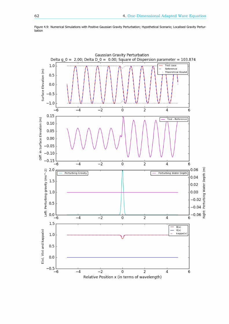
62 4. One-Dimensional Adapted Wave Equation
Figure 4.9: Numerical Simulations with Positive Gaussian Gravity Perturbation; Hypothetical Scenario; Localised Gravity Pertur-bation

4.7. Conclusions from One-Dimensional Adapted Shallow Water Waves 63
Figure 4.10: Numerical Simulations with Negative Gaussian Gravity Perturbation; Hypothetical Scenario; Localised Gravity Per-turbation

64 4. One-Dimensional Adapted Wave Equation
Figure 4.11: Numerical Simulations with Positive Gaussian Gravity Perturbation; Hypothetical Scenario

4.7. Conclusions from One-Dimensional Adapted Shallow Water Waves 65
Figure 4.12: Numerical Simulations with Negative Gaussian Gravity Perturbation; Hypothetical Scenario

66 4. One-Dimensional Adapted Wave Equation
Figure 4.13: Numerical Simulations with Positive Gaussian Gravity Perturbation; Physical Scenario - Incoming Tsunami Waves

4.7. Conclusions from One-Dimensional Adapted Shallow Water Waves 67
Figure 4.14: Numerical Simulations with Negative Gaussian Gravity Perturbation; Physical Scenario - Incoming Tsunami Waves

68 4. One-Dimensional Adapted Wave Equation
Figure 4.15: Numerical Simulations with Positive Gaussian Gravity Perturbation; Physical Scenario - Incoming Tidal waves

4.7. Conclusions from One-Dimensional Adapted Shallow Water Waves 69
Figure 4.16: Numerical Simulations with Negative Gaussian Gravity Perturbation; Physical Scenario - Incoming Tidal waves

70 4. One-Dimensional Adapted Wave Equation
Figure 4.17: Numerical Simulations with Positive Exponential Gravity and Mean Sea-Level Perturbation; Hypothetical Scenario

4.7. Conclusions from One-Dimensional Adapted Shallow Water Waves 71
Figure 4.18: Numerical Simulations with Positive Exponential Gravity and Mean Sea-Level Perturbation; Physical Scenario -Incoming Tsunami Waves

72 4. One-Dimensional Adapted Wave Equation
Figure 4.19: Numerical Simulations with Negative Exponential Gravity and Mean Sea-Level Perturbation; Physical Scenario -Incoming Tsunami Waves

4.7. Conclusions from One-Dimensional Adapted Shallow Water Waves 73
Figure 4.20: Numerical Simulations with Positive Exponential Gravity and Mean Sea-Level Perturbation; Physical Scenario -Incoming Tidal Waves

74 4. One-Dimensional Adapted Wave Equation
Figure 4.21: Numerical Simulations with Negative Exponential Gravity and Mean Sea-Level Perturbation; Physical Scenario -Incoming Tidal Waves

4.7. Conclusions from One-Dimensional Adapted Shallow Water Waves 75
Figure 4.22: Numerical Simulations with Positive Gaussian Gravity and Mean-Sea Level Perturbation; Physical Scenario - IncomingTsunami Waves

76 4. One-Dimensional Adapted Wave Equation
Figure 4.23: Numerical Simulations with Negative Gaussian Gravity and Mean-Sea Level Perturbation; Physical Scenario - In-coming Tsunami Waves

4.7. Conclusions from One-Dimensional Adapted Shallow Water Waves 77
Figure 4.24: Numerical Simulations with Positive Gaussian Gravity and Mean-Sea Level Perturbation; Physical Scenario - IncomingTidal waves

78 4. One-Dimensional Adapted Wave Equation
Figure 4.25: Numerical Simulations with Negative Gaussian Gravity and Mean-Sea Level Perturbation; Physical Scenario - In-coming Tidal waves

4.7. Conclusions from One-Dimensional Adapted Shallow Water Waves 79
Figure 4.26: Global Variation of Gravity


5Two-Dimensional Adapted Wave
Equation
In this chapter, the two-dimensional adapted wave equation will be discussed. Numerical solutions willbe investigated. Quantitative and qualitative behaviour of the solutions will be examined.
5.1. Diagnostic Formalism: LimitationsRecall that the set of equations (3.138) given by,
𝜕𝜂𝜕𝑡 + ∇ ⋅ U = U ⋅ ∇ ( ln (𝑔𝑔 )),
𝜕𝑈𝜕𝑡 + 𝑐
𝜕𝜂𝜕𝑥 = 0,
𝜕𝑉𝜕𝑡 + 𝑐
𝜕𝜂𝜕𝑦 = 0,
governs the small-amplitude surface waves in a spatially varying gravity field on a two-dimensionalplane.
Motivated by the treatment in one-dimensional space, a time-harmonic ansatz to the surface eleva-tion 𝜂(𝑥, 𝑦, 𝑡) = 𝜂 (𝑥, 𝑦)𝑒 is chosen to solve (3.138). This eventually gives rises to the second-orderpartial differential equation:
∇ 𝜂 + ∇ ln( 𝑐𝑔 ) ⋅ ∇𝜂 + 𝜔𝑐 𝜂 = 0, (5.1)
which is the two-dimensional generalisation of (4.3).Motivated by the one-dimensional case as in equation 4.4, applying a coordinate transformation
given by
ln 𝑟 = ln 𝜂 + 12 ln(𝑐𝑔 ), (5.2)
equation (5.1) becomes into
∇ 𝑟 + [𝜔𝑐 − (1𝑐 ∇ 𝑐 +3
4𝑔 ‖∇𝑔 ‖ − 12𝑔 ∇ 𝑔 − 1
𝑐𝑔 ∇𝑐 ⋅ ∇𝑔 )]𝑟 = 0 (5.3)
Using the definition of 𝑐(𝑥, 𝑦) = √𝑔 𝐷 given by (3.137), the above transformed differential equationcan be simplified into
∇ 𝑟 + [𝐸(𝑥, 𝑦) − 𝑉(𝑥, 𝑦)]𝐾 𝑟 = 0 (5.4)
81

82 5. Two-Dimensional Adapted Wave Equation
where 𝐸(𝑥, 𝑦) and 𝑉(𝑥, 𝑦) are given by
𝐸(𝑥, 𝑦) = 𝜔𝑔 𝐷𝐾 (5.5a)
𝑉(𝑥, 𝑦) = 14𝐾 ( 2𝐷∇ 𝐷 −
1𝐷 ‖∇𝐷‖ ) (5.5b)
and 𝐾 = √𝑘 + 𝑙 is the magnitude of a reference plane-wave wavevector �� = (𝑘 , 𝑙 ), whichis a constant. It is noted that (5.4) is similar to the two-dimensional time-independent Schrodingerequation, except that the ’energy’ 𝐸 is a function of spatial coordinates (𝑥, 𝑦) instead of a constant.This is the two-dimensional generalisation to (4.14).
In spite of the similarity, the two-dimensional time-independent ’Schrodinger’ equation (5.4) is notas useful as the one-dimensional one (4.14) discussed in the previous chapter. This is because, giventhe magnitude of wavevector 𝐾 , there are infinitely many possible wavevector �� that give rises to thesame 𝐾 . Such degeneracy complicates the analysis to the equation (5.4). Therefore the diagnosticformalism will not be further developed in this thesis.
5.2. Test Cases and Numerical Simulations5.2.1. Rationale and LimitationsRather than the analytical solutions, in this chapter only the numerical solutions to the two-dimensionaladapted shallow water wave equations (3.138) will be considered. This is because in the one-dimensionalstudies, it has been shown that the gravity variation on the Earth surface is only able to create veryminimal changes for surface waves. The outcome of this chapter is to show that the effects causedby the spatially-varying gravity field on ocean surface waves is also minimal in the three-dimensionalspace as well.
5.2.2. Methodology and Configurations of Test CasesNumerical ConfigurationsThe parameters used for constructing test cases are given in Tables 5.1 and 5.2. The parametersare obtained in the same manner as in the one-dimensional configurations in Table 4.1 and 4.2. Thedetailed meanings of each quantity have been discussed in section 4.2.
Similar to the one-dimensional studies, the hypothetical setting given by Table 5.1 targets at showingthe qualitative features while the physical setting given by 5.2 aims at providing insight about the surfacewaves in the actual ocean.
The numerical simulations are carried out using CLAWPACK, an open-source software package tosolve systems of hyperbolic equations numerically.
Explanation of FiguresEach of the figures shown in the following sections include four subplots. Each subplot represents ascalar field at a certain instant. All subplots share identical x-axis and y-axis, which mark the normalisedx and y-coordinates. The normalisation is relative to the wavelength of the prescribed incoming waves.The colour in the subplots represents the instantaneous value of the scalar field, with a colourbarbelow the subplots. The ticks in the colour bar represents the maximum and minimum value of theinstantaneous scalar field.
From left to right, the first subplot gives the surface elevation of reference waves. This serves as ayardstick for comparison with the second subplot, which gives the surface elevation of the test waves.The test waves usually differ from the reference waves by the presence of gravity perturbation, waterdepth perturbation or both. Details will be specified in the caption of the figures.
The third subplot shows the perturbation field of either the gravity or water depth. The final subplotgives the instantaneous difference between the test waves and reference waves. This provides a handytool to preliminarily investigate the effects of the gravity or depth perturbation on the waves. Readersare reminded that the instantaneous difference in surface elevation is not a very rigorous tool to studythe transmission-reflection mechanism of surface waves scattered by topography. A more sophisticatedtool should consider the time-independent surface elevation field by time-averaging. Yet for the purposeof this chapter, such analysis is omitted.

5.3. Test case 1: Hypothetical Surface Waves 83
Physical Parameters ValuesReference Gravity, 𝑔 10 msMean Depth of Fluid, �� 10 m
Amplitude of incoming wave, 𝜂 1 mPeriod of incoming wave, 𝑇 6 seconds or 120 secondsReference wavelength, 𝜆 𝑇√𝑔 𝐷 = 60 m or 1200 m
Maximum Perturbing Gravity, Δ𝑔 ±2 msMaximum Perturbing Mean-Sea Level, Δ𝐷 ±2 m
’Half-life’ Distance, 𝑟 𝜆 = 120 m
Numerical Parameters Values
Spatial domain of computation𝑥 ∈ [−5𝜆 ,−5𝜆 ] or [−2.5𝜆 , 2.5𝜆 ]
𝑦 ∈ [−2.5𝜆 , 2.5𝜆 ]Temporal domain of computation 𝑡 ∈ [0, 12𝑇]
Number of grid cells 250 × 250Left Boundary condition Incoming sinusoidal wavesRight Boundary condition Outflow boundaryBottom Boundary condition Outflow boundaryTop Boundary condition Outflow boundary
Table 5.1: Configuration for the hypothetical numerical simulations
5.3. Test case 1: Hypothetical Surface WavesIn this test case, the surface waves based on parameters given in Table 5.1 will be studied.
5.3.1. Test case 1a: Depth Perturbation vs Uniform Gravity and DepthTo begin with, the classical case of uniform water depth perturbed with a two-dimensional Gaussianfunction is reviewed. The gravity is uniform as in the classical theory. Figure 5.1 to 5.4 give thesimulation results. The fourth subplot, which measures the instantaneous difference between thesurface elevations of test and reference waves, serves as a preliminary indicator of the scattered wavedue to the topographical feature.
Figure 5.1: Hypothetical Waves with Gaussian Depth Perturbation. FWHM= m, m, wavelength= m. Reference:, .
It can be noted by comparing 5.1 and 5.3 that the dispersion of perturbation significantly affectsthe spatial structure of scattered waves. For a highly-localised (relative to the wavelengths) perturbeddepth, such as in Figure 5.3 or 5.4, the depth perturbation acts like a point-source for near-circularscattered waves. It is also noted that when the depth perturbation is positive, representing a bottom
84 5. Two-Dimensional Adapted Wave Equation
Physical Parameters ValuesReference Gravity, 𝑔 9.806228 ms
Mean Depth of Ocean, �� 4000 mMaximum Perturbing Gravity, Δ𝑔 50 mGal = 0.0005 ms
Maximum Perturbing Mean-Sea Level, Δ𝐷 50 m’Half-life’ Distance, 𝑟 500 km
Period of Tsunami wave, 𝑇 45 minutesPeriod of Tidal wave, 𝑇 12 hours
Reference Tsunami wavelength, 𝜆 540 kmReference Tidal wavelength, 𝜆 8640 kmAmplitude of incoming wave, 𝜂 5 m
Numerical Parameters Values
Spatial domain of computation (tsunami)𝑥 ∈ [−5𝜆,−5𝜆]𝑦 ∈ [−2.5𝜆, 2.5𝜆]
Spatial domain of computation (tidal)𝑥 ∈ [−2.5𝜆, −2.5𝜆]𝑦 ∈ [−2.5𝜆, 2.5𝜆]
Temporal domain of computation 𝑡 ∈ [0, 12𝑇]Number of grid cells 250 × 250
Left Boundary condition Incoming sinusoidal waveRight Boundary condition Outflow boundaryBottom Boundary condition Outflow boundaryTop Boundary condition Outflow boundary
Table 5.2: Parameters used to mimic the actual physical setting in the Ocean and its waves
pit, in addition to the near-circular scattered waves, other small-amplitude waves are also excited.On the other hand, for a dispersive perturbation as in Figure 5.1 or 5.2 such that the perturbed area
is comparable to the wavelength, the depth perturbation refracts and scatters plane waves. In partic-ular, when the plane waves propagate over a circular bottom pit, the plane waves are refracted awayand diverged from the pit. On the other hand, when the planes waves propagate over a subsurfacemountain, the waves converge towards the centre of mountain.
5.3.2. Test case 1b: Gravity Perturbation vs Uniform Gravity and DepthIn the next step, the case in which a uniform gravity field is perturbed Gaussianly will be studied.Figure 5.5 to 5.8 outline the numerical simulations where Gaussian gravity perturbations are added tohomogeneous gravity and water depth medium.
It can be noted that the figures are very similar to those in Test case 1a, which deals with waves inperturbed water depth. This motivates the comparison between the perturbation in gravity and depth,which will be presented in the next section.
5.3.3. Test case 1c: Gravity Perturbation vs Depth PerturbationRecall in Table 5.1 that the both the uniform and perturbed components of gravity and water depthare chosen to be equal in magnitude. This enables fair comparisons in this section.
In this test case, the test waves experience Gaussian gravity perturbation and the reference onesexperience Gaussian water depth perturbation. Figure 5.9 to 5.12 give the simulation results.
It can be immediately noticed from the subplots of instantaneous differences that the waves scat-tered respectively by the gravity and depth perturbation are nearly identical. This is not unexpectedsince the scattering property is controlled by the wave speed field 𝑐(𝑥, 𝑦), given by
𝑐(𝑥, 𝑦) = √𝑔 𝐷 ,
with 𝑔 and 𝐷 being the effective gravity and time-average water depth. In this test case the perturba-tion added respectively to 𝑔 and 𝐷 are identical in both spatial distribution and magnitude, resulting

5.3. Test case 1: Hypothetical Surface Waves 85
Figure 5.2: Hypothetical Waves with Gaussian Depth Perturbation. FWHM= m, m, wavelength= m. Reference:, .
Figure 5.3: Hypothetical Waves with Gaussian Depth Perturbation. FWHM= m, m, wavelength= m. Reference:, .
identical fields of wave speed 𝑐(𝑥, 𝑦) for both the test waves and reference waves. Hence the scatteredwaves are expected to be in phase.
Meanwhile, the instantaneous difference of surface elevation also reveals another feature in theadapted shallow water waves. Readers are reminded that the governing equations for the adaptedshallow water waves (3.138) differ from the standard ones only by an additional term U ⋅ ∇ ln( ) inthe right-hand side of depth-averaged continuity equation. In the one-dimensional analytic studiesgiven in Chapter 4 it has been shown that this additional term results in both changes of amplitudeand wavenumber of waves. Reader may refer to the derivation of equation (4.73) for the details.
By comparing the subplots of the gravity perturbation field and the instantaneous differences inFigure 5.9 to 5.12, it is clear that the spatially varying gravity field in the two-dimensional space doesa very similar job.
However, as discussed in Section 5.1, a handy diagnostic tool for wave dynamics in two-dimensionis hard to obtain. A closed form expression as given in (4.73) may thus be difficult to obtain analytically.To overcome this limitation, the numerical solutions can be analysed to obtain the time-independentwave amplitude field. After removing the effects of scattered waves, the maximum amplitude overtime at each numerical cell can be recorded to determine the spatial structure of the amplitude field.The results can thus be compared with the gravity field. For the purpose of this project, which focuseson ocean waves on the Earth surface, it will be demonstrated in the next test case that such analysisis unnecessary. Due to the time constraint, this analysis will be omitted in this project.

86 5. Two-Dimensional Adapted Wave Equation
Figure 5.4: Hypothetical Waves with Gaussian Depth Perturbation. FWHM= m, m, wavelength= m. Reference:, .
Figure 5.5: Hypothetical Waves with Gaussian Gravity Perturbation. FWHM= m, ms , wavelength= m. Reference:, .
5.4. Test case 2: Physical Surface WavesIn this test case, the surface waves based on parameters given in Table 5.2 will be studied. Bothidealistic tsunami and tidal waves will be reviewed.
5.4.1. Test case 2a: Gravity Perturbation vs Uniform Gravity and DepthBased on the configuration given in Table 5.2, a Gaussian gravity perturbation with peak 50 mGal isadded the uniform gravity field 9.80622 ms in constant water depth 4 km in this test case. Thesurface waves are compared with the reference waves in which no perturbation is experienced.
Figure 5.13 and 5.14 give an account for the effects of the gravity perturbations on the tsunamiwaves in the actual ocean. Figure 5.15 and 5.16 on the other hand suggest the possible consequenceswhen tidal waves propagate over a spatially-varying gravity field in the ocean.
It can be noted that since the wavelengths of tsunami waves are comparable to the length scaleof the gravity perturbation area, the resulted scattered field is highly similar to the hypothetical testwaves in Figure 5.5 and 5.5. On the other hand, the tidal waves are very similar to the hypotheticalwaves in 5.5 and 5.5 thanks to the similarity in relative length scales between wavelengths and gravityperturbation field.
It can be noted in all four figures from 5.13 and 5.16 that while the spatial structures of the scatteredwaves are very similar to the hypothetical scattered waves, the magnitudes of the scattered waves aremaximally of order 𝒪(10 m), which is much smaller than that in the hypothetical waves. This is notsurprising since the relative size of the gravity perturbation is much smaller in the physical setting thanthat in the hypothetical cases.

5.4. Test case 2: Physical Surface Waves 87
Figure 5.6: Hypothetical Waves with Gaussian Gravity Perturbation. FWHM= m, ms , wavelength= m. Refer-ence: , .
Figure 5.7: Hypothetical Waves with Gaussian Gravity Perturbation. FWHM= m, ms , wavelength= m.Reference: , .
From the four figures from 5.13 and 5.16, it can be concluded that the spatially-varying gravity fieldalone on Earth surface only lead to minimal changes to the ocean surface waves.
5.4.2. Test case 2b: Gravity and Depth Perturbation vs Uniform Gravity andDepth
In this test case, the changes in surface elevation due to water depth perturbation is also taken intoaccount. Same as the one-dimensional test cases given in the previous chapter, the changes in surfaceelevation are assumed to be linearly related to the gravity perturbation.
Figure 5.17 to 5.20 give the behaviour of tsunami and tidal waves in several physically representativescenarios. The configurations for each figure are specified in the captions.
The qualitative features in Figure 5.17 to 5.20 are very similar to Figure 5.13 and 5.14 respectively.The differences lie in the quantitative measures: when the depth perturbation is included, the scatteredwaves are at least 𝒪(10 𝑚) larger in amplitude, which makes it possibly observable in the nature. Inorder to identify the cause for the increase in wave amplitude, the next test case is introduced.
5.4.3. Test case 2c: Gravity and Depth Perturbation vs Uniform Gravity andDepth Perturbation
In the final test case, the ocean surface waves which experienced both gravity and depth perturbation(test waves) are compared against the waves which only encountered depth perturbation (referencewaves). Figure 5.21 to 5.24 give the corresponding scenarios. The purpose of the comparison is to’filter out’ the effects of depth perturbation from the combined perturbations. Hence the subplots of

88 5. Two-Dimensional Adapted Wave Equation
Figure 5.8: Hypothetical Waves with Gaussian Gravity Perturbation. FWHM= m, ms , wavelength= m.Reference: , .
Figure 5.9: Hypothetical Waves with Gaussian Gravity Perturbation. FWHM= m, ms , wavelength= m. Reference:, .
instantaneous difference between test and reference waves represents only the waves scattered bythe gravity perturbation. It is highlighted that the ’filtering’ is not rigorous since the scattered wavesare not necessarily linear. However for the sake of an overview, the result is sufficient.
It can be directly observed from the plots of instantaneous difference that the order of magnitudesof wave amplitudes are similar to that in Figure 5.13 to 5.16. This implies that the gravity-induceddepth perturbation is dominant in the combined effects.
The quantitative justification can also be noted from that fact that the gravity perturbation maximallycorresponds to 𝒪(10 %) change to the gravity, while the depth perturbation is capable of making upto 𝒪(1%) change in the actual geophysical setting.
5.5. Conclusions from Test CasesIn the hypothetical test cases, it has been shown that the gravity perturbation scatters surface wavesas what the depth does in the adapted shallow water model. It has also been noted that the fieldof wave amplitude is also associated with the gravity field, similar to the one-dimensional test casesstudied in the previous chapter.
In the physical test cases, it becomes clear that while in practice the surface waves can be alteredby the gravity perturbation, the effects are mainly attributed to the induced-changes of water depth.Based on the adapted shallow water model, the variations of gravity in itself are too weak to make upa huge difference for the ocean surface waves. In other words, the studies also justify the assumptionof uniform gravity for surface waves in the geophysical setting on Earth surface.

5.6. Final Remarks on Surface Waves on a Two-Dimension Plane 89
Figure 5.10: Hypothetical Waves with Gaussian Gravity Perturbation. FWHM= m, ms , wavelength= m.Reference: , .
Figure 5.11: Hypothetical Waves with Gaussian Gravity Perturbation. FWHM= m, ms , wavelength= m.Reference: , .
5.6. Final Remarks on Surface Waves on a Two-Dimension PlaneTypically on the two-dimension plane, the surface water waves are analysed by the ray theory, whichassumes a slowly-varying medium for the wave propagation. It appears to be possible that the adaptedshallow water waves equations (3.138) can be studied by the ray theory after certain adaptations.However, as seen in the test cases, the gravity variation on Earth is not strong enough to induce anyobservable difference. Hence the detailed analysis is not performed for the purpose of this project.
Interested readers may refer to any introductory text on wave dynamics in fluid, for instance,Pedlosky(2003), LeBlond and Mysak(1981) or Lighthill (1978), for the details of ray theory.
Readers are also reminded that the Coriolis force induced by the Earth’s rotation are neglected in thetest cases. In a more realistic modelling of large-scale ocean surface waves, the Coriolis force certainlyplays a very important role and should never be omitted. Pedlosky(2003) provides a comprehensiveintroduction to the ocean surface waves in a rotating frame for interested readers.

90 5. Two-Dimensional Adapted Wave Equation
Figure 5.12: Hypothetical Waves with Gaussian Gravity Perturbation. FWHM= m, ms , wavelength= m.Reference: , .
Figure 5.13: Physical Tsunami Waves with Gaussian Gravity Perturbation. FWHM= km, mGal, wavelength=km. Reference: , .
Figure 5.14: Physical Tsunami Waves with Gaussian Gravity Perturbation. FWHM= km, mGal, wavelength=km. Reference: , .

5.6. Final Remarks on Surface Waves on a Two-Dimension Plane 91
Figure 5.15: Physical Tidal Waves with Gaussian Gravity Perturbation. FWHM= km, mGal, wavelength= m.Reference: , .
Figure 5.16: Physical Tidal Waves with Gaussian Gravity Perturbation. FWHM= km, mGal, wavelength= m.Reference: , .
Figure 5.17: Physical Tsunami Waves with Gaussian Gravity Perturbation. FWHM= km, mGal, m,wavelength= km. Reference: , .

92 5. Two-Dimensional Adapted Wave Equation
Figure 5.18: Physical Tsunami Waves with Gaussian Gravity Perturbation. FWHM= km, mGal, m,wavelength= km. Reference: , .
Figure 5.19: Physical Tidal Waves with Gaussian Gravity Perturbation. FWHM= km, mGal, m,wavelength= m. Reference: , .
Figure 5.20: Physical Tidal Waves with Gaussian Gravity Perturbation. FWHM= km, mGal, m,wavelength= m. Reference: , .
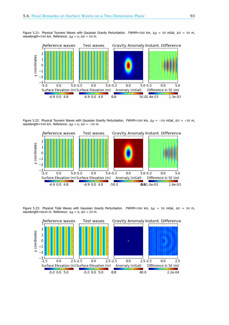
5.6. Final Remarks on Surface Waves on a Two-Dimension Plane 93
Figure 5.21: Physical Tsunami Waves with Gaussian Gravity Perturbation. FWHM= km, mGal, m,wavelength= km. Reference: , m.
Figure 5.22: Physical Tsunami Waves with Gaussian Gravity Perturbation. FWHM= km, mGal, m,wavelength= km. Reference: , m.
Figure 5.23: Physical Tidal Waves with Gaussian Gravity Perturbation. FWHM= km, mGal, m,wavelength= m. Reference: , m.

94 5. Two-Dimensional Adapted Wave Equation
Figure 5.24: Physical Tidal Waves with Gaussian Gravity Perturbation. FWHM= km, mGal, m,wavelength= m. Reference: , m.
6Generalised Airy’s Linear Wave
Theory
In this chapter, Airy’s linear wave theory will be generalised for a general conservative gravitationalfield. The chapter begins with a variational formalism for surface gravity waves. The linear waves willthen be studied in two-dimensional and three-dimensional space.
6.1. Derivation: Variational Formalism of Surface Gravity WavesIn this chapter, the variational formalism will be presented to derive a set of equations governing thesurface gravity waves in a fluid.
Luke (1967) considered the free surface gravity waves in incompressible, irrotational and inviscidfluids, which allows the expression of velocity field v by a velocity potential 𝜙 such that v = ∇𝜙. Heproposed a Lagrangian variational scheme to derive both linear and non-linear waves. For a conserva-tive gravity field g = −∇Ψ with geopotential Ψ and fluid of density 𝜌, the Lagrangian ℒ, also known asLuke’s Lagrangian, is given by
ℒ = −∫ 𝜌[∫( )(𝜕𝜙𝜕𝑡 +
12‖∇𝜙‖ + Ψ)𝑑𝑉]𝑑𝑡, (6.1)
where 𝑉(𝑡) is the control volume of fluid.In Luke’s paper only the special case where the gravity is uniform was discussed. That is, the special
case of Ψ = 𝑔 𝑧 where 𝑔 is a constant and 𝑧 is the vertical coordinate in the Cartesian coordinates.In the following discussion a general Ψ and standard Cartesian coordinates (𝑥, 𝑦, 𝑧) will be considered.
Similar to Luke’s approach, a layer of horizontally unbounded fluid with surface elevation 𝑧 =𝜂(𝑥, 𝑦, 𝑡) and bottom-bed 𝑧 = −ℎ(𝑥, 𝑦) is considered. This leads to the Luke’s Lagrangian:
ℒ(𝜙, 𝜂) = −∫ 𝜌[∫ℛ(∫
( , , )
( , )
𝜕𝜙𝜕𝑡 +
12‖∇𝜙‖ + Ψ𝑑𝑧)𝑑𝐴]𝑑𝑡, (6.2)
where ℛ refers to the whole horizontal plane.The next steps follows directly from the standard procedure of calculus of variation. Based on the
variation on velocity potential, the resulting equation is independent of the geopotential Ψ and gives:
∇ 𝜙(𝑥, 𝑦, 𝑧, 𝑡) = 𝜕 𝜙𝜕𝑥 + 𝜕 𝜙𝜕𝑦 + 𝜕 𝜙𝜕𝑧 = 0, (6.3)
subject to the boundary condition
at 𝑧 = −ℎ(𝑥, 𝑦): 𝜕𝜙𝜕𝑥𝜕ℎ𝜕𝑥 +
𝜕𝜙𝜕𝑦𝜕ℎ𝜕𝑦 =
𝜕𝜙𝜕𝑧 , (6.4a)
at 𝑧 = 𝜂(𝑥, 𝑦, 𝑡): 𝜕𝜂𝜕𝑡 +𝜕𝜙𝜕𝑥𝜕𝜂𝜕𝑥 +
𝜕𝜙𝜕𝑦𝜕𝜂𝜕𝑦 =
𝜕𝜙𝜕𝑧 . (6.4b)
95

96 6. Generalised Airy’s Linear Wave Theory
Meanwhile applying the variation of surface elevation gives rise to the equation containing Ψ
at 𝑧 = 𝜂(𝑥, 𝑦, 𝑡): 𝜕𝜙𝜕𝑡 +12‖∇𝜙‖ + Ψ = 𝑃 , (6.5)
where 𝑃 is the reduced atmospheric pressure, which can be taken as 0 without loss of generality. Thedetailed derivation of equations (6.3) and (6.4) can be found in Luke (1967) or Whitham’s textbook”Linear and Nonlinear Waves” (1974). The detailed derivation of (6.5) shares the same procedure asthe standard case where Ψ = 𝑔 𝑧, which can be found also in Whitham’s text.
The set of partial differential equations (6.3), (6.4) and (6.5) governs the surface gravity waves.It provides a framework to model non-linear surface gravity waves, which will not be studied in thisthesis.
The Laplace equation (6.3) is an equivalent expression for the continuity equation of irrotationalfluid. The equation (6.5) is Bernoulli’s principle applied at the surface of the fluid, which stems fromthe momentum equation of fluid. It is noted from the governing equations that the gravity field playsa role only in (6.5), which is related to the momentum equation only.
6.2. One-Dimensional Surface Gravity Waves6.2.1. Governing Equations for Linear WavesThe governing equations for surface waves (6.3) to (6.5) do not in general have closed-form solutions.To obtain analytic solution, the one-dimensional linear surface gravity waves in a general conservativegravity field will be studied first.
The one-dimensional waves are obtained by removing the 𝑦-coordinates in (6.3), (6.4) and (6.5),which gives
𝜕 𝜙𝜕𝑥 + 𝜕 𝜙𝜕𝑧 = 0, (6.6)
subject to the boundary condition
at 𝑧 = −ℎ(𝑥): 𝜕𝜙𝜕𝑥𝜕ℎ𝜕𝑥 =
𝜕𝜙𝜕𝑧 , (6.7a)
at 𝑧 = 𝜂(𝑥, 𝑡): 𝜕𝜂𝜕𝑡 +𝜕𝜙𝜕𝑥𝜕𝜂𝜕𝑥 =
𝜕𝜙𝜕𝑧 , (6.7b)
and
at 𝑧 = 𝜂(𝑥, 𝑡): 𝜕𝜙𝜕𝑡 +12[(
𝜕𝜙𝜕𝑥 ) + (𝜕𝜙𝜕𝑧 ) ] + Ψ = 0. (6.8)
Define 𝑧 = 𝛿𝑚(𝑥) to be the mean-sea level, such that Ψ(𝑥, 𝛿𝑚(𝑥)) = Ψ for some known constantΨ . For small amplitude motion |𝜂(𝑥, 𝑡)−𝛿𝑚(𝑥)| ≪ ℎ(𝑥), following the procedure given by Airy (1841),the governing equations for linear surface wave is given by
𝜕 𝜙𝜕𝑥 + 𝜕 𝜙𝜕𝑧 = 0, (6.9)
subject to the linearised boundary conditions
at 𝑧 = −ℎ(𝑥): 𝜕𝜙𝜕𝑧 +𝜕𝜙𝜕𝑥𝜕ℎ𝜕𝑥 = 0, (6.10a)
at 𝑧 = 𝛿𝑚(𝑥): 𝜕𝜂𝜕𝑡 =𝜕𝜙𝜕𝑧 , (6.10b)
at 𝑧 = 𝛿𝑚(𝑥): 𝜕𝜙𝜕𝑡 − Ψ(𝑥, 𝜂) = 0, (6.10c)
The set of equation (6.9) and (6.10) is the governing equations for the linear surface gravity wave influid. It is also a generalisation of the Airy’s linear wave theory for general conservative gravitationalfield.
Unlike the standard case where the the geopotential Ψ(𝑥, 𝜂) is simply given by Ψ(𝑥, 𝜂) = 𝑔 𝜂, thegeopotentialΨ is now a general function in spatial-coordinates (𝑥, 𝑧). This brings difficulty in the pursuitof ansatz. In order to address this issue, a coordinate transformation scheme is proposed in the nextsection.

6.2. One-Dimensional Surface Gravity Waves 97
6.2.2. Motivation for the Coordinate TransformationRecall that the geopotential Ψ(𝑥, 𝑧) satisfies the two-dimensional Laplace equation in free-space, thatis,
∇ Ψ = 0, (6.11)
subject to suitable boundary conditions.A classical result from complex analysis reveals that, if function 𝑞 (𝑥, 𝑧) is a solution to the Laplace
equation, there exists a harmonic conjugate 𝑞 (𝑥, 𝑧) that also satisfies the Laplace equation. Thefunction 𝑞 (𝑥, 𝑧) satisfies the Cauchy-Riemann condition, namely,
𝜕𝑞𝜕𝑥 = 𝜕𝑞
𝜕𝑧 , (6.12a)
𝜕𝑞𝜕𝑥 = −𝜕𝑞𝜕𝑧 . (6.12b)
Note that 𝑞 (𝑥, 𝑧) is unique up to a constant.Define a time-independent orthogonal coordinate transformation (𝑥, 𝑦) → (𝑞 , 𝑞 ), using the trans-
formation rule:
𝑞 (𝑥, 𝑧) = Ψ(𝑥, 𝑧) − Ψ𝑔 , (6.13a)
𝑞 (𝑥, 𝑧) = harmonic conjugate of 𝑞 (𝑥, 𝑧), subject to 𝑞 (0, 𝛿𝑚(0)) = 0, (6.13b)
where Ψ = Ψ(𝑥, 𝛿𝑚(𝑥)) is the mean-sea level potential and 𝑔 is a constant which takes the value ofreference gravity.
Physically 𝑞 (𝑥, 𝑦) measures the scaled potential difference at point (𝑥, 𝑦) with the mean-sea level,which reduces into the Cartesian vertical coordinates 𝑧 in the case of uniform gravity. Meanwhile, inthe case of uniform gravity, 𝑞 is reduced into the Cartesian horizontal coordinates 𝑥. Both 𝑞 and 𝑞are uniquely determined thanks to the condition in defining 𝑞 .
6.2.3. Properties of the Conformal Coordinate TransformationThe very first property of the coordinate transformation is that 𝑢 and 𝑣 are orthogonal to each others.
Consider the contrapositive basis
a( ) = ∇𝑞 (6.14a)
a( ) = ∇𝑞 (6.14b)
Since the Cauchy-Riemann condition is satisfied, ∇𝑞 ⋅∇𝑞 = 0, which implies the orthogonality between𝑞 and 𝑞 .
In addition, the Euclidean norm of ∇𝑞 and ∇𝑞 are equal due to the Cauchy-Riemann condition:
‖∇𝑞 ‖ = (𝜕𝑞𝜕𝑥 ) + (𝜕𝑞𝜕𝑧 ) = (𝜕𝑞𝜕𝑧 ) + ( − 𝜕𝑞𝜕𝑥 ) = ‖∇𝑞 ‖ , (6.15)
which implies the contrapositive basis a( ) and a( ) are equal in norm.It can then been shown that the covariant basis are therefore given by
a( ) =1
‖∇𝑞 ‖ [𝜕𝑞𝜕𝑧 , −
𝜕𝑞𝜕𝑥 ] =
1‖∇𝑞 ‖ [
𝜕𝑞𝜕𝑥 ,
𝜕𝑞𝜕𝑧 ] (6.16)
a( ) =1
‖∇𝑞 ‖ [ −𝜕𝑞𝜕𝑧 ,
𝜕𝑞𝜕𝑥 ] =
1‖∇𝑞 ‖ [
𝜕𝑞𝜕𝑥 ,
𝜕𝑞𝜕𝑧 ] (6.17)
With the explicit formulas for both the contrapositive and covariant basis, the metric tensors 𝑔 and𝑔 are computed by 𝑔 = a( ) ⋅ a( ) and 𝑔 = a( ) ⋅ a( ):
𝑔 = 𝑔 = ‖∇𝑞 ‖ = ‖∇𝑞 ‖ (6.18)
𝑔 = 𝑔 = 1‖∇𝑞 ‖ = 1
‖∇𝑞 ‖ (6.19)
𝑔 = 𝑔 = 𝑔 = 𝑔 = 0 (6.20)

98 6. Generalised Airy’s Linear Wave Theory
The quantity √𝑔 = √𝑔 𝑔 − 𝑔 𝑔 is thus given by:
√𝑔 =1
‖∇𝑞 ‖ = 1‖∇𝑞 ‖ (6.21)
Hence the differential operators in the transformed coordinates are well-defined.
6.2.4. Transformed Laplacian Operators and Laplace EquationApplying the metric tensor, the Laplacian operator in the transformed coordinates is thus given by
∇ 𝜙 = 1√𝑔
𝜕𝜕𝑞 (√𝑔𝑔
𝜕𝜙𝜕𝑞 + √𝑔𝑔
𝜕𝜙𝜕𝑞 ) + 1
√𝑔𝜕𝜕𝑞 (√𝑔𝑔
𝜕𝜙𝜕𝑞 + √𝑔𝑔
𝜕𝜙𝜕𝑞 )
= ‖∇𝑞 ‖ 𝜕𝜕𝑞 (1 ⋅ 𝜕𝜙𝜕𝑞 ) + ‖∇𝑞 ‖ 𝜕
𝜕𝑞 (1 ⋅ 𝜕𝜙𝜕𝑞 )
But since ‖∇𝑞 ‖ = ‖∇𝑞 ‖ , the Laplace equation is simply given by
‖∇𝑞 ‖ [ 𝜕𝜕𝑞 ( 𝜕𝜙𝜕𝑞 ) + 𝜕𝜕𝑞 ( 𝜕𝜙𝜕𝑞 )] = 0
or equivalently, when ‖∇𝑞 ‖ ≠ 0,𝜕 𝜙𝜕𝑞 + 𝜕 𝜙
𝜕𝑞 = 0 (6.22)
which preserves the structure of the Laplace equation in Cartesian coordinates.
6.2.5. Transformed Boundary conditionIn the Cartesian coordinates, the geometry of bottom boundary 𝑧 = −ℎ(𝑥) and surface elevation𝑧 = 𝜂(𝑥, 𝑡) can be interpreted as given by two level-set 𝑆 (𝑥, 𝑧) and 𝑆(𝑥, 𝑧, 𝑡) being equal to zero:
𝑆 (𝑥, 𝑧) = 𝑧 + ℎ(𝑥) = 0 (6.23)𝑆(𝑥, 𝑧, 𝑡) = 𝑧 − 𝜂(𝑥, 𝑡) = 0 (6.24)
While the explicit expression for the inverse coordinate transformation from (𝑥, 𝑦) to (𝑞 , 𝑞 ) is ingeneral absent, its existence and uniqueness is guaranteed by the implicit function theorem. Hence,by denoting the inverse transformation by (𝑢, 𝑣) → (𝑥(𝑞 , 𝑞 ), 𝑧(𝑞 , 𝑞 ), it is equivalent to express thelevel-sets by
�� (𝑞 , 𝑞 ) = 𝑆 (𝑥(𝑞 , 𝑞 ), 𝑧(𝑞 , 𝑞 )) = 𝑧(𝑞 , 𝑞 ) + ℎ(𝑥(𝑞 , 𝑞 )) = 0 (6.25)
��(𝑞 , 𝑞 , 𝑡) = 𝑆(𝑥(𝑞 , 𝑞 ), 𝑧(𝑞 , 𝑞 ), 𝑡) = 𝑧(𝑞 , 𝑞 ) − 𝜂(𝑥(𝑞 , 𝑞 ), 𝑡) = 0 (6.26)
As long as the conditions of the implicit function theorem are satisfied, the level-sets �� (𝑞 , 𝑞 ) = 0 and��(𝑞 , 𝑞 ) = 0 can be expressed by using 𝑞 as an independent coordinate, in other words, there existswell-defined function ℎ(𝑞 ) and ��(𝑞 , 𝑡) such that the level-sets �� (𝑞 , 𝑞 ) and ��(𝑞 , 𝑞 ) are given by
�� (𝑞 , 𝑞 ) = 𝑣 + ℎ(𝑞 ) = 0 (6.27)
��(𝑞 , 𝑞 , 𝑡) = 𝑣 − ��(𝑞 , 𝑡) = 0 (6.28)
By considering the total time-derivative of �� (𝑞 , 𝑞 ) and ��(𝑞 , 𝑞 ), the boundary condition in thetransformed coordinates are thus given by
at 𝑞 = −ℎ(𝑞 ): 𝜕𝜙𝜕𝑞𝜕ℎ𝜕𝑞 = − 𝜕𝜙𝜕𝑞 , (6.29)
at 𝑞 = ��(𝑞 , 𝑡): 𝜕𝜂𝜕𝑡 +𝜕𝜙𝜕𝑞
𝜕𝜂𝜕𝑞 = 𝜕𝜙
𝜕𝑞 , (6.30)
at 𝑞 = ��(𝑞 , 𝑡): 𝜕𝜙𝜕𝑡 +12|∇𝜙| − (𝑔 𝑞 − Ψ ) = 𝑃 (6.31)
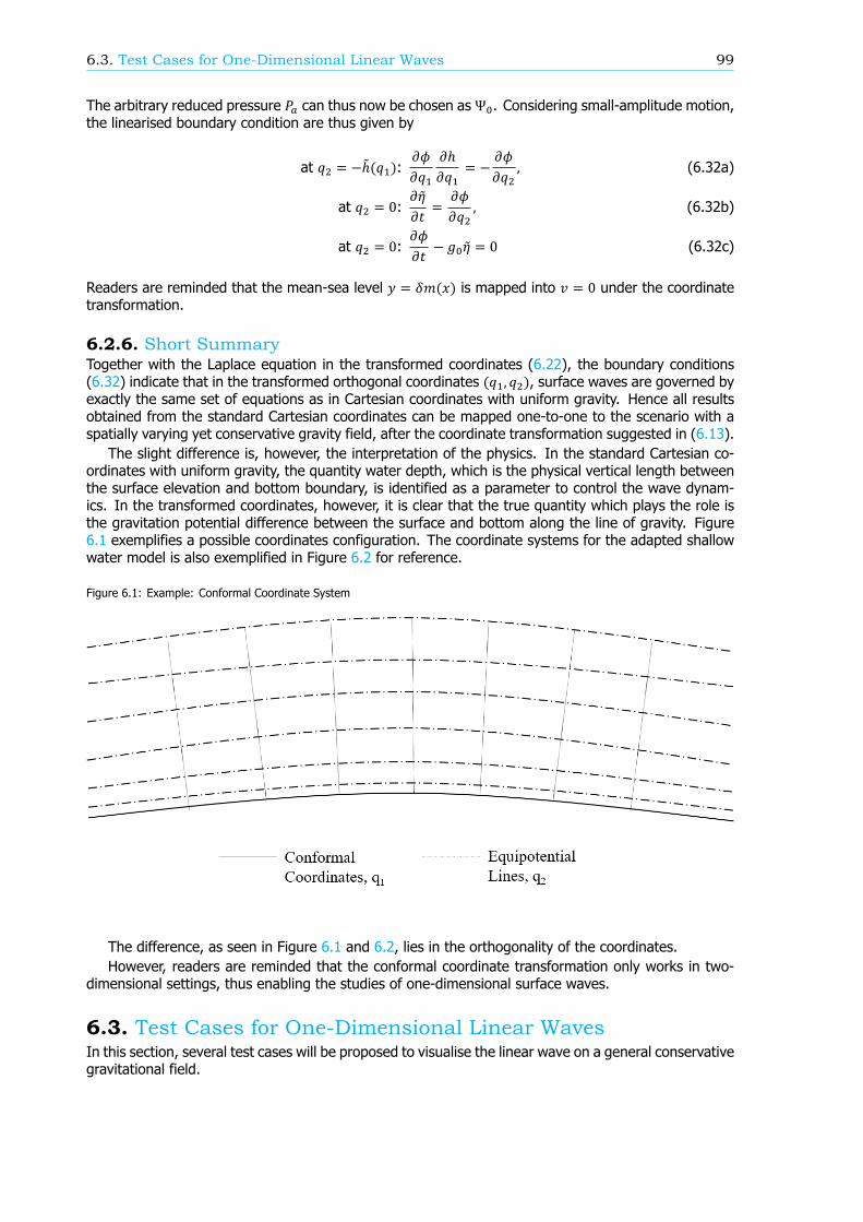
6.3. Test Cases for One-Dimensional Linear Waves 99
The arbitrary reduced pressure 𝑃 can thus now be chosen as Ψ . Considering small-amplitude motion,the linearised boundary condition are thus given by
at 𝑞 = −ℎ(𝑞 ): 𝜕𝜙𝜕𝑞𝜕ℎ𝜕𝑞 = − 𝜕𝜙𝜕𝑞 , (6.32a)
at 𝑞 = 0: 𝜕��𝜕𝑡 =𝜕𝜙𝜕𝑞 , (6.32b)
at 𝑞 = 0: 𝜕𝜙𝜕𝑡 − 𝑔 �� = 0 (6.32c)
Readers are reminded that the mean-sea level 𝑦 = 𝛿𝑚(𝑥) is mapped into 𝑣 = 0 under the coordinatetransformation.
6.2.6. Short SummaryTogether with the Laplace equation in the transformed coordinates (6.22), the boundary conditions(6.32) indicate that in the transformed orthogonal coordinates (𝑞 , 𝑞 ), surface waves are governed byexactly the same set of equations as in Cartesian coordinates with uniform gravity. Hence all resultsobtained from the standard Cartesian coordinates can be mapped one-to-one to the scenario with aspatially varying yet conservative gravity field, after the coordinate transformation suggested in (6.13).
The slight difference is, however, the interpretation of the physics. In the standard Cartesian co-ordinates with uniform gravity, the quantity water depth, which is the physical vertical length betweenthe surface elevation and bottom boundary, is identified as a parameter to control the wave dynam-ics. In the transformed coordinates, however, it is clear that the true quantity which plays the role isthe gravitation potential difference between the surface and bottom along the line of gravity. Figure6.1 exemplifies a possible coordinates configuration. The coordinate systems for the adapted shallowwater model is also exemplified in Figure 6.2 for reference.
Figure 6.1: Example: Conformal Coordinate System
The difference, as seen in Figure 6.1 and 6.2, lies in the orthogonality of the coordinates.However, readers are reminded that the conformal coordinate transformation only works in two-
dimensional settings, thus enabling the studies of one-dimensional surface waves.
6.3. Test Cases for One-Dimensional Linear WavesIn this section, several test cases will be proposed to visualise the linear wave on a general conservativegravitational field.

100 6. Generalised Airy’s Linear Wave Theory
Figure 6.2: Example: Coordinates for Adapted Shallow Water Model
6.3.1. Example 1: Gravity with Inverse-law in 2DConsider a solid circle of radius 𝑅 with centre lying at the origin of the 2-dimensional plane, as inFigure 6.3. Solving the Poisson equation for the gravitational potential gives rise to a geopotential
Ψ(𝑥, 𝑧) = 𝑔 ln(√𝑥 + 𝑧 ),
in the domain {(𝑥, 𝑦) ∶ 𝑥 + 𝑧 ≥ 𝑅 }, where 𝑔 is a positive constant.This also gives rises to a central-forced gravitational field F(𝑥, 𝑧) = −∇Ψ:
F(𝑥, 𝑧) = −𝑔 ( 𝑥𝑥 + 𝑧 �� +
𝑧𝑥 + 𝑧 ��), (6.33)
whose direction is always pointing towards the origin and magnitude ‖F(𝑥,𝑧)‖ =√
is decaying
inversely with the distance 𝑟 = √𝑥 + 𝑧 . Note that �� and �� are the unit vectors in the 𝑥 and 𝑧-directionin the Cartesian plane.
Consider a fixed volume of fluid attached to the surface of the circle. The hydrostatic balance willkeep the fluid in the domain 𝑅 ≤ √𝑥 + 𝑧 ≤ 𝑅 , for some positive constant 𝑅
The coordinate transformation proposed in (6.13) are then given by
𝑞 (𝑥, 𝑧) = tan (𝑥𝑧 ) (6.34a)
𝑞 (𝑥, 𝑧) = ln(√𝑥 + 𝑧𝑅 ) (6.34b)
An explicit expression for the inverse coordinate transformation can be obtained. Manipulating theexpression gives
𝑥𝑧 = tan(𝑞 ) (6.35)
𝑥 + 𝑧 = [𝑅 𝑒 ] , (6.36)
which suggests the inverse transformation by
𝑥(𝑞 , 𝑞 ) = 𝑅 𝑒 sin(𝑞 ) (6.37a)𝑧(𝑞 , 𝑞 ) = 𝑅 𝑒 cos(𝑞 ) (6.37b)

6.3. Test Cases for One-Dimensional Linear Waves 101
Figure 6.3: Schematic Sketch for Example 1 - a 2D Earth
Using the forward and inverse coordinate transformation given in equation (6.34) and (6.37), thephysical domain
{(𝑥, 𝑧) ∶ √𝑥 + 𝑧 ≥ 𝑅 }
can be mapped into the domain
{(𝑞 , 𝑞 ) ∶ −𝜋 < 𝑞 ≤ 𝜋, 𝑞 ≥ −ℎ },
where ℎ = ln( ) is denoted to simplify the notation.It is noted that 𝑞 is chosen to be bounded to ensure the one-to-one correspondence between the
physical coordinates and transformed coordinates. This additionally imposes the periodic boundarycondition on the solution of Laplace equation (6.22), which requires that both the surface elevation𝜂(𝑞 , 𝑡) and velocity potential 𝜙(𝑞 , 𝑞 , 𝑡) in the transformed coordinates satisfy
𝜂(−𝜋, 𝑡) = 𝜂(𝜋, 𝑡) (6.38)𝜙(−𝜋, 𝑞 , 𝑡) = 𝜙(𝜋, 𝑞 , 𝑡), (6.39)
in additional to the boundary conditions given in (6.32):
at 𝑞 = −: 𝜕𝜙𝜕𝑞 = 0, (6.40a)
at 𝑞 = 0: 𝜕𝜂𝜕𝑡 =𝜕𝜙𝜕𝑞 , (6.40b)
at 𝑞 = 0: 𝜕𝜙𝜕𝑡 − 𝑔 𝜂 = 0. (6.40c)

102 6. Generalised Airy’s Linear Wave Theory
These altogether suggest the monochromatic surface waves with amplitude 𝑎, angular frequency𝜔 and wave number 𝑘 in the transformed coordinates (𝑞 , 𝑞 ), whose surface elevation 𝑞 = 𝜂(𝑞 , 𝑡)and velocity potential 𝜙(𝑞 , 𝑞 , 𝑡) read
𝜂(𝑞 , 𝑡) = 𝑎 cos(𝑘𝑞 − 𝜔𝑡) (6.41a)
𝜙(𝑞 , 𝑞 , 𝑡) = (𝜔𝑘 𝑎)cosh(𝑘(𝑞 + ℎ ))
sinh(𝑘ℎ ) sin(𝑘𝑞 − 𝜔𝑡) (6.41b)
subject to the dispersion relation
𝜔 = 𝑔 𝑘 tanh(𝑘ℎ ) (6.42)
and the boundary condition
cos(𝑘𝜋 − 𝜔𝑡) = cos(−𝑘𝜋 − 𝜔𝑡), ∀𝑡 ⟺ 0 = 2 sin(2𝑘𝜋) sin(𝜔𝑡), ∀𝑡⟺ 2𝑘𝜋 = 𝑛𝜋
⟺ 𝑘 = 𝑛2 ,
with 𝑛 being an integer. This indicates that the wave number 𝑘 is quantised, limiting the modes ofwave available, which is not surprising since the fluid remains attached on a circular domain. One canthus also denote the wave number by 𝑘 = to emphasise its quantised nature.
Translating from the transformed coordinates (𝑞 , 𝑞 ) to the physical coordinates (𝑥, 𝑦) via equation(6.37) reveals that the surface elevation 𝑞 = 𝜂(𝑞 , 𝑡) is described by
ln(√𝑥 + 𝑦𝑅 ) = 𝑎 cos(𝑘 tan (𝑥𝑦) − 𝜔𝑡) (6.43)
To make the expression more readable, the standard polar coordinates is now introduced
𝑟 = 𝑥 + 𝑦 (6.44)
tan𝜃 = 𝑦𝑥 (6.45)
By noting the identity tan (𝑥)+ tan ( ) = 𝑠𝑔𝑛(𝑥) , where 𝑠𝑔𝑛(𝑥) is the sign function, the expres-sion for surface elevation (6.41a) becomes
𝑟 = 𝜂 (𝜃, 𝑡) = 𝑅 exp [𝑎 cos(𝜔𝑡 + 𝑘 𝜃 − 𝑘 𝑠𝑔𝑛(𝜃)𝜋2 )]. (6.46)
Note that the constant quantity −𝑘 𝑠𝑔𝑛(𝜃) corresponds to the phase shift which can be cancelledby shifting the time variable 𝑡. Hence the surface elevation is described by
𝑟 = 𝜂 (𝜃, 𝑡) = 𝑅 exp [𝑎 cos(𝜔𝑡 + 𝑘 𝜃)]. (6.47)
Note that by fixing 𝜃, the quantity exp [𝑎 cos(𝜔𝑡 + 𝑘 𝜃)] oscillates around 1 from exp(−𝑎) andexp(𝑎) in time. This indicates that the periodic variation of surface elevation takes place around of𝑟 = 𝑅 , albeit not in a linear sinusoidal manner.
One can also reinterpret the equation (6.47) in the framework of harmonic waves. For the waveamplitude 𝑎 in the transformed coordinates to be sufficiently small, the quantity exp [𝑎 cos(𝜔𝑡+𝑘 𝜃)]can be expanded as
exp [𝑎 cos(𝜔𝑡 + 𝑘 𝜃)] = 1 +∑ 𝑎𝑖! cos (𝜔𝑡 + 𝑘 𝜃) (6.48)

6.3. Test Cases for One-Dimensional Linear Waves 103
such that the surface elevation is given by
𝑟 = 𝜂 (𝜃, 𝑡) = 𝑅 [1 +∑ 𝑎𝑖! cos (𝜔𝑡 + 𝑘 𝜃)]. (6.49)
This indicates the presence of higher-order harmonics in the oscillation, when the waves are viewed inthe physical coordinates.
Note that the coefficients of the 𝑖-th order harmonics cos (𝜔𝑡 + 𝑘 𝜃), 𝑖 ≥ 2, given by ! , decreasewith the order 𝑖. Hence to first-order one can approximate the surface elevation also by
𝑟 = 𝜂 (𝜃, 𝑡) ≈ 𝑅 [1 + 𝑎 cos(𝜔𝑡 + 𝑘 𝜃)] (6.50)
or equivalently
𝑟 − 𝑅 ≈ 𝐴 cos(𝜔𝑡 + 𝑘 𝜃), (6.51)
where 𝐴 = 𝑅 𝑎 can be considered as the wave amplitude of the linear wave.
6.3.2. Example 2a: Vertical Downwards Gravity with Perturbation
Figure 6.4: Schematic Sketch for Example 2
Consider a horizontal layer of fluid over a bottom boundary given by 𝑧 = −ℎ(𝑥). The uniformgravity field due to the Earth can be regarded as g = −𝑔 ��, which points vertically downwards in the𝑧-direction.
Suppose, in addition, there is an excess point mass located at (𝑥, 𝑧) = (0, −𝑑) under the bottomboundary, that is, 𝑑 > ℎ(0). This leads to an additional perturbing gravity field �g given by
�g(𝑥, 𝑧) = −(𝛿𝑚(0) + 𝑑)𝛿𝑚(0) 𝐺 ( 𝑥𝑥 + (𝑧 + 𝑑) �� +
𝑧𝑥 + (𝑧 + 𝑑) ��), (6.52)
such that also at the mean-sea level at 𝑥 = 0, the perturbing gravity is simply given by −𝐺 ��. Themagnitude of the perturbing gravity ‖�g‖ is assumed to be much smaller than 𝑔 . For simplicity denote𝑔 = ( ( ) )
( ) 𝐺 . Figure 6.4 gives a schematic sketch for the configuration.

104 6. Generalised Airy’s Linear Wave Theory
The total gravity field g(𝑥, 𝑧) is given by the sum of the uniform component g and the perturbingcomponent �g:
g(𝑥, 𝑧) = − 𝑔 𝑥𝑥 + (𝑧 + 𝑑) �� − (𝑔 + 𝑔 𝑧
𝑥 + (𝑧 + 𝑑) )��, (6.53)
which suggests the geopotential Ψ(𝑥, 𝑧) is given by
Ψ(𝑥, 𝑧) = 𝑔 𝑧 + 𝑔2 ln(𝑥 + (𝑧 + 𝑑) ) + 𝐶, (6.54)
where 𝐶 is arbitrary constant.The constant 𝐶 is chosen by demanding Ψ = Ψ(𝑥, 𝛿𝑚(𝑥)) = 0, where 𝑧 = 𝛿𝑚(𝑥) is the mean-sea
level. The transformation rules in equation (6.13) suggest the new set of coordinates (𝑞 , 𝑞 ) by
𝑞 (𝑥, 𝑧) = 𝑥 + 𝑔𝑔 tan ( 𝑥𝑧 + 𝑑 ) (6.55)
𝑞 (𝑥, 𝑧) = 𝑧 + 𝑔2𝑔 ln(𝑥 + (𝑧 + 𝑑) ) (6.56)
Suppose, in addition, the bottom solid boundary of the fluid 𝑧 = −ℎ(𝑥) is chosen such that thegeopotential Ψ(𝑥,−ℎ(𝑥)) also remains constant on the boundary. In other words, 𝑧 = −ℎ(𝑥) coincideswith an equipotential line of the geopotential, such that the line 𝑧 = −ℎ(𝑥) can be mapped into 𝑞 = −ℎwith ℎ being a constant.
Hence the boundary conditions suggested in (6.40) is also applicable in this example. This givesrises to the same monochromatic wave solution as in (6.41a) and (6.41b):
𝜂(𝑞 , 𝑡) = 𝑎 cos(𝑘𝑞 − 𝜔𝑡) (6.57)
𝜙(𝑞 , 𝑞 , 𝑡) = (𝜔𝑘 𝑎)cosh(𝑘(𝑞 + ℎ ))
sinh(𝑘ℎ ) sin(𝑘𝑞 − 𝜔𝑡) (6.58)
subject to the dispersion relation
𝜔 = 𝑔 𝑘 tanh(𝑘ℎ ). (6.59)
Unfortunately an explicit inverse coordinate transformation from (𝑞 , 𝑞 ) to physical coordinates(𝑥, 𝑧) is absent, which makes the analysis complicated.
Furthermore, both coordinate functions 𝑞 (𝑥, 𝑧) and 𝑞 (𝑥, 𝑧) do not converge as 𝑟 = √𝑥 + 𝑦 → ∞,which makes the two limiting cases 𝑟 → 0 and 𝑟 → ∞ impotent in distinguishing different types of wavebehaviour.
This motivates the studies of next example, which is based on a non-physical scenario.
6.3.3. Example 2b: Vertical Downwards Gravity with PerturbationConsider the same physical setting in Example 2a except for the perturbing geopotential 𝛿Ψ(𝑥, 𝑧) thatsatisfies the Laplace equation, which is given by
𝛿Ψ(𝑥, 𝑧) = −𝐺 𝑥𝑥 + (𝑧 + 𝑑) . (6.60)
This physically corresponds to a dipole of mass and negative-mass centred at (𝑥, 𝑧) = (0, −𝑑). However,negative-mass is unlikely to be relevant to gravitational field on Earth.
Despite the physical irrelevance, the perturbing gravity field �g is still considered:
�g(𝑥, 𝑧) = −𝐺 ( 𝑥 − (𝑧 + 𝑑)[𝑥 + (𝑧 + 𝑑) ] �� +
2𝑥(𝑧 + 𝑑)[𝑥 + (𝑧 + 𝑑) ] ��), (6.61)
where 𝐺 is a positive constant. This suggests for |𝑥| > |𝑧 + 𝑑|, both the horizontal and verticalcomponent of the perturbation gravity is always negative. This motivates a domain of interest given

6.3. Test Cases for One-Dimensional Linear Waves 105
by {(𝑥, 𝑧) ∶ 𝑥 ≥ 𝑧 + 𝑑 > 0}, where it appears as if there is a certain attractive mass on the left side ofthe domain of interest.
The magnitude of the perturbing gravity ‖�g‖ given by
‖�g‖ = 𝐺𝑥 + (𝑧 + 𝑑) (6.62)
is assumed to be much smaller than 𝑔 .Hence the total gravity field g(𝑥, 𝑧) is given by the sum of the uniform component g and �g:
g(𝑥, 𝑧) = −𝐺 (𝑥 − (𝑧 + 𝑑) )[𝑥 + (𝑧 + 𝑑) ] �� − (𝑔 + 2𝐺 𝑥(𝑧 + 𝑑)
[𝑥 + (𝑧 + 𝑑) ] )��, (6.63)
which suggests the geopotential Ψ(𝑥, 𝑧):
Ψ(𝑥, 𝑧) = 𝑔 𝑧 − 𝐺 𝑥𝑥 + (𝑧 + 𝑑) + 𝐶, (6.64)
where 𝐶 is an arbitrary constant.The constant 𝐶 in the geopotential is chosen by demanding Ψ = Ψ(𝑥, 𝛿𝑚(𝑥)) = 0, where 𝑧 =
𝛿𝑚(𝑥) is the mean-sea level. Hence 𝐶 = −𝑔 𝛿𝑚(0). The transformation rules in equation (6.13)result in the new set of coordinates (𝑞 , 𝑞 ):
𝑞 (𝑥, 𝑧) = 𝑥 − 𝐺𝑔
𝑧 + 𝑑𝑥 + (𝑧 + 𝑑) + 𝐺
𝑔 (𝛿𝑚(0) + 𝑑) (6.65a)
𝑞 (𝑥, 𝑧) = 𝑧 − 𝐺𝑔
𝑥𝑥 + (𝑧 + 𝑑) − 𝛿𝑚(0) (6.65b)
Closed-form expressions for the inverse 𝑥 = 𝑥(𝑞 , 𝑞 ) and 𝑧 = 𝑧(𝑞 , 𝑞 ) actually exists and can beobtained by symbolic calculation using Maple or Mathematica. Yet the expression is lengthy and willnot be presented here.
Consider again the case that the bottom solid boundary of the fluid 𝑧 = −ℎ(𝑥) coincides with anequipotential line of the geopotential, such that the line 𝑧 = −ℎ(𝑥) can be mapped into 𝑞 = −ℎ withℎ being a constant. Note that 𝑑 is assumed to be 𝑑 < ℎ(𝑥) such that the excess mass is embeddedbeneath the fluid.
The boundary conditions suggested in (6.40) becomes applicable. This gives rise to the monochro-matic wave in (6.41a) and (6.41b):
𝜂(𝑞 , 𝑡) = 𝑎 cos(𝑘𝑞 − 𝜔𝑡) (6.66)
𝜙(𝑞 , 𝑞 , 𝑡) = (𝜔𝑘 𝑎)cosh(𝑘(𝑞 + ℎ ))
sinh(𝑘ℎ ) sin(𝑘𝑞 − 𝜔𝑡) (6.67)
subject to the dispersion relation
𝜔 = 𝑔 𝑘 tanh(𝑘ℎ ) (6.68)
Rewriting the equation for the surface elevation 𝑞 = 𝜂(𝑞 , 𝑡) = 𝑎 cos(𝑘𝑞 − 𝜔𝑡) by the physicalcoordinates (𝑥, 𝑧) gives
𝑧 − 𝐺𝑔
𝑥𝑥 + (𝑧 + 𝑑) − 𝛿𝑚(0) = 𝑎 cos [𝑘(𝑥 − 𝐺𝑔
𝑧 + 𝑑𝑥 + (𝑧 + 𝑑) ) − 𝜔𝑡 + 𝜃 ], (6.69)
where 𝜃 = 𝑘 ( ( ) ) is a constant phase which can be eliminated by shifting the time 𝑡.It is noted from the coordinate functions (6.65) that, in the far-field |𝑥| ≫ (𝑧 + 𝑑) where the very
weak perturbing gravity field points towards the negative 𝑥-direction, 𝑞 and 𝑞 can be approximatedby
𝑞 (𝑥, 𝑧) ≈ 𝑥 + 𝐺𝑔 (𝛿𝑚(0) + 𝑑) (6.70)
𝑞 (𝑥, 𝑧) ≈ 𝑧 + 𝐺𝑔 𝑥 −
𝛿𝑚(0)𝑔 (6.71)

106 6. Generalised Airy’s Linear Wave Theory
Hence it is expected that in the far-field the surface elevation in (6.69) can be described approxi-mately by
𝑧 ≈ 𝑎 cos [𝑘𝑥 − 𝜔𝑡 + 𝜃 ] − 𝐺𝑔 𝑥 +
𝛿𝑚(0)𝑔 (6.72)
For sufficiently large |𝑥| ≫ , the term becomes negligible to 𝑎 cos(⋅), then the wave number𝑘 and wave amplitude 𝑎 the transformed coordinates (𝑞 , 𝑞 ), can be interpreted as also the wavenumber and amplitude of surface waves in the physical coordinates (𝑥, 𝑧) in the far-field.
6.3.4. Example 2b: Numerical Visualisation and Comparison with AdaptedShallow Water Model
In order to examine the actual surface elevation in the physical coordinates, the level-set (𝑥, 𝑧) describedby (6.69) and the mean-sea level 𝑞 (𝑥, 𝑧) = 0 is visualised numerically using several configurations.
Figure 6.5: Surface Wave on fluid, spatially varying gravity field. Wavelength m.
Figure 6.5 to 6.8 gave the instantaneous surface elevation and mean-sea level in some hypotheticalscenarios at different wavelengths 𝐿. The second subplots in the figures plots the spatially varyinggravity at the mean-sea level. The depth of the fluid layer is 100 m in the far-field when gravityperturbation is absent. The difference among the figure are only the wavelength (and thus period) ofthe waves, which are described in the caption of each figure.
It can be concluded from all the figures, in regions with stronger gravity and thus higher and steepermean-sea level, an observer on a floating ship who aligns his local orthogonal coordinates along themean-sea level would observe a longer wavelength yet smaller wave amplitude than the counterpartin the far-field. This is consistent with the results derived from the shallow water model.
In order to provide a more quantitative justification, the wave amplitude is compared with thetheoretical wave amplitude given by the shallow water model.

6.3. Test Cases for One-Dimensional Linear Waves 107
Figure 6.6: Surface Wave on fluid, spatially varying gravity field. Wavelength m.
It has been shown in (4.35) that the wave amplitude in shallow water scales with 𝑔 , where 𝑔 (𝑥)is the effective gravity at position 𝑥, on the surface of fluid with uniform water depth. It is recalled thatin the shallow water model the horizontal coordinates are not transformed. The wave amplitude 𝑎(𝑥)at location 𝑥 has been defined by
𝑎(𝑥) =max{|𝜂(𝑥, 𝑡) − 𝛿𝑚(𝑥)|, ∀𝑡} (6.73)
where 𝑧 = 𝜂(𝑥, 𝑡) is the surface elevation.In order to make a fair comparison, the same definition of wave amplitude is applied to the surface
elevation described by (6.69) in the generalised Airy’s linear wave theory. The wave amplitudes arecompared with the theoretical prediction by the shallow water models at different wavelengths andare given in Figure 6.9 to 6.12. It can be noted from the figures when the wavelengths of surfacewaves increases, such that the fluid is getting more ’shallow’, the adapted shallow water model gainsconsistency with the generalised Airy’s theory.
Readers are reminded that no unphysical approximation is made in the generalised Airy’s linearwave theory. Thus this model is believed to be a more accurate model to describe surface waves in ageneral conservative gravity field. The consistency thus indirectly justifies the various approximationsused in the derivation of the adapted shallow water model.
REMARK: Strictly speaking, the wavenumber 𝑘 derived the should also be compared with the wavenum-ber field 𝑘 = 𝑘(𝑥) from the adapted shallow water model. However a straightforward comparison isdifficult since the surface waves derived by the generalised Airy’s theory are described implicitly bythe coordinates (𝑥, 𝑧). It becomes unclear on how to define the wavenumber field 𝑘 = 𝑘(𝑥) in theframework of generalised Airy’s linear theory. Due to the time constraints, such analysis is omitted inthis project. Further research is invited to explore this areas.
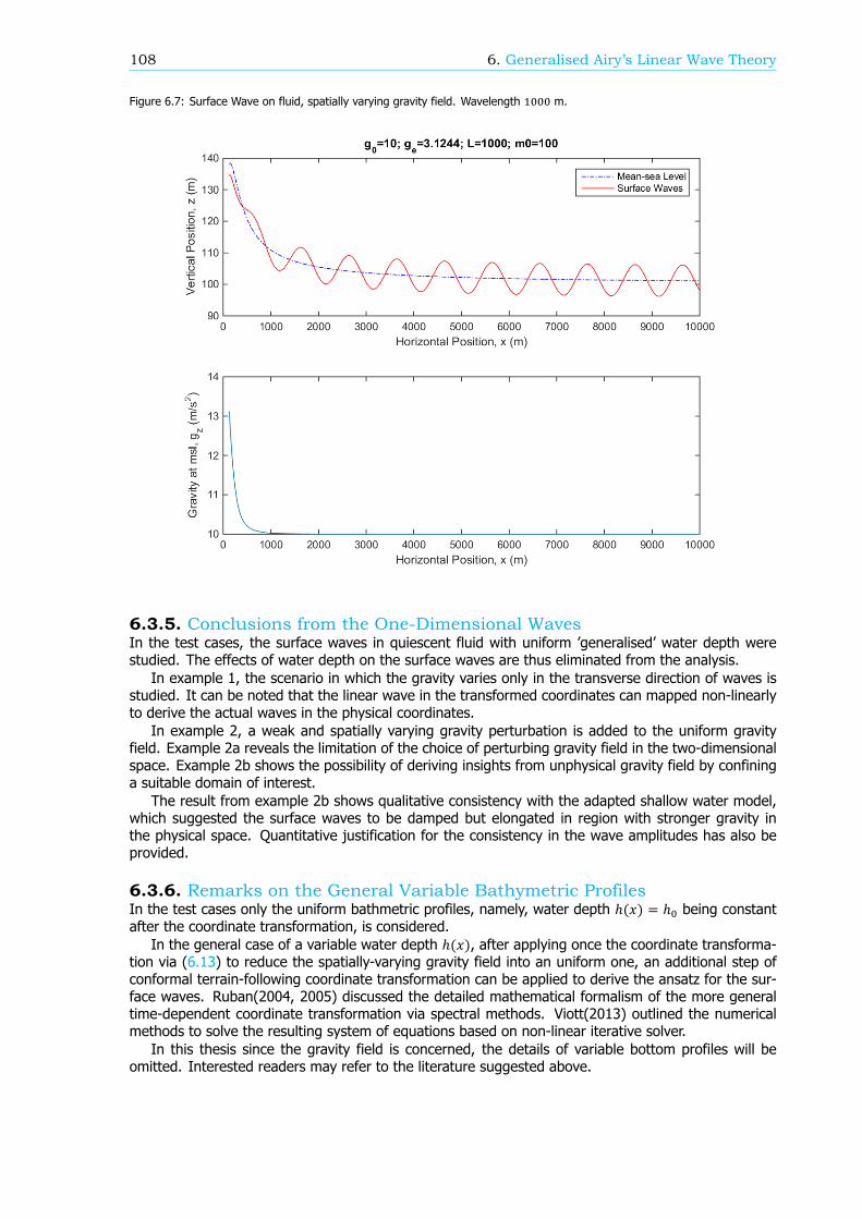
108 6. Generalised Airy’s Linear Wave Theory
Figure 6.7: Surface Wave on fluid, spatially varying gravity field. Wavelength m.
6.3.5. Conclusions from the One-Dimensional WavesIn the test cases, the surface waves in quiescent fluid with uniform ’generalised’ water depth werestudied. The effects of water depth on the surface waves are thus eliminated from the analysis.
In example 1, the scenario in which the gravity varies only in the transverse direction of waves isstudied. It can be noted that the linear wave in the transformed coordinates can mapped non-linearlyto derive the actual waves in the physical coordinates.
In example 2, a weak and spatially varying gravity perturbation is added to the uniform gravityfield. Example 2a reveals the limitation of the choice of perturbing gravity field in the two-dimensionalspace. Example 2b shows the possibility of deriving insights from unphysical gravity field by confininga suitable domain of interest.
The result from example 2b shows qualitative consistency with the adapted shallow water model,which suggested the surface waves to be damped but elongated in region with stronger gravity inthe physical space. Quantitative justification for the consistency in the wave amplitudes has also beprovided.
6.3.6. Remarks on the General Variable Bathymetric ProfilesIn the test cases only the uniform bathmetric profiles, namely, water depth ℎ(𝑥) = ℎ being constantafter the coordinate transformation, is considered.
In the general case of a variable water depth ℎ(𝑥), after applying once the coordinate transforma-tion via (6.13) to reduce the spatially-varying gravity field into an uniform one, an additional step ofconformal terrain-following coordinate transformation can be applied to derive the ansatz for the sur-face waves. Ruban(2004, 2005) discussed the detailed mathematical formalism of the more generaltime-dependent coordinate transformation via spectral methods. Viott(2013) outlined the numericalmethods to solve the resulting system of equations based on non-linear iterative solver.
In this thesis since the gravity field is concerned, the details of variable bottom profiles will beomitted. Interested readers may refer to the literature suggested above.

6.4. Discussion on the Three-Dimensional Potential 109
Figure 6.8: Surface Wave on fluid, spatially varying gravity field. Wavelength m.
6.4. Discussion on the Three-Dimensional PotentialIt is natural to seek a three-dimensional generalisation to the coordinate transformation schemes dis-cussed to analyse the surface waves. It will be shown in an example that, while an analogous methodto perform orthogonal coordinate transformation exists, the invariance property of the Laplacian op-erator cannot be preserved in general. The framework on which the coordinate transformation takesplace will be presented in the next section before proceeding to an illustrating example.
6.4.1. coordinate transformation in Three-Dimensional SpaceAnalogous to the two-dimensional problem discussed in previous section, given a geopotentialΨ(𝑥, 𝑦, 𝑧)which satisfies the Laplace equation ∇ Ψ = 0, it is attempted to seek a coordinate transformation(𝑥, 𝑦, 𝑧) → (𝑞 , 𝑞 , 𝑞 ) such that the following three properties hold:
1. The transformation (𝑥, 𝑦, 𝑧) → (𝑞 , 𝑞 , 𝑞 ) is uniquely defined and the inverse uniquely exists inthe interested domain.
2. The coordinates are orthogonal, that is ∇𝑞 ⋅ ∇𝑞 = 𝛿 , where 𝛿 is the Kronecker delta
3. The scalar function 𝑞 (𝑥, 𝑦, 𝑧) = (Ψ(𝑥, 𝑦, 𝑧)−Ψ ), such that 𝑞 (𝑥, 𝑦, 𝑧) physically measures thescaled potential difference from the mean-sea level Ψ
The Property 3 directly gives the explicit formula of 𝑞 . Hence it suffices to determine 𝑞 and 𝑞 .
6.4.2. Trial 1: Clebsch PotentialFor any divergence-free vector field u in ℛ with
∇ ⋅ u = 0,

110 6. Generalised Airy’s Linear Wave Theory
Figure 6.9: Comparison of adapted shallow water model and generalised Airy’s wave theory. Wavelength m.
it can be proved via techniques from algebraic topology that there exists a vector potential A such that
∇ × A = u.
The detailed proof can be obtained from intermediate-level Analysis texts.It is reminded that the vector potential A is not unique. For any scalar function 𝑓, the vector field
A = A+ ∇𝑓 is also a vector potential for u. This property is known as ’Gauge invariance’.Clebsch (1857) showed that locally the vector potential A can be decomposed into
A = 𝜂∇𝜉,
where 𝜂(𝑥, 𝑦, 𝑧) and 𝜉(𝑥, 𝑦, 𝑧) are two scalar functions. It follows that
u = ∇𝜂 × ∇𝜉,
which shows the the vector u is locally parallel to the intersection line of the surfaces 𝜂 = constant and𝜉 = constant.
Based on the definition given in the previous section, since 𝑞 (𝑥, 𝑦, 𝑧) satisfies the Laplace equation,the gradient of 𝑞 , ∇𝑞 , is a divergence-free vector field. For the field A to be the vector potential of∇𝑞 such that ∇ × A = ∇𝑞 , it then follows the coordinates function 𝑞 (𝑥, 𝑦, 𝑧) and 𝑞 (𝑥, 𝑦, 𝑧) can bechosen by
A = 𝑞 ∇𝑞 (6.74)
which leads to
∇𝑞 = ∇𝑞 × ∇𝑞 , (6.75)
If, in addition, ∇𝑞 and ∇𝑞 are orthogonal, (6.75) implies that ∇𝑞 , ∇𝑞 and ∇𝑞 are mutuallyorthogonal. Furthermore, considering the norm of vectors in (6.75), it can be noted that ‖∇𝑞 ‖ =

6.4. Discussion on the Three-Dimensional Potential 111
Figure 6.10: Surface Wave on fluid, spatially varying gravity field. Wavelength m.
‖∇𝑞 ‖‖∇𝑞 ‖. In other words, unless all three vectors ∇𝑞 are unit vector, the coordinates will not beequal in norm.
It is noted that the two-dimensional conformal coordinates discussed in (6.13) is a special caseunder Clebsch’s theory. If 𝑞 can be chosen such that 𝑞 (𝑥, 𝑦) is independent of the vertical Cartesiancoordinates 𝑧, by choosing 𝑞 (𝑥, 𝑦, 𝑧) = 𝑧, it follows that the coordinates 𝑞 (𝑥, 𝑦) is also independent of𝑧. The coordinates 𝑞 and 𝑞 satisfy the Cauchy-Riemann condition (6.12) automatically by the choiceof 𝑞 .
6.4.3. Example: Point-mass in three-dimensional spaceConsider the gravitational potential induced by a sphere of radius 𝑅 centred at the origin. To simplifythe notation, standard spherical coordinates (𝑟, 𝜃, 𝜙) with unit vectors ��, ��, �� will be used. By properrescaling the physical length 𝑟, the geopotential function Ψ(𝑟) is simply given by
Ψ(𝑟) = −𝑔𝑟 (6.76)
outside the sphere 𝑟 > 𝑅 , where 𝑔 is some positive constant. Suppose 𝑟 = 𝑅 is the mean-sea level.It follows that the coordinate function 𝑞 (𝑟, 𝜃, 𝜙) is simply given by
𝑞 (𝑟, 𝜃, 𝜙) = −1𝑟 +1𝑅 (6.77)
The contrapositive basis a( ) = ∇𝑞 is thus given by
a( ) = ∇𝑞 = 1𝑟 �� (6.78)
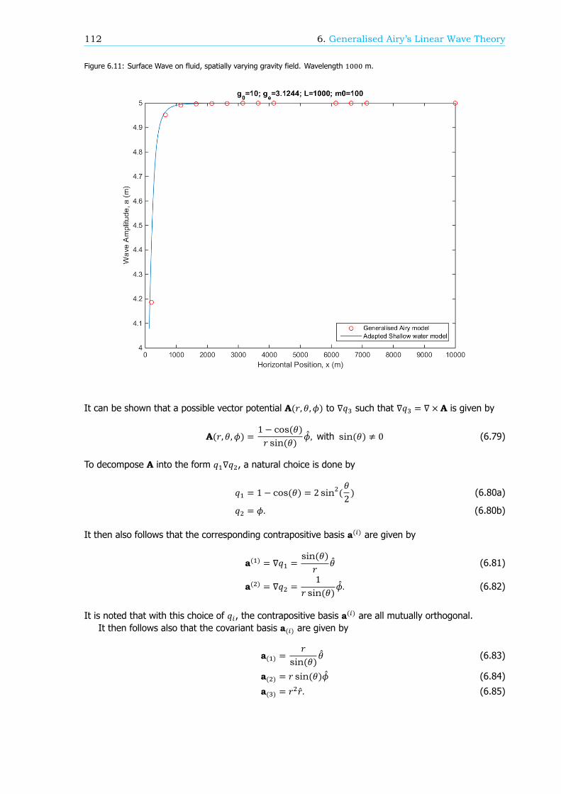
112 6. Generalised Airy’s Linear Wave Theory
Figure 6.11: Surface Wave on fluid, spatially varying gravity field. Wavelength m.
It can be shown that a possible vector potential A(𝑟, 𝜃, 𝜙) to ∇𝑞 such that ∇𝑞 = ∇ × A is given by
A(𝑟, 𝜃, 𝜙) = 1 − cos(𝜃)𝑟 sin(𝜃) ��, with sin(𝜃) ≠ 0 (6.79)
To decompose A into the form 𝑞 ∇𝑞 , a natural choice is done by
𝑞 = 1 − cos(𝜃) = 2 sin (𝜃2) (6.80a)
𝑞 = 𝜙. (6.80b)
It then also follows that the corresponding contrapositive basis a( ) are given by
a( ) = ∇𝑞 = sin(𝜃)𝑟 �� (6.81)
a( ) = ∇𝑞 = 1𝑟 sin(𝜃) ��. (6.82)
It is noted that with this choice of 𝑞 , the contrapositive basis a( ) are all mutually orthogonal.It then follows also that the covariant basis a( ) are given by
a( ) =𝑟
sin(𝜃) �� (6.83)
a( ) = 𝑟 sin(𝜃)�� (6.84)
a( ) = 𝑟 ��. (6.85)

6.4. Discussion on the Three-Dimensional Potential 113
Figure 6.12: Surface Wave on fluid, spatially varying gravity field. Wavelength m.
The metric tensor 𝑔 = a( ) ⋅ a( ) and 𝑔 = a( ) ⋅ a( ) are therefore given by
𝑔 = sin (𝜃)𝑟 , 𝑔 = 1
𝑟 sin (𝜃), 𝑔 = 1
𝑟 (6.86)
𝑔 = 𝑟sin (𝜃)
, 𝑔 = 𝑟 sin (𝜃), 𝑔 = 𝑟 (6.87)
and the quantity √𝑔 is given by
√𝑔 = √𝑔 𝑔 𝑔 = 𝑟 (6.88)
The Laplacian operator in the (𝑞 , 𝑞 , 𝑞 ) are thus given by
∇ 𝑓 = 1√𝑔
𝜕𝜕𝑞 (√𝑔𝑔
𝜕𝑓𝜕𝑞 ) + 1
√𝑔𝜕𝜕𝑞 (√𝑔𝑔
𝜕𝑓𝜕𝑞 ) + 1
√𝑔𝜕𝜕𝑞 (√𝑔𝑔
𝜕𝑓𝜕𝑞 )
= 1𝑟
𝜕𝜕𝑞 (𝑟 sin (𝜃)
𝑟𝜕𝑓𝜕𝑞 ) + 1
𝑟𝜕𝜕𝑞 (𝑟 1
𝑟 sin (𝜃)𝜕𝑓𝜕𝑞 ) + 1
𝑟𝜕𝜕𝑞 (𝑟 1
𝑟𝜕𝑓𝜕𝑞 )
= 1𝑟
𝜕𝜕𝑞 (𝑟 sin (𝜃) 𝜕𝑓𝜕𝑞 ) + 1
𝑟𝜕𝜕𝑞 ( 𝑟
sin (𝜃)𝜕𝑓𝜕𝑞 ) + 1
𝑟𝜕 𝑓𝜕𝑞
To simplify the notation, considering the coordinate transformation 𝑞 in (6.77), it is also possible torecast
𝑞 = 𝑞 − 1𝑅 (6.89)

114 6. Generalised Airy’s Linear Wave Theory
such that 𝑟 and can be expressed in terms of
𝑟 = −1𝑞 (6.90)
𝜕𝜕𝑞 = 𝜕
𝜕𝑞 (6.91)
To recast sin (𝜃) in terms of (𝑞 , 𝑞 , 𝑞 ), applying trigonometric identities and using (6.80) give
sin (𝜃) = 4 cos (𝜃2) sin (𝜃2) = 4(1 −𝑞2 )𝑞2 = (2 − 𝑞 )𝑞 (6.92)
Therefore the Laplacian operator ∇ 𝑓 in the (𝑞 , 𝑞 , 𝑞 ) coordinates are given by
∇ 𝑓 =𝑞 𝜕𝜕𝑞 ((2 − 𝑞 )𝑞 𝜕𝑓
𝜕𝑞 ) + 𝑞(2 − 𝑞 )𝑞
𝜕 𝑓𝜕𝑞 + 𝑞 𝜕 𝑓
𝜕𝑞
Hence the Laplace equation (6.3) for the velocity potential 𝜙 is rewritten as
∇ 𝜙 = 𝜕𝜕𝑞 ((2 − 𝑞 )𝑞 𝜕𝑓
𝜕𝑞 ) + 1(2 − 𝑞 )𝑞
𝜕 𝑓𝜕𝑞 + 𝑞 𝜕 𝑓
𝜕𝑞= 0 (6.93)
subject to the linearised boundary conditions
at 𝑞 = −ℎ : 𝜕𝜙𝜕𝑞 = 0, (6.94a)
at 𝑞 = 0: 𝜕𝜙𝜕𝑞 = 𝜕𝜂𝜕𝑡 . (6.94b)
together with an addition equation for surface elevation 𝑞 = 𝜂(𝑞 , 𝑞 , 𝑡):
at 𝑞 = 0: 𝜕𝜙𝜕𝑡 + 𝑔 𝜂 = 0, (6.95)
Readers are reminded that 𝑞 and 𝑞 are different merely by a shift proposed in (6.89).Equation (6.93) reveals that the Laplacian operator does not preserve the structure as that in the
Cartesian coordinates.As a first trial, consider a time-independent separable solution 𝑓 to equation (6.93), that is, take
𝑓(𝑞 , 𝑞 , 𝑞 ) = 𝑄 (𝑞 )𝑄 (𝑞 )𝑄 (𝑞 ), this gives rises to the partial differential equation:
(2 − 𝑞 )𝑞𝑄 (𝑞 )
𝑑𝑑𝑞 ((2 − 𝑞 )𝑞 𝑑𝑄
𝑑𝑞 ) + 1𝑄 (𝑞 )
𝑑 𝑄𝑑𝑞 + (2 − 𝑞 )𝑞 𝑞𝑄 (𝑞 )
𝑑 𝑄𝑑𝑞
= 0 (6.96)
For constant 𝑚, consider = −𝑚 𝑄 (𝑞 ) such that 𝑄 (𝑞 ) is sinusoidal, the Laplace equation canthen be separated into three ordinary differential equations:
𝑑𝑑𝑞 ((2 − 𝑞 )𝑞 𝑑𝑄
𝑑𝑞 ) = [−𝑙(𝑙 + 1) + 𝑚(2 − 𝑞 )𝑞 ]𝑄 (𝑞 ), (6.97a)
𝑑 𝑄𝑑𝑞 = −𝑚 𝑄 (𝑞 ), (6.97b)
𝑑 𝑄𝑑𝑞
= 𝑙(𝑙 + 1)𝑞
𝑄 (𝑞 ), (6.97c)
where 𝑙 is a constant.

6.4. Discussion on the Three-Dimensional Potential 115
After some attempts of solving, it turns out that the solution of (6.97) is equivalent to the separablesolution of Laplace equation in the standard spherical coordinates by recasting (𝑞 , 𝑞 , 𝑞 ) into (𝑟, 𝜃, 𝜙),which reads
𝑓(𝑟, 𝜃, 𝜙) =∑∑(𝐴 𝑟 + 𝐵 𝑟( ))𝑃 (cos(𝜃))[𝑆 sin(𝑚𝜙) + 𝐶 cos(𝑚𝜙)] (6.98)
where 𝑃 are the associated Legendre polynomials and 𝐴 , 𝐵 , 𝑆 , 𝐶 are some constants. This ansatzis known as spherical harmonics, which are discussed together with its applications extensively in manytexts, such as Lebedev(1965).
In the particular case when𝑚 = 0, which suggests azimuthal symmetry in the ansatz, it appears thatthe order of the Legendre function 𝑙 plays the role of wavenumber 𝑘 for sinusoidal-types of waves. Forinteger 𝑘, the term cos(𝑘𝜃) can always be expressed uniquely by linear combination 𝑃 (cos(𝜃)), 𝑙 ≤ 𝑘with the aid of Chebyshev polynomial. The details can be found in texts on special functions, forexample Lebedev(1965).
Conceptually, if the surface elevation 𝑞 = 𝜂(𝑞 , 𝑞 , 𝑡) is known everywhere at a given 𝑡, a boundary-value problem to the Laplace equation (6.93) with pure Neumann boundary conditions (6.94) is formed.It then follows the constants 𝐴 , 𝐵 , 𝑆 , 𝐶 and thus the instantaneous velocity potential can be deter-mined. Meanwhile the additional equation (6.95) can fix the uniqueness issue of the solution resultedfrom the ill-posed pure Neumann boundary condition.
Unfortunately this approach by separation of variables does not appear to possess the capabilityin deriving a wave-like and inseparable ansatz for the surface elevation 𝜂 = 𝜂(𝑘 𝑞 + 𝑘 𝑞 − 𝜔𝑡) witharbitrary constants 𝑘 and 𝑘 .
Further research shall be devoted to confirm the existence of such solutions and, if exists, analgorithm to obtain the solutions. The following sections outline alternative directions to obtain anotherset of coordinates, which may bring insights in constructing the wave-like ansatz.
6.4.4. Clebsch Potential: the Gauge InvarianceReaders are reminded again that vector potential A is unique only up to the Gauge transformation. Itmay be possible to choose a scalar function ℎ such that the coordinates function 𝑞 and 𝑞 , given by
A+ ∇ℎ = 𝑞 ∇𝑞 , (6.99)
fulfill the additional conditions
‖∇𝑞 ‖ = ‖∇𝑞 ‖ = 𝑔 = 𝑔 = 𝐺. (6.100)
In that case, the Laplacian operator becomes
∇ 𝑓 = 1√𝑔
𝜕𝜕𝑞 (√𝑔𝐺
𝜕𝑓𝜕𝑞 ) + 1
√𝑔𝜕𝜕𝑞 (√𝑔𝐺
𝜕𝑓𝜕𝑞 ) + 1
√𝑔𝜕𝜕𝑞 (√𝑔𝑔
𝜕𝑓𝜕𝑞 ) (6.101)
which separates the transverse direction (𝑞 , 𝑞 ) of surface waves from the longitudinal direction 𝑞 .If, in additional, both
√𝑔𝐺 = √𝑔𝐺(𝑞 ) (6.102)
√𝑔𝑔 = √𝑔𝐺(𝑞 ) (6.103)
are only functions of 𝑞 , then there exists symmetry in 𝑞 and 𝑞 , namely 𝑞 and 𝑞 are interchangeablewhile preserving the Laplacian operator. The symmetry seems to provide a gateway to guarantee theexistence of an arbitrarily-oriented wavevector �� = (𝑘 , 𝑘 ) on the 𝑞 -𝑞 plane, which is a condition ofthe hyperbolicity of systems of partial differential equations.
However, the existence of ℎ is not guaranteed and there is a lack of general procedure to obtainℎ. It is also uncertain whether it is possible to choose a coordinate such that 𝑞 and 𝑞 possess thesymmetry properties described in the previous paragraph. Further research shall be conducted torigorously understand the properties and explore this area.

116 6. Generalised Airy’s Linear Wave Theory
6.4.5. Trial 2: Geometric InspectionIn this section another trial to choose proper coordinates is presented. Although it appears to be alsoa failing attempt, it does provide insight for the right direction to move forward.
Readers are reminded that for a given coordinate 𝑞 , the goal has always been to seek two additionalmutually-orthogonal coordinates 𝑞 , 𝑞 which avoid cross-terms in the transformed Laplace equation.While the approach via Clebsch potential effectively generates the orthogonal coordinates, it does notseem to be effective in representing the physics in a mathematically concise manner.
For the particular example of point-mass geopotential, an alternative approach to propose thecoordinate transformation is given by a direct inspection of the algebraic and geometry properties ofthe transformation. The inspection will be presented in this section.
Recall the coordinates function 𝑞 is given by (6.77)
𝑞 (𝑟, 𝜃, 𝜙) = −1𝑟 +1𝑅 ,
which gives a contrapositive basis a( ):
a( ) = ∇𝑞 = 1𝑟 ��
It can be noted that a( ) is parallel to the unit vector ��. It is known that the unit vector �� is orthonormalto �� and ��. This suggests that, by choosing
𝑞 = 𝑞 (𝜃) = ∫ 𝑑𝜃sin(𝜃) =
12 ln(
1 − cos(𝜃)1 + cos(𝜃)) (6.104)
𝑞 = 𝑞 (𝜙) = 𝜙 (6.105)
which makes
a( ) = ∇𝑞 = 1𝑟 sin(𝜃) �� (6.106)
a( ) = ∇𝑞 = 1𝑟 sin(𝜃) ��, (6.107)
the contrapositive basis are mutually orthogonal. An additional property that a( ) and a( ) are equal innorm is also guaranteed. The covariant basis are then given by
a( ) = 𝑟 sin(𝜃)�� (6.108)
a( ) = 𝑟 sin(𝜃)�� (6.109)
a( ) = 𝑟 �� (6.110)
The metric tensor are computed and given by
𝑔 = 𝑔 = 1𝑟 sin (𝜃)
; 𝑔 = 1𝑟 (6.111)
𝑔 = 𝑔 = 𝑟 sin (𝜃); 𝑔 = 𝑟 (6.112)
with the quantity √𝑔 = √𝑔 𝑔 𝑔 = 𝑟 sin (𝜃).By recasting 𝑞 into 𝑞 in the same manner in (6.89), the inverse transformation from (𝑞 , 𝑞 , 𝑞 )
are given by
tanh(𝑞 ) = − cos(𝜃) (6.113)𝑞 = 𝜙 (6.114)
𝑞 = −1𝑟 (6.115)
after some algebraic manipulation. It follows also that sin (𝜃) = 1 − cos (𝜃) = 1 − tanh (𝑞 ) =cosh ( ) .

6.5. Short Conclusions 117
Hence the Laplacian operator is given by
∇ 𝑓 = 1𝑟 sin (𝜃)
[ 𝜕𝜕𝑞 (𝑟 𝜕𝑓𝜕𝑞 ) + 𝜕
𝜕𝑞 (𝑟 𝜕𝑓𝜕𝑞 ) + 𝜕
𝜕𝑞 ( sin (𝜃) 𝜕𝑓𝜕𝑞 )] (6.116)
= 𝑞 cosh (𝑞 )[ 1𝑞
𝜕 𝑓𝜕𝑞 + 1
𝑞𝜕 𝑓𝜕𝑞 + 1
cosh (𝑞 )𝜕 𝑓𝜕𝑞 ] (6.117)
The Laplacian equation on function 𝑓(𝑞 , 𝑞 , 𝑞 ) can thus be expressed by
𝜕 𝑓𝜕𝑞 + 𝜕 𝑓𝜕𝑞 + 𝑞
cosh (𝑞 )𝜕 𝑓𝜕𝑞 = 0. (6.118)
Considering again the the separable solution 𝑓(𝑞 , 𝑞 , 𝑞 ) = 𝑄 (𝑞 )𝑄 (𝑞 )𝑄 (𝑞 ) results in three ordi-nary differential equations
𝑑 𝑄𝑑𝑞 = [ −𝑙(𝑙 + 1)
cosh (𝑞 )+ 𝑚 ]𝑄 (𝑞 ), (6.119a)
𝑑 𝑄𝑑𝑞 = −𝑚 𝑄 (𝑞 ), (6.119b)
𝑑 𝑄𝑑𝑞
= 𝑙(𝑙 + 1)𝑞
𝑄 (𝑞 ), (6.119c)
which turns out to give an equivalent ansatz as (6.97) after recasting the coordinates into the stan-dard spherical coordinates (𝑟, 𝜃, 𝜙). In other words, with this seemingly ’better’ set of coordinates(𝑞 (𝜃), 𝑞 (𝜙), 𝑞 (𝑟)), the ansatz to the Laplace equation one can seek is no different from the ansatzby choosing the standard coordinates (𝑟, 𝜃, 𝜙).
This failing example highlights again the choice of coordinates actually implicitly restricts the ansatzone can obtain. With simple adaptation of the spherical coordinates, for example by (𝑞 (𝜃), 𝑞 (𝜙), 𝑞 (𝑟)),it is very unlikely to generate an insightful ansatz. This again motivates the further studies outlined insection 6.4.4 for a general coordinate transformation given by (𝑞 (𝑟, 𝜃, 𝜙), 𝑞 (𝑟, 𝜃, 𝜙), 𝑞 (𝑟)) satisfyingthe additional conditions (6.100) and (6.102).
6.5. Short ConclusionsIn this chapter Airy’s linear wave theory is generalised to deal with spatially non-uniform conservativegravitational field in two and three-dimensional space.
In the two dimensional space, an explicit scheme of coordinate transformation has been proposedto map the non-uniform conservative gravitational field into a uniform one, enabling the use of classicalresults to analyse surface gravity waves in fluid. It has also been demonstrated in test cases that thegeneralised linear wave theory is consistent with the adapted shallow water discussed in Chapter 3 inthe long-wave limit.
In the three dimensional space, however, the magic does not work in a straightforward manner. Itremains questionable whether a three-dimensional spatially-varying conservative field can be mappedinto a uniform field. Several attempts have been made to create the coordinate transformation schemein a special case but unfortunately unsuccessful. The reason of the failure has been analysed and newdirections have been proposed for further research.


7Conclusions and Further Research
Directions
In this thesis, the effects of non-uniformity of gravity field on the fluid surface waves are studiedanalytically and numerically.
In chapter 3 to 5 the shallow water long waves are studied. With the aid of both analytical and nu-merical studies, it has been demonstrated that the actual variation of gravity field on Earth solely is notcritical to surface waves in the ocean, despite all the possible changes in wave amplitude, wavenumberand wave scattering features induced by the gravity.
Despite this, it has been also illustrated that the sea-surface topography induced by the non-uniformgravity can possibly affect the wave dynamics, especially in waves scattering, via the changes in thetime-averaged water depth. This implies that while it remains justifiable to assume constant gravityremains, the spatial variation of time-averaged surface elevation due to gravity on the ocean shallnot be neglected. Hence the classical shallow water models remains applicable after properly takingaccount of the water depths. This also reveals the equivalence between a surface mountain in a non-uniform gravitatonal field and a seabed pit at the bottom in a uniform gravitational field, when it comesto surface waves dynamics.
In chapter 6 the generalised Airy’s linear wave theory provided a qualitative justification to theseemingly unrealistic approximations and assumptions used in the derivation of adapted shallow watermodel. Unfortunately, the generalisation which builds upon conformal mapping is by-far only limitedto the two-dimensional space. Further research is needed for the three-dimensional generalisation,in areas including the existence, uniqueness and algorithmic procedures for the three-dimensionalorthogonal mapping.
Another unanswered question includes the analytic aspects of two-dimensional waves scattering inthe adapted shallow water model, which appears to be possibly analysed by the standard techniquesfor waves scattering in general heterogeneous medium.
While it appears to be clear that the gravity force on the ocean is too weak to alter the surfacewaves, the theory developed in this thesis is not confined to surface waves on the ocean. In principle,it applies to fluid surface waves in any conservative and weakly non-linear force fields. It is thereforeexpected that analogous examples could be sought for in other physical scenarios, for instance, onplanets with stronger variation of gravity pull, in charged fluid in conservative electromagnetic fieldsand so on.
A setback of this project is that the theories developed lack experimental or empirical verification.While the gravity variation on Earth is too weak to result in any observable changes in practice, thevariation of restoring force to fluid surface waves can possibly be blown up in laboratory environments.This may be achieved by using electromagnetic forces for charged fluid. Another possible direction toconduct the experiment is by Direct Navier-Stokes simulation computationally. The validation of thetheories propose a new topic for further research.
119

Bibliography
[1] A. Adcroft, J. Marshall and K. Emanuel. Lecture Notes on Atmospheric and Oceanic Modeling. Freelyretrieve from http:www-paoc.mit.edu12.950_modelingnotesindex.htm. MIT.
[2] G.B. Airy. Tides and waves. Encyclopaedia Metropolitana. Mixed Sciences. 3:396, 1841.
[3] F. Barthelmes. Definition of functionals of the geopotential and their calculation from sphericalharmonic models. Tech. rep., Helmholtz Centre Potsdam, GFZ, 2009.
[4] L.Brillouin. La mecanique ondulatoire de Schroedinger: une methode generale de resolution parapproximations successives. Comptes Rendus de l’Academie des Sciences, 1926.
[5] A. Clebsch. Uber eine allgemeine Transformation der hydrodynamischen Gleichungen. J ReineAngew Math 54:293-313, 1857.
[6] S.S. Hough. On the Application of Harmonic Analysis to the Dynamical Theory of the Tides. PartI. On Laplace’s ’Oscillations of the First Species,’ and on the Dynamics of Ocean Currents. Philos.Trans. R. Soc, A. 189:201-257, 1897.
[7] H. Jeffrey. On certain approximate solutions of linear differential equations of the second order.Proceedings of the London Mathematical Society. 23: 428-436, 1924.
[8] H.A. Kramers.Wellenmechanik und halbzaehlige Quantisierung. Zeitschrift fuer Physik. 39 (10-11):828-840, 1926.
[9] P.H. LeBlond, L.A. Mysak. Waves in the Ocean. Elsevier, 1981.
[10] N.N. Lebedev. Special Functions and Their Applications. Prentice-Hall. Englewood Cliffs,N.J:308pp, 1965.
[11] R.J. LeVeque. Finite Volume Methods for Hyperbolic Problems. Cambridge University Press, 2002.
[12] J.C. Luke. A Variational Principle for a Fluid with a Free Surface. Journal of Fluid Mechanics. 27(2): 395-397, 1967.
[13] L.R. Maas. Topographic filtering and reflectionless transmission of long waves. J. Phys. Ocean.,27: 195-202, 1996.
[14] J. Marshall and R.A. Plume. Atmosphere, Ocean and Climate Dynamics: An Introductory Text.Academic Press, 2007.
[15] J. Pedlosky. Geophysical Fluid Dynamics. Springer-Verlag New York, 1979.
[16] J. Pedlosky. Waves in the Ocean and Atmosphere: Introduction to Wave Dynamics. SpringerScience & Business Media, 2003.
[17] V.P. Ruban. Water waves over a strongly undulanting bottom.. Phys. Rev. E, 70:066302, 2004.
[18] V.P. Ruban.Water waves over a time-dependent bottom: Exact description for 2D potential flows.Physics Letter A. 340:194-200, 2005.
[19] D.L. Turcotte, G. Schubert. Geodynamics. Cambridge University Press, 2002.
[20] C. Viotti. D. Dutykh. F. Dias. The Conformal-mapping Method for Surface Gravity Waves in thePresence of Variable Bathymetry and Mean Current. Procedia IUTAM: VOL11. IUTAM Symposiumon Nonlinear Interfacial Wave Phenomena from the Micro- to the Macro-Scale, 2013.
121

122 Bibliography
[21] G. Wentzel. Eine Verallgemeinerung der Quantenbedingungen f r die Zwecke der Wellen-mechanik. Proceedings of the London Mathematical Society. 23: 428-436.
[22] P. Wesseling. Principles of Computational Fluid Dynamics. Springer Science & Business Media,2001