Embed Size (px)
Citation preview
Impact of Solar Resource and
Atmospheric Constituents on
Energy Yield Models for
Concentrated Photovoltaic
Systems
© Jafaru Mohammed, Ottawa, Canada, 2013
Thesis submitted to the Faculty of Graduate and Postdoctoral Studies
in partial fulfillment of the requirement for a Master’s of Applied
Science in Electrical and Computer Engineering.
May 2013
School of Electrical Engineering and Computer Science
University of Ottawa

Jafaru Mohammed, 2013 ii
With Effort And Will, You Can Move Mountains.
Anonymous
Jafaru Mohammed, 2013 iii
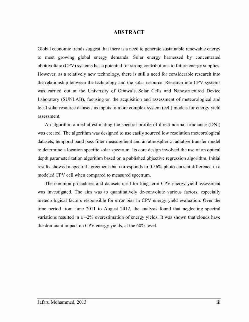
ABSTRACT
Global economic trends suggest that there is a need to generate sustainable renewable energy
to meet growing global energy demands. Solar energy harnessed by concentrated
photovoltaic (CPV) systems has a potential for strong contributions to future energy supplies.
However, as a relatively new technology, there is still a need for considerable research into
the relationship between the technology and the solar resource. Research into CPV systems
was carried out at the University of Ottawa’s Solar Cells and Nanostructured Device
Laboratory (SUNLAB), focusing on the acquisition and assessment of meteorological and
local solar resource datasets as inputs to more complex system (cell) models for energy yield
assessment.
An algorithm aimed at estimating the spectral profile of direct normal irradiance (DNI)
was created. The algorithm was designed to use easily sourced low resolution meteorological
datasets, temporal band pass filter measurement and an atmospheric radiative transfer model
to determine a location specific solar spectrum. Its core design involved the use of an optical
depth parameterization algorithm based on a published objective regression algorithm. Initial
results showed a spectral agreement that corresponds to 0.56% photo-current difference in a
modeled CPV cell when compared to measured spectrum.
The common procedures and datasets used for long term CPV energy yield assessment
was investigated. The aim was to quantitatively de-convolute various factors, especially
meteorological factors responsible for error bias in CPV energy yield evaluation. Over the
time period from June 2011 to August 2012, the analysis found that neglecting spectral
variations resulted in a ~2% overestimation of energy yields. It was shown that clouds have
the dominant impact on CPV energy yields, at the 60% level.

Jafaru Mohammed, 2013 iv
STATEMENT OF ORIGINALITY
Except where stated otherwise, the results presented in this thesis were obtained by the
author during the period of his MA.Sc. research under the supervision of Dr. Henry
Schriemer. They are to the best of his knowledge original.
ACKNOWLEDGMENTS
Dr. Henry Schriemer: Thank you for your patient guidance, your enduring efforts and
your attention to detail in supervising my research and thesis. I couldn’t have learnt so much
in such short time without your help. I’m most grateful.
Dr. Karin Hinzer: Thank you for your patience, your kindness and understanding. You
created an environment where I could learn and thrive. My research was made possible under
your enabling administration. Thank you for the motivations, I’m extremely grateful. .
Dr. Joan Haysom: Thank you for your assistance and guidance on the energy yield
analysis research. Thank you for the opportunity to manage the APECS data acquisition
systems; it gave me a sense of belonging and brought me fulfillment.
Mark Yandt: Thank you for your assistance on the concentrated cell model. Your
research provided the basic algorithms I needed to perform most of my energy yield analysis.
Sarah and Mohammed Maliki (Mom and Dad): Thank you so much for everything.
Words cannot describe the amplitude of gratitude I have for the opportunities you’ve given
me. I cannot thank you enough for the financial, emotional and psychological assistance
you’ve provided over the years. However, in this circumstance, the least I can write is thank
you very much.
Jafaru Mohammed, 2013 v
TABLE OF CONTENTS
ABSTRACT III
STATEMENT OF ORIGINALITY IV
ACKNOWLEDGMENTS IV
TABLE OF CONTENTS V
LIST OF FIGURES VIII
LIST OF TABLES XIII
LIST OF ACRONYMS XIV
1 INTRODUCTION 1
1.1 Background 2
1.1.1 History and Evolution of Photovoltaics 3
1.1.2 Renewable Energy for Sustainable Development 9
1.1.3 A Brief Introduction to PV Systems and their Limitations 9
1.2 Research Motivation 13
1.3 Thesis Objectives 14
1.4 Thesis Overview 15
2 THE SOLAR RESOURCE 17
2.1 Introduction 17
2.2 Earth and Sun 18
2.2.1 The Earth’s Incident Solar Radiation 19
2.2.2 Earth-Sun Temporal Coordinates 20

Jafaru Mohammed, 2013 vi
2.2.3 Solar Elevation and Azimuth 25
2.2.4 Time Systems 27
2.3 Calculating Solar Coordinates 28
2.4 Atmospheric Transmission of Sunlight 30
2.4.1 Air Mass 31
2.4.2 DNI, GHI and Diffuse Irradiance 33
2.4.2.1 Diffuse Irradiance 33
2.4.2.2 Direct Normal Irradiance 34
2.4.2.3 Global Horizontal Irradiance 34
2.5 Measuring the Solar Resource 35
2.6 Harvesting the Solar Resource 36
2.6.1 Trackers and Concentrators 37
3 MODELS, SIMULATIONS, HARDWARE AND RESEARCH TOOLS 41
3.1 Introduction - SUNLAB 41
3.1.1 Hardware Systems - Solar Simulators & Cell Characterization Equipment 42
3.1.1.1 Oriel Solar Simulator 42
3.1.1.2 XT-30 Solar Simulator 43
3.1.1.3 Sinton Flash Tester 45
3.1.1.4 Newport’s Quantum Efficiency Measurement Station 45
3.1.2 Software Systems 46
3.1.2.1 Simple, Pluggable Current-Voltage (IV) Utility 46
3.1.2.2 Spatial Uniformity Measurement Systems 50
3.1.2.3 Solar Cell Spatial Uniformity Utility 54
3.1.2.4 Light-Cycling Utility 56
3.2 Data Logging and Databasing of APECS Datasets 58
3.2.1 Overview of APECS, Test Site and Databasing Architecture 59
3.2.2 Measuring Instruments 60
3.2.2.1 Eppley PSP Pyranometer 60
3.2.2.2 Eppley NIP Pyrheliometer 61
3.2.2.3 ASDi FieldSpec3 Spectroradiometer 62
Jafaru Mohammed, 2013 vii
3.2.3 System Design 63
3.2.4 Data Logging and Backup Architecture 64
3.2.5 Measurements 65
3.3 Photovoltaic System Simulation 67
3.3.1 Review of the Single Diode System Model 68
3.3.2 Modeling Multi-Junction Cells 70
4 SPECTRAL ESTIMATION AND ENERGY YIELD ANALYSIS 72
4.1 Spectral Estimation Using Parameterized Aerosol Optical Depth 72
4.1.1 Optical Depth Extraction Algorithm 73
4.1.2 Aerosol Optical Depth Extraction 77
4.2 Investigating Energy Yield Analysis 80
4.2.1 Introduction / Background 80
4.2.2 Experiments and Analysis 82
4.2.2.1 Energy Yield Model Validation 83
4.2.2.2 Energy Yield Model Comparison 85
4.2.2.3 Input Dataset Comparison 89
4.2.2.4 De-convolution of Meteorological Bias Factors Affecting CPV Energy Yield 91
5 CONCLUSIONS 95
5.1 Overview / Summary 95
5.2 Future Work 98
6 REFERENCES 100
Jafaru Mohammed, 2013 viii
LIST OF FIGURES
Figure 1-1: A p-n junction in thermal equilibrium and zero bias voltage. Log scaled concentration of electron
and hole carriers are represented by the blue and red lines respectively. The two gray regions have neutral
charges while the red and blue region are positive and negative charged zones respectively. The direction of
flow of the electric field is shown and the direction of the electrostatic forces affecting the diffusion of holes
and electrons is illustrated. .................................................................................................................................... 3
Figure 1-2: Learning curve illustrating cost reduction in installed PV systems between 1990 and 2010. Adapted
from [16]. ............................................................................................................................................................... 5
Figure 1-3: Illustration of the evolution of efficiency for silicon cells. The black data points represent data from
the University of New South Wales, Australia. Adapted from [12]. ..................................................................... 6
Figure 1-4: Illustration of the evolution of commercial silicon module efficiency. The bars show the upper and
lower performance limits of modules commercially available, based on the nominal output of the module as
specified by the manufacturer. The solid line is a guide to the eye. Adapted from [12]. ...................................... 6
Figure 1-5: NREL’s chart of the best research cell efficiencies across various PV technologies over time.
Current multi-junction cell technology holds the highest efficiency record of 44% where silicon crystalline cells
seem to have leveled out at a maximum of 27.6% efficiency [24]. The slope of the curve for efficiency growth
in multi-junction cells suggests additional efficiency increase is expected in the future. ...................................... 8
Figure 1-6: Photon flux absorption in proportion to EQE for a sample triple junction solar cell with sub-cells
cell 1, cell 2 and cell 3. Each sub-cell is designed to absorb specific portions of the photon flux available
depicted by their band-gap thereby increasing efficiency. Sufficiently more sub-cells could be added to further
increase efficiency however the selection of materials is limited by their lattice constant. ................................. 11
Figure 1-7: Illustration of thermalization of an electron/hole pair. The diagram on the left represents the
excitation of an electron/hole from the valence to conduction band where the photon energy Eph is relatively
close to the band gap EG. The diagram on the right represents a similar excitation with photon energy greater
than the band gap energy. Thermalization occurs and is illustrated as ‘c’ where the electron/hole pair settles
back (thermalize) to the bottom of the conduction band. .................................................................................... 12
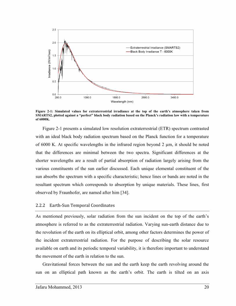
Figure 2-1: Simulated values for extraterrestrial irradiance at the top of the earth’s atmosphere taken from
SMARTS2, plotted against a “perfect” black body radiation based on the Planck’s radiation law with a
temperature of 6000K. ......................................................................................................................................... 20
Figure 2-2: The earth’s elliptical orbit around the sun (exaggerated), showing an axial tilt of about 23.44˚
relative to the elliptical orbital plane. The northern hemisphere points away and towards the sun at the winter
and summer solstice respectively while the earth’s axis is perpendicular to its orbit in the spring and fall
equinox. The four periods in the year as illustrated correspond to the four seasons. ........................................... 21
Figure 2-3: A representation of the earth’s celestial sphere. The equatorial plane is a projection of the earth’s
celestial equator to a position in space. The earth’s rotational axis forms the celestial North and South poles
Jafaru Mohammed, 2013 ix
when extended. The diagram illustrates a right of ascension of 6 hours, or 90˚ for the sun (Adapted from [39],
page 10). .............................................................................................................................................................. 22
Figure 2-4: Relation of solar angles from an observer’s perspective as seen in the northern hemisphere at 40˚
N. The north and south directions are in the plane of the page. The east and west directions are out of and into
the page respectively. The zenith line is perpendicular to the earth’s surface. The local meridional plane is the
plane of the page and is defined by the north, south and zenith points. The equatorial plane is perpendicular to
the polar axis about which the celestial sphere rotates. The solar hour angle, ha, is the angle between the sun’s
current position and the solar noon that is due south and measured along the equatorial plane in hours (about -2
hours in this Figure). (Adapted from [39]). ......................................................................................................... 23
Figure 2-5: Illustration of the equation of time in Ottawa, Canada for the duration of a year. Adjustments have
been made to cater for the earth’s tilt angle and its noncircular orbit around the sun.......................................... 24
Figure 2-6: Solar analemma for Ottawa, Canada with coordinates of approximately 45˚N and -75˚W. Solar
declination is plotted against the equation of time. .............................................................................................. 25
Figure 2-7: Illustration of the zenith, true horizon and the various angles referencing the sun from a fixed
position on the earth’s surface. “L” in the Figure represents the latitudinal angle. The altitude angle shown is
also known as the solar elevation and it forms a complementary angle with the solar zenith. ............................ 26
Figure 2-8: The path of the sun above the horizon as observed from the ground in a day. The azimuth angle is
usually measured from the north; in such a case, if the sun is directly over the east, it would have an azimuth
angle of 90˚. The azimuth can also be referenced to the south as depicted by in the Figure and by convention
is considered positive before noon. The elevation is also shown. .................................................................... 27
Figure 2-9: A flow diagram for deducing high accuracy elevation and azimuth angular values for the position
of the sun from any given longitude and latitude at any given time. ................................................................... 29
Figure 2-10: Comparison of a 6000K black body spectrum with spectra at various layers of the atmosphere. . 32
Figure 2-11: Transmission of radiation through the atmosphere. The diagram illustrates bands of the spectrum
absorbed by the atmospheric gasses and irradiance scattering phenomena such as Rayleigh scattering [43]. .... 32
Figure 2-12: SMARTS2 simulated direct normal spectra irradiance illustrating spectral variation due to air
mass change. ........................................................................................................................................................ 33
Figure 2-13: Components of sunlight passing through the atmosphere. ............................................................. 35
Figure 2-14: Illustration of primary and secondary optics arrangement with a solar cell in a CPV system (not to
scale). In this type, a Fresnel lens is used as the primary optics and a secondary optics is present [15]. ............ 36
Figure 2-15: The SUNRISE demonstrator at NREL, Ottawa Canada. [15]. ...................................................... 37
Figure 2-16: The APECS demonstrator at the University of Ottawa solar test site (Left). An illustration of the
light guide optics used to concentrate sunlight on the multi-junction cell (Right). ............................................. 37
Figure 2-17: An array of Emcore CPV systems with tilt and roll tracking and silicone on glass lens [46]. ....... 38
Figure 2-18: A parabolic light concentrating dish using mirrors at the Hermannsburg power station in Australia
[15, 45]. ............................................................................................................................................................... 38
Figure 2-19: Concentrix solar array.[46]. ........................................................................................................... 39
Jafaru Mohammed, 2013 x
Figure 2-20: Dome shaped Fresnel lenses concentrating systems. [44]. ............................................................ 40
Figure 2-21: CPV demonstrator developed by Solfocus, deployed in Kailua Kona at the National Energy
Laboratory of Hawaii [15, 47, 49]. ...................................................................................................................... 40
Figure 3-1: The Oriel Solar Simulator at SUNLAB, 2013. ................................................................................ 43
Figure 3-2: The XT-30 solar simulator and its accompanying hardware in SUNLAB’s laboratory, April 2013.
The green bin houses a high powered fan, the Xenon lamp and necessary filters for tuning the output light
spectral distribution. ............................................................................................................................................ 44
Figure 3-3: Flowchart illustrating an overview of the start-up procedure used in the application’s finite state
machine to ensure hardware and software interface is ready for use by the user. ............................................... 47
Figure 3-4: Flowchart illustrating the device initialization process for the source meters and the Vemex motor
control. ................................................................................................................................................................. 48
Figure 3-5: Main Interface of the developed application showing the IV-curve graph. The user friendly
interface offers intuitive Input controls. .............................................................................................................. 50
Figure 3-6: A contrast between configuration settings for a Keithley source meter (Left) and when a Kepco
source meter (right). The interface is generated according to the user’s input. ................................................... 50
Figure 3-7: Illustration of the beam alignment procedure to ascertain the size of the beam in terms of X and Y
coordinates and hence the limits of the scan. ....................................................................................................... 52
Figure 3-8: Flowchart illustrating the “raster-scan” procedure when capturing the uniformity of the XT-30
beam. ................................................................................................................................................................... 53
Figure 3-9: The application interface showing a sample run of spectral spatial uniformity measurement. ........ 54
Figure 3-10: 3D profile of the uniformity across the surface of a triple junction solar cell. ............................... 55
Figure 3-11: The two main interface of the Light Cycling Utility (not to scale). ............................................... 58
Figure 3-12: Google map satellite image of the environs around the sports complex of the University of
Ottawa. The red cross indicates the location of the APECS test site. .................................................................. 59
Figure 3-13: The Eppley PSP Pyranometer. ....................................................................................................... 61
Figure 3-14: The Eppley NIP Pyrheliometer. ..................................................................................................... 62
Figure 3-15: The ASDi FieldSpec3 Spectroradiometer. ..................................................................................... 62
Figure 3-16: Instrument panel on a tracker at the APECS test site. (a) Spectroradiometer attachment. (b)
Eppley NIP pyrheliometer; (c) CCD camera and (d) temperature controlled ASDi housing for
spectroradiometer environmental stabilization. ................................................................................................... 63
Figure 3-17: Parts of the spectroradiometer setup on the tracker at the site. The spectroradiometer from Figure
3-15 has been partially disassembled to fit into an environment controlled housing. (A) The spectroradiometer;
(B) The cosine receptor; (C) The direct attachment; (D) The housing for mounting the spectroradiometer; (E) A
flexible fiber optic cable which connects the spectroradiometer to the cosine receptor. Adapted from [15]. ..... 64
Figure 3-18: Diagram illustrating data collection and storage procedure between the SUNLAB data server and
the APECS test site. ............................................................................................................................................. 65
Figure 3-19: Measured DNI as a function of time from the APECS test site taken on the 13th of June 2012. The
anomaly in the recorded irradiance showed an increase in DNI of approximately 2.7%. ................................... 66
Jafaru Mohammed, 2013 xi
Figure 3-20: Graph illustrating a timeline for data collected and stored from the APECS test site. The data
available and accessible in the database from the commencement of measurements to the 19th of April 2013 is
represented. Factors responsible for major data losses are highlighted. .............................................................. 67
Figure 3-21: Equivalent circuit for a single junction solar cell. Adapted from [15]. .......................................... 69
Figure 3-22: Current – Voltage curves for an ideal solar cell. a) Represents a dark IV curve where no
illumination is present on the solar cell. b) Represents a light IV curve which has been illuminated. Adapted
from [15]. ............................................................................................................................................................. 69
Figure 3-23: A cell IV curve shifted to the first quadrant, illustrating points corresponding to the short circuit
current, open circuit voltage and maximum power. Adapted from [15]. ............................................................. 70
Figure 3-24: Equivalent circuit representation of a triple junction solar cell. Adapted from [15]. ..................... 70
Figure 4-1: The AM0 (extraterrestrial, blue) and AM1.5 (terrestrial, black) spectra, with illustrations of spectral
regions where particular atmospheric constituents dominate absorption. ............................................................ 74
Figure 4-2: (a) Integrated spectral irradiance as a function of time (left) on the 11th of May 2012. (b) The
corresponding natural logarithm of the irradiance for the marked sections between air mass 2 and 6 (right). .... 75
Figure 4-3: Top-left – Initial data, filtered to include only data points between AM2 and AM6. Top-right –
Removal of data points with positive gradients. Bottom-left – Removal of data points with negative gradients
greater than twice the mean of all gradients. Bottom-right – Removal of data points varying more than 1.5
standard deviations from a nominal regression line. The straight line is a final fit to the filtered data as per the
Langley regression. .............................................................................................................................................. 76
Figure 4-4: Optical depth as a function of wavelength calculated from measured spectra using an algorithm
adapted from the Langley objective regression algorithm. .................................................................................. 76
Figure 4-5: Block diagram illustrating the procedures implemented for calculating aerosol optical depth from
simulated optical depth and its application to SMARTS2 to derive simulated sky spectra. ................................ 77
Figure 4-6: Optical depth calculated from spectral irradiance data (blue line), simulated aerosol-free optical
depth (dashed red line). The difference between the two optical depths (dotted green line) represents the
modeled contribution to optical depth due to aerosols. ....................................................................................... 78
Figure 4-7: Measured DNI taking in the morning period of 2 July 2012 under clear sky conditions. Aerosol
optical depth at 500 nm calculated using the method described above was input into SMARTS2 to simulate an
equivalent clear sky DNI spectrum. ..................................................................................................................... 79
Figure 4-8: A sample CPV financial assessment block model that incorporates assesses energy yield inputs.
The diagram is taken from the project proposal “Low Cost PV Energy Yield Analysis for Canadian and Global
Locations” - CPVEYA). ...................................................................................................................................... 82
Figure 4-9: Sample media illustrating the operation of a data plotting application developed to aid analysis of
simulated cells stored in a database. .................................................................................................................... 83
Figure 4-10: External quantum efficiency (EQE) of a multi-junction solar cell being used for the subsequent
analysis. The top sub-cell is made up of Aluminum Gallium Indium Phosphide (AlGaInP), the middle sub-cell
is made up of Indium Gallium Arsenide (InGaAs) infused with quantum dots and bottom sub-cell is made up of
Germanium (Ge). ................................................................................................................................................. 84
Jafaru Mohammed, 2013 xii
Figure 4-11: Comparison of measured and simulated temperature dependent IV curves. We note the similarity
of the temperature matched simulated curve to the measured curve which validates the models performance.
Adapted from [64]. .............................................................................................................................................. 85
Figure 4-12: Modeled triple-junction cell output using a simple and complex model. The simple model result is
directly proportional to the input power but the complex model efficiency varies. ............................................ 86
Figure 4-13: Modeled cell efficiency as a function of time of day (air mass). We note the different current
profiles for the top and middle sub-cells that limit the cell current at various points of the day. Taken from [15].
............................................................................................................................................................................. 87
Figure 4-14: Modelled efficiency as a function of ambient temperature for a triple junction solar cell. The
temperature range is exaggerated to illustrate the gradual slope of the curve. .................................................... 87
Figure 4-15: Highly temporal simulated energy yield using the simple and complex model. We note the
marked difference in peak energy for the summer periods which correspond to high DNI. ............................... 88
Figure 4-16: Comparison of the APECS measured DNI taken between March 2011 and December 2012 to the
CWEC TMY dataset for the same time period. The Root Mean Square Deviation (RMSD) between the two
dataset is 4179.6Wh and the total energy difference is ~25.4% where the TMY underestimates measured
values. .................................................................................................................................................................. 89
Figure 4-17: CWEC TMY plotted against 19 years of CWEEDS datasets between 1953 and 1972. ................ 90
Figure 4-18: Block diagram illustrating the data input types for comparison against measured DNI spectra. ... 91
Figure 4-19: Cumulative energy profiles of CPV energy yield analysis using various dataset input with a flat
OTF profile with 100% transmission................................................................................................................... 92
Figure 4-20: Zemax simulated optical transfer function for a generic Poly (methyl methacrylate) (PMMA)
Fresnel lens. ......................................................................................................................................................... 93
Figure 5-1: Natural logarithm of the DNI at 500nm measured on the 3rd
of May 2013, plotted against morning
air mass. A 3rd
order polynomial was fitted to the filtered data and plotted. The polynomial fit provides a means
to resolve temporal OD. ....................................................................................................................................... 98
Jafaru Mohammed, 2013 xiii
LIST OF TABLES
Table 1: Basic specifications for some instruments on the APECS test site. ...................................................... 60
Table 2: Eppley Inc. specifications for the PSP pyranometer. ............................................................................ 61
Table 3: Some of the manufacturer’s specifications for the Eppley NIP pyrheliometer. .................................... 62
Table 4: Some of the manufacturer’s specification for the ASDi FieldSpec3 spectroradiometer installed at
APECS test site at the University of Ottawa. ...................................................................................................... 63
Table 5: Jsc comparison in top, middle and bottom sub-cells between measured and modeled spectra based on
data from Figure 4-7. ........................................................................................................................................... 79
Table 6: Cell parameters, specified and generated for modeling cell IV characteristics using temperature
dependent calculations based on the Varshni relation. Eg is the sub-cell band gap, and are semiconductor
material properties, and are series and shunt resistance respectively. .................................................... 84
Table 7: Input sample parameters for validating the cell simulation. ................................................................. 85
Table 8: Comparison between annual energy from TMY and CWEEDS over variable sample periods. ........... 90
Table 9: CPV energy yield difference measured and various data sets input. An OTF of 100% transmission was
assumed for the simulation. ................................................................................................................................. 93
Table 10: Overview of simulation results under three conditions that affect spectral variation and the DNI
resource................................................................................................................................................................ 94

Jafaru Mohammed, 2013 xiv
LIST OF ACRONYMS
AM Air Mass
AM0 Air Mass of extraterrestrial insolation
AM1.5d, AM1.5g Geometric Air Mass value of 1.5 for the direct and global insolation
AOD Aerosol Optical Depth
APECS Project Advancing Photovoltaics for Economical Concentrator Systems
ASTM American Society for Testing and Materials
CPV Concentrating Photovoltaic(s)
CWEC Canadian Weather year for Energy Calculation
CWEEDS Canadian Weather Energy and Engineering Datasets
DNI Direct Normal Irradiance
EQE External Quantum Efficiency
FF Fill Factor
IQE Internal Quantum Efficiency
ISO International Organization for Standardization
IV Current - Voltage
LCOE Localized Cost of Energy
OD Optical Depth
OTF Optical Transfer Function
PV Photovoltaic(s)
ROI Return on Investment
SMARTS2 Simple Model of the Atmospheric Radiative Transfer of Sunshine version 2
SUNLAB Solar Cells and Nanostructured Devices Laboratory
TMY Typical Meteorological Year
Jafaru Mohammed, 2013 1
1 Introduction
Industrialization, social and lifestyle demands are factors responsible for increasing energy
requirements. With a global population growth rising at rates faster than 2%, there is a clear
need for more energy [1]. Energy supply is expected to be proportional to energy demand,
but some issues hamper our capability to generate this required energy. There is
environmental concern regarding the contribution of energy supply systems to global
warming, pollution, ozone depletion, deforestation and radioactive byproducts. Handling
such environmental issues places ethical and political constraints on the energy supply
system thereby introducing significant cost increase on energy production [1]. Statistics
suggest that human population may increase by a factor of two by the mid twenty-first
century [2]. Thus, to maintain global economic and technological development, future
demands for energy will certainly increase, with some sources suggesting it might rise by
high an order of magnitude by year 2050, about 1.5 - 3 times its current rate [1, 2]. Over the
last few decades, many jurisdictions have experienced an increase in the cost of energy
resources. An ever increasing energy demand combined with increasing energy costs and
natural resource depletion renders future energy production problematic.
To meet future energy demands, our energy supply must minimize the costs due to
environmental concerns and the resources used must be sustainable. Sustainability has an
intimate relationship with the renewability of the energy resource [1]. Hence, the drive to
integrate sustainable and renewable energies into the energy supply diet is a positive step
towards preparing a viable future energy budget.
Of all energy sources, our sun is the principal supplier to the earth’s energy budget [2]
and so is of significant interest in our quest for sustainable energy. Powered by continuous
thermonuclear reactions resulting from the fusion of hydrogen atoms, the sun emits an
estimated at of light as a black body radiation spectrum [3]. Several
terawatts of this energy arrives at the earth’s surface, spectrally modified by its propagation
through the earth’s atmosphere, providing energy that heats the land and seas, feeds the
plants by photosynthesis, and fuels other climatic components necessary for life on earth.
The solar energy incident on the earth’s surface has been identified as a prime source for
Jafaru Mohammed, 2013 2
sustainable and renewable energy. While the science necessary for harnessing the energy into
useful form (electricity and heat) is significantly understood [1], “it is the engineering that is
difficult to construct” [2, 4].
Harvesting solar energy with PV technologies for electricity generation presently lacks
economic grid parity with non-renewable energy sources, limiting its market applicability.
This limitation has temporarily been addressed through subsidy and tariff programs driven
by the emerging social consensus on the need to develop the necessary future technologies
for sustainable and renewable energies. Photovoltaic technologies have received significant
global research attention as well as financial investments over recent years. Optimization
procedures are required to minimize the cost of energy produced with PV systems.
Geographic and meteorological irregularities are some of the factors that might affect the
implementation of PV systems, particularly the concentrating photovoltaic (CPV) systems
that are the subject of this thesis. With significantly varying global atmospheric conditions, a
“one size fits all” optimization routine may be inappropriate, hence understanding the
variability of the incident spectrum with atmospheric and meteorological conditions is
necessary. Additionally, since the incident solar resource has a temporal and spatial
dependence on atmospheric conditions, understanding the impact of local meteorological
conditions on the solar resource is necessary for optimal integration of PV systems into the
electrical grid [5, 6].
A key topic of this dissertation are the analyses of the solar resource to determine the
effects of local spectral variations on energy yield models used to forecast the generation and
distribution of PV energy. The effects of temporal and spatial local conditions, such as cloud
cover, temperature, aerosols and perceptible water vapour all affect the incident solar
resource. Research tools developed to characterise and measure PV systems are also
discussed. A case study for a specific site in Ottawa, Ontario, Canada is used since temporal
measurements of the direct normal solar spectrum and sky condition were accessible via the
University of Ottawa “Advanced Photonics for Economical Systems” project (APECS).
1.1 Background
In the simplest terms, solar energy can be described as the radiative energy, in the form of
light and heat, incident on the earth. Solar energy plays a vital role in the earth’s energy
Jafaru Mohammed, 2013 3
budget – for example, sustaining the food chain by providing plants the light needed for
photosynthesis. Harnessing the solar resource for various applications has been a goal over
the ages. With ever evolving technologies being developed, recent methods for harnessing
solar energy allow for direct efficient conversion of the sun’s radiation to heat (solar
thermal), and electricity (photovoltaics).
1.1.1 History and Evolution of Photovoltaics
The term “photovoltaics” refers to the use of materials that exhibit the photovoltaic effect,
where light (photons) is directly converted into electricity. In most scenarios, the materials
used for PV are solid state semiconductors. The discovery of this photovoltaic effect was
first made in 1839, and is credited to Edmund Becquerel [7, 8]. Becquerel had illuminated
silver-chloride in an acidic solution containing platinum electrodes, observing a photo-
voltage and photo-current [8]. The photovoltaic effect requires the separation of an electron-
hole pair created by photon absorption, pair recombination occurring after current flow
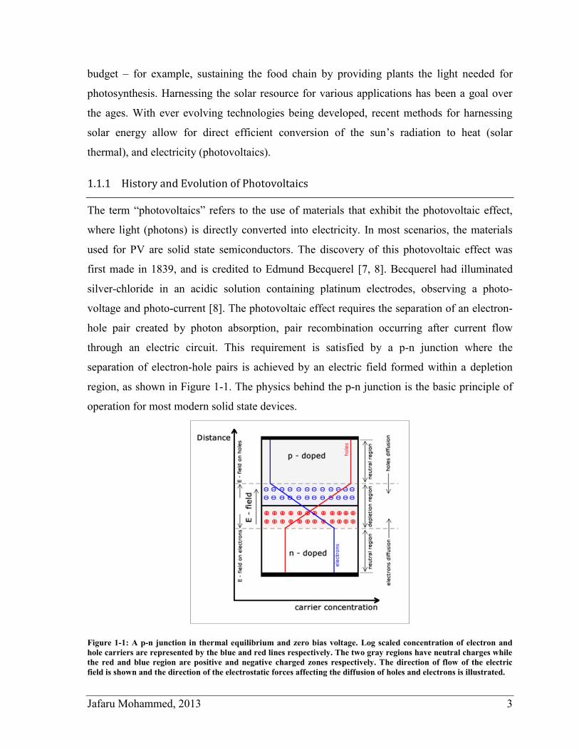
through an electric circuit. This requirement is satisfied by a p-n junction where the
separation of electron-hole pairs is achieved by an electric field formed within a depletion
region, as shown in Figure 1-1. The physics behind the p-n junction is the basic principle of
operation for most modern solid state devices.
Figure 1-1: A p-n junction in thermal equilibrium and zero bias voltage. Log scaled concentration of electron and
hole carriers are represented by the blue and red lines respectively. The two gray regions have neutral charges while
the red and blue region are positive and negative charged zones respectively. The direction of flow of the electric
field is shown and the direction of the electrostatic forces affecting the diffusion of holes and electrons is illustrated.
Jafaru Mohammed, 2013 4
A p-n junction is made of two adjacent semiconductor regions with different doping, as
diagramed in Figure 1-1. An equilibrium carrier concentration is achieved by diffusion of
electrons and holes across the interface, which creates a depletion region maintained by the
electric field arising from the exposed donor (n-region) and acceptor (p-region) dopants [9].
Detailed behaviour and characteristics of the p-n junction were first comprehensively
understood by William Shockley, and his findings were published by 1949-1950 [10].
Consequently, the understanding of p-n junctions paved the way for growth of the solid state
semiconductor industry in developing micro and macro devices such as diodes, transistors
and integrated circuits. Exploitation of PV devices advanced more rapidly in the early 1970’s
when the semiconductor technology had been better understood and methods for design and
fabrication of semiconductor devices had advanced significantly [11]. A detailed description
of the principles of operation for solar cells is presented in section three of this dissertation.
The literature [12] suggests that silicon PV modules were first designed and fabricated
for outdoor use in 1955. This effort was attributed to Bell laboratories in the aim to
investigate methods for powering telecommunication systems. These PV modules were
restricted to spacecraft applications for about 20 years post 1955 [12]. At this point, the race
for terrestrial PV power systems had begun. By the early 1970’s, semiconductor technology
had advanced enough to allow for the development of very large scale integrated circuits,
presaging the development of silicon PV technology for energy use. Increasing demand for
electrical energy brought about the re-evaluation of PV systems for terrestrial applications,
stimulated rapid development [12]. By 1976, some standardization in the manufacturing of
PV modules for terrestrial applications had developed, and PV technology was shown as a
viable source of electricity for terrestrial uses in small scale implementations. However, it
was also apparent that further development of the silicon PV system was required to improve
reliability and efficiency. By 1981, standards had been established for PV module quality
control, with the Jet Propulsion Laboratory publishing the first module qualification under
the US Department of Energy’s (DOE) low-cost solar array program [13]. This set of
qualification tests became the de-facto standard following the US government’s Block V
purchase of modules [11, 14]. Alternative technologies, such as amorphous silicon, cadmium
telluride (CdTe) and copper indium diselenide (CIGS)-based solar cells, began to emerge
creating a challenge for the utilization of the single qualification standard for all PV modules
Jafaru Mohammed, 2013 5
[14]. The increased interest and research into PV led to the proposal and implementation of
various standards for reliability, safety and qualification for a wider spectrum of PV
technologies [13]. Existing standards undergo continuous evolution as technology growth
and development occurs. They include the American Society for Testing and Materials
(ASTM), and the International Organisation for Standardization (ISO) maintained by the
International Electro-technical Commission (IEC) [15].
Despite the relatively poor performance of early PV systems, support continued from
government agencies and businesses alike (perhaps influenced by the power crisis of the
early 1970’s [12]) that perceived solar energy as a clean sustainable and renewable
alternative energy resource. By the year 2000, improvements in technology had brought
about upgrades in characterization and qualification procedures for PV modules, and the
financial value of the industry in the global energy market reached multi-billion dollar values
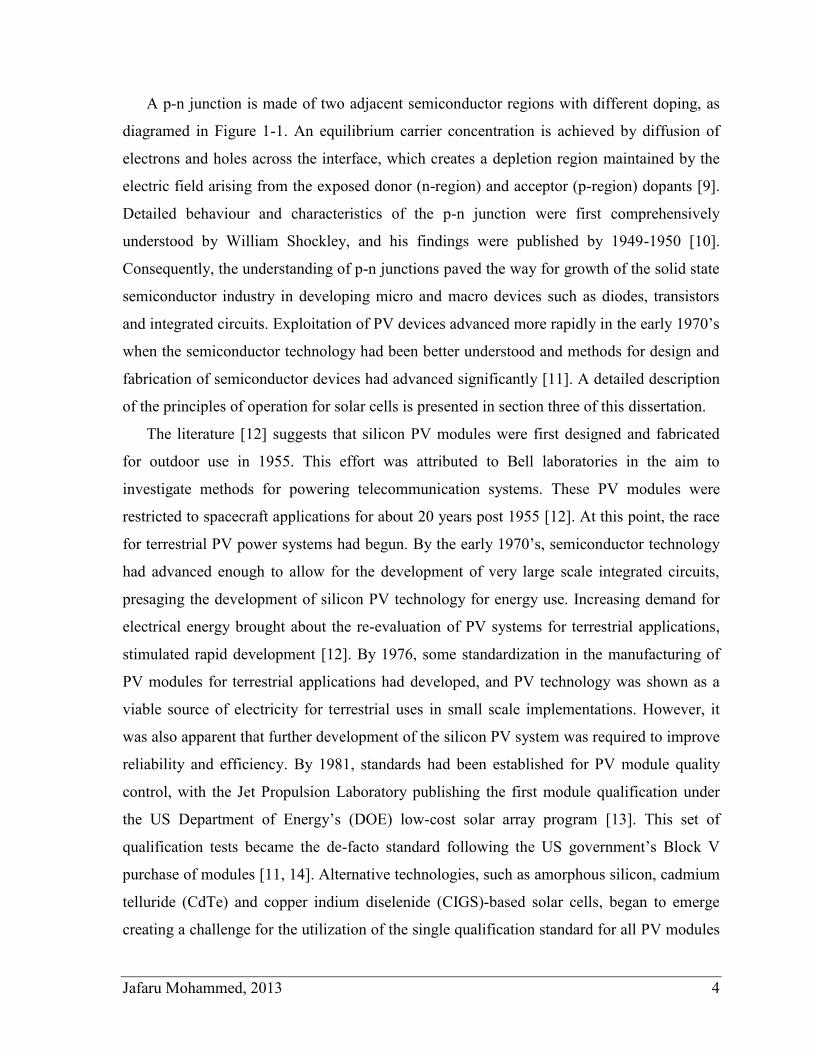
[14, 15]. The average price of solar energy then dropped to $4/W, largely due to increasing
system efficiencies and dwindling process cost. Figure 1-2 illustrates the learning curve for
solar electric energy cost per watt between 1985 and 2010, projected into the future. Future
projection suggests a continuous decrease in cost as the industry continues to mature, but the
projection curve is likely to soon trend asymptotic, with suggestions that this may be below
$1/W [15–17].
Figure 1-2: Learning curve illustrating cost reduction in installed PV systems between 1990 and 2010. Adapted from
[16].
Advances in the design and development of solar cells led to rapid improvements in the
conversion efficiency of silicon cells [12] which helped raise expectations for the efficiency
Jafaru Mohammed, 2013 6
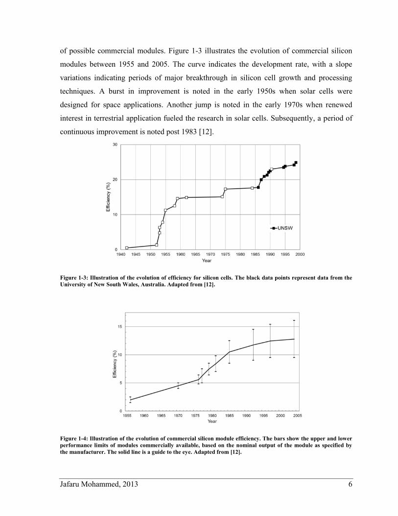
of possible commercial modules. Figure 1-3 illustrates the evolution of commercial silicon
modules between 1955 and 2005. The curve indicates the development rate, with a slope
variations indicating periods of major breakthrough in silicon cell growth and processing
techniques. A burst in improvement is noted in the early 1950s when solar cells were
designed for space applications. Another jump is noted in the early 1970s when renewed
interest in terrestrial application fueled the research in solar cells. Subsequently, a period of
continuous improvement is noted post 1983 [12].
Figure 1-3: Illustration of the evolution of efficiency for silicon cells. The black data points represent data from the
University of New South Wales, Australia. Adapted from [12].
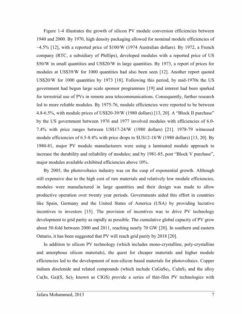
Figure 1-4: Illustration of the evolution of commercial silicon module efficiency. The bars show the upper and lower
performance limits of modules commercially available, based on the nominal output of the module as specified by
the manufacturer. The solid line is a guide to the eye. Adapted from [12].
Jafaru Mohammed, 2013 7
Figure 1-4 illustrates the growth of silicon PV module conversion efficiencies between
1940 and 2000. By 1970, high density packaging allowed for nominal module efficiencies of
~4.5% [12], with a reported price of $100/W (1974 Australian dollars). By 1972, a French
company (RTC, a subsidiary of Phillips), developed modules with a reported price of US
$50/W in small quantities and US$20/W in large quantities. By 1973, a report of prices for
modules at US$39/W for 1000 quantities had also been seen [12]. Another report quoted
US$20/W for 1000 quantities by 1973 [18]. Following this period, by mid-1970s the US
government had begun large scale sponsor programmes [19] and interest had been sparked
for terrestrial use of PVs in remote area telecommunications. Consequently, further research
led to more reliable modules. By 1975-76, module efficiencies were reported to be between
4.8-6.5%, with module prices of US$20-39/W (1980 dollars) [13, 20]. A “Block II purchase”
by the US government between 1976 and 1977 involved modules with efficiencies of 6.0-
7.4% with price ranges between US$17-24/W (1980 dollars) [21]. 1978-79 witnessed
module efficiencies of 6.5-8.4% with price drops to $US12-18/W (1980 dollars) [13, 20]. By
1980-81, major PV module manufacturers were using a laminated module approach to
increase the durability and reliability of modules; and by 1981-85, post “Block V purchase”,
major modules available exhibited efficiencies above 10%.
By 2005, the photovoltaics industry was on the cusp of exponential growth. Although
still expensive due to the high cost of raw materials and relatively low module efficiencies,
modules were manufactured in large quantities and their design was made to allow
productive operation over twenty year periods. Governments aided this effort in countries
like Spain, Germany and the United States of America (USA) by providing lucrative
incentives to investors [15]. The provision of incentives was to drive PV technology
development to grid parity as rapidly as possible. The cumulative global capacity of PV grew
about 50-fold between 2000 and 2011, reaching nearly 70 GW [20]. In southern and eastern
Ontario, it has been suggested that PV will reach grid parity by 2018 [20].
In addition to silicon PV technology (which includes mono-crystalline, poly-crystalline
and amorphous silicon materials), the quest for cheaper materials and higher module
efficiencies led to the development of non-silicon based materials for photovoltaics. Copper
indium diselenide and related compounds (which include CuGaSe2, CuInS2 and the alloy
Cu(In, Ga)(S, Se)2 known as CIGS) provide a series of thin-film PV technologies with
Jafaru Mohammed, 2013 8
complex material properties that appeared very promising in the early days of their discovery
[14]. The process conditions were very flexible and allowed the establishment of well
controlled systems for multisource co-evaporation, which launched CIGS as the fore-runner
in thin-film photovoltaics. Current methods for the production of CIGS cells are based on
mid-1980s methods developed by ARCO solar which involved the sputtering of metal films
with a subsequent selenisation step [12, 16]. The addition of Ga and S helped to increase
efficiency [14]. Another thin-film cell technology is based on cadmium telluride (CdTe),
which has produced cells with efficiencies of up to 16% and module efficiency of up to 10%
[14]. Ongoing research aims to significantly increase the efficiency as it holds great
prospects for large scale photovoltaics due to the CdTe material’s tolerance to dislocation
and its ease of production [14]. The quest for higher efficiencies also brought about the
development of tandem cell and concentrating system. By epitaxially stacking solar cells, III-
V materials have been successfully used to create multi-junction solar cells (MJSC). Such
MJSC typically exploit concentrating optics that deliver high intensity solar irradiation onto
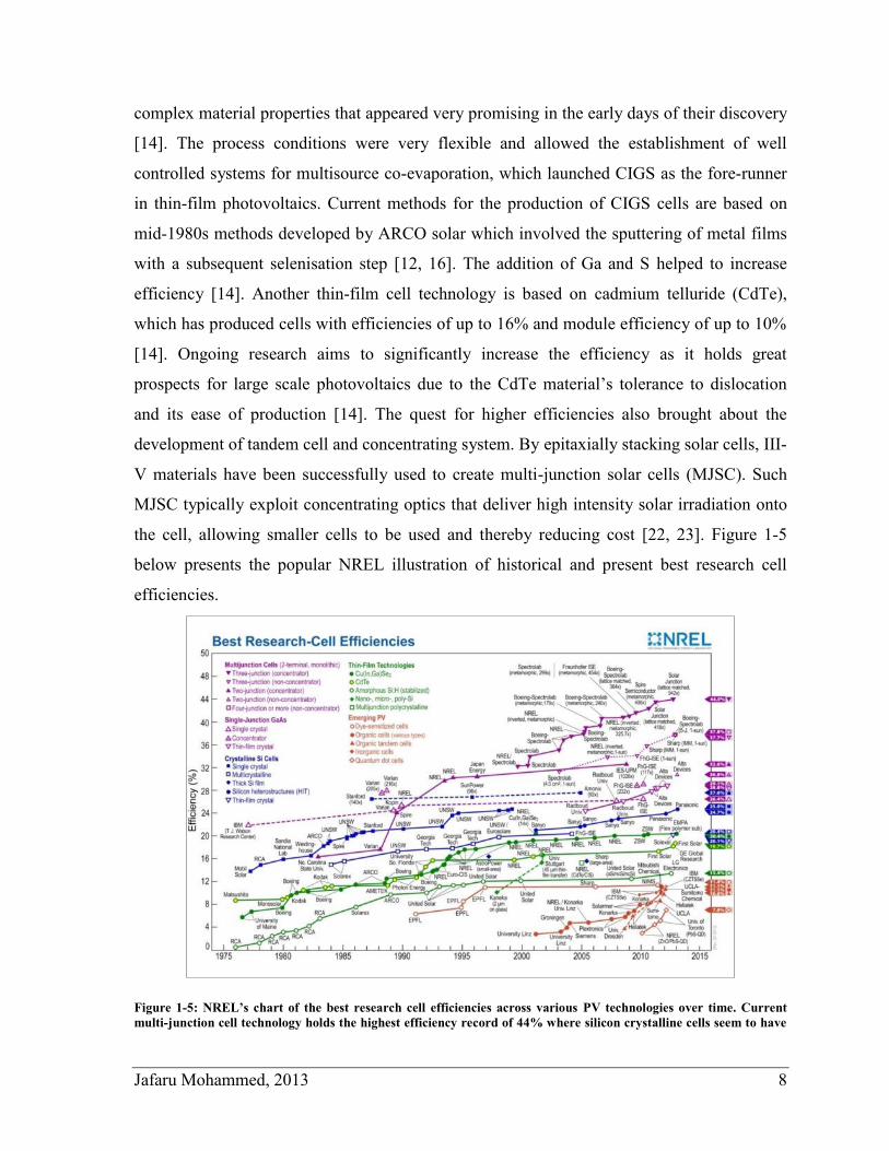
the cell, allowing smaller cells to be used and thereby reducing cost [22, 23]. Figure 1-5
below presents the popular NREL illustration of historical and present best research cell
efficiencies.
Figure 1-5: NREL’s chart of the best research cell efficiencies across various PV technologies over time. Current
multi-junction cell technology holds the highest efficiency record of 44% where silicon crystalline cells seem to have
Jafaru Mohammed, 2013 9
leveled out at a maximum of 27.6% efficiency [24]. The slope of the curve for efficiency growth in multi-junction
cells suggests additional efficiency increase is expected in the future.
1.1.2 Renewable Energy for Sustainable Development
Sustainable development as defined by the Brundland report [5] is described as
“development that meets the need of the present without compromising the ability of future
generations to meet their needs”, and it comprises two factors: (1) the concept of need,
especially those of the world’s poor, and (2) the idea of limitation, which technology and
social organization impose on the environment’s ability to meet present and future needs
[25]. A sense of responsibility towards future generations drives a general consensus, even in
fast developing economies, that there is a need to develop sustainably [5]. The increasing
global population and the growth of consumption imposes a continued increase in the
demand for energy. However, the current dependence on non-renewable sources of energy
poses significant issues that contradict the terms for sustainable development. A
complementary perspective is given by posing the question of how development can be
sustained when fossil and other non-renewable energy resources become depleted. In
addition, there is the emission of toxic waste that accumulates for future generations. The
degradation of the environment by the deposition of toxic materials has a potential to
indirectly hamper the ability of future generations to meet their needs. The choice of energy
resource for development determines the ability of society to develop sustainable [26–28].
Hence, to achieve sustainability, we must shift our energy dependence to clean and
renewable energies. PV technologies using semiconductor materials to directly convert solar
irradiation into electrical energy is one such clean and renewable energy.
1.1.3 A Brief Introduction to PV Systems and their Limitations
Fundamental physics constrains the ability of PV technology to convert incident solar
radiation into electrical energy. It is the band gap of the material from which a PV cell is
formed that determines the wavelengths of the incident spectrum available for solar
absorption. Factors such as carrier recombination, carrier life time and the probability of
electron/hole generation via photon excitation in a solar cell provide a basis for determining
the theoretical limit for various solar cell technologies. Cell efficiency η is a gauge for
performance and it is calculated as the ratio of the electrical power Pout generated by the solar
Jafaru Mohammed, 2013 10
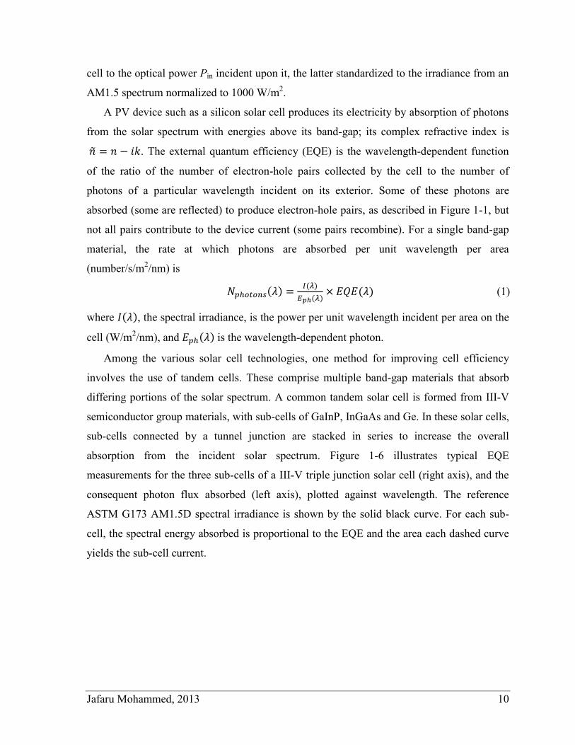
cell to the optical power Pin incident upon it, the latter standardized to the irradiance from an
AM1.5 spectrum normalized to 1000 W/m2.
A PV device such as a silicon solar cell produces its electricity by absorption of photons
from the solar spectrum with energies above its band-gap; its complex refractive index is
. The external quantum efficiency (EQE) is the wavelength-dependent function
of the ratio of the number of electron-hole pairs collected by the cell to the number of
photons of a particular wavelength incident on its exterior. Some of these photons are
absorbed (some are reflected) to produce electron-hole pairs, as described in Figure 1-1, but
not all pairs contribute to the device current (some pairs recombine). For a single band-gap
material, the rate at which photons are absorbed per unit wavelength per area
(number/s/m2/nm) is
( ) ( )
( ) ( ) (1)
where ( ), the spectral irradiance, is the power per unit wavelength incident per area on the
cell (W/m2/nm), and ( ) is the wavelength-dependent photon.
Among the various solar cell technologies, one method for improving cell efficiency
involves the use of tandem cells. These comprise multiple band-gap materials that absorb
differing portions of the solar spectrum. A common tandem solar cell is formed from III-V
semiconductor group materials, with sub-cells of GaInP, InGaAs and Ge. In these solar cells,
sub-cells connected by a tunnel junction are stacked in series to increase the overall
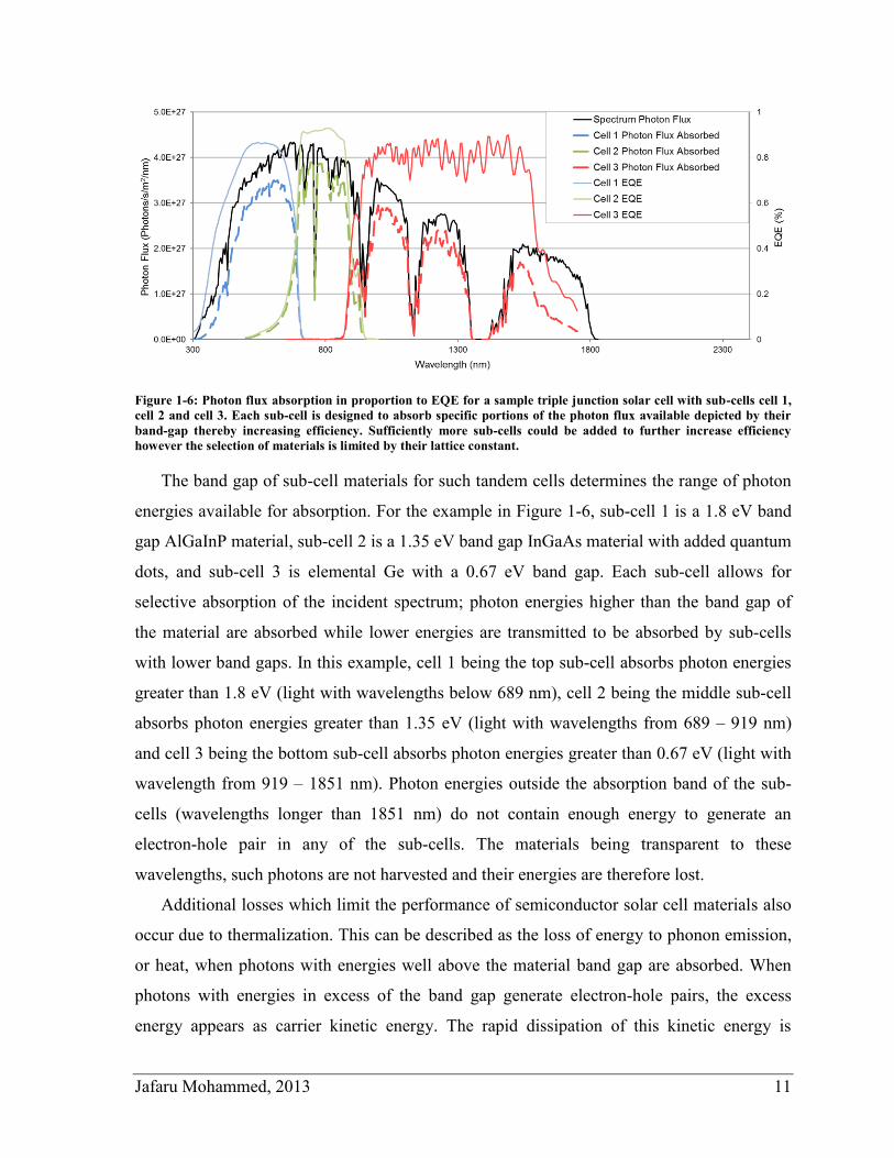
absorption from the incident solar spectrum. Figure 1-6 illustrates typical EQE
measurements for the three sub-cells of a III-V triple junction solar cell (right axis), and the
consequent photon flux absorbed (left axis), plotted against wavelength. The reference
ASTM G173 AM1.5D spectral irradiance is shown by the solid black curve. For each sub-
cell, the spectral energy absorbed is proportional to the EQE and the area each dashed curve
yields the sub-cell current.
Jafaru Mohammed, 2013 11
Figure 1-6: Photon flux absorption in proportion to EQE for a sample triple junction solar cell with sub-cells cell 1,
cell 2 and cell 3. Each sub-cell is designed to absorb specific portions of the photon flux available depicted by their
band-gap thereby increasing efficiency. Sufficiently more sub-cells could be added to further increase efficiency
however the selection of materials is limited by their lattice constant.
The band gap of sub-cell materials for such tandem cells determines the range of photon
energies available for absorption. For the example in Figure 1-6, sub-cell 1 is a 1.8 eV band
gap AlGaInP material, sub-cell 2 is a 1.35 eV band gap InGaAs material with added quantum
dots, and sub-cell 3 is elemental Ge with a 0.67 eV band gap. Each sub-cell allows for
selective absorption of the incident spectrum; photon energies higher than the band gap of
the material are absorbed while lower energies are transmitted to be absorbed by sub-cells
with lower band gaps. In this example, cell 1 being the top sub-cell absorbs photon energies
greater than 1.8 eV (light with wavelengths below 689 nm), cell 2 being the middle sub-cell
absorbs photon energies greater than 1.35 eV (light with wavelengths from 689 – 919 nm)
and cell 3 being the bottom sub-cell absorbs photon energies greater than 0.67 eV (light with
wavelength from 919 – 1851 nm). Photon energies outside the absorption band of the sub-
cells (wavelengths longer than 1851 nm) do not contain enough energy to generate an
electron-hole pair in any of the sub-cells. The materials being transparent to these
wavelengths, such photons are not harvested and their energies are therefore lost.
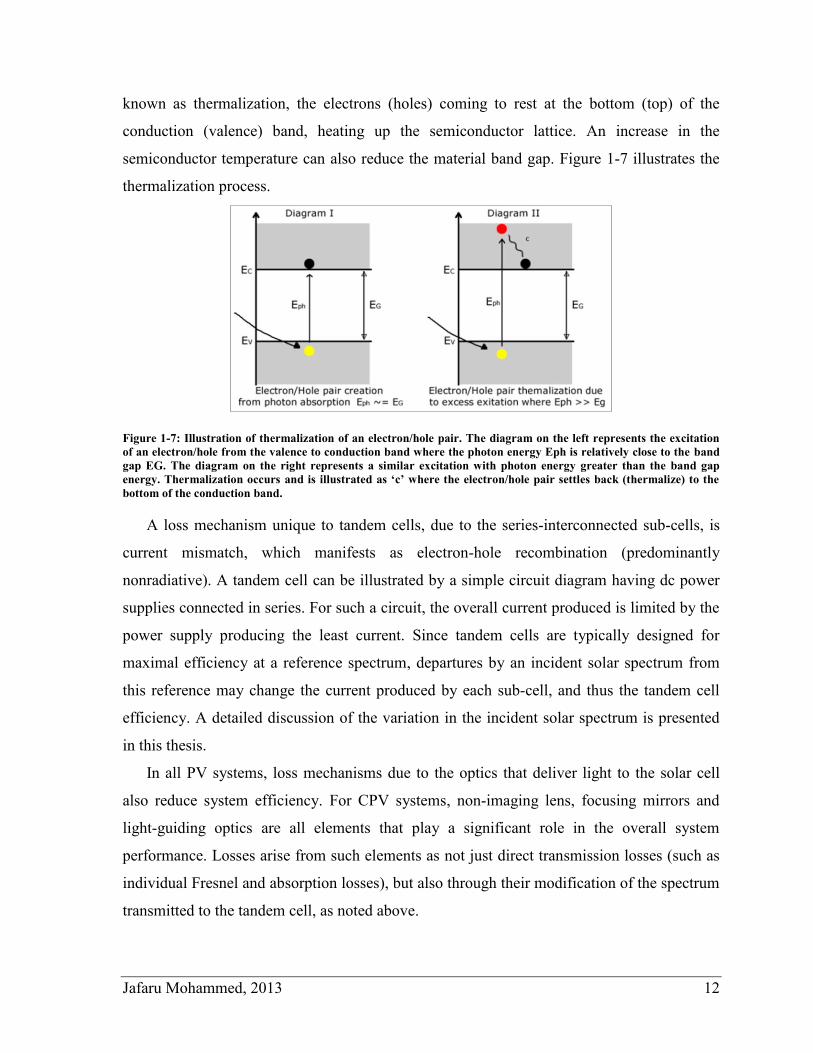
Additional losses which limit the performance of semiconductor solar cell materials also
occur due to thermalization. This can be described as the loss of energy to phonon emission,
or heat, when photons with energies well above the material band gap are absorbed. When
photons with energies in excess of the band gap generate electron-hole pairs, the excess
energy appears as carrier kinetic energy. The rapid dissipation of this kinetic energy is
Jafaru Mohammed, 2013 12
known as thermalization, the electrons (holes) coming to rest at the bottom (top) of the
conduction (valence) band, heating up the semiconductor lattice. An increase in the
semiconductor temperature can also reduce the material band gap. Figure 1-7 illustrates the
thermalization process.
Figure 1-7: Illustration of thermalization of an electron/hole pair. The diagram on the left represents the excitation
of an electron/hole from the valence to conduction band where the photon energy Eph is relatively close to the band
gap EG. The diagram on the right represents a similar excitation with photon energy greater than the band gap
energy. Thermalization occurs and is illustrated as ‘c’ where the electron/hole pair settles back (thermalize) to the
bottom of the conduction band.
A loss mechanism unique to tandem cells, due to the series-interconnected sub-cells, is
current mismatch, which manifests as electron-hole recombination (predominantly
nonradiative). A tandem cell can be illustrated by a simple circuit diagram having dc power
supplies connected in series. For such a circuit, the overall current produced is limited by the
power supply producing the least current. Since tandem cells are typically designed for
maximal efficiency at a reference spectrum, departures by an incident solar spectrum from
this reference may change the current produced by each sub-cell, and thus the tandem cell
efficiency. A detailed discussion of the variation in the incident solar spectrum is presented
in this thesis.
In all PV systems, loss mechanisms due to the optics that deliver light to the solar cell
also reduce system efficiency. For CPV systems, non-imaging lens, focusing mirrors and
light-guiding optics are all elements that play a significant role in the overall system
performance. Losses arise from such elements as not just direct transmission losses (such as
individual Fresnel and absorption losses), but also through their modification of the spectrum
transmitted to the tandem cell, as noted above.
Jafaru Mohammed, 2013 13
1.2 Research Motivation
Motivation for research in photovoltaics is driven globally by the emerging consensus on the
need for cleaner renewable energy for sustainable development. Achieving a greener future
requires better understanding future energy sources, which in this dissertation is solar energy.
A key consideration to effectively harvesting the solar resource is understanding its variation
in temporal and spatial dimensions, since these impact the economic decisions driving
investment into the technology. Energy yield analysis must be carried out to determine the
PV potential of a given site over the investment period. With better the input data, in both
time and space, more accurate energy yield models may be constructed.
Persistent increases in population, urbanization and developmental growth combined
with modern lifestyles requiring large scale manufacturing, construction and commerce lead
to very high energy demands [28] with escalating costs as non-renewable energy sources are
depleted. To ensure the availability of energy for future consumption, as well as a safe
environment free from pollutants, such costs must be comprehensively understood, and
should include such externalities as atmospheric pollutants and greenhouse gases (GHG)
emissions. To achieve these goals and mitigate future energy crisis, action must be taken
now to develop and utilize alternative renewable and sustainable energy technology such as
wind, solar and hydro energy. This need to develop and utilize new technology for energy
production provides the essential motivation for researching topics surrounding CPV solar
energy systems in this thesis.
The PV industry has long used measured datasets like the Canadian weather energy and
engineering datasets (CWEEDS), or simulated data from atmospheric radiative transfer
models such as SMARTS2, to provide energy yield estimates within acceptable error
margins. Their use has been employed in energy evaluation application packages such as PV
Watts and RetScreen. Spatial and temporal variations of atmospheric constituents like
aerosols and perceptible water vapour impact the components of the incident solar spectrum
(direct and scattered) to various degrees [29], and are of particular interest to CPV research
since tandem cells use spectral partitioning to increase efficiency. The cloud sensitivity of
CPV systems is considerably higher than that of PV systems, and research suggests that CPV
systems may also be more sensitive to spectral variations [30]. Hence, the assumptions which
allow PV systems to exploit existing solar resource datasets for accurate energy yield
Jafaru Mohammed, 2013 14
evaluation may not be true for CPV. This has motivated a study of the characteristics of the
local solar resource and drove the implementation of database architecture for acquiring and
storing spectral measurements and atmospheric data at 2-minute intervals. The data, from the
University of Ottawa’s SUNLAB APECS test site, provided the basis for analysing the local
spectral sensitivity of energy yield models.
1.3 Thesis Objectives
This thesis addresses four specific objectives: (1) developing software tools for measurement
systems; (2) the acquisition of solar spectra, their databasing and analysis; (3) developing
faster photovoltaic models; and (4) CPV energy yield analysis. These objectives are
described more comprehensively below.
Intuitive software packages enable researchers to perform required tasks in efficient
ways, saving time and increasing accuracies by reducing measurement errors. The
development of a current-voltage (IV) curve acquisition package was required to allow
measurement of IV systems using a Keithley or Kepco power supply with a Spectrolab solar
demonstrator (XT-30). Likewise, user-friendly software packages to perform cell spatial
uniformity measurements, light source spectral spatial uniformity and cell reliability tests
were developed.
A solar test site was instrumented at the University of Ottawa to measure direct normal
spectral irradiance, DNI and a range of meteorological conditions. Software and architecture
design was required for the collection and storage of highly temporal datasets to promote
ease of data retrieval. Data collection was implemented using a dedicated computer system
with adequate autonomous software packages capable of acquiring and storing data recorded
from the outdoor instruments. The datasets were used for location specific spectral analysis
and the evaluation of the local solar resource within the context of local meteorological
conditions.
Faster PV models enable assessing very large datasets at minimal cost. Functional
simulation concepts have been proposed for PV cells using a single or double diode
equivalent circuit model [31, 32]. Conventional methods for implementing such simulations
with sequential calculations consume considerable time. An object oriented tuneable PV cell
model with parallel programming was developed to ensure result accuracy with exponential
Jafaru Mohammed, 2013 15
reductions in bulk simulation times. The object characteristics of the PV cell model provide a
window for in-depth probes of cell parameters while persistent database storage of the
simulated cell model allows for post simulation detailed analysis.
Considering the economics and financing involved, energy yield analysis plays a critical
role in feasibility studies for CPV system implementation. Since CPV is sensitive to spectral
variation [30], which in turn is impacted by meteorological conditions, an in-depth
understanding of the local temporal meteorological effect on CPV energy yield is needed to
assist in long term predictive energy yield evaluation for site specific CPV feasibility studies.
Using our Ottawa locale as a case sturdy, the measured spectral datasets were compared with
other datasets representing historical norms, to constructively quantify the various factors
that affect energy yield evaluation. Using detailed CPV models, the energy yield analysis
involved temporal characterization of variations between the measured and other datasets
determining the overall effect of factors such as cloud cover and aerosols on various CPV
architectures, both at the cell and system level.
1.4 Thesis Overview
Five chapters encapsulate the main contents of this dissertation. Chapter one has presented
an introduction to the background of PV systems from an historical perspective, noting both
the need to develop and utilize sustainable and renewable energy sources and the challenges
faced in their realization. An historical evolution of PV systems was presented, and the basic
physical and practical limits to its implementation were highlighted. The introduction
provides the background for discussions of various factors affecting PV energy production
and usage, such as the solar resource and its relationship with the local atmospheric or
meteorological conditions and the economics involved in the implementation of grid
connected PV systems.
Chapter two discusses issues that relate to PV and CPV systems, reviewing the
fundamentals behind the nature of the incident solar resource. It focuses on the atmospheric
absorptive components responsible for altering the extraterrestrial black body spectral
profile. Here, a “Simple Model of the Atmospheric Radiative Transfer of Sunshine version
2” (SMARTS2), is exploited to simulate the spectral distribution and power of the solar
resource. An overview of the APECS test site at the University of Ottawa is given,
Jafaru Mohammed, 2013 16
presenting the data acquisition system and maintenance procedures for quality control of the
recorded dataset.
In chapter three, instruments and software tools developed for characterising and testing
CPV systems at the University of Ottawa’s SUNLAB research lab are discussed within the
context of their development, operation and results. A single diode model, based on
publications by Sakurada and Varshni [31, 32], is presented and discussed. Their theory was
used to develop a java application, which utilized object oriented programming techniques,
to model PV cell response. The java application utilizes parallel programming and database
storage methods to speed up simulation time and allow storage of runtime results for
recurrent post analysis.
In chapter four, an algorithm to reconstruct the spectral distribution of the solar
irradiance from parameterised aerosol optical depth data (taken from measured irradiance) is
presented. Data gathered from the measuring instruments on the APECS test site, historical
data and typical meteorological data was used in the model. A comprehensive approach was
taken to quantitatively de-convolute temporal effects that may affect long term CPV energy
yield analysis, such as meteorological variations, atmospheric aerosols and air-mass. A case
sturdy was performed for the APECS test site using the measured temporal spectral DNI data
sets. Using PV system simulation software introduced in chapter 3, constructive and
deconstructive comparisons were carried out on various energy yield recipes.
In chapter 5, the simulations, models and results are summarized. The advantages of the
systems developed in chapter 4 are discussed and their practical limitations are highlighted.
Suggestions for further investigation are proposed in the context of sustainable renewable
energy.
Jafaru Mohammed, 2013 17
2 The Solar Resource
To effectively analyse energy production in PV systems, modelling and simulation of the
solar resource is necessary. In this chapter, the fundamentals of the solar radiation incident
on the earth’s surface are described, and the relationship between the earth’s movement and
observed solar radiation is explained in terms of its spectral distribution. Calculation of the
solar azimuth and elevation angles is necessary for crude tracking in dual axis trackers which
is necessary for CPV system implementation. The algorithms presented in this section
explain the equations to derive temporal solar azimuth and elevation.
2.1 Introduction
The sun is the central energy generator within the earth’s solar system [33]. It is a class G2-V
yellow dwarf star having a radius of 6.96 x 10⁷ km. Nuclear fusion of hydrogen at its centre
produces radiant energy with helium as a waste by-product. The mean radiation intensity
from the surface of the sun is 2.01x10⁷ (Wm
-2sr
-1) for an integrated total of 2.85 x 10
26 W
[34]. A small portion of this solar energy arrives at the earth’s surface making life possible
on the planet. All natural cycles necessary for life on earth which include rain, wind,
photosynthesis and ocean current are directly or indirectly driven by the solar radiation
incident on the earth.
The energy from the sun is radiated by its corona at an effective blackbody temperature
of about 5800 K. At the mean Earth-Sun distance, the sun subtends a solid angle of 9.24
milliradians (or 0.53˚), thus the sun is truly not a point light source and the sun rays are not
truly parallel [34]. For the given portion of the solar energy received by the earth, the mean
distance between the earth and sun of 1.50 x 10⁹ km limits the power of the radiation
reaching the top of the earth’s atmosphere to about 1366.1 Wm-2
± 7.0 Wm-2
. The elliptical
nature of the earth’s orbit causes variations in the distance between the earth and sun (the
Earth’s radius vector) to the tune of about 3.39% [34]. This distance is from the perihelion
where the distance is closest to the aphelion where the distance is farthest. The variation in
distance causes an inversely proportional variation in solar radiation intensity received at the
top of the earth’s atmosphere denoted by 1/R2, where R is the radius vector or mean earth-sun
distance. For this reasons, the solar radiation intensity varies annually from December (1414
Jafaru Mohammed, 2013 18
Wm-2
) to July (1321 Wm-2
). Complementary causes for variation in the incident solar
intensity at the top of the earth’s atmosphere include variations in brightness of the sun,
sunspot cycle and solar oscillations. Where calculations of the solar resource incident on the
earth’s atmosphere (the extraterrestrial irradiance) are required, adequate corrections are
incorporated to address these fluctuations. The total annual energy received from the sun on
the earth’s surface is estimated to be about 1.5 x 10¹⁸
kWh which is more than the global
energy need in the year 2000 (~1014
kWh/a) [33] by a factor of 1500.
Solar energy incident on the earth’s surface has been attenuated by the atmosphere which
contains gaseous and aqueous molecules that absorb solar radiation as a function of
frequency. Diffraction, reflection and partial transmission by atmospheric constituents splits
the solar irradiance into several components that exhibit distinctive characteristics and
relationship. These components include the direct beam, global horizontal and global diffuse
irradiance. A range of simple to complex algorithms exists for modeling the atmospheric
radiative transfer of sunshine to estimate the various irradiance components. For the various
configurations for acquiring irradiance data, plane transfer algorithms also exist for
modelling sunshine observations at various planes.
The period and duration of sunshine depends on factors such as geographical location
and weather conditions. The amount of radiation incident yearly varies for various belts of
the planet. Locations at the northern and southern hemisphere generally receive less radiation
when compared to sub and middle belt areas. Measuring the solar irradiance incident on the
earth’s surface requires a plethora of instruments in various configurations to cover the
irradiance components. The spectral distribution of solar radiation is measured with
spectroradiometers sensitive to wavelengths between 280 and 4000 nanometers.
Pyrheliometer and pyranometer instruments are designed for absolute measurements of the
direct beam and global horizontal components respectively.
2.2 Earth and Sun
Electromagnetic radiation from the sun spans the electromagnetic spectrum, from X-rays and
gamma rays ranging to very long wavelength radio waves. In the context of this dissertation,
the range of wavelengths will be restricted to spectral regions relevant for CPV systems,
Jafaru Mohammed, 2013 19
namely that between the ultraviolet (UV, beginning at 280 nm) and the near infrared (NIR,
ending at 4000 nm).
2.2.1 The Earth’s Incident Solar Radiation
The sun is a black body radiator whose surface temperature is approximately 5800 K. The
sun has a spectral emission that can thus be characterised by the Stefan-Boltzmann and
Planck Radiation Law. The Stefan-Boltzmann law, a relation which describes the power
radiated from the black body as a function of its surface temperature is given as
, (2)
where is the energy flux density, is the emissivity for the emitting surface, is the
Stefan-Boltzmann constant (J K-1
), is the area of the emitting surface in
meters, is the temperature of the surface in Kelvin, and is the time in which the black
body is observed in seconds.
Planck’s Radiation Law describes the electromagnetic radiation emitted from a black
body at thermal equilibrium for any given temperature as
( )
(
) , (3)
where is the spectral irradiance or radiant flux per unit area which is a function of
wavelength and the absolute temperature , is Plank’s constant a (J s)
and is the speed of light.in vacuum constant at (ms-1
). Using these
equations, substituting the appropriate values for the sun, the overall power incident on the
earth’s atmosphere can be deduced. The Planck theory provides a first approximation to the
spectral distribution of the sun [34].
Research suggests that the sun is not a perfect radiator nor is it of uniform composition.
In estimates, the sun is elementally composed of 92% hydrogen and 7.8% helium. A smaller
fraction of the sun to the tune of 0.2% is made up of a mix of about 60 other elements which
are mainly metals such as iron, magnesium, chromium, carbon and silicon [35, 36]. Knowing
this, advanced models have been developed to predict its spectral irradiance. One such model
has been developed by Kurucz [35, 37, 38] who used elemental compositions to compute the
spectral irradiance at relatively high resolution. He predicted a significant departure from the
black body radiation.
Jafaru Mohammed, 2013 20
Figure 2-1: Simulated values for extraterrestrial irradiance at the top of the earth’s atmosphere taken from
SMARTS2, plotted against a “perfect” black body radiation based on the Planck’s radiation law with a temperature
of 6000K.
Figure 2-1 presents a simulated low resolution extraterrestrial (ETR) spectrum contrasted
with an ideal black body radiation spectrum based on the Planck function for a temperature
of 6000 K. At specific wavelengths in the infrared region beyond 2 µm, it should be noted
that the differences are minimal between the two spectra. Significant differences at the
shorter wavelengths are a result of partial absorption of radiation largely arising from the
various constituents of the sun earlier discussed. Each unique elemental constituent of the
sun absorbs the spectrum with a specific characteristic; hence lines or bands are noted in the
resultant spectrum which corresponds to absorption by unique materials. These lines, first
observed by Fraunhofer, are named after him [34].
2.2.2 Earth-Sun Temporal Coordinates
As mentioned previously, solar radiation from the sun incident on the top of the earth’s
atmosphere is referred to as the extraterrestrial radiation. Varying sun-earth distance due to
the revolution of the earth on its elliptical orbit, among other factors determines the power of
the incident extraterrestrial radiation. For the purpose of describing the solar resource
available on earth and its periodic temporal variability, it is therefore important to understand
the movement of the earth in relation to the sun.
Gravitational forces between the sun and the earth keep the earth revolving around the
sun on an elliptical path known as the earth’s orbit. The earth is tilted on an axis
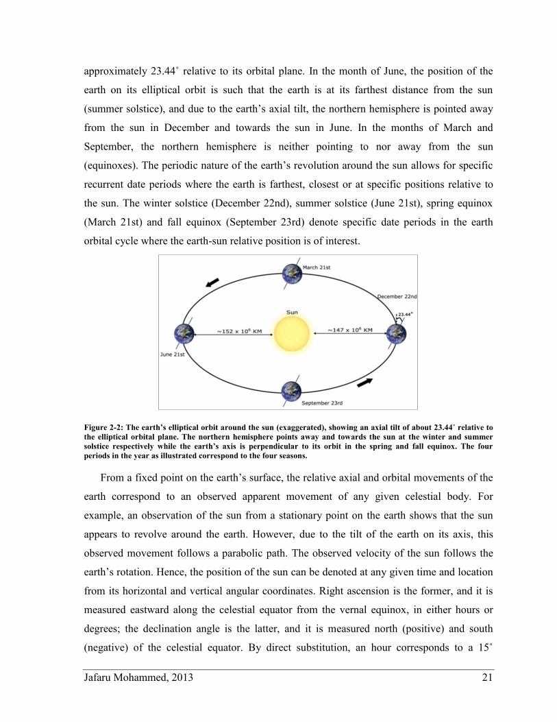
Jafaru Mohammed, 2013 21
approximately 23.44˚ relative to its orbital plane. In the month of June, the position of the
earth on its elliptical orbit is such that the earth is at its farthest distance from the sun
(summer solstice), and due to the earth’s axial tilt, the northern hemisphere is pointed away
from the sun in December and towards the sun in June. In the months of March and
September, the northern hemisphere is neither pointing to nor away from the sun
(equinoxes). The periodic nature of the earth’s revolution around the sun allows for specific
recurrent date periods where the earth is farthest, closest or at specific positions relative to
the sun. The winter solstice (December 22nd), summer solstice (June 21st), spring equinox
(March 21st) and fall equinox (September 23rd) denote specific date periods in the earth
orbital cycle where the earth-sun relative position is of interest.
Figure 2-2: The earth’s elliptical orbit around the sun (exaggerated), showing an axial tilt of about 23.44˚ relative to
the elliptical orbital plane. The northern hemisphere points away and towards the sun at the winter and summer
solstice respectively while the earth’s axis is perpendicular to its orbit in the spring and fall equinox. The four
periods in the year as illustrated correspond to the four seasons.
From a fixed point on the earth’s surface, the relative axial and orbital movements of the
earth correspond to an observed apparent movement of any given celestial body. For
example, an observation of the sun from a stationary point on the earth shows that the sun
appears to revolve around the earth. However, due to the tilt of the earth on its axis, this
observed movement follows a parabolic path. The observed velocity of the sun follows the
earth’s rotation. Hence, the position of the sun can be denoted at any given time and location
from its horizontal and vertical angular coordinates. Right ascension is the former, and it is
measured eastward along the celestial equator from the vernal equinox, in either hours or
degrees; the declination angle is the latter, and it is measured north (positive) and south
(negative) of the celestial equator. By direct substitution, an hour corresponds to a 15˚
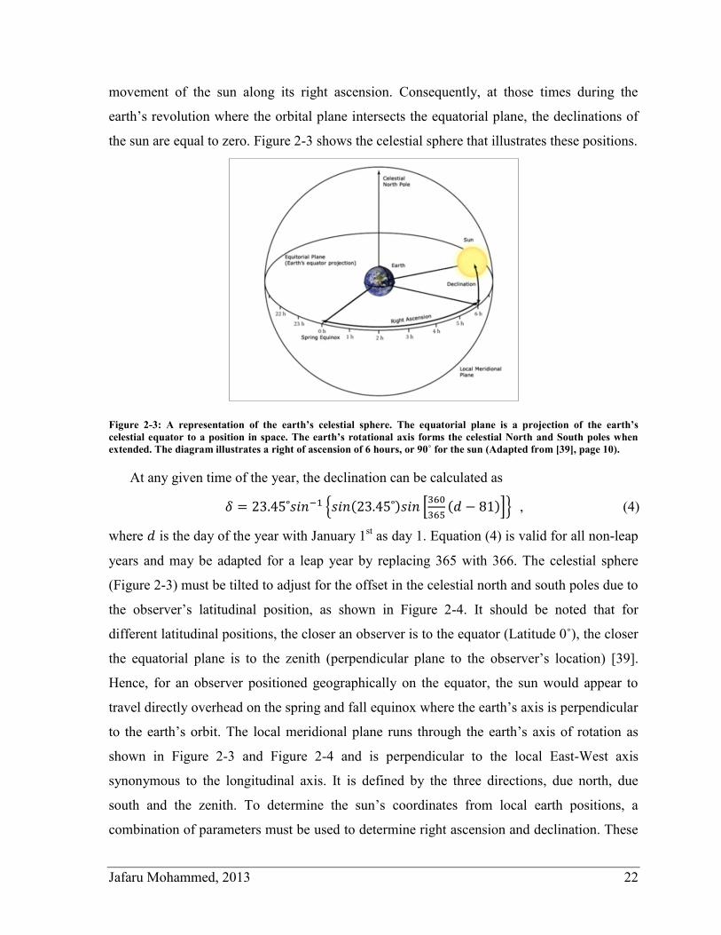
Jafaru Mohammed, 2013 22
movement of the sun along its right ascension. Consequently, at those times during the
earth’s revolution where the orbital plane intersects the equatorial plane, the declinations of
the sun are equal to zero. Figure 2-3 shows the celestial sphere that illustrates these positions.
Figure 2-3: A representation of the earth’s celestial sphere. The equatorial plane is a projection of the earth’s
celestial equator to a position in space. The earth’s rotational axis forms the celestial North and South poles when
extended. The diagram illustrates a right of ascension of 6 hours, or 90˚ for the sun (Adapted from [39], page 10).
At any given time of the year, the declination can be calculated as
{ ( ) [
( )]} , (4)
where is the day of the year with January 1st as day 1. Equation (4) is valid for all non-leap
years and may be adapted for a leap year by replacing 365 with 366. The celestial sphere
(Figure 2-3) must be tilted to adjust for the offset in the celestial north and south poles due to
the observer’s latitudinal position, as shown in Figure 2-4. It should be noted that for
different latitudinal positions, the closer an observer is to the equator (Latitude 0˚), the closer
the equatorial plane is to the zenith (perpendicular plane to the observer’s location) [39].
Hence, for an observer positioned geographically on the equator, the sun would appear to
travel directly overhead on the spring and fall equinox where the earth’s axis is perpendicular
to the earth’s orbit. The local meridional plane runs through the earth’s axis of rotation as
shown in Figure 2-3 and Figure 2-4 and is perpendicular to the local East-West axis
synonymous to the longitudinal axis. It is defined by the three directions, due north, due
south and the zenith. To determine the sun’s coordinates from local earth positions, a
combination of parameters must be used to determine right ascension and declination. These
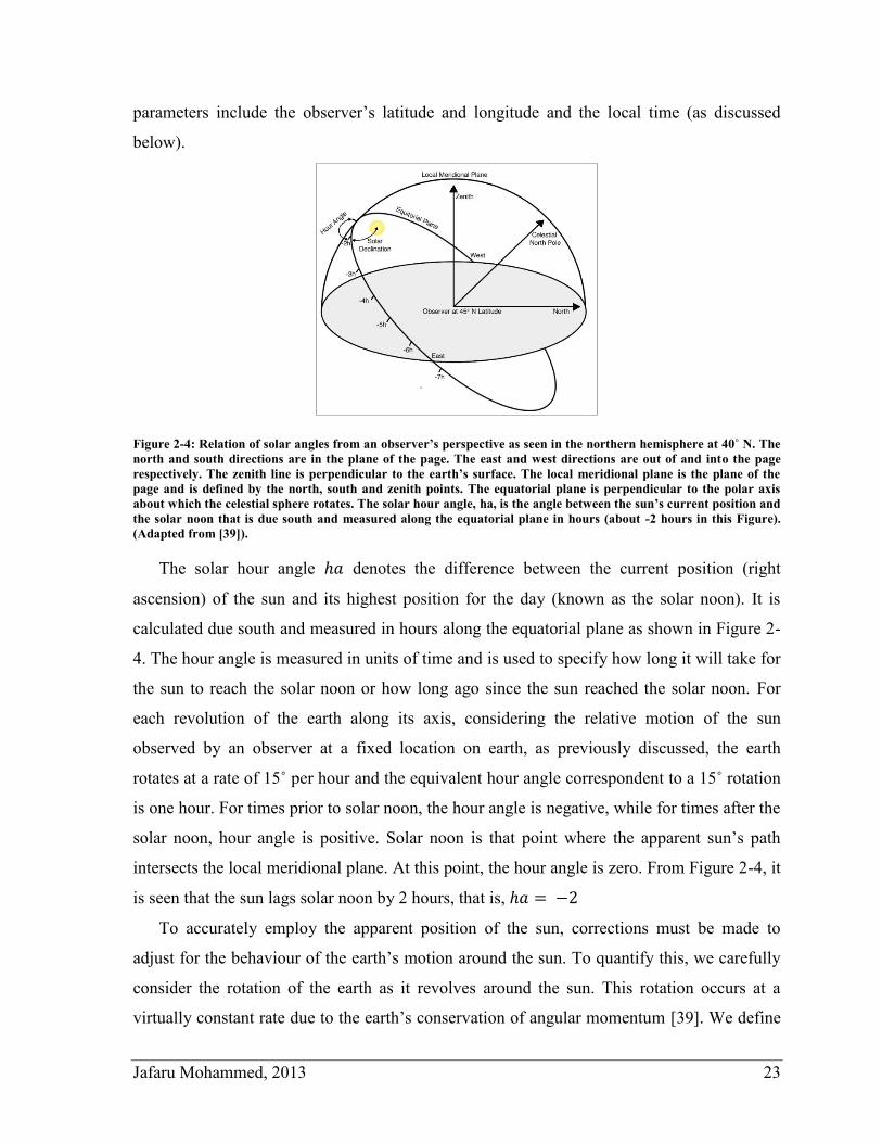
Jafaru Mohammed, 2013 23
parameters include the observer’s latitude and longitude and the local time (as discussed
below).
Figure 2-4: Relation of solar angles from an observer’s perspective as seen in the northern hemisphere at 40˚ N. The
north and south directions are in the plane of the page. The east and west directions are out of and into the page
respectively. The zenith line is perpendicular to the earth’s surface. The local meridional plane is the plane of the
page and is defined by the north, south and zenith points. The equatorial plane is perpendicular to the polar axis
about which the celestial sphere rotates. The solar hour angle, ha, is the angle between the sun’s current position and
the solar noon that is due south and measured along the equatorial plane in hours (about -2 hours in this Figure).
(Adapted from [39]).
The solar hour angle denotes the difference between the current position (right
ascension) of the sun and its highest position for the day (known as the solar noon). It is
calculated due south and measured in hours along the equatorial plane as shown in Figure 2-
4. The hour angle is measured in units of time and is used to specify how long it will take for
the sun to reach the solar noon or how long ago since the sun reached the solar noon. For
each revolution of the earth along its axis, considering the relative motion of the sun
observed by an observer at a fixed location on earth, as previously discussed, the earth
rotates at a rate of 15˚ per hour and the equivalent hour angle correspondent to a 15˚ rotation
is one hour. For times prior to solar noon, the hour angle is negative, while for times after the
solar noon, hour angle is positive. Solar noon is that point where the apparent sun’s path
intersects the local meridional plane. At this point, the hour angle is zero. From Figure 2-4, it
is seen that the sun lags solar noon by 2 hours, that is,
To accurately employ the apparent position of the sun, corrections must be made to
adjust for the behaviour of the earth’s motion around the sun. To quantify this, we carefully
consider the rotation of the earth as it revolves around the sun. This rotation occurs at a
virtually constant rate due to the earth’s conservation of angular momentum [39]. We define
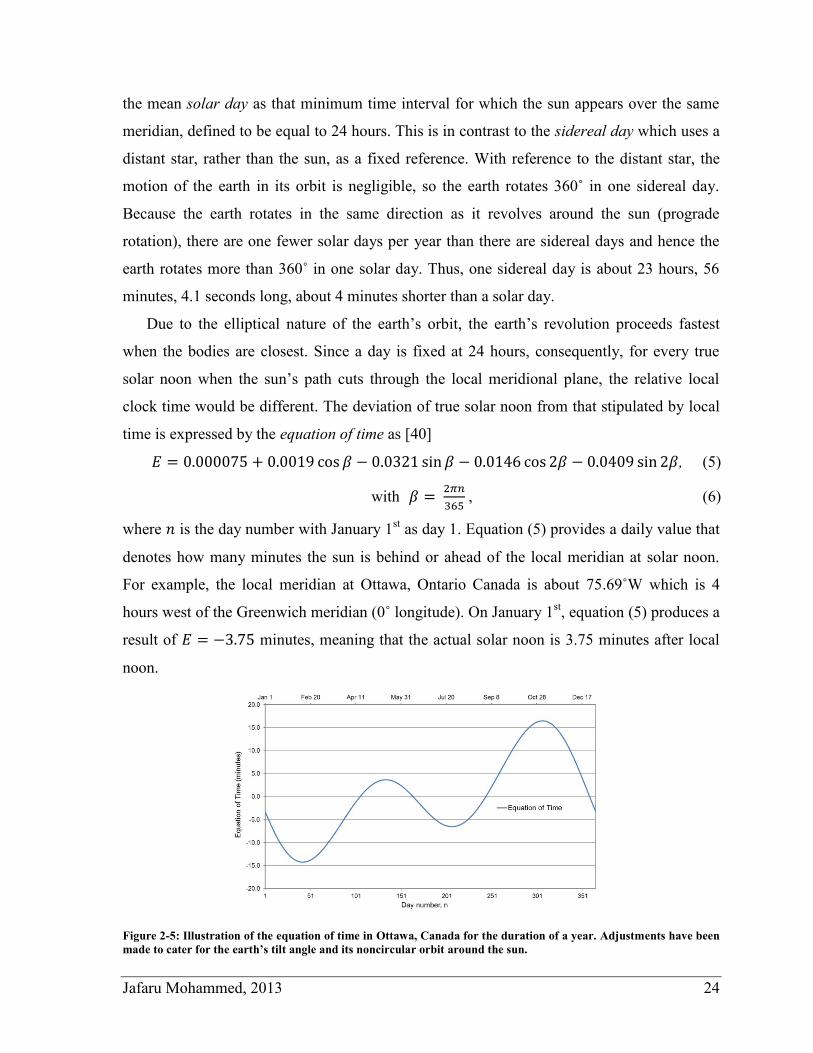
Jafaru Mohammed, 2013 24
the mean solar day as that minimum time interval for which the sun appears over the same
meridian, defined to be equal to 24 hours. This is in contrast to the sidereal day which uses a
distant star, rather than the sun, as a fixed reference. With reference to the distant star, the
motion of the earth in its orbit is negligible, so the earth rotates 360˚ in one sidereal day.
Because the earth rotates in the same direction as it revolves around the sun (prograde
rotation), there are one fewer solar days per year than there are sidereal days and hence the
earth rotates more than 360˚ in one solar day. Thus, one sidereal day is about 23 hours, 56
minutes, 4.1 seconds long, about 4 minutes shorter than a solar day.
Due to the elliptical nature of the earth’s orbit, the earth’s revolution proceeds fastest
when the bodies are closest. Since a day is fixed at 24 hours, consequently, for every true
solar noon when the sun’s path cuts through the local meridional plane, the relative local
clock time would be different. The deviation of true solar noon from that stipulated by local
time is expressed by the equation of time as [40]
, (5)
with
, (6)
where is the day number with January 1st as day 1. Equation (5) provides a daily value that
denotes how many minutes the sun is behind or ahead of the local meridian at solar noon.
For example, the local meridian at Ottawa, Ontario Canada is about 75.69˚W which is 4
hours west of the Greenwich meridian (0˚ longitude). On January 1st, equation (5) produces a
result of minutes, meaning that the actual solar noon is 3.75 minutes after local
noon.
Figure 2-5: Illustration of the equation of time in Ottawa, Canada for the duration of a year. Adjustments have been
made to cater for the earth’s tilt angle and its noncircular orbit around the sun.
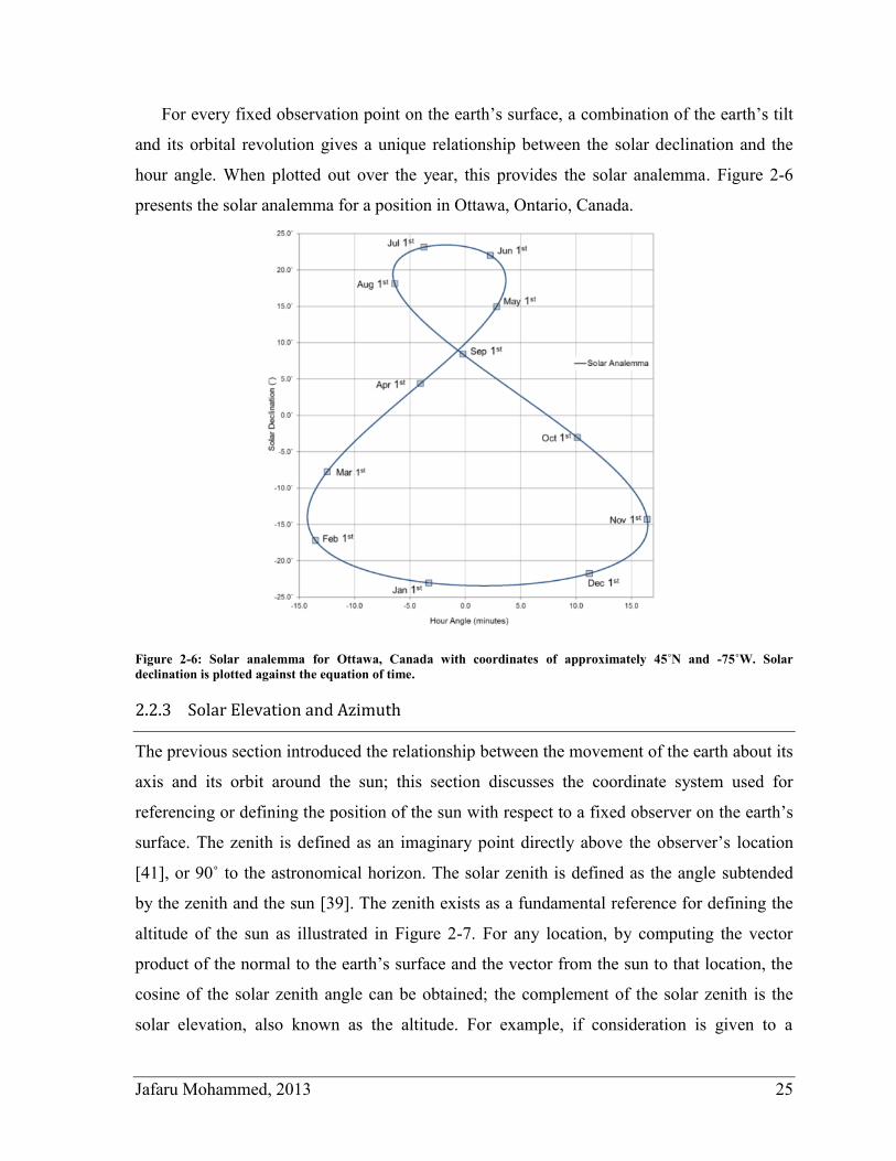
Jafaru Mohammed, 2013 25
For every fixed observation point on the earth’s surface, a combination of the earth’s tilt
and its orbital revolution gives a unique relationship between the solar declination and the
hour angle. When plotted out over the year, this provides the solar analemma. Figure 2-6
presents the solar analemma for a position in Ottawa, Ontario, Canada.
Figure 2-6: Solar analemma for Ottawa, Canada with coordinates of approximately 45˚N and -75˚W. Solar
declination is plotted against the equation of time.
2.2.3 Solar Elevation and Azimuth
The previous section introduced the relationship between the movement of the earth about its
axis and its orbit around the sun; this section discusses the coordinate system used for
referencing or defining the position of the sun with respect to a fixed observer on the earth’s
surface. The zenith is defined as an imaginary point directly above the observer’s location
[41], or 90˚ to the astronomical horizon. The solar zenith is defined as the angle subtended
by the zenith and the sun [39]. The zenith exists as a fundamental reference for defining the
altitude of the sun as illustrated in Figure 2-7. For any location, by computing the vector
product of the normal to the earth’s surface and the vector from the sun to that location, the
cosine of the solar zenith angle can be obtained; the complement of the solar zenith is the
solar elevation, also known as the altitude. For example, if consideration is given to a
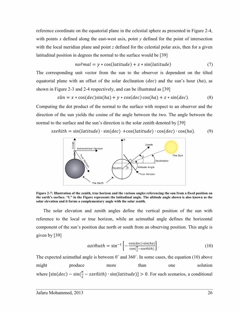
Jafaru Mohammed, 2013 26
reference coordinate on the equatorial plane in the celestial sphere as presented in Figure 2-4,
with points x defined along the east-west axis, point y defined for the point of intersection
with the local meridian plane and point z defined for the celestial polar axis, then for a given
latitudinal position in degrees the normal to the surface would be [39]
( ) ( ) (7)
The corresponding unit vector from the sun to the observer is dependent on the tilted
equatorial plane with an offset of the solar declination ( ) and the sun’s hour ( ), as
shown in Figure 2-3 and 2-4 respectively, and can be illustrated as [39]
( ) ( ) ( ) ( ) ( ). (8)
Computing the dot product of the normal to the surface with respect to an observer and the
direction of the sun yields the cosine of the angle between the two. The angle between the
normal to the surface and the sun’s direction is the solar zenith denoted by [39]
( ) ( ) ( ) ( ) ( ). (9)
Figure 2-7: Illustration of the zenith, true horizon and the various angles referencing the sun from a fixed position on
the earth’s surface. “L” in the Figure represents the latitudinal angle. The altitude angle shown is also known as the
solar elevation and it forms a complementary angle with the solar zenith.
The solar elevation and zenith angles define the vertical position of the sun with
reference to the local or true horizon, while an azimuthal angle defines the horizontal
component of the sun’s position due north or south from an observing position. This angle is
given by [39]
[ ( ) ( )
(
)
] . (10)
The expected azimuthal angle is between 0˚ and 360˚. In some cases, the equation (10) above
might produce more than one solution
where ( ) (
) ( ) . For such scenarios, a conditional
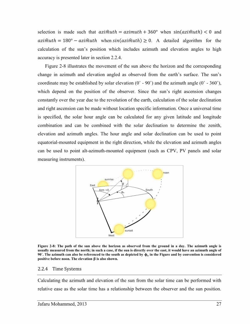
Jafaru Mohammed, 2013 27
selection is made such that when ( ) and
when ( ) . A detailed algorithm for the
calculation of the sun’s position which includes azimuth and elevation angles to high
accuracy is presented later in section 2.2.4.
Figure 2-8 illustrates the movement of the sun above the horizon and the corresponding
change in azimuth and elevation angled as observed from the earth’s surface. The sun’s
coordinate may be established by solar elevation (0˚ - 90˚) and the azimuth angle (0˚ - 360˚),
which depend on the position of the observer. Since the sun’s right ascension changes
constantly over the year due to the revolution of the earth, calculation of the solar declination
and right ascension can be made without location specific information. Once a universal time
is specified, the solar hour angle can be calculated for any given latitude and longitude
combination and can be combined with the solar declination to determine the zenith,
elevation and azimuth angles. The hour angle and solar declination can be used to point
equatorial-mounted equipment in the right direction, while the elevation and azimuth angles
can be used to point alt-azimuth-mounted equipment (such as CPV, PV panels and solar
measuring instruments).
Figure 2-8: The path of the sun above the horizon as observed from the ground in a day. The azimuth angle is
usually measured from the north; in such a case, if the sun is directly over the east, it would have an azimuth angle of
90˚. The azimuth can also be referenced to the south as depicted by in the Figure and by convention is considered
positive before noon. The elevation is also shown.
2.2.4 Time Systems
Calculating the azimuth and elevation of the sun from the solar time can be performed with
relative ease as the solar time has a relationship between the observer and the sun position.
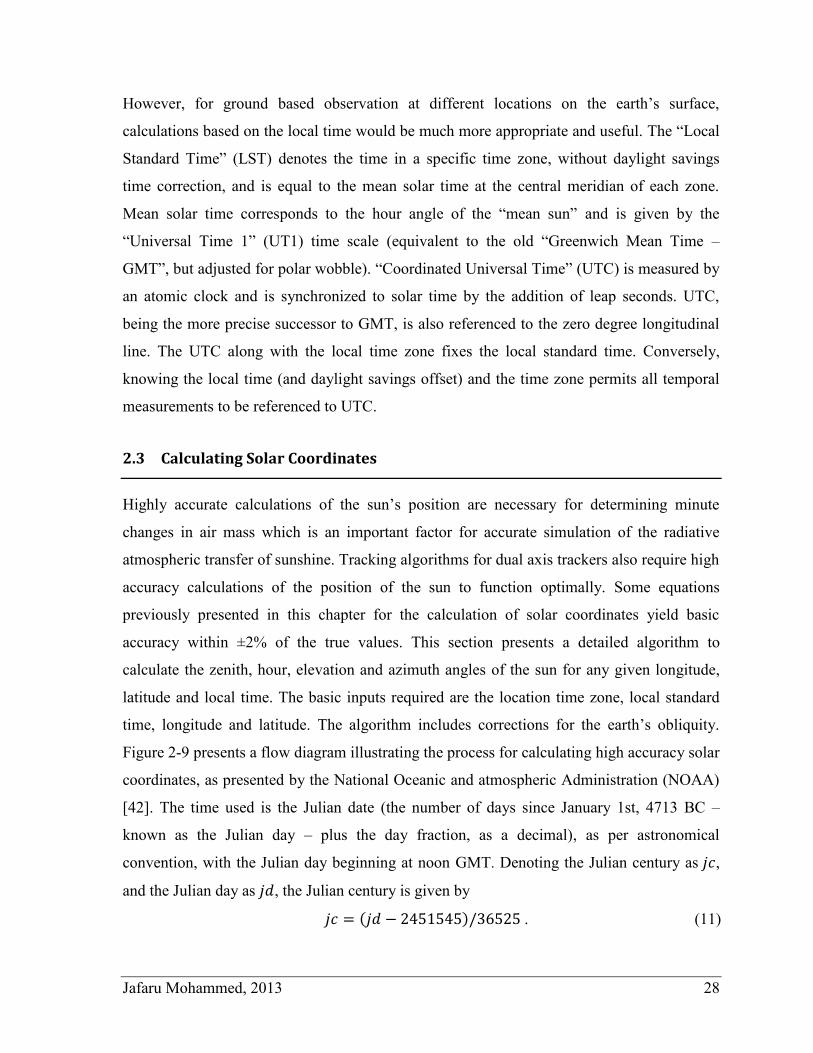
Jafaru Mohammed, 2013 28
However, for ground based observation at different locations on the earth’s surface,
calculations based on the local time would be much more appropriate and useful. The “Local
Standard Time” (LST) denotes the time in a specific time zone, without daylight savings
time correction, and is equal to the mean solar time at the central meridian of each zone.
Mean solar time corresponds to the hour angle of the “mean sun” and is given by the
“Universal Time 1” (UT1) time scale (equivalent to the old “Greenwich Mean Time –
GMT”, but adjusted for polar wobble). “Coordinated Universal Time” (UTC) is measured by
an atomic clock and is synchronized to solar time by the addition of leap seconds. UTC,
being the more precise successor to GMT, is also referenced to the zero degree longitudinal
line. The UTC along with the local time zone fixes the local standard time. Conversely,
knowing the local time (and daylight savings offset) and the time zone permits all temporal
measurements to be referenced to UTC.
2.3 Calculating Solar Coordinates
Highly accurate calculations of the sun’s position are necessary for determining minute
changes in air mass which is an important factor for accurate simulation of the radiative
atmospheric transfer of sunshine. Tracking algorithms for dual axis trackers also require high
accuracy calculations of the position of the sun to function optimally. Some equations
previously presented in this chapter for the calculation of solar coordinates yield basic
accuracy within ±2% of the true values. This section presents a detailed algorithm to
calculate the zenith, hour, elevation and azimuth angles of the sun for any given longitude,
latitude and local time. The basic inputs required are the location time zone, local standard
time, longitude and latitude. The algorithm includes corrections for the earth’s obliquity.
Figure 2-9 presents a flow diagram illustrating the process for calculating high accuracy solar
coordinates, as presented by the National Oceanic and atmospheric Administration (NOAA)
[42]. The time used is the Julian date (the number of days since January 1st, 4713 BC –
known as the Julian day – plus the day fraction, as a decimal), as per astronomical
convention, with the Julian day beginning at noon GMT. Denoting the Julian century as ,
and the Julian day as , the Julian century is given by
( ) . (11)
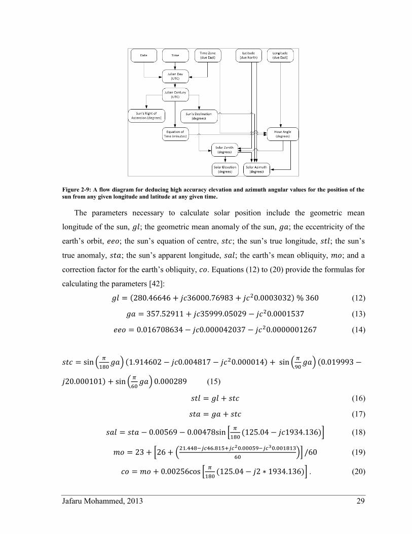
Jafaru Mohammed, 2013 29
Figure 2-9: A flow diagram for deducing high accuracy elevation and azimuth angular values for the position of the
sun from any given longitude and latitude at any given time.
The parameters necessary to calculate solar position include the geometric mean
longitude of the sun, ; the geometric mean anomaly of the sun, ; the eccentricity of the
earth’s orbit, ; the sun’s equation of centre, ; the sun’s true longitude, ; the sun’s
true anomaly, ; the sun’s apparent longitude, ; the earth’s mean obliquity, ; and a
correction factor for the earth’s obliquity, . Equations (12) to (20) provide the formulas for
calculating the parameters [42]:
( ) (12)
(13)
(14)
(
) ( ) (
) (
) (
) (15)
(16)
(17)
[
( )] (18)
[ (
)] (19)
[
( )] . (20)
Jafaru Mohammed, 2013 30
These parameters permit the sun’s right ascension ( in degrees) and declination angle (
in degrees) to be calculated as [42]
{ [ (
) (
) (
)]} (21)
{ [ (
) (
)]} . (22)
The equation of time ( , in minutes), the solar time ( , in minutes) and the hour angle ( ,
in degrees) can then be computed from the following [42]:
{ (
)}
(23)
[ (
) (
) (
) (
)
(
) (
)] (24)
( ) (25)
{ [
(
)
(
)
(
) (
) (
)]} (26)
where is the fraction of the day since midnight, is the observer’s longitude in
degrees due east, is the observer’s time zone and is the observer’s latitude due
north. The solar zenith and elevation angles can now be calculated as [42]
{ [ (
) (
) (
) (
) (
)]} (27)
(28)
Finally, the azimuth angle can be calculated using equation (10).
2.4 Atmospheric Transmission of Sunlight
The earth’s atmosphere is a layered sequence of gasses retained by the earth’s gravitational
force. The atmosphere is primarily composed of about 78% nitrogen (N) and 21% oxygen
(O2). Other gasses such as argon (AR), carbon dioxide (CO2), water vapour (H2O), methane
(CH4), ozone (O3) and particulate matter represent about 1% of the atmosphere’s
composition. The commonly referenced boundary between the earth’s atmosphere and outer
space is given by the Karman line. The atmosphere acts as a filter with variable transmission
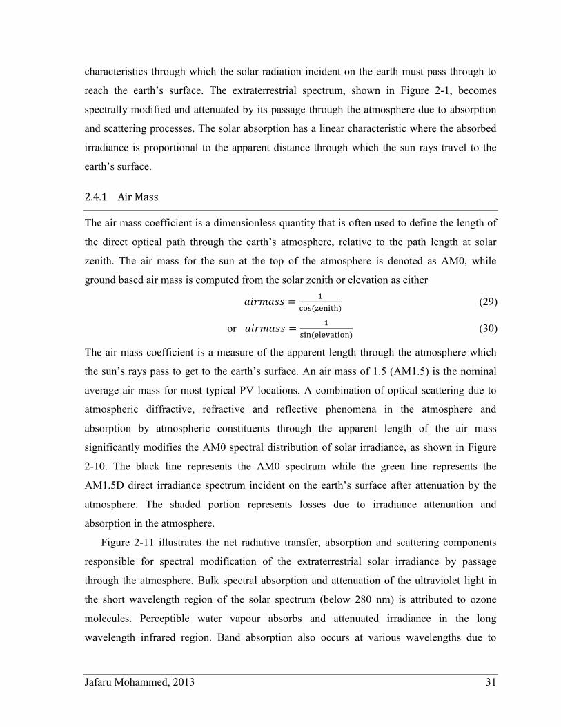
Jafaru Mohammed, 2013 31
characteristics through which the solar radiation incident on the earth must pass through to
reach the earth’s surface. The extraterrestrial spectrum, shown in Figure 2-1, becomes
spectrally modified and attenuated by its passage through the atmosphere due to absorption
and scattering processes. The solar absorption has a linear characteristic where the absorbed
irradiance is proportional to the apparent distance through which the sun rays travel to the
earth’s surface.
2.4.1 Air Mass
The air mass coefficient is a dimensionless quantity that is often used to define the length of
the direct optical path through the earth’s atmosphere, relative to the path length at solar
zenith. The air mass for the sun at the top of the atmosphere is denoted as AM0, while
ground based air mass is computed from the solar zenith or elevation as either
( ) (29)
or
( ) (30)
The air mass coefficient is a measure of the apparent length through the atmosphere which
the sun’s rays pass to get to the earth’s surface. An air mass of 1.5 (AM1.5) is the nominal
average air mass for most typical PV locations. A combination of optical scattering due to
atmospheric diffractive, refractive and reflective phenomena in the atmosphere and
absorption by atmospheric constituents through the apparent length of the air mass
significantly modifies the AM0 spectral distribution of solar irradiance, as shown in Figure
2-10. The black line represents the AM0 spectrum while the green line represents the
AM1.5D direct irradiance spectrum incident on the earth’s surface after attenuation by the
atmosphere. The shaded portion represents losses due to irradiance attenuation and
absorption in the atmosphere.
Figure 2-11 illustrates the net radiative transfer, absorption and scattering components
responsible for spectral modification of the extraterrestrial solar irradiance by passage
through the atmosphere. Bulk spectral absorption and attenuation of the ultraviolet light in
the short wavelength region of the solar spectrum (below 280 nm) is attributed to ozone
molecules. Perceptible water vapour absorbs and attenuated irradiance in the long
wavelength infrared region. Band absorption also occurs at various wavelengths due to
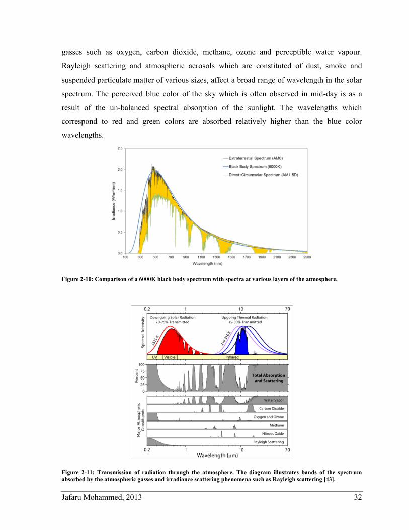
Jafaru Mohammed, 2013 32
gasses such as oxygen, carbon dioxide, methane, ozone and perceptible water vapour.
Rayleigh scattering and atmospheric aerosols which are constituted of dust, smoke and
suspended particulate matter of various sizes, affect a broad range of wavelength in the solar
spectrum. The perceived blue color of the sky which is often observed in mid-day is as a
result of the un-balanced spectral absorption of the sunlight. The wavelengths which
correspond to red and green colors are absorbed relatively higher than the blue color
wavelengths.
Figure 2-10: Comparison of a 6000K black body spectrum with spectra at various layers of the atmosphere.
Figure 2-11: Transmission of radiation through the atmosphere. The diagram illustrates bands of the spectrum
absorbed by the atmospheric gasses and irradiance scattering phenomena such as Rayleigh scattering [43].
Jafaru Mohammed, 2013 33
Air mass decreases from sunrise to noon and increases from noon to sunset and the
apparent depth of atmosphere that the rays of the sun needs to pass through varies
proportionally, as does the absorption of sunlight. Figure 2-12 illustrates the spectral effect of
the variation in absorption, refection, diffraction and refraction by atmospheric constituents
on the incident Direct Normal Irradiance (DNI) component of the sunshine. It should be
noted that the peak power wavelength shifts with airmass and this phenomenon poses a
challenge for current matching in epitaxially grown multi-junction solar cells.
Figure 2-12: SMARTS2 simulated direct normal spectra irradiance illustrating spectral variation due to air mass
change.
2.4.2 DNI, GHI and Diffuse Irradiance
The presence of particulate matter in the atmosphere results in the reflection and scattering of
sunlight. Sunlight detected by an observer from the entire sky dome is known as the global
irradiance, and it may be subdivided into several classes on the basis of its various angular
distributions. These components are the direct normal irradiance (DNI), the global horizontal
irradiance (GHI), and the diffuse irradiance (DHI). Each irradiance component has unique
optical characteristics that depend on atmospheric conditions, as described below.
2.4.2.1 Diffuse Irradiance
The diffuse irradiance (DHI) arises from a combination of sources. It consists of light
scattered from its direct path through the atmosphere by particulate matter (gases or clouds)
toward the observer. This scattered light can originate directly from the sun, from light
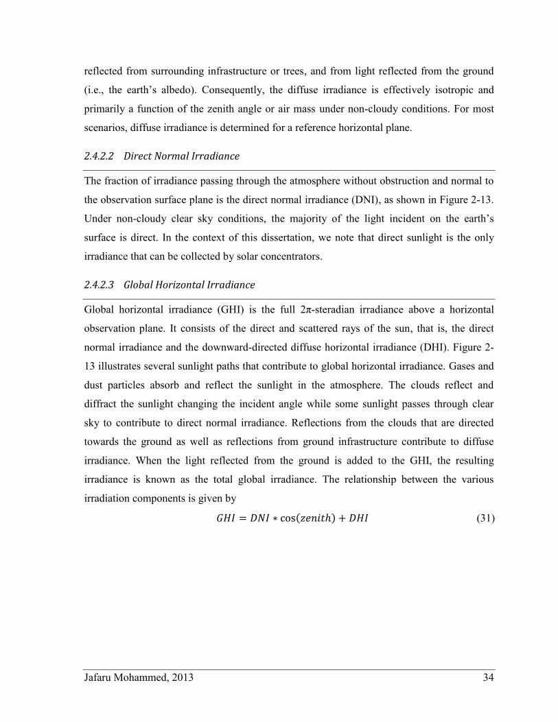
Jafaru Mohammed, 2013 34
reflected from surrounding infrastructure or trees, and from light reflected from the ground
(i.e., the earth’s albedo). Consequently, the diffuse irradiance is effectively isotropic and
primarily a function of the zenith angle or air mass under non-cloudy conditions. For most
scenarios, diffuse irradiance is determined for a reference horizontal plane.
2.4.2.2 Direct Normal Irradiance
The fraction of irradiance passing through the atmosphere without obstruction and normal to
the observation surface plane is the direct normal irradiance (DNI), as shown in Figure 2-13.
Under non-cloudy clear sky conditions, the majority of the light incident on the earth’s
surface is direct. In the context of this dissertation, we note that direct sunlight is the only
irradiance that can be collected by solar concentrators.
2.4.2.3 Global Horizontal Irradiance
Global horizontal irradiance (GHI) is the full 2π-steradian irradiance above a horizontal
observation plane. It consists of the direct and scattered rays of the sun, that is, the direct
normal irradiance and the downward-directed diffuse horizontal irradiance (DHI). Figure 2-
13 illustrates several sunlight paths that contribute to global horizontal irradiance. Gases and
dust particles absorb and reflect the sunlight in the atmosphere. The clouds reflect and
diffract the sunlight changing the incident angle while some sunlight passes through clear
sky to contribute to direct normal irradiance. Reflections from the clouds that are directed
towards the ground as well as reflections from ground infrastructure contribute to diffuse
irradiance. When the light reflected from the ground is added to the GHI, the resulting
irradiance is known as the total global irradiance. The relationship between the various
irradiation components is given by
( ) (31)
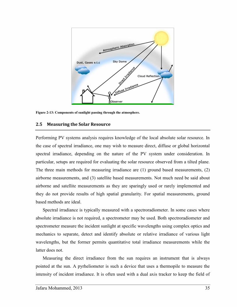
Jafaru Mohammed, 2013 35
Figure 2-13: Components of sunlight passing through the atmosphere.
2.5 Measuring the Solar Resource
Performing PV systems analysis requires knowledge of the local absolute solar resource. In
the case of spectral irradiance, one may wish to measure direct, diffuse or global horizontal
spectral irradiance, depending on the nature of the PV system under consideration. In
particular, setups are required for evaluating the solar resource observed from a tilted plane.
The three main methods for measuring irradiance are (1) ground based measurements, (2)
airborne measurements, and (3) satellite based measurements. Not much need be said about
airborne and satellite measurements as they are sparingly used or rarely implemented and
they do not provide results of high spatial granularity. For spatial measurements, ground
based methods are ideal.
Spectral irradiance is typically measured with a spectroradiometer. In some cases where
absolute irradiance is not required, a spectrometer may be used. Both spectroradiometer and
spectrometer measure the incident sunlight at specific wavelengths using complex optics and
mechanics to separate, detect and identify absolute or relative irradiance of various light
wavelengths, but the former permits quantitative total irradiance measurements while the
latter does not.
Measuring the direct irradiance from the sun requires an instrument that is always
pointed at the sun. A pyrheliometer is such a device that uses a thermopile to measure the
intensity of incident irradiance. It is often used with a dual axis tracker to keep the field of
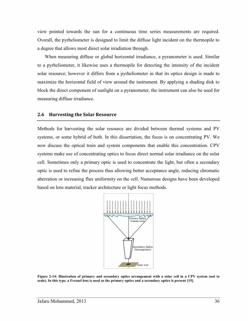
Jafaru Mohammed, 2013 36
view pointed towards the sun for a continuous time series measurements are required.
Overall, the pyrheliometer is designed to limit the diffuse light incident on the thermopile to
a degree that allows most direct solar irradiation through.
When measuring diffuse or global horizontal irradiance, a pyranometer is used. Similar
to a pyrheliometer, it likewise uses a thermopile for detecting the intensity of the incident
solar resource; however it differs from a pyrheliometer in that its optics design is made to
maximize the horizontal field of view around the instrument. By applying a shading disk to
block the direct component of sunlight on a pyranometer, the instrument can also be used for
measuring diffuse irradiance.
2.6 Harvesting the Solar Resource
Methods for harvesting the solar resource are divided between thermal systems and PV
systems, or some hybrid of both. In this dissertation, the focus is on concentrating PV. We
now discuss the optical train and system components that enable this concentration. CPV
systems make use of concentrating optics to focus direct normal solar irradiance on the solar
cell. Sometimes only a primary optic is used to concentrate the light, but often a secondary
optic is used to refine the process thus allowing better acceptance angle, reducing chromatic
aberration or increasing flux uniformity on the cell. Numerous designs have been developed
based on lens material, tracker architecture or light focus methods.
Figure 2-14: Illustration of primary and secondary optics arrangement with a solar cell in a CPV system (not to
scale). In this type, a Fresnel lens is used as the primary optics and a secondary optics is present [15].
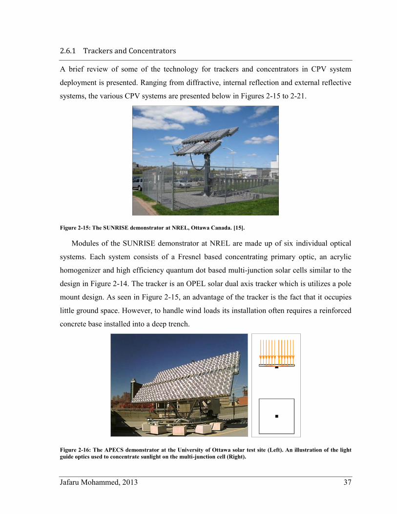
Jafaru Mohammed, 2013 37
2.6.1 Trackers and Concentrators
A brief review of some of the technology for trackers and concentrators in CPV system
deployment is presented. Ranging from diffractive, internal reflection and external reflective
systems, the various CPV systems are presented below in Figures 2-15 to 2-21.
Figure 2-15: The SUNRISE demonstrator at NREL, Ottawa Canada. [15].
Modules of the SUNRISE demonstrator at NREL are made up of six individual optical
systems. Each system consists of a Fresnel based concentrating primary optic, an acrylic
homogenizer and high efficiency quantum dot based multi-junction solar cells similar to the
design in Figure 2-14. The tracker is an OPEL solar dual axis tracker which is utilizes a pole
mount design. As seen in Figure 2-15, an advantage of the tracker is the fact that it occupies
little ground space. However, to handle wind loads its installation often requires a reinforced
concrete base installed into a deep trench.
Figure 2-16: The APECS demonstrator at the University of Ottawa solar test site (Left). An illustration of the light
guide optics used to concentrate sunlight on the multi-junction cell (Right).
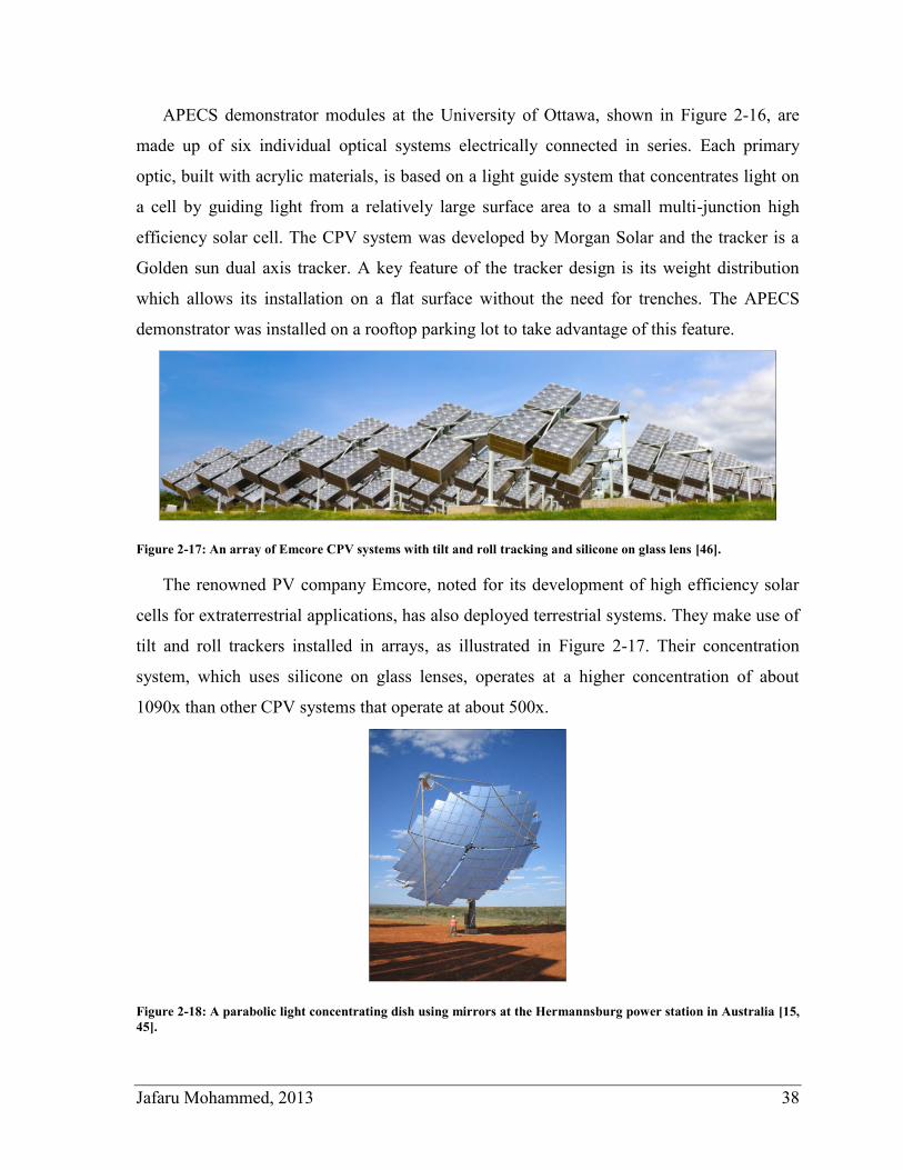
Jafaru Mohammed, 2013 38
APECS demonstrator modules at the University of Ottawa, shown in Figure 2-16, are
made up of six individual optical systems electrically connected in series. Each primary
optic, built with acrylic materials, is based on a light guide system that concentrates light on
a cell by guiding light from a relatively large surface area to a small multi-junction high
efficiency solar cell. The CPV system was developed by Morgan Solar and the tracker is a
Golden sun dual axis tracker. A key feature of the tracker design is its weight distribution
which allows its installation on a flat surface without the need for trenches. The APECS
demonstrator was installed on a rooftop parking lot to take advantage of this feature.
Figure 2-17: An array of Emcore CPV systems with tilt and roll tracking and silicone on glass lens [46].
The renowned PV company Emcore, noted for its development of high efficiency solar
cells for extraterrestrial applications, has also deployed terrestrial systems. They make use of
tilt and roll trackers installed in arrays, as illustrated in Figure 2-17. Their concentration
system, which uses silicone on glass lenses, operates at a higher concentration of about
1090x than other CPV systems that operate at about 500x.
Figure 2-18: A parabolic light concentrating dish using mirrors at the Hermannsburg power station in Australia [15,
45].
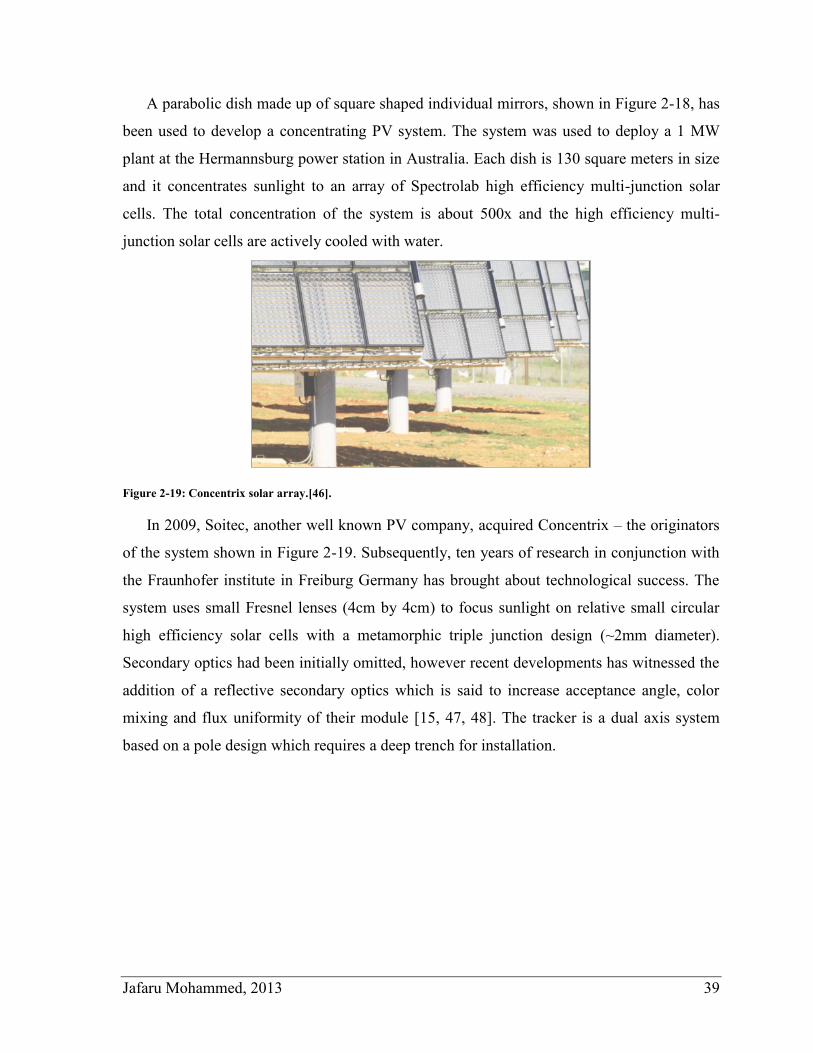
Jafaru Mohammed, 2013 39
A parabolic dish made up of square shaped individual mirrors, shown in Figure 2-18, has
been used to develop a concentrating PV system. The system was used to deploy a 1 MW
plant at the Hermannsburg power station in Australia. Each dish is 130 square meters in size
and it concentrates sunlight to an array of Spectrolab high efficiency multi-junction solar
cells. The total concentration of the system is about 500x and the high efficiency multi-
junction solar cells are actively cooled with water.
Figure 2-19: Concentrix solar array.[46].
In 2009, Soitec, another well known PV company, acquired Concentrix – the originators
of the system shown in Figure 2-19. Subsequently, ten years of research in conjunction with
the Fraunhofer institute in Freiburg Germany has brought about technological success. The
system uses small Fresnel lenses (4cm by 4cm) to focus sunlight on relative small circular
high efficiency solar cells with a metamorphic triple junction design (~2mm diameter).
Secondary optics had been initially omitted, however recent developments has witnessed the
addition of a reflective secondary optics which is said to increase acceptance angle, color
mixing and flux uniformity of their module [15, 47, 48]. The tracker is a dual axis system
based on a pole design which requires a deep trench for installation.
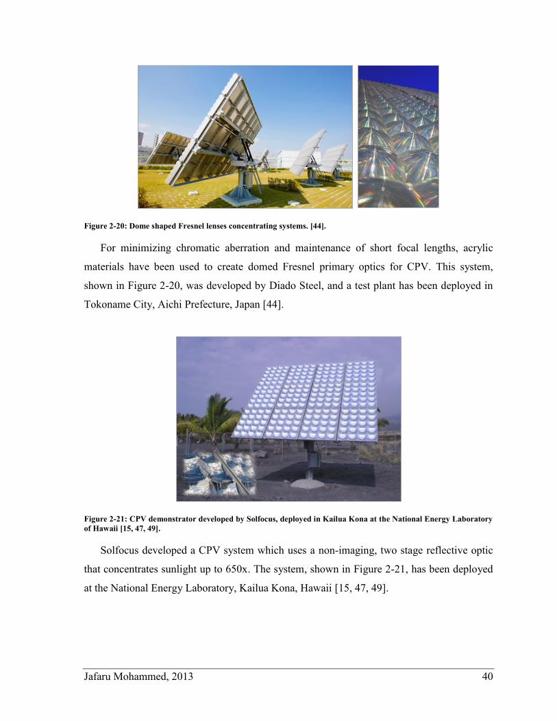
Jafaru Mohammed, 2013 40
Figure 2-20: Dome shaped Fresnel lenses concentrating systems. [44].
For minimizing chromatic aberration and maintenance of short focal lengths, acrylic
materials have been used to create domed Fresnel primary optics for CPV. This system,
shown in Figure 2-20, was developed by Diado Steel, and a test plant has been deployed in
Tokoname City, Aichi Prefecture, Japan [44].
Figure 2-21: CPV demonstrator developed by Solfocus, deployed in Kailua Kona at the National Energy Laboratory
of Hawaii [15, 47, 49].
Solfocus developed a CPV system which uses a non-imaging, two stage reflective optic
that concentrates sunlight up to 650x. The system, shown in Figure 2-21, has been deployed
at the National Energy Laboratory, Kailua Kona, Hawaii [15, 47, 49].
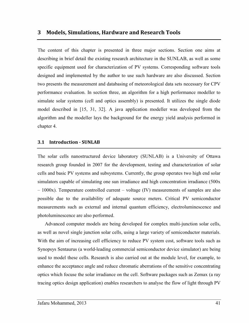
Jafaru Mohammed, 2013 41
3 Models, Simulations, Hardware and Research Tools
The content of this chapter is presented in three major sections. Section one aims at
describing in brief detail the existing research architecture in the SUNLAB, as well as some
specific equipment used for characterization of PV systems. Corresponding software tools
designed and implemented by the author to use such hardware are also discussed. Section
two presents the measurement and databasing of meteorological data sets necessary for CPV
performance evaluation. In section three, an algorithm for a high performance modeller to
simulate solar systems (cell and optics assembly) is presented. It utilizes the single diode
model described in [15, 31, 32]. A java application modeller was developed from the
algorithm and the modeller lays the background for the energy yield analysis performed in
chapter 4.
3.1 Introduction - SUNLAB
The solar cells nanostructured device laboratory (SUNLAB) is a University of Ottawa
research group founded in 2007 for the development, testing and characterization of solar
cells and basic PV systems and subsystems. Currently, the group operates two high end solar
simulators capable of simulating one sun irradiance and high concentration irradiance (500x
– 1000x). Temperature controlled current – voltage (IV) measurements of samples are also
possible due to the availability of adequate source meters. Critical PV semiconductor
measurements such as external and internal quantum efficiency, electroluminescence and
photoluminescence are also performed.
Advanced computer models are being developed for complex multi-junction solar cells,
as well as novel single junction solar cells, using a large variety of semiconductor materials.
With the aim of increasing cell efficiency to reduce PV system cost, software tools such as
Synopsys Sentaurus (a world-leading commercial semiconductor device simulator) are being
used to model these cells. Research is also carried out at the module level, for example, to
enhance the acceptance angle and reduce chromatic aberrations of the sensitive concentrating
optics which focuse the solar irradiance on the cell. Software packages such as Zemax (a ray
tracing optics design application) enables researchers to analyse the flow of light through PV
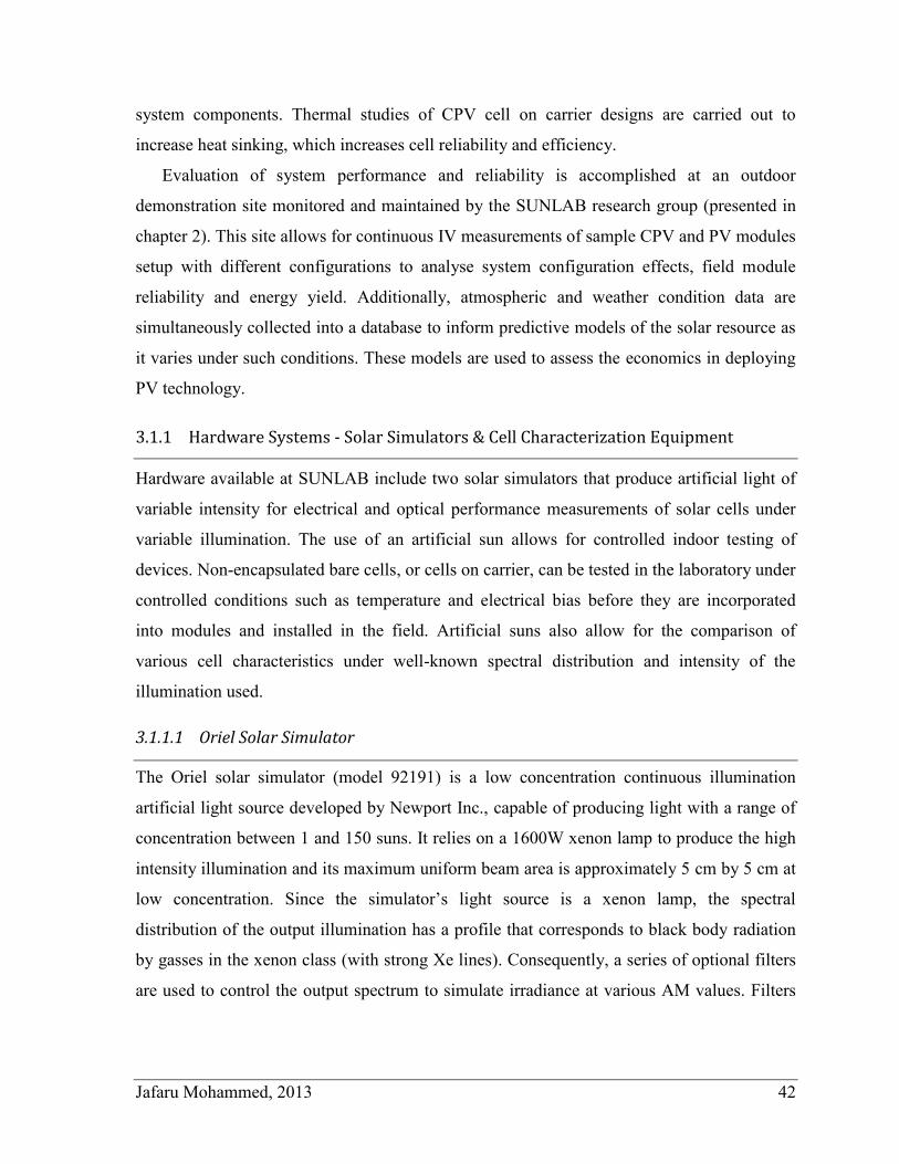
Jafaru Mohammed, 2013 42
system components. Thermal studies of CPV cell on carrier designs are carried out to
increase heat sinking, which increases cell reliability and efficiency.
Evaluation of system performance and reliability is accomplished at an outdoor
demonstration site monitored and maintained by the SUNLAB research group (presented in
chapter 2). This site allows for continuous IV measurements of sample CPV and PV modules
setup with different configurations to analyse system configuration effects, field module
reliability and energy yield. Additionally, atmospheric and weather condition data are
simultaneously collected into a database to inform predictive models of the solar resource as
it varies under such conditions. These models are used to assess the economics in deploying
PV technology.
3.1.1 Hardware Systems - Solar Simulators & Cell Characterization Equipment
Hardware available at SUNLAB include two solar simulators that produce artificial light of
variable intensity for electrical and optical performance measurements of solar cells under
variable illumination. The use of an artificial sun allows for controlled indoor testing of
devices. Non-encapsulated bare cells, or cells on carrier, can be tested in the laboratory under
controlled conditions such as temperature and electrical bias before they are incorporated
into modules and installed in the field. Artificial suns also allow for the comparison of
various cell characteristics under well-known spectral distribution and intensity of the
illumination used.
3.1.1.1 Oriel Solar Simulator
The Oriel solar simulator (model 92191) is a low concentration continuous illumination
artificial light source developed by Newport Inc., capable of producing light with a range of
concentration between 1 and 150 suns. It relies on a 1600W xenon lamp to produce the high
intensity illumination and its maximum uniform beam area is approximately 5 cm by 5 cm at
low concentration. Since the simulator’s light source is a xenon lamp, the spectral
distribution of the output illumination has a profile that corresponds to black body radiation
by gasses in the xenon class (with strong Xe lines). Consequently, a series of optional filters
are used to control the output spectrum to simulate irradiance at various AM values. Filters
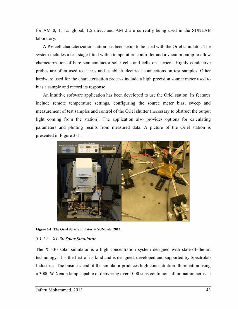
Jafaru Mohammed, 2013 43
for AM 0, 1, 1.5 global, 1.5 direct and AM 2 are currently being used in the SUNLAB
laboratory.
A PV cell characterization station has been setup to be used with the Oriel simulator. The
system includes a test stage fitted with a temperature controller and a vacuum pump to allow
characterization of bare semiconductor solar cells and cells on carriers. Highly conductive
probes are often used to access and establish electrical connections on test samples. Other
hardware used for the characterisation process include a high precision source meter used to
bias a sample and record its response.
An intuitive software application has been developed to use the Oriel station. Its features
include remote temperature settings, configuring the source meter bias, sweep and
measurement of test samples and control of the Oriel shutter (necessary to obstruct the output
light coming from the station). The application also provides options for calculating
parameters and plotting results from measured data. A picture of the Oriel station is
presented in Figure 3-1.
Figure 3-1: The Oriel Solar Simulator at SUNLAB, 2013.
3.1.1.2 XT-30 Solar Simulator
The XT-30 solar simulator is a high concentration system designed with state-of–the-art
technology. It is the first of its kind and is designed, developed and supported by Spectrolab
Industries. The business end of the simulator produces high concentration illumination using
a 3000 W Xenon lamp capable of delivering over 1000 suns continuous illumination across a
Jafaru Mohammed, 2013 44
uniform 1cm by 1cm area; higher concentrations can also be achieved by using a
homogenizer with smaller aperture. The system includes a filter to achieve an AM1.5D
terrestrial spectral distribution. Modification of the output spectrum profile can further be
achieved with the addition of band filters. Due to the excessive heat produced by the Xenon
lamp, integrated water cooling is required. An active pump system circulates chilled water
through pipes and around the housing covering the lamp. Similarly, stages upon which the
cells were mounted were also water cooled, allowing higher intensity illumination of cells
without overheating.
Other interesting features of the XT-30 solar simulator include a shutter for temporarily
obstructing the illumination, and the availability of four separate stages accessed by moving
the simulator’s beam output with an automated motor control system. This motor movement
capability allows for precise on-sample alignment of the XT-30. A heat dump is used to
dissipates light energy into the circulating chilled water supply when the simulator is idle.
The characterization system that accompanies the XT-30 includes electrical connections
on each stage, a source meter, a National Instrument Data Acquisition (DAQ) system and
precise motor control systems for moving the illumination head (Vemex controller). Intuitive
software provides remote control, configuration and measurement. Detail of the software
developed for performing various tasks is presented later.
Figure 3-2: The XT-30 solar simulator and its accompanying hardware in SUNLAB’s laboratory, April 2013. The
green bin houses a high powered fan, the Xenon lamp and necessary filters for tuning the output light spectral
distribution.
Jafaru Mohammed, 2013 45
3.1.1.3 Sinton Flash Tester
The Sinton flash tester is a flash tester capable of delivering a white light spectrum in a very
short time at high concentration. It is used for applications where measurements of the carrier
lifetimes are required. The speed of a flash test effectively removes temperature effects since
sample heating is minimal. The setup includes a vertically moveable head which houses a
homogenizer in the form of a glass cylinder connected to a diffuser. A high luminance
halogen lamp is managed by control electronics to produce the needed power for the flash. A
computer system provides remote control of the lamp and is used to take measurements.
3.1.1.4 Newport’s Quantum Efficiency Measurement Station
Quantum efficiency (QE) is a spectrally-dependent carrier collection probability generated
by single-wavelength illumination across the device thickness, relative to the number of
incident photons. It is indicative of the current production process when integrated over all
wavelengths and gives insight into the recombination processes that reduce cell efficiency.
The measurement process involves counting the number of photons at different wavelengths
incident on the sample active area and the number of electrons that are collected at the
terminal of the sample. External QE (EQE) is the ratio of the number of electrons collected
to the number of photons externally incident on the cell; internal QE (IQE) is that ratio
relative to the number of absorbed photons.
A Newport quantum efficiency test station is used for measuring the cell QE. The station
is capable of measuring the QE of sub-cells in a multi-junction PV device up to four
junctions. It consists of a number of light sources, a bias source meter, temperature control,
wide band detectors (silicon and germanium) and accompanying software. A Xenon lamp is
used in conjunction with a monochromator and filters to select individual optical
wavelengths used for the tests. Other light sources provide bias light for isolating individual
layers in the case of multi-junction solar cells. Temperature control keeps samples at 25 ºC
using a thermoelectric device for heating and cooling (since the processes involved in QE are
temperature dependent). The sample is fixed to a stage using suction from a vacuum pump,
and highly conductive gold plated probes are sometimes used to establish electrical
connection. A sample quantum efficiency measurement of a multi-junction high efficiency
solar cell with quantum dot technology is presented in Figure 1-6. The Figure distinguishes
Jafaru Mohammed, 2013 46
absorption efficiency of the 3 sub-cells within the solar cell. The corresponding portion of
the photon energy of an AM1.5D spectrum is also shown.
3.1.2 Software Systems
To enable characterisation of solar cells and systems, user friendly software applications are
required to control corresponding hardware. Most hardware venders provide basic software
applications but additional features are frequently required to perform specialized tasks. In
most cases where software needs to be modified for customized features, the process of
modification requires well thought plans for ensuring compatibility and ease of use.
Described below are new and modified software developed for a series of applications in
characterising and evaluating PV cells and systems.
3.1.2.1 Simple, Pluggable Current-Voltage (IV) Utility
Measuring dark and light IV curves of solar cells is a key requirement for cell
characterisation. In most cases, large, complex setups that come with specific vendor
hardware are the toolset available to take reliable IV measurements. The choice of a power
supply meter also determines the software to be used and the need to take multiple
measurements of a single sample is often ignored. For mobile measurements, quick IV
characterization and the use of multiple source meters in a user friendly manner, increases
research efficiency. Plug and play applications are ideal in such circumstances.
3.1.2.1.1 Aim
A simple, pluggable current-voltage measurement toolset was driven by the need for a
harmonized toolset for measuring IV curves on the XT-30 solar simulator. As with most
hardware systems, vendor specific software was available with limited functionalities. The
custom application aimed to increase efficiency in taking IV measurements. Designed for
using interchangeable power supply meters (the Keithley 2400 series and Kepco power
supply meter), the application was to provide a user friendly intuitive interface for taking and
storing multiple IV measurements with and without the XT-30 setup. The application was
design to be used with both a general purpose interface bus (GPIB) and a serial connection.
The features include:
plug and play application,
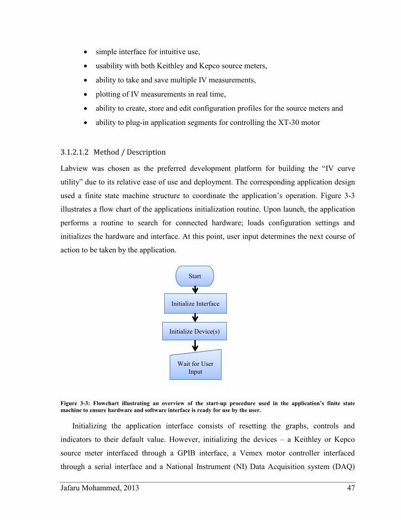
Jafaru Mohammed, 2013 47
simple interface for intuitive use,
usability with both Keithley and Kepco source meters,
ability to take and save multiple IV measurements,
plotting of IV measurements in real time,
ability to create, store and edit configuration profiles for the source meters and
ability to plug-in application segments for controlling the XT-30 motor
3.1.2.1.2 Method / Description
Labview was chosen as the preferred development platform for building the “IV curve
utility” due to its relative ease of use and deployment. The corresponding application design
used a finite state machine structure to coordinate the application’s operation. Figure 3-3
illustrates a flow chart of the applications initialization routine. Upon launch, the application
performs a routine to search for connected hardware; loads configuration settings and
initializes the hardware and interface. At this point, user input determines the next course of
action to be taken by the application.
Figure 3-3: Flowchart illustrating an overview of the start-up procedure used in the application’s finite state
machine to ensure hardware and software interface is ready for use by the user.
Initializing the application interface consists of resetting the graphs, controls and
indicators to their default value. However, initializing the devices – a Keithley or Kepco
source meter interfaced through a GPIB interface, a Vemex motor controller interfaced
through a serial interface and a National Instrument (NI) Data Acquisition system (DAQ)
Initialize Interface
Initialize Device(s)
Start
Wait for User
Input
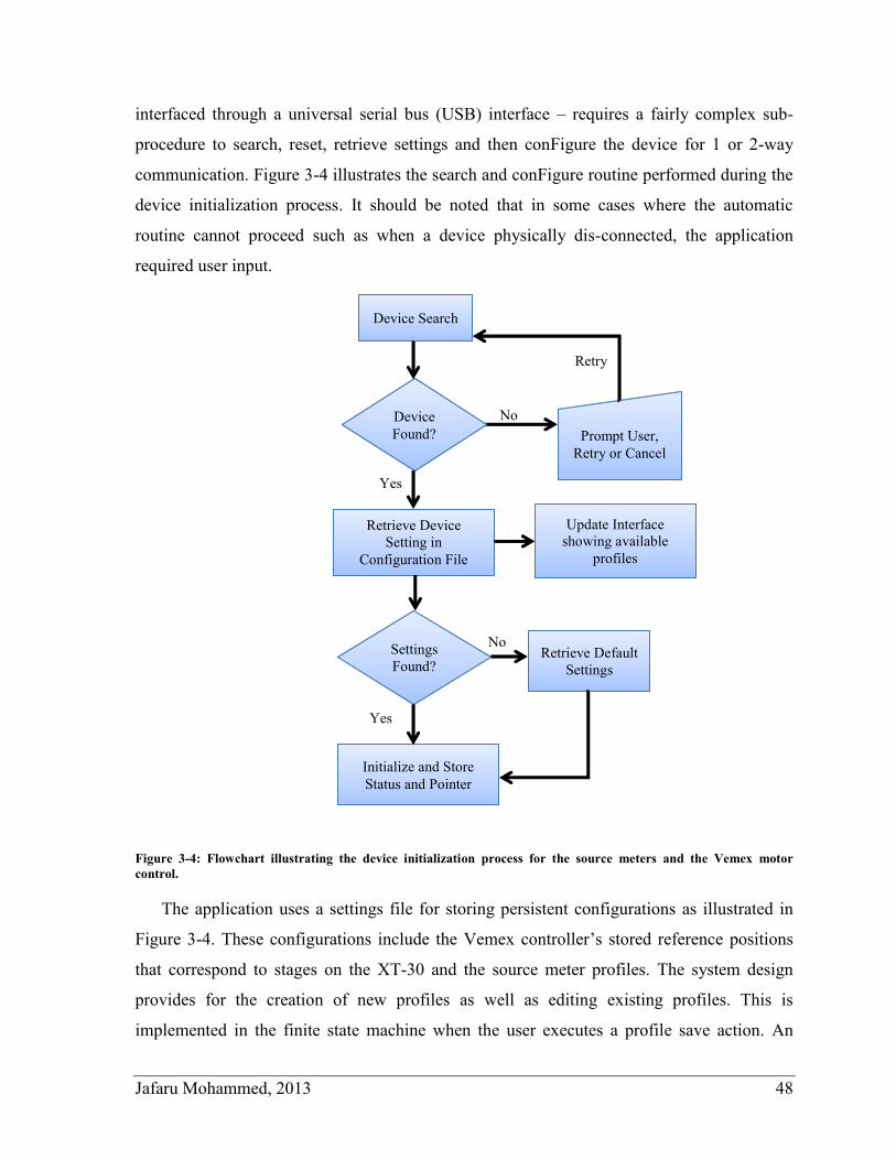
Jafaru Mohammed, 2013 48
interfaced through a universal serial bus (USB) interface – requires a fairly complex sub-
procedure to search, reset, retrieve settings and then conFigure the device for 1 or 2-way
communication. Figure 3-4 illustrates the search and conFigure routine performed during the
device initialization process. It should be noted that in some cases where the automatic
routine cannot proceed such as when a device physically dis-connected, the application
required user input.
Figure 3-4: Flowchart illustrating the device initialization process for the source meters and the Vemex motor
control.
The application uses a settings file for storing persistent configurations as illustrated in
Figure 3-4. These configurations include the Vemex controller’s stored reference positions
that correspond to stages on the XT-30 and the source meter profiles. The system design
provides for the creation of new profiles as well as editing existing profiles. This is
implemented in the finite state machine when the user executes a profile save action. An
Device Search
Device
Found? Prompt User,
Retry or Cancel
No
Retry
Retrieve Device
Setting in
Configuration File
Retrieve Default
Settings
Initialize and Store
Status and Pointer
Settings
Found?
Yes
Yes
No
Update Interface
showing available
profiles
Jafaru Mohammed, 2013 49
input to initialize a new profile creates a profile with default configurations that is expected
to be modified and saved by the application user. Factors such as voltage limit, protection
current, sweep range and sense mode are among the settings configurable by the user that
can be persisted. A sanity check was implemented to ensure profile names are unique with
default profile names automatically created from timestamp values. A delete feature was also
incorporated to remove profiles from the settings file.
For each power supply meter configured, a unique initialization (INI) file section records
a list of header keys. These correspond to section headings that store the settings for the
specified device. Depending on the device unique features, the range of key-value pairs
under each configuration key header varies significantly. Similarly, the Vemex controller
stores labels, including x and y coordinates for each position. Twelve positions in total are
available for configuration and persistence by the application user.
Within the finite state machine, a generic module was implemented to perform IV curve
sweep operations. The module was designed generic to allow re-usability between the
multiple source meters (Keithley and Kepco) and to be used as a plug-in within other
applications. This module is referred to as the IV measurement module. When the sweep
input is executed on the IV measurement utility, loaded configuration settings in conjunction
with initialized pointers to the hardware device are passed to the IV measurement module
which then returns results that include Voc, Isc, fill factor (FF) and maximum power (PMax).
Results returned from the IV measurement module are saved in an array with an initial id
label of the timestamp. Provisions are made for this id to be edited to a custom text of choice
by the application user. Simultaneously, the IV and power curve are plotted on two graphs. A
list option is available for the user to scroll through recorded measurements.
A feature to save single and multiple recorded results into a spreadsheet file was
implemented. The data for each measurement is recorded with identification of the
measurement label previously mentioned. Each record is saved on two spreadsheet rows
which allows ease of access to individual or multiple records. Basic error logging was
implemented to allow for debugging the application.
3.1.2.1.3 Result
Using the IV utility involves connecting required hardware to a computer system and
launching the application. Researchers began using the application by early 2013 at the
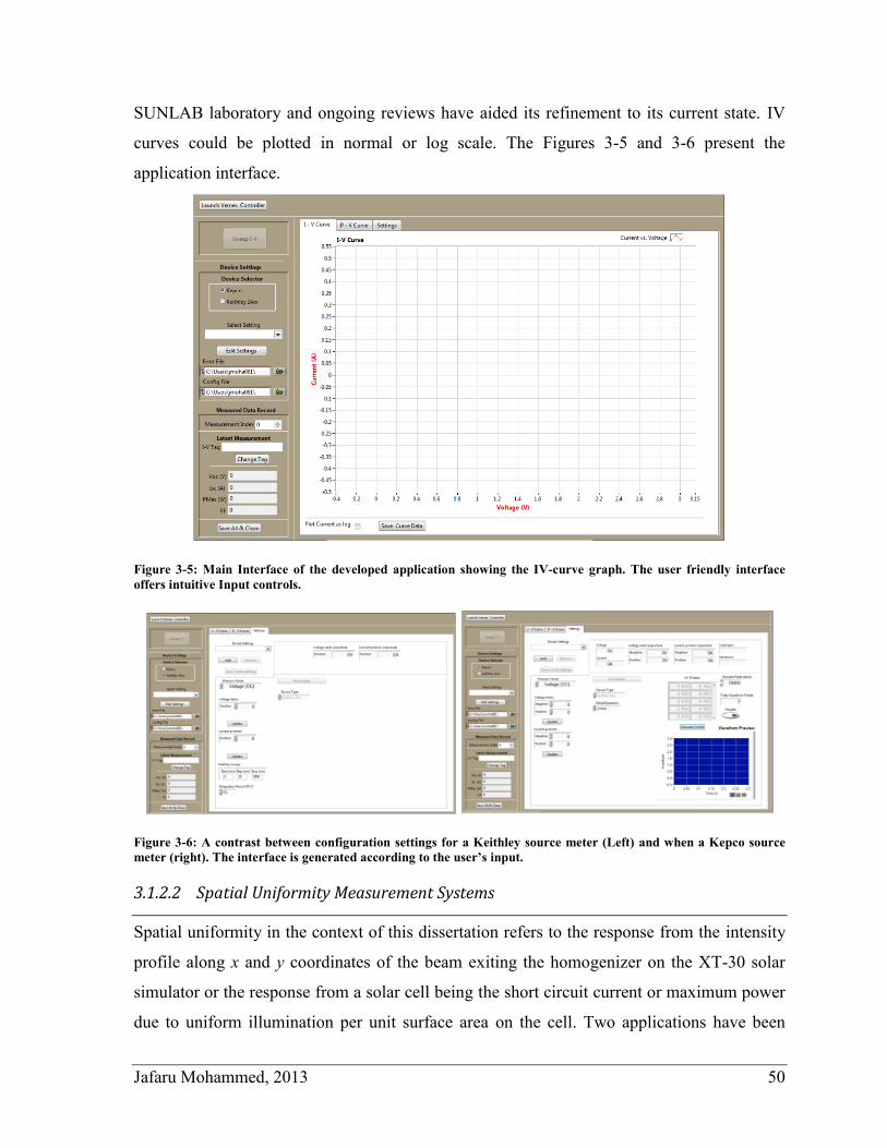
Jafaru Mohammed, 2013 50
SUNLAB laboratory and ongoing reviews have aided its refinement to its current state. IV
curves could be plotted in normal or log scale. The Figures 3-5 and 3-6 present the
application interface.
Figure 3-5: Main Interface of the developed application showing the IV-curve graph. The user friendly interface
offers intuitive Input controls.
Figure 3-6: A contrast between configuration settings for a Keithley source meter (Left) and when a Kepco source
meter (right). The interface is generated according to the user’s input.
3.1.2.2 Spatial Uniformity Measurement Systems
Spatial uniformity in the context of this dissertation refers to the response from the intensity
profile along x and y coordinates of the beam exiting the homogenizer on the XT-30 solar
simulator or the response from a solar cell being the short circuit current or maximum power
due to uniform illumination per unit surface area on the cell. Two applications have been
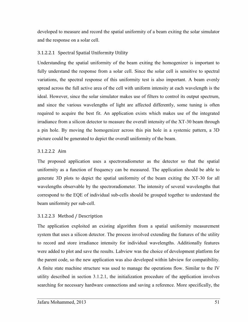
Jafaru Mohammed, 2013 51
developed to measure and record the spatial uniformity of a beam exiting the solar simulator
and the response on a solar cell.
3.1.2.2.1 Spectral Spatial Uniformity Utility
Understanding the spatial uniformity of the beam exiting the homogenizer is important to
fully understand the response from a solar cell. Since the solar cell is sensitive to spectral
variations, the spectral response of this uniformity test is also important. A beam evenly
spread across the full active area of the cell with uniform intensity at each wavelength is the
ideal. However, since the solar simulator makes use of filters to control its output spectrum,
and since the various wavelengths of light are affected differently, some tuning is often
required to acquire the best fit. An application exists which makes use of the integrated
irradiance from a silicon detector to measure the overall intensity of the XT-30 beam through
a pin hole. By moving the homogenizer across this pin hole in a systemic pattern, a 3D
picture could be generated to depict the overall uniformity of the beam.
3.1.2.2.2 Aim
The proposed application uses a spectroradiometer as the detector so that the spatial
uniformity as a function of frequency can be measured. The application should be able to
generate 3D plots to depict the spatial uniformity of the beam exiting the XT-30 for all
wavelengths observable by the spectroradiometer. The intensity of several wavelengths that
correspond to the EQE of individual sub-cells should be grouped together to understand the
beam uniformity per sub-cell.
3.1.2.2.3 Method / Description
The application exploited an existing algorithm from a spatial uniformity measurement
system that uses a silicon detector. The process involved extending the features of the utility
to record and store irradiance intensity for individual wavelengths. Additionally features
were added to plot and save the results. Labview was the choice of development platform for
the parent code, so the new application was also developed within labview for compatibility.
A finite state machine structure was used to manage the operations flow. Similar to the IV
utility described in section 3.1.2.1, the initialization procedure of the application involves
searching for necessary hardware connections and saving a reference. More specifically, the
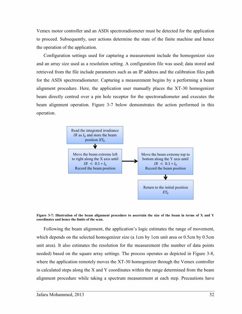
Jafaru Mohammed, 2013 52
Vemex motor controller and an ASDi spectroradiometer must be detected for the application
to proceed. Subsequently, user actions determine the state of the finite machine and hence
the operation of the application.
Configuration settings used for capturing a measurement include the homogenizer size
and an array size used as a resolution setting. A configuration file was used; data stored and
retrieved from the file include parameters such as an IP address and the calibration files path
for the ASDi spectroradiometer. Capturing a measurement begins by a performing a beam
alignment procedure. Here, the application user manually places the XT-30 homogenizer
beam directly centred over a pin hole receptor for the spectroradiometer and executes the
beam alignment operation. Figure 3-7 below demonstrates the action performed in this
operation.
Figure 3-7: Illustration of the beam alignment procedure to ascertain the size of the beam in terms of X and Y
coordinates and hence the limits of the scan.
Following the beam alignment, the application’s logic estimates the range of movement,
which depends on the selected homogenizer size (a 1cm by 1cm unit area or 0.5cm by 0.5cm
unit area). It also estimates the resolution for the measurement (the number of data points
needed) based on the square array settings. The process operates as depicted in Figure 3-8,
where the application remotely moves the XT-30 homogenizer through the Vemex controller
in calculated steps along the X and Y coordinates within the range determined from the beam
alignment procedure while taking a spectrum measurement at each step. Precautions have
Read the integrated irradiance
as and store the beam
position
Move the beam extreme left
to right along the X axis until
Record the beam position
Move the beam extreme top to
bottom along the Y axis until
Record the beam position
Return to the initial position
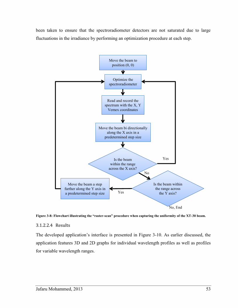
Jafaru Mohammed, 2013 53
been taken to ensure that the spectroradiometer detectors are not saturated due to large
fluctuations in the irradiance by performing an optimization procedure at each step.
Figure 3-8: Flowchart illustrating the “raster-scan” procedure when capturing the uniformity of the XT-30 beam.
3.1.2.2.4 Results
The developed application’s interface is presented in Figure 3-10. As earlier discussed, the
application features 3D and 2D graphs for individual wavelength profiles as well as profiles
for variable wavelength ranges.
Move the beam to
position (0, 0)
Optimize the
spectroradiometer
Read and record the
spectrum with the X, Y
Vemex coordinates
Move the beam bi directionally
along the X axis in a
predetermined step size
Is the beam
within the range
across the X axis?
Is the beam within
the range across
the Y axis?
Move the beam a step
further along the Y axis in
a predetermined step size
Yes
No
Yes
No, End
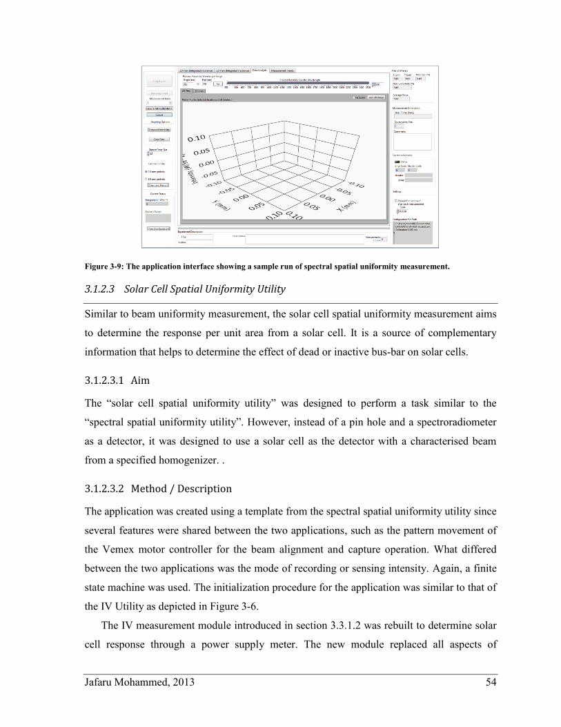
Jafaru Mohammed, 2013 54
Figure 3-9: The application interface showing a sample run of spectral spatial uniformity measurement.
3.1.2.3 Solar Cell Spatial Uniformity Utility
Similar to beam uniformity measurement, the solar cell spatial uniformity measurement aims
to determine the response per unit area from a solar cell. It is a source of complementary
information that helps to determine the effect of dead or inactive bus-bar on solar cells.
3.1.2.3.1 Aim
The “solar cell spatial uniformity utility” was designed to perform a task similar to the
“spectral spatial uniformity utility”. However, instead of a pin hole and a spectroradiometer
as a detector, it was designed to use a solar cell as the detector with a characterised beam
from a specified homogenizer. .
3.1.2.3.2 Method / Description
The application was created using a template from the spectral spatial uniformity utility since
several features were shared between the two applications, such as the pattern movement of
the Vemex motor controller for the beam alignment and capture operation. What differed
between the two applications was the mode of recording or sensing intensity. Again, a finite
state machine was used. The initialization procedure for the application was similar to that of
the IV Utility as depicted in Figure 3-6.
The IV measurement module introduced in section 3.3.1.2 was rebuilt to determine solar
cell response through a power supply meter. The new module replaced all aspects of
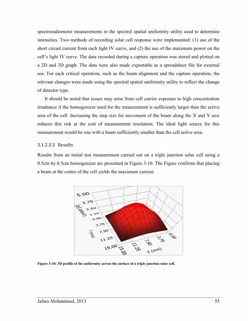
Jafaru Mohammed, 2013 55
spectroradiometer measurements in the spectral spatial uniformity utility used to determine
intensities. Two methods of recording solar cell response were implemented: (1) use of the
short circuit current from each light IV curve, and (2) the use of the maximum power on the
cell’s light IV curve. The data recorded during a capture operation was stored and plotted on
a 2D and 3D graph. The data were also made exportable as a spreadsheet file for external
use. For each critical operation, such as the beam alignment and the capture operation, the
relevant changes were made using the spectral spatial uniformity utility to reflect the change
of detector type.
It should be noted that issues may arise from cell carrier exposure to high concentration
irradiance if the homogenizer used for the measurement is sufficiently larger than the active
area of the cell. Increasing the step size for movement of the beam along the X and Y axis
reduces this risk at the cost of measurement resolution. The ideal light source for this
measurement would be one with a beam sufficiently smaller than the cell active area.
3.1.2.3.3 Results
Results from an initial test measurement carried out on a triple junction solar cell using a
0.5cm by 0.5cm homogenizer are presented in Figure 3-10. The Figure confirms that placing
a beam at the centre of the cell yields the maximum current.
Figure 3-10: 3D profile of the uniformity across the surface of a triple junction solar cell.
Jafaru Mohammed, 2013 56
3.1.2.4 Light-Cycling Utility
With the current growth rate of CPV implementation, besides enhancing cell efficiencies,
researchers also aim to increase reliability of solar cells for longer periods on sun.
Fluctuations of high concentration irradiance by movement of clouds and diurnal variations
stress CPV system components, particularly the cell-on-carrier. Degradation is expected to
be a delamination of the cell from its carrier due to crack propagation from voids in the
soldered joint between the cell and its carrier. For researchers to experimentally evaluate this
degradation effect, accelerated aging tests can be conducted in the lab by simulating
temperature fluctuations on a cell through optical cycling.
3.1.2.4.1 Aim
The aim of the light-cycling utility is to simulate fluctuation of the sun’s irradiance at high
concentration on a cell in an accelerated manner. The application should leverage the XT-
30’s ability to produce high concentration irradiance on a small surface area and its shutter
should be used to cut-off the irradiance on the cell at relatively fast rates. The utility should
be designed to accept scheduled commands and run in an automated fashion with little or no
human supervision. It should record a spectrum using the spectroradiometer, take an IV
curve using either a Kepco or Keithley source meter, move the XT-30 beam output across
stages and actuate a servo to open and close the XT-30 shutter using a parallel port interface.
The application features should include:
record and store spectrum,
record and store IV curves using either a Keithley or a Kepco source meter,
move the beam output using the Vemex controller across stages,
actuate a servo to open or close the XT-30 shutter,
implement a scheduled wait in seconds,
allow time relative scheduling of each operable feature and
allow saving and loading of schedules.
Jafaru Mohammed, 2013 57
3.1.2.4.2 Method / Description
Labview was chosen as the application development platform for this utility due to its
relative ease of use and deployment. A c++ platform was also used to create an application
library to communicate with a parallel port. The utility was designed in two parts: one for
system setup and one for actual use. The system setup design was made for the initialization
of connections to the Vemex controller and the power supply meters as well as configuration
setting for the source meters (described in section 3.1.2.1.2). The actual scheduling or
running of simulations was access restricted based on conditions that must be met, such as
availability of a connected source meter.
Upon application launch, source meter setup and configuration are done and a subsection
is launched. The subsection provides an interface to perform the actual target operation and
an initialization procedure to enable or disable features based on whether certain hardware
are connected and operable. A finite state machine structure was used to coordinate
operations. The application uses the IV curve module described earlier (in section
3.1.2.2.1.2). Similar modules were created for other segmented tasks, which include moving
the XT-30 beam output using the Vemex controller to any given X and Y coordinate, taking
a spectrum measurement using the spectroradiometer, and opening or closing the XT-30
shutter by broadcasting a binary command over the network. For the purpose of simplicity,
explicit details of the mode of operations of each respective module created have been
omitted. A c++ application library was created to accept broadcast messages and transfer the
binary content to a parallel port. The parallel port was connected to a servo circuit for
opening and closing the XT-30 shutter.
Each feature available in the utility after its initialization phase, besides the wait action, is
designed to be operated with and without a scheduler. This allows for application flexibility
if manual operation is required. Controls on the application allow for data results, in the form
of IV curve data or spectrum data, to be save to file. Scheduling actions involve adding the
required action step by step to a schedule list on the utility. The list can be edited by deleting
individual or bulk actions and it can be saved and loaded to and from a persistent file. For
each action scheduled, a memory space is allocated to store parameters unique to the action
(such as X and Y coordinate for a Vemex controller movement, or specific source meter
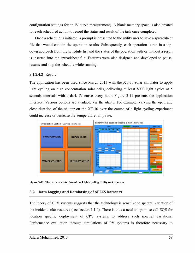
Jafaru Mohammed, 2013 58
configuration settings for an IV curve measurement). A blank memory space is also created
for each scheduled action to record the status and result of the task once completed.
Once a schedule is initiated, a prompt is presented to the utility user to save a spreadsheet
file that would contain the operation results. Subsequently, each operation is run in a top-
down approach from the schedule list and the status of the operation with or without a result
is inserted into the spreadsheet file. Features were also designed and developed to pause,
resume and stop the schedule while running.
3.1.2.4.3 Result
The application has been used since March 2013 with the XT-30 solar simulator to apply
light cycling on high concentration solar cells, delivering at least 8000 light cycles at 5
seconds intervals with a dark IV curve every hour. Figure 3-11 presents the application
interface. Various options are available via the utility. For example, varying the open and
close duration of the shutter on the XT-30 over the course of a light cycling experiment
could increase or decrease the temperature ramp rate.
Figure 3-11: The two main interface of the Light Cycling Utility (not to scale).
3.2 Data Logging and Databasing of APECS Datasets
The theory of CPV systems suggests that the technology is sensitive to spectral variation of
the incident solar resource (see section 1.1.4). There is thus a need to optimise cell EQE for
location specific deployment of CPV systems to address such spectral variations.
Performance evaluation through simulations of PV systems is therefore necessary to
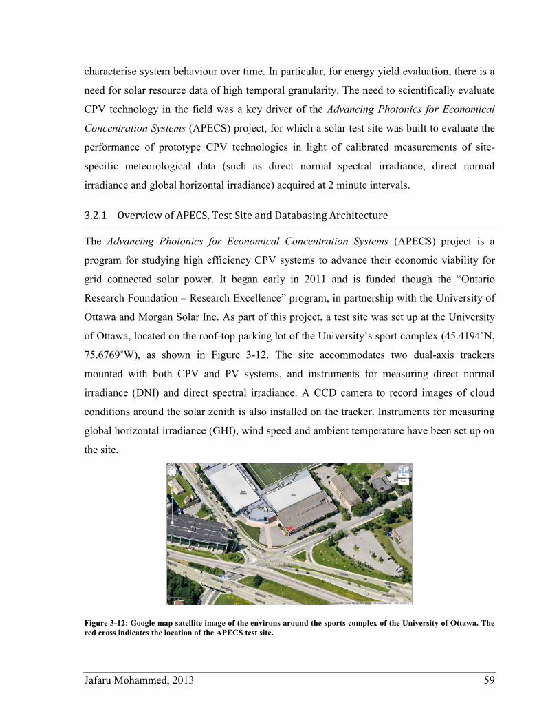
Jafaru Mohammed, 2013 59
characterise system behaviour over time. In particular, for energy yield evaluation, there is a
need for solar resource data of high temporal granularity. The need to scientifically evaluate
CPV technology in the field was a key driver of the Advancing Photonics for Economical
Concentration Systems (APECS) project, for which a solar test site was built to evaluate the
performance of prototype CPV technologies in light of calibrated measurements of site-
specific meteorological data (such as direct normal spectral irradiance, direct normal
irradiance and global horizontal irradiance) acquired at 2 minute intervals.
3.2.1 Overview of APECS, Test Site and Databasing Architecture
The Advancing Photonics for Economical Concentration Systems (APECS) project is a
program for studying high efficiency CPV systems to advance their economic viability for
grid connected solar power. It began early in 2011 and is funded though the “Ontario
Research Foundation – Research Excellence” program, in partnership with the University of
Ottawa and Morgan Solar Inc. As part of this project, a test site was set up at the University
of Ottawa, located on the roof-top parking lot of the University’s sport complex (45.4194˚N,
75.6769˚W), as shown in Figure 3-12. The site accommodates two dual-axis trackers
mounted with both CPV and PV systems, and instruments for measuring direct normal
irradiance (DNI) and direct spectral irradiance. A CCD camera to record images of cloud
conditions around the solar zenith is also installed on the tracker. Instruments for measuring
global horizontal irradiance (GHI), wind speed and ambient temperature have been set up on
the site.
Figure 3-12: Google map satellite image of the environs around the sports complex of the University of Ottawa. The
red cross indicates the location of the APECS test site.
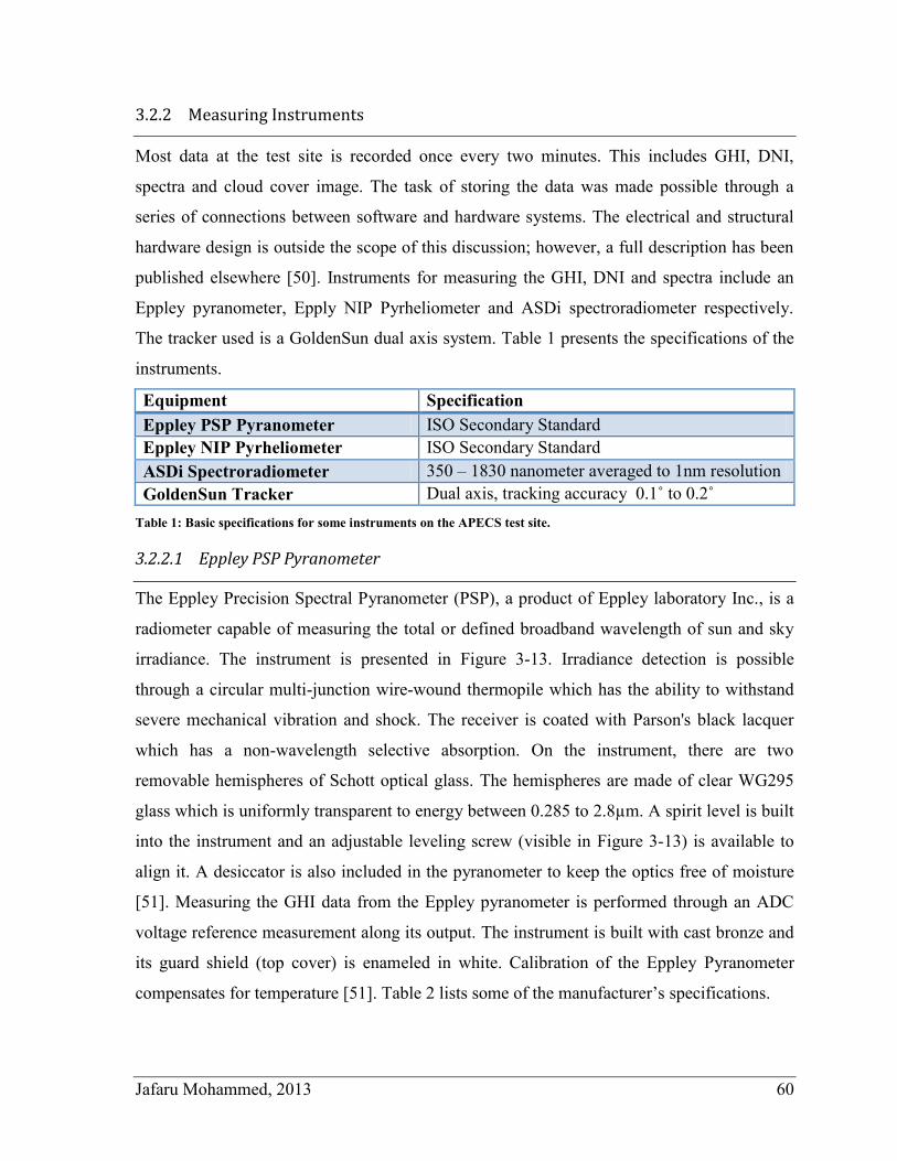
Jafaru Mohammed, 2013 60
3.2.2 Measuring Instruments
Most data at the test site is recorded once every two minutes. This includes GHI, DNI,
spectra and cloud cover image. The task of storing the data was made possible through a
series of connections between software and hardware systems. The electrical and structural
hardware design is outside the scope of this discussion; however, a full description has been
published elsewhere [50]. Instruments for measuring the GHI, DNI and spectra include an
Eppley pyranometer, Epply NIP Pyrheliometer and ASDi spectroradiometer respectively.
The tracker used is a GoldenSun dual axis system. Table 1 presents the specifications of the
instruments.
Equipment Specification
Eppley PSP Pyranometer ISO Secondary Standard
Eppley NIP Pyrheliometer ISO Secondary Standard
ASDi Spectroradiometer 350 – 1830 nanometer averaged to 1nm resolution
GoldenSun Tracker Dual axis, tracking accuracy 0.1˚ to 0.2˚
Table 1: Basic specifications for some instruments on the APECS test site.
3.2.2.1 Eppley PSP Pyranometer
The Eppley Precision Spectral Pyranometer (PSP), a product of Eppley laboratory Inc., is a
radiometer capable of measuring the total or defined broadband wavelength of sun and sky
irradiance. The instrument is presented in Figure 3-13. Irradiance detection is possible
through a circular multi-junction wire-wound thermopile which has the ability to withstand
severe mechanical vibration and shock. The receiver is coated with Parson's black lacquer
which has a non-wavelength selective absorption. On the instrument, there are two
removable hemispheres of Schott optical glass. The hemispheres are made of clear WG295
glass which is uniformly transparent to energy between 0.285 to 2.8µm. A spirit level is built
into the instrument and an adjustable leveling screw (visible in Figure 3-13) is available to
align it. A desiccator is also included in the pyranometer to keep the optics free of moisture
[51]. Measuring the GHI data from the Eppley pyranometer is performed through an ADC
voltage reference measurement along its output. The instrument is built with cast bronze and
its guard shield (top cover) is enameled in white. Calibration of the Eppley Pyranometer
compensates for temperature [51]. Table 2 lists some of the manufacturer’s specifications.
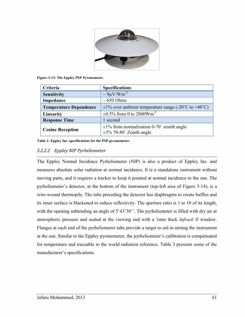
Jafaru Mohammed, 2013 61
Figure 3-13: The Eppley PSP Pyranometer.
Criteria Specifications
Sensitivity ~ 9µV/Wm-2
Impedance ~ 650 Ohms
Temperature Dependence ±1% over ambient temperature range (-20˚C to +40˚C)
Linearity ±0.5% from 0 to 2800Wm-2
Response Time 1 second
Cosine Reception ±1% from normalization 0-70˚ zenith angle
±3% 70-80˚ Zenith angle
Table 2: Eppley Inc. specifications for the PSP pyranometer.
3.2.2.2 Eppley NIP Pyrheliometer
The Eppley Normal Incidence Pyrheliometer (NIP) is also a product of Eppley Inc. and
measures absolute solar radiation at normal incidence. It is a standalone instrument without
moving parts, and it requires a tracker to keep it pointed at normal incidence to the sun. The
pyrheliometer’s detector, at the bottom of the instrument (top-left area of Figure 3-14), is a
wire-wound thermopile. The tube preceding the detector has diaphragms to create baffles and
its inner surface is blackened to reduce reflectivity. The aperture ratio is 1 to 10 of its length,
with the opening subtending an angle of 5˚43’30’’. The pyrheliometer is filled with dry air at
atmospheric pressure and sealed at the viewing end with a 1mm thick Infrasil II window.
Flanges at each end of the pyrheliometer tube provide a target to aid in aiming the instrument
at the sun. Similar to the Eppley pyranometer, the pyrheliometer’s calibration is compensated
for temperature and traceable to the world radiation reference. Table 3 presents some of the
manufacturer’s specifications.
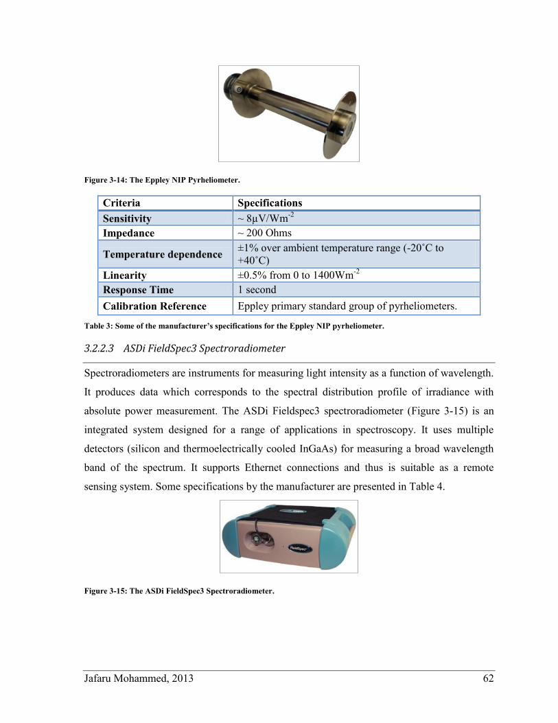
Jafaru Mohammed, 2013 62
Figure 3-14: The Eppley NIP Pyrheliometer.
Criteria Specifications
Sensitivity ~ 8µV/Wm-2
Impedance ~ 200 Ohms
Temperature dependence ±1% over ambient temperature range (-20˚C to
+40˚C)
Linearity ±0.5% from 0 to 1400Wm-2
Response Time 1 second
Calibration Reference Eppley primary standard group of pyrheliometers.
Table 3: Some of the manufacturer’s specifications for the Eppley NIP pyrheliometer.
3.2.2.3 ASDi FieldSpec3 Spectroradiometer
Spectroradiometers are instruments for measuring light intensity as a function of wavelength.
It produces data which corresponds to the spectral distribution profile of irradiance with
absolute power measurement. The ASDi Fieldspec3 spectroradiometer (Figure 3-15) is an
integrated system designed for a range of applications in spectroscopy. It uses multiple
detectors (silicon and thermoelectrically cooled InGaAs) for measuring a broad wavelength
band of the spectrum. It supports Ethernet connections and thus is suitable as a remote
sensing system. Some specifications by the manufacturer are presented in Table 4.
Figure 3-15: The ASDi FieldSpec3 Spectroradiometer.
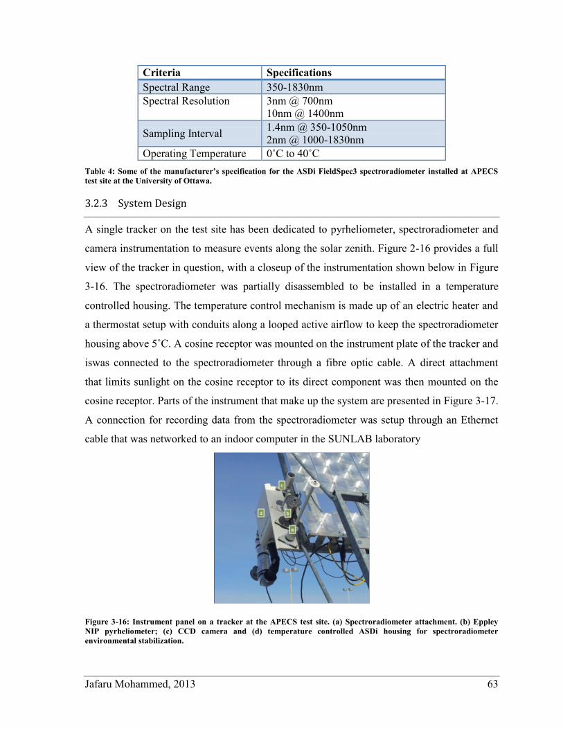
Jafaru Mohammed, 2013 63
Criteria Specifications
Spectral Range 350-1830nm
Spectral Resolution 3nm @ 700nm
10nm @ 1400nm
Sampling Interval 1.4nm @ 350-1050nm
2nm @ 1000-1830nm
Operating Temperature 0˚C to 40˚C
Table 4: Some of the manufacturer’s specification for the ASDi FieldSpec3 spectroradiometer installed at APECS
test site at the University of Ottawa.
3.2.3 System Design
A single tracker on the test site has been dedicated to pyrheliometer, spectroradiometer and
camera instrumentation to measure events along the solar zenith. Figure 2-16 provides a full
view of the tracker in question, with a closeup of the instrumentation shown below in Figure
3-16. The spectroradiometer was partially disassembled to be installed in a temperature
controlled housing. The temperature control mechanism is made up of an electric heater and
a thermostat setup with conduits along a looped active airflow to keep the spectroradiometer
housing above 5˚C. A cosine receptor was mounted on the instrument plate of the tracker and
iswas connected to the spectroradiometer through a fibre optic cable. A direct attachment
that limits sunlight on the cosine receptor to its direct component was then mounted on the
cosine receptor. Parts of the instrument that make up the system are presented in Figure 3-17.
A connection for recording data from the spectroradiometer was setup through an Ethernet
cable that was networked to an indoor computer in the SUNLAB laboratory
Figure 3-16: Instrument panel on a tracker at the APECS test site. (a) Spectroradiometer attachment. (b) Eppley
NIP pyrheliometer; (c) CCD camera and (d) temperature controlled ASDi housing for spectroradiometer
environmental stabilization.
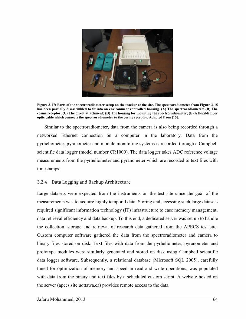
Jafaru Mohammed, 2013 64
Figure 3-17: Parts of the spectroradiometer setup on the tracker at the site. The spectroradiometer from Figure 3-15
has been partially disassembled to fit into an environment controlled housing. (A) The spectroradiometer; (B) The
cosine receptor; (C) The direct attachment; (D) The housing for mounting the spectroradiometer; (E) A flexible fiber
optic cable which connects the spectroradiometer to the cosine receptor. Adapted from [15].
Similar to the spectroradiometer, data from the camera is also being recorded through a
networked Ethernet connection on a computer in the laboratory. Data from the
pyrheliometer, pyranometer and module monitoring systems is recorded through a Campbell
scientific data logger (model number CR1000). The data logger takes ADC reference voltage
measurements from the pyrheliometer and pyranometer which are recorded to text files with
timestamps.
3.2.4 Data Logging and Backup Architecture
Large datasets were expected from the instruments on the test site since the goal of the
measurements was to acquire highly temporal data. Storing and accessing such large datasets
required significant information technology (IT) infrastructure to ease memory management,
data retrieval efficiency and data backup. To this end, a dedicated server was set up to handle
the collection, storage and retrieval of research data gathered from the APECS test site.
Custom computer software gathered the data from the spectroradiometer and camera to
binary files stored on disk. Text files with data from the pyrheliometer, pyranometer and
prototype modules were similarly generated and stored on disk using Campbell scientific
data logger software. Subsequently, a relational database (Microsoft SQL 2005), carefully
tuned for optimization of memory and speed in read and write operations, was populated
with data from the binary and text files by a scheduled custom script. A website hosted on
the server (apecs.site.uottawa.ca) provides remote access to the data.
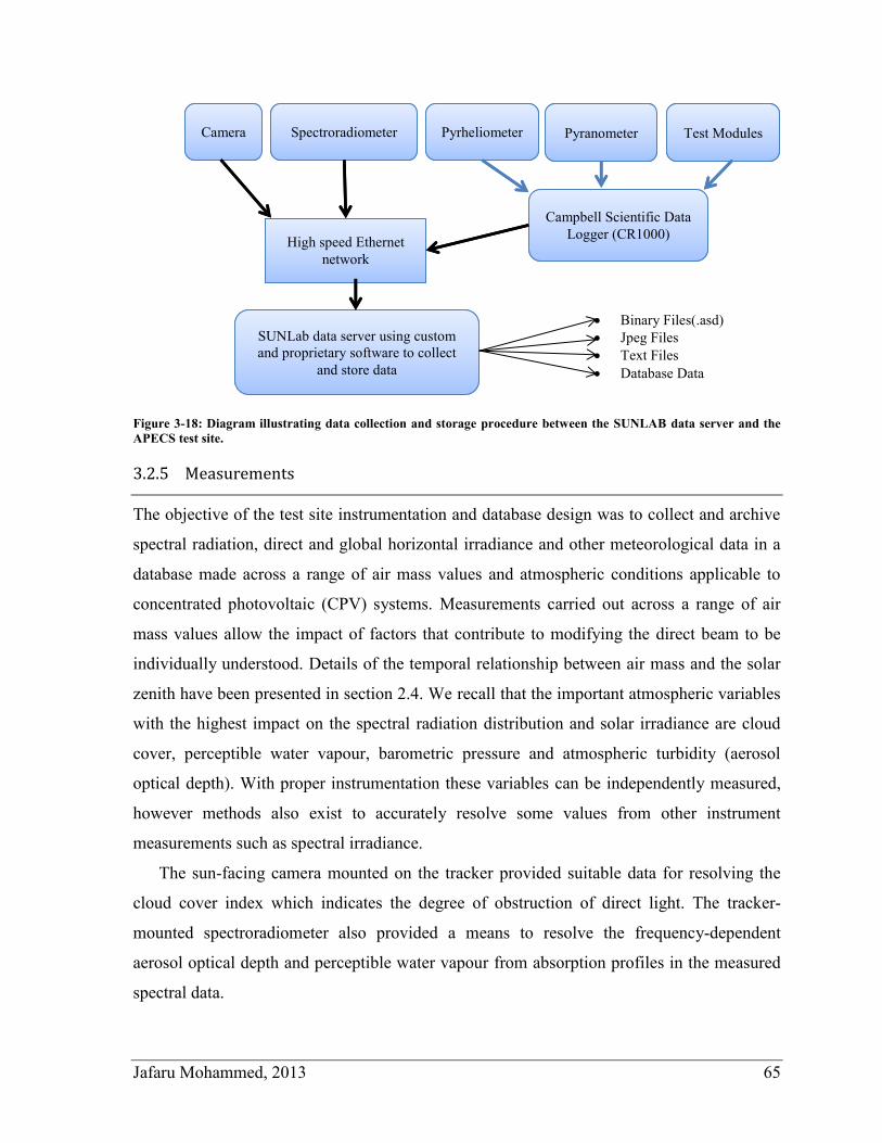
Jafaru Mohammed, 2013 65
Figure 3-18: Diagram illustrating data collection and storage procedure between the SUNLAB data server and the
APECS test site.
3.2.5 Measurements
The objective of the test site instrumentation and database design was to collect and archive
spectral radiation, direct and global horizontal irradiance and other meteorological data in a
database made across a range of air mass values and atmospheric conditions applicable to
concentrated photovoltaic (CPV) systems. Measurements carried out across a range of air
mass values allow the impact of factors that contribute to modifying the direct beam to be
individually understood. Details of the temporal relationship between air mass and the solar
zenith have been presented in section 2.4. We recall that the important atmospheric variables
with the highest impact on the spectral radiation distribution and solar irradiance are cloud
cover, perceptible water vapour, barometric pressure and atmospheric turbidity (aerosol
optical depth). With proper instrumentation these variables can be independently measured,
however methods also exist to accurately resolve some values from other instrument
measurements such as spectral irradiance.
The sun-facing camera mounted on the tracker provided suitable data for resolving the
cloud cover index which indicates the degree of obstruction of direct light. The tracker-
mounted spectroradiometer also provided a means to resolve the frequency-dependent
aerosol optical depth and perceptible water vapour from absorption profiles in the measured
spectral data.
Camera Spectroradiometer Pyrheliometer Pyranometer Test Modules
High speed Ethernet
network
Campbell Scientific Data
Logger (CR1000)
SUNLab data server using custom
and proprietary software to collect
and store data
Binary Files(.asd)
Jpeg Files
Text Files
Database Data
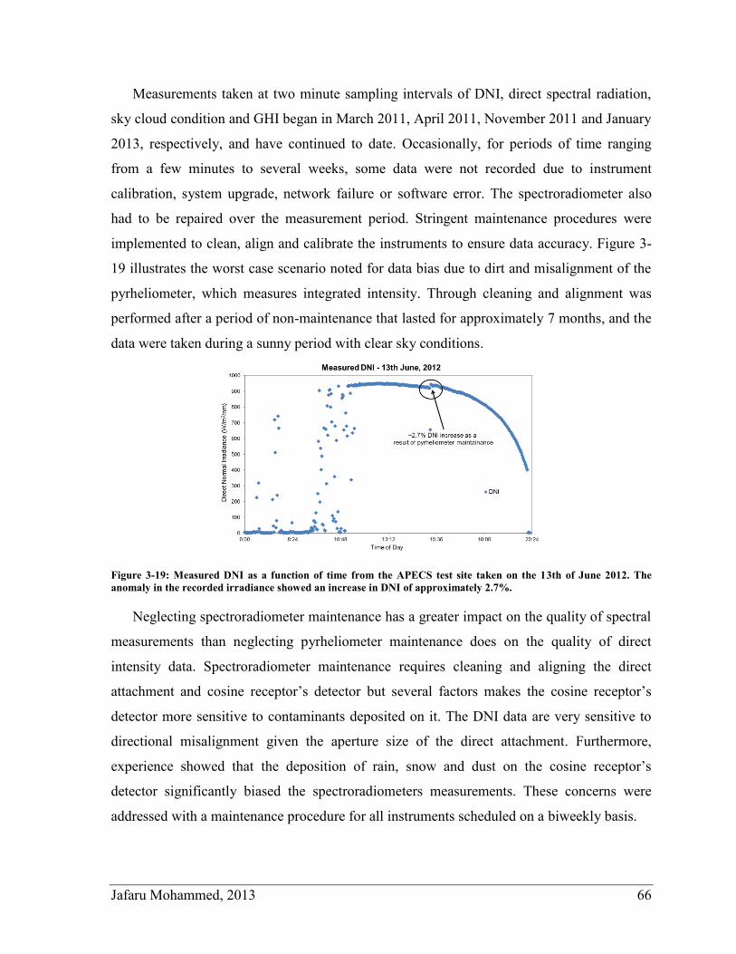
Jafaru Mohammed, 2013 66
Measurements taken at two minute sampling intervals of DNI, direct spectral radiation,
sky cloud condition and GHI began in March 2011, April 2011, November 2011 and January
2013, respectively, and have continued to date. Occasionally, for periods of time ranging
from a few minutes to several weeks, some data were not recorded due to instrument
calibration, system upgrade, network failure or software error. The spectroradiometer also
had to be repaired over the measurement period. Stringent maintenance procedures were
implemented to clean, align and calibrate the instruments to ensure data accuracy. Figure 3-
19 illustrates the worst case scenario noted for data bias due to dirt and misalignment of the
pyrheliometer, which measures integrated intensity. Through cleaning and alignment was
performed after a period of non-maintenance that lasted for approximately 7 months, and the
data were taken during a sunny period with clear sky conditions.
Figure 3-19: Measured DNI as a function of time from the APECS test site taken on the 13th of June 2012. The
anomaly in the recorded irradiance showed an increase in DNI of approximately 2.7%.
Neglecting spectroradiometer maintenance has a greater impact on the quality of spectral
measurements than neglecting pyrheliometer maintenance does on the quality of direct
intensity data. Spectroradiometer maintenance requires cleaning and aligning the direct
attachment and cosine receptor’s detector but several factors makes the cosine receptor’s
detector more sensitive to contaminants deposited on it. The DNI data are very sensitive to
directional misalignment given the aperture size of the direct attachment. Furthermore,
experience showed that the deposition of rain, snow and dust on the cosine receptor’s
detector significantly biased the spectroradiometers measurements. These concerns were
addressed with a maintenance procedure for all instruments scheduled on a biweekly basis.
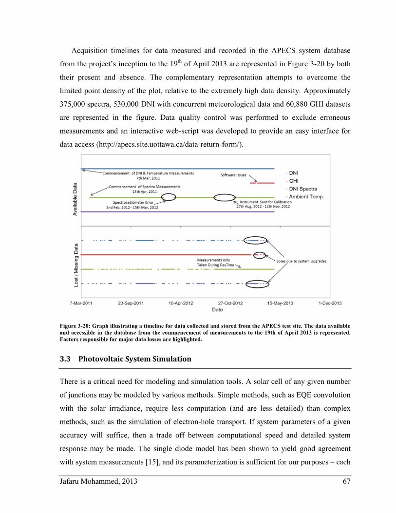
Jafaru Mohammed, 2013 67
Acquisition timelines for data measured and recorded in the APECS system database
from the project’s inception to the 19th
of April 2013 are represented in Figure 3-20 by both
their present and absence. The complementary representation attempts to overcome the
limited point density of the plot, relative to the extremely high data density. Approximately
375,000 spectra, 530,000 DNI with concurrent meteorological data and 60,880 GHI datasets
are represented in the figure. Data quality control was performed to exclude erroneous
measurements and an interactive web-script was developed to provide an easy interface for
data access (http://apecs.site.uottawa.ca/data-return-form/).
Figure 3-20: Graph illustrating a timeline for data collected and stored from the APECS test site. The data available
and accessible in the database from the commencement of measurements to the 19th of April 2013 is represented.
Factors responsible for major data losses are highlighted.
3.3 Photovoltaic System Simulation
There is a critical need for modeling and simulation tools. A solar cell of any given number
of junctions may be modeled by various methods. Simple methods, such as EQE convolution
with the solar irradiance, require less computation (and are less detailed) than complex
methods, such as the simulation of electron-hole transport. If system parameters of a given
accuracy will suffice, then a trade off between computational speed and detailed system
response may be made. The single diode model has been shown to yield good agreement
with system measurements [15], and its parameterization is sufficient for our purposes – each
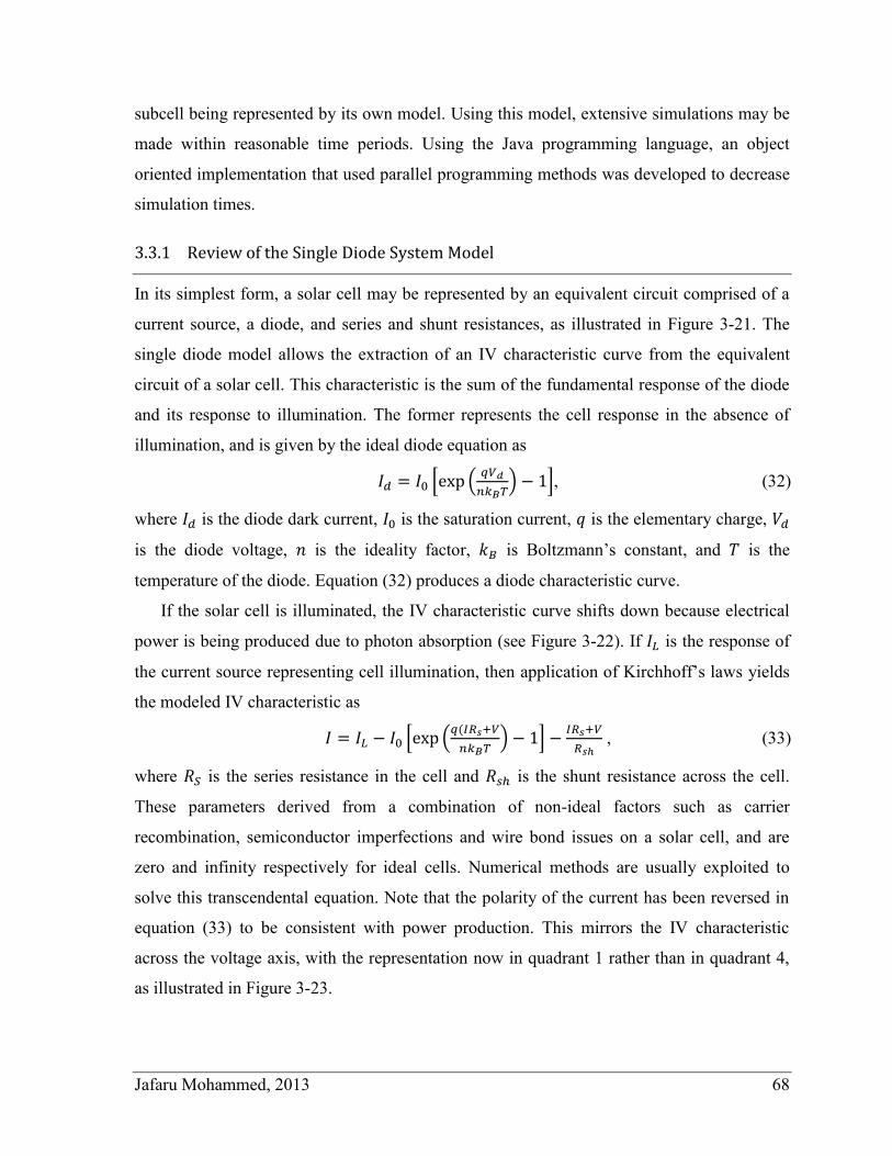
Jafaru Mohammed, 2013 68
subcell being represented by its own model. Using this model, extensive simulations may be
made within reasonable time periods. Using the Java programming language, an object
oriented implementation that used parallel programming methods was developed to decrease
simulation times.
3.3.1 Review of the Single Diode System Model
In its simplest form, a solar cell may be represented by an equivalent circuit comprised of a
current source, a diode, and series and shunt resistances, as illustrated in Figure 3-21. The
single diode model allows the extraction of an IV characteristic curve from the equivalent
circuit of a solar cell. This characteristic is the sum of the fundamental response of the diode
and its response to illumination. The former represents the cell response in the absence of
illumination, and is given by the ideal diode equation as
[ (
) ], (32)
where is the diode dark current, is the saturation current, is the elementary charge,
is the diode voltage, is the ideality factor, is Boltzmann’s constant, and is the
temperature of the diode. Equation (32) produces a diode characteristic curve.
If the solar cell is illuminated, the IV characteristic curve shifts down because electrical
power is being produced due to photon absorption (see Figure 3-22). If is the response of
the current source representing cell illumination, then application of Kirchhoff’s laws yields
the modeled IV characteristic as
[ ( (
) ]
, (33)
where is the series resistance in the cell and is the shunt resistance across the cell.
These parameters derived from a combination of non-ideal factors such as carrier
recombination, semiconductor imperfections and wire bond issues on a solar cell, and are
zero and infinity respectively for ideal cells. Numerical methods are usually exploited to
solve this transcendental equation. Note that the polarity of the current has been reversed in
equation (33) to be consistent with power production. This mirrors the IV characteristic
across the voltage axis, with the representation now in quadrant 1 rather than in quadrant 4,
as illustrated in Figure 3-23.
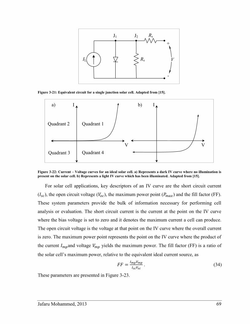
Jafaru Mohammed, 2013 69
Figure 3-21: Equivalent circuit for a single junction solar cell. Adapted from [15].
Figure 3-22: Current – Voltage curves for an ideal solar cell. a) Represents a dark IV curve where no illumination is
present on the solar cell. b) Represents a light IV curve which has been illuminated. Adapted from [15].
For solar cell applications, key descriptors of an IV curve are the short circuit current
( ), the open circuit voltage ( ), the maximum power point ( ) and the fill factor (FF).
These system parameters provide the bulk of information necessary for performing cell
analysis or evaluation. The short circuit current is the current at the point on the IV curve
where the bias voltage is set to zero and it denotes the maximum current a cell can produce.
The open circuit voltage is the voltage at that point on the IV curve where the overall current
is zero. The maximum power point represents the point on the IV curve where the product of
the current and voltage yields the maximum power. The fill factor (FF) is a ratio of
the solar cell’s maximum power, relative to the equivalent ideal current source, as
. (34)
These parameters are presented in Figure 3-23.
J1
I
Rs
V
Rs
h
a)
IL
b)
J2
V
V
I
-
Quadrant 4
+
Quadrant 1 Quadrant 2
Quadrant 3
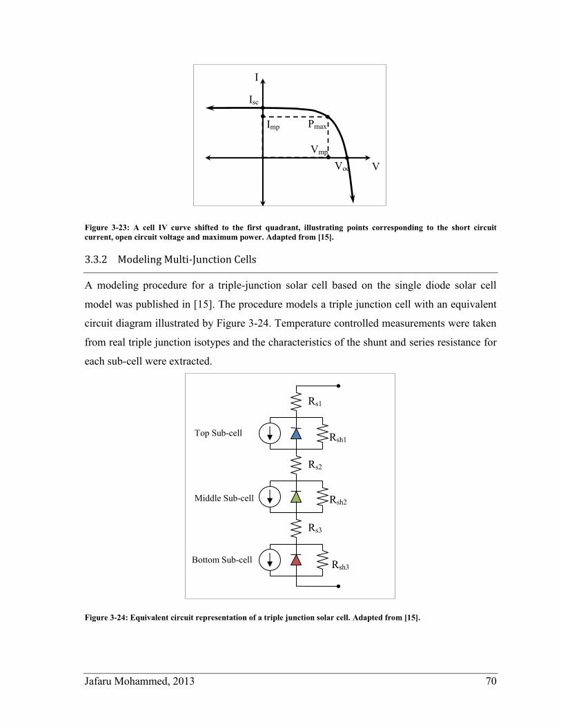
Jafaru Mohammed, 2013 70
Figure 3-23: A cell IV curve shifted to the first quadrant, illustrating points corresponding to the short circuit
current, open circuit voltage and maximum power. Adapted from [15].
3.3.2 Modeling Multi-Junction Cells
A modeling procedure for a triple-junction solar cell based on the single diode solar cell
model was published in [15]. The procedure models a triple junction cell with an equivalent
circuit diagram illustrated by Figure 3-24. Temperature controlled measurements were taken
from real triple junction isotypes and the characteristics of the shunt and series resistance for
each sub-cell were extracted.
Figure 3-24: Equivalent circuit representation of a triple junction solar cell. Adapted from [15].
V
Rsh1
I
Rsh2
Isc
Rsh3
Imp
Rs1
Pmax
Rs2
Vmp
Rs3
Voc
Middle Sub-cell
Bottom Sub-cell
Top Sub-cell
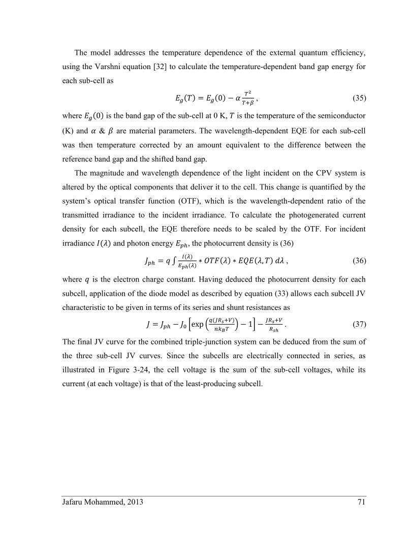
Jafaru Mohammed, 2013 71
The model addresses the temperature dependence of the external quantum efficiency,
using the Varshni equation [32] to calculate the temperature-dependent band gap energy for
each sub-cell as
( ) ( )
, (35)
where ( ) is the band gap of the sub-cell at 0 K, is the temperature of the semiconductor
(K) and & are material parameters. The wavelength-dependent EQE for each sub-cell
was then temperature corrected by an amount equivalent to the difference between the
reference band gap and the shifted band gap.
The magnitude and wavelength dependence of the light incident on the CPV system is
altered by the optical components that deliver it to the cell. This change is quantified by the
system’s optical transfer function (OTF), which is the wavelength-dependent ratio of the
transmitted irradiance to the incident irradiance. To calculate the photogenerated current
density for each subcell, the EQE therefore needs to be scaled by the OTF. For incident
irradiance ( ) and photon energy , the photocurrent density is (36)
∫ ( )
( ) ( ) ( ) , (36)
where is the electron charge constant. Having deduced the photocurrent density for each
subcell, application of the diode model as described by equation (33) allows each subcell JV
characteristic to be given in terms of its series and shunt resistances as
[ ( ( )
) ]
. (37)
The final JV curve for the combined triple-junction system can be deduced from the sum of
the three sub-cell JV curves. Since the subcells are electrically connected in series, as
illustrated in Figure 3-24, the cell voltage is the sum of the sub-cell voltages, while its
current (at each voltage) is that of the least-producing subcell.
Jafaru Mohammed, 2013 72
4 Spectral Estimation and Energy Yield Analysis
Two major research results are presented in this chapter: The first describes a method to
acquire spectral datasets through the design and implementation of a model, extending
results published by Harrison and Michalsky [52], that parameterises the aerosol optical
depth (AOD) from spectral measurements. The purpose of the extended model is to generate
time resolved clear sky spectra for any specified location. The second is an analysis aimed at
discovering the impact of meteorological effects on long term energy yield predictions.
4.1 Spectral Estimation Using Parameterized Aerosol Optical Depth
The design and operation of PV systems depends on the nature of the local solar resource.
For CPV systems, the local DNI is the key component of the solar resource responsible for
photocurrent generation. Long term local measurements of spectral DNI are essential for
assessing CPV system response at any particular site [53]. However, setting up systems to
measure the spectral distribution of the solar resource at every potential CPV site is
economically unviable due to time requirements and spectroradiometer costs. Wide area
satellite meteorological measurements are sometimes used as an input to radiative models,
but these only provide low resolution spectral irradiance of insufficient temporal granularity.
However, ground based measurements of meteorological conditions with less expensive
instruments can be used as an input to radiative models. One such model, a “Simple Model
for the Atmospheric Radiative Transfer of Sunshine version 2” (SMARTS2), has been
developed to describe average local radiation [54, 55]. It treats the optical depth of the
atmosphere in terms of its individual components, such as Rayleigh scattering, gaseous
absorption and aerosols.
Using SMARTS as a base model, the clear sky DNI for the APECS test station in Ottawa
was predicted and assessed using an extended method for extracting AOD from measured
spectra. Meteorological data gathered from various sources, such as the Canadian Weather
Energy and Engineering Data Sets (CWEEDS), were used to achieve this goal. Simulating
solar spectra with SMARTS2 is straightforward; the primary concerns are the locally
sensitive inputs to the model, and the AOD in particular.
Jafaru Mohammed, 2013 73
SMARTS2 provides built-in algorithms for deducing an atmospheric constituent’s optical
depth from basic meteorological data. For example, perceptible water vapour can be
calculated from temperature, atmospheric pressure and humidity data. In place of
meteorological measurements of the optical depth of atmospheric gases, the model typically
uses the concentrations of gases in the atmosphere to calculate individual absorptive profiles.
One exception is the determination of the AOD. Unlike basic meteorological parameters that
can be easily measured with conventional instruments, the wavelength dependence of the
AOD depends on the local distribution of particle sizes in the atmosphere and its direct
measurement is nontrivial. The temporal profile of the AOD is never particularly constant,
especially in urban areas due to the varying atmospheric concentrations of dust, smoke and
smog. For convenience, SMARTS2 makes use of the angstrom parameter to extrapolate a
known AOD ( ) at a particular wavelength (typically, 500 nm or 550 nm) to other
wavelengths. This parameter is defined by
(
)
, (38)
where is the optical depth at the required wavelength.
4.1.1 Optical Depth Extraction Algorithm
An algorithm for extracting optical depths from ground based measurements [52] was further
developed to extract optical depths from time resolved measured spectral DNI under clear
sky conditions. The hypothesis that spectral DNI may be adequately simulated on the basis
of single-frequency AOD extraction from clear sky spectral irradiance was self-consistently
tested against its generating spectra. The extraction process begins with the Langley
regression, which is a linear regression applied to Bouguer's law.
Bouguer's law describes the attenuation in intensity of light traversing a uniform medium
as
( )
( ) , (39)
where is the measured DNI at wavelength , is the path length traversed by the light
(which may be expressed as an air mass), and is the optical depth for the specified
wavelength [52]. It is necessary to calculate the air mass as a function of time of day and
year. The high precision solar calculation algorithm presented in section 2.4.1 was used to do
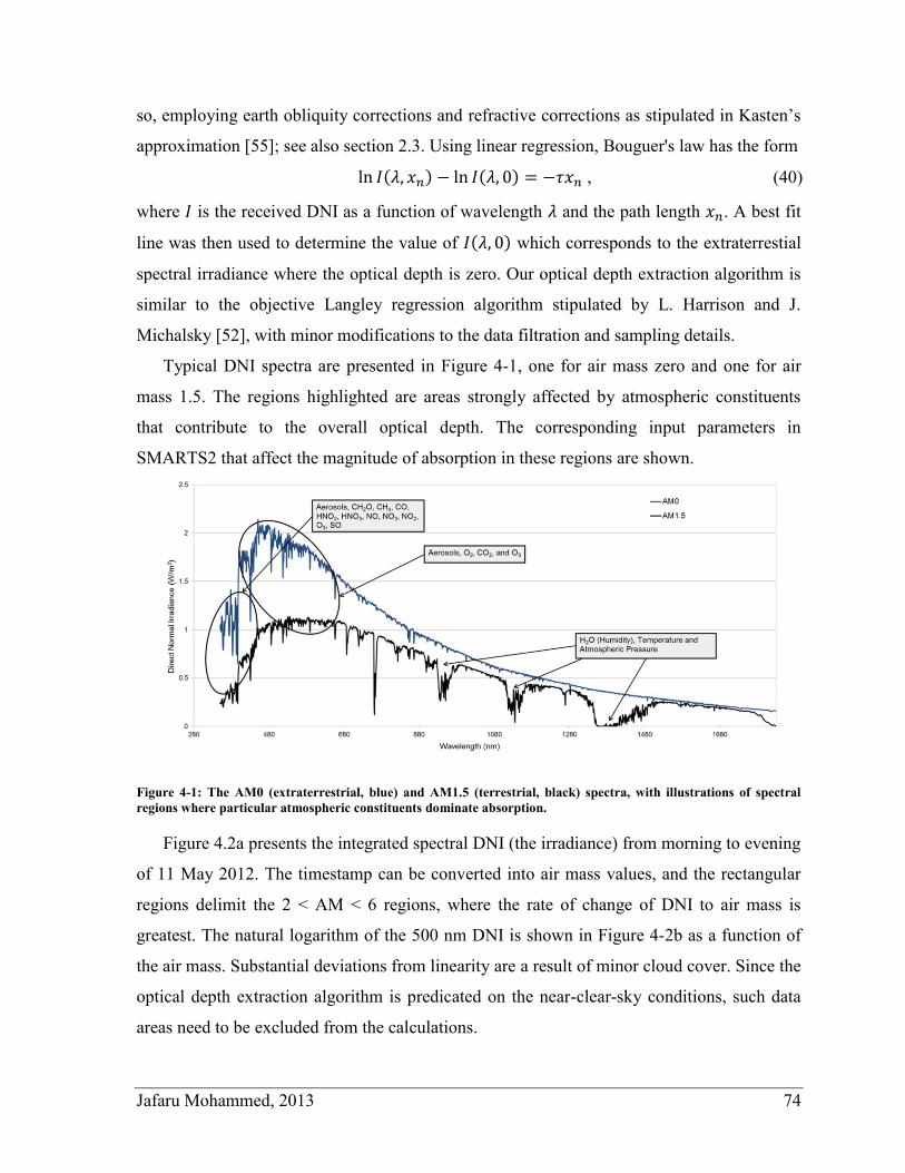
Jafaru Mohammed, 2013 74
so, employing earth obliquity corrections and refractive corrections as stipulated in Kasten’s
approximation [55]; see also section 2.3. Using linear regression, Bouguer's law has the form
( ) ( ) , (40)
where is the received DNI as a function of wavelength and the path length . A best fit
line was then used to determine the value of ( ) which corresponds to the extraterrestial
spectral irradiance where the optical depth is zero. Our optical depth extraction algorithm is
similar to the objective Langley regression algorithm stipulated by L. Harrison and J.
Michalsky [52], with minor modifications to the data filtration and sampling details.
Typical DNI spectra are presented in Figure 4-1, one for air mass zero and one for air
mass 1.5. The regions highlighted are areas strongly affected by atmospheric constituents
that contribute to the overall optical depth. The corresponding input parameters in
SMARTS2 that affect the magnitude of absorption in these regions are shown.
Figure 4-1: The AM0 (extraterrestrial, blue) and AM1.5 (terrestrial, black) spectra, with illustrations of spectral
regions where particular atmospheric constituents dominate absorption.
Figure 4.2a presents the integrated spectral DNI (the irradiance) from morning to evening
of 11 May 2012. The timestamp can be converted into air mass values, and the rectangular
regions delimit the 2 < AM < 6 regions, where the rate of change of DNI to air mass is
greatest. The natural logarithm of the 500 nm DNI is shown in Figure 4-2b as a function of
the air mass. Substantial deviations from linearity are a result of minor cloud cover. Since the
optical depth extraction algorithm is predicated on the near-clear-sky conditions, such data
areas need to be excluded from the calculations.
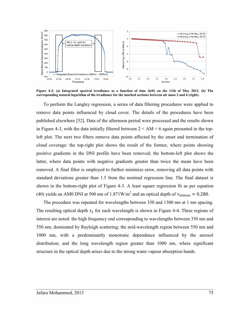
Jafaru Mohammed, 2013 75
Figure 4-2: (a) Integrated spectral irradiance as a function of time (left) on the 11th of May 2012. (b) The
corresponding natural logarithm of the irradiance for the marked sections between air mass 2 and 6 (right).
To perform the Langley regression, a series of data filtering procedures were applied to
remove data points influenced by cloud cover. The details of the procedures have been
published elsewhere [52]. Data of the afternoon period were processed and the results shown
in Figure 4-3, with the data initially filtered between 2 < AM < 6 again presented in the top-
left plot. The next two filters remove data points affected by the onset and termination of
cloud coverage: the top-right plot shows the result of the former, where points showing
positive gradients in the DNI profile have been removed; the bottom-left plot shows the
latter, where data points with negative gradients greater than twice the mean have been
removed. A final filter is employed to further minimize error, removing all data points with
standard deviations greater than 1.5 from the nominal regression line. The final dataset is
shown in the bottom-right plot of Figure 4-3. A least square regression fit as per equation
(40) yields an AM0 DNI at 500 nm of 1.871W/m2 and an optical depth of .
The procedure was repeated for wavelengths between 350 and 1300 nm at 1 nm spacing.
The resulting optical depth for each wavelength is shown in Figure 4-4. Three regions of
interest are noted: the high frequency end corresponding to wavelengths between 350 nm and
550 nm, dominated by Rayleigh scattering; the mid-wavelength region between 550 nm and
1000 nm, with a predominantly monotonic dependence influenced by the aerosol
distribution; and the long wavelength region greater than 1000 nm, where significant
structure in the optical depth arises due to the strong water vapour absorption bands.
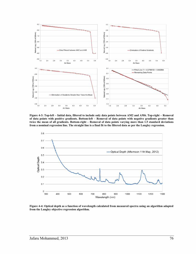
Jafaru Mohammed, 2013 76
Figure 4-3: Top-left – Initial data, filtered to include only data points between AM2 and AM6. Top-right – Removal
of data points with positive gradients. Bottom-left – Removal of data points with negative gradients greater than
twice the mean of all gradients. Bottom-right – Removal of data points varying more than 1.5 standard deviations
from a nominal regression line. The straight line is a final fit to the filtered data as per the Langley regression.
Figure 4-4: Optical depth as a function of wavelength calculated from measured spectra using an algorithm adapted
from the Langley objective regression algorithm.
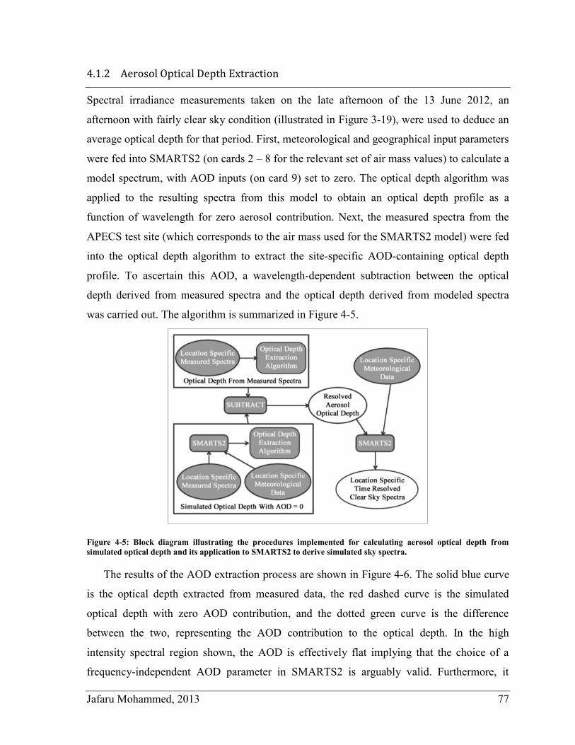
Jafaru Mohammed, 2013 77
4.1.2 Aerosol Optical Depth Extraction
Spectral irradiance measurements taken on the late afternoon of the 13 June 2012, an
afternoon with fairly clear sky condition (illustrated in Figure 3-19), were used to deduce an
average optical depth for that period. First, meteorological and geographical input parameters
were fed into SMARTS2 (on cards 2 – 8 for the relevant set of air mass values) to calculate a
model spectrum, with AOD inputs (on card 9) set to zero. The optical depth algorithm was
applied to the resulting spectra from this model to obtain an optical depth profile as a
function of wavelength for zero aerosol contribution. Next, the measured spectra from the
APECS test site (which corresponds to the air mass used for the SMARTS2 model) were fed
into the optical depth algorithm to extract the site-specific AOD-containing optical depth
profile. To ascertain this AOD, a wavelength-dependent subtraction between the optical
depth derived from measured spectra and the optical depth derived from modeled spectra
was carried out. The algorithm is summarized in Figure 4-5.
Figure 4-5: Block diagram illustrating the procedures implemented for calculating aerosol optical depth from
simulated optical depth and its application to SMARTS2 to derive simulated sky spectra.
The results of the AOD extraction process are shown in Figure 4-6. The solid blue curve
is the optical depth extracted from measured data, the red dashed curve is the simulated
optical depth with zero AOD contribution, and the dotted green curve is the difference
between the two, representing the AOD contribution to the optical depth. In the high
intensity spectral region shown, the AOD is effectively flat implying that the choice of a
frequency-independent AOD parameter in SMARTS2 is arguably valid. Furthermore, it
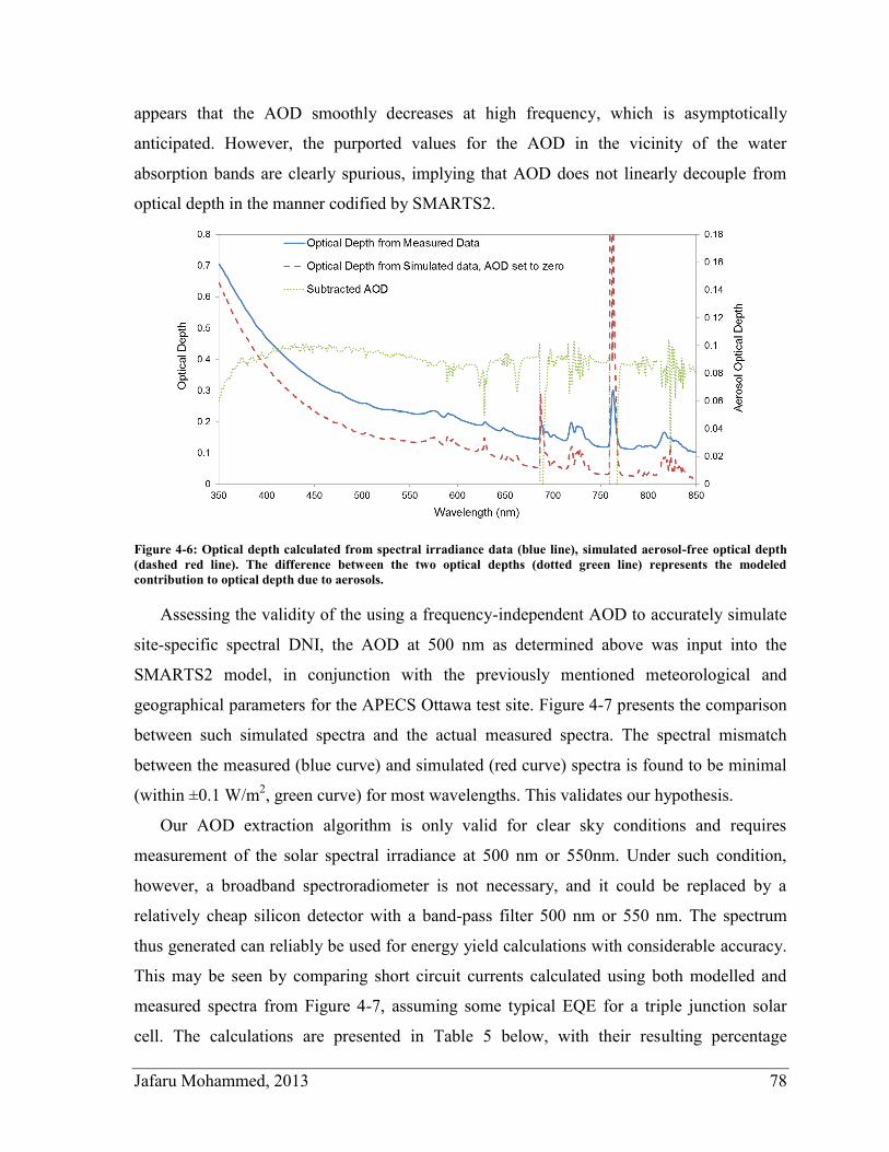
Jafaru Mohammed, 2013 78
appears that the AOD smoothly decreases at high frequency, which is asymptotically
anticipated. However, the purported values for the AOD in the vicinity of the water
absorption bands are clearly spurious, implying that AOD does not linearly decouple from
optical depth in the manner codified by SMARTS2.
Figure 4-6: Optical depth calculated from spectral irradiance data (blue line), simulated aerosol-free optical depth
(dashed red line). The difference between the two optical depths (dotted green line) represents the modeled
contribution to optical depth due to aerosols.
Assessing the validity of the using a frequency-independent AOD to accurately simulate
site-specific spectral DNI, the AOD at 500 nm as determined above was input into the
SMARTS2 model, in conjunction with the previously mentioned meteorological and
geographical parameters for the APECS Ottawa test site. Figure 4-7 presents the comparison
between such simulated spectra and the actual measured spectra. The spectral mismatch
between the measured (blue curve) and simulated (red curve) spectra is found to be minimal
(within ±0.1 W/m2, green curve) for most wavelengths. This validates our hypothesis.
Our AOD extraction algorithm is only valid for clear sky conditions and requires
measurement of the solar spectral irradiance at 500 nm or 550nm. Under such condition,
however, a broadband spectroradiometer is not necessary, and it could be replaced by a
relatively cheap silicon detector with a band-pass filter 500 nm or 550 nm. The spectrum
thus generated can reliably be used for energy yield calculations with considerable accuracy.
This may be seen by comparing short circuit currents calculated using both modelled and
measured spectra from Figure 4-7, assuming some typical EQE for a triple junction solar
cell. The calculations are presented in Table 5 below, with their resulting percentage
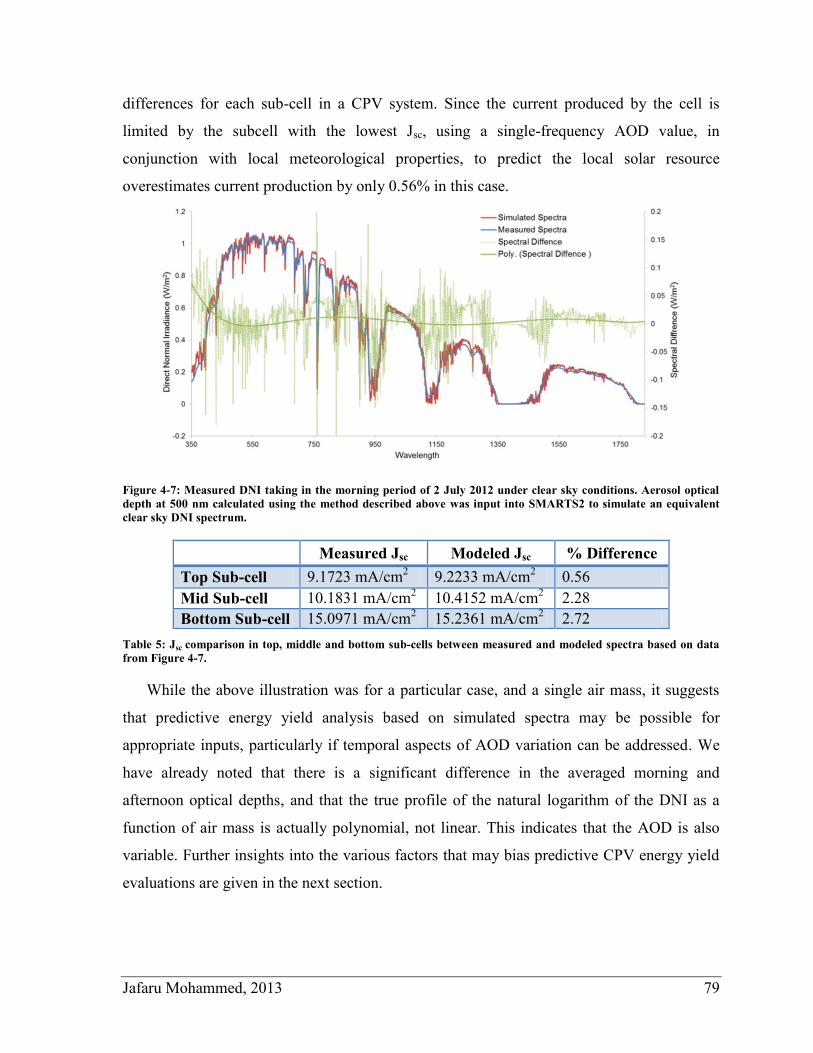
Jafaru Mohammed, 2013 79
differences for each sub-cell in a CPV system. Since the current produced by the cell is
limited by the subcell with the lowest Jsc, using a single-frequency AOD value, in
conjunction with local meteorological properties, to predict the local solar resource
overestimates current production by only 0.56% in this case.
Figure 4-7: Measured DNI taking in the morning period of 2 July 2012 under clear sky conditions. Aerosol optical
depth at 500 nm calculated using the method described above was input into SMARTS2 to simulate an equivalent
clear sky DNI spectrum.
Measured Jsc Modeled Jsc % Difference
Top Sub-cell 9.1723 mA/cm2 9.2233 mA/cm
2 0.56
Mid Sub-cell 10.1831 mA/cm2 10.4152 mA/cm
2 2.28
Bottom Sub-cell 15.0971 mA/cm2 15.2361 mA/cm
2 2.72
Table 5: Jsc comparison in top, middle and bottom sub-cells between measured and modeled spectra based on data
from Figure 4-7.
While the above illustration was for a particular case, and a single air mass, it suggests
that predictive energy yield analysis based on simulated spectra may be possible for
appropriate inputs, particularly if temporal aspects of AOD variation can be addressed. We
have already noted that there is a significant difference in the averaged morning and
afternoon optical depths, and that the true profile of the natural logarithm of the DNI as a
function of air mass is actually polynomial, not linear. This indicates that the AOD is also
variable. Further insights into the various factors that may bias predictive CPV energy yield
evaluations are given in the next section.
Jafaru Mohammed, 2013 80
4.2 Investigating Energy Yield Analysis
Energy yield analysis in the context of PV systems is associated with the determination of
energy production over a given time period. It is often a predictive process to evaluate a
potential PV site when planning, siting or financing PV installations. Where CPV is
concerned, due to the nature of the technology, it is unknown if the current methods used for
PV energy yield evaluation are directly applicable for all atmospheric conditions. This is
because CPV optics focus only the direct sunlight component, unlike PV which uses global
irradiance. The response of CPV to factors that affect its solar resource, such as cloud cover,
aerosol and perceptible water vapour, needs to be investigated and properly understood. The
literature [30] also documents that CPV cells are more spectrally sensitive to atmospheric
variation than PV cells. This is of particular concern since the models used for PV energy
yield evaluation do not need to address spectral variation.
In this section, a spectrally sensitive CPV model has been compared to a simple power –
efficiency product model (commonly used for PV evaluation) under different temporal
conditions to determine the presence and degree of bias in the use of simple models for CPV.
The choice of dataset used for PV energy yield evaluation spatially and temporally is also
investigated with an aim to de-convolute the degree of bias due to air mass variations,
aerosols, cloud cover and temperature changes. Temporally measured spectral from the
APECS test site (Ottawa, Ontario, Canada) between June 2011 and August 2012 was used
for the analysis. Data from the Canadian Weather Energy and Engineering Data Sets
(CWEEDS) and the Canadian Weather for Energy Calculation (CWEC) were utilized for
long term sturdy and typical meteorological analysis respectively.
4.2.1 Introduction / Background
Recent breakthroughs in high efficiency multi-junction solar cells towards 40% efficiency
[56] have driven interest in the use of CPV technology for developing utility-scale solar
farms. With ever growing interest in renewable energy for sustainable development, the role
of concentrated photovoltaics is bound to become more prominent in the global market [57].
CPV technology is fast becoming an economically viable option for utility-scale, clean
renewable electricity in global regions with high annual direct solar insolation. Presently,
over 360 MW of CPV generating capacity has been installed worldwide [58], and the trend
Jafaru Mohammed, 2013 81
in development suggests that the drop in cost and rise in efficiency could permit
economically viable use in some regions of Canada. For implementing CPV, the local solar
resource must be considered when siting and financing projects, and adequate energy yield
models are essential for the decision making processes.
CPV performance is dependent on its system efficiency profile, a function of the
temporal solar resource and the cell and optics efficiency. System performance has been
enhanced through cell tuning and customized optics [59]. The components of the optical
assembly deliver the solar resource to the cell and each component has a frequency-
dependent transmission efficiency known as the optical transfer function (OTF). For multi-
junction CPV systems, cell current is limited to that of the least producing sub-cell.
Optimally, light incident on the cells across all daylight air mass values should allow each
sub-cell to produce a current that does not limit performance. Best CPV system performance
may thus be achieved by tuning the solar cell and the system optical transfer function to the
spectrum of the local solar resource over all air mass values. Methods to tune the solar cell
for the standard spectrum have been reported [60, 61] and tuning a multi-junction cell to a
location specific spectrum has been shown to yield better system performance [61].
Predicting the spectrum of the local solar resource requires proper understanding of the
temporal behaviour of atmospheric and meteorological components such as clouds,
perceptible water vapour and aerosols which affect the local solar resource. Where measured
long term spectral DNI data are absent, as described in section 4.1, these components play an
important role as inputs into atmospheric radiation transfer models such as SMARTS2.
PV system output must be sold into a very competitive market with cost as the dominant
differentiator. Electricity providers such as Ontario Hydro are increasingly looking at ways
to match generation to demand in the most economical manner. The use of incentives to
reduce electricity consumption at peak hours is being implemented in Ontario and solar
generated electricity is well suited to provide electricity when demand is at its peak. To
assess economic potential under different pricing schemes, and to guide policy for incentive
programs, it is important to determine energy yields at high temporal granularity. The inputs
to energy yield analysis are key to levelized cost of energy (LCoE) calculations [62], the
basis for financial analysis of utility-scale PV projects.
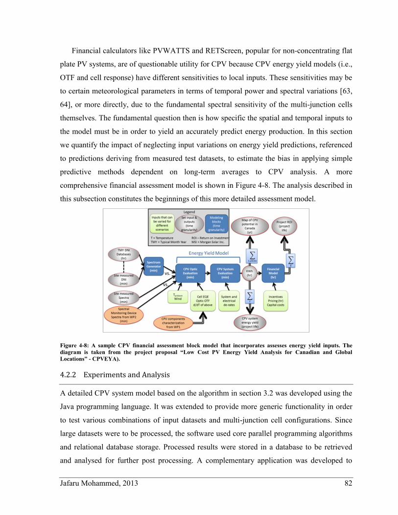
Jafaru Mohammed, 2013 82
Financial calculators like PVWATTS and RETScreen, popular for non-concentrating flat
plate PV systems, are of questionable utility for CPV because CPV energy yield models (i.e.,
OTF and cell response) have different sensitivities to local inputs. These sensitivities may be
to certain meteorological parameters in terms of temporal power and spectral variations [63,
64], or more directly, due to the fundamental spectral sensitivity of the multi-junction cells
themselves. The fundamental question then is how specific the spatial and temporal inputs to
the model must be in order to yield an accurately predict energy production. In this section
we quantify the impact of neglecting input variations on energy yield predictions, referenced
to predictions deriving from measured test datasets, to estimate the bias in applying simple
predictive methods dependent on long-term averages to CPV analysis. A more
comprehensive financial assessment model is shown in Figure 4-8. The analysis described in
this subsection constitutes the beginnings of this more detailed assessment model.
Figure 4-8: A sample CPV financial assessment block model that incorporates assesses energy yield inputs. The
diagram is taken from the project proposal “Low Cost PV Energy Yield Analysis for Canadian and Global
Locations” - CPVEYA).
4.2.2 Experiments and Analysis
A detailed CPV system model based on the algorithm in section 3.2 was developed using the
Java programming language. It was extended to provide more generic functionality in order
to test various combinations of input datasets and multi-junction cell configurations. Since
large datasets were to be processed, the software used core parallel programming algorithms
and relational database storage. Processed results were stored in a database to be retrieved
and analysed for further post processing. A complementary application was developed to
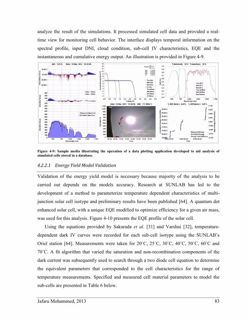
Jafaru Mohammed, 2013 83
analyze the result of the simulations. It processed simulated cell data and provided a real-
time view for monitoring cell behavior. The interface displays temporal information on the
spectral profile, input DNI, cloud condition, sub-cell IV characteristics, EQE and the
instantaneous and cumulative energy output. An illustration is provided in Figure 4-9.
Figure 4-9: Sample media illustrating the operation of a data plotting application developed to aid analysis of
simulated cells stored in a database.
4.2.2.1 Energy Yield Model Validation
Validation of the energy yield model is necessary because majority of the analysis to be
carried out depends on the models accuracy. Research at SUNLAB has led to the
development of a method to parameterize temperature dependent characteristics of multi-
junction solar cell isotype and preliminary results have been published [64]. A quantum dot
enhanced solar cell, with a unique EQE modified to optimize efficiency for a given air mass,
was used for this analysis. Figure 4-10 presents the EQE profile of the solar cell.
Using the equations provided by Sakurada et al. [31] and Varshni [32], temperature-
dependent dark IV curves were recorded for each sub-cell isotype using the SUNLAB’s
Oriel station [64]. Measurements were taken for 20˚C, 25˚C, 30˚C, 40˚C, 50˚C, 60˚C and
70˚C. A fit algorithm that varied the saturation and non-recombination components of the
dark current was subsequently used to search through a two diode cell equation to determine
the equivalent parameters that corresponded to the cell characteristics for the range of
temperature measurements. Specified and measured cell material parameters to model the
sub-cells are presented in Table 6 below.
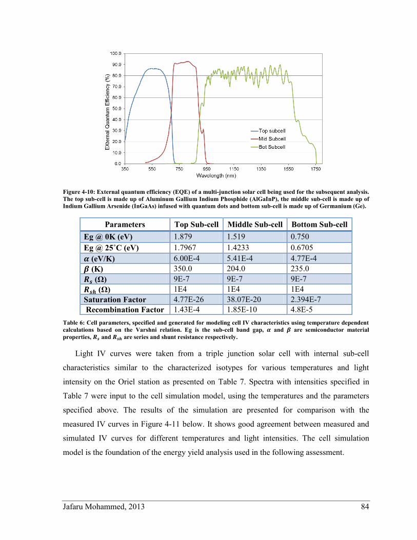
Jafaru Mohammed, 2013 84
Figure 4-10: External quantum efficiency (EQE) of a multi-junction solar cell being used for the subsequent analysis.
The top sub-cell is made up of Aluminum Gallium Indium Phosphide (AlGaInP), the middle sub-cell is made up of
Indium Gallium Arsenide (InGaAs) infused with quantum dots and bottom sub-cell is made up of Germanium (Ge).
Parameters Top Sub-cell Middle Sub-cell Bottom Sub-cell
Eg @ 0K (eV) 1.879 1.519 0.750
Eg @ 25˚C (eV) 1.7967 1.4233 0.6705
(eV/K) 6.00E-4 5.41E-4 4.77E-4
(K) 350.0 204.0 235.0
(Ω) 9E-7 9E-7 9E-7
(Ω) 1E4 1E4 1E4
Saturation Factor 4.77E-26 38.07E-20 2.394E-7
Recombination Factor 1.43E-4 1.85E-10 4.8E-5
Table 6: Cell parameters, specified and generated for modeling cell IV characteristics using temperature dependent
calculations based on the Varshni relation. Eg is the sub-cell band gap, and are semiconductor material
properties, and are series and shunt resistance respectively.
Light IV curves were taken from a triple junction solar cell with internal sub-cell
characteristics similar to the characterized isotypes for various temperatures and light
intensity on the Oriel station as presented on Table 7. Spectra with intensities specified in
Table 7 were input to the cell simulation model, using the temperatures and the parameters
specified above. The results of the simulation are presented for comparison with the
measured IV curves in Figure 4-11 below. It shows good agreement between measured and
simulated IV curves for different temperatures and light intensities. The cell simulation
model is the foundation of the energy yield analysis used in the following assessment.
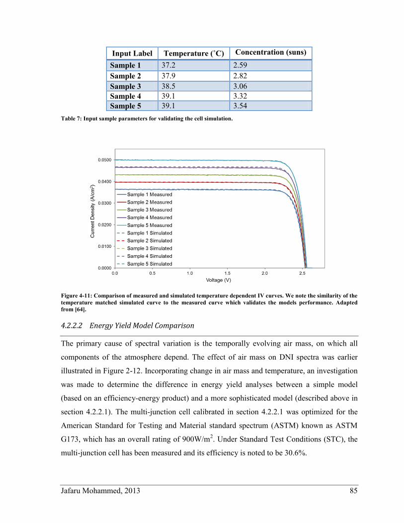
Jafaru Mohammed, 2013 85
Input Label Temperature (˚C) Concentration (suns)
Sample 1 37.2 2.59
Sample 2 37.9 2.82
Sample 3 38.5 3.06
Sample 4 39.1 3.32
Sample 5 39.1 3.54
Table 7: Input sample parameters for validating the cell simulation.
Figure 4-11: Comparison of measured and simulated temperature dependent IV curves. We note the similarity of the
temperature matched simulated curve to the measured curve which validates the models performance. Adapted
from [64].
4.2.2.2 Energy Yield Model Comparison
The primary cause of spectral variation is the temporally evolving air mass, on which all
components of the atmosphere depend. The effect of air mass on DNI spectra was earlier
illustrated in Figure 2-12. Incorporating change in air mass and temperature, an investigation
was made to determine the difference in energy yield analyses between a simple model
(based on an efficiency-energy product) and a more sophisticated model (described above in
section 4.2.2.1). The multi-junction cell calibrated in section 4.2.2.1 was optimized for the
American Standard for Testing and Material standard spectrum (ASTM) known as ASTM
G173, which has an overall rating of 900W/m2. Under Standard Test Conditions (STC), the
multi-junction cell has been measured and its efficiency is noted to be 30.6%.
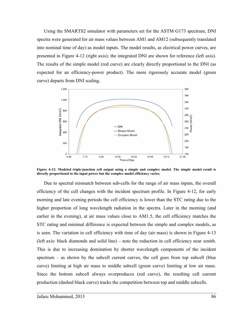
Jafaru Mohammed, 2013 86
Using the SMARTS2 simulator with parameters set for the ASTM G173 spectrum, DNI
spectra were generated for air mass values between AM1 and AM12 (subsequently translated
into nominal time of day) as model inputs. The model results, as electrical power curves, are
presented in Figure 4-12 (right axis); the integrated DNI are shown for reference (left axis).
The results of the simple model (red curve) are clearly directly proportional to the DNI (as
expected for an efficiency-power product). The more rigorously accurate model (green
curve) departs from DNI scaling.
Figure 4-12: Modeled triple-junction cell output using a simple and complex model. The simple model result is
directly proportional to the input power but the complex model efficiency varies.
Due to spectral mismatch between sub-cells for the range of air mass inputs, the overall
efficiency of the cell changes with the incident spectrum profile. In Figure 4-12, for early
morning and late evening periods the cell efficiency is lower than the STC rating due to the
higher proportion of long wavelength radiation in the spectra. Later in the morning (and
earlier in the evening), at air mass values close to AM1.5, the cell efficiency matches the
STC rating and minimal difference is expected between the simple and complex models, as
is seen. The variation in cell efficiency with time of day (air mass) is shown in Figure 4-13
(left axis: black diamonds and solid line) – note the reduction in cell efficiency near zenith.
This is due to increasing domination by shorter wavelength components of the incident
spectrum – as shown by the subcell current curves, the cell goes from top subcell (blue
curve) limiting at high air mass to middle subcell (green curve) limiting at low air mass.
Since the bottom subcell always overproduces (red curve), the resulting cell current
production (dashed black curve) tracks the competition between top and middle subcells.
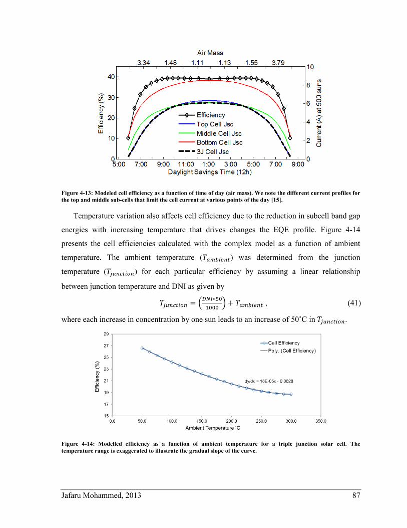
Jafaru Mohammed, 2013 87
Figure 4-13: Modeled cell efficiency as a function of time of day (air mass). We note the different current profiles for
the top and middle sub-cells that limit the cell current at various points of the day [15].
Temperature variation also affects cell efficiency due to the reduction in subcell band gap
energies with increasing temperature that drives changes the EQE profile. Figure 4-14
presents the cell efficiencies calculated with the complex model as a function of ambient
temperature. The ambient temperature ( ) was determined from the junction
temperature ( ) for each particular efficiency by assuming a linear relationship
between junction temperature and DNI as given by
(
) , (41)
where each increase in concentration by one sun leads to an increase of 50˚C in .
Figure 4-14: Modelled efficiency as a function of ambient temperature for a triple junction solar cell. The
temperature range is exaggerated to illustrate the gradual slope of the curve.
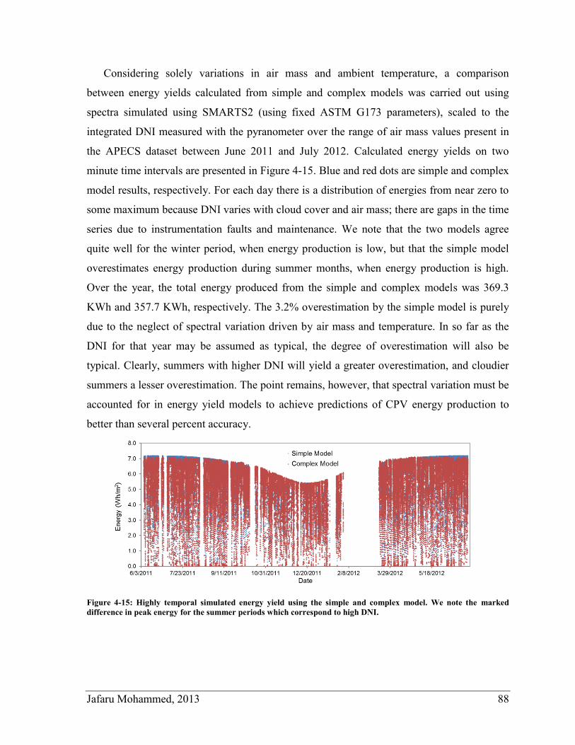
Jafaru Mohammed, 2013 88
Considering solely variations in air mass and ambient temperature, a comparison
between energy yields calculated from simple and complex models was carried out using
spectra simulated using SMARTS2 (using fixed ASTM G173 parameters), scaled to the
integrated DNI measured with the pyranometer over the range of air mass values present in
the APECS dataset between June 2011 and July 2012. Calculated energy yields on two
minute time intervals are presented in Figure 4-15. Blue and red dots are simple and complex
model results, respectively. For each day there is a distribution of energies from near zero to
some maximum because DNI varies with cloud cover and air mass; there are gaps in the time
series due to instrumentation faults and maintenance. We note that the two models agree
quite well for the winter period, when energy production is low, but that the simple model
overestimates energy production during summer months, when energy production is high.
Over the year, the total energy produced from the simple and complex models was 369.3
KWh and 357.7 KWh, respectively. The 3.2% overestimation by the simple model is purely
due to the neglect of spectral variation driven by air mass and temperature. In so far as the
DNI for that year may be assumed as typical, the degree of overestimation will also be
typical. Clearly, summers with higher DNI will yield a greater overestimation, and cloudier
summers a lesser overestimation. The point remains, however, that spectral variation must be
accounted for in energy yield models to achieve predictions of CPV energy production to
better than several percent accuracy.
Figure 4-15: Highly temporal simulated energy yield using the simple and complex model. We note the marked
difference in peak energy for the summer periods which correspond to high DNI.
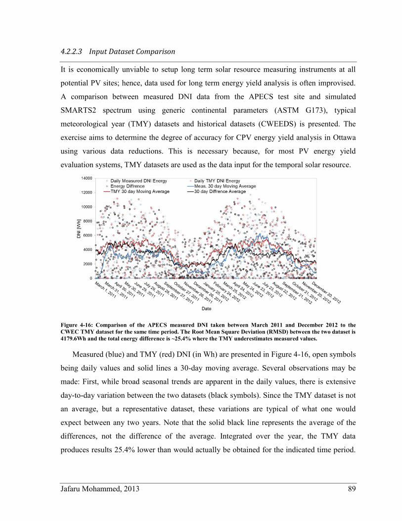
Jafaru Mohammed, 2013 89
4.2.2.3 Input Dataset Comparison
It is economically unviable to setup long term solar resource measuring instruments at all
potential PV sites; hence, data used for long term energy yield analysis is often improvised.
A comparison between measured DNI data from the APECS test site and simulated
SMARTS2 spectrum using generic continental parameters (ASTM G173), typical
meteorological year (TMY) datasets and historical datasets (CWEEDS) is presented. The
exercise aims to determine the degree of accuracy for CPV energy yield analysis in Ottawa
using various data reductions. This is necessary because, for most PV energy yield
evaluation systems, TMY datasets are used as the data input for the temporal solar resource.
Figure 4-16: Comparison of the APECS measured DNI taken between March 2011 and December 2012 to the
CWEC TMY dataset for the same time period. The Root Mean Square Deviation (RMSD) between the two dataset is
4179.6Wh and the total energy difference is ~25.4% where the TMY underestimates measured values.
Measured (blue) and TMY (red) DNI (in Wh) are presented in Figure 4-16, open symbols
being daily values and solid lines a 30-day moving average. Several observations may be
made: First, while broad seasonal trends are apparent in the daily values, there is extensive
day-to-day variation between the two datasets (black symbols). Since the TMY dataset is not
an average, but a representative dataset, these variations are typical of what one would
expect between any two years. Note that the solid black line represents the average of the
differences, not the difference of the average. Integrated over the year, the TMY data
produces results 25.4% lower than would actually be obtained for the indicated time period.
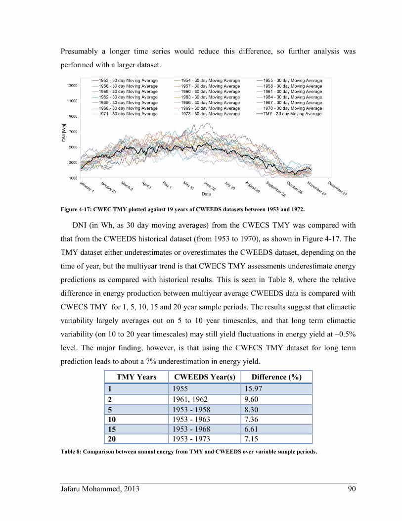
Jafaru Mohammed, 2013 90
Presumably a longer time series would reduce this difference, so further analysis was
performed with a larger dataset.
Figure 4-17: CWEC TMY plotted against 19 years of CWEEDS datasets between 1953 and 1972.
DNI (in Wh, as 30 day moving averages) from the CWECS TMY was compared with
that from the CWEEDS historical dataset (from 1953 to 1970), as shown in Figure 4-17. The
TMY dataset either underestimates or overestimates the CWEEDS dataset, depending on the
time of year, but the multiyear trend is that CWECS TMY assessments underestimate energy
predictions as compared with historical results. This is seen in Table 8, where the relative
difference in energy production between multiyear average CWEEDS data is compared with
CWECS TMY for 1, 5, 10, 15 and 20 year sample periods. The results suggest that climactic
variability largely averages out on 5 to 10 year timescales, and that long term climactic
variability (on 10 to 20 year timescales) may still yield fluctuations in energy yield at ~0.5%
level. The major finding, however, is that using the CWECS TMY dataset for long term
prediction leads to about a 7% underestimation in energy yield.
TMY Years CWEEDS Year(s) Difference (%)
1 1955 15.97
2 1961, 1962 9.60
5 1953 - 1958 8.30
10 1953 - 1963 7.36
15 1953 - 1968 6.61
20 1953 - 1973 7.15
Table 8: Comparison between annual energy from TMY and CWEEDS over variable sample periods.
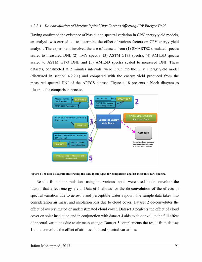
Jafaru Mohammed, 2013 91
4.2.2.4 De-convolution of Meteorological Bias Factors Affecting CPV Energy Yield
Having confirmed the existence of bias due to spectral variation in CPV energy yield models,
an analysis was carried out to determine the effect of various factors on CPV energy yield
analysis. The experiment involved the use of datasets from (1) SMARTS2 simulated spectra
scaled to measured DNI, (2) TMY spectra, (3) ASTM G173 spectra, (4) AM1.5D spectra
scaled to ASTM G173 DNI, and (5) AM1.5D spectra scaled to measured DNI. These
datasets, constructed at 2 minutes intervals, were input into the CPV energy yield model
(discussed in section 4.2.2.1) and compared with the energy yield produced from the
measured spectral DNI of the APECS dataset. Figure 4-18 presents a block diagram to
illustrate the comparison process.
Figure 4-18: Block diagram illustrating the data input types for comparison against measured DNI spectra.
Results from the simulations using the various inputs were used to de-convolute the
factors that affect energy yield. Dataset 1 allows for the de-convolution of the effects of
spectral variation due to aerosols and perceptible water vapour. The sample data takes into
consideration air mass, and insolation loss due to cloud cover. Dataset 2 de-convolutes the
effect of overestimated or underestimated cloud cover. Dataset 3 neglects the effect of cloud
cover on solar insolation and in conjunction with dataset 4 aids to de-convolute the full effect
of spectral variations due to air mass change. Dataset 5 complements the result from dataset
1 to de-convolute the effect of air mass induced spectral variations.
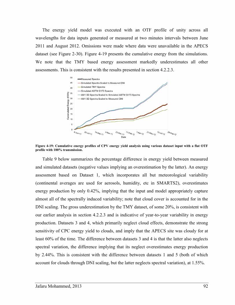
Jafaru Mohammed, 2013 92
The energy yield model was executed with an OTF profile of unity across all
wavelengths for data inputs generated or measured at two minutes intervals between June
2011 and August 2012. Omissions were made where data were unavailable in the APECS
dataset (see Figure 2-30). Figure 4-19 presents the cumulative energy from the simulations.
We note that the TMY based energy assessment markedly underestimates all other
assessments. This is consistent with the results presented in section 4.2.2.3.
Figure 4-19: Cumulative energy profiles of CPV energy yield analysis using various dataset input with a flat OTF
profile with 100% transmission.
Table 9 below summarizes the percentage difference in energy yield between measured
and simulated datasets (negative values implying an overestimation by the latter). An energy
assessment based on Dataset 1, which incorporates all but meteorological variability
(continental averages are used for aerosols, humidity, etc in SMARTS2), overestimates
energy production by only 0.42%, implying that the input and model appropriately capture
almost all of the spectrally induced variability; note that cloud cover is accounted for in the
DNI scaling. The gross underestimation by the TMY dataset, of some 20%, is consistent with
our earlier analysis in section 4.2.2.3 and is indicative of year-to-year variability in energy
production. Datasets 3 and 4, which primarily neglect cloud effects, demonstrate the strong
sensitivity of CPC energy yield to clouds, and imply that the APECS site was cloudy for at
least 60% of the time. The difference between datasets 3 and 4 is that the latter also neglects
spectral variation, the difference implying that its neglect overestimates energy production
by 2.44%. This is consistent with the difference between datasets 1 and 5 (both of which
account for clouds through DNI scaling, but the latter neglects spectral variation), at 1.55%.
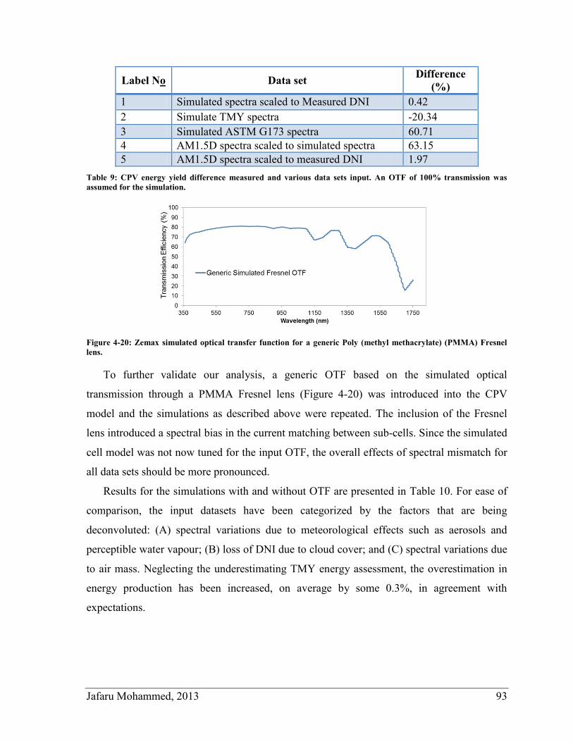
Jafaru Mohammed, 2013 93
Label No Data set Difference
(%)
1 Simulated spectra scaled to Measured DNI 0.42
2 Simulate TMY spectra -20.34
3 Simulated ASTM G173 spectra 60.71
4 AM1.5D spectra scaled to simulated spectra 63.15
5 AM1.5D spectra scaled to measured DNI 1.97
Table 9: CPV energy yield difference measured and various data sets input. An OTF of 100% transmission was
assumed for the simulation.
Figure 4-20: Zemax simulated optical transfer function for a generic Poly (methyl methacrylate) (PMMA) Fresnel
lens.
To further validate our analysis, a generic OTF based on the simulated optical
transmission through a PMMA Fresnel lens (Figure 4-20) was introduced into the CPV
model and the simulations as described above were repeated. The inclusion of the Fresnel
lens introduced a spectral bias in the current matching between sub-cells. Since the simulated
cell model was not now tuned for the input OTF, the overall effects of spectral mismatch for
all data sets should be more pronounced.
Results for the simulations with and without OTF are presented in Table 10. For ease of
comparison, the input datasets have been categorized by the factors that are being
deconvoluted: (A) spectral variations due to meteorological effects such as aerosols and
perceptible water vapour; (B) loss of DNI due to cloud cover; and (C) spectral variations due
to air mass. Neglecting the underestimating TMY energy assessment, the overestimation in
energy production has been increased, on average by some 0.3%, in agreement with
expectations.
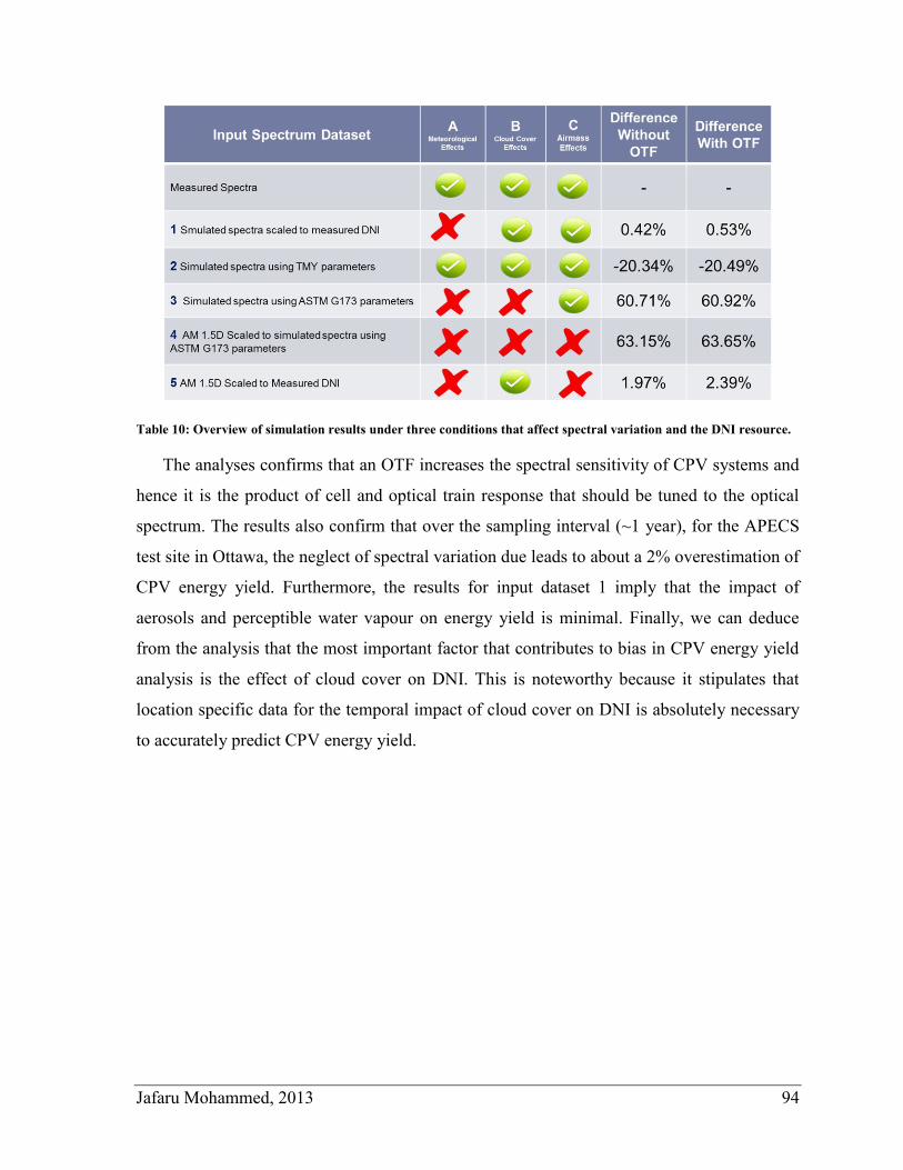
Jafaru Mohammed, 2013 94
Table 10: Overview of simulation results under three conditions that affect spectral variation and the DNI resource.
The analyses confirms that an OTF increases the spectral sensitivity of CPV systems and
hence it is the product of cell and optical train response that should be tuned to the optical
spectrum. The results also confirm that over the sampling interval (~1 year), for the APECS
test site in Ottawa, the neglect of spectral variation due leads to about a 2% overestimation of
CPV energy yield. Furthermore, the results for input dataset 1 imply that the impact of
aerosols and perceptible water vapour on energy yield is minimal. Finally, we can deduce
from the analysis that the most important factor that contributes to bias in CPV energy yield
analysis is the effect of cloud cover on DNI. This is noteworthy because it stipulates that
location specific data for the temporal impact of cloud cover on DNI is absolutely necessary
to accurately predict CPV energy yield.
Jafaru Mohammed, 2013 95
5 Conclusions
A brief history of PV and CPV technology was presented and the need for PV as a
sustainable source of renewable energy was highlighted. The solar resource and its source -
the sun; was discussed in terms of its spectral distribution and relationship with the earth
respectively. Equations and algorithms necessary to locate the sun spatially and temporally
were presented.
Details of research and characterization tools developed by the author for use with solar
demonstrators in the SUNLAB research group were discussed. Databasing procedures
carried out to acquire and store highly temporal meteorological data for CPV analysis under
the auspice of the APECS project were discussed.
A method to estimate the spectral distribution of the direct solar irradiance using
meteorological data sets, a spectral simulation model (SMARTS2) and temporally measured
DNI at a single wavelength (550 nm) was proposed and investigated. A CPV energy yield
model was developed and analysis was performed using data measured at the APECS test
site to determine factors that affect long term CPV energy yield analysis in Ottawa, Ontario,
Canada.
5.1 Overview / Summary
In chapter one, the ever increasing demand for energy and the issue of environmental
pollution as a result of fossil fuel consumption motivated research and development of PV
energy technologies. Depleting non-renewable energy resources was highlighted as a cause
for concern, and renewable PV generated electricity was proposed as an energy source that
would aid sustainable development in the future. The history of PV systems from its
dominance in extraterrestrial to terrestrial applications was discussed and its growth trend in
terms of price and efficiency was highlighted. The learning curve for PV which went into
full bloom for terrestrial use in 1976 was found to suggest that the price of PV would be less
than a dollar per watt by 2015. The history of standardization processes generated to
characterise various solar cell types was highlighted.
CPV technologies that promise cheaper energy systems were reported to have achieved
about 44% cell efficiencies. Unlike PV, which shows little scope for future improvement, the
Jafaru Mohammed, 2013 96
trend in efficiency growth for CPV is still strong. The basic operation of CPV cells were
contrasted with PV cells, with the enhancement in efficiency due to the multi-junction
architecture responsible for absorbing larger portions of the solar resource. The major issues
that negatively impact CPV (relative to PV), such as DNI-specificity and spectral mismatch,
were discussed.
In chapter two, the nature of the spectral distribution of the extraterrestrial solar resource
was discussed. The earth-sun temporal relationship was described and algorithms for
calculating precise coordinates of the sun from the earth’s surface spatially and temporally
were presented. Knowledge of elevation angles were necessary for calculating the air mass
as a precursor for simulating the temporal atmospheric transmission of sunlight through the
atmosphere. The algorithm also provide a method for calculating azimuthal and elevation
angles necessary for tracking the dual axis trackers used for CPV systems. Instrumentation
for measuring components of the solar resource were reviewed and notable CPV installations
were presented.
In chapter three, PV and CPV research within the uOttawa SUNLAB was highlighted,
and hardware tools, such as the high concentration XT-30 solar demonstrator and the
temperature controlled low concentration Oriel test station, were described. Software tools
developed by the author to characterise and test solar systems were discussed. The tools
included a pluggable IV testing utility, a spectral and spatial cell uniformity measurement
system and a light cycling utility.
The architecture for high temporal granularity data measurement and databasing within
the APECS project was presented. The datasets acquired were DNI, GHI, spectral DNI,
cloud cover and ambient temperature; the measuring instruments used were an Eppley NIP
pyrheliometer, Eppley PSP pyranometer, ASDi spectroradiometer and a CCD camera.
Ongoing measurements for each dataset began at various times in 2011 and were carried out
at 2 minutes intervals. A dedicated server was setup to record, store and publish the data sets
( http://www.apecs.site.uottawa.ca). A model for simulating the detailed IV characteristics of
a solar cell based on the diode equation [31] and Varshni relation [32] was presented. The
calculations were used to develop a java application for modelling PV systems.
In chapter four, investigations were carried out to assess the impact of using single
wavelength optical depth values on the accuracy of the simulation of the solar resource. The
Jafaru Mohammed, 2013 97
extraction of an aerosol optical depth from measured data was input to an atmospheric
radiative transfer model (SMARTS2) and the result validated against measured spectra from
the APECS test site. The results were used in a triple-junction cell model to predict short
circuit currents and a bias of ~0.6% between measured spectra and spectra was shown. It was
noted that the model is only valid for clear sky conditions.
Investigation of methods and datasets used for CPV energy yield analysis was performed.
Data from the CPV energy yield model was verified against measurements and the result
were in good agreement. Comparison was carried out between a simple and complex model
for CPV energy yield and the results suggested that the simple model overestimates annual
energy yield by ~3%. This was attributed to the neglect of spectral and temperature variation
in the simple model.
Using historical data sets from CWEEDS, the CWECS TMY dataset often used for PV
energy yield analysis was investigated. A comparison was carried out to determine the
overall energy bias against 1, 5, 10, 15 and 20 year CWEEDS energy yield assessments. The
results were that the CWECS TMY dataset still underestimated long term (> 5 years) energy
yields by about 7%.
An investigation was carried out to determine the degree to which certain factors
influence CPV energy yield. Five different spectral models, each neglecting one or more
significant factors, were compared against each other and measured spectra after their input
into the CPV energy yield model, both with and without an OTF. The results showed that for
the duration of the analysis (~1 year), and the specific location of the reference data
(Ottawa), the neglect of spectral variation (due to air mass) gave a ~2% overestimation in
CPV energy yield. Similarly, the neglect of spectral variation due to aerosol optical depth
and perceptible water vapour had a minimal impact on energy yield estimates,
overestimations of 0.42% and 0.53%, without and with an OTF, respectively. As expected,
the results verified that an OTF increased the bias in CPV energy yield analysis. The most
prominent contributor to CPV energy yield analysis was found to be cloud cover, at about
the 60% level. The results suggest that for accurate CPV energy yield prediction, the input
dataset must be one that addresses cloud cover.
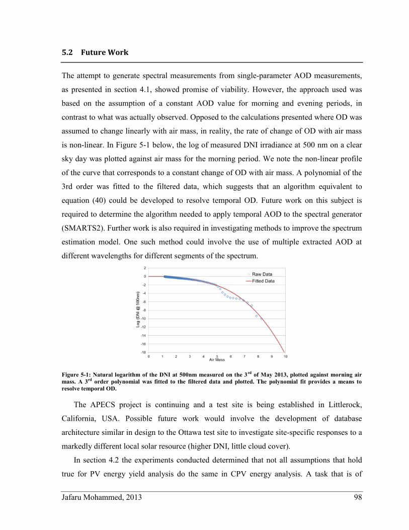
Jafaru Mohammed, 2013 98
5.2 Future Work
The attempt to generate spectral measurements from single-parameter AOD measurements,
as presented in section 4.1, showed promise of viability. However, the approach used was
based on the assumption of a constant AOD value for morning and evening periods, in
contrast to what was actually observed. Opposed to the calculations presented where OD was
assumed to change linearly with air mass, in reality, the rate of change of OD with air mass
is non-linear. In Figure 5-1 below, the log of measured DNI irradiance at 500 nm on a clear
sky day was plotted against air mass for the morning period. We note the non-linear profile
of the curve that corresponds to a constant change of OD with air mass. A polynomial of the
3rd order was fitted to the filtered data, which suggests that an algorithm equivalent to
equation (40) could be developed to resolve temporal OD. Future work on this subject is
required to determine the algorithm needed to apply temporal AOD to the spectral generator
(SMARTS2). Further work is also required in investigating methods to improve the spectrum
estimation model. One such method could involve the use of multiple extracted AOD at
different wavelengths for different segments of the spectrum.
Figure 5-1: Natural logarithm of the DNI at 500nm measured on the 3rd of May 2013, plotted against morning air
mass. A 3rd order polynomial was fitted to the filtered data and plotted. The polynomial fit provides a means to
resolve temporal OD.
The APECS project is continuing and a test site is being established in Littlerock,
California, USA. Possible future work would involve the development of database
architecture similar in design to the Ottawa test site to investigate site-specific responses to a
markedly different local solar resource (higher DNI, little cloud cover).
In section 4.2 the experiments conducted determined that not all assumptions that hold
true for PV energy yield analysis do the same in CPV energy analysis. A task that is of

Jafaru Mohammed, 2013 99
considerable interest for future work is the development of an interactive computer software
application to aid decision making for economic and financial circumstances in siting,
financing and maintaining CPV systems for grid connected electricity production. Such a
system would leverage the detailed CPV simulation model developed to perform energy
yield analysis and would complement the PV applications RetScreen and PVwatts. The
application would use measured data from multiple sources to minimize the LCOE and
maximizing Return on Investment (ROI).
Jafaru Mohammed, 2013 100
6 References
[1] I. Dincer, “Renewable energy and sustainable development: a crucial review,” Renew.
Sustain. Energy Rev. 4 (2), pp. 157–175, Jun. 2000.
[2] J. E. Cohen, “Human population: the next half century,” science 302 (5648), pp.
1172–1175, 2003.
[3] G. M. Masters, Renewable and efficient electric power systems. Wiley-Interscience,
2005.
[4] M. Harper, “Sustainable and Renewable Energy Development in Ontario : A look at
the Current Policy Frameworks and Discourses Surrounding Sustainable Energy and
Wind and Solar Power in Major Ontario Newspapers Sustainable and Renewable
Energy Development in Ontario : ,” 5 (1), 2009.
[5] J. Butlin, “Our common future. By World commission on environment and
development. (London, Oxford University Press, 1987, pp.383 £5.95.),” J. Int. Dev. 1
(2), pp. 284–287, 1989.
[6] E. Bequerel, “Recherches sur les effets de la radiation chimique de la lumière solaire,
au moyen des courants électriques,” CR Acad. Sci 9, pp. 145–149, 1839.
[7] A.-E. Becquerel, “Mémoire sur les effets électriques produits sous l’influence des
rayons solaires,” Comptes Rendus 9 (567), p. 1839, 1839.
[8] Wikipedia, “A. E. Becquerel --- Wikipedia, The Free Encyclopedia.” 2013.
[9] C.-T. Sah, R. Noyce, and W. Shockley, “Carrier Generation and Recombination in P-
N Junctions and P-N Junction Characteristics,” Proceedings of the IRE 45 (9), pp.
1228–1243, 1957.
[10] W. Shockley, “The theory of pn junctions in semiconductors and pn junction
transistors,” Bell Syst. Tech. J 28 (3), pp. 435–489, 1949.
[11] C. A. Wolden, J. Kurtin, J. B. Baxter, I. Repins, S. E. Shaheen, J. T. Torvik, A. A.
Rockett, V. M. Fthenakis, and E. S. Aydil, “Photovoltaic manufacturing: Present
status, future prospects, and research needs,” J. Vac. Sci. Technol., A 29 (3), p. 30801,
2011.
[12] M. A. Green, “Silicon photovoltaic modules: a brief history of the first 50 years,”
Prog. Photovolt. Res. Appl. 13 (5), pp. 447–455, 2005.
Jafaru Mohammed, 2013 101
[13] A. McEvoy, T. Markvart, L. Castañer, T. Markvart, and L. Castaner, Practical
Handbook of Photovoltaics: Fundamentals and Applications: Fundamentals and
Applications. Elsevier Science, 2003.
[14] A. Goetzberger, C. Hebling, and H.-W. Schock, “Photovoltaic materials, history,
status and outlook,” Materials Science and Engineering: R: Reports 40 (1), pp. 1–46,
Jan. 2003.
[15] M. Yandt, “Characterization and Performance Analysis of High Efficiency Solar Cells
and Concentrating Photovoltaic Systems,” University of Ottawa, 2012.
[16] D. Matin, “A Steeper Learning Curve for PV,” 2011. [Online]. Available:
http://www.interpv.net/market/market_view.asp?idx=94&part_code=03. [Accessed:
16-Apr-2013].
[17] K. Mitchell, C. Eberspacher, J. Ermer, and D. Pier, “Single and tandem junction
CuInSe2 cell and module technology,” in Conference Record of the Twentieth IEEE
Photovoltaic Specialists Conference, 1988, 1, pp. 1384–1389.
[18] “Solar cell prices dropping, but broad terrestrial use awaits mass production,”
Electronics, pp. 40–41, 19-Jul-1973.
[19] L. M. Magid, “The current status of the US photovoltaic conversion program,” in 12th
Photovoltaic Specialists Conference, 1976, 1, pp. 607–612.
[20] Y. Poissant, “Status and Trends of PV Technology in Canada,” Next Generation Solar
2013 Conference. [Online]. Available: http://www.youtube.com/watch?v=W-
I5RN2d31c.
[21] E. Christensen, “Electricity from photovoltaic solar cells. Flat-Plate Solar Array
Project of the US Department of Energy’s National Photovoltaics Program: 10 years
of progress,” NASA STI/Recon Technical Report N 88, p. 12188, 1985.
[22] J. Perlin, From space to earth: the story of solar electricity. Earthscan, 1999.
[23] M. R. Mack, “Solar power for telecommunications,” Telecommunication Journal of
Australia 29, pp. 20–44, 1979.
[24] Nrel, “Best Research - Cell Efficiencies,” 2013. [Online]. Available:
http://www.nrel.gov/ncpv/images/efficiency_chart.jpg. [Accessed: 16-Apr-2013].
[25] “What is sustainable development? Environmental, economic and social well-being
for today and tomorrow.” [Online]. Available: http://www.iisd.org/sd/. [Accessed: 16-
Apr-2013].
[26] G. Raisbeck, “The Solar Battery,” Scientific American 193, pp. 102–110, 1955.
Jafaru Mohammed, 2013 102
[27] H. Fischer and W. Pschunder, “Low-cost solar cells based on large-area
unconventional silicon,” IEEE T. Electron. Dev. 24 (4), pp. 438–442, Apr. 1977.
[28] J. S. Li and G. Q. Chen, “Energy and greenhouse gas emissions review for Macao,”
Renew. Sustain. Energy Rev. 22, pp. 23–32, 2013.
[29] A. Goetzberger and C. Hebling, “Photovoltaic materials, past, present, future,” Sol.
Energ. Mat. Sol. C. 62 (1), pp. 1–19, 2000.
[30] G. S. Kinsey and K. M. Edmondson, “Spectral response and energy output of
concentrator multijunction solar cells,” Prog. Photovolt. Res. Appl. 17 (5), pp. 279–
288, 2009.
[31] Y. Sakurada, Y. Ota, and K. Nishioka, “Simulation of Temperature Characteristics of
InGaP/InGaAs/Ge Triple-Junction Solar Cell under Concentrated Light,” Jpn. J. Appl.
Phys. 50 (4), p. 04DP13, 2011.
[32] Y. P. Varshni, “Temperature dependence of the energy gap in semiconductors,”
Physica 34 (1), pp. 149–154, 1967.
[33] W. W. Weiss, Solar heating systems for houses: a design handbook for solar
combisystems. James & James Science Publishers, 2003.
[34] K. Rajeshwar, R. D. McConnell, and S. Licht, Solar hydrogen generation: toward a
renewable energy future. Springer Science+ Business Media, 2008.
[35] R. L. Kurucz and E. H. Avrett, “Solar spectrum synthesis. I. A sample atlas from 224
to 300 nm,” SAO Special Report 391, 1981.
[36] B. Suresh, S. Schlag, and Y. Inogucji, “Chemical economics handbook marketing
research report,” SRI Consulting, 2004.
[37] J. Fontenla, O. R. White, P. A. Fox, E. H. Avrett, and R. L. Kurucz, “Calculation of
solar irradiances. I. Synthesis of the solar spectrum,” The Astrophysical Journal 518
(1), p. 480, 1999.
[38] R. L. Kurucz, “SYNTHE spectrum synthesis programs and line data,” Kurucz CD-
ROM, Cambridge, MA: Smithsonian Astrophysical Observatory,| c1993, December 4,
1993 1, 1993.
[39] F. Vignola, J. Michalsky, and T. Stoffel, Solar Resource Instrumentation. CRC Press,
2012.
[40] Wikipedia, “Equation of time --- Wikipedia, The Free Encyclopedia.” 2013.
Jafaru Mohammed, 2013 103
[41] E. C. McCullough and W. P. Porter, “Computing clear day solar radiation spectra for
the terrestrial ecological environment,” Ecology, pp. 1008–1015, 1971.
[42] “NOAA Solar Calculator.” [Online]. Available:
http://www.esrl.noaa.gov/gmd/grad/solcalc/. [Accessed: 04-May-2013].
[43] R. A. Rohde, “Radiation Transmitted by the Atmosphere,”
http://www.globalwarmingart.com/, 2007. [Online]. Available:
http://www.globalwarmingart.com/wiki/File:Atmospheric_Transmission_png.
[Accessed: 16-Apr-2013].
[44] Emcore, “Utility-Scale Concentrator Photovoltaic (CPV) System,” 2011. [Online].
Available: www.emcore.com%2Fwp-
content%2Fthemes%2Femcore%2Fpdf%2FGen%2520III_2011.pdf.
[45] P. J. Verlinden and J. B. Lasich, “Energy rating of Concentrator PV systems using
multi-junction III--V solar cells,” in Photovoltaic Specialists Conference, 2008.
PVSC’08. 33rd IEEE, 2008, pp. 1–6.
[46] P. Mints, “Solar electricity: 2009 surprise success,” Renewable Energy Focus 11 (3),
pp. 42–47, May 2010.
[47] SolFocus, “SolFocus Concentrator Photovoltaic (CPV) Systems,” Energy, 2010.
[Online]. Available:
http://www.solfocus.com/en/downloads/sustainability/sustainability-flyer.pdf.
[Accessed: 16-Apr-2013].
[48] J. Jaus, G. Peharz, A. Gombert, J. Rodriguez, F. Dimroth, F. Eltermann, O. Wolf, M.
Passig, G. Siefer, A. Hakenjos, and others, “Development of Flatcon® modules using
secondary optics,” in Photovoltaic Specialists Conference (PVSC), 2009 34th IEEE,
2009, pp. 1931–1936.
[49] SolFocus, “Featured SolFocus Deployments,” 2011. [Online]. Available:
http://www.solfocus.com/en/installations/. [Accessed: 16-Apr-2013].
[50] M. Wilkins, R. Beal, J. E. Haysom, J. F. Wheeldon, P. Mulet, G. Jamieson, N.
Youssef, D. Balachandreswaran, J. Fan, T. Hall, and others, “Design of a multiplexer
to characterize individual optics at a concentrating photovoltaic test site,” in Photonics
North 2011, 2011, p. 800725.
[51] Eppley Inc, “Precision Spectral Pyranometer.” [Online]. Available:
http://www.eppleylab.com/PrdPrecSpectralPyrmtr.htm. [Accessed: 16-Apr-2013].
[52] L. Harrison and J. Michalsky, “Objective algorithms for the retrieval of optical depths
from ground-based measurements.,” Applied optics 33 (22), pp. 5126–32, Aug. 1994.
Jafaru Mohammed, 2013 104
[53] L. T. Wong and W. K. Chow, “Solar radiation model,” Applied Energy 69 (3), pp.
191–224, Jul. 2001.
[54] C. Gueymard, SMARTS2: a simple model of the atmospheric radiative transfer of
sunshine: algorithms and performance assessment. Florida Solar Energy Center
Cocoa, FL, 1995.
[55] F. Kasten, “A new table and approximation formula for the relative optial air mass,”
Theoretical and Applied Climatology, 1965.
[56] R. R. King, D. C. Law, K. M. Edmondson, C. M. Fetzer, G. S. Kinsey, H. Yoon, R. A.
Sherif, and N. H. Karam, “40% efficient metamorphic GaInP/ GaInAs/ Ge
multijunction solar cells,” Appl. Phys. Lett. 90, p. 183516, 2007.
[57] S. Kurtz, “Opportunities and challenges for development of a mature concentrating
photovoltaic power industry (revision),” 2012.
[58] B. Prior and C. Seshan, “Concentrating Photovoltaics 2011: Technology, Costs and
Markets,” GreenTech Media Market Research Report, 2011.
[59] P. Perez-Higueras, E. Munoz, G. Almonacid, and P. G. Vidal, “High Concentrator
PhotoVoltaics efficiencies: Present status and forecast,” Renew. Sustain. Energy Rev.
15 (4), pp. 1810–1815, 2011.
[60] F. Dimroth, C. Baur, A. W. Bett, M. Meusel, and G. Strobl, “3-6 junction photovoltaic
cells for space and terrestrial concentrator applications,” in Photovoltaic Specialists
Conference, 2005. Conference Record of the Thirty-first IEEE, 2005, pp. 525–529.
[61] G. S. Kinsey, W. Bagienski, A. Nayak, M. Liu, R. Gordon, and V. Garboushian,
“Advancing Efficiency and Scale in CPV Arrays,” IEEE J. Photovolt. 3 (2), pp. 873–
878, Apr. 2013.
[62] M. Campbell, “LEVELIZED COST OF ENERGY FOR UTILITY-SCALE
PHOTOVOLTAICS,” Solar Cells and Their Applications 217, p. 251, 2010.
[63] C. A. Gueymard and S. M. Wilcox, “Spatial and temporal variability in the solar
resource: Assessing the value of short-term measurements at potential solar power
plant sites,” 2009.
[64] M. D. Yandt, J. F. Wheeldon, J. Cook, R. Beal, A. W. Walker, O. Thériault, H.
Schriemer, T. J. Hall, and K. Hinzer, “Estimating cell temperature in a concentrating
photovoltaic system,” in AIP Conference Proceedings, 2012, 1477, p. 172.


![Prototype Test Results of the Solar Tower Atmospheric ... · experiment called the Solar Tower Atmospheric Cherenkov Effect Experiment (STACEE) [11, 12, 13]. 2. The goal of STACEE](https://img.pdfslide.us/doc/110x75/6066499f5c678702f968ec52/prototype-test-results-of-the-solar-tower-atmospheric-experiment-called-the.jpg)