Embed Size (px)
Citation preview

1
A Work Project, presented as a part of the requirements for the Award of a Masters Degree
in Economics from the Faculdade de Economia da Universidade Nova de Lisboa.
Impact of Social Economic Indicators on RSI incidence
and Success
Bruno Miguel Gonçalves Duarte, 68
A project carried out on the Applied Policy Economics area, with the
supervision1 of:
Ana Balcão Reis
June 12, 2009
1 I would also like to say a special thank you to professors Susana Peralta and José Mário Lopes, whose
help was indispensable to the realization of this work project.

2
Abstract:
In this project we study the influence of socio-economic characteristics on the
percentage of beneficiaries of “Rendimento Social de Inserção” (RSI) and on the
percentage of exits from the RSI program that occur due to a change in income. The
results indicate that the % of beneficiaries tend to increase with unemployment, younger
people and reduced families, whereas it tends to reduce with high education levels and
GDP. As for the % of exists from the RSI, the results we obtained show evidence that,
on the one hand, they tend to increase with higher education, and on the other hand,
they tend to reduce with unemployment, reduced income of the beneficiaries before
entering the program, nuclear families and Local Purchasing Power.
Key Words:
“Rendimento Mínimo Garantido”, “Rendimento Social de Inserção”, Poverty,
Beneficiaries

3
1-Introduction
The central objective of income support is to provide population without
sufficient living resources support to help them obtain minimum living conditions. That
help may be monetary or in-kind and will allow people in poverty to access more
resources, in order to have a more decent life. In the current world society, poverty
arises as a common characteristic among countries, independently of the definition of
poverty we consider.
With the objective of fighting poverty and reduce social inequality, several
countries provide monetary and social schemes to help alleviate those who do not have
sufficient income. In Portugal, Social Security has several programs, but we will focus
on “Rendimento Social de Inserção” (RSI).
We will study in this work project the impact of some socio-economic
indicators, as for example, Local Purchasing Power (LPP), GDP, unemployment rate
(UR), type of family, among others, on the % of people that benefit from RSI. We will
also study the impact of how those indicators above, among others, may impact the
exits due to an income change from the RSI program. In order to achieve that, we will
begin with a literature review on the subject of poverty and welfare programs developed
with the aim to reduce it. After that we will focus our attention on the Portuguese
system, analysing the Portuguese welfare programs, focusing on the RSI evolution since
it was implemented in Portugal (its original denomination was “Rendimento Mínimo
Garantido” (RMG)). Afterwards, we will study the impact of some socio-economic
variables on the RSI incidence, as well as the impact of some of those variables on the
exits from the program due to a change in income. The last point is reserved for the
conclusions obtained, taking into account all the previous sections.

4
2-Some Literature Review
As mentioned above, we will start with a brief literature review and some
notions of what Poverty is. A person is considered poor if she does not have enough
resources to achieve a reasonable standard of living, although there are several
dimensions for which we can define poverty.
In this way, defining poverty is a not an easy task. We will focus on two
different ways of measuring poverty, which are the absolute and the relative concepts of
poverty, that are more related with the minimum standards of living and monetary
perspectives. The absolute concept states that a person is poor if she does not attain a
minimum level of income or consumption, and is commonly used in the United States
of America (USA). So a person is considered poor if “she cannot afford a minimum
consumption levels, such as a basic consumption basket with food, housing and
clothing” [1]. It is important to notice that this concept of poverty is only dependent on
time and place through prices effect. Unlike the previous one, the relative poverty
concept is closely linked with time and place where individuals live, and it states that “a
person is poor if she does not attain a minimum level of economic participation in
society”[1] (example: a poverty line=60% of GDPpc). This relative concept is more
used in Europe, and as we can notice that poverty in relative terms differs from country
to country, since a “rich” person in a poor country may be “poor” in a rich country. A
necessary first step to analyse poverty is the definition of a poverty line, which is the
level of income below which an individual is considered “poor”.
In order to reduce poverty, there are two types of transfers used: Cash and in-
kind transfers. All main social benefits come in one of these two types of transfers. In-
kind transfers are payments in commodities or services. Examples of these are food

5
stamps in the USA, the housing benefits that are used in several countries and that help
individuals to pay the rent, and free or subsidized health care.
From all types of cash transfers, we will focus on one in particular, the
guaranteed minimum income. The first use of this system was in England, in 1795, with
the “Speenhamland system”. Salanié [1] describes the theory of guaranteed minimum
income, where individuals with income Y below a certain guarantee minimum income
G, receive a transfer that allows them to achieve that minimum income. If individuals
are below that minimum income G, there is a 100% taxation rate for that area under the
G, which means that if you receive one more Euro of income, the G transfer will be
reduce by one Euro as well, maintaining the total income received after transfers. If
individuals have Y above G, this program does not apply for them. As this program has
a decrease of one-to-one with gross income, it brings disincentive to work for its
recipients2. It may also give incentives for recipients try to avoid the system by working
on the underground economy or claim they receive less than they actually do. As we
will see later, the Portuguese program takes this negative labour disincentive into
consideration.
We will now take the USA case as an example of guarantee minimum income.
Both Rosen [2] and Atkinson [3] mention the USA program Temporary Assistance for
Needy families (TANF), which was created in 1996, and this was the main government
cash transfer program. This program is different from the previous one, which was the
Aid to Families with Dependent Children (AFDC), since it is a temporary help, and
with a general time limit of 5 years. AFDC was administrated jointly by the federal
government and the states. The states determined their own benefit levels and eligibility
criteria, given some broad federal guidelines. The federal government provided part of
2 Recipients are the people who receive the income support while beneficiaries are the ones that live in
the same household and benefit from the income support

6
the funds, which varied depending on the state per capita income. With this new
program, the federal government gives block grants to finance welfare spending to each
state, determined in advance, so each state uses each block grant as it wants. The states
also have the power to decide the benefit reduction when welfare recipients earn
income, when before was one-to-one. This means that for each dollar the recipients
earned in their work, benefits were reduced by the same amount. This reduction gives
recipients more incentives to work. And this work-leisure trade-off was one of the big
victories of this new TANF in the USA, since a good transfer system requires a very
careful balance of incentives and equity considerations. This new program also has a
work requirement which states that 90% of the two parent families and 50% of the
single mother recipients have to be working or in work preparation programs.
3-Income support in Portugal
There are some public programs to reduce poverty, and in the Portuguese case,
the main program discussed in this work is the “Rendimento Mínimo Garantido”
(RMG), that later was replaced by the “Rendimento Social de Inserção” (RSI).
Portuguese Social Security states that RSI constitutes a “mechanism of poverty fight,
having as a main goal to ensure its citizens and households the resources that contribute
to the satisfaction of the minimum necessities and to foster their progressive social,
laboral and community integration”.
We will now characterize the program, in accordance with the Social Security.
The “Rendimento Mínimo Garantido” was approved in 1996 and implemented in July
of 1997. A person is considered eligible if the individual income is less than 100% of
the social pension, or if of the family aggregate income is below the following scale:
100% of the social pension value for each adult, until 2;
7
70% of the social pension value for each adult starting from the 3rd
;
50% of the social pension value for each minor.
The “Rendimento Social de Inserção” was implemented in July 2003 with the
objective of replace the RMG, which continued providing social transfers to its
beneficiaries until June 2006, because a few of them were still switching to the RSI. The
new program has similar rules to the RMG, but it also has some differences as the
intensification of the transitory subsidiary character of the attribution of the transfer,
mainly by the introduction of more strict measures of access and maintenance of the
transfer.
The only individuals that can apply for the RSI are those whose income is below
100% of the social pension value (which is €187, 18 in 2009), or the households whose
income is below the sum of the following equivalent scale:
a) 100% of the social pension value for each adult, until 2;
b) 70% of the social pension value for each adult starting from the 3rd
;
c) 50% of the social pension value for each minor, until 2;
d) 60% of the social pension value for each minor starting from the 3rd
child;
e) In case of pregnancy of the recipient, or his wife, to the amount in a) is
added 30% during the pregnancy, and 50% during the first year of the baby.
The amount of the social transfer is equal to the difference of the household
income in the previous 12 months of the social transfer request and the sum of the
weights above multiplied by the social pension. To this calculation, the household
income is only considered to 80% of its value, excluding house renting subsidy, social
security contributions and scholarships. This proves that the program takes into

8
consideration the labour supply disincentives that might arise, as we previously
discussed in section 2.
Entitlement to the RSI is also conditional to the recipients having a legal
residence in Portugal, and currently participating in some kind of insertion program.
Recipients also have to be able to prove that they are in a real situation of poverty. They
also have to be over 18 years old or if not, having minors at their care, and finally,
applying for a job if they are unemployed and able to work.
The program attribution is for a period of 12 months, and afterwards it may be
renewed if all the proper documentation is presented to the Local Committee, that
analyse case by case these requests.
Rodrigues and Gouveia [4] studied the impact of the RMG in Portugal, and they
reached the conclusion that the RMG have a positive impact in reducing poverty.
Now looking at some features that characterize the Portuguese society and how
some important socio-economic indicators have been evolving over the years.
According to the Eurostat, a person is considered poor if she has an equivalent
disposable income below the risk-of-poverty threshold, which is set at 60 % of the
national median equivalent disposable income. This is about 20% of the population
(after social transfers), although this value has been decreasing for the last 10 years. The
European Union (EU) average is about 16%, placing Portugal well above the average.
Table 1 - At-risk-of-poverty rate after social transfers ( %)
1995 1996 1997 1998 1999 2000 2001 2002 2003 2004 2005
EU-25 n.a. n.a n.a. 15 16 16 16 n.a. 15 16 16
EU-15 17 16 16 15 16 15 15 n.a. 15 17 16
Portugal 23 21 22 21 21 21 20 20 19 21 20
Source: Eurostat
One factor that may be associated with poverty is unemployment in a society.
Gallie, Paugam and Jacobs [5] tested this relationship for the EU, and they reached the
conclusion that unemployment increases the risk of poverty. Unemployment reduces the

9
disposable income of households, which might disable them from a sufficient income
necessary for their basic necessities.
Table 2: Unemployment rate (%)
1998 1999 2000 2001 2002 2003 2004 2005 2006 2007 2008
Portugal 4,9 4,4 3,9 4,0 5,0 6,3 6,7 7,6 7,5 7,8 7,8
Source: INE
Furthermore, rate of growth of GDP in Portugal has been decreasing if we
compare with the results from the 90s, as we can see in table 3 below. This is important,
since GDP might influence negatively poverty as Baldacci, Mello and Inchauste [6]
state in their work.
Table 3: GDP rate of growth (%)
Base 2000 1996 1997 1998 1999 2000 2001 2002 2003 2004 2005 2006 2007
2008
Portugal 3,6 4,2 4,7 3,9 3,9 2 0,8 -0,8 1,5 0,9 1,3 1,9 0
Source: INE
An important factor that may have an impact on the Portuguese high poverty
rates might be the early school leavers ( table 4), that represents about 39% of the
population aged 18-24 with no more than the mandatory education and proceeding any
further education or training. Consequently, Portuguese labour force is not as
capacitated as most of the Europeans to respond to high technologies demands. It still
remains a very traditional basis labour force in the economy. Branco and Gonçalves [7]
investigate how low levels of education may influence poverty, and they state that “the
proportion of poor people with at most a mandatory education is very superior to the
total of individuals”.
Table 4: Early school leavers - total % of the population aged 18-24 with no more than
mandatory education and not in further education or training
1995 1996 1997 1998 1999 2000 2001 2002 2003 2004 2005 2006 2007
EU - 27 - - - - - 17.6 17.3 17.1 16.5 16.0 15.6 15.3 15.2
EU - 15 26.2 21.6 20.6 23.6 20.5 19.5 19.0 18.7 18.1 17.6 17.3 17.0 16.9
Portugal 41.4 40.1 40.6 46.6 44.9 42.6 44.0 45.1 40.4 39.4 38.6 39.2 36.3
Source: Eurostat
10
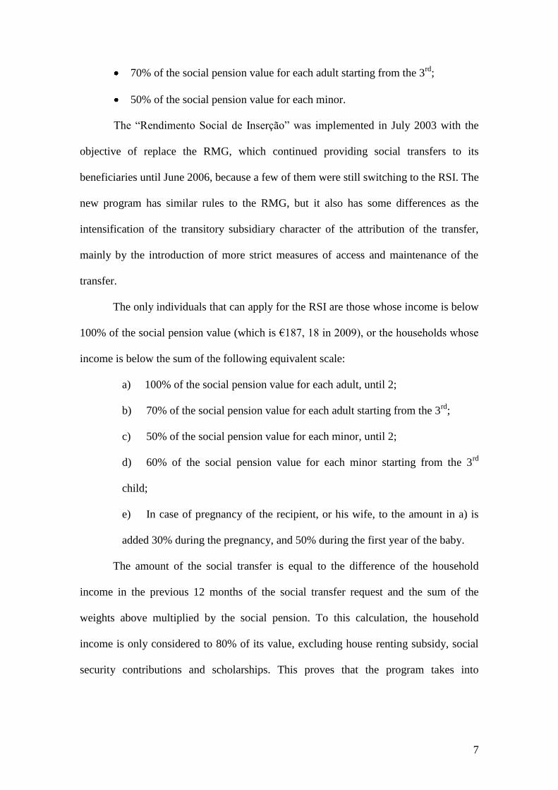
As we can see in table 5.1 and 5.2, Portugal spends less as % of GDP than the
EU. From the social expense for social protection, only 0, 2% are used for social
exclusion. Atkinson [8] showed there is a relation between higher social spending and a
reduction of poverty.
Table 5.1: Expenses in social protection as % of GDP
Expenses Social protection / GDP 1998 1999 2000 2001 2002 2003 2004
Portugal 21,9 22,6 22,7 23,8 24,1 24,5 25,5
EU-15 n/a 27,4 27,2 27,3 27,8 28,1 n/a
Source: Estatísticas da Protecção Social 2004
Table 5.2: Expenses in social protection by function for Portugal (%)
Functions 1998 1999 2000 2001 2002 2003 2004
Total 18,3 18,7 19,4 20,0 21,7 22,5 23,2
Health 8,2 8,3 8,7 8,7 9,2 9,1 9,5
Elderly 3,0 8,4 8,7 9,1 9,9 10,4 11,0
Family 1,0 1,0 1,0 1,1 1,4 1,5 1,2
Unemployment 0,9 0,7 0,7 0,7 0,9 1,2 1,3
Habitation 0,0 0,0 0,0 0,0 0,0 0,0 0,0
Social exclusion 0,2 0,2 0,3 0,3 0,3 0,3 0,2
Source: Estatísticas da Protecção Social 2004
4- Data analysis
The data used for the beneficiaries of RSI was collected from the Portuguese
Social Security statistical bulletins, which contained information about the RSI until
2006. For information after that period, the Portuguese Social Security provided the
data on our request, as long as they were able to provide it. As for Local Purchasing
Power (LPP), GDP, unemployment rate and education levels, the data was provided by
the “Instituto Nacional de Estatística” (INE).
This data collected enable us to study how these socio-economic indictors
impact both the % of people receiving RSI, and on the % of people leaving the RSI
program due to income changes. The data for these variables are organized
geographically at different levels: NUTS II, districts and municipalities (see appendix

11
A). We had to overcome this difficulty, since we some variables were only available in
a geographical level, which lead us to use different geographical data. We describe
below how we dealt with this problem. Whenever possible, we used municipalities data,
as it allows a higher number of observations and more accrued results. When it is not
possible due to lack of data, we use district data.
To test for the % of incidence of RSI, we use the 308 existing municipalities
data, obtained from the Censos 2001 survey. Some set of indicators as Age, Education,
family size and gender (see Appendix B), were used along with the unemployment rate
and the local purchasing power, to study these socio-economic indicators impact on the
% of RSI incidence. One of these indicators used, education, has two different
definitions in this work project. In this particular case, is the % of people that finish a
certain degree of study, to which we will call Education. This is different from the
education that we use for testing the same % of RSI incidence, but at a district level, as
there was not available data for the district level, so we used the amount of people
enrolled in a certain level of education, and we will define this education as EducE.
Table 6 -Determinants average on a municipality level
LPP UR e_low e_high age<25 age_25_64 age>64 f<3 f_3_7 f>8 male
Mean 67,32 6,50% 57,20% 19,31% 28,97% 50,47% 20,55% 47,81% 51,67% 0,53% 48,54%
Standard Deviation 27,12 2,57% 7,68% 7,04% 4,60% 3,53% 6,56% 8,91% 8,56% 0,65% 1,16%
Source: INE-Censos 2001
As for the % of beneficiaries that leave the RSI due to an increase in income, we
only use district data, which is the only geographical data given by the Social Security
annual reports. These reports provided different data over the years, which mean that
the set of indictors changed from one year to the other, so we had to use data only from
2002 until 2006, since during these years the indicators remain constant. The indicators
we use are “Income”, which is the income households already receive before joining the
RSI program, “Receive” is the amount households obtain from the RSI transfers,

12
“family” is the type of family of the beneficiaries (see Appendix C), and EducE, as
defined above.. We also use LPP, GDP and the unemployment rate, where we had some
problems with this data. For the unemployment rate, the data was only available in
NUTS II level, so we used for each district, the unemployment rate that corresponded to
the NUTS II region where that district belong to. Another data limitation was the fact
that LPP was not available for every year, since this study carried out by INE is bi-
annual. For instance, for 2003 there was no values, so we used and average of the values
of 2002 and 2004 to estimate the value of 2003, although this might bias our results. We
do not use data for the Madeira district, due to lack of information in some years, which
means we work on data from 19 districts. (see appendix D)
5- Descriptive analysis
Looking at the data collected, we are going to proceed to an overall analysis of
the evolution of the beneficiaries of the RMG and RSI programs, as well as of some
economic factors that might influence the number of beneficiaries.
Starting that analysis in terms of beneficiaries of the RMG and RSI, we can
notice in 2003 a break in the number of beneficiaries, mainly due to the introduction of
the RSI, which has stricter rules. We can also see that in 2006 there is a small break, due
to the end of the RMG, which had been working until then, since beneficiaries were still
switching from one program to the other.
Table 7: Evolution of the number of beneficiaries of RMG and RSI in Portugal
Year 1998 1999 2000 2001 2002 2003 2004 2005 2006 2007 2008
Benef 429268 529226 537503 470309 414678 369942 375118 372213 338791 370232 418446
Source: Social Security
Table 8 shows us the gender distribution of the beneficiaries, and we can see that
females have a slightly higher incidence of RSI than males.

13
Table 8: Beneficiaries of RMG and RSI by gender
Year 2002 2003 2004 2005 2006 2007 2008
Females 53% 53% 54% 53% 54% 54% 54%
Males 47% 47% 46% 47% 46% 46% 46% Source: Social Security
In what refers to age, we can see in table 9 that from the group under 18 years
old is who has more beneficiaries, though most of them are not truly recipients, since
they are only beneficiaries because they live in a household which receives RSI.
Table 9: % of beneficiaries by age
1998 1999 2000 2001 2002 2003 2004 2005 2006 2007 2008
<18 43% 41% 40% 39% 39% 38% 37% 37% 38% 38% 38%
18-34 22% 23% 23% 22% 23% 23% 22% 22% 22% 21% 22%
35-64 29% 30% 31% 31% 31% 31% 32% 33% 34% 35% 36%
>=65 6% 6% 6% 7% 8% 8% 9% 8% 7% 6% 5%
Source: Social security
Now, considering the type of families who receive RSI, we notice a significant
change on the families who receive RSI, since when comparing 2002 to 2006, we see a
decrease on almost all types of families. The only type of family that highly increased
was the extended/composed family.
Table 10: Beneficiaries of RMG and RSI by type of family
Year 2002 2003 2004 2005 2006
Extended3/Composed
4 4,08% 4,20% 11,56% 20,31% 48,93%
Single 27,64% 27,69% 25,81% 23,10% 15,30%
One parent family 23,55% 23,28% 21,26% 19,44% 12,68%
Nuclear family with children 31,27% 31,53% 28,16% 26,14% 16,29%
Nuclear family without children 13,47% 13,31% 13,22% 11,01% 6,81%
Source: Social Security
Finally, we analyse the reasons for the RSI ceased contracts, and as we can see
in table 11, the main reason is income change of the household. That reason is
increasingly becoming the most important one, and in 2006 is represents 56% of the
3 Extended family – at least one of the members of the household do not have any parental relationship
with the rest of the household 4 Composed family – all the members of the household do not have any family relationship with another
member of the household

14
ceased contracts. This might indicate that the program is working, and that social
transfers are in fact, playing and important role in reducing poverty.
Table 11 - % of the total ceased contracts
90 days after suspension of transfer
request of the recipient
change on the family type
Income change
False income reports
Application missing
Integration on the labour market
Death of the recipient
End of income transfer date Others
2002 n.a. 4% 2% 48% n.a. n.a. n.a. 4% n.a. 43%
2003 n.a. 3% 1% 50% n.a. n.a. n.a. 5% n.a. 41%
2004 5% 5% 5% 53% 6% 7% 2% 4% 5% 7%
2005 7% 8% 3% 50% 6% 7% 1% 5% 5% 9%
2006 5% 7% 4% 56% 4% 7% 1% 4% 2% 10%
Source: Social security annual reports
Table 12 – Average length of income transfer and average value of RSI transfers
Year 2002 2003 2004 2005 2006 2007 2008
Average value of transfers received by beneficiary (€) n.a, n.a. 64,51 69,45 77,3 81,72 86,76
Average lenght income transfers ( months) 31,8 34 13,5 14,1 16,8 20,6 24,6
Source: Social security
The average income transfer per beneficiary also has been increasing, providing
better contributions, as we can see in Table 12. One can also see in table 12 that the
average length of the RSI income transfer is increasing in the last years, although it
decreased on 2003, given the change from the RMG to the RSI program. This might
also show that the RSI has more strict rules, which reduced the program average length.
Finally, in table 13 we can see that the evolution of the % of families without
income has increased since the introduction of the RSI, and are now about 30%, which
may indicate that the program is giving more attention to the people that in fact have no
means to have minimum conditions of living.
Table 13 - % of families receiving RSI without income
1998 1999 2000 2001 2002 2003 2004 2005 2006
% of families without income 22,8 23,9 24,4 26,8 28,9 30,7 29,9 28,1 29,5
Source: Social Security annual reports

15
6-Methodology adopted
We will now study the impact of the indicators referred above on the % of RSI
incidence and on the % of exits from the program due to a change of income, which we
will designate as a possible success. We estimate some econometric relations in order to
try to conclude on the effects of the variables collected in explaining our objectives.
Firstly, we will see how indicators as LPP and UR, as well as some other
demographic indictors, have and impact on the % of beneficiaries.
In order to do that, we use municipality data to test how the characteristics of the
population might affect the % of beneficiaries incidence on the program. To do so, we
will use the following regression:
Equation 1
rrrrrrrr URLPPgenderhouseholdeducationageiesBeneficiar 654321 (1)
Where “r” refers to the municipality, “Beneficiaries” is the % of beneficiaries of
the RSI for each municipality, “Age” is the average age in each municipality,
“Education” is the % of people that attained a certain educational level, “Household”
is the average family size % in each municipality, “Gender” the % of male, “LPP” is
the local purchasing power per capita, UR is the unemployment rate and “μ” is the error
term. (see appendix B)
One important indicator studied is the Local Purchasing Power (LPP). This
variable is defined by INE and depends on a variety of 18 indicators, such as the value
of withdraws from ATMs, IRS paid, Income for IRS, Payments occurred through
ATMs. All this information is analysed in a factorial model per region, providing the
index used for this work as LPP. It reflects the weight of each district in terms of
purchasing power over the total of Portugal.

16
Also important might be the Unemployment rate, defined as the percentage of
unemployed people in the active labour force.
As Censos data is only available for 2001, our data is only for one year, which
provided us a number of observations of 308, corresponding to the number of
municipalities. We will use an Ordinary Least Squares (OLS) regression to capture the
effect of these variables on the % of beneficiaries of RSI.
Nevertheless, we need to control for multicollinearity problems, since as we can
see by the definition of the variables, some control for all the possibilities range or they
might be highly correlated (age and education, as we can see in appendix B). In this
case, we will not use all the indicators simultaneously, and we will try different
combinations of outcomes always with distinct combinations of variables.
After testing for the effects of some socio-economic indicators on the % of
beneficiaries, using municipality data as a mean to do so, we will use some indicators to
see their impact on the % of beneficiaries using district data. In equation 2, we use
different indicators than the ones used in equation 1, because they were not available on
a district level.
Equation 2
idididididid educEURGDPLPPiesBeneficiar 4321 (2)
In this equation, “i” is the year, “d” is the district, “LPP” is the local purchasing
power per capita, “GDP” is the % of GDP , “UR” is the unemployment rate, “educE”
is the % of people of each district enrolled in a determined level of education, “family”
is the % of the type of families and “μ” is the error term.
In this regression we use data from 2002 to 2006, for 19 districts of Portugal (we
exclude Madeira, as referred before), which would originally gives a sample of 95
observations. As we have more then one period and variable, we have to take into
17
consideration the fixed effects. Thus, we eliminate the fixed effects provided by the cross
sections effect and time effects. We tried several methods, and the one that best suited
our purpose is the OLS method, which provides robust results with our data. Like on
equation 1, we need to control for multicollinearity and highly correlated indicators, or
this might bias out results.
After studying the impact of those indicators on the % of beneficiaries, we will
now focus on trying to identify the determinants that influence the % of exits from the
RSI program due to income changes. We test for the % of beneficiaries leaving the
program due to income changes instead of the % of all beneficiaries who leave the RSI
because we think it might be interesting to test for the specific effect of LPP in this case,
and this indicator impact will be more visible on the % of beneficiaries who leave the
program due to income changes. Besides, the main reason for beneficiaries to leave the
RSI is the income change, with more than 50% of beneficiaries leaving for that reason.
We will use the same indicators as in equation 2, although adding other indicators
to test for their impact. For that, we will use the following regression:
Equation 3
ididididididididiid receiveincomefamilyeducEURGDPLPPSucinc 7654321 (3)
Where “i” is the “sucinc” is the % of people that leave the RSI due to a change in
income as a % of households, “LPP” is as defined in equation 2 and is one of the main
indicators studied here. “GDP”, “UR” and “educE” are also as defined in equation 2
above, whereas “family” is the % family types who receives RSI, “Income” is the % of
households who had a certain amount of income before joining the program, “Receive”
is the % of households who receive a certain amount of income from the program and
“μ” is the error term. In Appendix C we can see definitions of these variables.

18
This equation, like equation 2 before, will use data from 2002 to 2006, for 19
districts of Portugal but in this equation we will undertake our study with 76
observations, since we differentiate the LPP indicator to capture the variation effect
impact on the % beneficiaries leaving the program due to a change in income. Again as
in equation 2, we have to eliminate the fixed effects, and we will also use the OLS
model to test our estimations. Finally, and also like before, we will take into account
multicollinearity and highly correlated indicators problems.
7- Results
Considering the 1st equation, we can see in table 14 that column 1 tests for the
effect of LPP and UR on the % of beneficiaries. In column 2 and 3 we test the impact of
the level of education and gender. As for column 4, 5 and 6 we test for age, whereas in
columns 7 and 8 we test for family size.
So, in column 1 LPP and UR have statistical impact on explaining the % of RSI
incidence, despite the fact of a low R2 (10%). Nevertheless they behave as expected:
results show that an increase in LPP decreases, on average, the % of people receiving
RSI, considering that more purchasing power reduces that probability. With an opposite
effect, the unemployment rate increases the tendency of a higher % of beneficiaries,
because as people are unemployed, they have less income, and that may increase the %
of people eligible for the program. This result of UR is statistically significant at 1%
level in every equation estimated, whereas LPP is only statistically significant when
considered alone with the unemployment. This might happen due correlations with the
other variables or to data problems.
As we start introducing other variables in the equation, we notice a decrease on
the % of beneficiaries when the % of people with a higher education increases, with a
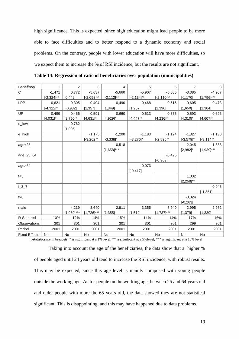
19
high significance. This is expected, since high education might lead people to be more
able to face difficulties and to better respond to a dynamic economy and social
problems. On the contrary, people with lower education will have more difficulties, so
we expect them to increase the % of RSI incidence, but the results are not significant.
Table 14: Regression of ratio of beneficiaries over population (municipalities)
Benef/pop 1 2 3 4 5 6 7 8
C -1,471 0,772 -5,637 -5,660 -5,907 -5,685 -3,385 -4,907
[-2,324]** [0,442] [-2,098]** [-2,112]** [-2,134]** [-2,110]** [-1.170] [1,796]***
LPP -0,621 -0,305 0,494 0,490 0,468 0,516 0,605 0,473
[-4,322]* [-0,932] [1,357] [1,349] [1,267] [1,396] [1,650] [1,304]
UR 0,499 0,466 0,591 0,660 0,613 0,575 0,593 0,626
[4,031]* [3,750]* [4,631]* [4,929]* [4,447]* [4,236]* [4,310]* [4,607]*
e_low 0,762
[1,005]
e_high -1,175 -1,200 -1,183 -1,124 -1,327 -1,130
[-3,262]* [-3,338]* [-3,276]* [-2,895]* [-3,579]* [-3,114]*
age<25 0,518 2,045 1,388
[1,658]*** [2,982]* [1,939]***
age_25_64 -0,425
[-0,363]
age>64 -0,073
[-0.417]
f<3 1,332
[2,258]**
f_3_7 -0,945
[-1,351]
f>8 -0,024
[-0,263]
male 4,239 3,640 2,911 3,355 3,940 2,995 2,982
[1,960]*** [1,726]*** [1,355] [1,512] [1,737]*** [1,379] [1,389]
R-Squared 10% 12% 14% 15% 14% 14% 17% 16%
Observations 301 301 301 301 301 301 299 301
Period 2001 2001 2001 2001 2001 2001 2001 2001
Fixed Effects No No No No No No No No
t-statistics are in braquets; * is significant at a 1% level; ** is significant at a 5%level; *** is significant at a 10% level
Taking into account the age of the beneficiaries, the data show that a higher %
of people aged until 24 years old tend to increase the RSI incidence, with robust results.
This may be expected, since this age level is mainly composed with young people
outside the working age. As for people on the working age, between 25 and 64 years old
and older people with more the 65 years old, the data showed they are not statistical
significant. This is disappointing, and this may have happened due to data problems.

20
As for families, the results show that families with a reduced number of
members tend to increase the program incidence, whereas medium and larger families
are not statistically significant. This may indicate that small families (less that 3 people)
have more difficulties in attaining a necessary income level to have a decent life.
Finally, the data showed us that an increase in the % of male people in the
population has the tendency to increase the RSI, and on the contrary, an increase in the
woman % on the population reduces, on average, the program incidence.
Table 15: % of Beneficiaries over population (districts)
Benef/pop 1 2 3 4 5
C -3,397 -6,497 -1,978 1,227 -0,974
[-11,705]* [-4,909]* [-3,933]* [-1,417] [-0,994]
LPP 7,149 1,285
[10,528]** [4,295]*
GDP -0,183 -0,125 -0,162 -0,174
[-4,187]* [-2,965]* [-3,172]* [-2,412]**
UR -3,018
[-1,182]
∆ UR 8,560
[2,040]**
High_edu -3,361 -5,915
[-0,528] [-1,090]
R-Squared 99,50% 99,50% 99,60% 99,40% 99,50%
Observations 95 95 95 95 76
Period 2002-2006 2002-2006 2002-2006 2002-2006 2002-2006
Fixed Effects Yes Yes Yes Yes Yes
t-statistics are in braquets; * is significant at a 1% level; ** is significant at a 5%level; *** is significant at a 10% level
Now, we will analyse the results for equation 2, which are demonstrated in table
15 above. In column 1 we test the impact of LPP on the % of beneficiaries. Column 2
tests for the impact of GDP and UR, column 3 test the impact of GDP, and we continue
to use this as the preferred variable, dropping LPP. In Column 4 we test the impact of
high education, whereas in column 5 we test for the impact of the variation of the UR.
Analysing the results obtained from these equations, we see that LPP is
statistically significant, although it does not have the expected sign, since we would
expect that a higher LPP would tend to reduce the % of beneficiaries. This result might

21
indicate high economic disparity among districts, with a small % of very rich people
and a high % of poor people. This result is disappointing, as it was on equation 1 with
this variable, since it was not very significant. From the other columns we can notice
that GDP, which is highly correlated with LPP, is statistically significant, as long as not
estimated with LPP, so we drop LPP from the equation. UR is disappointing as well,
since it is statistically insignificant in this equation, so we drop it from the equation.
However, when we test for the impact of the variation of the UR in column 5, an
increase in the variation of UR tends to contribute to a higher % of beneficiaries of RSI.
As for column 4, we see that high education is statistically insignificant, which
is also disappointing, and this might be due to data problems referred before.
Now, we analyse the results from equation 3, which show the impact of some
variables on the % of exits of RSI beneficiaries, whose reason of leaving the program
was the change of income.
In table 16 we have in column 1 the impact of the variation of LPP has on the %
of exits of households that benefit from the RSI. Column 2 shows the results of
including GDP and UR on the equation. Column 3 takes into consideration the impact
of the % of households receiving income, and in column 4 we have the results of the
impact of the % of households receiving income from the RSI on the % of beneficiaries
leaving RSI. Column 5 shows the impact of a higher education, whereas column 6
results show the impact of type of family on the % exits of beneficiaries from the
program due to income changes.
Analysing the results, we can see that the variation of LPP is statistically
significant on the exit of households from the program, but its sign is the opposite as
expected. This means that a positive variation of LPP in districts will reduce the % of
beneficiaries leaving the program, which is not what one would expect. Like it is

22
referred above, this might happen due to income distribution problems across districts,
which might bias our result. It would be interesting to analyse this result with more data
and for a wider number of years, complementing it with other data as income
distribution and inequality across districts, to better understand the results and their
policy implications.
Table 16: % of exits of beneficiaries from the RSI due to income change (districts)
Suc exits/Benef 1 2 3 4 5 6 7
C -2,350 0,359 0,659 0,066 -0,836 -0,846 11,381
[-44,073] [0,150] [0,904] [0,0519] [-0,879] [-0,834] [2,800]*
∆ LPP -2,731 -3,239 -2,574 -2,742 -2,820 -2,508
[-1,743]*** [-2,262]** [-2,109]** [-2,153]** [-2,413]** [-2,171]**
LPP -2,816
[-3,049]*
GDP -0,081
[-0,502]
UR -25,373 -17,063 -17,537 -27,713 -27,430 -13,353
[-2,163]** [-1,903]*** [-1,912]*** [-2,631]** [-2,564]** [-2,207]**
red_inc -3,955 -4,000 -3,694 -3,720 -3,660
[-3,770]* [-3,764]* [-3,780]* [-3,581]* [-4,058]*
under_rec 0,886
[0,566]
Nuclear -1,027 -1,541
[-2,301]** [-5,354]*
High_edu 31,541 37,325 22,047
[2,156]** [2,353]** [1,805]***
R-Squared 94,30% 94,50% 97,40% 97,50% 97,90% 97,5% 96,60%
Observations 76 76 76 76 76 76 95
Period 2002-2006 2002-2006 2002-2006 2002-2006 2002-2006 2002-2006 2002-2006
Fixed Effects Yes Yes Yes Yes Yes Yes Yes
t-statistics are in braquets; * is significant at a 1% level; ** is significant at a 5%level; *** is significant at a 10% level
In column 2 we test for UR and GDP effects, and the results show that UR as a
negative impact and it is highly robust. It behaves as expected, since an increase in the
unemployment rate, will reduce beneficiaries income, which will tend to reduce their
ability to successfully leave the RSI program. As for GDP, it is statistically
insignificant, and as the results also shows a high correlation between LPP and GDP.
We drop GDP from the equation
Now taking into consideration the results from the Income received by RSI
families before the RSI transfer, we notice that a higher % of households who receive a

23
reduce income diminishes the tendency of people leaving the program, which might be
expected, as families without much income will have more difficulties to leave the RSI
program. On the other hand, families with higher income contribute positively to the
exits of the program. Both of these variables effects are statistically significant.
In column 4 we test the income received by families provided by the RSI
program, but these effects are statistically insignificant, which is disappointing. Thus,
this might indicate the % of households leaving the RSI program due to income changes
does not depend on the amount the RSI transfers to those beneficiaries. This is
disappointing and would useful to use better data to analyse this result.
As for column 5, we test for the impact of a higher education level, and as we
can see the result is statistically significant, with a positive impact, as we would expect,
and confirming the results on the other equations.
Regarding for the type of family, we only demonstrate the results for nuclear
families as the other types of family’s results are statistically insignificant. Results show
a higher % of nuclear families will decrease the average % of households leaving the
program.
Finally, as for column 7, we tested the effect of an increase in LPP, and not on
the variation of LPP as on the other columns. The result is similar and it shows a
significant negative impact.
8- Conclusion
Overall, we have studied the impact on the % of beneficiaries of social-
economic indicators at municipality and district levels, and, more incisively, the
determinants that might increase the households % of exits from the RSI due to a
chance of income on a district level.

24
Regarding the impact of social-economic variables on the % of beneficiaries, we
notice that the Local Purchasing Power is not very robust nor consistent whereas GDP
presents more robust results. The Unemployment has statistical positive impact on the
% of RSI incidence, which is what we expect, since unemployed people have reduced
income, and that might increase the tendency of joining the program although on a
district level this result is not robust.This might be due to data problems. Furthermore,
taking education in consideration, we notice that people with low education tend
increase the average of incidence of RSI, whereas when regarding for the effect of
people with high education, it tends to decreases the % of RSI incidence, as it is
expected as well. These results are good for a municipality level, but for the district
level they are not statistically relevant. As for age indicator, the most relevant result is
that higher % of people age less than 25 years tend to increase the RSI incidence, which
is expected, since they are not in the working age, and are mainly young beneficiaries.
Now regarding family size, the most important result is that higher % of smaller
families tends to increase the % of RSI incidence, which may indicate that smaller
families face difficulties to attain a decent income to survive. Finally, the result show
that higher % of male tend to increase the % of RSI beneficiaries.
Now looking to the results of the indicators impact on the exits from the RSI due
to income increase, we found evidence that a positive variation in LPP tends to reduce
the average of beneficiaries leaving the RSI program. This is very disappointing and is
not expected, and it might result from data problems and due to income redistributions
across districts, that bias the result obtained.
On the contrary, a higher unemployment tends do decrease the % of exits, which
is what we expected, and is consistent with the increase of the tendency of people
joining the program. We also found evidence that a higher % of households with low

25
income reduce the % of households leaving the program, as people with high income
increase the tendency of successfully leave the program. Households who receive
contributions from the RSI are statistically insignificant, which is also disappointing.
For the type of families, only the nuclear family type has a robust result, to which we
found evidence that higher % nuclear families reduce, on average, % of people leaving
the program. As for people attending higher degrees of education, the results showed
evidence of an increase of the % of exits as the % of people with higher education
increase.
According to the results obtained, we might expect an increase on the % of
beneficiaries of RSI, as well as a decrease on the % of recipients leaving the program as
successes if the unemployment continues to rise in the next few years, as it is expected
according to the Eurostat. This will probably increase the budget to social exclusion by
the Social Security, and therefore the government might have more expenses with
Social Security.
These conclusions are obviously conditioned by the data we used, as it has its
limitations, since we do not use individual data, only aggregated data. Further research
might be undertaken when the program has more years, as we used few years of data
panel, which limited our results and conclusions. Other aspect to be studied would be
the reason why the data period used show LPP having a negative impact on the % of
exits from the program, and for that would be interesting to analyse district or
municipality income distribution and inequality across districts or municipalities, to
understand and explain the LPP effect better. Censos will be 2011 is released in a few
years, which will allow for more precise data and, with that, more effective conclusions.
9- References

26
[1] Salanié, Bernard. (2003). “Low Income Support” In The economics of Taxation,
161-185. Cambridge, Massachusetts MIT press.
[2] Rosen, Hervey. (2005). Expenditure Programs for the Poor” In Public Finance, 7th
edition, 166-190. New York: McGraw-Hill.
[3] Atkinson, A.B.. (1987). “Income Maintenance and Social Insurance” In Handbook
of Public Economics, vol II, 779-908. ed.A.J.Auerbach and M. Feldstein. Elsevier
Science Publishers B.V. (North-Holland)
[4] Rodrigues, Carlos and Gouveia, Miguel (1999) “The impact of a “Minimum
Guaranteed Income Program” in Portugal, Departamento de Economia – documentos de
trabalho nº3/99, ISEG/UTL
[5] Gallie, Duncan, Paugam, Serge and Jacobs, Sheila. (2003). “Unemployment,
Poverty and Social Isolation: Is there a vicious circle of social exclusion?”. European
Societies, 5(1): 1-32.
[6] Baldacci ,E , Mello, L and Inchauste,G.(2002). “Finantial crisis, poverty and income
distribution”. Finance&Development, 39(2): 1-6.
[7] Branco,Rui and Gonçalves,Cristina (2001) “Exclusão social e pobreza(s) em
Portugal: uma primeira abordagem aos dados de painel dos Agregados Familiares da
União Europeia ( 1994-1997)”
[8] Atkinson, A.B. (2000). “A European Social Agenda: Poverty Benchmarketing and
Social Tranfers”.
Data Sources:
Instituto Nacional de Estatística “Estudo do poder de compra concelhio” “Anuários estatísticos”
Eurostat
Social Security
Instituto do trabalho e da solidariedade

27
10- Appendices
Appendix A
NUTS II Districts
Norte Braga, Bragança, Porto, Viana do Castelo, Vila Real
Centro Aveiro, Castelo Branco, Coimbra, Guarda, Leiria, Viseu
Lisboa e Vale do Tejo Lisboa, Santarém, Setúbal
Alentejo Beja, Évora, Portalegre
Algarve Faro
R. A. Açores -
Appendix B
Characteristics of the data used in equation 1
age
Age<25 less than 25 years old (%)
age_25_64 between 25 and 64 years old (%)
Age>64 more than 64 years old (%)
education e_low none or basic education level (%)
e_high high school or higher level (%)
Family
f<3 family with less than 3 people (%)
f_3_7 family with 3 to 7 people (%)
f>7 family with more than 7 people (%)
Gender male Males (%)
female female % Source: INE, Censos 2001
Appendix C - Characteristics of the data used in equation 2 and 3
educE High_edu High school or more (%)
Family
enlarge enlarge/composed family (%)
isolated single person family (%)
mono monoparental family (%)
nuclear Nuclear family (%)
Income red_inc between 0€ and 200€
inc More than 200€
Receive under_rec Less than 200€
rec More than 200€ Source: Social security Reports

28
Appendix D: Determinants average on a district level
Districts LPP GDP UR e_high enlarge mono sinlge nuclear low_inc inc under_rec h_rec
Aveiro 78,57 14,38 4,34% 5,07% 0,77% 1,08% 1,38% 2,36% 2,80% 2,62% 2,71% 2,66%
Beja 63,23 11,73 8,56% 6,33% 0,77% 0,37% 0,40% 1,25% 1,19% 1,48% 1,33% 1,41%
Braga 63,09 10,49 7,42% 6,24% 0,86% 1,11% 1,17% 2,65% 2,56% 2,97% 2,77% 2,87%
Bragança 58,81 10,62 7,42% 8,74% 0,10% 0,18% 0,23% 0,50% 0,47% 0,51% 0,49% 0,50%
Castelo Branco 61,75 9,99 4,34% 8,39% 0,23% 0,27% 0,31% 0,65% 0,56% 0,83% 0,69% 0,76%
Coimbra 68,53 12,49 4,34% 11,78% 0,62% 0,96% 1,76% 1,90% 2,97% 2,26% 2,62% 2,44%
Évora 70,80 11,77 8,56% 8,10% 0,35% 0,41% 0,32% 0,92% 0,82% 1,08% 0,95% 1,02%
Faro 95,56 14,40 5,70% 6,36% 0,59% 1,32% 1,16% 2,38% 2,38% 2,88% 2,63% 2,75%
Guarda 58,05 10,49 4,34% 5,51% 1,17% 0,11% 0,14% 0,38% 0,61% 1,08% 0,85% 0,96%
Leiria 74,91 12,82 4,34% 5,65% 0,46% 0,45% 0,56% 0,86% 1,06% 1,21% 1,13% 1,17%
Lisboa 111,41 21,71 7,92% 9,38% 2,11% 3,83% 3,77% 5,09% 8,47% 5,80% 7,14% 6,47%
Portalegre 69,27 11,84 8,56% 5,73% 0,53% 0,32% 0,28% 0,70% 0,81% 0,91% 0,86% 0,89%
Porto 82,15 10,64 7,42% 7,30% 4,61% 4,49% 6,21% 8,74% 13,96% 10,71% 12,34% 11,53%
Santarém 77,81 12,05 7,92% 5,35% 1,02% 0,94% 1,32% 2,15% 2,71% 2,61% 2,66% 2,64%
Setúbal 102,91 11,04 7,92% 5,58% 0,98% 1,41% 1,26% 1,86% 3,09% 2,34% 2,72% 2,53%
Viana do Castelo 62,94 8,51 7,42% 5,09% 0,36% 0,52% 0,86% 1,28% 1,50% 1,44% 1,47% 1,46%
Vila Real 56,54 8,73 7,42% 6,77% 0,52% 0,43% 0,86% 1,63% 1,84% 1,60% 1,72% 1,66%
Viseu 56,02 10,05 4,34% 5,96% 1,06% 0,80% 1,11% 2,44% 2,54% 2,76% 2,65% 2,70%
R. A. Açores 64,96 12,08 3,36% 4,96% 0,85% 0,89% 0,71% 2,58% 1,86% 2,77% 2,31% 2,54%
Source: Social security Reports
Figure 1- % of successful exits from the RSI program due to income changes