HAL Id: halshs-01211575https://halshs.archives-ouvertes.fr/halshs-01211575

Preprint submitted on 5 Oct 2015

HAL is a multi-disciplinary open accessarchive for the deposit and dissemination of sci-entific research documents, whether they are pub-lished or not. The documents may come fromteaching and research institutions in France orabroad, or from public or private research centers.

L’archive ouverte pluridisciplinaire HAL, estdestinée au dépôt et à la diffusion de documentsscientifiques de niveau recherche, publiés ou non,émanant des établissements d’enseignement et derecherche français ou étrangers, des laboratoirespublics ou privés.

Impact of Rainfall Shocks on Child Health: Evidencefrom India

Vibhuti Mendiratta

To cite this version:Vibhuti Mendiratta. Impact of Rainfall Shocks on Child Health: Evidence from India. 2015. �halshs-01211575�

WORKING PAPER N° 2015 – 33

Impact of Rainfall Shocks on Child Health: Evidence from India

Vibhuti Mendiratta

JEL Codes: I12, Q54 Keywords: Anthropometric outcomes, Rainfall, India

PARIS-JOURDAN SCIENCES ECONOMIQUES

48, BD JOURDAN – E.N.S. – 75014 PARIS TÉL. : 33(0) 1 43 13 63 00 – FAX : 33 (0) 1 43 13 63 10

www.pse.ens.fr

CENTRE NATIONAL DE LA RECHERCHE SCIENTIFIQUE – ECOLE DES HAUTES ETUDES EN SCIENCES SOCIALES

ÉCOLE DES PONTS PARISTECH – ECOLE NORMALE SUPÉRIEURE – INSTITUT NATIONAL DE LA RECHERCHE AGRONOMIQUE

Impact of Rainfall Shocks on Child Health: Evidence

from India?

Vibhuti Mendiratta†

September, 2015

Abstract

While there is evidence of discrimination against girls in the allocation of resources within

a household under normal circumstances, it would be worthwhile to explore the e�ect of

extreme conditions such as rainfall shocks on the outcomes of surviving girls and boys. In

this paper, I estimate the impact of rainfall shocks in early childhood on the anthropometric

outcomes of girls and boys aged 13-36 months in rural India. I �nd that adverse negative

rainfall shocks (in utero and �rst year after birth) negatively impact height for age and weight

for age for both girls and boys. Further, I explore two channels through which rainfall a�ects

child health: by a�ecting the relative price of parent's time in childcare and through income

(as rainfall generates variation in income through its e�ect on agricultural output). I �nd

that positive rainfall has a positive e�ect on agricultural yield and arguably income in India.

This is further supported by the �nding that negative shocks are harder to insure in poorer

states and poorer households as re�ected by the poor anthropometric outcomes of children.

Keywords: Anthropometric outcomes, Rainfall, India.

JEL Classi�cation: I12, Q54.

?This work was supported by Région Île de France. I am grateful to Sylvie Lambert for her invaluable support,suggestions and comments throughout the preparation of this paper. I would also like to thank Luc Behaghel,Véronique Hertrich, Pierre Dubois, Pramila Krishnan, and participants at the Indian Statistical Institute, Delhifor helpful discussions and suggestions. Any remaining errors or omissions are my own.

†Paris School of Economics and INED, Address: 48 Boulevard Jourdan 75014 Paris, France.email: vmendira@pse.ens.fr

1

2

1 INTRODUCTION

The relative status of women in the developing world is poor, compared to developed countries.

The literature has highlighted the existence of gender inequalities in South Asia, attributed to

strong preferences for male child, often the result of traditional customs. Further, households in

India, as in much of the developing world, face substantial risk - an inevitable consequence of

engaging in rain-fed agriculture in a drought prone environment. This further a�ects the ability

of households to provide for their families and invest in children. Investments in children and

human capital are central to enhance the well being of households, break the intergenerational

transmission of poverty and �nally lead to the growth and development of a country.

The phenomenon of 'missing women', a term coined by Amartya Sen, was used to describe

that the gender ratio is much lower than would be expected if women and men were subject to

similar allocation of resources in a household (Sen, 1990). The comparative neglect of female

health and nutrition, especially but not exclusively during childhood, is largely responsible for

such a phenomenon. Indeed, the most striking evidence on skewed sex ratios and gender bias

in mortality comes from South Asia in general and India in particular. According to the gender

statistics of the Census of India in 2001, out of the total population of India, 532 million or

52 percent are males and 497 million are females constituting the remaining 48 percent in the

population. In sheer numbers, males outnumber females by 35 million in the population. Further,

Kynch and Sen (1983) explain the sex ratio by pointing out that �except in the period immediately

following birth, the death rate is higher for women than for men fairly consistently in all age

groups until the late thirties. This relates to higher rates of disease from which women su�er,

and ultimately to the relative neglect of females, especially in health care and medical attention�.

Given the literature on comparative neglect of women in India, one would expect to �nd evidence

of discrimination against girls in the allocation of resources within a household under normal

circumstances. The literature addressing this topic is mixed (Deolalikar and Rose, 1998; Subra-

manian, 1995; Subramanian and Deaton, 1990). Moreover, it is conceivable that under abnormal

circumstances like shocks faced by households, parents alter their behaviour in a way which leads

to discrimination against girls. Indeed, past research has provided us with some evidence that

abnormal circumstances matter. For example, Rose (1999) establishes that mortality among

girls in higher in the presence of a rainfall shock as compared to boys in India.

3

In a similar spirit, we assess the impact of rainfall shocks on the health of surviving children

and explore gender di�erences. To measure the impact of rainfall on child health, we use data

from the second round of Demographic and Health Survey conducted in 1998-99, and link it

to district level historical rainfall data for India. We examine the e�ect of weather shocks in

utero and early childhood on anthropometric outcomes of children aged 1-3 years living in rural

India. We �nd that children are very vulnerable to rainfall shocks in the �rst year of birth and

in utero as re�ected by the poor height for age and weight for age Z scores. We do not �nd a

di�erential impact of negative rainfall shocks on boys and girls and the results remain robust

to the inclusion of month of birth �xed e�ects and other variables. It must be mentioned that

the �ndings of Rose (1999) have some implications on our analysis in that we are comparing a

healthier sample of (surviving) girls with an average healthy sample of boys; thus pointing that

our �ndings are lower bound estimates of real causal impact. In addition, we also �nd that the

results are heterogeneous in that children living in poorer states, poorer households (in terms of

wealth) and girls with uneducated mothers have a harder time smoothing consumption with bad

rainfall years as re�ected by poorer anthropometric outcomes.

We identify three channels through which rainfall shocks could a�ect child health - income,

time spent by parents in childcare and spread of water borne diseases. Using the World Bank

India Agriculture and Climate dataset, we check the impact of rainfall on agricultural yields of

major crops in India and �nd that negative rainfall shocks do reduce yields of 4 out of 5 major

crops in India. Thus, negative rainfall represents a clear decline in income of Indian agricultural

households. In addition, more or less rainfall also has an impact on time spent by parents in

childcare. Using time use data in Rural Economic and Demographic Survey data from 1998-99,

we establish that mothers aged 15-30 years are indeed more likely to take up market work in

districts that experienced bad rainfall in the wet season of 1998. Whether this translates into

less time in childcare is unclear and we do not have time use data to check it. But we check the

impact of rainfall directly on childcare activities such as breastfeeding and vaccinations. One

of the ways this channel could manifest itself is if the mother is more likely to wean children

from breastfeeding during good rainfall season (as rainfall a�ects demand for parent's labour on

the farm). We check for this channel by looking at the direct impact of rainfall on the risk of

termination of breastfeeding by the mother and �nd no e�ect. We also �nd no e�ect of rainfall

shocks on the likelihood of being vaccinated except that boys are less likely to get the �rst

polio vaccination in the presence of positive rainfall. The third potential channel is through the

4

spread of water borne diseases such as malaria, however evidence indicates that there is very

little mortality due to malaria among 0-4 year old children with boys being more prone to die

than girls (Dash, 2009).

This paper contributes to the literature on the investigation of gender bias in India. Previous

studies have shown gender based di�erences in mortality while evidence related to anthropometric

outcomes and allocation of resources (food,nutrient, medical care etc.) is mixed. This paper

contributes to the literature by �nding no gender based discrimination in the face of shocks.

We do not �nd that the household changes the intra household allocation (in terms of nutrition,

medical care, breastfeeding practice among others) to the disadvantage of the girl so that it leads

to deteriorated health outcomes for her, as measured by anthropometric outcomes. In addition,

we check for possible mechanisms through which shocks could a�ect child health outcomes.

The paper is organized as follows. Section 2 discuss the associated literature, Section 3 sets

the conceptual framework. Section 4 describes the context of India and the data we use. In

Section 5, we describe the econometric speci�cation. Estimation results are reported in Section 6

and Section 7 concludes.

2 LITERATURE REVIEW

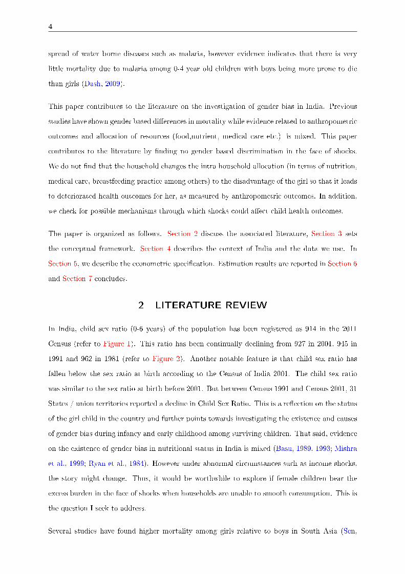
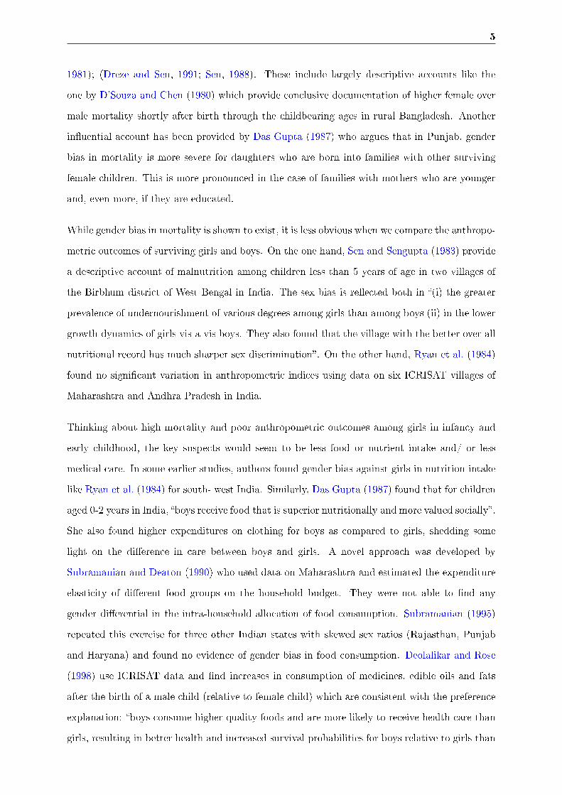
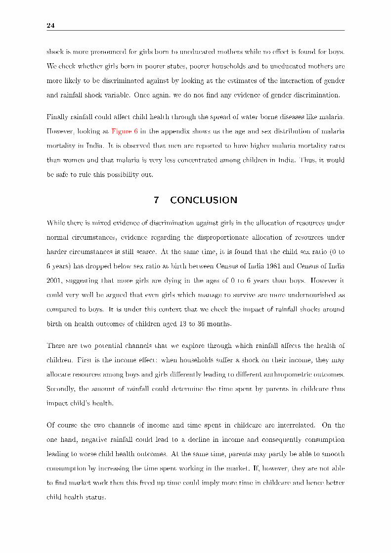
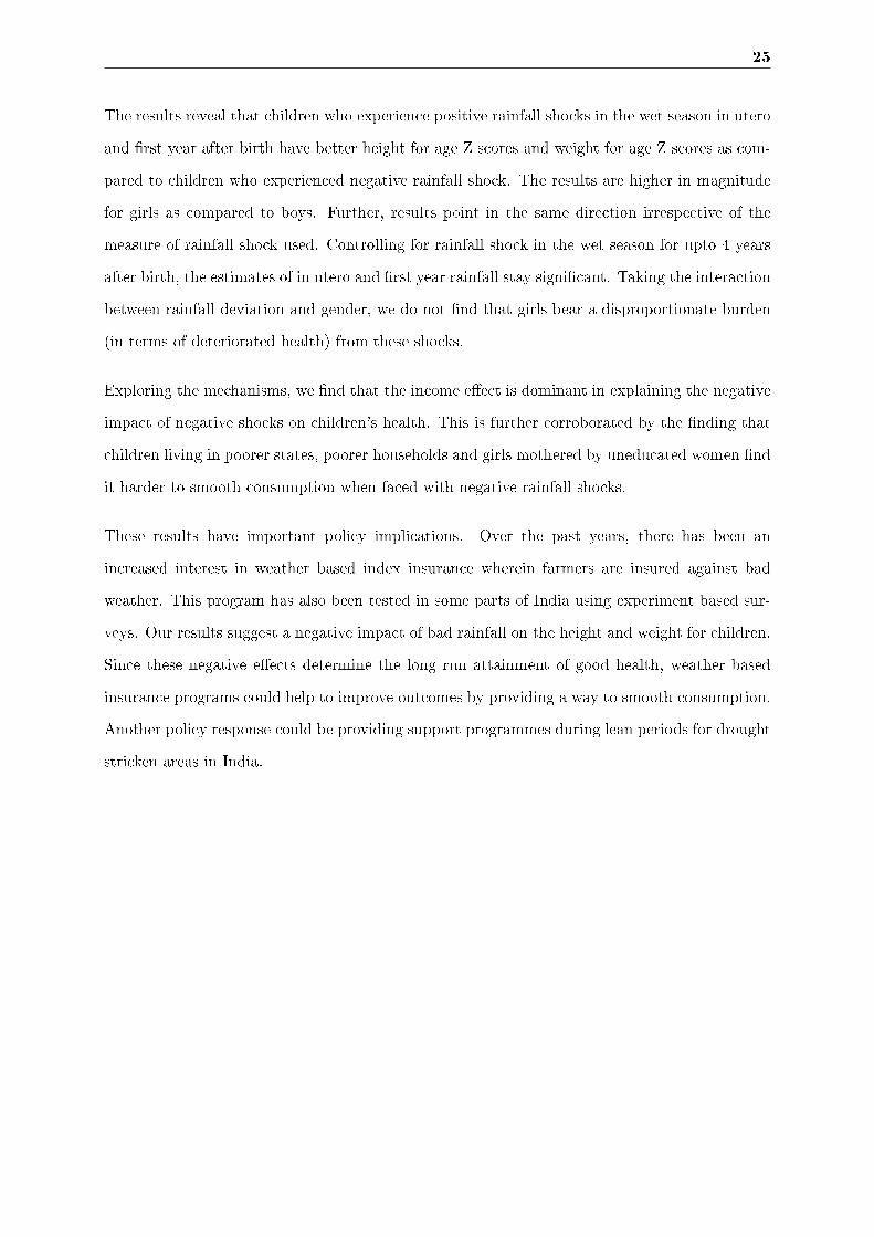
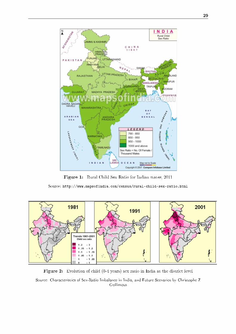
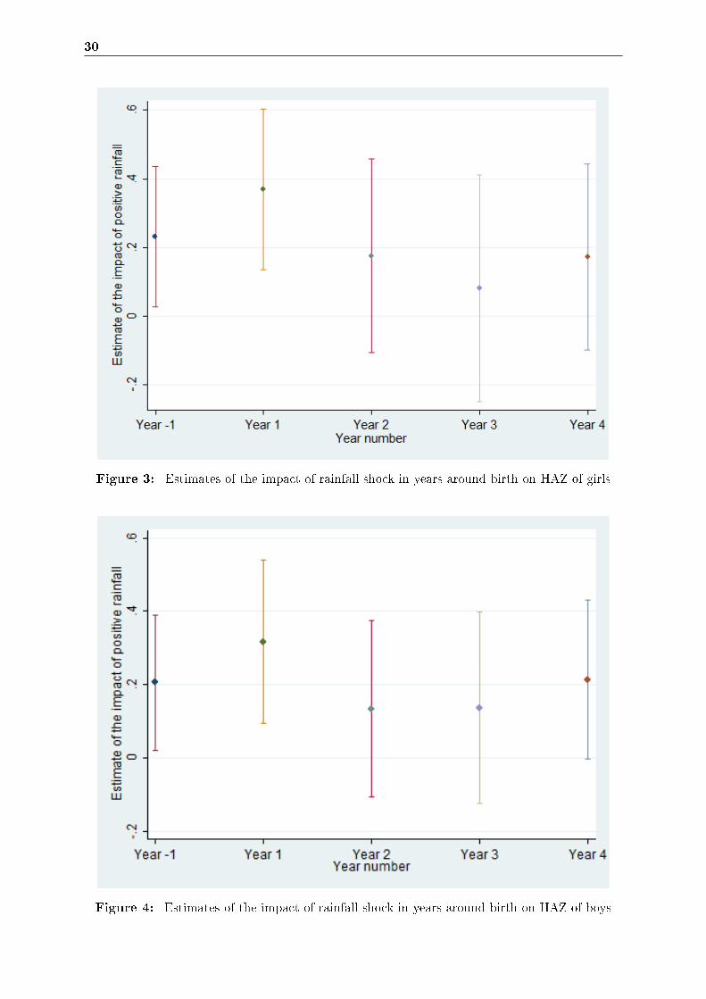
In India, child sex ratio (0-6 years) of the population has been registered as 914 in the 2011

Census (refer to Figure 1). This ratio has been continually declining from 927 in 2001, 945 in

1991 and 962 in 1981 (refer to Figure 2). Another notable feature is that child sex ratio has

fallen below the sex ratio at birth according to the Census of India 2001. The child sex ratio

was similar to the sex ratio at birth before 2001. But between Census 1991 and Census 2001, 31

States / union territories reported a decline in Child Sex Ratio. This is a re�ection on the status

of the girl child in the country and further points towards investigating the existence and causes

of gender bias during infancy and early childhood among surviving children. That said, evidence

on the existence of gender bias in nutritional status in India is mixed (Basu, 1989, 1993; Mishra

et al., 1999; Ryan et al., 1984). However under abnormal circumstances such as income shocks,

the story might change. Thus, it would be worthwhile to explore if female children bear the

excess burden in the face of shocks when households are unable to smooth consumption. This is

the question I seek to address.

Several studies have found higher mortality among girls relative to boys in South Asia (Sen,

5

1981); (Dreze and Sen, 1991; Sen, 1988). These include largely descriptive accounts like the

one by D'Souza and Chen (1980) which provide conclusive documentation of higher female over

male mortality shortly after birth through the childbearing ages in rural Bangladesh. Another

in�uential account has been provided by Das Gupta (1987) who argues that in Punjab, gender

bias in mortality is more severe for daughters who are born into families with other surviving

female children. This is more pronounced in the case of families with mothers who are younger

and, even more, if they are educated.

While gender bias in mortality is shown to exist, it is less obvious when we compare the anthropo-

metric outcomes of surviving girls and boys. On the one hand, Sen and Sengupta (1983) provide

a descriptive account of malnutrition among children less than 5 years of age in two villages of

the Birbhum district of West Bengal in India. The sex bias is re�ected both in �(i) the greater

prevalence of undernourishment of various degrees among girls than among boys (ii) in the lower

growth dynamics of girls vis-a-vis boys. They also found that the village with the better over-all

nutritional record has much sharper sex discrimination�. On the other hand, Ryan et al. (1984)

found no signi�cant variation in anthropometric indices using data on six ICRISAT villages of

Maharashtra and Andhra Pradesh in India.

Thinking about high mortality and poor anthropometric outcomes among girls in infancy and

early childhood, the key suspects would seem to be less food or nutrient intake and/ or less

medical care. In some earlier studies, authors found gender bias against girls in nutrition intake

like Ryan et al. (1984) for south- west India. Similarly, Das Gupta (1987) found that for children

aged 0-2 years in India, �boys receive food that is superior nutritionally and more valued socially�.

She also found higher expenditures on clothing for boys as compared to girls, shedding some

light on the di�erence in care between boys and girls. A novel approach was developed by

Subramanian and Deaton (1990) who used data on Maharashtra and estimated the expenditure

elasticity of di�erent food groups on the household budget. They were not able to �nd any

gender di�erential in the intra-household allocation of food consumption. Subramanian (1995)

repeated this exercise for three other Indian states with skewed sex ratios (Rajasthan, Punjab

and Haryana) and found no evidence of gender bias in food consumption. Deolalikar and Rose

(1998) use ICRISAT data and �nd increases in consumption of medicines, edible oils and fats

after the birth of a male child (relative to female child) which are consistent with the preference

explanation: �boys consume higher quality foods and are more likely to receive health care than

girls, resulting in better health and increased survival probabilities for boys relative to girls than

6

would exist if allocations were identical�.

Pitt et al. (1990) used the 1981-82 Nutrition Survey of Rural Bangladesh and incorporate controls

for activity level and body weight in the data analysis and do not �nd gender bias in nutrient

consumption. Thus, taking into account health endowments and productivity along with the

activities undertaken by Bangladeshi women, accounts for part of the di�erences in the average

consumption of nutrients.

Results on healthcare and medical care also diverge. Subramanian and Deaton (1990) found

no gender bias for medical expenses in Maharashtra, India. On the other hand, Deolalikar and

Rose (1998) found higher expenditure on medicines and healthcare for male Indian children.

Das Gupta (1987) also found much sharper sex di�erentials in medical care than in food alloca-

tion. The expenditure on medical care for sons was found to be 2.34 times higher than that for

daughters in Punjab, India.

In summary, the literature on gender bias in South Asia has explored several questions in the

past. There exists a plethora of descriptive evidence on skewed sex ratios and excess female

mortality in this region. However among the girls who manage to survive, results on food

allocation, anthropometric outcomes and medical care seem to diverge. A part of the divergent

results could be attributed to the speci�cities of the data used and the particular regions in which

these studies are conducted.

An important characteristic of developing countries is the exposure of its people to various kinds

of risks and volatilities in incomes both within a given year and from year to year. One of the

important sources of income volatility stems from poor rainfall, due to the dependence of a large

proportion of population on agriculture and related activities. There do exist some local market

and non-market mechanisms to smooth the impact of shocks across time and states of nature.

But shocks are still hard to insure because of the commonality of shocks to all in a given region.

The literature points that households can partially, but not completely smooth consumption

(Besley, 1995).

Past research has explored the links between shocks that a�ect child health at time period t

(like weather shocks, recessions etc.) and health states measured subsequently at period t+1.

For example, Rose (1999) examines the connection between gender bias in mortality and shocks.

She uses rainfall shock data for Indian districts and links it to the mortality at the district level,

7

checking for consumption smoothing at the time of shock: a favourable rainfall shock increases

the likelihood for a girl-relative to that of a boy- that she survives until school age. Similarly,

using DHS data, Bhalotra (2010) analyzes the impact of GDP deviations from trend across states

on infant mortality. By comparing children born to the same mother (for example, one born in

recession and the other not), she is able to identify the impact of recession on the risk of death.

She �nds that recessions are associated with an increase in infant mortality and that these e�ects

are heterogenous by gender. Finally, using ICRISAT data in India, Behrman (1988) found that

during the lean season, parents weigh a given health-related outcome for boys almost 5 percent

more heavily than the identical health-related outcome for girls. This result suggests that when

faced with lean season, parents exhibit male preference.

One can also draw from other similar studies in Africa. For example, Jensen (2000) uses data

from the Cote d'Ivoire and examines whether children living in areas which experience adverse

climatic shocks, had lower investments in education and health. He compares the di�erences in

height for weight Z score, children enrolled in school and the use of medical services in regions

which had an adverse shock as compared to regions which experienced normal rainfall. He found

an increase in the percentage of boys and girls who were malnourished and a decline in enrolment

for children in shock regions. No girl-boy di�erences were found. Hoddinott and Kinsey (2001)

examine the impact of drought (in 1995) on the growth in the heights of very young children;

those aged 12 to 24 months. They use a panel data set in Zimbabwe and are thus able to measure

the growth of children over time as opposed to estimating a level equation. They found that the

'drought cohort' or children aged 12 -24 months in 1995 grew, on an average, about 2 cm more

slowly than other children, when measured 12 months later.

It is important to examine the e�ect of shocks in infancy as the consequences of underinvestment

in female children during drought/ rainfall shock are likely to be high if such faltering has

permanent e�ects. �Children that experience slow height growth are found to perform less well

in school, score poorly on tests of cognitive function, have poorer psychomotor development and

�ne motor skills� (Dercon and Hoddinott, 2003). Indeed Maccini and Yang (2009) �nd that

higher deviation (of early-life rainfall from the mean rainfall in one's district) has positive e�ects

on the adult outcomes of women, but not of men in Indonesia.

8

3 CONCEPTUAL FRAMEWORK

In this paper, we are interested in estimating the impact of rainfall shock (R) in early childhood

for all years up to point t, on health status (H) as measured at time t.

Ht = h(R0, R1, .., Rt) (1)

Of course, we would like to understand the mechanisms through which rainfall a�ects child

health. Thus to go beyond the reduced form relationship as described in Equation (1), we need

to understand the inputs in the health demand function that can be a�ected by rainfall shocks.

Below is a discussion outlining the relevant inputs.

Following Grossman (1972), health status at time t is a function of a vector of inputs: nutrient

intake (including breastfeeding) until point t (N0, N1..), consumption of health related goods up

until point t (C0, C1..), time inputs to health (T0, T1..) at each time before t, individual, parental

and household endowments (K0), demographic variables such as gender and age of the child

and the individual making decisions about health (X), the availability of infrastructure in the

village/ community (V0, V1..) and the disease environment such as availability of sanitation and

clean water (D0, D1, ..).

Ht = h(N0, N1, .., Nt, C0, C1, ..Ct, T0, T1, .., Tt,K0, X, V0, V1, .., Vt, D0, D1, .., Dt) (2)

Nutrient intake (including breastfeeding), consumption of other goods (clothing, medicines, vac-

cinations, hygiene products etc.) and time inputs to health are assumed to have a positive impact

on child health but this positive impact is decreasing (thus the production function of health

is concave against each of these three inputs). There are many health bene�ts associated with

higher/ better quality nutrient (Blau, 1984) and breastfeeding as recognized by previous stud-

ies including improved cognitive development (Kramer et al., 2008) and reduced risk of obesity

(Kramer, 2010).

Regarding time inputs to health (T), health-promoting activities like �antenatal check-ups for

pregnant women or preventive health care visits for children, breastfeeding, cooking healthy

meals, or collecting clean water all take time to carry out� (Ferreira and Schady, 2009). These

9

activities also have direct bearing on health.

While the aforementioned variables are necessarily choice variables of the household, endowments

are not. There is indeed a well de�ned relationship between child growth and maternal height

as postulated by Hoddinott and Kinsey (2001). Next, we move to demographic variables such

as the age and gender of the individual making decisions about child health. Education of this

individual may a�ect child health through better knowledge about health practices and inputs

(e.g. knowledge about oral rehydration). For example, there are several studies which have

found a positive e�ect of mother's education on her child's health (Aslam and Kingdon, 2012;

Christiaensen and Alderman, 2004; Wolfe and Behrman, 1987). Finally, public expenditure

in the provision of healthcare and health related infrastructure are important determinants of

child health (Desai and Alva, 1998; Thomas et al., 1992). Disease environment determined by

parent's knowledge about health promoting behaviour, availability of clean water and sanitation

are important too.

Let us now discuss the inputs of the health demand function that can be a�ected by rainfall

shocks.

It can be argued that nutrient intake along with the consumption of health promoting goods is

a subset of the overall consumption by the household which in turn is a function of household

income. Household income in turn depends on rainfall, especially in rural India where agriculture

is major source of employment. Indeed, research has shown that there is a relationship between

negative shocks and household consumption expenditures by the way of the income channel.

For example, Bhalotra (2010) �nds that recessions are associated with a decline in household

consumption in India. Similarly, Stillman and Thomas (2008) analyzes the impact of a 2 year

economic contraction in Russia in late 1990s on household consumption expenditures of food.

This contraction was signi�cant in that it led to a decline in GDP by almost one-third. They �nd

that caloric intake was more or less una�ected by the contraction however households switched

to less costly sources of calories. Regarding the consumption of health promoting goods, Paxson

and Schady (2005) show that the Peruvian crisis in the late 1980s is associated with a lower health

care utilization, including a higher ratio of women giving birth at home and lesser antenatal check

ups. Bhalotra (2010) also �nds that mothers engaged in agriculture seek less of both antenatal

and post-natal health promoting activities during recessions in India. Similarly, Jensen (2000)

reports that children in drought a�ected areas in Cote d'Ivoire are less likely to use medical care

10

services.

Second, there is very little research that has looked at the impact of shocks on time use of parents.

A study by Bhalotra (2010) �nds that recessions are associated with an increase in maternal labor

supply in rural India. She also �nds a negative correlation between maternal labor supply and

child health outcomes. She goes on to conclude that mother's time in child care is indeed an

important determinant of child health. Following her argument, we can thus expect that in the

event of a negative rainfall shock, if a mother decides to take on market work, then child health

su�ers due to less time spent by mother in child care. However, if the mother decides to work

in the market because she is no longer needed on the farm (due to a negative rainfall shock),

then in fact it does not necessarily mean that she spends less time in childcare. The e�ect of

mother's time in childcare will ultimately depend on whether she is merely substituting farm

work (no e�ect on time spent in childcare) or taking up additional work (negative e�ect on time

spent in childcare). Even if she is taking up additional market work, she could entrust childcare

to another member of the household such as an older sibling. Finally, if the mother is unable to

�nd market work outside the farm, then a negative rainfall shock could imply more time spent

in childcare and hence better child health status. In e�ect, rainfall's impact on the time spent

by parents in childcare is ambiguous at best, but worth exploration.

In the discussion above, we argued that rainfall has an e�ect on income of agricultural rural

Indian households (we would also show the association between rainfall and agricultural yield

in India in Section 6 to provide further credence to this argument) as well time use of parents.

Lastly, rainfall could alter the disease environment through the spread of water borne diseases

such as malaria.

At the same time, rainfall should not have any impact on non-choice variables in theory. This

is not to say that non-choice variables like demographic variables (or endowment and public

expenditure) would not play out in the event of a rainfall shock. Of course variables like the

education of the household head would be important in determining how the household responds

to the shock. Public expenditure in the provision of healthcare can also plausibly be a�ected

by shocks if they are 'sizeable' in magnitude and a�ect the potential for state governments

to invest in health care provision. For example, the Peruvian crisis of the late 1980s induced

the government to cut public health expenditures by half and may explain to some extent the

spike in infant mortality (Paxson and Schady, 2005). We argue that with the exception of

11

severe droughts, rainfall shocks are largely local and should not have any e�ect on public health

expenditures. This is also a necessary condition for us as we are interested in estimating the

impact of constraints at the household level on child health, and not the impact of a decline in

public health expenditures, on child health.

Thus, we can write that consumption (C), nutrient intake (N), time spent in childcare (T) and

the disease environment (D) are all a function of rainfall, among other factors.

C = c(R,A) (3)

N = n(R,B) (4)

T = t(R,F ) (5)

D = d(R,E) (6)

We do not observe the choice variables in the health demand function (with some exceptions

like vaccinations). If rainfall is exogenous, then dropping the choice variables should not have

any e�ect on the estimates of rainfall on child health. Even if were to observe these variables

and include them as control variables in our regressions, we would run into many estimation

problems (for example the exogeneity of breastfeeding).

Thus, the rainfall variable captures the reduced form e�ect of choice variables (income, time use

and disease environment) on child health. We explore these channels separately at a later stage.

The relationship that we estimate is the following:

Ht = h(R0, R1, .., Rt, C0, C1, ..Ct,K0, X, V0, V1, .., Vt, D0, D1, .., Dt) (7)

In words, health is argued to be a function of rainfall in the period until time t (R0, R1, ..) along

with consumption of health promoting goods (vaccinations) and non-choice variables (endow-

12

ments, demographic variables and community infrastructure).

Of course the two channels of income and time spent in childcare are interrelated. On the

one hand, negative rainfall could lead to a decline in income and consequently consumption

leading to worse child health outcomes. At the same time, parents may partly be able to smooth

consumption by increasing the time spent working in the market. If, however, they are not able

to �nd market work then this freed up time could imply more time in childcare and hence better

child health status. To give an example, a negative rainfall shock might induce parents to not

get their children vaccinated (assuming vaccines are not free) but at the same time, they may

have more time to take their children to the health clinic for vaccinations.

In this paper, as a �rst step, we estimate the reduced form impact of rainfall on children's

anthropometric outcomes using Demographic and Health Surveys for India 1998-99. We control

for various determinants of health demand function as discussed in Equation (7). As a next step,

we explore the mechanisms through which rainfall a�ects child health. We use district- level

crop yield data (from the World Bank Agriculture and Climate Data) and check the impact of

district level rainfall shocks on agricultural yields for Indian crops. Next, we go on to check the

association between rainfall and time spent in market work by women (using Rural Economic

and Demographic Survey 1998-99).

We also directly check for relationships between rainfall and di�erent childcare activities like

breastfeeding and vaccinations. One of the most important parental investment in childcare that

could respond to changes in rainfall is breastfeeding. Indeed, some studies in developed countries

point that the most prominent reasons for breast milk weaning seem to be mother's return to

work (Baker and Milligan, 2008; Roe et al., 1999). However, literature capturing the impact of

mother's labor demand on time spent by her in breastfeeding is largely limited for developing

countries. In response to a positive rainfall shock, a woman might be more likely to wean the

child from breastfeeding, however, it must be recognized that mothers could resort to partial

breastfeeding as a result of working on the farm. In addition, Jayachandran and Kuziemko

(2011) �nds that girls are breastfed for a shorter duration than boys in India. Finally, the sex of

the older sibling has a bearing on the duration of breastfeeding.

13

4 BACKGROUND AND DATA

4.1 Rainfall and Agriculture in India

The monsoon in India plays a major role in determining the harvest of major Indian crops. The

agricultural season in India is divided into two prominent seasons- Kharif and Rabi (henceforth

wet and dry respectively). During the wet season, the sowing of crops is undertaken at the

beginning of the south-west monsoon (May- July depending on the location in India). The har-

vesting activities are undertaken at the end of the south-west monsoon (September to October).

During the dry season, the sowing of crops is undertaken at between October to December (a

relatively cooler time of the year) and the harvesting activities are undertaken between February

and April. Figure 5 in the appendix provides trends of production in wet and dry season for

India. Not only the wet crops have higher production in million tonnes but they also occupy

more land in India.

4.2 Rainfall Data

In the absence of publicly available station rainfall data for India, we use a gridded rainfall

dataset called 'Terrestrial Precipitation: 1900-2008 Gridded Monthly Time Series (Version 2.01)'

interpolated and documented by Kenji Matsuura and Cort J. Willmott (with support from IGES

and NASA) 1 This published dataset consists of interpolated (on a 0.5 degree latitude-longitude

grid) global monthly rainfall data, from 1901 to 2008. We use Mapinfo software to merge rainfall

data from 1122 weather stations spread throughout India to calculate monthly level rainfall for

Indian districts.

Using the latitude and longitude information, we assigned weather stations to each of the 411

districts in DHS data (for the DHS subsample that we use for this analysis- more details in the

next section). The idea was to assign to each district, weather stations in the 50 mile radius from

the centroid of the district. Thereafter, we used the Inverse Distance Weighting (please refer to

subsection 9.1 of the appendix for more on this) to interpolate monthly rainfall values for 411

districts.

1The dataset is provided by Center for Climatic Research, Department of Geography, University of Delaware.Terrestrial Precipitation: 1900-2008 Gridded Monthly Time Series - Version 2.01, interpolated and documentedby Kenji Matsuura and Cort J. Willmott (with support from IGES and NASA). For further information aboutthis dataset, please refer to Legates and Willmott (1990) as the source for rainfall data.

14

For regression analysis, we consider rainfall data corresponding to children in the age group of

13- 36 months at the time of the survey. We identify the months from May- October as the

wet season and consequently November- April as the dry season as these should be most closely

related to agricultural cycles. So if a child is born in August 1994, the �rst wet season for the

child would be May to October 1994 and the �rst dry season would be November 1994 to April

1995. The principal measure of rainfall that we use is de�ned below (we use other measures too

for robustness checks, please refer to subsection 9.2 in the appendix).

The measure of rainfall that we use based is on percentiles and has been used previously for

India. 2 The variable equals 1 if rainfall in wet season around birth is above the 20th percentile

(positive shock) for the district, and 0 if it is below the 20th percentile (negative shock). We use

rainfall in the wet seasons between 1971 and 2004 (44 years) to calculate percentiles. Similarly

we construct variables for rainfall experienced in utero, second year after birth, third year after

birth. We also used other measures of rainfall shock (refer to appendix for details).

4.3 Health Data

The data for the analysis of health outcomes among children comes from the second round of

Demographic and Health Surveys conducted in 1998-99.3 DHS is a nationally representative

household survey and provides data for a wide range of issues pertaining to in health, nutrition

and demographics. The survey was administered nationwide to ever married females aged 15-49

years. The rural sample in each state, which we use in the study was selected as follows: within

each state, primary sampling units (PSUs) were selected using a probability proportional to the

population. Thereafter, within each PSU, households were randomly selected.

We observe the height and weight for children in the age group of 0-36 months at the time of the

interview, born to mothers in the age group of 15-49 years. However we restrict this analysis to

children aged 13-36 months as the impact of rainfall in the years around birth is likely to show

up on children aged 1 and older. Another reason is the concern raised about the accuracy of

measuring height and weight for children less than 1 year of age.

The outcomes that we are interested in are height for age Z scores (HAZ) and weight for age Z

scores (WAZ). HAZ and WAZ are expressed as standard deviations from US National Center for

Health Statistics (NCHS) standard of mean, used by the World Health Organisation (WHO),

2See Jayachandran (2006)3We do not use the �rst round of DHS because there are a lot of missing observations for height and weight.

15

standardized by gender and age. While weight is a measure of short-term health status, height

on the other hand is a stock variable and can be considered to be a long term predictor of

nutrition. All eligible children had their height and weight measured, with some exceptions

(refer to Table A-1 in appendix to see the details of the sample used for analysis). Out of the

total 27250 children, anthropometric data was measured for 24855 children out of which 18044

live in rural areas. After accounting for missing observations and restricting this sample to

children only above 12 months of age, the �nal sample comprises of 5104 girls and 5556 boys.

As a �rst step, we estimate the reduced form impact of rainfall on children's anthropometric

outcomes. In examining the impact of birth year rainfall on HAZ and WAZ of children, we do

not have access to nutrient intake of children. We could control for the duration of breastfeeding

however it is likely to be endogenous as mothers are likely to breastfeed children who have poor

health. However, we include characteristics like wealth of the household and also include a

dummy for whether the child has had any vaccination.

Further, we control for individual characteristics such as birth order of the child, preceding birth

interval and season of birth. We also include the number of sisters and brothers under 13 years

of age, born to the mother and to other adult women in the household to control for composition

e�ects. In a separate speci�cation, we include month of birth �xed e�ects to account for fertility

decisions.

We do not have time -use data in the DHS, however we control for dummies of father's occupation,

whether the mother works on farm, distance to health centre and presence of traditional attendant

in village. Finally, we have included directly for height and weight for the mother of the children

thus accounting for genetic endowment. It is likely that taller and thinner mothers would have

taller and thinner children respectively, all else being same. For example, Hoddinott and Kinsey

(2001) �nd a well de�ned relationship between child growth and maternal height. As far as the

demographic variables are concerned, we use various parental and household level characteristics.

Household characteristics include an index of wealth, sex and age of household head and dummies

for caste and religion. Parental characteristics include variables such as the number of years of

completed schooling of the mother and father, the age and the square of age of mother. The age

of the mother has an ambiguous e�ect on the child's health: older mothers might be expected to

have more children thus putting a strain on the amount of time that is dedicated to the well being

of each child. However, it might be that older mothers have extensive experience in childcare

16

which might make them more knowledgeable about child health practices.

Finally, we include various village infrastructure variables which include distance from the near-

est all weather road, whether the village is electri�ed, population of the village, presence of a

traditional attendant in the village, distance to all weather road, to health sub centre and to

community health centre. The disease environment in part is captured by the rainfall shock

variables.

Table 1 provides descriptive statistics on anthropometric outcomes and explanatory variables

used in our analysis. The anthropometric outcomes that we are interested in are height for age

Z score (HAZ) and weight for age Z score (WAZ) for children in the ages of 13 to 36 months.

The value of these variables lies between -6 and 6. The height for age Z score for children

averages around -2.5 for girls and boys whereas the weight for age Z score averages around -1.9

for both groups. The children whose height (weight) for age Z score is between -2.0 and -2.99

standard deviations (SD) below the mean on the WHO international references standard are

classi�ed as moderately stunted (underweight). This sheds some light on the general status of

the underperformance on anthropometric outcomes in the country. At the same time, in line

with other studies, there does not seem to be any gender bias in anthropometric outcomes.

It is worthwhile to note that about 80 percent of boys and girls experienced positive rainfall in

the �rst wet season around birth. The duration of breastfeeding (which includes children still

being breastfed) is 19.26 months for boys and 18.58 months for girls, observed to be about 3/4

of a month higher for boys and signi�cant. The World Health Organization (2003, pp. 7-8)

recommends that infants should be exclusively breastfed throughout the �rst six months of their

life. It also recommends that mothers continue to breastfeed children after 6 months upto two

years or more even while other foods are being introduced into their diet. It seems that women

continue to breastfeed children for a long time in India.

A smaller percentage of girls aged 13-36 months have vaccination as compared to boys of the

same age. This is in line with evidence from Jayachandran (2006). About 80% of children have

received any vaccination in our sample. The birth order of the children in the sample averages

around 2.9 for girls and boys. Regarding household characteristics, the household head is a male

in 94 percent of the households with an average age around 43.82 for girls and 43.46 for boys.

The wealth score calculated using principal component analysis indicates that girls belong to

less wealthier households than boys. Mother's height and weight averages around 151.65 cm and

17

44.7 kg respectively. The average age of the mother is 25.77 for girls and 25.89 for boys. The

father and mother of boy households tend to be more educated that girl's parents. The fathers

also tend to be more educated than the mothers. There are no signi�cant di�erences for girls

and boys, on an average, on village and community characteristics.

5 EMPIRICAL STRATEGY

In examining the relationship between early life rainfall and subsequent health outcomes for

children, we use child's height for age Z score and weight for age Z scores at the time of the

interview. We restrict the sample to all eligible children in rural areas as the e�ect of the lack/

abundance of rainfall is likely to be highest here. We run all the regressions separately for boys

and girls.

We estimate the relationship between rainfall shock and health outcome for each gender as

follows:

Yihrt = β0 + β1 ∗Rrt + β2 ∗Xihrt + β3 ∗Ahrt + β4 ∗ C + δr + β5η + µihrt

Where Yihrt is the health outcome for child 'i' in household 'h' in district 'r' born in cohort

't'. Rrt is an indicator of rainfall shock in district 'r' in cohort/year 't'. Xihrt is a vector of

control variables at the level of the child. Ahrt is vector of household level and maternal control

variables which might have a direct bearing on child's health outcomes. C captures indicators

at the village level. District �xed e�ects (δr) capture time invariant features of districts, includ-

ing determinants of quality of care that do not change over time and accounts for unobserved

heterogeneity across districts. We also have season of birth �xed e�ects captured by η. The indi-

vidual speci�c standard error term is given by µihrt. Standard errors are clustered at the district

level. Clustering standard errors at the level of the DHS district allows for an arbitrary variance

covariance structure within birth districts to account for possible correlation of errors within

the same sampling cluster. Finally and to be sure, we identify the impact using the exogenous

change in rainfall in a district over time thus comparing children born in di�erent years (and

so experiencing di�erent rainfall) but in the same district and season. For robustness checks,

we also include rainfall variables for period 't-1' (in utero) and 2-4 years after birth. Rainfall

measures in the third and fourth year after birth should not have a signi�cant impact on child

health as the child has not experienced them yet.

18

One must recognize the role of selective mortality in India. Rose (1999) examined the connection

between gender bias in mortality and shocks for India. She uses rainfall shock data at the district

level and links to the mortality among girls, checking for consumption smoothing at the time

of shock: a favourable rainfall shock increases the likelihood relative to that of a boy that a

girl survives until school age. In such a case, one can argue that the weaker girls have already

died and we are left with a healthier sample of girls thus introducing selection. To employ a

selection model, it would be imperative to justify the exclusion restriction of the instrument used.

However, it is almost hardly possible to �nd a factor that a�ects the probability of a neonatal

death without having an impact on height and weight. Thus, it would be worthwhile to mention

that our impacts of rainfall on nutritional outcomes are lower bound estimates of the real causal

estimates.

6 RESULTS

6.1 Anthropometric outcomes

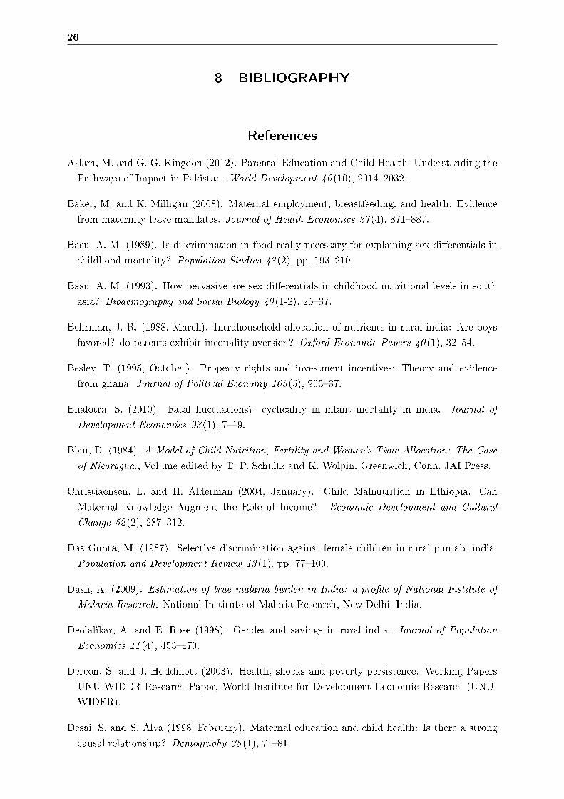
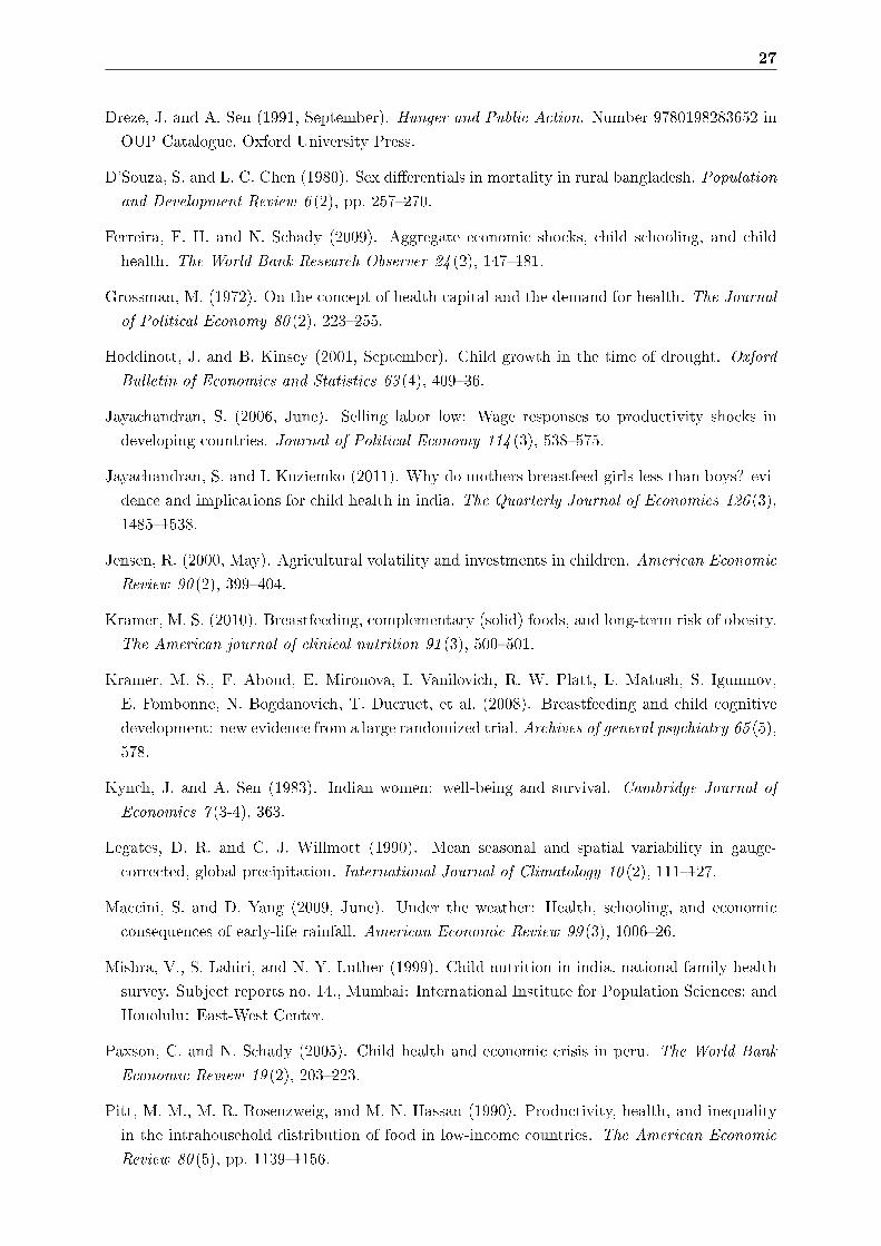
The measure of rainfall that we use in Table 2 is a rainfall shock variable in percentiles explained

in subsection 4.2. Taking negative rainfall as the base (rainfall in the lowest 20 percentile),

children born in areas which received positive rainfall in the �rst wet season after birth have

better outcomes. The magnitudes are large and signi�cant, although slightly larger for girls as

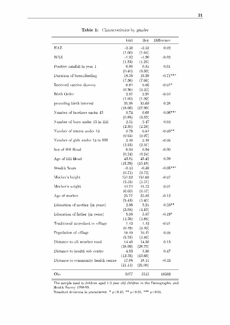
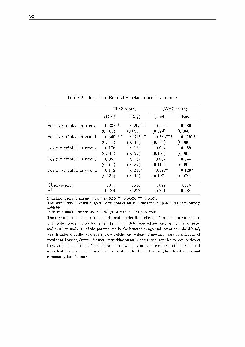
compared to boys. The placebo test is the inclusion of rainfall in other years after birth- they

do not seem to have an e�ect on child health (as demonstrated in Table 2 as well as Figure 3

and Figure 4). Thus, it is clear that the e�ect of rainfall manifests itself in utero and the �rst

year after birth only. Next we introduce month of birth �xed e�ects to the speci�cation, to

account for the choice of parents to have children at a particular month/ season in the year

(results not shown). Results for �rst year wet season rainfall remain the same. We also check

for robustness of these results using di�erent measures of rainfall shocks (results reported in

table A-3 in Appendix, refer to subsection 9.2 in appendix for more details on the construction

of these variables). Overall, it is clear that positive rainfall shocks have a signi�cant improving

e�ect on HAZ and WAZ of both girls and boys.

For detailed results, refer to table A-4 in appendix. Some interesting �ndings emerge. The higher

the number of sisters, the lower is the HAZ of girls. This is in line with much of the literature

on India which suggests that girls tend to have more siblings on an average as compared to

19

boys, thus fewer resources allocated to every child. Children living in wealthier households and

born to more educated mothers have better outcomes, irrespective of gender. Girls born to more

educated fathers also tend to have better outcomes but the same is not observed for boys. As

expected, mother's height and weight is signi�cant for all outcomes and across both genders.

Interestingly, girls born in households where the household head is male have better HAZ as

well. Age of the mother is seen to have no e�ect on outcomes. Finally, it is found that girls have

lower HAZ if they are from Muslim households and boys have better WAZ if they are from the

General caste (upper caste).

In table 2, we have run regressions separately for girls and boys. Thus, currently, we are compar-

ing girls who experienced low rainfall around birth with girls who received good rainfall around

birth, and similarly for boys. However, it would be interesting to see if negative rainfall deviation

a�ects girls more than boys. To capture this e�ect, we introduce an interaction between gender

and the rainfall variable and �nd (in Table 3) the interaction variables to be not statistically

signi�cant. Thus, from these results, it is not clearly evident that girls bear a disproportionate

burden from negative rainfall shocks.

6.2 Exploring the mechanisms

As discussed in the conceptual framework, in addition to the disease environment, there are two

potential channels through which rainfall could a�ect child health. Negative rainfall shocks have a

negative e�ect on income (through its impact on agricultural output), and and ambiguous impact

on the relative price of parent's time. We have found that negative rainfall shocks negatively

a�ect children's health outcomes. Let us now turn to each of the mechanisms.

In order to establish the link from rainfall to income to consumption to health, we would ideally

like to have information on consumption or income of households. In the DHS, this information

is not readily available. Thus, we resort to testing the e�ect of rainfall shocks on the crop

yields (data on crop yields sourced from the World Bank Agriculture and Climate Data). This

dataset contains crop yields of all major Indian crops at the district level from 1951 to 19874.

We test the impact of rainfall shock in each year and in the wet season on the yield of wheat,

rice, bajra, jowar and maize of that particular year, controlling for various agricultural inputs

(such as fertilizers, labor, bullocks and machines), population density and literacy of males in

the district. The results are provided in Table 4. We see that rainfall in the lowest quintile is

4We include only 1956 to 1987 in our analysis as the data for 1951 to 1955 contains a lot of missing data

20

associated with reduced yields for all 5 major Indian crops. Thus rainfall shocks represent a clear

income shock for rural India.

Some of negative e�ect of negative rainfall shocks can be smoothed by taking up market work.

Thus parents might respond to more or less rainfall by increasing or decreasing time spent in the

non-agricultural sector. However lesser labor demand on parents during lean season could also

mean more time spent in domestic chores including childcare. In order to test this hypothesis, we

use time-use data of adult women reported in the 1998-99 round of REDS survey conducted by

National Council of Applied Economic Research, Delhi5. The questionnaire asked about time use

for three time periods in the year 1998-99 (October/ November 1998, February 1999 and April/

May 1999). We restrict ourselves to women in the age group of 15-30 years old (see Table A-2 in

the Appendix for more details on the sample used for analysis). Table 5 shows the descriptive

statistics of time use in various activities for this group of women in 3 di�erent time periods in

the year. The period of October/ November is the key season for harvesting of wet season crops.

It is clear that women spend slightly more time in agricultural activities and less time in market

work in October/ November. With respect to household work of which childcare is a part, there

does not seem to be any signi�cant di�erence across seasons.

Let us now turn to checking the impact of rainfall on these various activities. We check the impact

of rainfall in the wet season of 1998 on time use of women in October/ November 1998, after

controlling for state �xed e�ects. Thus, we are comparing time use of women who experienced

di�erent rainfall in the wet season of 1998 within each state. Results are presented in Table 6 for

October/ November period. Using the measure of rainfall based on percentiles, we do not �nd

any impact of rainfall shocks on time spent in agriculture and related activities or market work

(here market work comprises of non-agricultural wage work, non-agricultural self employed work

and salaried work). However, using the continuous measure of rainfall (refer to subsection 9.2 in

appendix for more details on this measure), we do �nd evidence of more time spent on market

activities and less time spent in agricultural activities when the rainfall is less in wet season. We

5We use the 1998-1999 round of the REDS panel survey conducted by National Council of Applied EconomicResearch, Delhi in 1971, 1982 and 1999. The �rst round of REDS was conducted in 1971 and included completevillage and household information from 4,527 households spread over 259 villages from 17 major states of India.The 1971 sample was designed to be representative of rural areas in India. The 1981-1982 round excludedAssam because of an insurgency at the time, but is claimed to be nationally representative of rural areas. Itsurveyed a total of 4,979 households across 250 villages. Finally, the 1998-99 survey covered all surviving 1982households (except for those in Jammu and Kashmir due to unrest there) and added a small random sample ofnew households from the villages interviewed in previous rounds to make the sample representative. Together withhousehold division since 1982, this results in a sample of 7,474 households; a village-level survey also accompaniedthe household survey.

21

do not �nd any e�ect of rainfall on time spent in domestic work.

One must recognize that using two di�erent datasets to understand the e�ect of rainfall shocks

on anthropometric outcomes and time use poses problems. If the samples in the two datasets

represent di�erent segments of the population, then we may run into making misleading conclu-

sions. Thus in Table A-5, I compare the key characteristics of rural households where women

aged 15-30 were interviewed in the two surveys- REDS and DHS in 1998-99 (this is because the

sample of REDS is restricted to these women). As far as household size and sex of the household

head is concerned, the two surveys do not have any signi�cant di�erences. There are slightly

more number of Hindu households in the REDS surveys and the age of the household head is

2 years more in the REDS survey. Our conclusions regarding the results on time use and an-

thropometric outcomes may thus arguably be comparable. In any case, to further substantiate

whether negative shocks a�ect time spent in childcare, we check the impact of rainfall shocks

directly on some child care activities like breastfeeding and vaccinations.

In DHS 1998-99 data, we have in children for whom breastfeeding has �nished and for whom

it is still ongoing. Since the data is censored, we use Cox's proportional hazard model as this

technique adjusts for truncation bias by incorporating both complete and incomplete segments

of histories in the analysis of breastfeeding-related data6.

We now describe the set up of the data and the assumptions we make. We know for each child in

the age group of 0 to 36 months- the number of months the child has been breastfed and whether

or not the child is being breastfed at the time of the survey. We restrict our sample to children

for whom breastfeeding stopped in the wet season as rainfall is most likely to a�ect the choice

of the mother regarding breastfeeding their children in this period. We build a censor variable

equal to 1 if the event has occurred (breastfeeding had stopped for the child as reported in the

survey), and 0 otherwise. We then reconstruct the data to have one observation per child per

month. Our outcome variable is continuous- the number of months that the child was exposed to

the event (stoppage of breastfeeding). We assume that only one of the covariates is time-varying,

the rainfall shock variable (even though other covariates are also time-varying like distance to

an all weather road, however we only have information about those variables at the time of the

survey).

The rainfall shock variable is built as follows: For children 0-12 months old- it is equal to 1 if

6Please refer to subsection 9.3 in the Appendix for more details on the Cox's proportional hazard model.

22

rainfall experienced in the �rst wet season around birth is in the lowest 20 percentile and 0 zero

otherwise. For children 13-24 months old- it is equal to 1 if rainfall experienced in the second

wet season around birth is in the lowest 20 percentile and 0 zero otherwise. For children 25-36

months old- it is equal to 1 if rainfall experienced in the third wet season around birth is in the

lowest 20 percentile and 0 zero otherwise.

To give an example, imagine a 28 month old girl at the time of the survey for whom breastfeeding

has not stopped yet. For this child, there are 28 observations in the data corresponding to each

month that she was exposed to the risk of termination of breastfeeding. The censor variable is

0 for each of the 28 observations. The rainfall variable varies: this girl has experienced three

wet seasons. For the observations under 12 months of age, she is assigned the rainfall variables

corresponding to the �rst wet season around/ after birth. For observations between 13 and 24

months, she is assigned rainfall variable corresponding to the second wet season around/ after

birth. For observations between 25 and 28 months, she is assigned rainfall variable corresponding

to the third wet season around/ after birth. This is done to ensure that the rainfall variable

captures the e�ect of positive or negative shock in the year that the breastfeeding stopped, on

the outcome variable.

For the question at hand, the hazard function measures the risk of stoppage of being breastfed

at time 't', given that the child has been breastfed until time 't' and a set of characteristics X.

Based on this hazard function, a log partial likelihood function is maximized to produce maximum

partial likelihood estimates of the model parameters. In our case, the model we estimate gives

the impact of rainfall shock on risk of termination of breastfeeding for children aged 0-36 months

in rural India.

Table 7 shows the estimates of the impact of rainfall shock on the hazard of stoppage of breast-

feeding. Columns 1 and 2 show the coe�cients for girls and boys separately. We do not �nd that

stoppage of breastfeeding responds to positive shocks. Thus we cannot draw any meaningful

conclusion from this analysis. We do �nd though that high birth order children have a lower risk

of stoppage of breastfeeding.

In all the regressions with anthropometric status as outcome variables, we included a dummy

for vaccination as an explanatory variable. In addition, we check whether bad rainfall at the

age at which the child is supposed to receive di�erent vaccinations (following the vaccination

schedule of the Indian Academy of Pediatrics) a�ects the probability of being vaccinated (results

23

not shown). As discussed earlier, there are two ways in which rainfall could a�ect this outcome-

either by making it more or less a�ordable or by the e�ect through parent's time use. There is

no impact that we �nd here.

In addition to the above, we also check if rainfall a�ects the probability of getting medical treat-

ment when the child has fever/ cough (result not shown). Restricting to interviews conducted in

the wet season of 1998, we check if the rainfall in the wet season of 1998 a�ects the probability

of getting medical care (in the questionnaire, it was asked if medical care was sought recently in

the event of experiencing fever/ cough ). Again, we do not �nd any association between rainfall

shock in 1998 and the likelihood of getting medical attention for fever/ cough, among children

who did su�er from this ailment in the wet season of 1998.

In summary, higher income associated with positive rainfall could have made health care more

a�ordable. Even though women might spend more time in market work in lean season, we do

not �nd any indication in these results that negative rainfall is associated with more time spent

in childcare or vice-versa. Of course, even if our results pointed in the direction that mothers do

spend less time in child care during good rainfall years, it could just be that an older sibling or

other member of the household is spending more time in childcare instead.

6.3 Extensions

An important factor to consider is that rainfall is known to be quasi random and it could be

correlated over time. If it were to be correlated then it would be di�cult to isolate the impact of

birth year rainfall from the in utero rainfall or other years, calling into question the identi�cation.

As mentioned before, looking at the impact of rainfall in the third and fourth year of birth of

children who are 13 to 36 months old at the time of survey, we found no impact on children's

health.

Further, we must consider that the impact of rainfall shock on heterogeneous groups. Table 8

looks at the e�ect on shocks in the 7 richest and 6 poorest Indian states. Similarly in Table 9, we

check the impact of shocks based on the wealth of the household. It turns out that rainfall shocks

have an impact on child health only in poorer states and poorer households. It is likely that

poorer states and poorer households rely more heavily on agriculture for their income and hence

rainfall shocks a�ecting agriculture have a larger impact on them. Finally, Table 10 summarises

the results by education of mother. The results seem to point out that the impact of rainfall

24

shock is more pronounced for girls born to uneducated mothers while no e�ect is found for boys.

We check whether girls born in poorer states, poorer households and to uneducated mothers are

more likely to be discriminated against by looking at the estimates of the interaction of gender

and rainfall shock variable. Once again, we do not �nd any evidence of gender discrimination.

Finally rainfall could a�ect child health through the spread of water borne diseases like malaria.

However, looking at Figure 6 in the appendix shows us the age and sex distribution of malaria

mortality in India. It is observed that men are reported to have higher malaria mortality rates

than women and that malaria is very less concentrated among children in India. Thus, it would

be safe to rule this possibility out.

7 CONCLUSION

While there is mixed evidence of discrimination against girls in the allocation of resources under

normal circumstances, evidence regarding the disproportionate allocation of resources under

harder circumstances is still scarce. At the same time, it is found that the child sex ratio (0 to

6 years) has dropped below sex ratio at birth between Census of India 1981 and Census of India

2001, suggesting that more girls are dying in the ages of 0 to 6 years than boys. However it

could very well be argued that even girls which manage to survive are more undernourished as

compared to boys. It is under this context that we check the impact of rainfall shocks around

birth on health outcomes of children aged 13 to 36 months.

There are two potential channels that we explore through which rainfall a�ects the health of

children. First is the income e�ect: when households su�er a shock on their income, they may

allocate resources among boys and girls di�erently leading to di�erent anthropometric outcomes.

Secondly, the amount of rainfall could determine the time spent by parents in childcare thus

impact child's health.

Of course the two channels of income and time spent in childcare are interrelated. On the

one hand, negative rainfall could lead to a decline in income and consequently consumption

leading to worse child health outcomes. At the same time, parents may partly be able to smooth

consumption by increasing the time spent working in the market. If, however, they are not able

to �nd market work then this freed up time could imply more time in childcare and hence better

child health status.

25

The results reveal that children who experience positive rainfall shocks in the wet season in utero

and �rst year after birth have better height for age Z scores and weight for age Z scores as com-

pared to children who experienced negative rainfall shock. The results are higher in magnitude

for girls as compared to boys. Further, results point in the same direction irrespective of the

measure of rainfall shock used. Controlling for rainfall shock in the wet season for upto 4 years

after birth, the estimates of in utero and �rst year rainfall stay signi�cant. Taking the interaction

between rainfall deviation and gender, we do not �nd that girls bear a disproportionate burden

(in terms of deteriorated health) from these shocks.

Exploring the mechanisms, we �nd that the income e�ect is dominant in explaining the negative

impact of negative shocks on children's health. This is further corroborated by the �nding that

children living in poorer states, poorer households and girls mothered by uneducated women �nd

it harder to smooth consumption when faced with negative rainfall shocks.

These results have important policy implications. Over the past years, there has been an

increased interest in weather based index insurance wherein farmers are insured against bad

weather. This program has also been tested in some parts of India using experiment based sur-

veys. Our results suggest a negative impact of bad rainfall on the height and weight for children.

Since these negative e�ects determine the long run attainment of good health, weather based

insurance programs could help to improve outcomes by providing a way to smooth consumption.

Another policy response could be providing support programmes during lean periods for drought

stricken areas in India.

26

8 BIBLIOGRAPHY

References

Aslam, M. and G. G. Kingdon (2012). Parental Education and Child Health- Understanding the

Pathways of Impact in Pakistan. World Development 40 (10), 2014�2032.

Baker, M. and K. Milligan (2008). Maternal employment, breastfeeding, and health: Evidence

from maternity leave mandates. Journal of Health Economics 27 (4), 871�887.

Basu, A. M. (1989). Is discrimination in food really necessary for explaining sex di�erentials in

childhood mortality? Population Studies 43 (2), pp. 193�210.

Basu, A. M. (1993). How pervasive are sex di�erentials in childhood nutritional levels in south

asia? Biodemography and Social Biology 40 (1-2), 25�37.

Behrman, J. R. (1988, March). Intrahousehold allocation of nutrients in rural india: Are boys

favored? do parents exhibit inequality aversion? Oxford Economic Papers 40 (1), 32�54.

Besley, T. (1995, October). Property rights and investment incentives: Theory and evidence

from ghana. Journal of Political Economy 103 (5), 903�37.

Bhalotra, S. (2010). Fatal �uctuations? cyclicality in infant mortality in india. Journal of

Development Economics 93 (1), 7�19.

Blau, D. (1984). A Model of Child Nutrition, Fertility and Women's Time Allocation: The Case

of Nicaragua., Volume edited by T. P. Schultz and K. Wolpin. Greenwich, Conn. JAI Press.

Christiaensen, L. and H. Alderman (2004, January). Child Malnutrition in Ethiopia: Can

Maternal Knowledge Augment the Role of Income? Economic Development and Cultural

Change 52 (2), 287�312.

Das Gupta, M. (1987). Selective discrimination against female children in rural punjab, india.

Population and Development Review 13 (1), pp. 77�100.

Dash, A. (2009). Estimation of true malaria burden in India: a pro�le of National Institute of

Malaria Research. National Institute of Malaria Research, New Delhi, India.

Deolalikar, A. and E. Rose (1998). Gender and savings in rural india. Journal of Population

Economics 11 (4), 453�470.

Dercon, S. and J. Hoddinott (2003). Health, shocks and poverty persistence. Working Papers

UNU-WIDER Research Paper, World Institute for Development Economic Research (UNU-

WIDER).

Desai, S. and S. Alva (1998, February). Maternal education and child health: Is there a strong

causal relationship? Demography 35 (1), 71�81.

27

Dreze, J. and A. Sen (1991, September). Hunger and Public Action. Number 9780198283652 in

OUP Catalogue. Oxford University Press.

D'Souza, S. and L. C. Chen (1980). Sex di�erentials in mortality in rural bangladesh. Population

and Development Review 6 (2), pp. 257�270.

Ferreira, F. H. and N. Schady (2009). Aggregate economic shocks, child schooling, and child

health. The World Bank Research Observer 24 (2), 147�181.

Grossman, M. (1972). On the concept of health capital and the demand for health. The Journal

of Political Economy 80 (2), 223�255.

Hoddinott, J. and B. Kinsey (2001, September). Child growth in the time of drought. Oxford

Bulletin of Economics and Statistics 63 (4), 409�36.

Jayachandran, S. (2006, June). Selling labor low: Wage responses to productivity shocks in

developing countries. Journal of Political Economy 114 (3), 538�575.

Jayachandran, S. and I. Kuziemko (2011). Why do mothers breastfeed girls less than boys? evi-

dence and implications for child health in india. The Quarterly Journal of Economics 126 (3),

1485�1538.

Jensen, R. (2000, May). Agricultural volatility and investments in children. American Economic

Review 90 (2), 399�404.

Kramer, M. S. (2010). Breastfeeding, complementary (solid) foods, and long-term risk of obesity.

The American journal of clinical nutrition 91 (3), 500�501.

Kramer, M. S., F. Aboud, E. Mironova, I. Vanilovich, R. W. Platt, L. Matush, S. Igumnov,

E. Fombonne, N. Bogdanovich, T. Ducruet, et al. (2008). Breastfeeding and child cognitive

development: new evidence from a large randomized trial. Archives of general psychiatry 65 (5),

578.

Kynch, J. and A. Sen (1983). Indian women: well-being and survival. Cambridge Journal of

Economics 7 (3-4), 363.

Legates, D. R. and C. J. Willmott (1990). Mean seasonal and spatial variability in gauge-

corrected, global precipitation. International Journal of Climatology 10 (2), 111�127.

Maccini, S. and D. Yang (2009, June). Under the weather: Health, schooling, and economic

consequences of early-life rainfall. American Economic Review 99 (3), 1006�26.

Mishra, V., S. Lahiri, and N. Y. Luther (1999). Child nutrition in india. national family health

survey. Subject reports no. 14., Mumbai: International Institute for Population Sciences; and

Honolulu: East-West Center.

Paxson, C. and N. Schady (2005). Child health and economic crisis in peru. The World Bank

Economic Review 19 (2), 203�223.

Pitt, M. M., M. R. Rosenzweig, and M. N. Hassan (1990). Productivity, health, and inequality

in the intrahousehold distribution of food in low-income countries. The American Economic

Review 80 (5), pp. 1139�1156.

28

Roe, B., L. A. Whittington, S. B. Fein, and M. F. Teisl (1999). Is there competition between

breast-feeding and maternal employment? Demography 36 (2), pp. 157�171.

Rose, E. (1999). Consumption smoothing and excess female mortality in rural india. The Review

of Economics and Statistics 81 (1), pp. 41�49.

Ryan, J. G., P. D. Bidinger, N. P. Rao, and P. Pushpamma (1984). The determinants of individual

diets and nutritional status in six villages of south india. Technical report, Hyderabad, India:

ICRISAT-NIN-APAU.

Sen, A. (1981). Poverty and FaminesAn Essay on Entitlement and Deprivation. Oxford Univer-

sity Press.

Sen, A. (1990). More than 100 million women are missing. The New York Review of Books 37 (20),

61�66.

Sen, A. and S. Sengupta (1983). Malnutrition of rural children and the sex bias. Economic and

Political Weekly 18 (19/21), pp. 855�857+859�861+863�864.

Sen, A. K. (1988). Family and food: sex bias in poverty.

Stillman, S. and D. Thomas (2008). Nutritional status during an economic crisis: Evidence from

russia*. The Economic Journal 118 (531), 1385�1417.

Subramanian, S. (1995). Gender discrimination in intra-household allocation in india. mimeo,

Department of Economics, Cornell University.

Subramanian, S. and A. Deaton (1990). Gender e�ects in indian consumption patterns. Papers

147, Princeton, Woodrow Wilson School - Development Studies.

Thomas, D., V. Lavy, and J. Strauss (1992). Public Policy and Anthropometric Outcomes in

Cote d'Ivoire. Papers 89, World Bank - Living Standards Measurement.

Wolfe, B. L. and J. R. Behrman (1987, September). Women's schooling and children's health

: Are the e�ects robust with adult sibling control for the women's childhood background?

Journal of Health Economics 6 (3), 239�254.

29

Figure 1: Rural Child Sex Ratio for Indian states, 2011

Source: http://www.mapsofindia.com/census/rural-child-sex-ratio.html

Figure 2: Evolution of child (0-4 years) sex ratio in India at the district level

Source: Characteristics of Sex-Ratio Imbalance in India, and Future Scenarios by Christophe ZGuilimoto

30

Figure 3: Estimates of the impact of rainfall shock in years around birth on HAZ of girls

Figure 4: Estimates of the impact of rainfall shock in years around birth on HAZ of boys

31

Table 1: Characteristics by gender

Girl Boy Di�erence

HAZ -2.50 -2.52 0.02(1.66) (1.64)

WAZ -1.92 -1.90 -0.02(1.33) (1.26)

Positive rainfall in year 1 0.80 0.81 -0.01(0.40) (0.39)

Duration of breastfeeding 18.58 19.29 -0.71***(7.36) (7.66)

Received vaccine dummy 0.84 0.86 -0.01*(0.36) (0.35)

Birth Order 2.87 2.91 -0.04(1.90) (1.92)

preceding birth interval 35.98 35.69 0.28(18.66) (17.99)

Number of brothers under 13 0.74 0.68 0.06***(0.85) (0.83)

Number of boys under 13 in HH 2.51 2.47 0.04(2.30) (2.28)

Number of sisters under 13 0.79 0.84 -0.05**(0.93) (0.97)

Number of girls under 13 in HH 2.40 2.48 -0.08(2.23) (2.31)

Sex of HH Head 0.94 0.94 -0.00(0.24) (0.24)

Age of HH Head 43.81 43.42 0.39(15.39) (15.18)

Wealth Score -0.44 -0.39 -0.05***(0.71) (0.73)

Mother's height 151.62 151.69 -0.07(5.55) (5.51)

Mother's weight 44.74 44.72 0.01(6.60) (6.57)

Age of mother 25.77 25.89 -0.12(5.43) (5.45)

Education of mother (in years) 2.98 3.21 -0.23**(3.98) (4.19)

Education of father (in years) 5.68 5.87 -0.19*(4.76) (4.86)

Traditional attendant in village 1.42 1.43 -0.01(0.49) (0.49)

Population of village 10.49 10.41 0.08(5.78) (5.86)

Distance to all weather road 14.43 14.30 0.13(28.99) (28.70)

Distance to health sub centre 4.83 5.30 -0.47(12.55) (13.66)

Distance to community health centre 17.88 18.11 -0.23(21.14) (21.00)

Obs 5077 5515 10592

The sample used is children aged 1-3 year old children in the Demographic andHealth Survey 1998-99.Standard deviation in parentheses. * p<0.10, ** p<0.05, *** p<0.01.

32

Table 2: Impact of Rainfall Shocks on health outcomes

(HAZ score) (WAZ score)

(Girl) (Boy) (Girl) (Boy)

Positive rainfall in utero 0.232** 0.205** 0.124* 0.086(0.105) (0.093) (0.074) (0.066)

Positive rainfall in year 1 0.369*** 0.317*** 0.283*** 0.215***(0.119) (0.113) (0.081) (0.080)

Positive rainfall in year 2 0.176 0.133 0.092 0.069(0.143) (0.122) (0.101) (0.081)

Positive rainfall in year 3 0.081 0.137 0.032 0.044(0.169) (0.132) (0.111) (0.091)

Positive rainfall in year 4 0.172 0.213* 0.172* 0.129*(0.138) (0.110) (0.100) (0.078)

Observations 5077 5515 5077 5515R2 0.244 0.227 0.291 0.284

Standard errors in parentheses. * p<0.10, ** p<0.05, *** p<0.01.The sample used is children aged 1-3 year old children in the Demographic and Health Survey1998-99.Positive rainfall is wet season rainfall greater than 20th percentile.

The regressions include season of birth and district �xed e�ects. Also includes controls for

birth order, preceding birth interval, dummy for child received any vaccine, number of sister

and brothers under 13 of the parents and in the household, age and sex of household head,

wealth index quintile, age, age square, height and weight of mother, years of schooling of

mother and father, dummy for mother working on farm, categorical variable for occupation of

father, religion and caste. Village level control variables are village electri�cation, traditional

attendant in village, population in village, distance to all weather road, health sub centre and

community health centre.

33

Table 3: Impact of Rainfall Shocks on gender bias in health outcomes

(With SOB FE) (With MOB FE)

(HAZ) (WAZ) (HAZ) (WAZ)

Positive rainfall in year 1 0.211** 0.152** 0.158** 0.120**(0.082) (0.060) (0.076) (0.057)

Positive rainfall in utero 0.141* 0.094 0.071 0.054(0.082) (0.059) (0.074) (0.057)

Sex * positive rainfall in year 1 0.045 0.032 0.040 0.029(0.083) (0.060) (0.080) (0.060)

Sex * positive rainfall in year -1 0.075 -0.006 0.080 -0.004(0.074) (0.061) (0.072) (0.060)

Sex of child -0.136 -0.014 -0.134 -0.014(0.093) (0.070) (0.091) (0.069)

Observations 10592 10592 10592 10592R2 0.199 0.251 0.213 0.259

Standard errors in parentheses. * p<0.10, ** p<0.05, *** p<0.01.The sample used is children aged 1-3 year old children in the Demographic and Health Survey1998-99.The regressions include month or season of birth and district �xed e�ects. Also includes controlsfor birth order, preceding birth interval, dummy for child received any vaccine, number of sisterand brothers under 13 of the parents and in the household, age and sex of household head,wealth index quintile, age, age square, height and weight of mother, years of schooling of motherand father, dummy for mother working on farm, categorical variable for occupation of father,religion and caste. Village level control variables are village electri�cation, traditional attendantin village, population in village, distance to all weather road, health sub centre and communityhealth centre.The regressions include district �xed e�ects. SOB refers to season of birth and MOB refers tothe month of birth.

Positive rainfall is wet season rainfall greater than 20th percentile.

Table 4: Impact of Rainfall Shocks on crop yield

(Wheat) (Rice) (Jowar) (Maize) (Bajra)

Positive rainfall in wet season 0.054*** 0.149*** 0.058*** 0.065*** 0.059***(0.012) (0.013) (0.009) (0.017) (0.010)

Observations 7317 7317 7317 7317 7317R2 0.710 0.691 0.502 0.424 0.299

Standard errors in parentheses. * p<0.10, ** p<0.05, *** p<0.01.The sample consists of information on Indian districts between 1956 and 1987 from the World Bank Agriculture andClimate Data.Positive rainfall is wet season rainfall greater than 20th percentile.

The regressions include district �xed e�ects and controls for other agricultural inputs (fertilizers, labor, bullocks and

machines), population density and literacy of males in the district.

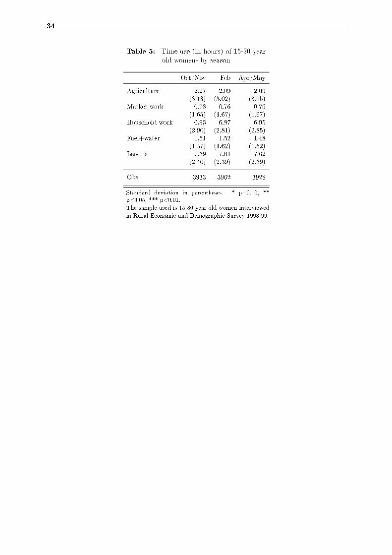
34

Table 5: Time use (in hours) of 15-30 yearold women- by season

Oct/Nov Feb Apr/May

Agriculture 2.27 2.09 2.09(3.13) (3.02) (3.05)

Market work 0.73 0.76 0.76(1.65) (1.67) (1.67)

Household work 6.93 6.87 6.95(2.90) (2.81) (2.85)

Fuel+water 1.51 1.52 1.48(1.57) (1.62) (1.62)

Leisure 7.39 7.61 7.62(2.40) (2.39) (2.39)

Obs 3933 3962 3928

Standard deviation in parentheses. * p<0.10, **p<0.05, *** p<0.01.The sample used is 15-30 year old women interviewedin Rural Economic and Demographic Survey 1998-99.

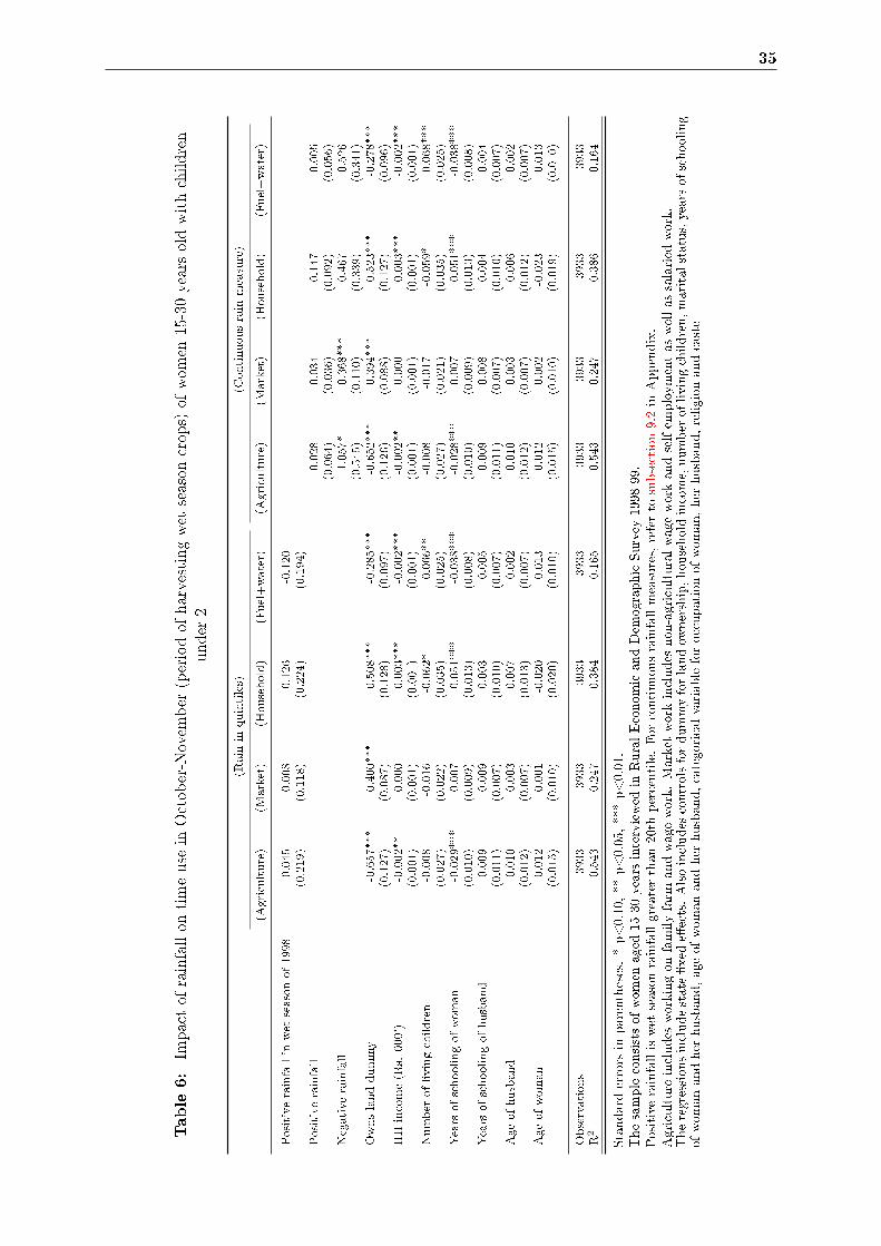
35

Table6:

Impactof

rainfallon

timeuse

inOctober-Novem

ber

(periodof

harvestingwet

season

crops)

ofwom

en15-30yearsoldwithchildren

under

2

(Rain

inquintiles)

(Continuousrain

measure)

(Agriculture)

(Market)

(Household)

(Fuel+water)

(Agriculture)

(Market)

(Household)

(Fuel+water)

Positiverainfallin

wet

seasonof1998

0.045

0.008

0.126

-0.120

(0.219)

(0.118)

(0.224)

(0.194)

Positiverainfall

0.028

-0.034

0.147

-0.005

(0.064)

(0.036)

(0.092)

(0.056)

Negativerainfall

-1.057*

0.368***

0.467

-0.526

(0.545)

(0.110)

(0.339)

(0.341)

Ownslanddummy

-0.657***

0.400***

0.508***

-0.285***

-0.652***

0.394***

0.523***

-0.278***

(0.127)

(0.087)

(0.128)

(0.097)

(0.126)

(0.088)

(0.127)

(0.096)

HHincome(Rs.000')

-0.002**

0.000

0.003***

-0.002***

-0.002**

0.000

0.003***

-0.002***

(0.001)

(0.001)

(0.001)

(0.001)

(0.001)

(0.001)

(0.001)

(0.001)

Number

oflivingchildren

-0.008

-0.016

-0.062*

0.066**

-0.008

-0.017

-0.059*

0.068***

(0.027)

(0.022)

(0.035)

(0.025)

(0.027)

(0.021)

(0.035)

(0.025)

Yearsofschoolingofwoman

-0.029***

0.007

0.051***

-0.038***

-0.028***

0.007

0.051***

-0.038***

(0.010)

(0.009)

(0.013)

(0.008)

(0.010)

(0.009)

(0.013)

(0.008)

Yearsofschoolingofhusband

-0.009

0.009

0.003

-0.005

-0.009

0.008

0.004

-0.004

(0.011)

(0.007)

(0.010)

(0.007)

(0.011)

(0.007)

(0.010)

(0.007)

Ageofhusband

0.010

0.003

-0.007

-0.002

0.010

0.003

-0.006

-0.002

(0.012)

(0.007)

(0.013)

(0.007)

(0.012)

(0.007)

(0.012)

(0.007)

Ageofwoman

0.012

0.001

-0.020

0.013

0.012

0.002

-0.023

0.013

(0.015)

(0.010)

(0.020)

(0.010)

(0.015)

(0.010)

(0.019)

(0.010)

Observations

3933

3933

3933

3933

3933

3933

3933

3933

R2

0.543

0.247

0.384

0.165

0.543

0.247

0.386

0.164

Standarderrors

inparentheses.*p<0.10,**

p<0.05,***p<0.01.

Thesampleconsistsof

wom

enaged

15-30yearsinterviewed

inRuralEconom

icandDem

ographicSurvey

1998-99.

Positiverainfalliswet

season

rainfallgreaterthan

20th

percentile.

For

continuousrainfallmeasures,referto

subsection9.2in

Appendix.

Agriculture

includes

workingon

familyfarm

andwagework.

Marketworkincludes

non-agriculturalwageworkandselfem

ploym

entas

wellas

salaried

work.

Theregressionsincludestate�xede�ects.Alsoincludes

controlsfordummyforlandow

nership,householdincome,number

oflivingchildren,maritalstatus,yearsofschooling

ofwom

anandher

husband,ageof

wom

anandher

husband,categoricalvariableforoccupationof

wom

an,her

husband,religion

andcaste

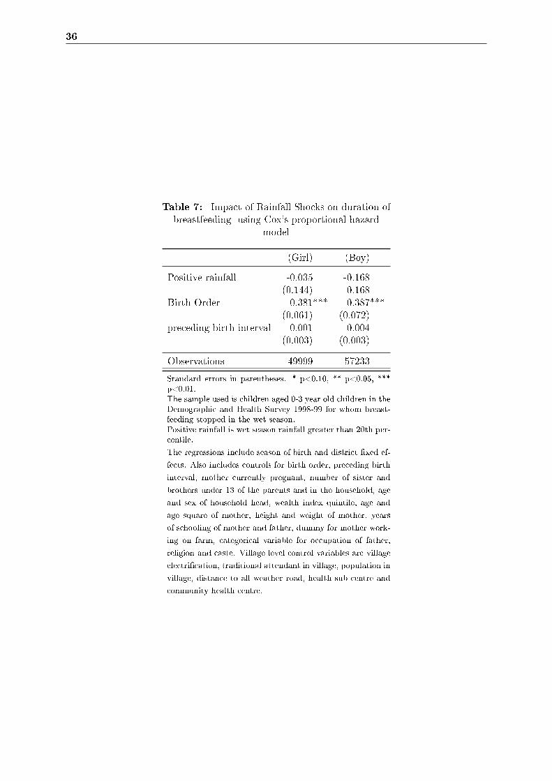
36

Table 7: Impact of Rainfall Shocks on duration ofbreastfeeding- using Cox's proportional hazard

model

(Girl) (Boy)

Positive rainfall -0.035 -0.168(0.144) -0.168

Birth Order -0.381*** -0.387***(0.061) (0.072)

preceding birth interval -0.001 -0.004(0.003) (0.003)

Observations 49999 57233

Standard errors in parentheses. * p<0.10, ** p<0.05, ***p<0.01.The sample used is children aged 0-3 year old children in theDemographic and Health Survey 1998-99 for whom breast-feeding stopped in the wet season.Positive rainfall is wet season rainfall greater than 20th per-centile.

The regressions include season of birth and district �xed ef-

fects. Also includes controls for birth order, preceding birth

interval, mother currently pregnant, number of sister and

brothers under 13 of the parents and in the household, age

and sex of household head, wealth index quintile, age and

age square of mother, height and weight of mother, years

of schooling of mother and father, dummy for mother work-

ing on farm, categorical variable for occupation of father,

religion and caste. Village level control variables are village

electri�cation, traditional attendant in village, population in

village, distance to all weather road, health sub centre and

community health centre.

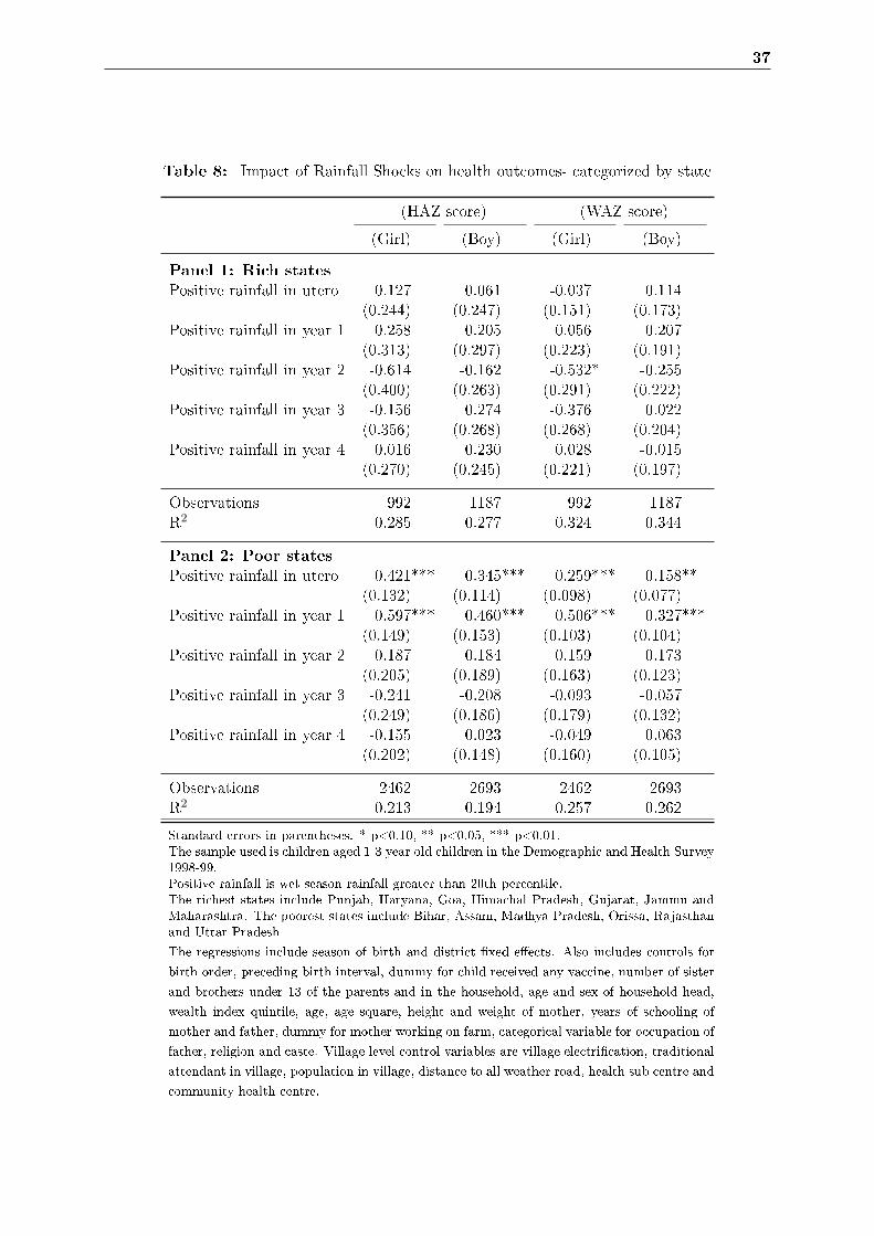
37

Table 8: Impact of Rainfall Shocks on health outcomes- categorized by state

(HAZ score) (WAZ score)

(Girl) (Boy) (Girl) (Boy)

Panel 1: Rich states

Positive rainfall in utero 0.127 0.061 -0.037 0.114(0.244) (0.247) (0.151) (0.173)

Positive rainfall in year 1 0.258 0.205 0.056 0.207(0.313) (0.297) (0.223) (0.191)

Positive rainfall in year 2 -0.614 -0.162 -0.532* -0.255(0.400) (0.263) (0.291) (0.222)

Positive rainfall in year 3 -0.156 0.274 -0.376 0.022(0.356) (0.268) (0.268) (0.204)

Positive rainfall in year 4 0.016 0.230 0.028 -0.015(0.270) (0.245) (0.221) (0.197)

Observations 992 1187 992 1187R2 0.285 0.277 0.324 0.344

Panel 2: Poor states

Positive rainfall in utero 0.421*** 0.345*** 0.259*** 0.158**(0.132) (0.114) (0.098) (0.077)

Positive rainfall in year 1 0.597*** 0.460*** 0.506*** 0.327***(0.149) (0.153) (0.103) (0.104)

Positive rainfall in year 2 0.187 0.184 0.159 0.173(0.205) (0.189) (0.163) (0.123)

Positive rainfall in year 3 -0.241 -0.208 -0.093 -0.057(0.249) (0.186) (0.179) (0.132)

Positive rainfall in year 4 -0.155 0.023 -0.049 0.063(0.202) (0.148) (0.160) (0.105)

Observations 2462 2693 2462 2693R2 0.213 0.194 0.257 0.262

Standard errors in parentheses. * p<0.10, ** p<0.05, *** p<0.01.The sample used is children aged 1-3 year old children in the Demographic and Health Survey1998-99.Positive rainfall is wet season rainfall greater than 20th percentile.The richest states include Punjab, Haryana, Goa, Himachal Pradesh, Gujarat, Jammu andMaharashtra. The poorest states include Bihar, Assam, Madhya Pradesh, Orissa, Rajasthanand Uttar Pradesh

The regressions include season of birth and district �xed e�ects. Also includes controls for

birth order, preceding birth interval, dummy for child received any vaccine, number of sister

and brothers under 13 of the parents and in the household, age and sex of household head,

wealth index quintile, age, age square, height and weight of mother, years of schooling of

mother and father, dummy for mother working on farm, categorical variable for occupation of

father, religion and caste. Village level control variables are village electri�cation, traditional

attendant in village, population in village, distance to all weather road, health sub centre and

community health centre.

38

Table 9: Impact of Rainfall Shocks on health outcomes- categorized by household wealth

(HAZ score) (WAZ score)

(Girl) (Boy) (Girl) (Boy)

Panel 1: Bottom 40 pctile on wealth index

Positive rainfall in utero 0.346** 0.348*** 0.195* 0.161*(0.143) (0.127) (0.102) (0.091)

Positive rainfall in year 1 0.505*** 0.405** 0.431*** 0.205*(0.160) (0.167) (0.107) (0.113)

Positive rainfall in year 2 0.386* 0.180 0.355** 0.139(0.199) (0.193) (0.152) (0.131)

Positive rainfall in year 3 -0.025 0.001 -0.059 0.089(0.248) (0.215) (0.181) (0.134)

Positive rainfall in year 4 0.027 0.173 -0.002 0.113(0.202) (0.174) (0.151) (0.117)

Observations 2409 2464 2409 2464R2 0.251 0.253 0.297 0.302

Panel 2: Top 60 pctile on wealth index

Positive rainfall in utero -0.006 -0.010 0.021 -0.019(0.157) (0.159) (0.105) (0.114)

Positive rainfall in year 1 0.110 0.165 0.081 0.215*(0.186) (0.166) (0.133) (0.122)

Positive rainfall in year 2 -0.037 -0.008 -0.160 -0.065(0.212) (0.173) (0.144) (0.124)

Positive rainfall in year 3 0.068 0.145 0.062 -0.007(0.217) (0.168) (0.145) (0.126)

Positive rainfall in year 4 0.150 0.235 0.242* 0.168(0.198) (0.152) (0.135) (0.115)

Observations 2668 3051 2668 3051R2 0.315 0.279 0.346 0.316

Standard errors in parentheses. * p<0.10, ** p<0.05, *** p<0.01.The sample used is children aged 1-3 year old children in the Demographic and Health Survey 1998-99.Positive rainfall is wet season rainfall greater than 20th percentile.

The regressions include season of birth and district �xed e�ects. Also includes controls for birth order, preceding

birth interval, dummy for child received any vaccine, number of sister and brothers under 13 of the parents and in the

household, age and sex of household head, wealth index quintile, age, age square, height and weight of mother, years

of schooling of mother and father, dummy for mother working on farm, categorical variable for occupation of father,

religion and caste. Village level control variables are village electri�cation, traditional attendant in village, population

in village, distance to all weather road, health sub centre and community health centre.

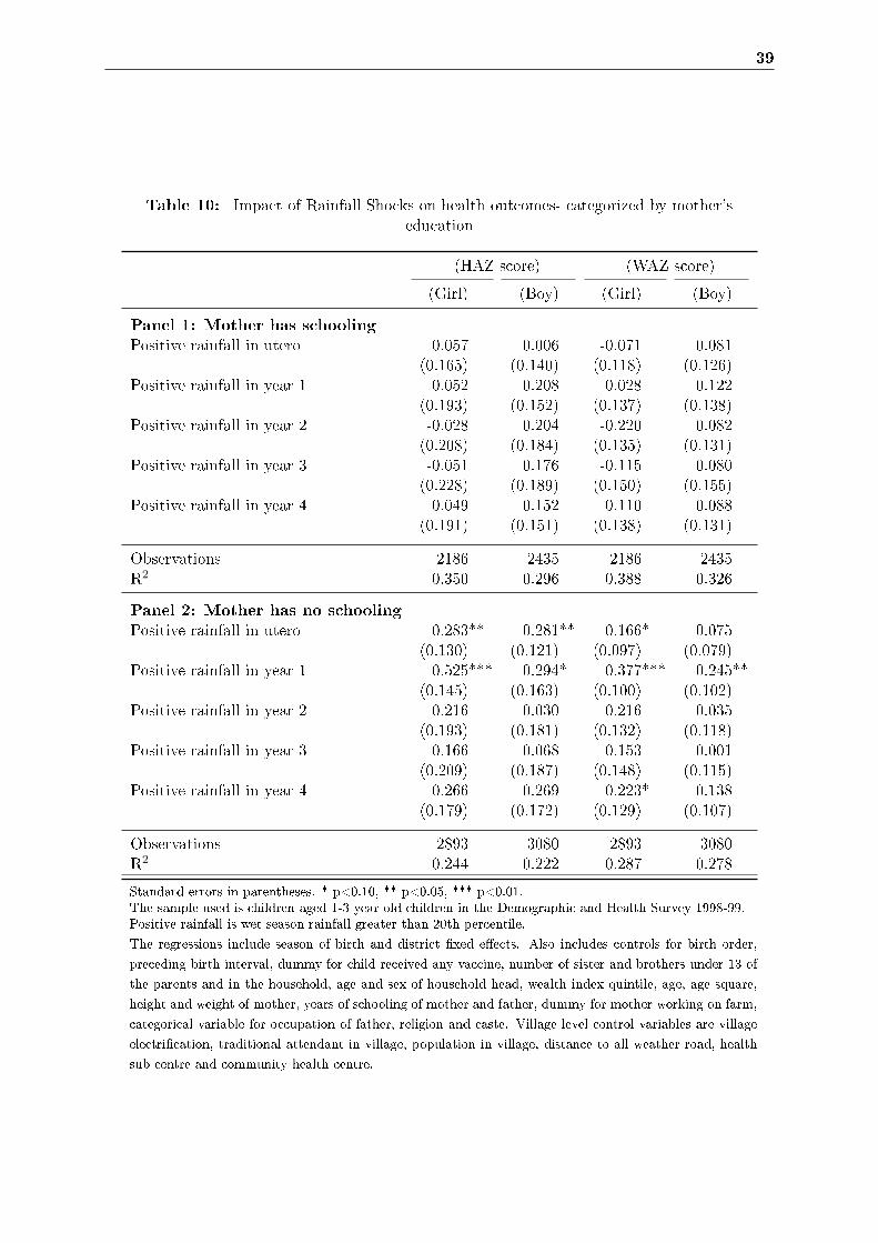
39

Table 10: Impact of Rainfall Shocks on health outcomes- categorized by mother'seducation

(HAZ score) (WAZ score)

(Girl) (Boy) (Girl) (Boy)

Panel 1: Mother has schooling

Positive rainfall in utero 0.057 0.006 -0.071 0.081(0.165) (0.140) (0.118) (0.126)

Positive rainfall in year 1 0.052 0.208 0.028 0.122(0.193) (0.152) (0.137) (0.138)

Positive rainfall in year 2 -0.028 0.204 -0.220 0.082(0.208) (0.184) (0.135) (0.131)

Positive rainfall in year 3 -0.051 0.176 -0.115 0.080(0.228) (0.189) (0.150) (0.155)

Positive rainfall in year 4 0.049 0.152 0.110 0.088(0.191) (0.151) (0.138) (0.131)

Observations 2186 2435 2186 2435R2 0.350 0.296 0.388 0.326

Panel 2: Mother has no schooling

Positive rainfall in utero 0.283** 0.281** 0.166* 0.075(0.130) (0.121) (0.097) (0.079)

Positive rainfall in year 1 0.525*** 0.294* 0.377*** 0.245**(0.145) (0.163) (0.100) (0.102)

Positive rainfall in year 2 0.216 0.030 0.216 0.035(0.193) (0.181) (0.132) (0.118)

Positive rainfall in year 3 0.166 0.068 0.153 -0.001(0.209) (0.187) (0.148) (0.115)

Positive rainfall in year 4 0.266 0.269 0.223* 0.138(0.179) (0.172) (0.129) (0.107)

Observations 2893 3080 2893 3080R2 0.244 0.222 0.287 0.278

Standard errors in parentheses. * p<0.10, ** p<0.05, *** p<0.01.The sample used is children aged 1-3 year old children in the Demographic and Health Survey 1998-99.Positive rainfall is wet season rainfall greater than 20th percentile.

The regressions include season of birth and district �xed e�ects. Also includes controls for birth order,

preceding birth interval, dummy for child received any vaccine, number of sister and brothers under 13 of

the parents and in the household, age and sex of household head, wealth index quintile, age, age square,

height and weight of mother, years of schooling of mother and father, dummy for mother working on farm,

categorical variable for occupation of father, religion and caste. Village level control variables are village

electri�cation, traditional attendant in village, population in village, distance to all weather road, health

sub centre and community health centre.

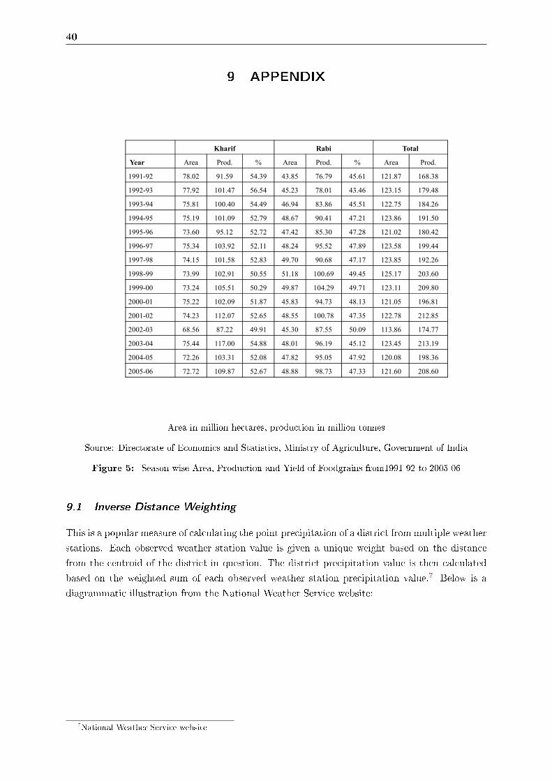
40

9 APPENDIX

Kharif Rabi Total

Year Area Prod. % Area Prod. % Area Prod.

1991-92 78.02 91.59 54.39 43.85 76.79 45.61 121.87 168.38

1992-93 77.92 101.47 56.54 45.23 78.01 43.46 123.15 179.48

1993-94 75.81 100.40 54.49 46.94 83.86 45.51 122.75 184.26

1994-95 75.19 101.09 52.79 48.67 90.41 47.21 123.86 191.50

1995-96 73.60 95.12 52.72 47.42 85.30 47.28 121.02 180.42

1996-97 75.34 103.92 52.11 48.24 95.52 47.89 123.58 199.44

1997-98 74.15 101.58 52.83 49.70 90.68 47.17 123.85 192.261997-98 74.15 101.58 52.83 49.70 90.68 47.17 123.85 192.26

1998-99 73.99 102.91 50.55 51.18 100.69 49.45 125.17 203.60

1999-00 73.24 105.51 50.29 49.87 104.29 49.71 123.11 209.80

2000-01 75.22 102.09 51.87 45.83 94.73 48.13 121.05 196.81

2001-02 74.23 112.07 52.65 48.55 100.78 47.35 122.78 212.85

2002-03 68.56 87.22 49.91 45.30 87.55 50.09 113.86 174.77

2003-04 75.44 117.00 54.88 48.01 96.19 45.12 123.45 213.19

2004-05 72.26 103.31 52.08 47.82 95.05 47.92 120.08 198.36

2005-06 72.72 109.87 52.67 48.88 98.73 47.33 121.60 208.60

Area in million hectares, production in million tonnes

Source: Directorate of Economics and Statistics, Ministry of Agriculture, Government of India

Figure 5: Season-wise Area, Production and Yield of Foodgrains from1991-92 to 2005-06

9.1 Inverse Distance Weighting

This is a popular measure of calculating the point precipitation of a district from multiple weather

stations. Each observed weather station value is given a unique weight based on the distance

from the centroid of the district in question. The district precipitation value is then calculated

based on the weighted sum of each observed weather station precipitation value.7 Below is a

diagrammatic illustration from the National Weather Service website:

7National Weather Service website

41

Source:(Dash, 2009), Figures presented for every thousand persons. N.S. = not speci�ed

Figure 6: Age and Sex distribution of malaria mortality in India in 1998

Figure 7: Evolution of child (0-4 years) sex ratio in India at the district level

42

9.2 Measure of rainfall shock

An additional measure of rainfall that we construct is continuous and captures the deviation of

rainfall in each wet season (and also separately dry season) around birth in the district in which

the child is born from the district's 40 year historical wet season (and dry season) mean excluding

the year in which the child is born, normalized in terms of standard deviation. The wet season

variable is graphed in Figure 8 by gender. It ranges from -1.41 to 6.55. The distribution shows

that the probability of being born in a district with negative (or positive) rainfall deviation is

the same for boys and girls. It also shows that there were no 'big' droughts during this time

period (in the districts that are covered by DHS 1998-99).

Figure 8: Distribution of deviation of wet season rainfall from historical mean, standardized

Another measure of rainfall that I use is categorical. I calculate for each district, the historical

mean (the 40 year wet season mean), historical mean minus one standard deviation, historical

mean plus one standard deviation. Then, I assigned rainfall shock to each child equal: 0 (negative

rainfall) if wet season rainfall around his/her birth is less than 'historical mean less 1 standard

deviation'; 1 (normal rainfall) if wet season rainfall around his/her birth lies between 'historical

mean less 1 standard deviation' and 'historical mean plus 1 standard deviation'; and 2 (positive

deviation) if wet season rainfall around his/her birth is greater than 'historical mean plus 1

standard deviation'.

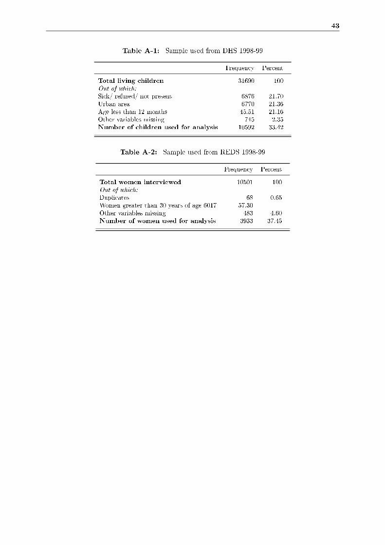
43

Table A-1: Sample used from DHS 1998-99

Frequency Percent

Total living children 31690 100Out of which:

Sick/ refused/ not present 6876 21.70Urban area 6770 21.36Age less than 12 months 45.51 21.16Other variables missing 745 2.35Number of children used for analysis 10592 33.42

Table A-2: Sample used from REDS 1998-99

Frequency Percent

Total women interviewed 10501 100Out of which:

Duplicates 68 0.65Women greater than 30 years of age 6017 57.30Other variables missing 483 4.60Number of women used for analysis 3933 37.45

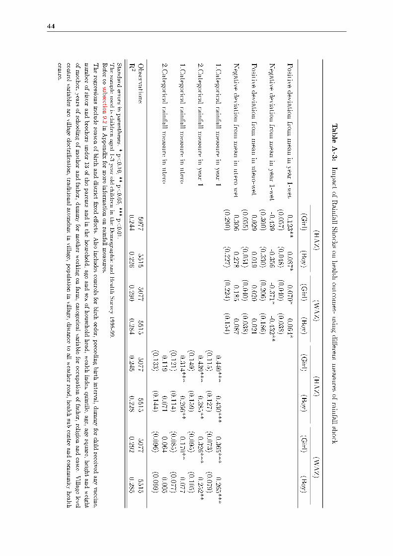
44

TableA-3:

Impact

ofRain

fallShockson

health

outcom

es-usin

gdi�eren

tmeasu

resof

rainfall

shock

(HAZ)

(WAZ)

(HAZ)

(WAZ)

(Girl)

(Boy)

(Girl)

(Boy)

(Girl)

(Boy)

(Girl)

(Boy)

Positive

deviation

frommean

inyear

1-wet

0.123**0.087*

0.070*0.064*

(0.057)(0.048)

(0.040)(0.038)

Negative

deviation

frommean

inyear

1-wet

-0.439-0.356

-0.371*-0.432**

(0.300)(0.330)

(0.206)(0.186)

Positive

deviation

frommean

inutero-w

et0.029

0.0190.020

0.021(0.055)

(0.051)(0.040)

(0.038)Negative

deviation

frommean

inutero-w

et-0.306

-0.278-0.185

-0.087(0.290)

(0.227)(0.224)

(0.154)1.C

ategoricalrain

fallmeasu

rein

year1

0.440***0.430***

0.365***0.265***

(0.115)(0.127)

(0.073)(0.079)

2.Categorical

rainfall

measu

rein

year1

0.439***0.385**

0.326***0.252**

(0.149)(0.159)

(0.095)(0.105)

1.Categorical

rainfall

measu

rein

utero

0.314***0.266**

0.170**0.077

(0.121)(0.114)

(0.085)(0.077)

2.Categorical

rainfall

measu

rein

utero

0.1190.071

0.0640.005

(0.133)(0.144)

(0.096)(0.099)

Observation

s5077

55155077

55155077

55155077

5515R

20.244

0.2260.290

0.2840.245

0.2280.292

0.285

Stan

dard

errorsin

parenth

eses.*p<0.10,

**p<0.05,

***p<0.01.

Thesam

pleused

ischild

renaged

1-3year

oldchild

renin

theDem

ographicandHealth

Survey

1998-99.Refer

tosubsection

9.2in

Appendix

formore

inform

ationon

rainfall

measu

res.

Theregression

sinclu

deseason

ofbirth

anddistrict

�xed

e�ects.

Also

inclu

des

controlsfor

birth

order,

preced

ingbirth

interval,dummyfor

child

receivedany

vaccine,

number

ofsister

andbroth

ersunder

13of

theparents

andin

thehouseh

old,age

andsex

ofhouseh

oldhead

,wealth

index

quintile,

age,age

square,

height

andweight

ofmoth

er,years

ofsch

oolingof

moth

erandfath

er,dummyfor

moth

erworkin

gon

farm,categorical

variablefor

occupation

offath

er,religion

andcaste.

Village

level

controlvariab

lesare

villageelectri�

cation,trad

itional

attendant

invillage,

population

invillage,

distan

ceto

allweath

erroad

,health

subcentre

andcom

munity

health

centre.

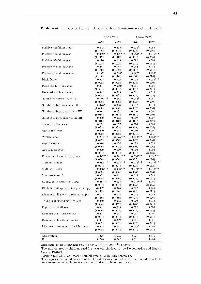
45

Table A-4: Impact of Rainfall Shocks on health outcomes- detailed result

(HAZ score) (WAZ score)

(Girl) (Boy) (Girl) (Boy)

Positive rainfall in utero 0.232** 0.205** 0.124* 0.086(0.105) (0.093) (0.074) (0.066)

Positive rainfall in year 1 0.369*** 0.317*** 0.283*** 0.215***(0.119) (0.113) (0.081) (0.080)

Positive rainfall in year 2 0.176 0.133 0.092 0.069(0.143) (0.122) (0.101) (0.081)

Positive rainfall in year 3 0.081 0.137 0.032 0.044(0.169) (0.132) (0.111) (0.091)

Positive rainfall in year 4 0.172 0.213* 0.172* 0.129*(0.138) (0.110) (0.100) (0.078)

Birth Order -0.005 -0.032 -0.038 -0.053***(0.028) (0.028) (0.024) (0.020)

Preceding birth interval 0.001 0.002* 0.001 0.001(0.001) (0.001) (0.001) (0.001)

Received vaccine dummy 0.022 0.083 0.031 0.044(0.094) (0.087) (0.058) (0.058)

Number of sisters under 13 -0.136*** 0.033 -0.062* 0.031(0.042) (0.036) (0.033) (0.029)

Number of brothers under 13 -0.076* -0.010 -0.017 0.016(0.040) (0.040) (0.032) (0.030)

Number of boys under 13 in HH 0.015 0.007 0.010 0.007(0.014) (0.014) (0.011) (0.009)

Number of girls under 13 in HH 0.000 -0.005 -0.009 -0.007(0.015) (0.013) (0.011) (0.009)

Sex of HH Head-male 0.151* -0.157 0.066 -0.006(0.083) (0.099) (0.069) (0.074)

Age of HH Head -0.000 -0.003 -0.000 0.001(0.002) (0.002) (0.001) (0.001)

Wealth Score 0.204*** 0.175*** 0.150*** 0.164***(0.047) (0.050) (0.042) (0.040)

Age of mother 0.014 0.024 0.002 0.032(0.040) (0.033) (0.030) (0.026)

Age of mother sq -0.000 -0.000 0.000 -0.000(0.001) (0.001) (0.001) (0.000)

Education of mother (in years) 0.022*** 0.041*** 0.024*** 0.031***(0.008) (0.008) (0.007) (0.006)

Mother's weight 0.012*** 0.015*** 0.032*** 0.030***(0.004) (0.004) (0.003) (0.003)

Mother's height 0.043*** 0.040*** 0.019*** 0.018***(0.005) (0.005) (0.004) (0.004)

Mom works on farm 0.021 -0.011 0.013 -0.044(0.065) (0.066) (0.048) (0.047)

Education of father (in years) 0.017** 0.004 0.014*** 0.005(0.007) (0.007) (0.005) (0.005)

Electri�ed village with irregular supply -0.092 0.046 0.082 0.105(0.113) (0.120) (0.092) (0.071)

Electri�ed village with regular supply -0.138 0.033 0.034 0.048(0.130) (0.116) (0.107) (0.076)

Traditional attendant in village 0.060 0.038 0.029 0.052(0.064) (0.057) (0.046) (0.041)

Population of village 0.001 -0.005 0.002 -0.005(0.006) (0.005) (0.005) (0.004)

Distance to all weather road 0.001 0.001 0.001 0.001(0.001) (0.001) (0.001) (0.001)

Distance to health sub centre -0.001 -0.002 0.001 -0.001(0.002) (0.002) (0.002) (0.001)

Distance to community health centre -0.002 -0.001 -0.002* -0.000(0.002) (0.001) (0.001) (0.001)

Observations 5077 5515 5077 5515R2 0.244 0.227 0.291 0.284

Standard errors in parentheses. * p<0.10, ** p<0.05, *** p<0.01.The sample used is children aged 1-3 year old children in the Demographic and HealthSurvey 1998-99.Positive rainfall is wet season rainfall greater than 20th percentile.The regressions include season of birth and district �xed e�ects. Also includes controlsfor categorical variable for occupation of father, religion and caste.

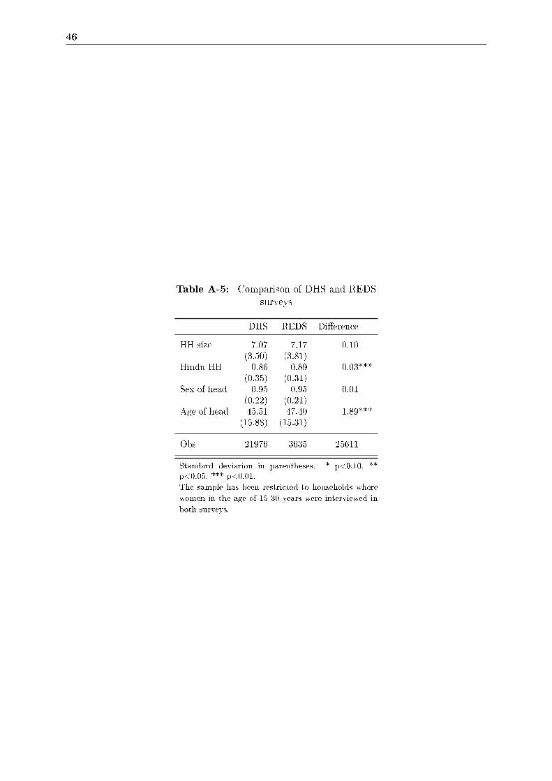
46

Table A-5: Comparison of DHS and REDSsurveys

DHS REDS Di�erence

HH size 7.07 7.17 0.10(3.50) (3.81)

Hindu HH 0.86 0.89 0.03***(0.35) (0.31)

Sex of head 0.95 0.95 0.01(0.22) (0.21)

Age of head 45.51 47.40 1.89***(15.88) (15.31)

Obs 21976 3635 25611

Standard deviation in parentheses. * p<0.10, **p<0.05, *** p<0.01.The sample has been restricted to households wherewomen in the age of 15-30 years were interviewed inboth surveys.

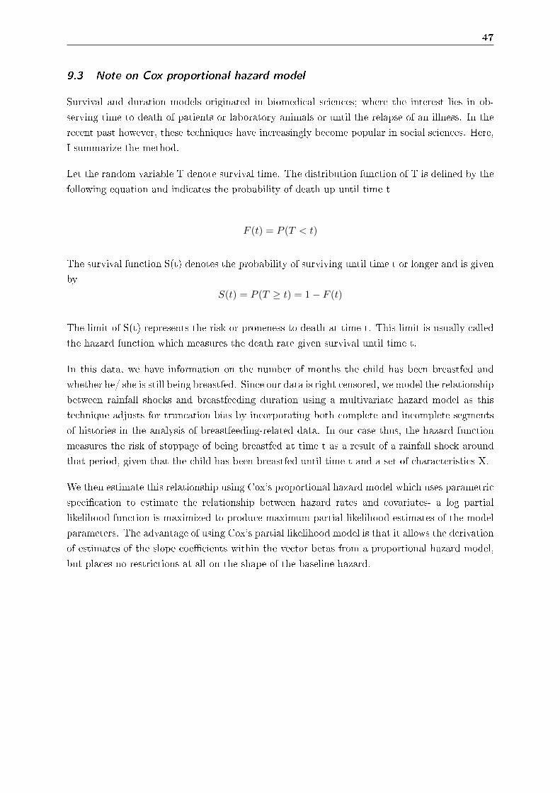
47

9.3 Note on Cox proportional hazard model

Survival and duration models originated in biomedical sciences; where the interest lies in ob-

serving time to death of patients or laboratory animals or until the relapse of an illness. In the

recent past however, these techniques have increasingly become popular in social sciences. Here,

I summarize the method.

Let the random variable T denote survival time. The distribution function of T is de�ned by the

following equation and indicates the probability of death up until time t

F (t) = P (T < t)

The survival function S(t) denotes the probability of surviving until time t or longer and is given

by

S(t) = P (T ≥ t) = 1− F (t)

The limit of S(t) represents the risk or proneness to death at time t. This limit is usually called

the hazard function which measures the death rate given survival until time t.

In this data, we have information on the number of months the child has been breastfed and

whether he/ she is still being breastfed. Since our data is right censored, we model the relationship

between rainfall shocks and breastfeeding duration using a multivariate hazard model as this

technique adjusts for truncation bias by incorporating both complete and incomplete segments

of histories in the analysis of breastfeeding-related data. In our case thus, the hazard function

measures the risk of stoppage of being breastfed at time t as a result of a rainfall shock around

that period, given that the child has been breastfed until time t and a set of characteristics X.

We then estimate this relationship using Cox's proportional hazard model which uses parametric

speci�cation to estimate the relationship between hazard rates and covariates- a log partial

likelihood function is maximized to produce maximum partial likelihood estimates of the model

parameters. The advantage of using Cox's partial likelihood model is that it allows the derivation

of estimates of the slope coe�cients within the vector betas from a proportional hazard model,

but places no restrictions at all on the shape of the baseline hazard.