I J A B E R, Vol. 11, No. 1, (2013): 99-113

* Assistant Professor, Department of Accounting and Finance, Prince Mohammad University,Al Khobar, Kingdom of Saudi Arabia, E-mail: hchowdh@yahoo.com

** Instructor, Department of Accounting and Finance, Prince Mohammad Bin Fahd University,E-mail: rsharmin@pmu.edu.sa

IMPACT OF MONETARY SHOCKS ON STOCK PRICESAND OTHER MACROECONOMIC VARIABLES:A Comparative Study on India and the U.S. Market

Shah Saeed Hassan Chowdhury* and Rashida Sharmin**

Abstract: This paper examines the response of stock prices and other macroeconomic variablesof the U.S. and India to monetary policy shocks. Comparison between the U.S. and Indiagives information on how effective respective central banks are to achieve stock market andother macroeconomic objectives. Results show that response of the U.S. variables is muchstronger than that of India, suggesting that central bank of the former is more efficient indriving economic activities through monetary policy actions. For the U.S., the relationshipbetween monetary shocks and stock prices is in line with the economic and finance theory.However, for India stock market does not always respond logically to policy shocks.

I. INTRODUCTION

Although money is thought to be neutral in the long run, it affects the output in theshort run. Thus, it is always interesting to know how the economy responds toexogenous monetary policy shock. However, the relationship between policy shocksand macroeconomic variables such as output, employment, and inflation is indirect.The immediate effect of policy shocks are observed in equity prices through changesin cost of capital and wealth effects, which may help policy makers to achieveultimate economic objectives (Bernanke and Kuttner, 2005). Thus, understandingthe relationship between monetary policy changes and stock price movement isimportant to know the policy transmission mechanism. In the context of a developedcountry such as the U.S. huge research has been conducted on this issue (Christianoet al., 1997; Christiano et al., 1998).

Economists and academicians have been in continuous search to improve theeconometric models to have a better knowledge about the monetary policy issues.However, over the years with various identification schemes there are someagreements as follows: after a contractionary monetary policy shock, short terminterest rates rise, aggregate output, employment, profits and various monetaryaggregates fall and price level responds very slowly (Christiano et al., 1998). On theother hand, relatively few investigations have been conducted to trace the effect ofmonetary shocks on the financial markets of developing countries. India, a fast

growing economy, is no exception in this regard. Reasons are probably the import-substitution policy adopted by India until 1980s and less autonomy of the centralbank in the determination of exchange rate and monetary policy interference beforeearly 1990s. Moreover, a longer data series is needed to come to a reasonableconclusion, which now India to some extent fulfills.

Stock price is the present value of all the future cash flows. The cash flowsdepend on firm-specific as well as market conditions. From the viewpoint of aportfolio manager the firm-specific risk can be diversified away in a large portfolioof many assets, but market risk cannot be eliminated. Market risk arises from themacroeconomic condition of the country concerned or even the world economicand political conditions. Thus any monetary shock is supposed to affect stock pricesthrough the output channel. In the past two decades, the importance of the stockmarket of an emerging country such asIndia has increased many folds. The mainreason is the low correlation between stock returns of emerging markets and thatof developed markets. Portfolio managers have the opportunity to diversify theportfolio even more efficiently in terms of risk-return trade-offs.

In this paper we investigate how monetary shocks may be related to stock marketin a high-performing emerging market such as India. In case of an organizeddeveloped economy like the U.S. stock price may even work as an indicator for thefuture growth of the economy (for example, Schwert, 1989). Schwert (1990) pointsout that a change in discount rate may affect stock price and investment in thesimilar fashion, but the change in output appears with a delay. Moreover, stockprice changes indicate wealth changes, which affect consumption and investment.Since Indian stock market is believed to be as one of the emerging stock markets inthe world, it may not be capable of predicting the future real activity of the economy.In this study, thus, we have assumed that the stock price is the contemporaneousoutcome of all the effects of the policy and macroeconomic performances.

Lastrapes (1998) finds that expansionary money supply shocks raise real stockprices and lower interest in short run and money supply shocks explain one-thirdof the variation in real stock prices in the short run. Patelis (1997), Thorbecke (1997),and Neri (2004), among many others, have also used VAR framework to study therelation between monetary policy and stock returns. All of these papers find thatstock returns respond negatively tocontractionary shocks of monetary policy, butsuch shocks can only explain a small portion of stock return variation. Rapach(2001) examines the effects of money supply, aggregate spending and aggregatesupply shocks on real U. S. stock prices in a structural VAR (Vector Autoregression)framework. Findings show that macroeconomic shocks affect stock prices andinterest rate has a negative relation with real stock returns. Barnanke and Kuttner(2005) also use structural VAR model to investigate the reaction of stock prices withregard to innovations in monetary policy and find that an unanticipated 25 basis-point cut in Federal funds rate results in one per cent increase in broad stock indexes.

Zeng (2010) uses event study method to find that a 25-basis-point rate cutsurprise results in 0.62 per cent to 0.70 per cent increase in the Australian stockmarket index.Bredinand Hyde (2007) and Gregoriou and Kontonikas (2009) alsofind that U. K. stock market reacts significantly to any surprise in monetary policychanges. Thorbecke (1997) and Ehrmann and Fratzscher (2004) also find similarresults with respect to domestic monetary shock. Laeven and Tong (2012) documentthat global stock prices go up after unexpected U.S. monetary loosening and godown after unexpected U.S. monetary tightening.

Maysami and Koh (2000) report that a positive relationship between innovationin money supply and stock returns in Singapore. Wongbangpo and Sharma (2002)examine the relationship between stock prices and selected macroeconomic factorsin five ASEAN countries. Their results show that stock prices are positively relatedto output in the long run. Moreover, in the short-run, stock prices are related topast and current values of macroeconomic variables. Bhattacharyya and Sensarma(2008) report that the impact of monetary policy shock on Indian stock market isnegligible during the 1996-2006 period, which is in fact a by-product of their researchon effect of monetary shocks to the economy. Hosseini et al. (2011) suggest thatthere are both short and long run linkages between macroeconomic variables andstock market index for India and China.

The objective of this paper is to examine the impact of monetary shocks (T-billshocks in the absence of monthly data of policy instrument such as Federal fundrate) onother macroeconomic variables and the prices of India and that of the U.S.stocks. Then the impact can be analyzed from the viewpoint of developed andemerging markets. As a corollary, the monetary impact on macroeconomic variables,both contemporaneous and lagged, are examined and compared. Macroeconomicvariables used in this study are industrial production, money supply (M1), consumerprice index, and 91-day T-bill rates (Federal fund rate for the U.S.). All these variablesare considered in a structural VAR framework. Appropriate restrictions are imposedto explore the likely contemporaneous and lagged relation among stock returnsand macroeconomic policy shocks.

Two types of identification schemes are used. In the first type, restrictions areimposed such that stock price acts as the outcome of all the contemporaneousrelation with other variables. In this setting, results show how long the impactstays in the stock prices after an innovation occurs. In an efficient market, stockprices must adjust tonew information very quickly. For example, the market iscomprised of huge number of analysts who should contribute to help adjust themacroeconomic information into the stock prices promptly. Violation of this meansopportunity for abnormal profit for some investors. In the second set up, the stockprice reacts to all the macroeconomic variables contemporaneously, but T-bill/fundrate is not influencing other variablesnow, rather T-bill/fund rate is reacting to thestate of the economy. Consequently, the T-bill/fund rate influences the output,

consumer price, commodity price and exchange rate next period. Similaridentification scheme is used in Christianno et al. (1998).

The paper is organized as follows. Following section gives a very brief reviewof the changes that occurred in India since early 1990s. Section III gives detailsabout the sources of data and the necessary transformation or modification of data.This section also provides how required restrictions are imposed in this study.Section IV explains the empirical results. Section V provides concluding remarks.

II. INDIAN ECONOMY AND CAPITAL MARKET SINCE EARLY 1990s

In the early 1990s, Indian economic policy suffered a serious balance of paymentcrisis. This resulted in a series of economic policy reforms. Subsequently, Indiangovernment introduced economic reforms in foreign exchange management,industrial policies, fiscal policies, monetary policies and international trade policies.Private sector and market were expected to play stronger role in the allocation ofresources.

In 1990s, India was one of the top 10 countries in the world in terms of averagegrowth of GDP (Bhide, 2001). The higher growth rate was a source of risk due tomore exposure to both domestic and international monetary shocks. The sourcesof domestic shock were various state subsidies, support to non-performinggovernment enterprises, etc. Some of the important international shocks were debt-servicing of foreign loans, exchange rate fluctuations, inflow and outflow of foreigninvestments, confidence of foreign investors, etc. The main concern of India in the1990s was to continue high growth and increase domestic income (in order to reducefiscal deficit). Government also reduced taxes to achieve the target. The initiativeto reduce external exposure started with the withdrawal of governmentalintervention in foreign exchange market. Thus, Reserve Bank of India (RBI), thecentral bank of India started giving only indicative rates to the market andallowedmarket forces to determine exchange rates (Bhide, 2001). As a part ofencouraging foreign investment, tariff and non-tariff trade barriers were reduced bydecreasing duties and relaxing many key import restrictions. Capital markets relaxedcontrol on prices. Industrial policy changes permitted easy licensing, more foreigncollaboration, import of machinery, and less bureaucracy. Monetary policy alsochanged to cope with other changes. There were substantial reforms in the bankingsector. Statutory reserves were reduced. The monetary authorities started using openmarket operations to control money supply of the economy to a greater extent.

During 2000-2005, market capitalization to GDP ratio skyrocketed to 77 percent, a strong indication of the trend in the foreign capital inflows and growth inthe capital market (Purfield et al., 2006). Foreign investors held about 10 per cent ofGDP in equity assets. The participation of domestic institutional investors grewsignificantly during the time. Insurance, pension and mutual funds’ assetsamounted to almost 15 per cent of GDP, with significant investment in stock market

(Purfield, 2007). The SENSEX increased at an annual compound rate of 17 per centduring the period 2003-2005. The inflow of foreign capital was approximately $26billion. This phenomenon was probably the outcome of prevailing low interestrates in the U.S. and growing attraction of Indian stock market. Market was relativelystable as India was able to nicely handle situation like Asian financial crisis. Suchevents boosted the confidence of both domestic and foreign investors, which couldbe illustrated by the Price-Earnings ratio of more than 20 (Purfield, 2007).

The year 2006 alone saw about 31 per cent growth in initial public offering. TheBSE SENSEX jumped from 8,929 in 2006 to 14,724 in February 2007. Obviously itraised questions whether or not the price could be supported by the fundamentalsof the economy.Over optimism sometimes gripped the stock market, whichwaspotentially very harmful for general investors since eventually the bubble mustbust. A good example could be the economic turmoil Malaysia faced when theAsian financial crises broke out in the region after initial high optimism. In thisbackdrop, this paper may give some idea about how the stock prices react to themonetary policy shocks. A weak relationship would mean the possible detachmentof financial market from the economy and inability of the stock market to act as avehicle for economic growth – a serious concern for the policy makers.

III. DATA AND METHODOLOGY

Monthly data for the period February 1993 through December 2006 have been usedfor India. The U.S. data covers the period January 1959 through September 2007.Industrial production, consumer price index (CPI), money supply (M1), stockindexes, and exchange rates(Rupee to U.S. dollar) are collected from theInternational Financial Statistics (IFS) published by the International Monetary Fund(IMF).1 91-day T-bill rates are collected from RBI.2 All the data except T-bills andfund rates are used in natural log form. T-bill and fund rates are used as short terminterest rate for India and U.S., respectively. Commodity price index is constructedfrom equally weighted food, beverage, agricultural raw material, metal, and oilprice indices.3 All the variables are set up in a VAR framework. We have used 14lags for the U.S. model. Due to smaller dataset, India has only 4 lags.4

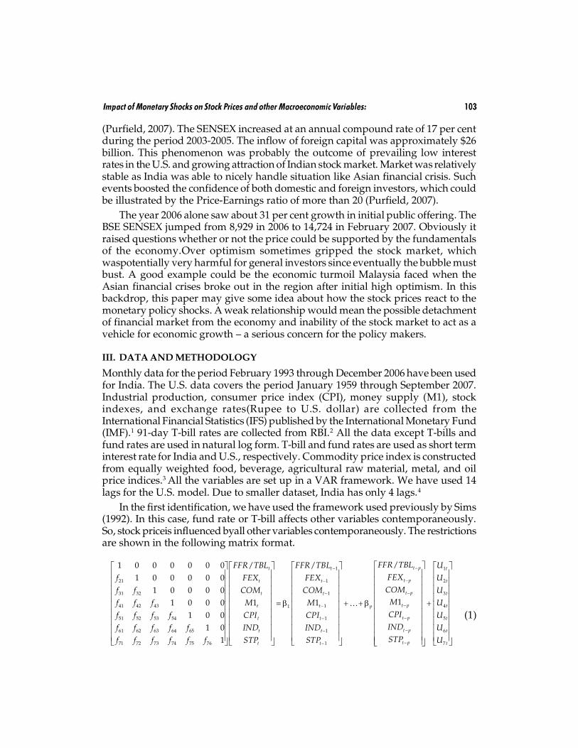
In the first identification, we have used the framework used previously by Sims(1992). In this case, fund rate or T-bill affects other variables contemporaneously.So, stock priceis influenced byall other variables contemporaneously. The restrictionsare shown in the following matrix format.

1

21 1

31 32 1

41 42 43 11

51 52 53 54

61 62 63 64 65

71 72 73 74 75 76

1 0 0 0 0 0 0 / /1 0 0 0 0 0

1 0 0 0 01 0 0 0 1 1

1 0 01 0

1

t t

t t

t t

t t

t t

t

t

FFR TBL FFR TBLf FEX FEXf f COM COMf f f M Mf f f f CPI CPIf f f f f INDf f f f f f STP

�

�

�

�

� � � �� � � �� � � �� � � �� � � � � �� � � �� � � �� � � �� � � �� � � �� � � �

1

2

3

4

1 5

1 6

1 7

/

1

t p t

t p t

t p t

t p tp

t p t

t pt t

t pt t

FFR TBL UFEX UCOM U

M UCPI UINDIND USTPSTP U

�

�

�

�

��

��

��

� �� � � �� �� � � �� �� � � �� �� � � �� �� � � �� � � �� �� � � �� �� � � �� �� � � �� �� � � �� �� � � �� �� � � �� �

�

(1)

where FFR or TBL is federal fund rate or 91-day T-bill rate, FEX isforeign exchangerate, CPI isconsumer price index, M1 is money supply, IND is industrial production,COM is commodity price index and STP is stock price.

In the second setting, the VAR model used by Christiano et al. (1998) isconsidered.5 As they did, we estimate this model where T-bill/fund rate is used asa policy instrument and in addition we have included stock price.Therefore, T-bill/fund rate is used here to be influenced by contemporaneous events in industrialproduction and price indices. Thus, this identification scheme is a closeapproximation to the benchmark identification scheme used by Christiano et al.(1998). In this setting, we hypothesize that output affects other variables includingstock prices contemporaneously. The setup for this model is

1

21 1

31 32 1

41 42 43 11

51 52 53 54 1

61 62 63 64 65 1

71 72 73 74 75 76

1 0 0 0 0 0 01 0 0 0 0 0

1 0 0 0 01 0 0 0

1 0 01 0 1 1

1

t t

t t

t t

t t

t t

t t

t

IND INDf CPI CPIf f COM COMf f f FEX FEXf f f f TBL TBLf f f f f M Mf f f f f f STP

�

�

�

�

�

�

� � � �� � � �� � � �� � � �� � � � � �� � � �� � � �� � � �� � � �� � � �� � � �

1

2

3

4

5

6

1 7

1

t p t

t p t

t p t

t p tp

t p t

t p t

t pt t

IND UCPI U

COM UFEX UTBL UM USTPSTP U

�

�

�

�

�

�

��

� �� � � �� �� � � �� �� � � �� �� � � �� �� � � �� � � �� �� � � �� �� � � �� �� � � �� �� � � �� �� � � �� �� � � �� �

�

(2)

Finally, for India and the U. S. we have used GARCH(1,1)-AR(1) model togenerate the conditional volatility series for all the variables.6 Then these volatilityseries are considered in a VAR framework. Only Sims’ identification scheme isused. This provides us the information about how T-bill/fund rate volatilityinnovations affect stock prices and other macro variables’ volatility.

IV. EMPIRICAL RESULTS

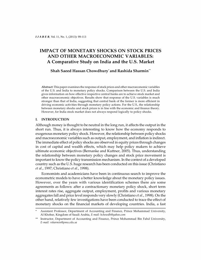
Figure 1 presents the impulse response function (IRF) derived from model (1) whichis similar to Sims (1992). The only difference is that the data are extended to 2007:09and a new variable, the log of stock price is included in the model.The IRF of thispaper and that of Sims’ study are not that much different. Only the responses of allthe variables with respect to the impulses to the Federal fund rate (or Treasury billrate) are reported. The fund rateinnovation affects all other variablescontemporaneously. Only the effect of exchange rate from fund rate shock seemsto be different. We find a negative impact on exchange rate that lasts from monthsix through month 48. In his study, Sims explains the positive effect as exchangerate appreciation. We calculate exchange rate as the US$ to SDR ratio.7 Thus thedecrease in the ratio means the appreciation in US$ and therefore our result is notdifferent from Sims’. The result is also supported by theory since monetary policycontraction should raise the value of the domestic currency.

Although not reported in the paper, interestingly like Sims we find a positiveshock to money creates negative impact on industrial production. However, it isplausible that policy makers may feel the forthcoming inflationary pressure andtake policy for contraction. Price may rise after contraction and the output may falldue to contraction of nominal demand and output.8 The interest rate innovationcauses stock prices to go down. Obviously as interest causes a positive innovation,the cost of capital or expected return goes up. Since the stock price is the presentvalue of all the future cash flows (or dividends), stock price consequently goesdown. It takes more than 30 months to absorb this shock.9 This result is alsosupported by the fact that industrial production decreases after a positive shock tointerest rates.

Identification as suggested by Christianno et al. (1998) is also used, but theresults do not change much. Sims (1992) also admits that correlationsamong

Figure 1: Impulse Response Function with respect to One Unit of Monetary Shock (U.S.)

Shock 1 represents innovation in fund rate

variables are so low that different identification schemes under structural VARframework do not give different results. This is probably a peculiarity when monthlymacroeconomic data are used. Therefore, we do not report the results from theVAR identification of Christianno et al. (1998).

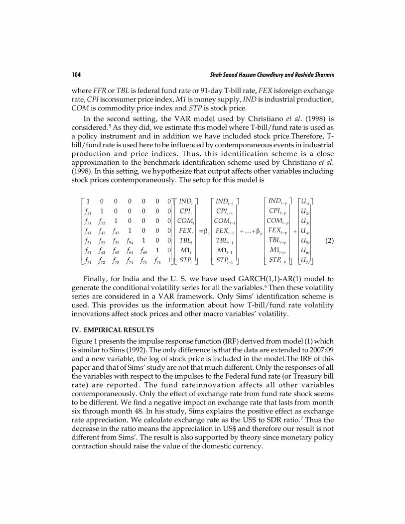
Figure 2 presents the responses of all the variables of India to one standarddeviation innovation in T-bill rate (contemporaneously) and stock prices (with one-month lag). Individual responses suggest weak relationship between monetaryinstrument and macroeconomic variables. The effect on output is positive for thefirst 17 months and then it tends to be negative. This contrasts sharply with theresults for the U. S. economy. The reason for such surprising result could be thatthe economies of developing countries are relatively more segregated from rest ofthe world and that the macroeconomic variables are less logically interlinked(partially due to less autonomy and expertise of central bank to take effective andtimely monetary decisions).

Figure 2: Impulse Response Function with Respect to One Unit of Monetary Shock (India)

Shock 1 represents innovation in T-bill rate

Innovations in T-bill rates cause negative response in stock price, which satisfiesthe notion that risk-free rate plays an important role in determining the risk-adjusteddiscount rate for the estimation of stock prices. However, the impact of interestrate on the Indian stock prices appears to be weaker than that on the U.S. stockprices. The effect on exchange rate is initially negative. For India, the exchange rateis defined as Rupee/Dollar, which means negative response stands for appreciationof Rupee against dollar. Thus, this result is also in line with the result for the U.S.However, Rupee starts depreciating against dollar after approximately sevenmonths.

The response of money supply is initially positive and then becomes negativeafter six months. For the U.S., this response is much larger compared to India.Although slightly, money supply initially increases. This result clearly shows howeffective interest rate is to control money supply in the U.S. compared to India.Therefore, there is a kind of inertia in Indian economy for the response of moneysupply to take place. Same thing happens for response of industrial production to

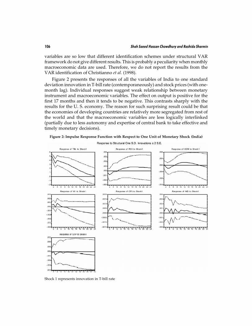
Figure 3: Impulse Response Function for Conditional Volatility of Macro-variables withRespect to Innovation in Conditional Volatility of Monetary Shock (U.S.)

Shock 1 = Innovation in federal fund rate volatility

interest rate innovation. For India, output take like 18 months to become negativewhereas for the U.S. it takes about eight months. Moreover, for India the responseis smaller in magnitude.

Figure 3 provides impulse response of all the variables’ volatility to a one-standard deviation shock to fund rate volatility. Almost all the responses are positive.Thisis an expectedresult since fund rate volatility has information regarding futuremacroeconomic volatility. Any positive change in interest rate volatility might implyuncertain future and thus it should increase the macroeconomic and stock marketvolatility. The noteworthy finding is the positive response of stock price volatility.This means a shock to interest volatility increases stock price volatility, makingstocks more risky. Consequently, expected return should go up and the stock priceshould ultimately go down. This explanation is also supported by the impulseresponse of figure 1.

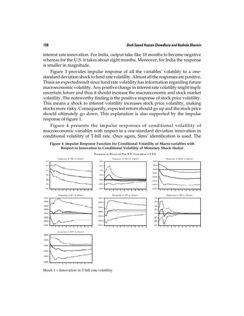
Figure 4 presents the impulse responses of conditional volatility ofmacroeconomic variables with respect to a one-standard deviation innovation inconditional volatility of T-bill rate. Once again, Sims’ identification is used. The

Figure 4: Impulse Response Function for Conditional Volatility of Macro-variables withRespect to Innovation in Conditional Volatility of Monetary Shock (India)

Shock 1 = Innovation in T-bill rate volatility

relationship between stock price volatility and T-bill rate volatility is as same asthat found in Figure 2. A shock to T-bill rate volatility also causes permanent shiftin response for price level volatility. A shock to T-bill volatility should cause positiveresponse for stock price volatility due to higher future uncertainty. In case of India,the response is surprisingly negative. This response indicates a persistent reductionof stock market volatility after interest rate volatility shock. Existing finance theorydoes not support this result. This finding is also just opposite of what is found forthe U.S stocks. This kind of mismatch is a source of under/over valuation of assetprices in markets such as India, suggesting possible scope for abnormal return.Shocks to T-bill volatility cause immediate large impact on foreign exchange ratevolatility and then adjusts very quickly. It probably indicates the rising importanceof trade in Indian economy in the past one and half decades. A Shock to T-billcauses positive responses (although small) for money supply volatility, but it diesout after about two years.

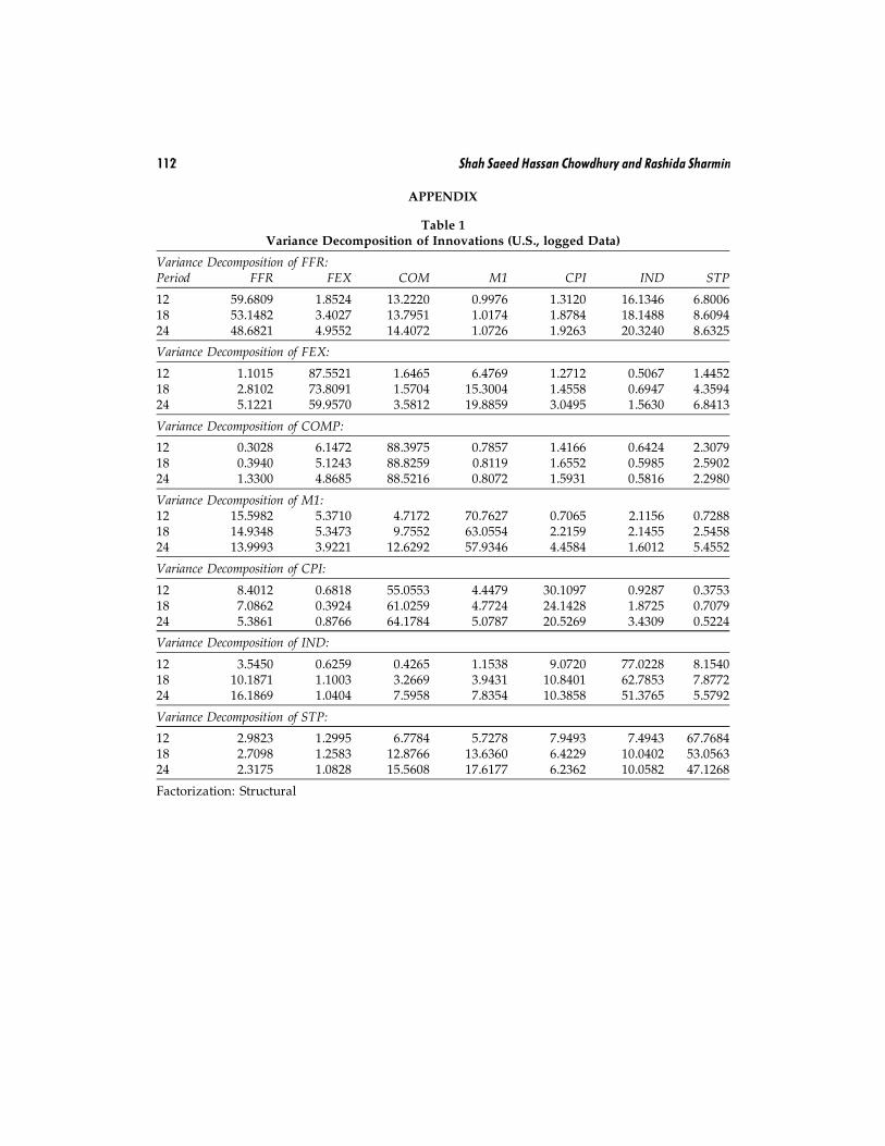
Table 1 of Appendix 1 provides the variance decomposition of each variable forthe U.S. It gives the proportion of the movements in the macroeconomic variablesand stock prices that are due to their own shocks, versus shocks to other variables.Thus it gives information about the relative importance of each shock to the variablesin the VAR. In case of U.S., commodity price, money supply, and industrialproduction account for most of the forecast error variance of stock prices at 24-stepahead.

Table 2 of Appendix 1 furnishes variance decomposition of each variable’sforecast error. Interestingly, for stock price, apart from itself, mostly variance iscaused by foreign exchange rate, money supply and CPI. Both for India and theU.S., a small portion of forecast error variance is explained by short term interestrate, whereas money supply appears to be an important factor. Probably, the effectof interest rate is taken away by the money supply, since both are very closelyrelated. Results also show that exchange rate is important for Indian stocks, whichsuggests the vulnerability of Indian firms to currency fluctuations.

V. CONCLUSION

We have used Sims’ (1992) identification scheme in a VAR framework to investigatethe effect of short term interest rate innovation on macroeconomic variables andstock price of India and the U.S. Moreover, we do the same type of investigationusing the conditional variance of interest rates for both the countries. Conditionalvariance series are created from a GARCH process.

Findings show that there are some similarities between the U.S. and Indianeconomy with respect to policy shocks. In most cases, responses of macroeconomicvariables are similar, but responses of India are smaller in magnitude. In case ofIndia, interest rate innovation results in depreciation of local currency, whichcontradicts exchange rate theory. However, the results for the U.S.satisfy the theory

in this regard. There are some dissimilarities when responses of stock prices aretaken into account. For both India and the U.S., the response of stock price is negativewith regard to an innovation to interest rate, which supports theory. But, whenconditional volatility series is used, interest rate volatility decreases Indian stockmarket volatility, which goes against the standard finance theory. However, for theU.S. market, both the volatilities are positively related. This finding probablyindicates that Indian stock market does not capture the economic shocks logically,thereby creating scopes for stock price valuation mismatch and resultantopportunity for abnormal return. Nonetheless, this finding is not unusual if weconsider the fact that Indian stock market has less liquidity, less number of analysts,relatively weak central bank and stock market regulatory body compared to theU.S. counterpart.

Notes1. Reason for choosing the data from 1993 is the fact that India started economic reform in 1991

and some elapse from that period is helpful for model estimation, analysis and inference. AlsoIndia started permitting rupee to float against other currencies since 1993. The exchange ratesare closely monitored by RBI, but there are no fixed target and fluctuation band.

2. T-bill is used for India due to few changes in the historical fund rates.

3. This index is created since IFS does not provide world price index for this long period. However,index for food, beverage, agricultural raw material, metal, and oil price indices are available.We construct the composite series by using equal weight for all the commodity prices.

4. For India lag length measures give conflicting results. Out of six measures in EVIEWS threesuggest up to lag length of four or less, other three suggest 12 or more.

5. Sims (1992) also finds same results when he uses almost same variables for five countries, namely,USA, France, UK, Japan and Germany.

6. GARCH stands for Generalized Autoregressive Conditional Heteroskedasticity.

7. SDR (Special Drawing Right) is issued by the IMF. Not a currency, SDRs instead represent aclaim to currency held by IMF member countries for which they may be exchanged. The valueof the SDR is determined by the value of several currencies important to the world’s tradingand financial systems.

8. Eichenbaum(1992) comments on the paper by Sims (1992) in the same journal and also supportsSims’ explanation.

9. Here we explain in terms of Capital Asset Pricing Model (CAPM). Even from the viewpoint ofAPT (Arbitrage Price Theory), we have same theoretical explanation. It is because both assetprice theories take into account risk premium for one additional unit of systematic risk.

ReferencesBhide, S. (2001), ”The Experience of India in Using Modeling for Macroeconomic Policy Analysis”.

Sub-regional Seminar on Macroeconomic Policy Analysis and Modeling in the Economies ofCentral Asia, Public Economic and Social Commission for Asia and the Pacific.

Bhattacharyya, I. and R. Sensarma (2008), “How Effective are Monetary Policy Signals in India:Evidence from A SVAR Model”, Working Paper, University of Hertfordshire, Available at https://uhra.herts.ac.uk/dspace/bitstream/2299/3463/1/902960.pdf.

Bernanke, B. S. and K. N. Kuttner (2005), “What Explains the Stock Market’s Reaction to FederalReserve Policy?” Journal of Finance, Vol. 60, pp. 1221–1257.

Bredin, D. and S. Hyde (2007), “UK Stock Returns and the Impact of Domestic Monetary PolicyShocks”, Journal of Business Finance and Accounting, Vol. 34, pp. 872–888.

Christiano, L. J., M. Eichenbaumand C. L. Evans (1997), “Sticky Price and Limited Participation Models:A Comparison”, European Economic Review, Vol. 41, pp. 1201–1249.

Christiano, L. J., M. Eichenbaumand C. L. Evans (1998), “Monetary Policy Shocks: What Have WeLearned and WhatEnd?”NBER Working Paper No. 6400.

Eichenbaum, M. (1992), “Comment on Interpreting the Macroeconomic Time SeriesFacts: The Effectsof Monetary Policy”, European Economic Review, Vol. 36, pp. 1001–1011.

Ehrmann, M. and M. Fratzscher (2004), “Taking Stock: Monetary Policy Transmission to EquityMarkets”, Journal of Money, Credit, and Banking, Vol. 36, pp. 719–737.

Gregoriou, A. and A. Kontonikas (2009), “Monetary Policy Shocks and Stock Returns: Evidence fromthe British Market”, Finance Market and Portfolio Management, Vol. 23, pp. 401–410.

Hosseini, S. M., Z. Ahmed and Y. W. Lai (2011), “The Role of Macroeconomic Variables on Stock MarketIndex in China and India”, International Journal of Economics and Finance, Vol. 3, pp. 233–243.

Laeven, L. and H. Tong (2012), “US Monetary Shocks and Global Stock Prices”, Journal of FinancialIntermediation, In press.

Lastrapes, W. D. (1998), “International Evidence on Equity Prices, Interest Rates and Money”,Journalof International Money and Finance, Vol. 17,pp. 377–406.

Neri, S. (2004), “Monetary Policy and Stock Prices”,Bank of Italy Working Paper No. 513.

Patelis, A. D. (1997), “Stock Return Predictability and the Role of Monetary Policy”,Journal of Finance,Vol. 52, pp. 1951–1972.

Purfield, C., H. Oura, C. Kramer and A. Jobst (2006), “Asia Equity Markets: Growth, Opportunitiesand Challenges”, IMF Working Paper06/266, Washington DC: IMF.

Purfield, C. (2007), “India: Asset Prices and Macroeconomy”,IMF Working PaperWP/07/221, WashingtonDC, International Monetary Fund.

Rapach, D. E. (2001), “Macro Shocks and Real Stock Prices”, Journal of Economics and Business, Vol. 53,pp. 5–26.

Schwert, W. G. (1989), “Why Does Stock Market Volatility Change over Time?” Journal of Finance, Vol.44, pp. 1115–1153.

Schwert, W. G. (1990), “Stock Returns and Real Activity: A Century of Evidence”, Journal of Finance,Vol. 45, pp. 1237–1257.

Sims, C. A. (1992), “Interpreting the Macroeconomic Time Series Facts: The Effects of Monetary Policy”,European Economic Review, Vol. 36, pp. 975–1011.

Thorbecke, W. (1997), “On Stock Market Returns and Monetary Policy”, Journal of Finance, Vol. 52, pp.635–654.

Wongbangpo, P. and S. C. Sharma (2002), “Stock Market and Macroeconomic Fundamental DynamicInteractions: ASEAN-5 Countries”, Journal of Asian Economics, Vol. 13, pp. 27–51.

Zeng, J. P. (2010), “Stock Market Reactions to Monetary Policy Shocks: Study in Australian Market”,Unpublished Masters Dissertation, Auckland University of Technology.

APPENDIX

Table 1Variance Decomposition of Innovations (U.S., logged Data)

Variance Decomposition of FFR:Period FFR FEX COM M1 CPI IND STP

12 59.6809 1.8524 13.2220 0.9976 1.3120 16.1346 6.800618 53.1482 3.4027 13.7951 1.0174 1.8784 18.1488 8.609424 48.6821 4.9552 14.4072 1.0726 1.9263 20.3240 8.6325

Variance Decomposition of FEX:

12 1.1015 87.5521 1.6465 6.4769 1.2712 0.5067 1.445218 2.8102 73.8091 1.5704 15.3004 1.4558 0.6947 4.359424 5.1221 59.9570 3.5812 19.8859 3.0495 1.5630 6.8413

Variance Decomposition of COMP:

12 0.3028 6.1472 88.3975 0.7857 1.4166 0.6424 2.307918 0.3940 5.1243 88.8259 0.8119 1.6552 0.5985 2.590224 1.3300 4.8685 88.5216 0.8072 1.5931 0.5816 2.2980

Variance Decomposition of M1:12 15.5982 5.3710 4.7172 70.7627 0.7065 2.1156 0.728818 14.9348 5.3473 9.7552 63.0554 2.2159 2.1455 2.545824 13.9993 3.9221 12.6292 57.9346 4.4584 1.6012 5.4552

Variance Decomposition of CPI:

12 8.4012 0.6818 55.0553 4.4479 30.1097 0.9287 0.375318 7.0862 0.3924 61.0259 4.7724 24.1428 1.8725 0.707924 5.3861 0.8766 64.1784 5.0787 20.5269 3.4309 0.5224

Variance Decomposition of IND:

12 3.5450 0.6259 0.4265 1.1538 9.0720 77.0228 8.154018 10.1871 1.1003 3.2669 3.9431 10.8401 62.7853 7.877224 16.1869 1.0404 7.5958 7.8354 10.3858 51.3765 5.5792

Variance Decomposition of STP:

12 2.9823 1.2995 6.7784 5.7278 7.9493 7.4943 67.768418 2.7098 1.2583 12.8766 13.6360 6.4229 10.0402 53.056324 2.3175 1.0828 15.5608 17.6177 6.2362 10.0582 47.1268

Factorization: Structural

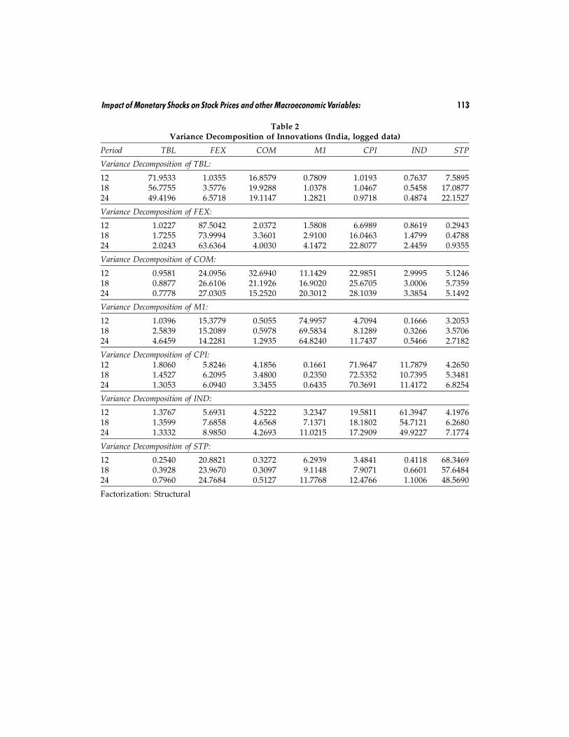
Table 2Variance Decomposition of Innovations (India, logged data)

Period TBL FEX COM M1 CPI IND STP

Variance Decomposition of TBL:

12 71.9533 1.0355 16.8579 0.7809 1.0193 0.7637 7.589518 56.7755 3.5776 19.9288 1.0378 1.0467 0.5458 17.087724 49.4196 6.5718 19.1147 1.2821 0.9718 0.4874 22.1527

Variance Decomposition of FEX:

12 1.0227 87.5042 2.0372 1.5808 6.6989 0.8619 0.294318 1.7255 73.9994 3.3601 2.9100 16.0463 1.4799 0.478824 2.0243 63.6364 4.0030 4.1472 22.8077 2.4459 0.9355

Variance Decomposition of COM:

12 0.9581 24.0956 32.6940 11.1429 22.9851 2.9995 5.124618 0.8877 26.6106 21.1926 16.9020 25.6705 3.0006 5.735924 0.7778 27.0305 15.2520 20.3012 28.1039 3.3854 5.1492

Variance Decomposition of M1:

12 1.0396 15.3779 0.5055 74.9957 4.7094 0.1666 3.205318 2.5839 15.2089 0.5978 69.5834 8.1289 0.3266 3.570624 4.6459 14.2281 1.2935 64.8240 11.7437 0.5466 2.7182

Variance Decomposition of CPI:12 1.8060 5.8246 4.1856 0.1661 71.9647 11.7879 4.265018 1.4527 6.2095 3.4800 0.2350 72.5352 10.7395 5.348124 1.3053 6.0940 3.3455 0.6435 70.3691 11.4172 6.8254

Variance Decomposition of IND:

12 1.3767 5.6931 4.5222 3.2347 19.5811 61.3947 4.197618 1.3599 7.6858 4.6568 7.1371 18.1802 54.7121 6.268024 1.3332 8.9850 4.2693 11.0215 17.2909 49.9227 7.1774

Variance Decomposition of STP:

12 0.2540 20.8821 0.3272 6.2939 3.4841 0.4118 68.346918 0.3928 23.9670 0.3097 9.1148 7.9071 0.6601 57.648424 0.7960 24.7684 0.5127 11.7768 12.4766 1.1006 48.5690

Factorization: Structural

�����������������������������������������������������������������������������������������������������������������������������������������������������������������������������������������������������������������