IMPACT OF LARGE-SCALE BIOFUELS PRODUCTION ON … · IMPACT OF LARGE-SCALE BIOFUELS PRODUCTION ON ... and Tyner is James and Lois Ackerman ... Impact of Large-Scale Biofuels Production

IMPACT OF LARGE-SCALE BIOFUELS PRODUCTION ON

CROPLAND-PASTURE AND IDLE LANDS

Dileep K. Birur*, Thomas W. Hertel, and Wallace E. Tyner1

Paper prepared for the presentation at the Thirteenth Annual Conference on

Global Economic Analysis “Trade for Sustainable and Inclusive Growth and

Development”, Bangkok, Thailand, June 9-11, 2010.

1Birur is Senior Economist at RTI International, Research Triangle Park, NC; Hertel is Distinguished Professor and

Executive Director, and Tyner is James and Lois Ackerman Professor and Senior Policy Advisor, at the Center for

Global Trade Analysis, Department of Agricultural Economics, Purdue University, West Lafayette, IN.

*Corresponding author: Dileep K. Birur, 3040 Cornwallis Road, P.O. Box 12194, Research Triangle Park, NC

27709. Emails: [email protected]; [email protected].

https://www.gtap.agecon.purdue.edu/events/Conferences/2007/default.asp

https://www.gtap.agecon.purdue.edu/events/Conferences/2007/default.asp

mailto:[email protected]

mailto:[email protected]

Impact of Large-Scale Biofuels Production on Cropland-Pasture and Idle Lands

Abstract

An important criticism of the indirect land use change (ILUC) estimates of biofuels to

date is that they have not accounted for the presence of marginal lands such as cropland-pasture

and idle-lands. This paper offers a novel framework for analyzing the impact of biofuels

production on these marginal lands. The methodology includes the steps involved in identifying

and incorporating marginal land data such as area under cropland-pasture and idle lands such

as U.S. Federal Conservation Reserve Program (CRP) enrolled land into the database,

computing the associated land-rents which imply productivity of land, and specifying the

marginal lands in the land supply function in a computable general equilibrium model. Two

policy scenarios are examined in this study: 1) implementing U.S. and EU biofuel mandates for

2015 and 2) implementing the corn-ethanol only mandate by 2015 in the U.S. These policy

experiments also look at the potential implications of releasing or fixing the CRP land

enrollment by the USDA on global land-use and land-cover changes. The results revealed that

though accessibility of these marginal lands dampens large shifts in cropping patterns, the ILUC

emissions measured in terms of grams of CO2 equivalent per MJ of biofuel produced, were

significantly affected mainly due to increase in deforestation when the cropland-pasture is used

for cultivation of crops. Future research to more accurately characterize the productivity of

these marginal lands will be needed.

JEL Classification: C68, Q18, Q23, Q24, Q42, R14

Keywords: Biofuels, computable general equilibrium (CGE), Agro Ecological Zones (AEZs),

land use change, marginal lands, idle lands, cropland-pasture, conservation reserve program

(CRP).

Table of Contents

Page

1. Introduction ............................................................................................................. 1

2. Analytical Framework ............................................................................................ 2

2.1 Incorporating Marginal Land Data ................................................................... 4

2.2 Accessibility of CRP Lands in the U.S. ............................................................ 7

2.3 Computing Land Rents for Marginal Lands ..................................................... 9

2.4 Incorporating Marginal Land-use into Land Supply Function ....................... 12

2.5 Cropland-Pasture in the Production Structure ................................................ 14

3. Experimental Design ............................................................................................. 15

4. Results: Land Use and Land Cover Change ......................................................... 16

4.1 Interactions at AEZ Level ............................................................................... 16

4.2 Land Interaction in the Livestock Sector ........................................................ 20

4.3 Baseline Experiment ....................................................................................... 22

4.4 U.S. and EU Biofuel Mandates ....................................................................... 24

4.5 U.S. Corn Ethanol Only Mandate ................................................................... 28

4.6 Decomposition of Land Supply Response ...................................................... 31

4.7 Sensitivity of Land Supply Response ............................................................. 34

5. Results: Implications on Land Use Emissions ...................................................... 35

6. Conclusions ........................................................................................................... 41

References ......................................................................................................................... 43

Appendices ........................................................................................................................ 47

1

Impact of Large-Scale Biofuels Production on Cropland-Pasture and Idle Lands

1. Introduction

As biofuels emerge as one of the important alternate fuels of the 21st century, they also

necessitate huge demand for feedstocks putting added pressure on land use. The only possible

ways to meet both food and fuel demands are by intensifying agriculture on current croplands or

by expanding the cropland area (expansion at the extensive margin). Several studies have raised

concerns about environmental and social impacts of biofuel programs. Kelly (2007) estimated

that the increased biofuels production in the U.S. could lead to a shift in cropping patterns

towards corn, and it could bring marginal land prone to erosion, forest, pasture land etc. under

corn2. Since biofuels are generally pursued as cleaner fuels supporting climate change

mitigation, the land-based greenhouse gas (GHG) emissions resulting from production of biofuel

feedstocks is decisive, particularly if the growing demand for biofuel feedstock is met by

extensification. Biofuels produced by accessing the additional land covers such as forest and

pastureland which typically involves burning of above ground biomass and tilling the soil, result

in release of carbon in to the atmosphere. This emission is regarded as the indirect land use

change (ILUC) emission, and it has drawn vital attention lately. Indeed, this has been the most

controversial element of the U.S. Environmental Protection Agency (EPA) regulation. The ILUC

issue was a key bargaining chip in the recent climate change bill. Several proponents of first

generation biofuels argue that the science on measuring life cycle emissions of biofuels is

rudimentary and must be improved.

Since accounting for ILUC includes world-wide conversion of forest and grassland to

cropland in response to higher commodity prices, it has been strongly debated across the biofuel

industry and among researchers. The U.S. EPA estimated the GHG emissions from renewable

fuels using life-cycle analysis. The corn-ethanol produced at a typical natural gas dry mill plant

was found to reduce CO2 equivalent emissions by 16% over a 100 year time period, but the same

emission increased by 5% over a 30 year time period (USEPA, 2009). The key contributing

factor in these emissions is the magnitude of international (indirect) land use change resulting

from producing the renewable fuels. The recent adoption of the Low Carbon Fuel Standard

2For example, Kelly (2007) reports that California‟s state law stipulates to increase the share of alternative fuels

from the current 6% to 20% by 2020 and 30% by 2030. This might require cutting down distant forests to grow

biofuel feedstocks consequently exacerbating the global warming.

2

(LCFS) by the California Air Resource Board (CARB) requires that the transportation fuels

supplied to California market should meet at least 10% declining standard of carbon intensity3.

CARB‟s measure of carbon intensity for biofuels includes emissions from indirect land use

change and this is sufficient to rule out corn-ethanol as a low carbon fuel in California. CARB

requires that estimates of the world-wide conversion of forest and grassland to cropland in

response to higher commodity prices be included while assessing the carbon intensity of

biofuels.

Studies on land-use competition from production of biofuels‟ feedstock have also drawn

attention of using degraded / idle / marginal lands. Though these terms are often used

synonymously, we adopt the term marginal land, as a summary of all land which is not as

productive as the regular cropland, which may be due to soil topography, water scarcity, poor

management practices, etc. With the increasing national targets for biofuel production across the

world, several studies have emphasized the potential pressure on these marginal lands to grow

biofuel feedstocks (Dufey, 2007; Fargione et al., 2008; Kløverpris et al., 2008; Pagel 2008).

Since changing vegetation on these marginal lands influences the GHGs-flux, it is important to

understand the indirect impact of biofuels production on these lands. Keeping this in view, in

this study we identify and incorporate the potential marginal lands into the model and estimate

the global land-use and land-cover implications of biofuel expansion on the marginal lands.

2. Analytical Framework

In order to analyze the world-wide land-use implications of biofuels in the presence of

marginal lands, we utilize the GTAP-BIO developed by Birur et al. (2008). The land supply

framework in the GTAP-BIO model follows Lee et al. (2005), where the land endowment is

broken into 18 Agro-Ecological Zones (AEZ) so as to yield a more accurate representation of

sectoral competition for land. As offered by Hertel et al. (2009), a nested constant elasticity of

transformation (CET) function is adopted, in which land-owners maximize return to land by

allocating land in two tiers (Figure 1). The land supply function is nested in the value added nest

of the firms‟ production structure which follows constant elasticity of substitution (CES) form.

3 http://www.arb.ca.gov/fuels/lcfs/lcfs.htm

http://www.arb.ca.gov/fuels/lcfs/lcfs.htm

3

Figure 1. Land Supply in the GTAP-BIO Model.

In the first stage, the land-owner makes optimal allocation of a given parcel of land under

crops, pasture or commercial forest, while the choice of crops is made in the second stage (five

categories of crops: coarse grains, oilseeds, sugar-crops, other grains, and other agriculture). The

ease with which the land in a given AEZi is transformed across uses is governed by the elasticity

of transformation, which will be discussed in Section 4.1. One important observation to be made

here is that the only way any given crop can expand is by displacing other sectors. However, in

reality, a crop can expand to other lands, called marginal lands, depending on the biophysical

availability.

Literature survey indicates that studies on analyzing implications of marginal lands in a

general equilibrium framework are scarce. However, Gurgel et al. (2007) offer some novel

approaches of introducing land in a CGE framework. Those authors utilize MIT Emissions

Predictions and Policy Analysis (EPPA) model, a recursive-dynamic multi-sector CGE model

with 16 regions, and analyze the land use implications of producing cellulosic biofuels. Those

authors disaggregate the agricultural sector into crops, livestock, and forestry sub-sectors and

allow for conversion of land across five land types: cropland, pastureland, harvested forestland,

natural grassland, and natural forestland. Those authors deviate from the CET approach since it

Land-AEZi

Cropland Pasture cover

Forest cover

1 = -0.20

2 =-0.5

Coarse grains

Oilseeds

Sugar-crops Other grains

Other agri

Cropland-pasture

CRP-land

4

is share preserving in nature and not appropriate for longer term analysis, and introduce a cost of

conversion approach. The advantage of this approach is that, the model keeps track of conversion

costs and value of the timber stock resulting from conversion. However, Gurgel et al. treat land

as one endowment without accounting for any heterogeneity such as AEZ classification. Though

the dynamic approach of the model is useful for longer term projections, the model is not

suitable for short or medium term analysis and also cannot track location of land use change

within a given region.

Van Meijl et al. (2006) and Eickhout et al. (2008) have introduced a framework that

combines an economic model (LEITAP) and a biophysical model (IMAGE) for estimating the

productivity of marginal lands. The IMAGE model calculates the productivity of seven food

crops at 0.5o grid level. The overall productivity is expressed on a scale of 0 to 1 on the basis of

potential crop productivity. When the grid cells are ordered from low to high productivity in

each region, we can get a land productivity curve. The inverse of the land productivity curve

determines the land supply curve for that region. Those authors introduce these land supply

curves with the assumption that most productive land is used first in production. If the gap

between agricultural land that is potentially available and land actually used in agriculture sector

is large any increase in demand for land would lead to a modest increase in price (as the land

conversion is easy at this stage). However, if the land in use is close to the total potentially

available land, any increase in demand will lead to greater increase in land rent and also land

conversion becomes difficult. The authors then use this land rent data for econometrically

estimating the parameters of the land supply curves required by the LEITAP model. This

approach takes into account detailed biophysical information, but does not allow for explicit

competition for land at the AEZ level. Therefore, we follow an alternative approach of finding

the additional categories of cropland that is idle in reality and may be brought under cultivation.

This approach permits us to retain the fixed land endowment.

2.1 Incorporating Marginal Land Data

As more attention is being paid on the potential use of marginal lands, equally

challenging for researchers is to identify and access this land. For instance, in the U.S., the

marginal lands that can be brought under cultivation of food/feedstock crops are cropland-

pasture (pasture-crop), idle cropland, rangeland, uncultivated horticultural areas, etc. Lubowski

5

et al. (2006) report a snapshot at land-use changes between 1982 and 1997, and found that most

of the changes from cultivation to uncultivation and vice versa were registered in cropland-

pasture and Federal Conservation Reserve Program (CRP) lands. Therefore, we choose to

include (a) cropland pasture and (b) Idle croplands in our land supply function. As Lubowski et

al. define; “idle croplands” in the U.S. include land cover under soil-conserving uses and

cropland enrolled in the Federal CRP and Wetland Reserve Program (WRP). In contrast,

“cropland-pasture” unlike permanent grassland pastures, is considered to be in long-term crop

rotation which is marginal for crop uses. Since data on these idle-land and cropland-pasture data

are not available at the AEZ level, we obtained the county/regional level data for the U.S. and

Brazil from several sources such as University of Tennessee, Oak Ridge National Laboratory, etc

(Table 1). These regional data were approximately mapped to the AEZ level, and we modified

the land cover data to account for these missing categories of land.

In this study we pay special attention to marginal lands in the U.S. and Brazil, as both are

leading producers of biofuels with vast implications on land-use and land-cover change. By

using historical land-use data, satellite imaging, and ecosystem models, Campbell et al. (2008)

estimated the global extent of abandoned cropland and pastureland that can be used to grow

biofuel feedstock crops. Their study revealed that, at the national scale, the U.S., Brazil and

Australia have the largest area of abandoned crop and pasture lands, which offer immense

potential for biofuel crops. Also, as evident from Table 1, both U.S. and Brazil possess

substantial areas of marginal lands that may be brought under cultivation of biofuel feedstock

crops. In the U.S., total cropland includes three broad categories: cropland used for crops (this

includes harvested cropland, crop failure, and summer fallow), idle cropland, and cropland

pasture (Figure 2). As seen from Table 1, about 40 million acres of idle land (CRP + other idle

lands) and 62 million acres of cropland-pasture in the U.S. has been brought into the data base.

In the case of Brazil, cropland-pasture area of about 58 million acres was incorporated

into the data base. For all other regions in the world, based on the estimates of previous studies,

we assume a region-specific range of 1 to 10% of pastureland area as the acreage under

cultivated cropland-pasture. The Food and Agricultural Organization of the United Nations

estimates that the global area of pasture-cover and fodder/pasture-crops together is about 8.6

billion acres in 2000, which is about 27% of total land area (FAO, 2008).

6

Table 1. Land Cover data with New Categories of Land in the U.S. and Brazil.

(million acres)

Land Cover Type

USA Brazil

SAGE NASS,

ERS/USDA Modified SAGE ORNL Modified

Crop-cover 454 442 454 127 124 124

Forest-cover 835 651 835 389 - 389

Pasture-cover 573 587 573 447 378 378

Unmanaged land 276 228 276 401 - 401

Total 2137 1908 2137 1365 1293

Harvested Area 326 340 326 120 - 120

Cropland-pasture

(U of T) 56 62 62 - 58 58

CRP+ Land (U of T) 28 40 40 - - -

Total 410 442 428 120 168

Note: For modifying land cover data, CRP+ lands, cropland-pasture data were obtained from various sources:

SAGE: Center for Sustainability and the Global Environment, University of Wisconsin-Madison, contributes

to the GTAP land-use data base at the global level.

ORNL: Pasture-crop data for Brazil was provided by the Oak Ridge National Laboratory, TN.

U of T: University of Tennessee, Knoxville, provided U.S. country level data on idle lands and pasture-crop

area, which was used for mapping at the AEZ level.

U.S. land cover data from SAGE is compared with the data reported by NASS, ERS-USDA.

0

50

100

150

200

250

300

350

400

450

500

1949 1954 1959 1964 1969 1974 1978 1982 1987 1992 1997 2002

(mill

ion

acre

s)

Data Source: Lubowski et al. (2006).

Figure 2. Major uses of Cropland in the U.S. (million acres)

62 m. acres

40 m. acres

340 m. acres

Harvested cropland

Crop failure

Summer fallow

Idle cropland

Cropland pasture

Total cropland Total cropland used for crops

7

In this study, we make a distinction between pasture-cover and cropland-pasture (area under

fodder-crops). Based on the FAO (2008) data on harvested area of fodder crops, we assume

about 10% of pasture-cover as area under cropland-pasture in Canada and Europe, 6% in Latin

American countries excluding Brazil, 1 to 3% in Asian countries, and 1% or less for African

countries.

A thirty-year trend analysis of the cropland-pasture area from 1980 through 2000 by FAO

(2008) indicates that the cropland-pasture acreage in South America has decreased by half

between 1980 and 2000, partially due to an increase in soybean area. The Eastern Africa region

also experienced a major decline in pasture area, due to large scale conversion in to agricultural

land. However area under cropland-pasture has slightly increased in Europe over the same time

period, because of its “set-aside” policy measure which, in the past required farmers to keep a

certain fraction of their land (about 10%) under fallow in return for receiving direct payments.

Alternatively, farmers could cultivate non-food crops such as pasture-crops on the set-aside land

under a “non-food on set-aside” regime. Keeping these findings in view, incorporating cropland-

pasture area for all the regions strengthens the analysis of this study.

2.2 Accessibility of CRP Lands in the U.S.

Though the CRP was originally was designed to reduce soil erosion and commodity

surpluses (Osborn, 1993), it has subsequently resulted in other environmental benefits such as

preserving wildlife habitat, water quality, soil carbon sequestration, etc (Best et al. 1997;

Sullivan et al. 2004). CRP rewards farmers with annual rental payments and cost-share

assistance. The data that we have utilized in this study pertains to the agricultural year 2000. Of

the 455 million acres of farm land in the United States, the CRP enrollment across 3144 counties

in the U.S. was about 34 million acres (7.5% of cropland). The county-wise distribution of CRP-

acreage is shown in Figure 3. After mapping the county-level data into AEZ level, the crops

compete directly for acreage in CRP land in a given AEZ.

The U.S. Department of Agriculture has a budget estimate of $1.8 billion to be

distributed over 430,000 farms, at an average of $50.93/acre, in the FY 2009. However, the

Food, Conservation, and Energy Act (Farm Bill) of 2008, extends the CRP enrollment authority

8

through September 30, 20124. The enrollment authority has set the target of 39.2 million acres

through 2009 and this will be reduced to 32.0 million acres for fiscal years 2010, 2011, and

2012. What determines any early withdrawal of land from CRP and voluntary enrollments are

the commodity prices, cost of production, and the relative payments to potential income.

Currently, there are severe penalties associated with premature CRP withdrawal – such as full

reimbursement of federal payments and a penalty of 25% of total payments received. In this

study we examine the potential impact of two policy options: (a) USDA adjusts the rental rates

offered in order to ensure a constant CRP total land area and (b) USDA does not adjust rental

rates, thereby allowing some CRP land to be released.

Source: FSA (2003)

Figure 3. Distribution of CRP Acreage in the U.S. (2000).

4 Similar to CRP for cropland, the USDA also administers the Grassland Reserve Program (GRP) for protecting the

grasslands and conserving the biodiversity of plants and animal populations in the U.S. The Farm Bill of 2008 has

set an increase in enrollment under GRP by 1.22 million acres during 2009-2012, from the current 115,000 acres. In

this study we have not included the GRP land.

9

2.3 Computing Land Rents for Marginal Lands

As discussed earlier, the land rents are the indicators of productivity in each AEZ. In the

GTAP data base, Lee et al. (2009) share out land rents for cropland, pasture-cover and forest-

cover based on the yearly economic activity in a given AEZ. They determine cropland rents

based on value of crops produced in a given AEZ using 0.5o grid level data on crop area

harvested and per hectare yield data offered by Monfreda et al. (2008), and prices from

FAOSTAT. The temperate AEZs with longer length of growing period (LGP) found to have the

highest land rents worldwide, followed by the tropical AEZs, and then boreal zones. Also, the

land rents are largest in those AEZs where high value crops such as vegetables, fruits and nuts,

and irrigated crops such as paddy-rice, sugarcane, etc. are grown.

For determining land rents for the livestock sector which includes the economic activities

of ruminants (cattle, sheep and goats), dairy production, wool, and non-ruminants (pigs and

poultry), Lee et al. draw on the direct competition between these sectors with the grazing land.

For this purpose, they utilize land cover (pasture cover) data provided by Ramankutty et al.

(2008) which explicitly shows the availability of pasture/grazing land in each AEZ for all the

regions in the world. For computing livestock sectors‟ land rent, Lee et al. use the average

coarse grain yield in each AEZ (as there is no „forage crop‟ sector in the GTAP data base) and

multiply it by the pasture land cover hectares. Overall, the aggregated land rent of livestock

sectors is smaller than the aggregated land rents of agricultural crops. For example, in the U.S.

observed average cropland cash rent is $70/acre and that of pastureland is only $9/acre, clearly

indicating the marginality of pasture land. Similarly, Lee et al. (2009) compute the forest cover

land rent by using information on timberland land rent and timberland area offered by Sohngen

et al. (2009). Since inaccessible forests do not generate any commercial land rents, by

definition, Lee et al. exclude the inaccessible forest area when computing the forest land rents. A

comparison of per hectare land rents indicates that forest land rents are slightly smaller than that

of aggregated pasture sector rents indicating their marginality – or perhaps the cost of

access/developing the land.

Now returning to marginal lands, after obtaining data on their physical area, we compute

per hectare land-rents (LR) for the new categories – CRP-lands and cropland-pasture as

explained below. Campbell et al. (2008) estimate that the potential yield in abandoned or

10

degraded farmlands across the globe, is equivalent to nearly half of the yield in regular cropland,

depending on local soils, climate, and cultivation practice. In the same way, we assume that

cropland-pasture is more productive than pasture-cover area (grassland) and less productive than

the regular cropland. A share-weighted rent for each existing AEZ was extracted from pasture-

cover and food crops’ land rents.

n

LR

LR

LR

LRn

FC

FC

PL

ir

PL

ir

PL

ir

PL

ir

CP

irir

).1(.

else,0if0

(1)

where iAEZs, CP cropland-pasture, PLpastureland or pasture-cover, FC food crops;

rUSA, Brazil, PLir is assumed to be 0.6 for the U.S. and 0.8 for Brazil. That is, the

productivity in cropland-pasture in the U.S. is the weighted sum of 60% of pasture-cover

productivity and 40% of cropland productivity. Similarly, the cropland-pasture in Brazil is

assumed to be between 80% of pasture-cover productivity and only 20% of regular cropland

productivity. This is because there is not much difference between the land rents for pasture

cover and the cropland used for growing field crops in Brazil. However, cropland used for

growing much lucrative sugarcane crop has higher rents.

Since irrigated crops such as sugarcane, vegetables, fruits etc. have higher land-rents,

extracting rents from these categories of crops for CRP-land and cropland-pasture is unrealistic.

In general the cropland allotted for cultivation of pasture-crops or set aside under CRP is

relatively less productive (Sullivan et al., 2004), we include only food crops (coarse grains,

oilseeds, paddy-rice and wheat) for extracting the land rents for the marginal lands. Similar to

land rents for cropland-pasture, rent for CRP-land was also calculated as given below.

n

LR

LR

n

FC

FCir

CRP

ir

CRP

ir

(2)

11

where iAEZs; jCRP land.; rUSA, CRP

ir is assumed to be 0.70 in the U.S. indicating that

CRP lands are 30% less productive than the regular croplands5. The per-hectare land rents are

used to compute the total land rents in each AEZ for the new categories of cropland.

The aggregated land rent of cropland-pasture was subtracted from the pasture-cover rents

(as cropland-pasture was part of pasture-cover in principle) and that of CRP-lands was subtracted

from „capital‟ endowment in the „government services‟ sector in the U.S. This is because the

government gives CRP rental payments to the participant farmers so that the loss incurred by

idling the cropland is compensated. In the GTAP data base, we equate the total CRP payments

made by the government to the reduction in its capital endowment in order to retain a balanced

data base. A similar land conservation policy called as „set-aside‟ program was being followed

in the European Union, the European Commission dropped the 10% set-aside program to 0%

starting 2008-09 crop year when the food prices soared in 2008 and hence EU set-aside land data

is not included in this study6.

The total land rental payments in the GTAP data base measured in million dollars, before

and after incorporation of CRP lands and cropland-pasture in the U.S. are provided in Table A1.

It is important to note that, although we have added these land categories to the physical area of

land, we have retained the economic value of total land endowment except for the CRP land

rents in the U.S. The per acre rental payment of land in each AEZ across uses in the U.S are

provided in Table A2. The key point here is that our computed rental payments for CRP-lands

and cropland-pasture are smaller than per acre rent for crops and larger than that of pasture-cover

and forest, indicating that the productivity of these marginal lands is in the same range.

Since cropland-pasture is an input into livestock production, we need to work it into a

revised production structure. In the GTAP-AEZ model, there is only one pasture input, and this

is identified as the “land” input in the livestock sector. However, now we have two potential

inputs into the sector: cropland pasture and pasture – each with a differing productivity.

5 Based on oral communication with Lubowski, R.

6 The European Union has been practicing a voluntary set-aside program since 1992 which has kept about 10% of its

cropland as idle. Unlike in the U.S. the acreage under set-aside varies based on the mandate set for each year. In

2007 about 9.4 million acres were set-aside in the EU. As the biofuel boom began, about 3.7 million acres was

brought under cultivation of biofuel feedstock (Gallagher, 2008). To combat the soaring food prices and to meet the

biofuel feedstock requirements, the European Commission abolished the set-aside program permanently in July

2008 (European Commission, 2008)

12

Therefore, we opt to treat cropland-pasture as an intermediate input for the livestock sector in the

model in order to differentiate it from pasture. Furthermore, the competition of livestock sector

for feed grains, oilseeds and by-products of biofuels (DDGS and oil-meal) is handled as an

intermediate demand function in the GTAP model (Taheripour et al. 2010). As the biofuels

production increase, there will be more supply of byproducts as well. With the increasing price

of feed grains and oilseeds (due to demand from biofuels sectors), the livestock sector would

substitute the low-cost by-products for expensive feed commodities up to a threshold level. On

the contrary, as the demand for livestock sector rises, the demand for feed commodities also

rises, leading to demand for additional land to produce the feed commodities. This indirect

interaction of livestock sector with land is discussed in Section 2.5.

We treat the CRP land rent as the tax/subsidy incurred by the government services

sector, as the government rents this land in practice and makes payments to land owners. The

CRP contracts for 10 to 15 years are made based on competitive bidding process which includes

an index of environmental indicators and the cost incurred (Lubowski et al. 2006). Unlike

cropland-pasture, treated as an extensive margin land, the CRP land movements are tracked

through rental payments. After including the data on newly created categories of marginal lands,

we check the balancing conditions of the data base which include standard accounting

relationships to ensure that the integrity of the data base has not been disturbed (Pearson, 1995).

2.4 Incorporating Marginal Land-use into Land Supply Function

After creating the two new categories of cropland, these are incorporated into the second

tier of the land-supply function7 (Figure 1). The land is distributed across alternative uses

through a CET function (equations (3) through (5) given in linearized form – as percentage

change) based on the response of relative rental rates. In the first tier of land-supply function,

the ease of land allocation across the three cover types is determined by the elasticity of

transformation, 1 which takes -0.20 as estimated by Ahmed et al. (2008). The percentage

change in the quantity of cropland croplandirqo is obtained from equation (3).

).(1

croplandir

landirir

croplandir pmpmqoqo (3)

7 The detailed layout on the interaction of the market price of AEZi and supply of the cropland is given in Birur

(2010)

13

where i,AEZs;

landirpm is the percentage change in market price of AEZ-land endowment i in

region r. croplandirpm is the percentage change in market price of cropland and irqo is the

percentage change in land output which is assumed as exogenous and fixed. The equation (4)

distributes the percentage change in quantity of land ( ijrqoes ) across non-crop uses (forestry and

pasture covers) with the same transformation parameter 1 .

).(1

esijr

landiririjr pmpmqoqoes (4)

where i,AEZs; jnon-crop covers.

esijrpm is the percentage change market price of AEZ-land

endowment i used by all non-crop sectors j in region r. In the second tier, the quantity of

cropland is distributed across seven categories of crops (five crop categories, cropland-pasture

and a CRP option) as given by equation (5).

).(2

esijr

croplandir

croplandirijr pmpmqoqoes (5)

where i AEZs; j crops ; 2 is the elasticity of transformation of land across crops, taken as -

0.50 which is the maximum acreage response elasticity for corn across different regions in the

United States (FAPRI, 2004). The absolute value of the CET parameter gives the upper bound

on the land supply elasticity in response to land rents for this CET land supply function. The

CET parameters 1 and 2 are non-positive and their absolute value increases in absolute terms

as the degree of sluggishness diminishes , thereby forcing the rental rates across alternative uses

to move more closely together (Hertel et al., 2009). Addition of two new sources of cropland in

the land-supply function is expected to reduce the pressure on forest and pasture covers. For

instance, Fischer et al. (2008) report that nearly two thirds of sugarcane expansion since 2006

has come from cropland-pasture lands in Brazil. The market clearing condition for land which

stipulates land supplied equals land demanded is given by the following equation.

ijrijr qfeqoes (6)

where ijrqfe is the percentage change demand for land AEZ i for use in sector j of region r.

For handling the CRP land in the U.S., we examine two policy alternatives: (a) when the

USDA decides defend the total amount of land enrolled under CRP, we fix (exogenize in the

14

closure) the percentage change in quantity ( ijrqoes ) of CRP-land in the U.S. and allow the rental

rate to adjust to ensure total CRP land is fixed (b) when the USDA does not adjust rental rates,

instead allowing the release of land enrolled under CRP, we fix the real rental rate on CRP land:

r

es

ijr

es

ijr cpipmrealpm

(7)

The equation (7) computes the percent change in real return to land, across all the uses.

When the percent change in real returns to CRP land (es

ijrrealpm ) is fixed, it implies that the rental

rates paid by the government are fixed. As market returns to crops change in the model, a given

parcel of land is reallocated depending on the crops‟ suitability within a given AEZ. When the

real return on CRP land is fixed and if the government wants to defend the CRP enrollment, then

the government should increase the ad valorem subsidy to the extent of the change in relative

consumer price index in the new market equilibrium. When the real-return to CRP land falls

compared to returns from growing crops, then it is expected that the CRP land shifts to the crop

of highest return in a given AEZi.

2.5 Cropland-Pasture in the Production Structure

Since the cropland-pasture is consumed by the livestock, we allow for substitution of

cropland-pasture with the land-composite in the value added nest of the production structure

(Figure 4). In the value added land nest, the price of the sub-product „land‟ and the demand for

inputs in the land nest are determined by equations (8) and (9), respectively.

k

kjrkjr

CSHPSTUR

jrland afpfpfkjr

).('' (8)

).( '''' jrlandijrijr

EPSTUR

jrjrlandijrijr pfafpfqfafqf

(9)

where i, k cropland-pasture, composite-land; j all the producing sectors; CSHPSTUR

kjr gives

the share of cropland-pasture and composite land in the livestock sector in region r; The

ijraf variable refers to technological change induced by use of factor i in sector j in region r.

15

Figure 4. Cropland-Pasture Substitution in the Production Structure of the Model

The CES substitution elasticity (EPSTURjr ) defines the ease with which the cropland-pasture and

land-composite substitute for one another in the livestock sector. We assume a value of 2 for

this parameter8.

3. Experimental Design

We consider two major biofuel policy scenarios: (1) to implement the U.S. and EU

biofuel programs simultaneously for the year 2015, starting from the baseline 2006, and (2) to

increase U.S. corn-ethanol production by 15 billion gallons per year in 2015, starting from 2001,

8 For determining a reasonable value of EPSTUR

jr , we have tried to calibrate based on econometric evidence on the

U.S. land use transition offered by Lubowski (2002). Based on nationwide survey data on land-use at the plot level

and county-level per acre profits in the U.S., Lubowski (2002) estimated land use transition across six different uses

due to change in economic profits. As suggested by their study, a one percent increase in returns to crops would

result in 0.044% increase in crop acreage with decline in pasture (-0.091%) and forest cover (0.007%) in the 5 year

time period. The study further suggests that the same exercise would result in 0.115% rise in crop acreage compared

to -0.197% and -0.024% change in pasture and forest covers, respectively. Though the study offers acreage

elasticities for 100 years at 5 years of time interval, ideally we would be interested in the acreage response for 5 to

15 years for the biofuels policy analyses. Our model suggested that a one percent increment in crop returns would

result in 0.121% rise in crop acreage with fall in pasture cover (-0.091%) and forest cover (-0.01%), when the value

of this parameter is 2. Furthermore, the acreage response was quite insensitive to variation in the value of EPSTURjr .

Value added & Energy Nest

Capital-Energy

composite

ESUBVA

Land Labor

AEZ18 AEZi

ESAEZ = 20

Natural

resources

Cropland-pasture All Other Land uses-

AEZi

EPSTUR = 2

16

the base year of the data base. Both of these policies also integrated with two policies on CRP

lands: (i) fixing the quantity of CRP land and (ii) fixing the real rents for CRP enrollment.

First we perform the baseline experiment as offered by Birur et al. (2008) to update the

model over 2001-2006 period. The post-simulation data base forms the baseline for 2006.

Following this 2006 baseline, in study, we have analyzed the first policy experiment mentioned

above – the interaction of U.S. and EU biofuel mandates. In this study, we implement the first

policy experiment analogous to Hertel et al. (2010a) experiment and distinguish the implications

of incorporating marginal lands in the general equilibrium model. Our first policy experiment

involves analyzing the impact of an increase in share of biofuels from 1.83% in 2006 to 5.09% in

2015 in the U.S., and that of EU from 1.23% to 6.25% (Table A3). The second policy

experiment is exclusively corn-ethanol mandate in the U.S. which has recently drawn lot of

attention due to its potential implications on indirect land use change. This experiment is

implemented directly from 2001 base – an increase of 757% in volume of ethanol production

from 1.75 billion gallons in 2001 to 15 billion gallons by 2015.

4. Results: Land Use and Land Cover Change

Since the purpose of this study is to examine the land-use implications due to marginal

lands, we focus our discussion on land related variables from the general equilibrium model.

Before we compare different policy scenarios, let us dwell on the 15 billion gallon U.S. corn-

ethanol experiment without imposing any restrictions on CRP lands. This means, the

government does not adjust the CRP land payments in response to market conditions and the

land owner can move land in and out of CRP contract. The rationale to consider this case is, as

we add new categories of marginal lands in the model, with no exogenous restrictions on a given

type of land, the land in each AEZ adjusts across uses based on the changes in rents. Since this

takes place at AEZ level, let us consider a case of AEZ-10 in the U.S. which basically covers the

corn-belt area.

4.1 Interactions at AEZ Level

When production of corn-ethanol increases in the U.S., it demands more feedstock which

in turn pushes the corn prices up, stimulating the acreage under corn-crop. As the demand for

land goes up, the rental rates also rise depending on the suitability of land for growing the

17

feedstock crop. As specified in equation (3), the quantity of cropland supplied is determined

based on the difference between changes in total land price versus cropland price, guided by the

transformation elasticity, 1 . Similarly based on the change in supply price of other land covers,

the quantity of forest and pasture covers are also determined by equation (4). As seen from

Table 2, the percentage changes in physical land of forest and pasture-cover are -0.44% and -

0.54%, respectively. But when the crops are grown on the converted land from these two cover

types, the average yields decrease (as indicated by the per acre rents) and hence the effective

land decreases more than do the physical acres.

It is important to note that the land rents which measure the economic contribution of

land and hence their productivity, vary widely across land cover types. The ex post result

indicates that average land rent in the U.S. corn-belt is $161/acre and that of forest and pasture

covers is only $10 and $6 per acre, respectively (Table 2). If we consider part of this varied

difference as an indicator of difference in productivity across cover types (the remaining

difference may be attributed to conversion costs that are not accounted for), then we can

envisage the decline in crop yield in the newly converted lands. In this study, following Hertel et

al. (2010a) we adjust the model predicted productivity differences with a parameter called

“ETA” which assumes based on professional judgment that the yields obtained in the newly

converted land are about two-thirds (ETA=0.66) to that of yields obtained in regular cropland.

Table 2. An Illustration of Land-Cover adjustment in the U.S. Corn-belt (AEZ-10)

Experiment: U.S. Corn Ethanol mandate (with no restriction on CRP).

Land cover

type

Rents in

AEZ-10

(US$/acre)

Percent change

Effective

land

Productivity

adjustment Physical land

Forest cover 10 -4.04 -3.60 -0.44 (-0.67 m. ac.)

Pasture cover 6 -4.14 -3.60 -0.54 (-0.15 m. ac.)

Cropland 161 0.42 -0.25 0.67 (+0.83 m. ac.)

Since the new cropland now includes additional converted land from the less productive

forest and pasture covers, the effective land decreases by 4% each. However, the land which

comes out of forest and pasture covers is the most productive within their cover type, and hence

18

the productivity drops by 3.60%. As a result, the change in physical land is only -0.44% (-0.67

m. acres) and -0.54% (-0.15 m. ac) for forest and pasture covers, respectively. Though, the

overall increase in physical area of cropland is 0.67% (0.83 m. acres), due to relatively less

productive land coming in from the forest and pasture covers, the effective increase in cropland

is only by 0.42%. In other words, in order to increase effective cropland area by 0.42%, we need

to increase physical harvested area by 0.67%. Recall that the pasture-cover rents are computed

based on coarse grain yield and that of forest cover is based on the value of timber production

within a given AEZ. Therefore, it is important to note that the land rents do not include any

access cost, involved in conversion across cover types. In lights of this point, the relative

productivity across cover types as indicated by the land rents could be exaggerated.

To further understand the distribution of effective cropland, Table 3 offers decomposition

of equations (3) and (5) by variables for AEZ-10 in the U.S. It is clear from the table that change

in supply price of cropland,esijrpm is much higher for coarse grains (mainly corn in the U.S.)

compared to all other crops including CRP-land and cropland-pasture. With the exception of

coarse grains, all other crop-categories show thatesijrpm < land

irpm <croplandirpm . As a result, the

additional land needed to grow corn in AEZ-10 is drawn out of all other crop-categories. The

percent change in cropland, ijrqoes for coarse grain is 12.3% and that of CRP-land and cropland-

pasture is -12.9% and -9.6%, respectively.

The land rents in AEZ-10 for the seven crop categories (Table 4) show that the irrigated

crops such as sugar-crops (mostly sugar-beet in the U.S. corn-belt), other agricultural crops such

as fruits and vegetables, showed higher rental rates compared to food grains and oilseeds. The

CRP-land rent was $76 per acre and that of cropland-pasture was only $12 per acre. The percent

change in land rent, ijrlr indicates that due to corn-ethanol production, the change in land rent

was highest for coarse grains (73%) compared to other crop categories.

19

Table 3. Distribution of Cropland in the U.S. Corn–belt (AEZ-10)

Experiment: U.S. Corn Ethanol mandate (with no restriction on CRP)

Crop

categories

% Ch in

effective

cropland

CET

parameters

% Ch in

market price

of cropland

% Ch in

market

price of

total land

% Ch in

supply

price of

cropland

% Ch in

cropland

distributed

croplandirqo 1 2 cropland

irpm landirpm

esijrpm ijrqoes

Coarse

Grains 0.42 -0.2 -0.5 44.6 41.6 80.8 12.3

Oilseeds 0.42 -0.2 -0.5 44.6 41.6 22.8 -7.5

Sugar-

crops 0.42 -0.2 -0.5 44.6 41.6 25.5 -6.5

Other

Grains 0.42 -0.2 -0.5 44.6 41.6 13.6 -11.0

Other Agri 0.42 -0.2 -0.5 44.6 41.6 31.3 -4.3

CRP-land 0.42 -0.2 -0.5 44.6 41.6 8.8 -12.9

Cropland-

pasture 0.42 -0.2 -0.5 44.6 41.6 14.7 -9.6

By using the price (esijrpm ) and quantity ( ijrqoes ) information from Table 3, we compute

the change in physical land area ( ijrha ) by dividing the new land revenue by rental rate ( ijrlr ) as

given in equation (10) in linearized form.

ijrijresijrijr lrqoespmha (10)

Based on the physical land data for 2001, we compute the ex post physical acres of harvested

area: ijrijrijr haHAHA .20012015 and the change in acres, 20012015ijrijrijr HAHAHA . As seen from

Table 4, the model predicts an increase of 5.85 million acres of coarse grains area in AEZ-10 and

much of this increment mainly comes from reduction in area under oilseeds, CRP-lands, and

cropland-pasture. The central part of this study is to get the change in physical land-use and

land-cover correct, as indirect land use emission is the major decisive factor in biofuel policy

formulations. Therefore we devote the rest of the study in examining the land use changes due to

various policy alternatives.

20

Table 4. Change in Physical Cropland Area in the U.S. Corn-belt (AEZ-10)


Crop

categories

2001 Rent

($/acre)

2015 Rent

($/acre)

% Change

in rent,

ijrlr

% Ch in

harvested

area, ijrha

Ch in harvested

area, ijrHA

(mill. acres)

Coarse

Grains 120.5 212.0 76 15.5 5.85

Oilseeds 47.9 57.1 19 -4.9 -1.53

Sugar-crops 265.8 324.4 22 -3.8 -0.02

Other Grains 145.4 160.7 11 -8.5 -0.63

Other Agri 198.7 253.8 28 -1.6 -0.43

CRP-land 76.4 80.9 6 -10.5 -1.51

Cropland-

pasture 12.4 14.1 14 -7.1 -0.90

4.2 Land Interaction in the Livestock Sector

In this section we illustrate the linkage established between cropland-pasture and land-

composite in the livestock sector (as explained in Section 2.5). When there was no cropland-

pasture in the model, consider the land supply represented as LS1 in Figure 5. If there is a shift

in land demand (LD2) due to corn-ethanol production in the U.S., LD2 intersects with LS1

resulting in equilibrium price, P1 and quantity, Q2. For instance, as seen from Table 5, the 15

bgy corn-ethanol experiment results in -3.12% change in land demanded by the livestock sector

as there is greater change in cropland rents. Decomposition of this result reveals that rise in land

demand in the livestock sector has been mainly due to fall in price in the model with cropland-

pasture. The interaction of price and quantities in the land market translate into change in land

rents. In the U.S. corn-belt (AEZ-10), the change in cropland rent in the livestock sector is

53.17% and that of pasture land is 9.71%.

When we introduce cropland-pasture to readily substitute with other land uses in the

livestock sector, the land supply curve becomes more elastic (LS2). A shift in land demand, LD2

due to biofuels production results in lesser change in cropland rent (P2) and hence more change

in cropland conversion (Q3) from non-cropland uses. As seen from Table 5, the change in land

demand from the livestock sector is -3.19% in the model with cropland-pasture and that of

change in cropland-rent falls to 44.25%, but raises that of pasture land and cropland-pasture

21

rents by 10.52% and 13.95%, respectively. Though there is greater conversion of cropland for

use in the livestock sector, the net change in land conversion from other land covers would

determine the intensity of GHGs emissions. This implies that corn-ethanol experiment would

require lesser cropland in aggregate in the presence of cropland-pasture, which is further

explored in Section 4.6.

Figure 5. Graphical Illustration of Land Interaction in the Livestock Sector

Another factor that influences the elasticity of land supply in the livestock sector is our

assumption on the value of the parameter, EPSTURjr . To explore further the role of this

parameter, consider the case in which we have taken its value as 2, which is comparable to the

land supply, LS1 in Figure 5. If the demand for land (LD2) due to U.S. corn-ethanol production

intersects with LS1, it results in equilibrium price, P1 and quantity, Q2. If we decompose

equation 9, the corn-ethanol experiment in the U.S. results in -3.714% change in price and -

6.246% change in quantity of cropland-pasture while the change in quantity of land-composite is

-2.291 (lower panel of Table 5).

Consider another case in which the value of EPSTURjr is 10 offering more ease with which

the cropland-pasture can substitute for other uses in the livestock sector, reflects a flatter land

supply, LS2. This means, the livestock sector can use as much land from cropland-pasture and

land-composite as it requires compared to the case of LS1. The market clearing condition which

equates land supply and demand, results in equilibrium price, P2 and quantity, Q3.

LS1

LD1

Land Market

P

Q

LS2

LD2

1P

2P

1Q 2Q 3Q

22

Table 5. Decomposition of Land Substitution in the U.S. Livestock Sector.


Model with

cropland-pasture

Model without

cropland-pasture

Percent change in total land in the livestock sector in the U.S.:

Quantity (qf) -3.197 -3.116 Contribution from price

change: -2.550 -2.388

Contribution from demand

change: -0.896 -0.956

U.S. corn-belt (AEZ-10) Model with

cropland-pasture

Model without

cropland-pasture

Percent change in land rents due to cropland-pasture linkage:

Cropland-pasture rent 13.953 -

Cropland rent 44.255 53.174

Pasture land rent 10.526 9.714

EPSTUR = 2 EPSTUR = 10

Percent change in total land in the livestock sector in the U.S.:

Quantity (qf) -3.197 -3.227 Contribution from price

change: -2.550 -2.583

Contribution from demand

change: -0.896 -0.899

Percent change in pasture and cropland-pasture in the livestock sector in the U.S.

pf (land-composite) 1.069 1.222 pf (cropland-pasture) -3.714 -4.259

qf (land-composite) -2.291 -2.195

qf (cropland-pasture) -6.246 -6.730

As indicated by the decomposed results from equation 9, the price of cropland-pasture falls more

(-4.259%) with greater use of cropland-pasture (-6.730%) in the livestock compared to the case

where the value of EPSTURjr was 2. However, greater the ease of cropland-pasture conversion

which in turn reduces the pasture conversion, also puts upward pressure on forest conversion due

to the CET structure of the land supply which allows new cropland to come from forest and

pasture covers.

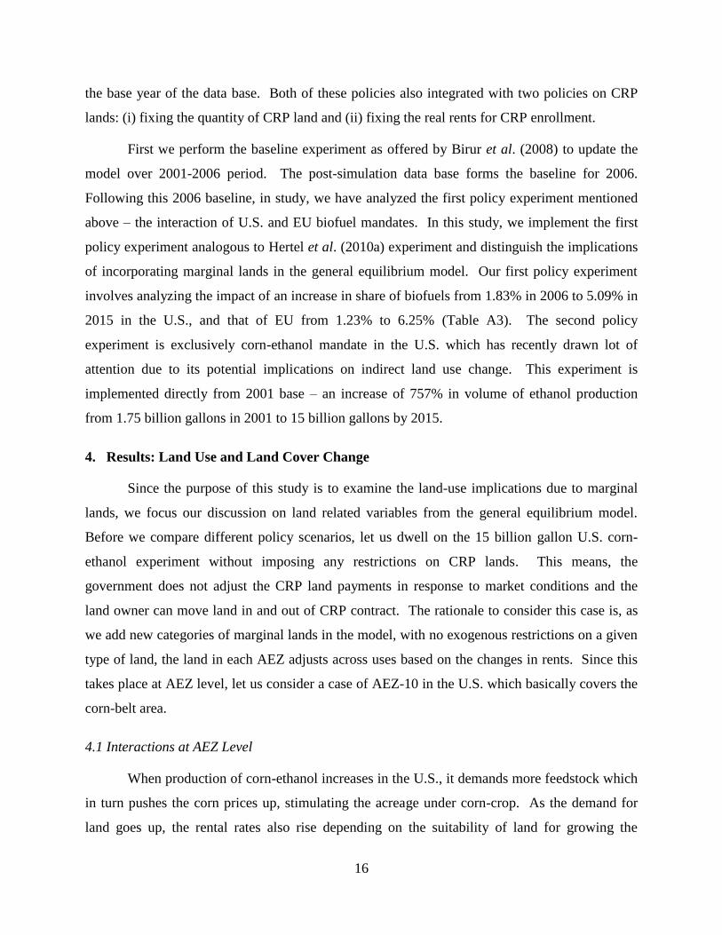
4.3 Baseline Experiment

As discussed in the earlier section, the baseline experiment which includes the key

biofuel drivers is essential to validate the model over the historical period 2001-2006 (Birur,

Hertel, and Tyner, 2008). Here we present a comparative analysis of four different scenarios of

23

the same baseline experiment. Table 5 presents the physical change in land use and land cover

for: (i) model with no marginal lands, (ii) model with marginal lands – without any restriction on

CRP acres9, (iii) model with CRP-land fixed, and (iv) model with CRP-land released (fixed real

rents to CRP).

As the key drivers induce biofuels production in the U.S., and EU, the economy demands

more feedstock, which in turn puts expansionary pressure on cropland from other land covers

such as commercial forest and pasture-cover. Due to intercrop substitution based on cropping

suitability of land, it is expected that addition of two marginal land categories in the model

would allow for greater degree of shift in cropping pattern within the cropland thereby offsetting

the pressure on forest or pasture covers. As presented in Table 6, when there are no marginal

lands in the model, the percent change in crop-cover is slightly larger (0.14% in U.S., 0.39% in

EU, 1.34% in Brazil) compared to that of the model with marginal lands (case-ii: 0.11% in U.S.,

0.37% in EU, 1.69% in Brazil). The most crucial result of this study, as expected, is the decline

in forest degradation with the introduction of marginal lands in all the three regions.

The change in physical acres of land-cover and harvested area (in million acres)

presented in the lower panel of Table 6 are the sum of all the existing AEZs‟ area in a given

region:

18

1i

ijrjr HAHA . The land cover change computed in the similar way showed that when

the marginal lands are not included, the pasture cover changed by -0.63, -0.21, +0.42 million

acres, in the U.S., EU, and Brazil respectively, versus -0.93, -0.31, -0.17 million acres with the

presence of additional marginal lands. This drastic reduction in degradation of pasture-cover is

expected to reduce the carbon-emission resulting due to biofuel drivers. However, the forest

cover showed greater decline when the marginal lands are included in the model relative to the

model with no marginal lands. For instance, the increase in sugarcane acreage in Brazil is

relatively much larger in the presence of marginal lands, which demands more deforestation.

This is because, the cropland-pasture incorporated in the land nest has slightly higher

productivity (land rents) than that of pasture-cover. Due to this difference cropland-pasture

responds faster to market forces and readily substitutes for pasture-cover, thereby putting

downward pressure on forest cover.

9 In this case, no restriction on CRP land is imposed exogenously in the closure. As a result, CRP land category

works just as other categories of crops. This case helps in clarifying comparison between the models with versus

without these additional categories of marginal lands.

24

Let us consider only the model with marginal lands in Table 6 and examine the CRP land

issues in the U.S. As noted earlier, although CRP land is treated as an additional possibility of

land use in the model, in reality it is the prerogative of the USDA to fix the quantity of CRP

enrollments or release any land for cultivation. Since the Farm Bill extends the CRP enrollment

to 32 million acres until 2012, we consider a case of fixing the quantity of CRP land ( ijrqoes )

and another case of fixing the real rents of the CRP land (esijrpmreal _ ) implying that the USDA

does not defend the CRP payments. As portrayed in Table 5, the baseline experiment shows

that when CRP lands are fixed, there are significant shifts in cropping pattern compared to the

case of when CRP is released. Interestingly, the release of CRP has a greater role in reducing the

pressure on decline in forest and pasture covers. With CRP contracts fixed, there is lesser

availability of cropland to allocate land across alternative uses. Due to this restriction on

intensive margin, the market induced demand for land puts additional pressure on extensive

margin and hence the forest cover goes up only by 0.06 million acres in the U.S., compared to

0.13 million acres of forest expansion when the CRP land is released for cultivation.

4.4 U.S. and EU Biofuel Mandates

The four cases after the baseline experiment discussed in the previous section form the

2006 baseline for implementing the U.S. and EU biofuel mandate experiment. Since this policy

experiment involves exogenous increase of corn-ethanol and biodiesel in the U.S., and biodiesel

in the EU for 2015, we expect greater demand for the respective feedstocks in the given regions.

As reported in Table 7, with no explicit marginal lands available for use in the model, there was

a strong cropping pattern shift towards the biofuel feedstocks but at a much larger reduction in

other crops. For instance, the model predicts an increase of 7.1% coarse grain area and 4%

oilseed area in the U.S., which required at least 8% reduction in other grains area. But in the

presence of marginal lands without any restrictions on CRP, the model predicted an 7.3%

increase in coarse grain area and 5.7% increase in oilseed area, but the reduction in other grains

area was only 5% and much of the shift came from reduction in cropland-pasture area (-7%).

Interestingly, with the additional marginal lands in place, the reduction in forest cover

was much larger in all the three regions (-1.3, -7.5, and -3.2 million acres in the U.S., EU, and

Brazil) compared to that of model with no marginal lands (-0.31, -6.9, and -0.5 million acres,

25

respectively). However, the reduction in pasture-cover in the U.S. was much larger in the U.S.

compared to decline in forest cover. This is because the pasture-cover is more responsive than

the other cover-types and hence much of the conversion results from pasture lands. Ahmed,

Hertel and Lubowski (2008) report that pasture-cover is more responsive than forest-cover to

increases in crop returns in the short-run. Even when the CRP land is fixed, the land cover

results are about same as that of the case with no restrictions on CRP land. However, when the

CRP land is released, the model predicts about 6.3 million acres of reduction in CRP land and

only 2 million acres of reduction in other grains area. In fact the harvested area under other

agricultural crops (vegetables, fruits, etc.) rises slightly in the U.S. when the CRP lands are

available for cultivation.

Furthermore, Table 7 indicates that with the presence of additional marginal lands, the

biofuel feedstocks acreage expand much faster without reduced much acreage under other crop

categories. As expected, the CRP release case showed the least amount of forest and pasture

cover decline relative to other two cases. Since this experiment involves implementing U.S. and

EU biofuel policies, it is important to understand the land cover implications, particularly in

Brazil, as it is a key player in supplying sugarcane based ethanol and soybean as biodiesel

feedstock. Interestingly, due to import demand of ethanol-2, sugarcane acreage expands much

faster compared to that of model with no marginal lands. This greater increase comes from large

reductions in cropland-pasture area (4.6 million acres), but also at the cost of forest cover (3.2

million acres). When CRP land is released, the cropping pattern shift shows much lesser pressure

on harvested area of competing food crops.

26

Table 6. Change in Land-Use and Land-Cover in the Baseline Experiment

2001-2006 Model with No Marginal

Lands

Model with Marginal

Lands

Marginal Lands with

fixed CRP

Marginal Lands with

CRP released

U.S. EU Brazil U.S. EU Brazil U.S. EU Brazil U.S. EU Brazil

Land use change (%):

Coarse Grains 2.36 -1.74 -0.30 2.63 -1.65 0.01 2.46 -1.64 0.02 2.64 -1.65 0.01

Oilseeds 0.55 12.57 0.29 1.02 12.86 0.37 0.81 12.89 0.41 1.03 12.86 0.37

Sugar-crops -1.03 -0.58 18.07 -0.67 -0.51 30.01 -0.80 -0.51 30.01 -0.67 -0.51 30.01

Other Grains -2.06 -1.29 -0.84 -1.25 -1.36 -0.84 -1.51 -1.36 -0.83 -1.24 -1.36 -0.84

Other Agri -0.50 -0.43 -1.42 -0.41 -0.26 -1.03 -0.48 -0.26 -1.03 -0.41 -0.265 -1.03

CRP-Land -1.86 - - 0 - - -1.94 - -

Cropland-pasture -1.28 -2.07 -2.22 -1.48 -2.10 -2.24 -1.27 -2.06 -2.22

Land cover change (%)

Crops 0.14 0.39 1.34 0.11 0.37 1.69 0.13 0.38 1.70 0.11 0.37 1.69

Forest 0.03 -0.26 -0.39 0.01 -0.28 -0.66 0.01 -0.28 -0.66 0.02 -0.28 -0.66

Pasture -0.16 -0.20 -0.04 -0.12 -0.14 0.11 -0.13 -0.15 0.11 -0.12 -0.14 0.11

Land use change (million acres)

Coarse Grains 2.12 -1.48 -0.09 2.36 -1.40 0.00 2.21 -1.39 0.01 2.37 -1.40 0.00

Oilseeds 0.44 4.00 0.10 0.82 4.09 0.13 0.65 4.10 0.15 0.83 4.09 0.13

Sugar-crops -0.03 -0.04 2.24 -0.02 -0.03 3.73 -0.02 -0.031 3.73 -0.02 -0.031 3.73

Other Grains -1.47 -0.82 -0.07 -0.74 -0.87 -0.09 -0.89 -0.86 -0.09 -0.73 -0.87 -0.09

Other Agri -0.41 -0.42 -0.49 -0.39 -0.26 -0.32 -0.46 -0.26 -0.32 -0.39 -0.26 -0.32

CRP-Land -0.74 - - 0 - - -0.77 - -


Land cover change (million acres)

Crops 0.66 1.25 1.70 0.51 1.20 2.15 0.60 1.22 2.15 0.50 1.20 2.15

Forest 0.27 -0.93 -1.53 0.12 -1.00 -2.57 0.06 -1.01 -2.58 0.12 -0.99 -2.57

Pasture -0.93 -0.31 -0.17 -0.63 -0.21 0.42 -0.66 -0.21 0.42 -0.62 -0.21 0.42

Pastures + CRP Combined -0.93 -0.31 -0.17 -2.16 -0.54 -0.87 -1.58 -0.55 -0.89 -2.19 -0.54 -0.87

27

Table 7. Change in Land-Use and Land-Cover due to U.S. and EU Mandates

2006-2015 Model with No

Marginal Lands

Model with Marginal

Lands

Marginal Lands with

fixed CRP

Marginal Lands with

CRP released

U.S. EU Brazil U.S. EU Brazil U.S. EU Brazil U.S. EU Brazil


Coarse Grains 7.12 -3.85 -3.89 7.35 -3.43 -3.10 7.71 -3.44 -3.19 9.37 -3.58 -3.24

Oilseeds 4.01 53.00 16.03 5.68 55.95 14.42 5.92 56.10 14.96 7.87 56.13 14.66

Sugar-crops -4.35 -0.86 5.18 -3.37 -0.49 45.05 -3.50 -0.28 45.49 -2.30 -0.24 45.64

Other Grains -7.56 -9.28 -8.60 -5.12 -9.73 -12.71 -5.41 -9.72 -13.04 -3.35 -9.69 -13.04

Other Agri -1.06 -0.64 -3.21 -0.82 0.39 -2.16 -0.88 0.63 -2.27 0.03 0.644 -2.24

CRP-Land 0.75 - - 0 - - -16.12 - -



Crops 0.77 2.89 2.67 0.77 2.84 3.63 0.80 2.85 3.67 0.69 2.84 3.65

Forest -0.04 -1.92 -0.13 -0.15 -2.09 -0.82 -0.16 -2.11 -0.84 -0.11 -2.10 -0.84

Pasture -0.56 -1.50 -0.65 -0.44 -1.12 -0.38 -0.45 -1.12 -0.38 -0.42 -1.11 -0.38


Coarse Grains 6.55 -3.21 -1.16 6.78 -2.86 -0.93 7.09 -2.87 -0.95 8.63 -2.98 -0.97

Oilseeds 3.24 18.96 5.63 4.62 20.07 5.07 4.80 20.13 5.26 6.40 20.13 5.15

Sugar-crops -0.11 -0.05 0.76 -0.08 -0.021 7.27 -0.09 -0.017 7.35 -0.06 -0.014 7.37

Other Grains -5.30 -5.79 -0.71 -2.98 -6.09 -1.43 -3.14 -6.08 -1.47 -1.95 -6.07 -1.47

Other Agri -0.86 -0.63 -1.08 -0.77 0.54 -0.67 -0.82 0.61 -0.70 0.03 0.63 -0.69

CRP-Land 0.29 - - 0 - - -6.29 - -



Crops 3.52 9.28 3.44 3.49 9.13 4.68 3.61 9.17 4.73 3.12 9.13 4.71

Forest -0.31 -6.92 -0.52 -1.26 -7.53 -3.19 -1.31 -7.58 -3.25 -0.96 -7.56 -3.23

Pasture -3.21 -2.36 -2.92 -2.24 -1.59 -1.49 -2.31 -1.59 -1.48 -2.16 -1.57 -1.48


28

4.5 U.S. Corn Ethanol Only Mandate

As discussed earlier, in this experiment we examine the implications of an increase in

corn ethanol to 15 billion gallons by 2015. As evident from Table 8, when the marginal land

categories are not included, the model prediction is that acreage under coarse grains in the U.S.

increases by more than 15% (14 million acres) which comes mainly at the expense of decline in

area under all other crops - particularly the oilseeds area by 5% (-4 million acres) and that of

other grains (paddy rice and wheat) by 9% (-6 million acres). Furthermore, the cropland cover

expands by 0.8% (3.6 million acres) in the U.S., which comes at the cost of 1.2 million acres of

forest cover and 2.3 million acres of pasture-cover. As the U.S. agricultural supply and demand

flux due to ethanol mandate imparts to rest of the world through trade linkages, the cropland in

Brazil expands only by 0.6 million acres, much of which is devoted to grow much demanded

coarse grain (corn) and the U.S. displaced oilseeds (soybean). This cropping shift occurs with

the forest loss of 0.1 million acres and conversion of pasture-cover into cropland of 0.5 million

acres. In the presence of marginal lands, without imposing any restrictions on CRP lands, the

U.S. corn-ethanol policy has much lesser impact on land-covers in the EU. Whereas, though

pasture-cover reduction is much smaller in Brazil, astonishingly forest cover declines much more

in the model with additional marginal lands.

Furthermore, when we fix the quantity of CRP land, with the cropland-pasture area in

place to substitute for, the coarse grains area increases by 16% (14 million acres), but there is

greater reduction in oilseed and other grains area is by 5% (3.9 million acres) and 7% (4.2

million acres), respectively in the U.S. However, this reduction in oilseed area has been picked

up partially by EU and Brazil. The major portion of cropping pattern shift in the U.S. comes

from the less productive cropland-pasture area (5%, 3.4 million acres). Consequently, the U.S.

cropland expands by 3.5 million acres with forest and pasture cover degradation of 2 and 1.4

million acres, respectively. When the CRP land is released, the cropping pattern adjusts such

that the CRP land and cropland-pasture area gives in by 11.5% (4.6 million acres) and 4% (2.6

million acres), respectively in the U.S. As expected, when the CRP land is released, the land

cover impact is slightly smaller than that of other cases.

29

Table 8. Change in Land-Use and Land-Cover due to U.S. Corn-Ethanol Mandate

2001-2015 Model with No Marginal

Lands

Model with Marginal

Lands

Marginal Lands with

fixed CRP

Marginal Lands with

CRP released

U.S. EU-27 Brazil U.S. EU-27 Brazil U.S. EU-27 Brazil U.S. EU-27 Brazil


Coarse Grains 15.57 0.28 1.20 16.95 0.32 1.52 15.86 0.34 1.62 17.25 0.32 1.50

Oilseeds -4.93 1.23 1.39 -3.80 1.11 1.57 -4.91 1.28 1.81 -3.50 1.07 1.51

Sugar-crops -2.87 -0.07 -0.95 -1.45 -0.02 -0.51 -2.18 -0.02 -0.51 -1.22 -0.02 -0.51

Other Grains -8.65 0.18 -0.09 -5.77 0.18 -0.02 -7.14 0.21 0.00 -5.38 0.17 -0.02

Other Agri -0.22 0.09 -0.44 0.52 0.15 0.07 0.02 0.17 0.10 0.69 0.139 0.07

CRP-Land -8.55 - - 0 - - -11.6 - -



Crops 0.79 0.26 0.45 0.68 0.21 0.31 0.77 0.24 0.35 0.65 0.21 0.30

Forest -0.15 -0.15 -0.03 -0.21 -0.14 -0.08 -0.24 -0.15 -0.09 -0.20 -0.13 -0.08

Pasture -0.41 -0.19 -0.10 -0.26 -0.13 -0.02 -0.28 -0.15 -0.02 -0.25 -0.13 -0.02


Coarse Grains 13.98 0.24 0.36 15.22 0.27 0.46 14.24 0.29 0.48 15.49 0.27 0.45

Oilseeds -3.97 0.39 0.49 -3.06 0.35 0.55 -3.95 0.41 0.63 -2.82 0.34 0.53

Sugar-crops -0.07 0.00 -0.12 -0.04 0.00 -0.06 -0.05 -0.001 -0.06 -0.03 -0.001 -0.06

Other Grains -6.19 0.12 -0.01 -3.41 0.11 0.00 -4.21 0.13 0.00 -3.17 0.11 0.00

Other Agri -0.18 0.09 -0.15 0.50 0.14 0.02 0.02 0.17 0.03 0.66 0.14 0.02

CRP-Land -3.40 - - 0 - - -4.60 - -



Crops 3.57 0.83 0.57 3.07 0.69 0.39 3.49 0.77 0.44 2.97 0.67 0.38

Forest -1.24 -0.54 -0.11 -1.77 -0.49 -0.31 -2.04 -0.55 -0.35 -1.70 -0.48 -0.30

Pasture -2.32 -0.29 -0.46 -1.30 -0.19 -0.08 -1.45 -0.22 -0.10 -1.27 -0.18 -0.08


30

The land use results discussed above are normalized in terms of requirement to produce

1000 gallons of corn ethanol and the results are depicted in Figure 6, with different policy

alternatives. When there are no marginal lands in the model, the model prediction is that 0.28

hectares of cropland is required globally to produce 1000 gallons of ethanol10

. With the

inclusion of marginal lands and allowing CRP land and cropland-pasture areas to substitute

freely, the cropland requirement drops down to 0.24 hectares per 1000 gallons.

Note: A: Model with No Marginal Lands B: Model with Marginal Lands

C: Model with Marginal Lands - CRP fixed D: Model with Marginal Lands - CRP released

Figure 6. Land Cover Impact of U.S. Corn-Ethanol Production (Ha/1000 gallons)

If the USDA chooses to fix the CRP enrollment until 2015, the global cropland

requirement goes up to 0.27 hectares (Figure 6). If the CRP land is officially released for

cultivation, the requirement of global cropland eases to only 0.23 hectares per thousand gallons

10

The land cover estimates and the resulting CO2E estimations from this study are much higher than Hertel et al.

(2010b) and CARB (2009) studies. This is because, Hertel et al. assume that the converted land from pasture and

forest covers is two-thirds as productive as regular cropland as opposed to the model predicted productivity in this

study. Since a one percent rise in harvested area does not require an equal amount of rise in land cover, those

authors pre-multiply the land cover change by the ratio of harvested area to the land-cover.

31

of ethanol. The cropland requirement as decomposed into contribution of forest and pasture

covers indicates that any reduction in cropland requirement comes mainly from lesser

degradation of pasture-cover at the global scale.

4.6 Decomposition of Land Supply Response

As noted from the results above, though availability of cropland-pasture and CRP lands

in the model has reduced impact on cropland expansion, the pasture-cover turns out to be much

more responsive in the biofuel production scenarios. To understand these results, let us consider

the land supply equation (4) discussed earlier.

).(1esijr

landiririjr pmpmqoqoes

Where, landirpm is the percentage change in market price of AEZ-land endowment i in region r,

computed as the sum of land revenue share weighted change in price of land across the three

cover types (Birur, Hertel, and Tyner, 2008).

es

k

LCikr

landir ikr

pmpm .

By substituting for land

irpm in (4), we get:

)..(1esijr

esikr

k

LCikririjr pmpmqoqoes (11)

Since the total land endowment is exogenous and fixed ( 0irqo ) and 0 es

ikr

es

ijr pmpm ,

equation (11) becomes,

)1.(1 LCikres

ikr

ijr

pm

qoes

(12)

The left hand side of the above equation indicates the change in quantity of land with respect to

its own price, represented as the elasticity of land supply (LCj

) in a given region.

)1.(1 LCij

LCj

(13)

32

If the land revenue share,

k

ikik

ijijLCij

QOESPMES

QOESPMES

*

*0 in a given land using sector, then,

1LCj . In this study, for example in the U.S., we have added CRP land and transferred a

portion of pasture-cover as cropland-pasture, into the cropland sector. So the revenue share

( LCij ) of cropland has increased simultaneously decreasing the share of pasture-cover and

forest-cover. Since the elasticity of transformation ( 1 ) is constant, an increase in LCij reduces

the land supply response, LCj . The land revenue shares and supply response for all the

scenarios that we have examined in the study are reported in Table 9. As seen from the table,

before incorporating additional marginal lands in to the model the land revenue share of cropland

in the U.S., was 0.789 and it has increased to 0.829 after incorporating additional categories of

marginal lands. At the same time, we can also notice the decline in land revenue of share of

pasture-cover, from 0.103 to 0.067. The impact of this change in land revenue share is evident in

the supply response – the cropland supply response has reduced and that of pasture-cover has

increased slightly. If we revisit the land cover change results reported in Tables 6 - 8, after the

new marginal lands are explicitly available in the model, the change in cropland cover has

relatively declined, with much reduction in pasture cover change. Interestingly, this has resulted

in further change in forest cover. The land revenue shares and supply response provided in the

table for all the experimental scenarios facilitate in better understanding the dynamics of land

cover results discussed in the previous sections.

In the second stage of land supply structure, from equation (5) we can derive the cropland

supply response, LUj with respect to change in land use revenue shares (

LUij ) as follows.

)1.(2 LUij

LUj

(14)

After allowing for cropland-pasture and CRP lands to substitute in the land use nest, the revenue

share of all other land uses (LU

ij ) fall as the share of the new marginal lands increase (Table

A4). Since 2 is constant (= -0.50), as the revenue shares fall, the land supply response increases

in crop sectors resulting in robust shift in cropping pattern as observed in Tables 6 – 8.

33

Table 9. Change in Land Cover Supply Response and Land Revenue Shares in the U.S.

Illustration: U.S. Land Revenue Share Land Supply Response

Model Version Cropland Pasture Forest Cropland Pasture Forest

2001 base data

Pre-sim With No Marginal Lands 0.7895 0.1027 0.1078 0.0421 0.1795 0.1784

Pre-sim With Marginal Lands 0.8298 0.0671 0.1031 0.0340 0.1866 0.1794

Experiment: 15 bgy corn ethanol increment in the US from 2001 base

Post-sim With No Marginal Lands 0.8306 0.0814 0.0880 0.0339 0.1837 0.1824

Post-sim With Marginal Lands 0.8580 0.0559 0.0861 0.0284 0.1888 0.1828

Post-sim Marginal Lands with

fixed CRP 0.8615 0.0546 0.0839 0.0277 0.1891 0.1832


CRP released 0.8572 0.0562 0.0866 0.0286 0.1888 0.1827

Experiment: Baseline experiment (2001-2006)




fixed CRP 0.8352 0.0643 0.1005 0.0330 0.1871 0.1799


CRP released 0.8344 0.0646 0.1010 0.0331 0.1871 0.1798

Experiment: US & EU 2015 Mandate experiment (2006-2015)




fixed CRP 0.8671 0.0507 0.0822 0.0266 0.1899 0.1836


CRP released 0.8622 0.0525 0.0853 0.0276 0.1895 0.1829

Note: “Pre-sim” and “Post–sim” indicate the results before and after the simulation experiments, respectively.

Since the revenue share of land under other agriculture is the highest in the U.S.,

followed by the Coarse Grains, these crop sectors showed greater degree of change in the

harvested area in the presence of cropland-pasture and CRP-lands. The land supply response of

cropland-pasture and CRP lands is relatively high compared to other crop sectors indicating the

ease of substitutability with response of biofuel production shocks.

34

4.7 Sensitivity of Land Supply Response

As noted from the results on land use and land cover change due to biofuels production

(Tables 6 - 8), interestingly forest cover responds more after incorporating cropland-pasture and

CRP-lands. In order to investigate further, we changed the land transformation elasticities as -

0.20 in both the tiers of the land supply structure. This implies a case where all the land using

sectors including the land cover types compete together in a given AEZ. When the 15 billion

gallon corn-ethanol production experiment (with no restriction on CRP lands) is implemented, in

the absence of marginal lands, the forest cover change was -0.13% in the U.S., -0.15% in the EU,

and -0.02 in Brazil (Table 10). When the marginal lands were available, the changes in forest

and pasture cover were almost the same as that of the model with no marginal lands. This

implies that the land transformation parameters significantly influence the pattern of land use and

land cover change Apart from testing the parameters, we also tested if the data modification on

cropland-pasture rents would influence results11

.

Table 10. Sensitivity of Land Supply Parameters on Land Use Change

Experiment: U.S. Corn-Ethanol Production (2001-2015)

Model with No Marginal Lands Model with Marginal Lands

U.S. EU-27 Brazil U.S. EU-27 Brazil Land use change (%):

Coarse Grains 10.56 0.62 1.70 11.23 0.63 1.90

Oilseeds -2.95 0.68 0.62 -2.42 0.65 0.76

Sugar-crops -2.08 -0.05 -0.77 -1.36 -0.03 -0.53

Other Grains -4.24 -0.01 -0.22 -2.87 -0.02 -0.26

Other Agri -0.24 0.07 -0.36 0.09 0.10 -0.05

CRP-Land -4.05 - -

Cropland-pasture -2.07 -0.49 -0.53

Land cover change (%):

Crops 0.84 0.25 0.38 0.79 0.23 0.32

Forest -0.13 -0.15 -0.02 -0.14 -0.14 -0.02

Pasture -0.48 -0.17 -0.09 -0.48 -0.17 -0.08

11

When we incorporated cropland-pasture rents in the data base, we deducted the computed cropland-pasture rents

from the pasture-cover rents in each region, thereby ensuring that the data base is balanced. When we relaxed this

modification and did not deduct the cropland-pasture rents from the pasture-cover rents implying that former is an

addition to the data base, the corn-ethanol experiment revealed significantly larger change in forest cover when the

value of land transformation parameters were -0.2 and -0.5 in the first and second tiers, respectively. This indicates

that it is the land transformation parameters that drive the key results and the treatment of pasture rents.

35

5. Results: Implications on Land Use Emissions

One of the major driving forces for the popularity of biofuels use is their potential for

GHGs savings. It has been argued that biofuels will reduce CO2 emissions to fossil fuels and also

growing feedstocks could be a CO2 sink. As Searchinger et al. (2008) explain, when forest or

pasture cover is converted to cropland for growing biofuel feedstock crops, loss of carbon occurs

due to removal of vegetation, burning of trees, and soil carbon loss can occur due to plowing up

the soil. As the standing vegetation sequesters carbon, it may be a net loss of carbon sequestered

if growing forest is replaced by field crops. In the case of marginal lands, if the cropland is idled

under CRP or being used to grow long-term pasture crops, the vegetation on these marginal lands

sequesters carbon from the atmosphere into the soils. If this land is undisturbed for several years

(CRP is enrolled typically for at least ten years), the accumulated carbon in the soils enhances

the productivity of these marginal lands (Sullivan et al. 2004).

Typically the impact of biofuels on global GHG emissions has largely been explored

using Life Cycle Analysis (LCA) – a form of engineering analysis with limited economic

content. Hill et al. (2006) use LCA and find that the corn-ethanol yields 25% more energy and

reduces 12% of GHGs, and soybean-biodiesel yields 93% more energy and reduces 41% of

GHGs relative to fossil fuels. As Dufey (2007) reports, the reduction in CO2 emissions vary by

the type of feedstock – wood biofuel being extremely promising to the lowest from corn-ethanol.

However, recently, results from economic models have been combined with LCA in order to

permit assessment of more complex aspects of the problem, including international land use

change. For instance, studies by Fargione et al. (2008) and Searchinger et al. (2008) indicate

that U.S. corn-ethanol is a net emitter of GHGs when indirect land-use emissions are included.

When accounting for land use emission, the direct and indirect changes are the

commonly used terms. The direct land use change refers to change induced by specific biofuel

activity in a given region and the repercussions of a region‟s biofuel activity in another region is

referred as indirect land use change (Kim et al., 2009). Recently, the indirect land use change

(ILUC) has raised serious concerns among the biofuel policy makers as the magnitude of ILUC

determines if a particular type of biofuel is net GHG emitter or not. In this study we estimate the

ILUC emissions based on the land cover change results discussed in the previous sections. For

this purpose we utilize the carbon emission factors measured as Mega grams of CO2 equivalent

36

(CO2e) per hectare for a period of 30 years (Table 11) adopted by CARB (2009) and Hertel et al.

(2010b). These emission factors are computed following Searchinger et al. (2008) based on the

global carbon flux data on oxidation and recovery of carbon in vegetation, soils, and forest

products provided by Houghton and Hackler (2001). Though these carbon factors pertain to

forest and pasture cover conversion, we consider that conversion of idled or marginal croplands

also emit carbon in the same way as that of pasture-cover since most of the croplands grow

grasses when they are kept idle.

Several studies have estimated the carbon flux in the marginal lands such as CRP land in

the U.S. Brenner et al. (2001) reports that if the CRP land is converted to grasslands, it

sequesters about 6.78 Mg of CO2e per hectare per year in Iowa soils and that of Nebraska is only

2.64 Mg of CO2e/ha/year (Brenner et al., 2002). The Chicago Climate Exchange has set a

protocol on carbon sequestration rate on CRP lands at 2.47 Mg CO2e/ha/year (CCX, 2007).

Fargione et al. (2008) report that when the abandoned lands such as CRP are converted to grow

corn, net emissions are about 69 Mg of CO2e/ha. Given this wide range of carbon factors, we

settle for using the pasture-cover carbon factors adopted by CARB (2009) and Hertel et al.

(2010b) for CRP as well as cropland-pasture (Table 11).

Carbon emissions from land cover change are computed by multiplying the carbon factors from

Table 11 with the change in physical hectares of forest, pasture-cover, CRP land, and cropland-

pasture, presented in Section 4 (Tables 6 through 8, for all the regions in the world). Table 12

reports land use emissions from implementing the U.S. and EU combined biofuel mandate, when

there no marginal lands and when the quantity of CRP land is fixed (which is the current realistic

scenario). With the combined mandate of the two regions, the total world-wide emissions were

about 3.96 billion Metric tons of CO2equivalent, of which, the total emission from EU alone is

about 1.18 billion Metric tons of CO2E, followed by Canada (856 mt), U.S. (696 mt), and Brazil

(691 mt), when the additional marginal lands are present in the model (second panel of Table

12). Clearly, most of this total emission came from forest cover change (2 billion tons of CO2E,

globally) followed by 1 billion tons from pasture cover change and 0.86 billion tons from change

in cropland-pasture. However, in the absence of explicit cropland- pasture sector in the model,

the total global emissions from the U.S. and EU biofuel mandates was 2.14 billion tons of CO2E,

of which more than 1.23 billion tons are from pasture cover change and the remainder from

forest cover change.

37

Table 11. CO2e Emission Factors by Land Cover type (Mg CO2e per hectare)

Regions

Forest-

lost

Forest-

gained

Pasture

cover lost

CRP-

lost

Cropland-

pasture

lost

U.S.A. 759.5 219.4 106.3 106.3 106.3

Canada 705.3 433.7 196.4 196.4

EU-27 297.4 362.0 155.6 155.6

Brazil 388.3 164.5 71.5 71.5

Japan 573.7 223.5 85.4 85.4

China-Hong Kong 573.7 223.5 196.4 196.4

India 573.7 223.5 196.4 196.4

Latin American Energy Exporters 388.3 164.5 71.5 71.5

Rest of Latin America & Caribbean 388.3 164.5 71.5 71.5

Eastern Europe & FSU Energy Exp 311.0 392.1 155.6 155.6

Rest of Europe 297.4 362.0 155.6 155.6

Middle Eastern N Africa energy exporters

152.4 58.7 82.4 82.4

Sub Saharan Energy exporters 305.1 129.3 42.5 42.5

Rest of North Africa & SSA 305.1 129.3 42.5 42.5

South Asian Energy exporters 936.6 337.0 85.4 85.4

Rest of High Income Asia 573.7 223.5 85.4 85.4

Rest of Southeast & South Asia 936.6 337.0 85.4 85.4

Oceania countries 388.2 197.8 97.9 97.9

Source: The carbon emission factors are adapted from CARB (2009) and Hertel et al. (2010b) studies, which are

computed in line with Searchinger et al. (2008), based on the carbon flux data from Houghton and Hackler

(2001).

Although addition of cropland-pasture has resulted in relatively lesser conversion of

pasture and hence the emissions, but the forest cover emissions have increased (Table 12). This

could be due to the reason that when the cropland-pasture is taken away from livestock grazing,

the pressure from the displaced livestock sector would lead to increased forest clearing. The

forest cover emission from EU-27, Canada, Brazil, and the U.S. are much higher compared to

other regions, mainly due to import of oilseeds by EU-27 for its biodiesel production, which has

resulted in significant land-use emissions. Due to this large magnitude of this indirect land use

emissions, policy makers still debate whether it is appropriate to include these emissions when

assessing the carbon intensity of biofuels. Since the mandate experiment involved exogenous

fixing of CRP land in the U.S., there is no change in emissions resulting from conversion of CRP

38

land. However, there are some offsets in emissions due to forest cover expansion in China,

Eastern Europe and Russian regions.

Table 12. Land-Use Emissions due to U.S. and EU Biofuel Mandates (2006-2015)

Regions


(CRP land fixed in the U.S.)

Emissions (Million Metric Tons of CO2 Equivalent)

Forest-

cover

Pasture-

cover Total

Emission

Forest-

cover

Pasture-

cover

Cropland-

Pasture Total

Emission

U.S.A. 95 138 233 402 99 196 696

Canada 631 83 714 733 82 41 856

EU-27 833 149 981 913 100 164 1,176

Brazil 82 84 166 510 43 138 691

Japan 7 0 7 8 0 0 8

China-HK -114 110 -4 -119 120 25 27

India 47 14 61 56 15 1 71

LAEEx -15 35 20 20 26 35 81

RoLAC -94 53 -41 -78 45 14 -19

EE &

FSUEx -507 357 -150 -386 304 208 126

RoE 9 51 59 16 44 22 82

MEAST &

NAEx 0 14 14 0 16 4 20

SSA_Ex -23 91 69 -14 101 11 98

RoAFR -1 13 12 1 14 4 19

SASIA-Ex -38 4 -34 -39 4 0 -35

RoHIA 0 0 0 0 0 0 0

RoASIA -3 5 2 -2 5 1 4

Oceania -2 31 28 -1 33 3 35

World 907 1232 2139 2,017 1,053 866 3,936

The land use emissions from the U.S. corn ethanol experiment are presented in Table 13.

As seen from the first panel of the table, when there are no marginal lands, production of 15

billion gallons of corn ethanol in the U.S., results in total global emissions of 794 million metric

tons of CO2E from land conversion, two-thirds of which came from the U.S. alone. The only

other region which contributed significantly to the total emissions was Canada. The forest cover

change contributed 506 million tons towards global total emissions, while the pasture cover

emissions were 288 million tons.

39

However, as seen from the second panel of Table 13, when cropland-pasture was

available in the model, the total global emissions from corn-ethanol production were 1.28 billion

tons, of which interestingly the forest cover sourced emissions were 829 million tons, and that of

pasture cover and cropland-pasture were 213 and 240 million tons, respectively. Due to the

linkage between cropland-pasture and pasture-cover that we established in the livestock sector,

as expected the ethanol production experiment resulted in slightly smaller emissions from the

pasture cover change. However, it is important to note that we used the same carbon intensity

factors for cropland-pasture as that of pasture cover. Most of the increase in forest cover

emissions came from the U.S. alone and impact on rest of the world was relatively much smaller

as the feedstock demand for ethanol production in the U.S. is met from its domestic production.

Table 13. Land-Use Emissions due to U.S. Corn Ethanol Production (2001-2015)

Regions


(CRP land fixed in the U.S.)

Emissions (Million Metric Tons of CO2 Equivalent)

Forest-

cover

Pasture-

cover Total

Emission

Forest-

cover

Pasture-

cover

Cropland-

Pasture Total

Emission

U.S.A. 382 100 482 627 62 146 835

Canada 159 24 183 164 21 10 195

EU-27 65 19 83 67 14 14 94

Brazil 17 13 31 54 3 19 76

Japan 3 0 3 3 0 0 3

China-HK -16 17 2 -15 17 5 7

India 5 2 7 5 2 0 7

LAEEx 0 10 10 18 6 12 35

RoLAC -11 8 -3 -7 6 4 2

EE &

FSUEx -94 54 -40 -82 44 23 -15

RoE 4 6 10 4 5 3 12

MEAST &

NAEx 0 5 5 0 5 1 6

SSA_Ex -2 18 15 -2 17 2 18

RoAFR 1 3 4 1 3 1 5

SASIA-Ex -9 1 -8 -9 1 0 -8

RoHIA 0 0 0 0 0 0 0

RoASIA 2 1 3 2 1 0 3

Oceania 0 8 8 0 8 1 8

World 506 288 794 829 213 240 1,283

40

A comparative summary of all the policy scenarios depicting the role of marginal lands is

presented in Table 14. The U.S. corn ethanol mandate of increase to 15 billion gallons per year

by 2015, starting from 2001 base, is an exogenous increment of 1.17 exa joules on energy basis.

This mandate results in emission of 22.6 grams of CO2E per mega joule of ethanol produced,

when the there are no marginal lands in the model. After incorporating the CRP land and

cropland-pasture in the model, the emissions increased to 36 g CO2E/MJ of ethanol when the CRP

quantity or its real rent are not fixed. This is mainly due to the fact that, the forest cover

experienced much larger reductions when the new marginal lands are incorporated into the

model. Though the new marginal lands, as expected lessened the impact on pasture-cover, they

also resulted in contrasting impact on forest cover.

Table 14. Global Land-Use Emissions across different Biofuel Policy Scenarios

U.S. 15 bgy U.S. & EU Mandate

(2001-2015) (2006-2015)

Biofuels increment (EJ) 1.17 1.68

Total Emission of CO2e Million Metric Tons of CO2e

(i) Model with No Marginal Lands 794.1 2138.9

(ii) Model with Marginal Lands 1265.6 3825.7

(iii) CRP land fixed 1282.6 3936.5

(iv) CRP land released 1274.7 4003.6

Emission per MJ of Biofuel Grams of CO2e emitted / MJ of Biofuel

(i) Model with No Marginal Lands 22.60 42.38

(ii) Model with Marginal Lands 36.00 75.82

(iii) CRP land fixed 36.48 78.02

(iv) CRP land released 36.26 79.34

Note: The land use emissions estimated here are based on the physical land cover change results. It is important to

note that following Hertel et al. (2010b), we have used the value of effective cropland adjustment (ETA)

parameter as 0.66 in estimating the acres of land cover change in this paper.

Interestingly, the emissions did not change much when the quantity of CRP land was

fixed or released (36 g CO2E/MJ). This implies that bringing in marginal lands under cultivation

substantially increased the indirect land use emissions. It is important note that since the biofuels

41

induced pasture cover change in the model with marginal lands is considerably low; the

emissions are higher compared to that of the model with no marginal lands. This is because, in

the model with marginal lands, as more of cropland-pasture and less of pasture-cover get

converted, the net impact is such that it results in further reduction in forest cover. Since forest

cover change results in large scale carbon flux (as implied in Table 11), even a small decline in

forest cover would lead to large increase in emissions.

Furthermore, the U.S. and EU mandate experiment which involved a total exogenous

increase in biofuels by 1.68 EJ by 2015 starting from the baseline 2006, showed very high

emission rates. Though the model with marginal lands showed substantially larger land use

emissions, the role of CRP land restrictions did not make much difference in the emission levels.

This may be attributed to the fact that availability of CRP land further boosted acreage expansion

in feedstock crops with lesser reduction in acreage under other crops, but the global impact on

forest and pasture cover remain unchanged.

6. Conclusions

As the importance of biofuels across the world as alternative fuels is growing, several

concerns are raised particularly on their potential indirect land use emissions. In order to reduce

these indirect land use changes which result in global level large scale deforestation or

degradation of grasslands, one possibility is to grow biofuel crops in idle croplands or marginal

lands. This study offers a novel framework, in which we first identify the marginal lands such as

Federal Conservation Reserve Program (CRP) enrolled lands in the U.S., and cropland-Pasture

area in the world. We aggregate this data at Agro-Ecological Zonal (AEZ) level and incorporate

these additional land categories in the land-supply function and analyze the implications of

biofuel policies in a general equilibrium framework.

In this paper, we examine two policy scenarios: (1) U.S. and EU biofuel programs

implemented simultaneously for 2015 starting from the baseline 2006, and (2) U.S. corn-ethanol

production by 15 billion gallons per year in 2015 from its 2001. In both of these policies we also

examine the potential impact of USDA (i) fixing the quantity of CRP land, alternatively (ii)

fixing the real rent of CRP (USDA does not defend the CRP rents). The results showed that

availability of additional marginal lands reduces the land-cover change substantially; particularly

forest degradation which is a major contributor is GHG emissions. The estimated indirect land

42

use emissions showed that the models without marginal lands, put pressure on larger

deforestation to meet the demand for cropland required for growing biofuel feedstocks. As more

land is available after incorporating the marginal lands, due to fall in price than before, the model

predicts much larger conversion of land than the model without the explicit marginal lands. The

ILUC emissions were smaller when CRP land is allowed for cultivation. The 15 bgy increment

of corn-ethanol only experiment revealed to emit 22.6 g CO2E per MJ of ethanol produced in the

U.S. by 2015, when there are no marginal lands in the model. The same experiment

implemented by Searchinger et al. (2008) showed that it results in 104 g CO2E per MJ of ethanol.

However, when the marginal lands are incorporated into the model, the emissions increased to 36

g CO2E per MJ of ethanol.

The key finding of this study is by including cropland-pasture and CRP lands in the land

use nest, we acknowledge the relatively greater ease of moving these additional marginal lands

back into crops as demand for cropland rises. Since cropland-pasture rents are tied closely to

pasture land rents through their substitutability in livestock production, there is a tendency for

cropland expansion to come disproportionately at the expense of pasture. This assertion is

supported by the econometric work of Lubowski et al. (2006), as interpreted in Ahmed, Hertel

and Lubowski (2008). However, in this study, with larger forest conversion, the overall GHG

emissions intensity of corn ethanol due to ILUC rises by one-third. It is important to note that

the carbon emission factors used for marginal lands are same as that of pasture-cover. The

relatively smaller carbon factors estimated by several studies as discussed above can result in

substantially lesser carbon emission.

One important qualification of this study is that the land supply framework that we have

followed here allows for explicit availability of cropland-pasture and CRP lands for cultivation

of crops. Due to more elastic land supply in the presence of these additional land uses, the

biofuel policy experiments resulted in slightly larger conversion of forest, which however

contributes significantly to land use emissions. This needs further investigation as modeling

explicit demand for accessible forests was beyond scope of this study. As the agricultural

commodity prices are rising and also production of biofuels, there is mounting pressure on

bringing in marginal lands under cultivation. With this backdrop, this study offers insights into

the potential economy-wide implications of biofuels in the presence of marginal croplands.

43

References

Ahmed, A. S., T. W. Hertel, and R. Lubowski (2008) “Calibration of a Land Cover Supply

Function Using Transition Probabilities”. GTAP Research Memorandum No 12. Center

for Global Trade Analysis, Purdue University, West Lafayette, IN, USA.

Best, L.B., et al. (1997). “Bird Abundance and Nesting in CRP Fields and Cropland in the

Midwest: a Regional Approach.” Wildlife Society Bulletin 25(4): 864–877.

Birur, Dileep K., Thomas W. Hertel, and Wallace E. Tyner (2008) “Impact of Biofuel Production

on World Agricultural Markets: A Computable General Equilibrium Analysis.” GTAP

Working Paper 53, Center for Global Trade Analysis, Purdue University, West Lafayette,

IN.

Birur, Dileep K. (2010) “Global Impacts of Biofuels on Agriculture, Trade, and Environment: A

Computable General Equilibrium Analysis.” Ph.D. Dissertation, Purdue University,

West Lafayette, IN.

Brenner, J. et al. (2001). “Quantifying the Change in Greenhouse Gas Emissions due to Natural

Resource Conservation Practice Application in Iowa.” Final report to the Iowa

Conservation Partnership, Colorado State University Natural Resource Ecology

Laboratory and USDA Natural Resources Conservation Service, Fort Collins, CO, USA.

Brenner, J. et al. (2002). “Quantifying the Change in Greenhouse Gas Emissions due to Natural

Resource Conservation Practice Application in Nebraska.” Report to the Nebraska

Conservation Partnership, Colorado State University Natural Resource Ecology

Laboratory and USDA Natural Resources Conservation Service, Fort Collins, CO, USA.

Campbell, J.E.; D.B. Lobell, R.C. Genova, and C.B. Field (2008). “The Global Potential of

Bioenergy on Abandoned Agriculture Lands.” Environmental Science and Technology,

42: 5791-5794.

CARB (2009) “Proposed Regulation to Implement the Low Carbon Fuel Standard.” Staff

Report: Initial Statement of Reasons released on March 5. California Environmental

Protection Agency, California Air Resources Board, Sacramento, CA. Available at: http://www.arb.ca.gov/fuels/lcfs/lcfs.htm

Dufey, Annie (2007) “International Trade in Biofuels: Good for Development? And Good for

Environment?” Environment for the MDGS – An International Institute for Environment

and Development (IIED) Briefing. www.iied.org

FAPRI (2004) “Documentation the FAPRI Modeling System.” FAPRI-UMC Report #12-04,

Food and Agricultural Policy Research Institute, Iowa State University, University of

Missouri-Columbia, Ames, IA, USA. December 2004.

Fargione J. et al. (2008) “Land Clearing and the Biofuel Carbon Debt.” Science, 319(5867):

1235-1238.

Fischer, Günther et al. (2008) “Land use Dynamics and Sugarcane Production” Chapter-2 In:

Peter Zuurbier and Jos van de Vooren (Eds.) “Sugarcane Ethanol: Contributions to

Climate Change Mitigation and the Environment.” Wageningen Academic Publishers,

the Netherlands.

http://www.arb.ca.gov/fuels/lcfs/lcfs.htm

44

FSA (2003) “Conservation Reserve Program Reports.” Farm Service Agency (FSA), U.S.

Department of Agriculture. Available at: http://www.fsa.usda.gov/FSA/webapp? area= home

&subject=copr&topic=rns

Gurgel, Angelo; John Reilly, and Sergey Paltsev (2007) “Potential Land Use Implications of a

Global Biofuels Industry.” Journal of Agricultural & Food Industrial Organization, 5(2):

1-34. Available at: http://www.bepress.com/jafio/vol5/iss2/ art9.

Hertel, T.W., H. Lee, S. Rose and B. Sohngen (2009). "Modeling Land-use Related Greenhouse

Gas Sources and Sinks and their Mitigation Potential", Chapter-6 in Economic Analysis

of Land Use in Global Climate Change Policy. Edited by T. Hertel, S. Rose and R. Tol.

Routledge Press.

Hertel, Thomas W., Wallace E. Tyner and Dileep K. Birur (2010a) “The Global Impacts of

Biofuel Mandates.” The Energy Journal, 31(1): 75-100.

Hertel, Thomas W. et al. (2010b) “Effects of US Maize Ethanol on Global Land Use and

Greenhouse Gas Emissions: Estimating Marketmediated Responses.” Bioscience, 60 (3):

222-231.

Eickhout, B. H., van Meijl, A. Tabeau, and E. Stehfest (2008). “The Impact of Environmental

and Climate Constraints on Global Food Supply” GTAP Working Paper No. 47, Center

for Global Trade Analysis, Purdue University, West Lafayette, IN, USA.

FAO (2008) “Biofuels: Prospects, Risks, and Opportunities” In: The State of Food and

Agriculture 2008, ISSN 0081-4539, Food and Agriculture Organization of the United

Nations, Rome, Italy.

Houghton, R. A., and J. L. Hackler (2001). “Carbon Flux to the Atmosphere from Land-Use

Changes: 1850 to 1990.” ORNL/CDIAC-131, NDP-050/R1, Carbon Dioxide

Information Analysis Center, U.S. Department of Energy, Oak Ridge National

Laboratory, Oak Ridge, TN. Available at: http://cdiac.esd.ornl.gov/ndps/ndp050 .html

Kelly, W. (2007) “Biofuels Shift Could Trigger Land-Use Changes.” California Energy Circuit

Inc., Berkeley, CA. March 09, 2007. Available at: http://www.californiaenergycircuit.net/

Kim, H., S. Kim, and B.E. Dale (2009) “Biofuels, Land Use Change, and Greenhouse Gas

Emissions: Some Unexplored Variables.” Environmental Science & Technology, 43(3):

961-967.

Kløverpris J., H. Wenzel, M. Banse, L.M. Canals, and A. Reenberg (2008) “Conference and

Workshop on Modeling Global Land Use Implications in the Environmental Assessment

of Biofuels.” International Journal of Life Cycle Analysis, 13(3): 178-183.

Lee, H.-L., T.W. Hertel, B. Sohngen and N. Ramankutty (2005) “Towards and Integrated Land

Use Data Base for Assessing the Potential for Greenhouse Gas Mitigation.” GTAP

Technical Paper # 25, Center for Global Trade Analysis, Purdue University, West

Lafayette, IN, USA.

Lee, H.-L., T.W. Hertel, S. Rose and M. Avetisyan (2009) “An Integrated Global Land Use Data

Base for CGE Analysis of Climate Change Policy Options.” Chapter-4 in T. Hertel, S.

Rose and R. Tol (eds.) Economic Analysis of Land Use in Global Climate Policy,

http://www.fsa.usda.gov/FSA/webapp?%20area=%20home%20&subject=copr&topic=rns

http://www.fsa.usda.gov/FSA/webapp?%20area=%20home%20&subject=copr&topic=rns

http://www.bepress.com/jafio/vol5/iss2/%20art9

http://cdiac.esd.ornl.gov/ndps/ndp050%20.html

http://www.californiaenergycircuit.net/

45

Routledge Publishing, London, New York, pp: 72-88. Also available as GTAP Working

Paper # 42, Center for Global Trade Analysis, Purdue University, West Lafayette, IN,

USA.

Lubowski, R.N. et al. (2002) “Major Uses of Land in the United States, 2002.” EIB-14, Economic

Research Service, U.S. Department of Agriculture, Washington, DC.

Lubowski, R.N., A. J. Plantinga, and R. N. Stavins (2005) “Land-Use Change and Carbon Sinks:

Econometric Estimation of the Carbon Sequestration Supply Function.” Regulatory

Policy Program Working Paper RPP-2005-01. Cambridge, MA: Center for Business and

Government, John F. Kennedy School of Government, Harvard University.

Lubowski, R.N.; M. Vesterby, S. Bucholtz, A. Baez, and M.J. Roberts (2006) “Major Uses of

Land in the United States, 2002.” Economic Information Bulletin # 14, Economic

Research Service, U.S. Department of Agriculture, Washington D.C. Available at: http://www.ers.usda.gov/Publications/EIB14/

Monfreda, C., N. Ramankutty, and J. A. Foley (2008), “Farming the Planet: 2. Geographic

Distribution of Crop Areas, Yields, Physiological Types, and Net Primary Production in

the Year 2000,” Global Biogeochem. Cycles, 22, GB1022, doi:10.1029/2007GB002947.

Osborn, T. (1993) “The Conservation Reserve Program: Status, Future, and Policy Options.”

Journal of Soil and Water Conservation, 48: 271-278.

Pagel, Geovana (2008) “For UN, Brazil‟s Biofuel Model is a Win, Win, Win Strategy.”

International Centre for Trade and Sustainable Development (ICTSD), Geneva,

Switzerland. http://ictsd.net/i/trade-and-sustainable-development-agenda/34226/.

Pearson, K. and C. Arndt (2000) “Implementing Systematic Sensitivity Analysis Using

GEMPACK.” GTAP Technical Paper No. 3, Center for Global Trade Analysis, Purdue

University. West Lafayette, IN, USA.

Ramankutty, N., A. Evan, C. Monfreda, and J. A. Foley (2008), “Farming the Planet: 1.

Geographic Distribution of Global Agricultural Lands in the Year 2000.” Global

Biogeochem. Cycles, 22, GB1003, doi:10.1029/2007GB002952.

Searchinger, T. R. et al. (2008) “Use of US Croplands for Biofuels Increases Greenhouse Gases

through Emissions from Land-Use Change.” Science 319 (5867): 1238-1240.

Sohngen, B., C. Tennity, M. Hnytka and Karl Meeusen (2009), “Global Forestry Data for the

Economic Modeling of Land Use”, Chapter-3 in T. Hertel, S. Rose and R. Tol (eds.)

Economic Analysis of Land Use in Global Climate Policy, forthcoming from Routledge,

also available as GTAP Working Paper # 41, Center for Global Trade Analysis, Purdue

University, West Lafayette, IN, USA.

Sullivan, P. et al. (2004). “The Conservation Reserve Program: Economic Implications for Rural

America.” Agricultural Economic Report No. 834. U.S. Department of Agriculture,

Economic Research Service. Available at: http://www.ers.usda.gov/Publications/AER834/.

Taheripour, F., T.W. Hertel, W.E. Tyner, J. F. Beckman, and D.K. Birur (2010) “Biofuels and

their By-Products: Global Economic and Environmental Implications.” Biomass and

Bioenergy, 34(3): 278-289.

http://www.ers.usda.gov/Publications/EIB14/

http://www.ers.usda.gov/Publications/AER834/

46

USEPA (2009) “EPA Lifecycle Analysis of Greenhouse Gas Emissions from Renewable Fuels.”

Technical Highlights, EPA-420-F09-024 (May 2009), Office of Transportation and Air

Quality, U.S. Environmental Protection Agency, Ann Arbor, MI.

Van Meijl, H.; Van Rheenen, T., Tabeau, A. and Eickhout, B. (2006) “The Impact of Different

Policy Environments on Land Use in Europe.” Agriculture, Ecosystems and

Environment, 114: 21-38.

47

Appendices

Table A1. Land Rental Payments in the U.S. ($ million)

Before

Modif‟n

Cr.

Grains

Other

Grains Oilseeds

Sugar-

crops

Other

Agri.

Pasture-

cover Forest

AEZ1 0 0 0 0 0 0 0

AEZ2 0 0 0 0 0 0 0

AEZ3 0 0 0 0 0 0 0

AEZ4 0 0 0 0 0 0 0

AEZ5 0 0 0 0 0 0 0

AEZ6 0 0 0 0 0 0 0

AEZ7 356 424 80 101 2643 2745 29

AEZ8 317 349 254 34 2265 641 116

AEZ9 391 152 317 105 1505 119 77

AEZ10 1770 281 1330 132 4105 404 1435

AEZ11 832 293 932 16 1940 252 1012

AEZ12 113 146 311 166 1393 127 2430

AEZ13 2 22 1 4 75 72 43

AEZ14 2 3 0 1 22 24 43

AEZ15 0 1 0 0 5 2 10

AEZ16 0 0 0 0 1 0 34

AEZ17 0 0 0 0 0 0 0

AEZ18 0 0 0 0 0 0 0

TOTAL 3784 1671 3225 560 13953 4387 5229

After

Modif‟n

Cr.

Grains

Other

Grains Oilseeds

Sugar-

crops

Other

Agri.

Pasture-

cover Forest CRP-lands

Cropland-

pasture

AEZ1 0 0 0 0 0 0 0 0 0

AEZ2 0 0 0 0 0 0 0 0 0

AEZ3 0 0 0 0 0 0 0 0 0

AEZ4 0 0 0 0 0 0 0 0 0

AEZ5 0 0 0 0 0 0 0 0 0

AEZ6 0 0 0 0 0 0 0 0 0

AEZ7 356 424 80 101 2643 2095 29 189 471

AEZ8 317 349 254 34 2265 502 116 143 97

AEZ9 391 152 317 105 1505 59 77 59 41

AEZ10 1770 281 1330 132 4105 139 1435 428 139

AEZ11 832 293 932 16 1940 75 1012 128 75

AEZ12 113 146 311 166 1393 45 2430 127 45

AEZ13 2 22 1 4 75 60 43 10 9

AEZ14 2 3 0 1 22 20 43 1 3

AEZ15 0 1 0 0 5 2 10 0 0

AEZ16 0 0 0 0 1 0 34 0 0

AEZ17 0 0 0 0 0 0 0 0 0

AEZ18 0 0 0 0 0 0 0 0 0

TOTAL 3784 1671 3225 560 13953 2999 5229 1085 881

Capital endowment in service sector before adjustment 3275607

Capital endowment in service sector after adjustment 3274522

Change in capital endowment (= CRP rental payments) 1085

Notes: The upper panel shows the original producer expenditure on land rental payments (measured at agent prices)

in each land using sector in the U.S., obtained from the GTAP version-6 data base. The lower panel shows land

rental payments after incorporating the CRP-lands and cropland-pasture in the U.S. The CRP payments are obtained

from the capital endowment in the government services sector.

48

Table A2. Land Rents across AEZs in the U.S. ($/acre)

Before

modification

Cr.

Grains

Other

Grains Oilseeds

Sugar

crops

Other

Agri.

Pasture-

cover Forest

AEZ7 37 22 59 245 154 8 1

AEZ8 33 22 34 208 157 7 3

AEZ9 42 24 38 192 260 9 3

AEZ10 47 38 42 227 156 10 9

AEZ11 42 49 37 263 101 9 8

AEZ12 35 53 45 234 133 7 15

AEZ13 19 17 23 203 90 4 1

AEZ14 22 25 39 210 98 5 0

AEZ15 26 39 49 0 132 6 0

AEZ16 0 62 0 0 339 0 3

After

modification

Cr.

Grains

Other

Grains Oilseeds

Sugar

crops

Other

Agri.

Pasture-

cover Forest

CRP-

lands

Cropland-

pasture

AEZ7 37 22 59 245 154 6 1 27 20

AEZ8 33 22 34 208 157 6 3 21 16

AEZ9 42 24 38 192 260 5 3 24 19

AEZ10 47 38 42 227 156 5 9 30 11

AEZ11 42 49 37 263 101 4 8 30 6

AEZ12 35 53 45 234 133 4 15 31 9

AEZ13 19 17 23 203 90 3 1 14 10

AEZ14 22 25 39 210 98 4 0 20 14

AEZ15 26 39 49 132 6 0

AEZ16 62 339 0 3

49

Table A3. The Changing Structure of the Biofuel Economy

US EU

Fuel Consumption: Units 2001 2006 2015 2001 2006 2015

Liquid fuels for Transport:

Petroleum Quad Btu 25.96 27.57 29.63 18.20 18.20 18.50

Total Biofuels1 Quad Btu 0.150 0.503 1.508 0.037 0.224 1.156

Ethanol

Quad Btu 0.149 0.471 1.341 - 0.035 0.183

Biodiesel Quad Btu 0.001 0.032 0.167 0.037 0.189 0.973

Share of biofuels in liquids

for transport (energy basis) % 0.58 1.83 5.09 0.20 1.23 6.25

Baseline Experiment 2001 2006 2001 2006

Biofuel Policies:

Subsidy for Ethanol $/gallon 0.51 0.51 - 1.00

Average Price of Ethanol2 $/gallon 1.48 2.58 1.48 1.96

Ad valorem equivalent of subsidy 1.34 1.20 1.00 1.51

% ch in subsidy (2001-2006) -10.9 51.0

Subsidy for Biodiesel3

$/gallon 1.00 1.00 - 1.90

Average Price of Biodiesel4

$/gallon 2.45 3.23 2.33 2.34

Ad valorem equivalent of subsidy 1.41 1.31 1.00 1.81

% ch in subsidy (2001-2006) -7.0 81.2

Source: Hertel et al. (2010a).

50

Table A4. Change in Land Use Supply Response and Land Revenue Shares in the U.S.

Land Revenue Share Land Supply Response

Cr.

Grains

Other

Grains Oilseeds

Sugar

crops

Other

Agri

Cropland-

pasture

CRP

lands

Cr.

Grains

Other

Grains Oilseeds

Sugar

crops

Other

Agri

Cropland-

pasture

CRP

lands

2001 base data

Pre-sim With No Marginal Lands 0.255 0.167 0.095 0.017 0.466 0.000 0.000 0.373 0.417 0.452 0.491 0.267 0.500 0.500

Pre-sim With Marginal Lands 0.232 0.152 0.087 0.016 0.424 0.024 0.066 0.384 0.424 0.457 0.492 0.288 0.488 0.467

Experiment: 15 bgy corn ethanol increment in the US from 2001 base

Post-sim With No Marginal Lands 0.367 0.119 0.076 0.015 0.424 0.000 0.000 0.317 0.441 0.462 0.493 0.288 0.500 0.500

Post-sim With Marginal Lands 0.343 0.114 0.072 0.014 0.392 0.019 0.046 0.328 0.443 0.464 0.493 0.304 0.491 0.477

Post-sim Marginal Lands with fixed CRP

0.336 0.109 0.070 0.013 0.388 0.018 0.065 0.332 0.445 0.465 0.493 0.306 0.491 0.467


CRP released 0.345 0.115 0.072 0.014 0.393 0.019 0.042 0.327 0.443 0.464 0.493 0.303 0.491 0.479

Experiment: Baseline experiment (2001-2006)



Post-sim Marginal Lands with fixed CRP

0.249 0.143 0.089 0.015 0.415 0.023 0.066 0.375 0.428 0.455 0.492 0.293 0.489 0.467


CRP released 0.250 0.144 0.090 0.015 0.416 0.023 0.062 0.375 0.428 0.455 0.492 0.292 0.489 0.469

Experiment: US & EU 2015 Mandate experiment (2006-2015)




fixed CRP 0.304 0.112 0.105 0.013 0.385 0.017 0.065 0.348 0.444 0.448 0.494 0.307 0.492 0.467


CRP released 0.315 0.119 0.110 0.013 0.392 0.017 0.034 0.343 0.441 0.445 0.493 0.304 0.491 0.483

Note: “Pre-sim” and “Post-sim” indicate the results before and after the simulation experiments, respectively.

Documents

IMPACT OF LARGE-SCALE BIOFUELS PRODUCTION ON … · IMPACT OF LARGE-SCALE BIOFUELS PRODUCTION ON ... and Tyner is James and Lois Ackerman ... Impact of Large-Scale Biofuels Production