Impact of India’s demonetization on domesticagricultural markets

Nidhi Aggarwal∗1 and Sudha Narayanan2

1Indian Institute of Management, Udaipur, India. e-mail: nidhi.aggarwal@iimu.ac.in

2Indira Gandhi Institute of Development Research, Mumbai, India. e-mail: sudha@igidr.ac.in

September 13, 2019

Abstract

This paper examines the impact of an extreme monetary shock, India’s demon-etization event in 2016, on domestic agricultural trade. Using data on arrivals andprices from around 3000 regulated markets for 35 major crops, we find that demoneti-zation reduced trade value by 13% in the short run, settling at 10% eight months afterdemonetization - driven more by a decline in prices than of arrivals. Triple differenceestimates suggest that the impacts are sharpest for kharif /monsoon crops, perishablesand crops where government intervention is minimal or absent; markets in areas withlimited bank and market access fared worse. Our results suggest that demonetizationleft a lasting implosion of agricultural trade domestically.

Keywords: demonetization, agricultural markets, difference-in-differences, tripledifferences, IndiaJEL Classification Codes : E5, E51, Q02, Q11, Q13

∗We thank without implicating Anisha Chaudhary and Pravin Dalvi for research and technical assistance.We thank Bharat Ramaswami, Ashok Kotwal, Jean Dreze and participants at various seminars for usefuldiscussions, comments and suggestions. The errors that remain are ours. No seniority in authorship isassigned.

1

1 Introduction

On November 8, 2016, the Government of India declared that two widely held denominationsof the Indian Rupee - the Rs.500 and Rs.1000 notes - would cease to be legal tender aftermidnight.1 In that one act, as much as 86% of the money in circulation was deemed illegaltender, engineering a currency squeeze that has few parallels elsewhere in recent times. Inthe days that followed, as people across the country deposited these two denominationsin banks, the central bank of India began replacing these with new currency. By March31, 2017, however, the value of currency in circulation was only 74% of that on the eve ofdemonetization (Figure 1). It took more than two years for the central bank to restore thecurrency in circulation back to its pre-demonetization levels. In scale and scope, the Indianexperience of demonetization is perhaps larger and deeper than any other in recent recordedhistory.2

Demonetization was expected to have economy-wide impacts; it was anticipated that itwould affect the informal sector and agriculture more, given their heavy reliance on cashfor daily transactions. In this paper, we assess the impact of demonetization on trade indomestic agricultural markets. We focus on government regulated markets (or mandis),where typically farmers sell their produce to traders in a designated space. We estimatethe value of domestic agricultural trade that was displaced on account of demonetizationand examine the underlying drivers of these impacts - specifically, whether these impactsmanifest via demand or supply factors.

Our motivation for investigating the impact on agricultural trade is manifold. We rec-ognize that the impacts on agriculture trade and prices are at best intermediate, proxyindicators that fall short of estimating the welfare implications for farmers, in terms of ei-ther their incomes or expenditures. However, given that nationally representative data onfarmer incomes are not routinely collected3 and data from household expenditure surveyswill likely take a while, the impacts on domestic agricultural trade offer the best proxy forfarmer receipts. This is especially since most farmers do not stock or store most cash cropsbeyond a few weeks. Second, even with regard to impacts on transaction volumes and pricesin the mandis, there has only been anecdotal evidence during the weeks following demone-tization. Limited research based on secondary data remains equivocal. Some claimed, soonafter demonetization, that trade would not be impacted since many transactions are check-based and that fears of an implosion of agricultural trade domestically are exaggerated.4

Others found that trade in these mandis reduced, at least in the immediate aftermath of

1Circular Number RBI/2016-2017/122 DCM(plg)No.1226/10.27.00/2016-17 issued on November 8, 2016.See Reddy (2017); Ghosh et al. (2017) for accounts of demonetization.

2Myanmar’s demonetization in 1987 that invalidated 80% of the currency in circulation without a smoothtransition is by far the most like the Indian experience.

3National surveys of farmer incomes are available from the 70th and 59th Rounds, conducted by theNational Sample Survey Organization in 2013 and 2003 respectively. There have been no other systematicdata collection efforts to gauge farmer incomes in India thus far.

4For example, see Reassessing the Impact of Demonetisation on Agriculture and Informal Sector, RACE,IDF, 2017 and Agricultural Growth after Demonetization, NITI Aayog blog series, 2017. Both these studiescompare pre-post differences in mandi trade and prices from secondary sources, and argue that demoneti-zation did not have an adverse impact.

2

demonetization.5 Given these conflicting perspectives, our study aims to shed light on thisdebate using a larger coverage of crops, markets, time periods and appropriate identificationstrategies that support causal inference. Third, despite agriculture’s declining importance asa contributor to GDP, accounting for 14.9% of the country’s GDP, about half of all peoplederive livelihoods from agriculture (Government of India, 2016b). Agriculture is known toimpact overall economic growth as a result, an observation made with predictable regularityin most discussions of economic growth in India. We can thus assess the slowdown in growthrates in India’s Gross Domestic Product (GDP), in the quarters following demonetization,in light of the impacts on India’s agricultural sector.

Our analysis also contributes to uncovering some understudied relationships betweenmonetary policy and agriculture in developing and transition economies. India’s demoneti-zation was akin to a sudden, even if exceptional, monetary tightening by the central bank.That monetary policy can have significant impacts on (real) sectors that are not well inte-grated into the modern economy is an old concern (Chambers, 1984; Chambers and Just,1982; Schuh, 1974). There have also been several historical studies on impacts of demoneti-zation and monetary contraction (Hamilton, 1987; Miskimin, 1964; Ciriacy-Wantrup, 1940).Early theoretical work on the impacts of monetary policy emphasizes that it can have non-neutral effects on agriculture, with a restrictive policy depressing agricultural prices andincomes, at least in the short and medium run (Chambers, 1984; Frankel, 1986; Belongia,1991; Ardeni and Freebairn, 2002; Frankel, 2008; Diaz-Bonilla and Robinson, 2010). Exist-ing empirical literature assessing the relationship between monetary policy and commodityprices too mostly support these claims (Barnett et al., 1983; Frankel and Rose, 2010). Mostof these more recent studies focus on the fallout of U.S. monetary policy shocks on com-modity prices. There are as yet few contemporary studies from other countries, especiallydeveloping economies. Our paper contributes to this redressing this gap in the literature.

Identifying causal impacts of monetary policy is empirically challenging because monetarypolicy shocks could themselves be endogenous responses to commodity prices (Anzuini etal., 2013). For example, Bernanke et al. (1997) argue that positive oil price shocks inducesa monetary policy response that can further amplify the effect of the oil price shock itself.In contrast, India’s demonetization was not driven by general economic conditions and itsstated objective was to rein in the black economy. The fully exogenous and unanticipatednature of the event offers greater scope to identify empirically the consequences of monetarycontraction on the agricultural sector.6

Our paper adds to a small and growing body of works that analyze the consequencesof India’s demonetization. These include impacts on economic activity (Chodorow-Reichet al., 2018), employment and livelihood strategies (Dewan and Sehgal, 2019; Krishnanand Siegel, 2017) stock markets (Dharmapala and Khanna, 2018), digitization of financialtransactions (Agarwal et al., 2018; Karmakar et al., 2018) and political outcomes (Bhavnaniand Copelovitch, 2018; Banerjee et al., 2018). Chodorow-Reich et al. (2018) present a model

5See Aggarwal, N and Narayanan S, “Demonetisation and agricultural markets”, Ideas for India, 2016;and Banerjee, A and Kala, N, “The economic and political consequences of India’s demonetisation”, VoxDevBlogs, 2017. Banerjee and Kala, for example, report that sales of agricultural commodities was 83% of thepredicted value.

6As a coarse verification that this was indeed a surprise, we graph the trend in google search in Englishbased on four variants of spelling (Figure 2).

3

Figure 1 Value of Notes in Circulation in India: July 2016 to June 30, 2017

Source: Reserve Bank of India.Table 2, Liabilities and Assets, Accessed March 31, 2018. The dashed verticalline is the date on which demonetization was announced. The second vertical line represents the date onwhich some of the withdrawal restrictions were eased for farmers and mandi traders. The last vertical dottedline represents the last date for legally depositing old currency notes in banks.

of demonetization to understand the importance of cash in facilitating transactions, and itsconsequences for real economic activity; they use data on variation in demonetization shockacross different regions in India to show that it had an adverse impact on real economicactivity. Dharmapala and Khanna (2018) analyze stock market’s reaction to demonetizationto determine the impact on the stated goals of demonetization, that is, tax evasion andcorruption. While all these studies provide a macro-perspective on the impacts of the episode,our study, by analyzing the domestic agricultural markets in particular, provides a detailedanalysis of the impacts at a more micro-level.

We use data on arrivals and prices from 2953 regulated markets in India for 35 majoragricultural commodities for the period 2011-2017. These 35 commodities account for anoverwhelming share of land under cultivation and value of production and are hence repre-sentative of Indian agriculture in more than one sense. The specific challenge of attributingcausal impacts to demonetization is the absence of an obvious counterfactual since the pol-icy was implemented countrywide. Reflexive comparisons before and after demonetizationdo not work since the post-treatment period coincides with a routine tapering off of theharvest season, when mandi -based trade declines for many commodities. We navigate thisdifficulty by choosing earlier years as counterfactuals for 2016-17, i.e., 2016-17 serves as the“treatment” unit/ year and 2011-16 as comparison years; we use the date, November 8th, topartition pre-treatment and post-treatment time periods. Our empirical strategy involves theuse of a difference-in-differences (DD) technique, but we frame our difference-in-differencesin time-time space rather than state-time space. We assess impacts for varying windowsafter demonetization and find that demonetization displaced domestic agricultural trade inregulated markets over 13% in the short run settling at almost 10% even after the end of the8 months (233 days) after demonetization.7 We find that most of this decline is on account of

7Our other models with alternate specifications predict similar impacts of around 13-14% settling to

4

Figure 2 Trend in internet searches on Google for demonetization

Notes: These are weekly data with 100 denoting the highest number of searches, notebandi is the word fornote ban in Hindi, the most commonly spoken language in India (as on October 15, 2017).

the significant decline in prices rather than of arrivals, which appear to have recovered over aperiod of three months. Specific crop groups and geographies drive these results. We uncoverthe heterogeneity of impacts across mandis and crop types using a set of commoditywise DDmodels and a set of triple differences (TD) models, described later in the paper. The TDmodels help identify impacts for perishable crops, monsoon crops - whose harvests coincidewith the time of demonetization and for mandis in areas with relatively better financial andmarket access, and proximity to urban centres. Overall, the negative impacts are largestfor kharif or monsoon crops that had just been harvested when demonetization occurred, incommodities where government intervention is minimal and for perishables, where farmersdid not have the choice to store in anticipation of better prices. The impacts are the leastfor crops where governments actively procure, for rabi winter crops that would come to themarket only months after demonetization and for non-perishables. Trade in perishables wasdisplaced to the extent of 17% more than for non-perishables a month after demonetization.It recovered, but not fully, over the 8 months that followed. We find, as expected, most ofthis decline in value of perishables came from decline in prices, the most compelling evidenceof the impact on farmers’ incomes.

We also find as expected that mandis in district with better access to bank branches sawmore muted impacts relative to those with poorer access to cash; access to Automated TellerMachines (ATMs) do not seem to have made a difference. Smaller mandis and mandis indistricts with higher market density also appear to have lower impacts than larger mandis andthose in districts with fewer mandis, respectively. Farmers in districts with a dense networkof mandis were perhaps on average close enough to smaller mandis, at least in the short run.Smaller mandis seem to have crowded in trade relative to the larger mandis briefly but at theend of eight months after demonetization, there was no difference. Mandis in districts withcities over one million, however, did worse than those in more rural districts. All of theseimpacts conform accounts from that time. Robustness checks and falsification tests largelysupport our findings that the impacts we identify are most likely due to demonetization.

The paper is organized into six sections. Following this discussion, we describe the context

around 11-12% by the end of 90 days.

5

of domestic agricultural trade in India. We then conceptualize the pathways through whichdemonetization is expected to impact domestic agricultural trade. Section 3 discusses thedata used and empirical strategy. Section 4 discusses the results, with Section 5 devoted tochecking the robustness of results. Section 6 summarizes these results and discusses some ofthe coping strategies farmers used in the immediate aftermath of demonetization.

2 The context of agricultural transactions in India

Domestic agricultural trade in India typically occurs in designated markets declared underthe Agricultural Produce Marketing Committee Act (APMC Act). Historically, farmerswere mandated to sell in these markets to licensed intermediaries. Although several stateshave reformed this law allowing private trade, contract farming and direct procurement, formost commodities a significant proportion of trade passes through these mandis, even if thefirst trade might be a sale by a farmer to an itinerant trader or within the village. In atypical process at a regulated mandi, a farmer brings his/her produce to the mandi, takesit to the commission agent of his /her choice, unloads the produce in the agent’s premises(Aggarwal et al., 2017). Bidding take place for each lot, which gets a unique identificationnumber. During the designated trading hours, prospective buyers, including traders andprocessors, each of whom holds a licence to trade in the specific mandi, visits the agent’spremises, examines the quality of the produce and quotes a bid price. The bidding is eitherclosed tender - the bid is private and written down on a paper slip or on a computer - or it isthrough an open-cry auction. The former system dominates for commodities that see largedaily arrivals. At the end of the trading window, the highest bid price is declared as thewinning bid. The farmer has the right to reject the bid; in this case, his/her lot is placed forbidding on the next trading day in the mandi. If the farmer accepts the price, the produceis weighed and a sales bill is generated. The trader pays the commission agent, who, afterdeducting his/her commission and the mandi fee, pays the farmer, usually in cash. Traderstypically do not pay the commission agents immediately and instead buy on credit, whilethe payment is settled anytime between fifteen days to six months after the transaction. Thecommission agent however pays the farmer, at the time of the transaction or within one ortwo days, after deducting any interest for or repayments against loans that (s)he may haveprovided to the farmer in the past.

Virtually all of these transactions are cash-based. Although check payments and directbank transfers are increasingly being used by processors, this still forms a small portion oftransactions (Aggarwal et al., 2017). As of 2015, there were 6746 such regulated markets(2479 of them termed primary markets and the rest called submarket yards or minor mar-kets), with each district in the country having at least one such market (Government of India,2016b).8 The context we study therefore involves a large number of heterogeneous markets- in terms of size, commodities traded, location and so on. Different states allow privatemarkets direct trade outside the mandi regularly. Despite heterogeneity and the existenceof credit relations that are long-term relationships, cash transactions dominate mandi -basedtrade and the mandi is a key channel for a bulk of the produce.

8There are also a reported 26519 rural markets - primary and wholesale that are not regulated Governmentof India (2016b).

6

2.1 Conceptual Pathways and Hypotheses

What is the likely impact of demonetization on domestic agricultural markets, as representedby mandi -based trade? We expect that a shared shortage of liquidity reduces demand forcommodities because commission agents and traders are unable to pay the farmers in cash.The traders themselves may face a demand shock if their buyers are also cash-constrainedor are only willing to purchase on credit or bank-based payments. In the latter case, tradersand commission agents might still face a cash constraint because even with banks, access toliquidity was restricted.9 Our own field visits to prosperous regions near the national capitalrevealed that even with a high number of bank branches and ATMs in the town, there wasa shortage of cash.10 These factors together would shift the demand curve inwards reducingthe quantity traded as well as the price.

From the supply side, most farmers in India typically sell their cropsimmediately afterharvest due to liquidity constraints. It is however possible that with demonetization, farmersheld back their produce from sale, anticipating a collapse in demand and consequent lowprices. Alternatively, the transactions costs (labour and transportation) of bringing theproduce to mandis could result in farmers postponing their journey to the market, potentiallyoverriding an urgent need to sell produce for cash.11 Either or both of these has the effectof contracting supply in the mandis, resulting in lower traded quantity and higher price.

The net effect would depend upon which factor dominates. We posit the following hy-potheses:

• With a contraction of both demand and supply we would expect the volumes of manditrade to decline, especially for non-perishable commodities where the farmer mightstore it and sell at a future date. This may not happen for perishables, where storingis not an option available to the farmer. Nor would one expect strong impacts forcommodities that either see government procurement12 or are vertically coordinatedand where transactions are based on contracts, rather than spot markets.

• The prediction for prices is less obvious. If as described above, both demand andsupply contract, then the impact on prices depends on which effect is stronger giventheir relative elasticities. In some cases, especially for perishables, where storing thecommodity is not an option, or if the farmer is in an urgent need of the money, there

9For instance, post-demonetization, cooperative banks, a key rural financial institution, were not allowedto accept deposits of old currency, even in exchange for new currency. Withdrawal and exchange limits onnew currency were in force for weeks after demonetization (Appendix A online). It was not until November21, 2016that farmers were granted some latitude to withdraw upto Rs.25000 per week in cash from specificdeposit accounts. Traders registered with APMC markets / mandis were allowed to withdraw, in cash, Rs50,000/- in a week with some conditions (Figure 1).Loans for the following cropping season were permittedaround the same time. The new currency notes were slow to reach rural areas and access to cash throughATM and banks was not easy. Further, old ATMs had to be recalibrated to dispense new notes that weresmaller than the notes that were banned.

10These field visits were to regulated markets in Gannaur (Haryana) and Azadpur (Delhi) during November29-December 1, 2016. Field visits involving conversations with farmers included Karnataka in June and July,2017; Madhya Pradesh, March, 2017 and Tamil Nadu, March 2017.

11We expect that this latter effect would be weak given the shared scarcity of cash.12See “No demonetisation impact on FCI, rice procurement soars 17%”, Financial Express, January 6,

2017, accessed on December 1, 2018.

7

would be a decline in the prices. Consumers might change their consumption pattern orreallocate expenditures within food groups, in the context of a cash crunch, away fromrelatively more expensive to less expensive foods. The net impact is not immediatelyobvious and would vary across commodities, the nature of government interventionand market structure for each commodity.

We examine mandi arrivals and prices to understand which effect dominates in the im-pacts we see on total value of domestic agricultural trade.

We also anticipate heterogenous impacts on total value of trade, and on arrivals andprices across mandis. Our hypothesis is that mandis that have limited penetration of banksand are relatively less connected to urban areas are likely to be more affected. According tothe Report of the Committee on Medium-term Path on Financial inclusion, in June 2015,the number of branches per 100,000 of population in rural and semi-urban areas in Indiawas 7.8, less than half the number in the urban and metropolitan areas (18.7). The medianglobal value as per the data from the World Bank in 2015 was 12.62.13 It could also bethe case that farmers don’t simply choose whether or not to sell in the mandi but pick themandi they wish to go to. Our field visits in the aftermath of demonetization suggest thatsome farmers coped with the cash constraints by choosing to sell in nearer, rather than theirpreferred distant mandis. This diversion of trade to mandis closer to the point of productioncould imply that smaller mandis closer to production centres saw lower decline in arrivalsrelative to larger mandis. At the same time, the farmer might associate larger mandis witha greater probability of finding a buyer and might hence divert produce to larger mandis.

There are several reasons, however, that an anticipated implosion of agricultural marketsmight not occur, especially with respect to arrivals. Many creative ways to circumvent theban surfaced in the weeks after demonetization. For example, our field visits revealed thatin many mandis, despite the ban, old currency continued to be accepted for payment ata discount. Across mandis, a sophisticated schedule of prices for produce had developeddepending on whether one was trading in new or the old illegal currency.14 There were alsoreports that consequently those who had stashes of old currency, possibly black money, werebuying up agricultural produce rather than deposit these in banks.15 Most often however, wefound that goods were passing through but not money, so that farmers, agents and traderswere transacting on credit.16 Sometimes multilateral arrangements had evolved where farmerbought inputs for the impending agricultural sowing from family members of traders whothey had just sold to on credit, thus settling the transaction in kind. In each of thesecases, one would not expect to see a sharp impact on arrivals. In these cases, the impact ofdemonetization is likely on consumption and savings.17

13The World Bank, World Development Indicators, accessed on November 1, 2017.14See for example, Krishnamurthy, M, “Trading Notes”, Hot Spots, Cultural Anthropology, 2017.15Paddy mandi a green pasture for black money hoarders, The New Indian Express, November 22, 2016,

last accessed on November 2, 2017.16See for example, At Delhi’s Azadpur mandi, Lack of Money is Slowly Choking Business and Also Work-

ers, The Wire, November 18, 2016, last accessed on November 2, 2017.17Our fieldwork also indicated that the persons who were likely most affected were the farm workers and

their families, who had not been paid wages since the farmer had no cash. For this group, remittanceshome had dried up and farm workers reported that they had cut back food consumption too to keep afloat.See: Jobless, these labourers can barely get one meal a day, The Economic Times, December 11, 2016, last

8

Likewise if successive notifications easing restrictions on access to new currency were trulyreleasing constraints on cash, we would see a muted impact on average or a tapering off ofnegative impacts, if any.18 These also include innovative solutions by state governments.For example, in the southern state of Telangana, the government, along with a bank, issuedcoupons to trade in farmers’ markets that could later be encashed. In Tamil Nadu, templesunder the state government opened up their cash donation boxes containing offerings madeby pilgrims to exchange banned tender.19 All or any of these factors would mitigate thenegative impacts of demonetization. We also believe that if itinerant small traders who pickup produce at the farmgate were themselves cash starved, we might actually witness tradethat would have otherwise occurred locally within the village, making its way to the mandis,where perhaps the likelihood of finding a buyer is higher. In effect, the actual impact ofdemonetization on domestic agricultural trade is an empirical question.

3 Data and Empirical Strategy

3.1 Data

For the analysis, we choose 35 commodities that represent each of about twelve commoditygroups identified by the Ministry of Agriculture.20 The choice of these crops is based on thecultivated (gross/net) area with each commodity group in 2015, although we have taken carethat these broadly reflect the shares over the period 2012-2017 (See Table 1). We are thereforeable to account for commodities that reflect Indian agriculture broadly. For foodgrains (i.e.,cereals and pulses), the crops we consider account for 85% of land under foodgrains, foroilseeds, the proportion is 87% and for horticulture (fruits, vegetables, aromatic plants,plantation crops and spices), the commodities included account for close to 60% of the totalarea under such crops.21

Not all of these commodities are produced in all the states or in all seasons. Our list ofcrops include kharif or monsoon crops, that were either being harvested or were ready forharvest at the time of demonetization. The typical kharif crop involves sowing in June andharvests ranging from October to January depending on the crop and the varieties. Our

accessed on November 2, 2017.18See for example, the following reports, Demonetisation: Govt relaxes rules, allows farmers to use Rs.500

notes to buy seeds, Business Standard, November 21, 2016, last accessed on November 2, 2017 and Furtherdemonetisation relaxation likely for farm sector, weddings, Business-Standard, November 23, 2016, lastaccessed on November 2, 2017.

19See for example, Temple donations in TN see slump post demonetisation, The New Indian Express,November 19, 2016, last accessed on November 2, 2017. and Telangana govt has a creative solution forfarmers’ market in demonetisation woes, The News Minute, November 19, 2016, last accessed on November2, 2017.

20Commodities are grouped into cereals, pulses, oilseeds, fibres, sugar and beet, plantation crops, spices,fruits, vegetables, flowers, aromatic crops and honey. Livestock products are considered separate from“crops” and are excluded from the analysis. While live animals are traded in mandis, livestock products arenot.

21It is difficult to get an estimate of the selected commodities’ contribution to the value of production ofall crops, without also selecting a set of prices that represent a normal year. We therefore use acreage as thecriterion.

9

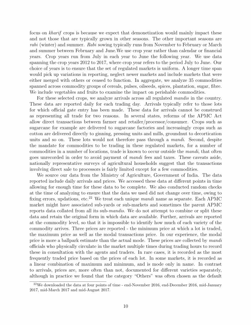
focus on kharif crops is because we expect that demonetization would mainly impact theseand not those that are typically grown in other seasons. The other important seasons arerabi (winter) and summer. Rabi sowing typically runs from November to February or Marchand summer between February and June.We use crop year rather than calendar or financialyears. Crop years run from July in each year to June the following year. We use dataspanning the crop years 2012 to 2017, where crop year refers to the period July to June. Ourchoice of years is to ensure that the set of regulated markets is uniform. A longer time spanwould pick up variations in reporting, neglect newer markets and include markets that wereeither merged with others or ceased to function. In aggregate, we analyze 35 commoditiesspanned across commodity groups of cereals, pulses, oilseeds, spices, plantation, sugar, fibre.We include vegetables and fruits to examine the impact on perishable commodities.

For these selected crops, we analyze arrivals across all regulated mandis in the country.These data are reported daily for each trading day. Arrivals typically refer to those lotsfor which official gate entry has been made. These data for arrivals cannot be construedas representing all trade for two reasons. In several states, reforms of the APMC Actallow direct transactions between farmer and retailer/processor/consumer. Crops such assugarcane for example are delivered to sugarcane factories and increasingly crops such ascotton are delivered directly to ginning, pressing units and mills, groundnut to decorticationunits and so on. These lots would not therefore pass through a mandi. Second, despitethe mandate for commodities to be trading in these regulated markets, for a number ofcommodities in a number of locations, trade is known to occur outside the mandi, that oftengoes unrecorded in order to avoid payment of mandi fees and taxes. These caveats aside,nationally representative surveys of agricultural households suggest that the transactionsinvolving direct sale to processors is fairly limited except for a few commodities.

We source our data from the Ministry of Agriculture, Government of India. The datareported include daily arrivals and prices. We accessed these data at different points in timeallowing for enough time for these data to be complete. We also conducted random checksat the time of analyzing to ensure that the data we used did not change over time, owing tofixing errors, updations, etc.22 We treat each unique mandi name as separate. Each APMCmarket might have associated sub-yards or sub-markets and sometimes the parent APMCreports data collated from all its sub-mandis. We do not attempt to combine or split thesedata and retain the original form in which data are available. Further, arrivals are reportedat the commodity level, so that it is impossible to identify how much of each variety of thecommodity arrives. Three prices are reported - the minimum price at which a lot is traded,the maximum price as well as the modal transactions price. In our experience, the modalprice is more a ballpark estimate than the actual mode. These prices are collected by mandiofficials who physically circulate in the market multiple times during trading hours to recordthese in consultation with the agents and traders. In rare cases, it is recorded as the mostfrequently traded price based on the prices of each lot. In some markets, it is recorded asa linear combination of maximum and minimum, and is mode only in name. In contrastto arrivals, prices are, more often than not, documented for different varieties separately,although in practice we found that the category “Others” was often chosen as the default

22We downloaded the data at four points of time - end-November 2016, end-December 2016, mid-January2017, mid-March 2017 and mid-August 2017.

10

Figure 3 Marketing channels for kharif crops, 2012-13.

even when the variety was clearly distinguishable.We use all data for the selected commodities, including all varieties reported. We use

the minimum prices since it systematically and reliably records the lowest price of the day,though we also estimate our models using modal and maximum prices to check the sensitivityof results.23 In our knowledge, ours is the first study which conducts a detailed analysis ofgovernment regulated agricultural mandis using the price and arrivals data at daily level.Goyal (2010) used monthly data on soyabean to analyse the impact of a change in theprocurement strategy of a private buyer on the functioning of rural markets in India.

Table 1 presents percentage of arrivals during the kharif season for each selected commod-ity and the average number of mandis that reported arrivals during 2012-16. .Commoditiessuch as paddy, maize, soyabean, cotton are primarily grown as kharif crops. The major rabicrops include wheat, cumin and Bengal gram. Arrivals for cereals such as paddy, wheat,maize, bajra soyabean, and pulses, including tur and Bengal gram, are reported by a largeset of mandis. Within perishables, we see a large number of mandis reporting arrivals foronion, potato, tomato and brinjal. A smaller number of mandis report arrivals for the fruits,spices and plantation crops analyzed in the study. As discussed in Section 2, not all agricul-tural produce pass through mandis (Figure 3). Some of it is directly sold to co-operativesand government agency, mills and processors and to private traders through contracts.24

Commodities such as wheat, maize, bajra (peal millet), tur (pigeonpea) and Bengal gram(chickpea) have a large share of production that is sold via mandis. Others such as ragi(finger millet), jowar (sorghum), groundnut, soyabean have a much smaller share.25 Figure4 illustrates weekly arrivals for six selected commodities for three of the crop years analyzed.

23We caution that our data are not transaction-level data, and to that extent, provide us an indicativevalue of the impact of the event on mandi trade. The use of minimum price also ensures that we do not overestimate the impacts.

24The 70th Round of the National Sample Survey conducted in 2012-13 offers the best estimates of mar-keting channels for commodities that is nationally representative of agricultural households in India. Figure3 shows the commodity wise share transacted via different channels by the farmer. Several trades that occurthrough private buyers who are typically itinerant vendors who visit the village also pass through mandiswhere the produce is aggregated and sold onward.

25As mentioned earlier, soyabean and groundnut are often bought by processors. Ragi and jowar typicallygrown by poorer farmers and are sold within the village.

11

The shaded region in the graph indicates the kharif season, the period that was hit bydemonetization (Week 18-19). For non-perishables, arrivals are uneven throughout the year.The peak season for paddy, soyabean and cotton is the kharif season. Tur harvests typicallyarrive between December to January. In contrast, arrivals for perishables such as tomatoand banana are spread throughout the year. Thus, at least for some major commodities, apre-post comparison in value of trade would not make sense, given the intra-seasonal patternsof arrival.

3.2 Empirical strategy

3.2.1 Difference-in-Differences

Our main empirical strategy is a Differences-in-Differences (DD) regression framework toanalyze the impact of demonetization. We define the event of demonetization as the treat-ment, the crop year, 2017 as the treatment unit, and the preceding five years, 2012-2016 asthe comparison units. The period before (after) November 8 in each crop year representsthe pre (post)-treatment variable. Thus, we have one treated year, and five comparisonyears (2011-12 to 2015-16). We then use the days before (after) November 8 in each year asthe pre(post)-treatment variable. We therefore apply the DD technique to time-time spacerather than the customary state-time space.26 This approach enables us to distill the effectof intra-year variation in the outcome of interest and is similar to the seasonal adjustmentused in time series analysis.

We analyze the impact on total value of trade (computed as the product of the minimumprice and arrivals) at a mandi for each commodity on a day using the following regressionequation:

lnVc,m,t = α0 + α1Dpost−Nov8,t + α2D2016,t + α3Dpost−Nov8,t ×D2016,t +

ζXm,t + εc,m,t (1)

where lnVc,m,t represents logarithm of daily value of arrivals for commodity, c, traded inmandi, m, on date, t. D2016,t is a dummy that takes value one for the year 2016-17, and zerootherwise. Dpost−Nov8,t takes value one for days from November 9 to July 31 in a year, zerootherwise. α1 measures the difference on average between post-November 8 arrivals valuerelative to pre-November 8 arrivals value. This controls for the trend in arrivals value overthe season, which ensures that the impact is not contaminated by an underlying intra-seasontrend in arrivals pre and post demonetization. The coefficient α2 measures the average dailyarrivals value for 2016-17 relative to other years. If for example, the year 2016-17 saw abumper harvest or a greater area was devoted to a particular crop, translating into greaterproduction and hence larger arrivals, one would expect arrivals (and thus their value) tobe higher on average than in previous years. This is especially important in the context of

26We prefer this innovation to using a predictive model because we believe the predicted values are asso-ciated with large errors. A related issue is that predicted values using rain might be irrelevant for irrigatedagriculture. Likewise, the predictions of arrivals, even in rainfed areas, may depend more on the timing ofonset of the monsoon and this could vary from year to year. Further, produce often travels long distancesand across multiple states. In these instances, rainfall in the district where the mandi is located has limitedbearing on arrivals; rainfall in the production sheds are more likely to matter.

12

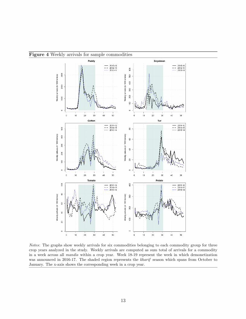
Figure 4 Weekly arrivals for sample commodities

Notes: The graphs show weekly arrivals for six commodities belonging to each commodity group for threecrop years analyzed in the study. Weekly arrivals are computed as sum total of arrivals for a commodityin a week across all mandis within a crop year. Week 18-19 represent the week in which demonetizationwas announced in 2016-17. The shaded region represents the kharif season which spans from October toJanuary. The x-axis shows the corresponding week in a crop year.

13

demonetization, since 2016-17 coincided with a good agricultural season in terms of adequaterains, leading to bumper harvests for many commodities. Many observers have commentedthat the price declines observed could well be due to the high supply this year. Further,estimates of productionin 2016-17 suggests that it is in fact true for at least a few os thecommodities studied (Table 2). X’s indicate control variables discussed later in this section.The estimate from this model is the best proxy for value of trade displaced (or decline)domestically in the mandis and is therefore central to our analysis.

In all the regressions, we use mandi fixed effects to remove time invariant characteristicsof mandis.Agricultural policy in India is a state subject, and several ongoing market reforminitiatives could influence agricultural marketing transactions. We therefore include interac-tions between year and states as controls in part to account for these differential trends in allour pooled regressions. These state-year interactions would also pick up variations in pro-duction patterns across states and years. In addition, we also include year-month interactioneffects. This controls for specific patterns of imports and exports, especially in crops wherethe government manages much of the external trade. It would also control for other macroe-conomic factors (including the scale of replenishment of currency post-demonetization).

We control for day-of-the-week effects, to account for mandi trading days and tradediversion effects between mandis since different mandis might have different holidays. Ourpreferred model includes data for the full year, notwithstanding the fact that the crops maygrow only in a particular season and most of it is marketed within a span of 3-4 months.We use dummy variables for each month to capture the variations in arrivals across months.Month and day effects also take care of variation in number of mandis reporting the data.For all models, we trim 0.05% of the data; we compute robust standard errors. One potentialproblem is the possibility of serial correlation, which could lead to wrong inferences (Bertrandet al., 2004; Angrist and Pischke, 2008). In an alternate version not presented here, we clusterthe errors by mandi -crop, the results don’t change.

In addition, we include a dummy variable to capture the effect of various festivals sincethey have a direct impact on the volume of arrivals and prices. For example, Diwali is animportant festival celebrated across India. The date of the festival, determined based onthe traditional lunar calendar, falls in the month of October or November and varies fromyear to year. To the extent that in the period of our analysis, it straddles pre and post-demonetization dates (November 8) in different years, this could confound the identificationof our estimates. In most of the years in our sample period, the Diwali date was very close tothe date on which demonetization was announced.27 Our analysis of mandi trading patternsaround Diwali indicates that arrivals start falling two days prior Diwali, and pick up aftertwo days of Diwali (see Figure 5). Thus, we control for this effect by including a festivaldummy which takes value one for the period of two days pre and post Diwali, zero otherwise.The festival dummy takes one and zero values around all the other festivals as well. We donot distinguish across these festivals to remove the chances of any bias that may result fromour subjective judgement on the effect of each festival. We also control for the possible effectof national holidays28 by including a holiday dummy that takes value one on these days, and

27During our sample period, the festival of Diwali was on the following dates: November 26, 2011; Novem-ber 13, 2012; November 3, 2013; October 24, 2014; November 11, 2015; and October 30, 2016.

28India has three national holidays: 26th January (Republic day), 15th August (Independence day), and2nd October (Mahatma Gandhi Jayanti).

14

Figure 5 Diwali analysis for a few sample commodities

Notes: The graphs show event-study analysis 15 days pre and post Diwali. The bold blue line indicatesthe mean of arrivals during 2011-12 to 2015-16. The upper dashed blue line indicates the maximum arrivalsin any of the years around Diwali, while the lower dashed line indicates the minimum arrivals. The blackdashed vertical line indicates the Diwali day. The x-axis shows days spanning 15 days before Diwali to 15days post Diwali. We exclude the crop year 2016-17 from this analysis.

15

zero otherwise.Finally, we control for rainfall in all our regression specifications. Rainfall is measured

monthly at the district level. We map all mandis studied here to their corresponding districts.We compute rainfall deficit or surplus as the difference between rainfall in a particularmonth and its historical average in that month over the past ten years. This is normalizedusing the standard deviation of the historical 10-year rainfall data for that month. We usethese positive (and negative) normalized deviation of rainfall as two separate variables toaccount for the differential effect of surplus or deficient rainfall. We include twelve lags ofrainfall data in the specification, to capture the entire cropping season that might potentiallyaffect production, yield and marketed surplus. We particularly care that the pattern ofarrivals across control and treatment years might vary based on the rains, since the latteroverwhelmingly determine sowing and harvest dates. Controlling for lagged rainfall measuresof varying lengths accounts for these differences.

We implement the DD analysis using varying windows after demonetization in order tounderstand whether the impacts are transient or not and to track the strength of the impactof demonetization over time. The variation in impacts over time is likely to arise because oftwo key factors, as mentioned earlier. First, the government took several measures to easethe difficulties farmers were facing as new currency was replenished (as shown in Figure 1and Appendix A). These involved setting higher withdrawal limits for farmers and tradersand enabling cooperative banks in rural areas to transact, among other things. Second, it ispossible that farmers have limited capacity or ability to store and were only able to hold outfor a short time after which they would bring it to mandis for sale even if the prices werelow and their own circumstances challenging. We estimate the model for different windowsaround the event, starting with a comparison of one day after to 233 days after, until June30, 2017, eight months after demonetization.

The identification strategy in this study is predicated on the assumption of parallel trends(i.e., time-invariant unobservable differences across comparison and treatment groups). Thisimplies that in the absence of treatment, the treated unit and control units would have shareda similar trend. We check this by plotting mean pattern of cumulated arrivals and cumulatedvalue of traded for control years vis-a-vis the pattern in the treatment year. Figure 6 showsthe graph for the two variables aggregated across sample commodities and all mandis.29 Wesee that the arrivals as well as the total value of trade follow a similar trend for the treatedand control years, for most of the pre-November 8 period. Nevertheless, our month-yearinteractions take into account the possibility of time-varying trends across the comparisonand treatment years.

We also check for any unusual dips or spikes prior to demonetization and account for thefestival effects to control for Diwali that fell on October 30 in 2016. We believe that otherthan the festival, which we control for, the pre-treatment dip is largely irrelevant becausethe announcement of withdrawal of currency came as a surprise. The announcement cameat 8 p.m. with currency remaining legal tender until midnight that day(Figure 2 earlier).Given that this is not a window for business in agricultural markets it is unlikely that therewas transaction activity in anticipation of the change.

29The blips in the two graphs for the treatment year correspond to Sundays, when most of the mandis areclosed for trading.

16

Figure 6 Cumulated arrivals and value of trade aggregated across all sample commoditiesand mandis for control and treated year

Notes: The graphs show the mean patterns of cumulated arrivals and cumulated value of trade for controlyears vis-a-vis the pattern in treatment year across all commodities and all mandis. We use the mean valueof the cumulated arrivals and value of trade for the control years.

3.3 Triple difference

In Section 2.1, we highlighted that impacts on domestic agricultural trade are likely to differacross commodities as well as mandis. A set of triple-difference regressions aim to capturethese impacts. The generic specification to estimate the impact on total value of trade(Vc,m,t) is given as:

lnVc,m,t = α0 + α1Dpost−Nov8,t + α2D2016,t + α3Dpost−Nov8,t ×D2016,t +

α4Dhet−impact,c/m + α5D2016,t ×Dhet−impact,c/m + α6Dpost−Nov8 ×Dhet−impact,c/m +

α7Dpost−Nov8,t ×D2016,t ×Dhet−impact,c/m + ζXm,t + εc,m,t (2)

Dhet−impact,c/m is a dummy that takes value one for the heterogenous effect that we want toanalyze, zero otherwise. The coefficient associated with the third level interaction term, α7,captures the magnitude of the heterogenous or differential impact.

To isolate the differential impacts on perishables, relative to non-perishables, we definethe variable Dhet−impact,c/m as one for perishables and zero for non-perishables. Similarly,to analyze the impact on kharif crops relative to rabi, we allocate one and zero values toDhet−impact,c/m for kharif and rabi crops, respectively. We expect α7 < 0 for both theseimpacts.

To estimate the differential impacts on mandis with low bank penetration vis-a-vis highbank penetration we set Dhet−impact,c/m to one for mandis in districts with low bank pen-etration, and zero otherwise. Bank penetration is measured at the district level based onpercentage of villages within a district with at least one commercial bank within 5 kms. ofthe village and come from the Census of India, 2011. We divide the sample into terciles,based on the percentage of villages with access, where the first tercile indicates low penetra-tion (lower percentage of villages with access to banks) and the third tercile indicates highpenetration. We assign the dummy variable, Dhet−impact,c/m as one for mandis falling into

17

the first tercile, and zero for mandis in the second or third terciles. The dummy variable,Dhet−impact,c/m in Model 2 is defined similarly to examine the differential impacts in mandiswhich are in districts with low ATM density, relative to the ones with high ATM density.For both bank penetration and ATM density, we expect α7 < 0.30

We also examine variation in impacts across mandis in districts with high market densityversus those in districts with low market density. Market density is captured as the numberof mandis within a district. We define Dhet−impact,c/m = 1 for mandis in the first tercile(low market density) and zero otherwise. We expect that mandis within districts with highmarket density provided farmers more number of options to sell their produce following thecash crunch, and hence the impacts are lower than in mandis with low market density, sothat α7 < 0.

Further, we also estimate Model 2 to assess the variation in impacts by organizing mandisaccording to share in total value of trade in the comparison years. Mandis with less than 2%share in trade value take the value 1, as opposed to the rest. Trade diversion could involveboth a migration to bigger mandis where the prospect for finding a buyer is higher or awayfrom these if they are far relative to smaller mandis. Finally, we assess the impacts onmandis in districts which are identified as urban centres (district with cities with more thanone million inhabitatnts) vis-a-vis other districts. Mandis in these districts are assigned thedummy variable, Dhet−impact,c/m value of one, and zero otherwise. A contraction of consumerdemand and the difficulty of getting produce to the big urban centres is likely to translateinto a higher negative impact near urban centres. At the same time, better access to cashmight support demand and mute the negative impacts. For both these models α7 could beeither greater or less than 0.

4 Results

4.1 Impact on trade value

Our main results are the DD estimates from Model 1. The dependent variable is the loga-rithm of value of arrivals for each mandi, by commodity, each day. We run 233 regressionsto estimate the impact of demonetization on the value of trade for incrementally longer win-dows following the date of demonetization up until the whole period spanning 233 days (fromNovember 8, 2016 to June 30, 2017). This regression pools all commodities traded in eachmandi and to account for commodity specific variation, in addition to the controls detailedin Model 1, we use commodity fixed effects. Figure 7 shows the average treatment effectswith successively larger windows for regressions with and without commodity fixed effects.The largest impacts occurred within a fortnight of demonetization with a trade displacementeffect of around 13% on average at its worst. Thereafter, we observe a steady revival of mar-kets that plateaus quickly after a few days, suggesting reluctant recovery. Remarkably, itseems that the recovery stalled altogether after the 200 day mark. By the end of 233 days

30Chodorow-Reich et al. (2018) argue that the distribution of new notes across different regions in Indiawas almost random, at least in the first few months of demonetization. Since banks and ATMs were the onlymode of new currency notes dissemination to public, the extent of shock would have been further exacerbatedin regions with low bank / ATM density.

18

Figure 7 Impact on mean daily value of trade: DD Estimates

Notes: The graph plots the point estimates along with 95% confidence intervals of the treatment effectsobtained from estimating the DD regression from Model 1. The model is estimate with commodity effectsand without commodity effects. The confidence intervals are based on robust standard errors.

after demonetization, mandis were still seeing an average loss of value of trade to the extentof 10% per mandi per day.

We find that all of these results are statistically significant at 1%. This shows that theimpact of demonetization persisted even after eight months. This is in sharp contrast tothe government’s narrative that agriculture showed significant resilience to the effect of de-monetization (Chand and Singh, 2017). The apparent displacement of domestic agriculturaltrade in value terms could come from a decline in arrivals (supply-side) or a collapse in prices(demand-side) or from a combination of both and we examine this question in detail later.

Despite controls for time-varying trends across the demonetization and comparison yearsand for the pre-November 8 dip in 2016 due to Diwali, there could still be systematic un-observable factors that confound our identification of the causal impact of demonetization.We therefore implement two sets of of placebo tests - ‘in-year’ placebo and ‘in-time’ placebo.The ‘in-year’ placebo assumes that demonetization happened on November 8 in another year,and not in 2016. This involves dropping 2016-17 from the dataset and setting each year from2011-12 to 2015-16 as the year of demonetization, and computing the impacts using the re-maining control years. The ‘in-time’ placebo assumes that the year of demonetization wasthe true year, 2016-17, but occurred on a date before the actual date, that is, November 8,2016. We start by advancing the date of demonetization by one day at a time, and continueto use the remaining years as control. However, we truncate the dataset at November 8 toassess the placebo effect. We start by setting the faux date of demonetization as November7, and compute the 1-day impact on minimum value of trade, then set it as November 6 tocompute the 2-day impact, and so on, until November 1, for which we compute the 5-dayimpact of presumed demonetization. We implement the ‘in-time’ placebo for the faux yearstoo. The effect estimated from both these placebos should either show no patterns or havepatterns that are different from that implied by demonetization. In particular, for 2016-17 ifthe impacts we see are indeed due to demonetization, we should see a significant difference

19

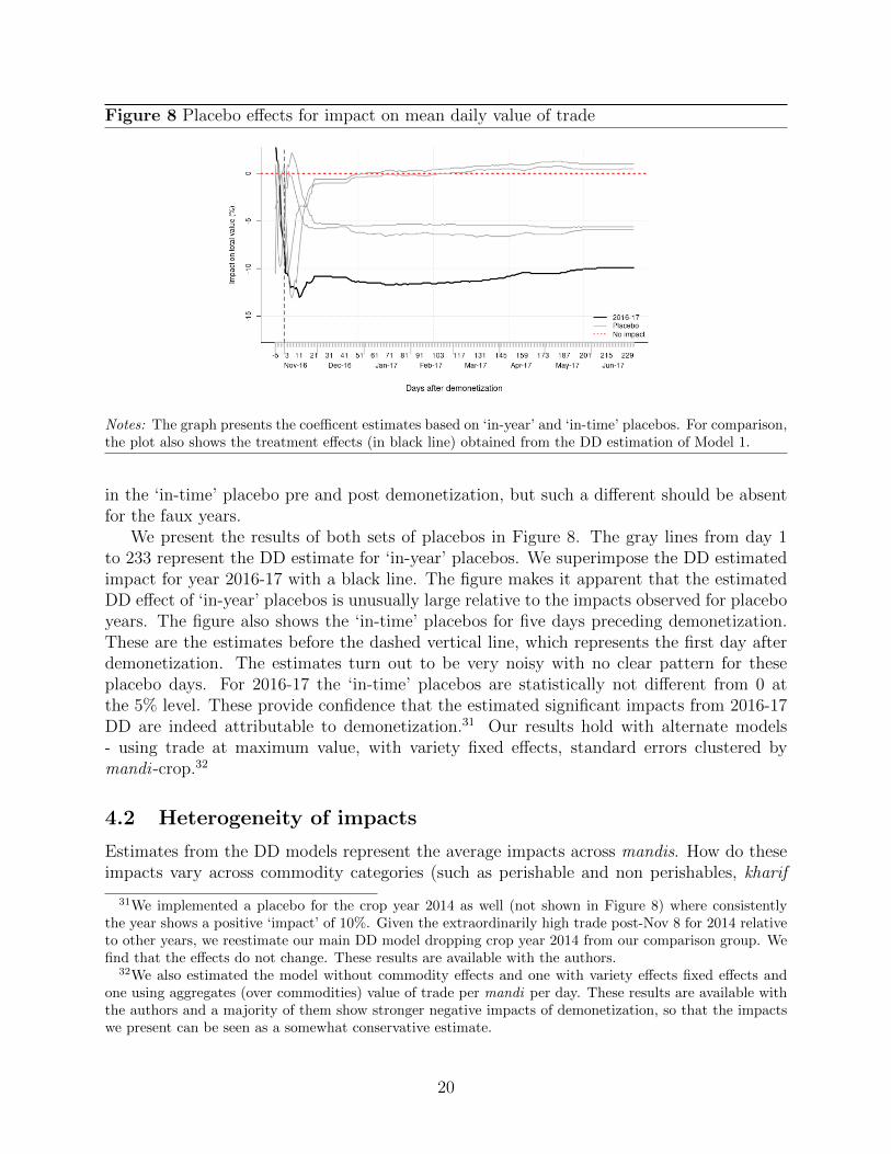
Figure 8 Placebo effects for impact on mean daily value of trade

Notes: The graph presents the coefficent estimates based on ‘in-year’ and ‘in-time’ placebos. For comparison,the plot also shows the treatment effects (in black line) obtained from the DD estimation of Model 1.

in the ‘in-time’ placebo pre and post demonetization, but such a different should be absentfor the faux years.

We present the results of both sets of placebos in Figure 8. The gray lines from day 1to 233 represent the DD estimate for ‘in-year’ placebos. We superimpose the DD estimatedimpact for year 2016-17 with a black line. The figure makes it apparent that the estimatedDD effect of ‘in-year’ placebos is unusually large relative to the impacts observed for placeboyears. The figure also shows the ‘in-time’ placebos for five days preceding demonetization.These are the estimates before the dashed vertical line, which represents the first day afterdemonetization. The estimates turn out to be very noisy with no clear pattern for theseplacebo days. For 2016-17 the ‘in-time’ placebos are statistically not different from 0 atthe 5% level. These provide confidence that the estimated significant impacts from 2016-17DD are indeed attributable to demonetization.31 Our results hold with alternate models- using trade at maximum value, with variety fixed effects, standard errors clustered bymandi -crop.32

4.2 Heterogeneity of impacts

Estimates from the DD models represent the average impacts across mandis. How do theseimpacts vary across commodity categories (such as perishable and non perishables, kharif

31We implemented a placebo for the crop year 2014 as well (not shown in Figure 8) where consistentlythe year shows a positive ‘impact’ of 10%. Given the extraordinarily high trade post-Nov 8 for 2014 relativeto other years, we reestimate our main DD model dropping crop year 2014 from our comparison group. Wefind that the effects do not change. These results are available with the authors.

32We also estimated the model without commodity effects and one with variety effects fixed effects andone using aggregates (over commodities) value of trade per mandi per day. These results are available withthe authors and a majority of them show stronger negative impacts of demonetization, so that the impactswe present can be seen as a somewhat conservative estimate.

20

and rabi crops) and across mandis (based on their locations, access to banks)?The DDD estimates are mostly along expected lines (Equation 2). Columns 3-6 in Table 3

show the α7 estimates for differences across commodity categories. In the weeks immediatelyafter demonetization, perishables saw a decline in total value of trade in the range of 10-17%more in Week 3-7 (22-50 days). Even after 33 weeks (233 days), we see that the declinein total value of trade for perishables was 6.4% more than non perishables. Kharif crops,whose harvests were trading at peak volumes does not show a negative impact of the eventin the short term. We in fact see a positive α7. The effect may be driven by the commoditiessuch as paddy which saw heavy volumes of government procurement in the period followingdemonetization. However, over time, we begin to see strong negative impacts Kharif crops,which at the end of 33 weeks was 4% more than for rabi crops.

Mandis located in districts with lower market density experienced a larger loss in valueof domestic trade (6%) relative to those in districts with more regulated markets (Column 7,Table 3). The size of the mandis captured by market share however does not seem to havemattered. For a brief period, smaller mandis seem to have crowded in trade at the expenseof larger mandis. Presumably during that time, the advantages of better prospects of findinga buyer in the larger mandis were trumped by the higher transactions costs associated withmoving produce all the way to the bigger mandis. It appears that mandis in districts withcities with more than one million inhabitants fared worse than those in less urban districts.The former mandis lost 2.4% more trade than the latter. This is consistent both with acollapse in demand in major consumption centres or inability of traders to move the produceto consumption centres. Both explanations are plausible and the latter interpretation inparticular is largely consistent with our findings on bigger mandis described previously.

Mandis in districts that had better access to commercial banks had smaller adverseimpacts relative to other mandis. Mandis with higher bank penetration saw a lower declinein total value of trade relative to the ones with low bank penetration (1-6.1%). Over eightmonths after demonetization, these differences disappear, as one would expect. Access toATMs on the other hand had no impact, likely many ATMs routinely ran out of cash or notget timely replenishments. ATMs also had to be recalibrated to dispense new notes and thiswas a long drawn out process. This result is therefore not surprising.

4.3 Sources of impacts: Arrivals versus Prices

Our findings thus far are broadly consistent with expected outcomes and have an intuitiveinterpretation. Yet it is unclear what is driving these impacts. Is the decline in value of tradeled predominantly by the supply-side factors or demand-side factors or both? In this section,we attempt to parse the impacts on value to see if they are generated by declines in arrivalsand/or prices. In the absence of clear ways to separate these two impacts, we interpret theprice effect as representing demand-side effects, since mandi prices are typically set by tradersand reflects their demand for farm produce. This is especially the case since our models toestimate price impacts also control for quantity of arrivals. Arrivals are based overwhelminglyon farmers’ decision to take the produce to mandi. Only a fraction of the farmers hold their

21

stock for sale.33 We can therefore interpret the decline in arrivals as approximating supply-side effects. To uncover these patterns, we analyze each of the 35 commodities separately,in part, because aggregating different units and prices are problematic but also to be ableto identify systematic differences between crop characteristics or groups, discussed later inthis section.

We estimate the following models for arrivals and prices respectively.

lnYc,m,t = β0 + β1Dpost−Nov8,t + β2D2016,t + β3Dpost−Nov8,t ×D2016,t + ζXc,m,t

+εc,m,t (3)

where Yc,m,t denotes the logarithmic values daily arrivals in tons for commodity, c, mandi m,and date, t. Similarly, to analyze the impact on prices (lnPc,m, t), we estimate the followingregression:

lnPc,m,t = γ0 + γ1Dpost−Nov8,t + γ2D2016,t + γ3Dpost−Nov8,t + γ4Yc,m,t + ζXc,m,t +

ηc,m,t (4)

We include logarithmic values of arrivals (Yc,m,t) in the specification for prices (Model 4) toaccount for the influence of supply on prices. Thus the coefficient, γ3 provides an estimateof the overall impact on prices. β3 and γ3 represent the coefficient of interest, which capturethe average impact of demonetization on arrivals, and prices in percentage terms. We usethe same set of controls as we did for the previous models. As with the main regression,we estimate the regression for arrivals and prices using varying window sizes ranging from 1days to 233 days after demonetization (Section 3.2).

We present results eight commodities as illustrative examples of the heterogeneity inimpacts - these kharif crops, representing, different commodity groups, include paddy, soy-abean, cotton, tur (pigeon pea), tomato and potato. Paddy markets involve heavy gov-ernment intervention through procurement for food distribution. Soyabean, an oilseed ofconsiderable importance is non-perishable and has strong industry linkages. Cotton is ahigh value cash crop that can be stored. Tur is a key pulse in many Indian diets. Tomatoand Potato represent two of the most important horticultural crops in the country, of whichtomatoes are highly perishable. A and Tables 7-13 present the results for all commodities.

4.3.1 Impact on arrivals

Figure 9 shows the β3 estimates along with the 95% confidence intervals based on Model 3from the regression on arrivals for these commodities.

The β3 coefficient for paddy indicates that there was, in fact, a positive impact on arrivalsafter demonetization, implying higher arrivals. High procurement by various state agencies34

33A nationally representative survey of farmers conducted in 2012-13 suggests that for most crops, Indianfarmers tend to sell their entire harvest in one lot and usually to one buyer.

34As much as 30% of annual production of rice is procured by the Government and much of this is procuredduring November to February. While some of it is procured in the form of rice from millers, a significantshare is bought as paddy and custom milled by the government. Payment for these procurements is, in mostcases, made directly to the bank account of the farmer, with the exception of two states, where it is firsttransferred to the bank accounts of commission agents, who then transfer it to farmers’ bank accounts.

22

Figure 9 Estimated effect of demonetization on arrivals

Notes: The graphs show the β3 coefficient estimate and 95% confidence intervals based on the regressionspecified in Equation 3. The x-axis shows the size of the event window. Confidence intervals are based onrobust standard errors.

23

justify this result. Government reports suggest that paddy procurement for the season 2016-17 as of February 28, 2017 was 8.27% higher than the previous year (Government of India,2016a). Mandis could therefore have crowded in paddy trade.

In the case of soyabean, initially, there was a severe impact of demonetization, witharrivals falling by as much as 80% by Day 7. The situation improved after a few days, withthe decline in arrivals reducing to 50%, but continue to be significantly low. Even after233 days, there are no signs of recovery. Like, soyabean, cotton arrivals too declined by 25%immediately after demonetization, with no sign of recovery. Given the non-perishable natureof the two commodities, the finding is attributable to the supply-side impact.

Among pulses, we see some impact on tur arrivals in the initial few days of demonetiza-tion, but it recovered in later weeks.

For the two horticultural commodities, tomato and potato, as expected, we do not seea decline in arrivals of these commodities. The effects are not statistically different fromzero. Tomato is highly perishable and for potato, other than in eastern India, access tocold storages is still somewhat limited, restricting the ability of farmers to store the crop.Thus, as expected, the results indicate that the supply-side factors were absent in perishablecommodities.

4.3.2 Impact on prices

Commodity-wise price impacts are estimated based on specific regressions described in Model4. Figure 10 presents γ3 estimates and the corresponding 95% confidence intervals for thesame set of commodities presented in Section 4.3.1.

For both paddy and soyabean, there was no impact on prices after demonetization. Cot-ton prices increased in the range of 2-5% after demonetization. In the case of soyabean andcotton, the steep decline in arrivals caused prices to increase, given relatively stable demandfrom solvent extractors and ginning units and spinning mills. Further, as discussed in Sec-tion 4.3.1, paddy and cotton are also procured by the state, hence the payments for thesecommodities is made via checks. In addition, higher purchase of paddy by those seeking todispose old illegal currency, as a way of utilizing the hoarded black money, could have keptthe demand high, and buoyed prices. 35 Prices of tur on the other hand show a decline aftera week of demonetization, in the range of 2-4%. A possible reason for the observed fall inboth prices and arrivals of tur could be attributed to the bumper crop that was observed in2016-17, that might have led farmers to continue selling even at lower prices on account ofstorage constraints 36

Tomato saw a significant decline in prices in the range of 2-7%, but the impacts reducedafter 120 days. In contrast, we see a larger decline in the case of potato prices, with littlesigns of recovery. Prices of potato show a decline of 9-13% in the first few weeks afterdemonetization, and the effect continues to remain even after 233 days. The larger declinein both tomato and potato prices is in line with the hypothesis that relatively more perishablecommodities where farmers did not have a choice to store were sold at significantly low prices

35See Demonetisation effect: cotton arrivals wilt, but prices bloom, Hindu Business Line, November 7,2016.

36See As prices head south, tur dal farmers seek centre’s support, Business Line, Decemeber 6, 2016 andCommodity profiles for Pulses, March 2017

24

Figure 10 Estimated effect of demonetization on prices

Notes: The graphs show the γ3 coefficient estimate and 95% confidence intervals based on the regressionspecified in Equation 4. The x-axis shows the size of the event window. Confidence intervals are based onrobust standard errors.

25

following demonetization. At the same time, this is also consistent with demand contraction,either at the consumer or traders’ end.

In summary, the results indicate the greater dominance of supply-side factors for non-perishable commodities (e.g. soyabean and cotton). Commodities such as paddy which areprocured by state agencies, in fact, instead saw a positive supply-side impact of demoneti-zation due to higher purchases by these agencies. Perishable commodities such as tomatoand potato saw

5 Robustness checks and caveats

In this section, we validate our findings in several ways. We first focus on commodities thatwere not impacted by demonetization as falsification tests. If the withdrawal of notes onlyimpinges on cash transactions, we would not expect it to impact those commodities thatalready have been contracted or where trade is based on electronic payments. Internationaltrade too would not get affected since most trade occurs based on prior, forward contracts.Further, to the extent that such trade is in processed forms of agricultural commodities, theexport of processed commodities would remain unaffected as the processing would have likelyhappened pre-demonetization. For exportables, non-delivery on contracts to internationalclients often has serious costs in terms of reputation. For these reasons too, we believe thatexporters would have found ways of tiding over the crisis and one would not expect negativeimpacts of demonetization. To assess if this is indeed the case, we focus on two sets of exportcommodities: five varieties of coffee (robusta, arabica, plantation, ground, instant) and fiveoilmeals (soyabean, rapeseed, groundnut, ricebran, castorseed). A robustness check for eachof the five coffee exports and oil meals exports shows no effects, when a similar differencein differences strategy is adopted using monthly export data from 2012-2017. Results fromthese tests, reported in Table 4 lends credence to our findings on demonetization impacts.

Our earlier results also suggested that commodities where there is government interven-tion may have been affected to a lesser extent. We focus on milk marketing in the Indianstate of Maharashtra, where three types of buyers dominate, the government dairies, pri-vate dairies and farmer-owned and managed dairy cooperatives. This allows us to check ifprocurement by government has a cushioning influence on the potential negative impactson trade post-demonetization. In the case of milk, we find, as expected, that governmentprocurement of milk shows no impacts (Table 4). However, procurement by private playersand cooperatives are impacted suggesting that the latter likely faced cash shortages in thewake of demonetization. Similarly, the results on procurement of grain are consistent withthe patterns found in the mandi data. Paddy procurement before milling is higher post-demonetization relative to other years and to before demonetization, but this is not the casewith other grains. These estimations use monthly data and do not control for rainfall andare hence best interpreted as a coarse consistency check.

We also analyze data on the quantity and value traded on the futures market platform, theNational Commodities and Derivatives Exchange (NCDEX) to see if the patterns of impactson select commodities are consistent with those from mandi trades. While overall trade onthe NCDEX (both agriculture and non-agricultural commodities) declined (results not shownhere), analysis for an illustrative list of commodities comprising wheat (foodgrain), soyabean

26

(oilseed/pulse), cotton (fibre) and turmeric (spice) that had adequate data is reported inTable 4. We find, as with the results for mandi, cotton and wheat show no impacts whereasthe impact on turmeric and soyabean is quite substantial with the value traded showing alarger negative impact relative to quantity, suggesting that prices were impacted as well.These patterns correspond broadly to the results for mandis.

One concern with attributing impacts from the analysis to demonetization is the con-temporaneous election of a new president in the United States. We believe this is not aconcern for several reasons. Other than a few commodities that are integrated with globalmarkets, most agricultural commodities in India are somewhat insulated from world trade.There is not much evidence that the US elections impacted agricultural commodity marketsworldwide. Given that India is not a key trading partner with the US for most agriculturalcommodities, this is perhaps an unlikely confounding factor. Existence evidence suggests a0.9 to 1.5% decline in soy, corn and wheat futures on November 9, 2016, attributed to theelection results in the US, but nothing beyond.

While our research suggests that there is an impact on many commodities, this effect maybe overestimated if one believes that farmers are diverting trade away from mandis to localmarkets. In this case, the impacts estimated here represent at least in part displacementof trade rather than destruction of trade. In the absence of reliable data it is difficult toget a sense of the extent of displacement.37 Even with these caveats, it is possible that ourestimates of trade displacement potentially seriously underestimates actual welfare losses tofarmers. If, as our field based evidence suggest, transactions did occur at specified prices, butthere was only an exchange of goods but not of money with traders promising farmers to paythem in four or five months, the time lag between trade and payments entails a significantloss of income. To tide over the cash crunch and transacting virtually fully on credit, manyfarmers were borrowing from informal lenders at very high interest rates / consumptionloans.38 One would then expect any negative impacts of demonetization to manifest witha lag akin to a “sleeper effect”. Similarly, the loss of value traded in domestic regulatedmarket entails a loss in revenue earned by the government in terms of mandi fees and taxesand a similar loss to commission agents, brokers and workers in these markets. Our paperdoes not venture to estimate the potential loss to these stakeholders.

We also stop short of estimating longer term consequences of demonetization beyondseven months since it is difficult to gauge whether we are seeing second round effects ofresponses to demonetization rather than demonetization itself. For example, if farmers wereholding out in order to cope with demonetization, it could well be that delayed arrivals causepotential glut in the markets - as all the stored stocks make their way into the market withina narrow window - thereby bringing down prices. The reverse could also be true, that theprice decline post-demonetization attracts traders and processors presumably with betteraccess to credit or financial resources, wish to take advantage of the low prices to buy upstocks, leading to the opposite effect and crowding in trade at the mandi. It is virtuallyimpossible to parse these effects through secondary data. In addition, the anticipation ofthe introduction of Goods and Services Tax (GST) complicates clean identification beyond

37Estimating outside-mandi trade based on marketed surplus estimates applied to secondary data onproduction are notoriously unreliable in the context of Indian agriculture.

38As one farmer in the southern state of Tamil Nadu put it “today, anyone who has cash (that is legaltended) is a money lender” January 07, 2017 Field visit, Madurai/Trichy.

27

a certain window.39 These caveats are relevant while interpreting the results of our analysis.

6 Concluding Remarks

Often, the consequences of monetary policy for the agricultural sector (and perhaps otherinformal) sectors are left unexamined, likely because of the huge challenges in securing thedata to make these assessments. This paper set out to evaluate the short term impacts ofdemonetization on domestic agricultural trade in India, using daily trade data on arrivals ingovernment regulated markets across the country. Using difference in differences techniquesusing past years data as controls, we found that demonetization displaced over 13% of dailytrade on average in the very short run, the effect tapering off only gradually over the nexteight months, the period where our study ends. It is apparent however that the value oftrade in the mandis never really recovered fully and trade was down by 10% on average,even at the end of eight months.

The impacts estimated in this paper offer insights into the the slowdown in GDP growthrates in the three quarters following demonetization. Our findings also provide some un-derstanding of the farmer discontent in recent months across the country. Several Indianstates have seen farmer protests - including Madhya Pradesh, Tamil Nadu, Rajasthan, Ma-harashtra - in the two years following demonetization, including a ‘Long March’ which saw50,000 farmers in Maharashtra walk several hundred kilometres to the state capital to makea representation to the Chief Minister.

Early narratives suggested that demonetization had perhaps not had a big impact (Chandand Singh, 2017). The Economic Survey of India 2016-17, for example, concluded withcautious optimism that perhaps the impacts of demonetization on agriculture had beenoverstated. “Contrary to early fears, as of January 15, 2017 aggregate sowing of the twomajor rabi crops - wheat and pulses (gram)-exceeded last year’s planting by 7.1 percentand 10.7 percent.”(Government of India, 2016a). Yet it would seem that these impactsestimated in this paper suggest significant welfare consequences for farmers. As of 2016-17,horticulture production at 300 million tonnes outstripped the production of foodgrains (275million tonnes). If horticulture trade saw impacts of the magnitude estimated in this paper,especially without improvements even after eight months post-demonetization, one wouldexpect this to reflect perhaps with a lag. It is interesting that although rabi sowing andproduction were healthy, in the immediate aftermath of demonetization, there are markeddeclines in sowing for the kharif season 2017-18 as of September 2017. These shortfalls insowing figures, despite adequate and timely rainfall, is suggestive then, perhaps, of a laggedresponse to the monetary shock of demonetization (Table 5).

If, as pointed out earlier, farmers rely on borrowings at usurious interest rates, then thenegative consequences of trade displacement could be higher than implied by our estimates.There exist ample evidence on poverty traps that suggest that in the absence of markets forcredit and insurance, shocks can push people into poverty and entrap them (Azariadis andStachurski, 2005; Bowles et al., 2006; Carter and Barrett, 2006; Carter et al., 2007; Krishna,2004). If on the other hand, demonetization engineers a transformation of the financial

39Goods and Services Tax (GST) is an indirect tax introduced countrywide on 1 July 2017 replacingmultiple cascading taxes by the federal and state governments.

28

landscape in a way that farmers are integrated into the formal banking system, this couldhold benefits in the long run in ways that may counterbalance these losses. Whether or howmuch farmers welfare is impacted remains to be seen, but the results from our analysis pointto lingering impacts of demonetization on farmers and adverse distributional consequencesoverall.

29

References

Agarwal, Sumit, Debarti Basu, Pulak Ghosh, Bhuvanesh Pareek, and JianZhang, “Demonetization and Digitization,” June 2018. Available at SSRN: https:

//ssrn.com/abstract=3197990.

Aggarwal, Nidhi, Sargam Jain, and Sudha Narayanan, “The Long road to transfor-mation of agricultural markets in India: Lessons from Karnataka,” Economic and PoliticalWeekly, 2017, 52(41), 47–55.

Angrist, Joshua D and Jorn-Steffen Pischke, Mostly Harmless Econometrics: AnEmpiricist’s Companion, Princeton university press, 2008.

Anzuini, A., M. J. Lombardi, and P. Pagano, “The Impact of Monetary Policy Shockson Commodity Prices,” International Journal of Central Banking, September 2013, 9 (3),125–150.

Ardeni, Pier Giorgio and John Freebairn, “Chapter 28 The Macroeconomics of Agri-culture,” in “Agriculture and its External Linkages,” Vol. 2 of Handbook of AgriculturalEconomics, Elsevier, 2002, pp. 1455 – 1485.

Azariadis, Costas and John Stachurski, “Chapter 5 Poverty Traps,” in Philippe Aghionand Steven N. Durlauf, eds., , Vol. 1 of Handbook of Economic Growth, Elsevier, 2005,pp. 295 – 384.

Banerjee, Abhijit, Emily Breza, Arun G Chandrasekhar, and Benjamin Golub,“When Less is More: Experimental Evidence on Information Delivery During India’sDemonetization,” Working Paper 24679, National Bureau of Economic Research June2018.

Barnett, Richard C., David A. Bessler, and Robert L. Thompson, “The MoneySupply and Nominal Agricultural Prices,” American Journal of Agricultural Economics,1983, 65 (2), 303–307.

Belongia, Michael T, “Monetary policy and the farm/nonfarm price ratio: a comparisonof effects in alternative models,” Federal Reserve Bank of St. Louis Review, 1991, 73(July/August 1991).

Bernanke, Ben, Mark Gertler, and Mark Watson, “Systematic Monetary Policy andthe Effects of Oil Price Shocks,” Brookings Papers on Economic Activity, 1997, 28 (1),91–157.

Bertrand, Marianne, Esther Duflo, and Sendhil Mullainathan, “How much shouldwe trust differences-in-differences estimates?,” The Quarterly Journal of Economics, 2004,119 (1), 249–275.

Bhavnani, Rikhil and Mark Copelovitch, “The Political Impact of Monetary shocks:Evidence from India’s 2016 Demonetization,” 2018. Available at SSRN: https://ssrn.com/abstract=3095228.

30

Bowles, Samuel, Steven N Durlauf, and Karla Hoff, Poverty Traps, Princeton Uni-versity Press, 2006.

Carter, Michael R and Christopher B Barrett, “The Economics of Poverty Trapsand Persistent Poverty: An Asset-based Approach,” The Journal of Development Studies,2006, 42 (2), 178–199.

, Peter D Little, Tewodaj Mogues, and Workneh Negatu, “Poverty traps andnatural disasters in Ethiopia and Honduras,” World Development, 2007, 35 (5), 835–856.

Chambers, Robert G., “Agricultural and Financial Market Interdependence in the ShortRun,” American Journal of Agricultural Economics, 1984, 66 (1), 12–24.

Chambers, Robert G and Richard E Just, “An Investigation of the Effect of MonetaryFactors on Agriculture,” Journal of Monetary Economics, 1982, 9 (2), 235–247.

Chand, Ramesh and Jaspal Singh, NITI Aayog, Government of India, Blog series, 2017.

Chodorow-Reich, Gabriel, Gita Gopinath, Prachi Mishra, and AbhinavNarayanan, “Cash and the Economy: Evidence from India’s Demonetization,” Work-ing Paper 25370, National Bureau of Economic Research December 2018.

Ciriacy-Wantrup, Siegfried V, “The Relation of War Economics to Agriculture withParticular Reference to the Effects of Income and Price Inflation and Deflation,” TheAmerican Economic Review, 1940, 30 (1), 366–382.

Dewan, Ritu and Radha Sehgal, Demonetisation: From Deprivation to Destitution,Himalaya Publishing House, Delhi, 2019.

Dharmapala, Dhammika and Vikramaditya Khanna, “Stock Market Reactions toIndia’s 2016 Demonetization: Implications for Tax Evasion, Corruption, and FinancialConstraints,” Working Paper 844, Coase-Sandor Working Paper Series in Law and Eco-nomics 2018.

Diaz-Bonilla, Eugenio and Sherman Robinson, “Macroeconomics, macrosectoral poli-cies, and agriculture in developing countries,” Handbook of Agricultural Economics, 2010,4, 3035–3213.

Frankel, Jeffrey A., “Expectations and Commodity Price Dynamics: The OvershootingModel,” American Journal of Agricultural Economics, 1986, 68 (2), 344–348.

, “The Effect of Monetary Policy on Real Commodity Prices,” in “Asset Prices and Mon-etary Policy,” University of Chicago Press, 2008, pp. 291–333.

and Andrew Rose, “Determinants of Agricultural and Mineral Commodity Prices,” inRenee Fry, Callum Jones, and Christopher Kent, eds., Inflation in an Era of Relative PriceShocks, RBA Annual Conference Volume, Reserve Bank of Australia, December 2010.

Ghosh, Jayati, CP Chandrasekhar, and Prabhat Patnaik, Demonetisation Decoded:A Critique of India’s Currency Experiment, Taylor & Francis, 2017.

31

Government of India, “Price Policy for Kharif Crops, Agricultural Marketing Year 2017-18,” 2016.

, “State of Agriculture in India 2015-16,” 2016.

Goyal, Aparajita, “Information, Direct Access to Farmers, and Rural Market Performancein Central India,” American Economic Journal: Applied Economics, 2010, 2 (3), 22–45.

Hamilton, James D., “Monetary factors in the Great Depression,” Journal of MonetaryEconomics, 1987, 19 (2), 145 – 169.

Karmakar, Bikram, Bhuvanesh Pareek, Dylan S. Small, and Pulak Ghosh, “TheEffect of Demonetization on Digital Payments in India:Causal Inference in the Absence ofControls,” Working Paper November 2018.

Krishna, Anirudh, “Escaping poverty and becoming poor: who gains, who loses, andwhy?,” World Development, 2004, 32 (1), 121–136.

Krishnan, Deepa and Stephan Siegel, “Effects of demonetization: Evidence from 28slum neighbourhoods in Mumbai,” Economic and Political Weekly, 2017, 52(3).

Miskimin, Harry A., “Monetary Movements and Market Structure: Forces for Contractionin Fourteenth- and Fifteenth-Century England,” The Journal of Economic History, 1964,24 (4), 470–490.

Reddy, C. Rammanohar, Demonetisation and the Black Economy, Orient Blackswan,Delhi, 2017.

Schuh, G Edward, “The Exchange Rate and US Agriculture,” American Journal of Agri-cultural Economics, 1974, 56 (1), 1–13.

32

Table 1 Commodities selected for analysis

The table presents the list of commodities selected for the analysis. Arrivals during kharif is computedas percentage of arrivals during October to January in a crop year. Average across 2012-2016 is reported.Mandis reported is computed as number of unique mandis that reported arrivals in a crop year.

Commodity Group Area under cultivation # of mandis Season Arrivals(2015-16, in million hectares) reporting trade during kharif (%)

Bajra Cereals 6.98 437 kharif 50.28Jowar Cereals 5.65 434 37.88Maize Cereals 8.69 762 kharif 56.24Paddy Cereals 43.39 1,073 kharif 76.75Ragi Cereals NA 104 kharif 35.49Rice Cereals NA 497 35.58Wheat Cereals 30.23 1,136 rabi 9.46

Bengal Gram Pulses 8.35 519 rabi 17.75Tur Pulses 3.75 492 kharif 34.66

Soyabean Oilseeds 11.67 450 kharif 63.03Mustard Oilseeds 5.76 582 rabi 16.54Groundnut Oilseeds 4.56 364 kharif 56.62

Cumin Spices 0.70 82 rabi 14.25Coriander Seed Spices 0.62 136 17.81Dry Chillies Spices 0.79 79 24.47Turmeric Spices 0.19 100 19.37

Arecanut Plantation 0.47 93 40.58Cashewnuts Plantation 1.04 52 6.95Copra Plantation 2.09 66 41.22

Cotton Fibre 11.87 464 kharif 64.16

Brinjal Vegetable 0.66 646 34.50Cabbage Vegetable 0.39 526 40.51Cauliflower Vegetable 0.43 543 46.05Okra Vegetable 0.49 539 20.64Onion Vegetable 1.23 836 34.05Potato Vegetable 2.13 835 34.52Tomato Vegetable 0.76 724 33.10

Apple Fruits 0.31 332 47.50Banana Fruits 0.85 444 34.25Guava Fruits 0.25 186 49.16Lemon Fruits 0.26 241 24.31Lime Fruits included above 68 29.98Sweet Lime Fruits 0.22 193 23.23Orange, others Fruits 0.46 212 73.25

1 Area from Agricultural Statistics at a Glance 2016. Some are advance estimates.2 NA is Not available

33

Table 2 How was production in 2016-17 compared to 2003-04 to 2015-16?

This table provides a comparative perspective of production in 2016 in relation to the years 2003-04 to2015-16. We compare the 2016 production with the minimum, maximum and mean of these years and deem2016 to have been better if production exceeded the maximum for that period.

Crop Season Units 2016 production Minimum Maximum Mean Was 2016 better?

Rice Kharif m.tons 93.88 72.23 92.78 84.1 BetterWheat Rabi m.tons 68.64 95.85 82.9Jowar Kharif m.tons 2.42 1.71 4.84 3.3Bajra Kharif m.tons 8.55 6.51 12.11 9.0Maize Kharif m.tons 19.3 11.48 17.14 14.5 BetterRagi/Finger millet Kharif m.tons 1.85 1.44 2.43 2.0Small Millets Kharif m.tons 0.34 0.37 0.56 0.5Coarse Cereals Kharif m.tons 32.45 23.83 33.08 29.2Tur Kharif m.tons 4.29 2.27 3.17 2.7 BetterUrad Kharif m.tons 2.01 0.81 1.43 1.1 BetterMoong Kharif m.tons 1.35 0.44 1.53 1.0Other Kharif Kharif m.tons 1.06 0.49 1.33 0.8Groundnut Kharif h.t.tons 64.98 31.87 80.58 56.0Castorseed Kharif h.t.tons 17.31 7.62 22.95 13.4Sesamum Kharif h.t.tons 6.75 5.88 8.93 7.3Nigerseed Kharif h.t.tons 1.01 0.76 1.21 1.0Rapeseed-Mustard Rabi h.t.tons 58.34 81.79 71.5Linseed Rabi h.t.tons 1.32 1.97 1.6Sunflower Kharif h.t.tons 1.34 0.68 4.63 2.7Soyabean Kharif h.t.tons 142.23 68.76 146.66 102.4Cotton Total lakh

bales#321.23 137.29 359.02 266.7

Jute Total lakhbales

99.05 93.99 112.3 102.9

Mesta Total lakhbales

5.01 5.08 9.9 7.3

Sugarcane Total h.t.tons 3052.46 2338.62 3623.33 3188.0

Cereals Kharif m.tons 126.33 98.59 125.22 113.2769 BetterTotal Pulses Kharif m.tons 8.7 4.2 7.12 5.552308 BetterTotal Foodgrains Kharif m.tons 135.03 103.31 131.27 118.8277 BetterTotal Nine Oilseeds Kharif h.t.tons 233.63 140.12 226.12 182.8054 BetterJute -Mesta Total lakh

bales104.05 102.72 118.17 110.14

Sugarcane Total h.t.tons 3052.46 2338.62 3623.33 3188.014Cotton Total lakh

bales#321.23 137.29 359.02 266.7269

1 Area from Agricultural Statistics at a Glance 2016. Some are advance estimates.2 # means bales are 170kg. Otherwise bales are 180 kgs.3 m. tons and h.t.tons are million and hundred thousand tons repectively.

34

Tab

le3

Het

erog

eneo

us

impac

tsac

ross

com

modit

ies

and

man

di

cate

gori

eson

valu

eof

trad

eaf

ter

dem

onet

izat

ion

Th

eta

ble

pre

sents

het

erog

eneo

us

imp

acts

onth

eva

lue

of

trad

efo

rd

iffer

ent

com

mod

ity

an

dm

an

di

cate

gori

esfr

om

Wee

k0

toW

eek

33

aft

erd

emon

etiz

atio

n.

Th

eco

effici

ents

are

bas

edon

the

trip

led

iffer

ence

regre

ssio

nes

tim

ati

on

of

min

imu

mva

lue

of

tran

sact

ion

sin

each

man

di

each

day

.T

he

firs

tco

lum

nsh

ows

the

nu

mb

erof

wee

ks

afte

rd

emon

etiz

ati

on

.T

he

rem

ain

ing

colu

mn

ssh

owth

ere

sult

sacr

oss

diff

eren

tsu

bgro

up

s.

Days

Week

Peris

hable

sK

harif

Market

Market

Urb

an

Ban

kA

TM

den

sity

share

centr

es

bran

ch

es

pen

etr

ati

on

α7

SE

α7

SE

α7

SE

α7

SE

α7

SE

α7

SE

α7

SE

10

-0.0

05

(0.0

3)

0.1

35

(0.0

7)

-0.0

02

(0.0

5)

0.0

06

(0.2

3)

-0.0

29

(0.0

5)

-0.0

65

(0.0

4)

-0.0

09

(0.0

4)

81

-0.0

03

(0.0

2)

0.2

00

(0.0

4)

-0.0

02

(0.0

2)

0.0

11

(0.1

3)

-0.0

08

(0.0

3)

-0.0

60

(0.0

2)

-0.0

42

(0.0

2)

15

2-0

.052

(0.0

1)

0.1

64

(0.0

3)

-0.0

26

(0.0

2)

0.0

21

(0.1

0)

-0.0

33

(0.0

2)

-0.0

28

(0.0

1)

-0.0

17

(0.0

2)

22

3-0

.098

(0.0

1)

0.1

18

(0.0

2)

-0.0

60

(0.0

2)

-0.0

30

(0.0

8)

-0.0

41

(0.0

2)

-0.0

31

(0.0

1)

-0.0

10

(0.0

1)

29

4-0

.140

(0.0

1)

0.0

91

(0.0

2)

-0.0

85

(0.0

1)

-0.0

34

(0.0

7)

-0.0

32

(0.0

2)

-0.0

19

(0.0

1)

0.0

08

(0.0

1)

36

5-0

.155

(0.0

1)

0.0

72

(0.0

2)

-0.0

93

(0.0

1)

-0.0

22

(0.0

7)

-0.0

32

(0.0

1)

-0.0

15

(0.0

1)

0.0

19

(0.0

1)

43

6-0

.171

(0.0

1)

0.0

63

(0.0

2)

-0.1

05

(0.0

1)

-0.0

07

(0.0

6)

-0.0

27

(0.0

1)

-0.0

12

(0.0

1)

0.0

26

(0.0

1)

50

7-0

.168

(0.0

1)

0.0

66

(0.0

2)

-0.1

14

(0.0

1)

0.0

05

(0.0

6)

-0.0

22

(0.0

1)

-0.0

17

(0.0

1)

0.0

23

(0.0

1)

57

8-0

.168

(0.0

1)

0.0

63

(0.0

2)

-0.1

22

(0.0

1)

-0.0

10

(0.0

6)

-0.0

20

(0.0

1)

-0.0

30

(0.0

1)

0.0

16

(0.0

1)

64

9-0

.166

(0.0

1)

0.0

80

(0.0

1)

-0.1

27

(0.0

1)

-0.0

11

(0.0

6)

-0.0

22

(0.0

1)

-0.0

40

(0.0

1)

0.0

13

(0.0

1)

71

10

-0.1

66

(0.0

1)

0.0

88

(0.0

1)

-0.1

32

(0.0

1)

0.0

03

(0.0

5)

-0.0

25

(0.0

1)

-0.0

46

(0.0

1)

0.0

09

(0.0

1)

78

11

-0.1

56

(0.0

1)

0.0

93

(0.0

1)

-0.1

35

(0.0

1)

0.0

16

(0.0

5)

-0.0

31

(0.0

1)

-0.0

54

(0.0

1)

0.0

08

(0.0

1)

85

12

-0.1

48

(0.0

1)

0.0

86

(0.0

1)

-0.1

34

(0.0

1)

0.0

25

(0.0

5)

-0.0

29

(0.0

1)

-0.0

57

(0.0

1)

0.0

08

(0.0

1)

92

13

-0.1

43

(0.0

1)

0.0

74

(0.0

1)

-0.1

32

(0.0

1)

0.0

31

(0.0

5)

-0.0

26

(0.0

1)

-0.0

61

(0.0

1)

0.0

06

(0.0

1)

99

14

-0.1

39

(0.0

1)

0.0

63

(0.0

1)

-0.1

28

(0.0

1)

0.0

39

(0.0

5)

-0.0

25

(0.0

1)

-0.0

62

(0.0

1)

0.0

04

(0.0

1)

106

15

-0.1

33

(0.0

1)

0.0

39

(0.0

1)

-0.1

27

(0.0

1)

0.0

52

(0.0

5)

-0.0

28

(0.0

1)

-0.0

62

(0.0

1)

0.0

05

(0.0

1)

113

16

-0.1

27

(0.0

1)

0.0

21

(0.0

1)

-0.1

26

(0.0

1)

0.0

53

(0.0

5)

-0.0

29

(0.0

1)

-0.0

58

(0.0

1)

0.0

07

(0.0

1)

120

17

-0.1

23

(0.0

1)

-0.0

12

(0.0

1)

-0.1

22

(0.0

1)

0.0

60

(0.0

5)

-0.0

30

(0.0

1)

-0.0

53

(0.0

1)

0.0

09

(0.0

1)

127

18

-0.1

16

(0.0

1)

-0.0

22

(0.0

1)

-0.1

18

(0.0

1)

0.0

73

(0.0

5)

-0.0

29

(0.0

1)

-0.0

48

(0.0

1)

0.0

11

(0.0

1)

134

19

-0.1

12

(0.0

1)

-0.0

49

(0.0

1)

-0.1

16

(0.0

1)

0.0

76

(0.0

5)

-0.0

30

(0.0

1)

-0.0

43

(0.0

1)

0.0

14

(0.0

1)

141

20

-0.1

08

(0.0

1)

-0.0

68

(0.0

1)

-0.1

12

(0.0

1)

0.0

81

(0.0

5)

-0.0

33

(0.0

1)

-0.0

41

(0.0

1)

0.0

13

(0.0

1)

148

21

-0.1

03

(0.0

1)

-0.0

78

(0.0

1)

-0.1

10

(0.0

1)

0.0

87

(0.0

5)

-0.0

36

(0.0

1)

-0.0

41

(0.0

1)

0.0

10

(0.0

1)

155

22

-0.1

04

(0.0

1)

-0.0

99

(0.0

1)

-0.1

06

(0.0

1)

0.0

86

(0.0

4)

-0.0

39

(0.0

1)

-0.0

40

(0.0

1)

0.0

09

(0.0

1)

162

23

-0.1

07

(0.0

1)

-0.1

21

(0.0

1)

-0.1

00

(0.0

1)

0.0

85

(0.0

4)

-0.0

35

(0.0

1)

-0.0

37

(0.0

1)

0.0

08

(0.0

1)

169

24

-0.1

04

(0.0

1)

-0.1

16

(0.0

1)

-0.0

90

(0.0

1)

0.0

82

(0.0

4)

-0.0

32

(0.0

1)

-0.0

30

(0.0

1)

0.0

13

(0.0

1)

176

25

-0.1

00

(0.0

1)

-0.1

04

(0.0

1)

-0.0

83

(0.0

1)

0.0

72

(0.0

4)

-0.0

31

(0.0

1)

-0.0

24

(0.0

1)

0.0

17

(0.0

1)

183

26

-0.0

92

(0.0

1)

-0.0

89

(0.0

1)

-0.0

75

(0.0

1)

0.0

64

(0.0

4)

-0.0

28

(0.0

1)

-0.0

20

(0.0

1)

0.0

17

(0.0

1)

190

27

-0.0

87

(0.0

1)

-0.0

81

(0.0

1)

-0.0

71

(0.0

1)

0.0

57

(0.0

4)

-0.0

28

(0.0

1)

-0.0

18

(0.0

1)

0.0

18

(0.0

1)

197

28

-0.0

82

(0.0

1)

-0.0

74

(0.0

1)

-0.0

69

(0.0

1)

0.0

56

(0.0

4)

-0.0

27

(0.0

1)

-0.0

15

(0.0

1)

0.0

18

(0.0

1)

204

29

-0.0

78

(0.0

1)

-0.0

67

(0.0

1)

-0.0

67

(0.0

1)

0.0

56

(0.0

4)

-0.0

25

(0.0

1)

-0.0

13

(0.0

1)

0.0

20

(0.0

1)

211

30

-0.0

74

(0.0

1)

-0.0

58

(0.0

1)

-0.0

65

(0.0

1)

0.0

55

(0.0

4)

-0.0

25

(0.0

1)

-0.0

10

(0.0

1)

0.0

22

(0.0

1)

218

31

-0.0

71

(0.0

1)

-0.0

50

(0.0

1)

-0.0

63

(0.0

1)

0.0

52

(0.0

4)

-0.0

26

(0.0

1)

-0.0

07

(0.0

1)

0.0

23

(0.0

1)

225

32

-0.0

67

(0.0

1)

-0.0

47

(0.0

1)

-0.0

61

(0.0

1)

0.0

55

(0.0

4)

-0.0

25

(0.0

1)

-0.0

07

(0.0

1)

0.0

24

(0.0

1)

233

33

-0.0

64

(0.0

1)

-0.0

44

(0.0

1)

-0.0

57

(0.0

1)

0.0

57

(0.0

4)

-0.0

24

(0.0

1)

-0.0

07

(0.0

1)

0.0

24

(0.0

1)

35

Table 4 Robustness Checks: Estimates for select commodities - export, procurement, com-modity exchange based trade

This table presents difference in differences estimates for oilmeal and coffee exports, milk procurement inthe state of Maharashtra by government, cooperatives and private dairy players, grain procurement bygovernment. In addition, estimates for the value and quantity traded of specific commodities in the NationalCommodities and Derivatives Exchange (NCDEX).

Commodity D-in-D estimates Standard Error Details

1 Total Oilmeal exports 6726.52 (61759.54) Monthly data, 2013-2017Soyameal -4956.17 (59728.63) (tonnes)Rapeseed meal 1469.74 (18793.42)Groundnut meal -65.91 (151.14)Castormeal -15763.46 (24495.68)

2 Total Coffee Exports 3330.25 (3342.45) Monthly data, 2001-2017(tonnes)

3 Total milk procure-ment (Maharashtra)

-40.85* (16.81) Monthly data, 2013-2016

Government 0.25 (0.91) (in lakh litres per day)Cooperatives -4.60* (2.07)Private -35.51* (14.88)

4 Total grain procure-ment

-0.14 (0.07) Monthly data, 2011-2017

Rice Procurement -0.17 (0.11) in log (procurement in tenthousand tonnes)

Wheat procurement -0.14 (0.09)Total grain procurement -0.14 (0.07)Unmilled Paddy procure-ment

0.61** (0.14)

Coarse grain procurement -0.5 (0.29)

5a NCDEX Quantitytraded

Daily data 2013-17

Wheat 0.080 (0.38) log (traded qty. in tonnes)Turmeric -1.504** (0.34)Soyabean -1.189* (0.46)Cotton(Shankar/kapas) -0.014 (0.05)

5b NCDEX Value traded Daily data 2013-17Wheat 0.170 (0.32) log (value in lakhs)Turmeric -1.548** (0.36)Soyabean -1.237** (0.44)Cotton(Shankar/kapas) 0.007 (0.08)

1 Coefficients and standard errors presented for the interaction of November-June (cropyear) and 2016, the year of demoneti-zation.

2 ** refers to 1% level of significance, *5% level of significance.3 For milk procurement, the analysis is restricted to the state of Maharashtra, due to data availability.4 The full results are available with the authors.

36

Table 5 Kharif and rabi sowing, 2016-17 and 2017-18

The table presents the area sown in kharif 2017-18 (as on 22.09.2017) and rabi 2016-17 (as on 03.02.2017).

Kharif sowing %age change Rabi sowing %age change

2016-17 (5 yr-avg.) 2017-18 (5 yr-avg.)

CerealsWheat 6.9 4.5Rice -1.3 -4.8 -11.7 -41.2

Pulses -3.5 33.7 11.2 13.5Gram 10.7 12.0Tur -18.0 10.2 21.2 12.6Urad 21.6 72.9 9.0 13.8Moong -8.0 35.5 3.4 -30.5Fieldpea 17.4 18.4Kulthi 6.1 -71.0 -10.9 68.0Lathyrus 9.6 -17.4Other pulses -2.0 43.9 12.1 160.9

Coarse cereals -2.5 -3.5 -5.6 -11.6Jowar -7.4 -22.4 -13.9 -15.8Bajra 1.9 -6.5 9.3 -93.5Ragi 1.0 -12.1 -33.4 -12.7Maize -4.8 9.3 9.4 5.6Small millets -10.9 -27.8Barley 7.5 18.8

Oilseeds -8.7 -6.0 6.2 -0.7Groundnut -11.4 0.1 3.4 -27.2RapeseedMustard 9.3 11.6Safflower -18.6 -53.9Sunflower -14.6 -40.2 -47.4 -65.5Sesamum -12.6 -9.0 -19.8 -81.1Linseed 31.1 23.5Other Oilseeds -36.4 241.2Soyabean -7.7 -4.0Niger 6.7 -27.7Caster -2.6 -30.7

Sugarcane 9.4 -0.2Jute and Mesta -6.5 -15.6Cotton 18.7 -0.6

1 All India Crop Situation obtained from the website of the Department of Agriculture Cooperation and farmers welfare,URL: http://agricoop.nic.in/all-india-crop-situation?page=1.

2 Missing data means the crop is not grown mainly in that season.

37

For Online Publication

A RBI Notifications

38

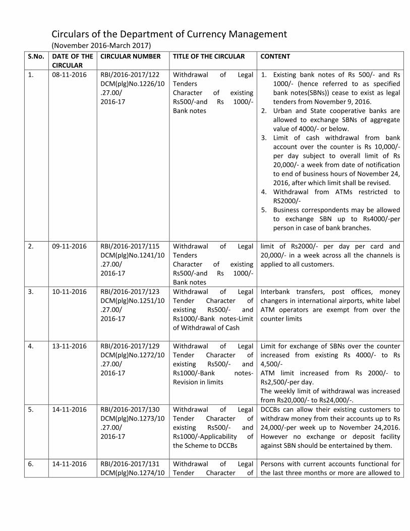
Circulars of the Department of Currency Management (November 2016-March 2017)

S.No. DATE OF THE CIRCULAR

CIRCULAR NUMBER TITLE OF THE CIRCULAR CONTENT

1. 08-11-2016 RBI/2016-2017/122 DCM(plg)No.1226/10.27.00/ 2016-17

Withdrawal of Legal Tenders Character of existing Rs500/-and Rs 1000/- Bank notes

1. Existing bank notes of Rs 500/- and Rs 1000/- (hence referred to as specified bank notes(SBNs)) cease to exist as legal tenders from November 9, 2016.

2. Urban and State cooperative banks are allowed to exchange SBNs of aggregate value of 4000/- or below.

3. Limit of cash withdrawal from bank account over the counter is Rs 10,000/- per day subject to overall limit of Rs 20,000/- a week from date of notification to end of business hours of November 24, 2016, after which limit shall be revised.

4. Withdrawal from ATMs restricted to RS2000/-

5. Business correspondents may be allowed to exchange SBN up to Rs4000/-per person in case of bank branches.

2. 09-11-2016 RBI/2016-2017/115 DCM(plg)No.1241/10.27.00/ 2016-17

Withdrawal of Legal Tenders Character of existing Rs500/-and Rs 1000/- Bank notes

limit of Rs2000/- per day per card and 20,000/- in a week across all the channels is applied to all customers.

3. 10-11-2016 RBI/2016-2017/123 DCM(plg)No.1251/10.27.00/ 2016-17

Withdrawal of Legal Tender Character of existing Rs500/- and Rs1000/-Bank notes-Limit of Withdrawal of Cash

Interbank transfers, post offices, money changers in international airports, white label ATM operators are exempt from over the counter limits

4. 13-11-2016 RBI/2016-2017/129 DCM(plg)No.1272/10.27.00/ 2016-17

Withdrawal of Legal Tender Character of existing Rs500/- and Rs1000/-Bank notes-Revision in limits

Limit for exchange of SBNs over the counter increased from existing Rs 4000/- to Rs 4,500/- ATM limit increased from Rs 2000/- to Rs2,500/-per day. The weekly limit of withdrawal was increased from Rs20,000/- to Rs24,000/-.

5. 14-11-2016 RBI/2016-2017/130 DCM(plg)No.1273/10.27.00/ 2016-17

Withdrawal of Legal Tender Character of existing Rs500/- and Rs1000/-Applicability of the Scheme to DCCBs

DCCBs can allow their existing customers to withdraw money from their accounts up to Rs 24,000/-per week up to November 24,2016. However no exchange or deposit facility against SBN should be entertained by them.

6. 14-11-2016 RBI/2016-2017/131 DCM(plg)No.1274/10

Withdrawal of Legal Tender Character of

Persons with current accounts functional for the last three months or more are allowed to

Circulars of the Department of Currency Management (November 2016-March 2017)

.27.00/ 2016-17

Specified Bank Notes- Expanding the distribution location for deposit and withdrawal of cash

withdraw up to Rs50,000/- per week.

7. 16-11-2016 RBI/2016-2017/135 DCM(plg)No.1287/10.27.00/ 2016-17

Withdrawal of Legal Tender Character of Specified Bank Notes- Compliance with provision of 114B of the Income Tax Rules ,1962

For deposits more than Rs50,000/- in cash a copy of the PAN card has to be submitted in case the bank account is not seeded with the PAN.

8. 17-11-2016 RBI/2016-2017/139 DCM(pg)No.1302/10.27.00/ 2016-17

Withdrawal of Legal Tender Character of existing Rs500/- and Rs1000/-Bank notes-Exchange over the counters

Limit of exchange of SBNs in cash, across the counter of the banks shall be Rs2000/- per person with effect from November 18, 2016.

9. 20-11-2016 RBI/2016-2017/141 DCM(plg)No.1304/10.27.00

Withdrawal of Legal Tender Character of existing Rs500/- and Rs1000/-Bank notes-Revision in limits

Banks may continue to dispense Rs 50/- and Rs 100/- bank notes through the non –recalibrated ATMs until they are re-calibrated with no change in the withdrawal limits.

10. 21-11-2016 RBI/2016-2017/142 DCM(plg)No.1317/10.27.00/ 2016-17

Withdrawal of Legal Tender Character of Specified Bank Notes- Cash Withdrawal Limits

Holders of current / overdraft / cash credit accounts, which are operational for the last three months or more, may now withdraw up to Rs50000 /-in cash, in a week.

11. 21-11-2016 RBI/2016-2017/146 DCM(plg)No.1323/10.27.00/ 2016-17

Withdrawal of Legal Tender Character of existing Rs500/- and Rs1000/-Bank notes-Revisions

Farmers may be allowed to draw up to Rs 25000/- per week in cash from their loan (including Kisan Credit Card limit) or KYC compliant deposit accounts. Traders registered with APMC markets / mandis are allowed to withdraw, in cash, Rs 50,000/- in a week from their KYC complaint current account subject to certain terms and conditions.

12. 22-11-2016 RBI/2016-2017/148 DCM(plg)No.1345/10.27.00/ 2016-17

Making cash available for Rabi Crop Season -Advisory to banks

To ensure adequate credit for farmers in the Rabi season, an estimated Rs 35,000/- crore would be required by the DCCBs for sanctions and disbursement of crop loan to the farmers at the rate Rs10,000/- crore per week. NABARD would utilize its own Cash Credit limits up to about Rs 23,000/- crore to enable DCCBs to disburse the required crop loans to PACS and farmers.

13. 23-11-2016 RBI/2016-2017/151 DCM(plg)No.1351/10.27.00/2016-17

Deposit of Specified Banknotes (SBN) in Small Saving Schemes

Banks are advised not to accept SBNs for deposits in Small Savings Scheme with immediate effect.

14. 24-11-2016 RBI/2016-2017/155 Discontinuation of over No over the counter exchange (in cash) of

Circulars of the Department of Currency Management (November 2016-March 2017)

DCM(plg)No.1391/10.27.00 / 2016-17

the Counters Exchanges of SBN

SBNs will be permitted after midnight of November 24, 2016, instead SBNs can be deposited in the account.

15. 25-11-2016 RBI/2016-2017/158 DCM(plg)No.1424/10.27.00/ 2016-17

Withdrawal of cash – Weekly limit

Cash withdrawals (including ATM withdrawals) allowed up to Rs 24,000/- per week, till further instructions.

16. 28-11-2016 RBI/2016-2017/163 DCM(plg)No.1437/10.27.00/ 2016-17

Withdrawal of cash from bank deposit accounts -Relaxation

Withdrawal of deposits made in current legal tender notes on or after November 29, 2016 beyond the current limits; preferably, available higher denominations bank notes of Rs 2000 /-and Rs 500/- are to be issued for such withdrawals.

17. 29-11-2016 RBI/2016-2017/165 DCM(plg)No.1450/10.27.00/ 2016-17

Accounts under PMJDY - Precautions

Fully KYC compliant account holders may be allowed to withdraw Rs10, 000/- from their account, in a month, while Non KYC compliant account holders may be allowed to withdraw Rs 5,000/- per month from the amount deposited through SBNs after November 09, 2016 within the overall ceiling of Rs10,000/-.

18. 19-12-2016 RBI/2016-2017/189 DCM(plg)No.1859/10.27.00/ 2016-17

Withdrawal of Legal Tender Character of existing Rs500/- and Rs1000/-Bank notes(SBN)- Deposit of Specified Bank Notes into bank accounts

Restrictions on deposits of SBNs into bank accounts 2016 are as indicated below: a. Tenders of SBNs in excess of Rs5000/- into

a bank account will be received for credit only once in KYC complaint accounts during the remaining period till December 30, 2016 after due inspection.

b. Tenders of SBNs up to Rs 5000/- in value received across the counter will allowed to be credited to bank accounts in the normal course until December 30, 2016.

c. Non KYC compliant credits may be restricted up to Rs 50,000/-.

d. The equivalent value of SBNs tendered may be credited to an account maintained by the tenderer or a third party account at any bank in accordance with standard banking procedure and on production of valid proof of Identity.

e. The above restrictions shall not apply to tenders of SBNs for the purpose of deposits under the Taxation and Investment Regime for the Pradhan Mantri Garib Kalyan Yojana, 2016.

19. 30-12-2016 RBI/2016-2017/204 DCM(plg)No.2142/10.27.00/

Cash Withdrawals from ATMs –enhancement of Daily limits

Cash withdrawal from ATMs has been increased with effect from January 01,2017, from the existing Rs 2500/- to Rs 4500/- per

Circulars of the Department of Currency Management (November 2016-March 2017)

2016-17 day per card .

20. 16-01-2017 RBI/2016-2017/213 DCM(plg)No.2559/10.27.00/ 2016-17

Enhancement of withdrawal limits from ATMs and Current Accounts

Limit on withdrawal from ATMs has been enhanced from current limit of Rs4,500/- to Rs10,000/- per day per card and from RS50,000/- to RS1,00,00,/- per week for cuurent, Overdraft and cash credit accounts.

21. 30-01-2017 RBI/2016-2017/217 DCM(plg)No.2905/10.27.00 / 2016-17

Limits on Cash withdrawals from Banks accounts and ATMs – Restoration of status quo ante

Limits placed on cash withdrawal from Saving Bank accounts will continue till February 01, 2017 while limits on Current Accounts/ Cash Credit Accounts/Overdraft Accounts stand withdrawn.

22. 08-02-2016 RBI/2016-2017/224 DCM(plg)No.3107/10.27.00/ 2016-17

Removal of limits of withdrawal of cash from Savings Bank Accounts

Limit on cash withdrawals from Savings Banks Accounts will be enhanced to Rs 50,000/- per week( from current limit of Rs24,000/- per week) and no such limit effective March 13, 2017.

B Impacts on prices and arrivals of individual com-

modities

Table 6 shows the impact on arrivals in the regulated mandis after the note ban of Nov 8,2016. As hypothesized, we find that the arrivals fell in the week after the note ban, acrossalmost all non perishable commodities. The decline in arrivals for perishable commodities ismuch lower than the non perishable commodities.40 Some perishables show even a positivechange in the first week after demonetization. This is similar to the trends observed incontrol years. The table also reports change in arrivals two weeks after demonetizationrelative to the week prior the event. Apple, which has a relatively longer shelf-life than theother perishables analyzed in the study, also saw a significant decline in arrivals in the twoweeks post demonetization. While it appears that the decline in a few commodities such asmaize, rice, tur, cashewnuts recovered slightly, several other commodities continued to seea sharp fall. To put these numbers in perspective, we also examine the mean week-on-weekchanges in arrivals for the control years as well. Except for paddy and raw turmeric, wedo not see such a sharp decline in non perishables arrivals in the remaining years. The lastcolumn in the table also shows the proportion of arrivals that come during the kharif season.The table shows that the impact of the event was not only restricted to kharif crops suchas maize and soyabean but was also observed on rabi crops such as wheat and Bengal gram.

We estimate separate regressions for each commodity to analyze the differential impactson arrivals and prices across commodities. Table 7-10 provide coefficient estimates of theinteraction term that captures the treatment effect.We find that the commodities that werehit the hardest in the immediate aftermath of demonetization were soyabean and corianderseed.41 Soyabean arrivals fell by 75% per mandi per day over the seven to fifteen day periodfollowing demonetization. Coriander seed, on the other hand, saw a decline in trade tothe extent of 98% over the same period. Both these commodities started showing signs ofrecovery over the course of 30 days following demonetization, however the impacts remainstrong even after 200 days. We also see that commodities such as paddy saw a positiveimpact on trade even in the week immediately after the event of demonetization. This couldbe attributed to the increase in procurement of paddy by government to reduce the possibleimpact of the event.42

Perishable commodities including apple, okra, brinjal, cauliflower, potato show an impacton arrivals in the range of 3-216% following the first fifteen days of demonetization. Eventhough the size of the impact is smaller than non perishables, the most likely reason for thisvariation in impacts is due to demand and supply forces. While in the case of perishables,only the demand may have shrunk, depressing only the prices, in the case of non perishables,it is likely that both demand and supply was shrunk.

We also analyze the impact on prices obtained from regressing prices for each commodity.Table 11-14 presents the treatment effects for each commodity. As expected, non perishables

40It is likely that perishables saw a significant decline in prices relatively to the week before demonetization.We analyze this in the section on “Impact on prices”.

41We re-estimate these regressions using maximum value of trade computed as the product of maximumprices and arrivals. Our findings remain the same.

42See Section 2.1 for details.

43

saw lower impact on prices relative to perishables. Dry chilli prices fell by 9% immediatelyafter demonetization, but recovered after 15 days. Other commodities such as soyabeanand tur seed saw a decline of 2-4% in prices in the period following demonetization, butrecovered after a week. The evidence on prices along with the sharp decline in arrivals showsthe supply side impact that dominated for non perishable commodities.

Perishables, where storing is not an option, saw significant impacts on prices due todemonetization. In the week following the announcement, the decline in the prices of perish-ables was in the range of 1-16%. It worsened in the week thereafter, with the impacts beingsignificantly large for cauliflower (29-34%). Other commodities like Brinjal, Lime also saw adecline in prices in the range of 10-16%. The fall in prices of perishables with no impact onarrivals could be attributed to demand contraction.

44

Table 6 Weekly changes in arrivals prior and post demonetization

The table presents one and two weeks changes in arrivals vis-a-vis the week prior demonetization. Columns2 and 3 show the change for 2016-17, that is the year of demonetization. The next two columns show theaverage change around the same date for the remaining years. Since Diwali can have a significant impacton arrivals, the weekly changes for the remaining years are also shown by excluding the impact of Diwali(Column 6 and 7). This is done by excluding three days prior and three days post Diwali if the date ofDiwali falls within the weeks analyzed around demonetization. The last columns shows the proportion ofarrivals that come during the kharif season for each of the sample commodities. All values are presented aspercentage of arrivals in the week prior demonetization.

Treatment year (2016-17) Control years (with Diwali) Control years (w/o Diwali) KharifCommodity Post 1 week Post 2 weeks Post 1 week Post 2 weeks Post 1 week Post 2 weeks arrivals

Paddy -41.51 -29.57 -33.71 -29.84 -36.43 -37.99 76.75Maize -43.14 -8.48 -13.02 34.03 7.93 23.21 56.25Bajra -54.75 -31.91 -3.39 27.27 -2.13 7.30 50.28Jowar -66.84 -54.97 -8.45 42.35 13.80 28.15 37.88Rice -15.81 24.62 4.01 43.33 9.07 34.92 35.58Ragi -13.69 -17.32 -3.81 14.54 12.67 2.81 35.49Wheat -42.11 -44.81 -2.92 30.26 -0.89 3.33 9.46

Soyabean -86.82 -77.50 -13.82 20.33 -6.57 -7.22 63.03Groundnut -55.40 -33.23 17.98 64.64 -1.87 16.55 56.63Mustard -47.39 -44.68 -4.67 21.14 -2.87 -5.33 16.54

Dry Chilli -11.55 28.03 -9.01 33.22 7.05 35.88 24.48Turmeric -55.75 -54.21 62.34 152.65 72.45 153.28 19.30Coriander seed -81.20 -74.96 1.64 72.09 21.66 20.60 17.81Cumin -89.11 -49.74 65.49 266.80 20.47 126.28 14.25

Tur -34.03 4.95 -11.87 19.12 -5.14 15.91 34.66Bengal Gram -69.01 -50.02 -6.96 42.60 6.44 12.20 17.75

Copra -47.31 -13.03 1.47 26.61 -11.69 1.47 41.22Arecanut -32.06 9.84 1.91 58.11 11.97 50.15 40.58Cashewnuts -25.97 26.99 23.78 27.68 36.29 39.52 6.95

Cotton -30.11 3.13 11.91 55.10 5.15 29.81 64.16

Orange 13.51 -49.82 14.48 27.18 -2.68 25.74 73.25Guava 102.75 157.10 36.61 115.16 81.52 116.98 49.16Apple -8.03 -32.68 33.76 99.96 23.31 55.78 47.50Banana -3.69 35.17 -4.02 5.57 -8.73 -6.92 34.25

Cauliflower 10.42 43.53 8.30 44.89 14.19 45.76 46.05Cabbage -2.20 21.66 -1.10 26.48 4.46 24.37 40.51Potato 0.45 17.22 -0.84 30.36 1.60 25.17 34.52Brinjal -7.51 17.09 -4.92 26.63 3.33 29.06 34.50Onion -7.63 1.79 4.81 40.88 3.08 21.95 34.05Tomato -6.05 20.08 -8.60 19.28 -4.95 15.53 33.10Okra -2.82 16.74 -18.36 -4.64 -18.22 -12.13 20.64Lime -9.05 -5.10 -13.10 71.07 -19.52 51.59 29.98Lemon 33.38 4.03 -16.10 11.09 -12.36 16.37 24.31Sweet Lime -15.43 -10.77 5.47 26.47 -0.11 9.74 23.23

45

Tab

le7

Impac

ton

arri

vals

acro

ssco

mm

odit

ies

bet

wee

nday

s1

to25

afte

rdem

onet

izat

ion

1d

ay

aft

er

7d

ays

aft

er

15

days

aft

er

β3

SE

Ob

s.T

reate

dR

2β3

SE

Ob

s.T

reate

dR

2β3

SE

Ob

s.T

reate

dR

2

Pad

dy

0.0

1(0

.06)

207,8

48

701

0.0

5-0

.01

(0.0

5)

219,8

66

2,4

60

0.0

50.1

3(0

.05)

237,5

36

5,2

57

0.0

6M

aiz

e-0

.19

(0.0

9)

101,0

21

406

0.1

2-0

.34

(0.0

7)

106,3

39

1,2

68

0.1

3-0

.25

(0.0

6)

115,5

10

2,9

50

0.1

4B

ajr

a-0

.53

(0.1

)73,2

76

187

0.1

7-0

.50

(0.1

1)

76,5

47

554

0.1

7-0

.39

(0.0

8)

82,1

22

1,3

83

0.1

6Jow

ar

-0.1

9(0

.13)

45,3

11

119

0.0

6-0

.38

(0.0

9)

47,1

96

335

0.0

6-0

.27

(0.0

7)

50,7

28

888

0.0

6R

ice

-0.0

9(0

.04)

112,6

28

289

0.0

3-0

.08

(0.0

3)

117,5

21

1,0

51

0.0

3-0

.10

(0.0

3)

124,4

80

2,1

69

0.0

4R

agi

-0.1

1(0

.23)

9,6

02

31

0.1

9-0

.27

(0.1

8)

9,9

45

82

0.1

9-0

.05

(0.1

3)

10,4

61

160

0.1

9W

hea

t-0

.14

(0.0

6)

226,6

84

353

0.0

6-0

.40

(0.0

5)

234,5

50

1,1

44

0.0

6-0

.39

(0.0

4)

248,3

86

3,1

69

0.0

7S

oyab

ean

-0.4

6(0

.13)

82,8

35

213

0.4

1-0

.81

(0.1

3)

87,0

74

644

0.4

2-0

.75

(0.0

9)

95,1

31

2,0

16

0.4

2G

rou

nd

nu

t-0

.27

(0.1

6)

44,3

79

115

0.1

8-0

.34

(0.1

1)

46,6

81

362

0.1

9-0

.18

(0.1

)50,6

64

851

0.1

9M

ust

ard

-0.3

0(0

.08)

108,4

72

140

0.0

7-0

.25

(0.0

7)

112,1

73

486

0.0

7-0

.33

(0.0

6)

118,0

82

1,1

87

0.0

8D

ryC

hilli

-0.2

1(0

.14)

8,7

45

34

0.3

2-0

.14

(0.1

2)

9,1

43

101

0.3

1-0

.09

(0.1

1)

9,7

54

209

0.3

1T

urm

eric

-0.4

3(0

.46)

10,4

67

34

0.1

4-0

.38

(0.3

4)

10,8

94

93

0.1

4-0

.35

(0.1

9)

11,5

21

198

0.1

4C

ori

an

der

seed

-0.7

7(0

.22)

17,7

43

25

0.1

2-0

.98

(0.1

7)

18,3

78

72

0.1

2-1

.04

(0.1

5)

19,5

72

227

0.1

2C

um

in0.3

1(0

.27)

15,1

22

12

0.2

20.2

3(0

.23)

15,5

85

20

0.2

20.1

1(0

.27)

16,4

68

56

0.2

2A

rhar

-0.1

6(0

.11)

41,5

21

104

0.1

4-0

.17

(0.1

)42,8

57

309

0.1

4-0

.14

(0.0

9)

45,1

47

796

0.1

3B

engalG

ram

-0.0

4(0

.09)

77,0

42

139

0.1

5-0

.18

(0.0

7)

79,6

94

442

0.1

5-0

.21

(0.0

6)

84,0

02

1,1

28

0.1

5C

op

ra0.0

0(0

.13)

9,2

08

41

0.1

1-0

.07

(0.0

8)

9,6

40

138

0.1

0-0

.06

(0.0

8)

10,2

84

274

0.1

1A

reca

nu

t-0

.02

(0.1

)17,5

45

71

0.2

00.0

1(0

.07)

18,2

35

241

0.2

0-0

.01

(0.0

7)

19,3

76

500

0.2

1C

ash

ewnu

ts0.4

2(0

.26)

2,8

00

50.2

7-0

.06

(0.1

8)

2,8

99

25

0.2

60.0

8(0

.16)

3,0

37

45

0.2

7C

ott

on

-0.0

3(0

.08)

49,0

54

332

0.2

9-0

.19

(0.0

7)

53,8

70

1,1

38

0.2

9-0

.22

(0.0

7)

62,1

86

2,4

86

0.2

9O

ran

ge

0.1

2(0

.1)

13,2

88

79

0.2

5-0

.04

(0.0

9)

15,1

39

293

0.2

5-0

.09

(0.0

9)

17,9

98

619

0.2

5G

uava

0.0

9(0

.12)

20,1

04

53

0.1

80.0

3(0

.1)

21,2

80

200

0.1

70.0

1(0

.12)

23,2

11

454

0.1

7A

pp

le0.0

1(0

.06)

95,6

49

254

0.2

9-0

.05

(0.0

5)

100,2

19

889

0.2

8-0

.13

(0.0

4)

106,5

26

1,7

80

0.2

7B

an

an

a-0

.04

(0.0

5)

111,2

79

285

0.0

4-0

.02

(0.0

4)

115,9

76

1,0

02

0.0

4-0

.02

(0.0

3)

122,6

87

2,0

84

0.0

4C

au

lifl

ow

er0.0

2(0

.03)

122,4

93

516

0.1

80.0

1(0

.03)

130,3

08

1,9

04

0.1

90.0

6(0

.03)

141,7

98

3,9

83

0.2

1C

ab

bage

0.0

3(0

.04)

107,5

00

411

0.0

60.0

4(0

.03)

113,2

78

1,4

24

0.0

60.0

2(0

.03)

121,8

89

3,0

14

0.0

7P

ota

to0.0

4(0

.03)

263,6

28

749

0.0

40.0

5(0

.02)

274,9

20

2,6

51

0.0

40.0

2(0

.02)

291,1

66

5,5

02

0.0

5B

rin

jal

0.0

3(0

.03)

203,3

28

622

0.0

50.0

2(0

.02)

212,1

51

2,1

58

0.0

50.0

4(0

.02)

224,6

13

4,4

09

0.0

5O

nio

n0.0

1(0

.03)

235,3

40

682

0.0

80.0

1(0

.02)

245,3

57

2,3

09

0.0

8-0

.02

(0.0

2)

260,2

20

4,8

82

0.0

8T

om

ato

0.0

2(0

.03)

230,9

43

676

0.0

5-0

.01

(0.0

2)

240,7

94

2,4

45

0.0

50.0

0(0

.02)

254,8

30

5,0

12

0.0

6O

kra

-0.0

8(0

.05)

150,5

45

338

0.0

9-0

.09

(0.0

4)

154,6

13

1,1

10

0.1

0-0

.07

(0.0

4)

160,0

42

2,2

21

0.1

0L

ime

0.2

5(0

.11)

12,2

96

39

0.1

20.1

2(0

.08)

12,7

49

112

0.1

20.1

2(0

.07)

13,4

07

220

0.1

2L

emon

-0.0

7(0

.09)

54,6

81

113

0.1

5-0

.04

(0.0

7)

56,6

23

368

0.1

5-0

.08

(0.0

5)

59,4

30

764

0.1

5S

wee

tL

ime

0.0

1(0

.09)

52,5

64

91

0.0

8-0

.01

(0.0

6)

54,5

14

296

0.0

9-0

.02

(0.0

6)

57,1

42

572

0.1

0

46

Tab

le8

Impac

ton

arri

vals

acro

ssco

mm

odit

ies

bet

wee

nday

s22

to45

afte

rdem

onet

izat

ion

22

day

aft

er

30

days

aft

er

45

days

aft

er

β3

SE

Ob

s.T

reate

dR

2β3

SE

Ob

s.T

reate

dR

2β3

SE

Ob

s.T

reate

dR

2

Pad

dy

0.1

8(0

.05)

251,7

13

7,6

09

0.0

70.1

7(0

.05)

268,6

62

10,5

30

0.0

70.1

7(0

.05)

300,0

75

15,7

59

0.0

8M

aiz

e-0

.22

(0.0

6)

123,1

16

4,4

64

0.1

5-0

.21

(0.0

5)

132,0

73

6,3

34

0.1

5-0

.23

(0.0

5)

148,3

00

9,5

16

0.1

5B

ajr

a-0

.32

(0.0

8)

86,8

01

2,2

12

0.1

6-0

.31

(0.0

7)

92,4

44

3,2

95

0.1

5-0

.30

(0.0

7)

102,4

20

5,1

77

0.1

4Jow

ar

-0.2

5(0

.07)

53,7

46

1,4

38

0.0

6-0

.24

(0.0

7)

57,3

95

2,1

45

0.0

6-0

.26

(0.0

7)

64,0

03

3,3

89

0.0

5R

ice

-0.1

0(0

.03)

130,4

33

3,1

27

0.0

4-0

.10

(0.0

3)

137,4

67

4,2

12

0.0

4-0

.10

(0.0

3)

150,1

94

6,1

47

0.0

4R

agi

-0.0

6(0

.12)

10,8

90

222

0.1

9-0

.06

(0.1

2)

11,3

86

304

0.2

0-0

.07

(0.1

1)

12,4

13

494

0.2

0W

hea

t-0

.32

(0.0

4)

260,0

50

5,1

75

0.0

7-0

.32

(0.0

4)

274,0

91

7,6

85

0.0

7-0

.32

(0.0

4)

299,3

32

12,0

61

0.0

7S

oyab

ean

-0.5

7(0

.07)

101,5

95

3,3

04

0.4

2-0

.57

(0.0

7)

109,4

58

5,0

66

0.4

2-0

.58

(0.0

7)

123,2

77

7,9

53

0.4

1G

rou

nd

nu

t-0

.05

(0.1

)53,9

64

1,3

50

0.2

0-0

.06

(0.1

)57,8

68

1,9

87

0.2

0-0

.09

(0.0

9)

64,8

47

3,0

98

0.1

9M

ust

ard

-0.2

8(0

.06)

123,0

54

1,9

14

0.0

8-0

.28

(0.0

6)

129,1

57

2,8

41

0.0

8-0

.28

(0.0

6)

140,2

45

4,5

88

0.0

8D

ryC

hilli

-0.1

2(0

.12)

10,2

48

299

0.2

9-0

.11

(0.1

2)

10,8

70

423

0.2

8-0

.09

(0.1

2)

12,0

17

614

0.2

7T

urm

eric

-0.3

4(0

.17)

12,0

60

289

0.1

3-0

.34

(0.1

7)

12,6

81

391

0.1

3-0

.33

(0.1

7)

13,8

30

581

0.1

2C

ori

an

der

seed

-0.8

3(0

.12)

20,5

80

433

0.1

3-0

.83

(0.1

1)

21,8

39

713

0.1

3-0

.83

(0.1

1)

24,0

87

1,2

14

0.1

4C

um

in0.2

4(0

.28)

17,2

21

114

0.2

20.2

4(0

.28)

18,1

74

215

0.2

20.2

1(0

.28)

19,9

24

419

0.2

2A

rhar

-0.1

0(0

.09)

47,1

35

1,2

40

0.1

3-0

.12

(0.0

9)

49,8

19

1,8

66

0.1

2-0

.14

(0.0

9)

55,7

69

3,2

02

0.1

1B

engalG

ram

-0.1

6(0

.06)

87,6

04

1,7

69

0.1

5-0

.17

(0.0

6)

91,9

03

2,5

67

0.1

5-0

.18

(0.0

6)

99,6

79

3,9

56

0.1

6C

op

ra-0

.05

(0.0

8)

10,8

02

386

0.1

1-0

.05

(0.0

8)

11,4

07

517

0.1

1-0

.05

(0.0

7)

12,5

81

769

0.1

1A

reca

nu

t-0

.01

(0.0

7)

20,3

29

717

0.2

1-0

.01

(0.0

7)

21,4

35

985

0.2

1-0

.00

(0.0

7)

23,5

07

1,4

55

0.2

1C

ash

ewnu

ts0.1

5(0

.16)

3,1

48

63

0.2

80.1

5(0

.16)

3,2

65

83

0.2

80.1

4(0

.15)

3,4

82

117

0.2

9C

ott

on

-0.2

3(0

.07)

69,3

94

3,7

55

0.2

9-0

.25

(0.0

7)

78,2

93

5,4

09

0.2

8-0

.26

(0.0

7)

94,9

29

8,3

49

0.2

7O

ran

ge

-0.1

0(0

.1)

20,3

67

916

0.2

5-0

.11

(0.1

)23,3

49

1,2

79

0.2

4-0

.15

(0.1

)28,5

99

1,9

10

0.2

3G

uava

-0.0

5(0

.13)

24,9

55

693

0.1

7-0

.07

(0.1

3)

27,3

96

984

0.1

7-0

.10

(0.1

3)

32,0

17

1,5

36

0.1

6A

pp

le-0

.15

(0.0

4)

111,5

60

2,4

87

0.2

6-0

.15

(0.0

4)

117,4

79

3,2

73

0.2

6-0

.16

(0.0

4)

128,3

12

4,7

83

0.2

6B

an

an

a-0

.02

(0.0

3)

128,1

69

2,9

43

0.0

4-0

.02

(0.0

3)

134,6

39

3,9

41

0.0

4-0

.02

(0.0

3)

146,3

90

5,7

48

0.0

5C

au

lifl

ow

er0.0

5(0

.03)

151,4

77

5,7

26

0.2

10.0

5(0

.03)

163,1

92

7,8

00

0.2

20.0

5(0

.03)

184,9

85

11,6

26

0.2

2C

ab

bage

0.0

0(0

.03)

129,1

76

4,3

39

0.0

70.0

0(0

.03)

138,0

93

5,9

18

0.0

8-0

.00

(0.0

3)

154,8

16

8,8

42

0.0

9P

ota

to0.0

0(0

.02)

304,7

89

7,8

22

0.0

50.0

1(0

.02)

321,4

67

10,6

12

0.0

50.0

1(0

.02)

352,2

51

15,6

75

0.0

5B

rin

jal

0.0

4(0

.02)

234,7

53

6,2

30

0.0

50.0

4(0

.02)

246,8

34

8,3

75

0.0

50.0

4(0

.02)

268,1

76

12,2

15

0.0

5O

nio

n-0

.02

(0.0

2)

272,6

57

6,9

54

0.0

7-0

.02

(0.0

2)

287,8

07

9,4

11

0.0

7-0

.02

(0.0

2)

315,7

83

13,9

62

0.0

7T

om

ato

0.0

1(0

.02)

266,4

69

7,0

81

0.0

60.0

0(0

.02)

281,0

09

9,5

90

0.0

60.0

0(0

.02)

308,0

67

14,1

40

0.0

6O

kra

-0.0

6(0

.04)

164,1

85

3,0

68

0.1

1-0

.05

(0.0

4)

168,8

04

4,0

30

0.1

1-0

.05

(0.0

4)

177,0

43

5,6

47

0.1

1L

ime

0.1

0(0

.08)

13,9

77

310

0.1

10.0

9(0

.08)

14,6

00

401

0.1

10.0

8(0

.08)

15,7

48

569

0.1

1L

emon

-0.0

9(0

.05)

61,7

53

1,0

81

0.1

5-0

.09

(0.0

5)

64,4

69

1,4

62

0.1

5-0

.09

(0.0

5)

69,2

67

2,1

77

0.1

5S

wee

tL

ime

0.0

2(0

.06)

59,1

12

760

0.1

00.0

2(0

.06)

61,3

75

970

0.1

10.0

2(0

.06)

65,2

56

1,3

21

0.1

3

47

Tab

le9

Impac

ton

arri

vals

acro

ssco

mm

odit

ies

bet

wee

nday

s60

to12

0af

ter

dem

onet

izat

ion

60

day

aft

er

90

days

aft

er

120

days

aft

er

β3

SE

Ob

s.T

reate

dR

2β3

SE

Ob

s.T

reate

dR

2β3

SE

Ob

s.T

reate

dR

2

Pad

dy

0.1

7(0

.05)

328,4

70

20,3

02

0.0

80.1

6(0

.05)

383,1

45

29,4

44

0.0

80.1

6(0

.05)

431,6

79

37,3

08

0.0

8M

aiz

e-0

.24

(0.0

5)

162,9

84

12,1

38

0.1

5-0

.25

(0.0

5)

191,8

73

17,9

28

0.1

4-0

.26

(0.0

5)

218,6

85

23,2

61

0.1

3B

ajr

a-0

.30

(0.0

7)

111,6

63

6,6

68

0.1

3-0

.28

(0.0

7)

129,5

77

10,0

59

0.1

3-0

.28

(0.0

7)

147,2

27

13,3

42

0.1

3Jow

ar

-0.2

7(0

.07)

70,1

01

4,4

06

0.0

5-0

.28

(0.0

6)

82,1

24

6,7

14

0.0

5-0

.28

(0.0

6)

94,3

69

9,1

42

0.0

5R

ice

-0.1

1(0

.03)

162,1

63

7,7

56

0.0

4-0

.11

(0.0

3)

187,8

83

11,6

56

0.0

4-0

.11

(0.0

3)

213,8

23

15,5

76

0.0

4R

agi

-0.0

6(0

.11)

13,4

72

690

0.2

0-0

.05

(0.1

1)

15,6

01

1,0

21

0.2

0-0

.03

(0.1

1)

17,9

67

1,3

84

0.1

9W

hea

t-0

.33

(0.0

4)

322,6

48

15,6

96

0.0

8-0

.33

(0.0

4)

370,7

54

24,3

53

0.1

0-0

.32

(0.0

4)

420,7

68

33,8

65

0.0

9S

oyab

ean

-0.6

0(0

.07)

135,5

06

10,3

97

0.4

0-0

.60

(0.0

7)

160,3

10

15,9

39

0.3

8-0

.61

(0.0

7)

183,2

36

21,1

56

0.3

6G

rou

nd

nu

t-0

.11

(0.0

9)

71,1

81

4,0

93

0.1

8-0

.11

(0.0

9)

83,3

88

6,2

21

0.1

7-0

.11

(0.0

9)

95,1

09

8,4

27

0.1

5M

ust

ard

-0.2

8(0

.06)

150,4

42

5,9

38

0.0

8-0

.27

(0.0

6)

172,2

37

9,7

18

0.0

8-0

.24

(0.0

6)

200,1

54

15,0

82

0.1

0D

ryC

hilli

-0.0

8(0

.13)

13,1

20

796

0.2

5-0

.09

(0.1

3)

15,3

88

1,2

03

0.2

5-0

.09

(0.1

4)

17,8

99

1,6

30

0.2

3T

urm

eric

-0.3

3(0

.17)

14,9

43

761

0.1

2-0

.32

(0.1

7)

17,2

88

1,1

90

0.1

1-0

.32

(0.1

7)

19,8

60

1,6

32

0.1

2C

ori

an

der

seed

-0.8

2(0

.11)

26,1

73

1,6

35

0.1

5-0

.81

(0.1

1)

30,7

54

2,6

12

0.1

5-0

.73

(0.1

1)

37,1

40

3,9

92

0.2

3C

um

in0.2

2(0

.29)

21,5

98

616

0.2

20.1

9(0

.29)

24,7

43

1,1

25

0.2

20.2

2(0

.29)

28,8

64

1,8

98

0.2

2A

rhar

-0.1

5(0

.09)

63,4

92

4,7

70

0.1

3-0

.12

(0.0

9)

83,1

09

9,4

27

0.1

9-0

.06

(0.0

9)

103,5

46

14,7

64

0.2

2B

engalG

ram

-0.1

9(0

.06)

107,2

77

5,0

55

0.1

6-0

.20

(0.0

6)

125,5

81

8,0

39

0.1

5-0

.16

(0.0

6)

149,3

85

13,2

76

0.1

6C

op

ra-0

.04

(0.0

7)

13,6

79

1,0

06

0.1

1-0

.05

(0.0

7)

15,9

44

1,5

37

0.1

1-0

.06

(0.0

7)

18,3

49

2,0

84

0.1

0A

reca

nu

t0.0

1(0

.07)

25,6

88

1,9

05

0.2

10.0

2(0

.07)

30,2

83

2,9

21

0.2

20.0

3(0

.07)

35,0

69

3,9

89

0.2

1C

ash

ewnu

ts0.1

3(0

.15)

3,6

85

152

0.3

20.1

4(0

.16)

4,2

14

240

0.2

90.1

5(0

.16)

5,2

29

491

0.2

2C

ott

on

-0.2

7(0

.07)

110,2

57

10,7

82

0.2

6-0

.30

(0.0

7)

141,1

98

16,2

21

0.2

4-0

.30

(0.0

7)

170,2

26

21,4

53

0.2

2O

ran

ge

-0.1

6(0

.1)

32,5

55

2,3

40

0.2

1-0

.18

(0.1

)39,9

39

3,3

88

0.2

0-0

.19

(0.1

)49,5

78

5,0

49

0.1

7G

uava

-0.1

2(0

.13)

36,0

96

1,9

66

0.1

6-0

.14

(0.1

3)

44,0

05

2,9

02

0.1

5-0

.15

(0.1

3)

49,0

07

3,4

25

0.1

6A

pp

le-0

.16

(0.0

4)

137,5

85

5,8

95

0.2

6-0

.16

(0.0

4)

156,8

24

8,5

92

0.2

7-0

.16

(0.0

4)

176,0

45

11,3

80

0.2

8B

an

an

a-0

.02

(0.0

3)

156,5

87

7,2

07

0.0

5-0

.02

(0.0

3)

178,7

54

10,7

88

0.0

6-0

.01

(0.0

3)

201,8

36

14,4

80

0.0

6C

au

lifl

ow

er0.0

4(0

.03)

205,1

40

14,8

30

0.2

10.0

4(0

.03)

249,3

46

22,6

53

0.2

10.0

4(0

.03)

292,8

58

30,4

51

0.2

0C

ab

bage

-0.0

0(0

.03)

170,5

66

11,4

11

0.0

9-0

.01

(0.0

3)

204,4

55

17,5

25

0.1

0-0

.01

(0.0

3)

238,7

44

23,7

22

0.0

9P

ota

to0.0

1(0

.02)

380,4

70

19,8

03

0.0

50.0

1(0

.02)

441,4

96

29,9

17

0.0

50.0

1(0

.02)

502,8

39

40,2

26

0.0

6B

rin

jal

0.0

4(0

.02)

287,0

70

15,3

51

0.0

50.0

4(0

.02)

326,4

51

22,7

46

0.0

50.0

4(0

.02)

365,8

22

30,0

50

0.0

5O

nio

n-0

.02

(0.0

2)

341,7

67

17,8

21

0.0

7-0

.02

(0.0

2)

396,7

23

27,1

55

0.0

7-0

.02

(0.0

2)

452,0

19

36,7

31

0.0

7T

om

ato

0.0

0(0

.02)

333,0

73

17,9

92

0.0

6-0

.00

(0.0

2)

387,0

77

27,1

60

0.0

6-0

.01

(0.0

2)

441,5

93

36,5

02

0.0

6O

kra

-0.0

4(0

.04)

184,5

80

7,0

20

0.1

1-0

.04

(0.0

4)

200,4

21

10,1

50

0.1

2-0

.04

(0.0

4)

218,1

68

13,7

07

0.1

2L

ime

0.0

8(0

.08)

16,8

86

723

0.1

10.0

8(0

.08)

19,1

62

1,0

17

0.1

10.0

8(0

.08)

21,5

19

1,3

26

0.1

1L

emon

-0.0

9(0

.05)

73,4

87

2,7

37

0.1

5-0

.10

(0.0

5)

82,1

70

4,1

21

0.1

5-0

.10

(0.0

5)

91,4

83

5,6

70

0.1

5S

wee

tL

ime

0.0

3(0

.06)

68,2

33

1,5

75

0.1

40.0

3(0

.06)

74,6

71

2,2

10

0.1

70.0

4(0

.06)

82,3

11

3,0

51

0.1

8

48

Tab

le10

Impac

ton

arri

vals

acro

ssco

mm

odit

ies

bet

wee

nday

s15

0to

233

afte

rdem

onet

izat

ion

150

day

aft

er

200

days

aft

er

233

days

aft

er

β3

SE

Ob

s.T

reate

dR

2β3

SE

Ob

s.T

reate

dR

2β3

SE

Ob

s.T

reate

dR

2

Pad

dy

0.1

6(0

.05)

472,8

91

43,9

17

0.0

80.1

6(0

.05)

541,0

08

55,6

50

0.0

70.1

7(0

.05)

590,1

64

63,4

28

0.0

7M

aiz

e-0

.26

(0.0

5)

242,6

61

27,7

70

0.1

2-0

.25

(0.0

5)

282,8

78

35,9

99

0.1

1-0

.26

(0.0

6)

311,6

21

41,1

67

0.1

1B

ajr

a-0

.27

(0.0

7)

161,9

84

15,9

86

0.1

4-0

.26

(0.0

7)

187,9

12

20,9

88

0.1

3-0

.27

(0.0

7)

207,6

29

24,6

88

0.1

2Jow

ar

-0.2

8(0

.07)

104,7

53

11,2

55

0.0

5-0

.28

(0.0

7)

122,3

37

14,7

57

0.0

5-0

.29

(0.0

7)

136,5

48

17,1

27

0.0

5R

ice

-0.1

1(0

.03)

239,3

71

19,4

26

0.0

4-0

.11

(0.0

3)

281,9

36

26,3

25

0.0

3-0

.11

(0.0

3)

311,9

39

31,3

16

0.0

3R

agi

-0.0

2(0

.12)

20,3

57

1,7

83

0.1

80.0

5(0

.13)

24,5

60

2,5

18

0.1

70.0

4(0

.13)

27,3

06

2,9

74

0.1

7W

hea

t-0

.30

(0.0

4)

471,6

76

43,7

73

0.1

3-0

.29

(0.0

4)

592,8

62

66,0

91

0.2

3-0

.29

(0.0

4)

659,9

78

78,3

37

0.2

2S

oyab

ean

-0.6

2(0

.07)

200,0

51

24,9

41

0.3

5-0

.60

(0.0

7)

230,4

48

31,5

12

0.3

5-0

.60

(0.0

7)

252,9

82

35,1

51

0.3

4G

rou

nd

nu

t-0

.11

(0.1

)105,2

00

10,0

93

0.1

4-0

.11

(0.1

)122,6

16

12,9

51

0.1

3-0

.14

(0.1

)136,6

77

15,0

59

0.1

2M

ust

ard

-0.2

1(0

.06)

232,1

43

20,9

43

0.1

9-0

.17

(0.0

6)

290,2

80

30,9

77

0.2

3-0

.17

(0.0

6)

326,4

63

36,9

28

0.2

2D

ryC

hilli

-0.1

1(0

.14)

20,2

55

1,9

92

0.2

1-0

.11

(0.1

4)

23,9

32

2,5

99

0.1

9-0

.13

(0.1

3)

26,4

67

3,0

03

0.1

8T

urm

eric

-0.3

0(0

.16)

22,5

17

2,1

06

0.1

2-0

.29

(0.1

7)

27,2

54

3,0

55

0.1

4-0

.29

(0.1

7)

30,6

35

3,6

73

0.1

4C

ori

an

der

seed

-0.6

7(0

.12)

43,1

97

5,1

87

0.2

8-0

.64

(0.1

2)

53,4

69

7,3

44

0.2

8-0

.66

(0.1

2)

59,8

36

8,4

30

0.2

7C

um

in0.2

2(0

.29)

33,5

09

2,7

14

0.3

30.2

6(0

.29)

42,5

16

4,1

16

0.3

50.2

7(0

.29)

48,0

18

4,8

43

0.3

3A

rhar

-0.0

5(0

.1)

120,7

20

19,2

31

0.2

2-0

.01

(0.1

)148,4

24

26,2

11

0.2

10.0

1(0

.1)

165,2

68

30,2

01

0.2

0B

engalG

ram

-0.1

3(0

.06)

174,0

56

19,1

25

0.2

0-0

.08

(0.0

6)

218,5

00

29,9

65

0.2

3-0

.08

(0.0

6)

246,8

26

35,9

76

0.2

2C

op

ra-0

.05

(0.0

7)

20,5

22

2,5

92

0.1

0-0

.05

(0.0

7)

24,1

72

3,4

13

0.1

0-0

.06

(0.0

7)

26,8

18

4,0

01

0.0

9A

reca

nu

t0.0

2(0

.07)

39,6

01

4,9

76

0.2

10.0

2(0

.07)

47,4

29

6,5

67

0.2

00.0

2(0

.07)

53,0

00

7,6

55

0.2

1C

ash

ewnu

ts0.1

6(0

.16)

6,7

44

832

0.2

20.1

9(0

.17)

10,4

68

1,5

59

0.1

90.2

3(0

.17)

12,0

18

1,8

29

0.1

8C

ott

on

-0.3

2(0

.07)

192,3

37

25,0

89

0.2

2-0

.31

(0.0

7)

218,4

19

29,3

79

0.2

3-0

.30

(0.0

7)

228,2

01

30,7

95

0.2

4O

ran

ge

-0.1

9(0

.11)

61,3

98

6,9

67

0.1

6-0

.17

(0.1

1)

72,9

10

8,7

60

0.1

6-0

.17

(0.1

1)

74,9

47

9,0

62

0.1

6G

uava

-0.1

5(0

.13)

51,7

69

3,6

54

0.1

8-0

.15

(0.1

3)

53,2

49

3,8

06

0.1

9-0

.15

(0.1

3)

53,9

03

3,9

02

0.1

9A

pp

le-0

.16

(0.0

4)

193,4

84

13,8

45

0.3

0-0

.16

(0.0

4)

217,3

39

17,6

53

0.3

2-0

.15

(0.0

4)

230,9

47

20,2

68

0.3

4B

an

an

a-0

.01

(0.0

3)

225,3

95

18,0

73

0.0

6-0

.01

(0.0

3)

264,8

98

24,1

76

0.0

6-0

.01

(0.0

3)

291,6

65

28,5

42

0.0

5C

au

lifl

ow

er0.0

4(0

.03)

333,7

05

37,3

85

0.1

80.0

6(0

.03)

380,4

53

45,5

04

0.1

90.0

6(0

.03)

404,4

06

50,0

59

0.2

0C

ab

bage

-0.0

2(0

.03)

271,7

25

29,4

85

0.0

9-0

.01

(0.0

3)

315,4

21

37,1

45

0.0

8-0

.01

(0.0

3)

341,3

00

41,8

89

0.0

9P

ota

to0.0

1(0

.02)

563,9

00

50,3

21

0.0

50.0

1(0

.02)

662,1

97

67,0

52

0.0

50.0

2(0

.02)

729,7

98

78,9

99

0.0

6B

rin

jal

0.0

4(0

.02)

406,8

61

37,4

73

0.0

50.0

4(0

.02)

482,3

45

50,5

36

0.0

50.0

4(0

.02)

532,9

80

59,2

65

0.0

4O

nio

n-0

.02

(0.0

2)

507,3

11

45,9

38

0.0

7-0

.02

(0.0

2)

602,2

36

61,9

25

0.0

7-0

.02

(0.0

2)

667,4

84

73,2

13

0.0

7T

om

ato

-0.0

1(0

.02)

495,2

30

45,6

45

0.0

5-0

.01

(0.0

2)

584,7

16

60,9

89

0.0

5-0

.01

(0.0

2)

644,5

57

71,5

66

0.0

5O

kra

-0.0

4(0

.04)

239,3

95

18,0

60

0.1

2-0

.06

(0.0

4)

292,6

18

28,0

32

0.1

2-0

.07

(0.0

4)

335,8

16

35,4

75

0.1

1L

ime

0.0

7(0

.08)

23,9

89

1,6

58

0.1

10.0

7(0

.08)

28,4

05

2,3

12

0.1

10.0

6(0

.08)

31,7

55

2,8

00

0.1

0L

emon

-0.1

0(0

.05)

101,2

42

7,1

81

0.1

4-0

.12

(0.0

5)

121,6

96

10,3

79

0.1

4-0

.12

(0.0

5)

137,3

62

12,7

67

0.1

5S

wee

tL

ime

0.0

5(0

.06)

91,5

02

4,0

98

0.1

70.0

5(0

.06)

108,6

74

6,2

82

0.1

50.0

5(0

.06)

119,9

72

7,7

65

0.1

4

49

Tab

le11

Impac

ton

pri

ces

acro

ssco

mm

odit

ies

bet

wee

nday

s1

to25

afte

rdem

onet

izat

ion

1d

ay

aft

er

7d

ays

aft

er

15

days

aft

er

β3

SE

Ob

s.T

reate

dR

2β3

SE

Ob

s.T

reate

dR

2β3

SE

Ob

s.T

reate

dR

2

Pad

dy

0.0

1(0

)207,8

48

701.0

00.5

20.0

0(0

)219,8

66

2,4

60.0

00.5

10.0

0(0

)237,5

36

5,2

57.0

00.5

0M

aiz

e-0

.00

(0.0

1)

101,0

21

406.0

00.4

70.0

1(0

.01)

106,3

39

1,2

68.0

00.4

70.0

1(0

)115,5

10

2,9

50.0

00.4

8B

ajr

a-0

.00

(0.0

1)

73,2

76

187.0

00.6

70.0

0(0

.01)

76,5

47

554.0

00.6

70.0

2(0

.01)

82,1

22

1,3

83.0

00.6

7Jow

ar

0.0

4(0

.02)

45,3

11

119.0

00.3

30.0

4(0

.01)

47,1

96

335.0

00.3

30.0

3(0

.01)

50,7

28

888.0

00.3

3R

ice

-0.0

0(0

.01)

112,6

28

289.0

00.4

9-0

.00

(0)

117,5

21

1,0

51.0

00.4

9-0

.00

(0)

124,4

80

2,1

69.0

00.4

9R

agi

0.0

7(0

.04)

9,6

02

31.0

00.7

30.0

5(0

.02)

9,9

45

82.0

00.7

30.0

5(0

.03)

10,4

61

160.0

00.7

3W

hea

t-0

.00

(0.0

1)

226,6

84

353.0

00.7

4-0

.01

(0)

234,5

50

1,1

44.0

00.7

50.0

1(0

)248,3

86

3,1

69.0

00.7

4S

oyab

ean

-0.0

4(0

.02)

82,8

35

213.0

00.6

4-0

.03

(0.0

1)

87,0

74

644.0

00.6

4-0

.01

(0.0

1)

95,1

31

2,0

16.0

00.6

3G

rou

nd

nu

t0.0

2(0

.02)

44,3

79

115.0

00.3

2-0

.00

(0.0

2)

46,6

81

362.0

00.3

20.0

0(0

.02)

50,6

64

851.0

00.3

2M

ust

ard

0.0

1(0

)108,4

72

140.0

00.7

60.0

0(0

)112,1

73

486.0

00.7

6-0

.00

(0)

118,0

82

1,1

87.0

00.7

6D

ryC

hilli

-0.0

9(0

.05)

8,7

45

34.0

00.5

2-0

.04

(0.0

3)

9,1

43

101.0

00.5

2-0

.02

(0.0

3)

9,7

54

209.0

00.5

1T

urm

eric

-0.0

0(0

.02)

10,4

67

34.0

00.4

50.0

3(0

.01)

10,8

94

93.0

00.4

60.0

1(0

.02)

11,5

21

198.0

00.4

6C

ori

an

der

seed

-0.0

3(0

.03)

17,7

43

25.0

00.6

8-0

.00

(0.0

3)

18,3

78

72.0

00.6

9-0

.04

(0.0

2)

19,5

72

227.0

00.6

9C

um

in-0

.06

(0.0

5)

15,1

22

12.0

00.3

4-0

.08

(0.0

4)

15,5

85

20.0

00.3

4-0

.08

(0.0

3)

16,4

68

56.0

00.3

4A

rhar

-0.0

4(0

.02)

41,5

21

104.0

00.7

1-0

.02

(0.0

2)

42,8

57

309.0

00.7

0-0

.03

(0.0

1)

45,1

47

796.0

00.7

0B

engalG

ram

0.0

0(0

.02)

77,0

42

139.0

00.8

40.0

2(0

.01)

79,6

94

442.0

00.8

4-0

.02

(0.0

1)

84,0

02

1,1

28.0

00.8

3C

op

ra0.0

3(0

.03)

9,2

08

41.0

00.8

10.0

2(0

.02)

9,6

40

138.0

00.8

00.0

1(0

.02)

10,2

84

274.0

00.7

9A

reca

nu

t0.0

2(0

.03)

17,5

45

71.0

00.5

80.0

1(0

.02)

18,2

35

241.0

00.5

70.0

0(0

.02)

19,3

76

500.0

00.5

7C

ash

ewnu

ts0.0

3(0

.02)

2,8

00

5.0

00.2

70.0

4(0

.02)

2,8

99

25.0

00.2

80.0

0(0

.03)

3,0

37

45.0

00.2

9C

ott

on

0.0

2(0

.01)

49,0

54

332.0

00.2

30.0

4(0

.01)

53,8

70

1,1

38.0

00.2

40.0

4(0

.01)

62,1

86

2,4

86.0

00.2

4O

ran

ge

-0.0

7(0

.06)

13,2

88

79.0

00.3

70.0

1(0

.05)

15,1

39

293.0

00.3

70.0

5(0

.07)

17,9

98

619.0

00.3

7G

uava

0.0

0(0

.06)

20,1

04

53.0

00.4

3-0

.11

(0.0

5)

21,2

80

200.0

00.4

3-0

.13

(0.0

5)

23,2

11

454.0

00.4

3A

pp

le0.0

0(0

.02)

95,6

49

254.0

00.3

60.0

1(0

.02)

100,2

19

889.0

00.3

50.0

2(0

.02)

106,5

26

1,7

80.0

00.3

5B

an

an

a0.0

0(0

.01)

111,2

79

285.0

00.3

7-0

.01

(0.0

1)

115,9

76

1,0

02.0

00.3

7-0

.01

(0.0

1)

122,6

87

2,0

84.0

00.3

7C

au

lifl

ow

er-0

.08

(0.0

2)

122,4

93

516.0

00.3

7-0

.14

(0.0

2)

130,3

08

1,9

04.0

00.4

0-0

.29

(0.0

2)

141,7

98

3,9

83.0

00.4

5C

ab

bage

-0.0

4(0

.02)

107,5

00

411.0

00.4

0-0

.03

(0.0

1)

113,2

78

1,4

24.0

00.4

0-0

.05

(0.0

2)

121,8

89

3,0

14.0

00.4

1P

ota

to-0

.03

(0.0

1)

263,6

28

749.0

00.7

8-0

.06

(0.0

1)

274,9

20

2,6

51.0

00.7

8-0

.09

(0.0

1)

291,1

66

5,5

02.0

00.7

8B

rin

jal

-0.0

7(0

.02)

203,3

28

622.0

00.3

4-0

.09

(0.0

1)

212,1

51

2,1

58.0

00.3

5-0

.14

(0.0

2)

224,6

13

4,4

09.0

00.3

5O

nio

n0.0

9(0

.01)

235,3

40

682.0

00.8

20.1

1(0

.01)

245,3

57

2,3

09.0

00.8

10.1

7(0

.01)

260,2

20

4,8

82.0

00.8

1T

om

ato

-0.0

7(0

.01)

230,9

43

676.0

00.4

3-0

.06

(0.0

1)

240,7

94

2,4

45.0

00.4

4-0

.05

(0.0

1)

254,8

30

5,0

12.0

00.4

5O

kra

-0.0

0(0

.02)

150,5

45

338.0

00.2

3-0

.02

(0.0

2)

154,6

13

1,1

10.0

00.2

3-0

.07

(0.0

2)

160,0

42

2,2

21.0

00.2

4L

ime

-0.1

4(0

.09)

12,2

96

39.0

00.3

6-0

.16

(0.0

7)

12,7

49

112.0

00.3

6-0

.11

(0.0

6)

13,4

07

220.0

00.3

6L

emon

-0.0

5(0

.04)

54,6

81

113.0

00.4

9-0

.01

(0.0

3)

56,6

23

368.0

00.4

8-0

.04

(0.0

2)

59,4

30

764.0

00.4

8S

wee

tL

ime

0.0

5(0

.03)

52,5

64

91.0

00.5

00.0

2(0

.03)

54,5

14

296.0

00.4

9-0

.00

(0.0

2)

57,1

42

572.0

00.4

9

50

Tab

le12

Impac

ton

pri

ces

acro

ssco

mm

odit

ies

bet

wee

nday

s22

to45

afte

rdem

onet

izat

ion

22

day

aft

er

30

days

aft

er

45

days

aft

er

β3

SE

Ob

s.T

reate

dR

2β3

SE

Ob

s.T

reate

dR

2β3

SE

Ob

s.T

reate

dR

2

Pad

dy

-0.0

0(0

)251,7

13

7,6

09

0.4

9-0

.00

(0)

268,6

62

10,5

30

0.4

9-0

.00

(0)

300,0

75

15,7

59

0.4

9M

aiz

e0.0

1(0

)123,1

16

4,4

64

0.4

80.0

1(0

)132,0

73

6,3

34

0.4

80.0

1(0

)148,3

00

9,5

16

0.4

8B

ajr

a0.0

2(0

.01)

86,8

01

2,2

12

0.6

70.0

2(0

.01)

92,4

44

3,2

95

0.6

70.0

2(0

.01)

102,4

20

5,1

77

0.6

7Jow

ar

0.0

3(0

.01)

53,7

46

1,4

38

0.3

20.0

3(0

.01)

57,3

95

2,1

45

0.3

20.0

3(0

.01)

64,0

03

3,3

89

0.3

1R

ice

-0.0

1(0

)130,4

33

3,1

27

0.4

9-0

.01

(0)

137,4

67

4,2

12

0.4

9-0

.01

(0)

150,1

94

6,1

47

0.4

9R

agi

0.0

5(0

.03)

10,8

90

222

0.7

30.0

5(0

.03)

11,3

86

304

0.7

40.0

5(0

.03)

12,4

13

494

0.7

5W

hea

t0.0

1(0

)260,0

50

5,1

75

0.7

50.0

1(0

)274,0

91

7,6

85

0.7

60.0

1(0

)299,3

32

12,0

61

0.7

6S

oyab

ean

-0.0

0(0

)101,5

95

3,3

04

0.6

3-0

.00

(0)

109,4

58

5,0

66

0.6

3-0

.00

(0)

123,2

77

7,9

53

0.6

3G

rou

nd

nu

t0.0

1(0

.01)

53,9

64

1,3

50

0.3

30.0

1(0

.01)

57,8

68

1,9

87

0.3

30.0

1(0

.01)

64,8

47

3,0

98

0.3

3M

ust

ard

-0.0

0(0

)123,0

54

1,9

14

0.7

6-0

.00

(0)

129,1

57

2,8

41

0.7

5-0

.00

(0)

140,2

45

4,5

88

0.7

4D

ryC

hilli

-0.0

3(0

.03)

10,2

48

299

0.5

1-0

.02

(0.0

3)

10,8

70

423

0.5

0-0

.02

(0.0

3)

12,0

17

614

0.4

9T

urm

eric

0.0

1(0

.02)

12,0

60

289

0.4

70.0

1(0

.02)

12,6

81

391

0.4

70.0

1(0

.02)

13,8

30

581

0.4

8C

ori

an

der

seed

-0.0

3(0

.02)

20,5

80

433

0.6

9-0

.03

(0.0

2)

21,8

39

713

0.6

9-0

.03

(0.0

2)

24,0

87

1,2

14

0.6

9C

um

in-0

.04

(0.0

3)

17,2

21

114

0.3

4-0

.04

(0.0

3)

18,1

74

215

0.3

4-0

.03

(0.0

3)

19,9

24

419

0.3

4A

rhar

-0.0

4(0

.01)

47,1

35

1,2

40

0.7

0-0

.03

(0.0

1)

49,8

19

1,8

66

0.7

1-0

.03

(0.0

1)

55,7

69

3,2

02

0.7

1B

engalG

ram

-0.0

2(0

.01)

87,6

04

1,7

69

0.8

3-0

.02

(0.0

1)

91,9

03

2,5

67

0.8

3-0

.03

(0.0

1)

99,6

79

3,9

56

0.8

3C

op

ra0.0

1(0

.02)

10,8

02

386

0.7

90.0

1(0

.02)

11,4

07

517

0.7

90.0

2(0

.02)

12,5

81

769

0.7

8A

reca

nu

t-0

.00

(0.0

2)

20,3

29

717

0.5

6-0

.00

(0.0

2)

21,4

35

985

0.5

6-0

.00

(0.0

2)

23,5

07

1,4

55

0.5

6C

ash

ewnu

ts0.0

1(0

.03)

3,1

48

63

0.2

90.0

1(0

.03)

3,2

65

83

0.3

00.0

1(0

.03)

3,4

82

117

0.3

1C

ott

on

0.0

5(0

.01)

69,3

94

3,7

55

0.2

40.0

4(0

.01)

78,2

93

5,4

09

0.2

50.0

4(0

.01)

94,9

29

8,3

49

0.2

7O

ran

ge

0.1

0(0

.08)

20,3

67

916

0.3

60.1

1(0

.08)

23,3

49

1,2

79

0.3

70.1

1(0

.09)

28,5

99

1,9

10

0.4

1G

uava

-0.1

1(0

.05)

24,9

55

693

0.4

3-0

.11

(0.0

5)

27,3

96

984

0.4

2-0

.11

(0.0

5)

32,0

17

1,5

36

0.4

1A

pp

le0.0

2(0

.02)

111,5

60

2,4

87

0.3

40.0

2(0

.02)

117,4

79

3,2

73

0.3

40.0

2(0

.02)

128,3

12

4,7

83

0.3

4B

an

an

a-0

.02

(0.0

1)

128,1

69

2,9

43

0.3

7-0

.02

(0.0

1)

134,6

39

3,9

41

0.3

7-0

.02

(0.0

1)

146,3

90

5,7

48

0.3

7C

au

lifl

ow

er-0

.34

(0.0

2)

151,4

77

5,7

26

0.4

7-0

.34

(0.0

2)

163,1

92

7,8

00

0.5

0-0

.33

(0.0

2)

184,9

85

11,6

26

0.5

3C

ab

bage

-0.0

4(0

.02)

129,1

76

4,3

39

0.4

1-0

.04

(0.0

2)

138,0

93

5,9

18

0.4

1-0

.04

(0.0

2)

154,8

16

8,8

42

0.4

4P

ota

to-0

.13

(0.0

1)

304,7

89

7,8

22

0.7

7-0

.13

(0.0

1)

321,4

67

10,6

12

0.7

6-0

.13

(0.0

1)

352,2

51

15,6

75

0.7

5B

rin

jal

-0.1

6(0

.02)

234,7

53

6,2

30

0.3

4-0

.16

(0.0

2)

246,8

34

8,3

75

0.3

5-0

.16

(0.0

2)

268,1

76

12,2

15

0.3

6O

nio

n0.1

9(0

.01)

272,6

57

6,9

54

0.8

00.1

9(0

.01)

287,8

07

9,4

11

0.8

00.1

9(0

.01)

315,7

83

13,9

62

0.7

9T

om

ato

-0.0

4(0

.01)

266,4

69

7,0

81

0.4

6-0

.04

(0.0

1)

281,0

09

9,5

90

0.4

7-0

.04

(0.0

1)

308,0

67

14,1

40

0.4

9O

kra

-0.0

7(0

.02)

164,1

85

3,0

68

0.2

4-0

.07

(0.0

2)

168,8

04

4,0

30

0.2

5-0

.08

(0.0

2)

177,0

43

5,6

47

0.2

6L

ime

-0.1

0(0

.07)

13,9

77

310

0.3

5-0

.10

(0.0

7)

14,6

00

401

0.3

5-0

.11

(0.0

7)

15,7

48

569

0.3

5L

emon

-0.0

6(0

.02)

61,7

53

1,0

81

0.4

8-0

.06

(0.0

2)

64,4

69

1,4

62

0.4

8-0

.05

(0.0

2)

69,2

67

2,1

77

0.4

8S

wee

tL

ime

-0.0

1(0

.03)

59,1

12

760

0.4

9-0

.01

(0.0

3)

61,3

75

970

0.4

9-0

.01

(0.0

3)

65,2

56

1,3

21

0.4

9

51

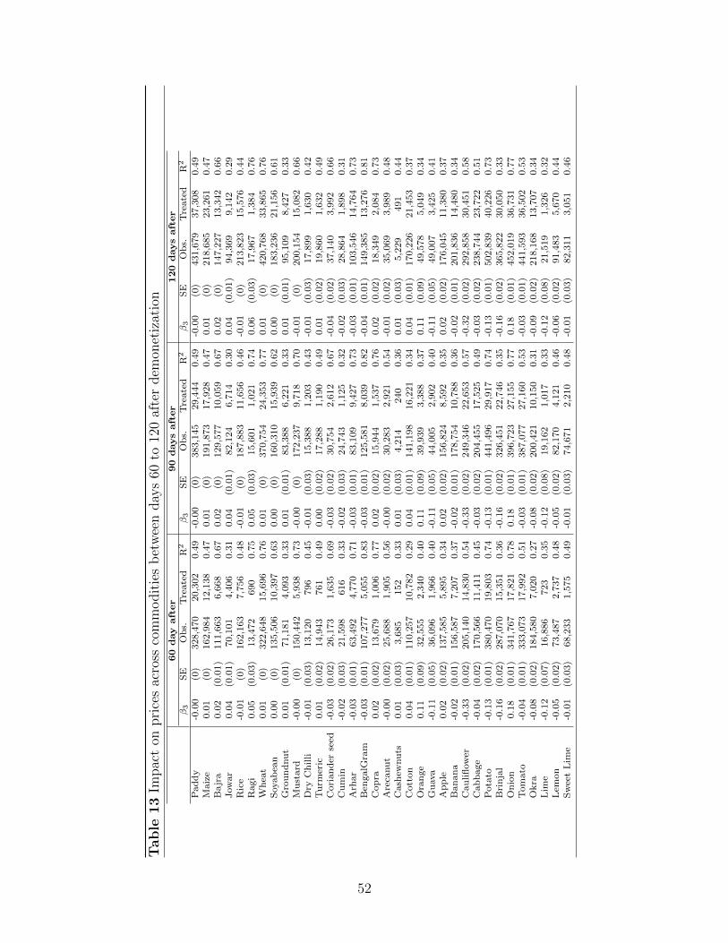
Tab

le13

Impac

ton

pri

ces

acro

ssco

mm

odit

ies

bet

wee

nday

s60

to12

0af

ter

dem

onet

izat

ion

60

day

aft

er

90

days

aft

er

120

days

aft

er

β3

SE

Ob

s.T

reate

dR

2β3

SE

Ob

s.T

reate

dR

2β3

SE

Ob

s.T

reate

dR

2

Pad

dy

-0.0

0(0

)328,4

70

20,3

02

0.4

9-0

.00

(0)

383,1

45

29,4

44

0.4

9-0

.00

(0)

431,6

79

37,3

08

0.4

9M

aiz

e0.0

1(0

)162,9

84

12,1

38

0.4

70.0

1(0

)191,8

73

17,9

28

0.4

70.0

1(0

)218,6

85

23,2

61

0.4

7B

ajr

a0.0

2(0

.01)

111,6

63

6,6

68

0.6

70.0

2(0

)129,5

77

10,0

59

0.6

70.0

2(0

)147,2

27

13,3

42

0.6

6Jow

ar

0.0

4(0

.01)

70,1

01

4,4

06

0.3

10.0

4(0

.01)

82,1

24

6,7

14

0.3

00.0

4(0

.01)

94,3

69

9,1

42

0.2

9R

ice

-0.0

1(0

)162,1

63

7,7

56

0.4

8-0

.01

(0)

187,8

83

11,6

56

0.4

6-0

.01

(0)

213,8

23

15,5

76

0.4

4R

agi

0.0

5(0

.03)

13,4

72

690

0.7

50.0

5(0

.03)

15,6

01

1,0

21

0.7

40.0

6(0

.03)

17,9

67

1,3

84

0.7

6W

hea

t0.0

1(0

)322,6

48

15,6

96

0.7

60.0

1(0

)370,7

54

24,3

53

0.7

70.0

1(0

)420,7

68

33,8

65

0.7

6S

oyab

ean

0.0

0(0

)135,5

06

10,3

97

0.6

30.0

0(0

)160,3

10

15,9

39

0.6

20.0

0(0

)183,2

36

21,1

56

0.6

1G

rou

nd

nu

t0.0

1(0

.01)

71,1

81

4,0

93

0.3

30.0

1(0

.01)

83,3

88

6,2

21

0.3

30.0

1(0

.01)

95,1

09

8,4

27

0.3

3M

ust

ard

-0.0

0(0

)150,4

42

5,9

38

0.7

3-0

.00

(0)

172,2

37

9,7

18

0.7

0-0

.01

(0)

200,1

54

15,0

82

0.6

6D

ryC

hilli

-0.0

1(0

.03)

13,1

20

796

0.4

5-0

.01

(0.0

3)

15,3

88

1,2

03

0.4

3-0

.01

(0.0

3)

17,8

99

1,6

30

0.4

2T

urm

eric

0.0

1(0

.02)

14,9

43

761

0.4

90.0

0(0

.02)

17,2

88

1,1

90

0.4

90.0

1(0

.02)

19,8

60

1,6

32

0.4

9C

ori

an

der

seed

-0.0

3(0

.02)

26,1

73

1,6

35

0.6

9-0

.03

(0.0

2)

30,7

54

2,6

12

0.6

7-0

.04

(0.0

2)

37,1

40

3,9

92

0.6

6C

um

in-0

.02

(0.0

3)

21,5

98

616

0.3

3-0

.02

(0.0

3)

24,7

43

1,1

25

0.3

2-0

.02

(0.0

3)

28,8

64

1,8

98

0.3

1A

rhar

-0.0

3(0

.01)

63,4

92

4,7

70

0.7

1-0

.03

(0.0

1)

83,1

09

9,4

27

0.7

3-0

.03

(0.0

1)

103,5

46

14,7

64

0.7

3B

engalG

ram

-0.0

3(0

.01)

107,2

77

5,0

55

0.8

3-0

.03

(0.0

1)

125,5

81

8,0

39

0.8

2-0

.04

(0.0

1)

149,3

85

13,2

76

0.8

1C

op

ra0.0

2(0

.02)

13,6

79

1,0

06

0.7

70.0

2(0

.02)

15,9

44

1,5

37

0.7

60.0

2(0

.02)

18,3

49

2,0

84

0.7

3A

reca

nu

t-0

.00

(0.0

2)

25,6

88

1,9

05

0.5

6-0

.00

(0.0

2)

30,2

83

2,9

21

0.5

4-0

.01

(0.0

2)

35,0

69

3,9

89

0.4

8C

ash

ewnu

ts0.0

1(0

.03)

3,6

85

152

0.3

30.0

1(0

.03)

4,2

14

240

0.3

60.0

1(0

.03)

5,2

29

491

0.4

4C

ott

on

0.0

4(0

.01)

110,2

57

10,7

82

0.2

90.0

4(0

.01)

141,1

98

16,2

21

0.3

40.0

4(0

.01)

170,2

26

21,4

53

0.3

7O

ran

ge

0.1

1(0

.09)

32,5

55

2,3

40

0.4

00.1

1(0

.09)

39,9

39

3,3

88

0.3

70.1

1(0

.09)

49,5

78

5,0

49

0.3

4G

uava

-0.1

1(0

.05)

36,0

96

1,9

66

0.4

0-0

.11

(0.0

5)

44,0

05

2,9

02

0.4

0-0

.11

(0.0

5)

49,0

07

3,4

25

0.4

1A

pp

le0.0

2(0

.02)

137,5

85

5,8

95

0.3

40.0

2(0

.02)

156,8

24

8,5

92

0.3

50.0

2(0

.02)

176,0

45

11,3

80

0.3

7B

an

an

a-0

.02

(0.0

1)

156,5

87

7,2

07

0.3

7-0

.02

(0.0

1)

178,7

54

10,7

88

0.3

6-0

.02

(0.0

1)

201,8

36

14,4

80

0.3

4C

au

lifl

ow

er-0

.33

(0.0

2)

205,1

40

14,8

30

0.5

4-0

.33

(0.0

2)

249,3

46

22,6

53

0.5

7-0

.32

(0.0

2)

292,8

58

30,4

51

0.5

8C

ab

bage

-0.0

4(0

.02)

170,5

66

11,4

11

0.4

5-0

.03

(0.0

2)

204,4

55

17,5

25

0.4

9-0

.03

(0.0

2)

238,7

44

23,7

22

0.5

1P

ota

to-0

.13

(0.0

1)

380,4

70

19,8

03

0.7

4-0

.13

(0.0

1)

441,4

96

29,9

17

0.7

4-0

.13

(0.0

1)

502,8

39

40,2

26

0.7

3B

rin

jal

-0.1

6(0

.02)

287,0

70

15,3

51

0.3

6-0

.16

(0.0

2)

326,4

51

22,7

46

0.3

5-0

.16

(0.0

2)

365,8

22

30,0

50

0.3

3O

nio

n0.1

8(0

.01)

341,7

67

17,8

21

0.7

80.1

8(0

.01)

396,7

23

27,1

55

0.7

70.1

8(0

.01)

452,0

19

36,7

31

0.7

7T

om

ato

-0.0

4(0

.01)

333,0

73

17,9

92

0.5

1-0

.03

(0.0

1)

387,0

77

27,1

60

0.5

3-0

.03

(0.0

1)

441,5

93

36,5

02

0.5

3O

kra

-0.0

8(0

.02)

184,5

80

7,0

20

0.2

7-0

.08

(0.0

2)

200,4

21

10,1

50

0.3

1-0

.09

(0.0

2)

218,1

68

13,7

07

0.3

4L

ime

-0.1

2(0

.07)

16,8

86

723

0.3

5-0

.12

(0.0

8)

19,1

62

1,0

17

0.3

3-0

.12

(0.0

8)

21,5

19

1,3

26

0.3

2L

emon

-0.0

5(0

.02)

73,4

87

2,7

37

0.4

8-0

.05

(0.0

2)

82,1

70

4,1

21

0.4

6-0

.06

(0.0

2)

91,4

83

5,6

70

0.4

4S

wee

tL

ime

-0.0

1(0

.03)

68,2

33

1,5

75

0.4

9-0

.01

(0.0

3)

74,6

71

2,2

10

0.4

8-0

.01

(0.0

3)

82,3

11

3,0

51

0.4

6

52

Tab

le14

Impac

ton

pri

ces

acro

ssco

mm

odit

ies

bet

wee

nday

s15

0to

233

afte

rdem

onet

izat

ion

150

day

aft

er

200

days

aft

er

233

days

aft

er

β3

SE

Ob

s.T

reate

dR

2β3

SE

Ob

s.T

reate

dR

2β3

SE

Ob

s.T

reate

dR

2

Pad

dy

-0.0

0(0

)472,8

91

43,9

17

0.4

9-0

.00

(0)

541,0

08

55,6

50

0.4

9-0

.00

(0)

590,1

64

63,4

28

0.4

8M

aiz

e0.0

1(0

)242,6

61

27,7

70

0.4

60.0

1(0

)282,8

78

35,9

99

0.4

60.0

1(0

)311,6

21

41,1

67

0.4

6B

ajr

a0.0

2(0

)161,9

84

15,9

86

0.6

50.0

2(0

)187,9

12

20,9

88

0.6

50.0

2(0

)207,6

29

24,6

88

0.6

5Jow

ar

0.0

4(0

.01)

104,7

53

11,2

55

0.2

90.0

4(0

.01)

122,3

37

14,7

57

0.2

70.0

4(0

.01)

136,5

48

17,1

27

0.2

8R

ice

-0.0

1(0

)239,3

71

19,4

26

0.4

4-0

.01

(0)

281,9

36

26,3

25

0.4

4-0

.01

(0)

311,9

39

31,3

16

0.4

4R

agi

0.0

6(0

.03)

20,3

57

1,7

83

0.7

70.0

6(0

.03)

24,5

60

2,5

18

0.7

80.0

6(0

.03)

27,3

06

2,9

74

0.7

8W

hea

t0.0

1(0

)471,6

76

43,7

73

0.7

30.0

1(0

)592,8

62

66,0

91

0.6

90.0

1(0

)659,9

78

78,3

37

0.6

9S

oyab

ean

-0.0

0(0

)200,0

51

24,9

41

0.6

10.0

0(0

)230,4

48

31,5

12

0.6

20.0

0(0

)252,9

82

35,1

51

0.6

1G

rou

nd

nu

t0.0

1(0

.01)

105,2

00

10,0

93

0.3

30.0

1(0

.01)

122,6

16

12,9

51

0.3

30.0

1(0

.01)

136,6

77

15,0

59

0.3

3M

ust

ard

-0.0

1(0

)232,1

43

20,9

43

0.6

3-0

.01

(0)

290,2

80

30,9

77

0.6

0-0

.01

(0)

326,4

63

36,9

28

0.5

9D

ryC

hilli

-0.0

1(0

.03)

20,2

55

1,9

92

0.4

2-0

.02

(0.0

3)

23,9

32

2,5

99

0.4

3-0

.02

(0.0

3)

26,4

67

3,0

03

0.4

4T

urm

eric

0.0

1(0

.02)

22,5

17

2,1

06

0.5

00.0

0(0

.02)

27,2

54

3,0

55

0.5

20.0

0(0

.02)

30,6

35

3,6

73

0.5

3C

ori

an

der

seed

-0.0

3(0

.02)

43,1

97

5,1

87

0.6

4-0

.03

(0.0

2)

53,4

69

7,3

44

0.6

3-0

.03

(0.0

2)

59,8

36

8,4

30

0.6

3C

um

in-0

.02

(0.0

3)

33,5

09

2,7

14

0.3

3-0

.03

(0.0

3)

42,5

16

4,1

16

0.3

6-0

.03

(0.0

3)

48,0

18

4,8

43

0.3

7A

rhar

-0.0

3(0

.01)

120,7

20

19,2

31

0.7

3-0

.03

(0.0

1)

148,4

24

26,2

11

0.7

4-0

.03

(0.0

1)

165,2

68

30,2

01

0.7

4B

engalG

ram

-0.0

4(0

.01)

174,0

56

19,1

25

0.8

1-0

.04

(0.0

1)

218,5

00

29,9

65

0.8

1-0

.04

(0.0

1)

246,8

26

35,9

76

0.8

1C

op

ra0.0

3(0

.02)

20,5

22

2,5

92

0.7

40.0

3(0

.02)

24,1

72

3,4

13

0.7

50.0

3(0

.02)

26,8

18

4,0

01

0.7

4A

reca

nu

t-0

.00

(0.0

2)

39,6

01

4,9

76

0.4

5-0

.00

(0.0

2)

47,4

29

6,5

67

0.4

4-0

.00

(0.0

2)

53,0

00

7,6

55

0.4

4C

ash

ewnu

ts0.0

1(0

.03)

6,7

44

832

0.5

10.0

1(0

.03)

10,4

68

1,5

59

0.5

10.0

1(0

.03)

12,0

18

1,8

29

0.5

2C

ott

on

0.0

4(0

.01)

192,3

37

25,0

89

0.3

90.0

4(0

.01)

218,4

19

29,3

79

0.3

80.0

4(0

.01)

228,2

01

30,7

95

0.3

7O

ran

ge

0.1

1(0

.09)

61,3

98

6,9

67

0.3

40.1

1(0

.09)

72,9

10

8,7

60

0.3

70.1

1(0

.09)

74,9

47

9,0

62

0.3

8G

uava

-0.1

1(0

.05)

51,7

69

3,6

54

0.4

2-0

.11

(0.0

5)

53,2

49

3,8

06

0.4

2-0

.11

(0.0

5)

53,9

03

3,9

02

0.4

2A

pp

le0.0

2(0

.02)

193,4

84

13,8

45

0.3

90.0

2(0

.02)

217,3

39

17,6

53

0.4

30.0

1(0

.02)

230,9

47

20,2

68

0.4

6B

an

an

a-0

.02

(0.0

1)

225,3

95

18,0

73

0.3

3-0

.02

(0.0

1)

264,8

98

24,1

76

0.3

2-0

.02

(0.0

1)

291,6

65

28,5

42

0.3

1C

au

lifl

ow

er-0

.32

(0.0

2)

333,7

05

37,3

85

0.5

6-0

.32

(0.0

2)

380,4

53

45,5

04

0.5

3-0

.33

(0.0

2)

404,4

06

50,0

59

0.5

3C

ab

bage

-0.0

2(0

.02)

271,7

25

29,4

85

0.5

0-0

.02

(0.0

2)

315,4

21

37,1

45

0.4

7-0

.02

(0.0

2)

341,3

00

41,8

89

0.4

6P

ota

to-0

.13

(0.0

1)

563,9

00

50,3

21

0.7

2-0

.13

(0.0

1)

662,1

97

67,0

52

0.7

0-0

.13

(0.0

1)

729,7

98

78,9

99

0.6

9B

rin

jal

-0.1

6(0

.02)

406,8

61

37,4

73

0.3

0-0

.15

(0.0

2)

482,3

45

50,5

36

0.2

8-0

.15

(0.0

2)

532,9

80

59,2

65

0.2

6O

nio

n0.1

8(0

.01)

507,3

11

45,9

38

0.7

60.1

8(0

.01)

602,2

36

61,9

25

0.7

60.1

8(0

.01)

667,4

84

73,2

13

0.7

5T

om

ato

-0.0

2(0

.01)

495,2

30

45,6

45

0.5

2-0

.02

(0.0

1)

584,7

16

60,9

89

0.4

7-0

.02

(0.0

1)

644,5

57

71,5

66

0.4

5O

kra

-0.0

9(0

.02)

239,3

95

18,0

60

0.3

5-0

.08

(0.0

2)

292,6

18

28,0

32

0.3

2-0

.07

(0.0

2)

335,8

16

35,4

75

0.3

1L

ime

-0.1

2(0

.08)

23,9

89

1,6

58

0.3

5-0

.12

(0.0

8)

28,4

05

2,3

12

0.3

7-0

.12

(0.0

8)

31,7

55

2,8

00

0.3

5L

emon

-0.0

6(0

.02)

101,2

42

7,1

81

0.4

5-0

.05

(0.0

2)

121,6

96

10,3

79

0.4

8-0

.06

(0.0

2)

137,3

62

12,7

67

0.4

6S

wee

tL

ime

-0.0

1(0

.03)

91,5

02

4,0

98

0.4

4-0

.01

(0.0

3)

108,6

74

6,2

82

0.4

3-0

.01

(0.0

2)

119,9

72

7,7

65

0.4

4

53