IMPACT OF FOREIGN AND DOMESTIC ORDER IMBALANCES ON …

AAMJAF, Vol. 10, No. 1, 1–19, 2014

© Asian Academy of Management and Penerbit Universiti Sains Malaysia, 2014

ASIAN ACADEMY of MANAGEMENT JOURNAL

of ACCOUNTING and FINANCE

IMPACT OF FOREIGN AND DOMESTIC ORDER IMBALANCES ON RETURN AND VOLATILITY-

VOLUME RELATION

Irwan Adi Ekaputra

Department of Management, Faculty of Economics and Business, Universitas Indonesia, Depok 16424, Indonesia

E-mail: [email protected]

ABSTRACT Innovating from Chan and Fong (2000), this paper decomposes order imbalance into foreign and domestic order imbalances. Foreign and domestic order imbalances significantly affect the daily variation of returns in the Indonesian Market. The impact of foreign order imbalance is more pronounced in larger-cap stocks, while domestic order imbalance is more significant in smaller-cap stocks. Using both absolute residuals and realized volatility as measures of volatility, this study finds the number of trades to be the primary factor in volatility-volume relations, supporting Jones, Kaul and Lipson (1994). Consistent with previous research in more developed markets, this study also finds that absolute order imbalance does not explain realized volatility. Keywords: domestic order imbalance, foreign order imbalance, Indonesia, realized volatility, volatility-volume INTRODUCTION The relations between volume and volatility have been extensively studied due to their important implications for market participants, as documented by Karpoff (1987), amongst others. Early empirical work such as Jones, Kaul and Lipson (1994) investigates the volatility-volume association using a sample of NASDAQ stocks. They use absolute return as the measure of daily stock returns volatility and find that daily price volatility can be explained by the daily number of trades and average trade size. They conclude that the number of trades plays a major role, while average trade size plays an insignificant role, in the volatility-volume relation. This finding supports strategic microstructure models in which informed traders engage in stealth trading by breaking up their trades into more frequent smaller trades. Therefore, the effect of number of trades on volatility dominates the impact of average trade size.

Irwan Adi Ekaputra

2

In other studies, order imbalance has been considered theoretically and empirically to be one of the factors in volatility-volume relations. Market microstructure theories such as Kyle (1985), and Admati and Pfleiderer (1988) regard order imbalance as a signal of informed trades. These models predict that price volatility may be induced by net order flow because market makers will adjust prices upwards (downwards) when they observe excess buy (sell) orders. Following this prediction, Chan and Fong (2000) examine the roles of number of trades, size of trades, and order imbalance (buyer-initiated versus seller-initiated trades) in explaining the volatility-volume relation for a sample of NYSE and NASDAQ stocks. They find that a substantial portion of daily stock return is explained by order imbalance. Although they do not test the direct impact of order imbalance on volatility, they find that, after filtering the effects of order imbalance on returns, number of trades marginally describes absolute residuals. They conclude that it is order imbalance, rather than number of trades, that drives the volatility-volume relation. Furthermore, contrary to Jones et al. (1994), Chan and Fong (2000) reconfirm the significance of trade size, beyond that of number of trades, in the volatility-volume relation in both markets.

Chan and Fong (2006) re-examine the impact of number of trades, trade

size and order imbalance on daily stock return volatility. Differing from Chan and Fong (2000), they use realized volatility instead of absolute return as the measure of daily stock return volatility. They argue that absolute return is a very noisy estimator of true latent volatility. Because daily absolute returns are computed based on opening and closing prices, computed volatility may be very low if the opening and closing prices happen to be very close, even if there is significant intraday volatility. In general, they confirm the conclusion of Jones et al. (1994) that number of trades is the dominant factor in the volatility-volume relation. Neither trade size nor absolute order imbalance provides additional significant explanatory power regarding realized volatility.

Further studies, such as Giot, Laurent and Petitjean (2010), decompose

realized volatility relations into a continuously varying component and a discontinuous jump component. Their results confirm that number of trades is the dominant factor in the volatility-volume relation, whatever the volatility component considered. They also reveal that trade variables are only positively related to the continuous component and that absolute order imbalance does not increase explanatory power regarding the volatility-volume relation. Similar to Giot et al. (2010), outside the US market, Shahzad, Duong and Singh (2012) study the volatility-volume relation in the Australian stock market by splitting volume into number of trades and average trade size, and realized volatility into continuous and jump components. Absolute order imbalance is also used as one of the factors affecting volatility. They conclude that the number of trades is the

Foreign and Domestic Order Imbalances

3

most important variable driving realized volatility and that absolute order imbalance does not seem to affect volatility in the Australian market.

This paper attempts to enrich existing literature in many ways. First, this

paper utilises data from the Indonesian Stock Exchange (IDX), which has markedly different market microstructures from the US and even from other emerging markets (Comerton-Forde & Rydge, 2006). Second, this paper measures volatility using both squared residuals (Chan & Fong, 2000) and realized volatility (Chan & Fong, 2006). Third, the structure of IDX transaction data permits the researcher to classify every trade completely as either a buy-initiated or sell-initiated trade, without resorting to the approach of Lee and Ready (1991). Therefore, all trades are clearly classified as buy-initiated or sell-initiated. Finally, this paper decomposes order imbalance into foreign and domestic order imbalances. The IDX data permit the researcher to determine whether the foreign or domestic investor initiates the trade. Hence, it is possible to further classify all trades into foreign buy-initiated, foreign sell-initiated, domestic buy-initiated or domestic sell-initiated. These classifications lead to the possibility of calculating foreign order imbalance and domestic order imbalance. In this paper, order imbalance is calculated as the number of buy-initiated trades minus the number of sell-initiated trades.

FOREIGN INVESTORS IN THE INDONESIA STOCK EXCHANGE Foreign investors have played important roles in the Indonesian stock market since the Indonesian government removed the foreign ownership restriction on 4 September 1997. Apparently, the presence of foreign investors creates positive wealth effects in the Indonesian market (Hanafi & Rhee, 2004). By the end of 2010, foreign ownership in the IDX was more than Rp 1,184 trillion, or 62% of the market capitalisation. Meanwhile, domestic investors only owned slightly more than Rp 701 trillion, or less than 38% of the market. The dominance of foreign ownership is partly due to the limited number of Indonesian investors. Even as of November 2013, the number of Indonesian capital market investors is only approximately 400,000.1

Since the removal of the foreign ownership restriction, there is no policy to limit foreign ownership in the Indonesian market.

The decomposition of order imbalance into foreign and domestic order imbalances is motivated by the existing literature contrasting foreign and domestic investors in Indonesia. Agarwal, Chiu, Liu and Rhee (2010) find that foreign investors behave differently from domestic investors. Both domestic and foreign investors from a particular brokerage firm tend to herd, but the foreign investors exhibit a greater propensity to herd than do domestic investors.

Irwan Adi Ekaputra

4

Not only do they behave differently, but foreign and domestic investors also possess different advantages. Dvorak (2005) finds that local brokerages tend to have better short-term information than foreign brokerages, but foreign brokerages tend to perform better in the end. Moreover, foreign brokerages’ domestic clients tend to earn higher profits than do foreign clients. The higher profit results from the seamless combination of domestic investors’ local information advantage and foreign brokerage companies’ global expertise.

In line with Dvorak (2005), Agarwal, Faircloth, Liu and Rhee (2009) also

find that foreign investors in the IDX pay 9 basis points more than domestic investors when they buy, while they receive 14 basis points fewer than domestic investors when they sell. However, in the Indonesian market, foreign investors underperform domestic investors only in non-initiated orders. Foreign investors outperform domestic investors when they place buy- and sell-initiated orders.

Because foreign investors behave differently from domestic investors

(Agarwal et al., 2010), and both possess their own advantages (Agarwal et al., 2009; Dvorak, 2005), they may exhibit different trading activities. Each group’s trading activities may lead to diverse order imbalances, which will eventually impact return variations.

IDX MICROSTRUCTURE AND TRANSACTION DATA Differing from NYSE and NASDAQ, IDX is a purely order-driven market. During this study period, trades were conducted continuously during morning and afternoon sessions from Monday through Friday. The Monday to Thursday morning session lasts from 09:30 until 12:00; the afternoon session continues from 13:30 until 16:00. However, the Friday morning session lasts from 09:30 until 11:30, while the afternoon session spans 14:00 until 16:00. The longer lunch break on Friday is due to the Friday Moslem prayer. IDX applies the pre-opening call session from 09:10 until 09:25 for 45 stocks included in the LQ45 most liquid stocks index. The eligibility of the stocks to be included in the index is reviewed every six months.

The IDX stock trades rely on an automated trading system known as the

Jakarta Automated Trading System (JATS), which was first implemented on 22 May 1995. On 2 March 2009, it was replaced with JATS-NextG. Transaction data acquired from IDX consists of the following fields: (1) trading number; (2) trading date; (3) trading time; (4) stock code (which consists of four letters for every stock); (5) trading board (this study only uses transactions on the regular board, which are marked as “RG”); (6) trade price; (7) trade quantity (volume in number of shares); (8) trade value; (9) firm ID (broker’s ID, which consists of


5

two letters); (10) trading account (investor’s account classification: “A” stands for “asing” or foreign, and “I” stands for “Indonesia” or domestic); (11) CP firm ID (counter party broker’s ID); (12) CP trading account (counter party investor’s account classification); (13) buying or selling (identifies whether a particular order number is a “B” for a buy order or an “S” for a sell order); (14) order number.

To classify an order as buy-initiated or sell-initiated, this study sorts the

transaction data based on trading number (field [1]), followed by order number (field [14]). The IDX transaction data always show a pair of orders with different order number but the same trading number. An order that is submitted later is assigned a higher order number in the system. After sorting the data in this manner, the next step is to look at field (13) (buying or selling). A trade is buy-initiated (sell-initiated) if field (13) of the higher order number is “B” (“S”). Furthermore, a trade is initiated by a foreign (domestic) investor if field (10) (trading account) is “A” (“I”). The earlier order with lower order number is not a trade classification deciding factor because it enters the system as a limit order and is held until a later order is entered to initiate the trade.

Because of the peculiar IDX transaction data structure, different from

previous studies, this research does not follow the Lee and Ready (1991) algorithm to classify trades. Furthermore, this study is able to classify all trades into buy- or sell-initiated and decomposes them further into foreign versus domestic buy- or sell-initiated.

DATA AND METHODOLOGY This research utilises year 2010 transaction data from IDX. The choice of year 2010 is an attempt to minimise the possible impact of the subprime and Eurozone crises on stock return volatility. We refer to a report by Budipratama (2010) from the most prominent local bond rating agency, stating that in 2010 there is no corporate bond default in Indonesia, while in 2008 and 2009 there are correspondingly one and two occurrences of default.

To be included in the sample, stocks must always be included in the

LQ45 index from 4 January 2010 through 30 December 2010 for at least three reasons. First, these stocks tend to have the highest market caps and are more likely to be traded by both foreign and domestic investors. Second, these stocks go through a pre-opening call process, whereas other non-LQ45 stocks do not. Previous studies such as Chang, Rhee, Stone and Tang (2008) have shown that the pre-opening call process affects both intraday and inter-day stock volatility. Third, the eligibility of a stock to be included in LQ45 is reviewed every six

Irwan Adi Ekaputra

6

months. Hence, to ensure that there is no effect from the inclusion or exclusion of stocks from the index (Liu, 2009), only stocks that are always included in the LQ45 index during 2010 can be included in the sample. The result of these selection criteria is that only 38 stocks can be included in the research sample.

The sample is then divided into five quintiles based on the stocks’

market capitalisation as of 30 December 2010. Quintile 1 is the highest market cap, while quintile 5 is the lowest. Unfortunately, the sample cannot be divided evenly into five quintiles. Hence, the top 14 stocks are evenly allocated to quintiles 1 and 2, while the remaining 24 stocks are evenly distributed to quintiles 3, 4 and 5.

Absolute Residuals The first part of this study employs a two stage regression methodology following Chan and Fong (2000). The first-stage regression is presented in equation (eq.) (1), where Rit is the daily stock return of stock-i in period-t, and OIit is the daily order imbalance of stock-i in period-t. Order imbalance is measured as buy-initiated frequency minus sell-initiated frequency. As in Chan and Fong (2000), eq. (1) also includes day of the week dummy variables (Dkt) and 12 lag returns (Rit–j) to account for possible return correlations. The residuals (εit) are then saved for the second-stage regression.

∑∑=

−=

+++=12

1

5

1 jitjitijiti

kktikit ROIDR εδβα

(1)

This study also innovates from Chan and Fong (2000) by decomposing

daily order imbalance into foreign and domestic order imbalances as presented in eq. (2). Rit is the daily stock return of stock-i in period-t. FOIit is the daily foreign order imbalance of stock-i in period-t. Foreign order imbalance is measured as foreign buy-initiated frequency minus foreign sell-initiated frequency. DOIit is the daily domestic order imbalance of stock-i in period-t. Domestic order imbalance is the difference between domestic buy-initiated frequency and domestic sell-initiated frequency. Similar to eq. (1), eq. (2) also includes day of the week dummy variables (Dkt) and 12 lag returns (Rit–j) to account for possible return correlations. The residuals (ηit) are also saved for the second-stage regression.

∑∑=

−=

++++=12

1

5

1 jitjitijitiiti

kktikit RDOIFOIDR ηλνγφ

(2)


7

The second-stage regressions are presented in eq. (3) and (4). Both models are the same except for the dependent variables. Eq. (3) utilises absolute residuals ( |ˆ| itε ) from eq. (1), while eq. (4) uses absolute residuals ( |ˆ| itη ) from eq. (2). NTit is the daily number of trades, and TSit is the daily average trade size. Following Chan and Fong (2000), both models also include a Monday dummy (Mt) and 12 lagged absolute residuals ( |ˆ| jit−ε ) in eq. (3) and ( |ˆ| jit−η ) in eq. (4) to account for persistence in volatility. All models are calculated using Ordinary Least Square (OLS) with Newey-West robust standard error.

ititiitij

jitijtimiit TSNTM ωρπεθθθε +++++= ∑=

−

12

10 |ˆ||ˆ|

(3)

ititiitij

jitijtimiit TSNTM ωρπηθθθη +++++= ∑=

−

12

10 |ˆ||ˆ|

(4)

Realized Volatility To measure daily volatility, the second part of this study employs realized volatility, which is also recognised as integrated volatility. Following Chan and Fong (2006), Giot et al. (2010), and Shahzad et al. (2012), realized volatility is calculated as the sum of squared intraday returns. Differing from their research, which utilises 5-minute intraday observation intervals, this study employs a 10-minute intraday sampling frequency.

Although Andersen, Bollerslev and Lange (1999) state that the choice of

sampling frequency is often arbitrary and guided by the data availability, this study relies on the work of Henker and Husodo (2010). Employing a volatility signature plot, they find that the average optimal sampling frequency to estimate realized volatility in IDX is every nine minutes. The optimal sampling frequency is expected to achieve measurement efficiency and, at the same time, to minimise market microstructure biases due to price discreteness, bid-ask bounces, and strategic order flows (Andersen & Benzoni, 2008). For simplicity, this study rounds up the observation interval to every 10 minutes. Hence, every Monday-Thursday the daily realized volatility is the sum of 30 intraday squared returns, while every Friday, due to the longer lunch break period, the daily realized volatility consists of 24 intraday squared returns.

To learn the impact of absolute foreign order imbalance (|FOI|it), absolute domestic order imbalance (|DOI|it), number of trades (NTit), and average trade size (TSit) on realized volatility (RVit), eq. (5) is calculated using OLS

Irwan Adi Ekaputra

8

regression with Newey-West robust standard error. Following Chan and Fong (2006), Giot et al. (2010), and Shahzad et al. (2012), the model includes a Monday dummy (Mit) and 12 lags of the realized volatility variable (RVit-n) to account for volatility persistence.

itn

itiitiitiitinitinitimiit eTSdNTdDOIdFOIdRVcMccRV ∑=

− +++++++=12

143210 ||||

(5)

RESULTS AND DISCUSSIONS Figure 1 illustrates the dynamics of daily average realized volatility (Panel A) and total volume (Panel B) of all 38 stocks in the sample during 2010. Panel A shows that daily realized volatility is highest on 4 January 2010. The highest volatility on 4 January is due to accumulated information and inability to trade during the year-end market close. The accumulated information during a trading halt causes volatility jolts when the market opens (Lee, Ready, & Seguin, 1994).

Panel A also portrays a cluster of high realized volatilities in the month

of May. During the sample year, the second highest realized volatility is reached on 26 May 2010. On that date, the Jakarta Composite Index (JCI) registers the highest daily return of approximately 7%. High volatilities in May are due to flows of good news pertaining to Indonesian corporations and macro-economic performance. Moreover, the World Bank and International Monetary Fund (IMF) both praise Indonesia for its remarkable economic growth amid the global economic slump. They even predict that Indonesia will achieve high economic growth relative to other Asian countries here.

Panel B depicts the daily total transaction volume of the 38 stocks in the

sample during 2010. Transaction volume tends to be low at the beginning and end of the year. In line with realized volatility, transaction volume tends to be relatively high in May. The highest transaction volume of more than 10,380 million shares is reached on 18 November 2010. Further data analysis reveals that 10 November transactions are dominated by Bakrie & Brothers (BNBR) stock, whose transactions totalled more than 7,570 million shares. Inspecting both panels, volatility and volume tend to rise in the same period, although the magnitudes are not necessarily proportional.


9

Figure 1. Daily average realized volatility (Panel A) and total volume (Panel B) of the 38 stocks in the sample for the period of 2010

Summary statistics of the variables are presented in Table 1. The daily

number of trades varies between stocks. The maximum number of trades is more than 19,000 per day, while the minimum is only 16 per day. The mean number of trades is slightly more than 1,122 per day; the median is approximately 776 per day. The mean trade size is approximately 38,899 shares per trade; the median is approximately 17,366 shares per trade.

Irwan Adi Ekaputra

10

Table 1 Daily summary statistics

Notes: All reported statistics are based on daily observation interval. NT: number of trades; TS: average trade size (transaction volume divided by NT); BF: buy-initiated frequency; SF: sell-initiated frequency; FBF: foreign buy-initiated frequency; FSF: foreign sell-initiated frequency; DBF: domestic buy-initiated frequency; DSF: domestic sell-initiated frequency; |OI|: absolute order imbalance (|BF–SF|); |FOI|: absolute foreign order imbalance (|FBF–FSF|);and |DOI|: absolute domestic order imbalance (|DBF–DSF|).

During the study period, overall buy frequency tends to be higher than

sell frequency. The mean of buy-initiated frequency is approximately 596 times per day, while the sell-initiated frequency is approximately 532 times per day. Consistently, foreign and domestic buy-initiated frequencies are also higher than their sell-initiated counterparts. The mean of the foreign buy-initiated frequency is approximately 153 times per day, while the foreign sell-initiated frequency is approximately 135 times per day. The daily domestic buy-initiated mean is approximately 442 times, while the domestic sell-initiated mean is approximately 396 times. The mean of the daily absolute domestic order imbalance is approximately 200, while the daily absolute foreign order imbalance is only approximately 143.

The first-stage regression results based on eq. (1) and (2) are presented in

Table 2. The estimation results of eq. (1) show that order imbalance significantly affects all stocks in the sample. All t-statistics in all quintiles are positive and greater than 1.65. This finding is in line with the result of Chan and Fong (2000), which also reveals the significant impact of daily order imbalance on daily stock return. The calculated result of eq. (2) shows that foreign order imbalance and domestic order imbalance also play significant roles in explaining the variation of daily stock return.


11

Table 2 Summary of t-statistics of eq. (1) and eq. (2) using OLS regressions and Newey-West robust standard errors

Notes: 5 12

1 1(1)it ik kt i it ij it j it

k jR D OI Rα β δ ε−

= =

= + + +∑ ∑

5 12

1 1

(2)it ik kt i it i it ij it j itk j

R D FOI DOI Rφ γ ν λ η−= =

= + + + +∑ ∑

The residuals from eq. (1) and (2) will be saved and used in the second-stage regressions in eq. (3) and (4), respectively. T-stats are in bold print if greater than or equal to 1.65. For brevity, not all t-statistics are reported.

Irwan Adi Ekaputra

12

Examining all quintiles closely, one can detect an interesting t-stats pattern. In quintiles 1, 2 and 3, which consist of larger market cap stocks, the t-stats of foreign order imbalance coefficients are all higher than the t-stats of domestic order imbalance coefficients. Meanwhile in quintiles 4 and 5, which consist of smaller market cap stocks, the t-stats pattern starts to reverse. In quintile 4, t-stats of domestic order imbalance are higher than the foreign order imbalance in five out of eight stocks. In quintile 5, the t-stats of domestic order imbalance are higher than the foreign order imbalance in seven out of eight stocks. This pattern perhaps shows that foreign investors are more influential in explaining variations of daily stock returns only in highly liquid, large cap stocks. Perhaps this phenomenon relates to the foreign investor herding behaviour explained by Agarwal et al. (2010). Possibly it is also in line with Agarwal et al. (2009), who reveal that foreign investors perform better than domestic investors only in initiated orders. It may also relate to hot money flows (Guo & Huang, 2010) to the Indonesian market. Hot money tends to seek liquid assets, which can be liquidated quickly if, for some reason, the market turns negative.

The overall average adjusted R2 of eq. (2) is approximately 44%, while

the average adjusted R2 of eq. (1) is only approximately 41%. This result shows that the decomposition of order imbalance into foreign and domestic order imbalances provides a better explanation of the variation of daily return. The absolute residuals from the estimation of eq. (1) and (2) are then used as the measure of daily volatility in the second-stage regressions, as presented in eq. (3) and (4).

Table 3 presents summary statistics of the absolute residuals and

realized volatility. The mean absolute residuals from eq. (1) and (2) are 1.42% and 1.35%, respectively. The lower mean and coefficient of variation of the absolute residuals from eq. (2) also indicate that order imbalance decomposition adds more explanatory power for daily stock returns. Meanwhile, the mean realized volatility is 0.13%, implying an average daily standard deviation of 3.62% and an annualised standard deviation of 56.61% (there are 245 trading days in 2010). These results are markedly higher than the Dow 30 stocks’ mean absolute residuals of only 1.21% and their annualised standard deviation of 27.5% (Chan & Fong, 2006). For the period of 2006–2010, the Australian market average realized volatility is 0.093%, implying a daily standard deviation of 3.05% and an annualised standard deviation of approximately 47.73% (Shahzad et al., 2012). The IDX’s much higher annualised standard deviation, compared to the US and Australian markets, reflects its character as an emerging market with a high risk-high gain profile, as previously acknowledged in many studies such as Lesmond (2005).


13

Table 3 Summary of daily volatility statistics

Notes: Panel A shows summary statistics of absolute residuals: |εitI from eq. (1). Panel B shows summary statistics of absolute residuals: |ηit| from eq. (2). Panel C shows summary statistics of realized volatility (RV), which is the sum of daily 10-minute intraday squared returns. Every Monday–Thursday (Friday) consists of 30 (24) intraday squared returns. Friday lunch break is one hour longer due to Moslem Friday prayer.

Irwan Adi Ekaputra

14

The second-stage regression results based on eq. (3) and (4) are presented in Table 4. The results show that number of trades significantly dominates trade size in explaining absolute residuals, and support previous studies such as Jones et al. (1994) and Chan and Fong (2006). Based on eq. (3) the number of trades significantly explains absolute residuals in 32 of 38 stocks, while trade size is only significant in 8 of 38 stocks. Correspondingly, based on eq. (4), the number of trades significantly explains absolute residuals in 34 of 38 stocks, while trade size is only significant in 5 of 38 stocks.

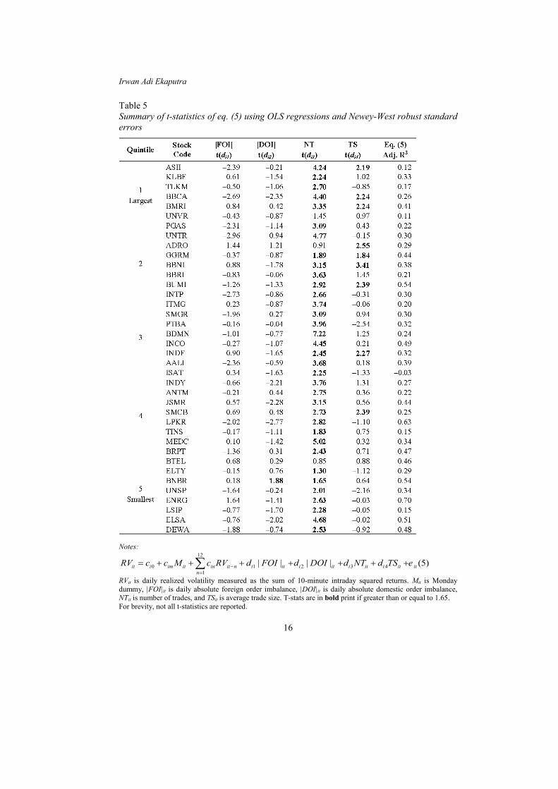
The second part of this study utilises realized volatility as volatility

measure. The calculated results of eq. (5) are presented in Table 5. Consistent with previous results, number of trades significantly dominates other factors in explaining realized volatility. Number of trades is statistically significant in 35 of 38 stocks, while trade size is only significant in 9 of 38 stocks. In line with Chan and Fong (2006), Giot et al. (2010), and Shahzad et al. (2012), absolute foreign order imbalance does not explain realized volatility, and absolute domestic order imbalance is only significant in 1 of 38 stocks. The results of several studies, including this one, seem to converge to the inability of absolute order imbalance to explain realized volatility.2 Henceforth, it can be concluded that absolute order imbalance is not a good proxy for the arrival of informed trading as originally intended.

On the other hand, order imbalance is the right proxy for informed

trading arrival, and explains the variation of stock returns. Hence, supporting Chan and Fong (2000), this study also finds that one major driving force for the volatility-volume relation is related to the impact of the daily order imbalance on stock returns. Further decomposition of order imbalance into foreign and domestic order imbalances adds more power in explaining variations of stock returns and volatility-volume relation.


15

Table 4 Summary of t-statistics of eq. (3) and eq. (4) using OLS regressions and Newey-West robust standard errors

Notes: 12

01

ˆ ˆ| | | | (3)it i im t ij it j i it i it itj

M NT TSε θ θ θ ε π ρ ω−=

= + + + + +∑12

01

ˆ ˆ| | | | (4)it i im t ij it j i it i it itj

M NT TSη θ θ θ η π ρ ω−=

= + + + + +∑

The dependent variables of eq. (3) and (4) are the absolute residuals from eq. (1) and (2), respectively. Mt is Monday dummy, NTit is the number of trades, and TSit is the average trade size. T-stats are in bold print if greater than or equal to 1.65. For brevity, not all t-statistics are reported.

Irwan Adi Ekaputra

16

Table 5 Summary of t-statistics of eq. (5) using OLS regressions and Newey-West robust standard errors

Notes: 12

0 1 2 3 41

| | | | (5)it i im it in it n i it i it i it i it itn

RV c c M c RV d FOI d DOI d NT d TS e−=

= + + + + + + +∑

RVit is daily realized volatility measured as the sum of 10-minute intraday squared returns. Mit is Monday dummy, |FOI|it is daily absolute foreign order imbalance, |DOI|it is daily absolute domestic order imbalance, NTit is number of trades, and TSit is average trade size. T-stats are in bold print if greater than or equal to 1.65. For brevity, not all t-statistics are reported.


17

CONCLUDING REMARKS This study is divided into two parts based on the volatility measures used. The first part uses absolute residuals, following the two stage regression methodology by Chan and Fong (2000). The second part employs realized volatility, following Chan and Fong (2006), Giot et al. (2010) and Shahzad et al. (2012).

Motivated by previous research contrasting the roles of foreign and

domestic investors in the Indonesian market, the first part of the study decomposes order imbalance in the first-stage regression into foreign and domestic order imbalances. The results show that foreign and domestic order imbalances explain the daily variation of returns better than undivided order imbalance. The impact of foreign order imbalance is more pronounced in larger cap stocks, while domestic order imbalance plays a more significant role in smaller-cap stocks. In the second-stage regressions, number of trades consistently dominates trade size in explaining variations of absolute residuals. The first part of the study confirms that foreign and domestic order imbalances are major driving forces for the volatility-volume relation through their impact on daily stock returns. In other words, foreign order imbalance, domestic order imbalance, and number of trades play important roles in the volatility-volume relation.

In the second part of this study, number of trades is again proven to be

the dominant factor in explaining realized volatility. Absolute foreign and domestic order imbalances do not seem to play any significant role, while average trade size minimally explains realized volatility. Consistent with previous studies such as Chan and Fong (2006), Giot et al. (2010) and Shahzad et al. (2012), absolute order imbalances do not seem to capture the arrival of informed trading as intended; hence, they do not explain realized volatility variations. Further studies should not use absolute order imbalance as a factor in volatility-volume relations but should instead attempt to find a better measure of informed trading arrival.

NOTES

1. http://www.beritasatu.com/investasi-portofolio/152296-kalangan-pasar-modal-satu-tekad-dongkrak-jumlah-investor-domestik.html. Retrieved 7 December 2013.

2. This study also employs non-decomposed absolute order imbalance as a factor and finds

consistent results. The results are not reported but are available upon request.

http://www.beritasatu.com/investasi-portofolio/152296-kalangan-pasar-modal-satu-tekad-�

http://www.beritasatu.com/investasi-portofolio/152296-kalangan-pasar-modal-satu-tekad-�

Irwan Adi Ekaputra

18

REFERENCES Admati, A. R., & Pfleiderer, P. (1988). A theory of intraday patterns: Volume and price

variability. Review of Financial Studies, 1(1), 3–40. Agarwal, S., Chiu, I-M., Liu, C., & Rhee, S. G. (2010). The brokerage firm effect in

herding: Evidence from Indonesia. Journal of Financial Research, 33(4), 317–337.

Agarwal, S., Faircloth, S., Liu, C., & Rhee, S. G. (2009). Why do foreign investors underperform domestic investors in trading activities? Evidence from Indonesia. Journal of Financial Markets, 12(1), 32–53.

Andersen, T. G., & Benzoni, L. (2008, July 22). Realized volatility (FRB of Chicago Working Paper). Retrieved 2 April 2013 from http://dx.doi.org/10.2139/ssrn.1092203

Andersen, T. G., Bollerslev, T., & Lange, S. (1999). Forecasting financial market volatility: Sample frequency vis-avis forecast horizon. Journal of Empirical Finance, 6(5), 457–477.

Budipratama, S. (2010). Pefindo's corporate default and rating transition study (1996–2010). Jakarta: PT. Pemeringkat Efek Indonesia (Pefindo).

Chan, C. C., & Fong, W. M. (2006). Realized volatility and transactions. Journal of Banking and Finance, 30(7), 2063–2085.

Chan, K., & Fong, W-M. (2000). Trade size, order imbalance, and the volatility-volume relation. Journal of Financial Economics, 57(2), 247–273.

Chang, R. P., Rhee, S. G., Stone, G. R., & Tang, N. (2008). How does the call market method affect price efficiency? Evidence from the Singapore Stock Market. Journal of Banking and Finance, 32(10), 2205–2219.

Comerton-Forde, C., & Rydge, J. (2006). The current state of Asia-Pacific stock exchanges: A critical review of market design. Pacific-Basin Finance Journal, 14(1), 1–32.

Dvorak, T. (2005). Do domestic investors have an information advantage? Evidence from Indonesia. Journal of Finance, 60(2), 817–839.

Giot, P., Laurent, S., & Petitjean, M. (2010). Trading activity, realized volatility and jumps. Journal of Empirical Finance, 17(1), 168–175.

Guo, F., & Huang, Y. S. (2010). Does "hot money" drive China's real estate and stock markets? International Review of Economics & Finance, 19(3), 452–466.

Hanafi, M., & Rhee, S. G. (2004). The wealth effect of foreign investor presence: Evidence from the Indonesia Market. Management International Review, 44(2), 157–171.

Henker, T., & Husodo, Z. A. (2010). Noise and efficient variance in the Indonesia Stock Exchange. Pacific-Basin Finance Journal, 18(2), 199–216.

Jones, C. M., Kaul, G., & Lipson, M. L. (1994). Transactions, volume and volatility. Review of Financial Studies, 7(4), 631–651.

Karpoff, J. (1987). The relation between price changes and trading volume: A survey. Journal of Financial and Quantitative Analysis, 22(1), 109–126.

Kyle, A. S. (1985). Continous auctions and insider trading. Econometrica, 53(6), 1315–1336.

Lee, C. M., & Ready, M. J. (1991). Inferring trade direction from intraday data. Journal of Finance, 46(2), 733–746.


19

Lee, C. M., Ready, M. J., & Seguin, P. J. (1994). Volume, volatility, and New York Stock Exchange Trading Halts. Journal of Finance, 49(1), 183–214.

Lesmond, D. A. (2005). Liquidity of emerging markets. Journal of Financial Economics, 77(2), 411–452.

Liu, S. (2009). Index membership and predictability of stock returns: The case of the Nikkei 225. Pacific Basin Finance Journal, 17(3), 338–351.

Shahzad, H., Duong, H., & Singh, H. (2012). Information flow, realized volatility, and jumps in the Australian Stock Market. 14th Malaysian Finance Association Conference. Parkroyal Penang Resort, Penang, Malaysia, 2–3 June 2012. Penang: Universiti Sains Malaysia.

Documents

IMPACT OF FOREIGN AND DOMESTIC ORDER IMBALANCES ON …